&
.
,
,
I
I
. .
&


Fun and Games
A Text on Game Theory
Ken Binmore
University of Michigan
Ann Arbor
D. C. Heath and Company
Lexington, Massachusetts Toronto

Address editorial correspondence to:
D. C. Heath
125 Spring Street
Lexington, MA 02173
Cover Photograph: Eric S. Fordham
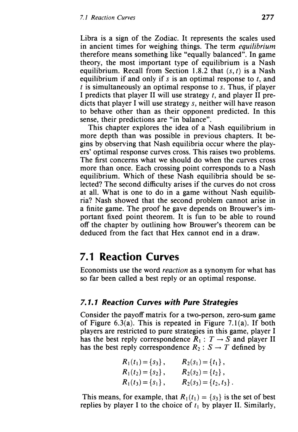
The John Tenniel illustrations on pages v, vii, 1, 23, 65, 93, 127,
167,217,275,345,391,443,499, and 571, and the "Ocean Chart"
on page xv by Henry Holiday are taken from The Complete Il-
lustrated Works of Lewis Carroll, published by Chancellor Press,
London, 1982.
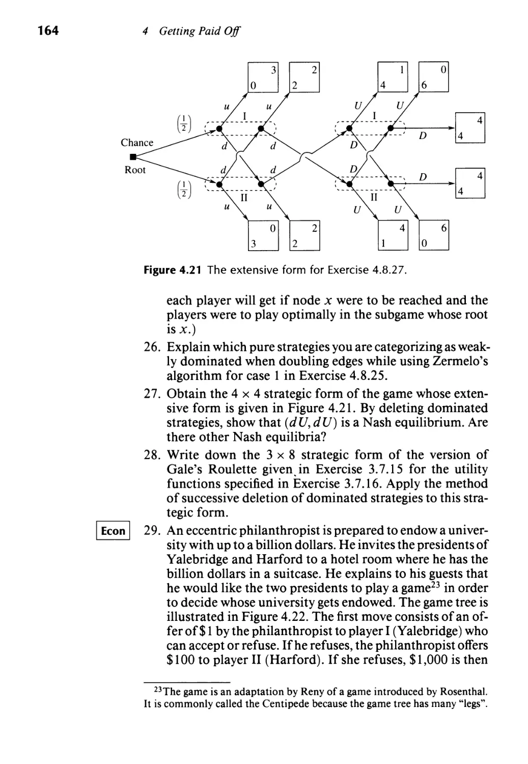
Technical art by Tech-Graphics, Woburn, Mass.
Copyright @ 1992 by D. C. Heath and Company.
All rights reserved. No part of this publication may be reproduced
or transmitted in any form or by any means, electronic or mechan-
ical, including photocopy, recording, or any information storage or
retrieval system, without permission in writing from the publisher.
Published simultaneously in Canada.
Printed in the United States of America.
International Standard Book Number: 0-669-24603-4
Library of Congress Catalog Number: 90-83786
10 9 8 7 6 5 4 3 2 1

I dedicate
Fun and GaInes
to my wife
Josephine.

Preface
......
o
Game theory is an activity like skiing or tennis that is only
fun if you try to do it well. But learning to do something well
is seldom quick and easy, and game theory is no exception.
Moreover, unlike skiing or tennis, it really matters that we
learn to use game theory well. Its aim is to investigate the
manner in which rational people should interact when they
have conflicting interests. So far, it provides answers only
in simple situations, but these answers have already led to
a fundamental restructuring of the way in which economic
theorists think about the world, and the time is perhaps not
too far distant when the same will be true for all the social
sCiences.
Thus, although I have tried to develop the theory with a
light touch, this is a serious book about a serious subject.
..
VII

...
VIII
Preface
Above all, Fun and Games is a how-to-do-it book. It is not
like one of those television programs in which you look over
an artist's shoulder while he briskly applies ready-mixed
paints to an already-prepared canvas using techniques that
are never fully explained lest the viewer lose interest and
switch to another channel. Encouraging people to appreciate
art is doubtless a worthy activity, but I am not interested in
trying to do the same thing for game theory. My aims are
more ambitious. I hope that, after reading this book, you
will be able to do more than admire how other people have
used game theory. My hope is that you will be able to apply
game-theoretic skills to simple problems all by yourself.
Fun and Games is intended to be a serious book on game
theory that is suitable for teaching both undergraduate and
graduate students. I know that the book works for both pur-
poses because I have been using it and its less-polished pre-
decessors for more than fifteen years at various institutions
both in the United States and in Europe. I also know that
other approaches that seem as though they might work do
not. The practicalities of running a serious course in game
theory for undergraduates impose severe limitations on what
it is wise to attempt both in terms of content, and in terms of
presentation. To these I have added two further constraints.
The first is that the focus of the book is on noncooperative
game theory. Very little is said about cooperative game the-
ory. This is partly because of the second constraint, which
may be less popular. I have to confess to being squeamish
about teaching things to undergraduates that might turn out
to be wrong. I know that it is fun for the teacher to weigh the
pros and cons of new ideas, but undergraduates tend to treat
anything said in class as though Moses had brought it down
from the mountain engraved on tablets of stone. Where in-
tellectual honesty allows, I have therefore tried very hard to
exclude controversial theoretical ideas altogether.!
The book is suitable for teaching students from a number
of disciplines. However, the binding practical constraint is
that of attracting and holding an audience large enough to
merit a case for game theory being retained on the list of
undergraduate courses offered by an economics department.
Perhaps the increasing recognition of the importance of game
1 Game theory is still being developed at a very fast rate. In such cir-
cumstances, it is inevitable that many of the new ideas being tried out will
be found wanting and discarded after enjoying a brief period in the lime-
light. I have adopted the very conservative policy of including only those
ideas that I believe are sure to survive. This still leaves more than enough
material to fill a semester course for undergraduates twice over.

Preface
.
IX
theory will change things in the future, but as things stand at
present, one cannot realistically ask for much in the way of
mathematical prerequisites from the students; nor can one
restrict entry to economics majors-unless one is to aban-
don the ambition of teaching a serious how-to-do-it course
in favor of a superficial romp through a collection of over-
simplified applications whose significance the students will
have no way of evaluating. The Teaching Guide that follows
this Preface explains the implications in detail. In brief, there
is a limit to how much mathematical technique can be taught
along the way, and there is a need to respect the wide interests
of your audience in choosing the examples used to illustrate
the theory.
This is not a scholarly work. It contains no references and,
with a few exceptions, mention is made only of the great
pioneers in game theory. This would be standard in a book
at this level in more established disciplines. Apologies need to
be made on this count in a book on game theory only because
much of the work is recent and those who contributed are
mostly still alive and kicking. All I can say to those who feel
that they should have been cited explicitly is that they are in
very good company. However, I do want to express my thanks
to some individuals whose efforts helped to shape this book,
either directly, or indirectly through their published work.
First, there is the Victorian artist John Tenniel, whose
magnificent illustrations from Lewis Carroll's Alice Through
the Looking Glass and elsewhere I have shamelessly stolen.
Second, my thanks go to Donald Knuth and to Leslie Lamport
for providing the TEX typesetting program in which the text
was written. Third, I want to thank my publisher D. C. Heath
for tolerating such idiosyncracies as punctuating "like this",
instead of "like this." George Lobell and Jennifer Brett were
particularly helpful in getting the book on the road. Fourth,
Pat O'Connell-Young deserves thanks for typing most of the
current version, and Mimi Bell for typing a previous version
of the book. Fifth, there are D. C. Heath's reviewers: James
Bergin, Engelbert Dockner, Ray Farrow, Chris Harris, David
Levine, George Mailath, Andrew McLennan, Michael Meurer
and Max Stinchcombe. Finally, there is a long list of other
economists and mathematicians to whom I owe a debt of grat-
itude: Steve Alpern, Bob Aumann, Pierpaolo Battigalli, Ted
Bergstrom, Adam Brandenburger, James Friedman, Drew
Fudenberg, David Gale, John Harsanyi, David Kreps, Herve
Moulin, Roger Myerson, Barry O'Neill, Adam Ostaszewski,
Barry Nalebuff, John Nash, Andy Postelwaite, Phil Reny,
Bob Rosenthal, Ariel Rubinstein, Larry Samuelson, Reinhard

x
Preface
Selten, Avner Shaked, John Sutton, Jean Tirole, Hal Varian
and Robert Wilson.
Finally, on the subject of what pass for jokes in the text,
let me say that I feel entitled to the same immunity from
criticism as the musician in the Western saloon whose pi-
ano was reported by Oscar Wilde to carry a notice saying,
"Please do not shoot the pianist. He is doing his best". It
isn't easy to sustain a light-hearted atmosphere in a work of
this kind. Perhaps it was over-ambitious to promise both Fun
and Games. Certainly, I thought it wise to write in a more
deadpan style in the earlier chapters. However, I hope that
some readers at least will agree that I did eventually try to
live up to my title.
K. B.

Contents
Teaching Guide xv
Introduction 1
0.1 What Is Game Theory About? 3
0.2 Where Is Game Theory Coming From? 11
0.3 Where Is Game Theory Going To? 13
0.4 What Can Game Theory Do for Us? 14
0.5 Conclusion 21
1 Winning Out
1.1 Introduction 25
1.2 The Rules of the Game 25
1.3 Strategies 30
1.4 Zermelo's Algorithm 32
1.5 Nim 35
1.6 Hex 37
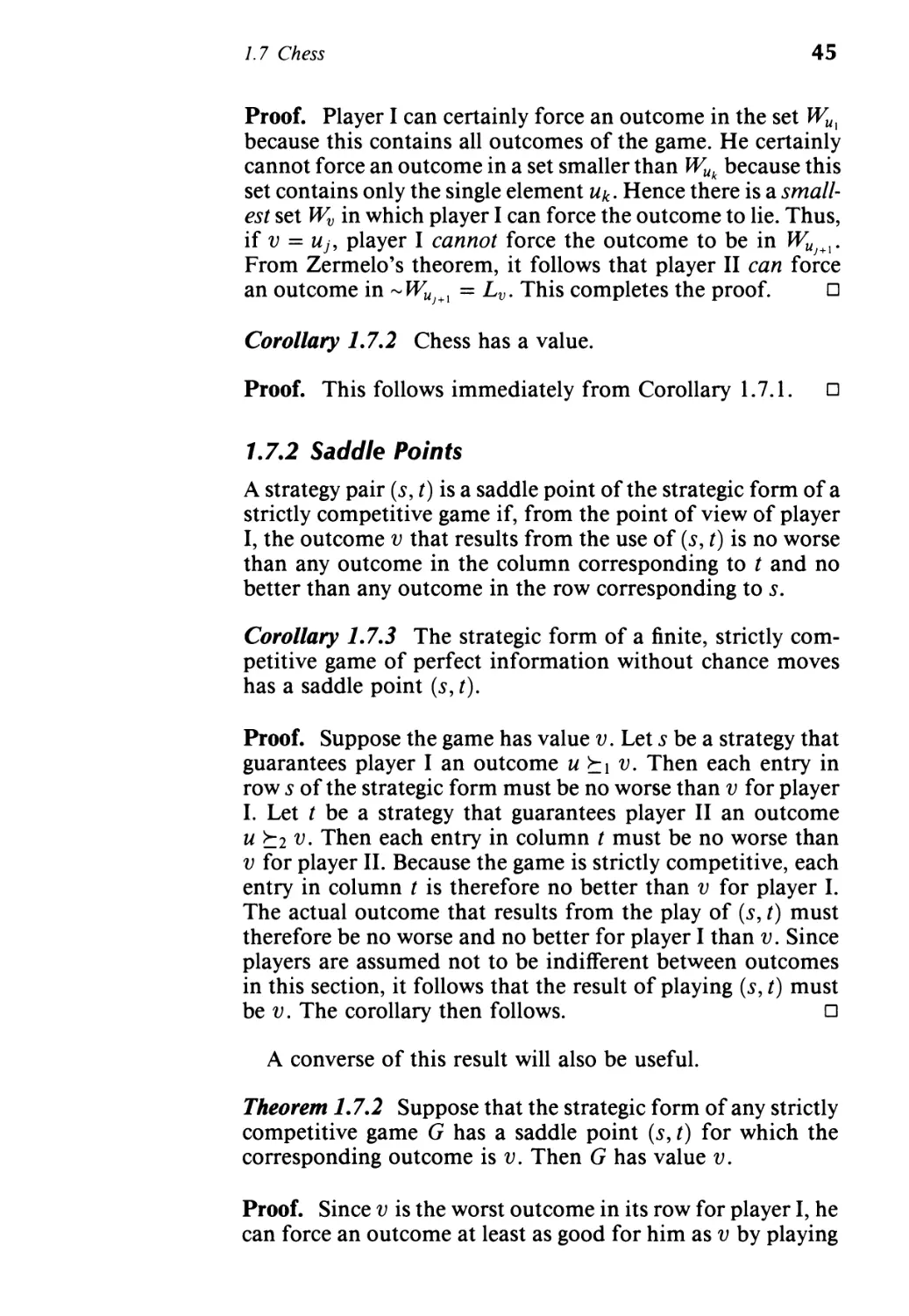
1. 7 Chess 41
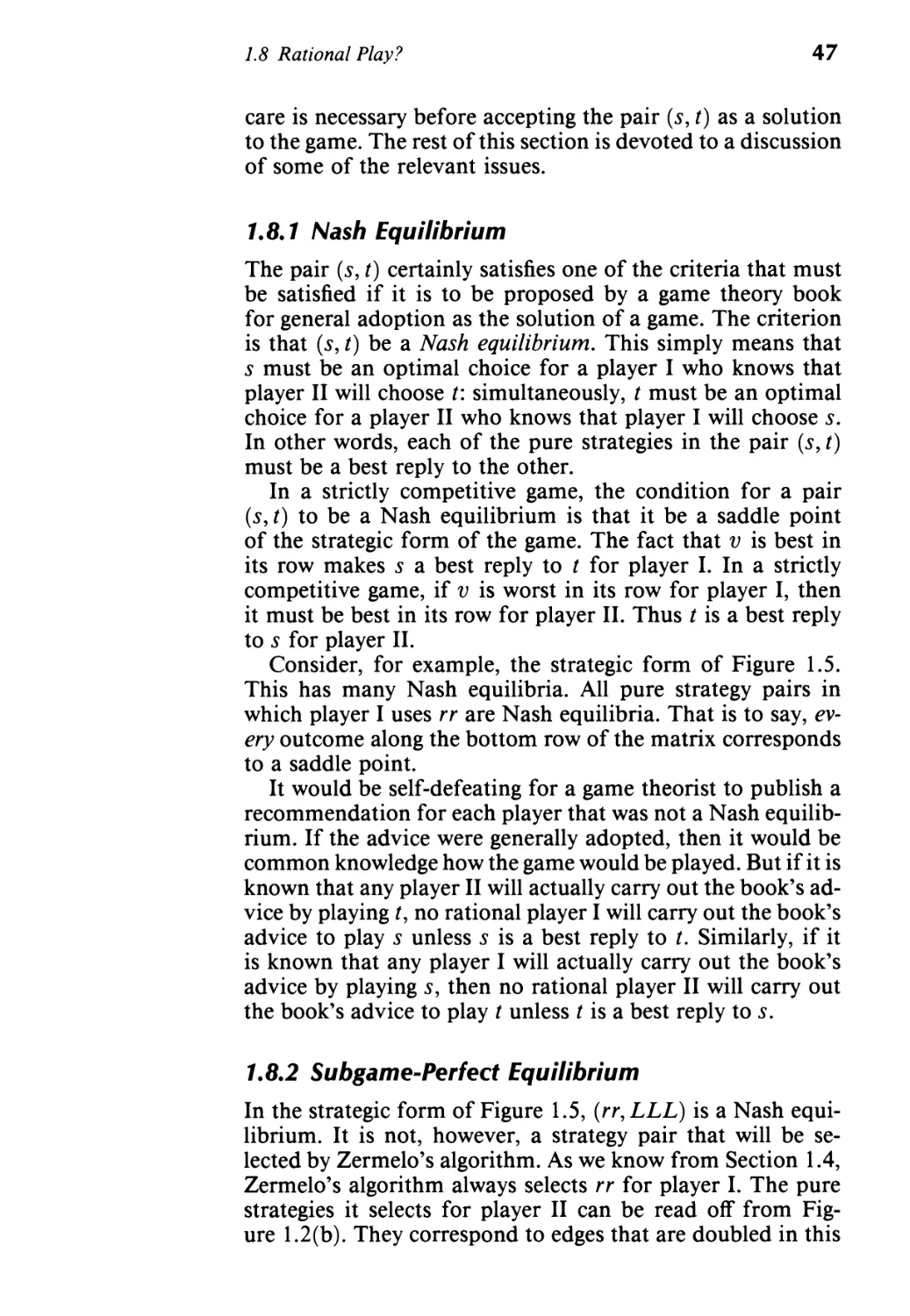
1.8 Rational Play? 46
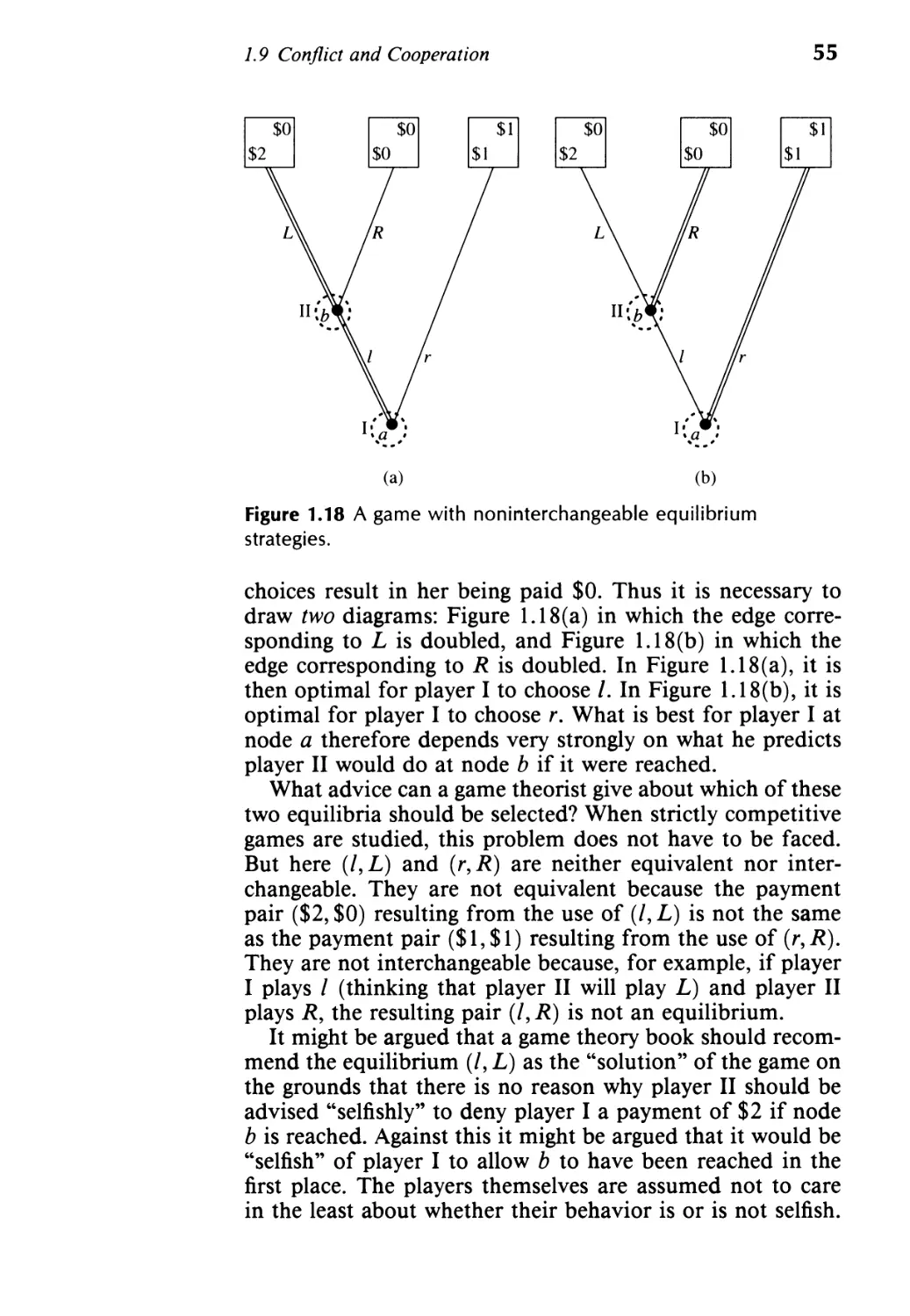
1.9 Conflict and Cooperation 51
1.1 0 Exercises 57
23
2 Taking Chances 65
2.1 Introduction 67
2.2 Lotteries 72
2.3 Game Values 75
2.4 Duel 76
2.5 Parcheesi 81
2.6 Exercises 86
.
XI

..
XII
Contents
3 Accounting for Tastes 93
3.1 Rational Preferences 95
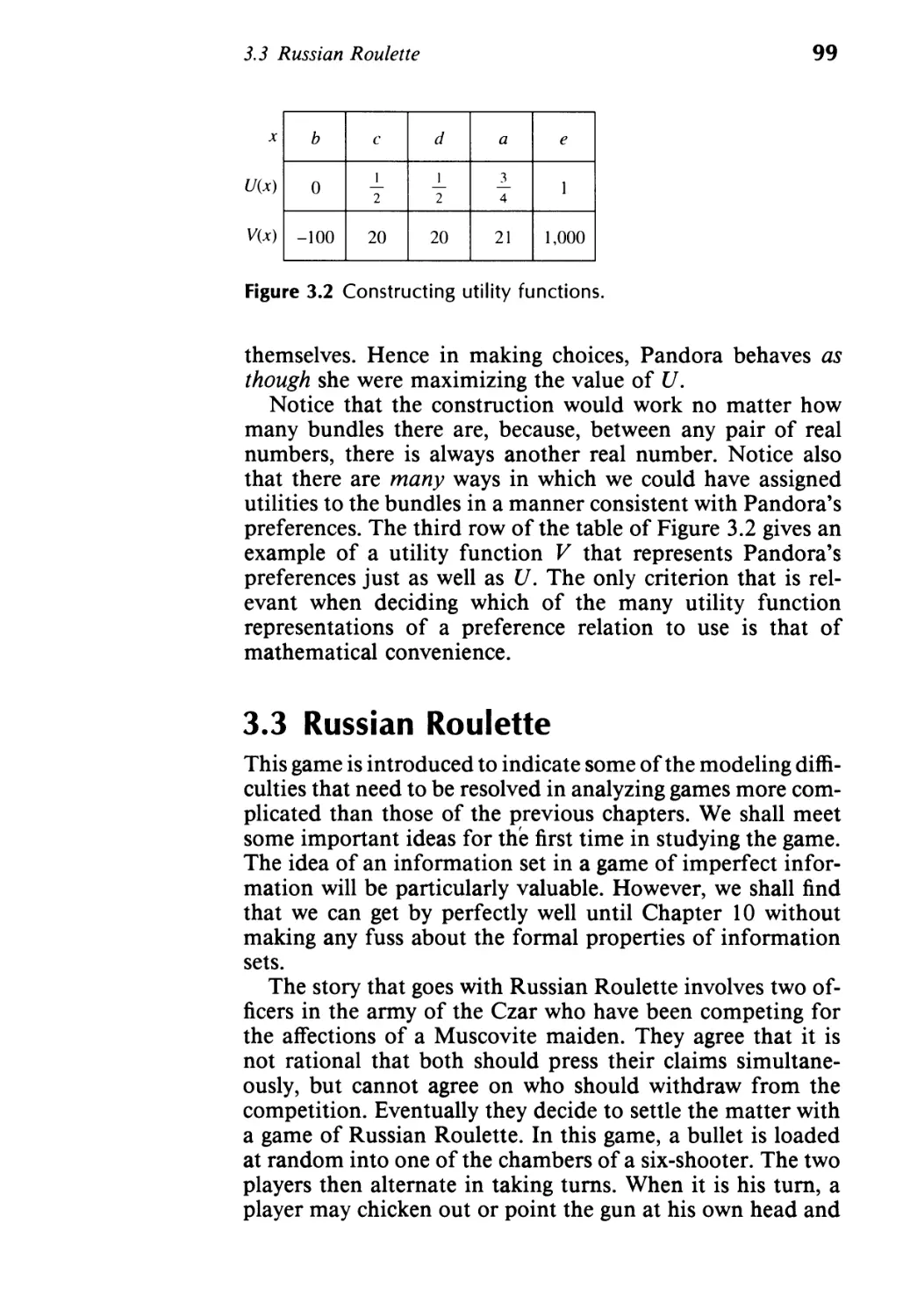
3.2 Utility Functions 96
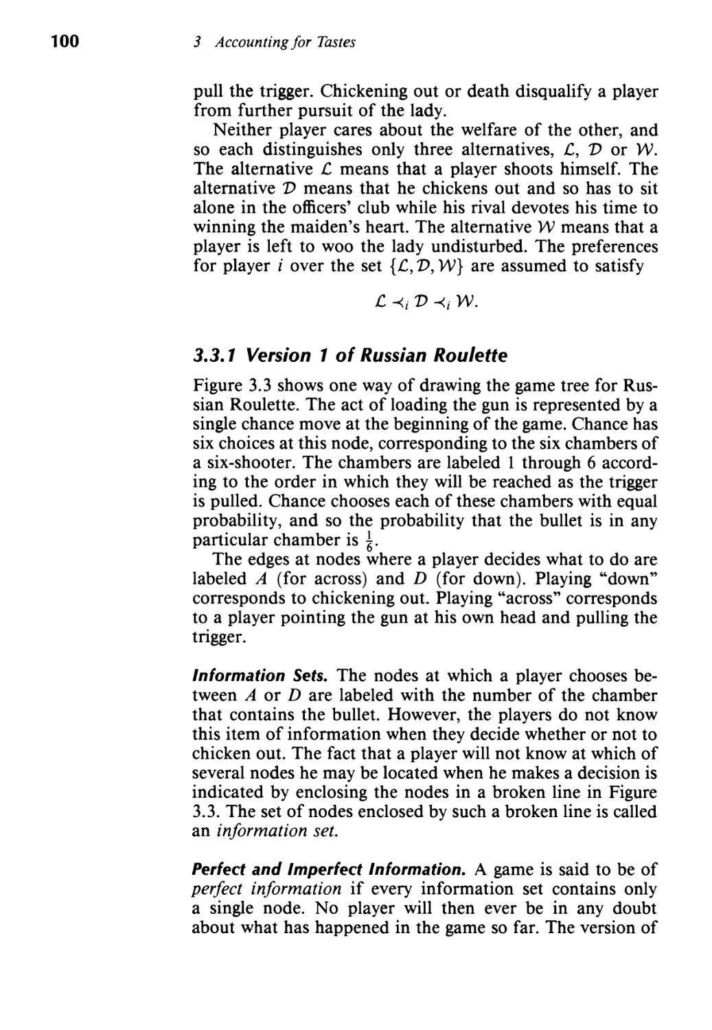
3.3 Russian Roulette 99
3.4 Making Risky Choices 104
3.5 Utility Scales 112
3.6 The Noble Savage 115
3.7 Exercises 120
4 Getting Paid Off 127
4.1 Payoffs 129
4.2 Bimatrix Games 133
4.3 Matrices 135
4.4 Vectors 138
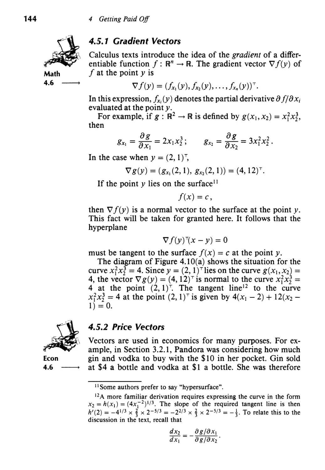
4.5 Hyperplanes 142
4.6 Domination 146
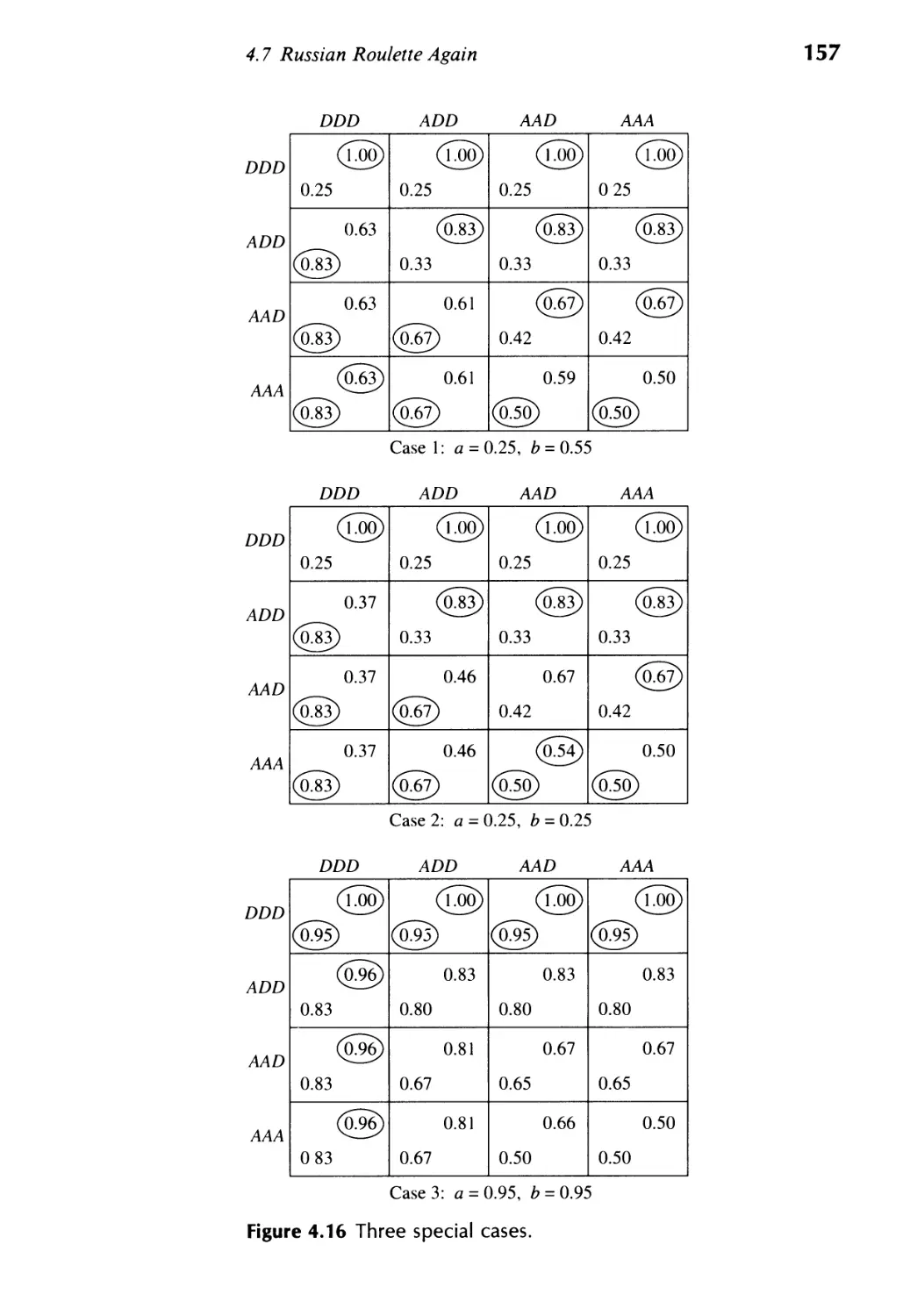
4.7 Russian Roulette Again 153
4.8 Exercises 159
5 Making Deals 167
5.1 Introduction 169
5.2 Convexity 169
5.3 Cooperative Payoff Regions 174
5.4 The Bargaining Set 176
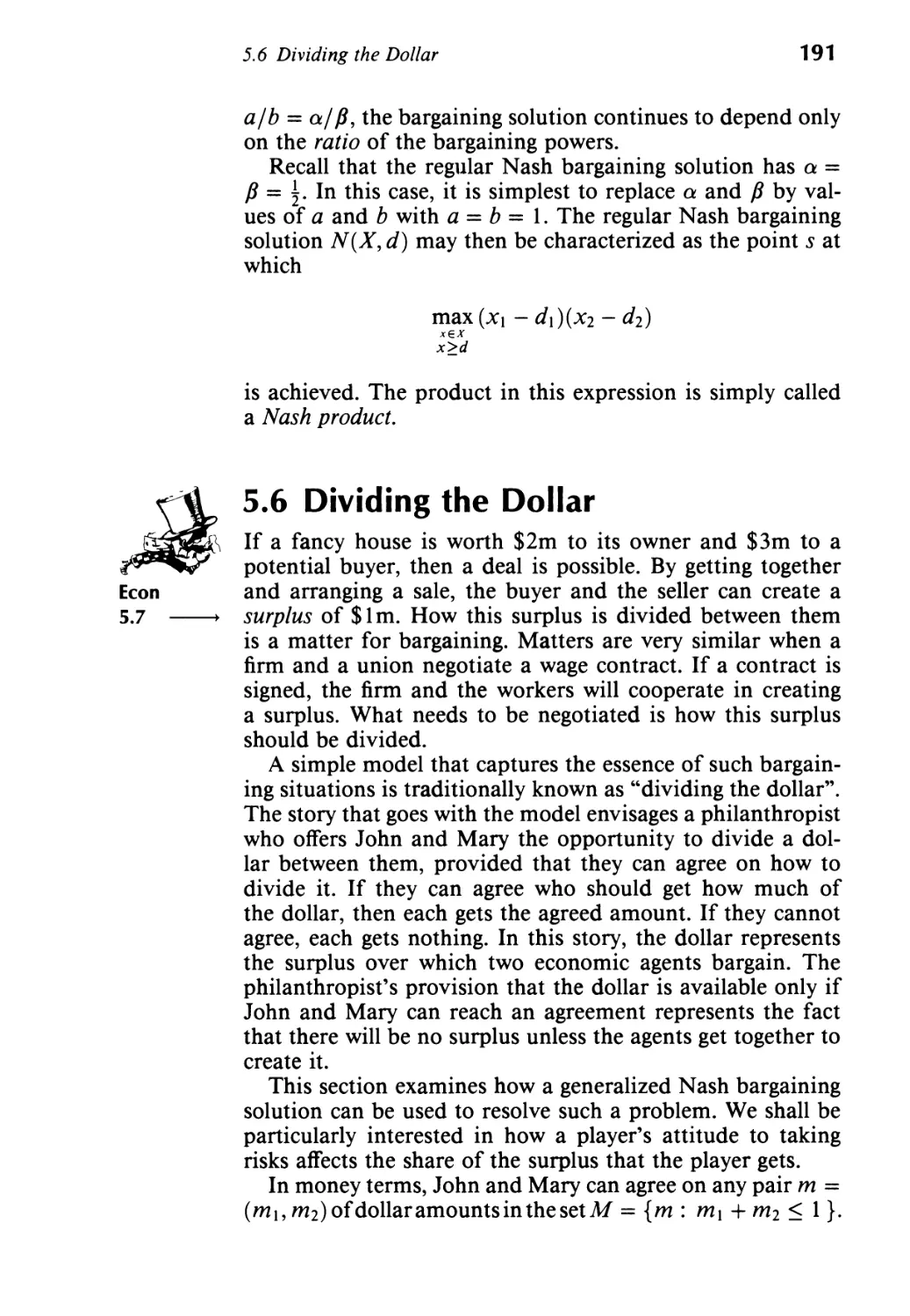
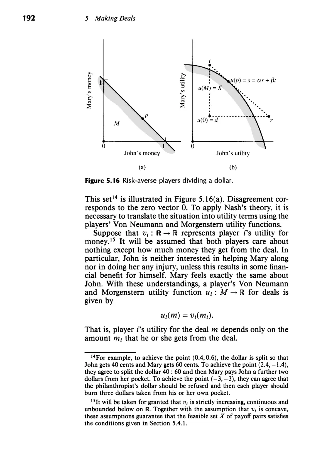
5.5 Nash Bargaining Solutions 180
5.6 Dividing the Dollar 191
5.7 Cooperative and Noncooperative Games 195
5.8 Bargaining Models 196
5.9 Exercises 212
6 Mixing Things Up 217
6.1 Introduction 219
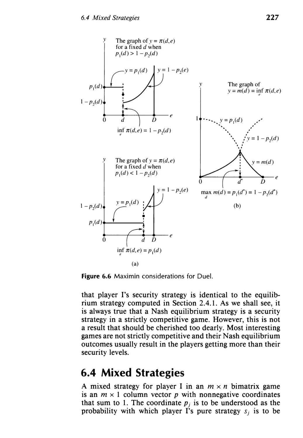
6.2 Minimax and Maximin 219
6.3 Safety First 224
6.4 Mixed Strategies 227

Contents
...
XIII
6.5 Zero-Sum Games 237
6.6 Separating Hyperplanes 245
6.7 Battleships 254
6.8 The Inspection Game 257
6.9 N ash Threat Game 261
6.10 Exercises 265
7 Keeping Your Balance 275
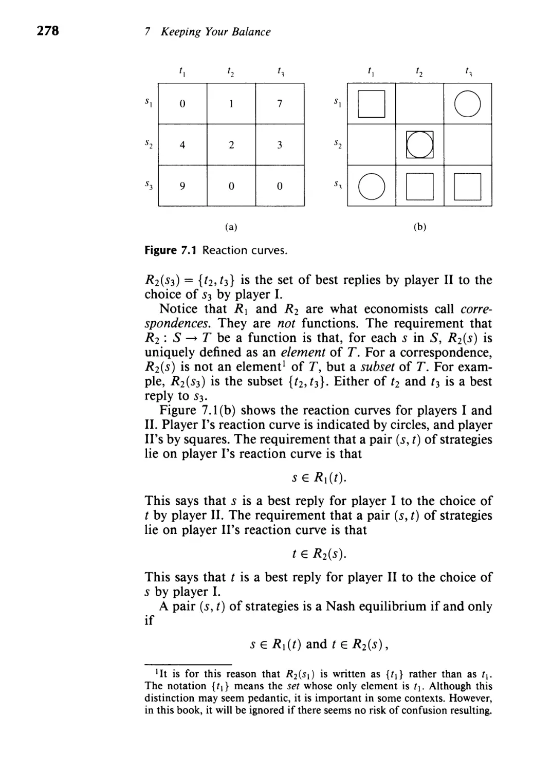
7.1 Reaction Curves 277
7.2 Oligopoly and Perfect Competition 286
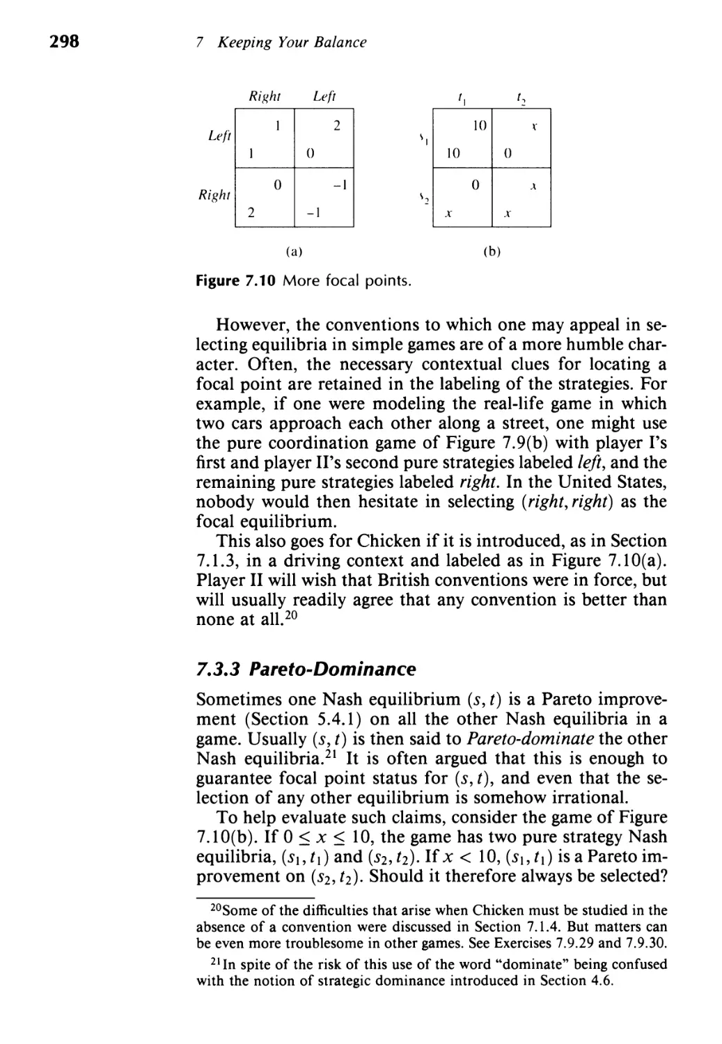
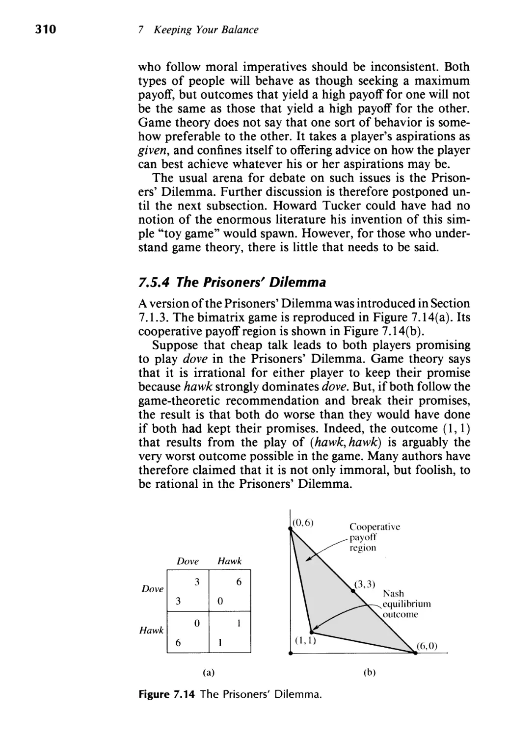
7.3 Equilibrium Selection 295
7.4 N ash Demand Game 299
7.5 Pre-play Negotiation 304
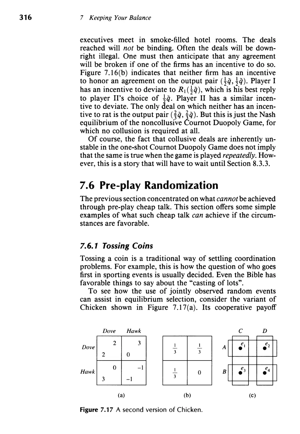
7.6 Pre-play Randomization 316
7.7 When Do Nash Equilibria Exist? 319
7.8 Hexing Brouwer 323
7.9 Exercises 329
8 Repeating Yourself 345
8.1 Reciprocity 347
8.2 Repeating a Zero-Sum Game 348
8.3 Repeating the Prisoners' Dilemma 353
8.4 Infinite Repetitions 360
8.5 Social Contract 379
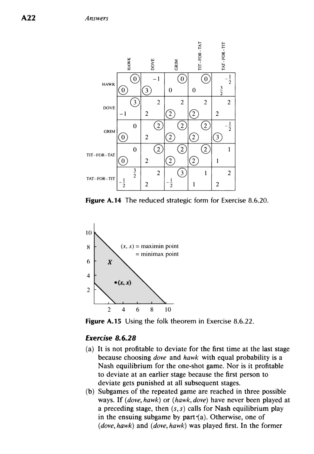
8.6 Exercises 382
9 Adjusting to Circumstances 391
9.1 Spontaneous Order 393
9.2 Bounded Rationality 396
9.3 Economic Libration 398
9.4 Social Libration 412
9.5 Biological Libration 414
9.6 Evolutionary Stability 422
9.7 The Evolution of Cooperation 429
9.8 Exercises 434

.
XIV
Contents
10 Knowing Your Place 443
10.1 Bob's Your Uncle 445
10.2 Knowledge 446
10.3 Possibility 449
10.4 Information Sets 454
10.5 Bayesian Updating 462
10.6 Common Knowledge 467
10.7 Agreeing to Disagree? 472
10.8 Common Knowledge in Game Theory 478
10.9 Exercises 488
11 Knowing Who to Believe 499
11.1 Complete and Incomplete Information 501
11.2 Typecasting 503
11.3 Bayesian Equilibrium 510
11.4 Continuous Random Variables 511
11.5 Duopoly with Incomplete Information 515
11.6 Purification 519
11.7 Auctions and Mechanism Design 523
11.8 Assessment Equilibrium 536
11.9 More Agreeing to Disagree 546
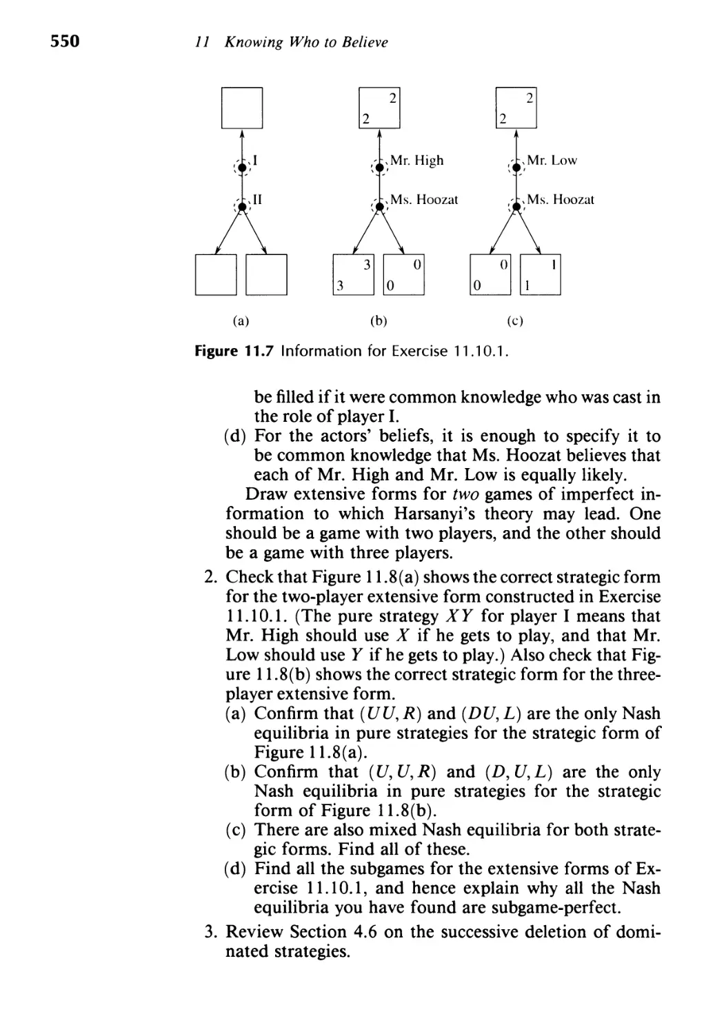
11.10 Exercises 549
12 Bluffing It Out 571
12.1 Poker 573
12.2 Conditional Probability Densities 577
12.3 Borel's Poker Model 579
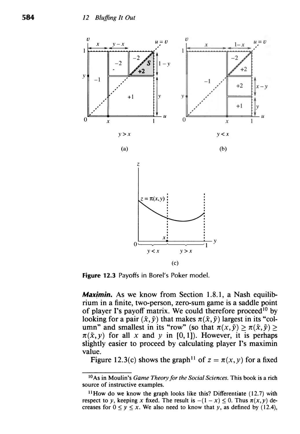
12.4 Von Neumann's Poker Model 585
12.5 Why Bluff? 591
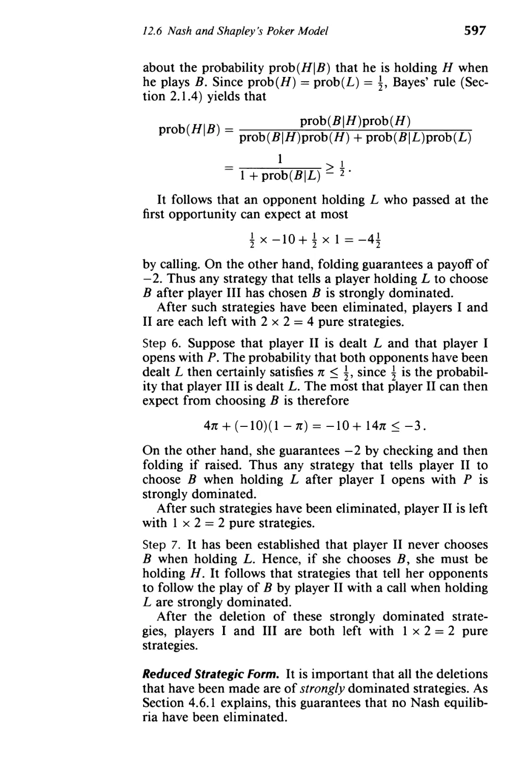
12.6 Nash and Shapley's Poker Model 593
12.7 Conclusion 602
Answers Al
Index A34

Teaching Guide
LA.TITl DE
'lC'RTH
C"UA. "OR
1 2
2
.
Z


.

z
..
c
:
JI




r
 I

...,

-!
..
2
I .
! 

c
z
I
I
L
I 
I 

::'(al, -;;- iftf-;; -
OCEAN-CHART.
Charting a Course
Fun and Games is aimed at two distinct groups of students,
and is therefore written on two distinct levels. Teachers there-
fore need to chart a careful course through the material since
things could go awry if there is a mismatch between the stu-
dents and the topics chosen for study. Or, to say the same
thing more colorfully, in seeking to reveal the nature of the
snark to your students, beware lest you show them a boojum
by mistake. As Lewis Carroll put it, your audience will then
"softly and suddenly vanish away", like the Bellman's crew
in the Hunting of the Snark. However, the Bellman had only
the Ocean Chart shown above to guide him.
xv

.
XVI
Teaching Guide
One aim of Fun and Games is to provide a semester course
in game theory for undergraduates. The undergraduates do
not need to have much prior knowledge of anything, but they
will have to be well motivated. Note, in particular, that the
undergraduates do not need to be economics majors. This
latter point is quite important, since, in many institutions,
an undergraduate course in game theory at the level of this
book may not be viable if aimed exclusively at economists.
However, my experience is that one attracts a respectable
audience 1 if one is willing to admit students from all disci-
plines, and to teach material that takes account of their wide
range of interests.
Another aim is to provide "pre-med" material in game the-
ory for graduate students in economics. In this role, the book
is not intended as a competitor to the excellent books written
by Fudenburg and Tirole and by Myerson. It is intended to
serve only as an easy way into the serious stuff for those who
do not feel the urge to plunge in immediately at the deep
end.
The two aims frequently dovetail very neatly, and the join
between the two levels of exposition would not always be
easy to spot if it were not pointed out explicitly. Teachers
must decide for themselves how often to cross this boundary
line. I certainly cross it myself when the idiosyncracies of my
audience seem to call for it. However, it is unwise to cross the
line too often, since the risk of frightening off one audience
and boring the other is considerable. Of course, nothing will
or should prevent enthusiastic undergraduates from reading
the more advanced material on the side. At the same time,
graduate students will need to skim the more elementary ma-
terial in order to make sense of the topics written specifically
for them. In class, however, I recommend keeping on the
appropriate side of the demarcation line nearly all the time.
Material that is a candidate for being skipped when teach-
ing a semester course to undergraduates is indicated by a
stylized version of John Tenniel's Mad Hatter in the margin.
When the Mad Hatter is running away, consider very care-
fully whether the material following his appearance is suit-
able for your undergraduates. If not, then skip the material
and go to the section number indicated beneath the fleeing
Mad Hatter. When I teach economics undergraduates, for
example, my instructions are that the Mad Hatter is to be
1 Last term I taught game theory at the University of Michigan to 46
undergraduates taking the course for credit, and an indeterminate number
of auditors of various types.

Teaching Guide
..
XVII
followed wherever he goes, except when he is skipping some
economics. When I teach mathematics undergraduates, my
instructions are more complicated.
Nothing whatever in the book is too hard for graduate
students. They should certainly not follow the Mad Hatter
anywhere at all. On the contrary, his appearance should sig-
nal the fact that the material that follows contains something
that merits their close attention.
Sometimes the Mad Hatter in the margin is not running
away. Instead he is shown somewhat apprehensively hang-
ing around to see what happens next. Usually what happens
next is something mathematical. Such passages may be diffi-
cult for some undergraduates, but cannot be skipped without
disrupting the continuity of the exposition.
Review
Econ
As in the examples given above, all the marginal Mad Hat-
ters are equipped with a label indicating the type of material
to which they refer. The five labels used are
Review Math Econ Phil Fun
The same labeling is used to categorize many of the exercises
that appear at the end of each chapter. What do these labels
mean?
Review. My experience is that one cannot run a viable course
for undergraduates if the mathematical prerequisites are set
too high. The most one can realistically do is to restrict en-
try to students who have passed a serious freshman calculus
course. Many of the students will know more than this. The
others will have to pick up what extra mathematics they need
along the way. Students seem ready to put in the necessary
work on the side provided that what is required of them
is made very clear. This explains the presence of the REVIEW
sections. The chief topics covered in these sections are proba-
bility, matrices and vectors, and convexity. Calculus does not
get the same treatment, since students are assumed to know
what little is needed already. However, reminders about how
to do various things sometimes appear as footnotes. 2
2 Although I know that those who need such reminders do not read such
things as footnotes, appendices and introductions.

...
XV III
Teaching Guide
Do not think for one moment of teaching the review ma-
terial at the blackboard. I have already pulled the rug out
from under such a project by using the label REVIEW. It seems
a universal knee-jerk reaction in the human species to switch
off as soon as this word is mentioned in the classroom. What
I do myself is to point out those mathematical ideas in the
REVIEW sections that are indispensable, and then sneak some
discussion of them into the hours devoted to going over the
exercises.
Actually, there is a lot more in these REVIEW sections than
undergraduate students are going to need to study Fun and
Games. When writing them, I also had graduate students in
mind. If my experience is anything to go by, many gradu-
ate students would be advised to skim these mathematical
REVIEW sections very slowly.
Math. When teaching undergraduates, you will probably wish
to skip nearly all the MATH sections that the Mad Hatter
is shown running away from, unless your audience consists
primarily of mathematics majors. However, mathematicians
should not take this to imply that the MATH sections are
written in a formal style. None of the arguments offered
come anywhere near meeting the standards of a mathemati-
cal proof. Mostly, I follow the Bellman and use the principle
that what I tell you three times is true. On the other hand, I
have tried hard to be intellectually honest. All the arguments
offered can be fleshed out into formal proofs without call-
ing for mathematical techniques that would be beyond the
understanding of an average undergraduate willing to take
some time and trouble. I hope that these proof schemata will
be particularly useful to graduate students who are too of-
ten shortchanged with a list of cookbook techniques whose
validity they are expected to take on trust.
Econ. I have taught game theory in numerous institutions.
The undergraduate classes consist mostly of economists, but
there is always a substantial number of students majoring
in other disciplines whose presence livens things up a fair
amount. The disciplines include mathematics, engineering,
philosophy and political science. Some of the ECON sections
are intended to acquaint such students with relevant elemen-
tary ideas from economics. These sections are intended to be
read on the side. Later ECON sections indicate some of the more
straightforward applications of game theory to economics. Al-
though the Mad Hatter is shown running away from these sec-
tions because they are not usually strictly necessary to the flow

Teaching Guide
.
XIX
of the exposition, economists will want to teach this mate-
rial unless it has been adequately covered in other economics
courses. My experience with majors in other disciplines is that
they welcome the opportunity to learn a little economics.
If Fun and Games proceeds to a second edition, I plan to
include an organized supplement on simple applications of
game theory in economics and elsewhere. In the meantime,
three things should be noted. First, those applications cov-
ered in the text are not covered in a superficial way. That is,
the text provides enough detail to make it possible for the
students to work problems on the material. Second, many of
the ECON exercises at the end of each chapter are very instruc-
tive. (I hope that graduate students will not neglect to attempt
as many of these as time allows.) My own preference is to
encourage students to teach themselves how to apply game
theory to economics via these exercises. Finally, remember
that some of your audience will not be economics majors.
Phil. It is not wise to try to teach the foundations of game
theory to undergraduates in a formal way. On the other
hand, your more adventurous students are not going to be
fobbed off with easy answers. Somehow it is necessary to
satisfy the sceptics without bewildering the rest of the class.
I try to do this with the PHIL sections. My recommendation
is to soft-pedal this material when teaching undergraduates.
Personally, I find the issues fascinating. However, trying
to discuss them seriously with undergraduates can some-
times be very frustrating. Fortunately, most undergraduates
are only too happy to leave philosophical questions to the
philosophers.
Graduate students, on the other hand, cannot dispense
with a view on these issues. But a fully rounded view will
have to be obtained from some other source since I have
tried hard in writing this book to steer clear of controver-
sial matters. However, perhaps the PHIL sections will make it
clear what some of the issues are on which a view is needed.
Perhaps they will also serve to instill a little scepticism about
some of the views that are currently fashionable.
Fun. I hope that you will not skip all the FUN sections. Some
of them are very instructive.
How Far to Go
My advice to graduate students is simple. I advocate reading
everything (including the final chapter on Poker) as much

xx
Teaching Guide
for the mathematical techniques that will be encountered as
for the content. As a focus for your studies, I suggest that
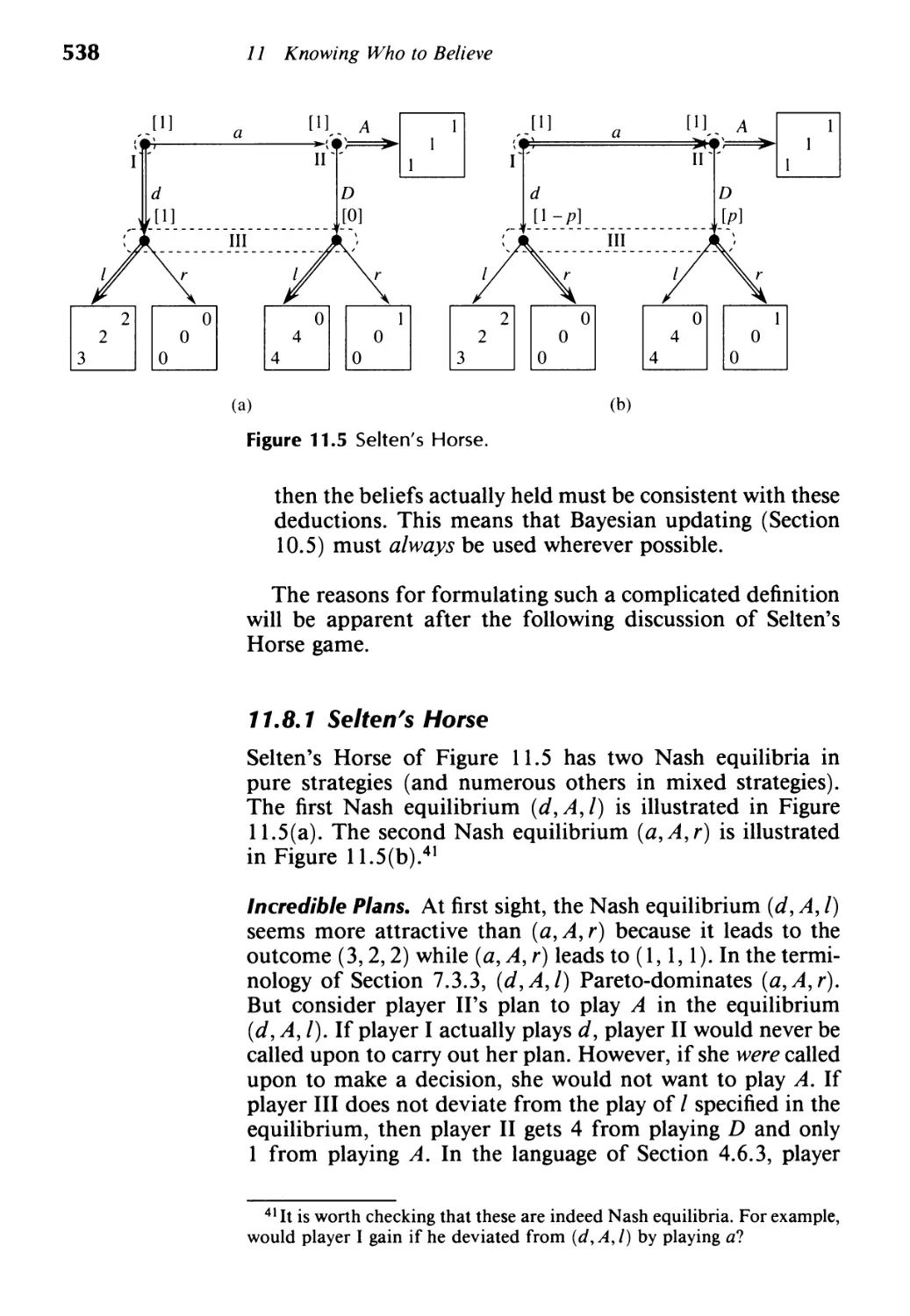
you make it your objective to get to Chapters 7, 8, 10 and
11 as soon as possible. Otherwise there is nothing more that
needs to be said to a graduate student except that it is a
waste of time to read anything at all without planning to
work at least some of the exercises. However, the position
for undergraduates is more complicated.
Even if the Mad Hatter is followed wherever he goes, Fun
and Games still contains a lot more material than it would
be wise to try and teach to undergraduates in a one-semester
course. Given that adequate time is set aside for discussion
of the exercises, there is a choice to be made about what
topics to cover. To a large extent, this is a judgment call.
However, if this book is to be used, I do not recommend
changing the order in which topics are introduced, even when
the order I have chosen may seem curious. I have been ex-
perimenting with various approaches for more than fifteen
years, and my reasons for doing it my way may not always
be immediately obvious. For example, why does the chapter
on bargaining precede the chapter on zero-sum games? The
reason is that the chapter on zero-sum games is more tech-
nically demanding for undergraduates than you might think.
In particular, whatever their background, you cannot always
rely on your students' knowing anything useful about con-
vexity at all. However, after the chapter on bargaining, they
will no longer think of a convex set as being some mysteri-
ous and incomprehensible mathematical object. Why is the
notion of a Nash equilibrium introduced in Chapter 1 and
then kept simmering all the way up to Chapter 7 before it is
discussed comprehensively? This is because undergraduates
can become overwhelmed if you try to tell them everything
at once. They often need time to build up some confidepce
in their ability to cope before you hit them with too mtich.
Why so much fuss about Hex in Chapter I? Because it is
going to get used in Chapter 7 in a discussion of fixed point
theorems. 3 Such a litany of questions and answers could be
continued indefinitely. In brief, some of the later material
depends on earlier material in ways that may not be imme-
diately apparent.
The list of chapters given next indicates what each chapter
is intended to achieve. Three routes through the material are
3 However, if you follow the Mad Hatter, you will skip most of the fuss
about Hex and all the discussion of fixed point theorems-although I have
taught both topics successfully to undergraduates.

Teaching Guide
.
XXI
then proposed, of which I would advocate the first if you are
teaching game theory to undergraduates for the first time.
Introduction. The introduction provides some ammuni-
tion for a preliminary pep-talk if this seems necessary. It is
about where game theory came from and where it is going
to, what it can do and why it matters.
1. Winning Out. The formal definition of a game is not in-
troduced all at once. This chapter introduces two-player
games of perfect information with no chance moves. A
few results about the strictly competitive case are proved
carefully to indicate the flavor of what is to come. The
ideas of Nash and subgame-perfect equilibrium make a
first tentative appearance.
2. Taking Chances. Chance moves and lotteries are intro-
duced. Elementary probability ideas are reviewed and put
to use.
3. Accounting for Tastes. A review of elementary utility the-
ory is followed by an extended example that touches upon
the modeling of imperfect information and emphasizes
that rational behavior may depend on the players' atti-
tudes to taking risks. Von Neumann and Morgenstern util-
ity theory is then discussed.
4. Getting Paid Off. The notion of a Von Neumann and Mor-
genstern payoff is systematically exploited. After an ex-
tended review of vectors and matrices, the idea of succes-
sively deleting dominated strategies is explained. Common
knowledge is mentioned briefly, and the distinction be-
tween Nash and subgame-perfect equilibrium is stressed.
5. Making Deals. This chapter is about bargaining. After
reviewing convexity, it introduces the Nash bargaining
solution. (This is the only use of cooperative game the-
ory in the book.) The remainder of the chapter uses the
Rubinstein bargaining model to press home the idea of a
subgame-perfect equilibrium.
6. Mixing Things Up. Mixed strategies are introduced as a
preliminary to a conventional analysis of zero-sum games.
(Note that mixed strategies are needed in all later chap-
ters, and minimax ideas are relevant in studying repeated
games. )
7. Keeping Your Balance. Now that Nash equilibrium is fa-
miliar, its properties are studied in some detail. Here is
where the Prisoners' Dilemma is first discussed. Reac-
tion curves, applications to oligopoly, equilibrium selec-
tion and existence are all in this long chapter. Even the
mathematics of fixed point methods is not neglected.

..
XXII
Teaching Guide
8. Repeating Yourself. This chapter is about repeated games.
It begins with an example intended to emphasize how
complicated strategies can get in this context. This ex-
ample motivates the chapter's use of finite automata in
describing strategies. A simple version of the folk the-
orem is given together with some philosophizing about
social contracts.
9. Adjusting to Circumstances. This chapter describes some
simple trial-and-error adjustment processes. It includes an
introduction to the use of game theory in evolutionary bi-
ology and a discussion of the "evolution of cooperation".
10. Knowing Your Place. This chapter contains an unusually
careful account of the role of the theory of knowledge
in game theory. Information sets are finally tied down
properly, and signaling is introduced. Common knowl-
edge gets a thorough airing, and some foundational issues
are raised.
11. Knowing Who to Believe. Incomplete information is dis-
cussed in detail. The chapter includes material on sig-
naling, auctions, the revelation principle and mechanism
design. The reasons why refinement theory is controver-
sial are mentioned.
12. Bluffing It Out. This chapter is ostensibly about Poker,
but is really an extended exercise in the use of the tech-
niques the book has introduced.
There are at least three viable routes through the book for
a one-semester course for undergraduates. Whether you wish
to prefix any of these routes with some propaganda about the
importance of game theory drawn from the Introduction is
a matter of taste. I find that there is time for a few excuri
sions off the main routes. What diversions I make depend
on whom I am teaching. When teaching mostly economists,
for example, I do not always follow the Mad Hatter past the
economics sections.
. Route 1. Begin at Chapter 1 and follow the Mad Hatter all
the way through to the end of Chapter 7.
. Route 2. Follow the first route until the end of Chapter 4,
and then skip forward to Chapter 7 and follow the Mad
Hatter onwards from there (perhaps omitting Chapter 9
and looking instead at some of the more advanced material
in Chapters 10 and 11). You will need to do some patching
on the subject of mixed strategies in Chapter 7.
. Route 3. Spend as little time as possible on Chapters 1, 2
and 3, and then follow the Mad Hatter from Chapter 4

Teaching Guide
...
XXIII
onwards (perhaps omitting some of Chapters 5, 6 or 9 to
leave more time for Chapters 10 and 11).
If the third and most ambitious route is followed, some
cautionary remarks may be helpful. Chapters 2 and 3 can be
telescoped into discussions of the games Duel and Russian
Roulette. You will not be able to evade saying something
about lotteries and expected utility, but what you say can
be kept very brief. 4 However, Chapter 1 does not compress
so readily. You will need at least to cover the extensive and
strategic forms of a game, some version of Zermelo's algo-
rithm, the notion of the value of a strictly competitive game
like Chess, and the ideas of Nash and subgame-perfect equi-
librium. However, I have two reasons for suggesting that this
chapter not be taken quite so swiftly. The first is that it is
never wise to hurry the first few lectures of any course. The
second is that Chapter 1 is partly designed to fulfill a screen-
ing role. Some of the arguments offered are therefore more
closely reasoned than is perhaps strictly necessary so as not
to give a false impression about what is coming later.
Questions and Answers
I attach very great importance to the working of exercises in
whatever course I teach. For this reason, Fun and Games con-
tains large numbers of exercises for students to work by them-
selves. Normally, I insist on written answers being handed in
to about five exercises a week. If you do this, it is impor-
tant to explain that you understand that your class is only
human, and that you are not so unreasonable as to expect
perfect answers to every problem. Some of the problems are,
and ought to be, challenging. What you want from the stu-
dents is their best shot. However, this includes being careful
about the presentation of their answers. Students learn aston-
ishingly quickly that it is not acceptable to embed a correct
answer in a few lines of indecipherable scrawl, or to sub-
merge the answer in several pages of irrelevant waffle. My
impression is that they like being made to do things right.
The students will, of course, be worried about your grading
policy, so make it clear from the outset that you understand
4Provided that your students are confident about their ability to cope with
simple probabilistic problems. Personally, I think it a great pity to skip the
Yon Neumann and Morgenstern theory of decision-making under risk. All
sorts of misunderstandings are commonly made because this theory is not
understood. However, I recognize that this is a judgment call.

.
XXIV
Teaching Guide
that they are not a randomly drawn sample from the student
population. They are a highly self-selected group and your
grades will reflect this reality. After setting some demand-
ing exercises, you can reinforce this piece of propaganda by
complimenting them on how cleverly the class as a whole ap-
proached the difficulties, even though few of them may have
been able to see their way through to a triumphant conclu-
sion. Usually, this will be nothing less than the plain truth.
Things will be going well if, after some time, you find the stu-
dents arguing among themselves about last week's problems
when you enter the classroom. As for examinations, I think
it reasonable to tell the students that you plan to ask them
questions that are similar to those that they have been asked
to do for homework, or else are even more similar to other
exercises of comparable difficulty that appear in the book.
The exercises at the end of each chapter are a mixed bunch.
They range from questions that require little more than re-
peating a definition to problems that might stump Von Neu-
mann himself. A little care is therefore necessary in selecting
problems for your students to answer. The list below is a set
of possible weekly assignments. The starred items are suitable
Assignment Exercise section
Questions
1 1.10 2 3 7 10 20
2t 1.10 21 22 23 24 25
3 2.6 5 7 1 1 21 23
4 3.7 5 9 1 1 14 22
5 4.8 2 16 21 24 25
6 5.9 13 15 21 23 25
7 6.10 4 14 15 18 19
8 6.10 27 29 34 36 41
9 7.9 1 1 1 13 14 18
lOt 7.9 27 29 34 35 40
1 1 8.6 5 8 10 21 23
12* 9.8 2 7 15 17 23
13 10.9 1 1 1 12 15 17
14*t 10.9 20 23 30 31 35
15 11.10 1 2 3 4 1 1
16*t 11.10 22 23 24 27 29
17*t 11.10 38 41 42 43 44

Teaching Guide
xxv
only for graduate students. Those marked with a dagger cover
topics that you may prefer to incorporate into the main body
of your course.
I am grateful to Bruce Linster for providing outline an-
swers to a selection of ten questions from each chapter at
the end of the book. For the earlier chapters, the answers
are mostly to questions that one might reasonably ask un-
dergraduates to attempt. These mainstream answers are sup-
plemented with a few hints on how to solve the occasional
brainteaser with which the exercises have been salted. There
is no overlap between the questions to which answers are
provided and those that appear in the suggested assignments.
Teachers can obtain a full set of answers from the publisher.
Why Teach This Way?
Notice the Mad Hatter in the margin inviting you to escape
the philosophical remarks coming up by skipping forward to
Intro the Introduction. The philosophical question to be consid-
ered is why I chose to write a book like this, rather than a
romp through some undemanding "applications" of the the-
ory in easily described economic models.
Early this morning, one of the more talented students in
my undergraduate Intermediate Microeconomics class at the
University of Michigan asked me when he was going to be
taught something with some substance: something that he
could get his teeth into. I had to tell him that Intermediate
Microeconomics is about as challenging as regular undergrad-
uate courses in economics get. Later this morning, I have to
teach a graduate class, Microeconomic Theory II. The con-
tent of this graduate course is not intrinsically difficult and
the students are intelligent, but many of them have to work
very hard to keep abreast of things. They are very ready to
work hard, but such effort would not be necessary in an ideal
world. In such a world, a person at the end of his or her un-
dergraduate career would have been equipped with the learn-
ing skills needed to cope comfortably with serious material
presented seriously. I am not talking here about a lack of
technical skills, although this is certainly part of the problem.
What holds the students back is their lack of self-confidence.
Before many of them can begin to learn in earnest, they first
have to learn that they really are able to learn. Such confi-
dence comes only through studying at least one challenging
subject in depth. Nobody can be confident about their learn-
ing skills if they have never been offered the opportunity to
do more than skim the surface of the subjects they are taught.

.
XXVI
Teaching Guide
However, too many undergraduates are never offered such an
opportunity.
Much of what passes for an undergraduate education, both
in the United States and in Europe, seems to me little more
than an unwitting conspiracy between the teacher and the stu-
dent to defraud whoever is paying the fees. The teacher pre-
tends to teach, and the student pretends to learn, material that
both know in their hearts is so emasculated that it cannot pos-
sibly be properly understood in the form in which it is pre-
sented. Even the weaker students grow tired of such a diet of
predigested pap. They understand perfectly well that "appre-
ciating the concepts" is getting them nowhere except nearer to
a piece of paper that entitles them to write letters after their
names. But most students want more than this. They want to
learn things properly so that they are in a position to feel that
they can defend what they have been taught without having
to resort to the authority of their teachers or the textbook. Of
course, learning things properly can be hard work. But my ex-
perience is that students seldom protest at being worked hard
provided that their program of study is organized so that they
quickly see that their efforts are producing tangible dividends.
However, it is one thing to see that our system of education
could be improved, but quite another to do something about
it. When teaching traditional courses in economics and the
other social sciences, one tends to get trapped by the system.
It is particularly hard to organize a serious course in a way that
allows students to see their efforts being quickly rewarded.
Teachers of introductory courses will typically already have
skimmed the cream from the material that you are supposed
to teach by discussing most of the intellectually exciting ideas
in some diluted form. But you will seldom be able to rely on
students' knowing what is taught in such introductory courses
sufficiently well that you can make use of their knowledge. In-
deed, what lodges in the minds of students when they are "ap-
preciating the concepts" in introductory courses is sometimes
so confused that they need to be "untaugpt" before further
progress is possible. A great deal of what students will despise
as "review material" is therefore inevitable unless you are will-
ing to be innovative about the syllabus. But monkeying around
with the syllabus is seldom a practical option unless your col-
leagues teaching companion courses are unusually tolerant.
Teaching game theory provides an opportunity to break
free from some of these constraints, because traditions about
how it should be taught have yet to evolve. In particular, it
usually gets only a passing mention in introductory courses.
Most students who sign up for game theory therefore come

Teaching Guide
..
XXVII
with an open mind in the hope of being taught something
new and interesting. They sometimes even think that the ma-
terial may be fun to learn. They also know that the subject
does not depend too heavily on material that should have
been mastered in earlier courses but is now water long gone
under the bridge. In none of these expectations will they be
disappointed. It is also true that game theory has assumed
a central role in much of economic theory, and so students
who are contemplating graduate work can congratulate them-
selves on doing something that will certainly be useful to
them. At the same time, you can truthfully tell students that
the role of game theory is bound to expand in the future, not
only within economics, but also in the other social sciences.
It already has, for example, firm footholds in biology and
political science.
All of this means that someone teaching game theory can
afford to be more ambitious than the teacher of a more tra-
ditional subject. The students come with a positive attitude,
and you can carry them forward quickly into areas that will
seem new and exciting to them. An opportunity therefore ex-
ists to provide some genuine education-to train some minds
in how to think about serious problems seriously. I believe
that, although the substantive content of game theory is cer-
tainly of great importance, it is this opportunity that should
excite us most. That is to say, in teaching game theory, it really
is true that the medium is at least as important as the message.
Other Books
Robert Aumann, Lectures on Game Theory, Westview Press
(Underground Classics in Economics), 1989. These are the
classroom notes of one of the great game theorists.
Robert Aumann and Sergio Hart, Handbook of Game Theory.
This will be a comprehensive collection of survey articles on
game theory and its applications for research workers in the
field.
Elwyn Berlekamp, John Conway and Richard Guy, Winning
Ways for Your Mathematical Plays, Academic Press, 1982.
This is a witty and incredibly inventive book about com-
binatorial game theory. The authors try very hard to make
their ideas accessible to the layman, but I suspect one needs
mathematical training for it to hold the attention.
Ken Binmore, Essays on the Foundations of Game Theory,
Blackwell, 1990. Some of these essays grapple with the con-
troversial issues that Fun and Games avoids, but don't expect

...
XXV III
Teaching Guide
any definitive answers. (Readers of Fun and Games will be
able to skip Chapters 2, 3 and 4.)
Steven Drams, Superior Beings, Springer-Verlag, 1983. If you
thought game theory had no applications in theology-think
again!
Avinash Dixit and Darry Nalebuff, Thinking Strategically,
Norton, 1991. This is a delightful collection of stories and
anecdotes drawn from real life that illustrate game theory in
action. Its accessibility is attested to by its appearance on the
Book-of-the-Month Club list.
James Friedman, Game Theory with Applications to Econom-
ics, second edition, MIT Press, 1990. James Friedman pio-
neered the application of repeated games to problems in indus-
trial organization. Here you can learn the tricks of the trade.
Drew Fudenberg and Jean Tirole, Game Theory, MIT Press,
1991. This is the book to read if you want to be published
in Econometrica. It is remarkable how much ground they
manage to cover.
Josef Hofbauer and Karl Sigmund, The Theory of Evolution
and Dynamical Systems, Cambridge University Press, 1988.
This is a highly accessible and unfussy introduction to the
mathematics of evolutionary systems.
Tashiro Ichiishi, Game Theory for Economic Analysis, Aca-
demic Press, 1983. This is a formal book that concentrates
on cooperative game theory. The mathematical exposition is
admirably clear and unfussy.
David Kreps, A Course in Microeconomic Theory, Princeton
University Press, 1990. This big book takes it for granted
that game theory is part of microeconomic theory. It is a
must for those planning to make a career in economics. The
problems are often very instructive indeed.
David Kreps, Game Theory and Economic Modelling, Ox-
ford University Press, 1990. Listen to what daddy says on
economic modeling and you won't go far wrong!
Duncan Luce and Howard Raiffa, Games and Decisions, Wi-
ley, 1957. This evergreen classic is a model for how a book
should be written.
John Maynard Smith, Evolution and the Theory of Games,
Cambridge University Press, 1982. Everyone should at least
dip into this beautiful book.
Herve Moulin, Game Theory for the Social Sciences, second
revised edition, New York University Press, 1986. This is an
elementary introduction to game theory in which the mathe-

Teaching Guide
.
XXIX
matics is allowed to speak for itself. It is particularly valuable
as a source of instructive problems. (You want both volumes.)
Roger Myerson, Game Theory: Analysis of Conflict, Harvard
University Press, 1991. Roger Myerson is the prime mover in
the subject of mechanism design. His book is an encyclopedic
introduction to game theory in which each brick is carefully
laid precisely where it belongs. This is a book for those who
feel that things should be done properly.
Peter Ordeshook, Game Theory and Political Theory, Cam-
bridge University Press, 1986. This is the place to look for
applications in political science.
Martin Osborne and Ariel Rubinstein, Bargaining and Mar-
kets, Academic Press, 1990. If you want more on bargaining
than Chapter 5 of Fun and Games has to offer, this is an
excellent place to begin.
Guillermo Owen, Game Theory, second edition, Academic
Press, 1982. This elegant book is particularly strong on co-
operative game theory.
Eric Rasmusen, Games and Information, Blackwell, 1989.
This is a book for those who want to get straight to the eco-
nomic applications without having to fiddle around with the
theory first.
Thomas Schelling, The Strategy of Conflict, Harvard Univer-
sity Press, 1960. This is a classic that will remain on every-
body's reading list for many years to come.
Martin Shubik, Game Theory in the Social Sciences, MIT
Press, 1984. Martin Shubik is one of the great pioneers in
applying game theory to economics. 'The second volume of
this monumental work is where he gives us the benefit of his
wide experience.
Jean Tirole, The Theory of Industrial Organization, MIT
Press, 1988. This beautiful book is a model of its kind. Those
who want a quick introduction to game theory will find their
needs catered to in a magnificently concise appendix.
John Yon Neumann and Oskar Morgenstern, The Theory of
Games and Economic Behavior, Princeton University Press,
1944. I have read the great classic of game theory from cover
to cover, but I do not recommend the experience to others!
Its current interest is largely historical.
Herbert Yardley, The Education of a Poker Player, Jonathan
Cape, 1959. Don't waste time on Chapter 12 of Fun and
Games if what you care about is how to make money playing
Poker.

Introduction
1


0.1 What Is Game Theory About?
3
The poet Horace advised his young disciples to begin in me-
dia res. I think he was right. The way to learn game theory is
to turn straight to the first chapter and plunge into the mid-
dle of things. This introduction is for the faint-hearted and
the middle-aged who want some questions answered before
making a commitment.
. What is game theory about?
. Where is it coming from?
. Where is it going to?
. What can it do for us?
These are big questions to which there are no neat and tidy
answers. An introduction can only give some flavor of the
answers that game theorists offer. l But perhaps this will be
enough to whet your appetite.
0.1 What Is Game Theory About
A game is being played whenever people interact with each
other. If you drive a car in a busy city street, you are playing
a game with the drivers of the other cars. When you make
a bid at an auction, you are playing a game with the other
bidders. When a supermarket manager decides the price at
which she will try to sell cans of beans, she is playing a game
with her customers and with the managers of rival supermar-
kets. When a firm and a union negotiate next year's wage
contract, they are playing a game. The prosecuting and de-
fending attorneys are playing a game when each decides what
arguments to put before the jury. Napoleon and Wellington
were playing a game at the Battle of Waterloo, and so were
Khrushchev and Kennedy during the Cuban missile crisis.
If all these situations are games, then game theory is clearly
something important. Indeed, one could argue that all the so-
cial sciences are nothing more than subdisciplines of game
theory. However, this doesn't mean that game theorists are
the people to ask for answers to all the world's problems.
This is because game theory, as currently developed, is mostly
about what happens when people interact in a rational man-
ner. If this observation tempts you to return Fun and Games
1 Chapter 1 of my Essays on the Foundations of Game Theory (Black-
well, 1990) is a longer introduction to the subject. Dixit and Nalebuff's
Thinking Strategically (Norton, 1991) is a delightful collection of stories
and anecdotes showing game theory in action in real-life situations. Kreps'
Game Theory and Economic Modelling (Oxford University Press, 1990) is
an introduction that emphasizes the uses of game theory in economics.

4
Introduction
to the bookstore in the hope of getting your money refunded,
think again. Nobody is saying that people always behave ra-
tionally. But neither is it true that people always act irra-
tionally. Most of us try at least to spend our money sensibly,
and most of the time we don't do too badly. Otherwise, eco-
nomic theory wouldn't work at all. Even when we are not
actively thinking things out in advance, it does not neces-
sarily follow that we are behaving irrationally. In fact, game
theory has had some notable successes in analyzing the be-
havior of insects and plants, neither of which can be said
to think at all. Their behavior is rational because those in-
sects and plants whose genes programmed them to behave
irrationally are now extinct. Evolution removed them. And,
just as biological evolution acts to remove biologically un-
fit behavior, so other kinds of evolution can act to remove
socially or economically unfit behavior. For example, firms
that manage their affairs stupidly tend to go bankrupt and so
disappear from the scene.
Perhaps you will agree that rational interaction between
groups of people is an exciting area to study, but why call it
game theory? Do we not trivialize the problems that people
face by calling them games? Worse still, do we not devalue
our humanity by reducing our struggle for fulfillment to the
status of mere play in a game?
The proper answers to these questions stand them on their
heads. The more deeply we feel about issues, the more im-
portant it is that we do not allow ourselves to be misled by
wishful thinking. Game theory makes a virtue out of using
the language of parlor games like Chess or Poker to discuss
the logic of strategic interaction. I know that Bridge players
sometimes shoot their partners. I have sometimes felt the
urge myself. Nevertheless, most of the time, people are able
to think about the strategic issues that arise in parlor games
dispassionately. That is to say, they are willing to follow the
logic wherever it goes without throwing their hands up in
horror if it leads to an unwelcome destination. In insisting
on using the language of parlor games, game theorists are
therefore not revealing themselves to be cold-hearted follow-
ers of Machiavelli who care nothing for the sorrows of the
world. They are simply attempting to separate those features
of a problem that are susceptible to uncontroversial rational
analysis from those that are not.
Human beings are not naturally very good at thinking about
problems of strategic interaction. We become distressed when
confronted with circular reasoning. But circular reasoning
cannot be evaded in considering strategic issues. If John and

0.1 What Is Game Theory About?
5
Mary are playing a game, then John's choice of strategy will
depend on what he predicts Mary's choice of strategy will be.
But she is simultaneously choosing a strategy, using her pre-
diction of John's strategy choice. Given that it is necessarily
based on such involuted logic, it is perhaps not surprising that
game theory abounds with surprises and paradoxes.
. Is it possible, do you think, that someone at a committee
meeting might find it optimal to vote for the alternative
they like the least?
. Could it be be a good idea for a general to toss a coin to
decide whether to attack today or tomorrow?
. Can it be optimal for a Poker player always to bet the max-
imum when dealt the worst possible hand?
. Could it ever make sense for someone with goods to trade
to begin by throwing some of them away?
. Might it ever be rational for someone with a house to sell to
use an auction in which the highest bidder gets the house, but
only has to pay the bid made by the second-highest bidder?
You will have guessed, of course, that the seemingly crazy
answer is correct in each case. Let us look at the first and
last questions to try and understand why our intuitions are
so unhelpful. This will simultaneously provide some feel for
the whole book, since problems of the first kind are discussed
in Chapter 1 at the beginning of the book, and problems of
the last kind are discussed in Chapter 11 towards its end.
0.1. 1 Strategic Voting
Boris, Horace and Maurice are the membership committee
of the very exclusive Dead Poets Society. The final item on
their agenda one morning is a proposal that Alice should be
admitted as a new member. No mention is made of another
possible candidate called Bob, and so an amendment to the
final item is proposed. The amendment states that Alice's
name should be replaced by Bob's. The rules for voting in
committees call for amendments to be voted on in the order
in which they are proposed. The committee therefore begins
by voting on whether Bob should replace Alice. If Alice wins,
they then vote on whether Alice or Nobody should be made
a new member. If Bob wins, they then vote on whether Bob
or Nobody should be made a new member. Figure O.I(a) is a
diagrammatic representation of the order in which the voting
takes place. Figure 0.1 (b) shows how the three committee
members rank the three possible outcomes.

6
Introduction
Alice
Alice
or
Nobody Bons Horace Maunce
Nobody I. Alice I. Nobody I. Bob
Alice
or 2. Nobody 2. Alice 2. Alice
Bob
Nobody 3. Bob 3. Bob 3. Nobody
Bob
or (b)
Nobody
Bob
(a)
Figure 0.1 Strategic voti ng.
The doubled lines in Figure 0.1 (a) show who would win
the vote if everybody just voted according to their rankings.
For example, in a vote between Alice and Bob, Alice would
win because both Boris and Horace rank Alice above Bob and
so Maurice would be outvoted. Thus, if there is no strategic
voting, Alice will be elected to the club because she will also
win when she is matched against Nobody.
However, if Horace looks ahead, he will see that there is
no point in voting against Bob at the first vote. If Bob wins
the first vote, then Nobody will triumph at the second vote,2
and Nobody is Horace's first preference. Thus, Horace should
switch his vote from Alice at the first vote, and cast his vote
instead for Bob, who is the candidate he likes the least. If
Boris and Maurice do not also vote strategically, the result
will be that Nobody is elected.
But this is not the end of the story. Maurice may anticipate
that Horace will vote strategically. If so, Maurice will also
vote strategically by switching his vote from Bob to Alice.
Maurice will then fail to vote for the candidate he likes the
most. His reason for doing so is that he thereby ensures that
Alice is elected rather than Nobody.
The reasoning used by Horace and Maurice in this story is
called backwards induction. They predict what would happen
in the future and then reason backwards to the present. The
mathematician Zermelo applied the same type of reasoning
2 Why is there no point in anyone voting strategically at the second vote?

0.1 What Is Game Theory About?
7
to Chess as long ago as 1912. For this reason, the process is
called Zermelo's algorithm in Section 1.4 of the text.
Game theorists care about what happens when everybody
reasons optimally. Here this means that everybody uses Zer-
melo's algorithm, and hence everybody votes strategically.
Does this mean that Alice gets elected? You will be able to
work this out for sure after reading Chapter I!
Econ
0.1.3
o. 1.2 Auctions
Mad Hatters, like the little guy who has just appeared in the
margin, are designed to help you find your way around the
text. The Teaching Guide explains their significance in detail.
) Here he is rushing on to Section 0.1.3 to avoid learning some
economics. Mathematical folk may think him wise. As Lewis
Carroll put it:
And what mean all these mysteries to me
Whose life is full of indices and surds?
x 2 + 7x + 53
11
=.'.3
However, you won't get much from this book if you just read
the mathematical bits.
Alice wants to get the best price she can for her very fancy
house. There are two potential buyers, Horace and Maurice.
If she knew the maximum each would be willing to pay, her
problem would be easy. However, although she doesn't know
their reservation prices, she is not entirely ignorant. It is com-
mon knowledge that each potential buyer has a reservation
price of either three million or four million dollars, and that
each value is equally likely. Moreover, the two reservation
prices are independent of each other (Section 2.1.2).
An auctioneer advises her to run a "second-price auction".
In such an auction, each bidder secretly seals his bid in an
envelope. The envelopes are then publicly opened, and the
house is sold to the highest bidder,3 but not at the price he
bid. Instead it is sold to him at the highest price bid by a
loser. The advantage of such an arrangement, the auctioneer
explains, is that it induces rational people to bid their true
reservation prices. Horace, for example, would reason like
this. Suppose that Maurice's bid is for less than my reser-
vation price. Then I want to win the auction, and I can do
so just by bidding my own reservation price truthfully. On
3 If there is a tie, it is broken at random.

8
Math
o. 1.3
Introduction
the other hand, if Maurice's bid is for more than my reser-
vation price, then I don't want to win, and I can guarantee
not doing so by bidding my own reservation price truthfully.
Thus, in a second-price auction, telling the truth about your
reservation price is a heads-I-win-tails-you-Iose proposition.
Game theorists say that bidding truthfully is a strategy that
dominates all its alternatives.
Alice understands all this, but she doesn't much like what
she hears. It seems obvious to her that she must do better by
selling the house for the highest price that gets bid rather than
for the second highest price. So she fires the first auctioneer
and hires instead a second auctioneer who tells her what she
wants to hear. He organizes a sealed-bid auction just like the
first auctioneer's, except that the house is now sold to the
highest bidder at whatever price he bids.
But Alice is wrong. Her expected selling price is $3!m in
both cases. 4 This is easy to see in the case of the second-price
auction. Alice will then make $3m except when both Horace
and Maurice have a reservation price of $4m. The probabil-
ity that both have a high reservation price is ! x ! = !. Her
expected selling price in millions of dollars is therefore
3 x  + 4 x ! = 3!.
Perhaps this mention of probabilities and expected values
makes you feel apprehensive. If so, take careful note of the
Mad Hatter who has appeared in the margin, and follow him
by rushing on to the next section. What you need to know
about probabilities and expected values (which isn't much)
will be reviewed in Chapter 2. As for the piece of mathemat-
ics that the Mad Hatter is rushing on to avoid, you might use
this as a test for how suitable Fun and Games is for someone
with your background. At the end of the book, I hope that
such an argument will seem transparently clear. However, if
you get more than a general impression about what is going
on right now, then you should perhaps be thinking of reading
a more advanced book 5 than this!
To figure out what selling price Alice can expect in a "first-
price" sealed-bid auction, we need to solve the bidding prob-
lem such an auction poses for Horace and Maurice. A
consultant game theorist will see no reason to advise someone
with a reservation price of $3m to do anything but bid this
truthfully. However, if Horace has a high reservation price of
4 Provided that Horace and Maurice bid rationally and are risk-neutral
(Section 3.4.3).
5Like Fudenberg and Tirole's Game Theory (MIT Press, 1991) or Myer-
son's Game Theory: Analysis of Conflict (Harvard University Press, 1991).

0.1 What Is Game Theory About?
9
$4m, he may get some curious advice from the game theorist.
The game theorist will explain that, whatever bid Horace may
think of sealing in his envelope, there is a risk that Maurice
will predict it. If he does, Maurice will then win the auction
by bidding one penny more on those occasions when he also
has a high reservation price. The only way that Horace can be
sure of keeping Maurice guessing is by using a mixed strategy.
What this means is that Horace should randomize over the
bids that it is sensible for him to make.
If Horace is still listening, the game theorist will now start
getting serious about how Horace should randomize. The ad-
vice might go like this. Never bid less than $3m or more than
$3m. Randomize over all the bids between $3m and $3m
in such a way that the probability of your bidding less than
$b is precisely (b - 3)/(4 - b).
If Maurice is also getting exactly the same advice from an-
other game theorist, how much should Horace expect to make
when his randomizing device tells him to seal $bm in his enve-
lope? If he outbids Maurice, he will make $ (4 - b )m, because
this is the difference between what he pays and what the house
is worth to him. If he loses, he makes nothing. How often will
Horace win? Half the time he will win for certain because
Maurice's reservation price will be only $3m. The other half
of the time, Horace will win with probability (b - 3)/( 4 - b),
because this is the probability that Maurice will bid less than
$bm when his reservation price is $4m. Thus, the total prob-
ability that Horace wins when he bids $bm is
11 ( b-3 ) 1
2 + 2 4 - b = 2(4 - b) ·
His expected gain is obtained by multiplying this probabil-
ity by $(4 - b)m, which is what he gets when he wins. His
expected gain is therefore always $m whatever bid $bm be-
tween $3m and $3m he may make.
The reason that game theorists will offer such complicated
advice to Horace and Maurice is that, if they follow it, then
each will be responding optimally to the strategy choice of
the other. In particular, there is nothing that Horace can do
to improve on $m. He will certainly never want to bid $Bm
when B > 3 because, although this guarantees his winning
the auction, his victory will be hollow since he will make only
$(4 - B) from his triumph. 6
It will be clear that Alice was premature in thinking that
6 Assuming that his reservation price is high. If his reservation price is
low, he will never want to bid more than $3m.

10
Introduction
anything in this situation is "obvious". Much of the time, Ho-
race and Maurice will be bidding far below their true reserva-
tion prices. Alice therefore needs to calculate quite hard
before she is entitled to an opinion on the relative merits of
first and second price auctions. If she assumes that Horace and
Maurice follow the advice of their tame game theorists, she
will find that her expected selling price will be exactly the same
in a first-price auction as in a second-price auction-namely
$3!m. It will also be the same in various other types of auction.
In particular, the expected selling price is exactly the same in
the familiar type of auction in which the buyers keep raising
each other's bids until only one contender is left bidding.
Should we conclude that Alice is wasting her time in look-
ing for a better auction? Far from it! If Alice reads Fun and
Games as far as Section 11.7.4, she will discover that, if she
is clever, she can design an auctioning mechanism that raises
her expected selling price to a magnificent $3tm.
o. 1.3 What Is the Mora/I
The two preceding examples are intended to make it clear
that game theory is good for something. Our untutored in-
tuition is not very reliable in strategic situations. We need
to train our strategic intuition by considering instructive ex-
amples. These need not be realistic. On the contrary, there
are often substantial advantages in studying toy games, if
these are carefully chosen. In such toy games, all the irrel-
evant clutter that typifies real-world problems can be swept
away so that attention can be focused entirely on the strategic
questions for which game theory exists to provide answers.
Often, game theorists introduce their toy games with silly
stories. It is a little silly, for example, that the committee mem-
bers in the strategic voting example were called Boris, Horace
and Maurice. 7 But even such silliness is not without its value.
Here, it allows us to disengage our emotions from the prob-
lem. Nobody can get worked up about fictions like Boris, Ho-
race and Maurice. However, if they were recognizable as real
people, we might let our indignation at the fact that the chair-
man has "rigged the agenda", or that Horace is planning to
"vote dishonestly", distract our attention from the underlying
strategic realities. For a game theorist, this would be an error
comparable to a mathematician's fudging on the laws of arith-
metic because he dislikes the answers he is coming up with.
7Those whose native language is not the Queen's English may be surprised
to learn that these names rhyme.

Phil
0.4
0.2 Where Is Game Theory Coming From?
11
0.2 Where Is Game Theory
Coming From 
Game theory was created by Von Neumann and Morgenstern
in their classic book The Theory of Games and Economic
Behavior, published in 1944. Others had anticipated some
of the ideas. The economists Cournot and Edgeworth were
particularly innovative in the nineteenth century. Later con-
tributions mentioned in this book were made by the math-
ematicians Borel and Zermelo. Von Neumann himself had
already laid the groundwork in a paper published in 1928.
However, it was not until Von Neumann and Morgenstern's
book appeared that the world realized what a powerful tool
for studying human interaction had been discovered.
When the penny dropped, people went overboard in their
enthusiasm. The social sciences, so it was thought, would be
revolutionized overnight. But this was not to be. Von Neu-
mann and Morgenstern's book proved to be just he first step
on a long road. However, there is no mind more closed than
that of a disappointed convert, and once it became clear that
The Theory of Games and Economic Behavior was not be
compared with the tablets of stone that Moses brought down
from the mountain, game theory languished in the doldrums.
One can still find old men who will explain that game theory
is useless because life is not a "zero-sum game", or because
one can get any result one likes by selecting an appropriate
"cooperative solution concept".
Fortunately, things have moved on very rapidly in the last
twenty years, and this and other modern books on game the-
ory are no longer hampered by some of the restrictive assump-
tions that Von Neumann and Morgenstern found necessary to
make progress. As a consequence, the early promise of game
theory is beginning to be realized. Its impact on economic
theory in recent years has been nothing less than explosive.
However, it is still necessary to know a little about game the-
ory's short history, if only to understand why some of the
terminology is used.
Yon Neumann and Morgenstern investigated two distinct
possible approaches to the theory of games. The first of these
is the strategic or noncooperative approach. This requires
specifying in close detail what the players can and cannot
do during the game, and then searching for a strategy for
each player that is optimal. At first sight, it is not even clear
what optimal might mean in this context. What is best for
one player depends on what the other players are planning
to do, and this in turn depends on what they think the first

12
Introduction
player will do. Von Neumann and Morgenstern solved this
problem for the particular case of two-player games in which
the players' interests are diametrically opposed. Such games
are called strictly competitive or zero-sum because any gain
by one player is always exactly balanced by a corresponding
loss by the other. Chess, Backgammon and Poker are games
that usually get treated as zero-sum.
In the second part of their book, Von Neumann and Mor-
genstern developed their coalitional or cooperative approach,
in which they sought to describe optimal behavior in games
with many players. Since this is a much more difficult prob-
lem, it is not surprising that their results were much less
sharp than for the two-player, zero-sum case. In particu-
lar, they abandoned the attempt to specify optimal strate-
gies for individual players. Instead, they aimed at classifying
the patterns of coalition formation that are consistent with
rational behavior. Bargaining, as such, had no explicit role
in this theory. In fact, they endorsed a view that had held
sway among economists since at least the time of Edgeworth,
namely that two-person bargaining problems are inherently
indeterminate.
In a sequence of remarkable papers in the early fifties, the
mathematician John Nash broke open two of the barriers
that Von Neumann and Morgenstern had erected for them-
selves. On the noncooperative front, they seem to have felt
that the idea of an equilibrium in strategies, as introduced
by Cournot in 1832, was not an adequate notion in itself
on which to build a theory-and hence their restriction to
zero-sum games. However, Nash's general formulation of the
equilibrium idea made it clear that no such restriction is nec-
essary. Nowadays the notion of a Nash equilibrium 8 is per-
haps the most important of the tools that game theorists have
at their disposal. Nash also contributed to Von Neumann and
Morgenstern's cooperative approach. He disagreed with the
view that game theorists must regard two-person bargaining
problems as indeterminate, and proceeded to offer arguments
for determining them. His views on this subject were widely
misunderstood and, perhaps in consequence, game theory's
years in the doldrums were largely spent pursuing Von Neu-
mann and Morgenstern's cooperative approach along lines
that ultimately turned out to be unproductive.
8This arises when each player's strategy choice is a best reply to the
strategy choices of the other players. Horace and Maurice were advised to
use a Nash equilibrium by their consultant game theorist when wondering
how to bid in the first-price auction of Section 0.1.2.

0.3 Where Is Game Theory Going To?
13
The history of game theory in the last twenty years is too
packed with incident to be chronicled here. However, there
are some names that cannot pass unmentioned. The acronym
NASH may assist in remembering who they are. Nash himself
gets the letter N; A is for Aumann; S is for both Shapley and
Selten; and H is for Harsanyi. By the end of the book, you
won't be needing an acronym!
What is perhaps most important about the last twenty
years in game theory is that all the major advances have
been made in noncooperative theory. For this reason, Fun and
Games confines its attention almost entirely to this branch of
the subject. This is not because I believe that no insights are
to be found in cooperative game theory, but simply because
I share with many others the belief that one cannot sensibly
discuss the cooperative branch of the subject without first
having mastered the noncooperative branch.
0.3 Where Is Game Theory Going To?
It is hard to explain where game theory is going to an audi-
ence that doesn't know where it's at. So these remarks are
Phil for people who know some game theory already.
0.4 I have some very firm views on where game theory ought
to be going, and it is encouraging to see that things seem to
be moving in the right direction. However, I have kept these
views out of the text nearly everywhere, because I think a
book written at this level should contain a minimum of con-
troversial material. However, it is only right that I should lay
my cards on the table somewhere. So let me say that I think
most of the literature on "refinements of Nash equilibrium"
belongs on the same shelf with the works of the medieval
scholastics. Even more controversially, let me say that at-
tempts to make Bayesianism the foundation stone for game
theory should be likened not so much to building houses
upon the sand, but to the building of castles in the air. In
retrospect, the current elevation of Bayesian decision the-
ory to something more than a convenient analytical tool will
seem very odd indeed. 9
My gesture to the future is Chapter 9, which some may
feel is an idiosyncratic inclusion. It is about how equilibrium
may be achieved by evolutionary trial-and-error processes
when the players are not fully rational. The appearance of
finite automata in Chapter 8 is also partly motivated by the
9Chapters 4, 5 and 6 of my Essays on the Foundations of Game Theory
(Blackwell, 1990) summarize my views on these issues.

14
Introduction
importance I attach to getting some sort of handle on the
problem of bounded rationality in game theory. Of course,
those who disagree about the way ahead are free to skip this
material.
0.4 What Can Game Theory Do
for Us
This section gives some indications of how game theory can
be applied. Economics is the biggest customer for the ideas
churned out by game theorists, and so this is the discipline
with which to begin.
0.4. 1 Applications in Economics
It should not be surprising that game theory has found ready
application in economics. The dismal science is supposedly
about the allocation of scarce resources. If resources are
scarce, it is because more people want them than can have
them. Such a scenario creates all the necessary ingredients
for a game. Moreover, neoclassical economists proceed on
the assumption that people will act rationally in this game.
In a sense, neoclassical economics is therefore nothing other
than a branch of game theory. Economists who do not re-
alize this are like M. Jourdain in Moliere's Le Bourgeois
Gentilhomme who was astonished to learn that he had been
speaking prose all his life without knowing it. However, al-
though economists may always have been closet game the-
orists, their progress was hampered by the fact that they
did not have access to the tools provided by Von Neumann
and Morgenstern. As a consequence, they could only analyze
particularly simple games. This explains why monopoly and
perfect competition are well-understood, while all the vari-
eties of imperfect competition that lie between these two
extremes are only now beginning to get the detailed treat-
ment they deserve.
The reason that monopoly is simple from a game-theoretic
perspective is that it can be treated as a game with only one
player. The reason that perfect competition is simple is that
the number of players is effectively infinite, so that each indi-
vidual agent can have no effect on market aggregates if he or
she acts alone. A toy model may help to clarify this point. It
will also indicate why game theory is so intimately connected
with the problem of imperfect competition. lo
lOSection 7.2 covers the same ideas in more detail.

0.4 What Can Game Theory Do for Us?
15
Cournot Oligopoly. An industry contains N firms who all have
constant unit cost c. Each firm simultaneously decides on an
outputqj. Whenthetotaloutputq = ql + q2 +... + qNgetsun-
loaded on the market, the price at which it sells is given by the
demand equationp = D(q). The ith firm's profit is then
nj = pqj - cqj = (D(q) - c)qj,
which is its revenue minus its cost.
A game theorist sees such a Cournot oligopoly problem as
a game with N players, each of whom chooses a strategy qj
with the purpose of maximizing profit nj. At a Nash equilib-
rium, each player's choice of strategy will be optimal given
the strategy choices of the others.
To make a best reply to the strategy choices of the other
firms, the ith firm will choose its own strategy qj so that
an.
_ a I = D' ( q ) q j + D ( q) - c = 0 .
qj
If all the firms behave like this, they will all choose the same
output. Thus qj = q / N, where
D'(q)  + D(q) - c = o.
Consider the special case in which the price elasticity of
demand is constant. This just means that p = D(q) = kq-e,
where k and e are positive constants. The equation then sim-
plifies to
p_ ( e ) -l
-- 1--
c N.
This formula will be familiar to economists in the case
N = 1 as the profit-maximizing mark-up for a monopolist.
When N  00, we obtain that p = c. This is the classic result
of perfect competition that says that the equilibrium price
must equal marginal cost. For intermediate values of N, we
have a result about equilibrium behavior in a model with
imperfect competition.
Such calculations require no special knowledge of game the-
ory. However, as soon as one turns to models in which timing
or risk is important, or in which the handling of information
matters, then one is helpless without the conceptual scaffold-
ing that game theory provides. Auctions, insurance markets,
patent races, entry deterrence and bargaining are just some
of the topics on which we can now speak with some author-
ity where previously little or nothing could usefully be said.
Some of these topics are studied in a preliminary way in Fun

16
Introduction
and Games. However, you will have to look elsewhere for a
systematic exploitation of game theory ideas in economics. 1 1
If such a task were attempted here, no room would be left to
describe the theory itself.
0.4.2 Applications in Political Science
Game theory has not had the same impact in political sci-
ence as in economics. Perhaps this is because people behave
less rationally when their ideas are at stake rather than their
money. Nevertheless, it has become an important tool for
clarifying the underlying logic of a number of paradigmatic
problems. Strategic voting was mentioned in Section 0.1.1.
Here a simple model will be studied that seeks to cast some
light on how parties choose their political platforms. It bears
a family resemblance to economic models in which the in-
cumbent firms in an industry distort their behavior in an
attempt to deter new firms from entering the industry.
Choosing a Platform. This toy game begins with two political
parties: the Formalists and the Idealists. Neither cares any-
thing for matters of principle. They care only about power,
and so choose a platform with the sole aim of maximizing
their vote at the next election. The voters, on the other hand,
care only about matters of principle and hence are devoid
of party loyalties. For simplicity, the opinions a voter might
hold are identified with the real numbers x in the interval
[0, 1 ].12 One can imagine that this interval represents the
left-right political spectrum. Thus, someone with the opin-
ion x = 0 believes society should be organized like an anthill,
while someone with the opinion x = 1 thinks it should be or-
ganized like a pool of sharks.
Each party chooses its platform somewhere along the po-
litical spectrum and is not able to shift its position later. The
voters then cast their votes for the party whose position is
nearest to their own. Since the voters are assumed to be uni-
formly distributed 13 over the political spectrum, it is easy
to see how many votes each party will get once both have
chosen their platforms. The secret is to look for the median
11 Perhaps Tirole's Theory of Industrial Organization (MIT Press, 1988)
or, at a more advanced level, Fudenburg and Tirole's Game Theory (MIT
Press, 1991).
12The interval [0, 1] is the set of values of x satisfying 0  x  1.
13This just means that a fraction I of the population have views lying in
any interval of length I.

0.4 What Can Game Theory Do for Us?
17
Median
Idealists voter Formalists
o  x = , {x = ,7 0 1 1
.
I
I
v  \... v
40% 60%
(a)
Idealists Intuitionists Formalists
i { I {
I
I
0 1 I 1 1
. I .
I
I I
v  v
37.5% 250/0 37.50/0
(b)
Idealists Formalists
0 1 i { 1 1
I .
I
I
v  \. v
50% 50%
(c)
Figure 0.2 Choosing a political platform.
voter amongst those whose opinions lie between the two party
platforms. The median voter is located halfway between the
political positions of the two parties. Hence those to the right
of the median voter cast their votes for one party, and those
to the left cast their votes for the other. Figure 0.2(a) pro-
vides an example.
Suppose that the parties enter the political arena one by
one. First the Idealists choose a platform and then the For-
malists. Where should each locate? Such problems can be
solved by backwards induction, as explained in Section 0.1.1.
For each possible platform x, the Idealists ask what would
happen if they located at x. If x < !, the Formalists would re-
spond by locating just to the right of x. The Idealists would
then pick up a fraction x of the voters and the Formalists
ould pick up 1 - x. The Idealists would then receive less
than half the vote. The same is true if the Idealists locate at
x > !, except that now the Formalists will respond by locat-
ing just to their left. It is therefore best for the Idealists to
locate at the center of the political spectrum. The Formalists
will then also locate at x = !, and the vote will split fifty-fifty.
Such a model may make sense for the American politi-
cal scene. Certainly Europeans find it hard to discern any

18
Introduction
significant difference between Democrats and Republicans.
However, the model clearly bears little resemblance to the
European political scene. Should Americans therefore de-
duce that European political parties actually care about the
principles that they espouse? Such a conclusion would be
premature because it is doubtful whether the European situ-
ation can be sensibly analyzed with a two-party model, even
in countries like Britain where only two of the parties get
a sizable number of votes at most elections. To explore this
observation, let us consider how things would change if there
were a third party to be taken into account.
In this model, the Intuitionist party chooses a platform
after the Idealists and the Formalists. This changes things a
great deal. The Idealists and the Formalists will now certainly
not locate at the center of the political spectrum. If they were
to do so, the Intuitionists could locate immediately to their
left or right. They would then take half the vote, leaving the
original parties to split the other half. A backwards induction
argument 14 shows that the Idealists and the Formalists will
locate at x = ! and x = i, leaving the Intuitionists to take
up the centralist position x = t as shown in Figure 0.2(b).
Each of the original parties will then receive i of the vote,
and the Intuitionists will pick up only!.
But why should the Intuitionists bother to enter the po-
litical arena at all if they are doomed to the role of Cin-
derella, with the original parties playing the Ugly Sisters? Let
us therefore modify the model so that the Intuitionists think
it worthwhile forming a party only if they anticipate receiv-
ing more than 26% of the vote. The Idealists will then shift
a little towards the center, but not enough to allow the Intu-
itionists to enter by outflanking them to the left. They will
therefore shift only from x = 0.25 to x = 0.26. Similarly the
Formalists will shift from x = 0.75 to x = 0.74. The result
will be a two-party election as in Figure 0.2(c). In this elec-
tion, the Idealists and the Formalists split the vote equally,
and the Intuitionists stay out.
A political commentator who was unaware of the threat
of entry by the Intuitionists might easily misunderstand the
reasons for the platforms chosen by the Idealists and the
Formalists. The commentator might even assume that each
was deterred from an attempt to seize the middle ground by
14There are some subtleties that arise from the fact that an infinite num-
ber of political views are available. Here and later, these can be evaded by
imagining that the Idealists and the Formalists take up positions that are
slightly more extreme than those described.

0.4 What Can Game Theory Do for Us?
19
considerations of principle. It is only after a strategic anal-
ysis, that the behavior of the two parties can be properly
assessed. Note, in particular, that their behavior is deter-
mined by something that did not actually happen. As Sher-
lock Holmes explained, it is often the fact that the dog didn't
bark in the night that is significant.
0.4.3 Applications in Biology
One cannot hope to match the elan with which evolution-
ary biologists who use game theory tell stories about animal
behavior. I5 I don't know whether they choose indelicate sto-
ries deliberately to spice their performance with a little sexual
innuendo, or whether these really are the best examples with
which to illustrate how game theory is relevant. In any case,
here is what biologists say about the bluegill sunfish.
The male of the species comes in two types. The first is a
regular homebody who takes seven years to grow to maturity.
Once he is grown, he builds a nest which attracts egg-laying
females. When the eggs are laid, he not only fertilizes them,
but defends the resulting family as best he can while the
female gets on with her life elsewhere. The other type of
male is a rogue. As biologists tell it, he is physically little
more than a self-propelled sexual organ. This gives him an
advantage over a regular male in that he grows to maturity
in only two years. However, he is not capable of caring for a
family. Instead, he lurks in hiding until a female has laid her
eggs in response to the signals of a regular male, and then
rushes out to fertilize the eggs before tlie regular male has an
opportunity to do so. If the rogue is successful, the regular
male then defends a family who are not related to him at all,
but carry instead the genes of the rogue.
Game theory helps to explain how the two types of male
can co-exist together in fixed proportions. Imagine a lake
that supports N males of the species, where N is large. One
can then think in terms of a game with N players. Each
player's aim is to maximize his expected number of offspring.
A player's possible strategies in the game are homebody and
rogue. The payoff a player gets from choosing one of these
strategies depends on the strategy choices made by the other
players. If enough of the other players choose homebody, the
best strategy is to choose rogue because there will be an ample
supply of potential cuckolds to exploit. If enough of the other
15S ee , for example, Maynard Smith's Evolution and the Theory of Games
(Cambridge University Press, 1982).

20
Introduction
players choose rogue, the best strategy to choose is homebody
because of the difficulty of finding someone to cuckold. When
homebody is sufficiently popular as a strategy choice, there is
therefore an incentive to buck the trend by choosing rogue.
Similarly, when rogue is sufficiently popular, there is an in-
centive to switch to homebody.
A Nash equilibrium in this N-player game occurs when the
proportion of players who choose homebody and the propor-
tion who choose rogue is so finely balanced that each player
finds himself just indifferent between using his current strat-
egy and switching to its alternative. Once this is understood,
it becomes easy to understand why the two types of male
both survive, and why their population frequencies remain
stable-or rather, it would become easy to understand if fish
were rational optimizers able to make choices about what
genes they should carry.
For a game-theoretic story to hold together in this context,
we need an explanation of how the distribution of genes came
to be just what was needed to ensure that each fish would be
optimizing, given the current population mix of homebodies
and rogues. It is not enough to say that Nature "red in tooth
and claw" will act so that only the fit survive. Such a reply
evades the question of how and why it sometimes turns out
that being fit entails acting rationally. This seems to be one
of those big questions that have no easy answers. Chapter
9 does no more than point out some of the directions in
which answers may lie. Perhaps current research will result
in a breakthrough in this area. If so, game theory will really
hit the big-time!
0.4.4 Applications in Social Philosophy
This fashionable area of application certainly is a great deal
of fun. Was it really the toy game called the Prisoners' Dilem-
ma (Section 7.5.4) that Thomas Hobbes had in mind in his
Leviathan of 1654, when he categorized man's state of nature
as the "war of all against all" in which life is "solitary, poor,
nasty, brutish and short"? Or did he mean the game Chicken?
Does Immanuel Kant's categorical imperative tell us to co-
operate in the Prisoners' Dilemma or should it be seen only
as an equilibrium selection criterion? Was Karl Marx talk-
ing about a game when he wrote about the exploitation of
the working class? How do real people play the Stag-Hunt
Game of Jean-Jacques Rousseau? Is it really rational to use
the maximin principle in the "original position" as postulated
by John Rawls in his celebrated Theory of Justice?

0.5 Conclusion
21
I am too irreverent a person to be entitled to an opinion on
such weighty questions. However, for what it is worth, I think
that the works of the great philosophers are usually more
valuable for the questions they raise than for the answers
they offer. Even more irreverently, I believe that there is a
whole category of questions to which the great philosophers
of the past could not be expected to provide answers because
this would involve their having anticipated at least some of
the insights that game theory has brought to modern social
philosophy.
However, the philosopher David Hume is a very notable
exception to this judgment. Game theorists believe that they
can demonstrate formally how even the most selfish individ-
uals will often find it in their own enlightened self-interest
to cooperate with their neighbors in a long-term relation-
ship. For this purpose, they study the equilibria of repeated
games-games that the same players play with each other
over and over again. Little of what they have discovered in
this area so far would have come as a surprise to David Hume
who had already articulated the essential mechanisms some
two hundred years before. However, these insights are now
firmly grounded in formal models. Future advances will have
to await progress on the problem of selecting equilibria in
games that have many equilibria. When such progress comes,
I suspect that social philosophy without game theory will be
regarded as something inconceivable-and that David Hume
will be universally regarded as its true founding father.
0.5 Conclusion
If you have read this far, you are probably hooked. But don't
swallow the line and sinker as well. Listen to what this and
other game books say, and then make up your own mind. A
great deal of nonsense has been written about game theory,
and who is to say that this book is not more of the same? It
is true, as Bertrand Russell said of philosophy, that reading
game theory is like reading a fairy tale-you must suspend
disbelief while the tale is being told if you are to appreciate
what is going on. But don't forget to resume your skeptical
mode when the story is over!

c
H
A
p
T
E
R
OJ
..-
...,
-

- '.  
Winning Out
23

1.2 The Rules of the Game
25
1.1 Introduction
The formal definition of a game is quite simple from a math-
ematical point of view, but it is not so simple to appreciate
what the formal definition means. The necessary ideas will
therefore be introduced bit by bit in the next few chapters.
In the current chapter, only two-player games of perfect in-
formation without chance moves will be considered. More-
over, attention will be largely restricted to strictly competitive
games. This simply means that the players' aims are diamet-
rically opposed.
Tictactoe (or Noughts and Crosses) is a simple example
of such a game. Chess is a much more complex example.
These are games of perfect information because, whenever
a player has to move, he knows everything that he might
wish to know about what has happened in the game so
far. Parcheesi (or Ludo) is a two-player, strictly competitive
game with chance moves. What a player can do when it is
his turn to move depends on the roll of a dice. Poker is a
game of imperfect information. When deciding how to bet
in Poker, everyone would like to know the hands that the
other players are holding, but this information is concealed
from them.
1.2 The Rules of the Game
The rules of a game must tell us who can do what and when
they can do it. They must also indicate who gets how much
when the game is over. The structure used to convey such
information in game theory is called a tree. This is a special
case of what is called a graph in combinatorial mathematics.
A graph in this sense is simply a set of nodes (or vertices)
some of which are linked by edges. A tree is a connected
graph with no cycles, as illustrated in Figure 1.1.
Whenl The first move of a game is identified with a distin-
guished node of the game tree. This is often called the root
of the tree.
A play of the game consists of a connected chain of edges
starting at the root of the tree and ending, if the game is
finite, at a terminal node. The terminal nodes of the tree
correspond to the possible outcomes of the game. The tree of
a game G is shown in Figure I.2(a). (Ignore Figure I.2(b) for
the moment.) The root of the tree is labeled with the letter
a. A possible play of the game is indicated by thickening
appropriate edges.

26
1 Winning Out
( Node
(Edge
.
/ Terminal
I node
.
Di sconnected
graph
Tree
Graph wi th
cycle
Figure 1.1 Some graphs.
Whatl The nodes in the tree represent the possible moves in
the game. The edges leading away from a node represent the
choices or actions available at that move. Thus there are two
choices available at the first move in the game tree of Figure
1.2(a). These have been labeled I and r.
Whol Each node other than a terminal node is assigned a
player's name or number so that it is known who makes the
choice at that move. In the game tree of Figure 1.2(a), it is
player I who chooses at the first move. If he chooses action
r, then it will be player II who makes the next move. She has
three choices labeled L, M and R. If she chooses action R,
then the game is over. If she chooses action L, then she gets
to move again.
(Some games have chance moves. For example, in Parchee-
si, what the players can do depends on how large a number
they score when a dice is thrown. Such situations are dealt
with by assigning some moves to a mythical player called

1.2 The Rules of the Game
27
I
(a)
Figure 1.2 The game tree of G.
(b)
Chance. Each action at a chance move is labeled with the
probability that it will be chosen. This issue will be discussed
in the next chapter.)
How Much? Each terminal node must be labeled with the
consequences for each player if the game ends in the out-
come corresponding to that terminal node. For the moment,
attention will be restricted to examples of games that can
only be lost or won. Each terminal node may then be labeled
either with W (to mean a win for player I and a loss for
player II), or with £, (to mean a loss for player I and a win
for player II). The game G of Figure 1.2(a) is an example. It
will be taken for granted that neither player is motivated by
a perverse desire to lose. The aim of both players is to win
the game if they can.
1.2. 1 Two Examples
Tictactoe. Everybody knows how to play this game. Its game
tree is very large in spite of the simplicity of the game. Fig-
ure 1.3 therefore just shows part of the tree. Only three of
its many terminal nodes are shown. These are labeled with
the letters W, £, and 'D to indicate a win, loss and a draw
respectively for player I.
Nim. This is a simple game that people sometimes play. It
begins with several piles of matches. Two players take al-
ternate moves. On his or her move, a player selects one of
the piles and removes at least one match from that pile. The
last player to remove a match wins. The game tree is shown

28
1 Winning Out
II
II
0 x
x 0 x 0 0 x x
0 0 0
II I II I
f:£E x
x 0
0 0
II II II I I
0 0 x
x 0 0 0 -
x 0
Root
I II I I II I
0 x  ,
0 0 0 - 0 x
x x
I II II I I I
 0 x  x
0 0 0 0 0
x x
I I I II I II
0 0 0 0 0
0 0 0 0 x 0 0 x 0 0 x 0 0 x
x x x x x x x x x x 0
, W II [, V I
 0 0 0 0 x 0 0 x 0
 0 0 0 0 x - 0 0 x
x x  x x    x x 0 x x 0
, " ,
"
Terminal
node
Term i nal
node
Terminal
node
Figure 1.3 Tictactoe.

1.2 The Rules of the Game
29
[,
[,
[,
[,
\ w w 7
.
. .
[, . [,
II \ II / 7 II I II
 
. .
 . 
. .. .. . 
II . II
1 "I 17 I
w W
. .
I i--- .. .. "-- =
. .
I II II I
I
.
.. Root
[, II . W
=  I
. I II II
. . .
"'. i--- .
[, II. . .
= . ,
I I I
11./ . . .
.
[, .
t?"
. II/IIII
/'/
W
. .
.
[, [, [,
Figure 1.4 The game of Nim.
in Figure 1.4 for the case when the game begins with three
piles of matches, two containing only one match and the
other containing two matches. (Ignore for the moment the
fact that some of the edges in the tree have been doubled.)
The terminal nodes are all labeled with either W or L. Un-
like Tictactoe, Nim cannot end in a draw. One player or the
other must win. Only games of this type will be considered
until Section 1.7, when Chess will be studied.

30
1 Winning Out
1.3 Strategies
At this point only pure strategies need to be discussed. l A
pure strategy for player i in the games considered in this
chapter 2 is a statement that specifies an action at each of the
decision nodes at which it would be player i's duty to make a
decision if that node were actually reached. If all the players
in a game select a pure strategy and stick with it, then this
totally determines how a game without chance moves will be
played.
Consider the game G of Figure 1.2(a). The nodes at which
it would be up to player I to make a decision are labeled a
and b. A pure strategy for player I must therefore specify
an action for player I at node a and an action for player I
at node b. Since there are 2 available actions for player I
at node a and 2 available actions at node b, it follows that
player I has a total of 2 x 2 = 4 pure strategies. These can be
labeled as follows:
II, lr, rl, rr.
The pure strategy labeled I r means that action I is to be used
if node a is reached and action r is to be used if node b is
reached. The pure strategy rr means that action r is to be
used at both node a and node b. (Notice that, if player I
uses pure strategy lr, then it is impossible that node b will
be reached whatever player II may do. However, the formal
definition of a strategy still requires the specification of an
action at node b even though the action specified at node b
will never have any affect on how the game gets played.)
The nodes at which it would be up to player II to make
a decision are labeled c, d and e for the game G of Figure
1.2(a). A pure strategy for player II must therefore specify
an action for player II at node c, an action for player II at
node d, and an action for player II at node e. Since there are
2 available actions for player II at node c, 3 available actions
at node d and 2 available actions at node e, it follows that
player II has a total of 2 x 3 x 2 = 12 pure strategies. These
can be labeled as follows:
LLL, LLR, LM L, LM R, LRL, LRR,
RLL, RLR, RM L, RM R, RRL, RRR.
1 A mixed strategy requires a player to randomize between his pure
strategies.
2 In games of imperfect information, the definition of a strategy has to
be modified so that one asks only for a specification of an action for each
information set at which it would be up to player i to choose an action if
that information set were reached.

1.3 Strategies
31
LLL LLR LML LMR LRL LRR RLL RLR RML RMR RRL RRR
II
w w w w w w [, [, [, [, [, [,
W W W W W W [, [, [, [, [, [,
[, W W W W W [, W W W W W
W W W W W W W W W W W W
lr
rl
rr
Figure 1.5 The strategic form of the game G.
The pure strategy labeled LM R means that action L is to be
used if node c is reached, action M is to be used if node d
is reached and action R is to be used if node e is reached.
The play of the game G in Figure 1.2(a) begins at the root
node a with player I choosing action r. This leads to node d
at which player II chooses action L. This in turn takes the
game to node e, where player II chooses action R. The game
is thereby brought to an end at a terminal node labeled with
W to indicate a win for player I. Such a play of the game will
be denoted by the sequence [r LR] of actions that generates
it. (The square parentheses are intended to emphasize that a
play is not at all the same thing as a pure strategy.)
What are the strategies that result in the play [r LR] of G?
The pair of strategies chosen by the players must be of the
form (rx, X LR), where rx stands for any strategy for player
I in which r is chosen at node a. There are 2 such strategies,
namely rl and rr. Similarly, X LR stands for any strategy for
player II at which L is chosen at node d and R is chosen at
node e. There are 2 such strategies, namely LLR and RLR.
Hence the total number of strategy pairs that result in the
play [rLR] is 2 x 2 = 4.
Figure 1.5 shows the strategic form 3 of the game G of Fig-
ure 1.2(a). The game tree representation of G in Figure 1.2(a)
is called the extensiveform of G. The strategic form indicates,
for each pair of strategies, what the outcome of the game will
3Game theory as a discipline began with the publication ofVon Neumann
and Morgenstern's book, The Theory of Games and Economic Behavior, in
1944. The book begins by discussing the extensive form of a game. This is
based on the notion of a game tree as described in Section 1.2. It continues
by defining the normal form of a game. As their terminology indicates, Von
Neumann and Morgenstern felt that the "normal" procedure in analyzing a
game should always be to discard the extensive form in favor of the normal
form. However, it turns out that this would often be unwise. To signal this
fact, I follow those game theorists who prefer to speak of the strategic form
of a game rather than the normal form. However, it is necessary to bear
in mind that the normal form and the strategic form of a game are exactly
the same thing.

32
1 Winning Out
be if that pair of strategies is used. The rows of the matrix
represent player I's pure strategies, and the columns repre-
sent player II's pure strategies. Thus, the cell in row rl and
column LLR contains the letter W. This indicates that player
I will win the game if he uses pure strategy rl and player II
uses pure strategy LLR. This fact was checked out in the pre-
vious paragraph by tracing the play [rLR] that results from
the use of strategy pairs of the form (rx, X LR).
1.4 Zermelo's Algorithm
Zermelo used this method way back in 1912 to analyze Chess.
It requires starting from the end of the game and then work-
ing backwards to its beginning. For this reason, the technique
is sometimes called "backwards induction". In Operations
Research essentially the same notion goes by the name of
"dynamic programming". The very simple idea is illustrated
using the game G of Figure 1.2(a). What will be proved is
that player I has a strategy for G that guarantees him victory
no matter what strategy player II may employ. The method
used will be one that can be applied in general to such games.
1.4. 1 Analyzing the Game G
Figure 1.6 shows all the subgames of G. In the case of the
games considered in this chapter, each node x other than a
terminal node determines a subgame. 4 The subgame consists
simply of node x together with all of the game tree that follows
x. (Notice that the definition makes G a subgame of itself.)
Let us say that the value v (H) of a subgame H of G is W if
player I has a strategy for H that wins the game H whatever
strategy player II may use. Similarly, let the value v(H) of
the subgame H be £ if player II has a strategy that wins the
game H whatever strategy player I may use. Notice that there
is no a priori reason why either of these statements should
be true, and so it is conceivable that a subgame H might not
have a value at all according to our definition. It turns out
that all the subgames do in fact have a value, but this is not
something that should be taken for granted. (It is, in fact, a
feature special to strictly competitive games.)
Consider first the one-player subgames Go and G3 of Figure
1.6. Player II wins Go by choosing action R. (Recall that an
4 For games of imperfect information, like Poker, this is false and a more
careful definition that takes into account what people know or don't know
at each stage of the game must be employed.

w [,
V
Go
1.4 Zermelo's Algorithm
33
w
w
w wV
I G
1
G 2
II
G)
G
Figure 1.6 The game G and its subgames.
outcome is labeled with an £ when player II wins.) Thus
v(G o ) = £. Similarly, player I wins G 3 by choosing action r.
Thus v(G 3 ) = w.
Next consider the game G' of Figure 1.7. This is obtained
from G by replacing the subgame Go with a terminal node
labeled with the value £ of Go, and replacing the subgame
G 3 with a terminal node labeled with the value W of G 3 . If
player I has a strategy s' that always wins in game G', then
he has a strategy s that always wins in G. Why is this?
Whatever the strategy used by player II, player I's use of
the strategy s' in G' will result in a play of G' that leads to
a terminal node x of G' labeled with W. Such a terminal
node x may correspond to a subgame G x of G. If so, then
v(G x ) = W. Hence player I has a winning strategy Sx in G x .
It follows that player I has a winning strategy s in G. This
consists of playing according to s' until one of the subgames
G x is reached and then playing according to Sx.
A very similar argument shows that, if player II has a strat-
egy t' that always wins in game G', then she has a strategy t
that always wins in G. It follows that, if G' has a value, then
so does G and v(G') = v(G).
V((;) = w
w
w
w
w w
w
G'
2
II
G'
I
G'
Figure 1.7 The game G' and its subgames.

34
1 Winning Out
v(G;) = w
w
II
G"
I
G"
Figure 1.8 The game G" and its subgames.
Next consider the game G" of Figure 1.8. This is obtained
from G' by replacing the subgame G by a single terminal node
labeled with the value W of G. The reason why v(G) = W
is that player II loses in the one-player game G, no matter
which of the actions L or R she chooses. By the reasoning used
before, if G" has a value, then so does G' and v ( G") = v ( G').
Finally, consider the game G'" of Figure 1.9. This is ob-
tained from G" by replacing the subgame G' by a single ter-
minal node labeled with the value of G;'. As previously, if
G'" has a value, then so does G" and v ( G''') = v ( G").
But G'" is a one-player game that player I can win by
choosing r. Thus G'" has a value and v(G"') = W. It fol-
lows that G also has a value, and v(G) = v(G') = v(G") =
v(G''') = W. Hence, player I has a strategy that wins in G
whatever strategy is used by player II.
1.4.2 What Is a Winning Strategy in Gl
One way of finding a winning strategy for player I in G is to
read it off from the strategic form of the game as given in Fig-
ure 1.5. Notice that the row corresponding to player I's pure
strategy rr contains only W's. This means that, if player I uses
pure strategy rr, then he will win no matter what pure strategy
is chosen by player II. Thus rr is a winning strategy. (In G,
no other strategy for player I is a winning strategy, but often
games will have many winning strategies.) However, except in
very simple cases, this is not a sensible way of locating a win-
ning strategy because the heavy labor involved in constructing
the strategic form makes the method impractical.
v(G o ) = [, V(G'I') = w
y
Figure 1.9 The game G"'.

1.5 Nim
35
A better way of finding a winning strategy is to mimic the
method by means of which it was proved that a winning strat-
egy exists for G. Begin by looking at the smallest subgames of
G (those with no subgames of their own). In each such sub-
game, double the edges that correspond to optimal choices
in the subgame. Now pretend that the undoubled edges in
these subgames do not exist. This creates a new game G*.
Now repeat the procedure with G* and continue in this way
until there is nothing left to do. At the end of the procedure
there will be at least one play of G whose edges have all been
doubled. These are the only plays that can be followed if
it is common knowledge between the players that each will
always try to win under all circumstances.
This procedure has been carried through for the game G
in Figure 1.2(b). Only one play of the game has all its edges
doubled and this leads to a win for player I, thus confirming
that it is player I who has a winning strategy. A winning pure
strategy can be read off directly from the diagram by choosing
one of the doubled edges at each node where it would be up
to player I to make a decision if the node were reached. In
the case of G, only the r edge is doubled at each of these
nodes. Hence player I has only one winning pure strategy,
and this is rr.
1.5 Nim
The procedure just described has also been carried through
for the version of Nim given in Figure 1.4. Observe that, in
order to guarantee victory, player I must take all the matches
in the pile containing two matches. This is all player I really
needs to know. Notice, however, that he does not have a
unique winning strategy because, at some of the nodes at
which he would have the move if they were reached, more
than one edge is doubled. Notice also that, if he does not use
a winning strategy, it is not guaranteed that he will lose. If
he fails to take the winning action at the first move, then a
subgame is reached in which player II has a winning strategy.
But player II may fail to use her winning strategy in this
subgame.
This procedure for finding winning strategies is easy to use
when the game tree is given explicitly. But usually one has to
construct the game tree from a set of rules that are given only
verbally. This may involve much labor. Moreover the game
tree, once constructed, may be very large. This is true even
of simple games like Tictactoe or Nim (unless the numbers
of matches in each pile are very small). One therefore has to

36
1 Winning Out
842
..... 5
......... 9
.... 4
0 1 0 1
1 0 0 1
0 1 0 0
Figure 1.10 N i m with many matches.
look around for less mechanical ways of discovering things
about the winning strategies.
For Nim, there is an elegant way of proceeding that avoids
the necessity of constructing a game tree. This will be illus-
trated using the version of Nim given in Figure 1.10. In this
figure, the numbers of matches in each pile have first been con-
verted into decimal notation and then into binary notation. 5
Call a game of Nim balanced if each column of the binary
representation has an even number of 1 s, and unbalanced
otherwise. The example of Figure 1.10 is unbalanced because
the eights column has an odd number of 1 s. It is easy to verify
that any admissible move in Nim converts a balanced game
into an unbalanced game. 6
The player who moves first in a balanced game cannot win
on his first move. The reason is that a balanced game must
have matches in at least two piles. The player moving therefore
cannot pick up the last match immediately because he or she is
allowed to take matches from only one pile at a time. It follows
that one of the players has a winning strategy of which the
crucial feature is that an unbalanced situation should always
be converted into a balanced situation. 7 The reason such a
strategy wins is that it ensures that the opponent cannot win
on the next move. Since this is true at every stage in the game,
it follows that the opponent cannot win at all. But, someone
must pick up the last match. If it is not my opponent, it must
be me. Hence I must be using a winning strategy.
Notice that it is not always player I who has a winning
strategy. If the original configuration of matches is unbal-
anced, then it will be player I who has a winning strategy. If
the original configuration is balanced, it will be player II who
has the winning strategy.
5For example, the number whose decimal notation is 9 comprises 1 eight,
o fours, 0 twos and lone. Hence its representation in binary form is 1001.
6 At least one 1 in the binary representation of the pile from which
matches are taken will necessarily be changed to a O. If the column in
which this occurs had 2n 1 s, it will then have 2n - 1 afterwards.
7Why is this always possible?

1.6 Hex
37
.
0 1 0 1
000 1
0 1 o 0
II
0 1 0 1
1 o 0 1
0 1 o 0
.
o 0 1 1
000 1
0 1 o 0
1 I
I(
o 0 1 0
000 1
o 0 1 0
II
o 0 I 1
000 1
o 0 I 0
o 0 1 0
o 0 I 0
I(
111
o 0 1 0
000 1
000 1
I
II
. .
.
0001 000 I
WIns
Figure 1.11 Player I uses a winning strategy in Nim.
A possible play of the version of N im given in Figure 1.10
is shown in Figure 1.11. Player I is using a winning strategy.
It is worth noticing that, once player I is faced with only two
piles of matches with equal numbers of matches in each, then
he can win by "strategy-stealing". All he need do is to take as
many matches from one pile as player II took from the other.
1.6 Hex
The game of Hex is played on a board consisting of n 2 hexa-
gons arranged in a parallelogram as illustrated in Figure
I.I2(a). The players move alternately. A move consists of la-
beling a vacant hexagon on the board with a circle (for player
I) or a cross (for player II). The hexagon then becomes part
of the territory of the player who labeled it. At the begin-
ning, each player's territory consists of two opposite sides
of the board. The winner is the first to link their two sides
of the board by a continuous chain of hexagons labeled with
their emblem. In the game that has just concluded in Figure
I.12(b), it is Cross who was the winner. Hex is interesting for
a number of reasons. First, it was investigated by John Nash
of whom much more will be heard later. Second, it turns out
to be significant that the game cannot end in a draw, but a con-
clusive proof of this fact requires some close thinking. Third,
although the arguments given in Section 1.4 show that one of

38
1 Winning Out
t h )
Figure 1.12 Hex.
the players has a winning strategy for Hex, it is not known
what the winning strategies are unless n is quite small. Nev-
ertheless, it is possible to prove that it must be the first player
to move who has a winning strategy.
1.6.1 Why Hex Cannot End in a Draw
There is one sense in which it is "obvious" that Hex can-
not end in a draw. If the circles are thought of as water and
the crosses as land, then, when all the hexagons have been
labeled, either water will flow between the two oceans origi-
nally belonging to Circle, or else the channel will be dammed.
In the first case, Circle wins. In the second case, Cross wins.

1.6 Hex
39
(b)
(a)
Figure 1.13 Gale's algorithm for Hex.
To prove such a result requires some mathematical reason-
ing, as the appearance of a Mad Hatter in the margin indicates.
The Teaching Guide explains in detail how such Mad Hatters
should be used to help find one's way around in the text. Here
Math you are invited to skip forward to Section 1.7 unless you are
1.7 a mathematical enthusiast. If reading this book is your first
experience of game theory, you may want to consider simply
following the Mad Hatter wherever he goes.
The following algorithm of David Gale shows that, if ev-
ery hexagon is labeled with a circle or a cross, then one of
the two opposite pairs of sides must be linked. Start from a
corner, as indicated in Figure 1.13(a), and trace out a path
using the principle that the next segment of the path is al-
ways chosen so that a circled hexagon lies on one side and a
crossed hexagon on the other. 8
Such a path can never terminate on the board. Nor can it
return to a point it has visited before. The two diagrams of
Figure 1.13 are meant to indicate why these assertions are
true.
Figure 1.13 (a) shows a path that has reached the point a
in the interior of the board. To get to a it has to have just
passed between a crossed hexagon A and a circled hexagon
B. There must be a third hexagon C for which a is a vertex.
If this is crossed, as in Figure 1.13(a), then the path can be
continued by passing between Band C. If it is circled, then
the path can be continued by passing between A and C. If a
is on the edge of the board, the argument has to be adapted
slightly, but still holds. Only if a is one of the four points off
8This could be done by immediately going back the way you just came,
but this is understood not to be allowed.

40
1 Winning Out
the corners of the board does the argument fail. These are
the only points where the path can terminate.
Figure 1.13 (b) shows a path that has returned to a point
b that it has visited before. But to do this, the path has had
to violate the requirement that it keep a crossed hexagon
on one side and a circled hexagon on the other. To check
that a path can never loop back on itself without violating
this requirement, suppose that b is the first point the path
revisits. For it to be possible for b to have been visited the
first time, the three hexagons A, C and D with a common
vertex at b cannot all be labeled the same. Suppose, as in
Figure 1.13 (b), that D is circled and the other two hexagons
are crossed. Then the path must have passed between D and
C and between D and A on the first visit. Since b is the first
revisited point on the path, then the path cannot have got
back to b via e or f. It must have got back to b from a.
But A and C are both crossed and so this is impossible. As
before, the argument has to be modified slightly for a point
on the edge of the board, but it still holds.
Since the Hex board is finite and the path cannot stop
on the board or return to where it has been before, it must
terminate at one of the points off the corners of the board
other than that from which it began. It follows, as illustrated
in Figure I.I2(b), that one of the two opposite sides of the
board must be linked. Thus Hex cannot end in a draw.
1.6.2 Why Player I Has a Winning Strategy
The argument is by contradiction. The structure of such ar-
guments can sometimes be confusing and so the logic will be
outlined in advance. Let P be the proposition that player II
has a winning strategy. It will be shown that P  (not p).9
Thus, if P were true, then (not P) would be true as well. But
it is contradictory for both P and (not P) to be true simul-
taneously. Therefore P cannot be true. Hence (not P) must
be correct. Thus player II does not have a winning strategy.
But we know from Section 1.4 that someone has a winning
strategy. Since it is not player II, it must be player I. Thus
player I has a winning strategy for Hex.
To prove that P  (not P), we have to show that, if player
II has a winning strategy, then player I must have a winning
9The notation P => Q means that P implies Q. That is to say, if P is true,
then Q is true.

1.7 Chess
41
strategy as well. Nash gave a "strategy-stealing" argument that
demonstrates this fact.
If player II has a winning strategy, then player I can steal
it by obeying the following instructions:
1. At the first move, choose a hexagon at random and label
it with a circle.
2. At any later move, pretend that the last hexagon you la-
beled with a circle is unlabeled. Next pretend that the re-
maining circled hexagons are all crossed, and the crossed
hexagons are all circled. You have now imagined your-
self into a position to which player II's winning strategy
applies. Pick the hexagon that player II would choose in
this position if she were to use her winning strategy. La-
bel this with a circle. The only possible snag is that this
hexagon may be the hexagon you are only pretending is
unlabeled. If so, then you do not need to steal player II's
winning move for the position because you have already
stolen it. Just choose a free hexagon at random to label
with a circle.
This strategy must win for player I because he is simply do-
ing what supposedly guarantees player II a win. Not only this,
he does everything one move sooner than player II would do
it. The fact that he has an extra hexagon labeled with his em-
blem does not hurt him at all. On the contrary, its presence
may serve to provide him with a victory sooner than would
otherwise have been the case.
1.7 Chess
Except for Tictactoe, the games considered so far have nec-
essarily ended in a victory for one player or the other. How-
ever, Chess may end in one of three possible ways. To the
possibilities that White might win or lose, we have to add the
possibility that the game might end in a draw. These three
possibilities will be labeled W, £ and 'D respectively. Player
I's preferences over these outcomes are indicated by writing
£ l 'D l W.
Player II's preferences are given by
£ >-2 'D >-2 W ·
In general, the notation a  i b means that player i likes

42
1 Winning Out
outcome b at least as much as a. The notation a -<; b means
that player i strictly prefers b to a. That is to say, he or she
will never choose a when b is available. The notation a f'V; b
means that player i is indifferent between a and b. To write
a -< ; b is therefore equivalent to saying that either a -<; b or
else a f'V; b.
The properties of such preference relations will be dis-
cussed more carefully in Chapter 3. For the moment, it will
be enough to observe that the preferences attributed to play-
ers I and II make Chess a strictly competitive game. In terms
of preference relations, this means IO that, for each outcome
a and b,
a -< 1 b {:} b -<2 a .
Math The players' aims are therefore diametrically opposed. What-
1.7.1 ever is good for one is bad for the other.
The principal result in this section is that Chess has a value.
This will be deduced from a more general theorem whose
proof is little more than a tidying up of the account of Zer-
melo's algorithm given in Section 1.4. In the statement of the
theorem, the assertion that player i can force an outcome in
a set S means that player i has a strategy that guarantees that
the outcome will be in the set S whatever strategy is used by
the opponent. The notation rvS is used for the complement 11
of a set S. In the theorem, for example, rvT consists of all
outcomes of the game that are not in the set T.
Theorem 1.7.1 (Zermelo) Let T be any set of outcomes in a
finite 12 two-player game of perfect information without chance
moves. Then, either player I can force an outcome in T, or
player II can force an outcome in rvT.
Proof. Label all outcomes in T with the letter W, and all out-
comes in rvT with the letter L. In the rest of the proof attention
laThe notation P {::} Q means that P is true if and only if Q is true. That is
to say, P {::} Q means that both P => Q and Q => P are true. To express the
fact that P => Q one can say that P is a sufficient condition for Q. Similarly,
Q => P means that P is a necessary condition for Q. Thus, P {::} Q may also
be translated as P is a necessary and sufficient condition for Q.
11 The notation XES means that x is an element (or a member) of
the set S. The notation x ft S means that x is not an element of S. The
complement rvS of a set S can therefore be defined symbolically as rvS =
{x : x ft S}. For the definition to be meaningful, it is necessary to know
the range of the variable x in advance. In the text, the range is understood
to be the set V of all outcomes of the game under study.
12This just means that the game tree has a finite number of nodes.

1.7 Chess
43
may then be restricted to finite, two-player games whose ter-
minal nodes are all labeled with W or £. As in Section 1.4,
define the value v (H) of such a game H to be W if player I can
force a win in Hand £ if player II can force a win in H. The
theorem will be proved if it can be shown that any game H
of the type under study has a value. Clearly, the argument of
Section 1.4 can be used for this purpose. However, since this
is to be the proof of a formal theorem, the argument ought to
be given reasonably carefully.
Let the rank of a game be the number of edges in its longest
possible play. It is certainly true that any game of rank 1 has
a value. Such a game consists of a root and some terminal
nodes. If player I chooses at the root, then he can win imme-
diately if one of the terminal nodes is labeled with W. Oth-
erwise all the terminal nodes are labeled with £ and hence
player II can force a win without doing anything at alL Sim-
ilar reasoning shows that a game of rank 1 has a value/if it
is player II who chooses at its root.
Next suppose that, for some value of n, all games of rank
n have a value. It will be shown that all games of rank n + 1
must then have a value also.
Let G be a game of rank n + 1. On each play of length
n + 1 in G, locate the last nonterminal node x on the play.
Construct a new game G' by deleting everything that follows
each such node x in G. The nodes x then become terminal
nodes of G'. Label each such terminal node x with the value
v(G x ) of the subgame G x whose root is x. Such subgames are
of rank 1 and hence have a value.
Since the game G' is of rank n, it has a value. Suppose it is
player I who has a strategy s' that wins the game G' against
any strategy that player II might use. The use of s' guarantees
that G' will end at a terminal node of G' labeled with W. If
this terminal node corresponds to a subgame G x of G, then
v(G x ) = Wand so player I has a winning strategy Sx in G x .
Thus player I can force a win in G by playing s' in G' and Sx
in each subgame G x for which he has a winning strategy. The
same reasoning applies if it is player II who has a winning
strategy in G'. Thus one of the players can force a win in G
and so G has a value.
It has been shown that games of rank 1 have a value. It has
also been shown that, if all games of rank n have a value, then
so do all games of rank n + 1. It follows that all games have a
value. To see why this is the case, begin by taking n = 1. Since
games of rank 1 have a value, we can deduce that games of
rank 2 have a value. Now take n = 2. This allows us to deduce

44
1 Winning Out
Player II can force an outcome in here.
...
I u, I u 2 I
v = u J I u J + , I
I u. I
..
Player I can force an outcome in here.
Figure 1.14 The value v of a strictly competitive game.
that games of rank 3 have a value. This allows us to deduce
that games of rank 4 have a value, and so on. 13
It has been shown that all the games under study have a
value. Thus, either player I can force an outcome in T, or
else player II can force an outcome in ",T. 0
1.7. 1 Values of Strictly Competitive Games
Notice first that a Mad Hatter has appeared in the margin. The
Teaching Guide explains in detail what his appearance signi-
fies. Usually, he is running away to some other section, and
beginners would be advised to follow him. Here he is not run-
ning away, although he looks as though he would like to. This
means that something a little tougher than usual is coming up,
but that the temptation to rush on by should be resisted.
An outcome v will be said to be a value of a finite, strictly
competitive game G if and only if player I can force an out-
come in the set  = {u: U >- 1 v } and player II can force an
outcome in the set Lv = {u : U >- 2 v}. Without loss of gen-
erality in what follows, it will be assumed that player I is not
indifferent between any pair of outcomes of G. Thus the out-
comes in the set U = {u I, U2, . . . , Uk} of all possible outcomes
of G can be labeled so that
UI 1 U2 I ... I Uk.
Player II's preferences then satisfy UI >-2 U2 >-2 . .. >-2 Uk. Fig-
ure 1.14 illustrates what it means for such a game to have a
value v.
Corollary 1.7.1 Any finite, strictly competitive game of per-
fect information without chance moves has a value.
13The general statement of this mode of reasoning is called the Principle
of Induction. It asserts that, if P(n) is a proposition that is defined for each
n = 1, 2, . . . , and
1. P( 1) is true;
2. For each n, P(n) => P(n + 1) is true;
then P(n) is true for all values of n.

1. 7 Chess
45
Proof. Player I can certainly force an outcome in the set W U1
because this contains all outcomes of the game. He certainly
cannot force an outcome in a set smaller than W Uk because this
set contains only the single element Uk. Hence there is a small-
est set  in which player I can force the outcome to lie. Thus,
if v = Uj, player I cannot force the outcome to be in W UJ + 1 .
From Zermelo's theorem, it follows that player II can force
an outcome in ",WU;+I = Lv. This completes the proof. 0
Corollary 1.7.2 Chess has a value.
Proof. This follows immediately from Corollary 1.7.1. 0
1.7.2 Saddle Points
A strategy pair (s, t) is a saddle point of the strategic form of a
strictly competitive game if, from the point of view of player
I, the outcome v that results from the use of (s, t) is no worse
than any outcome in the column corresponding to t and no
better than any outcome in the row corresponding to s.
Corollary 1.7.3 The strategic form of a finite, strictly com-
petitive game of perfect information without chance moves
has a saddle point (s, t).
Proof. Suppose the game has value v. Let s be a strategy that
guarantees player I an outcome U >- 1 v. Then each entry in
row s of the strategic form must be no worse than v for player
I. Let t be a strategy that guarantees player II an outcome
U >- 2 v. Then each entry in column t must be no worse than
v for player II. Because the game is strictly competitive, each
entry in column t is therefore no better than v for player I.
The actual outcome that results from the play of (s, t) must
therefore be no worse and no better for player I than v. Since
players are assumed not to be indifferent between outcomes
in this section, it follows that the result of playing (s, t) must
be v. The corollary then follows. 0
A converse of this result will also be useful.
Theorem 1.7.2 Suppose that the strategic form of any strictly
competitive game G has a saddle point (s, t) for which the
corresponding outcome is v. Then G has value v.
Proof. Since v is the worst outcome in its row for player I, he
can force an outcome at least as good for him as v by playing

46
1 Winning Out
t
[,
V
[,
s V
w V V
w
[,
V
V
Figure 1.15 The strategic form of Chess.
s. Since v is the best outcome in its column for player I, it is
the worst in its column for player II. Hence player II can force
an outcome at least as good for her as v by playing t. 0
These results are illustrated in Figure 1.15, which is a no-
tional strategic form for Chess. Chess is so complicated that
its actual value v may never be known. If v = W, then White
can force a win. If v = £, then Black can force a win. If v = 'D,
then both players can force a draw. Figure 1.15 is drawn on the
assumption that this third possibility is correct. The strategy
s represents a pure strategy that guarantees a draw or better
for player I and t represents a pure strategy that guarantees a
draw or better for player II. By Corollary 1.7.3, the pair (s, t)
is then a saddle point of the strategic form of Chess.
1.8 Rational Play
What advice should a game theory book give to each of two
players who are about to playa strictly competitive game G of
perfect information without chance moves? If the game has
value v, the answer may seem easy. Surely each player should
simply choose pure strategies that guarantee each an outcome
no worse than v. If such a pair (s, t) of pure strategies is used,
then the outcome of the game will be V. 14 However, a little
14 Assuming, as in the preceding section, that the players are not indiffer-
ent between any of the outcomes. If they are sometimes indifferent between
two outcomes, then the result of the play of (s, t) might be an outcome w
that is not the same as v, but which both players regard as equivalent to v.

1.8 Rational Play?
47
care is necessary before accepting the pair (s, t) as a solution
to the game. The rest of this section is devoted to a discussion
of some of the relevant issues.
1.8.1 Nash Equilibrium
The pair (s, t) certainly satisfies one of the criteria that must
be satisfied if it is to be proposed by a game theory book
for general adoption as the solution of a game. The criterion
is that (s, t) be a Nash equilibrium. This simply means that
s must be an optimal choice for a player I who knows that
player II will choose t: simultaneously, t must be an optimal
choice for a player II who knows that player I will choose s.
In other words, each of the pure strategies in the pair (s, t)
must be a best reply to the other.
In a strictly competitive game, the condition for a pair
(s, t) to be a Nash equilibrium is that it be a saddle point
of the strategic form of the game. The fact that v is best in
its row makes s a best reply to t for player I. In a strictly
competitive game, if v is worst in its row for player I, then
it must be best in its row for player II. Thus t is a best reply
to s for player II.
Consider, for example, the strategic form of Figure 1.5.
This has many Nash equilibria. All pure strategy pairs in
which player I uses rr are Nash equilibria. That is to say, ev-
ery outcome along the bottom row of the matrix corresponds
to a saddle point.
It would be self-defeating for a game theorist to publish a
recommendation for each player that was not a Nash equilib-
rium. If the advice were generally adopted, then it would be
common knowledge how the game would be played. But if it is
known that any player II will actually carry out the book's ad-
vice by playing t, no rational player I will carry out the book's
advice to play sunless s is a best reply to t. Similarly, if it
is known that any player I will actually carry out the book's
advice by playing s, then no rational player II will carry out
the book's advice to play t unless t is a best reply to s.
1.8.2 Subgame-Perfect Equilibrium
In the strategic form of Figure 1.5, (rr,LLL) is a Nash equi-
librium. It is not, however, a strategy pair that will be se-
lected by Zermelo's algorithm. As we know from Section 1.4,
Zermelo's algorithm always selects rr for player I. The pure
strategies it selects for player II can be read off from Fig-
ure 1.2(b). They correspond to edges that are doubled in this

48
1 Winning Out
diagram. That is to say, they are the pure strategies of the
form RXY. The pure strategy LLL is not one of these.
The reason that Zermelo's algorithm does not select LLL
is that this pure strategy calls upon player II to plan to
make the irrational choice of L at node c. The choice is
said to be irrational because, if node c were reached, then
player II could win by playing R, whereas playing L leads
to her losing. The fact that the strategy LLL incorporates
such an irrational plan is not detected by the definition of a
Nash equilibrium because, if player I uses his Nash equilib-
rium strategy of rr, then node c will not be reached. Hence
player II will never be called upon to use her irrational
plan of action at node c. The point here is that restricting
attention to Nash equilibrium strategies only ensures that
players will behave rationally at nodes on the equilibrium
path. This is the play of the game that is followed when the
equilibrium strategies are used. Off the equilibrium path,
Nash equilibrium strategies may call for all sorts of crazy
behavior.
Consider, for example, the game of Chess. If the value
of Chess is 'D, then player I can guarantee a draw or better
by playing a pure strategy s. But he cannot do any better if
player II uses a pure strategy t that guarantees her a draw
or better. But perhaps player II might make a momentary
error that results in a subgame being reached that would not
have been reached if player II had not deviated from t by
mistake. The use of strategy s will still guarantee a draw or
better for player I because s guarantees such a result whether
player II plays well or badly. However, after player II has
made a mistake, it may be that player I can do better than
forcing a draw. In the subgame reached as a result of player
II's blunder, it may be that player I has a winning strategy.
If so, then he may not wish to stick with pure strategy s. If s
guarantees only a draw in the subgame, but there is another
strategy s' that guarantees victory, then player I will wish to
switch from s to s'.
It is therefore clear that a game theorist would be fail-
ing in his duty if he were content to recommend any Nash
equilibrium of Chess as its solution. A theorist must offer
more refined advice. In particular, the strategy pairs (s, t)
selected by Zermelo's algorithm are not only Nash equi-
libria in the whole game: they also induce Nash equilib-
ria in every subgame. Following Reinhard Selten, a pair of
strategies with this property is said to be a subgame-perfect
equilibrium.

1.8 Rational Play?
49
I
Root
II
I
I
II
I
II
I
II
I
II
W IOI
WI W 2 W 3
W 49 'P'SO W 51 £52 W 53
W 98 W 99 W IOO
Figure 1.16 A Chess-like game.
1.8.3 Exploiting Bad Play
Would a game theorist be safe in recommending a subgame-
perfect equilibrium as the solution of Chess? Consider the
Phil example of Figure 1.16, which is like Chess to the extent
1.9 that players I and II move alternately and the labels W, £ or
V refer to a win, draw or loss for player I. However, unlike
Chess, the players are assumed to care about how long the
game lasts. Player I's. preferences are given by
WI >-1 W 2 >-1 ... >-1 W IOI >-1 'D 50 >-1 £52.
Player II is assumed to hold opposing preferences. This makes
the game strictly competitive. The doubled edges in Figure
1.16 show the result of applying Zermelo's algorithm.
Since only one edge is doubled at every node, there is only
one subgame-perfect equilibrium. This requires player II to
play "down" at node 50. Is this good advice? The answer is
that it all depends on what is known about the opponent. It is
sound advice if player II is so sure that player I is rational that
no evidence to the contrary will change her mind. A rational
player I would certainly play "down" if he found himself at
node 51 because this results in an immediate victory for him.
Hence player II had best not let node 51 be reached. Instead
she should settle for a draw by playing "down" at node 50.
But, in order for the game to reach node 50, player I must
have played "across" on 25 consecutive occasions when it was
rational to play "down". This evidence is not consistent with
player II's hypothesis that player I is rational. She may, how-
ever, argue that even players who are rational nearly all the
time sometimes make mistakes. If so, then she can attribute
player I's behavior in always playing "across" to 25 indepen-
dent random errors. Each time, she can argue, he meant to
play "down", but fate intervened by jogging his elbow or by
distracting his attention at a crucial moment so that he fin-
ished up playing "across". She will agree that only a very small
probability p should be attached to his making each mistake,
and hence the probability p25 of his making 25 independent

50
1 Winning Out
mistakes will be an incredibly small number. 15 Nevertheless, it
is logically coherent for her to believe that this unlikely event
has occurred rather than give up the hypothesis that her oppo-
nent can be expected to play rationally with high probability
in the future even though he has not done so in the past.
Of course, in real life, nobody is that sure of the rationality
of an opponent. In particular, nobody seeking to explain the
behavior of an opponent in Chess who has just made 25
consecutive bad moves would think it plausible that he really
meant to make a good move every time but inadvertently
moved the wrong piece each time. The natural conclusion to
draw from observing bad play is that the opponent is a weak
player. The question then arises as to how to take advantage
of his weakness. 16
In the game of Figure 1.16, player I's weakness seems to
consist of a fixation on playing "across" no matter what. A
player II at node 50 who thinks that this explanation of his
behavior is very likely may care to risk playing "across" her-
self. The risk is that player I may deviate from his pattern
of behavior in the past by playing "down" at node 51. If so,
then player II has passed up the chance for a draw to no
avail. However, if player I continues to play "across" at node
52, then player II can win at node 52 by playing "down".
What is important here is that game theory does not pre-
tend to tell you how to make judgments about the shortcom-
ings of an opponent. In making such judgments, you would be
better advised to consult a psychologist than a game theorist.
Game theory is about what players will do when it is under-
stood that both are rational in some sense. Sometimes, as in
the case of the Chess-like game of Figure 1.16, this means that
an orthodox game-theoretic analysis is not necessarily a very
helpful guide on how to play against real people. Perhaps this
is just as well for those games that are played mostly for fun.
Watching two people play Poker optimally would be about
as interesting as watching paint dry: and nobody would play
Chess at all if it were known how to play it optimally.
Does this mean that game theory is useless? Obviously I do
15 If there i less than one chance in ten of making one mistake, then
there is less than one chance in one billion, billion, billion of making 25
such mistakes.
16 In general, one may be taking a risk in doing so. The opponent could
conceivably be a hustler who is setting you up for a sting. However, this
is not possible in the game of Figure 1.16. No possible advantage can ac-
crue to player I from playing "across" 25 times in a row when he can win
immediately on each occasion just by playing "down".

1.9 Conflict and Cooperation
51
not think so or I would not devote my time to it. It is however
true that, unless there are good reasons for supposing that the
people involved will behave rationally, game theory cannot
realistically be used in a naive way to make predictions about
what real people will do. As a consequence, a player would
often be unwise to use the strategy that a game theory book
may label as "optimal" because this will usually only be op-
timal if everyone plans to play optimally. Of course, there
are circumstances in which it is reasonable to work on the
hypothesis that people will behave in a reasonably rational
manner. Economics is somewhat shakily founded on the as-
sumption that this will typically be the case in commercial
and business transactions. However, it would be skating on
very thin ice to use game theory for predictive purposes if
none of the following criteria were satisfied:
. The game is simple.
. The players have played the game many times before 17
and hence have had much opportunity for trial-and-error
learning.
. The incentives for playing well are adequate.
The second and third criteria are satisfied, for example, when
Poker is played by experts at the "World Poker Champi-
onships". Moreover, while Poker is not as simple as Tictactoe
or Nim, it is simple when compared to Chess. That is to say,
it can be analyzed successfully. Thus, the first criterion is also
satisfied to some degree. It is therefore reassuring that play at
these championships is much closer to what game theory pre-
dicts for rational players than is the case for nickel-and-dime
neighborhood games}8However, even when all three criteria
are satisfied, game-theoretic predictions can only realistically
be applied with great caution.
1.9 Conflict and Cooperation
So far this chapter has been concerned with strictly com-
Phil petitive games in which what is good for one player is bad
1.10 for the other. The theory of such games is very much better
17 Against different opponents each time. If you are to playa particular
game against the same opponent many times, one must model the repeated
situation as a single "super-game".
18For example, game theory recommends much bluffing on very bad
hands.

52
1 Winning Out
developed than for games in general. As a consequence, game
theory books tended to concentrate on such games until com-
paratively recently. This has led some critics in the past to the
erroneous conclusion that game theory is only about strictly
competitive games. If such a conclusion were correct, they
would certainly be right to reject game theory as having little
practical significance. It is seldom the case that the games we
have to play in real life present us with no opportunities at
all to cooperate with the other players.
Real-life games typically offer opportunities both for con-
flict and for cooperation, and many of the really interesting
questions are concerned with when it is or is not rational
to cooperate with other rational players. However, a serious
look at these issues is delayed until Chapter 5, which consid-
ers some bargaining games. In contrast to strictly competi-
tive games, it is always rational in these bargaining games
for the players to cooperate by coming to an agreement. But
they are not free from conflict altogether because the players'
views on what agreement should be chosen will not neces-
sarily coincide.
In the current section, attention will be restricted to some
simple examples of games that are not strictly competitive.
They are chosen largely to make it clear that most of the
pleasant properties of strictly competitive games that have
been studied in this chapter so far do not carry over to more
general games. In each example, outcomes will be labeled
with a pair ($x, $y) of dollar amounts. The interpretation is
that, if the game ends in an outcome labeled ($x, $y), then
player I gets a payment of $x and player II gets a payment of
$y. Each player is assumed to prefer more money to less and
to care about nothing in the game except how much money he
or she is paid at the end. In diagrams, the outcome ($x, $y)
will be represented by a box with player I's payment of $x
in the southwest corner and Player II's payoff of $y in the
northeast corner.
1.9.1 A Team Game
A team game is as far from a strictly competitive game as it is
possible to get. In team games, the players' interests coincide.
Whatever is good for one player is also good for the others.
Figure 1.17(a) provides a very simple example. Zermelo's
algorithm has been applied by doubling appropriate edges.
There is a unique subgame-perfect equilibrium (I, L) which
leads to the outcome ($2, $2). One can check that this is

1.9 Conflict and Cooperation
53
$2
$2
$0
$0
$1
$1
L
R
I
$2 $0
$2 $0
$1 $1
$1 $1
r
(b)
(a)
Figure 1.17 A team game.
a Nash equilibrium in the strategic form shown in Figure
1.1 7 (b) by noting that player I's payment of $2 is the largest
of his payments in the column corresponding to L. Thus I is
a best reply to L. At the same time, $2 is the largest of player
II's payments in the row corresponding to I. Thus L is a best
reply to I.
Team games of perfect information are not very interest-
ing because one might as well analyze them as one-player
games. 19 But the current example will serve to make one im-
portant point: namely that games that are not strictly com-
petitive do not necessarily have a value v in the sense that
this was defined in Section 1.7.1.
One might wish to argue that the outcome ($2, $2) should
be regarded as the value of the game, but it is false that
player I has a strategy s that guarantees him a payment of $2
or better whatever player II does. Player I has to play pure
strategy I and to rely on player II choosing pure strategy L
in order to get a payment of $2. But if player II were irra-
tionally to choose pure strategy R, player I would get only a
payment of $0. The largest payment that player I can guaran-
tee is $1. He guarantees this by choosing pure strategy r. The
largest payment that player II can guarantee is also $1. She
19When information is imperfect, however, team games can be very in-
teresting indeed. For example, their study can teach us things about opti-
mal ways of transmitting information within organizations whose members
share a common goal.

54
1 Winning Out
guarantees this by playing pure strategy L. (This choice will
yield a payment of $2 if player I chooses I, but only $1 if
player I chooses r.)
In a later chapter, we shall say that pure strategy r is player
I's security strategy and that the payment $1 that this secures
is player I's security level. Similarly, player II's security strat-
egy is L and her security level is $1. In a strictly competitive
game, both players secure the value of the game by playing
one of their security strategies. All that will be noted here,
is that security strategies are only of secondary importance
to an analysis of the game. In particular, player I would be
unwise to be overconcerned about what he can guarantee. He
has actively to predict player II's prospective behavior if he
is to make a sensible decision about what to do.
1.9.2 Multiple Equilibria
In the strictly competitive games studied in this chapter, the
existence of multiple equilibria is not a problem. A pure
strategy pair (s, t) is a subgame-perfect equilibrium for such
a game if and only if s guarantees that player I will get
no worse an outcome in any subgame than its value and t
does the same for player II. Thus, if (s, t) and (s', t') are
two subgame-perfect equilibria, player I does not have to
worry about whether player II will use t or t' in deciding
which of s or s' to choose. Either will do equally well. If
player I chooses s and player II chooses t' then (s, t') is still a
subgame-perfect equilibrium whose use in any subgame will
yield an outcome equivalent to the value of the subgame.
(Technically, (s, t) and (s', t') are said to be equivalent and
interchangeable as explained in Section 7.3.1.) However, for
games in general, the problems raised by multiple equilibria
can be very troublesome.
The game of Figure 1.18 has two Nash equilibria, namely
(I, L) and (r, R). Both of these are subgame-perfect equilib-
ria. One can check this using Zermelo's algorithm. However,
in games that are not strictly competitive, it is necessary to
take more care about what happens when a player has more
than one optimal choice of action at a node. In strictly com-
petitive games, one may simply work with a single game tree
and double all the edges corresponding to optimal choices.
For games that are not strictly competitive, one must usually
draw a separate diagram for each optimal choice at a node.
Figure 1.18 illustrates this point. If node b is reached, then
player II is indifferent between playing Land R because both

1.9 Conflict and Cooperation
55
$0
$2
$0
$0
$1
$1
$0
$2
$0
$0
$1
$1
(a)
(b)
Figure 1.18 A game with non interchangeable equilibrium
strategies.
choices result in her being paid $0. Thus it is necessary to
draw two diagrams: Figure 1.18(a) in which the edge corre-
sponding to L is doubled, and Figure 1.18 (b) in which the
edge corresponding to R is doubled. In Figure 1.18(a), it is
then optimal for player I to choose I. In Figure 1.18 (b), it is
optimal for player I to choose r. What is best for player I at
node a therefore depends very strongly on what he predicts
player II would do at node b if it were reached.
What advice can a game theorist give about which of these
two equilibria should be selected? When strictly competitive
games are studied, this problem does not have to be faced.
But here (I, L) and (r, R) are neither equivalent nor inter-
changeable. They are not equivalent because the payment
pair ($2, $0) resulting from the use of (I, L) is not the same
as the payment pair ($1, $1) resulting from the use of (r, R).
They are not interchangeable because, for example, if player
I plays I (thinking that player II will play L) and player II
plays R, the resulting pair (I, R) is not an equilibrium.
It might be argued that a game theory book should recom-
mend the equilibrium (I, L) as the "solution" of the game on
the grounds that there is no reason why player II should be
advised "selfishly" to deny player I a payment of $2 if node
b is reached. Against this it might be argued that it would be
"selfish" of player I to allow b to have been reached in the
first place. The players themselves are assumed not to care
in the least about whether their behavior is or is not selfish.

56
1 Winning Out
By hypothesis, they care only about how much money they
make. A game theorist who wishes to propose one equilib-
rium rather than another on ethical grounds will therefore
have to impose his own value judgments or prejudices on
the situation.
In any case, there are other arguments. One might argue
in favor of the equilibrium (r, R) on the grounds that player
I "ought" to believe a threat from player II that she plans
to play R. The reason is that she has nothing to lose by car-
rying through the threat if node b is reached. Against this
is the undeniable fact that neither would she have anything
to gain. One might argue that she will wish to carry out the
threat to "teach player I a lesson". But, by hypothesis, she
is not interested in teaching anyone a lesson: she is inter-
ested only in how much money she makes. If one wishes
to take account of other factors that may motivate players,
one should alter the players' preferences over the outcomes
to reflect this fact.
Not all game theorists share this opinion, but I believe
the appropriate attitude to the equilibrium selection prob-
lem is the same as that a mathematician takes to a quadratic
equation. If you ask him which of the two roots should be
recommended as the "correct" solution, he will think the
question stupid. It is not a question that makes any sense in
the abstract. When a quadratic equation arises in a mathe-
matical model constructed to represent some aspect of the
real world, one computes both its roots and then asks which
of them makes sense for the concrete phenomenon in the
real world that the model is intended to describe. Often, for
example, one of the roots is positive and the other is nega-
tive, and the latter can be rejected because it would not have
a meaningful interpretation in the real world. Similarly, the
question of which equilibrium in a game should be selected
is often meaningless until one considers the context to which
the game is to be applied. 2o Sometimes, a close examination
of the context will suggest a study of a more complicated
game that has a unique equilibrium. More often, one is left
to exercise one's modeling judgment in making a selection
from the available equilibria.
20 Cognoscenti should not read this as asserting that there is nothing
to be gained from the study of refinements of Nash equilibria. All that
is being said is that the question of which refinement, if any, should
be employed is a matter that usually calls for more information than is
encoded in the formal definition of a game.

1.10 Exercises
57
v
[,
w
v
Figure 1.19 The game for Exercise 1.10.1.
1.10 Exercises
1. Figure 1.19 illustrates the tree of a strictly competitive
game G of perfect information without chance moves.
(a) How many pure strategies does each player have?
(b) List each player's pure strategies using the notation
of Section 1.3.
(c) What play results from the use of the pure strategy
pair (rll, LM)?
(d) Find all pure strategy pairs that result in the play [r Rl].
(e) Write down the strategic form of G.
(f) Find all the saddle points.
2. Dominoes can be placed on an m x n board so as to cover
two squares exactly. Two players alternate in doing this.
The first to be unable to place a domino is the loser. Draw
the game tree for the case m = 2 and n = 3.
3. Figure 1.20 is a skeleton for the tree of a game called
Blackball. A committee of three club members (I, II and
III) has to select one from a list of four candidates (A,
B, C and D) as a new member of the club. Each commit-
tee member is allowed to blackball (veto) one candidate.
This right is exercised in rotation, beginning with player
I and ending with player III.
Label each nonterminal node on a copy of Figure 1.20
with the numeral of the player who decides at that node.
The edges representing choices at the node should be
labeled with the candidates who have yet to be black-
balled. Each terminal node should be labeled with the
letter of the candidate elected to the club if the game
ends there.

58
I Math I
I Fun I
I Fun I
1 Winning Out
Figure 1.20 A skeleton for the- tree of Blackball.
How many pure strategies does each player have? What
information has not been supplied that is necessary to
analyze the game?
4. Begin to draw the game tree for Chess. Include at least
one complete play of the game in your diagram.
5. Two players alternately choose either 0 or 1 forever. A
play of this infinite game can therefore be identified with
a sequence of Os and 1 s. For example, the play 101000. . .
began with player I choosing 1. Then player II chose
0, after which player I chose 1 again. Thereafter both
players always chose O. A sequence of Os and 1 s can be
interpreted 21 as the binary expansion of a real number x
satisfying 0 < x < 1. For a given set of E of real num-
bers, player I wins if x E E but loses if x E ",E.
Begin to draw the game tree.
6. Apply Zermelo's algorithm to the game G of Exercise
1.10.1. What is the value of G? What is the value of the
subgame starting at node b? What is the value of the
subgame starting at node c? Show that the pure strategy
rrr guarantees that player I gets the value of G or bet-
ter. Why is this pure strategy not selected by Zermelo's
algorithm?
7. Apply Zermelo's algorithm to the 2 x 3 version of the
domino-placing game of Exercise 1.10.2. Find the value
of the game and determine a winning strategy for one of
the players.
8. Who would win a game of Nim with n > 2 piles of
matches of which the kth pile contains 2 k - 1 matches?22
21 For example, i = .101000.. . , because i = 1 (!) + 0(!)2 + 1 (!)3 + .. . .
22Try this with particular values of n to begin with. For example, n = 3.

I Fun I
I Fun I
I Fun I
I Fun I
I Math I
1.10 Exercises
59
Describe a play of the game in which n = 3 and the
winner plays optimally while the loser always takes one
match from a pile with the median number of matches.
(The median pile is the middle-sized pile).
9. Repeat the previous exercise for 2 n - 1 piles of which the
kth pile contains k matches.
10. Who has a winning strategy in the domino-placing game
of Exercise 1.10.2 when:
(a) m and n are even;
(b) m is even and n is odd;
(c)m=n=3?
Justify your answers.
11. What are the winning opening moves in 3 x 3, 4 x 4 and
5 x 5 Hex?
12. On an n x (n + 1) Hex board, with the first player having
to link the more distant sides, show that the second player
has a winning strategy.
13. The game board of Figure 1.21 represents the downtown
street plan of a city. Players I and II represent groups of
gangsters. Player I controls the areas to the north and to
the south of the city. Player II controls the areas to the
east and west. The nodes in the street plan represent
street intersections. The players take turns in labeling
nodes that have not already been labeled. Player I uses
a circle as his label. Player II uses a cross. A player who
manages to label both ends of a street controls the street.
N
w
E
s
Figure 1.21 A city street plan.

60
I Math I
I Math I
1 Winning Out
. . . . .
0 0 0 0 0 0
. . . . .
0 0 0 0 0 0
. . . . .
0 0 0 0 0 0
. . . . .
0 0 0 0 0 0
. . . . .
0 0 0 0 0 0
. . . . .
Figure 1.22 The board for Bridgit.
Player I wins if he links the north and south with a
route that he controls. Player II wins if she links the east
and west.
Why is this game entirely equivalent to Hex?
14. The game of Bridgit was invented by David Gale. It is
played on a board like that shown in Figure 1.22. Black
tries to link top and bottom by joining neighboring black
nodes horizontally or vertically. White tries to link left
and right by joining neighboring white nodes horizontally
or vertically. Neither player is allowed to cross a linkage
made by the other.
(a) Find an argument, like that used for Hex, which shows
that the game cannot end in a draw.
(b) Why does it follow that someone can force a win?
(c) Why is it the first player who has a winning strategy?
(d) What is a winning strategy?23
15. Two players alternately remove nodes from a connected
graph g. Except in the case of the first move, a player
may only remove a node if it is joined by an edge to
the node removed by the previous player. The player left
with no legitimate vertex to remove loses.
Explain why the second player has a winning strategy if
there exists a set E of edges with no endpoint in common
such that each node is the endpoint of an edge in the set
E. Show that no such set E exists for the graph of Figure
1.23. Find a winning strategy for the first player.
230on't feel bad if you cannot answer this last question. It is difficult!

I Math I
I Math I
1.10 Exercises
61
Figure 1.23 A graph 9 for Exercise 1.10.15.
16. The value of Chess is unknown. It may be W, 'D or L. Ex-
plain why a simple strategy-stealing argument cannot be
used to eliminate the possibility that the value of Chess
is L.
17. Explain why player I has a winning strategy in the num-
ber construction game of Exercise 1. 10.5 when E =
{x : x > !}. What is player I's winning strategy when
E = {x : x >  }? What is player II's winning strategy
when E = {x : x >  }? Explain why player II has a win-
ning strategy when E is the set of all rational numbers. 24
(A rational number is the same thing as a fraction.)
18. Let (s, t) and (s', t') be two different saddle points for a
strictly competitive game. Prove that (s, t') and (s', t) are
also saddle points.
19. Find all Nash equilibria in the game G of Exercise 1.10.1.
Which of these are subgame-perfect?
20. Find the subgame-perfect equilibria for Blackball of Ex-
ercise 1.10.3 in the case when the players preferences
satisfy:
A >-1 B >-1 C >-1 D,
B >-2 C >-2 D >-2 A ,
C >-3 D >-3 A >-3 B .
240ne may ask whether this infinite game always has a value whatever
the set E may be. The answer is abstruse. If one assumes a set-theoretic
principle called the Axiom of Choice, then there are sets E for which the
game has no value. But some mathematicians have proposed replacing the
Axiom of Choice with an axiom that would imply that the game has a value
for every set E.

62
I Econ I
I Econ I
1 Winning Out
$2
$2
$0
$0
$1
$5
Figure 1.24 Selten's Chain-store Game.
Who gets elected to the club if a subgame-perfect equi-
librium is used? Find at least one Nash equilibrium that
is not subgame-perfect.
21. In the Chain-store Game of Figure 1.24, find:
(a) The strategic form.
(b) The players' security strategies.
( c) The players' security levels.
(d) All Nash equilibria.
(e) All subgame-perfect equilibria.
22. The Chain-store Game studied in Exercise 1.10.21 is
often used to illustrate the logic of "entry deterrence".
Player I is an incumbent monopolist in an industry, who
makes $5m if left to enjoy his privileged position undis-
turbed. Player II is a firm that could enter the industry,
but earns $1 m if it chooses not to enter. If the poten-
tial entrant decides to enter, then the monopolist can do
one of two things: he can fight by flooding the market
with his product so as to force down the price, or he can
acquiesce and split the market with the entrant. A fight
is damaging to both players. They then make only $Om
each. If they split the market, each will make $2m.
(a) Explain how the actions I, r, Land R in Figure 1.24
should be interpreted for the Chain-store Game to fit
the preceding story.
(b) The incumbent monopolist will threaten the potential
entrant that he will fight if she disregards his warning
to keep out of the industry. Why will she not find his
threat credible?
(c) What will happen if both players act rationally?

I (con I
I (con I
1.10 Exercises
63
23. How would matters change in Exercise 1.10.22 if, before
the game, the incumbent monopolist could prove to the
potential entrant that he had made an irrevocable com-
mitment to fight if she were to enter?
(a) Write down a new game tree that represents the story
of Exercise 1.10.22 preceded by a preliminary move
at which player I decides whether or not to make a
commitment to fight if player II should enter.
(b) Find a subgame-perfect equilibrium of the new game.
( c) Can you think of ways in which player I could make
an irrevocable commitment to fighting? If so, how
would he convince player II of the fact that he was
committed?
24. The point of the last item in Exercise 1.10.23 is that it
is very hard in real life to commit yourself to a plan of
action for the future that will not be in your interests
should certain contingencies actually arise. Just saying
that you are committed will not convince anyone who
believes that you are rational. However, sometimes it is
possible to find irreversible actions that have the same
effect as making a commitment. As in the story that fol-
lows, such actions usually need to be costly so that the
other players can see that you are putting your money
where your mouth is.
Suppose that the incumbent monopolist in Exercise
1.10.22 can decide, before anything else happens, to make
an irreversible investment in extra capacity. This will in-
volve a dead loss of $2m if he tnakes no use of the ca-
pacity, and the only time that the extra capacity would
get used is if the monopolist decides to fight the entrant.
He will then make $1 m (inclusive of the cost of the ex-
tra capacity) instead of $Om because the existence of the
extra capacity will make it cheaper for him to flood the
market. Player II's payoffs remain unchanged.
(a) Draw a new game tree illustrating the changed sit-
uation. This will have five nodes of which the first
represents player I's investment decision. If he in-
vests, the payoffs resulting from later actions in the
game will need to be modified to take into account
the costs and benefits of the extra capacity.
(b) Determine the unique subgame-perfect equilibrium.
(c) Someone who knows no game theory might say that
it is necessarily irrational to invest in extra capacity
that you do not believe you will ever use. How might
a game theorist reply?

64
I Econ I
1 Winning Out
25. Find all subgame-perfect equilibria in the game of Figure
1.25. Which equilibrium would you recommend if the
players sought your advice?
$0 $3
$0 $0
Figure 1.25 The game for Exercise 1.10.25.

c
H
A
p
T
E
R
rn
-.
.
. ".. / ...--
- , ,
:-----.= -/: l-/f' ,"
_ - ..:,: _ v ,' - ./.' /' 
_ -::<- ___-" " ,/ /- //L
,/ - "-;'./   -/,
?- ..I..--.... _, , r- T'!- .. /..AIII". ,
"... . 7 n..... ,--"..;  ./"
_.  _ <.., ,c...;. / ____-
-' ;::...- - -  -' - -,'

/-r I
Taking Chances
65

Review
2.2.3
2.1 Introduction
67
2.1 Introduction
Most of the preceding chaptef is about two-player, strictly
competitive games of perfect information. This chapter con-
tinues their study with the innovation that chance moves are
now to be admitted. Attention will be restricted to the case
when the only possible outcomes are W or L. In such games,
the motivation of a rational player is to maximize the proba-
bility of winning. The chaptef is therefore largely concerned
with how to use probabilities in a game context.
2.1.1 Probability Measures
Suppose a dice is rolled. When it comes to rest, it will show
one of the numbers 1, 2, 3, 4, 5 Of 6. Statisticians call the set
Q = {I, 2, 3, 4, 5, 6}
a sample space. They identify possible events that can re-
sult ffom rolling the dice with the subsets of Q. Thus the
event that the dice shows an even number may be identified
with the set E = {2, 4, 6}. Let S denote the set of all possible
events. (Thus S is the set of all subsets of Q.)
A probability measure is a function 1
prob: S -. [0,1]
such that
(i) prob(0) = 0; prob(Q) = 1
(ii) prob(E U F) = prob(E) + prob(F),
whenevef E n F = 0.
The number prob(E) is to be interpreted as the probability of
the event E. The empty set 0 is defined to be the set with no
elements. To write prob(0) = 0, as in item (i), is therefore to
assert that the probability of the impossible event that noth-
ing at all will happen is zero. To write prob(Q) = 1 means
that the probability of the certain event that something will
happen is 1.
Item (ii) in the definition of a probability measure has
more substance than item (i). If E and F are events, then
E n F represents the event that both E and F occur. To
1 A function j: A  B is a rule that assigns to each a E A a unique
b E B. The object b assigned to a is denoted by j(a). It is said to be the
value of the function at the point a. The notation [a, b] represents the set
{x : a  x  b } of real numbers. The function prob : S  [0, 1] therefore
assigns to each event E E S a unique real number x = prob(E) satisfying
Ox 1.

68
2 Taking Chances
nF 
F
EnF=0
F
\
.,
l
EuF
\
E
E
E u f"
Q
n
(a)
Figure 2.1 Venn diagrams of E U F.
(b)
write E n F = 0 therefore means that E and F cannot both
occur simultaneously. The events E and F are then said to
be disjoint. The situation is illustrated in the "Venn diagram"
of Figure 2.I(b). The set E U F represents the event that at
least one of E or F occurs. Item (ii) therefore says that, if two
events cannot occur together, then the probability that one or
the other will occur is the sum of their separate probabilities.
Suppose, for example, that the dice is "fair". Then it will
be true that prob({l}) = prob({2}) = ... = prob({6}) = !.
The probability that an even number will appear is therefore
prob(E) = prob( {2, 4, 6})
= prob({2}) + prob({4}) + prob({6})
-1 + 1 + 1-1
-6 6 6-2.
The proper interpretation of probabilities is a subject for phi-
losophers. For the purposes of game theory, it is usually enough
to say that a statement like prob(E) = 1 means that there is
one chance in two that E will occur. To write prob( { 4}) = !
means that there is one chance in six of 4 being rolled.
In gambling terminology, to say that prob ( { 4}) = ! is the
same as saying that the odds are 5: 1 against rolling 4. In
general, if the odds against an event in a "fair" bet are a : b,
then its probability is b/(a + b).
2. 1.2 Independent Events
If A and B are sets, the set A x B consists of all the pairs 2
(a, b) with a E A and b E B. Figure 2.2(a) shows the sample
2The notation (a, b) here means the pair of real numbers a and b with a
taken first. If the order of the numbers were irrelevant, one would simply
use the notation {a, b} for the set containing a and b. It is worth noting

2.1 Introduction
69
Second throw
..
F
ExF
Firs t
throw
3
I 2 I 3  5 6 I
11.1) (I ) 0,3) (1.4) 0,5) (1.6)
(3,4) (3.5) 
(3.1 ) (3.) (3.3) (3,6)
(-t I ) (-t2 (.t3) (-t4) (4. ) (4.6)
(). I) ().) ()  ) (). 1) ().)) ().b)
(6. I ) (6 ) (6. ) (6.4) (6.1) (6.6)
I:' and I,' reinterpreted
t' 2
E
EnF

5
F
6
i2 x i1
i2 x Q
(a)
(b)
Figure 2.2 The sample space 0 x 0 for two independent rolls of
the dice.
space 0 2 = 0 x 0 obtained when two independent rolls of
the dice are observed. In this diagram, (5,4) represents the
event that 5 is rolled with the first dice and 4 with the second.
This is not the same event as (4,5) which means that 4 is
rolled with the first dice and 5 with the second. The event
E x F has been shaded. It is the event that a 3 or less is
thrown with the first dice and a 3 or more with the second
dice.
There are 36 = 6 x 6 entries in the square representing
o x O. With the independence assumption, each of these is
equally likely. The probability of each is therefore 3 1 6 . This
means that the probability of E x F must be
prob(E x F) =  = l.
Notice that prob(E) = ! and prob(F) = . Thus
prob(E x F) = prob(E) x prob(F).
This identity holds whenever E and F are independent events.
Usually this conclusion is expressed by saying that
prob(E n F) = prob(E) prob(F)
when E and F are independent. That is, the probability that
both of two independent events will occur simultaneously is
that mathematicians use the notation (a, b) ambiguously. It also means the
open interval {x : a < x < b} of real numbers (as opposed to the closed
interval [a, b] = {x : a  x  b } ). One has to deduce from the context how
(a, b) is being used.

70
2 Taking Chances
the product of their separate probabilities. Strictly speaking,
this requires reinterpreting E and F as events in Q x Q as
indicated in Figure 2.2(b). In this diagram, E is no longer
the event that the first dice will show 1, 2 or 3. Such an
event is a subset of Q. It is instead the subset of Q x Q
corresponding to the event in which the first dice shows 1,
2 or 3 and the second dice shows anything. Similarly F be-
comes the subset of Q x Q corresponding to the event that
the first dice shows anything and the second dice shows 3,
4, 5 or 6. Such care in interpreting E and F is admittedly
pedantic, but a failure to exercise such care can often lead
to much confusion.
2. 1.3 Paying on the Mafia
A man needs $1,000 to payoff the Mafia tomorrow, but only
has a total of $2. He therefore buys two lottery tickets costing
$1 each in two independent lotteries. The winner in each
lottery gets a prize of $1 ,000 (and there are no second prizes).
If the probability of winning in each lottery is q = 0.0001,
what is the probability that the man will win enough money
to payoff the Mafia tomorrow?
Let W I and £ I be the events that the man wins or loses in
the first lottery. Let W2 and £2 be defined similarly. Then
prob(W I ) = q ;
prob(W 2 ) = q ;
prob(£I) = I-prob(W I ) = l-q;
prob(£2) = 1 - prob(W 2 ) = 1 - q .
What we require is prob(W I U W'2). But this is not equal to
prob(W I ) + prob(W 2 ) because WI and W2 are not disjoint
events. They can occur simultaneously. The man might win
both lotteries.
However, WI n W 2 , WI n £2 and £1 n W 2 are disjoint
events, and so
prob(W I U W 2 ) = prob(W I n W2) + prob(W I n £2)
+prob(£1 n W 2 )
= prob(W I ) prob(W2) + prob(W I ) prob(£2)
+prob(£I) prob(W 2 )
= q2 + q(1 - q) + (1 - q)q = 0.00019998.
Our hero's prospects with the Mafia are therefore not good.
He has less than two chances in ten thousand of coming up
with the money.
In such problems, it is often easier to work out the prob-
ability that the event will not happen. Here this is the event

2.1 Introduction
71
£1 n £2 that he loses in both lotteries. The required answer
is then simply
I-prob(£1 n£2) = 1- (l-q)2 = 0.00019998
as before.
2.1.4 Conditional Probability
What of the probability of E n F when the events E and F
are not independent? In this case, the appropriate formula is
prob(E n F) = prob(E) prob(FIE),
where prob(FIE) is the conditional probability of F given E.
That is to say, prob(FIE) is the probability that one would
attach to the event F if one knew that E had already occurred.
For example, suppose someone rolls a dice and tells you
that the outcome is the event E that the result is even. What
is the conditional probability that the dice is actually showing
3? Obviously, prob( {3}IE) = 0, because it is impossible that
the dice can show 3 if an even number was rolled. What is
the conditional probability that the dice is showing 2? Given
that the outcome is even, there are only three possibilities: 2,
4 and 6. Each of these is equally likely. Hence the probability
of each must be 1. Thus prob( {2}IE) = t.
The principle teing used in making these calculations is
embodied in the formula
prob(FIE) = prob(E n F)jprob(E).
Forexample, prob( {2}IE) = prob(E n {2} )jprob(E). Since
En {2} = {2}, it follows that prob(E n {2}) = prob( {2}) = i.
Also prob(E) = i +  + i = !. Hence prob( {2}IE) = i j! = t.
Sometimes the calculations can be eased by appealing to
Bayes' Rule. This asserts that
b (FIE) = prob(EIF) prob(F)
pro prob(E).
Although a lot of fuss is made of this result, it is far from
being deep. It follows immediately from the fact that
prob(FIE) prob(E) = prob(E n F) = prob(EIF) prob(F).
Its use is best illustrated with an example.
2.1.5 Guessing in Examinations
In a multiple choice test, a candidate has to choose among
m answers. Each candidate is either entirely ignorant and

72
2 Taking Chances
simply chooses an answer at random, or else is omniscient
and knows the right answer for sure. If the proportion of
omniscient candidates is p, what is the probability that a
candidate who got the answer right was guessing?
With notation that is intended to be self-explanatory, we
are asked to compute prob(ignorantlright). Bayes' Rule tells
us that this probability is given by
b( ' I . h ) - prob(rightlignorant)prob(ignorant)
pro Ignorant rig t - b( · h ) ·
pro rig t
An ignorant candidate chooses at random, and so prob(rightl
ignorant) = l/m. We are given that prob(ignorant) = 1 - p.
What of the denominator prob(right)?
It is often wise to avoid calculating the denominator by
using the following trick. Write c = l/prob(right). Then
prob(ignorantlright) = c(1 - p)/m.
The same mode of reasoning also shows that
prob(omniscientlright) = cp,
becauseprob(rightlomniscient) = 1 andprob(omniscient) = p.
However, a candidate who got the answer right must either
be ignorant or omniscient and cannot be both. Hence
prob(ignorantlright) + prob(omniscientlright) = 1 .
It follows that c(1 - p)/m + cp = 1 and thus c = m/(I-
p + pm). This concludes the calculation. The final result is
that
prob(ignorantlright) = 1 1 - p .
-p+pm
For example, if there are three answers to choose from and
only one person in a class of 100 is not ignorant, then m =
3 and p = 0.0 1. The probability that a person who got the
answer right was guessing is then 0.971.
2.2 Lotteries
2.2. 1 Random Variables
Formally, a random variable is a function 3 X : Q ---+ R. For
example, you would probably want to bet with someone who
maintains that the odds are more than 3 : 2 against an even
3The letter R denotes the set of all real numbers. Thus, for any W E Q,
X (w) is a real number.

2.2 Lotteries
73
number being rolled with a fair dice. 4 A bookie who quotes
such odds would be willing to take a bet in which you pay
him $2 if an odd number appears and he pays you $3 if
an even number appears. The sample space in this case is
Q = {I, 2,3,4,5, 6} and the random variable X that describes
the bet is defined by
X(w) = { _3, f w _ 2,4 or 6,
2, If w - 1, 3 or 5 .
Thus X = 3 when you win $3 because the dice shows an
even number, and X = -2 when you lose $2 because the dice
shows an odd number. The probability that X = 3 is then
given by prob( {2, 4, 6}) = !. Similarly, the probability that
X = -2 is given by prob( {I, 3, 5}) = !.
2.2.2 Expectation
The expectation or expected value EX of a random variable
X is defined by
EX = L:kprob(X = k),
where the summation extends over all values of k for which
prob(X = k) is not zero. 5 If many independent observations
of the value of X are averaged, then the probability that this
"long-run average" will differ from EX will be small.
For example, your expected dollar winnings in the bet de-
scribed above are given by
EX = L:kprob(X = k)
= 3 x ! + (-2) x !
_1
- 2.
This tells you that, if you bet over and over again on the out-
come of the roll of a fair dice, winning $3 when the outcome
was even and losing $2 when the outcome was odd, then you
would make an average of 50 cents per bet in the long-run.
2.2.3 Lotteries
Usually reference will be made to lotteries rather than to
random variables. For example, accepting the bet described
above can be thought of as choosing the lottery L illustrated
4This is the same as saying that the probability of getting an even number
when rolling a fair dice is less than .
5It is assumed implicitly here that the set of all such k is finite. If not, a
more sophisticated definition needs to be used.

74
2 Taking Chances
L=
$3 -$2
1 I
- -
2 2
M=
-$2 $12 $3
I I I
- - -
2 6 3
(a)
Figure 2.3 Two lotteries.
(b)
in Figure 2.3(a). The top row shows the possible final out-
comes or prizes, and the bottom row shows the respective
probabilities with which these occur. The lottery M in Figure
2.3(b) is a little more complicated in that it has three prizes.
The big prize of $12, for example, occurs with probability i.
In mathematical expressions, L is identified with the ran-
dom variable which is equal to the prize that results when
the lottery is used. If the prizes have numerical values, the
expectation of L can be calculated. To compute eL, simply
multiply the numerical value of each prize by the probability
with which it occurs, and then sum the resulting products.
For the examples of Figure 2.3, we already know that the
expectation in dollars of the lottery L is eL = t. The expected
dollar value of the lottery M is
eM = (- 2) x t + 1 x t + 12 x i = 2 .
2.2.4 Compound Lotteries
A compound lottery is a lottery in which the prizes are them-
selves lotteries. What you win is then a chance of winning in
a second lottery. Unless otherwise stated, it should always be
assumed that all the lotteries involved are independent.
Figure 2.4 illustrates the compound lottery pL + (1 - p )M.
The notation means that you get the lottery L with probabil-
ity p and the lottery M with probability 1 - p.
A compound lottery can always be reduced to a simple lot-
tery by computing the total probability of each final outcome.
In the example of Figure 2.4:
ql = P x t + (1 - p) x t = t
q2 = (1 - p) x i = i - !p
q3 = P x t + (1 - p) x t = t + ip.
The value of q3, for example, may be calculated as follows.
The probability of winning the prize L in the compound lot-
tery is p. The probability of winning $3 in the lottery L is
t. These events are independent and hence the probability

2.3 Game Values
75
$3 -$2 -$2 $12 $3
1 1 1 I I
- - - - -
2 2 2 6 J
P I-p
=
-$2 $12 $3
ql q2 q,
Figure 2.4 The compound lottery pL + (1 - p) M.
of the event E that they both occur is p x !o Similarly, the
event F that M is won in the compound lottery and that $3
is won in the lottery M has probability (1 - p) x t. Since E
and F cannot both happen, they are disjoint events and so
the event E u F that the final outcome is $3 has probability
q3 = P x ! + (1 - p) x t.
2.3 Game Values
In Chapter 1, it was shown that every two-player, strictly
competitive game of perfect information without chance
moves has a value v. That is, player I has a pure strategy
s that guarantees him an outcome that is at least as good
for him as v, while player II has a pure strategy t that guar-
antees her an outcome that is at least as good for her as
v. For games with chance moves, neither player will usually
be able to guarantee doing at least as well as some partic-
ular final outcome v every time that the game is played. If
luck is against a player, he may lose no matter how cleverly
he plays. We therefore have to cease thinking about what
can be achieved for certain. After each player has chosen a
pure strategy, all that will be determined is the probability
with which each final outcome occurs. A pure strategy pair
therefore determines only a lottery over the final outcomes.
Instead of asking what final outcomes can be achieved for
certain, we should therefore be asking what lotteries over the
final outcomes can be achieved for certain. Thus, one must
anticipate that the value of a strictly competitive game with
chance moves will be a lottery.
Matters are considerably simplified in the current chapter
by confining attention to games in which the only possible final
outcomes are W or £. A lottery then takes the form illustrated
in Figure 2.5. As always in strictly competitive games, the label
W indicates a win for player I and a loss for player II. Similarly,
£ represents a loss for player I and a win for player II.

76
2 Taking Chances
p=
w [,
p I-p
Figure 2.5 A lottery in a winning or losing game.
It will be assumed that, in games for which the only possi-
ble final outcomes are W or £, a rational player will seek to
maximize the probability of winning. Player I's preferences
can then be described by saying that he likes the lottery p at
least as much as the lottery q if and only if p > q. The lot-
tery p assigns player II a probability of 1 - p of winning. She
therefore likes the lottery I» at least as much as the lottery q if
and only if p < q. When only the two final outcomes Wand
£ have to be considered, it follows that a game is necessarily
strictly competitive even if it has chance moves. That is to
say,
p  1 q {::} P >- 2 q.
2.4 Duel
Two duelists approach one another. In the interests of real-
ism, both are assumed to be male in this example. Each is
armed with a pistol loaded with one bullet. The probability
of hitting the opponent increases the closer the two approach.
How close should a duelist get to his opponent before firing?
This is literally a question of life and death because, if one
duelist fires and misses, the othe will be able to advance
to point-blank range with fatal consequences for the duelist
who fired first.
2.4. 1 An Extensive Form for Duel
One way of modeling the situation is as follows. Take the ini-
tial distance between the players to be D. Then select points
do,d1,...,d n so that
o = do < d 1 < . . · < d n = D.
These serve as decision nodes for player I and player II in
the finite game of Figure 2.6(a). In this figure, W indicates
player I's survival and player II's demise. Similarly, £ indi-
cates player II's survival and player I's demise.
The square nodes are chance moves. At these nodes, Chance
decides whether a player will hit or miss the opponent when he
fires his pistol. The probability of player I hitting when he fires

2.4 Duel
77
[,
-
1- P 2 (d o ) , ,
Fire , 0: II
, ,
W W Wait
-
, , pt(d t )
- I dl . Fire
, ,
I dl 
, .. Fire
Wait
[, [,
-
1- P 2 (d 2 ) , ,
Fire , 2: II
, .... ,
F o Pt(b)
ue
w
Wait
I-P 2 (c)
Fire
-
, ,
, c:II
. . -'
Wait
-
, ,
I  d ,
'.... .
Fire
Pt(d)
Wait
1- P 2 (e)
Fire
-
,
, e:n
,
[,
1- P 2 (d n _ 1 )
Wait
-
'd '
I ,n,' Fire
Root
w
-
'd '
I  n ,
'... -'
Fire
pt(d n )
w
Root
[,
(a)
Figure 2.6 Extensive forms for Duel.
(b)

78
2 Taking Chances
at distance d is Pi(d). Hence the probability of his missing is
1 - Pi(d).
The first step in analyzing the game is to recognize that a
subgame rooted at a chance move is simply a lottery. If player
I survives in the subgame with probability P, the subgame
is equivalent to the lottery p. When Zermelo's algorithm is
applied, each such subgame may therefore be replaced with
a terminal node labeled with the symbol p. This first step has
been carried through in Figure 2.6(b).
This reduced game has no chance moves at all, and so it
can be analyzed just as in the previous chapter. In partic-
ular, it has a value. This will be a lottery v. Player I has a
strategy s that guarantees him v or better and player II has a
strategy t that guarantees him v or better. What this means
is that s guarantees that player I will survive with probability
v or more, and t guarantees that player II will survive with
probability 1 - v or more.
To continue using Zermelo's algorithm, look next at node
d l in Figure 2.6(b). Player I can secure the lottery Pl(d 1 ) by
firing. If he waits, he will get the lottery 1 - P2(d o ). He will
therefore fire if
PI (d l ) > 1 - P2(d o ) ,
PI (d l ) + P2(d o ) > 1 ·
In order to know whether such an inequality holds, it is
necessary to make some assumptions about the functions
Pi : [0, D] -. [0, 1]. It will be assumed that these are contin-
uous and strictly decreasing 6 on [0, D], with Pi(O) = 1 and
Pi(D) = 0, as illustrated in Figure 2.7(a). It is also necessary
to be informed about the location of the points do, d l , . . . , d n .
The interesting assumption to make is that there are a very
large number of such points and that the distance between
each pair of neighboring points is very small.
With these assumptions, PI (d l ) + P2(d o ) will be nearly equal
to 2. Thus PI (d l ) + P2 (do) > 1, and so player I will fire at node
d l . The edge that represents this choice has therefore been
doubled in Figure 2.6(b).
At node d 2 , player II secures the lottery 1 - P2( d 2 ) by firing
and gets the lottery PI (d 1 ) by waiting. Player II will therefore
fire if
1 - P2(d 2 ) < PI (d l )
PI ( d I) + P2 ( d 2) > 1 ·
6 A real-valued function f is continuous on an interval if its graph above
the interval can be drawn without lifting the pen from the paper. It is strictly
decreasing if, for each x and y in the interval, x < y => f(x) > f(y).

2.4 Duel
79
o = do d)
bed e
d d = D
n-) n
(a)
2
o
C5
D
(b)
Figure 2.7 Hitting probabilities for Duel.
Since PI (d l ) + P2 (d 2 ) is only slightly less than PI (d l ) + P2 (do),
this last inequality will be satisfied. Hence player II will fire
at node d 2 .
Continuing in this way, all the firing edges will be doubled
until the first time that neighboring nodes c and d are reached
with the property that
PI (d) + P2(C) < 1.
This must happen eventually because PI (d n ) + P2 (d n - I ) is

80
2 Taking Chances
nearly O. To keep things simple, only the case when c < d
and PI (d) + P2(C) < 1 is considered in detail. This case is il-
lustrated in Figure 2.6(b). At node d, player I can secure the
lottery PI (d) by firing. If he waits, he gets the lottery 1 - P2( c).
Since PI (d) + P2 (c) < 1, he prefers the latter. Thus player I
waits at node d, and hence the waiting edge at d has been
doubled.
At the smallest node e larger than d, player II can secure
the lottery 1 - P2 (e) by firing. If he waits, he gets the lottery
1 - P2(C). He prefers the latter because P2(C) > P2(e). Thus
player II waits at node e. In fact, similar reasoning shows
that both players wait whenever they are more than d apart. 7
All the waiting edges at such nodes are therefore doubled.
Since c and d are the first pair of neighboring nodes for
which PI (d) + P2(C) < 1, it must be true that PI (b) + P2(C) >
1. But b, c and d are assumed to be close together. Moreover,
PI and P2 are continuous. It follows that b, c and d must all
be close to the point  at which
PI ( ) + P2 ( ) = 1 ,
as illustrated in Figure 2. 7(b).
Zermelo's algorithm therefore selects a pure strategy s for
player I that consists of waiting until the opponent is ap-
proximately  away and then planning to fire at all subse-
quent opportunities. 8 The pure strategy t selected for player
II is approximately the same. The value of the game is ap-
proximately v, where v = PI () = 1 - P2(). Thus, if the pure
strategy pair (s, t) is used, player I will survive with probabil-
ity about v and player II will survive with probability about
1 -v.
If, for example, PI (d) = 1- (djD)andp2(d) = 1 - (djD)2,
then you should plan to wait until your opponent is about
distance  away, where
1- (jD) + 1- (/D)2 = 1.
Taking the positive root of this quadratic equation, we ob-
tain that the duelists should open fire when approximately
distance ! D( v'5 - 1) apart. Player II will have the great-
est probaf,ility of surviving because the probability of his
7 A formal argument is not really necessary. If you plan to fire before the
other guy, it is obvious that you should plan to fire just before he plans to
do so in order to maximize the probability of a hit.
80f course, if you do fire at your first opportunity, you will not be able
to fire at subsequent opportunities because your pistol contains only one
bullet. Your plan to fire at a subsequent opportunity is therefore contingent
on your not having fired earlier for some reason.

2.5 Parcheesi
81
W L W L
q l-q r l-r
p I-p
w
L
=
pq + (I - p)r p( I - q) + (I - p)( I - r)
Figure 2.8 The identity pq + (1 - p) r = pq + (1 - p) r.
scoring a hit at any given distance is always greater than
player I's.
A much simplified version of Parcheesi (or Ludo) will now
be studied. Its analysis requires the use of compound lotter-
Fun ies. This is particularly easy when the only prizes available
2.6 are W or £. As illustrated in Figure 2.5, the notation p can
then be used for the lottery in which the prize W occurs
with probability p and the prize £ with probability 1 - p.
Figure 2.8 shows the compound lottery pq + (1 - p )r. It is
easy to check that this is equivalent to the simple lottery
pq+(l-p)r.
Parcheesi is strictly an infinite game in that the rules al-
low it to continue forever. However, such an eventuality
occurs with zero probabilit y 9 and so is irrelevant to an anal-
ysis of the game. In any case, this and other technical issues
will be ignored in the discussion. It will simply be taken for
granted that Parcheesi and all its subgames have values, and
attention will be concentrated on determining what these
values are.
2.5 Parcheesi
2.5.1 The Rules of Simplified Parcheesi
The game is played between Player I (White) and Player II
(Black) on the board indicated in Figure 2.9. The winner is
the first to reach the shaded square following the routes in-
dicated. The players alternate in taking turns starting with
player I. Before each of their turns, a fair coin is tossed.
The player concerned may then choose to move his or her
counter, or leave it where it is. If the counter is moved, it
must be moved one square if tails is thrown. If heads is
thrown, the counter must be moved two squares. The last
9 A zero probability event need not be impossible. For example, it is
possible that, if a fair coin is tossed an infinite number of times, the
result will always be heads. But this event has zero probability.

82
2 Taking Chances
Figure 2.9 The board for simplified Parcheesi.
rule has an exception. If the winning square can be reached
in one move, the winning move is allowed even when heads
has been thrown.
If a player's counter finishes on the same square as the
opponent's, then the opponent's counter is sent back to its
starting place.
If both players choose not to move their counters on con-
secutive turns, the game ends and the winner is determined
simply by tossing the coin.
2.5.2 Possible Positions in Simplified Parcheesi
Figure 2.10 lists the eight possible positions in which player
I might find himself when it is his turn to move. It is taken
for granted that each subgame of Parcheesi that begins from
Position 1 Posit" 0 Po iti n 3 P s.ti n
0 0
01 0 e
e e e
1 a b
Positi n 5
I os.tion 6
P 1sitiol1 7
ositi
tItj
o
e
0
e
-
1 0 1
' 0 1
tItj
c
d
c
Figure 2.10 Possible positions when it is White's turn in Parcheesi.

2.5 Parcheesi
83
P s.ti 9 Poc;i . OD L Pl si. n II Positi n I
0 0 0
e e 0
e e
0 0 -3 I-b
Posi .on 11 Position 14 Position 15 Posit; n 16
0 0
0
e e e e
l-c I-d l-e I-f
Figure 2.11 Possible positions when it is Black's turn in Parcheesi.
one of these positions has a value. The value corresponding
to a position is written beneath it. Thus positions 1 and 2
have the lottery 1 written beneath them because player I can
win for certain if these positions are reached when it is his
turn to move.
It is also necessary to consider eight possible positions
when it is player II's turn to move. These are listed in Fig-
ure 2.11. Their values can be determined from Figure 2.10.
For example, position 11 looks the same to Black as posi-
tion 3 looks to White. Hence the value for position 11 is
1- a.
The value for simplified Parcheesi is f since the game starts
in this position with White to take the first turn. But to com-
pute f using a version of Zermelo's algorithm, it is necessary
to calculate a thru e simultaneously.
2.5.3 Analyzing the Game
Step 1. The diagram for a subgame rooted at position 3 in
Figure 2.12 shows the optimal actions for player I after the
coin is tossed. It follows that a = !1 + !(l - d). Hence
a = ! (1) + ! (1 - d)
a + !d = 1 . (2.1)

84
2 Taking Chances
1
o
o
I-d
o.
o
.
o
o
.
.
I-d
o
o
o
o
o .
o 0
. .
.
0 0
Position . Position .
3 (,
a d
1 I-b 1 I-b I-e 2 I-e
I-a=- I-d =-
6 3
0 0 0 0
0 0 0 0
. . . . . . . .
0
Position
4
.
b
1 I-c I-b=-.!.. I-c
1 a--
- - 6 3
0 0 0
0
. . . .
o
Position
7
.
e
Position
5
.
c.
I-d= I-f
3

1 3
-e--
- 4
I-f
o
o
.
.
.
o
POSltU..Hl
8
.
f
Figure 2.12 Reaching one Parcheesi position from another.
Step 2. Now look at position 6 in Figure 2.12. Proceeding as
before, we obtain that
d = !(1 - d) + !(O)
d - 1
- 3'
and hence, from equation (2.1),
a - 5
- 6.

2.5 Parcheesi
85
Step 3. Next consider position 4 in Figure 2.12. It is not im-
mediately obvious whether player I should move his counter
after a tail appears. If 1 - b < i and so b > , it is optimal
to move after a tail. But then
b=t(I)+t(l-a)
= t(l) + t(i)
b - 7
- 12'
which is a contradiction. Hence it is optimal not to move,
and
b=t(I)+t(l-b)
b -£
- 3 ·
Step 4. Positions 5 and 7 in Figure 2.12 are taken together. If
it were the case that 1 - e >  and so e < t, then an
examination of position 5 shows that
c= t(I)+t(l-e)
c + te = 1 .
But then 1 - c = te < i, and hence, from position 7,
e = t(1 - a) + t(1 - b)
- 1 ( 1 ) + 1 ( 1 )
- 2 6 2 3
e - 1
- 4.
It follows from equation (2.2) that
c = i · (2.4)
Equation (2.4) was obtained on the assumption that e < t.
Suppose, on the other hand, that e > t. Then, from position 5,
c = t ( I) + t (I - d)
= t(l) + t() =,
and so, from position 7,
e - 1 ( 1 )+ 1 ( 1 ) _ 1
-26 23-4'
which contradicts the fact that e > t. Thus equations (2.3)
and (2.4) hold.
Step 5. A strategy-stealing argument shows that f > t. Hence
1 - f < t and thus, from position 8,
f=!(I-d)+!(I-e)
- 1 ( 1 ) + l ( J )
- 2 3 2 4
f - 1.1
- 24.
(2.2)
(2.3)

86
I Review I
I Review I
I Review I
I Review I
2 Taking Chances
This concludes the analysis. The value of the game is  .
Player I can guarantee that he will win with probability at
least  . To do this, he always moves his counter unless a tail
is thrown in positions 4, 5 or 6. In positions 4 and 5 he should
not move his counter if a tail is thrown. In position 6, his
decision is irrelevant. Player II's optimal strategy is a mirror
image of player I's. Her play of this strategy guarantees that
she will win with probability at least 2 7 4 .
2.6 Exercises
1. Explain why the number of distinct possible hands in
Straight Poker is
( 52 ) = 52! = 52 x 51 x 50 x 49 x 48
5 5!47! 5 x 4 x 3 x 2 xl.
(A deck of cards contains 52 cards. A Straight Poker hand
contains 5 cards. You are therefore asked how many ways
there are of selecting 5 cards from 52 cards when the
order in which they are selected is irrelevant.)
What is the probability of being dealt a royal flush in
Straight Poker? (A royal flush consists of the A, K, Q, J
and 10 of the same suit.)
2. Suppose that you are dealt the A, K, Q and 10 of hearts
and the 2 of clubs. In Draw Poker, you get to change
some of your cards after the first round of betting. If you
discard the 2 of clubs, hoping to draw the J of hearts,
what is the probability that you will be successful?
What is the probability of drawing a straight?lO (Any
J will suffice for this purpose.)
3. A man is prepared to make a bet that Punter's Folly will
win the first race when the odds are 2: 1 against. He is
prepared to make a bet that Gambler's Ruin will win
the second race when the odds are 3: 1 against. He is
not prepared to bet that both horses will win when the
odds for this event offered are 15: 1 against. If the two
races are independent, is the man consistent in his betting
behavior?
4. A bookie offers odds of ak: 1 against the kth horse in a
race being the winner. If there are n horses in the race
lOThis is the classic act of folly: drawing to an inside straight. However,
it is only an act of folly if you make a substantial bet at the first round of
betting in order to be able to make the draw.

I Review I
2.6 Exercises
87
and
111
+ +...+ <1
al + 1 a2 + 1 an + 1 '
how should you bet if you want to be certain of winning?
5. John believes that the Democrat will be elected in a presi-
dential election with probability i. Mary believes the Re-
publican will be elected with probability . Neither gives
third party candidates any chance at all. They agree to
bet $10 on the outcome at even odds. (Thus John will
pay Mary $10 if the Republican wins, and she will pay
him $10 if the Democrat wins.) What is John's expected
dollar gain? What is Mary's?
How would you be able to make money for sure by
betting with John and Mary if they are both always ready
to accept any bet that they believe has a nonnegative
dollar expectation?
6. What is the expected value in dollars of the compound
lottery of Figure 2.4 in the case when p = !?
7. Figure 2.13 illustrates a game with only chance moves.
Each chance move represents the independent toss of a
fair coin. Express the situation as a simple lottery. Also
express the situation as a simple lottery in the case when
the chance moves are not independent, but all refer to a
single toss of the same coin.
w
[,
[,
w
Root
Figure 2.13 A game with only chance moves.
8. A box contains one gold and two silver coins. Two coins
are drawn at random from the box. A man looks at the
coins that have been drawn without your being able to
see. He then selects one of the coins and shows it to you.
It is silver. At what odds will you bet with him that the
other is gold?
At what odds will you bet if the coin that you are
shown is selected at random from the drawn pair?

88 2 Taking Chances
c d
a 0.01 0.09
h 0 0.9
I Review I
I Review I
Figure 2.14 The table for Exercise 2.6.9.
9. The table of Figure 2.14 shows the probabilities of the
four pairs (a, c), (a, d), (b, c) and (b, d). The random
variable x can take either of the values a or b. The ran-
dom variable y can take either of the values c or d. Cal-
culate the following probabilities:
(a) prob(x = a) (b) prob(y = c)
(c) prob(x = a and y = c) (d) prob(x = a or y = c)
(e) prob(x=aly=c) (f) prob(y=clx=a)
10. The n countries of the world have populations M 1 , M 2 ,
. . ., M n . The number of left-handed people in each coun-
try is L 1 , L 2 , . . . , Ln. What is the probability that a
left-handed person chosen at random from the world
population comes from the first country?
11. Player I can choose I or r at the first move in a game
G. If he chooses I, a chapce move selects L with proba-
bility p or R with probability 1 - p. If L is chosen, the
game ends in the outcome £. If R is chosen, a subgame
identical in structure to G is played. If player I chooses
r, then a chance move selects L with probability q or
R with probability 1 - q. If L is chosen, the game ends
in the outcome W. If R is chosen, a subgame is played
that is identical to G except that the outcomes Wand
£ are interchanged together with the roles of players I
and II.
(a) Begin the game tree.
(b) Why is this an infinite game?
(c) With what probability will the game continue forever
if player I always chooses I?
(d) If the value of G is v, show that v = q + (1 - q)( 1 - v),
and hence work out the probability v that player I will
win if both players use optimal strategies.
(e) What is v when q = 1?
12. Analyze Nim when the players do not alternate in moving
but always toss a fair coin to decide who moves next.
13. How close to the opponent before firing should one get
in Duel when PI (d) =P2(d) = 1- (d/D)2?

I Math I
I Math!
!Math!
I Fun I
I Fun I
I Fun I
I Fun I
I Fun I
2.6 Exercises
89
14. The analysis of Duel of Section 2.4.1 looks in detail only
at the case when c < d and PI (d) + P2(C) < 1. How do
things change if PI (c) + P2(d) < I? What happens when
c < d and PI (d) + P2(C) = I?
15. How does the analysis of Duel change if PI (D) + P2(D) >
1 ? What if PI (0) + P2(0) < 1 ?WhatifPI (d) + P2(d) = 1 for
all d satisfying t D < d <  D?
16. How does the analysis of Duel change if extra nodes are
introduced between d k and d k + I , all of which are assigned
to the player who decides at node d k ?
17. What will optimal play look like in Duel if the players
do not alternate in having the opportunity to fire, but
the player who gets to fire at each node is decided by
a chance move that assigns equal probabilities to both
players?
18. What is the probability that the simplified Parcheesi of
Section 2.5 will continue for five moves or more if both
players always move their counters the maximum num-
ber of squares consistent with the rules?
19. What is the strategy-stealing argument appealed to at
step 5 in Section 2.5.3 during the analysis of simplified
Parcheesi? What strategy-stealing argument shortens the
argument at step 3?
20. No mention is made in Section 2.5.3 of the possibility
that neither player may choose to move at all on con-
secutive turns. Why does this possibility not affect the
analysis?
21. Analyze the simplified Parcheesi game of Section 2.5
with the modification that, when a head is thrown, a
player may move 0, 1 or 2 squares at his or her discretion.
Assume that the other rules remain unchanged.
22. Analyze the simplified Parcheesi game of Section 2.5
with the modification that, when a counter is exactly one
square from the winning square, then only the throw of
a tail permits it to be advanced. I I Assume that the other
rules remain unchanged.
23. When a "roulette wheel" from Figure 2.15 is spun, each
number on it is equally likely to result. In Gale's Roulette,
11 This modification makes the game more like real Parcheesi. The new
version can be solved by the same method as the original version, but the
algebra is a little harder. In particular, positions 1 and 2 of Figure 2.10 no
longer have value 1. If their values are taken to be g and h respectively, you
will be able to show that a contradiction follows unless d < g < h.

90
2 Taking Chances
Wheel 1
Wheel 2
Wheel 3
Figure 2.15 Gale's Roulette wheels.
player I begins by choosing a wheel and spinning it. While
player I's wheel is still spinning, player II chooses one
of the remaining wheels and spins it. The player whose
wheel stops on the larger number wins and the other
player loses.
(a) If player I chooses wheel 1 and player II chooses wheel
2, the result is a lottery p. What is the value of p?
(Assume that the Roulette wheels are independent.)
(b) Draw a game tree for Gale's Roulette.
( c) Reduce the game tree to one without chance moves,
as was done for Duel in Section 2.4.
(d) If both players choose optimally, show that player II
will win with probability .
(e) A superficial analysis of Gale's Roulette argues that
player I should choose the best wheel. Player II will
then have to be content with the second-best wheel.
But this cannot be right because player I would then
win more often than player II. What is the fallacy in
the argument?12
24. Let Q = {I, 2, 3,..., 9}. If player I chooses wheel 2 in
Gale's Roulette of Exercise 2.6.23, he is selecting a lottery
L 2 with prizes in Q. Express this lottery as a table of the
type given in Figure 2.3. Show that
£L I = £L 2 = £L 3 = 5 .
Let LI - L 2 denote the lottery in which the winning prize
is WI - W2 if the outcome of lottery LI is WI and the
outcome of lottery L 2 is W2. What is the probability of
the prize - 2 = 4 - 6 in the lottery LI - L 2 ? Why is it true
that £ (L I - L 2 ) = £L I - £L 2 ? Deduce that
£(L I - L 2 ) = £(L 2 - L 3 ) = £(L I - L 3 ) = O.
12This exercise provides an advance example of an intransitive relation
(Section 3.1).

I Fun I
2.6 Exercises
91
25. In an alternative version of Gale's Roulette, each of the
three roulette wheels is labeled with four equally likely
numbers. The numbers on the first wheel are 2, 4, 6 and 9;
those on the second wheel are 1, 5, 6 and 8; and those on
the third wheel are 3, 4, 5 and 7. If the two wheels chosen
by the players stop on the same number, the wheels are
spun again and again until someone is a clear winner.
(a) If player I chooses the first wheel and player II chooses
the second wheel, show that the probability p that
player I will win satisfies p = ! + /6 P .
(b) What is the probability that player I will win the
whole game if both players choose optimally?
26. In a popular television quiz game, contestants are offered
the opportunity of choosing one of three doors. One of
the doors conceals a prize. The others have nothing be-
hind them. The contestant has no reason to believe that
any particular door is more likely to conceal the prize
than any other.
The quizmaster knows which door conceals the prize.
After the contestant has provisionally chosen a door, he
must open one of the other doors. The contestant then
has the opportunity to change her mind about which door
to select. Assume that the contestant wishes to maximize
her probability of getting the prize, and that the quiz-
master wishes to minimize her probability.
(a) Describe an optimal strategy for the quizmaster. As-
sume from now on that he plays according to the
strategy you have described.
(b) If the contestant never switches her original choice,
explain why her probability of winning before the
quizmaster opens a door is !. Why does her proba-
bility of winning remain t even after the quiz master
has opened a door? Why might a naive person think
the latter probability would be t?
(c) If the contestant always switches her choice after the
quizmaster has opened a door, explain why her prob-
ability of winning is now , if she and the quizmaster
play optimally. Why might a naive person think the
probability would be t?
(d) Discuss how the situation would alter if the quizmas-
ter was not forbidden to open the door provisionally
chosen by the contestant, but was free to open any of
the three doors.

C HAP T E R
w
Accounting for Tastes
93

3.1 Rational Preferences
95
3.1 Rational Preferences
The most primitive way of describing preferences is with a
preference relation  defined on the set Q of outcomes. The
idea was introduced in Section 1.7, but without any discus-
sion of the properties that the preferences of a rational indi-
vidual should satisfy. The necessary assumptions taken for
granted previously are that:
a  b
a  b
or b  a
and b  c 
a  c
(totality)
( transi ti vi ty )
for all a, band c in Q.
It is only transitivity that is genuinely a rationality require-
ment. Totality only ensures that the individual is always able
to express a preference between any two outcomes. l
3.1. 1 The Money Pump
Why should a rational person have transitive preferences?
Suppose instead that a man's preferences over a, band c
were to satisfy
a  b  c  a.
If a, band c are objects that can be traded, then he could be
pumped dry of money in the following way.
Suppose that the victim begins by possessing a. Since he
likes b at least as much as a, he should be ready to trade a
for b. Similarly, he should be ready to trade b for c. But he
strictly prefers a to c. Hence he should be willing to pay a
small sum of money, say one penny, to trade c for a. But, if
he makes these trades, then the victim will end up holding
a again but with one penny less. To extract all his money,
simply repeat the process until his wallet is empty.
3. 1.2 Indifference and Strict Preference
A preference relation  should not be confused with the or-
der relation < used to indicate which of two real numbers is
larger. The latter satisfies an extra condition:
a < b and b < a {::} a = b
1 In mathematics, a relation satisfying totality and transitivity is called
a (total) pre-ordering. If totality is replaced by a  a (reflexivity), then 
becomes a partial pre-ordering.

96
3 Accounting for Tastes
that we definitely do not want to hold for preference relations
in general. Instead the indifference relation "J is defined by:
a  band b  a {::} a "J b.
The strict preference relation  is defined by:
a  band not(a "J b) {::} a  b.
3.2 Utility Functions
Decision problems reduce to finding the outcome (j) in a sub-
set S of Q that the decision-maker most prefers. 2
Such a problem looks easy when stated in this abstract
way but, in practice, it can be hard to resolve if the objects
in Q are complicated and so the preference relation  is diffi-
cult to describe. Utility functions are a mathematical device
intended to simplify the situation.
A function u : Q ---. IR is a utility function representing the
preference relation  if and only if
u(a) < u(b) {::} a  b.
If the utility function u represents the preference relation  ,
then the problem of finding an optimal (j) in S reduces to
the more tractable problem of finding a value of (j) in S for
which
u( (j)) = max u(s).
sES
3.2. 1 Optimizing Consumption
Pandora regards alcohol as desirable. For her, gin and vodka
are perfect substitutes. She is always willing to trade these at
Econ a rate of 5 bottles of gin for 3 bottles of vodka.
3.3 Let (g, v) represent the commodity bundle consisting of g
bottles of gin and v bottles of vodka. Let Q denote the set
of all such bundles. One can express Pandora's preferences
over Q in terms of a preference relation  . Such a preference
relation is often represented graphically as in Figure 3.1 by
drawing its indifference curves. 3
2Such an w may not exist if S is infinite. There is, for example, no largest
number in the open interval (0,1). However, such difficulties are evaded in
the text.
3 An indifference set for  consists of all S E Q that satisfy S "oJ W for some
given w. Such a set is usually a curve in the examples commonly considered
by economists.

3.2 Utility Functions
97
v
10 


 U> 50

U < 50 



4g + v = 1 0  u
 .;::::.<'"
... ... "... JJ O
......... -...
 
 
 
...... ......
......... u .........
.;::::.3. 
 /.  0
 C/ 
 .;::::. 
 1<'" 
  
 
 
 
 
6
Optimal commodity
bundle
3
o
5
10
g
Figure 3.1 Optimizing alcohol consumption.
Pandora's preference relation can be represented by the
utility function U : Q -+ IR defined by:
U(g, v) = 3g + 5v.
Thus, for example, the fact that she is indifferent between
the commodity bundles (5,0) and (0,3) is reflected in the
fact that
U(5,0) = U(0,3) = 15.
Pandora lived long ago when the price of a bottle of gin
was $4 and the price of a bottle of vodka was $1. If she has
$1 0 to spend on gin or vodka, then she can buy any bundle
(g, v) on her budget line 4g + v = 10. What bundle should
she buy if she spends all $1 O?
Figure 3.1 shows how this question can be answered graph-
ically. To solve the problem using the utility function U, ob-
serve that -the utility of a bundle (g, v) on her budget line is
given by
U(g, 10 - 4g) = 3g + 5(10 - g) = 50 - 17g.
This is obviously maximized when g is smallest: namely
when g = O. It follows that her optimal consumption bun-
dle is (0, 10). That is, she should buy 10 bottles of vodka and
no bottles of gin.
3.2.2 A Fallacy
Once utility functions have become familiar, it is easy to fall
into the habit of saying that a decision-maker prefers a to b
because the utility of a exceeds that of b. This is harmless

98
3 Accounting for Tastes
if not taken too literally. However, it is as well to be aware
that, in the approach to utility theory being discussed here,
it is fallacious to argue that a person's preference for a over
b is caused by the fact that the utility of a exceeds that of
b. On the contrary, it is because a >- b that a utility function
satisfying u(a) > u(b) is chosen.
Economists are very careful not to claim that people re-
ally have utility generators inside their heads. It is true that
the brain contains pleasure and pain centers, but what is
known about these is too slender to form the basis of a vi-
able theory. When economists discuss utility maximization,
they therefore only claim that rational individuals will be-
have as though their aim were to maximize a utility function.
The reason for introducing utility functions is to simplify the
mathematics, not to provide an explanation of why people
do what they do. In consumer theory, people's choice behav-
ior is taken as given and no attempt to explain it is offered
at all.
3.2.3 Constructing Utility Functions
Suppose that Pandora has five commodity bundles, a, b, c,
d and e to consider. If her preferences are rational, then the
five bundles can be ranked in terms of increasing preference.
To be specific, suppose that
b  c "J d  a  e.
Thus, if Pandora has to make a choice from the set {b, c, d},
she will definitely not choose b, but she might choose either
c or d.
To find a utility function U: {a, b, c, d, e} -. IR that repre-
sents her preferences is very easy. She regards the bundle b
as being the worst available. We therefore define U(b) = O.
She regards e as the best bundle. Therefore define U(e) = 1.
Next choose any bundle intermediate between the worst
bundle b and the best bundle e and define its utility to be !.
In Pandora's case, d is a convenient bundle intermediate be-
tween band e and so we define U (d) = !. Since c "J d, we then
have no choice but to define U (c) = ! also. Only the bundle
a is now left. This is intermediate between d and e and so we
define its utility to be , because  is intermediate between
U(d) = ! and U(e) = 1. Thus U(a) is defined to be .
As the table of Figure 3.2 shows, the utilities assigned
to the bundles are ranked in the same way as the bundles

3.3 Russian Roulette
99
x
b c d a e
0 I I 3 1
- - -
2 2 4
-100 20 20 21 1 ,000
U(x)
V(x)
Figure 3.2 Constructing utility functions.
themselves. Hence in making choices, Pandora behaves as
though she were maximizing the value of U.
Notice that the construction would work no matter how
many bundles there are, because, between any pair of real
numbers, there is always another real number. Notice also
that there are many ways in which we could have assigned
utilities to the bundles in a manner consistent with Pandora's
preferences. The third row of the table of Figure 3.2 gives an
example of a utility function V that represents Pandora's
preferences just as well as U. The only criterion that is rel-
evant when deciding which of the many utility function
representations of a preference relation to use is that of
mathematical convenience.
3.3 Russian Roulette
This game is introduced to indicate some of the modeling diffi-
culties that need to be resolved in analyzing games more com-
plicated than those of the previous chapters. We shall meet
some important ideas for the first time in studying the game.
The idea of an information set in a game of imperfect infor-
mation will be particularly valuable. However, we shall find
that we can get by perfectly well until Chapter 10 without
making any fuss about the formal properties of information
sets.
The story that goes with Russian Roulette involves two of-
ficers in the army of the Czar who have been competing for
the affections of a Muscovite maiden. They agree that it is
not rational that both should press their claims simultane-
ously, but cannot agree on who should withdraw from the
competition. Eventually they decide to settle the matter with
a game of Russian Roulette. In this game, a bullet is loaded
at random into one of the chambers of a six-shooter. The two
players then alternate in taking turns. When it is his turn, a
player may chicken out or point the gun at his own head and

100
3 Accounting for Tastes
pull the trigger. Chickening out or death disqualify a player
from further pursuit of the lady.
Neither player cares about the welfare of the other, and
so each distinguishes only three alternatives, £, 'D or W.
The alternative £ means that a player shoots himself. The
alternative 'D means that he chickens out and so has to sit
alone in the officers' club while his rival devotes his time to
winning the maiden's heart. The alternative W means that a
player is left to woo the lady undisturbed. The preferences
for player i over the set {£, 'D, W} are assumed to satisfy
£ -<i 'D -<i W.
3.3. 1 Version 1 of Russian Roulette
Figure 3.3 shows one way of drawing the game tree for Rus-
sian Roulette. The act of loading the gun is represented by a
single chance move at the beginning of the game. Chance has
six choices at this node, corresponding to the six chambers of
a six-shooter. The chambers are labeled 1 through 6 accord-
ing to the order in which they will be reached as the trigger
is pulled. Chance chooses each of these chambers with equal
probability, and so the probability that the bullet is in any
particular chamber is i.
The edges at nodes where a player decides what to do are
labeled A (for across) and D (for down). Playing "down"
corresponds to chickening out. Playing "across" corresponds
to a player pointing the gun at his own head and pulling the
trigger.
Information Sets. The nodes at which a player chooses be-
tween A or D are labeled with the number of the chamber
that contains the bullet. However, the players do not know
this item of information when they decide whether or not to
chicken out. The fact that a player will not know at which of
several nodes he may be located when he makes a decision is
indicated by enclosing the nodes in a broken line in Figure
3.3. The set of nodes enclosed by such a broken line is called
an information set.
Perfect and Imperfect Information. A game is said to be of
perfect information if every information set contains only
a single node. No player will then ever be in any doubt
about what has happened in the game so far. The version of

3.3 Russian Roulette
101
I
6
I
6
I
/" 1 \ A
, , ,
, .-
: ," "D £
, ,"
,"'/ 
I "
- ,,' ; V II
6" "
,,' 2 / A """2  '.A £
. 1 . ) ,
: , ,' D : ,,' D W
, , , ,
//  ' w //  ' V
 ,  I
,,' : v,,' ; w ,
" 3:A ,/ 3 :A ,,,' f;{3 \A W
: ! ,' : ) ! " .' ) "
: ,," D : " ' D · , , " D £
, / , / , /
,// ,// //
,.:") A V :/ JAW :/ .fA V :)  ':A r
, l ' /) 1 / :) ! ,) L
: "", ' v : " , iJ : ",' , D : ",' 'D W
1/ 1/ " 1/
,"""/  ,",'I,'  II"/  II,':' 
/ , / ' / , , ,
I " , , ,
"" , V ""' W ""; V "" I W I
, I I' " I' ,_
" I' I, I' "
, 5 ' A ' 5,' A ,'5 , A ' 5 ' A ," 5 '. A
'' , ' :), I)T ' ' )T ' :) '-
: /fD i ,''fD : ,"r  : "'i'D : ___ "D  £
II"','  III,'",'  /;:  II//  III'/ 
I , , , , , I , ,
I' · V I" W "", V "". W "". V II
I' I' ", " "'
I I " I, I' I' ,,-,
1 6 · , 6 ' , 6' ' 6 ' , 6' " 6*' 
: ! ,'A :> ! .'A ,') ! ,A :) ! .'A :) 1 'A /> ;;- :A £
' I . I . , I" I I
" \' \, " ,I \ W
,- D '-' D '-, D '-- D '-'D ,--,' D
     
Root
W
W
Figure 3.3 Russian Roulette-version 1.
Russian Roulette illustrated in Figure 3.3 is therefore a game
of imperfect information.
Strategies with Imperfect Information. In a game of imper-
fect information, a pure strategy for a player does not consist
of a choice of action at every node at which the player's de-
cision determines what happens. A pure strategy in a game
of imperfect information specifies an action only at each of
the player's information sets.
The pure strategy pair (AAA, AAD) for the first version of
Russian Roulette has been indicated in Figure 3.3 by dou-
bling edges. Notice that all six "across" edges at player I's

102
3 Accounting for Tastes
first information set have been doubld. It is impossible for
him to plan to play differently at different nodes in the same
information set, because he will not be able to tell the nodes
apart when he makes his decision.
A Play. Once player I has chosen pure strategy AAA and player
II has chosen pure strategy AAD, the course of the game is
entirely determined except for the initial decision made by
Chance. Suppose that Chance places the bullet in chamber 6.
The action in the game will then start at the root and proceed
vertically downward to the first node labeled with a 6. It is now
player I's move. His pure strategy tells him to choose action
A. That is to say, he pulls the trigger. This shifts the action
horizontally to the second node labeled with a 6. Here it is
player II's move. His pure strategy tells him to play A also,
and so the action shifts horizontally again to the third node
labeled with a 6. This continues until node 6* is reached at the
bottom right of Figure 3.3. Here it is player II's move. Since
player II is using pure strategy AAD, he now plays D. This
action concludes the game by taking it vertically downward to
a payoff box in which player I gets the outcome W (because
player II just chickened out), and player II gets the outcome 'D
(which is better than the outcome £ that player II would have
got if he had chosen to pull, the trigger at node 6*).
There is a lot to keep in mind when working with a com-
plicated game tree. But, when working with a game of imper-
fect information, it is vital not to lose track of who knows
what as you trace a play through the tree. In the play just
considered, you and I knew tbe chamber in which Chance
had placed the bullet. But the players were in suspense until
node 6* was reached. In particular, when player I chose to
pull the trigger at his first move, he did not know he was
about to pull the trigger on an empty chamber. Although
we knew that the game had reached the node labeled 6 in
his first information set, he thought it just as likely that the
game had reached any of the other nodes in the informa-
tion set. He therefore thought he was taking a risk when he
pulled the trigger. To be precise, he thought the probability
that he would shoot himself when he pulled the trigger was
i, because this is the probability with which Chance places
the bullet in chamber 1.
Subgames. Version 1 of Russian Roulette has only one prop-
er subgame. The root of this subgame is the node labeled 6*.

3.3 Russian Roulette
103
r I A f  r II A f :  f  r f   f  r il A 
D 6 D 5 !D 4 !D 3 !D 2 D 0
GJGJGJGJGJGJ
o
I
6
o
I
6
o
I
6
o
I
6
o
I
6
I
6
Figure 3.4 Russian Roulette-version 2.
No other nonterminal node, except for the opening chance
move, can serve as the root of a subgame. Each such node
is enclosed with other nodes in an information set and one
cannot disentangle it from its companions without making
nonsense of the informational assumptions of the problem. 4
It follows that Zermelo's algorithm will not take us very far
in analyzing this version of Russian Roulette.
3.3.2 Version 2 of Russian Roulette
Figure 3.4 shows a second way of drawing a game tree for
Russian Roulette that dispenses with the need to indicate
information sets because the new version is a game of perfect
information. The price paid for this simplification is that six
chance moves have to be included: one for each chamber of
the six-shooter.
4 After a game is over, one has to be able to say which play of the
game actually occurred. Otherwise nobody would know what the result of
the game was! But if the game began with an information set containing
more than one node, one would not even know what the first node
in the play of the game had been. This is why the definition of a
game insists that it begin with a unique root. (Sometimes one could get
away with a weaker definition. It would be possible to allow a game
to begin with an information set containing more than one node if,
for some reason, it were possible to assign unambiguous probabilities to
each of the nodes in the information set proposed as the "first move"
of the game. One could then imagine that, before the game began, a
suppressed opening chance move had selected one of the nodes in the
information set being regarded as the "first move". As it happens, such
a more relaxed definition of a game would allow each information set
in version 1 of Russian Roulette to be seen as the "first move" of a
"subgame". If this were not the case, it would be impossible to produce
a remodeled version 2 of Russian Roulette that is a game of perfect
information. However, the rewards from using a more relaxed definition
are not worth the effort of formulating it carefully.)

104
3 Accounting for Tastes
Once both players have chosen their pure strategies, the en-
tire course of the game is determined, except for the chance
moves. Consider, for example, the strategy pair (AAA, AAD),
which has been indicated by doubling edges in Figure 3.4. Its
use results in the various terminal nodes being reached with
the probabilities written beneath them. Thus, if the strategy
pair (AAA, AAD) is used, then player I will end up with the
outcome W half the time and with the outcome £ the re-
mainder of the time. On the other hand, if the strategy pair
(DDD, AAD) is used, then player I will get 'D for certain.
If player I knows or guesses that player II will chooseAAD,
which of his pure strategies AAA or DDD should
he prefer?
The question is unanswerable with the information we
have so far about player I's preferences. It is not enough to
know that £ l 'D l W. We need to know whether or not he
prefers the outcome 'D to the lottery in which W occurs with
probability 1 and £ with probability 1. This will depend on
his attitude to taking risks. If player I were especially young
and romantic, he might perhaps prefer the lottery. Middle-
aged gentlemen like myself will not see the potential rewards
as being worth much of a risk. However, both of us will
agree in seeing 'D as an outcome intermediate between W
and £.
3.4 Making Risky Choices
The problem raised at the end of the previous section is
that of finding a mathematically tractable way of describing
a player's preferences over lotteries that involve more than
two prizes.
A naive response to this problem is to replace each prize in
a lottery by its monetary equivalent 5 and then to compute the
expected value in dollars of the new lottery. Would a rational
person then not simply prefer whichever of two lotteries has
the largest dollar expectation?
The inadequacy of such an approach is usually pointed
out with the aid of a story, which, like that accompanying
Russian Roulette, is set in the last days of the Czars.
5The smallest amount in dollars for which the player would be willing to
forgo enjoying the prize.

3.4 Making Risky Choices
105
Prize $2 $4 $8 $16 $2 k
Coin sequence H TI/ TTH TTTH TT ... TH
Probability I I I I (+)k
- - - -
2 4 8 16
Figure 3.5 The St. Petersburg lottery.
3.4.1 The St. Petersburg Paradox
A casino in St. Petersburg, 6 so the story goes, was willing to run
any lottery whatever, provided that the management could set
the price of a ticket to participate.
Consider the lottery illustrated in Figure 3.5. This can be
realized by tossing a fair coin repeatedly until it shows heads
for the first time. If this occurs on the kth trial, you win
$2 k . How much should you be willing to pay in order to
participate in this lottery?
Assuming that each toss of the coin is independent, the
probabilities are calculated as indicated below for the case
k = 4:
prob(TTTH) = prob(T) prob(T) prob(T) prob(H)
_ ( 1 ) 4_ 1
- 2: - 16.
The expectation in dollars of the St. Petersburg lottery L is
therefore
£(L) = 2prob(H) + 4prob(Tlf) + 8prob(TTH) +...
=2x!+4x+8xk+'.'
= 1+1+1+1+...,
which means that the expected dollar value of the lottery is
"infinite". Should you therefore be willing to liquidate your
entire worldly wealth in order to buy a ticket to participate in
the lottery? Few people would be willing to do so, especially
after noting that the probability of ending up with more than
$8 is only k.
This is not to argue that always choosing the lottery with
the largest expectation in dollars is irrational. All that is being
said is that a theory that claims that only such behavior is
rational will not suffice. Nor will any theory that purports
6 Renamed Leningrad by the Bolsheviks.

106
3 Accounting for Tastes
to be able to deduce people's attitudes to taking risks from
their attitudes in nonrisky situations. Something more subtle
is required. An adequate theory needs to recognize that the
extent to which people are willing to bear risk is as much
part of their preference profile as their willingness to eat ice
cream or to listen to Beethoven.
3.4.2 Von Neumann and Morgenstern Utility
Although the St. Petersburg paradox shows that a rational
person would not necessarily wish to maximize the expected
monetary value of a lottery, Yon Neumann and Morgenstern
gave a list of rationality postulates about preferences in risky
situations that imply that a rational person will behave as
though maximizing something. What is this "something"?
A clue to what is required is already present in Chap-
ter 2. Attention was there restricted to the case of lotteries
in which the only prizes are drawn from the set Q = {£, W}.
As before, it will be assumed that W >- £. If a utility func-
tion u: Q  IR represents this preference, it must be that
u(£) = a and u(W) = b, where a < b.
Recall that p denotes the lottery in which W occurs with
probability p and £ with probability 1 - p. The set of lotteries
with prizes drawn from the set Q will be denoted by 10tt(Q).
Thus p is a member of the set lott ({W, £}). The expected
utility derived from the lottery p is given by
£u(p) = p u(W) + (I - p) u(£)
=pb+(I-p)a
=a+p(b-a). (3.1)
Since b - a > 0, it follows that £u(p) is largest when the prob-
ability p of winning is largest.
The first ofVon Neumann and Morgenstern's assumptions
about rational preferences is now required. It is the assump-
tion that, of two lotteries whose prizes consist only of Wand
£, a rational player will always prefer whichever attaches the
larger probability to W. When this assumption is satisfied,
equation (3.1) tells us that £u is necessarily a utility function
for a rational player's preferences over lott ({W, £}). That is,
a rational player acts as though maximizing expected utility
when making decisions involving those lotteries with prizes
drawn from the set Q = {W, £}.
Matters become more complicated when prizes intermedi-
ate between Wand £ have to be considered as well, so that Q

3.4 Making Risky Choices
107
becomes a larger set. Extra rationality assumptions must be
made, and it ceases to be true that £u is a utility function for
a rational player's preferences over lotteries whenever u is a
utility function for his or her preferences over prizes. If £u
is to represent a rational player's preferences over lotteries, it
is generally necessary to select the utility function u : Q ---. IR
very carefully from the large class of utility functions that
represent a player's preferences over prizes. A utility func-
tion u : Q ---. IR selected in this careful way is called a Von
Neumann and Morgenstern utility junction.
The second of Von Neumann and Morgenstern's assump-
tions about rational preferences is that each prize w inter-
mediate between the best prize Wand the worst prize £ is
equivalent to some lottery involving only Wand £. That is
to say, for each prize (j) in the set Q, there is a probability q
such that
W f"J q .
For example, if W = $100 and £ = $0, what would be your
value of q when w = $1 O? It is unlikely that you would pay
$10 to participate in the lottery q if q = 0.01. But you might
be willing to pay $10 to participate when q = 0.25. If so, then
somewhere between 0.01 and 0.25, there is a value of q that
will make you just indifferent between participating at a cost
of $10 and not participating at all.
It is now possible to construct a Von Neumann and Mor-
genstern utility function u : Q -. IR. This is defined so that
the value of u(w) is the probability q in the above discussion.
Thus q = u(w) is defined so as to make it true that the ratio-
nal player under consideration is indifferent between getting
w for certain and getting the lottery in which W occurs with
probability u(w) and £ with probability 1 - u(w).
To check that u is a Yon Neumann and Morgenstern util-
ity function, it is necessary to confirm that £u is a utility
function for the rational player's preferences over lotteries.
Figure 3.6 illustrates the two steps in the argument that justi-
fies this conclusion. Each step requires a further assumption.
The first step requires the assumption that rational players
will not care if a prize in a lottery is replaced by another
prize that they regard as equivalent to the prize it replaces. 7
7 Critics of the theory often forget that, if one of the prizes is itself a
lottery, then it is implicitly assumed that this lottery is independent of all
other lotteries involved.

108
3 Accounting for Tastes
L=
(01 (02 (03 . . . (0
n
PI P2 P3 . . . Pn
w [, W [, W [, W [,
. . .
ql 1 - ql q2 1 -q2 q3 l-q qn 1 -qn
3
PI P2 P3 . . . Pn
w [,
plql + P2 q 2 + ... + pnqn 1 - (Plql + P2 q 2 + ... + Pnqn)
Figure 3.6 Von Neumann and Morgenstern's argument.
In Figure 3.6, the prizes available in an arbitrary lottery L are
WI, W2,..., W n . Each prize Wk is then replaced by a lottery
qk that the player regards as being equivalent to Wk. That
is, qk is chosen so that Wk  qk. In the compound lottery
that results, the total probability 'that the outcome will be W
is r = PIqI + P2q2 +... + Pnqn. (Recall Figure 2.9.) The final
assumption needed is that a rational player will not care if
the compound lottery is replaced by the simple lottery r. 8
It will then be true that original lottery L is equivalent to a
compound lottery that is in turn equivalent to r.
The argument shows that, given two lotteries like L, ratio-
nal players will prefer that which corresponds to the larger
value of r. Thus they behave as though they are seeking to
. .
maximize
r = PI qI + P2q2 + · · · + Pnqn
= PIU(WI) + P2 U (W2) +... + PnU(W n )
= £u(L) .
It follows that £u : lott (Q) -. IR is a utility function that rep-
8Sometimes Yon Neumann and Morgenstern utility functions are said to
measure how much fun people get from gambling. However, this assump-
tion about reducing compound lotteries to simple lotteries makes it clear
that this is not the case. Players who enjoyed the process of gambling for
its own sake would presumably prefer the compound lottery to its simple
equivalent.

3.4 Making Risky Choices
109
resents the player's preferences over lotteries. Thus u : Q ---. IR
is a Von Neumann and Morgenstern utility function for the
player's preferences over prizes.
3.4.3 Risk-Aversion
How does the Von Neumann and Morgenstern theory deal
with the St. Petersburg paradox?
Consider a rational person whose utility for money is given
by the Von Neumann and Morgenstern utility function 9
u : IR+ ---. IR defined by
u(x) = 4y'X.
(3.2)
His or her expected utility for the St. Petersburg lottery L of
Figure 3.5 is
£u(L) = ! u(2) + (! )2u(22) + (! )3u(23) + · · ·
= 4 {!J2 + (t)2y'22 + (t)3V23 +...}
=4{()+()2 +(f +...}
4
1-
4V2
- V2  4 x 3.42.
2 - 1
The player will be indifferent between the lottery L and a
sum of money X if and only if their utilities are the same.
Thus, $X is the dollar equivalent of the lottery if and only if
u(X) = £u(L)
4VX  4 x 3.42
X  (3.42)2 = 11.70
Thus $11.70 is the most that the player will pay to participate
in the St. Petersburg lottery.
9The set R+ = {x : x  O} is the set of all nonnegative real numbers.
The following observations will be helpful in the argument that follows:
1. .;an = (a n )1/2 = a n / 2 = (v'Q)n;
2. Vblb = I/Vb;
3. If Irl < 1, then the geometric series 1 + r + r 2 + . . . adds up to something
finite. Its sum s satisfies s = 1 + r + r 2 + . . . = 1 + r( 1 + r + . . .) = 1 + rs,
and hence s = 1 I (1 - r).

110
3 Accounting for Tastes
M=
$1 $16
4 I
- -
5 5
y
'
,
,
,
,
,
,
,
,
,
,
,
,
,
,
,
,
,
,
,
,
,
,
,
,
u(4) = 8 ,'
I ,
4 I I ,
Su(l) + Su(16) = 6.4 ---- ,:;fl p
,
,
,
u( 1) = 4 - '
u(16) = 16
>--

.-
-
.-

::J
0$1
$4
$16
x
Money
Figure 3.7 A lottery with dollar expectation equal to $4.
The lottery M of Figure 3.7 is simpler than the St. Peters-
burg lottery. A player whose preferences are represented by
the square root utility function of (3.2) will assign this lottery
a utility of
£u(M) = u(l) + u(16)
=  x 4V1 +  x 4m
-lQ + lQ - 64
- 5 5 - ..
The expectation of the lottery M in dollars is
£M =  x 1 +  x 16 = 4.
The graph on the right of Figure 3.7 illustrates the fact that
the player prefers getting $4 for certain to participating in the
lottery M. In algebraic terms, the requirement is that u(4) >
£u(M). This inequality is satisfied because u(4) = 4V4 = 8
and £u(M) = 6.4.
A person who would always be prepared to sell the op-
portunity to participate in a lottery with money prizes for
an amount equal to its expected value in dollars is said to
be risk-averse over money. A person who would always be
prepared to buy the opportunity to participate in a lottery
for an amount equal to its expected value in dollars is said
to be risk-loving. A person who is always indifferent between
buying and selling is said to be risk-neutral.

3.4 Making Risky Choices
111
Concave = risk-averse
Affine = risk-neutral
Convex = risk-loving
Figure 3.8 How the shape of a utility function determines
attitudes to risk.
Figure 3.8 illustrates the graphs of utility functions that re-
spectively represent risk-averse, risk-neutral and risk-loving
preferences. As we saw in Figure 3.7, chords drawn to the
graph of the utility function of a risk-averse person lie on
or below the graph. Mathematicians call a function with this
property concave. 10 They refer to a function whose chords lie
on or above its graph as convex. A person with a convex Von
Neumann and Morgenstern utility function is risk-loving.
A function with a straight-line graph is said to be affine.
An affine function is therefore simultaneously convex and
concave (but not strictly convex nor strictly concave). A per-
son with an affine Von Neumann and Morgenstern utility
function is therefore risk-neutra1. 1l He or she is always indif-
ferent between buying or selling a lottery for a dollar amount
equal to its expected value in dollars, and hence is simul-
taneously risk-loving and risk-averse. As explained in the
next section, one would normally wish to choose the utility
scale of a risk-neutral player so that his or her preferences
10 A differentiable function u is concave on an interval I if and only
if its derivative u' is decreasing inside I. Economists refer to u'(x) as a
marginal utility. Thus a risk-averse player has decreasing marginal utility
for money. Each extra dollar is worth less than its predecessor to such a
player.
A differentiable function is decreasing on I if and only if u' (x)  0
when x is inside I. Thus, if u can be differentiated twice, it is concave
on I if and only if u"(x)  0 when x is inside I. In the case u(x) =
.;x, u'(x) = !X- l / 2 > 0 for x > 0, and so u is (strictly) increasing on
R+. Also u"(x) = - !x- 3 / 2 < 0 for x > 0, and so u is (strictly) concave
on R+.
A function u is convex on I if and only if -u is concave on I. Thus
a criterion for a function u to be convex on I is that u" (x)  0 when x
is inside I.
11 Because affine functions have a straight-line graph, they are often
said to be "linear". Thus risk-neutral players are sometimes said to have
preferences that are "linear in money".

112
3 Accounting for Tastes
over money are represented by the simple utility function
u : IR+ ---. IR defined by
u(x) = x.
The fallacy that makes the St. Petersburg story seem para-
doxical is that a rational person must necessarily be risk-
neutral. This mayor may not be the case. A rational person
who happens to be risk-neutral (or risk-loving) will indeed be
prepared to pay anything whatever to be allowed to partici-
pate in the St. Petersburg lottery. However, as we have seen,
a rational person who is sufficiently risk-averse will not be so
reckless. In particular, a person with the square root utility
function will only pay $11.70 to participate. 12
3.5 Utility Scales
The requirement for u : Q ---. IR to be a utility function repre-
senting the preference relation  defined on the set Q
Math is that a  b {::} u(a) < u(b) for each a and b in Q. Since
3.5.2 u(a) < u(b) {::} (u(a))3 < (u(b))3, it follows that the function
v : Q ---. IR defined by v(s) = (U(S))3 is also a utility function
for  .
Similarly, u(a) < u(b) {::} 2u(a) + 5 < 2u(b) + 5. Thus the
function w : Q ---. IR defined by w(s) = 2u(s) + 5 is another
utility function for  . Any of these utility functions and innu-
merable others are equally good representations of the pref-
erence relation  on Q.
The same freedom is not available when choosing a Von
Neumann and Morgenstern utility function u : Q ---. IR. It is
true that (£U)3 and 2 (£u) + 5 represent a rational player's
preferences over lotteries just as well as £u when u is a Von
Neumann and Morgenstern utility function. It is also true
that u 3 represents the rational player's preferences over prizes
just as well as u. But it is generally false that u 3 is a Yon
Neumann and Morgenstern utility function. That is to say, it
is generally not true that £ (u 3 ) represents the rational player's
preferences over lotteries.
But it is true that 2u + 5 is necessarily a Von Neumann
and Morgenstern utility function whenever u is. The reason is
12This demolishes only one form of the St. Petersburg paradox. Others
can be constructed if unbounded Von Neumann and Morgenstern utility
functions are allowed (Exercise 3.7.21). However, such recondite forms of
the paradox need not concern us since we shall nearly always be working
only with a finite number of possible prizes.

3.5 Utility Scales
113
that, for any constants A > 0 and B, it is always the case that
£(Au + B) = A£u + B. Hence, maximizing £u is the same as
maximizing £(Au + B) when A > O.
3.5. 1 Affine Transformations
The function Au + B is said to be a strictly increasing affine
transformation 13 of u. The next theorem says that only strictly
increasing affine transformations of a V on Neumann and Mor-
genstern utility function can also be Von Neumann and Mor-
genstern utility functions for the same preference relation.
Theorem 3.5.1 Suppose that u 1 : 0 ---+ IR and U2 : 0 ---+ IR are
both Von Neumann and Morgenstern utility functions for the
preference relation  defined on lott (0). Then there exist con-
stants A > 0 and B such that
U2 = AUI + B.
Proof. Choose constants Ai > 0 and B i so that the Von Neu-
mann and Morgenstern utility functions Vi = Aiui + B i sat-
isfy V i (£) = 0 and Vi(W) = 1. Consider any prize w in 0
and choose q so that W "J q. Then
Vi(W) = £Vi(q) = qVi(W) + (1 - q)V i (£) = q.
Thus A1uI(w) + BI = A2u2(w) + B 2 . The conclusion of the
theorem follows on solving this equation for U2(W). 0
3.5.2 Temperature Scales
Theorem 3.5.1 shows that the origin and unit of a Von Neu-
mann and Morgenstern utility scale can be chosen in an arbi-
trary fashion, but then there is no more room for maneuver. In
13The terminology used in this context can often be confusing. As noted
earlier, some authors refer to the affine function f: R -+ R defined by
f( x) = Ax + B as "linear" because it has a straight-line graph. But this usage
is inconsistent with the way mathematicians use the word linear in linear
algebra. This requires that a linear function f: R -+ R satisfy f(x) = Ax.
Sometimes f is said to be a "positive" affine function (because A > 0).
However, the natural definition of a positive function simply requires that
it take only positive values. Other authors insist on referring to Yon Neu-
mann and Morgenstern utility functions 1-: : Q -+ R in general as "linear".
They do not mean that u necessarily has a straight-line graph. They mean
that Eu is obtained from u using the linear operator E. It is true that E is a
linear operator in the strict mathematical sense, but this does not seem an
adequate excuse for introducing such a misleading piece of terminology.

114
3 Accounting for Tastes
introducing the idea, Von Neumann and Morgenstern made
a useful analogy with the measurement of temperature.
The Centigrade or Celsius scale assigns O°C to the freezing
point of water at a stated atmospheric pressure and 100°C
to its boiling point. Once these choices have been made, the
Centigrade value for all other temperatures is determined.
The Fahrenheit scale assigns 32°F to the freezing point ofwa-
ter and 212°F to its boiling point. Again, once these choices
have been made, the Fahrenheit value for all other temper-
atures is determined. Observe that the Fahrenheit tempera-
ture f is a strictly increasing affine function of the Centigrade
temperature c. In fact,
f = c + 32.
One may establish a V on Neumann and Morgenstern utility
scale in a similar way. Having found one Yon Neumann and
Morgenstern utility function u : Q ---. IR, one may recalibrate
the scale it defines as follows. Choose an outcome Wo in Q to
correspond to the origin of the new utility scale. Choose an-
other outcome WI in Q with WI  Wo to define the unit of the
new scale. Now look for a V on Neumann and Morgenstern util-
ity function U : Q -. IR for which U( wo) = 0 and U( WI) = 1.
By Theorem 3.5.1, U = Au + B. Thus, A and B must be
chosen to satisfy the equations:
o = Au(wo) + B
1 = AU(WI) + B.
The values of A and B that solve this pair of linear equations
are not important. All that matters is that the equations have
a solution and so a new Von Neumann and Morgenstern
utility scale with an arbitrary origin and unit can always be
established. 14
14 An ordinal property of a function u : Q -+ R is one that is invariant
under strictly increasing transformations. That is, for any strictly increas-
ing f: R -+ R, the composite function fa u : Q -+ R must retain the same
property. The composite function fa u is defined by fa u(s) = f (u(s)).
A cardinal property is one that is invariant under strictly increasing
affine transformations. That is, for any A > 0 and any B, the function
Au + B must retain the same property. The property of defining a tem-
perature scale is therefore cardinal as is that of being a Yon Neumann and
Morgenstern utility function that represents a given preference relation .
The property of being any utility function at all that represents  is ordinal.
The interest in these terms is largely historical, dating from a time when
economists believed the idea of a cardinal utility function to be intrinsically
meaningless.

3.6 The Noble Savage
115
3.5.3 Comparing Utils
The unit on a Von Neumann and Morgenstern utility scale
is sometimes called a util just as the unit on a temperature
scale is called a degree. In using this terminology, various
fallacies have to be avoided of which the most important for
game theory purposes is that which assumes that player I's
utils can be directly compared with player II's.
Since the choice of origin and unit on a Von Neumann and
Morgenstern utility scale is arbitrary, it will be clear that to
take for granted that one player's util is "worth" the same as
another's makes as much sense as arguing that two rooms are
equally warm because their temperatures are the same with-
out first checking that the thermometers in the two rooms
both use the same temperature scale.
This is not to say that comparing utils is intrinsically non-
sensical, only that the Yon Neumann and Morgenstern theory
provides no basis for doing so.
3.6 The Noble Savage
This section is not about noble savages a la Rousseau. It briefly
discusses how the statistician Savage elaborated the Yon Neu-
mann and Morgenstern theory to include a description of how
a person who makes rational decisions must organize his or
her beliefs in situations when objective probabilities are not
specified.
3.6.1 Allais' Paradox
First it needs to be said that the Von Neumann and Morgen-
stern theory is not without critics. The economist Allais has
Econ been particularly vocaL His intervention during a talk given
3.7 ) by Savage is much quoted.
Allais asked for Savage's preferences between some lotter-
ies, and then demonstrated that the preferences that Savage
expressed are inconsistent with the Von Neumann and Mor-
genstern rationality principles. The moral meant to be drawn
is that, if an arch-advocate of the theory like Savage does not
honor the rationality principles, why should anyone else?
Allais' point can be illustrated with the four lotteries of
Figure 3.9. The prizes in the set Q = {$Om, $lm, $5m} have
been given in millions of dollars to dramatize the situation.
Like Savage, most people express the preference J  K be-
cause J guarantees $1 m for sure, while K seems comparatively

116
3 Accounting for Tastes
J=
$Om $Im $5m
0 I 0
K=
$Om $Im $5m
.01 .89 .10
L=
$Om $Im $5m
.89 . II 0
M=
$Onl $Im $5m
.9 0 . I
Figure 3.9 Lotteries for Allais' paradox.
unattractive because of the risk of getting nothing at all.
Again like Savage, most people express the preference M >- L.
Here the risk of ending up with nothing at all cannot be avoid-
ed. On the contrary, the risk of this final outcome is high
in both cases. However, if the probability .89 in L is
rounded up to .9 and .11 is rounded down to .1, then any-
one who understands what is going on would prefer M to the
new L. If one thinks that the new L is essentially the same
as the old L, one therefore has a reason for preferring M to
the old L.
The preferences J >- K and M >- L are inconsistent with
the Von Neumann and Morgenstern rationality assumptions.
Otherwise they could be described with a Von Neumann and
Morgenstern utility function u: Q ---+ IR. But the following
argument shows that this is impossible.
Two points on a utility scale can be fixed in an arbitrary
manner. In this case, it is convenient to fix u(O) = 0 and
u( 5) = 1. What can then be said about Savage's value for
x = u( I)? Observe that
£u(J) = u(O) x 0.0 + u(l) x 1.0 + u(5) x O.O=x
£u(K)=u(O) x .01 +u(l) x .89+u(5) x .10=.89x+.l0.
Since J >- K, it must therefore be true that
x>.89x+.l0
10
x > TI.
On the other hand,
£u(L) = u(O) x .89 + u( 1) x .11 + u( 5) x 0.0 = .llx
£u(M)=u(O) x .9+u(l) x 0+u(5) x .10 =.10

3.6 The Noble Savage
117
Since L  M, it must therefore be true that
.llx < .10
10
X < IT.
But it cannot be true simultaneously that x > : and x < : .
Savage's preferences are therefore inconsistent with the Von
Neumann and Morgenstern rationality postulates.
Should we conclude from such examples that the Von Neu-
mann and Morgenstern postulates are not acceptable as ratio-
nality principles? One might as well conclude from the fact
that great mathematicians are famous for making elementary
arithmetical errors that there is something wrong with the
laws of arithmetic. In essence, this was Savage's response to
Allais. Once his inconsistencies had been pointed out, Savage
confessed to having made a mistake and hastened to correct
the preferences he was willing to express.
3.6.2 Bayesian Rationality
In the lotteries that have been discussed so far, the probabil-
ities were given in advance. The implicit understanding has
Phil been that these were objective probabilities.
3.7 For example, if one suspects that a pair of dice is weighted,
one could roll them perhaps 3,600 times. If the dice were fair,
snake eyes (a pair of ones) should appear about 100 times,
because the probability of snake eyes in a single roll is 1/36.
However, if snake eyes appears only 10 times in 3,600 rolls,
then one would have to be very trusting indeed not to reject
the hypothesis that the dice are fair. Indeed, the evidence
suggests that the probability of rolling snake eyes in a single
throw is about 1/360.
When a large amount of data is available, as in the pre-
ceding example, one is entitled to speak of objective proba-
bilities. However, one would often like to make use of the
Von Neumann and Morgenstern theory in situations where
objective probabilities are not available.
Suppose, for example, that John has a date with Mary, but
she does not turn up at the appointed time. How long should
John wait before deciding that he has been stood up? If this
is their first date, he will have no data. Nevertheless, he still
has a decision to make.
One might simplify John's decision by distinguishing only
two events that he need consider. The first event E is that
Mary will turn up eventually if he waits for her. The second

118
3 Accounting for Tastes
event F is that she has stood him up, and so he will wait
for her in vain. If he waits, and she does turn up eventually,
he gets a prize W. If he waits, and she does not turn up, his
prize is £. He also has the option of abandoning his vigil and
just going home. This option will be identified with another
prize D. Does he prefer the prize D or does he prefer the
"lottery" in which he gets W if the event E occurs, and £ if
the event F occurs?
Savage gave a list of postulates about the preferences a
rational person might be anticipated to hold in such cir-
cumstances. He showed that a person who satisfies these
postulates will make decisions as though maximizing a Yon
Neumann utility function u : Q ---+ IR relative to some prob-
ability measure prob: Q ---+ IR. Thus, if John is rational, he
will behave as though he were choosing the larger of u(V)
and
u(W)prob(E) + u(£)prob(F) .
The beauty of Savage's theory is that it allows a rational
decision-maker to be characterized simply in terms of his or
her tastes and beliefs. John's tastes are summarized by the
utility function u: Q ---+ IR. His beliefs are summarized by
the probability measure prob: Q ---+ IR. The numbers prob(E)
and prob(F) are called subjective probabilities. This is to em-
phasize that nobody is claiming that John's probabilities nec-
essarily reflect any objective data about the world. All that is
claimed is that, unless John behaves as though he had be-
liefs summarized by such subjective probabilities, he would
necessarily be inconsistent in the way he makes decisions. In
particular, he would be vulnerable to having a Dutch book
made against him. This means that someone could propose a
system of bets to which John would willingly agree, but which
ensures that he would be bound to lose overall no matter what
happens. A Dutch book is therefore the betting equivalent of
the money pump with which the idea of transitive preferences
was defended in Section 3.1.1.
Of course, there is a lot more to being rational than sim-
ply being consistent in how one makes decisions. For this
reason, a person who does not violate Savage's postulates
when making decisions is said to be Bayesian rational. This
is something of a misnomer. The theory itself certainly has
nothing to do with Thomas Bayes, whose rule was mentioned
in Section 2.1.4. However, it is true that a Bayesian-rational
person will often find Bayes' rule useful, and so the termi-
nology is not entirely off the wall.

3.6 The Noble Savage
119
Savage emphasized that one should only anticipate his ra-
tionality postulates being satisfied under certain conditions.
Roughly speaking, he argued that it only makes sense for
a rational person to be consistent if he or she has had the
opportunity to consider what his or her attitudes would be
under all possible contingencies that might arise. He called
this restriction on the range of applicability of his theory the
small world assumption. Only when the range of possibili-
ties is sufficiently small will it be practical for someone to
evaluate in advance the implications of anything that might
conceivably happen.
Even with this proviso, not everyone would agree that Sav-
age's postulates make sense. Allais is among those who take
issue with Savage's sure-thing principle. In John's problem,
for example, suppose that John likes the outcome 'D at least
as much as the outcome £. Then the sure-thing principle
implies that, if the prize £ in the "lottery" that he gets by
deciding to wait is replaced by the prize 'D, then he will nec-
essarily prefer the new lottery to the old}S It may seem hard
to dispute such a rationality principle. However, as we saw
in Section 3.6.1, things become more problematic when the
prizes are themselves lotteries.
In choosing material for this book, my aim has been to
avoid including material that is controversial. However, there
is no way that a book on game theory can be written if
Bayesian rationality cannot be assumed. My own view is that
criticisms like those made by Allais should be directed not at
the plausibility of Savage's rationality assumptions, but at the
plausibility of treating ordinary people as though they make
decisions in a consistent way when faced by situations that
make them feel uncertain. On the other hand, those critics
who attack the rationality assumptions as rationality assump-
tions, are usually responding to some of the wilder assertions
of "naive Bayesians" who do not think it necessary to honor
Savage's small world restriction.
Game theorists can fortunately steer a middle course.
They can agree with Allais that real people are often not
Bayesian-rational, but explain that game theory is about
those situations when they behave as though they are. Nor
need they feel any reason to sympathize with naive Bayesians.
Savage's small world assumption is automatically satisfied
15It may be helpful to look over Section 3.4.2 again with a view to locating
where an equivalent of the sure-thing principle is used in deriving Von
Neumann and Morgenstern utility functions.

120
I Math I
I Math I
I Math I
I Math I
I Econ I
I Econ I
3 Accounting for Tastes
within the narrow confines of a game. The use that game the-
orists make of the theory is therefore not easy to attack suc-
cessfully so long as they resist the temptation to stray outside
their bailiwick.
3.7 Exercises
1. If -< is a rational preference relation in the sense of Sec-
tion 3.1, show that one and only one of
a -< b,
af'Jb
,
ab
holds.
2. Show that any rational preference relation -< is reflexive.
That is, for any a in the set Q, a -< a.
3. If -< is a rational preference relation and f'J is the asso-
ciated indifference relation, show that f'J satisfies totality
and transitivity. Show that the associated strict prefer-
ence relation -< satisfies only transitivity.
4. If -< is a rational preference relation, show that
a -< band b -< c => a -< c .
5. A club committee with three members (I, II and III) de-
termines its collective preferences over three candidates
(A, B and C) for membership in the club by voting. The
individual preferences of the committee members are
A -<1 B -<1 C, B -<2 C -<2 A and C -<3 A -<3 B. Thus, in
a vote on who of A and B is to be preferred, B will win
because he gets two votes and A 'gets only one vote. Show
that a collective preference for the committee obtained
in this way is not transitive. 16
6. Solve Pandora's optimization problem of Section 3.2.1
in the case when U : Q --+ IR is defined by:
(a) U(g, v) = gv (b) U(g, v) = g2 + v 2
7. Construct two different utility functions that represent
the preferences
a f'J b -< c -< d -< e f'J f.
I Econ I 8. Pandora can buy gin and vodka in only one of the four
following packages: A = (1,2), B = (8,4), C = (2,16) or
D = (4, 8). When purchasing, she always has precisely $24
16This apparent breakdown of "collective rationality" is sometimes re-
ferred to as the "paradox of voting".

3. 7 Exercises
121
to spend. If gin and vodka are both sold at $2 a bottle, she
sometimes buys bundle B and sometimes bundle D. If
gin sells for $4 a bottle and vodka for $1 a bottle, then she
always buys C. Find a utility function U : {A, B, C, D} -.
IR that is consistent with this behavior.
9. The preferences of a rational person satisfy £  'VI 
'V 2  W. The person regards 'VI and 'V 2 as being equiv-
alent to certain lotteries whose only prizes are W or £.
The appropriate lotteries are given in Figure 3.10. Find
a Von Neumann and Morgenstern utility function that
represents these preferences. Use this to determine the
person's preferences between the lotteries Land M of
Figure 3.10.
[, W
[, W
V I -
V 2 -
0.6 0.4
0.2 0.8
L=
[, VI  W
.25 .25 .25 .25
M=
[, VI  W
.20 .15 .50 .15
Figure 3.10 Lotteries for Exercise 3.7.9.
10. A person's preferences over money are represented by
a Von Neumann and Morgenstern utility function
u : IR+ -. IR defined by u(x) = x a . What would be implied
about his or her preferences if a < O? What if a = O?
Explain why the person is risk-averse if 0 < a < 1 and
risk-loving if a > 1.
If a = 2, explain why the person would pay $1 m for the
opportunity to participate in the lottery K of Figure 3.9.
What is the person's dollar equivalent for the lottery K?
11. Pandora's Von Neumann and Morgenstern utility func-
tion is chosen so that u($O) = 0 and u($1 0) = 1.
(a) If Pandora is risk-averse, explain why u($I) > 0.1
and u($9) > 0.9.
(b) In one lottery L, the prizes $0, $1, $9 and $10 are
available with respective probabilities 0.4, 0.3, 0.2
and 0.1. In a second lottery M, the same prizes are
available with respective probabilities 0.5, 0.2, 0.1

122
I Math I
I Econ I
I Econ I
3 Accounting for Tastes
and 0.2. Explain why a risk-averse Pandora would vi-
olate the Von Neumann and Morgenstern rationality
axioms if she expressed the preference L  M.
12. If u : Q ---. IR is a Von Neumann and Morgenstern utility
function and L is a lottery, explain why it is true that
£ (Au(L) + B) = A£u(L) + B.
13. What is the Fahrenheit temperature when it is 20°C?
What is the Centigrade temperature when it is -10°F?
14. Reverse the prizes $Om and $5m in the lotteries of Figure
3.9. Are Savage's original preferences still inconsistent?
15. The rules of Gale's Roulette of Exercise 2.6.23 are
changed so that the loser must pay the winner an amount
in dollars equal to the difference in their scores. If both
players are risk-neutral over money, explain why they
will not care which choices they make in the game. (See
Exercise 2.6.24.)
16. In the version of Gale's Roulette of Exercise 3.7.15, player
I's preferences are altered so that his utility for money
is described by the Von Neumann and Morgenstern util-
ity function 4>1 : IR -. IR given by 4>1 (x) = 3 x . Denote the
event that player I chooses wheel i and player II chooses
wheel j by (L" LJ). List the six possible events of this type.
For each such event, find player I's dollar expectation and
the utility that he assigns to getting a dollar amount equal
to this expectation. Also find player I's expected utility for
each of the six events.
Is player I risk-averse? Assume that player II's util-
ity for money is described by the Yon Neumann and
Morgenstern utility function 4>2 : IR ---. IR given by 4>2(X) =
-3- x . Is she risk-averse?
17. A charity is to run a garden party to raise money, but the
organizer is anxious about the possibility of rain, which
will occur on the day chosen for the event with prob-
ability p. She therefore considers insuring against rain.
Her Von Neumann and Morgenstern utility for money
u : IR ---. IR satisfies u'(x) > 0 and u"(x) < 0 for all x. Why
does she like more money rather than less? Why is she
strictly risk-averse? Why is the function u' strictly de-
creasing?
If it is sunny on the day of the event, the charity will
make $y. If it rains, the charity will make only $z. The
insurance company offers full insurance against the

3. 7 Exercises
123
potential loss of $(y - z) from rain at a premium of $M,
but the organizer may elect against full coverage by paying
only a fraction 1 of the full premium. This means that she
pays $M 1 before the event, and the insurance company
repays $0 if it is sunny and $(y - z)1 if it rains. (Keep
things simple by not making the realistic assumption that
1 is restricted to the range 0 < 1 < I.)
(a) What is the insurance company's dollar expectation
if she buys full insurance? Why does it make sense
to call the insurance contract (actuarially) "fair" if
M = p (y - z)?
(b) Why does the organizer choose 1 so as to maximize
(I - p)u(y - M I) + pu(z + (y - z)1 - M I)? What
do you get when this expression is differentiated with
respect to I?
( c) Show that the organizer buys full insurance (I = I)
if the insurance contract is "fair".
(d) Show that the insurance contract is "fair" if the or-
ganizer buys full insurance.
(e) If the insurance contract is "unfair"with M>p(y-z),
show that the organizer definitely buys less than full in-
surance (I < I).
(f) How would the organizer feel about taking out a "fair"
insurance contract if she were risk-neutral?
I Fun I 18. A misanthropic billionaire enjoys seeing people make
mistakes. Claiming to be a philanthropist, he shows Pan-
dora two closed boxes containing money. Pandora is to
keep the money in whichever box she chooses to open.
The billionaire explains that, however much she finds in
the box she opens, the probability that the other box will
contain twice as much is !. Since the boxes are identical
in appearance, Pandora opens one at random. It contains
$n. Being risk-neutral, she now calculates the expected
dollar value of the other box as !(!n) + !(2n) = 5nj4.
When she laments at having chosen wrongly, the misan-
thropic billionaire departs chuckling with glee.
(a) Could Pandora have chosen better?
(b) What is paradoxical about this story?
( c) Did Pandora calculate the expected dollar value of
the other box correctly?
(d) Suppose that the billionaire actually chose the boxes
so that the probability of one containing $2 k and
the other containing $2 k + 1 is Pk (k = 0,:f:1,:f:2,...).
If Pandora knew this, and opened a box containing
$n = 2 k , explain why her conditional probability that

124
I Math I
I Math I
I Econ I
3 Accounting for Tastes
the other box contains $2n would be Pk/(Pk + Pk-l).
What would her conditional probability be for the
event that the other box contains $!n?
(e) Continuing (d), which law of probability would the
probabilities Pk fail to satisfy if what the billionaire
said to Pandora were correct?
19. The billionaire of the previous exercise is displeased at
being exposed as a liar, and so he proposes another choice
problem for Pandora. He chooses a natural number k
with probability Pk > 0 (k = 1,2,...) and then puts $M k
in one box and $M k + 1 in the. other. Pandora again selects
a box at random. If the billionaire arranges matters so
that M 2 > M 1 and
Mk+1Pk + Mk-1Pk-l > MkPk + MkPk-l
(k = 1,2,...),
explain why Pandora will always regret not having chosen
the other box. Check that the choices M k = 3 k and Pk =
(!)k suffice to make the billionaire's plan work.
20. Suppose that Pandora is no longer risk-neutral in the
previous exercise. Instead M k now represents a Yon Neu-
mann and Morgenstern utility for whatever the billion-
aire puts in a box. Explain why her expected utility before
she looks in a box is given by
00
!P1M 1 + L !(Pk + Pk-l)M k .
k=2
If this expected utility is finite, show how summing the
displayed inequality of the previous exercise between ap-
propriate limits leads to the conclusion that M k - 1 > M k
(k = 2,3,...).
Explain why it follows that the billionaire cannot play
his trick on Pandora unless her intitial expected utility
is infinite. Relate this conclusion to the St. Petersburg
paradox of Section 3.4.1.
21. Continuing the last exercise, explain why Pandora will
only be immune to the billionaire's trick if her Von Neu-
mann and Morgenstern utility for money is bounded. If
she is immune, why does it follow that she cannot al-
ways be risk-loving when choosing among lotteries whose
prizes are monetary amounts?
22. Critics ofVon Neumann and Morgenstern's utility theory
sometimes sharpen up Allais' paradox (Section 3.6.1) by
proposing the following variant. A rich man is forced to
playa version of Russian Roulette that is quite different

3. 7 Exercises
125
from that of Section 3.3. The cylinder of a six-shooter re-
volver containing two bullets is spun and the barrel is then
pointed at his head. He is now offered the opportunity of
paying money to have the two bullets removed before the
trigger is fired. It turns out that the payment can be made
as high as $10,000,000 before he becomes indifferent be-
tween paying and taking the risk of getting shot.
(a) Why would the rich man also be indifferent between
having the trigger pulled when the revolver contains
four bullets and paying $10,000,000 to have one of
the bullets removed before the trigger is pulled? (As-
sume that he is rational in the sense of Von Neumann
and Morgenstern.)
(b) Why would the rich man not be willing to pay as much
as $10,000,000 to have one bullet removed from a
revolver containing only one bullet?
(c) Would you be willing to pay more to have one bul-
let removed from a revolver containing four bullets
than to have one bullet removed from a revolver
containing only one bullet? If you answer yes, then
you are not rational in the sense of Von Neumann
and Morgenstern. But perhaps you would prefer not
to bep7
17My own reaction to this and similar examples is not what critics of the
Yon Neumann and Morgenstern theory would wish. I have no gut feelings
about whether I would rather pay more to get one bullet removed from a
revolver containing only one bullet than to get one bullet removed from
a revolver containing four bullets. You might as well ask me whether I
would prefer to have 11 x 17 x 29 dollars or 13 x 19 x 23 dollars. In both
cases, I feel the need to calculate before I can answer the question. As for
the gut feelings that other people seemingly have that contradict what the
Von Neumann and Morgenstern theory prescribes, would such folk also be
willing to pay more to get one bullet removed from a revolver containing
one bullet than to get one bullet removed from a revolver containing six
bullets? I suspect not. But getting one bullet removed when there are six
bullets is not so different from getting one bullet removed when there are
five bullets. This, in turn, is not so different from getting one bullet removed
when there are four bullets. How different is the difference between each
of these cases? This is a question that gut feelings do not seem very well
adapted to answer.

c
H
A
p
T
E
R
[!]
Getting Paid Off
127

4.1 Payoffs
129
4. 1 Payoffs
In Chapter 1, strategic forms of various games were con-
structed. For example, Figure 1.5 shows the outcome, W or
£, that would result for each possible pure strategy choice the
players might make in the game G of Sections 1.3 and 1.4.
Figure 1.1 7 shows a strategic form of a game in which the
outcomes are money payments. In more complicated situa-
tions, the outcomes may be more difficult to describe. Chap-
ter 2, for example, makes it clear that it would sometimes be
necessary to include lotteries as possible outcomes.
Things would often get very messy if it were not possible
to appeal to the work of Chapter 3. We learned there to iden-
tify each outcome in a game with a list of payoffs, one for
every player. Each player i is assumed to be rational in the
sense ofVon Neumann and Morgenstern. He or she therefore
acts as though seeking to maximize the expected value of a
Von Neumann and Morgenstern utility function U; : Q ---. IR
defined on the set Q of final outcomes of the game. Player
i's payoff at an outcome w is then simply the Von Neumann
and Morgenstern utility u;(w).
4. 1.1 Payoff Functions
Let S be the set of player I's pure strategies in a two-player
game and let T be the set of player II's pure strategies. If
player I chooses pure strategy s and player II chooses pure
strategy t, then the course that the game then takes is entirely
determined, except for the chance moves. Thus the pair (s, t)
determines a lottery L over the set Q of final outcomes of
the game. The payoff 1l;(s, t) that player i gets when the pair
(s, t) is used is the expected utility of the lottery L. That is,
1l;(s, t) = £u; (L).
4. 1.2 A Strategic Form for Duel
As an example of the use of payoff functions, consider the
game Duel introduced in Section 2.4. Recall that W denotes
the outcome in which player II gets shot and £ denotes the
outcome in which player I gets shot. The lottery in which W
occurs with probability q and £ occurs with probability 1 - q
is denoted by q.
What matters about a pure strategy in Duel is how close
it permits the opponent to get before the trigger is pulled. A
pure strategy that calls for a player to wait until a particular

130
4 Getting Paid' Off
node d has been reached, and then to plan to fire at d will
be denoted by d. I
If player I uses pure strategy d and player II uses pure
strategy e, then the outcome of the game depends on who
fires first. If d > e, so that player I fires first, the result is the
lottery PI ( d). This is the lottery in which player I survives
with probability PI (d) and player II survives with probability
1 - PI (d). If d < e, so that player II fires first, the result is
the lottery 1 - P2(e).
The payoff 1C I (d, e) that player I gets if he uses pure strategy
d and player II uses pure strategy e is therefore given by
( d ) - { PI (d), if d > e , ( 4 1 )
1C I , e - 1 - P2 ( e ), if d < e , ·
provided that player I's Von Neumann and Morgenstern util-
ity function UI : {.c, W} -. IR is chosen, as in Section 3.4.2,
so that UI (.c) = 0 and UI (W) = 1.
Similarly, the payoff1C2(d,e) that player II gets if he uses
pure strategy e and player II uses pure strategy d is given by
( d ) - { I - PI (d), if d > e , ( 4.2 )
1C 2 , e - P2 ( e ), if d < e ,
provided that player II's Von Neumann and Morgenstern
utility function U2 : {.c, W} -. IR is chosen so that U2(.c) = 1
and U2(W) = O.
In the rest of the example, take D = 1 and let do = 0, d l =
0.1, d 2 = 0.2 and so on. Thus d iO = 1 is the root of the game
tree of Figure 2.6. The probability PI (d) is taken to be 1 - d,
and P2 (d) to be 1 - d 2. These are the choices for PI (d) and
P2 (d) used in the final paragraph of Section 2.4.1 for the case
when D = 1.
It is now possible to construct a table showing the pay-
offs for each pair of pure strategies (d, e) under consideration.
1 In fact, there will be many such pure strategies. Recall from Section 1.3
that a pure strategy must specify what a player will do at every decision
node at which he makes the move, including those that will not be reached
if he follows his own plan. To do things properly, we should therefore
also specify what a player would do even at a node e < d that will only be
reached if he fails to carry out his plan of firing at node d. The simplest such
pure strategy calls for him to plan to fire not only at d, but at any subsequent
node if some misadventure should result in its being reached. The reason
that we need not distinguish between the different pure strategies that are to
be labeled with the letter d is that any two pure strategies of this type never
lead to different outcomes. This is because they specify different behavior
only at nodes that will never be reached. Two such pure strategies would
therefore be indistinguishable if both were included in the strategic form
of Duel.

4.1 Payoffs
131
d 9 = 0.9
d 7 = 0.7
d s = 0.5
d 3 = 0.3
d) = 0.1
d g = 0.8
@ @ @ @ @
0.00 0.00 0.00 0.00 0.00
0.19 cQQ) cQQ) cQQ) @
@ 0.20 0.20 0.20 0.20
0.19 0.51 @  @
@ 8 @ 0.40 0.40
0.19 0.51 @ 040 0.40
@ 8 0.25 @ 0.60
0.19 0.51 0.75 @J) 0.20
@ 8 0.25 0.09 @)
0.19 0.51 0.75 0.91 @
@ 8 0.25 0.09 0.01
d lO = 1.0
d 6 = 0.6
d 4 = 0.4
d 2 = 0.2
do = 0.0
Figure 4.1 A reduced strategic form for Duel.
Consider, for example, the pair (d 2 , d s ) = (0.2,0.5). Since
d 2 < d s ,
7r1 (d 2 , d s ) = 1 - P2(d s ) = 1 - (1 - dl) = dl = (0.5)2 = 0.25;
7r2(d2,ds) =P2(d s ) = I-dl = 1-0.25 = 0.75.
These payoffs belong in the cell of Figure 4.1 that lies in row
d 2 and column d s . Player I's payoff goes in the southwest
corner of this cell and player II's payoff goes in the northeast
corner.
4.1.3 Nash Equilibrium
The idea of a Nash equilibrium can be expressed particu-
larly easily in terms of payoff functions. Recall from Section
1.8.1 that a pair (a,!) of strategies is a Nash equilibrium in
a two-player game if a is a best reply to 1', and l' is simulta-
neously a best reply to a. This is the same as requiring that
the inequalities
7r1 (a,!) > 7r1 (s, 1') } (4.3)
7r2(a,1') > 7r2(a, t)
hold for all pure strategies sand t. The first inequality says
that player I cannot improve on a if player II does not deviate

132
4 Getting Paid Off
from !. The second inequality says that player II cannot im-
prove on ! if player I does not deviate from a.
A reduced strategic form for Duel is given in Figure 4.1.
The best payoff for player I in each column has been circled.
For example, 0.40 has been circled in column d s . Since 0.40
lies in row d 6 , this tells us that pure strategy d 6 is player
I's best reply to a choice of pure strategy d s by player II.
Often there will be many best replies. For example, any pure
strategy except d lo is a best reply for player I to a choice of
pure strategy d 9 by player II.
The best payoff for player II in each row has also been
circled. For example, 0.60 has been circled three times in row
d 6 . Pure strategies d s , d 3 and d l are therefore best replies for
player II to a choice of pure strategy d 6 by player I.
Notice that the only cell in Figure 4.1 that has both payoffs
circled is that which lies in row d 6 and column d s . Thus the
only pure strategy pair that constitutes a Nash equilibrium is
(d 6 , d s ). Each pure strategy in this pair is a best reply to the
other. 2
How does this conclusion compare with the analysis of
Duel offered in Section 2.4.1? In Section 2.4.1, Zermelo's
algorithm was used to determine a subgame-perfect equilib-
rium for Duel. The method used in the current section is
less refined in that it finds the set of all Nash equilibria. 3
The subgame-perfect equilibria lie in this set because any
subgame-perfect equilibrium is also a Nash equilibrium (Sec-
tion 1.8). But the set may also contain Nash equilibria that
are not subgame-perfect. Fortunately, this difficulty does not
arise here because only one Nash equilibrium exists and so
this must be the subgame-perfect equilibrium that an appli-
cation of Zermelo's algorithm would reveal.
The final paragraph of Section 2.4.1 observes that rational
players will open fire when they are distance J = (v'5 - 1 )/2 =
0.62 apart, provided that the nodes do, d l , . . . , d n are very
2Notice that (d 6 , d s ) is a saddle point in Figure 4.1. As explained in Sec-
tion 1. 7.2, this means that the outcome 7Cl (d 6 , d s ) = 0.4 is best for player
I in its column, and worst for player I in its row. However, it is only in
strictly competitive games like Duel that a Nash equilibrium is necessarily
the same as a saddle point. In strictly competitive games, the second in-
equality of (4.3) is equivalent to 7Cl (a, T)  7Cl (a, t) because what is good
for player II in such games is bad for player I. However, in more general
games there need be no relationship at all between what is good for player
II and what is bad for player I.
3That is, the set of all pure strategy Nash equilibria. There may also be
mixed strategy Nash equilibria. (See Chapter 6.)

4.2 Bimatrix Games
133
t l
t 2
t,
51
1 0 -1
1 2 3
0 0 0
2 4 6
52
Figure 4.2 A bimatrix game.
closely spaced. In the version of Duel studied here, the
spacing between nodes is 0.1. This is not very small when
compared with D = 1. Nevertheless, player I opens fire at
distance d 6 = 0.60, which is quite close to J.
4.2 Bimatrix Games
The payoff functions 1Cj : S x T ---. IR are nothing more than
a symbolic representation of the strategic form of a game.
For example, suppose that player I has two pure strategies,
Sl and S2, while player II has three pure strategies, tl, t2 and
t3. The players' payoff functions are defined by
1Cl(Sj, tj) = ij
1C 2 ( S j, t j) = (i - 2) (j - 2) .
The situation is illustrated by Figure 4.2. In this figure, row
S represents player I's pure strategy S and column t represents
player II's pure strategy t. Player I's payoff 1Cl (s, t) is placed
in the southwest corner of the cell in row s and column t.
Player II's payoff 1C2(S, t) is placed in the northeast corner.
Sometimes such a strategic form representation is called a
bimatrix game because it is determined by two payoff matri-
ces. 4 In Figure 4.2, player I's payoff matrix is A and player
II's payoff matrix is B, where
[ 1 2 3 ]
A= 2 4 6 ;
B=[6  (/].
4.2. 1 Simultaneous-Move Games
In passing from the extensive form of a game to the strategic
form, one makes things simpler from a mathematical point
4 Matrices are briefly discussed in Section 4.3.

134
4 Getting Paid Off
1
o
-1
o
o
o
o
o
o
-}
o
2
3
2
4
6
2
2
4
3
6
(a)
Figure 4.3 Simultaneous-move games.
(b)
of view. A game tree is a complicated mathematical object,
whereas two matrices are easy to describe. Sometimes the
gain in simplicity is achieved without any price having to be
paid. For example, our study of a strategic form of Duel in
Section 4.1.2 led to the same conclusion as our study of its
extensive form in Section 2.4.1. However, as we shall see,
matters are not always so satisfactory.
There is one class of games for which it is guaranteed that
nothing is lost in passing to the .strategic form. This is the
class of simultaneous-move games. At first sight, it might be
thought impossible to model such games as extensive forms,
since a game tree, by its very nature, imposes a sequential
order on the times at which events take place. However, con-
sider the two games illustrated in Figure 4.3.
In the game of Figure 4.3(a), player I moves first, but the
information set enclosing player II's two decision nodes en-
sures that she does not know player I's decision when she
makes her own choice. Thus the two players might as well
be moving simultaneously. The same is true in the game of
Figure 4.3(b). Although player II moves first in this game, the
fact that player I is ignorant of her choice when he decides
on his own move means that both might as well be moving
simultaneously.
Everything that matters about the two extensive forms of
Figure 4.3 is therefore embodied in their common strategic
form. This is the bimatrix game of Figure 4.2.
We have seen that nothing is lost in confining attention to
the strategic form of a simultaneous-move game. The same is
sometimes argued of games in general. The argument is that
Phil rational players can condense all their considerations into a
4.3 single instant before the play of the game. In this instant,

Review
4.5
4.3 Matrices
135
they simultaneously choose a pure strategy. Since rational
players make optimal choices, the need for reconsideration
will never arise. Thus, so the argument goes, all games can
be regarded as simultaneous-move games, and therefore any
extensive form can be replaced without loss by its strategic
form.
This argument is not sound. 5 However, it is true that much
can often be learned by examining only the strategic form of
a game. Sometimes, as in Duel, one can learn everything that
one wants to know.
4.3 Matrices
It is not necessary to know much about matrices to study
bimatrix games. Even the material that follows is more than
is really essential.
An m x n matrix is a rectangular array of numbers with
m rows and n columns. Some examples are
A = [ 1
B = [
: 1 ] .
1
o
] ;
Note that A is a 2 x 3 matrix and B is a 3 x 2 matrix. Some-
times the notation used invites confusion between a matrix
and a number. For example, the zero matrix, of whatever
dimensions, is always denoted by O. One writes
o = [
o = [
]
o
o
] ;
and leaves the reader to deduce from the context whether 0
is the zero number or a zero matrix. However, it is always
important to be quite clear about what is a number and what
is a matrix. Often the difference is emphasized by referring
to numbers as scalars.
5Even though it was proposed by Yon Neumann and Morgenstern and
continues to be defended by some eminent game theorists. The reason the
argument is not sound is that an analysis of a game that takes for granted
that suboptimal strategies are literally impossible cannot be adequate. For
example, if suboptimal play were literally impossible in Duel, then the
strategic form of Figure 4.1 would consist only of the single cell (d 6 , d 5 ).
To explain why strategies are optimal, it is necessary to consider the con-
sequences of alternative strategies being played so that their suboptimality
can be demonstrated. However, this rebuttal would not be adequate in the
face of more sophisticated versions of the argument.

136
4 Getting Paid Off
4.3. 1 Matrix Arithmetic
Transposition. The transpose 6 M T of a matrix M is obtained
by taking the rows of M T to be the columns of M. For ex-
ample,
AT= [r  1]; BT= [ 1 6].
Three simple facts are worth noting. First, it is always true
that (MT)T = M. Second, if M is a 1 x 1 matrix, then M =
MT. Third, if M is an m x n matrix, then M = M T can only
hold if m = n, which means that M is a square matrix. If
M = M T does hold, then M is called a symmetric matrix.
Matrix Addition. Two matrices can be added if and only if
they have the same dimensions. Simply add the correspond-
ing entries. For example,
A + B T = [1 6 ] + D 1 6] = D ! 1 ];
B + 0 = [ : 1] + [ ] = [ : 1].
One has to assume that the 0 in B + 0 represents the 3 x
2 zero matrix to make the expression meaningful. Notice,
however that there is no way in which the expression
A + B = [1 6 ] + [ : 1]
can be rendered meaningful.
Scalar Multiplication. Any matrix can be multiplied by any
scalar. Simply multiply each matrix entry by the given scalar.
For example,
[ 0 1 3 ] [ 0 4
4A = 4 -1 0 2 = -4 0
[ 1 2 ] [ 0 -1 ]
B-A T =  (} +(-1)   =
18 2 ]
[ 1
!1 ] .
-2
60ften the notation M' is used for the transpose of M.

4.3 Matrices
137
First column of B Second row and
Second row of A first column of AB
2
0 1 9 -1 ]
0 -I IT]
-1 0 -2
3 0
-1 0 2 o
o
...........
Figure 4.4 Multiplying matrices.
Matrix Multiplication. The matrix product CD is meaningful
if C has the same number of columns as D has rows: but not
otherwise. If C is an m x n matrix and D is an n x p matrix,
then CD is an m x p matrix.
For example, if A is a 2 x 3 matrix and B is a 3 x 2 matrix,
then the product AB is meaningful. It is the 2 x 2 matrix
given by
AB = [1  ] [ : 1] = [ =].
The entries of AB are calculated as follows:
9= Oxl+lxO+3x3; -1= Ox2+lx-I+3xO;
5 = -I x 1 + 0 x 0 + 2 x 3; -2 = -I x 2 + 0 x -I + 2 x O.
Consider the entry 5. This is in the second row and first col-
umn of AB. It is therefore computed using the second row of
A and the first column of B. Simply multiply corresponding
entries in the second row of A and the first column of Band
sum the results as illustrated in Figure 4.4.
Some more examples of matrix products are
BA = [ : 1] [1  ] = [2  :2 ]
BTAT= D 1 6] [  1] - [!1 2].

138
4 Getting Paid Off
Notice that (AB)T = BTAT. This useful identity is true when-
ever the product AB is meaningful.
It is necessary to be more than a little cautious when mul-
tiplying matrices. There is no guarantee that the product of
two arbitrary matrices is meaningful. For example, one can-
not multiply a 2 x 3 matrix by another 2 x 3 matrix, and so
it is not meaningful to write AB T . Even when all the matrix
products involved make sense, only some of the usual laws
of multiplication are valid. For example, it is always true
that (LM)N = L(M N) when all the products are meaning-
ful, but it need not be true that LM = M L, even when both
sides make sense. Notice, for example, that AB :/= BA. The
two matrices do not even have the same dimensions. The
matrix AB is 2 x 2, whereas BA is 3 x 3.
4.4 Vectors
An n-dimensional vector can be thought of as a list of n real
numbers Xl, X2, . . . , Xn. This list can be specified with the aid
of the n x 1 matrix
Xl
X2
X=
X n
The entries Xl, X2, ..., X n in this matrix are called the co-
ordinates of the column vector x. Such a representation of
a vector as a column is convenient when matrix algebra is
to be used. Otherwise, it is more convenient to represent a
vector as the 1 x n matrix
XT = [Xl X2 ... X n ] ,
since this consumes less space on a page. This notation for a
row vector will be used interchangeably with the more com-
mon XT= (XI,X2,...,X n ).
The set of all n-dimensional vectors is denoted by IR n =
IR x IR x.. · x IR. A vector in 1R2 is usually interpreted as the
location of a point in a plane referred to Cartesian axes. The
zero vector 0 = (0, 0) serves as the origin for the pair of axes.
Figure 4.5(a) shows the location of X = (XI,X2) when this is
thought of as specifying a point.
Figure 4.5(b) shows an alternative interpretation of a vec-
tor X as a displacement. With this interpretation, X means
"move everything Xl units to the right and X2 units up". This
displacement can be represented with an arrow whose blunt

4.4 Vectors
139
X 2 - - - - - - - - - - -, x = (x I' X 2 )
x,
')
-
0=(0,0)
XI
o
XI
(a)
(b)
Figure 4.5 Vectors as points or displacements.
end is at 0 and whose sharp end lies at the location x. How-
ever, the same displacement can be represented by any arrow
with the same length and direction.
4.4. 1 Vector Arithmetic
Since vectors can be represented as matrices, they can be
added together and multiplied by a scalar in the same way
as matrices. If a and P are scalars, and x and yare vectors
in 1R2, then the linear combination ax + PY is defined by
ax + py = a(xl,x2) + P(Yl,Y2) = (axl + PYl, ax 2 + PY2).
(Notice that a row vector representation has been chosen so
that the definition will fit on just one line.)
The geometric significance of such expressions is very im-
portant. More on this will appear in Chapter 5. For the mo-
ment, simply observe that x + Y can be interpreted as the
displacement that results from first using the displacement x
and then using the displacement y. Figure 4.6(a) illustrates
the idea. (It also clarifies why the rule for adding vectors x
and Y is called the parallelogram law.)
4.4.2 Orthogonal Vectors
Suppose that x and yare n-dimensional column vectors. One
cannot simply multiply x and Y because the product of two
n x 1 matrices is not meaningful (unless n = 1). However,
the product xTy is meaningful because x T is a 1 x n matrix

140
4 Getting Paid Off
X 2
I
I
I
I
I
I
I
I
I
I
I
I
I
I
I
.
[R2
ax
X 2 + Y2
Y2
YI
Xl Xl + Yt
o
Vector addition
(a)
Scalar multiplication
(b)
,
, ',Y - X
,
,
,
,
,
,
[R2
[R2
Vector subtraction
(c)
Negative vector
(d)
Figure 4.6 Vector addition and scalar multiplication.
and Y is an n x 1 matrix. The product of two such matrices
is a 1 x 1 matrix. Thus xTy is the scalar given by
YI
Y2
XTY=[XI X2 xn] =XIYI+X2Y2+...+ X nYn.
Yn
Mathematicians usually refer to xTy as the inner product 7 of
the vectors x and y.
As in the previous section, the geometric significance of
the idea is important. To see why, it is necessary to introduce
70ften the notation (x,y) = x Ty is used in spite of the risk of confusion
with the other uses of (x,y). Sometimes x Ty is called a scalar product.
Sometimes it is written as x . y and called the dot product.

4.4 Vectors
141
x
.
o
Xl
(a)
Figure 4.7 Pythagoras' theorem.
(b)
the notion of the length IIxll of a vector x. This is
defined by
II 11 2 - T - 2 2 2
X - X X - Xl + X2 + · · . + x n .
The case n = 2 is illustrated in Figure 4.7(a). Pythagoras'
theorem then tells us that IIxll is simply the length of the
arrow that represents X when thought of as a displacement.
Now apply Pythagoras' theorem in the right-angled trian-
gle of Figure 4.7(b). Then, because 8 yT x = xTy,
IIx - Yll2 = IIxl1 2 + IIYll2
(x - y)T(X - y) = xTx + yT y
xTx - yT x _ xTy + yT y = xTx + yT y
xTy = o.
The important lesson to be learned from this piece of algebra
is that a necessary and sufficient condition for two vectors x
and y to be orthogonal (or perpendicular, or "at right angles")
is that their inner product xTy be zero.
4.4.3 Ordering Vectors
If x and yare n-dimensional vectors, then x < y means that
Xl < YI, X2 < Y2, ..., X n < Yn. For example,
(4, -1, 2, 0) < (4, 0, 3, 1) ;
[ 1 ] < []
(4.4)
8Both sides of the equation are equal to XIYl + X2Y2 + . . . + XnYn. Or,
more elegantly, since Y TX is a scalar, it is equal to its own transpose. Thus
Y TX = (y TX) T = X T(y T) T = X v.

142
4 Getting Paid Off
X 2
X 2
XY
y
y
xy
XI 0
XI
(a)
Figure 4.8 Ordering vectors in n 2 .
(b)
Figure 4.8(a) shows the set of all x in n 2 such that x < y.
Figure 4.8(b) shows the set of all x in n 2 such that x > y.
Notice that these two sets do not make up the whole of n 2 .
That is, for some x and y, it is neither true that x < y nor
true that x > y. For example, it is false that (1, 2) > (2, 1)
and false that (1, 2) < (2, 1).
The notation x < y will be used to mean that x < y but
x i=- y. One may therefore replace both the < symbols in (4.4)
by < symbols. The notation x «y will be used to mean that
Xl < YI, X2 < Y2, . . . , X n < Yn. It would therefore be incorrect
to replace the < symbols in (4.4) by « symbols. Some correct
statements are
(4,-1,2,0)« (5,0,4,1);
[ 1 ] « [n ·
4.5 Hyperplanes
What is the equation of a plane in n 3 ? More precisely, what
is the equation of the plane that passes through the point
y == (1, 2, 3) T and is orthogonal to the vector p == (2, 2, 8) T?
The diagram of Figure 4.9(a) will help in answering this
question. If the point x == (XI, X2, X3)T lies in the plane, it
must be that p is orthogonal to the vector x - y. The inner
product of the vectors p and x - y is therefore zero. That is,
p T( X - y) == 0 .
Thus the equation of the plane is
pT X == c,

4.5 Hyperplanes
143
==(2.2, )T
p _ 2 8)T
x-y
(a)
Figure 4.9 Hyperplanes.
(b)
where c = pTy = 2 x 1 + 2 x 2 + 8 x 3 = 30. Alternatively,
the equation can be written as
2Xl + 2X2 + 8X3 =" 30. (4.5)
One might similarly ask for the equation of the line in 1R2
that passes through the point y = (1, 2)T and is orthogonal
to the vector P = (2,8)T. This line is illustrated in Figure
4.9(b). The same reasoning as before shows the line to be
pTX=C, where c=pT y =2x 1+8x2= 18. This can be
written as
2Xl +8X2 = 18.
In general, if P i=- 0, the set of all x in IR n that satisfies the
equation p TX = c is called a hyperplane. 9 The vector p is a
normal to the hyperplane. This simply means that it is or-
thogonal to the hyperplane. We have seen that the hyperplane
2Xl + 8X2 = 18 in 1R2 is a line that has (2, 8) T as a normal. The
hyperplane 2xI + 2X2 + 8X3 = 30 in 1R3 is a regular plane with
(2, 2, 8) T as a normal. In IR n , the linear equation
PIXI + P2 X 2 + . . . + PnXn = c
defines a hyperplane with p = (PI, P2, . . . , Pn) T as a normal. 10
9The prefix "hyper" signifies an n-dimensional analog of some familiar
three-dimensional object. Its use will be familiar from shows like Star Trek.
lOA hyperplane does not have a unique normal. If p is a normal and A t= 0
is a scalar, then AP is also a normal. For example, (1, 1, 4) T is a second
normal to the plane defined by (4.5) since this equation can be rewritten
as Xl + X2 + 4X3 = 15.

144
Math
4.6
4 Getting Paid Off
4.5. 1 Gradient Vectors
Calculus texts introduce the idea of the gradient of a differ-
entiable function I: IR n -. IR. The gradient vector V I(y) of
I at the point y is
V I (y) = (I X 1 (y), I X 2 (y), . . . , Ix n (y) ) T ·
In this expression, Ix; (y) denotes the partial derivative 8 118 Xi
evaluated at the point y.
For example, if g : 1R2 -. IR is defined by g(XI, X2) = xf x?,
then
8g 2 2
g X 2 = _ 8 = 3X I X 2 .
X2
8g
g X 1 = _ 8 = 2XIX? ;
Xl
In the case when y = (2, I) T,
Vg(y) = (g x 1(2, I), g X 2(2, I)) = (4, 12)T.
If the point y lies on the surface I I
I(x)=c,
then V I(y) is a normal vector to the surface at the point y.
This fact will be taken for granted here. It follows that the
hyperplane
V l(y)T(X - y) = 0
must be tangent to the surface I(x) = c at the point y.
The diagram of Figure 4.1 o( a) shows the situation for the
curve xfx? = 4. Since y = (2, I)Tlies on the curve g(Xt,X2) =
4, the vector V g(y) = (4, 12) T is normal to the curve xf xl =
4 at the point (2, I) T. The tangent line l2 to the curve
xfx? = 4 at the point (2, I)T is given by 4(XI - 2) + 12(x2-
I) = O.
4.5.2 Price Vectors
Vectors are used in economics for many purposes. For ex-
ample, in Section 3.2.1, Pandora was considering how much
Econ gin and vodka to buy with the $10 in her pocket. Gin sold
4.6 at $4 a bottle and vodka at $1 a bottle. She was therefore
11 Some authors prefer to say "hypersurface".
12 A more familiar derivation requires expressing the curve in the form
X2 = h(Xl) = (4x 1 2 )1/3. The slope of the required tangent line is then
h'(2) = _4 1 / 3 x  x 2- 5 / 3 = _2 2 / 3 x  x 2- 5 / 3 = -1. To relate this to the
discussion in the text, recall that
dX2 _ 8g/ 8x l
dXl - - 8g/ 8x 2 .

4.5 Hyperplanes
145
x")
V g(2, I) = (4, 12) T
Xl
VU(2, I) = (4, 12)T
o
XI
Indifference
curve
 = (l,3)T Optimal
consumption
bundle
U
X2X")3=4
I _
U(XI' x 2 ) = 4
XI
4(x I - 2) + 12(x 2 - I) = 0
XI + 3x 2 = 5
(a)
(b)
Figure 4.10 Normals and tangents.
able to buy any commodity bundle (g, V) on her budget line
4g + v = 10. The immediate point is simply that the com-
modity bundle (g, v) is a two-dimensional vector.
In a more complicated situation, Pandora may have n
commodities to consider. She would then have to choose an
n-dimensional vector x from those she can afford. To deter-
mine which commodity bundles x she can afford, she needs
an n-dimensional price vector p. The kth coordinate Pk of
the price vector p is the price at which the kth commod-
ity is traded. Thus the value of the commodity bundle x
is PIXI + P2X2 + · · · + PnXn. If she has $1 in her pocket and
spends it all, the commodity bundle x that she buys will
therefore satisfy PIXI + P2X2 + · · · + PnXn = I. Treating P and
x as column vectors, we obtain the conclusion that a com-
modity bundle x purchased at prices p for an amount I lies
on Pandora's budget hyperplane
pT X = I.
Figure 4.1 O(b) shows the case when n = 2. Pandora's util-
ity function U: IR -+ IR is defined by U(XI,X2) = xfxl. The
price vector p is given by P = (1, 3) T. Thus the first com-
modity (gin) costs $1 per unit and the second commodity
(vodka) costs $3 per unit. She has $5 to spend. Her problem
is to choose the optimal consumption bundle x subject to the
constraint that x lie on her budget line XI + 3X2 = 5.
The optimal bundle y must be located at a point where
an indifference curve U(x) = c touches the budget line pT X =
I. At such a point, normals to U(x) = c and pT X = I must

146
4 Getting Paid Off
point in the same (or opposite) direction, as illustrated in Fig-
ure 4.10(b). Two vectors u and v point in the same (or oppo-
site 13 ) direction if and only if there is a scalar A :/= 0 such that
U = AV. Since p is a normal to U(x) = cat y, a necessary con-
dition that y be optimal is that there exist a scalar A :/= 0 such
that
P = AVU(y). (4.6)
(Those who know about such things will recognize A as a
"Lagrangian multiplier" or "shadow price".)
In Pandora's case, (4.6) reduces to
[ 1 ] = P = A V U (y) = A [ UXI (y) ] = [ 2 AYY ] .
3 U X2 (y) 3AYlY2
This vector equation can be written as the two scalar equa-
tions
1 = 2AYly1 ,
3 = 3AYfYi ·
On dividing these equations, we obtain that
1 = 2Y2
Yl ·
This has to be solved along with the equation
Yl + 3Y2 = 5,
which says that Y lies on the budget line. The solutions are
Yl = 2 and Y2 = 1. Thus the optimal consumption bundle is
Y = (2, 1) T.
4.6 Domination
In the bimatrix game of Figure 4.2, player I has two pure
strategies, Sl and S2. Pure strategy S2 strongly dominates pure
strategy Sl. This means that it is better for player I to use S2
rather than Sl, whatever player II may do. The criterion in
algebraic terms is that
1l: 1 (S2, t) > 1l: 1 (s 1 , t) ,
for all three values of player II's pure strategy t. Row Sl of
player I's payoff matrix is (1,2,3). Row S2 is (2,4,6). The
criterion for S2 to strongly dominate Sl can be expressed in
terms of these rows by writing
[246]»[1 2 3].
13They point in the same direction if A. > 0, and in opposite directions if
A. < o.

4.6 Domination
147
None of player II's pure strategies in the bimatrix game of
Figure 4.2 are strongly dominated. However, pure strategy tl
weakly dominates pure strategy t2. This means that player II
can never lose by playing tl instead of t2, and may sometimes
gain. The criterion is therefore that
1l2(S, tl) > 1l2(S, t2) ,
for each value of player I's pure strategy s, with strict in-
equality for at least one value of s. In terms of the columns
of player II's payoff matrix, this translates into the require-
ment that
[6] > [] ·
Similarly, it is true that
[6]>[</]
and
[] > [0 1 ] .
Hence, pure strategy tl weakly dominates pure strategy t3,
and pure strategy t2 weakly dominates pure strategy t3.
If strategy a strongly dominates strategy b, then it is also
true that a weakly dominates b. Thus, to say that one strategy
weakly dominates another includes the possibility that the
domination may be strong. Confusion on this point can be
avoided by simply saying that a dominates b where necessary.
This implies that a weakly dominates b without risking the
misunderstanding that the possibility of strong domination
is to be excluded.
4.6.1 Deleting Dominated Strategies
A rational player will never use a strongly dominated strategy.
In seeking the Nash equilibria of a bimatrix game, one may
therefore begin by deleting all the rows and columns corre-
sponding to strongly dominated strategies. For example, row
Sl may be deleted in the bimatrix game of Figure 4.2. This
leaves the simple 1 x 3 bimatrix game of Figure 4.11.
In the 1 x 3 bimatrix game of Figure 4.11, none of player
II's pure strategies are dominated, not even in the weak sense.
t)
t 2
t,
.5 2 12 0 14 0 16 0 1
Figure 4.11 A simplified version of Figure 4.2.

148
4 Getting Paid Off
d 9
d 7
d s
d 3
d)
d g
Step 1
Step 3
Step 2 Nash
Step 4 Step 9 Step 8
Step 7 Step 6
Step 5
d lO
d 6
d 4
d 2
do
Figure 4.12 Successively deleting dominated strategies in Duel.
No further reductions can therefore be achieved using dom-
ination arguments. One can check that (S2, tl), (S2, t2) and
(S3, t3) are all Nash equilibria of the game Figure 4.2. How-
ever, it will not always be true that only Nash equilibria
are left after the process of deleting dominated strategies is
complete.
Figure 4.12 demonstrates the use of the same technique with
the 6 x 5 bimatrix game of Figure 4.1. Domination considera-
tions are used to reduce the game to the single cell (d 6 , d s ) that
we already know to be the unique Nash equilibrium of this
version of Duel. The steps in the reduction are listed below:
Step 1. Delete row d lo because it is strongly dominated by
row d 8 .
Step 2. In the 5 x 5 bimatrix game remaining, delete column
d 9 because it is strongly dominated by column d 7 .
Step 3. In the 5 x 4 bimatrix game remaining, delete row d 8
because it is strongly dominated by row d 6 .
Step 4. In the 4 x 4 bimatrix game remaining, delete column
d 7 because it is strongly dominated by column d s .
Step 5. In the 4 x 3 bimatrix game remaining, delete row do
because it is strongly dominated by row d 6 .
These deletions lead to a 3 x 3 bimatrix game in which no
pure strategies are strongly dominated. If further progress is

4.6 Domination
149
to be made, weakly dominated strategies must be deleted. But
some caution is necessary in doing so. It cannot harm a ratio-
nal player to discard his or her weakly dominated strategies,
but this does not imply that it can never be rational to use
a weakly dominated strategy. After the process of deleting
dominated strategies is concluded, the simplified game that
remains will always include at least one Nash equilibrium of
the original game. But other Nash equilibria of the original
game may have been lost if it became necessary to resort to
weak domination along the way.
Step 6. In the 3 x 3 bimatrix game remaining after Step 5,
delete column d l because it is weakly dominated by col-
umn d 3 .
Step 7. In the 3 x 2 bimatrix game remaining, delete row d 2
because it is strongly dominated by row d 6 .
Step 8. In the 2 x 2 bimatrix game remaining, delete column
d 3 because it is weakly dominated by column d s .
Step 9. In the 2 x 1 bimatrix game remaining, delete row d 4
because it is strongly dominated by row d 6 .
This long sequence of deletions leaves the 1 x 1 bimatrix
game consisting of the single cell of the original game that
lies in row d 6 and column d s . Thus, the pure strategy pair
(d 6 , d s ) must be a Nash equilibrium of the original game.
4.6.2 Rationality and Dominated Strategies
A player does not need to know anything about the oppo-
nent to decide that it can never be optimal to use a strongly
dominated strategy. It is irrational to use a strongly dom-
inated strategy regardless of whether the opponent is Von
Neumann or a chimpanzee. However, to justify deleting col-
umn d 9 at Step 2 in Section 4.6.1, player II has to know that
player I is sufficiently rational that he can be relied upon not
to use the strongly dominated strategy dIO. Similarly, to jus-
tify deleting row d g at Step 3, player I has to know that
player II will delete column d 9 at Step 2. Thus player I has
to know that player II knows that player I is not so irrational
as to playa strongly dominated strategy. To justify the dele-
tion of column d 7 at Step 4, player II has to know that player
I knows that player II knows that player I is not so irra-
tional as to playa strongly dominated strategy. To justify an

150
4 Getting Paid Off
arbitrary number of deletions of strongly dominated strate-
gies, it is necessary to assume that it is common knowledge
that no player is sufficiently irrational as to play a strongly
dominated strategy.
This is not the first time that common knowledge has been
mentioned. At this stage, however, it is important that the ter-
minology be understood in the technical sense in which game
theorists use it. In game theory, something is common knowl-
edge if everybody knows it; everybody knows that everybody
knows it; everybody knows that everybody knows that ev-
erybody knows it; and so on. Game theorists usually assume
that the rules of the game and the preferences of the players
are common knowledge. In analyzing a game, they typically
need also to assume that the fact that all the players sub-
scribe to appropriate rationality principles is also common
knowledge, although they are seldom explicit on this point.
The weakest of all such rationality principles is that which
counsels against the use of strongly dominated strategies. 14
4.6.3 Perfection and Dominated Strategies
The game to be used in this section is given in Figure 4.13.
Both its extensive form and its strategic form are shown. (No-
tice that player II has four pure strategies LL, LR, RL and
RR for the reasons given in Section 1.3.) The best payoffs
for player I in each column of the strategic form have been
circled. Similarly, for player II's best payoffs in each row.
This allows us to identify the three pairs of pure strategies
that are Nash equilibria: namely, (r,LR), (I,RL) and (r,RR).
The doubled edges in the extensive form are obtained by us-
ing Zermelo's algorithm. This reveals that only (r, RR) is a
subgame-perfect equilibrium. Recall from Section 1.8.2 that
some Nash equilibria are not acceptable, since they call upon
players to plan to make irrational moves at nodes that would
not be reached if the Nash equilibrium strategies were used.
For example, the Nash equilibrium (r, LR) calls upon player
II to take action L at node b. This is an irrational plan
because choosing L at node b gives player II a payoff of 0
while choosing R at node b gives her a payoff of 3. Similarly,
the Nash equilibrium (I,RL) calls upon player II to make
the irrational choice L at node c. Only the subgame-perfect
14More on these issues appears in Chapter 10. Section 10.8.2 is particu-
larly relevant.

4.6 Domination
151
032
2 () 3
LL LR RL RR
I
0 0 G) G)
CD 1 en 2
1 en 1 en
0 G) 0 G)
r
Figure 4.13 Nash and subgame-perfect equilibria.
Nash equilibrium (r, RR) is free from such irrationalities and
hence is viable as a rational solution of the game.
One might object that it does not matter that player II plans
to act irrationally at node c when the Nash equilibrium (I, RL)
is used, because node c will not be reached if player I chooses
I at node a. But this is not correct. The reason that players
continue to use their equilibrium strategies is because of what
would happen if they were to deviate. Suppose, for example,
that a supposedly authoritative game theory book recommend-
ed the Nash equilibrium (I,RL) for rational players in the
game of Figure 4.13. After reading the book, player I would
anticipate that player II would play R if node b were reached,
and L if node c were reached. He would therefore want to fol-
low the book's advice to play I because this gives him a payoff
of 2 whereas playing r gives him a payoff of only O. Thus node
c would not be reached. But the book's statement of what II
should plan to do if node c is reached is far from irrelevant. It
is this plan that deters player I from choosing r. But player I
should not be so easily deterred. Instead of trusting the game
theory book, he should ask himself: will player II really follow
the book's advice and choose L if I play r? Since it is incredible
that a rational player II would do so, player I ought to conclude
that the game theory book's advice is worthless. A game the-
ory book that recommends (I, RL) therefore cannot sustain a
reputation for being authoritative. It will only survive the type
of critical examination outlined above if it recommends the
subgame-perfect equilibrium (r, RR).
So far this section has been a reprise of ideas that have been
presented earlier. Now the time has come to link the ideas with
the deletion of dominated strategies. In the strategic form of

152
4 Getting Paid Off
Figure 4.13, player II's pure strategy RR strongly dominates
LL. It also weakly dominates both LR and RL. On deleting
LL, LR and RL, we are left with a 2 x 1 game in which player
I's pure strategy r strongly dominates I. Thus, the successive
deletion of dominated strategies leads to the subgame-perfect
equilibrium (r, RR).
This is no accident. Zermelo's algorithm and the deletion
of dominated strategies are closely related in finite games of
perfect information. 15 For example, the edge R at node b is
doubled in the game tree of Figure 4.13 because the use of
R at b gives player II a payoff of 3 while the use of L at b
gives her only O. In terms of strategies, this observation may be
expressed by saying that Rx weakly dominates Lx, both when
x = L and when x = R. That is to say, Rx is at least as good as
Lx, whatever player I may do. Similarly, the doubling of edge
R at node c corresponds to the observation that y R weakly
dominates y L, both when y = L and when y = R. Doubling
the R edges at nodes band c therefore corresponds to deleting
the dominated strategies LL, LR and RL from the strategic
form. Doubling edge r at node a corresponds to deleting the
dominated strategy I in the game that then remains.
4.6.4 Words of Warning
Some game theorists are very enthusiastic about the suc-
cessive deletion of dominated strategies. You will therefore
sometimes find the method recommended without reserva-
tion as a way of "solving" those games in which its use leads
to a unique strategy profile. My own view is that, since it
is not necessarily irrational to use a weakly dominated strat-
egy, caution is necessary when such strategies are deleted lest
something that matters is thrown away by mistake}6
However, there is no doubt of the value of the technique
as a computational device, provided that it is used with dis-
cretion. In particular, it is important to bear in mind that
equilibria may be lost when weakly dominated strategies are
deleted. Section 4.6.1 makes this point for the case of Nash
equilibria, but it is also true that subgame-perfect equilibria
15Recall that a game of perfect information is one in which a player
always knows what has happened in the game so far. Information sets
always enclose only one node. The simultaneous-move games of Section
4.2.1 are therefore games of imperfect information.
16The literature now contains a number of examples that confirm the
need for such caution. Van Damme's example appears as Exercise 7.9.34.

4. 7 Russian Roulette Again
153
can be eliminated-even in finite games of perfect informa-
tion. Usually, the equilibria that get eliminated deserve no
better fate, because nobody would ever use them in the real-
world situation from which the game was abstracted. But one
cannot count on this being the case.
For this reason, the method of successively deleting domi-
nated strategies is used sparingly in this book-and never to
decide which of several equilibria should be regarded as the
"solution" of a game. For example, in Section 4.7, it is used
as an auxiliary device to determine the subgame-perfect equi-
libria of a finite game of perfect information whose strategic
form is known. As Section 4.6.3 explains, it can be used for
this purpose provided that dominated strategies are deleted
from the strategic form in the same order that they would
be deleted when Zermelo's algorithm is used in the exten-
sive form. One is then guaranteed that no subgame-perfect
equilibria will be lost along the way. 17 If the end product is
unique, it must therefore be a subgame-perfect equilibrium. 18
The order in which dominated strategies are deleted has been
emphasized in the preceding discussion because it really can
sometimes make a difference. It never matters in which order
strongly dominated strategies are deleted, but Exercise 4.8.20
illustrates that different end products may sometimes be
obtained by changing the order in which weakly dominated
strategies are eliminated. In particular, it is possible to lose
subgame-perfect equilibria in a finite game of perfect infor-
mation if one deletes weakly dominated strategies in the wrong
order.
4.7 Russian Roulette Again
The game of Russian Roulette was introduced in Section 3.3
to make it clear that one cannot analyze games in general
without information about the players' attitudes to taking
1 7 However, one is not guaranteed that only subgame-perfect equilibria
will be left at the end of the process. Even in finite games of perfect infor-
mation, there need be no precise correspondence between using Zermelo's
algorithm and deleting dominated strategies in the appropriate order. The
reason is that, when using Zermelo's algorithm, one sometimes has a choice
to make about which of several equally good edges to double-as in the
game of Figure 1.18. No strategies are dominated in the strategic form of
this game, and hence the successive deletion of dominated strategies elim-
inates nothing at all.
18Since Zermelo's algorithm necessarily terminates after a finite num-
ber of steps, finite games of perfect information always have at least one
subgame-perfect equilibrium.

154
4 Getting Paid Off
risks. Von Neumann and Morgenstern utility functions take
care of this problem. This section returns to Russian Roulette
to see how this works out in practice.
In Russian Roulette, each player has to evaluate three
outcomes, £, D and W, which we can think of as death,
disgrace and triumph. Let Q = {£, D, W}, and choose Von
Neumann and Morgenstern utility functions Ul : Q --+ IR and
U2 : Q --+ IR so that
Ul(£)=O, ul(D)=a, Ul(W)= 1,
U2(£) = 0, u2(D) = b, U2(W) = 1 .
Recall that u;(D) = q means that player i will swap V for the
lottery q in which he gets £ with probability 1 - q and W
with probability q. Thus, the smaller the value of u;(D), the
readier a player will be to take a risk. 19
Figure 4.14( a) shows an extensive form of version 2 of
Russian Roulette in which each terminal node is labeled with
the payoffs corresponding to the outcome it represents. Fig-
ure 4.14(b) is a simplified strategic form in which only four
of each player's eight pure strategies have been included. Rus-
sian Roulette is a game of timing like Duel. All that really
matters is how long a player is prepared to wait before chick-
ening out. Thus we only really need one pure strategy for each
possible waiting time.
Figure 4.15 illustrates a method for calculating the en-
tries in the strategic form for the pure strategy pair (AAD,
ADD). When this pure strategy pair is used, the possible
plays of the game that might result depend on the choices
made by Chance. Her choices are denoted by a for "across"
and d for "down". The play [AaAaAd] occurs if Chance
plays a at the first and second chance move and then d
at the third chance move. The probabilit y 20 of this play
is prob(aad) =  x  x ! = i. The expected utility of the
19If you feel that the awfulness of being dead is being undervalued in
this discussion, note first that it would make no substantive difference to
the analysis if we were to take Uj(.c) = -1,000 instead of u,(.c) = O. This
would just represent a recalibration of the utility scales as explained in
Section 3.5. It would be totally unrealistic to take u;(.c) = -00, even if this
were allowed by the Yon Neumann and Morgenstern theory. Such a choice
would imply that a player would be unwilling to cross a busy street even if
offered a million dollars to do so. The reason is that, no matter how much
care he took, there would still remain some small but positive probability
of his being run over. The player's expected utility from taking up the offer
would therefore necessarily be -00.
20Rather than calculate, one may simply observe that this is the prob-
ability t that the bullet 1S in the third chamber of the revolver.

4. 7 Russian Roulette Again
155
r r r r r r r r r r r D
D[JDDD[JDDD[JD
(a)
DDD
ADD
AAD
AM
DDD
I I 1 I
a a a a
I 5 b 5 5 5
- +- - - -
6 6 6 6 6
5 I 2 I 2 I 2
- - +-a - +-a - +-a
6 6 3 6 3 6 3
I +b I +b 2 2
- - - -
6 6 3 2 3 3
5 2 I I I I
- - - +-a - +-a
6 3 3 3 3 3
I 5 b I +b I +b I
- +- - - -
6 6 3 2 2 6 2
5 2 I I
- - - -
6 3 2 2
ADD
AAD
AM
(b)
Figure 4.14 A simplified strategic form for Russian Roulette.
lottery resulting from the use of (AAD, ADD) is obtained
by multiplying each of a player's payoffs by the probability
with which it occurs and then summing the resulting prod-
ucts. Thus
1l:} (AAD, ADD) = 0 x i + 1 x i + 0 x i + 1 x! = ,
1l:2(AAD, ADD) = 1 x i + 0 x i + 1 x i + b x! = ! + !b.
Case 1 of Figure 4.16 has a = 0.25 and b = 0.55. Thus
player I is more reckless than player II. How does this affect
the way the game is played? To answer this question, we shall
study the the subgame-perfect equilibria of the game.
As Exercise 4.8.25 illustrates, the chance moves in the ex-
tensive form of Russian Roulette complicate the direct use
of Zermelo's algorithm. However, we can mimic the use of

156
4 Getting Paid Off
Plays
[Ad] [AaAd] [AaAaAd] [AaAaAaD]
I 0 I b
0 I 0 I
I 5 I I 5 4 I I 5 4 3 I
- -x-=- -x-x-=- -x-x-=-
6 656 6 5 4 6 6 5 4 2
Payoffs
Probabi lities
Figure 4.15 The lottery that results from the use of (AAD, ADD).
Zermelo's algorithm in the extensive form of the game by
deleting dominated strategies from the strategic form in the
same order that they would be eliminated if Zermelo's algo-
rithm were used in the extensive form. In using Zermelo's
algorithm, we would begin at the last decision node, where
player II has to choose between A and D. As explained in
Section 4.6.3, this choice is equivalent to deciding between
her pure strategies AAA and AAD. Our first step in deleting
strategies from case 1 of Figure 4.16 is therefore to decide
which of the columns AAA and AAD dominates the other.
For the second step, it is necessary to transfer our attention
to the last decision node but one. At this node, player I has
to choose between A and D. This choice is equivalent to
deciding between his pure strategies AAA and AAD. Thus
step 2 consists of determining which of rows AAA and AAD
dominates the other after the column deleted at step 1 has
been removed. The full sequence of steps is as follows:
Step 1. Delete column AAA because it is dominated by col-
umn AAD.
Step 2. Delete row AAD in the game that remains because it
is dominated by row AAA.
Step 3. Delete column AAD in the game that remains be-
cause it is dominated by column ADD.
Step 4. Delete row ADD in the game that remains because it
is dominated by row AAA.
Step 5. Delete column ADD in the game that remains be-
cause it is dominated by column DDD.
Step 6. Delete row DDD in the game that remains because
it is dominated by row AAA.
After these deletions have been made, only the pure strategy
pair (AAA, DDD) remains. For the reasons given in

4. 7 Russian Roulette Again
157
DDD
ADD
AAD
AAA
DDD
ADD
AAD
AAA
DDD
ADD
AAD
AAA
DDD
ADD
AAD
AAA
@ @ @ @
0.25 0.25 0.25 025
0.63 @ @ @
@ 0.33 0.33 0.33
0.63 0.61 @ @
@ @ 0.42 0.42
@ 0.61 0.59 0.50
@ @ (Q (Q
Case 1: a = 0.25, b = 0.55
DDD
AAA
ADD
AAD
@ @ @ @
0.25 0.25 0.25 0.25
0.37 @ @ @
@ 0.33 0.33 0.33
0.37 0.46 0.67 @
@ cQD 0.42 0.42
0.37 0.46 @ 0.50
@ cQD (Q9) (Q
Case 2: a = 0.25, b = 0.25
DDD
AAD
AAA
ADD
@ @ @ @
@ @ @ @
@ 0.83 0.83 0.83
0.83 0.80 0.80 0.80
@ 0.81 0.67 0.67
0.83 0.67 0.65 0.65
@ 0.81 0.66 0.50
083 0.67 0.50 0.50
Case 3: a = 0.95, b = 0.95
Figure 4.16 Three special cases.

158
4 Getting Paid Off
Parameter val ues
Player I
Player II
Both reckless
a = 0.25 b = 0.55 AAA DDD
a = 0.25 b = 0.25 AAA AAD
a = 0.95 h = 0.95 DDD DDD
I reckless, II cautious
Both cautious
Figure 4.17 Comparing behavior in the three cases studied.
Section 4.6.4, it follows that this is the unique subgame-
perfect equilibrium of the game. 21
Case 2 of Figure 4.16 has a = 0.25 and b = 0.25, so that
both player I and player II are reckless. Proceeding as in
case 1 by deleting dominated strategies in the appropriate
order, we find that the unique subgame-perfect equilibrium
is (AAA, AAD).
Case 3 has a = 0.95 and b = 0.95, so that both player I
and player II are cautious. Here the unique subgame-perfect
equilibrium is (DDD, DDD). (Notice that, in case 3, there
are four Nash equilibria, but three of these get deleted along
the way and so are not subgame-perfect.)
Figure 4.1 7 summarizes the conclusions. The important
thing to observe is that the players' attitudes to taking risks
make a big difference to the way the game is played. But do
not seek to draw any conclusions from the payoffs that each
player gets in different versions of the game. Recall from
Section 3.5.3 that it does not necessarily make any sense to
compare different players' utils.
One should not, for example, compare case 2 and case
3, and conclude that two middle-aged, cautious gentlemen
do better in playing the game against each other than two
hot-blooded youngsters. It is true that both players get a
payoff of about 1 in case 3, while both players get a payoff
of only about ! in case 2. But how sweet is it to triumph for
certain when you are an old man? Not nearly as sweet
perhaps as half a chance of triumphing may seem to a youth,
even if the down side of the coin is half a chance of
getting shot.
21 An alternative route to the same conclusion is to circle the best payoff
for player I in each column and the best payoff for player II in each row.
This will show that the only pure strategy pair that is a Nash equilibrium is
(AAA, DDD). Since a subgame-perfect equilibrium exists and any subgame-
perfect equilibrium is also a Nash equilibrium (Section 1.8.2), it follows
that (AAA, DDD) must be subgame-perfect.

I Review I
4.8 Exercises
159
4.8 Exercises
1. Construct a simplified strategic form for Duel just as in
Section 4.1.2, but taking Pl(d) = P2(d) = 1 - d 2 . (This
case was studied in Exercise 2.6.13, but here D = 1.) Cir-
cle the best payoff for player I in each column and the
best payoff to player II in each row. Hence locate a Nash
equilibrium. How close will the players be when someone
fires? Who will fire first?
2. Jerry can hide in the bedroom, the den or the kitchen.
Tom can search in one and only one of these locations.
If he searches where Jerry is hiding, he catches Jerry for
certain. Otherwise Jerry escapes.
(a) Assign appropriate Von Neumann and Morgenstern
utilities to the possible outcomes.
(b) Draw the game tree for the case when Tom can see
where Jerry hides before searching. Find the 3 x 27
bimatrix game that is the corresponding strategic form.
( Jerry is player I.)
(c) Draw the game tree for the case when Jerry can see
where Tom searches before hiding. Find the 27 x 3 bi-
matrix game that is the corresponding strategic form.
(d) Draw two game trees that both correspond to the case
when Tom and Jerry each make their decisions in ig-
norance of the other's choice. Find the 3 x 3 bimatrix
game that is the corresponding strategic form.
(e) In each case, find all pure strategy pairs that are Nash
equilibria. 22
3. Given
A = [3 1  6]' B = [ : 1]' C = [ : 1 ! ]
decide which of the following expressions are meaning-
ful. Where they are meaningful, find the matrix they rep-
resent.
(a) A + B
(d) 3A
(b) B + C
(e) 3B - 2C
(c) AT + B
(f) A - (B + C)T
22The economics literature is often confusing when considering economic
equivalents of such cat-and-mouse games. See Section 7.2.2 for a discussion
of the notion of a "Stackelberg equilibrium".

160 4 Getting Paid Off
I Review I 4. Answer the following questions for the matrices
A=[ !], B=[ ], c=D n.
(a) Why is AB meaningful? Why is BA not meaningful?
Calculate AB.
(b) Why are both BC and CB meaningful? Is it true that
BC = CB?
(c) Work out (AB)C and A(BC) and show that these are
equaL
(d) Check that (BC)T = CTB T .
I Review I 5. Show that the system of "linear equations"
2XI -X2=4 }
Xl - 2X2=3
can be expressed in the form Ax = b, with
A = [7 =], x = [], and b = [j] ·
I Review I 6. Given the 2 x 1 column vectors
x = [n '
Y = [ 3] ,
z = [] ,
I Review I
find
(a) X + y
(b) 3y
(c) -2z
(d) y - z
( e) 2x + y
Illustrate each result geometrically.
7. If X and yare n x 1 column vectors, explain why xTy and
xyTare always both defined, but xTy:/= xyTunless n = 1.
Why is it true that xTy = yT x for all n?
8. Given the 3 x 1 column vectors
I Review I
x=[], Y=[ l :]' z=[ l ],
I Review I
find
(a) xTx (b) xTy (c) xTz
(d) yTz (e) Ilxll (f) Ilx - yll
Verify that x T (3y + 2z) = 3x T y + 2x T z.
9. Use the results of Exercise 4.8.8 to determine each of the
following:

I Review I
I Math I
I Econ I
I Econ I
I Fun I
4.8 Exercises
161
(a) The distance from 0 to x
(b) The distance from x to y
( c) Which two of the vectors x, y and z are orthogonal
10. For each 1 x 2 vector y, the sets
A = {x : x > y}
B = {x : x > y}
C = {x : x »y}
represent regions in n 2 . Sketch these regions in the case
y = (1,2). For each of the following 1 x 2 vectors z, de-
cide whether z is a member of A, B or C:
(a) z = (2,3) (b) z = (2,2)
(c) z = (1,2) (d) z = (2,1)
11. Each of the following equations defines a plane in n 3 .
In each case, write down a vector P that is orthogonal to
the plane and has the property that PI > 0, P2 > 0, P3 > 0
and PI + P2 + P3 = 1.
(a) Xl + 2X2 + 3X3 = 10
(b) -Xl - 3X2 - 2X3 = 6
(c) X2 + X3 = 0
12. Each of the following equations defines a line in 1R2. In
each case, write down a vector P that is orthogonal to
the line and has the property that PI > 0, P2 > 0 and PI +
P2 = 1.
(a) Xl + 2X2 = 10
(b) -Xl - 3X2 = 6
(c) X2 = 0
How is the slope of each of these lines related to the ratio
PI / P2?
13. Find V g( 1, 2) in the case when g : 1R2 -. IR is defined by
g(XI, X2) = Xf X2. Hence determine a normal vector to the
curve Xf X2 = 2 at the point (1, 2) T. Write down the equa-
tion of the tangent line at (1, 2) T.
14. Pandora's utility function U: IR -. IR is defined by
U(XI,X2) = XfX2. The price vector P is given by P =
(2, 1) T. She has $4 to spend. What is her optimal con-
sumption bundle subject to her budget constraint?
15. Pandora's utility function U: IR -. IR is defined by
U(XI, X2, X3) = Xf X2X3. The price vector P is given by
P = (1, 1, 1) T. She has $8 to spend. What is her optimal
consumption bundle subject to her budget constraint?
16. Colonel Blotto can send each of his five companies to
one of ten locations whose importance is valued at 1,

162
I Phil I
4 Getting Paid Off
2, 3, ..., 10 respectively. No more than one company
can be sent to anyone location. His opponent, Count
Baloney, must simultaneously do the same with his four
companies. A commander who attacks an undefended lo-
cation, captures it. If both commanders attack the same
location, the result is a stand-off at that location. A com-
mander's payoff is the sum of the values of the locations
he captures minus the sum of the values of the locations
captured by the enemy. What would Colonel Blotto do
if he knew what a dominated strategy was?
17. Use the method of successively deleting dominated stra-
tegies in the simplified strategic form obtained in Ex-
ercise 4.8.1. Why is the result a subgame-perfect
equilibrium?
18. Show that the game of Section 1.9.2 has two subgame-
perfect equilibria. Write down a strategic form and apply
the method of successively deleting dominated strategies
insofar as this is possible. Hence, show that the method
does not necessarily eliminate pure strategy pairs that are
not Nash equilibria.
19. Use the bimatrix game of Figure 4.18 to show that Nash
equilibria may be lost when the method of successively
deleting dominated strategies is applied. Is the Nash equi-
librium that is lost one that we should be sorry to lose?
1 a
1 100
100 100
a 100
Figure 4.18 The bimatrix game for Exercise 4.8.19.
20. Use the bimatrix game of Figure 4.19 to show that differ-
ent end products may be obtained if weakly dominated
strategies are deleted in different orders.
21. If the pure strategy pair (d 6 ,d s ) were to be defended as
the solution of the bimatrix game of Figure 4.1 on the
basis of statements like:
Everybody knows that everybody knows that. . . every-
body knows that nobody ever uses a weakly dominated
strategy,

4.8 Exercises
163
0 1
0 0
0 0
1 0
Figure 4.19 The bimatrix game for Exercise 4.8.20.
how many times would the phrase "everybody knows"
need to appear?
22. Construct a finite game of perfect information in which a
subgame-perfect equilibrium is lost if weakly dominated
strategies are deleted from the strategic form in a suitable
order. (Your game tree need not be very complicated.)
23. In version 2 of Russian Roulette, explain why
111 (ADD, AAD) = i + a ,
1l2(ADD, AAD) =  .
24. Show that there are two Nash equilibria in the simplified
strategic form of Russian Roulette in the case when a =
0.25 and b = 0.65 (Section 4.7). Why is only one of these
subgame-perfect?
25. Use Zermelo's algorithm for version 2 of Russian Rou-
lette to find all subgame-perfect equilibria in cases 1, 2
and 3 of Section 4.7. (Use a different copy of the skeleton
of the game tree given in Figure 4.20 for each case. Work
backwards from the end of the tree, doubling the edges
that represent optimal play. In the boxes drawn above
each nonterminal node x, write down the payoffs that
------, ------, ------, ------, ------, ------, ------, ------, ------, ------, ------,
1 1 ' 1 1 1 1 1 ' 1 ' 1 ' I 1 I 1 1 1 I 1
1 1 1 1 1 1 1 , 1 1 1 I 1 1 1 1 1 1 1 1 1
1 I 1 1 1 1 1 1 1 1 I 1 1 I 1 I 1 1 1 1 1
1 I 1 1 1 1 1 , ' 1 ' 1 1 I 1 I 1 1 1 I 1
1 1 1 1 1 1 1 1 1 1 1 1 1 1 1 1 1 1 1 1 1 1
1- _ _ _ _ _ 1 1_ _ _ _ _ _ 1 1_ _ _ _ _ _ 1 1_ _ _ _ _ _ 1 1_ _ _ _ _ _ 1 1_ _ _ _ _ _ 1 1_ _ _ _ _ _ 1 1_ _ _ _ _ _ 1 1_ _ _ _ _ _ 1 1_ _ _ _ _ _ 1 1_ _ _ _ _ _ 1
r I A f  r II A f : r I A f  r II A f  r I A f  r ii AD
D -- D - D - D - D - D
6 5 4 3 2
DDDDDDDD
Figure 4.20 A skeleton game tree for Russian Roulette.

164
4 Getting Paid Off
3 2 1 0
0 2 4 6
I D 0
D 0
o
2
6
3
2
1
o
Figure 4.21 The extensive form for Exercise 4.8.27.
I Econ I
each player will get if node x were to be reached and the
players were to play optimally in the subgame whose root
is x.)
26. Explain which pure strategies you are categorizing as weak-
ly dominated when doubling edges while using Zermelo's
algorithm for case 1 in Exercise 4.8.25.
27. Obtain the 4 x 4 strategic form of the game whose exten-
sive form is given in Figure 4.21. By deleting dominated
strategies, show that (dU, dU) is a Nash equilibrium. Are
there other Nash equilibria?
28. Write down the 3 x 8 strategic form of the version of
Gale's Roulette given in Exercise 3.7.15 for the utility
functions specified in Exercise 3.7.16. Apply the method
of successive deletion of dominated strategies to this stra-
tegic form.
29. An eccentric philanthropist is prepared to endow a univer-
sity with up to a billion dollars. He invites the presidents of
Yalebridge and Harford to a hotel room where he has the
billion dollars in a suitcase. He explains to his guests that
he would like the two presidents to playa game 23 in order
to decide whose university gets endowed. The game tree is
illustrated in Figure 4.22. The first move consists of an of-
fer of$1 by the philanthropist to player I (Yalebridge) who
can accept or refuse. Ifhe refuses, the philanthropist offers
$100 to player II (Harford). If she refuses, $1,000 is then
23The game is an adaptation by Reny of a game introduced by Rosenthal.
It is commonly called the Centipede because the game tree has many "legs".

4.8 Exercises
165
I II I II I II I II I II D
rrrrrrrrrro
D l1OllOllW3lroll105lroll107lrollJ09l
1 
Figure 4.22 Rosenthal's Centipede.
I Econ I
offered to player I, and so on. After each refusal, an amount
ten times larger is offered to the other player. If there are
ten refusals, player II will be offered the whole billion dol-
lars. (A billion is 10 9 = 1, 000, 000, 000.) If she refuses, the
philanthropist takes his money back to the bank.
(a) Analyze this game using Zermelo's algorithm and
hence find the unique subgame-perfect equilibrium.
What would be the result of successively deleting
weakly dominated strategies in the game?
(b) Is it likely that the presidents of Yale bridge and Har-
ford are so sure of each other's rationality that one
should expect to see the subgame-perfect equilibrium
played in practice? (See Section 1.8.3.) What predic-
tion would you make about what the president of Yale-
bridge would do when offered $100,000 if it happened
that both presidents had refused all smaller offers?
( c) How would you play this game?24
30. Player I first plays the Chain-store Game of Figure 1.24
with player II and then he plays the game again with player
III replacing player II. The result is the three-player game
illustrated in Figure 4.23.
(a) Show that either Zermelo's algorithm or the succes-
sive deletion of weakly dominated strategies leads to
the conclusion that all players will choose "left" in the
game of Figure 4.23.
24S ome people see a similarity between this problem and the story of the
"unexpected test". A teacher tells her pupils that she is going to give them a
test on one of the days in the coming week. They ask which day it will be.
She replies that the test will be on a day when they don't expect it. They
deduce that the test cannot be on Friday, because they would expect the
test on Friday if it had not taken place on Monday, Tuesday, Wednesday
or Thursday. They then reason that the test therefore cannot take place on
Thursday either. And so on. Thus, so the class argues, the test cannot take
place at all, and nobody studies. But on Monday morning the teacher runs
a test and everybody is surprised!

166
4 Getting Paid Off
2 2
4
2 0
2
2 1
7
o 2
2
o 0
o
0 1
5
1 2
7
1 0
5
1
10
Figure 4.23 The Chain-store Game played twice.
(b) Explain why the same conclusion will result if player
I plays the Chain-store Game successively against 100
different people. 25
(c) Review Exercises 1.10.22 and 1.10.23. Interpret player
I as an incumbent monopolist and the other players as
independent potential entrants in 100 different towns.
If it happened that the potential entrants did actually
enter the market in 99 towns and the incumbent mo-
nopolist chose to respond by fighting in all 99 towns,
what prediction would the potential entrant in the last
town be likely to make about how the monopolist
would respond to his entering the market? How would
the last potential entrant behave after making the pre-
diction you have attributed to him? How does this
compare with the behavior assigned to the last poten-
tial entrant when Zermelo's algorithm or the succes-
sive deletion of weakly dominated strategies is used
to analyze the game?
(d) What would you do as the incumbent monopolist? Why
is this behavior not irrational?
25This is Selten's "Chain-store paradox". The remainder of the exercise
is concerned with why the conclusion should be thought to be paradoxical.

c
H
A
p
T
E
R
w
--- - -- -- - -- --
--...--=---  - - - ....- -- - - - -- - ..
: - - - -  .: ..: -=-:::=:--:: - -_?-:=-_:==:;-_ - - --- -=--=::c-.;;?_-=- - :: _ -=-:_
.. -- -=- . --:.. - r _
"
.
1
1 I .
Making Deals
167


Review
5.3
5.2 Convexity
169
5.1 Introduction
Game theory is not only about conflict; it is also about coop-
eration. For example, if one person wants to sell a house and a
second person wants to buy it, then the two individuals have
a common interest in transferring the property from one to
the other. This requires their cooperation in signing a deed of
sale. However, there are many prices at which the house can
be sold. The seller prefers high prices and the buyer prefers
low prices. Potential therefore exists for conflict. If the buyer
and seller are not to lose the joint gains available from coop-
eration, they have to find some way of resolving this conflict.
Social institutions have arisen that govern how such trans-
actions are made. In particular, house sales are usually pre-
fixed by a period of bargaining followed by the signing of a
binding contract. The current chapter is concerned with at-
tempts to model such institutions using game-theoretic ideas.
5.2 Convexity
The first part of the chapter describes an axiomatic approach
to the problem of bargaining. The approach requires some
preliminary discussion of the notion of a convex set. This is
an idea that will be valuable in later chapters as welL
5.2.1 Convex Combinations
If a and P are scalars and x and yare vectors in 1R2, the
linear combination ax + py is defined by
ax + py = a(xl,x2) + P(Yl,Y2) = (axl + PYl, ax 2 + PY2).
A linear combination w = ax + PY is said to be an affine
combination of x and Y when a + P = 1. Thus
w = ax + (1 - a)y = Y + a (x - y)
is an affine combination of x and y. Figure 5.1(a) illustrates
that the set of all affine combinations of x and y is the straight
line through the points located at x and y. (Or, equivalently,
it is the straight line through y in the direction of the vector
v = x - y.)
A convex combination of two vectors x and y is a linear
combination W = ax + py in which a + P = 1, a > 0 and
P > O. Figure 5.1 (b) illustrates the fact that the set of all
convex combinations of x and y is the straight line segment
joining x and y.

170
5 Making Deals
w = v + av = ax + (I - a)v
, - .
,
,
,
,
,
,
,
, x
,
,
,
,
,
,
,
,
, x
,
,
,,' w = y + av = ax + (I - a)y
,
,
, ,
, ,
, ,
v = x - yt. "",
. y
a v,' .
. .
 ........
,
av."
I
I
I
I ,
v=x-y"

.
.
.
.
.
.
o
o
(a)
(b)
Figure 5.1 Affine and convex combinations.
Let the length of the vector v = x - y in Figure 5.1 (b) be
d. Then the length of the vector v is d. It follows that
w = x + ty
is located at the point on the line segment joining x and y
that is a distance td from x and a distance d from y. Think
of the line segment as a weightless piece of rigid wire with
a weight of mass  at x and a weight of mass 1 at y. Then
w lies at the center of gravity of the system. As shown in
Figure 5.2(a), the system will balance if supported at w.
The expression
w = alXI + a2 X 2 + · · · + akxk
is a linear combination of the k vectors Xl, X2, . . . , Xk. This
becomes an affine combination when al + a2 + ... + ak = 1.
x .
Weight of 
mass a
,w=ax + /3y
. . y
Weight of 
mass f3
Weight of
mass a
 Weight of
y mass f3
Center of gravity
w=ax+{3y+rz
z
(a)
Figure 5.2 Centers of gravity.
(b)

5.2 Convexity
171
onvex
sets
Nonconv'x
sets
C 2
Figure 5.3 Convex and nonconvex sets.
It is a convex combination when al + a2 + .. · + ak = 1 and
a 1 > 0, a2 > 0, . . . , ak > O. Figure 5.2(b) illustrates that the
convex combination w .= alXl + · · · + akXk lies at the center
of gravity of the system with weights of mass ai at the points
Xi.
In economics, vectors are used in describing commodity
bundles. For example, in Section 3.2.1, the vector (2, 6) sig-
nifies the bundle in which Pandora gets 2 bottles of gin and
6 bottles of vodka. The bundle (5, 3) assigns her 5 bottles of
gin and 3 bottles of vodka. The convex combination
(2,6) + i(5,3) = (4,4)
then corresponds to a physical mixture of the two bundles.
The amount of each commodity in the mixture is obtained by
taking  of that commodity in the first bundle and combining
it with i of the commodity in the second bundle.
5.2.2 Convex Sets
A set C is convex if, whenever it contains two points X and y,
it also contains the line segment joining x and y. Figure 5.3
shows some convex sets C l , C 2 and C 3 together with some
sets Dl and D 2 that are not convex.
In algebraic terms, 1 a set C is convex if, whenever x E C
and y E C, then
aX + p y E C ,
for any convex combination ax + py of x and y. It is easy
to check that a convex set necessarily contains all convex
combinations of any number of its members.
1 Recall that XES means that x is an element (or member) of the set S.

172
5 Making Deals
c nv S2
conv D I )
Figure 5.4 Convex hulls.
The convex hull of a set 8 is denoted by conv(8). It is the
smallest convex set containing 8. This is simply the set of
all convex combinations of points in 8. Figure 5.4 shows the
convex hulls of the sets 8 1 = {(O, 1), (2,0), (1, 3), (1, I)} and
8 2 = {( 1, 6), (4, 3)}. It also shows the convex hulls of the sets
DI and D 2 of Figure 5.3.
5.2.3 Supporting Lines
A line splits the plane R 2 into two "half-spaces" as illustrated
in Figure 5.5. If the interior of a convex set C lies in one of the
half-spaces defined by a line I that passes through a boundary
point b of C, then I is said to be a supporting line of C at b.
Line
1R2
Supporting line.
Half-space
Half-space
Supporting line
Figure 5.5 Supporting lines.

5.2 Convexity
173
5.2.4 Concave, Convex and Affine Functions
Recall that the criterion for a concave function is that chords
drawn to its graph lie on or below the graph. Thus, in Fig-
ure 3.7, the line segment joining the points (I, u( I)) and
( 16, u( 16)) must lie on or below the graph of the function
u : IR+ -. IR defined by u(x) = 4VX. Points on this line seg-
ment are convex combinations of (I, u( I)) and (16, u( 16)).
The point P indicated in Figure 3.7 is the convex combina-
tion
 (I, u(I)) +! (16, u(16)) = (4, u(l) + !u(16)) .
Since this point lies on or below the graph, it must be the
case that
u(4) = u( x 1 + ! x 16) > u(l) + !u(16).
The general version of this argument leads to the following
algebraic criterion for a concave function. Let C be a convex
set. A function f: C -. IR is concave on C if and only if, for
each x and y in C,
f(o:x + py) > o:f(x) + Pf(y)
whenever 0: + P = I, 0: > 0 and P > O. Geometrically, this
translates into the requirement that the set of points on or
below the graph of the function is convex.
For a convex function, the requirement is that, for each x
and y in C,
f(o:x + py) < o:f(x) + P f(y)
whenever 0: + P = I, 0: > 0 and P > O. Geometrically, this
translates into the requirement that the set of points on or
above the graph of the function is convex.
For an affine function, the requirement is that, for each x
and y in C,
f(o:x + py) = o:f(x) + Pf(y)
whenever 0: + P = I, 0: > 0 and P > 0. 2 Affine functions are
therefore characterized by the fact that they preserve convex
combinations. More precisely, if z is a convex combination
of x and y, then f( z) is the same convex combination of f(x)
and f(y). That is, z = o:x + py =* f(z) = o:f(x) + Pf(y). It
follows that affine functions preserve convex structures. For
2If C = R n , the requirement that a  0 and p  0 is redundant. With-
out the requirement that 0+ P = 1, the condition f(ox + py) = of(x) +
p f(y) characterizes a linear function.

174
5 Making Deals
(_I 1
,- I)
t I l2 13
-.1 2 0 X
s) -1
0 ( ,0
S2 
(a)
Figure 5.6 A payoff region.
(b)
example, if I is a supporting line to the convex set 8 at b,
then f(l) is a supporting line to the convex set f(8) at f(b).3
5.3 Cooperative Payoff Regions
Suppose that the players in a game can sign a binding agree-
ment before the game is played about what strategies should
be used. The set of payoff pairs that they can achieve in this
way will be called the cooperative payoff region for the game.
5.3. 1 Contracts That Specify Lotteries
Figure 5.6(a) shows a bimatrix game. The convex hull of all
the payoff pairs that appear in this bimatrix game is shown
in Figure 5.6(b).
If the players are allowed to sign a binding contract before
the game is played about what pure strategies are to be used,
then they can achieve any payoff pair in the set X. This is
obvious, for example, in the case of the payoff pair (1, 1).
The contract need only specify that the pure strategy pair
(S2, tl) be used. However, no pure strategy pair leads to the
payoff pair (2, 0).
To achieve the payoff pair (2,0), the players must sign a
3When X is a set, the notation f(X) denotes the image of the set X under
the function f. That is,
f(X) = {f(x): x EX}.

5.3 Cooperative Payoff Regions
175
contract that specifies the use of a lottery. For example, the
contract may specify that a fair coin is to be tossed. If this
shows heads, then the pure strategy pair (S2, t3) is to be used.
If it shows tails, the pure strategy pair (Sl, tl) is to be used.
The Von Neumann and Morgenstern utility that player I then
gets is
! 111 (S2, t 3) + ! 111 (s 1 , t 1) = ! x 2 + ! x 2 = 2 ,
where 1lj denotes player i's payoff function. Player II gets
! 112 (S2, t 3) + ! 112 (s 1 , t 1) = ! x 1 + ! x (-1) = 0 .
Notice that the resulting payoff pair (2, 0) is given by
(2,0) = !(2, 1) + !(2, -1) ,
where (2, 1) is the payoff pair that results when (S2, t3) is used
and (2, -1) is the payoff pair that results when (Sl, tl) is used.
Similar reasoning shows that all the convex combinations
in X are achievable by signing contracts that specify suitable
lotteries.
If no other expedients are available to the players in sign-
ing contracts, then X is the cooperative payoff region for the
game.
5.3.2 Free Disposal
What other expedients might be available to the players in
signing contacts? One possibility is that each might contract
to burn some money before the game begins. This is not
likely to be an attractive prospect for either player, but it is
not a possibility that can logically be excluded. When this
possibility is included, economists say that free disposal is
being admitted.
With free disposal, the set X of Figure 5.6(b) needs to be re-
placed by the set Y of Figure 5.7(a). For example, to achieve
the payoff pair (3, -2), a contract can specify that the pure
strategy pair (S2, t2) is to be used in the game but, before the
game is played, player II must burn just enough money to en-
sure that her resulting payoff of 0 is reduced to -2.
5.3.3 "Transferable Utility"
Sometimes it is assumed that contracts can be written that
specify that some utils are to be transferred from one player
to another after the play of the game. If this is possible, then
the set Y of Figure 5.7(a) must be replaced by the set Z of

176
5 Making Deals
y
......
, ....
, ..
,
,
,
,
,
,
,
z
(- 1 ,2)
(-1,2)
-...
....
....
....
....
....
....
,
,
,
,
,
,
,
,
,
,
,
,
,
,
,
,
,
,
,
,
, ,
, ,
, ,
, ,
, ,
, ,
, ,
" ,.
, ,
, ,
(2,-1)
,
,
,
,
,
,
,
,
, .
, .
, ,
"(2,-1 )
(3, - 2
a
(h)
Figure 5.7 More cooperative payoff regions.
Figure 5. 7(b). For example, to achieve the payoff pair (1, 2),
the contract may specify the use of the pure strategy pair
(S2, t3) followed by a transfer of one util from player I to
player II. The use of (S2, (3) yields the payoff pair (2, 1). Trans-
ferring one uti I from player I to player II changes this to
(2 - 1, 1 + 1) = (1, 2) .
Alert readers will be suspicious about such transfers of utils
for the reasons giyen in Section 3.5.3. Utils are not real
objects and so cannot really be transferred; only physical
commodities can actually be exchanged. Transferable util-
ity therefore only makes proper sense in special cases. The
leading case is that in which both players are risk-neutral and
their Yon Neumann and Morgenstern utility scales have been
chosen so that their utility for a sum of money x is simply
u;(x) = x. Transferring one util from one player to another
is then just the same as transferring one dollar.
5.4 The Bargaining Set
What can be said about the contracts that rational players
faced with the game of Figure 5.6(b) might sign? Von Neu-
mann and Morgenstern argued that the most that a game
theorist can say is that the result will lie in what they called

5.4 The Bargaining Set
177
the bargaining set. 4 This is the set of all individually ratio-
nal, Pareto-efficient payoff pairs in the cooperative payoff
region X. What this means is explained in the following
subsections.
5.4. 1 Pareto-Efficiency
Something is feasible if it is possible to select it. An outcome
x in a feasible set X is Pareto-efficient 5 if there is no other
outcome y in X that all the players like at least as much as
x and some players like more than x.
If X is a set of payoff pairs, the requirement that a point
x in X is Pareto-efficient translates into the condition that,
for all y,
y>x =* yX.
(5.1)
Recall that the notation y > x means that Yi > Xi for each
i. The notation 6 y » x means that Yi > Xi for each i. The
notation Y > x means that y > x but Y :/= x. If y > x, then y
is a Pareto improvement on x. The condition (5.1) therefore
says that x is Pareto-efficient when no Pareto improvements
on x are feasible.
Figure 5.8 shows the Pareto-efficient points 7 of the sets X,
Y and Z of Figures 5.6 and 5.7. The shaded sets indicate
the Pareto improvements on x. In each case, z is a feasible
point for which x is a Pareto improvement.
4The idea of a bargaining set is closely related to the notion of a contract
curve introduced by the economist Edgeworth. It is also closely related to
the two-player case of the core as defined in cooperative game theory. It
coincides with the second notion when the disagreement payoffs happen to
be the same as the players' security levels.
5The notion is named after the Italian sociologist Pareto who introduced
the idea. Sometimes a Pareto-efficient point is said to be Pareto-optimal, but
this is an unfortunate piece of terminology since it suggests that a Pareto-
efficient point cannot be improved on. But it is Pareto-efficient for a mother
to give all the cookies in her cooky jar to one of her children, leaving the
others with nothing. No child can then have its situation improved without
making another worse off. However, nobody would wish to claim that the
mother's decision is necessarily socially optimal.
60 ne may define weak Pareto-efficiency by y » x => y ft X. The condi-
tion given in the text may then be referred to as strong Pareto-efficiency.
The latter is stronger than the former because fewer x satisfy the latter
criterion.
7Notice that it is not true that all boundary points of Yare Pareto-
efficient. However, it is true that all boundary points of Yare weakly Pareto-
efficient.

178
5 Making Deals
Pareto-efficient
 po'nts 0 X
Pareto-efficient
1nts of Y
y
z
(a)
b)
Pareto-effi Clent
points of Z
z
z.
(c)
Figure 5.8 Pareto-efficient points.
5.4.2 Individual Rationality
An agreement is individually rational if it assigns each player
a utility that is at least as large as a player can guarantee for
himself in the absence of an agreement. In this chapter, it
will be taken for granted that a disagreement point d in the
set X exists. 8 The interpretation is that, if the players are
unable to agree on which contract to sign, then it is common
knowledge that the consequence will be that player I gets a
payoff of d 1 and player II gets a payoff of d 2 . A payoff pair
x in the set X then corresponds to an individually rational
contract if and only if x > d.
8What should one do if no disagreement point is given? There are no
easy answers. Section 6.9 considers one possible way of determining a dis-
agreement point, but there are many others.

5.4 The Bargaining Set
179
Bargaining
set
Bargaining
set
y
d=(I,O)
(a)
(b)
z
d = (1,0)
(c)
Figure 5.9 Some bargaining sets.
5.4.3 Some Bargaining Sets
Recall that the bargaining set consists of all individually ra-
tional, Pareto-efficient points in X. Figure 5.9 shows the bar-
gaining sets for the sets X, Y and Z of Figure 5.8 in the case
when the disagreement point d = (1,0).
It will be obvious why Von Neumann and Morgenstern
suggested that rational players will not sign a contract that
is not individually rational. Rather than sign such an agree-
ment, at least one of the players would prefer to disagree
and hence pick up the disagreement payoff. It is only slight-
ly less obvious why they excluded contracts that are not
Pareto-efficient. In the diagrams of Figure 5.8, the point
z is not Pareto-efficient because x is a feasible Pareto im-
provement. If it were proposed that a contract be signed
yielding the outcome z, at least one player would have
an incentive to propose a contract yielding the outcome x

180
5 Making Deals
(a)
· t
.,
I ,
q
. ,
. '
.
.
.
.
.
.
.
. ,
..----.... ..---
d r
,
,
,
,
,
,
,
,
..----..-- --.--
d r
(b)
(c)
Figure 5.10 Nash bargaining problem.
instead, and the other player would have no rational ob-
jection to make. 9
5.5 Nash Bargaining Solutions
John Nash argued that more can be said about the payoff pair
on which two rational players will agree than merely that it
must be in the bargaining set. He gave a list of "axioms" that
such a payoff pair should satisfy for an abstract bargaining
problem and then proved that only one payoff pair satisfies
the axioms. This payoff pair is said to be the Nash bargaining
solution of the problem.
5.5. 1 Nash Bargaining Problems
Mathematically, a Nash bargaining problem is simply a pair
(X, d) in which X represents the set of feasible payoff pairs
and d is a point in X representing the consequences of dis-
agreement. Figure 5.1 O(a) illustrates such a pair (X, d). Only
certain types of feasible sets will be considered. The require-
ments are:
1. The set X is convex.
9If the second player is indifferent between x and z, the first player can
propose an outcome y that is a little bit worse than x for the first player
and a little bit better than z for the second player.

5.5 Nash .Bargaining Solutions
181
2. The set X is closed and bounded above. to
3. Free disposal is allowed.
The set of all bargaining problems (X, d) satisfying these re-
quirements will be denoted by B.
5.5.2 Bargaining Solutions
A bargaining solution is a function F : B ---+ 1R2 with the prop-
erty that F(X, d) is in the set X. One interprets F(X, d) as
the payoff pair on which rational players will agree when con-
fronted with the bargaining problem (X, d).
For an example of a bargaining solution, take a > 0 and
p > 0 with a + P = I. Then define G(X, d) to be s in Figure
5.IO(b). In this diagram, s is a boundary point of X and the
line through r, sand t is a supporting line to X at s. The
point s and the supporting line are chosen to ensure that
S = ar + pt .
The function G : B ---+ 1R2 defined in this way is called the
generalized Nash bargaining solution corresponding to the
"bargaining powers" a and p. The larger a player's bargaining
power, the more he or she will get when the generalized Nash
bargaining solution is used. Nash himself considered only the
case when the players have equal bargaining powers. For this
reason, the regular Nash bargaining solution N: B ---+ 1R2 is
understood to refer to the special case when a = p = !. If the
Nash bargaining solution is mentioned without a qualifier, it
will be the regular version that the author has in mind.
Figure 5.1 O( c) illustrates the fact that s will be halfway
between rand t when the regular Nash bargaining solution
is used. Of course, neither the point s nor the supporting
line to X at s will be the same as in Figure 5.IO(b). A point
halfway between rand t in Figure 5.1 O(b) would not even be
in the set X.
5.5.3 Finding Nash Bargaining Solutions
It is particularly easy to compute Nash bargaining solutions
in' the case of a set like Z in Figure 5.7 (b). A supporting line
10 A set is closed if it contains all its boundary points. Thus the inter-
val [0,1] is closed because it contains both its boundary points 0 and 1.
The open interval (0,1) contains neither of its boundary points. A set S is
bounded above if there exists b such that x  b for each x in S.

182
5 Making Deals
) 1 s = ar + (31
(2'2-) r=(3,O)
. = a r + (31
r=(3,O)
d = (1.(»
a=:{3=
d=(1.0)
a= l. /3 = I
.., , ..,
(a)
(h)
.
I S = a r + /31
( ) t_ )
"',,
d=(1.0)
I ..,
a=3:: f3 = "
(c)
Figure 5.11 Nash bargaining solutions.
to a point s on the boundary of Z is simply the straight line
that forms the boundary of Z. It follows that rand tare
necessarily located where the horizontal and vertical lines
through the disagreement point d cut the boundary of Z.
The situation is illustrated in Figure 5.11 for the case when
d = (1,0). It is then true that r = (3,0) and t = (1,2). Figure
5.11(a) shows the location of the generalized Nash bargain-
ing solution s = G(Z, d) in the case when a =  and p = .
Figure 5.11 ( c) shows the location of s = G( Z, d) when a = t
and p = j. Figure 5.11 (b) shows the location of the regular
Nash bargaining solution s = N(Z, d).
In locating these bargaining solutions, it is worth remem-
bering that s = ar + pt is true if and only if Sl = arl + Ptl
and S2 = ar2 + pt2. For example, when s = N(Z, d) so that
a = 1 and p = 1, Sl = 1 x 3 + 1 x 1 = 2 and S2 = 1 x 0 + 1 x
2 = 1.
It is not always so easy to work out bargaining solutions.
The set Y of Figure 5.7(a) will serve to illustrate this point.

5.5 Nash Bargaining Solutions
183
t! = ( I. 2 )
.' 7"
· ., ( .t ' t)
. ,
. "
, (2, I )
.\' = ( -},  ) = ar + f3t
:d=(1.0)
· x
t!,= (1, -)
. "
'. .:..I) = ar + PI
""--
:d=(I,O) -_
y
r=(.3,0)
r=(IIO)
J '
 I
a - - " 13 -
-"4' --
J f3 5
a= X; =H
(a)
(b)
.
.
.
.
.
.
. "'
d=(l )
t----., '...
, .\' = (2, I ) = a r + f3t
,
,
:d=(1.0)
.
.
.
.
.
.
· 4
t = ( 1, T) J 7
s = ( 2'(;- )
.
.
y .
.
.
,
,
:d=(I,O)
.........
.........
.........
r=(4,O)
r = (5,0)
I '1
a = . f3 =
J ' J
a=. f3 =2
x ' x
(c)
(d)
Figure 5.12 More Nash bargaining solutions.
Figure 5.12 shows the generalized Nash bargaining solution
s = G( Y, d) for d = (I, 0) and four different pairs of bargain-
ing powers. Notice that the supporting line at s is different
in each case. In particular, both when a = i and P = i and
when a = ! and P = j, the solution s is located at (2, I), but
different supporting lines to Y at s have to be chosen in the
two cases.
One may evade making this choice in a simple problem
like (Y, d) by arguing like Sherlock Holmes. As he said, when
all other possibilities have been eliminated, the remaining
possibility must be correct. We know that s lies in the bar-
gaining set, as illustrated in Figure 5.1 O(b). It follows that,
unless s is located at one of the corners (3,0) or (2, 1), a
supporting line to Y at s must either be as illustrated in Fig-
ure 5.12(a) or as in Figure 5.12(d). But rand t cannot, for
example, be located as in Figure 5.12(a) when a = i and
P = i, because (, i) = ar + pt would then not be in the set
Y. Similarly, rand t cannot be located as in Figure 5.12(d),

184
5 Making Deals
because (, ) = o:r + p t would not be in the set Y. Thus,
when 0: = i and p = i, s must lie at one of the corner points
(3,0) or (2, I). It cannot be that s = (3,0), since then 0: = O.
Thus, s = (2, I) as shown in Figure 5.12(b). For similar rea-
sons, it is also true that s = (2, I) when 0: = t and p = , as
shown in Figure 5.12(c).
It is worth noting that, in all these examples, the larger 0:
is relative to p, the more the bargaining solution assigns to
player I. Similarly, the larger p is relative to 0:, the more the
bargaining solution assigns to player II. Thus, if the bargain-
ing problem is to be solved using a generalized Nash bar-
gaining solution, then it is good to be a player with a large
bargaining power.
5.5.4 Nash's Axioms
What properties would be satisfied by a rational procedure
for settling bargaining problems? The criteria proposed by
Nash can be loosely expressed as follows:
. The final outcome should not depend on how the players'
utility scales are calibrated.
. The agreed payoff pair should always be in the bargaining
set.
. If the players sometimes agree on the payoff pair s when t
is feasible, then they never agree on t when s is feasible.
. In symmetric situations, both players get the same.
The first property simply recognizes the fact that the choice
of an origin and a unit for a utility scale is arbitrary. The
second property was discussed in the previous section. The
fourth property is not so much a rationality assumption as
a decision to confine attention to bargaining procedures that
treat the players symmetrically. It will not be used in proving
the theorem that follows. This leaves the third property to be
considered.
The third property is a version of the Independence of Ir-
relevant Alternatives. The kind of story told in defense of
the assumption goes like this. Two people are choosing a
dish to share in a Chinese restaurant. The menu lists three
alternatives: Chow Mein, Chop Suey and Egg Foo Young.
After much discussion, they choose Chop Suey. The waiter
then appears and informs them that Chow Mein is actually
not available. If this leads the diners to change their decision
from Chop Suey to Egg Foo Young, then they will be violating
the Independence of Irrelevant Alternatives. The idea is that

Math
5.6
5.5 Nash Bargaining Solutions
185
the choice between Chop Suey and Egg Foo Young should
be independent of the availability of Chow Mein. The latter
is an irrelevant alternative because it would not get chosen
even if it were available.
To prove a theorem, it is necessary to formulate the prop-
erties given above as mathematical assumptions about a bar-
gaining solution f: B ---. 1R2. Once expressed mathematical-
ly, the properties are somewhat grandiosely referred to as
.
aXioms.
The first axiom must say that it does not matter how the
utility scales are calibrated. Suppose, for example, that the
bargaining solution awards 50 utils to player II. She now
adopts a new utility scale so that an outcome whose old utility
was u is assigned a utility of U = 2u + 32 on the new scale.
If nothing else has changed, player II should then be awarded
 x 50 + 32 = 112 new utils by the bargaining solution.
To express this idea more generally, two strictly increasing
affine transformations 't'l : IR ---. IR and 't'2 : IR ---. IR are needed.
Recall that a strictly increasing affine transformation is
defined br 'fi(U) = Aiu + B i where Ai > O. A function
't' : 1R2 ---. IR can be constructed from 't'l and 't'2 by defining
't' (x) = ('t'l (Xl), 't'2(X2)) = (AlxI + B I , A 2 x 2 + B 2 ).
Axiom 5.1 Given any strictly increasing affine transforma-
tions 't'l and 't'2,
F ('t' (X), 't' (d)) = 't' (F(X, d)).
The second axiom must say that F(X, d) lies in the bar-
gaining set for the bargaining problem (X, d). It therefore
has two parts. The first part says that F(X, d) is individually
rational. The second part says that F(X, d) is Pareto-efficient.
Axiom 5.2
(i) F(X, d) > d
(ii) y > F(X, d) =* y ft X.
The third axiom is the Independence of Irrelevant Alterna-
tives. It is illustrated in Figure 5.13. The set Y is a subset of
X that contains F(X, d). The members of X that are not in Y
are irrelevant alternatives. If the bargaining solution selects
F(X, d) for the bargaining problem (X, d), then it should also
select F(X, d) for the bargaining problem (Y, D), because the
choice should be independent of the availability or unavail-
ability of irrelevant alternatives.

186
5 Making Deals
F (X,d) = F( Y,d)
.
d
Irrelevant
altemati ves
Figure 5.13 Independence of Irrelevant Alternatives.
Axiom 5.3 If d E Y C X, then
F(X, d) E Y =* F(Y, d) = F(X, d).
Any generalized Nash bargaining solution G : B ---+ 1R2 sat-
isfies Axioms 5.1, 5.2 and 5.3. The interest of the next theo-
rem is that it says that these are the only bargaining solutions
that satisfy the axioms.
Theorem 5.5.1 (Nash) If G : B ---+ R 2 satisfies Axioms 5.1,
5.2 and 5.3, then F is a generalized Nash bargaining solution
for some bargaining powers a and p. II
Proof. Begin with the simple bargaining problem (Z,O) in
which the disagreement point is the zero vector 0 = (0,0),
and the feasible set Z consists of all payoff pairs x that sat-
isfy XI + X2 < I. The problem (Z,O) is illustrated in Figure
5.14(a).
By Axiom 5.2, the solution s' = F(Z, 0) for the bargaining
problem (Z,O) lies somewhere on the line segment joining
r' = (1, 0) and t' = (0, I).
Choose a and p satisfying a + p = I, a > 0, p > 0 so that
s' = ar' + Pt'.
Next consider any bargaining problem (X, d). A typical
problem is illustrated in Figure 5.14(c). Let s = G(X,d),
where G is the generalized Nash bargaining solution
11 This is actually a generalization of the theorem proved by Nash. It
can be generalized further by omitting Axiom 5.2(ii) provided that the
conclusion is altered to admit the possibility that F(X, d) = d for all
(X, d).

5.5 Nash Bargaining Solutions
z
s' = F(Z.O)
()
(a)
X' = i(X)
o = i( d)
187
t
.
. "
. "
. "
. "
"
. "
. "
. "
"
"
"
"
"
"
"
,
"
.
.
.
.
I
.
.
.
I
.
.
.
.
.
.
: X
I
I
.
I
I
.
.
I
I "
.--------------... -
d
o
s = G(X,d)
r
(c)
(b)
Figure 5.14 Diagrams for Nash's bargaining theorem.
corresponding to the bargaining powers a and p. Then s =
ar + pt in Figure 5.14(c). The aim is to prove that F(X, d) =
G(X, d).
Change player I's utility scale using a strictly increasing,
affine transformation 't'l : IR ---. IR chosen so that 't'l (d 1 ) = 0
and 't'l (r2) = 1. Similarly, change player II's utility scale using
a strictly increasing, affine transformation 't'2 : R ---. IR cho-
sen so that 't'2(d 2 ) = 0 and 't'2(t2) = 1. The affine function
't' : 1R2 ---. 1R2 then has the property that 't' (d) = 0, 't' (r) = r'
and 't' (t) = t', as illustrated in Figure 5.14(b).
Notice that, since affine functions preserve convex struc-
tures, the image of the line through r, sand t remains a

188
5 Making Deals
supporting line to the image of the set X. That is, the line
Xl + X2 = 1 through r', s' and t' is a supporting line to the
convex set X' = 't' (X). In particular, since 't' preserves con-
vex combinations, s' = 't' (s). Thus, by Axiom 5.1,
F(Z,O) = 't' (G(X, d)).
(5.2)
The next sentence is the heart of the proof. It consists of
the simple observation that, since X' c Z, it follows from
Axiom 5.3 that F(X',O) = F(Z,O). The rest of the proof is
just mathematical book-keeping.
Since X' = 't' (X) and 0 = 't' (d), it follows from (5.2) that
F ('t' (X), 't' (d)) = 't' (G(X, d)).
Thus,
G(X, d) = 't' -1 (F('t' (x), 't' (d))), (5.3)
where 't' -1 : 1R2 ---. 1R2 is the inverse function 12 to 't'.
It remains to apply Axiom 5.1 to the right-hand side of
(5.3). Axiom 5.1 is applied, not with 't', but with 't' -1. Thus
G(X,d) = F (t- 1 (t(x)),t- 1 (t(d))) = F(X,d).
This is what had to be proved.
o
5.5.5 Syet
Recall that the regular Nash bargaining solution N: B ---. IR
is the special case of a generalized Nash bargaining solution
that occurs when the bargaining powers a and p are equal
(a = p = !). Since the bargaining powers are equal, the regu-
lar Nash bargaining solution treats the players symmetrically.
This fact can be expressed mathematically using the function
P : 1R2 ---. 1R2 defined by P(XI, X2) = (X2, Xl).
Thus P simply swaps the players' payoffs over. In particu-
lar, the regular Nash bargaining solution satisfies the follow-
ing symmetry axiom.
12 A function I: X -+ Y has an inverse function if the equation y =
I(x) has a unique solution x E X for each y E Y. The inverse function
1-1 : Y -+ X is then defined by x = 1-1 (y) <=> y = I(x). Observe that
1-1 (/(x)) = f-l(y) = x.
If the affine function 1 j : R -+ R is defined by 1 j (u) = a2 U + hi where
aj > 0, then the equation v = aj U + h j has a unique solution u = (v - hi) / aj
for each v. Thus 1j-l (v) = (v - h j )/ aj. The inverse of 1 : R 2 -+ R 2 is then
gi ven by 1 - 1 (x) = (1 1- 1 (x.), 1 2 - 1 (x 2) ).

5.5 Nash Bargaining Solutions
189
Axiom 5.4 F (p(X), p(d)) = p (F(X, d)).
This axiom says that the bargaining solution does not care
who is labeled player I and who is labeled player II. If the
players' labels are reversed, each will still get the same payoff.
Corollary 5.5.1 (Nash) If F : B -. 1R2 satisfies Axioms 5.1-
5.4, then F is the regular Nash bargaining solution N.
Proof. The bargaining problem (Z,O) in the proof of The-
orem 5.5.1 is symmetric. Thus Axiom 5.4 requires that the
solution be symmetric. This forces a = P = !. 0
5.5.6 Nash Products
The generalized Nash bargaining solution G(X, d) correspond-
ing to the bargaining powers a and p may be characterized as
the point s at which
max (Xl - d l )a(X2 - d 2 )P
xEX
x'?,d
is achieved. The product in this expression is called a gener-
alized Nash product.
Figure 5.15 illustrates the situation. It is necessary to con-
firm that, if rand t are located on the tangent line to (Xl -
d l )a(X2 - d 2 )P = c at s as indicated in the figure, then s =
ar + pt in accordance with the definition of G.
As we saw in Section 4.5.1, if I: 1R2 -. IR is differentiable,
then
IXI (S)(XI - Sl) + .h 2 (S)(X2 - Sl) = 0
is a general formula 13 for the tangent line to I(Xl, X2) = c at
the point s. When I(Xl, X2) = (Xl - d l )a(X2 - d 2 )P, the tan-
gent line is therefore
a ( Xl - Sl ) + p ( X2 - S2 ) = O.
Sl - d l S2 - d 2
This can be written as
( Xl - 51 ) ( X2 - S2 ) 0
a Sl - tl + p S2 - r2 = ,
13The formula may be expressed more briefly as V' f(S)T(X - s) = o.

190
5 Making Deals
.
.
.
.
.
.
.
.
.
t
x
(XI - d) YX(x 2 - d 2 )fJ = c
o
t)
SI
r)
Figure 5.15 Maximizing a Nash product.
because d = (d l , d 2 ) = (tl, r2). Since rand t lie on the tangent
line,
( r l - SI ) ( t2 - S2 )
a SI - tl - P = 0 ; -a + P S2 - r2 = O.
Solving these equations for SI and S2, we obtain that
SI = arl + Ptl ;
S2 = ar2 + p t 2.
It follows that S = ar + P t, which is what had to be shown.
The definition given so far for a generalized Nash bargain-
ing solution with bargaining powers a and b requires that
a + b = 1. This limitation is sometimes inconvenient. If it is
only given that a > 0, b > 0 and a + b > 0, then the general-
ized Nash bargaining solution with bargaining powers a and
b is taken to be the same as that with powers a = aj(a + b)
and P = b j (a + b). This definition works out well with gen-
eralized Nash products because
b { } (a+b)
(XI - d l )a(x2 - d 2 ) = (Xl - d l )O(X2 - d 2 )P .
Thus the expression (XI - d l )a(x2 - d 2 )b is maximized wher-
ever (XI - d l )O(X2 - d 2 )P is maximized. Notice that, since

5.6 Dividing the Dollar
191
a/b = a/ P, the bargaining solution continues to depend only
on the ratio of the bargaining powers.
Recall that the regl1lar Nash bargaining solution has a =
P = !. In this case, it is simplest to replace a and P by val-
ues of a and b with a = b = 1. The regular Nash bargaining
solution N(X, d) may then be characterized as the point s at
which
max (Xl - d l )(X2 - d 2 )
xEX
xd
is achieved. The product in this expression is simply called
a Nash product.
5.6 Dividing the Dollar
If a fancy house is worth $2m to its owner and $3m to a
potential buyer, then a deal is possible. By getting together
Econ and arranging a sale, the buyer and the seller can create a
5.7 ) surplus of $1 m. How this surplus is divided between them
is a matter for bargaining. Matters are very similar when a
firm and a union negotiate a wage contract. If a contract is
signed, the firm and the workers will cooperate in creating
a surplus. What needs to be negotiated is how this surplus
should be divided.
A simple model that captures the essence of such bargain-
ing situations is traditionally known as "dividing the dollar".
The story that goes with the model envisages a philanthropist
who offers John and Mary the opportunity to divide a dol-
lar between them, provided that they can agree on how to
divide it. If they can agree who should get how much of
the dollar, then each gets the agreed amount. If they cannot
agree, each gets nothing. In this story, the dollar represents
the surplus over which two economic agents bargain. The
philanthropist's provision that the dollar is available only if
John and Mary can reach an agreement represents the fact
that there will be no surplus unless the agents get together to
create it.
This section examines how a generalized Nash bargaining
solution can be used to resolve such a problem. We shall be
particularly interested in how a player's attitude to taking
risks affects the share of the surplus that the player gets.
In money terms, John and Mary can agree on any pair m =
(ml,m2)ofdollaramountsinthesetM = {m: ml + m2 < I}.

192
5 Making Deals

\-,
ro


ro
::E

(l)
s:::::
o
E

...
.-
-
.-
...
;:j

r
u(M) = X
M
,

,
,
,
,
,
,
,
,
,
,
,
.------------.. ---
u(O) = d r
V'J
o
I
John '  money
o
John's utility
(a)
(b)
Figure 5.16 Risk-averse players dividing a dollar.
This set l4 is illustrated in Figure 5.16(a). Disagreement cor-
responds to the zero vector O. To apply Nash's theory, it is
necessary to translate the situation into utility terms using the
players' Yon Neumann and Morgenstern utility functions.
Suppose that Vi : R -+ IR represents player i's utility for
money. IS It will be assumed that both players care about
nothing except how much money they get from the deaL In
particular, John is neither interested in helping Mary along
nor in doing her any injury, unless this results in some finan-
cial benefit for himself. Mary feels exactly the same about
John. With these understandings, a player's Von Neumann
and Morgenstern utility function Ui : M -+ IR for deals is
given by
Ui(m) = vi(mi).
That is, player i's utility for the deal m depends only on the
amount mi that he or she gets from the deaL
14For example, to achieve the point (0.4,0.6), the dollar is split so that
John gets 40 cents and Mary gets 60 cents. To achieve the point (2.4, -1.4),
they agree to split the dollar 40 : 60 and then Mary pays John a further two
dollars from her pocket. To achieve the point (-3, -3), they can agree that
the philanthropist's dollar should be refused and then each player should
bum three dollars taken from his or her own pocket.
15It will be taken for granted that Vi is strictly increasing, continuous and
unbounded below on R. Together with the assumption that Vi is concave,
these assumptions guarantee that the feasible set X of payoff pairs satisfies
the conditions given in Section 5.4.1.

5.6 Dividing the Dollar
193
Figure 5.16(b) illustrates the bargaining problem (X, d)
that corresponds to dividing the dollar in the case when John
and Mary are risk-averse so that UI and U2 are concave func-
tions. In this case u(M) is convex 16 and so one simply takes
X = u(M) and d = u(O). The generalized Nash bargaining
solution s = G(X, d) corresponding to the bargaining powers
et and p is shown in Figure 5.16(b). This corresponds to the
pair p of dollar amounts that satisfies s = u(p).
5.6.1 Risk-Averse Players
As an example, consider the case when VI : IR+ ---+ IR is defined
by VI (z) = zY and V2 : IR+ ---+ IR by V2(Z) = zt5. (Since these
functions are not defined when z < 0, we have to proceed
on the assumption that the players have no money in their
pockets to burn or give away in this example.) If 0 < Y <
1 and 0 < J < 1, then VI and V2 are strictly increasing and
concave. Thus the players prefer more money to less and are
risk-averse.
The Pareto-efficient utility pairs in X are of the form (zY,
(1 - z)O), where z is the share of the dollar that John gets
and 1 - z is Mary's share. The disagreement utility pair is
d = (0,0). Thus the value of the generalized Nash product
(XI - d l )Q(X2 - d 2 )P when XI = zY and X2 = (1 - z)O is
zQY (1 - z )PO .
The generalized Nash bargaining solution G(X, d) occurs
where this product is maximized (subject to the constraint
that 0 < z < 1). The solution 17 to this optimization problem
.
IS
z = Yet ·
Yet + J p ,
The regular Nash bargaining solution is the special case
Jp
1 - z = )'0: + 6 p ·
16Just as m is the pair (ml, m2), so u(m) is the pair (Ul (m), u2(m)). The
set u(M) is then defined by u(M) = {u(m) : m EM}. An argument that
u(M) is convex goes like this. Suppose that x and yare in u(M). This means
that x = u(m) and y = u(n) for some m and n in M. To prove that u(M)
is convex, it must be shown that ax + by is in u(M) for each a and b with
a + b = 1, a  0 and b  O. Since M is convex, am + bn is in M. Thus
u(am + bn) is in u(M). If u(am + bn)  z, it follows that z is in u(M)
because free disposal is possible in the situation under discussion. The
utility function Uj is concave. Thus uj(am + bn)  aUj(m) + bUj(n) (i =
1,2). Hence, u(am + bn)  au(m) + bu(n) = ax + by. It follows that z =
ax + by is in u(M) and so u(M) is convex.
17Differentiate z)'Q( 1 - z)c5P with respect to z and set the result equal to
zero.

194
5 Making Deals
when the bargaining powers are equal. Observe that, when
Q; = P, the dollar is split in the ratio}' : J. The moral of this
story is that it is disadvantageous to be risk-averse in this
kind of bargaining situation. The more risk-averse you are,
the less money you get. For example, if }' = 1, then John is
risk-neutral. If Mary were risk-neutral as well so that J = 1
also, then they would split the dollar 50 : 50. But suppose
that J = ! so that Mary is strictly risk-averse. Then the split
will be 7:, : 25.
It is for this kind of reason that real-life bargainers seek
to conceal the extent of the distress they would feel if the
negotiations were to break down. However, in the simple
models considered in this chapter, such attempts at deception
are not possible since it is taken for granted that the players'
preferences are common knowledge.
5.6.2 Risk-Loving Players
If }' > 1 and J > 1 in the previous example, both players
are risk-loving. One could carry through the algebra of the
preceding subsection, but the answer would be completely
wrong because Figure 5.16(b) does not apply in this case.
The reason is that u(M) is not convex. The set X of feasi-
ble deals is therefore not u(M) but the convex hull of u(M).
Figure 5.17(b) illustrates the situation. (As in the previous
subsection, arguments that require players to dip into their
pockets are excluded.)
t = u(O, I ) X is the convex
  hull of u(M).
(l) .....
c:: I I
0 ..... s = N( X, d) =  r + -:;- s
E ::3
:r; :r;
 

 
ro ro
::E ::E u(M)
r = u( I. 0)
M u(O) = d
John · s money
o
o
John's utility
(a)
(b)
Figure 5.17 Risk-loving players dividing a dollar.

Phil
5.8
5. 7 Cooperative and Noncooperative Games
195
The regular Nash bargaining solution is easily found. It is
the point s halfway between rand t. Since r corresponds to as-
signing the whole dollar to John and t corresponds to assigning
the whole dollar to Mary, s corresponds to the lottery in which
John and Mary agree to toss a fair coin. If it falls heads, John
gets the dollar. If it falls tails, Mary gets the dollar.
We shouldn't be surprised that John and Mary should
agree on a deal in which each risks getting nothing. It is true
that most people would not be very enthusiastic about such
a deal, but most people are risk-averse in such situations.
However, John and Mary love to take risks.
5.7 Cooperative and Noncooperative
Games
Von Neumann and Morgenstern introduced the subject of
game theory in a book called The Theory of Games and
) Economic Behavior, published in 1944. Their approach was
mildly schizophrenic in that the style of analysis in the first
part differs markedly from the second. This schizoid ten-
dency is preserved in modern game theory by the distinction
drawn between cooperative game theory and noncooperative
game theory.
Noncooperative game theory is the more fundamental of
the two. It calls for a complete description of the rules of the
game to be given so that the strategies available to the players
can be studied in detail. The aim is then to find a suitable
pair of equilibrium strategies to label as the solution of the
game. All the games in Chapters 1, 2, 3 and 4 were studied
from this viewpoint.
Cooperative game theory takes a more freewheeling atti-
tude. It is concerned with those situations in which players
can negotiate before the game is played about what to do in
the game. Moreover, it is assumed that these negotiations can
be concluded by the signing of a binding agreement. Under
these conditions, so it is argued, the precise strategies avail-
able in the game will not matter very much. What matters
is the preference structure of the game, since it is this that
determines what contracts are feasible. The material covered
so far in the current chapter therefore counts as cooperative
game theory.
5.7. 1 Nash Program
Both cooperative and noncooperative theory have their pluses
and their minuses. A big plus for cooperative theory is that

196
5 Making Deals
it offers simple-minded answers to simple-minded questions.
This makes it easy to use in applications. The correspond-
ing minus is that one can never be entirely sure that one is
supplying the right simple-minded answer to the right simple-
minded question.
The big plus for noncooperative theory is that it cuts no
corners and so, if an analysis leads to an unambiguous con-
clusion, one can be confident that the problem is genuinely
solved. The corresponding minus is that the conclusion only
applies to one specific game. If the details of the rules are
changed slightly, the conclusion need no longer be valid.
Nash did not regard cooperative and noncooperative the-
ory as rivals. He regarded them as providing complementary
insights. For example, he recognized that the plausibility of his
axioms for the Nash bargaining solution is open to question,
and therefore proposed constructing noncooperative bargain-
ing models to test the axioms. The idea is to model the various
ploys open to the players when they are negotiating as strategies
within a bargaining game whose rules are explicitly specified in
detail. If the equilibrium outcomes of a sufficiently wide class
of such bargaining games turn out to satisfy the Nash axioms,
then the Nash bargaining theory will be vindicated. Otherwise
it had best be abandoned.
This proposed line of research is referred to as the Nash
program. In principle, it can be applied whenever a concept
from cooperative game theory is in doubt. However, in what
follows, attention will be restricted to generalized Nash bar-
gaining solutions and to one particularly interesting type of
noncooperative bargaining model. 18
5.8 Bargaining Models
Section 5.6 studied how a generalized Nash bargaining so-
lution can be used to resolve "divide the dollar" problems.
Econ But why should we use a generalized Nash bargaining solu-
5.9 tion rather than one of the many other "bargaining solutions"
18S ome authors misunderstand Nash's motives in formulating his bar-
gaining solution and imagine that his axioms can sensibly be interpreted
as criteria for a "fair arbitration scheme". It would take too long to ex-
plain why Nash's axioms are ill-suited for this purpose. However, other
axiom systems have been introduced to characterize other so-called "bar-
gaining solutions" that do make sense as fair arbitration schemes. It would,
of course, be silly to use the Nash program to "test" axiom systems of this
type. There is no reason why rational agents exploiting whatever bargaining
power they may possess should arrive at a "fair" outcome.

5.8 Bargaining Models
197
that economists have proposed? It is true that Section 5.5.4
gives a list of characterizing axioms for the generalized Nash
bargaining solution that seem very reasonable. However, peo-
ple other than Nash have also given lists of axioms that seem
very reasonable when stated in the abstract. For example, the
Kalai-Smorodinsky bargaining solution described in Exer-
cise 5.9.1 9 can also be characterized in terms of a system of
axioms that look reasonable at first sight. Rather than dis-
cussing the competing claims of such rival axiom schemes,
this section tries to tackle the question directly by examin-
ing the strategic realities of situations in which bargains are
reached by a process of offer and counteroffer that continues
until an agreement is concluded.
This is an ambitious project. It will therefore be wise for us
to begin by first examining some primitive bargaining mod-
els in which only one or two offers are allowed. These are not
very interesting in themselves, but they provide an opportu-
nity to review the ideas of Nash equilibrium 19 and subgame-
perfect equilibrium that were introduced in Section 1.8 and
Section 4.6.3.
5.8.1 The Ultimatum Game
The bargaining problem will be that of "dividing a dollar" as
studied in Section 5.6. To keep things simple, let v;(x) = x.
We can then identify dollars and utils. In Section 5.6, noth-
ing was said about the procedure that governs the manner in
which John and Mary bargain. The Ultimatum Game provides
a model for the simplest of all possible bargaining procedures.
In the Ultimatum Game, player I makes a proposal to
player lIon how to divide the dollar. Player II may then ac-
cept or refuse. If she accepts, player I's proposal is adopted.
If she refuses, the game ends with both players getting noth-
ing. Although this procedure is very simple, it is not entirely
unrealistic. It is, in fact, the bargaining procedure that is nor-
mally employed when you buy something in a store. The store
writes a price on an item of merchandise. You then take it
or leave it.
The game tree is illustrated in Figure 5.18. The edges at
the root are labeled with the amounts that player I claims
for himself. After each such claim, player II can choose Y or
19The temptation to confuse a Nash equilibrium with a Nash bargaining
solution is hard to resist. However, the only thing they have in common is
that they were both invented by John Nash.

198
5 Making Deals
I
(a)
Figure 5.18 The Ultimatum Game.
(b)
N. To choose Y signifies acceptance. To choose N signifies a
refusal. After a refusal, both players get nothing. Each player
is assumed to prefer more money to less, and to care about
nothing else.
The doubled edges in Figure 5.18(a) indicate one of the
many Nash equilibria of the game. The outcome is very
counterintuitive. Player I offers everything to player II who
accepts. How can such an odd outcome result from Nash
equilibrium play?
Denote the pure strategy for player I indicated in Fig-
ure 5.18(a) by s. Thus s calls upon player I to offer the entire
dollar to player II. A pure strategy for player II is much more
complicated. For each possible proposal that I might make,
she must say whether she would accept it or refuse it. The
pure strategy t indicated in Figure 5.18(a) calls for her to
refuse every proposal except that in which she is offered the
whole dollar.
The pure strategy pair (s, t) is a Nash equilibrium. To
check this, it is necessary to confirm that s is a best reply
to t and t is simultaneously a best reply to s. This is not hard
for player II. She cannot get more than the whole dollar, and
this is what she gets when she plays t in reply to s. Player I's
situation is less rosy. He gets nothing by replying to t with s.
But nor would he get anything if he used any other pure strat-
egy, because any other proposal will be refused if player II
uses t. Therefore s is a best reply to t since it does at least as
well as any other reply.
However, the pair (s, t) is not subgame-perfect. It calls for
player II to plan to play irrationally in subgames that are not
reached when (s, t) is used. A game theory apprentice might
perhaps write a book recommending that (s, t) be used, but
player I will find it incredible that player II would follow the

5.8 Bargaining Models
199
advice. 2o For example, pure strategy t calls upon player II to
refuse when offered ten cents. It is true that ten cents is not
very much, but it is better than nothing. A rational player II
will therefore accept the ten cents if it is offered. One can argue
that she might refuse out of spite, or to "teach player I a les-
son", or because she wishes to establish a reputation as a tough
cookie. But all of these arguments require attributing motives
to player II other than a love of money. Of course, if she has
the opportunity, player II might threaten to refuse niggardly
offers, but a player I who knows that player II is rational will
dismiss such threats as idle bombast and ignore them.
Figure 5.18(b) illustrates the use of Zermelo's algorithm
in finding the unique subgame-perfect equilibrium. This calls
for player II to plan to accept all offers, and for player II to
demand the whole dollar.
The use of Zermelo's algorithm is not quite so straightfor-
ward as in previous applications because the game is infinite.
Player I can choose any real number in the interval [0, 1] as
his demand. The procedure will therefore be described care-
fully. Three steps are required:
Step 1. Double all the edges corresponding to an acceptance
by player II of a demand x < 1 by player I. To accept such
a demand is optimal because 1 - x > o.
Step 2. Double the edge in which player I demands 1. No
demand x < 1 can be optimal because a demand y with
x < y < 1 would be accepted and hence yield a better pay-
off than the demand x.
Step 3. Double the edge corresponding to an acceptance by
player II of the demand 1 by player I. It is true that refusal is
also optimal. But refusal does not correspond to a subgame-
perfect equilibrium. If player II plans to refuse the demand
of 1 by player I, then player I would do better to make some
demand x < 1 because this will necessarily be accepted. But
we have seen that such a demand cannot be optimal.
The basic principle will be met again in more complicated
models, and so it is worth stating it explicitly.
In equilibrium, a proposer always plans to offer the responder
an amount that will make the responder indifferent between
2oProvided that player I knows that player II is rational. But this is taken
as gIven.

200
5 Making Deals
accepting and refusing. In equilibrium, the responder always
plans to accept such an offer or better, and to refuse anything
worse.
Even if you follow the mechanics of the argument that led
to the principle just stated, you may remain uncomfortable
with the idea that player II must necessarily accept what she
is offered in equilibrium, even though she is indifferent be-
tween accepting and refusing. Such discomfort often arises in
problems involving infinite numbers of possibilities, because
we are only used to thinking about finite situations. Section
5.8.2, which looks at afinite version of the Ultimatum Game,
may help in clarifying precisely what is going on.
5.8.2 A Finite Version of the Ultimatum Game
The principle that concludes the preceding subsection will
prove very useful. But it is not possible to state such a sim-
Phil pIe principle for the finite version of the Ultimatum Game
5.8.3 in which player I is restricted to making demands in whole
numbers of cents. On the other hand, in such a finite game,
Zermelo's algorithm is easier to apply. It can be applied ex-
actly as described in Section 1.9.2.
In analyzing the Ultimatum Game when player I can only
make demands in whole numbers of cents, the first step is
precisely the same as in the preceding subsection. Double all
the edges corresponding to an acceptance by player II of a de-
mand by player I that leaves something positive for player II.
After this step, 100 edges will be doubled, one for each whole
number of cents from a to 99'. Player II is indifferent between
accepting and refusing a demand of 100 cents since she gets
nothing either way. The second step is therefore to duplicate
the game tree, doubling the edge corresponding to an accep-
tance of a demand of 100 cents in one copy and doubling
the edge corresponding to a refusal in the other. Figure 5.19
shows the two cases. The third and final step is to double
the edge corresponding to an optimal demand by player I. In
Figure 5.19(a), where player I's demand of 100 cents will be
accepted, it is optimal for player I to demand 100 cents. In
Figure 5.19(b), where player I's demand of lOa cents will be
refused, it is optimal for player I to demand 99 cents. Thus,
in the finite version of the Ultimatum Game, there are two
subgame-perfect equlibria 21 as illustrated in Figure 5.19.
21 If only pure strategies are considered.

5.8 Bargaining Models
201
I
I
(a)
(b)
Figure 5.19 Ultimata in whole numbers of cents.
Instead of working in whole numbers of cents, one could
repeat the previous discussion using smaller units of cur-
rency. If the smallest unit of currency allowed were one mil-
lionth of a dollar, then there would be two subgame-perfect
equilibria: one in which player I demands the whole dollar
and player II accepts, and one in which player II would refuse
a demand for the whole dollar but accepts player I's demand
for 0.999999 of the dollar.
This conclusion may help to dispel any doubts about the
reasonableness of the principle stated at the end of Section
5.8.1. Since player II is indifferent between accepting and re-
fusing when she is offered nothing, one feels that there should
be two subgame-perfect equilibria; one in which she accepts
when offered nothing, and one in which she refuses when of-
fered nothing. In the finite case, we found precisely this. How-
ever, when the smallest unit of currency is allowed to become
very small, both of these equilibria converge on the single
subgame-perfect equilibrium of the limiting infinite game.
5.8.3 A Two-Stage Bargaining Game
The principle proposed at the end of Section 5.8.1 is now
used in a model in which player II gets to make a counter-
proposal if she chooses to reject player I's initial proposal on
how to divide the dollar. To make the problem interesting, it
is necessary to suppose that the players not only prefer more
money to less, but that they also prefer to get the money
sooner rather than later. 22
The basic bargaining problem remains that of "dividing
the dollar" as studied in Section 5.6. We also continue to
22If they did not care when they got the money, player I's opening pro-
posal would be irrelevant. Player II would ignore it and make the optimal
proposal in the ensuing ultimatum game. She would then get the whole
dollar.

202
5 Making Deals
y8 2 0
(l-y)8) 0
o
8 2 8 2
o 0
I
I
(a)
(b)
Figure 5.20 A two-stage bargaining game.
make the simplification Vj(x) = x. However, now it becomes
necessary to introduce discount factors J 1 and J 2 satisfying
o < 6 i < 1. Plater i's utility for getting $x at time t is then
taken to be xJ j.
Discount factors are a simple way of modeling how im-
patient players are. A player with a discount factor close to
zero is very impatient. A player with J j = 1 would not be
impatient at all. For such a player, getting fifty cents now is
no different from being sure of getting fifty cents in ten years
time.
Figure 5.20(a) illustrates the game tree for the two-stage
bargaining game. Player I makes the first proposal at time O.
If player II rejects the proposal, she makes a counterproposal
at time l' > O. If this is refused by player I, then both play-
ers get nothing. No loss of generality is entailed in studying
only the case l' = 1. After this case has been analyzed, the
corresponding results for the general case are found simply
by replacing J j everywhere it appears by 0;.
The subgames rooted at nodes where player II makes a
counterproposal are just copies of the Ultimatum Game. If
such a subgame is reached and equilibrium strategies are used
in the subgame, then player II will get the whole dollar. She
will assign this outcome a utility of IJ 2 = J 2 since she gets
the dollar at time 1. Player I assigns the same event a utility
of OJ 1 = o.

5.8 Bargaining Models
203
Zermelo's algorithm now tells us to replace each of the
subgames by a terminal node labeled with the payoff pair
(0, J 2 ) that results from equilibrium play in the subgame.
This reduces the situation to that shown in Figure 5.20(b).
In this reduced game, player I's optimal proposal is that
which makes player II indifferent between accepting and re-
fusing. He should therefore demand 1 - J 2 because this leaves
J 2 for player II, and this is what she gets in equilibrium from
refusing. In equilibrium, she accepts player I's demand of
1 - J 2 for the reasons given in the previous section.
Notice that, if J 2 is nearly zero so that player II is a very
impatient person, then player I gets nearly all the dollar. If
J 2 is nearly 1 so that player II is a very patient person, then
player II gets nearly all the dollar.
The length of the time interval that elapses between one
stage of the game and the next is also significant. If this is
T instead of 1, then J i must be replaced everywhere by J;.
Player I will therefore demand 1 - J in equilibrium, which
player II will accept. Since J -. 1 as T -. 0, it follows that
player II gets nearly everything if T is sufficiently small. Thus,
if player II could choose how long to wait before making her
counterproposal, she would choose to wait as short a time T
as possible.
5.8.4 The Infinite Horizon Game
The simple bargaining games of the preceding subsections were
studied in preparation for the model that follows. This is per-
haps the most natural of all possible bargaining models. It is
therefore a striking vindication of Nash's approach to bar-
gaining that the subgame-perfect equilibrium outcomes can
be described using a generalized Nash bargaining solution.
The basic bargaining problem remains that of "dividing
the dollar". In Section 5.6, player i's Von Neumann and
Morgenstern utility for $x was denoted by Vi(X). In Sections
5.8.1 and 5.8.3, the special case when Vi(X) = x was studied.
This simplification will now be abandoned. Thus we shall no
longer be able to identify a util with a dollar delivered at
time zero. Instead, we reintroduce the assumptions about Vi
that were made in Section 5.6. In particular, the players will
be risk-averse so that Vi is concave.
As in Section 5.8.3, the players' attitudes to the passage of
time will also be important. 23 Player i's Von Neumann and
23With an infinite horizon, this point becomes transparent. If it did not
matter when the players agreed, it would not matter if they agreed.

204
5 Making Deals
Morgenstern utility for getting $x at time t will be taken to
be v;(x)J. This makes it necessary to set v;(O) = 0
so as to ensure that a player who is going to get nothing
will be indifferent about when the check for zero dollars is de-
livered. For convenience, we also choose a utility scale with
v;(l) = I.
Figure 5.16(a) shows the possible deals open to the players
in money terms. They can agree on any pair m = (ml, m2) of
money payments in the set M. We must also take account of
when the agreement is reached. We therefore need John and
Mary's utility for a deal m reached at time t. These utilities
are given by
u;(m, t) = v;(m;)J .
In the bargaining game G to be studied, John makes the
first proposal at time O. If Mary rejects the proposal, she
makes a counterproposal at time 't'. If John rejects this pro-
posal, he makes a counter-counterproposal at time 2't'. They
continue in this way until a proposal is accepted. However,
nothing prevents all proposals being refused, in which case
the game will go on forever. Both players attach a utility of
zero to this even tuali ty. As in Section 5.8.3, the case 't' = I is
studied to keep the algebra simple.
A companion game H will also be needed. This is exactly
the same as G except that the roles of the players are reversed.
That is, Mary makes the first proposal.
The tree for the game G is shown in Figure 5.21(a). Fig-
ure 5.21(b) shows the set Xo = u(M,O) of feasible utility
pairs at time O. The set Xl = u(M, I) of feasible utility pairs
at time 1 is smaller. The set X 2 = u(M, 2) is smaller still.
The economist Ariel Rubinstein, who first studied this model,
likes to think of Xt as a pie that gradually shrinks over time.
This shrinkage provides an incentive for the players to reach
an early agreement. Each proposal that is refused means that
there is less pie to be divided.
The doubled edges in the tree of Figure 5.21(a) illustrate
the use of stationary strategies by the players. Strategies are
said to be stationary when they ignore a player's history.
Whatever may have happened in the past, a player using a
stationary strategy always plans to play the same in the fu-
ture. Thus, for example, whenever it is John's turn to make a
proposal, he always proposes the deal m regardless of the his-
tory of rejected offers and counteroffers that may have gone
before. Similarly, Mary always proposes the deal n.
We study the special case in which Mary always plans to

5.8 Bargaining Models
u,,(m,2)
u\(m,2)
ulm, I)
u\(m,l)
u 2 (m,0)
u)(m,O)
I
(a)
205
8 2

(a)8\, a 2 8 2 )
\ Xo = u(M,O)
X) = u(M, 1)
X 2 = u(M,2)
o
Sf
8\
(b)
Figure 5.21 The infinite horizon game.
accept the deal m (or anything better for her) and to refuse
anything worse. Similarly, John always plans to accept the
deal n (or anything better for him) and to refuse anything
worse. Can such pure strategies constitute a subgame-perfect
equilibrium? The answer is surprisingly simple.
Let the vectors a and b be defined by a = u(m, 0) and
b = u(n, 0). Thus, for example, a2 = u2(m, 0) is the utility
that Mary gets from accepting the deal m at time 0, and at =
ul(m,O) is the utility that John gets if the deal m is accepted
at time O. From the discussion of the previous subsections,
we have the principle that an equilibrium offer should make
the player who responds indifferent between accepting and
refusing. If John proposes m at time 0 in game G, then Mary
will get a utility of a2 from accepting. If she refuses, then
she will propose n at time 1 and John will accept. She will

206
5 Making Deals
therefore get a utility of b 2 J 2 from rtfusing. To make her
indifferent between accepting and refusing, the requirement
is that
a2 = b 2 J 2 . (5.4)
Notice that (5.4) implies that a2J = b2J+l for any t. Thus
Mary will be indifferent between accepting and refusing m
whenever this may be proposed by John.
A similar condition is necessary for John. This is most
easily formulated by repeating the preceding discussions for
the companion game H in which it is Mary who makes the
first proposal at time O. If Mary proposes n at time 0 in
game H, then John will get a utility of b l from accepting. If
he refuses, then he will propose m at time 1 and Mary will
accept. He will therefore get a utility of al J 1 from refusing.
To make him indifferent between accepting and refusing, the
requirement is that
b l = alJ l . (5.5
Notice again that (5.5) implies that blJ = alJ+l for any t.
Thus John will be indifferent between accepting and refusing
n whenever this may be proposed by Mary.
The conditions (5.4) and (5.5) are illustrated in Figure
5.21(b). Condition (5.4) just says that the points (al,a2) and
(b l J l ,b 2 J 2 ) are on the same horizontal line. Condition (5.5)
says that the points (b l ,b 2 ) and (alJl,a2J2) are on the same
vertical line. 24
Equations (5.4) and (5.5) characterize the equilibrium deal
in the case when the time interval 't' between successive pro-
posals satisfies 't' = 1. However, to work out what the equi-
librium deal actually is requires more calculating. Such
calculation can be evaded if we turn our attention to the
limiting case when 't' ---. O. Fortunately, this limiting case is
24 Mathematicians will wish to be reassured that points a and b sat-
isfying these requirements exist. Observe that al = VI (ml), a2 = v2(m2),
b l = VI (nl) and b 2 = v2(n2). Since a and b are Pareto-efficient, ml + m2 =
1 and n 1 + n2 = 1. Thus b i = f(ai), where f: [0, 1] -+ [0, 1] is defined
by f(x) = V2( 1 - VII (x)). Equation (5.4) may therefore be written as
f(a.) = 2f(b.). Combining this with (5.5) yields that f(a.) = 2f(al .).
A condition for existence is therefore that the function g : [0, 1] -+ [0, 1]
defined by g(x) = f(x) - 2f(x') is zero somewhere in [0,1]. Note that
g(O) = 1 - 2 > 0 and g( 1) = 0 - 2f( 1) < O. But a continuous function
that is positive at 0 and negative at 1 must take the value zero somewhere
between 0 and 1.
Actually, a and b are uniquely defined by (5.4) and (5.5) when VI and
V2 are concave, since the function g is then strictly decreasing on' [0,1].

5.8 Bargaining Models
207
the case of greatest interest because, in the real world, noth-
ing constrains a negotiator to keep to a strict timetable and,
given that a player has just refused an offer, the optimal thing
to do next is to make a counteroffer as soon as possible.
To deal with the case when 1':/= 1, J I and J 2 in (5.4) and
(5.5) must be replaced by J and J. It will make life easier
if we simultaneously write J I = e- PI and J 2 = e- P2 . We then
obtain that
a2 = b 2 e- P2 !,
b l = ale-PI!.
In these formulae, P I and P2 are discount rates. 25
(5.6)
(5.7)
Theorem 5.8.1 Suppose that the stationary subgame-perfect
equilibrium specified by (5.6) and (5.7) leads to the payoff
pair s( 1'). Then
s ( 1') ---. S as l' ---. 0,
where s is the generalized Nash bargaining solution corre-
sponding to the bargaining powers a = 1/ PI and p = 1/ P2
for the bargaining problem (Xo,O).
Proof. It follows from (5.6) and (5.7) that
(  ) p = ( : ) a = e- t
(5.8)
because a = 1/ PI and p = 1/ P2. But (5.8) implies that
a1af = bfbf ·
Thus the points a = (aI, a2) and b = (b l , b 2 ) both lie on the
same curve xfxf = c, as illustrated in Figure 5.21(b) for the
case l' = 1.
Since e-! ---. 1 as l' ---. 0, equation (5.8) tells us that a2/ b 2 ---.
1 and b l / al ---. 1 as l' ---. O. Hence the points a and b con-
verge on the same value 26 s. This tells us something inter-
esting about Figure 5.21 (b) in the case when J i is replaced
everywhere by J;. When l' ---. 0, the revised figure reduces
to Figure 5.15 with X = Xo and d = O. Thus s(1') ---. s as
l' ---. O. 0
25They correspond to what economists would call the "instantaneous rate
of interest".
26 A prior assumption that a and b converge is unnecessary. The argument
shows that all limit points of a as T -+ 0 are equal to s. Thus a cannot have
different limit points and so converges. A similar argument applies to b.

208
5 Making Deals
5.8.5 The Moral of the Story
There are several lessons to be learned from the preceding
analysis.
The first lesson is that the intuitions embodied in the Nash
axioms of Section 5.5.4 are sound. If the interval 't' between
successive proposals in the Rubinstein bargaining model is
sufficiently small, then a stationary subgame-perfect equilib-
rium outcome necessarily approximates a generalized Nash
bargaining solution with bargaining powers a = 1/ PI and
p = 1/ P2. As noted in Section 5.7.1, if no reasonably real-
istic bargaining model could be found with this property,
then the research strategy embodied in the Nash program
would call for the idea of the Nash bargaining solution to be
abandoned. 27
The second lesson concerns the interpretation of the bar-
gaining powers a = 1/ P I and p = 1/ P2. Recall that P2 is
player i's discount rate. Since t5 i = e- P ', a high discount rate
Pi corresponds to a low discount factor t5 i. That is, people
with high discount rates are more impatient than people with
low discount rates. A patient person will therefore get a larger
bargaining power than an impatient person. In consequence,
his share of the dollar will be higher.
The third lesson is more a word of warning. The Rubin-
stein bargaining model was studied as a game of perfect in-
formation. In particular, the preferences of each player are
assumed to be common knowledge. This includes how impa-
tient they are and how averse they are to taking risks. As we
have seen, both impatience and risk-aversion are undesirable
properties for a successful bargainer.
However, it will seldom be realistic to assume that such
characteristics of bargainers are common knowledge before
the negotiations begin. In real life, people have to learn
about those with whom they negotiate while the negotia-
tions are proceeding. This may not be easy, especially if the
opponent is anxious to conceal his weaknesses and is clever
in doing so.
One should therefore not expect even rational bargainers
to agree immediately as in the Rubinstein bargaining model
27When rival "bargaining solutions" to those of Nash are mentioned, it is
the Kalai-Smorodinsky bargaining solution of Exercise 5.9.19 that tends to
get most attention. There are noncooperative games whose unique subgame-
perfect equilibrium outcome coincides with the Kalai-Smorodinsky bar-
gaining solution. However, these noncooperative games are not at all
realistic as bargaining models.

5.8 Bargaining Models
209
unless they are both unusually well-informed about their bar-
gaining partner.
5.8.6 Uniqueness of Equilibrium
The study of Rubinstein's infinite horizon model in Sec-
tion 5.8.4 is incomplete. It was shown that the model has a
Math subgame-perfect equilibrium outcome that approximates the
5.9 generalized Nash bargaining solution with bargaining pow-
ers a = 1/ PI and p = 1/ P2. A complete analysis is much
more convincing in that it shows that the game has no other
subgame-perfect equilibrium outcomes. The generalized Nash
bargaining solution therefore has no competitors if the play-
ers use subgame-perfect strategies.
For a proof of this result, we return to the special case in
which each player's Von Neumann and Morgenstern util-
ity for a sum of money x delivered at time 0 is simply
v;(x) = x. Thus an agreement that assigns x of the dollar
to John and 1 - x of the dollar to Mary at time t will be
assigned a utility of xJ by John and (1 - x)J by Mary. As
in previous sections, the algebra will be simplified by taking
't'= 1.
Theorem 5.8.2 (Rubinstein) The infinite horizon bargaining
game G has a unique subgame-perfect equilibrium outcome.
Proof. In principle, the game G may have many subgame-
perfect equilibrium outcomes from each of which John gets
a different payoff. Let the largest 28 subgame-perfect equilib-
rium payoff to John be Al and let the smallest be al.
Recall that H denotes the companion game in which Mary
makes the first proposal. Let the largest subgame-equilibrium
payoff to Mary in H be B 2 and let the smallest be b 2 .
The proof consists of showing that Al = al and B 2 = b 2 .
Two inequalities are needed.
1. In the game G, a subgame-perfect equilibrium cannot
assign Mary less than b 2 J 2 because she can always refuse
whatever John proposes at time o. The game H will then be
played starting at time 1. But the smallest subgame-perfect
28The set S of subgame-perfect equilibrium payoffs to John turns out to
have a maximum and a minimum. However, it is not necessary to assume
this. The proof works equally well if A I is taken to be the supremum of S
and a 1 is the infimum.

210
5 Making Deals
equilibrium outcome for Mary in H is b 2 , which has to be
discounted by a factor J 2 because of the delay of length I.
If Mary gets at least b 2 J 2 in equilibrium, then John can get
no more than I - b 2 J 2 because there is only I dollar to be
divided. This justifies the first inequality:
Al < I - b 2 J 2 .
(5.9)
2. Suppose that x < I - B 2 J 2 . Then it will be shown that x
is not a member of the set S of subgame-perfect equilibrium
payoffs for John in G.
Let x < y < I - B 2 J 2 . Since I - y > B 2 J 2 , a demand by
John of y at time 0 would necessarily be accepted by Mary in
equilibrium. The reason is that, if she refuses, the companion
game H will be played at time I. The largest subgame-perfect
equilibrium outcome for Mary in H is B 2 , which has to be
discounted by a factor of J 2 because of the time delay of
length I. She therefore gets more by accepting I - y than the
largest amount B 2 J 2 she could get by refusing.
It follows that it cannot be optimal for John to use a strat-
egy that results in his receiving a payoff of x because he can
get y at time 0 simply by demanding y. Hence x rt. S. Since
this is true for each x < I - B 2 J 2 , the smallest element al of
S must satisfy
al > I-B 2 J 2 .
(5.10)
Two further inequalities may be obtained by exchanging
the roles of G and H in the preceding discussion. The in-
equalities are:
B 2 < I-a I J I ,
b 2 > I - A I J I .
(5.11)
(5.12)
It follows from (5.12) that -b 2 < -(I - AIJ I ). This conclu-
sion may be substituted in (5.9) and so
A I < I - b 2 J 2 < I - J 2 (I - A I J I) = I - J 2 + A I J I J 2 .
It follows that
I - J 2
Al < 1-l5 1 l5 2 ' (5.13)
Similarly, it follows from (5.11) that -B 2 > -(I - aIJ I ). This
conclusion may be substituted in (5.10) and so
al > I-B 2 J 2 > I-J 2 (I-a I J I ) = l-0 2 +a I J I J 2 .

5.8 Bargaining Models
211
It follows that
I - J 2
a) > 1 - <5) <5 2 ·
(5.14)
But al is the minimum of the set S and Al is the maximum
of the set S. Hence al < AI. Thus (5.13) and (5.14) and the
corresponding inequalities for B 2 and b 2 imply that
I-J 2 I-J I
al = Al = J J ; b 2 = B 2 = J J ·
1- 12 1- 12
This completes the proof of the theorem. 0
What subgame-perfect equilibrium strategy pair yields
John's unique equilibrium payoff of al? It turns out that
the necessary pure strategies are those discussed in Section
5.8.4. In particular, John proposes the deal a = (al,a2) =
(a I, 1 - a I) at time 0 and Mary accepts. 29
Does the conclusion check with the result of Section 5.8.4
that the agreed deal a approximates the generalized Nash
bargaining solution with bargaining powers a = 1/ PI and
P = 1/ P2 when the interval 't' between successive proposals is
sufficiently small? To investigate this point, it is necessary to
replace J i everywhere by J;, and then to consider the limiting
value of al as 't' ---+ O. By L'Hopital's rule,30
 ( 11_ -<5f ) =  C 2 ;-P:P2) )
= lim ( 't' P2 ) = P2
r-+O 't' (PI + P2) PI + P2 ·
29If it were in equilibrium for Mary to refuse John's opening proposal,
then the game H would be played at time 1. The unique subgame-perfect
equilibrium payoff for John in H is b l = 1 - b 2 , which needs to be dis-
counted by  1 because of the time delay of length 1. But it is easy to check
that b l  1 < ale Hence a refusal by Mary at time 0 would make it impossible
for John to get his unique equilibrium payoff.
30If f and g are continuous at a, then
lim f(x) = f(a)
x-a g(x) g(a)
provided that g(a) 1= O. What happens if g(a) = O? The limit may still be
finite provided that f(a) = O. L'Hopital's rule says that
lim f(x) = lim f'(x)
x-a g(x) x-a g'(x)
provided that f and g are differentiable close to a and the right-hand limit
exists.

212
I Review I
I Review I
I Review I
I Review I
I Review I
5 Making Deals
Thus the deal a = (aI, a2) splits the dollar between John
and Mary in the ratio P2 : Pl. This is exactly what the gen-
eralized Nash bargaining solution with bargaining powers
a = 1/ PI and p = 1/ P2 predicts.
5.9 Exercises
I. Explain why the vector w = (3 - 2a, 2, I + 2a) is the lo-
cation of a point on the straight line through the points
x = (1, 2, 3) and Y = (3, 2, 1). For what value of a does
the vector w lie halfway between x and y? For what value
of a does the vector w lie at the center of gravity of a
mass of t at x and a mass  at y?
2. Draw a diagram that shows the vectors (I, I), (4, 2), (2, 4)
and (3,3) in !fi2. Indicate the convex hull H of the set con-
sisting of these four vectors. Why is (3, 3) a convex com-
bination of (4,2) and (2, 4)? Indicate in your diagram the
vectors (I, I) + t(4, 2) and t(l, I) + t(4, 2) + t(3, 3).
3. Sketch the following sets in !fi2. Which are convex? What
are their convex hulls?
(a) A = {x : Xf + xi = 4 }
(b) B = {x : Xf + xi < 4 }
(c) C = {x : Xl = 4 }
(d) D = {x : Xl < 4 }
(e) E = {x : Xl = 4 or X2 = 4 }
4. Draw supporting lines to the convex set H of Exercise
5.9.2 at the points (1,1), (2,4), (3,3) and (2, ). Where
it is possible to draw more than one supporting line, draw
several supporting lines.
5. Check that the function f: !fi2 -+ !fi2 defined by (YI, Y2) =
f(XI,X2) if and only if
YI = Xl + 2X2 + 1
Y2 = 2XI + X2 + 2
is affine. Indicate the points f( 1, 1), f( 2, 4) and f( 4, 2)
on a diagram. Also indicate the images f(H) and f(l)
for the set H and one of the supporting lines I that you
drew in Exercise 5.9.4.
6. Find the cooperative payoff region X for the bimatrix
game of Figure 5.22 in the case when the players can
make binding agreements to use a lottery, but cannot
freely dispose of utils nor transfer them.

I Econ I
5.9 Exercises
213
t) t 2 t 3
5)
-1 3 0
-1 1 3
0 1 3
1 0 0
52
Figure 5.22 The bimatrix game for Exercises 5.9.6, 5.9.7 and 5.9.8.
7. Find the cooperative payoff region Y for the bimatrix
game of Figure 5.22 in the case when free disposal is
permitted but utils cannot be transferred.
8. Find the cooperative payoff region Z for the bimatrix
game of Figure 5.22 in the case when free disposal is
permitted and utils can be transferred from one player
to the other.
9. Which of the following values of y satisfy y > x and
hence are Pareto improvements on x = (2, 3)?
(a) y = (4,4) (b) y = (1,2) (c) y = (2,4)
(d) y = (3,3) (e) y = (2,3) (f) y = (3,2)
For which of these values of y is it true that y > x? For
which values of y is it true that y » x?
1 O. Explain why (dD, dD) is a Pareto-efficient pure strategy
pair of the game of Exercise 4.8.27. Is this a Nash equi-
librium of the game?
11. Find the Pareto-efficient points for the sets Y and Z of
Exercises 5.9.7 and 5.9.8. What are the bargaining sets
when the disagreement point is d = (0, I)? What are the
bargaining sets when the disagreement point is e = (1, O)?
12. Find the value of the regular Nash bargaining solution
for each of the problems (Y, d), (Z, d), (Y, e) and (Z, e),
where Y, Z, d and e are defined as in the previous exer-
cise.
13. Find the values of the generalized Nash bargaining solu-
tion with bargaining powers Q; = land P = i for each of
the bargaining problems of the previous exercise.
14. Repeat the previous exercise with Q; = i and P = l.
15. A firm makes sprockets that sell at $8 each. To make
sprockets it requires various inputs, but these are all
free except for labor. The firm's production function
I: IR+ -+ IR+ is given by s = 1(1) = 0, where s is the
number of sprockets produced in a day when I hours of
labor are used. If the hourly wage is w, explain why the
firm's daily profit is 1C = 80- wi. If the worker regards
each hour of leisure as being worth $1, explain why his

214
I Phil I
I Math I
I Math I
5 Making Deals
daily income is I = wi + (24 - I). Both the worker and
the firm are risk-neutral.
(a) Find the value of I that maximizes the surplus s =
1C + I available to the firm and worker jointly.
(b) Suppose that the worker and the firm bargain about
both the wage and the number of hours to be worked.
What is their disagreement point? How will the sur-
plus be divided if the regular Nash bargaining solu-
tion is used? What wage will be agreed upon? What
will be the length of the working day?
( c) For each w, determine the length I of the working
day that maximizes the firm's profit.
(d) Suppose now that the worker and the firm only bar-
gain about the wage w. After a wage has been agreed,
the firm unilaterally sets the number of hours of labor
per day that it wishes to buy. Determine the value of
the regular Nash product that then arises as a func-
tion of w. What wage will be agreed? What will be
the length of the working day?
(e) Why will the firm say that there is overmanning (too
many hours worked) in case (b)? Why can the worker
respond by saying that case (d) is socially inefficient?
16. For a bargaining problem (X, d) in which X satisfies con-
ditions (1), (2) and (3) of Section 5.5.1, explain why ev-
ery payoff pair in the bargaining set is the generalized
Nash bargaining solution for some bargaining powers Q
and p. Should we deduce that Theorem 5.5.1 is devoid
of substantive content?
17. For a bargaining problem (X, d) in which X satisfies con-
ditions (1), (2) and (3) of Section 5.5.1, let ml be the
largest value of Xl such that (Xl, d 2 ) E X. Let m2 be the
largest value of X2 such that (d l , X2) E X. Find ml and m2
for each of the bargaining problems of Exercise 5.9.12.
Explain why the regular Nash bargaining solution always
assigns a utility of at least ! (m; - d;) to player i.
18. Find two bargaining problems (X, d) and (Y, d) such that
Y C X but the regular Nash bargaining solution assigns
more to player II in (Y, d) than in (X, d). Sometimes
it is suggested that the regular Nash bargaining solution
would be a good candidate for adoption by an arbitrator
looking for a scheme that settles disputes fairly. Is the
property of the regular Nash bargaining solution studied
in this exercise likely to be one that such an arbitrator
would welcome?

I Econ I
I Econ I
I Phil I
I Econ I
5.9 Exercises
215
19. The Kalai-Smorodinsky bargaining solution K : B --+ 1R2
is defined by taking K(X, d) to be the unique Pareto-
efficient point of X that lies on the straight line joining
the points d and fn, where m is defined as in Exercise
5.9.17. Find K(X, d) for each of the bargaining problems
of Exercise 5.9.12.
20. The Kalai-Smorodinsky bargaining solution K : B --+ 1R2
defined in the previous exercise fails to satisfy only one
of the four axioms of Section 5.5.4. Which axiom does
it fail to satisfy? Give examples of specific bargaining
problems for which the axiom fails when applied to
K : B --+ 1R2.
21. John and Mary may divide a dollar between them if they
can agree on how it should be divided. How will they di-
vide the dollar if they use the generalized Nash bargain-
ing solution with bargaining powers Q; ==  and fJ ==  in
the case when John's Von Neumann and Morgenstern
utility for $x is VI (x) == x Y and Mary's is V2(X) = x c5 ,
where y ==  and 0 == i? Whose share of the dollar would
increase if both y and 0 were changed to !?
22. Repeat the previous exercise for the case when y = 3 and
0==2.
23. Find a Nash equilibrium for the Ultimatum Game of
Section 5.8.1 that results in the dollar being split 50 : 50.
24. Take T == 1 and 0 I == 02 == 0.9 in the two-stage bargaining
game of Section 5.8.3. Find all subgame-perfect equilib-
ria when proposers are confined to making proposals in
whole numbers of cents.
25. Suppose that the two-stage bargaining game of Section
5.8.3 is extended so that it has three stages, with player
II making the first proposal. There is a unique subgame-
perfect equilibrium. How much does this assign to
player II?
26. In Rubinstein's infinite horizon bargaining game of Sec-
tion 5.8.4, suppose that the players are restricted to pro-
posing either that John should get the whole dollar or
that Mary should get the whole dollar.
(a) Show that there is a subgame-perfect equilibrium in
which John begins by proposing that he get the whole
dollar and Mary agrees.
(b) Show that there is a subgame-perfect equilibrium in
which John begins by proposing that the whole dollar
be given to Mary and she agrees.

216 5 Making Deals
( c) Show that there are other subgame-perfect equilibria
in which agreement does not occur immediately.31
I Fun I 27. Suppose that John and Mary play the following bargain-
ing game about the division of a dollar donated by a
philanthropist. The philanthropist specifies that only the
splits 10: 90, 20 : 80, 50 : 50 and 60 : 40 are to be per-
mitted. Moreover, John and Mary are to alternate in ve-
toing splits that they regard as unacceptable. What split
will result if subgame-perfect strategies are used and John
has the first opportunity to veto? What split will result if
Mary begins?
31 Section 5.8.2 studies a finite version of the Ultimatum Game in which
the dollar can only be split into whole numbers of cents. Two subgame-
perfect equilibria were then identified. Using the techniques required for
Exercise 5.9.26, one can show that multiple equilibria may also exist in Ru-
binstein's infinite horizon model if proposals must be made in whole num-
bers of cents. In fact, if the players' discount factors are sufficiently close
to 1, any deal is then a subgame-perfect equilibrium outcome in Rubin-
stein's model. This is to be contrasted with the result of Section 5.8.6 that
the continuous version of the Rubinstein bargaining model has a unique
subgame-perfect equilibrium. Should we conclude, as some would argue,
that the latter result is nothing more than a mathematical curiosity? My
own view is that it would be naive to argue that, because some aspect of
the physical world is discrete, therefore a discrete model necessarily best
models how players perceive the world. In the current case, one cannot
evade asking what it is that determines the value of the smallest unit of
currency. This unit changes over time, but is always so small that one unit
more or less is a matter of practical indifference even to the poorest citizen.
The money scale can therefore be conveniently perceived as a continuum.
If one unit more or less, were not a matter of practical indifference, peo-
ple would find their own ways of subdividing the units. For example, John
might propose to Mary that she should get 47 cents if a coin falls heads,
and 48 cents if it falls tails.


-------::- - ,,-
c
p
E
R
H
A
T
[]]
-
- -
Mixing Things Up
217

6.2 Minimax and Maximin
219
6.1 Introduction
This chapter is about mixed strategies. A player uses a mixed
strategy when his or her choice of pure strategy is made at
random. For example, a player with two pure strategies might
decide to use one pure strategy with probability t and the
other with probability .
It may seem odd that a rational player should choose to ran-
domize in this way. But consider bluffing in Poker. It is obvi-
ous that rational play must involve some bluffing. Suppose, for
example, that Mary never bluffs. When she bets high, everyone
will therefore know that she must have a good hand. Thus her
opponents will all hasten to fold, except on those rare occa-
sions when someone thinks he has an even better hand. Mary
will therefore seldom win much when dealt a good hand, and
occasionally she will lose. To have a chance of winning a size-
able pot when she has a good hand, Mary must sometimes bet
high when she has a bad hand. That is, she must sometimes
bluff. Of course, it will do her no good at all to bluff if the other
players can anticipate when she is going to bluff. She needs to
make her bluffing behavior unpredictable. This can be guaran-
teed by delegating the choice of when to bluff to a carefully
chosen random device. Even Mary will then not be able to
predict in advance when she will be bluffing. Such a stratagem
will therefore certainly keep her opponents guessing.
Those who have played Poker may see this as a clinching
argument for the rational use of mixed strategies. But there
remains the question of which mixed strategy to choose. How
often should a rational player bluff, and on what hands? This
question is left for a later chapter. The current chapter only
considers the use of mixed strategies in much simpler games
than Poker.
6.2 Minimax and Maximin
Von Neumann's minimax theorem is perhaps the most cel-
ebrated result of game theory. This section contains some
preliminary material for the case when the players are re-
stricted to using pure strategies.
6.2.1 Computing Minimax and Maximin Values
Let S be the set of rows in the matrix M of Figure 6.1, and
let T be the set of columns. Denote the entry in row sand
column t by n(s, t). Then
max n(s, t) and min n(s, t)
sES tE T

220
Math
6.2.2
6 Mixing Things Up
t) t 2 t 3 t) t 2 t 3
5) 0 0 5) 6 
52 2 0 3 52 2  3
51 lm CD 51 rm 4
m = min max n(s,t) m = max min n(5, t)
lE T \'E oS \E ') lE T
(a) (b)
Figure 6.1 Minimax and maximin values for the matrix M.
are respectively the largest entry in column t and the smallest
entry in row s. The largest entries in each column are circled
in Figure 6.1 (a). The smallest entries in each row are enclosed
in a square in Figure 6.1 (b). Notice that
max 1l ( s, t 1) = 3 min 1l (s 1, t) = 0 ,
sES IE T
max 1l(S, t2) = 6 min 1l(S2, t) = 0,
sES tE T
max 1l(s, t3) = 4 min 1l(S3, t) = 2.
sES tE T
It follows that
m = min{max1l(s,t)} = min{3,6,4} = 3,
tE T sES
m = max{min1l(s,t)} = max{O,O,2} = 2.
sES tE T
The quantity m is the minimax value of the matrix M.
The quantity m is the maximin value of the matrix M.
Theorem 6.2.1 m < m .
Proof. For any t E T, mintET 1l(s, t) < 1l(s, t). Hence
max min 1l ( s, t) < max 1l ( s, t) .
sES tE T sES
Now apply this inequality with the particular value of t E T
that minimizes the right-hand side. 0
The example that precedes Theorem 6.2.1 shows that it
can happen that m is strictly smaller than m so that m < m .
When is it true that m = m ? This does sometimes happen,
as the case of matrix N illustrated in Figure 6.2 shows. To
say something more general, it is necessary to return to the
idea of a saddle point previewed in Section 1.7.2.

6.2 Minimax and Maximin
221
t)
t 2
t,
t) I t 2
t 3
SI
0 1 (j)
4 , 3
(2) 0 0
J
5)
 1 7
4 f 3
I
9 (  
\
52
52
53
53
m = min max n(5, t)
lE T \"E 5
m = max mIn n(5, t)
\"E 5 lE T
(a)
(b)
Figure 6.2 Minimax and maximin values for the matrix N.
6.2.2 Saddle Points
Let n(s, t) be the entry in row s and column t of a matrix
N. The pair ((J, T) is a saddle point for the matrix N when
n ( (J, T) is the largest en try in its column and the smallest
entry in its row. The matrix N of Figure 6.3(a) has been
copied from Figure 6.2. The largest entry in each column
has been circled, and the smallest entry in each row has been
enclosed in a square. The entry in row S2 and column t2 gets
both a circle and a square. It follows that (S2, t2) is a saddle
point of the matrix.
The heights of the obelisks in Figure 6.4(a) represent the
entries in the matrix N of Figure 6.3(a). Thus the obelisk in
row S2 and column tl is 4 because n(s2, tl) = 4. If one looks
closely at the picture, the reason that the pair (S2, t2) is called
a saddle point will become apparent. However, the saddle
drawn would be very uncomfortable to sit upon.
Figure 6.4(b) looks more like a saddle. It shows a saddle
point ((J, T) for a continuous function 1C : S x T --+ IR in the
t l t 2 t,
S)  (j)
S1 4 3
.\', (2)
Saddle pOInt
t)
t 2
t 3
51
I G) 
2  3
G) [2] CD
52
5,
No saddle pOInt
(a)
Figure 6.3 Finding saddle points.
(b)

222
6 Mixing Things Up
/'V"A 
\,  )
= 'If I I

,
,
,
s x T"',
,
, ....
, ....
.. .... .. ..: :,( CJ/f)
,
,
,
,
<"
(a)
(b)
Figure 6.4 Saddle points.
case when Sand T are closed intervals of real numbers. The
real numbers in the set S are to be thought of as labeling
the rows of a "matrix". The columns are labeled by the real
numbers in the set T. The entry in the row S and column t
of the "matrix" is 1C(S,t). The requirement that (0-,1') be a
saddle point is that the payoff 1C (0- , 1') be largest in its column
and smallest in its row. In mathematical terms,
1C(o-,t) > 1C(o-,1') > 1C(S,1') (6.1)
for all s in S and all t in T.
The matrix M of Figure 6.3(b) has been copied from Fig-
ure 6.1. Recall that the maximin and minimax values of M
are not equal. The largest payoff in each column of M has
been circled, and the smallest payoff in each row has been en-
closed in a square. No payoff gets both a circle and a square,
and so the matrix M has no saddle point.
On the other hand, we have seen that the maximin and
minimax values of the matrix N of Figure 6.3(a) are equal
and the matrix does have a saddle point (0-, T) = (S2, t2). An
examination of Figure 6.2 shows that 0- = S2 is the row S that
Math makes minlET 1C(S, t) largest, and T = t2 is the column t that
6.3 makes maxsES 1C(S, t) smallest. In formal terms,
min1C(o-,t) = maxmin1C(s,t) = m (6.2)
lET sES lET
max1C(S,1') = minmax1C(s,t) = m (6.3)
sES tE T sES

6.2 Minimax and Maximin
223
The next theorem confirms that this connection between max-
imin and minimax values and saddle points holds in general.
Theorem 6.2.2 A necessary and sufficient condition that ((J, T)
be a saddle point is that (J and T are given by (6.2) and (6.3) and
m = m . When ((J, T) is a saddle point, m = n( (J, T) = m .
Proof. 1. Suppose first that ((J, T) is a saddle point. Thus,
n((J, t) > n((J, T) > n(s, T) for all s in Sand t in T. This im-
plies that
min n ( (J , t) > n ( (J, T) > max n ( S, T )
tE T sES
and hence
m = max(JES mintET n( (J, t) > mintET n( (J, t)
> maxsES n(s, T) > minTETmaxsES n(s, T) = m .
But Theorem 6.2.1 asserts that m < m . Thus, all the > signs
in the preceding expression may be replaced by = signs.
2. Next suppose that m = m . It must then be shown that
a saddle point ((J, T) exists. Choose (J and T to satisfy (6.2)
and (6.3). Then, given any s in Sand t in T,
n ( (J , t) > min n ( (J , t) = m = m = max n (s, T) > n ( S, T ) .
tE T sES
Taking s = (J and t = T in this inequality demonstrates that
m = n((J, T) = m . Hence the requirement for ((J, T) to be a
saddle point is satisfied. 0
6.2.3 Suprema and Infima
The discussion of the preceding subsections is technical. It
would have been very much more technical if attention had
not been restricted to the case when the sets Sand T are fi-
nite. In the finite case, the minima and maxima under discus-
sion always exist. However, sometimes one needs to consider
infinite pure strategy sets. In this case, the existence of max-
ima and minima is not assured. The notion of a maximum
must then be replaced by that of a supremum (abbreviated
to sup) and the notion of a minimum by that of an infimum
(abbreviated to inf).l At the same time, extra conditions must
I The supremum of a set is its smallest upper bound. For example, the
open interval (0,1) has no maximum element. But everything in the set
(0, 1) is smaller than 2. Thus 2 is an upper bound for (0, 1). The smallest
upper bound is 1. It follows that 1 is the supremum of the set (0, I). It
cannot be the maximum of the set because it is not a member of the set.
By definition, the maximum of a set is its largest element. Not being in
the set, 1 is therefore not even a candidate for its maximum. Note that the
open interval (0, I) also has no minimum, but its infimum is o.

224
6 Mixing Things Up
be imposed on the payoff function 1C : S x T -+ IR in order to
get results. In what follows, no account is taken of the fact
that such difficulties can arise beyond the fact that "sup"
and "inf" will occasionally be written instead of "max" and
"min".
6.3 Safety First
Security levels and security strategies were previewed in Sec-
tion 1.9.1. The idea now needs to be examined more closely.
6.3. 1 Security Levels
A player's security level in a game is the largest expected pay-
off he or she can guarantee whatever the other players may
do. To compute their security levels, a player therefore has
to carry out a worst-case analysis. For example, suppose that
John and Mary are the protagonists in a two-player game. To
compute his security level, John must ask himself what he
would do under the paranoid assumption that Mary will pre-
dict his strategy choice, and then act to minimize his payoff.
A strategy John would choose under this paranoid hypothe-
sis is called a security strategy. Thus, if John uses one of his
security strategies, he is guaranteed a payoff at least as large
as his security level.
Suppose that John is player I and Mary is player II in the
bimatrix game of Figure 6.5(a). John's payoff matrix in this
game is the matrix of Figure 6.2. In working through a worst-
case scenario, John may reason in the following way. If he
leads off by choosing row Sl, then perhaps Mary will neglect
her own welfare in favor of minimizing John's. If so, then
t)
t 2
t 3
t l
t 2
t 3
5)
1 2 3
 1 7
6 0 2
4 [0 3
0 3 4
9  
5)
0 4 9
1 6 0
1 2 0
2 0 3
7 3 0
3 2 4
52
52
53
53
(a)
Figure 6.5 Two bimatrix games.
(b)

6.3 Safety First
225
she will follow by choosing column tl. John will then get a
payoff of O. If John leads with row S2, Mary will follow with
column t2 so that his payoff is 2. If he leads with row S3,
Mary will follow with column t2 or column t3 so that John
gets a payoff of O. Thus a worst-case analysis places John's
payoff in the set {O, 2, O} of payoffs enclosed in squares in the
diagram of Figure 6.5(a). The best payoff in this set is the
circled payoff of 2. Thus John can guarantee a payoff of at
least 2 by using pure strategy S2. Referring back to the matrix
of Figure 6.2(b), we note that 2 = m .
The preceding argument can be employed in general to
show that player I always has a pure strategy that guarantees
a payoff at least as good as the maximin value m of his payoff
matrix. Does this mean that m is player I's security level?
Theorem 6.3.1 If player I's payoff matrix has a saddle point
((J, T), then his security level is m = 111 ((J, T) = m , and (J is
one of his security strategies.
Proof. Recall from (6.1) that the requirement for a saddle
point is that 1l( (J, t) > 1l( (J, T) > 1l(s, T) for each s in Sand
each t in T. The inequality 1l ((J, t) > 1l ( (J , T) says that player
I must get at least m = 1l((J, T) from playing (J whatever pure
strategy t E T player II may use. The inequality 1l( (J, T) >
1l(s, T) says that player I cannot guarantee more than m =
1l((J, T) by using another pure strategy s, because player II
can always respond by playing T. 0
Since John's payoff matrix N in the game -of Figure 6.5(a)
has a saddle point, the theorem confirms that John's security
level is 2 and that S2 is a security strategy.
Next consider John's security level in the bimatrix game of
Figure 6.5(b). John's payoff matrix is then the matrix M of
Figure 6.1. Its maximin value is m = 2. But, since the matrix
M has no saddle point, Theorem 6.3.1 does not tell us that 2
is John's security level. In fact, John's security level is 2. To
understand why, it is necessary to consider the use of mixed
strategies in the game. This question is taken up in Section 6.4.
6.3.2 More Dueling
The game of Duel has been analyzed twice, once in Chapter
2 using Zermelo's algorithm, and once in Chapter 4 using the
Math method of successive deletion of dominated strategies. The
6.4 ) game will be used here to illustrate how security strategies
may be calculated in complicated games.

226
6 Mixing Things Up
As in Section 4.1.2, attention is confined to a simplified
strategic form in wl1ich a player is restricted to those pure
strategies in which he keeps his itchy finger off the trigger only
until the duelists are distance d apart. Such a pure strategy is
denoted by d. In Section 4.1.2, only a finite number of values
of d were permitted, but here each player will be allowed to
choose any d in the closed interval [0, D].2 This leaves us with
an infinite "matrix" to consider rather than the 6 x 5 matrix
of Section 4.1.2. However, we shall take it for granted that the
new "matrix" also has a saddle point 3 so that player I's security
level is equal to the maximin value m of the "matrix".
Recall that the probability that a player who fires first will
hit his opponent if they are distance d apart is p;(d). Suppose
that player I plans to wait until the players are distance d
apart before firing, and player II plans to wait until they are
distance e apart. Then the entry n(d, e) in row d and column
e of player I's payoff "matrix" is the probability that he will
survive when these strategies are used. Thus,
n(d e)= { PI(d), fd>e,
, 1 - P2(e), If d < e.
Player I's security level is given by
m = ffijlX ifll(d, e),
where "inf" has been written instead of "min" for the reasons
given in Section 6.2.3.
From the diagrams of Figure 6.6(a)
(d) -' f (d ) - { I - P2(d), if PI (d) > 1 - P2(d) ,
m - I n ,e - PI (d), if PI (d) < 1 - P2(d).
The quantity m(d) is graphed in Figure 6.6(b). Its maximum
value occurs where 1 - P2(d) = PI (d). Recalling from Section
2.4 that d* is defined by PI (d*) + P2(d*) = 1, it follows that
m = m(d*) = infn(d*,e) = maxinfn(d,e).
e d e
Thus player I guarantees his security level of m = PI (d*) =
1 - P2(d*) or better by firing at distance d*. It is no accident
2S ome thing needs to be added to the story of Section 2.4.1, since this
does not specify what would happen if both players were planning to fire
at precisely the same distance apart. It will be assumed that the result of
both players planning to fire simultaneously is that Chance selects one of
the players at random to get his shot in just before the other. In the lottery
that results, player I survives with probability q = ! (PI (d) + 1 - P2(d)).
3 If you are unwilling to believe this, you can work out its maximin value
m by the same method as that used in the text to calculate m and then
check that m = m in accordance with Theorem 6.2.2.

6.4 Mixed Strategies
227
y The graph of y = n(d,e)
for a fixed d when
p)(d) > 1 - p/d)
y = p)(d) y = 1 - p/e)
pl(d) y
I
.
1 - p2(d)
e
0 D
inf n(d,e) = 1 - p/d)
e
The graph of
y = m(d) = inf n(d,e)
e
-......... y = p)(d) ,,'"
.. '
, ,
, ,
, ,
, ,
, I
, \ " Y = 1 - P 2 ( d)
, I
, I
, I
y = 1 - P2(e)
e
Y The graph of y = n(d,e)
for a fixed d when
p)(d) < 1 - p/d)
p)(d)
y = p)(d) :
It
max m(d) = P ) (d*) = 1 - p,,(d*)
d -
(b)
1 - p2(d)
o
e
D
inf n(d,e) = p,(d)
e
(a)
Figure 6.6 Maximin considerations for Duel.
that player I's security strategy is identical to the equilib-
rium strategy computed in Section 2.4.1. As we shall see, it
is always true that a Nash equilibrium strategy is a security
strategy in a strictly competitive game. However, this is not
a result that should be cherished too dearly. Most interesting
games are not strictly competitive and their Nash equilibrium
outcomes usually result in the players getting more than their
securi ty levels.
6.4 Mixed Strategies
A mixed strategy for player I in an m x n bimatrix game
is an m x 1 column vector p with nonnegative coordinates
that sum to 1. The coordinate p j is to be understood as the
probability with which player I's pure strategy Sj is to be

228
6 Mixing Things Up
used. Similarly, a mixed strategy for player II is an n x 1
column vector q. The coordinate qk is the probability with
which player II's pure strategy tk is to be used. The set of all
player I's mixed strategies will be denoted by P and the set
of all player II's mixed strategies by Q.
Consider the 3 x 3 bimatrix game of Figure 6.5(b). As an
example of a mixed strategy for John in this game, con-
sider the 3 x 1 column vector p = (!, !, !) T. To implement
this choice of mixed strategy, John might draw a card from
a well-shuffled deck of cards and use his first pure strategy
if he draws a heart, his second pure strategy if he draws a
diamond, and his third pure strategy otherwise. An exam-
ple of a mixed strategy for Mary is the 3 x 1 column vec-
tor q = (!, !,O)T. She may implement this mixed strategy by
tossing a fair coin and using her first pure strategy if heads
appears and her second pure strategy if tails appears. No-
tice that the mixed strategy q attaches zero probability to her
third pure strategy.
6.4.1 Domination and Mixed Strategies
Why should rational players care about mixed strategies? One
reason is that a pure strategy that is not dominated by any
Phil other pure strategy may be dominated by a mixed strategy.
6.4.2 Consider, for example, the bimatrix game of Figure 6.5(b).
John's pure strategy S2 is strongly dominated by his pure strat-
egy S3. After S2 has been deleted, the bimatrix game of
Figure 6.7(a) is obtained. None of Mary's pure strategies
dominates any other in this game. However, her pure strate-
gy t2 is strongly dominated by her mixed strategy q = (!, 0, !)T
which attaches probability! to tl and probability! to t3. To
see this requires some calculation.
If Mary uses q and John uses Sl, each of the outcomes
(Sl, tl) and (Sl, t3) will occur with probability!. Thus Mary's
t)
t 2
t 3
t)
t 3
51
0 4 9
1 6 0
7 3 0
3 2 4
5)
0 9
1 0
7 0
3 4
53
53
(a)
(b)
Figure 6.7 Domination by a mixed strategy.

6.4 Mixed Strategies
229
expected payoff will be 0 x 1 + 9 x 1 = 41. Since 4! > 4,
Mary does better with q than with t2 when John uses SI.
Mary also does better with q than with t2 when John uses his
other pure strategy S3, because 7 x 1 + 0 x 1 = 31 > 3. Thus
q is better for Mary than t2 whatever John does. This means
that q strongly dominates t2.
The game that results after column t2 has been eliminated
is shown in Figure 6.7 (b). In this reduced game, S3 strongly
dominates SI. After row Sl has been deleted, tl strongly dom-
inates t3. The method of successive deletion of dominated
strategies therefore leads to the unique pure strategy pair
(S3, tl).
6.4.2 Securing Payoffs with Mixed Strategies
Section 6.3.1 ended with the observation that John's security
level in the bimatrix game of Figure 6.5 (b) is 2 . A secu-
rity strategy for John in this game is p = (i, 0, ) T. Thus, to
guarantee an expected payoff of 2, John must use a mixed
strategy. Some calculations are necessary to see why this is
true.
John's pure strategy S2 is strongly dominated by his pure
strategy S3. Whatever scenario John contemplates, he will
therefore never use pure strategy S2. The first step is there-
fore to delete row S2, leaving the bimatrix game of Figure
6.7(a). John's payoff matrix in this reduced game is shown in
Figure 6.8(a).
Suppose that John uses row SI with probability 1 - rand
row S3 with probability r. That is, he uses the mixed strategy
p = (1 - r, 0, r) T in the original game. It is easy to calculate
the expected payoff x = Ek(r) that John will get if Mary uses
column tk. If Mary uses column tl, then John will get a payoff
of 1 with probability 1 - r and a payoff of 3 with probabil-
ity r. His expected payoff is therefore 1(1 - r) + 3r = 1 + 2r.
Similar calculations for Mary's other columns t2 and t3 show
that
E 1 (r) = 1 (1 - r) + 3r = 1 + 2r;
E 2 (r) = 6( 1 - r) + 2r = 6 - 4r;
E 3 (r) = O( 1 - r) + 4r = 4r .
The three lines x = E 1 (r), x = E 2 (r) and x = E3(r) are
graphed in Figure 6.8(b). (Such graphs do not usually need to
be drawn with great precision, but they do need to be drawn
with sufficient care to make it worthwhile having graph paper
to hand.)

230
6 Mixing Things Up
t)
x
6
5
x = E(r)
, # - .
4 ,
3 ......
2 ,
, ,
,
2 x = E 2 (r)
v=2-
- 3
I
I
I
..
r
0 r() I r l 3 5
- - -
2 4 6
(b)
t 2
t 3
.\'1
1 6 0
3 2 4
'\'3
(a)
Figure 6.8 Computing a mixed security strategy for player I.
Recall that John has to contemplate a worst-case scenario
in determining his security level. He therefore assumes that
Mary will predict his choice of mixed strategy4 and act to
minimize his payoff.
Once John has chosen r, his paranoic assumption is that
Mary will choose her strategy so as to assign John whichever
of E1(r), E 2 (r) or E 3 (r) is smallest. 5 John therefore antici-
pates an expected payoff of
m(r) = min {EI (r), E 2 (r), E 3 (r)} .
The graph of x = m(r) is shown with a bold line in Figure
6.8(b). For example, when r.= ro, m(r) = E 3 (r). When r = rl,
m(r) = EI (r).
A worst-case analysis therefore tells John that, whatever
value of r he chooses, his consequent payoff will be m(r). The
4 An even worse case would be if Mary were able to predict how a tossed
coin will fall, or what card will be drawn from a shuffled deck. But an
analysis that attributed such superhuman powers to Mary would not be
very interesting.
5 Alert readers will want to know why Mary neglects her mixed strategies.
The reason is that, for each r, the minimizing value of John's payoff is
achieved using a pure strategy. For example, suppose that John chooses
r = ro in Figure 6.8(b). Then Mary can ensure that John gets any payoff x
in the interval [E3(rO), E2(rO)] by using a suitable mixed strategy. But the
strategy that minimizes John's payoff is the pure strategy 13.

6.4 Mixed Strategies
231
value of r that guarantees him the most is therefore found
by maximizing m(r). That is, John can ensure an expected
payoff of at least
v = max m(r) = max min Ek(r)
r r k
by choosing r carefully.
Figure 6.8(b) shows that the value of r satisfying 0 < r < 1
at which m(r) is largest occurs where the lines x = E 1 (r) and
x = E 2 (r) cross. Since the solution to the equation
1 + 2r = 6 - 4r
is r = t, John can secure an expected payoff of
v = m( t) = E 1 (t) = 1 + 2 x t = 2
or better by using the mixed strategy p = (i, 0, ) T. In fact,
v is the largest payoff that can be secured using a mixed
strategy. By the end of this section, we shall know that this
ensures that v is John's security leve1. 6
6.4.3 Are Mixed Security Strategies Paradoxical?
The conclusion that John secures v = 2 or better by using
the mixed strategy p = (i, 0, ) T strikes some people as para-
Phil doxical. How can something be secure if what you get de-
6.4.4 pends on rolling a dice or drawing a playing card at random?
It may help if a reminder of what is involved in working with
Von Neumann and Morgenstern utilities is provided.
Suppose that John's Yon Neumann and Morgenstern util-
ity for a sum of money x > 0 is given by 4ft as in Section
3.4.3. Now offer him the choice of $4 for certain or the lottery
L in which he gets $0 with probability  and $16 with prob-
ability . He will choose the lottery L because this secures
a Von Neumann and Morgenstern utility of  x 4VI6 = 12,
whereas the Von Neumann and Morgenstern utility of $4 is
only 4V4 = 8. One might argue that, by choosing L, John
might end up with nothing if he is unlucky, while the $4 on
offer is a certainty. If he wants to be safe, the argument con-
tinues, he should therefore take the $4. What this argument
neglects is that Von Neumann and Morgenstern utilities al-
ready take into account John's feelings about taking risks in
situations where the probabilities are well-defined. The Von
6S ome authors would be willing to deduce that v is John's security level
without further ado. However, it seems more satisfactory to exhibit the fact
that Mary has a strategy that holds John to v or less.

232
6 Mixing Things Up
Neumann and Morgenstern utility of L exceeds that of get-
ting $4 for certain because, after assessing the risks, John tells
us that he prefers L.
However, when facing Mary in a game, John's uncertain-
ties about what Mary will do are not given in terms of
well-defined probabilities. 7 If he could reliably attach proba-
bilities to each of her pure strategies, it would make no sense
to speak of a worst-case analysis. There would only be one
case to consider. John would simply choose whatever strategy
maximizes his expected utility.
The moral of the story is that it is not a good idea to
second-guess Von Neumann and Morgenstern. The naive in-
terpretation of a payoff is the right one when computing se-
curi ty levels.
6.4.4 Payoff Functions for Mixed Strategies
Sections 6.4.1 and 6.4.2 make it clear that rational players
will sometimes think it worthwhile to consider the use of
mixed strategies. The current subsection develops some of
the necessary apparatus.
In considering pure strategies, the payoff functions
1CI : S x T ---+ IR and 1C2 : S x T ---+ IR proved useful. Recall
that 1Ci(S, t) is the payoff to player i when player I uses pure
strategy s and player II uses pure strategy t. When mixed
strategies need to be considered, more complicated payoff
functions TII : P x Q ---+ IR and TI 2 : P x Q ---+ IR need to be
introduced. The notation TIj(p, q) represents player i's ex-
pected utility when player I uses mixed strategy p and player
II uses mixed strategy q.
Suppose that John uses mixed strategy p = (!,!, t)T and
Mary uses mixed strategy q = (t, t, 0) T in the bimatrix game
of Figure 6.5(b). What is the probability that the result will be
that John's pure strategy S2 and Mary's pure strategy tl will
get used? To answer this question, a standard assumption
7 Although, if he knows that Mary gets her advice on how to play from
a game theory book, John will be able to predict in advance what mixed
strategy she will use by looking up the appropriate page in his own copy of
the book. Thus he will be able to attach probabilities to each of her pure
strategies. This is one of the lines of reasoning used to justify restricting
attention to Nash equilibria in games for which it is common knowledge
that both players are rational. However, when in the paranoic frame of
mind necessary for a security level calculation, he will not feel able to
predict what strategy she will use until after he has made his own choice of
strategy, since he proceeds as though her choice were dependent on his.

6.4 Mixed Strategies
233
for a noncooperative analysis of a game is needed: namely,
that the random devices used by the players in implementing
their mixed strategies are independent. 8 This should always
be assumed to be the case unless something is said to the
contrary.
The probability of the event that both S2 and tl get used
is therefore obtained by multiplying their respective proba-
bilities (Section 2.1.2). Since John uses S2 with probability 
and Mary uses tl with probability!, the probability that both
S2 and tl are used is therefore P2ql =  x ! = l. Thus, John
will get the payoff 111 (S2, tl) = 2 with probability P2ql = l.
The probability of each of John's payoffs can be calculated
in the same way. Thus it is straightforward to calculate John's
expected utility TII (p, q). The formula to which such calcu-
lations lead is most elegantly expressed in terms of John's
payoff matrix A. The formula, together with the correspond-
ing formula for Mary's expected utility in terms of her payoff
matrix B, is given by
TII(p,q) =pTAq; (6.4)
TI 2 (p, q) = pTBq. (6.5)
In the case of the bimatrix game of Figure 6.5(b), the
expected payoff to John when he uses mixed strategy p =
(,, !)Tand Mary uses mixed strategy q = (!, !,O)Tis given
by
[ 1 6 0 ] [ 1 ]
nl(p,q)=pTAq=[  t] ;   ! =2i.
Notice that, when this expression is expanded, TII (S2, tl) = 2
gets multiplied by P2ql = l. The expected payoff to Mary
when John uses mixed strategy p and she uses mixed strategy
q is given by
TI 2 (p, q) = pTBq = [ 
I
4
[ 0 4 9 ] [ 1 ]
t]  ;  ! = 3i ·
8 In a cooperative analysis, on the other hand, one will certainly wish
to allow the players to use correlated random devices. For example, in
Section 5.3.1, the payoff pair (2,0) is achieved by tossing a fair coin. If
heads appears, player I uses pure strategy S2 and player II uses pure strategy
t3. If tails appears, player I uses pure strategy Sl and player II uses pure
strategy t 1. This contract can be seen as requiring player I to use the mixed
strategy p = (!, ! ) T and player II to use the mixed strategy q = (!, !, 0) T.
But, since both players are to use the same coin, their mixed strategies will
very definitely not be independent.

234
6 Mixing Things Up
6.4.5 Minimax and Maximin with Mixed Strategies
This topic is easy since all that is required is some transcrip-
tion of the results of Section 6.2.
Let A be an m x n matrix and define the payoff function
TI: P x Q -+ IR by
TI(p,q) =pTAq.
Thus TI(p, q) is what a player with payoff matrix A gets if
player I uses mixed strategy p and player II uses mixed strat-
egy q.
Let the minimax value of the payoff function TI be v . Let
its maximin value be v. Thus
v = maxminTI(p,q) = minTI(j),q)
pEP qEQ qEQ
v = minmaxTI(p,q) = maxTI(p,q)
qEQ pEP pEP
where j) is the mixed strategy p in P for which minqEQ TI(p, q)
is largest, and q is the mixed strategy q in Q for which
maxpEP TI(p, q) is smallest.
A saddle point for the payoff function TI is a pair (j), q) of
mixed strategies such that
(6.6)
(6.7)
TI(j), q) > TI(j), q) > TI(p, q) ,
for all p in P and all q in Q.
If one thinks of TI(p, q) as being the entry in row p and
column q of a generalized "matrix", then the following the-
orems are natural. Their proofs can be copied from those of
Theorems 6.2.1, 6.2.2 and 6.3.1.
Theorem 6.4.1 v < v .
Theorem 6.4.2 A necessary and sufficient condition that (j), q)
be a saddle point is that j) and q are given by (6.6) and (6.7)
and v = v . When (j), q) is a saddle point, v = TI(j), q) = v .
Theorem 6.4.3 If player I's payoff function TI has a saddle
point (j),q), then his security level is v = TI(j),q) = v , andj)
is one of his security strategies.
These results make it important to know under what cir-
cumstances it is true that v = v . Von Neumann's minimax
theorem says that, when there is only a finite number of pure
strategies, the answer is: always. Thus, in finite games, v is
always player I's security level.

6.4 Mixed Strategies
235
6.4.6 Minimax Theorem
The following "proof" of Von Neumann's minimax theo-
rem is loosely based on an inductive argument of Guillermo
Math Owen. His proof has the advantage that it does not depend
6.5 on any deep theorems. However it does require some smart
footwork with matrix algebra that beginners would find trou-
blesome. In the "proof" offered below, the algebra will still be
troublesome for beginners, but it has been reduced to some
manipulations with maxima and minima. However, simpli-
fying the algebra in this way makes it necessary to appeal to a
more complicated induction argument. The fact that this ar-
gument is intuitively appealing is taken as an excuse to gloss
over its details.
Theorem 6.4.4 (Von Neumann) v = v .
Proof. We know from Theorem 6.4.1 that v < v . The proof
of Von Neumann's minimax theorem consists of showing
that, if v < v , then the strategy sets P and Q can be replaced
by nonempty convex subsets P' and Q', one of which is a
strictly smaller set, without decreasing the size of the gap
v - v . That is, v ,_ v ' > v - v . The same can then be done
to P' and Q'. And so on.
But a nonempty set is smallest when it contains only one
point. Thus, if the minimax theorem is false for a "matrix"
with rows P and columns Q, it must also be false for some
"matrix" with just one row and column. 9 But the maximin
and minimax values of a 1 x 1 matrix are obviously the same.
Thus the assumption that v < v leads to a contradiction. It
follows that v = v , which is what the theorem says.
If v < v , then either 10 v < TI(jJ, q) or TI(jJ, q) < v . The
former inequality will be assumed to hold. If the latter in-
equality holds, a parallel argument is necessary in which it is
P that shrinks in size rather than Q as in the line followed
below.
9Provided that the induction process ever gets as far as the smallest pos-
sible nonempty set. To achieve this end, the induction needs to be trans-
finite. To justify the transfinite jumps, it is enough if the strategy spaces
are compact and the payoff function is continuous. These requirements are
automatically true if the original sets of pure strategies are finite. How-
ever, cognoscenti will note that the proof goes through under much weaker
conditions.
lOIf 12.  ll(j}, q) and ll(j}, q)  v , then v  v .

236
6 Mixing Things Up
Take Q' to be the convex set consisting of all q in Q for
which
TI(j), q) < v + e , (6.8)
where 0 < e < TI(p, q) - v . Then Q' is strictly smaller than
Q because it does not contain q. Let P' = P.
With j)' and q' defined in the obvious way, consider the
convex combinations p = aj) + pj)' and q = aq + pq'. Ob-
serve that 11
v = minmaxTI(p,q) < maxTI(p,q)
qEQ pEP pEP
= max{aTI(p,q) + PTI(p,q')}
pEP
< amaxTI(p,q) + pmaxTI(p,q')
pEP pEP'
= a v + p v '. (6.9)
An inequality for v requires more effort. Note to begin
with that 12
minTI(p,q) > aminTI(j),q) + pminTI(j)',q)
qEQ' qEQ' qEQ'
> a min TI(j), q) + p min TI(j)', q)
qEQ qEQ'
= a V + p v '. (6.10)
Also,13
inf TI(p, q) > a inf TI(j), q) + p inf TI(j)', q)
qQ' qf/.Q' qQ'
> a( v +e)+pc. (6.11)
We shall want (6.10) to be smaller than (6.11). To arrange
this, a = 1 - P and P have to be carefully chosen. By taking
p to be very small, (6.10) can be made as close to v as we
choose. Similarly (6.11) can be made as close to v + e as we
choose. Thus, if p is chosen to be sufficiently small, then
(6.10) is less than (6.11). However, it is important that p is
not actually zero.
11 In the ensuing argument, one needs to recall that ll(p, q) = P T Aq,
and then to note that p TA(oq + pq') = op TAq + pp TAq'. For the valid-
ity of the next step, consider the example: 3 = max { -1 + 2, 2 + 0,0 + 3} 
maxi -1,2, O} + max{2, 0,3} = 2 + 3. The third step simply uses the defi-
nitions of q and q'.
12 At the second step, one needs to observe that the minimum of a smaller
set must be larger. For example, 2 = min{2, 3}  mini 1,2, 3} = 1.
13At the second step, one must remember that, if ll(j},q)  v + f, then
q lies in the set Q' by (6.8). The constant c is simply an abbreviation for
infqQ' ll(j}', q).

6.5 Zero-Sum Games
237
An inequality for v is now possible:
v = max min ll(p, q) > min ll(p, q)
pEP qEQ qEQ
= min { min ll(p, q), inf ll(p, q) }
qEQ' qf/.Q'
> min{a v + fJ v ' , a( v + e) + fJc}
= a V + fJ v ' . (6.12)
Multiply inequality (6.12) by -1 and add it to inequality
(6.9). Then,
v - v < a( v - v ) + fJ( v ' - v ')
fJ( v - v ) < fJ( v ' - v ').
Thus v - v < v ' - v ', which is what we were trying to prove.
D
6.5 Zero-Sum Games
It will usually be irrational for John to proceed on the para-
noic assumption used in a security level calculation. Why
should he assume that Mary is intent on doing him an injury?
If she is rational she will be seeking to maximize her own
payoff rather than minimizing John's. But there are games in
which paranoia is entirely rational. These occur when Mary's
interests are diametrically opposed to John's. Maximizing her
payoff will then be the same as minimizing John's payoff.
Such games were called strictly competitive in Chapter 2.
Here we shall learn to call them zero-sum.
6.5.1 Diametrically Opposed Preferences
A zero-sum game is a game in which the payoffs always sum to
zero. In the case of two players, the requirement is therefore
that
Ul(W) + U2(W) = 0,
for each w in the set Q of final outcomes. In accordance
with previous usage, U 1 : Q -+ IR and U2 : Q -+ IR denote the
players' Yon Neumann and Morgenstern utility functions.
A two-player, zero-sum game G is necessarily strictly com-
petitive. This is not entirely obvious when the game involves
random events because the two players must then have dia-
metrically opposed preferences, not only over the final

238
6 Mixing Things Up
outcomes, but also over lotteries as well. However, if UI +
U2 = 0, then £UI + £U2 = O. Thus
L  I M {::} £Ul (L) < £UI (M)
{::} -£UI (L) > -£UI (M)
{::} £u2(L) > £u2(M) {::} L  2 M.
Sometimes the attitudes that players have to taking risks
are overlooked when modeling situations as zero-sum games.
For example, it is often taken for granted that games like
Poker and Backgammon are zero-sum because whatever sum
of money is won by one player is necessarily lost by the others. 14
But it does not follow that Backgammon or two-player Poker
are therefore necessarily strictly competitive. They certainly
will not be if both players are strictly risk-averse. (In a zero-
sum game, UI = -U2, and hence one player's utility function
is concave if and only if the other's is convex.) 15
When games like Poker or Backgammon are analyzed as
zero-sum games, the implicit understanding is that the play-
ers are risk-neutral so that a player's Von Neumann and Mor-
genstern utility function U : IR -+ IR can be chosen to satisfy
u(x) = x.
We know from studying the St. Petersburg paradox that risk-
neutrality is unlikely to be a good assumption about people's
preferences in general. But assuming risk-neutrality may not
be too bad an approximation when, as in neighborhood Poker
games, the sums of money that may change hands lie in a
restricted range.
6.5.2 Constant-Sum Games
A constant-sum game is a game in which the players' payoffs
always sum to a fixed constant c. For example, if player I
uses pure strategy d and player II uses pure strategy e, then
the probability that player I will survive in Duel was denoted
by n(d, e) in Section 6.3.2. Player I's probability of survival
is therefore 1 - n(d,e). With these Von Neumann and Mor-
genstern utility functions, Duel is a unit-sum game, since the
14Except when Poker is played in casinos. Usually the house takes 10% of
the pot.
15This was one of the reasons for restricting attention in Chapter 2 to
games in which the only outcomes are W or £. Only when consideration is
restricted to lotteries with just two possible prizes can one deduce from the
fact that players have opposing preferences over prizes that they necessarily
have opposing preferences over lotteries.

6.5 Zero-Sum Games
239
t)
t 2
t",
1)
t 2
T-
05 2
52
1 6 0
2 0 3
3 2 4
5
I
-1 -6 0
1 6 0
-2 0 -3
2 0 3
-3 -2 -4
3 2 4
05 1
5",
05 3
(a)
Figure 6.9 A zero-su m strategic form.
(b)
payoffs always sum to one. Any constant-sum game can be
changed into a strategically equivalent zero-sum game by the
simple expedient of subtracting the constant c from all of one
of the player's payoffs. For example, in Duel one may replace
player II's payoff of 1 -n(d,e) everywhere by -n(d,e). This
puts the game into a zero-sum format without altering player
II's strategic considerations at all.
6.5.3 Matrix Games
The bimatrix game of Figure 6.9(a) is the strategic form of a
zero-sum game because the payoffs in each cell sum to zero.
Player I's payoff matrix A and player II's payoff matrix B
therefore satisfy A + B = 0 and so B = -A. It is therefore re-
dundant to write down player II's payoffs. Instead, the strate-
gic form of a zero-sum game is usually represented by player
I's payoff matrix alone as in Figure 6.9(b). One must remem-
ber that such a matrix only records player I's payoffs. It is
easy to forget that player II seeks to minimize these payoffs.
6.5.4 Values of Two-Player, Zero-Sum Games
In Section 1.7.1, the value v of a strictly competitive game
was defined to be an outcome with the property that player I
has a strategy (J that forces a result that is at least as good for
him as v, while player II simultaneously has a strategy T that
forces a result that is at least as good for her as v. The only
new twist on this idea is that we will now redefine the value
v of a two-player, zero-sum game to be a payoff to player I
rather than an outcome.

240
6 Mixing Things Up
It will be immediately apparent that, for a payoff v to be
the value of a two-player, zero-sum game, v must be player
I's security level v and (J must be one of his security strate-
gies. Since player II gets -v when player I gets v, it must
simultaneously be true that -v is player II's security level in
the game and T must be one of her security strategies.
Up to now, we have concentrated on calculating player I's
security level in games. This is the maximin value v ofTI I (p, q).
Now it is necessary to consider player II's security level. This,
of course, is the maximin value of TI 2 (p, q). In general, there
is no reason why player II's security level should bear any re-
lation to player I's. However, things are simpler in two-player,
zero-sum games because, in such games, player II's security
level is simply - v .
To see this, it is only necessary to note that the payoffs in
a zero-sum matrix game are losses to player II because the
entries in the matrix are gains to player I. In considering a
worst-case scenario, player II will therefore proceed on the
assumption that player I will anticipate her strategy choice
and then act to maximize her loss. She will therefore choose
the strategy that minimizes her maximum loss. This will re-
sult in a loss of at most v . This is the same as a gain of at
least - V }6
The condition for a two-player, zero-sum game to have a
value v is therefore that v = v = v . But this is precisely what
Von Neumann's minimax theorem says. The conclusion is
worth quoting as a theorem:
Theorem 6.5.1 Any finite two-player, zero-sum game has a
value v = v = v . To ensure that he gets an expected payoff
of at least v or more, player I can use any of his security
strategies ft. To ensure that player II gets at least -v or more,
she can use any of her security strategies q.
6.5.5 An Example
Consider the two-player, zero-sum game of Figure 6.9. John's
pure strategy S2 is strongly dominated by his pure strategy S3.
After deleting row S2, John is left with the payoff matrix of
Figure 6.1 O(a). This reduced payoff matrix is identical to that
given in Figure 6.8(a). Thus the calculations of Section 6.4.2
16 A more formal derivation of player II's security level proceeds as fol-
lows:
max min{ -ll(p, q)} = max{ - max n(p, q)} = -{min max n(p, q)} = - v .
qEQ pEP qEQ pEP qEQ pEP

6.5 Zero-Sum Games
241
\'
11
1 2
13
y = M(r,s)
y = E1(r, s)
51
I 6 0
3 2 4

,1/>   
......... 
1 , 
. 
..:::::- I '
53
(I I)
") , 2
r + S \
s
r
(a)
(b)
Figure 6.10 Computing a mixed security strategy for player II.
that determined John's security level and security strategy for
this payoff matrix apply here also. We therefore painlessly
obtain the conclusion that the value of our zero-sum game is
v = v = 2, and that John guarantees this value or better by
using the mixed strategy jJ = (i, 0, ) T in the original 3 x 3
matrix game.
Von Neumann's minimax theorem assures us that Mary's
security level in the game is - v = -2j, but does not offer any
clue as to how she secures this amount. A security strategy
for Mary will be computed here using the same method as
Math that employed in Section 6.4.2. It is not an ideal method in
6.5.6 this case because it requires drawing the three-dimensional
diagram of Figure 6.10(b). A more satisfactory method will
be described later. I7
17It is important also to note that neither procedure is appropriate ex-
cept in two-player, zero-sum games, because only then is it guaranteed that
player II's security strategy can be calculated using player I's payoff matrix.
In more general games, one simply uses the method of Section 6.4.2, but
with player II's payoff matrix replacing player I's.

242
6 Mixing Things Up
Suppose that Mary uses column t} with probability l-r-
s, column t2 with probability r, and column t3 with probabil-
ity s. That is, she uses the mixed strategy q = (l-r-s, r, S)T.
It is then easy to calculate the expected loss y = Ek (r, s) that
Mary will sustain if John uses row Sk. If John uses row S},
then Mary will suffer a loss of 1 with probability l-r-s, a
loss of 6 with probability r, and a loss of 0 with probability
s. Her expected loss is therefore 1 (1 - r - s) + 6r + Os = 1 +
5r - s. A similar calculation for John's other row S2 shows
that:
E} (r, s) = 1 (1 - r - s) + 6r + Os = 1 + 5r - s;
E 2 (r, s) = 3( 1 - r - s) + 2r + 4s = 3 - r + s.
Thetwoplanesy = E}(r,s)andy = E 2 (r,s) are graphed in Fig-
ure 6.1 O(b). In Figure 6.8(b), we considered only those values
of r that satisfy 0 < r < 1. Here attention must be restricted to
those values of rand s that satisfy r > 0, s > 0 and r + s < 1.
The pairs (r, s) that satisfy these restrictions lie in the triangle
bounded by the lines r = 0, s = 0 and r + s = 1.
Recall that Mary has to contemplate a worst-case scenario
in determining her security level. She therefore assumes that
John will predict her choice of mixed strategy and then act
to maximize her loss.
Once Mary has chosen rand s, her paranoic assumption
is that John will choose his strategy so as to assign Mary
whichever of E} (r, s) and E 2 (r, s) is larger. Mary therefore
anticipates sustaining an expected loss of
M(r,s) = max{E}(r,s),E 2 (r,s)} .
The surface y = M(r,s) has been shaded in Figure 6.10(b).
A worst-case analysis therefore tells Mary that, whatever
values of rand s she chooses, her consequent loss will be
M(r, s). The values of rand s that guarantee her the smallest
loss are therefore found by minimizing M(r, s). That is, Mary
can ensure an expected loss of at most
v = minM(r,s) = minmaxEk(r,s)
r,s r,s k
by choosing rand s carefully.
Figure 6.1 O(b) reveals that the pair (r, s) at which M(r, s) is
smallest occurs where the planes y = E 1 (r, s) and y = E 2 (r, s)
cut. We are therefore interested in those pairs (r, s) which
satisfy the equation
E 1 (r, s) = 1 + 5r - s = 3 - r + s = E 2 (r, s).
The pairs (r, s) that satisfy this equation therefore lie on the
line 3r - s = 1. Which of these pairs makes M (r, s) smallest?

6.5 Zero-Sum Games
243
The two candidates are the points where the line 3r - s = 1
meets s = 0 and where it meets r + s = 1. The first of these
points is (r, s) = (t, 0) and the second is (r, s) = (!, !). But
M(!, 0) = EI (!, 0) = 1 + 5 x ! = 2 and M(!,!) = EI (!, !) =
1 + 5 x ! - ! = 3. Since 2 < 3, the pair (r, s) that minimizes
M(r,s) is (r,s) = (!,O) and the minimum value is v = 2.
To summarize: Mary can guarantee that her expected loss
will be no more than v = 2 by using the mixed strategy
q = (l-r-s,r,s)T= (, t,O)T. John can guarantee that his
expected gain will be no less than v = 2  by using the
mixed strategy jJ = (, 0, i) T. The value of the two-player,
zero-sum game is v = 2 .
6.5.6 Saddle Points and Nash Equilibria
The payoff matrices of certain two-player, zero-sum games
have a saddle point ((J, T). Corollary 1.7.3, for example, says
that this is true if the matrix is derived from a finite, strict-
ly competitive game of perfect information without chance
moves. 18
Recall from (6.1) that, if n(s, t) is the entry in row sand
column t of a payoff matrix A, then the condition for ((J, T)
to be a saddle point of the matrix A is that
n((J, t) > n((J, T) > n(s, T),
for all s in S and all t in T. When a saddle point ((J, T) ex-
ists for the payoff matrix of a two-player, zero-sum game,
it follows from Theorem 6.2.2 that the value of the game
is necessarily v = n ((J, T ). Player I guarantees v or better by
playing (J, while player II guarantees -v or better by play-
ing T. For example, the two-player, zero-sum game with the
matrix of Figure 6.2 has value 2, because (S2, t2) is a saddle
point of the matrix and n(s2, t2) = 2.
As we know, a matrix does not always have a saddle point.
But the minimax theorem tells us that v = v , and so it follows
from Theorem 6.4.2 that any pair (jJ, q) of security strategies
for the two players is a saddle point for the mixed strategy
payoff function II. That is to say,
jJTAq > jJTAq > pTAq, (6.13)
for all p in P and all q in Q. The value of the game is then
v = jJTAq.
18The restriction to games without chance moves is unnecessary. At
the time the corollary was presented, chance moves had not yet been
introduced.

244
6 Mixing Things Up
Nash equilibria were introduced in Section 1.8.1. As noted
in Section 4.1.3, the requirement that a pair (jJ, q) of strate-
gies be a Nash equilibrium in a two-player game is that
II 1 (jJ, q) > II 1 (p, q) , ( 6. 1 4 )
II 2 (jJ, q) > II 2 (jJ, q) , ( 6. 1 5)
for all p in P and all q in Q. The first inequality expresses
the fact that jJ is a best reply to q, and the second inequality
expresses the fact that q is a best reply to jJ.
In a two-player, zero-sum game, II1(p,q) =pTAq and
II 2 (p, q) = -p TAq. Thus inequality (6.15) can be rewritten as
-jJTAq > -jJTAq, which is the same as jJTAq > jJTAq. Inequal-
ity (6.14) can be rewritten as jJ TAq > P TAq. The result of
combining the rewritten inequalities is the condition (6.13)
for a saddle point.
These conclusions are summarized in the theorem below:
Theorem 6.5.2 If A is player I's payoff matrix in a two-player,
zero-sum game, then the following statements are equivalent:
1. Player I has jJ as a security strategy, player II has q as a
security strategy, and the value of the game is v = jJTAq.
2. The pair (jJ, q) is a saddle point.
3. The pair (jJ, q) is a Nash equilibrium.
6.5.7 When to Play Maximin
Some authors advocate the use of maximin strategies as a
general rule for making decisions in risky situations. How-
ever, unless your relationship with the universe has reached
such a low ebb that you keep your pants up with both belt
and suspenders, you will probably think it right to disregard
this advice. It is usually irrational to be so cautious. It is cer-
tainly false that, if both players use security strategies in a
general bimatrix game, then each will be making a best reply
to the strategy choice made by the other.
Consider, for example, the bimatrix game of Figure 6.5(b).
Player I's security level of 2 in this game was calculated in
Section 6.4.2. His security level is jJ = (i, 0, i) T. Player II's se-
curity level is 2, and her security strategy is q = (0, 1, 0) T. (She
is in the identical situation as player I in the bimatrix game of
Figure 6.5(a). Her security level and strategy are therefore the
same as those calculated for player I in Section 6.3.1.) How-
ever, jJ is certainly not a best reply to q. The best reply to q is
for player I to use his first pure strategy for certain.

Phil
6.6
6.6 Separating Hyperplanes
245
The preceding example shows that a pair (jJ, q) of max-
imin strategies in a general bimatrix game need not be a
Nash equilibrium. Theorem 6.5.2 is therefore definitely only
a theorem about two-player, zero-sum games. However, even
when playing in a two-player, zero-sum game, you would be
ill-advised to use a maximin strategy when you have good
reason to suppose that your opponent will play badly. Play-
ing your security strategy will certainly guarantee you your
security level however the opponent plays, but you ought to
be aiming for more than your security level against a bad
player. You should be probing the opponent's play for sys-
tematic weaknesses, and deviating from your security strat-
egy in order to exploit these weaknesses. You will be taking
a risk in doing so, but it is irrational to be unwilling to take
a calculated risk when the odds are in your favor and every-
thing is properly expressed in terms of Von Neumann and
Morgenstern utilities.
The play of security strategies in a two-player, zero-sum
game has only been defended for the case in which it is com-
mon knowledge that both players are rational in an appro-
priate sense. There is no particular reason why you should
playa security strategy in a game that is not zero-sum. Nor
is there any particular reason for playing a security strategy
in a game that is zero-sum if you know that your opponent
is irrational.
6.6 Separating Hyperplanes
The theorem of the separating hyperplane has important ap-
plications. It is often used, for example, in proving the ex-
istence of clearing prices in general equilibrium models of
the economy. Fortunately, in spite of its formidable name,
the theorem is easy to understand. It concerns the condi-
tions under which two convex sets can be separated by
a hyperplane.
Figure 6.11(a) shows two convex sets Hand K in !fi2 sep-
arated by the hyperplane pT X = c. Recall from Section 4.5
that a hyperplane in !fi2 is simply a line. The vector p is a
normal to this line. (Figure 6.11 (b) shows a degenerate case
in which the set K consists of a single boundary point k of
H. The separating line is then a supporting line as discussed
in Section 5.2.3.)
In Section 5.2.3, it was noted that a line splits !fi2 into two
half-spaces. Similarly, a hyperplane p TX = c splits !fin into two
half-spaces. The half-space "above" the hyperplane is the set

246
6 Mixing Things Up
(a)
Figure 6.11 Separating hyperplanes.
(b)
of all x for which pT X > c. This is the half-space into which
the vector p points. The half-space "below" the hyperplane
is the set of all x for which pT X < c.
To say that Hand K are separated by a hyperplane means
that one of the sets lies above the hyperplane and the other
lies below. The condition for H to lie above the hyperplane
can be expressed algebraically as the requirement that
p Th > C
for all h in H. The condition for K to lie below the hyper-
plane translates into the requirement that
p Tk < c
for all k in K.
Various versions of the theorem of the separating hyper-
plane exist. The simplest useful version is quoted below.
Notice that it allows Hand K to have boundary points in
common.
Theorem 6.6.1 (Theorem of the Separating Hyperplane) Let
Hand K be convex sets in IR n . Suppose that K has interior
points, but that none of these lie in H. Then there exists a
hyperplane p TX = c that separates Hand K.
6.6.1 Separation and Saddle Points
Von Neumann's minimax theorem can be seen as a special
case of the theorem of the separating hyperplane. Indeed, it
is often deduced from the separating hyperplane theorem.

6.6 Separating Hyperplanes
247
The connection is useful to understand because it provides
a geometric interpretation of the vectors jJ and q in the ex-
pression jJTAq > jJTAq > pTAq for a saddle point. Recall that
v = jJTAq is the value of the zero-sum game with matrix A.
Our aim in this section is therefore to investigate how the
inequalities
jJTAq > v > pTAq (6.16)
manifest themselves geometrically. This will then provide us
with a method of finding jJ, q and v that is relatively painless
since it minimizes on the amount of algebra that needs to be
done. 19
The situation will be illustrated using the matrix
A = [   ] (6.1 7)
Math of Figure 6.8(a). We then know from Section 6.4.2 that jJ =
6.6.2 (i, )T and v = 2. From Section 6.5.5, we also know that
q = (, !, 0) T.
The set H is taken to be the convex hull (Section 5.2.4)
of the columns of the matrix A. A point h in H is therefore
a convex combination (Section 4.2.3) of the columns of A.
That is, for some q in Q,
h = ql D] + q2 [] + q3 []
_ [ 1 ql + 6q2 + Oq3 ]
- 3ql + 2q2 + 4q3
= D  ] [::] = Aq.
This argument shows that the convex hull of the columns of
the matrix A is the set
H = {Aq : q E Q}
illustrated in Figure 6.12(a).
The set K is shown in Figure 6.12(b). It is defined by
K = {k : k 1 < v and k 2 < v } ,
19 If the explanation that follows is puzzling, you might try reading Sec-
tIon 6.6.2 first. This describes the mechanics of using the geometry to solve
simple zero-sum games.

248
6 Mixing Things Up
.r,
x,
[]
,
,
,
,
,
,
,
,
,
,
,
XI x
,
,
,
,
,
,
,
,
,
,
,
,
,
,
,
,
,
,
,
,
,
,
,
,
,
,
,
[]
" (v. V)
,
,
,
,
,
,
,
,
" K
,
,
,
o
.\ I
XI
o
(a)
(b)
X 2
p
---6
......--
H
Separating
(line
J......... pTx = V
... ... .
K
o
XI
(c)
Figure 6.12 A geometric representation of security strategies.
where v = jJ TAq. It is helpful to note 20 that k lies in K if and
only if
pTk < v,
( 6.18)
for all p in P.
The hyperplane jJTx = v separates Hand K. It is imme-
diate that K lies below the hyperplane, because we can take
p = jJ in (6.18). To see that H lies above the hyperplane, we
20If k l < v and k 2  v, then
P Tk = PI k l + P2 k 2  (PI + P2)V = v
for all P in P, because PI  0, P2  0 and PI + P2 = 1. Equally, if P Tk  v
for all P in P, then k l  v and k 2  v. To see this, consider the particular
values P = (0, 1) T and P = (1,0) T.

6.6 Separating Hyperplanes
249
need the left half of (6.16). This says that jJTAq > v, for all
q in Q. On writing h = Aq, it follows that
jJTh > v
for all h in H.
The right half of (6.16) has not yet been used. This says
that pTAq < v for all p in P. Thus, Aq, which we already
know to lie in H, must also lie in K by (6.18). That is, the
set H n K of all points common to Hand K contains Aq.
Although Hand K are separated by the hyperplane jJ TX = v,
they therefore still have the point Aq in common, as illus-
trated in Figure 6.12(c).
Summary. What has been shown can be briefly summarized.
The inequalities (6.16) characterize (jJ,q) as a saddle point
in mixed strategies with v = jJ TAq. An alternative geometric
characterization exists. Once the sets Hand K have been
constructed, jJ appears as a normal to the hyperplane jJ TX = v
that separates the convex sets Hand K. The vector q can be
found using the fact that the point Aq lies in the set H n K.
6.6.2 Solving Games Using Separation
The preceding subsection explains how the minimax theo-
rem can be interpreted geometrically. In this subsection, the
geometry will be used to solve some two-player, zero-sum
games. The method works for any payoff matrix with only
two rows.
Example 1. Consider the two-player, zero-sum game with
payoff matrix (6.17). This is an old friend whom we met
most recently in the preceding subsection.
Step 1. Mark the location of the columns (1, 3) T, (6, 2) T and
(0, 4)T of the matrix A on a piece of graph paper. Then
draw their convex hull H as in Figure 6.12(a).
Step 2. Draw the line Xl = X2. The point (v, V)T lies on this
line. The set K is as shown in Figure 6.12(b). The number
v is assigned the smallest value such that Hand K have at
least one point in common 21 as illustrated in Figure 6.12( c).
21 The sets Hand K must have a point in common because Aq belongs to
both. It must contain as few other points as possible because the theorem
of the separating hyperplane requires that H contain no interior' point
of K.

250
6 Mixing Things Up
(v. v)
.. (v v)
K ..
.
.
.
.
.
.
.
,..
K ..
,
..' -HnK:t0
.
,
.
.
.
.
o
o
(a)
Figure 6.13 Choosing the number v.
(h)
(Figure 6.13(a) shows a case where v has been chosen too
small so that Hand K have no points in common. Figure
6.13(b) shows a case where v has been chosen too large. It
could be made a little smaller and the sets Hand K would
still have points in common.)
Step 3. Draw the separating line jJ TX = v, as in Figure 6.12( c).
Step 4. Find jJ. This is a normal to the separating line. Often
it can be found without the need to calculate, but here it
is necessary to write down the equation of the separating
line. Since the separating line passes through (1, 3) T and
(6, 2) T, it has equation
X2 - 3 2 - 3 -1
-
Xl - 1 6 - 1 5.
This can be rewritten as Xl + 5X2 = 16. From Section 4.5,
we know that the coefficients 1 and 5 of this equation are
the coordinates of a normal vector. Thus (1, 5) T is a normal
to the separating line. But we need to find a normal jJ that
satisfies PI > 0, P2 > 0 and PI + P2 = 1, and hence lies in
the set P. The normal (1, 5) T is therefore replaced 22 by the
normal jJ = (, ) T.
Step 5. Find the value v of the game. Here (v, v) T is the point
where the lines XI = X2 and Xl + 5X2 = 16 meet. Therefore
v + 5v = 16, and so v = 16/6 = 2.
22 If A 1= 0, then A( 1, 5) T points in the same (or the opposite) direction
to (1, 5) T, and hence is also a normal to the separating line. For a normal
whose coordinates sum to 1, we take A = .

6.6 Separating Hyperplanes
251
Step 6. Find q, using the fact that Aq lies in the set H n K.
One must first identify H n K. In the current example,
HnK consists of the single point (v, v) = (2,2). Thus,
[   ] [ ; ] = [!] .
q3 3
One could make this into a system of three simultane-
ous linear equations by appending the requirement that
qI + q2 + q3 = 1. However, usually there is an easier way
to proceed.
Recall that H is the convex hull of the columns of A.
Thus Aq is a convex combination of the columns of A. In
fact, Aq lies at the center of gravity of weights qI, q2 and
q3 located at the points (1, 3)T, (6, 2)T and (0, 4)T (Section
5.2.3). In Figure 6.12(c), (V,V)T = Aq looks as though it
is one-third of the way along the line segment joining the
point (1, 3) T to the point (6, 2) T. If so, then the appropriate
weights must be qI = , q2 = t and q3 = O. To check this,
observe that
2 [ 1 ] I [ 6 ] 0 [ 0 ] _ [ 2 ]
:3 3 +:3 2 + 4 - 2 ·
Thus, with a minimum of calculation, it has been es-
tablished that player II has a unique security strategy q =
( , t, 0) T.
T . · - 2 2 ... - ( I 5 ) T d ... - ( 2 I O) T Th
o summanze. v - 3' P - 6'  an q - 3' 3' · ese
results agree with those obtained In Sections 6.4.2 and 6.5.5.
Example 2. Consider the two-player, zero-sum game with
matrix
[ 4 3 3 ]
B= 5 2 0 ·
This yields the configuration shown in Figure 6.14(a). The
separating line has equation Xl = 3, and hence jJ = (1,0) T.
The value of the game is v = 3. The set H n K consists of
all points on the line segment £ joining (3, O)T and (3, 2)T. If
Aq lies on £, then q is a security strategy for player II. If
weights q}, q2 and q3 are placed at (4, 5)T, (3, 2)T and (3,0)T,
when will their center of gravity lie on £? The only restriction
necessary is that qI = O. Thus, any q in Q with qI = 0 is a
security strategy for player II.
Notice that player II's first column is strongly dominated
by her third column. This could therefore have been deleted

252
6 Mixing Things Up
x,
K
X
Separating x I = 3
line C
.
[3J
XI
p=[6]
K
u
.
'."...., p
p'
(a)
Figure 6.14 Two further examples.
(b)
to begin with. Her second column is weakly dominated by
the third column. If this had also been deleted, all but one
of her security strategies (that with q. = q2 = 0) would have
been lost.
Example 3. Consider the two-player, zero-sum game with
matrix
[ 2 3 3 4 ]
c= 2 3 1 2 ·
This yields the configuration of Figure 6.14(b). There are
many separating lines, of which three have been drawn: the
two extremal cases with jJ' = (!, !) T and jJ" = (0, 1) T, and
an intermediate case jJ = (1 - r, r) T. Any jJ with ! < r < 1 is
therefore a security strategy for player I. The value of the
game is v = 2. The set H n K consists of the single point
(2,2)T. For Aq to be equal to (2,2)T, all the weight must be
assigned to the single column (2,2)T. Thus player II has a
unique security strategy q = (1,0,0, O)T.
6.6.3 Security Strategies and Domination
The method for solving two-person, zero-sum games given
above works whatever the dimensions of the payoff matrix.
However, it is useful as a practical tool only when the payoff
matrix has only two rows or two columns. 23 In larger games,
23 In the latter case, switch the roles of players I and II. The rows and
columns of the payoff matrix A then have to be switched. This yields the

6.6 Separating Hyperplanes
253
it is usually necessary to try some other tricks. If no such
tricks can be found, two-player zero-sum games can always
be solved using linear programming techniques. However,
such techniques are beyond the scope of this book.
What tricks are available for dealing with big games? The
tricks listed below are often useful if you only care about find-
ing the value of a two-player, zero-sum game and at least one
security strategy for each player. If you want to find all secu-
rity strategies for the players, it is necessary to work harder.
. The first trick is not very clever. Simply check to see whether
the payoff matrix has a saddle point. Ifit does, we are home
and dry. There is then no need to fuss about with mixed
strategies at all.
. The second trick is to look for symmetries. The example
coming up in Section 6.7 shows how these can sometimes
be used to simplify things.
. The third trick is even more crude. It consists of deleting
dominated strategies as described in Section 4.6.1. What
was said there about Nash equilibrium strategies applies di-
rectly to security strategies in two-player, zero-sum games
because Theorem 6.5.2 tells us that Nash equilibrium strate-
gies and security strategies are the same thing in two-player,
zero-sum games. However, what is said below applies in any
game, whether zero-sum or not.
Recall that one can always delete strongly dominated strat-
egies without fear of losing anything that matters. Nash equi-
librium strategies never assign positive probability to strongly
dominated strategies. Nor do security strategies. Things are a
little more delicate with weakly dominated strategies. Some-
times Nash equilibrium strategies do assign positive probabil-
ity to weakly dominated strategies. So do security strategies.
If you are looking for all Nash equilibrium strategies or all
security strategies, you are therefore taking a risk of losing
something you care about when deleting a weakly dominated
strategy. However, if you are only looking for some Nash
equilibrium strategy, or some security strategy, then delet-
ing a weakly dominated strategy is harmless. There is always
transpose matrix A T. The signs of all the payoffs in this matrix then need
to be reversed, so that they become the payoffs of the new player I (who is
the old player II) rather than the payoffs of the old player I (who is the new
player II). The new game therefore has payoff matrix _AT. After analyzing
the new game, security stategies p, q and a value v will be found. The old
game then has value -v. A security strategy for the old player I is q. A
security strategy for the old player II is p.

254
6 Mixing Things Up
some Nash equilibrium strategy that assigns zero probability
to a given weakly dominated strategy. This goes for security
strategies also.
6.7 Battleships
This game is popular with children. Each player has a grid
on which they secretly mark a number of battleships. The
Fun players then alternate in calling out a grid reference they wish
6.8 to bomb on the other player's grid. The aim is to be the first
to eliminate the enemy's fleet.
A highly simplified and asymmetric version of the game
will be considered here. John will have just one battleship,
which he places on a 4 x 1 board representing a harbor. The
battleship occupies two adjacent squares. The diagrams of
Figure 6.15(a) show the three possible locations in the harbor
where John can place his battleship. These therefore repre-
sent John's three pure strategies.
Mary does not know where John has located the battleship
but seeks to destroy it by bombing. Both squares occupied by
the battleship must be bombed for it to be destroyed. One by
one, in any order she chooses, Mary bombs the squares that
make up the harbor. Each time that Mary names the square
she wishes to bomb, John responds by (truthfully) telling her
whether or not she has scored a hit. John's aim is to place the
battleship so as to maximize the expected number of bombs
required to sink it. Mary's aim is to minimize the expected
number of bombs.
The diagrams of Figure 6.15(b) represent Mary's pure strat-
egies. The symbols 0 or * indicate where she plans to drop the
first bomb. The symbol 0 is used to indicate that, if the first
bomb is a miss, then the second and third bombs should be
dropped on the squares marked with x. The symbol * is used
   
(a)
(b)
Figure 6.15 Pure strategies for John and Mary in Battleships.

6. 7 Battleships
255
 i ;     



3 3 4 4 3 3 2 2
2 4 2 3 @ CD 3 3
4 2 3 2 CD @ 3 3
Figure 6.16 John's payoff matrix for Battleships.
to indicate that, if the first bomb is a hit, then the second
bomb should be dropped on the square marked with x. What
should Mary do under other contingencies? For example, if
the symbol 0 is used and the first bomb is a hit, where should
she drop the second bomb? All such questions are answered
by considering only strategies that do not require Mary to con-
tinue stupidly. For example, if the symbol * is used and the
first bomb is a miss, then Mary knows the location of the bat-
tleship precisely, and it would be stupid for her not to place
her second and third bombs so as to- sink it.
Figure 6.16 shows John's payoff matrix for this two-player,
zero-sum game. For example, the entry 2 in row 2 and col-
umn 3 is calculated by observing that, if John uses row 2
and Mary uses column 3, then Mary's first bomb will be a
hit. She then knows the location of the remainder of the bat-
tleship and hence uses her second bomb to sink it entirely.
Thus only two bombs will be needed to end the game.
The 3 x 8 payoff matrix in Figure 6.16 takes no account
of various stupid pure strategies available to Mary. Neverthe-
less, it is still too complicated for the method of the preceding
section to be usable. A further simplification will therefore be
made. If two pure strategies are the same except that north
is swapped with south, then it will be assumed that each of
the two pure strategies is used with equal probabilities. For
example, it will be assumed that John uses row 2 and row 3
with equal probabilities. Similarly, Mary will be assumed to
use columns 7 and 8 with equal probabilities. This reduces

256
6 Mixing Things Up
 ;!  


3 4 3 2
3 2 2 3
2 2
Figure 6.17 A simplified version of John's payoff matrix for
Battles hips.
John's payoff matrix to the manageable 2 x 4 matrix shown
in Figure 6.17.
As an example of how the entries in this simplified matrix
are calculated, consider the entry 2! in row 2 and column
3 of Figure 6.17. This is obtained when John uses row 2
and row 3 of Figure 6.16 each with probability!, and Mary
independently uses column 5 and column 6 each with prob-
ability!. The circled payoffs in Figure 6.16 then each occur
with probability! x ! = !. The expected payoff to John is
therefore 2! = !(2 + 3 + 2 + 3).
Figure 6.18 shows the method of the preceding section ap-
plied with the 2 x 4 simplified version of the payoff matrix. 24
The separating line is Xl + 2X2 = 8. A suitable normal is jJ =
(t,)T. The set HnK consists of a single point (2,2)T,
which can be found by solving Xl + 2X2 = 8 simultaneously
with Xl = X2. The value of the game is v = 2. The point
(2, 2) is one third of the way along the line segment that
joins (3, 2!)T and (2, 3)T. Hence q must assign weight  to col-
umn 3 of the payoff matrix of Figure 6.1 7 and ! to column
4. Columns 1 and 2 get zero weight. Thus q = (0,0, j, t )T.
SO how should Battleships be played? In terms of the orig-
inal 3 x 8 payoff matrix of Figure 6.16, John should 25 use the
240ne could note that Mary's column 4 weakly dominates column 1. Also,
column 3 weakly dominates column 2. Eliminating the first and second
columns would simplify things slightly.
25you ought to check that the pair of mixed strategies advocated for John
and Mary really is a saddle point for the game of Figure 6.16. No proof was
offered that symmetric strategies should be used with equal probabilities in
this game.

Econ
6.9
6.8 The Inspection Game
257
.\",
- 2 I T
p=(-.-)
/ . J XI =x 2
· .... [ 3 ] ......
, 3,
, ,
3 4 3 2
3 2 2 3
2 2
u
U"
(v, v) = (2  ,2  ) r 3 ] ""
, 2 I ,
, -,
" 2',
, ,
, ,
,
,
,
,
,
,
_\ I
H
[2 4 d
'}
K
XI + 2x 2 = 8
Figure 6.18 Separating convex sets for Battleships.
mixed strategy (1,1, 1)T (because this assigns equal probabil-
ities to rows 2 and 3 that sum to jJ = j). Mary should use the
mixed strategy (0,0,0,0, 1, 1, i, i )T. If these mixed strategies
are used, then the average number of bombs needed to sink
the battleship will be v = 2.
It is perhaps not so hard to guess that John should use each
of his three possible hiding places with equal probabilities.
However, Mary's bombing strategy is not so transparent.
6.8 The Inspection Game
This example combines mixed strategies in two-player, zero-
sum games with the use of Zermelo's algorithm.
An environmental protection agency knows that an un-
scrupulous firm is determined to discharge a pollutant into a
river on one of n days. The agency will learn immediately
when the river is polluted because of the telephone com-
plaints it will receive from local residents. However, to obtain
a conviction, the agency has to catch the firm red-handed.
This means that it must try and guess in advance the day on
which the firm will pollute the river so as to have an inspec-
tor on the spot. Unfortunately, the agency's resources are so
overstretched that it can only afford to dispatch an inspector
to the site on one of the n days, and the firm knows this.
This situation can be modeled as a two-player game in
which player I is the agency and player II is the firm. It will
be assumed that the agency wins if it chooses to inspect the
firm on the day the firm pollutes the river. Otherwise the firm

258
6 Mixing Things Up
Act Wait
Act 1
-1
Wait - 1
V
n-I
Figure 6.19 The Inspection Game.
wins. Both players assign a payoff of + 1 to winning and -1 to
losing. The game is then zero-sum. Its value will be denoted
by v n .
On each day, the players decide whether or not to act. On
the first of the n days, they therefore play the matrix game of
Figure 6.19. If both act, then the agency will inspect on the
day the river is polluted. The agency then wins and so the
entry on the top left of the payoff matrix is + 1. If one player
waits while the other acts, then the agency loses. Hence the
entries on the top right and bottom left of the payoff matrix
are both -1. What about the entry on the bottom right? If
both players decide to wait on the first day, then nothing will
happen until the second day. At the beginning of the second
day, things will be the same as at the beginning of the first
day, except that only n - 1 days remain. The value of the
inspection game played over n - 1 days is Vn-I. Hence this
is the appropriate payoff when both players wait on the first
day.26
Of course, if n = 1, this discussion does not apply, since
there will then be no second day. However, when n = 1, the
firm has no choice about when to pollute the river and so it
is sure to be caught. Thus VI = 1.
Rather than providing another illustration of the separat-
ing hyperplane method of solving zero-sum games, we take
the opportunity of revising the method used in Sections 6.4.2
and 6.5.5 for finding security strategies.
If the agency (player I) uses mixed strategy p = (1 - r, r)T,
then its expected payoff is EI (r) = (1 - r) - r = 1 - 2r when
the firm acts, and E 2 (r) = -(1 - r) + rVn-1 = -1 + r(l+
Vn-I) when the firm waits. To find a security strategy, the
agency first needs to graph m(r) = min{E I (r),E 2 (r)}. This
graph is shown with a bold line in Figure 6.20(a). The next
26The use of this technique is sometimes signaled by a reference to the
theory of "stochastic games". This can be confusing for the uninitiated.
"Stochastic" means "random", but the technique is viable whether or not
there is any randomness involved.

6.8 The Inspection Game
259
x
x
o
x = E/r)
,
,
,
V n _)
x = E/r)
,
,
,
r
o
x = M(r)
V n _)
r
-1
-1
,
,
,
x = E)(r)
x = E)(r)
(a)
(b)
Figure 6.20 Security strategies in the Inspection Game.
step is to find the value of r at which m(r) is largest. The dia-
gram makes it clear that this occurs where the lines x = EI (r)
and x = E2(r) cross. The solution to the equation 1 - 2r =
-1 + r(1 + Vn-I) is r = 2/(3 + Vn-I), and so this is the prob-
ability with which the agency should wait on the first day.
The agency's security level, and hence the value V n of the
inspection game, is therefore
( "" ) 1 2 "" Vn-I - 1
V n = m r = - r = 3 .
Vn-I +
The firm (player II) can compute a security strategy in a
similar way.27 As in Section 6.5.5, it is necessary to remember
that the payoffs in the matrix are losses to player II, and hence
the roles of "max" and "min" in the discussion have to be
reversed.
If the firm (player II) uses mixed strategy q = (1 - r, r) T,
then its expected payoff is EI (r) = (1 - r) - r = 1 - 2r when
the agency acts, and E 2 (r) = -(1 - r) + Vn-Ir = -1 + r(1 +
Vn-I) when the agency waits. To find a security strategy,
the firm first needs to graph M(r) = max{EI (r), E 2 (r)}. This
graph is shown with a bold line in Figure 6.20(b). The next
step is to find the value of r at which M(r) is smallest.
( 6.19)
27 Computations can be evaded by noticing that the payoff matrix is sym-
metric. It follows that player Irs security strategy will be the same as player
I's. However, it is easier to carry through the calculations than to explain
why this is true. The reason is not entirely transparent.

260
6 Mixing Things Up
The diagram makes it clear that this occurs where the lines
x = EI (r) and x = E 2 (r) cross. The solution to the firm's
problem is therefore the same as the solution to the agency's
problem: the firm should wait on the first day with probabil-
ity r = 2/(3 + Vn-I).
After making the substitution Vk = w k l - 1 and simplify-
ing, equation (6.19) reduces to
W n -Wn-I =! (n> 1).
The fact that it can be reduced to this form makes it easy
to understand why equations like (6.19) are called difference
equations. Solving such equations is not always easy, but here
things go very smoothly:
W n - WI = (w n - Wn-I) + (Wn-I - W n -2) +... + (W2 - WI)
I I I
=2+2+...+2
= !(n-l).
But WI = ! because VI = 1. Hence W n = !n. Thus the valu'e
V n of the inspection game is given by
-I 2
V n = w n - 1 = -1 + -.
n
Suppose that the firm must pollute the river on one of the
days in a specified week, but Sunday and Monday have passed
without the river being polluted or an inspection being made.
What is the probability with which the agency should inspect
on Tuesday? On Tuesday morning, the players are faced with
the inspection game with n = 5 because there are only five days
left in the week. Thus the agency should inspect with probabil-
ity 1 - r, where r = 2/(V4 + 3) = . Thus, if nothing happens
on Sunday and Monday, the agency should inspect with prob-
ability! on Tuesday. Similarly, the firm should pollute the
river with probability!. In general, if nothing has happened
up to now and there are k days remaining, each player should
act with probability 1/ k today.
A Quick Fix. The method used to solve the Inspection Game
can be used in a wide variety of circumstances. However,
for the Inspection Game itself, there is a short and brutal
alternative approach that exploits the fact that the strategic
form of the game is particularly simple.
As with other games of timing like Duel or Russian Rou-
lette, the only pure strategies that need to be considered are
those that say when a player proposes to act. Each player has
n such strategies, one for each of the days on which the river
might be polluted. Player I therefore has an n x n payoff ma-

6.9 Nash Threat Game
261
trix. The entries are + 1 on the main diagunal,28 and - 1 every-
where else. This reflects the fact that the agency wins if the two
players choose to act on the same day, and loses otherwise.
The entries in each column of the matrix sum to -(n - 2).
Thus, if player I uses each of his pure strategies with equal prob-
ability, then he guarantees an expected payoff of -(n - 2)/n
whatever player II may do. The entries in each row also sum
to -(n - 2). Playing each pure strategy with equal probabil-
ity therefore also guarantees Player II an expected payoff of
(n - 2)/n whatever player I may do. It follows that it is a se-
curity strategy for each player to use each of their pure strate-
gies with equal probability.29 The value of the game is player
I's security level: namely,
2
V n = -(n - 2)/n = -1 + n '
which is exactly what we found previously.
6.9 Nash Threat Game
The Nash bargaining solution was discussed in Chapter 5. If
(X, d) is a bargaining problem in which X is the set of feasi-
Econ ble payoff pairs, and d is the disagreement point, recall that
6.10 the regular Nash bargaining solution determines a payoff pair
s = N(X, d) in X as a candidate for the result of a rational
agreement between the two players.
In this section, the payoff region X will be the set Z illus-
trated in Figure 6.21(a). The upper boundary of this set has
equation Xl + X2 = 12. If John and Mary are both risk-neutral
in respect of money, one can therefore think of their bargain-
ing problem as that of dividing $12 kindly contributed by a
passing philanthropist. Figure 6.21 (a) shows that the regular
Nash bargaining solution s = N(Z, d) is located where the line
of slope 1 through d cuts the boundary of Z. Figure 6.21 (b)
shows that, if s is the solution when the disagreement point
is d, and t is the solution when the disagreement point is e,
then the solution is as + pt when the disagreement point is
28Which stretches from the northwest corner of the matrix to the southeast
corner.
29This is not inconsistent with what was said earlier. For example, suppose
that n == 3. Let player I plan to act on the first day with probability 1/3. Let
him plan to act on the second day with probability 1/2, if he did not act
on the first day. Let him plan to act on the third day with probability 1, if
he did not act on either of the two previous days. Before anything happens,
the probability that he will act on the second day is then  x ! == 1- The
probability that he will act on the third day is  x ! x I == 1.

262
6 Mixing Things Up
X 2
.
.
.
.
.
.
.
· L ,#
. ,
. ,
. '
,
.-----------
d
z
o
(a)
X 2
XI
XI
(b)
Figure 6.21 Nash bargaining solutions.
ad + pee Thus, the function defined by L(d) = N(Z, d) satis-
fies L(ad + pe) = aL(d) + pL(e). Mathematicians call func-
tions with this property linear.
The location of the Nash bargaining solution depends heav-
ily on where the disagreement point is. But what happens if
John and Mary are not given a disagreement point in advance
of their negotiation? Nash argued that, in the event of a dis-
agreement, some game would then have to be played nonco-
operatively. In this example, the disagreement game is taken
to have the strategic form shown in Figure 6.22(a).
Suppose that d ij represents the payoff pair in the ith row
and jth column of the disagreement game. Then, for example,
d 22 = (6,2). Figure 6.22(c) shows the outcomes Sij = L(dij) =
N (Z, dij) that would result if the regular Nash bargaining so-
lution were used with dij as the disagreement point. These
outcomes Sij are tabulated in Figure 6.22(b).
If John and Mary are unable to commit themselves before
the negotiations begin as to what they will do in the Dis-
agreement Game should the negotiations fail, then matters
are fairly simple. The Disagreement Game has a unique Nash
equilibrium whose play results in the payoff pair (4/3,96/13)
(Exercise 7.8.5(d)). Since both players know that this is what
they will get by failing to agree, a disagreement point has
been identified. Things can then proceed as in Chapter 5.
However, if John and Mary are able to commit them-
selves to a course of action in the Disagreement Game should
the negotiations break down, they can use this power to ex-
ert leverage on their opponent. Nash considered the case in
which the players open the negotiations by simultaneously

6.9 Nash Threa(Game
263
3 0 2
5 12 2
0 2 1
6 6 9
5 0 6
7 12 6
3 4 2
9 8 10
Disagreement Game
Threat Game
(a)
(b)
X 2
z
SI3 = (6,6)
,
,,' SII = (7,5)
,
" 11
, ,
" ,
, ,
, ,
, ,
, ,
, ,
, ,
, .
"" d ll = (5,3)
.
d 13 = (2,2)
S22 = (8,4)
11
#
,
,
,
,,' 11
, .
. "
d 22 = (6,2) "
, , .-tf
" .
,,' d 23 = (9, 1 )
,
,
XI
d I2 =sI2=(12,0)
o
d 21 = (6,0)
(c)
Figure 6.22 Nash bargaining with no disagreement point.
announcing a strategy for the Disagreement Game. These
announcements are to be interpreted as threats. If the nego-
tiations are unsuccessful, then the understanding is that the
threat must be implemented. It is important that the players
should not have the freedom to back down from their threats
when the time comes to carry them out.
In general, John and Mary will want to threaten to use
mixed strategies in the Disagreement Game. If John an-
nounces the mjxed strategy p and Mary announces the
mixed strategy q, then disagreement will result in John

264
6 Mixing Things Up
getting d 1 = pTAq and Mary getting d 2 = pTBq, where A and
B are their respective payoff matrices in the Disagreement
Game. Thus, once their threats have been made, they know
that the result of disagreement will be the payoff pair d.
When the regular Nash bargaining solution is used to re-
solve the ensuing bargaining problem, the result is therefore
S = L(d) = N(Z, d).
If John and Mary are rational, they will seek to influence
the outcome S in their favor by choosing p and q strate-
gically. They will therefore see themselves as playing a
game in which John chooses p, Mary chooses q, and the
result is L(pTAq,pTBq). Since L is linear, L(pTAq,pTBq) =
(p TC q, p TDq), where C and D are the payoff matrices in the
"Threat Game" shown in Figure 6.22(b).
For example, if p = (1, O)T and q = (!, 0, ! )T, then
(pTAq,pTBq) = (! x 5 + ! x 2,! x 3 + ! x 2)
= !(5, 3) + !(2, 2)
= !d 11 + !d 13 .
Thus, L(pTAq,pTbq) = L(!d ll + !d 13 )
= !L(d 11 ) + !L(d 13 )
= !Sll + !S13
= !(7, 5) + !(6, 6)
= (! x 7 + ! x 6, ! x 5 + ! x 6)
= (pTCq,pTDq).
It follows that the solution of the game in which John
and Mary negotiate after threatening to use particular mixed
strategies in the Disagreement Game is the same as the so-
lution of the Threat Game shown in Figure 6.22(b). Because
Z was chosen carefully, the Threat Game is easy to solve. 3D
It is constant-sum, because the payoffs in each cell always
sum to 12. As noted in Section 6.5.2, such a game is strate-
gically equivalent to a zero-sum game. In fact, subtracting
6 from each payoff yields the strategically equivalent zero-
sum game of Figure 6.23(a). John's payoff matrix for this
zero-sum game has been written by itself in Figure 6.23(b).
John's payoff matrix in this zero-sum game is familiar. In
Sections 6.4.2 and 6.5.5, it was shown that John should play
jJ = (i, )T and Mary should play q = (, !, O)T. John will
then get 2 and Mary will get -2. Since this zero-sum
game is strategically equivalent to the original Threat Game,
30However, the methodology would be much the same even if the Threat
Game were more complicated.

I M01th I
6.10 Exercises
265
-1 -6 0
1 6 0
-3 -2 -4
3 2 4
1 6 0
3 2 4
(a)
(b)
Figure 6.23 Zero-sum form of the Threat Game.
John and Mary will play the original Threat Game in precisely
the same way as they play the zero-sum game. The only differ-
ence is that their payoffs will be 6 utils larger. Thus, John will
get 8  and Mary will get 3 t .
This concludes the analysis. John should threaten to play
his first pure strategy in the Disagreement Game with proba-
bility ! and his second pure strategy with probability . Mary
shoulJ threaten to play her first pure strategy with probabil-
ity  and her second pure strategy with probability!. The
result is an agreement on how to split the $12 in which John
gets $8 and Mary gets $3!.
How realistic such a conclusion is depends on how reason-
able it is for John and Mary to be assumed able to commit
themselves irrevocably to their opening threats. In practice,
making such commitments can be very difficult. John may
threaten to do some dreadful thing if Mary is unwilling to make
concessions, but Mary does not need to believe that he really
will carry out his threat. In fact, if carrying out his threat dam-
ages John more than backing down, he will not carry out the
threat when the time comes to do so unless he falls prey to some
irrational impulse. The situation is close to that discussed in
Section 4.6.3. Players who make incredible threats in bargain-
ing situations are no more to be believed than game theory
books that make incredible predictions about what players will
do if there is a deviation from the equilibrium path.
6.10 Exercises
1. If A and B are finite sets of real numbers, then 31
A C B => maxA < maxB.
31 Recall that A  B means that each element of the set A is also an
element of the set B. The notation max A means the largest element of A.
If A and B are allowed to have an infinite number of elements, it would be
necessary to write sup instead of max.

266 6 Mixing Things Up
I Math I 2. Explain why
max{al +bl,a2+b2,...,an+bn} <
max { a I , a 2, . . . , an} + max { b I , b 2 , · · · , b n } .
Give an example with n = 2 in which the inequality is
strict.
I Math I 3. Explain why
max{ -aI, -a2,..., -an} = - min{al, a2,..., an}
min{ -aI, -a2,..., -an} = - max{al, a2,..., an}.
I Math I
I Math I
I Math I
4. Find the maximin m and minimax m values of the fol-
lowing matrices:
A = D ]
B = [ ]
c = [  ; ];
D=[   t].
For which matrices is it true that m < m ? For which is
it true that m = m ?
5. Show that, for any matrix A,
maximin (-AT) = -minimax (A).
6. Find all saddle points for the matrices of Exercise 6.10.4.
7. For each matrix of Exercise 6.10.4, find all values of s
that maximize mintET n(s, t) and all values of t that mini-
mize maXsEt n(s, t), where n(s, t) denotes the entry of the
matrix that lies in row s and column t. What have your
answers to do with Exercise 6.1 0.6?
8. Explain why all m x 1 and n x 1 matrices necessarily
have a saddle point.
9. Explain why the open interval (1, 2) consisting of all real
numbers x that satisfy 1 < x < 2 has no maximum and
no minimum element. What are the supremum and infi-
mum of this set?
10. Let M be player I's payoff matrix in a game. Show that,
if M is A or D in Exercise 6.10.4, then player I has a pure
security strategy. Find his security level in each case and
all his pure security strategies. Decide in each case what
player II should do in order to guarantee that player I
gets no more than his security level.

I Math I
I Math I
6.10 Exercises
267
11. Repeat Exercise 6.10.10 but with the roles of player I and
player II reversed. (You mayor may not find Exercise
6.10.5 helpful.)
12. In Section 6.3.2, it is shown that m = PI (d*) = 1 - P2(d*).
Employ a similar methodology to show also that m =
PI (d*) = 1 - P2(d*), where
m = min sup n(d, e).
e d
Why does this confirm that firing at distance d* is a se-
curity strategy for player I in Duel?
13. Suppose that player I has a 4 x 3 payoff matrix. What vec-
tor represents the mixed strategy in which he never uses
his second pure strategy and uses each of his other pure
strategies with equal probabilities? What random device
could player I use to implement this mixed strategy?
14. If one of the matrices in Exercise 6.10.4 is taken to be
player II's payoff matrix in a game, then player II has
a pure strategy that is strongly dominated by a mixed
strategy but not by any pure strategy. Which of A, B,
C and D is the matrix with this property? What is the
dominated pure strategy? What is the dominating mixed
strategy?
15. Player I's payoff matrix in a game is
[ 1 2 3 4 5 ]
9 7 5 3 1 .
The matrix has no saddle point and hence player I's se-
curity strategies are mixed. Find player I's security level
in the game and a mixed security strategy for player I.
16. Any mixed strategy is a security strategy for player I if his
payoff matrix is D in Exercise 6.10.4. Why is this true?
What is player I's security level?
17. Explain why the use of the mixed strategy P = ( t, t, t) T
by player I guarantees him an expected utility of at least
3 if his payoff matrix is C in Exercise 6.10.4. Show that
the use of player II's fourth pure strategy guarantees that
player I gets at most 3. What is player I's security level?
What is a security strategy for player I?
18. Find player I's security strategies when his payoff matrix
is B in Exercise 6.10.4.
19. Let P = (1 - X,X)T and q = (1 - y,y)T, where 0 < x < 1
and 0 < y < 1. If player I's payoff matrix is B in Exercise

268
I Math I
I Math I
I Math I
6 Mixing Things Up
6.10.4, show that his expected utility if he uses mixed
strategy p and player II uses mixed strategy q is given by
TI1(p,q) = I(x,y) = 1 + 3x + 2y - 4yx.
Find the values of (x,y) for which ai/ax = allay =
O. Explain why these are saddle points of the function
I: [0, 1] x [0, 1] -. IR. Relate this conclusion to your an-
swer for Exercise 6.10.18.
20. Player I has payoff matrix A in a finite, two-player game.
Explain why his mixed strategy jJ is a best reply to some
mixed strategy for player II if and only if
3 q E Q V pEP (jJ T A q > P T A q) ,
where P is player I's set of mixed strategies and Q is
player II's set of mixed strategies. 32 Why is the above
statement equivalent to
min max pTA q < 0,
qEQ pEPo
where Po = {p - jJ : pEP}?
21. With the notation of Exercise 6.10.20, explain why player
!'s mixed strategy jJ is strongly dominated (possibly by a
mixed strategy) if and only if
3p E P V q E Q (pTAq > jJTAq).
Deduce that jJ is not strongly dominated if and only if 33
Vp E P 3q E Q (pTAq < jJTAq).
Why is the second statement equivalent to
max minpTAq < O?
pEP o qEQ
22. Use Exercises 6.10.20 and 6.10.21 to show that a mixed
strategy in a finite, two-player game is a best reply to
some mixed strategy choice by the opponent if and only
if it is not strongly dominated. You will need to appeal
to Von Neumann's minimax theorem. 34
23. John and Mary simultaneously announce whether or not
they will bet on the outcome of an election in which
32The notation "3 q E Q" means, "there exists a q in the set Q such that".
The notation "Vp E P" means, "for any p in the set P". If this notation is
unfamiliar, it may be best to skip Exercises 6.10.20 thru 6.10.22.
33Why is it true that "not (3pVq...)" is equivalent to "Vp3q (not... )"?
34With P replaced by Po. Cognoscenti will recognize the relevance of the
problem to the notion of "rationalizability".

I Math I
6.10 Exercises
269
only a Republican and a Democrat are running. If they
both bet, John pays Mary $10 if the Republican wins and
Mary pays John $10 if the Democrat wins. Otherwise
neither pays anyone anything.
(a) If both are risk-neutral and attach the same probabil-
ity to the event that the Republican will win, explain
why the game is zero-sum.
(b) If both are risk-neutral, but John thinks the Democrat
will win with probability i and Mary believes the
Republican will win with probability , explain why
the game is not zero-sum. (See Exercise 2.6.5.)
(c) If both attach the same probability to the event that
the Republican will win and both are strictly risk-
averse, explain why the game is not zero-sum.
24. In the version of Gale's Roulette of Exercise 3.7.15, as-
sume that player I has the risk-loving preferences over
money specified by the V on Neumann and Morgenstern
utility function cPl : IR --+ IR of Exercise 3.7.16. What must
player II's utility function be if the game is to be zero-
sum? What are the players' security strategies in this
game? (See Exercise 4.8.28.)
Is it possible that both player I and player II can be
risk-loving if the game is zero-sum? Is it possible that
both can be risk-averse?
25. The game of Duel from Section 2.4 is sometimes called
Noisy Duel to distinguish it from Silent Duel. This is the
same except that the pistols make no noise when fired and
so neither duelist knows at any time whether or not his
opponent has already fired his pistol (unless, of course,
he is shot). In Section 6.5.2, it was explained that Noisy
Duel is a unit-sum game. Assuming that players continue
to seek to maximize their probability of surviving, is the
same true of Silent Duel?
26. Player I's payoff matrix in a zero-sum game is A. Why
would he be equally happy to be player II in a zero-
sum game with payoff matrix - A T? A matrix A is skew-
symmetric if A = _AT. Why is a matrix game with
a skew-symmetric payoff matrix said to be "symmet-
ric"? Show that the value of such a game is necessarily
zero.
27. Find the values of the zero-sum games that have the fol-
lowing payoff matrices using the method of Section 6.4.2.
Check that the method of Section 6.6.2 yields the same
answers.

270
I Math I
I Math I
(a) [-o 4 5 !8 6 2 3 ]
( b ) [ 1 2 3 4 5 ]
5 4 3 2 1
Find all security strategies for both players. What are the
Nash equilibria for these games?
28. Find the values and all security strategies of the following
matrix games using the method of Section 6.6.2.
[ -2 0 ]
(a) D  i] (b) [  6] (c) = 3
29. Find the value and at least one security strategy for each
player in each of the following matrix games.
7 2 1 2 7
26262
(a) 5 4 3 4 5
26262
7 2 127
30. A 2 x 2 matrix A has no saddle point. If A is player I's
payoff matrix in a zero-sum game, show that:
(a) A player who uses a security strategy will get the same
payoff whatever the opponent does.
(b) A player will get the same payoff whatever he or she
does, provided the opponent uses a security strategy.
31. A 2 x 2 matrix A has no saddle point. If A is player I's
payoff matrix in a zero-sum game, show that the value of
the game is given by v = {eTA-1e}-I, where e = (1, I)T.
32. Find the values of the following matrix games by exploit-
ing any symmetries you can find.
(a) [  i  ]
231
1 230
( b ) 3 1 2 0
2 3 1 0
000 1
124 1
( c ) 2 1 1 4
3 1 1 0
130 1
6 Mixing Things Up
(b)
1
o
3
-7
3 2 5
-1 6 7
4 2 3
2 2 1

I Math I
I Fun I
I Fun I
I Fun I
I Math I
6.10 Exercises
271
33. Let (jJ, q) and (p, Q) be two Nash equilibria for a two-
player, zero-sum game with matrix A. Prove that the two
Nash equilibria are equivalent and interchangeable (Sec-
tion 1.9.2). (It is enough to show that (jJ, Q) is a Nash
equilibrium and that jJTAq = PTAQ.)
34. Colonel Blott0 35 has four companies that he can dis-
tribute among two locations in three different ways: (3, 1),
(2,2) or (1,3). His opponent, Count Baloney, has three
companies that he can distribute among the same two lo-
cations in two different ways: (2, 1) or (1, 2). Suppose that
Blotto sends ml companies to location 1 and Baloney
sends nl companies to location 1. If ml = nl, the result is
a stand-off and each commander gets a payoff of zero for
location 1. If m 1 :/= n 1, the larger force overwhelms the
smaller force without loss to itself. If ml > nl, Blotto gets
a payoff nl and Baloney gets a payoff of -nl for location
1. If m 1 < n 1, Blotto gets a payoff - m 1 and Baloney gets
a payoff of ml for location 1. Each player's total payoff
is the sum of his payoffs at both locations.
Find the strategic form of this simultaneous-move
game. Show that it has no saddle point. Determine a
mixed-strategy Nash equilibrium.
35. Repeat the previous exercise for the case when Blotto has
five companies and Baloney has four companies. (You
may want to use the trick from Section 6.7 by means of
which Figure 6.16 was reduced to Figure 6.1 7.)
36. Analyze the game of Battleships from Section 6.7 on the
assumption that Mary has only three bombs. Her aim is
to win by sinking the battleship before her bombs are
exhausted. John's aim is to avoid being sunk.
37. The Inspection Game of Section 6.8 is modified so that
the agency may inspect on two days freely chosen from
the n days on which the river might be polluted. The firm
still chooses just one of the n days on which to pollute
the river. If the value of this game is Un, show that, for
n > 3,
Un-l + Vn-l
Un = 2 '
Un-l - Vn-l +
35This is not the Colonel Blotto we met in Exercise 4.8.16. There are
many variants of the Colonel Blotto game. That described in the current
exercise is not very similar in structure to that of Exercise 4.8.16.

272
I Fun I
I Econ I
6 Mixing Things Up
where Vk = -1 + 2/ k.. as in Section 6.8. Work out the
value of U4 and determine the probability with which
the agency should inspect on the first day when n = 4.
38. Colonel Blotto has to match wits with Count Baloney in
yet another new military situation. This time Blotto com-
mands two companies, and Baloney commands only one.
Each tries to succeed in capturing the enemy camp with-
out losing his own. Every day, each commander sends
however many companies he chooses to attack the en-
emy camp. If the defenders of a camp are outnumbered
by the attackers, then the camp is captured. Otherwise
the result is a stand-off. This continues for a period of n
days, unless someone is victorious in the interim. Any-
thing short of total victory counts for nothing. Each army
then abandons any gain it may have made and retreats
to its own camp until the next day.
Counting a defeat as -1, a victory as + 1, and a stand-
off as 0, determine optimal strategies for the two play-
ers, and compute Blotto's expected payoff if the optimal
strategies are used.
39. Sketch the cooperative payoff regions (Section 5.3) for
each of the games of Figure 6.24. Assume "free disposal"
and "transferable utility".
3 6
3 0
0 1
6 2
1 2
1 0
0 -1
2 -2
Figure 6.24 Games for Exercise 6.10.39.
In each case, John and Mary can get any payoff pair in
the cooperative region on which they are able to agree.
Once a disagreement point is located, they will use the
regular Nash bargaining solution. However, no a priori
disagreement point is given. If they fail to agree, the given
game will have to be played without an agreement. As in
Section 6.9, the negotiations open with each player simul-
taneously making an irrevocable commitment to a mixed
strategy that is to be used without fail if no agreement
is reached. For each of the two given games, determine

6.10 Exercises
273
what the final outcome will be and what threats the play-
ers will make.
40. Odd Man Out is a three-player, zero-sum game. Each of
three risk-neutral players simultaneously chooses heads
or tails. If all make the same choice, no money changes
hands. If one player chooses differently from the others,
he must pay the others one dollar each. What is a security
strategy for a player in this game? Find a Nash equilib-
rium in which no player uses his security strategy. Why
does the existence of such a Nash equilibrium contrast
with the situation in the two-player case?
41. In O'Neill's Card Game, each of two players has the A, K,
Q and J from one of the suits in a deck of playing cards.
They each simultaneously show a card. Player I wins if
both show an A or if there is a mismatch of picture cards.
Player II wins if both show the same picture card or if
one shows an A and the other doesn't.
(a) Why can this game be analyzed without further in-
formation being supplied about the players' attitudes
to taking risks?
(b) Find the 4 x 4 strategic form of the game.
(c) Reduce the strategic form to a 2 x 2 matrix using the
trick from Section 6.7 by means of which Figure 6.16
was reduced to Figure 6.17.
(d) Find the unique, mixed-strategy Nash equilibrium of
the game.

c
H
A
p
T
E
R
o
-. ,'.
:', , / I
I, d\ I '
, .,." l  I
/ "\). L ,
I" ,
(f I (I \ ,J! 1\ .
""/ :,, .  ''i'l .
.:' ;"":.- "- ?" ,\'
,'... -
----_.
Keeping Your Balance
275

7.1 Reaction Curves
277
Libra is a sign of the Zodiac. It represents the scales used
in ancient times for weighing things. The term equilibrium
therefore means something like "equally balanced". In game
theory, the most important type of equilibrium is a Nash
equilibrium. Recall from Section 1.8.2 that (s, t) is a Nash
equilibrium if and only if s is an optimal response to t, and
t is simultaneously an optimal response to s. Thus, if player
I predicts that player II will use strategy t, and player II pre-
dicts that player I will use strategy s, neither will have reason
to behave other than as their opponent predicted. In this
sense, their predictions are "in balance".
This chapter explores the idea of a Nash equilibrium in
more depth than was possible in previous chapters. It be-
gins by observing that Nash equilibria occur where the play-
ers' optimal response curves cross. This raises two problems.
The first concerns what we should do when the curves cross
more than once. Each crossing point corresponds to a Nash
equilibrium. Which of these Nash equilibria should be se-
lected? The second difficulty arises if the curves do not cross
at all. What is one to do in a game without Nash equilib-
ria? Nash showed that the second problem cannot arise in
a finite game. The proof he gave depends on Brouwer's im-
portant fixed point theorem. It is fun to be able to round
off the chapter by outlining how Brouwer's theorem can be
deduced from the fact that Hex cannot end in a draw.
7.1 Reaction Curves
Economists use the word reaction as a synonym for what has
so far been called a best reply or an optimal response.
7. 1.1 Reaction Curves with Pure Strategies
Consider the payoff matrix for a two-person, zero-sum game
of Figure 6.3(a). This is repeated in Figure 7.1 (a). If both
players are restricted to pure strategies in this game, player I
has the best reply correspondence R I : T --+ S and player II
has the best reply correspondence R 2 : S --+ T defined by
R I (t I) = {S3} ,
RI (t2) = {S2},
R 1 (t3)={SI},
R 2 (SI)={tl},
R 2 (S2) = {t2} ,
R 2 (S3) = {t2, t3}'
This means, for example, that R1(tl) = {S3} is the set of best
replies by player I to the choice of t I by player II. Similarly,

278
7 Keeping Your Balance
t)
t 2
t,
t)
t 2
t,
53
0 1 7
4 2 3
9 0 0
5)
52
52
D 0
D
0 D D
5)
5,
(a)
(b)
Figure 7.1 Reaction curves.
R 2 (S3) = {t 2, t 3} is the set of best replies by player II to the
choice of S3 by player I.
Notice that R 1 and R 2 are what economists call corre-
spondences. They are not functions. The requirement that
R 2 : S ---+ T be a function is that, for each s in S, R 2 (s) is
uniquely defined as an element of T. For a correspondence,
R 2 (s) is not an element 1 of T, but a subset of T. For exam-
ple, R 2 (S3) is the subset {t2, t3}. Either of t2 and t3 is a best
reply to S3.
Figure 7.1 (b) shows the reaction curves for players I and
II. Player I's reaction curve is indicated by circles, and player
II's by squares. The requirement that a pair (s, t) of strategies
lie on player I's reaction curve is that
sER 1 (t).
This says that s is a best reply for player I to the choice of
t by player II. The requirement that a pair (s, t) of strategies
lie on player II's reaction curve is that
t E R 2 (s).
This says that t is a best reply for player II to the choice of
s by player I.
A pair (s, t) of strategies is a Nash equilibrium if and only
if
s E R1(t) and t E R 2 (s),
lIt is for this reason that R 2 (s.) is written as {tl} rather than as tl.
The notation {t I} means the set whose only element is t 1. Although this
distinction may seem pedantic, it is important in some contexts. However,
in this book, it will be ignored if there seems no risk of confusion resulting.

7.1 Reaction Curves
279
so that sand t are best replies to each other. The Nash equi-
libria therefore occur where the reaction curves cross. Thus,
for the game of Figure 7.1 (a), there is a unique Nash equi-
librium at (S2, t2).
This observation is nothing new. An identical pattern of
circles and squares to that of Figure 7.1 (b) appears in Figure
6.3(a). Section 6.2.2 explained why the pair (S2, t2) of strate-
gies is a Nash equilibrium by pointing out that the cell (S2, t2)
contains both a circle and a square. But this is exactly what
is required for the reaction curves to cross at (S2, t2).
7. 1.2 Reaction Curves with Mixed Strategies
We have been discussing the game of Figure 6.3(a). The cir-
cles and squares in Figure 6.3(b) show two reaction curves for
another two-person, zero-sum game. These reaction curves
do not cross. It follows that this game has no Nash equi-
librium if the players are confined to using pure strategies.
Such difficulties led to the introduction of mixed strategies
in Chapter 6.
Reaction curves when mixed strategies are involved are
easy to draw only in the 2 x 2 case. Consider, for example,
the payoff matrix for a two-person, zero-sum game shown in
Figure 7.2(a). This game has no Nash equilibrium in pure
strategies, and so mixed strategies must be considered.
A mixed strategy for player I is a vector (1 - p, p) T, where
1 - p is the probability with which SI is to be played, and p
is the probability with which S2 is to be played. Each mixed
strategy for player I therefore corresponds to a real num-
ber p in the interval [0, 1]. Similarly, each mixed strategy
(1 - q, q) T for player II corresponds to a real number q in
the interval [0, 1]. Each pair of mixed strategies for the two
players therefore corresponds to a point (p, q) in the square
of Figure 7.2(b).
If player II chooses the mixed strategy corresponding to
q, then player I's expected payoff when he uses his first pure
stra tegy is
EI (q) = (1 - q) + 4q = 1 + 3q .
If he uses his second pure strategy, his expected payoff is
E2(q) = 3(I-q)+2q = 3-q.
It is therefore best for him to reply with his first pure strate-
gy if q > !, because this inequality holds if and only if

280
7 Keeping Your Balance
q
0
0
Player I'  0
0
reactIon 0
curve 0
 0
0
I 0
- OOOOOOOOOOOOOOOOOO
t] t 2 2 /0
Nah equilibrium 0
1 4 0
51 0
Player I I' s 0
reaction 0
I curve 0
S2 3 2 0
0
p
0 3
-
4
(a) (b)
Figure 7.2 Reaction curves with mixed strategies.
1 + 3q > 3 - q. Similarly, it is best for him to reply with his
second pure strategy if q < !.
What if q = 1? In this case, player I is indifferent between
his first and second pure strategies. Thus, either is a best reply
to q = 1. Not only this, any mixture of his first and second
pure strategies is also a best reply to q = !. This illustrates a
principle that is often useful:
A mixed strategy is a best reply to something if and only if
each of the pure strategies to which it assigns positive prob-
ability is also a best reply to the same thing. A player who
optimizes by using a mixed strategy will therefore necessar-
ily be indifferent between all the pure strategies to which
the mixed strategy assigns positive probability.
The reason is simple. Nobody would ever want to make a
reply that used some pure strategy s with positive probability
if there were another strategy t that was definitely a better
reply than s. Whenever you were supposed to use s, you could
use t instead.
To summarize: player I's best reply when q < ! is to use his
second pure strategy. This corresponds to taking p ==
1. His best reply when q > ! is to use his first pure strategy.
This corresponds to taking p = O. Any mixed strategy is

7.1 Reaction Curves
281
a best reply when q = . His best reply correspondence
Rl : [0,1] -+ [0,1] is therefore given by
{I}, if 0 < q <  '
R 1 (q) = [0, 1], if q =  '
{O}, if  < q < 1 .
The reaction curve that represents this correspondence is
shown with small circles in Figure 7.2(b). For example, the
set of best replies for player I to q = ! is found by locating
the values of p at which the horizontal line q = ! cuts player
I's reaction curve. In this case, only p = 1 has this property.
Thus, p = 1 is the only best reply to q = !.
Player II's reaction curve can be found in a similar way.
If player I uses the mixed strategy corresponding to p, then
player II gets
E1(p) = -(1 - p) + -3p = -1 - 2p,
if she uses her first pure strategy, and
E 2 (p) = -4(1 - p) + -2p = -4 + 2p,
if she uses her second pure strategy. Her first pure strategy is
therefore her only best reply if p < , because this inequal-
ity holds if and only if -1 - 2p > -4 + 2p. Her second pure
strategy is her only best reply if p > . If p = , any of her
mixed strategies is a best reply. Her best reply correspon-
dence R 2 : [0, 1] -+ [0, 1] is therefore given by
{O}, if 0 < p < ,
R 1 (p) = [0, 1], if p =  '
{I}, if i < p < 1 ·
The reaction curve that represents this correspondence is
shown with small squares in Figure 7.2(b). For example, the
set of best replies for player II to p =  is found by locating
the values of q at which the vertical line p =  cuts player
II's reaction curve. In this case, only q = 0 has this property.
Thus, q = 0 is the only best reply to p = .
Nash equilibria occur where the reaction curves cross. From
Figure 7.2(b), it is clear that only (jJ,q) = (i,) corresponds
to a Nash equilibrium. Since we are dealing with a two-person,
zero-sum game, it follows from Chapter 6 that jJ = i is a se-
curity strategy for player I, and q = t is a security strategy for
player II.

282
7 Keeping Your Balance
7. 1.3 Games for the Birds
The games studied in the preceding subsections are zero-
sum, but the same methodology works equally well for any
two-person game. 2 As an example, consider the Hawk-Dove
Game of Figure 7.3(a). This is the standard bimatrix game
used to introduce evolutionary ideas in a game theory con-
tex t.
Two birds of the same species compete for a territory
whose value in terms of evolutionary fitness is V. Each bird
can adopt a hawkish or a dovelike strategy in a simultaneous-
move game. If both behave like doves, they split the territory.
If one behaves like a dove and the other like a hawk, the hawk
gets the territory. If both behave like hawks, there is a fight.
The evolutionary fitness of a bird that has to fight is W. Usu-
ally it is understood that each bird is equally likely to win the
fight and hence gain the territory. However, the fight is costly
because of the risk of injury. Thus, W = ! V - C, where C
represents the cost of fighting.
More will be said about this game in Chapter 9. At the
moment, just note that the choice of parameters V = 6 and
C = 2 produces a version of what is undoubtedly the most
famous of all the "toy games" that game theorists love to
cite. This is the Prisoners' Dilemma to which we will return
repeatedly in the remainder of this book. However, at this
stage, more will be said about a second "toy game" called
Chicken. This is obtained from the Hawk-Dove Game by
choosing the parameters to be V = 2 and C = 2.
Both the Prisoners' Dilemma and Chicken come with little
stories quite separate from that used to motivate the general
Hawk-Dove Game. Such stories are not to be taken too se-
riously. Chiefly they exist to help everyone remember what
the payoffs in the games are. The usual story that goes with
Chicken concerns teenage virility rites. However, its strate-
gic structure would seem equally well to represent the game
2 Indeed, it works equally well with any number of players. If the set of
player i's mixed strategies is pi, then p-i is often used to denote the set of
strategy vectors jointly available to all the players except player i. Thus, for
example, in a three-player game P - 2 = p I x p3, and hence denotes the set
of all vectors of the form (Pl,P3), where PI is a mixed strategy for player
I and P3 is a mixed strategy for player III. If R 2 : p-2 -+ p2 is player II's
best reply correspondence, then R 2 (Pl,P3) represents the set of player II's
best replies to the use of PI by player I and P3 by player III. For a Nash
equilibrium, one looks for a triple at which the three reaction "surfaces"
representing R., R 2 and R3 cross. Nothing of what is discussed in this
chapter fails in the n-person case. Attention is confined to the two-person
case only to keep the algebra manageable.

Dove
Hawk
7.1 Reaction Curves
283
Dove Hawk
Dove Hawk
Dove Hawk
IV V
2
IV 0
2
0 W
V W
3 
3 0
0 OJ
@ CD
Hawk
Dove
Dove
1 [I]
1 @
[Q] -1
CD -1
Hawk
Prisoners' Dilemma
Chicken
(a)
(b)
(c)
Figure 7.3 Hawk-Dove Games.
played in grim earnest by middle-aged businessmen whose
cars approach one another at speed along city streets that are
too narrow for the cars to pass safely unless at least one driver
slows down. If one player chickens out by slowing while the
other continues to speed, the player who slows loses self-
esteem and the other gains. If both slow, their initial levels
of self-esteem remain unchanged. If neither slows, the con-
sequences are unpleasant for both. 3
Reaction curves for the Prisoners' Dilemma and Chicken
when both players are restricted to the use of pure strategies
are indicated by circles and squares in Figure 7.3. Notice
that (hawk, hawk) is a Nash equilibrium for the Prisoners'
Dilemma. Chicken has two Nash equilibria in pure strate-
gies: (hawk, dove) and (dove, hawk). But we should not be
content with these Nash equilibria. It may be that further
Nash equilibria will emerge when mixed strategies are con-
sidered. In fact, since games typically have an odd number
of Nash equilibria, we ought to look especially closely at the
mixed strategies for Chicken. On the other hand, no further
Nash equilibria will be found for the Prisoners' Dilemma,
because dove is strongly dominated by hawk, and hence no
rational player will ever choose to play dove with positive
probability.
Figure 7.4 shows reaction curves for the Prisoners' Dilem-
ma and for Chicken when mixed strategies are allowed. These
reaction curves are calculated as in Section 7.1.2. The only
difference is that player II's payoff matrix B is no longer equal
to -A, as in a two-person, zero-sum game.
In the Prisoners' Dilemma, the reaction curves cross only
3It is a pity that this version of the story requires confusing a chicken
with a dove. But most readers of this book will perhaps be city folk for
whom one domestic fowl is much the same as another.

284
q
7 Keeping Your Balance
q
o
Player II'S)
reaction
curve
1
'- Nash  Player II's
equilibrium 0 reaction
 curve
D
o
o
I 0
2 OOOOOOOSOOOOOOOOOO
Playr I's./' 
reactIon 0 Nash
curve 0 ' l ' b '
equI I na
i
Player I's
reaction
curve
P
Po
I
2
Chicken
Prisoners' Dilemma
(a)
(b)
Figure 7.4 Reaction curves for the Prisoners' Dilemma and
Chicken.
where (jJ, q) = (1, 1). This confirms that the only Nash equi-
librium is for both players to play hawk.
In Chicken, the reaction curves cross in three places: where
(jJ, q) = (0, 1), where (jJ, q) = (1,0) and where (jJ, q) = (!, !).
The first and second of these alternatives are the pure strategy
Nash equilibria already located. The third alternative is a
mixed strategy Nash equilibrium in which both players use
each of hawk and dove with probability!.
Notice that player I's reaction curve for Chicken is vertical
when player II uses q = !. Similarly, player II's reaction curve
is horizontal when player I uses jJ = !. These observations
illustrate the fact that a player will necessarily be indif
ferent between all the pure strategies that he or she should
play with positive probability when a mixed strategy equi-
librium is in use. This fact can often be useful in finding a
mixed equilibrium without first constructing best reply
correspondences.
For example, to find the mixed Nash equilibrium in
Chicken, one need only look for the jJ that makes player I
indifferent between dove and hawk, and the q that makes

7.1 Reaction Curves
285
player II indifferent between dove and hawk. These require-
ments generate the equations:
1 (1 - p) + Op = 2( 1 - p) + ( -1)P ,
1 (1 - q) + Oq = 2( 1 - q) + ( -1)q .
The equations have the unique solution p = q = 1.
7.1.4 Mixing in Chicken
Unless some outside factor is available to break the sym-
metry, a game theorist cannot recommend either of the pure
Phil Nash equilibria in Chicken because any argument in favor of
7.2 one is equally good as an argument in favor of the other. On
the other hand, Section 1.8.1 explains why it would be self-
defeating to recommend anything other than a Nash equilib-
rium. If our game theorist is to make any recommendation
at all, there therefore seems little choice but to recommend
the mixed strategy Nash equilibrium. But this reasoning is
entirely negative. Is there anything positive that can be said
in favor of the mixed equilibrium?
The defense offered in Chapter 6 for the use of mixed
strategy Nash equilibria in two-person, zero-sum games will
no longer suffice. An equilibrium strategy is necessarily a se-
curity strategy in such games. Its use therefore guarantees
a player's security level or more. Since a player cannot rea-
sonably anticipate getting more than this in a two-person,
zero-sum game, one has a good positive argument to put to a
doubtful player about the wisdom of following the game the-
orist's recommendation. But this argument is not valid for a
general bimatrix game. 4
It is tempting for the game theorist to argue that a game
theory book need contain no defense of the Nash equilibrium
it recommends beyond the fact that it is the Nash equilib-
rium that the game theorist chooses to nominate. But such a
patrician attitude will cut no ice with a player I who reads the
book and then notices that all his strategies in Chicken are
equally good if his opponent follows the book's advice and
uses the mixed equilibrium strategy recommended for her.
4Exercise 6.10.40 provides an example of a three-person, zero-sum game,
Odd-Man-Out, for which equilibrium strategies are not necessarily secu-
nty strategies. Chicken is a bimatrix game that is not zero-sum. The play-
ers' security levels are both 0 which they guarantee by playing dove. But
(dove, dove) is not a Nash equilibrium. Moreover, each player gets a payoff
of ! when they use the mixed Nash equilibrium.

286
7 Keeping Your Balance
If player I is confident that player II will follow the book's
recommendation, he might as well deviate and play any strat-
egy that takes his fancy. 5 But then he must ask himself how
reasonable it is to be confident that player II will follow the
book's advice if he sees no particular reason to do so himself.
Such considerations expose the weakness of introducing
Nash equilibria only with a story about the recommendations
that game theorists should write in books about the play of
a one-shot game (played once and once only). In Chapter 9,
situations will be discussed in which mixed Nash equilibria
emerge as a consequence of the players' learning to play bet-
ter as time goes by during a long sequence of repetitions of
the same game. 6 For the moment, it will perhaps be enough
to observe that a Nash equilibrium need not be naively in-
terpreted as a straightforward prescription on how to play
a game. Instead it can be seen as describing the probabili-
ties that rational players can reasonably assign to the actions
open to their opponents. 7 Thus (jJ, q) becomes a pair of pre-
dictions rather than a pair of prescriptions. The game theory
book then no longer tells players what they should do: only
what they should believe. This may sometimes not be very
helpful, as when players in Chicken are told to regard the
choice of dove and hawk by the opponent as being equally
likely. But such anodyne advice might be the best that can
be offered in the absence of extra information about the cir-
cumstances in which the game is played.
7.2 Oligopoly and Perfect Competition
Econ Economists are enthusiastic about the merits of perfect com-
7.3 petition as opposed to imperfect competition. A proper ac-
5In Exercises 7.9.29 and 7.9.30, this problem is even more severe than
in Chicken.
6Section 6.1 already anticipates such a scenano by motivating mixed
strategies using the example of bluffing during a long sequence of Poker
games.
7 A player need then not be seen as deliberately randomizing. His or her
choice may be entirely determinate from the player's own standpoint. But
it need not seem so to an opponent. For example, decisions about when to
devalue a currency are typically made by "experts" who certainly do not
toss any coins during their deliberations. Nevertheless, their decisions are
difficult for speculators to predict because the speculators do not know on
what data the "experts" will condition their decision. Such "purification"
stories are more convincing when accompanied by a detailed account of
how the actual choice gets made and why this process is not fully known
by the opponent. The best known model that satisfies these criteria is due
to Harsanyi. This is discussed in Section 11.6.

7.2 Oligopoly and Perfect Competition
287
count of the reasons for their enthusiasm is beyond the scope
of this book. However, something of the flavor of the argu-
ments they offer can be garnered from this section, which is
devoted to the game-theoretic analysis of some very simple
models of imperfect competition. This is one of the major
areas in which game-theoretic reasoning has revolutionized
the way that people think about certain types of economic
problem.
7.2.1 Cournot Models
Widgets are a small novelty item produced at a cost of $c
each. A lot of people will buy a few widgets each if the price
is not too high. The market behavior of such potential con-
sumers is described in this example by a demand equation 8
p + q = M,
in which M is a much larger number than c. If the price of a
widget is $p, the demand equation tells us that the number
of widgets that will be sold is q = M - p.
Very simple assumptions have been made about the be-
havior of consumers so that attention can be concentrated
on the producers. Economists speak of perfect competition
when there is a very large number of firms, each of whose
production has a negligible effect on the market. Such a firm
does not need to consider what impact its own production
will have on the price at which widgets sell. However, in an
oligopoly, matters are not so simple.
An oligopoly is an industry with n producers, each of
which is of appreciable size. No firm can therefore neglect
the effect that its own production decisions will have on the
market price. A monopoly occurs when n = 1. This case is
not very interesting from a game theory point of view, but
it will be useful to analyze it first so as to have a benchmark
for later comparison.
Monopoly. How many widgets will a monopolist manufac-
ture if his aim is to maximize profit? It would be stupid for
him to make more widgets than he can sell at the price he
proposes to set. If he produces q widgets, he will therefore
80 n l y prices and quantities in the range [0, M] are considered. But be
warned that economists will often speak of "linear" demand even when
prices p > M are permitted, although the quantity q then demanded will
always be zero, so that the demand curve will necessarily have a kink where
(q,p) = (0, M).

288
7 Keeping Your Balance
sell them at price p = M - q because this is the largest price
at which they will all be sold. 9
Profit is always the difference between the revenue ob-
tained by selling what is produced and the cost of making
it. The monopolist's profit is therefore
11:(q) = pq - cq = (p - c)q = (M - q - c)q.
To find the output q that maximizes profit, 11:(q) is differ-
entiated, and the derivative set equal to zero. Since
d11:
d q = M - c - 2q,
profit is maximized when q = t(M - c). Price is then jJ =
t(M + c) and the maximum profit is 11: = {t(M - C)}2.
Duopoly. Now consider the case when there are two pro-
ducers. The widget industry is then said to be a duopoly.
For this special situation, the French economist Cournot an-
ticipated the idea of a Nash equilibrium by more than a
century. Economists therefore sometimes refer to a Cournot-
Nash equilibrium when speaking about what is called a Nash
equilibrium in this book.
Cournot's model has both producers choosing their output
in ignorance of the choice of the other. The price at which
widgets are sold is then determined by the demand for wid-
gets. That is, the price adjusts until supply equals demand.
Supply is simply the total number q = ql + q2 of widgets pro-
duced. The demand for widgets when the price is p is M - p.
Thus the price at which widgets are sold satisfies
p = M - ql - q2 ·
In modeling the situation as a game, the two firms become
player I and player II. They playa simultaneous-move game
in which each player chooses a number qj from the interval
[0, M]. The players' payoffs in the game are identified with
their profits. The payoff functions are therefore
11:1 (ql, q2) = (p - C)ql = (M - c - ql - q2)ql ,
11:2(ql,q2) = (p -C)q2 = (M -C-ql-q2)q2.
9Sometimes a monopolist is able to price discriminate by selling the same
thing to different people at different prices. Airlines, for example, sell tickets
cheaper to students than to professors. However, in this example, a firm
must sell all the widgets it makes at the same price.

7.2 Oligopoly and Perfect Competition
289
The game is infinite because each player's strategy set is
infinite. Such games are not necessarily harder to analyze
than finite games because one can often get quick answers
using calculus. Here, for example, it is easy to find the unique
Nash equilibrium (ql,q2).
To find his best replies to player II's choice of q2, player I
need only differentiate his profit function and set the deriva-
tive equal to zero. Since
on
- = M - c - 2ql - q2 ,
Oql
player I has a unique best reply to q2, namely,
ql = Rl (q2) = !(M - c - q2) ·
Notice that it is necessary to differentiate partially with re-
spect to ql keeping q2 fixed, because player II's choice of ql
is independent of player II's choice of q2. Player I's reaction
curve 10 is illustrated in Figure 7.5(a).
Player II's reaction curve is illustrated in Figure 7.5(b).
Because things are symmetric, its equation is obtained simply
by swapping ql and q2 in the formula for Rl (q2). Thus player
II's unique best reply to the choice of ql by player I is
q2 = R 2 (ql) = !(M - c - ql).
A Nash equilibrium (ql, q2) occurs where the reaction
curves cross. To find qt and q2, the equations ql = R 1 (q2)
and q2 = R 2 ( ql) must be solved simultaneously. The two
equations are:
2ql + q2 = M - c ,
ql + 2q2 = M - c,
and so ql = q2 = !(M - c). (Exercise 10.9.36 indicates how
this same conclusion can be obtained using the method of
successively deleting strongly dominated strategies.)
laThe curves drawn with broken lines are player I's isoprofit curves. Along
such a curve, player I's profit is constant. For example, 1C 1 (ql , q2) = 3 is the
isoprofit curve along which player I's profit is equal to 3. This curve has
equation (M - c - ql - q2)q2 = 3 and hence is a hyperbola with asymptotes
ql + q2 = M - c and q2 = O. (It may help to note that all hyperbolas of the
form (ax + by + c)(Ax + By + C) = d have the same asymptotes, which
can be found by looking at the degenerate member of the family obtained
by setting d = O. This degenerate hyperbola consists of the pair of lines
ax + by + c = 0 and Ax + By + C = O. These two lines are the asymptotes
for the family.) Notice that each horizontal line q2 = Q is tangent to an
isoprofit curve where ql = Rl (Q). This is because, in computing a best
reply to q2 = Q, player I must find the point on q2 = Q at which his profit
is largest.

290
7 Keeping Your Balance
q2
q2
Q
Player I's
reacti on
curve
-
q2
,
.
.
.
.
.
.
.
.
.
I
.
,
,
,
,
,
,
,
,
,
,
.
.

o ,
o '"
,
, . .. "
, O ' ,
 ,
, ,
, ,
O " ,
, ,
, ,
,
,
,
,
-
q2
R 2 (Q)
Player II's
reaction
curve
,
,
,
,
,
,
,
o
o
o
,
,
,
,
'
'
,
,
,
,
'
....
......
..-..
o
-
Rl(Q) ql
I
- (M - c)
2
ql
o
-
ql Q
ql
(a)
Figure 7.5 Cournot duopoly.
(b)
Thus, in the Cournot model of duopoly, there is a unique
Nash equilibrium in which each player produces !(M - c)
widgets. The total number of widgets produced is therefore
j(M - c), and so the price at which they are sold is jJ =
M - j(M - c) = tM + jc. Each player's profit is {t(M - C)}2.
Oligopoly. The duopoly story can be told again, but with n
players instead of only two. Player I's profit function is then
n 1 ( q 1 , q2, · · · , q n) = (M - c - q 1 - q2 - . . . - q n ) q 1 ·
A Nash equilibrium is found by solving the equations
2ql + q2 + . . . + qn = M - c ,
ql + 2q2 + . . . + qn = M - c ,
ql + q2 + . . . + 2qn = M - c ·
These have the unique solution
Aw Aw Aw 1 (M )
ql = q2 = . . . = qn = n + 1 - c ·
Suppose, for example, that n = 9. Then each firm produces
/0 (M - c) widgets. The total number of widgets produced
is therefore 190 (M - c), and so the price at which they are

7.2 Oligopoly and Perfect Competition
291
sold is P = M - 1 9 0 (M - c) = /O M + 190 C. Each player's profit
is { /0 (M - c) } 2 ·
Perfect Competition. Firms are "price-takers" in a perfectly
competitive industry. They do not believe that anything they
do can affect the price at which widgets sell. The reason is
that p = M - q, where q is the total number of widgets pro-
duced, and each individual firm is assumed not to be able to
produce enough by itself to alter q appreciably. In seeking to
maximize its profit
11: ( q) = (p - c) q ,
a firm therefore treats p as a constant p. If P < c, profit is
maximized by producing nothing. Hence no firms would be
in business. If p > c, profit cannot be maximized because,
however much a firm produces, it would increase its profit
by producing more. But a firm that produced a huge amount
would not have a negligible impact on the market price. Thus,
the only value of p consistent with a perfectly competitive
story is p = c. In a perfectly competitive market, the price at
which widgets sell is therefore the unit cost of manufacturing
them, and each firm makes zero profit.
To check the validity of this rather abstract argument, con-
sider what happens when the number of firms in an oligopoly
is allowed to become very large. If n --+ 00 in the preceding
oligopoly model, then the number of widgets produced con-
verges to M - c, and the price at which they are sold con-
verges to p = c. Each firm then gets zero profit. These are
exactly the conclusions obtained by considering the idealized
case of perfect competition.
The table of Figure 7.6 compares the equilibrium out-
comes for each of the market structures considered in this
subsection. I I Notice the improvement in the lot of the con-
sumers as the industry becomes more competitive. The price
of widgets goes down and the number of widgets produced
goes up. This goes a long way towards explaining why econo-
mists enthuse about the virtues of perfectly competitive
industries.
11 The entries in the consumer surplus column show how much the con-
sumers as a whole save in dollars compared with what they would have
to pay a monopolist who did not have to charge each consumer the same
price, but was able to extract from everybody the maximum they would be
willing to pay to get another widget (Exercise 7.9.20). Economists regard
this quantity as a measure of how well off the consumers are under differing
regImes.

292
7 Keeping Your Balance
Total output
Price
Total profit Consumer surplus
Monopoly
1 1 1 !(M-c)2 1 2
- (M - c) -M+-c - (M - c)
2 2 2 4 8
2 1 2 (M-C)2  (M - C)2
- (M - c) -M+-c
3 3 3 9 9
1 M n ,
 (M - c)  (M- C)2 n 2
- +-c (M - c)
n+1 n+1 n+1 (n + 1)2 2(n+I)2
M-c c 0 1 M 2
- ( - c)
2
Duopoly
Oligopoly
Competition
Figure 7.6 Comparing different market structures.
7.2.2 Following the Leader
The chief subject for this subsection is the Stackelberg du-
opoly model. The way economists discuss this topic can be
very confusing for those who know some game theory. It
may therefore help to begin by describing how a standard
economics text would present a Stackelberg analysis of the
simple bimatrix game of Figure 7.7(a).
One of the players is designated as the leader, and the other
as the follower. Who is the leader and who the follower usu-
ally makes a big difference (as in the cat-and-mouse games of
Exercise 4.8.2). Here player I will be the leader and player
II the follower. This means that player I chooses between Sl
and S2 first. After player II has learned his choice, she chooses
5) 0
(b)
5)
52 2
1
52
(a)
Figure 7.7 Following the leader.
(c)

7.2 Oligopoly and Perfect Competition
293
between tl and t2. She can therefore be sure of making a best
reply to whatever player I chooses. He will anticipate that she
will make such a best reply. Thus he operates on the assump-
tion that, whatever row he selects, the final outcome will be
the cell in the row he chooses in which player II's payoff is
enclosed in a square. Of the two cells (Sl, tl) and (S2, t2) with
this property, player I prefers the latter, because 1 > O. He
will therefore select S2, to which player II will respond with t2.
Economists call the pair (S2, t2) a "Stackelberg equilibrium"
after the German economist V on Stackelberg.
It is easy to be misled by such language because it tempts
one to think of the bimatrix game of Figure 7.7 (a) as being
the strategic form of the game under study. But it is not. It is
the strategic form of the simultaneous-move game in which
both player I and player II make their choices in ignorance of
the choice of the other. The strategy pair (S2, t2) is certainly
not a Nash equilibrium of this simultaneous-move game. The
simultaneous-move game has no pure strategy Nash equilib-
ria at all (Exercise 7.9.1).
To find the strategic form of the leader-follower game whose
"Stackelberg equilibrium" is (S2, t2), it is a good idea to be-
gin by looking at its extensive form 12 as illustrated in Figure
7.7 (b). Player II has two decision nodes at each of which she
can make one of two choices. She therefore has 2 x 2 = 4 pure
strategies. In the terminology of Section 1.3, these are labeled
tl tl, tl t2, t2 t l and t2t2. For example, t2tl means that t2 is to be
played if player I uses Sl, and tl is to be played if player I uses
S2. In the leader-follower game, player I's choice of action is
therefore a function that makes her choice contingent on the
choice made by player I. In the simultaneous-move game, the
players make their choices independently.
The 2 x 4 strategic form of the leader-follower game is illus-
trated in Figure 7.7(c). The use of Zermelo's algorithm in the
extensive form 13 shows that the game has a unique subgame-
perfect equilibrium (S2, tl t2). In the notation of Section 1.3,
the play that results from the use of this subgame-perfect equi-
librium is [S2t2]. It is this play of the leader-follower game that
economists call a "Stackelberg equilibrium". 14
12This differs from the extensive form of the simultaneous-move game
in that player II's two decision nodes are not enclosed in an information
set (as in Figure 4.3(a)).
l30r the observation that (Sl, 11 (2) is a unique Nash equilibrium for the
strategic form.
14 11 would be less confusing if they spoke of a "Stackelberg play". Better
still, they could identify Stackelberg with the follow-the-Ieader scenario and
speak of a subgame-perfect equilibrium in a Stackelberg game.

294
7 Keeping Your Balance
Stackelberg Duopoly. Stackelberg's model differs from Cour-
not's only in that player I decides first on how many widgets
to produce. He is therefore the leader. Player II observes
player I's production decision, and then decides how many
widgets she will produce. She is therefore the follower}5
In analyzing the model, the important consideration to
keep in mind is that a pure strategy for player II is a function
f: [0, M] -+ [0, M]. When player I chooses ql, player II then
replies by producing q2 = f(ql). She has a unique best reply
R 2 (qt) to each qt. Her optimal pure strategy is therefore the
function R 2 : [0, M] -+ [0, M]. Player I knows that player II
will select R 2 , and hence anticipates a profit of
111 (qt, R 2 (ql))
from choosing ql. Since he is a profit maximizer, he will
therefore choose the output ql that maximizes this quan-
tity. The "Stackelberg equilibrium" will therefore be (qt, q2),
where q2 = R 2 (ql).
All the necessary calculations have already been made while
analyzing the Cournot model. Since R 2 (ql) = !(M - c - ql)
15 Such stories are often complicated in the economics literature by a
reluctance on the part of authors to commit themselves to a particular
set of rules that govern the actions of the agents. Instead, the agents are
seen as being constrained by the type of "conjecture" they find themselves
entertaining about their opponent. For example, in the simultaneous-move
game used earlier to model a Cournot duopoly, the two firms make once-
and-for-all production decisions. They are offered no later opportunity to
revise this decision once they have observed the output of the other firm.
Often, however, the Cournot outcome will be defended with a story in
which the firms can revise their output level if they so choose. The story is
that, in making their initial production choice, they conjecture that, if they
were to revise their output at a later stage, the opposing firm would not
respond at all, but stick with its initial production decision. If firms have
such Cournot conjectures, they will choose their initial outputs precisely as
the Cournot model in the text specifies.
The equivalent story for the Stackelberg model attributes Cournot con-
jectures to player II, but Stackelberg conjectures to player I. He is supposed
to believe that player II is so flexible that she will respond to any revi-
sion of his initial output decision with an immediate switch to an optimal
response.
Game theorists are traditionally suspicious of such stories on the
grounds that one can defend almost any outcome by being sufficiently in-
genious in the type of "conjectural variations" to which the agents are as-
sumed to confine their attention. They feel that proponents of "conjectural
variation" theories have a duty to explain why the type of irrationality they
attribute to their agents is more plausible than all of the many other kinds
of irrationality to which the human species is prey.

7.3 Equilibrium Selection
295
Total output
Price
Total profit Consumer surplus
Stackelberg
3 I 3 (M-c)2 9 M 2
- (M - c) -M+-c - ( - c)
4 4 4 16 32
Figure 7.8 The Stackelberg duopoly model.
and 7r1(ql,q2) = (M - c - ql - Q2)ql, player I has to maxI-
mize
(M - c - Ql - R 2 (QI))QI = !(M - c - ql)ql .
This expression for a Stackelberg leader's profit is always
exactly half what a monopolist who produced ql would
get. Player I will therefore make the same output decision
ql = !(M - c) as a monopolist. Player II's output is then
q2 = R 2 (ql) = !(M - c). Total production is therefore
(M - c), and so widgets are sold at price jJ = !M + c.
Figure 7.8, which is to be compared with Figure 7.6, indi-
cates why consumers prefer a Stackelberg duopoly to a Cour-
not duopoly.
7.3 Equilibrium Selection
It often happens that the players' reaction curves cross sev-
eral times. The game will then have more than one Nash
equilibrium. Which of these should be selected?
Sometimes the appropriate response is that the question
is misconceived. For example, the Ultimatum Game studied
in Section 5.8.1 has many Nash equilibria, but the issue is
not really which of these should be selected. Only subgame-
perfect equilibria make sense for rational players in such
a game, and the Ultimatum Game has only one subgame-
perfect equilibrium.
However, this section is concerned with what is to be done
when the equilibrium selection problem cannot be evaded in
this kind of way.16
16S ome game theorists would maintain that the equilibrium selection
problem can nearly always be solved by replacing the idea of a Nash equi-
librium by some more refined equilibrium notion. However, no consensus
exists on what the appropriate refinement should be, except in simple cases.
This is one of the reasons that little is said about refinements other than
subgame-perfect equilibrium in this book. There is more than enough ma-
terial to cover without getting into controversial areas.

296
7 Keeping Your Balance
7.3.1 Interchangeability and Equivalence
Occasionally, it does not matter which equilibrium is selected.
This happens if all the Nash equilibria are interchange-
able and equivalent. Recall from Section 1.9.2 that two Nash
equilibria (s, t) and (s', t') are equivalent if 111 (s, t) = 111 (s', t')
and 1l2(S, t) = 1l2(S', t'). Since both players then get the same
payoff at each equilibrium, neither will then care which gets
selected. Two Nash equilibria (s, t) and (s', t') are interchange-
able if (s, t') and (s', t) are also Nash equilibria.
If the Nash equilibria of a game have the property that
any pair are equivalent and interchangeable, then the selec-
tion problem disappears. Even if Von Neumann had written
a book recommending the equilibrium (s, t), and Morgen-
stern had written a rival book recommending (s', t'), their
failure to agree would not trouble the players at all. If player
I follows Von Neumann, then he will play s. If player II fol-
lows Morgenstern, she will play t'. The result will be the Nash
equilibrium pair (s, t') which assigns each player exactly the
payoff they were anticipating.
Theorem 6.5.2 shows that the Nash equilibria of a two-
person, zero-sum game are necessarily interchangeable and
equivalent, but this is seldom the case otherwise.
7.3.2 Conventions
Two saboteurs are parachuted into enemy territory. During
the jump, they unexpectedly get separated, but it is essential
to their mission that they meet up again. If you were such a
saboteur, seeking to rendezvous with your colleague, where
would you go on the map shown in Figure 7.9(a)? Nearly
everyone answers that they would go to the bridge. It is what
Schelling l7 calls a focal point.
In the jargon of Section 1.9.1, the saboteurs are playing a
team game. Each chooses a location on the map. Both can then
be seen as receiving a winning payoff of 1 if they choose the
same location, and a losing payoff of 0 otherwise. Their objec-
tives are therefore identical. Since their goals do not conflict
in the slightest, their problem is one of pure coordination.
Figure 7.9(b) shows a simpler game of pure coordination.
As in the saboteurs' game, the pure strategy Nash equilibria
are equivalent but not interchangeable. However, here no fo-
cal point is apparent. Nor is there any point in looking at the
17 One of the essays in his evergreen Strategy of Conflict contains many
ingenious and instructive examples of this type.

7.3 Equilibrium Selection
297
0 1
0 1
1 0
1 0
(b)
(a)
Figure 7.9 Looking for focal points.
structure of the game itself in seeking a reason to select one
equilibrium rather than the other. To locate a focal point,
it is necessary to look for clues, not in the game itself, but
in the real-world situation from which the game has been
abstracted. 18
Fortunately, human societies abound with conventions that
exist precisely for such purposes. In their purest form, such
conventions are entirely arbitrary. People do not imagine that
making contact at the "meeting point" in an airport terminal
will enhance the joys of reunion. They meet at the "meeting
point" because it is conventional to do so. The same is true
of other conventions like "driving on the right"19 or "doing
things in alphabetical order".
It is easy to underestimate the importance of such coor-
dinating conventions. But notice that the words in this book
have meaning only by convention. Money is only valuable be-
cause it is conventional to regard it as valuable. Indeed, such
considerations have led some authors to claim that society
is "nothing but" the system of conventional understandings
that bind it together.
18Recall that, in Section 1.9.2, an analogy was drawn between selecting
an equilibrium in a game and deciding which root of a quadratic equation
to choose.
19 Although one can argue that "driving on the right" is not so much
arbitrary, as perverse. The British, for example, claim that it is sensible to
drive on the left on the grounds that right-handed people can then keep
their more adept hand on the wheel when changing gear. However, driving
on the right is certainly preferable to the convention of selecting the mixed
equilibrium in which the side of the road on which to drive is chosen at
random.

298
7 Keeping Your Balance
Riht
Left
t]
t..,
Leji
1 2
1 0
0 -1
2 -1
\ I
10 t
10 0
0 A
X X
Right
\1
(a)
Figure 7.10 More focal points.
(b)
However, the conventions to which one may appeal in se-
lecting equilibria in simple games are of a more humble char-
acter. Often, the necessary contextual clues for locating a
focal point are retained in the labeling of the strategies. For
example, if one were modeling the real-life game in which
two cars approach each other along a street, one might use
the pure coordination game of Figure 7.9(b) with player I's
first and player II's second pure strategies labeled left, and the
remaining pure strategies labeled right. In the United States,
nobody would then hesitate in selecting (right, right) as the
focal equilibrium.
This also goes for Chicken if it is introduced, as in Section
7.1.3, in a driving context and labeled as in Figure 7.10(a).
Player II will wish that British conventions were in force, but
will usually readily agree that any convention is better than
none at all. 2o
7.3.3 Pareto-Dominance
Sometimes one Nash equilibrium (s, t) is a Pareto improve-
ment (Section 5.4.1) on all the other Nash equilibria in a
game. Usually (s, t) is then said to Pareto-dominate the other
Nash equilibria. 21 It is often argued that this is enough to
guarantee focal point status for (s, t), and even that the se-
lection of any other equilibrium is somehow irrational.
To help evaluate such claims, consider the game of Figure
7.1 O(b ). If 0 < x < 10, the game has two pure strategy Nash
equilibria, (Sl, tl) and (S2, t2). If x < 10, (Sl, tl) is a Pareto im-
provement on (S2, t2). Should it therefore always be selected?
20S ome of the difficulties that arise when Chicken must be studied in the
absence of a convention were discussed in Section 7.1.4. But matters can
be even more troublesome in other games. See Exercises 7.9.29 and 7.9.30.
21 In spite of the risk of this use of the word "dominate" being confused
with the notion of strategic dominance introduced in Section 4.6.

7.4 Nash Demand Game
299
Nobody would deny (Sl, tl) focal point status when x = 1.
But what if x = 9? What if x = 9.9? What if x = 9.99?22
7.3.4 Stability
A convention for selecting an equilibrium will not survive for
long if it is not stable. 23 What this means in precise terms
will depend on the context. Roughly speaking, the idea is
that small mistakes in using the convention should not lead
to disastrous coordination failures.
Only one example in which this idea is important will be
worked through. However, this example is the Nash Demand
Game, which is sufficiently important to deserve a section of
its own.
7.4 Nash Demand Game
The Nash Demand Game is a simultaneous-move game based
on a Nash bargaining problem (X, d) of the type described in
Econ Section 5.5.1. Its study will not only illustrate how "stability"
7.5 considerations can sometimes assist in equilibrium selection
problems, it will also provide some further insight into the
circumstances under which the Nash bargaining solution of
Section 5.5.2 can usefully be employed.
John and Mary each simultaneously announce a demand.
Their demands Xl and X2 are either compatible or incom-
patible. They are compatible if the pair x = (Xl, X2) lies in
the set X of feasible payoff pairs. Otherwise they are in-
compatible. If the demands are compatible, both players get
their demands. If the demands are incompatible, both players
22 Harsanyi and Selten distinguish between "Pareto-dominance" and
"risk-dominance". The latter notion is intended to embody the idea that
some equilibria are riskier than others. For example, (Sl, tl) is riskier than
(S2, t2) because a player aiming for the latter is sure to get x, while a player
aiming for the former will get nothing if there is a coordination failure.
The manner in which Harsanyi and Selten quantify the risk involved makes
(S2, t2) risk-dominate (Sl, tl) when x > 5. But does risk-dominance ever out-
weigh Pareto-dominance? For Harsanyi and Selten's answers to such ques-
tions, you will have to read their book, A General Theory of Equilibrium
Selection in Games.
23Cognoscenti should note that reference is not being made to stability
in the technical sense of Kohlberg and Mertens, or others. Nor is an op-
portunity being taken to sneak refinement ideas in through a back door.
In refinement theory, the "trembles" implicitly or explicitly considered are
derived from the structure of the game itself. Here the intention is that the
"trembles" actually exist in the real-life situation from which the game was.
abstracted.

300
7 Keeping Your Balance
d=O
XI
X 2
X 2
Z2
x
x
Compatible
\
. 2 - - - - - - - - - - - - - .,.\'
."
"'I
d=O
(a)
Figure 7.11 The Nash Demand Game.
(b)
receive their disagreement payoffs. The players' payoff func-
tions tri : R 2 ---+ R are therefore defined by
. ( ) _ { Xi, if X EX,
7r, X - d . . f d X
" I X 'F ·
Figure 7.11(a) illustrates a bargaining problem (X,d). Re-
call that the zero and the unit on a player's Von Neumann
and Morgenstern utility scale can be chosen in any way that
it is convenient. In this problem it simplifies the mathematics
slightly if the utility scales are chosen so that d = O. Nothing
much is simplified by making a specific choice for the units
in which the utility scales are measured, but these have been
chosen so that the frontier of X passes through the points
(0, 1) and (1,0). As a further simplification, John and Mary
will be restricted to making demands from the interval [0, 1].
The players' reaction curves for this specialized version of
the game are shown in Figure 7.11 (b). Notice that if Mary
makes a demand satisfying 0 < X2 < 1, then John's best reply
is to choose the demand Xl that makes (Xl, X2) Pareto-efficient
in X. It would be stupid for John to claim less because he
would then get less. It would be equally stupid to claim more,
since the demands would then be incompatible, and so John
would get only d l = O. If Mary makes her maximum demand
of X2 = 1, then John will get nothing whatever he does. Thus
any demand is a best reply for him in this case.
Figure 7.11 (b) shows that any point in the bargaining set

7.4 Nash Demand Game
301
(Section 5.4) for the bargaining problem (X, d) corresponds
to a Nash equilibrium for the Nash Demand Game. There
is also a "non-cooperative" Nash equilibrium that results if
both players are greedy enough to make their maximum pos-
sible demand. They both then get nothing.
An infinite number of Nash equilibria therefore exist for
the Nash Demand Game. This creates a major equilibrium
selection problem. However, only one convention for select-
ing an equilibrium from the many available is "stable".
7.4. 1 The Smoothed" Nash Demand Game
To explain the sense in which the word "stable" is intended,
it is necessary to consider a "smoothed" version of the Nash
Math Demand Game in which the players are not quite sure what
7.5 the feasible set X is. They therefore do not know in advance
whether a pair (XI, X2) will prove to be compatible or not.
The best they can do is to attach a probability P(XI, X2) to
the event that a pair of demands (XI,X2) will be compatible.
Figure 7.12(a) indicates some contours for the function
P : [0, 1]2 -+ [0, 1]. For example, if a demand pair X =
(XI,X2) lies on or below the contour p(x) = , then the prob-
ability that the demand pair X will prove to be compatible
is at least j. In such a situation the players know that the
frontier of the set X is somewhere in the strip sandwiched
between the regions labeled p(x) = 0 and p(x) = 1. If the
x,
pcr) = 0
I
p(x) = -
l ')
p(x) =-=-
l
17(...-) = I
- -- -- ----------,
p(x) = 0
X 2 John's
reaction curve
-----<=r()----;:---------
DDDDd), _
x 2 ________________x Mary's
;([J reaction
Cf] curve
WD/
09
o
o
p(x) = 1
d=O
.\ I
d=O
-
XI
XI
(a)
(b)
Figure 7.12 The lismoothed" Nash Demand Game.

302
7 Keeping Your Balance
amount of uncertainty to which they are subject is small,
then the strip will be narrow. The focus of the study will be
on what happens as its width becomes vanishingly small.
Player i's payoff function in the smoothed demand game
IS
llj(XI, X2) = XjP(XI, X2)
because, if the pair of demands (Xl, X2) is chosen, the result
is a lottery in which player i gets Xj with probability P(XI, X2)
and nothing with probability 1 - P(XI, X2).
It will be assumed that the function P : [0, 1]2 -+ [0, 1] is
sufficiently well-behaved that a naive approach to calculat-
ing the players' reaction functions for the smoothed demand
game will be successfu1. 24 In finding his best replies to Mary's
demand of X2, John can then simply differentiate his payoff
function partially with respect to Xl, keeping X2 fixed. The
resulting partial derivative 0111 /0 Xl is then set equal to zero.
This yields the equation 25
XIPXt (Xl, X2) + P(XI, X2) = 0
(7.1 )
for John's reaction curve. Similarly, Mary's reaction curve
has the equation
X2P X 2 (Xl, X2) + P(XI, X2) = 0 .
(7.2)
Figure 7 .12(b) shows the typical shape of the reaction curves. 26
A Nash equilibrium x = (Xl, X2) occurs where these two
reaction curves cross. Figure 7 .12(b) shows the two reaction
curves crossing once. But it may happen that the reaction
curves cross several times, so that multiple Nash equilibria
exist. But, however many Nash equilibria there may be, the
following analysis shows that they all approximate the regular
24 Amongst the assumptions normally made are that p is differentiable,
quasi-concave and strictly decreasing.
25 Recall that the notation PXt simply means a P / a x 1.
26 If John and Mary were less naive in calculating their reaction curves,
they might pay special attention to what happens when Xl = 1 or X2 = 1.
Depending on what is assumed about P, they might or might not discover
that their reaction curves bend back, as in Figure 7.11 (b), and cross at
a "non-cooperative" Nash equilibrium in which both players get nothing
because each greedily demands everything. This possibility is ignored in the
text because, if it did occur, one would simply reject the "non-cooperative"
Nash equilIbrium as a candidate for selection anyway.

7.4 Nash Demand Game
303
t = (0. 2.t -, )
Y
.t =  (r + t) = N( Y. 0)
2
d=O
_ x\
I r = (2x l .0)
Figure 7.13 Characterizing Nash equilibria in the "smoothed"
game.
Nash bargaining solution when the players are fairly certain
about what Xis. 27
As explained in Section 4.5.1, the tangent to the curve
p(x) = p(x) at the point x has equation Vp(X)T(X - x) = o.
When written in full, the equation for the tangent becomes
Px.(XI,X2)(XI - XI) + P X 2(XI,X2)(X2 - X2) = O. (7.3)
If x = (XI, X2) is a Nash equilibrium, it must lie on both
John's and Mary's reaction curves. Thus (7.1) and (7.2) are
both true with x = X. This observation allows the partial
derivatives in (7.3) to be eliminated, yielding the simpler
equation
p(XI,X2) ( _- )+ p(XI,X2) ( _- ) - 0
_ XI XI _ X2 X2 - .
XI X2
A little algebra reduces this to
XI X2
2xI + 2X2 = 1 ·
Figure 7.13 serves as a reminder that this is the equation of
the tangent line to p(x) = p(x) at the point X.
In Figure 7.12, the tangent line cuts the XI axis at the
point r = (2XI, 0). It cuts the X2 axis at the point t = (0,2X2).
. Thus, the Nash equilibrium X = (XI, X2) lies at the midpoint
o-f the line segment joining rand t. If Y is the shaded region
27Figure 5.1 O(b) shows how the regular Nash bargaining solution is de-
fined. If your recollection of this material is hazy, it would be wise to review
SectIon 5.5.

304
7 Keeping Your Balance
in Figure 7.13, it then follows that x is the regular Nash
bargaining solution for the bargaining problem (Y, 0). In the
notation of Section 5.5, x = s = N(Y, 0).
The frontier of the set Y is a probability contour. All such
contours converge on the frontier of the set X as the width 28
of the strip shown in Figure 7.11 (a) approaches zero. It fol-
lows that N(Y, 0) converges on N(X, 0). That is to say, when
the amount of uncertainty about the location of X is suf-
ficiently small, all Nash equilibria of the smoothed game
approximate the regular Nash bargaining solution of the bar-
gaining problem (X, 0).
This conclusion was offered by Nash as a reason for using
the Nash bargaining solution as a convention for selecting a
Nash equilibrium in the (unsmoothed) Nash Demand Game.
His argument was that any other convention is necessarily un-
stable because, although such an alternative convention may
serve perfectly well as a device for selecting a Nash equilib-
rium when everyone is certain about the feasible set X, the
slightest hint of doubt will generate a game for which the
convention does not even come near selecting a Nash equi-
librium at all. If such doubts are endemic, then only the Nash
bargaining solution can be expected to survive as an equilib-
rium selection convention because it is the only convention
that is stable when such doubts are present.
7.5 Pre-play Negotiation
The preceding sections on equilibrium selection assume that
the players have no opportunity for pre-play negotiation. Any
common understandings between the players are tacit. In this
section, players will be vocal. They will be able to talk to
each other before the play of the game. Often, such pre-play
negotiation is referred to as a "bull session" taking place "in
the bar" the night before the game is to be played. In such
"bull sessions", the players may rewrite their game theory
books, or invent new conventions. Even the fact that they
may jointly observe the fall of a coin will turn out to be
significant.
Phil Of course, pre-play negotiation properly falls under the
7.5.1 heading of bargaining. The Nash program, described briefly
28 Mathematicians should note that the "width" of the strip may be taken
to be the Hausdorff distance between the set where p = 0 and the set where
p = 1. They will need to reassure themselves that the Nash bargaining so-
lution is continuous with respect to the Hausdorff metric.

7.5 Pre-play Negotiation
305
in Section 5.7.1, calls for all negotiation ploys in a bargain-
ing situation to be modeled explicitly as moves in a for-
mal bargaining game. If this ambitious program were carried
through, each player would be faced with the problem of
choosing a grand strategy for an enlarged game. This would
incorporate a bargaining strategy for conducting the nego-
tiations and then a strategy for playing the original game
that would be contingent on the course the negotiations took.
Since the enlarged game would need to be analyzed tacitly,
it follows that tacit games should be regarded as being more
fundamental than vocal games. 29 That is to say, if game the-
ory were properly worked out, the theory of vocal games
would appear as a consequence of the theory of tacit games.
However, such deep questions will be irrelevant for the ele-
mentary considerations to which this section is confined.
7.5. 1 Commitment and Cooperation
It is easy to get confused about what is or is not allowed during
pre-play negotiations. Recall from Section 5.7 that, in coop-
erative game theory, any agreement reached during pre-play
negotiations is taken to be binding on the players. It has the
status of a legal contract. A player cannot agree to play strat-
egy s before the game, and then sneakily switch to something
more advantageous later. A player's agreement to play s im-
poses a commitment on the player. In game theory, this term
is not used loosely. When a player has made a commitment,
the door is closed to second thoughts. For petter or worse, a
committed player is one who has no choice but to carry out
the commitment.
However, the study of Nash equilibria, with which this
chapter is mainly concerned, belongs very definitely to non-
cooperative game theory. In non-cooperative game theory,
nothing that happens during any pre-play negotiations binds
anyone to anything. If players honor agreements, it is not
because they must honor them, but because they believe it
advantageous to do so.
This section seeks to make it clear why these distinctions
matter. Examples illustrating the ideas appear in Sections
7.5.4 and 7.5.5. However, first a brief review of what Chapter
5 had to say about cooperative game theory is required.
29 1 like to use the word contest to refer to games that have to be analyzed
without any common understandings at all between the players, whether
vocalized or not. Such games are even more fundamental than what are
called tacit games in the text.

306
7 Keeping Your Balance
Cooperative Payoff Regions. The power to make commit-
ments, or to conclude binding agreements, can be very use-
ful indeed. For example, if the players have the ability to
write binding agreements during the pre-play negotiations,
they need not confine their attention to Nash equilibria of
the game to be played the next morning. They can agree to
implement any payoff pair in the cooperative payoff region of
the game. Section 5.3 explains why this is simply the convex
hull of the payoff pairs in the game's strategic form. 3o
As an example, the cooperative payoff region for the Pris-
oners' Dilemma is shown in Figure 7.14(b). It is the convex
hull of the payoff pairs (3,3), (0,6), (6,0) and (3,3) that
appear in the strategic form for the Prisoners' Dilemma of
Figure 7. 14 (a) .
Recall that hawk strongly dominates dove in the Prisoners'
Dilemma. Thus the only Nash equilibrium for the game is
(hawk, hawk). This yields the outcome (1, 1). Players who are
able to make binding agreements can therefore do a whole
lot better than those confined to choosing Nash equilibria.
For example, they can achieve the outcome (3, 3) simply
by signing an agreement to play (dove, dove). (Alternatively,
they might agree to toss a fair coin together and to play
(hawk, dove) if the coin falls heads, and (dove, hawk) if it
falls tails.) When the time comes to play according to the
agreement, neither player will want to play dove because this
is strongly dominated by hawk. But, in cooperative game the-
ory, agreements must be honored.
Nash's Threat Theory. One may ask: On which of all the
possible outcomes in the cooperative payoff region will the
players agree? Such a question takes us into the realm of
bargaining theory considered in Chapter 5. One might, for
Econ example, seek to answer the question by using some version
7.5.2 of the Nash bargaining solution. Among the problems that
then have to be faced is the location of the disagreement
point d.
For an environment in which the players have the power
to make unlimited commitments, as usually envisaged in co-
operative game theory, Nash offers a convincing answer. In
such an environment, player I would be in deep trouble if
he delayed making a commitment. Player II would then get
in first, and commit herself to play the game in a very dam-
aging way for player I unless he agrees to sign a contract
30To keep things simple, the possibility of free disposal or "transferable
utility" is neglected for the moment.

7.5 Pre-play Negotiation
307
on her terms. He would then be stuck in a take-it-or-Ieave-it
situation with no room for maneuver. 31
Since neither player can afford to delay, pre-play negotia-
tion between rational players in such an environment would
be telescoped into the opening instant of the negotiation pe-
riod. In the spirit of the Nash program, Nash sought to model
the situation by having the players simultaneously commit
themselves once-and-for-all to a threat of the form: unless
you sign an agreement that grants me my demand of D, I
will carry out threat T in the game.
This sketch of the Nash threat theory is incidental to the
main thrust of the section, and so it will only be noted that
the relevance of the regular Nash bargaining solution in an
unlimited commitment environment can be justified by an
appeal to the preceding section on the Nash Demand Game,
where the players were envisaged as simultaneously exchang-
ing nonnegotiable demands. Threats become significant when
no disagreement point is given. The mechanics of how to
work out what the final outcome will be were described in
Section 6.9.
In the case of the Prisoners' Dilemma, things turn out to
be particularly simple. Each player demands a payoff of 3
and threatens to play hawk if this demand is not met. In
consequence, the players agree to play (dove, dove) or some
other strategy combination that leads to the outcome (3, 3).
7.5.2 Incredible Threats and Promises
Agreements between two parties that are legally binding are
nothing remarkable. But, one must bear in mind that the
range of circumstances for which such contracts can be writ-
ten is restricted, and that they are not binding in the strict
sense. They bind only to the extent that each party prefers
not to incur the penalties that may arise from breaching the
contract. However, in many cases, it will not pay the other
party to sue even if you do fail to live up to your legal obli-
gations. Nevertheless, cooperative game theory has a wide
range of application.
On the other hand, the assumptions built into Nash's threat
theory about the power that players have to make unilat-
eral commitments are almost never satisfied. The following
31 Read Section 5.8.1 on the UltImatum Game again if you are tempted
to respond that player I should not submit to such blackmail even if it does
damage him to be defiant. This behavior is not rational unless there is some
payoff to establishing a reputation for being hard to blackmail.

308
Phil
7.5.3
7 Keeping Your Balance
kidnapping story32 is often told to illustrate how difficult it
is in practice to convince another person that what you say
is a commitment is in fact a commitment.
John has kidnapped Mary. The ransom has been paid, and
John is now considering Mary's release. He does not wish to
kill her. Indeed, he would be delighted to release her if he
could count on her not revealing his identity once she is free.
Mary does not wish to be killed, and fervently promises that
she will remain silent if released. But what is her promise
worth? She needs to convince John that she is committed to
remaining silent. If she had some incriminating documents
proving her guilty of some major crime of her own, she could
perhaps post these with John as a bond for her good behav-
ior. But Mary almost certainly has no such expedient to fall
back on. Her promises, no matter how earnestly they are
expressed, will strike John as incredible. He will simply not
believe her.
The same goes for incredible threats. Consider, for exam-
ple, the discussion of subgame-perfect equilibrium in Section
4.6.3. Player II may threaten that she will follow player I's
choice of r by playing L. Her aim in making such a threat
during pre-play negotiations would be to blackmail player I
into an agreement on the Nash equilibrium (I, RL). But, un-
less she has some way of convincing player. I that her threat
has the status of a commitment, he will dismiss it as idle bom-
bast. He knows that, if she is rational, she will not carry out
her threat if he actually does play r because she will then get a
payoff of 1 instead of the payoff of 2 that she would get from
playing R. It is for this reason that the rationale behind the
notion of a subgame-perfect equilibrium is often expressed
by saying that the players only recognize threats that are cred-
ible. These are threats that it would actually be in the interests
of a rational player to carry out if called upon to do so.
None of this means that it is never possible to make com-
mitments. However, game theorists usually prefer to build
any opportunities that the players have for making com-
mitments into the formal structure of the game. The en-
larged game is then analyzed using an equilibrium concept
like subgame-perfection that does not take commitment pos-
sibilities for granted. Nor does the fact that Nash's own de-
fense of the Nash bargaining solution is flawed by modern
standards imply that it has no value. It has other more pow-
erful justifications. One of these was studied in Section 5.8.4.
32 For this story, and other cautionary tales of a similar nature, see again
Schelling's Strategy of Conflict.

7.5 Pre-play Negotiation
309
7.5.3 Cheap Talk
In non-cooperative game theory, players cannot make com-
mitments in any pre-play negotiation. Nor can they make
binding agreements. Pre-play interchanges between the play-
ers are therefore confined to "cheap talk". Nothing any-
one says constrains their future behavior. Thus, if a player
chooses to honor an agreement that has been made, it will
be because it is optimal to do so. The only agreements that
will be honored are therefore those that are selfpolicing in
the sense that nobody deviates because nobody has anything
to gain from deviating. The only worthwhile deals that can
result from cheap talk are therefore agreements to coordinate
on an equilibrium. An agreement on anything else is doomed
because there will then necessarily be at least one player with
an incentive to cheat who cannot be prevented from doing so.
It is for this reason that modern economists have learned to
restrict their attention to what they call incentive-compatible
agreements. However, the essence of what matters was al-
ready clear to the philosopher Thomas Hobbes way back in
1661, when he dramatized the point by writing, "Covenants
without the sword are but words".
Game theorists are often accused of being naive about hu-
man nature for saying such things. It is argued that people
are guided by more than narrow self-interest: they also pay
heed to moral promptings. It may perhaps be in an individ-
Phil ual's narrow self-interest to cheat, but the story is that we
7.5.5 can often count on people to keep their word because they
feel a moral obligation to do so.
But such accusations miss a major point. Game theory is
neutral on moral issues. It is not wedded to the notion that
the "end justifies the means"33 or any other Machiavellian
principles. Those who maintain otherwise are simply con-
fused.
When game theorists describe players as "rational", they
mean no more than that they make choices consistently. With
the morally neutral assumptions on consistent behavior made
in Chapter 3, it turns out that a consistent person can be char-
acterized as one who acts as though maximizing the expected
value of a Von Neumann and Morgenstern utility function.
In Chapter 4, such expected values were called payoffs. But
nothing in the theory says that consistent players must pur-
sue selfish goals. Nor is there any reason why unselfish people
33Indeed, a game-theoretic formulation makes "ends" inseparable from
the "means" by which they are achieved. Each terminal node in an extensive
form is determined uniquely by the play that leads to it.

310
7 Keeping Your Balance
who follow moral imperatives should be inconsistent. Both
types of people will behave as though seeking a maximum
payoff, but outcomes that yield a high payoff for one will not
be the same as those that yield a high payoff for the other.
Game theory does not say that one sort of behavior is some-
how preferable to the other. It takes a player's aspirations as
given, and confines itself to offering advice on how the player
can best achieve whatever his or her aspirations may be.
The usual arena for debate on such issues is the Prison-
ers' Dilemma. Further discussion is therefore postponed un-
til the next subsection. Howard Tucker could have had no
notion of the enormous literature his invention of this sim-
ple "toy game" would spawn. However, for those who under-
stand game theory, there is little that needs to be said.
7.5.4 The Prisoners' Dilemma
A version of the Prisoners' Dilemma was introduced in Section
7.1.3. The bimatrix game is reproduced in Figure 7.14(a). Its
cooperative payoff region is shown in Figure 7 .14(b).
Suppose that cheap talk leads to both players promising
to play dove in the Prisoners' Dilemma. Game theory says
that it is irrational for either player to keep their promise
because hawk strongly dominates dove. But, if both follow the
game-theoretic recommendation and break their promises,
the result is that both do worse than they would have done
if both had kept their promises. Indeed, the outcome (1, 1)
that results from the play of (hawk, hawk) is arguably the
very worst outcome possible in the game. Many authors have
therefore claimed that it is not only immoral, but foolish, to
be rational in the Prisoners' Dilemma.
(0.6
Coop rativc
payoff
rc g Ion
Dove
Hawk
Nash
cquilihnull1
outcolnc
Dove
3 6
3 0
0 1
6 1
Hawk
(a)
(b)
Figure 7.14 The Prisoners' Dilemma.

7.5 Pre-play Negotiation
311
Dove Hawk Dove
Dove 3 Dove D
Dove
3
Hawk Hawk
Dove
Hawk
3 6-x
3 0
0 I-x
6-x I-x
(a)
(b)
(c)
Figure 7.15 Games that are not the Prisoners' Dilemma.
Fallacy of the Twins. Those who claim that breaking your
promise in the Prisoners' Dilemma is an act of folly are of-
ten victims of some version of the "fallacy of the twins". The
fallacy is particularly inviting in the Prisoners' Dilemma be-
cause the game is symmetric. Assuming that the players do
not use mixed strategies and nothing external intervenes to
break the symmetry, it is not unreasonable to argue that ra-
tional players will make the same choice of pure strategy.
The final outcome will therefore be either (hawk, hawk) or
(dove, dove). Both players prefer the latter to the former.
Thus, so this particular fallacy goes, rationality demands the
choice of the latter.
The fallacy is commonplace in contexts much grander than
the Prisoners' Dilemma. Its appearance is usually signaled by
the question, "What if everyone were to behave like that?"34
This question misdirects attention only to what happens
when everybody does the same thing. Since it is nearly always
worse for everyone if everyone behaves "selfishly" than if
everyone behaves "unselfishly", the - mistaken conclusion is
drawn that "selfish" behavior makes no sense.
In brief, it is false that rational players can restrict their
attention in the Prisoners' Dilemma to the main diagonal of
the payoff table as indicated in Figure 7.15 ( a). This would
only make sense if the two players did not reason indepen-
dently. If player I could count on player II reasoning precisely
as he reasons, then it would be as though he could force her
34The philosopher Spinoza introduces his version of the fallacy by writ-
ing, "What if a man could save himself from the present danger of death
by treachery? ... If reason should recommend that, it would recommend
it to all men". He then implicitly concludes that only his equivalent of the
outcomes (hawk, hawk) or (dove, dove) need to be consIdered. Kant's cele-
brated "'categorical imperative" is that one should act only on the maxim
which you can at the same time will to become a universal law. What does
this mean for the Prisoners' Dilemma? Nobody seems to know for sure.
What do you think?

312
7 Keeping Your Balance
to choose whichever strategy he found expedient simply by
choosing it himself. Perhaps this conclusion could be justified
in the case when the players are an idealized pair of twins
who are so indistinguishable that they might as well be the
same person. Such an hypothesis would reduce the Prisoners'
Dilemma to a one-player game for which any game theorist
would be happy to recommend the play of dove. But two
rational players are not such a pair of twins. If they reason
in the same way in identical circumstances, it is not because
they have no alternative but to think identically: it is because
the rational thing to think is the same in both cases. 35
It is rational in the Prisoners' Dilemma to play hawk be-
cause this strongly dominates dove. A rational player I who
knows that his opponent is rational therefore knows that she
will play hawk. He knows that he will play hawk as well be-
cause he is rational too. In a passing moment of whimsy,
he might perhaps contemplate the play of dove. If he were
feeling especially whimsical, he might even contemplate the
possibility that his opponent is simultaneously experiencing
an identical bout of whimsy. But this would only reinforce
his conviction that hawk is a good idea since the use of dove
by player II makes hawk even more attractive for him than
her use of hawk.
Morality. What of the claim that game theory is immoral
to advocate breaking cheap-talk promises? Such criticism
seems very unreasonable to a game theorist. If a moral the-
orist wishes to maintain that there are "natural laws" of
behavior that should be honored regardless of the conse-
quences, then a game theorist will be very happy to put the
tools of the game theory trade at his disposal. Such "natural
laws" can be incorporated into the rules of the game under
study. However, if one of the rules is that promises should
never be broken, then players will not be able to play the
Prisoners' Dilemma after a cheap-talk promise to use dove.
The game they will be playing is shown in Figure 7.15(b).
The possibility of hawk being played has been eliminated
because its use is incompatible with the "natural law" be-
ing postulated. To proceed in this way is to deny that the
Prisoners' Dilemma can be preceded by talk that is "cheap"
35 A player cannot argue: I am rational. Therefore, my acceptance of ar-
gument A makes it a rational argument. Hence a rational opponent will
necessarily accept argument A. Therefore my opponent will do whatever I
do. This puts the horse before the cart. An argument is not rational because
it is accepted by a rational person. On the contrary, a person is rational be-
cause he or she accepts only rational arguments.

7.5 Pre-play Negotia1ion
313
in any meaningful sense. Cheap talk is simply impossible in
such a setting.
Similar considerations apply to those who are anxious to
deny that people seek only their own narrowly conceived self-
ish ends. They argue that the players may care about the
welfare of their opponents, or that they may actively want
to keep their promises out of feelings of group solidarity
or because they would otherwise suffer the pangs of a bad
conscience. Such players will not be playing the Prisoners'
Dilemma. They will be playing some other game with differ-
ent payoffs. Figure 7.15(c) shows one possibility. It is derived
from the Prisoners' Dilemma by supposing that the players
have made cheap-talk promises to play dove that they prefer
not to break because they do not like breaking promises. This
disposition to keep promises is reflected in the payoffs written
into the table. Playing hawk is not impossible for these play-
ers, but it results in their losing x utils. If x > 3, hawk does
not dominate dove in the new game. On the contrary, dove
now dominates hawk. Thus rational play will result in the
outcome (dove, dove). As many commentators have observed,
this is a situation where everybody will end up better off if
it is common knowledge that everyone likes to keep their
promises. (Similarly, both John and Mary would be better off
in the kidnapping story of Section 7.5.2 if it were common
knowledge that Mary suffers unbearable mental distress if she
breaks a promise.) But notice that, in this story, it is not the
Prisoners' Dilemma that gets played after promises have been
made. Again, a story has been invented that makes cheap talk
impossible. Far from being cheap, breaking a promise in the
story costs at least three utils.
In summary, the reaction of game theorists to their crit-
ics in this context goes something like this. Perhaps you know
the right way to think about some social problem. If so, it may
be helpful in persuading others if you are able to deduce what
you believe to be right from a game-theoretic analysis of a suit-
able game. But make sure you analyze the right game. How-
ever right your conclusion, nothing whatever is to be gained
by deducing it from a wrong analysis of the wrong game. 36
The critic may respond that the game theorist's victory in
the debate is at best Pyrrhic, since it is bought at the cost of
36My own view is that the Prisoners' Dilemma is almost never a suitable
paradigm for the cooperation problems it is said to epitomize. The repeated
Prisoners' Dilemma, as studied in Chapter 8, makes a lot more sense in such
a role. But, if one insists on restricting the search for a suitable paradigm
to one-shot games, there is much to be said for something like the Nash
Demand Game.

314
Econ
7.6
7 Keeping Your Balance
reducing the propositions of game theory to the status of
"mere" tautologies. But such an accusation disturbs a game
theorist not in the least. There is nothing a game theorist
would like better than for his propositions to be entitled to the
status of tautologies, just like proper mathematical theorems.
7.5.5 Collusion in Cournot Duopoly
Profit-maximizing firms do not like competition, whether
perfect or imperfect. They prefer to get together in cosy car-
tels whose members do not make their economic decisions
independently, but collude to avoid the inroads into their
profits that competition brings. Such collusion can take many
forms. At its crudest, it may consist of a straight price-fixing
deal, or an arrangement that assigns each cartel member a
negotiated market share. At its most subtle, there may be
no explicit deal at all. Instead, over the years, the firms may
establish an unspoken understanding that neither will press
the other too hard. At this stage, only crude collusive deals
will be considered. To study more subtle arrangements, the
theory of repeated games introduced in the next chapter is
required.
One advantage of studying pre-play negotiation in the con-
text of an oligopoly is that most people are only too ready
to take for granted that moral scruples will be of small im-
portance in determining the behavior of commercial enter-
prises. This prejudice is incorporated into the discussion of
the Cournot Duopoly Game that follows by assuming, as we
have in the past, that each firm cares only about maximizing
its own profit. Defending such an assumption is particularly
easy when collusion is under study. After all, even when col-
lusive deals are not illegal, it is hardly compatible with an
upright nature to enter into a conspiracy whose aim is to
screw the consumer. Indeed, in real life, colluding executives
seem to take relish in their shady dealing by choosing to meet
in smoke-filled hotel rooms late at night-just like gangsters
in the movies.
We begin by finding the cooperative payoff region Z for the
Cournot Duopoly Game. This is easy to determine
because the most money that can be squeezed from the
consumers is the amount ft that a profit-maximizing monop-
olist would achieve. As Figure 7.6 records, this profit level
is achieved when a monopolist's output is q == !(M - c). A
colluding pair of duopolists will therefore maximize the cake
they have to share between them by ensuring that their out-
puts satisfy ql + q2 == q. The total profit they earn between

7.5 Pre-play Negotiation
315
1r.,
q
1-
2 q
Isoprofit
curve for
player II
M-(
Collusion
(outcome
1 - + Nash
Tr .............. .........
") i equilibrium
outcome
1 ,
Tr+Tr=- ( M-c ) -
) 2 4
Isoprofit
curves for
player I
1-
---.,- Tr
Tr)
I...... R 1-
2 q I ( 2- q )
Output space
ql
M-c
Profit space
(a)
Figure 7.16 Collusion in a Cournot duopoly.
(b)
them will then satisfy 111 + 112 = fe. In this context, it makes
most sense to assume that both "transferable utility" and
free disposal are possible. The cooperative payoff region Z
is then as illustrated in Figure 7.16(a). Figure 7.16(b), which
should be compared with Figure 7.5, does not show profit
pairs (1l1,1l2), but output pairs (qt, q2). The line ql + q2 = lJ
of Pareto-efficient output deals is marked. 37
What profit pair in Z will result if the duopolists negotiate
under the assumption that their agreement will be binding?
This will depend on the circumstances under which they bar-
gain. Since the whole setup is symmetric, the most likely out-
come is that they will split fifty-fift y 38 so that each produces
!lJ and receives a profit of !fe.
However, the point of this example is that any such
collusive deal is inherently unstable. Talk is cheap when
37Notice that the isoprofit curves touch along this line. Economists who
know about Pareto-efficiency in the Edgeworth box will be familiar with this
phenomenon. Others should ask themselves why an output pair at which
the isoprofit curves cross cannot be Pareto-efficient.
38This would be the result, for example, if the regular Nash bargaining
solution were used with the disagreement point d located at the pair of
profits each would receive if they were to use the unique Nash equilibrium
that results when the Cournot Duopoly Game is analyzed without collusion.
The same result would also follow if the Nash threat theory were applied.
For an asymmetric result, some asymmetry would need to be introduced
Into the bargaining procedure. Perhaps, for example, it might be appropri-
ate to place the disagreement point d at the pair of profits each receives in
a Stackelberg model.

316
7 Keeping Your Balance
executives meet in smoke-filled hotel rooms. The deals
reached will not be binding. Often the deals will be down-
right illegal. One must then anticipate that any agreement
will be broken if one of the firms has an incentive to do so.
Figure 7 .16(b) indicates that neither firm has an incentive
to honor an agreement on the output pair (!q, !q). Player I
has an incentive to deviate to R1(!q), which is his best reply
to player II's choice of !q. Player II has a similar incen-
tive to deviate. The only deal on which neither has an incen-
tive to rat is the output pair (q, Iq). But this is just the Nash
equilibrium of the noncollusive Cournot Duopoly Game, for
which no collusion is required at all.
Of course, the fact that collusive deals are inherently un-
stable in the one-shot Cournot Duopoly Game does not imply
that the same is true when the game is played repeatedly. How-
ever, this is a story that will have to wait until Section 8.3.3.
7.6 Pre-play Randomization
The previous section concentrated on what cannot be achieved
through pre-play cheap talk. This section offers some simple
examples of what such cheap talk can achieve if the circum-
stances are favorable.
7.6. 1 Tossing Coins
Tossing a coin is a traditional way of settling coordination
problems. For example, this is how the question of who goes
first in sporting events is usually decided. Even the Bible has
favorable things to say about the "casting of lots".
To see how the use of jointly observed random events
can assist in equilibrium selection, consider the variant of
Chicken shown in Figure 7.17(a). Its cooperative payoff
Dove Hawk
c
D
Dove
2 3
2 0
0 -1
3 -1
1 1
- -
3 3
I 0
-
3
A
Hawk
B
e l e 2
. .
e 3 e 4
. .
(a)
(b)
(c)
Figure 7.17 A second version of Chicken.

7.6 Pre-play Randomization
C'ooperative
payoff
region
(2.2)
(3.0)
, 
,
,
,
,
,
,
,
,
,
,
,
,
,
,
,
, -
.---
(-1 -I)
---
---
---
(-I. 1
(a)
(b)
Figure 7.18 Payoff regions for Chicken.
317
Correlated
equilihrium
outconle
, ..
,
,
,
,
,
,
,
,
,
.
,
,
,
,
,
, -
.---
(-I.-I)
--- ') ')
(--=--. -)
(c)
region is shown in Figure 7.18(a). The game has three Nash
equilibria: (dove, hawk), (hawk, dove), and  mixed equilib-
rium in which each player uses dove and nawk with equal
probability.
If binding agreements are possible, the players can agree on
the outcome (2,2). Without the possibility of making a bind-
ing agreement, the players are confronted with an equilib-
rium selection problem. As we have seen in studying Chicken
previously, such selection problems may not be easy to re-
solve when no obvious convention is at hand to break the
symmetry. But, if cheap talk is permitted, the players may
be able to invent a convention of their own.
For example, they can break the symmetry by jointly watch-
ing the toss of a fair coin. Before the toss, they agree to play
(dove, hawk) if it falls heads, and (hawk, dove) if it falls tails.
Each will evaluate the agreed lottery to be worth I! utils. The
outcome (1 !, 1 !) is not as good as (2, 2), but it is better than
the outcome (1, 1) that results from the use of the mixed Nash
equilibrium.
The set of all outcomes they can achieve in this way is in-
dicated in Figure 7.18(b). This set is the convex hull (Section
5.2.2) of the three Nash equilibrium outcomes: (0,3), (3,0)
and (1, 1). For example, to achieve the outcome
( 1, 1 ) =  (0, 3) +  ( 1, 1) + ! (3, 0) ,
the players can jointly watch the fall of two independent fair
coins. They play (dove, hawk) if the result is HH, and the
mixed Nash equilibrium if the result is HT. Otherwise they
play (hawk, dove).
Notice that such an agreement is selfpolicing provided there
is no opportunity for the players to try and renegotiate the

318
7 Keeping Your Balance
arrangement after the fall of the coin has been observed. 39 The
observation of HH, for example, establishes (dove, hawk) as
a focal point. Player I will wish that what had been observed
was TH or TT, but will have little choice but to live with his
disappointment. Given that HH has been observed, he will an-
ticipate that player II will honor the deal by playing hawk. If
she does, it is optimal for player I to play dove.
7.6.2 Correlated Equilibrium
Even when cheap talk is allowed, it may not always be easy
to find a jointly observable random event that takes place
after the players' opportunity for discussion is over. It will
be even harder to organize things so that Aumann's no-
tion of a correlated equilibrium can be employed. However,
if the circumstances are favorable, all the outcomes in the
set shown in Figure 7.18 ( c) become available. This set in-
cludes the outcome (1 , 1 ), which is a definite improve-
ment on the outcome (1 1, 11) obtained by using each of the
Nash equilibria (dove, hawk,) and (hawk, dove) with equal
probabilities.
Suppose that, during their cheap-talk discussion, the play-
ers are able to hire a referee at negligible cost. Their instruc-
tions to the referee are that he is to use a random device to
select one of the cells in the payoff table for Chicken accord-
ing to the probabilities shown in Figure 7.17(b). The referee
is not to inform either player of the cell that is selected. In-
stead, he secretly tells player I to use the row in which the
cell occurs, and player II to use the column in which the cell
occurs. The players' agreement is that they will do whatever
the referee tells them to do. If they honor the agreement, the
result will be that (dove, dove), (dove, hawk) and (hawk, dove)
each get played with probability 1. Thus the agreement cor-
responds to the outcome
(1, 1) = 1(2,2) + t(0,3) + 1(3,0).
What is important is that this agreement is selfpolicing.
It is optimal for each player to honor the agreement. 40 The
39This does not mean that attempts at renegotiation by a disappointed
player will necessarily succeed in displacing the focal point established by
the fall of the coin, but matters then become much less clear-cut.
4oProvided that renegotiation is not an option, and that there are no op-
portunities for a player to find out more about the random event organized
by the referee than the player is supposed to learn.

7.7 When Do Nash Equilibria Exist?
319
notion of a conditional probability introduced in Section
2.1.4 is required to explain why this is true.
For example, in the sample space g = {el, e2, e3, e4} of
Figure 7.17(c), the probability that the event A will occur,
conditional on the knowledge that the event C has already
occurred, is given by
b(AIC) _ prob(A n C) _ prob(ed
pro - prob(C) - prob(el) +prob(e2)'
Now suppose that the referee tells player II to use dove.
She can then calculate
1
prob(I hears dove I II hears dove) = 1 3 1 =!,
3 + 3
1
prob(I hears hawk I II hears dove) = 1 3 1 = ! .
3+3
Her expected payoff from honoring her agreement to play
dove when told to do so is therefore ! x 2 + ! x 0 = 1. Her
expected payoff from cheating on the agreement and playing
hawk when told to play dove is ! x 3 + ! x (-1) = 1. She
therefore loses nothing by honoring the deal when told to
play dove.
What if the referee tells her to play hawk? She then calcu-
lates
1
prob(I hears dove I II hears hawk) = 1 3 = 1 ,
-+0
3
o
prob(I hears hawk I II hears hawk) = 1 = o.
-+0
3
Hence it is again optimal for her to honor the deal by playing
hawk, because 1 x 3 + 0 x (-1) = 3 > 2 = 1 x 2 + 0 x O.
Because the situation is symmetric, exactly the same con-
siderations show that player II also has nothing to gain by
deviating from the agreement. The result is an example of
what Aumann calls a correlated equilibrium.
7.7 When Do Nash Equilibria Exist?
Nash equilibria occur where the players' reaction curves cross.
So far we have been mostly concerned with what to do if the

320
7 Keeping Your Balance
reaction curves cross several times. But suppose the reaction
curves do not cross at all? It is tempting to respond by echo-
ing the author of the little piece of doggerel verse that goes:
Yesterday upon the stair,
I met a man that wasn't there.
He wasn't there again today.
How I wish he'd go away!
However, the fact that Nash equilibria may not exist is a
problem that has to be taken seriously. Infinite games often
do have no Nash equilibria, even when mixed strategies are
admitted. Fortunately, Nash accompanied his definition of
Nash equilibrium with a proof that such a problem can never
arise in a finite game.
Strategies and Payoffs. The proof to be outlined shortly does
not only work for finite games. It works for any game in
which player I chooses his strategies from a set P and player
II chooses her strategies from a set Q, provided that these
Math sets and the payoff functions TIl : P x Q --+ IR and TI 2 : Px
7.9 Q --+ IR satisfy some simple properties. The proof also works
equally well for the case when there are many players. But,
as elsewhere in this book, the multi-player case is neglected
so as not to complicate the algebra.
The notation introduced above has been encountered pre-
viously for finite games in Section 6.4.4. But it will help to
review their significance by seeing what these various mathe-
matical objects turn out to be in the case of a 2 x 2 bimatrix
game like those considered in Section 7.1.3.
A mixed strategy (1 - p, p) T in a 2 x 2 bimatrix game is
determined by naming a real number p in the interval I =
[0, 1]. In 2 x 2 bimatrix games, it is therefore possible to take
I = P = Q. As explained in Section 6.4.4, the payoff func-
tions may be expressed in terms of the players' 2 x 2 payoff
matrices, A and B, as described in Section 6.4.4. If player I
chooses p and player II chooses q, then player I's expected
payoff is
TI 1 (p, q) = [ 1 _ p p] [ all a 12 ] [ 1 - q ] .
a2l a22 q
Thus, for example, in the version of Chicken given in Section
7.1.3,
TI 1 (p, q) = (1 - q) + p (1 - 2q) .
This conclusion illustrates the fact that, for each fixed value

7.7 When Do Nash Equilibria Exist?
321
of q, III (p, q) is an affine 41 function of p. Affine functions
are not only always continuous, they are also simultaneously
convex and concave.
In what follows, the things that will matter about the strat-
egy sets and payoff functions are the following:
. Each player's strategy set must be convex and compact. 42
This is automatically true for the strategy sets P and Q in
a finite game.
. Each player's payoff function must be continuous. It must
also be concave when the other players' strategies are held
constant. The reasons why these conditions are automati-
cally satisfied for a finite game were indicated above.
These properties are required to ensure that the players' best
reply correspondences R 2 : P ---. Q and R I : Q ---. P are nicely
behaved. Recall that these objects were introduced in Section
7.1.1.
Fixed Points. For a correspondence R : X ---. Y to be nicely
behaved in the sense that will be needed, it must satisfy the
following properties when X and Yare convex, compact sets:
. For each x E X, the set R(x) is nonempty and convex.
. The graph G of R : X ---. Y is a closed subset of X x Y.
Figure 7.19(a) illustrates the case when both X and Yare
compact intervals. It shows the graph G of a nicely behaved
correspondence R : X ---. Y.
Figure 7 .19(b) illustrates a nicely behaved correspondence
F : X ---. X that maps X back into itself. Kakutani's fixed
point theorem says that such correspondences necessari-
ly have at least one fixed point. This is a point x with the
property
x E F(x) .
41 As explained in Section 3.4.3, an affine function f: R -+ R has a
straight line graph. Such functions are often said to be "linear" although
such a usage is not stricly kosher. The text invites some smatI confusion on
this point. The reason is that the notation in use differs from that of Section
6.4.4. In Section 6.4.4, p does not denote a real number, but the vector that
appears above as (1 - p,p)T. With the old notation, nl(p,q) = p TAq, and
so n 1 (p, q) is indeed a linear function of p when q is held fixed.
42To be compact, a set in R n must be both closed and bounded. To be
closed, it must contain all its boundary points. Thus, the compact interval
[0, 1] is closed because it contains both its boundary points 0 and 1.

322
7 Keeping Your Balance
Graph of
R:XY
Y
I
I X
I
I
I
I
I 1_
:x IX
0 . v v (c)
X X
(a) (b)
Graph of
F:XX
Figure 7.19 Nicely behaved correspondences and fixed points.
As Figure 7 .19(b) shows, it is evident that F : X -+ X must
have a fixed point x when X is a compact interval. How-
ever, it is far from evident that this is always true when X
is any nonempty, convex, compact set in nn. But this is what
Kakutani's fixed point theorem says. More will appear on
this subject in the next section. For the moment, the theo-
rem will be taken for granted. Figure 7 .19( c) illustrates the
conclusion of Kakutani's theorem in the case when X is a
convex, compact set in n 2 .
Theorem 7.7.1 (Nash) Every finite game has at least one
Nash equilibrium if mixed stategies are allowed.
Proof. The proof is sketched only for the two-player case.
The first step is to check that, in a finite game, the players'
best reply correspondences R 2 : P -+ Q and Rl : Q -+ Pare
nicely behaved. Properties of strategy sets and payoff func-
tions that guarantee this conclusion are listed above, but the
linking algebra is omitted even though it is not very difficult.
The second step in the proof is to construct a correspon-
dence F : P x Q -+ P X Q to which Kakutani's fixed point
theorem can be applied. For each (p, q) in P x Q, F(p, q) is
defined as a set in P x Q. To be precise,
F(p, q) = Rl (q) x R 2 (p).
This definition is illustrated in Figure 7.20(a) for the 2 x 2
bimatrix game case when P = Q = I.
The third step is to deduce that F is nicely behaved using
the fact that the same is true of Rl and R 2 . Again, the not
very difficult algebra is omitted.

7.8 Hexing Brouwer
323
R ,( p) {         -      JF<p,q>1
__ I - F(p,q)
R (p) 1 ! lI..____ ·
: (p, q)
I
I
I
.
.
.
.
:p
fJ
'-------v----"
R1(q)
R1(q)
(a)
(b)
Figure 7.20 The correspondence F in Nash's theorem.
The fourth step is to apply Kakutani's fixed point theo-
rem. This demonstrates the existence of a fixed point (jJ, q)
satisfying
(jJ, q) E F (jJ, q) == R I ( q) x R 2 (jJ) .
The situation is illustrated in Figure 7 .20(b).
The final step is to notice that (jJ, q) is a Nash equilibrium.
The mixed strategy jJ is a best reply to q because jJ E RI (q).
The mixed strategy q is a best reply to jJ because q E R 2 (jJ).
D
7.8 Hexing Brouwer
Fixed point theorems are widely used in many disciplines.
They are particularly important for ..economists because of
Fun their preoccupation with equilibria in economic systems. The
7.9 proof of Nash's theorem given in the previous section ex-
hibits the archetypal method by means of which the existence
of such equilibria may be demonstrated.
Brouwer's fixed point theorem is quoted below. This is the
big daddy of the family of such theorems. It is even simpler
than Kakutani's theorem.
Theorem 7.8.1 (Brouwer) Suppose that X is a nonempty,
compact, convex set in R n . If the function f: X -+ X is con-
tinuous, then a fixed point x exists satisfying
x==j(x).
Usually, Brouwer's theorem is proved by appealing to a
combinatorial result called Sperner's lemma. However, David
Gale has shown that Sperner's lemma can be replaced by a

324
7 Keeping Your Balance
appeal to the fact that the game of Hex cannot end in a draw,
as established in Section 1.6.1. His argument is something of
a curiosity from the mathematical point of view, but it is far
too much fun to be passed over in a book on game theory,
especially since the version of Hex to be used was invented
by Nash. Proving Brouwer's theorem will, in any case, allow
an opportunity for some brief discussion of compactness and
continuity.
7.8.1 Continuity and Compactness
Continuity and compactness are profound mathematical
ideas, but one does not need to know much about them to
Math avoid being intimidated by the use that is made of them in
7.8.2 most economics texts.
Continuity. It first needs to be emphasized that the discussion
has now turned to functions rather than correspondences as in
the previous section. In what follows, X and Y will be subsets
of R n and R m respectively. A function f: X  Y assigns a
unique element y of the set Y to each element x in the set X.
The element y in Y assigned by f to x is denoted by f(x).
Like most really important mathematical concepts, the no-
tion of a function is accompanied by a bewildering array of
alternative terminologies and notations. The language an au-
thor chooses to use in discussing a function will depend on
the use to which the idea is to be put. Here it is perhaps most
useful to think of a function as some sort of process that acts
on x and changes it into f(x). This way of thinking is often
signaled by calling a function an operator, a transformation
or a mapping.
For example, in discussing Brouwer's theorem, one may
think of X as a tank full of water. A continuous function
f: X  X can then be envisaged as a stirring of the water.
After the water has been stirred, a droplet that was located
at point x will have been shifted to a new location f(x) in
the tank. Brouwer's theorem can then be seen as the far from
obvious proposition that, however the water is stirred, there
will always be at least one droplet that is returned to its initial
location. 43
43The metaphor incidentally helps to explain why the statement of
Brouwer's theorem is confined to convex sets. Imagine a car's inner tube
filled with water. The water is now rotated a few degrees about the car's
axle. Such a rotation defines a continuous function that clearly has no fixed
point. But the space inside an inner tube is not convex because of the hole
at its center.

7.8 Hexing Brouwer
325
f:X-)X
x
 " ------------:::::::::::---. I
X ----- -. I
\ 10 - - - X '
\ - 7 I ·
:-: 6 - - - - - - .. I. :
,*- -,. .
", ## X,  :
' -  ..
I X 2 II · ·
: I :V
I X I
, .
, .
'" "'.X :
1 .
.
X 4 "
-...
.
.
.
.
. I
. I
. I
: \ x)
, -- -- - - - .. .. --
IX --------
__9 _ _ _ _ _ _
--------------
Xx
_--W
x
(a)
(b)
Figure 7.21 Continuity and compactness.
A function f: X -+ Y is continuous if it is always true that
Xk -+ X as k -+ 00 implies that f(Xk) -+ f(x) as k -+ 00. 44
Such a definition forbids discontinuities like that created by
Moses when he parted the waters of the Red Sea. If wa-
ter is shifted around according to a continuous process, sets
of droplets that are neighbors at the beginning will still be
neighbors at the end. Our definition of continuity focuses
on a point x that is assumed to be a neighbor 45 of the set
S == {x I, X2, . . .}. After the water has been stirred, the require-
ment for continuity can then be interpreted as saying that the
droplet of water that started at x should still be a neighbor
of the set of droplets of water that were initially located in
S. Figure 7.21 (a) provides a schematic representation of the
idea.
When X and Yare intervals of real numbers, it is easy to
tell whether a function f: X -+ Y is continuous just by look-
ing at its graph. If the graph can be drawn without having to
lift the pencil off the paper, then the function is continuous.
Things are less straightforward in the multidimensional case.
Fortunately, only the very easy proposition that affine func-
tions are always continuous was needed for Nash's theorem.
44To say that Yk -+ Y as k -+ 00 means that the distance IIYk - YII between
Yk and Y can be made as small as one chooses by taking k to be sufficiently
large. This may seem simple enough if you have not met the idea before.
Be warned, however, that it is an idea that has broken the heart of many
aspiring mathematics majors!
45 It is, in fact a boundary point of the set S. The French call x a point
d'adherence of S. This captures nicely the idea that x is somehow "glued"
to the set S.

326
7 Keeping Your Balance
Compactness. It has been explained several times that a com-
pact set in R n is one that is closed and bounded. This makes
it easy to know when a set is compact and when it is not.
But it does not help to explain why compact sets are so use-
ful. The reason is that any sequence of points chosen from
a compact set necessarily has a convergent subsequence. The
importance of this proposition 46 is not easy to appreciate
until one has seen it being used repeatedly in the proofs of
important theorems. Its use in the next paragraph to prove a
stepping stone to Brouwer's theorem is typical.
In proving Brouwer's theorem, it will be shown that, for
each natural number k, a vector Xk in the compact set X can
be found that satisfies
1
Ilxk -f(Xk)11 < k .
(7.4)
From this, the existence of a fixed point x satisfying x == f(x)
can be deduced, provided that the function f: X --4 X is
continuous. How is this done?
The first step is to check that the function g : X --4 R de-
fined by g(x) == Ilx - f(x)11 is continuous. If Xk --4 X as k --4
00, it then follows that g(Xk) --4 g(x) as k --4 00. But it is
given that g(Xk) --4 0 as k --4 00. Thus, it would seem that
g(x) == 0 and the required result has been obtained.
Unfortunately, there is no guarantee that the sequence
XI, X2, X3, . .. converges. If X were not compact, this would
be an obstacle that might well be insuperable. But if X is
compact, the possible failure of the sequence to converge,
as illustrated in Figure 7.21 (b), is something to be taken in
one's stride. One simply discards the original sequence and
replaces it by a convergent subsequence. In Figure 7.21 (b),
the convergent subsequence marked begins with the terms
X2,X6,XIO,....
Only two of the many other consequences of the availi-
bility of this technique will be mentioned here. The first is
the fact that continuous functions necessarily attain a max-
imum and a minimum value on a compact set. Economists
are particularly fond of this conclusion since they are always
maximizing or minimizing something or other.
The second fact is that a function is continuous on a com-
pact set if and only if it has a closed graph. This fact is
mentioned to provide some intuition about why Kakutani's
theorem can be seen as a consequence of Brouwer's. Given
46Which is a version of a nontrivial theorem attributed jointly to the
mathematicians Bolzano and Weierstrass.

7.8 Hexing Brouwer
327
a nicely behaved correspondence F : X ---+ X, one can imag-
ine using it to construct a function f: X ---+ X that satisfies
f(x) E F(x), for each x E X. (The easiest thing to do would
be to make f(x) the center of gravity, or centroid, of the
nonempty, convex set F(X).) If the function f: X ---+ X so
constructed is continuous, an application of Brouwer's the-
orem to f: X ---+ X then demonstrates the existence of an
x satisfying x == f(x). Since f(x) E F(x), the conclusion of
Kakutani's theorem follows immediately. Of course, if the
original correspondence F : X ---+ X were not continuous in
some generalized manner that makes sense for correspon-
dences, then there would be no hope that f: X ---+ X could
be continuous. However, nicely behaved correspondences do
satisfy such a generalized criterion. In particular, they have
closed graphs.
7.8.2 Proof of Brouwer's Theorem
This outline of a proof will be confined to the two-dimensional
case. Moreover, the set X will be taken to be the unit square
[2 == [0, 1] x [0, 1]. The second restriction is easily relaxed. 47
Relaxing the first restriction requires extending the argument
of Section 1.6.1 to show that n-dimensional Hex cannot end
in a draw. This is not difficult but the details are tedious.
The version of Hex invented by Nash is explained in Ex-
ercise 1.10.13. The board is reproduced in Figure 7.22(a).
The hexagon superimposed on the board is intended to help
clarify why Nash's Hex is really the same as the more con-
ventional version studied in Section 1.6. The board of Figure
7.22(b) shows a winning situation for player I in Nash's Hex.
His circles label all the nodes on a route linking Nand S.
Player II's aim is to label all the nodes on a route linking W
and E with crosses. Since the game is equivalent to regular
Hex, it cannot end in a draw. More than this, if all the nodes
on the board are labeled with either a circle or a cross, then
either player I must have won or player II must have won. 48
Pick some d > O. Let ON be the set of all x in [2 that f
shifts a distance of more than d towards the north. Let X E
47 If g : X -+ [2 is a homeomorphism, one gets Brouwer's theorem for
X by considering the continuous function F : ]2 -+ ]2 defined by F = g 0
fog - I. A homeomorphism is something that preserves the topological
properties of a set. Here the relevant topological property of ]2 is that it
has no holes. Mathematically, a homeomorphism is a continuous function
that has a continuous inverse.
48The fact that both players cannot have won may be used to prove the
Jordan curve theorem, but that is another story!

328
7 Keeping Your Balance
N
N
w
E
w
E
s
s
(a)
(b)
Figure 7.22 Nash's Hex.
be the set of all x in [2 that f shifts a distance of more than
d towards the east. Similarly for the sets Os and X w. Figure
7.23(a) shows what these sets might look like. The unshaded
set S in the diagram is the set of all x in [2 that belong to
none of the four sets ON, Os, X E or Xw.
If S is not an empty set, then there must be at least one x
in [2 that f does not shift very far in any direction. In fact,
f(x) must lie within a square of side 2d centered at x. The
point x is therefore "nearly" fixed. If such an approximate
fixed point can be found no matter how small the positive
N
w
E
" v' X E
jty)
X E
ON
S
(a)
(b)
Figure 7.23 Proving Brouwer's theorem.

7.9 Exercises
329
number d may be, then (7.4) of the previous subsection must
always be valid. But we have seen that the compactness of
X and the continuity of f then imply the existence of an
exact fixed point x. The problem has therefore been reduced
to showing that S is never empty. This will be proved using
an argument by contradiction.
Suppose that S were empty for some d > O. Then each x
in [2 would be in one of the two sets 0 = ON U Os or X =
X E U Xw. Cover [2 with a Hex grid of tiny mesh, as shown
in Figure 7.23(b). Each node on this grid is now labeled with
a circle or a cross depending on whether it lies in the set 0 or
the set X. (If it lies in both sets, label it at random.) One of
the players must have won the Hex position created in this
way. Suppose that the winner is player II.
A westernmost node on player II's winning route must be
in X E . An easternmost node on her winning route must be in
X w. Somewhere in between, there must therefore be a pair
of adjacent nodes, x and y, one of which lies in X wand the
other in X E .
This implies that f shifts a point x at least d to the west,
and simultaneously shifts the adjacent point y to the east.
Since the distance between x and y can be made as small as
we please by taking the mesh of the Hex grid sufficiently tiny,
this conclusion contradicts the assumption that f is without
discontinuities. 49
7.9 Exercises
1. Find the best reply correspondences for the bimatrix
game of Figure 7.7(a). Draw reaction curves in the man-
ner of Figure 7.2. Explain why the game has a unique
Nash equilibrium, and determine what it is. Check that
it can be located by using the fact that each player's Nash
equilibrium strategy must make the other player indiffer-
ent between each of the pure strategies that he or she is
supposed to use with positive probability.
49 A formal expression of the argument must go to the compactness well
again. The text establishes that, for each sufficiently large natural number k,
Xk and Yk can be found so that IIxk - Yk II < 1/ k but Ilf(xk) - f(Yk) II  d.
If Xk -+  as k -+ 00, then it follows that Yk -+  as k -+ 00. Also, since f is
continuous, f(Xk) -+ f() as k -+ 00, and f(Yk) -+ f() as k -+ 00. But this
implies that 0  IIf() - f()11  d. The derivation of this contradiction
assumes that the sequence XI, X2, X3, . . . converges; but it may not. However,
the compactness of X comes to the rescue. There will always be at least one
subsequence that does converge.

330
I Math I
7 Keeping Your Balance
2. Find the best reply correspondences for the bimatrix
games 50 of Figure 7.24. Draw reaction curves in the man-
ner of Figure 7.2. Determine all Nash equilibria for both
games.
Box
Ball
Ball
Box
Box
1 0
2 0
0 2
0 1
Ball
Box
-1 0
-2 0
0 -2
0 -1
Ball
Battle of the Sexes
(a)
(b)
Figure 7.24 Games for Exercise 7.9.2.
3. Show that the best reply correspondence for a bimatrix
game remains unchanged if a constant is added to each
of player I's payoffs in some column. Show that the same
is true if a constant is added to each of player II's payoffs
in some row. Use this fact to show that the two versions
of Chicken that appear in this chapter necessarily have
the same Nash equilibria. 51
4. Explain why a mixed strategy is a best reply to something
if and only if every pure strategy to which it assigns pos-
itive probability is a best reply to the same thing.
5. Consider the bimatrix game of Figure 6.22(a). Each
mixed strategy (1 - p,p)T for player I is determined by
50 The first of these is another well-known "toy game" that passes under
the name of the Battle of the Sexes. Although it dates from before women's
liberation, it does at least treat both players symmetrically. A young married
couple on their honeymoon get separated in a large city with which they
are unfamiliar. Each has to decide independently of the other where to
go in the evening in the hope of getting together again. At breakfast, they
ruled out all possible evening entertainments except for a boxing match
and a ballet performance. Preferences between these are assumed to fit the
traditional stereotypes.
51 Sometimes it is argued that- once the best reply correspondences for a
game have been determined, all the remaining structure of the game can
be abandoned as irrelevant. If so, then the fact that one Nash equilibrium
may Pareto-dominate the others cannot be a significant fact in selecting an
equilibrium. For example, in the Battle of the Sexes of Figure 7.24(a), one
may make (box, box) Pareto-dominate (ball, ball) by adding 2 to each of
player I's payoffs in column 1 and to each of player II's payoffs in row 1.
This does not change the best reply correspondences.

7.9 Exercises
331
A
B
A
B
B
--4 0
2 0
2 0
0 -8
0 4
0 4
A
B
-6 0
3 0
3 0
0 -2
0 1
0 1
A
Player III chooses A.
Player III chooses B.
Figure 7.25 The three-player game for Exercise 7.9.6.
a real number p satisfying 0 < p < 1. Each mixed strat-
egy for player II is determined by a pair (q, r) of real
numbers q and r satisfying 0 < q, 0 < rand q + r < 1.
(a) For each (q, r), find the set RI (q, r) of all player I's
best replies. Sketch the three-dimensional graph p =
RI (q, r). (The plane 7q - 6r = 1 will be relevant.)
(b) For each p, find the set R 2 (p) of all player II's best re-
plies to p. Sketch the three-dimensional graph (q, r) =
R 2 (p ). (The values p = ! and p =  will be relevant.)
( c) Where do the best reply graphs cross? What is the
unique Nash equilibrium? Who gets how much when
this is played?
(d) The game studied here is the disagreement game of
Section 6.9. Who gets how much if the regular Nash
bargaining solution is used on the assumption that, if
agreement cannot be reached, the Nash equilibrium
will be played in the disagreement game?52
6. Consider the three-person, zero-sum, simultaneous-move
game of Figure 7.25 in which each player chooses be-
tween A or B.
(a) Find the two Nash equilibria in pure strategies.
(b) Find the Nash equilibrium in mixed strategies.
(c) Suppose that, before the game, it is common knowl-
edge that players I and II can make a binding agree-
ment on what to play. What agreement do you
predict they would make? Would it be in player II's
interests to honor the agreement if she were released
from her obligation to do so without the other players
52 As opposed to the assumption of Section 6.9, which is that the play-
ers are forced to carry out the threats to which they have earlier made
commitments. The assumption of Exercise 7.9.5 makes sense when such
commItments are not possible.

332
I Math I
I Math I
I Math I
I Econ I
7 Keeping Your Balance
becoming aware of this? What if both player I and
player II were released from their obligations with-
out player III becoming aware of this?
7. Explain why a Nash equilibrium strategy never calls for
a strongly dominated strategy to be used with positive
probability. Give an example of a game in which a Nash
equilibrium strategy is weakly dominated. Explain why
every finite game has at least one Nash equilibrium in
which no weakly dominated strategy is used with positive
probability. 53
8. Why is a bimatrix game "symmetric" if the payoff ma-
trices satisfy A == B T . Prove that a symmetric bimatrix
game necessarily has a symmetric Nash equilibrium.
9. A completely mixed strategy assigns positive probabil-
ity to each of a player's pure strategies. If each player's
payoff matrix in a bimatrix game is nonsingular, show
that the game can have at most one Nash equilibrium
in which both players use completely mixed strategies.
10. Let ili : P x Q  R be player i's payoff function in a bi-
matrix game in which player I's set of mixed strategies is
P and player II's set of mixed strategies is Q. Show that,
for any Nash equilibrium (p, q),
max min ill (p, q) < min max ill (p, q) < ill (p, q).
pEP qEQ qEQ pEP
What is the corresponding inequality for player II's pay-
off function? Why do the two inequalities imply that nei-
ther player can get less than their security level at a Nash
equilibrium? Can you think of a way of seeing why this
must be true without calculating at all?
11. Recall from Exercise 7.9.1 that the bimatrix game of Fig-
ure 7.7(a) has a unique Nash equilibrium. Show that the
play of this Nash equilibrium results in the players get-
ting only their security levels. Show, however, that player
I's security strategy is not the same as his Nash equilib-
rium strategy.
12. Sketch the cooperative payoff regions for the Prisoners'
Dilemma 54 and Chicken given in Figure 7.3. If the play-
ers negotiate a binding agreement using the Nash threat
53For the last sentence, begin by applying Nash's theorem on the existence
of Nash equilibria in finite games to the game obtained by deleting all
weakly dominated strategies.
54you can cheat by copying this payoff region from Figure 7.14, but do
not copy the other cooperative payoff region from Figure 7.18 because this
is derived from a different version of Chicken.

I (con I
I (con I
I (con I
7.9 Exercises
333
theory of Section 6.9, decide in each game which of the
outcomes in its cooperative payoff region will be selected.
Find the threats that the players will make about the
mixed strategy they will use in the game if negotiations
break down.
13. In Section 7.2.1, all firms manufacture the same prod-
uct at a unit cost of c. Consider instead the case when
the goods are differentiated. Perhaps player I continues
to produce widgets at unit cost CI, but player II now pro-
duces wowsers at unit cost C2. If qI widgets and q2 wowsers
are produced, the respective prices for the two goods are
determined by the demand equations PI == M - 2qI - q2
and P2 == M - qI - 2q2. Adapt Cournot's duopoly model
to this new situation, and find:
(a) The players' reaction curves
(b) The quantities produced in equilibrium and the prices
at which the goods are sold
(c) The equilibrium profits
14. Repeat Exercise 7.9.13 with the demand equations PI ==
M - 2qI + q2 and P2 == M + qI - 2q2. Comment on how
the consumers' view of the products must have changed
to yield these new demand equations.
15. In the Cournot duopoly model of Section 7.2.1, it is com-
mon knowledge that both players have unit cost c. Sup-
pose this continues to be true of player II's unit cost, but
that player I's unit cost is now known only by himself, so
that player II is forced to guess at it when she makes her
production decision. Take it to be common knowledge
that player II is sure that player I's unit cost is in the set
C == {CI, C2,..., Ck}, and that she attaches probability ri
to each alternative Ci. Both players should be assumed to
aim at maximizing expected profit.
Model this situation as a game by introducing an initial
chance move that selects player I's unit cost. Player I learns
the outcome of this chance move, but player II does not.
Then the Cournot simultaneous-move game is played.
(a) Draw a schematic game tree for this situation. Pay
particular attention to where the information sets go.
(b) Explain why a pure strategy q2 for player II is just a
number in the interval [0, M], but a pure strategy for
player I is a function qI : C  [0, M]. 55
(c) If player I will produce qI (Ci) widgets after learning
that his unit cost is Ci, what will player II's expected
55Section 7.2.2 is a place in the text where a pure strategy is also a
function.

334
I Econ I
I Econ I
7 Keeping Your Balance
profit be if she produces q2 widgets? What is her best
reply to player I's use of the pure strategy q.?
(d) If player II produces q2 widgets, how much would it
be optimal for player I to produce after learning that
his unit cost is Ci. But player I has to choose a pure
strategy q. before learning his unit cost. What is his
best reply to player II's use of the pure strategy q2?
(e) What is a Nash equilibrium in this game? How much
does player II produce in equilibrium? How much
does player I produce if his unit cost is Ci?
16. Now consider the n-player Cournot oligopoly game of
Section 7.2.1.
(a) Suppose that the game is modified so that each firm
has to pay a fixed cost of F regardless of the quan-
tity it produces in order to enter the widget industry.
Show that nodody's behavior is modified, provided
that the fixed cost F is less than each player's equi-
librium profit.
(b) If the fixed cost exceeds the equilibrium profit with
n players, then at least one firm would have been
better off if it had not entered the widget industry.
Assuming there are no barriers to entry other than
payment of the fixed entry cost of F, determine the
number of firms that will end up producing widgets.
What happens as F ---+ O?
17. In the Cournot duopoly model of Section 7.2.1, the firms
independently decide how many widgets to produce, and
then the price at which widgets are sold is determined by
the demand equation. The Bertrand model of imperfect
competition is quite different. In the Bertrand model, the
firms independently select the price at which they will sell
widgets. 56 The firm that sets the lower price then supplies
the entire demand at that price. The firm with the higher
price sells no widgets at all. 57 If everything else is as in
Section 7.2.1, prove that the only Nash equilibrium re-
quires both firms to sell widgets at the unit cost C of
production. What will their profits then be? How is this
56 A firm is not allowed to lower its price if it finds it is gettIng no cus-
tomers. This is seldom a realistic assumption. Nor does it become more
realistic if the model is explained in terms of the players having Bertrand
conjectures". With this story, the players could change prices if they wished,
but each firm conjectures that a change In its own price will not lead the
other firm to change ItS prIce.
5? Assume that the demand is divided equally among the firms if they set
the same price.

I Econ I
I Econ I
7.9 Exercises
335
conclusion related to perfect competition? How do things
change if the firms do not have the same unit cost?
18. Exercises 7.9.13 and 7.9.14 are about the Cournot duopo-
ly model with differentiated products. Repeat these exer-
cises for the case of a Bertrand duopoly.
19. Widget consumers are located with uniform density58 p
along a single street of length I. Each consumer has a need
for at most one widget. A consumer will buy the widget
he needs from whatever source costs him the least. 59 In
counting costs he considers not only the price at which
a widget is sold at an outlet, but his transportation ex-
penses. It costs a consumer $tx 2 to travel a distance x
and back again.
Two widget firms are to open outlets in the street. Each
firm independently decides on where to locate its out-
let. After their outlets have been opened, they engage
in Bertrand competition. They simultaneously announce
the prices at which they will trade and then meet what-
ever demand is forthcoming at that price. The unit cost
to a firm is always $c. There are no fixed costs.
(a) Suppose that player I locates his outlet a distance x
from the west end of the street and the second player
locates her outlet a distance X from the east end of
the street. If player II now sets price P, determine the
number of customers player I will get if he sets price
p. What will his profit be?
(b) After x and X have been chosen, the subgame that
ensues is a simultaneous-move game in which the
pure strategies for players I and II are their prices
p and P. Find the unique Nash equilibrium of this
subgame for all values of x and X. What profits will
the players get if this Nash equilibrium is played?
(c) Now consider the simultaneous-move game in which
the locations x and X are chosen. Take for granted
that a Nash equilibrium will be played in the price-
fixing game that follows. What is the unique Nash
equilibrium?
( d) Comment on the relevance of the idea of a subgame-
perfect equilibrium to the preceding analysis.
(e) Where do the firms locate in equilibrium? What prices
do they set? What are their profits?
58This means that there are px consumers in any segment of the street
of length x.
59His reservation price for a widget is so high that it need not be
considered.

336
I Econ I
I Econ I
I Econ I
I Econ I
7 Keeping Your Balance
20. In the story of Section 7.2.1, all consumers pay the same
price for widgets. However, sometimes a firm is able
to discriminate among customers and to charge some
a higher price than others. A perfectly discriminating 60
monopolist is one who is able to sell each widget at the
maximum price its purchaser would be willing to pay to
get it.
Suppose that $A is spent on buying widgets when all
widgets are sold at price $P. The consumer surplus is then
$(B - A), where $B is the amount that would be spent on
buying widgets if a perfectly discriminating monopolist
were to sell the same widgets to the same consumers.
If the demand equation is p = M - q, explain why the
consumer surplus is the area trapped between the lines
q = 0, p = P and p + q = M. Check that the values given
for consumer surpluses in Sections 7.2.1 and 7.2.2 are
correct.
21. Analyze the leader-follower game of Figure 7.7(a) as in
Section 7.2.2, except with player II as the leader and
player I as the follower. What is the "Stackelberg equi-
librium"?
22. The Nash Demand Game of Section 7.4 is a simultaneous-
move game. What would the outcome be if player I were
to act as a leader by moving first, and player II were to
act as a follower by moving second. How is this situation
related to the Ultimatum Game of Section 5.8.1?
23. Analyze the n-player oligopoly model of Section 7.2.1
again, but without the assumption that the players move
simultaneously. Assume instead that they play follow-
the-leader. Player I chooses the quantity ql that he will
produce first. Player II chooses her quantity q2 second,
after having observed player I's choice. Then player III
chooses q3, after having observed ql and q2. And so on.
What is a "Stackelberg equilibrium" for this game.
Show that the equilibrium outcome approaches perfect
competition as n --4 00.
24. Analyze the n-player oligopoly model of Section 7.2.1
again, but without the assumption that the players all
move simultaneously. Assume instead that player I
chooses the quantity ql first. After observing his choice,
all the remaining players then choose how much to pro-
duce simultaneously. What happens as n --4 oo?
60This is "first degree" price discrimination. Economists also distinguish
second and third degrees.

I Econ I
I Econ I
7.9 Exercises
337
25. In the location game of Exercise 7.9.19, show that the
conclusion is unchanged if one firm acts as a leader by
locating first, provided that everything else remains the
same.
26. Each of n farmers can costlessly produce as much wheat
as he chooses. Suppose that the kth farmer produces W k ,
so that the total amount of wheat produced is W == WI +
W 2 + . . . + W n . The price p at which wheat sells is then
determined by the demand equation p == e- w .
(a) Show that the strategy of producing one unit of wheat
strongly dominates all of a profit-maximizing farmer's
other strategies. Check that the use of this strategy
yields a profit of e- n for a farmer.
(b) Explain why the best of all agreements that treat each
farmer equally requires each to produce only 1 In
units of wheat. Check that a farmer's profit would
then be lien. Why would such an agreement need to
be binding for it to be honored by profit-maximizing
farmers?
(c) Confirm that xe- X is largest when x == 1. Deduce that
all the farmers would make a larger profit if they all
honored the agreement rather than each producing
one unit and so flooding the market.
(d) Political scientists refer to such situations as "trage-
dies of the commons".61 Why is such an n-player
game a generalization of the Prisoners' Dilemma?
27. A problem that political scientists see as being related
to the "tragedy of the commons" discussed in Exercise
7.9.26 concerns the reasons why people vote. Suppose
that 100 people live in a village of whom 51 support the
conservative candidate and 49 support the liberal candi-
date. Villagers get a payoff of + 10 if their candidate gets
elected, and a payoff of -10 if the opposition candidate
gets elected. But voting is a nuisance that costs voters
one util. Those who stay at home and do not vote evade
this cost, but are rewarded or punished just the same as
those who shoulder the cost of voting.
(a) Why is it not a Nash equilibrium for everybody to
vote?
(b) Why is it not a Nash equilibrium for nobody to vote?
61 The usual story concerns peasants who can each put as many animals
as they choose to graze on a piece of land they hold in common. The result
is that the common is ruined through overgrazing. Of course, in ExercIse
7.9.26, it is no tragedy for the consumer that the market is flooded with
wheat.

338
7 Keeping Your Balance
(c) Find a Nash equilibrium in which all conservatives
use the same strategy and all liberals use the same
strategy.62 What is the expected number of villagers
who will vote when this Nash equilibrium is used?
28. In Victorian England, a lady and a gentleman approach
a newfangled revolving door. In the variant of Chicken
with which they are confronted, there are two pure strat-
egy Nash equilibria: the lady can wait for the gentleman
to go first, or the gentleman can wait for the lady. Which
of these equilibria is focal?
29. The Battle of the Sexes is given in Figure 7.24(a).
(a) Sketch a diagram that shows the cooperative payoff
region for the Battle of the Sexes on the assumption
that neither free disposal nor transferable utility is
admitted. Verify that the outcome (,) is feasible
when binding pre-play agreements are possible.
(b) Sketch a diagram that shows the convex hull of the
Nash equilibria for the Battle of the Sexes. What non-
binding agreement made during pre-play cheap talk
could lead to the outcome (, )?
( c) Sketch a diagram that shows the non-cooperative pay-
off region for the Battle of the Sexes. This is the set of
outcomes that can result when the players make their
choices of strategy completely independently. Pre-
play coordination is therefore disbarred. 63 Confirm
that the non-cooperative payoff region is not convex.
If both players independently use the mixed strategy
that assigns probability ! to each pure strategy, the
resulting outcome is (, ). Show that this outcome is
a Pareto-efficient point of the non-cooperative payoff
region. In particular, the point (, ) is not available
as an outcome when the players are forced to choose
independently.
(d) Suppose that the players have no opportunity for pre-
play negotiation in the Battle of the Sexes, but that
62 If an equal number of liberals and conservative turn out to vote, the
election is decided by tossing a fair coin.
63This is harder than it looks at first sight. One way of proceeding is
to consider first the outcomes that are possible if player I uses the mixed
strategy (1 - p, p) T. When p = 0, this is the line segment joining (2, 1) and
(0,0). When p = 1, it is the line segment joining (0,0) and (1,2). When
p = !, it is the line segment joining a = ! (2, 1) + ! (0,0) and b = ! (0,0) +
! (1,2). The point a is located halfway between (2, 1) and (0,0). The point
h is located halfway between (0,0) and (1,2). After such line segments have
been drawn for p = 0, 11 0 , 1 2 0 '.. . , 1, the shape of the non-cooperative payoff
region will be apparent. The use of graph paper is recommended!

7.9 Exercises
339
the same convention for selecting an equilibrium as
considered in Exercise 7.9.28 is in force. What will
be the outcome?
(e) Suppose that the players not only have no oppor-
tunity for pre-play negotiation in the Battle of the
Sexes, but that no convention is available to break
the symmetry. Why does this leave only the mixed
Nash equilibrium as a possible recommendation for
a game theory book to make? The mixed Nash equi-
librium calls for player I to use his first pure strategy
with probability  and for player II to use her second
pure strategy with the same probability. Confirm that
the resulting outcome is (, ).
(f) Show that each player's security level in the Battle of
the Sexes is , but that the players' security strategies
are not the same as their mixed equilibrium strate-
gies. Player I's security strategy calls for him to use
his first pure strategy with probability 1 and player
II's security strategy calls for her to play her second
pure strategy with probability 1.
30. One might call the game of Figure 7 .24(b) Australian
Battle of the Sexes because its cooperative and non-
cooperative payoff regions are "upside-down" versions of
those for the Battle of the Sexes. For each of the ques-
tions posed for the Battle of the Sexes in Exercise 7.9.29,
answer an analogous question for its Australian cousin.
31. Suppose that, before the Battle of the Sexes is played,
player I has the opportunity to make a commitment to
one of his pure strategies. If he makes such a commit-
ment, he must honor the commitment when the Battle
of the Sexes is played later. If he chooses not to make
a commitment, the Battle of the Sexes is played in the
regular way. Draw the extensive form of a game in which
this commitment opportunity is modeled as an open-
ing move by player I. Assume that player II knows what
choice player I made at the opening move when the Bat-
tle of the Sexes is played later. Analyze the game you
have constructed.
How would your extensive form differ if player II did
not know what player I chose at his opening move? Would
this affect your analysis?
32. Suppose that the payoffs in the Battle of the Sexes of
Figure 7.24(a) are dollar amounts, and that both play-
ers are risk neutral in money. Before the Battle of the
Sexes is played, player I first gets the opportunity to

340
I Phil I
I Phil I
7 Keeping Your Balance
threaten player II. He may commit himself to the play
of any mixed strategy when the Battle of the Sexes is
played, unless player II pays him a specified amount of
money. Player II may then pay up or refuse. If she re-
fuses, player I must carry out his threat. If she pays up,
he has no further opportunity for blackmail, but may
commit himself to one of his pure strategies in the Bat-
tle of the Sexes, as in Exercise 7.9.31. What will player
I threaten 64 and how much will he demand? Why will
player II pay up?
33. When the Battle of the Sexes is played tacitly without a
symmetry-breaking convention, a game theory book that
recommends anything has no choice but to recommend
the mixed equilibrium. In Exercise 7.9.29, it was noted
that both players get only their security levels when this
mixed equilibrium is used. But they can guarantee their
security levels by deviating from the book's advice and
playing their security strategies. One might counter this
objection by observing that a player gets more with the
mixed equilibrium strategy than with the security strat-
egy if the opponent switches to the security strategy.
Check that this is true for the Battle of the Sexes, but
false for the Australian version of Exercise 7.9.30.
Comment on the soundness of a recommendation in
favor of the mixed equilibrium in such circumstances. Re-
view Exercise 7.9.11 and then comment on the proposi-
tion that, when a bimatrix game has only one Nash equi-
librium, this must be what a game theory book should
recommend that the players use. 65
34. Player I and player II are risk neutral in money. They
are to play a version of the Battle of the Sexes given in
Figure 7.24(a) in which the payoffs are dollar amounts,
and each 2 is replaced by a 4. The only pre-play interac-
tion allowed is for player I to produce two dollars from
his pocket, which he may then burn or not burn as he
chooses. Player II passively watches this display. Figure
7.26(a) is a schematic for the enlarged game in which
this pre-play action is incorporated as a formal move.
(a) Write down the 4 x 4 strategic form of the enlarged
game.
64 If player II is defiant, the worst possible consequence is that she gets
her security level. Why is Yon Neumann's minimax theorem relevant to
this conclusion?
65 As observed in Section 7.1.4, one cannot always offer advice that a
player will find very useful.

I Econ I
7. 9 Exercises
341
1 0
2 -2
0 4
-2 -1
1 0
4 0
0 4
0 1
0 1 0
0 0 1
0 0 1
1 0 0
1 0 0
0 1 0
I
(a)
(b)
Figure 7.26 The games for Exercises 7.9.34 and 7.9.40.
(b) Find all Nash equilibia in pure stategies. Which of
these are subgame-perfect equilibria?
(c) Using the method of successive deletion of weakly
and strongly dominated strategies, reduce the equi-
libria to just one. 66
(d) The remaining equilibrium should call on player I
not to burn the money, and for the equilibrium most
favorable to him to be played in the Battle of the
Sexes subgame that ensues. It is often argued that
equilibria that do not survive the successive deletion
of dominated strategies should never be selected. Is
your confidence in such a principle shaken by this
example?67
35. Section 7.5.5 discusses collusive behavior in the Cournot
Duopoly Game.
66Do not be disturbed if you delete a subgame-perfect equilibrium. This is
a game of imperfect information because the players move simultaneously
in the Battle of the Sexes subgames.
67The example exhibits the controversial idea of "forwards induction"
proposed by Kohlberg and Mertens, in which a player's actions in the early
stages of the game are seen as "signaling" the equilibrium the player is
aiming at. In evaluating the equilibrium selection argument offered in the
example, ask yourself what you would believe about an opponent who os-
tentatiously burnt two dollars before sitting down to play the Battle of the
Sexes with you. There are situations in which it might pay him to adver-
tise his contempt for money, but here such behavior cannot be rational
unless the equilibrium selection argument is invalid. However, during the
iterated deletion of dominated strategies used to defend the equilibrium
selected, we have to proceed as though this display of irrationality were
Irrelevant. As we know from Exercise 4.8.21, justifying such deletions re-
quires quite strong assumptions about what the players know about each
other's rationality.

342
I Econ I
I Econ I
7 Keeping Your Balance
(a) Suppose that binding agreements can be made, and
the alternative to an agreement is that the noncollu-
sive Cournot Duopoly Game is played. What is the
bargaining set (Section 5.4.3) for the bargaining prob-
lem that then arises?
(b) Suppose that player I can be relied upon to keep any
agreement reached, but that player II will fink on any
deal if she has an incentive to do so. What Pareto-
efficient deal is then incentive-compatible?
36. Suppose that the firms in the version of the Cournot
Duopoly Game given in Exercise 7.9.13 attempt to col-
lude.
(a) What is the cooperative payoff region? (Assume
"transferable utility" and free disposal.)
(b) If binding agreements are possible, determine the
profit pair that will result if the Nash bargaining solu-
tion with bargaining powers Q: == 1 and p ==  is used,
and the disagreement point d is placed at the profit
pair that results when the unique Nash equilibrium
of the noncollusive game is played. What will each
firm's output be under this collusive arrangement?
( c) If the agreement were not binding on player I, what
would he do?
37. Suppose that binding threats and agreements are possible
in the collusive version of a Cournot duopoly studied in
Section 7.5.5. It is then obvious that, if the players use the
Nash threat theory described in Section 6.9, then their
collusive arrangement will be that each produces half a
monopolist's output. Why is this? It is not so obvious
what threats the firms will make when the negotiations
begin.
(a) If the regular Nash bargaining solution is used in Fig-
ure 7.16(a) with the disagreement point d == (nl, n2),
what agreement will be reached?
(b) Deduce that the choice of threats in Nash's threat
theory reduces to a zero-sum game in which player I
seeks to maximize nl - n2.
(c) Express nl - n2 in terms of the outputs ql and q2.
Hence compute player I's security level in the zero-
sum game.
(d) Explain why each player will open the negotiations
by threatening to produce the monopoly output if
the negotiations should fail.
38. Section 7.6.2 discusses the idea of a correlated equilib-
rium for the variant of Chicken given in Figure 7.17(a).

I Math I
I Math I
7.9 Exercises
343
Suppose that the matrix of Figure 7.1 7 (b) is replaced by
a matrix whose entries are the probabilities Pi}. If the
story of Section 7.6.2 is repeated with this new matrix of
probabilities, show that the result is a correlated equilib-
rium if and only if each probability on the main diagonal
of the new matrix exceeds neither of the probabilities off
the main diagonal.
39. Exercise 7.9.38 characterizes all correlated equilibria for
the variant of Chicken given in Figure 7.17(a). Express
the four inequalities obtained in Exercise 7.9.38 in terms
of PI I , PI2 and P2I using the fact that probabilities must
sum to one. Write down the further inequalities that
these three quantities must satisfy simply because, to-
gether with P22, they form a system of probabilities. The
system of inequalities you have constructed defines a
convex set in R 3 . Find the extreme points of this set.
40. Show that the bimatrix game of Figure 7 .26(b) has a
unique Nash equilibrium in which both players use each
pure strategy with probability t. Show that the players get
more if they are able to use a correlated equilibrium in
which each cell off the main diagonal is assigned a prob-
ability of i. Draw the cooperative payoff region (Section
5.3) for the game. Explain why the correlated equilib-
rium outcome you have found is a Pareto-efficient point
of this region.
41. A firm's output consists of a commodity bundle chosen
from a compact and strictly convex production set Y in
R n . The output bundle is chosen to maximize profit P T y ,
where P is the price vector. 68 Because Y is strictly con-
vex, there is always a unique profit-maximizing ouput
y == s(p) for each price vector p. The function s : R ---+ Y
is then the firm's supply junction. Answer the parenthet-
ical questions in the following "proof' that the supply
function is continuous, and point to a flaw in the argu-
ment. What can be done to patch up the proof?69
Let Pk ---+ P as k ---+ 00. Write Yk == S(Pk). Then, for any
z in Y, Pk T Z < Pk T yk . (Why?) If Yk ---+ Y as k ---+ 00, it
follows that, for any z in Y, P T Z < P T y . (Why?) Hence
Y == s(p). (Why?) Thus, S(Pk) ---+ s(p) as k ---+ 00, and so
s is continuous.
68S ome of the coordinates of Y may be negatIve, and so represent inputs.
It is not therefore being assumed that production is costless.
69 A sequence Yt, Y2, Y3,. . . of points in a compact set Y converges to Y if
and only If all its convergent subsequences converge to y. (Proof?)

344
I Math I
7 Keeping Your Balance
42. The equilibria of economic theory are not always the
equilibria of some game. It may be, for example, that
the ith player's strategy set is S;, but that some constraint
prevents a free choice from all the strategies in S;. Often
the subset T i to which the player is confined depends on
the vector s of all the players' choices. 7o That is, T; ==
G;(s), where G i : SI x S2 X ... X Sn ---+ S;.
(a) Use Kakutani's fixed point theorem to outline a proof
that there is at least one S for which Si E Gi(s) (i ==
1, 2, . . . , n). List the mathematical assumptions that
your proof takes for granted.
(b) Soup up your argument to obtain a version of De-
breu's "social equilibrium theorem". This asserts that
s can be found for which it is not only true that (a)
holds, but s; is player i's optimal choice from the set
G;(s).
70 Such a situation arises, for example, in a simple exchange economy.
Economic activity in such an economy is restricted to trading of the players'
initial endowments of goods. Each player can be envisaged as selling his or
her endowment at the going prices. The sum realized then imposes a budget
constraint on what the player can then buy with the money. However, the
going prices are determined by supply and demand in the market as a whole.
That is, they depend on how everybody chooses to spend their money. What
each player can choose is therefore a function of what everybody actually
does choose.

c
R
p
T
E
H
A
[ID
.-. -- ....._ /: -L..-,....- ...._ .,/1;, '
r J",, v-- / o" '. / _ , /" -";'..-7 /-1.,.".  -;;-'::=- -t', -1'2J,-'''-f f} d'' · --,.\
  , J,/ / l' /'. ),/.... ".- "L-j. , -6 D .. T"" , J./ "
r -_.  -- - .. . , '//"',ii 1J//' Iff,J/'-1.ft:;J"'l)I/I_fJAI./V' 0/y/' '/: " "
-  ('...../ \ /\ "",.r ... , \." I \..I' 'r  ' 11,  t1! 
.// '_' // Y \ . ',_ /. r "\ . -,,-'/ ""'1 vL'I\','/.< -'   ILl V . <-
, -- -- 1'1' .' Jt, ,,11// I. .r((t...,  ,
.....,..----;//....- . f / )< -\........../-../-,' - O{/V;f",.,)..,,,....-VL /""
.# L: .J ", ..:  / - -- / ___ A,I.'-'f/"'; '_"'> -',. - .. -
- -___-=--- _ __  /..  ';;r!:..6_
Repeating Yourself
345

8.1 Reciprocity
347
8.1 Reciprocity
Game theorists speak of one-shot games when they wish to
emphasize that the recommendation they are offering applies
only when the game is to be played once and once only.
But people seldom playa game just once in real life. Games
usually get played over and over again. Repeated games are
therefore of much practical importance.
Only one of many the issues that arise in the study of re-
peated games will receive any emphasis in this chapter. 1 As
we learned in Chapter 7, rational players have to forgo the
full fruits of cooperation in one-shot games like the Prison-
ers' Dilemma, unless some external means of enforcing their
pre-play agreements is available. One might say that rational
players need a policeman to help them cooperate in one-
shot games. However, this difficulty often disappears when
the game is repeated many times. Cooperative agreements
may then become available as equilibrium outcomes in the
enlarged situation.
The reason is simple. Without a policeman, pre-play prom-
ises may be broken with impunity in a one-shot game. But,
if player I breaks his word in a repeated game, then player
II has the opportunity to punish him later for his bad be-
havior. Sometimes, it is enough if player II simply plans to
withdraw from their previous understanding. In such circum-
stances, player I will choose not to fink on their deal, because
the prospective future benefits from continuing his relation-
ship with player II outweigh the momentary advantage to
be obtained from fin king. If player II also sees it as being
in her interest to stay honest for the same reason, then the
two players will not need any help in getting along together.
No policeman is necessary, because each player polices the
behavior of the other.
Everybody understands that such selfpolicing or incentive-
compatible arrangements are important in ordinary life. The
essence of what is involved is summarized in the phrase, "I'll
scratch your back if you'll scratch mine". People provide a
service to others expecting to get something in return. If the
service a person provides is not reciprocated to his or her
satisfaction, then the service will be withdrawn. Sometimes,
some disservice will be offered instead. Many authors be-
lieve that this type of reciprocity is the glue that holds human
1 Reputation is one of the important issues that is neglected. It may be
stupid to act tough in a one-shot game, but very sensible to act tough if the
situation is to be repeated. The reason is that a reputation for toughness
may be a very valuable asset in future play.

348
8 Repeating Yourself
societies together. It is certainly true that many more ongo-
ing relationships between human beings are buttressed by
a reciprocity understanding than is generally acknowledged.
We like to tell ourselves that it is from the goodness of our
hearts that we help our neighbors. It is no accident, however,
that what our hearts commend often turns out to coincide
with what our heads would command if given the chance.
We all maintain a complex network of reciprocal arrange-
ments with those around us, but, as with riding bicycles,
the fact that we do it does not imply that we understand
how we do it. What game theory has to offer is some insight
into the nuts-and-bolts of self-policing agreements. How do
they work? Why do they survive? What outcomes can be sup-
ported in such a way?
8.2 Repeating a Zero-Sum Game
When investigating any new problem, it is nearly always best
to look at very simple cases first. We therefore begin the study
of repeated games by seeing what happens when a two-player,
zero-sum game is played twice. This means that the search for
insight into the nature of self-policing agreements in repeated
games will have to wait for a short while. There is no scope at
all for agreements of any type between two players in a zero-
sum situation because the players' interests are diametrically
opposed. However, this fact leaves us free to concentrate on
the technical problems raised by the study of repeated games.
It is particularly important npt to get confused about what
pure strategies look like in repeated games.
Consider the simple two-player, zero-sum game Z of Fig-
ure 8.1 (a). Recall that the matrix shows only player I's
payoffs. The players' security strategies in the game are
(1 - p, p) T == (!, ! ) T and (1 - q, q) T == (!, ! ) T. The value of the
game is v == !.
Suppose that the game Z is played twice by the same play-
ers. Then Z is said to be the stage-game of a repeated 2 game
Z 2. In this section, it will be assumed that the payoffs in
the repeated game Z2 are obtained simply by summing the
payoffs in each stage-game. For example, if the strategy pair
(Sl, t2) is used at the first stage and the strategy pair (S2,12)
is used at the second stage, then player I is assumed to get
o + 1 == 1 in the repeated game Z 2 .
2If the stage-games are not all the same, one says supergame Instead.

8.2 Repeating a Zero-Sum Game
349
t 1 t,
.\") I 0 .5).\")
.\"]. 0 I .\").\"].
Z .5 2 .\"1
(a)
.\"]..5 2
t) t) t) t]. t / ) t "It ,
2 I I 0
I 2 0 I
1 0 2 I
0 I I 2
M
(b)
Figure 8.1 Two zero-sum games.
It is tempting, but badly mistaken, to think that the strategic
form of Z2 can be identified with the matrix game M of Figure
8.1(b). If 0 < p < !, it is easy to check that the mixed strat-
egy (! - p, p, p, ! - p) T guarantees an expected payoff of + 1
to player I in the game with matrix M. Similarly, (! - q, q, q,
! - q) T guarantees -1 to player II, provided 0 < q < !. Thus,
for example, (0, !, !, 0) T is a security strategy for player I in M.
Suppose, however, that player I were to toss a fair coin to
decide which of SlS2 and S2S1 to play. Assume that player II
knows or guesses that this is what player I is doing. Then, if
player I uses Si at stage one, player II should use ti at stage
two. She will then get 0 at the second stage. Her expected
payoff will then be -! + 0 == -to Thus, player I gets only
+!, which is less than the supposedly secure + 1.
The reason for this anomaly is that the pure strategies for
M ignore the fact that players will wish to make their behav-
ior at the second stage contingent on what happened at the
first stage. A pure strategy for Z2 is therefore more compli-
cated than for M.
Let S == {Sl, S2} be the set of pure strategies for player I in
the stage-game Z. These pure strategies will be called actions
so as not to confuse them with pure strategies in Z2. The set
of actions for player II in the stage-game Z is T == {tl, t2}' At
the second stage, the players will remember what happened
at the first stage. Four possible histories of the game must
therefore be considered. These are the four elements of the
set H == S x T. For example, the history h 12 == (Sl, t2) means
that player I used action Sl and player II used action t2 at the
first stage.

350
8 Repeating Yourself
IIIII:HS
h ll h l2 h 21 h 22
51 51 51 51
1 1211 : H  S
hI I h l2 h 21 h 22
51 52 51 51
12111:HS
h ll h l2 h 21 h 22
52 51 51 51
1 2211 : H  S
h ll h l2 h 21 h 22
52 52 51 51
11112:HS
h ll h l2 h 21 h 22
5 51 51 52
I
1 1212 : H  S
h ll h l2 h 21 h 22
51 52 51 52
12112:HS
h ll h l2 h 21 h n
52 51 51 .\'2
1 2212 : H  S
h ll h l2 h 21 h 22
52 52 .\ I 52
11121:HS
h ll h l2 h 21 h 22
51 51 S2 SI
1 1221 : H  S
h ll h l2 h 21 h 22
51 52 2 51
1 2121 : H  S
h ll h l2 h 21 h 22
52 SI .\'2 SI
1 2221 : H  S
h ll h l2 h 21 h 22
52 52 52 .\'1
1 1122 : H  S
h ll h l2 h 21 h 22
51 51 52 52
1 1222 : H  S
h ll h l2 h 21 h 22
.\ I '\2 52 52
1 2122 : H  S
h ll h l2 h 21 h 22
.\'2 .\'1 '\2 .\,
/2222 : H  S
h ll h l2 h 21 h 22
'\2 '\'2 .\'2 S2
(a)
GII:ST G I2 : S  T G 21 : S  T G n : S T
tffiE   .\'1 S2
t l t l t I t 2 t 2 t l t 2 t 2
(b)
Figure 8.2 Some fu nctions.
A pure strategy for player I in Z2 is a pair (s, f) in which s
is an action in S to be used at the first stage, and f: H  S
is a function. If player II uses action t at the first stage, then
the history of the game at the second stage will be h = (s, t),
and so player I will take action f(h) = f(s, t) at the second
stage.
There are 16 possible functions f: H -+ S. These are shown
as tables in Figure 8.2(a). For example, fi212(h 21 ) = Sl and
h221(h 11 ) = S2. Since player I has two choices for sand 16
choices for f, he has 2 x 16 choices in Z2. The situation
for player II is the same, and so the strategic form of Z2 is
represented by a 32 x 32 matrix. It is therefore much more
complicated than the 4 x 4 matrix of the game M.
The 32 x 32 strategic form of the repeated game Z2 is
shown in Figure 8.3(a). This is not so horrendous as it ap-
pears at first, because each row and column is repeated four

(sl,/lIlI)
(sl,/1I12)
(sl,/1I21)
(S 1,/ 1122 )
(sl,/1211)
(sl,/1212)
(S 1,/ 1221 )
(S 1,/ 1222 )
(S,,/ 2111 )
(S ,,/ 2112 )
(S,,/ 2121 )
(S,,/ 2122 )
(sl,/ 22I1 )
(sl,/ 2212 )
(S" 1 2221 )
(S 1,/ 2222 )
(s2'/lIlI)
(s2,/1I12)
(s2,/1I21)
(s2,/1122)
(S2' 1 1211 )
(s2,/1212)
(s2,/1221)
(s2,/1222)
(s2,/ 2111 )
(s2,/ 2112 )
(s2,/ 2121 )
(s2,/ 2122 )
(s2,/ 22 II)
(s2,/ 2212 )
(s2,/ 2221 )
(s2,/ 2222 )
8.2 Repeating a Zero-Sum Game
351
----------------------------------------------------------------
_ N - N - N - N - N - N - N - N _ N - N - N - N _ N - N - N - N
- - N N - - N N - - N N - - N N _ _ N N - - N N - - N N - - N N
- - - - N t"1 N N - - - - N N N N - - - - t"1 N N N - - - - t"1 t"1 t"1 t"1
- - - - - - - - N N N N t"1 N N N - - - - - - - - t"1 t"1 t"1 t"1 t"1 t"1 t"1 t"1

... ... ... ... ... ... ... ... ... ... ... .... ... .... ... ... ... ... ... ... ... ... ... ... ... ... ... ... ... ... ... ...
- - - - - - - - - - - - - - - - t"1 N N N N N N N t"1 N N N t"1 N N t"1
- - - - - - - - - - - - - - - - - - - - - - - - - - - - - - - -
--------------------------------
1 0 1 0
2 1
0 1 0 1
1 0 1 0
1 2
0 1 0 1
1 0 1 0 1 0 1 0 2 I 2 I 2 I 2 I 2 I 2 I 2 I 2 I
I 2 I 2 I 2 I 2 I 2 I 2 I 2 I 2
0 1 0 1 0 1 0 1 2 I 2 I 2 I 2 I 2 I 2 I 2 I 2 I
I 2 I 2 I 2 I 2 I 2 I 2 I 2 I 2
1 0 1 0 1 0 1 0 2 I 2 I 2 I 2 I 2 I 2 I 2 I 2 I
I 2 I 2 I 2 1 2 I 2 I 2 I 2 I 2
0 I 0 1 0 1 0 1 2 I 2 I 2 I 2 I 2 I 2 I 2 I 2 I
I 2 I 2 I 2 I 2 I 2 I 2 I 2 I 2
1 0 1 0 1 0 1 0 2 I 2 I 2 I 2 I 2 I 2 I 2 I 2 I
I 2 I 2 I 2 I 2 I 2 I 2 I 2 I 2
0 1 0 1 0 1 0 1 2 I 2 1 2 1 2 1 2 I 2 I 2 I 2 1
I 2 I 2 I 2 I 2 I 2 I 2 I 2 I 2
1 0 1 0 1 0 1 0 2 I 2 I -2 I 2 I 2 I 2 I 2 I 2 I
I 2 I 2 I 2 I 2 I 2 I 2 I 2 I 2
0 1 0 1 0 1 0 1 2 1 2 I 2 I 2 I 2 I 2 I 2 I 2 I
I 2 I 2 I 2 I 2 I 2 I 2 I 2 I 2
(a)
-- -- -- -- -- -- -- --
N N N N N
N N N
\:) \:) \:) \:) \:) \:) \:) \:)
...: N N N N
- - - - - - -
- - - - - - - -
(Sl' F II )
2 2 1 1 1 1 0 0
2 2 1 1 0 0 1 1
1 1 2 2 1 1 0 0
1 1 2 2 0 0 1 1
1 0 1 0 2 1 2 1
1 0 1 0 1 2 1 2
0 1 0 1 2 1 2 1
0 1 0 1 1 2 1 2
(Sl' F 12 )
(Sl' F 21 )
(s I' F 22 )
(S2' F II )
(S2' F 12 )
(S2' F 21 )
(S2' F 22 )
(b)
Figure 8.3 Some big matrices.

352
8 Repeating Yourself
times. If each distinct row and column is written down only
once, the 8 x 8 matrix of Figure 8.3(b) is obtained. This 8 x 8
matrix is a reduced strategic form for Z2 in which the only
pure strategies included are those in which a player condi-
tions his or her behavior at the second stage only on what
the opponent did at the first stage. 3 A pure strategy for a
player II who ignores what she did herself at the first stage,
is a pair (t, G) in which t is an action in T and G : S ---+ T
is a function. If player I uses action S at the first stage, then
player II will use action t at the first stage and action G(s) at
the second stage. The four possible functions G : S ---+ Tare
shown as tables in Figure 8.2(b).4
The symmetries in the zero-sum game of Figure 8.3(b)
make it easy to solve. For example, it is a security strategy
for player I to use each of his pure strategies with probability
l. He then gets an expected payoff of 1, whatever player II
does. She similarly guarantees an expected payoff of -1 by
playing each of her pure strategies with probability l.
These are not the only security strategies. The choice of
(SI, F I2 ), (SI, F 2I ), (S2, F I2 ) and (S2, F 2I ), each with probability
, is also secure. So is the choice of (SI, F II ), (SI, F 22 ), (S2, F II )
and (S2, F 22 ), each with probability .
It is this last security strategy that comes naturally to mind.
Notice that, since player I uses only F II and F 22 , he ignores
what player II does. In fact, the security strategy can be re-
alized by player I choosing each action SI and S2 at the first
stage with probability!, and then independently doing the
same thing at the second stage. This ensures that player II is
unable to deduce anything about what player I will do at the
second stage from what he did at the first stage.
This conclusion should come as no surprise. It is obvious
that rational players with a sequence of two-player, zero-sum
games to play will act so as to ensure that their past play
3 If player II plans to use action t2 at stage one, it will not help her much
to say what she would do at stage two if she found she had actually used
action t 1 at stage one.
4Consider, for example, G 21 : S -+ T. If player II is using this function
and player I uses Sl at stage one, then player II will use t2 = G 21 (Sl) at
stage two regardless of what she did at stage one. Thus, for both histories
h ll = (sJ, tl) and h 12 = (SI, (2), she plans to play 12 at stage two. If player I
uses S2 at stage one, player II will use II = G 21 (S2) at stage two, regardless
of what she did at stage one. Thus, for both histories h 21 = (S2, 11) and
h 22 = (S2, (2), she plans to play II at stage two. The function G 21 : S -+ T
therefore corresponds to g2211 : H -+ T. Following this through, one can
check that the matrix of Figure 8.3(b) is obtained from that at the top by
taking the 1 st, 6th, 11 th, 16th, 17th, 22nd, 27th and 32nd rows, and the
1 st, 4th, 13th, 16th, 17th, 20th, 29th and 32nd columns.

8.3 Repeating the Prisoners' Dilemma
353
will not help the opponent predict their future play. This
is because, whatever is good for one player in a two-player,
zero-sum game is necessarily bad for the other. What then
have we learned in this section?
One useful feature of the discussion has been that it con-
tains a full account of how a strategic form may be reduced
to something simpler by eliminating duplicated rows or col-
umns. The details of the procedure were skimped when it
was used previously in discussing Duel (Section 4.1.2) and
Russian Roulette (Section 4.7).
However, what matters most is that the notion of a pure
strategy in a repeated game has been clarified. In general, a
pure strategy for a repeated game does not simply name an
action for each stage of the game. It names an action for
the first stage of the game and then, for each later stage, it
names afunction that makes the choice of action at that stage
contingent on the history of the game so far. A repeated game
with many stages therefore has a very complicated set of pure
strategies.
8.3 Repeating the Prisoners' Dilemma
The Prisoners' Dilemma (Sections 7.1.3 and 7.5.4) is repro-
duced in Figure 8.4(a). In this section, the game obtained by
repeating it n times will be studied. If n == 10, each player
then has 2 349 ,525 pure strategies (Exercise 8.6.3). This is an
unimaginably large number. The repeated game therefore has
an enormously large strategic form even when n is compara-
tively small. Nevertheless, the game is easy to analyze. There
is a unique subgame-perfect equilibrium in which each player
always chooses hawk.
The reason is straightforward. Before the last stage of the
repeated game, it is possible that a player might be deterred
from choosing hawk because of the fear of retaliation by
the opponent later in the game. But, at the final stage, no
later retaliation is possible. Since hawk dominates dove in
the Prisoners' Dilemma, both players will therefore choose
hawk at the nth and last stage, whatever the previous history
of play may have been.
Now consider the penultimate stage. Both players know
that, regardless of their current choice, (hawk, hawk) will be
played at the final stage. Nobody can therefore be punished
for playing hawk at the penultimate stage because the worst
punishment the opponent could inflict at the final stage is to
use hawk. But the opponent is planning to use hawk at the
final stage anyway, no matter what happens previously. Both

354
Math
8.3.1
8 Repeating Yourself
Dove Hawk
Dove
3 6
3 0
0 1
6 1
3 + y( h) 6 + y( h)
3 +x(h) o +x(h)
o + y( h) 1 + y(h)
6 + x( h) 1 +x(h)
Hawk
(a)
(b)
Figure 8.4 Prisoners' Dilemma.
players will therefore use hawk at the last stage but one. The
same argument can then be applied at the last stage but two.
And so on.
A more formal version of the argument is given as the
proof of the following mini-theorem.
Theorem 8.3.1 The finitely repeated Prisoners' Dilemma
has a unique subgame-perfect equilibrium in which both
players plan always to use hawk.
Proof. Let P(n) be the proposition that the theorem is true
for the n-times repeated Prisoners' Dilemma. Then P( 1) is
correct for the reasons given in Section 7.1.3. To deduce
the theorem from the Principle of Induction, it is neces-
sary to show, in addition, that P(n) => P(n + 1) for each
n = 1, 2, . . . .
To this end, assume that P(n) holds for some particular
value of n, and consider the (n + 1 )-times repeated Prisoners'
Dilemma. Suppose that the last stage has been reached after
a history h of play. If the play at the kth stage during this
history resulted in a payoff of Xk to player I, then he will
have accumulated a total payoff of x(h) = Xl + X2 + ... + X n
by the time the (n + 1) st and final stage comes to be played.
Player II will similarly have accumulated a payoff of y(h).
The game to be played at the (n + 1 )st stage is therefore
as illustrated in Figure 8.4(b). Since hawk strongly domi-
nates dove in this game, it has the unique Nash equilibrium
(hawk, hawk). In fact, the game of Figure 8.4(b) is strate-
gically identical to the Prisoners' Dilemma of Figure 8.4(a).
The new Von Neumann and Morgenstern utility function ob-
tained by adding x(h) to each of player I's payoffs describes
precisely the same preferences as the old Yon Neumann and
Morgenstern utility function (Section 3.5).

8.3 Repeating the Prisoners' Dilemma
355
Subgame-perfect equilibria are found using Zermelo's
algorithm (Section 1.8.2). The game of Figure 8.4(b) is a
smallest subgame of the (n + 1 )-times repeated Prisoners'
Dilemma. Zermelo's algorithm calls for each such smallest
subgame to be replaced by a terminal node labeled with the
payoff pair that results from using a Nash equilibrium in the
subgame. Since (hawk, hawk) is the only Nash equilibrium in
Figure 8.4(b), the required payoff pair is (1 + x(h), 1 + y(h)).
The new game obtained by this reduction is precisely the
same as the n-times repeated Prisoners' Dilemma, except that
1 is added to each payoff. s It is therefore strategically equiva-
lent to the n-times repeated Prisoners' Dilemma. Since P(n)
is being assumed, hawk will therefore always be used by both
players in the new game. We already know that they will play
hawk at the final stage of the (n + 1 )-times repeated Prison-
ers' Dilemma. It follows that they always play hawk in the
(n + I)-times repeated Prisoners' Dilemma. Thus P(n + 1)
has been established.
The argument shows that P( 1) holds, and that P( n) =>
P(n + 1), for all n = 1,2,.... The fact that P(n) is al-
ways true then follows from the Principle of Induction
(Section 1.7). 0
8.3.1 Rational FooIs1
We saw in Section 7.5.4 that there are people who argue
that it is foolish to be rational in the one-shot Prisoners'
Phil Dilemma. Usually, they labor under the mistaken impres-
8.3.2 sion that the assumptions about rationality that game theo-
rists make in recommending the play of hawk are the same
in the finitely repeated case as they are in the one-shot case.
This misapprehension leads them to concentrate their fire on
the finitely repeated Prisoners' Dilemma, where the failure of
two rational players in an ongoing relationship to succeed in
cooperating certainly is disturbing to the intuition.
Since hawk strongly dominates dove, it is best for a rational
player in the one-shot Prisoners' Dilemma to choose hawk,
whatever mayor may not be known about the rationality of
the opponent. This is far from being the case in the finitely
repeated Prisoners' Dilemma. The question of what rational
players need to know or believe to justify backwards induction
arguments was discussed in Section 1.8.3, and again in Section
4.6.3. In brief, it is not enough that the players are rational. It is
5Not to the stage-game payoffs, but to the payoffs in the n-times repeated
Prisoners' Dilemma as a whole.

356
8 Repeating Yourself
not even enough that it is common knowledge that the players
are rational, although this is much more to ask. It also needs
to be assumed that the players' beliefs about these matters are
so firmly rooted that nothing that happens in the game can
lead to their being abandoned. No matter how often a player
behaves irrationally, the opponent continues to attribute the
behavior to some transient influence that cannot be expected
to persist into the future. If a player's rationality was common
knowledge before the game, it remains common knowledge
during the game no matter what may happen. 6
Of course, in real life, such idealizing assumptions will sel-
dom be realistic. In particular, towards the end of a long re-
peated game, one has to work hard in suspending disbelief to
maintain that a player with an unbroken history of irrational-
ity will still be likely to behave rationally in the future. But this
does not imply that the analysis of the finitely repeated Pris-
oners' Dilemma given in this section is wrong: only that the
assumptions on which the analysis is based are overly simple.
When the same method of analysis is applied with more re-
alistic assumptions, different conclusion are obtained. In par-
ticular, equilibria exist that call for the play of dove.
Game theorists have considered various ways of making
the underlying model more realistic. The most popular in-
volves looking at repetitions of the Prisoners' Dilemma that
may go on forever. In such a game, any history of play will
necessarily be short compared with the potential length of the
game. Deviations from rationality during such a short history
will therefore not cost the deviant much compared with what
he or she stands to gain in the future. The assumption that a
player will behave rationally in the future, in spite of having
behaved irrationally in the past, therefore ceases to be quite
so implausible.
One might object that one implausibility has been erad-
icated only by introducing another. Surely it is impossible
that a real-life game could go on forever? However, games
with a potentially infinite horizon are often more realistic
than those with a finite horizon.
When people interact in real life, they seldom know in
advance how long their relationship will last. They know it
will come to an end eventually because neither expects to live
forever. But they will almost never be sure of the precise date
of their final meeting.
6In fact, only sentences of the form "[Everybody knows that]N everybody
is rational" need to hold for large enough values of N. How large N needs
to be is discussed in Exercise 4.8.21.

8.3 Repeating the Prisoners' Dilemma
357
The simplest way of modeling such uncertainty in the
case of the repeated Prisoners' Dilemma is by introducing
a chance move after each repetition that decides whether or
not the game will continue. Consider, in particular, the case
in which the probability is ! that any stage reached is the
last. One might, for example, roll a fair dice after each stage
and continue if and only if neither 5 nor 6 appears.
Such a model does not have a finite horizon. Whatever N
may be, the game is not certain to end at the Nth stage or
sooner. The probability that it will persist until at least the
Nth stage is ()N-I. This is the probability that no 5 nor 6
will ever appear in N - 1 rolls of a fair dice. It is true
that ()N  0 as N -+ 00, and hence the probability that the
game will literally go on forever is zero. But it is still a game
with an infinite horizon. Its study is taken up in the next
subsection.
8.3.2 An Infinite Horizon Example
Cooperation is not necessarily irrational when the Prisoners'
Dilemma is repeated an indefinite number of times. In this
example, we study the case when the probability that the
game will continue from whatever stage it has reached to the
next is always . At the beginning of the game, the probability
that the Nth stage will be reached is therefore ()N-I.
Consider the strategy s that calls for dove to be played as
long as the opponent reciprocates by playing dove also. 7 If
the opponent ever fails to do so, the strategy calls for hawk
always to be played thereafter. Any deviation will therefore
be well and truly punished. However, if both players use the
strategy s, no occasion for punishment will arise. The play-
ers will cooperate forever. Each player's expected payoff will
then be
C == 3 + 3( ) + . . . + 3(  )N-I
+ 3( )N + 3(  )N+l + 3(  )N+2 + . . . .
Can a player gain by deviating? If a player deviates by playing
hawk for the first time at the (N + 1 )st stage, then the deviant
will get at most
D == 3 + 3( ) + . . . + 3(  )N-I
+ 6()N + l()N+I + 1()N+2 +... .
7This is called the GRIM strategy in the next section.

358
8 Repeating Yourself
If C > D, then it is unprofitable to deviate. We therefore
consider,
C - D = (3 - 6)(j)N + (3 - l)(j)N+l + (3 - 1)(j)N+2 +...
= ()N {-3 + 2(  + ()2 +...)}
= ()N { -3 + 2 ( 1 !  ) }
= (j)N(-3 + 4) = (j)N > o.
Since C > D, it follows that it is unprofitable to deviate, pro-
vided that the opponent sticks to the strategy s. Thus, (s, s)
is a Nash equilibrium that requires players to cooperate all
the time in the infinite horizon game.
This story explains why rational cooperation may be viable
in a repeated Prisoners' Dilemma with an infinite horizon.
It is such a good story that it deserves to be told over and
over again-and it will be, since this chapter has every inten-
tion of living up to its title. The story is first retold for the
case of the colluding duopolists considered in Section 7.5.5.
This retelling of the story will serve to make it clear that one
should expect a close connection between the outcomes that
would be available to players in the one-shot case if bind-
ing agreements were possible, and the outcomes that can be
achieved by the use of equilibrium strategies when the game
is repeated with an infinite horizon. The chapter then contin-
ues by exploring this issue in detail for a class of particularly
simple infinite horizon, repeated games.
8.3.3 Collusion in a Repeated Cournot Duopoly
Section 7.5.5 explained that collusion is difficult to sustain in
a one-shot Cournot Duopoly Game because the players have
Econ an incentive to cheat on any deal that is worth the trouble
8.4 of negotiating. A natural response is that the one-shot game
is not very realistic. In the real world, oligopolists have to
make repeated production decisions over long time periods
of indefinite duration. As we shall see, such a climate is very
much more favorable for sustaining collusive deals than a
harsh one-shot environment. To demonstrate this, it is only
necessary to copy the argument of Section 8.3.2 that shows
cooperation to be feasible in the indefinitely repeated version
of the Prisoners' Dilemma.
In the collusive dea] studied in Section 7.5.5, the two
firms agree that their total production should be chosen te be

8.3 Repeating the Prisoners' Dilemma
359
q, which is the output of a profit-maximizing monopolist. In
the repeated version to be studied now, let us suppose that
they agree that player I will produce qI in each period and
that player II will produce q2, where q. + q2 == q. Suppose
that the implementation of this agreement leads to player I
earning a profit of a per period and player II earning a profit
of b. However, unlike in the one-shot case, the firms can
now build a provision into their agreement about what action
should be taken if someone cheats. The simplest provision is
that, if someone cheats, then the partnership is dissolved and
both then play their one-shot Nash equilibrium strategies in
all succeeding periods. The question we care about is whether
such a deal is incentive-compatible. Does either player have
an incentive to cheat?
Consider what player I gets if he does not cheat. If his
discount factor (Section 5.8.3) is J, where 0 < J < 1, he will
evaluate the income stream he gets when neither deviates
from the agreement as being worth
C == a + aJ + aJ 2 + . . . + aJ N + . . . .
If player II sticks to the agreement but player I deviates, how
much will player I get? Suppose that player I deviates for the
first time at the (N + 1 )st stage. He will then get
D == a + aJ + ... + aJ N - 1 + BJ N + cJN+I + cJN+2 + ... ,
where B is the bonanza that player I enjoys from cheating on
player II at the (N + 1 )st stage, and c is the profit per period
that each firm receives when each plays the one-shot Nash
equilibrium strategy. The precise values 8 of a, Band c do
not matter much, since all that is necessary for the argument
that follows is that c < a < B.
The requirement for it to be unprofitable for player I to
cheat is that C > D. We therefore consider
C - D == IN {(a - B) + (a - c)J + (a - C)2J2 +...}
J
= 6 N {(a - B) + (a - c) 1 _ 6 }.
The agreement is therefore incentive-compatible for player I
when
B-a
J >B-c .
SIn fact, if qt = q2, then a = b = k(M - c)2 and c = (M - c)2. The op-
timal deviation for player I at the Nth stage is Ql = Rl (q2) = i (M - c),
for which the corresponding profit is B = {i (M - c)}2.

360
8 Repeating Yourself
This condition is satisfied when the discount factor l5 is suf-
ficiently large because the right hand side is less than 1 when
c < a < B. Since a similar condition holds for player II under
similar circumstances, it follows that collusion is indeed vi-
able in the repeated Cournot Duopoly Game, provided that
the players do not discount the future too heavily.
We have seen that a range of collusive deals can be sus-
tained as Nash equilibrium outcomes when a Cournot du-
opoly is modeled as a repeated game with an infinite horizon,
provided that the players care sufficiently about their future
income streams. Does this mean that we should expect collu-
sion to be endemic in oligopolistic situations? It is certainly
true that many cases of blatant collusion have come to light,
and the documented cases are doubtless only the tip of a very
large iceberg. However, one must remember that the model we
have been studying neglects many important issues. In partic-
ular, the notion of a repeated game introduced in Section 8.2
takes for granted that both players know for certain what ac-
tion the other took at all previous stages of the game. This
makes it easy for each player to monitor whether the other is
sticking to the deal. But in the real world, things are seldom
so clear-cut. Random events outside both players' control may
intervene to confuse the issue. If player's II's profit falls be-
low what she expects, this may be because player I has cheated,
but it also may be because of some external glitch over which
he has no control. Designing incentive-compatible collusive
deals when such informational difficulties intrude is not nec-
essarily easy, as we shall see when the subject of mechanism
design is touched upon briefly in Section 11.7. Hasty conclu-
sions about what is or is not possible in the real world are
therefore inappropriate.
8.4 Infinite Repetitions
The preceding examples make it clear that the study of in-
finitely repeated games is worth pursuing. However, the study
Phil of such games is technically demanding, and so attention will
8.4.1 be restricted here to some highly simplified situations. At
least three problems will be finessed:
. As Section 8.2 shows, strategy sets in repeated games are
huge and complicated. This difficulty is handled by restrict-
ing attention to strategies that can be represented by finite
automata (Section 8.4.1).
. Realistic models require that payoffs received late in the
game are discounted more than payoffs received early in

8.4 Infinite Repetitions
361
the game, as in the models of Sections 8.3.2 and 8.3.3. If
the discount factor is sufficiently small, it can then happen
that what players do early in the game makes a significant
difference to their final earnings. The mathematical diffi-
culties created by such considerations are evaded here by
not discounting at all. Thus it is only what the players do
in the long run that matters to what they finally get.
. As noted at the end of Section 8.3.3, monitoring the oppo-
nent's play can often be a problem. In particular, problems
arise if mixed strategies are allowed. Perhaps player II is sup-
posed to use one of two actions with equal probability each
time she moves, but player I observes that she has always
used her first action in the past. Should he now conclude
that she has cheated and therefore deserves punishment? Or
should he give her the benefit of the doubt on the grounds
that it is not actually impossible that her coin fell heads ev-
ery time? Rather than face the statistical problems raised by
such questions, the monitoring issue will be avoided alto-
gether by restricting players to the use of pure strategies.
8.4.1 Finite Automata
Afinite automaton is an idealized computing machine. 9 When
strategies can be represented by finite automata, one can there-
fore think of a player's choice of strategy as being a decision to
delegate the play of the game to a suitably programmed com-
puter.
Mathematicians distinguish various types of finite automa-
ta. Those suitable for playing repeated games are called Moore
machines. When stimulated by an appropriate input, a Moore
machine responds by generating an output. The Moore
machine chosen by player I will have player II's stage-game
actions as its possible inputs. Its outputs will be player I's
stage-game actions. The machine then responds to what player
II does at the nth stage by choosing an action for player I at
the (n + 1 )st stage. Information other than player II's last ac-
tion has to be held in the machine's memory"o As we shall
90 r , if you prefer, it is the program that runs such a machine.
lOOne could reduce the demands on a machine's memory by increasing
the set of signals it can accept as inputs. One might, for example, allow
the machine to input, not only the opponent's last action, but its own last
action as well. Or one might let the machine have access to a clock, so that
it can know what stage the game has reached without having to keep track
of this internally. Or one might let the machine have access to random
inputs so that it can play mixed strategies. However, all these possibilities
and others are suppressed so as to keep things simple.

362
8 Repeating Yourself
see, a finite automaton can only remember a finite number of
things. For this reason, a finite automaton cannot keep track of
all possible histories in a repeated game. Confining attention
to strategies that can be represented by a finite automaton is
therefore a definite restriction on what the players can choose.
Each conceivable configuration of memories that a finite
automaton can sustain is a possible state of the machine. A
careful description of a finite automaton would begin by list-
ing the set of all its possible states. This set must be finite.
One of these states is its initial state: the state in which the
machine finds itself at the beginning of the game. To com-
plete the description, an output function and a transition func-
tion are required. The output function specifies what action
the machine will take in each state. The transition function
tells the machine how to move from one state to another
after it receives as input the action taken by the opponent.
However, for the purposes of this chapter, it will be ade-
quate to describe finite automata pictorially as in Figure 8.5.
This shows various finite automata capable of playing the
repeated Prisoners' Dilemma. Each circle represents a possi-
ble state of the machine. The letter written within the circle
is the output the machine offers in that state. 11 The arrows
indicate transitions.
Consider, for example, the machine of Figure 8.5 ( d), which
is called TIT-FOR-TAT because it always does next time what its
opponent did last time. In particular, if it is in the state in
which it outputs H, it will stay in the same state if it receives
the input H (indicating the play of hawk by the opponent). On
the other hand, if it receives the input D, it switches to the state
in which it outputs D. Each machine has one arrow that comes
from nowhere. This indicates the machine's initial state. For
example, TIT-FOR-TAT is a nice machine in that it begins by
playing dove.
Figure 8.6(a) shows what happens when TIT-FOR-TAT plays
TWEEDLEDUM. Figure 8.6(b) shows what happens when TWEE-
DLEDUM plays his brother TWEEDLEDEE. Notice that, in both
cases, the two machines end up by cycling through the same
sequence of states forever. In Figure 8.6(a), the cycle is four
stages long and begins immediately. In Figure 8.6(b), the cycle
is only one stage long and it begins only after some preliminary
jostling in stages one, two and three.
Any two finite automata playing each other in a repeated
game will eventually end up cycling through the same
II The letter D means that dove IS to be played. The letter H means that
hawk is to be played.

8.4 Infinite Repetitions
-ft
(a) HAWK
D
ft
-----.
H
(c) GRIM
D D D
- gg :J}J
H
(e) TWEEDLEDUM
363
-fJ
(b) DOVE
D
H
-----.
D
(d) TIT-FOR-TAT
D D D
gg:JJr
H
(f) TWEEDLEDEE
(h) DUMPTY
(g) HUMPTY
Figure 8.5 Some finite automata.
sequence of states over and over again. As we shall see in Sec-
tion 8.4.2, this makes it easy to work out their total payoffs in
the repeated game.
8.4.2 Evaluating Income Streams
Suppose that the result of player I's choosing strategy a and
Math player II's choosing strategy b in a repeated game is that player
8.4.3 I uses action Sn at the nth stage of the game and player II uses

364
8 Repeating Yourself
Cycle
A
Cycle
A
Cycle
A
( Payoff
I TIT -FOR- TAT
0 1 1 6 0 1 ] 6 0 1 ] 6 0 1\
D H H H D H H H D H H H D HI
] 2 3 4 5 6 7 8 9 ]0 ] 1 ]2 ]3 ]4\
\
H H H D H H H D H H H D H H
6 ] ] 0 6 ] 1 0 6 ] ] 0 6 1
Stage
( TWEEDLEDUM
II
Payoff
(a)
Cycle Cycle Cycle Cycle Cycle
,.....-J
( Payoff
I TWEEDLEDUM
6 1 ] 3 3 3 3 3 3 3 3 3 3 
H H H D D D D D D D D D D D
] 2 3 4 5 6 7 8 9 10 ] 1 ]2 13 ]4
\
D H H D D D D D D D D D D D
0 1 1 3 3 3 3 3 3 3 3 3 3 -1
..;
Stage
( TWEEDLEDEE
II
Payoff
(b)
Figure 8.6 Computer wars.
action t n at the nth stage. Player I will then get a payoff of
n 1 (Sn, t n ) at the nth stage of the game. To determine his total
payoff in the repeated game as a whole when he uses strategy
a and player II uses strategy b, he must therefore evaluate the
income stream
n 1 (s 1 , t 1 ), n 1 (S2, t 2), n 1 (S3, t 3), ... ·
In economics, there are often good reasons for supposing
that an agent will maximize the discounted sum of such
an income stream. Player I's payoff function nl : S x T --+ R
in the repeated game would then take the form
n 1 (a, b) = n 1 (s 1 , t 1) + J n 1 (S2, t 2) + l5 2n 1.( S3, t 3) + . .. ,
where J is player I's discount factor. 12 For example, player
I's income stream in Figure 8.6( a) is 0, 1, 1, 6, 0, 1, 1, 6, 0, . . . .
12Suppose for example, that an economic agent wishes to compare two in-
come streams of money payments. This is done by computing their present
values. For example, if the yearly interest rate is fixed at r%, then the
present value of an IOU promising to pay $X three years from now is
$ Y = $X / (1 + r) 3 . This is because $ Y is the amount you would have to

8.4 Infinite Repetitions
365
This income stream can be evaluated as a discounted sum
with a discount factor J satisfying 0 < J < 1. If a is TIT-FOR-
TAT and b is TWEEDLEDUM, a player I who evaluates income
streams this way would then get a payoff in the repeated game
equal to
VI (a, b) == 0 + J + J2 + 6J 3 + 0 + J5 + J6 + 6J 7 + . ..
== (0 + J + J2 + 6(3) + (0 + J + J2 + 6J 3 )J4
+ (0 + J + J2 + 6(3)J8 + . . .
== (0+J+J 2 +6J 3 )(1 +J 4 +J 8 +...)
= (0 + 15 + 15 2 + 6153) C  15 4 ) · (8.1)
Earlier in the chapter, when considering finitely repeated
games, income streams were evaluated using a discount fac-
tor J == 1. 13 One cannot simplify so gracefully in the infinite
horizon case because the series obtained when J == 1 will usu-
ally diverge. For example, 0 + 1 + 1 + 6 + 0 + 1 + 1 + 6 + . . .
diverges to +00. A little fancy footwork is therefore required.
First, recall from Section 3.5.1 that the utility functions
VI and A VI + B represent the same preferences. Thus VI
can be replaced by (1 - J) VI without changing the strategic
situation. One can then consider the limit as J ---+ 1. For ex-
ample, in Equation (8.1),
lim (1 - J)V 1 (a, b) == lim (0 + J + J2 + 6(3) ( 1 - :4 )
t51 t51 1 -
== (O + 1 + 1 + 6) == 2,
which is simply what player I gets on average as his stage-
game payoffs cycle through the values 0, 1, 1 and 6, as indi-
cated in Figure 8.6( a).14 .
invest in a bank now to get $X three years hence. Equivalently, $ Y is the
largest amount at which you could hope to sell the IOU right now. Nobody
would pay $Z > $ Y, because $Z invested in a bank would yield $Z (1 + r)3
three years from now, which is more than $X.
The present value of an income stream Xo, X h X 2 ,.. ., in which $X t is
to be received t years from 110W, is simply Xo + l5X l + l5 2 X 2 + . . ., where
l5 = (1 + r)-I is the discount factor associated with the fixed interest rate r.
I 3 However, Section 8.3.3 used a discount factor l5 < 1, and in Section
8.3.2, the discount factor was l5 = j.
14There are various ways of calculating the limit of (1 - l5) / (1 - l5 4 ) as
l5 -+ 1. One can use L'Hopital's rule as in Section 5.8.6. Alternatively, one
can remember the formula for a geometric progression: namely 1 + l5 + l5 2 +
l5 3 = (1 -(5 4 )/( 1 -l5). The limit of 1 + l5 + l5 2 + l5 3 as l5 -+ 1 is obviously 4.

366
8 Repeating Yourself
One of the advantages of working with finite automata is
that this trick always works. When two finite automata play
each other in a repeated game, they will eventually end up
cycling through a fixed sequence of states. Each will then be
assumed to evaluate the income stream they obtain by taking
the average of the payoffs they receive during this cycle. IS This
corresponds to the case t5 = 1 in finite-horizon games.
Figure 8.6(b) provides a second example. Each player eval-
uates their income stream as being worth 3 utils. Notice that
the initial jostling for position at the beginning of the game
is ignored in this evaluation. The players are assumed to care
only about what happens in the long run.
8.4.3 Nash Equilibria
What equilibria can be found for the infinitely repeated Pris-
oners' Dilemma? It would be pleasant to give some neat
answers in which the equilibria considered were subgame-
perfect. However, except for the sketchy remarks of Section
8.4.5, attention will be confined to the case of Nash equilibria,
so as to keep things reasonably simple.
Throughout the rest of this chapter, it will be taken for
granted that the players evaluate income streams in terms of
their long-run average payoff as discussed in Section 8.4.2. In
the case when the stage-game is the Prisoners' Dilemma of
Figure 8.4(a), Figure 8.7 then shows the strategic form of the
game that would result if the players were restricted to choos-
ing one of the finite automata of Figure 8.5.
A careful count will reveal that this strategic form admits
18 Nash equilibria in pure strategies. All of these remain Nash
equilibria when the players are allowed to select any finite au-
tomaton to play the infinitely repeated Prisoners' Dilemma.
As we shall see, these 18 Nash equilibria are just represen-
tatives of a huge class of other Nash equilibria in the game
when any finite automaton may be chosen. However, for the
15Since evaluating in this way is equivalent to using a utility function
defined by
. 1 N
VI (a, b) = 11m N L1rI(Sn,tn),
N-oo
n=1
it IS often referred to as the limit-of-the-means criterion. Nothing guarantees
that the limit-of-the-means exists in the general case. This IS one reason
for confining attention to strategies representable by finite automata. The
expedient of writing "lim inf" for "lim" when the latter does not exist is
not very satisfying.

8.4 Infinite Repetitions 367
f- :E UJ
 ::J UJ
0 0
I UJ UJ
Oi:: ...J ...J >- >-
 0 0 0 b: b:
UJ :E u... UJ UJ
 > I UJ UJ :E :E
<t: 0 C2 f-   ::J ::J
:I: 0 CJ f: f- f- :I: 0
GRIM
CD 0 CD CD 2 2 CD CD
3 3
CD @ 1 1 2 2 1 CD
3 3
@ 3 3 3 @ 3 1 1
0 3 CD CD 0 CD 1 CD
1 CD CD CD 2 CD 1 1
3
CD 3 CD CD 2 CD 1 CD
3
1 CD CD CD 2 CD 1 1
CD 3 CD CD 2 CD 1 CD
2 0 2 2 CD CD 1 1
3 3
2 @ 2 2 (}) (}) 1 CD
3 3
2 CD CD CD CD CD 1 1
3
2 3 (}) (}) (}) (}) 1 CD
3
1 1 1 1 1 1 1 G)
CD 1 1 1 1 1 1 CD
CD CD CD CD CD CD CD CD
CD 1 1 1 1 1 CD CD
HAWK
DOVE
TIT -FOR- TAT
TWEEDLEDUM
TWEEDLE DEE
HUMPTY
DUMPTY
Figure 8.7 A restricted strategic form.
moment, only four of the equilibria will be examined more
closely.
Hawk v. Hawk. If one player always uses hawk, then the other
player can do no better than always to use hawk as well. Thus
(HAWK, HAWK) is a Nash equilibrium in the repeated game.
This illustrates a general fact. Whenever (s, t) is a Nash
equilibrium of the one-shot game, it is invariably a Nash equi-
librium of the repeated game for player I always to plan to
use s and for player II always to plan to use t. However, such
equilibria in the repeated game are seldom those on which it
is interesting to focus.
Grim v. Grim. Notice that, when the GRIM automaton plays
itself, the result is cooperation. Both machines always use the
action dove. To check that (GRIM, GRIM) is a Nash equilibrium

368
8 Repeating Yourself
for the repeated game, it is necessary to confirm that GRIM is
a best reply to itself.
If this were false, then there would be some other machine
DEVIANT that got a bigger payoff than 3 when playing GRIM.
Thus DEVIANT could not always use dove when playing GRIM.
Eventually, it would have to use hawk. But, as soon as DE-
VIANT plays hawk, GRIM retaliates by switching to a state in
which it plays hawk itself. Thus, when DEVIANT plays GRIM,
the latter will be using hawk and only hawk in the long run.
The best that DEVIANT can then do is to play hawk as well in
the long run. Thus DEVIANT will get a payoff of 1, which is cer-
tainly not better than 3. This contradiction shows that there is
no DEVIANT machine that does better than GRIM when playing
GRIM. It follows that (GRIM, GRIM) is a Nash equilibrium.
Tit-for- Tat v. Tit-for- Tat. The GRIM strategy gets its name be-
cause it punishes any deviant behavior relentlessly. An of-
fender is offered no opportunity for repentance. Once a trans-
gression has been observed, the opponent is damned forever.
The TIT-FaR-TAT strategy is more forgiving. It punishes any
transgression enough to make the transgression unprofitable.
But, after the punishment has been administered, the offender
is welcomed back to the fold once more until he or she offends
agaIn.
Notice that, when TIT-FaR-TAT plays itself, the result is co-
operation and both machines get a payoff of 3. To check that
(TIT-FaR-TAT, TIT-FaR-TAT) is a Nash equilibrium, consider a
machine DEVIANT that gets a payoff of more than 3 when play-
ing TIT-FaR-TAT. The DEVIANT machine would have to play
hawk eventually. But then TIT-FaR-TAT retaliates by playing
hawk until DEVIANT plays dove again. Thus, as Figure 8.8
makes clear, DEVIANT gains nothing. For each stage at which
Deviation Pcn.mce
 
Payoff
3 3 3 6 I I I () \
0 D [) H H H H [) 0'
I 2 3 4 5 6 7 X 9
[) 0 [) D H H H H 0
3 3 3 0 I I I 6 -
I !
DEVIAN (
Stage
j II r "OR I A J
II
Pa y 0 ff
v
Pum...hmcnt
Figure 8.8 Punishment and redemption.

8.4 Infinite Repetitions
369
Dove Hawk
Dove
3 6
3 0
0 1
6 1
(a)
.(O,6 (HI1MPTY,DUMPTYJ
I :/,..,
(1,5) (TIT -FOR TAT, TIT -(-<OR TAT)
\ i r- (GRIM,GRIM)
I \  (3,3) (DU PTY, HU\1PTY)
I , : , Y /
(HAWK, HAWK)
'iIIo.. I . w.... _ .. .. ... w .. _ w _ .. _ to> 'roo (5_, _1) _ _ _
X
(6,0)
Hawk
(b)
Figure 8.9 Nash equilibrium outcomes.
it gets a stage-game payoff of 6 by playing hawk when TIT-
FOR-TAT plays dove, DEVIANT has to suffer a counter-balancing
stage-game payoff of 0 when it plays dove to get TIT-FaR-TAT
out of its punishment phase.
Humpty v. Dumpty. When HUMPTY plays DUMPTY, they cycle
through the sequence of action pairs (D, H), (D, H), (D, H),
(D, H), (D, H), (H, D) over and over again. If either were to
deviate, eternal punishment would follow as in the GRIM strat-
egy. Thus (HUMPTY, DUMPTY) is a Nash equilibrium.
8.4.4 Folk Theorem
Figure 8.9(a) shows the one-shot Prisoners' Dilemma yet
again. Figure 8. 9(b) illustrates its cooperative payoff region X.
All the Nash equilibrium outcomes for the infinitely repeated
version of the Prisoners' Dilemma studied in Section 8.4.3
are shown in Figure 8.9(b). There are also many more Nash
equilibrium outcomes. If they were all marked in Figure 8. 9(b),
they would fill up the deeply shaded part of X completely. 16
This fact is a consequence of a general result that game
theorists call the folk theorem. 17 Its proof is easy, but some
time will be spent getting ready for the proof. Most of what
16To be precise, any x in X satisfying x  (1, 1) is a Nash equilibrium
provided that Xl and X2 are rational numbers. The latter restriction is
necessary because only strategies representable by finite automata are being
considered.
17 Folk as in folklore. In the early days of game theory it seems that every-
body knew the theorem but nobody knew to whom it should be attributed.

370
i
Math
8.5
8 Repeating Yourself
needs to be done consists simply of restating ideas already
introduced for the infinitely repeated Prisoners' Dilemma in
a more general way.
The Game G#. In what follows, the role previously played by
the Prisoners' Dilemma will be taken over by a general finite
game G. This will be the stage-game for an infinitely repeated
game Goo. Player I's pure strategy set S for the one-shot game
G will be the set of actions available to him at each stage of
Goo. Player II's pure strategy set T for G will be the set of
actions available to her at each stage of Goo .
As we know, the pure strategies for the players in Goo are
very complicated. Attention will therefore be restricted to
pure strategies in Goo that can be represented by finite au-
tomata. The set of Moore machines with input set T and
output set S will be denoted by A. The set of Moore ma-
chines with input S and output set T will be denoted by B.
The sets A and B will be the pure strategy sets for a game
G# that is to be the final object of study. One may regard
player I's choice of an automaton a in A as being the deci-
sion to delegate responsibility for playing Goo to the machine
a. Similarly, player II's choice of b in B can be seen as the
decision to delegate responsibility to b.
To analyze G#, payoff functions JIi : A x B -+ R need to be
introduced. The definitions make use of the payoff functions
1Ci : S x T -+ R of the original one-shot game G.
If player I chooses a in A, and player II chooses b in B,
then the two automata will eventually cycle through the same
sequence of states forever. IS Figure 8.6 gives some examples.
Suppose the cycle is N stages long, and that the pairs of ac-
tions through which the machines cycle are (SI, tI), (S2, t2), . . . ,
(sn, t n ). Then player i's payoff in G# is defined as
1 N
V;(a,b) = N L1I:i(Sn,ln).
n=I
(8.2)
Thus, a player's payoff in G# is what the player gets on
average during the cycle into which play finally settles. As
explained in Section 8.4.2, evaluating the players' income
streams in this way is an attempt to evade the difficulties that
would arise with a discount factor t5 == 1.
18If a has m states and b has n states, then there are only mn pairs of
states. Thus, after mn stages, the two machines must return to a situation
identical to one they have jointly experienced previously. They" are then
doomed to reiterate their past behavior from that point on.

8.4 Infinite Repetitions
371
Consider, as an example, the case illustrated in Figure
8.6(a). The one-shot game G is the Prisoners' Dilemma. The
automaton a is TIT-FOR-TAT and the automaton b is TWEE-
DLEDUM. The length of a cycle is N == 4, and (SI, S2) == (D, H),
(S2, t2) == (S3, t3) == (H, H), (S4, t4) == (H, D). Thus
(Vi (a, b), JI2(a, b)) == {(O, 6) + (1, 1) + (1,1) + (6, O)}
==(O,6) + !(1, 1) + (6,O) == (2,2).
Lemma 8.4.1 Any outcome of G# is necessarily a point of the
cooperative payoff region of the one-shot game G.
Proof. Suppose that (s, t) is a pure strategy pair for G. Then
(1tl (s, t), 1t2(S, t)) is the pair of payoffs that goes in the sth row
and tth column of the strategic form of G. The cooperative
payoff region of G is the convex hull of all such payoff pairs
(Section 5.3). From (8.2),
1 N
(Vi (a, b), (a, b)) = N L (11:) (sn, t n ), 11:2 (Sn, t n )) ,
n=1
and hence the outcome (Vi (a, b), JI2(a,b)) of the game G# is
a convex combination (Section 5.2.1) of payoff pairs in the
strategic form of G. It therefore lies in the cooperative payoff
region of G. 0
Minimax Point. Player i's maximin value m i for the one-shot
game G is defined in terms of his or her payoff matrix M i as
discussed in Section 6.2. This is player i's security level in G
if the players are confined to using pure strategies (Section
6.3.1). It is important to emphasize that it is not player i's
maximin value that will matter here, but his or her minimax
value m i. It is always true that m j < m j (Theorem 6.2.1), but
m i == m i if and only if it happens that the payoff matrix M i
has a saddle point (Theorem 6.2.2).19
The minimax point m = ( m l, m 2) for the Prisoners' Di-
lemma is (1, 1). In this special case (1, 1) is also the maximin
point m . The minimax point m for the bimatrix game 20 of
19Yon Neumann's minimax theorem (Theorem 6.4.4) says that V i = V i.
But v i and V i are player i's maximin and minimax values when mixed
strategies are allowed. In this section, mixed strategies are excluded in an
attempt to keep things reasonably simple, although the results would be
more elegant if mixed strategies were admitted. (Exercise 8.6.26.)
20Its payoff matrices will be familiar from Section 6.2. Player I's payoff
matrix is M of Figure 6.1. Player II's payoff matrix is the transpose of the
matrix N of Figure 6.2 (Why the transpose of N?)

372
8 Repeating Yourself
(0, )
1)
1 2
1 1
5)
0 4 9
1 6 0
1 2 0
2 0 3
7 3 0
3 2 4
x
52
5)
y
6 4)
(a)
(2,3)
.
(0.2) m = (2,)
(2,1)
.
(1.0) (3,0)( 4,0)
(b)
Figure 8.10 A minimax point.
Figure 8.10(a) is (3,2). Its maximin point m is (2,2). As
always, m < m . Figure 8.1 O(b) shows the cooperative payoff
region of the game together with the location of m and m .
Some rephrasing of the definition of the minimax value m I
will help with the next lemma. For each pure strategy t in T
available to player II, let '1 (t) be one of player I's best replies
in S (Section 7.1.1). Then
1t I (, I ( t), t) == max 1t I (s, t) .
sES
It follows that
m l == min max 1tl (s, t) == min 1tl ('1 (t), t) . (8.3)
lET sES lET
One trivial consequence of this rephrasing of the definition
is that any Nash equilibrium (0',1') in pure strategies of the
one-shot game G necessarily assigns each player at least his
or her minimax value. The reason is simple. Since 0' is a best
reply to 1',
1t I ( 0', 1') == 1t I ('1 ( l' ) , 1') > min 1t I (, I ( t ), t) == m i.
lET
Similarly, the fact that l' is a best reply to 0' implies that
1t2(0',1') > m 2.
The following lemma says something that is superficialJy
very similar. But remember that G# is a very different game

8.4 Infinite Repetitions
373
from G. The pure strategies in G# are automata that play the
repeated game Goo.
Lemma 8.4.2 Any Nash equilibrium of G# assigns each player
at least his or her minimax value in the one-shot game G.
Proof. It will be shown that, if player I's payoff Vi (a, b) is less
than m I, then player I has a better reply to b than a, and hence
(a, b) cannot be a Nash equilibrium for G#. The better reply
is easy to find. Simply take an automaton c in A that makes a
best one-shot reply to b at every stage of the repeated game. 21
If 1t1 (sn, t n ) is the very worst stage-game payoff that c ever gets
in playing b, then
Vi(c,b) > 1t1(Sn,t n )
= 1t1(rl(tn),tn)
> min 1t1 (rl (t), t) = m l .
lET
Nobody says that c is a best reply to b, but it is a better reply
than a when Vi (a, b) < m I. It follows that, if (a, b) is a Nash
equilibrium for G#, then Vi (a, b) > m I. Similarly, (a, b) >
m 2. 0
The conclusions of Lemmas 8.4.1 and 8.4.2 are illustrated
in two special cases by Figures 8.9(b) and 8.10(b). All pure
strategy, Nash equilibrium outcomes for the game G# lie in
the set Y = {x : x E X and x > m }.
In the case of the Prisoners' Dilemma of Figure 8.1 O(b),
various particular Nash equilibrium outcomes for G# are in-
dicated. When G is the game of Figure 8.10(a), no Nash
equilibrium outcomes for G# have been studied so far. One
equilibrium is easy to identify. Since (S3, tl) is a Nash equi-
librium for the one-shot game G, it must be a Nash equilib-
rium in G# for player I to choose an automaton that always
plays S3, and for player II to choose an automaton that always
plays tl. Thus (3,7) is a Nash equilibrium outcome for G#.
However, the next theorem shows that this Nash equilibrium
outcome for G# is only one of many more.
Theorem 8.4.1 (Folk Theorem) Let X be the cooperative
payoff region of a finite one-shot game G, and let m be its
21 If b plays t 1 at stage one, then c should play rl (t I) at stage one. After
observing c's play, b will switch states and play 12 at stage two. Thus c
should play rl (12) at stage two. And so on. Eventually, b will return to a
state it has occupied previously. The two automata will then begin to cycle.
Note that c needs no more states than b.

374
Math
8.4.5
8 Repeating Yourself
minimax point. Then the outcomes corresponding to Nash
equilibria in pure strategies of the game G# are dense 22 in
the set
y = {x : x E X and x > m } .
Proof. Suppose that XI, X2, . . . , XK are payoff pairs that ap-
pear in the strategic form of G. Let ql, q2, . . . , qK be nonnega-
tive rational numbers satisfying ql + q2 + . . . + qK = 1. Then
y = qlxl + q2 X 2 + . . · + qKXK
is a convex combination of XI, X2,..., XK and hence lies in X.
The set of all such y is dense in X. The idea of the proof is to
show that, if y > m , then y is a Nash equilibrium outcome
of G#.
Let the pure strategy pairs that generate the outcomes
XI, X2, . . · , XK of G be (SI, t l ), (S2, t2), . . . , (SK, tK)' This means
that Xk = (11:1 (Sk, tk), 11:2 (Sk, tk)), for k = 1,2,..., K.
Next look at the fractions ql, q2, ..., qK. These can be
written with a common denominator N so that qk = nk/N
(k = 1,2,... K), where nk is a nonnegative integer. It is then
true that
nl + n2 + . . . + nK = N .
To achieve the outcome y of G#, two automata a and b will
be constructed that perpetually cycle through a sequence of
N action pairs. First they play (SI, tl) for nl stages, then they
play (S2, t2) for n2 stages, then they play (S3, t3) for n3 stages,
and so on. Finally, they complete the cycle by playing (SK, tK)
for nK stages, after which the cycle begins again. Player i's
payoff in G# is then
1 K K
N L nk 1l i(Sk, lk) = L Qk 1l i(Sk,lk),
k=1 k=1
which is the ith coordinate of y. Thus, when automaton a
plays automaton b, the outcome of G# that results is the pay-
off pair y.
22 For example, the rational numbers are dense in the set R of all real
numbers. Each real number can be approximated arbitrarily closely by a
rational number. Consider, for example, the real number 1C = 3.14159 . . . .
A rational number that approximates 1C to within an accuracy of 0.0005
is 3.142. A rational number that approximates 1C within an accuracy of
0.00005 is 3.1416.
Recall that a rational number is a fraction m / n in which m and n i- 0
are integers. The integers are 0, ::i: 1, ::i:2, ::i:3 . . . .

8.4 Infinite Repetitions
375
tl
 .\) ..
5)
 1 1 
52
Part of automaton a
Part of automaton b
(a)

t 2

Automaton a
Automaton b
(b)
Figure 8.11 Automata for the folk theorem.
As an example, consider the case when K = 2 and ql = ,
q2 = i. Then the common denominator of the fractions ql
and q2 is N = 6, with nl = 5 and n2 = 1. Figure 8.11(a) shows
the structure of the automata a and b so far specified in this
special case.
The automata HUMPTY and DUMPTY of Figure 8.5 provide
a fully specified version of the example just considered. In
their case, the one-shot game G is the Prisoners' Dilemma,
for which X and m are as in Figure 8.9(b). The payoff vectors
Xl and X2 are (0,6) and (6,0) respectively. (These are gener-
ated by the pure strategy pairs (Sl, tl) = (D, H) and (S2, t2) =
(H, D).) The payoff pair y that results when HUMPTY plays
DUMPTY in G# is given by
y = qlXI + q2 X 2 = (O, 6) + i(6, 0) = (1,5).
Notice that y lies in the set Y of Figure 8.9(b).
HUMPTY and DUMPTY have more structure than the un-
completed automata drawn in Figure 8.11(a). Their extra
structure guarantees that each is a best reply to the other,
so that (HUMPTY, DUMPTY) is a Nash equilibrium for G#. The

376
8 Repeating Yourself
extra structure specifies how the opponent is to be punished
if it ever deviates from the specified cycle of behavior in
which one (H, D) stage is always followed and preceded by
five (D, H) stages. In the case of HUMPTY and DUMPTY, the
punishment consists of the grim expedient of always play-
ing hawk after a deviation by the opponent. Neither player
can therefore gain by replacing HUMPTY or DUMPTY or by a
DEVIANT machine for the reasons given in Section 8.4.3.
To finish the proof of the folk theorem, it remains to com-
plete the construction of a and b. As in HUMPTY and DUMPTY,
punishments must be found that will deter either player from
replacing a or b by a deviant machine that departs from the
cycle of behavior leading to the outcome y in G#.
The significant feature about hawk as a punishment in the
infinitely repeated Prisoners' Dilemma is that it minimaxes
the opponent. In general, the action "5 by player I that mini-
maxes player II in G satisfies
7r2 ("5, '2("5)) = min 7r2 (s, '2(S)) = m 2 .
sES
Thus, even if player II makes a best reply '2("5) to "5, she still
gets no more than her minimax value m 2.
The idea of minimaxing actions "5 and t for players I and
II in the one-shot game G allows the construction of the
automata a and b to be completed as illustrated in Figure
8.11 (b). If there is a departure from the sequence that sus-
tains y, the deviant is minimaxed by the opponent at all later
stages.
Player I, for example, will now have nothing to gain by
replacing a by some deviant automaton c provided that y >
m I. If c plays like a, it will get only YI. If it deviates from the
way a plays, it will trigger b's punishment phase and get only
m i. Similarly, player II can do no better than b provided that
Y2 > m 2.
This proves the folk theorem. Provided Y > m , each of a
and b is a best reply to the other. Since the outcome when
a plays b in G# is y, it follows that y is a Nash equilibrium
outcome of G#. 0
The preceding proof leaves some loose ends that need to
be tied up. The first question that arises is why only Nash
equilibria have been discussed, although previous chapters
have stressed the importance of subgame-perfect equilibria.
This question is taken up in Section 8.4.5. For the moment,
attention will be focused on a second question. What happens
if the minimax point m does not lie below the Pareto frontier

8.4 Infinite Repetitions
377
of X, as in Exercise 8.6.23? Lemmas 8.4.1 and 8.4.2 then tell
us that G# has no Nash equilibria at all in pure strategies.
In such cases, the lesson of Chapter 6 is that one should
look for equilibria in mixed strategies. The folk theorem then
continues to hold, but m is replaced by v (the minimax point
of G when mixed strategies are allowed).23
8.4.5 Who Guards the Guardians?
In previous chapters, much fuss was made about the inade-
quacy of the Nash equilibrium concept. However, in discuss-
ing the folk theorem, only Nash equilibria were considered.
Why have subgame-perfect equilibria been neglected?
It is not that the issues that led to our introducing subgame-
perfect equilibria are irrelevant here. On the contrary, the
problems raised in Sections 1.8.2, 4.6.3 and 7.5.2 are at least
as pressing for repeated games as anywhere else. For example,
in the preceding section, Nash equilibria were studied that
sustained cooperative outcomes. In these equilibria, players
are deterred from departing from cooperative play by the
prospect of being punished. They believe that, if they were to
deviate, the opponent would retaliate by minimaxing them.
Hence they never actually deviate and so the punishment
is never actually inflicted. In such situations, one should al-
ways ask whether the beliefs attributed to the players make
sense. Is it really credible that, if player I were to deviate,
player II would minimax him relentlessly thereafter, regard-
less of how damaging this may be to her own payoff in the
game?24 Clearly the answer is no. The question then arises:
can equilibrium strategies be found in which the planned
punishments are always credible, and hence will deter ratio-
nal players from deviating? The answer to this question is
yes. That is to say, a version of the folk theorem holds with
Nash equilibria replaced by subgame-perfect equilibria.
A precise proof for such a souped-up version of the folk
theorem is not offered because it is full of fussy details. How-
ever, it is not hard to explain what a subgame-perfect strategy
23By Yon Neumann's minimax theorem (Theorem 6.4.4), v = v . By
Nash's theorem (Theorem 7.7.1), the one-shot game G always has a Nash
equilibrium if mixed strategies are allowed. If this Nash equilibrium gen-
erates the outcome y, then we know from Exercise 7.9.10 that v ::; y E X.
It follows that the set Y of the folk theorem with mixed strategies is never
empty.
24For example, in the game of Figure 8.10(a), if player I always mini-
maxes player II, he gets less than his own minimax value, assuming that
she responds by making the optimal reply.

378
8 Repeating Yourself
Someone
deviates
from the
cooperati ve
sequence
Back to
cooperati ve
sequence
Figure 8.12 Guarding the guardians.
looks like in general terms. Figure 8.12 shows a suitable pun-
ishment scheme. If someone departs from the cooperative
sequence,25 they are then punished for however many stages
are necessary to render the deviation unprofitable. 26 If the
punishment is successfully administered, both players then
return to their cooperative phase. But what if someone fails
to punish when punishment is called for? Then this behavior
is punished. And if someone fails to punish someone who
has failed to punish when punishment IS called for, then this
behavior is punished also. And so on.
Such constructions provide a formal answer to an age-old
question that is usually posed by quoting in Latin from the
Roman satirist Juvenal:
Pone seram; cohibe:
Sed quis custodiet ipsos custodes?
Cauta est, et ab illis incipit uxor. 27
The italicized phrase translates as: who guards the guardians?28
The game-theoretic answer is that, if things are properly
25 In the story told here, both players then switch into the punishment
schedule. This means that the Moore machines would need to input, not
only what the opponent did, but also what they did themselves last time.
26In Figure 8.12, three stages of punishment are taken to be adequate.
27Who says this isn't a classy text?
28 Who they are guarding and why the guards might prove untrustworthy
is best left unsaid. Someone with Juvenal's views about the status of women
would not last long on a modem university campus.

8.5 Social Contract
379
organized, they can successfully be left to guard each other.
Of course, this answer comes as no surprise to those who run
secret police forces in totalitarian states.
8.5 Social Contract
What is the cement that holds society together? Since ancient
times, philosophers have tried to frame explanations in terms
Phil of a "social contract". This is to be envisaged as an implicit
8.6 agreement to which we are all party and which we use to
regulate our dealings with each other.
The word "contract" is unfortunate. It suggests both that
we are fully conscious of the terms of the agreement, and
that something enforces our adherence to its terms. But nei-
ther of these properties of a contract as normally understood
necessarily applies in the case of a social contract. In partic-
ular, if it does make sense to envisage a social contract as
providing the organizing principle of a society, then it has
to be explained why people honor the terms of the contract.
One cannot postulate any policemen for this purpose. Before
the social contract was in place, there were no policemen. In-
deed, part of what a social contract is about is the provision
of a police force.
By this stage, it will be clear what answer a game theorist
will make. If the social contract embodies an agreement to
coordinate on a suitable equilibrium, then people will honor
the terms of the social contract because it is in their inter-
ests to do so. The social contract will be selfpolicing. The
guardians will guard each other. No cement will be neces-
sary to hold society together. It will have the character of
a dry-stone wall in which each stone is held in place by its
neighbors and reciprocates, in its turn, by helping to hold its
neighbors in their places.
Such a viewpoint identifies the idea of a social contract
with the notion of a convention as discussed in Section 7.3.2.
In discussing conventions, the philosopher David Hume em-
phasized the fact that society is not a one-shot game. In a
famous passage from his Treatise on Human Nature he says:
I learn to do service to another, without bearing him
any real kindness: because I foresee that he will return my
service, in expectation of another of the same kind, and in
order to maintain the same correspondence of good offices
with me or others. And accordingly, after I have serv'd him
and he is in possession of the advantage arising from my
action, he is induc'd to perform his part, as foreseeing the
consequences of his refusal.

380
8 Repeating Yourself
This was written more than 200 years before the theory
of repeated games was conceived, but it already captures ev-
erything that matters about equilibria that sustain coopera-
tive outcomes. The secret is reciprocity. Usually, this word is
used to describe I'll-scratch-your-back-if-you'll-scratch-mine
principles. 29 However, Hume mentions not only the impor-
tance to someone I help of his maintaining good offices with
me, but also the importance of his maintaining good offices
with others. How might such an I-won't-scratch-your-back-if-
you-won't-scratch-their-backs principle work?
8.5. 1 An Overlapping Generations Model
This simple model is intended to answer the question that
concluded the preceding discussion of the social contract. It
will also serve as a further example of the ideas behind the
folk theorem.
Imagine a world in which there are only two people alive at
any stage: a mother and a daughter. 3o Each individual lives
for precisely two periods. The first of these is a player's youth
and the second is her old age. Some details of a player's life
history are fixed. In her youth, she works, and earns two units
of a perishable good. This is wholesome if and only if it is
consumed in the same period that it is earned. At the end of
her youthful stage, each player gives birth to a daughter. The
mother then enters her elderly stage during which she is too
feeble to work, and so earns nothing. 31
Everyone would prefer not to consume all their earnings
in their youth. All players would prefer to consume one unit
in their youth and one unit in their old age. Unfortunately,
the consumption good cannot be stored, and so the second
possibility cannot be achieved unless there are transfers of
the good from one player to another.
One equilibrium is for each player to consume everything
she earns in her youth. Everyone will then have to endure a
miserable old age, but everyone will be optimizing given the
choices of the others.
29These would be better phrased as I-won't-scratch-your-back-If-you-
won 't-scratch-mine.
30 As the world in which the game is played contains no males, one must
imagine that reproductIon is parthenogenetic.
31 To avoid chIcken and egg problems, assume that the past has an Infi-
nite horizon just like the future. The resulting model will not strictly be a
game, because It has no first move. However, this does not affect anything
Important here.

8.5 Social Contract
381
A more socially desirable outcome would be for each daugh-
ter to give her mother one of the two units of the daughter's
consumption good. Everyone would then be able to enjoy one
unit of consumption in each period of her life. But is such
behavior sustainable as an equilibrium?
Suppose first that each daughter adopts the strategy of giv-
ing one unit of her earnings to her mother if and only if her
mother behaved similarly in the previous period. This is a
Nash equilibrium. No deviant would gain anything if every-
body else stuck to their equilibrium strategies. The best a
deviant could do is to consume all her own income in her
youth, but then her daughter's equilibrium strategy calls for
the daughter to punish such selfish behavior. The punishment
consists of the daughter's withholding the gift of one unit of
the consumption good that she would otherwise make. The
deviant will then be left with nothing in her old age.
Notice, however, that a daughter would not want to punish
her deviant mother. If she did, she too would be punished
by her daughter. The Nash equilibrium we have discovered is
therefore not a subgame-perfect equilibrium because it calls
for behavior off the equilibrium path that is not credible for
rational players. A subgame-perfect equilibrium that sustains
the cooperative outcome is easy to find. Each daughter gives
one unit of the consumption good to her mother if and only
if nobody has ever done anything different in the past. The
punishments in this subgame-perfect equilibrium are grim in-
deed. Punishment extends, not only to the third and fourth
generation as in the Bible, but to all descendants of the trans-
gressor. Can we not find a subgame-perfect equilibrium in
which only the guilty are punished?
To this end, call a player a conformist if she gives her
mother one unit of the consumption good, provided that her
mother acts as a conformist should. Otherwise, a conformist
daughter gives her mother nothing. In this set-up, conformists
reward other conformists and punish nonconformists. Thus,
it is a subgame-perfect equilibrium for everybody to be a
conformist. 32
Some people are outraged by such stories about how soci-
eties might, in principle, be held together. The stories are said
to "denigrate the human spirit", or to "devalue the human
capacity for love". To react this way is to miss the point of
such stories. Game theorists are just as fond of apple pie and
32The circularity built into the definition of a conformist is only apparent.
Once a daughter at time t who gives her mother a unit of the consumption
good at time t has been judged to have conformed, this determines whether
any player at a later time is conformist or nonconformist.

382
8 Repeating Yourself
their mothers as anyone else. They know perfectly well that
daughters often look after their elderly mothers because they
love them. The overlapping generations model is a parable. It
is not meant to be a realistic statement about the human con-
dition. It is meant to focus attention very sharply on just one
aspect of human existence, and it does so very successfully.
It teaches us that, even if all daughters were stonyhearted
and selfish, it would not necessarily follow that their moth-
ers would be neglected. In a society that has coordinated on a
suitable social contract, mothers would be cared for because
it would be in the daughters' best interests to do so. If what
their heads tell them to do happens to be what their hearts
yearn for, so much the better for the daughters-and for the
stability of the society in which they live.
8.6 Exercises
1. Section 8.2 studies the twice-repeated, zero-sum game
Z of Figure 8.1 (a) under the assumption that a player's
payoff in the repeated game Z2 is x + y, where x is the
player's payoff at the first stage and y is his or her payoff
at the second stage. What matrix would replace Figure
8.3(b) if the payoffs in Z2 were taken to be
(a) x + !y (b) xy ?
2. The set H in Section 8.2 is the set of possible histories
of play just before Z is played for the second time. How
many elements does Z have? How many elements would
H have if Z were a 3 x 4 matrix game? How many ele-
ments would H have if it were the set of histories of play
just before Z was played for the fifth time?
I Math I 3. Show that the n-times repeated Prisoners' Dilemma has
24° x 2 41 X 2 42 X ... X 2 4n - 1 = 2(4 n -l)/3
pure strategies. Give an estimate of how many decimal
digits it takes to write down the number of pure strategies
in the ten-times repeated Prisoners' Dilemma.
4. A repeated game Gn results when G is played precisely
n times in succession. The payoffs in Gn are obtained
by summing the payoffs in each stage-game. If G has
a unique Nash equilibrium, show that Gn has a unique
subgame-perfect equilibrium and that this requires each
player to plan always to use his or her Nash equilibrium
strategy at every stage.

I Math I
I Econ I
I Phil I
8.6 Exercises
383
5. Recall that the game Chicken of Figure 7.3(c) has three
Nash equilibria. Why does it follow that the game ob-
tained by repeating Chicken twice and summing the
stage-game payoffs has at least nine subgame-perfect
equilibria?
6. Theorem 8.3.1 shows that, when the Prisoners' Dilemma
is repeated a finite number of times, there is a unique
subgame-perfect equilibrium in which each player always
plans to play hawk. Prove that all Nash equilibria also
lead to hawk always actually being played, but that Nash
equilibria exist in which players plan to use dove under
certain contingencies that never arise when the equilib-
rium is used.
7. Theorem 8.3.1 shows that, when the Prisoners' Dilemma
is repeated a finite number of times, there is a unique
subgame-perfect equilibrium in which each player always
plans to play hawk. Use a similar formal argument to
prove the conclusion of Exercise 4.8.30(b) for the finitely
repeated Chain-store Game.
8. Section 8.3.2 studies a version of the repeated Prisoners'
Dilemma in which the probability p that any particular
repetition will be the last is given by p = !. What is the
largest value of p for which the pair of GRIM strategies de-
scribed in Section 8.3.2 constitutes a Nash equilibrium?
What is the largest value of p for which the same is true
when the underlying Prisoners' Dilemma game has the
payoffs shown in Figure 8.13(a)?
Dove Hawk
Box
Ball
Dove
2 3
2 -1
-1 0
3 0
Ball
Box
1 -1
2 -1
-1 2
-1 1
Hawk
(a)
(b)
Figure 8.13 The games for Exercises 8.6.8 and 8.6.29.
9. Section 8.3.1 concerns perfectly rational players whose
behavior may look foolish to a kibitzer. Imperfectly ra-
tional players may find it easier to cooperate in the finite-
ly repeated Prisoners' Dilemma. Consider, for example,

384
I Econ I
I Econ I
8 Repeating Yourself
players who are "satisficers" in the sense proposed by
Herbert Simon. Such players are satisfied with a strategy
that yields nearly the optimum payoff. 33 For satisficers,
the idea of a Nash equilibrium should perhaps be re-
placed by that of an e-equilibrium. This is a pair (a,-r)
of strategies for which requirement (4.3) for a Nash equi-
librium is replaced by the requirement that
1t}(a, -r) > 1t}(s, -r) - e }
1t2(a, -r) > 1t2(a, t) - e
for all s in S and all t in T. Here e is some small positive
number that represents how close the players need to be
to the optimum in order to be satisfied.
Consider the n-times repeated Prisoners' Dilemma of
Figure 8.4(a) in which the payoffs are taken to be the
average of the payoffs in the stage-games. If n is suf-
ficiently large, show that Nash equilibria exist for this
repeated game in which the players cooperate at every
stage. (Consider a pair of GRIM strategies, as described in
Section 8.3.2.) How large does n need to be as a function
of e? How large does n need to be when the stage-game
is the version of the Prisoners' Dilemma given in Figure
8.13(a)?
10. Figure 7.16(a) shows the cooperative payoff region Z
when the firms can make binding collusive agreements
in the Cournot duopoly problem of Section 7.2.1. Indi-
cate the bargaining set obtained in Exercise 7.9.35(a) on
a copy of this diagram. On the same diagram, show the
set of all pairs (a, b) of profits per period that can be sus-
tained as equilibrium outcomes in the manner described
in Section 8.3.3, provided that the discount factor t5 is
sufficiently large.
11. In Exercise 4.8.30 and in Exercise 8.6.7, we learned that
an incumbent monopolist in the finitely repeated Chain-
store Game cannot establish a reputation for being tough
by fighting early entrants into his markets. This exercise
concerns the infinitely repeated case. Assume that the
monopolist evaluates his income stream using a discount
factor t5 satisfying 0 < t5 < 1.
33They may, for example, care about the costs involved in calculating
the precise optimum. If so, one should then properly model the costs of
calculation, and how the players go about estimating the,se. However, as is
frequently the case, doing things properly is not very easy.

I Phil!
! Math!
8.6 Exercises
385
Consider a strategy s for the monopolist that calls for
him to fight an entrant if and only if he has never acqui-
esced to an entry in the past. Consider a strategy tj for
the ith potential entrant that calls for entering the market
if and only if the monopolist has acquiesced to an entry
in the past. Is this strategy profile a Nash equilibrium if
t5 is sufficiently large? Is it subgame-perfect?
12. Figure 8.5 gives pictorial representations of some finite
automata suitable for playing the repeated Prisoners' Di-
lemma. Draw pictures of the 26 such machines that have
at most two states.
13. Exercise 8.6.9 considers one way in which imperfect ra-
tionality can lead to cooperation in the finitely repeated
Prisoners' Dilemma. In the current exercise, the players
are perfectly rational, but they are forced to express their
strategies as computer programs drawn from a restricted
set. The computer programs are modeled as Moore
machines of the type considered in Section 8.4.1, with
the proviso that only machines with at most 100 states
are available for selection. 34 Why can such a machine
not count up to 101? Why does it follow that the pair
(GRIM, GRIM) is a Nash equilibrium in the automaton-
selection game when the Prisoners' Dilemma is to be
repeated 101 times?35
14. Given an input set T and an output set S, a Moore ma-
chine is formally a quadruple (Q, qo, A., 11) in which Q is a
set of states, qo is the initial state, A.: Q -+ S is the output
function, and 11 : Q x T -+ Q is the transition function.
Which of the machines of Figure 8.5 is determined by
the following specifications?
. S = T = {D, H}
· qo = D
. A(D) = D ; A(H) = H
. I1(D, D) = D; I1(D, H) = H; I1(H, D) = D;
I1(H, H) = H
34 A kibitzer who didn't know that the players had been forced to delegate
the play of the repeated game to simple computer programs might therefore
think that the players are boundedly rational. It would seem to him that the
players are incapable of solving computational problems whose resolution
requires a finite automaton with more than 100 states.
35Neyman has shown that cooperation remains possible as a Nash equi-
librium outcome even when the number of states allowed is very large com-
pared with the number of times the Prisoners' Dilemma is to be repeated.

386
I Math I
I Econ I
I Econ I
I Math I
8 Repeating Yourself
15. When cooperation in the infinitely repeated Prisoners'
Dilemma is discussed, attention is often concentrated on
strategies that are "nice" in that they are never the first
to play hawk. Thus, for example, GRIM and TIT-FOR-TAT
of Figure 8.5(c) and Figure 8.5(d) are both "nice".
(a) Explain why the finite automaton TAT-FOR-TIT of Fig-
ure 8.14 is "nasty".
(b) Draw diagrams like those of Figure 8.6 showing what
happens when TAT-FOR-TIT plays itself, and what hap-
pens when it plays TIT-FOR-TAT in the repeated Pris-
oners' Dilemma based on Figure 8.13(a).
D D
H
Figure 8.14 The machine TAT-FOR-TIT.
16. Exercise 8.6.14 discusses the formal specification of a
Moore machine as a quadruple (Q, qo, A, f.1). Give such a
specification for the machine TAT-FOR-TIT of Figure 8.14.
17. The interest rate is fixed at 1 0%. You are offered an asset
that pays $1,000 from now until eternity at yearly inter-
vals. You find its present value by calculating the sum
of the discounted annual payments in the income stream
secured by the asset. What discount factor will you use?
Assuming there are no uncertainties, at what price will
the asset be traded?
18. You borrow $1,000 and agree to pay back 12 monthly
installments of $100.
(a) It cost you $200 to borrow $1,000 for a year. Why
is your yearly interest rate not equal to 200/1,000 =
20 0 /0?
(b) What is the present value of the income stream 1,000,
-100, -100, .. . , -100 if the monthly interest rate is
m? Find the approximate monthly interest rate f.1 you
are paying by determining the value of m that makes
this present value equal to zero.
(c) What yearly interest rate is equivalent to the monthly
interest rate f.1?
19. Suppose that TWEEDLEDUM evaluates his income stream
in Figure 8.6(a) by computing its discounted sum using
the discount factor t5" where 0 < t5 < I. Find the result

I Math I
8.6 Exercises
387
U 2 (a, b) of this calculation, and show that (1 - (5) U 2 (a, b)
-+ (6 + 1 + 1 + 0) == 2 as t5 -+ 1. What is the correspond-
ing result for TWEEDLEDUM in the case of the income
stream of Figure 8.6(b)?
20. Find a restricted strategic form like that of Figure 8.7
for the infinitely repeated Prisoners' Dilemma based on
Figure 8.13(a). Include only the strategies HAWK, DOVE,
GRIM, TIT-FOR-TAT, together with the strategy TAT-FOR-TIT
of Figure 8.14. Find all pure strategy Nash equilibria for
this restricted strategic form.
21. Show that a pair of TAT-FOR-TIT strategies, as specified
in Figure 8.14, is a Nash equilibrium for the infinitely re-
peated Prisoners' Dilemma game based on Figure 8.13(a).
(Assume that only strategies representable by finite au-
tomata are possible, and that players evaluate income
streams by calculating their long-run average payoff.)
22. Consider the strategic form of Figure 7.10(a) for a value
of x satisfying 0 < x < 10.
(a) Sketch the cooperative payoff region X on the as-
sumption that neither free disposal nor transferable
utili ty is possible. (Section 5.3.)
(b) Find the maximin and minimax points, assuming that
only pure strategies are permitted. Mark these on
your diagram. (Sections 6.2.1 and 8.4.4.)
(c) What does the folk theorem tell us about pure strat-
egy Nash equilibria in the infinitely repeated ver-
sion of the game? (Assume that only strategies
representable by finite automata are possible, and that
players evaluate an income stream by calculating its
long-run average payoff.)
(d) What happens if x > 10? What happens if x < O?
23. Consider the strategic form of Figure 7.7(a).
(a) Sketch the cooperative payoff region X on the as-
sumpion that neither free disposal nor transferable
utility is possible. (Section 5.3.)
(b) Why do all Nash equilibrium payoff pairs lie in X?
( c) Find the maximin and minimax points, assuming that
only pure strategies are permitted. Mark these on
your diagram. (Sections 6.2.1 and 8.4.4.)
(d) It follows from your diagram and Lemma 8.4.2 that
the strategic form has no Nash equilibria in pure
strategies. Why is this?
(e) Check the preceding conclusion directly by circling
payoffs in the strategic form that correspond to best
replies. (Section 7.1.1.)

388
I Math I
I Phil I
8 Repeating Yourself
(f) What does the folk theorem tell us about pure strat-
egy Nash equilibria in the infinitely repeated ver-
sion of the game? (Assume that only strategies rep-
resentable by finite automata are possible, and that
players evaluate an income stream by calculating its
long-run average payoff.)
(g) Find the unique Nash equilibrium in mixed strategies
for the one-shot game. (Exercise 7.9.1.)
(h) Find a Nash equilibrium for the twice-repeated game.
Find a Nash equilibrium for the infinitely repeated
game.
24. Suppose that the two-player, zero-sum game of Figure
6.3(a) is repeated infinitely often. (Assume that only
strategies representable by finite automata are possible,
and that players evaluate an income stream by calcu-
lating its long-run average payoff.) What does the folk
theorem tell us about pure strategy Nash equilibria in
the repeated game? Answer the same question for the
infinitely repeated version of the two-player, zerO-SUIT...
game of Figure 6.3(b).
25. Find the maximin amd minimax points in the Cournot
Duopoly Game of Section 7.2.1. What is the coopera-
tive payoff region X if neither "transferable utility" nor
free disposal are allowed? What does the folk theorem
tell us about pure strategy Nash equilibria in the in-
finitely repeated version? (Assume that only strategies
representable by finite automata are possible, and that
players evaluate an income stream by calculating its long-
run average payoff.)
26. Obtain a version of the folk theorem that concerns mixed
strategy equilibria. Assume that each player can directly
observe the randomizing devices employed by the oppo-
nent in the past, and not just the actions that the oppo-
nent actually used. Why does this assumption matter?
27. Suppose that it is common knowledge that the players in
a repeated game always jointly observe the fall of a coin
before each stage is played. Give an example to show why
this might be relevant.
28. The version of Chicken given in Figure 7.17(a) is re-
peated 100 times. The repeated game payoffs are just the
sum of the stage-game payoffs. Consider a strategy s that
tells you always to choose dove up until the 100th stage
and to use dove and hawk with equal probabilities at the
100th stage-unless the two players have failed to use

I Math I
8.6 Exercises
389
the same actions at every preceding stage. If such a coor-
dination failure has occurred in the past, s tells a player
to look for the first stage at which differing actions were
used and then always to use whatever action he or she
did not play at that stage.
(a) Why is (s, s) a Nash equilibrium?
(b) Prove that (s, s) is a subgame-perfect equilibrium.
( c) Give some examples of income streams other than
2, 2, 2, . . . , 2, 1 that can be supported as equilibrium
outcomes in a similar way.
(d) What is it about Chicken that allows such "folk the-
orem" results to be possible in the finitely repeated
case?
29. Consider the version of the Battle of the Sexes given in
Figure 8.13(b). Find the three Nash equilibria and ex-
plain why there is an equilibrium selection problem in
the one-shot case. Now suppose that this version of the
Battle of the Sexes is repeated n times. The repeated
game payoffs are just the sum of the stage-game payoffs.
Consider a strategy s that tells you always to choose
box and ball with equal probabilities up until the last
stage of the game, unless your choice coincides with that
of the opponent at some stage. If the latter eventuality
occurs, s requires you to continue by alternating between
box and ball to the end of the game. If the last stage
is reached without the players' choices ever being the
same at any previous stage, s tells you to use your one-
shot mixed equilibrium strategy at the final stage. Explain
why (s, s) is a Nash equilibrium. Is it a subgame-perfect
equilibrium?
30. If both players use the strategy s in Exercise 8.6.29, let
the expected payoff to one of the players be X n , where n
is the number of stages in the repeated game. Show that,
for n > 2,
40x n - 20X n -1 == 30n - 33 + ( -1)n 13 .
Solve this difference equation with the boundary condi-
tion Xl == !, and hence compute a player's expected util-
ity in the case when n == 100.

c
H
A
p
T
E
R
[[]
""'"
/
Adjusting to Circumstances
391

9.1 Spontaneous Order
393
9.1 Spontaneous Order
The buzz words for this chapter are spontaneous order and
bounded rationality. Spontaneous combustion will perhaps
be a familiar term. It is usually applied to hay stacks that
catch fire by themselves without anybody setting them alight.
Spontaneous order is said to arise when order emerges from
confusion without anybody doing any organizing.
The favorite example of spontaneous order among econo-
mists is the perfectly competitive market. Buyers and sellers
in a market do not care whether the scarce commodities in
which they trade are produced and distributed in an efficient
manner. They just want to make money. Nevertheless, their
interaction in the market pushes the prices at which com-
modities are traded to the equilibrium levels at which supply
is equal to demand. 1 Not only this, when trading at the equi-
librium prices is complete, the outcome is Pareto-efficient.
That is, nobody can be made better off without someone else
being hurt. No socialist economy has ever come anywhere
near such an achievement, in spite of the armies of planners
and organizers that they traditionally use in seeking to make
things better.
Biologists have even better examples. If the theory of evo-
lution is to be believed, then all living organisms are exam-
ples of spontaneous order. Anthropologists can point to the
organization of primitive societies. Nobody planned these.
They evolved along with man himself. Sociologists and polit-
ical scientists can similarly observe that much of what mat-
ters about modern societies is also unplanned. Even when
attempts are made to reorganize society in a more humane
or efficient manner, things seldom turn out to be much like
the planners intended.
9. 1. 1 Chance and Necessity
Schelling's Micromotives and Macrobehavior contains a ver-
sion of Solitaire that very effectively demonstrates how or-
derly arrangements can arise spontaneously, although nobody
plans it that way. In his example, the order that arises is so-
cially undesirable. However, there is a real sense in which
nobody can be blamed. It was nobody's intention that the
I Subjects in laboratory simulations of market mechanisms often com-
plain of a feeling of helplessness as they watch the prices quoted zeroing
in on the market-clearing values, in spite of all their attempts to buck the
trend.

394
9 Adjusting to Circumstances
0 . 0 . 0 . 0 .
. 0 . 0 . 0 . 0
0 . 0 . 0 . 0 .
. 0 . 0 . 0 . 0
0 . 0 . 0 . 0 .
. 0 . 0 . 0 . 0
0 . 0 . 0 . 0 .
. 0 . 0 . 0 . 0
(a)
. . . . 0 0 0
. . . . 0 0 0
. . . . 0 0
. . . . . 0
0 . . . .
0 0 0 0 0 0 .
0 0 0 0 0 . .
0 0 0 0 0 . .
. . 0 . 0
. 0 . 0 . 0 . 0
0 . 0 0 . 0
. 0 . 0 . . 0
0 . . 0 . 0 .
0 . 0 0 . 0
0 . 0 . 0 . 0 .
0 . 0 . .
(b)
. . . . 0 0
. . . . . 0 0
. . . 0 0
. . 0 0 0
0 . . . 0 0 0 .
0 0 . 0 0 0 . .
0 0 0 0 . .
0 0 0 . . .
(d)
(c)
Figure 9.1 Schelling's Solitaire.
simulated neighborhoods in his example should turn out to
be segregated.
Schelling's Solitaire is played on a Chessboard with black
and white counters as illustrated in Figure 9.1. Each counter
represents a householder. The square the counter occupies
represents his or her house. The surrounding squares (up to
eight) represent the householder's neighborhood. A counter
occupying one of these squares is therefore a neighbor.
Each counter is sensitive to the colors of its neighbors.
Whites wish one half or more of their neighbors to be white.
Blacks wish one third or more of their neighbors to be black.
Discontented counters are moved to squares on which they
are content until everybody is satisfied, or else no squares
remain where discontented counters would be content. The
order in which discontented counters are chosen for removal
and the new location to which they are moved are not of
great significance for the point being made. One can make
these choices at random.
Schelling recommends that the process be started from a
housing scheme like that shown in Figure 9.1 (b). This is ob-
tained by making some random removals from the scheme
of Figure 9.1 (a) in which black and white counters are evenly

Phil
9.2
9.1 Spontaneous Order
395
distributed. Only a few counters in Figure 9.1 (b) are
discontented, but as they move elsewhere, others are made
discontent in a chain reaction that typically culminates in a
segregated pattern like those of Figure 9.I(c) or 9.I(d). This
is one of those statements that it is better not to take on
trust. It is not until you have played Schelling's Solitaire a
number of times that you get any feeling for how inexorable
the separation process can be.
Biologists like to emphasize the roles of chance and necessi-
ty in such a process. If the process converges, it is necessary
that the end-product be orderly. However, the particular end-
product that emerges is a matter of chance. For example, be-
fore the discovery of Australia, it would perhaps have been
possible to predict that something would occupy the ecolog-
ical niche of the duck-billed platypus. But who could have
guessed that the occupant of this niche would be an egg-
laying mammal with the beak of a duck? The conventions
of Section 7.3.2 provide another example. It is necessary for
the survival of a convention that it select an equilibrium. But
it may well be only by chance that a society comes to adopt
one particular convention rather than another. Driving on
the right rather than the left is a particularly clear-cut case.
Such interplay between chance and necessity will be mani-
fest in several of the models of this chapter. When the
processes studied converge, they always converge to an
equilibrium of the underlying game. But, when the game has
several equilibria, the particular equilibrium to which the
process converges will depend on the historical accident of
where the process started from.
9. 1.2 Teleological Language
Human languages are not good at expressing the sponta-
neous order idea. Teleological imagery2 is almost impossible
to avoid in discussing the subject. Adam Smith's reference
to an invisible hand that somehow equates supply and de-
mand is a particularly well-known example. Even in writing a
book specifically to deny the "argument by design", Richard
Dawkins finds The Blind Watchmaker an irresistible title. 3
Game theory goes even further down this primrose path. It
does not just tolerate teleological metaphors; it uses them
2That is, imagery which attributes a purpose to what is being described.
3To recognize the phenomenon of spontaneous order is not to deny the
existence of God. Who is to say that what sceptics attribute to Chance is
not actually the workings of Divine Providence?

396
9 Adjusting to Circumstances
as a positive tool in describing aspects of the phenomenon
of spontaneous order with which it would otherwise be very
hard to come to grips. But one must not allow oneself to
become a victim of the imagery. Often nobody is optimizing
at all. Sometimes there aren't even any players. Nevertheless,
things work out as though fully rational players were choosing
equilibrium strategies. How and why is the subject of this
chapter.
9.2 Bounded Rationality
Real people are not very good at figuring things out from
first principles. They learn by trial-and-error. Sometimes they
learn by imitating the behavior of other people who seem
to be getting by reasonably well. Sometimes they learn by
reading books, or through attending classes. Often they do
not understand why what they have learned works out in
practice. Indeed, many people become impatient when asked
how the method they are using works. It is not a question they
see as relevant to anything practica1. 4
Riding bicycles is an example. Nobody can easily explain
how they keep their balance. Nevertheless they do. A robot
designed for riding bicycles might have a complicated pro-
gram that monitors such factors as the wind speed and the
camber of the road, and then solves a complicated system of
differential equations to decide what action to take. But peo-
ple manage to achieve the same effect without being aware of
doing any of this. They only behave as though they were con-
sciously gathering all the necessary data and then calculating
an optimal response.
When bounded rationality is mentioned, it signals that play-
ers are no longer assumed to be mathematical prodigies with
access to encyclopedic manuals written by omniscient game
theorists. The question then is: how can it come about that
people behave as though they were the idealized decision-
makers with which traditional game theory is concerned?
The answer usually offered is that people can sometimes
find their way to optimal solutions by trial-and-error adapta-
tion if the situation is encountered sufficiently frequently. In
a game-theoretic context, this means that players need not
necessarily be supplied with an authoritative game theory
book in order to get to equilibrium. If they play the game re-
peatedly, they may gradually adjust their behavior over time
411 if ain't broke, don't fix it.

9.2 Bounded Rationality
397
until there is no further room for improvement. At this stage,
they will have achieved equilibrium. Their behavior will be as
though they had consulted the game theory book. But nobody
organized this result. It just happened by itself. A kibitzerS
would therefore be able to congratulate himself on having
observed a case of spontaneous order.
The reference to repeated games in the previous paragraph
is important. A player cannot adapt to situations that are
encountered only once. However, one must not confuse the
method of analysis used in this chapter with that of the pre-
ceding chapter on repeated games. Both chapters study games
that are played repeatedly, but the players are fully rational in
Chapter 8. They use all the information available to them in
an optimal manner. In this chapter, the players are boundedly
rational. Economists call such players myopic or short-sighted
to indicate that they see only what is under their noses, and
perhaps not even that. In biological applications, the play-
ers often cannot be said to think at all. Their rationality is
so bounded that even a chocolate dispensing machine might
score higher on an IQ test. Nevertheless, game theory may
still be useful in describing what happens in the long run.
Adaptation, adjustment, tatonnement, learning-by-doing,
evolution-these are just some of the words used in describ-
ing the processes that may lead players who have no clear
idea about what is going on to behavior that may look very
rational indeed to a kibitzer. We shall use the word libration
as a generic term for any such equilibriating process. How-
ever, it is important to understand that there is very little
that can be said about librations in general. Asking how such
processes work is like opening Pandora's box. 6 The equilib-
riating processes that one might study are innumerable. En-
tirely different processes operate in different environments.
Sometimes they may work fast; sometimes they may work
slow. Different librations may converge to different equilib-
ria of the same game. One cannot even rely on a given li-
bration converging at all. Often perfectly respectable looking
processes will generate wildly erratic behavior.
No attempt will be made to try and classify all the possi-
bilities. Instead, attention will be confined to a few examples.
The first examples will be of what might be called economic
5 A kibitzer is someone who watches a game but does not play himself.
It seems to be a law of nature that kibitzers are always more expert than
those actually playing.
6Recall that she opened the box containing mankind's gifts from the
gods, and all but one flew away and were lost. The only exception was the
gi ft of hope.

398
9 Adjusting to Circumstances
libration, in which people learn on the job. The next example
will be a case of sociallibration, in which learning is passed
on to the next generation through the educational system.
Finally, but most importantly, there is biologicallibration.
Everybody knows that Darwin's theory of evolution is
based on the principle of the "survival of the fittest". For ex-
ample, the dodo illustrated in the frontispiece to this chapter
is extinct because it was unable to adapt to the invasion of its
habitat by nineteenth century sailors hungry for fresh meat.
Section 9.5 attempts to sketch how such natural selection
may serve to guide animal populations to an equilibrium of
an underlying game. However, a warning is necessary. All of
the librations studied in this chapter are highly stylized. In
particular, the successes that biologists have had in model-
ing evolutionary processes should not be judged by stripped-
down models examined here. Nor would it be wise to repeat
what is said in this chapter about the natural history of the
dodo in the hearing of any zoologists.
9.3 Economic Libration
9.3.1 Cournot Duopoly
The Cournot model of duopoly was discussed in Section 7.2.1.
Figure 9.2(a) shows the reaction curves for the two players.
Econ These are copied from Figure 7.5. Recall that a Nash equilib-
9.3.2 rium occurs where the reaction curves cross. In Section 7.2.1,
it is shown that the unique Nash equilibrium (q l' q2) for the
Cournot duopoly game has ql == q2 == 1(M - c).
Suppose now that the duopolisis are not fully rational. In
fact, they are so unable to think clearly that, when they play
the Cournot duopoly game repeatedly with the same opponent,
they always proceed on the assumption that the other guy will
always produce this period exactly what he or she produced last
period. Their predictions will always be wrong, but the players
are too stubborn or stupid to switch to a more sophisticated
method of predicting what their opponent will do.
Suppose that, in period t, player I produces qf and player II
produces q. If player II assumes that player I will also produce
qf in period t + 1, then player II's best reply is q+ 1 == R 2 (qf) ==
!(M - c - qf). The algebra merits less attention than the ge-
ometry illustrated in Figure 9.2(a). Observe that qt+l is located
at the opposite corner of the shaded rectangle from qt.
Figures 9.2(b) and 9.2( c) show what happens as time passes.
The amounts produced converge to the Nash equilibrium lev-
els. This is true whatever the initial qO may be. (See Exercise

9.3 Economic Libration
399
q2
q+1
q
2ql + q2 = M - ('
00 Playr I's
o reactIon
o V curve
o 0 Playr II's
o reactIon
DD crve
0..-0 q
L..JD qt+ I
R 2 0 0 qt
· ;0 ql+2q2=M-c
---- 00
00
q+ l q
ql
RI
o
(a)
-
q 2
.. q.....q!....q'!,
(b)
(c)
Figure 9.2 Myopic responses in a Cournot duopoly.
10.9.36.) Thus the players get to the Nash equilibrium even
though neither has thought things out properly.
Unfortunately, matters do not always work out so well.
Figure 9.3(a) is derived from Figure 9.2(a) by swapping the
players' reaction curves over. 7 In the new situation, it is
7This is easily achieved by adapting the Cournot duopoly model of Sec-
tion 7.2.1 so that the demand equation is p = !M - ql - q2, and the cost
to a firm of producing q; is !cq; - !ql. A firm with such a cost function
enjoys increasing returns to scale. The more it produces, the less each extra
unit costs to manufacture. However, it would not make much sense for
the cost of an extra unit to become negative, and so attention should be
restricted to the case when q; < ! c.

400
9 Adjusting to Circumstances
.....
r
D Player I's
D reaction
curve
D
D
o D ..... Player II's
00 D  q reaction
0o curve
.
o
D 000
D
D
r =,.s - - - - -, ,-1
.
.
.
.
.
,2
,n
.....
p
(a)
(b)
53 = 55 = 57 = . . .
r
.....
r -----------------------------------
- - - - - - - - - - - - - - - - - "15 1
s
6-----------
sO
-J(
52 = 54 = 56 = . . .
.....
p
.....
p
(c)
Figure 9.3 Basins of attraction.
(d)
necessary to take account of when a player's best reply is
to produce nothing at all. This will always be the correct re-
sponse if the opponent produces an excessively large amount,
but the segments of the reaction curves corresponding to this
possibility have been irrelevant until now. However, if they
were neglected here, two of the three Nash equilibria, p, q
and r, indicated in Figure 9.3(a) would be overlooked.

9.3 Economic Libration
401
Figures 9.3(b) and 9.3(c) show that what happens as time
passes depends on the historical accident of where the pro-
cess begins. If the initial point pO is in the set P of Figure
9.3(d), the process converges to the Nash equilibrium p. If
the initial point r O is in the set R, the process converges to
the Nash equilibrium r as shown in Figure 9.3(b). If the ini-
tial point SO is in the set S, the process oscillates as shown in
Figure 9.3 ( c). An oscillating process never converges at all.
Finally, there is the possibility that the initial point qO lies
in the set Q consisting just of the single point q. Only in this
case is there convergence to the Nash equilibrium q.
An important moral can be drawn from this second ex-
ample. It concerns the problem of equilibrium selection dis-
cussed at much length in Chapter 7. When equilibrium is
achieved as the result of a trial-and-error adjustment pro-
cess, the question of which equilibrium is reached may be
answerable only if something is known about the history of
interaction between the players. No quantity of armchair phi-
losophizing, however erudite, will substitute for real-world
data in such situations.
9.3.2 Dynamic Processes
The preceding discussion is about the convergence of a dis-
crete dynamic process. The dynamic processes studied in the
remainder of the chapter are all continuous. However, the
same terminology will do for both.
An initial point of a dynamic process is the point from
which it begins at time O. In the Cournot duopoly model
just examined, the initial point was qO. Starting from the
designated initial point, the process describes a trajectory (or
a flow or orbit). In Figure 9.2(b), the trajectory described is
th ° 1 2
e sequence q , q , q ,....
A trajectory may do various things. In particular, it may
converge or diverge. In Figure 9.2(b), the trajectory illus-
trated converges to q. Except in pathological cases, a con-
vergent trajectory will converge to a rest point (or a fixed
point) of the process. The rest points are found by locating
those initial points from which the dynamic process never
moves. If it begins at a rest point, it remains there forever.
For example, in Figure 9.3(d) there are three rest points, p,
q and r.
A rest point is often said to be an "equilibrium" of the
dynamic process. This is a very reasonable piece of termi-
nology, but it invites confusion in a game theory context. In
the Cournot duopoly model, for example, the rest points of

402
9 Adjusting to Circumstances
the dynamic process all turn out to be Nash equilibria of the
underlying Cournot duopoly game. However, we would be in
danger of deceiving ourselves into thinking that this did not
need to be proved if we were in the habit of referring to rest
points as "equilibria" of the dynamic system.
The basin of attraction of a rest point r is the set of ini-
tial points from which the dynamic process converges to r.
The basin of attraction of r in Figure 9.3 ( d) is the set R. If
the basin of attraction consists of every possible initial point,
then the rest point is a global attractor. 8 For example, q is
a global attractor in Figure 9.2(b). Local attractors are also
important. 9 The local attractors that will be of most inter-
est in this chapter are asymptotic attractors. An asymptotic
attractor is a rest point that lies in the interior of its basin
of attraction. to For example, P and r are local attractors in
Figure 9.3(d). The rest point q in Figure 9.3(d) is not an
attractor of any kind.
Figure 9.4(a) shows a global attractor for a continuous dy-
namic process together with a number of trajectories. Figure
9.4(b) shows two local attractors and a rest point that is not
an attractor at all. No economist would ever want to be found
predicting that the long-run outcome of a dynamic process
will be a rest point that is not an attractor. Even if the pro-
cess started at such a rest point, any small disturbance could
push it onto a trajectory that heads off somewhere else en-
tirely. His prediction would then not only be wrong, it would
be wildly wrong.
Dynamic processes that do not converge are said to di-
verge. We only consider bounded processes that cannot wan-
der off to infinity. If they diverge, they must therefore
oscillate in some way. The oscillation shown in Figure 9.3( c)
is periodic. After some preliminary jostling, the trajectory
so, s t , S2 , . .. settles into a cycle of period 2. That is to say,
st+2 == st, once t is sufficiently large. Figure 9 .4( c) shows some
periodic trajectories of a continuous dynamic process. Take
note of the rest point that is labeled as a local attractor in
8Sometimes a less stringent definition is used.
9Global or local attractors are often said to be globally or locally "stable
equilibria" of the dynamic process.
I 0This means that the rest point is not a boundary point of its basin
of attraction, and so all trajectories that start near enough the rest point
finish there. In deciding whether something is a boundary point, do not
consider possibilities that cannot be initial points. For example, points with
a negative coordInate are not admissible in the Cournot duopoly model. In
the language of topology, the rest point must be in the relative Interior of
its basin of attractIon.

9.3 Economic Libration
403
Local
attract
(a)

Local
attractor
(b)
Periodic
trajectory
Limit
cycle
(c)
(d)
Figure 9.4 Continuous trajectories.
this diagram. The general requirement for a local attractor
is simply that trajectories that begin near it remain near it.
However, in Figure 9.4(c) the trajectories that begin near the
local attractor do not converge to it, and so the local attractor
is not an asymptotic attractor.
Figure 9.4(d) shows some less pleasant things that trajec-
tories can do. One has to live with the fact that there is noth-
ing outlandish about such behavior. Even chaotic behavior,
in which a trajectory comes arbitrarily near every point in
some region arbitrarily often, is not uncommon. There are
no good reasons at all for assuming that the trajectories of
a dynamic process will behave nicely. I I It is something that
needs to be checked out.
II However, a trajectory that crosses itself many times as illustrated in
Figure 9 .4( d) will not be possible with the dynamic processes considered
in this chapter.

404
Math
9.4
9 Adjusting to Circumstances
9.3.3 Mixed Strategies
Dynamic processes can behave very wildly, but people do
not need to use wild dynamic processes. The process stud-
ied in Section 9.3.1, for example, assumes that the Cournot
duopolists are very myopic indeed. If they start in the oscil-
lating region S of Figure 9 .3( d), they are so short-sighted that
they never notice that their predictions are always absurdly
wrong. They just keep on predicting that the opponent will
behave exactly as in the previous period. But real people are
not so stupid, especially if substantial sums of money are
involved. 12 They will notice if their predictions are always
wrong and try out different ways of making predictions.
Simply guessing that the opponent will always do tomor-
row what he or she did yesterday is very naive. A more so-
phisticated prediction rule will therefore be examined here.
Its study will lead us to an interpretation of a mixed strategy
that is not vulnerable to the difficulties discussed in Section
7.1.4. However, because the adjustment process is more so-
phisticated, the game to which it is applied needs to be sim-
pler than the Cournot duopoly game, unless the analysis is
to get harder.
We met the game to be studied previously in Figure 7.7(a)
and Exercise 7.9.1. Its payoff table is repeated here as Figure
9.5 (a). Figure 9.5 (b) shows mixed-strategy reaction curves
like those drawn for the Prisoners' Dilemma and Chicken in
Figure 7.4. The reaction curves cross at (!, !). This confirms
that the game has a unique Nash equilibrium in which both
players use each pure strategy with equal probability.
The game will be played repeatedly by myopic players. At
every stage, each player estimates the probability with which
the opponent will use each of his or her pure strategies. After
estimating these probabilities, the players choose their own
pure strategy for the next stage so as to maximize their esti-
mated expected payoff. The calculation is the same as finding
a best reply to a mixed strategy.
How does player I estimate the probability q with which
player II will use her second pure strategy? Suppose that n
stages have elapsed, and that she used her second pure strategy
on m of these occasions. The frequency with which she used
her second pure strategy is therefore min. The frequency with
12 Behavioral psychology notwithstanding. My own laboratory experi-
ments, and those of other economists, show that people do not behave
stupidly, provided that: the task is comprehensible the subjects have time
to learn and to experiment with possible solutions and the incentives for
success are adequately large.

9.3 Economic Libration
1)
1 2
5)
2 0
0 3
1 3
2 1
52
(a)
(a)
(0,1)
(1,1)
D
c
A
,

", B
,
,

,
.......... ',
.... ,
.... ,
---.. "
-----------.:-::
(0,0)
(1,0)
(c)
405
q
1
o
o
o
o
o
o
o
o
o
-000000000
(P(t),q(t) RJ
.-------- -----------------
1
2
p
°
1
2
1
(b)
-
-.
"
"" ,
, ,
, ,
, ,
, ,
, '
, '
, "
, ,
, ,
, ,
, ,
, ,
, '
,
,
.
.
"
"
"
,',
, ,
, ,
, ,
, ,
, ,
, ,
, ,
, ,
" ,
, ,
, ,
, ,
,
, ,
,
, ,
, ,
, ,
, ,
, ,
, ,
, ,
, ,
..'
,,
.
-
.
.
,
,
,
,
,
" "
" "
"" "
, ,
" "
" ,
",' ,
.. ".
1
2
(d)
Figure 9.5 Convergence to a mixed equilibrium.
which she used her first pure strategy is (n - m)/n. These fre-
quencies will be player !'s estimates of the probabilities 1 - q
and q with which player II will use her first and second strate-
gies at the (n + 1 )st stage. Player II will make her estimates of
player I's behavior in a similar way.
This way of guessing what the opponent will do is not
naive, but neither is it fully rational. For example, if player

406
9 Adjusting,Jo Circumstances
II were trained in game theory, she might easily guess player
I's guessing rule. She would then be able to predict his next
action precisely, instead of needing to estimate probabilities.
The model described so far is not complicated but its anal-
ysis requires some attention to detail. This will be evaded
here by adopting the mathematician's trick of moving from
discrete time to continuous time. Let p(t) denote the fre-
quency with which player I has used his second pure strategy
up to time t, and let q(t) denote the frequency with which
player II has used her second pure strategy up to time t. As
long as (p(t), q(t)) remains in the shaded region A of Figure
9.5(c), a study of the reaction curves shows that player I will
want to use his second pure strategy and player II will want
to use her first pure strategy. If (p( t), q( t)) is inside the region
A, then it will continue to lie inside A until time t + T, pro-
vided T > 0 is sufficiently small. Thus player I will be using
his first pure strategy and player II will be using her second
pure strategy between time t and time t + T.
How many times will player I have played his second pure
strategy at time t + T? If AT represents the number 13 of games
played during a period of length T, he will have played his
second pure strategy Atp(t) times up to time t. Between t and
t + T, he plays AT games, using his second pure strategy on
each occasion. The second pure strategy is therefore played
Atp(t) + AT times between 0 and t + T. Its frequency of play
is therefore
( ) _ Atp(t) +AT _ tp(t) + T
P t + l' - A(t + 1') - t + l' ·
This information will be used to find a differential equa-
tion 14 for the function p. By the definition of a derivative,
' ( ) I . p(t + T) - p(t)
P t == 1m
1'-+0 T
== 1 . ! { tP(t)+T _ ( )}
1m t + T P t
1'-+0 T
== lim { tp(t) + T - p(t)t - TP(t) }
1'-+0 T (t + T)
_ I . I-p(t) _ I-p(t)
- 1' t + T - t .
(9.1)
13When T is a small number, one can think of A.T as being the probability
that a game will be played during the period.
14If c is a constant, the equation I(x) = x + c defines a function
I: R -+ R. If the equation is differentiated, the result is the differential
equation I' (x) = 1. Usually one needs to reverse this process. A differential

9.3 Economic Libration
407
It is now necessary to derive a similaf diffefential equation
fOf the function q. Since playef II uses only hef first pure
stfategy between t and t + !,
( ) _ Atq(t) + A!a _ tq(t)
q t+r - A(t+r) - t+r O
Thus
' ( ) I . q(t + !) - q(t)
q t == 1m
1'-+0 !
_ I . 1 { tq(t) ( )}
- 1m - - q t
1'-+O! t + !
== lim { tq(t) - tq(t) - !q(t) } = -q(t) 0 (9.2)
1'-+0 ! (t + !) t
Solving diffefential equations can be very difficult. FOf-
tunately, OUf diffefential equations can be solved without
knowing anything whatevef about the theory. Ffom (9.1),
we have the diffefential equation tp' + p == 1. Notice that the
left-hand side is what is obtained by diffefentiating the pfod-
uct tp. The diffefential equation can thefefofe be wfitten as
d
dt (tP) == 1 ·
Integfating l5 both sides, we obtain that
tp == t - a
a
1 - p == t' (9.3)
whefe a is a constant of integfation. 16
equation is given, and the problem is to integrate it. This can be very dif-
ficult indeed, even when the differential equation looks quite simple. But
the techniques for solving differential equations will not be needed in this
book. This footnote is only intended to make the point that a differen-
tial equation does not have a unique solution. For example, each value of
the constant c determines a different solution I(x) = x + c of the differen-
tial equation I' (x) = 1. To tie down the solution to a differential equation
uniquely, something extra is required. Physicists call the extra information
a boundary condition, although it has nothing to do with the boundaries
of the regions we shall consider. Our boundary condition will always sim-
ply be a specification of the initial point of the dynamic process that the
differential equation describes. For example, a boundary condition for the
differential equation I' (x) = 1 is the requirement that 1(0) = 2. The only
solution that satisfies this boundary condition is I(x) = x + 2.
15Remember Newton's great discovery that integrating is the opposite of
differentiating.
16If you don't believe that tp = t - a is a solution of tp' + p = 1 for each
constant a, differentiate both sides of the equation with respect to t.

408
9 Adjusting to Circumstances
The same method solves the differential equation of (9.2).
Rewrite the equation tq' = -q as
d
dt (t q ) = O.
Integrating both sides, we obtain that
tq = b
b
q = t' (9.4)
where b is a constant of integration.
Dividing equations (9.3) and (9.4), we obtain the formula
1 - p a
q b.
The points (p, q) that satisfy this equation lie on a straight
line that passes through the point (1,0) in Figure 9.5(c). It
follows that, in the shaded region A of Figure 9.5(c), (p(t),
q(t)) moves along a straight line trajectory towards the target
point (1,0). Several such trajectories are drawn. When such
a trajectory reaches the edge of the shaded region, our
analysis needs to be sent back to the workshop for a retread.
What changes when the trajectory reaches the edge of one
of the regions of Figure 9.5(c) is the target point. In region
B, the target point becomes (1, 1). In region C, it is (0, 1).
In region D, it is (0, 0). Figure 9.5( d) shows the complete
trajectory when the initial point is (p(O), q(O)). The impor-
tant observation is that the process converges. It converges
to (1,1) whatever the initial point may be. Thus (1,1) is a
global attractor. Game theorists are interested in this conclu-
sion because (1, 1) is also the unique Nash equilibrium of
the game under study.
An important lesson to be learned from this analysis re-
lates to the interpretation of mixed strategy equilibria. As
we saw in Section 7.1.4, problems arise when attention is re-
stricted to the one-shot case with fully rational players. But
with a myopic adjustment story, these difficulties evaporate.
No player need ever be asked to toss coins or roll dice in
deciding what to do. Players always choose a pure strategy
that maximizes expected payoff given their beliefs. But their
beliefs change as they observe their opponent's play. In the
long run, their beliefs converge on the Nash equilibrium of
the game. The Nash equilibrium is therefore an equilibrium
in beliefs rather than an equilibrium in actions.
To a kibitzer, of course, it may not be obvious that
the players are not randomizing. He will see the players

9.3 Economic Libration
409
sometimes doing one thing and sometimes another. If he
observes the long-run frequency with which each pure strat-
egy is used, it will match the Nash equilibrium probability
for that pure strategy. To the kibitzer, it will therefore be
as though the players were randomizing their choices, even
though the players are behaving entirely deterministically.
9.3.4 Shapley's Shimmy
Early game theorists, having formulated the idea of an equi-
librium, were much concerned with the problem of how equi-
Math libria in complicated games should be calculated. One
9.4 method they explored is called fictitious play. It consists of
nothing more than seeing what happens in the long run when
the game is played by robots programmed to use the trial-
and-error adjustment process we considered in Section 9.3.3.
Thus, each robot computes the frequency with which an op-
ponent has used a pure strategy in the past, and optimizes on
the assumption that the pure strategy will be used with that
probability at the next stage.
For the game of Section 9.3.3, fictitious play led to the
unique Nash equilibrium. However, Shapley produced an ex-
ample that shows that the process need not converge at all.
It need not even get into a cycle that repeats itself over and
over agaIn.
For us, there are two lessons. The first is that nothing
should be taken for granted about the convergence of trial-
and-error adjustment processes. The second is that, even
when the process does not converge, equilibrium ideas are
not irrelevant to the situation.
For reasons that will soon be apparent, the analog of Shap-
ley's game to be studied here will be called Shapley's Shimmy.
Its payoff table is given in Figure 7.26(b). The payoff table
is repeated again with various embellishments in Figure
9.6(a). Player I's pure strategies have been labeled T, M and
B. Player II's pure strategies have been labeled L, C and R.
Exercise 7.9.40 was concerned with equilibria of Shapley's
Shimmy. There is a unique Nash equilibrium in which both
players use each of their pure strategies with probability t.
Each then expects a payoff of t. Correlated equilibria were
introduced in Section 7.6.2. The correlated equilibrium for
Shapley's Shimmy examined in Exercise 7.9.40 was based on
the probability distribution that assigns i to each off-diagonal
cell of the payoff table (and 0 to the diagonal cells). When this
correlated equilibrium is used, each player expects a payoff
of 1.

410
9 Adjusting to Circumstances
L C R P3
0 1 0 (0,0, J)
T PI PI + P2 + P3 = 1
0
0 1
M P 2
1 0 .
,J
, ..
0 ,. ....
B ' ....
P 3 " ..
# ..
0 0 .,' ......
# ,
, ,
ql q2 q3
(a) (b)
(P3 = 1)
R (q?, = 1)
17
1 4 # #
, L t#"t#
, #
C#R
.
.
.
.
.
.
:1 6
----------.---------
T (PI = 1)
(P2= 1) M
L (ql= 1)
(q2=1) C
(c)
Figure 9.6 Shapley's Shimmy.
(d)
To analyze "fictitious play" in Shapley's game, it is not
necessary to solve any new differential equations, because
the considerations are all pretty much the same as in the
previous example. We shall have to split our space up into
regions. Within each region the trajectories will be straight
lines aimed at a target point. This will all be taken for
granted here so that attention can be concentrated on the
problem of coping with the fact that we no longer have
a two-dimensional situation. We have six variables. First,
there are the frequencies PI, P2 and P3 with which player
I has used T, M and B in the past. Then there are the
frequencies ql, q2 and q3 with which player II has used
L, C and R in the past. Fortunately, things are simplified

9.3 Economic Libration
411
somewhat because it must be true that PI + P2 + P3 = 1 and
ql + q2 + q3 = 1.
Figure 9 .6(b) shows a geometrical method of keeping track
of the location of P = (PI, P2, P3) as a point in an equilateral
triangle. This triangle is shown again in Figure 9.6(c). The
triangle of Figure 9.6(d) keeps track of the location of q =
(ql, q2, q3). Note that we need to trace the movement of two
points simultaneously. As time passes, P and q will move
around their triangles. Which way P moves will depend on
where q is. Which way q moves will depend on where pis.
The triangle showing player II's frequencies is divided into
three regions labeled T, M and B. In the region labeled T,
q3 is the largest of ql, q2 and q3. When this is the case, player
I's best reply to the mixed strategy (ql, q2, q3) is to use pure
strategy T. The regions M and B are labeled for similar rea-
sons. So are the regions C, T and L in the triangle showing
player I's frequencies. For example, P2 is the largest of PI, P2
and P3 in the region labeled R. Under these circumstances,
player II's best reply to the mixed strategy (PI, P2, P3) is to
use pure strategy R.
This labeling of regions makes identifying target points
easy. For example, when q is in region T of Figure 9.6(d),
the target point for P is the vertex T of the triangle in Figure
9.6(c). When P is in region R of Figure 9.6(c), the target
point for q is the vertex R of the triangle in Figure 9.6(d).
The trajectories drawn in Figures 9.6(c) and 9.6(d) give
an indication of how the system develops. The state of the
system at various times is shown by labeling pairs of points
to, tl, t2, .... Neither trajectory converges on (t, t, t). A
kibitzer will not therefore think that the players are using the
unique Nash equilibrium of the game in the long run. The
Nash equilibrium is not an attractor of any kind. Unless the
initial point is at the Nash equilibrium, a trajectory will not
converge at all. Indeed, either Figure 9.6(c) or 9.6(d) would
serve well as a substitute for Figure 7.21 (b), which was used
to illustrate the idea of a divergent process.
How will things look to a kibitzer? Until time tl, he sees the
pure strategy pair (T, C) being played. At time tl, the players
switch to (D, C), where they remain until time t2 when they
switch to (D, L). If he follows their play for a long time, he
will observe the players' shimmying l7 through the cells of the
payoff table as shown in Figure 9.6(a).
17 As in the immortal lines:
I wish I could shimmy like my sister Kate,
Lord how she shimmies, like a jelly on a plate.

412
9 Adjusting to Circumstances
Notice that the cells on the main diagonal are not visited
at all. The long-run behavior generated by the process shares
this property with the correlated equilibrium discussed in Ex-
ercise 7.9.40. To a kibitzer, it will therefore seem as though
the players are employing a rough-and-ready counterpart of
the idea of a correlated equilibrium. IS
9.4 Social Libration
As we have seen, people can learn to play equilibria by trial-
and-error without ever doing anything clever. But they can
Math learn faster if they are taught by someone who is an expert
9.5 already, or if they imitate the play of someone whom they
. . .
see IS wInning.
A simple model will be used to illustrate this point. The
game to be studied will be that of Figure 9.5(a). We shall find
that much of the mathematics used in discussing this game in
Section 9.3.3 can be redeployed here. In consequence, what
needs to be said can be made very brief.
The same two players will not play each other over and
over again in this model. Instead, every time the game is
repeated, the players are chosen anew from the population
at large. A boy is chosen at random to be player I, and a girl is
chosen at random to be player II. Before entering the game-
playing population, everybody attends a gaming school where
they are taught the "correct" strategy, which they never think
to question in later life. The players are therefore myopic in
that they do not exploit their knowledge to the full.
The schooling players receive is enlightened to the extent
that the strategy it designates as "correct" is always correct at
the time the instruction is given. That is to say, if a fraction p( t)
of boys in the current population have been taught to use their
pure second strategy, the girls who graduate from school at
time t will be taught to optimize against the mixed strategy (1 -
p(t),p(t)). Similarly, if a fraction q(t) of girls in the current
population have been taught to use their second pure strategy,
then the boys who graduate from school at time t will be taught
to optimize against the mixed strategy (1 - q(t), q(t)).
18Cognoscenti will recognIze how rough-and-ready, especially if they have
met Shapley's Shimmy elsewhere in studying "hypercycles". The text ne-
glects the question of how long the process remains in each cell while shim-
mying through the payoff table. In fact, the time it spends in each cell
before moving on to the next Increases exponentially. In consequence, av-
erage payoffs to the players oscillate between 1 / 3 and 2 / 3. Recall, however,
that players get only 1 /3 at the mIxed Nash equlltbrium. At the correlated
equilIbrium of Exercise 7.9.40, they get 1/2.

9.4 Social Libra[ion
413
It will be assumed that there are always exactly N boys
and N girls, where N is very large. In any period of length
T, the probability that any boy or girl will retire from the
game-playing population is AT. Such retirements are exactly
balanced by new recruits just leaving school.
If (p(t), q(t)) lies in the shaded region of Figure 9.5(c),
then all boys who leave school between times t and t + Twill
be trained to use their second pure strategy, provided that T is
sufficiently small. There will be N AT such boys, because this is
the number of retirees in the period. The population of boys
at time t + T will therefore consist of N - N AT veterans and
N AT recruits. How many of these use their second pure strat-
egy? All of the recruits and a fraction p(t) of the veterans play
this way. The total number is therefore N(l - AT)p(t) + NAT.
But, if N is sufficiently large, this number is approximately
the same as Np(t + T). It follows that
' ( ) I . p(t + T) - p(t)
P t = 1m
1'-+0 T
= lim (1 - A:r)p(t) + A:r - p(t) = -Ap(t) + A.
1'-+0 T
Similarly
' ( ) I . (l-AT)q(t) -q(t) 1 ( )
q t = 1m = -Aq t .
1'-+0 T
The linear differential equation 19 p' + AP = A has solution 1 -
p(t) = ae-J..t, where a is a constant of integration. Similarly,
the linear differential equation q' + Aq = 0 has solution q =
be-J..t, where b is a constant of integration. It follows that, as
in Section 9.3.3,
I-p(t) a
q(t) b'
when (p(t), q(t)) is in the shaded region of Figure 9.5(c).
No further discussion is necessary. The trajectories for this
social adjustment model are precisely the same 20 as those
19The word "linear" in this orthodox usage is intended to refer to the role
of p' and p in the equation. To solve the equation, multiply throughout by
e).t. Then notice that
p' ([ )e).t + AP (t )e).t = (p ([ )e).t) I .
Now integrate both sides of (p (t )e).t)' = Ae).t with respect to t. This yields
p(t)e).t = e-).t a . Hence p(t) = 1 - ae-).t.
20The only difference is that the trajectories are traversed faster because
e-).t decreases much more quickly than [-I. However, one must remember
that social time units will be months or years, whereas economic time units
may be only seconds.

414
9 Adjusting to Circumstances
shown in Figure 9.5( d). In particular, they converge on the
mixed Nash equilibrium.
9.5 Biological Libration
Maynard Smith's Evolution and the Theory of Games spot-
lights many interesting applications of game theory to biol-
ogy. This section can do no more than indicate the flavor of
the ideas. Even then, much of the savor will be lost, since
only sexless reproduction will be considered.
9.5. 1 Replicators
At first sight, it seems unlikely that game theory could be
successfully applied in evolutionary biology. How could an
insect, for example, be a player in a game? Insects cannot
reason. Their behavior is instinctive. They just do what they
are programmed to do.
Nevertheless, some of the most promising applications of
game theory have been biological. Paradoxically, the less de-
veloped an organism's thinking abilities, the better the theory
tends to work. It is sometimes even usable when the protag-
onists are trees or flowers. How can this be so?
The secret is that the players in the game are not taken
to be the organisms under study. If the behavior being in-
vestigated is instinctive, then it is coded in the organism's
genes. One may think of the genes as part of the hardware of
a natural computer: the part where the computer's programs
are stored. Some of the programs control the organism's be-
havior. The programs we shall be interested in are those that
select a strategy for the organism in a particular game. It is
these programs that must be seen as substitutes for players
when game theory is applied.
An important property of computer programs is that they
can be copied from one computer to another. "Computer
viruses" copy themselves from one computer to another. They
are selfreplicating programs. 21 The programs imprinted on
an animal's genes are also self-replicating. But their replica-
tion is immensely complicated compared with the replication
-of a computer virus. Nature not only has to copy programs
from one natural computer to another, she has to create a
21 A virus is a type of self-replicating molecule. Computer viruses usually
do more than replicate themselves. Those widely publicized are akin to the
biological virus for the common cold in that they create mayhem inside
their host.

9.5 Biological Libration
415
new natural computer to which the programs may be copied.
Crick and Watson's discovery of how Nature works this trick
using the device of the "double helix" is one of the great sci-
entific adventure stories. But its thrills will have to be enjoyed
elsewhere. All that is important here is that we understand
that something exists that does two things:
. It replicates itself.
. It determines strategic behavior in a game.
Such an entity will be called a replicator. 22
Replicators do not only arise in a biological context. Rules-
of-thumb, codes-of-conduct, fashions, life-styles, creeds and
scientific ideas are all replicators of a kind. 23 Their mode
of replication is not biological. They spread from one hu-
man mind to another through imitation or education (as in
Section 9.4). However, given our current state of knowledge,
one can only speculate about the detailed mechanics of such
socio-economic replication. It therefore seems wiser to stick
with the biological paradigm in what follows.
All this insistence on the importance of replicators is a pre-
liminary to a discussion of Charles Darwin's notion of natu-
ral selection, which the philosopher Spencer encapsulated in
the phrase "survival of the fittest".
To survive, replicators need hosts in whose genes they are
imprinted. If we define the fitness of a host to be some mea-
sure of how frequently it gets to reproduce its genes, then it
becomes almost a tautology that replicators that confer high
fitness on their hosts will come to control a larger share of
hosts than those that confer low fitness. If the environment
will only support a restricted number of hosts, the replica-
tor conferring low fitness on its hosts may die out altogether.
The fittest replicator will then have survived.
A kibitzer watching the situation evolve might try to make
sense of what he sees by attributing a goal or purpose to
a replicator: that of maximizing the fitness of its hosts.
If natural selection operates for long enough in a stable
22This follows Dawkin's usage in his magnificent book, The Selfish Gene.
The term is not intended to denote anything physical here. A computer pro-
gram should not be confused with the hardware that stores it, nor a story
with the book in which it is written. Similarly, when a double helix unrav-
els, two different molecules result whose atoms are arranged in the same
pattern. Neither of these molecules is the replicator. It is their common
pattern that is the replicator.
23 In the Selfish Gene, Dawkin's calls such socio-economic replicators
"memes" .

416
9 Adjusting to Circumstances
environment, only those replicators that are good at maxi-
mizing the fitness of their hosts will remain in existence. To
the kibitzer, it would therefore seem as though the surviv-
ing replicators were consciously seeking to attain the goal he
had assigned to them. In brief, it would seem as though a
replicator were acting like a player in a game.
Game theory is relevant because the behavior that confers
high fitness on a host will often depend on what other hosts
in the population are doing. Evolution should therefore be
expected to generate an equilibrium of some kind among the
surviving replicators. In this equilibrium, each replicator will
be maximizing the fitness of its hosts, given the behavior in-
duced in other organisms in the population by the replicators
they are hosting.
9.5.2 Fitness
Maynard Smith's Evolution and the Theory of Games uses the
Hawk-Dove Game of Figure 7.3(a) to illustrate the ideas of
Section 9.5.1. To make things even simpler, the special form
of the Hawk-Dove Game called Chicken in Figure 7 .3( c) will
be used here. This is shown again in Figure 9.7(a). Recall
from Section 7.1.2 that Chicken has three Nash equilibria. It
has two Nash equilibria in pure strategies, (hawk, dove) and
(dove, hawk). It also has a mixed Nash equilibrium in which
both players use each pure strategy with probability!. The
latter is a symmetric equilibrium because both players do the
same thing.
Although the pure strategies are labeled hawk and dove,
Chicken is not to be interpreted as an inter-species game
between hawks and doves. Think of it in terms of conflict
between different members of the same species. To empha-
size that the example is only an illustrative parable, we shall
call the animal being studied the dodo. Dodos are extinct
in real life, and so we are free to follow the example of
historians in inventing any facts about them that suit our
convenience. In particular, our dodos are all female and so
reproduce asexually. 24
A dodo's day is not 24 hours long, but some fraction of! of
a year. During the daylight hours, dodos search for food. All
dodos are equally good at foraging, but some may be unlucky
because there is only enough food to support N dodos. Those
24The assumption of an all-female species is not so crazy as it may seem.
Certain beetles dispense wIth a male sex and reproduce parthogenetlcally.

9.5 Biological Libration
417
Dove Hawk
Dove
1 2
1 0
0 -1
2 -1
Chicken
Morning: Dodos
begin to forage. \
Hawk
Afternoon:
Unlucky dodos
die.
(a)
Night: Dodo
chicks grow
up.
\ Evening: Dodos
compete for
nesting sites.
Dove Hawk
Dove
U + 1 U+2
U + 1 U
U U - 1
U+2 U - I
(c)
Hawk
(b)
Figure 9.7 The facts of dodo life.
who fail to find food die. This is particularly tragic since a
dodo that found food every day would be immortal.
In the evening, the N surviving dodos compete for favored
nesting sites in the following way. Pairs of dodos chosen at
random from the population are matched against each other
to play Chicken. Remember that the real players are not the
dodos, but the replicators that they are hosting. Only two
types of replicator are considered a! this stage: a replicator
D that induces its host to play dove, and a replicator H that
induces its host to play hawk.
A dodo that plays hawk against an opponent who plays
dove gets exclusive possession of a favored nesting site. The
opponent is excluded altogether. If both play dove, the site is
shared. If both play hawk, there is a fight.
These different outcomes each affect the chances of a dodo
laying an egg that evening differently. The dodo chicks that
hatch out grow to maturity overnight, and are indistinguish-
able next morning from other dodos. Since older dodos have
forgotten everything they knew the day before, they all start
the new day on an equal basis. Figure 9. 7 ( c) illustrates a
dodo's daily round.
The precise fitnesses for the various possible strategy com-
binations for Chicken are shown in Figure 9.7(b). These are

418
9 Adjusting to Circumstances
given as the expected number of chicks a dodo will mother
in a year. This means, for example, that a mother excluded
altogether from a favored nesting site will expect U! chicks
on any particular evening. A mother who is sharing a site will
expect (U + I)! chicks. A mother who has exclusive posses-
sion of a site will expect (U + 2)! chicks. A mother who had
to fight will expect (U - I)! chicks.
Notice that everything is stated in terms of expected num-
ber of chicks. We do not care about the number of chicks
born to any particular dodo on any particular evening. We
only care about the total number of dodos who will be host-
ing a particular replicator tomorrow.
Since reproduction is asexual, a chick's genes will be a
copy of its mother's.25 A chick therefore hosts the same repli-
cator as her mother. To find the number of chicks hosting
the D replicator tonight, we therefore have to add up all the
chicks born to mothers hosting the D replicator. If the num-
ber of such mothers is sufficiently large, adding up the ex-
pected numbers of chicks and the actual numbers will nearly
be the same thing.
This is why it is expected fitness that matters in biological
discussions, just as it is expected Von Neumann and Mor-
genstern utility that matters in conventional game theory. In
fact, nothing goes wrong if fitnesses are treated exactly like
Von Neumann and Morgenstern payoffs. In particular, sub-
tracting U from each entry in the fitness table of Figure 9.7 (b)
makes no difference to anything, as we shall see in Section
9.5.3. One therefore might as well confine attention to the
regular Chicken game of Figure 9. 7 (a) in which the payoffs
are incremental fitnesses. 26
9.5.3 The Replicator Equation
The time has now come to follow the evolution of the dodo
population in detail. To this end, let 1 - p(t) denote the frac-
tion of dodos hosting the D replicator who survive the day-
light hours on some particular day. Let p(t) denote
the fraction hosting the H replicator. We shall abbreviate
p(t) to p in what follows, but the fact that p depends on
time must not be forgotten.
25Unless a mutation occurs. But this possIbility is neglected for the
moment.
26That is, fitnesses in excess of the background level of U. In general,
Nature cares nothing about absolutes. She cares only about how well one
replicator does relative to another.

9.5 Biological Libration
419
How many chicks does a mother hosting the D replicator
expect before Chicken is played to apportion nesting sites?
The answer is
r:fD(P) == r:V + r:(1 - p), (9.5)
which is what the play of dove in Figure 9.7 (b) would yield
if the opponent used the mixed strategy (1 - P, p) T. It is true
that the opponent will not use a mixed strategy, but the effect
is the same because the opponent is chosen at random from a
population in which a fraction 1 - P play dove and a fraction
P play hawk.
Since only N dodos survive until the evening, there will
be N(1 - p) mothers hosting the D replicator. Thus N(1 -
P)r:fD(P) chicks hosting the D replicator will be born. Since
the mothers will be around in the morning too, the total num-
ber of dodos hosting the D replicator next morning is
N (1 - p) (1 + r: fD (p )) .
The corresponding expression for the total number of do-
dos next morning hosting the H replicator is
Np(1 + r:fH(P)),
where
r:fH(P) == r:V + 2r:(1 - p) - r:p. (9.6)
Because all dodos have an equal chance of surviving the
next day, the fraction p (t + r:) of dodos hosting the H replica-
tor who make it to the next evening is necessarily the same as
the fraction of dodos hosting the H replicator next morning.
Thus
p(t + r) = Np(t)(l + !./H(P)) = p(t) ( 1 + r:fi(P) )
N( 1 + r:f(p)) 1 + r:f(p)
wh ere r:f(p) == (1 - P)r:fD(P) + Pr:fH(P), so that N(I+
r:f(p)) is the total number of dodos next morning.
It remains to rewrite the expression for p(t + r:) as
p(t + r) - p(t) = p { fH(P) -=-f(P) } .
r: 1 + r:f(p)
After Section 9.3.3, it will come as no surprise that the limit
will now be taken as r:  O. The result is the replica tor equa-
tion
p' == P(fH(P) - f(p)). (9.7)
In this differential equation, recall that p(t) is the fraction
of dodos hosting the H replicator. The quantity fH(P) is the

420
9 Adjusting to Circumstances
fitness 27 conferred on a host by the H replicator, given the
current population mix. The quantity f(p) = (I - P)fD(P) +
PfH(P) is the average fitness of the population as a whole.
The story that led us to the replicator equation is more
than a little far-fetched. But it is only one of many stories
that lead to the same conclusion. Other stories require less
fanciful assumptions about the natural history of the organ-
ism under study, but they take longer to tell.
9.5.4 Who Survives?
Substitute (9.5) and (9.6) in the replicator equation (9.7).
Notice that the background fitness U cancels out, confirm-
ing that only the incremental fitnesses of Figure 9.7(a) are
relevant. The result is the differential equation
t =p(1-p)(1-2p). (9.8)
This differential equation governs the evolution of the do-
do population. If we could solve it, we would know the
fraction of hawkish dodos at every time t. But solving com-
plicated differential equations is a headache even for experts.
Fortunately, we can evade this difficult task because we care
only about what happens in the long run.
As we know from our previous study of dynamic processes,
the rest points of the process are likely to be significant. The
rest points for (9.8) are jJ = 0, jJ = 1 and jJ = !. If the process
is started at one of these points, it will never move anywhere
else, because the replicator equation tells us that the rate at
which it starts moving isp'(O) = jJ(1 - jJ)(1 - 2jJ) = O.
Our study of Shapley's Shimmy warns us not to leap to any
conclusions about the convergence properties of the dynamic
process when it does not start at a rest point. However, here
things are easy. If P > !, then
p'(t) = p(1 - p)(1 - 2p) < 0
and so the function p is strictly decreasing. If p < !, then
p' (t) > 0 and so the function p is strictly increasing. This
tells us what the shape of the graph of p must look like. The
posibilities are illustrated in Figure 9.8(a). Only jJ = ! is a
local attractor.
Neither of the rest points jJ = 0 or jJ = 1 is stable. The first
corresponds to a population in which only the H replicator is
present. If no D replicator ever appears, the population just
27 Expressed in expected number of chIcks per year.

9.5 Biological Libration
421
FractIon of H
p( 0) = I
 < p(O) < I
p=l
- I
p =2
p(O) = 
o < p( 0) < 
p( 0) = 0
p=o
Chicken
(a)
p( 0) = I
p=l
o < p( 0) < 1
o < p( 0) < 1
p(O) = 0
])=0
Prisoner' Dilemma
(b)
Figure 9.8 The evolution of dodos.
stays the way it is. But, if there should be a mutation that
generates even a tiny fraction of dodos hosting the D replica-
tor, then that fraction will grow over time until the numbers
of dodos hosting the Hand D replicators are equalized. The
same goes for the rest point jJ == 1. A population in which
only the D replicator is present is vulnerable to an invasion
by a tiny fraction of H mutants. Such a tiny fraction will grow
until the numbers of Hand D replicators are equalized.
The only population invulnerable to such invasions is one
in which half the population is hosting the H replicator and
half is hosting the D replicator. This corresponds to the rest
point jJ == ! for the replicator equation.
Recall that Chicken has three Nash equilibria. The local
attractor jJ == 4 corresponds to the mixed Nash equilibrium
in which both players use each pure strategy with probability
!. However, no dodo tosses any coins. We have yet another

422
9 Adjusting to Circumstances
interpretation of a mixed-strategy equilibrium in which no
player actually randomizes. The randomization is done by
Nature when she pairs off the dodos to play Chicken. To a
kibitzer, it will seem as though a dodo is choosing hawk and
dove with probability!. But this is only because the kibitzer
is ignorant of the replicator the dodo is hosting. In fact, a
dodo's behavior is entirely deterministic.
Biologists refer to populations in which distinct behaviors
coexist together as polymorphous. 28 However, it will be evi-
dent that it is not only in biology that polymorphy matters.
In particular, when mixed Nash equilibria are important, it
will often be because the players have been randomly selected
from a polymorphous population even when the context is
economic or sociological.
Of the three Nash equilibria for Chicken, only the mixed
equilibrium corresponds to a local attractor. What is wrong
with (hawk, dove) and (dove, hawk)? In brief, they are not
symmetric. Nothing asymmetric can emerge from the story
told about the evolution of dodos, because both player I and
player II are chosen at random from the same population.
Hence, the probability that any pure strategy is used must be
the same for each player.
It remains to say something about Figure 9.8(b). Exer-
cise 9.8.10 asks for the replicator equation to be obtained
for the case in which Chicken is replaced by the Prisoners'
Dilemma of Figure 7.3(b). Since the only Nash equilibrium
of the Prisoners' Dilemma is (hawk, hawk), it is no surprise
that the only local attractor is then p == 1, which corresponds
to the case when all dodos are hostipg the H replicator. It
is true that p == 0 is also a rest point, but a population con-
sisting of dodos hosting the D replicator can be invaded by
a mutant H replicator that takes over a tiny fraction of the
dodo population. The fraction of the population hosting the
H replicator will expand over time until the D replicator is
displaced altogether.
9.6 Evolutionary Stability
Local attractors for the replicator dynamics in Chicken and the
Prisoners' Dilemma correspond to symmetric Nash equilibria.
This is no accident. It is another example in which a trial-and-
error adjustment process leads to the use of optimal strategies,
even though nobody did any conscious optimizing. Mutations
28This means "many forms".

9.6 Evolutionary Stability
423
provide the source of new strategies to be tried,29 and natural
selection is the mechanism for the correction of errors.
It is tempting to seek to short-circuit the painful study
of the mathematics of replication, and to leap directly to
the conclusion that evolution is bound to lead to optimizing
behavior in the long run. The idea of evolutionary stability
is an attempt to put such intuitions into concrete form.
9.6.1 Mutant Invasions
Imagine that only one replicator is present in a population
of dodos. This replicator will be denoted by N to indicate
that it is the "normal" replicator. A new mutant replicator
M now appears. At first, the fraction of the population host-
ing M is some tiny number € > O. Will this mutant inva-
sion be repelled, or will the mutant replicator establish itself
permanently? The condition for evolutionary stability is that
the mutant replicator will necessarily be driven to extinction,
provided that € is sufficiently small.
Figure 9.9(a) is a fitness table. For example, f(N, M) is the
fitness of a dodo hosting the N replicator when it is matched
against a dodo hosting the M replicator. Any dodo has prob-
ability 1 - € of being matched against a dodo carrying the
N replicator and probability € of being matched against a
dodo carrying the M replicator. The overall fitness of a dodo
carrying the N replicator is therefore
(I - € )f(N, N) + €f(N, M) .
The overall fitness of a dodo carrying the M replicator is
(I - €)f(M, N) + €f(M, M).
The condition that the mutant invasion be repelled is that
mutant dodos be less fit than normal dodos. Evolutionary
stability therefore requires that
(1-€)f(N,N)+€f(N,M) > (1-€)f(M,N)+€f(M,M),
(9.9)
for sufficiently small € > O.
29Here biologists have an advantage over economists. Their discipline
provides them with hard information about what mutations it is sensible
to include in the model. For example, the phrase "dead as a dodo" would
perhaps not be in common usage if a mutant strain of evil-smelling, skunk-
like dodos had appeared at the appropriate time. Howevr, science-fiction
movies to the contrary, biologists know enough about how genes work to
be able to dismiss such an eventuality as absurdly unlikely. However, very
little is known about how humans come up with new "mutant" ideas for
making money. Economists can therefore only guess at what strategies they
should include in deciding what game to study.

424
9 Adjusting to Circumstances
1-£ £
A , r A
N M .....
P P
N
f(N, N) f(M, N)
f(N, N) f(N, M)
f(N, M) f(M, M)
f(M, N) f(M, M)
.....
p
 'W'
.
pTAp pTAp
- - " .
pTAp pTAp
-r
. .
. .
 pTAp
" .
pTAp pTAp
. .
.
M
p
(a)
(b)
Figure 9.9 Evolutionary stability.
Evolutionary fitness in our dodo story depends on how a
game is played. In Section 9.5.2, the game was Chicken. Here
it will be any symmetric bimatrix game. An entry in the n x n
payoff matrix A is to be interpreted as player I's incremental
fitness. The game is symmetric because we are modeling a
situation that looks precisely the same to both players. In
algebraic terms, the requirement for symmetry is that player
II's payoff matrix B be given by B == AT. Figure 9.9(b) shows
what the fitnesses will be if the N replicator induces its hosts
to use the mixed strategy jJ, and M induces its hosts to use
the mixed strategy p.
9.6.2 Symmetric Nash Equilibria
A mixed strategy in a symmetric n x n bimatrix game is an
n x 1 column vector. Recall from Section 6.4.4 that player
I's payoff from using mixed strategy p when player II uses
mixed strategy q is n1(p,q) ==pTAq. Player II's payoff 30 is
n 2 (p, q) == pTBq == qTAp == n 1 (q,p). Section 6.5.6 gives the
requirement that (jJ, q) be a Nash equilibrium in the form
n 1 (jJ, q) > n 1 (p, q)
n 2 (jJ, q) > n 2 (jJ, q) .
The first inequality says that jJ is a best reply to q since it is
at least as good as any other reply p. The second inequality
says that q is a best reply to jJ since it is at least as good as
any other reply q.
30Since p T B q is a scalar, it is equal to its transpose. For the reasons given
in Section 4.3.1, (p TBq) T.== q TBTp == q TAp. The last step uses the symmetry
of the game. Since B == AT, B T == (AT)T == A.

9.6 Evolutionary Stability
425
Only symmetric Nash equilibria in our symmetric game
are of interest here. For a symmetric equilibrium, jJ == q. The
second of the two inequalities characterizing a Nash equilib-
rium then becomes n 2 (jJ,jJ) > n 2 (jJ, q), which is the same as
n l (jJ, jJ) > n l (q, jJ). If q is replaced by P, this is exactly the
same as the first inequality:
n. (jJ,jJ) > n. (p,jJ). (9.10)
In brief, the condition that (jJ,jJ) be a Nash equilibrium for
our symmetric game is that the inequality (9.10) holds for
all mixed strategies p. This guarantees that jJ is a best reply
to jJ for both players.
9.6.3 Evolutionarily Stable Strategies
Suppose that the normal replicator N induces its host to use
the mixed strategy jJ, and the mutant replicator M induces
its host to use the mixed strategy p.31 Then (9.9) translates
into the requirement that, for all sufficiently small € > 0,
(1 - €)nl(jJ,jJ) + €nl(j},p) > (1 - €)nl(p,jJ) + €nl(p,p).
(9.11 )
If this requirement holds for all mixed strategies p, then the
mixed strategy jJ is said to be an evolutionarily stable strategy. 32
Lemma 9.6.1 A necessary and sufficient condition that jJ be
an evolutionarily stable strategy is that
(i) n. (jJ,jJ) > n l (p,jJ) (for all p)
and (ii) n. (jJ, jJ) == n 1 (p, jJ) ::;. n 1 (jJ, p)
>nl(p,p) (forallp#jJ)
Proof. To obtain necessary conditions, we begin with (9.11)
and see what follows. The first step is to consider the limit as
€  O. This yields (i) immediately.33 Item (ii) is even easier
31 For a biologist, Nand M are genotypes. These express themselves in the
phenotype of an animal. An animal's phenotype is the set of its observable
attributes. In our case, what matters about the phenotype of a dodo is the
mixed strategy it uses in the game.
32To be precise, the requirement is that, for any p there exists  > 0 such
that the inequality holds for each E satisfying 0 < E < . Notice that several
different replicators may induce jJ. Thus the evolutionary stability of jJ does
not guarantee evolutionary stability for any particular replicator.
3311 does not yield the conclusion n l (jJ,jJ) > n l (p,jJ). For example, if
E > 0, then 2E > E. But we cannot take the limit as E -+ 0 in this inequality
and deduce that 0 > O. We can only deduce that 0  O. If you suspect that
even this is wrong (on the grounds that what is true is 0 = 0), then consider
carefully what 0  0 means.

426
s
t
s
0 0
0 1
1 2
0 2
t
(a)
9 Adjusting to Circumstances
Rock Sci.Hors Paper
Rock
0 -1 1
0 1 -I
1 0 -1
-1 0 1
-1 1 0
1 -1 0
0 1 0 0
0 0 0 1
0 0 1 0
1 0 0 0
0 0 0 1
0 1 0 0
1 0 0 0
0 0 1 0
Scissors
Paper
(b)
(c)
Figure 9.10 Evolutionarily stable strategies.
to deduce. Just put O} (jJ, jJ) == O} (p, jJ) in (9.11) and see what
happens.
For (i) and (ii) to be sufficient conditions, we must be
able to use them to derive (9.11). If (i) holds, then either
O} (jJ, jJ) > O} (p, jJ) or O} (jJ, jJ) == O} (p, jJ). In the second
case, (9.11) follows immediately from (ii). For the first case,
simply note that the left side of (9.11) can be made as close
to O}(p,jJ) as we choose by taking € > 0 sufficiently small.
Similarly, the right side can be made as close to O} (p,jJ)
as we choose. Thus, when O} (jJ,jJ) > O} (p,jJ), the inequal-
ity (9.11) must hold provided € > 0 is chosen to be small
enough.34 0
The criteria for an evolutionarily stable strategy jJ given
in Lemma 9.6.1 have a straightforward game-theoretic inter-
pretation. Criterion (i) is identical to (9.10) and hence says
that (jJ,jJ) is a Nash equilibrium. Thus jJ is a best reply to
itself. But jJ need not be the only best reply to itself. Crite-
rion (ii) asks us to consider an alternative best reply p to jJ.
It then insists that, for jJ to be evolutionary stable, jJ must be
a better reply to p than p is to itself.
Figure 9.10(a) shows a 2 x 2 symmetric game in which the
symmetric Nash equilibria in pure strategies are (s, s) and
(t, t). Although t is evolutionarily stable, s is not. The reason
is that t is an alternative best reply to s, but s is not a better
reply to t than t is to itself.
34 Let a = 0 1 (j),j)) - 0 1 (p,j)) and b = 0 1 (p,p) - 0 1 (j),p). If b  0,
any f > 0 will suffice. Otherwise a > 0 and b > 0, and f. must be chosen
to satisfy 0 < f. < aj(a + b).

9.6 Evolutionary Stability
427
9.6.4 Replicator Dynamics
Evolutionarily stable strategies were introduced in an attempt
to short-circuit the difficulties involved in modeling the de-
tails of biological adaptation processes. How successful are
they in this role? Our crazy model of the evolution of dodos
can be used to examine this question. Its lack of realism is
no handicap for this purpose because, if the ideas that led us
to the concept of evolutionary stability are valid, then they
would still be valid in crazy counterfactual worlds like that
inhabited by our dodos. The use of such unrealistic, over-
simplified formal models for the purpose of testing the in-
ternal consistency of theories that do claim to be realistic is
very important indeed, although widely misunderstood. 35
Before discussing how evolutionarily stable strategies are
related to attractors of the replicator dynamics, it is necessary
to say something about mixed strategies. Animals do some-
times use mixed strategies, but it seems that they seldom do
so in one-on-one contests. If a mixed strategy is used, it will
usually be when an animal is "playing the field". That is,
when it is competing simultaneously with a large number of
its fellows. So why take the trouble to define an evolutionar-
ily stable mixed strategy? Why not stick to pure strategies? As
regards the replicator dynamics, we shall do precisely that.
Only replicators that induce their hosts to use pure strate-
gies will be considered. However, in studying Chicken, we
discovered that polymorphic populations may turn out to be
stable. These are populations in which different animals may
be hosting different replicators. Although we shall not study
the case when any particular animal makes random choices,
we shall find the idea of an evolutionarily stable mixed strat-
egy useful in describing stable polymorphic populations.
It is not necessary to repeat the derivation of the replicator
equation (9.7) from Section 9.5.3. When Chicken is replaced
by a symmetric game in which player I's payoff matrix is A,
it is true that things get a little more complicated. Instead of
two replicators, one needs n replicators, one for each pure
strategy. At any time, the state of the population will then
be determined by a vector p = (PI, P2, . . . , Pn) T that gives the
35 Some social scientists are touchy about the "scientific" status of their
subject, and insist that a model is worthwhile if and only if it predicts ac-
tual behavior. One might characterize this attitude as "naive positivism".
Physicists, of course, know better. In particular, they understand mathe-
matics well enough to appreciate the importance of searching for logical
counterexamples when confronted with a conjecture.

428
9 Adjusting to Circumstances
fractions of the population hosting each replicator. If the
ith replicator induces its host to play the ith pure strategy,
its fitness fi(p) can be calculated from the matrix A.36 The
argument of 9.5.3 then yields the replicator equation in the
form
p; == pi(fi(p) - f(p)) ·
(9.12)
Let A be any symmetric 2 x 2 matrix whose rows are not
both the same. 37 The replicator dynamics for such a matrix
are not difficult to study. The argument of Section 9.5.4 suf-
fices to prove part (ii) of the simple proposition stated below
(Exercise 9.8.12). Part (i) is equally easy (Exercise 9.8.16).
Proposition 9.6.1 When n == 2,
(i) The payoff matrix A always admits at least
one evolutionarily stable strategy p.
(ii) A population state p is an asymptotic attractor
of the replicator dynamics if and only if jJ is
an evolutionarily stable strategy.
When n > 2, the world becomes more complicated. Nei-
ther (i) nor (ii) is then true. The Rock-Scissors-Paper game
of Figure 9.1 O(b) is a counterexample to (i) . It has no evolu-
tionarily stable strategy.38 (Exercise 9.8.17). The 4 x 4 analog
of Shapley's Shimmy given in Figure 9.10(c) is a counter-
example to (ii). The population state jJ == (*, *, *, *) T is an
asymptotic attractor of the replicator dynamics, but p is not
an evolutionarily stable strategy.39 However, some useful
things are true in the general case. The following proposi-
tion summarizes some of these.
Proposition 9.6.2 Let jJ be an n x 1 vector whose coordi-
nates are nonnegative and sum to one. Then, for any sym-
metric n x n game, the following implications hold:
36The fitnesses f, (p) are incremental fitnesses per unit of time. The n x 1
column vector f(p) is given by f(p) = Ap. The average fitness f (p) of a
member of the population is given by f (p) = P Tf(p) = P TAp.
37 If both rows are the same, then both pure strategies are equally good
no matter what the other player does. This trivial case therefore has to be
excluded (Exercise 9.8.12(c)).
38The only Nash equilibrium is for each player to use the mixed strategy
p = (!, !, ! ) T. Both players then get zero. Anything is a best reply to p. In
particular, rock is an alternative to p as a best reply to p. But P is not a
strIctly better reply to rock than rock is to itself.
39This is a little troublesome to prove. Exef(ise 9.8.26 provIdes a less
elegant example that is easIer to analyze.

9.7 The Evolution of Cooperation
429
(i) jJ is an evolutionarily stable strategy
=> (ii) jJ is an asymptotic attractor of the replicator
dynamics
=> (iii) jJ is a Nash equilibrium
=> (iv) jJ is a rest point of the replicator dynamics.
The failure of Proposition 9.6.1 to generalize means that
the idea of an evolutionarily stable strategy does not allow
us to escape the painful task of studying the replicator dy-
namics in detail. However, it remains a useful tool. The fact
that evolutionarily stable strategies sometimes fail to exist at
all should not lead us to change our minds on this point. 40
Indeed, the nonexistence of an evolutionarily stable strategy
may well be a useful indication in itself that the replicator
dynamics need particularly careful study.
9.7 The Evolution of Cooperation
Axelrod's Evolution of Cooperation has been so influential a
book that it is often taken for granted that the repeated Pris-
oners' Dilemma is the right and proper vehicle for the study
of this question. However, it is complicated to study repe-
titions of a repeated game. Moreover, the question of how
cooperative behavior may evolve becomes entangled with a
second even more important question: namely, how do learn-
ing rules evolve? This second question is unavoidable when
boundedly rational players confront each other in a repeated
game. A replicator that did not program its host to respond
to the way the opponent is playing would usually not stand
much chance of surviving.
Since little seems to be known about the evolution of learn-
ing rules, it seems wiser to continue to use Chicken to il-
lustrate how cooperation may evolve. However, it will be
necessary to examine a souped-up version of Chicken with
four pure strategies instead of two.
9.7. 1 Chicken Soup
If two hawkish dodos are matched to play the original version
of Chicken, they fight and thereby risk injury. However, in
real life, contests between animals of the same species are
often settled by a ritualized battle. Both animals begin by
40S ome game theonsts make existence for all games a sine qua non for
an equilibrium concept.

430
9 Adjusting to Circumstances
D
H
B
R
R
1 2 2 1+£
1 0 0 1-£
0 -I 0 -I - £
2 -I 2 -I + £
0 2 1 2
2 0 1 0
1-£ -I + £ 0 1
1 + £ -I - £ 2 1
D
H
B
Figure 9.11 Displaying in Chicken.
displaying their prowess. One animal will then often concede
what is in dispute to the other, and neither gets hurt.
Figure 9.11 is a souped-up version of Chicken that at-
tempts to capture the idea of a preliminary round in which
animals have the opportunity to signal to each other. The
hawk and dove strategy are as before, except that one must
imagine that those dodos using hawk signal their hawkish-
ness before Chicken gets played, and those dodos using dove
signal that they are dove-like.
In addition to these truthful strategies, there is the bully
strategy and the retaliator strategy. A dodo using the bully
strategy never fights, but she displays as though she intends
to. This strategy deceives only dodos playing dove.
If a bullying dodo resembles Benito Mussolini, then a re-
taliator is like the character portrayed by Clint Eastwood in
a spaghetti Western. A dodo using the retaliator strategy be-
gins by acting like a dove, but switches to a hawkish stance at
the first hint of hawkishness from the opponent. The value of
€ > 0 in Figure 9.11 is very small. It is included to give hawk
a slight advantage over retaliator, since a hawkish dodo will
have the initiative in a fight. Similarly, retaliator gets a slight
advantage over dove. 41
Figure 9.6(c) shows how to represent a population state
P = (PI, P2, P3) T as a point in a triangle. Here we have to cope
with a four-dimensional population state P = (PI, P2, P3, P4) T.
This can be represented as a point in a tetrahedron as
41 Without these added touchts of realIsm, the rephcator dynamics need
not converge.

(p = J) H
9.7 The Evolution of Cooperation
431
R
B
R
R(p-4=:]
[) (fJ J = )
(a)
(b)
Figure 9.12 Replicator dynamics for Souped-Up Chicken.
illustrated in Figure 9.12(a). Figure 9.12(b) shows the faces
of the tetrahedron unfolded with the trajectories of the repli-
cator dynamics indicated. 42
Figure 9.12(b) shows three rest points, M, Nand R. The
first corresponds to a polymorphic population of half hawks
and half bullies. The second to a polymorphic mixture of
hawks, doves and retaliators. The third to a population of
all retaliators. In accordance with Proposition 9.6.2, each
of these rest points corresponds to a Nash equilibrium of
Souped-Up Chicken. The rest point N is not a local attrac-
tor. Proposition 9.6.2 therefore tells us that it does not corre-
spond to an evolutionarily stable strategy. Both M and Rare
asymptotic attractors. This need not imply that they corre-
spond to evolutionarily stable strategies, but in this case they
do. (Exercise 9.8.27)
42This diagram follows the mathematician Zeeman, who elaborated on
Maynard Smith's original model.

432
9 Adjusting to Circumstances
9.7.2 Cheap- Talking Dodos
The first thing to notice is that cooperation need not triumph.
The hawk-bully equilibrium M is equivalent to the hawk-
dove equilibrium discovered for regular Chicken in Section
9.5.4. The only difference is that bullies replace doves.
This observation prompts some comment about cheap talk
(Section 7.5.3) in the animal kingdom. Sometimes the displays
observed are very elaborate indeed, but if the display conveys
no hard information about the displayer's physical characteris-
tics,43 then the opponent often appears unimpressed by this
animal equivalent of cheap talk. Presumably, those replicators
that were deceived no longer survive, just as the D replicator
no longer survives at the hawk-bully equilibrium.
9.7.3 Strong-but-Silent Takeover
In studying the evolution of cooperation, it is the equilibrium
in which all dodos host the R replicator that is of interest. At
the R attractor in Figure 9.12, a kibitzer will never see any
fighting. All games will be settled with both dodos behaving
like doves and dividing the disputed resource between them.
But how could the strong-but-silent R replicator get estab-
lished in the first place? If the population at time 0 contains
positive fractions only of the D, Hand B replicators, then
the initial population state will lie inside the triangle DH B
of Figure 9.12 and hence in the basin of attraction of the
attractor M. If a mutant R replicator were to appear and to
take over a tiny fraction of the population, this would not be
enough to break out from the basin. Thus, eventually the R
replicator would be squeezed to extinction.
Here are various ways in which enough R replicators might
appear on the scene to force the population state out of M's
basin of attraction. The simplest supposes that mutations ap-
pear at a specific locality in the first instance. As hosts carry-
ing the mutant replicator wander, the mutant replicator will
later diffuse throughout the whole habitat if it is successful.
But to begin with, mutants will only be encountered in a re-
stricted area. Within that area, the mutant need not be hosted
by a negligible fraction of the local population. For example,
although the members of your family form a negligible frac-
tion of the world's population, they very definitely do not
43That is, information that cannot be simulated by an animal without
these characteristics. Certain spiders, for example, apparently convey infor-
mation about their body weight to their rivals by strumming the spider web
over whose possession they are in dispute.

9.7 The Evolution of Cooperation
433
form a negligible fraction of the people you encounter in the
family home. The local population state may therefore lie
outside M's basin of attraction. If so, all the replicators ex-
cept R will be squeezed out locally. But then the area within
which the above analysis applies will expand. Eventually it
will expand until the whole habitat is included. All but the
R replicator will then be eliminated, and evolution will have
created a cooperative world for dodos to live in.
9.7.4 Axelrod's Olympiad
In his Evolution of Cooperation, Robert Axelrod describes
two computer tournaments for which he invited various peo-
ple to submit computer programs that would then compete
against each other in the repeated Prisoners' Dilemma. The
strategy TIT-FaR-TAT of Figure 8.5( d) won both times. His
next step was to simulate the effect of running further tourna-
ments. He began with an initial population in which each of
the 63 strategies used in his second tournament was equally
numerous. He then used a version of the replicator dynamics
to make a guess at the profile of strategies that would have
been submitted in later tournaments. The idea is that strate-
gies that have been unsuccessful in the past are unlikely to be
popular candidates for submission in the future. In the long
run, the process settled on a polymorphic profile in which
TIT-FaR-TAT had the largest share. 44
In consequence of Axelrod's study, some authors use the
phrase TIT-FaR-TAT as though it were a synonym for a self-
enforcing, cooperative agreement. It is certainly true that
TIT-FaR-TAT is an elegant embodiment of a number of ideas
studied in this and the previous chapter. If both players use
TIT-FaR-TAT, cooperation is sustained because neither player
has anything to gain by deviating. Any such deviation will be
punished. At the same time, TIT-FaR-TAT is a close enough
cousin to the retaliator strategy studied in Section 9. 7.1 for
44 Axelrod's methodology has been criticized. In particular, although
his second tournament was advertised as an infinite-horizon Prisoners'
Dilemma, his evolutionary simulation used a finite-horizon version. If all
pure strategies for this finite-horizon Prisoners' Dilemma had been in the
initial population, then the replicator dynamics would necessarily converge
on a population state in which everyone always plays hawk. However,
replications of his simulation that use the advertised infinite-horizon Pris-
oners' Dilemma yield much the same conclusion as that reported in the
text. On the other hand, such simulations do not show TIT-FOR-TAT coming
out on top most of the time when different initial mixtures of the original
63 strategies are used. In fact, TIT-FOR-TAT wins out only about 26 percent of
the time in simulations for which the initial mixture is chosen at random.

434
I Econ I
I Econ I
9 Adjusting to Circumstances
it to be clear how a story would go that sought to make it
plausible that evolutionary forces could lead to a population
who all play TIT-FOR-TAT.
However, there is nothing inevitable about TIT-FOR-TAT,
even when attention is restricted to the infinite-horizon Pris-
oners' Dilemma. What evolution produces will largely be a
matter of historical accident. In particular, one ought not to
be at all confident that evolution will necessarily eliminate
"nasty" strategies that, unlike TIT-FOR-TAT, begin by playing
hawk. 45 Such strategies need not be stupid. For example, the
strategy TAT-FOR-TIT of Figure 8.14 is "nasty", but the pair
(TAT-FOR-TIT, TAT-FOR-TIT) is a Nash equilibrium that yields
the cooperative outcome in the long run. (Exercises 8.6.15
and 8.6.21)
9.8 Exercises
1. The initial position for Schelling's Solitaire in Figure
9.1(b) has 26 black counters and 26 white counters. Is
it possible to find a stable configuration with the same
number of black and white counters in which all the black
counters are on the black squares of a chessboard and all
the white counters on the white squares?
2. Exercises 7.9.13 and 7.9.14 ask for the reaction curves
and the Nash equilibria for two Cournot models with
differentiated products. Draw the reaction curves in each
case. Show some trajectories for the libration described
in Section 9.3.1. What are the basins of attraction for the
Nash equilibria?
3. Exercise 7.9.18 asks for a Bertrand analysis of the two
models of the previous exercise. In a Bertrand model,
each firm selects the price at which it sells its product
(Exercise 7.9.1 7). Draw the Bertrand reaction curves for
45 Maynard Smith's Evolution and the Theory of Games quotes Axelrod
as having proved that TIT-FOR-TAT is an evolutionarily stable strategy for
the infinitely repeated Prisoners' Dilemma, provided that this is played
with a sufficiently high discount factor. This result is false, since a mutant
invasion by any other "nice" machine will obviously not be driven out.
What Axelrod proves is that TIT-FOR-TAT is what he calls "collectively stable".
This just means that it is a Nash equilibrium against itself as proved in
Section 8.4.3 for limit-of-the-means payoffs. Axelrod observes that, with
one exception, the propositions in his book Evolution of Cooperation remain
valid if collective stability is replaced by evolutionary stability, provided
that attention is restricted to "nice" machines. However, this does not imply
that collective stability is an adequate substi\ute for evolutionary stability,
even if it were appropriate to exclude "nasty" machines from consideration.

I (con I
I (con I
I (con I
I Math I
I Math I
9.8 Exercises
435
each model. Show some trajectories for a libration that
is the same as that of Section 9.3.1 except that each firm
chooses its price in the current period on the assumption
that the other firm will choose the same price as it chose
in the previous period.
4. Consider the following libration. Both players nearly al-
ways just do the same in the current period as they did
in the previous period. However, in each period there
is a small probability that a bell will ring in a player's
mind. If the bell rings, the player takes note of the other
player's action in the previous period, and switches to a
best reply to this.
Show that this new libration always converges in both
the Cournot duopoly models of Section 9.3.1. Describe the
nature of the historical accidents that determine what the
libration converges to in the second model.
5. Investigate a less naive libration for the second Cournot
model of Section 9.3.1. The players are now slightly more
sophisticated and do not simply predict that the oppo-
nent will do the same as in the last period. Instead, each
firm predicts that the opponent will produce the average
of what it produced in the previous two periods. Each
firm then makes a best reply to their prediction of the
opponent's output. Find the trajectory that results when
the output pair in period 0 is jJ in Figure 9.3(a) and the
output pair in period 1 is r. Does this trajectory converge?
6. Repeat Exercise 9.8.5 with even more sophisticated play-
ers. They predict that the opposing firm's output will be
a + !b, where a is the opposing firm's output last pe-
riod, and b is its output in the period before that.
7. Draw a diagram showing basins of attraction and typical
trajectories for the "fictitious play" libration of Section
9.3.3 in the case of each of the following games:
(a) Prisoners' Dilemma (Figure 7.3(b))
(b) Chicken (Figure 7.3(c))
(c) Battle of the Sexes (Figure 7.24(a))
( d) Australian Battle of the Sexes (Figure 7 .24(b ) )
How will these diagrams differ if the libration of Section
9.4 is used instead?
8. Show that the considerations of Section 9.3.3 remain un-
changed if Shapley's Shimmy is replaced by the Rock-
Scissors-Paper game of Figure 9.1 O(b).
9. In the libration story of Section 9.4, veteran players retire
from the game-playing population at the same rate as they

436
9 Adjusting to Circumstances
are replaced by rookies. The population size N therefore
remains unchanged. Consider a different model in which
veterans never fade away or die, but rookies continue to
join the population at the same rate as before.
(a) If the population at time t is N(t), why will the pop-
ulation at time t + T be approximately N(t)(1 + AT)?
(b) Derive differential equations for the new libration.
( c) Why do these new differential equations lead to the
same trajectories as the old differential equations?
10. To what does the replicator equation (9.7) reduce when
the underlying game is not Chicken, but the Prisoners'
Dilemma of Figure 7.3(b)? Explain why solutions to the
equation have graphs like those of Figure 9.8.
11. Show that the replicator equation (9.7) is unchanged if
each payoff x in the Chicken matrix of Figure 9.7(a) is
replaced by ax + b, where a > 0 and b are constants.
12. A general symmetric 2 x 2 bimatrix game is given in Fig-
ure 9.13(a). With this game, show that the replicator
equations (9.7) for the fractions PI and P2 of the pop-
ulation using strategies SI and S2 respectively are:
P  == PI (1 - PI) {p I (a - c) + (1 - PI) (b - d)}
P == P2 (1 - P2) {P2 (d - b) + (1 - P2) (c - a)}
51
52
.5)
52
.5 3
5)
a c
a b
b d
c d
51
0 -3 -1
0 6 -4
6 0 3
-3 0 5
-4 5 0
-1 3 0
52
.5 2
(a)
5
3
(b)
Figure 9.13 Evolutionary stability problems.
(a) Explain why (p I' P2) == (1, 0) is always a rest point of
the replicator dynamics. Show that it is an asymptotic
attractor if and only if (i) a > c or (ii) a == c and
b > d.
(b) Explain why (p I , P 2) == (0, 1) is always a rest point of
the replicator dynamics. Show that it is an asymptotic

9.8 Exercises
437
attractor if and only if (i) d > b or (ii) d == band
c > a.
(c) Explain why any pair (PI,P2) is a rest point of the
replicator dynamics if a == c and d == b. Explain why
none of these rest points is an asymptotic attractor
(although they are local attractors).
(d) Suppose that (a, d) i= (c, b). LetpI == (d - b)/(a - c +
d - b) and P2 == 1 - P I. Explain why (p I' P2) is a rest
point of the replicator dynamics if and only if either
a > c and d > b or else a < c and d < b.
(e) Show that a rest point (PI,P2) of the type considered
in part (d) is an asymptotic attractor if and only if
a < c or d < b.
(f) If a rest point (PI,P2) is completely mixed, explain
why it is an asymptotic attractor if and only if a < c
and d < b. (Recall that a completely mixed strategy
uses each pure strategy with positive probability.)
13. Show that any Nash equilibrium of the general symmet-
ric 2 x 2 bimatrix game of Figure 9.13 (a) is a rest point
of its replicator dynamics. Give a counterexample to the
proposition that a rest point of the replicator dynamics
is always a Nash equilibrium of the game.
14. Prove the following assertions for the general symmetric
2 x 2 bimatrix game of Figure 9.13(a):
(a) The pure strategy SI is evolutionarily stable if and
only if (i) a > c or (ii) a == c and b > d.
(b) The pure strategy S2 is evolutionarily stable if and
only if (i) d > b or (ii) d == band c > a.
(c) A completely mixed strategy is evolutionarily stable
if and only if a < c and d < b.
15. Use Exercises 9.8.12 and 9.8.14 to show that a popula-
tion state is an asymptotic attractor of the replicator dy-
namics for the general symmetric 2 x 2 bimatrix game of
Figure 9.13(a) if and only if the corresponding strategy
is evolutionarily stable.
16. Show that an evolutionarily stable strategy for the general
symmetric 2 x 2 bimatrix game of Figure 9.13(a) fails to
exist only in the case a == c and d == b.
17. Show that the Rock-Scissors-Paper game of Figure 9.10(b)
has no evolutionarily stable strategy.
18. Why can a strongly dominated strategy not be evolution-
arily stable? Is it possible for a weakly dominated strategy
to be evolutionarily stable?

438
I Math I
9 Adjusting to Circumstances
19. Evolutionary stability is studied throughout the chapter
for the case when both players are drawn from the same
population to fill the roles of player I and player II. An-
other possibility is that player I is drawn from one pop-
ulation and player II is drawn from an entirely separate
population. Mutations will appear in only one of these
two populations at a time. Explain why the condition for
evolutionary stability of Section 9.6.1 then becomes
f(n, n) > f(m, n),
instead of the more complicated formula (9.9). What is
the corresponding version of Lemma 9.6.1? Relate your
answer to the notion of a strong Nash equilibrium. 46
20. Section 9.6 discusses the replicator dynamics for a pop-
ulation state P = (PI,P2,... ,Pn)T when player I's n x n
payoff matrix in the underlying symmetric game G is A.
Prove that the replicator equation (9.7) reduces to
P; = Pi{(Ap)i - pTAp},
where (Ap)i denotes the ith coordinate of the n x 1 col-
umn vector Ap.
21. Explain why AT = - A in a symmetric, zero-sum, bimatrix
game. Deduce that pTAp = 0 for all p. Hence show that
the replicator equation in the previous exercise reduces
to P; = Pi(Ap)i in the zero-sum case.
22. Let jJ be a completely mixed, evolutionarily stable strat-
egy for a symmetric bimatrix game in which player I's
n x n payoff matrix is A.
(a) Explain why there is a constant w such that (AjJ) i = W
for all values of i. Deduce that jJTAjJ = pTAjJ for all p.
(b) Explain why any p is an alternative best reply to p.
(c) Deduce that jJTAp > pTAp for all p =I- jJ.
(d) If the game is zero-sum, AT = -A. Deduce that
pTAjJ < pTAp for all p. Use this fact and the previ-
ous exercise to show that a symmetric zero-sum game
cannot have a completely mixed, evolutionarily sta-
ble strategy.
23. Show that the replicator equations for the Rock-Scissors-
Paper game of Figure 9.10 are
p / PI = P2 - P3 ,
P/P2 = P3 - PI,
P/P3 =PI -P2.
Prove that the only rest point for these equations IS
46This is a pair of strategies, each of which is a strong best reply to the
other. That is, each strategy is strictly better than any alternative.

I Math I
I Math I
9.8 Exercises
439
jJ == (1, J' 1). Confirm that (jJ, jJ) is a symmetric Nash
equilibrIum for the game.
24. Add the three equations of the previous exercise. Hence
show that the trajectories have equations of the form
PIP2P3 == c, where c is a constant whose value depends
on the initial point. (Do not forget that only states with
P == (PI,P2,P3) satisfying PI > 0, P2 > 0, P3 > 0 and PI +
P2 + P3 == I are admissible.)
(a) Prove that PIP2P3 achieves a strict maximum of 2 1 7
subject to the constraint PI + P2 + P3 == I when PI ==
P2 == P3 == 1. Deduce that no trajectory PIP2P3 == c with
c < 2 1 7 approaches jJ == (t, !, t). Why does this imply
that there are no asymptotIc attractors in this model?
(b) If 0 < c < 2 1 7 ' let PI (c) denote the smallest value of PI
that satisfies PIP2P3 == c and PI + P2 + P3 == I. Show
that PI(c)(1 - PI(C))2 == 4c, and deduce that PI (c) -+
t as c -+ 2 1 7 . Why does this imply that a trajectory
that starts near jJ == (t, t, t) remains near jJ? Why is
jJ a local attractor but not an asymptotic attractor?
(c) Using a triangular diagram like those of Figure 9.6,
sketch the trajectories for the replicator dynamics in
the Rock-Scissors-Paper game.
25. Show that SI is an evolutionarily stable strategy for the
game of Figure 9.13(b). If jJ == (t, t, t), show that (jJ,jJ)
is a Nash equilibrium for the game, but that jJ is not an
evolutionarily stable strategy.
26. Use Exercise 9.8.20 to help write down the replicator
equations for the game of Figure 9.13 (b).
(a) Why is jJ of the previous exercise a rest point for
these dynamics?
(b) Change the variable in the replicator equations from
P to q == P - jJ. Use the fact that ql + q2 + q3 == 0 to
eliminate q3 from the first two equations. Hence re-
duce the system to the form
, I 7 27
q I == 9 q I + 9q2 + G I ( q I , q2) ,
, 19 23
q2 == -9 ql - 9q2 + G2(ql,q2),
where the error terms GI(ql,q2) and G2(ql,q2) are
quadratic and hence small when q is close to 0. 47
47you have "linearized" the system of differential equations. Provided
that q stays near 0, its trajectory will be approximately the same as the
trajectory obtained from the linear system that results from suppressing
the error terms G I and G2.

440
I Math I
I Math I
9 Adjusting to Circumstances
(c) Check that the eigenvalues of the matrix of coefficients
in the system of differential equations of part (b) are
!( -1 :i: i/2).
(d) The eigenvalues obtained in part (c) have negative
real part. Why does this imply that jJ is an asymptotic
attractor even though it is not an evolutionarily stable
strategy?
27. In the Souped-Up Chicken game of Figure 9.11,
(a) Show that R is an evolutionarily stable strategy.
(b) Show that the mixed strategy in which Hand Bare
each used with probability ! is an evolutionarily sta-
ble strategy.
28. In the game of Figure 9.14(a), show that S3 is stable
against invasion by Sl or S2 alone, but not against an
invasion by both Sl and S2 simultaneously.
.5)
Dove
Hawk
.5 2
s,
Mix
.5)
0 10 1
0 10 1
10 0 1
10 0 1
1 1 1
1 1 1
Hawk
Dove
1 1 2
-
2
I
1 2 0
I I I
2 2 2
3 I I
2 2 2
0 I -1
2
I
2 2 -1
.\'2
Mix
05"
(a)
(b)
Figure 9.14 More evolutionary stability problems.
29. The mixed strategy jJ in which dove and hawk are each
used with probability ! is an evolutionarily stable strat-
egy for the game of Chicken given in Figure 9.7(a). The
game of Figure 9. 14(b) is constructed from Chicken by
introducing a new pure strategy mix. The payoffs as-
signed to the pure strategy mix in the new game are the
same as those that would be obtained from the use of the
mixed strategy jJ in Chicken.
(a) Show that mix is not evolutionarily stable in the new
game.
(b) Show that the mixed strategy in which dove and hawk
are each used with probability! is not evolutionarily
stable in the new game.

I Math I
9.8 Exercises
441
30. The game of Chicken of Figure 7.3 ( c) comes with a story
about cars that approach each other at speed along a nar-
row city street, with neither driver wishing to lose face
by taking evasive action. It is true that Chicken captures
the essentials of this strategic situation, but the follow-
ing variant of a game called the War of Attrition does
so better. It is a game of timing like Duel or Russian
Roulette.
As in the game of Russian Roulette studied in Sec-
tion 4.7, think of the outcomes for each player as death,
disgrace or triumph. Both players attach payoffs of 0, a
and 1 to these outcomes, where 0 < a < 1. Decisions are
made at times to, tl, t2, . . . , where 0 = to < tl < t2 < . . . <
T and tk -+ T as k -+ 00. At these times, both players
simultaneously decide whether to hold on or to chicken
out. A player who chickens out is disgraced. A player who
holds on when the opponent has chickened out is tri-
umphant. A collision leads to certain death. If both play-
ers hold out until time tk without a collision occurring,
the probability of a collision between time tk and time
tk+l is n(tk). The function n : [0, T] -+ [0, 1] is continu-
ous and strictly increasing with n(O) = 0 and n(T) = 1.
(a) Why are times after T being neglected?
(b) Show that it is a Nash equilibrium for player I always
to plan to chicken out and for player II always to plan
to hold on.
(c) Suppose that both players have held on until time tk.
If player I believes that player II will now chicken
out with probability P(tk), why will he be indifferent
between chickening out now and chickening out at
time tk+l if
a =P(tk) + (1 - n(tk))a?
(d) Why is it a symmetric Nash equilibrium for both
players to plan to chicken out at each time tk with
probability P(tk) = an(tk) unless someone chickened
out previously?48
(e) What is the probability that there will be a collision if
the symmetric Nash equilibrium strategies are used?
If there is no collision, what is the probability that
48The mixed strategies that the players use in this symmetric equlibrium
are not described directly in terms of the probabilities to be assigned to
each pure strategy. Instead they are specified indirectly in terms of the
conditional probabilities with which each available action is taken at a
decision node, should that decision node ever be reached. In Section 10.4.3,
we shallleam to call such a specification a behavioral strategy.

442
I Phil I
9 Adjusting to Circumstances
someone will chicken out before time t? You may find
it more convenient to give the answers for a contin-
uous time version of the model.
31. A souped-up version of Chicken was introduced in Sec-
tion 9. 7.1. A dynamic version of Chicken was introduced
in Exercise 9.8.30. What would correspond to the dove,
hawk and bully strategies of Section 9.7.1 in the game of
Exercise 9.8.30?
Symmetric Nash equilibria in the version of Chicken
studied in the previous exercise require the players to use
mixed strategies (Exercise 9.8.30(d)). Modify the game
of Exercise 9.8.30 so that each player observes not only
what the opponent did in the time period just finished,
but also the probability that the opponent assigned to
holding on or chickening out in that period. A retaliator
strategy can then be seen as one that assigns a high proba-
bility p to holding on in any particular period,49 provided
that the opponent has been holding on with probability
p in the past. If the opponent fails to behave this way,
the retaliator strategy calls for switching to the strategy
of a hawk at all future times.
(a) Does the hypothesis that players can observe the prob-
ability with which each uses a particular action make
any sense in the context of a contest between animals?
(b) Show that, if the time interval between successive
stages is sufficiently small and the value of p is suf-
ficiently high, then two players who both use the re-
taliator strategy will do nearly as well as two players
who both use dove.
(c) Use the model proposed in this exercise to evalu-
ate the plausibility of the payoffs in the Souped-Up
Chicken matrix of Figure 9.11.
49Not i ce that this does not imply that there will be a high probability
that two retaliators will meet wIth a disaster. Even if the probability of
holding on at the kth stage, should this be reached, IS 0.99, the probability
that a player will chicken out at some time in the first hundred stages is
1 - (.99) 100, which is approxImately 0.6.

C HAP T E R
[Q]
t
-
_ .J16 -
-
;
Knowing Your Place
443

10.1 Bob's Your Uncle
445
10.1 Bob's Your Uncle
The frontispiece to this chapter shows three travelers in a
Victorian railway carriage. They are Bob, his niece Alice, and
an old family retainer affectionately known as Nanny. Each
has a dirty face. However, nobody is blushing with shame,
even though any Victorian traveler who was conscious of ap-
pearing in public with a dirty face would surely do so. We
can therefore deduce that none of the travelers knows that
his or her own face is dirty, although each can clearly see the
dirty faces of their companions.
A railway guard now looks in through the window and
announces that someone in the carriage has a dirty face. He
is the sort of person who can be relied upon to make such an
announcement if and only if it is true. One of the travelers
now blushes. Why should this be? Did not the guard simply
tell the travelers something they already knew?
To understand what is going on, it is necessary to examine
the nuts and bolts of the chain of reasoning that leads to the
conclusion that one of the travelers must blush. If neither
Bob nor Nanny blushes, Alice would reason as follows:
Alice: Suppose that my face were clean. Then Bob
would reason as follows:
Bob: I see that Alice's face is clean. Suppose
that my face were also clean. Then
Nanny would reason as follows:
Nanny: I see that Alice and Bob's faces are clean.
If my face were clean, nobody's face
would be dirty, which I know to be false.
Thus my face is dirty and I must blush.
Bob: Since Nanny has not blushed, my
face is dirty. Thus I must blush.
Alice: Since Bob has not blushed, my face is dirty.
Thus I must blush.
What the guard added to what the travelers already knew is
information about what the travelers would know under var-
ious hypothetical circumstances. Thus Alice needs to know
what Bob would know if she had a clean face. Moreover,
she needs to know what Bob would know about what Nanny
would know if Alice and Bob had clean faces. It is this in-
formation that the guard's announcement supplied. I
I Notice that no claim is made that all the travelers wIll necessarily blush.
In fact, the Information supplied is insufficient to allow this conclusion tD
be drawn. (See SectIon 10.3.4.)

446
10 Knowing Your Place
In brief, the guard's announcement ensures that it will
be common knowledge that a dirty-faced traveler is present
whenever this is actually true. The idea of common knowl-
edge has been touched upon several times in previous chap-
ters. The current chapter begins by using the story of Alice,
Bob and Nanny as a hook on which to hang a general discus-
sion of how game theory tackles problems of knowledge and
information within a game. 2 More details are given for this
topic than for corresponding topics elsewhere in the book be-
cause the theory is not yet part of the folklore of the subject.
The chapter concludes with a thorough airing of the notion
of common knowledge.
1 0.2 Knowledge
The hallmark of philosophical accounts of knowledge is gran-
diose terminology. The subject itself is called epistemology.
Phil And, in this context, the humble sample space Q of Sectin
10.4 2.1.1 becomes a set of possible states of the world. The set Q
itself is sometimes called the universe of discourse. However,
as previously, a subset E of Q is simply called an event.
If the subject under discussion is the roll of a dice, the
universe of discourse will be Q == {I, 2, 3, 4, 5, 6}. If the result
of rolling the dice is 6, then (J) == 6 is the state of the world.
When the true state of the world is (J), an event E is said to
have occurred if and only if (J) E E. For example, the event
E == {2, 4, 6} that an even number is rolled occurs when the
true state of the world is (J) == 6.
10.2. 1 Knowledge Operators
What Alice knows can be specified with the aid of a knowl-
edge operator K. For each event E, the set KE is the set of
states of the world in which Alice knows that E has occurred.
More briefly, KE is the event that Alice knows E.
For the story of the dirty-faced travelers, a set Q with eight
states is required. These will be numbered as in Figure 10.1.
The event that Alice's face is dirty is then D A == {2, 5,6, 8}. If
blushing were not part of the story, she would know that her
face was dirty after the guard's announcement only when the
true state of the world is (J) == 2, because this is the only state
in which the other two travelers have clean faces. Thus, under
these circumstances, KD A == {2}. But the true state of the
2This part of the chapter is based on an article written jointly with Adam
Brandenburger.

Alice
Nanny
10.2 Knowledge
447
2
7
8
3
4
5
6
Bob
Clean Dirty Clean Clean Dirty Dirty Clean Dirty
Clean Clean Dirty Clean Dirty Clean Dirty Dirty
Clean Clean Clean Dirty Clean Dirty Dirty Dirty
Figure 10.1 Victorian states of the world.
world is given to be (J) == 8. Without a blushing component
to the story, Alice would therefore not know she had a dirty
face because it would then be true that 8  KD A .
The properties that game theorists assume about knowl-
edge are listed in Figure 10.2.1. Properties (KO) and (Kl) are
book-keeping assumptions. 3 It follows from property (Kl)
that E C F => ICE C KF (because E C F {::} E n F == E). Prop-
erty (K2) says that Alice cannot know something unless it ac-
tually happens. In property (K3), K 2 E means K(KE). Thus
K 2 E is the event that Alice knows that she knows E has oc-
curred. Property (K3) therefore says that Alice cannot know
something without knowing that she knows it.
To interpret (K4), it is necessary to discuss the possibil-
ity operator P. Not knowing that something didn't happen is
the same as thinking it possible that it did happen. The pos-
sibility operator is therefore defined by PE == "-JK"-JE, where
"-JF means the complement of the set F as explained in Sec-
tion 1.7. Property (K4) therefore says that, if Alice thinks
something is possible, then she knows that she thinks it pos-
sible. The list (PO)-(P4) of properties for the possibility oper-
ator P in Figure 10.2.1 are straightforward deductions from
(KO)-(K4).
Assumptions (KO)-(K4) are too strong to be generally ap-
plicable to all situations in which knowledge needs to be
(KO) ICQ == Q
(Kl) IC(E n F) == KE n ICF
(K2) ICE C E
(K3) ICE C K 2 E
(K4) PE C ICPE
(PO) P0 == 0
(PI) P(E U F) == PE U PF
(P2) PE ::) E
(P3) PE ::) P2E
(P4) KE ::) PKE
Figure 10.2 Knowledge and possibility.
3The text takes it for granted that n is a finite set. If infinite sets n are
to be considered, (Kl) must be replaced by the requirement that, for any.
index set I, K n lEI E j = n jEI KE j .

448
10 Knowing Your Place
discussed. The assumptions only make good sense when the
universe of discourse is sufficiently small that all the possi-
bilities can be enumerated in advance of any action being
taken, and all the implications of all possibilities explored in
detail so that they can be neatly labeled and placed in their
proper pigeonholes. The statistician Savage (Section 3.6.2)
called this proviso on the type of universe of discourse to be
considered, the small world assumption.
The English language dimly recognizes that some distinc-
tion should be made between discussions of knowledge in
small and large worlds. For example, (K4) seems plausible
enough when expressed in terms of what Alice thinks is pos-
sible. But suppose we choose to interpret it as saying that, if
something is conceivable for Alice, then she knows that it is
conceivable. We are then claiming that Alice has already con-
ceived of everything of which she is capable of conceiving.
Only in a small world is such a claim defensible.
Fortunately, the possible things that can happen within a
game are firmly tied down by its rules. The rules therefore
create precisely the type of microcosm to which the small
world assumption applies. 4
10.2.2 Truisms
A truism for Alice is something that cannot be true without
her knowing it. More precisely, T is a truism if and only if
T C ICT.
For example, if the guard can be relied upon to announce
that someone has a dirty face if and only if this is true, then
it is a truism for Alice that someone has a dirty face. If
one thinks of a truism as embodying the essence of what
is involved in making a direct observation, then there is a
sense in which all knowledge is derived from truisms. The
following theorem expresses this formally. It is not a result
of any substance, but its proof will provide some practice in
using the knowledge properties (KO)-(K4).
Theorem 10.2.1 Alice knows that E has occurred if and only
if a truism T that implies E has occurred.
Proof. To say that E has occurred means"that the true state
(J) of the world satisfies (J) E E. To say that Alice knows
that E has occurred means that (J) E ICE. Take T = ICE. Then
4 As observed in Section 10.8.2, this does not apply to a world large
enough to encompass the thinking processes of the players.

10.3 Possibility
449
T C E, by (K2). Moreover, T is a truism because KT =
K2E ::J KE = T, by (K3). If (J) EKE, we can therefore find
a truism T such that (J) E T C E. Thus a truism that implies
E has occurred. This deals with the only if part of the the-
orem. For the if part, one begins with a truism T for which
(J) E T C E. Since T C E, KT C KE by (Kl). Since T is a tru-
ism, T C KT. Thus (J) E T C KT e KE, and so Alice knows
that E has occurred. 0
10.3 Possibility
Recall that P E is the set of states of the world in which Alice
thinks that event E is possible. Thus P{ (J)} is the event that
Alice thinks it possible that (J) has occurred.
Theorem 10.3.1 The smallest truism containing (J) is P { (J) }.
Proof. The fact that (J) E P { (J)} follows immediately from
(P2) of Figure 10.2.1. That P{ (J)} is a truism follows im-
mediately from (K4). It remains to show that P{(J)} is the
smallest truism containing (J).
Suppose that T is another truism containing (J). We need
to show that P{ (J)} C T. Rewrite (J) E T C KT in the form
{(J)} C T C KT. Then it follows that
P{(J)} C PT C PKT (by (PI))
PKT C KT C T (by (P4) and (K2))
Thus P{ (J)} C T and so P{ (J)} is smaller than any other tru-
ism T. 0
10.3. 1 Possibility Sets
Let P( (J)) be the set of states that Alice thinks are possible
when (J) occurs. As we shall see, this idea is closely related
to the notion of an information set which we encountered
in Section 3.3.1. However, P((J)) will be called a possibility
set. If (J) occurs, Alice will not necessarily know that (J) has
occurred. She will only be able to say that something in P( (J))
has occurred.
I t turns out that P ( (J)) = P { (J) }. Recall that P { (J)} is the
set of states in which Alice thinks (J) is possible. It is now
claimed that P{ (J)} is also the set of states that Alice thinks
is possible when (J) occurs.
To see this, imagine that (J) has occurred. If (J) E T and T is
a truism, then Alice knows that anything outside T is impos-
sible. Hence P( (J)) must be a subset of all truisms containing

450
Alice
10 Knowing Your Place
Bob
Nanny
Communal
Figure 10.3 Possibility sets before the guard speaks.
w. But P( (jJ) must itself be a truism, because Alice cannot fail
to know what it is that she regards as possible. Thus P( (jJ) is
the smallest truism containing w, namely P{ (jJ}.
The story of the dirty-faced travelers provides some ex-
amples of possibility sets. Recall from Section 10.2 that the
universe of discourse is Q == {I, 2,3,4,5,6,7, 8}. Figure 10.3
shows possibility sets for each of the travelers before the
guard makes his announcement. (Ignore the fourth column
for the moment.) For example, whatever Alice sees when she
looks at the faces of her companions, it remains possible for
Alice that her own face is clean or dirty. Thus, writing P A to
indicate that we are discussing what Alice thinks is possible,
P A (I) == P A (2) == {1,2}.5
Figure 10.4 shows possibility sets for the travelers after the
guard's announcement, but before any blushing takes place.
(Ignore the fourth column again.) When Alice sees two clean
faces, she can now deduce the state of her own face from
whether or not the guard says anything. Thus P A ( 1) == {I}
and P A (2) == {2}.
Knowledge and Possibility. Describing a person's knowledge
with possibility sets simplifies things a great deal because of
the following theorem.
Theorem 10.3.2 Alice knows that E has occurred in state (j)
if and only if P(w) C E.
5Since we know that the actual state of the world is w = 8, why does
Figure 10.3 list possibility sets other than PA(8), P B (8) and P N (8)? The
reason for not neglecting what people would believe if the actual state were
something other than w = 8 is so that we will to be able to follow the
arguments of someone who does not share our omniscient viewpoint, and
hence does not know the true state of the world. The argument that Alice
used in Section 10.1 is a good example. She was forced to consider several
hypotheses about the nature of the true state that other players might be
entertaining before reaching the conclusion that her face was dirty.

CD
Alice
Math
10.3.3 --+
10.3 Possibility
451
CD
o
CD
CD
Bob
Nanny
Communal
Figure 10.4 Possibility sets after the guard speaks, before blushing
begins.
Proof. If P(w) C E, then Theorem 10.2.1 tells us that Alice
knows E in state W because P(w) is a truism that contains
w. On the other hand, if Alice knows that E has occurred,
there must be a truism T such that wET C E. But P( w) is the
smallest truism containing w. Thus W E P(w) C T C E. 0
10.3.2 Partitions
An important feature of the possibility sets in Figures 10.3
and 10.4 is that they partition the set Q. In general, a col-
lection C of sets with union Q is a partition of Q if distinct
members of C have no elements in common.
The next theorem says that the collection of all possibility
sets P(w) partitions the set Q.
Theorem 10.3.3
P{WI} i= P{W2}::;' P{WI} np{w2} == 0
Proof. The theorem is proved 6 by showing that, if P{ WI}
and P{ W2} have an element , in common, then P{ WI} ==
P { W2 } ·
The statement' E P{ WI} means that Alice thinks WI is pos-
sible when' occurs. The statement WI E P( ,) also means that
Alice thinks that WI is possible when' occurs. Since P( ,) ==
P{ '}, it follows that' E P{ WI} if and only if WI E P{ '}.
The next step is to note that, if , E P{ WI}, then P{ ,} C
P{WI} (by (PI) and (P3)). ButwI E P{'},andsoitisalsotrue
that P{ WI} C P{ '}. Hence, if' E P{ WI}, P{ ,} == P{ WI}.
Thus, if , E P{ WI} and' E P{ W2}, then P{ WI} == P{ ,} ==
P{ W2}. 0
6The statement A  B is equivalent to its "contrapositive" (not B) 
(not A).

452
10 Knowing Your Place
Some possibility partitions can be compared. A partition
C is a refinement of a partition V if each set in C is a subset
of a set in V. Under the same circumstances, V is said to be a
coarsening of C. For example, Alice's partition in Figure 10.4
is a refinement of her partition in Figure 10.3. Equivalently,
her partition in Figure 10.3 is a coarsening of her partition in
Figure 10.4. This reflects the fact that she is better informed
in the latter case.
10.3.3 Refining Your Knowledge
In general, as people get more information, their possibil-
ity partitions get more refined. Figure 10.5(a) illustrates this
point. It is constructed on the assumption that the opportu-
nity to blush rotates among the three travelers, starting with
Alice. This leads to the following sequence of events.
Step 1. Before the guard has the opportunity to speak the
knowledge situation is as illustrated in Figure 10.3.
Step 2. After the guard has had the opportunity to speak, the
knowledge situation is as illustrated in Figure 10.4. This
is repeated as the first row of Figure 10.5(a) but with the
states in which a traveler has a dirty face indicated by the
addition of some shading. (Ignore the fourth column of
the figure until Section 10.6.4.)
Step 3. Alice now has the opportunity to blush (but not
Bob or Nanny). She will blush only in state 2 because
this is the only state in which she knows her face to be
dirty. Alice's own information is unchanged whether she
blushes or not. However, Bob and Nanny learn some-
thing from her behavior. If Alice blushes, the true state
must be (J) == 2. This allows Bob to split his possibil-
ity set {2,5} into two subsets {2} and {5}. Notice that,
like the dog that didn't bark in the Sherlock Holmes
story, observing that Alice does not blush is as useful
information for Bob when his possibility set is {2,5} as
observing that she does. Her not blushing then excludes
the possibility that the true state is (J) == 2. It must there-
fore be that (J) == 5. Nanny also makes similar inferences
and so is able to split her possibility set {2,6} into
{2} and {6}. The result is shown in the second row of
Figure 1 0.5( a).
Step 4. Bob now has the opportunity to blush (but not Nanny
or Alice). He blushes only in states 3 and 5. This is very
informative for Nanny whose new possibility partition

10.3 Possibility
CD
o
Alice
Bob
CD
00
CD
Alice
Bob
CD
Nanny
CD
Nanny
453
CD
COlnlnunal
CD
Conununal
CD CD CD CD
00 000
CD 000
CD
AlIce Bob Nann) COlnlnunal
(a)
No Yes No No No No No No
No No Yes No Yes No No No
No No No Yes No Yes Yes Yes
2
3
Alice blushes
Bob blushes
Nanny blushes
4
5
(b)
Figure 10.5 Blushing in rotation.
6
7
8

454
10 Knowing Your Place
becomes as refined as it can possibly get. Alice, however,
learns nothing. In particular, her possibility set {3, 5} can-
not be refined because Bob will blush both in state 3 and
in state 5. The result is shown in the third row of Figure
10.5(a).
Step 5. Nanny now has the opportunity to blush (but not
Alice or Bob). She blushes in states 4,6,7 and 8. However,
neither Alice nor Bob can refine their possibility partitions
on the basis of this information.
Step 6. Alice now has the opportunity to blush again. She
blushes only in state 2. This helps neither Bob nor Nanny.
Step 7. Bob now has the opportunity to blush again. He
blushes only in states 3 and 5. This helps neither Alice
nor Nanny.
No further steps need be examined since steps 5, 6 and 7
will just repeat over and over again. The final informational
situation is therefore as recorded in the third row of Figure
10.5(a).
10.3.4 Who Blushes?
The preceding discussion allows something to be said about
who blushes in the story of the dirty-faced travelers. Recall
that persons who know they have a dirty face necessarily
blush. The blushing table of Figure 10.5(b) can therefore
be constructed using the third row of Figure 10.5(a). For
example, Bob's possibility set when (J) == 8 is PB(8) == {6, 8}.
The event that he has a dirty face is DB == {3, 5, 7, 8}. It is
therefore false that P B (8) C DB. Hence, by Theorem 10.3.2,
Bob does not blush when the true state is (J) == 8. How-
ever, P N (8) == {8} and DN == {4, 6, 7, 8}. Thus P N (8) C D N ,
and therefore Nanny blushes when the true state is (jJ == 8.
However, the story of blushing in rotation is only one of
several stories that could have been told that are consistent
with the informational specifications given in the tale of the
dirty-faced travelers. Other possibilities are explored in Exer-
cises 10.9.13 and 10.9.14. Someone always blushes, but who
it is depends on how the blushing mechanism works.
10.4 Information Sets
The time has now come to begin to relate what has been
learned so far about the theory of knowledge to game theory.

10.4 Information Sets
455
o
o
0+0
0+2
1+0
1+2
3
,- -  - - - - - - - - - - - - - - - - - -.[ - - - :11
QUICHE
Quiche
Quiche
TOUGH...
I \
I"'" I
3
Beer
Chance
2
3
... WIMP
, \
\ I
..... I
Beer
D
DD
o
BEER
(a) Kohlberg's Dalek
DDDD
(b) Krep's Quiche
Figure 10.6 Games of imperfect information.
The immediate topic for study is the notion of an informa-
tion set. Information sets were introduced in Section 3.3.1,
and have been used since then without any critical discus-
sion of their properties. However, now that possibility sets
are part of our lexicon, it is feasible to discuss the implica-
tions of modeling the players' knowledge during a game with
information sets.
The most important property of information sets is that
they must not overlap. More precisely, a player's informa-
tion sets must partition the player's set of decision nodes.
After Theorem 10.3.3, we know that this simply reflects the
fact that the assumptions to be made about the knowledge
a player has about where he or she is in the game are the
standard assumptions listed in Figure 10.2.1.
Figure 10.6 shows information sets in use in two well-
known games. In a game of perfect information, each infor-
mation set contains exactly one decision node. Thus, when
a player makes a decision in a game of perfect information,
he or she knows everything that has happened so far in the
game. Kohlberg's Oalek game of Figure 10.6(a) is an exam-
ple of a game of imperfect information. When player II de-
cides between Land R, she knows only that player I did not

456
10 Knowing Your Place
,- L u -- u - - - - -- -- }
:-1\-- y 
' - ----------- ,
II
,- - - - - - - - - - - - - - - - - --
: x y 
.... - -------------- - 
(a)
(b)
Figure 10.7 Illegal information sets.
begin by choosing a. If he had done so, she would not have
been called upon for a decision. However, she does not know
which of I or r were chosen by player I. If he chose I, then
she is deciding at node x. If he chose r, then she is deciding
at node y. Her possibility set is therefore {x, y}. She may
have reason to believe that one of the two possibilities x and
y is more likely than the other, but what she knows is simply
that she is deciding at one of these two nodes.
One cannot partition a player's set of decision nodes just
anyhow and expect to obtain a game in which the informa-
tion sets make sense. In particular, neither of the situations
of Figure 10. 7 is admissible if {x, y} is to be interpreted as an
information set. In Figure 10.7 ( a), Player II could tell which
decision node he was at by counting the choices available to
him. In Figure 10.7(b), he could deduce where he was from
the labels used to describe his choices.
10.4.1 Perfect Recall
The word "perfect" is over-used in game theory. In particular,
it is easy to confuse a game of perfect recall with a game of
perfect information. However, both the games of Figure 10.6
are games of perfect recall, but neither are games of perfect
information.
In a game of perfect recall, nobody ever forgets something
they once knew. Figure 10.8 shows two one-player games that
do not exhibit perfect recall. The single player in each case
will be called Terence, in honor of an Oxford economist who
is well-known for being absent-minded. In Figure 10.8(a) Ter-
ence is assumed to forget that he has already made a decision
in the game when he gets to node y. If he remembered that
he had already visited the information set {x, y}, he would
necessarily know that he must now be at its second node.
In Figure 10.8(b), which shows a game beginning with a
Chance move, Terence must have forgotten at node X that
he just chose action r. Otherwise he would know that he was
at node X.

Phil
10.4.3 --+
10.4 Information Sets
457
Chance
- - - - - - - - - - - - - -  I
R
L
(a)
(b)
TrR
Q r L
TlL
TlR
Possibility sets at
the second decision
Possibility sets
immediately
after the first
decision
Possibility sets
immediately
after the second
decision
(c)
(d)
(e)
Figure 10.8 Forgetful players.
It may help to relate the notion of perfect recall to the
knowledge considerations explored in earlier sections. For
this purpose, take the state space Q to be the set of Ter-
ence's pure strategies in the game of Figure 10.8 (a). Recall
that a pure strategy for a player assigns an action to each of
his information sets. In this case, there are two information
sets, and the set of pure strategies is Q = {I L, I R, r L, r R}.
Imagine that Terence has consulted a game theorist who,
knowing him to be absent-minded, has written advice on
what pure strategy to use on a piece of paper pinned to Ter-
ence's shirt.
The first time Terence has to make a decision, he consults
his paper and acts accordingly. However, he forgets not only
what the paper says, but even the fact that he has already
made a decision in the game. Now he is called upon for a
second decision. But, although Terence is forgetful, he has
an enquiring mind. He therefore asks himself what he can

458
10 Knowing Your Place
deduce about what is written on the paper from the nature
of the decision he is now asked to make.
He will be at node z if and only if I L or IRis written on
the paper. He can deduce that he is at node z from the fact
that his current choice is between Land R. Thus two of his
possibility sets are P(IL) == P(IR) == {IL,IR}. He will be at
node y if and only if r L or r R is written on the paper. He
cannot deduce that he is at node y from the fact that he is
asked to choose between I and r. This would also be true at
node x. Thus P(rL) == P(rR) == {IL,IR,rL,rR} as indicated
in Figure lO.8(c). The point here is that Terence's possibility
sets at this stage of the game do not partition Q. Terence
therefore violates one of our knowledge requirements.
One can proceed similarly with the game of Figure lO.8(b).
But here Terence has to take account, not only of the fact that
he does not know what the game theorist wrote on the pa-
per pinned to his shirt, but also of his ignorance of whether
Chance has selected H or T. Thus Q contains the eight ele-
ments listed in Figure 1 O.8( d). There is no violation of the
knowledge requirements here, but notice that the partition
of Figure lO.8(e) is not a refinement of the partition of Fig-
ure 10.8 ( d). This is a straightforward case of forgetfulness.
For someone who never forgets, later partitions are always
refinements of earlier partitions.
Few people would claim to be perfectly rational. But, if we
were perfectly rational, we would not need to go around with
reminders pinned to our shirts. Hence, in the idealized world
inhabited by game theorists, perfect recall should always be
taken for granted unless something is said to the contrary.
In a game of perfect recall, players are always able to deduce
from their current circumstances everything that they once
knew. Thus, even if players were to forget things, it would
never do them any harm provided they always take into ac-
count all the implications of having arrived at a particular
information set.
10.4.2 Agents
Games like that of Figure lO.8(a) are unlikely ever to be use-
ful as models because they generate incoherent knowledge
structures. 7 However, models in which there is some forget-
fulness can sometimes be useful. Bridge is an example.
7Not all game theorists would agree with this. My wife does not even
agree that fully rational folk can dispense with reminders pinned to their
shirts.

10.4 Information Sets
459
One may study Bridge as a four-player game. It will then be
a game of imperfect information and perfect recall. North and
South will be two separate players who happen to have iden-
tical preferences. Sometimes such a set of players is called a
team. East and West will also be a team, but with diametrically
opposed preferences to the North-South partnership.
Alternatively, one may study Bridge as a two-player, zero-
sum game. Player I is then a manager for the North-South
partnership. North and South act as puppets who simply fol-
low his instructions given in detail before the game begins.
One says that North and South are player I's agents. Simi-
larly East and West are agents for player II. This may seem
a simpler formulation because two-player games are easier
than four-player games. But notice that, if Bridge is formu-
lated according to the second model, it is a game of imperfect
recall. It would make nonsense of the game if, when player
I puts himself into South's shoes, he were able to remem-
ber what cards North had when player I was in his shoes a
moment before.
10.4.3 Behavioral Strategies
The reason it is worth distinguishing games of perfect recall
from their more forgetful cousins, is because one can work
with behavioral strategies in such games. If you can remem-
ber what a behavioral strategy is, and that such strategies can
be used as substitutes for mixed strategies in games of per-
fect recall, then you have a grip on what really matters in
this part of the chapter. Perfect recall of all the details is not
necessary for most purposes.
A pure strategy assigns a specific action to each of a player's
information sets. For example, when n = 10, player I has five
information sets in the game Duel of Figure 2.6. At each
information set, he has two choices. It follows that he has
2 5 = 32 pure strategies in all.
A mixed strategy P is a vector whose coordinates corre-
spond to the pure strategies of a game. A player's use of the
mixed strategy P results in his or her ith pure strategy being
played with probability Pi. Since Duel has 32 pure strate-
gies, its mixed strategies are cumbersome objects requiring
the specification of 32 probabilities PI, P2, · · · , P32.
A behavioral strategy is like a pure strategy in that it says
what to do at each of a player's information sets. But in-
stead of selecting a specific action at each information set, it
assigns a probability to each of the available actions. One
may imagine that a player using a behavioral strategy is

460
10 Knowing Your Place
delegating his decisions to an army of agents, one for each
of the player's information sets. Each agent is given a piece
of paper saying with what probability the agent should select
each of the available actions at the information set the agent
is responsible for. Each agent then acts independently of all
the others. 8
Using behavioral strategies often simplifies things im-
mensely. For example, in Duel, a behavioral strategy is de-
termined by only five probabilities ql, Q2, . . . , Q5, where Qj is
the probability with which player I is to fire his pistol if his
ith information set is reached.
A player who uses a behavioral strategy delays his random-
izing activity until the last possible moment. Only when an
information set is reached does the player rattle a dice-box
or spin a roulette wheel. This contrasts sharply with the case
of a player using a mixed strategy. Such a player does all his
or her randomizing before the game begins. This determines
a pure strategy to which the player sticks throughout the rest
of the game.
Since mixed and behavioral strategies are so different, it
is something of a surprise that they should turn out to be
effectively equivalent in games of perfect recall. The next
result states this fact in precise terms. To understand the
result, it is necessary to recall that, once all the players have
chosen their strategies (whether pure, mixed or behavioral),
what is determined is a lottery over the outcomes of the
game.
Proposition 10.4.1 (Kuhn) Whatever mixed or behavioral
strategy s that player i may choose in a game of perfect recall,
he or she has a strategy t of the other type with the property
that, however the opponents play, the resulting lottery over
the outcomes of the game is the same for both sand t.
Kuhn's theorem is one of those propositions that has very
little substantive content, but which requires marshalling
much mathematical notation if a formal proof is to be given.
For this reason, all that will be offered in its defense is an
illustration of how it works for the simple game of Figure
10.9. However, simple though the game is, it exhibits all the
considerations that matter for Kuhn's theorem.
Figure 10.9(a) shows player II's pure strategy LLR. Fig-
ure 10.9(b) shows her pure strategy RRL. Our aim will be to
8 An economist might say that the player thereby decentralizes his or her
decision process.

10.4 Information Sets
461
- :-:-----------
I' L
OJ s OJ 6 OJ 7
- - \ II
OJ g
_ :/\ -- -- -- -- -- -- -- -- -- - -. -:j:t
1 \ Y '\
OJ s OJ 6 OJ 7 OJ g
(a)
Figure 10.9 Ku h n' 5 theorem.
(b)
find a behavioral strategy b that is equivalent to the mixed
strategy m that assigns probability! to LLR and  to RRL.
The behavioral strategy will be specified by three probabili-
ties qI, q2 and q3, representing the probabilities with which
player II is to use R at each of her three information sets.
Suppose that player II's first information set is reached. If
the randomizing specified by m leads the use of LLR, then
L will get played at this information set. If the randomizing
leads to the use of RRL, then R will be played at the infor-
mation set. Hence L will be played at the information set
with probability! and R with probability . To mimic this
behavior with the behavioral strategy b, it is only necessary
to take qI == . Player II's second information set will never
be reached ir the randomizing specified by m leads to the
use of LLR. Hence, if the second information set is reached,
the randomizing called for by m must have led to the use
of RRL. Thus R will be played for certain at the second
information set. To mimic this behavior with b, take q2 == 1.
The third information set cannot be reached at all when m
is used. Hence q3 can be chosen to be anything. Figure 10.10
shows the lottery over outcomes that results if player II uses
b or m, and player I chooses I with probability 1 - p and r
with probability p.

462
10 Knowing Your Place
WI W 2 W" W 4 W s W 6 W 7 W 8
I I 2 ')
-(] - p) -p -( 1 - p) p 0 0 0 0
3 3 3 3
Figure 10.10 A lottery over outcomes.
1 0.5 Bayesian Updating
In game theory, it is necessary to keep track not only of what
players know, but also of what they believe. As explained in
Section 3.6.2, decision-makers who honor certain rationality
postulates behave as though maximizing expected Von Neu-
mann and Morgenstern utility rel&tive to a probability mea-
sure prob : Q -+ [0,1]. The number prob(E) is then said to
be the player's prior subjective probability for the event E.
It describes the player's belief about the event E before any
information is available.
For example, in the story of the dirty-faced travelers, Alice
will not be able to exclude any of the possible states listed in
Figure 10.1 until after she enters the railway carriage. Before
she enters the railway carriage, she knows nothing whatever
about what is the true state. But this does not prevent her
having beliefs. These are summarized by a prior probabil-
ity measure defined on the set Q of all possible states. For
example, it may be that:
prob{l} = 0.2; prob{2} = prob{3} = prob{4} = 0.15;
prob{5} = prob{6} = prob{7} = 0.1; prob{8} = 0.05.
The event D A = {2, 5,6, 8} that her own face is dirty there-
fore has a prior probability of prob (D A) = 0.15 + 0.1 + 0.1 +
0.05 = 0.4. This is a prior probability because it represents
her belief about D A before she gets any information.
When she gets into the railway carriage, she sees the faces of
her fellow travelers. This will lead her to update her probabil-
ity for D A. The new probability will be her posterior probabil-
ity for D A, because it represents her belief about D A after she
gets some information. If the true state is (J) = 8, she will know
that only states in the set E = {7, 8} are possible after she sees
the faces of her companions. (The event E is the possibility set
P A (8) illustrated in Figure 10.3.) Her posterior probability for
D A is therefore the conditional probability prob(DAIE). Con-
ditional probabilities are calculated as explained in Section
2.1.4. In this case,
r ob ( D I E ) = prob(D A nE) = prob{8} = 0.05 =!
P A prob(E) prob{7,8} 0.1 + 0.05 3.

10.5 Bayesian Updating
463
Alice's prior probability of  for the event DAis therefore
revised downwards to a posterior probability of 1.
Although Bayes' rule is only sometimes used in the pro-
cess, the activity of deducing posterior probabilities from
prior probabilities after receiving some information is called
Bayesian updating. Often, Alice's prior probability measure
is referred to simply as her prior. Similarly, her posterior is
not what she sits upon, but her posterior probability measure.
10.5.1 Real Men Don't Eat Quiche
Kreps' Quiche of Figure 1 O.6(b) is an example of a signaling
game. However, the version studied in this chapter is not very
interesting for making points about signaling because, as we
shall see, it has only one Nash equilibrium. It is introduced
here for two purposes. The first is to provide a serious exam-
ple of how Bayesian updating is used in computing equilibria
in a game of imperfect information. The second is to clear
the way for the next chapter, where this and other versions
of Quiche will be used in illustrating how game theory copes
with problems of incomplete information. 9
In Quiche, Chance begins by deciding whether player I will
be tough or wimpish. In either case, player I then has to face
player II who may choose to bully player I or defer to him. She
would defer to him if she knew he were tough, and she would
bully him if she knew he were a wimp. But only player I knows
for sure the temperament with which he has been endowed by
Nature. However, he can send signals to player II by acting
tough or behaving like a wimp. Here the signals are stylized
as drinking beer or eating quiche. Tough guys prefer beer and
wimps prefer quiche. But they will not necessarily consume
what they prefer. For example, a wimp may conceal his distaste
for beer in the hope of being mistaken for a tough guy.
Figure lO.6(b) shows that Nature chooses tough guys with
probability 1, and wimps with probability . The information
sets labeled TOUGH and WIMP show that player I knows his
own temperament. The information sets labeled QUICHE and
BEER show that player II knows only the signal sent by player
I but not whether he is tough or wimpish. The payoffs are
chosen so that player I gets a bonus of 2 if player II defers
to him, plus a bonus of 1 if he avoids consuming something
he dislikes. Player II gets a bonus of 1 for guessing right.
9Incomplete information is not the same as imperfect information.
The former anses, for example, if the players do not know each other's
pfef erences.

464
10 Knowing Your Place
bb
bd
db
dd
qq
2 2 I I
3 3 3 3
2 2 8 8
3 3 3 3
2 0 1 I
3 3
4 2
0 3 3 2
2 1 0 I
3 3
5 7
1 3 3 3
2 I 2 I
3 3 3 3
I 7 I 7
3 3 3 3
qb
bq
bb
Figure 10.11 The strategic form for Quiche.
Player I has four pure strategies. 1o These are:
(quiche, quiche); (quiche, beer); (beer, quiche); (beer, beer).
Player II also has four pure strategies:
(bully, bully); (bully, defer); (defer, bully); (defer, defer).
Quiche therefore has a 4 x 4 strategic form. For the sake of
completeness, this is given in Figure 10.11. However, painful
experience has taught us that such strategic forms are often
laborious to compute, and not always very illuminating once
computed. How can we get by without using it?
Nash Equilibria in Pure Strategies? It seems sensible to begin
by looking for Nash equilibria in pure strategies. If player II
uses (bully, bully), player I's best reply is (beer, quiche), be-
cause if he is going to get bullied anyway, there is no point
in his consuming something distasteful. But, player II's best
reply to (beer, quiche) is not (bully, bully). It is (bully, defer).
If player I simply consumes what he likes, he gives his iden-
tity away and player II can then exploit this information.
The conclusion is that there are no Nash equilibria in which
player II uses (bully, bully).
Suppose that player II uses (bully, defer). Then player I's
best reply is (beer, beer). It pays him to drink beer even when
he is a wimp because he thereby avoids getting bullied. But
player II's best reply to (beer, beer) is not (bully, defer). It is
(???, bully). That is, what she should do if player I eats quiche
IOThe decision at his left information set TOUGH is written as the first
component of each pair. For player II' pure strategies, the decision at her
top information set QUICHE is written first.

10.5 Bayesian Updating
465
is undetermined. However, she should bully if he drinks beer.
To see why, it is necessary to consider what her beliefs will
be after seeing her opponent quaff a glass of ale. If it is
correct 11 for player I to use (beer, beer), then the fact that he
drinks beer gives her no information at all. Her prior prob-
abilities therefore remain unchanged. She believes that he is
tough with probability! and wimpish with probability . But
her payoffs are such that she always bullies when it is more
likely that he is a wimp. Thus (???, bully) is a best reply to
(beer, beer). The conclusion is that there are no Nash equi-
libria in which player II uses (bully, defer).
In fact there are no Nash equilibria in pure strategies at
all. This can easily be confirmed by following through simi-
lar chains of reasoning to those just given for the cases when
player II uses (defer, bully) or (defer, defer). We therefore have
to look for an equilibrium in mixed strategies. Nash's theo-
rem (Theorem 7. 7.1) assures us that such a search is sure
to be successful. However, mixed strategies are complicated
things. In a game of perfect recall like Quiche, they can be
replaced by behavioral strategies.
Behavioral Strategies. A behavioral strategy for player I must
state the probability B with which he will drink beer at the in-
formation set TOUGH, and the probability b with which he will
drink beer at the information set WIMP. The corresponding
probabilities for eating quiche are Q == 1 - Band q == 1 - b.
A behavioral strategy for player II must state the probability
d with which she will defer at the information set QUICHE,
and the probability D with which she will defer at the infor-
mation set BEER.
If player I's equilibrium behavioral strategy (B, b) is writ-
ten in a game theory book, player II will know what it is. She
can use this knowledge to update her beliefs about player I's
temperament. If player I uses (B, b), the probability that node
e will be reached in Figure 1 O.6(b) is ! Q. The probability that
node f will be reached is q. Hence, at the information set
QUICHE, player II's posterior probabilities are
b(I . gh II . h ) prob(e)
pro IS tou eats qUIC e == b( ) b (f)
pro e + pro
!Q
tQ + q ,
II That is, written in a game theory book for all to see.

466
10 Knowing Your Place
b(I . · II . h ) prob(f)
pro IS a wimp eats qUlc e == b( ) b (f)
pro e + pro
q
tQ + q .
Recall that she defers if she thinks it more likely that I
is tough. She therefore defers at QUICHE when Q > 2q. She
bullies at QUICHE when Q < 2q. She is indifferent between
deferring and bullying when Q == 2q.
The same analysis applies at player II's information set
BEER. She defers at BEER when B > 2b. She bullies at BEER
when B < 2b. She is indifferent between deferring and bul-
lying when B == 2b.
From our discussion of pure strategies, we know that player
II must randomize in equilibrium. It can only be optimal to
randomize among a set of possible choices if the player is in-
different about which choice is made. Thus, either Q == 2q or
B = 2b (or both).
Consider first the case Q = 2q. Then 1 - B == 2( 1 - b), and
so 2b = 1 + B. Thus 2b > B. It follows that player II will
bully at BEER. But then player I has nothing to gain by drink-
ing beer at WIMP, and so he will eat quiche for certain. Thus
q = 1. But then Q == 2q == 2, which is impossible. It follows
that there cannot be a Nash equilibrium with Q = 2q.
The only remaining possibility is B = 2b. Then (1 - Q) ==
2( 1 - q), and so 2q == 1 + Q. Thus 2q > Q. It follows that
player II will bully at QUICHE. But then player I has nothing
to gain from eating quiche at TOUGH, and so he will drink
beer for certain. Thus B = 1, and so b == !B == !. Since b == !,
player I is randomizing between quiche and beer at WIMP.
Because he gets a payoff of 1 from eating quiche at WIMP, he
must also get a payoff of 1 from drinking beer. Thus player
II must be randomizing at BEER. In fact, it must be true that
1 = O( 1 - D) + 2D. Therefore, D == !, and so player II bullies
with probability! and defers with probability! at BEER.
Conclusion. This method of systematically eliminating pos-
sible Nash equilibria is a very powerful technique. One con-
siders the possibilities one by one and investigates what would
follow if the possibility were a Nash equilibrium. If a contra-
diction is obtained, the possibility is not a NCJ.sh equilibrium.
Here the method leads to a unique Nash equilibrium.
In this equilibrium, player I drinks beer for certain at
TOUGH. Player II bullies for certain at QUICHE. Player I vacil-
lates at WIMP. With probability! he eats quiche in accordance
with his wimpish nature. But with probability!, he drinks

10.6 Common Knowledge
467
beer and hopes to be mistaken for a tough guy. This keeps
player II guessing at BEER. In equilibrium, she bullies with
probability! and defers with probability!.
In terms of mixed strategies, player I uses (0, 0, !, ! ) T and
player II uses (!, !, 0, 0) T. It is easy to check that it is indeed
a Nash equilibrium by using the strategic form of Figure
1 O.II} 2 It is even easier to check that there are no Nash
equilibria in pure strategies.
10.6 Common Knowledge
This chapter began with a discussion of the theory of knowl-
edge. It continued by exploring the implications for game
Phil theory of some of the basic ideas. This took us quite far
10.9 afield. But now the time has come to return to the theory of
knowledge, since further progress in game theory requires us
to square up to the idea of common knowledge.
As always, the story of the dirty-faced travelers will be used
to illustrate the necessary concepts. Section 10.1 emphasized
the importance of the fact that the guard's announcement
made it common knowledge that someone has a dirty face.
Earlier chapters also occasionally mentioned in passing that
this or that was assumed to be common knowledge. What is
common knowledge and why does it matter?
The philosopher David Lewis defined something to be
common knowledge if everybody knows it, everybody knows
that everybody knows it, everybody knows that everybody
knows that everybody knows it; and so on. This section de-
scribes how the game theorist Robert Aumann 13 put this idea
into operational form.
10.6.1 Mutual Knowledge
Different people often know different things. For the story of
the dirty-faced travelers we therefore need three knowledge
operators, K A , K B and KN.
Something is mutual knowledge if everybody knows it.
More precisely, if the relevant individuals are Alice, Bob and
Nanny, then the "everybody knows" operator is defined by
(everybody knows)E = KAE n KBE n KNE.
12 After the labor of constructing the strategic form IS over, one can delete
dominated strategies until only a 2 x 2 bimatrix game remains. The mlxed-
strategy Nash equilibrium of this IS easy to compute.
13In spIte of the paper hat, Uncle Bob of Section 10.1 IS not meant as a
caricature of this distinguished scholar.

468
10 Knowing Your Place
Thus E is mutual knowledge when the true state of the world
is (J) if and only if (J) E (everybody knows)E.
For example, before the guard made his announcement, it
was mutual knowledge that someone in the railway carriage
has a dirty face. To see this, recall that D A = {2, 5,6, 8} is
the event that Alice's face is dirty. Similarly, DB = {3, 5,7, 8}
and DN = {4, 6,7, 8} are the events that Bob and Nanny have
dirty faces. The event that someone has a dirty face is there-
fore D = D A U DB U DN = {2, 3,4,5,6,7, 8}. Notice that
KAD = {3, 4,5,6,7, 8}, KBD = {2, 4,5,6,7, 8} and KND =
{2,3,5,6, 7,8}. flence
(everybody knows)D = KAD n KBD n KND = {5, 6,7, 8}.
The true state of the world is actually (J) = 8. Thus, D is
mutual knowledge because 8 E (everybody knows)D.
The operator K = (everybody knows) satisfies properties
(KO), (Kl) and (K2) of Figure 10.2.1. It does not satisfy (K3).
For example, in state 5 of Figure 10.3, everybody knows that
someone has a dirty face, but Bob thinks state 2 is possible.
In state 2, Alice thinks state 1 is possible. Since everybody
has a clean face in state 1, it is therefore false that everybody
knows that everybody knows someone has a dirty face in state
5. To find an operator that satisfies (K3), a little more work
IS necessary.
10.6.2 Common Knowledge Operator
Because the (everybody knows) operator satisfies (K2) of Fig-
ure 10.2.1, it follows that
E ::J (everybody knows)E
::J (everybody knows)2 E
::J (everybody knows) 3 E
::J (everybody knows)N E
= (everybody knows)N+l E
= (everybody knows)N+2 E
Why do the inclusions start becoming identities at the Nth
step? The reason is simple. If the finite set Q contains only N
elements, we will run out of things that can be discarded to
make (everybody knows)n E a strictly smaller set on or before
the Nth step.

10.6 Common Knowledge
469
The common knowledge operator I4 is defined by
(everybody knows) 00 E == (everybody knows)N E .
Lewis' criterion for something to be common knowledge
can now be expressed fairly easily. An event E is common
knowledge when the true state is (J) if and only if
(J) E (everybody knows)OO E.
There is no dificulty in checking that the common knowl-
edge operator K == (everybody knows)OO satisfies (K3) of Fig-
ure 10.2.1 along with (KO)-(K2). It is more painful to show
that it also satisfies (K4), but this is true as well. Thus the
common knowledge operator has the same properties as the
knowledge operator of an individual.
10.6.3 Common Truisms
We saw in Section 10.2.2 that it was a truism for Alice that
someone has a dirty face provided that the guard can be re-
lied upon to announce this if and only if it is true. However,
the event that someone has a dirty face is not only a truism
for Alice, it is a truism for everybody. This makes it a com-
mon truism. IS More precisely, the requirement for an event
E to be a common truism is that
T C (everybody knows)T.
(10.1 )
Lemma 10.6.1 An event is a common truism if and only if
T C (everybody knows)OOT.
(10.2)
Proof. If (10.1) holds, then (10.2) follows because the (ev-
erybody knows) operator satisfies (K2). If (10.2) holds then
T ::J (everybody knows)T ::J (everybody knows)OOT ::J T,
and hence T == (everybody knows)T. 0
The common knowledge operator (everybody knows)OO
shares all the properties (KO)-(K4) with a regular knowledge
operator. Lemma 10.6.1 shows that a common truism is just
14If Q is an infinite set, (everybody knows) 00 E may be defined as the
intersection of all the sets (everybody knows)n E.
15The idea was introduced by Milgrom, who aptly described it as a public
event. Unfortunately there seems no way to adapt his terminology so that
the analogy between truisms and common truisms is preserved.

470
10 Knowing Your Place
like a regular truism but with the common knowledge opera-
tor replacing a regular knowledge operator. We can therefore
return to Section 10.2 and 10.3 and restate its results about
the knowledge of individuals as results about the common
knowledge of sets of individuals.
Proposition 10.6.1 It is common knowledge that E has oc-
curred if and only if a common truism that implies E has
occurred.
Proof. Copy the proof of Theorem 10.2.1.
o
Justifying Alice's Argument. It is now at last possible to final-
ize the argument of Section 10.1. Alice's reasoning depends
on three things. She needs to know that a dirty-faced trav-
eler is present. She needs to know that Bob knows it. And
she needs to know that Nanny knows that Bob knows it. In
fact, much more than this is true. We have already seen that
the presence of a dirty-faced traveler is a common triusm be-
cause of the gabby railway guard. It therefore follows from
Proposition 10.6.1 that the presence of a dirty-faced traveler
is common knowledge in state w = 8.
10.6.4 Communal Possibility Sets
Recall that the possibility operator P for individuals is de-
fined by P E = KE. This says that something is possible if
it is not known not to have occurred. The possibility operator
M for communities is defined by
ME = (everybody knows)OOE
Proposition 10.6.2 The smallest common truism containing
w is M { w } .
Proof. Copy the proof of Theorem 10.3.1.
o
The notation M (w) will be used for "the set of states that
the community as a whole cannot reject as being irrelevant
to their concerns". The set M(w) will be called a communal
possibility set. As in Section 10.3.1, M(w) can be identi-
fied with the smallest common truism containing w, and so
M(w) = M{w}.
The notion of communal possibility is a wide one. Just as
it is hard for something to be common knowledge, so it is
easy for something to be communally possible. For example,

Alice
10.6 Common Knowledge
471
8
00
o
8
000
000
CD
Bob
Nanny
Communal
Figure 10.12 Communal possibility sets.
it is enough for something to be communally possible if Alice
thinks it possible. But it is also enough if Bob thinks it possi-
ble that Alice thinks it possible; or if Nanny thinks it possible
that Bob thinks it possible that Alice thinks it possible. And
so on.
It is easiest to keep track of these possibility chains in a
diagram. Figure 10.12 shows how this is done. The possibility
partitions for Alice, Bob and Nanny are those of the third row
of Figure 10.5(a). The communal possibility sets are shown
in the fourth column. To find these sets, join up two states
with a line if they belong to the same possibility set for at
least one individual. For example, 4 and 7 get linked because
they are both included in one of Bob's possibility sets. When
all such links have been drawn, two states belong to the same
communal possibility set if and only if they are connected by
a chain of linkages. For example, 4 and 8 belong to the same
communal possibility set because 4 gets linked to 7, and 7
gets linked to 8.
The advantage of thinking about communal possibility sets
is that they make it easy to tell what is or is not common
knowledge. All that one needs to know for this purpose ap-
pears in the following proposition.
Proposition 10.6.3 It is common knowledge that E has oc-
curred in state (J) if and only if M ( (J)) c .
Proof. Copy the proof of Theorem 10.3.2.
o
With Proposition 10.6.3 in hand, it is possible to go back
to the story of the dirty-faced travelers so as to trace the
evolution of what is common knowledge as time passes. The
fourth columns of Figures 10.3, 10.4 and 10.5(a) show how
the communal possibility sets change as information perco-
lates through the community. The event that someone has

472
10 Knowing Your Place
a dirty face is D = {2, 3,4,5,6,7, 8}. This becomes common
knowledge in Figure 10.4 because M(8) C D. The event that
Nanny has a dirty face is DN = {4, 6,7, 8}. This becomes
common knowledge in the third row of Figure 10.5(a). Only
then does it become true that M(8) C DN.
10.6.5 Meet
The partition of Q = {I, 2, 3, 4, 5, 6, 7, 8} shown in the fourth
column of Figure 10.12 is the meet 16 of Alice, Bob and Nan-
Math ny's possibility partitions. In general, the meet of a collection
10.7 of partitions is their finest common coarsening. Thus, the
meet is the most refined partition that is simultaneously a
coarsening of each partition in the collection.
10.7 Agreeing to Disagree?
In Exercise 2.6.5, John believes that the Democrat will win
a presidential election with probability i. Mary believes that
the Democrat will win with probability *. Their beliefs are
no secret because each is willing to take bets based on what
they believe. But they do not believe the same thing. They
"agree to disagree" about the prospects of the Democratic
candidate.
There is something paradoxical about such a situation. Ex-
ercise 2.6.5 focuses on the fact that a third party can guaran-
tee making money out of John and Mary by placing suitable
bets with them. But this is not very remarkable. Bookies make
a living in precisely this way.
Consider, however, the problem of splitting a dollar with
which John and Mary were faced in Section 5.6. Why do they
not agree that John should get the whQle dollar if the Demo-
crat wins, and Mary should get the whole dollar otherwise?
Such a deal has a dollar expectation of $i for John and $
for Mary. Since the sum of their expectations exceeds the
dollar to be divided, their deal has the character of a per-
petual motion machine. Something is somehow created out
of nothing. Their agreement to disagree violates the funda-
mental economic precept that there is no such thing as a free
lunch.
Can rational people genuinely agree to disagree? The fol-
lowing story will help us to formulate an answer.
16S ome times, the word "join" is substituted for "meet". But this implies
a rather perverse ordering of the lattice of partitions.

10. 7 Agreeing to Disagree?
473
10.7.1 Crime Busters
One of Alice, Bob and Nanny is guilty of a crime. The only
available clues are the state of their faces in the railway car-
riage. John and Mary are engaged to solve the mystery. The
size of their fees limits the time each is able to devote to the
case. They therefore agree that John will pursue one of two
possible lines of inquiry, and Mary will follow up another.
At the end of the inquiry, each investigator will have reduced
the state space Q == {I, 2,3,4,5,6,7, 8} to one of a number
of possibility sets. However, John's possibility partition will
not be the same as Mary's because they will have received
different information during their separate investigations. It
may be, for example, that John and Mary's possibility par-
titions will be as in Figure 10.13(a) after their inquiries are
concluded.
Notice that each possibility set P( w) in Figure 10.13 is
labeled with one of the suspects. This is the person that the
investigator will accuse if the true state is w. Thus, if the
true state is w == 8, John will accuse Nanny because PJ(w) ==
{6, 8}.
OALIC: OB
(VC[J)
ALlC0 CJ2v
John
a
o 0)
ALlCL \ /
John
(JUC: OB
o
ALICl:
Mary
(a)
a
o 0)
ALln \ /
Mary
(b)
Figure 10.13 Who done it?

474
10 Knowing Your Place
It is important for the story that John and Mary reason in
the same way. Perhaps they both went to the same detective
school (or read the same game theory book). Thus it is given
that, if John and Mary arrive at the same possibility set,
they will both accuse the same person. For example, PJ ((jJ) ==
PM(W) == {6, 8} when W == 8. Thus John and Mary will both
accuse Nanny if W == 8.
Now suppose that John and Mary discuss the case after
both have completed their inquiries, but before reporting
their findings. Each simply tells the other whom they plan to
accuse on the basis of their current evidence. Can they agree
to disagree? For example, if the true state is w == 3, will John
persist in accusing Bob while Mary points the finger at Alice?
In the circumstances of Figure 10.13 ( a), the answer is no.
Suppose that the true state is w == 3, and John and Mary si-
multaneously name the suspect they would accuse if they got
no further information. Thus John names Bob, and Mary
names Alice. Such a naming of suspects is very informative
for both John and Mary. They use this new information to re-
fine their possibility partitions. The new partitions are shown
in Figure 10.13(b). These partitions are the same for both
John and Mary. Thus, the investigators will now accuse the
same person. In Figure 10.13(b), the person accused is taken
to be Bob.
The point here is that John, for example, would be stupid
not to react to Mary's conclusion. She reasons exactly as he
would reason if he had her information. Thus, when she re-
ports her conclusion, this conclusion isjust as much a piece of
hard evidence for John as the evidence he collected himself.
10.7.2 Reaching a Consensus
The preceding story makes it clear why John and Mary might
reach a consensus on whom to accuse. Robert Aumann ex-
plained the circumstances under which such a result will arise
in the general case. The version of his idea given here is due
to Michael Bacharach. What turns out to be important is that
John and Mary's conclusions be common knowledge. Other
requirements are mentioned along the way.
Suppose that John and Mary have completed their investi-
gations. Not only this, they have met and it is now common
knowledge between them whom each plans to accuse. Can
each now point a finger at a different person?
Imagine that John's final possibility partition of Q is ALICE,
BOB 1, BOB2, BOB3, NANNY. Here, for example, BOB2 represents
a possibility set in which John will accuse Bob. Suppose that,

10.7 Agreeing to Disagree?
475
when the true state is w, John actually will accuse Bob. Then,
by Proposition 10.6.3,
M(w) C 8081 U 8082 U 8083.
But the partition M is a coarsening of John's possibility
partition. Thus, for example, either 8082 C M( w) or 8082 C
f'VM(w). Similar inclusion relations hold for John's other pos-
sibility sets. It follows that M ( w) must be the union of some
of the possibility sets in which John accuses Bob. It may be,
for example, that
M(w) = 8082 U 8083.
(10.3)
To proceed further, an assumption about John's rational-
ity is required. 17 In his detective school, he was trained how
to decide who should be accused under all possible contin-
gencies. If his investigations lead him to the conclusion that
the set of possible states of the world is E, his training will
therefore tell him the right person to accuse. Denote this per-
son by d(E). For example, when E = ALICE, the person John
will accuse is d(E) = Alice.
Let E and F be disjoint events. This means that they can-
not both occur simultaneously. Then John's decision rule will
be required to have the following property. If d(E) = d(F),
then d(E U F) = d(E) = d(F). If John's decision rule vio-
lates this requirement, he would sometimes find himself in
court replying to the defense attorney as follows:
Did you accuse my client Bob?-Yes.
When you accused him, what did you know about the state
of Alice's face?-Nothing.
Whom would you have accused if you had known Alice's
face was dirty?-Nanny.
Whom would you have accused if you had known Alice's
face was clean?-Nanny.
Are you not using an irrational decision rule?-l guess so.
Returning to (10.3), we can use the rationality requirement
just discussed to conclude that
d(M(w)) = Bob,
(10.4 )
when it is common knowledge that John will accuse Bob.
A second assumption is necessary. This is that John and
Mary reason in the same way. To be precise, the requirement
17This assumption is closely related to Savage's sure-thing principle,
which was mentioned in Section 3.6.2. It is therefore not surprising that
Bayesian-rational people necessarily make decisions in accordance with it.

476
10 Knowing Your Place
is that they use the same decision rule. Thus, if it were com-
mon knowledge that Mary will accuse Alice, then the same
argument that led to (10.4) will yield
d ( M ( (J) )) == Alice.
(10.5)
But (10.4) and (10.5) cannot both be true, because Alice
is not the same person as Bob. Thus, the argument shows
that, if it is common knowledge whom John and Mary plan
to accuse, they must be planning to accuse the same person.
They cannot agree to disagree.
10.7.3 No Free Lunches
The Harsanyi doctrine I 8 is that rational people must necessar-
ily have common prior beliefs. That is to say, each person's
prior probability measure on the set Q is the same. The argu-
ment offered in defense of this claim is that rational human
beings, like John and Mary in the preceding section, will,nec-
essarily process data in the same way. If they have different
beliefs, it must therefore be because they have different data.
However, before anything happens, two people cannot have
different data. Thus, so the argument goes, their prior beliefs
must be the same. It does not, of course, follow that their
posterior beliefs, after one or both has received some private
information, will necessarily be the same. For example, John
and Mary's prior probabilities for the election of the Demo-
crat might both be !. However, if Mary is secretly told that the
Democratic candidate is involved in a scandal that will break
in tomorrow's headlines, then her posterior probability may
go down to . John may hear something scandalous about the
Republican and revise his probability up to i.
If this defense of the Harsanyi doctrine is thought plausible,
then one should also think it plausible that it should be com-
mon knowledge that everybody has a common prior. After all,
since the Harsanyi doctrine is defended on rational grounds,
it cannot be correct without all rational people knowing it to
be correct. It must therefore be a common truism.
Bayesian-rational people obtain their posterior probabili-
ties by updating their priors as explained in Section 10.5. If
it is common knowledge that everybody is Bayesian-rational
and that the Harsanyi doctrine holds, then it follows that
it is common knowledge that everybody uses the same deci-
sion rule for assigning probabilities to events. For the reasons
18 Although Robert Aumann hung this label on him, John Harsanyi is not
in the least doctrinaire.

10.7 Agreeing to Disagree?
477
given in Section 10.7.2, players cannot then agree to disagree
about these probabilities (Exercise 10.9.29). Thus, it cannot
become common knowledge that John's posterior probability
for the Democrat being elected is i while Mary's is  without
one or both changing their beliefs.
No free lunch is therefore available for John and Mary.
The mere fact that John is willing to bet on terms that would
be unfavorable for him if Mary's beliefs are accurate, would
lead Mary to revise her beliefs. And similarly for John when
he learns the terms on which Mary is willing to bet. 19
Should we believe the Harsanyi doctrine? Alert readers will
have noticed that the argument offered in its defense aban-
dons Savage's small world hypothesis. The set Q on which
players' priors are defined is not even specified in precise
terms. To my mind, this is a fatal flaw. I prefer to defend
the Harsanyi doctrine as a working hypothesis rather than
as a philosophical principle. Just as people with intransitive
preferences can be exploited using the "money pump" de-
scribed in Section 3.1.1, so groups of people who believe in
communal free lunches can be exploited.
As noted at the beginning of Section 10.7, Exercise 2.6.5
provides an example of how an outsider can make a Dutch
book (Section 3.6.2) against a group who agree to disagree,
and hence guarantee taking money from the group no matter
what happens. What the outsider has to do is very simple. In
the example, John and Mary are risk-neutral. John believes
that the Democrat will be elected with probability i. Mary
believes that the Democrat will be elected with probability .
The outsider proposes a bet to John in which John gets $3 if
the Democrat wins, but pays the outsider $5 if the Republi-
can wins. John evaluates such a bet as having zero expectation
and so should be willing to accept it if paid a penny. Simul-
taneously, the outsider proposes a bet to Mary in which she
gets $2 if the Republican wins, but pays the outsider $6 if the
Democrat wins. As with John, she should accept this bet if
offered a penny to do so. The outsider is now guaranteed an
income of $3 no matter who wins the election.
19Economists will prefer the version of this result formulated by Paul
Milgrom and Nancy Stokey . It is common knowledge that two risk-averse
economic agents have a common prior. Before receiving any information,
they negotiate a Pareto-efficient trading contract. The trades specified will
include securities whose values are contingent on the outcome of events
about which the agents are currently uninformed. Each then gets some pri-
vate information. Is it possible that they will now renegotiate their contract?
The answer is no. As with John and Mary, the mere fact that the otRer guy
is willing to deal is evidence that the deal IS not a good idea.

478
10 Knowing Your Place
Such reasoning does not show that any particular indi-
vidual in a group that repeatedly agrees to disagree will
necessarily suffer when the group is exploited by an out-
sider. It shows only that the group as a whole cannot sur-
vive as an economic entity if its members have inconsistent
models of the world that repeatedly lead them to estimate
probabilities differently. In assuming the Harsanyi doctrine,
game theorists exclude such exploitable groups. A theory
that did not do so would be more widely applicable, but
things are hard enough even when the Harsanyi doctrine is
assumed.
10.8 Common Knowledge
in Game Theory
The philosopher Hobbes said that a man is characterized by
his strength of body, his passions, his experience, and his
reason. This list of properties provides a convenient hook
on which to hang a discussion of what needs to be common
knowledge in a game.
Strength of body. This determines what someone can or can-
not do. An athlete may plan to run a mile in four min-
utes, but such a plan would be impossible for most of
us to execute. Game theory incorporates such considera-
tions into the rules of the game. These determine what is
feasible for a player. More precisely, a player is confined
to choosing from his or her set of strategies in the game.
This section is mostly concerned wit why it is important
that the rules of the game be common knowledge among
the players.
Passion and experience. These correspond to the preferences
and beliefs of a player. Both must be common knowledge
for a game-theoretic analysis to be possible in most cases.
However, this is an issue taken up in the next chapter.
Reason. In one-person decision problems, economists sim-
ply assume that players maximize their expected payoff
given their beliefs. In a game, matters are more compli-
cated because the idea of an equilibrium takes for granted
that players know something about how everybody reasons.
Only a little will be said on this topic, because exactly who
needs to know how much about what remains controversial
at this time.

10.8 Common Knowledge in Game Theory
479
10.8.1 Common Knowledge of the Rules
Why do the rules of a game need to be common knowledge
among the players? The finitely repeated Prisoners' Dilemma
of Section 8.3 will be used to clarify this point. In Exer-
cise 8.6.6, we saw that all Nash equilibria in the n-times
repeated Prisoners' Dilemma result in hawk being played all
the time. 2o Like many results in game theory, the dependence
of this conclusion on the fact that the value of n must be com-
mon knowledge is not immediately evident. However, as the
following example shows, if the value of n is not common
knowledge, Nash equilibria exist in which players use dove,
except possibly at the very last stage of the game.
Ignorance Is Bliss. Sometimes it is claimed that rational peo-
ple cannot fail to profit from being better informed. This is
true in one-person decision problems. However, groups of
people can certainly be made worse off through certain infor-
mation becoming common knowledge. As an example, con-
sider the ten-times repeated Prisoners' Dilemma of Figure
7.3(b). Since the rules of a game are assumed to be common
knowledge, then the fact that the tenth stage is the last stage
will be common knowledge. As a consequence, in a Nash
equilibrium, both players will use hawk, and each will get a
low payoff of only 10.
But suppose it were not common knowledge that the tenth
stage were the last. In order to bring game-theoretic tools to
bear, it is necessary to say what would be common knowledge
instead. Consider, therefore, the following story. All the de-
tails of the story are common knowledge between the players.
Player I knows that he is playing a version of the repeated
Prisoners' Dilemma with either 2m - 1 or 2m stages. Player II
knows that she is playing a version of the repeated Prisoners'
Dilemma with either 2n or 2n + 1 stages. 21 Actually, the game
has 10 stages. Thus, player I's possibility set is {9, 10} and
player II's is { 10, II}. But player I thinks it possible that player
II's possibility set is {8,9}, and player II thinks it possible
that player I's possibility set is {II, 12}. Moreover, player I
thinks it possible that player II thinks it possible that player
!'s possibility set is {7, 8}. And so on. Figure 10.14 shows some
of the possibility sets that need to be taken into account.
200n the equIlibrium path. Theorem 8.3.1 says that, when a subgame-
perfect equilibrium IS used, players always plan to use hawk both on and
off the equilibrium path.
21 Unless n = 1. In this case, player II's possIbIlity set IS Just {I}.

480
II
10 Knowing Your Place
I
CC]) c[3)  c[J) cC3> 
8c[J)
Figure 10.14 How long does this go on for?
It is not enough for us to consider what the players will
do given their actual information. For example, in seeking
to predict what player II will do, player I must not only con-
sider the case in which player II's possibility set is {I 0, II}.
He must also consider what player II would do if her possi-
bility set were {8,9}. This partly depends on what she be-
lieves he would do if his possibility set were {7,8}. And
so on. We therefore have to say what the players would do
for each of their possibility sets. Since the players are ratio-
nal, the decisions that they would make at each possibility
set will, of course, be optimal, given the beliefs they would
then hold.
This brings us to the question of what is to be assumed
about the players' beliefs. To keep things as simple as pos-
sible, suppose that a player always believes that, of the two
pieces of information the opponent might have, each is equal-
ly likely.22 Thus, for example, when player I's possibility set
is {9, 10}, he thinks that player II's possibility set is {8,9}
with probability !, and {I 0, II} with probability !.
The time has now come to say what strategies the play-
ers are to use. We will study the case in which each player
uses a "grim-trigger" strategy. With such a strategy, a player
uses dove until one of two things happen. The first possibility
is that the opponent plays hawk on some occasion. Such an
opponent is punished with the grim response of always play-
ing hawk thereafter no matter what. The second possibility
is that a "trigger" stage of the game is reached. Hawk is then
played from that stage on, no matter how cooperative the
opponent may have been. In this example, the trigger stage
is the stage that the player knows to be the very last stage of
the game when it is reached. For example, when player I's
possibility set is {I 0, II}, his trigger stage will be 11. Reach-
ing this stage triggers the hawk strategy no matter what might
have happened previously.
22 Except again in the case when player II's possibility set is {I}. She is
then certain that player I's possibility set is {I, 2}. A second problem will
occur to those who recall Exercise 3.7.18 (e). Some discussion of this point
appears in Section 11.9. 1.

10.8 Common Knowledge in Game Theory
481
If players can be relied upon always to use such a grim-
trigger strategy whatever their information, then the result is
an equilibrium. 23 No player would ever have an incentive to
deviate.
Consider, for example, a player I whose possibility set is
{6, 7}. If his opponent has the possibility set {5, 6}, then the
actual length of the game must be 6. If both use the grim-
trigger strategy, then player I's income stream is 3, 3, 3, 3, 3, O.
If the opponent has the possibility set {7,8}, then the ac-
tual length of the game is 7 and player I's income stream
is 3,3,3,3,3,3,6. Thus player I gets !(15 + 24) = 39/2 by
sticking to his grim-trigger strategy.
What can he get by deviating? He does best by beating an
opponent whose possibility set is {5, 6} to the punch. That
is, if he is going to deviate, he should plan to play hawk at
stage 5 and thereafter. This generates the two income streams
3, 3, 3, 3, 6, 1 and 3, 3, 3, 3, 6, 1, 1. Thus the most that player I
can get from deviating is !(19 + 20) = 39/2.
The same argument shows that no player ever has an in-
centive to deviate from grim-trigger. But, if grim-trigger is
played when the Prisoners' Dilemma is actually repeated ten
times, then the players will cooperate until the ninth stage.
Only at the tenth stage will player II disturb the harmony by
playing hawk. Player I will then get a total payoff of 27 and
player II will get a total payoff of 33. This is a great improve-
ment on the payoff of 10 that each gets when the length of
the game is common knowledge.
Rationa/ Foo/s? Of course, since we have to envisage an in-
finite number of possibility sets, we are really only gilding
the lily of Section 8.3.2 as far as rational cooperation in the
Prisoners' Dilemma is concerned. Notice, however, that the
game considered here does not have an infinite horizon. It is
common knowledge that the game has a finite horizon. When
the game actually has length 10, everybody knows that the
length is at most 11. Moreover, everybody knows that every-
body knows that the length is at most 12. In fact, one can
write "everybody knows that" as many times as one chooses
in front of the assertion that the game has a finite horizon,
and the result will be a true statement. It is therefore false
that rational cooperation is impossible when it is common
knowledge that the Prisoners' Dilemma is to be repeated a
finite number of times.
23 More on this issue will appear in Section 11.9.

482
Phil
10.9
10 Knowing Your Place
10.8.2 Common Knowledge of How Players Reason
The notion of an equilibrium is fundamental to game the-
ory. But why should players be anticipated to use equilibrium
strategies?
Two kinds of answers have been offered so far. First there
is the eductive type of answer. This assumes that the players
find their way to equilibrium as a result of careful reasoning.
They are not frightened of sentences that begin "If I think
that he thinks that I think. . . ". On the contrary, they pursue
all such reasoning chains to the bitter end.
However, the eductive answer is not the only possible an-
swer. There are also evolutive answers. These see equilibrium
being achieved, not through the players thinking everything
out in advance, but as a consequence of myopic players ad-
justing their behavior by trial-and-error as they playa game
repeated over possibly long periods of time. Such evolutive
libration processes were studied in Chapter 9. We found no
neat and tidy theory. Economic, social and biological libra-
tions all have their own idiosyncrasies about which it is diffi-
cult to say anything very general. Nevertheless, the examples
offered make it clear that the notion of an equilibrium is
essential to an understanding of what is going on.
My own opinion is that eductive answers are less important
than evolutive answers. This is not to deny that game theo-
rists sometimes have to answer questions that need to be an-
swered eductively.24 However, the chief reason that eductive
answers are interesting is because of the hope that they will
provide insight into the end-product of relevant evolutionary
processes. Perhaps the future will show that such optimism
is ill-founded, but in the meantime enough encouraging ex-
amples exist to make the enterprise seem worthwhile.
Such an attitude lessens the importance of a single-minded
investigation of the eductive foundations of equilibrium
ideas. Indeed, if an eductive analysis becomes too sophis-
ticated, there is a danger of generating concepts that are not
relevant at all in an evolutionary context. However, it re-
mains of interest to follow where eductive reasoning leads.
In this section, two approaches are described. The first was
proposed independently by two economists, Bernheim and
Pearce. The second is the brainchild of Robert Aumann.
The exposition is very much more brisk than elsewhere in
24 For example, what is the optimal way to play Blackjack given the
casino's house strategy? Or, what is the optimal way of programming an
antiballistic missile?

10.8 Common Knowledge in Game Theory
483
the book because the material is controversial, and so there
is not much point in attempting to do more than give the
general flavor of the ideas.
Rationalizability. Recall from Section 3.6.2 how a Bayesian-
rational decision-maker behaves in situations where the out-
come of the decision to be made depends on events about
which the decision-maker is uncertain. He or she acts as
though equipped with a probability measure that assigns sub-
jective probabilities to the events that are uncertain.
In a finite, two-player game, each player is uncertain about
which pure strat egy 25 the opponent will finally use. A Bayes-
ian-rational player therefore assigns a subjective probability
to each of the possible alternatives. The player then chooses
a strategy to play that maximizes his or her expected pay-
off with respect to these subjective probabilities. He or she
therefore behaves as though choosing a best reply to one of
the opponent's mixed strategies. 26
How does a Bayesian-rational player know what to op-
timize against? Where do his or her subjective beliefs come
from? Game theory takes for granted that a player's beliefs
about what an opponent will do depend on what the player
knows about the opponent. However, it is far from clear
precisely what should be assumed about what players know
about their opponents. The idea of rationalizability is built
on the assumption that it should at least be common knowl-
edge that both players are Bayesian-rational.
Suppose that player II's set of mixed strategies is M. Then
a Bayesian-rational player I will necessarily choose a strat-
egy from the set BM of best replies to strategies in M. A
Bayesian-rational player II who knows that player I is Bayes-
ian-rational will therefore choose a strategy from the set
B 2 M = B(BM) of best replies to strategies in BM. A Bayes-
ian-rational player I who knows that player II is a Bayesian-
rational player who knows that player I is Bayesian-rational
will therefore choose a strategy from B3 M. And so on, in a
style that will by now be familiar.
25 Even if the opponent mixes, the final result will be that some pure
strategy gets played.
26If the mixed strategy to which a best reply is chosen is q = (!, !, !) T,
it does not necessarily follow that the Bayesian-rational player believes that
the opponent will use the mixed strategy q. It may equally well mean that
the Bayesian-rational player is sure that the opponent will use a pure strat-
egy but cannot think of a reason for favonng one pure strategy rather than
another.

484
10 Knowing Your Place
Exercise 6.10.22 can now be used to relate this line of rea-
soning to something we have met before. The exercise says
that a mixed strategy is a best reply to some mixed strategy
choice of the opponent if and only if it is not strongly dom-
inated. It follows that the only strategies that can be played
when it is common knowledge that the players are Bayesian-
rational are simply those that survive the successive deletion
of strongly dominated strategies as described in Section 4.6.
Some games have no strongly dominated strategies at all.
In such games, all strategies are rationalizable. Does this
mean that we can forget about the equilibria of such games
and simply tell the players that anything goes?
One would have to answer yes to this question if it really
were the case that the only piece of common knowledge avail-
able about the players was the fact that they are Bayesian-
rational. However, a theory that assumed only this would be
very barren. Real people, even total strangers from different
countries, have a great deal more in common than rationaliz-
ability assumes. The mere fact that we are all human ensures
that we share a common culture to some extent.
Orthodox game theory seeks to capture this, albeit crudely,
by discussing what should be written in game theory books.
The implicit assumption is that what is written in the game
theory book will be common knowledge among the players.
More generally, the implicit assumption behind much game-
theoretic reasoning is that the way to behave in a game-the
conventional thing to do-is somehow common knowledge
among the players. Attention can then be concentrated on
those commonly understood conventions that are not self-
destabilizing. These are the conventions that select equilib-
ria. Of course, like all idealizations, the assumption that the
convention in use is common knowledge will sometimes be
wildly inappropriate. But there will be few situations, espe-
cially in economics, when we can truthfully say that we know
nothing at all about what the opponent will do beyond the
fact that it will be something Bayesian-rational.
Correlated Equilibrium. How can one express the fact that the
players in a game share a common culture? Aumann suggests
that it should be assumed that it is "common knowledge" that
the players share the same universe of discourse. He further
suggests that the states (J) in this universe Q should be taken
to be all-embracing. This means that, if you should ever get
to know that state (J) has occurred for sure, then you would
know absolutely everything that might conceivably be rele-
vant to you as a decision-maker. The description of a state

10.8 Common Knowledge in Game Theory
485
Dove Hawk
C D

Dove
2 3
2 0
0 -1
3 -1
I 1
- -
3 3
1 0
-
3
A{
B{
Hawk
(a)
(b)
(c)
Figure 10.15 Correlated equilibrium again.
must therefore specify every detail of the "possible world"
it represents. This includes not only how the players behave,
but also what their states of mind are. Since the players are
Bayesian-rational, their states of mind can be summarized by
two things: what they know and what they believe.
One should not be surprised if such heroic assumptions
lead to heroic conclusions. Consider, in particular, what the
players know and believe. What Alice knows in state w is
determined by her possibility set P(w). All this is part of
the specification of the state w. Thus it is "common knowl-
edge" what Alice would know and believe in every state w.
It follows that Alice's possibility partition P and her prior
probability measure prob : g -+ [0, 1] are always "common
knowledge".
Now consider the game of Chicken given in Figure 7.17(a).
This is repeated as Figure 10.15(a). Recall that this was the
version of Chicken used to illustrate the idea of a correlated
equilibrium in Section 7.6.2.
Since a state w specifies everything that there is to specify,
it specifies the strategy that Alice and Bob will use if they
play Chicken in state w. For simplicity, consider only the
possibility that pure strategies are used. Suppose that Alice
uses pure strategy a(w) when she is player II and Bob uses
pure strategy b(w) when he is player I. It is assumed that both
players are Bayesian-rational in every state. 27 This implies
that the strategy t = a(w) must maximize the expected value
of Alice's payoff 1l:2(b(w), t), given her knowledge that the
true state of the world lies in her possibility set P(w).
27 Since their behavior is determined by the state that occurs, the players
cannot be said to think their way to an equilibrium-or, rather, their rea-
soning processes are not explicitly modeled. As Aumann puts it, the players
"just do what they do". However, whatever the un modeled reasoning pro-
cesses may be, they result in Bayesian rational behavior.

486
10 Knowing Your Place
Figure 10.15(c) shows a schematic picture of the universe
Q. The set C is the set of states in which Alice uses dove.
That is, C == {(J) : a ( (J)) == dove}. The set D is the set in which
she uses hawk. If Alice always knows what she is doing, then
C and D will be truisms for her. For reasons like those of
Section 10.7.2, it follows that C and D are both unions of
some of Alice's possibility sets. As in Section 10.7.2 again,
this implies that Alice would choose dove even if she knew
only that C had occurred. Similarly, she would choose hawk
if she knew only that D had occurred. Bob's situation is
analogous.
Figure 10.15 should be compared with Figure 7.1 7. The
resemblance becomes even stronger if el, e2, e3 and e4 of Fig-
ure 7.17(c) are identified with the events E 1 , E 2 , E3 and E4
of Figure 10.15(c). If Alice and Bob share the same prior 28
with prob(E 1 ) == prob(E 2 ) == prob(E 3 ) == 1, and prob(E 4 ) ==
0, then Figure 10.15 and Figure 7.1 7 become essentially the
same. A kibitzer will therefore be unable to distinguish Al-
ice and Bob's behavior from that of two players using the
correlated equilibrium discussed in Section 7.6.2.
Aumann's approach would make it almost tautological that
Bayesian-rational players will use a correlated equilibrium
in a game. Where does this leave other equilibrium ideas? In
particular:
What about Nash equilibrium? The idea of a Nash equilib-
rium fits comfortably inside Aumann's system because it
can be seen as a special kind of correlated equilibrium. It
is a correlated equilibrium in which the events A and B
are independent of the events C and D. What this means
is that Alice and Bob make their choices independently.
Or to say the same thing another way, neither can learn
anything about the choice of the other by examining the
choice they plan to make themselves. Obviously, this is an
assumption that one will wish to make very frequently.
What about rationalizability? This idea can also be fitted into
Aumann's system. In describing how Aumann sees corre-
lated equilibria arising in his very general setting, the play-
ers' priors were taken to be the same, as prescribed by the
Harsanyi doctrine. If the Harsanyi doctrine is not invoked,
280ur assumptions do not imply that they must share the same prior.
Unless the Harsanyi doctrine is imposed, nothing prevents players hav-
ing different priors even when these priors are "common knowledge". The
"agreeing to disagree" result of Section 10.7.3 shows that it cannot be com-
mon knowledge that people have different posteriors if it is given to be
common knowledge that their priors are the same.

10.8 Common Knowledge in Game Theory
487
then the players' priors may be different. One is then led
to a generalization of the idea of a correlated equilibrium
that Aumann calls a "subjective correlated equilibrium".
The fact that this is very closely connected with the notion
of a rationalizable strategy was noted by the economists
Brandenburger and Dekel. It turns out that the set of a
player's rationalizable strategies is identical to the set of all
the strategies that a player might be called upon to play in
some subjective correlated equilibrium. Exercise 10.9.37
draws attention to some of the consequences.
Bayesianism. It will be apparent from the preceding discus-
sion that Bayesianism does not call for much mental prowess
on the part of the players. They mechanically update their
subjective probabilities as new information becomes avail-
able, and then decide what to do by the equally mechanical
procedure of maximizing their expected payoff given their
current beliefs.
Naive Bayesians do not think it necessary to ask where
players get their priors from, or how they know what their
possibility partitions are. 29 Aumann offers this attitude some
of the trappings of respectability by making the universe re-
sponsible for what players know and believe, rather than the
players themselves. However, if Bayesians wish to achieve re-
spectability by following this route, they have a heavy price
to pay. They must abandon Savage's "small world" proviso.
Whatever the virtues of Aumann's universe of discourse may
be, smallness is not one of them!
Personally, I have little patience with Bayesianism as a
creed. Bayesian decision theory seems to me no more than
a useful tool to be used wherever it is appropriate. It is
not a glass slipper into which any foot will fit. There is a
good reason, for example, why the method used by scien-
tists in making discoveries about the physical world is not
Bayesian. It is because scientists are not sufficiently silly to
imagine that they can predict in advance every idea that
might occur to some scientist in the future. That is to say,
they understand that concepts will be formulated in the fu-
ture that are inconceivable in the present. What is true for
outer space is even more sharply true for inner space. A
29In particular, they believe that Bayesian rationality endows those who
embrace it with the capacity to pluck their subjective beliefs from the air.
This attitude leads very naive Bayesians to argue that game theory is a waste
of time. It is certainly true that, if we did not need to concern ourselves
with why people belIeve what they believe, then equilibrium considerations
would become irrelevant.

488
!Math!
I Math !
I Math I
I Math I
I Math !
10 Knowing Your Place
mind literally cannot itemize and docket every detail of its
own operation, let alone the operation of other equally com-
plex minds.
Bayesianism is therefore not an appropriate framework
within which to study how people reason. Bayesians will
protest that they are running the only viable game in town. I
agree that alternative methodologies are simply too ad hoc to
be worthy of serious attention. However, like Prince Charm-
ing, I would rather remain a bachelor than force the glass
slipper onto the foot of one of the Ugly Sisters. Or to say
the same thing in plain words, I do not agree that a Bayesian
account of the foundations of equilibrium theory is better
than no account at all.
1 0.9 Exercises
1. What subsets of the universe Q of Figure 10.1 correspond
to the following events?
(a) Bob has a dirty face.
(b) Nanny has a clean face.
( c) Precisely two travelers have dirty faces.
Which of these events occur when the true state of the
world is (J) = 3?
2. Use the knowledge properties (KO)-(K4) of Section 10.2.1
to prove the following:
(a) E C F => KE C KF
(b) KE = K 2 E
(c) (K)2E C KE
Offer an interpretation of each of these statements.
3. Show that (KO)-(K4) of Section 10.2.1 are equivalent to
(PO)-(P4).
4. Write down properties of the possibility operator P that
are analogous to those given in Exercise 10.9.2. Interpret
these properties.
5. In the story of the dirty-faced travelers of Section 10.1,
it is true that everybody has a dirty face. Why is this not
a truism for Alice before the guard speaks?
6. Show that an event T is a truism if and only if T = /CT.
7. Show that, for any event E, all of the following are tru-
Isms:
(a) KE (b) KE (c) PE (d) PE
8. If Sand T are truisms, show that the same is true of S,
S n T, and S u T.

10.9 Exercises
489
I Math I 9. Explain why
n KE c n E c
wElCE wElCE
n KE = n KE.
wElC(lCE) wElCE
Use Theorem 10.3.1 and Exercise 10.9.6 to deduce that
P{w} = n E.
wElCE
I Math I 10. Use Theorem 10.3.1 to prove that
KE = {w: P{w} c E} .
11. Suppose that the guard in the story of the dirty-faced
travelers of Section 10.1 no longer announces that some-
body has a dirty face whenever this is true. Instead, he
announces that there are at least two dirty-faced travel-
ers if and only if this is true. Assuming that the travelers
know the guard's disposition, draw a diagram showing
the travelers' possibility sets after the guard has had the
opportunity to make an announcement.
12. Continue the preceding exercise by drawing diagrams like
those of Figure 10.5(a) to show how the travelers refine
their possibility partitions if the opportunity to blush ro-
tates among them as in Section 10.3.1.
13. Suppose that the dirty-faced travelers no longer take
turns in having the opportunity to blush as in Section
10.3.3. Instead, all three travelers have the opportunity
to blush precisely one second after the guard's announce-
ment, and then again precisely two seconds after the an-
nouncement, and so on. Draw diagrams to show how the
travelers' possibility partitions get refined as time passes.
Who will blush in this story? How many seconds after the
announcement will the first blush occur?
14. Find a blushing story that leads to a different final config-
uration of possibility sets than those obtained in Section
10.3.3 and Exercise 10.9.13.
15. For the game of Figure 10.9:
(a) Find a mixed strategy for player II that always leads
to the same lottery over outcomes as the behavioral
strategy in which she assigns equal probabilities to
each action at each information set.
(b) Find a behavioral strategy for player II that always
leads to the same lottery over outcomes as the mixed
strategy in which RLR is used with probability  and
LRL with probability 1.

490
10 Knowing Your Place
16. For the game of Figure 4.21:
(a) Explain why the game has imperfect information but
perfect recall.
(b) Find a behavioral strategy for player II that always
leads to the same lottery over outcomes as the mixed
strategy in which she uses dD with probability  and
uU with probability!.
17. In the one-player game of Figure 10.8(a):
(a) State the payoff that the player gets for each of his
four pure strategies Ll, Lr, Rl, Rr.
(b) Explain why all mixed strategies yield a payoff of
zero.
( c) Find a behavioral strategy that yields a payoff of *.
(d) Why does Kuhn's theorem not apply?
18. In the one-player game of Figure 10.8(b):
(a) Find a mixed strategy that leads to the same lottery
over outcomes as the behavioral strategy in which r
is chosen with probability p and R is chosen with
probability P.
(b) Show that no behavioral strategy results in the same
lottery over outcomes as the mixed strategy that as-
signs probability ! to I L and probability ! to r R.
(c) Why does Kuhn's theorem not apply?
19. Suppose that player II uses the behavioral strategy of Ex-
ercise 10.9.16(b) in the game of Figure 4.21. If player I
knows this, what probabilities will he assign to the two
nodes in his first information set should this be reached?
What probabilities will he assign to the two decision nodes
in his second information set should this be reached?
20. Nanny's prior probability measure on Q is specified by
prob( 1) = prob(2) = ... = prob( 4) = /2 ' and prob( 5) =
prob'(6) = ... = prob(8) = i. If the true state of the
world is (J) = 8, how will these probabilities be updated
as she progresses through steps 1-7 of Section 10.3.3?
21. Explain how the entries in the strategic form of Quiche
given in Figure 10.11 are calculated. Write down the cal-
culations for the entries in the cell in row (quiche, beer)
and column (defer, bully). Use the method of successively
deleting weakly and strongly dominated strategies to re-
duce the strategic form to a 2 x 2 bimatrix game. Find the
mixed-strategy Nash equilibrium of this reduced game.
22. Use the strategic form of Figure 10.11 to check that
Quiche has no Nash equilibria in pure strategies. Verify
that when player I uses his mixed strategy (0, 0, !, !) T,

I Phil I
I Math I
I Math I
I Math I
10.9 Exercises
491
player II is indifferent between her first and second pure
strategies. Verify that when player II uses her mixed strat-
egy (!, !, 0, 0) T, player I is indifferent between his third
and fourth pure strategies. Check that this pair of mixed
strategies is a Nash equilibrium.
23. Find all Nash equilibria in the game Quiche of Figure
1 0.6(b) when the Chance move is replaced by a new
Chance move that selects a wimp with probability  and
a tough guy with probability .
24. Write down the 3 x 2 strategic form of the Dalek game
of Figure 10.6(a). Find all the Nash equilibria in pure
strategies. Which of these are subgame-perfect? One of
player I's pure strategies is strongly dominated. If player
II assumes that it is certain that player I will never use a
strongly dominated strategy, what probabilities will she
assign to nodes x and y if called upon to play? What
behavior will these beliefs induce? What will player I do
if he predicts these beliefs? What does this say about the
Nash equilibrium that will actually get played?30
25. Prove that the K = (everybody knows) operator of Sec-
tion 10.6.1 satisfies properties (KO), (Kl) and (K2) of
Figure 10.2. An example is given in Section 10.6.1 to
show that everybody can know something without every-
body knowing that everybody knows it. Give an alterna-
tive example.
26. How should the operator K = (somebody knows) be de-
fined in formal terms? Why does this operator not satisfy
(Kl) of Figure 10.2?
27. Why does the common knowledge operator K = (every-
body knows)OO satisfy (K3) of Figure 10.2 as claimed in
Section 10.6.2?
28. Return to Exercises 10.9.12 and 10.9.13. In each case,
find the communal possibility partitions at each stage of
30This is a "forwards induction" argument of the same general type as
that considered in Exercise 7.9.34. An objection is that, if a game theory
book specifies (a, r) as "correct", then player I must have made a mistake
If player II is called upon to play. However, if player I is making mistakes,
why not the mistake of using a strongly dominated strategy? The objection
is more difficult to sustain when the players get the opportunity for some
"cheap talk" before the game is played. Player I can then adamantly deny
that he regards the game theory book as authoritative. He can, moreover,
explain very carefully that he understands that R is strongly dominated
and so has no intention of playing it. In fact, player I will continue, he is
entirely resolved to play L. Such a speech will surely convInce all but the
most stubborn player II.

492
I Math I
10 Knowing Your Place
the blushing process. Eventually, it is common knowledge
that Bob and Nanny both have dirty faces when this is
true. Explain why. In the case of Exercise 10.9.12, why
does it never become common knowledge that Bob and
Nanny both have clean faces when this is true?
29. Bayesian-rational players make whatever decision max-
imizes their expected payoff given their current beliefs.
Prove that such a decision rule satisfies the rationality
principle of Section 10.7.2. That is, if E and F cannot
occur simultaneously and d(E) = d(F), then d(E U F) =
d(E) = d(F).
30. It is common knowledge that Gino and Polly always tell
the truth. The state space is Q = {I, 2,3,4,5,6,7,8, 9}.
The players' initial possibility partitions are shown in
Figure 1 0.16(a). The players alternate in announcing how
many elements their current possibility set contains.
(a) Why does Gino begin by announcing 3 in all states
of the world?
(b) How does Gino's announcement change Polly's pos-
sibility partition?
( c) Polly now makes an announcement. Explain why the
possibility partitions afterwards are as in Figure
10.16(b).
Gino cr= 2 y  5 Y  8 Y
Polly C 2 3 Y C 6 7 Y 0
(a)
Gino cr= 2 y . 5 Y ([30
Polly C 2 3 yC 6 7 3> 0
(b)
Gino CC 2 Y 8 cc=v ([30
Polly cr= 2 y 8 cc=v ([30
(c)
Figure 10.16 Reaching consensus.

10.9 Exercises
493
(d) Continue updating the players' possibility partitions
as announcements are made. Eventually, Figure
10.16(c) will be reached. Why will there be no further
changes?
(e) In Figure 10.16(c), the event E that Gino's possibil-
ity set contains 2 elements is {5, 6, 7, 8}. Why is this
common knowledge when the true state is (J) = 5? Is
E a common truism?
31. In the previous exercise, it is common knowledge that
Gino and Polly each attach a prior probability of ! to
each element of Q. Instead of announcing how many
elements their current possibility set contains, they an-
nounce their current subjective probability for the event
F = {3, 4}.
(a) In Figure 10.16(a), explain why the event that Gino
announces! is {I, 2, 3, 4, 5, 6}, and the event that he
announces 0 is {7, 8, 9}.
(b) What is Polly's possibility partition after Gino's ini-
tial announcement? Explain why the event that Polly
now announces ! is {I, 2, 3, 4}, and the event that she
announces 0 is {5, 6,7,8, 9}.
(c) What is Gino's new possibility partition after Polly's
announcement? Explain why the event that Gino now
announces ! is {I, 2, 3}, the event that he announces
I is {4}, and the event that he announces 0 is
{5,6,7,8,9}.
(d) What is Polly's new possibility partition? Explain why
the events that Polly will now announce !, 1 or 0 are
the same as in (c).
(e) Explain why each player's posterior probability for
the event F is now common knowledge, whatever the
true state of the world.
(f) In Figure 10.16(a), why is it true that no player's pos-
terior probability for F is common knowledge in any
state?
(g) What will the sequence of announcements be when
the true state of the world is (J) = 2?
32. Alice, Bob and Nanny's initial possibility partitions are
as shown in Figure 10.17. It is common knowledge that
their common prior attaches equal probability to each
state. The table on the right of Figure 10.1 7 shows Al-
ice, Bob and Nanny's initial posterior probabilities for
F for each state, and also the average of these probabil-
ities. Each player now privately informs a kibitzer of his

494
2
4
Alice
I Phil I
10 Knowing Your Place
State Alice Bob Nanny Average
I 2 2 I II
J J 2 IX
2 2 I 2 II
J 2  IX
3 I 2 2 II
2 J J IX
4 2 I 2 II
J 2  IX
5 I 2 I 5
2 J 2 ()
3
5
Bob
Nanny
Figure 10.17 Reaching consensus again.
or her posterior probability for the event F = {I, 2, 3}.
The kibitzer computes the average of these three prob-
abilities, and announces the result of his computation
publicly. Bob and Nanny update their probabilities for F
in the light of this new information. They then privately
report their current posterior probabilities to the kibitzer
who again publicly announces their average. And so on.
( a) Draw Figure 10.1 7 again, but modified to show the
situation after the kibitzer's first announcement.
(b) Repeat (a) for the kibitzer's second announcement.
(c) Repeat (a) for the kibitzer's third announcement.
(d) How many announcements are necessary before con-
sensus is reached on the probability of F?
( e) What will the sequence of events be when the true
state of the world is (J) == I?
(f) If the true state of the world is (J) == 1, does this ever
become common knowledge?
(g) If (J) == 5 is not the true state, at which stage will this
fact become common knowledge?
(h) If (J) is even, at what stage does this become common
knowledge?
(i) Consensus is reached when everybody reports the same
probability for F to the kibitzer. Why is it common
knowledge that consensus has been reached as soon as
it happens?
33. Explain why a Nash equilibrium will necessarily be played
in a game if the strategy choice of each player is mutual
knowledge, and each player is Bayesian-ratioftal.

I Econ I
10.9 Exercises
495
34. Give an example of a 2 x 2 bimatrix game in which every
pair of pure strategies is rationalizable.
35. If the criterion of rationalizability from Section 10.8.2 is
applied to the bimatrix game of Figure 10.18, a unique
pair of pure strategies is obtained. Determine what the
pair of strategies is. (Don't forget that mixed strategies
may be relevant.)
2 6 4 3
5 2 I 0
I 4 I 2
4 3 2 I
0 I 5 I
I I I 5
3 I 2 4
,.., 0 0 4
Figure 10.18 A game to rationalize.
36. In the Cournot Duopoly Game of Section 7.2.1:
(a) Confirm that each player's profit is strictly concave
as a function of the player's output. Deduce that
mixed strategies are never best replies jn the game,
and hence can be ignored in the rest of this exercise.
(b) Use Figure 7.5 to assist in drawing a large diagram
showing both player I's reaction curve ql == R( q2) and
player II's reaction curve q2 == R( ql), where R(x) ==
!(M - c - x) for 0 < x < M - c.
( c) Let Xo == 0, and define x n + I == R ( x n ) for n == 0, 1, . . . .
If X n ---+ X as n ---+ 00, explain why x == R(X).31 Deduce
that x == 1(M - c). Thus (x, x) turns out to be the
same as the unique Nash equilibrium for the Cournot
Duopoly Game computed in Section 7.2.1.
(d) Mark XI on both players' axes in the diagram drawn
for part (b). Explain why it is never a best reply for
31 MathematIcians should confirm that the sequence (X2n) IS IncreasIng
and bounded above by M - c. It therefore converges to a limit a. The se-
quence (X2n _ I) decreases and IS bounded below by o. It therefore converges
to a limit b. Explain why b = R(a) and a = R(b). Deduce that a = b = x-.

496
I Phil I
10 Knowing Your Place
player i to choose any qi > Xl' Then erase the part of
your diagram with ql > Xl or q2 > Xl.
( e) Mark X2 on both players' axes in your diagram. Ex-
plain why it is never a best reply for player i to choose
any qi < X2 if it is known that the strategy choices
erased in part (d) will never be used. Then erase the
part of your diagram with ql < X2 or q2 < X2-
(f) Mark X3 on both players' axes in your diagram, and
then decide which part of your diagram should now
be erased.
(g) Explain why a strategy choice qi that never gets erased
in the process whose initial three steps are described
above, must satisfy X2n < qi < X2n+l for n = 0, 1, . . . .
(h) Deduce that the only rationalizable strategy pair for
the Cournot Duopoly Game is the game's unique
Nash equilibrium (x, x).
(i) Show directly that each strategy erased in the proce-
dure is strongly dominated in the game from which
previously erased strategies have been eliminated.
U) Use the methodology of this exercise to prove that
one always obtains convergence to the unique Nash
equilibrium, whatever the initial point used in the
libration studied in Section 9.3.1.
37. Figure 10.1 9 shows some prior probabilities for the sets
E l , E 2 , E3 and E4 of Figure 10.15(c). These priors form
o
o
o
o
o
o
Q
Q
(a)
(b)
1 1
- -
4 4
I 1
- -
4 4
0 1
0 0
0 0
1 0
Q
Q
(c)
(d)
Figure 10.19 Priors for correlated equilibria in Chicken.

10.9 Exercises
497
the basis for different correlated equilibria (Section 7.6.2)
of the version of Chicken of Figure 7.1 7 (a).
(a) Why do the prior probabilities of Figures 10.19(a),
10.19(b) and 10.19(c) correspond to Nash equilibria
of Chicken? What are the Nash equilibria to which
they correspond?
(b) Figure 10.19(d) shows a case where the players agree
to disagree about their priors. What payoff does the
"subjective correlated equilibrium" (Section 10.8.2)
based on these different priors assign each player? Is
this a free lunch?

C HAP T E R
IT]

Knowing Who to Believe
499

11.1 Complete and Incomplete Information
501
11. 1 Complete and Incomplete
Information
The distinction between complete and incomplete infor-
mation is not at all the same as that between perfect and
imperfect information. To say that a game is of perfect or
imperfect information is to say something about its rules. I
To say that a game is of complete or incomplete information
is to say something about what is known about the circum-
stances under which the game is played.
All the games studied in this book, whether they have
perfect or imperfect information, are games of complete in-
formation. Roughly speaking, this means that enough infor-
mation has been supplied to allow the game to be analyzed.
For this to be true in general, various things are taken to be
common knowledge. 2 The requirements were dramatized in
Section 10.8 by quoting the philosopher Hobbes' characteri-
zation of man in terms of his strength of body, his passions,
his experience and his reason.
In game theory, a player's strength of body is determined
by the rules of the game. A player's reason is assumed to lead
him to make decisions in accordance with the principles of
Bayesian rationality. 3 This chapter focuses on the remaining
properties of a man: his passions and his experience. These
correspond to a player's preferences over the possible out-
comes of the game, and the player's beliefs about the moves
made by Chance in the game.
11.1.1 Knowing Your Enemy
Consider preferences in the first instance. It is not overly re-
strictive to assume that the players' preferences are common
knowledge in many of the games that are used to illustrate
game-theoretic ideas. In Chess, for example, it seems quite
harmless to assume that it is common knowledge that both
players prefer winning to losing. But what of a game like Rus-
sian Roulette? In Section 4.7, we saw that the way this game
I To be precise, a game is of perfect information if and only if the
rules specify that each information set contains just one node.
2 Although this does not mean that some games cannot be analyzed suc-
cessfully under weaker assumptions. For example, to analyze the Prison-
ers' Dilemma, no more is needed than that each player know that hawk
strongly dominates dove.
3The doubts of Section 10.8.2 can be put aside in this chapter. Harsanyi's
theory of incomplete information is definitely a "small world" theory.

502
11 Knowing Who to Believe
gets played by rational players depends on how risk-averse
they are. However, it is not very realistic to assume that each
player will have reliable information about how ready the
other is to take risks, especially since both players have an
incentive to pretend to be more reckless than they actually
are. The same applies to bargaining games like those stud-
ied in Chapter 5. Players then have an incentive not only to
misrepresent how risk-averse they are, but also to misrepre-
sent how patient they are. In the Cournot Duopoly Game of
Section 7.2.1, it seems a relatively innocent assumption that
it is common knowledge that both firms seek to maximize
profit. But a firm's profit depends partly on what its costs
are. How reliably can one firm estimate the costs of another?
The answer depends on the circumstances, but it will be clear
that there will be many cases in which hard evidence about
an opponent's costs may be very hard to acquire, particu-
larly if the opponent understands the strategic importance
of misleading rival firms about such matters.
Harsanyi's theory of incomplete information offers a means
of getting a handle on such problems. Usually, it is said to
be a theory of "games of incomplete information". However,
strictly speaking, there is no such thing as a game of incom-
plete information. Harsanyi's theory is a technique for com-
pleting a structure in which information is incomplete. The
theory leaves a great deal to the judgment of those who use it.
It points a finger at what is missing in an informational struc-
ture, but does not say where the missing information is to be
found. What it has to offer are the right questions. Coming
up with the right answers is something that Harsanyi leaves to
you and me.
If we can answer the questions adequately, the result will
be a game of imperfect information. It is superfluous to say
that the game that emerges after Harsanyi's theory has been
applied is a game of complete information. If it wasn't, it
wouldn't be a game. 4
Harsanyi's theory is not very difficult. Otherwise it would
not have been possible to sneak some examples of its use into
4 However, it is necessary to live with the fact that many authors signal
the fact that they have just used Harsanyi's theory by describing the end-
product as a "game of incomplete information". Sometimes it is said that
Harsanyi's theory makes "incomplete information a special case of imper-
fect information". However, this is a view that needs to be taken with a
pinch of salt. Nothing guarantees that the questions posed by Harsanyi's
theory have the sort of answers that his theory requires. If they do not, then
It will simply be impossible to remodel the given problem of incomplete
information as a game of imperfect information.

11.2 Typecasting
503
earlier chapters. It will be useful to return to one of these ex-
amples while the theory is being outlined in the next section.
11.2 Typecasting
The language of the theater lends itself very aptly to an expo-
sition of Harsanyi's theory of incomplete information. 5 We
can think of the rules of a two-player game as a script 6 with
roles for two actors. The casting director is Chance.
There will be a set M of out-of-work male actors who
turn up to be auditioned for the role of player I. Similarly,
F is the set of out-of-work female actors who audition for
the role of player II. Chance selects one of the actors from
the set M to fill the role of player I. She also selects one
of the actors from the set F to fill the role of player II. This
move by Chance will be called the casting move.
An actor who has been cast in one of the roles will know
this fact. But he or she will not know who has been cast in
the OppOSi11g role. Actors must therefore decide what strategy
to use in ignorance of the identity of their opponent.
The strategy an actor chooses will depend on his or her
type. All actors are assumed to be Bayesian-rational (Section
3.6.2). It follows that an actor's type is entirely determined
by his or her:
1. Preferences. These are specified by a Von Neumann and
Morgenstern utility function defined over the set of out-
comes allowed for in the script. It IS important that these
preferences may depend on the type of the actor who fills
the opposing role.
2. Beliefs. These are specified by the subjective probabilities
the actor assigns to the choices available to Chance at the
casting move. 7
5The standard version in which only players' preferences and beliefs are
in doubt is described. However, one can use the theory equally well to
deal with doubts about the rules of the game. Indeed, we did precisely this
In Section 10.8.1. Aumann argues that one can also proceed in the same
way when the players' rationality is in doubt, but thIs is a much more
controversial application.
6Sometimes thIs is called a game-form.
7This casting move will be the root of the game of imperfect information
that Harsanyi's theory requires be constructed. Of course, the actors' beliefs
about later Chance moves will also matter, but it is assumed that these
are given in terms of objective probabilities by the rules of the game. For
example, if cards have to be dealt, the rules should specify a thorough and
public shuffling.

504
11 Knowing Who to Believe
Quiche
Mr. Tough
.  J
Mr. Wimp
I ,' \
\ ,
Beer
o
1
1
o
o
2
1
3
Defer
{.....' Ms. Nasty
DD
Quiche
Quiche
(a)
Mr. Tough ( .. 
( ..  Mr. Wimp
Beer
Beer
o
1
D
o
3
2
(c)
(d)
Figure 11.1 Com pleti ng an i ncom plete structure.
Such a description of an actor's type is too abstract to be
easily appreciated without at least one concrete example. The
game of Quiche studied in Section 10.5.1 will be used for this
purpose.
11.2. 1 Real Men Drink Beer
Quiche is an example of a game of imperfect information
that emerges after Harsanyi's theory has been used to com-
plete an incomplete information structure. What needs to be
discussed is the process that leads to its emergence.

11.2 Typecasting
505
o
1
1
o
o
1
1
o
o
o
1
3
o
2
o
o
o
2
1
3
QUICHE :,_ _ _ _ _ _ _ _¥_S.: _ _ _ _ _ _ _ __
: QUICHE
Quiche
Quiche
Quiche
Quiche
Mr. Tough (  \
Casting move , .
{  Mr. WImp
l-r r ,..
,-
I { \
Casting move
{'  I
1 - r r
Beer
Beer
Beer
Beer
BEER: _ _ _ _ _ M ty_ _ _ _ __
Defer Bully
II
 BEER
uDDDD
(e)
Figure 11.1 (continued)
(t)
Script. The script with which the story begins is illustrated
in Figure 11.1 ( a) . Notice that the payoff boxes are empty.
Information that is necessary for a game-theoretic analysis
is therefore missing. What should be written in the payoff
boxes depends on the characteristics of the players. In our
theatrical terminology, this means that we need to know the
set of actors auditioning for each of the two roles.
Actors. The sets M and F are illustrated in Figure 11.1 (b).
Two actors are available for the role of player I: Mr. Tough
and Mr. Wimp. Only Ms. Nasty is available for the role of
player II.
Preferences. Figures 11.1 ( c) and 11.1 (d) show how the pay-
off boxes would be filled if it were common knowledge who
had been cast in each role. In brief, Ms. Nasty prefers de-
ferring to Mr. Tough to bullying him. She prefers bullying
Mr. Wimp to deferring to him. Both Mr. Tough and Mr.
Wimp think that being deferred to is what they care about
most, but, other things being equal, Mr. Tough prefers beer
to quiche, and Mr. Wimp prefers quiche to beer.

506
11 Knowing Who to Believe
Beliefs. Figures 11.1 (c) and 11.1 (d) summarize the prefer-
ences of the three types of actor. Next their beliefs must be
considered. These beliefs concern the actors who will be se-
lected at the casting move. All that is at issue here is whether
Mr. Tough or Mr. Wimp gets selected for the role of player
I. It is Ms. Nasty who will be ignorant about this question.
It will be assumed that she attaches a subjective probability
of 1 - r to Mr. Tough's being chosen and a subjective prob-
ability of r to Mr. Wimp's being chosen. (In Section 10.5.1,
r == ).
Casting Move. Figure 11.1 (e) includes the casting move. At
the casting move, Chance selects Mr. Tough with probability
1 - r, and Mr. Wimp with probability r.
Payoffs. Notice that each payoff box in Figure 11.I(e) con-
tains three entries. The southwest corner has a payoff for Mr.
Tough, the center has a payoff for Mr. Wimp, and the north-
east corner has a payoff for Ms. Nasty. Figures 11.1 ( c) and
11.1 (d) tell us what payoffs to write in the boxes in the case
of an actor who is chosen to fill a role. An actor who is not
chosen for a role is assigned a payoff of zero. 8 For example,
if Mr. Tough eats quiche after being chosen for the role of
player I and Ms. Nasty follows by deferring, then the appro-
priate triple of payoffs is (2, 0, 1). The payoffs of 2 for Mr.
Tough and 1 for Ms. Nasty come from Figure 11.I(c). Mr.
Wimp gets 0 because he was not chosen to play.
Information Completed. Figure 11.1 (a) has the form of a
two-player game of perfect information. However, its infor-
mation is incomplete. After the information is completed,
the result is the three-player game of imperfect information
given in Figure 11.1 (e). It is important that all the details
of this game of imperfect information are common knowl-
edge. This is by no means an assumption that can be taken
for granted. Sometimes it makes sense and sometimes it
does not. In Quiche, for example, it is not very realistic
that Ms. Nasty's beliefs should be common knowledge un-
less they are based on publicly available survey data about
the distribution of different temperaments in the population
at large.
8 It does not matter what payoff is assigned to an actor who is not cast
in a role since he or she does not get to influence anything. The choice of
zero is just for convenience.

11.2 Typecasting
507
11.2.2 On with the Show
After completing an incomplete information structure, the
result is a game of imperfect information. How should this
be analyzed? There are two superficially different approaches
depending on who is seen as being a player in the game.
Approach l---Actors Are Players. This is the more natural
approach for Quiche. Section 11.2.1 is therefore organized
from this viewpoint.
In this approach, the actors are seen as separate and dis-
tinct individuals. They know that they may be cast in one of
the roles in the game and so have decided in advance what
strategy to use should this happen. Chance then decides who
will actually play by randomly choosing a male actor for the
role of player I, and a female actor for the role of player II.
If the characteristics of the populations of male and female
actors from which Chance makes her selection are matters
of public record, then the probability with which any given
actor is chosen can be assumed to be common knowledge. If
there are m male actors and f female actors, the result will
be an (m + f)-player game of imperfect information. Noth-
ing special needs to be said about its analysis. It is just a
game like any other. In particular, it is a good idea to begin
by identifying its Nash equilibria.
Approach 2-Actors Are Agents. The second approach re-
tains the two-player structure of the original script.
Imagine that the male actor cast in the role of player I
consults Von Neumann about what strategy he should use.
Similarly, the female actor cast in the role of player II con-
sults Morgenstern. In order to induce Von Neumann and
Morgenstern to give optimal advice, their commissions must
be arranged so that each has identical preferences to the ac-
tor they are advising. Von Neumann will then give advice
to the actor that is contingent on his type. For example, in
Quiche, Yon Neumann will recommend a different strategy
to an actor cast in the role of player I who reports that he is
Mr. Tough than he would to an actor who reports that he is
Mr. Wimp. Similarly, Morgenstern will give type-contingent
advice to the fmale actor cast in the role of player II.
This approach reduces the actors to puppets. The actual
players in this version of the story are the guys who pull
their strings: namely, Yon Neumann and Morgenstern. Be-
fore Chance makes her casting decisions, Yon Neumann and

508
Phil
11.2.3 
11 Knowing Who to Believe
Morgenstern have a complicated game to consider. Each must
have instructions in readiness for every actor who might call
upon them for advice. In the language of Section 10.4.2, each
such actor is an agent for Von Neumann or Morgenstern.
At first sight, this second approach seems to lead to a sim-
pler framework than the first approach. One can say that
player I is Von Neumann and player II is Morgenstern. Only a
two-player game need then be considered. But this two-player
game is no simpler than the (m + f)-player game of the first
approach. Although the latter game has many players, each
player has a relatively simple strategy set. However, in the
two-player game played by Yon Neumann and Morgenstern,
both players have complicated strategy sets. In fact, a pure
strategy for Von Neumann consists of a function F : M  S,
where S is the set of pure strategies assigned to role I in the
original script. Once he has chosen F, he has decided on what
instructions to give each of his agents. If the casting director
casts actor a in role I, the strategy that Yon Neumann recom-
mends will be F(a). As we learned in Section 8.2, the set of
all functions F : M -+ S is not something that is necessarily
easy to handle even when M and S are not large sets.
It is therefore an illusion that the second approach is sim-
pler than the first. The two are equivalent provided that each
potential actor gets cast with positive probability. The situa-
tion is entirely analogous to that considered in Section 10.4.3.
The first approach is simply a decentralized version of the
second approach.
Which Approach Should Be Used? From the mathematical
point of view, the answer does not matter. One can pass
back and forward between the two approaches, just as one
can pass back and forward between mixed and behavioral
strategies. Usually, the choice of approach depends on where
the game came from. If there really are populations M and
F from which Chance really does make an objective choice
of who is to play, then the first approach is natural. But this
is not always the case.
For example, in Section 10.8.1, there isn't really an infinite
population of male actors auditioning for the role of player
I, all with different information about how many times the
Prisoners' Dilemma is to be repeated. The infinite popula-
tion exists only in the minds of those playing. Actors other
than those actually playing are mental constructs invented
by the real actors in order to make sense of the informa-
tion with which they are provided. The technique involved
is very powerful, but one must bear in mind that, in such

11.2 Typecasting
509
a story, the probabilities with which the mythical actors get
chosen are entirely subjective constructs that exist only in-
side the heads of the actual players. One is assuming a great
deal, when one assumes that these subjective constructs are
common knowledge.
11.2.3 More Beer and Quiche
In the game of Quiche, the first approach of Section 11.2.2
reduces the original incomplete information structure to the
three-player game of Figure 11.1 ( e), as described in Section
11.2.1. The second approach reduces it to the two-player
game of Figure 11.1 (f). Here Von Neumann is identified with
player I and his payoffs are taken to be identical to those of
Mr. Tough when he is advising Mr. Tough, and identical to
those of Mr. Wimp when he is advising Mr. Wimp.9 Mor-
genstern is identified with player II and hence just gets Ms.
Nasty's payoff.
The strategic form of Figure 11.1 ( e) is a 2 x 2 x 4 object.
The strategic form of Figure 11.1(f) is a 4 x 4 object. 10 It is
seldom a good idea to compute either strategic form in the
first instance. An analysis that considers behavioral strategies
in the extensive form is usually less troublesome. Section 10.4
does this for Quiche, using the second approach in the case
when r == . If the first approach had been used, the analysis
would have been identical except that the wording would
have occasionally been less cumbersome.
11.2.4 An Evolutionary Application
Section 9.5.1 explains how evolutionary questions can some-
times usefully be discussed in game-theoretic terms. When
Phil doing so, we can often leave any agonizing over who the
11.3 players are to the philosophy profession. But such a free-
wheeling attitude will not always suffice. It is then useful to
think about things using the language of Harsanyi's theory.
Section 9.5 told a tale about an all-female society of do-
dos who compete for nesting sites by playing Chicken. To
fit this into Harsanyi's framework, one must first begin by
9 An alert reader might suspect that the strictures of Section 3.5.3 about
comparing different players' utils is being violated here. However, if Yon
Neumann were awarded 3t + 5 utils when advising a Mr. Tough whose
payoff is t, and 17w - 23 utils when advising a Mr. Wimp whose payoff is
w, then the new game would be strategically equivalent to that of the text.
l°lt is given, for the case r = j, in Figure 10.11.

510
11 Knowing Who to Believe
replacing the two sets M and F from which the actors are
drawn by a single set R. This will often contain only two
agents: Ms. Normal and Ms. Mutant. Nature is the casting
director. She selects two actors at random with replacement
from R to fill the roles of player I and player II. The probabil-
ities with which actors are chosen will reflect the frequencies
with which the normal and mutant replicators exist in the
population.
With the first approach of Section 11.2.2, we now have
a game to study in which the real players are seen as Ms.
Normal and Ms. Mutant with a simple strategy choice be-
tween hawk and dove. If one prefers the second approach
of Section 11.2.2, the players can be identified instead with
the roles I and II that the actors occupy. Neither Yon Neu-
mann nor Morgenstern must then be told the role of the actor
to whom they are giving advice. 11 They will then necessar-
ily give advice that is type-contingent but role-independent.
The first approach is closer to the biological realities, but the
second facilitates comparisons with the conventional equi-
librium ideas of game theory.
11.3 Bayesian Equilibrium
No special terminology is really needed to analyze the game
that emerges after Harsanyi's methodology has been used to
Phil complete an incomplete information structure. Otherwise, it
11.4 would not have been possible to analyze the Quiche game
of Section 10.5.1 before any of the apparatus of Harsanyi's
theory had been introduced. Much of the standard terminol-
ogy is, in fact, more than a little confusing for beginners,
and I have therefore been sparing in its use. In particular,
nothing whatever has been said about the idea of a Bayesian
equilibrium.
The economics literature is full of references to "Bayesian
equilibria in games of incomplete information". What this
means in precise terms usually has to be deduced from the
context. The context always involves an underlying prob-
lem in which information is incomplete. The reference to a
Bayesian equilibrium signals that this problem is to be dealt
with using Harsanyi's methodology. It is important to under-
stand that the manner in which the incomplete information
II If they were to be told, the model would need to be changed so that
dodos are able to condition their behavior on whether they are player I or
player II. Sometimes this is appropnate, as when one of the protagonists has
a pre-established "claim" to a territory. But this POSSibIlIty was excluded in
Section 9.5.

Review
11.5
11.4 Continuous Random Variables
511
structure is to be completed is not somehow built into the
definition of a Bayesian equilibrium. In particular, the au-
thor still has to tell us who the potential actors are, and how
Chance chooses amongst them. After this has been done, a
game of imperfect information emerges. What one is to un-
derstand by a "Bayesian equilibrium in a game of incomplete
information" is nothing other than a Nash equilibrium in
the game of imperfect information that emerges after the in-
complete information structure has been completed. Nearly
always, the terminology adopted uses the second approach
of Section 11.2.2, and the players' choices are expressed in
terms of behavioral strategies.
Some authors like to recognize the fact that they are mak-
ing use of nothing more than the idea of a Nash equilibrium
by speaking of a Bayesian-Nash equilibrium rather than a
Bayesian equilibrium. This seems like a respectable compro-
mise to me. The "Bayesian" at the front reminds you to ask
yourself who the actors are and what the casting move is,
while the "Nash" at the rear tells you what calculations need
to be made. However, it still makes life difficult for the novice
who very reasonably thinks that the mention of Bayes must
surely mean that Bayes' Rule is necessarily going to be in-
voked somewhere along the way.
11.4 Continuous Random Variables
It will be clear by now that Harsanyi's theory of incomplete
information involves no new concepts at all. Insofar as it is
difficult to use in practice, it is because one has to keep many
things in mind simultaneously. Paradoxically, the technical
difficulties are often eased by looking at models with infinite
populations of actors.
Section 2.2.1 explains that a random variable is a function
X : Q ---+ IR. SO far, only discrete random variables have been
considered, since attention has been restricted to finite sam-
ple spaces Q. But, if we are to exploit the simplifications of
Harsanyi's theory that become possible when infinite popu-
lations are considered, it will be necessary to allow infinite
sample spaces.
11.4. 1 Probability Density Functions
A fair pointer is spun. When it stops spinning, the clock-
wise angle (J) between where i t start s and finishes is measured
in degrees. You then win $ vi (J) / 10. Since 0 < (J) < 360, your
winnings will be something between $0 and $6. What is the

512
11 Knowing Who to Believe
y
y
1 -----------------------------------
1
-
4
0 x x
3 6 0 3 6
(a) (b)
Figure 11.2 Probability distribution and density functions.
probability that you will win no more than $3 if each angle
is equally likely?
The sample space is n = [0,360). The rando m va riable
X : n -+ R of interest is defined by X(w) = V w/10. The
probability distribution of the random variable X is a func-
tion P: R -+ [0, 1] defined by
P(x) = prob{w: X(w) < x}.
We care about the value of P(3), but P(x) will be calculated
for all values of x.
Notice first that P(x) = 0 when x < 0, because it is im-
possible that you will win less than $0. Similarly, P(x) = 1
when x > 6. When 0 < x < 6, P(x) can be calculated using
the fact that X(w) < x if and only if w < 10x 2 . The value of
P(x) is therefore the probability that w lies in the interval
[0, 10x 2 ]. Since each angle is equally likely, this probability
must be proportional to the length of the interval. Hence
P(x) = lOx 2 /360 = (  r (0 < x < 6).
In particular, the probability P(3) that you win $3 or less is
(3/6)2 = .
Figure 11.2(a) shows the graph of the probability distribu-
tion function P : R -+ [0, 1]. Sometimes a random variable
has a probability density function as well as a probability dis-
tribution function. 12 When this is true, the probability density
12 But nothing guarantees that a random variable has a probability den-
sity function. Indeed, random variables in earlier chapters could take only

11.4 Continuous Random Variables
513
function is just the derivative of the probability distribution
function, wherever the derivative is defined. For example,
the probability density function p : R -+ R+ for the random
variable X we have been considering is defined by
p(x) = P'(x) = ; = :8 .
when 0 < x < 6. When x < 0 or x > 6, p(x) == P'(x) == O.
When x == 0 or x == 6, it does not matter how p(x) is defined.
The reason that probability density functions are useful is
that they allow probabilities to be expressed as integrals. For
example, prob(O < X < 3) is equal to the shaded area in Fig-
ure 11.2(b). In general, the probability that X lies between
a and b is equal to the area under the graph of the prob-
ability density function between a and b. To see this, note
that prob(a < X < b) == P(b) - P(a). But, since integrating a
derivative takes you back to where you started,
l b l b b
p(x) dx == P'(x) dx == [ P(x)] == P(b) - P(a).
a a a
In particular,
prob(O < X < 3) = 1 3 /s x dx = .
11.4.2 Fundamental Theorem of Calculus
The fundamental result of calculus is that integration is the
opposite of differentiation. This fact was just used in demon-
strating how to use probability density functions. However,
the fundamental theorem gets used whenever someone car-
ries through an integration. If p is continuous on [a, b] and
one of a set of discrete values. Such a discrete random variable does not
have a probability density function. A graph of its probability distribution
function looks like a flight of steps. Such a step function can be differ-
entiated except where it jumps. It therefore has a zero derivative "almost
everywhere". But this zero derivative is useless as a candidate for a proba-
bility density function p because we certainly shall not recover the
probability distribution function P by integrating the zero function. Even
probability distribution functions that increase continuously can have zero
derivatives "almost everywhere". Cognoscenti will know that almost every-
where means "on a set of Lebesgue measure zero". They will also know that
the condition for a probability distribution function to admit a probability
density function is that it be absolutely continuous. Others should simply
note that there will sometimes be unstated restrictions on the range of va-
lidity of what is said in the text. In particular, various equations would be
qualified with the phrase "almost everywhere" in a formal discussion.

514
11 Knowing Who to Believe
Q'(x) == p(x) for each x in (a, b), then the fundamental the-
orem tells us that
b . b
1 p(x) dx == 1 0 Q'(x) dx = [ Q(x)] = Q(b) - Q(a) ·
a a a
The function Q can be anything whose derivative is p. Such a
Q is called a primitive or indefinite integral for p. Primitives
are never unique. If Q is a primitive, then so is Q + c, where
c is any constant.
The simplest example of a primitive for p is the function
P defined by
P(x) = l x p(y) dy.
To check that P is a primitive, one need only remember that
the fundamental theorem tells us that differentiation is the
opposite of integration, and SOl3
d 1 x
P'(x) = dx a p(y) dy = p(x).
(11.1)
It may seem superfluous to state something so obvious as
(11.1), but the appalling notation commonly used for prim-
itives often leads to confusion on this issue. The appalling
notation consists of writing Q(x) == J p(x) dx in specifying a
primitive Q. This notation invites beginners to imagine that,
when they use the fact that Q'(x) == p(x), they have somehow
contrived to carry out the absurd operation of differentiating
with respect to a variable of integration. 14 However, once this
misunderstanding is put aside, nothing could be simpler than
differentiating an indefinite integral as in (11.1). One simply
evaluates the integrand at the upper limit of integration. This
will be a useful fact to remember in the next chapter.
11.4.3 Integrating by Parts
Let u and v be functions that are continuous on [a, b] and
differentiable on (a, b). Let V and V be primitives for the
two functions. The formula for differentiating a product says
that ( V V)' == V' V + V V' == u V + V V'. From the fundamen-
tal theorem, it follows that
1 b 1 b b
(uV + VV') dx == (VV)' dx == [ VV]
a a a
13 If an integrable p has discontinuities, then the result is still true, pro-
vided the incantation "almost everywhere" is not forgotten.
14Think about differentiating Jg y2 dy = 9 with respect to y.

Econ
11.6
11.5 Duopoly with Incomplete Information
515
l b b l b
uV dx == [ UV] - UV' dx.
a a a
This is the formula for integrating by parts. It is useful when-
ever a product has to be integrated. You have to decide
which of the terms of the product to be integrated should
be u and which should be V. Usually you will want to make
V whichever term is the more complicated, since it may
become simpler when differentiated. You also get a choice
about which primitive U for u to use. Usually it is best to
choose a primitive that vanishes at one of the limits of inte-
gration. (See, for example, Exercise 11.10.17.)
11.4.4 Expectation
Section 2.2.2 explains how expected values are calculated by
multiplying each possible value of the random variable by its
probability and then summing. The equivalent definition for
a continuous random variable X with a probability density
function p is
EX = f xp(x) dx ,
where the range of integration extends over all values taken
by X. For example, your dollar expectation in the problem
of Section 11.4.1 is $4 because
EX = [6 xp(x) dx = [6 /8 X2 dx = /8 [6 !x 3 ] = 4.
J o J o 0
This expectation is easy to calculate, but often one needs to
know how to integrate by parts, as in Exercise 11.10.21.
11.5 Duopoly with Incomplete
Information
Some recapitulation of the Cournot duopoly model of Sec-
tion 7.2.1 may be helpful. Recall that firm I and firm II are
producers of widgets. Each simultaneously decides how many
widgets to produce. If firm I produces qI widgets and firm II
produces q2 widgets, the price p at which widgets sell is deter-
mined by the demand equation p == M - qI - q2. Each firm
is assumed to seek to maximize its expected profit, where
firm j's profit is given by
7ri(q., q2) == (p - Ci )qi == (M - Ci - qI - q2)qi .

516
11 Knowing Who to Believe
Here Cj is firm j's unit cost. This is assumed to be constant,
and so each widget costs Cj to manufacture.
If all this information is common knowledge, one may
proceed as in Section 7.2.1 and compute a Nash equilibrium
(Ql, Q2). When Cl == C2 == C, we found a unique Nash equilib-
. . h - - 1 (M )
numwlt ql==q2==) -c.
11.5.1 Incomplete Information About Costs
In the story15 that follows, it continues to be common knowl-
edge that firm II's cost is c, but now only firm I knows its
own unit cost for sure.
Harsanyi's theory tells us to begin by asking what actors
we wish to consider. Let M be the set of all the possible
unit costs that might characterize firm I. Each a in M will
correspond to a possible actor whom Chance might select to
run firm I. The preferences of Mr. a are specified by his profit
function
7r a (ql, q2) == (M - a - ql - q2)ql ·
Recall, however, that an actor's type is determined not only
by his preferences but also by his beliefs. It will therefore be
necessary to return to Mr. a later to specify what he believes.
In the meantime, consider firm II. If Chance selects Ms. b
to run firm II, her preferences are fixed by her profit function
7rb(ql, q2) == (M - C - ql - q2)q2 .
However, Ms. b's beliefs are not necessarily fixed. To make
things interesting, it will be assumed that each b in the set F
corresponds to a different piece of information about firm I's
technology. Each Ms. b therefore has her own beliefs about
firm I's unit cost. These will be summarized by a probability
density function mb : M --+ R+. In particular, Ms. b's expec-
tation of firm I's unit cost is
a (b) = 1M amb(a) da.
Now return to Mr. a. His beliefs were not specified. How-
ever, just as Ms. b's probability density function describes her
beliefs about which Mr. a is running firm I, so Mr. a needs
a probability density function to describe, his beliefs about
which Ms. b is running firm II. To keep things as simple as
15This is an elaboration of Exercise 7.9.15.

11.5 Duopoly with Incomplete Information
517
possible,16 all Mr. a's will be assumed to have the same prob-
ability density function f: F ---+ IR+. In particular, any Mr. a
will have the same expectation a of what Ms. b's expectation
of firm I's unit cost will be. In fact:
a = L a (b)f(b) db.
If everything specified so far is common knowledge, 17 then
the original incomplete information problem has been con-
verted into a game of imperfect information. It is usual, in
this context, to regard it as a two-player game. That is, in the
language of Section 11.2.2, player I will be identified with
Yon Neumann who regards each Mr. a as one of his agents.
Player II is identified with Morgenstern. He similarly regards
each Ms. b as one of his agents.
Player I has to choose afunction Ql : M ---+ IR+. If Mr. a is
chosen to run firm I, he tells Von Neumann his type, and asks
how much he should produce. Von Neumann's reply will be
Ql (a). Similarly, player II chooses a function Q2 : F ---+ IR+. If
Ms. b is chosen to run firm II, her advice from Morgenstern
will be Q2 ( b ) .
Finding a Nash Equilibrium. For a Nash equilibrium, each
QI and Q2 must be a best reply to the other. Thus, player
I's advice to each Mr. a must be optimal given that player
II has chosen Q2. Hence ql = QI (a) must maximize Mr. a's
expected profit:
ll a (ql, Q2) = Eb {ll a (Ql, Q2(b))}
= L (M - a - q. - Q2(b))qtf(b) db.
To find the maximizing Q., differentiate 18 this expression
16 If different actors who might be running firm I were allowed to have
different beliefs, it would be necessary to expand the set M. The type of
an actor M would then specify, not only his unIt cost Q, but also what he
believed about the actor running firm II.
17This is a big assumption here. To make Harsanyi's methodology work,
one always has to cut off the chains that go "I believe that he believes that
I belIeve.. . " somewhere. How much sense it makes to do so depends on
the circumstances.
18Do not be afraid to differentIate under the integral sign. This works
for the same reason that the derivatIve of a sum is the sum of the deriva-
tives. Only in pathological situations do difficulties arise. If you are still
worried about differentIating under Integral signs, you can integrate before
differentiating in thIs case.

518
11 Knowing Who to Believe
with respect to ql, keeping everything else constant. Then set
the derivative equal to zero. This yields
o = L (M - a - 2ql - Q2(b))f(b) db
== (M - a - 2ql) - Q 2 ,
where Q 2 is Mr. a's expectation of firm II's output. 19 It fol-
lows that the function QI that is a best reply to the function
Q2 is given by
1 -
QI(a) == "2(M - a - Q2)'
(11.2)
The advice that player II gives to Ms. b must also be op-
timal given that player I has chosen QI. Hence q2 == Q2(b)
must maximize Ms. b's expected profit:
llb(QI,q2) == t'a{llb(QI(a),q2)}
= 1M (M - c - QI (a) - q2)q2 mb(a) da
f 1 -
= 1 M (M - c - I(M - a - Q2) - q2)q2 mb(a) da.
Differentiate this expression with respect to q2 keeping ev-
erything else constant, and then set the result equal to zero.
This yields
1 1- 1-
o == 2 M - c + 2 Q 2 - 2q2 + "2a(b).
It follows that the function Q2, which is a best reply to the
function QI that satisfies (11.2), is given by
Q2(b) == M - !c +  Q 2 +  a (b). (11.3)
So far, we have been working with Q2 without knowing
what it is. However, since it is the expected value of Q2, it
can be computed from (11.3). In fact,
- 1 1 1- 1 f -
Q2 = "4 M - I C + "4 Q 2 + "4 1 F a(b)f(b) db
3- 1 1 1=
4 Q 2 == 4 M - "2 c + 4 a
- 1 =
Q2 == 3(M - 2c + a) .
19Given by Q 2 = IF Q2(b)f(b) db. Keep in mind that IF f(b) db = 1
because it is certain that b is in :F.

11.6 Purification
519
On substituting this conclusion in (11.3), we obtain formu-
las for the functions QI and Q2 that make (QI,Q2) a Nash
equilibrium. The formulas are
I =
QI(a) == 6(2M + 2c - 3a - a),
Q2(b) == /2 (4M - 8c + 3 a (b) + a ).
Discussion. Two points are worthy of note. The first is that,
in the special case when it is common knowledge that firm I's
unit cost is c, a == a (b) == a == c, and hence the result collapses
back to the situation studied in Section 7.2.1.
Secondly, it is worth noting how firm I's output depends
on what the guy running the firm believes about what the
guy running firm II believes about firm I's unit cost. This
dependence is explicit in the term a . The same term also
directly affects firm II's output.
To take an extreme case, suppose that the Mr. a running
firm I actually has a very low unit cost. This would put him
in a powerful position if his low unit cost were common
knowledge. However, it may be that nearly all Ms. b's believe
it very unlikely that firm I has low unit cost. If so, then a (b)
and hence a will be large. A kibitzer who knew nothing about
who believes what might then be very puzzled about why firm
I's production is so low and firm II's is so high.
A recurring matter of concern in the latter part of this book
has been the story to be told about Nash equilibria in mixed
Math strategies (Sections 6.4.3, 7.1.4 and 9.3.3). The interpreta-
11.7 tion pursued here eliminates the need for players to be seen
as actively randomizing their strategy choices. Each player
makes a no-nonsense choice of a pure strategy without any
spinning of roulette wheels or rattling of dice-boxes. How-
ever, the other players are uncertain about what this choice
will be. They therefore attach subjective probabilities to the
options open to their opponents, and then optimize given
these beliefs. That is to say, each player chooses as though
their opponents were using mixed strategies.
Such a story is said to purify the idea of a mixed Nash
equilibrium. Insofar as any mixing occurs, it occurs inside
the players' heads as they seek to predict what their
11.6 Purification

520
11 Knowing Who to Believe
.\ I
, I
'2
, 1
'.,
\ 1
2 0
0 3
I 3
2 I
.\'1
2 + III 0+/ 12
0+ ell 3 + e l2
I + 1 21 3 + 12
2 + e 21 I + e""
.\ .,
.\'2
s.,
(a)
(b)
(c)
q
q
-
q
q(F)
j(E)
I
2
Mr. E'
/ reactlon
curve
0000000000
Player rs/
reaction curve
when E = 0
p
o
Ms F's 0
reactiono
curve \g
o
o
o
o
o
o
i(F) I
.,
Player II' 
reaction
curve
when
F=O

p(E)
-
p
p
(d)
Figure 11.3 Purifying mixed strategies.
(e)
opponents will do. The equilibrium then becomes an equi-
librium in beliefs rather than an equilibrium in actions. 2o
At first sight, a purification story does not seem to make
sense. If nobody is randomizing, how come people are un-
certain about what will happen? As an application of his the-
ory of incomplete information, Harsanyi offered an elegant
model that explains how this circle can be squared. His argu-
ment will be outlined here for the bimatrix game of Figures
7. 7 (a) and 9.5 (a). The game is repeated yet again as Figure
11.3(a). Player I's payoff matrix in the game will be denoted
by A, and player II's by B.
Figure 9.5(b) shows both players' reaction curves for the
game. They cross just once, showing that the game has a
unique Nash equilibrium. This Nash equilibrium would usu-
ally be described by saying that both players use each of their
pure strategies with probability!. Our task is to formulate a
purified alternative interpretation.
20This is an attractive idea but it should not be allowed to displace other
interpretations altogether. In particular, Poker players will often be wise to
randomize very actively.

11.6 Purification
521
Fluctuating Payoffs. Since the players are not to randomize,
the random element that creates uncertainty in everybody's
mind has got to come from somewhere else. Harsanyi sup-
poses that there is some small uncertainty in each player's
mind about what the other players' preferences are. This
does not mean that there need be any doubt about whether
the opponent prefers $100 to a slap in the face. However,
as noted in Section 11.1.2, there may perhaps be small un-
certainties about how risk-averse an opponent is. Indeed, a
person's attitude to risk may vary slightly from day to day.
Such variations will be reflected in a player's Von Neumann
and Morgenstern utility function, and hence in the payoffs
to the game. Introducing such uncertainty creates an incom-
plete information situation. This will be studied using the
first approach of Section 11.2.2.
The script with which the model begins is shown in Fig-
ure 11.3 (b). The fact that the cells in this table are empty
indicates that information is incomplete. An actor, Mr. E, in
the set M of male actors will be identified with a 2 x 2 ma-
trix E. The entries of E represent fluctuations from player
I's payoffs in the basic game of Figure 11.3(a). An actor, Ms.
F, in the set F of female actors will also be identified with
a 2 x 2 matrix F representing fluctuations from player II's
payoffs in the basic game of Figure 11.3(a). Thus, if it were
common knowledge who had been cast in each role, then the
game being played would be that of Figure 11.3( c). However,
the actor, Mr. E, cast in role I knows only that his own pay-
off matrix is A + E. He is uncertain about the payoff matrix
of his opponent. Similarly, the actor, Ms. F, cast in role II
knows only that her own payoff matrix is B + F.
Specifying the actors' payoff matrices determines their pref-
erences. As regards their beliefs, it is common knowledge that
the casting director's selections of Mr. E and Ms. F are made
independently. We shall not need to write down what the prob-
ability density functions are that govern this choice. 21
Computing a Nash Equilibrium. Before the casting move,
each Mr. E chooses a 2 x 1 column vector P(E). Such column
vectors represent his mixed strategies. The second coordinate
of P(E) will be denoted by p(E). This is the probability with
which P(E) requires Mr. E's second pure strategy to be used.
If our purification project is successful, the mixed strategy
21 Looking back over Section 11.5.1, you wIll find that we did not really
need to specify the probability densIty functions there either.

522
11 Knowing Who to Believe
P(E) will actually turn out to be a pure strategy and so p(E)
will be 0 or 1. Player II does not know what E is, but she can
compute that the expected mixed strategy choice by player
I is P = EE{P(E)}. The second coordinate of this 2 x 1 col-
umn vector will be denoted by p .
Similar notation is needed for Ms. F. She chooses a 2 x 1
Q(F) that represents a mixed strategy for her. Its second
coordinate is denoted by q(F). Player I's calculation of the
expected mixed strategy choice by player II yields that Q =
EF{Q(F)}. The second coordinate of this 2 x 1 column vec-
tor will be denoted by q .
Recall from Section 6.4.4, that Mr. E's payoff when he is
matched with Ms. F is given by P(E)T(A + E)Q(F). Since
he does not know who his opponent is, he calculates the ex-
pected value of this quantity:
EF{P(E)T(A + E)Q(F)} = P(E)T(A + E)EF{Q(F)}
= P(E)T(A + E) Q . (11.4)
Similarly, Ms. F's expected payoff is:
EE{P(E)T(B + F)Q(F)} = EE{P(E)j(B + F)Q(F)
= P T(B + F)Q(F). (11.5)
If each actor is making a best reply to the choices of the
others, as required for a Nash equilibrium, then (11.4) tells
us that P(E) must be a best reply to Q in a game in which
player I's payoff matrix is A + E. Figure 11.3(d) shows player
I's reaction curve in such a game. 22 In seeking a best reply to
Q, Mr. E cares about whether q > j(E) or q < j(E). In the
former case, he takes p(E) = 0; in the latter case he takes
p(E) = 1. Only when q = j(E) is it possible that Mr. E might
use a mixed strategy because it is only then that he is indif-
ferent between his two pure strategies.
The corresponding situation for Ms. F is shown in Figure
11.3(e). She takes q(F) = 0 if p < i(F), and q(F) = 1 if p >
i(F). Only when p = i(F) might she use a mixed strategy.
Small Fluctuations. So far no use has been made of the fact
that the entries in E and F represent small fluctuations in
the payoffs of the game of Figure 11.3(a). This requirement
is needed so that the reaction curves of Figures 11.3( d) and
11.3(e) are close to the reaction curves for the case when E
22 Recall that, in such diagrams, our convention IS to graph the probabil-
ities with which each player uses his or her second pure strategy.

11.7 Auctions and Mechanism Design
523
and F are the zero matrix. In particular, both i(F) and j(E)
will then both be close to ! for all E and F. 23
It follows that p and q must be close to !. This conclusion
is a consequence of the fact that the original game of Figure
11.3(a) has no pure strategy equilibria. Suppose, for exam-
ple, that p were so much larger than! that i(F) < ! for all
F. Then q(F) = 1 for all F and so q = 1. Hence p(E) = 0
for all E, and so p = O. But this is not consistent with the
assumption that p > !.
Taking Stock. What does the argument show?
1. All actors use a pure strategy.24
2. The beliefs of the actor in role I about what his opponent
will do are summarized by q . This is the probability with
which it seems to player I that player II will use her second
pure strategy. Similarly, p is the probability with which it
seems to player II that player I will use his first pure strategy.
3. When the fluctuations become small, p and q approach !.
Thus, although the players actually use pure strategies,
their beliefs about what the opponent will do approach the
Nash equilibrium of the underlying game as the fluctuations
in the payoffs become vanishingly small. This is the promised
purification of the mixed Nash equilibrium.
11.7 Auctions and Mechanism Design
It is traditional that those who seek revelation must first be
purified. The previous section provided an initiation into
Econ what passes for a purification rite in game theory. The time
11.8 has therefore come to unveil the mysteries of the revelation
principle. However, first something needs to be said about
the problem of designing games to meet a specific purpose.
11.7. 1 Auctions
People with objects to sell usually want to sell them for the
highest price they can get. Sometimes, they have no choice
23To be precise, let all entries of E and F be less than  in absolute
value. Then, given any e > 0, there exists o such that li(F) - ! I < e and
Ij(E) - ! I < e provided 0 <  < o.
24 Except possibly for the Mr. E for whom q = j (E) and the Ms. F for
whom p = i(F). But the probability that either will be chosen at the casting
move IS zero.

524
11 Knowing Who to Believe
but to bargain with prospective purchasers as discussed in
Chapter 5. Often, there is an established market that takes
the problem of price-setting out of their hands. However, in
some cases, the seller can choose a set of rules that govern
how her object will be sold. Such a set of rules is called a
mechanism for selling the object. A risk-neutral seller with
the power to commit herself to a specific selling mechanism
will obviously want to choose whatever mechanism maxi-
mizes the expected selling-price. She will therefore be seeking
an optimal mechanism.
Whenever the question of what is optimal arises, it is first
necessary to consider what is feasible. What is the set of
mechanisms from which the seller can choose? This is sel-
dom an easy question to answer in precise terms. Indeed,
the revelation principle is useful largely because it allows
the question to be evaded for some purposes. However, it
is not hard to give examples of some of the mechanisms a
seller might consider. We call the mechanisms to be consid-
ered auctions, although they do not necessarily involve an
auctioneer with a block and hammer. Where it matters, ev-
erybody will be assumed to be risk-neutral in an attempt to
keep things simple.
The simplest kind of auction is perhaps that conducted by
retail outlets. One might call this a take-it-or-leave-it auction.
A price is written on the object and prospective buyers can
take it or leave it. 25
A sealed-bid auction is a little more complicated. Each po-
tential buyer privately writes his or her bid on a piece of
paper and seals it in an envelope. The seller commits herself
to selling the object to whoever makes the highest bid. (She
needs some means of breaking ties. Our assumption will al-
ways be that the winner is chosen at random from those who
make the highest bid.)
The so-called 26 English auction is the most commonly used
type of auction. An auctioneer invites oral bids. The bid-
ding continues until no-one is willing to go above the last bid
made. Whoever made the final bid then gets the object at the
price bid.
Dutch auctions require the auctioneer to begin by announc-
ing a high price. This is then lowered gradually until a buyer
25 Although the customer ought not to be too ready to believe that the
store is really committed to this mechanism. Even the most high-class stores
will often resort to bargaining about their more valuable merchandise if
pressed sufficiently firmly.
26 1 suspect it is called this only to distinguish it from a Dutch auction.

11.7 Auctions and Mechanism Design
525
calls a halt. The first buyer to do so then acquires the object
at the price outstanding when he or she intervened. Used fur-
niture stores sometimes run a Dutch auction by reducing the
price of unsold pieces by 10 % each month.
Other more exotic auctions can also be considered. In-
structors in game theory courses, for example, are fond of
auctioning a dollar according to the following rules. The bid-
ding is as in an English auction, with the highest bidder get-
ting the dollar, but everyone pays their highest bid including
those who do not win the dollar. 27
In a Vickrey auction, the object is sold to the highest bid-
der, but at the highest price bid by a loser. This will be the
second-highest price unless there is a tie for first place. (The
winner is then chosen at random from the highest bidders.)
Only the case when the bids are submitted using the sealed-
bid mechanism will be considered. (If confusion is possible,
one can always make clear what sort of sealed-bid auction
is being considered by distinguishing between first-price and
second-price auctions as in Section 0.1.2.)
At first sight it may seem crazy for a seller to choose a
Vickrey auction. Why should she settle for the second-highest
price? Why not use a first-price, sealed-bid auction and sell
the object to the highest bidder at the the price he bid? This
is one of those paradoxical questions that were considered
in the Introduction. The reason is that the seller stands to
get higher bids if a Vickrey auction is used. In fact, in a
Vickrey auction, it is a weakly dominating strategy for each
buyer to seal his true valuation 28 of the object into his en-
velope. You can never benefit from bidding below your true
valuation, because, whatever bids the other buyers may have
sealed in their envelopes, bidding below your own valuation
can only lessen your probability of winning the auction with-
out altering the amount you will pay if you win. Equally, you
can never benefit from bidding above your true valuation be-
cause, if this is necessary in order to win, it must be because
some other player has submitted a bid that is at least equal
to your true valuation. In this case, you would have to pay at
least your true valuation if you won, and perhaps you would
have to pay more.
Using a Vickrey auction therefore guarantees the seller the
second-highest valuation amongst the set of potential buyers,
27 My experience is that American students will bid, sometimes quite
fiercely. English students will not.
28This is the same as his reservation price-the price that makes him
indifferent between acquiring the object and leaving it in the seller's hands.

526
11 Knowing Who to Believe
provided that these can be counted on to use the weakly dom-
inating strategy (Exercise 11.10.31). An English auction does
no better. In fact, it generates exactly the same outcome. No-
body is going to stop bidding in an English auction if there is
still an opportunity to buy the object for less than his valuation,
and nobody is going to continue bidding once his last rival has
stopped raising. Like Vickrey auctions, English auctions there-
fore result in the object being sold at the second-highest valu-
ation among the potential buyers (Exercise 11.10.33). What is
more surprising is that one cannot count on doing any better
with a first-price sealed-bid auction (Section 0.1.2 and Exer-
cise 11.10.39). Nor does a Dutch auction advance matters at
all. Just as an English auction is essentially the same as a Vick-
rey auction, so a Dutch auction is essentially the same as a
first-price, sealed-bid auction (Exercise 11.10.34).
Of course, if the seller knew all the buyers' true valua-
tions, she could sell the object to the buyer with the highest
valuation at his or her reservation price. 29 Economists would
then say that she had extracted the entire surplus from the
situation, and hence achieved a "first-best" outcome. How-
ever, the seller will seldom be well-informed about the buy-
ers' true valuations. She will therefore have to settle for a
"second-best" outcome. How much of the surplus she is able
to extract will depend on how cleverly she chooses the selling
mechanism. We have seen that a Vickrey auction guarantees
her the second-highest valuation among the prospective buy-
ers. But sometimes she may be able to do better.
11.7.2 Principals and Agents
How is the problem of mechanism design to be formulated
in game-theoretic terms? The discussion is often couched in
terms of a principal and one or more agents. 30 In Section
11.7.1, the principal is the seller and the potential buyers
are the agents. However, the same setting will also suffice for
numerous other related problems.
For example, the principal might be an employer and the
agents might constitute the firm's work-force. The employer
would like to maximize the effort that the workers exert but
is unable to monitor them closely. The employer therefore
290r perhaps at one penny less than the reservation price. As in the
Ultimatum Game of Section 5.8.1, she would make a take-it-or-Ieave-it
demand.
30 These are not agents in the sense of Section 10.4.2. They are separate
individuals who act on their own behalf.

11.7 Auctions and Mechanism Design
527
needs to invent an incentive scheme that rewards the indus-
trious and penalizes the idle. But how are these to be dis-
tinguished if their work habits cannot be directly observed?
Such a principal-agent problem is often addressed under the
heading of moral hazard. The reason for this terminology is
that the principal will be taking a risk if she relies on the
moral scruples of her workers to ensure that they will do
what they promise after agreeing to an employment contract
that is not compatible with their incentives.
Moral hazard problems are sometimes called hidden action
problems because the principal cares about actions taken by
the agents that she cannot observe. Although the methods of
analysis for both types of problem are much the same, our
focus will be on what one might call a hidden type problem,
since Harsanyi's theory is already set up in such terms. Text-
books often introduce such principal-agent problems with
examples of adverse selection. If an insurance company, for
example, is not careful in how it designs the insurance con-
tracts it sells, it might easily find that only high-risk types
choose to buy them. Its clientele will then be self-selected in
a manner that is adverse for the insurance company's profits.
Economists who have studied Akerlofs "lemons model", in
which only defective used cars get traded in equilibrium, will
be familiar with the difficulties that can arise.
However, the principal-agent problem with hidden types
appears in perhaps its purest form when the principal is a
benevolent government seeking to redistribute wealth from
the rich to the poor. The agents are then the nation's citizens.
How does the government determine who is rich and who
is poor? It would be unwise to rely on a questionnaire if
everybody knows that the result of declaring oneself rich is
a tax demand, and the result of declaring oneself poor is a
benefit check!
It is possible to formulate the principal-agent problem in
an abstract manner that encompasses a whole range of appli-
cations simultaneously. But nothing so ambitious will be at-
tempted here. Instead, the ideas will be illustrated with a sim-
plified version of the auctioning problem discussed in Section
11.7.1. This is a problem with hidden types because the seller
does not know the valuations that the potential buyers place
on the object that she has to sell. One advantage of working
with an auctioning model is that things remain interesting
when it is taken to be common knowledge that everybody
is risk-neutral. Other variants of the principal-agent problem
often hinge on the fact that the principal and the agents have
different attitudes to taking risks.

528
11 Knowing Who to Believe
Formulating a Principal-Agent Problem. Ms. Principal has a
fancy house to sell that is worth nothing to her if it cannot
be sold. There are two interested parties, agent I and agent
II. An agent knows his or her own valuation of the house,
but this information is unknown to anybody else. A problem
of incomplete information therefore has to be faced.
The set M of actors who may be cast in the role of agent I
will be assumed to consist of just two individuals, Mr. High
and Mr. Low. Similarly, the set F of actors who may be cast
in the role of agent II will consist of just Ms. High and Ms.
Low. High actors value the house at $4m. Low actors value
the house at $3m. It will be assumed to be common knowl-
edge that the casting move selects male and female actors
independently, and that the probability that the Low actor is
chosen in each case is p.
Ms. Principal begins by choosing a mechanism. It is im-
portant that she be committed to her choice of mechanism.
She cannot chose one mechanism, thereby tempting agents
into revealing some information, and then turn around and
announce that she has decided to use some other mechanism
after all. 31
Her choice of mechanism constitutes a script with two
roles: one for agent I and one for agent II. Harsanyi's theory
converts this script into a game of imperfect information. If
the agents are rational, Ms. Principal will be able to predict
how the game she has invented for them will be played. In
particular, she will be able to predict her own expected gain.
The final step is to postulate that she will choose the mecha-
nism that maximizes this expected gain. She will then have
designed an optimal mechanism for the problem.
The first-best outcome for Ms. Principal would be to sell
the house for $4m when one of the agents is a High, and to
sell for $3m when both agents are Lows. Since both agents
are Lows with probability p2, Ms. Principal's expected payoff
wi th this first-best outcome is 3p2 + 4( 1 - p2) = 4 - p2. How-
ever, Ms. Principal's ignorance of the agents' true valuations
means that she will not be able to achieve this first-best re-
sult. It is instructive to see how close she can come by using
some of the simple auctions discussed in Section 11.7.1.
Take-It-or-Leave-It. If Ms. Principal decides simply to post a
take-it-or-Ieave-it price, she would be stupid to consider any
prices except 3 or 4 (million dollars). If she sets the price at
31 Which is one reason the theory is not always appropriate when the
principal is a government.

11.7 Auctions and Mechanism Design
529
3, the house will be sold at that price whoever the agents may
be,32 and her expected payoff will therefore be 3. This is a
second-best result because 3 < 4 - p2 except when p == 1.
If she sets the price at 4, the house will be sold at that
price unless both agents are Lows. If both are Lows, the house
will not be sold at all. With this arrangement, her expected
payoff is therefore 4( 1 - p2). This is also second-best, because
4( 1 - p2) < 4 - p2 except when p == o.
If Ms. Principal were confined to using take-it-or-Ieave-
it auctions, she would choose to post a price of 3 when
3 > 4( 1 - p2). This occurs if and only if p > !. If p < !, she
would choose to post a price of 4.
Vickrey. We already know that it is a Nash equilibrium for
each agent to bid his true valuation in a Vickrey auction.
In this example, the highest price bid by a loser will there-
fore be 3 unless both agents are High. In the latter case,
the highest losing bid is 4. (Recall that ties are broken at
random.) With such an auction, Ms. Principal's expected
payoff is 4(1 - p)2 + 3(1 - (1 - p)2) == 3 + (1 - p)2. This is
a second-best, because 3 + (1 - p)2 < 4 - p2 unless p == 0 or
p == 1.
However, the Vickrey auction is better than posting a take-
it-or-Ieave-it price of 3 unless p == 1. It is better than posting
a take-it-or-Ieave-it price of 4 when 3 + (1 - p)2 > 4( 1 - p)2.
This occurs when  < p < 1.
English. Looking at an English auction takes us nowhere new
because an English auction and a Vickrey auction are essen-
tially the same thing.
First-Price, Sealed-Bid. Here we get into deep waters, because
agents with a high valuation will necessarily randomize their
bids. Section 0.1.2 describes a Nash equilibrium in the case
when p == !. Exercise 11.10.39 asks for the same to be done
for the general case. It is remarkable that the expected selling-
price when this Nash equilibrium is used is 3 + (1 - p)2, just
as in a Vickrey auction. This is no accident, as Exercise
11.10.38 confirms.
Dutch. A Dutch auction is essentially the same as a first-
price, sealed-bid auction. We are therefore still doing no bet-
ter than in a Vickrey auction.
32Why WIll a Low actor buy although indifferent between buying and
selling? Recall the dIscussIon of Section 5.8.2.

530
11 Knowing Who to Believe
Modified Vickrey. So far the Vickrey auction is looking good
when  < p < 1. However, it is possible to improve on a
Vickrey auction. Restrict the agents to bids of 3 or 4, and
make the winner pay the average of the winning and losing
bids.
It remains a Nash equilibrium for all actors to plan to bid
their true valuations. To see this, consider Mr. Low first. If
he bids 3, he gets nothing if he loses and nothing if he wins
(because he has to pay his true valuation). If he bids 4, he gets
nothing if he loses, and at most 3 - ! (3 + 4) = -! if he wins.
Thus he does best by bidding 3, and so does Ms. Low.
Now consider Mr. High. If he bids 4, he gets nothing when
he wins and nothing when he loses on those occasions when
his opponent is Ms. High. When his opponent is Ms. Low, he
will win, and gain 4 - !(3 + 4) = !. Thus his expected payoff
from bidding 4 is !p. If he bids 3, he gets nothing when his
opponent is Ms. High. When his opponent is Ms. Low, he will
win with probability!. Thus his expected payoff from bidding
3 is !(4 - 3)p = !p. It follows that Mr. High has no incentive
to switch from bidding 4 to bidding 3 because he is indifferent
between the two bids. The same goes for Ms. High.
What does Ms. Principal get when this Nash equilibrium is
used? Her expected payoff is 4(1 - p)2 + !(3 + 4)p(1 - p) +
!(3 + 4)(1 - p)p + 3p2 = 4 - p. This is still second-best, be-
cause 4 - p < 4 - p2 except when p = O. But it is better than
the regular Vickrey auction unless p = 0 or p = 1. It is also
better than posting a take-it-or-Ieave-it price of 4 provided
4 - p > 4(1 - p2). This occurs when  < p < 1.
Summary. Of the auctions considered, posting a take-it-or-
leave-it price of 4 does best when 0 < p <  and the modi-
fied Vickrey auction does best when  < p < 1. In fact, using
these schemes is optimal for Ms. Principal. To see why, some
more theory is necessary.
11.7.3 Revelation Principle
The time has come for the mountain to heave and bring forth
a mouse. The mechanisms considered in Section 11.7.1 are
indirect mechanisms. In a direct mechanism, the agents are
asked straight out what their type is. The revelation principle
says that, whatever can be done with an indirect mechanism
can also be done with a direct mechanism.
This result is a mouse because no effort whatsoever is re-
quired to deduce it from a careful statement of what the

11.7 Auctions and Mechanism Design
531
principal-agent problem says. However, as we shall see, it is
a very useful mouse, and so it is worth stating the principal-
agent problem again to make sure all its wrinkles have been
ironed out.
The principal commits herself to mechanism M with the
aim of inducing one or more agents to behave in a manner
favorable to her. She does not know the types of the agents.
However, it is common knowledge how Chance selects the
actors for the various agent roles. The principal's choice of
M therefore serves as the script for a game G. The actors'
behavior in G determines an outcome x. If the actors are
rational, the principal will only be able to achieve those out-
comes x that result when the actors use a Nash equilibrium
in G. Such an x is implementable for the principal. She can
get it if she wants it 33 by selecting the mechanism M.
The revelation principle simplifies the task of deciding
whether or not an outcome is implementable. In precise terms,
it says the following:
Theorem 11.7.1 (Gibbard) Any implementable x can also be
implemented as a truth-telling Nash equilibrium of a game
H derived from a direct mechanism D.
Proof. Since x is implementable, there is a mechanism M
that implements it. To implement x with a direct mechanism,
the principal need only announce that the mechanism M
is to be used, but that she proposes to save the agents the
trouble of thinking out what strategies to use in the game G
that the choice of M forces them to play. She will play their
strategies for them. They need only tell her their types, and,
for each type of actor, she will use the strategy that such an
actor would play in the Nash equilibrium of G that yields
the outcome x.
No actor then has an incentive to do other than tell the
truth about his or her type, provided all other actors also
plan to tell the truth. Nothing can be gained from misleading
the principal. The last thing you want her to do is to play
a strategy on your behalf that you would not have chosen
yourself if given the opportunity. 0
Since it has so little content, one should not expect too
much of the revelation principle. In particular, it does not
33 Provided that, when multiple Nash equilibria exist in G, she can induce
the actors to use the equilibrium she nominates. Sometimes this is a ques-
tionable assumption, but it is not questioned here. In particular, the merits
of a truth-telling equilibrium in a direct mechanism are not compared with
the merits of other possible equilibria.

532
11 Knowing Who to Belzeve
provide a magical means of inducing people to report their
true incomes so that they can be taxed fairly. It says only that,
if something can be done, then it can be done just by ask-
ing people to reveal their true characteristics. However, this
is a valuable insight for the optimal design of mechanisms,
because it means that, in considering what outcomes are im-
plementable, it is only necessary to consider outcomes that are
implementable by direct mechanisms. To see how this works,
it will be helpful to return to the example of Section 11.7.2.
11.7.4 Designing an Optimal Auction
Section 11.7.2 considered various auctioning schemes that
the principal might use. There are many others. She might set
entry fees to be paid by alJ bidders. She might designate min-
imum bids, or otherwise restrict the bids that can be made.
She might even seed the auction room with shills primed to
push the bidding up if things look slow. The possibilities are
bewilderingly large. However, the revelation principle tells
us that, in considering what outcomes can be achieved, all
the possibilities that do not arise from a truth-telling equi-
librium in a direct mechanism can be ignored. This fact will
be exploited here to solve the auction-design problem raised
in Section 11.7.2. To keep things simple, attention will be
restricted to the case of symmetric equilibria of mechanisms
that treat agents I and II symmetrically.34 As always when
auctions are under study, we assume it to be common knowl-
edge that everybody is risk-neutral.
Characterizing Truth-Telling Equilibria. The direct mecha-
nism chosen by Ms. Principal will be characterized by four
numbers, h, I, Hand L. They are defined as follows. Pro-
vided that the other actors tell the truth, an actor who an-
nounces "High" will win the auction with some probability
and make some payment. Let the probability with which he
wins the auction be h. How much he pays will depend on
whether he wins the auction, and possibly on other things as
well. The parameter H is therefore taken to be the expected
value of the amount he will pay. An actor who announces
"Low" in the same circumstances will win the auction with
probability 1 and have an expectation of paying L. A High
34 So-called "games of incomplete Information" are often called "games of
asymmetric information", presumably because, after the casting move, the
actors occupying the roles of players I and II may be of dIfferent types. This
has the unfortunate effect of making it necessary to describe a game like
that being consIdered as a "symmetric game of asymmetric information".

11.7 Auctions and Mechanism Design
533
actor who announces "High" will therefore get an overall ex-
pected payoff of 4h - H if cast as an agent. A High actor
who announces "Low" will get 41 - L. For truth-telling to be
optimal for a High actor, it is therefore necessary that
4h - H > 41 - L .
(11 .6)
Similarly, for truth-telling to be optimal for a Low actor,
31 - L > 3h - H .
(11 .7)
The inequalities (11.6) and (11.7) are called incentive-
compatibility constraints because they express the require-
ment that the principal must provide incentives that make it
optimal for the agents to take the actions that the principal
is designing the mechanism to induce. A simple consequence
of the current incentive-compatibility conditions is that h > I
and H > L. Thus a High actor wins more often than a Low
actor, but expects to pay more.
Ms. Principal's Optimization Problem. Ms. Principal does not
know the agents' types. She therefore expects each agent to
pay her
F==(I-p)H+pL.
(11.8)
Her aim is to maximize the quantity F by choosing h, I, H
and L suitably. However, she cannot choose these parameters
freely. She cannot, for example, make Hand L as large as she
likes. If she makes them too big, no actor would be willing
to play. To ensure the participation of both types of actor, it
is necessary that
4h - H > 0,
31 - L > O.
(11.9)
(11.10)
The inequalities (11.9) and (11.10) are called individual ra-
tionality constraints because, as in Section 5.4.2, they express
the requirement that the mechanism that the principal is de-
signing must offer the agents at least as much for their par-
ticipation as their best outside option.
As for the probabilities h and I, Ms. Principal believes
that the probability that agent I will win is (1 - p)h + pl. In
a symmetric auction, this cannot exceed !. A bound must
also be placed on h. In a symmetric auction, a High ac-
tor cannot do better than win all the time against a Low
opponent and half the time against a High opponent. Thus

534
11 Knowing Who to Believe
I
L
I
(I - p)h + pi = -
'")
s
I
(I - p)11 + (p - - )1 = G
, -+
\ I
, ( p  -)
\ -+
,
,
,
,
, I
\ (I - p)h + (p - - )1 = G
, , -+
, , I
\ " (p  -)
, , 4
, ,
, ,
, ,
, ,
,
,
,
,
, '
,
(I - p)H + p? = F H - L = 3(h - /)
,
,
,
,
,
,
,
,
,
,
,
41 .. .. ... ... ... .. ... . .. . ....... ... ... ... ..... ... .  t.. ... ... .. ............. ... ..
,
,
,
31 ......................... ..... .......................
, .
, :
..
:'
. ,
. ,
: '
I
I - - I'
.,
h
H
o
, I
" - (p + I)
, .,
, -
,
o
311
411
(a)
Figure 11.4 Designing an optimal auction.
(b)
h < p + !(1 - p) == !(p + 1). Similarly, I < 1 - !p. The in-
equalities constraining h and I are therefore,
(1 - p)h + pi < !
h < !(p+l)
I < 1 - !p .
(11.11)
(11.12)
(11.13)
Figure 11.4(a) shows the set S of pairs (h, I) that satisfy these
inequalities. 35
Perhaps more constraints on Ms. Principal's choice of h,
I, Hand L are necessary, but let us see what the solution
of her optimization problem is with the constraints listed so
far. She is, in fact, faced with a linear programming problem.
Her objective is to maximize the "linear objective function"
(1 - p)H + pL subject to the "linear inequalities" (11.6),
(11.7), (11.9), (11.10), (11.11), (11.12) and (11.13). Such
problems can be quite formidable unless one is willing to in-
dulge in some judicious guesswork. The issue that matters is:
which of the constraints are active?36
35Notethat !(p+ 1)  !(I-p)-l and !(I-p)  !p-l.
36For example, if the solution to the problem is (ii, 1, H, L), then (11.6)
is active if 4ii - H = 41- L. It is inactive if 4ii - H < 41- L.

11.7 Auctions and Mechanism Design
535
Simplifying the Problem. Here it is not hard to guess that
the active constraints involving Hand L must be (11.6) and
(11.10). The intuition is that it is a High actor who will have
the greater inducement to lie and the Low actor who will have
the greater inducement not to participate. The intuition can
be checked by examining Figure 11.4(b), which shows the
set T of all feasible pairs (H, L) for a pair (h, I). Observe
that, whenever h > I, the expression F == (1 - p) H + p L is
maximized 37 at the point (H, L) satisfying
H - L == 4(h -I)
L == 31 .
(11.14)
(11.15)
This observation simplifies the problem immensely. Sub-
stitute H == 4h - I and L == 31 into (11.8). We then have to
maXImIze
G == (1 - p)h + (p - *)1
subject to the constraints (11.11), (11.12) and (11.13). The
location of the maximum depends on whether p > * or p <
*. Figure 11.4(a) shows that the maximum is achieved at m
in the former case, and at n in the latter case. 38
The case p >  . Since m == (! (p + 1), !p), optimal values for
h and I in the case p > * are h == !(p + 1) and 1 == !p. The
corresponding values for Hand L are H == 4h - 1 == p + 2
and L == 31 == p. Ms. Principal then gets an expected payoff
of 2F == 2(1 - p)H + 2pL == 4 - p.
The case p <  . Since n == (!(p + 1),0), optimal values for
h and I in the case p < * are h == ! (p + 1) and 1 == O. The
corresponding values for fI and L are fI == 4h - 1 == 2(p + 1)
and L == 31 == O. Ms. Principal then gets an expected payoff
of 2F == 2(1 - p)H + 2pL == 4(1 - p2).
What Is Optima/l Recall the conclusion of Section 11.7.2.
We learned there that Ms. Principal can get an expected pay-
off of 4( 1 - p2) by using a take-it-or-Ieave-it auction with
37 If the reason for this IS not clear, see Section 3.2.1.
38 If p > , the line G == (1 - p)h + (p - )I slopes down more steeply
than (1 - p)h + pi == !. If p < !, the line G == (I - p)h + (p - )I slopes up-
wards. If p == , the line G == (1 - p)h + (p -  )lls vertical, and any point
on the lIne segment JOInIng m and n IS optImal.

536
11 Knowing Who to Believe
the posted price of 4. Now we know that this outcome is
optimal 39 when 0 < p < *.
We also learned that Ms. Principal can get an expected
payoff of 4 - p by using a modified Vickrey auction. Now we
know that this outcome is optimal when * < p < 1.
Neither of these auctions is first-best unless p == 0 or p == 1.
However, there is no way that Ms. Principal can extract all
the surplus. Some of the surplus will inevitably be retained by
the agents. She has to be satisfied with a second-best outcome.
Our analysis tells her how to avoid making do with a third-
best outcome.
11.8 Assessment Equilibrium
So far, this chapter has been concerned with the Nash equi-
libria of games of imperfect information obtained by com-
pleting incomplete informational structures. However, the
previous chapters provide many examples of cases for which
the idea of a Nash equilibrium is inadequate. Our major tool
in such cases has been the idea of a subgame-perfect equilib-
rium. This often works very well in games of perfect infor-
mation, but we shall see that it is much less successful when.
games of imperfect information need to be studied.
As is often the case, one needs to return to first princi-
ples in order to make some progress with this difficulty. Re-
call that a Bayesian-rational player always behaves as though
maximizing expected utility with respect to a subjective prob-
ability distribution. This suggests that an equilibrium in a
game between Bayesian-rational players should be defined
not just in terms of what players do, as in a subgame-perfect
equilibrium, but also in terms of what they believe.
What Players Do. As previously, this will be described by a
strategy profile s consisting of one strategy for each player. In
what follows, attention will be restricted to games of perfect
recall (Section 10.4.1), and the strategies will be taken to be
behavioral strategies (Section 10.4.3).
What Players Believe. When a player has to decide what ac-
tion to take at an information set, he or she will be uncertain
about which node within the information set h the game has
39Since we can actually point to an auction that achieves the outcome
4( 1 - p2), we need no longer worry about whether we succeeded in listing
all the constraints in the optimization problem. Adding further constraints
could only make the maximum smaller.

11.8 Assessment Equilibrium
537
reached. A Bayesian-rational player will therefore attach sub-
jective probabilities to each node in h. These probabilities rep-
resent the player's beliefs. They are summarized by a belief
profile f.1 which assigns a probability measure f.1h to each in-
formation set h. It is to be understood that, if information set
h is reached, then the player with the move at h will assign
probability f.1h {x} to each node x in the information set h.
As an example, consider the game Quiche of Figure
1 O.6(b). A belief profile f.1 for Quiche consists of four proba-
bility measures f.1T' f.1w, f.1Q and f.1B corresponding to the four
information sets TOUGH, WIMP, QUICHE and BEER. The proba-
bility measures for the information sets TOUGH and WIMP are
easy. A player with the move at TOUGH or WIMP will know for
sure the node the game has reached because each of these in-
formation sets contains only one node. This single node must
therefore be assigned a probability of 1.
The information set QUICHE contains two nodes, e and
f. The probability measure f.1Q must assign probabilities to
these. It may be, for example, that f.1Q {e} == i and f.1Q {f} == .
Similarly, f.1B must assign probabilities to the two nodes in
the information set BEER.
Assessments. Following Kreps and Wilson, a pair (s, f.1) is
called an assessment. An assessment is therefore a profile of
behavioral strategies together with a belief profile.
Assessment Equilibrium. An assessment equilibrium 40 will be
an assessment (s, f.1) for which two properties hold:
1. The first property requires that the players always plan to
choose an optimal action. More precisely, a player with
the move at an information set h assumes that after his
or her move, play will be according to s. The action at h
designated by s must then be optimal, given the player's
beliefs f.1h about the node in h that the game has reached.
2. The second property is that the players' beliefs respect the
laws of probability. More precisely, wherever beliefs can
be deduced from other beliefs and the fact that s is in use,
40This is not a standard piece of terminology. What is being defined is a
watered down version of what Kreps and Wilson call a sequential equilib-
rium. Kreps and Wilson call the first property that follows sequential ratio-
nality. The second property is part of what they call consistency. Fudenberg
and Tirole propose less stringent consistency requirements than Kreps and
Wilson, and call what results a perfect Bayesian equilibrium. Property 2
is substantially weaker than the consistency requirements in both of these
equilibrium notions.

538
11 Knowing Who to Believe
[l]__  A ) 
1\" U
d D
[1 - p] [p]
,- - - - - - - - - - - - - - - - - - - - - - - --
. A- --- ___I!! --- ---- -- - ,
Y \\ I
D  D 
[ 1 ]
a
[1]" A 8
{  ) 1
II ,.. 1
D
[0]
[ 1 ]
a
I
\
I
: III
..... - -------------------- - 
(a)
Figure 11.5 Selten's Horse.
(b)
then the beliefs actually held must be consistent with these
deductions. This means that Bayesian updating (Section
10.5) must always be used wherever possible.
The reasons for formulating such a complicated definition
will be apparent after the following discussion of Selten's
Horse game.
11.8.1 Selten's Horse
Selten's Horse of Figure 11.5 has two Nash equilibria in
pure strategies (and numerous others in mixed strategies).
The first Nash equilibrium (d, A, I) is illustrated in Figure
11.5(a). The second Nash equilibrium (a, A, r) is illustrated
in Figure 11.5(b).41
Incredible Plans. At first sight, the Nash equilibrium (d, A, I)
seems more attractive than (a, A, r) because it leads to the
outcome (3, 2, 2) while (a, A, r) leads to (1, 1, 1). In the termi-
nology of Section 7.3.3, (d, A, I) Pareto-dominates (a, A, r).
But consider player II's plan to play A in the equilibrium
(d, A, I). If player I actually plays d, player II would never be
called upon to carry out her plan. However, if she were called
upon to make a decision, she would not want to play A. If
player III does not deviate from the play of I specified in the
equilibrium, then player II gets 4 from playing D and only
1 from playing A. In the language of Section 4.6.3, player
41 It is worth checking that these are indeed Nash equilibria. For example,
would player I gain if he deviated from (d, A, l) by playing a?

11.8 Assessment Equilibrium
539
,: A
, \
\
II ,
D
1
III
III
2
o
o
2
o
o
1
2
o
4
o
2
o
4
o
3
o
4
o
3
o
4
o
(a)
Figure 11.6 Horse play.
(b)
II's plan to play A in the equilibrium (d, A, I) is incredible. A
game theory book that recommended (d, A, I) would not be
taken seriously.42
Subgame-Periect Equilibria. Section 4.6.3 was about sub-
game-perfect equilibria. This notion is at its most powerful
for games of perfect information, because such games have
many subgames. In a game of perfect information, any deci-
sion node is the root of a subgame. This is false for games of
imperfect information. Indeed, Selten's Horse has no proper 43
subgames at all. The structure of Figure 11.6(a) that is ob-
tained by deleting everything that precedes player II's infor-
mation set is not a subgame. It does not have a root to rep-
resent its first move. If it were treated as a game, we would
not know whether to start at node x or node y. The same goes
for the structure of Figure 11.6(b) obtained by deleting every-
thing that precedes player Ill's information set. In this case,
we would not know whether to start at node y or node z.
A subgame-perfect equilibrium is a Nash equilibrium that
induces Nash equilibrium play in all subgames. But Horse
has no proper subgames. Hence, any Nash equilibrium for
Horse is necessarily a subgame-perfect equilibrium. Sub-
game-perfection does not therefore serve to eliminate in-
credible plans in a game like Horse. Something with more
bite is needed.
42 If it claimed to be authoritative. However, the story need not be the
same if different game theory books were in circulation, some advocating
(d, A, I) and others (a, A, r).
43 A game is always a subgame of itself. When the whole game is to be
excluded, one speaks of a proper subgame.

540
11 Knowing Who to Believe
Assessment Equilibrium. How does an assessment equilibrium
deal with the problem of incredible plans? Consider the strat-
egy profile s == (d, A, I) for Horse. What belief profile 11 can be
twinned with this to produce an assessment (s, 11) that satisfies
the two properties for an assessment equilibrium?
Refer to Figure 11.5(a). Player I and player II's information
sets each contain only one node. Thus 11 must assign probabil-
ity 1 to the single node in each of these information sets. These
assignments are shown in square brackets in Figure 11.5(a).
The probabilities that 11 must assign to the nodes in player
Ill's information set are tied down by property 2 for an as-
sessment equilibrium. Player III knows 44 that player I will use
d. Hence, player III can deduce that he is at the left node of
his information set when called upon to play. Thus 11 must
assign probability 1 to the left node and 0 to the right node.
But the assessment (s,l1) we have constructed does not
satisfy property 1 for an assessment equilibrium. Players I
and III are certainly optimizing given their beliefs, but player
II is not. Although her information set will not be reached in
equilibrium, if it were reached for some reason, she would
play D and not A.
Having checked that s == (d, A, I) cannot be part of an
assessment equilibrium, we ought also to check that s ==
(a, A, r) is part of an assessment equilibrium. As before,
11 must assign probability 1 to the single node in each of
player I and player II's information sets. However, property
2 for an assessment equilibrium does not help with player
Ill's information set. This is not reached in the equilib-
rium under study, and hence Bayesian updating does not
apply. However, property 1 does restrict the probabilities
1 - p and p that 11 assigns to the left and right nodes of
player Ill's information set. If r is to be optimal for player
III given her beliefs, she must expect more from choosing
r than from choosing I. Thus
O( 1 - p) + Ip > 2( 1 - p) + Op
p >  .
As long as p satisfies p > , it follows that (s,l1) is an assess-
ment equilibrium for Horse. 45
44 Because it IS written in the game theory book for all to see.
450ne might ask: Why does player III believe that his right node is more
likely that hIs left? However, Bayesianism does not offer answers to such
questions.

Econ
11.8.3 
11.8 Assessment Equilibrium
541
11.8.2 Signaling
When the game Quiche of Figure 11.1 (f) was studied in Sec-
tion 10.5.1, attention was restricted to the case r = , so that
there would always be a positive probability that every infor-
mation set is reached in equilibrium. Problems about incred-
ible plans off the equilibrium path were thereby evaded. But
things are different if r = 1. One then obtains a game that
typifies the difficulties that arise in signaling problems.
In Section 10.5.1, the signaling issues were straightfor-
ward. A tough player I signalled his toughness by drinking
beer. It was clear to player II that beer-drinking was the
"right" signal for a tough guy, and so she bullied an opponent
who ate quiche. A wimpish player I therefore found it in his
best interests not to eat quiche all the time. Instead of always
sending the "right" signal for his type, he bluffed by sending
the "wrong" signal just enough of the time to keep player II
guessing about the nature of a beer-drinking adversary.
In such discussions, it is useful to speak of beer and quiche,
and of tough guys and wimps, because it is easy to lose track
of what everybody's preferences are without the help of some-
thing to jog the memory where necessary. However, one has
to be careful not to allow the meanings of the words used in
describing the game to prejudice an equilibrium analysis of
the game. In particular, if beer-drinking is the "right" signal
for a tough guy to send, this conclusion should emerge en-
dogenously from the analysis. After an equilibrium has been
computed, it may make sense to ask how the players interpret
the signals they receive while using the equilibrium strategies.
However, before the equilibria are computed, one is not enti-
tled to take for granted that any particular signal will be in-
terpreted in any particular way.46 When communicating in
an ironic or satirical mode, for example, we play by different
460ne must not confuse the problem of deciding what the equilibria of a
game are with the problem of selecting an equilibrium from those available.
In Section 7.3.2, we saw that the conventions used for selecting equilibria
may very well depend on issues that are arbitrary from the game-theoretic
point of view-like which letter comes first in the alphabet. Indeed, the
mere fact that I have chosen to write this book in English is a recognition
that a large part of the world has chosen to coordinate on an equilibrium
in which certain signals have specific conventional meanings. However, the
meanings are not intrinsic to the signals. Words mean what they mean only
because a series of historical accIdents has led society to coordinate on
one equIlibrIum rather than another. If we wanted to know what the other
possible equilibria might have been, we would need to separate the words
we use from their familiar meanings in English and treat them as abstract
sIgnals.

542
11 Knowing Who to Believe
rules than when simply communicating facts. We do not then
expect the words we use to be taken literally. What we say
is often the opposite of what we mean, and yet we would be
astonished to be misunderstood.
Matters are usually less subtle in economic games, but the
essential issues are just the same. What does it mean, for
example, if the other firm lowers its price? Is it a sign of
strength or weakness? Sometimes a study of the equilibria
of the game allows an unambiguous interpretation of such
signals to be made, as in the version of Quiche studied in
Section 10.5.1. However, in the version of Quiche with r == 
that follows, we shall find that matters are much less simple.
Quiche-Eaters Are Wimps. Consider first the strategy profile
s in which player I uses (beer, beer) and player II uses (bully,
defer). Property 2 for an assessment equilibrium then re-
quires that f.1 assign probability j to the left node in the BEER
information set, and  to the right node. The reason is that
the signal beer conveys no information. Player I will drink
beer whatever his type may be. Thus Bayesian updating at
BEER leaves the probabilities 1 - r ==  and r ==  that player
II assigns to the two possible types of player I unchanged.
Property 2 says nothing about how f.1 should assign prob-
abilities to the nodes in QUICHE. The reason is that this in-
formation set will be reached with zero probability if player
I plays according to s. Thus it is impossible to use Bayesian
updating at QUICHE. We are therefore free to assign probabil-
ity 0 to the left node and 1 to right node. Given the beliefs
built into f.1, everybody is then always planning to optimize.
Thus (s, f.1) satisfies both property 1 and property 2 for an
assessment equilibrium.
In this assessment equilibrium, player II believes that a
quiche-eater is necessarily a wimp. The result is that both
wimps and tough guys drink beer, and player II defers to
both.
In Section 10.5.1, a version of Quiche was studied in which
player II was able to elicit some information about player I's
type from the signal that he sent. Sometimes, signaling games
have equilibria in which player II is able to deduce everything
about player I's type from his signal. In such equilibria, the
choice of whether to eat quiche or to drink beer might be
said to "separate the men from the boys". It is therefore
appropriate that economists refer to an equilibrium of this
kind as a separating equilibrium. However, in the equilib-
rium just examined, both types of player I send the same

11.8 Assessment Equilibrium
543
signal, and hence player II can deduce nothing about player
I's type from his signal. Economists call such an equilibrium
a pooling equilibrium.
Beer-Drinkers Are Wimps. We have examined one pooling
equilibrium for Quiche. But there is another. Consider next
the strategy profile s in which player I uses (quiche, quiche)
and player II uses (defer, bully). Property 2 tells us that 11
must assign probability  to the left node in QUICHE, and 1
to the right node. Property 2 does not help with the BEER
information set, and so we are free to assign 0 to its left
node and 1 to its right node. The result is an assessment
equilibrium in which player II believes that a beer-drinker
is necessarily a wimp. Both wimps and tough guys therefore
eat quiche and player II defers to both.
Kreps' Intuitive Criterion. The second of these assessment
equilibria may seem very perverse. The signals have some-
how reversed their "natural" meaning. However, such per-
versity is endemic in the signaling games of which Quiche is
a typical example. My own attitude is that one must look to
the circumstances in which the game is being played when
seeking a justification for eliminating perverse equilibria-
just as a mathematician looks at the circumstances under
which a quadratic equation arose when seeking reasons for
eliminating one of the roots. It may be, for example, that
the players have the opportunity for an extended period of
"cheap talk" before Quiche is played. If so, Kreps argues that
a tough player I would "refute" a supposedly authoritative
game theory book that recommends the perverse equilibrium
by making the following speech.
Mr. Tough: I am Mr. Tough. The game theory book says
that both Mr. Wimp and I will eat quiche. However, I plan
to drink beer anyway. I'm telling you this so you don't
make the mistake of bullying me.
Ms. Nasty: How do I know that you're not really Mr. Wimp
trying to fool me?
Mr. Tough: You can tell that I'm Mr. Tough from the fact
that I'm trying to persuade you not to follow the book. I
have a motive for doing so while Mr. Wimp does not. If
I succeed in persuading you, I will get a payoff of 3 after
drinking beer, whereas I would only get a payoff of 2 if we
all follow the book. On the other hand, Mr. Wimp hs no

544
11 Knowing Who to Believe
incentive to drink beef whether you are persuaded or not
by my argument. According to the book he gets 3, whereas
the most he can get after drinking beer is 2.
Should Ms. Nasty be persuaded by this argument? If I were
Ms. Nasty, I would not easily be convinced. My response
would go like this:
Ms. Nasty: You argue that I should believe that you are Mr.
Tough because Mr. Wimp would have no grounds for seek-
ing to challenge the authority of the game theory book. How-
ever, I put it to you that, if it were correct for me to be per-
suaded not to follow the book every time it was challenged
by an argument like yours, then the book would not be au-
thoritative. Mr. Wimp would then have no sound reason for
anticipating a payoff of 3. In any case, whatever he is expect-
ing to get, he would certainly not remain silent when offered
the opportunity to make a speech. He would see this'asjust
another opportunity for sending a signal and so would be
careful to make precisely the same speech as Mr. Tough
would make. Any such speech is therefore meaningless.
This criticism of Kreps' intuitive criterion is not intended
as a last word on the subject. It simply reflects my view that
the labyrinthine twists and turns of game-theoretic reasoning
require maintaining an attitude of healthy skepticism. Such
an attitude is particularly valuable when evaluating the myri-
ads of equilibrium selection criteria that have been proposed
for signaling games like Quiche!
11.8.3 Refinements
The preceding discussion of Quiche raises the issue of refine-
ments of Nash equilibrium. For example, subgame-perfect
Phil equilibria are a refinement of Nash equilibria. Assessment
11.9 equilibria are a refinement of subgame-perfect equilibria. It
is natural to look for further refinements in an attempt to
short-circuit the equilibrium selection problem. Kreps' in-
tuitive criterion represents one possible attempt at such a
refinement.
My intention in writing this book has been to avoid con-
troversial matters except when it would be intellectually dis-
honest to do so. This means that little can be said about the
subject of refinements of Nash equilibrium. It is the most
controversial of subjects within game theory. Every game

11.8 Assessment Equilibrium
545
theorist has his own favorite recipe for refining Nash equi-
libria-and so, it sometimes seems, do all their uncles, broth-
ers, cousins and aunts. It is true that this chapter is supposed
to be about knowing whom to believe, but this is an area in
which I recommend not believing anyone until the experts
achieve some sort of consensus. Nothing whatever will there-
fore be said about particular refinements other than those
already considered. It may be helpful, however, to say some-
thing about the general problem that the refinement literature
seeks to address.
Property 2 for an assessment equilibrium (s, f.1,) tells us
to use Bayesian updating in computing the belief profile f.1,
whenever possible. The only time that Bayesian updating at
an information set h will be impossible is when h cannot be
reached if s is used. This is because one cannot condition on
a zero probability event. Bayesian updating calls for the cal-
culation of conditional probabilities of the form prob(AIB) ==
prob(A n B)jprob(B). But this expression is undefined if
prob(B) == O.
Kolmogorov's famous book, The Theory ofProbability, has
a proposal for dealing with such difficulties. He recommends
considering a sequence of events Bn such that Bn -+ B as
n -+ 00, but for which prob(B n ) > O. One can then seek to
define prob(AIB) as
lim prob(AIB n ).
n-+oo
However, Kolmogorov warns against using the "wrong"
events Bn by giving examples in which the derived values
of prob(AIB) do not make any sense. In the geometric prob-
lems that Kolmogorov considers, it is not hard to see what
the "right" value of prob(AIB) ought to be, but game theo-
rists are not so fortunate. This makes it vital that no mistakes
be made in choosing the events Bn.
It is tempting to shrug one's shoulders at these difficulties.
Rational players will not stray from the equilibrium path. So
why should we care about what they would believe if they
were to stray? The reason is simple. Rational players do not
stay on the equilibrium path just because a game theory book
recommends doing so. They remain on the equilibrium path
because of what they anticipate would happen if they were
to deviate. It is therefore impossible to say anything sensible
about what happens in equilibrium without considering out-
of-equilibrium play simultaneously. But out-of-equilibrium
play occurs with zero probability if the players are rational.

546
Phil
11.10 ----+
11 Knowing Who to Believe
Philosophers speak of counterfactuals in such contexts. It
is, for example, coullterfactual that a rational player will do
something irrational. It is therefore counterfactual that a ra-
tional player will stray from the equilibrium path. Reasoning
with such counterfactuals is like negotiating a minefield, but
game theory cannot evade the difficulties. They have to be
faced squarely. Philosophers seek to do so by using the lan-
guage of possible worlds.'
The ideal world of the game theorist is only one of many
possible worlds. A zero probability event B in the world of
game theory may correspond to an event Bn that occurs with
positive probability in some nearby possible world. One may
then ask what people would believe in this nearby possible
world if Bn were to occur, and use these beliefs as approxi-
mations to what they would believe if B were to occur in the
world of game theory.
How successful this line of attack will be depends on which
nearby possible world is employed. This choice will deter-
mine what refinement emerges. So far game theorists have
chosen to study nearby possible worlds that are mathemat-
ically easy to handle. 47 My own view is that the choice of
nearby possible worlds is not up for grabs. Games are
abstracted from real-world situations. When the level of ab-
straction selected leaves matters unresolved that need reso-
lution, one nlust then return to the real-world situation for
more information. In particular, this is the place to look for
insight into what nearby possible worlds are worthy of at-
tention. It may be that the insight one gains is unwelcome
because one is forced to consider models that one cannot
analyze successfully. However, unwelcome facts are part of
life's rich tapestry.
11.9 More Agreeing to Disagree
This section explains how the notion of an assessment equi-
librium fits into Harsanyi's theory of incomplete informa-
tion. Particular attention will be paid to the question of
whether the players have consistent beliefs.
47Section 1.8.3 considers the kind of nearby possible world subsumed in
Selten's trembling-hand perfect equilibrium. In such a possible world, no-
body ever fails to think things out correctly, but the players' hands tremble
so that even very bad actions get used with some minimal positive proba-
bility. As observed in Section 1.8.3, this is not a very realistic setting for a
game like Chess. However, it is a setting that admits a concise mathematical
description.

11.9 More Agreeing to Disagree
547
Up to now in this chapter, the Harsanyi doctrine has been
taken for granted. Recall from Section 10.7.3 that this as-
serts that it is common knowledge that the players have com-
mon priors. In particular, it is common knowledge that they
all attach the same prior probabilities to the outcomes of
Chance moves in the game. This assumption will continue
to be maintained here, except in respect of the casting move
that opens a game obtained by completing an incomplete in-
formation structure.
In fact, for the ideas that follow, we can dispense with a
casting move altogether. Assessment equilibria make sense in
rootless games. 48 By this is meant a structure that has all the
properties of a game except that no first move is designated.
Figure 11.6 provides two simple examples. 49
As with most of the ideas in this chapter, the notion of an
assessment equilibrium in a rootless game was anticipated ear-
lier. In particular, Section 10.8.1 uses the idea. Recall that Sec-
tion 10.8.1 is about the finitely repeated Prisoners' Dilemma
when the players do not know for sure how many repetitions
there are to be. In the language of Section 11.2, each nonneg-
ative integer n corresponds to an actor who knows that, if he
or she is chosen to play, then the Prisoners' Dilemma will be
repeated either n or n + 1 times. 50 Actors who correspond to
an odd integer are male and hence candidates for the role of
player I. Actors corresponding to an even integer are female
and hence candidates for the role of player II.
However, in the formulation of Section 10.8.1, no cast-
ing move appears. Instead, beliefs are attributed to the ac-
tors. Mr. n, for example, must assign probabilities to the two
nodes in his information set {n, n + I}. These probabilities
may be expressed in the form prob{II = n - 11 I = n} and
prob{II = n + 11 I = n}, since they are the conditional prob-
abilities that Mr. n assigns to the possible actors who might
be filling the role of player II, given that he is filling the role
of player I. Section 10.8.1 considers the case in which each
actor with n > 1 attaches probability ! to each actor who
might be filling the opposing role. After Section 11.8, the ar-
gument of Section 10.8.1 can be seen as demonstrating the
480f course, something that doesn't have a root is not really a game, and
so this is an abuse of our terminology.
49 A complicated rootless game might involve histories that recede into the
indefinite past, with each node having an infinite number of predecessors.
The model of Section 8.5.1 is an example of such a structure.
50Except for Ms. Zero who knows that the Prisoners' Dilemma will be
played exactly once if she is cast as player II.

548
11 Knowing Who to Believe
existence of an assessment equilibrium with these beliefs in
which the players cooperate until the last stage of the game.
11.9.1 Consistency
Although the preceding discussion shows that one can dis-
pense with a casting move in using Harsanyi's theory of in-
complete information, some caution is appropriate in doing
so. The reason is that the device of the casting move ensures
that the Harsanyi doctrine of Section 10.7.3 is satisfied. This
requires that it be common knowledge that the players have
common priors. In this context, the players' priors are de-
termined by the subjective probabilities they assign to the
Chance moves in the game. Under the standard assumptions
for a game, it is common knowledge that all players agree on
what probabilities should be attached to the actions available
at a move made by Chance.
Without a casting move, there is therefore a possibility that
the players' beliefs may involve some agreeing to disagree. 51
In some situations, the availability of a free lunch may best
represent the realities of what has to be modeled. However,
it is not an assumption that any modeler would wish to make
without being fully aware of what he or she is doing.
Consider, for example, the repeated Prisoners' Dilemma
model of Section 10.8.1. Suppose that this is modeled with a
casting move in which Chance selects the number of stages
to be n with probability Pn > O. Mr. n can then calculate
his beliefs at the information set {n, n + I} using Bayesian
updating. In fact,
prob{II == n - 11 I == n} == Pn ,
Pn + Pn+1
prob{II == n + 11 I == n} == Pn+1 .
Pn + Pn+1
Section 10.8.1 assumes that both these conditional probabil-
ities are !. Thus Pn == Pn+l. But, if this is true for all n > 1,
the probabilities Pn cannot sum to 1. The reason is that, if
51 With so much else to think about, it is easy forget that the common
knowledge problems associated with a casting move do not vanish when
one adopts the format of a rootless game. The problems just appear in
a new guise as problems about who knows what about the equilibrium in
use. In particular, when an assessment equilibrium (s, f.1) is studied, it is
implicitly assumed that it is common knowledge what (s, f.1) is. Or, as it
would have been expressed in earlier chapters, it is common knowledge
what game theory book the players are using.

11.10 Exercises
549
a positive number is added to itself sufficiently often, then
the resulting sum can be made as large as we choose. This
shows that there is no casting move that is consistent with
the beliefs that Section 10.8.1 attributes to the actors. 52
The beliefs that the actors hold are therefore inconsistent
in the sense that they cannot be deduced from a common
prior. As observed earlier, how worrying this is will depend
on the context. It is certainly worrying in the context of Sec-
tion 10.8.1, where the actors do not represent different people
who might have historical reasons for agreeing to disagree. In
Section 10.8.1, the male actors are all alter egos of Mr. Ten.
They represent Mr. Ten as he might have been if he had re-
ceived different information. One is certainly skating on thin
ice if one argues that such alter egos might have beliefs in-
consistent with that held by Mr. Ten, especially in a context
in which the emphasis is on what is or is not rational. 53
My own view is easy to predict after Section 10.8.2. Work-
ing with inconsistent beliefs pushes the Bayesian approach
beyond its legitimate domain of application. Real people do,
of course, have inconsistent beliefs about many things, but a
good theory of this phenomenon will not follow Bayesianism
in neglecting the question of where people get their beliefs
from in the first place.
11.10 Exercises
1. Section 11.2.1 explains how Harsanyi's theory can be
used to complete an incomplete informational structure.
This exercise asks you to follow the same procedure with
a simpler problem of the same general type.
( a) The underlying rules are shown in Figure 11.7 ( a). In
the terminology of Section 11.2.1, this figure shows a
script for a game.
(b) The actors who might be cast as player I are Mr. High
and Mr. Low. The only actor available for the role of
player II is Ms. Hoozat.
( c) The actors' preferences are shown in Figures 11. 7 (b)
and 11. 7 (c). As in Section 11.2.1, these diagrams show
how the empty payoff boxes of Figure 11. 7 ( a) would
52Recall Exercise 3.7.18(a).
53In fact, there is no way to rescue the cooperative conclusion of Section
10.8.1 if the actors are required to hold consistent beliefs. However, if
slightly different payoffs are used in the Prisoners' Dilemma, the problem
evaporates (Exercise 11.10.49).

550
11 Knowing Who to Believe
D D D
" ,Mr. High ,',Mr.Low
, ... I , I
...
3 0
3 0
o
o
(a) (b)
(c)
Figure 11.7 Information for Exercise 11.10.1.
be filled if it were common knowledge who was cast in
the role of player I.
(d) For the actors' beliefs, it is enough to specify it to
be common knowledge that Ms. Hoozat believes that
each of Mr. High and Mr. Low is equally likely.
Draw extensive forms for two games of imperfect in-
formation to which Harsanyi's theory may lead. One
should be a game with two players, and the other should
be a game with three players.
2. Check that Figure 11.8(a) shows the correct strategic form
for the two-player extensive form constructed in Exercise
11.10.1. (The pure strategy X Y for player I means that
Mr. High should use X if he gets to play, and that Mr.
Low should use Y if he gets to play.) Also check that Fig-
ure 11.8(b) shows the correct strategic form for the three-
player extensive form.
(a) Confirm that (UU,R) and (DU,L) are the only Nash
equilibria in pure strategies for the strategic form of
Figure 11.8(a).
(b) Confirm that (U, U, R) and (D, U, L) are the only
Nash equilibria in pure strategies for the strategic
form of Figure 11.8(b).
(c) There are also mixed Nash equilibria for both strate-
gic forms. Find all of these.
(d) Find all the subgames for the extensive forms of Ex-
ercise 11.10.1, and hence explain why all the Nash
equilibria you have found are subgame-perfect.
3. Review Section 4.6 on the successive deletion of domi-
nated strategies.

11.10 Exercises
551
Mr. Low
A
Mr. Low
A
L
R
u
u
D
D
UU
2 2
2 2
1 1 !
2
I 1 !
2
2! I
2
2! 1
2
1 ! I
2 2
1 ! I
2 2
(b)
2 1
1 0
1 1
2! 1 !
2 2
1 0
1 ! 1 !
2 2
u
u
2 1 !
2
1 I
2
1 1
I I
2
1 I
2
0 0
UD
Mr.
High
D
D
DU
Ms. Hoozat
chooses L.
Ms. Hoozat
chooses R.
DD
(a)
Figure 11.8 Strategic forms for Exercise 11.1 0.2.
(a) Which of the Nash equilibria of Exercise 11.10.2(a)
and Exercise 11.1 0.2(b) survive the successive dele-
tion of dominated strategies?
(b) For most purposes it does not matter whether one
models the problem of Exercise 11.10.1 as a two-
player or a three-player game of imperfect informa-
tion, but occasionally subtle differences arise. Detect
such a difference by considering how things change
in part (a) when only strongly dominated strategies
are deleted.
4. The game of Exercise 11.10.1 can be seen as a signaling
game in which Mr. High seeks to communicate his iden-
tity to Ms. Hoozat so that she can select the outcome that
he and she jointly prefer. Since the players in such team
games (Section 1.9.1) have identical goals, the games of-
ten provide a particularly uncluttered arena for the study
of signaling problems.
( a) Exercise 11.10.2 identifies two subgame-perfect equi-
libria in pure strategies. Reformulate these as assess-
ment equilibria (Section 11.8).
(b) Which of the two equilibria is selected by Kreps' "in-
tuitive criterion" (Section 11.8.2).
(c) Give an alternative selection criterion based on Ex-
ercise 11.10.3.

552 11 Knowing Who to Believe
II
A
t l t 2
51
I
52
Mr. A
Scri pt
(a)
Ms.C Ms. D
Mr. B
Mr. A 0.01 0
Ms.C
-8 8
8 -8
0 4
0 -4
8 -12
-8 12
12 -16
-12 16
Mr. B 0.09
0.9
Preferences
Casting move
(b)
Ms.D
4 -8
-4 8
0 -12
0 12
-4 4
4 -4
0 8
0 -8
(c)
Figure 11.9 I nformation for Exercise 11.10.5.
5. This exercise requires Harsanyi's theory to be applied to
a problem that is a little more distant from Section 11.2.1
than Exercise 11.10.1.
(a) The underlying rules are shown in Figure 11.9(a). In
the terminology of Section 11.2.1, this figure shows a
script for a game.
(b) The actors who might be cast as player I are Mr. A
and Mr. B. The actors who might be cast in the role
of player II are Ms. C and Ms. D.
(c) Figure 11.9(b) shows how Chance casts the roles of
player I and player II. For example, the probability that
Mr. B and Ms. D are cast as player I and player II is 0.9.
(d) The actors' preferences are shown in Figure 11.9(c).
As in Section 11.2.1, these diagrams show how the
empty payoff boxes of Figure 11.9(a) would be filled if
it were common knowledge how the players had been
cast. Notice that the payoffs always sum to zero. 54
54 As a consequence, the game of imperfect information obtained by com-
pleting the incomplete information structure will be zero-sum, although we
would not be entitled to draw this conclusion if the actors had inconsistent
beliefs (Exercise 11.10.10).

11.10 Exercises
553
Explain why it is not true that Chance's choice of who
is to be player I is independent of her choice of who is
to be player II. Find the probability prob(BIC) that Ms.
C will assign to the event that her opponent is Mr. B,
conditional on Ms. C learning that she has been cho-
sen to be player II. (Exercise 2.6.9.) Also find the other
seven conditional probabilities of this tyge. (It may be
convenient to list these in tables using the format illus-
trated in Figure 11.11.) Who are the actors who will
know for sure who their opponent is should they be
chosen to play?
6. This exercise continues Exercise 11.10.5.
(a) Solve each of the four two-player, zero-sum games
shown in Figure 11.9(c). Mark the cell in each payoff
table that will result when the solution strategies are
used. These four games show the four possible ways
Figure 11.9(a) could be completed if it were common
knowledge who was occupying what role.
(b) Think of the game of imperfect information described
in Exercise 11.10.5 as a four-player game whose play-
ers are Mr. A, Mr. B, Ms. C and Ms. D. Solve this
four-player game by successively deleting strongly
dominated strategies. (You will not need to calculate
carefully. For example, if Ms. C gets to play, she be-
lieves it very likely that her opponent is Mr. B. Her
second pure strategy in this eventuality is so adverse 55
that she will always play her first pure strategy.)
( c) What did you assume to be common knowledge in
part (b)?
(d) Return to 11.9(c) and mark the cell in each payoff
table that will result if the actors for that table are
chosen to play, and each uses the pure strategy you
calculated in part (b). (Your mark should not be the
same as that used in part (a)!)
(e) Comment on the difference between the cells marked
in part (a) and part (d). Explain, in particular, how
Mr. A is able to exploit Ms. C's ignorance. 56
55The calculation that you are being recommended to evade goes like this.
Ms. C's second pure strategy yields at most 8 if her opponent is Mr. A, and
at most - 12 if she is playing Mr. B. The former occurs with probability 110
and the latter wIth probability 1 9 0 . Her expected payoff from her second pure
strategy is therefore at most (8 - 12 x 9) /10. A similar calculation shows
that she gets at least (-8 + 8 x 9)/10 from her first pure strategy.
56If he is chosen to play, then he knows, not only that hIs opponent is
Ms. C, but that she IS much less well-Informed than he.

554
11 Knowing Who to Believe
7. This exercise is a second approach to Exercise 11.10.5.
(a) Section 11.2.2 suggests thinking of player I as being a
reincarnation of Von Neumann who gives advice to
Mr. A and Mr. B. Similarly, player II may be seen as
a reincarnation of Morgenstern who gives advice to
Ms. C and Ms. D. Figure 11.10 shows the shape of
the extensive form of the game that Von Neumann
and Morgenstern will then see themselves as playing.
Fill in the payoff boxes.
II
: Mr. A
1'-- ---------------------- ,
I
Casting move
Figure 11.10 The skeleton game tree for Exercise 11.1 0.7.
I Phil I
(b) Von Neumann and Morgenstern each have four pure
strategies. What are they?
(c) Find the strategic form of the game between Von
Neumann and Morgenstern. 57 Confirm that the game
is zero-sum. (See Exercise 11.10.10.)
(d) Observe that Von Neumann's payoff matrix has a sad-
dle point. Hence solve the game. Check that your solu-
tion coincides with that obtained in Exercise 11.10.6.
( e) Check that the game can also be solved by the suc-
cessive deletion of dominated strategies.
8. Von Neumann and Morgenstern will get the right answer
in the two-player, zero-sum game constructed in Exercise
11.10.7 by selecting their strategies using the "maximin
principle" (Section 6.5.7). Confirm that the same is not
true of the actors in Exercise 11.10.6. Why is this?
57This is hard work!

I Phil I
11.10 Exercises
555
9. This exercise asks yet more about the problem of Exercise
11.10.5.
(a) How does the tree of Figure 11.10 need to be mod-
ified for it to represent the four-player game studied
in Exercise 11.1 0.6?
(b) If the players needed to randomize, explain why the
approach of Exercise 11.10.6 would amount to using
behavioral strategies where Exercise 11.10.7 would
use mixed strategies.
Ms.C Ms. D
I I
2 2
Mr. A's beliefs
I
2
o
Mr. A
Mr. A
(a)
Mr. B
I
2
1
Mr. B
Ms. C Ms. D
I
2
I
2
Ms. C's
beliefs
Ms. D's
beliefs
Mr. B's beliefs
(c)
(d)
(b)
Figure 11.11 Tables for Exercise 11.10.10.
10. This is the final exercise based on the problem of Exer-
cise 11.10.5. Suppose that it is no longer true that there
is common knowledge of the probabilities with which
a casting move selects the actors. Thus Figure 11. 9(b)
no longer applies. It is therefore necessary to consider a
rootless game as described in Section 11.9. It is common
knowledge that the actors' beliefs in this rootless game
are those given in Figure 11.11.
(a) Show that the specified beliefs are not consistent with
the Harsanyi doctrine. That is, there is no casting
move that would lead to the actors holding these be-
liefs after learning that they were to play. (It may
help to review Exercise 11.10.5.)
(b) Model the situation as a two-player game of imper-
fect information played between Yon Neumann and
Morgenstern.

556
I Econ I
11 Knowing Who to Believe
( c) Compute enough of the strategic form to demonstrate
that the game is not zero-sum, even though the pay-
offs in each cell of Figure 11. 9( c) sum to zero.
11. Each of two agents simultaneously decides whether to
pay for the provision of a public good. The good is said
to be public because, if it is made available, an agent who
free-rides by paying nothing gets just as much pleasure
from its enjoyment as an agent who paid for it. Figure
II.I2(a) shows what the payoffs would be if all costs and
benefits were common knowledge. In this payoff table, Ci
represents the cost to player i of ensuring that the public
good is available.
Pay Free-ride
High cost Low cost
Pay
4-c 4
2
4-c 4-c
] ]
4 - c 2 0
4 0
0.1
High cost 0.1
0.4
Free-ride
Low cost 0.4
(a)
(b)
Figure 11.12 Information for Exercise 11.10.11.
(a) Explain why Figure II.I2(a) is a version of Chicken
(Figure 7.3(c) and Figure 7.17(a)). Find its three Nash
equilibria in the case when 0 < Ci < 4. If Cl = C2 = 1
and the mixed Nash equilibrium is used, how often will
the public good be provided? Answer the same ques-
tion when Cl = C2 = 3.
(b) Now consider the case when the costs Ci are not com-
mon knowledge. Assume instead that each agent's
cost can be "high" (Ci = 3) or "low" (Ci = 1). It is
common knowledge that each cost is determined in-
dependently, and that the probability of an agent
having a high cost is p. Use Harsanyi's theory to
model this situation as a simultaneous-move game
with four players. If * < p < , show that the game
has a Nash equilibrium in which low-cost agents pay
up and high-cost agents ride free. How often will the
public good be provided?
(c) What do symm@tric Nash equilibria look like when p
is not in the range * < p < ?

I Econ I
I Review I
I Review I
I Review I
11.10 Exercises
557
(d) Find a symmetric Nash equilibrium when the as-
sumptions of part (b) about what is commonly known
about the distribution of costs is replaced by the as-
sumption that Chance selects (CI, C2) on the basis of
the table of Figure 11.12(b). How often will the pub-
lic good be provided?
12. In Exercise 11.1 0.11 (b), a benevolent government steps
in to ensure that the public good is always provided.
However, it still insists that the cost of providing the
good be borne by the players. This cost cannot be
shared between the players, and so the government's
task is to decide who should pay. It would prefer to
assign the cost to a player whose cost is low, but only
the players themselves know their true costs. However,
civil servants are well-educated people who are aware
that the revelation principle of Section 11.7.3 exists.
An economist is therefore employed to design a direct
mechanism that induces both players to report their
true costs of providing the public good. Why will the
government be disappointed with the scheme the econ-
omist designs?
13. Let I == [a, b] be an interval of length I == b - a. For val-
ues of x inside I, a function p : IR --+ IR+ is given by
p(x) == I-I. For values of x outside I, p(x) == O. A
random variable X that has p as its probability densi-
ty function (Section 11.4.1) is said to be uniformly dis-
tributed on the interval I. Such a random variable
never takes values outside I, and is "equally likely"
to take any of the values inside I (Section 12.2.1).
Show that the probability distribution function
P:IR--+[O,I] for X satisfies P(x) ==0 when x<a,
P(x) == 1 when x > b, and P(x) == (x - a)/l when
a < x < b.
14. Calculate the probability that a random variable which is
uniformly distributed on the interval [3, 5] takes a value
in the interval [2,4].
15. A random variable is exponentially distributed on the
interval [0,(0) if it has a probability density function
p : IR --+ IR+ given by p(x) == 0 when x < 0 and p(x) ==
ae- ax when x > O. The parameter a must be positive.
What is the corresponding probability distribution
function? Why would it not be admissible to seek to
specify that p(x) == 0 for x < 0, and p(x) == e- 2x for
x > O?

558
I Review I
I Review I
I Review I
I Review I
I Review I
I Review I
I (con I
I (con I
11 Knowing Who to Believe
16. Compute 58
(a) fx (J; (1 + yIO)-20)
(b) fx (123(1 + y IO )- 20 dY)
(c) fx (1;7(1 + y IO )- 20 dY)
(d) fx (1:\ 1 + yIO)-20 dy )
17. Let f: [3,4]  R be continuous on [3,4] and differen-
tiable on (3,4). Assume that f(3) == O. Integrate by parts
(Section 11.4.3) to show that
1 4 f(v) dv = - 1 4 (v - 4)f'(v) dv.
18. Why is a probability distribution function P : R  [0, 1]
increasing? Why does it follow that a continuous 59 prob-
ability density function p : R -+ R+ must be nonnega-
tive? If P(a) == P(b) and a < b, why must it be true that
p(x) == 0 for a < x < b?
19. Give an example of a random variable that has no prob-
ability density function. (Any random variable from an
earlier chapter will suffice.) Explain why no probability
density function exists.
20. If the random variable X is uniformly distributed (Exer-
cise 11.10.13) on the interval [a, b], confirm that EX ==
t(a+b).
21. If the random variable X is exponentially distributed as
in Exercise 11.10.15, confirm that EX == 1/ a.
22. Answer Exercise 11.1 0.11 (b) again, but with the assump-
tion that the agents' costs are independent and uniformly
distributed on the interval [0,4]. You will now need to
formulate your own criterion for what number y should
constitute the dividing line between "high" and "low"
cost, since you are still seeking an equilibrium in which
low-cost agents pay and high-cost agents free-ride.
23. In the Cournot duopoly model of Section 11.5.1, take
M == [0, c] and F == [y, c], where 0 < y < c < M. For each
58 Before trying to evaluate the integrals, recall the fundamental theorem
of calculus (Section 11.4.2). For part (d), remember the rule for differen-
tiating a "function of a function". In this case, you have to differentiate
an expression of the form F(x 2 ), and so the derivative will take the form
F' (x 2 )2x.
59 Without this proviso it would be strictly necessary to qualify the state-
ments that follow with the phrase "almost everywhere".

I Econ I
I Econ I
I Econ I
11.10 Exercises
559
b in F, assume that Ms. b's beliefs about the firm I's
unit cost a are represented by a uniform probability dis-
tribution on [0, b]. Assume that the beliefs of each Mr.
a (about the parameter b that describes firm II's beliefs
about firm I's unit cost) are represented by a uniform
probability distribution on [y, c]. Using the notation of
Section 11.5.1, show that a (b) = !b and a = *(y + c).
Deduce that Mr. a's expected profit is {( 8M + 7 c-
12a - y)j24}2, and that Ms. b's expected profit is
{(16M - 31c + 6b + y)j48}2.
24. Take M = 10, c = 5 and y = 0 in Exercise 11.10.23. As-
sume it to be common knowledge that firm II must now
pay a fixed cost of F2 = /6 to enter the industry, while
firm I continues to face no fixed cost at all. If Ms. b
plans to stay out when b < b* < c and to enter when
b > b* > 0, explain why her expected profit when she en-
ters is {(5 + 6b + b*)j48}2. Deduce that the equilibrium
value of b* is 1.
25. Section 7.2.1 describes a Cournot Duopoly Game in
which two firms with constant unit cost compete in the
presence of the demand equation p = M - q. Section
11.5.1 introduced some incomplete information into the
story. The current exercise studies a simpler problem of
incomplete information based on the same duopoly prob-
lem. Each firm knows its own unit cost, but is uncertain
about the other firm's unit cost. However, there is no
uncertainty about what each firm believes about its op-
ponent's unit cost. In fact, it is common knowledge that
every firm's beliefs are described by the same probability
density function. Show that the equilibrium ouput of a
firm with unit cost c is Q(c) = !( M - c -1 c ), where c
is the expected unit cost of the opponent.
26. This exercise is another incomplete information variant
of the Cournot Duopoly Game. In this version, it is com-
mon knowledge that all firms have zero unit cost. How-
ever, the demand equation is unknown. It is common
knowledge that the equation has the form p = w - q, but
the precise value of w > 0 is uncertain. Different types of
firm will have different beliefs about the probability den-
sity function for w. Each firm knows its own type but
not the type of its opponent. It therefore needs a sec-
ond probability density function to describe its beliefs
about the type of the opponent. It is common knowledge
that this second probability density function is the same
whatever the other characteristics of a firm may be. In

560
I Econ I
11 Knowing Who to Believe
equilibrium, show that 3 Q == w , where Q is what a firm
expects the other's output to be, and w is what a firm
expects the other's expectation of w to be. (Assume that
each firm's expected value of w is close to w .)
27. This exercise returns to the setting of Section 11.5.1 to
pose a problem about entry deterrence with signaling.
The industry is now to operate for two periods after
which it will cease to exist. Each of two firms seeks to
maximize its sum of profits over both periods. Firm I is
an incumbent monopolist who produces in both periods.
In the first period he is the only producer. The demand
equation is p == M - q and his unit cost is a. However,
firm I does not necessarily produce the monopoly output
of !(M - a) in the first period because this may convey
useful information about his costs to firm II, who is wait-
ing in the wings with a view to entering the industry in
the second period.
At the beginning of the first period, everybody's knowl-
edge is as described for the Cournot model with incom-
plete information of Section 11.5.1. However, at the end
of the first period, firm II will update her beliefs about
firm I's unit cost a using any information he has revealed
by his production decision in the first pe'riod. Using her
updated beliefs, she now predicts what will happen if she
were to enter the industry. If she stays out, firm I will be
pleased, since he is then free to produce the monopoly
output in the second period. However, firm II will enter
if her expected profit exceeds the positive fixed cost F2
of entry. Assume that F2 is common knowledge.
Proceed on the assumption that a separating equilib-
rium (Section 11.8.2) exists. In a separating equilibrium,
each Mr. a plans to produce a different amount. Firm I's
output therefore fully reveals its unit cost to firm II. This
trivializes the updating problem for each Ms. b.
(a) If firm II knows that firm I's cost is a, show that she
will enter in the second period if a > a* and stay out
if a < a*, where a* == 3F + 2c - M. To ,keep things
simple, assume it to be common knowledge that ev-
ery Ms. b has a probability density function that is
positive on (a* - t5, a* + ) for some t5 > o.
(b) In a separating equilibrium, no Mr. a will wish to
mimic the behavior of a Mr. a with a =I- a. In partic-
ular, no Mr. a with a < a* will wish to mimic a Mr.
a with a < a*. Deduce that any Mr. a with a* - l5 <
a < a* must be producing his monopoly output in the
first period.

I Econ I
I Econ I
11.10 Exercises
561
(c) A Mr. a with a* < a < a* + t5 decides to deviate from
his separating equilibrium output in the first period.
Instead, he copies the first-period output of a Mr. Q
with a* - t5 < Q < a*. Why does Mr. a gain
H(M - a)}2 - H(M + c - 2a)}2
in the second period. Show that this quantity is pos-
itive when a = a*. Given any e > 0, explain why Mr.
a's deviation in the first period can be guaranteed to
cost less than e by taking both a and Q sufficiently
close to a*.
(d) Deduce that no separating equilibria can exist under
the conditions considered in this exercise.
28. Show that a separating equilibrium can exist in Exercise
11.10.27 if the conditions are changed. Consider the case
in which it is common knowledge that Mr. a can only be
one of two types.
29. This exercise investigates pooling equilibria (Section
11.8.2) in the entry deterrence game of Exercise 11.10.27,
but with the assumptions of Exercise 11.10.24. In a pool-
ing equilibrium, each Mr. a plans to produce the same
output in the first period. This trivializes the updating
problem for Ms. b because what happens in the first pe-
riod conveys no information to her.
(a) Consult Exercises 11.10.23 and 11.10.24, and so ob-
tain an expression for Mr. a's expected second-period
profit in a pooling equilibrium.
(b) Whether it is profitable for Mr. a to deviate depends
on what firm II will believe if she should observe such
out-of-equilibrium behavior. Show that there is an as-
sessment equilibrium in which all Mr. a's produce the
output of 5 in the first period that would be produced
by a monopolist with zero unit cost. Let each Ms. b
have the optimistic belief that, if firm I deviates from
producing 5 in the first period, then its unit cost must
be as large as it can possibly be. After such a devia-
tion, Ms. b therefore enters and produces 5/3 in the
second period, because this is optimal against an op-
ponent with unit cost a = 5. The deviant Mr. a then
produces his best reply to 5/3 in the second period.
(c) Why might a kibitzer who is unaware of the possi-
bility of a rival appearing in the second period be
puzzled while watching the production decisions of
a firm I with unit cost 5 in those cases when firm II
decides not to enter?

562
I Phil!
I Econ !
I Econ !
11 Knowing Who to Believe
30. Explain why a principal who is confined to using a take-
it-or-Ieave-it mechanism in auctioning her house can be
seen as playing a kind of Ultimatum Game (Section 5.8)
with the potential buyers. Use the analogy to discuss how
reasonable it is in designing mechanisms to assume that
ties should be broken in favor of the principal.
31. A painting is to be sold at a Vickrey auction. It is com-
mon knowledge that all the dollar valuations of the paint-
ing by potential buyers are different positive integers, but
the valuations themselves are unknown. Section 11.7.1
explains why it is a weakly dominating strategy for each
potential buyer to bid his true valuation. Explain why
it is also an equilibrium for each potential buyer to bid
one dollar less than his true valuation. Why is this lying
equilibrium a Pareto-improvement on the truth-telling
equilibrium? Explain why auction theory disregards such
alternatives to the truth-telling equilibrium.
32. An antique Chess set is to be sold at a dealer's auction.
One of the 32 pieces is slightly chipped, and so the set
is worth only $10,000. If it were perfect, it would be
worth $100,000. For reasons beyond anyone's control,
each of the N dealers has time to inspect only 31 of
the pieces carefully. Nearly all the dealers therefore find
the damaged piece, but some may not. To a dealer who
happens not to inspect the damaged piece, it will seem
that good care has been taken of the Chess set, and so he
assigns a probability of 0.9 to the event that the set is
perfect.
(a) What is the probability that all the dealers find the
damaged piece? What is the probability that exactly
one dealer fails to find the damaged piece?
(b) Why is the probability that two or more dealers fail
to find the damaged piece equal to
1 _ ( J.! ) N _ ( N ) ( J.! ) N-I ?
32 32 32 ·
Estimate this probability for the cases N = 2, N = 10
and N = 100.
(c) The dealers are risk-neutral, and the Chess set is sold
using the sealed-bid, Vickrey mechanism (Section
11.7.1). At what prices is it possible that the set might
sell?
(d) For each of the cases of part (b), determine the prob-
ability that the Chess set will be sold for $100,000.
( e) Guess what economists mean when they speak of the
winner's curse!

I Econ I
I Econ I
I Econ I
I Econ I
I Econ I
11.10 Exercises
563
33. Various auctioning mechanisms are described in Section
11.7.1. Model an English auction as a game of timing
like Duel of Section 2.4.1. Insist that the initial bid is $0,
and that subsequent bids raise the previous bid by a fixed
amount $m. Why is it a dominating strategy to plan to
continue raising until you win, unless this would require
you to make a bid that exceeds your valuation? If players
use these strategies, why is the seller's expected selling
price the same as in a Vickrey auction for the limiting
case when m -+ O? In Section 6.3.2, a "continuous time"
strategic form for Duel is given. Offer a similar model
for an English auction and hence pinpoint its essential
equivalence to a Vickrey auction.
34. Why is a Dutch auction essentially equivalent to a (first-
price) sealed-bid auction?
35. It is common knowledge that the valuations JIi and JI2
of the two risk-neutral potential buyers at a Vickrey auc-
tion are independent and uniformly distributed on [3,4].
If 3 < v < 4, explain why the probability that both val-
uations exceed v is (4 - V)2. Assuming that the object
is sold at a price equal to the smaller of the two valu-
ations, it follows that the probability that it is sold for
v or less is P(v) = 1 - (4 - V)2. You can use this fact to
find a probability density function p for the selling price.
Use this to show that the expected selling price is 3!.
(Assume that the owner is willing to sell at any positive
price.) Why is the expected selling price the same in an
English auction?
36. With the same assumptions about buyers as in the pre-
ceding exercise, use the following method to show that
there is an equilibrium in a (first-price) sealed-bid auc-
tion in which each potential buyer bids his expectation
of the other buyer's valuation conditional on this being
less than his own. A potential buyer with valuation v will
then bid !(v + 3). If all the actors who might be occupy-
ing the role of the other buyer behave this way but you bid
w, you will win the auction with probability 2w - 6 when
3 < w < 3!. If your valuation for the object is v, your
expected payoff will then be (v - w)(2w - 6). In equilib-
rium, you will have chosen w to maximize this quantity.
37. Continuing the previous exercise, show that the expected
selling price is 3! when the equilibrium strategies are
used. (If you use the same method as Exercise 11.10.29,
you will need to show that the probability that both buy-
ers bid w or less is P(w) = (2w - 6)2 when 3 < w < 3!.
When w > 3!, P(w) = 1.)

564
I Econ I
I Econ I
I Econ I
I Econ I
11 Knowing Who to Believe
38. Under the assumptions about buyers of Exercise 11.10.35,
the last few exercises have shown that the expected selling
price will be the same for sealed-bid, English, Dutch and
Vickrey auctions. Such a result is called a revenue equiva-
lence theorem. Why will a risk-neutral principal who uses
her optimal take-it-or-Ieave-it auction demand whatever
value of w maximizes w {I - (w - 3)2 { ? Show that her ex-
pected selling price is then less than 3 3 .
39. If 0 < p < 1, find a formula for Q: [3,B] -+ [0,1]
which has Q(3) = 0 and Q(B) = 1, and which makes
{p + (1 - p)Q(b)}(4 - b) constant for 3 < b < B. This
will be helpful in adapting the technique of Section 0.1.2
to obtain a Nash equilibrium in the game that the agents
play in Section 11.7.2 when the principal chooses the
first-price, sealed-bid auctioning mechanism. Use a tech-
nique like that of Exercise 11.10.35 to show that the ex-
pected selling price is 3 + (1 - p)2 when this equilibrium
is used. Exercise 11.10.38 mentions a revenue equiva-
lence theorem. What is the revenue equivalence theorem
here?
40. Section 11. 7.2 considered various auctioning mechanisms
for selling a house. None of the mechanisms envisaged
the possibility that the seller might charge the potential
buyers a fee to participate in the auction. Is this possibility
also neglected in Section 11.7.4, where the design of an
optimal auctioning mechanism is discussed?
41. Exercises 11.10.35 through 11.10.38 are about auctions
in which everybody is risk-neutral and the valuations
of the two potential buyers are independent and uni-
formly distributed on [3,4]. The next four exercises are
concerned with designing an optimal symmetric auction
when these facts are common knowledge. As in Section
11.7.4, the revelation principle tells us that it is only nec-
essary to look at truth-telling Nash equilibria of direct
mechanisms in which each potential buyer announces a
valuation v. In Section 11.7.4, a valuation could only pe
3 or 4, but here v may be any number in [3,4]. After
announcing v, a buyer expects to pay f(v), and to win
the auction with probability p( v). (It will be assumed
throughout that the functions f and p are continuous on
[3,4] and differentiable on (3,4).)
(a) Explain why the incentive-compatibiliiy constraints
vp(v) - f(v) > vp(w) - f(w)
(11.16)
must be satisfied for all v and w in [3,4]. (Recall

I Econ I
I Math I
11. 10 Exercises
565
(11.6) and (11.7) of Section 11.7.4.) Deduce that
v(p(v) - f(v), p(v) and f(v) are all increasing. 6o
(b) Inequality (11.16) says that vp(w) - f(w) is maxi-
mized when w = v. Deduce that a necessary condi-
tion for incentive-compatibility is that
v p' ( v) = f' ( v) ,
(11 . 1 7)
for each v in (3,4).
42. Continue the previous exercise by showing that the in-
dividual rationality constraints corresponding to (11.9)
and (11.10) in Section 11. 7.4 are
vp(v) - f(v) > 0,
(11.18)
for all v in [3, 4]. Explain why (11.18) is necessarily satis-
fied when the incentive-compatibility constraints (11.16)
are satisfied, provided only that (11.18) holds for v = 3.
Why must the individual rationality constraint 3p(3) -
f(3) = 0 for a potential buyer with the lowest possible
valuation be active for an optimal mechanism?61 It turns
out thatp(3) = f(3) = 0, butp(v) > 0 for v > 3. To keep
the algebra under control, these properties of the optimal
mechanism will be assumed in the following exercises. 62
43. Following Section 11.7.4, the next step in continuing the
optimal design problem of the preceding exercises is to
consider the constraints corresponding to ( 11.11 ), (11.12)
and (11.13) that govern the values that the probabilities
p(v) can assume. Write
P(v) = l v p(w) dw .
Suppose the principal is told that a particular agent has a
valuation less than v, but is otherwise uninformed. Why
does she assign a probability of P(v)j(v - 3) to the event
60 Remember that increasing does not mean the same as strictly increas-
ing. The method by which you prove these "monotonicity" results is widely
useful in mechanism design.
61 Consider the result of replacing the function 1 by 1 - t.
620nly a few extra calculations are entailed in replacing the assumption
p(3) = 1(3) = 0 by 3p(3) - 1(3) = O. However, the final sentence of the
next exercise depends on the fact that any buyer with a valuation above the
minimum does sometimes win the auction. If it is not true that p(v) > 0
for v > 3, one can let m be the largest valuation for which p( m) = O. The
coming exercises can then be answered with [m,4] replacing [3,4] where
appropriate. A final extra step is then needed to determine m.

566
I Math I
I Math I
11 Knowing Who to Believe
that he will win the auction?63 Recalling that only sym-
metric mechanisms are permitted, explain why P( 4) < t
says that it is impossible that both agents can win. Ex-
plain why P(v)j(v - 3) > !(v - 3) says that it is impos-
sible that both agents will lose, given that both valuations
are less than v.
44. This exercise continues the optimal design problem of
the preceding exercises by observing that the principal
expects to collect
F = 1 4 j(v)dv
from each of the two agents (rather than (11.8) as in Sec-
tion 11.7.4.) Integrate by parts (Exercise 11.10.17), and
then use (11.17). Integrate what results twice by parts 64
to obtain that
F=4P(4)-21 4p (V)dv.
Deduce from the previous exercise that 2F < 31. How-
ever, Exercise 11.10.35 tells us that an expected selling
price of 31 can be achieved. Why does it follow that the
sealed-bid, English, Dutch and Vickrey auctions are all
optimal for the principal?
45. Find all Nash equilibria in Selten's Horse of Section
11.8.1, including those in mixed strategies. Which of
the Nash equilibria can be twinned with a belief sys-
tem to produce an assessment equilibrium? (Since each
player has only one information set, mixed and behav-
ioral strategies coincide in this game.)
46. This exercise illustrates the problems raised by moral haz-
ard. A risk-neutral manager is responsible for two workers
who can operate at two effort levels: idle (E = 0) or busy
(E = 8). Their effort levels cannot be directly monitored.
The manager therefore constructs an incentive scheme
based on a worker's output. Each worker can either out-
put a satisfactory item worth $10, or a reject item worth
$0. The manager pays the worker $X in the first instance,
and $ Y in the second. When a worker's wage is Wand
his effort level is E, his utility is U(W,E) = 10v'W - E.
Each worker has a reservation utility of 10.
63Section 12.2 explains how to compute conditional probabilities in such
circumstances.
64 11 is amazing how often integrating by parts turns out to be a good idea!

I Econ I
11.10 Exercises
567
Idle
Busy
Idle
$0 $10 $0 $10
$0 8 1 $0 3 5
12 12 12 12
$]0 1 2 $]0 1 3
12 12 12 12
$0 $10 $0 $10
$0 3 1 $0 2 1
12 12 12 12
$]0 5 3 $10 1 8
12 12 12 12
Busy
Figure 11.13 The table for Exercise 11.10.46.
Figure 11.13 shows how the workers' effort levels are
related to their outputs. The entries are probabilities that
reflect factors in the production process outside anyone's
control. Find the principal's optimal values for $X and
$ Y given that her aim is to induce both workers to re-
main in her employ operating at the busy effort level. 65
Compare the principal's expected payoff from the use of
the optimal scheme with the "first-best" payoff that she
could obtain if she were able to monitor the workers'
effort levels directly.
47. AkerloPs "Market for Lemons" is a celebrated example
of the operation of adverse selection (Section 11.7.2). In
the following simplified version, a used car is sold at a
take-it-or-Ieave-it auction. The car may either be an or-
ange or a lemon,66 but you have to own the car before you
can tell the difference. Everybody is risk-neutral. Work-
ing in units of a thousand dollars, sellers value oranges
65you are being invited to write down individual rationality and incentive
compatibility constraints. The form of the workers' utility function also
imposes the additional implicit constraints that X  0 and Y  o.
66For those whose native language is not English, "being left with a
lemon" means ending up with something unexpectedly bad. Presumably,
this is because a lemon can sometimes be mistaken for an orange until the
first bite is taken. But why should "being sold a pup" mean the same thing?

568
I Math I
11 Knowing Who to Believe
at $9 k and lemons at $3 k. The many potential buyers
all value oranges at $12 k and lemons at $6 k. All this is
common knowledge.
(a) If it is common knowledge that there is a probability
p of the car being a lemon, why does the car sell for
6(2 - p)?
(b) Why does a value of ! < p < 1 deny the rationality
of some participant?
( c) If the circumstances are such that more lemons are
brought for sale to such auctions than oranges, what
can be said about the number of oranges that will get
auctioned this way?
48. This exercise provides a more dramatic version of the
"Market for Lemons" problem studied in Exercise
11.10.47. Everybody is still risk-neutral, and you still
have to own a car to know its type. But now there are
many types of car. At a take-it-or-leave-it auction, there
are many potential buyers who would pay $( 1 + e)x k for
a car worth $x k to its current owner if they knew for sure
what they were buying. To make things interesting, as-
sume that e > 0, and that nobody attributes a negative
valuation to a car.
(a) If a car is offered at price $y k, write down a formula
for the buyer's expected valuation of the car in terms
of his probability density function f for the owner's
valuation.
(b) Explain why the car will not be bought unless
(1 +e) l Y xf(x)dx > y l Y f(x)dx.
( c) Let e -+ a in this formula, and then integrate the left-
hand side of the resulting formula by parts.
(d) If there is a positive probability that the owner values
the car below $y k, show that the car will not be sold
at price $y k when e is sufficiently small.
( e) What can be said about the type of car that will be
offered for auction, and the price at which it will sell
in the case when e is small? What does this have to
do with lemons?
(f) What implicit assumptions have been made about
what is common knowledge?
49. Section 10.8.1 studied the finitely repeated Prisoners'
Dilemma of Figure 7.3(b) when the number of repeti-
tions is not common knowledge. Section 11.9 explains
why the model of Section 10.8.1 has the structure of a

I Phil I
11.10 Exercises
569
rootless game. Section 11.9.1 explains why the actors'
beliefs in the assessment equilibrium considered in Sec-
tion 10.8.1 are not consistent with the Harsanyi doctrine.
In this exercise, different beliefs are assigned to the ac-
tors. Let an actor whose information set is {n, n + I} as-
sign probability 1/( 1 + £5) to the node n and probability
£5/(1 + £5) to the node n + 1.
(a) Why are these beliefs consistent when 0 < £5 < I? If a
casting move were provided to give the game a root,
with what probability would Chance choose Mr. n?
(b) Why does the cooperating equilibrium of Section
10.8.1 not survive this change in beliefs?
(c) Show that the same cooperating equilibrium is vi-
able if the changed beliefs have £5 > , provided that
each 6 in the payoff table for the one-shot Prisoners'
Dilemma of Figure 7.3(b) is replaced by a 5.
50. A novelty shop used to sell large decks of cards contain-
ing only Jokers and Knaves. It is common knowledge
that the fraction p of Jokers in a deck was uniformly
distributed on [0, 1]. Over the years, all but one of the
decks is lost or destroyed. Current fashion now decrees
that the remaining deck is valuable, but that its value is
a function of the number of Jokers it contains. Before
seeking to sell the deck, the owner visits all the collec-
tors of such curiosities. Time allows each collector to
inspect only a randomly chosen 10 % of the cards in the
deck. Each collector uses this information to update her
prior for p. Why is the knowledge structure of this situ-
ation similar to that of Section 11.5.1? Use the analogy
to comment on whether the model of Section 11.5.1 is
consistent with the Harsanyi doctrine.

C HAP T E R

Bluffing It Out
571

12.1 Poker
573
12.1 Poker
This last chapter contains no new ideas. It is a series of
exercises on how to construct and analyze game-theoretic
models} The topic to be studied is Poker. There are sev-
eral reasons for this choice. The first is sentimental. It was
Yon Neumann's second Poker model that led to my getting
interested in game theory. I thought I knew that good Poker
players had to bluff a lot, but I was amazed at the bluffing
behavior that Yon Neumann characterized as optimal.
The second reason for studying Poker is also sentimental
to some extent. It provides an opportunity to pay tribute, not
only to Von Neumann, but also to Borel, Nash and Shapley.
The credit for creating game theory as a discipline has to go
to Von Neumann, but the French mathematician Borel went
some of the way before him. For example, Borel seems to have
been the first to formulate the notion of a pure strategy.2 Nash
is, of course, an old friend, but little has been heard of Shapley
because his best-known contributions are in cooperative game
theory, about which this book has had little to say.
The third reason for studying Poker is not at all sentimen-
tal. Perhaps the most important thing that game theory has to
offer is a language within which informational questions can
be discussed sensibly. What people know and believe matters
enormously to how they treat each other. This is particularly
true in economics. But, until game theory came along, those
who thought about such matters at all had nothing more solid
to work with than their untutored intuition. And, as my own
experience with Yon Neumann's second Poker model bears
witness, untutored intuition can be way off the mark in such
matters. However, Poker presents at least some of the issues
in a very pure form, unadulterated by the controversial em-
pirical or policy questions that make it so hard to keep the
logic straight in more complicated situations. It is not for
nothing that a set of Poker-players is called a school. Once
rational play in Poker has been mastered, it becomes impos-
sible to make a certain class of errors in a broader context.
This goes not only for Poker, but for numerous other parlor
games also. It is particularly obvious in the case of toy games
like Chicken and the Prisoners' Dilemma.
I Those who have been assiduously working the exercises in previous
chapters will be relieved to learn that this chapter therefore requires no
exercise section of its own.
2 However, he thought that the minimax theorem was probably false.
Fortunately, Yon Neumann was unaware of Borel's work otherwise he
might have been discouraged.

574
12 Bluffing It Out
People who do not understand how human knowledge
is advanced are often scornful of such claims. What is the
point, they say, of studying a silly parlor game like Poker
if the aim is to gain insight into the broad sweep of human
affairs? I like to characterize such folk as naive positivists.
They have seldom received any serious mathematical train-
ing. Otherwise they would have learned that difficult prob-
lems do not commonly succumb to frontal attacks. One has
to lay siege to them. In graduate school, mathematicians are
taught to look at simpler versions of their problems first.
Examples help to rid the mind of misconceptions and clar-
ify what the difficulties are. They are also taught to look
for analogies between the problem at hand and other prob-
lems that may have been solved, or perhaps are solvable.
Such a search for insight may take one far afield. A politi-
cal scientist may end up studying the Prisoners' Dilemma.
Economists may look at the literature on Poker models.
Naive positivists will think their labors ridiculous. But this
is because naive positivists do not understand that nobody
ever solved a difficult problem who had not learned to solve
simple problems first.
12. 1. 1 How to Play Poker
Poker is a card game for which one needs about seven players
for the variants normally played to be entertaining. Neigh-
borhood games are often played for nickels and dimes, but
there is really no point in playing Poker except for sums of
money that it would really hurt to lose. Otherwise it is im-
possible to bluff effectively, and bluffing is what Poker is all
about.
In Straight Poker, each player is dealt a hand consisting of
five cards. For our purposes, it is only necessary to know that
some hands are better than others. However, for the sake of
completeness, the various types of hands are listed below in
increasing order:
Bust (no distinguishing feature)
Pair
Two pair
Three of a kind
Straight (five cards of any suit in sequence)
Flush (five cards all of the same suit)
Full house (three of a kind plus a pair)
Four of a kind
Straight flush

12.1 Poker
575
8 7 .l.  . .:.,.
\0. .. .. "..1 (f
\ . ... ". .
It . .. I . tJC - .
II "
.. \ t I' .
 ..
l'  .9
Bust Pair Two pair
 A 7 .] S 9 104 J 4 !
... .. .." . . .. 6 . . .
. 1 ..'
  .. \ ..
. .. IJC .. ..
\
I't .c 1 .,
\ 5,. 4 .....
..
l'  
Three of a land Straight Flush
4"  S 5 J ./0.
. ... ., ... .c \. .v.. ,, .. ....
i&- .c . \ I   "II' ..
..
.. II'
... 444
\ 4 .. ..
 
Full house Four of a kind Straight flush
Figure 12.1 Poker hands.
Examples of the possible hands are shown in Figure 12.1.
The hands are also ordered within each category. Thus, for
example, a pair of Kings beats a pair of nines. 3 I have never
been dealt a straight flush, and it is unlikely you will be any
luckier. Often a pair is enough to win the pot in Straight
Poker.
After the deal, the betting begins. Usually the players buy
Poker chips to use instead of money. The chips that have been
bet constitute the pot. In most Poker schools, each player is
3 An Ace curiously counts as the highest card. Thus the sequence
A,K,Q,J, 10 is the best possible straight. However, the Ace is not allowed
to forget its humble origins altogether, since the sequence A,2,3,4,5 is the
lowest possible straight.

576
12 Bluffing It Out
required to sweeten the pot by paying an amount called the
ante before anything else happens. The player to the dealer's
left then makes the first bet. After each bet, the next player on
the left must fold, call or raise. To raise is to bet more than
the last player. To call is to bet the same as the last player. 4
A player who does not call or raise, must fold. Such a player
takes no further part in the game and loses all the chips he
or she has staked so far. This is true even if a hand that was
folded turns out to be better than the hand that finally wins
the pot.
Once everyone who has not folded has the same number
of chips in the pot, the betting is over. In a lively game,
this may sometimes require several rounds of betting with
numerous raises and reraises. Everyone still in the game now
shows their cards, and the best hand takes the pot.
Usually limits are imposed on how much can be bet. With
pot-limit betting, nobody can bet more than is currently in
the pot. With table-stakes, nobody can be forced to play for
more than the number of chips they choose to keep on the ta-
ble. Limits of some sort are necessary to prevent rich players
from "buying the pot", but, as mentioned previously, Poker
becomes dull if the limits are too low.
Straight Poker, as such, is almost never played. However,
innumerable variants flourish. In Draw Poker, there are two
rounds of betting, with an opportunity to change some cards
in between. In Five Card Stud, the first card is dealt face
down. Each subsequent card is dealt face up, followed by
a round of betting (making four rounds of betting in all).
Seven Card Stud is similar in that some cards are dealt face
up. Sometimes, the rules call for cards to be passed from
one player to another. Sometimes wild cards 5 are designated.
Nowadays, Hi-Lo games are very popular. In such games the
high hand and the low hand split the pot.
Unlike Chess, Poker is not too complex to be analyzed
with the help of a computer. However, detailed analyses
of Poker variants that are actually played are of limited
interest. They are of limited interest to those whose goal
is to make a quick buck because game theory concerns it-
self with what to do when the opponents play optimally.
But, with some exceptions-like the World Poker Cham-
pionships-real Poker players seldom come anywhere near
4 If nobody has bet anything previously, to call is to bet zero. This is
known as check; ng.
5 A wild card counts as anything that a player who holds it finds
convenient.

Review
12.3
12.2 Conditional Probability Densities
577
optimizing. One makes money against such opponents by
exploiting their mistakes, not by assuming that they don't
make them.
Nor is a game-theoretic analysis of a Poker variant that
is actually played of great interest to those, like us, who are
seeking insight into how much bluffing and deceit one should
anticipate from rational individuals. For this purpose, one
wants to study simple models so that any insights that emerge
are not hidden amongst a mass of detail.
One simplification will be to sweep away all the colorful
but irrelevant labeling of Poker hands. Instead, each hand
will be assigned a number, with the understanding that high
numbers beat low numbers. A second simplification will be
to look at Poker games played only by two or three play-
ers. The third simplification is to treat Poker as a zero-sum
game. As observed in Section 6.5.1, this is not an assump-
tion that can be taken for granted. It is true that whatever
is won by one player must be lost by the others, but this
will make the game zero-sum only if the players are risk-
neutral and care only about money. However, real Poker
players are often more concerned with finding opportuni-
ties for some macho posturing than with actually making
money and, if the stakes are large, they are unlikely to be
risk-neutral even if nloney is their major concern. However,
it is the fourth simplification that is the most serious. The
manner in which the players can bet will be restricted. For-
tunately, this can be done in a way that leaves the essential
strategic issues unaltered.
12.2 Conditional Probability Densities
Section 11.4 explains what it means to say that a random
variable X has a probability distribution function P : R -+
[0, 1] and a probability density function p : R -+ R+. If some
new information about X is obtainea-, these functions have to
be updated. Suppose the new information is that a < X < b.
What will the new distribution function Q : R -+ [0, 1] and
the new density function q : R -+ R+ be, conditional on this
new information?
Since one cannot condition on a zero probability event, it
is necessary to assume that
c- I = prob(a < X < b) = lb p(v) dv
is not zero. A formula for Q(x) == prob(X < x I a < x < b)

578
12 Bluffing It Out
is then easy to obtain using the definition of a conditional
probability from Section 2.1.4.
Q(x) = prob(X  x and a < X  b)
prob(a < )( < b)
= cprob()( < x and a <)( < b),
and so
{ 0 , if x < a
Q(x) = c prob(a < )( < x), if a < x < b
1 , if x > b .
The interesting range is therefore a < x < b. For values of x
in this range,
Q(x) = c l x p(u) du.
It is therefore an easy matter to write down a formula for
the density of X conditional on the fact that a < )( < b. We
have that q(x) = 0 unless a < x < b. When a < x < b,
{ b } -l
q(x) = cp(x) = p(x) 1 p(u) du ·
(12.1)
12.2.1 The Uniform Distribution
A random variable X is uniformly distributed on [0, 1] if it
has the probability density function f: R -+ R+ defined by
f(u) = { I, if 0 <  < 1
0, otherwise.
If I is an interval in [0, 1], then the fact that )( is uniformly
dIstributed on [0, 1] implies that the probability that )( lies
in I is simply equal to the length I of the interval I. Thus,
given any two intervals I of equal length in [0, 1], it is just as
likely that )( lies in one as the other. This is what is meant
when people say that )( is "equally likely" to take all values
in [ 0, 1]. 6
What is the conditional probability density fi for )( when
the conditioning information is that )( lies in an interval I
6It does not mean that prob(X = x) = prob(X = y) for all x and y in
[0, 1]. This is true whenever X has a probability density function because
the probability that X takes any particular value is then zero.

12.3 Borel)s Poker Model
579
of length I > 0 inside [0, I]? This can be read off from (12.1).
We have that fi(u) = 0 unless u is in I. If u is in I, then
fi(u) = f(u)ll = Ill.
(12.2)
12.3 Borel's Poker Model
Borel modeled Poker as a two-player, zero-sum game with the
very simple game tree shown in Figure 12.2(a). Figure 12.2(b)
shows the game tree for the second of Von Neumann's Poker
models. What these models have to tell us about bluffing is
very instructive. However, comment is delayed until Section
12.5 when both models are considered together.
The Rules. Both players are assumed to be risk-neutral so that
bets can be quoted in dollars. To begin with, each player pays
an ante of $1. The cards are then dealt. One can tell that
1--=1l1--=1li=2l
l::U
1--=1l1--=1li=2l
l::U

l:U l:U
1--=1l

IV;I
Chance
U I < V < u 2
I \/;;, I
Chance
Borel
Yon Neumann
(a)
Figure 12.2 Some Poker models.
(b)

580
12 Bluffing It Out
mathematicians constructed these models from the fact that
a hand is simply a real number in the interval [0, 1]. Player
I's hand is the value u of a random variable U, and player
II's hand is the value v of a random variable V. The random
variables U and V are independent and uniformly distributed
on [0, 1].
In Figure 12.2, two possible hands, u I and U2, for player I
are shown. For convenience in drawing the game tree, player
II is shown receiving her hand v after player I has decided
how to bet. Notice that the hand v shown in Figure 12.2
satisfies Ul < v < U2.
In Borel's model, player I can only fold or raise after seeing
his hand. If he folds, then he loses his 7 ante of $1 to player
II. A raise consists of betting a further $1. After player II sees
her hand, she can fold or call. If she folds, then she loses her
ante of $1 to player I. To call, she must put a further $1 in
the pot. The game is then over, and the players sh'ow their
cards. Whoever has the better hand takes the whole pot. 8 The
loser is then down by the $2 that the winner gains.
12.3.1 First Approach to Borel's Model
This chapter is an extended exercise on the techniques of
elementary game theory. Two analyses of Borel's model are
therefore offered. Although one would not normally think of
Poker in terms of "incomplete information", the two analy-
ses are close cousins of the two approaches distinguished in
Section 11.2.2.
In the first approach, one can imagine that a player waits
until after he or she has been dealt a card before deciding
what action to take. If it helps, one can therefore think of
a player I holding hand u as Mr. u, and a player II holding
hand v as Ms. v.
To keep things simple, we will look for an equilibrium in
which the strategies used are those that Colonel Blotto would
appreciate. They tell a player to bet high with a high hand and
low with a low hand. More precisely, the plan is to look for
7The word his is tendentious here. A major source of error among novice
Poker players is to suppose that the money you put in the pot is still some-
how yours. It is not. It now belongs to whoever finally wins the pot, and
this also goes for any further money that you may bet in "seeking to pro-
tect your investment". As economists say, any money you have bet is a sunk
cost.
8If the hands are equal, assume that the pot is split equally. However,
what one chooses to assume is irrelevant since the event occurs with zero
probability.

12.3 Borel's Poker Model
581
values of x and y such that player I should raise if and only if
u > x, and player II should call if and only if v > y.
Suppose that player I raises. If player II is holding v,
should she call? The answer depends on her probability w
of winning. If she folds, her payoff is -1. If she calls, her
payoff is 2w - 2(1 - w). It is therefore 0ptimal for her to
call if and only if
w > .
(12.3)
To calculate w, player II consults a game theory book and dis-
covers that player I raises if and only if u > x. The probabil-
ity w = prob{U < v Ix < U < I} can be found using (12.2).
It is is given by
w _ f v du _ v - x
- x l-x- I-x
(x < v < 1).
Substitute this result in (12.3) to give 4v > 3x + 1 as the
necessary and sufficient condition for it to be optimal for a
player II holding v to call. It follows that y must be given by
4y = 3x + 1 .
(12.4 )
Next, consider player I. If he is dealt u < y, then he knows
that he wiUlose $2 if he raises and player II calls. However,
he will win $1 if he raises and player II folds. Since she
folds with probability y, his expected payoff from raising is
- 2 (1 - y) + y. His payoff from folding is -1. Three cases
need to be considered, depending on whether - 2 (1 - y) + y
is greater than, less than, or equal to -1.
Case 1: y > !. In this case, it is optimal for player I to raise
whenever u < y. This implies that x = O. But then (12.4)
yields that y = , which is incompatible with y > !.
Case 2: y < !. In this case, it is optimal for player II to fold
whenever u < y. This implies that x > y. But then (12.4)
yields that y > 1, which is incompatible with y < !.
Case 3: y = !. In this case, player I is always indifferent be-
tween raising and folding when u < y. Since the other
cases have been eliminated, this is the case that must hold
if our search for an equilibrium is not to fail.
The final step is to substitute y = ! into (12.4) to find x.
This yields
X -I. Y - 1
- 9' - 3.
(12.5)

582
12 Bluffing It Out
Notice that 0 < x < y. Thus, although player I is indiffer-
ent between raising and folding when u < y, nevertheless
he folds when 0 < u < x and raises when x < u < y in this
equilibrium. 9
Comments. (1) The first comment is that the better hand
sometimes gets folded. In fact, player I folds the better hand
with probability 1 1 8 ' and player II folds the better hand with
probability 227 ' There is an important moral. If you never
fold a hand that would have been a winner, then you must
be playing badly.
(2) The second comment is that nothing guarantees that
all the Nash equilibria have been found. It is easy to see
that player I's strategy can be modified without disturbing
the equilibrium. He must raise when u > 1, but he has a
lot of freedom when u < 1. The only constraint is that the
probability with which he folds given that u < 1 is equal to
1. Section 12.4 describes one method of finding all Nash
equilibria in such models.
12.3.2 Second Approach to Borel's Poker Model
In the preceding discussion, optimizing decisions were
taken after the deal. One could therefore think of each dif-
ferent hand as specifying a particular type of actor, as in the
first approach of Section 11.2.2. However, in what follows, op-
timizing decisions will be made before the deal. If it helps, one
can therefore think of player I as Yon Neumann and player
II as Morgenstern in the story of Section 11.2.2. Or, more
straightforwardly, one can observe that the plan is to look for
Nash equilibria in the strategic form of Borel's model.
Strategic Form. To construct the strategic form, it is first
necessary to specify the game's pure strategies. A pure
strategy for player I is a function g: [0, 1] ---+ {fold, raise}.
Such a function tells player I what he should do for each
hand u that he might be dealt. If dealt u, he should fold if
g( u) == fold and he should raise if g( u) == raise. Similarly,
a pure strategy for player II is a function h: [0, 1] -+
{fold, call}.
9We ought to check that it is optimal for player I to raise when u > y,
since only the case that u ::; y is considered in the text. However, he must
expect more from raising when u > y than when u::; y because he will
sometimes win the showdown in the former case.

12.3 Borel's Poker Model
583
As in Section 12.3.1, no attempt will be made to exam-
ine all pure strategies. Attention will be confined to Colonel
Blotto strategies of the form
{ fold, if u < x
g(u) = raise, if u > x
h(v) == { fold, f v < y
call, If v > y .
Each of player I's pure strategies to be considered therefore
corresponds to a real number x in [0, 1]. Similarly, each
of player II's pure strategies corresponds to a real number y
in [0, 1]. For the strategic form of the game, we need to
determine player I's payoff function n : [0, 1] x [0, 1] -+ IR.
Since the game is zero-sum, player II's payoff function will
be determined simultaneously.
Figures 12.3(a) and 12.3(b) are designed to lighten the
work involved in finding a formula for n(x,y). Figure 12.3(a)
applies when y > x. It shows how much player I wins when
the pair (u, v) of cards dealt lies in various regions of the
square [0, 1] x [0, 1]. For example, if (u, v) lies inside the re-
gion S of Figure 12.3(a), then u > x and v > y. Thus player
I raises and player II calls. They then show their cards. No-
tice that the region S lies below the line u == v. Thus, when
(u, v) lies in S, u > v and so player I wins the showdown.
The amount he wins is $2.
Of course, before the cards are dealt nobody knows what
the hands will be. Thus n(x,y) must be calculated as an ex-
pectation over all the possibilities. Recall that Figure 12.3( a)
applies when y > x. Calculating n (x, y) when x > y there-
fore requires multiplying each amount that player I might
win in this figure by the probability with which that amount
is won. The expectation n (x, y) is then the sum of the result-
ing products.
Fortunately, it is fairly easy to find the necessary probabil-
ities because U and V are independent and uniformly dis-
tributed on [0, 1]. Thus, the probability that (u, v) lies in any
region R of [0, 1] x [0, 1] is simply the area of R. It follows
that, for y > x,
n(x,y) == -x + (1 - x)y - 2(1 - y)(y - x).
(12.6)
(Notice that it is not necessary to work out the areas of the
triangular regions in Figure 12.3( a) because the contributions
from these regions cancel out when the expectation is calcu-
lated.) Proceeding similarly with Figure 12.3(b), we obtain
that, for y < x,
n(x,y) == -x + (1 - x)y + 2(1 - x)(x - y).
(1 '2.7)

584
12 Bluffing It Out
v u=v V u=V
x y-x # X I-x #
II. .. # .I( .. # #
, 1
,
! 1 - y
-"'>
y
-] # !X-y
# -1
# ,
# +2
# ,
# #
#
# ,
#
+1 ,. y #
, 1 y
# ,
, #
# , +1
# ,
# ,
, ,
# ,
# ,
0 U 0 U
x x 1
y>x y<x
(a) (b)
z
z = 1t(x,y)
x
0 '
A
J 1 Y
y<x y>x
(c)
Figure 12.3 Payoffs in Borel's Poker model.
Maximin. As we know from Section 1.8.1, a Nash equilib-
rium in a finite, two-person, zero-sum game is a saddle point
of player !'s payoff matrix. We could therefore proceed 10 by
looking for a pair (x,y) that makes n(x,y) largest in its "col-
umn" and smallest in its "row" (so that n(x,y) > n(x,y) >
n(x,y) for all x and y in [0, 1]). However, it is perhaps
slightly easier to proceed by calculating player !'s maximin
value.
Figure 12.3(c) shows the graph 1 1 of z = n(x,y) for a fixed
lOAs in Moulin's Game Theory for the Social Sciences. This book is a rich
source of instructive examples.
11 How do we know the graph looks like this? Differentiate (12.7) with
respect to y, keeping x fixed. The result is -(1 - x)  O. Thus n(x,y) de-
creases for 0  y  x. We also need to know that y, as defined by (12.4),

12.4 Von Neumann's Poker Model
585
value of x. Since its minimum occurs when x < y < 1, one
finds the minimum by writing
an = 0
ay ,
(12.8)
using the formula (12.6) for n. This yields that 4y = 3x + 1
as in (12.4). Let y = y(x) = i(3x + 1) be the solution of this
equation. Then we need to maximize w = n(x,y(x)) to find
player I's maximin value.
Recalling (12.8), we have that
dw an an dy an
- + -
dx - ax ay dx - ax
= 1 - 3y(x).
The possibilities x = 0 and x = 1 for the point at which
w = n(x,y(x)) is maximized can be eliminated because the
fact that 4y(x) = 3x + 1 tells us that dw / dx is positive at the
former and negative at the latter. Since there are no corner
solutions, w = n(x,y(x)) is maximized where dw/dx = O.
Thus, at the maximum, y(x) = ! and so the maximizing
value of x is !. These conclusions confirm the results of
(12.5).
The conclusions of Section 12.3.1 have therefore been con-
firmed by an alternative method. The formula (12.6) makes
it easy to calculate the value of the game. In a two-person,
zero-sum game, this is player I's security level (and what he
actually gets if both players act optimally). Substituting the
values of x = ! and y = ! from (12.5) in (12.6), we obtain
that the value of the game is -!. Since the value is negative,
player I would prefer not to play if he could avoid it.
12.4 Yon Neumann's Poker Model
Von Neumann proposed two Poker models of which that
to be described here is the second and more interesting. Its
Math game tree is shown in Figure 12.2(b). It differs from Borel's
12.5 model in being more realistic about the betting opportunities
available to player I. In Borel's model, he must fold if he does
not raise. However, in a real Poker game, to fold at the first
betting opportunity is a weakly dominated strategy for player
lies between x and 1. If x > y. then it follows from ( 12.4) that 4x > 3x + 1,
and so x > 1, which is not allowed. If 1 < y, then it follows from (12.4)
that 4 < 3x + 1, and so x > 1 again.

586
12 Bluffing It Out
I because he can always check and fold later if necessary. To
check is simply to bet zero chips.
Although player I's situation is made more realistic in Yon
Neumann's model, player II's situation continues to be arti-
ficially constrained. If player I checks, she is forced to call.
If player I raises, she is not allowed to raise him back. She
may only choose between calling and folding. In spite of these
seemingly very tight restrictions, Von Neumann's model cap-
tures the essence of what bluffing is all about in Poker in a
way that Borel's model does not.
Finding All Nash Equilibria. In the analysis of Borel's model
in Section 12.3, only some of the possible pure strategies
were considered. We called these Colonel Blotto strategies
because their use does not call for much creative thinking.
Mixed strategies were not considered at all. This section
is more ambitious. The analysis goes most of the way to
finding all Nash equilibria of the game. 12 Partly, this is be-
cause Colonel Blotto strategies will not suffice in Yon Neu-
mann's Poker model. But mostly, it is because the analysis
provides an instructive exercise in the use of behavioral
strategies.
Behavioral Strategies. Pure strategies for Yon Neumann's
Poker model are functions g: [0, 1] -+ {check, raise} and
h : [0,1] -+ {fold, call}, pretty much as described in Section
12.3.2 for Borel's model. A mixed strategy is therefore a
mathematical object of considerable complexity}3 The rea-
sons given in Section 10.4.3 for working with behavioral
strategies rather than mixed strategies are therefore partic-
ularly cogent here.
A behavioral strategy for player I in Von Neumann's Poker
model is a function p : [0,1] -+ [0,1], where p(u) is the prob-
ability with which he plans to raise if dealt the hand u.
Similarly, a behavioral strategy for player II is a function
12What all should mean here is open to some debate. We consider,
for example, only behavioral strategies that are measurable functions
of what a player is dealt. We also ignore the fact that what a player
plans to do on a set of hands that is dealt with probability zero is
irrelevant to his expected winnings. The functions p and q of Figure
12.4(c) and 12.4(d) can therefore be changed on a set of measure
zero without altering the fact that (p, q) is a Nash equilibrium.
13 However, often it is possible to get by in such situations by restrict-
ing attention to mixed strategies with finite support. Such a mixed strategy
assigns positive probability only to a finite number of pure strategies.

12.4 Von Neumann's Poker Model
587
q : [0, 1]  [0,1], where q(v) is the probability with which
she plans to raise if dealt the hand v.
These are not mixed strategies. An example of a mixed
strategy for player II would be for her to toss a coin, before
the deal, and to use one Colonel Blotto pure strategy if it falls
heads and a second Colonel Blotto pure strategy if it falls
tails. Suppose that the first Blotto strategy required her to
raise if and only if v > , and the second to raise if and only
if v > . An equivalent behavioral strategy Q: [0, 1] -+ [0, 1]
would then be given by
{ 0, if v < 
Q(v) = !, if  < v < 
1 , if v >  .
With such a behavioral strategy, player II waits until after
the deal before deciding what to do. This signals that the first
approach of Section 12.3 is to be adopted. In particular, one
can think of the deal as a casting move that completes an
incomplete information structure. The actor Mr. u is then
player I holding hand u, and the actor Ms. v is player II
holding hand v.
Expected PayoUs. Suppose that the players use the behavioral
strategies p and q. After the deal, a kibitzer who can see both
hands will then be able to compute player I's expected gain
z(u, v). What this is depends on who has the better hand.
Suppose first that u > v. Then player I has to be satisfied
with winning player II's ante of $1, unless he raises and she
calls, when he will win $2. The latter possibility occurs with
probability p(u)q(v), and so for u > v,
z(u, v) = 1 - p(u)q(v) + 2p(u)q(v)
= 1 + p(u)q(v).
Next suppose that u < v. (We ignore the case u = v since
this occurs with zero probability.) Player I may then still win
$1 by raising, because player II will then fold with probability
1 - q (v). Otherwise, player I loses $1 if he checks, and $2 if
he raises and player II calls. It follows that, for u < v,
z(u, v) = p(u)( 1 - q(v)) - 2p(u)q(v) - (1 - p(u))
= 2p(u) - 1 - 3p(u)q(v).
Although a kibitzer can calculate z(u,v), player I cannot

588
12 Bluffing It Out
because he does not know what player II is holding. He must
therefore calculate the expectation
EI(u) =Evz(u,v) = r z(u,v)dv + r z(u,v)dv
Jv<u Jv>u
= 1 u (1+pq)dV + 1 1 (2 P -1-3 pq )dV,
in which p and q are not constant, but are abbreviations for
p(u) and q(v). It follows that
E I ( u) == p ( u) S I ( u) + TI ( u) , (1 2. 9 )
where
SI(u)=2(1-u) + 1 Uq (V)dV - 31 Iq (V)dV, (12.10)
TI ( u) == 2 u - 1 .
The same sequence of steps for player II yields that
E 2 (u) = -Eu z(u, v) = - r z(u, v) du - r z(u, v) du
Ju<v Ju>v
=-1 v (2 P -1-3 Pq )dU -l l (l+pq)dU,
and thus
E 2 (v) == q(V)S2(V) + T 2 (v),
(12.11)
where
S2(V) = 31 vp (U)dU -l lp (U)dU, (12.12)
T 2 (v) = 2v - 1 -l tp (U) du.
This is a daunting list of formulas. However, all that mat-
ters in looking for a Nash equilibrium (jJ, q) are the signs of
the functions 51 and 52 obtained by writing q(v) == q(v) and
p( u) == jJ( u) in (12.10) and (12.12). Why is this?
First consider player I. He looks in a game theory book
and observes that player II is advised to use the behavioral
strategy q : [0, 1] -+ [0, 1]. That is, she should raise with prob-
ability q(v) when dealt v. From (12.9), it then follows that
player I will get a payoff of p( u)5 I (u) + t I (u) if he raises with
probability p(u) when dealt u. After looking at his hand u,
player I is free to make any choicerof the number p(u) in the
interval [0, 1]. If 51 (u) > 0, the choice p(u) == 1 is optimal. If

12.4 Von Neumann's Poker Model
589
.
.
.
.
I
.
0 : 11: 0
: I v : I u
. .
. .
. .
. .
. .
. I
. .
.
.
.
(a) (b)
.
I . I
r--.
I .
.
I .
.
I .
.
I .
.
YH
q :
I :
I
I
I -
I P
0 V 0 u
 S 11 I  11 1
(c) (d)
Figure 12.4 Finding p and q in Von Neumann's model.
5 1 (u) < 0, the choice p(u) = 0 is optimal. Only if 81(U) = 0
are other choices of p(u) optimal... Since similar considera-
tions apply to player II, we obtain the following criteria for
jJ and q:
51 (u) > 0::;. jJ(u) = 1 ;
5 1 (u) <0::;. jJ(u)=O;
O<jJ(u)<I::;. S\(u)==O;
8 2 (v) > 0::;. q(v) == 1
8 2 (v) < 0::;. q(v)=O
o < q(v) < 1 ::;. 8 2 (v) == O.
Figure 12.4(a) shows what the graph z == 8 2 (v) looks like.
To check this, begin by differentiating (12.12), as explained
in Section 11.4.2, to obtain that 14
s (v) = 4jJ (v) .
(12.13)
Since the right-hand side is nonnegative, it follows that the
function 52 increases. Writing v == 0 in (12.13), we learn that
5 2 (0) < O. Writing v = 1, we learn that 8 2 (1) > O. Since 8 2
14Here and elsewhere a careful account would add "almost everywhere".

590
12 Bluffing It Out
is necessarily continuous on [0, 1], it follows that there is a
smallest number c; in [0,1] for which S2(c;) = 0, and a largest
number t1 in [0,1] for which 5 2 (t1) = O. (Unless c; = t1, the
function 52 is therefore not strictly increasing.)
The information about 52 summarized in Figure 12.4( a)
tells us a great deal about the function q. What we now know
about q is summarized in Figure 12.4(c).
The identity (12.13) is informative about the function jJ.
Since 52 (v) = 0 for c; < v < t1, it follows that 5;(v) = 0 for
c; < v < t1, and therefore that jJ(v) = 0 on the interval (c;, t1).
However, jJ(v) cannot be zero on a larger open interval I,
because (12.13) implies that 52 (v) would then be constant
on I. This constant would need to be zero because 52 (v) =
o on [c;, t1]. However, [c;, t1] is the largest interval on which
5 2 (v) = 0, and so a contradiction would arise.
What we have learned about jJ tells us something about
S 1. It cannot be that S 1 (u) < 0 immediately to the left of c;
because then jJ(u) = 0 immediately to the left of C;. Because
S 1 is continuous, it follows that S 1 (C;) > O. For similar reasons
51 (t1) > O. However, differentiating (12.10), we obtain that
5'1 (u) = -2 + 4q(u).
(12.14)
But Figure 12.4(c) tells us that q(u) = 0 for 0 < u < C;, and
q(u) = 1 for t1 < u < 1. Thus 5 1 (u) < 0 for 0 < u < C;, and
S 1 (u) > 0 for t1 < u < 1. Consequently, 5 1 decreases on [0, c;]
and increases on [t1, 1] as indicated in Figure 12.4(b).
Figure 12.4(b) makes it possible to tie down jJ completely.
We already know that jJ(u) = 0 for c; < u < t1. But now we
know that 51 (u) > 0 on [0, c;) and (t1, 1]. Thus, jJ(u) = 1 on
these intervals, as shown in Figure 12.4( d).
This completes the interesting part of the analysis. One
can check that
c; = 1 1 0 ;
_ 7
t1 - TO
using the fact that 51 (C;) = 5 1 (t1) = S2(c;) = 5(t1) = O. Thus
jJ is determined uniquely. However, q is not determined
uniquely. For c; < t1, q(v) can be chosen freely, subject to
the constraints
l1 ittq(V)dV=!; l1u lttq(V)dV > !.
The simplest possibility for q is the Blotto strategy indicated
in Figure 12.4(c), where
y-
 - 5 .

12.5 Why Bluff?
591
Comments. The most interesting outcome of the preceding
analysis is the light it casts on the nature of bluffing. Com-
ment on this appears in Section 12.5. At this stage, only
a secondary point will be made. Notice that pure strategy
Nash equilibria exist, both in Borel's model and in Yon Neu-
mann's}S But Poker is all about keeping the other guy guess-
ing. So how can it be that the use of mixed strategies can
be evaded? The answer takes us back to the issu of "purifi-
cation" last mentioned in Section 11.5. In brief, the deal in
Poker is a "natural purification device". In the models stud-
ied, player I has no need to make life harder for player II by
randomizing because her ignorance about the hand dealt to
him is already enough to keep her guessing. However, this is
not true in all Poker models. In particular, mixed strategies
get used in the Poker model of Nash and Shapley described
in Section 12.6. 16
12.5 Why Bluff?
Von Neumann's Poker model is especially interesting because
of the starkness of the behavior that a game-theoretic anal-
ysis requires of player I. As Figure 12.4(d) illustrates, Nash
equilibrium play calls for player I to raise for certain when his
hand is sufficiently bad. Such go-for-broke behavior is hard
to get a feel for, but it is important to do so because the be-
havior is not a by-product of Von Neumann's simplification
of the strategic realities of Poker. On the contrary, his model
captures the essence of the situation. In particular, a com-
puter analysis of two-person, pot-limit, Straight Poker shows
that the opening player should always raise when dealt the
worst possible hand. 17
Most Poker players behave very differently in neighbor-
hood games. They know they ought to bluff, but they bluff
too cautiously. They are reluctant to bluff on really bad
hands, and try instead to hedge their bets by "bluffing" on
15 In both cases, Nash equilibria in which one of the players uses a mixed
strategy exist also, but this is beside the point.
16And in Yon Neumann's first Poker model, which is even simpler than
the second model described here.
17 Also as in Yon Neumann's model, he should always call with a moder-
ate hand (like a pair of twos), and fold if raised. There are also other sur-
prises. Against a rational opponent, rational play with a really good hand
like four of a kind seems incredibly cautious to the untutored intuition.
Cutler, who carried out the analysis, remarks that Poker played rationally
is about as interesting as watching paint dry!

592
12 Bluffing It Out
z
PIa yer I's
payoff from
raising
z
Player I's
payoff from ,
checking  '
, .
.
I ·
 -, r ·
 2 , .
11 1
: ,:
.
.
. ,
:,
,
u
x=!y=!
o 9 3
I
9 ·
.
.
.
.
.
.
.
.
.
-1 ---------------------- --
. .
. .
x
o
,.
.
, .
, .
.
.
.
.
(a)
Figure 12.5 Poker payoffs.
(b)
middle-range hands because they figure that they might win
on such a hand even if there is a showdown. Why is such
thinking mistaken when it is common knowledge that the
players are rational?
At one level, the answer to this question is very straightfor-
ward in Von Neumann's Poker model. Figure 12.5(a) shows
player !'s expected winnings for each possible hand that he
might be dealt, and for each possible betting choice he can
make. The assumption about player II in this diagram is that
she uses the Blotto strategy of raising if and only if v > ,.
As the diagram clearly shows, player I gets more by raising
when dealt u == 0 than he gets by checking.
What Figure 12.5(a) illustrates is the crudest motivation
for bluffing. This is the hope that a raise will induce the op-
ponent to fold a good hand so that the bluffer's bad hand can
win the pot.
However, it would be a major error to regard this moti-
vation for bluffing as being the only reason that a rational
player will bluff. A player bluffs not only because of the hope
of winning money on a bad hand, but because bluffing on
bad hands is necessary to ensure making money when dealt
a good hand. Players who never raise on a bad hand might as
well light up a neon sign advertising their strength on those
occasions when they do raise. The other players will then fold
except when holding a hand that is especially strong.
This point is easier to see in Borel's model than Von Neu-
mann's. Figure 12.5(b) shows player I's payoff z == n(x,y)

12.6 Nash and Shapley's Poker Model
593
when player II uses her Nash equilibrium strategy y == 1.
The graph is horizontal for 0 < x < y. Anything in this range
is therefore a best reply to y. So why does player I select
x ==  as specified in (12.5)? It is because of what would hap-
pen if he did not}S As we know from Section 12.3, player
II's best reply y(x) to player I's choice of x is given by
4y(x) == 3x + 1. Thus, if player I were to bluff less than the
Nash equilibrium level specified in x by choosing x > x, then
player II would respond by choosing y > y. That is, player
II would use a more stringent criterion for calling a raise by
player I. Player I would therefore win less on his good hands,
since his raises would be called less often.
12.6 Nash and Shapley's Poker Model
This is a three-player model in which the betting rules are
very much more realistic than in the Poker models consid-
Math ered so far. However, to prevent the analysis becoming dif-
12.7 ficult, it is necessary to be less realistic about the hands that
can be dealt.
In analyzing the model, a new type of deceit will be uncov-
ered. Bluffing occurs when a player with a bad hand seeks to
deceive the other players into thinking that the hand might
be good by making a raise. Sandbagging 19 occurs when a
player with a good hand seeks to deceive the other players
into thinking that the hand might be bad by not making a
raise.
The Rules. As previously, all players are assumed to be risk-
neutral so that bets can be quoted in dollars. To begin with,
each player pays an ante of $2. The cards are then dealt. One
must imagine that the deck contains only two types of card,
Hand L. Each player receives a hand consisting of one card.
It is assumed that it is equally likely that any player will be
dealt H or L, and that each player's hand is independent of
what the other is holding.
The betting now begins. The opportunity to place a bet
rotates, starting with player I. Each player can bet (B) or
180f course, if Borel's model is played only once, then player II would not
learn about player I's deviation. However, the story that follows implicitly
assumes that the game is played repeatedly and that the players learn by
trial-and-error as discussed in Chapter 9.
19In kinder times, muggers would lurk in dark alleys with a sock filled
with sand. Such a weapon disables the victim without the risk of causing
permanent injury.

594
HHH
HHL
HLH
HLL
rJ:J
C;

o
LHH
LHL
LLH
12 Bluffing It Out
Betting sequences
A
BBB BBP BPB BPP PBBP PBPP PPBPP PPP
PBBB PBPB PPBBP PPBPB
PPBBB
LLL
0 -2 1 -2 1 -2 4 0
0 1 -2 -2 1 4 -2 0
0 1 1 4 -2 -2 -2 0
-10 -2 -10 -2 -10 -2 4 0
5 1 -2 -2 12 4 -2 0
5 1 12 4 -2 -2 -2 0
5 -2 1 -2 12 -2 4 0
-10 -10 -2 -2 -10 4 -2 0
5 12 1 4 -2 -2 -2 0
-10 -2 -10 -2 1 -2 4 0
-10 -10 -2 -2 1 4 -2 0
20 12 12 4 -2 -2 -2 0
5 -2 12 -2 1 -2 4 0
5 12 -2 -2 1 4 -2 0
-10 -10 -10 4 -2 -2 -2 0
-10 -2 1 -2 -10 -2 4 0
20 12 -2 -2 12 4 -2 0
-10 -10 1 4 -2 -2 -2 0
20 -2 12 -2 12 -2 4 0
-10 1 -2 -2 -10 4 -2 0
-10 1 -10 4 -2 -2 -2 0
0 -2 1 -2 1 -2 4 0
0 1 -2 -2 1 4 -2 0
0 1 1 4 -2 -2 -2 0
Figure 12.6 Payoffs in the Nash-Shapley Poker model.
pass (P). A bet consists of contributing $8 to the pot. A pass
consists of contributing nothing to the pot. Players are al-
lowed to bet only once. However, having passed at the first
opportunity does not prevent a player from betting later.
Figure 12,.6 shows who wins what after each possible bet-
ting sequence. This is determined according to the usual rules
of Poker except that, if everyone passes, there is no show-
down and everyone gets their ante back. (Note that, if there
is more than one winner at the showdown, the winners split
the pot equally.)
Pure Strategies. Player I has eight infqrmation sets at which
he might be called upon to make a decision. A pure strategy
must specify whether he will select B or P at each of these

12.6 Nash and Shapley's Poker Model
595
PBB PBP PPB
B
P PPBB PPBP
BB BP PB PP
H H H
r l = 51 = t l =
L L L
0 B B B
I I I
P P P P
2 5 7 5
B 0 B B
I I I
P P P P
3 6 5 5
B B B B
I I I 4
P P P 0
3 3 7
PBB PBP PPB
B
P PPBB PPBP
BB BP PB PP
H H H
r 2 = 52 = 1 2 =
L L L
0 B B B
I I I
P P P P
2 5 7 5
B 0 B B
I I I
P P P P
3 6 5 5
B B B B
I I I 4
P P P 0
3 3 7
(a) (b) (c)
Figure 12.7 Two pure strategies for each player.
information sets. He therefore has 8 x 2 = 16 pure strategies.
Figure 12.7(a) illustrates two of these pure strategies, rl and
r2. For example, at the information set where what player
I knows is that he has been dealt H and that the betting
so far has been PPB, then r2 specifies that player I should
choose B. Figures 12. 7 (b) and 12. 7 ( c) similarly show two
pure strategies each for players II and III.
The various embellishments of the tables in Figure 12. 7
will be explained shortly. At this point, observe only that the
circled actions indicate where the two pure strategies shown
for each player differ.
Plan of Attack. The aim of the analysis is to locate the Nash
equilibria in Nash and Shapley's model. It turns out, in fact,
that there is a unique Nash equilibrium. However, we face
some formidable technical problems because the strategic
form is huge. Its dimensions are 16 x 16 x 16.
However, we can use the method of successively deleting
strongly dominated strategies as discussed in Section 4.6.1.
This reduces the situation to a 2 x 2 x 2 problem. Recall that
no Nash equilibria will be lost along the way as long as the
temptation to delete strategies that are only weakly domi-
nated is resisted.
Deleting Dominated Strategies. The only pure strategies that
survive the successive deletion of strongly dominated strate-
gies are those shown in Figure 12.7. The small numbers in
each cell of Figure 12. 7 indicate the step in the process a
which the alternative to the action shown is eliminated.

596
12 Bluffing It Out
Step 1. Any pure strategy that calls on a player to fold when
holding H is strongly dominated. A player who folds loses his
ante. However, a player holding H who remains until the show-
down always recovers his ante, and sometimes may win more.
After the deletion of these strongly dominated strategies,
each player has 5 x 2 == 10 pure strategies left to consider.
Step 2. Suppose that player I is dealt L. The initial probabil-
ity that both of the other players are holding L is ! x ! == t.
The probability that at least one of the opponents IS holding
H is therefore 1 - t == . Such an opponent will never fold
because of Step 1. Hence the most that player I can get if he
opens the betting by choosing B is
 x -10 + t x 4 == -6!.
(If he bets, and one of the opponents is holding H, player I
loses 2 + 8 == 10. If he bets and both opponents are holding
L, then they mayor may not fold. If player I is lucky and
they both fold, he will win their antes and so get 2 + 2 == 4.)
Since player I can get -2 by passing, it follows that any
pure strategy that tells him to open with B when dealt L is
strongly dominated. After such strategies have been elimi-
nated, player I is left with 4 x 2 == 8 pure strategies.
Step 3. In view of Step 2, players II and III must update
their beliefs about what player I is holding if he opens with
B. They then know for certain that he was dealt H. An oppo-
nent holding L then has nothing to play for, because Step 1
establishes that player I will never fold. Hence, any pure strat-
egy that tells player II or III to choose B when dealt L after
player I has opened with B must be strongly dominated.
After such strategies have been eliminated, player II is left
with 4 x 2 == 8 pure strategies, and player III is left with 3 x
2 == 6 pure strategies.
Step 4. Suppose that player III has been dealt H, and the
previous betting has been P P. If player III chooses P, he gets 0
(because the hand is then passed out). However, if he chooses
B he will have a positive probability of winning something
provided that the betting sequence PP does not guarantee
that players I and II are both holding H. This is admittedly
a somewhat unlikely possibility, but it has to be ruled out to
ensure that we eliminate only strongly dominated strategies.
Fortunately, it was ruled out at Step 2, which shows that
player I always opens with P when dealt L.
Step 5. Steps 1 through 4 establish that player III never bets
when holding L. This fact tells the other players something

12.6 Nash and Shapley's Poker Model
597
about the probability prob(HIB) that he is holding H when
he plays B. Since prob(H) == prob(L) == !, Bayes' rule (Sec-
tion 2.1.4) yields that
rob(HIB) = prob(BIH)prob(H)
p prob(BIH)prob(H) + prob(BIL)prob(L)
1 1
>-
1 + prob(BIL) - 2 ·
It follows that an opponent holding L who passed at the
first opportunity can expect at most
! x -10+ ! x 1 == -4!
by calling. On the other hand, folding guarantees a payoff of
-2. Thus any strategy that tells a player holding L to choose
B after player III has chosen B is strongly dominated.
After such strategies have been eliminated, players I and
II are each left with 2 x 2 == 4 pure strategies.
Step 6. Suppose that player II is dealt L and that player I
opens with P. The probability that both opponents have been
dealt L then certainly satisfies n < !, since ! is the probabil-
ity that player III is dealt L. The most that player II can then
expect from choosing B is therefore
4n + (-10)(I-n) == -10+ 14n < -3.
On the other hand, she guarantees - 2 by checking and then
folding if raised. Thus any strategy that tells player II to
choose B when holding L after player I opens with P is
strongly dominated.
After such strategies have been eliminated, player II is left
with 1 x 2 == 2 pure strategies.
Step 7. It has been established that player II never chooses
B when holding L. Hence, if she chooses B, she must be
holding H. It follows that strategies that tell her opponents
to follow the play of B by player II with a call when holding
L are strongly dominated.
After the deletion of these strongly dominated strate-
gies, players I and III are both left with 1 x 2 == 2 pure
strategies.
Reduced Strategic Form. It is important that all the deletions
that have been made are of strongly dominated strategies. As
Section 4.6.1 explains, this guarantees that no Nash equilib-
ria have been eliminated.

598
12 Bluffing It Out
51
52
51
52
r l
8) -4
-2 0
-2 -2
-4 -20
-2 @)
0 @
r l
0 CD
@ -4
G) CD
CD G)
CD -3
-4 -3
r 2
r 2
Player III
chooses t I .
Player III
chooses t 2'
Figure 12.8 A red uced strategic form.
It remains to analyze the 2 x 2 x 2 reduced strategic form
of Figure 12.8. The payoffs in this strategic form are cal-
culated using the table of Figure 12.9. The cells in the ta-
ble indicate what each player gets for each possible strategy
profile and for each possible deal. When the strategy profile
(r, s, t) is used, a player's expected payoff before the deal is
therefore obtained by summing his or her payoffs in the
column corresponding to (r, s, t), and then multiplying the
result by k. However, for the payoffs in Figure 12.8, the
final multiplication by k is omitted to avoid introducing
fractions.
The circled payoffs in Figure 12.8 show best replies. Since
no cell gets all its payoffs circled, it follows that the game has
no pure strategy Nash equilibria. It is therefore necessary to
look at mixed strategies.
Mixed Strategies. The next stage of the analysis of the Poker
model of Nash and Shapley is to look for the Nash equilibria
of the reduced strategic form of Figure 12.8 in which players
I, II and III use their second pure strategies with probabilities
a, band c respectively. We shall be particularly interested in
the probability a with which player I opens by checking when
holding H.
Step 1. In a Nash equilibrium, player III must use a com-
pletely mixed strategy. This means that each pure strategy
is used with positive probability, and so the claim is that
o < c < 1. Figure 12.8 helps to show this. If c == 0, so that
player III uses t}, then strong domination in the game that
ensues between players I and II shows that they must then
use r2 and S2 respectively. But (r2, S2, t}) is not a Nash equi-
librium. Similarly, if c == 1, so that player III uses t2, then

HHH
HHL
HLH
HLL
rJ:J


o
LHH
LHL
LLH
12.6 Nash and Shapley's Poker Model
599
Strategy profiles
A
(rl,sl'tt) (rI'St,t 2 ) (rl's2,tt) (rl's2,t 2 ) (r 2 ,sl'tt) (r 2 ,sl't 2 ) (r 2 ,s2,tt) (r 2 ,s2,t 2 )
LLL
BBB BBB BBB BBB PBBB PBBB PPBBB PPBBB
0 0 0 0 0 0 0 0
0 0 0 0 0 0 0 0
0 0 0 0 0 0 0 0
BBP BBP BBP BBP PBPB PBPB PPBBB PPP
-2 -2 -2 -2 -2 -2 -10 0
1 1 1 1 1 1 5 0
1 1 1 1 1 1 5 0
BPB BPB BPB BPB PPBBP PPBBP PPBBP PPBBP
1 ] 1 1 1 1 1 1
-2 -2 -2 -2 -2 -2 -2 -2
1 1 1 1 1 1 1 1
BPP BPP BPP BPP PPBBP PPP PPBBP PPP
-2 -2 -2 -2 10 0 10 0
-2 -2 -2 -2 -2 0 -2 0
4 4 4 4 12 0 12 0
PBBP PBBP PPBPB PPBPB PBBP PBBP PPBPB PPBPB
] 1 1 1 1 1 1 ]
1 1 1 1 1 1 1 1
-2 -2 -2 -2 -2 -2 -2 -2
PBPP PBPP PPBPB PP.,P PBPP PBPP PPBPB PPP
-2 -2 -]0 0 -2 -2 -10 0
4 4 12 0 4 4 12 0
-2 -2 -2 0 -2 -2 -2 0
PPBPP PPBPP PPBPP PPBPP PPBPP PPBPP PPBPP PPBPP
4 4 4 4 4 4 4 4
-2 -2 -2 -2 -2 -2 -2 -2
-2 -2 -2 -2 -2 -2 -2 -2
PPBPP PPP PPBPP PPP PPBPP PPP PPBPP PPP
4 0 4 0 4 0 4 0
-2 0 -2 0 -2 0 -2 0
-2 0 -2 0 -2 0 -2 0
Expected 1 4 1 0 1 -4 1 2 1 -4 1 2 1 -20 1 6 1
payoff -2 0 6 -4 -2 2 ]0 -3
x 8 -2 0 -2 2 6 -4 10 -3
Figure 12.9 Computing payoffs for the reduced strategic form.
players I and II must use rl and SI respectively. But (rl, SI, t2)
is not a Nash equilibrium.
Step 2. Since player III uses a completely mixed strategy, he
must be indifferent between tl and t2 (Section 7.1.2). Thus
[ 4 -4 ] [ 1 - b ]
[1-a a] -4 -20 b
[ 0 2 ] [ 1-b ]
== [ 1 - a a] 2 6 b '

600
12 Bluffing It Out
because the left-hand side is what he gets from using t I and
the right-hand side from using t2. It follows that
[ 4 -6 ] [ 1-b ]
[ 1 - a a] -6 -26 b == O.
(12.15)
Step 3. We have some way to go before we are ready to claim
that players I and II also use completely mixed strategies.
However, when this is established, we shall know that
[ -8 4 ] [ 1 - C ]
[1-a a] -12 5 c ==0,
(12.16)
because player II is indifferent between Sl and S2. Since Figure
12.8 treats players I and II symmetrically, (12.16) will also
be true when a is replaced by b.
Step 4. It is not possible that a == 1 because this would make
the left-hand side of (12.15) negative. Can it be possible that
a == O? If so, then (12.15) implies that b == . Thus player II
is using a completely mixed strategy, and so (12.16) applies.
Since a == 0, it follows that c == . However, the best reply20
for player I to the choice of b ==  by player II and c ==  by
player III is a == 1.
This argument establishes that 0 < a < 1. By symmetry, it
follows that 0 < b < 1 also.
Step 5. It has now been shown that a Nash equilibrium for
the reduced strategic form of Figure 12.8 requires each player
to use a completely mixed strategy.21 Thus (12.16) holds, and
so does the same equation with b replacing a. It follows that
a == b. The quadratic equation
5a 2 + lOa - 2 == 0
is obtained by writing a == b in (12.15). Its solutions are
a == -1 :I: vrT5. Of these, only a == -1 + vrT5  0.18 is ac-
ceptable as a probability. It then only remains to write this
value in (12.16) to obtain that
4a + 8
c == 5a + 12  0.68 ·
20No calculating is necessary. It is apparent from Figure 12.8 that, if
player III uses (1 more frequently than (2, then r2 is optimal for player I
whatever player II may do.
210ne may deduce immediately from Exercise 7.9.9 that the game has
a unique Nash equilibrium. It then follows via -Exercise 7.9.8 that a = b.
However, the text ignores such short cuts.

12.6 Nash and Shapley's Poker Model
601
Summary. It has been shown that the Poker model of Nash
and Shapley has a unique Nash equilibrium that requires
all three players to use mixed strategies. These mixed strate-
gies assign zero probability to all pure strategies except those
listed in Figure 12.7. Player I uses '2 with probability a 
0.18. Player II uses S2 with probability b  0.18. Player III
uses t2 with probability c  0.68. Our final task is to consider
what moral should be drawn from these conclusions.
12.6.1 Sandbagging
Notice first that player III has an advantage in the Poker
model of Nash and Shapley. (In equilibrium, he expects to
win about 80 cents, and his opponents expect to lose about
40 cents each.) Player III has this advantage because he bets
last. He exploits this advantage by sometimes bluffing after
his opponents have both passed and therefore apparently ad-
vertised that they are weak. As we have seen, he bluffs a lot
in this situation. When holding L, he raises about two-thirds
of the time after the betting sequence PP. At real Poker ta-
bles, such behavior is sometimes contemptuously referred to
as an attempt to "buy the pot".
However, player III does not have things all his own way.
Players I and II have read the game theory book also, and
so they know that player III often raises with a bad hand
after the sequence PP. Both player I and player II therefore
have an incentive to set a trap for player III. Sometimes each
opens by checking when holding H. This is sandbagging. If
players I or II were always to raise when holding H, player
III would never call the raise when holding L.
How often does player III get sandbagged? The probability
prob(LIP) that player I is holding L when he opens with P
can be calculated using Bayes' Rule (Section 2.1.4). Since the
prior probabilities for Hand L are prob(H) == prob(L) == !,
rob (LIP) = prob(PIL)prob(L)
p prob(PIL)prob(L) + prob(PIH)prob(H)
1
 1 + 0.18  0.85 .
An identical calculation shows that, after I has opened with
P, the probability that player II is holding L if he follows with
P also, is 0.85 as well. Thus, after the betting sequence PP,
the probability that either player I or player II is sandbagging
is 1 - (0.85)2 == 0.28. When player III bluffs, he expects to get
his knuckles wrapped more than a quarter of the time.

602
12 Bluffing It Out
12.7 Conclusion
As promised in Section 12.1, this chapter has no exercise
section. The time h&s therefore come for me to say farewell,
and to apologize to anyone who had got this far for sandbag-
ging you so mercilessly. You were tempted in with promises
of fun and games, but what you got was sweat and tears. I
hope it now seems worthwhile. Game theory is currently in
its infancy, but if we ever get a handle on the bounded ra-
tionality issues raised in Chapter 9, it may well revolutionize
the way we run our societies one of these days. Perhaps it
is optimistic to look forward to a time when the stupidity,
ignorance and prejudice with which we currently run our af-
fairs withers away under the cool light of reason. If so, then
I don't mind admitting to be an optimist.

Answers
Selected Exercises
This chapter contains Bruce Linster's outline answers to ten
exercises selected from each of Chapters 1 through 11. The
exercises to which answers are provided are listed in the ta-
ble below. The questions from the earlier chapters to which
answers are given are mostly of the type that one might rea-
sonably ask undergraduates to attempt. These mainstream an-
swers are supplemented with a few hints on how to solve the
occasional brain-teaser with which the exercises have been
salted. There is no overlap between the questions to which
answers are provided and those that appear as suggested as-
signments in the Teaching Guide. Teachers can obtain a full
set of answers from the publisher.
Exercise section
Exercises
1.10 1 4 5 8 9 1 1 12 14 17 18
2.6 1 3 6 8 10 12 18 22 25 26
3.7 1 2 3 7 10 17 18 19 20 21
4.8 1 4 8 9 17 18 19 20 29 30
5.9 2 4 6 7 8 1 1 12 18 20 26
6.10 5 6 17 20 21 22 28 37 38 40
7.9 2 3 5 6 10 15 17 26 37 41
8.6 1 4 6 9 13 14 19 20 22 28
9.8 5 8 10 12 14 20 22 24 25 26
10.9 7 9 13 14 18 28 29 32 33 36
11.10 5 6 7 8 9 10 26 35 39 46
A1

A2
Answers
Exercises 1.10
Exercise 1. 10. 1
(a) Player I has 3 x 2 x 2 = 12 pure strategies. Player II has
3 x 3 = 9 pure strategies.
(b) III llr lrl lrr
mil mlr mrl mrr
rll rlr rrl rrr
(c) [rM]
(d) (rll, LR), (rrl, LR), (rll, M R), (rrl, M R), (rll, RR), (rrl, RR)
(e) See Figure A.l.
LL
ML
RL
LL
MM
RM
LR
MR
RR
LL LL LR ML MM MR RL RM RR
ill
v V V V V V [, [, [,
V V V V V V [, [, [,
[, [, [, V V V [, [, [,
[, [, [, V V V [, [, [,
V V V V V V V V V
V V V V V V V V V
V V V V V V V V V
V V V V V V V V V
W V W W V W W V W
W V V W V V W V V
W V W W V W W V W
W V V W V V W V V
ilr
lrl
lrr
mil
mlr
mrl
mrr
ril
rlr
rrl
rrr
Figure A.1 The strategic form for the game G of Exercise 1.10.1 (e).
(f) The saddle points are of the form (mxy, X M), where x and y
are in the set {I, r} and X is in the set {L, R, M}.
Exercise 1.10.4 See Figure A.2. The complete play shown is
called Fool's Mate.
Exercise 1.10.5 See Figure A.3.
Exercise 1.10.8 Player I always has a winning strategy be-
cause the game is unbalanced. With n == 3, player I begins by
taking a match from the Jargest pile. Play then continues as
in Section 1.5.

( terminal
node)
Answers
A3
Black is
t checkmated.
V)

I
CJ
t



I




I




I

t



I



I

t
t White


CI
I



t


I




I
Z
I




I
z
LLLL l  /S--



I

L

Z

I

t Black


CJ
I

t t t t t t


I




I


CJ
I

(root) White
Figure A.2 Beginning the game tree for Chess.

A4
Answers
Figure A.3 The game tree for Exercise 1.10.5.
x
x
Figure A.4 An asymmetric Hex board.
Exercise 1.10.9 Player II always has a winning strategy be-
cause the game is balanced.
Exercise 1.10. 11 In 3 x 3 and 5 x 5 Hex, Circle should open
by playing in the central hexagon. In 4 x 4 Hex, with the
board orientated as in Figure 1.2(a), he should play in the
topmost hexagon not on the boundary.
Exercise 1.10.12 Cros should always reply to Circle by oc-
cupying the hexagon labeled with the same letter in Figure

Answers
AS
A.4 as that just occupied by Circle. Such a blocking strat-
egy makes it impossible for Circle to win, and so Cross must
win. I

I
,
.. ":ill..
(a)
. . . . .
0 , 0 , 0 , 0 0 0
, , ,
, , ,
, , ,
. , . , . , , . .
, , ,
,
,
,
0 0 0 0 0 , , 0
, , ,
, , ..
, , - - --
, ,
. , . , , . . .
, , ,
, ,
, ,
, ,
0 0 0 0 , 0 , 0
, , , ,
, ..
, - - - -
,
. , . . . .
, , ," ,
, , ,
, , ,
, , ,
0 0 0 , 0 , 0 , , 0
, ,
..
I , . , . , . , .
, , , ,
, , , ,
, , , ,
0 0 , 0 , 0 , 0 , , 0
,
. . . .
(b)
Figure A.5 Diagrams for Bridgit.
Exercise 1. 10. 14
(a) Figure A.5(a) shows a Bridgit board on which no further
linkages can be made without violating the rules. The result is
a sort of maze. Someone who entered the maze at the
I This solution and the next are borrowed from Martin Gardner's now
sadly defunct puzzle column in Scientific American.

A6
Answers
bottom-left would finally exit at the bottom-right, having kept
White's linkages always on his left. Thus White must have
won.
(b) 'Since the outcome V is impossible, the value of Bridgit must
be either W or £.
(c) A strategy-stealing argument just like that given for Hex
applies.
( d) If Black moves first, he should begin by moving as shown in
Figure A.5(b). It is pointless for either player to link two
nodes that lie on the edge of the board. If White avoids such
pointless moves, her linkages will always touch an end of one
of the broken lines shown in Figure A.5(b). Black should
always reply by making a linkage that touches the other end
of this broken line.
Exercise 1.10.17 Player I can ensure victory when E = {x :
x > !} by choosing 1 at both the first and the second oppor-
tunity. To win when E = {x : x > j }, player I must choose
1 at every opportunity. Player II can ensure victory when
E = {x : x > } by choosing 0 at every opportunity. The
decimal expansion of a rational number is one that is even-
tually periodic, and the same is true for binary expansions.
To win when E is the set of all rational numbers, player II
therefore merely needs to destroy any periodicity that looks
as though it might be getting established. If she is satisfied to
win with probability 1, she can do this simply by playing at
random.
Exercise 1.10.18 Since (s, t) is a saddle point, v (a, t)  1
V (s, t)  1 V (s, b), for all a in S and all b in T. Similarly,
v(c, t')  1 v(s', t')  1 v(s', d), for all c in S and all d in T.
To prove that (s, t') is a saddle point, take a = s' and d = t.
Then v ( c, t')  1 V (s' , t')  1 V (s' , t)  1 V (s, t)  1 V (s, b).
Exercises 2.6
Exercise 2.6.1 The first card in your hand can be chosen in 52
ways. This leaves 51 choices for your second card, 50 for your
third card, and so on. The number of ways in which you can
be dealt a hand is therefore 52 x 51 x 50 x 49 x 48. But this
calculation takes into account the order in which the cards
are dealt. To find the answer to the question, it is therefore
necessary to divide by the number of ways that the five cards
you are dealt can be reshuffled into a different order. There
are 5 places to which the first card you are dealt may be

Answers
A7
relocated. This leaves 4 places to which the second card may
be relocated, 3 places for the third, and so on. The number of
ways of reshuffling your hand is therefore 5 x 4 x 3 x 2 x 1.
The total number of possible hands is therefore N = 52 x
51 x 50 x 49 x 48 j 5 x 4 x 3 x 2 x 1. There are only 4 royal
flushes, one for each suit. Thus the probability of being dealt
a royal flush in a fair deal is 4jN.
Exercise 2.6.3 No. Since he is prepared to bet on Punter's
Folly, he believes that the probability that Punter's Folly will
win is at least 1. Similarly, he believes that the probability
that Gambler's Ruin will win is at least *. Therefore, he must
believe that the probability that both will win is at least /2 .2
Exercise 2.6.6 !(-2) + /2 (12) + *(3) = .
Exercise 2.6.8 Accept the bet only if the man offers you odds
of 1 : 2 or better against the unseen coin drawn from the box
being gold. This means that you believe the probability of
the coin being gold is . The fact that he has shown you a
silver coin does not raise the probability that the second coin
is gold. The man will show you a silver coin whatever pair of
coins are drawn. Things are different if the coin you get to see
is chosen at random from the drawn pair. Bayes' Rule then
tells you to accept the bet if offered odds of 1 : 1 or better.
Exercise 2.6.10 No calculation is necessary to see that the an-
swer is prob( IlL) = Ll j L, where L = Ll + . . . + Ln. To check
this using Bayes' Rule, note that
Ll M 1 Ll
prob(lIL)prob(L) = prob(Lll)prob(l) = M 1 x M = M '
where M = M 1 + . . . + M n . But
prob(L) = prob(LII)prob(I) +... + prob(Lln)prob(n)
Ll Ln L
= M +...+ M = M '
Exercise 2.6.12 Since each player always has an equal chance
of being put into a winning position, v = !.
Exercise 2.6.18 i2
Exercise 2.6.22 j
2 A more careful answer would be qualified by some discussion of risk-
averse or risk-loving preferences (Section 3.4.3). In brief, one then needs
the utility functions to be smooth, and to confine attention to small bets.

A8
Answers
Exercise 2.6.25
(a) There are 16 ways the wheels can stop. Player I wins outright
when the wheels stop showing (2,1), (4,1), (6,1), (6,5), (9,1),
(9,5), (9,6) or (9,8). He therefore wins outright with
probability !. However, with probability /6 ' the wheels stop
showing (6, 6). If so, they are spun again, so that player I wins
with probability p. It follows that p = ! + /6 P , and so p = 1 8 5 .
(b) Player I should choose wheel 1, in which case he wins with
probability 1 8 5 .
Exercise 2.6.26
(a) Open a door that does not conceal a prize.
(b) The prize is equally likely to be behind any of the three doors.
She knew that the quizmaster would show her an empty
box before she made her choice, and so she has no reason
to update her probability of winning with the box she
has chosen after being shown an empty box. After an empty
box has been opened, a naive person might argue that there
was an equal chance of the prize being in either of the two
remaining boxes.
(c) Since her probability of winning if she sticks with the original
box is !, her probability of winning if she switches is
necessarily j. A naive person would argue as iq part (b).
(d) If the contestant knows that the quizmaster opens any of the
three doors at random, then her probability of winning after
an empty box has been opened is ! whether she switches
or not.
Exercises 3.7
Exercise 3.7.1 Totality says that a -< b or b -< a. When math-
ematicians write "P or Q", they mean that one and only one
of"P and Q", "P and (notQ)", "(notP) and Q" is true. The
first of these possibilities yields the definition of a  b, the
second yields a -< b, and the third a  b.
Exercise 3.7.2 Take a = b in the totality formula a -< b or
b -< a.
Exercise 3.7.3 Since totality and transitivity apply to both 
and  , they must also apply to . If a -< band b -< c, then
a -< c by the transitivity of -< . But it cannot also be that c -< a,
since we could then use transitivity to show that b -< a. To
show that -< does not satisfy totality, apply Exercise 3.7.1
with a = b.

Answers
A9
Exercise 3.7.7
x
a b c d e f
a a ] 3 I I
2 4
-loa -loa 20 21 1,000 I , 000
U(x)
V(x)
Exercise 3.7.10 With a < 0, the person prefers less money to
more money. With a = 0, the person doesn't care how much
money he or she has. When 0 < a < 1, u" (x) < 0, and so the
person is risk-averse. When a > 1, u"(x) > 0, and so the per-
son is risk-loving. If a = 2, Eu(K) = 0.01 x 0 2 + 0.89 x 1 2 +
0.1 x 52 = 3.39, where money is counted in units of one mil-
lion. This has to be compared with the utility u( 1) = 1 2 = 1
of getting $1 m for certain. Since 3.39 > 1, the person would
prefer participating in the lottery to owning $1 m. The dollar
equivalent X of the lottery K is fo und by solving the equation
u(X) = Eu(K). Thus X = v 3.39.
Exercise 3.7.17 The organizer's utility function u is strictly
increasing when u'(x) > 0 for all x. It is strictly concave when
u"(x) < 0 for all x. The function u' is strictly decreasing be-
cause its derivative is u".
(a) M - p(y - z). "Actuarially fair" means that the insurance
company gets zero expected profit.
(b) Her utility is u(y - M f) if it is sunny, and
u(z + (y - z)f - M f) if it rains. Differentiating her expected
utility yields
E = -M(1 - p)u'(y - Mf)
+p(y - z - M)u'(z + (y - z)f - M f).
(c) and (d) If f = 1, then E = 0 if and only if M = p(y - Z).3
(e) Iff > 1,thens=y-Mf < z+(y-z)f-Mf=r.Hence
u'(s) > u'(r), and so E < u'(r){ -M(l - p) + p(y - z - M)} =
u'(r){ -M + p(y - z)} < o.
Exercise 3.7. 18
(a) No.
(b) She will necessarily regret whatever choice she makes.
(c) Yes.
3The concavity of u implies that one need not be concerned with second
order conditions.

A10
Answers
(d) The billionaire has arranged that an integer j be chosen with
probability Pi' When Pandora opens her box and finds $2 k ,
she knows that j is either k - 1 or k. The event
B = {k - 1, k} has therefore occurred. The event that the
other box contains $2 k + 1 is A = {k}. The conditional
probability we need is therefore prob(AIB) =
prob(A n B)/prob(B) = prob(A)/prob(B) = Pk/(Pk-I + Pk).
(e) If the billionaire were right, then Pk / (Pk _I + Pk) = ! for all k.
But then all the probabilities Pi are all equal, and so they
cannot sum to 1.
Exercise 3.7.19 If Pandora opens her box and finds $M 1
inside, she will certainly regret her choice because M 1 < M 2 .
If she finds $Mk with k > 2, she will assign probability
Pk-l / (Pk-l + Pk) to the event that the other box contains
$Mk-l andpk/(Pk-l + Pk) to the event that it contains $Mk+l.
Her expected value for the contents of the other box is there-
fore $(Mk-1Pk-l + Mk+1Pk)/(Pk-l + Pk). If she regrets her
choice, this must exceed $M k . For the last sentence of the
question, simply substitute the values given for M k and Pk
into the inequality.
Exercise 3.7.20 The formula is justified by computing the
probability that Pandora will get M k . When k > 2, she can
get M k only when the billionaire selects k or k - 1. Her prob-
ability of getting M k conditional on his choosing k is !, and
it is also! conditional on his choosing k - 1. The total prob-
ability of her getting M k is therefore !(Pk + Pk-l).
If her initial expected utility is finite, it makes sense to sum
both sides of the formula of Exercise 3.7.19 between K and
infinity, and then to cancel identical terms on each side. 4
This leaves MK-1PK-l > MKPK-l. However, the billionaire
needs M 2 > M 1 to work his trick. The exercise shows that the
Yon Neumann and Morgenstern theory does not eliminate all
problems of the type exposed by the St. Petersburg paradox.
Exercise 3.7.21 Let probabilities Pk > 0 be given. Having
chosen M 1 , M 2 , . . . , M k suitably, the billionaire needs to
choose Mk+l to satisfy the formula of Exercise 3.7.19 if he
is to be able to play his trick. If Pandora's Yon Neumann
and Morgenstern utility function u : R+ -+ R is unbounded,
his task is easy since he need only find a sum of money $X
that makes Mk+l == u(X) sufficiently large. Pandora cannot
4The sums need to add up to something finite for this canceling to be
legitimate. One cannot, for example, deduce"lhat 1 = 0 from the fact that
1+1+1+---=0+1+1+ --

Answers
A11
always be risk-loving because u cannot be strictly increas-
ing and bounded if it is convex.
Exercises 4.8
Exercise 4.8.1 See Figure A.6.
d 9
d 7
d s
d 3
d l
d lO
@ @ @ @ @
0.0 0.0 0.0 0.0 0.0
0.19 8 8 8 8
0
0.36 0.36 0.36 0.36
0.19 €V 0.36 0.36 0.36
0 8 €V 0.64 0.64
0.19 0.51 8 0.16 0.16
0 8 €V
0.25 0.84
0.19 0.51 0.75 0 0.04
0 8 @
0.25 0.09
0.19 0.51 0.75 0.81 @
0 8
0.25 0.09 0.01
d 8
d 6
d 4
d 2
do
Figure A.6 The strategic form for Exercise 4.8.1 .
Exercise 4.8.4
(a) If M N is to be meaningful, the matrix M must have the same
number of columns as N has rows.
AB = (i )
(b) BC and CB are meaningful because Band C are both 2 x 2
matrices. BC # CB.
(c) (AB)C = ( 16  ) = A(BC)
6 12

A12
Answers
(d) (BC)T = (i ) = CTB T
Exercise 4.8.8
(a) xTx = 14
(d) yTz == 0
(b) xTy == -9
(e) IIxll == vTI
(c) xTz == -1
(f) Ilx - yll = V46
Exercise 4.8.9
(a) VI4
(b) V46
(c) y and z
Exercise 4.8.17 The strategy profile (d 6 , d 7 ) is a subgame-
perfect equilibrium because it is what remains after domi-
nated strategies are deleted in the Same order that they would
be deleted when Zermelo's algorithm is used.
Exercise 4.8.18 The two subgame-perfect equilibria are (I, L)
and (r, R). Nothing can be eliminated by deleting dominated
strategies in this game.
Exercise 4.8.19 The Nash equilibrium outcome (100,100) is
eliminated when weakly dominated strategies are deleted.
Yes.
Exercise 4.8.20 If the row player's weakly dominated strategy
is deleted first, we are left with the bottom row. If the column
player's weakly dominated strategy is deleted first, we are left
with the right column.
Exercise 4.8.29
(a) The subgame-perfect equilibrium is (DDDDD, DDDDD).
This would also be the result of successively deleting weakly
dominated strategies.
(b) No. If the president of Yaleton is offered $100,000, he may
believe he is playing an irrational player and move across.
Exercise 4.8.30
(a) Just double edges in Figure 4.23 in the familiar way.
(b) At every stage, I's optimal choice is I whatever the other
players may do.
(c) The potential entrant would probably predict that the
incumbent was irrationally aggressive, and hence decide not
to enter. However, in a subgame-perfect equilibrium, the
I
potential entrant would enter.
(d) I would resist for the first few stages in the hope of
convincing the potential entrants that I am irrational. It is
irrational not to play according to the subgame-perfect
equilibrium only if nobody can ever be persuaded that the

Answers
A13
other players might play irrationally in the future no matter
what they have done in the past.
Exercises 5.9
Exercise 5.9.2 See Figure A.7(a).
(4, 2)
X
I
x
x
(2, 4)
I
, ' - ( 'I _ )
t - -'3
(L I)
XI
(a)
(b)
Figure A.7 The diagrams for Exercises 5.9.2 and 5.9.4.
Exercise 5.9.4 See Figure A.7(b).
Exercise 5.9.6 See Figure A.8(a).
Exercise 5.9.7 See Figure A.8(b).
Exercise 5.9.8 See Figure A.8(c).
Exercise 5.9.11 The set of Pareto-efficient points of Y is the
straight line segment joining (1,3) and (3,0). The bargain-
ing set for Y when the disagreement point is e == (1, 0) is the
same. When the disagreement point is d == (0, 1), the bargain-
ing set is the straight line segment joining (1,3) and (21,1).
The set of Pareto-efficient points of Z is the whole of the line
with equation Xl + X2 == 4. The bargaining set for Z when
the disagreement point is d == (0, 1) is the line segment
joining (3,1) and (0,4). When the disagreement point is
e == (1,0), the bargaining set is the line segment joining
(I, 3) and (4,0).
Exercise 5.9. 12 (1 , 2), (I!, 2! ), (2, I!), (2!, I!)
Exercise 5.9.18 See Figure A.9 for the first sentence. No.
Exercise 5.9.20 The Kalai-Smorodinsky bargaining solution
fails to satisfy Axiom 5.3. For an example, (X, d) can be

A14
Answers
11 2
III
(a)
3
z
,
,
,
" 2
,
,
,
"I
,
,
,
,
y
---
---
---
---
. ....-
. ........
..--
" 0
(b)
(c)
Figure A.8 The diagrams for Exercises 5.9.6, 5.9.7 and 5.9.8.
almost anything, and Y can be the set obtained by delet-
ing everything in X to the right of the Kalai-Smorodinsky
solution.
Exercise 5.9.26
(a) John always plans to demand the whole dollar and to refuse
unless offered the whole dollar. Mary always plans to offer the
whole dollar to John and to accept if offered nothing.
(b) Here John and Mary swap the stategies from part (a). John's
planned behavior is always optimal given Mary's strategy
because he will get nothing whatever he does. Why does the
same argument not apply in Section 5.8.6?

Answers
A15
U2
y
d=O
U 1
Figure A.9 The Nash bargaining solution is not monotone.
Exercises 6.10
Exercise 6.10.5 Here is a formal argument:
maximin( - A')
= max{min{ -all,..., -al n },..', {min{ -amI,.." -a mn }}
= max { - max { a II , . . . , a In}, . . . , { - max { am I , . . . , a mn } }
= - min{max{all,.'., al n },.'., {max{aml,..., a mn }}
= -minimax(A)
Exercise 6.10.6 A: (S2, t2); Band C: no saddle point; D: (S3, t4).
Exercise 6. 10. 17 If player II uses t I, t 2 or t 3, then player I gets
an expected payoff of 4 by using p. If player II uses t4, player
I is certain to get 3 whatever he does. Player I's security level
is 3, and p is a security strategy.
Exercise 6.10.20 The formal statement just says that, for
some q, jJ is at least as good for player I as any p. The state-
ment'Vp (jJTAq > pTAq) is equivalent to 'Vp ((p - jJ)TAq < 0).
This is equivalent to maxp(p - jJ)TAq < O. Now prefix the last
formula by 3q and express what results in terms of minq.
Exercise 6.10.21 The first formal statement says that some p
is better for player I than jJ whatever q player II may choose.
The second formal statement is equivalent for the reason
given in footnote 33 of Chapter 6. The final statement is
derived using the methodology of Exercise 6.10.20.
Exercise 6.10.22 The minimax that concludes Exercise 6.1 0.20
is equal to the maximin that concludes Exercise 6.10.21.
Exercise 6.10.28
(a) v = 1, jJ = (0, I)T, q = (0,1, O)T
(b) v = 1, jJ = (!, !) T, q = (a, b, a) T
( C ) v = - 2, jJ = (a, b, 0) T, q = (1, 0) T

A16
Answers
Exercise 6.10.37 Proceed as in Section 6.8 but with Fig-
ure 6.19 modified so that its top-right cell is Vn-I and its bot-
tom-right cell is Un-I. Then EI(r) == 1 - 2r and E 2 (r) ==
(1 - r)vn-I + rUn-I. Player I's security strategy r is found by
setting these equal. The formula for Un then follows by writ-
ing Un == EI(;). Since U2 == 1, it follows that U3 == ! and there-
fore that U4 == O. The agency should inspect with probability
! on the first day.
Exercise 6.10.38 The optimal strategies are for Colonel Blot-
to to send 1 or 2 companies each with probability!.
Count Baloney sends 0 or 1 companies each with proba-
bility !. Colonel Blotto's expected payoff is V n , where V n ==
! (1 + Vn-I). Since Va == 0, it follows that V n == 1 - (!)n.
Exercise 6.10.40 The only security strategy is to choose heads
and tails with equal probability. It is a Nash equilibrium if
all players choose heads. For a two-player zero-sum game,
a strategy profile is a Nash equilibrium if and only if each
player uses one of his or her security strategies.
Exercises 7.9
Exercise 7.9.2 See Figure A.I O.
1 DDDDDDDDDDDDDDD 0 DDDDDDDDDDDDDDD
II'S D 0 II's  D
D 0 D
reaction D 0 reaction D
D 0 D
curve D 0 curve D
D 0 D
D 0 D
D 0 D
D 0 D
D 0 D
D 0 D
D 0 D
] D 0 I D
- OOOOOOOOOOOOOOOOOOO - OOOOOOOOOOOOOOOOOOO
3 ( I's D 3 ( I's D 0
D D 0
reaction D reaction D 0
curve D curve D 0
D D 0
0 2 0 2
- -
3 3
(a) (b)
Figure A.10 Reaction curves for Exercise 7.9.2.

Answers
A17
Exercise 7.9.3 Let E i be a matrix with 1 s in its ith column
and Os elswhere. Then pT(A + kEi)q = pTAq + kqi. Since the
term kqi does not depend on p, it follows that the same p
maximizes both pT(A + kEi)q and pTAq.
The second version of Chicken (Figure 7.1 7 (a)) is obtained
from the first (Figure 7.3(c)) by adding 1 to player I's payoffs
in the first column and 1 to player II's payoffs in the first
row. The two versions therefore have the same best reply
correspondences, and hence the same Nash equilibria.
Exercise 7.9.5
(a) See Figure A.II (a).
(b) See Figure A.II (b).
r
r
q
_ ,1
- ,
- ,
- ,
- ,
""
"
2 ·
p=- .
3 .
r+q= 1 :
7 q - 6r = 1
p=o
p
q
The correspondence R 1 (q, r)
The correspondence R 2 ( p)
(a)
(b)
Figure A.11 A reaction surface and a reaction curve for Exercise
7.9.5.
(c) The Nash equilibrium is (, 1 7 3 ' t3 )' The equilibrium values of
q and r are obtained by solving the equations q + r = I and
7q - 6r = I simultaneously. The equilibrium outcome is
( 96 4 )
13' 3 .
(d) (9.03,2.97)
Exercise 7.9.6
(a) (A, A, A); (B, B, B)
(b) (!,!, )
(c) They should agree to play (A, A). It would not be in player II's
interest to back out of the agreement. Players I and II should
switch to (B, B) if they are sure that player III believes that
they will play (A, A).

A18
Answers
Exercise 7.9.10 If (jJ, q) is a Nash equilibrium, then jJ is
a best reply to q. It follows that n 1 (jJ,q) = max p n 1 (p,q) >
minq max p n 1 (p, q). The rest of the inequality comes from
Theorem 6.4.1. The corresponding inequality for player II is
max q minp n 2 (p, q) < minp max q n 2 (p, q) < n(jJ, q). The left-
hand side of the last inequality is player II's security level.
She therefore gets at least this much in a Nash equilibrium.
Similarly for player I. No calculations are really necessary
to see this because players can guarantee their security lev-
els independently of what the opponent may do. They must
therefore get at least as much by making a best reply to what-
ever strategy the other player actually does use.
Exercise 7.9.15
(a) See Figure A.12.
-----------------------
(root) Chance
Figure A.12 A schematic game tree for Exercise 7.9.15.
(b) The quantity that player I produces depends on the unit cost
with which he is endowed by Chance. However, player II's
unit cost is given.
(c) Player II's expected profit is £1Ct = (M - C - qt - q2)q2, where
ql = £ql = rtqt(cl) + r2ql(c2) +... + rkqt(ck). Her best reply to
qt is q2 = ! (M - C - qt).
(d) If player II produces Q2, then player I should produce
! (M - C; - q2). Thus, the pure strategy that is a best reply for
player I to player II's choice of q2 is the function
qt : C --+ [0, M] defined by qt (c;) =1= ! (M - C; - q2). Player I's
expected output when he uses this best reply strategy is
ql = !(M - c - q2), where c = £c; = rtCt + r2C2 + ... + rkCk.
(e) To find a Nash equilibrium, solve the equations
Q2 = !(M - C - qt) and qt = !(M - c - Q2) for Q2. Then

Answers
A19
substitute this value in ql (c,) = ! (M - Cj - q2). The equilibrium
outputs are ql(C,) = i(M - 3c, + 2c - c) and q2 = !(M - 2c + c).
Exercise 7.9.17 Suppose that PI > c. Then player II can prof-
itably capture the whole market by choosing P2 to be slightly
less than PI. Similarly, player I can profitably capture the
whole market by taking PI slightly less than P2 if P2 > c. Thus,
for a Nash equilibrium with two firms in the market produc-
ing positive amounts, it must be the case that PI == P2 == c.
Each will then make zero profit-as in the case of perfect
competition. If the firms do not have the same unit cost, the
firm with the lower unit cost can profitably capture the whole
market by setting a price slightly below the unit cost of its
rival. There are no Nash equilibria in which both firms pro-
duce positive amounts. The high-cost firm will be forced out
of the market, and the low-cost firm will set a price equal to
its potential rival's cost to ensure that it is not worthwhile
for it to reenter.
Exercise 7.9.26
(a) The kth farmer's profit is 1Ck = e- W Wk. This has a strict
maximum at W k = 1 whatever the outputs of the other
farmers. If all farmers produce 1 unit, then W = n, and so
1Ck=e-n.
(b) A monopolist controlling all wheat production would
maximize profit by taking W = 1. If the farmers form a cartel
and jointly produce the same output as a monopolist would
produce, each individual's output will be 1/ n. The cartel
agreement would need to be binding because it is strictly
dominating for each individual farmer to produce 1, whatever
the other farmers may do.
(c) If each farmer produces 1, then each gets profit e- n . If each
produces 1/ n, each gets profit e -I / n. The latter exceeds the
former if and only if ne- n < 1 e- I .
(d) If all farmers use their strictly dominating strategies, the
result is Pareto-inferior.
Exercise 7.9.37
(a) ft 1 = ! (1C 1 + ft - 1C 2), ft 2 = ! (1C 2 + ft - 1C I), where
ft = (M - C)2.
(b) ft l + ft 2 = ft. The game is therefore constant-sum, and so
strategically equivalent to a zero-sum game. 1C1 - 1C2 = 21C1 - ft.
(c) 1C1 - 1C2 = (M - C - ql - q2)(ql - q2). Player I's security level
is o.
(d) Each player's security strategy is to produce the output that a
monopolist would choose.

A20
Answers
Exercise 7.9.41 The answers to the parenthetical questions
are:
1. Yk maximizes profit at prices Pk.
2. The function f: Rn -+ R defined by f(p, y) = P T y is con-
tinuous.
3. y maximizes profit at prices p.
The flaw in the argument is that nothing ensures the con-
vergence of the sequence Yk. To patch up the proof, we need
to invoke the fact that Y is compact. It is then guaranteed
that Yk has a convergent subsequence. We can then continue
as before using this subsequence instead of the original se-
quence.
Exercises 8.6
Exercise 8.6.1 See Figure A.I3.
t)t) t l t 2 til ti2
tltl t l t 2 t 2 t) t 2 t 2
5 1 5 1
1 I
2 1 2 0
1 3 0 I
2 2
I 0 3 1
2 2
0 ) 1 3
2 2
5 1 5 1
1 0 0 0
0 1 0 0
0 0 0 1
0 0 0 1
5 1 5 2
5 1 5 2
5 2 5 1
5 2 5 1
5 2 5 2
5 2 5 2
(a)
Figure A.13 Strategic forms for Exercise 8.6.1.
(b)
Exercise 8.6.4 Zermelo's algorithm requires that the unique
Nash equilibrium be played at the last stage. Now consider
the penultimate stage, and reason as in Section 8.3.
Exercise 8.6.6 Consider a pure strategy profile s whose use
leads to a play P of the repeated game. Let j be the last stage
on the play P at which someone does not play hawk. Then
a player who chose dove at stage j can improve his or her
payoff in the repeated game by choosing hawk at stage j and
thereafter. Thus s cannot be a Nash equilibrium unless no

Answers
A21
such stage j exists. 5 Consider a pure strategy e for the twice-
repeated Prisoners' Dilemma in which each player plans to
play hawk at the first stage, and hawk at the second stage
if the opponent plays hawk at the first stage. If something
other than (hawk, hawk) were to occur at the first stage, let
the strategy specify the play of dove at the second stage. Then
(e,e) is a Nash equilibrium that is not subgame-perfect.
Exercise 8.6.9 If each player uses GRIM, then each will get
an average payoff of 3. A player who deviates from GRIM
does best by playing dove up to the last stage and only then
switching to hawk. If the deviant's opponent sticks to GRIM,
the deviant will get an average payoff of (3 (n - 1) + 6) In ==
3 + 31n. For (GRIM, GRIM) to be an approximate Nash equi-
librium, the requirement is therefore that 31n < G. For the
version of the Prisoners' Dilemma of Figure 8.13(a), the con-
dition is I/n < G.
Exercise 8.6.13 A Moore machine with 100 states cannot
count to 101 because it needs a new state for each num-
ber that it counts. If player I uses GRIM, player II can only
improve on playing GRIM herself by using dove up to the last
stage and then using hawk. But this improvement is unavail-
able to her if she must use a machine with only 100 states
because such a machine cannot count up to 101, and hence
it is unable to identify the last stage.
Exercise 8.6.14 TIT-FOR-TAT.
Exercise 8.6.19 U 2 (a,b)==(6+J+J 2 )/(I-J 4 ). But I-J4==
(I-J)(1 +J+J 2 +( 3 ), and so (I-J)U 2 (a,b) == (6+J+
J 2 ) I (1 + J + J 2 + J 3 )   (6 + 1 + 1) == 2 as J  1.
Exercise 8.6.20 Figure A.14 shows the required strategic form.
The cells corresponding to Nash equilibria have both their pay-
offs circled.
Exercise 8.6.22
(a) and (b) See Figure A.15.
(c) The Nash equilibrium outcomes in pure strategies are dense
in the set of all (rl, r2) such that rl + r2 < 10, rl > x and
r2 > x. This set is empty if x > 5.
(d) If x > 10, then only (x, x) is a Nash equilibrium outcome. If
x < 0, only (10, 10) is a Nash equilibrium outcome.
5If mixed strategies are to be considered, define j as the last stage at
which someone plays dove with positive probability.

A22
Answers
E- E-
 1=
I I
 
0 0
 L.I.J u.. u..
 >  I I
<1: 0 02 E- 
:I: 0 0 1= E-
GRIM
@ -1 @ @ ]
2
@ 0 0 0 3
2
0 2 2 2 2
-1 2 CD CD 2
0 CD CD CD ]
2
@ 2 CD CD 0
0 CD CD CD 1
@ 2 CD CD 1
3 2 0 1 2
2
] ]
2 2 2 1 2
HAWK
DOVE
TIT -FOR- TAT
TAT -FOR- TIT
Figure A.14 The reduced strategic form for Exercise 8.6.20.
10
8 (x, x) = maximin point
= minimax point
6 X
4
2
2 4 6 8 10
Figure A.15 Using the folk theorem in Exercise 8.6.22.
Exercise 8.6.28
(a) It is not profitable to deviate for the first time at the last stage
because choosing dove and hawk with equal probability is a
Nash equilibrium for the one-shot game. Nor is it profitable
to deviate at an earlier stage because the first person to
deviate gets punished at all subsequent stages.
(b) Subgames of the repeated game are reached in three possible
ways. If (dove, hawk) or (hawk, dove) have never been played at
a preceding stage, then (s, s) calls for Nash equilibrium play
in the ensuing subgame by part i a). Otherwise, one of
(dove, hawk) and (dove, hawk) was played first. In the former

Answers
A23
case, the Nash equilibrium (hawk, dove) of the one-shot game
is played thereafter. In the latter case, the Nash equilibrium
(dove, hawk) of the one-shot game is played thereafter.
( c) 3, 0, 2, 3, 0, 2, . . . , 3, 0, 2, 1
(d) Chicken has multiple Nash equilibria so that deviants can be
punished by switching to a Nash equilibrium of the one-shot
game that the deviant doesn't like.
Exercises 9.8
Exercise 9.8.5 Yes. See Figure A.16.
qO
,
,
,
..
,
,
,
,
,
,
,
,
,
,
,
,
,
,
,
", an = l.(qn-l + qn-2)
, 2
..
,
,
..
..
" a 2

Player 
II's
reaction curve
,
,
Player "
..
!'s "
,
reaction curve "
,
,
,
,
,
,
,
,
,
,
,
,
,
,
,
"
,
,
,
,
q2
a 3 = a 4
ql = q3 = q4 = a5 = q5 = ...
Figure A.16 Convergence to equilibrium in Exercise 9.8.5.
Exercise 9.8.8 See Figure A.17(a).
Exercise 9.8.10 p' == p( 3 - 2p)( 1 - p). The rest points are p ==
o and p == 1. If p(O) == 0, then p' == O. Otherwise p' > 0 and
p increases to the limit 1.
Exercise 9.8.12
(a) If only one strategy is present, the population cannot change
its composition. Thus (1,0) is a rest point. If a > c then there
exists a p close to 1 such that p' > o. If a = c and b > d then
p' > 0 for all p E (0, 1].
(b) The argument is similar to part (a).

A24
Answers
Rock Scissors Paper
0 -1
Rock
0 -1
-1
Scissors
1 -1
0
Paper
-1 1 0
P2 = 1
(a)
P - 1
3-
Pt P 2 P 3 = c
P - 1
1-
(b)
Figure A.17 Diagrams for Exercises 9.8.8 and 9.8.24( c).
(c) In this case the population does not move from its initial
point. Thus, any point is a rest point, but no point is an
asymptotic attract or.
(d) Write PI =Pl andp2 =P2 in the right-hand side of the
replicator equations.
(e) If PI > PI, then P < O. Similarly, if PI < PI, then P > O.
(f) If these strict inequalities hold, P will be negative if PI is
greater than PI and positive if it is less.
Exercise 9.8.14 We can deduce these conclusions from Exer-
cises 9.8.12(a), 9.8.12(b) and Exercise 9.8.12(£) using Lemma
9.6.1, but it is just as easy to use the definition of an evolu-
tionarily stable strategy directly.
Exercise 9.8.20 Simply replace the expected payoff to player
i by (Ap)i and the average expected payoff by pTAp.
Exercise 9.8.22
(a) If P is an evolutionarily stable strategy, then (p,p) is a Nash
equilibrium. Thus each pure strategy to which p assigns
positive probability must be a best reply to the choice of p by
the opponent. But, since p is completely mixed, it assigns
positive probability to an pure strategies. Thus (Ap); is the
same for all i.
(b) Any P is an alternative best reply because all replies yield the
same payoff.
(c) Lemma 9.6.1.
( d) Since AT = - A we have - P TAp > - P TAp by taking transposes.
Thus, P TAp < P TAp. But P TAp = P TAp = w. Hence
p TAp < P TAp, which contradicts the hypothesis that p is
evolutionarily stable.

Answers
A25
Exercise 9.8.24 On adding the three equations, we obtain
d(PIP2P3)/dt == O. This differential equation has the imme-
diate solution PIP2P3 == c.
(a) A cute method for the maximizatio n uses the inequality of the
arithmetic and geometric means: P IP2P3 < !(PI + P2 + P3),
with equality if and only if PI = P2 = P3. An asymptotic
attractor would need to be p because this is the only rest
point. But no trajectories approach p.
(b) Since PI (c), P2(C) and P3(C) are all close to p when c "is close to
2 1 7 ' it follows that the whole trajectory PIP2P3 = c must also be
close to p.
(c) See Figure A.17(b).
Exercise 9.8.25 n(SI, Sl) == 0 > n(S2, Sl) == -3 and n(SI, Sl) ==
o > n(S3, Sl) == -1. The strategy profile (jJ, jJ) is a Nash equi-
librium because anything is a best reply to the opponent's
choice of jJ. However, n(jJ,SI) == -4/3 < n(Sl,SI), and so jJ
is not an evolutionarily stable strategy.
Exercise 9.8.26
(a) (Ap)i = P TAp = j
(b) After eliminating quadratic terms from the replicator
equation, q;  1 {(Aq)i - P TAq - q TAp}.
(c) This is easy if you know what an eigenvalue is.
( d) eAt --+ 0 as t --+ 00 if  < O. Thus q --+ p as f --+ 00, provided
that q(O) is close enough to p.
Exercises 10.9
Exercise 10.9.7
(a) By (K3), ICE  IC(ICE). Thus ICE is a truism.
(b) Show that f'VICF is a truism by writing E = f'VF in (K4) and
recalling the definition of p.
(c) Use (K4).
(d) Put F = f'VE, and use the fact that f'VICF is a truism by part (b).
Exercise 10.9.9 The first inclusion is implied by (K2). The
second follows from the fact that the set of all E is larger
than the set of those E of the form E == KF. The next identity
follows from Exercise lO.9.2(b). For the final part, one uses
the earlier parts to show that
P { w} == n T == n ICE == n ICE
WE T WEIC{ICE) wEICE
by the first part of the exercise.

A26
Answers
Exercise 10.9.13 Nobody blushes until the third second, at
which time everybody blushes simultaneously. See Figure
A.18.
Exercise 10.9.14 Let Alice have the first opportunity to blush,
and then let Bob and Nanny have the opportunity to blush
simultaneously one second later. Then let Alice have the op-
portunity to blush, and so on.
Exercise 10.9. 18
(a) The pure strategies IL, IR, rL and rR should be used with
probabilities (1 - p)( 1 - P), (1 - p)P, p( I - P) and pP.
(b) The given mixed strategy assigns probability  to each of the
plays [HI], [HrR], [Tr] and [TIL]. A behavioral strategy in
which action r is chosen with probability p and action R with
probability P assigns probabilities !(1 - p), !pP, !P and
1(1 - p)(l - P) to these plays. No values of p and P make
each of these probabilities equal to .
(c) Kuhn's theorem does not apply because the game has
imperfect recall.
Exercise 10.9.28 Only the case of Exercise 10.9.13 is consid-
ered. See Figure A.18 for the communal possibility sets. The
event that both Bob and Nanny have dirty faces is DB,N =
{7, 8}. If this event occurs, then either the true state is (jJ = 7
or w = 8. Eventually, M(7) = {7} and M(8) = {8}. In both
cases, M(w) C DB,N.
Exercise 10.9.29 In the general case, d(S) may be a set of ac-
tions because there need not be a unique optimum. Let E u(x IS)
denote the expected utility of x given that event S has occurred.
When E and F are disjoint, Eu(xiE U F) = pEu(xIE)+
qEu(xIF), wherep = prob(EIE U F) andq = prob(FIE U F).
Hence, Eu(xiE U F) < pEu(yIE) + qEu(yIF) = Eu(yiE U F),
for each y in the set d(E) = d(F). We may deduce that
y E d(E) => y E d(E U F) when d(E) = d(F). One can simi-
larly showthaty tt d(E) =} y tt d(E U F).
Exercise 10.9.32
(a) See Figure A.19(a).
(b) See Figure A.19(b).
(c) The same as in Figure A.19(b).
(d) 2
(e) See Figure A.20.
(f) No.
(g) After the first announcement.

Before the guard speaks:
5
V
Alice
Answers
Bob
7
Nanny
A27
Communal
After the guard speaks. . . nobody blushes in state 8:
CD CD CD CD
0
Alice Bob Nanny Communal
One second later. . . nobody blushes in state 8:
CD CD CD CD
008 000 000 000
0V 0 (2) 0
Alice Bob Nanny Communal
Two seconds later. . . nobody blushes in state 8:
CD
008
000
CD
AlIce
CD
000
080
CD
Bob
CD
000
000
CD
Nanny
CD
000
000
o
Commv nal
Figure A.18 Simultaneous blushing for Exercise 10.9.13.

A28
Answers
State Alice Bob Nanny Average
CD
2 CD
G) G) CD
Alice Bob Nanny
1 2 1 1 8
3 9
2 2 I 2 11
3 2 3 18
3 1 1 2 8
3 9
4 2 I 2 II
3 2 3 18
5 0 0 0 0
(a)
State Alice Bob Nanny Average
CD CD
CD CD
G) G) G)
Alice Bob Nanny
1 1 1 1 1
2 I I I I
2 2 2 2
3 1 1 1 1
4 I I I I
2 2 2 2
5 0 0 0 0
(b)
Figure A.19 Diagrams for Exercise 10.9.32(a) and (b).
(h) After the second announcement.
(i) Everybody's posterior probabilities will equal the average.
Exercise 10.9.33 Bayesian-rational players optimize given
their information. If each knows the strategy choice of the
other, each will therefore make a best reply to the strategy
chosen by the other.
Exercise 10.9.36
(a) The second derivative of 7rl (q}, q2) with respect to ql is -2. If
firm 1 chooses output a with probability a and output b with
probability P, his expected profit is a 7r l (a, q2) + P 7r l (b, q2) <
7rl (aa + pb, q2) because 7r1 is strictly concave.

Answers
A29
2
3
4 5
Alice Bob Nanny
CD CD
CD 0)
G) G) G) 0
Alice Bob Nanny
CD CD
CD 0) CD CD 0)
G) G) G) G) G) 0
Alice Bob Nanny
Figure A.20 Possibility sets for Exercise 10.9.32(e).
(b) See Figure A.21 (a).
(c) The function R is continuous.
(d) Player j's reaction curve never gets above the line qj = XI. See
Figure A.21 (b).
(e) For the same reason as part (d). See Figure A.21(c).
(f) Delete the shaded part of Figure A.21 (c).
(g) The sequence X2n increases and the sequence X2n+ I decreases.
(h) This follows from part (g) and part (c).
Exercises 11.10
Exercise 11.10.5 Since prob(A n C) == 0.01, prob(A) == 0.01,
and prob( C) == 0.1, prob(A n C) i- prob(A)prob( C). See
Figure A.22. Mr. A and Ms. D will know who their op-
ponent is for sure.

A30
Answers
q')
Player
I's
reactIon curve

XI
X') X 3 xl
XI
tlQ
X tiJ
Player
Irs
reaction curve
X')
X
2
Xo
x
')
ql
x] XI
Xo
x
')
XI
(a) (b) (c)
Figure A.21 Diagrams for Exercise 10.9.36(b), (d), (e) and (f).
Ms. C Ms. D
Ms. C Ms. D
o
I
11
10
II
Mr. A's beliefs
(a)
Mr. B' S belie(
(b)
Mr. A Mr. B
Mr. A Mr. B
1 9
10 10
1 0
Ms. C's beliefs
(c)
Ms. D's beliefs
(d)
Figure A.22 Beliefs in Exercise 11.10.5.
Exercise 11. 10.6
(a) Mr. A against Ms. C: bottom-right. Mr. A against Ms. D:
bottom-left. Mr. B against Ms. C: top-left. Mr. B against Ms.
D: top-right.
(b) (al,b.,d 2 ,Cl)
(c) The payoffs and the probabilities for the casting move are
assumed to be common knowledge.
(e) Mr. A knows that if he is chosen to play he is playing Ms. C,
but she thinks she is most likely playing Mr. B.

Answers
A31
Exercise 11. 10.7
(a) See Figure A.23.
II
: Mr. A
1'-- ---------------------- 
I
Casting move
Figure A.23 The game tree for Exercise 11.1 O.7(a).
(b) Yon Neumann: SIS}' SIS2, S2S1 and S2S2. Morgenstern: tl tl, tl t2,
t2tl and t2t2.
(c) See Figure A.24.
c1d l c 1 d 2 c 2 d 1 c 2 d 2
a1b 1
2.91 4.6 -4.24 -2.6
2.88 4.64 -4.32 -2.56
-1 1.46 -8.2 -5.74
-1.08 1.5 -8.28 -8.7
a 1 b 2
a 2 b 1
a 2 b 2
Figure A.24 The strategic form for Exercise 11.1 O.7(c).
Exercise 11.10.8 Only in two-player zero-sum games is it nec-
essarily true that a Nash equilibrium calls for a player to use
a security strategy. But the game of Exercise 11.10.6 is a
four-player game.

A32
Answers
Exercise 11. 10.9
(a) Erase the references to players I and II.
(b) One can think of Mr. A and Mr. B as being Yon Neumann's
agents (as explained in Section 10.4.2).
Exercise 11.10.10
(a) Ms. D believes that he can only be playing Mr. B, and so the
casting director would have to put 0 in the top-right cell when
constructing the table corresponding to Figure 11.9(b). But
then Mr. A would have to believe that he is playing against
Ms. C for sure, which is not consistent with his beliefs.
(b) and ( c) Proceed as in Exercise 11.10.7 ( c).
Exercise 11.10.26 Let W t be the expected value for W used by
a firm of type t. If-Erm 1 is of l)'pe t, then its expected prof-
it is ql( w t - ql - Q2)' where Q2 is the expected output of
firm 2. Firm 1 therefore optimizes by taking ql = QI (t) =
1- - - 1=
2(W t - Q2). Thus, QI = 2(W - Q2). For the same reason,
- 1 = - - 1=
Q2 = 2(W - QI). Hence, QI = Q2 = "jw.
Exercise 11.10.35 prob( > v) = 4 - v. Thus, prob( > v
and JI2 > v) = (4 - V)2. The probability density function is
pv) = P'(v) = 2(4 - v). The expected selling price is E(P) =
J 3 2t( 4 - t)d t = 31. Section 11.7.1 explains why the expected
selling price is the same in Vickrey and English auctions.
Exercise 11.10.39 Q(b)=p(b-3)j(l-p)(4-b) (3 < b < B),
where B = 4 - p. As in Section 0.1.2, Low buyers bid their
true valuation of $3m and High buyers randomize by making
bids between 3 and B so that the probability of bidding less
than b is precisely Q(b). If both buyers turn out to be High,
the probability that the higher bid will be less than b is R( b) =
Q2 (b). The expected selling price for this equilibrium is:
3(1-P)2+2P(1-p)lB b Q '(b)db+ p2 1 B bR'(b) db.
This expected selling price is the same as for English, Dutch
and Vickrey auctions.
Exercise 11.10.46 If both workers are busy, the manager's ex-
pected profit is 1 2 2 (0 - 2Y) + 1 2 2 (10 - Y - X) + 1 8 2 (20 - 2X).
To maximize this is to minimize 3x 2 + y2, where x = 10VX
and y = 1 OVY. However, the workers will not remain busy un-
less their incentives are adequate. Their incentive com-
patibility constraint is 1 9 2 (10VX - 8) + ?2 (10VY - 8) >
1 (10VX - 0) + 1 8 2 (10VY - 0), whichsimplifiest05x - 5y >

Answers
A33
96. Their individual rationality constraint is 1 9 2 (1 ov'x - 8) +
?2 ( 1 oVY - 8) > 10, which simplifies to 3x + y > 8. These con-
straints on the manager's maximization problem need to be
supplemented with x > 0 and y > O. The active constraints are
the first and the last, so that the optimizing val ues of x and yare
19.2 and O. Thus the manager will pay $3.69 for a good article
and nothing for a bad article.

Index
absolutely continuous, 513
action, 26, 349
active constraint, 534
actor, 503
adaptation, 397
adjustment, 397
adverse selection, 527
affine combination, 169
affine function, Ill, 173, 321
affine transformation, 113
agent, 458
agreeing to disagree, 472, 546
Akerlof, 567
Allais, 11 5
almost everywhere, 513
ante, 576
arbitration, 196
assessment, 537
assessment equilibrium, 536, 537
asymptotic attractor, 402
auctions, 7, 523
Aumann, 13, 482
Axelrod, 429
Axelrod's olympiad, 433
backwards induction, 6, 18, 32
bargaining power, 181, 1 90
bargaining set, 1 77, 1 79
bargaining solution, 181
basin of attraction, 402
Battle of the Sexes, 330, 338
Battleships, 254, 271
Bayes' rule, 71, 597
Bayesian decision theory, 13
Bayesian equilibrium, 510
Bayesian rationality, 117, 483,
486
Bayesian updating, 462, 463
A34
Bayesianism, 13, 487
Bayesian-Nash equilibrium, 511
Bayesian-rational, 117,475,476,
483, 486, 494, 536
behavioral strategy, 459, 536
belief profile, 537
Bernheim, 482
Bertrand model, 334
best reply, 131
best reply correspondence, 277
bimatrix game, 133
binding, 305
binding agreement, 174
Blackball, 57
bluegill sunfish, 1 9
bluffing, 219, 573, 592, 593
Bolzano and Weierstrass, 326
Borel, 11, 573
Borel's Poker model, 579
boundary condition, 407
bounded above, 181
bounded rationality, 393
Brandenburger, 446, 487
Bridge, 459
Bridgit, 60
Brouwer's fixed point theorem,
323
budget hyperplane, 145
bust, 574
call, 576
cardinal, 114
Carroll, 7
casting director, 503
casting move, 503
categorical imperative, 20, 311
center of gravity, 170
Centipede, 164

Index
Chain-store Game, 62, 165, 383
chance move, 76
cheap talk, 309, 312
check, 586
Chess, 41
Chicken, 20, 282, 383, 416, 442
closed interval, 69
closed set, 181
coarsening of partition, 452
collusion, 314, 358
Colonel Blotto, 161, 271, 272,
586
column vector, 138
commitment, 63
commitment and cooperation,
305
commodity bundle, 96
common knowledge, 150, 467
common truism, 469
communal possibility set, 470
compact, 321
compactness, 324
complement, 42
completely mixed, 332
completing an incomplete
information structure, 507
compound lottery, 74
concave function, 111, 173
conditional probability, 71, 578
connected graph, 25
consensus, 474
consistency, 537, 546, 548
consistent belief, 546
constant-sum game, 238
consumer surplus, 291, 336
contest, 305
continuity, 324
continuous, 325
continuous function, 78
continuous random variable, 511
contract, 174
contract curve, 1 77
contrapositive, 451
conventions, 297
convergent subsequence, 326
convex combination, 169
convex function, 111, 173
convex hull, 172, 212
convex set, 169, 1 71
convexity, 169
A35
cooperative game theory, 195,
305
cooperative payoff region, 174,
212, 272, 306
coordinate, 138
correlated equilibrium, 318, 412,
484
correspondence, 278
cost, 288
counterfactual, 546
Coumot, 11, 287
Coumot conjectures, 294
Coumot duopoly, 398
Cournot Duopoly Game, 314,
495, 559
Coumot duopoly model, 558
Coumot oligopoly, 15
Coumot-Nash equilibrium, 288
Cutler, 591
cycle, 25
Darwin, 415
Dawkins, 395
Debreu's social equilibrium
theorem, 344
Dekel, 487
deleting dominated strategies, 147
demand equation, 287
difference equation, 260
differential equation, 406
differentiated goods, 333
direct mechanism, 530
disagreement point, 178
discount factor, 202, 364
discount rates, 207
discrete random variable, 513
disjoint, 68
displacement, 138
dividing the dollar, 1 91
dominate, 147
domination, 146, 252
domination and mixed strategies,
228
dot product, 140
Draw Poker, 86, 576
Duel, 76, 88, 129, 148, 159, 225,
269, 563
DUMPTY, 369
duopoly, 288

A36
Index
duopoly with incomplete
information, 515
Dutch auction, 524, 563
Dutch book, 118, 477
dynamic process, 401
edge, 25
Edgeworth, 11, 1 77, 315
eductive, 482
eigenvalue, 440
English auction, 524, 563
entry deterrence, 62
epistemology, 446
equilibrium selection, 295
equivalent, 55, 271, 296
event, 67, 446
everybody knows, 163, 467
evolution, 397
evolution of cooperation, 429
evolutionarily stable strategy, 425
evolutionary biology, 1 9
evolutionary stability, 423
evolutive, 482
expectation, 73, 515
expected utility, 106
expected value, 73
exponentially distributed, 557
extensive form, 31
fair arbitration scheme, 196
fallacy of the twins, 311
fictitious play, 410
finite automaton, 361
finite support, 586
first-price auction, 8, 525
fitness, 416
Five Card Stud, 576
fixed point, 321, 401
flow, 401
flush, 574
focal point, 296
fold, 576
folk theorem, 369, 373
forwards induction, 341, 491
four of a kind, 574
free disposal, 175
free-ride, 556
Fudenberg, 8, 16, 537
full house, 574
fundamental theorem of calculus,
513
Gale, 39, 60, 323
Gale's Roulette, 90, 164, 269
game of complete information,
502
game of imperfect information,
455
game of incomplete information,
502
game of perfect information, 455
game of perfect recall, 456
game of timing, 154
generalized Nash bargaining
solution, 181
genotype, 425
Gibbard, 531
global attractor, 402
gradient, 144
GRIM strategy, 367
grim-trigger, 481
half-space, 172
hand in Poker, 574
Harsanyi, 13, 299, 502, 520
Harsanyi doctrine, 476, 547
Harsanyi's theory of incomplete
information, 503
Hausdorff metric, 304
Hawk-Dove Game, 282, 416
Hex, 37, 59, 324, 327
hidden action problem, 527
hidden type problem, 527
history, 349
Hobbes, 20,309,478,501
homeomorphism, 327
Hume, 21, 379
HUMPTY, 369
hypercycles, 412
hyperplane, 143,245
image, 1 74
imperfect competition, 14
imperfect information, 101, 501
implementable, 531
inactive constraint, 534
incentive scheme, 527
I
incentive-com pati bil i ty
constraint(s), 533, 564
incentive-compatible, 309, 347,
359
income stream, 363

Index
incomplete information, 463,
501, 502
incredible plans, 538
incredible threats and promises,
307
incremental fitness, 418
indefinite integral, 514
Independence of Irrelevant
Alternatives, 184, 185
independent, 69, 233
indifference, 96
indifference curve, 96
indirect mechanism, 530
individual rationality
constraint(s), 533, 565
individually rational, 1 78
infimum, 223
infinitely repeated games, 360
information set, 100, 455
inner product, 140
inside straight, 86
Inspection Game, 257, 271
insurance, 122
integrating by parts, 514
interchangeable, 55, 271, 296
inverse function, 188
isoprofit curve, 289
Jordan curve theorem, 327
J uvenal, 378
Kakutani's fixed point theorem
,
321
Kalai, 197
Kalai-Smorodinsky, 197
Kalai-Smorodinsky bargaining
solution, 208, 215
Kant, 20
knowledge, 446
knowledge operator, 446
Kohlberg, 341
Kohlberg's Dalek, 455
Kolmogorov, 545
Kreps, 463, 537
Kreps' intuitive criterion, 543
Kuhn, 460
Lagrangian multiplier, 146
leader-follower game, 293
leaming-by-doing, 397
Lebesgue measure zero, 513
A37
Lewis, 467
L'Hopital's rule, 211, 365
libration, 397
linear combination, 139, 169
linear function, 1 73
linear programming problem, 534
local attractor, 402
lottery, 73, 129
Ludo, 81
Mad Hatter: 7
mapping, 324
marginal utility, 111
market for lemons, 567
mark-up, 15
Marx, 20
matrix, 135
matrix addition, 136
matrix game, 239
matrix multiplication, 137
matrix product, 137
maximin, 220, 244
maximin principle, 20, 554
Maynard Smith, 1 9
mechanism, 524
mechanism design, 523
median voter, 1 7
meet, 472
Mertens, 341
Milgrom, 469, 477
minimax, 220
minimax point, 371
minimax theorem, 235
minimax value, 371
mixed strategy, 9, 227, 459
monopoly, 14,287
Moore machine, 361
moral hazard, 527, 566
morality, 312
move, 25
multiple equilibria, 54
mutant, 423
mutation, 423
mutual knowledge, 467
Myerson, 8
Nash, 12,37, 180, 186,322,573
Nash bargaining problem, 180
Nash bargaining solution, 180
Nash Demand Game, 299

A38
Index
Nash equilibrium, 12, 20, 47,
131, 151, 197,244,278
Nash product, 189
Nash program, 196
Nash and Shapley's Poker model,
593
Nash Threat Game, 261
Nash's axioms, 184
natural laws, 312
Nim, 29, 35, 58, 88
node, 25
noncooperative game theory, 195,
305
normal, 143
Odd Man Out, 273
odds, 68
oligopoly, 290
O'Neill's Card Game, 273
one-shot game, 347
open interval, 69
operator, 324
optimal auction, 532
orbit, 401
ordering vectors, 141
ordinal, 114
orthogonal, 141
outcome, 129
output function, 362
overlapping generations, 380
Owen, 235
pair, 574
paradox of voting, 120
parallelogram law, 139
Parcheesi, 81, 89
Pareto, 1 77
Pareto improvement, 177
Pareto-dominance, 298
Pareto-efficient, 177
Pareto-optimal, 1 77
partial derivative, 144
partition, 451
payoff, 129, 158
payoff function, 129, 232
payoff matrix, 133
Pearce, 482
perfect Bayesian equilibrium, 537
perfect competition, 14, 291
perfect information, 100
perfect recall, 456, 536
perfection and dominated
strategies, 1 50
phenotype, 425
play, 25, 102
Poker, 219, 573
Poker chips, 575
political platforms, 16
polymorphism, 427
pooling equilibria, 561
possibility set, 449
possible world, 546
posterior, 463
pot, 575
preference relation, 95, 120
pre-play negotiation, 304
pre-play randomization, 316
present value, 364
price elasticity of demand, 15
price vector, 144
primitive, 514
principal-agent problem, 527
prior, 463
Prisoners' Dilemma, 20, 282,
310, 353, 354, 479
prize, 74
probability density, 512
probability distribution, 512
probability measure, 67
production function, 213
profit, 288
proper subgame, 102, 539
public event, 469
public good, 556
punishment, 368, 377
pure coordination, 296
pure strategy, 30, 101,459
purification, 519
Pythagoras' theorem, 141
Quiche, 463, 504
raise, 576
random variable, 72
rate of interest, 207
rational fools, 355, 481
rational numbers, 374
rationality and dominated
strategies, 149
rationalizability, 268, 483

Index
Rawls, 20
feaction curve, 278
reciprocity, 347, 380
reduced strategic form, 352, 597
refinement of a partition, 452
refinement( s) of Nash
equilibrium, 13, 544
reflexive, 120
reflexivity, 95
regular Nash bargaining solution,
181
Reny, 164
fepeated Cournot duopoly, 358
fepeated Prisoners' Dilemma, 358
replicator, 414
replicator equation, 41 9
reputation, 347
reservation price, 7, 525
rest point, 401
revelation prInciple, 530
revenue, 288
revenue equivalence theorem, 564
fisk-averse, 110
risk-domInance, 299
risk-loving, 110
risk-neutral, 110
Rock-Scissors-Paper, 428, 435
role, 503
root, 25, 103
rootless game( s), 547, 569
Rosenthal, 164
Rousseau, 20
row vector, 138
royal flush, 86
Rubinstein, 204, 209, 215
Rubinstein bargaining model, 208
rules of a game, 25
Russian Roulette, 99, 153, 163
saddle point, 45, 221, 244
sample space, 67
sandbagging, 593, 601
Savage, 115, 448
scalar, 135
scalar multiplication, 136
scalar product, 140
Schelling, 296, 393
script, 503
sealed-bid auction, 8, 524
second-price auction, 7, 525
A39
security level, 54, 224
security strategy, 54, 224, 244
self-policing, 309, 318, 347, 379
Selten, 13, 48, 299
Selten's Horse, 538
separating equilibrium, 560
separating hyperplane, 246
sequential equilibrium, 537
sequential rationality, 537
Seven Card Stud, 576
shadow price, 146
Shapley, 13, 573
Shapley's Shimmy, 409
Sherlock Holmes, 19, 183
signaling, 541
simultaneous-move game, 134
skew-symmetric, 269
small world assumption, 119, 448
Smith, 395
smoothed Nash Demand Game,
301
Smorodinsky, 197
social contract, 379
social philosophy, 20
Spencer, 415
Spemer's lemma, 323
Spinoza, 311
spontaneous order, 393
square matrix, 136
Stackelberg conjectures, 294
Stackelberg duopoly, 294
Stackelberg equilibrium, 293, 336
stage-game, 348
Stag-Hunt Game, 20
state of an automaton, 362
state of the world, 446
stationary strategies, 204
Stokey,477
St. Petersburg paradox, 105, 124
straight, 574
straight flush, 574
Straight Poker, 86, 574
strategic form, 31, 129
strategic voting, 5
strategy profile, 536
strategy stealing, 37, 41
strict preference, 96
strictly competitive, 42
strictly increasing affine
transformation, 185

A40
Index
strong Pareto-efficiency, 1 77
strongly dominate, 146
subgame, 32, 102, 539
subgame-perfect equilibrium, 48,
132, 151, 197, 536
subjective correlated equilibrium,
487
sunk cost, 580
supergame, 348
supply fUl}ction, 343
supporting line, 1 72
supremum, 223
sure-thing principle, 119, 475
surplus, 1 91
symmetric, 269
symmetric matrix, 136
tacit, 304
take-it-or-Ieave-it auction, 524
TAT-FOR-TIT, 386, 434
tatonnement, 397
team, 459
team game, 52, 551
terminal node, 25
theorem of the separating
hyperplane, 245
threat(s), 263, 308
three of a kind, 574
Tictactoe, 27
Tirole, 8, 16, 537
TIT-FOR-TAT, 362, 368, 433
tossing coins, 316
totali ty, 95
toy game, 10
tragedy of the commons, 337
traj ectory, 40 1
transferable utility, 176
transformation, 324
transition function, 362
transitivity, 95
transpose, 136
tree, 25
trembling-hand perfect
equilibrium, 546
truism, 448
truth-telling Nash equilibrium,
531
Tucker, 310
TWEEDLEDEE, 362
TWEEDLEDUM, 362
two pair, 574
two-stage bargaining game, 201
Ultimatum Game, 197, 295, 526,
562
uniform distribution, 557, 578
uniformly distributed, 557
unilateral commitments, 307
universe of discourse, 446
util, 115
utility function, 96
value, 44, 75, 239
vector, 138
vector addition, 140
Vickrey auction, 525, 562
vocal, 304
Yon Neumann, 235, 573
Yon Neumann and Morgenstern,
11,106,195
Yon Neumann and Morgenstern
utility function, 107
Yon Neumann's Poker model,
585
Yon Stackelberg, 293
voting in committees, 5
wage contract, 1 91
weak Pareto-efficiency, 177
weakly dominate, 147
Wilson, 537
winner's curse, 562
World Poker Championship, 576
Zeeman, 431
Zermelo, 11
Zermelo's algorithm, 7, 32, 78
zero matrix, 135
zero-sum game, 237