/


Текст
>
AK
fl
f 1
SECOND EDITION
THE CALCULUS
with analytic geometry
/ y~f SECOND EDITION /
THE CALCULUS
with analytic geometry
/ \J SECOND EDITION /
Louis Leithold
UNIVERSITY OF SOUTHERN CALIFORNIA
HARPER & ROW, PUBLISHERS
NEW YORK, EVANSTON, SAN FRANCISCO, LONDON
Cover art: "Calculus," an etching and engraving by Stanley William Hayter
(Courtesy La Tortue Galerie, Santa Monica, Calif.)
Art for chapter headings: details from "Hydroides," an engraving by
Stanley William Hayter
THE CALCULUS WITH ANALYTIC GEOMETRY, second edition
Copyright © 1968, 1972 by Louis Leithold. Printed in the United States of America. All
rights reserved. No part of this book may be used or reproduced in any manner whatsoever
without written permission except in the case of brief quotations embodied in critical
articles and reviews. For information address Harper & Row, Publishers, Inc., 49 East 33rd
Street, New York, N.Y. 10016.
STANDARD BOOK NUMBER: 06-043959-9
LIBRARY OF CONGRESS CATALOG CARD NUMBER: 74-168364
To my son, Gordon Marc Leithold
Contents
Preface xiii
1. Real numbers 1.1 Real Numbers and Inequalities 1
and introduction 1.2 Absolute Value 10
to analytic geometry 1.3 The Number Plane and Graphs of Equations 17
page J 14 Distance Formula and Midpoint Formula 23
1.5 Equations of a Line 29
1.6 The Circle 39
1.7 The Parabola 44
1.8 Translation of Axes 49
1.9 Inequalities in the Plane 53
2. Functions, limits, 2.1 Functions and Their Graphs 63
and continuity 2.2 Function Notation and Operations on Functions
page 63 2.3 Types of Functions and Some Special Functions
2.4 The Limit of a Function 77
2.5 Theorems on Limits of Functions 85
2.6 One-Sided Limits 92
2.7 Limits at Infinity 96
2.8 Infinite Limits 101
2.9 Horizontal and Vertical Asymptotes 110
2.10 Additional Theorems on Limits of Functions 113
2.11 Continuity of a Function at a Number 118
2.12 Theorems on Continuity 123
2.13 Continuity on an Interval 130
Viii CONTENTS
3. The derivative 3.1 The Tangent Line 136
page 136 32 Instantaneous Velocity in Rectilinear Motion 141
3.3 The Derivative of a Function 147
3.4 Differentiability and Continuity 151
3.5 Some Theorems on Differentiation of Algebraic Functions 156
3.6 The Derivative of a Composite Function 163
3.7 The Derivative of the Power Function for Rational
Exponents 168
3.8 Implicit Differentiation 172
The Derivative as a Rate of Change 179
Related Rates 183
Maximum and Minimum Values of a Function 186
Applications Involving an Absolute Extremum on a Closed
Interval 195
Rolle's Theorem and the Mean-Value Theorem 201
Increasing and Decreasing Functions and the First-Derivative
Test 208
Derivatives of Higher Order 214
The Second-Derivative Test for Relative Extrema 218
Additional Problems Involving Absolute Extrema 221
Concavity and Points of Inflection 227
Applications to Drawing a Sketch of the Graph of a Function 234
An Application of the Derivative in Economics 237
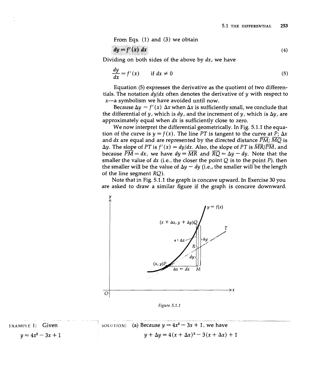
The Differential 251
Differential Formulas 256
The Inverse of Differentiation 260
Differential Equations with Variables Separable 268
Antidifferentiation and Rectilinear Motion 273
Applications of Antidifferentiation in Economics 276
The Sigma Notation 282
Area 288
The Definite Integral 295
Properties of the Definite Integral 304
The Mean-Value Theorem for Integrals 313
The Fundamental Theorem of the Calculus 319
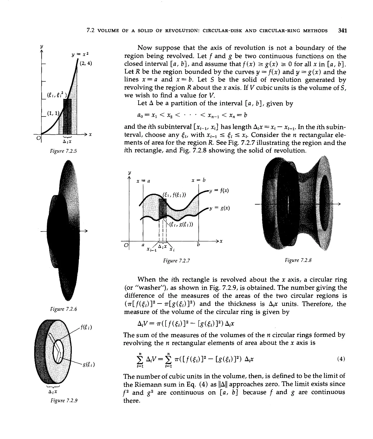
Area of a Region in a Plane 330
Volume of a Solid of Revolution: Circular-Disk and Circular-Ring
Methods 339
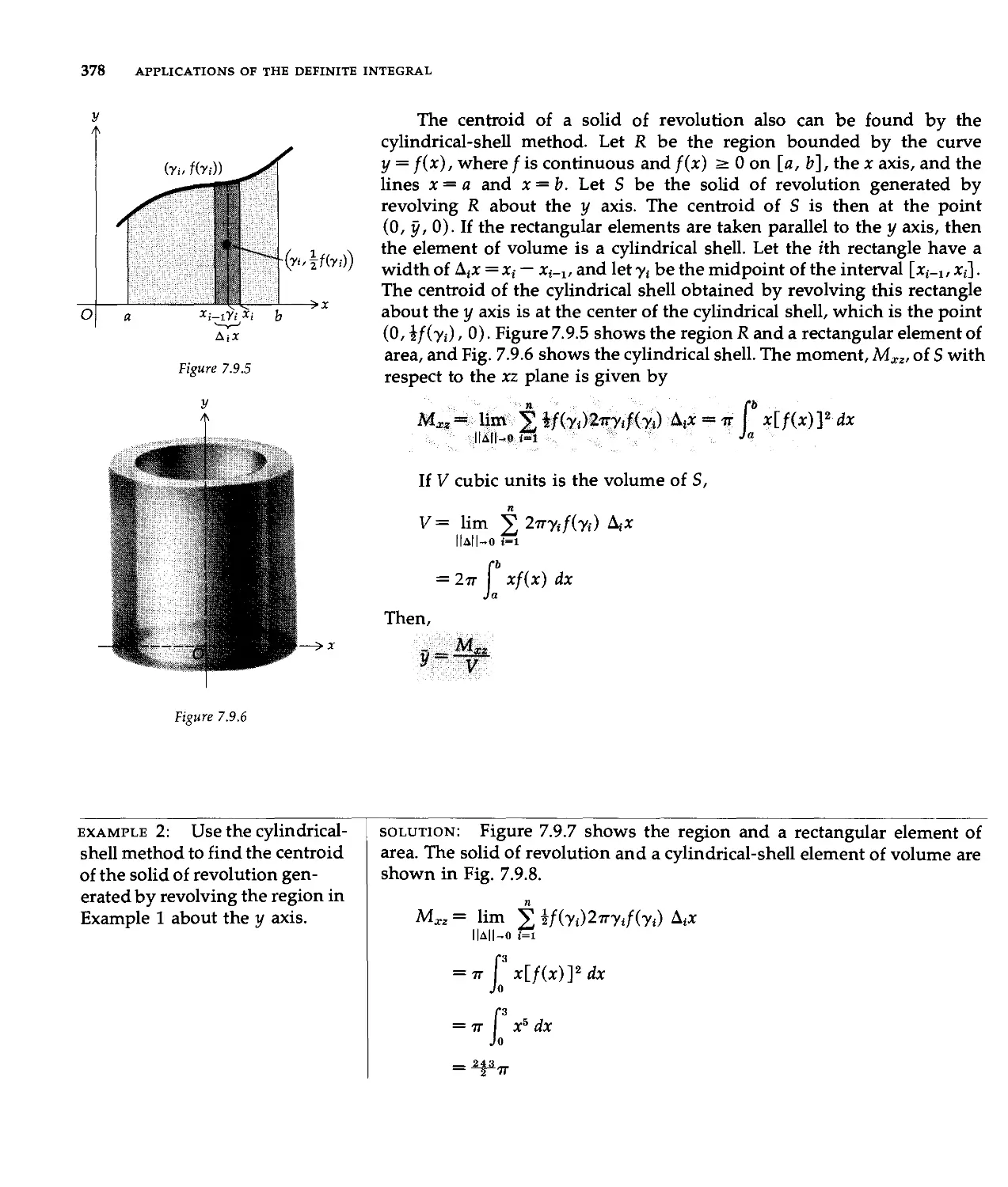
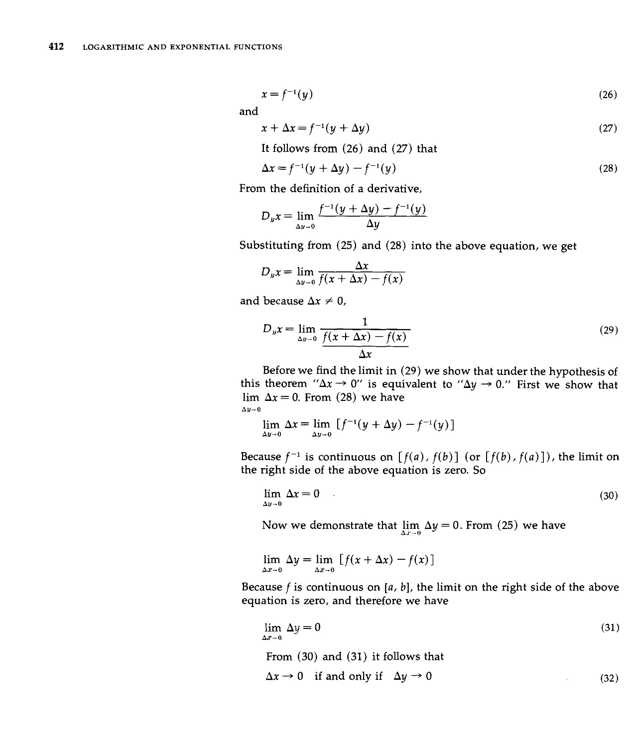
Volume of a Solid of Revolution: Cylindrical-Shell Method 345
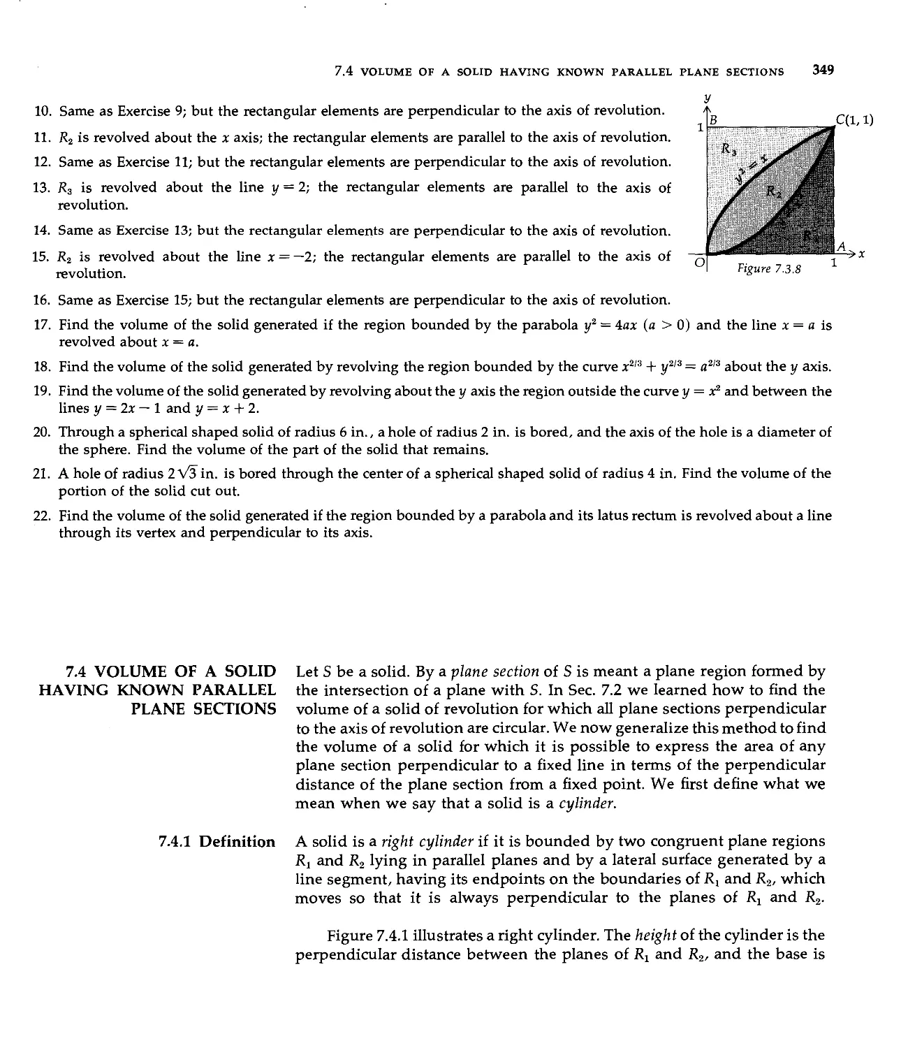
Volume of a Solid Having Known Parallel Plane Sections 349
Work 352
4. Applications
of the derivative
page 179
5. The differential and
antidifferentiation
page 251
6. The definite integral
page 282
7. Applications
of the definite
integral
page 330
4.1
4.2
4.3
4.4
4.5
4.6
4.7
4.8
4.9
4.10
4.11
4.12
5.1
5.2
5.3
5.4
5.5
5.6
6.1
6.2
6.3
6.4
6.5
6.6
7.1
7.2
7.3
7.4
7.5
CONTENTS iX
7.6 Liquid Pressure 356
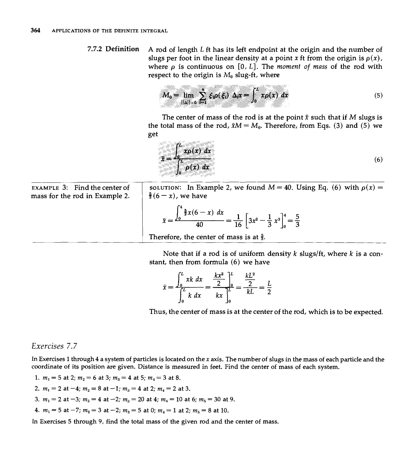
7.7 Center of Mass of a Rod 360
7.8 Center of Mass of a Plane Region 365
7.9 Center of Mass of a Solid of Revolution 375
7.10 Length of Arc of a Plane Curve 381
8. Logarithmic and 8.1 The Natural Logarithmic Function 390
exponential functions 8.2 The Graph of the Natural Logarithmic Function 400
page 390 8 3 xhe Inverse of a Function 404
8.4 The Exponential Function 415
8.5 Other Exponential and Logarithmic Functions 424
8.6 Laws of Growth and Decay 430
9. Trigonometric and 9.1 The Sine and Cosine Functions 439
hyperbolic functions 9.2 Derivatives of the Sine and Cosine Functions 447
page 439 93 Integrals Involving Powers of Sine and Cosine 456
9.4 The Tangent, Cotangent, Secant, and Cosecant Functions 460
9.5 An Application of the Tangent Function to the Slope of <
Line 470
9.6 Integrals Involving the Tangent, Cotangent, Secant, and
Cosecant 474
9.7 Inverse Trigonometric Functions 479
9.8 Derivatives of the Inverse Trigonometric Functions 485
9.9 Integrals Yielding Inverse Trigonometric Functions 490
9.10 The Hyperbolic Functions 495
9.11 The Inverse Hyperbolic Functions 502
10. Techniques of integration 10.1 Introduction 510
page 510 jo.2 Integration by Parts 511
10.3 Integration by Trigonometric Substitution 517
10.4 Integration of Rational Functions by Partial Fractions. Cases 1
and 2: The Denominator Has Only Linear Factors 522
10.5 Integration of Rational Functions by Partial Fractions. Cases 3
and 4: The Denominator Contains Quadratic Factors 530
Integrals Yielding Inverse Hyperbolic Functions 534
Integration of Rational Functions of Sine and Cosine 539
Miscellaneous Substitutions 541
The Trapezoidal Rule 544
Simpson's Rule 549
Polar coordinates
page 558
10.6
10.7
10.8
10.9
10.10
11.1
11.2
11.3
11.4
11.5
11. Polar coordinates 11.1 The Polar Coordinate System 558
Graphs of Equations in Polar Coordinates 563
Intersection of Graphs in Polar Coordinates 572
Tangent Lines of Polar Curves 576
Area of a Region in Polar Coordinates 580
X CONTENTS
16.
12. The conic sections
page 586
13. Indeterminate forms,
improper integrals,
and Taylor's formula
page 626
14. Infinite series
page 655
15. Vectors in the plane
and parametric equations
page 738
ctors in three-dimensional
space and solid
analytic geometry
page 802
12.1
12.2
12.3
12.4
12.5
12.6
13.1
13.2
13.3
13.4
13.5
14.1
14.2
14.3
14.4
14.5
14.6
14.7
14.8
14.9
14.10
14.11
15.1
15.2
15.3
15.4
15.5
15.6
15.7
15.8
15.9
15.10
16.1
16.2
16.3
16.4
16.5
16.6
16.7
16.8
Some Properties of Conies 586
Polar Equations of the Conies 590
Cartesian Equations of the Conies 598
The Ellipse 604
The Hyperbola 611
Rotation of Axes 619
The Indeterminate Form 0/0 626
Other Indeterminate Forms 634
Improper Integrals with Infinite Limits of Integration 638
Other Improper Integrals 644
Taylor's Formula 647
Sequences 655
Monotonic and Bounded Sequences 662
Infinite Series of Constant Terms 668
Infinite Series of Positive Terms 679
The Integral Test 688
Infinite Series of Positive and Negative Terms 691
Power Series 700
Differentiation of Power Series 707
Integration of Power Series 715
Taylor Series 722
The Binomial Series 731
Vectors in the Plane 738
Vector Addition, Subtraction, and Scalar Multiplication 741
Dot Product 749
Vector-Valued Functions and Parametric Equations 756
Calculus of Vector-Valued Functions 764
Length of Arc 771
Plane Motion 777
The Unit Tangent and Unit Normal Vectors and Arc Length as a
Parameter 784
Curvature 788
Tangential and Normal Components of Acceleration 796
Rs, the Three-Dimensional Number Space 802
Vectors in Three-Dimensional Space 809
The Dot Product in Vs 815
Planes 819
Lines in R3 827
Cross Product 832
Cylinders and Surfaces of Revolution 842
Quadric Surfaces 847
CONTENTS Xi
17. Differential calculus
of functions of
several variables
page 871
18. Multiple integration
page 968
16.9
16.10
17.1
17.2
17.3
17.4
17.5
17.6
17.7
17.8
17.9
17.10
17.11
18.1
18.2
18.3
18.4
18.5
18.6
18.7
Curves in R3 854
Cylindrical and Spherical Coordinates
863
Functions of More Than One Variable 871
Limits of Functions of More Than One Variable 880
Continuity of Functions of More Than One Variable 891
Partial Derivatives 897
Differentiability and the Total Differential 905
The Chain Rule 918
Directional Derivatives and the Gradient 925
Tangent Planes and Normals to Surfaces 933
Higher-Order Partial Derivatives 937
Extrema of Functions of Two Variables 944
Some Applications of Partial Derivatives to Economics 955
The Double Integral 968
Evaluation of Double Integrals and Iterated Integrals 974
Center of Mass and Moments of Inertia 982
The Double Integral in Polar Coordinates 988
Area of a Surface 994
The Triple Integral 1000
The Triple Integral in Cylindrical and Spherical
Coordinates 1005
Appendix Table 1 Powers and Roots A-2
page A-i Table 2 Natural Logarithms A-3
Table 3 Exponential Functions A-5
Table 4 Hyperbolic Functions A-12
Table 5 Trigonometric Functions A-13
Table 6 Common Logarithms A-14
Table 7 The Greek Alphabet A-16
Answers to Odd-Numbered Exercises
Index A-41
A-17
ACKNOWLEDGMENTS
Reviewers
Professor William D. Bandes, San Diego Mesa College
Professor Archie D. Brock, East Texas State University
Professor Reuben W. Farley, Virginia Commonwealth University
Professor Jacob Golightly, Jacksonville University
Professor Albert Herr, Drexel University
Professor Gordon L. Miller, Wisconsin State University
Professor William W. Mitchell, Jr., Phoenix College
Professor Roger B. Nelsen, Lewis and Clark College
Sister Madeleine Rose, Holy Names College
Professor George W. Schultz, St. Petersburg Junior College
Professor Donald R. Sherbert, University of Illinois
Professor John Vadney, Fulton-Montgomery Community College
Professor David Whitman, San Diego State College
Production Staff at Harper & Row
Blake Vance, Mathematics Editor
Howard Boyer, Special Projects Editor
Karen Judd, Production Editor
Rita Naughton, Designer
Assistants for Answers to Exercises
Jacqueline Dewar, University of Southern California
Kenneth Kast, University of Southern California
Cover and Chapter Opening Artist
Stanley William Hayter, Atelier 17, Paris, France
To these people and to all the users of the first edition who have suggested
changes, I express my deep appreciation.
L. L.
Preface
This textbook is available either in one volume or in two parts: Part I
consists of the first fourteen chapters, and Part II comprises Chapters 14
through 18 (Chapter 14 on Infinite Series is included in both parts to
make the use of the two-volume set more flexible). The material in Part I
consists of the differential and integral calculus of functions of a single
variable and plane analytic geometry, and it may be covered in a one-
year course of nine or ten semester hours or twelve quarter hours. The
second part is suitable for a course consisting of five or six semester
hours or eight quarter hours. It includes the calculus of several variables
and a treatment of vectors in the plane, as well as in three dimensions,
with a vector approach to solid analytic geometry.
The second edition, like the first, can be used for courses designed
for prospective mathematics majors as well as for those having students
whose primary interest is in engineering, the physical sciences, or
nontechnical fields. It is assumed that the reader has a knowledge of high-
school algebra and geometry.
The objectives of the first edition have been maintained. I have
endeavored to achieve a healthy balance between the presentation of
elementary calculus from a rigorous approach and that from the older,
intuitive, and computational point of view. Bearing in mind that a
textbook should be written for the student, I have attempted to keep the
presentation geared to a beginner's experience and maturity and to leave
no step unexplained or omitted. I desire that the reader be aware that
proofs of theorems are necessary and that these proofs be well motivated
Xiv PREFACE
and carefully explained so that they are understandable to the student
who has achieved an average mastery of the preceding sections of the
book. If a theorem is stated without proof, I have generally augmented
the discussion by both figures and examples, and in such cases I have
always stressed that what is presented is an illustration of the content of
the theorem and is not a proof.
Major changes in the second edition occur in the chapters on
trigonometric functions, infinite series, and multiple integration; these
chapters have been completely rewritten and expanded to include additional
subject matter. Other changes include the following: (1) the rewording
in certain sections and the addition of examples to clarify the
explanations; (2) a reordering of some topics, such as placing the chapter on
infinite series at the conclusion of the study of the calculus of functions of a
single variable, unifying the discussion of functions, limits, and
continuity into a single chapter, incorporating the presentation of hyperbolic
functions with that of the trigonometric functions, and treating vectors
in space immediately following vectors in the plane; (3) additional
applications of the calculus including some to the fields of economics and
business; (4) a complete revision of the exercise sets so that there is a
larger number of theoretical problems, as well as some more challenging
ones and those giving a wider variety of applications; (5) the addition of
a set of Review Exercises at the end of each chapter; (6) the use of color
to clarify the figures, emphasize the statements of definitions and
theorems, and improve the overall design of the book.
Basic facts about the real-number system are given in Chapter 1. I
have avoided presenting sophisticated, tricky arguments merely for the
purpose of showing that some of the properties can be derived from
others. It has been my experience that few students of beginning calculus
are capable of appreciating such discussions and that these
considerations belong to a course in abstract algebra. Chapter 1 also gives an
introduction to analytic geometry, and it includes the traditional material on
straight lines as well as a discussion of the circle and the parabola. These
sections may be omitted by those who have already had a course in
analytic geometry.
Chapter 2 is the heart of any first course in the calculus. I have
defined a function as a set of ordered pairs and have used this idea to point
up the concept of a function as a correspondence between sets of real
numbers. The notion of a limit of a function is first given a step-by-step
motivation, which brings the reader from computing the value of a
function near a number, through an intuitive discussion of the limiting
process, up to a rigorous epsilon-delta definition. A sequence of examples
progressively graded in difficulty is included. All the limit theorems are
stated, and some proofs are presented in the text, while other proofs have
been outlined in the exercises. In the discussion of continuity, I have
used as examples and counterexamples "common, everyday" functions
PREFACE XV
and have avoided those that would have little intuitive meaning for the
reader.
In Chapter 3, before giving the formal definition of a derivative, I
have defined the tangent line to a curve and instantaneous velocity in
rectilinear motion in order to demonstrate in advance that the concept
of a derivative is of wide application, both geometrical and physical.
Theorems on differentiation are proved and illustrated by examples.
Chapter 4 gives the traditional applications of the derivative to
problems involving related rates, maxima and minima, and curve sketching,
as well as some to business and economics.
The antiderivative is treated in Chapter 5. I use the term "antidiffer-
entiation" instead of indefinite integration, but the standard notation
Sf(x) dx is retained so that the reader will not be given a bizarre new
notation that would make the reading of standard references difficult. This
notation will suggest to the student that some relation must exist between
definite integrals, introduced in Chapter 6, and antiderivatives, but I
see no harm in this as long as he is presented with the theoretically proper
view of the definite integral as the limit of sums. Exercises involving the
evaluation of definite integrals by finding limits of sums are given in
Chapter 6, to impress upon the reader that this is how they are calculated.
The introduction of the definite integral follows the definition of the
measure of the area under a curve as a limit of sums. Elementary
properties of the definite integral are derived and the fundamental theorem of
the calculus is proved. It is emphasized that this is a theorem, and an
important one, because it provides us with an alternative to computing
limits of sums. It is also emphasized that the definite integral is in no
sense some special type of antiderivative. In Chapter 7, I have given
numerous applications of definite integrals. The presentation stresses not
only the manipulative techniques but also the fundamental principles
involved. In each application, the definitions of the new terms are
intuitively motivated and explained.
The treatment of logarithmic and exponential functions in Chapter 8
is the modern approach. The natural logarithm is defined as an integral,
and after the discussion of the inverse of a function, the exponential
function is defined as the inverse of the natural logarithm function. An
irrational power of a real number is then defined. The trigonometric
functions are defined in Chapter 9 as functions assigning numbers to numbers.
The important trigonometric identities are derived and used to obtain the
formulas for the derivatives and integrals of these functions. Sections on
the differentiation and integration of the trigonometric functions as well
as of the inverse trigonometric functions are followed by two sections on
hyperbolic functions. The geometric interpretation of the hyperbolic
functions is postponed until Chapter 15 because it involves the use of
parametric equations.
Chapter 10, on techniques of integration, involves one of the most
important computational aspects of the calculus. I have explained the
theoretical backgrounds of each different method after an introductory
motivation. The mastery of integration techniques depends upon the
examples, and I have used as illustrations problems that the student will
certainly meet in practice, those which require patience and persistence
to solve. The material on the approximation of definite integrals includes
the statement of theorems for computing the bounds of the error involved
in these approximations. The theorems and the problems that go with
them, being self-contained, can be omitted from a course if the instructor
so wishes.
Polar coordinates and some of their applications are given in
Chapter 11. In Chapter 12, conies are treated as a unified subject to impress
upon the reader their natural and close relationship to each other.
Equations of the conies in polar coordinates are treated first, and the cartesian
equations are derived from the polar equations. The topics of
indeterminate forms, improper integrals, and Taylor's formula, and the
computational techniques involved are presented in Chapter 13.
I have attempted in Chapter 14 to give as complete a treatment of
infinite series as is feasible in an elementary calculus text. In addition
to the customary computational material, I have included the proof of
the equivalence of convergence and boundedness of monotonic sequences
based on the completeness property of the real numbers and the proofs
of the computational processes involving differentiation and integration
of power series.
The first five sections of Chapter 15 on vectors in the plane can be
taken up after Chapter 3 if it is desired to introduce vectors earlier in the
course. The approach to vectors is modern, and it serves both as an
introduction to the viewpoint of linear algebra and to that of classical vector
analysis. The applications are to physics and geometry. Chapter 16 treats
vectors in three-dimensional space and, if desired, the topics in the first
three sections of this chapter may be studied concurrently with the
corresponding topics of Chapter 15.
Limits, continuity, and differentiation of functions of several
variables are considered in Chapter 17. The discussion and examples are
applied mainly to functions of two and three variables; however,
statements of most of the definitions and theorems are extended to functions
of n variables. Applications to the solution of extrema problems and an
introduction to Lagrange multipliers are presented as well as a section
on applications of the partial derivative in economics. The double
integral of a function of two variables and the triple integral of a function of
three variables, along with some applications to physics, engineering, and
geometry, are given in Chapter 18.
Louis Leithold
1.1 REAL NUMBERS
AND INEQUALITIES
1.1.1 Sum and product
1
Real Numbers
and mtrxxfuefion
to Analytic
Geometry
The real number system can be completely described by a set of axioms.
With these axioms we can derive the properties of the real numbers
from which follow the familiar algebraic operations of addition,
subtraction, multiplication, and division, as well as the algebraic concepts of
solving equations, factoring, and so forth. In this book we are not
concerned with showing how such properties are derived from the axioms
because these considerations belong to a course in abstract algebra.
However, because elementary calculus involves real numbers, you should be
familiar with some of the fundamental properties of the real number
system given below.
If a and b are any real numbers, there is one and only one real number,
denoted by a + b, called their sum, and there is one and only one real
number, denoted by ab (or a X b, or a • b), called their product.
1.1.2 Commutative laws If a and b are any real numbers,
a + b = b + a and ab = ba
1.1.3 Associative laws If a, b, and c are any real numbers,
a + (b + c) = (a + b) + c and a(bc) = (ab)c
1.1.4 Distributive law If a, b, and c are any real numbers,
a(b + c) = ab + ac
l
2 REAL NUMBERS AND INTRODUCTION TO ANALYTIC GEOMETRY
1.1.5 Existence of There exist two distinct real numbers 0 and 1 such that for every real
identity elements number a
a + 0 = a and a • 1 = a
1.1.6 Existence of negatives Every real number a has a negative, denoted by — a, such that
a+ (-a) =0
1.1.7 Existence of reciprocals Every real number a # 0 has a reciprocal, denoted by 1/fl, such that
fl-i=l
a
1.1.8 Definition of subtraction If a and b are any real numbers, the'difference between a and b, denoted
by a — b, is defined by
a — b = a + (— b)
1.1.9 Definition of division If a is any real number, and b is any real number except 0, the quotient of
a and b is defined by
a 1
To enable us to refer to one real number being greater (or less) than
another, we introduce the concept of a real number being positive and an
order relation.
1.1.10 Axiom of order In the set of real numbers, there exists a subset called the positive
numbers such that
(i) if a is any real number, exactly one of these three statements
holds: fl = 0; a is positive; —a is positive,
(ii) the sum of two positive numbers is positive,
(iii) the product of two positive numbers is positive.
1.1.11 Definition The real number a is negative if and only if—a is positive.
1.1.12 Definition The symbols < ("is less than") and > ("is greater than") are defined as
follows:
(i) a < b if and only if b — a is positive,
(ii) a > b if and only if a — b is positive.
1.1.13 Definition The symbols < ("is less than or equal to") and > ("is greater than or
equal to") are defined as follows:
(i) a < b if and only if either a < b or a = b.
(ii) a > b if and only if either a > b or a = b.
1.1 REAL NUMBERS AND INEQUALITIES 3
Expressions such as a < b, a > b, a < b, and a > b are called
inequalities. Some examples are 2 < 7, —5 < 6, —5 < —4, 14 > 8, 2 > —4,
—3 > —6, 5 > 3, —10 < —7. In particular, a < b and a > fr are called strict
inequalities, whereas a < b and a > fr are called nonstrict inequalities.
The following properties can be proved by using 1.1.1 through
1.1.13.
1.1.14 Property (i) a > 0 if and only if a is positive.
(ii) a < 0 if and only if a is negative,
(iii) a > 0 if and only if —a < 0.
(iv) a < 0 if and only if — a > 0.
1.1.15 Property If a < b and b < c, then a < c.
example: 3 < 6 and 6 < 14; so 3 < 14.
1.1.16 Property If a < b, then a + c < b + c, if c is any real number.
example: 4 < 7; so 4 + 5 < 7 + 5; and 4 — 5 < 7 — 5.
1.1.17 Property If a < b and c < d, then a + c < b + d.
example: 2 < 6 and -3 < 1; so 2 + (-3) < 6 + 1.
1.1.18 Property If a < b, and c is any positive number, then ac < be.
example: 2 < 5; so 2 • 4 < 5 • 4.
1.1.19 Property If a < b, and c is any negative number, then ac > be.
example: 2 < 5; so 2(-4) > 5(-4).
1.1.20 Property If 0 < a < b and 0 < c < d, then ac < bd.
example: 0 < 4 < 7 and 0 < 8 < 9; so 4(8) < 7(9).
Property 1.1.18 states that if both members of an inequality are
multiplied by a positive number, the direction of the inequality remains
unchanged, whereas Property 1.1.19 states that if both members of an
inequality are multiplied by a negative number, the direction of the
inequality is reversed. Properties 1.1.18 and 1.1.19 also hold for division,
because dividing both members of an inequality by a number d is
equivalent to multiplying both members by 1/rf.
To illustrate the type of proof that is usually given, we present a
proof of Property 1.1.17:
Since a < b, b — a is positive (by 1.1.12(i)).
REAL NUMBERS AND INTRODUCTION TO ANALYTIC GEOMETRY
Since c < d, d — c is positive (by 1.1.12(i)).
Hence, (b — a) + (d — c) is positive (by l.l.lO(ii)).
Therefore, (b + d) - (a + c) is positive (by 1.1.3, 1.1.2, and 1.1.8).
Therefore, a + c <b + d (by 1.1.12(i)).
The following properties are similar to Properties 1.1.15 to 1.1.20
except that the direction of the inequality is reversed.
1.1.21 Property If a > b and b > c, then a > c.
example: 8 > 4 and 4 > —2; so 8 > —2.
1.1.22 Property If a > b, then a + c > b + c, if c is any real number.
example: 3 > —5; so 3 — 4 > —5 — 4.
1.1.23 Property If a > b and c > d, then a + c > b + d.
example: 7 > 2 and 3 > —5; so 7 + 3 > 2 + (—5).
1.1.24 Property If a > b and if c is any positive number, then ac > be.
example: —3 > — 7; so (—3)4 > (—7)4.
1.1.25 Property If a > b and if c is any negative number, then ac < be.
example: -3 > -7; so (~3)(-4) < (-7)(-4).
1.1.26 Property If a > b > 0 and c > d > 0, then ac > bd.
example: 4 > 3 > 0 and 7 > 6 > 0; so 4(7) > 3(6).
From Axiom 1.1.10 and Definition 1.1.11, it follows that a real number
is either a positive number, a negative number, or zero. Any real number
can be classified as a rational number or an irrational number. A rational
number is any number that can be expressed as the ratio of two integers.
That is, a rational number is a number of the form p/q, where p and q
are integers and q # 0. The rational numbers consist of the following:
The integers (positive, negative, and zero)
. . . ,-5,-4,-3,-2,-1,0,1,2,3,4,5, . . .
The positive and negative fractions such as
2. 4. 83
7 5 5
The positive and negative terminating decimals such as
2.36 = 1^ -0.003251 =-^2^—
100 1,000,000
1.1 REAL NUMBERS AND INEQUALITIES 5
i \ !
J I I LU LLJ I L
-4 I -2 0 ' 21 4
The positive and negative nonterminating repeating decimals such as
0.333. . . = i -0.549549549. . . = —fc
The real numbers which are not rational numbers are called irrational
numbers. These are positive and negative nonterminating, nonrepeating
decimals, for example,
V3 = 1.732. . . 77 = 3.14159. . . tan 140° = -0.8391. . .
The set of all real numbers is denoted by R,. Rt can be represented
geometrically by points on a horizontal line, called an axis, which is
illustrated in Fig. 1.1.1.
A point on the axis is chosen to represent the number 0. This point
Figure l.i.i is called the origin. A unit of distance is selected. Then each positive
number n is represented by the point at a distance of n units to the right
of the origin, and each negative number n is represented by the point at
a distance of — n units to the left of the origin. (It should be noted that if
n is negative, then — n is positive.) There is a one-to-one correspondence
between Rt and the points on the axis; that is, to each real number there
corresponds a unique point on the axis, and with each point on the axis
there is associated only one real number. So the points on the axis are
identified with the numbers they represent, and we shall use the same
symbol for both the number and the point representing that number on
> the axis. Because of the one-to-one correspondence, we identify Rj with
J~ the axis, and we call Rj the number line.
We see that a < b if and only if the point representing the number a
Figure 1.1.2 is to the left of the point representing the number b. Similarly, a > b if
and only if the point representing a is to the right of the point
representing b. For instance, the number 2 is less than the number 5 and the
~| point 2 is to the left of the point 5. We could also write 5 > 2 and say
b that the point 5 is to the right of the point 2.
A number x is between a and b if and only if a < x and x < b. We can
Figure 1.1.3 write this as a continued inequality as follows:
a < x < b (1)
The continued inequality (1) denotes an open interval.
1.1.27 Definition The open interval from a to b, denoted by {a, b), is the set of all real
numbers x such that a < x < b.
The closed interval from a to b consists of all numbers between, and
including, a and b.
1.1.28 Definition The closed interval from a to b, denoted by [a, b], is the set of all real
numbers x such that a < x < b.
Figure 1.1.2 illustrates the open interval (a, b), and Fig. 1.1.3
illustrates the closed interval [a, b\.
6 REAL NUMBERS AND INTRODUCTION TO ANALYTIC GEOMETRY
The interval half-open on the left consists of all numbers between
a and b as well as b, but not a.
1.1.29 Definition The interval half-open on the left, denoted by (a, b], is the set of all real
numbers x such that a < x < b.
1.1.30 Definition
1-
Figure 1.1.4
Figure 1.1.5
Figure 1.1.6
Figure 1.1.7
We define an interval half-open on the right in a similar way.
The interval half-open on the right, denoted by [a, b), is the set of all real
numbers x such that a < x < b.
Figure 1.1.4 illustrates the interval {a, b], and Fig. 1.1.5 illustrates the
interval [a, b).
We shall use the symbol +°° ("positive infinity") and the symbol
— °° ("negative infinity"); however, care must be taken not to confuse
these symbols with real numbers, for they do not obey the properties of
the real numbers.
The notation {a, +°°) denotes the set of all numbers greater than a.
We can also state that (a, +°°) is the set of all real numbers x such that
x > a. Similarly, (— °°, b) denotes the set of all numbers less than b; or,
(—°°, b) is the set of all real numbers x such that x < b. Figure 1.1.6
illustrates the interval (a, +°°), and Fig. 1.1.7 illustrates the interval (—oc, b).
The interval [a, +°°) is the set of all real numbers x such that x > a;
and (—°°, b] is the set of all real numbers x such that x < b. Finally,
(—°°, +°°) denotes the set of all real numbers.
For each of the intervals (a, b), [a, b], [a, b), and {a, b] the numbers a
and b are called the endpoints of the interval. The closed interval [a, b]
contains both its endpoints, whereas the open interval (a, b) contains
neither endpoint. The interval [a, b) contains its left endpoint but not its
right one, and the interval (a, b] contains its right endpoint but not its
left one. An open interval can be thought of as one which contains none
of its endpoints, and a closed interval can be regarded as one which
contains all of its endpoints. Consequently, the interval [a, +°°) is considered
to be a closed interval because it contains its only endpoint a. Similarly,
(—oo, b] is a closed interval, whereas (a, +°°) and (—°°, b) are open. The
intervals [a, b) and {a, b] are neither open nor closed. Since the interval
(—°°, +°°) has no endpoints, it can be considered as both containing them
and not containing them, and hence is thought of as being both open
and closed.
Let us now solve some inequalities and express the solutions as
intervals.
example 1: Find all real
numbers satisfying the inequality
2 + 3x < 5x + 8
solution: If x is a number such that
2 + 3x < 5x + 8
1.1 REAL NUMBERS AND INEQUALITIES 7
-3 0
Figure 1.1-8
then
2 + 3x - 2 < 5x + 8 - 2 (by 1.1.16)
or
3x < 5x + 6
Then, adding — 5x to both members of this inequality, we have
-2x < 6 (by 1.1.16)
Dividing on both sides of this inequality by —2 and reversing the
direction of the inequality, we obtain
x > -3 (by 1.1.19)
What we have proved is that if
2 + 3x < 5x + 8
then
x >— 3
Each of the steps is reversible; that is, if we start with
x >-3
we multiply on each side by —2, reverse the direction of the inequality,
and obtain
-2x <6
Then we add 5x and 2 to both members of the inequality, and we get
2 + 3x < 5x + 8
Therefore, we can conclude that
2 + 3x < 5x + 8 if and only if x > — 3
So the interval solution of the given inequality is (—3, +°°), which is
illustrated in Fig. 1.1.8.
example 2: Find all real
numbers satisfying the inequality
4 < 3x - 2 < 10
H ( }-
0 2 4
Figure 2.2.9
solution: Adding 2 to each member of the inequality, we obtain
6 < 3x < 12
Dividing each member by 3, we get
2 < x <4
Each step is reversible; so the interval solution is (2, 4], as is illustrated
in Fig. 1.1.9.
8 REAL NUMBERS AND INTRODUCTION TO ANALYTIC GEOMETRY
example 3: Find all real
numbers satisfying the inequality
- > 2 x¥= 0
x
Figure 1.1.10
solution: We wish to multiply both members of the inequality by x.
However, the direction of the inequality that results will depend upon
whether x is positive or negative. So we must consider two cases.
Case 1: x is positive; that is, x > 0.
Multiplying on both sides by x, we obtain
7>2x
Dividing on both sides by 2, we get
i > x or, equivalently, x < \
Therefore, since the above steps are reversible, the solution of Case 1 is
the set of all numbers x such that x > 0 and x < 1; that is, 0 < x < \,
which is the interval (0, |).
Case 2: x is negative; that is, x < 0.
Multiplying on both sides by x and reversing the direction of the
inequality, we find
7 <2x
Dividing on both sides by 2, we have
\ < x or, equivalently, x>\
Again, because the above steps are reversible, the solution of Case 2 is
the set of all numbers x such that x < 0 and x > \. But it is impossible to
find a value for x satisfying both of these inequalities. Hence, Case 2 has
no solution.
From Cases 1 and 2 we conclude that the solution of the given
inequality is the open interval (0, f), which is illustrated in Fig. 1.1.10.
example 4: Find all real
numbers satisfying the inequality
x-3
<4
x* 3
solution: To multiply both members of the inequality by x — 3, we
must consider two cases, as in Example 3.
Case 1: x — 3 > 0; that is, x > 3.
Multiplying on both sides of the inequality by x — 3, we get
x < Ax — 12
Adding — Ax to both members, we obtain
-3x < -12
Dividing on both sides by—3 and reversing the direction of the inequality,
we have
x > 4
1.1 REAL NUMBERS AND INEQUALITIES 9
3 4
Figure 1.1.11
Thus, the solution of Case 1 is the set of all numbers x such that x > 3
and x > 4. This is the set of all x such that x > 4, or the interval (4, +°°).
Case 2: * — 3 < 0; that is, x < 3.
Multiplying on both sides by x — 3 and reversing the direction of
the inequality, we have
x > 4x - 12
or
-3x > -12
or
x < 4
Therefore, x must be less than 4 and also less than 3. Thus, the solution
of Case 2 is the interval (— °°, 3).
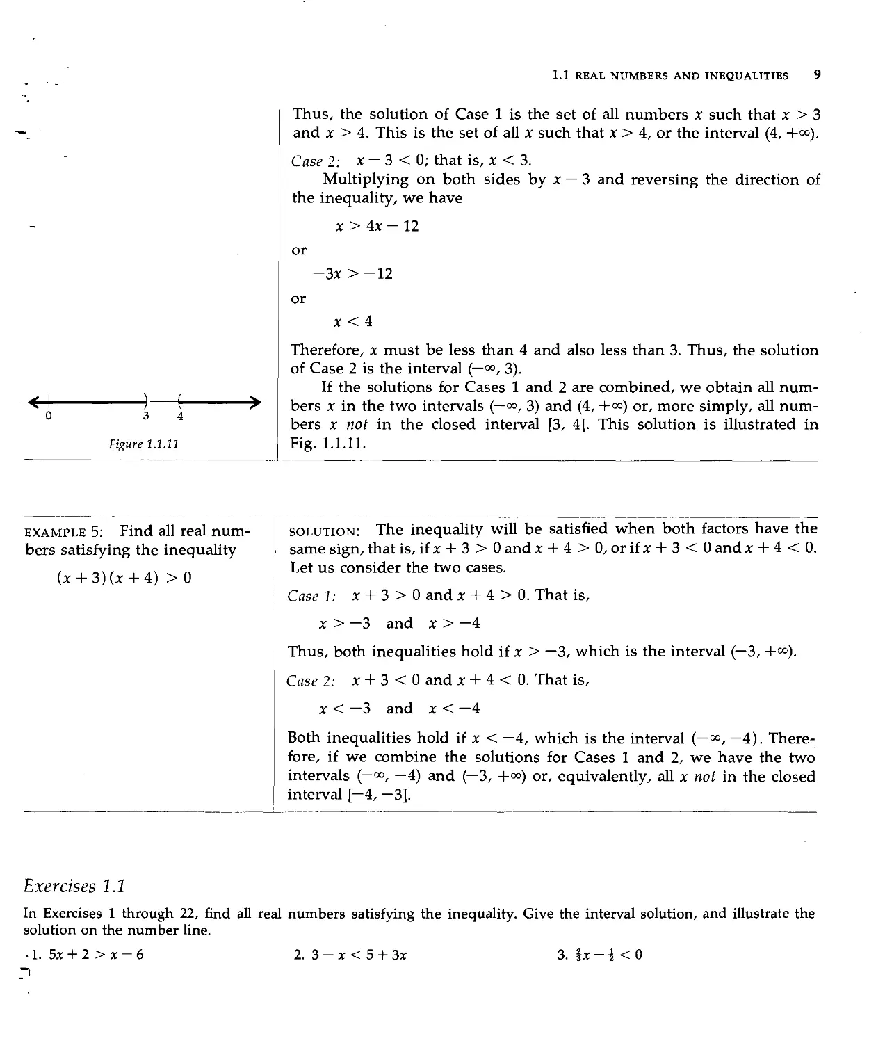
If the solutions for Cases 1 and 2 are combined, we obtain all
numbers x in the two intervals (—°°, 3) and (4, +°°) or, more simply, all
numbers x not in the closed interval [3, 4]. This solution is illustrated in
Fig. 1.1.11.
example 5: Find all real
numbers satisfying the inequality
(x + 3)(x + 4) >0
solution: The inequality will be satisfied when both factors have the
same sign, that is, if x + 3 > 0 and x + 4 > 0, or if x + 3 < 0 and x + 4 < 0.
Let us consider the two cases.
Case 1: x + 3 > 0 and x + 4 > 0. That is,
x > — 3 and x > — 4
Thus, both inequalities hold if x > —3, which is the interval (—3, +°°).
Case 2: x + 3 < 0 and x + 4 < 0. That is,
x < —3 and x < —4
Both inequalities hold if x < —4, which is the interval (—°°, —4).
Therefore, if we combine the solutions for Cases 1 and 2, we have the two
intervals (—°°, —4) and (—3, +°°) or, equivalently, all x not in the closed
interval [—4, —3].
Exercises 1.1
In Exercises 1 through 22, find all real numbers satisfying the inequality. Give the interval solution, and illustrate the
solution on the number line.
• 1. 5x + 2 > x -
2. 3 - x < 5 + 3x
3. f x - i < 0
10 REAL NUMBERS AND INTRODUCTION TO ANALYTIC GEOMETRY
4.
7.
.0.
.3.
.6.
n
3x — 5 < - x H -—
2 > -3 - 3x > -7
T^>
(x - 3) (x + 5) > 0
x2 + 3x + 1 > 0
1 . 2
5. 13 > 2x - 3 > 5 6. 2 < 5 - 3x < 11
9. --3 >--7
a: a:
12. x2 < 9
15. 1 - x - 2X2 > 0
18. 2X2 - 6x + 3 < 0
21. X - 4
8.
11.
14.
17.
?0
x 4
x2 >4
x2 - 3x + 2 > 0
4x2 + 9x < 9
x+ 1 „ x
x + 13x-l '2-x 3+x '3x-7-3-2a:
22. x3 + 1 > x2 + x 23. Prove Property 1.1.15. 24. Prove Property 1.1.16.
25. Prove Properties 1.1.18 and 1.1.19.
26. If a > b > 0, prove that a2 > b2.
27. If a and b are nonnegative numbers, and a2 > b2, prove that a > b.
28. Prove that if a > 0 and b > 0, then a2 = b2 if and only if a = b.
29. Prove that if b > a > 0 and c> 0, then
a + c £
b + c > b
30. Prove that if x < y, then x < i(* + y) < y.
1.2 ABSOLUTE VALUE The absolute value of x, denoted by \x\, is defined as
1.2.1 Definition , , ., ^ _
\x\ = x if x > 0
|x| =— x it x < 0
|0|=0
Thus7 the absolute value of a positive number or zero is equal to
the number itself. The absolute value of a negative number is the
corresponding positive number because the negative of a negative number
k-b- a=\a- b\->\ [s positive. For example,
J
3|=3 |_5|=_(_5)=5 |8-14| = |-6|=-(-6)=6
« u
We see from the definition that the absolute value of a number is either
a positive number or zero; that is, it is nonnegative.
L u _ fa _ i _ bi_^| In terms of geometry, the absolute value of a number x is its distance
from 0, without regard to direction. In general, \a— b\ is the distance
between a and b without regard to direction, that is, without regard to
which is the larger number. Refer to Fig. 1.2.1.
I
b a
Figure 1.2.1 We have the following properties of absolute values.
1.2 ABSOLUTE VALUE 11
1.2.2 Theorem
1.2.3 Corollary
1.2.4 Theorem
1.2.5 Corollary
|x| < a if and only if —a < x < a, where a > 0.
|x| < a if and only if — a < x < a, where a > 0.
|x| > « if and only if x > a or x < —a, where a > 0.
|x| > a if and only if x > a or a: < —a, where a > 0.
The proof of a theorem that has an "if and only if" qualification
requires two parts, as illustrated in the following proof of Theorem 1.2.2.
part 1: Prove that |x| < « if — a < x < a, where a > 0. Here, we have to
consider two cases: x > 0 and x < 0.
Case 1: x > 0.
Then |x| = x. Because x < a, we conclude that |x| < a.
Case 2: x < 0.
Then |x| = —x. Because —a < x, we apply Property 1.1.19 and obtain
a > —x or, equivalently, — x < a. But because — x= \x\, we have |x| < a.
In both cases, then,
Ixl < a if — a < x < a,
where a > 0
part 2: Prove that |x| < a only if —a < x < a, where a > 0. Here we
must show that whenever the inequality |x| < a holds, the inequality
— a < x < a also holds. Assume that |x| < a and consider the two cases
x > 0 and x < 0.
Case 1: x > 0.
Then |x| = x. Because |x| < a, we conclude that x < a. Also, because
a > 0, it follows from Property 1.1.25 that—a < 0. Thus, we have—a < 0
< x < a, or — a < x < a.
Case 2: x < 0.
Then |x| =—x. Because |x| < a, we conclude that — x < a. Also,
because x < 0, it follows from Property 1.1.19 that 0 < —x. Therefore, we
have — a < 0 < — x < a, or —a < —x < a, which by applying Property
1.1.19 yields— a < x < a.
In both cases,
|x| < a only if —a < x < a, where a > 0 ■
The proof of Theorem 1.2.4 is left for the reader (see Exercise 27).
The following examples illustrate the solution of equations and
inequalities involving absolute values.
12 REAL NUMBERS AND INTRODUCTION TO ANALYTIC GEOMETRY
example 1: Solve for x:
[3x + 2| =5.
solution: This equation will be satisfied if either
3x + 2 = 5 or 3x + 2=-5
Considering each equation separately, we have
x = 1 and x = —1
which are the two solutions to the given equation.
example 2: Solve for x:
\2x-\\ = |4x + 3|.
solution: This equation will be satisfied if either
2x-l = 4x + 3 or 2x-1 =-(4x +3)
Solving the first equation, we have x = — 2; solving the second, we get
x = — i, thus giving us two solutions to the original equation.
example 3: Solve for x:
|5x + 4|=-3.
solution: Because the absolute value of a number may never be
negative, this equation has no solution.
example 4: Find all real num
bers satisfying the inequality
|x-5| < 4.
_i—<
0 1
Figure 1.2.2
+-
9
solution: If x is a number such that
|x-5| < 4
then
-4<x-5<4 (by 1.2.2)
Adding 5 to each member of the preceding inequality, we obtain
1< x< 9
Because each step is reversible, we can conclude that
\x — 5| < 4 if and only if 1 < x < 9
So, the interval solution of the given inequality is (1, 9), which is
illustrated in Fig. 1.2.2.
example 5: Find all real
numbers satisfying the inequality
3-2*
2 + x
solution: By Corollary 1.2.3, the given inequality is equivalent to
a 3-2* .
—4 < ■< 4
* ~ 2 + x ~*
If we multiply by 2 + x, we must consider two cases, depending upon
whether 2 + x is positive or negative.
1.2 ABSOLUTE VALUE 13
Case 1: 2 + x > 0 or x > —2.
Then we have
-4(2 + x) < 3 - 2x < 4(2 + x)
or
-8 - 4x < 3 - 2x < 8 + 4x
So, if x > —2, then also — 8 - 4x < 3 - 2x and 3 - 2x < 8 + 4x. We solve
these two inequalities. The first inequality is
-8 - 4x < 3 - 2x
Adding 2x + 8 to both members gives
-2x < 11
Dividing both members by —2 and reversing the inequality sign, we
obtain
The second inequality is
3 - 2x < 8 + 4x
Adding — 4x — 3 to both members gives
-6x <5
Dividing both members by —6 and reversing the inequality sign, we
obtain
x >-£
Therefore, if x > —2, then the original inequality holds if and only if
x > —V- and x > —%.
Because all three inequalities x > —2, x > —1r, and x > — f must be
satisfied by the same value of x, we have x > —f, or the interval [—f, +°°).
Case 2: 2 + x < 0 or x < -2.
Thus, we have
-4(2 + x) >3-2x>4(2 + x)
or
-8 - 4x > 3 - 2x > 8 + 4x
Considering the left inequality, we have
-8 - 4x > 3 - 2x
or
-2x > 11
or
x<-¥
14 REAL NUMBERS AND INTRODUCTION TO ANALYTIC GEOMETRY
From the right inequality we have
3 - 2x > 8 + 4x
or
-6x>5
or
x <-•|
Therefore, if x < — 2, the original inequality holds if and only if x < — V"
and x < —f.
Because all three inequalities must be satisfied by the same value of
x, we have x < —V", or the interval (—°°, —V1].
Combining the solutions of Case 1 and Case 2, we have as the
solution the two intervals (—°°, — "¥-] and [— f, +°°) or, more simply, all x not
in the interval (— -¥-, —f).
example 6: Find all real
numbers satisfying the inequality
|3x+ 2| > 5
solution: By Theorem 1.2.4, the given inequality is equivalent to
3x + 2>5 or 3x + 2<-5 (1)
That is, the given inequality will be satisfied if either of the inequalities
in (1) is satisfied.
Considering the first inequality, we have
3x + 2 > 5
or
X>1
Therefore, the interval (1, +°°) is a solution.
From the second inequality, we have
3x + 2 < -5
or
x<-i
Hence, the interval (—°°, —J) is a solution.
The solution of the given inequality consists of the two intervals
(—°°, —J) and (1, +oo) or, equivalently, all x not in the closed interval [— i, 1].
The reader may recall from algebra that the symbol Vfl, where a > 0,
is defined as the unique nonnegative number x such that x2 = a. We read
Vfl as "the principal square root of a." For example,
Vi=2 V0=0 VS = f
note: V4 # —2; —2 is a square root of 4, but V4 denotes only the
positive square root of 4.
1.2 ABSOLUTE VALUE 15
Because we are concerned only with real numbers in this book, Va
is not defined if a < 0. From the definition of Va, it follows that
V? = [x|
For example, VW = 5 and VPW = 3.
The following theorems about absolute value will be useful later.
1.2.6 Theorem If a and b are any numbers, then
\ab\ = \a\ • \b\
Expressed in words, this equation states that the absolute value of the
product of two numbers is the product of the absolute values of the
two numbers.
proof:
\ab\ = V(aW
= VdW
= Va~2 ■ V¥
= \a\ • \b\
1.2.7 Theorem If a is any number and b is any number except 0,
\a\
"W\
That is, the absolute value of the quotient of two numbers is the quotient
of the absolute values of the two numbers.
The proof of Theorem 1.2.7 is left to the reader (see Exercise 28).
1.2.8 Theorem If a and b are any numbers, then
The Triangle Inequality
\a + b\ < \a\ + \b\
proof: We consider four cases.
Case 1: a > 0 and b > 0.
Then \a\ = a, \b\ = b, and \a + b\ = a + b = \a\ + \b\; thus, the
theorem holds.
Case 2: a < 0 and b < 0.
Then \a\ =-«, \b\ =~b, and \a + b\ =-(« + b) = {-a) + (-b) =
\a\ + \b\, and so the theorem holds.
Case 3: a > 0 and b < 0.
16 REAL NUMBERS AND INTRODUCTION TO ANALYTIC GEOMETRY
or
Then \a\ = a, \b\ =—b. Therefore,
\a + b\ = a + b ii a + b > 0
\a + b\=-(a+b) if a + b < 0
But, a + b < a + (—b) = \a\ + \b\, because b < 0 and a > 0; also, —(a + b)
= {—a) + {—b) < a + {—b) = \a\ + \b\, because b < 0 and a > 0. In either
case, |« + b|<|«| + |b|, and the theorem holds.
Case 4: a < 0 and b > 0.
The proof of this case is identical with the proof of Case 3. Therefore,
for all the cases we have
\a + b\ < \a\ + \b\ ■
Theorem 1.2.8 has two important corollaries which we now state
and prove.
1.2.9 Corollary If a and b are any numbers, then
\a-b\ < \a\ + \b\
1.2.10 Corollary
proof: \a — b\ = \a + (—b)\ < \a\ + |(— b)\ = \a\ + \b\. ■
If a and b are any numbers, then
\a\- \b\ < \a-b\
proof: \a\ = \{a— b) + b\ < \a — b\ + \b\; thus, subtracting \b\ from
both members of the inequality, we have
\a\ - \b\ <\a-b\ ■
Exercises 1.2
In Exercises 1 through 10, solve for x.
1. |4x+3| = 7
4. |4 + 3x| = l
7. |7x| =A-x
3x + 8
10
2. |3x —8| =4
5. |5x-3| = |3x + 5|
8. 2x + 3= |4x+5|
3.
5 - 2x| = 11
6. |x-2| = |3-2x|
9.
x + 2
x-2
= 5
2x-3
In Exercises 11 through 14, find all the values of x for which the number is real.
11. V8x-5
12. Vx
16
1.3 THE NUMBER PLANE AND GRAPHS OF EQUATIONS 17
In Exercises 15 through 26, find all real numbers satisfying the given inequality; give the interval solution; illustrate the
solution on the real line.
15.
18.
21.
x + 4|
< 7
6 - 2x\ > 7
x-+ 4| < \2x -
6-5x
3 + x
1
< —
~2
-6
16. |2x-5| <3
19. |2x-5| >3
22. |3x| > |6 - 3x\
x+2
17. |3x-4| <2
20. |3 + 2x\ < |4 - x\
23. |9 - 2x\ > |4x|
25,
<4
26.
2x-3
27. Prove Theorem 1.2.4. 28. Prove Theorem 1.2.7.
In Exercises 29 through 32, solve for x and use absolute value bars to write the answer,
a — x
5
2x-\
>
1
x-2
x — ci
29. =—- > 0
31.
x+ a
x-2
30.
fl + x
>0
>
x + 2
32. £±5 < £L
x + a x-
33. Prove Theorem 1.2.8 by adding corresponding members of the inequalities —\a\ < a < |a| and —1&| < b < |&|, and
then applying Corollary 1.2.3.
34. Prove that if a and b are any numbers, then \a — b\ < \a\ + \b\. (hint: Write a — basa+ (—b) and use Theorem 1.2.8.)
35. Prove that if a and b are any numbers, then \a\ — \b\ < \a — b\. (hint: Let |fl| = \(a—b) + b\, and use Theorem 1.2.8.)
36. What single inequality is equivalent to the following two inequalities: a > b + c and a > b — c?
1.3 THE NUMBER PLANE AND
GRAPHS OF EQUATIONS
1.3.1 Definition
Ordered pairs of real numbers will now be considered. Any two real
numbers form a pair, and when the order of the pair of real numbers is
designated, we call it an ordered pair of real numbers. It x is the first real
number and y is the second real number, we denote this ordered pair by
writing them in parentheses with a comma separating them as (x, y). Note
that the ordered pair (3, 7) is different from the ordered pair (7, 3).
The set of all ordered pairs of real numbers is called the number plane,
and each ordered pair (x, y) is called a point in the number plane. The
number plane is denoted by R2-
Just as we can identify J?, with points on an axis (a one-dimensional
space), we can identify R2 with points in a geometric plane (a
two-dimensional space). The method we use with R2 is the one attributed to the
French mathematician Rene Descartes (1596-1650), who is credited with
the invention of analytic geometry in 1637.
A horizontal line is chosen in the geometric plane and is called
the x axis. A vertical line is chosen and is called the y axis. The point of
intersection of the x axis and the y axis is called the origin and is denoted
by the letter O. A unit of length is chosen (usually the unit length on
each axis is the same). We establish the positive direction on the x axis
to the right of the origin, and the positive direction on the y axis above
the origin.
18 REAL NUMBERS AND INTRODUCTION TO ANALYTIC GEOMETRY
We now associate an ordered pair of real numbers (x, y) with a point
P in the geometric plane. The distance of P from the y axis (considerec
as positive if P is to the right of the y axis and negative if P is to the left
of the y axis) is called the abscissa (or x coordinate) of P and is denotec
by x. The distance of P from the x axis (considered as positive if P is above
the x axis and negative if P is below the x axis) is called the ordinate (oi
y coordinate) of P and is denoted by y. The abscissa and the ordinate of z
point are called the rectangular cartesian coordinates of the point. There is
a one-to-one correspondence between the points in a geometric plane
and R2, that is, with each point there corresponds a unique ordered paii
(x, y), and with each ordered pair (x, y) there is associated only one point.
This one-to-one correspondence is called a rectangular cartesian
coordinate system. Figure 1.3.1 illustrates a rectangular cartesian coordinate
system with some points plotted.
The x and y axes are called the coordinate axes. They divide the plane
into four parts, called quadrants. The first quadrant is the one in which
the abscissa and the ordinate are both positive, that is, the upper righl
quadrant. The other quadrants are numbered in the counterclockwise
direction, with the fourth, for example, being the lower right quadrant.
Because of the one-to-one correspondence, we identify R2 with the
geometric plane. For this reason we call an ordered pair (x, y) a point.
Similarly, we refer to a "line" in R2 as the set of all points corresponding
to a line in the geometric plane, and we use other geometric terms for
sets of points in R2.
Consider the equation
y = x2-2 (i;
where (x, y) is a point in R2. We call this an equation in R2.
By a solution of this equation, we mean an ordered pair of numbers,
one for x and one for y, which satisfies the equation. For example, if x is
replaced by 3 in Eq. (1), we see that y = 7; thus, x = 3 and y = 7
constitutes a solution of this equation. If any number is substituted for x in
the right side of Eq. (1), we obtain a corresponding value for y. It is seen,
then, that Eq. (1) has an unlimited number of solutions. Table 1.3.1 gives
a few such solutions.
Table 1.3.1
X
y = x*-2
0 12 3 4-1-2-3-4
-2 -1 2 7 14 -1 2 7 14
- If we plot the points having as coordinates the number pairs (x, y)
satisfying Eq. (1), we have a sketch of the graph of the equation. In Fig.
Figure 1.3.2 1.3.2 we have plotted points whose coordinates are the number pairs ob-
y
(-4,5).
i J i 1
(-6,0)
(0,
•(-8,-6)
/
1
O
-4)
V
-•(1,2)
1 4 1 1 1
-(2,0)
■—
-
• (8, 5)
1 1 1 1 j
•(9,
Figure 1.3.1
1.3 THE NUMBER PLANE AND GRAPHS OF EQUATIONS 19
1.3.2 Definition
tained from Table 1.3.1. These points are connected by a smooth curve.
Any point (x, y) on this curve has coordinates satisfying Eq. (1). Also,
the coordinates of any point not on this curve do not satisfy the equation.
We have the following general definition.
The graph of an equation in R2 is the set of all points (x, y) in R2 whose
coordinates are numbers satisfying the equation.
We sometimes call the graph of an equation the locus of the equation.
The graph of an equation in R2 is also called a curve. Unless otherwise
stated, an equation with two unknowns, x and y, is considered an
equation in R2.
example 1: Draw a sketch of the
graph of the equation
y2-x-2 = 0 (2)
Figure 1.3.3
solution: Solving Eq. (2) for y, we have
y = ±Vx + 2
Equations (3) are equivalent to the two equations
y= Vx + 2
y = -Vx + 2
(3)
(4)
(5)
The coordinates of all points that satisfy Eq. (3) will satisfy either
Eq. (4) or (5), and the coordinates of any point that satisfies either Eq.
(4) or (5) will satisfy Eq. (3). Table 1.3.2 gives some of these values of
x and y.
Table 1.3.2
X
y
0
V2
0
-V2
1
V3
1 2
-V3 2
2
-2
3
V5
3
-V5
-1
1
-1
-1
-2
0
Note that for any value of x < —2 there is no real value for y. Also,
for each value of x > — 2 there are two values for y. A sketch of the graph
of Eq. (2) is shown in Fig. 1.3.3. The graph is a parabola.
example 2: Draw sketches of
the graphs of the equations
and
y= Vx + 2
y = - Vx + 2
(6)
solution: Equation (6) is the same as Eq. (4). The value of y is non-
negative; hence, the graph of Eq. (6) is the upper half of the graph of
Eq. (3). A sketch of this graph is shown in Fig. 1.3.4.
Similarly, the graph of the equation
y = - Vx + 2
20 REAL NUMBERS AND INTRODUCTION TO ANALYTIC GEOMETRY
a sketch of which is shown in Fig. 1.3.5, is the lower half of the parabole
of Fig. 1.3.3.
Figure 1.3.4
Figure 1.3.5
example 3: Draw a sketch of the
graph of the equation
y=\x + 3\
1
/
1 i i i i 1 Vi i
o
Figure 1.3.6
1
1 1
(7)
1 1 _
solution: From the definition of the absolute value of a number, wt
have
y = x + 3 if x + 3 > 0
and
y = -{x + 3) if x + 3<0
or, equivalently,
y = x + 3 if x > —3
and
y = -{x + 3) if x<-3
Table 1.3.3 gives some values of x and y satisfying Eq. (7).
Table 1.3.3
X
y
0 12 3-1-2-3-4 -5 -6 -7 -8 -9
3456210123456
A sketch of the graph of Eq. (7) is shown in Fig. 1.3.6.
example 4: Draw a sketch of the
graph of the equation
(x-2y + 3){y-xi)=0 (8)
solution: By the property of real numbers that ab = 0 if and only U
a = 0 or b = 0, we have from Eq. (8)
x - 2y + 3 = 0 (9)
and
y - x% = 0 (10)
The coordinates of all points that satisfy Eq. (8) will satisfy either
Eq. (9) or Eq. (10), and the coordinates of any point that satisfies either
1.3 THE NUMBER PLANE AND GRAPHS OF EQUATIONS 21
J L
I
o
Figure 1.3.7
Eq. (9) or (10) will satisfy Eq. (8). Therefore, the graph of Eq. (8) will
consist of the graphs of Eqs. (9) and (10). Table 1.3.4 gives some values of x
and y satisfying Eq. (9), and Table 1.3.5 gives some values of x and y
satisfying Eq. (10). A sketch of the graph of Eq. (8) is shown in Fig. 1.3.7.
Table
X
y
1.3.4
0 1
f 2
2
5
2
3
3
-1
1
-2
i
2
-3
0
-4
i
2
-5
-1
Table 1.3.5
X
0
y o
i
i
2
4
3
9
-1
1
-2
4
-3
9
1.3.3 Definition An equation of a graph is an equation which is satisfied by the coordinates
of those, and only those, points on the graph.
For example, in R2, y = 8 is an equation whose graph consists of those
points having an ordinate of 8. This is a line which is parallel to the x
axis, and 8 units above the x axis.
In drawing a sketch of the graph of an equation, it is often helpful
to consider properties of symmetry of a graph.
1.3.4 Definition
1.3.5 Definition
Two points P and Q are said to be symmetric with respect to a line if and
only if the line is the perpendicular bisector of the line segment PQ. Two
points P and Q are said to be symmetric with respect to a third point if and
only if the third point is the midpoint of the line segment PQ.
In particular, the points (3, 2) and (3, —2) are symmetric with respect
to the x axis, the points (3, 2) and (—3, 2) are symmetric with respect to
the y axis, and the points (3, 2) and (—3, —2) are symmetric with respect to
the origin. In general, the points (x, y) and (x, — y) are symmetric with
respect to the x axis, the points (x, y) and (— x, y) are symmetric with
respect to the y axis, and the points (x, y) and (— x, —y) are symmetric with
respect to the origin.
The graph of an equation is symmetric with respect to a line / if and only
if for every point P on the graph there is a point Q, also on the graph,
such that P and Q are symmetric with respect to /. The graph of an
equation is symmetric with respect to a point R if and only if for every point
P on the graph there is a point S, also on the graph, such that P and S
are symmetric with respect to R.
22 REAL NUMBERS AND INTRODUCTION TO ANALYTIC GEOMETRY
From Definition 1.3.5 it follows that if a point (x, y) is on a graph
which is symmetric with respect to the x axis, then the point (x, — y) also
must be on the graph. And, if both the points (x, y) and (x, —y) are on the
graph, then the graph is symmetric with respect to the x axis. Therefore,
the coordinates of the point (x, — y) as well as (x, y) must satisfy an
equation of the graph. Hence, we may conclude that the graph of an equation
in x and y is symmetric with respect to the x axis if and only if an
equivalent equation is obtained when y is replaced by —y in the equation. We
have thus proved part (i) in the following theorem. The proofs of parts
(ii) and (iii) are similar.
1.3.6 Theorem
Tests for Symmetry
The graph of an equation in x and y is
(i) symmetric with respect to the x axis if and only if an equivalent
equation is obtained when y is replaced by — y in the equation;
(ii) symmetric with respect to the y axis if and only if an equivalent
equation is obtained when x is replaced by — x in the equation;
(iii) symmetric with respect to the origin if and only if an equivalent
equation is obtained when x is replaced by — x and y is replaced
by — y in the equation.
example 4: Draw a sketch of the
graph of the equation
The graph in Fig. 1.3.2 is symmetric with respect to the y axis, and
for Eq. (1) an equivalent equation is obtained when x is replaced by —x.
In Example 1 we have Eq. (2) for which an equivalent equation is
obtained when y is replaced by —y, and its graph sketched in Fig. 1.3.3 is
symmetric with respect to the x axis. The following example gives a graph
which is symmetric with respect to the origin.
solution: We see that if in Eq. (11) x is replaced by— x and y is replaced
by —y, an equivalent equation is obtained; hence, by Theorem 1.3.6(iii)
the graph is symmetric with respect to the origin. Table 1.3.6 gives some
values of x and y satisfying Eq. (11).
Table 1.3.6
X
y
i
i
2
i
2
3
i
3
4
i
4
1
2
2
* i
3 4
-1
-1
~2
i
2
-3
i
3
-4
i
1
2
-2
i
3"
-3
i
— 4~
-4
From Eq. (11) we obtain y = 1/x We see that as x increases through
positive values, y decreases through positive values and gets closer and
closer to zero. As x decreases through positive values, y increases through
positive values and gets larger and larger. As x increases through
negative values (i.e., x takes on the values —4, —3, —2, —1, —|, etc.), y takes
on negative values having larger and larger absolute values. A sketch of
the graph is shown in Fig. 1.3.8.
1.4 DISTANCE FORMULA AND MIDPOINT FORMULA 23
3.
6.
9.
12.
15.
18.
21.
24.
27.
P(2
P(0
y =
y =
y =
y =
y =
3x2
x4-
,2)
,-3)
Vx-3
5
|x-5|
-W+2
4x3
- 13xi/ - 10j/2 =
- 5x2y + 4y2 = 0
0
Exercises 1.3
In Exercises 1 through 6, plot the given point P and such of the following points as may apply:
(a) The point Q such that the line through Q and P is perpendicular to the x axis and is bisected by it. Give the
coordinates of Q.
(b) The point R such that the line through P and R is perpendicular to and is bisected by the y axis. Give the coordinates
of R.
(c) The point S such that the line through P and S is bisected by the origin. Give the coordinates of S.
(d) The point T such that the line through P and T is perpendicular to and is bisected by the 45° line through the origin
bisecting the first and third quadrants. Give the coordinates of T.
1. P(l,-2) 2. P(-2, 2)
4. P(-2,-2) 5. P(-l,-3)
In Exercises 7 through 28 draw a sketch of the graph of the equation.
7. y = 2x + 5 8. y = 4*-3
10. y = -Vx-3 11. y2 = x-3
13. x = -3 14. x = y2 + 1
16. y = -|x + 2| 17. y= |x| -5
19. Ax2 + 9y2 = 36 20. 4x2 - 9y2 = 36
22. y2 = 4x3 23. 4x2-i/2 = 0
25. 4x2 + i/2 = 0 26. (2x + i/-l)(4y + x2)=0
28. (y2 - x + 2) (y + V-F7!) = 0
29. Draw a sketch of the graph of each of the following equations:
(a) y= V2x (b) y = -V2x (c) y2 = 2x
30. Draw a sketch of the graph of each of the following equations:
(a) y= V=2i (b) y = -^=Tx (c) y2 = -2x
31. Draw a sketch of the graph of each of the following equations:
(a) x + 3y = 0 (b) x - 3y = 0 (c) x2 - 9y2 = 0
32. (a) Write an equation whose graph is the x axis, (b) Write an equation whose graph is the y axis, (c) Write an equation
whose graph is the set of all points on either the x axis or the y axis.
33. (a) Write an equation whose graph consists of all points having an abscissa of 4. (b) Write an equation whose graph
consists of all points having an ordinate of —3.
34. Prove that a graph that is symmetric with respect to both coordinate axes is also symmetric with respect to the origin.
35. Prove that a graph that is symmetric with respect to any two perpendicular lines is also symmetric with respect to their
point of intersection.
1.4 DISTANCE FORMULA If A is the point (xu y) and B is the point (x2, y) (i.e., A and B have the
AND MIDPOINT FORMULA same ordinate but different abscissas), then the directed distance from
A to B, denoted by AB, is defined as x2 — x1. Following are some examples,
which are illustrated in Fig. 1.4.1(a), (b), and (c).
24 REAL NUMBERS AND INTRODUCTION TO ANALYTIC GEOMETRY
* A{3,4)
O
B(9, 4)
•
J L
J L
AB = 6
(a)
4 I I I i I i i
3/
4\
(-8,0)
B
1111
->x
O (6,0)
AB = 14
(b)
Figure 1.4.1
3/
O
B(l, 2) A(i, 2)
- • >
J I I L
AB= -3
(c)
->x
A
o
K
J
_i
-i
'C(l,
*D(l,
CD= ~
(a)
y
i
D(-2,4) 1
-2)
-8) C(-2,-3)J
>
1
O
i
\
—
~
-6 CD = 7
(b)
Figure 1.4.2
If A is the point (3, 4) and B is the point (9, 4), then AB = 9 - 3 = 6.
If A is the point (-8, 0) and B is the point (6, 0), then_AB = 6 - (-8) = 14.
If A is the point (4, 2) and B is the point (1, 2), then AB = 1 - 4 = -3. We
see that AB is positive if B is to the right of A, and AB is negative if B is
to the left of A.
It C is the point (x, yt) and D is the point (x, y2), then the directed
distance from C to D, denoted by CD, is defined as y2 — J/i. The following
examples are illustrated in Fig. 1.4.2(a) and (b).
If C is the point (1, -2) and D is the point (1, -8), then CD = -8
^_(-2) = -6. If C is the point (-2^-3) and D is the point (-2, 4), then
CD = 4 — (—3) = 7. The number CD is positive if D is above C, and CD
is negative if D is below C.
We consider a directed distance AB as the signed distance traveled
by a particle that starts at A and travels to B. In such a case, the abscissa
of the particle changes from xx to x2, and we use the notation Ax ("delta
x") to denote this change; that is,
Ax = x2 — *!
Therefore, AB = Ax.
It is important to note that the symbol Ax denotes the difference
between the abscissa of B and the abscissa of A, and it does not mean "delta
multiplied by x."
Similarly, if we consider a particle moving along a line parallel to
the y axis from a point C(x, y,) to a point D(x, y2), then the ordinate of
the particle changes from yx to y2. We denote this change by Ay or
Ay = y2- y1
Thus, CD = Ay.
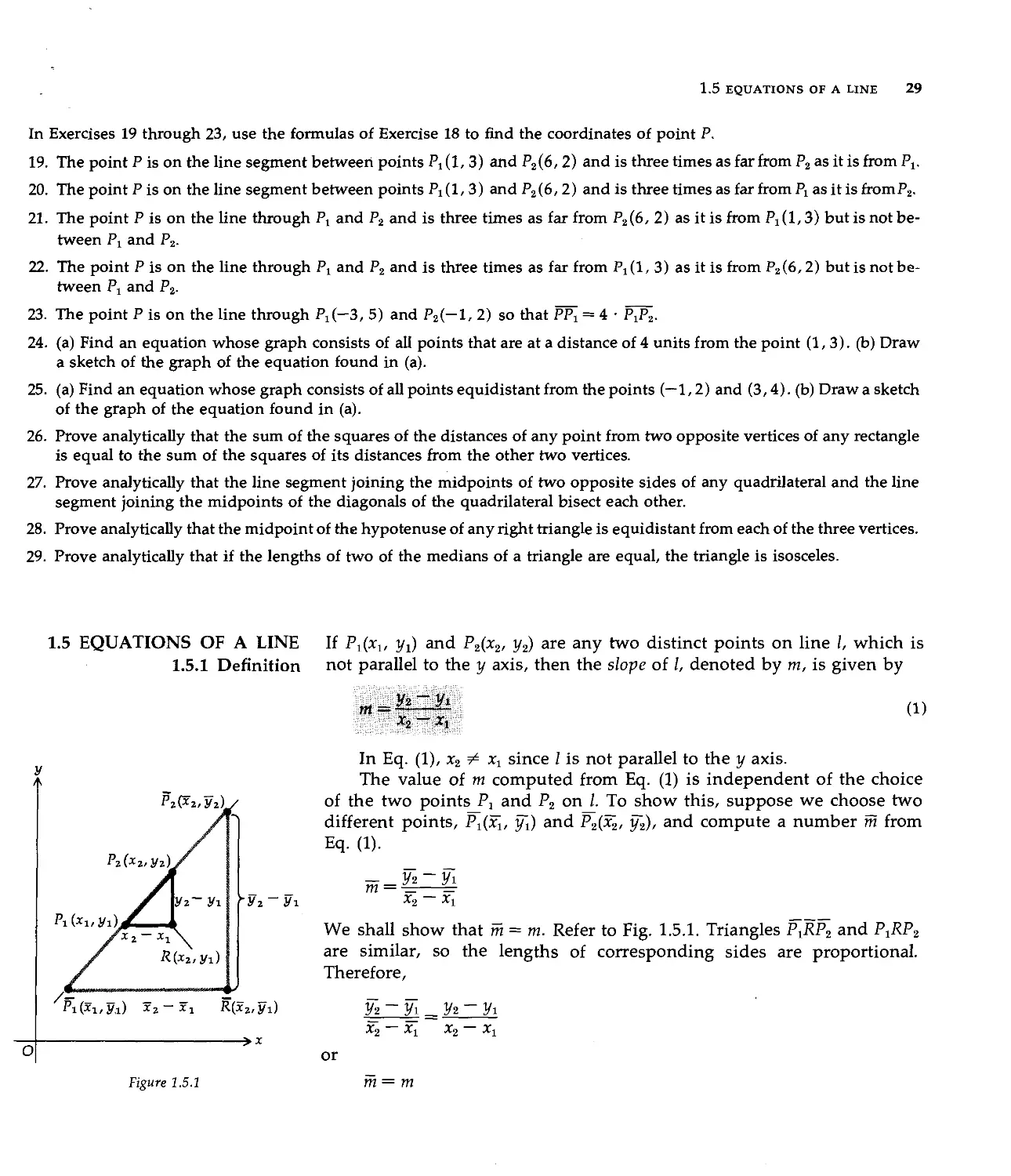
Now let Pi(*i, j/J and P2(x2, y2) be any two points in the plane. We
wish to obtain a formula for finding the nonnegative distance between
these two points. We shall denote this distance by |P,P2|. We use
absolute-value bars because we are concerned only with the length, which is
a nonnegative number, of the line segment between the two points ?! and
1.4 DISTANCE FORMULA AND MIDPOINT FORMULA 25
P2. To derive the formula, we note that |P1P2| is the length of the
hypotenuse of a right triangle P-lMP?,. This is illustrated in Fig. 1.4.3 for Pt and
P2, both of which are in the first quadrant.
P2 (*2, 3/2)
)■ Ay = 3/2 - 3/1
So
or
Figure 1.4.3
Using the Pythagorean theorem, we have
|PVP^[2= |Ax|2+ |Ay|2
|P7P~2| = V|Ax|2+|Ay|2
|PiP*l = Vfe-x^+O/s-j/J2 (l)
Formula (1) holds for all possible positions of Pt and P2 in all four
quadrants. The length of the hypotenuse will always be |P1P2|, and the
lengths of the two legs will always be |Ax| and |Ay| (see Exercises 1 and
2). We state this result as a theorem.
1.4.1 Theorem The undirected distance between the two points P^Xv yt) and P2(x2, y2)
is given by
|P,P2| = V(x2-x1)2+(y2-y])2
example 1: If a point P(x, y) is
such that its distance from
A(3, 2) is always twice its
distance from B(— 4, 1), find an
equation which the coordinates
of P must satisfy.
solution: From the statement of the problem
\PA\=2\PB\
Using formula (1), we have
V(x-3)2+ (y-2)2 = 2V(x + 4)2+ (y-1)2
Squaring on both sides, we have
x2 - 6x + 9 + y2 - iy + 4 = 4(%2 + 8x + 16 + y2 - 2y + 1)
26 REAL NUMBERS AND INTRODUCTION TO ANALYTIC GEOMETRY
or
3x2 + 3y2 + 38* - 4y + 55 = 0
example 2: Show that the
triangle with vertices at A(—2, 4),
B(-5, l),and C(-6, 5) is
isosceles.
y
A
C{-6,5)
\ ^^>l(-2,4)
V?
V
B(-5,l)
1 1 1 1 1 1
O
fi^"re 1.4.4
solution: The triangle is shown in
\BC\ = V(-6 + 5)2 + (5 - l)2 =
\AC\= V(-6 + 2)2+ (5-4)2 =
\BA\ = V(-2 + 5)2+ (4-1)' =
Therefore,
\BC\ = \AC\
Hence, triangle ABC is isosceles.
Fig. 1.4.4.
VI+ 16= V17
V16+1= V17
V9 + 9 =3V2
example 3: Prove analytically
that the lengths of the diagonals
of a rectangle are equal.
A (a, 0)
Figure 1.4.5
solution: Draw a general rectangle. Because we can choose the
coordinate axes anywhere in the plane, and because the choice of the position
of the axes does not affect the truth of the theorem, we take the origin at
one vertex, the x axis along one side, and the y axis along another side.
This procedure simplifies the coordinates of the vertices on the two axes.
Refer to Fig. 1.4.5.
Now the hypothesis and the conclusion of the theorem can be stated.
Hypothesis: OABC is a rectangle with diagonals OB and AC.
Conclusion: \OB\= \AC\.
proof:
\OB\ = V(a-0)2+ (b-0)2= Vfl2 + b2
\AC\ = V(O-a)2
Therefore,
m\ = \Ac\
(fc-0)2= V¥
Let Pita, i/x) and P2(x2, y2) be the endpoints of a line segment. We
shall denote this line segment by P1P2. This is not to be confused with the
notation PjP2, which denotes the directed distance from Px to P2. That is,
1.4 DISTANCE FORMULA AND MIDPOINT FORMULA 27
PlP2 denotes a number, whereas PiP2 is a line segment. Let P(x, y) be the
midpoint of the line segment P1P2- Refer to Fig. 1.4.6.
o
Pi{^2,yz)
T(*2,y)
JS(x2/yi)
Figure 1.4.6
In Fig. 1.4.6 we see that triangles PX.RP and PTP2 are congruent.
Therefore, |Pxi?| = |PT|, and so x — x1 = x2 ~ x, giving us
Y=*i_±Jk
2
(2)
Similarly, \RP\ = |TP2|. Then y — yY = y2 — y, and therefore
., __ vi + y*
y 2
(3)
Hence, the coordinates of the midpoint of a line segment are,
respectively, the average of the abscissas and the average of the ordinates of
the endpoints of the line segment.
In the derivation of formulas (2) and (3) it was assumed that x% > xx
and y2 > yv The same formulas are obtained by using any orderings of
these numbers (see Exercises 3 and 4).
example 4: Prove analytically
that the line segments joining the
midpoints of the opposite sides
of any quadrilateral bisect each
other.
solution: Draw a general quadrilateral. Take the origin at one vertex
and the x axis along one side. This method simplifies the coordinates of
the two vertices on the x axis. See Fig. 1.4.7.
Hypothesis: OABC is a quadrilateral. M is the midpoint of OA, N is
the midpoint of CB, R is the midpoint of OC, and S is the midpoint of AB.
Conclusion: MN and RS bisect each other.
proof: To prove that two line segments bisect each other, we show that
they have the same midpoint. Using formulas (2) and (3), we obtain the
coordinates of M, N, R, and S. M is the point (ia, 0), N is the point
(i(b + d), i(c + e)), R is the point (id, ie), and S is the point (i(a + b), ic).
28
REAL NUMBERS AND INTRODUCTION TO ANALYTIC GEOMETRY
o\
v
c (d, ey
kA—^"
B(b, c)
3^^\
I __-»-—**\^
M A(a,0) '"
Figure 1.4.7
The abscissa of the midpoint of MNisi[ia + i(b + d)]=i(a + b + d).
The ordinate of the midpoint of MN is |[0 + i(c + e)] = i(c + e).
Therefore, the midpoint of MN is the point (i(a + b + d), i(c + e)).
The abscissa of the midpoint of RS is £[|d + k(a + b)] =\{a + b + d).
The ordinate of the midpoint of RS is j[ie + ic] = \(c + e).
Therefore, the midpoint of RS is the point (\{a + b + d), %(c + e)).
Thus, the midpoint of MN is the same point as the midpoint of RS.
Therefore, MN and RS bisect each other. ■
Exercises 1.4
1. Derive distance formula (1) if Pi is in the third quadrant and P2 is in the second quadrant. Draw a figure.
2. Derive distance formula (1) if Pi is in the second quadrant and P2 is in the fourth quadrant. Draw a figure.
3. Derive midpoint formulas (2) and (3) if Pt is in the first quadrant and P2 is in the third quadrant.
4. Derive midpoint formulas (2) and (3) if Pi(*i, yx) andP2(x2, j/2) are both in the second quadrant and x2 > X[ and y, > y2.
5. Find the length of the medians of the triangle having vertices A(2, 3), B(3, —3), and C(—1, —1).
6. Find the midpoints of the diagonals of the quadrilateral whose vertices are (0, 0), (0, 4), (3, 5), and (3,1).
7. Prove that the triangle with vertices A(3,-6),B(8,-2)/ and C(-l, -1) is a right triangle. Find the area of the triangle.
(hint: Use the converse of the Pythagorean theorem.)
8. Prove that the points A(6, -13), B(-2, 2), C(13, 10), and D(21, -5) are the vertices of a square. Find the length of
a diagonal.
9. By using distance formula (1), prove that the points (—3, 2), (1, —2), and (9, —10) lie on a line.
10. If one end of a line segment is the point (—4, 2) and the midpoint is (3, —1), find the coordinates of the other end of
the line segment.
11. The abscissa of a point is —6, and its distance from the point (1, 3) is V74. Find the ordinate of the point.
12. Determine whether or not the points (14, 7), (2, 2), and (—4, —1) lie on a line by using distance formula (1).
13. If two vertices of an equilateral triangle are (—4, 3) and (0, 0), find the third vertex.
14. Find an equation that must be satisfied by the coordinates of any point that is equidistant from the two points (—3,2)
and (4,6).
15. Find an equation that must be satisfied by the coordinates of any point whose distance from the point (5,3) is always
two units greater than its distance from the point (—4,-2).
16. Given the two points A(—3, 4) and B(2, 5), find the coordinates of a point P on the line through A and B such thatP
is (a) twice as far from A as from B, and (b) twice as far from B as from A.
17. Find the coordinates of the three points that divide the line segment from A(—5, 3) to B(6, 8) into four equal parts.
18. If ri and r2 are positive integers, prove that the coordinates of the point P(x, y), which divides the line segment P1P2
in the ratio ri/r2—that is, iP^I/lPiPal = rjr2—are given by
x _ (r2-ri)*i + >"i*2 and = (r2 ~ rt)yi + rty2
r2 r2
1.5 EQUATIONS OF A LINE 29
In Exercises 19 through 23, use the formulas of Exercise 18 to find the coordinates of point P.
19. The point P is on the line segment between points Px (1, 3) and P2(6, 2) and is three times as far from P2 as it is from Px.
20. The point Pis on the line segment between points Pi(l, 3) and P2(6,2) and is three times as far from Px asitisfromP2.
21. The point P is on the line through P1 and P2 and is three times as far from P2(6, 2) as itis from P^l^) but is not
between P1 and P2.
22. The point P is on the line through P1 and P2 and is three times as far from Px (1, 3) as it is from P2 (6,2) but is not
between P1 and P2.
23. The point P is on the line through Px(-3, 5) and P2(-l, 2) so that PP[ = 4 • P^F2.
24. (a) Find an equation whose graph consists of all points that are at a distance of 4 units from the point (1, 3). (b) Draw
a sketch of the graph of the equation found in (a).
25. (a) Find an equation whose graph consists of all points equidistant from the points (—1,2) and (3,4). (b) Draw a sketch
of the graph of the equation found in (a).
26. Prove analytically that the sum of the squares of the distances of any point from two opposite vertices of any rectangle
is equal to the sum of the squares of its distances from the other two vertices.
27. Prove analytically that the line segment joining the midpoints of two opposite sides of any quadrilateral and the line
segment joining the midpoints of the diagonals of the quadrilateral bisect each other.
28. Prove analytically that the midpoint of the hypotenuse of any right triangle is equidistant from each of the three vertices.
29. Prove analytically that if the lengths of two of the medians of a triangle are equal, the triangle is isosceles.
1.5 EQUATIONS OF A LINE If P1(x1, yj and P2(x2, y2) are anv two distinct points on line /, which is
1.5.1 Definition not parallel to the y axis, then the slope of /, denoted by m, is given by
m =
yz-yi
x2 xx
(1)
y
o
P2(^2,y2L
Pz(*z,yz
fVz~ yi
Pi(*i,yi)
Pi(*i,y,i)
In Eq. (1), x2 ¥= xt since / is not parallel to the y axis.
The value of m computed from Eq. (1) is independent of the choice
of the two points Px and P2 on /. To show this, suppose we choose two
different points, Pi(3ti, y~i) and P2(3^, y~2), and compute a number m from
Eq. (1).
X2 Xi
We shall show that m = m. Refer to Fig. 1.5.1. Triangles P~jlP2 and P^RPi
are similar, so the lengths of corresponding sides are proportional.
Therefore,
X2 - Xi
Figure 1.5.1
R(X2,Vl)
or
Vi ~ Vi _ Vi - Vi
X2 ~~~ X\ X2 X\
m= m
30 REAL NUMBERS AND INTRODUCTION TO ANALYTIC GEOMETRY
Figure 1.5.2
»x
Hence, we conclude that the value of m computed from Eq. (1) is the same
number no matter what two points on / are selected.
In Fig. 1.5.1, x2 > xu y2 > yu x2 > *i> and y~2 > y[. The discussioi
above is valid for any ordering of these pairs of numbers since Definition
1.5.1 holds for any ordering.
In Sec. 1.4 we defined Ay = y2 — yt and Ax=x2 — xt. Substituting
these values into Eq. (1), we have
m
= Ay
Ax
Multiplying on both sides of this equation by Ax, we obtain
Ay = m Ax
(2
Figure 1.5.3
It is seen from Eq. (2) that if we consider a particle moving along
line /, the change in the ordinate of the particle is proportional to the
change in the abscissa, and the constant of proportionality is the slope
of the line.
If the slope of a line is positive, then as the abscissa of a point on the
line increases, the ordinate increases. Such a line is shown in Fig. 1.5.2.
In Fig. 1.5.3, we have a line whose slope is negative. For this line, as the
abscissa of a point on the line increases, the ordinate decreases. Note that
if the line is parallel to the x axis, then y2 = i/i and so m = 0.
If the line is parallel to the y axis, x2 = x,; thus, Eq. (1) is meaningless
because we cannot divide by zero. This is the reason that lines parallel
to the y axis, or vertical lines, are excluded in Definition 1.5.1. We say that
a vertical line does not have a slope.
example 1: Let / be the line
through the points Pi(2, 3) and
P2(4, 7). Find the slope of /.
solution: The slope of /, by Definition 1.5.1, is given by
7-3
m = ■
= 2
P4(-i,-3)/ -
Figure 1.5.4
Refer to Fig. 1.5.4. If P(x, y) and Q(x
on /, then
AV „
Ax
Ax, y + Ay) are any two points
or
Ay = 2 Ax
Thus, if a particle is moving along the line /, the change in the ordinate
is twice the change in the abscissa. That is, if the particle is at P2(4, 7)
and the abscissa is increased by one unit, then the ordinate is increased
by two units, and the particle is at the point P3(5, 9). Similarly, if the
particle is at P](2,3) and the abscissa is decreased by three units, then the
ordinate is decreased by six units, and the particle is at the point P4(— 1,— 3).
1.5 EQUATIONS OF A LINE 31
Since two points Pi(xu 1/1) and P2(x2, y2) determine a unique line, we
should be able to obtain an equation of the line through these two points.
Consider P(x, y) any point on the line. We want an equation that is
satisfied by x and y if and only if P(x, y) is on the line through Pi(xx, yt) and
P2(x2, 3/2)- We distinguish two cases.
Case 1: x2 = xt.
In this case the line through P1 and P2 is parallel to the y axis, and all
points on this line have the same abscissa. So P(x, y) is any point on the
line if and only if
x=Xi (3)
Equation (3) is an equation of a line parallel to the y axis. Note that this
equation is independent of y; that is, the ordinate may have any value
whatsoever, and the point P(x, y) is on the line whenever the abscissa is Xi.
Case 2: x2 ¥= xv
The slope of the line through Px and P2 is given by
m = y-^l (4)
X2 X\
If P(x, y) is any point on the line except (xu yx), the slope is also
given by
The point P will be on the line through Pi and P2 if and only if the value
of m from Eq. (4) is the same as the value of m from Eq. (5), that is, if and
only if
y - 3/1 = 3/2 - yi
X X\ X% X\
Multiplying on both sides of this equation by (x — x^, we obtain
y-yi = T^T(x~Xi) (6)
Equation (6) is satisfied by the coordinates of Pi as well as by the
coordinates of any other point on the line through Px and P2.
Equation (6) is called the two-point form of an equation of the line.
It gives an equation of the line if two points on the line are known.
If in Eq. (6) we replace (y2 — yi)l(x2 — xx) by m, we get
y-y1 = m(x-xl) (7)
32 REAL NUMBERS AND INTRODUCTION TO ANALYTIC GEOMETRY
Equation (7) is called the point-slope form of an equation of the line
It gives an equation of the line if a point Pi(xlr yx) on the line and the
slope m of the line are known.
If we choose the particular point (0, b) (i.e., the point where the line
intersects the y axis) for the point (xu i/i) in Eq. (7), we have
or
y — b = m(x— 0)
y = mx + b
(s;
The number b, which is the ordinate of the point where the line
intersects the y axis, is called the y intercept of the line. Consequently,
Eq. (8) is called the slope-intercept form of an equation of the line. This
form is especially important because it enables us to find the slope of a
line from its equation. It is also important because it expresses the y
coordinate explicitly in terms of the x coordinate.
example 2: Given the line
having the equation 3x + iy = 7,
find the slope of the line.
solution: Solving the equation for y, we have
y = -\x-
Comparing this equation with Eq. (8), we see that m =
Therefore, the slope is
-f and b = \.
4-
Another form of an equation of a line is the one involving the
intercepts of a line. We define the x intercept of a line as the abscissa of the
point at which the line intersects the x axis. The x intercept is denoted
by a. If the x intercept a and the y intercept b are given, we have two
points (a, 0) and (0, b) on the line. Applying Eq. (6), the two-point form,
we have
n ft-0i \
or
or
—ay = bx— ab
bx + ay = ab
Dividing by ab, if a ¥= 0 and b ¥= 0, we obtain
x y
a b
(9)
Equation (9) is called the intercept form of an equation of the line.
Obviously it does not apply to a line through the origin, because for such
a line both a and b are zero.
1.5 EQUATIONS OF A LINE 33
example 3: The point (2, 3)
bisects that portion of a line
which is cut off by the
coordinate axes. Find an equation of
the line.
Figure 1.5.5
solution: Refer to Fig. 1.5.5. If a is the x intercept of the line and b is
the y intercept of the line, then the point (2, 3) is the midpoint of the
line segment joining (a, 0) and (0, b). By the midpoint formulas, we have
2 = —^— and 3 = ——
Then
a = 4 and b = 6
The intercept form, Eq. (9), gives us
4 6
= 1
or
3x + 2y = 12
1.5.2 Theorem The graph of the equation
Ax + By + C = 0
(10)
where A, B, and C are constants and where not both A and B are zero, is
a straight line.
proof: Consider the two cases B ¥= 0 and B = 0.
Case 1: B * 0.
Because B ¥= 0, we divide on both sides of Eq. (10) by B and obtain
A C
y=-Bx~B
(11)
Equation (11) is an equation of a straight line because it is in the slope-
intercept form, where m = —A/B and b = —C/B.
Case 2: B = 0.
Because B = 0, we may conclude that A ¥= 0 and thus have
Ax + C = 0
or
C
x = —
(12)
Equation (12) is in the form of Eq. (3), and so the graph is a straight line
parallel to the y axis. This completes the proof. ■
Because the graph of Eq. (10) is a straight line, it is called a linear
equation. Equation (10) is the general equation of the first degree in x and y.
34 REAL NUMBERS AND INTRODUCTION TO ANALYTIC GEOMETRY
Because two points determine a line, to draw a sketch of the graph of
a straight line from its equation we need only determine the coordinates
of two points on the line, plot the two points, and then draw the line.
Any two points will suffice, but it is usually convenient to plot the two
points where the line intersects the two axes (which are given by the
intercepts).
example 4: Given line lu having
the equation 2x — 3y = 12, and
line Z2, having the equation
4x + 3y = 6, draw a sketch of
each of the lines. Then find the
coordinates of the point of
intersection of k and Z2.
l
o
\ 1 1 1 1 j/\ 1 ^r
X ' ^^ ^ X
- y&,-2)
Figure 1.5.6
solution: To draw a sketch of the graph of k, we find the intercepts a
and b. In the equation of lu we substitute 0 for x and get b = —4. In the
equation of llr we substitute 0 for y and get a = 6. Similarly, we obtain
the intercepts a and b for Z2, and for Z2 we have a = f and b = 2. The two
lines are plotted in Fig. 1.5.6.
To find the coordinates of the point of intersection of h and Z2, we
solve the two equations simultaneously. Because the point must lie on
both lines, its coordinates must satisfy both equations. If both equations
are put in the slope-intercept form, we have
y = ix — 4 and y = — ix + 2
Eliminating y gives
|x-4=-*x + 2
or
2x - 12 = -ix + 6
or
6x=18
or
x=3
So
y = i(3)-4
or
y = -2
Therefore, the point of intersection is (3, —2).
1.5.3 Theorem If k and Z2 are two distinct nonvertical lines having slopes m1 and m2,
respectively, then lt and l2 are parallel if and only if m, = m2.
Let an equation of lx be y = mxx + bu and let an equation of Z2
be y = m2x+ b2. Because there is an "if and only if" qualification, the
proof consists of two parts.
Prove that lx and Z2 are parallel if mx = m2.
Assume that U and Z2 are not parallel. Let us show that this
assumption leads to a contradiction. If li and l2 are not parallel, then they intersect.
1.5 EQUATIONS OF A LINE 35
Call this point of intersection P(x0, y0). The coordinates of P must satisfy
the equations of k and l2, and so we have
y0 = niiX0 + bi and y0 = m2x0 + b2
But m, = m2, which gives
y0 = niiX0 + bi and y0 = m^ + b2
from which it follows that b^ = b2. So, if m, = m2 and bx = b2, then both
lines /, and l2 have the same equation, y = m^x + bu and so the lines are
the same. But this contradicts the hypothesis that /, and l2 are distinct
lines. Therefore, our assumption is false. So we conclude that Zx and l2
are parallel.
part 2: Prove that /, and l2 are parallel only if m, = m.,. Here we must
show that if Zx and l2 are parallel, then m1 — m2.
Assume that m1 ¥= m2. Solving the equations for /, and /2
simultaneously, we get, upon eliminating y,
m^x + bi = m2x + b2
from which it follows that
(m1 — m2)x= b2 — bx
Because we have assumed that mx ¥= m2, this gives
x = — -
m1 — m2
Hence, /] and l2 have a point of intersection, which contradicts the
hypothesis that /, and l2 are parallel. So our assumption is false, and
therefore m1 = m2. ■
In Fig. 1.5.7, the two lines Zx and l2 are perpendicular. We state and
prove the following theorem on the slopes of two perpendicular lines.
36 REAL NUMBERS AND INTRODUCTION TO ANALYTIC GEOMETRY
1.5.4 Theorem If neither line k nor line l2 is vertical, then lt and l2 are perpendicular if
and only if the product of their slopes is —1. That is, if m, is the slope of
lt and m2 is the slope of l2, then k and l2 are perpendicular if and only if
mxm2 = —1.
proof:
part 1: Prove that U and l2 are perpendicular only if mxm2 = —1.
Let Lj be the line through the origin parallel to lx and let L2 be the
line through the origin parallel to l2. See Fig. 1.5.7. Therefore, by Theorem
1.5.3, the slope of line Lx is m, and the slope of line L2 is m2. Because neither
Lj nor L2 is vertical, these two lines intersect the line x = 1 at points Pi
and P2, respectively. The abscissa of both Px and P2 is 1. Let y be the
ordinate of Pi. Since Lt contains the points (0, 0) and (1, y) and its slope is m1,
we have from Definition 1.5.1
and so y = mx. Similarly, the ordinate of P2 is shown to be m2.
Applying the Pythagorean theorem to right triangle PiOP2, we get
|OP",|2+ |OPT2|2= IP^KI2 (13)
By applying the distance formula, we obtain
|OP",|* = (1 - 0)2 + (ffl, - 0)2 = 1 + m,2
|OP"2|2 = (1 - 0)2 + (m2 - 0)2 = 1 + m22
|P^|2 = (j _ 1)2 + (mg - mi)2 = m2 _ 2mim2 + m2
Substituting into Eq. (13) gives
(1 + m^) + (1 + m22) = m22 - 2mlm2 +■ m,2
1 = —2mlm2
m{tn2 = —\
part 2: Prove that k and l2 are perpendicular if mlm2 = —1. Starting with
mxm2 = — 1, we can reverse the steps of the proof of Part 1 and obtain
|op;i2+ |op;i2= ip^i2
from which it follows, from the converse of the Pythagorean theorem,
that Lj and L2 are perpendicular; hence, lx and l2 are perpendicular. ■
Theorem 1.5.4 states that if two lines are perpendicular and neither
one is vertical, the slope of one of the lines is the negative reciprocal of
the slope of the other line. For example, if line /[ is perpendicular to line
l2 and the slope of k is |, then the slope of l2 must be —f.
1.5 EQUATIONS OF A LINE 37
example 5: Prove by means of
slopes that the four points •
A{6, 2), B(8, 6), C(4, 8), and
D(2, 4) are the vertices of a
rectangle.
B(8, 6)
Figure 1.5.8
solution: See Fig. 1.5.8. Let
^ o
rrii — the slope of AB — -z—7 = 2.
o 6
m2 = the slope of BC =
8-6
4-8
-4
_1
2'
m3 = the slope of DC = . _ = 2.
4 — 2 1
m4 = the slope of AD = -z 7 = — -.
2 — 6 2
Because
m, = m3, AB \\ DC.
m2 = m4, BC || AD.
m1mi = -l,AB 1 BC.
Therefore, quadrilateral ABCD has opposite sides parallel and two
adjacent sides perpendicular, and we conclude that ABCD is a rectangle.
example 6: Given the line /
having the equation
2x + 3y - 5 = 0
find an equation of the line
perpendicular to line / and
passing through the point
A(-l, 3).
solution: Because the required line is perpendicular to line /, its slope
must be the negative reciprocal of the slope of /. We find the slope of / by
putting its equation into the slope-intercept form. Solving the given
equation for y, we obtain
y = ~\x + I
Therefore, the slope of / is —f, and the slope of the required line is f.
Because we also know that the required line contains the point (—1, 3), we
use the point-slope form, which gives
3 = !(* + !)
or
or
y
2y - 6 = 3x + 3
3x-2y + 9 = 0
Exercises 1.5
In Exercises 1 through 4, find the slope of the line through the given points.
1. (2, -3), (-4, 3) 2. (5, 2), (-2, -3)
3. d, i), (-», t) 4. (-2.1, 0.3), (2.3, 1.4)
38 REAL NUMBERS AND INTRODUCTION TO ANALYTIC GEOMETRY
In Exercises 5 through 14, find an equation of the line satisfying the given conditions.
5. The slope is 4 and through the point (2, —3).
6. Through the two points (3, 1) and (—5, 4).
7. Through the point (—3, —4) and parallel to the y axis.
8. Through the point (1,-7) and parallel to the x axis.
9. The x intercept is —3, and the y intercept is 4.
10. Through (1,4) and parallel to the line whose equation is 2x — 5y + 7 = 0.
11. Through (—2,-5) and having a slope of V3.
12. Through the origin and bisecting the angle between the axes in the first and third quadrants.
13. Through the origin and bisecting the angle between the axes in the second and fourth quadrants.
14. The slope is —2, and the x intercept is 4.
15. Find an equation of the line through the points (1, 3) and (2, —2), and put the equation in the intercept form.
16. Find an equation of the line through the points (3,-5) and (1,-2), and put the equation in the slope-intercept form.
17. Show by means of slopes that the points (—4, — 1), (3, f), (8, —4), and (2, —9) are the vertices of a trapezoid.
18. Three consecutive vertices of a parallelogram are (—4, 1), (2, 3), and (8, 9). Find the coordinates of the fourth vertex.
19. For each of the following sets of three points, determine by means of slopes if the points are on a line: (a) (2, 3),
(-4,-7), (5,8);(b) (-3,6), (3,2), (9, -2); (c) (2,-1), (1, 1), (3, 4); and (d) (4, 6), (1, 2), (-5,-4).
20. Prove by means of slopes that the three points A{3, 1), B(6, 0), and C(4, 4) are the vertices of a right triangle, and find
the area of the triangle.
21. Given the line / having the equation 2y — 2>x = 4 and the point P(l, —3), find (a) an equation of the line through P
and perpendicular to /; (b) the shortest distance from P to line /.
22. If A, B, C, and D are constants, show that (a) the lines Ax + By + C = 0 and Ax + By + D = 0 are parallel and (b) the
lines Ax + By + C = 0 and Bx — Ay + D = 0 are perpendicular.
23. Given the line /, having the equation Ax + By + C = 0, B ¥= 0, find (a) the slope, (b) the y intercept, (c) the x intercept,
(d) an equation of the line through the origin perpendicular to I.
24. Find an equation of the line which has equal intercepts and which passes through the point (8, —6).
25. Find equations of the three medians of the triangle having vertices A(3, —2), B(3, 4), and C(—1, 1), and prove that
they meet in a point.
26. Find equations of the perpendicular bisectors of the sides of the triangle having vertices A(— 1, —3), B(5, —3), and
C(5, 5), and prove that they meet in a point.
27. Find an equation of each of the lines through the point (3,2), which forms with the coordinate axes a triangle of area 12.
28. Let /i be the line having the equation Atx + Bty + Q = 0, and let l2 be the line having the equation A2x + B2y + C2 = 0.
If li is not parallel to l2 and if k is any constant, the equation
Atx + Bty + Q + k(A2x + B2y + C2) =0
represents an unlimited number of lines. Prove that each of these lines contains the point of intersection of h and l2.
29. Given an equation of \x is 2x + 3y — 5 = 0 and an equation of l2 is 3x + 5y — 8 = 0, by using Exercise 28 and without
finding the coordinates of the point of intersection of lx and l2, find an equation of the line through this point of
intersection and (a) passing through the point (1,3); (b) parallel to the x axis; (c) parallel to the y axis; (d) having slope—2;
(e) perpendicular to the line having the equation 2x + y = 7; (f) forming an isosceles triangle with the coordinate axes.
1.6 THE CIRCLE 39
30. Find an equation of each straight line that is perpendicular to the line having the equation 5x — y = 1 and that forms
with the coordinate axes a triangle having an area of measure 5.
31. Prove analytically that the diagonals of a rhombus are perpendicular.
32. Prove analytically that the line segments joining consecutive midpoints of the sides of any quadrilateral form a
parallelogram.
33. Prove analytically that the diagonals of a parallelogram bisect each other.
34. Prove analytically that if the diagonals of a quadrilateral bisect each other, then the quadrilateral is a parallelogram.
1.6 THE CIRCLE A circle is the set of all points in a plane equidistant from a fixed
1.6.1 Definition point. The fixed point is called the center of the circle, and the measure
of the constant equal distance is called the radius of the circle.
1.6.2 Theorem The circle with center at the point C(h, k) and radius r has as an equation
(x-h)*+(y-k)* = r*
proof: The point P(x, y) lies on the circle if and only if
\PC\ = r
that is, if and only if
(1)
V(x-h)2+ (y-k)2 = r
This is true if and only if
(x-h)2 + (y-i)* = r*
which is Eq. (1). Equation (1) is satisfied by the coordinates of those and
only those points which lie on the given circle. Hence, (1) is an equation
of the circle. ■
From Definition 1.3.2, it follows that the graph of Eq. (1) is the circle
with center at (h, k) and radius r.
If the center of the circle is at the origin, then h — k — 0; therefore,
its equation is x2 + y2 — r2.
example 1: Find an equation of
the circle with center at (2, —3)
and radius equal to 4.
solution: The circle is shown in Fig. 1.6.1. In this example, h = 2,
k = —3, r = 4. Substituting into Eq. (1), we have
or
(x-2)2+ [y- (-3)]2 = 42
(x-2)2+ (y + 3)2=16
40 REAL NUMBERS AND INTRODUCTION TO ANALYTIC GEOMETRY
>X
Figure 1.6.1
Squaring and then combining terms, we have
x2 - 4x + 4 + y2 + 6y + 9 = 16
or
x2 + y2 - 4x + by - 3 = 0
example 2: Given the equation
x2 + y2 + 6x - ly - 15 = 0
prove that the graph of this
equation is a circle, and find its
center and radius.
solution: The given equation may be written as
{x2 + 6x) + {y2-2y) =15
Completing the squares of the terms in parentheses by adding 9 and 1
on both sides of the equation, we have
{x2 + 6x + 9) + {y2 - ly + 1) = 15 + 9 + 1
or
(x + 3)2+ (y-l)2 = 25
Comparing this equation with Eq. (1), we see that this is an equation oi
a circle with its center at (—3, 1) and a radius of 5.
In Eq. (1), removing parentheses and combining terms gives
x2 + y2-2hx-2ky+ {h2 + k2 - r2) =0 (2)
Equation (2) is of the form
x2 + y2 + Dx + Ey + F = 0 (3)
where D = -2h, E = -2k, and F = h2 + k2 - r2
Equation (3) is called the general form of an equation of a circle,
whereas Eq. (1) is called the center-radius form. Because every circle has
a center and a radius, its equation can be put in the center-radius form,
and hence into the general form.
We now consider the question of whether or not the graph of every
equation of the form
x2 + y2 + Dx + Ey + F = 0
is a circle. To determine this, we shall attempt to write this equation in the
center-radius form. We rewrite the equation as
x2 + y2 + Dx+Ey = -F
1.6 THE CIRCLE 41
and complete the squares of the terms in parentheses by adding \D2 and
\E2 on both sides, thus giving us
(x2 + Dx + iD2) + {y2 + Ey + i£2) = -F + |D2 + \E2
or
(x + |D)2+(y + iE)2 = i(D2 + E2-4F) (4)
Equation (4) is in the form of Eq. (1) if and only if
i(D2 + E2 - 4F) = r2
We now consider three cases, namely, (D2 + E2 — 4F) as positive,
zero, and negative.
Casel: (D2 + E2 - 4F) > 0.
Then r2 = i(D2 + E2 — 4F), and so Eq. (4) is an equation of a circle
having a radius equal to |VD2 + E2 — 4F and its center at (— |D, — |E).
Case 2: D2 + E2-4F=0.
Equation (4) is then of the form
(x + W)2+ (y + m2 = 0. (5)
Because the only real values of x and y satisfying Eq. (5) are x = —\D and
y = —\E, the graph is the point (— iD, —\E). Comparing Eq. (5) with
Eq. (1), we see that h = —iD, k = — \E, and r = 0. Thus, this point can be
called a point-circle.
Case 3: (D2 + E2 - 4F) < 0.
Then Eq. (4) has a negative number on the right side and the sum of
the squares of two real numbers on the left side. There are no real values
of x and y that satisfy such an equation; consequently, we say there is
no real locus.
Before stating the results of these three cases as a theorem, we
observe that an equation of the form
Ax2 + Ay2 + Dx + Ey + F=0 where A ^ 0 (6)
can be written in the form of Eq. (3) by dividing by A, thereby obtaining
x2 + y2 + Dx+Ey+F = 0
Equation (6) is a special case of the general equation of the second degree:
Ax2 + Bxy + Cy2+Dx+Ey + F=0
in which the coefficients of x2 and y2 are equal and which has no xy term.
We have, then, the following theorem.
1.6.3 Theorem The graph of any second-degree equation in R2 in x and y, in which the
42 REAL NUMBERS AND INTRODUCTION TO ANALYTIC GEOMETRY
coefficients of x2 and y2 are equal and in which there is no xy term, is
either a circle, a point-circle, or no real locus.
example 3: Determine the graph
of the equation
2x2 + 2y2 + Ylx - 8y + 31 = 0
solution: The equation is of the form (6), and therefore the graph is
either a circle, a point-circle, or no real locus. If the equation is put in the
form of Eq. (1), we have
x2 + y2 + 6x - 4y + ^ = 0
(x2 + 6x) + (y2-4y)=-^
(x2 + 6x + 9) + (y2 - \y + 4) = -^ + 9 + 4
(x + 3)2+(y-2)2 = -i
Therefore, there is no real locus.
example 4: Find an equation of
the circle through the three
points A(4, 5), B(3, —2), and
C(l, -4).
solution: The general form of an equation of the circle is
x2 + y2 + Dx + Ey + F = 0
Because the three points A, B, and C must lie on the circle, the
coordinates of these points must satisfy the equation. So we have
16 + 25 + 4D + 5E + F = 0
9+ 4 + 3D-2E + F=0
1 + 16+ D-4E + F=0
or
4D + 5E + F = -41
3D-2E + F = -13
D-4E + F = -17
Solving these three equations simultaneously, we get
D=7 E=-5 F = -44
Thus, an equation of the circle is
x2 + y2 + 7x - 5y - 44 = 0
In the following example we have a line which is tangent to a circle.
The definition of the tangent line to a general curve at a specific point is
given in Sec. 3.1. However, for a circle we use the definition from plane
geometry which states that a tangent line at a point P on the circle is the
line intersecting the circle at only the point P.
1.6 THE CIRCLE 43
example 5: Find an equation of
the circle with its center at the
point C(l, 6) and tangent to the
line / having the equation
x-y-l = 0.
Figure 1.6.2
solution: See Fig. 1.6.2. Given that h = 1 and k = 6, if we find r, we can
obtain an equation of the circle by using the center-radius form.
Let /i be the line through C and the point P, which is the point of
tangency of line / with the circle.
r= \PC\
Hence, we must find the coordinates of P. We do this by finding an
equation of /i and then finding the point of intersection of lx with /. Since lx
is along a diameter of the circle, and / is tangent to the circle, /] is
perpendicular to /. Because the slope of / is 1, the slope of lx is —1. Therefore,
using the point-slope form of an equation of a line, we obtain as an
equation of /i
y-6 = -l(x-l)
or
x+y-7=0
Solving this equation simultaneously with the given equation of /, namely,
x-y-l=0
we get x = 4 and y = 3. Thus, P is the point (4, 3). Therefore,
r= \PC\ = V(4-l)2+ (3-6)2
or
r= Vl8
So, an equation of the circle is
(x-l)2 + (y-6)2 = (Vl8)2
or
x2 + y2 - 2x - My + 19 = 0
Exercises 1.6
In Exercises 1 through 4, find an equation of the circle with center at C and radius r. Write the equation in both the center-
radius form and the general form.
2. C(0, 0),r=8
4. C(-l, l),r=2
1. C(4,-3),r=5
3. C(-5,-12),r=3
In Exercises 5 through 10, find an equation of the circle satisfying the given conditions.
5. Center is at (1, 2) and through the point (3, —1).
6. Center is at (—2, 5) and tangent to the line x = 7.
44 REAL NUMBERS AND INTRODUCTION TO ANALYTIC GEOMETRY
7. Center is at (-3, -5) and tangent to the line 12x + 5y - 4 = 0.
8. Through the three points (2, 8), (7, 3), and (-2, 0).
9. Tangent to the line 3x + y + 2 = 0 at (-1, 1) and through the point (3, 5).
10. Tangent to the line 3x + 4y — 16 = 0 at (4, 1) and with a radius of 5. (Two possible circles.)
In Exercises 11 through 14, find the center and radius of each circle, and draw a sketch of the graph.
11. x2 + y2 - 6x - 8y + 9 = 0 12. 2x2 + 2y2 - 2x + 2y + 7 = 0
13. 3X2 + 3y2 + 4y - 7 = 0 U. x2 + y2 - Wx - lOy + 25 = 0
In Exercises 15 through 20, determine whether the graph is a circle, a point-circle, or no real locus.
15. x2 + y2 - 2x + lOy + 19 = 0 16. 4k2 + 4y2 + 24x - 4y + 1 = 0 17. x2 + y2 - 10* + 6y + 36 = 0
18. x2 + y2 + 2x - Ay + 5 = 0 19. 36x2 + 36y2 - 48x + 36y - 119 = 0 20. 9x* + 9y2 + 6x - 6y + 5 = 0
21. Find an equation of the common chord of the two circles x2 + y2 + Ax — 6y — 12 = 0 and a5 + y2 + 8x — 2y + 8 = 0.
(hint: If the coordinates of a point satisfy two different equations, then the coordinates also satisfy the difference of
the two equations.)
22. Find the points of intersection of the two circles in Exercise 21.
23. Find an equation of the line which is tangent to the circle x2 + y2 — 4x + 6y — 12 = 0 at the point (5,1).
24. Find an equation of each of the two lines having slope — £ which are tangent to the circle x2 + y2 + 2x — 8y — 8 = 0.
25. From the origin, chords of the circle x2 + y2 + Ax = 0 are drawn. Prove that the set of midpoints of these chords is a circle.
26. Prove analytically that a line from the center of any circle bisecting any chord is perpendicular to the chord.
27. Prove analytically that an angle inscribed in a semicircle is a right angle.
28. Given the line y=mx+b tangent to the circle x2 + y2 = r2, find an equation involving m, b, and r.
1.7 THE PARABOLA A conic section is a curve of intersection of a plane with a right circulai
cone of two nappes. There are three types of curves that occur in this way:
the parabola, the ellipse (including the circle as a special case), and the
hyperbola. The resulting curve depends on the inclination of the axis oi
the cone to the cutting plane. In this section we study the parabola; the
ellipse and the hyperbola are discussed in Chapter 12.
When the cutting plane is parallel to an element of the cone, a parabola
is obtained. Following is the analytic definition of a parabola.
1.7.1 Definition A parabola is the set of all points in a plane equidistant from a fixed poinl
and a fixed line. The fixed point is called the focus, and the fixed line is
called the directrix.
We now derive an equation of a parabola from the definition. Ir
order for this equation to be as simple as possible, we choose the x axis
as perpendicular to the directrix and containing the focus. The origin is
taken as the point on the x axis midway between the focus and the
directrix. It should be stressed that we are choosing the axes (not the parabola]
in a special way. See Fig. 1.7.1.
1.7 THE PARABOLA 45
Let p be the directed distance OF. The focus is the point F{p, 0), and
the directrix is the line having the equation x = —p. A point P(x, y) is on
the parabola if and only if P is equidistant from F and the directrix. That
is, if Q(—p, y) is the foot of the perpendicular line from P to the directrix,
then P is on the parabola if and only if
\FP\
Because
\QP\
\FP\ = V{x-p)2 + y2
and
\qp\= V(x + Py+(y-yy
P is on the parabola if and only if
V(x-p)2 + y2= V(x + p)2
By squaring on both sides of the equation, we obtain
x2 — Ipx + p2 + y2 = x2 + 2px + p2
or
y2 = 4px
This result is stated as a theorem.
1.7.2 Theorem An equation of the parabola having its focus at (p, 0) and as its directrix
the line x = — p is
y2 = ipx
(1)
In Fig. 1.7.1, p is positive; p may be negative, however, because it is
the directed distance OF. Figure 1.7.2 shows a parabola for p < 0.
Q(-p.y)»
Directrix1
y
*x
F(P,01
Figure 1.7.1
Figure 1.7.2
O
Directrix
From Figs. 1.7.1 and 1.7.2, we see that for the equation y2 = \px the
parabola opens to the right if p > 0 and to the left if p < 0. The point
midway between the focus and the directrix on the parabola is called the
46 REAL NUMBERS AND INTRODUCTION TO ANALYTIC GEOMETRY
1.7.3 Theorem
vertex. The vertex of the parabolas in Figs. 1.7.1 and 1.7.2 is the origin.
The line through the vertex and the focus is called the axis of the parabola.
The axis of the parabolas in Figs. 1.7.1 and 1.7.2 is the x axis.
In the above derivation, if the x axis and the y axis are interchanged,
then the focus is at the point F(0, p), and the directrix is the line having
the equation y = —p. An equation of this parabola is x2 = 4py, and the
result is stated as a theorem.
An equation of the parabola having its focus at (0, p) and as its directrix
the line y =—p is
x~ = 4py
(2)
If p > 0, the parabola opens upward as shown in Fig. 1.7.3; and
if p < 0, the parabola opens downward as shown in Fig. 1.7.4. In
each case the vertex is at the origin, and the y axis is the axis of the
parabola.
When we draw a sketch of the graph of a parabola, it is helpful to
draw the chord through the focus, perpendicular to the axis of the
parabola. This chord is called the latus rectum of the parabola. The length
of the latus rectum is |4p|. (See Exercise 17.)
1
o
Directrix
1
s
y=-p
y
Directrix * y = — p
P
/ F(0,p) \
Figure 1.7.3
Figure 1.7.4
example 1: Find an equation of
the parabola having its focus at
(0, —3) and as its directrix the
line y = 3. Draw a sketch of the
graph.
solution: Since the focus is on the y axis and is also below the directrix,
the parabola opens downward, and p = — 3. Hence, an equation of the
parabola is
x2 = -12y
The length of the latus rectum is
|4(-3)| = 12
A sketch of the graph is shown in Fig. 1.7.5.
Any point on the parabola is equidistant from the focus and the
1.7 THE PARABOLA 47
directrix. In Fig.
we have
\FPl\=\PlQ
.
1.7.5, three such points (P,, P2, and P3) are shown, and
1 \FPt\ = |P2Q2| |FPa| = IP3Q3I
y
Qt A Q
Directrix
O
y^\
/ F(0,-3)
Figure 1.7.5
z Q3
ft
J/ •»
V
example 2: Given the parabola
having the equation
y2 = 7*
find the coordinates of the focus,
an equation of the directrix, and
the length of the latus rectum.
Draw a sketch of the graph.
solution: The given equation is of the form of Eq. (1); so
4p = 7
or
n = 1
V 4
Because p > 0, the parabola opens to the right. The focus is at the point
F(l, 0). An equation of the directrix is x = — \. The length of the latus
rectum is 7. A sketch of the graph is shown in Fig. 1.7.6.
Directrix I
Figure 1.7.6
Exercises 1.7
For each of the parabolas in Exercises 1 through 8, find the coordinates of the focus, an equation of the directrix, and the
length of the latus rectum. Draw a sketch of the curve.
1. x2 = 4y 2. y2 = 6x 3. y2 = -8x
4.x2=-16y 5.x* + y=0 6.y2-5x = 0
7. 2y2 - 9x = 0 8. 3x2 + 4y = 0
48 REAL NUMBERS AND INTRODUCTION TO ANALYTIC GEOMETRY
In Exercises 9 through 16, find an equation of the parabola having the given properties.
9. Focus, (5, 0); directrix, x = —5.
10. Focus, (0, 4); directrix, y = — 4.
11. Focus, (0,-2); directrix, y— 2= 0.
12. Focus, (—f, 0); directrix, 5 - 3x = 0.
13. Focus, (i, 0); directrix, 2x + 1 = 0.
14. Focus, (0, §); directrix, 3y + 2 = 0.
15. Vertex, (0, 0); opens to the left; length of latus rectum = 6.
16. Vertex, (0, 0); opens upward; length of latus rectum = 3.
17. Prove that the length of the latus rectum of a parabola is |4p|.
18. Find an equation of the parabola having its vertex at the origin, the x axis as its axis, and passing through the point
(2,-4).
19. Find an equation of the parabola having its vertex at the origin, the y axis as its axis, and passing through the point
(-2,-4).
20. A parabolic arch has a height of 20 ft and a width of 36 ft at the base. If the vertex of the parabola is at the top of the
arch, at what height above the base is it 18 ft wide?
21. The cable of a suspension bridge hangs in the form of a parabola when the load is uniformly distributed horizontally.
The distance between two towers is 1500 ft, the points of support of the cable on the towers are 220 ft above the
roadway, and the lowest point on the cable is 70 ft above the roadway. Find the vertical distance to the cable from a point
in the roadway 150 ft from the foot of a tower.
22. Assume that water issuing from the end of a horizontal pipe, 25 ft above the ground, describes a parabolic curve, the
vertex of the parabola being at the end of the pipe. If, at a point 8 ft below the line of the pipe, the flow of water has
curved outward 10 ft beyond a vertical line through the end of the pipe, how far beyond this vertical line will the water
strike the ground?
23. A reflecting telescope has a parabolic mirror for which the distance from the vertex to the focus is 30 ft. If the distance
across the top of the mirror is 64 in., how deep is the mirror at the center?
24. Using Definition 2.7.1, find an equation of the parabola having as its directrix the line y = 4 and as its focus the point
(-3,8).
25. Using Definition 2.7.1, find an equation of the parabola having as its directrix the line x = —3 and as its focus the
point (2, 5).
26. Find all points on the parabola y2 = 8x such that the foot of the perpendicular drawn from the point to the directrix,
the focus, and the point itself are vertices of an equilateral triangle.
27. Find an equation of the circle passing through the vertex and the endpoints of the latus rectum of the parabola x2 = — 8y.
28. Prove analytically that the circle having as its diameter the latus rectum of a parabola is tangent to the directrix of
the parabola.
29. A focal chord of a parabola is a line segment through the focus and with its endpoints on the parabola. If A and B are
the endpoints of a focal chord of a parabola, and if C is the point of intersection of the directrix with a line through
the vertex and point A, prove that the line through C and B is parallel to the axis of the parabola.
30. Prove that the distance from the midpoint of a focal chord (see Exercise 29) of a parabola to the directrix is half the
length of the focal chord.
1.8 TRANSLATION OF AXES 49
1.8 TRANSLATION OF AXES
Figure 1.8.1
The shape of a curve is not affected by the position of the coordinate
axes; however, an equation of the curve is affected. For example, if a
circle with a radius of 3 has its center at the point (4, —1), then an
equation of this circle is
or
(x-4)2+ (y + l)2 = 9
x2 + y2 - 8x + 2y + 8 = 0
However, if the origin is at the center, the same circle has a simpler
equation, namely,
x2 + y2 = 9
If we may take the coordinate axes as we please, they are generally
chosen in such a way that the equations will be as simple as possible.
If the axes are given, however, we often wish to find a simpler equation
of a given curve referred to another set of axes.
In general, if in the plane with given x and y axes, new coordinate
axes are chosen parallel to the given ones, we say that there has been a
translation of axes in the plane.
In particular, let the given x and y axes be translated to the x' and y'
axes, having origin (h, k) with respect to the given axes. Also, assume that
the positive numbers are on the same side of the origin on the x' and y'
axes as they are on the x and y axes (see Fig. 1.8.1).
A point P in the plane, having coordinates (x, y) with respect to the
given coordinate axes, will have coordinates (x', y') with respect to the
new axes. To obtain relationships between these two sets of coordinates,
we draw a line through P parallel to the y axis and the y' axis, and also
a line through P parallel to the x axis and the x' axis. Let the first line
intersect the x axis at the point A and the x' axis at the point A', and the
second line intersect the y axis at the point B and the y' axis at the point B'.
With respect to the x and y axes, the coordinates of P are (x, y), the
coordinates of A are (x, 0), and the coordinates of A' are (x, k). Because
AT = AP- AA', we have
y' = y-k
or
y = y' + k
With respect to the x and y axes, the coordinates of B are (0, y), and
the coordinates of B' are (h, y). Because B'P = BP — BB', we have
x' = x — h
or
x = x' + h
These results are stated as a theorem.
50 REAL NUMBERS AND INTRODUCTION TO ANALYTIC GEOMETRY
1.8.1 Theorem
If (x, y) represents a point P with respect to a given set of axes, and (x', y')
is a representation of P after the axes are translated to a new origin having
coordinates (h, k) with respect to the given axes, then
or
x=x' + h and y = y' + k
x' = x — h and y' = y ■
(1)
(2)
Equations (1) or (2) are called the equations of translating the axes.
If an equation of a curve is given in x and y, then an equation in x'
and y' is obtained by replacing x by (x' + h) and y by (y' + k). The graph
of the equation in x and y, with respect to the x and y axes, is exactly the
same set of points as the graph of the corresponding equation in x' and
y' with respect to the x' and y' axes.
solution: A point P, represented by (x, y) with respect to the old axes,
has the representation (x', y') with respect to the new axes. Then by Eqs.
(1), with h = —5 and k=\, we have
x = x' — 5 and y=y' + l
Substituting these values of x and y into the given equation, we obtain
(x' - 5)2 + 10(x' - 5) + 6(y' + 1) + 19 = 0
example 1: Given the equation
x2 + 10x + 6y + 19 = 0, find an
equation of the graph with
respect to the x' and y' axes after
a translation of axes to the new
origin (—5, 1).
Directrix
or
or
1CV + 25 + 1CV - 50 + 6y' + 6 + 19 = 0
-6y'
Figure 1.8.2
The graph of this equation with respect to the x' and y' axes is a
parabola with its vertex at the origin, opening downward, and with 4p = —6.
The graph with respect to the x and y axes is, then, a parabola having its
vertex at (—5, 1), its focus at (—5, — \), and as its directrix the line y = i
(see Fig. 1.8.2).
The above example illustrates how an equation can be reduced to a
simpler form by a suitable translation of axes. In general, equations of
the second degree which contain no term involving xy can be
simplified by a translation of axes. This is illustrated in the following example.
example 2: Given the equation
9x2 + 4y2 - 18x + 32y + 37 = 0,
translate the axes so the equation
of the graph with respect to the
x' and y' axes contains no
first-degree terms.
solution: We rewrite the given equation:
9(x2-2x) + 4(y2 + 8y)=-37
Completing the squares of the terms in parentheses by adding 9 • 1 and
4 • 16 on both sides of the equation, we have
9(x2-2x+l) + 4(y2 + 8y + 16) =-37 + 9 + 64
1.8 TRANSLATION OF AXES 51
or
>X
; t->x
Figure 1.8.3
9(x-l)2 + 4(y + 4)2=36
Then, if we let x' = x — 1 and y' = y + 4, we obtain
9x'2 + 4y'2 = 36
From Eq. (2), we see that the substitutions of x' = x - 1 and y' = y + 4
result in a translation of axes to a new origin of (1, —4). In Fig. 1.8.3, we
have a sketch of the graph of the equation in x' and y' with respect to
the x' and y' axes.
Figure 1.8.4
1.8.2 Theorem
We shall now apply the translation of axes to finding the general
equation of a parabola having its directrix parallel to a coordinate axis
and its vertex at the point (h, k). In particular, let the directrix be
parallel to the y axis. If the vertex is at point V(h, k), then the directrix
has the equation x=h — p, and the focus is at the point F(h + p, k).
Let the x' and y' axes be such that the origin O' is at V(h, k) (see
Fig. 1.8.4).
An equation of the parabola in Fig. 1.8.4 with respect to the x' and
y' axes is
y'2 = 4px'
To obtain an equation of this parabola with respect to the x and y
axes, we replace x' by (x — h) and y' by (y — k) from Eq. (2), which gives us
(y-k)2 = Ap(x-h)
The axis of this parabola is parallel to the x axis.
Similarly, if the directrix of a parabola is parallel to the x axis and
the vertex is at V(h, k), then its focus is at F(h, k + p) and the directrix
has the equation y = k — p, and an equation of the parabola with respect
to the x and y axes is
(x-rly = 4p(y-k)
The axis of this parabola is parallel to the y axis. We have proved, then,
the following theorem.
If p is the directed distance from the vertex to the focus, an equation of
the parabola with its vertex at (h, k) and with its axis parallel to the x
axis is
h)
(3)
(y — k)2= ip(x
A parabola with the same vertex and with its axis parallel to the y axis
has for an equation
(x— h)2 = 4p(y — k)
(4)
52
REAL NUMBERS AND INTRODUCTION TO ANALYTIC GEOMETRY
example 3: Find an equation of
the parabola having as its
directrix the line y = 1 and as its
focus the point F(—3, 7).
solution: Since the directrix is parallel to the x axis, the axis will be
parallel to the y axis, and the equation will have the form (4).
Since the vertex V is halfway between the directrix and the focus,
V has coordinates (—3, 4). The directed distance from the vertex to the
focus is p, and so
p=7-4=3
Therefore, an equation is
(x + 3)2 = 12(y - 4)
Squaring and simplifying, we have
x2 + 6x - 12y + 57 = 0
A sketch of the graph of this parabola is shown in Fig. 1.8.5.
example 4: Given the parabola
having the equation
y2 + 6x + 8y + 1 = 0
find the vertex, the focus, an
equation of the directrix, an
equation of the axis, and the
length of the latus rectum, and
draw a sketch of the graph.
Directrix
Pi III
F(l,-4) Iv(*,-4)
Figure 1.8.6
solution: Rewrite the given equation as
y2 + 8y = -6x-l
Completing the square of the terms involving y on the left side of this
equation by adding 16 on both sides, we obtain
or
y2 + 8y + 16 = -6x+15
(y + 4)2 = -6(x-f)
h = i
Comparing this equation with (3), we let
k = -4
and
4p = —6
or p = -
Therefore, the vertex is at (f, —4); an equation of the axis is y = — 4; the
focus is at (1, —4); an equation of the directrix is x = 4; and the length of
the latus rectum is 6. A sketch of the graph is shown in Fig. 1.8.6.
Exercises 1.8
In Exercises 1 through 8, find a new equation of the graph of the given equation after a translation of axes to the new origin
as indicated. Draw the original and the new axes and a sketch of the graph.
1. x2+y2 + 6x + 4y = 0; (-3,-2)
3. y2 - 6x + 9 = 0; (f, 0)
5. x2 + 4y2 + 4x + 8y + 4 = 0; (-2, -1)
7. y-4 = 2(x-l)3; (1,4)
2. x2 + y2 - 10x + 4y + 13 = 0; (5, -2)
4. y2 + 3x - 2y + 7 = 0; (-2, 1)
6. 25X2 + y2 - 50x + 20y - 500 = 0; (1, -10)
8. (y + l)2 = 4(x-2)3; (2,-1)
1.9 INEQUALITIES IN THE PLANE 53
In Exercises 9 through 12, translate the axes so that an equation of the graph with respect to the new axes will contain no
first-degree terms. Draw the original and the new axes and a sketch of the graph.
9. x2 + 4y2 - 16x + 24y + 84 = 0 10. 16*2 + 25y2 - 32x - lOOy - 284 = 0
11. 3X2 - 2y2 + 6x - 8y - 11 = 0 12. x2 - y2 + \4x - 8y - 35 = 0
In Exercises 13 through 18, find the vertex, the focus, an equation of the axis, and an equation of the directrix of the given
parabola. Draw a sketch of the graph.
13. x2 + 6x + 4y + 8 = 0 14. 4X2 - 8x + 3y - 2 = 0 15. y2 + 6x + lOy + 19 = 0
16. 3y2-8x-12y-4 = 0 17. 2y2 = 4y-3x 18. y = 3*2-3x + 3
In Exercises 19 through 28, find an equation of the parabola having the given properties. Draw a sketch of the graph.
19. Vertex at (2, 4); focus at (-3, 4).
20. Vertex at (1, -3); directrix, y = 1.
21. Focus at (-1, 7); directrix, y = 3.
22. Focus at (—f, 4); directrix, x = —f.
23. Vertex at (3, —2); axis, x = 3; length of the latus rectum is 6.
24. Axis parallel to the x axis; through the points (1, 2), (5, 3), and (11, 4).
25. Vertex at (-4, 2); axis, y = 2; through the point (0, 6).
26. Directrix, x = —2; axis, y = 4; length of the latus rectum is 8.
27. Directrix, x = 4; axis, y = 4; through the point (9, 7).
28. Endpoints of the latus rectum are (1, 3) and (7, 3).
29. Given the parabola having the equation y = ax2 + bx + c, with a ^ 0, find the coordinates of the vertex.
30. Find the coordinates of the focus of the parabola in Exercise 29.
31. Find an equation of every parabola containing the points A(—3, —4) and B(5, —4), such that points A and B are each
5 units from the focus.
32. Given the equation 4xs — 12x2 + Ylx — 3y — 10 = 0, translate the axes so that the equation of the graph with respect
to the new axes will contain no second-degree term and no constant term. Draw a sketch of the graph and the two sets
of axes, (hint: Let x = x' + h and y = y' + k in the given equation.)
33. Given the equation x3 + 3x2 — y2 + 3x + 4y — 3 = 0, translate the axes so that the equation of the graph with respect
to the new axes will contain no first-degree term and no constant term. Draw a sketch of the graph and the two sets of
axes (see hint for Exercise 32).
34. If a parabola has its focus at the origin and the x axis is its axis, prove that it must have an equation of the form
y2 = 4kx + 4k2, k * 0.
1.9 INEQUALITIES IN Expressions of the form Ax + By + C> 0, Ax + By + C > 0, Ax + By
THE PLANE + C < 0, and Ax + By + C < 0, where A and B are not both zero, are
inequalities of the first degree in the number plane R2. By the graph of such
an inequality, we mean the set of all points (x, y) in R2 whose coordinates
satisfy the inequality.
Every line in a plane divides the plane into two regions, one on each
side of the line, and each of these regions is called a half plane. We show
54 REAL NUMBERS AND INTRODUCTION TO ANALYTIC GEOMETRY
1
L
o
• (x,y)
>. (x, mx + b)
Figure 1.9.1
^ X
that the graph of a strict inequality of the first degree in R2 is a half plane.
Let L be the line having the equation Ax + By + C = 0. If B ¥^ 0,
then L is nonvertical and its equation can be written as y = mx + b, where
m =—A/B and b =—C/B. If (x, y) is any point in R2, it follows from the
axiom of order (1.1.10) that exactly one of the following statements holds:
y = mx + b, y > mx + b, or y < mx + b.
Now, y > mx + b if and only if the point (x, y) is above the point
(x, mx+ b) on line L (see Fig. 1.9.1), and y < mx + b if and only if the
point (x, y) is below the point (x, mx + b) on L (see Fig. 1.9.2). Hence, the
line L divides the plane into two regions. One region is the half plane
above line L, which is the graph of the inequality y > mx + b, and the
other region is the half plane below L, which is the graph of the inequality
y < mx+ b.
If B = 0, then L is a vertical line and its equation can be written as
x= a, where a = —C/A. If (x, y) is any point in R2, it follows from the
axiom of order (1.1.10) that exactly one of the following statements is
true: x— a, x > a, or x < a. The point {x, y) is to the right of the point
(a, y) if and only if x > a; hence, the graph of the inequality x > a is the
half plane lying to the right of the line x = a. Similarly, the graph of x < a
is the half plane lying to the left of the line x= a, because x < a if and
only if the point (x, y) is to the left of the point (a, y). We have proved
the following theorem.
1.9.1 Theorem The graph of any strict inequality of the first degree in R2 is a half plane.
In particular,
(i) the graph of y > mx + b is the half plane lying above the line
y = mx + b;
(ii) the graph of y < mx + b is the half plane lying below the line
y = mx + b;
(iii) the graph of x > a is the half plane lying to the right of the line
x= a;
(iv) the graph of x < a is the half plane lying to the left of the line
x= a.
o
y~>mx + b
s
o
y < mx + b \
->x
V
Figure 1.9.3
Figure 1.9.4
1.9 INEQUALITIES IN THE PLANE 55
example 1: Draw a sketch of
the graph of the inequality
x - 2y + 8 > 0.
To draw a sketch of the graph of a strict inequality we shade the
appropriate half plane. Figures 1.9.3 and 1.9.4 show sketches of the graphs
of y > mx + b and y < mx + b, respectively. The graph of the line y =
mx + b is indicated by a broken line to show that it is not part of the
graph.
solution: The given inequality is equivalent to y < \x + 4. The
required sketch is shown in Fig. 1.9.5, which is the half plane below the
line y = \x + 4.
y
I I I IJ-ffl IJU
O
Figure 1.9.5
i-L
II I I.
->x
A closed half plane is a half plane together with the line bounding it,
and it is the graph of a nonstrict inequality.
example 2: Draw a sketch of the
graph of the inequality
6x + 3y — 4 > 0.
solution: Writing the given inequality as y > — 2x + |, we see that the
graph is the closed half plane consisting of the line y = —2x + i and the
half plane above it. The sketch is shown in Fig. 1.9.6.
Figure 1.9.6
Two intersecting lines divide the points of the plane into four regions.
Each of these regions is the intersection of two half planes and is defined
by a pair of linear inequalities. For example, the two inequalities
2x - y - 3 > 0 and x - 3y - 4 < 0
describe the region which is the intersection of the half plane below the
56 REAL NUMBERS AND INTRODUCTION TO ANALYTIC GEOMETRY
1
I
1 1 1 1 1 1
o
- i
/
i
/
Q
//
"3
'/.
,V
/ *^-
i i i i-r-T ills.
I
Figure 2.9.7
example 3: Draw a sketch of the
region defined by the inequalities
8x - 3y + 15 > 0
x + \y - 20 < 0
x — y < 0
Figure 1.9.8
line y = 2x — 3 and the half plane above the line y = \x — \. This is the
darkly shaded region shown in Fig. 1.9.7.
The above is an example of a region defined by a system of two linear
inequalities. We now give an example involving a system of three linear
inequalities.
solution: Each of the inequalities defines a half plane, two of which
are closed. Let L, be a line having the equation 8x — 3y + 15 = 0, L2 the
line having the equation x + 4y — 20 = 0, and L3 the line having the
equation x — y = 0. The lines Li and L2 intersect at the point P(0, 5), Lx and
L3 intersect at Q(-3, -3), and L2 and L3 intersect at R(4, 4). See Fig. 1.9.8.
The first inequality, y < fx + 5, defines the half plane below line L^ The
inequality y < — ix + 5 defines the half plane below L2 together with L2,
and y > x defines the half plane above L3 together with L3. The region,
whose points satisfy all three inequalities, consists of the interior of
triangle PQR and the points on line segments PR and QR, excluding the
points P and Q.
The following example illustrates a procedure which can be extended
to an arbitrary number of linear inequalities. Such systems occur in the
fields of economics, statistics, science, and engineering, among others.
In practice, many unknowns are usually involved as well as a large
number of inequalities, and electronic computers do most of the work.
example 4: Find the region, if
there is one, whose points satisfy
each of the inequalities:
x-y-2<0 (l)
solution: Let lines Llt L2, L3, L4, and L5 have the following equations,
which are obtained from inequalities (1) through (5), respectively:
L1:y = x-2
W- y = -f x + ¥
1.9 INEQUALITIES IN THE PLANE 57
6x + 7y - 25 < 0
5x - 4y + 48 > 0
9x + 5y - 60 < 0
x + 3y + 2 > 0
(2)
(3)
(4)
(5)
L3: y = f x + 12
U y = -fx + 12
L5: y = -ix - |
We proceed to determine if there are any points which satisfy each
of the inequalities. Solving simultaneously the equations for L, and L2
we obtain the point of intersection P(3, 1). We check to see if the
coordinates of this point satisfy inequalities (3), (4), (5), and we see that they do.
The coordinates of P then satisfy each of the five inequalities, and hence
P is in the required region. We find the point of intersection of Lj and L3
to be Q(— 56, —58). The coordinates of Q satisfy inequalities (2) and (4)
but not (5). So the point Q is not in the required region.
Continuing on, we see that I^ and L4 intersect at the point R(5, 3),
and the coordinates of R satisfy inequalities (3) and (5) but not (2). Lj and
L5 intersect at the point S(l, —1) and the coordinates of this point satisfy
the three inequalities (2), (3), and (4). Therefore, the point S is in the
required region. Taking the equations in pairs, we have ten points of
intersection. We see that the point of intersection of L2 and L3, which is
T(— 4, 7), and the point of intersection of L3 and L5, which is U(— 8, 2), are
in the required region. The other remaining points are not. Then we have
four points, P, S, T, and U, whose coordinates satisfy all five inequalities.
We plot these four points and the five lines, as shown in Fig. 1.9.9.
Considering the closed half planes defined by inequalities (1) through (5),
we see that the interior and the sides of the quadrilateral PSTU give us
all the points whose coordinates satisfy the given system.
Figure 1.9.9
58 REAL NUMBERS AND INTRODUCTION TO ANALYTIC GEOMETRY
and
The inequalities
y < Ax2 + Bx + C
y > Ax2 + Bx + C
are quadratic inequalities, and we can draw a sketch of their graphs by
a method similar to that for linear inequalities. The following example
illustrates the method.
example 5: Draw a sketch of the
region defined by the inequality
y < 2x2 - Sx + 5
solution: By equating the two members of the given inequality, we
obtain the equation y = 2x2 — 8x + 5, which is equivalent to y + 3 = 2(x — 2)2.
A sketch of the graph of this parabola is shown in Fig. 1.9.10 by a broken
curve, because the parabola is not part of the graph of the inequality. The
required region is below the parabola and is shaded in the figure.
O
i i iU /
\ /
Figure 1.9.10
example 6: Draw a sketch of the
region defined by the system of
inequalities
y < 4 — x2
\x\ > 1
solution: The given system consists of the four inequalities x2 — 4 < y,
y < 4 — x2, x > 1, and x < —1. The graph of each of these inequalities is
shaded in Fig. 1.9.11. The triple-shaded region in the figure is the one
required.
Figure 1.9.11
1.9 INEQUALITIES IN THE PLANE 59
Consider now a circle having its center at C(h, k) and radius r. All
the points (x, y) whose coordinates satisfy the equation
\/(x-h)2 + (y-k)2 = r
are r units from C and hence lie on the circle. The points whose
coordinates satisfy the inequality
V(x-h)2 + (y-k)2 < r (6)
are at a distance less than r units from C, and these points are in the region
called the interior of the circle. Similarly, the points whose coordinates
satisfy the inequality
\/(x-h)2+ (y-k)2 > r (7)
are in the region called the exterior of the circle because these points are
at a distance greater than r units from C. By squaring both members of
inequalities (6) and (7), we have the following theorem.
1.9.2 Theorem The graph of the inequality
(x-h)2+ (y-k)2 < r2
is the interior of the circle having center at (h, k) and radius r, and the
graph of the inequality
(x~h)2+ (y-k)2 >r2
is the exterior of the circle.
In Figs. 1.9.12 and 1.9.13 we have shaded the interior and exterior,
respectively, of the circle whose center is at (—2,1) and whose radius is 3.
/
\
\
\
.*"
/
/
/
-v
X
\
\
/
Figure 1.9.12
Figure 1.9.13
Exercises 1.9
In Exercises 1 through 16, draw a sketch of the graph of the given inequality.
1. y > 3x - 1 2. y < 3x - 1
4. y + 6 < 0 5. 2x - 4y + 5 < 0
7. 9x + 3y - 7 > 0 8. 5x - 2y + 6 > 0
3. 3x - 5 > 0
6. 3y - x - 8 > 0
9. y - 4k2 < 0
60 REAL NUMBERS AND INTRODUCTION TO ANALYTIC GEOMETRY
10. 2x2 + 9y>0 11. x2-4y + 8>0 12. x2 + Ay + 6x + 8 < 0
13. x2 + y2<16 14. x2 + y2>25 15. x2 + y2 > 2(3y-2x)
16. 3s2 + 3y2 - 6x + 8y < 1
In Exercises 17 through 38, draw a sketch of the region (if any) defined by the given system of inequalities.
17. 2x + y < 4, y — 2x < 4 18. 2x + y > 4, y — 2x > 4
19. -1 < x - y < 2 20. 3 + y<x<y-4
21. 4x + 3y - 7 > 0, 6x - y - 5 < 0 22. 6x - 2y - 7 < 0, Ax + y - 6 > 0
23. 4 < x2 + y2 < 9 24. x2 + y2 < 36, x > 3, y < 3
25. x - 2y - 4 < 0, y > 11 - 6x, Ax + 5y < 29 26. x - y - 1 < 0, x + y + 1 > 0, x - y + 1 > 0, x + y -1 < 0
27. x2-y + 4>0,x-y<4 28. x2-y+l<0, x+y-4>0
29. x2 + y2 > 16, y > x2 30. x2 - 3 < y < 3 - x2
31. x2 + y2 < 25, x2 - y - 3 < 0, x2 + y - 3 < 0 32. 16 < x2 + y2 < 25, x2 + 2 < y < x2 + 4
33. 4 < x2 + y2 < 9, |x - y| < 1 34. 4 < x2 + y2 < 9, |x| + 2 < y < |x| + 3
35. x>0, y>0, y<3, x + y-5<0, 2x + y-8<0 36. x>0, y>0, y-x+l>0,x + y-5<0, x + 3y-8<0
37. x>l, y<0, 2x-y-4<0, 3x-y-4<0,x + y-7<0
38. l-x-y<0, x>3-y, y>2, 2x + y-l>0, x<2,y<6
In Exercises 39 through 44, define the given region by a single inequality or a system of inequalities.
39. The closed half plane bounded by 3x — 4y + 5 = 0 and containing the point (—4, 1).
40. The half plane below the line 2x + 3y — 6 = 0 and to the right of the y axis.
41. The region containing the interior and sides of the triangle having vertices at (2, 2), (3, 6), and (4, 1).
42. The region containing the interior and sides of the quadrilateral having vertices at (—3,4), (—3,6), (—1,8), and (2,6).
43. The region which is exterior to the circle having its center at (—3, 4) and a radius of 2 and interior to the circle having
its center at (—3, 4) and a radius of 6.
44. The region that is common to the interiors of the circles x2 + y2 — lOx — 6y + 18 = 0 and x2 + y2 — lOx + 6y + 18 = 0.
Review Exercises (Chapter 1)
In Exercises 1 through 6 find all real numbers satisfying the given inequality. Give the interval solution and illustrate the
solution on the number line.
1. 8<5x + 4<10 2.-^—>\ 3. 2x2 + x<3
x— 1 A
A. —5— < —?— 5. |3 + 5x\ < 9 6.
x + A x — 5
2-3x
3 + x
7. Define the following sets of points by either an equation or an inequality: (a) the point circle (3,-5); (b) the set of all
points whose distance from the point (3,-5) is less than 4; (c) the set of all points whose distance from the point (3,-5)
is at least 5.
8. Prove that the points (1, —1), (3, 2), and (7, 8) are collinear in two ways: (a) by using the distance formula; (b) by
using slopes.
REVIEW EXERCISES 61
9. Find equations of the lines passing through the origin that are tangent to the circle having its center at (2, 1) and a
radius of 2.
10. Prove that the quadrilateral having vertices at (1, 2), (5, —1), (11, 7), and (7, 10) is a rectangle.
11. Determine the values of k and h if 3x + ky + 2 = 0 and 5x — y + h = 0 are equations of the same line.
12. Show that the triangle with vertices at (—8, 1), (—1, —6) and (2, 4) is isosceles and find its area.
13. Two vertices of a parallelogram are at (—3, 4) and (2, 3) and its center is at (0, —1). Find the other two vertices.
14. Two opposite vertices of a square are at (3, —4) and (9, —4). Find the other two vertices.
15. Determine all values of k for which the graphs of the two equations x2 + y2 = k and x + y = k intersect.
16. Prove that if x is any real number, \x\ < x2 + 1.
17. Find an equation of the circle circumscribed about the triangle having sides on the lines x — 2>y + 2 = 0,3x — 2y + 6 = 0,
and 2x + y - 3 = 0.
18. Find an equation of the circle having as its diameter the common chord of the two circles x2 + y2 + 2x — 2y — 14 = 0
and x2 + y2 - Ax + Ay - 2 = 0.
19. Find an equation of the parabola having vertex at (5, 1), axis parallel to the y axis and through the point (9, 3).
20. Show that any equation of the form xy + ax + by + c = 0 can always be written in the form x'y' = k by a translation
of the axes, and determine the value of k.
21. Any section of a parabolic mirror made by passing a plane through the axis of the mirror is a segment of a parabola.
The altitude of the segment is 12 in. and the length of the base is 18 in. A section of the mirror made by a plane
perpendicular to its axis is a circle. Find the circumference of the circular plane section if the plane perpendicular to the
axis is 3 in. from the vertex.
22. Find an equation of the line through the point of intersection of the lines 5x + 6y — A = 0 and x — 2>y + 2 = 0 and
perpendicular to the line x — Ay — 20 = 0 without finding the point of intersection of the two lines, (hint: See Exercise
28 in Exercises 1.5.)
23. The sides of a parallelogram are on the lines x + 2y — 10 = 0, 3x — y + 20 = 0, x + 2y — 15 = 0, and 3x — y + 10 = 0.
Find the equations of the diagonals without finding the vertices of the parallelogram, (hint: See Exercise 28 in
Exercises 1.5.)
24. Draw a sketch of the region defined by the inequalities: 2x— y>l,x+y<2, and x — 2y > 2.
25. Draw a sketch of the region defined by the inequalities: 9 < x2 + y2 < 25, and x2 + 1 < y < x2 + 2.
26. Prove that the two lines A^x + B{y + Q = 0 and A2x + B2y + C2 = 0 are parallel if and only if AiB2 — A2Bi = 0.
27. Prove analytically that the three medians of any triangle meet in a point.
28. Prove analytically that the line segment joining the midpoints of any two sides of a triangle is parallel to the third side
and that its length is one-half the length of the third side.
29. Prove analytically that if the diagonals of a rectangle are perpendicular, then the rectangle is a square.
30. Prove analytically that the set of points equidistant from two given points is the perpendicular bisector of the line
segment joining the two points.
31. In a triangle the point of intersection of the medians, the point of intersection of the altitudes, and the center of the
circumscribed circle are collinear. Find these three points and prove they are collinear for the triangle having vertices
at (2,8), (5,-1), and (6,6).
32. Find the length of a side of an equilateral triangle having a vertex at the origin and inscribed in the parabola x2 = Apy.
62 REAL NUMBERS AND INTRODUCTION TO ANALYTIC GEOMETRY
33. The directrix of the parabola y2 = Apx is tangent to a circle having the focus of the parabola as its center. Find an
equation of the circle and the points of intersection of the two curves.
34. Prove that the midpoints of all chords parallel to a fixed chord of a parabola lie on a line which is parallel to the axis of
the parabola.
35. The points P and Q are on the parabola y2 = 4px and the line segment PQ is perpendicular to the axis of the parabola.
If the length of PQ is 8\p\, prove that the lines OP and OQ are perpendicular.
36. Line segments are drawn from a fixed point P to all points on a fixed circle C. Determine the curve on which the
midpoints of these line segments lie.
2
Functiona
Liinffa
and Conf lmrity
2.1 FUNCTIONS AND We intuitively consider a quantity y to be a function of another quantity
THEIR GRAPHS x if there is some rule by which a unique value is assigned to y by a
corresponding value of x. Familiar examples of such relationships are given
by equations such as
y = 2x2 + 5
and
y= V?^9
(1)
(2)
It is not necessary that x and y be related by an equation in order for
a functional relationship to exist between them. For example, if y is the
number of cents in the postage of an airmail letter, and if x is the number
of ounces in the weight of the letter, then y is a function of x. For this
functional relationship, there is no equation involving x and y; however,
the relationship between x and y may be given by means of a table, such
as Table 2.1.1.
Table 2.1.1
x: number of ounces in the
weight of the letter
y: number of cents in
airmail postage
0 < x < 1 1 < x < 2 2 < x < 3 3 < x < 4 4 < x < 5 5 < x < 6
11
22
33
44
55
66
63
64 FUNCTIONS, LIMITS, AND CONTINUITY
The formal definition makes the concept of a function precise.
2.1.1 Definition A function is a set of ordered pairs of numbers (x, y) in which no two
distinct ordered pairs have the same first number. The set of all possible
values of x is called the domain of the function, and the set of all possible
values of y is called the range of the function.
In Definition 2.1.1, the restriction that no two distinct ordered pairs
can have the same first number assures us that y is unique for a specific
value of x.
Equation (1) defines a function. Let us call this function /. The
equation gives the rule by which a unique value of y can be determined
whenever x is given: that is, multiply the number x by itself, then multiply
that product by 2, and add 5. The function / is the set of all ordered pairs
(x, y) such that x and y satisfy Eq. (1). The numbers x and y are called
variables. Because for the function / values are assigned to x and because
the value of y is dependent upon the choice of x, we call x the independent
variable and y the dependent variable. The domain of the function is the set
of all possible values of the independent variable, and the range of the
function is the set of all possible values of the dependent variable. For
the function / under consideration, the domain is the set of all real
numbers which can be denoted with interval notation as (— °°,+°°). The smallest
value that y can assume is 5 (when x = 0). The range of / is then the set
of all positive numbers greater than or equal to 5, which is [5, +°°).
Now, let g be the function which is the set of all ordered pairs (x, y)
defined by Eq. (2): y = Vx2 — 9. Because the numbers are confined to
real numbers, y is a function of x only for x > 3 or x < —3 (or simply
\x\ > 3) because for any x satisfying either of these inequalities a unique
value of y is determined. However, if x is in the interval —3 < x < 3, a
square root of a negative number is obtained, and hence no real number
y exists. Therefore, we must restrict x, and we say that the function g is
the set of all ordered pairs (x, y) such that
y = Vx2 — 9 and \x\ > 3
The domain of g is (—°°, —3] and [3, +°°), and the range of g is [0, +°°).
It should be stressed that in order to have a function there must be
exactly one value of the dependent variable for a value of the independent
variable in the domain of the function.
2.1.2 Definition If / is a function, then the graph of / is the set of all points (x, y) in R2 for
which (x, y) is an ordered pair in /.
Hence, the graph of a function is a curve which is the set of all points
in R2 whose cartesian coordinates are given by the ordered pairs of
numbers (x, y). Because for each value of x in the domain of the function there
corresponds a unique value of y, no vertical line can intersect the graph
of the function at more than one point.
2.1 FUNCTIONS AND THEIR GRAPHS 65
example 1: Let / be the function
which is the set of all ordered
pairs (x, y) such that
y=V5zrx
Find the domain and range of /,
and draw a sketch of the graph
of/.
solution: A sketch of the graph of / is shown in Fig. 2.1.1. The domain
of / is the set of all real numbers less than or equal to 5, which is (—00,5],
and the range of / is the set of all nonnegative real numbers, which is
[0, +00).
Figure 2.1.1
i.\ .\mh I .?■ Let g be the function
which is the set of all ordered
pairs (x, y) such that
[-3 if x < -1
y = \ 1 if-1 < x < 2
[ 4 if 2 < x
Find the domain and range of g,
and draw a sketch of the graph
oig.
solution: The domain of g is (—«
of the three numbers —3, 1, and 4.
Fig. 2.1.2.
, +00), while the range of g consists
A sketch of the graph is shown in
y
J I L
- l
i
1
1
—I
O-
I
I
I
1
O
J L
->x
Figure 2.1.2
Note in Fig. 2.1.2 that there is a break at x = — 1 and another at x = 2.
We say that g is discontinuous at —1 and 2. Continuous and
discontinuous functions are considered in Sec. 2.11.
i xami'i i. 3: Let h be the
function which is the set of all
ordered pairs (x, y) such that
y = \x\
Find the domain and range of h,
and draw a sketch of the graph
oth.
solution: The domain of h is (—°°, +00), and the range of h is [0, +°°).
A sketch of the graph of h is shown in Fig. 2.1.3.
> X
Figure 2.1.3
66 FUNCTIONS, LIMITS, AND CONTINUITY
example 4: Let F be the
function which is the set of all
ordered pairs (x, y) such that
y =
3x-2
x2
if x < 1
if 1 <x
Find the domain and range of F,
and draw a sketch of the graph
off.
solution: A sketch of the graph of F is shown in Fig. 2.1.4. The domain
of F is (—0°, +0°), and the range of F is (—°°, +oo).
Figure 2.1.4
example 5: Let G be the
function which is the set of all
ordered pairs (x, y) such that
**-9
y=T=3
Find the domain and range of G,
and draw a sketch of the graph
of G.
Figure 2.1.5
solution: A sketch of the graph is shown in Fig. 2.1.5. Because a value
for y is determined for each value of x except x = 3, the domain of G
consists of all real numbers except 3. When x= 3, both the numerator and
denominator are zero, and 0/0 is undefined.
Factoring the numerator into {x — 3) (x + 3), we obtain
y-
(x-3){x + 3)
(x-3)
or y = x + 3, provided that x ¥= 3. In other words, the function G consists
of all ordered pairs (x, y) such that
y = x + 3 and i/3
The range of G consists of all real numbers except 6. The graph
consists of all points on the line y = x + 3 except the point (3, 6).
example 6: Let H be the
function which is the set of all
ordered pairs (x, y) such that
solution: A sketch of the graph of this function is shown in Fig. 2.1.6.
The graph consists of the point (3, 2) and all points on the line y = x + 3
except the point (3, 6). Function H is defined for all values of x, and there-
2.1 FUNCTIONS AND THEIR GRAPHS 67
y =
x + 3
2
if x ¥= 3
if x = 3
Find the domain and range of H,
and draw a sketch of the graph
of H.
fore the domain of H is (—°°, +°°). The range of H consists of all real
numbers except 6.
Figure 2.1.6
example 7: Let $ be the
function which is the set of all
ordered pairs (x, y) such that
^ (x2 + 3x-4)(x2-9)
V {x2 + x-12){x + 3)
Find the domain and range of $,
and draw a sketch of the graph
of 0.
solution: A sketch of the graph of this function is shown in Fig. 2.1.7.
Factoring the numerator and denominator, we obtain
(x + 4)(x-l)(x-3)(x + 3)
y {x + 4)(x-3)(x + 3)
We see that the denominator is zero for x = —4, —3, and 3; therefore,
<t> is undefined for these three values of x. For values ot x ¥= —4, —3, or 3,
we may divide numerator and denominator by the common factors and
obtain
y = x — \ if x t^-4, -3, or 3
Therefore, the domain of $ is the set of all real numbers except —4,
—3, and 3, and the range of 0 is the set of all real numbers except those
values of (x — 1) obtained by replacing x by —4, —3, or 3, that is, all real
I numbers except —5, —4, and 2. The graph of this function is the straight
line y = x — 1, with the points (—4, —5), (—3 —4), and (3, 2) deleted.
Figure 2.1.7
68 FUNCTIONS, LIMITS, AND CONTINUITY
example 8: Let / be the function
which is the set of all ordered
pairs (x, y) such that
x2 \ix=£2
7 iix=2
y =
Find the domain and range of /,
and draw a sketch of the graph
of/.
solution: A sketch of the graph of / is shown in Fig. 2.1.8. The graph
consists of the point (2, 7) and all points on the parabola y = x2, except
the point (2, 4). Function / is defined for all values of x, and so the domain
of / is (—°°, +00). The range of/ consists of all nonnegative real numbers.
y
0\ 2
figure 2.1.8
->X
example 9: Let h be the
function which is the set of all
ordered pairs (x, y) such that
x - 1 if x < 3
2x + 1 if 3 < x
y =
Find the domain and range of h,
and draw a sketch of the graph
of h.
solution: A sketch of the graph of h is shown in Fig. 2.1.9. The domain
of h is (—0°, +oo). The values of y are either less than 2 or greater than or
equal to 7. So the range of h is (—oo, 2) and [7, +oo) or, equivalently, all
real numbers not in [2, 7).
Figure 2.1.9
2.2 FUNCTION NOTATION AND OPERATIONS ON FUNCTIONS 69
example 10: Let g be the
function which is the set of all
ordered pairs (x, y) such that
y= y/x(x-2)
Find the domain and range of g,
and draw a sketch of the graph
oig-
y
\
\
, , \
O
F
/
1 / 1 1 1 >x
gure 2.1.10
solution: Because \/x(x — 2) is not a real number when x(x — 2) < 0,
the domain of g consists of the values of x for which x(x — 2) > 0. This
inequality will be satisfied when one of the following two cases holds:
Case 1: x > 0 and x — 2 > 0.
That is,
x > 0 and x > 2
Both inequalities hold if x > 2, which is the interval [2, +00).
Case 2: x < 0 and x — 2 < 0.
That is,
X < 0 and x < 2
Both inequalities hold if x < 0, which is the interval (— °°, 0].
Combining the solutions for the two cases, we obtain for the domain
of g the two intervals (— °°, 0] and [2, +00). The range of g is the interval
[0, +0°). Figure 2.1.10 shows a sketch of the graph of g.
Exercises 2.1
In each of the following exercises, the function is the set of all ordered pairs (x, y) satisfying the given equation. Find
the domain and range of the function, and draw a sketch of the graph of the function.
1./:y = 3x-l
4. G:y= Vx+1
7. g:y = Vx^i
4x2-l
10. F: y ■-
13.
2x+l
1
2x-
0
j6x +
if x^2
if x = 2
if x s -2
if -2 < x
19. /: y = Vx2 - 3x - 4
x3 - x2 - 13x -
n.f.y = -
x+3
2. g:y = x2 + 2
5. ft: y = V3x-
8. H:y=|x-3|
11. G:y = {
14. *: y
f-2
2
if x <3
if 3 <x
[V25-X2
1 x-5
if x s5
if 5 < x
17.
20.
03
F:
y =
y =
(x+l)(x2 + 3x-
x2 + 6x + 5
10)
V6X2 - 5x - 4
x3 + 9x2 + 27x + 35
3. F:y-
6.f:y =
^3x2-6
9. 4.:y=|3x+2|
12. ^:y =
-4
-1
3
fx2-
[2x-
if x < -2
if -2 < x < 2
if 2 < x
-4 if x < 3
- 1 if 3 < x
is. H-y={2
_ (x2 + 3x - 4) (x2 - 5x + 6)
x + 5
18. G: y
21- g:y =
24. F:y =
(x2 - 3x + 2) (x - 3)
x3-2x2
x-2
x4 - 3x3 -
llx2 + 23x + 6
x2 + x-6
2.2 FUNCTION NOTATION If f is the function having as its domain values of x and as its range
AND OPERATIONS values of y, the symbol f(x) (read "/ of x") denotes the particular value
ON FUNCTIONS of y which corresponds to the value of x. Therefore, in Example 1
70 FUNCTIONS, LIMITS, AND CONTINUITY
of Sec. 2.1, we may write f(x) = V5 — x; because when x = 1, V5 — x = 2,
we write /(l) = 2. Similarly, /(-6) = vTT, /(0) = V5, and so on. In
Example 2 of Sec. 2.1, because the function is denoted by g, we would use
the symbol g(x) to denote the function value corresponding to x; thus, we
have g(-5) = -3, g(0) = l,g(2) = 1, £(17) = 4, and so on.
When defining a function, the domain of the independent variable
must be given either explicitly or implicitly. For example, if we are given
f{x) = 3x2 - 5x + 2
it is implied that x can be any real number. However, if we are given
f(x) = 3x2-5x + 2 1 < x < 10
then the domain of / consists of all real numbers between and including
one and ten.
Similarly, if g is defined by the equation
it is implied that x ¥= —4, because the quotient is undefined for x = —4;
hence, the domain of g is the set of all real numbers except —4.
If we are given
h(x) = V^^x2
it is implied that x is in the closed interval —3 < x < 3, because V9 — x2
is undefined (i.e., not a real number) for x > 3 or x < —3. So the domain
of h is [—3, +3], and the range of h is [0, 3].
example 1: Given that / is the
function defined by f(x) = x2
+ 3x-4,find:(a)/(0);(b)/(2);
(c) /(ft); (d) /(2/z); (e) f(2x);
(t)f(x+h);(g)f(x) + f(h).
solution:
(a) /(0)=02 + 3 -0-4=-4
(b) /(2) =22+ 3-2-4 = 6
(c) f(h) = h2 + 3h-4
(d) /(2/z) = (2/z)2 + 3(2/z) - 4 = 4/z2 + 6/z - 4
(e) f(2x) = (2x)2 + 3(2x) - 4 = 4x2 + 6x - 4
(f) f(x + h) = (x + h)2 + 3(x + h) - 4
= x2 + 2hx + h2 + 3x + 3/z - 4
= x2 + (2/z + 3)x + (/z2 + 3/z - 4)
(g) fix) +f(h) = (x2 + 3x-4) + (h2 + 3h-4)
= x2 + 3x+{h2 + 3h-8)
example 2: Given
find
g(x) = V37^T
I
g(x + h) -g(x)
h
h ^0
solution:
g(x + h) - g{x) _ V3(x + h) - 1 - V3x - 1
/z /z
2.2 FUNCTION NOTATION AND OPERATIONS ON FUNCTIONS 71
(V3x + 3/z - 1 - V5x=l){ V3x + 3/z - 1 + VsT^7!)
/z(V3x + 3/z-l + V3x-1)
(3x + 3/z-l)- (3x-l)
/z(V3x + 3/z-l + V3x-1)
3/z
h(V3x+3h-l + V3x-1)
3
V3x + 3/z - 1 + V3x-1
In the second step of this solution, the numerator and denominator
were multiplied by the conjugate of the numerator in order to rationalize
the numerator, and this gave a common factor of h in the numerator and
the denominator.
We now consider operations (i.e., addition, subtraction,
multiplication, division) on functions. The functions obtained from these
operations—called the sum, the difference, the product, and the quotient of
the original functions—are defined as follows.
2.2.1 Definition Given the two functions / and g:
(i) their sum, denoted by (/ + g), is the function defined by (/ + g)(x)
= f(x)+g(x);
(ii) their difference, denoted by (/ — g), is the function defined by
(f-8)(x) = f(x)-g(x);
(iii) their product, denoted by (/ • g), is the function defined by
(f-g)(x) = f(x)-g(x);
(iv) their quotient, denoted by {fig), is the function defined by
(f/g)(x) = f(x)lg(x).
In each case the domain of the resulting function consists of those
values of x common to the domains of / and g, with the exception that in
case (iv) the values of x for which g(x) = 0 are excluded.
example 3: Given that / is
the function defined by
f(x) — y/x + 1 and g is the
function defined by
g(x) = Vx=4, find: (a) (f + g)(x);
(b)(f-g)(x);(c)(f-g)(x);
(d) (flg){x). In each case,
determine the domain of the resulting
function.
solution:
(a) (f + g)(x)= VxTl + Vx-4
(b) (/- g) (x) = Vx~Tl - Vx^l
(c) (/ • g) (x) = VxTl • Vx^4
(d) (//*)« = ^22
The domain of / is [— 1, +°°), and the domain of g is [4, +°°). So in
parts (a), (b), and (c) the domain of the resulting function is [4, +°°). In
part (d) the denominator is zero when x = 4; thus, 4 is excluded from the
domain, and the domain is therefore (4, +°°).
72 FUNCTIONS, LIMITS, AND CONTINUITY
To indicate the product of a function / multiplied by itself, or / • /,
we write f2. For example, if / is defined by f(x) = 3x, then f2 is the
function defined by f2(x) = (3x)(3x) = 9x2.
In addition to combining two functions by the operations given in
Definition 2.2.1, we shall consider the composite function of two given
functions.
2.2.2 Definition
Given the two functions / and g, the composite function, denoted by / ° g,
is defined by
(f°g)W=f(g(x))
and the domain of / ° g is the set of all numbers x in the domain of g such
that g(x) is in the domain of /.
example 4: Given that / is
defined by f(x) = Vx and g is
defined by g(x) = 2x - 3, find F(x) if
F = f ° g, and find the domain
off.
solution: F(x) = (f = g)(x) = = f(g(x))
= f(2x-3)
= V2x-3
The domain of g is (—°°, +°°), and the domain of/ is [0, +°°). So the
domain of F is the set of real numbers for which 7.x — 3 > 0 or, equiva-
lently, [f, +oo).
example 5: Given that / is
defined by f(x) = Vx and g is
defined by g(x) = x2 — 1, find:
(a)f°f;(b)gog;(c)f°g;(d)g°f.
Also find the domain of the
composite function in each part.
solution: The domain of / is fO, +°°), and the domain of g is (— °°, +<»).
(a) (/«/)(*) =/(/(*)) =/(\£) = V^=^
The domain of / ° / is [0, +oo).
(b) (g°g)(x)=g(g(x))=g(xt-l) = (x*-l)t-l = x*-2x*
The domain of g ° g is (— oo, +oo).
(c) (fog)(x)=f(g(x))=f(x2-l)=VxY=l
The domain of / ° g consists of the two intervals (— °°, —1] and
[1, +00) or, equivalently, all x not in (—1, 1).
(d) (g o f)(X) = g(f(x)) = g{V~x) = {V~xY- 1 = x- I
The domain of g ° / is [0, +oo). Note that even though x — 1 is
defined for all values of x, the domain of g ° /, by Definition 2.2.2,
is the set of all numbers x in the domain of / such that f(x) is in
the domain of g.
A function / is said to be an even function if for every x in the domain
of /, /(— x) = f(x); and / is said to be an odd function if for every x in the
domain of /, /(— x) = —f(x), it being understood that — x is in the domain
of / whenever x is. In particular, if / is the function defined by f(x) = 3x*
- 2x2 + 7, then f(-x) = 3(-x)4- 2{-x)2 + 7 = 3x4~ 2x2 + 7 = f{x), and so
/ is an even function. The function g for which g(x) = 2xh + 5xs — 8x is an
2.2 FUNCTION NOTATION AND OPERATIONS ON FUNCTIONS 73
odd function since g(~x) = 2{~xf + 5(-x)3- 8(~x) = —2xb — 5x3 + 8x =
—(2x!i + 5xs — 8x) = —g(x). Furthermore, the function h for which h(x) =
2X4, + 5X3 — x2 + 8 is neither even nor odd.
From the definition of an even function and Theorem 1.3.6(ii) it
follows that the graph of an even function is symmetric with respect to the
y axis. From Theorem 1.3.6(iii) and the definition of an odd function, we
see that the graph of an odd function is symmetric with respect to the
origin.
Exercises 2.2
1. Given f{x) = 2x2 + 5x - 3, find:
(a)/(-2) (b)/(-l) (c)/(0) (d)/(3)
(e)/(h + D (f)/(2*«) (g)/(*2-3) (h)/(x+ft)
(i) f(x) + /(ft) (j) /(*+*)-?(*), h + o
2. Given g(x) =3^-4, find:
(a) g(-4) (b) g(i) (c) g(x*) (d) g(3x* - 4)
(e) g(x - ft) (f) g(x) - g(h) (g) g(*+h) 8Wt h ^ 0
3. Given F(x) = \/2x + 3, find:
(a) F(-l) (b) F(4)
- (d) F(30) (e) F(2x + 3)
4. Given G(x) = V2F+T, find:
(a) G(-2) (b) G(0)
(d) G(« (e)G(2x*-l)
5. Given
(c) F(i)
F(x+ft)-
(0 ft
(c) G(«
G(x+ft)-
(f) ft
" Hx) ft / n
,/tr U
"GW ft '0
/oo =
-^ if X 5^ 0
a:
,1 if x = 0
find: (a) /(l); (b) /(-l); (c) /(4); (d) /(-4); (e) /(-x); (f) f(x+ 1); (g) /(x2); (h) /(-x2).
6. Given /(f) = I3 + M ~ M-3 express /(f) without absolute-value bars if (a) I>0;(b)-3<1< 0; (c) f < -3.
In Exercises 7 through 12 the functions / and g are defined. In each problem define the following functions and determine
the domain of the resulting function: (a) f+g; (b) /- g; (c) / • g; (d) f/g; (e) g/f; (f)/°g;(g)g« /.
74 FUNCTIONS, LIMITS, AND CONTINUITY
7. f(x)=x-5;g(x)=x2-l 8. f{x) = Vx; g(x) = x* + 1 9. f{x) = f=y; *(*) =\
10. f(x) = V7^2;gU)=i 11. /(x) = VF=T; g(x) = Vx=T 12. f(x) = |x|; g(x) = \x- 3|
13. For each of the following functions, determine whether / is even, odd, or neither.
(a) f(x) = 2x4 - 3x2 + 1 (b) f(x) = 5x3 - 7x (c) f(s) = s2 + 2s + 2
(d)/(x)=x6-l (e)/(0=5f + l (f)/(x) = |*l
(g)/(y)=^ (h)/W=Sl
14. Prove that if / and g are both odd functions, then (/ + g) and (/ — g) are also odd functions.
15. Prove that if / and g are both odd functions, then / • g and fig are both even functions.
16. Prove that any function can be expressed as the sum of an even function and an odd function by writing
/(*) = *[/(*) + /(-*)] + «/(*) - /(-*) ]
and showing that the function having function values i[/(x) + /(—*)] is an even function and the function having
function values i[f{x) — /(—x)] is an odd function.
17. Use the result of Exercise 16 to express the functions defined by the following equations as the sum of an even function
and an odd function: (a) f(x) =x2 + 2; (b)f(x) = x3-l; (c)f(x) = x4 + x3- x + 3; (d)f(x) = 1/x; (e)/(x) = (x- l)/(x + 1);
(t)f(x) = \x\ + \x-l\.
18. There is one function that is both even and odd. What is it?
19. Determine whether the composite function / ° g is odd or even in each of the following cases: (a) /and g are both even;
(b) / and g are both odd; (c) / is even and g is odd; (d) / is odd and g is even.
20. The function g is defined by g(x) = x2. Define a function / such that (/ ° g) (x) — x if (a) x a^ 0; (b) x < 0.
21. Find the domain and range of / ° g and formulas for (/ ° g) (x) if
fO if x < 0 fl if x < 0
f{x)=\2x if0<x<l and g(x)=Hx if 0 < x < 1
[0 if x > 1 U if x > 1
22. Find the domain and range of g ° / and formulas for (g ° /) (x) for the functions of Exercise 21.
23. Find the domain and range of / ° g and formulas for (/ ° g) (x) if
fO if x < 0 fl if x < 0
/(x)={x2 ifOsx^l and g(x)={2x if 0 < x £ 1
1.0 if x > 1 U if x > 1
24. If /(x) = x2, find two functions g for which (/ ° g) (x) = 4X2 — 12x + 9.
25. If /(x) = x2 + 2x + 2, find two functions g for which (/ ° g) (x) = x2 - 4x + 5.
2.3 TYPES OF FUNCTIONS If the range of a function / consists of only one number, then / is called a
AND SOME SPECIAL constant function. So if f(x) = c, and if c is any real number, then / is a
FUNCTIONS constant function and its graph is a straight line parallel to the x axis at
a directed distance of c units from the x axis.
2.3 TYPES OF FUNCTIONS AND SOME SPECIAL FUNCTIONS 75
If a function / is defined by
f(x) = a0xn + flx*"-1 + a2xn~2 + ■ ■ • + an-xx + an
where n is a nonnegative integer, and a0, au . . . , an are real numbers
(a0 ^ 0), then / is called a polynomial function of degree n. Thus, the
function / defined by
f(x) = 3x5-x2 + 7x-l
is a polynomial function of degree 5.
If the degree of a polynomial function is 1, then the function is called
a linear function; if the degree is 2, the function is called a quadratic
function; and if the degree is 3, the function is called a cubic function. So the
function / defined by f(x) = 3x + 4 is a linear function. The function g
defined by g(x) = 5x2 — 8x + 1 is a quadratic function. The function h
defined by h(x) = 8X3 — x + 4 is a cubic function. If the degree of a
polynomial function is zero, the function is a constant function.
The general linear function is defined by
f{x) = mx+ b
where m and b are constants and m ^ 0. The graph of this function is a
straight line having m as its slope and b as its y intercept.
The particular linear function defined by
f(x) = x
is called the identity function. The general quadratic function is defined by
f{x) = ax2 + bx + c
where a, b, and c are constants and a ^ 0. The graph of the quadratic
function is a parabola, which opens upward if a > 0 and downward if
a < 0.
If a function can be expressed as the quotient of two polynomial
functions, the function is called a rational function. For example, the
function / defined by
fix) = x2_9
is a rational function, for which the domain is the set of all real numbers
except 3 and —3.
An algebraic function is a function formed by a finite number of
algebraic operations on the identity function and the constant function. These
algebraic operations include addition, subtraction, multiplication,
division, raising to powers, and extracting roots. An example of an algebraic
function is the function / defined by
(^-3x + l)»
t(x) ~ Vx^TT
76 FUNCTIONS, LIMITS, AND CONTINUITY
example 1: / is the function
defined by
fix) = lln if n — 1 < x < n
where n is a positive integer.
This is the function referred to in
Table 2.1.1. Draw a sketch of the
graph of this function.
example 2: F is the greatest
integer function, defined by
Fix) = Q>]] = n, if n < x < n + 1,
where n is an integer. Draw a
sketch of the graph of F. State the
domain and range of F.
In addition to algebraic functions, transcendental functions are
considered in elementary calculus. Examples of transcendental functions are
trigonometric functions, logarithmic functions, and exponential functions,
which are discussed in later chapters. The following examples illustrate
some special functions.
solution: From the definition of the function it follows that
f{x) = 11 if 0 < x < 1
f{x) =22 if 1 < x < 2
fix) =33 if 2 < x < 3
fix) = 44 if 3 < x < 4
and so on. See Fig. 2.3.1.
i
1
A
88
77
66
55
44
33
22
i ^
<>^
^4 !
94 ! 1
- ^4 I i !
-Hill !
-Hill!!
IK*-* 1 1 1 i i i
1 1 1 1 1 1 1 1 ^
o
12345678
Figure 2.3.1
In the following example, the symbol Q>]] is used. \[x]\ is defined as
the greatest integer which is less than or equal to x. Therefore, [[1]] = 1,
11.3]] = 1, BI = 0, 1-4.2]] =-5, 1-8]] =-8, [[9.8]] = 9. The function
F is defined by Fix) = \[x]\ is called the greatest integer function.
Figure 2.3.2
solution: A sketch of the graph is shown in Fig. 2.3.2, where y =
-5 < x < -
-4 < x <
-3 < x < -
-2 < x <-
-1 < x <
0 < x <
1 < x<
2<x<
3 < x <
4 < x <
-4
-3
-2
-1
0
1
2
3
4
5
0XD=-5
Q>]] = -4
0XD=-3
QXD=-2
0XD=-i
0XD= o
QXD= i
M= 2
M= 3
0XD= 4
= M.
The domain of F is the set of all real numbers. The range of F consists
of all the integers.
2.4 THE LIMIT OF A FUNCTION 77
example 3: G is the function
defined by G(x) = Q>]] - x.
Draw a sketch of the graph of G.
State the domain and range of G.
y
4-3-2-10 12 3 4
»3C
-1
Figure 2.3.3
SOLUTION:
If 0 < x < 1,
If 1 < x < 2,
It 2 < x < 3,
If—1 <x <0,
0XD =
M =
M =
M=-
0;
l;
2;
-l;
so
so
so
so
G(x)=-x.
G(x) = l-x.
G(x) =2-x.
G(x)=-l-x
and so on.
A sketch of the graph is shown in Fig. 2.3.3. The domain of G is the
set of all real numbers, and the range of G is (—1, 0],
Exercises 2.3
For each of the functions in the following exercises, draw a sketch of the graph and state the domain and range. In
Exercises 3 through 14, the function U is the unit step function defined in Exercise 1 and the function sgn is the signum
function defined in Exercise 2.
1. U is the function defined
by 17(0 = {J
if t <0
if t >0
This function U is called the unit step function.
2. The signum function (or sign function), denoted by sgn, is defined by
f-1 if x < 0
sgn x = ] 0
1
if x = 0
if x > 0
sgn x is read "signum of x."
3. f(x) = U(x-l)
5. g(x) = sgn(x + 1) - sgn(x - 1)
7. h(x) = x- U(x)
9. G(x) = (x + 1) -U(x + l)-x- U(x)
11. F(x) = x — 2 sgnx
13. f(x) = sgnx- U(x+1)
15. /(x) = |x| + |x-l|
17. G(x)=x-Q>]|
19. h(x) = Ex2]]
23. /(x) = 2 + (-1)", where n = [[x]]
4. s(x) = !i(x)-!i(x-l)
6. /(x) = sgn x2 — sgn x
8. F(x) = (x + 1) • U(x + 1)
10. h(x) = sgn x - U(x)
12. /(x) = sgn x + x • U(x)
14. G(x) = sgn(!i(x))
16. g(x) = \x\ -|x-l|
18. F(x) = Ex + 2]]
20. H(x) = |x| + D>]]
22. /(x) = (x
24. /z(x) =
M)2
1*1
2.4 THE LIMIT OF
A FUNCTION
Consider the function / defined by the equation
/(*) =
(2x + 3)(x-l)
(x-l)
(1)
78 FUNCTIONS, LIMITS, AND CONTINUITY
/ is defined fcfr all values of x except x=l. Furthermore, if x ^ 1, the
numerator and denominator can be divided by (x — 1) to obtain
f{x) = 2x + 3 x¥^\
(2)
We shall investigate the function values, f(x), when x is close to 1 but not
equal to 1. First, let x take on the values 0, 0.25, 0.50, 0.75, 0.9, 0.99, 0.999,
0.9999, and so on. We are taking values of x closer and closer to 1, but less
than 1; in other words, the variable x is approaching 1 through values
that are less than 1. We illustrate this in Table 2.4.1. Now, let the variable
Table 2.4.1
X
f{x) = 2x + 3
0 0.25 0.5 0.75
3 3.5 4 4.5
0.9 0.99 0.999 0.9999 0.99999
4.8 4.98 4.998 4.9998 4.99998
x approach 1, through values that are greater than 1; that is, let x take on
the values 2, 1.75, 1.5, 1.25, 1.1, 1.01, 1.001, 1.0001, 1.00001, and so on.
Refer to Table 2.4.2.
Table 2.4.2
X
fix) = 2x + 3
(x*l)
2 1.75
7 6.5
1.5 1.25
6.0 5.5
1.1 1.01 1.001 1.0001 1.00001
5.2 5.02 5.002 5.0002 5.00002
We see from both tables that as x gets closer and closer to 1, fix) gets
closer and closer to 5; and the closer x is to 1, the closer fix) is to 5. For
instance, from Table 2.4.1, when x = 0.9, fix) = 4.8; that is, when x is 0.1 less
than 1, fix) is 0.2 less than 5. When x = 0.999, fix) = 4.998; or when x is
0.001 less than 1, fix) is 0.002 less than 5. Furthermore, when x = 0.9999,
fix) = 0.49998; or when x is 0.0001 less than 1, fix) is 0.0002 less than 5.
Table 2.4.2 shows that when x = 1.1, fix) = 5.2; or when x is 0.1 greater
than 1, fix) is 0.2 greater than 5. When x = 1.001, fix) = 5.002; or when x
is 0.001 greater than 1, fix) is 0.002 greater than 5. When x= 1.0001,
fix) = 5.0002; or when x is 0.0001 greater than 1, fix) is 0.0002 greater
than 5.
Therefore, from the two tables, we see that when x differs from 1 by
±0.001 (i.e., x= 0.999 or x= 1.001), fix) differs from 5 by ±0.002 [i.e.,
fix) = 4.998 or fix) = 5.002]. And when x differs from 1 by ±0.0001, fix)
differs from 5 by ±0.0002.
Now, looking at the situation another way, we consider the values
of fix) first. We see that we can make the value of fix) as close to 5 as we
please by taking x close enough to 1. Another way of saying this is that
we can make the absolute value of the difference between fix) and 5 as
small as we please by making the absolute value of the difference be-
2.4 THE LIMIT OF A FUNCTION 79
tween x and 1 small enough. That is, \f(x) — 5| can be made as small as
we please by making \x — l| small enough.
A more precise way of noting this is by using two symbols for these
small differences. The symbols usually used are e (epsilon) and 8 (delta).
So we state that | f{x) — 51 will be less than e whenever | x — 11 is less than
8 and \x — l| ¥= 0 (since x ¥= 1). It is important to realize that the size of
8 depends on the size of e. Still another way of phrasing this is: Given any
positive number e, we can make \f(x) — 5| < e by taking \x— 1| small
enough; that is, there is some sufficiently small positive number 8 such
that
|/(x)-5|<e whenever 0 < |x — l| < 8 (3)
We see from the two tables that \f(x) — 5| = 0.2 when \x — 1| = 0.1.
So, given e = 0.2, we take 8 = 0.1 and state that
|/(x)-5| < 0.2 whenever 0 < |x— 1| < 0.1
This is statement (3), with e = 0.2 and 8 = 0.1.
Also, \f(x) - 5| = 0.002 when \x - 1| = 0.001. Hence, if e = 0.002, we
take 8 = 0.001, and then
\f(x) - 5| < 0.002 whenever 0 < \x - 1| < 0.001
This is statement (3), with e = 0.002 and 8 = 0.001.
Similarly, if e = 0.0002, we take 8 = 0.0001 and state that
\f{x) - 5| < 0.0002 whenever 0 < \x- 1| < 0.0001
This is statement (3), with e = 0.0002 and 8 = 0.0001.
We could go on and give e any small positive value, and find a
suitable value for 8 such that \f(x) — 5| will be less than e whenever \x — l|
is less than 8 and x ¥= 1 (or \x — 1| > 0). Now, because for any e > 0 we
can find a 8 > 0 such that \f(x) — 5| < e whenever 0 < \x— 1| < 8, we
state that the limit of f(x) as x approaches 1 is equal to 5 or, expressed in
symbols,
lim f{x) = 5 (4)
You will note that we state 0 < \x— 1|. This condition is imposed
because we are concerned only with values of f(x) for x close to 1, but not
for x ~ 1. As a matter of fact, this function is not defined for x = 1.
Let us see what this means geometrically for the particular function
defined by Eq. (1). Figure 2.4.1 illustrates the geometric significance of
e and 8. We see that f(x) on the vertical axis will lie between 5 — e and
5 + e whenever x on the horizontal axis lies between 1 — 8 and 1 + 8; or
|/(x)-5|<e whenever 0<|x-l|<8
Another way of stating this is that f(x) on the vertical axis can be
restricted to lie between 5 — e and 5 + e by restricting x on the horizontal
axis to lie between 1 — 8 and 1 + 8.
80 FUNCTIONS, LIMITS, AND CONTINUITY
Note that the values of e are chosen arbitrarily and can be as small
as desired, and that the value of a 8 is dependent on the e chosen. We
should also point out that the smaller the value of e, the smaller will be
the corresponding value of 8.
Summing up for this example, we state that lim f(x) = 5 because for
any e > 0, however small, there exists a 8 > 0 such that
\f(x) — 5| < e whenever 0 < \x— l| < 8
We are now in a position to define the limit of a function in general.
2.4.1 Definition Let / be a function which is defined at every number in some open
interval I containing a, except possibly at the number a itself. The limit of
f(x) as x approaches a is L, written as
lim f(x) = L (5)
if for any e > 0, however small, there exists a 8 > 0 such that
\f(x) — L\ < e whenever 0 < \x— a\ < 8 (6)
In words, Definition 2.4.1 states that the function values f(x) approach
a limit L as x approaches a number a if the absolute value of the difference
between f(x) and L can be made as small as we please by taking x
sufficiently near a, but not equal to a.
It is important to realize that in the above definition nothing is
mentioned about the value of the function when x = a. That is, it is not
necessary that the function be defined for x = a in order for the lim f(x) to exist.
In particular, we saw in our example that
lim(2* + 3)(*-l) = 5
x-l (X-1)
but that
(2x + 3)(x-l)
is not defined for x= 1. However, the first sentence in Definition 2.4.1
requires that the function of our example be defined at all numbers
except 1 in some open interval containing 1.
We now consider some examples of finding a 8 which corresponds to
a specific e in some simple cases.
example 1: Let the function /
be defined by the equation
f(x)=Ax-l
Given lim f(x) = 11, find a 8 for
solution:
|/(x)-ll|=|(4x-l)-ll|
= |4x-12|
= 4|x-3|
2.4 THE LIMIT OF A FUNCTION 81
e = 0.01 such that
|/(x)-ll| <0.01
whenever
0 < \x~3\ < 8
Therefore, we want
4|x-3| < 0.01 whenever 0<|x-3|<8
or
\x - 3| < 0.0025 whenever 0 < \x - 3| < 8
If we take 8 = 0.0025, we have
|(4x-l)-111 < 0.01 whenever 0 < \x~ 3| < 0.0025
(7)
It is important to realize that in this example any positive number less
than 0.0025 can be used in place of 0.0025 as the required 8. That is, if
0 < y < 0.0025 and statement (7) holds, then
|(4x- 1) -11| < 0.01 whenever 0<|x-3|<y
(8)
because every number x satisfying the inequality 0 < \x — 3| < y also
satisfies the inequality 0 < \x — 3| < 0.0025.
The solution of Example 1 consisted of finding a 8 for a specific e.
If for any e we can find a 8 that will work, we shall have established that
the value of the limit is 11. We do this in the next example.
example 2: Using Definition
2.4.1, prove that
lim (4x-l) = ll
x~3
solution: We must show that for any e > 0 there exists a 8 > 0 such that
|(4x- 1) - 11| < e whenever 0<|x-3|<S
From Example 1, we note that
|(4x— 1) — 11| = |4x— 12|
= 4|x-3|
Therefore, we want
4|x — 3| < e whenever 0<|x — 3| < S
or, equivalently,
\x — 3| < ie whenever 0 < |x— 3| < S
So if we choose 8 = ie, we have
4|x — 3| < 48 whenever 0<|x — 3| < S
or
4|x — 3| < 4 • ie whenever 0 < \x — 3| < 8
or
4\x — 3| < e whenever 0<\x — 3| < 8
giving us
|(4x-l) - 111 < e whenever 0<|x-3|<8
82 FUNCTIONS, LIMITS, AND CONTINUITY
if 8 = ie. This proves that lim (4x — 1) = 11.
In particular, if e = 0.01, then we take 8 = 0.01/4, or 0.0025, which
corresponds to our result in Example 1.
Any positive number 8' < ie can be used in place of ie as the
required 8 in this example.
example 3: Using Definition
2.4.1, prove that
lim x2 = 4
solution: We must show that for any e > 0 there exists a 8 > 0 such that
\x2 — 4| < e whenever 0<|x — 2| < S
Factoring, we get
|x2-4|= \x-2\
\x + 2\
We want to show that \x2 — 4| is small when x is close to 2. To do this, we
first find an upper bound for the factor \x + 2|. If x is close to 2, we know
that the factor \x — 2| is small, and that the factor \x + 2| is close to 4.
Because we are considering values of x close to 2, we can concern ourselves
with only those values of x for which \x — 2\ < 1; that is, we are requiring
the 8, for which we are looking, to be less than or equal to 1. The inequality
\x-2\ < 1
is equivalent to
-1 < x-2 < 1
which is equivalent to
1 < x < 3
or
3 < x + 2<5
This means that if \x — 2| <C 1, then 3 < \x -\- 2\ < 5; therefore, we have
Ix2 — 4| = \x — 2\ ■ \x + 2\ < \x — 2\ ■ 5 whenever \x — 2| < 1
Now we want
\x — 2\ ■ 5 < e or, equivalently, \x — 2\ < ie
Thus, if we choose 8 to be the smaller of 1 and ie, then whenever \x — 2\
< 8, it follows that \x — 2\ < ie and \x + 2\ < 5 (because this is true when
\x — 2\ < 1) and so \x2 — 4| < (ie) • (5). Therefore, we conclude that
|x2-4|<e whenever 0<|x-2|<S
if 8 is the smaller of the two numbers 1 and ie, which we write as
8 = min(l, ie).
2.4 THE LIMIT OF A FUNCTION 83
example 4: Using Definition
2.4.1, prove that
^^3
= 2
solution: We must show that for any e > 0 there exists a 8 > 0 such that
8
Now
< e whenever 0 < It— 7\ < 8
8-2(t-3)
t-3
14-2t
t-3
• 17-
t
t-
= t-7
t-3
We wish to show that |8/(t —3) — 2| is small when t is close to 7. We
proceed to find some upper bound for the fraction 2/11 — 31. By requiring
the 8 for which we are looking to be less than or equal to 1, we can say
that whenever \t — 7\ < 8, then certainly \t— 7\ < 1. The inequality
\t-7\ < 1
is equivalent to
-1 < t-7 < 1
which is equivalent to
3 < t-3 < 5
or
3 < |t-3| <5
Therefore, whenever \t — 7\ < 1, \t — 3| > 3, and because we have shown
that |8/(t-3) -2| = |t-7| • 2/|t - 3|, we have
8
-2
= \t-7\
t-3
< \t-7\
whenever If— 7\ < 1
We want then \t — 7\ ■ f < e or, equivalently, \t — 7\ < f e. Consequently,
we take 8 as the smaller of 1 and f e, which assures us that whenever
\t — 7\ < 8, then \t — 7\ < fe and |f — 3| > 3 (because this is true when
\t — 7\ < 1). This gives us
8
-2 <|t-7|-§<fe-§
or
8.
t-3
-2 < e
84 FUNCTIONS, LIMITS, AND CONTINUITY
whenever 0 < \t — 7\ < 8, and where 8 = min(l, fe). We have therefore
proved that lim [8/(t - 3)] = 2.
The following theorem states that a function cannot approach two
different limits at the same time. It is called a uniqueness theorem because
it guarantees that if the limit of a function exists, it is unique.
2.4.2 Theorem If lim f{x) = Lt and lim f{x) = L2, then Lx = L2.
proof: We shall assume that L^ ^ L2 and show that this assumption
leads to a contradiction. Because lim f(x) = Llt it follows from Definition
2.4.1 that for any e > 0 there exists a b^ > 0 such that
\f(x) — Lx| < e whenever Q<\x—a\<b1 (9)
Also, because lim f(x) = L2, we know that there exists a 82 > 0 such that
x~a
\f(x) - L2\ < ~e whenever 0 < \x - a\ < 82 (10)
Now, writing L^ — L2 as L^ — f(x) + f(x) — L2 and applying the triangle
inequality, we have
\L1-L2\ = \[L1-f(x)] + [f(x)-L2]\
< \U-f{x)\ + |/(x)-L2| (11)
So from (9), (10), and (11) we may conclude that for any e > 0 there exists
a Sj > 0 and a 82 > 0 such that
\L1 — L2\<e + e whenever 0 < \x— a\ < 8j and 0 < \x— a\ < 82 (12)
If 8 is the smaller of Si and 82, then 8 < Si and 8 < 82, and (12) states that
for any e > 0 there exists a 8 > 0 such that
\U — L2\ < 2e whenever 0 < \x— a\ < 8 (13)
However, if we take e. = :k\L1 — L2\, then (13) states that there exists a
8 > 0 such that
\U — L2\ < ILj - L2\ whenever 0 < \x - a\ < 8 (14)
Because (14) is a contradiction, our assumption is false. So Lj = L2, and
the theorem is proved. ■
Exercises 2.4
In Exercises 1 through 8, we are given f(x), a, and L, as well as lim f(x) = L. Determine a number S for the given e such
that \f{x) - L\ < e whenever 0 < \x - a\ < S.
1. lim (2x + 4) = 10; e = 0.01 2. lim (4x - 5) = 3; e = 0.001 3. lim (3 - 4x) = 7; e= 0.02
x-3 x-2 X 1
9.
12.
15.
18.
lim (5x - 3) = 2
x-1
.. Vx-2 1
11111 ,1 = ^
^4 a: - 4 4
4
lim = 2
lim = —1
x--4 At + 3
2.5 THEOREMS ON LIMITS OF FUNCTIONS 85
4. lim (2 + 5x) = -8; e = 0.002 5. lim x2 = 9; e = 0.005 6. lim Vx = 2; e = 0.005
a- 2 x-3 x-4
x2 — 4 9X2 — 1
7. lim —— = -4; e = 0.01 8. lim * _ = 2; e = 0.01
x—2 * + ^ x-1/3 3* 1
In Exercises 9 through 29, establish the limit by using Definition 2.4.1; that is, for any e > 0, find a 8 > 0, such that
\f{x) — L\ < e whenever 0 < \x - a\ < 8
10. lim (7 - 2x) = 11 11. limfLzi = 6
13. lim a:2 = 1 14. lim x2 = 9
x-1 X--3
16. lim—^-=2 17. lim—?—= 2
x-6 x - 3 ^5 a: - 4
19. lim (a:2 - 3x) = 10 20. lim (x2 + 2x - 1) = 7
*-5 x-2
21. lim (5-x-x*)=-l 22. Hm3-^=| 23. limVTT5 = 3
•T--3 x-1/2 3 x " x~i
24. lim J =\
x-i »5 X 2
25. Prove that lim x2 = a2 if a is any positive number.
x-a
26. Prove that lim a^ = a2 if a is any negative number.
x—a
27. Prove that lim Vx = Va if a is any positive number.
x—a
28. Prove that lim ~Vx = Va. (hint: a3 - b3 = (a - b)(a2 + Ab + b2).)
x-.a
29. Prove that if lim f(x) exists and is L, then lim \f(x)\ exists and is \L\.
x-a x—a
2.5 THEOREMS ON LIMITS In order to find limits of functions in a straightforward manner, we shall
OF FUNCTIONS need some theorems. The proofs of the theorems are based on Definition
2.4.1. These theorems, as well as other theorems on limits of functions
appearing in later sections of this chapter, will be labeled "limit theorems"
and will be so designated as they are presented.
2.5.1 Limit theorem 1 If m and b are any constants,
lim {mx + b) = ma + b
proof: To prove this theorem, we use Definition 2.4.1. For any e > 0,
we must prove that there exists a 8 > 0 such that
\{mx+ b) — {ma + b)] < e whenever 0 < \x— a\ < 8 (1)
86 FUNCTIONS, LIMITS, AND CONTINUITY
Case 1: m ^ Q.
Because \(mx+ b) — {ma + b)\ = \mx — ma\ = \m\ ■ \x— a\, we want
to find a 8 > 0 for any e > 0 such that
\m\ ■ \x — a\ < e whenever 0 < \x— a\ < 8
or, because m^O,
\x— a\ < i—r whenever 0 < \x— a\ < 8 (2)
' \m\
Statement (2) will hold if we take 8 = e/\m\. So we conclude that
\(mx+ b) — {ma + b)\ < e whenever 0<\x—a\<8 if 8 = -,—r
11 ' ' \m\
This proves the theorem for Case 1.
Case 2: m = 0.
If m = 0, then | (mx + b) — {ma + b) \ = 0 for all values of x. So we
take 8 to be any positive number, and statement (1) holds. This proves
the theorem for Case 2. ■
2.5.2 Limit theorem 2 If c is a constant, then for any number a,
lim c= c
proof: This follows immediately from Limit theorem 1 by taking m = 0
and b= c. ■
2.5.3 Limit theorem 3 nm x = a
proof: This also follows immediately from Limit theorem 1 by taking
m = 1 and b = 0. ■
2.5.4 Limit theorem 4 if Hm f(x) = l and lim g{x) = M, then
lim t/(x)±g(x)] = L±M
x~a
proof: We shall prove this theorem using the plus sign. Given
lim f{x) = L (3)
x~a
and
lim g{x) = M (4)
we wish to prove that
lim [/(x)+g(x)] = L + M (5)
2.5 THEOREMS ON LIMITS OF FUNCTIONS 87
To prove Eq. (5), we must use Definition 2.4.1; that is, for any e > 0 we
must prove that there exists a 8 > 0 such that
\{f(x) +g(x) - (L + M)| < e whenever 0<\x-a\<8 (6)
Because we are given Eq. (3), we know from the definition of a limit
that for ie > 0 there exists a 8t > 0 such that
\f(x) -L\ < ie whenever 0 < \x- a\ < 8j
Similarly, from Eq. (4), for ie > 0 there exists a 82 > 0 such that
\g{x) — M\ < ie whenever 0 < \x— a\ < S2
Now, let 8 be the smaller of the two numbers 81 and 82. Therefore,
8 < 8} and 8 < 82. So we can say
\f(x) -L\ < ie whenever 0 < \x- a\ < 8
and
\g{x) — M\ < ie whenever 0 < \x— a\ < 8
Hence, we have
\[f(x)+g(x)]-(L + M)\=\(f(x)-L) + (g(x)-M)\
<|/(x)-L| + |g(x)-M|
< ie + je = e whenever 0 < \x — a\ < 8
In this way, we have obtained statement (6), thereby proving that
lim [/(*) +g(x)] = L + M
The proof of Limit theorem 4 using the minus sign is left for the
reader (see Exercise 24). ■
Limit theorem 4 can be extended to any finite number of functions.
2.5.5 Limit theorem 5 If lim f^x) = Lu lim f2{x) = L2, . . . , and lim /„(*) = L„, then
lim [f1(x)±f2(x)± ■ ■ ■ ±/B(x)] = L1±L2± • • • ± Ln
x~a
This theorem may be proved by applying Limit theorem 4 and
mathematical induction (see Exercise 25).
2.5.6 Limit theorem 6 If lim f{x) — L and lim g(x) = M, then
x-a x-a
lim f{x) ■ g{x) =L-M
88 FUNCTIONS, LIMITS, AND CONTINUITY
The proof of this theorem is more sophisticated than those of the
preceding theorems, and it is often omitted from a beginning calculus
text. We have outlined the proof in Exercises 27 and 28, with some steps
left to be supplied by the reader.
Limit theorem 6 also can be extended to any finite number of
functions by applying mathematical induction.
2.5.7 Limit theorem 7 If lim f^x) = Lu lim f2{x) = L2, . . . , and lim /„(*) = Ln, then
x~a x~a x~a
lim [/jW • f2{x) /„(*)] = L!- L2 L„
x~>a
The proof is left for the reader (see Exercise 29).
2.5.8 Limit theorem 8 If lim f(x) = L and n is any positive integer, then
x~>a
lim [/(*)]«= L"
x~a
The proof follows immediately from Limit theorem 7 by taking
f(x) = fi{x) = f2(x) = • • • = fn(x) and L=U = L2= ■ • • = Ln
2.5.9 Limit theorem 9 If lim f(x) = L and lim g(x) = M, and M ^ 0, then
x-a g(x) M
The proof, based on Definition 2.4.1, is also frequently omitted from
a beginning calculus text. However, a proof is given in Sec. 2.12. Although
we are postponing the proof, we apply this theorem when necessary.
2.5.10 Limit theorem 10 If lim f(x) = L, then
x~>a
lim ^]{xj = VL
x-*a
if L > 0 and n is any positive integer, or if L < 0 and n is a positive odd
integer.
A proof of this theorem is given in Sec. 2.12, and as is the case with
the preceding theorem, we apply it when necessary.
Following are some examples illustrating the application of the above
theorems. To indicate the limit theorem being used, we use the
abbreviation "L.T." followed by the theorem number; for example, "L.T. 2"
refers to Limit theorem 2.
2.5 THEOREMS ON LIMITS OF FUNCTIONS 89
example 1: Find
lim (x2 + 7x-5)
x~3
and, when applicable, indicate
the limit theorems which are
being used.
solution:
lim {x2 + 7x-
x-3
- 5) = lim x2 + lim 7x — lim 5
x-3 x-3 x-3
= lim x ■ lim x + lim 7 • lim x -
x-3 x-3 x-3 x-3
= 3 -3 + 7 • 3-5
= 9 + 21-5
= 25
(L.T. 5)
- lim 5 (L.T. 6)
x-3
(L.T. 3 and L.T. 2)
It is important, at this point, to realize that the limit in Example 1
was evaluated by direct application of the theorems on limits. For the
function / defined by f{x) = x2 + 7x - 5, we see that f(3) = 32 + 7 • 3
— 5 = 25, which is the same as lim (r2 + 7x — 5). It is not always true that
x-3
we have lim f(x) = f(a) (see Example 4). In Example 1, lim f(x) = f(3) be-
x-a x-3
cause the function / is continuous at x = 3. We discuss the meaning of
continuous functions in Sec. 2.11.
example 2: Find
/x3 + 2x + 3
and when applicable indicate the
limit theorems being used.
solution:
lim J
x-2 '
+ 2*+ 3
x2 + 5
/,. x3 + 2;c + 3
->te x- + 5
/lim (x3 + 2x + 3)
I X—2
~ J lim (x2 + 5)
' x-2
/ lim x3 + lim 2x + lim 3
/ x-2 x-2 x-2
a/ lim x2 + lim 5
' x-2 x-2
/(lim x)3 + lim 2 • lim x + lim 3
/ x^2 x-2 x-2 x-2
~J (limx)2 + lim5
V x-2 x-2
/23 + 2 • 2 + 3
V 22 + 5
/8 + 4 + 3
= V 9
Vl5
3
(L.T.
(L.T.
(L.T. 10)
(L.T. 9)
(L.T. 5)
7 and L.T. 8)
3 and L.T. 2)
90 FUNCTIONS, LIMITS, AND CONTINUITY
EXAMPLE
lim
x-3
3:
x3-
x-
Find
-27
-3
and, when applicable, indicate
the limit theorems being used.
example 4: Given that / is the
function defined by
/(*) =
find lim/(x).
if x¥= 4
if x = 4
5
1
o
1
-
1 XI 1 51
X 4
Figure 2.5.2
solution: Here we have a more difficult problem since Limit theorem 9
cannot be applied to the quotient (x3 — 27) I {x — 3) because lim (x — 3) = 0.
x-3
However, factoring the numerator, we obtain
x3 - 27 ^ (x - 3) (x2 + 3s + 9)
x—3 x—3
This quotient is (r2 + 3x + 9) if x ¥= 3 (since if x ^ 3 we can divide the
numerator and denominator by (x — 3)).
When evaluating lim [(x3— 27)j(x — 3)], we are considering values of
x~3
x close to 3, but not equal to 3. Therefore, it is possible to divide the
numerator and denominator by (x — 3). The solution to this problem takes
the following form:
lim
x-3
x3-27 .. (x-3)(x2 + 3x + 9)
^r- = lim _
= lim (x2 + 3x + 9) dividing numerator and denomi-
x"3 nator by (x— 3) since x ^ 3
= lim x2 + lim (3x + 9)
x-3 x-3
= (lim x)2 + 18
x-3
= 32 + 18
= 27
(L.T. 4)
(L.T. 8 and L.T. 1)
(L.T. 3)
Note that in Example 3 {x3~~ 27)/{x— 3) is not defined when x=3,
but lim [(x3 — 27) I(x — 3)] exists and is equal to 27.
solution: When evaluating lim f(x), we are considering values of x
x-4
close to 4 but not equal to 4. Thus, we have
lim f(x) = lim (x — 3)
x-4 x-4
= 1
In this example, lim f(x)
(L.T. 1)
1 but /(4) = 5; therefore, lim f{x) =t /(4).
x-4 x-4
This is an example of a function which is discontinuous at x = 4. In
terms of geometry, this means that there is a break in the graph of the
function at the point where x= 4 (see Fig. 2.5.1). The graph of the
function consists of the isolated point (4, 5) and the straight line whose
equation is y = x — 3, with the point (4, 1) deleted.
2.5 THEOREMS ON LIMITS OF FUNCTIONS 91
Exercises 2.5
In Exercises 1 through 17, find the value of the limit, and when applicable indicate the limit theorems being used.
1. lim(r! + 2x-l) 2. lim (y3-2y2 + 3y-4) 3. lim ^^
a i- 2x+l _ .. y3+8 , ,. s3-l
4. lim -j—-——- 5. lim J 6. lim -
x_-i x2 - 3x + 4 ih-iJ + 2 s-1 s-1
x2 + 5x + 6 Q .. 3x2-17x + 20 „ .. /87TT
"". -5 7^ 8. lim -r-=—s=—r^7 9. lim \/——-
^-a^-x-lZ x_4 4x2-25x + 36 r_, Vr+3
7- km -t rr 8. hm -r-=————— 9. lim J——
x„3x?-x-12 x_4 4x2- 25x + 36 r_i Vr + :
■m i- /*2 + 3x+4 .. .. / y2-9 ,„ ,. [W=.
10. hm -W j-—— 11. hm J. /, _——• 12. lim W—-5—
*.2 V x3 + l ^_3V2y2 + 7y + 3 ^a« > 4t*-
„„ .. Vx + 2- V2~ , „ . ,. , , 2-vT=r7
13. lim (hint: Rationalize the numerator.) 14. lim
-27
9
15. iim A^~1 16. lim X3~X":XI\10 17. lim -^ " ^ ~ 2x ~ 3
ft-o fc ' *—2 *2 + 3x + 2 ^"3 4x3 - 13x2 + 4x - 3
18. If f(x) = x2 + 5x - 3, show that lim f(x) = /(2).
x-2
19. If F(x) = 2x3 + 7x - 1, show that lim F(x) = F(-l).
20. If g(x) = (x2 - 4)1 (x - 2), show that lim g(x) = 4 but that #(2) is not defined.
x-~2
21. If h(x) = (Vx + 9 - 3)1 x, show that lim h(x)=i but that fc(0) is not defined.
x~0
22. Given that / is the function defined by
f(x) = \2x-l iix*2
n> U ifx = 2
(a) Find lim/(x), and show that lim/(x) 5^ /(2).
x-2 x-2
(b) Draw a sketch of the graph of /.
23. Given that / is the function defined by
/<*>-£
x2 - 9 if x 5^ -3
if x = -3
(a) Find lim /(x), and show that lim f(x) =t /(-3).
X--3 X--3
(b) Draw a sketch of the graph of /.
24. Using Definition 2.4.1, prove that if
lim f(x) = L and lim g(x) = M
x~a x-a
then
lim [f(x)-g(x)] = L-M
x~a
25. Prove Limit theorem 5 by applying Limit theorem 4 and mathematical induction.
26. Prove that if lim f(x) = L, then lim (f(x) - L) = 0.
92 FUNCTIONS, LIMITS, AND CONTINUITY
27. Using Definition 2.4.1, prove that if
lim f(x) = L and lim g(x) = 0
then
limf(x) g(x)=0
x~a
(hint: In order to prove that lim/(x) • g(x) =0, we must show that for any e > 0 there exists a 8 > 0 such that
.r-.a
\f(x) ■ g(x)\ < e whenever 0 < \x— a\ < 8. First show that there is a 8j > 0 such that \f(x)\ < 1 + \L\ whenever
0 < \x— a\ < 8j, by applying Definition 2.4.1 to lim/(x) = L,withe = 1 and8= bu and then use the triangle inequality.
Then show that there is a 82 > 0 such that \g(x) \ < e/(l + \L\) whenever 0 < \x — a\ < 82, by applying Definition 2.4.1
to lim g(x) = 0. By taking 8 as the smaller of the two numbers 8j and 82, the theorem is proved.)
x—a
28. Prove Limit theorem 6: If lim f(x) = L and lim g(x) = M, then
lim [/(*) • g(x)] =L- M
(hint: Write f(x) ■ g(x) = [f(x) — L]g(x) + L[g(x) - M] + L ■ M. Apply Limit theorem 5 and the results of
Exercises 26 and 27.)
29. Prove Limit theorem 7 by applying Limit theorem 6 and mathematical induction.
30. Prove that, if f{x) = g(x) for all values of x except x= a, then lim f(x) = lim g(x) if the limits exist.
x~ a x~a
2.6 ONE-SIDED LIMITS When considering lim f{x) we are concerned with values of x in an open
interval containing a but not at a itself, that is, at values of x close to a
and either greater than a or less than a. However, suppose, for example,
that we have the function / for which f{x) = Vx~- 4. Because f(x) does not
exist if x < 4, / is not defined on any open interval containing 4. Hence,
we cannot consider lim Vx— 4. However, if x is restricted to values
x~4
greater than 4, the value of Vx— 4 can be made as close to 0 as we please
by taking x sufficiently close to 4 but greater than 4. In such a case as this,
we let x approach 4 from the right and consider the one-sided limit from
the right or the right-hand limit, which we now define.
2.6.1 Definition Let / be a function which is defined at every number in some open
interval (a, c). Then the limit of f{x), as x approaches a from the right, is L,
written
lim f{x) = L
x~a+
if for any e > 0, however small, there exists a 8 > 0 such that
\f(x) — L\ < e whenever 0 < x— a < 8 (1)
Note that in statement (1) there are no absolute-value bars around
x — a since x — a > 0, because x > a.
2.6 ONE-SIDED LIMITS 93
It follows from Definition 2.6.1 that
lim Vx-4 = 0
2.6.2 Definition
example 1: Let / be defined by
fix) = sgn x =
■1 ifx<0
0 if x = 0
1 if 0 < x
(a) Draw a sketch of the graph of
/. (b) Determine lim f(x) if it
exists. (c) Determine lim f(x) if it
.T-0+
exists.
If when considering the limit of a function the independent variable
x is restricted to values less than a number a, we say that x approaches a
from the left; the limit is called the one-sided limit from the left or the left-
hand limit.
Let / be a function which is defined at every number in some open
interval (d, a). Then the limit of fix), as x approaches a from the left, is L, written
lim/(x) = L
x~a-
if for any e > 0, however small, there exists a 8 > 0 such that
\f{x) — L\ < e whenever — 8 < x— a < 0
We can refer to lim f(x) as the two-sided limit, or the undirected limit,
to distinguish it from the one-sided limits.
Limit theorems 1-10 given in Sec. 2.5 remain unchanged when
"x —» a" is replaced by "x —> a+" or "x —» a~."
solution: A sketch of the graph is shown in Fig. 2.6.1. lim f(x) = —1
x~0-
since, if x is any number less than 0, f(x) has the value — 1. Similarly,
lim f(x) = +1.
.T-0+
y
A
1Q
o
->!
r1
Figure 2.6.1
In the above example lim fix) ¥= lim /(*). Because the left-hand limit
x~0- O--0 +
and the right-hand limit are not equal, we say that the two-sided limit,
lim fix), does not exist. The concept of the two-sided limit failing to exist
X-.0
because the two one-sided limits are unequal is stated in the following
theorem.
2.6.3 Theorem lim fix) exists and is equal to L if and only if lim fix) and lim fix) both
x~a x~a- x~a*
exist and both are equal to L.
The proof of this theorem is left for the reader (see Exercise 16).
94 FUNCTIONS, LIMITS, AND CONTINUITY
example 2: Let g be defined by
, , fix! if i^ 0
*(x) = l2 ifx = 0
(a) Draw a sketch of the graph of
g. (b) Find lim g(x) if it exists.
.r-0
solution: A sketch of the graph is shown in Fig. 2.6.2.
lim g{x) = lim (—x) = 0 and lim g{x) = lim x = 0
.r-0- .r-0- .r-0* ,r-0 +
Therefore, by Theorem 2.6.3 lim g(x) exists and is equal to 0. Note that
.r-0
g(0) = 2, which has no effect on lim g(x).
.r-0
y
N^. at- /
i i i i >
S\ i i i ^..
of
Figure 2.6.2
example 3: Let ft be defined by
, , , f4 - x2 if x =s 1
M*) = l2 + r> ifKx
(a) Draw a sketch of the graph of
h. (b) Find each of the following
limits if they exist: lim h(x),
lim h(x), lim h(x).
solution: A sketch of the graph is shown in Fig. 2.6.3.
lim fc(x) = lim (4-Xs) =3
limh(x) = lim (2 + x2) = 3
X-1+ X-1 +
Therefore, by Theorem 2.6.3 lim h(x) exists and is equal to 3. Note that
Ml) = 3.
>x
figure 2.6.3
Exercises 2.6
In Exercises 1 through 10, draw a sketch of the graph and find the indicated limit if it exists; if the limit does not exist,
give the reason.
2.6 ONE-SIDED LIMITS 95
2 ifX< 11
1. j{x) = ■ -1 if x = 1 ; (a) lim /(*); (b) lim /(*); (c) lim /(x)
-3 if 1 < xj x~* *-'" *-'
2. *(s) = {* + ^ JJlf ~2\; (a) lim #(*); (b) lim g(s); (c) lim #(S)
IJ S II Z "^ SJ s--2* s—2~ a--2
3. h(x) = fe + J. H It l}> (a) lim fc(x); (b) lim fc(x); (c) lim h(x)
1.1U X II J S X) X-3* x^3- x~3
4. F(x) = {^_ ^ !J* J 2J. (a) ij^ F(x). (b) jim F(x). (c) ym F(x)
5./(r)=-
2r+3 ifr<l
2 if r=l
7 - 2r if 1 < r
; (a) Urn /(r); (b) lim /(r); (c) lim /(r)
f3 + f2 iff<-2]
6.g(t)=\0 if t = -2 [; (a) lim g{t); (b) lim g(t); (c) lim g(t)
[ll-f2 if-2<tj *—2+ '—2" '—2
- 7. F(x) = |x - 5|; (a) lim F(x); (b) lim F(x); (c) lim F(x)
8. /(x) =3 + |2x —4|; (a) lim /(x); (b) lim f{x); (c) lim f(x)
x^2* x~2- x-2
9. f{x) =^; (a) lim/W; (b) lim/(x); (c) lim/(x)
* *-0+ x-0- x-0
10. The absolute value of the signum function (see Exercise 2 in Exercises 2.3).
(a) lim |sgn x\; (b) lim |sgn x\; (c) lim |sgn x\.
11. F is the function of Exercise 11 in Exercises 2.3. Find, if they exist:
(a) Urn F(x); (b) lim F(x); (c) lim F(x).
X-.0+ X—Q- x-0
12. ft is the function of Exercise 10 in Exercises 2.3. Find, if they exist: (a) lim h(x); (b) lim h(x); (c) lim h(x).
X-0 + X-0" X-0
13. Find, if they exist: (a) lim []>]]; (b) lim []>]]; (c) lim []>]].
x-2+ x-2- x-2
14. Let G(x) = H>]| + [[4 - xfl. Draw a sketch of the graph of G. Find, if they exist: (a) lim G(x); (b) lim G(x); (c) lim G(x).
x~3+ x~3^ x~3
15. Given
,,, tf + 3 ifxsl , , , ix2 ifxsl
/(*) = (x+l lf,>l and SW = (2 ifx>l
(a) Show that lim f{x) and lim /(x) both exist but are not equal, and hence lim f(x) does not exist.
x-l- x-l+ x^l
(b) Show that lim g(x) and lim g(x) both exist but are not equal, and hence lim g(x) does not exist.
x^l- x^l* x~l
(c) Find formulas for/(x) ■ g(x).
(d) Prove that lim/(x) • g(x) exists by showing that lim/(x) • g(x) = lim/(x) ■ g(x).
16. Prove Theorem 2.6.3.
96 FUNCTIONS, LIMITS, AND CONTINUITY
2.7 LIMITS AT INFINITY Consider the function / defined by the equation
/(*) =
2x2
x2 + l
A sketch of the graph of this function is shown in Fig. 2.7.1. Let x take on
the values 0, 1, 2, 3, 4, 5, 10, 100, 1000, and so on, allowing x to increase
without bound. The corresponding function values are given in Table 2.7.1.
Table 2.7A
x 0
n*)-J*+1 |o
i
i
2
8
5
3
18
10
4
32
17
5
50
26
10
200
101
100
20,000
1000
2,000,000
10,001 1,000,001
We see from Table 2.7.1 that as x increases through positive values, the
function values f(x) get closer and closer to 2. In particular, when x = 4,
2s* 32 _ 2
x* + l 17 17
Therefore, the difference between 2 and f(x) is tV when x = 4. When
x=100,
2 2s2 _2 20,000 2
r' + l
10,001 10,001
Hence, the difference between 2 and f(x) is 2/10,001 when x = 100.
Continuing on, we intuitively see that we can make the value of f{x)
as close to 2 as we please by taking x large enough. In other words, we
can make the difference between 2 and/(x) as small as we please by taking
x large enough; or going a step further, for any e > 0, however small, we
can find a number N > 0 such that \f(x) — 2| < e whenever x > N.
When an independent variable x is increasing without bound through
positive values, we write "x —» +00." From the illustrative example above,
then, we can say that
2x2
lim „
x-^+oo XT ~r 1
= 2
In general, we have the following definition.
2.7.1 Definition Let / be a function which is defined at every number in some interval
(a, +oo). The limit of f{x), as x increases without bound, is L, written
lim f{x) = L
(1)
if for any e > 0, however small, there exists a number N > 0 such that
\f(x) — L\ < e whenever x > N
2.7 LIMITS AT INFINITY 97
note: It should be stressed again (as in Sec. 1.1) that +00 is not a real
number; hence, when we write x —» +00, it does not have the same
meaning as, for instance, x —» 1000. The symbolism "x —> +°°" indicates the
behavior of the variable x. However, we can read Eq. (1) as "the limit of
f{x) as x approaches positive infinity is L," bearing in mind this note.
Now let us consider the same function and let x take on the values
0, -1, -2, -3, -4, -5, -10, -100, -1000, and so on, allowing x to
decrease through negative values without bound. Table 2.7.2 gives the
corresponding function values of f(x).
Tabic 2.7.2
x
i'7/V 2x2
0 -1
0 1
-2
8
5
-3
18
10
-4
32
17
-5
50
26
-10
200
201
20.000 2,000,000
10.001 1,000,001
Note that the function values are the same for the negative numbers
as for the corresponding positive numbers. So we intuitively see that as
x decreases without bound, f(x) approaches 2, and formally we say that
for any e > 0, however small, we can find a number N < 0 such that
\f(x) — 21 < e whenever x < N. Using the symbolism "x —» —°°" to denote
that the variable x is decreasing without bound, we write
Ix2
lim-^=2 (2)
In general, we have the following definition.
2.7.2 Definition Let / be a function which is defined at every number in some interval
(—00, a). The limit of fix), as x decreases without bound, is L, written
lim f{x) — L
if for any e > 0, however small, there exists a number N < 0 such that
\fix) — L\ < e whenever x < N
note: As in the note following Definition 2.7.1, the symbolism "x —> —00"
only indicates the behavior of the variable x, but we can read Eq. (2) as
"the limit of fix) as x approaches negative infinity is L."
Limit theorems 2, 4, 5, 6, 7, 8, 9, and 10 given in Sec. 2.5 remain
unchanged when "x —*■ a" is replaced by x —> +00 ori^ —00. We have the
following additional limit theorem.
.3 1 imit theorem 11 If r is any positive integer, then
(i) lim fr=0 (ii) lim 1=0
98 FUNCTIONS, LIMITS, AND CONTINUITY
proof of (i): To prove part (i), we must show that Definition 2.7.1
holds for /(x) = l/xr and L = 0; that is, we must show that for any e > 0
there exists a number N > 0 such that
:-0
< e whenever x > N
or, equivalently,
i i 1
\x\r > - whenever x > N
e
or, equivalently, since r > 0,
, i /l\1/r
\x\ > l-l whenever x > N
In order for the above to hold, take N = (l/e)1/r. Thus, we can conclude that
< e whenever x > N, if N =
Vr
This proves part (i). ■
The proof of part (ii) is analogous and is left for the reader (see
Exercise 16).
example 1: Find
4x-3
lim
2x + 5
and when applicable indicate the
limit theorems being used.
solution: To use Limit theorem 11, we divide the numerator and the
denominator by x, thus giving us
,. 4x-3
lim
2x + 5
lim
X-+oo
lim
lim
X^ + oo
lim
X-+oo
lim
lim
X^+oo
4-3/x
2 + 5/x
(4-
-3/x)
(2 + 5/x)
4-
2 +
4-
lim
X-+t»
lim
X-+oo
lim
X-+oo
(3/x)
(5/x)
3 • lim
X^+oo
(1/x)
lim 2 + lim 5 ■ lim (1/x)
X-+oo x-+"° X-+oo
_4-3-0
2 + 5-0
= 2
(L.T.9)
(L.T. 4)
(L.T. 6)
(L.T. 2 and L.T. 11)
2.7 LIMITS AT INFINITY 99
example 2: Find
2x2 - x + 5
lim
4X3-!
and when applicable indicate the
limit theorems being used.
solution: To use Limit theorem 11, we divide the numerator and the
denominator by the highest power of x occurring in either the numerator
or denominator, which in this case is x3. So we have
Um 2x2 - x + 5 _ 2/x - 1/x2 + 5/x3
X-.-00 4x3 — 1 x,-» 4—1/x3
lim (2/x - 1/x2 + 5/x3)
~~ lim (4-1/x3)
X-— oo
lim (2/x)- lim (1/x2) + lim (5/x3)
x— — oo a:——oo j;_—oo
~~ lim 4- lim (1/x3)
X- — oo 0*- — oo
lim 2 • lim (1/x) - lim (1/x2) + lim 5 • lim (1/x3)
j1-.—oo ,r-—oo
lim 4- lim (1/x3)
j*-.— oo X- — °°
2 • 0-0 + 5 • 0
(L.T. 9)
(L.T. 5)
(L.T. 6)
4-0
(L.T. 2 and L.T. 11)
= 0
example 3: Find
,. 3x + 4
and when applicable indicate the
limit theorems being used..
solution: We divide the numerator and the denominator
tion by x. In the denominator we let x = V? since we are
only positive values of x.
of the frac-
considering
3x + 4
lim —- „ _ = lim
3 + 4/x
VZx2"
V2X2 -5/VP
lim (3 + 4/x)
.T-+00
lim V2 - 5/x2
X-+oo
lim (3 + 4/x)
Vlim (2-5/x2)
0*-. + oo
lim 3+ lim (4/x)
j:^+oo .r-+oo
V lim 2 - lim (5/x2)
•T-+00 0*-+oo
lim 3+ lim 4 * lim (1/x)
j*_+oo j;_+oo j;_+oo
Vlim 2- lim 5 • lim (1/x2)
(L.T. 9)
(L.T. 10)
(L.T. 4)
(L.T. 6)
100
FUNCTIONS, LIMITS, AND CONTINUITY
3 + 4- 0
V2 - 5 • 0
3
V2
(L.T. 2 and L.T. 11)
example 4: Find
,. 3x + 4
solution: The function is the same as the one in Example 3; however,
since we are considering negative values of x, in this case V?=— x or,
equivalently, —Vx2 = x. Hence, in the first step when we divide
numerator and denominator by x, we let x = —Vx2 in the denominator, and we
have
,. 3x + 4 ,.
lim ,. „ _ = lim
3 + 4/x
V2X2"
V2x2-5/(-Vx2)
lim (3 + 4/x)
lim (-V2 - 5/x2)
lim 3+ lim (4/x)
.r^ —oo X"—oo
-Vlim (2-5/x2)
The remaining steps are similar to those in the solution of Example 3, and
in the denominator we obtain —V2 instead of V2. Hence, the limit is
-3/V2.
Exercises 2.7
In Exercises 1 through 12, find the limits, and when applicable indicate the limit theorems being used.
. ,. 2x+l
1. lim
*,+. 5x - 2
2. lim
4s2+ 3
2s2 -1
3. lim
x + 4
x_.+Qo 3at ■
2x+5
- x +
4x3 + 2X2 - 5
4 j^x'+x+l
5. lim
„,+„ y + 4
7' ji™ 8x° + x + 2
8. lim
Vy2 + 4
+ 4
3X4 - 7x2 + 2
10. lim (VF+x-x)
2x4+l
11. lim (f?+l - ^x^TT)
Vx2 + 4
6. lim
^_„ x + 4
9. lim (VF+T-x)
12. lim
vt + vr+"vt
VFTT
For the functions defined in Exercises 13 and 14, prove that lim /(x) = 1 by applying Definition 2.7.1; that is, for any
e > 0, show that there exists a number N > 0 such that |/(x) — 1| < e whenever x > N.
13. fix)
x2 + 2x
14/W-^TTT
2.8 INFINITE LIMITS 101
15..Prove that
.. 8x+3 .
hm = 4
by showing that for any e > 0 there exists a number N < 0, such that
8x + 3
< e
2x-l
whenever x < N.
16. Prove Limit theorem ll(ii) (2.7.3).
2.8 INFINITE LIMITS Let / be the function defined by
/W=773
>x
Figure 2.8.1
(x-2)2
A sketch of the graph of this function is in Fig. 2.8.1.
We investigate the function values of / when x is close to 2. Letting
x approach 2 from the right, we have the values of f(x) given in Table
2.8.1. From this table we intuitively see that as x gets closer and closer
Table 2.8.1
fix)
(x-2)2
21
TIT
m
mi
12 27 48 300 30,000 3,000,000
to 2 through values greater than 2, f(x) increases without bound; in other
words, we can make f(x) as large as we please by taking x close enough
to 2. We write
lim
-£(x-2):
; = +oo
If we let x approach 2 from the left, we have the values of f{x) given
in Table 2.8.2. We intuitively see from this table that as x gets closer and
Table 2.8.2
X
f(v\
nX> " (x-2)2
1
3
3
2
12
5
7
27
4*
ffl
48 300 30,000 3,000,000
closer to 2, through values less than 2, f(x) increases without bound; so
we write
102 FUNCTIONS, LIMITS, AND CONTINUITY
lim
(x-iy
:+00
Therefore, as x approaches 2 from either the right or the left,/(x) increases
without bound, and we write
lmo^r
= +00
We have the following definition.
2.8.1 Definition Let / be a function which is defined at every number in some open
interval J containing a, except possibly at the number a itself. As x approaches
a, f(x) increases without bound, which is written
lim f(x) = +oo
(1)
if for any number N > 0 there exists a 8 > 0 such that f(x) > N whenever
0 < \x- a\ < 8.
> x
Figure 2.8.2
note: Equation (1) can be read as "the limit of f(x) as x approaches a is
positive infinity." In such a case the limit does not exist, but the
symbolism "+oo" indicates the behavior of the function values f(x) as x gets
closer and closer to a.
In words, Definition 2.8.1 states that we can make f(x) as large as we
please (i.e., greater than any positive number N) by taking x sufficiently
close to a.
In an analogous manner, we can indicate the behavior of a function
whose function values decrease without bound. To lead up to this, we
consider the function g defined by the equation
£(*) = (x-2)2
A sketch of the graph of this function is in Fig. 2.8.2.
The function values given by g(x) =—3/(x — 2)2 are the negatives of
the function values given by f(x) = 3/(x — 2)2. So for the function g as x
approaches 2, either from the right or the left, g(x) decreases without
bound, and we write
lim ,
x-2 \%
-3
2)2
In general, we have the following definition.
2.8.2 Definition Let / be a function which is defined at every number in some open
interval I containing a, except possibly at the number a itself. As x approaches
a, f(x) decreases without bound, which is written
lim/(x) =—oo
(2)
2.8 INFINITE LIMITS 103
if for any number N < 0 there exists a 8 > 0 such that f(x) < N whenever
0 < \x- a\ < 8.
Figure 2.8.3
note: Equation (2) can be read as "the limit of f{x) as x approaches a is
negative infinity," noting again that the limit does not exist and the
symbolism "— °°" indicates only the behavior of the function values as
x approaches a.
We can consider one-sided limits which are "infinite," In particular,
lim f(x) = +oo if f is defined at every number in some open interval (a, c)
x~a +
and if for any number N > 0 there exists a 8 > 0 such that/(x) > 0
whenever 0 < x — a < 8. Similar definitions can be given if lim f{x) = +°°,
lim f(x) = —oo, and lim f(x) = — °°.
o*-a+ x-a
Now suppose that h is the function defined by the equation
2x
h(x)
x-1
(3)
A sketch of the graph of this function is in Fig. 2.8.3. By referring to Figs.
2.8,1, 2,8.2, and 2.8.3, note the difference in the behavior of the function
whose graph is sketched in Fig. 2.8.3 from the functions of the other two
figures. We see that
lim —
x-l- X
2x
and
lim —
x-l+ X
2x
= +00
That is, for the function defined by Eq. (3), as x approaches 1 through
values less than 1, the function values decrease without bound, and as
x approaches 1 through values greater than 1, the function values increase
without bound. To refer to the two-sided limit of this function at 1, we
use the concept of "unsigned infinity," which we denote by °°. We have
the following definition.
2.8.3 Definition
lim f(x) = oo
x-a
is equivalent to
lim \f(x)\ =+oo
(4)
note: Equation (4) can be read as "the limit of f{x) as x approaches a is
unsigned infinity,"
104 FUNCTIONS, LIMITS, AND CONTINUITY
Since
2x
lim
x-i
= +oo
x-1
we can write, from Definition 2.8.3,
lim _ = oo
X-l * 1
"Infinite" limits at infinity can be considered. There are formal
definitions for each of the following.
lim /(x)=+°° lim /(x)=+oo
X~ + °o X-.-00
lim /(x) = —oo Hm /(x) = —oo
x~+°° a*-.—oo
lim f(x) = oo Hm /(x) = oo
x-+oo x--a>
For example, lim /(x) = +oo if the function / is defined on some interval
X-+oo
(a, +oo) and if for any number N > 0 there exists an M > 0 such that
/(x) > N whenever x > M. The other definitions are left for the reader
(see Exercise 17).
Before giving some examples, we need two limit theorems involving
"infinite" limits.
2.8.4 Limit theorem 12 If r is any positive integer, then
(i) lim-=oo
X-0 ■*•
(ii) lim —= +oo
X-0+ X
..... ,. 1 f—oo if r is
(in) hm—= \ ., .
x-o-xr [+oo if r is
—oo if r is odd
even
proof: According to Definition 2.8.3, part (i) will be true if
1
lim
x-o
= +oo (4)
If parts (ii) and (iii) are true, then Eq. (4) follows; thus, part (i) will be
true. Therefore, we prove part (ii) first. We must show that for any N > 0
there exists a 8 > 0 such that
\
— > N whenever 0 < x < 8
xr
or, equivalently, because x > 0 and N > 0,
2.8 INFINITE LIMITS 105
xr < -tj whenever 0 < x < 8
or, equivalently, since r > 0,
/l\1/r
x < (-^-j I whenever 0 < x < 8
The above statement holds if 8= (l/N)1/r. We conclude that
i /iy,r
— > N whenever 0 < x < 8, if 8 = i^j
The proof of (iii) is analogous and is left for the reader (see Exercise 23).
2.8.5 Limit theorem 13 If a is any real number, and if lim f{x) = 0 and lim g(x) = c, where c is a
x-a x-a
constant not equal to 0, then
(i) if c > 0 and if f(x) —> 0 through positive values of f(x),
limf^ = +oo
(ii) if c > 0 and if f(x) —> 0 through negative values of f(x),
limfM oo
x-a fix)
(iii) if c < 0 and if f(x) —> 0 through positive values of f(x),
lim #4 = -»
x-a fix)
(iv) if c < 0 and if f(x) —> 0 through negative values of f{x),
limf}4 = +oo
x-a f(X)
The theorem is also valid if "x —> a" is replaced by "x —> a+," "x —> fl~,"
"x -> +oo," or "x -> —oo."
proof: We prove part (i) and leave the proofs of the other parts for the
reader (see Exercises 24-26). To prove that
limf^ = +oo
x-a fix)
we must show that for any N > 0 there exists a 8 > 0 such that
gix)
-j7-^- > N whenever 0 < |x— a\ < 8 (5)
Since lim g(x) = c > 0, by taking e = \c in Definition 2.4.1, it follows that
106 FUNCTIONS, LIMITS, AND CONTINUITY
there exists a 8j > 0 such that
\g(x) — c\ < §c whenever 0 < \x — a\ < 8j
By applying Theorem 1.2.2 to the above inequality, it follows that there
exists a 8j > 0 such that
—ic < g(x) — c < ic whenever 0 < \x— a\ < 8j
or, equivalently,
ic < g(x) < ic whenever 0 < \x — a\ < 8j
So there exists a 8j > 0 such that
g(x) > \c whenever 0 < \x— a\ < 8j (6)
Now lim f(x) = 0. Thus, for any e > 0, there exists a 82 > 0 such that
x-a
\f(x)\ < e whenever 0 < \x— a\ < 82
Since f(x) is approaching zero through positive values of f(x), we can
remove the absolute-value bars around f(x); hence, for any e > 0 there
exists a 82 > 0 such that
f(x) < e whenever 0 < \x — a\ < 82
(7)
From statements (6) and (7) we can conclude that for any e > 0 there exist
a 8j > 0 and a 82 > 0 such that
g(x) ic
TTyr > — whenever 0 < \x — a\ < 8j and 0 < \x — a\ < 82
Hence, if e = cjlN and 8 = min(8,, 82), then
g(x)
>
ic
= N whenever 0 < \x — a\ < 8
/(*) " c/2N"
which is statement (5). Hence, part (i) is proved.
example 1: Find:
x2 + x + 2
(a) lim
-»♦**
2x-3
x2 + x + 2
(b) S-X--2X-3
x2 + x + 2
(c)1im^-2x-3
SOLUTION:
. , ,. x2 + x + 2 ,. x2 + x + 2
(a) S^-2x-3 = S (x-3)(x + l)
The limit of the numerator is 14, which can be easily verified.
lim (x-3)(x+ 1) = lim (x-3) • lim (x+ 1)
x-3* x-3* x-3*
= 0 •4 = 0
The limit of the denominator is 0, and the denominator is approaching
0 through positive values. Then applying Limit theorem 13(i), we
obtain
2.8 INFINITE LIMITS 107
lim
X-3+
x2 + x + 2
= +00
,u\ v x2 + x + 2 ,. x2 + x + 2
<b) S-*-2*-3 = I™ (x-3)(x+l)
As in part (a), the limit of the numerator is 14.
lim (x-3)(x+l) = lim (x-3) • lim (x + 1)
*-3- x^3~ x^3~
= 0 •4 = 0
In this case, the limit of the denominator is zero, but the denominator
is approaching zero through negative values. Applying Limit theorem
13(ii), we have
lim
x2 + x + 2
i-x2-2x-3'
x2 + x + 2
(c) lim o_0y_„ =» because lim
x-3 X LX 3 _„ 3
x2 + x + 2
2x-3
= -(-00
example 2: Fin(j
x2
lim ——-
X-+oo X "T 1
solution: Dividing the numerator and the denominator by x2, we
obtain
lim
X^+oo
X+ 1 x_+oo 1/x + 1/x2
Evaluating the limit of the denominator, we have
lim (- + 4) = lim - + lim -^ = 0 + 0 = 0
Therefore, the limit of the denominator is 0, and the denominator is
approaching 0 through positive values.
The limit of the numerator is 1, and so by Limit theorem 13(i) it
follows that
lim
x2
x+1
= +00
example 3: Find
lim 2x-x2
#—+■00 OX "T" D
solution: iim
2x-x2 .. 2/x-l
-^ r-^r = lim ' , ,_,
3x + 5
3/x + 5/x2
We consider the limits of the numerator and the denominator separately.
lim
X-.+00
(- - l) = lim - - lim 1 = 0 - 1 = -1
108 FUNCTIONS, LIMITS, AND CONTINUITY
lim
\x x2) x\
lim - + lim -^=0 + 0 = 0
Therefore, we have the limit of a quotient in which the limit of the
numerator is —1 and the limit of the denominator is 0, where the
denominator is approaching 0 through positive values. By Limit theorem 13(iii)
it follows that
,. 2x-x2
lim = —°°
3x + 5
Remember that because +°°, —°°, and °° are not numbers, the Limit
theorems 1-10 of Sec. 2.5 do not hold for "infinite" limits. However, we
do have the following properties regarding such limits. The proofs are
left for the reader (see Exercises 28-30).
2.8.6 Theorem if iim f(x) = °° and lim g(x) = c, where c is any constant, then
x-a x-a
lim [/(x)+$(*)]=»
x-a
The theorem holds if °° is replaced by +°° or—°°. Furthermore, the theorem
is valid if "x —> a" is replaced by "x —> a+," "x —» a~," "x—t+cn," or
"X -> -oo."
2.8.7 Theorem if Hm f(x) = +oo and lim g(x) = c, where c is any constant except 0, then
x~a x~a
(i) if c > 0, lim f(x) • g(x) = +».
x~a
(ii) if c < 0, lim f(x) ■ g(x) = — °°.
x~a
The theorem is valid if "x —> a" is replaced by "x —> a+," "x —> a~,"
"x -> +oo," or "x -> —oo."
2.8.8 Theorem if Hm f(x) = —oo and lim g(x) = c, where c is any constant except 0, then
x-a x-a
(i) if c> 0, lim f(x) • g(x) = -oo.
(ii) if c < 0, lim f{x) • g(x) = +oo.
x-a
The theorem is valid if "x —> a" is replaced by "x —> a+," "x —> a-,"
"x -> +oo," or "x -> —oo."
2.8 INFINITE LIMITS 109
Exercises 2.8
In Exercises 1 through 12, evaluate the limit.
LS?S^4 z1%9=* 3-!lm^i
. ,. t + 2 _ ,. t + 2 ^ ,. V3Tx*
4. km -5—- 5. km -=—r 6. Urn
«-2- f2 - 4 w?-4 _,,♦ a:
7. km 8. km 9. lim ———
■m i- V16-^ „ ,. 2y3-4 .„ ,. 5a:3-12a:+ 7
10. km — 11. km / , „ 12. km ——;
x^- x-i „_+„ 5y + 3 *_-_„ 4a:2 - 1
13. 11»M^£ 14. lim J^ 15
x^3- 3 X x_l- AT 1
. lim( -r)
x_0 \^ *V
16. lim
U 3—)
\s - 2 s2 - 4/
17. Give a definition for each of the following: (a) lim f{x) = — °°; (b) lim f(x) = +°°; (c) lim f(x) = —°o; (d) lim /(at)
(e) km /(at) = <».
3
18. Prove that lim (■c_2)z = +0° by usin8 Definition 2.8.1.
—2
19. Prove that lim _ = —» by using Definition 2.8.2.
20. Prove that
5-x
lim
x 3
= +00
3 + X
by using Definition 2.8.1, and then apply Definition 2.8.3 to prove that
,. 5 — x
1™1Tx = x
21. Prove that lim (x2 — 4) = +°° by showing that for any N > 0 there exists an M > 0 such that (x2 — 4) > N whenever
x~+
x> M.
22. Prove that lim (6 — x — x2) = — °° by applying the definition in Exercise 17(a).
X—1-="
23. Prove Theorem 2.8.4(iii). 24. Prove Theorem 2.8.5(ii).
„,- t, ™ „„=,■■■■> 26. Prove Theorem 2.8.5(iv).
25. Prove Theorem 2.8.5(m). v '
27. Prove Theorem 2.8.5(i) if "x —> a" is replaced by "x —* +°o."
28. Prove Theorem 2.8.6. 29. Prove Theorem 2.8.7.
30. Prove Theorem 2.8.8.
110 FUNCTIONS, LIMITS, AND CONTINUITY
2.9 HORIZONTAL AND
VERTICAL ASYMPTOTES
An aid in drawing the sketch of the graph of a function is to find, if there
are any, the horizontal and vertical asymptotes of the graph. Consider the
function / defined by
f(x) =7 T7
; (x— a)2
(1)
>x
Figure 2.9.1
A sketch of the graph of / is in Fig. 2.9.1. Any line parallel to and above
the x axis will intersect this graph in two points: one point to the left of
the line x = a and one point to the right of this line. Thus, for any k > 0,
no matter how large, the line y = k will intersect the graph of / in two
points; the distance of these two points from the line x = a gets smaller
and smaller as k gets larger and larger. The line x = a is called a vertical
asymptote of the graph of /. Following is the definition of a vertical
asymptote.
2.9.1 Definition The line x = a is said to be a vertical asymptote of the graph of the
function / if at least one of the following statements is true:
(i) lim f(x) = +oo.
(ii) lim f{x) = —oo.
x~a*
(iii) lim f(x) = +oo.
x^a-
(iv) lim f(x) = —oo.
x^a-
For the function defined by Eq. (1), both parts (i) and (iii) of the
above definition are true. If g is the function defined by
SW—£
ay
Figure 2.9.2
2.9.2 Definition
then both parts (ii) and (iv) are true, and the line x = a is a vertical
asymptote of the graph of g. This is shown in Fig. 2.9.2.
A horizontal asymptote of a graph is a line parallel to the x axis.
The line y = b is said to be a horizontal asymptote of the graph of the
function / if at least one of the following statements is true:
(i) lim f(x) = b.
X-+°°
(ii) lim f(x) = b.
example 1: Find the horizontal
asymptotes of the graph of the
function / defined by
/(*) =
VFTT
solution: First we consider lim f(x), and we have
X-+°°
lim f{x) = lim /-^-—-
X-+oo x-+oo VAT T 1
To evaluate this limit we write x = Vx1 (x > 0, because x —> +oo) and then
2.9 HORIZONTAL AND VERTICAL ASYMPTOTES 111
and draw a sketch of the graph.
Figure 2.9.3
divide the numerator and the denominator, under the radical sign, by x2.
lim , „ = lim - ,-s
X-+0O VX2+ 1 X-+0O \/X2+ 1
= lim
X-+00
VlT;
1/x2
V1 + lim
(l/*2)
= 1
Therefore, by Definition 2.9.2(i), the line y = 1 is a horizontal asymptote.
Now we consider lim f(x); in this case we write x= — Vx2 because
X — —oo
if x —> — oo, x < 0. So we have
—Vx2
lim f(x) = lim ,
0*-— oo x~* —oo VA T^ 1
= lim
ar_— oo
VlT2:
:~ VI + lim
(1/x2)
= -1
Accordingly, by Definition 2.9.2(ii), the line y = — 1 is a horizontal
asymptote. A sketch of the graph is in Fig. 2.9.3.
example 2: Find the vertical
and horizontal asymptotes of the
graph of the equation
xy2 — 2y2 — 4x = 0, and draw a
sketch of the graph.
solution: Solving the given equation for y, we obtain
'=±1ix
x-2
Equation (2) defines two functions:
and
y = fi (x) where fx is defined by f1 (x) = +2 *J—^,
y = fa(x) where f2 is defined by /2(x) = —2 v-^
(2)
The graph of the given equation is composed of the graphs of the two
functions fx and /2. The domains of the two functions consist of those
values of x for which x/(x — 2) > 0. By using the result of Example 10,
Sec. 2.1, and excluding x = 2, we see that the domains of fa and/2 are the
two intervals (—oo, 0] and (2, +oo).
112 FUNCTIONS, LIMITS, AND CONTINUITY
Figure 2.9.5
->x
Now, consider fx. Because
lim/,(*) = lim 2 J^J = +°o
X-2+ x-2* » * ^
by Definition 2.9.l(i) the line x = 2 is a vertical asymptote of the graph
of /,.
lim f,{x) = lim 2aP^ = lim 2J—±— = 2
X-+00 X-+QO " -*- ^- X-+QO " -1 ^7-*-
So by Definition 2.9.2(i), the line y = 2 is a horizontal asymptote of the
graph of /j.
Similarly, lim /!(x)=2. A sketch of the graph of /j is shown
J*- — oo
Fig. 2.9.4.
in
lim/2(x) = lim[-2J^
x-2* x~2* L ' ■*
Hence, by Definition 2.9.1(ii) the line x = 2 is a vertical asymptote of the
graph of /2.
lim /2(x) = lim -2v/—^ = lim -2a/ _ ,
X-+oo r- + oo [. 1 -l *-J x-+oo L ' x ^V-*.
= -2
So by Definition 2.9.2(i) the line y = — 2 is a horizontal asymptote of the
graph of /2.
Also, lim /2(;t) = —2. A sketch of the graph of/2 is shown in Fig. 2.9.5.
The graph of the given equation consists of the graphs of /x and /2, and a
sketch is shown in Fig. 2.9.6.
Figure 2.9.6
2.10 ADDITIONAL THEOREMS ON LIMITS OF FUNCTIONS 113
Exercises 2.9
In Exercises 1 through 14, find the horizontal and vertical asymptotes of the graph of the function defined by the given
equation, and draw a sketch of the graph.
1. /(*) =
4. F(x) =
7. h(x) =
x-5
2-^)=^+3
x2 + 8x + 16
Ax2
x2-9
5. f(x)
8- fix)
-1
x2 + 5x - 6
4-r=
-3*
V^ + 3
3. gix) =
6. Gix) =
ix + 2)2
2x
6x2 + Ux - 10
2
—3x*
14' f{x) = Vx» + 7x + 10
4x2
13-/W=W^2
In Exercises 15 through 21, find the horizontal and vertical asymptotes of the graph of the given equation, and draw a
sketch of the graph.
15. 3xy - 2x - 4y - 3 = 0 16. 2xy + 4x - 3y + 6 = 0 17. x2y2 - x2 + 4y2 = 0
18. 2xy2 + 4y2 - 3x = 0 19. (y2 - 1) ix - 3) = 6 20. xy2 + 3y2 - 9x = 0
21. x2y + 6xy - x2 + 2x + 9y + 3 = 0
2.10 ADDITIONAL THEOREMS There are two limits that we need in order to prove Limit theorems 9 and
ON LIMITS OF FUNCTIONS 10 in Sec. 2.12. They are given in the following two theorems.
2.10.1 Theorem If a is any number except zero,
lim - = -
x-a X a
proof: We need to consider two cases: a > 0 and a < 0. We prove the
theorem if a > 0 and leave the proof for a < 0 to the reader (see
Exercise 1).
So, if a is any positive number, from Definition 2.4.1 we must show
that for any e > 0 there exists a 8 > 0 such that
< e whenever 0 < Ix — a\ < 8
1_
X
1
a
Now
1_
X
1
a
x— a
ax
\x — a\
\a\\x\
and because a > 0, we have
1_1
x a
= x — a\
a\x\
(1)
114 FUNCTIONS, LIMITS, AND CONTINUITY
We proceed to find some upper bound for the fraction l/a|x|. If we
require the 8 for which we are looking to be less than or equal to ia, then
certainly whenever \x — a\ < 8, we know |^c — a| < ia. The inequality
is equivalent to
—\a < x— a < \a
which is equivalent to
\a < x < fa
or, since a > 0,
ia < \x\ < \a
Hence, whenever \x — a\ < ia, \x\ > ia. So from Eq. (1) we have
1_1
x a
i i 1 ^ i i 1 i i 2
x— a • —j—r < \x— a\ 7—= \x — a\ • —i
' a\x\ a ■ ia ' ' aA
whenever
\x— a\ < ia
We want then \x — a\ ■ {2/a2) < e or, equivalently, \x — a\ < ia2e. Hence,
we take 8 as the smaller oi ia and ia2e, which assures us that whenever
\x— a\ < 8, then \x— a\ < ia2e and \x\ > ia (because this is true when
\x — a\ < ia). This gives us
1_1
x a
or
1_1
x a
1/12 1
-j—r< ia2e ■ j—
a\x\ a • ia
< e
whenever 0 < \x — a\ < 8, and where 8 = min(|a, ia2e). Hence, we have
proved that lim (1/x) = 1/a if a is any positive number. ■
The proof of the next theorem makes use of the following formula,
where n is any positive integer.
an - bn = {a - b) {an~l + an-2b + an~3b2 + ■ ■ ■ + a2bn-3 + abn-2 + b"'1) (2)
The proof of Eq. (2) follows.
a{an-1 + an~2b + • • • + abn~2 + b"'1) = a" + an~lb + • • • + a2bn~2 + abn~l (3)
b(an~' + an'2b + • • • + ab"'2 + b""1) = an~xb + • • • + fl2b"-2 + abn~' + bn (4)
2.10 ADDITIONAL THEOREMS ON LIMITS OF FUNCTIONS 115
Subtracting terms of Eq. (4) from terms of Eq. (3) gives us Eq. (2).
2.10.2 Theorem If « is a positive integer, then
lim Vx = Va
x~a
if either
(i) a is any positive number, or
(ii) a is a negative number or zero and n is odd.
proof: We prove part (i) and leave the proof of part (ii) to the reader
(see Exercise 2).
Letting a be any positive number and using Definition 2.4.1, we
must show that for any e > 0 there exists a 8 > 0 such that
| Vx — Va\ < e whenever 0 < \x — a\ < 8
To express | Vx — Va\ in terms of \x — a\, we use Eq. (2). We have
(x""-fl';")[(x"")"-'+ (x';")"-2fl""+ • • • +x""(fl'/")"-2+ (a"")"-']
(x"")"-1 + (x"")"-2fl1/n + • • • + x""(a"")"-2 + (fl"")"-1
Applying Eq. (2) to the numerator, we have
| VX Vfl| \X tt\ i^n_1)/n _|_ ^n-2)/nfll/n _)_ . . . _|_ xl/nfl(n-2)/n _j_ fl(n-l)/n| *■ '
We wish to find an upper bound for the fraction on the right side of Eq.
(5). If we require the 8 for which we are looking to be less than or equal
to a, then whenever \x— a\ < 8, we know that \x— a\ < a, which is
equivalent to
—a < x — a < a
or
0 < x < 2a
So, whenever \x — a\ < a, then x > 0. Therefore, if in the denominator
of the fraction on the right side of Eq. (5) the x is replaced by 0, we
obtain l/a(n_1)/n, which is greater than the fraction appearing in Eq. (5).
Hence, whenever | re — a | < a, we have
\Vx~-Vi\ <\x-a\ ~
We want, then, \x - a\ ■ l/a*"-1"" < e or, equivalently, \x - a\ < a^1'"^.
Thus, we take 8 as the smaller of a and a(n~1)tne, which assures us that
whenever \x— a\ < 8, then \x — a\ < al-n'l)lne and x > 0. Therefore,
116 FUNCTIONS, LIMITS, AND CONTINUITY
\Vx~~ Vt\
= \x ■
|~(n-l)/n i y{n-2)ln„\ln _i_
1
+ r1'"^"-2)'" + a<n-1)'n|
< fl(n-l)/ne
a(n-l)ln
whenever 0 < |^c — a\ < 8, where 8 = min(a, a(n 1)/ne). We have therefore
proved that lim Vx = Va, if a is any positive number. ■
x-a
To illustrate Theorem 2.10.2, from part (i) it follows that lim Vx = V5
.r-5
and lim *tyx = 2; from part (ii) it follows that lim *¥x = —3. We do not
x~ 16 J--27
consider a limit such as lim Vx because Vx is not defined on any open
X~ -4
interval containing —4.
We now discuss five theorems which are needed to prove some
important theorems in later chapters. After the statement of each theorem,
an example is given to illustrate it.
2.10.3 Theorem If lim f(x) exists and is positive, then there is an open interval containing
x~a
a such that f(x)>0 for every x ¥= a in the interval.
To illustrate this theorem, consider the function / defined by
A sketch of the graph of / is in Fig. 2.10.1. Because lim f(x) = 1, and 1 > 0,
according to Theorem 2.10.3 there is an open interval containing 3 such
that f(x) > 0 for every x ¥= 3 in the interval. Such an interval is (2, 4).
Actually, any open interval {a, b) for which | < a < 3 and b > 3 will suffice.
proof of theorem 2.10.3: Let L = lim f{x). By hypothesis, L > 0. Apply-
x~a
ing Definition 2.4.1 and taking e = R, we know there is a 8 > 0 such that
\f(x) — L\ < H whenever 0 < \x — a\ < 8 (6)
Also, \f{x) — L\ < H is equivalent to —|L < f{x) — L < iL, which in turn
is equivalent to
Figure 2.10.1 iL < ^) < |L (7)
Also, 0 < \x — a\ < 8 is equivalent to —8 < x — a < 8 but x ¥= a, which
in turn is equivalent to
a — 8 < x < a + 8 but x ¥= a
>x
2.10 ADDITIONAL THEOREMS ON LIMITS OF FUNCTIONS 117
which is equivalent to stating that
x is in the open interval (a — 8, a + 8) but x ¥= a
(8)
From statements (7) and (8), we can replace (6) by the statement H < f{x)
< f L when x is in the open interval (a — 8, a + 8) but x ¥= a.
Since L > 0, we have the conclusion f(x) > 0 for every x ¥^ a in the
open interval (a — 8, a + 8). ■
2.10.4 Theorem If lim f(x) exists and is negative, there is an open interval containing a
x-a
such that f{x) < 0 for every x ^ a in the interval.
The proof of this theorem is similar to the proof of Theorem 2.10.3
and is left for the reader (see Exercise 3). Theorem 2.10.4 is illustrated
by the function g defined by
g{x)='
Figure 2.10.2
2x
Figure 2.10.2 shows a sketch of the graph of g. lim g(x) = — 4 < 0; hence,
x-2
by Theorem 2.10.4 there is an open interval containing 2 such that g(x) < 0
for every x ¥= 2 in the interval. Such an interval is (I, 3). Any open interval
(a, b) for which f < a < 2 and 2 < b < 6 will suffice.
The following theorem is sometimes referred to as the squeeze theorem.
2.10.5 Theorem Suppose that the functions /, g, and h are defined on some open interval
I containing a except possibly at a itself, and that f(x) < g{x) < h(x) for
all x in I for which x ¥= a. Also suppose that lim f{x) and lim h{x) both
x-a x-a
exist and are equal to L. Then lim g(x) also exists and is equal to L.
x-a
The proof is left for the reader (see Exercise 4). To illustrate Theorem
2.10.5, consider the functions /, g, and h defined by
/(x)=-4(;t-2)2 + 3
gW-e-w_-«+r>
h(x) = 4(x - 2)2 + 3
The graphs of the functions / and h are parabolas having their vertex at
(2, 3). The graph of g is a parabola with its vertex (2, 3) deleted. Sketches
of these graphs are shown in Fig. 2.10.3. The function g is not defined
when x = 2; however, for all x ¥= 2, f{x) < g(x) <h{x). Furthermore,
lim f(x) = 3 and lim h(x) = 3. The hypothesis of Theorem 2.10.5 is there-
X-2 X-2
fore satisfied, and it follows that lim g(x) = 3.
Figure 2.10.3
118 FUNCTIONS, LIMITS, AND CONTINUITY
2.10.6 Theorem
/
3
9
\ 4
\2
1
o
V
—
-
—p
1
2
r-7\
i i
i
3
2
1
2
? X
Figure 2.20.4
2.10.7 Theorem
Suppose that the function / is defined on some open interval I containing
a, except possibly at a. Also suppose that there is some number M for
which there is a 8 > 0 such that/(;t) < M whenever 0 < \x — a\ < 8. Then,
if lim f{x) exists and is equal to L, L < M.
The proof is left for the reader (see Exercise 5). Figure 2.10.4 shows
a sketch of the graph of a function / satisfying the hypothesis of Theorem
2.10.6. From the figure we see that /(1) is not defined, but / is defined on the
open interval (|, f) except at 1. Furthermore,/^) < f, whenever 0 < \x — 11
< \. Thus, we can conclude from Theorem 2.10.6 that if lim f{x) exists and
x-l
is L, then L < f. From the figure we observe that there is an L and it is 2.
Suppose that the function / is denned on some open interval I containing
a, except possibly at a. Also suppose that there is some number M for
which there is a 8 > 0 such that f{x) > M whenever 0 < \x— a\ < 8.
Then if lim f(x) exists and is equal to L, L > M.
The proof is left for the reader (see Exercise 6). Figure 2.10.4 also
illustrates Theorem 2.10.7. From the figure we see that f(x) > f whenever
0 < \x— 1| < i; and, because as previously stated, / is defined on thf
open interval (1, f) except at 1, Theorem 2.10.7 states that if lim f{x) exists
x~l
and is L, then L > f.
Exercises 2.10
1. Prove Theorem 2.10.1 if a < 0.
2. Prove Theorem 2.10.2 if a is a negative number or zero and n is odd.
3. Prove Theorem 2.10.4.
4. Prove Theorem 2.10.5. (hint: First show that when \x — a\ is sufficiently small, and e > 0, the following inequalities
must hold: l~e< f(x) < L + e, and L - e < h(x) <L + e.)
5. Prove Theorem 2.10.6. (hint: Assume M < L, and show that this assumption leads to a contradiction.)
6. Prove Theorem 2.10.7.
2.11 CONTINUITY OF A In Sec. 2.4 we considered the function / denned by the equation
FUNCTION AT A NUMBER
/(*) =
(2x + 3)(x-l)
Figure 2.11.1
2.11 CONTINUITY OF A FUNCTION AT A NUMBER 119
We noted that / is defined for all values of x except 1. A sketch of the
graph consisting of all points on the line y = 2x + 3 except (1, 5) is shown
in Fig. 2.11.1. There is a break in the graph at the point (1, 5), and we state
that the function / is discontinuous at the number 1.
If we define /(l) = 2, for instance, the function is defined for all
values of x, but there is still a break in the graph, and the function is still
discontinuous at 1. If we define /(l) = 5, however, there is no break in
the graph, and the function / is said to be continuous at all values of x.
We have the following definition.
2.11.1 Definition
The function / is said to be continuous at the number a if and only if the
following three conditions are satisfied:
(i) f(a) exists,
(ii) lim f{x) exists.
(iii) Tim f{x) = f{a).
If one or more of these three conditions fails to hold at a, the function /
is said to be discontinuous at a.
We now consider some examples of discontinuous functions. In each
example we draw a sketch of the graph, determine the points where there
is a break in the graph, and show which of the three conditions in
Definition 2.11.1 fails to hold at each discontinuity.
example 1: Let / be defined as
follows:
U2x + 3)(x-l)iix^1
f{x)=\ x-1
12 if x = 1
Figure 2.11.2
1
'z1
/ o
f. 1
1
- 1 /
/ 1
(- 1
1
l_ 1
1
1
1 -s v
solution: A sketch of the graph of this function is given in Fig. 2.11.2.
We see that there is a break in the graph at the point where x = 1, and so
we investigate there the conditions of Definition 2.11.1.
/(I) =2; therefore, condition (i) is satisfied,
lim f(x) = 5; therefore, condition (ii) is satisfied.
lim f{x) = 5, but /(l) = 2; therefore, condition (iii) is not satisfied.
We conclude that / is discontinuous at 1.
Note that if in Example 1 /(l) is defined to be 5, then lim f{x) = /(l)
and / would be continuous at 1.
120 FUNCTIONS, LIMITS, AND CONTINUITY
example 2: Let / be defined by
fM=7=:
Figure 2.11.3
solution: A sketch of the graph of / is given in Fig. 2.11.3. There is a
break in the graph at the point where x = 2, and so we investigate there
the conditions of Definition 2.11.1.
/(2) is not defined; therefore, condition (i) is not satisfied.
We conclude that / is discontinuous at 2.
example 3: Let g be defined by
g(x) =\x-2
3 itx = 2
O
Figure 2.11.4
solution: A sketch of the graph of g is shown in Fig. 2.11.4.
Investigating the three conditions of Definition 2.11.1 at 2 we have the following.
g(2) = 3; therefore, condition (i) is satisfied.
lim g(x) = — °°, and lim g(x) = +°°; therefore, condition (ii) is not
X~2~ X-2 +
satisfied.
Thus, g is discontinuous at 2.
example 4: Let h be defined by
, . , f3 + x if x < 1
h(x) = \n .,.,
v ' [3- x if 1 < x
solution: A sketch of the graph of h is shown in Fig. 2.11.5. Because
there is a break in the graph at the point where x = 1, we investigate the
conditions of Definition 2.11.1 at 1. We have the following.
h{\) =4; therefore, condition (i) is satisfied.
lim h(x) = lim (3 + x) = 4
lim h(x) = lim (3 — x) = 2
X~l+ .T-1+
2.11 CONTINUITY OF A FUNCTION AT A NUMBER 121
Because lim h(x) # lim h(x), we conclude that lim h(x) does not exist;
x~\- x-1* x~l
therefore, condition (ii) fails to hold at 1.
Hence, h is discontinuous at 1.
Figure 2.11.5
example 5: Let F be defined by
-31
F(x) =
if x #3
if x = 3
Figure 2.11.6
solution: A sketch of the graph of F is shown in Fig. 2.11.6. We
investigate the three conditions of Definition 2.11.1 at the point where x = 3.
We have
F(3) = 2; therefore, condition (i) is satisfied.
lim F(x) = 0 and lim F(x) = 0. So lim F(x) exists and is 0; therefore,
x-3~ x-3* x~3
condition (ii) is satisfied.
lim F(x) = 0 but F(3) = 2; therefore, condition (iii) is not satisfied.
x~3
Therefore, F is discontinuous at 3.
It should be apparent that the geometric notion of a break in the
graph of a certain point is synonymous with the analytic concept of
a function being discontinuous at a certain value of the independent
variable.
After the solution of Example 1 we mentioned that if /(l) had been
defined to be 5, then / would be continuous at 1. This illustrates the
concept of a removable discontinuity. In general, suppose that / is a function
which is discontinuous at the number a, but for which lim f(x) exists.
x~a
Then either f(a) ¥= lim f(x) or else f{a) does not exist. Such a discontinuity
x~a
is called a removable discontinuity because if / were redefined at a so
that f(a) = lim f(x), f becomes continuous at a. If the discontinuity is not
x~a
removable it is called an essential discontinuity.
example 6: In each of the solution: In Example 1 the function is discontinuous at 1 but lim f(x) =
Examples 1 through 5, determine
if the discontinuity is removable
or essential.
5. By redefining /(l) = 5, we have lim f{x) = f{\), and so the disconti-
x-l
nuity is removable.
122 FUNCTIONS, LIMITS, AND CONTINUITY
In Example 2, the function / is discontinuous at 2. lim f{x) does not
x~2
exist; hence, the discontinuity is essential.
In Example 3, lim g(x) does not exist, and so the discontinuity is
essential.
In Example 4, the function h is discontinuous because lim h(x) does
x-l
not exist, and so again the discontinuity is essential.
In Example 5, lim F(x) = 0, but F(3) = 2, and so F is discontinuous at
3. However, if F(3) is redefined to be 0, then the function is continuous at
3, and so the discontinuity is removable.
Exercises 2.11
In Exercises 1 through 22 draw a sketch of the graph of the function; then by observing where there are breaks in the graph,
determine the values of the independent variable at which the function is discontinuous and show why Definition 2.11.1
is not satisfied at each discontinuity.
1
1- fix)
4. h(x)
7. h(x)
10. H(x)
13. f(x)
16. f(x)
if x * 4
if x = 4
16
x + 3
x2 + x-6
2- gix)
5- gix)
»■*(*) = x<
if x < — 2
if -2 < x < 2
if 2 <x
|x-3|
fx2 +
aril- fix)
14. F(x)
x+2
if x ^
if x = -
17. The greatest integer function. (See Example 2 in Sec. 2.3.)
18. The unit step function. (See Exercise 1 in Exercises 2.3.)
19. The signum function. (See Exercise 2 in Exercises 2.3.)
20. The function of Exercise 4 in Exercises 2.3.
21. The function of Exercise 13 in Exercises 2.3.
22. The function of Exercise 12 in Exercises 2.3.
3. Fix)
6. fix)
9. fix)
12. Gix)
15. gix)
x* + .
x + 3
x3-2x2-
llx+12
x2 - 5x + 4
f-1 if x
0 if x
< 0
= 0
x if 0 < x
(|2* + 5|
f2x + 3
8-3*
[ x + 3
if x 7^-
iix = -
if x < 1
if 1 <x
if2<x
-f
-f
< 2
2.12 THEOREMS ON CONTINUITY 123
In Exercises 23 through 30 prove that the function is discontinuous at the number a. Then determine if the discontinuity
is removable or essential. If the discontinuity is removable, define f{a) so that the discontinuity is removed.
9X2 — 4 2 I—-— ii s ¥= —51
23. /W=§3j;« = | 24./(s)=s+ 5 "S 5;« = -5
[0 if s = —5}
oC t, \ fk-3| ifx^31 „„ ,, , [** ~4* +3 ifx*3]
25./(x) = U ifx = 3(;fl = 3- 26. /(x) = x — 3 \; a = 3
L J [5 if x = 3j
17■ /(*) = ——^—;a =8 28- /(y) = ;«= °
29- ^(f) U itt>2\'a = 1 30- /<*> = x '' a = °
31. Let / be the function defined by
ax) = J I* ~ MI if M is even
|x-D>+1]]| if flYD is odd
Draw a sketch of the graph of /. At what numbers is / discontinuous?
32. The function / is defined by
/« = lim ^~-x
Draw a sketch of the graph of /. At what values of x is / discontinuous?
2.12 THEOREMS ON By applying Definition 2.11.1 and limit theorems, we have the following
CONTINUITY theorem about functions which are continuous at a number.
2.12.1 Theorem If / and g are two functions which are continuous at the number a, then
(i) f + g is continuous at a.
(ii) f—gis continuous at a.
(iii) / • g is continuous at a.
(iv) fig is continuous at a, provided that g(a) t4 0.
To illustrate the kind of proof required for each part of this theorem,
we prove part (i):
Because / and g are continuous at a, from Definition 2.11.1 we have
lim/(*)=/(«) (1)
and
lim g(x)=g(a) (2)
Therefore, from Eqs. (1) and (2) and Limit theorem 4, we have
lim [f(x)+g(x)]=f(a)+g(a) (3)
124 FUNCTIONS, LIMITS, AND CONTINUITY
Equation (3) is the condition that / + g is continuous at a, which furnishes
the proof of (i).
The proofs of parts (ii), (iii), and (iv) are left for the reader (see
Exercises 1-3).
2.12.2 Theorem A polynomial function is continuous at every number.
To prove this theorem, consider the polynomial function / defined by
fix) = b0xn + bxxn~x + b2xn-2 + • • • + bn^x + bn b0 * 0
where n is a nonnegative integer, and b0, bu . . . , bn are real numbers.
By successive applications of limit theorems, we can show that if a is
any number
lim fix) = b0an + b^"'1 + b2an-2 + ■ ■ ■ + bn^a + bn
from which it follows that
lim/(*)=/(«)
x~a
thus establishing the theorem. The details of the proof are left for the
reader (see Exercise 4).
2.12.3 Theorem A rational function is continuous at every number in its domain.
proof: If f is a rational function, it can be expressed as the quotient of
two polynomial functions. So / can be defined by
fix)=^-
/W h(x)
where g and h are two polynomial functions, and the domain of / consists
of all numbers except those for which hix) = 0.
If a is any number in the domain of /, then hid) ¥= 0; and so by Limit
theorem 9,
lim gix)
lm^) = mnTu) W
x~a
Because g and h are polynomial functions, by Theorem 2.12.2 they are
continuous at a, and so lim gix) = gia) and lim hix) = hia). Consequently,
x-a x-a
from Eq. (4) we have
X™J{X)=W)
Thus, we can conclude that / is continuous at every number in its
domain. ■
2.12 THEOREMS ON CONTINUITY 125
Definition 2.11.1 states that the function/is continuous at the number
a if f(a) exists, if lim f(x) exists, and if
x~a
lim/(*)=/(«) (5)
x^a
Definition 2.4.1 states that lim f(x) = L if for any e > 0 there exists a
x-a
8 > 0 such that
\f{x) — L\ < e whenever 0 < \x — a\ < 8
Applying this definition to Eq. (5), we have lim f{x) = f{a) if for any
x~a
e > 0 there exists a 8 > 0 such that
\f(x) — f(a)\ < e whenever 0<\x~a\<8 (6)
If / is continuous at a, we know that f{a) exists; thus, in statement (6)
it is not necessary that \x — a\ > 0 because when x = a, statement (6)
obviously holds. We have, then, the following definition of continuity of a
function by using e and 8 notation.
2.12.4 Definition The function / is said to be continuous at the number a if / is defined on
some open interval containing a and if for any e > 0 there exists a 8 > 0
such that
\f(x) — f(a)\ < e whenever \x—a\<8
This alternate definition is used in proving the following important
theorem regarding the limit of a composite function.
2.12.5 Theorem If lim g(x) = b and if the function / is continuous at b,
\im(f°g)(x)=f(b)
x~a
or, equivalently,
Km f(g(x)) = f(lim g(x))
x^a x~a
proof: Because / is continuous at b, we have the following statement
from Definition 2.12.4: For any ex > 0 there exists a 8X > 0 such that
\f(y) —fib)| < ex whenever \y — b\ < 8X (7)
Because lim gix) = b, for any 8X > 0 there exists a 82 > 0 such that
x~a
\gix) — b\ < 8X whenever 0 < \x— a\ < 82 " (8)
Whenever 0 < \x — a\ < 82, we replace y in statement (7) by gix) and
obtain the following: For any ex > 0 there exists a 8X > 0 such that
\figix)) ~ fib)\ < ex whenever \g(x) - b\ < 8X (9)
126 FUNCTIONS, LIMITS, AND CONTINUITY
From statements (9) and (8), we conclude that for any ex > 0 there exists
a S2 > 0 such that
\f(g(x)) — f(b)\ < ei whenever 0<|x —a|<S2
from which it follows that
Km f(g(x)) = f(b)
or, equivalently,
Km f(g(x)) = f(lim g(x)) ■
An immediate application of Theorem 2.12.5 is in proving Limit
theorems 9 and 10, the proofs of which were deferred until now. We
restate these theorems and prove them, but before the statement of each
theorem a special case is given as an example.
example 1: By using Theorem
2.12.5 and not Limit theorem 9
(limit of a quotient), find
4x -3
iim*2 + 2;t + 5
solution: Let the functions / and g be defined by
f(x)=4x-3 and g(x) = x2 + 2x + 5
We consider f(x)/g(x) as the product of f{x) and l/g{x) and use Limit
theorem 6 (limit of a product). First of all, though, we must find lim l/g(x)
x~2
and this we do by considering l/g{x) as a composite function value.
If h is the function defined by h(x) = 1/x, then the composite function
h ° g is the function defined by h(g(x)) = l/g(x). Now
lim g(x) = lim (x2 + 2x + 5) = 13
x-2 x~2
To use Theorem 2.12.5, h must be continuous at 13, which follows from
Theorem 2.10.1. We have, then,
5" x2 + 2x + 5
lim
-2 g(x)
= lim h(g(x))
= ft (lim g(x)) (by Theorem 2.12.5)
= h(13)
i
— T3
Therefore, by using Limit theorem 6, we have
4*-3 ,. ,„ „s ,. 1
lim
x2 + 2x + 5
= lim (4x - 3)
52?+2* + 5
= 5
_5_
— 13
1
13
2.12 THEOREMS ON CONTINUITY 127
Limit theorem 9 If lim f{x) = L and if lim g(x) = M and M ¥= 0, then
x~a x~a
Hm/(*)=l
x^a g(x) M
proof: Let ft be the function defined by h(x) = 1/x. Then the composite
function h ° g is defined by h(g(x)) = l/g(x). The function h is continuous
everywhere except at 0, which follows from Theorem 2.10.1. Hence,
= fe(limg(x)) (by Theorem 2.12.5)
=j_
M
Applying Limit theorem 6 and the above result, we have
lim ' . { — lim f(x) • lim . .
x~a &(.*/ j-a x~a $(.*,)
= L
M
_L_
M
example 2: By using Theorem
2.12.5 and not Limit theorem 10,
find
lim V3x - 5
J?-7
solution: Let the functions / and h be defined by
f(x)=3x-5 and h(x) = Vx
The composite function h ° f is defined by h{f{x)) = ^3x — 5. lim f(x) =
x~7
lim (3x— 5) = 16; so, to use Theorem 2.12.5 for the composite function
h ° f, h must be continuous at 16, which follows from Theorem 2.10.2(i).
The solution, then, is as follows.
lim V3x-5 = lim fr(/(*))
x-7 x~l
= fc(lim f(x)) (by Theorem 2.12.5)
J?-7
=fe(16)
= ^16
= 2
128 FUNCTIONS, LIMITS, AND CONTINUITY
Limit theorem 10 If lim fix) = L, then
x -a
lim VfOO = VL
if L > 0 and n is any positive integer, or if L < 0 and n is a positive odd
integer.
proof: Let h be the function defined by h{x) = Vx. Then the composite
function h ° f is defined by h(f(x)) = V/(x). From Theorem 2.10.2 it
follows that h is continuous at L if L > 0 and n is any positive integer or if
L < 0 and n is a positive odd integer. Therefore, we have
lim S/fixj= lim hifix))
x~a x~a
= ft (lim f{x)) (by Theorem 2.12.5)
x~a
= Vlim /(*)
= \/L ■
Another application of Theorem 2.12.5 is in proving that a continuous
function of a continuous function is continuous. This is now stated as a
theorem.
2.12.6 Theorem If the function g is continuous at a and the function / is continuous at
gia), then the composite function / ° g is continuous at a.
proof: Because g is continuous at a we have
lim gix)= gia) (10)
x~a
Now / is continuous at gia); thus, we can apply Theorem 2.12.5 to the
composite function f ° g, thereby giving us
lim if °g)ix) = lim figix))
x^a j?-a
= fHim gix))
x^a
= f(g(a)) (byEq. (10))
= (f°g)(a)
which proves that / ° g is continuous at a. ■
Theorem 2.12.6 enables us to determine the numbers for which a
particular function is continuous. The following example illustrates this.
2.12 THEOREMS ON CONTINUITY 129
example 3: Given
h(x)= V4^r*
determine the values of x for
which h is continuous.
solution: If g(x) = 4 - x2 and f(x) = Vx, then h(x) = (/ ° g) (x).
Because g is a polynomial function, g is continuous everywhere.
Furthermore, / is continuous at every positive number. Therefore, by Theorem
2.12.6, h is continuous at every number x for which g(x) > 0, that is, when
4 — x2 > 0. Hence, h is continuous at every number in the open interval
(-2, 2).
Exercises 2.12
1. Prove Theorem 2.12.1 (ii).
2. Prove Theorem 2.12.1(iii).
3. Prove Theorem 2.12.l(iv).
4. Prove Theorem 2.12.2, showing step by step which limit theorems are used.
In Exercises 5 through 10 show the application of Theorem 2.12.5 to find the limit.
5. lim
f + 4
x^3 x2 - 2x + 2
8. lim Vx3+1
7. lim "v/3yT4
10. lim
x + 3
In Exercises 11 through 26 determine all values of x for which the given function is continuous. Indicate which theorems
you apply.
11. f(x)=x2(x + 3)3
x+2
14. h(x)
12. /(x) = (x-5)3(x2 + 4)5
x2 + 2x - 8
13. g(x)
x2-*
7x-6
15. F(x)
x3 + 6x2 + 5x - 12
17. f{x) = Vx2 - 16
20. /(*) ^ ^
23. /(x) = ^(x-2 + x-1'2)3
18. F(x) = V16-*2
21. /(x) = |x-5|
x2
16. g(x) = VF+4
19.
J. Mx) = yj:
<x+J_
lx-4
22. g{x) = \9-x2\
24. G(x)
/ x2 IV
\x2 - 4 x/
25. £(x) = IVT-Tr5]!
26. F(x) = 1 - x + M - |[1 - x]]
27. Prove that if the function / is continuous at t, then lim f(t—h)=f(t).
28. Prove that if / is continuous at a and g is discontinuous at a, then / + g is discontinuous at a.
29. If
,, x f-x ifx<0 , , -. Jl ifx<0
/(x)=ll ifx^O md 8(x)=[x ifx^O
prove that / and g are both discontinuous at 0 but that the product / • g is continuous at 0.
130 FUNCTIONS, LIMITS, AND CONTINUITY
30. Give an example of two functions that are both discontinuous at a number a, but the sum of the two functions is
continuous at a.
31. Give an example to show that the product of two functions / and g may be continuous at a number a where / is
continuous at a but g is discontinuous at a.
32. If the function g is continuous at a number a and the function / is discontinuous at a, is it possible for the quotient of
the two functions, fig, to be continuous at a? Prove your answer.
2.13 CONTINUITY ON
AN INTERVAL
2.13.1 Definition
In Example 3 of Sec. 2.12 we showed that the function h, for which
h(x) = V4 — x2, is continuous at every number in the open interval
(—2, 2). Because of this fact, we say that h is continuous on the open
interval (—2, 2). Following is the general definition of continuity on an
open interval.
A function is said to be continuous on an open interval if and only if it is
continuous at every number in the open interval.
EXAMPLE 1: If/(*) = 1/(X-
on what open intervals is /
continuous?
3),
solution: The function / is continuous at every number except 3. Hence,
by Definition 2.13.1, / is continuous on every open interval which does
not contain the number 3.
2.13.2 Definition
We refer again to the function h for which h{x) = V4 — x2. We know
that h is continuous on the open interval (—2, 2). However, because h is
not defined on any open interval containing either —2 or 2, we cannot
consider lim h(x) or lim h(x). Hence, to discuss the question of the
continuity of h on the closed interval [—2,2], we must extend the concept
of continuity to include continuity at an endpoint of a closed interval.
We do this by first defining right-hand continuity and left-hand continuity.
The function / is said to be continuous from the right at the number a if
and only if the following three conditions are satisfied:
(i) f{a) exists,
(ii) lim f(x) exists.
(iii) lim/(*)=/(«).
2.13.3 Definition
The function / is said to be continuous from the left at the number a if and
only if the following three conditions are satisfied:
(i) f{a) exists,
(ii) lim f(x) exists.
(iii) lim/(*)=/(«).
2.13 CONTINUITY ON AN INTERVAL 131
2.13.4 Definition
A function whose domain includes the closed interval [a, b] is said to
be continuous on [a, b] if and only if it is continuous on the open interval
(a, b), as well as continuous from the right at a and continuous from the
left at b.
example 2: Prove that the
function h, for which
h(x) = V4 — x2, is continuous on
the closed interval [—2, 2].
solution: The function h is continuous on the open interval (—2, 2) and
lim V4-r2 = 0 = /i(-2)
•T--2 +
and
lim V4~=rxi=0=h{2)
Thus, by Definition 2.13.4, h is continuous on the closed interval [—2, 2].
2.13.5 Definition
(i) A function whose domain includes the interval half-open on the
right [a, b) is said to be continuous on [a, b) if and only if it is
continuous on the open interval {a, b) and continuous from the
right at a.
(ii) A function whose domain includes the interval half-open on the
left (a, b] is said to be continuous on (a, b] if and only if it is
continuous on the open interval (a, b) and continuous from the left
at b.
example 3: Given / is the
function defined by
/(*) = 4:
2-x
3 + x
determine whether / is
continuous or discontinuous on
each of the following intervals:
(-3, 2), [-3, 2], [-3, 2), (-3, 2].
solution: We first determine the domain of /. The domain of / is the
set of all numbers for which (2 — x)/(3 + x) is nonnegative. Thus, any
values of x for which the numerator and the denominator of this fraction
have opposite signs are excluded from the domain. The numerator changes
sign when x = 2, and the denominator changes sign when x = —3. We
make use of Table 2.13.1 to determine when the fraction is positive,
negative, zero, or undefined, from which we are able to determine the values
of x for which f{x) exists. The domain of / is then the interval half-open
on the left (—3, 2]. The function / is continuous on the open interval
(—3, 2). It is continuous from the left at 2 because
im J-,
■_2- ™ *
2-x
3 + x
= 0 = /(2)
However, / is not continuous from the right at —3 because
—
'3 + x
= +00
We conclude that / is continuous on (—3, 2] and discontinuous on [—3,2]
and [-3, 2).
132 FUNCTIONS, LIMITS, AND CONTINUITY
Table 2.13.1
x<-3
x = ~3
—3 < x < 2
x = 2
2 < x
2-x
+
5
+
0
—
3 + x
—
0
+
3
+
2-x
3 + x
—
undefined
+
0
—
/(*)
does not exist
does not exist
+
0
does not exist
example 4: Given g(x) = QYQ
and 1 < x < 3. Discuss the
continuity of g.
3h
2
1
O
•—O
J I L
12 3
>x
Figure 2.13.1
solution: Figure 2.13.1 shows a sketch of the graph of g. Suppose that
u is any number in (1, 2). Then [[wj = 1, and lim [[*]] = 1. Hence, if
x^u
1 < u < 2, lim g(x) = g{u), and so g is continuous on (1, 2).
x~u
limg(x) = lim lxj = \ = g{\)
X-1+ X-1+
Therefore, g is continuous from the right at 1. But
lim g(x) = lim flXD = 1
X-2- X-2-
and g(2) = 2. So g is not continuous from the left at 2. The function g is
therefore continuous on the interval half-open on the right [1, 2).
Similarly, g is continuous at every number u for which 2 < u < 3.
At 2, g is continuous from the right since lim g{x) = g(2), but g is not
X -2*
continuous from the left at 3 because lim g(x) = 2 and g(3) = 3. Hence,
g is also continuous on the interval [2, 3).
Exercises 2.13
In Exercises 1 through 16 determine whether the function is continuous or discontinuous on each of the indicated intervals.
1. /(*)
2. f(r)
x + 5'
r + 3
r2-4'
(3,7), [-6,4], (-«=,0), (-5,+°o), [-5,+oo), [-10,-5).
; (0,4], (-2,2), (-oo,-2], (2,+»)# [-4,4], (-2,2].
3. g(x)= VP^7?; (-oo,-3), (-oo,-3], (3,+oo), [3,+°o), (-3,3).
4. /(*)= M; (-*,«, &i), (1,2), [1,2), (1,2].
If-l
5. /(f) =7^; (-00- l)»(-°°, 1]» [-1-1], (-l,+oo),(l,+oo).
2.13 CONTINUITY ON AN INTERVAL 133
6. h(x)
\2x~3 if x < -2 1
I x - 5 if -2 s x < 11; (-
3 - x if 1 < x I
1), (-2,+°°), (-2,1), [-2,1).
7. /(*) = V?^7^; (-2,2), [-2,2], [-2,2), (-2,2], (-°°,-2], (2, +»).
8- /(*) = >/f=| (-2, 2), [-2, 2], [-2, 2), (-2, 2], (-», -2), [2, +»).
(-1,3), [-1,3], [-1,3), (-1,3].
9-F(y)-V3 + 2y_y2
10. f{x) = V3 + 2x - x2; (-1, 3), [-1, 3], [-1, 3), (-1, 3].
11. G(x) = ^^f; (-», -3), (-3, 3), [-3, 3], [-3, 3), [3, 4], (3, 4], [4, +»), (4, +»).
12. *(x) = ^/Q—5; (~°°' "5)' (~°°' "5]' ["5' ~2]' ["2' 5]' ["2' 5)' ("2' 5]' ("2' 5)' [5' +00)' (5' +00)'
In Exercises 13 through 20 determine the intervals on which the given function is continuous.
13- /M = ^
14. g(y)
y + i
15. fr(*) = Vx2 - x - 12
16.
F(x) ^ ^
x + 6
17. The function of Exercise 5 in Exercises 2.3.
18. The function of Exercise 6 in Exercises 2.3.
19. The function of Exercise 21 in Exercises 2.3.
20. The function of Exercise 24 in Exercises 2.3.
In Exercises 21 through 28, functions / and g are defined. In each exercise define / » g, and determine all values of x for
which / ° g is continuous.
21. f{x) =x3;g(x) = Vx
24. f{x) = Vx;gix) =x+l
27.fix)=^\;gix) = Vx
22. fix) = x2; gix) = x2 - 3
1
23. fix) = Vx; gix)
25. fix)
■gix)= Vx
x-2
26. fix) = "v7*; gix) = Vx+ 1
28. fix) = Vx+1; gix) = Vx
In Exercises 29 through 32, find the values of the constants c and k that make the function continuous on (—°°, +00) and
draw a sketch of the graph of the resulting function.
1!^4 30. fix) = HX~1 *f*<2
if 4 < x ' [kx2 if 2 < x
29. f(x)
f3x + 7
[kx-1
f x + 2c if x < -2
32. fix) = \3cx + k if-2<x<l
I 3x - 2k if 1 < x
fx if x < 1
31. /(x)=|cx + fc ifl<x<4
[-2x if 4 < x
33. Given that / is defined by
f(r\ = {g(x) ifa<x<b
n ' \hix) if b < x < c
If g is continuous on [a, b), and h is continuous on [b, c], can we conclude that/is continuous on [a, c]? If your answer
is yes, prove it. If your answer is no, what additional condition or conditions would assure continuity of / on [a, c] ?
134 FUNCTIONS, LIMITS, AND CONTINUITY
34. If / is the function defined by f(x) = Vx™, where m and n are positive integers, prove that / is continuous on the
interval [0,+°°).
Review Exercises (Chapter 2)
In Exercises 1 through 4, for the given functions / and g, define the following functions and determine the domain of the
resulting function: (a) / + g; (b)f-g; (c) / ■ g; (d) fig; (e) glf; (f) f ° g; (g) g ° f
1. f(x) = x2 - 4 and g(x) = 4x - 3.
2. f{x) = Vx + 2 and g(x) = x2 + 4.
3. /(x) = l/(x - 3) and g(x) = x/(x + 1).
4. /(x) = Vx and g(x) = 1/x2.
In Exercises 5 through 10, evaluate the limit, and when applicable indicate the limit theorems being used.
h2 — 4 V9 — t — 3
5. lim (3x2 - 4x + 5) 6. lim ",, 7. lim /—-
x-2 /i-i 3« + 6 (^0 f
_ ,. /5y + 4 . .. 8x3-5x2 + 3 „ .. Vx2^!
8. hm -i/-2—=- 9. hm ^ - , _ 10. lim — —
,,^-4 V y - 5 x^+a 2x3 + 7x — 4 ^_„ 2x - 4
In Exercises 11 through 14, draw a sketch of the graph and discuss the continuity of the function.
11. f(x) = VW=9 12. g(x) = y[[
4-x
13. h(x) = V(x-3)(4-x) 14. F(x) = ^"^
In Exercises 15 and 16 find (/ ° g) (x) and discuss the continuity of / ° g if / is the signum function (see Exercise 2 in
Exercises 2.3) and g is the given function.
15. g(x) = x2 + 1 16. g(x) = x2 - x
In Exercises 17 through 22, establish the limit by using Definition 2.4.1; that is, for any e > 0 find a 8 > 0 such that
|/(x) - L\ < e whenever 0 < |x - a\ < 8.
17. lim (8 - 3x) = 14 18. lim {Ix2 - x - 6) = 9 19. lim VF3^ = 1
20. limr-^—- = \ 21. lim!±^- = 2 22. lim x3 = -8
j/-5 *■}! 1 J x~3 2X + 1 x 2
23. Prove that lim Vf2 — 4 = 0 by showing that for any e > 0 there exists a 8 > 0 such that Vf2 — 4 < € whenever
(-2 +
0 < f-2 < 8.
24. Prove that
hm _ =2
x^+oo ^X D
by showing that for any e > 0 there exists an M > 0 such that
4x + 7
2x-5
< e whenever x > M
REVIEW EXERCISES 135
25. If f{x) = (\x\ -x)/x, evaluate:
(a) lim/(x); (b) lim/(x); (c) lim/(x).
x~0- x^0+ x~0
26. Prove that x sgn x= \x\.
In Exercises 27 through 33 evaluate the limit.
2Vx-6 5-VT+li
28. lim -
,-.-, 7 - s
30. lim —
x-8 X 8
27.
29.
31.
lim —
x-9 * °
,:_. V(f + a)2-Vfl2
(-0 t
,. Vx4 + 1 - Vx2 + 1
lim .
( ,*7-. ^FTT-VFTT l-VPTT , ffiF+T-1
hint: Write ; = ; 1 ;
lx2l\ ~ IxT
32. lim (VF+f-VF + 4) 33. lim- . ,
34. Draw a sketch of the graph of / if f(x) = ([1 - x2]] and -2 < x < 2. (a) Does lim f(x) exist? (b) Is / continuous at 0?
x~0
35. Draw a sketch of the graph of g if g(x) = (x — 1) Jx]], and 0 < x < 2.
(a) Does lim g(x) exist? (b) Is g continuous at 1?
x~l
36. Give an example of a function for which lim \f(x) | exists but lim f(x) does not exist.
x^O x^O
37. Give an example of a function whose domain is the set of all real numbers and that (a) is continuous at every number
except 0; (b) continuous at every number except 0 and 1; (c) continuous from the left at 1 but discontinuous from the
right at 1.
38. Give an example of a function / that is discontinuous at 1 for which (a) lim f(x) exists but/(l) does not exist; (b) /(l)
x~l
exists but lim f(x) does not exist; (c) lim f(x) and /(l) both exist but are not equal.
x^l x~l
39. Let / be the function defined by
,/ n _ f 1 if x is an integer
' [0 if x is not an inte
iteger
(a) Draw a sketch of the graph of /. (b) For what values of a does lim f(x) exist? (c) At what numbers is / continuous?
x^a
40. If the function g is continuous at a and / is continuous at g(a), is the composite function / ° g continuous at a? Why?
41. If f(x) = 2x1 Vx2 — 6x — 7, find the horizontal and vertical asymptotes of the graph of / and draw a sketch of the graph.
42. (a) Prove that if lim f(x + h) = f(x) then lim f(x + h) = lim f(x — h). (b) Show that the converse of the theorem in
(a) is not true by giving an example of a function for which lim f(x + h) = lim f(x — h) but lim f(x + h) ¥" f(x).
/i-0 /i-0 /i-0
43. If the domain of / is the set of all real numbers, and / is continuous at 0, prove that if f(a + b) = f(a) ■ f(b) for all a and
b, then / is continuous at every number.
44. If the domain of / is the set of all real numbers and / is continuous at 0, prove that if f(a + b) = f(a) + f(b) for all a
and b, then / is continuous at every number.
3.1 THE TANGENT LINE
Figure 3.1.1
n*i))
«*.)
»x
Figure 3.1.2
3 __ _
The Derivative
Many of the important problems in calculus depend on the problem of
finding the tangent line to a given curve at a specific point on the curve.
If the curve is a circle, we know from plane geometry that the tangent
line at a point P on the circle is defined as the line intersecting the circle
at only one point P. This definition does not suffice for a curve in general.
For example, in Fig. 3.1.1 the line which we wish to be the tangent line
to the curve at point P intersects the curve at another point Q.
In this section we arrive at a suitable definition of the tangent line
to the graph of a function at a point on the graph. We proceed by
considering how we should define the slope of the tangent line at a point,
because if we know the slope of a line and a point on the line, the line is
determined.
Let the function / be continuous at xv We wish to define the slope of
the tangent line to the graph of / at P(xu /(^)). Let Q(x2, f(x2)) be another
point on the graph of / such that x2 is also in I. Draw a line through P
and Q. Any line through two points on a curve is called a secant line;
therefore, the line through P and Q is a secant line. See Fig. 3.1.2. In the
figure, Q is to the right of P. However, Q may be on either the right or
left side of P.
Let us denote the difference of the abscissas of Q and P by Ax so that
A.X = X2 — Xj
Ax may be either positive or negative. The slope of the secant line PQ then
is given by
136
3.1 THE TANGENT LINE 137
mPQ
/(*2)-/(*l)
Ax
Because x2 = x± + Ax, we can write the above equation as
J(Xl + Ax)-f(Xl)
mPQ = -
Ax
(1)
Now, think of point P as being fixed, and move point Q along the
curve toward P; that is, Q approaches P. This is equivalent to stating
that Ax approaches zero. As this occurs, the secant line turns about the
fixed point P. If this secant line has a limiting position, it is this limiting
position which we wish to be the tangent line to the graph at P. So we
want the slope of the tangent line to the graph at P to be the limit of mPQ
as Ax approaches zero, if this limit exists. If lim mPQ = °°, then as Ax
A.r-0
approaches zero the line PQ approaches the line through P which is
parallel to the y axis. In this case we would want the tangent line to the
graph at P to be the line x = xv The preceding discussion leads us to the
following definition.
3.1.1 Definition If the function / is continuous at xu then the tangent line to the graph of
/ at the point P(xlf f{x1)) is
(i) the line through P having slope m(x1), given by
m
te)-Un,^ + ^>-^»
if this limit exists; or
r-\ *u i- •* r f(Xi + Ax)-f(Xl)
(n) the line x = x± if lim r = '
A.r_n AX
(1)
If neither (i) nor (ii) of Definition 3.1.1 holds, then there is no tangent
line to the graph of / at the point P(x1, /(*i)).
example 1: Find the slope of
the tangent line to the curve
y = x2 — 4x + 3 at the point
(Xi, 1/i).
solution: f(x) = x2 — 4x + 3; therefore, /(xj = x? — 4*! + 3, and
/(*! + Ax) = (xi + Ax)2 - 4(xi + Ax) + 3. From Eq. (1), we have
f(Xl + Ax)-f(Xl)
m(x1)= km ; -r-—'-
A.r-0 ^X
- lim [ (*' + A*)2 ~ 4{Xl + A*} + 31 ~ [X* ~ 4X' + 31
A.r^ (1 AX
= lim
A.r-0
x,2 + 2x, Ax + (Ax)2 - 4*! - 4 Ax + 3 - x,2 + 4s, - 3
Ax
,. 2Xl Ax + (Ax)2 - 4 Ax
= lim — \—
A.r^ n AX
138 THE DERIVATIVE
Because Ax # 0, we can divide the numerator and the denominator by
Ax and obtain
m(xl) = lim (2*! + Ax — 4)
A.r-0
or
m(x1)=2x1-4 (2)
We now draw a sketch of the graph of the equation in Example 1. We
plot some points and a segment of the tangent line at some points. We
take values of x arbitrarily and compute the corresponding value of y
from the given equation, as well as the value of m from Eq. (2). The
results are given in Table 3.1.1, and a sketch of the graph is shown in Fig.
3.1.3. It is important to determine the points where the graph has a
horizontal tangent. Because a horizontal line has a slope of zero, these points
are found by setting m(xi) = 0 and solving for xv Doing this calculation
for this example, we have 2xx — 4 = 0, which gives xt = 2. Therefore, at
the point having an abscissa of 2, the tangent line will be parallel to the
x axis.
Table 3.1.1
X
2
1
0
-1
3
4
5
y
-l
0
3
8
0
3
8
m
0
-2
-4
-6
2
4
6
example 2: Find an equation of
the tangent line to the curve of
Example 1 at the point (4, 3).
solution: Because the slope of the tangent line at any point (xu j/J is
given by
mixi) = 2xt — 4
the slope of the tangent line at the point (4, 3) is m(4) = 2(4) —4 = 4.
Therefore, an equation of the desired line, if we use the point-slope
form, is
y-3 = 4(x-4)
or
Ax - y - 13 = 0
Figure 3.1.3
3.1 THE TANGENT LINE 139
3.1.2 Definition The normal line to a curve at a given point is the line perpendicular to
the tangent line at that point.
example 3: Find an equation of
the normal line to the curve
y = Vx — 3 which is parallel to
the line 6x + 3y - 4 = 0.
solution: Let I be the given line. To find the slope of /, we write its
equation in the slope-intercept form, which is
y = -2x + i
Therefore, the slope of / is —2, and the slope of the desired normal line
is also —2 because the two lines are parallel.
To find the slope of the tangent line to the given curve at any point
(*!, j/0, we apply Definition 3.1.1 with f(x) = Vx — 3, and we have
m(xl) = lim
A.r-0
Vxj + Ax - 3 - VxT
Ax
To evaluate this limit, we rationalize the numerator.
mixt) = 1
A.r-0 i
Ax
(Vxi + Ax-3- Vx^H)(Vxt + Ax^S + Vx^l)
AxCVxj-f Ax-3+ Vxi - 3)
= lim
A.r-o Ax(Vxi +Ax-3 + Vxi-3)
Dividing numerator and denominator by Ax (since Ax # 0), we obtain
1
mta) = lim
ax-o V*! + Ax - 3 + Vxj-3
1
2\^Tr3
Because the normal line at a point is perpendicular to the tangent
line at that point, the product of their slopes is —1. Hence, the slope of
the normal line at (xlt yt) is given by
-2V*7^
As shown above, the slope of the desired line is —2. So we solve the
equation
-2VxT-3 = -2
giving us
Therefore, the desired line is the line through point (4, 1) on the curve
and has a slope of —2. Using the point-slope form of an equation of a
line, we obtain
140 THE DERIVATIVE
Figure 3.1.4
y-l=-2(x-4)
or
2x + y - 9 = 0
Refer to Fig. 3.1.4, which shows a sketch of the curve together with
the line /, the normal line PN at (4, 1), and the tangent line PT at (4,1).
Exercises 3.1
In Exercises 1 through 8, find the slope of the tangent line to the graph at the point (xu j/J. Make a table of values of x, y,
and m at various points on the graph, and include in the table all points where the graph has a horizontal tangent. Draw a
sketch of the graph.
1. y = 9-x2
4. y = \x2
7. y = Ax3 - 13x2 + 4x - 3
2- V-
6x + 9
5. y = x3 — 3x
3. y = 7 - 6x - x2
6. y = x3 - x2 - x + 10
8. y= VxTT
In Exercises 9 through 18, find an equation of the tangent line and an equation of the normal line to the given curve at the
indicated point. Draw a sketch of the curve together with the resulting tangent line and normal line.
9. y = x2-Ax-5. (-2,7) 10. y = x2 + 2x + l; (1,4) 11. y = ix3; (4, 8)
12. y = 2x-x3; (-2,4) 13. y= V9 - Ax; (-4,5) 14. y= V4x-3; (3,3)
15. y = |;(3,2) 16. y = -^; (4, -4) 17. y = Vx; (8, 2)
18. y = ^T:rx; (-3,2)
19. Find an equation of the tangent line to the curve y = 2.x2 + 3 that is parallel to the line 8x — y + 3 = 0.
20. Find an equation of the normal line to the curve y = x3 — 3x that is parallel to the line 2x + 18y — 9 = 0.
21. Find an equation of the tangent line to the curve y = V4x — 3 — 1 that is perpendicular to the line x + 2y — 11 = 0.
22. Find an equation of each line through the point (3, —2) that is tangent to the curve y = x2 — 7.
23. Find an equation of each line through the point (2, —6) that is tangent to the curve y = 3x2 — 8.
24. Prove analytically that there is no line through the point (1,2) that is tangent to the curve y = 4 — x2.
3.2 INSTANTANEOUS VELOCITY IN RECTILINEAR MOTION 141
3.2 INSTANTANEOUS Consider a particle moving along a straight line. Such a motion is called
VELOCITY IN rectilinear motion. One direction is chosen arbitrarily as positive, and
RECTILINEAR MOTION the opposite direction is negative. For simplicity, we assume that the
motion of the particle is along a horizontal line, with distance to the right
as positive and distance to the left as negative. Select some point on the
line and denote it by the letter O. Let / be the function determining the
directed distance of the particle from O at any particular time.
To be more specific, let s feet be the directed distance of the particle
from O at t seconds of time. Then / is the function defined by the equation
s = f(t) (1)
which gives the directed distance from the point O to the particle at a
particular instant of time. Equation (1) is called an equation of motion of
the particle.
In particular, let
s = F + It - 3
Then, when t = 0, s = —3; therefore, the particle is 3 ft to the left of point
O when t = 0. When t=\, s = 0; so the particle is at point O at 1 sec.
When t = 2, s = 5; so the particle is 5 ft to the right of point O at 2 sec.
When t = 3, s = 12; so the particle is 12 ft to the right of point O at 3 sec.
Figure 3.2.1 illustrates the various positions of the particle for
specific values of t.
f = 0 f = 1 f = 2 f = 3
ill I I I I
< I I I I I I I I I I I I I I I I I I I I I >, |
-5 0 +5 +10 +15 s
Figure 3.2.1
Between the time for t = 1 and t = 3, the particle moves from the
point where s = 0 to the point where s = 12; thus, in the 2-sec interval
the change in the directed distance from O is 12 ft. The average velocity
of the particle is the ratio of the change in the directed distance from a
fixed point to the change in the time. So the number of feet per second in
the average velocity of the particle from t = 1 to t = 3 is ^ = 6. From t = 0
to t = 2, the change in the directed distance from O of the particle is 8 ft,
and so the number of feet per second in the average velocity of the particle
in this 2-sec interval is f = 4.
The average velocity of the particle is obviously not constant; and
the average velocity supplies no specific information about the motion
of the particle at any particular instant. For example, if a person is driving
a car a distance of 70 miles in the same direction, and it takes him 2 hr,
we say his average velocity in traveling that distance is 35 mi/hr. How-
142 THE DERIVATIVE
ever, from this information we cannot conclude anything about the
speedometer reading of the car at any particular time in the 2-hr period. The
speedometer reading at a specific time is referred to as the instantaneous
velocity. The following discussion enables us to arrive at a definition of
what is meant by "instantaneous velocity."
Let Eq. (1) define s (the number of feet in the directed distance of the
particle from point O) as a function of t (the number of seconds in the
time). When t= tlr s = st. The change in the directed distance from O is
(s — sj ft over the interval of time (t — tj sec, and the number of feet per
second in the average velocity of the particle over this interval of time is
given by
S— Si
or, because s = f(t) and st = /(fj, the average velocity is found from
fit)-fit,)
t-h
Now the shorter the interval is from t, to t, the closer the average velocity
will be to what we would intuitively think of as the instantaneous
velocity at tj.
For example, if the speedometer reading of a car as it passes a point
Pj is 40 mi/hr and if a point P is, for instance, 100 ft from Plr then the
average velocity of the car as it travels this 100 ft will very likely be close
to 40 mi/hr because the variation of the velocity of the car along this short
stretch is probably slight. Now, if the distance from Pt to P were shortened
to 50 ft, the average velocity of the car in this interval would be even
closer to the speedometer reading of the car as it passes Pv We can
continue this process, and the speedometer reading at Pl can be represented
as the limit of the average velocity between Pl and P as P approaches Pt.
We have, then, the following definition.
3.2.1 Definition If / is a function given by the equation
s = fit) (1)
and a particle is moving along a straight line so that s is the number of
units in the directed distance of the particle from a fixed point at t units
of time, then the instantaneous velocity of the particle at time t, sec is vfa)
units of velocity where
... .. fit)-fit,)
v{tt) = lim ——-r (2)
if this limit exists.
Because t # t1, we can write
3.2 INSTANTANEOUS VELOCITY IN RECTILINEAR MOTION 143
t = tt + At
and conclude that
"t —» tx" is equivalent to "At
0"
(3)
(4)
From Eqs. (2) and (3) and statement (4), we obtain the following
expression for u(ti):
v(tt) = lim
A<-0
/(f, + Af)-/(*,)
At
(5)
if this limit exists.
Formula (5) can be substituted for formula (2) in the definition of
instantaneous velocity.
The instantaneous velocity may be either positive or negative,
depending on whether the particle is moving along the line in the positive
or the negative direction. When the instantaneous velocity is zero, the
particle is at rest.
The speed of a particle at any time is defined as the absolute value
of the instantaneous velocity. Hence, the speed is a nonnegative number.
The terms "speed" and "instantaneous velocity" are often confused. It
should be noted that the speed indicates only how fast the particle is
moving, whereas the instantaneous velocity also tells us the direction
of motion.
example 1: A particle is moving
along a straight line according to
the equation of motion
s = 2t3 - 4Z2 + It - 1
Determine the intervals of time
when the particle is moving to
the right and when it is moving
to the left. Also determine the
instant when the particle reverses
its direction.
solution: f(t) = 2t3-4t2 + 2t-l.
Applying formula (2) in the definition of the instantaneous velocity
of the particle at tu we have
vitj.) = hm'——1
t-ti l n
= lim
= lim
(2t3 - 4t2 + It - 1) - (2t,3 - 4tt2 + It, - 1)
t-^
2(t3 - t,3) - 4(t2 - tt2) + 2(t ~ tj
t-t,
- lim 2{t ~ tl] [(F + ttl + tl2) ~ 2{t + h) + 1]
t^ti t — ti
Dividing the numerator and the denominator by t — fj (because t ¥= tj,
we obtain
vitj = lim 2{t2 + «! + h2 -It- 2tt + 1)
t-u
= 2{t2 + t2 + t2 - 2tt - 2tt + 1)
= 2(3t12-4t1 + l)
= 2(3^-1)^-1)
144
THE DERIVATIVE
Table 3.2.2
t
-1
0
i
1
2
s
-9
-1
19
27
-1
3
u
18
2
0
0
10
The instantaneous velocity is zero when ^ = 4 and ^ = 1. Therefore, the
particle is at rest at these two times. The particle is moving to the right
when u^) is positive, and it is moving to the left when u^) is negative.
We determine the sign of u^) for various intervals of tlt and the results
are given in Table 3.2.1.
Table 3.2.1
t,<i
k = h
i < *i < 1
*i = l
1 < ti
3*! - 1 ti
—
0
+
+
+
— 1 Conclusion
— u^) is positive, and the particle is
moving to the right
— vitj) is zero, and the particle is
changing direction from right to
left
— v^j) is negative, and the particle is
moving to the left
0 p^j) is zero, and the particle is
changing direction from left to
right
+ vfa) is positive, and the particle is
moving to the right
The motion of the particle, indicated in Fig. 3.2.2, is along the
horizontal line; however, the behavior of the motion is indicated above the
line. The accompanying Table 3.2.2 gives values of s and v for specific
values of t.
(t = 2)
(t = -1)
> »
<f = 1> V , ' y
1-^
(f = 0)
I 1 I I I I I I
-10
-5
10
Figure 3.2.2
In the above example, v^) can also be found by applying formula
(5). (See Exercise 1.)
example 2: A ball is thrown
vertically upward from the
ground with an initial velocity of
64 ft/sec. If the positive direction
solution: f(tj) = the number of feet per second in the instantaneous
velocity of the ball at t1 sec.
s = f(t) where f{t) =-l6t2 +(At
3.2 INSTANTANEOUS VELOCITY IN RECTILINEAR MOTION 145
of the distance from the starting
point is up, the equation of
motion is
s = -16t2 + 64t
If t is the number of seconds in
the time which has elapsed since
the ball was thrown, and s is the
number of feet in the distance of
the ball from the starting point
at t sec, find: (a) the
instantaneous velocity of the ball at the
end of 1 sec; (b) the
instantaneous velocity of the ball at the
end of 3 sec; (c) how many
seconds it takes the ball to reach
its highest point; (d) how high
the ball will go; (e) the speed of
the ball at the end of 1 sec and at
the end of 3 sec; (f) how many
seconds it takes the ball to reach
the ground; (g) the instantaneous
velocity of the ball when it
reaches the ground. At the end of
1 sec is the ball rising or falling?
At the end of 3 sec is the ball
rising or falling?
(f = 2)
rs
(f = 3)
('"§)
(f = 4)
(f = l)
28
('"*)
(f = 0)
-64
-48
O
Figure 3.2.3
Applying formula (2), we find that
viti) = hm '-———
= lim
= lim
-16t2 + 64t-(-16t12 + 64t1)
t- tj
-MO8-*!*) +64(t-t1)
Dividing the numerator and the denominator by t — t1 (because t # tj,
we obtain
v{h) = lim [-16(t + tj) + 64] = —32f, + 64
(a) v{\) =— 32(1) + 64 = 32; so at the end of 1 sec the ball is rising
with an instantaneous velocity of 32 ft/sec.
(b) v(3) = -32(3) + 64 = -32; so at the end of 3 sec the ball is falling
with an instantaneous velocity of —32 ft/sec.
(c) The ball reaches its highest point when the direction of motion
changes, that is, when v^) = 0. Setting v(ti) = 0, we obtain
-32*! + 64 = 0 or ^ = 2
(d) When t = 2, s = 64; therefore, the ball reaches a highest point of
64 ft above the starting point.
(e) |t>(fi)| = the number of feet per second in the speed of the ball
at t1 sec.
|p(l)| = 32 and |u(3)| = 32
(f) The ball will reach the ground when s = 0. Setting s = 0, we have
—16t2 + 64t = 0, from which we obtain t = 0 and t = 4. Therefore, the ball
will reach the ground in 4 sec.
(g) p(4) =—64; when the ball reaches the ground, its instantaneous
velocity is —64 ft/sec.
Table 3.2.3
t
0
1
1
2
3
7
4
s
0
28
48
64
48
28
0
V
64
48
32
0
-32
-48
-64
Table 3.2.3 gives values of s and v for some specific values of t. The
146 THE DERIVATIVE
motion of the ball is indicated in Fig. 3.2.3. The motion is assumed to
be in a straight vertical line, and the behavior of the motion is indicated
to the left of the line.
Exercises 3.2
1. Apply formula (5) to find t^fj) for the rectilinear motion in Example 1.
2. Apply formula (5) to find t^fj) for the rectilinear motion in Example 2.
In Exercises 3 through 8, a particle is moving along a horizontal line according to the given equation of motion, where s f1
is the directed distance of the particle from a point O at t sec. Find the instantaneous velocity v(ti) ft/sec at tx sec; and then
find v{tx) for the particular value of tt given.
3. s = 3f + 1; *! = 3 4. s = 8 - f; h = 5 5. s = VFFT; h = 3
In Exercises 9 through 12, the motion of a particle is along a horizontal line according to the given equation of motion,
where s ft is the directed distance of the particle from a point O at t sec. The positive direction is to the right. Determine
the intervals of time when the particle is moving to the right and when it is moving to the left. Also determine when the
particle reverses its direction. Show the behavior of the motion by a figure similar to Fig. 3.2.2, choosing values of t at
random but including the values of t when the particle reverses its direction.
9. s = t3 + 3t2 - 9t + 4 10. s = 2t3-3t2- Ylt + 8
1 + f „ t
11- s = , ,„ 12. s =
4 + t2 1 + t2
13. If an object falls from rest, its equation of motion is s = — 16f2, where t is the number of seconds in the time that has
elapsed since the object left the starting point, s is the number of feet in the distance of the object from the starting
point at t sec, and the positive direction is upward. If a stone is dropped from a building 256 ft high, find: (a) the
instantaneous velocity of the stone 1 sec after it is dropped; (b) the instantaneous velocity of the stone 2 sec after it is
dropped; (c) how long it takes the stone to reach the ground; (d) the instantaneous velocity of the stone when it reaches
the ground.
14. If a stone is thrown vertically upward from the ground with an initial velocity of 32 ft/sec, the equation of motion is
s = —16f2 + 32t, where t sec is the time that has elapsed since the stone was thrown, s ft is the distance of the stone
from the starting point at t sec, and the positive direction is upward. Find: (a) the average velocity of the stone during
the time interval: f < t < f; (b) the instantaneous velocity of the stone at f sec and at } sec; (c) the speed of the stone
at f sec and at } sec; (d) the average velocity of the stone during the time interval: | < t < f; (e) how many seconds it
will take the stone to reach the highest point; (f) how high the stone will go; (g) how many seconds it will take the stone
to reach the ground; (h) the instantaneous velocity of the stone when it reaches the ground. Show the behavior of the
motion by a figure similar to Fig. 3.2.3.
15. If a ball is given a push so that it has an initial velocity of 24 ft/sec down a certain inclined plane, then s = 24f + lOt2,
where s ft is the distance of the ball from the starting point at t sec and the positive direction is down the inclined
plane, (a) What is the instantaneous velocity of the ball at tt sec? (b) How long does it take for the velocity to increase
to 48 ft/sec?
16. A rocket is fired vertically upward, and it is s ft above the ground t sec after being fired, where s = 560f — 16t2 and the
positive direction is upward. Find (a) the velocity of the rocket 2 sec after being fired, and (b) how long it takes for
the rocket to reach its maximum height.
3.3 THE DERIVATIVE OF A FUNCTION 147
3.3 THE DERIVATIVE
OF A FUNCTION
3.3.1 Definition
In Sec. 3.1 the slope of the tangent line to the graph of y = f(x) at the
point (xu /(*i)) is defined by
m(x1) = lim
fix, + Ax) -f(Xl)
Ax
(1)
In Sec. 3.2 we learned that if a particle is moving along a straight
line so that its directed distance s units from a fixed point at t units of
time is given by s = f(t), then if v(ti) units of velocity is the instantaneous
velocity of the particle at tt units of time,
v(ti)
lim
At~0
f(h + At) - f{h)
At
(2)
The limits in formulas (1) and (2) are of the same form. This type of
limit occurs in other problems too, and it is given a specific name.
The derivative of the function / is that function, denoted by /', such that
its function value at any number x in the domain of / is given by
f(x) = lim/ii±^WW
(3)
if this limit exists. (/' is read "/ prime," and f'(x) is read "/ prime of x.")
Another symbol that is used instead of f'(x) is Dxf(x), which is read
"the derivative of / of x with respect to x."
If y = fix), then f'(x) is the derivative of y with respect to x, and we
use the notation Dxy. The notation y' is also used for the derivative of y
with respect to an independent variable, if the independent variable is
understood.
If #! is a particular number in the domain of /, then
riXi) = ]iml^±^:
A.r-.0 **X
fix,)
(4)
if this limit exists. Comparing formulas (1) and (4), note that the slope of
the tangent line to the graph of y = f(x) at the point (Xi,/(*i)) is precisely
the derivative of / evaluated at xv
It a particle is moving along a straight line according to the equation
of motion s = f(t), then upon comparing formulas (2) and (4), it is seen
that v(t^) in the definition of instantaneous velocity of the particle at t1
is the derivative of / evaluated at tt or, equivalently, the derivative of s
with respect to t evaluated at tt.
example 1: Given f(x) = 3s2+ 12,
find the derivative of /.
solution: If x is any number in the domain of /, from Eq. (3) we obtain
f(x + Ax)-f(x)
f ix) = hm y -r-
148 THE DERIVATIVE
Um [3(x + A*)2 + 12l-(3*2 + 12)
AX-0 AX
= lim
Ax-0
3s2 + 6x Ax + 3 (Ax)2 + 12 - 3s2 - 12
Ax
,. 6s As+ 3 (As)2 ,. ,, , . . .
= lim r—-—— = hm (6x + 3 Ax)
&X Ax^O
Ax-0
= 6x
Therefore, the derivative of / is the function /' defined by f'(x) = 6x. The
domain of /' is the set of all real numbers, which is the same as the domain
of/.
In Sec. 3.2 we showed that the limit
,. fit, + At)-fit,)
lim 7-
is equivalent to
IK./"'-/"-'
t-u t rt
Therefore, an alternative formula to (4) ior fix,) is given by
fix)-fix,)
/'(*,) = lim
x — x,
(5)
example 2: For the function / of
Example 1, find the derivative of
/ at 2 in three ways: (a) apply
formula (4); (b) apply formula
(5); (c) substitute 2 for x in the
expression for f'(x) in Example 1.
solution: (a) Applying formula (4), we have
/'(2) = lim'(2 + 2y-'(2)
AX-0 &X
_ Um [3(2 + A*)2 + 121 ~ [3(2)2 + 121
ax-o Ax
= lim
Ax-0
= lim
Ax-0
12 + 12 Ax + 3(Ax)2 + 12-12-12
Ax
12 As + 3(A;t)2
Ax
= lim (12 + 3 Ax)
Ax-0
= 12
(b) From formula (5) we obtain
x-2
x-2
3.3 THE DERIVATIVE OF A FUNCTION 149
= lim<3*2 + ^-24
= lim x-2
x-2 ■* *■
= 3lim^-2^+2)
x-2 X 2.
= 3 lim (x + 2)
x-2
= 12
(c) Because, from Example 1, /' (x) = 6x, we obtain /' (2) = 12.
If the function / is given by the equation y = f(x), we can let
Ay = f(x + Ax)-f(x)
and write Dxy in place of /' (x), so that from formula (3) we have
Av
D,.y= lim ^
(6)
A derivative is sometimes indicated by the notation dy/dx. But we
avoid this symbolism until we have defined what is meant by dy and dx.
example 3: Given
2 + x
y =
3-x
find Dxy.
solution:
Dxy = lim -£
Ax-0 AX
= lim
Ax-0
= lim
Ax-0
f(x+Ax)-f(x)
Ax
(2 + x+Ax)l(3-x-Ax) - (2 + x)l(3-x)
Ax
= y (3 - x) (2 + x + Ax) - (2 + x) (3 - x - Ax)
Axmo toc(3-x-toc)(3-x)
= lim
Ax-0
= lim
(6 + x - x2 + 3 Ax - x Ax) - (6 + x - x2 - 2 Ax - x Ax)
Ax{3-x- Ax){3-x)
5 Ax
ax-o Ax(3 — x — Ax) (3 — x)
5
= lim
ax-o (3-x - Ax) (3 - x)
5
(3-x)2
150 THE DERIVATIVE
example 4: Given fix) = x2'3,
find/'(*)•
-8-6-4-20 2 4 6 8
Figure 3.3.1
solution:
f(x + Ax)-f(x) (x + Ax)2'3-x2'3
f ix) = lim r- = hm —
Ax-0 ii-1 AX-0
Ax
We rationalize the numerator in order to obtain a common factor of Ax
in the numerator and the denominator; this yields
,,,,,. [(x + Ax)2'3 - x2l3][jx + Ax)413 + jx + A*)2'3*2'3 + x4'3]
' W axTo Ax[ (x + Ax)4/3 + (x + Ax)2/3x2'3 + x413]
= lim (* + A*)2 ~ *2
™0 Ax[(x + Ax)4'3 + (x + Ax)2/3x2'3 + x413]
= i- x2 + 2x(Ax) + (As)2-*2
axTo Ax[(x + Ax)4'3 +ix+ Ax)2'3*2'3 + x4'3]
= lim 2x(Ax) + (Ax)2
ax-o Ax[ (x + Ax)4'3 + (x + Ax)2/3x2'3 + x4'3]
= ,. 2x +Ax
I™ (x + Ax)4'3 + (x + Ax)2/3x2'3 + x4'3
2x
^4/3 _|_ ^2/3^2/3 _|_ ^4/3
2x
3x4'3
= 2
3x1/3
Note that /'(0) does not exist even though / is continuous at 0. A
sketch of the graph of / is shown in Fig. 3.3.1.
If for the function of Example 4 we evaluate
hm t at xt = 0
Ax-0 ^X
we have
lim
Ax-0
/(0 + Ax)-/(0)_ (Ax)2'3 - 0
Ax ax-o Ax
= lim
1
ax"o (Ax)1'3
Therefore, we conclude that the tangent line to the graph of / at the origin
is the y axis.
Example 4 shows that/' (x) can exist for some values of x in the domain
of / but fails to exist for other values of x in the domain of /. We have the
following definition.
3.4 DIFFERENTIABILITY AND CONTINUITY 151
3.3.2 Definition The function / is said to be differentiable at xt if /' (xj exists.
From Definition 3.3.2 it follows that the function of Example 4 is
differentiable at every number except 0.
3.3.3 Definition A function is said to be differentiable if it is differentiable at every number
in its domain.
Exercises 3.3
In Exercises 1 through 10, find /' (x) for the given function by applying formula (3) of this section.
1. /(x) = 4X2 + 5x + 3 2. /(x)=x3 3./(x) = Vx
4. f(x) = V3xTB" 5. f(x) = ^~ 6. f(x) = V3x
7./<*)-£-* 8-/«=db 9-f{x) = VxlTT
10. f(x) = "v^x + 3
In Exercises 11 through 16, find/'(a) for the given value of a by applying formula (4) of this section.
11. f(x) = l-x*;a = 3 12. f(x) = ±; a = 2 13. f(x) = J;; a = 6
14. /(x)=^--l;fl = 4 15. f{x) = VF=9; a = 5 16. f(x) = \ + x + x2; a = -3
In Exercises 17 through 22, find f'(a) for the given value of a by applying formula (5) of this section.
17. f{x) = 3x + 2; a = -3 18. f(x) = x2 - x + 4; a = 4 19. f(x) = 2 - x3; a = -2
20. /(*) = VTT9x;fl = 7 21. /(*) = ^J_-fl = 3 22. /(*) =^ - x; fl = -8
23. Given/(x) = "^x — 1, find/'(x). Is / differentiable at 1? Draw a sketch of the graph of/.
24. Given f(x) = "v'(4x —3)2, find /' (x). Is / differentiable at f? Draw a sketch of the graph of /.
25. If g is continuous at a and/(x) = (x— a)g(x), find f'(a). (hint: Use Eq. (5).)
26. Let / be a function whose domain is the set of all real numbers and f(a + b) = f(a) ■ f(b) for all a and b. Furthermore,
suppose that/(0) = 1 and/'(0) exists. Prove that/'(x) exists for all x and that/'(x) =/'(0) • f(x).
17. If / is differentiable at a, prove that
(l, v ,. f(" + Ax) -f(a -Ax)
f (") = hm —
il-0 ^ iiX
(hint: /(a + Ax) -/(« - Ax) =/(« + Ax) -/(a) +/(«) - f(a - Ax).)
28. Let / be a function such that |/(x) | s x2 for all x. Prove that / is differentiable at 0 and that /' (0) = 0. (hint: Use
Theorem 2.10.5.)
3.4 DIFFERENTIABILITY The function of Example 4 of Sec. 3.3 is continuous at the number zero
AND CONTINUITY but is not differentiable there. Hence, it may be concluded that continuity
152 THE DERIVATIVE
of a function at a number does not imply differentiability of the function
at that number. However, differentiability does imply continuity, which
is given by the next theorem.
3.4.1 Theorem If a function / is differentiable at xu then / is continuous at xv
proof: To prove that / is continuous at xlr we must show that the three
conditions of Definition 2.11.1 hold there. That is, we must show that
(i) f(x1) exists; (ii) lim f(x) exists; and (iii) lim f(x) = /(Xi).
X^Xl X~Xl
By hypothesis,/ is differentiable at xx. Therefore,/'^) exists. Because
by formula (5) of Sec. 3.3
/'(*!> = km ' (1)
X^Xl x -M
we conclude that f(x^} must exist; otherwise, the above limit has no
meaning. Therefore, condition (i) holds at xu Now, let us consider
lim [/(*)-/(*,)]
fix)-fix,)
X~X1
We can write
lim [/(*)-/(*,)] = lim
(x - xt)
Xi
(2)
Because
lim (x-Xl)=0 and lim /(*) ~/(*i) = j,^
x^xi x~xi X Xi
we apply the theorem on the limit of a product (Theorem 2.5.6) to the
right side of Eq. (2), and we have
lim [f(x) - /(*,)] = lim (x - Xl) ■ lim /U)~{fc) = 0 • /' (*,)
X-Xl X~Xl X^Xl X Xl
so that
lim [f(x)-f(Xl)]=0
X^Xl
Then we have
lim/(*) = lim [f(x)-f(Xl)+f(Xl)]
X^Xl X^Xl
= lim [/(*)-/(*,)] +lim/(*,)
X^Xl X^Xl
= 0 + /(x1)
which gives us
lim f(x) =f(xt) (3)
3.4 DIFFERENTIABILITY AND CONTINUITY 153
From Eq. (3) we may conclude that conditions (ii) and (iii) for continuity
of / at Xi hold. Therefore, the theorem is proved. ■
As previously stated, Example 4 of Sec. 3.3 shows that the converse of
the above theorem is not true. Before giving an additional example of a
function which is continuous at a number but which is not differentiable
there, the concept of a one-sided derivative is introduced.
3.4.2 Definition If the function / is defined at xlr then the derivative from the right of / at
xlf denoted by f'+ixj), is defined by
/'■(»,)■ lim/(jCl + AAX)~^)
' Ax
AJT-0
or, equivalently,
nM,Umfj£LzMl
x ~j.y
if the limit exists.
(4)
(5)
3.4.3 Definition If the function / is defined at xlr then the derivative from the left of /at xu
denoted by /l(*i), is defined by
Aa:-0- a*
or, equivalently,
/Lfc) - lim M^Sl
if the limit exists.
(6)
(7)
example 1: Let/be the
function defined by
/(*)
\2x-
I 8-
1 if x < 3
x if 3 =£ x
(a) Draw a sketch of the graph of
/. (b) Prove that / is continuous
at 3. (c) Find /L(3) and /V(3).
(d) Is / differentiable at 3?
solution: (a) A sketch of the graph is shown in Fig. 3.4.1.
(b) To prove that / is continuous at 3, we verify the three conditions
for continuity at a number:
(i) /(3) = 5
(ii) lim f{x) = lim (2x - 1) = 5
x-3- x-3-
lim fix) = lim (8 - x) = 5
X-3+ x-3f
Therefore,
lim f(x) = 5
x-*3
(iii) lim/(x)=/(3)
154 THE DERIVATIVE
Figure 3.4.1
Because conditions (i), (ii), and (iii) all hold at 3, / is continuous at 3.
1:_ /(3 + A*)-/(3)
O; J-W) ~ inn Ar
Ax-O' A*
[2(3 + Ax) - 1] - 5
~ Ar
Ax-O' ^x
.. 6 + 2 Ar-6
— hm .
Ax-O' AX
,. 2 Ar
= hm Ar
= lim 2
Ax-O-
= 2
/V(3)=lim^(3 + Af-^3)
Ax-0+ AX
[8-(3 +Ax)]-5
~ A*
AX-0+ A*
,. 8-3-Ax-5
= hm Ax
Ax-O* AX
= hm Ax
= lim (-1)
Ax-0+
= -1
(d) Because
lim/(3 + Ax)-/(3)^lim/(3 + Ax)-
AX-O- AX AX-0+ AX
we conclude that
/(3 + A*)-/(3)
llm Ax
AX-0 ^X
-/(3)
does not exist. Hence, / is not differentiable at 3. However, the derivative
from the left and the derivative from the right both exist at 3.
The function in Example 1 gives us another illustration of a function
which is continuous at a number but not differentiable there.
3.4 DIFFERENTIABILITY AND CONTINUITY 155
Exercises 3.4
In Exercises 1 through 14, do each of the following: (a) Draw a sketch of the graph of the function; (b) determine if / is
continuous at xt; (c) find f'-{xt) and f'+ixi) if they exist; (d) determine if / is differentiable at xt.
i (lv\ _fx + 2ifx<-4 , ,n J3-2I if):<2
*i = —4 Xi = 2
3. f(x) = |jc-3|;3d = 3 4. fix) = l + \x + 2\;xl=-2
5 f(x) = h1 Hx<0 6 f() = lx ifx<0
°- n ' lx-1 ifxaO n ' [x2 if x > 0
xt = 0 xt = 0
7 *,„-> = f*2 if x s 0 R ,, v _ !**-4 if x < .
7- /U)-(_^ ifx>0 8-^)_lV^2 ifx>:
2
2
JCi = 0 xt = 2
fte^/VT^ ifx<l 10 f(x) = Ix» ifx<-l
'{x) 1(1 -x)2 ifxal 1U'/W 1-1-2* ifxa-1
11. /(*) = ^cTT; Xi = -1 12. /(x) = (jc - 2)~2; xt = 2
10 ^ \ I 5_6* if *-3 14 /y^ J-*2'3 if^^O
i3./w = {_4_x2 iix>3 u.fix) = yl3 iix>Q
Xi = 3 Xi = Q
15. Given fix) = \x\, draw a sketch of the graph of /. Prove that / is continuous at 0. Prove that/ is not differentiable at 0,
but that /' ix) = \x\/x for all x ^ 0. (hint: Let |x| = V?.)
16. Given fix) = V9 — x2, prove that / is continuous on the closed interval [—3,3]. Prove that neither the derivative from
the right at —3 nor the derivative from the left at 3 exist. Draw a sketch of the graph.
17. Given fix) = x312, prove that /+ (0) exists and find its value. Prove that / is continuous from the right at 0. Draw a sketch
of the graph.
18. Given fix) = (1 — x2)312, prove that / is continuous on the closed interval [—1,1]. Prove that/'(x) exists for all values
of x in the open interval (—1, 1), and that both /+(—1) and f'-il) exist. Draw a sketch of the graph of/on [—1,1].
19. Find the values of a and b so that/'(l) exists if
/(*) = {
x2 if x < 1
ax+ b if x > 1
20. Given fix) = ([*]], find /'(*i) if xi is not an integer. Prove by applying Theorem 3.4.1 that/'ta) does not exist if x4
is an integer. If xt is an integer, what can you say about f'-ixt) and f'+ixi)?
21. Given fix) = (x— 1) OXfl. Draw a sketch of the graph of / for x in [0, 2]. Find: (a) /L(l); (b) /|(1); (c) /'(1).
22. Given
/">-&
if x < 0
if x > 0
where n is a positive integer, (a) For what values of n is / differentiable for all values of x? (b) For what values of n is
/' continuous for all values of x?
23. Given fix) = sgn x. (a) Prove that /;(0) = +°° and /i(0) = +°°. (b) Prove that lim /' ix) = 0 and lim /' ix) = 0.
156 THE DERIVATIVE
24. Let the function / be defined by
f(x)=\ x-a
lg'(a) ifx=a
Prove that if g' (a) exists, / is continuous at a.
3.5 SOME THEOREMS ON The operation of finding the derivative of a function is called differenti-
DIFFERENTIATION OF ation, which can be performed by applying Definition 3.3.1. However,
ALGEBRAIC FUNCTIONS because this process is usually rather lengthy, we state and prove some
theorems which enable us to find the derivative of certain functions more
easily. These theorems are proved by applying Definition 3.3.1.
Following the proof of each theorem, we state the corresponding formula of
differentiation.
3.5.1 Theorem If c is a constant and if f(x) = c for all x, then
proof:
,. f(x + Ax)-f(x)
) v
D,
Th
X) — urn
Ax-0
= lim —
Ax-0
= lim 0
Ax-0
= 0
(c) = 0
e derivative
— c
Ax
of a
Ax
constant
is zero.
(1)
example 1: Given y = 5, find
Dx!/.
solution: Dxy = 0.
3.5.2 Theorem If n is a positive integer and if f(x) = xn, then
f'(x) =nxn~1
proof:
Ax-0
Ax
3.5 SOME THEOREMS ON DIFFERENTIATION OF ALGEBRAIC FUNCTIONS 157
.. (x + Ax)n-xn
= hm XT
Ax-0 AX
Applying the binomial theorem to (x +Ax)n, we have
/'(*) = lim
A.r-0
n(n-l)
x" + nx"'1 Ax + 2]— x"-2(Ax)2 + ■
+ nxiAx)"-1 + (Ax)"
Ax
■■ lim -
Ax-0
x"-' Ax + "("2, X) x"-z(Ax)z + •
■ • + nx(Ax)n-' + (Ax)n
Ax
Dividing the numerator and the denominator by Ax, we have
f'(x) = lim Inx"'1 + n^~^- xn~2(Ax) + • • • + nx{Ax)n~2+ (Ax)"-1
Ax-0 L *■■
Every term, except the first, has a factor of Ax; therefore, every term,
except the first, approaches zero as Ax approaches zero. So we obtain
f'(x) = nxn-1 U
DAx") = MX""'
(2)
example 2: Given f(x) = x8,
Bndf'(x).
solution: f'(x) = 8x7.
example 3: Given f(x) = x,
find/'(*).
solution: f'(x) = 1 ■ x°= 1 ■ 1 = 1.
3.5.3 Theorem If / is a function, c is a constant, and g is the function defined by
g(x) = c ■ fix)
then it f (x) exists,
g'(x) = c-f'(x)
proof:
Ax-0 AX
lim
Ax-0
cf(x + Ax) - cf(x)
Ax
= lim c ■
Ax-0
f(x + Ax) - f(x)
Ax
158 THE DERIVATIVE
= c • lim
Ax-0
f(x + Ax)-f(x)
Ax
= cf'ix)
D,.[c-f(x)] = c-Dxf(x)
(3)
The derivative of a constant times a function is the constant times the
derivative of the function if this derivative exists.
By combining Theorems 3.5.2 and 3.5.3 we obtain the following
result: If fix) = cxn, where n is a positive integer and c is a constant,
f'ix) = cnxn-1
Dx(cxn) = cnxn~1
(4)
example 4: Given fix) = 5x7,
tindf'ix).
solution: /' ix) = 5 • 7x6 = 35x6.
3.5.4 Theorem If / arid g are functions and if h is the function defined by
hix) = fix) + gix)
then if fix) andg'(x) exist,
h'ix)=f'ix)+g'ix)
proof:
h'ix) = lim
hjx + Ax) ~hjx)
ax-o Ax
= lim
Ax -0
[fix + Ax) + gjx + Ax))- [fjx) + gjx)]
Ax
,. [fix + Ax) - fjx)] + [gjx + Ax) - gjx)]
Ax-0 ^X
= lim/(* + A*)~/(*) | lim gix + Ax)-gjx)
Ax-0 AX Ax-0 AX
= f'ix)+g'ix)
DAf(x) + Six)] = DJix) + D.rg(x)
(5)
The derivative of the sum of two functions is the sum of their derivatives
if these derivatives exist.
3.5 SOME THEOREMS ON DIFFERENTIATION OF ALGEBRAIC FUNCTIONS 159
The result of the preceding theorem can be extended to any finite
number of functions, by mathematical induction, and this is stated as
another theorem.
3.5.5 Theorem The derivative of the sum of a finite number of functions is equal to the
sum of their derivatives if these derivatives exist.
From the preceding theorems the derivative of any polynomial
function can be found easily.
example 5: Given
f(x) = 7x* - 2x3 + 8x + 5
find/'(*).
solution:
/'(x) = Dx(7x4 - 2xa + 8x + 5)
= Dx(7x4) + Dx(-2x3) + Dx(8x) + Dx(5)
= 28X3 - 6x2 + 8
3.5.6 Theorem If / and g are functions and if h is the function defined by
h(x) = f(x)g(x)
then itf'(x) andg'(;c) exist,
h'(x)=f(x)g'(x)+g(x)f'(x)
proof:
h(x + Ax) -h(x)
h'(x) = lim
Ax-0 l\x
f(x + Ax) • g(x + Ax) ~f(x) ■ g(x)
= lim r
Ax-0 ^^
We subtract and add f(x + Ax) ■ g(x) in the numerator, thereby
giving us
h,( = Hm f(x+ Ax) -g(x + Ax)-f(x+Ax) -g(x)+f(x+Ax) -g{x)-f{x) ■ g{x)
Ax-0
Ax
lim \Hx + Ax)-^X + ^-^x)+g(x) ./('+**>-/('>
x-o L Ax 6 Ax
Ax
&[>*+"> ■"**%=**]
♦iisK"*^]
160 THE DERIVATIVE
= lim/(»+A»)-limg(J+y-g(X)
A.»'-,0 A.r-,0 &X
+ hm g(x) • hm " r—^—
Aj-0 Ax-0 i»*
Because / is differentiable at x, by Theorem 3.4.1, / is continuous at x;
therefore, lim f(x + Ax) = f(x). Also,
Ax-0
g(x + Ax) -g(x)
!im t- = g (x)
Ax-0 ii*
llm A^~ =f W
Ax-0 i**
and
lim g(x) = g(x)
Ax-0
thus giving us
h'(x)=f(x)g'(x)+g(x)f'(x)
Dr\f(x)g(x)]=f(x) ■ D.rg(x) +g(x) ■ Dxf{x)
(6)
77/u derivative of the product of two functions is the first function times
the derivative of the second function plus the second function times the
derivative of the first function if these derivatives exist.
example 6: Given
h(x) = (2x3 - 4a:2) (3a:5 + x2)
findh'(x).
solution:
h' (x) = (2x3 - 4a:2) (15a:4 + 2x) + (3a:5 + x2) (6x2 - 8x)
= (30a:7 - 60a:6 + 4a:4 - 8a:3) + (18a:7 - 24a:6 + 6a:4
= 48a:7 - 84a:6 + 10a:4 - 16a:3
8a:3)
In this example, note that if we multiply first and then perform the
differentiation, the same result is obtained. Doing this, we have
h(x) = 6xs - 12a:7 + 2a:5 - 4a:4
Thus,
h' (x) = 48a-7 - 84a-6 + 10a:4 - 16a:3
3.5.7 Theorem If / and g are functions and if h is the function defined by
h(x) =
fix)
g(x)
where g(x) ¥= 0
3.5 SOME THEOREMS ON DIFFERENTIATION OF ALGEBRAIC FUNCTIONS 161
then if f'(x) andg'(x) exist,
g(x)f'(x)-f(x)g'(x)
h'(x)='-
proof:
h'(x) = lim
hjx + Ax) -h{x)
= lim
Ax-0
= lim
Ax-0
f(x + Ax) f(x)
g(x+Ax) g(x)
Ax
f(x + Ax) -g(x)~f(x) -gjx+Ax)
Ax • g(x) • g(x + Ax)
Subtracting and adding f(x) ■ g(x) in the numerator, we obtain
= Hm fix + Ax) • gjx) - f(x) ■ gjx) - f(x) ■ gjx + Ax) + f(x) ■ gjx)
aj-o Ax-g(x) ■ gix+ Ax)
lim
Ar-0
*(*)•
fix + to)-fix)]
Ax
-
|"fr.A gix + Ax)-gix)~\
fix) Ax
gix) ■ gix + Ax)
.. . . .. fix + Ax)-fix) ,.
hm gix) ■ hm ; -rf—'—^- lim
A.r-0 A.r-0 "■* A.r-0
f(x). Iim *(* + Ax)-?(x)
A.r-0 AX
lim g(x) • lim gix+ Ax)
gjx) -fix)-fix) -g'jx)
gix) ■ gix)
gix)f'ix)-fix)g'jx)
[gix)Y
°<m=
g(x)Dtf(x) - f(x)Dtf(x)
[g(*)]2
(7)
The derivative of the quotient of two functions is the fraction having as
its denominator the square of the original denominator, and as its numerator
the denominator times the derivative of the numerator minus the numerator
times the derivative of the denominator if these derivatives exist.
example 7: Given
h(x) = (2X3 + 4)1 ix2 - 4x+l)
Bxidh'(x).
solution:
h,(r,ix2-4x+l)i6x*)-i2x3 + 4)i2x-4)
W ix2-4:X+l)2
162 THE DERIVATIVE
6x4 - 24s3 + 6x2 - Ax4 + 8x3 - 8x + 16
{x2-Ax+\Y
2x4 - 16s3 + 6x2 - 8x + 16
(x2-4;c+l)2
3.5.8 Theorem If /(*) = x n, where — n is a negative integer and x ¥= 0, then
/'(x) =-n;Tn-1
proof: If —n is a negative integer, then n is a positive integer. We write
Applying Theorem 3.5.7, we have
/'(*) =
xn • 0 — 1 ■ nx
(xnY
-n-l
n—l MYn—1
nx"
= -nxn'1-2n
= —nx
example 8: Given
/«=!
find/'(x).
solution: f{x) = 3x 5. Hence,
/' (x) = 3 (-5x-6) = -15s-6 = - ^
If r is any positive or negative integer it follows from Theorems
3.5.2 and 3.5.8 that
Dx(xr) = r*r-'
and from Theorems 3.5.2, 3.5.3, and 3.5.8 we obtain
DJ.(cxr) = crxr~l
(8)
(9)
Exercises 3.5
In Exercises 1 through 26, differentiate the given function by applying the theorems of this section.
1. f(x) = x3-3x2 + 5x-2 2. f{x) = 3X4 - 5x2 + 1 3. f{x) = ixs - x4
4. g(x) = x7 - 2x5 + 5x3 - 7x 5. F(t) = it4 - it2 6. H(x) = ix3 - s + 2
1
7. ■u(r) = 4T7r!
8. G(y) = y1» + 7y5-y3 + l
9. F(x) = x2 + 3x + ■
3.6 THE DERIVATIVE OF A COMPOSITE FUNCTION 163
10. /(*)=*<-5+ AT2 + 4aT< 11. g(x)=A + l 12. H(x)=^g
13. /(s) = V3(s3-s2) 14. g(x) = (2r2 + 5)(4jc-l) 15. f(x) = (2a:4- 1)(5a:3 + 6x)
16. g(x) = (4*2 + 3)2 17. H(x) = ^+_2*XX\ 18- F(V) = f^I
19./(*)=—^- 20. /(*) = (x2-3x + 2)(2x3 + l) 21.h(x) = 5*
1+lx2
*. , w . *-2^.,+ l a ^ . £| 24. ^ _ £g
25- /(*) = f^y (3x - 1) 26. g(x) = £±| (x* - 2ar' + 1)
27. If /, g, and h are functions and if <j>(x) = f{x) • g(x) ■ h(x), prove that if f'(x), g'(x), and h'(x) exist, <j>'{x) =
f{x) ■ g(x) ■ h'(x) +f(x) ■ g'(x) ■ h(x) +f'(x) ■ g(x) ■ h(x). (hint.- Apply Theorem 3.5.6 twice.)
Use the result of Exercise 27 to differentiate the functions in Exercises 28 through 31.
28. /(a:) = (^ + 3) (2a:-5) (3a:+ 2) 29. h(x) = (3x + 2)2(r!- 1)
30. g(x) = (3x3 + a:"3) (x + 3) (x2 - 5) 31. 0(jc) = {2x2 + x + l)3
32. Find an equation of the tangent line to the curve y = 8/(a^ + 4) at the point (2,1).
33. Find an equation of each of the lines through the point (—1,2) which is a tangent line to the curve y = (a: — 1)/(a: + 3).
34. Find an equation of each of the tangent lines to the curve 3y = a:3 — 3a:2 + 6a: + 4, which is parallel to the line
2a: - y + 3 = 0.
35. Find an equation of each of the normal lines to the curve y = a:3 — 4a: which is parallel to the line x + 8y — 8 = 0.
36. An object is moving along a straight line according to the equation of motion s = 3f/(f2 + 9), with t > 0, where s ft is
the directed distance of the object from the starting point at t sec. (a) What is the instantaneous velocity of the object
at fj sec? (b) What is the instantaneous velocity at 1 sec? (c) At what time is the instantaneous velocity zero?
3.6 THE DERIVATIVE OF Suppose that y is a function of u and u, in turn, is a function of x. For
A COMPOSITE FUNCTION example, let
y = f(u)=U5 (1)
and
u = g(x) = 2x3 - 5x2 + 4 (2)
Equations (1) and (2) together define y as a function of x because if we
replace u in (1) by the right side of (2) we have
y = h(x) = f(g(x)) = (2x3- 5x2 + 4)5
where h is a composite function which was defined previously (refer to
Definition 2.2.2).
We now state and prove a theorem for finding the derivative of a
composite function. This theorem is known as the chain rule.
3.6.1 Theorem If y is a function of u, defined by y = f(u), and Duy exists, and if u is a
Chain Rule function of x, defined by u = g(x), and Dxu exists, then y is a function of
x and Dxy exists and is given by
Dxy = Duy ■ Dxu
proof: From Eq. (6) of Sec. 3.3, we have
Ay
Duy =lim^J
Hence, when |Am| is small (close to zero but not equal to zero) the
difference
is numerically small. Denoting the difference by r\, we have
^-DMy=T, ifAu^O
or, equivalently,
-£=Duy + r! itAu^O
The above equation defines tj as a function of Am, provided that Aw ¥= 0.
Letting tj = F(Am) and solving for F(Am), we obtain
F(Au)=^-Duy HAu^O (3)
Equation (3) defines F(Am) provided that Au ¥= 0. Now, as we see later,
we want the function F to be continuous at 0, and so we define F(0) to be
lim F(Au). From Eq. (3) we have
Au-0
Ay
lim F(Am) = lim -p- — lim Duy
Aw-0 Am-0 AU Au-0
= Duy - Duy
= 0
Hence, we define F(0) = 0, and we have
TV a a \-T--Vuy if Am ^ 0
F(Au) = <Au 3
[o if Am = 0
Solving Eq. (3) for Ay, we obtain
Ay = DMy ■ Am + Am ■ F(Am) if Am ^ 0 (4)
3.6 THE DERIVATIVE OF A COMPOSITE FUNCTION 165
Note that Eq. (4) also holds if Am = 0 because we have Ay = 0 (remember
that Ay =/(m + Am) -/(m)).
Dividing on both sides of Eq. (4) by Ax, where Ax # 0, we obtain
Ay ^ Am Am „.. .
Taking the limit on both sides of the above equation as Ax approaches
zero and applying limit theorems, we have
lim — = lim Duy ■ lim -r— + lim -r— • lim F(Am)
Ax-0 &X Ax-0 Ax-0 &X Ax-0 &X Ax-0
or
Dxy = Duy • Dxu + Dxu ■ lim F(Aw) (5)
Ax-0
We now show that lim F(Am) = 0 by making use of Theorem 2.12.5. We
Ax-0
first express Am as a function of Ax. Because
lim -t— = Dxu
Ax-0 &X
it follows that when |Ax| is small and Ax # 0, Au/Ax differs from Dxu by
a small number which depends on Ax, which is called cf>(Ax). Hence,
we write
j^ = Dxu + 4>(Ax) if Ax # 0
and multiplying by Ax we obtain
Am = Dxu ■ Ax + (f>(Ax) Ax if Ax # 0
The above equation expresses Am as a function of Ax. Calling this
function G, we have
G(Ax) = Dxu ■ Ax + (t>(Ax) ■ Ax if Ax =t 0
Hence, F(Am) = F(G(Ax)), and
lim F(Am) = lim F(G(Ax))
Ax-0 Ax-0
Because lim G(Ax) = 0 and F is continuous at 0 (remember that we made
Ax-0
it so), we can apply Theorem 2.12.5, to the right side of the above equation
and we have
lim F(Am) =F(lim G(Ax))
Ax-0 Ax-0
= F(0)
= 0
166 THE DERIVATIVE
So in Eq. (5) if we replace lim F(Aw) by 0 we obtain
or
Dxy = Duy ■ Dxu + Dxu ■ 0
Dxy = Duy • Dxu
Now let us apply the chain rule to our previous example.
example 1: Given
y= (2s3-5s2 + 4)5
find Dxy.
solution: Considering y as a function of u, where u is a function of
x, we have
y = u5 where u = 2x3 — 5x2 + 4
Therefore, from the chain rule,
Dxy = Duy ■ Dxu = 5^(6^ - 10s)
= 5(2s3 - 5s2 + 4)4(6x2 - lOx)
example 2: Given
/(*) =
find/'(*)■
1
4X3 + 5x2 - 7x + 8
solution: Write f(x) = (4x3 + 5x2 — 7x + 8) 1, and apply the chain rule
to obtain
/'(x) = -l(4x3 + 5x2-7x + 8)"2(12x2 + lOx- 7)
_ -12s2-10s+ 7
(4:X3 + 5x2-7x + 8)2
example 3: Given
find/'(*)•
solution: Applying the chain rule, we have
/'(*)= 4
_ a /2*±1Y (3x-l)(2)-(2x+l)(3)
m)
(3s-l)2
4(2s + l)3(-5)
(3s-l)5
20(2s+l)3
(3s-l)5
example 4: Given
/(s) = (3s2 + 2)2(s2-
find/'(s).
-5s)3
solution: Consider / as the product of the two functions g and h, where
g(x) = (3s2 + 2)2 and h(x) = (s2 - 5s)3
Using Theorem 3.5.6 for the derivative of the product of two functions,
we have
f(x)=g(x)h'(x) + h(x)g'(x)
We find h' (s) and g' (s) by the chain rule, thus giving us
3.6 THE DERIVATIVE OF A COMPOSITE FUNCTION
167
/'(*) = (3x2 + 2)2 [3 (x2- 5x)2 (2x -5)] + (x2 - 5x)3[2(3x2 + 2) (6x)]
= 3(3x2 + 2) (x2 - 5x)2[(3x2 + 2) (2x~ 5) + ^(x2 - 5x)]
= 3C3X2 + 2) (x2 - 5x)2[6;c3 - 15;c2 + 4x - 10 + 4;c3 - 20*2]
= 30X2 + 2) (x2 - 5x)2(10x3 - 35x2 + 4x - 10)
Exercises 3.6
In Exercises 1 through 20, find the derivative of the given function.
1. F(x)= (x2 + 4x-5)3 2. f(x) = (10-5x)4 3. f(t) = (2t4- 7f + 2t- l)2
4. g(r) = (2r4 + 8r2 + l)5 5. f{x) = (x + 4)"2 6. H(z) = (z3- 3z2 + 1)~3
7. /z(m) = (3m2 + 5)3(3m - l)2 8. f{x) = (4x2 + 7)2(2x3 + l)4 9. g(x) = (2x - 5)"1(4j: + 3)"2
10. /(*) = (x2 - 4x'2)2(x2 + 1)- 11. /(y) = (^|)2 12. g(t) = (|fJ-J|)2
13" '« = 7*2+L-l U- *W = (tf-^+e)' 15' f{r) = (^ + m2r + 5)2
16. /(y) = (y + 3)3(5y + l)2(3y2 - 4) 17. /(z) = g~^ 18. g(x) = (2x - 9)2(x3 + Ax - 5)3
(4s-l)'(x* + 2)« (5x-8)-2
19- G W _ (3x2 + 5)2 2°- FU) _ (x2 + 3)-
21. A particle is moving along a straight line according to the equation of motion s = [(f2 — l)/(f2 + l)]2, with t > 0,
where s ft is the directed distance of the particle from the origin at t sec. (a) What is the instantaneous velocity of the
particle at tx sec? (b) What is the instantaneous velocity of the particle at 1 sec? (c) What is the instantaneous velocity
at $ sec?
22. Find an equation of the tangent line to the curve y = 2/(4 — x)2 at each of the following points: (0, i), (1, f), (2, i),
(3, 2), (5, 2), (6, i). Draw a sketch of the graph and segments of the tangent lines at the given points.
23. Find an equation of the normal line to the curve y = 2/(x2 — 2x — 4)2 at the point (3, 2).
24. Find an equation of the tangent line to the curve y = (x2 — 4)2/(3x — 5)2 at the point (1, ?).
25. Given f(x) = x3 and g(x) = fix2). Find: (a) fix2); (b) g'(x).
26. Given f(u) = u2 + 5u + 5 and g(x) = (x + \)j{x — 1). Find the derivative of / ° g in two ways: (a) by first finding
(/ ° g) (x) and tnen finding (f ° g)'(x); (b) by using the chain rale.
27. Suppose that / and g are two functions such that (i) g'(*i) and /'(g(*i)) exist and (ii) for all x ¥■ xx in some open
interval containing xu g(x) — g(*i) ¥" 0. Then
(/ ° g) (x) - {f ° g) (Xl) {f o g) (x) - {f o g) (»,) g(x) - g(Xl)
x-xx g(x) - g(xt) x-xl
(a) Prove that as x —» xu g(x) —» g(*i) and hence that
(/°g)'te)=/'(gte))g'fe)
thus simplifying the proof of the chain rule under the additional hypothesis (ii); (b) Show that the proof of the chain
rale given in part (a) applies if f(u) = u2 and g(x) = x3, but that it does not apply if f(u) = u2 and g(x) = sgn x.
168 THE DERIVATIVE
28. Use the chain rule to prove that (a) the derivative of an even function is an odd function, and (b) the derivative of an
odd function is an even function, provided that these derivatives exist.
29. Use the result of Exercise 28(a) to prove that if g is an even function and g' (x) exists, then if h(x) = (f°g) (x) and /
is differentiable everywhere, h' (0) = 0.
30. Suppose that / and g are functions such that /' (x) = \jx and f(g(x)) = x. Prove that if g' (x) exists then g' (x) = g(x).
31. Suppose that y is a function of v, v is a function of u, and u is a function of x, and that the derivatives Dvy, Duv, and
Dxu all exist. Prove the chain rule for three functions:
Dxy=(Dvy)(Duv)(Dxu)
3.7 THE DERIVATIVE OF THE The function / defined by
POWER FUNCTION FOR
RATIONAL EXPONENTS
/(*) = *r (1)
is called the power function. In Sec. 3.5 we obtained the following formula
for the derivative of this function when r is a positive or negative integer:
f,{x) = rxr~l (2)
We now show that this formula holds when r is a rational number, with
certain stipulations when x= 0.
We first consider x ¥= 0, and r= \jq, where q is a positive integer.
Equation (1) then can be written
f{x) = xm
From Definition 3.3.1, we have
,,, , ,. (x + Ax)ll9-x119
f (*) = I"" ^ f- (3)
AX-0 ii-*
To evaluate the limit in Eq. (3) we must rationalize the numerator. To do
this, we use formula (2) in Sec. 2.10, which is
a" - bn = (a - b) (a*-1 + an~2b + an-3b2 + • • • + a2bn~3 + abn~2 + b""1) (4)
So we rationalize the numerator of the fraction in Eq. (3) by applying
Eq. (4), where a = (x + Ax)m, b = xllQ, and n = q. So we multiply the
numerator and denominator by
[(x + A*)1"](«-1)+[(x + A*)1"](«-S!)x1'«+ • • •
+ (x + Ax)1'«(x1'«)<«-«+ (^'«)(«-D
We have, then, from Eq. (3), f (x) equals
[(x+ \x)llq- xllq][(x + Ax)(g-'>'g + (x+ Ay)(g-2)/ga:"g+ ■ ■ ■ + y(«-D^]
1™ Ax[(x+ A3c)<«-1)'«+ (x+ Ax)<"-2>'V9+ ■ ■ ■ + xC-1)'9] (
and now applying Eq. (4) to the numerator we get (x + Ax)vlv — X9'9,
which is Ax. So from (5) we obtain
3.7 THE DERIVATIVE OF THE POWER FUNCTION FOR RATIONAL EXPONENTS 169
^'W lxmo Ax[ (x + &xy~»lQ +(x + Axy-Wx11" + • • • + *(«-i)'«]
= 1. 1
™0 (x + Axy-V"1 + (x + Axy-^x11" + • • • +xc-iv
1
X(Q-l)lQ -(- y(Q-l)lQ -(- . . . -(- ^Q-l)lQ
Because there are exactly q terms in the denominator of the above
fraction, we have
f (x> = qx1~(m
or, equivalently,
fix)=±x^ (6)
which is formula (2) with r = IIq.
Now, in Eq. (1) with x # 0, let r = p/q, where p is any nonzero
integer, and q is any positive integer; that is, r is any rational number except
zero. Then Eq. (1) is written as
fix) = xpl"
or, equivalently,
fix) = ixllQ)p
Because p is either a positive or negative integer, we have, from the chain
rule and Theorems 3.5.2 and 3.5.8,
f'ix) = pixllT-1-DxixllQ).
Applying formula (6) for DxixVQ), we get
f'ix) = pixm)p-1 -Ix11"-1
f (x) = — xp/Q~llQ+llQ~i
f'ix)=^xplc'-1 (7)
Formula (7) is the same as formula (2) with r = p/q.
If r = 0, and x =t 0, Eq. (1) becomes fix) = x° = 1. In this case/'(x) = 0,
which can be written as fix) = 0 • x0'1. Therefore, formula (2) holds if
r = 0 with x =£ 0. We have therefore shown that formula (2) holds when
r is any rational number and x ¥= 0.
Now 0 is in the domain of the power function / if and only if r is a
170 THE DERIVATIVE
positive number because when r =£ 0, /(0) is not defined. Hence, we wish
to determine for what positive values of r, /'(0) will be given by formula
(2). We must exclude the numbers in the interval (0, 1] because for those
values of r, xr~l is not a real number when x= 0. Suppose, then, that
r > 1. By the definition of a derivative
rr — 0r
/' (0) = lim _" = lim x1-1
x~0 X U x~0
When r > 1, lim xr_1 exists and equals 0 provided that r is a number such
that xr_1 is defined on some open interval containing 0. For example, if
r=\, xr_1 = x3,2_1 = x112, which is not defined on any open interval
containing 0 (since xm does not exist when x < 0). However, if r = f, xr_1
_ £5/3-1 = x2/3f whjch is defined on every open interval containing 0.
Hence, we conclude that formula (2) gives the derivative of the power
function when x = 0 provided that r is a number for which xr~l is defined
on some open interval containing 0. Thus, we have proved the following
theorem.
3.7.1 Theorem If f is the power function, where r is any rational number (i.e., f{x) = xr),
then
f'(x) = rxr-1
For this formula to give /'(0), r must be a number such that xr_1 is defined
on some open interval containing 0.
An immediate consequence of Theorem 3.7.1 and the chain rule is
the following theorem.
3.7.2 Theorem If f and g are functions such that f{x) = [g{x)Y, where r is any rational
number, and if g' (x) exists, then
f'(x) = r[g(x)y-Y(x)
For this formula to give /' (0), r must be a number such that [g(^)]r_1 is
defined on some open interval containing 0.
example 1: Given
fix) = 4^F
Bndf'(x).
solution: f(x) = 4x2'3.
Applying Theorem 3.7.1, we find
/'U) = 4-|[^2'3-1]
- - r-i'3
3
3.7 THE DERIVATIVE OF THE POWER FUNCTION FOR RATIONAL EXPONENTS 171
8
3x1/3
8
3^x
example 2: Given
h(x) = V2x3 - 4x + 5
Bndh'(x).
solution: h (x) = (2xs - 4x + 5)1/2.
Applying Theorem 3.7.2, we have
h' (x) = H2x3 - 4x + 5)-1/2(6x2 - 4)
3^-2
V2x3 - Ax + 5
example 3: Given
imdg'(x).
solution: Writing the given fraction as a product we have
g(x) = xtito* - l)-lla
Using Theorems 3.5.6 and 3.7.2, we have
g' (x) = 3x2{3xi - I)"1'3 - i(3x2 - l)~4'3(6;c) (x3)
= x»(3x» - l)-*3[3(3^2 - 1) - 2x2]
_x2(7x2-3)
(3X2-!)4'3
Exercises 3.7
In Exercises 1 through 18 find the derivative of the given function.
1. f(x) = (3x + 5)2'3 2. /(s) = V2 - 3s2
5. f{x) = 4a:1'2 + 5JT1'2
4-^)=VFTT
7. F(x) = V2xa - 5x2 + x
10. f{x) = 3x2'3 - 6a:1'3 + jc-
,, ., s Vx — 1
13-*(*)=?ttt
16. G(0 = ^
8. gix) = V(3^ + 5j:-1)2
11. F(x) =
Vx2"^7!
14. /(s) = (s4 + 3s2+l)-
6- g(y) = (y2 + 3)1'3(y3-l)1'2
9. g(t) = V2l+^/|
12. G(x)=-
4x + 6
17. /(x) = V9+ V9=x
19. Find an equation of the tangent line to the curve y = Vx2 + 9 at the point (4, 5).
Vx2 + 3x + 4
15. /(x) = VF^I^FTlJ
18. g(x)
Vv3-1
172 THE DERIVATIVE
20. Find an equation of the tangent line to the curve y = (6 — 2a:)1'3 at each of the following points: (—1, 2), (1, Vi),
(3, 0), (5, —^4), (7, —2). Draw a sketch of the graph and segments of the tangent lines at the given points.
21. Find an equation of the normal line to the curve y = xVl6 + x2 at the origin.
22. Find an equation of the tangent line to the curve y= 1/"v7a: —6 which is perpendicular to the line 12a: — 7y + 2 = 0.
23. An object is moving along a straight line according to the equation of motion s = V4t2 + 3, with t > 0. Find the values
of t for which the measure of the instantaneous velocity is (a) 0; (b) 1; (c) 2.
24. Given /(«) = 1/m2 and g(x) = Vx/V2a:3 — 6x + 1, find the derivative of / ° g in two ways: (a) by first finding (/ ° g) (x)
and then finding (/ ° g)' (a:); (b) by using the chain rule.
In Exercises 25 through 28, find the derivative of the given function, (hint: \a\ = V?.)
25. f(x) = I*2 - 4| 26. g(x) = x|x|
27. g(x) = |x|3 28. /z(x) = •v'lxl +x
29. Suppose g(x) = |/(x)|. Prove that if f'(x) and g'ix) exist, then \g'(x)\= \f'(x)\.
30. Suppose that g(x) = V9 - x2 and h(x) = f(g(x)) where / is differentiable at 3. Prove that h' (0) = 0.
31. If g and h are functions and if/ is the function defined by
/(*) = [g(x)Ylh(x)y
where r and s are rational numbers, prove that if g' (x) and h! (x) exist
/'(*) = [g(A:)]r-1[/z(A:)]s-1[r • fc(x)g'(x) + s • g(x)fc'(x)]
In Exercises 32 through 35, use the result of Exercise 31 to find the derivative of the given function.
32. g(x)= (4x + 3)1'2(4-x2)1'3 33. f(x)= (3x + 2)4(x2 - l)2'3
34- /W = (;2^y)3(jJ + 4)1'3 35. F(t) = (t3-2t + l)3li(i2 + t + 5)113
3.8 IMPLICIT If y is a function of x defined by the equation
DIFFERENTIATION
y = 3x2 + 5x + 1 (1)
then y is defined explicitly in terms of x, and we can write
y = f(x) where /(x) = 3x2 + 5x + 1
However, not all functions are defined explicitly. For example, if we
have the equation
x6 - 2x = 3y6 + y5 - y2 (2)
we cannot solve for y explicitly as a function of x; however, there may
exist one or more functions / such that if y = fix), Eq. (2) is satisfied, that
is, such that the equation
xe-2x=3[fix)y+ [fix)Y- [f(x)]2
is true for all values of x in the domain of /. In this case we state that y
is defined implicitly as a function of x, or that the function / is defined
implicitly by the given equation.
3.8 IMPLICIT DIFFERENTIATION 173
Using the assumption that Eq. (2) defines y as one or more differen-
tiable functions of x, we can find the derivative of y with respect to x by
the process called implicit differentiation, which we now do.
The left side of Eq. (2) is a function of x, and the right side is a
function of y. Let F be the function defined by the left side of (2), and let G
be the function defined by the right side of (2). Thus,
F(x) = xe-2x (3)
and
G(y) = 3y6 + y5-y2 (4)
where y is a function of x, say,
y = f(x)
So we write Eq. (2) as
F(x) = G(f(x)) (5)
Equation (5) is satisfied by all values of x in the domain of / for which
G[f(x)] exists.
Then for all values of x for which / is differentiable, we have
Dx[x6 - 2x] = Dx[3y6 + y5 - y2] (6)
The derivative on the left side of Eq. (6) is easily found, and we have
Dx[x6 - 2x] = 6x5 - 2 (7)
We find the derivative on the right side of Eq. (6) by the chain rule,
giving us
Dx[3y6 + y5 - y2] = 18y5 • Dxy + 5y« • Dxy - 2y • Dxy (8)
Substituting the values from (7) and (8) into (6), we obtain
6x5 - 2 = [18y5 + 5y4 - 2y] • Dxy
Solving for Dxy, we get
6x5-2
Dxy =
I8y5 + 5y4 - 2y
Equation (2) is a special type of equation involving x and y because
it can be written so that all the terms involving x are on one side of the
equation and all the terms involving y are on the other side. We use the
method of implicit differentiation to find Dxy from an equation such as
3x4y2 - 7xy3 = 4 - 8y (9)
assuming that there exist one or more differentiable functions / such that
if y = f(x), Eq. (9) is satisfied. Differentiating on both sides of Eq. (9)
(bearing in mind that y is one or more differentiable functions of x), and
174
THE DERIVATIVE
applying the theorems for the derivative of a product, the derivative of
a power, and the chain rule, we obtain
\2x3y2 + 3x*[2y ■ Dxy] - 7y3 - 7x[3y2 • Dxy] = 0 - 8Dxy
Solving for Dxy, we have
Dxy[6x*y - 2\xy2 + 8] = 7y3 - 12x3y2
7ya - 12x3y2
Dxy
6x*y - 2\xy2 + 8
Remember that we assumed that both Eqs. (2) and (9) define y as
one or more differentiable functions of x. It may be that an equation in
x and y does not imply the existence of any real-valued function, as is
the case for the equation
x2 + y2 + A = 0
which is not satisfied by any real values of x and y. Furthermore, it is
possible that an equation in x and y may be satisfied by many different
functions, some of which are differentiable and some of which are not. A
general discussion is beyond the scope of this book, but can be found in
an advanced calculus text. In subsequent discussions, when we state that
an equation in x and y defines y implicitly as a function of x, we assume
that one or more of these functions is differentiable. Example 3, which
follows, illustrates the fact that implicit differentiation gives the
derivative of every differentiable function defined by the given equation.
example 1: Given
(x + y)2— (x— y)2 =
find Dxy.
= x4 + y4
solution: Differentiating implicitly with respect to x, we have
2(x + y) (1 + Dxy) - 2(x - y) (1 - Dxy) = Ax3 + Ay3 ■ Dxy
from which we obtain
2x + 2y+ (2x + 2y)Dxy - 2x + 2y + (2x - 2y)Dxy = Ax3 + Ay3Dxy
Dxy(Ax — Ay3) = Ax3 — Ay
y.3 _ y
x" x — y3
solution: Differentiating implicitly with respect to x, we obtain
3x2 + 3y2 ■ Dxy = 0
Hence,
example 2: Find an equation of
the tangent line to the curve
x3 + y3 = 9 at the point (1, 2).
Dxy =
y2
3.8 IMPLICIT DIFFERENTIATION 175
Therefore, at the point (1, 2), Dxy = —\. An equation of the tangent line
is then
y-2 = -i(x-l)
example 3: Given the equation
x2 + y2 = 9, find: (a) Dxy by
implicit differentiation; (b) two
functions defined by the
equation; (c) the derivative of each of
the functions obtained in part (b)
by explicit differentiation,
(d) Verify that the result obtained
in part (a) agrees with the results
obtained in part (c).
solution: (a) Differentiating implicitly, we find
2x + 2yDxy = 0 and so Dxy = —
y
(b) Solving the given equation for y, we obtain
y = V9 - x2 and y = -V9- x2
Let /x be the function for which
/t(x) = V9-=x*
and f2 be the function for which
f2{x)=-y/9=x~2
(c) Because ft(x) = (9 — x2)112, by using the chain rule we obtain
/i'(x)=i(9-x»)-ira(-2x)
x
Vs^x2
Similarly, we get
x
h'ix)=W=72
(d) For y = fi(x), where /i(x) = V9 — x2, we have from part (c)
X_
y
which agrees with the answer in part (a). For y = f2(x), where f2(x)
—V9 — x2, we have from part (c)
vw-w-
x1-
X
-V9~
y
which also agrees with the answer in part (a).
176 THE DERIVATIVE
Exercises 3.8
In Exercises 1 through 16, find Dxy by implicit differentiation.
1. x2 + y2 = 16 2. 2x3y + 3xy3 = 5 3. x3 + y3 = 8xy
4. X2 = £±22/ 5. ^ + -=1 6. ^-4y=x
x - 2y x y y *
7. Vx+Vy" = 4 8. y+V5y"=3x3 9.x2y2 = x2 + y2
W.yV2T3x + xVTT]j=x 11. (x + y)2-(x-y)2 = x3 + y3 12. (2x + 3)4 = 3y4
13.-^—= 2 + x2 1A. Vy + ^y + Vy = x 15. Vxy + 2x=Vy
16. x*y3 = x4 - y4
In Exercises 17 through 20, consider y as the independent variable and find Dux.
17. x4 + y4 = 12x*y 18. y = 2x3 - 5x
19. x3y + 2y4 - x4 = 0 20. y Vx - xVy = 9
21. Find an equation of the tangent line to the curve 16x4 + y4 = 32 at the point (1, 2).
22. There are two lines through the point (—1,3) which are tangent to the curve
x2 + 4y2 - 4x - 8y + 3 = 0
Find an equation of each of these lines.
23. Prove that the sum of the x and y intercepts of any tangent line to the curve x1'2 + y1'2 = k112 is constant and equal to k.
24. If xnym = (x + y)n+m, prove that x ■ Dxy = y.
In Exercises 25 through 30, an equation is given. Do the following in each of these problems: (a) Find two functions
defined by the equation, and state their domains, (b) Draw a sketch of the graph of each of the functions obtained in part (a),
(c) Draw a sketch of the graph of the equation, (d) Find the derivative of each of the functions obtained in part (a) and
state the domains of the derivatives, (e) Find Dxy by implicit differentiation from the given equation, and verify that the
result so obtained agrees with the results in part (d). (f) Find an equation of each tangent line at the given value of x^
25. y2 = 4x - 8; x, = 3 26. x2 + y2 = 25; xx = 4
27. x2 - y2 = 9; x, = -5 28. y2 - x2 = 16; x, = -3
29. x2 + y2 - 2x - Ay - 4 = 0; x, = 1 30. x2 + Ay2 + 6x - 40y + 93 = 0; x, = -2
Review Exercises (Chapter 3)
In Exercises 1 through 14, find Dxy.
1-3/ = ^ 2-y = W^ 3. 4^ + 4y2-y3 = 0
4. y = VI + x + VI - x 5. y=(Vx+-T-j 6. y- **
?- y=^+T 8. xy2 + 2y3 = x-2y 9. y = -
10. x2'3 + y213 = a213 11. y = (x2 - 1)3'2(^ - 4)1'2 12. y = ■ ^ = r^r—
y Vx2 + 1 — Vx2 — 1
(x + 2)2(4x-5)
1
x - Vx2 - 1
Vx2 + 1 + Vx2 -
1
REVIEW EXERCISES 177
13. y = x2 + [x3 + (x4 + x)2Y 14. y = ^z~
15. A particle is moving in a straight line according to the equation of motion s = t3 — lit2 + 24t + 100 where s ft is the
directed distance of the particle from the starting point at t sec. (a) The particle is at the starting point when t = 0. For
what other values of t is the particle at the starting point? (b) Determine the velocity of the particle at each instant
that it is at the starting point, and interpet the sign of the velocity in each case.
16. Find equations of the tangent lines to the curve y = 2x? + Ax2 — x that have the slope i.
17. Find equations of the tangent line and normal line to the curve 2x3 + 2y3 — 9xy = 0 at the point (2, 1).
18. An object is sliding down an inclined plane according to the equation of motion s = 12^ + 6t where s ft is the directed
distance of the object from the top t sec after starting, (a) Find the velocity 3 sec after the start, (b) Find the initial velocity.
19. Using only the definition of a derivative find/'(x) if f(x) = V4x — 3.
20. Using only the definition of a derivative find/'(5) if f(x) = ^3x + 1.
21. Find/'(x) if/(x) = (|x + l|-|x|)2.
22. Find/'(x) if f(x) = x- I*]].
23. Given f(x) = \x\3. (a) Draw a sketch of the graph of /. (b) Find lim f(x) if it exists, (c) Find /' (0) if it exists.
24. Given f(x) = x2 sgn x. (a) Discuss the differentiability of/, (b) Is /' continuous on its domain?
25. Find/'(-3) if f(x) = gx + i]\-^9x.
26. Find/'(-3) iff(x) = (\x\-x)^9x.
27. Prove that the line tangent to the curve y = —x4 + 2X2 + x at the point (1, 2) is also tangent to the curve at another
point, and find this point.
28. Find an equation of the normal line to the curve x — y = Vx + y at the point (3, 1).
29. A ball is thrown vertically upward from the top of a house 112 ft high. Its equation of motion is s = —16J2 + 96t where
s ft is the directed distance of the ball from the starting point at t sec. Find: (a) the instantaneous velocity of the ball
at 2 sec; (b) how high the ball will go; (c) how long it takes for the ball to reach the ground; (d) the instantaneous velocity
of the ball when it reaches the ground.
30. Prove that the tangent lines to the curves Ay3 — x?y — x + 5y = 0 and x4 — Ay3 + 5x + y = 0 at the origin are perpendicular.
31. Given
/(*) =
ax2 + b if x < 1
A if x > 1
\x\
Find the values of a and b so that/'(l) exists.
32. If the two functions / and g are differentiable at the number xu is the composite function / ° g necessarily
differentiable at Xj? If your answer is yes, prove it. If your answer is no, give a counterexample.
33. Suppose f(x) =3x+ \x\ and g(x) =§x- i\x\. Prove that neither /'(0) norg'(O) exists but that (/ ° g)'(0) does exist.
34. Give an example of two functions / and g for which / is differentiable at g(0), g is not differentiable at 0, and / ° g is
differentiable at 0.
35. Give an example of two functions / and g for which / is not differentiable at g(0), g is differentiable at 0, and / ° g is
differentiable at 0.
36. In Exercise 27 of Exercises 3.3, you are to prove that if / is differentiable at a, then
178 THE DERIVATIVE
,,. , ,. /(a + Ax)-/(a-Ax)
f («) = lim YIx
A.r-0 ^ £"
Show by using the absolute value function that it is possible for the limit in the above equation to exist even though
f (a) does not exist.
37. If /'(*,) exists, prove that
lim Z~Z = f(xi)-x1f'(x1)
x^xi X Xj
38. Let / and g be two functions whose domains are the set of all real numbers. Furthermore, suppose that (i) g(x) = xf(x)
+ 1; (ii)g(fl + b) =g(a) ■ g(b) for all a and b; (iii) lim f(x) = 1. Prove that g'(x) =g(x).
39. The remainder theorem of elementary algebra states that if P(x) is a polynomial in x and r is any real number, ther
there is a polynomial Q(x) such that P(x) = Q(x) (x - r) + P(r). What is lim Q(x)?
4
4.1 THE DERIVATIVE AS A The concept of velocity in rectilinear motion corresponds to the more
RATE OF CHANGE general concept of instantaneous rate of change. For example, if a particle
is moving along a straight line according to the equation of motion s = f(f),
we have seen that the velocity of the particle at t units of time is
determined by the derivative of s with respect to t. Because velocity can be
interpreted as a rate of change of distance per unit change in time, we
see that the derivative of s with respect to t is the rate of change of s per
unit change in t.
In a similar way, if a quantity y is a function of a quantity x, we may
express the rate of change of y per unit change in x. The discussion is
analogous to the discussions of the slope of a tangent line to a graph and
the instantaneous velocity of a particle moving along a straight line.
If the functional relationship between y and x is given by
y = f(x)
and if x changes from the value x1 to jcx + Ax, then y changes from /(xj to
f(x1 + Ax). So the change in y, which we may denote by Ay, is f(xt + Ax)
— /(*i) when the change in x is Ax. The average rate of change of y, per
unit change in x, as x changes from xt to x1 + Ax is then
/(x1 + Ax)-/(x1) Ay
Ax Ax {1)
It the limit of this quotient exists as Ax —» 0, this limit is what we
intuitively think of as the instantaneous rate of change of y per unit change
in x at xt. Accordingly, we have the following definition.
179
180 APPLICATIONS OF THE DERIVATIVE
4.1.1 Definition
o
fMto
v = /to
Figure 4.1.1
It y — f(x), the instantaneous rate of change of y per unit change in x at xt
is /'(xj or, equivalently, the derivative of y with respect to x at xu if it
exists there.
The instantaneous rate of change of y per unit change in x may be
interpreted as the change in y caused by a change of one unit in x if the
rate of change remains constant. To illustrate this geometrically, letf'ix^
be the instantaneous rate of change of y per unit change in x at xv Then if
we multiply/' (xt) by Ax (the change in x) we have the change that would
occur in y if the point (x, y) were to move along the tangent line at (xu yx)
of the graph of y = f(x). See Fig. 4.1.1. The average rate of change of y
per unit change in x is given by the fraction in Eq. (1), and if this is
multiplied by Ax, we have
Ay
Ax
■ Ax = Ay
which is the actual change in y caused by a change of Ax in x when the
point (x, y) moves along the graph.
example 1: Let V cubic inches
be the volume of a cube having
an edge of length e inches. Find
the average rate of change of the
volume per inch change in the
length of the edge as e changes
from (a) 3 to 3.2; (b) 3 to 3.1;
(c) 3 to 3.01. (d) What is the
instantaneous rate of change of
the volume per inch change in
the length of the edge when
e = 3?
solution: Because the formula for finding the volume of a cube is
V= e3, let / be the function defined by /(e) = e3. Then the average rate
of change of V per unit change in e as e changes from e1 to e1 + Ae is
/(ei + Ae)-/(ei)
Ae
(a) e1 = 3, Ae = 0.2, and
(b) ex = 3, Ae = 0.1,and
(c) ex = 3, Ae = 0.01, and
0.2
2.791
/(3.2)-/(3) (3.2)3-33 5.768
0.2
/(3.D-/0)
0.1
/(3.0D-/O)
0.01
0.2
(3.1)3-
= 28.84
0.1
(3.01)3-
0.01
0.1
0.2709
0.01
= 27.91
27.09
In part (a) we see that as the length of the edge of the cube changes
from 3 inches to 3.2 inches, the change in the volume is 5.768 cubic inches
and the average rate of change of the volume is 28.84 cubic inches per
inch change in the length of the edge. There are similar interpretations
of parts (b) and (c).
(d) The instantaneous rate of change of V per unit change in e at 3
is/'(3).
f'(e) = 3e2
Hence,
/'(3)=27
4.1 THE DERIVATIVE AS A RATE OF CHANGE 181
Therefore, when the length of the edge of the cube is 3 inches, the
instantaneous rate of change of the volume is 27 cubic inches per inch change
in the length of the edge.
example 2: The annual gross
earnings of a particular
corporation t years after January 1, 1970,
is Tp millions of dollars and
p = ff2 + 2f+10
Find: (a) the rate at which the
gross earnings were growing
January 1, 1972; (b) the rate at
which the gross earnings should
be growing January 1, 1976.
solution: (a) On January 1, 1972, t = 2; hence, we find Dtp when t = 2.
Dtp = U + 2 Dtp] =#+2 = 3.6
So on January 1, 1972, the gross earnings were growing at the rate of 3.6
million dollars per year.
(b) On January 1, 1976, t = 6 and
Dtp] =
J (=6
¥ + 2 = 6.8
Therefore, on January 1, 1976, the gross earnings should be growing at
the rate of 6.8 million dollars per year.
The results of Example 2 are meaningful only if they are compared
to the actual earnings of the corporation. For example, if on January 1,
1971, it was found that the earnings of the corporation for the year 1970
had been 3 million dollars, then the rate of growth on January 1, 1972,
of 3.4 million dollars annually would have been excellent. However, if
the earnings in 1970 had been 300 million dollars, then the growth rate
on January 1, 1972, would have been very poor. The measure used to
compare the rate of change with the amount of the quantity which is
being changed is called the relative rate.
4.1.2 Definition If y = f(x), the relative rate of change of y per unit change in x at xt is given
by /'(*i)//(;ci) or, equivalently, Dxyjy evaluated at x= x^
It the relative rate is multiplied by 100, we have the percent rate of
change.
example 3: Find the relative
rate of growth of the gross
earnings on January 1, 1972, and
January 1,1976, for the
corporation of Example 2.
solution: (a) When t = 2, p = 1(4) +2(2) + 10 = 15.6. Hence, on
January 1, 1972, the relative rate of growth of the corporation's annual gross
earnings was
^1 =M = 0-231 = 23.1
V \t=2 15-6
%
(b) When t = 6, p = f (36) + 2(6) + 10 = 36.4. Therefore, on January
1976, the relative rate of growth of the corporation's annual gross
182 APPLICATIONS OF THE DERIVATIVE
earnings should be
M\ =^1=0.187=18.7%
V lt=e 36.4
Note that the growth rate of 6.8 million dollars for January 1, 1976, is
greater than the 3.6 million dollars for January 1, 1972; however, the
relative growth rate of 18.7% for January 1, 1976, is less than the relative
growth rate of 23.1% for January 1, 1972.
Exercises 4.1
1. If A in.2 is the area of a square and s in. is the length of a side of the square, find the average rate of change of A with
respect to s as s changes from (a) 4 to 4.6; (b) 4 to 4.3; (c) 4 to 4.1. (d) What is the instantaneous rate of change of A with
respect to s when s is 4?
2. Suppose a right-circular cylinder has a constant height of 10 in. If V in.3 is the volume of the right-circular cylinder,
and r in. is the radius of its base, find the average rate of change of V with respect to r as r changes from (a) 5 to 5.4;
(b) 5 to 5.1; (c) 5 to 5.01. (d) Find the instantaneous rate of change of V with respect to r when r is 5.
3. Let r be the reciprocal of a number n. Find the instantaneous rate of change of r with respect to n and the relative rate
of change of r per unit change in n when n is (a) 4 and (b) 10.
4. Let s be the principal square root of a number x. Find the instantaneous rate of change of s with respect to x and the
relative rate of change of s per unit change in x when x is (a) 9 and (b) 4.
5. If water is being drained from a swimming pool and V gal is the volume of water in the pool t min after the draining
starts, where V = 250(40 — t)2, find (a) the average rate at which the water leaves the pool during the first 5 min, and
(b) how fast the water is flowing out of the pool 5 min after the draining starts.
6. The supply equation for a certain kind of pencil is x = 3p2 + 2p where p cents is the price per pencil when 1000*
pencils are supplied, (a) Find the average rate of change of the supply per 1 cent change in the price when the price is
increased from 10 cents to 11 cents, (b) Find the instantaneous (or marginal) rate of change of the supply per 1 cent
change in the price when the price is 10 cents.
7. The profit of a retail store is 100y dollars when x dollars are spent daily on advertising and y = 2500 + 36x — 0.2x2.
Use the derivative to determine if it would be profitable for the daily advertising budget to be increased if the current
daily advertising budget is (a) $60 and (b) $100.
8. A balloon maintains the shape of a sphere as it is being inflated. Find the rate of change of the surface area with
respect to the radius at the instant when the radius is 2 in.
9. In an electric circuit, if E volts is the electromotive force, R ohms is the resistance, and I amperes is the current, Ohm's
law states that IR = E. Assuming that E is constant, show that R decreases at a rate that is proportional to the inverse
square of I.
10. Boyle's law for the expansion of a gas is PV = C, where P is the number of pounds per square unit of pressure, V is
the number of cubic units in the volume of the gas, and C is a constant. Find the instantaneous rate of change of the
volume per change of one pound per square unit in the pressure when P = 4 and V = 8.
11. A bomber is flying parallel to the ground at an altitude of 2 mi and at a speed of 4i mi/min. If the bomber flies directly
over a target, at what rate is the line-of-sight distance between the bomber and the target changing 20 sec later?
12. At 8 a.m. a ship sailing due north at 24 knots (nautical miles per hour) is at a point P. At 10 a.m. a second ship sailing
due east at 32 knots is at P. At what rate is the distance between the two ships changing at (a) 9 a.m. and (b) 11 a.m.?
4.2 RELATED RATES 183
4.2 RELATED RATES
There are many problems concerned with the rate of change of two or
more related variables with respect to time, in which it is not necessary
to express each of these variables directly as functions of time. For
example, suppose that we are given an equation involving the variables x
and y, and that both x and y are functions of a third variable t, where
t sec denotes time. Then, because the rate of change of x with respect to
t and the rate of change of y with respect to t are given by Dtx and Dty,
respectively, we differentiate on both sides of the given equation with
respect to t by applying the chain rule and proceed as below.
example 1: A ladder 25 ft long
is leaning against a vertical wall.
If the bottom of the ladder is
pulled horizontally away from
the wall at 3 ft/sec, how fast is
the top of the ladder sliding
down the wall, when the bottom
is 15 ft from the wall?
figure 4.2.1
solution: Let t = the number of seconds in the time that has elapsed
since the ladder started to slide down the wall;
y = the number of feet in the distance from the ground
to the top of the ladder at t sec;
x = the number of feet in the distance from the bottom
of the ladder to the wall at t sec.
See Fig. 4.2.1. Because the bottom of the ladder is pulled horizontally
away from the wall at 3 ft/sec, Dtx = 3. We wish to find Dty when x = 15.
From the Pythagorean theorem, we have
y2 = 625-x2 (1)
Because x and y are functions of t, we differentiate on both sides of
Eq. (1) with respect to t and obtain
2y Dty = ~2x Dtx
giving us
Dty = --Dtx
(2)
When x = 15, it follows from Eq. (1) that y = 20. Because Dtx = 3, we
get from (2)
Dty] =-
Jj/=20
Therefore, the top of the ladder is sliding down the wall at the rate of
2i ft/sec when the bottom is 15 ft from the wall. (The significance of the
minus sign is that y is decreasing as t is increasing.)
example 2: A tank is in the
form of an inverted cone, having
an altitude of 16 ft and a base
radius of 4 ft. Water is flowing
into the tank at the rate of
2 ft3/min. How fast is the water
solution: Let t = the number of minutes in the time that has elapsed
since water started to flow into the tank;
h = the number of feet in the height of the water level at
t min;
r = the number of feet in the radius of the surface of the
water at t min;
V= the number of cubic feet in the volume of water in
the tank at t min.
184
APPLICATIONS OF THE DERIVATIVE
level rising when the water is
5 ft deep?
|€-4ft-*-
16 ft
hit
Figure 4.2.2
At any time, the volume of water in the tank may be expressed in
terms of the volume of a cone (see Fig. 4.2.2).
V=iTrr2h (3)
V, r, and h are all functions of t. Because water is flowing into the tank at
the rate of 2 ft3/min, DtV = 2. We wish to find Dth when h = 5. To express
r in terms of h, we have from similar triangles
_4_
16
r=\h
Substituting this value of r into formula (3), we obtain
V=\ir{\h)2{h) or V = JsTrh* (4)
Differentiating on both sides of Eq. (4) with respect to t, we get
DtV = M2 Dth
Substituting 2 for DtV and solving for Dth, we obtain
nu 32
Trh
Therefore,
We conclude that the water level is rising at the rate of 32/25 it ft/min
when the water is 5 ft deep.
example 3: Two cars, one going
due east at the rate of 37.5 mi/hr
and the other going due south at
the rate of 30 mi/hr, are traveling
toward an intersection of the two
roads. At what rate are the two
cars approaching each other at
the instant when the first car is
400 ft and the second car is 300 ft
from the intersection?
solution: Refer to Fig. 4.2.3, where the point P is the intersection of
the two roads.
Let x = the number of feet in the distance of the first car from P at
t sec;
y = the number of feet in the distance of the second car from P
at t sec;
z = the number of feet in the distance between the two cars at
t sec.
Because the first car is approaching P at the rate of 37.5 mi/hr =
37.5 • ff ft/sec = 55 ft/sec and because x is decreasing as t is increasing,
it follows that Dtx = — 55. Similarly, because 30 mi/hr =30 • fl ft/sec =
44 ft/sec, Dty = —44. We wish to find Dtz when x = 400 and y = 300.
From the Pythagorean theorem we have
< = x2 + y2
(5)
4.2 RELATED RATES 185
Figure 4.2.3
Differentiating on both sides of Eq. (5) with respect to t, we obtain
2z Dtz = 2x Dtx + 2y Dty
and so
DtZ = xDtx + yDty
(6)
When x = 400 and y = 300, it follows from Eq. (5) that z = 500. In Eq. (6),
substituting Dtx = -55, Dty =7-44, x = 400, y = 300, and z = 500, we get
Jz=500
(400) (-55)+ (300) (-44) _
500 U'4
Therefore, at the instant in question the cars are approaching each other
at the rate of 70.4 ft/sec.
Exercises 4.2
1. A kite is flying at a height of 40 ft. A boy is flying it so that it is moving horizontally at a rate of 3 ft/sec. If the string
is taut, at what rate is the string being paid out when the length of the string released is 50 ft?
2. A spherical balloon is being inflated so that its volume is increasing at the rate of 5 ft3/min. At what rate is the diameter
increasing when the diameter is 12 ft?
3. A spherical snowball is being made so that its volume is increasing at the rate of 8 ft3/min. Find the rate at which the
radius is increasing when the snowball is 4 ft in diameter.
4. Suppose that when the diameter is 6 ft the snowball in Exercise 3 stopped growing and started to melt at the rate of
i ft3/min. Find the rate at which the radius is changing when the radius is 2 ft.
5. Sand is being dropped at the rate of 10 ft8/min onto a conical pile. If the height of the pile is always twice the base
radius, at what rate is the height increasing when the pile is 8 ft high?
6. A light is hung 15 ft above a straight horizontal path. If a man 6 ft tall is walking away from the light at the rate of
5 ft/sec, how fast is his shadow lengthening?
7. In Exercise 6 at what rate is the tip of the man's shadow moving?
8. A man 6 ft tall is walking toward a building at the rate of 5 ft/sec. If there is a light on the ground 50 ft from the
building, how fast is the man's shadow on the building growing shorter when he is 30 ft from the building?
9. A water tank in the form of an inverted cone is being emptied at the rate of 6 ft3/min. The altitude of the cone is 24 ft,
and the base radius is 12 ft. Find how fast the water level is lowering when the water is 10 ft deep.
10. A trough is 12 ft long and its ends are in the form of inverted isosceles triangles having an altitude of 3 ft and a base
of 3 ft. Water is flowing into the trough at the rate of 2 ft3/min. How fast is the water level rising when the water is
1 ft deep?
11. Boyle's law for the expansion of gas is PV = C, where P is the number of pounds per square unit of pressure, V is the
number of cubic units of volume of the gas, and C is a constant. At a certain instant the pressure is 3000 lb/ft2, the
volume is 5 ft3, and the volume is increasing at the rate of 3 ftVmin. Find the rate of change of the pressure at this instant.
12. The adiabatic law (no gain or loss of heat) for the expansion of air is PV-4 = C, where P is the number of pounds per
square unit of pressure, V is the number of cubic units of volume, and C is a constant. At a specific instant, the
pressure is 40 lb/in.2 and is increasing at the rate of 8 lb/in.2 each second. What is the rate of change of volume at this instant?
186 APPLICATIONS OF THE DERIVATIVE
13. An automobile traveling at a rate of 30 ft/sec is approaching an intersection. When the automobile is 120 ft from the
intersection, a truck traveling at the rate of 40 ft/sec crosses the intersection. The automobile and the truck are on roads
that are at right angles to each other. How fast are the automobile and the truck separating 2 sec after the truck leaves
the intersection?
14. A man on a dock is pulling in a boat at the rate of 50 ft/min by means of a rope attached to the boat at water level. If
the man's hands are 16 ft above the water level, how fast is the boat approaching the dock when the amount of rope
out is 20 ft?
15. A ladder 20 ft long is leaning against an embankment inclined 60° to the horizontal. If the bottom of the ladder is being
moved horizontally toward the embankment at 1 ft/sec, how fast is the top of the ladder moving when the bottom is
4 ft from the embankment?
16. A horizontal trough is 16 ft long, and its ends are isosceles trapezoids with an altitude of 4 ft, a lower base of 4 ft, and
an upper base of 6 ft. Water is being poured into the trough at the rate of 10 fWmin. How fast is the water level rising
when the water is 2 ft deep?
17. In Exercise 16 if the water level is decreasing at the rate of i ft/min when the water is 3 ft deep, at what rate is water
being drawn from the trough?
18. Water is being poured at the rate of 8 ft3/min into a tank in the form of a cone. The cone is 20 ft deep and 10 ft in
diameter at the top. If there is a leak in the bottom, and the water level is rising at the rate of 1 in./min, when the water
is 16 ft deep, how fast is the water leaking?
4.3 MAXIMUM AND
MINIMUM VALUES
OF A FUNCTION
4.3.1 Definition
We have seen that the geometrical interpretation of the derivative of a
function is the slope of the tangent line to the graph of a function at a
point. This fact enables us to apply derivatives as an aid in sketching
graphs. For example, the derivative may be used to determine at what
points the tangent line is horizontal; these are the points where the
derivative is zero. Also, the derivative may be used to find the intervals for
which the graph of a function lies above the tangent line and the intervals
for which the graph lies below the tangent line. Before applying the
derivative to draw sketches of graphs, we need some definitions and theorems.
The function / is said to have a relative maximum value at c if there exists
an open interval containing c, on which / is defined, such that/(c) > f(x)
for all x in this interval.
Figures 4.3.1 and 4.3.2 each show a sketch of a portion of the graph
of a function having a relative maximum value at c.
/I\
a c b Figure 4.3.1
a c b Figure 4.3.2
4.3 MAXIMUM AND MINIMUM VALUES OF A FUNCTION 187
4.3.2 Definition The function / is said to have a relative minimum value at c if there exists
an open interval containing c, on which / is defined, such that/(c) < f{x)
for all x in this interval.
Figures 4.3.3 and 4.3.4 each show a sketch of a portion of the graph
of a function having a relative minimum value at c.
a c b
figure 4.3.3
->x
a c b
figure 4.3 .4
-+x
If the function / has either a relative maximum or a relative minimum
value at c, then / is said to have a relative extremum at c. (The plurals of
maximum and minimum are maxima and minima; the plural of extremum
is extrema.)
The following theorem enables us to locate the possible values of c
for which there is a relative extremum.
4.3.3 Theorem If f{x) exists for all values of x in the open interval {a, b) and if / has a
relative extremum at c, where a < c < b, then if/'(c) exists, /'(c) = 0.
proof: The proof will be given for the case when / has a relative
minimum value at c.
If /'(c) exists, from formula (5) of Sec. 3.3 we have
/'(c) = lim
f(x)-f(c)
x — c
(1)
Because / has a relative minimum value at c, by Definition 4.3.2, if x is
sufficiently close to c, it follows that
f{x)-f{c) >0
If x is approaching c from the right, x — c > 0, and therefore
f(x)-f{c)
0
x — c
By Theorem 2.10.7, if the limit exists,
x — c
(2)
188 APPLICATIONS OF THE DERIVATIVE
Figure 4.3.5
»x
Similarly, if x is approaching c from the left, x — c < 0, and therefore
fix) ~ fiO ^Q
x — c
so that by Theorem 2.10.6, if the limit exists,
limfi£izJ«£)s0
(3)
Because /'(c) exists, the limits in inequalities (2) and (3) must be
equal, and both must be equal to /' (c). So from (2) we have
/'(c) a 0 (4)
and from (3),
/'(c) <0 (5)
Because both (4) and (5) are taken to be true, we conclude that
/'(c) =0
which was to be proved.
The proof for the case when / has a relative maximum value at c is
similar and is left for the reader (see Exercise 37). ■
The geometrical interpretation of Theorem 4.3.3 is that if / has a
relative extremum at c and if/' (c) exists, then the graph of y = fix) must have
a horizontal tangent line at the point where x = c.
If / is a differentiable function, then the only possible values of x for
which / can have a relative extremum are those for which fix) = 0.
However, fix) can be equal to zero for a specific value of x, and yet / may not
have a relative extremum there. For example, consider the function /
defined by
fix) = ix-\y
A sketch of the graph of this function is shown in Fig. 4.3.5. fix) =
3(x- l)2, and so /'(l) =0. However, fix) < 0, if x < 1, and f(x) > 0,
if x > 1. So / does not have a relative extremum at 1.
Furthermore, / may have a relative extremum at a number, and /'
may fail to exist there. This is illustrated by the function / defined as
follows:
fix)
-{
2x-
8-
if* <3
if 3 < x
Figure 4.3.6
A sketch of the graph of this function is shown in Fig. 4.3.6. The
function / has a relative maximum value at 3. The derivative from the
left at 3 is given by /1(3) = 2, and the derivative from the right at 3 is
given by /+(3) =—1. Therefore, we conclude that /'(3) does not exist.
4.3 MAXIMUM AND MINIMUM VALUES OF A FUNCTION 189
This example demonstrates why the condition "/'(c) exists" must be
included in the hypothesis of Theorem 4.3.3.
In summary, then, if a function / is defined at a number c, a necessary
condition for / to have a relative extremum there is that either/'(c) = 0
or /'(c) does not exist. But we have noted that this condition is not
sufficient.
4.3.4 Definition If c is a number in the domain of the function / and if either /' (c) = 0 or
/' (c) does not exist, then c is called a critical number of /.
Because of this definition and the previous discussion, we can
conclude that a necessary condition for a function to have a relative extremum
at a number c is for c to be a critical number.
4 4 4 _ A(x +1)
example 1: Find the critical solution: /' (x) = ^ x113 + ^ x~m = ^ x~2l3(x + 1) = v ^/3
numbers of the function /
defined by /(*) = *4/3 + 4x113. f (x) = 0 when x = -1, and /' (x) does not exist when x = 0. Both -1
and 0 are in the domain of /; therefore, the critical numbers of / are — 1
andO.
We are frequently concerned with a function which is defined on a
given interval, and we wish to find the largest or smallest function value
on the interval. These intervals can be either closed, open, or closed at
one end and open at the other. The greatest function value on an interval
is called the absolute maximum value, and the smallest function value on
an interval is called the absolute minimum value. Following are the
precise definitions.
4.3.5 Definition The function / is said to have an absolute maximum value on an interval if
there is some number c in the interval such that /(c) > f(x) for all x in
the interval. In such a case, /(c) is the absolute maximum value of / on
the interval.
4.3.6 Definition The function / is said to have an absolute minimum value on an interval if
there is some number c in the interval such that /(c) < f(x) for all x in
the interval. In such a case, /(c) is the absolute minimum value of / on
the interval.
An absolute extremum of a function on an interval is either an
absolute maximum value or an absolute minimum value of the function on
the interval. A function may or may not have an absolute extremum on a
given interval. In each of the following examples a function and an
interval are given, and we determine the absolute extrema of the function
on the interval if there are any.
190 APPLICATIONS OF THE DERIVATIVE
example 2: Given
find the absolute extrema of / on
the interval [1, 4) if there are any.
solution: A sketch of the graph of / on [1, 4) is shown in Fig. 4.3.7.
The function / has an absolute minimum value of 2 on [1,4). There is no
absolute maximum value of /on [1, 4), because lim fix) = 8, but fix) is
X-.4"
always less than 8 on the given interval.
EXAMPLE 3:
Given
-x2
find the absolute extrema of / on
(—3,2] if there are any.
solution: A sketch of the graph of / on (—3, 2] is shown in Fig. 4.3.8.
The function / has an absolute maximum value of 0 on (—3, 2]. There is
no absolute minimum value of / on (—3, 2] because lim f(x) = —9, but
f(x) is always greater than —9 on the given interval.
Figure 4.3.8
example 4: Given
x
fix)
1
solution: A sketch of the graph of / on (—1, 1) is shown in Fig. 4.3.9.
The function / has neither an absolute maximum value nor an absolute
minimum value on (—1,1).
4.3 MAXIMUM AND MINIMUM VALUES OF A FUNCTION 191
find the absolute extrema of / on
(—1,1) if there are any.
lim/(*)=— oo and lim/(*)=+=
>x
Figure 4.3.9
example 5: Given
,, . \x + 1 if x < 1
"x) ~ [x2 - 6x + 7 if 1 s x
find the absolute extrema of / on
[—5, 4] if there are any.
solution: A sketch of the graph of / on [—5, 4] is shown in Fig. 4.3.10.
The absolute maximum value of / on [—5, 4] occurs at 1, and /(l) =2; the
absolute minimum value of / on [—5, 4] occurs at —5, and /(—5) = —4.
Note that / has
value at 3. Also,
exist at 1, and 3
1 i i 11/
(-5,-4)
Figure
a relative maximum value at 1 and a relative minimum
note that 1 is a critical number of / because /' does not
is a critical number of / because /' (3) = 0.
y
' 111 1 1 ^
o
\ (4-1)"
(3, -2)
4.3.10
example 6: Given
find the absolute extrema of / on
the interval [1, 5] if there are any.
solution: A sketch of the graph is shown in Fig. 4.3.11. The function
/ has neither an absolute maximum value nor an absolute minimum value
on [1, 5]. lim/(x) =—oo; So f(x) can be made less than any negative
X-3~
number by taking (3 — x) > 0 and less than a suitable positive 8. Also,
lim f(x) = +oo; so f(x) can be made greater than any positive number
X-3+
by taking (x — 3) > 0 and less than a suitable positive 8.
192
APPLICATIONS OF THE DERIVATIVE
Figure 4.3.11
We may speak of an absolute extremum of a function when no
interval is specified. In such a case we are referring to an absolute extremum
of the function on the entire domain of the function.
4.3.7 Definition /(c) is said to be the absolute maximum value of the function / if c is in
the domain of / and if /(c) > f{x) for all values of x in the domain of /.
4.3.8 Definition /(c) is said to be the absolute minimum value of the function / if c is in the
domain of / and if /(c) < f{x) for all values of x in the domain of /.
example 7: Given
f(x) = x2 - Ax + 8
determine the absolute extrema
of / if there are any.
solution: The graph of / is a parabola, and a sketch is shown in Fig.
4.3.12. The vertex of the parabola is at the point (2, 4), and the parabola
opens upward. The function has an absolute minimum value of 4 at 2.
There is no absolute maximum value of /.
Figure 4.3.12
4.3 MAXIMUM AND MINIMUM VALUES OF A FUNCTION 193
4.3.9 Theorem
Extreme-Value Theorem
Referring back to Examples 2-7, we see that the only case in which
there is both an absolute maximum function value and an absolute
minimum function value is in Example 5, where the function is continuous on
the closed interval [—5, 4]. In the other examples, either we do not have
a closed interval or we do not have a continuous function. If a function
is continuous on a closed interval, there is a theorem, called the extreme-
value theorem, which assures us that the function has both an absolute
maximum value and an absolute minimum value on the interval. The
proof of this theorem is beyond the scope of this book, but we can state
it without proof. The reader is referred to an advanced calculus text for
the proof.
If the function / is continuous on the closed interval [a, b], then / has an
absolute maximum value and an absolute minimum value oh [a, b].
An absolute extremum of a function on a closed interval must be
either a relative extremum or a function value at an endpoint of the
interval. Because a necessary condition for a function to have a relative
extremum at a number c is for c to be a critical number, we can determine
the absolute maximum value and the absolute minimum value of a
continuous function / on a closed interval [a, b] by the following procedure:
(1) find the function values at the critical numbers of / on [a, b\;
(2) find the values of f(a) and fib);
(3) the largest of the values from steps (1) and (2) is the absolute
maximum value, and the smallest of the values from steps (1)
and (2) is the absolute minimum value.
example 8: Given
f{x) =x3 + x2-x+l
find the absolute extrema of / on
l~2, i].
Table 4.3.1
X
fix)
-2
-1
-1
2
i
22
i
i
solution: Because / is continuous on [—2, i], the extreme-value theorem
applies. To find the critical numbers of / we first find /':
f'ix) = 3x2 + 2x-l
f ix) exists for all real numbers, and so the only critical numbers of/will
be the values of x for which /' ix) = 0. Setting /' ix) = 0, we have
(3x-l)(x + l) = 0
from which we obtain
x = i and x = —\
The critical numbers of / are —1 and i, and each of these numbers is
in the given closed interval [—2, £]. We find the function values at the
critical numbers and at the endpoints of the interval, which are given
in Table 4.3.1.
194
APPLICATIONS OF THE DERIVATIVE
(-1-2)
Figure 4.3.13
The absolute maximum value of / on [—2, i] is therefore 2, which
occurs at — 1, and the absolute minimum value of / on [—2, i] is — 1, which
occurs at the left endpoint —2. A sketch of the graph of this function on
[-2, i] is shown in Fig. 4.3.13.
example 9: Given
/(*)= (x~2)213
find the absolute extrema of / on
[1, 5].
Table 4.3.2
X
/(*)"'
1 2 5
1 0 NK9
Figure 4.3.14
solution: Because / is continuous on [1, 5], the extreme-value theorem
applies.
2
f'M=3(x-2y>3
There is no value of x for which f'(x) = 0. However, because f'(x) does
not exist at 2, we conclude that 2 is a critical number of /, so that the
absolute extrema occur either at 2 or at one of the endpoints of the
interval. The function values at these numbers are given in Table 4.3.2.
From the table we conclude that the absolute minimum value of /
on [1,5] is 0, occurring at 2, and the absolute maximum value of / on [1,5]
is ^9, occurring at 5. A sketch of the graph of this function on [1, 5] is
shown in Fig. 4.3.14.
Exercises 4.3
In Exercises 1 through 10, find the critical numbers of the given function.
1. fix) = x3 + 7x2 - 5x 2. fix) = 2x3 - 2x2 - 16* + 1
4. fix) = x7'3 + x4'3 - 3x113 5. fix) = x6'5 - 12x1/5
7. fix) = ix2 - 4)2'3 8. fix) = ix3 - 3x2 + 4)1'3
3. fix) =x4 + 4x3-Ix2- \2x
6. fix) = x4 + Ux3 + 34r* + 15* - 2
4.4 APPLICATIONS INVOLVING AN ABSOLUTE EXTREMUM ON A CLOSED INTERVAL 195
In Exercises 11 through 24, find the absolute extrema of the given;function on the given interval, if there are any, and find
the values of x at which the absolute extrema occur. Draw a sketch of the graph of the function on the interval.
11. /(x)=4-3x; (-1,2]
14. /(x)=~[2,3)
12. f{x) = x2 - 2x + 4; (-», +oo)
15. f(x) = VT+x; [-3, +»)
17. fix)=-
[2,5]
(*-3)2'
20. /(x) = 14-x2!; (-oo,+oo)
23. /(x)=x-fl>]]; (1,3)
18. f{x) =
21. /(*)• =
V4 - X2; (-2, 2)
—^-r if x # 5
x — 5
2 if x = 5
[3,5]
24. /(x) = Uix) - Uix - 1); (-1, 1)
13./(x)=±;[-2,3]
16./(»)=9^;(-3,2)
19. /(x) = |x-4| + l;(0,6)
In Exercises 25 through 36, find the absolute maximum value and the absolute minimum value of the given function on
the indicated interval by the method used in Examples 8 and 9 of this section. Draw a sketch of the graph of the function
on the interval.
25. fix) = x3 + 5x - 4; [-3, -1]
27. fix) = x4-8x2+ 16; [-4, 0]
29. fix) = x4 - 8x2 + 16; [0, 3]
31. fix) =~, [-1,2]
26. f(x) = xa + 3x2- 9x; [-4, 4]
28. fix) = x4-8x* + 16; [-1,4]
30. fix) = x4- 8x2 + 16; [-3, 2]
32./(x)=§^|;[-5,2]
x + 2
33./(x)=(x+l)2'3;[-2,l]
« ((v\-\3x-± if-3<x<l|. r , ,,-, ,, ,, . _ f 4- (x + 5)2 if
35. /(*) - [^ _ 2 if ! s x s 3 ]; [-3, 3] 36. fix) - ^ _{x+ 1)2 .f
37. Prove Theorem 4.3.3 for the case when / has a relative maximum value at c.
x-3'
34. /(x) = l-(x-3)2'3; [-5,4]
—6 < x <
-4 < x
= -4};[-6,0]
4.4 APPLICATIONS
INVOLVING AN
ABSOLUTE EXTREMUM ON
A CLOSED INTERVAL
We consider some problems in which the solution is an absolute ex-
tremum of a function on a closed interval. Use is made of the extreme-
value theorem, which assures us that both an absolute maximum value
and an absolute minimum value of a function exist on a closed interval
if the function is continuous on that closed interval. The procedure is
illustrated by some examples.
example 1: A cardboard box
manufacturer wishes to make
open boxes from pieces of
cardboard 12 in. square by cutting
equal squares from the four
corners and turning up the sides.
solution: Let x = the number of inches in the length of the side of the
square to be cut out;
V = the number of cubic inches in the volume of the box.
The number of inches in the dimensions of the box are then x,
(12 — 7.x), and (12 — 7.x). Figure 4.4.1 represents a given piece of
cardboard, and Fig. 4.4.2 represents the box.
1%
APPLICATIONS OF THE DERIVATIVE
Find the length of the side of the
square to be cut out in order to
obtain a box of the largest
possible volume.
Figure 4.4.1
Figure 4.4.2
The volume of the box is the product of the three dimensions, and
so V is a function of x, and we write
V(x) = x(12-2x)(12-2x) (l)
If x = 0, V = 0, and if x = 6, V = 0. The value of x that we wish to find is
in the closed interval [0,6]. Because V is continuous on the closed interval
[0, 6], it follows from the extreme-value theorem that V has an absolute
maximum value on this interval. We also know that this absolute
maximum value of V must occur either at a critical number or at an endpoint
of the interval. To find the critical numbers of V, we find V (x), and then
find the values of x for which either V (x) = 0 or V {x) does not exist.
From Eq. (1), we obtain
V(x) = ltex - 48x2 + Ax3
Thus,
V {x) = 144 - 96* + 12x2
V (x) exists for all values of x. Setting V (x) = 0, we have
12(x*-8x-H2)=0
from which we obtain
x = 6 and x = 2
The critical numbers of V are 2 and 6, both of which are in the closed
interval [0, 6]. The absolute maximum value of V on [0, 6] must occur at
either a critical number or at an endpoint of the interval. Because V(0) = 0
and V(6) = 0, while V(2) = 128, we conclude that the absolute maximum
value of V on [0, 6] is 128, occurring at 2.
Therefore, the largest possible volume is 128 in.3, and this is
obtained when the length of the side of the square cut out is 2 in.
We should emphasize that in Example 1 the existence of an absolute
maximum value of V is guaranteed by the extreme-value theorem. In the
following example, the existence of an absolute minimum value is
guaranteed by the same theorem.
example 2: An island is at
point A, 6 miles offshore from
the nearest point Bona straight
beach. A store is at point C, 7
miles down the beach from B. If
a man can row at the rate of 4
mi/hr and walk at the rate of
solution: Refer to Fig. 4.4.3. Let P be the point on the beach where the
man lands. Therefore, the man rows from A to P and walks from P to C.
Let x = the number of miles in the distance from B to P.
T = the number of hours in the time it takes the man to make the
trip from A to C.
Then T = the number of hours in the time to go from A to P plus the
number of hours in the time to go from P to C. Because time is obtained
4.4 APPLICATIONS INVOLVING AN ABSOLUTE EXTREMUM ON A CLOSED INTERVAL 197
5 mi/hr, where should he land in
order to go from the island to the
store in the least possible time?
Figure 4.4.3
-.*••
by dividing distance by rate, we have
T_ \AP\ | \PC\
4 ' 5 <2>
From Fig. 4.4.3, we see that \AP\ is the length of the hypotenuse of right
triangle ABP. Therefore,
\AP\= Vx2 + 36
We also see from the figure that \PC\ = 7 — x. So from Eq. (2) T can be
expressed as a function of x, and we have
~, , V^ + 36 . 7-x
T(*) = a + —£—
Because the distance from B to C is 7 miles and because P can be any
point on the line segment BC, we know that x is in the closed interval
[0,7].
We wish to find the value of x for which T has an absolute minimum
value on [0, 7]. Because T is a continuous function of x on [0, 7], we know
that such a value exists. The critical numbers of T are found by first
computing T (x):
T(x)
x _1
4 V*2+ 36 5
T (x) exists for all values of x. Setting T (x) = 0 and solving for x, we have
x
) =-1 = 0
4 V*2+ 36 5
(3)
5x = 4Vr! + 36
25x2 = 16(r! + 36)
9x2 = 16-36
x2 = 64
x = ±8
The number —8 is an extraneous root of Eq. (3), and 8 is not in the
interval [0, 7]. Therefore, there are no critical numbers of T in [0, 7]. The
absolute minimum value of T on [0, 7] must therefore occur at an endpoint
of the interval. Computing T(0) and T(7), we get
T(0)=B and T(7) =iV85
Since iV85 < f{f, the absolute minimum value of T on [0, 7] is iV85,
occurring when x=7. Therefore, in order for the man to go from the
island to the store in the least possible time, he should row directly there
and do no walking.
198 APPLICATIONS OF THE DERIVATIVE
example 3: A rectangular field
is to be fenced off along the bank
of a river and no fence is
required along the river. If the
material for the fence costs $2 per
running foot for the two ends
and $3 per running foot for the
side parallel to the river, find the
dimensions of the field of largest
possible area that can be enclosed
with $900 worth of fence.
solution: Let x = the number of feet in the length of an end of the field;
y = the number of feet in the length of the side parallel
to the river;
A = the number of square feet in the area of the field.
Hence,
A = xy
(4)
Since the cost of the material for each end is $2 per running foot and
the length of an end is x ft, the total cost for the fence for each end is 2x
dollars. Similarly, the total cost of the fence for the third side is 3y dollars.
We have, then,
2x + 2x + 3y = 900
(5)
To express A in terms of a single variable, we solve Eq. (5) for y in terms
of x and substitute this value into Eq. (4), yielding A as a function of x,
and
A(x) = x(3O0 - tx)
(6)
If y = 0, x = 225, and if x = 0, y = 300. Because both x and y must be non-
negative, the value of x that will make A an absolute maximum is in the
closed interval [0, 225]. Because A is continuous on the closed interval
[0, 225], we conclude from the extreme-value theorem that A has an
absolute maximum value on this interval. From Eq. (6), we have
A(x) = 300* - U2
Hence,
A' (x) = 300 - |ac
Because A' (x) exists for all x, the critical values of A will be found by
setting A'(x) = 0, which gives
x = 112£
The only critical number of A is 112i, which is in the closed interval
[0, 225]. Thus, the absolute maximum value of A must occur at either 0,
112i or 225. Because ,4(0) = 0 and ,4(225) = 0, while A(112i) = 16,875,
we conclude that the absolute maximum value of A on [0, 225] is 16,875
occurring when x= \Y1\ and y = 150 (obtained from Eq. (5) by
substituting \Y1\ for x).
Therefore, the largest possible area that can be enclosed for $900 is
16,875 square feet, and this is obtained when the side parallel to the
river is 150 ft long and the ends are each 112i ft long.
example 4: In the planning of a
coffee shop it is estimated that if
solution: Let x = the number of places in the seating capacity;
P = the number of dollars in the total weekly profit.
4.4 APPLICATIONS INVOLVING AN ABSOLUTE EXTREMUM ON A CLOSED INTERVAL 199
there are places for 40 to 80
people, the weekly profit will be
$8 per place. However, if the
seating capacity is above 80
places, the weekly profit on each
place will be decreased by 4 cents
times the number of places above
80. What should be the seating
capacity in order to yield the
greatest weekly profit?
The value of P depends upon *, and it is obtained by multiplying x
by the number of dollars in the profit per place. When 40 s x < 80, $8 is
the profit per place, and so P = 8x. However, when x > 80, the
number of dollars in the profit per place is [8 — 0.04(* — 80)], thus giving
P = x[8 - 0.04(* - 80)] = 11.20* - 0.04*2. So we have
P(x)
[8*
111.
if 40 < x < 80
20* - 0.04*2 if 80 < x < 280
The upper bound of 280 for x is obtained by noting that 11.20* — 0.04*2 = 0
when * = 280; and when * > 280, 11.20* — 0.04*2 is negative.
Even though *, by definition, is an integer, to have a continuous
function we let * take on all real values in the interval [40, 280]. Note that
there is continuity at 80 because
lim P(x) = lim 8* =640
X-80~ X-80~
and
lim P(*)= lim (11.20*-0.04*2)= 640
X-80+ X-80 +
from which it follows that the two-sided limit lim P(*) = 640 = P(80).
X-80
So P is continuous on the closed interval [40, 280] and the extreme-value
theorem guarantees an absolute maximum value of P on this interval.
When 40 < * < 80, P' (*) = 8, and when 80 < * < 280, P' (*) = 11.20
- 0.08*. P'(80) does not exist since P'-(80) = 8 and P;(80) = 4.80. Setting
P'(*) = 0, we have
11.20*-0.08* = 0
*=140
The critical numbers of P are then 80 and 140. Evaluating P(*) at the end-
points of the interval [40,280] and at the critical numbers, we have P(40) =
320, P(80) = 640, P(140) = 784, and P(280) = 0. The absolute maximum
value of P, then, is 784 occurring when * = 140.
The seating capacity should be 140 places, which gives a total weekly
profit of $784.
example 5: Find the dimensions
of the right-circular cylinder of
greatest volume which can be
inscribed in a right-circular cone
with a radius of 5 in. and a
height of 12 in.
solution: Let r = the number of inches in the radius of the cylinder;
h = the number of inches in the height of the cylinder;
V = the number of cubic inches in the volume of the
cylinder.
Figure 4.4.4 illustrates the cylinder inscribed in the cone, and Fig.
4.4.5 illustrates a plane section through the axis of the cone.
If r = 0 and h = 12, we have a degenerate cylinder, which is the axis
of the cone. If r = 5 and h = 0, we also have a degenerate cylinder, which
200
APPLICATIONS OF THE DERIVATIVE
Figure 4.4.5
is a diameter of the base of the cone. We conclude that r is in the closed
interval [0, 5] and h is in the closed interval [0,12].
The following formula expresses V in terms of r and h:
V=Trr2h
(7)
To express V in terms of a single variable we need another equation
involving r and h. From Fig. 4.4.5, and using similar triangles, we have
or
12-
i
h =
-h
60-
12
5
-12r
(8)
Substituting from Eq. (8) into formula (7), we obtain V as a function of
r and write
V(r) = ^(5r2 - r3) with r in [0, 5]
(9)
Because V is continuous on the closed interval [0, 5], it follows from
the extreme-value theorem that V has an absolute maximum value on this
interval. The values of r and h that give this absolute maximum value for
V are the numbers we wish to find.
V (r) = ^7r(10r - 3r2)
To find the critical numbers of V, we set V'(r) =0 and solve for r.
r(10-3r) =0
from which we obtain
r = 0 and
v 10
r — -r
Because V (r) exists for all values of r, the only critical numbers of V are
0 and x§-, both of which are in the closed interval [0,5]. The absolute
maximum value of V on [0, 5] must occur at either 0, Jjp, or 5. From Eq. (9) we
obtain V(0) = 0, V(^) = H^tt, and V(5) = 0. We therefore conclude that
the absolute maximum value of V is ^7r, and this occurs when r = ^.
When r = f,we find from Eq. (8) that h = 4.
Thus, the greatest volume of an inscribed cylinder in the given cone
is ^-tt in.3, which occurs when the radius is ^ in. and the height is 4 in.
Exercises 4.4
1. Find the area of the largest rectangle haying a perimeter of 200 ft.
2. Find the area of the largest isosceles triangle having a perimeter of 18 in.
4.5 rolle's theorem and the mean-value theorem 201
3. A manufacturer of tin boxes wishes to make use of pieces of tin with dimensions 8 in. by 15 in. by cutting equal squares
from the four corners and turning up the sides. Find the length of the side of the square to be cut out if an open box
having the largest possible volume is to be obtained from each piece of tin.
4. A rectangular plot of ground is to be enclosed by a fence and then divided down the middle by another fence. If the
fence down the middle costs $1 per running foot and the other fence costs $2.50 per running foot, find the dimensions
of the plot of largest possible area that can be enclosed with $480 worth of fence.
5. Points A and B are opposite each other on shores of a straight river that is 3 mi wide. Point C is on the same shore as B
but 6 mi down the river from B. A telephone company wishes to lay a cable from A to C. If the cost per mile of the cable is
25% more under the water than it is on land, what line of cable would be least expensive for the company?
6. Solve Exercise 5 if point C is only 3 mi down the river from B.
7. Solve Example 2 of this section if the store is 9 mi down the beach from point B.
8. Example 2 and Exercises 5, 6, and 7 are special cases of the following more general problem. Let f(x) = u Va2 + x2
+ v(b — x), where x is in [0, b] and u > v > 0. Show that in order for the absolute minimum value of / to occur at a
number in the open interval (0, b) the following inequality must be satisfied: av < b Vu2 — v2.
9. Find the dimensions of the right-circular cylinder of greatest lateral surface area that can be inscribed in a sphere with
a radius of 6 in.
10. Find the dimensions of the right-circular cylinder of greatest volume that can be inscribed in a sphere with a radius
of 6 in.
11. Given the circle having the equation x2 + y2 = 9, find (a) the shortest distance from the point (4, 5) to a point on the
circle, and (b) the longest distance from the point (4, 5) to a point on the circle.
12. A manufacturer can make a profit of $20 on each item if not more than 800 items are produced each week. The profit
decreases 2 cents per item over 800. How many items should the manufacturer produce each week in order to have
the greatest profit?
13. A school-sponsored trip will cost each student $15 if not more than 150 students make the trip; however, the cost per
student will be reduced 5 cents for each student in excess of 150. How many students should make the trip in order for
the school to receive the largest gross income?
14. Solve Exercise 13 if the reduction per student in excess of 150 is 7 cents.
15. A private club charges annual membership dues of $100 per member less 50 cents for each member over 600 and plus
50 cents for each member less than 600. How many members would give the club the most revenue from annual dues?
16. Suppose a weight is to be held 10 ft below a horizontal line AB by a wire in the shape of a Y. If the points A and B are
8 ft apart, what is the shortest total length of wire that can be used?
17. A piece of wire 10 ft long is cut into two pieces. One piece is bent into the shape of a circle and the other into the shape
of a square. How should the wire be cut so that (a) the combined area of the two figures is as small as possible and
(b) the combined area of the two figures is as large as possible?
18. Solve Exercise 17 if one piece of wire is bent into the shape of an equilateral triangle and the other piece is bent into
the shape of a square.
4.5 ROLLE'S THEOREM AND Let / be a function which is continuous on the closed interval [a, b], dif-
THE MEAN-VALUE THEOREM ferentiable on the open interval (a, b), and let f(a) = 0 and f(b) = 0. The
French mathematician Michel Rolle (1652-1719) proved that if a function
202 APPLICATIONS OF THE DERIVATIVE
Figure 4.5.3
f satisfies these conditions, there is at least one number c between a and
b for which /'(c) = 0.
Let us see what this means geometrically. Figure 4.5.1 shows a sketch
of the graph of a function / that satisfies the conditions in the preceding
paragraph. We intuitively see that there is at least one point on the curve
between the points (a, 0) and (b, 0) where the tangent line is parallel to
the x axis; that is, the slope of the tangent line is zero. This situation is
illustrated in Fig. 4.5.1 at the point P. So the abscissa of P would be the
c such that /'(c) = 0.
The function, whose graph is sketched in Fig. 4.5.1, not only is differ-
entiable on the open interval (a, b) but also is differentiable at the end-
points of the interval. However, the condition that / be differentiable at
the endpoints is not necessary for the graph to have a horizontal tangent
line at some point in the interval; Fig. 4.5.2 illustrates this. We see in Fig.
4.5.2 that the function is not differentiable at a and b; there is, however,
a horizontal tangent line at the point where x = c, and c is between a and b.
It is necessary, however, that the function be continuous at the end-
points of the interval to guarantee a horizontal tangent line at an interior
point. Figure 4.5.3 shows a sketch of the graph of a function that is
continuous on the interval [a, b) but discontinuous at b; the function is
differentiable on the open interval (a, b), and the function values are zero at
both a and b. However, there is no point at which the graph has a
horizontal tangent line.
We now state and prove Rolle's theorem.
4.5.1 Theorem
Rolle's Theorem
Let / be a function such that
(i) it is continuous on the closed interval [a, b];
(ii) it is differentiable on the open interval (a, b);
(in) f(a)=f(b)=0.
Then there is a number c in the open interval (a, b) such that
f'(c) = 0
proof: We consider two cases.
Casel: f(x) = 0 for all x in [a, b].
Then f (x) = 0 for all x in (a, b); therefore, any number between a
and b can be taken for c.
Case 2: f(x) is not zero for some value of x in the open interval (a, b).
Because / is continuous on the closed interval [a, b], we know by
Theorem 4.3.9 that / has an absolute maximum value on [a, b] and an
absolute minimum value on [a, b]. Because f(a) = f(b) = 0 by hypothesis,
and for this case f(x) is not zero for some x in (a, b), we can conclude that
/ will have either a positive absolute maximum value at some Cj in (a, b)
or a negative absolute minimum value at some c2 in (a, b), or both. Thus,
4.5 rolle's theorem and the mean-value theorem 203
Figure 4.5.4
for c = cit or c = c2 as the case may be, we have an absolute extremum at
an interior point of the interval [a, b]. Therefore, the absolute extremum
/(c) is also a relative extremum, and because/'(c) exists by hypothesis,
it follows from Theorem 4.3.3 that /'(c) = 0. This proves the theorem. ■
It should be noted that there may be more than one number in the
open interval (a, b) for which the derivative of / is zero. This is illustrated
geometrically in Fig. 4.5.4, where there is a horizontal tangent line at the
point where x = c1 and also at the point where x = c2, so that both /' (cj = 0
and/'(c2) = 0.
The converse of Rolle's theorem is not true. That is, we cannot
conclude that if a function / is such that /' (c) = 0, with a < c < b, then the
conditions (i), (ii), and (iii) must hold. (See Exercise 40.)
example 1: Given
9x
f(x) = 4X3
verify that conditions (i), (ii), and
(iii) of the hypothesis of Rolle's
theorem are satisfied for each of
the following intervals: [— I, 0],
[0, I], and [-§, I]. Then find a
suitable value for c in each of
these intervals for which
/'(c) =0.
solution: f'(x) = 12*2 — 9; f'(x) exists for all values of x, and so / is
differentiable on (— °°, +oo) and therefore continuous on (— °°, +oo).
Conditions (i) and (ii) of Rolle's theorem thus hold on any interval. To
determine on which intervals condition (iii) holds, we find the values of x for
which f{x) = 0. Setting f(x) = 0, we have
Ax{x* - f) = 0
which gives us
x=—f x=0
x =
1,0].
Taking a = — f and b = 0, we see that Rolle's theorem holds on [-
Similarly, Rolle's theorem holds on [0, I] and [—f, f].
To find the suitable values for c, we set f'(x) = 0 and get
Ux2 - 9 = 0
which gives us
x = -iV3 and x = £V3
Therefore, in the interval [— |, 0] a suitable choice for c is — £V3. In the
interval [0, f], we take c = £ V3. In the interval [—f, f] there are two
possibilities for c: either -£ V3 or £ V3.
We apply Rolle's theorem to prove one of the most important
theorems in calculus—that known as the mean-value theorem (or law of the
mean). The mean-value theorem is used to prove many theorems of both
differential and integral calculus. You should become thoroughly familiar
with the content of this theorem.
4.5.2 Theorem
Mean-Value Theorem
Let / be a function such that
(i) it is continuous on the closed interval [a, b];
(ii) it is differentiable on the open interval (a, b).
204 APPLICATIONS OF THE DERIVATIVE
Figure 4.5.5
Then there is a number c in the open interval (a, b) such that
Before proving this theorem, we interpret it geometrically. If we
draw a sketch of the graph of the function /, then [f(b) — f(a) ]l(b — a) is
the slope of the line segment joining the points A(a, f(a)) and B(b,f(b)).
The mean-value theorem states that there is some point on the curve
between A and B where the tangent line is parallel to the secant line through
A and B; that is, there is some number c in (a, b) such that
f'(c) =
f(b)-f(a)
b-a
Refer to Fig. 4.5.5.
Notice that if the x axis were along the line segment AB, then the
mean-value theorem is a generalization of RoUe's theorem, which is used
in its proof.
proof: An equation of the line through A and B in Fig. 4.5.5 is
f(b)-f(a)
y-f{d)='-
(x-a)
or
y
f(b)-f(a)
(x-a)+f(a)
Now if F(x) measures the vertical distance between a point (x, f(x)) on
the graph of the function / and the corresponding point on the secant
line through A and B, then
F(»)=/(«)-/(^:{(fl) (»-«)-/(«)
a)
We show that this function F satisfies the three conditions of the
hypothesis of Rolle's theorem.
The function F is continuous on the closed interval [a, b] because it
is the sum of / and a linear polynomial, both of which are continuous
there. Therefore, condition (i) is satisfied by F. Condition (ii) is satisfied
by F because / is differentiable on (a, b). From Eq. (1) we see that F(a) = 0
and F(b) = 0. Therefore, condition (iii) of Rolle's theorem is satisfied by F.
The conclusion of Rolle's theorem states that there is a c in the open
interval (a, b) such that F'(c) = 0.
But
F'(*)=/'(*)
f(b)-f(a)
b-a
4.5 rolle's theorem and the mean-value theorem 205
Thus
PW_nc)-ffl£M
Therefore, there is a number c in (a, b) such that
0 = /'(c)
f(b)-f(a)
b-a
or, equivalently,
' (C) b-a
which was to be proved.
example 2: Given
f(x) = x3-5x2-3x
verify that the hypothesis of the
mean-value theorem is satisfied
for a = 1 and b = 3. Then find
all numbers c in the open
interval (1,3) such that
solution: Because / is a polynomial function, / is continuous and dif-
ferentiable for all values of x. Therefore, the hypothesis of the mean-value
theorem is satisfied for any a and b.
f'(x) = 3x2-10x-3
/(l)=-7 and /(3)=-27
Hence,
/(3)-/(l)=-27-(-7)_
3-1 2
Setting /'(c) = -10, we obtain
3c2-10c-3 = -10
or
3c2 - 10c + 7 = 0
or
(3c-7)(c-l)=0
which gives us
c = \ and c = 1
Because 1 is not in the open interval (1, 3), the only possible value for c
isf.
example 3: Given
f(x) = x213
draw a sketch of the graph of /.
Show that there is no number c
in the open interval (—2,2) such
that
solution: A sketch of the graph of / is shown in Fig. 4.5.6.
2 Figure 4.5.6
206
APPLICATIONS OF THE DERIVATIVE
/'(C) =
f(2)-f(-2)
2-(-2)
Which condition of the
hypothesis of the mean-value theorem
fails to hold for / when a = — 2
and b = 2?
So
/'(*) = §;r1/3
2
f'(c)
3c1
/(2)-/(-2)_41/3-41/3
2 - (-2) 4
= 0
There is no number c for which 2/3c1/3 = 0.
The function / is continuous on the closed interval [—2, 2]; however,
/ is not differentiable on the open interval (—2, 2) because /'(0) does not
exist. Therefore, condition (ii) of the hypothesis of the mean-value
theorem fails to hold for / when a = —2 and b = 2.
Exercises 4.5
In Exercises 1 through 4, verify that conditions (i), (ii), and (iii) of the hypothesis of Rolle's theorem are satisfied by the
given function on the indicated interval. Then find a suitable value for c that satisfies the conclusion of Rolle's theorem.
1. f(x) = x2 - 4x + 3; [1, 3] 2. f(x) = x3-2x2-x + 2; [1, 2]
3. f{x) = x3-2x2-x + 2; [-1, 2] 4. f(x) = x3 - \6x; [-4, 0]
5. For the function / defined by f(x) = 4x3 + 12*2 — x — 3, determine three sets of values for a and b so that conditions (i),
(ii), and (iii) of the hypothesis of Rolle's theorem are satisfied. Then find a suitable value for c in each of the three open
intervals (a, b) for which /'(c) = 0.
In Exercises 6 through 13, verify that the hypothesis of the mean-value theorem is satisfied for the given function on the
indicated interval. Then find a suitable value for c that satisfies the conclusion of the mean-value theorem.
6. f(x) = x3 + x2-x; [-2,1]
9. f(x) = x2'3; [0,1]
12. f(x)=^f;[2,6]
7. f{x) = x2 + 2x-\; [0,1]
8. f(x) = x-l+-
r; [i 3]
10. f(x) = V100 - x2; [-6, 8]
x2 - 3x - 4
11. f(x) = y/x+2; [4, 6]
13. f{x)=-
x + 5
-;[-l,4]
In Exercises 14 through 23, (a) draw a sketch of the graph of the given function on the indicated interval; (b) test the three
conditions (i), (ii), and (iii) of the hypothesis of Rolle's theorem and determine which conditions are satisfied and which,
if any, are not satisfied; and (c) if the three conditions in part (b) are satisfied, determine a point at which there is a
horizontal tangent line.
14. f(x) = x314 - 2xm; [0, 4]
\b.f(x)=2x2-*X~3;[-h^
18-^ = K-4!fl^R2'4]
15. f(x) = x413 - 3x113; [0, 3]
19. f(x) =
x2 - x - 12
[-3,4]
4.5 rolle's theorem and the mean-value theorem 207
22. f(x) = 1 - |x|; [-1, 1] 23. /(x) = \9 - 4x*|; [-*, 4]
24. If f{x) = (2x — l)/(2x — 4) and if a = 1 and b = 2, show that there is no number c in the open interval (a, b) that
satisfies the conclusion of the mean-value theorem. Which part of the hypothesis of the mean-value theorem fails to hold?
Draw a sketch of the graph of/on [1, 2].
The geometric interpretation of the mean-value theorem is that for a suitable c in the open interval (a, b), the tangent
line to the curve y = f(x) at the point (c, /(c)) is parallel to the secant line through the points (a, /(«)) and (b, f(b)). In
Exercises 25 through 30, find a value of c satisfying the conclusion of the mean-value theorem, draw a sketch of the graph
on the closed interval [a, b], and show the tangent line and secant line.
25. /(x)=x2;a = 3,b = 5 26. f{x) = x2; a = 2, b = 4 27. f{x) = ^r; a = 3.1, b = 3.2
28. f(x) = x - 1; a = 10, b = 26 29. f(x) = x3 - 9x + 1; a = -3, b = 4 30. /(x) = —3-; a = 3.01, b = 3.02
For each of the functions in Exercises 31 through 34, there is no number c in the open interval (a, b) that satisfies the
conclusion of the mean-value theorem. In each exercise, determine which part of the hypothesis of the mean-value theorem
fails to hold. Draw a sketch of the graph of y = /(x) and the line through the points (a, f(a)) and (b, f(b)).
31-/W = (~3]i;«=l'& = 6 32. /(x)=f^;a=l,b = 2
33. f(x) = 3(x - 4)2'3; a = -4, b = 5 34. /(x) = {g + \x j{ \ < j}; a = -1, b = 5
35. If /(x) = x4 - 2x3 + 2f - x, then /'(x) = 4x3 - 6x2 + 4x - 1. Prove by Rolle's theorem that the equation 4x3 - 6X2
+ 4x — 1 = 0 has at least one real root in the open interval (0, 1).
36. Prove by Rolle's theorem that the equation x3 + 2x + c = 0, where c is any constant, cannot have more than one real root.
37. Use Rolle's theorem to prove that the equation xh + x3 + 2x — 3 = 0 has exactly one root that lies in the interval (0,1).
(hint: First show that there is at least one number in (0,1) that is a root of the equation. Then assume that there is
more than one root of the equation in (0,1) and show that this leads to a contradiction.)
38. Suppose s = f{t) is an equation of motion of a particle moving in a straight line where / satisfies the hypothesis of the
mean-value theorem. Show that the conclusion of the mean-value theorem assures us that there will be some instant
during any time interval when the instantaneous velocity will equal the average velocity during that time interval.
39. Suppose that the function / is continuous on [a, b] and /' (x) = 1 for all x in {a, b). Prove that /(x) = x — a + f(a) for
all x in [a, b].
40. The converse of Rolle's theorem is not true. Make up an example of a function for which the conclusion of Rolle's
theorem is true and for which (a) condition (i) is not satisfied but conditions (ii) and (iii) are satisfied; (b) condition (ii)
is not satisfied but conditions (i) and (iii) are satisfied; (c) condition (iii) is not satisfied but conditions (i) and (ii) are
satisfied. Draw a sketch of the graph showing the horizontal tangent line for each case.
41. Use Rolle's theorem to prove that if every polynomial of the fourth degree has at most four real roots, then every
polynomial of the fifth degree has at most five real roots, (hint: Assume a polynomial of the fifth degree has six real roots
and show that this leads to a contradiction.)
42. Use the method of Exercise 41 and mathematical induction to prove that a polynomial of the nth degree has at most
n real roots.
20. f(x)
x* - 5x + 4
if x¥= 1
if x = 1
208 APPLICATIONS OF THE DERIVATIVE
4.6 INCREASING AND
DECREASING FUNCTIONS
AND THE
FIRST-DERIVATIVE TEST
Suppose that Fig. 4.6.1 represents a sketch of the graph of a function
/ for all x in the closed interval [xlf x7]. In drawing this sketch, we have
assumed that, for all values of x in this interval, / is defined and that the
first and second derivatives of / exist. Then, because / is differentiable for
all x in the interval, it follows that / is continuous on the interval.
Because the second derivative of / exists for all values of x in the interval,
/' is differentiable for all x in the interval, and so /' is continuous on the
interval. Therefore, the slope of the tangent line to the curve is a
continuous function of x; thus, as a point P moves along the curve so that its
abscissa x increases, the tangent line to the curve at P turns continuously.
Figure 4.6.1
Figure 4.6.1 shows that as a point moves along the curve from A to
B, the function values increase as the abscissa increases, and that as a
point moves along the curve from B to C, the function values decrease
as the abscissa increases. We say, then, that / is increasing on the closed
interval [xt, x2] and that / is decreasing on the closed interval [x2, x3].
Following are the precise definitions of a function increasing or decreasing
on an interval.
4.6.1 Definition A function / defined on an interval is said to be increasing on that interval
if and only if
/(*i) < f(x2) whenever xx < x2
where xt and x2 are any numbers in the interval.
The function of Fig. 4.6.1 is increasing on the following closed
intervals: [x1, x2\, [xs, x4]; [x5, x6\; [x6, x^]; [x5, x^].
4.6 INCREASING AND DECREASING FUNCTIONS AND THE FIRST-DERIVATIVE TEST 209
4.6.2 Definition A function / defined on an interval is said to be decreasing on that interval
if and only if
/(*i) > f{x2) whenever xt < x2
where Xj and x2 are any numbers in the interval.
The function of Fig. 4.6.1 is decreasing on the following closed
intervals: [x2, x3]; [x4, x5].
If a function / is either increasing on an interval or decreasing on
an interval, then / is said to be monotonic on the interval.
Before stating a theorem that gives a test for determining if a given
function is monotonic on an interval, let us see what is happening
geometrically. Referring to Fig. 4.6.1, we observe that when the slope of the
tangent line is positive the function is increasing, and when the slope of
the tangent line is negative the function is decreasing. Because f'(x) is
the slope of the tangent line to the curve y = f(x),fis increasing when
f'{x) > 0, and / is decreasing when f'(x) < 0. Also, because f'(x) is the
rate of change of the function values f{x) with respect to x, when/'(x) > 0,
the function values are increasing as x increases; and when f'(x) < 0, the
function values are decreasing as x increases. We have the following
theorem.
4.6.3 Theorem Let the function / be continuous on the closed interval [a, b] and differ-
entiable on the open interval (a, b):
(i) if f'(x) > 0 for all x in (a, b), then / is increasing on [a, b\;
(ii) if f'{x) < 0 for all x in (a, b), then / is decreasing on [a, b].
proof of (i): Let Xj and x2 be any two numbers in [a, b] such that Xj < x2.
Then / is continuous on [xlr x2] and differentiable on (xlr x2). From the
mean-value theorem it follows that there is some number c in (xu x2)
such that
»/x _/(*») ~/(*l)
; x2-x1
Because Xj < x2, then x2 — Xj > 0. Also, /'(c) > 0 by hypothesis.
Therefore /(x2) —/(xj > 0, and so /(x2) > /(xj. We have shown, then, that
/(xj < /(x2) whenever Xj < x2, where Xj and x2 are any numbers in the
interval [a, b]. Therefore, by Definition 4.6.1, it follows that/ is increasing
on [a, b].
The proof of part (ii) is similar and is left for the reader (see
Exercise 34). ■
An immediate application of Theorem 4.6.3 is in the proof of what
is known as the first-derivative test for relative extrema of a function.
210 APPLICATIONS OF THE DERIVATIVE
4.6.4 Theorem
First-Derivative Test for Relative Extrema
"W < o
Figure 4.6.2
Figure 4.6.3
>x
Figure 4.6.4
Let the function / be continuous at all points of the open interval (a, b)
containing the number c, and suppose that /' exists at all points of (a, b)
except possibly at c:
(i) if f'{x) > 0 for all values of x in some open interval having c as
its right endpoint, and if f'(x) < 0 for all values of x in some
open interval having c as its left endpoint, then / has a relative
maximum value at c;
(ii) if f'{x) < 0 for all values of x in some open interval having c as
its right endpoint, and if /'(*) > 0 for all values of x in some
open interval having c as its left endpoint, then / has a relative
minimum value at c.
proof of (i): Let (d, c) be the interval having c as its right endpoint
for which /' (x) > 0 for all x in the interval. It follows from Theorem
4.6.3(i) that / is increasing on [d, c]. Let (c, e) be the interval having c as
its left endpoint for which /' (x) < 0 for all x in the interval. By Theorem
4.6.3(ii) / is decreasing on [c, e]. Because / is increasing on [d, c], it
follows from Definition 4.6.1 that if xt is in [d, c] and x1 ¥= c, then f(xt) <
f{c). Also, because / is decreasing on [c, e], it follows from Definition 4.6.2
that if x2 is in [c, e] and x2 ¥= c, then /(c) > f(x2). Therefore, from
Definition 4.3.1, / has a relative maximum value at c.
The proof of part (ii) is similar to the proof of part (i), and it is left
for the reader (see Exercise 35). ■
The first-derivative test for relative extrema essentially states that if
/ is continuous at c and f'{x) changes algebraic sign from positive to
negative as x increases through the number c, then / has a relative
maximum value at c; and if f'(x) changes algebraic sign from negative to
positive as x increases through c, then / has a relative minimum value at c.
Figures 4.6.2 and 4.6.3 illustrate parts (i) and (ii), respectively, of
Theorem 4.6.4 when /' (c) exists. Figure 4.6.4 shows a sketch of the graph
of a function / that has a relative maximum value at a number c, but /'(c)
does not exist; however, /' (x) > 0 when x < c, and /' (x) < 0 when x > c.
In Fig. 4.6.5, we show a sketch of the graph of a function / for which c is
a critical number, and f'(x) < 0 when x < c, and f'(x) < 0 when x > c;
f does not have a relative extremum at c.
Further illustrations of Theorem 4.6.4 occur in Fig. 4.6.1. At x2 and x4
the function has a relative maximum value, and at x3 and x5 the function
has a relative minimum value; even though x6 is a critical number for the
function, there is no relative extremum at x6.
In summary, to determine the relative extrema of a function /:
(1) Find/'(*).
(2) Find the critical numbers of /, that is, the values of x for which
4.6 INCREASING AND DECREASING FUNCTIONS AND THE FIRST-DERIVATIVE TEST 211
o
f'(x) = 0 or for which f'(x) does not exist.
(3) Apply the first-derivative test (Theorem 4.6.4).
1
T
->*
Figure 4.6.5
The following examples illustrate this procedure.
example 1: Given
f(x) = x3 - 6X2 + 9x + 1
find the relative extrema of / by
applying the first-derivative test.
Determine the values of x at
which the relative extrema occur,
as well as the intervals on which
/ is increasing and the intervals
on which / is decreasing. Draw a
sketch of the graph.
solution: /' (x) = 3x* - \2x + 9.
/' (x) exists for all values of x. Setting /' (x) = 0, we have
3X2 - Ylx + 9 = 0
or
3(ac-3)(ac-l)=0
which gives us
x = 3 and x = 1
Thus, the critical numbers of / are 1 and 3. To determine whether / has a
relative extremum at either of these numbers, we apply the first-derivative
test. The results are summarized in Table 4.6.1.
We see from the table that 5 is a relative maximum value of / occur-
Table 4.6.1
x< 1
x = \
\<x<3
x = 3
3 < x
fix)
5
1
/'(*)
+
0
—
0
+
Conclusion
/ is increasing
/ has a relative maximum value
/ is decreasing
/ has a relative minimum value
/ is increasing
212
APPLICATIONS OF THE DERIVATIVE
ring at 1, and 1 is a relative minimum value of / occurring at 3. A sketch
of the graph is shown in Fig. 4.6.6.
Figure 4.6.6
example 2: Given
/(*) =
x2 - 4 if x < 3
8-x if 3 < x
find the relative extrema of / by
applying the first-derivative test.
Determine the values of x at
which the relative extrema occur,
as well as the intervals on which
/ is increasing and the intervals
on which / is decreasing. Draw a
sketch of the graph.
>x
Figure 4.6.7
solution: If x < 3, f'(x) = 2x. If x > 3, f'{x) = -1. Because /_'(3) = 6
and /+(3) = —1, we conclude that /'(3) does not exist. Therefore, 3 is a
critical number of /.
Because /' (x) = 0 when x = 0, it follows that 0 is a critical number
of /. Applying the first-derivative test, we summarize the results in Table
4.6.2. A sketch of the graph is shown in Fig. 4.6.7.
Table 4.6.2
x < 0
x = 0
0 < x < 3
x = 3
3 < x
fix)
-4
5 .
/'(*)
—
0
+
does not exist
—
Conclusion
/ is decreasing
/ has a relative minimum value
/ is increasing
/ has a relative maximum value
/ is decreasing
example 3: Given
fix) = x413 + ix113
find the relative extrema of /,
determine the values of x at
solution: /'(*) = I*1'3 + I*"2'3 = ix'2l3ix + 1)
Because /' ix) does not exist when x = 0, and /' (x) = 0 when x = —1,
the critical numbers of / are —1 and 0. We apply the first-derivative test
and summarize the results in Table 4.6.3. A sketch of the graph is shown
in Fig. 4.6.8.
4.6 INCREASING AND DECREASING FUNCTIONS AND THE FIRST-DERIVATIVE TEST 213
which the relative extrema occur,
arfd determine the intervals on
which / is increasing and the
intervals on which / is decreasing.
Draw a sketch of the graph.
>x
Figure 4.6.8
Table 4.6.3
x<-l
x = -l
-1 < x < 0
x = 0
0 < x
fix)
-3
0
/'(*)
—
0
+
does not exist
+
Conclusion
/ is decreasing
/ has a relative minimum
value
/ is increasing
/ does not have a relative ex-
tremum at x = 0
/ is increasing
Exercises 4.6
In Exercises 1 through 30, do each of the following: (a) find the relative extrema of / by applying the first-derivative test;
(b) determine the values of x at which the relative extrema occur; (c) determine the intervals on which / is increasing;
(d) determine the intervals on which / is decreasing; (e) draw a sketch of the graph.
2. f(x) = x3 - 9X2 + \5x - 5
4. f{x) = x4 + 4x
6. /(x)=2x + ^
1.
3.
5.
7.
/(*) =
/(*) =
/(*) =
/(*) =
= x2-
= 2x3-
= x5-
= vs
4x-l
- x2 + 3x -
5x3 - 20x
1
~^7x
l
-2
9. fix) = 2xVT- x
11. fix) = il-x)iil + x)3
13. /(x)=2-3(x-4)2'3
10. fix) = xVB^l?
12. fix) = (jc + 2)2(jc-1)2
14. fix) =2- (jc-1)1'3
15. f(x) =
17. f(x) =
19. /(x)-{{J
2x + 1 if x < 4
13 — x if 4 < x
16. /(x) =
5 - 2x if x < 3
3x - 10 if 3 < x
2x + 9 if jc < -2
x2 + 1 if -2 < x
1S f(r\ = \ 4~(x + 5)2 ifx<-4
io- TW {i2-(x + l)2 if —4 < x
x-2)2-
x + 7)
3 if x < 5
if 5 <x
20. fix)
= f V25- (x + 7)2
[l2 - x2
if x < -3
if -3 < x
214 APPLICATIONS OF THE DERIVATIVE
(3x + 5 if x < -1
21. f{x) = \ x2 + 1 if-l<x<2
{ 7 — x if 2 < x
f(x + 9)2-8 ifx<-7
23. f(x) = J-V25 - (x + 4)2 if-7<x<0
U*-2)2-7 ifO<x
25. f(x) = x514 + 10x1/4
27. f(x)= (x + l)2l3(x - 2)113
(x — 6 if x < 6
22. /(x) = |-V4- (x-8)2 if6<x<10
[20 - 2x if 10 < x
[12 - (x + 5)2 if x < -3
24. /(x)=J5-x if-3<xs-l
|.VlOO-(x-7)2 if-l<x
26. /(x) = x5'3 - 10x2'3
28. /(x) = (4x-a)1/3(2x-a)2'3
29. f(x) = xll3ix + 4)"2'3 30. fix) = (x - a)215 + 1
31. Find a and b so that the function defined by fix) = x3 + ax2 + b will have a relative extremum at (2,3).
32. Find a, b, and c so that the function defined by fix) = ax2 + bx + c will have a relative maximum value of 7 at 1 and the
graph of y = fix) will go through the point (2,-2).
33. Find a,b, c, and d so that the function defined by fix) = ax3 + bx2 + ex + d will have relative extrema at (1,2) and (2,3).
34. Prove Theorem 4.6.3(ii). 35. Prove Theorem 4.6.4(H).
36. Given that the function / is continuous for all values of x, /(3) = 2, f ix) < 0 if x < 3, and /' ix) > 0 if x > 3, draw a
sketch of a possible graph of / in each of the following cases, where the additional condition is satisfied: (a) /' is
continuous at 3; ib)f'ix) = -lifx < 3, andf(x) = 1 if x > 3; (c) lim fix) = -l,lim/'(x) = l,and/'(a) ^ fib) if a ^ b.
x~3- x~3*
37. Given fix) = xp(l — x)9, where p and q are positive integers greater than 1, prove each of the following: (a) if p is even,
/ has a relative minimum value at 0; (b) if q is even, / has a relative minimum value at 1; (c) / has a relative maximum
value at p/(p + q) whether p and q are odd or even.
38. Prove that if / is increasing on an interval I and if g is increasing on I, then if / ° g exists on I, f ° g is increasing on I.
39. The function / is increasing on the interval I. Prove: (a) if gix) = —fix), then g is decreasing on I; (b) if hix) = Ijfix),
then h is decreasing on I.
40. The function / is differentiable at each number in the closed interval [a, b~\. Prove that if/'(a) • fib) < 0, there is a
number c in the open interval (a, b) such that /'(c) = 0.
4.7 DERIVATIVES OF If f is the derivative of the function /, then /' is also a function, and it is
HIGHER ORDER the first derivative of /. It is sometimes referred to as the first derived
function. If the derivative of /' exists, it is called the second derivative of /, or
the second derived function, and can be denoted by/" (read as "/ double
prime"). Similarly, we define the third derivative of /, or the third derived
function, as the first derivative of/" if it exists. We denote the third
derivative of / by /'" (read as "/ triple prime").
The nth derivative of the function /, where n is a positive integer
greater than 1, is the first derivative of the (n — l)st derivative of /. We
denote the nth derivative of / by f(n). Thus, if /(n) denotes the nth derived
function, we can denote the function / itself by /(0). Another symbol for
the nth derivative of / is Dxnf. If the function / is defined by the equation
y = f(x), we can denote the nth derivative of / by Dxny.
4.7 DERIVATIVES OF HIGHER ORDER 215
example 1: Find all the
derivatives of the function / defined by
fix) = 8x4 + 5x3-x2 + 7
solution:
fix) = 32x3 + 15x2 - 2x
f"ix)=96x2 + 30x-2
f'"(x) = 192x + 30
fix) = 192
f\x) = 0
/«(*)= 0 n>5
Because /' ix) gives the rate of change of fix) per unit change in x,
fix), being the derivative of fix), gives the rate of change of fix) per
unit change in x. The second derivative fix) is expressed in units of
/' ix) per unit of x, which is units of fix) per unit of x, per unit of x. For
example, in straight-line motion, if fit) feet is the distance of a particle
from the origin at t seconds, then fit) feet per second is the velocity of
the particle at t seconds, and fit) feet per second per second is the
instantaneous rate of change of the velocity at t seconds. In physics, the
instantaneous rate of change of the velocity is called the instantaneous
acceleration. Therefore, if a particle is moving along a straight line according
to the equation of motion s = fit), where the instantaneous velocity at t
sec is given by v ft/sec and the instantaneous acceleration is given by
a ft/sec2, then a is the first derivative of v with respect to t or, equivalently,
the second derivative of s with respect to t; that is,
v = Dts and a = Dtv = Dt2s
example 2: A particle is moving
along a straight line according to
the equation of motion
1 ,2 , 4(
S = 2f +MTT
where s ft is the directed distance
of the particle from the origin at
t sec. If v ft/sec is the
instantaneous velocity at t sec and a
ft/sec2 is the instantaneous
acceleration at t sec, find t, s, and v
when a = 0.
solution:
v = D,s =t +
it + D2
8
(f + D3
a = Dtv = Dt2s = 1 -
Setting a = 0, we have
(f + l)3-8
t + 1
or
(f + l)3 = 8
from which the only real value of t is obtained from the principal cube
root of 8, so that
t + 1 = 2 or t = 1
216
APPLICATIONS OF THE DERIVATIVE
When t = 1
1 4 1 1
S 2 ( ' +1 + 1 2
and
v = l +
(1 + D2
= 2
If (x, y) is any point on the graph of y = f(x), then Dry gives the slope
of the tangent line to the graph at the point (x, y). Then Dx2y is the rate of
change of the slope of the tangent line with respect to x at the point (x, y).
example 3: Let m(x) be the
slope of the tangent line to the
curve y = x3 — 2x2 + xat the
point (x, y). Find the
instantaneous rate of change of m per
unit change in x at the point
(2, 2).
solution: m = Dxy = 3x2 — 4x + l.
The instantaneous rate of change of m per unit change in x is given
by Dxm or, equivalently, Dx2y.
Dxm = Dx2y = 6x — 4
At the point (2, 2), Dx2y = 8. Hence, at the point (2, 2), the change in m
is 8 times the change in x.
Further applications of the second derivative are its uses in the
second-derivative test for relative extrema (Sec. 4.8) and the sketching
of the graph of a function (Sees. 4.10 and 4.11). An important application
of other higher-ordered derivatives is to determine infinite series as
shown in Chapter 14.
The following example illustrates how the second derivative is found
for functions defined implicitly.
example 4: Given
Ax2 + 9y2 = 36
find Dx2y by implicit
differentiation.
solution: Differentiating implicitly with respect to x, we have
8x + 18y • Dxy = 0
so that
D*y=-% w
To find Dx2y, we find the derivative of a quotient and keep in mind that
y is a function of x. So we have
9y(-4)-(-4*)(9Dxy)
uxy~ 81y2 (2)
Substituting the value of Dxy from Eq. (1) into Eq. (2), we get
—4r
-36y+ (36x) -£± ., 2 ,. 2
» 9y _-36y2-16x2
x y 81y2 81y3
4.7 DERIVATIVES OF HIGHER ORDER 217
or
Dx2y =
-4(9y2 + 4*2)
81y3
(3)
Because any values of x and y satisfying Eq. (3) must also satisfy the
original equation, we can replace (9y2 + Ax2) by 36 and obtain
n,,. = ~4(36)_ 16
x y 81 y3 9y3
Exercises 4.7
In Exercises 1 through 10, find the first and second derivative of the function defined by the given equation.
1. f(x) =x5-2x3 + x
4. G(t) = t3-f + t
7. F(x)=x2Vx~5x
,n ,, s 2- Vx
10. f(x) =——7=
; 2+ Vx
11. Find D*3]/ if y = x4 - 2x* + x - 5.
12. Find Dt3s if s = VAt + 1.
a:
2. F(x) = 7x3 - 8x2
5. f(x) = VF + T
8. g(r) = Vr + ^
Vr
13. Find D//(x) if f(x) =
14. Find/(4»U) if/(x) =
(l-x)*
2
x-1
15. Find Dx4y if y = x7'2 - 2x512 + jc1'2.
16. Find D3u if u = pVu^I.
17. Given x3 + y3 = 1, show that Dx2y =
-2x
: y5-
3. g(s) = 2s4 - 4s3 + 7s - 1
6. My)=^2y3 + 5
1
9. G(x) =
V3 + 2r!
18. Given x112 + y1'2 = 2, show that Dx2y = 1/r"2.
19. Given x4 + y4 = a4 (a is a constant), find D/y in simplest form.
20. Given b2*2 — a2y2 = a2b2 (a and b are constants), find Dx2y in simplest form.
21. Find the slope of the tangent line at each point of the graph of y = x4 + x3 — Sx2 where the rate of change of the slope
is zero.
In Exercises 22 and 23, a particle is moving along a straight line according to the given equation of motion, where s ft is
the directed distance of the particle from the origin at t sec. If v ft/sec is the velocity and a ft/sec2 is the acceleration of the
particle at t sec, find t; and a in terms of t. Also find when the velocity is an absolute maximum and the intervals of time
when the particle is moving toward the origin and when it is moving away from the origin.
22. s = t3 - 9t2 + 15* 23. s=it4- 2t3 + 4P
218 APPLICATIONS OF THE DERIVATIVE
In Exercises 24 through 27, a particle is moving along a straight line according to the given equation of motion, where s
ft is the directed distance of the particle from the origin at t sec. Find the time when the instantaneous acceleration is zero,
and then find the directed distance of the particle from the origin and the instantaneous velocity at this instant.
24. s = It3 - 6t2 + 3t - 4, t > 0
25-S=16FT32-lt5'^0
26. 8 = 9^ + 2 V2TTI, t > 0 27. s = |f3'2 + 2tm, t > 0
In Exercises 28 through 31, find formulas for /' (x) and /" (x) and state the domains of /' and /".
\x2
28. f(x) = \x\
30. f(x) = \x\:
if x #0
if x= 0
29.
/<*> = t
if x < 0
if x > 0
31. /(*) =
32. For the function of Exercise 30 find f'"(x) when it exists.
33. For the function of Exercise 31 find f'"(x) when it exists.
34. Show that if xy = 1, then D/y • Dy2x = 4.
35. If /', g', f", and g" exist and if h = f » g, express h" (x) in terms of the derivatives of / and g.
36. If / and g are two functions such that their first and second derivatives exist and if h is the function defined by h (x) =
f(x) • g(x), prove that
h"(x)=f(x) ■g"(x)+2f'(x) -g'(x)+f"(x) -g(x)
37. If y = xn, where n is any positive integer, prove by mathematical induction that Dxny = n\
38. If
prove by mathematical induction that
2nn\
Dxny-
(l-2x)"
4.8 THE SECOND- In Sec. 4.6 we learned how to determine whether a function / has a rela-
DERIVATIVE TEST FOR tive maximum value or a relative minimum value at a critical number c
RELATIVE EXTREMA by checking the algebraic sign of /' at numbers in intervals to the left
and right of c. Another test for relative extrema is one that involves only
the critical number c, and often it is the easier test to apply. It is called
the second-derivative test for relative extrema, and it is stated in the
following theorem.
4.8.1 Theorem Let c be a critical number of a function / at which f'(c) = 0, and let /'
Second-Derivative Test for Relative Extrema exigt for aU valueg of x [n SQme Qpen interval containing C. Then if /"(c)
exists and
4.8 THE SECOND-DERIVATIVE TEST FOR RELATIVE EXTREMA 219
(i) if /" (c) < 0, / has a relative maximum value at c;
(ii) if /"(c) > 0, / has a relative minimum value at c.
proof of (i): By hypothesis, f"(c) exists and is negative; so we have
Therefore, by Theorem 2.10.4, there is an open interval I containing c
such that
fM-n°><„ (1)
x — c '
for every x ¥" c in the interval.
Let I' be the open interval containing all values of x in I for which
x < c; therefore, c is the right endpoint of the open interval /'. Let I" be
the open interval containing all values of x in I for which x > c; so c is the
left endpoint of the open interval T'.
Then if x is in V, (x — c) < 0, and it follows from inequality (1) that
[f'(x)-f'(c)] > 0 or, equivalents,/'(x) > /'(c). If x is in J", (x - c) >
0, and it follows from (1) that [f'(x) — /'(c)] < 0 or, equivalently,
f{x) </'(c).
But because /' (c) = 0, we conclude that if x is in V, /' (x) > 0, and if
x is in I", f (x) < 0. Therefore,/' (x) changes algebraic sign from positive
to negative as x increases through c, and so by Theorem 4.6.4, / has a
relative maximum value at c.
The proof of part (ii) is similar and is left for the reader (see
Exercise 18). ■
Note that if /" (c) = 0, as well as /' (c) = 0, nothing can be concluded
regarding a relative extremum of / at c. For example, if f(x) = x*, then
f'(x) = 4x3 and f"(x) = 12x2; hence, /(0), /'(0), and /"(0) all have the
value zero. In this case, / has a relative minimum value at 0, as can be seen
by applying the first-derivative test. If g(x) = —x*, then g' (x) = —Ax3 and
g"(x) =-\2xi; thus, g(0) = g'(0) = g" (0) =0. By applying the
first-derivative test, we see that g has a relative maximum value at 0. If h(x) = x3,
then h'(x) = 3x* and h"(x) = 6x; so h(0) = fc'(0) = h"(0) = 0. The
function does not have a relative extremum at 0 because if x < 0,h(x) < /i(0);
and if x > 0, h(x) > h(0). Here we have examples of three functions, each
of which has zero for its second derivative at a number for which its first
derivative is zero; yet one function has a relative minimum value at that
number, another function has a relative maximum value at that number,
and the third function has neither a relative maximum value nor a
relative minimum value at that number. Sketches of the graphs of these
functions /, g, and h are shown in Figs. 4.8.1, 4.8.2, and 4.8.3, respectively.
220 APPLICATIONS OF THE DERIVATIVE
example 1: Given
fix) = x4 + ix3 - Ax2
find the relative maxima and the
relative minima of/ by applying
the second-derivative test.
solution:
/'(*)= Ax3 + 4x2-8*
f"ix) = l2x2 + 8x-8
Setting /' ix) = 0, we have
4x(x + 2)(x-l) = 0
which gives
x = 0 x = —2 x = l
Thus, the critical numbers of / are —2, 0, and 1. We determine whether or
not there is a relative extremum at any of these critical numbers by
finding the sign of the second derivative there. The results are summarized
in Table 4.8.1.
Table 4.8.1
x = -2
x = 0
x = l
fix)
-¥
0
5
/'(*)
0
0
0
/"(*)
+
—
+
Conclusion
/ has a relative minimum value
/ has a relative maximum value
/ has a relative minimum value
Exercises 4.8
In Exercises 1 through 14, find the relative extrema of the given function by using the second-derivative test, if it can be
applied. If the second-derivative test cannot be applied, use the first-derivative test.
1. f(x) =3x2-2x + l
4. hix) =2x3-9x2 + 27
7. Gix) = (x-3)4
10. fix) = xVJF^F
13. Fix) = 6x113 - x213
2. gix) = x3 - 5x + 6
5. fix) = ix-A)2
8. fix)=xix-l)3
11. fix) = 4*1'2 + 4x"1/2
14. G(x)=x2/3(x-4)2
3. fix) = -4x3 + 3X2 + 18x
6. Gix) = (x + 2)3
9. hix) =xVx + 3
9 x2
U.gix)=- + -
15. Given fix) = x3 + 3rx + 5, prove that (a) if r > 0, / has no relative extrema; (b) if r < 0, /has both a relative maximum
value and a relative minimum value.
16. Given fix) = xr — rx + k, where r > 0 and r^l, prove that (a) if 0 < r < 1, / has a relative maximum value at 1; (b) if
r > 1, / has a relative minimum value at 1.
17. Given fix) = x2 + rx-1, prove that regardless of the value of r, / has a relative minimum value and no relative
maximum value.
18. Prove Theorem 4.8.1(h).
4.9 ADDITIONAL PROBLEMS INVOLVING ABSOLUTE EXTREMA 221
4.9 ADDITIONAL PROBLEMS
INVOLVING
ABSOLUTE EXTREMA
The extreme-value theorem (Theorem 4.3.9) guarantees an absolute
maximum value and an absolute minimum value for a function which is
continuous on a closed interval. We now consider some functions defined
on intervals for which the extreme-value theorem does not apply and
which may not have absolute extrema.
example 1: Given
t( \ X2-27
find the absolute extrema of / on
the interval [0, 6) if there are any.
solution: / is continuous on the interval [0, 6) because the only
discontinuity of / is at 6, which is not in the interval.
f, M _ 2x(x-6)~(x2-27)
' w (*-6)2
x2 - 12* + 27 _ (x - 3)(x - 9)
(x-6)2 (x-6)2
f (x) exists for all values of x in [0, 6), and /' (x) = 0 when x = 3 or 9; so
the only critical number of / in the interval [0, 6) is 3. The first-derivative
test is applied to determine if / has a relative extremum at 3. The results
are summarized in Table 4.9.1.
Table 4.9.1
0 <x < 3
x = 3
3 < x < 6
fix)
6
/'(*)
+
0
—
Conclusion
/ is increasing
/ has a relative maximum value
/ is decreasing
Because / has a relative maximum value at 3, and / is increasing on
the interval [0, 3) and decreasing on the interval (3, 6), we conclude that
on [0, 6) / has an absolute maximum value at 3, and it is /(3) which is 6.
Noting that lim f(x) = — °°, we conclude that there is no absolute mini-
.r-6-
mum value of / on [0, 6).
example 2:
/(*) =
Given
—x
(x2 + 6)2
find the absolute extrema of / on
[0, +oo) if there are any.
solution: f is continuous for all values of x.
-l(r! + 6)2 + 4r!(r! + 6) ~(x2 + 6) + 4*2^ 3x
6
(x2 + 6)
(x2 + 6)5
(x2 + 6)3
f (x) exists for all values of x. Setting /' (x) = 0, we obtain x = ± V2; so
V2 is the only critical number of / in [0, +»). The first-derivative test is
applied at V2, and the results are summarized in Table 4.9.2.
Because / has a relative minimum value at V2 and because / is
decreasing on [0, V2) and increasing on (V2, +°°), we conclude that / has
an absolute minimum value at V2 on [0, +°°). The absolute minimum
value is — &V2~. There is no absolute maximum value of / on [0, +°°).
222
APPLICATIONS OF THE DERIVATIVE
Table 4.9.2
0<KV^
x= V2
VI < X < +00
/(*)
-ihV2
/'(*)
—
0
+
Conclusion
/ is decreasing
/ has a relative minimum value
/ is increasing
example 3: Find the shortest
distance from the point A(2, i) to
a point on the parabola y = x2,
and find the point on the
parabola that is closest to A.
A(2,i)
O
Figure 4.9.1
solution: Let z = the number of units in the distance from the point
A(2, i) to a point P(x, y) on the parabola. Refer to Fig. 4.9.1.
z= V(x-2)2+ (y
i)2
(1)
Because P(x, y) is on the parabola, its coordinates satisfy the equation
y = x2. Substituting this value of y into Eq. (1), we obtain z as a function
of x and write
or
z(x) = V(x-2)2+ (xz-i)2
z(x) = Vx4 - Ax + ¥
(2)
Because P can be any point on the parabola, x is any real number.
We wish to find the absolute minimum value of z on (—°°, +°°).
z' (x) = i(4*3 - 4) (*< - Ax + -*)"'« = 2Uj!)(f t^1}
W — Ax + t
z' (x) exists for all values of x because the denominator is z(x), which
is never zero. Consequently, the critical numbers are obtained by setting
z' (x) = 0. The only real solution is 1; thus, 1 is the only critical number
of z. We apply the first-derivative test and summarize the results in
Table 4.9.3.
Table 4.9.3
—<x><x<l
x=l
1 < X < +oo
z(x)
iV5
z'(x)
0
+
Conclusion
z is decreasing
z has a relative minimum value
z is increasing
Because z has a relative minimum value at 1, and because z is
decreasing on (—0°, 1) and increasing on (1, +oo), we conclude that z has
4.9 ADDITIONAL PROBLEMS INVOLVING ABSOLUTE EXTREMA 223
an absolute minimum value of iV5 at 1. So the point on the parabola
closest to A is (1, 1).
We can show that the point A(2, i) lies on the normal line at (1,1) of
the graph of the parabola. Because the slope of the tangent line at any
point (x, y) of the parabola is 7.x, the slope of the tangent line at (1,1) is 2.
Therefore, the slope of the normal line at (1, 1) is — \, which is the same
as the slope of the line through A(2, z) and (1, 1).
4.9.1 Theorem
In the next two examples, where the second-derivative test is used
to determine the relative extrema, we use the following theorem to
determine the absolute extrema.
Let the function / be continuous on the interval I containing the
number c. If /(c) is the one and only relative extremum of / on I, then /(c) is
an absolute extremum of / on I. Furthermore,
(i) if /(c) is a relative maximum value of / on I, then /(c) is an
absolute maximum value of / on I;
(ii) if /(c) is a relative minimum value of / on I, then /(c) is an
absolute minimum value of / on I.
The proof of this theorem is beyond the scope of this book and can
be found in an advanced calculus text.
example 4: A closed box with a
square base is to have a volume
of 2000 cubic inches. The material
for the top and bottom of the box
is to cost $3 per square inch, and
the material for the sides is to
cost $1.50 per square inch. If the
cost of the material is to be the
least, find the dimensions of
the box.
solution: Let x= the number of inches in the length of a side of the
square base;
y = the number of inches in the depth of the box;
C = the number of dollars in the cost of the material.
The total number of square inches in the combined area of the top
and bottom is 2x?, and for the sides it is 4xy; so we have
C = 3(2x2) +f(4xi/) (3)
Because the volume of the box is the product of the area of the base and
the depth, we have
x*y = 2000 (4)
Solving Eq. (4) for y in terms of x and substituting into Eq. (3) we get
12,000
C = 6X2 +
(5)
x is in the interval (0, +°°), and C is a function of x, which is continuous
on (0, +oo). From Eq. (5) we obtain
12,000
DrC = 12x-
x2
(6)
224
APPLICATIONS OF THE DERIVATIVE
DXC does not exist when x = 0, but 0 is not in (0, +00). Hence, the only
critical numbers will be those obtained by setting DXC = 0. The only real
solution is 10; thus, 10 is the only critical number. To determine if x = 10
makes C a relative minimum we apply the second-derivative test. From
Eq. (6) it follows that
D^2C=12 + 2MQ0
x3
The results of the second-derivative test are summarized in Table 4.9.4.
Table 4.9.4
x =10
DXC
0
D/C
+
Conclusion
C has a relative minimum value
From Eq. (5) we see that C is a continuous function of x on (0, +°°).
Because the one and only relative extremum of C on (0, +°°) is at x = 10, it
follows from Theorem 4.9.1 (ii) that this relative minimum value of C is
the absolute minimum value of C. Hence, we conclude that the total cost
of the material will be the least when the side of the square base is 10 in.
and the depth is 20 in.
In the preceding examples and in the exercises of Sec. 4.4, the variable
for which we wished to find an absolute extremum was expressed as a
function of only one variable. Sometimes this procedure is either too
difficult or too laborious, or occasionally even impossible. Often the given
information enables us to obtain two equations involving three variables.
Instead of eliminating one of the variables, it may be more advantageous
to differentiate implicitly. The following example illustrates this method.
example 5: If a closed tin can of
specific volume is to be in the
form of a right-circular cylinder,
find the ratio of the height to the
base radius if the least amount of
material is to be used in its
manufacture.
solution: We wish to find a relationship between the height and the
base radius of the right-circular cylinder in order for the total surface area
to be an absolute minimum for a fixed volume. Therefore, we consider
the volume of the cylinder a constant.
Let V = the number of cubic units in the volume of a cylinder (a
constant).
We now define the variables:
r = the number of units in the base radius of the cylinder; 0 < r <
+oo;
h = the number of units in the height of the cylinder; 0 < h < +°°;
S = the number of square units in the total surface area of the
cylinder.
We have the following equations:
S = 277T2 + lirrh
V=wr2h
(7)
(8)
4.9 ADDITIONAL PROBLEMS INVOLVING ABSOLUTE EXTREMA 225
Because V is a constant, we could solve Eq. (8) for either r or h in terms of
the other and substitute into Eq. (7), which will give us S as a function
of one variable. The alternative method is to consider S as a function of
two variables r and h; however, r and h are not independent of each other.
That is, if we choose r as the independent variable, then S depends on
r; also, h depends on r.
Differentiating S and V with respect to r and bearing in mind that
h is a function of r, we have
DrS = 4ttt + 2irh + 2irr Drh (9)
and
DrV = 2irrh + irr2 Drh (10)
Because V is a constant, DrV = 0; therefore, from Eq. (10) we have
lirrh + irr2 Drh = 0
with r ¥= 0, and we can divide by r and solve for Drh, thus obtaining
2h
Drh = -^f (11)
Substituting from Eq. (11) into Eq. (9), we obtain
DrS = 277- \2r+h + r{~^y\
or
DrS = 2ir(2r-h) (12)
To find when S has a relative minimum value, we set DrS = 0 and
obtain 2r — h = 0, which gives us
r = \h
To determine if this relationship between r and h makes S a relative
minimum, we apply the second-derivative test. From Eq. (12) we find that
Dr2S = 2-ir(2-Drh) (13)
Substituting from Eq. (11) into (13), we get
D('S = 2.[2-(=f)]=2.(2 + f)
The results of the second-derivative test are summarized in Table 4.9.5.
Table 4.9.5
r = ih
DrS
0
D2S
+
Conclusion
S has a relative minimum value
226 APPLICATIONS OF THE DERIVATIVE
From Eqs. (7) and (8) we see that S is a continuous function of r on
(0, +<»). Because the one and only relative extremum of S on (0, +°°) is at
r = ih, we conclude from Theorem 4.9.1 (ii) that S has an absolute
minimum value at r = ih. Therefore, the total surface area of the tin can will
be least for a specific volume when the ratio of the height to the base
radius is 2.
Exercises 4.9
In Exercises 1 through 8 find the absolute extrema of the given function on the given interval if there are any.
2. g(x) =x3 + 2x* - 4tx + 1; (-3, 2) 3. F(x) = ^-| [-4, 4]
5. g(x) = 4X2 - 2x + 1; (-0°, +oo) 6. G(x) = (x - 5)2'3; (-», +oo)
a/« = ^f;(—,4)
9. A rectangular field, having an area of 2700 yd2, is to be enclosed by a fence, and an additional fence is to be used to
divide the field down the middle. If the cost of the fence down the middle is $2 per running yard, and the fence along
the sides costs $3 per running yard, find the dimensions of the field so that the cost of the fencing will be the least.
10. A rectangular open tank is to have a square base, and its volume is to be 125 yd3. The cost per square yard for the
bottom is $8 and for the sides is $4. Find the dimensions of the tank in order for the cost of the material to be the least.
11. A box manufacturer is to produce a closed box of specific volume whose base is a rectangle having a length that is
three times its width. Find the most economical dimensions.
12. Solve Exercise 11 if the box is to have an open top.
13. A funnel of specific volume is to be in the shape of a right-circular cone. Find the ratio of the height to the base radius
if the least amount of material is to be used in its manufacture.
14. A Norman window consists of a rectangle surmounted by a semicircle. Find the shape of such a window that will
admit the most light for a given perimeter.
15. Solve Exercise 14 if the window is such that the semicircle transmits only half as much light per square unit of area
as the rectangle.
16. The strength of a rectangular beam is proportional to the breadth and the square of its depth. Find the dimensions of
the strongest beam that can be cut from a log in the shape of a right-circular cylinder of radius a in.
17. The stiffness of a rectangular beam is proportional to the breadth and the cube of its depth. What is the shape of the
stiffest beam that can be cut from a log in the shape of a right-circular cylinder?
18. A page of print is to contain 24 in.2 of printed area, a margin of li in. at the top and bottom, and a margin of 1 in. at
the sides. What are the dimensions of the smallest page that would fill these requirements?
19. A one-story building having a rectangular floor space of 13,200 ft2 is to be constructed where a 22-ft easement is
required in the front and back and a 15-ft easement is required on each side. Find the dimensions of the lot having the
least area on which this building can be located.
20. Find the point on the curve y2 — x2 = 1 that is closest to the point (2, 0).
1. f{x) = x2; (-3, 2]
*-W=xT3>[-4'-V
7-/00= *4)3/2;[0,+°°)
4.10 CONCAVITY AND POINTS OF INFLECTION 227
A direct current generator has an electromotive force of £ volts and an internal resistance of r ohms. £ and r are
constants. If R ohms is the external resistance, the total resistance is (r + R) ohms and if P watts is the power, then
P = . E2R
(r + R)2
What external resistance will consume the most power?
A right-circular cone is to be inscribed in a sphere of given radius. Find the ratio of the altitude to the base radius of
the cone of largest possible volume.
A right-circular cone is to be circumscribed about a sphere of given radius. Find the ratio of the altitude to the base
radius of the cone of least possible volume.
Prove by the method of this section that the shortest distance from the point Pl(xl, yt) to the line 1, having the
equation Ax + By + C = 0, is \AXi + By^ + C|/VA2 + B2. (hint: If s is the number of units from Pt to a point P(x, y) on I,
then s will be an absolute minimum when s2 is an absolute minimum.)
4.10 CONCAVITY AND
POINTS OF INFLECTION B{x2,y2)
G(x , y )
D(.xt,yt)
Figure 4.10.1
Figure 4.10.1 shows a sketch of the graph of a function / whose first and
second derivatives exist on the closed interval [xlr x7]. Because both /and
/' are differentiable there, / and /' are continuous on [xu x7].
If we consider a point P moving along the graph of Fig. 4.10.1 from
A to G, then the position of P varies as we increase x from xt to x7. As P
moves along the graph from A to B, the slope of the tangent line to the
graph is positive and is decreasing; that is, the tangent line is turning
clockwise, and the graph lies below the tangent line. When the point P
is at B, the slope of the tangent line is zero and is still decreasing. As P
moves along the graph from B to C, the slope of the tangent line is
negative and is still decreasing; the tangent line is still turning clockwise, and
the graph is below its tangent line. We say that the graph is concave
downward from A to C. As P moves along the graph from C to D, the slope
of the tangent line is negative and is increasing; that is, the tangent line
is turning counterclockwise, and the graph is above its tangent line. At
D, the slope of the tangent line is zero and is still increasing. From D to
£, the slope of the tangent line is positive and increasing; the tangent line
is still turning counterclockwise, and the graph is above its tangent line.
228 APPLICATIONS OF THE DERIVATIVE
4.10.1 Definition
We say that the graph is concave upward from C to £. At the point C, the
graph changes from concave downward to concave upward. Point C is
called a point of inflection. We have the following definitions.
The graph of a function / is said to be concave upward at the point (c, /(c))
if /'(c) exists and if there is an open interval 7 containing c such that for
all values of x ^ c in 7 the point (x, f(x)) on the graph is above the tangent
line to the graph at (c, /(c)).
4.10.2 Definition
The graph of a function / is said to be concave downward at the point
(c, /(c)) if /'(c) exists and if there is an open interval 7 containing c such
that for all values oix ¥" c in 7 the point (x, f(x)) on the graph is below the
tangent line to the graph at (c, /(c)).
4.10.3 Theorem
Figure 4.10.2 shows a sketch of a portion of the graph of a function
/ that is concave upward at the point (c, /(c)), and Fig. 4.10.3 shows a
sketch of a portion of the graph of a function / that is concave downward
at the point (c, /(c)).
ic. m)
(c, ftc))
Figure 4.10.2 Figure 4.10.3
The graph of the function / of Fig. 4.10.1 is concave downward at all
points (x, f(x)) for which x is in either of the following open intervals:
(xu x3) or {x5, x6). Similarly, the graph of the function / in Fig. 4.10.1 is
concave upward at all points (x, f(x)) for which x is in either (x3, x5) or
(x6, x7). The following theorem gives a test for concavity.
Let / be a function which is differentiable on some open interval
containing c. Then
(i) if /"(c) > 0, the graph of / is concave upward at (c, /(c));
(ii) if/"(c) < 0, the graph of / is concave downward at (c, /(c)).
proof of (i):
r(c)=im/w:^>
x—c % C
Because/"(c) > 0,
4.10 CONCAVITY AND POINTS OF INFLECTION 229
Then, by Theorem 2.10.3, there is an open interval 7 containing c such that
f'(x)-f'(c) n
x— c v '
for every x ¥^ c in 7.
Now consider the tangent line to the graph of / at the point (c, /(c)).
An equation of this tangent line is
y-f(c)=f'(c)(x-c)
or
y = f(c)+f'(c)(x-c) (2)
Let x be a number in the interval 7 such that x ¥= c, and let Q be the
point on the graph of / whose abscissa is x. Through Q draw a line parallel
to the y axis, and let T be the point of intersection of this line with the
tangent line (see Fig. 4.10.4).
To prove that the graph of / is concave upward at (c, /(c)), we must
show that the point Q is above the point T or, equivalently, that the
directed distance TQ > 0 for all values of x ¥= c in 7. TQ equals the
ordinate of Q minus the ordinate of T. The ordinate of Q is f{x), and the
ordinate of T is obtained from Eq. (2); so we have
TQ = /(*)-[/(c)+/'(c)(x-c)]
or
TQ =[/(*)-/(c) ]-/'(c)(x-c) (3)
From the mean-value theorem there exists some number d between
x and c such that
' ' x— c
or
f(x) — /(c) = /' (d) (x — c) for some d between x and c (4)
Substituting from Eq. (4) into (3), we have
TQ = f'(d)(x-c)-f'(c)(x-c)
or
TQ=(x-c)[f'(d)-f'(c)] (5)
Because d is between x and c, d is in the interval /, and so by taking x—d
in inequality (1), we obtain
f'(d) -f'(c)
1 ' ' > 0 (6)
fl— c
To prove that TQ > 0, we show that both of the factors on the right
side of Eq. (5) have the same sign. If (x — c) > 0, then x > c. And be-
APPLICATIONS OF THE DERIVATIVE
cause d is between x and c, then d > c; therefore, from inequality (6),
[f'(d) -/'(c)] > 0. If (x—c) < 0, then x < c, and so d < c; therefore,
from (6), [/'(rf)-/'(c)] < 0. Weconcludethat (x- c) and [/'(rf) -/'(c)]
have the same sign; therefore, TQ is a positive number. Thus, the graph
of / is concave upward at (c, /(c)), which is what we wished to prove.
The proof of part (ii) is similar and is left for the reader (see
Exercise 27). ■
The converse of Theorem 4.10.3 is not true. For example, if / is the
function defined by f(x) = x4, the graph of / is concave upward at the
point (0, 0) but /"(0) = 0 (see Fig. 4.8.1). Accordingly, a sufficient
condition for the graph of a function / to be concave upward at the point
(c, f(c)) is that/"(c) > 0, but this is not a necessary condition. Similarly,
a sufficient—but not a necessary—condition that the graph of a function
/ be concave downward at the point (c, /(c)) is that /"(c) < 0.
If there is a point on the graph of a function at which the sense of
concavity changes, then the graph crosses its tangent line at this point,
as shown in Figs. 4.10.5, 4.10.6, and 4.10.7. Such a point is called a point
of inflection.
4.10.4 Definition
Figure 4.10.5
The point (c, /(c)) is a point of inflection of the graph of the function / if
the graph has a tangent line there, and if there exists an open interval 7
containing c such that if x is in 7, then either
(i) /" (x) < 0 if x < c and /" (x) > 0 if x > c; or
(ii) /" (x) > 0 if x < c and /" (x) < 0 if x > c
Figure 4.10.5 illustrates a point of inflection where condition (i) of
the above definition holds; in this case, the graph is concave downward
at points immediately to the left of the point of inflection, and the graph
is concave upward at points immediately to the right of the point of
inflection. Condition (ii) is illustrated in Fig. 4.10.6, where the sense of
concavity changes from upward to downward at the point of inflection.
Figure 4.10.7 is another illustration of condition (i), where the sense of
Figure 4.10.6
Figure 4.10.7
4.10 CONCAVITY AND POINTS OF INFLECTION 231
concavity changes from downward to upward at the point of inflection.
Note that in Fig. 4.10.7 there is a horizontal tangent line at the point of
inflection. For the graph in Fig. 4.10.1 there are points of inflection at
C, E, and F.
Definition 4.10.4 indicates nothing about the value of the second
derivative of / at a point of inflection. The following theorem states that
if the second derivative exists at a point of inflection, it must be zero
there.
4.10.5 Theorem If the function / is differentiable on some open interval containing c, and
if (c, /(c)) is a point of inflection of the graph of/, then if/"(c) exists,
/"(c) =0.
proof: Let g be the function such that g(x) = /'(*); theng'(x) = /"(*).
Because (c, /(c)) is a point of inflection of the graph of /, then f"(x)
changes sign at c and so g' (x) changes sign at c. Therefore, by the first-
derivative test (Theorem 4.6.4), g has a relative extremum at c, and c is a
critical number of g. Because g' (c) = /"(c) and since by hypothesis /"(c)
exists, it follows that g' (c) exists. Therefore, by Theorem 4.3.3 g' (c) = 0
and /"(c) =0, which is what we wanted to prove. ■
The converse of Theorem 4.10.5 is not true. That is, if the second
derivative of a function is zero at a number c, it is not necessarily true
that the graph of the function has a point of inflection at the point where
x = c. This can be shown by again considering the function / defined by
f(x) = x\ f'{x) = 4x3 and f"(x) = Ux2. Further, /"(0) = 0; but because
f"{x) > 0 if x < 0 and f"(x) > 0 if x > 0, the graph is concave upward
at points on the graph immediately to the left of (0, 0) and at points
immediately to the right of (0, 0). Consequently, (0, 0) is not a point of
inflection. We showed previously that this function / has a relative
minimum value at zero and that the graph is concave upward at the point (0,0)
(see Fig. 4.8.1).
The graph of a function may have a point of inflection at a point, and
the second derivative may fail to exist there. For example, if / is the
function denned by f(x) = xm, then
f'(x) = ix-2ls and f"(x)=-ix-5'3
/"(0) does not exist; but if x < 0, f" (x) > 0, and if x > 0, f"(x) < 0.
Hence, / has a point of inflection at (0, 0). A sketch of the graph of this
function is shown in Fig. 4.10.8. Note that for this function /'(0) also
fails to exist. The tangent line to the graph at (0,0) is the y axis.
In drawing a sketch of a graph having points of inflection, it is helpful
to draw a segment of the tangent line at a point of inflection. Such a
tangent line is called an inflectional tangent.
Figure 4.10.8
232 APPLICATIONS OF THE DERIVATIVE
example 1: For the function in
Example 1 of Sec. 4.6, find the
points of inflection of the graph
of the function, and determine
where the graph is concave
upward and where it is concave
downward.
y
r v2,3)/
1 1 1 1 ST
o >x
Figure 4.10.9
solution:
fix) = x3 - 6X2 + 9x + 1
/' (x) = 3X2 - 12x + 9
/"(x)=6x-12
/"(x) exists for all values of x; so the only possible point of
inflection is where /"(x) =0, which occurs at x = 2. To determine whether
there is a point of inflection at x = 2, we must check to see if /" (x) changes
sign; at the same time, we determine the concavity of the graph for the
respective intervals. The results are summarized in Table 4.10.1.
Table 4.10.1
—oo < x < 2
x = 2
2 < x < +oo
/(*) /'(*) /"(*) Conclusion
— graph is concave downward
3 —3 0 graph has a point of inflection
+ graph is concave upward
In Example 1 of Sec. 4.6 we showed that / has a relative maximum
value at 1 and a relative minimum value at 3. A sketch of the graph
showing a segment of the inflectional tangent is shown in Fig. 4.10.9.
EXAMPLE 2: If /(*) = (1 - 2X)3,
find the points of inflection of
the graph of / and determine
where the graph is concave
upward and where it is concave
downward.
Figure 4.10.10
solution:
/'(x)=-6(l-2x)2
/"(x)=24(l-2x)
Because /"(x) exists for all values of x, the only possible point of
inflection is where /" (x) = 0, that is, at x = i. By using the results
summarized in Table 4.10.2, we see that /" (x) changes sign from "+" to "—"
at x = \, and so the graph has a point of inflection there. Note also that
because /' (i) = 0, the graph has a horizontal tangent line at the point
of inflection. A sketch of the graph is shown in Fig. 4.10.10.
Table 4.10.2
—oo < x < i
x = i
i< X < + oo
/(*)
0
/'(*)
0
/"(*)
+
0
—
Conclusion
graph is concave upward
graph has a point of inflection
graph is concave downward
4.10 CONCAVITY AND POINTS OF INFLECTION 233
Exercises 4.10
In Exercises 1 through 10 determine where the graph of the given function is concave upward, where it is concave
downward, and find the points of inflection if there are any.
2. g(x) = x3 + 3x* - 3x - 3
4. /(*) = 16X4 + 32x3 + 24X2 - 5x - 20
6- GW = (;c2+*4)3,2
7. /(*) = (x - 2)1'5 8. F(x) = (2x - 6)3'2 + 1
1.
3.
5.
/(*) =
F(x)--
*(*) =
= x3 + 9x
= x4~ 8x3
X
x2-l
+ 24x2
if x < 1
3 if x > 1
9-^ = {-*° SxiS 10./(x) = g_4al + 7:r_
11. If /(x) = ax3 + fax2, determine a and b so that the graph of / will have a point of inflection at (1,2).
12. If f(x) = ax3 + bx2 + ex, determine a, b, and c so that the graph of / will have a point of inflection at (1, 2) and so that
the slope of the inflectional tangent there will be —2.
13. If f(x) = ax3 + bx2 + cx + d, determine a, b, c, and d so that / will have a relative extremum at (0, 3) and so that the
graph of / will have a point of inflection at (1,-1).
14. If f(x) = ax4 + bx3 + ex2 + dx+ e, determine the values of a, b, c, d, and e so the graph of / will have a point of
inflection at (1,-1), have the origin on it, and be symmetric with respect to the y axis.
In Exercises 15 through 24, draw a sketch of a portion of the graph of the function / through the point where x = c if the
given conditions are satisfied. If the conditions are incomplete or inconsistent, explain. It is assumed that / is continuous
on some open interval containing c.
15. /'(*) > 0 if x< c;f'{x) < 0ifx> c;f"(x) > 0 if x < c;f"(x) > 0 if x > c.
16. f'(x) > 0 if x< c;f'(x) >0if*> c;f"(x) > 0 if x < c;f"(x) < 0 if x > c.
17. /"(c)=0;/'(c)=0;/"(z) > 0 if x < c;f"(x) > 0 if x > c.
18. f'(c)=0;f'(x) >0iix< c;f"(x) > 0 if x > c.
19. /' (c) = 0; /' (x) < 0 if x < c; f" (x) > 0 if x > c.
20. f"{c)=0;f'(c)=hf"(x) > 0 if x < c; f" (x) < 0 if x > c.
21. /'(c) does not exist; /"(*) > 0 if x < c; f"(x) > 0 if x > c.
22. /'(c) does not exist; /"(c) does not exist; /"(*) < 0 if x < c; /"(*) > 0 if x > c.
23. lim/'(z)=+°°;lim/'(z)=0;/"(z) > 0 if x < c;f"(x) < 0 if x > c.
x-c- x-c+
24. lim/'(z)=+°°;lim/'(*)=-»;/"(*) > 0 if x < c; f" (x) > 0 if x > c.
X~C- X-C+
25. Draw a sketch of the graph of a function / for which f(x), /' (x), and /" (x) exist and are positive for all x.
26. If f(x) = 3X2 + x\x\, prove that /" (0) does not exist but the graph of / is concave upward everywhere.
27. Prove Theorem 4.10.3(ii).
28. Suppose that / is a function for which f"(x) exists for all values of x in some open interval / and that at a number c in
J, /"(c) = 0 and /'"(c) exists and is not zero. Prove that the point (c, f(c)) is a point of inflection of the graph of/.
(hint: The proof is similar to the proof of the second-derivative test (Theorem 8.7.1).)
234 APPLICATIONS OF THE DERIVATIVE
4.11 APPLICATIONS TO
DRAWING A SKETCH
OF THE GRAPH
OF A FUNCTION
We now apply the discussions in Sees. 4.6, 4.8, and 4.10 to drawing a
sketch of the graph of a function. If we are given f(x) and wish to draw a
sketch of the graph of/, we proceed as follows. First, find/'(x) and/"(x).
Then the critical numbers of / are the values of x in the domain of / for
which either/'(x) does not exist or f'{x) = 0. Next, apply the
first-derivative test (Theorem 4.6.4) or the second-derivative test (Theorem 4.8.1) to
determine whether we have at a critical number a relative maximum value,
a relative minimum value, or neither. To determine the intervals on which
/ is increasing, we find the values of x for which/'(x) is positive; to
determine the intervals on which / is decreasing, we find the values of x
for which f'{x) is negative. In determining the intervals on which / is
monotonic, we also check the critical numbers at which / does not have a
relative extremum. The values of x for which f"(x) = 0 or f"(x) does not
exist give us the possible points of inflection, and we check to see if f"(x)
changes sign at each of these values of x to determine whether we actually
have a point of inflection. The values of x for which f"(x) is positive and
those for which f"{x) is negative will give us points at which the graph
is concave upward and points at which the graph is concave downward.
It is also helpful to find the slope of each inflectional tangent. It is
suggested that all the information so obtained be incorporated into a table,
as illustrated in the following examples.
example 1: Given
f{x) = Xs - 3X2 + 3
find: the relative extrema of /; the
points of inflection of the graph
of /; the intervals on which / is
increasing; the intervals on which
/ is decreasing; where the graph
is concave upward; where the
graph is concave downward; and
the slope of any inflectional
tangent. Draw a sketch of the
graph.
solution: f'(x) =3x2 — 6x; f"(x) =6x — 6. Setting f'(x) = 0, we
obtain x = 0 and x = 2. Setting f"(x) = 0, we obtain x = 1. In making the
table, we consider the points at which x = 0, x = 1, and x = 2, and the
intervals excluding these values of x:
-oo<x<0 0 < x < 1
1 < x < 2
2 < x <+»
Using the information in Table 4.11.1 and plotting a few points, we
obtain the sketch of the graph shown in Fig. 4.11.1.
»x
4.
TO DRAWING A SKETCH OF THE GRAPH OF A FUNCTION 235
—00 < X < 0
x = 0
0 < x < 1
x = l
1 < x < 2
x = 2
2 < X < +00
/(*)
3
1
-1
/'(*)
+
0
—
-3
—
0
+
/"(*)
—
~
—
0
+
+
+
Conclusion
/ is increasing; graph is
concave downward
/ has a relative maximum
value; graph is concave
downward
/ is decreasing; graph is
concave downward
/ is decreasing; graph has a
point of inflection
/ is decreasing; graph is
concave upward
/ has a relative minimum
value; graph is concave
upward
/ is increasing; graph is
concave upward
example 2: Given
f(x) = 5x213 - x513
find: the relative extrema of /; the
points of inflection of the graph
of /; the intervals on which / is
increasing; the intervals on which
/ is decreasing; where the graph
is concave upward; where the
graph is concave downward; and
the slope of any inflectional
tangent. Draw a sketch of the
graph.
solution:
f'(x)=i£x-m-%x2'3 and /"(x) =—Vx"4'8-^^1'3
/' (x) does not exist when x = 0. Setting /' (x) = 0, we obtain x = 2.
Therefore, the critical numbers of /are 0 and 2. f" (x) does not exist when x = 0.
V
/
(-1,6)\
1 '
O
V
—
-
—
— (2,3^4)
1 1 1 ! \ ~>x
Figure 4.11.2
236
APPLICATIONS OF THE DERIVATIVE
Setting fix) = 0, we obtain x = —l. In making the table, we consider
the points at which x = —l,x = 0, and x = 2, and the following intervals:
-oo < x < -1 -1 < x < 0
0 < x < 2
2 < x < +oo
A sketch of the graph, drawn from the information in Table 4.11.2
and by plotting a few points, is shown in Fig. 4.11.2.
Table 4.11.2
-oo < x < -1
x = -l
-1 < x < 0
x = 0
0 < x < 2
x = 2
2 < X < +oo
/(*)
6
0
3^4 =
/'(*)
—
-5
does
not
exist
+
4.8 0
"
/"(*)
+
0
does
not
exist
—
"
Conclusion
/ is decreasing; graph is
concave upward
/ is decreasing; graph
has a point of
inflection
/ is decreasing; graph is
concave downward
/ has a relative
minimum value
/ is increasing; graph is
concave downward
/ has a relative
maximum value; graph is
concave downward
/ is decreasing; graph is
concave downward
Exercises 4.11
For each of the following functions find: the relative extrema of /; the points of inflection of the graph of /; the intervals
on which / is increasing; the intervals on which / is decreasing; where the graph is concave upward; where the graph is
concave downward; the slope of any inflectional tangent. Draw a sketch of the graph.
1. f(x) = 2x3 - 6x + 1
4. f(x) = 3x4 + 2x3
7. fix) = x4 - 3x3 + 3x* + 1
10. fix) = 3x4 + 4r> + 6x2 - 4
2. fix) =x3 + x*-5x
5. fix) = x3 + 5x2 + 3x - 4
8. fix) =x4- 4x3 + 16*
x2 if x < 0
2x2 if x > 0
3. fix) =X*- 2x3
6. fix) = 2x3 - ix2 - 12* + 1
9. fix) = \x4 - ix3 - x2 + 1
"•«={/ «*:
ii. /(*)
14. fix)
12. f(x)
-x3 if x < 0
2(x-l)3 if jc < 1
.(x-1)4 ifx>l
if x > 0
15. /(*) = (x+l)3(x-2)2
4.12 AN APPLICATION OF THE DERIVATIVE IN ECONOMICS 237
16. f(x) = x2ix + 4)3
19. f(x) = 3x213 - 2x
22. fix) = 3X4'3 - 4x
25. fix) =2+ ix-3)5'3
28. f(x) =3+ ix+l)m
31. /(*)
34. f(x) =
(*+l)2
x* + l
x-1
x^-lx + 2
17. fix) = 3x5 + 5X4
20. fix) = 3x1'3 - x
23. fix) =2+ ix-3)1'3
26. fix) = 2 + ix - 3)2'3
29. /(x)=r!V4Trlc
9x
32. /(x) =
x2 + 9
18. /(*) = 3x5 + 5x3
21. /(*) = x1'3 + 2x413
24. fix) =2+ ix-3)4'3
27. fix) =3+ ix+ l)6'5
30. /(*) = xV9^?
33. /(x) = (x + 2)V=x
4.12 AN APPLICATION
OF THE DERIVATIVE
IN ECONOMICS
In economics the variation of one quantity with respect to another can be
described by either an average concept or a marginal concept. The
average concept expresses the variation of one quantity over a specified range
of values of a second quantity, whereas the marginal concept is the
instantaneous change in the first quantity that results from a very small
unit change in the second quantity. For example, in our discussion of
rectilinear motion (Sec. 3.2) we considered both an average concept and
a marginal concept. The average velocity in traveling a distance of s miles
in t hours is s/t mi/hr, whereas the instantaneous velocity is a marginal
concept as it gives the rate of change of s with respect tb a small unit
change in t at a particular instant of time. We begin our examples in
economics with the definitions of average cost and marginal cost. It should
be clear that to define a marginal concept precisely we must use the
notion of a limit, and this will lead to the derivative.
Suppose that C(x) dollars is the total cost of producing x units of a
commodity. The function C is called a total cost function. In normal
circumstances, x and C(x) are nonnegative. If zero is in the domain of C, C(0)
is called the overhead cost of production. Note that since x represents the
number of units of a commodity, x must be a nonnegative integer.
However, to apply the calculus we assume that x is a nonnegative real number
(and then round off any noninteger values of x to the nearest integer),
thus giving us the continuity requirements for the function C.
The average cost of producing each unit of a commodity is obtained
by dividing the total cost by the number of units produced. Letting Q(x)
be the number of dollars in the average cost, we have
Q(x) =
C(x)
and Q is called an average cost function.
Now, let us suppose that the number of units in a particular output
is Xi and this is changed by Ax. Then the change in the total cost is given
238 APPLICATIONS OF THE DERIVATIVE
4.12.1 Definition
by C(Xi + Ax) — C^), and the average change in the total cost with
respect to the change in the number of units produced is given by
C(xt + Ax) -
Ax
C(Xl)
(1)
Economists use the term marginal cost for the limit of the quotient in (1)
as Ax approaches zero, provided the limit exists. Being the derivative of
C at xlr this limit gives us the following definition.
If C(x) is the number of dollars in the total cost of producing x units of a
commodity, then the marginal cost, when x= X\, is given by C'fo) if it
exists. The function C is called the marginal cost function.
In the above definition, C (Xj) can be interpreted as the rate of change
of the total cost per unit change in the quantity produced, when xx units
are produced.
example 1: Suppose that C(x)
is the number of dollars in the
total cost of producing x picture
frames (x > 10) and
C(x) = 15 + 8x + —
x
Find: (a) the marginal cost
function; (b) the marginal cost when
x = 50; (c) the cost of producing
the fifty-first frame.
solution: (a) C (x) = 8 —
50
x2
(b) C'(50)
50
8-^ = 8-0.02 = 7.98
(c) The number of dollars in the cost of producing the fifty-first frame
is C(51) - C(50) = 423.9804 - 416 = 7.9804.
Note that the answers in parts (b) and (c) differ by 0.0004. This
discrepancy occurs because the marginal cost is the instantaneous rate of
change of C(x) with respect to a unit change in x. Hence C (50) is the
approximate number of dollars in the cost of producing the fifty-first frame.
4.12.2 Definition
Reasoning similar to that preceding Definition 4.12.1 leads to the
following definition.
If Q(x) is the number of dollars in the average cost of producing one unit
of x units of a commodity, then the marginal average cost, when x = xu is
given by Q'(*i) if it exists, and Q' is called the marginal average cost
function.
The graphs of the total cost function, the marginal cost function, and
the average cost function are called the total cost curve (labeled TC), the
marginal cost curve (labeled MC), and the average cost curve (labeled AC),
respectively. Q' (Xj) gives the slope of the tangent line to the average cost
curve at the point where x = xx.
Consider now a linear total cost function.
C(x) = mx+ b
4.12 AN APPLICATION OF THE DERIVATIVE IN ECONOMICS 239
Figure 4.12.1
Note that b represents the overhead cost (the total cost when* = 0). The
marginal cost is given by C (x) = m. If Q is the average cost function,
Q{x) =m+ b\x, and the marginal average cost is given by Q' {x) = —b/x2.
Refer to Fig. 4.12.1 for sketches of the total cost curve and the average
cost curve. The total cost curve is a segment of a straight line in the first
quadrant having slope m and y-intercept b. The average cost curve is a
branch of an equilateral hyperbola in the first quadrant having as
horizontal asymptote the line y = m. Because Q'{x) is always negative, the
average cost function is always decreasing, and as x increases, the value
of Q(x) gets closer and closer to m.
Now suppose that we have a quadratic total cost function
C(x) = ax2 + bx + c
where a and c are positive. Here c is the number of dollars in the
overhead cost. The total cost curve is a parabola opening upward. Because
C (x) =2ax+ b, a critical number of C is —b/2a. We distinguish two
cases: b > 0 and b < 0.
Case 1: b > 0. —b\1a is then either negative or zero, and the vertex of
the parabola is either to the left of the y axis or on the y axis. Hence, the
domain of C is the set of all nonnegative numbers. A sketch of TC for
which b > 0 is shown in Fig. 4.12.2.
Case 2: b < 0. —b\1a is positive; thus, the vertex of the parabola is to
the right of the y axis, and the domain of C is restricted to numbers in the
interval [— b/2a, + <»). A sketch of TC for which b < 0 is shown in Fig. 4.12.3.
y
TC
Figure 4.12.2
Figure 4.12.3
example 2: Suppose that C(x)
dollars is the total cost of
producing 100* units of a commodity
and C(x) = \x2 - 2x + 5. Find the
function giving (a) the average
solution:
(a) If Q is the average cost function,
Q{x)=\x-2 + \
240
APPLICATIONS OF THE DERIVATIVE
cost; (b) the marginal cost; (c) the
marginal average cost, (d) Find
the absolute minimum average
unit cost, (e) Draw sketches of
the total cost curve, the average
cost curve, and the marginal cost
curve on the same set of axes.
Figure 4.12.4
(b) The marginal cost function is C, and
C(x)=x-2
(c) Q' is the marginal average cost function, and
(d) Settings Q' {x) = 0, we obtain VlO as a critical number of Q, and
Q(VlO) = VlO-2 - 1.16. Because Q"(x) = 10/x3, Q"( VlO) > 0, and
so Q has a relative minimum value of approximately 1.16 at x= VlO.
From the equation defining Q{x) we see that Q is continuous on (0, +°°).
Because the only relative extremum of Q on (0, +°°) is at x = VlO, it
follows from Theorem 4.9.1(ii) that Q has an absolute minimum value there.
When x = VlO = 3.16, 100* = 316, and so we conclude that the absolute
minimum average unit cost is $1.16 when 316 units are produced.
The sketches of the curves TC, AC, and MC are shown in Fig. 4.12.4.
In Fig. 4.12.4 note that the lowest point on curve AC occurs at the
point of intersection of the curves AC and MC, and this is the point where
the marginal average cost is zero. This is true in general and it follows from
the fact that the value of x which causes the marginal average cost to be
zero is a critical number of the function Q. That is, since Q{x) = C{x)/x,
Q'(x)
xC(x) -C(x)
and so Q' {x) = 0 when xC (x) — C{x) = 0 or, equivalently, when
C{x)=Cixl
x
You should note the economic significance that when the marginal cost
and the average cost are equal, the commodity is being produced at the
very lowest average unit cost.
In normal circumstances, when the number of units of the commodity
produced is large, the marginal cost will be eventually increasing or zero;
hence, C" (x) > 0 for x greater than some positive number N. So unless
C" (x) = 0, the graph of the total cost function is concave upward for x > N.
However, the marginal cost may decrease for some values of x; hence, for
these values of x, C"(x) < 0, and therefore the graph of the total cost
4.12 AN APPLICATION OF THE DERIVATIVE IN ECONOMICS 241
function will be concave downward for these values of x. The following
example involving a cubic cost function illustrates the case in which the
concavity of the graph of the total cost function changes.
example 3: Draw a sketch of
the graph of the total cost
function C for which
C{x) = x3 - 6x2 + 13x + 1
Determine where the graph is
concave upward and where it is
concave downward. Find any
points of inflection and an
equation of any inflectional tangent.
Draw a segment of the
inflectional tangent.
solution:
C (x) = 3x2 - Ylx + 13
C"(x)=6x-12
C'(x) can be written as 3(x — 2)2 + l. Hence, C(x) is never zero.
C"{x) = 0 when x = 2. To determine the concavity of the graph for the
intervals (0, 2) and (2, +°°) and if the graph has a point of inflection at
x = 2, we use the results summarized in Table 4.12.1.
Table 4.12.1
0 < x < 2
x = 2
2 < x < +oo
C(x)
11
C(x)
1
C"(x)
—
0
+
Conclusion
graph is concave downward
graph has a point of
inflection
graph is concave upward
An equation of the inflectional tangent is x — y + 9 = 0. A sketch of
the graph of the total cost function together with a segment of the
inflectional tangent is shown in Fig. 4.12.5.
Consider now an economic situation in which the variables are the
price and quantity of the commodity demanded. Let p dollars be the price
of one unit of the commodity and x be the number of units of the
commodity. Upon reflection, it should seem reasonable that the amount of
the commodity demanded in the marketplace by consumers depends on
the price of the commodity. As the price falls, consumers generally
demand more of the commodity. Should the price rise, the opposite occurs.
Consumers demand less. Thus, if Pi and p2 are the number of dollars in
the prices of *i and x2 units, respectively, of a commodity, then
Pi > p2 if and only if Xj < x2
(1)
An equation giving the relationship between the amount, given by
242 APPLICATIONS OF THE DERIVATIVE
x, of a commodity demanded and the price, given by p, is called a demand
equation. If the equation is solved for p, we have
p = P(x)
The function P is called the price function and P(x) is the number of dollars
in the unit price for which x units of the commodity are demanded at that
price. Because of statement (1), P is a decreasing function. In a normal
economic situation, x and P(x) are nonnegative numbers. Even though x
should be an integer (because x is the number of units of a commodity)
we assume only that x is a real number in order that P may be a continuous
function so that we can apply the calculus.
Another function important in economics is the total revenue function,
which we denote by R, and
R(x) =xP(x)
where P{x) dollars is the price of each unit and x is the number of units
sold. When x ¥= 0, from the above equation we obtain
R{x)
X
P{x)
which shows that the revenue per unit (the average revenue) and the
price per unit are equal.
4.12.3 Definition
If R(x) is the number of dollars in the total revenue obtained when x units
of a commodity are demanded, then the marginal revenue, when x = xu
is given by K'(*i), if it exists. The function R' is called the marginal revenue
function.
R'ixJ can be positive, negative, or zero, and it can be interpreted as
the rate of change of the total revenue per unit change in the demand when
*! units are demanded. The graphs of the functions R and R' are called
the total revenue curve (labeled TR) and the marginal revenue curve (labeled
MR), respectively. The graph of the demand equation is called the demand
curve.
example 4: The demand
equation for a particular commodity is
p2 + x — 12 = 0. Find the price
function, the total revenue
function, and the marginal revenue
function. Draw sketches of the
demand curve, the total revenue
curve, and the marginal revenue
curve on the same set of axes.
solution: If the demand equation is solved for p, we find p
Since P{x) > 0, we have
■ ±Vrr::r.
P(x) =
R(x) =
R'(x) =
Vl2-x
*V12 - x
24 -3x
2Vl2~
Setting R' {x) = 0, we obtain x = 8. Using the information in Table 4.12.2,
we see that the required sketches are drawn as shown in Fig. 4.12.6.
4.12 AN APPLICATION OF THE DERIVATIVE IN ECONOMICS 243
Table 4.12.2
X
0
3
8
11
12
P(x)
Vl2
3
2
1
0
R(x)
0
9
16
11
0
R'(x)
Vl2
5
2
0
-f
does not
exist
y
/
15
10
5
o
-5
\
-
n i
—
_ demand
i ii>h
5
curve
a i r
TR
ll
II
ll
ll
Figure 4.12.6
We have seen that for a given demand equation the amount
demanded by the consumer depends only on the price of the commodity.
Under a monopoly (which means that there is only one producer of a
certain commodity), price and, hence, demand can be controlled by
regulating the quantity of the commodity produced. The producer under a
monopoly is called a monopolist, and he wishes to control the quantity
produced and, hence, the price per unit so that the profit will be as large
as possible.
The profit earned by a business is the difference between the total
revenue and the total cost. That is, if S{x) dollars is the profit obtained
by producing x units of a commodity, then
S{x) = R(x) - C(x)
(2)
where R(x) dollars is the total revenue and C(x) dollars is the total cost.
S is called the profit function. From Eq. (2), if we differentiate with respect
to x, we obtain
S'{x) = R'(x) - C (x)
and
S"{x) = R"{x) ~C"(x)
(3)
(4)
It follows from Eq. (3) that S' (x) > 0 if and only if R' (x) > C (x);
therefore, the profit is increasing if and only if the marginal revenue is greater
than the marginal cost. Let us determine what level of production is
necessary to obtain the greatest profit. S has a relative maximum function value
at a number x for which S'(x) = 0 and S"(x) < 0. From Eqs. (3) and (4)
we observe that this will occur at a value of x for which the marginal
244 APPLICATIONS OF THE DERIVATIVE
Figure 4.12.7
revenue equals the marginal cost and R" (x) < C"(*). The values of x
will be restricted to a closed interval, in which the left endpoint is 0 (since
x > 0) and the right endpoint (the largest permissible value of x) is
determined from the demand equation. At each of the endpoints there will
be no profit, and so the absolute maximum value of S occurs at a value
of x where S has a relative maximum value.
To illustrate this geometrically, refer to Fig. 4.12.7 where both the
total revenue curve and the total cost curve are drawn on the same set
of axes. The vertical distance between the two curves for a particular
value of x is S(x), which gives the profit corresponding to that value of x.
When this vertical distance is largest, S(x) is an absolute maximum. This
is the distance AB in the figure where A and B are the points on the two
curves where the tangent lines are parallel, and hence C'(x) = R'{x).
example 5: Suppose that the
demand equation for a certain
commodity is p = 4 — 0.0002*,
where x is the number of units
produced each week and p
dollars is the price of each unit. The
number of dollars in the total
cost of producing x units is
600 + 3x. If the weekly profit is
to be as large as possible, find:
(a) the number of units that
should be produced each week;
(b) the price of each unit; (c) the
weekly profit.
solution: The price function is given by P(*) = 4 — 0.0002*, and x is in
the closed interval [0, 20,000] because x and P{x) must be nonnegative.
R{x) = xP{x), and so
R(x) = 4* - 0.0002*2 x in [0, 20,000] (5)
The cost function is given by
C{x)=600 + 3x (6)
If S{x) dollars is the profit, S{x) = R{x) — C(*), and so
S{x) =x- 0.0002*2 - 600 x in [0, 20,000]
From Eqs. (5) and (6) we obtain
R' (*) = 4 - 0.0004*
and
C (*) = 3
Also, R"(x) =-0.004 and C" (x) =0. Equating R'(x) and C (x) we get
4 - 0.0004* = 3
* = 2500
Because R"(x) is always less than C"(x), S" (*) = R" (x) - C" (x) < 0,
and so we conclude that S(2500) is an absolute maximum value. (Note
that S(x) is negative for * = 0 and * = 20,000.) P(2500)=3.50 and
S(2500) =650.
Therefore, to have the greatest weekly profit, 2500 units should be
produced each week to be sold at $3.50 each for a total profit of $650.
example 6: Solve Example 5 if a
tax of 20 cents is levied by the
solution: With the added tax, the total cost function is now given by
C(x) = (600 + 3*) + 0.20*
4.12 AN APPLICATION OF THE DERIVATIVE IN ECONOMICS 245
government on the monopolist
for each unit produced.
and so the marginal cost function is given by
C(x) =3.20
Equating R'{x) and C'(x), we get
4 - 0.0004* = 3.20
x = 2000
As in Example 5 it follows that when x = 2000, S has an absolute
maximum value on [0, 20,000]. From P{x) =4 - 0.0002* and S(x)=0.8x
- 0.0002x2 - 600, we have P(2000) = 3.60 and S(2000) = 200.
Therefore, if the tax of 20 cents per unit is levied, only 2000 units
should be produced each week to be sold at $3.60 in order to attain a
maximum total weekly profit of $200.
It is interesting to note that in comparing the results of Examples
5 and 6, the entire 20 cents rise should not be passed on to the consumer
to achieve the greatest weekly profit. That is, it is most profitable to raise
the unit price by only 10 cents. The economic significance of this result
is that consumers are sensitive to price changes, which prohibits the
monopolist from passing on the tax completely to the consumer.
A further note of interest in the two examples is how the fixed costs
of a company do not affect the determination of the number of units to
be produced or the unit price such that maximum profit is obtained. The
fixed cost of a company is the cost that does not change as the company's
output changes. Regardless of whether anything is produced, the fixed
cost must be met. In Examples 5 and 6, because C{x) = 600 + 3x and
600 + 3.2x, respectively, the fixed cost is $600. If the 600 in the
expressions for C(x) is replaced by any constant k, C {x) is not affected; hence,
the value of x for which the marginal cost equals the marginal revenue
is not affected by any such change. Of course, a change in fixed cost
affects the unit cost and hence the actual profit; however, if a company
is to have the greatest profit possible, a change in its fixed cost will not
affect the number of units to be produced nor the price per unit.
Exercises 4.12
1. The number of dollars in the total cost of manufacturing x watches in a certain plant is given by C(x) = 1500 + 30x
+ 20/x. Find (a) the marginal cost function, (b) the marginal cost when x = 40, and (c) the cost of manufacturing the
forty-first watch.
2. If C(x) dollars is the total cost of manufacturing x toys and C(x) = 110 + 4x + 0.02*2, find (a) the marginal cost
function, (b) the marginal cost when x = 10, and (c) the cost of manufacturing the eleventh toy.
3. Suppose a liquid is produced by a certain chemical process and the total cost function C is given by C(x) = 6 + iVx,
where C(x) dollars is the total cost of producing x gallons of the liquid. Find (a) the marginal cost when 16 gal are
produced and (b) the number of gallons produced when the marginal cost is 40 cents per gal.
246 APPLICATIONS OF THE DERIVATIVE
4. The number of dollars in the total cost of producing x units of a certain commodity is C(x) = 40 + 3x + 9 V2x. Find
(a) the marginal cost when 50 units are produced and (b) the number of units produced when the marginal cost is $4.50.
5. The number of dollars in the total cost of producing x units of a commodity is C(x) = x2 + 4x + 8. Find the function
giving (a) the average cost, (b) the marginal cost, and (c) the marginal average cost, (d) Find the absolute minimum
average unit cost, (e) Draw sketches of the total cost, average cost, and marginal cost curves on the same set of axes.
Verify that the average cost and marginal cost are equal when the average cost has its least value.
6. If C(x) dollars is the total cost of producing x units of a commodity and C(x) = 3x2 — 8x + 4, find (a) the average cost
function, (b) the marginal cost function, and (c) the marginal average cost function, (d) What is the range of C? (e) Find
the absolute minimum average unit cost, (f) Draw sketches of the total cost, average cost, and marginal cost curves on
the same set of axes. Verify that the average cost and marginal cost are equal when the average cost has its least value.
7. The total cost function C is given by C(x) = %x3 — 2x2 + 5x + 2. (a) Determine the range of C. (b) Find the marginal
cost function, (c) Find the interval on which the marginal cost function is decreasing and the interval on which it is
increasing, (d) Draw a sketch of the graph of the total cost function; determine where the graph is concave upward
and where it is concave downward, and find the points of inflection and an equation of any inflectional tangent.
8. If C(x) dollars is the total cost of producing x units of a commodity and C(x) = 2x2 — 8x + 18, find (a) the domain and
range of C, (b) the average cost function, (c) the absolute minimum average unit cost, and (d) the marginal cost
function, (e) Draw sketches of the total cost, average cost, and marginal cost curves on the same set of axes.
9. The fixed overhead expense of a manufacturer of children's toys is $400 per week, and other costs amount to $3 for each
toy produced. Find (a) the total cost function, (b) the average cost function, and (c) the marginal cost function, (d) Show
that there is no absolute minimum average unit cost, (e) What is the smallest number of toys that must be produced
so that the average cost per toy is less than $3.42? (f) Draw sketches of the graphs of the functions in (a), (b), and (c) on
the same set of axes.
10. The number of hundreds of dollars in the total cost of producing 100* radios per day in a certain factory is C(x) = 4x + 5.
Find (a) the average cost function, (b) the marginal cost function, and (c) the marginal average cost function, (d) Show
that there is no absolute minimum average unit cost, (e) What is the smallest number of radios that the factory must
produce in a day so that the average cost per radio is less than $7. (f) Draw sketches of the total cost, average cost, and
marginal cost curves on the same set of axes.
11. If the demand equation for a particular commodity is 3x + 4p = 12, find (a) the price function, (b) the total revenue
function, and (c) the marginal revenue function. Draw sketches of the demand, total revenue, and marginal revenue
curves on the same set of axes. Verify that the marginal revenue curve intersects the x axis at the point whose abscissa
is the value of x for which the total revenue is greatest and that the demand curve intersects the x axis at the point whose
abscissa is twice that.
12. The demand equation for a particular commodity is px2 + 9p — 18 = 0 where p dollars is the price per unit when 100*
units are demanded. Find (a) the price function, (b) the total revenue function, and (c) the marginal revenue function,
(d) Find the absolute maximum total revenue.
13. Follow the instructions of Exercise 12 if the demand equation is x2 + p2 — 36 = 0.
14. Let R(x) dollars be the total revenue obtained when x units of a commodity are demanded and R(x) = 2 + 3 Vac — 1,
where x is in the closed interval [2, 17]. Find (a) the demand equation, (b) the price function, and (c) the marginal
revenue function, (d) Find the absolute maximum total revenue, (e) Draw sketches of the demand, total revenue, and
marginal revenue curves on the same set of axes.
15. The demand equation for a certain commodity is x + p = 14, where x is the number of units produced daily and p is
the number of hundreds of dollars in the price of each unit. The number of hundreds of dollars in the total cost of
producing x units is given by C(x) = x2 — 2x + 2, and x is in the closed interval [1, 14]. (a) Find the profit function and
draw a sketch of its graph, (b) On a set of axes different from that in (a), draw sketches of the total revenue and total
cost curves and show the geometrical interpretation of the profit function, (c) Find the maximum daily profit, (d) Find
REVIEW EXERCISES 247
the marginal revenue and marginal cost functions, (e) Draw sketches of the graphs of the marginal revenue and
marginal cost functions on the same set of axes and show that they intersect at the point for which the value of x makes the
profit a maximum.
16. Follow the instructions of Exercise 15 if the demand equation is x2 + p = 32 and C(x) = 5x.
17. The demand equation for a certain commodity is p = (x — 8)2, and the total cost function is given by C(x) = 18x — x2,
where C(x) dollars is the total cost when x units are purchased, (a) Determine the permissible values of x. (b) Find
the marginal revenue and marginal cost functions, (c) Find the value of x which yields the maximum profit, (d) Draw
sketches of the marginal revenue and marginal cost functions on the same set of axes.
18. A monopolist determines that if C(x) cents is the total cost of producing x units of a certain commodity, then C(x) =
25x + 20,000. The demand equation is x + 50p = 5000, where x units are demanded each week when the unit price
is p cents. If the weekly profit is to be maximized, find (a) the number of units that should be produced each week,
(b) the price of each unit, and (c) the weekly profit.
19. Solve Exercise 18 if the government levies a tax on the monopolist of 10 cents per unit produced.
20. Solve Exercise 18 if the government imposes a 10% tax based upon the consumer's price.
21. For the monopolist of Exercise 18, determine the amount of tax that should be levied by the government on each unit
produced in order for the tax revenue received by the government to be maximized.
22. Find the maximum tax revenue that can be received by the government if an additive tax for each unit produced is
levied on a monopolist for which the demand equation is x + 3p = 75, where x units are demanded when p dollars
is the price of one unit, and C(x) = 3x + 100, where C(x) dollars is the total cost of producing x units.
23. The demand equation for a certain commodity produced by a monopolist is p = a — bx, and the total cost, C(x) dollars,
of producing x units is determined by C(x) = c + dx, where a, b, c, and d are positive constants. If the government levies
a tax on the monopolist of t dollars per unit produced, show that in order for the monopolist to maximize his profits
he should pass on to the consumer only one-half of the tax; that is, he should increase his unit price by it dollars.
Review Exercises (Chapter 4)
1. Given f(x) = |9 — x2\. Find the absolute extrema of / on the interval [—2, 3].
2. Given f(x) = x4 - Ux2 + 36. Find the absolute extrema of / on the interval (a) [-2, 6] and (b) [0, 5].
3. Two towns A and B are to get their water supply from the same pumping station to be located on the bank of a straight
river that is 15 mi from town A and 10 mi from town B. If the points on the river nearest to A and B are 20 mi apart and
A and B are on the same side of the river, where should the pumping station be located so that the least amount of
piping is required?
4. Find the shortest distance from the point ($, 0) to the curve y = Vx.
5. A ship leaves a port at 12 noon and travels due west at 20 knots. At 12 noon the next day, a second ship leaves the
same port and travels northwest at 15 knots. How fast are the two ships separating when the second ship has traveled
90 nautical miles?
6. The demand in a certain market for a particular kind of breakfast cereal is given by the demand equation px + 25p
— 2000 = 0, where p cents is the price of one box and x thousands of boxes is the quantity demanded per week. If the
current price of the cereal is 40 cents per box and the price per box is increasing at the rate of 0.2 cents each week, find
the rate of change in the demand.
7. A particle is moving in a straight line according to the equation of motion s = Va + bf2, where a and b are positive
constants. Prove that the measure of the acceleration of the particle is inversely proportional to s3 for any t.
248 APPLICATIONS OF THE DERIVATIVE
8. As the last car of a train passes under a bridge, an automobile crosses the bridge on a roadway perpendicular to the
track and 30 ft above it. The train is traveling at the rate of 80 ft/sec and the automobile is traveling at the rate of 40 ft/sec.
How fast are the train and the automobile separating after 2 sec?
9. A manufacturer offers to deliver to a dealer 300 tables at $90 per table and to reduce the price per table on the entire
order by 25 cents for each additional table over 300. Find the dollar total involved in the largest possible transaction
between the manufacturer and the dealer under these circumstances.
10. A particle is moving along the curve x2 — y2 = 9, and the ordinate of the point of its position is increasing at the rate of
3 units per second. How fast is the abscissa changing at the point (5, —4)?
11. A funnel in the form of a cone is 10 in. across the top and 8 in. deep. Water is flowing into the funnel at the rate of
12 in.3/sec, and out at the rate of 4 in.3/sec. How fast is the surface of the water rising when it is 5 in. deep?
12. Prove that among all the rectangles having a given perimeter the square has the greatest area.
13. Prove that among all the rectangles of a given area, the square has the least perimeter.
14. If / is the function defined by/(x) = |2jc — 4| — 6, then/(—1) =/(5) = 0. However,/' never has the value 0. Show why
Rolle's theorem does not hold.
15. (a) If / is a polynomial function and f(a) = f(b) = f'(a) = /' (b) = 0 prove that there are at least two numbers in the
open interval (a, b) that are roots of the equation f"(x) = 0. (b) Show that the function defined by the equation
f(x) = (x? — 4)2 satisfies part (a).
16. If / is a polynomial function, show that between any two consecutive roots of the equation f'(x) = 0 there is at most
one root of the equation f(x) = 0.
17. Suppose that/ and g are two functions that satisfy the hypothesis of the mean-value theorem on [a, b]. Furthermore,
suppose that /' (x) = g' (x) for all x in the open interval (a, b). Prove that f(x) — g(x) = f(a) — g(a) for all x in the
closed interval [a, b].
18. Let / and g be two functions that are differentiable at every number in the closed interval [a, b]. Suppose further that
f(a) = g(a) and f(b) =g(b). Prove that there exists a number c in the open interval (a, b) such that/'(c) =g'(c).
(hint: Consider the function / — g.)
19. Find the dimensions of the right-circular cone of least volume that can be circumscribed about a right-circular cylinder
of radius r in. and altitude h in.
20. A tent is to be in the shape of a cone. Find the ratio of the measure of the radius to the measure of the altitude for a
tent of given volume to require the least material.
21. Two particles start their motion at the same time. One particle is moving along a horizontal line and its equation of
motion is x = f2 — 2f where x ft is the directed distance of the particle from the origin at t sec. The other particle is
moving along a vertical line that intersects the horizontal line at the origin and its equation of motion is y = f — 2,
where y ft is the directed distance of the particle from the origin at t sec. Find when the directed distance between the
two particles is least, and their velocities at that time.
22. A property development company rents each apartment at p dollars per month when x apartments are rented and
p = 10 V300 — 2x. How many apartments must be rented before the marginal revenue is zero?
23. Using Boyle's law for the expansion of gas (Exercise 10 in Exercises 4.1) find the rate of change of the pressure of a
certain gas at the instant when the pressure is 8 lb/in.2 and the volume is 700 ft3 if the volume of the gas is increasing
at the rate of 3 ft3/min.
24. Suppose y is the number of workers in the labor force needed to produce x units of a certain commodity, and x = 4y2.
If the production of the commodity this year is 250,000 units and the production is increasing at the rate of 18,000 units
per year, what is the current rate at which the labor force should be increased?
25. Suppose C is the number of millions of dollars in the capitalization of a certain corporation, P is the number of mil-
REVIEW EXERCISES 249
lions of dollars in the corporation's annual profit, and P = 0.05C — 0.004C2. If its capitalization is increasing at the rate
of $400,000 per year, find the rate of change of the corporation's annual profit if its current capitalization is (a) $3 million
and (b) $6 million.
In Exercises 26 through 29 find: the relative extrema of /; the points of inflection of the graph of /; the intervals on which /
is increasing; the intervals on which / is decreasing; where the graph is concave upward; where the graph is concave
downward; the slope of any inflectional tangent. Draw a sketch of the graph.
26. f{x) = (x + 2)4'3 27. f(x) =(x- 4)2(* + 2):!
28. f{x) = xV25 - x2 29. fix) = (x-3)5,3+l
30. If
CI \ X+1
f{x) = ¥Tl
prove that the graph of / has three points of inflection that are collinear. Draw a sketch of the graph.
31. If fix) — x\x\, show that the graph of / has a point of inflection at the origin.
32. Let fix) = xn where n is a positive integer. Prove that the graph of / has a point of inflection at the origin if and only
if n is an odd integer and n > 1. Furthermore show that if n is even, /has a relative minimum value at 0.
33. If fix) = ix2 + a2)", where p is a rational number and p^0, prove that if p < i the graph of / has two points of
inflection and if p > i the graph of / has no points of inflection.
34. Suppose the graph of a function has a point of inflection at x = c. What can you conclude, if anything, about (a) the
continuity of / at c; (b) the continuity of/' at c; (c) the continuity of/" at c?
35. The demand equation for a particular commodity is (p + 4) ix + 3) = 48 where p dollars is the price per unit when
100* units are demanded. Find (a) the price function, (b) the total revenue function, (c) the marginal revenue function,
(d) Find the absolute maximum total revenue, (e) Draw sketches of the demand, total revenue, and marginal revenue
curves on the same set of axes.
36. The demand equation for a certain commodity is p — 2 Vx — 1 = 6 and the total cost function is given by C(x) = Ix2 — x.
(a) Determine the permissible values of x. (b) Find the marginal revenue and marginal cost functions, (c) Find the
value of x which yields the maximum profit.
37. The demand equation for a certain commodity is
Wyx = 109 - 2 • W6x + 18 • 103x2 - 6x3
where x is the number of units produced weekly and p dollars is the price of each unit, and x > 100. The number of
dollars in the average cost of producing each unit is given by Qix) = -£sx — 24 + 11 • 103x-1. Find the number of units
that should be produced each week and the price of each unit in order for the weekly profit to be maximized.
38. When 1000* boxes of a certain kind of material are produced, the number of dollars in the total cost of production is
given by C(x) = 135x1/3 + 450. Find (a) the marginal cost when 8000 boxes are produced and (b) the number of boxes
produced when the marginal cost (per thousand boxes) is $20.
39. A ladder is to reach over a fence h ft high to a wall w ft behind the fence. Find the length of the shortest ladder that
may be used.
40. Draw a sketch of the graph of a function / on the interval 1 in each case: (a) 1 is the open interval (0, 2) and/is
continuous on 1. At 1, / has a relative maximum value but /' (1) does not exist, (b) 1 is the closed interval [0,2 ]. The
function / has a relative minimum value at 1, but the absolute minimum value of / is at 0. (c) 1 is the open interval (0,2),
and /' has a relative maximum value at 1.
APPLICATIONS OF THE DERIVATIVE
Suppose
>K ' [ax2 + bx + c if x a 1
Find the values of a, b, and c so that/"(l) exists.
(a) If f{x) = 3|x| + 4|x — 1|, prove that / has an absolute minimum value of 3. (b) If g(x) = 4|x| + 3\x — 1|, prove that
g has an absolute minimum value of 3. (c) If h(x) = a\x\ + b\x — 1|, where a > 0 and b > 0 prove that /i has an
absolute minimum value that is the smaller of the two numbers a and b.
If f(x) = \x\" ■ \x— 1|6, where a and b are positive rational numbers, prove that / has a relative maximum value of
aabbl(a + b)a+b.
Suppose g(x) = \f(x)\. If f(n)(x) exists and/(x) ^ 0, prove that
5
The Differential
and Anfidifferenf iafion
5.1 THE DIFFERENTIAL Suppose that the function / is defined by
y = f{x)
Then, when /' (x) exists
/'(*)= lim-^
' ax-o Ax
where Ay = / (x + Ax) — / (x). Because
lim
Ax-0
^T-f'(x)] = lim ^-~ lim /'(x)
.AX J Ax-0 AX Ax-0 ' V '
= /'(x)-/'(x)
= 0
it follows that for any e > 0 there exists a 8 > 0 such that
< e whenever 0 < |Ax| < 8
£-''<*>
which is equivalent to
|Ay — /'(x) Ax| < e|Ax| whenever 0 < |Ax| < 8
This means that |Ay —/'(x) Ax| can be made as small as we please by
taking |Ax| sufficiently small. Hence,/'(x) Ax is a good approximation to
251
252 THE DIFFERENTIAL AND ANTIDIFFERENTIATION
the value of Ay for a sufficiently small | Ax|. Using the symbol ~, meaning
"is approximately equal to," we say then that
Ay «/'(*) Ax
if | Ax | is sufficiently small. The right side of the above expression is
defined to be the differential of y.
5.1.1 Definition If the function / is defined by y = / (x), then the differential of y, denoted by
dy, is given by
dy = /'(x)Ax (1)
where x is in the domain of /' and Ax is an arbitrary increment of x.
This concept of the differential involves a special type of function of
two variables (a detailed study of such functions will be given in Chapter
17). The notation df may be used to represent this function, where the
symbol df is regarded as a single entity. The variable x can be any number
in the domain of /', and Ax can be any number whatsoever. To state that df
is a function of the two independent variables x and Ax means that to each
ordered pair (x, Ax) in the domain of df there corresponds one and only
one number in the range of df, and this number can be represented by
df (x, Ax), so that
df(x, Ax) =/'(x) Ax (2)
Comparing Eqs. (1) and (2) we see that when y = f(x), dy and df(x, Ax)
are two different notations for /' (x) Ax. We shall use the "dy" symbolism
in subsequent discussions.
As a particular example, if y = 4x2 — x, then / (x) = 4x2 — x, and so
/' (x) = 8x — 1. Therefore, from Definition 5.1.1, dy = (8x — 1) Ax. In
particular, if x = 2, dy = 15 Ax.
When y = /(x), Definition 5.1.1 indicates what is meant by dy, the
differential of the dependent variable. We also wish to define the
differential of the independent variable, or dx. To arrive at a suitable definition for
dx that is consistent with the definition of dy, we consider the identity
function, which is the function / defined by /(x) = x. Then /' (x) = 1 and
y = x; so dy = 1 • Ax = Ax. Because y = x, we want dx to be equal to dy for
this particular function; that is, for this function we want dx — Ax. It is this
reasoning that leads us to the following definition.
5.1.2 Definition If the function / is defined by y = /(x), then the differential of x, denoted by
dx, is given by
dx = Ax (3)
where Ax is an arbitrary increment of x, and x is any number in the
domain of/'.
5.1 THE DIFFERENTIAL 253
From Eqs. (1) and (3) we obtain
dy = f'(x)dx
Dividing on both sides of the above by dx, we have
!H'«
if dx ^ 0
(4)
(5)
Equation (5) expresses the derivative as the quotient of two
differentials. The notation dyldx often denotes the derivative of y with respect to
x—a symbolism we have avoided until now.
Because Ay ~ f (x) Ax when Ax is sufficiently small, we conclude that
the differential of y, which is dy, and the increment of y, which is Ay, are
approximately equal when dx is sufficiently close to zero.
We now interpret the differential geometrically. In Fig. 5.1.1 the
equation of the curve is y = / (x). The line PT is tangent to the curve at P; Ax
and dx are equal and are represented by the directed distance PM; MQ is
Ay. The slope of PT is /' (x) = dy/dx. Also, the slope of PT is MRjPM, and
because PM = dx, we have dy = MR and RQ = Ay — dy. Note that the
smaller the value of dx (i.e., the closer the point Q is to the point P), then
the smaller will be the value of Ay — dy (i.e., the smaller will be the length
of the line segment RQ).
Note that in Fig. 5.1.1 the graph is concave upward. In Exercise 30 you
are asked to draw a similar figure if the graph is concave downward.
O
(x + Ax, y +
/M
r
Ay ,X
Ax = dx M
->x
Figure 5.1.1
example 1: Given
y = 4X2 - 3x + 1
solution: (a) Because y = 4x2 — 3x + 1, we have
y + Ay = 4(x + Ax)2-3(x + Ax) + 1
254
THE DIFFERENTIAL AND ANTIDIFFERENTIATION
find Ay and dy for (a) any x and
Ax; (b) x = 2, Ax = 0.1; (c) x = 2,
Ax = 0.01; (d) x = 2, Ax = 0.001.
Also,
or
(4x2 - 3x + 1) + Ay = 4x2 + 8x Ax + 4(Ax)2 - 3x - 3 Ax + 1
Ay= (8x-3) Ax + 4(Ax)2
dy = f'{x)dx
dy = (8x - 3) dx
= (8x - 3) Ax
The results for parts (b), (c), and (d) are given in Table 5.1.1, where Ay =
(8x - 3) Ax + 4(Ax)2 and dy = (8x - 3) Ax.
Table 5.1.1
X
2
2
2
Ax
0.1
0.01
0.001
Ay
1.34
0.1304
0.013004
dy
1.3
0.13
0.013
Ay- dy
0.04
0.0004
0.000004
Note from Table 5.1.1 that the closer Ax is to zero, the smaller is the
difference between Ay and dy. Therefore, dy is an approximation of Ay
when Ax is small. Or, if x is changed by a small amount Ax, the
corresponding change in y is approximately dy.
example 2: Find an
approximate value for \//28~ without using
tables.
solution: Consider the function / defined by /(x) = "$T and let
y = /(x). Hence,
and
y + Ay = W+Ai
dy = f'{x)dx
1
3x2/3
dx
Because the nearest perfect cube to 28 is 27, we take x = 27 and Ax = 1.
Therefore, x + Ax = 28, dx = Ax = 1, and
dy =
3(27)2
(1)
Then,
28 = ^27 + 1
5.1 THE DIFFERENTIAL 255
= Vx + Ax
= y + Ay
Because Ay ~ dy, we have
^2B ~y + dy
or
^28 « 3+iV
Hence, N^T « 3.037.
example 3: Find the approxi- solution: We consider the volume of the spherical shell as an increment
mate volume of a spherical shell of the volume of a sphere.
whose inner radius is 4 in. and Let r = the number of inches in the radius of a sphere;
whose thickness is tV in. V = the number of cubic inches in the volume of a sphere;
AF = the number of cubic inches in the volume of a spherical shell.
V = hrr3 so that dV = 4irr2 dr
Substituting r = 4 and dr=~h into the above, we obtain
dV=477(4)2TB
= 477
Therefore, AV ~ 47T, and we conclude that the volume of the spherical
shell is approximately 4tt in.3.
Exercises 5.1
In Exercises 1 through 6, find (a) Ay; (b) dy; (c) Ay — dy.
1. y=x3 2. y = 4x2-3x+l
4. y = -r^— 5. y = 2x3 + 3x2
y r' + l y
In Exercises 7 through 12, find for the given values: (a) Ay; (b) dy; (c) Ay — dy.
7. y = x2-3x;x = 2; Ax =0.03 8. y = x2 - 3x; x = -l; Ax= 0.02
10. y= x3+l; x = -l; Ax = 0.1 11. y = ^; x= 2; Ax= 0.01
In Exercises 13 through 20, use differentials to find an approximate value for the given quantity. Express each answer to
three significant digits.
3. y= Vx
6-y=4x
9. y = x3 + 1; x = 1; Ax = -0.5
12. y = -^; x = -3; Ax = -0.1
256 THE DIFFERENTIAL AND ANTIDIFFERENTIATION
16. V82 17. ^0.00098 18. V0.042 19. ^q 20- ^5
21. The measurement of an edge pf a cube is found to be 15 in. with a possible error of 0.01 in. Using differentials find
the approximate error in computing from this measurement (a) the volume; (b) the area of one of the faces.
22. The altitude of a right-circular cone is twice the radius of the base. The altitude is measured as 12 in., with a possible
error of 0.005 in. Find the approximate error in the calculated volume of the cone.
23. An open cylindrical tank is to have an outside coating of thickness i in. If the inner radius is 6 ft and the altitude is
10 ft, find by differentials the approximate amount of coating material to be used.
24. A metal box in the form of a cube is to have an interior volume of 64 in.3. The six sides are to be made of metal \ in.
thick. If the cost of the metal to be used is 8 cents per cubic inch use differentials to find the approximate cost of the
metal to be used in the manufacture of the box.
25. If the possible error in the measurement of the volume of a gas is 0.1 ft3 and the allowable error in the pressure is
0.001C lb/ft2, find the size of the smallest container for which Boyle's law (Exercise 10 in Exercises 4.1) holds.
26. A contractor agrees to paint on both sides of 1000 circular signs each of radius 3 ft. Upon receiving the signs, it is
discovered that the radius is i in. too large. Use differentials to find the approximate percent increase of paint that will
be needed.
27. The measure of the electrical resistance of a wire is proportional to the measure of its length and inversely
proportional to the square of the measure of its diameter. Suppose the resistance of a wire of given length is computed from
a measurement of the diameter with a possible 2% error. Find the possible percent error in the computed value of
the resistance.
28. If t sec is the time for one complete swing of a simple pendulum of length I ft, then 4ttH = gf2, where g = 32.2. A clock
having a pendulum of length 1 ft gains 5 min each day. Find the approximate amount by which the pendulum should
be lengthened in order to correct the inaccuracy.
29. For the adiabatic law for the expansion of air of Exercise 12 in Sec. 4.2, prove that dP/P = —1.4 dV/V.
30. Draw a figure similar to Fig. 5.1.1, if the graph is concave downward. Indicate the line segments whose lengths
represent the following quantities: Ax, Ay, dx, and dy.
5.2 DIFFERENTIAL Suppose that y is a function of x and that x, in turn, is a function of a third
FORMULAS variable t; that is,
y = f(x) and x = g(t)
The two equations in (1) together define y as a function of t. For example,
suppose that y = x3 and x = 2t — 1. Combining these two equations, we
get y = (2t — l)3. In general, if the two equations in (1) are combined, we
obtain
y = f(g(t)) (2)
The derivative of y with respect to t can be found by the chain rule,
which yields
Dty = Dxy Dtx (3)
Equation (3) expresses Dty as a function of x and t because Dxy is a
function of x and Dtx is a function of t.
5.2 DIFFERENTIAL FORMULAS 257
Because Eq. (2) defines y as a function of the independent variable t,
the differential of y is obtained from Definition 5.1.1:
dy = Dty dt (4)
Equation (4) expresses dy as a function of t and dt. Substituting from (3)
into (4), we get
dy = Dxy Dtx dt (5)
Now because x is a function of the independent variable t, Definition
5.1.1 can be applied to obtain the differential of x, and we have
dx = D(x dt (6)
Equation (6) expresses dx as a function of t and dt. From (5) and (6), we get
dy = Dxy dx (7)
You should bear in mind that in Eq. (7) dy is a function of t and dt, and that
dx is a function of t and dt. If Dxy in Eq. (7) is replaced by /' (x), we have
dy = f'(x) dx (8)
Equation (8) resembles Eq. (4) of Sec. 5.1. However, in that equation x
is the independent variable, and dy is expressed in terms of x and dx,
whereas in Eq. (8) t is the independent variable, and both dy and dx are
expressed in terms of t and dt. Thus, we have the following theorem.
5.2.1 Theorem lty = f(x), then when/'(x) exists
dy = f (x) dx
whether or not x is an independent variable.
If on both sides of Eq. (8) we divide by dx (provided dx ¥= 0), we
obtain
/'(*)=-^ dx^Q (9)
Equation (9) states that if y = /(*), then/'(x) is the quotient of the two
differentials dy and dx, even though x may not be an independent
variable.
We now proceed to write the chain rule for differentiation by
expressing the derivatives as quotients of differentials. If y = / (u) and Duy
exists, and if u = f(x) and Dxu exists, then the chain rule gives
Dxy = Duy Dxu (10)
But Dxy = dy/dx if dx ¥= 0; Duy = dy/du if du ¥= 0; and Dxu = du/dx if
dx ¥= 0. From (10), therefore, we have
258 THE DIFFERENTIAL AND ANTIDIFFERENTIATION
The German mathematician Gottfried Leibnitz (1646-1716) was the
first to use the notation dy/dx for the derivative of y with respect to x. The
concept of a derivative was introduced, in the seventeenth century, almost
simultaneously by Leibnitz and Sir Isaac Newton (1642-1727), who were
working independently. Leibnitz probably thought of dx and dy as small
changes in the variables x and y and of the derivative of y with respect to x
as the ratio of dy to dx as dy and dx become small. The concept of a limit as
we know it today was not known to Leibnitz.
Corresponding to the Leibnitz notation dy/dx for the first derivative
of y with respect to x, we have the symbol d2y/dx2 for the second
derivative of y with respect to x. However, d2y/dx2 must not be thought of as a
quotient because in this text the differential of a differential is not
considered. Similarly, dny\dxn is a notation for the nth derivative of y with
respect to x. The symbolism /', /", /'", and so on, for the successive
derivatives of a function / was introduced by the French mathematician
Joseph Lagrange in the eighteenth century.
Earlier in this chapter, we derived formulas for finding derivatives.
These formulas are now stated by using the Leibnitz notation. Along with
the formula for the derivative, we shall give a corresponding formula for
the differential, which is obtained by multiplying on both sides of the first
formula by dx. In these formulas, u and v are functions of x, and it is
understood that the formulas hold if Dxu and Dxv exist. When c appears,
it is a constant.
I' d(c) = 0
II' d(xn) = nxn~l dx
III' d(cu) = cdu
IV d(u + v) = du + dv
V d{uv) = u dv + v du
, (u\ v du — u dv
I
II
III
IV
V
VI
VII
die) _
dx
d(xn)
dx
d(cu)
dx
d(u +
dx
d(uv)
dx
<(S).
dx
d(un)
dx
■ 0
= nxn'1
_ du
dx
v) _ du
dx
dv
dx
du
dx
= nu"'1
■ + -
+ v
— u
V2
du
dx
dv
dx
du
dx
dv
dx
})-
VII' d(un) = nun~l du
The operation of differentiation is extended to include the process of
finding the differential as well as finding the derivative. Ity =f{x), dy can
5.2 DIFFERENTIAL FORMULAS 259
be found either by applying formulas I'-VH' or by finding/' (x) and
multiplying it by dx.
example 1: Given
y = -
find dy.
vF+T
2x+l
solution: Applying formula VI', we obtain
dy =
From formula VII',
(2s+ 1) d{VxTTT)-VxTTT d(2x + l)
(2x + l)2
d(Vx2 + l ) =Hx2 + D"1'2 2x dx = x(x2 + l)"1'2 dx
and
d(2x + l) = 2dx
Substituting values from (12) and (13) into (11), we get
. x(2x + 1) {x2 + 1)~1B dx - 2JX2 + 1)1/2 dx
Uy (2x+l)2
or
or
dy =
dy =
(2x2 + x) dx-2(x2 + l) dx
(2x + l)2(x2 + l)1'2
x-2
(2x+l)2Vx2 + T
dx
(11)
(12)
(13)
example 2: Given
2x2y2 - 3x3 + 5y3 + 6xy2 = 5
where x and y are functions of a
third variable t, find dy/dx by
finding the differential term by
term.
solution: This is a problem in implicit differentiation. Taking the
differential term by term, we get
4xy2 dx + 4x2y dy - 9x2 dx + 15y2 dy + 6y2 dx + 12xy dy = 0
Dividing by dx, if dx ¥= 0, we have
(4x2y + 15y2 + Uxy) -JL = -ixy2 + 9x2 - 6y2 -
dy 9x2 — 6y2 — 4xy2
dx ix2y + 15y2 + 12xy
Exercises 5.2
In Exercises 1 through 8, find dy.
1. y= (3^-2x+l)3
3x
4. y =
x* + 2
2. y= V^l?
3. y = x2V2x + 3
6. y= (x + 2)1,3(x-2)2'3
260 THE DIFFERENTIAL AND ANTIDIFFERENTIATION
7-y = WTT 8.y=V3x^f4^x^l
In Exercises 9 through 16, x and y are functions of a third variable t. Find dy/dx by finding the differential term by term
(see Example 2).
9. 3x3 + 4y2 = 48 10. 8x2 - y2 = 32
11. Vx + Vy = 4 12. 2x2y - 3xy3 + 6y2 = 1
13. x4 - 3x3y + 4xy3 + y4 = 2 14. x2'3 + y2'3 = a2'3
15. 3x3 - x2y + 2xy2 -y3-3x2 + y2 = l 16. x2 + y2 = ^x + y
In Exercises 17 through 24, find dy/dt.
17. y = 3x3-5x2+l;x=f2-l 18. y = ^rf;x= (2f-l)2
19. y = x2 - 3x + 1; x = Vf2 - £ + 4 20. y = "v'Sx - 1; x = V2f + 3
21. y = x2-5x+l;x = s3-2s + l;s= VFTT 22. y = ^y;x= y^"^; s = t2 - 4t + 5
23. x3 - 3x2y + y3 = 5; x = U2 + 1 24. 3x2y - 4xy2 + 7y3 = 0; 2x3 -3xt2 + t3=l
5.3 THE INVERSE OF The reader is already familiar with inverse operations. Addition and sub-
DIFFERENTIATION traction are inverse operations; multiplication and division are also
inverse operations, as well as raising to powers and extracting roots. The
inverse operation of differentiation is called antidifferentiation.
5.3.1 Definition A function F is called an antiderivative of a function / on an interval / if
F' (x) = / (x) for every value of x in L
For example, if F is defined by F(x) = 4x3 + x2 + 5, then F'(x) =
12x2 + 7.x. Thus, if / is the function defined by / (x) = Ylx2 + 2x, we state
that/ is the derivative of F and that F is an antiderivative of /. If G is the
function defined by G{x) = ix3 + x2 — 17, then G is also an antiderivative
of / because G' (x) = 12x2 + 2x. Actually any function whose function
value is given by 4x3 + x2 + C, where C is any constant, is an
antiderivative of /.
In general, if a function F is an antiderivative of a function / on an
interval / and if G is defined by
G(x) = F(x) + C
where C is an arbitrary constant, then
G'(x) = F'(x)=f(x)
and G is also an antiderivative of / on the interval I.
In the next chapter we state that if / is a continuous function on an
interval /, then an antiderivative of / exists on L We now proceed to prove
5.3 THE INVERSE OF DIFFERENTIATION 261
that if F is any particular antiderivative of / on an interval 7, then all
possible antiderivatives of / on 7 are defined by F (x) + C, where C is an
arbitrary constant. First, two preliminary theorems are needed.
5.3.2 Theorem If / is a function such that /' (x) = 0 for all values of x in the interval 7, then
/ is constant on 7.
proof: Let us assume that/ is not constant on the interval 7. Then there
exist two distinct numbers xt and x2 in 7 where xl < x2 such that /(xt) ^
/ (x2). Because, by hypothesis,/' (x) = 0 for all x in 7, then/' (x) = 0 for all x
in the closed interval [xu x2]. Hence, /is differentiable at all x in [xlr x2]
and / is continuous on [xl, x2~\. Therefore, the hypothesis of the mean-
value theorem is satisfied, and we conclude that there is a number c, with
xt < c < x2, such that
/>(c) =/(*)-/(*> (1)
Xi X2
But because /' (x) = 0 for all x in the interval [xt, x2], then /' (c) = 0, and
from Eq. (1) it follows that /(xt) = /(x2). Yet our assumption was that
/(xt) ¥= /(x2). Hence, there is a contradiction, and so / is constant on 7,
which is what we wished to prove. ■
5.3.3 Theorem If/ and g are two functions such that /' (x) =g' (x) for all values of x in the
interval 7, then there is a constant K such that
f{x) =g(x) +K for all x in 7
proof: Let h be the function defined on 7 by
h(x)=f(x)-g(x)
so that for all values of x in 7 we have
h'ix)=f'ix)-g'ix)
But, by hypothesis, /' (x) = g' (x) for all values of x in 7. Therefore,
h' (x) = 0 for all values of x in 7
Thus, Theorem 5.3.2 applies to the function h, and there is a constant K
such that
/z(x) = K for all values of x in 7
Replacing hix) by fix) — gix), we have
/(x) = gix) + K for all values of x in 7
and the theorem is proved. ■
The next theorem follows immediately from Theorem 5.3.3.
262 THE DIFFERENTIAL AND ANTIDIFFERENTIATION
5.3.4 Theorem If F is any particular antiderivative of / on an interval /, then the most
general antiderivative of / on / is given by
F(x)+C (2)
where C is an arbitrary constant, and all antiderivatives of / on / can be
obtained from (2) by assigning particular values to C.
proof: Let G be any antiderivative of / on /; then
G'(x)=f(x) on I (3)
Because F is a particular antiderivative of / on /, we have
F'(x)=f(x) on I (4)
From Eqs. (3) and (4), it follows that
G'(x) = F'(x) on I
Therefore, from Theorem 5.3.3, there is a constant K such that
G(x) = F(x)+K for all x in I
Because G is any antiderivative of / on /, it follows that all antiderivatives
of / can be obtained from F{x) + C, where C is an arbitrary constant.
Hence, the theorem is proved. ■
If F is an antiderivative of'/, then F' (x) = f (x), and so
d(F(x))=f(x) dx
Antidifferentiation is the process of finding the most general antiderivative
of a given function. The symbol
/
/■
denotes the operation of antidifferentiation, and we write
f{x) dx=F(x)+C (5)
where
F'(x)=f(x)
or, equivalently,
d(F(x))=f(x)dx (6)
From Eqs. (5) and (6), we can write
/
d(F(x)) = F(x)+C (7)
Equation (7) says that when we antidifferentiate the differential of a
function we obtain that function plus an arbitrary constant. So we can
think of the / symbol for antidifferentiation as meaning that operation
5.3 THE INVERSE OF DIFFERENTIATION 263
which is the inverse of the operation denoted by d for finding the
differential.
Because antidifferentiation is the inverse operation of differentiation,
we can obtain antidifferentiation formulas from differentiation formulas.
We use the following formulas that can be proved from the corresponding
formulas for differentiation.
5.3.5 Formula 1 / dx = x + C.
5.3.6 Formula 2 / af(x) dx = aff(x) dx, where a is a constant.
Formula 2 states that to find an antiderivative of a constant times a
function, first find an antiderivative of the function, and then multiply it
by the constant.
5.3.7 Formula 3 / [ft(x) + /2 (x) ] dx = fft(x) dx + //2(x) dx.
Formula 3 states that to find an antiderivative of the sum of two
functions, find an antiderivative of each of the functions separately, and then
add the results. It is understood that both functions must be defined on
the same interval. Formula 3 can be extended to any finite number of
functions. Combining Formula 3 with Formula 2, we have Formula 4.
5.3.8 Formula 4 / [^(x) + c2/2(x) + • • • + cn/n(x)] dx
= CiSfi(x) dx + c2ff2(x) dx+ ■ ■ ■ +c„Sfn(x) dx.
5.3.9 Formula 5 f x" dx =
(n + 1)
+ C if n ?*-l.
example 1: Evaluate
j (3x + 5) dx
As stated above, these formulas follow from the corresponding
formulas for finding the differential. Following is the proof of Formula 5:
/ x"+1 \ (n + l)x» ,
= xn dx
Application of the above formulas is illustrated in the following
examples.
solution:
f (3x + 5) dx = 3 I xdx + 5 I dx (by Formula 4)
= 3 (y + Q j + 5 (x + C2) (by Formulas 5 and 1)
= f x2 + 5x + 3Ct + 5C2
264 THE DIFFERENTIAL AND ANTIDIFFERENTIATION
Because 3Q + 5C2 is an arbitrary constant, it may be denoted by C, and so
our answer is
\x2 + 5x + C
This answer may be checked by finding the derivative. Doing this, we
have
DAIx2 + 5x + C) = 3x + 5
example 2: Evaluate
^o?dx
/
solution:
/*?*-/
x2'3 dx
f+1
+ C (from Formula 5)
example 3: Evaluate
/£+£)*
solution: f (^ + ^=j dx = \ (*~4 + x_1'4) dx
Y-4+l Y-1/4+1
— \ + C
-4 + 1 ' -1+1 +U
v-3 v3/4
= — h^ h C
-3 + ! + u
1 4
= —^— + — x3/4 + C
3x3 3 C
Many antiderivatives cannot be found directly by applying formulas.
However, sometimes it is possible to find an antiderivative by the
formulas after changing the variable. For example, suppose that we wish to
find
f 2xVl + x2 dx (8)
If we make the substitution u = 1 + x2, then du = 2x dx, and (8) becomes
f u1/2 du
which by Formula 5 gives
fu3'2 + C
Then, replacing u by (1 + x2), we have as our result
|(l + x2)3/2 + C
Justification of this procedure is provided by the following theorem,
5.3 THE INVERSE OF DIFFERENTIATION 265
which is analogous to the chain rule for differentiation, and hence may be
called the chain rule for antidifferentiation.
5.3.10 Theorem Letg be a differentiable function of x, and let the range of g be an interval 7.
Chain Rule for Antidifferentiation Suppose that / is a function defined on 7 and that F is an antiderivative of/
on 7. Then if u = g (x),
ff(g(x))g'(x)dx = ff(u)du = F(u) + C = F(g(x))+C
proof: Because u = g(x), then u is in 7; and because F is an
antiderivative of / on 7, it follows that
^ = /M (.)
and
/■
f(u) du = F(u) +C (10)
Also,
dF(g(x)) _dF(u)
dx dx ( '
Applying the chain rule for differentiation to the right side of Eq. (11), we
obtain
(12)
dF(g(x)) dF(u) du
dx du dx
Substituting from Eq. (9) into (12) gives
Because u = g(x), from Eq. (13) we have
from which we conclude that
f(g(x))-g'(x)dx=F(g(x))+C (14)
Because u = g(x), we have
F(g(x)) + C=F(u)+C (15)
Therefore, from (10), (14), and (15), we have
jf(g(x))g'(x)dx = jf(u)du = F(u) + C = F(g(x)) + C
which is what we wished to prove. ■
/
266 THE DIFFERENTIAL AND ANTIDIFFERENTIATION
As a particular case of Theorem 5.3.10, from Formula 5 we have the
generalized power formula for antiderivatives, which we state as
Formula 6.
5.3.11 Formula 6 * If g is a differentiate function, then if u = g(x),
f f h"+1 n?(x)l"+1
j [g(x)]"g'{x)dx = ju«du = 1^-[ + C=lg(nlil +C
where n ¥^ —1.
Examples 4, 5, and 6 illustrate the application of Formula 6.
example 4: Evaluate
/
V3x + 4 dx
solution: To apply Formula 6, we make the substitution u = 3x + 4; then
du = 3 dx, or | du = dx. Hence,
= hju112
du
1 um
= ium + c
= f(3x+4)3'2 + C
The details of the solution of Example 4 can be shortened by not
explicitly stating the substitution of u. The solution then takes the
following form.
/
V3x + 4 dx
"*/
(3x + 4)1/23rfx
_ J. (3* + 4)a
+ C
= -f(3x + 4)3/2 + C
example 5: Evaluate
( t{5 + 3t2)gdt
solution: Since d(5 + 3f) = 6t dt, we write
[ t(5 + 3f2)8 dt = * [ (5 + 3f2)86f dt
. 1 (5 +St2)9 r
6 9
= ^(5 + 3f2)9 + C
5.3 THE INVERSE OF DIFFERENTIATION 267
example 6: Evaluate
/
x2^7-±x3 dx
solution:
[ x2^7-4x3 dx=-^ I" {7 - ±x3yih{-\2x2) dx
1 (7-4X3)6'5
12
■ + C
= -M7-4x3)6li + C
example 7: Evaluate
r
1 x2 Vl + x dx
solution: Let v= Vl + x ; then i>2 = 1 + x. Hence, x = v2 -
dx = 2v dv. Making these substitutions, we have
f f
x2 VI + x dx = (i>2 - l)2 • o • (2o dv)
= 2 j v6 dv-4 j v4dv + 2 J i>2 di>
= fz>7 - |z>5 + §z>3 + C
= f (1 + x)7'2 - «1 + x)5'2 + 1(1 + x)3'2 + C
- 1, and
The answers to each of the above examples can be checked by finding
the derivative (or the differential) of the answer. In particular, in Example
5, we have
/
t(5 + 3t2)sdt = ^(5 + 3t2)9 + C
Checking by differentiation gives
D(hV(5 + 3f2)9] = sV-9(5 + 3f2) 8-6f
= t(5 + 3f2)8
In Example 7, we have
/
x2VfTTrfx = f(l + x)7'2- f(l + x)5'2+ f(l + x)3'2 + C
Checking by differentiation gives
DAHl + x)m ~ Hi + *)5'2 + 1(1 + x)3'2]
= (l + x)5/2-2(l+x)3/2+ (1 + x)1'2
= (1 + x)1'2 [(l+x)2-2(l + x) + l]
= (1 + x)1/2 [1 + 2x + x2 - 2 - 2x + 1]
= x2vnr~x
Exercises 5.3
In Exercises 1 through 26 find the most general antiderivative. In Exercises 1 through 10 check by finding the derivative
of your answer.
268 THE DIFFERENTIAL AND ANTIDIFFERENTIATION
1. 3x4 dx
4. I (ax2 + bx+ c) dx
10. J x^(4-x2)2 dx
16. f (x2-4x + 4)4/3dx
19. f VF7^: x2 da:
22. f V3Tl(s+l)2ds
27. Evaluate / (2x + l)3 dx by two methods: (a) Expand (2x + l)3 by the binomial theorem, and apply Formulas 1, 4, and
5; (b) make the substitution u — 2x + 1. Explain the difference in appearance of the answers obtained in (a) and (b).
3.
6.
9.
12.
15.
18.
T\
24.
f (3 - 2f + f2) if
fy« + 2y»-l
J V~y d»
f xWx3-l dx
| V5r + 1 dr
[ x^il-x2)3 dx
f 2rdr
J (1-r)2'3
f (a:2 + 2x) dx
J Vj:3 + 3x* + 1
f (2f2+l)1'3f3df
28. Evaluate /Vx—1 x2 dx by two methods: (a) Make the substitution u = x — 1; (b) make the substitution v = Vx — 1.
Compare the answers obtained in (a) and (b) and explain the difference in appearance of the answers.
29. Let/(x) = 1 for all x in (-1, 1) and
U) = (-1 if-KxsO
xv ' U if 0 < x < 1
Then /' (x) = 0 for all x in (—1, 1) and g' (x) = 0 whenever g' exists in (—1, 1). However, /(x) ^ g(x) + K for x in
(-1,1). Why doesn't Theorem 5.3.3 hold?
30. Let/(x) =sgn x and F(x) = |x|. Show that F(x) =/(x) if x ¥= 0. Is Fan antiderivative of/on (-<», +oo)? Explain.
31. Let /(x) = |x| and F be defined by
f-ix2 if jc < 0
(ix2 if x > 0
Show that F is an antiderivative of / on (—°°, +00).
32. Show that the unit step function U (Exercise 1 in Exercises 2.3) does not have an antiderivative on (—°°, +°°). (hint:
Assume that U has an antiderivative F on (—°°, +00), and a contradiction is obtained by showing that it follows from
the mean-value theorem that there exists a number k such that F(x) = x + k if x > 0, and F(x) = fc if x < 0.)
5.4 DIFFERENTIAL If F is a function defined by the equation
EQUATIONS WITH = ()
VARIABLES SEPARABLE V W (1)
5.4 DIFFERENTIAL EQUATIONS WITH VARIABLES SEPARABLE 269
(2)
(3)
and / is the derivative of F, then
and F is an antiderivative of /.
Writing Eq. (2) using differentials, we have
dy = f(x) dx
Equations (2) and (3) are very simple types of differential equations.
They are differential equations of the first order (because only derivatives
of the first order are involved) for which the variables are separable. To
solve Eq. (3) we must find all functions G for which y = G(x) so that the
equation is satisfied. So if F is an antiderivative of /, all functions G are
defined by G(x) = F(x) + C, where C is an arbitrary constant. That is, if
d(G(x)) = d(F(x) + C) = f(x) dx, then what is called the complete solution
of Eq. (3) is given by
y = F(x) +C
(4)
Often in problems involving differential equations it is desired to
find particular solutions which satisfy certain conditions called boundary
conditions or initial conditions. For example, if differential equation (3) is
given as well as the boundary condition that J/ = J/i when x = xu then after
the complete solution (4) is found, if x and y in (4) are replaced by x1 and
j/i, a particular value of C is determined. When this value of C is
substituted back into Eq. (4), a particular solution is obtained.
Equation (4) represents a family of functions depending on an
arbitrary constant C. This is called a one-parameter family. The graphs of these
functions form a one-parameter family of curves in the plane, and through
any particular point (*i,i/i) there passes just one curve of the family.
example 1: Find the complete
solution of the differential
equation
dy = 2x dx
and then find the particular
solution satisfying the boundary
condition that y = 6 when x = 2.
solution: The most general antiderivative for the left side of the given
equation is (y + d), and the most general antiderivative of 2x is
{x2 + C2). So we have
y + d = x2 + C2
Because (C2 — CJ is an arbitrary constant if C2 and Ct are arbitrary, we
can replace (C2 — CJ by C, thereby obtaining
y = x2 + C (5)
which is the complete solution of the given differential equation.
Equation (5) represents a one-parameter family of functions. Figure
5.4.1 shows sketches of the graphs of the functions corresponding to
C = -4, C = -l,C = 0,C=l,andC = 2.
270
THE DIFFERENTIAL AND ANTIDIFFERENTIATION
Figure 5.4.1
To find the particular solution for which y = 6, when x = 2, we
substitute these values in Eq. (5) and solve for C, giving 6 = 4 + C, or C = 2.
Substituting this value of C in (5), we obtain
y = x2 + 2
which is the particular solution desired.
Another type of differential equation is
(6)
Equation (6) is a differential equation of the second order. Two
successive antidifferentiations are necessary to solve Eq. (6), and two arbitrary
constants occur in the complete solution. The complete solution of Eq. (6)
therefore represents a two-parameter family of functions, and the graphs of
these functions form a two-parameter family of curves in the plane.
example 2: Find the complete
solution of the differential
equation
cPy_
dx2
= 4*+ 3
solution: Because d2y/dx2= dy'/dx, the given equation can be written
as
dx
4x + 3
Writing this in differential form, we have
dy' = (4x + 3) dx
Antidifferentiating, we have
I" dy' = I" (4x + 3) dx
from which we get
y' = 2x2 + 3x + Cx
5.4 DIFFERENTIAL EQUATIONS WITH VARIABLES SEPARABLE 271
Because y' = dyjdx, we make this substitution in the above equation
and get
dx
= 2x2 + 3x+C1
Using differentials, we have
dy = (2x2 + 3x + d) dx
Antidifferentiating, we obtain
/*-/
(2x2 + 3x + d) dx
from which we get
y = fx3 + is2 + d* + d
which is the complete solution.
example 3: Find the particular
solution of the differential
equation in Example 2 for which y = 2
and y' = —3 when x = 1.
solution: Because y' = 2x2 + 3x + Cir we substitute —3 for y' and 1 for x,
giving —3 = 2 + 3 + Ci, or d = —8. Substituting this value of d int° the
complete solution gives
y = fx3 + |x2 - 8x + d
Because y = 2 when x = 1, we substitute these values in the above
equation and get 2= I +1 — 8 + C2, from which we obtain C2 = *$-. The
particular solution desired, then, is
y = f x3 + f x2 - 8x + ¥
A more general type of differential equation of the first order is of the
form
dx
fix)
g(y)
(7)
For such equations, the variables can be separated by multiplying on both
sides of the equation byg(y) dx; thus, Eq. (7) can be written as
g(y) dy = f(x) dx
The following example gives us an equation of this type.
example 4: The slope of the
tangent line to a curve at any point
{x, y) on the curve is equal to
3x2y2. Find an equation of the
curve if it contains the point (2, 1).
solution: Because the slope of the tangent line to a curve at any point
{x, y) is the value of the derivative at that point, we have
dx y
272 THE DIFFERENTIAL AND ANTIDIFFERENTIATION
This is a first-order differential equation, in which the variables can be
separated, and we have
^=3x2dx
y
Antidifferentiating, we have
I" y~2 dy= i 3x2 dx
from which we obtain
-- = x3 + C
y
This is an equation of a one-parameter family of curves. To find the
particular curve of this family which contains the point (2,1), we substitute 2 for
x and 1 for y, which gives us — 1 = 8 + C, from which we obtain C = —9.
Therefore, the required curve has the equation
y
Exercises 5.4
In Exercises 1 through 8, find the complete solution of the given differential equation.
dy
1. -y- = 3x2 + 2x -7
dx
ds r-
4.^ = 5^
d2y
7. -rj = 5x2 + l
dx2
2.^- = (3x+l)3
dx
5.
y
dy _ 3xVl + y2
dx
d2y ,
8. -ji= V2x-3
dr
dy _ Vx + x
' dx Vy-y
In Exercises 9 through 14, for each of the differential equations find the particular solution determined by the given
boundary conditions.
dy
9. -f = x2 — 2x — 4; y = -6 when x = 3
dx 4 dy
11. — = ; y = — 2 when x = 4
y x
13. -t4 = 4(1 + 3x)2; y = -1 and y' = -2 when x = -1 14. -^f = N^x - 1; y = 2 and y' = 5 when x = 3
10. -p = (x + 1) (x + 2); y = -f when x = -3
dy x
12-^ = 4W+"?F;y = 0when*=1
d2y_
dx2
dx2
15. The point (3, 2) is on a curve, and at any point (x, y) on the curve the tangent line has a slope equal to 2x — 3. Find an
equation of the curve.
16. The slope of the tangent line at any point (x, y) on a curve is 3Vx. If the point (9, 4) is on the curve, find an equation
of the curve.
5.5 ANTIDIFFERENTIATION AND RECTILINEAR MOTION 273
17. The points (—1,3) and (0, 2) are on a curve, and at any point (x, y) on the curve D/y = 2 — Ax. Find an equation of
the curve.
18. An equation of the tangent line to a curve at the point (1, 3) is y = x + 2. If at any point (x, y) on the curve, D/y = 6x,
find an equation of the curve.
19. At any point (x, y) on a curve, Dx2y = 1 — x2, and an equation of the tangent line to the curve at the point (1, 1) is
y = 2 — x. Find an equation of the curve.
20. At any point (x, y) on a curve, Dx3y = 2, and (1,3) is a point of inflection at which the slope of the inflectional tangent
is —2. Find an equation of the curve.
21. The equation x2 = 4ay represents a one-parameter family of parabolas. Find an equation of another one-parameter
family of curves such that at any point (x, y) there is a curve of each family through it and the tangent lines to the two
curves at this point are perpendicular, (hint: First show that the slope of the tangent line at any point (x, y), not on the
y axis, of the parabola of the given family through that point is 2yfx.)
22. Solve Exercise 21 if the given one-parameter family of curves has the equation x3 + y3 — a3.
5.5 ANTIDIFFERENTIATION
AND RECTILINEAR MOTION
We learned in Sees. 3.2 and 4.7 that in considering the motion of a particle
along a straight line, when an equation of motion, s = f(t), is given, then
the instantaneous velocity and the instantaneous acceleration can be
determined from the equations
v = Dts = f'(t)
and
a = Dt2s = Dtv = f"(t)
Hence, if we are given v or a as a function of t, as well as some boundary
conditions, it is possible to determine the equation of motion by antidif-
ferentiation. This is illustrated in the following example.
example 1: A particle is moving
on a straight line; s is the number
of feet in the directed distance of
the particle from the origin at t sec
of time, v is the number of ft/sec
in the velocity of the particle at t
sec, and a is the number of ft/sec2
in the acceleration of the particle
at t sec. If a = 2t — 1 and v = 3,
and s = 4 when t = 1, express v
and s as functions of t.
solution: Because a = Dtv, we have
dt Zt
which, expressed in differential form, gives
dv= (2f-l) dt
Antidifferentiating, we have
[ dv= [ (2f-l) dt
from which we get
v = t2-t + C1
Substituting v = 3 and t = 1, we have
3 = 1-1 + 0!
(1)
274
THE DIFFERENTIAL AND ANTIDIFFERENTIATION
and hence Cx = 3. Therefore, substituting this value of Cx into Eq. (1), we
obtain
v=P-t + 3 (2)
which expresses v as a function of t.
Now, letting v = Dts in Eq. (2), we have
ds
^-=f-t + 3
at
and writing this in differential form gives
ds = (r2 - t + 3) dt
Antidifferentiating, we get
s=ht3-it2 + 3t + C2 (3)
Letting s = 4 and t = 1 in the above equation and solving for C2, we obtain
C2 = i. Therefore, by substituting § for C2 in Eq. (3) we have s expressed
as a function of t, which is
s=it3-it2 + 3t + i
If an object is moving freely in a vertical line and is being pulled
toward the earth by a force of gravity, the acceleration of gravity, denoted
by g ft/sec2, varies with the distance of the object from the center of the
earth. However, for small changes of distances the acceleration of gravity
is almost constant, and an approximate value of g if the object is near sea
level is 32.
example 2: A stone is thrown
vertically upward from the ground
with an initial velocity of 128
ft/sec. If the only force considered
is that attributed to the
acceleration of gravity, find how high the
stone will rise and the speed with
which it will strike the ground.
Also, find how long it will take for
the stone to strike the ground.
solution: The motion of the stone is illustrated in Fig. 5.5.1. The positive
direction is taken as upward.
Let t = the number of seconds in the time that has elapsed since the
stone was thrown;
s = the number of feet in the distance of the stone from the
ground at t sec of time;
v = the number of feet per second in the velocity of the stone at t
sec of time;
\v\ = the number of feet per second in the speed of the stone at t
sec of time.
The stone will be at its highest point when the velocity is zero. Let s
be the particular value of s when v = 0. When the stone strikes the ground,
s = 0. Let Fand v be the particular values of t and v when s = 0, and t ¥> 0.
Table 5.5.1 is a table of boundary conditions for this problem.
The positive direction of the stone from the starting point is taken as
upward. Because the only acceleration is due to gravity, which is in the
downward direction, the acceleration has a constant value of —32 ft/sec2.
5.5 ANTIDIFFERENTIATION AND RECTILINEAR MOTION 275
Because a is the derivative of v with respect to *, we have
Writing this in differential form, we have
iv = -32 it
Antidifferentiating, we have
/*-/-
32 it
from which we obtain
v = -32t + d
Because v = 128 when t = 0, we substitute these values in the above and
get Ct = 128. Therefore, we have
v = -32* + 128 (4)
Because v is the derivative of s with respect to t, then v = is/it, and so
-^ = -32* + 128
it
which in differential form is
is = (-32* + 128) it
Antidifferentiating gives
/*=/<-
32* + 128) it
from which we obtain
s = -16*2 + 128* + C2
Because s = 0 when t = 0, we get C2 = 0, and substituting 0 for C2 in the
above equation gives
s = -16*2 + 128*
Substituting * for * and 0 for s, we get
0 = -16*(*-8)
from which we obtain t = 0 and 7=8. However, the value 0 occurs when
the stone is thrown; so we conclude that it takes 8 sec for the stone to strike
the ground.
To obtain v, substitute 8 for * and v for v in Eq. (4), which gives
v= (-32)(8) + 128, from which we obtain v = -128. So \v\ = 128.
Therefore, the stone strikes the ground with a speed of 128 ft/sec.
276 THE DIFFERENTIAL AND ANTIDIFFERENTIATION
Exercises 5.5
In Exercises 1 through 4, a particle is moving on a straight line, s ft is the directed distance of the particle from the origin
at t sec of time, v ft/sec is the velocity of the particle at t sec, and a ft/sec2 is the acceleration of the particle at t sec.
1. a = 5 — 2t; v = 2 and s = 0 when t = 0. Express v and s in terms of t.
2. a = 3t — t2; v = i and s = 1 when t = 1. Express v and s in terms of t.
3. a = 800; v = 20 when s = 1. Find an equation involving z; and s. I hint: a^~n = ~r'7l= v ~Tj
4. a = 2s + 1; v = 2 when s = 1. (hint: See Hint for Exercise 3.)
In Exercises 5 through 10, the only force considered is that due to the acceleration of gravity, which we take as 32 ft/sec2
in the downward direction.
5. A stone is thrown vertically upward from the ground with an initial velocity of 20 ft/sec. How long will it take the
stone to strike the ground, and with what speed will it strike? How long will the stone be going upward, and how
high will it go?
6. A ball is dropped from the top of the Washington monument, which is 555 ft high. How long will it take the ball to
reach the ground, and with what speed will it strike the ground?
7. A man in a balloon drops his binoculars when it is 150 ft above the ground and rising at the rate of 10 ft/sec. How
long will it take the binoculars to strike the ground, and what is their speed on impact?
8. A stone is thrown vertically upward from the top of a house 60 ft above the ground with an initial velocity of 40 ft/sec.
At what time will the stone reach its greatest height, and what is its greatest height? How long will it take the stone
to pass the top of the house on its way down, and what is its velocity at that instant? How long will it take the stone
to strike the ground, and with what velocity does it strike the ground?
9. A ball is thrown vertically upward with an initial velocity of 40 ft/sec from a point 20 ft above the ground. If v ft/sec
is the velocity of the ball when it is s ft from the starting point, express v in terms of s. What is the velocity of the ball
when it is 36 ft from the ground and rising? (hint: See Hint for Exercise 3.)
10. If a ball is rolled across level ground with an initial velocity of 20 ft/sec and if the speed of the ball is decreasing at the
rate of 6 ft/sec2 due to friction, how far will the ball roll?
11. If the driver of an automobile wishes to increase his speed from 20 mi/hr to 50 mi/hr while traveling a distance of
528 ft, what constant acceleration should he maintain?
12. What constant acceleration (negative) will enable a driver to decrease his speed from 60 mi/hr to 20 mi/hr while
traveling a distance of 300 ft?
13. If the brakes are applied on a car traveling 50 mi/hr and the brakes can give the car a constant negative acceleration of
20 ft/sec2, how long will it take the car to come to a stop? How far will the car travel before stopping?
14. A ball started upward from the bottom of an inclined plane with an initial velocity of 6 ft/sec. If there is a downward
acceleration of 4 ft/sec2, how far up the plane will the ball go before rolling down?
15. If the brakes on a car can give the car a constant negative acceleration of 20 ft/sec2, what is the greatest speed it may
be going if it is necessary to be able to stop the car within 80 ft after the brake is applied?
5.6 APPLICATIONS OF In Sec. 4.12 we learned that the marginal cost function and the marginal
ANTIDIFFERENTIATION revenue function are the first derivatives of the total cost function and the
IN ECONOMICS total revenue function, respectively. Hence, if the marginal cost function
5.6 APPLICATIONS OF ANTIDIFFERENTIATION IN ECONOMICS 277
and the marginal revenue function are known, the total cost function and
the total revenue function are obtained from them by antidifferentiation.
In finding the total cost function from the marginal cost function, the
arbitrary constant can be evaluated if we know either the fixed cost (i.e.,
the cost when no units are produced) or the cost of production of a specific
number of units of the commodity. Because it is generally true that the
total revenue is zero when the number of units produced is zero, this fact
may be used to evaluate the arbitrary constant when finding the total
revenue funcijon from the marginal revenue function.
example 1: If the marginal
revenue is given by 27 — 12x + x2, find
the total revenue function and the
demand equation. Also determine
the permissible values of x. Draw
sketches of the demand curve, the
total revenue curve, and the
marginal revenue curve on the
same set of axes.
35
30
25
20
\TR
I demand curve
15
10
5
o
— 5
- 10
-\ I
\ 1
\ 5
MR^
Y >r
ho
Figure 5.6.1
solution: If R is the total revenue function, the marginal revenue
function is R', and
R'(x) = 27 - 12x + x2
Antidifferentiating, we get
R(x) = 27x - 6x2 + &3 + C
Because R(0) = 0, we get C = 0. Hence,
R(x) = 27x - 6x2 + he3
If P is the price function, R(x) = xP(x), and so
P(x) = 27-6x+ h2
If we let p dollars be the price of one unit of the commodity when x units
are demanded, and because p = P(x), the demand equation is
3p = 81 - 18x + x2
To determine the permissible values of x, we use the facts that x > 0,
p > 0, and P is a decreasing function. Because
P'(x)=-6+fe
P is decreasing when x < 9 (i.e., when P'(x) < 0). Also, when x = 9,
p = 0, and so the permissible values of x are the numbers in the closed
interval [0, 9]. The required sketches are shown in Fig. 5.6.1.
example 2: The marginal cost
function C is given by C (x) =
4x — 8. If the cost of producing 5
units is $20, find the total cost
solution: The marginal cost must be nonnegative. Hence, Ax — 8 > 0,
and therefore the permissible values of x are x > 2.
C'(x)=4x-8
278
THE DIFFERENTIAL AND ANTIDIFFERENTIATION
function. Determine the
permissible values of x and draw
sketches of the total cost curve and
the marginal cost curve on the
same set of axes.
Therefore,
C(x) = f (4x - 8) dx
= 2x2-8x+k
Because C(5) =20, we get k = 10. Hence,
C(x) = 2x2-8x+10 (x>2)
The required sketches are shown in Fig. 5.6.2.
example 3: After
experimentation, a certain manufacturer
determined that if x units of a
particular commodity are produced
per week, the marginal cost is
given by 0.3x — 11, where the
production cost is in dollars. If the
selling price of the commodity is
fixed at $19 per unit, and the fixed
cost is $100 per week, find the
maximum weekly profit that can
be obtained.
solution: Let C(x) = the number of dollars in the total production cost
of x units;
P(x) = the number of dollars in the selling price of one
unit if x units are produced;
R(x) = the number of dollars in the total revenue
obtained by selling x units;
S(x) = the number of dollars in the profit obtained by
selling x units.
Because R(x) = xP(x), we have
R(x) = 19x
The marginal revenue then is given by
R'(x) = 19
C is the marginal cost function, and we are given that
C'(x)=0.3x-ll
The profit will be a maximum when marginal revenue equals marginal
cost (see Sec. 4.12). Equating R' (x) and C (x), we get x = 100. So 100 units
should be produced each week for maximum profit.
CM-J
(0.3x-ll) dx
5.6 APPLICATIONS OF ANTIDIFFERENTIATION IN ECONOMICS 279
= 0.15x2 - llx + k
Because the fixed cost is $100, C(0) = 100, and hence k = 100. Therefore,
C(x) = 0.15x2-llx + 100
Setting S(x) = R(x) - C(x), we have
S(x) =19x - (0.15x2 - llx + 100)
= -0.15*2 + 30x - 100
Hence, S(100) = 1400. Therefore, the maximum weekly profit is $1400,
which is obtained if 100 units are produced weekly.
example 4: A business firm has
made an analysis of its production
facilities and its personnel. With
the present equipment and
number of workers, the firm can
produce 3000 units per day. It was
estimated that without any
change in investment, the rate of
change of the number of units
produced per day with respect to a
change in the number of
additional workers is 80 — 6x112, where
x is the number of additional
workers. Find the daily
production if 25 workers are added to the
labor force.
solution: Let y = the number of units produced per day. Then
dx
= 80 - 6x112
from which we get
dy = (80 - 6x1/2) dx
Antidifferentiating gives us
y = 80x - 4x3/2 + C
Because y = 3000 when x = 0, we get C = 3000. Hence,
y = 80x - 4x3/2 + 3000
Letting y25 be the value of y when x = 25, we have
y25 = 2000 - 500 + 3000
= 4500
Therefore, 4500 units are produced per day if the labor force is increased
by 25 workers.
Exercises 5.6
1. Find an equation of the total revenue curve of a company if its slope at any point is given by 12 — 3x and P(4) = 6,
where P is the price function. Draw sketches of the total revenue curve and the demand curve on the same set of axes.
2. The rate of change of the slope of the total cost curve of a particular company is the constant 2, and the total cost curve
contains the points (2, 12) and (3, 18). Find the total cost function.
3. Find the demand equation for a commodity for which the marginal revenue function is given by 10/(x + 5)2 — 4.
4. The marginal cost function is given by 3/V2X + 4. If the fixed cost is zero, find the total cost function.
5. The marginal revenue function is given by 16 — 3x*. Find the permissible values of x, the total revenue function, and
280 THE DIFFERENTIAL AND ANTIDIFFERENTIATION
the demand equation. Draw sketches of the demand curve, the total revenue curve, and the marginal revenue curve
on the same set of axes.
6. Find the total revenue function, the demand equation, and the permissible values of x if the marginal revenue function
is given by \ x2 — Wx + 12. Also draw sketches of the demand curve, the total revenue curve, and the marginal revenue
curve on the same set of axes.
7. The marginal cost function is given by 3a:2 + 8x + 4, and the fixed cost is $6. If C(x) dollars is the total cost of x units,
find the total cost function, and draw sketches of the total cost curve and the marginal cost curve on the same set of axes.
8. The marginal cost function C is defined by C (x) = 6x, where C(x) is the number of hundreds of dollars in the total
cost of x hundred units of a certain commodity. If the cost of 200 units is $2000, find the total cost function and the
fixed cost. Draw sketches of the total cost curve and the marginal cost curve on the same set of axes.
9. The cost of a certain piece of machinery is $700 and its value depreciates with time according to the formula DtV =
—500(f + 1)~2 where V dollars is its value t years after its purchase. What is its value three years after its purchase?
10. Suppose that a particular company estimates its growth in income from sales by the formula DtS = 2(t — l)2'3, where
S millions of dollars is the gross income from sales t years hence. If the gross income from the current year's sales is
$8 million, what should be the expected gross income from sales two years from now?
Review Exercises (Chapter 5)
In Exercises 1 through 6, find the most general antiderivative.
1. J H dx 2. /(^-^) dt 3. j 5*V2T3? dx
4. J (r> + x) V?T3 dx 5. j V4x + 3(x2 + 1) dx 6. J"(^jjr^) ^x~\dx
In Exercises 7 through 10, find the complete solution of the given differential equation.
dv „ dy x+1
7.A:2y^=(y2-l)2 8-fx = Wx-
d2v
9. y2 dx + y2 dy= dy 10. -^ = 12a:2 - 30a:
11. If y = 80a: - 16a:2, find the difference Ay - dy if (a) x = 2, Ax = 0.1; (b) x = 4, Ax = -0.2.
12. Use differentials to find an approximate value of \S/126.
13. The slope of the tangent line at any point (x, y) on a curve is 10 — Ax and the point (1, —1) is on the curve. Find an
equation of the curve.
14. At any point (x, y) on a curve D/y = 4 — x2 and an equation of the tangent line to the curve at the point (1, —1) is
2x — 3y = 3. Find an equation of the curve.
15. If x3 + y3 - 3xy2 + 1 = 0, find dy at the point (1, 1) if dx = 0.1.
16. Find dy/dt if y = x3 - 2x + 1 and x3 + t3 - 3t = 0.
17. Find dy/dt if 8x3 + 27y3 - 4xy = 0 and t3 + t2x -x3 = 4.
18. Evaluate /(x4)^*3 dx as fu6 du and as /4a:27 dx and compare the results.
19. Evaluate /(x3 + 1)2a:2 dx by two methods: (a) Make the substitution u = x3 + 1; (b) first expand (a:3 + l)2. Compare
the results and explain the difference in the appearance of the answers obtained in (a) and (b).
20. Find the particular solution of the differential equation x2 dy = y3 dx for which y = 1 when x = 4.
REVIEW EXERCISES 281
21. Find the particular solution of the differential equation Dx2y = Vx + i for which y = 3 and y' = 2 when x = 4.
22. A ball is thrown vertically upward from the top of a house 64 ft above the ground, and the initial velocity is 48 ft/sec.
How long will it take the ball to reach its greatest height, and what is its greatest height? How long will it take the
ball to strike the ground and with what velocity does it strike the ground?
23. Suppose the ball in Exercise 22 is thrown downward with an initial velocity of 48 ft/sec. How long will it take the
ball to strike the ground and with what velocity does it strike the ground?
24. Suppose the ball in Exercise 22 is dropped from the top of the house. Determine how long it takes for the ball to strike
the ground and the velocity when it strikes the ground.
25. Neglecting air resistance, if an object is dropped from an airplane at a height of 30,000 ft above the ocean, how long
would it take the object to strike the water?
26. Suppose a bullet is fired directly downward from the airplane in Exercise 25 with a muzzle velocity of 2500 ft/sec.
If air resistance is neglected, how long would it take the bullet to reach the ocean?
27. A container in the form of a cube having a volume of 1000 in.3 is to be made by using 6 equal squares of material
costing 2 cents per square inch. How accurately must the side of each square be made so that the total cost of the material
shall be correct to within 50 cents?
28. The measure of the radius of a right-circular cone is i times the measure of the altitude. How accurately must the
altitude be measured if the error in the computed volume is not to exceed 3%?
29. If t sec is the time for one complete swing of a simple pendulum of length I ft, then 4irH = gf, where g = 32.2. What is
the effect upon the time if an error of 0.01 ft is made in measuring the length of the pendulum?
30. An automobile traveling at a constant speed of 60 mi/hr along a straight highway fails to stop at a stop sign. If 3 sec
later a highway patrol car starts from rest from the stop sign and maintains a constant acceleration of 8 ft/sec2, how
long will it take the patrol car to overtake the automobile, and how far from the stop sign will this occur? Also
determine the speed of the patrol car when it overtakes the automobile.
31. If/(x) =x+ |x-l|, and
F(X) = \x if x < 1
K> lx*-x+l ifxsl
show that F is an antiderivative of / on (—°°, +°°).
32. Let / and g be two functions such that for all x in (— °°, +00), /' (x) = g(x) and g' (x) = —f(x). Furthermore, suppose
that/(0) = 0 andg(0) = 1.Prove that [f(x)]2 + [g(x)]2 = 1. (hint: Consider the functions F and G where F(x) = [f(x)]2
and G(x)=-[g(x)]2 and show that F (x) = G'(x) for all x.)
33. The marginal revenue function is given by abj(x + b)2 — c. Find the total revenue function and the demand equation.
6
The Definite
Integral
In this chapter we are concerned with the sums of many terms, and so a
notation called the sigma notation is introduced to facilitate writing these
sums. This notation involves the use of the symbol 2, the capital sigma of
the Greek alphabet, which corresponds to our letter S. Here are some
examples of the sigma notation:
£ i2 = l2 + 22 + 32 + 42 + 52
1=1
2 (3« + 2) = [3(-2) + 2] + [3(-l) + 2] + [3 • 0 + 2]
i=-2
+ [3 • 1 + 2] + [3 • 2 + 2]
= (-4) + (-1)+2 + 5+8
2/3=l3 + 23 + 33+ • • • +n3
3=1
£3k~3 +4+5 + 6 + 7 + 8
We have, in general,
n
2 F(0 = F(m) + F(m + 1) + F(m + 2) + • • • + F(n) (i)
where m and n are integers, and m s n.
6.1 THE SIGMA NOTATION 283
The right side of formula (1) consists of the sum of (n — m + 1) terms,
the first of which is obtained by replacing i by m in F(i), the second by
replacing i by (m + 1) in F(i), and so on, until the last term is obtained by
replacing i by n in F(i).
The number m is called the lower limit of the sum, and n is called the
upper limit. The symbol i is called the index of summation. It is a "dummy"
symbol because any other letter can be used. For example,
2 i2 = 32 + 42 + 52
i=3
is the same as
2 A:2 = 32 + 42 + 52
fc=3
We give an example of formula (1):
i, i2 32 , 42 , 52 , 62
^ i + 1
+ t^-t- + -ir^-r + ■
i=3 . . - 3 + 14 + 15 + 16 + 1
Sometimes the terms of the sum involve subscripts, as illustrated
here:
n
^Ai = A1+A2+ ■ ■ ■ +An
^ kbk = 4&4 + 5b5 + 6fc6 + 7fc7 + 8*78 + 9fc9
fc=4
£ /(*,) Ax = /(*,) Ax + /(x2) Ax + f(x3) Ax + /(x4) Ax + f(xs) Ax
t=i
The following properties of the sigma notation are useful, and they
are easily proved.
n
6.1.1 Property 1 ^ c = en where c is any constant.
i=\
The proof is left for the reader (see Exercise 9).
n n
6.1.2 Property 2 ^ c • F(z') = c ^ F(z') where c is any constant.
proof:
2 c • F(f) = c • F(l) + c • F(2) + c • F(3) + • • • + c • F(n)
284 THE DEFINITE INTEGRAL
= c[F(l) + F(2) + F(3) + • • • + F(n)]
= c f F(i) m
1=1
6.1.3 Property 3 J [F(i) +0(1)]=^ F(i) + £ G(0-
The proof is left for the reader (see Exercise 10). Property 3 can be
extended to the sum of any number of functions.
6.1.4 Property 4 £ [f(f) ~ F(» ~ D ] = F(«) ~ F(0) •
t=i
proof:
^[F(0-F(f-1)]=[F(1)-F(0)] + [F(2)-F(l)] + [F(3)-F(2)]+ • • •
i=i
+ [F(n - 1) - F(n - 2)] + [F(n) - F(n) - 1]
= -F(0) + [F(l) - F(l)] + [F(2) - F(2)]
+ • • • + [F(n - 1) - F(n - 1)] + F{n)
= -F(0) +0 + 0+---+0 + F(n)
= F(n)-F(0) ■
The following formulas/ which are numbered for future reference/ are
also useful.
r -. r- r l- ^l • «(« + 1)
6.1.5 Formula 1 ^ i = —^—-.
6.1.6 Formula 2 y f2= »(n + l)(2n + 1)
« 6
6.1.7 Formula 3 £ i3 = n'(" + 1)2.
,, ft „ . . J, .4 n(n + l)(6n3 + 9n2 + n-l)
6.1.8 Formula 4 ^ r = — — ~ -.
These formulas can be proved with or without using mathematical
induction.
6.1 THE SIGMA NOTATION 285
example 1: Prove Formula 1
without using mathematical
induction.
solution:
J) f=l+2+3+- • • + (n - 1) + n
and
X i = n + (n — 1) + (w — 2) + • • • +2 + 1
If we add these two equations term by term, the left side is
n
and on the right side there are n terms, each having the value (n + 1).
Hence,
2 2 ' = (n + 1) + (n + 1) + (n + 1) + ■ ■ • + (n + 1) n terms
= n(n + l)
Therefore,
^ ,_ n(n + l)
6 2
The proof of Formula 1 by mathematical induction is left for the reader
(see Exercise 11).
example 2: Prove Formula 2 by
mathematical induction.
solution: We wish to prove that
V •'=- »(» + l)(2« + l)
i=i
First the formula is verified forn = 1. The left side is then ^ z'2 = 1. When
n = 1, the right side is [1(1 + 1) (2 + l)]/6 = (1 • 2 • 3)~/6 = 1.
Therefore, the formula is true when n = 1. Now we assume that the
formula is true for n = k, where k is any positive integer; and with this
assumption we wish to prove that the formula is also true for n = k + 1. If
the formula is true for n = k, we have
* _ k(k+l)(2k + l)
H 6
(2)
286 THE DEFINITE INTEGRAL
fc+1
2
When n = k + 1, we have
ic+i
j) i2 = l2 + 22 + 32 + • • • + k2 + (k + 1)
= 2 f2+ (A: + l)2
_ fc(* + D(2fc + l)
+ (k + ir (by applying Eq. (2))
_ k(k + l)(2k + l) +6(k + l)2
6
= (k + l)[k(2k + 1) + 6(fc + l)]
6
= (A:+l)(2A:2 + 7A: + 6)
6
_ (A: + l)(A: + 2)(2A: + 3)
^ (fc+!)[(*+l)+l][2(fc+ !)+!]
6
Therefore, the formula is true for n = k + 1. We have proved that the
formula holds for n = 1, and we have also proved that when the formula
holds for n = k, the formula also holds for n = k + 1. Therefore, it follows
that the formula holds when n is any positive integer.
A proof of Formula 2, analogous to the proof of Formula 1, without
using mathematical induction is left for the reader. The proofs of Formulas
3 and 4 are also left to the reader (see Exercises 12 to 16).
EXAMPLE 3*.
n
J=l
Evaluate
- 41"1)
solution:
n
2<4i
i=i
From Property 4, where F(i) = 4\ it follows that
— 4i_1) = 4n — 4°
= 4n-l
example 4: Evaluate
2»(3i-2)
t=i
by using Properties 1-4 and
Formulas 1-4.
solution:
2«(3«-2)=2) (3?-2i)
= J (3f2) + J) (-20 (by Property 3)
6.1 THE SIGMA NOTATION 287
= 3 £ i2 - 2 J) i (by Property 2)
= 3.n(n + lK2n + l) _ 2 . n(n_Kl) (by Formulas 2 and 1}
_ 2n3 + 3n2 + n- In2 - In
2
2n3 + n2 — n
Exercises 6.1
In Exercises 1 through 8, find the given sum.
1. £(3i-2) 2. £(f + l)2 3-i-T=T
!=1 t=2
6 T 3 3 1
4-^7(73^ 5. 22< 6-SiT^
j=3 ■'V-' ' i=-2 f=0
9. Prove Property 1 (6.1.1).
10. Prove Property 3 (6.1.3).
11. Prove Formula 1 (6.1.5) by mathematical induction.
12. Prove Formula 2 (6.1.6) without using mathematical induction, (hint: P — (i — l)3 = 3Z2 — 3f + 1, so that
£ [P-(«-l)»]=2(3?-3i+l)
1=1 !=1
On the left side of the above equation, use Property 4; on the right side, use Properties 1, 2, and 3 and Formula 1.)
13. Prove Formula 3 (6.1.7) without using mathematical induction, (hint: i4 — (f — l)4 = 4i3 —6/2+4i — 1, and use a method
similar to the one for Exercise 12.)
14. Prove Formula 4 (6.1.8) without using mathematical induction (see hints for Exercises 12 and 13 above).
15. Prove Formula 3 (6.1.7) by mathematical induction.
16. Prove Formula 4 (6.1.8) by mathematical induction.
In Exercises 17 through 25, evaluate the indicated sum by using Properties 1 through 4 and formulas 1 through 4.
25 20
17.2 2/(i-D 18. ^ 3l'(1-2 + 2)
i=i *=i
19. J (10i+1 - 101') 20. J (2*-1 - 2")
fc=l
40
ioo ri i n 40
21-2[i-ITr] 22.g[v27TT-v27^T]
288 THE DEFINITE INTEGRAL
23. £ 4?(i - 2) 24. £ 2i(l + J2)
t=i
25. £ [(3-*-3*)2-(3fc-1 + 3-fc-1)2]
27. (a) Use Property 4 to show that
2 [F(« + 1) - F(« - 1)] = F(» + 1) + F(») - F(l) - F(0)
(b) Prove that
2 [(i + l)3 - (i - l)3] = (n + l)3 + «3 - 1
(c) Prove that
£ [(i+l)3-(i-l)3]=2 (6? + 2) = 2» + 6 2 «*
(d) Using the results of parts (b) and (c), prove Formula 2.
28. Use the method of Exercise 27 to prove Formula 3.
n T / f \ 2-11/2 n r /,-\
26. Prove: 2 [l ~ (~) J = 2 g [l " fc)
+ 1
2*
29
. If jc = -t^—, prove that £ (*< - *)2 = 2 *'* _ * S Xj
t=i t=i «=i
6.2 AREA
o
Figure 6.2.1
y = «x)
->x
Figure 6.2,2
We use the word measure extensively throughout the book. A measure
refers to a number (no units are included). For example, if the area of a
triangle is 10 in.2, we say that the measure of the area of the triangle is 10.
You probably have an intuitive idea of what is meant by the measure of
the area of certain geometrical figures; it is a number that in some way
gives the size of the region enclosed by the figure. The area of a rectangle
is the product of its length and width, and the area of a triangle is half the
product of the lengths of the base and the altitude.
The area of a polygon can be denned as the sum of the areas of
triangles into which it is decomposed, and it can be proved that the area thus
obtained is independent of how the polygon is decomposed into triangles
(see Fig. 6.2.1). However, how do we define the measure of the area of a
region in a plane if the region is bounded by a curve? Are we even certain
that such a region has an area?
Let us consider a region R in the plane as shown in Fig. 6.2.2. The
region R is bounded by the x axis, the lines x = a and x=b, and the curve
having the equation y = f(x), where / is a function continuous on the
closed interval [a, b]. For simplicity, we take f(x) > 0 for all x in [a, b]. We
wish to assign a number A to be the measure of the area of R. We use a
limiting process similar to the one used in denning the area of a circle: The
area of a circle is defined as the limit of the areas of inscribed regular
polygons as the number of sides increases without bound. We realize intui-
6.2 area 289
tively that, whatever number is chosen to represent A, that number must
be at least as great as the measure of the area of any polygonal region
contained in R, and must be no greater than the measure of the area of any
polygonal region containing R.
We first define a polygonal region contained in R. Divide the closed
interval [a, b] into n subintervals. For simplicity, we shall now take each of
these subintervals as being of equal length, for instance, Ax. Therefore,
Ax = (b — a)ln. Denote the endpoints of these subintervals by x0, xu
x2, . . . , xn-u xn, where x0 = a, xx = a + Ax, . . . , xt= a + i Ax, . . . ,
xn-i = a + (n — 1) Ax, xn = b. Let the fth subinterval be denoted by [xt-v xt].
Because / is continuous on the closed interval [a, b], it is continuous on
each closed subinterval. By the extreme-value theorem (4.3.9), there is a
number in each subinterval for which / has an absolute minimum value.
In the fth subinterval, let this number be c,, so that /(q) is the absolute
minimum value of / on the subinterval [xi-1, xj\. Consider n rectangles,
each having a width Ax units and an altitude /(c,) units (see Fig. 6.2.3).
Let the sum of the areas of these n rectangles be given by Sn square units;
then
Sn = /(c,) Ax + f(c2) Ax+ ■
or, with the sigma notation,
+ /(c,) Ax +
+ /(cn) Ax
Sn = ^f(Ci)Ax
(1)
y = /(*)
>*
figure 6.2.3
290 THE DEFINITE INTEGRAL
The summation on the right side of Eq. (1) gives the sum of the
measures of the areas of n inscribed rectangles. Thus, however we define
A, it must be such that
A>Sn
In Fig. 6.2.3 the shaded region has an area of Sn square units. Now, let
n increase. Specifically, multiply n by 2; then the number of rectangles is
doubled, and the width of each rectangle is halved. This is illustrated in
Fig. 6.2.4, showing twice as many rectangles as Fig. 6.2.3. By comparing
the two figures, notice that the shaded region in Fig. 6.2.4 appears to
approximate the region R more nearly than that of Fig. 6.2.3. So the sum of
the measures of the areas of the rectangles in Fig. 6.2.4 is closer to the
number we wish to represent the measure of the area of R.
6.2.1 Definition
y = /(*)
Figure 6.2.4
As n increases, the values of Sn found from Eq. (1) increase, and
successive values of Sn differ from each other by amounts that become
arbitrarily small. This is proved in advanced calculus by a theorem which
states that if / is continuous on [a, b], then as n increases without bound,
the value of Sn given by (1) approaches a limit. It is this limit that we take
as the definition of the measure of the area of region R.
Suppose that the function/ is continuous on the closed interval [a, b], with
f(x) > 0 for all x in [a, b], and that R is the region bounded by the curve
y = f(x), the x axis, and the lines x= a and x = b. Divide the interval [a, b]
6.2 AREA 291
into n subintervals, each of length Ax=(b — a)/n, and denote the ith subin-
terval by [x^, xj. Then if f(c{) is the absolute minimum function value on
the ith subinterval, the measure of the area of region R is given by
A= lim 5)/(Cf) Ax
(2)
Equation (2) means that, for any e > 0, there is a number N > 0 such that
2)/(c<) Ax-A
< e
whenever n > N
and n is a positive integer.
We could take circumscribed rectangles instead of inscribed
rectangles. In this case, we take as the measures of the altitudes of the
rectangles the absolute maximum value of/ on each subinterval. The
existence of an absolute maximum value of/ on each subinterval is guaranteed
by the extreme-value theorem (4.3.9). The corresponding sums of the
measures of the areas of the circumscribed rectangles are at least as great
as the measure of the area of the region R, and it can be shown that the
limit of these sums as n increases without bound is exactly the same as the
limit of the sum of the measures of the areas of the inscribed rectangles.
This is also proved in advanced calculus. Thus, we could define the
measure of the area of the region R by
A= lim 2/(d{) Ax (3)
n-+oo i=i
where /(d{) is the absolute maximum value of / on [x,_i, xj.
The measure of the altitude of the rectangle in the ith subinterval
actually can be taken as the function value of any number in that sub-
interval, and the limit of the sum of the measures of the areas of the
rectangles is the same no matter what numbers are selected. This is also
proved in advanced calculus, and later in this chapter we extend the
definition of the measure of the area of a region to be the limit of such a sum.
example 1: Find the area of the
region bounded by the curve
y = x2, the x axis, and the line
x = 3 by taking inscribed
rectangles.
solution: Figure 6.2.5 shows the region and the ith inscribed rectangle.
We apply Definition 6.2.1. Divide the closed interval [0, 3] into n
subintervals, each of length Ax: x0 = 0,x1 = Ax, x2 = 2 Ax, . . . , x< = i Ax, . . . ,
xn_i = (n — 1) Ax, xn = 3.
n
Ax =
The function value /(x) = x2 and because / is increasing on [0,3], the
absolute minimum value of / on the ith subinterval [xj-j, x{] is /(x4_i).
292 THE DEFINITE INTEGRAL
(3,9)
>x
Figure 6.2.5
Therefore, from Eq. (2)
A = lim J/(x,_,) A*
Because Xj_i = (i — 1) Ax and f{x) = x2, we have
/(xf_1) = [(i-D Ax]2
Therefore,
2/(*«-i) Ax = 2 (i-l)2(Ax)3
(4)
But Ax = 3/n, so that
27 27 ,2. ,.
^/(x,-,) Ax = 2 (i-D2^ = ^S (i-D
27
2«*-22i + 2i
i=i (=i
and using Formulas 2 and 1 and Property 1 from Sec. 6.1, we get
27
n(n + l)(2n + l) ? n(n + l)
6 2
•]
27 2n3 + 3n2 + n- 6n2 -6n + 6n
n3 ' 6
9 2n2 - 3n + 1
2 n2
Then, from Eq. (4), we have
[9 2n2-3n + l
A= lim
2 n_+00\ n n2/
= 1(2-0 + 0)
= 9
Therefore, the area of the region is 9 square units.
example 2: Find the area of the
region in Example 1 by taking
circumscribed rectangles.
solution: We take as the measure of the altitude of the ith rectangle the
absolute maximum value of / on the ith subinterval [xj_i, x,] which is
f(xf). From Eq. (3), we have
A = lim 2 f(x() Ax
(5)
5.2 area 293
Because xt = i Ax, then f(xt) = (i Ax)2, and so
±f(xt)Ax = ±mxy = ¥r±i*
_ 27 rn(n + l)(2n + l)1
n3 L 6 J
9_ 2n2 + 3n + 1
2 ' n2
Therefore, from Eq. (5), we obtain
A = lim | • (2 + - + -V)
= 9 (as in Example 1)
example 3: Find the area of the
trapezoid which is the region
bounded by the line 2x + y = 8,
the x axis, and the lines x= 1 and
x = 3. Take inscribed rectangles.
Figure 6.2.6
solution: The region and the ith inscribed rectangle are shown in Fig.
6.2.6. The closed interval [1,3] is divided into n subintervals, each of length
Ax; x0 = 1, *i = 1 + Ax, x2 = 1 + 2 Ax, . . . , xt = 1 + i Ax, . . . , xn_i =
1 + (n-1) Ax, xn = 3.
Ax =
3-1
2
n
Solving the equation of the line for y, we obtain y = —2x + 8.
Therefore, f{x) = —2x + 8, and because / is decreasing on [1, 3], the absolute
minimum value of f on the ith subinterval [xt-lr xj is /(*,). Because x( =
1 + i Ax, and f(x) = -2x + 8, /(*,) = -2(1 + i Ax) + 8 = 6 - 2i Ax. From
Eq. (2), we have
A = lim J) /(*,) Ax
n-+°° (=1
= lim 2 (6 - 2i Ax) Ax
= lim J [6 Ax-2i(Ax)2]
n- + °° 1=1
.. rui. 8 » :
= hm — 21-^S1
Using Property 1 (6.1.1) and Formula 1 (6.1.5), we have
A=lim\^.n-^.nin±A]
± In rr 2 1
294 THE DEFINITE INTEGRAL
= lim (8--)
= 8
Therefore, the area is 8 square units. Using the formula from plane
geometry for the area of a trapezoid, A = ^(fej + b2), where h, bu and b2 are,
respectively, the number of units in the lengths of the altitude and the two
bases, we get A = i(2)(6 + 2) = 8, which agrees with our result.
Exercises 6.2
In Exercises 1 through 14, use the method of this section to find the area of the given region; use inscribed or circumscribed
rectangles as indicated. For each exercise, draw a figure showing the region and the ;th rectangle.
1. The region bounded by y = x2, the x axis, and the line x — 2; inscribed rectangles.
2. The region of Exercise 1; circumscribed rectangles.
3. The region bounded by y = 2x, the x axis, and the lines x = 1 and x = 4; circumscribed rectangles.
4. The region of Exercise 3; inscribed rectangles.
5. The region above the x axis and to the right of the line x= 1 bounded by the x axis, the line x=\, and the curve
y = 4 — x2; inscribed rectangles.
6. The region of Exercise 5; circumscribed rectangles.
7. The region lying to the left of the line x = 1 bounded by the curve and lines of Exercise 5; circumscribed rectangles.
8. The region of Exercise 7; inscribed rectangles.
9. The region bounded by y = 3x4, the x axis, and the line x = 1; inscribed rectangles.
10. The region of Exercise 9; circumscribed rectangles.
11. The region bounded by y = Xs, the x axis, and the lines x = — l and x = 2; inscribed rectangles.
12. The region of Exercise 11; circumscribed rectangles.
13. The region bounded by y = mx, with m > 0, the x axis, and the lines x— a and x = b, with b > a > 0; circumscribed
rectangles.
14. The region of Exercise 13; inscribed rectangles.
15. Use the method of this section to find the area of an isosceles trapezoid whose bases have measures bt and b2 and whose
altitude has measure h.
16. The graph of y = 4 — \x\ and the x axis from x = — 4 tox = 4 form a triangle. Use the method of this section to find the
area of this triangle.
In Exercises 17 through 22, find the area of the region by taking as the measure of the altitude of the ith rectangle f(mt),
where mt is the midpoint of the ;'th subinterval. (hint: mt = i(xt + Xj-j).)
17. The region of Example 1. 18. The region of Exercise 1. 19. The region of Exercise 3.
20. The region of Exercise 5. 21. The region of Exercise 7. 22. The region of Exercise 9.
6.3 THE DEFINITE INTEGRAL 295
6.3 THE DEFINITE INTEGRAL In the preceding section, the measure of the area of a region was defined
as the following limit:
lim 2 /(c) Ax (1)
n-+co i=i
To lead up to this definition, we divided the closed interval [a, b] into
subintervals of equal length and then took ct as the point in the fth subin-
terval for which / has an absolute minimum value. We also restricted the
function values f(x) to be nonnegative on [a, b] and further required / to be
continuous on [a, b].
To define the definite integral, we need to consider a new kind of
limiting process, of which the limit given in (1) is a special case. Let / be a
function defined on the closed interval [a, b]. Divide this interval into n
subintervals by choosing any (n — 1) intermediate points between a and b.
Let x0 = a and xn = b, and xlf x2, ■ . ■ , xn-1 be the intermediate points so
that
Xq *C Xj *C X2 *C * * * *C Xn—1 "^ Xn
The points x0, xlf x2, ■ ■ ■ , xn-lf xn are not necessarily equidistant. Let Aj*
be the length of the first subinterval so that Axx = xx — x0; let A2x be the
length of the second subinterval so that A2x = x2 — x^, and so forth, so that
the length of the fth subinterval is Atx, and
AjX = Xi Xj-i
A set of all such subintervals of the interval [a, b] is called a partition of the
interval [a, b]. Let A be such a partition. Figure 6.3.1 illustrates one such
partition A of [a, b].
-J 1 1 1 1 1 J-^x
a = x0 xx x2 I, x4 xn_1 x„-b
Figure 6.3.1
The partition A contains n subintervals. One of these subintervals is
longest; however, there may be more than one such subinterval. The
length of the longest subinterval of the partition A, called the norm of the
partition, is denoted by ||A||.
Choose a point in each subinterval of the partition A: Let ^ be the
point chosen in [x0, xj so that x0 ^ £1 < *i. Let £2 be the point chosen in
[*i, x2] so that Xi < £2 < x2, and so forth, so that £{ is the point chosen in
[Xj_i, xx], and x{_i < £ < xt. Form the sum
/(ft) A,x + /(ft) A2x+ • • • +/(&) A*+ • • • +/(&) Anx
or
1 /(ft) A{*
i=l
Such a sum is called a Riemann sum.
296 THE DEFINITE INTEGRAL
example 1: Given f(x) = 10 — x2,
with i < x < 3, find the Riemann
sum for the function /on \\, 3] for
the partition A: x0 = i, *i = 1,
*2 == 1^, ^3 == It, *4 == 2j, x5 = 3,
andft=ift=lift = lift = 2,
ft = 2f. Draw a sketch of the
graph of the function on [{, 3],
and show the rectangles, the
measures of whose areas are the terms
of the Riemann sum. What is the
norm of the partition?
solution: Figure 6.3.2 shows a sketch of the graph and the five
rectangles.
2 /(ft) Atx = /(ft) A,x + /(ft) A2x + /(ft) A3x + /(ft) A4x + /(ft) A5x
=/a) (1 - i) + m (u -1) + m at - h)
+ /(2)(2i-lf)+/(V)(3-2i)
= (9i)(f) + (8tV)(*) + (*»)(*) + (6)(i) + (2A)(i)
= 18tj
The norm of A is the length of the longest subinterval. Hence, ||A|| = f.
Figure 6.3.2
6.3 THE DEFINITE INTEGRAL 297
Because the function values f{x) are not restricted to nonnegative
values, some of the/(ft) could be negative. In such a case, the geometric
interpretation of the Riemann sum would be the sum of the measures of the
areas of the rectangles lying above the x axis plus the negatives of the
measures of the areas of the rectangles lying below the x axis. This
situation is illustrated in Fig. 6.3.3. Here
10
£ /(ft) Atx = A, + A% - A3 - A4 - A6 + A6 + A7 - A8 - A, - A10
i=l
because /(ft), /(ft), /(ft), /(ft), /(ft), and /(ft0) are negative numbers.
y
a
-r-
i ^
1 A*
i
*ofi xi £i O
*2
\ ^3 *3
A^
r 4
a
A*\
A,
U *6 A?
y - fM /
^¥
tA,|
1
9
10 1
1ft
,b ^
\
*10
Figure 6.3.3
We are now in a position to define what is meant by a function / being
integrable on the closed interval [a, b].
6.3.1 Definition Let/ be a function whose domain includes the closed interval [a, b]. Then/
is said to be integrable on [a, b] if there is a number L satisfying the
condition that, for every e > 0, there exists a 8 > 0 such that
£/(ft) Atx-L
< e
for every partition A for which ||A|| < 8, and for any ft in the closed interval
[Xi-uXf], f=l,2, .
n.
In words, Definition 6.3.1 states that, for a given function / defined on
the closed interval [a, b], we can make the values of the Riemann sums as
close to L as we please by taking the norms ||A|| of all partitions A of [a, b]
sufficiently small for all possible choices of the numbers ft for which x,-_i _
ft _ xt. If Definition 6.3.1 holds, we write
lim £/(ft) Apc=L
ll_.ll—0 4=1
(2)
298 THE DEFINITE INTEGRAL
The above limiting process is different from that discussed in Chapter
2. From Definition 6.3.1, the number L in (2) exists if for every e > 0 there
exists a 8 > 0 such that
j?/(6) A{x-L
< €
for every partition A for which ||A|| < 8, and for any £ in the closed interval
[Xi-uXi],i=l,2, . . . , n.
In Definition 2.4.1 we had the following:
lim/(x) = L (3)
■r~-a
if for every e > 0 there exists a 8 > 0 such that
\f(x) — L\ < e whenever 0 < \x — a\ < 8
In limiting process (2), for a particular 8 > 0 there are infinitely many
partitions A having norm ||A|| < 8. This is analogous to the fact that in limiting
process (3), for a given 8 > 0 there are infinitely many values of x for
which 0 < \x — a\ < 8- However, in limiting process (2), for each partition
A there are infinitely many choices of £4. It is in this respect that the two
limiting processes differ.
In Chapter 2 (Theorem 2.4.2) we showed that if the number L in
limiting process (3) exists, it is unique. In a similar manner we can show
that if there is a number L satisfying Definition 6.3.1, then it is unique.
Now we can define the definite integral.
6.3.2 Definition If / is a function defined on the closed interval [a, b], then the definite
integral of / from a to b, denoted by /„* f(x) dx, is given by
fbf{x)dx= lim y/(ft) Atx
J" IIaII-o £j
(4)
if the limit exists.
Note that the statement, "the function / is integrable on the closed
interval [a, b\," is synonymous with the statement, "the definite integral of/
from a to b exists."
In the notation for the definite integral /„* f(x) dx,f(x) is called the
integrand, a is called the lower limit, and b is called the upper limit. The
symbol
/
is called an integral sign. The integral sign resembles a capital S, which is
appropriate because the definite integral is the limit of a sum. It is the
6.3 THE DEFINITE INTEGRAL 299
same symbol we used in Chapter 5 to indicate the operation of antidif-
ferentiation. The reason for the common symbol is that a theorem (6.6.2),
called the fundamental theorem of the calculus, enables us to evaluate a
definite integral by finding an antiderivative (also called an indefinite
integral).
A question that now arises is as follows: Under what conditions does
a number L satisfying Definition 6.3.1 exist; that is, under what conditions
is a function / integrable? An answer to this question is given by the
following theorem.
6.3.3 Theorem If a function / is continuous on the closed interval [a, b] then / is integrable
on [a, b].
The proof of this theorem is beyond the scope of this book and is
given in advanced calculus texts. The condition that / is continuous on
[a, b], while being sufficient to guarantee that/is integrable on [a, b], is not a
necessary condition for the existence of /„* f(x) dx. That is, if / is
continuous on [a, b], then Theorem 6.3.3 assures us that /„* f(x) dx exists; however,
it is possible for the integral to exist even if the function is discontinuous
at some numbers in [a, b]. The following example gives a function which is
discontinuous and yet integrable on a closed interval.
example 2: Let/ be the function
defined by
/(*)
0 if x ^ 0
1 if x = 0
Let [a, b] be any interval such that
a < 0 < b. Show that/is
discontinuous on [a, b] and yet
integrable on [a, b].
solution: Because lim f(x) =0 ¥■ f(0),f is discontinuous at 0 and hence
discontinuous on [a, b].
To prove that / is integrable on [a, b] we show that Definition 6.3.1 is
satisfied. Consider the Riemann sum
2 /(ft) A**
If none of the numbers &, i;2, ■
zero. Suppose that ^ = 0. Then
^f({t)Aix=l-Ajx
In either case
i„ is zero, then the Riemann sum is
Hence,
2 /(ft) *#
l|A||
2/(ft) A{*-0
< e
whenever ||A|| <
300 THE DEFINITE INTEGRAL
Comparing the above with Definition 6.3.1 where 8= e and L = 0, we see
that / is integrable on [a, b].
In Definition 6.3.2, the closed interval [a, b] is given, and so we
assume that a < b. To consider the definite integral of a function / from a to b
when a > b, or when a = b, we have the following definitions.
6.3.4 Definition If a > b, then
P f(x) dx = - [" f{x) dx
Ja Jb
if fba f(x) dx exists.
6.3.5 Definition /» f(x) dx = 0itf(a) exists.
At the beginning of this section, we stated that the limit used in
Definition 6.2.1 to define the measure of the area of a region is a special case of
the limit used in Definition 6.3.2 to define the definite integral. In the
discussion of area, the interval [a, b] was divided into n subintervals of equal
length. Such a partition of the interval [a, b] is called a regular partition. If
Ax is the length of each subinterval in a regular partition, then each
Atx = Ax, and the norm of the partition is Ax. Making these substitutions
in Eq. (4), we have
[ f{x)dx=\im^f{Q Ax
Furthermore,
Ax =
b — a
and
b — a
n = - Ax
So from Eq. (6)
lim Ax = 0
(5)
(6)
(7)
(8)
and from (7), because b > a and Ax approaches zero through positive
values (because Ax > 0),
lim n-
Ax-0
:+CO
(9)
6.3 THE DEFINITE INTEGRAL 301
From limits (8) and (9), we conclude that
Ax —* 0 is equivalent to n —* +°°
Thus, we have from Eq. (5) and statement (10),
I" f(x)dx= lim 2/(6) Ax
Jd M_4-00 j=1
(10)
(11)
It should be remembered that ft can be any point in the fth subinterval
In applications of the definite integral regular partitions are often
used; therefore, formulas (5) and (11) are especially important.
Comparing the limit used in Definition 6.2.1, which gives the
measure of the area of a region, with the limit on the right side of Eq. (11),
we have in the first case:
lim 2 /(c) Ax
(12)
n-+°° i=l
where/(cj) is the absolute minimum function value on [xt-u xt]. In the
second case, we have
lim £ /(ft) Ax
(13)
where ft is any number in [xi-lr xt].
Because the function / is continuous on [a, b], by Theorem 6.3.3,
/<? f(x) dx exists; therefore, this definite integral is the limit of all Riemann
sums of / on [a, b] including those in (12) and (13). Because of this, we
redefine the area of a region in a more general way.
6.3.6 Definition Let the function / be continuous on [a, b] and f(x) > 0 for all x in [a, b]. Let
R be the region bounded by the curve y = f(x), the x axis, and the lines
fix) x= a and x=b. Then the measure of the area of region R is given by
A= lim 2/(ft)Aix=f/Wdx
||A||-0 1=1 J"
Figure 6.3.4
INI
The above definition states that if f(x) > 0 for all x in [a, b], the
definite integral /,? f(x) dx can be interpreted geometrically as the measure of
the area of the region R shown in Fig. 6.3.4.
Equation (11) can be used to find the exact value of a definite integral
as illustrated in the following example.
302 THE DEFINITE INTEGRAL
example 3: Find the exact value
of the definite integral
f
x2 dx
(1,1)
(3,9)
>*
solution: Consider a regular partition of the closed interval [1, 3] into n
subintervals. Then Ax = 2jn.
If we choose & as the right endpoint of each subinterval, we have
■'6 = 1 + ,'(»)'
..,f,= l+»(f)
fl = l+f,fl=l+2(f),6=l+3(f),
Because f(x) = x2,
Therefore, by using Eq. (11) and applying properties and formulas
from Sec. 6.1, we get
f,dx=l^JU_2LJl
Jl n-+°° i=l x '
= lim -^ 2 ("2 + 4m' + 4f2)
= lim^\n2±l + 4n±i + 4±r
= lim —3 n2n
n-+oo w L
= lim^r„3 + 2„3 + 2«2 + 2»i2«i+3«^li
= lim \e+-
= lim [6 + -
, L n
, . w(w + l) , 4n(n + l)(2n + l)
+ 4n • v 2—- H * g-*
8n2 + 12n + 4
. + l + i + _4_
3 n 3n2
=6+0+f+0+0
Let us interpret the result of this example geometrically. Because x2 > 0
for all x in [1, 3], the region bounded by the curve y = x2, the axis, and the
lines x = 1 and x = 3 has an area of 8| square units. The region is shown
in Fig. 6.3.5.
6.3 THE DEFINITE INTEGRAL 303
Exercises 6.3
In Exercises 1 through 6, find the Riemann sum for the function on the interval, using the given partition A and the given
values of f t. Draw a sketch of the graph of the function on the given interval, and show the rectangles the measure of whose
areas are the terms of the Riemann sum. (See Example 1 and Fig. 6.3.2.)
1. f{x) = x2, 0 < x < 3; for A: x0 = 0,x1= h x2 = li, x3 = 2i, x4 = 3; ft = i, ft = 1, ft = li & = 2i
2. fix) = r=, 0 < x < 3; for A: x„ = 0, * = i x2 = li, x3 = 2, x4 = 2t x5 = 3; ft = i, ft = 1, ft = *$' & = 2i, ft = 2f
3. /(x) = 1/x, 1 < x < 3; for A: x„ = 1, at, = If, x2 = 2i, x3 = 2f, x4 = 3; f, = li ft = 2, ft = 2i, ft = 2f
4. /(x) = r3, -1 < x < 2; for A: X6 l,*i = -*, x2 = i, x3 = 1, x4 = li, x5 = 2; ft = -*, ft = 0, ft = f, ft = 1, ft = H
5. /(x) =x2-x+l,0 sx < 1; for A: x„ = 0, ^ = 0.2, x2 = 0.5, X3 = 0.7, x4 = 1; ft = 0.1, ft = 0.4, ft = 0.6, ft = 0.9
6. /(x) = l/(x + 2),-l <x <3; for A: x0 = -l, x1=-\, x2 = 0, x3 = h xt = li, x5 = 2, x6 = 2i x7 = 2f, x8 = 3; ft = ~i
ft = 0, ft = i ft = 1, ft = li ft = 2, ft = 2i ft = 3
In Exercises 7 through 14, find the exact value of the definite integral. Use the method of Example 3 of this section.
7. J x2 dx 8. f x2 dx 9. C x3 dx
10. f x4 dx 11. £ (x2 + 4x + 5) rfx 12. P (x2 + x - 6) dx
13. T ix3 + 1) dx 14. [ (4x3-3x2)dx
In Exercises 15 through 20, find the exact area of the region in the following way: (a) Express the measure of the area as the
limit of a Riemann sum with regular partitions; (b) express this limit as a definite integral; (c) evaluate the definite
integral by the method of this section and a suitable choice of ft Draw a figure showing the region.
15. Bounded by the line y = 2x — 1, the x axis, and the lines x = 1 and x = 5.
16. Bounded by the line y = 2x — 6, the x axis, and the lines x = 4 and x = 7.
17. Bounded by the curve y = 4 — x2, the x axis, and the lines x = 1 and x = 2.
18. Bounded by the curve y = (x + 3)2, the x axis, and the lines x = —3 and x = 0.
19. Bounded by the curve y = 12 — x — x2, the x axis, and the lines x = —3, and x = 2.
20. Bounded by the curve y = 6x + x2 — x3, the x axis, and the lines x = — 1 and x = 3.
n
21. Express as a definite integral: lim ^ (8f2/n3). (hint: Consider the function / for which fix) = x2.)
n-+oo i=l
n
22. Express as a definite integral: lim ^ l/(n + i). (hint: Consider the function / for which fix) = 1/x on [1, 2].)
n
23. Express as a definite integral: lim ^ in/?), (hint: Consider the function / for which fix) = 1/x2.)
n-+oo i=l
24. Let [a, b] be any interval such that a < 0 < b. Prove that even though the unit step function (Exercise 1 in Exercises 2.3)
is discontinuous on [a, b], it is integrable on [a, b] and /a6 !i(x) dx = b.
25. Prove that the signum function is discontinuous on [—1, 1] and yet integrable on [—1,1]. Furthermore show that
/ij sgn x dx = 0.
304 THE DEFINITE INTEGRAL
26. Prove that the greatest integer function is discontinuous on [0, f] and yet integrable on [0, £]. Furthermore, show that
Jos«0>]|<k=i.
6.4 PROPERTIES OF THE Evaluating a definite integral from the definition, by actually finding the
DEFINITE INTEGRAL limit of a sum as we did in Sec. 6.3, is usually quite tedious and frequently
almost impossible. To establish a much simpler method we first need to
develop some properties of the definite integral. First the following two
theorems about Riemann sums are needed.
6.4.1 Theorem If A is any partition of the closed interval [a, b], then
n
lim Y Atx = b — a
I|A||-0<=1
proof:
2 Atx- (b-a) = (b-a)~ (b-a)=0
Hence, for any e > 0 any choice of 8 > 0 guarantees the inequality
n
^ Ajx - (b - a) < e whenever ||A|| < 8
i=i
and so by Definition 6.3.1
n
lim V Atx = b — a ■
IIaII-o <=i
6.4.2 Theorem If / is defined on the closed interval [a, b] and if
lim J) /(ft) AiX
exists, where A is any partition of [a, b], then if k is any constant,
lim J) */(£) Atx= k lim £ /(&) Apr
||a||-o i=i IIa||-o j=i
The proof of this theorem is left for the reader (see Exercise 1).
We now state and prove some theorems that give important
properties of the definite integral.
6.4.3 Theorem If the function / is integrable on the closed interval [a, b] and if k is any
constant, then
I" kf(x) dx=k I" f(x) dx
Ja Jn
6.4 PROPERTIES OF THE DEFINITE INTEGRAL 305
proof: Because/ is integrable on [a, b], lim 2 /(£4) Atx exists and so by
lUII-o <=i
Theorem 6.4.2
lim J) fc/(£) V = * lim ^ /(6) A**
I|a||-o<=i ||a||-o<=i
Therefore,
P jt/(x) rfx = k P /(*) rfx
Ja Ja
6.4.4 Theorem If the functions / and g are integrable on [a, b], then / + g is integrable on
[a, b] and
| [/m + .?(*)] dx = fix) dx +■ yd) d.v
proof: The functions / and g are integrable on [a, b\; thus, let
J /(x)d* = M and f"g(x)dx = N
Ja Ja
To prove that/ + g is integrable on [a, b] and that /* [f(x) + g(x)] dx =
M + N, we must show that for any e > 0 there exists a 8 > 0 such that
2 [/(6)+*(6)] A,x-(M + N) <e
for all partitions A for which ||A|| < 8 and for any & in [*;_!, xj. Because
M= lim 2/(6) V and N= lim 2 #(6) A,x
IIaII-o ;=i "■" - • -
A -0 1=1
it follows that for any e > 0 there exist a 8t > 0 and a 82 > 0 such that
2/(6) A,x-M
< y and
2*(6) A.X-N
<i
for all partitions A for which ||A|| < 8t and ||A|| < 82, and for any £ in
[Xi-U x{]. Therefore, it 8= min^, 82), then for any e > 0
£/({,) A.jr-M + Jsfft) 4.JT-N
<T+f-
(1)
for all partitions A for which ||A|| < 8 and for any £4 in [*«-!, xj].
By the triangle inequality, we have
2 /(£) A;x - M+ 12 *(6) V - N
2/(6) A;x-M + 2 *(6) A;x-N
" 1 i=l
(2)
306 THE DEFINITE INTEGRAL
< e
(3)
From inequalities (1) and (2), we have
(J) /(ft) Atx + J) #(ft) Atx) -(M + N)
M=l i=l '
From Property 3 (6.1.3) of the sigma notation, we have
2 /(ft) A,x + 2 S(ft) A^ = 2 [/(ft) +*(ft)] A;x (4)
i=l i=l i=l
So by substituting from (4) and (3) we can conclude that for any e > 0
2 [/(ft)+S(ft)] AiX-(M + N)
< €
for all partitions A for which ||A|| < 8, where 8 = min^, 82) and for any ft
in [Xj-i, Xi\. This proves that / + g is integrable on [a, b] and that
f [/(*) + *(*)] «** = P/(*) dx+ fg(x) dx
Ja Ja Ja
Theorem 6.4.4 can be extended to any number of functions. That
is, if the functions /,, /2, . . . , /„ are all integrable on [a, b], then
(/1 +/j + " ' ' +/«) is integrable on [a, b] and
f [flW + ft(x) + ■ ■ ■ +fn(x)] dx
Ja
= P/t(x) rf^+ P/2(x) rfs:
Ja Ja
+
+
£/„(*
) rfa:
The plus sign in the statement of Theorem 6.4.4 can be replaced by a
minus sign as a result of applying Theorem 6.4.3, where k = — 1.
6.4.5 Theorem If the function / is integrable on the closed intervals [a, b], [a, c], and [c, b],
("f(x)dx= p f(x)dx+ \"f(x)dx
Ja Ja Jc
where a < c < b.
proof: Let A be a partition of [a, b]. Form the partition A' of [a, b] in the
following way. If c is one of the partitioning points of A (i.e., c = xt for
some i), then A' is exactly the same as A. If c is not one of the partitioning
points of A but is contained in the subinterval [X;-i, xt], then the partition
A' has as its partitioning points all the partitioning points of A and, in
addition, the point c. Therefore, the subintervals of the partition A' are the
same as the subintervals of A, with the exception that the subinterval
[*;_!, xt] of A is divided into the two subintervals [Xi-U c] and [c, xt].
It ||A'|| is the norm of A' and if ||A|| is the norm of A, then
IIA'H < ||A||
6.4 PROPERTIES OF THE DEFINITE INTEGRAL 307
If in the partition A' the interval [a, c] is divided into r subintervals and
the interval [c, b] is divided into (n — r) subintervals, then the part of the
partition A' from a to c gives a Riemann sum of the form
2 /(ft) A,x
and the other part of the partition A', from c to b, gives a Riemann sum of
the form
2 /(ft) A,*
y = fto
FigHre 6.4.1
Using the definition of the definite integral and properties of the
sigma notation, we have
fbf(x)dx= lim 2/(6) A**
= lim [2/(ft) A«x+ J) /(ft) A,*
||a||-o Lf-i i-r+i
= lim 2 /(ft) A** + lim £ /(ft) Aix
IIaII^o f-i IIa||-o i=r+i
Since 0 < ||A'|| < |jA||, we can replace ||A|| —> 0 by ||A'|| —> 0, giving us
r
fix) dx = lim 2 /(ft) A<* + lim 2 /(ft) A<*
" "" - ' ' l|A'|l-0 f=r+l
*0 i=l
Applying the definition of the definite integral to the right side of the
above equation, we have
P f{x) dx = \' fix) dx + I"" fix) dx
Ja Ja Jc
We now interpret Theorem 6.4.5 geometrically. If fix) > 0 for all x in
[a, b], then Theorem 6.4.5 states that the measure of the area of the region
bounded by the curve y = fix) and the x axis from a to b is equal to the
sum of the measures of the areas of the regions from a to c and from c to b
(see Fig. 6.4.1).
The result of Theorem 6.4.5 is true for any ordering of the numbers a,
b, and c. This is stated as another theorem.
6.4.6 Theorem If / is integrable on a closed interval containing the three numbers a, b, and
c, then
P/(x)dr- I* fix)dx+ \" f(x)dx
Ja Ja Jr
(5)
308 THE DEFINITE INTEGRAL
regardless of the order of a, b, and c.
proof: If a, b, and c are distinct, there are six possible orderings of these
three numbers: a <b < c, a < c < b, b < a < c, b < c < a, c <a < b, and
c < b < a. The second ordering, a < c < b, is Theorem 6.4.5. We make use
of Theorem 6.4.5 in proving that Eq. (5) holds for the other orderings.
Suppose that a < b < c; then from Theorem 6.4.5 we have
I f{x) dx + [ fix) dx = i fix) dx (6)
Ja Jb Ja
From Definition 6.3.4
f° fix) dx = - JJ f(x) dx (7)
Substituting from (7) into (6), we obtain
f fix) dx - f fix) dx = P fix) dx
Ja Jr Ja
or
f fix) dx = f fix) dx + f fix) dx
Ja Ja Jc
which is the desired result.
The proofs for the other four orderings are similar and are left for the
reader (see Exercises 2 to 5).
There is also the possibility that two of the three numbers are equal;
for example, a = c < b. Then
f fix) dx = \ fix) dx = 0 (by Definition 6.3.5)
Ja Ja
Also, because a = c,
P fix) dx = P fix) dx
Jc Ja
Therefore,
P fix) dx + f fix) dx = 0+ P fix) dx
Ja Jc Ja
which is the desired result. ■
6.4.7 Theorem If k is any constant and if/ is a function such that/(x) = k for all x in [a, b],
then
f fix) dx= \ kdx = kib-a)
Ja Ja
6.4 PROPERTIES OF THE DEFINITE INTEGRAL 309
Figure 6.4.2
proof: From Definition 6.3.2,
Ja
f(x)dx= lim 2/(6) A<*
I|a||-o i=i
n
= lim 2 k Atx
IIa|I-o f-i
= k lim J) Ai* (W Theorem 6.4.2)
IIaII-o f-i
= k(b-a) (by Theorem 6.4.1) ■
A geometric interpretation of Theorem 6.4.7 when k > 0 is given by
Fig. 6.4.2. The definite integral $% k dx gives the measure of the area of the
shaded region, which is a rectangle whose dimensions are k units and
(b — a) units.
6.4.8 Theorem If the functions / and g are integrable on the closed interval [a, b] and if
f(x) > g(x) for all x in [a, b], then
I f{x) dx > I g(x) dx
Ja Ja
proof: Because / and g are integrable on [a, b], Sa fix) dx and /a6 gix) dx
both exist. Therefore (by Theorem 6.4.3),
?f(x) dx- f gix) dx= f"fix) dx + f [-gix)] dx
Ja Ja Ja Ja
= \ [fix)-gix)] dx (by Theorem 6.4.4)
Ja
Let h be the function defined by
hix) = fix) - gix)
Then /i(x) > 0 for all x in [a, b] because fix) > gix) for all x in [a, b].
We wish to prove that /a6 [fix) -gix)] dx > 0.
f [/(*) - g(x)] dx= f" hix) dx= lim J) fc(ft) A,J
Ja Ja IIaIUo i=l
Assume that
lim Jihi{i)Aix = L<0
lUll-o i=i
(8)
(9)
Then by Definition 6.3.1, with e = —L, there exists a 8 > 0 such that
THE DEFINITE INTEGRAL
£M6) a;x-l
1=1
But because
< — L whenever ||A|| < 8
(10)
£/i(6) A;x-L<
^/i(^) A,x-L
from inequality (10) we have
J] ft (£) A** - L < -L whenever ||A|| < 8
or
j? /i(£) A;X < 0 whenever ||A|| < 8
(11)
But statement (11) is impossible because every fe(&) is nonnegative and
every Atx > 0; thus, we have a contradiction to our assumption (9).
Therefore, (9) is false, and
lim 2fe(6) Ai*s°
I|a||-o i-i
From (8) and (12), we have
p[/(*)-s(*)]^°
J a
y = f(x) Hence,
Ja Ja
and so
(12)
? f(x) dx> £g(x) dx
Figure 6.4.3 Figure 6.4.3 gives a geometric interpretation of Theorem 6.4.8 when
f{x) > g(x) > 0 for all x in [a, b]. fa fix) dx gives the measure of the area
of the region bounded by the curve y = f(x), the x axis, and the lines x = a
and x = b. /„ g(x) dx gives the measure of the area of the region bounded
by the curve y = g(x), the x axis, and the lines x= a and x= b. In the
figure we see that the first area is greater than the second area.
6.4.9 Theorem Suppose that the function / is continuous on the closed interval [a, b].\im
and M are, respectively, the absolute minimum and absolute maximum
function values of / on [a, b] so that
6.4 PROPERTIES OF THE DEFINITE INTEGRAL 311
m
m < fix) < M for a < x < b
then
m(b-a) < P/(*) dx^M(b-a)
proof: Because / is continuous on [a, b], the extreme-value theorem
(4.3.9) guarantees the existence of m and M.
By Theorem 6.4.7
6
m dx = m{b — a) (13)
/.
and
fb
f
Ja
Mdx = M(b-a) (14)
Because/ is continuous on [a, b], it follows from Theorem 6.3.3 that/ is in-
tegrable on [a, b]. Then because f{x) > m for all x in [a, b], we have from
Theorem 6.4.8
I /(*) dx > I m dx
Ja Ja
which from (13) gives
Cb
f{x) dx> m(b- a) (15)
r
Similarly, because M > f{x) for all x in [a, b], it follows from Theorem 6.4.8
that
f Mdx> I" f(x) dx
Ja Ja
which from (14) gives
M(b-a) > I f{x) dx (16)
Ja
Combining inequalities (15) and (16) we have
m(b-a) < \ f{x) dx<M(b-a) ■
Ja
A geometric interpretation of Theorem 6.4.9 is given in Fig. 6.4.4,
where fix) > 0 for all x in [a, b]. The integral £? fix) dx gives the measure
of the area of the region bounded by the curve y = fix), the x axis, and
the lines x= a and x=b. This area is greater than that of the rectangle
whose dimensions are m and (b — a) and less than that of the rectangle
whose dimensions are M and ib — a).
312 THE DEFINITE INTEGRAL
example 1: Apply Theorem 6.4.9
to find the smallest and largest
possible values of
r
(x3 - 6x2 + 9x + 1) dx
Use the results of Example 1,
Sec. 4.6.
solution: Referring to Example 1, Sec. 4.6, we see that / has a relative
minimum value of 1 at x = 3 and a relative maximum value of 5 at x = 1.
f(i) = ^ and/(4) = 5. Hence, the absolute minimum value off on [i, 4] is 1,
and the absolute maximum value is 5. Taking m=\ and M = 5 in
Theorem 6.4.9, we have
1(4
Ju
(x3 - 6x2 + 9x + 1) dx < 5(4 - i)
and so
Ju
(x3 - 6x2 + 9x + 1) dx sV
In Example 2, Sec. 6.6, the exact value of the definite integral is shown to
be lOff.
example 2: Apply Theorem 6.4.9
to find the smallest and largest
possible values of
£
(x413 + Ax113) dx
Use the results of Example 3,
Sec. 4.6.
solution: From Example 3, Sec. 4.6, we see that / has a relative minimum
value of —3 at x = —1. Furthermore, /(l) = 5. Hence, on [—1, 1] the
absolute minimum value of / is — 1 and the absolute maximum value is 5. So,
taking m = — 1 and M = 5 in Theorem 6.4.9, we have
(—1)[1 — (—1)] <f (x4,3 + 4x1/3) dx <5[1- (-1)]
Therefore,
-2<f (x4/3 + 4x1/3) dx <10
The exact value of the definite integral is f as shown in Example 3, Sec. 6.6.
Exercises 6.4
1. Prove Theorem 6.4.2.
In Exercises 2 through 7, prove that Theorem 6.4.6 is valid in each case using the result of Theorem 6.4.5.
2. b < a < c
5. c < b < a
3. b < c < a
6. a < c= b
4. c < a <b
7. a=b < c
In Exercises 8 through 17, apply Theorem 6.4.9 to find a smallest and a largest possible value of the given integral.
8. 3x dx
J2
ll. f V5T7 dx
9. I x2 dx
Jo
i4. r ^
J-5 X-.
dx
■ f
Jo
12. P (^-8^+ 16) dx
(x+l)2l3dx
13. f° (x4 - 8x2 + 16) dx
16. f VJFTJ dx
6.5 THE MEAN-VALUE THEOREM FOR INTEGRALS 313
17. f \x-2\ dx
18. Show that if/ is continuous on [—1, 2] then
( f{x) dx+ ( f{x) dx+ ('fix) dx+ ( 'fix) dx=0
19. Show that J x dx > | x2 dx but J x dx < J x2 dx
20. If/ is continuous on [a, b], prove that
\[" fix)dx\ ^ \"\fix)\dx
\Ja \ Ja
(hint:-|/(x)| </(x) s|/(x)|.)
6.5 THE MEAN-VALUE Before stating and proving the mean-value theorem for integrals, we
THEOREM FOR INTEGRALS discuss an important theorem about a function that is continuous on a
closed interval. It is called the intermediate-value theorem, and we need to
use it to prove the mean-value theorem for integrals.
6.5.1 Theorem
Intermediate-Value Theorem
If the function / is continuous on the closed interval [a, b] and if/(a) ¥= f(b),
then for any number k between f(a) and fib) there exists a number c
between a and b such that /(c) = k.
The proof of this theorem is beyond the scope of this book; it can be
found in an advanced calculus text. However, we discuss the geometric
interpretation of the theorem. In Fig. 6.5.1, (0, k) is any point on the y axis
between the points (0, f(a)) and (0, f(b)). Theorem 6.5.1 states that the line
y = k must intersect the curve whose equation is y = f(x) at the point
(c, k), where c lies between a and b. Figure 6.5.1 shows this intersection.
Note that for some values of k there may be more than one possible
value for c. The theorem states that there is always at least one value of c,
but that it is not necessarily unique. Figure 6.5.2 shows three possible
values of c (clr c2, and c3) for a particular k. Theorem 6.5.1 states that if the
function / is continuous on a closed interval [a, b], then / assumes every
value between/(a) and f(b) as x assumes all values between a and b. The
importance of the continuity of / on [a, b] should be pointed out. For
example, consider the function /, defined by
/(*) =
x-1 if0<x<2
x2 if 2 < x < 3
Figure 6.5.2
A sketch of the graph of this function is shown in Fig. 6.5.3.
The function / is discontinuous at 2, which is in the closed interval
[0, 3]; /(0) = — 1 and /(3) = 9. If k is any number between 1 and 4, there is
no value of c such that /(c) = k because there are no function values
between 1 and 4.
314 THE DEFINITE INTEGRAL
Let us consider an example of another function for which Theorem
6.5.1 does not hold. Let g be defined by
A sketch of the graph of this function is shown in Fig. 6.5.4.
>x
Figure 6.53
Figure 6.5,4
The function g is discontinuous at 4, which is in the closed interval
[2, 5]; g(2) = —1 and g(5) = 2. If k is any number between —1 and 2, there is
no value of c between 2 and 5 such that g(c) = k. In particular, if k = 1, then
g(6) = 1, but 6 is not in the interval [2, 5].
example 1: Given the function /
defined by
f(x) = 4 + 3x-x2 2<x<5
verify the intermediate-value
theorem if k= 1.
solution: /(2) = 6, /(5) = —6.
To find c, set /(c) = k = 1, or
4 + 3c - c2 = 1
c2-3c
This gives
3±
0
c = -
We reject \ (3 — v5T) because this number is outside the interval
[2, 5]. The number \ (3 + v5T) is in the interval [2, 5], and
/
(3^) =
6.5 THE MEAN-VALUE THEOREM FOR INTEGRALS 315
We are now ready to state and prove the mean-value theorem for
integrals.
6.5.2 Theorem If the function/is continuous on the closed interval [a, b], then there exists
Mean-Value Theorem a number X such that a < X < b, and
for Integrals
r" f(x)dx = f(X)(b-a)
f
Ja
proof: Because / is continuous on [a, b], from the extreme-value theorem
(4.3.9) / has an absolute maximum value and an absolute minimum value
on [a, b].
Let m be the absolute minimum value occurring at x = xm. Thus,
f(xm) = m a <xm<b (l)
Let M be the absolute maximum value, occurring at x = xM. Thus,
f(xM) =M a <xM <b (2)
We have, then,
m < f{x) < M for all x in [a, b]
From Theorem 6.4.9 it follows that
m
(b-a) < f f(x) dx < M(b - a)
Ja
Dividing by (b — a) and noting that (b — a) is positive because b > a, we
get
ill
x) dx
b — a
But from Eqs. (1) and (2), m = f(xm) and M = f{xM), and so we have
f f(x)dx
f(xm)^Jab_a </(*M) (3)
From inequalities (3) and the intermediate-value theorem (6.5.1), there
is some number X in a closed interval containing xm and xM such that
ff(x)dx
or
Cb
Ja
f(x) dx = f(X)(b-a) a<X<b
316 THE DEFINITE INTEGRAL
y
o
y = m
To interpret Theorem 6.5.2 geometrically, we consider f(x) > 0 for all
values of x in [a, b]. Then /a6 f(x) dx is the measure of the area of the region
bounded by the curve whose equation is y = / (x), the x axis, and the lines
x = a and x = b (see Fig. 6.5.5). Theorem 6.5.2 states that there is a number
X in [a, b] such that the area of the rectangle AEFB of height / (X) units and
width (b — a) units is equal to the area of the region ADCB.
The value of X is not necessarily unique. The theorem does not
provide a method for finding X, but it states that a value of X exists, and
this is used to prove other theorems. In some particular cases we can find
the value of X, as is illustrated in the following example.
Figure 6.5.5
example 2: Find the value of X
such that
f*f(x)dx = f(X) (3-1)
itf(x) = x2. Use the result of
Example 2 in Sec. 6.3.
solution: In Example 2 of Sec. 6.3, we obtained
P x*dx = 8i
Therefore, we wish to find X such that
/(X) -(2)=-tf
or
X2 = ^
Therefore,
X = ±£v59~
We reject — \V39 since it is not in the interval [1, 3], and we have
£/(*)<i* = /(iv59")(3-i)
The value /(X) given by Theorem 6.5.2 is called the mean value (or
average value) of / on the interval [a, b]. It is a generalization of the
arithmetic mean of a finite set of numbers. That is, if f(x1),f(x2), . . . ,f(xn)is
a set of n numbers, then the arithmetic mean is given by
2 /(*<)
To generalize this definition, consider a regular partition of the closed
interval [a, b], which is divided into n subintervals of equal length Ax =
(b — a)/n. Let £4 be any point in the z'th subinterval. Form the sum:
2 /(ft)
(4)
6.5 THE MEAN-VALUE THEOREM FOR INTEGRALS 317
The quotient (4) corresponds to the arithmetic mean of n numbers.
Because Ax = (b — a)jn, we have
n = ■
b-a
Ax
(5)
Substituting from (5) into (4), we obtain
2 /(&)
1=1
(b-a)
Ax
or
2/(6) Ax
i=i
b-a
Taking the limit as n —* +°° (or Ax -» 0), we have, if the limit exists,
2/(6) Ax P/(x)dx
lim
b-a
b-a
This leads to the following definition.
6.5.3 Definition If the function/ is integrable on the closed interval [a, b], the average value
of / on [a, b] is
I
f(x) dx
example 3: Find the average
value of the function / defined by
f{x) = x2 on the interval [1, 3].
solution: In Example 2, Sec. 6.3, we obtained
/:
x2 dx = 2f
So if A.V. = the average value of /on [1,3], we have
¥ __ 13
3-1 3
A.V.=
An important application of the average value of a function occurs in
physics and engineering in connection with the concept of center of mass.
This is discussed in the next chapter.
In economics, Definition 6.5.3 can be used to find an average total cost
or an average total revenue. For example, if the total cost function C is
given by C(x) = x2, where C(x) thousands of dollars is the total cost of
318 THE DEFINITE INTEGRAL
producing 100x units of a certain commodity, then the number of
thousands of dollars in the average total cost, when the number of units
produced takes on all values from 100 to 300, is given by the average value
of C on [1, 3]. From Example 3, this is ^= 4.33. Hence, the average total
cost is $4333.
Exercises 6.5
In Exercises 1 through 8, a function / and a closed interval [a, b] are given. Determine if the intermediate-value theorem
holds for the given value of k. If the theorem holds, find a number c such that/(c) = k. If the theorem does not hold, give the
reason. Draw a sketch of the curve and the line y = k.
1. f(x) = 2 + x-x2; [a, b] = [0, 3]; k = 1
2. f(x) = x2 + 5x-6; [a, b] = [-1, 2]; k = 4
3. f(x) = V25 - x2; [a, b] = [-4.5, 3]; k = 3
4. f(x) =-^00-^; [a, b] = [0, 8]; fc = -8
5. f(x) =~2' la> fe] = t-3' !];* = *
. ,, n fl + x if-4<x<—2] r , r * n i i
7. /(*) •
*-l iflS,S3 !;[«'«-[-2,3]; fc = -l
8./W=^7T;[a,b]=[0,l];fc = 2
In Exercises 9 through 13, find the value of X satisfying the mean-value theorem for integrals. For the value of the definite
integral, use the results of the corresponding Exercises 9 through 13 in Exercises 6.3. Draw a figure illustrating the
application of the theorem.
9. ? x3 dx 10. J x*dx 11. J"' (x2 + 4x + 5) dx
12. f4 (x2 + x - 6) dx 13. f (x3 + l)dx
14. Find the average value of the function / defined by f{x) = x2 on the interval [2,4], and find the value of x at which it
occurs. Make a sketch. Use the result of Exercise 8 of Exercises 6.3 for the value of the definite integral.
15. Suppose a ball is dropped from rest and after t sec its velocity is v ft/sec. Neglecting air resistance, express v in terms of t
as v = f{t) and find the average value of / on [0, 2].
16. Suppose C(x) hundreds of dollars is the total cost of producing 10x units of a certain commodity, and C(x) = x2. Find the
average total cost when the number of units produced takes on all values from 0 to 20. Use the result of Exercise 7 in
Exercises 6.3 for the value of the definite integral.
6.6 THE FUNDAMENTAL THEOREM OF THE CALCULUS 319
17. Find the average value of the function / defined by f(x) = Vl6 — x2 on the interval [—4, 4]. Draw a figure, (hint: Find
the value of the definite integral by interpreting it as the measure of the area of a region enclosed by a semicircle.)
18. Find the average value of the function/ defined byf(x) = V49 — x2 on the interval [0, 7]. Draw a figure, (hint: Find the
value of the definite integral by interpreting it as the measure of the area of a region enclosed by a quarter-circle.)
19. Show that the intermediate-value theorem guarantees that the equation x3 — 4x2 + x + 3 = 0 has a root between 1 and 2.
20. Suppose/ is a function for which 0 < f(x) < 1 if 0 < x < 1. Prove that there is at least one number c in [0, 1] such that
/(c) = c. (hint: If neither 0 nor 1 qualifies as c, then /(0) > 0 and/(l) < 1. Consider the function g for which
g(x) = f(x) — x and apply the intermediate-value theorem to g on [0, 1].)
21. If / is continuous on [a, b] and /a6 f(x) dx = 0, prove that there is at least one number c in [a, b] such that /(c) = 0.
6.6 THE FUNDAMENTAL
THEOREM OF THE
CALCULUS
Historically the basic concepts of the definite integral were used by the
ancient Greeks many years before the differential calculus was discovered. In
the seventeenth century, almost simultaneously but working
independently, Newton and Leibnitz showed how the calculus could be used to
find the area of a region bounded by a curve or a set of curves, by
evaluating a definite integral by antidifferentiation. The procedure
involves what is known as the fundamental theorem of the calculus. Before we
state and prove this important theorem, we discuss definite integrals
having a variable upper limit, and a preliminary theorem.
Let / be a function continuous on the closed interval [a, b]. Then the
value of the definite integral /„ f{x) dx depends only on the function/ and
the numbers a and b, and not on the letter x, which is used here as the
independent variable. In Example 2, Sec. 6.3, we found the value of Jf x2 dx
to be 8f. Any other letter instead of x could have been used; for example,
/*3 /*3 /*3
t2dt=\ u2du=\ r2dr = 8f
If/ is continuous on the closed interval [a, b], then by Theorem 6.3.3 and
the definition of the definite integral, /a6 f(t) dt exists. We previously
stated that if the definite integral exists, it is a unique number. If x is a
number in [a, b], then / is continuous on [a, x] because it is continuous on
[a, b]. Consequently, Jax f(t) dt exists and is a unique number whose value
depends on x. Therefore, Jax/(f) dt defines a function F having as its
domain all numbers in the closed interval [a, b] and whose function value
at any number x in [a, b] is given by
F(«)
-j>
dt
(1)
As a notational observation, if the limits of the definite integral are
320 THE DEFINITE INTEGRAL
y = /(0
»t
Figure 6.6.1
variables, different letters are used for these limits and for the
independent variable in the integrand. Hence, in Eq. (1), because x is the upper
limit, we use the letter t as the independent variable in the integrand.
If, in Eq. (l),/(f) > 0 for all values of t in [a, b], then the function value
F(x) can be interpreted geometrically as the measure of the area of the
region bounded by the curve whose equation is y = f(t), the t axis, and
the lines t = a and t = x. (See Fig. 6.6.1.) Note that F(a) = /aa fit) dt, which
by Definition 6.3.5 equals 0.
We now state and prove an important theorem giving the derivative
of a function F defined as a definite integral having a variable upper limit.
6.6.1 Theorem Let the function / be continuous on the closed interval [a, b] and x be any
number in [a, b]. If F is the function defined by
Fix) =T fit)
Ja
dt
then
r (*)=/(*)
(2)
(If x = a, the derivative in (2) may be a derivative from the right, and if
x = b, the derivative in (2) may be a derivative from the left.)
proof: Consider two numbers x1 and {x1 + Ax) in [a, b]. Then
Hx1) = ja f(t)dt
and
F(x, + Ax)
so that
-i:
fit) dt
fXl+AX fXl
F(Xl + Ax) - F(Xl) = f(t) dt - f(t) dt
Ja Ja
By Theorem 6.4.6,
fxi fxi+Ax fxi+Ax
fit)dt+\ fit)dt=\ f(t)dt
Ja Jx\ Ja
or, equivalently,
fxi+Ax fxi fxi+Ax
f(t)dt-\ fit)dt=\ f(t)dt
Ja Ja J xi
Substituting from Eq. (4) into (3), we get
fxi+Sx
(3)
Fix, + Ax) - Fix
fx
l)=J
JX<
fit) dt
(4)
(5)
6.6 THE FUNDAMENTAL THEOREM OF THE CALCULUS 321
By the mean-value theorem for integrals (6.5.2), there is some number
X in the closed interval bounded by xt and (xt + Ax) such that
f(t) dt = f(X)te (6)
JXl
From Eqs. (5) and (6), we obtain
F(x1 + Ax)-F(x1)=f(X)Ax
or, if we divide by Ax,
F(x1 + Ax) - F(xt) _ ,,Ys
A* ~'W
Taking the limit as Ax approaches zero, we have
limF(*,+A*)-F(*,) = lim/(x) (7)
Ax-0 AX Ax-0
The left side of Eq. (7) is F' (xj. To determine lim /(X), recall that X is in
Ax-0
the closed interval bounded by xt and Xj + Ax, and because
lim Xj = Xj and lim (*j + Ax) = xlr
Ax^O Ax-0
it follows from the squeeze theorem (2.10.5) that lim X = xt. Because f is
Ax-0
continuous at xu we have lim /(X) = lim /(X) =/(Xj); thus, from Eq.
AX-0 X-Xi
(7) we get
F'(x1)=f(x1) (8)
If the function/ is not defined for values of x less than a but is
continuous from the right at a, then in the above argument, if xt = a in Eq. (7), Ax
must approach 0 from the right. Hence, the left side of Eq. (8) will
be FV(Xj). Similarly, if / is not defined for values of x greater than b but is
continuous from the left at b, then if xt = b in Eq. (7), Ax must approach 0
from the left. Hence, we have F!_(xj) on the left side of Eq. (8).
Because xt is any number in [a, b], Eq. (8) states what we wished to
prove. ■
Theorem 6.6.1 states that the definite integral /ax f(t) At, with variable
upper limit x, is an antiderivative of /.
6.6.2 Theorem Let the function / be continuous on the closed interval [a, b] and g be a
Fundamental Theorem function such that
of the Calculus
g'(x)=f(x) (9)
for all x in [a, b]. Then
I
"f(t)dt = g(b)-g(a)
(If x = a, the derivative in (9) may be a derivative from the right, and if
x = b, the derivative in (9) may be a derivative from the left).
proof: If/ is continuous at all numbers in [a, b], we know from Theorem
6.6.1 that the definite integral Ja fit) dt, with variable upper limit x,
defines a function F whose derivative on [a, b] is /. Because by hypothesis
g' (x) = f(x), it follows from Theorem 5.3.3 that
g(x)= (X f(t) dt + k (io)
Ja
where k is some constant.
Letting x = b and x = a, successively, in Eq. (10), we get
gib)**? f(t) dt+k (ii)
Ja
and
gia)= 1° fit) dt + k (12)
Ja
From Eqs. (11) and (12), we obtain
g(b)-g(a)=ff(t)dt- P7(0*
Ja Ja
But, by Definition 6.3.5, I f{i) dt = 0, and so we have
gib)-gia)= f"fit)dt
Ja
which is what we wished we prove.
If / is not defined for values of x greater than b but is continuous from
the left at b, the derivative in (9) is a derivative from the left, and we have
g'-ib) = FLib) from which (11) follows. Similarly, if/is not defined for
values of x less than a but is continuous from the right at a, then the
derivative in (9) is a derivative from the right, and we have g'+ia) = F+(fl) from
which (12) follows. ■
We are now in a position to find the exact value of a definite integral
by applying Theorem 6.6.2. In applying the theorem, we denote
[gib)~gia)-\ by gix)T
Ja
6.6 THE FUNDAMENTAL THEOREM OF THE CALCULUS 323
example 1: Evaluate
f
x2 dx
by the fundamental theorem of
the calculus.
solution: In this example, f(x) = x2.
An antiderivative of x2 is ix3. From this we choose
x3
Therefore, from Theorem 6.6.2, we get
;*■*--si*—i
= 8f
Compare this result with that of Example 3, Sec. 6.3.
Because of the connection between definite integrals and antideriva-
tives, we used the integral sign / for the notation //(*) dx for an
antiderivative. We now dispense with the terminology of antiderivatives
and antidifferentiation and begin to call Jf(x) dx the indefinite integral of "/
of x, dx." The process of evaluating an indefinite integral or a definite
integral is called integration.
The difference between an indefinite integral and a definite integral
should be emphasized. The indefinite integral ff(x) dx is defined as a
function g such that its derivative Dx[g(x)] = f(x). However, the definite
integral /a6 f(x) dx is a number whose value depends on the function/and
the numbers a and b, and it is defined as the limit of a Riemann sum. The
definition of the definite integral makes no reference to differentiation.
The general indefinite integral involves an arbitrary constant; for
instance,
/
x2 dx = ~ + C
This arbitrary constant C is called a constant of integration. In applying the
fundamental theorem to evaluate a definite integral, we do not need to
include the arbitrary constant C in the expression iorg(x) because the
fundamental theorem permits us to select any antiderivative, including the
one for which C = 0.
example 2: Evaluate
f
Jl/2
(x3 - 6x2 + 9x + 1) dx
solution:
•4
P (x3 - 6x2 + 9x + 1) dx = \ x3 dx-6 f
Jl/2 Jl/2 Jll
I x dx + I
Jl/2 Jl/2
6 1 x2 dx
/1/2
+ 9
dx
324 THE DEFINITE INTEGRAL
= (64-128 + 72 + 4) - (A~ i + * + i)
679
— 64
example 3: Evaluate
I
(xm + Axm) dx
solution: I"' (xm + Ax113) dx = fx713 + 4 • fx4'31*
= f + 3-(-f + 3)
j6
— 7
example 4: Evaluate
f2
r
Jo
2x2 Vx3 + 1 dx
/:
solution: 2x2Vx3~+T dx
-r
_2 (x3 +
— ■a 3
Vx3 + 1 (3x2) dx
1)3/2 "12
JO
= f(8 + l)3'2-|(0 + l)3'2
= 1(27-1)
example 5: Evaluate
r
xVT+x dx
dx = 2u du
solution: To evaluate the indefinite integral I xVl + x dx we let
u = Vl +x u2 = 1 + x x = u2 - 1
Substituting, we have
f x VTT^ ix = f (u2 - l)u(2tt du)
= 2 [ (u4-u2) du
= §u5-§u3 + C
= f(l+x)5/2-f(l+x)3'2 + C
Therefore, the definite integral
f x\/T+~Tdx = f(l+x)5/2- f(l+x)
3/2
= f(4)5'2-!(4)3/2-t(l)5
(I)3
. 64 16 2 I 2
5 3 5 13
= W
Another method for evaluating the definite integral in Example 5
involves changing the limits of the definite integral to values of u. Because
6.6 THE FUNDAMENTAL THEOREM OF THE CALCULUS 325
u = Vl + x , we see that when x = 0, u = 1; and when x = 3, u = 2. Thus,
we have
j xvTT7(!x = 2 j (u4-u2) du
:fu5-!u3
= ¥-¥-* +
15
Often this second method is shorter, and its justification follows
immediately from Theorems 5.3.10 and 6.6.2.
example 6: Evaluate
\x + 21 dx
I
solution: If we let f(x) = \x + 2|, instead of finding an antiderivative of/
directly, we write f{x) as
flr\ = [ X + 2 iix^~2
n ' \-x-2 if x < -2
Applying Theorem 6.4.6, we have
[ |x + 2| ^ = f 2 (-* - 2) dx +| (x + 2)
dx
= 4+18
= ¥
+
y + 2x
example 7: Find the area of the
region in the first quadrant
bounded by the curve whose
equation is y = xVx2 +5, the x
axis, and the line x = 2. Make a
sketch.
solution: See Fig. 6.6.2: The region is shown together with one of the
rectangular elements of area.
We take a regular partition of the interval [0, 2]. The width of each
rectangle is Ax units, and the altitude of the z'th rectangle is gf V^2 + 5
units, where g( is any number in the z'th subinterval. Therefore, the
measure of the area of the rectangular element is &V&2 + 5 Ax. The sum
of the measures of the areas of n such rectangles is
i=i
which is a Riemann sum. The limit of this sum as Ax approaches zero (or
n -* +°o) gives the measure of the desired area. The limit of the Riemann
sum is a definite integral which we evaluate by the fundamental theorem
of the calculus.
326 THE DEFINITE INTEGRAL
y
o
y = x\/x2 + 5
/
K'
Lis2 "
ax
Figure 6.6.2
Let A = the number of square units in the area of the region. Then,
n
A = lim ^ &V&2 +5 Ax
Ax-0 t=l
f2
= xVa^ + S dx
f2
= i 1 Vx2 + 5 (2
= i- !(x2 + 5)3'2
x dx)
2
0
= i[(9)3/2-(5)3'2]
= i(27-5V5)
Hence, the area is 4(27 — 5 V5~) square units.
example 8: Given
f(x) = xVx-4
find the average value of/on the
interval [5, 8].
solution: Let A.V. = the average value of / on [5, 8]. We have, from
Definition 6.5.3,
1 f8
A \F A I v\A- * J-
AA-"8-5 J5X'J
Let u = Vx — 4; then u2 =
= x — 4; x = u2 + 4; dx = 2u du. When x = 5, u = 1;
when x = 8, u = 2. Therefore,
A.V. = J I"* (u2 + i)u(2u du)
= i r (M4+4M2) dM
= l[iu5 + |u3
2
1
= ![¥ + ¥-*-*]
= W
Exercises 6.6
In Exercises 1 through 18, evaluate the definite integral by using the fundamental theorem of the calculus.
(x2 - 2x) dx
3. j\y*-y* + l)dy
f (3x2 + 5x-l) dx
dy
'•/:
(y + 2)3
6.6 THE FUNDAMENTAL THEOREM OF THE CALCULUS 327
fO [3 x fa
3. I 3w \4 - w2 dw 6.
(3x2-l)3
5
V3 + Ixl dx
X dx
3x3
24x2 + 48x + 5
dx
? r (y2 + 2y)dy g f
' J0 ^y3 + 3y2 + 4 ' J"
ri5_j£_^_ 10. f (x + dvx+T
J„ (l+H>)3/4 J-2
11. P \x - 3| ix 12- J_
i3. f vrf^ ix 14-1
15- Jt (x + l)2 ■'-3 * _ 8x + 16
(hint: Divide the numerator by the denominator.)
17. P* ( VT-y= + W\ dt 18. [' Vx VlTxVx dx
In Exercises 19 through 22, use Theorem 6.6.1 to find the indicated derivative.
19. Dx J"* V4 + f6 dt 20. Dx P VTTF dt
In Exercises 23 through 28, find the area of the region bounded by the given curve and lines. Draw a figure showing the
region and a rectangular element of area. Express the measure of the area as the limit of a Riemann sum and then as a
definite integral. Evaluate the definite integral by the fundamental theorem of the calculus.
23. y = 4x — x2; x axis; x = 1, x = 3 24. y = x2 — 2x + 3; x axis; x = — 2, x = 1
25. y = Vx + 1; x axis, y axis; x = 8 26. y = xVx2 + 9; x axis, y axis; x = 4
27. y = xVxTW; x axis; x = -1, x = 4 28. y = ~- x; x axis; x = 2, x = 3
In Exercises 29 through 32, find the average value of the function / on the given interval [a, b]. In Exercises 29 and 30, find
the value of x at which the average value of / occurs and make a sketch.
29. f{x) = 8x - x2; [a, b] = [0, 4] 30. /(x) = 9 - x2; [a, b] = [0, 3]
31. /(x) = x2 Vx^T; [a, b] = [7, 12] 32. /(x) = 3xVx2 - 16; [a, b] = [4, 5]
33. A ball is dropped from rest and after t sec its velocity is v ft/sec. Neglecting air resistance show that the average velocity
during the first iT sec is one-third of the average velocity during the next IT sec.
34. A stone is thrown downward with an initial velocity of v0 ft/sec. Neglect air resistance, (a) Show that if v ft/sec is the
velocity of the stone after falling s ft, then v = Vi>02 + 2gs . (b) Find the average velocity during the first 100 ft of fall if the
initial velocity is 60 ft/sec. (Take g = 32 and downward as the positive direction.)
35. The demand equation for a certain commodity is x2 + p2 = 100, where p dollars is the price of one unit when lOOx units
of the commodity are demanded. Find the average total revenue when the number of units demanded takes on all values
from 600 to 800.
36. Let/be a function whose derivative/' is continuous on [a, b]. Find the average value of the slope of the tangent line of
the graph of / on [a, b] and give a geometric interpretation of the result.
328 THE DEFINITE INTEGRAL
Review Exercises (Chapter 6)
In Exercises 1 and 2, find the exact value of the definite integral by using the definition of the definite integral; do not use the
fundamental theorem of the calculus.
1.
(x3 + 2x) dx
J~2
In Exercises 3 and 4 find the
3.
5.
100
2 2i(i3-l)
n j n \2
Prove that V r3 = Y i)
sum.
and i
J* (a* - I)2
dx
4. ^ (^3/ - 1 - Nfat + 2 )
and verify the formula for n = 1, 2, and 3.
n
6. Express as a definite integral and evaluate the definite integral: lim Y (8VT/n3'2) (hint: Consider the function/ for
which f(x) = Vx.)
In Exercises 7 through 16, evaluate the definite integral by using the fundamental theorem of the calculus.
7. [ (t6 — 3f) dt
f5 iir
Q UX
J, V3x-1
f2
11. xV3x + ^
Jo
P v2 /iv
I dx
13. | ^if_
J_! Vx + 2
„ f1 (x3 - 6X2 + 12x + 5) ix
15"L (x-2)«
17. Show that each of the following inequalities
«■>/.:/w;
18. If
/(*) =
0 if a
fc if x
1 if c
= c
< X
(b)
< c
f
ix
> P rf*
"A x-3
holds
-; (c)
/:
« r#
r5
10. 1 2x W + 2 dx
P x ix
'A V5 - x
14. (x2 + 4x) Vx3 + 6x2 + l dx
Jo
f2 x
16. , ,, dx
J-2 \x-3\
dx ___ p ix
x — 3 J4 x
prove that / is integrable on [a, b] and I /(x) dx = b — c regardless of the value of k.
Ja
In Exercises 19 and 20 find a smallest and a largest possible value of the given integral.
19. f V5 + 4X-X2 dx 20. P \fcx3-3x2 + l ix
In Exercises 21 through 24, find the area of the region bounded by the given curve and lines. Draw a figure showing the
region and a rectangular element of area. Express the measure of the area as the limit of a Riemann sum and then as a
definite integral. Evaluate the definite integral by the fundamental theorem of the calculus.
21. y = 9 — x2; x axis; y axis; x = 3 22. y = 16 — x2; x axis; x = —4, x = 4
REVIEW EXERCISES 329
23. y = 2Vx— 1; x axis; x = 5, x=17 24. y = -r- x; x axis; x = -2, x = —l
25. If f(x) = x?y/x — 3, find the average value of / on [7, 12].
26. Interpret the mean-value theorem for integrals (6.5.2) in terms of an average function value.
27. A body falls from rest and travels a distance of s ft before striking the ground. If the only force acting is that of gravity,
which gives the body an acceleration of g ft/sec2 toward the ground, show that the average value of the velocity,
expressed as a function of distance, while traveling this distance is f V2gs ft/sec, and that this average velocity is two-
thirds of the final velocity.
28. Suppose a ball is dropped from rest and after t sec its directed distance from the starting point is s ft and its velocity is v
ft/sec. Neglect air resistance. When t = tt, s = st, and v = vt. (a) Express i>asa function of t as v = f(t) and find the
average value of / on [0, t,]. (b) Express ziasa function of s as v = g(s) and find the average velocity of g on [0, sj. (c)
Write the results of parts (a) and (b) in terms of U, and determine which average velocity is larger.
29. The demand equation of a certain commodity is p2 + x — 10 = 0, where p dollars is the price of one unit when 100* units
of the commodity are demanded. Find the average total revenue when the number of units demanded takes on all values
from 600 to 800.
30. (a) Find the average value of the function / defined by f(x) = 1/x2 on the interval [1, r]. (b) If A is the average value
found in part (a), find lim A.
f2x 1
31. Given F(x) = - dt and x > 0. Prove that F is a constant function by showing that F'(x) = 0. (hint: Use Theorem
J x t
6.6.1 after writing the given integral as the difference of two integrals.)
32. Make up an example of a discontinuous function for which the mean-value theorem for integrals (a) does not hold, and
(b) does hold.
33. Let/ be continuous on [a, b] and J f(t) dt ¥= 0. Showthat forany numberfcin (0,1) thereis anumber cin (a, b) such
J a
that
f f(t)dt = k \"f(t)dt
J a Ja
(hint: Consider the function F for which F(x) = J f(t) dt / I f(t) dt and apply the intermediate-value theorem.)
7
7.1 AREA OF A REGION If/is a function continuous on the closed interval [a, b] and if f(x) > Ofor
IN A PLANE all x in [a, b], then the number of square units in the area of the region
bounded by the curve y = f(x), the x axis, and the lines x = a and x = b
was defined in Chapter 6 to be
lim £ /(£) Ax
Ax-0 i=l
which is equal to the definite integral /„* f(x) dx.
Suppose that/(x) < 0 for all* in [a, b]. Then each/(£) is a negative
number, and so we define the number of square units in the area of the
region bounded by y = f(x), the x axis, and the lines x = a and x = b to be
lim £ ["/(ft)] Ax
Ax-0 i=l
which equals
- l"f(x)dx
Ja
example 1: Find the area of the solution: The region, together with a rectangular element of area, is
region bounded by the curve y = shown in Fig. 7.1.1.
x2 — 4x, the x axis, and the lines If one takes a regular partition of the interval [1,3], the width of each
x = 1 and x = 3. rectangle is Ax. Because x2 — 4x < 0 on [1,3], the altitude of the z'th
330
7.1 AREA OF A REGION IN A PLANE 331
O
Ax
(€u if ~ «<)
y = x
figure 7.1.1
2 - 4x
»x
rectangle is — (&2 — 4&) = 4& — &2. Hence, the sum of the measures of the
areas of n rectangles is given by
The measure of the desired area is given by the limit of this sum as Ax
approaches 0; so if A square units is the area of the region, we have
A = lim £ (4f, - m Ax
i
= I (4x — x2) dx
= 2x2 - |x3
3
Thus, the area of the region is ^ square units.
example 2: Find the area of the
region bounded by the curve y =
x3 — 2x2 — 5x + 6, the x axis, and
the lines x = —\ and x = 2.
y = /(*)
solution: The region is shown in Fig. 7.1.2. Let/(x) = x3 — 2x2 ~5x + 6.
Because f(x) > 0 when x is in the closed interval [—1, 1] and f(x) < 0
when x is in the closed interval [1, 2], we separate the region into two
parts. Let Aj be the number of square units in the area of the region when
x is in [— 1, 1 ], and let A2 be the number of square units in the area of the
region when x is in [1,2]. Then
A,= lim 2/(6) Ax
= r /<*) dx
*3 - 2x2 - 5x + 6) dx
i
I.
= | ^ (x3
and
S [-/(fi)] Ax = i2 -(x3 - 2x2 - 5x + 6) dx
If A square units is the area of the entire region, then
A = Ay + A2
= P (x3 - 2x2 - 5x + 6) dx - f (x3 - 2x2 - 5x + 6) dx
ix4 - |x3 - fx2 + 6x
4 X
f x3 — f x2 + 6x
Figure 7.1.2 (?!,/(?,■))
332 APPLICATIONS OF THE DEFINITE INTEGRAL
= [tt-§-f + 6)-(i+§-f-6)]
-[(4-4f-10+12)-(i-f-f+6)]
— 3 I 12^
= w
The area of the region is therefore W square units.
Now consider two functions / and g continuous on the closed interval
[a, b] and such that f(x) ^g(x) for all* in [a, b]. We wish to find the area
of the region bounded by the two curves y =f(x) and y =g(x) and the two
lines x = a and x=b. Such a situation is shown in Fig. 7.1.3.
Figure 7.1.3
Take a regular partition-of the interval [a, b], with each subinterval
having a length of Ax. In each subinterval choose a point £,. Consider the
rectangle having altitude [/(&) — g(&) ] units and width Ax units. Such a
rectangle is shown in Fig. 7.1.3. There are n such rectangles, one associated
with each subinterval. The sum of the measures of the areas of these n
rectangles is given by the following Riemann sum:
2 [/(&)-£ (6)] Ax
This Riemann sum is an approximation to what we intuitively think of as
the number representing the "measure of the area" of the region. The
larger the value of n—or, equivalently, the smaller the value of Ax—the
closer is this approximation. If A square units is the area of the region,
we define
A=]im2lf(£i)-g(&)]*x (1)
Aa:-0 t=l
7.1 AREA OF A REGION IN A PLANE 333
Because/andg are continuous on [a, b], so also is (f~g); therefore,
the limit in Eq. (1) exists and is equal to the definite integral
f
Ja
[f(x)-g(x)]dx
EXAMPLE
region b
y = x2 ar
oj
3: F
ounde
\dy =
V
K
(fi.Mf
/ Of
Ur\ i
ind the area of the
d by the curves
—x2 + Ax.
y = g(x)
jf(2,4)
^(fi.Xtf*))
1 1 . ..
*i_ift*i
Figure 7.1.4
solution: To find the points of intersection of the two curves, we solve
the equations simultaneously and obtain the points (0, 0) and (2, 4). The
region is shown in Fig. 7.1.4.
Let f(x) = —x2 + Ax, and g(x) = x2. Therefore, in the interval [0, 2]
the curve y = f(x) is above the curve y = g(x). We draw a vertical
rectangular element of area, having altitude [/(&) — #(£,)] units and width Ax
units. The measure of the area of this rectangle then is given by
[/(&) — &(&)] Ax. The sum of the measures of the areas of n such
rectangles is given by the Riemann sum
i u(ti) - g(&)] ax
t=i
If A square units is the area of the region, then
A = Urn ^ [f(i,) -g(i,)] Ax
Ax^O t=l
and the limit of the Riemann sum is a definite integral. Hence,
A= I'[f(x) -g(x)] dx
Jo
= f [(-x2 + 4x)-x2] dx
Jo
= f (-2x2 + Ax) dx
Jo
= [-|x3 + 2x2
2
0
= -^ + 8-0
8
3
The area of the region is f square units.
example 4: Find the area of the
region bounded by the parabola
y2 = 2x — 2 and the line y = x — 5.
solution: The two curves intersect at the points (3, —2) and (9, 4). The
region is shown in Fig. 7.1.5.
The equation y2 = 2x — 2 is equivalent to the two equations
y-
V2x —2 and y = —V2x — 2
334 APPLICATIONS OF THE DEFINITE INTEGRAL
with the first equation giving the upper half of the parabola and the
second equation giving the bottom half. If we let f^x) = V2x — 2 and
fi (x) = — V2x —2 , the equation of the top half of the parabola is y = /x (x),
and the equation of the bottom half of the parabola is y = f2{x). If we let
g(x) = x — 5, the equation of the line is y = g(x).
In Fig. 7.1.6 we see two vertical rectangular elements of area. Each
rectangle has the upper base on the curve y =f1(x). Because the base of the
first rectangle is on the curve y = f2(x), the altitude is [f1(^t) — /2(£,)]
units. Because the base of the second rectangle is on the curve y = g(x), its
7.1 AREA OF A REGION IN A PLANE 335
altitude is [/i(&) — #(&)] units. If we wish to solve this problem by using
vertical rectangular elements of area, we must divide the region into two
separate regions, for instance Rx and R2, where Rx is the region bounded by
the curves y = fi(x) and y = f2(x) and the line x = 3, and where R2 is the
region bounded by the curves y = /i(x) and y = g(x) and the line x = 3
(see Fig. 7.1.7).
y = sto
If A1 is the number of square units in the area of region Ru we have
A^lim J [/i(6)-/,(&)] Ax
Ax^O 1=1
= £[/i(«)-/*(*)]<**
= 1 [ V2x - 2 + V2x - 2 ] dx
= 2 j3 V2x-2 dx
= !(2x-2)3/:
If A2 is the number of square units in the area of region R2, we have
A2=lim j) [/i(f,)-g(ft)] Ax
Ax^o i=l
= |39[/i(x)-?(x)]dx
336 APPLICATIONS OF THE DEFINITE INTEGRAL
=.
=
J [V2x-2 - (x-5)] dx
i(2x - 2)3'2 - ix2 + 5xJ
= [¥-¥ + 45]-[|-t+15]
= ¥
Hence Ax + A2 = ^ + -^ = 18. Therefore, the area of the entire region is 18
square units.
example 5: Find the area of the
region in Example 4 by taking
horizontal rectangular elements of
area.
solution: Figure 7.1.8 illustrates the region with a horizontal rectangular
element of area.
Figure 7.1
If in the equations of the parabola and the line we solve for x, we have
x = i(y2 + 2) and x=y + 5
Letting (f>(y) =i(y2 + 2) and \(y) = y + 5, the equation of the parabola
may be written as x = <My) and tne equation of the line as x = A.(y). If we
consider the closed interval [—2, 4] on the y axis and take a regular
partition of this interval, each subinterval will have a length of Ay. In the ith
subinterval [yj_i, yj, choose a point &. Then the length of the ith
rectangular element is [X(&) — <M&)] units and the width is Ay units. The
measure of the area of the region can be approximated by the Riemann
sum:
J [X(6)-<M6)] Ay
7.1 AREA OF A REGION IN A PLANE 337
If A square units is the area of the region, then
A=lim£ U(6)-<M&)] Ay
Ax-0 i=l
Because X and (f> are continuous on [—2, 4], so also is (A.— (/>), and the
limit of the Riemann sum is a definite integral:
A = j^ My) - 4>{y)} dy
= [ii(y + 5)~Hy2 + 2)]dy
= ij42(-y2 + 2y + 8)dy
= i
-iy3 + y2 + 8y
4
-2
= *[-¥ +16+ 32)-(f +4-16)]
= 18
Comparing the solutions in Examples 4 and 5, we see that in the first
case we have two definite integrals to evaluate, whereas in the second case
we have only one. In general, if possible, the rectangular elements of area
should be constructed so that a single definite integral is obtained. The
following example illustrates a situation where two definite integrals are
necessary.
example 6: Find the area of the solution: The points of intersection of the two curves are (0, 0), (3,—3),
region bounded by the two and (4, 0). The region is shown in Fig. 7.1.9.
curves y = x3 - 6x2 + 8x and Let / (x) = x3- 6x2 + 8x and g{x) = x2 - 4x. In the interval [0, 3] the
y=x2 — Ax. curve y = f(x) is above the curve y = g(x), and in the interval [3, 4] the
curve y = g(x) is above the curve y = f (x). So the region must be divided
into two separate regions Rt and R2r where Rt is the region bounded by the
two curves in the interval [0, 3] and R2 is the region bounded by the two
curves in the interval [3, 4]. Letting A1 square units be the area of Rt and
A2 square units be the area of R2, we have
A=Hm J [/(ft)-g(ft)] Ax
Ax-0 1=1
and
A2=lim J [g(fi)-/(fi)] A*
Ax-0 i=l
338 APPLICATIONS OF THE DEFINITE INTEGRAL
((l.<i
i, my)
,~2)
Figure 7.1.9
so that
dx
A, + A2= P [(x3 - 6x2 + 8x) - (x2 - 4*)]
Jo
+ f [(x2 - Ax) - (x3 - 6x2 + 8x)] dx
= P (x3 - 7x2 + 12x) dx + P (-x3 + 7x2 - \2x) dx
Jo J3
= ix4 - ix3 + 6x2]3 + \-ix4 + ix3 - 6x2] *
4 T TY
— 6
Therefore, the required area is ty square units.
Exercises 7.1
In Exercises 1 through 20, find the area of the region bounded by the given curves. In each problem do the following: (a)
Draw a figure showing the region and a rectangular element of area; (b) express the area of the region as the limit of a
Riemann sum; (c) find the limit in part (b) by evaluating a definite integral by the fundamental theorem of the calculus.
1. x2 = -y;y = -4
2. y2 = —x; x = -2; x = -4
3. x2 + y + 4 = 0; y = —8. Take the elements of area perpendicular to they axis.
4. The same region as in Exercise 3. Take the elements of area parallel to the y axis.
5. x3 = 2y2; x = 0,y = -2 6. y3 = 4x; x = 0; y = -2 7. y = 2 - x2; y = -x
8. y = x2; y = x4 9. y2 = x - 1; x = 3 10. y = x2; x2 = 18 - y
11. y = Vx; y = x3 12. x = 4 - y2; x = 4 - 4y 13. y3 = x2; x - 3y + 4 = 0
14. xy2 = y2 — 1; x = 1; y = 1; y = 4 15. x = y2 — 2; x = 6 — y2 16. x = y2 — y; x = y — y2
17. y = 2x3 - 3x2 - 9x; y = x3 - 2x2 - 3x 18. 3y = x3 - 2x2 - 15x; y = x3 - 4x2 - llx + 30
19. y= |x|,y = x2-l,x = -l,x=l 20. y = |x + 1| + |x|, y = 0, x = -2, x = 3
21. Find by integration the area of the triangle having vertices at (5, 1), (1, 3), and (—1, —2).
22. Find by integration the area of the triangle having vertices at (3, 4), (2, 0), and (0, 1).
23. Find the area of the region bounded by the curve x3 — x2 + 2xy — y2 = 0 and the line x = 4. (hint: Solve the cubic
equation for y in terms of x, and express y as two functions of x.)
24. Find the area of the region bounded by the three curves y = x2, x = y3, and x + y = 2.
25. Find the area of the region bounded by the three curves y = x2, y = 8 — x2, and 4x — y + 12 = 0.
7.2 VOLUME OF A SOLID OF REVOLUTION: CIRCULAR-DISK AND CIRCULAR-RING METHODS 339
26. Find the area of the region above the parabola x2 = 4py and inside the triangle formed by the x axis and the lines y = x
+ 8p and y = — x + 8p.
27. (a) Find the area of the region bounded by the curves y2 = 4px and x2 = 4py. (b) Find the rate of change of the measure
of the area in part (a) with respect to p when p = 3.
28. Find the rate of change of the measure of the area of Exercise 26 with respect to p when p = f.
29. If A square units is the area of the region bounded by the parabola y2 = 4x and the line y = mx (m > 0), find the rate of
change of A with respect to m.
30. Determine m so that the region above the line y = mx and below the parabola y = 2x — x2 has an area of 36 square
units.
7.2 VOLUME OF A SOLID
OF REVOLUTION.
CIRCULAR-DISK AND
CIRCULAR-RING METHODS
Figure 7.2.1
We have developed a method for finding the area of a plane region. Now
this process is extended to find the volume of a solid of revolution, which is
a solid obtained by revolving a region in a plane about a line in the plane,
called the axis of revolution, which either touches the boundary of the
region or does not intersect the region at all. For example, if the region
bounded by a semicircle and its diameter is revolved about the diameter, a
sphere is generated (see Fig. 7.2.1). A right-circular cone is generated if
the region bounded by a right triangle is revolved about one of its legs
(see Fig. 7.2.2).
We must first define what is meant by the "volume" of a solid of
revolution; that is, we wish to assign a number, for example V, to what we
intuitively think of as the measure of the volume of such a solid. We define
the measure of the volume of a right-circular cylinder by 7rr2h, where r and
h are, respectively, the number of units in the base radius and altitude.
Consider first the case where the axis of revolution is a boundary of
the region that is revolved. Let the function / be continuous on the closed
interval [a, ib] and assume that f(x) > 0 for all x in [a, b]. Let R be the
region bounded by the curve y = f{x), the x axis, and the lines x = a and
x = b. Let S be the solid of revolution obtained by revolving the region R
about the x axis. We proceed to find a suitable definition for the number V
which gives the measure of the volume of S.
Let A be a partition of the closed interval [a, b] given by
U — Xq ^ X\ <- X2 <-'*'<- Xn—i <- Xn
= b
Then we have n subintervals of the form [xj-i, *,], where 1 = 1,2, . . . , n,
with the length of the ith subinterval being AjX = xt — xt-v Choose any
point &, with xt-t < & < xlr in each subinterval and draw the rectangles
having widths A,cc units and altitudes f(£{) units. Figure 7.2.3 shows the
region R together with the ith rectangle.
When the ith rectangle is revolved about the x axis, we obtain a
circular disk in the form of a right-circular cylinder whose base radius is
given by/(^j) units and whose altitude is given by A(x units, as shown in
Fig. 7.2.4. The measure of the volume of this circular disk, which we
denote by AtV, is given by
Figure 7.2.3
A,V=77[/(6)]2A,*
(1)
340 APPLICATIONS OF THE DEFINITE INTEGRAL
Because there are n rectangles, n circular disks are obtained in this way,
and the sum of the measures of the volumes of these n circular disks is
given by
2^iV=JJ7T[f(ii)]2^X
(2)
7.2.1 Definition
which is a Riemann sum.
The Riemann sum given in Eq. (2) is an approximation to what we
intuitively think of as the number of cubic units in the volume of the solid
of revolution. The smaller we take the norm ||A|| of the partition, the larger
will be n, and the closer this approximation will be to the number V we
wish to assign to the measure of the volume. We therefore define V to be
the limit of the Riemann sum in Eq. (2) as ||A|| approaches zero. This limit
exists because /2 is continuous on [a, b], which is true because / is
continuous there. We have, then, the following definition.
Let the function / be continuous on the closed interval [a, b], and assume
that/(x) > 0 for all x in [a, b]. If S is the solid of revolution obtained by
revolving about the x axis the region bounded by the curve y = f{x), the x
axis, and the lines x — a and x=b, and if V is the number of cubic units in
the volume of S, then
V = Urn £ 7r[/(&)]2 A«x = tt f [/(*)]• dx
(3)
A similar definition applies when both the axis of revolution and a
boundary of the revolved region is the y axis or any line parallel to either
the x axis or the y axis.
example 1: The region bounded
by the curve y = x2, the x axis, and
the lines x=\ and x = 2 is
revolved about the x axis. Find the
volume of the solid of revolution
generated.
solution: Refer to Fig. 7.2.5, showing the region and a rectangular
element of area. Figure 7.2.6 shows an element of volume and the solid of
revolution. The measure of the volume of the circular disk is given by
A,V=ir(tf)
2 AjX = 7T&4 A;X
Then
V= lim ^irtfApc
HaII-o i=i
= 77 1 X4 dx
= 7T(ijCS)
= ¥77
2
1
Therefore, the volume of the solid of revolution is ^ir cubic units.
7.2 VOLUME OF A SOLID OF REVOLUTION: CIRCULAR-DISK AND CIRCULAR-RING METHODS 341
(2,4)
Figure 7.2.6
ftfi)
«(fi)
Now suppose that the axis of revolution is not a boundary of the
region being revolved. Let / and g be two continuous functions on the
closed interval [a, b], and assume that f(x) > g(x) > 0 for all x in [a, b].
Let R be the region bounded by the curves y = f{x) and y = g(x) and the
lines x = a and x = b. Let S be the solid of revolution generated by
revolving the region R about the x axis. If V cubic units is the volume of S,
we wish to find a value for V.
Let A be a partition of the interval [a, b], given by
_! < xn = b
(In — X\ "^ Xo "^
< X„
and the rth subinterval [xt-u xt] has length AjX = xt — x^. In the z'th subin-
terval, choose any &, with *,-_! s & s x4. Consider the n rectangular
elements of area for the region R. See Fig. 7.2.7 illustrating the region and the
ith rectangle, and Fig. 7.2.8 showing the solid of revolution.
v = «*)
y = sM
Figure 7.2.8
When the ith rectangle is revolved about the x axis, a circular ring
(or "washer"), as shown in Fig. 7.2.9, is obtained. The number giving the
difference of the measures of the areas of the two circular regions is
(^[/(l*)]2- irigigi)]2) and the thickness is Apr units. Therefore, the
measure of the volume of the circular ring is given by
The sum of the measures of the volumes of the n circular rings formed by
revolving the n rectangular elements of area about the x axis is
2 A,V=2 77([/(&)]2- [2(&)]2) A*
(4)
The number of cubic units in the volume, then, is denned to be the limit of
the Riemann sum in Eq. (4) as ||A|| approaches zero. The limit exists since
f2 and g2 are continuous on [a, b] because / and g are continuous
there.
342 APPLICATIONS OF THE DEFINITE INTEGRAL
7.2.2 Definition Let the functions / and g be continuous on the closed interval [a, b], and
assume that/(x) > g(x) > 0 for all x in [a, b]. Then if V cubic units is the
volume of the solid of revolution generated by revolving about the x axis
the region bounded by the curves y = f(x) and y = g(x) and the lines
x = a and x = b,
v= am V tt([/(6);p- [gW2) ^x= 77 f (if(x)y- [gwy) dX <5)
IUII-0 ftl J" -
As before, a similar definition applies when the axis of revolution is
the y axis or any line parallel to either the x axis or the y axis.
example 2: Find the volume of
the solid generated by revolving
about the x axis the region
bounded by the parabola
y = x2 + 1 and the line y = x + 3.
solution: The points of intersection are (—1,2) and (2,5). Figure 7.2.10
shows the region and a rectangular element of area. An element of volume
and the solid of revolution are shown in Fig. 7.2.11.
Figure 7.2.10
Figure 7.2.11
Taking f(x) = x + 3 and g(x) = x2 + 1, we find that the measure of
the volume of the circular ring is
A,V= tt( [/(ft)]2-[$(6)]2) A,x
7.2 VOLUME OF A SOLID OF REVOLUTION: CIRCULAR-DISK AND CIRCULAR-RING METHODS 343
If V cubic units is the volume of the solid, then
V= lim 2f([/(f()]'-[?(fi)]')V
lUH-o i=i
= "W (UM]2-[g(x)Y)dx
= 77 P [(x + 3)2- (x2 + l)2] dx
= 7! P [-x4 - x2 + 6x + 8] rfx
= 7T [-ix5 - ix3 + 3r> + 8x
= w[(-¥ - f + 12 + 16) - (* + i + 3 - 8) ]
= -UX-
Therefore, the volume of the solid of revolution is H^-tt cubic units.
example 3: Find the volume of
the solid generated by revolving
about the line x = — 4 the region
bounded by the two parabolas
x = y — y2 and x = y2 — 3.
S - G(y)
Figure 7.2.12
solution: The curves intersect at the points (—2, —1) and (—\, f). The
region and a rectangular element of area are shown in Fig. 7.2.12. Figure
7.2.13 shows the solid of revolution as well as an element of volume, which
is a circular ring.
Figure 7.2.13
Let F(y) = y — y2 and G(y) = y2 — 3. The number of cubic units in
the volume of the circular ring is
AtV = 77 ([4 + F(6)]2 - [4 + G(6)]2) A;y
Thus,
V= lim j?7r([4 + F(6)]2-[4 + G(6)]2) A*y
lUII-o i=i
f3/2
= 77 J i [(4 + y - y2)2 - (4 + y2 - 3)2] dy
344 APPLICATIONS OF THE DEFINITE INTEGRAL
f3/2
= 17 (-2y3 - 9y2 + 8y + 15) dy
-iy4 - 3y3 + 4y2 + 15y
= 77
= WW
3/2
-1
The volume of the solid of revolution is then Wf cubic units.
Exercises 7.2
C(4,8)
>*
In Exercises 1 through 8, find the volume of the solid of revolution when the given region of
Fig. 7.2.14 is revolved about the indicated line. An equation of the curve in the figure is y2 = x3.
1. OAC about the x axis 2. OAC about the line AC
3. OAC about the line BC 4. OAC about the y axis
5. OBC about the y axis 6. OBC about the line BC
7. OBC about the line AC 8. OBC about the x axis figure 7.2.24 O
9. Find the volume of the sphere generated by revolving the circle whose equation is x2 + y2 = r2 about a diameter.
10. Find by integration the volume of a right-circular cone of altitude h units and base radius a units.
11. Find the volume of the solid generated by revolving about the x axis the region bounded by the curve y = x3 and the
lines y = 0 and x = 2.
12. Find the volume of the solid generated by revolving the region in Exercise 11 about the y axis.
13. Find the volume of the solid generated by revolving about the line x = —4 the region bounded by that line and the
parabola x = 4 + 6y — 2y2.
14. Find the volume of the solid generated by revolving the region bounded by the curves y2 = 4x and y = x about the x axis.
15. Find the volume of the solid generated by revolving the region of Exercise 14 about the line x = 4.
16. An oil tank in the shape of a sphere has a diameter of 60 ft. How much oil does the tank contain if the depth of the oil is
25 ft?
17. A paraboloid of revolution is obtained by revolving a parabola about its axis. Find the volume bounded by a paraboloid
of revolution and a plane perpendicular to its axis if the plane is 10 in. from the vertex, and if the plane section of
intersection is a circle having a radius of 6 in.
18. Find the volume of the solid generated by revolving about the x axis the region bounded by the loop of the curve whose
equation is 2y2 = x(x2 — 4).
19. Find the volume of the solid generated when one loop of the curve whose equation is x2y2= (x2 — 9) (1 — x2) is revolved
about the axis.
20. The pentagon having vertices at (—4, 4), (—2, 0), (0, 8), (2, 0), and (4, 4) is revolved about the x axis. Find the volume
of the solid generated.
7.3 VOLUME OF A SOLID OF REVOLUTION: CYLINDRICAL-SHELL METHOD 345
7.3 VOLUME OF A SOLID
OF REVOLUTION:
CYLINDRICAL-SHELL
METHOD
Figure 7.3.1
fix)
>x
Figure 7.3.2
In the preceding section we found the volume of a solid of revolution by
taking the rectangular elements of area perpendicular to the axis of
revolution, and the element of volume was either a circular disk or a circular ring.
If a rectangular element of area is parallel to the axis of revolution, then
when this element of area is revolved about the axis of revolution, a
cylindrical shell is obtained. A cylindrical shell is a solid contained between
two cylinders having the same center and axis. Such a cylindrical shell is
shown in Fig. 7.3.1.
If the cylindrical shell has an inner radius rx units, outer radius r2
units, and altitude h units, then its volume V cubic units is given by
V = irr22h - irr^h
(1)
Let R be the region bounded by the curve y = f(x), the x axis, and the
lines x = a and x = b, where / is continuous on the closed interval [a, b]
and f(x) > 0 for all x in [a, b]; furthermore, assume that a > 0. Such a
region is shown in Fig. 7.3.2. If R is revolved about the y axis, a solid of
revolution S is generated. Such a solid is shown in Fig. 7.3.3. To find the
volume of S when the rectangular elements of area are taken parallel to the
y axis, we proceed in the following manner.
Let A be a partition of the closed interval [a, b] given by
a = x0 < Xi < x2 <
"^ *n-l *"■- *n — b
Figure 7.3.3
Let rrii be the midpoint of the z'th subinterval [*,-_!, xt]. Then m{ =
£(*i-i + xd- Consider the rectangle having altitude f{tnt) units and width
Ap: units. If this rectangle is revolved about the y axis, a cylindrical shell is
obtained. Figure 7.3.3 shows the cylindrical shell generated by the
rectangular element of area.
If Ay gives the measure of the volume of this cylindrical shell, we
have, from formula (1), where rs = x^, r2 = xv and h = / (m{),
A{V = TTX?f{mi) - iTXi-flimt)
346 APPLICATIONS OF THE DEFINITE INTEGRAL
7.3.1 Definition
= ir(x,2-xi-12)f(m{)
AtV = ir(x{ - x^J {x, + Xt-Jfintt) (2)
Because xt — x^ = Atx and because xt + xt-! = 2m{, we have from Eq. (2)
A{V = 27rm1/(m1) AjX (3)
If n rectangular elements of area are revolved about the y axis, n
cylindrical shells are obtained. The sum of the measures of their volumes
is given by
2 AlV=^2irmif{mi) Atx
(4)
which is a Riemann sum.
Then we define the measure of the volume of the solid of revolution to
be the limit of the Riemann sum in Eq. (4) as ||A|| approaches zero. The
limit exists because if / is continuous on [a, b], so is the function having
function values 2irxf(x).
Let the function /be continuous on the closed interval [a, b] where a > 0.
Assume that f(x) > 0 for all x in [a, b]. If R is the region bounded by the
curve y = f(x), the x axis, and the lines x = a and x = b, if S is the solid of
revolution obtained by revolving R about the y axis, and if V cubic units is
the volume of S, then
n fft
V= lim V 27rmi/(mj) Atx = 2ir I xf(x) dx
IUII-0 4=1 J"
(5)
Definition 7.3.1 is consistent with Definitions 7.2.1 and 7.2.2 for the
measure of the volume of a solid of revolution for which the definitions
apply.
The formula for the measure of the volume of the shell is easily
remembered by noticing that 2Trmir f(m{), and Ap: are, respectively, the
numbers giving the circumference of the circle having as radius the mean
of the inner and outer radii of the shell, the altitude of the shell, and the
thickness.
example 1: The region bounded
by the curve y = x2, the x axis, and
the line x = 2 is revolved about
the y axis. Find the volume of the
solid generated. Take the elements
of area parallel to the axis of
revolution.
solution: Figure 7.3.4 shows the region and a rectangular element of
area. Figure 7.3.5 shows the solid of revolution and the cylindrical shell
obtained by revolving the rectangular element of area about the y axis.
The element of volume is a cylindrical shell the measure of whose
volume is given by
Ay = 2TTtni(mi2)Atx = 2i:m? Ap
7.3 VOLUME OF A SOLID OF REVOLUTION: CYLINDRICAL-SHELL METHOD 347
Figure 7.3.4
Figure 7.3.5
Thus,
V = lim 2 27rm{3 A{x
llA||-0 <=l
x3 dx
= 2ir(i*«) I'
Jo
Therefore, the volume of the solid of revolution is 8tt cubic units.
example 2: The region bounded
by the curve y = x2 and the lines
y = 1 and x = 2 is revolved about
the line y = —3. Find the volume
of the solid generated by taking
the rectangular elements of area
parallel to the axis of revolution.
solution: The region and a rectangular element of area are shown in Fig.
7.3.6.
The equation of the curve is y = x2. Solving for x, we obtain x = ± Vy.
Because x > 0 for the given region, we have x = Vy.
The solid of revolution as well as a cylindrical shell element of volume
is shown in Fig. 7.3.7. The outer radius of the cylindrical shell is (yt + 3)
units and the inner radius is (y^ + 3) units. Hence, the mean of the inner
and outer radii is (m( + 3) units. Because the altitude and thickness of
the cylindrical shell are, respectively, (2 — VmJ) units and A,-y units,
AtV = 2-n-(m{ + 3) (2 - Vm7) A;y
Hence, if V cubic units is the volume of the solid of revolution,
V= lim j?2ir(mi + 3)(2-VTru)Aiy
llA||-0 t=l
348 APPLICATIONS OF THE DEFINITE INTEGRAL
3.
/
1
~o\
-3
' x =
J
(Vm7, m.-)/
f^-yZSggg
„/ 1
2
—
= 2
.a: = Vy"
f (2, 4) J
J
^H
>- mi + 3 ^|
y - -» l
Figure 7.3.6
= f*2ir{y + 3){2-rf)dy
= 2tt £ (-y3'2 + 2y - 3y"2 + 6) dy
= 2tt F-f y5/2 + y2 - 2y3/2 + 6yT
= ¥77
Therefore, the volume is ^ tt cubic units.
J^^^HSr3r-*'j
f «4
■ ^^^^^H^—
Figure 7.3.7
Exercises 7.3
1-8. Solve Exercises 1 through 8 in Sec. 7.2 by taking the rectangular elements parallel to the axis of revolution.
In Fig. 7.3.8 the region bounded by the x axis, the line x=l, and the curve y = x2 is denoted by R:; the region bounded
by the two curves y = x2 and y2 = x is denoted by R2; the region bounded by the y axis, the line y = 1, and the curve y2 = x is
denoted by R3. In Exercises 9 through 16, find the volume of the solid generated when the indicated region is revolved about
the given line.
9. Rj is resolved about the y axis; the rectangular elements are parallel to the axis of revolution.
7.4 VOLUME OF A SOLID HAVING KNOWN PARALLEL PLANE SECTIONS 349
y
10. Same as Exercise 9; but the rectangular elements are perpendicular to the axis of revolution.
11. R2 is revolved about the x axis; the rectangular elements are parallel to the axis of revolution.
12. Same as Exercise 11; but the rectangular elements are perpendicular to the axis of revolution.
13. R3 is revolved about the line y = 2; the rectangular elements are parallel to the axis of
revolution.
14. Same as Exercise 13; but the rectangular elements are perpendicular to the axis of revolution.
15. R2 is revolved about the line x = —2; the rectangular elements are parallel to the axis of
revolution.
16. Same as Exercise 15; but the rectangular elements are perpendicular to the axis of revolution.
17. Find the volume of the solid generated if the region bounded by the parabola y2 = Aax (a > 0) and the line x = a is
revolved about x = a.
18. Find the volume of the solid generated by revolving the region bounded by the curve xw + ym = a213 about the y axis.
19. Find the volume of the solid generated by revolving about the y axis the region outside the curve y = x2 and between the
lines y = 2x — 1 and y = x + 2.
20. Through a spherical shaped solid of radius 6 in., a hole of radius 2 in. is bored, and the axis of the hole is a diameter of
the sphere. Find the volume of the part of the solid that remains.
21. A hole of radius 2 V3 in. is bored through the center of a spherical shaped solid of radius 4 in. Find the volume of the
portion of the solid cut out.
22. Find the volume of the solid generated if the region bounded by a parabola and its latus rectum is revolved about a line
through its vertex and perpendicular to its axis.
7.4 VOLUME OF A SOLID Let S be a solid. By a plane section of S is meant a plane region formed by
HAVING KNOWN PARALLEL the intersection of a plane with S. In Sec. 7.2 we learned how to find the
PLANE SECTIONS volume of a solid of revolution for which all plane sections perpendicular
to the axis of revolution are circular. We now generalize this method to find
the volume of a solid for which it is possible to express the area of any
plane section perpendicular to a fixed line in terms of the perpendicular
distance of the plane section from a fixed point. We first define what we
mean when we say that a solid is a cylinder.
7.4.1 Definition A solid is a right cylinder if it is bounded by two congruent plane regions
Rt and R2 lying in parallel planes and by a lateral surface generated by a
line segment, having its endpoints on the boundaries of Ri and R2, which
moves so that it is always perpendicular to the planes of Rx and R2.
Figure 7.4.1 illustrates a right cylinder. The height of the cylinder is the
perpendicular distance between the planes of Rx and R2, and the base is
,C(i, l)
350 APPLICATIONS OF THE DEFINITE INTEGRAL
!**■'*»>„■
V.
*Pi.>>
Figure 7.4.1
Figure 7.4.2
Figure 7.4.3
either Rj or R2. If the base of the right cylinder is a region enclosed by a
circle, we have a right-circular cylinder (see Fig. 7.4.2); if the base is a
region enclosed by a rectangle, we have a rectangular parallel-piped (see
Fig. 7.4.3).
If the area of the base of a right cylinder is A square units and the
height is h units, then by definition we let the volume of the right cylinder
be measured by the product of A and h. As stated above, we are
considering solids for which the area of any plane section that is
perpendicular to a fixed line is a function of the perpendicular distance of the plane
section from a fixed point. The solid S of Fig. 7.4.4 is such a solid, and it
lies between the planes perpendicular to the x axis at a and b. We represent
the number of square units in the area of the plane section of S in the plane
perpendicular to the x axis at x by A(x), where A is continuous on [a, b].
Let A be a partition of the closed interval [a, b] given by
a = x0 < Xi < x2 <
< x„ = b
We have, then, n subintervals of the form [**_!, x4], where i = 1,2, . . . ,
n, with the length of the rth subinterval being Atx = xt — x^. Choose any
number &, with x(_t < £• < x{, in each subinterval and construct the
right cylinders of heights Aj* units and plane section areas A(^t) square
units. The volume of the /th cylinder is A{^i) Aj* cubic units. We obtain n
right cylinders, and the sum of the measures of the volumes of these n
cylinders is given by the Riemann sum
2 M&) A»*
(i)
This Riemann sum is an approximation of what we intuitively think of as
the measure of the volume of S, and the smaller we take the norm ||A|| of the
partition A, the larger will be n, and the closer this approximation will be
to the number we wish to assign to the measure of the volume. We have,
then, the following definition.
7.4.2 Definition Let S be a solid such that S lies between planes drawn perpendicular to the
x axis at a and b. If the measure of the area of the plane section of S drawn
7.4 VOLUME OF A SOLID HAVING KNOWN PARALLEL PLANE SECTIONS 351
perpendicular to the x axis at x is given by A (x), where A is continuous on
[a, b], then the measure of the volume of S is given by
V= lim V A(&) A,x= f A(x) dx
||j|!-of^1 J"
(2)
Note that Definitions 7.2.1 and 7.2.2 are special cases of Definition
7.4.2. If in Eq. (2) we take A(x) = tt[/(x)]2, we have Eq. (3) of Sec. 7.2. If
we take A(x) = ir([f(x)]2 - [g(x)]2), we have Eq. (5) of Sec. 7.2.
example 1: If the base of a solid
is a circle with a radius of r units
and if all plane sections
perpendicular to a fixed diameter of the
base are squares, find the volume
of the solid.
Figure 7.4.5
solution: Take the circle in the xy plane, the center at the origin, and the
fixed diameter along the x axis. Therefore, an equation of the circle is x2
+ y2 = r2. Figure 7.4.5 shows the solid and an element of volume, which is
a right cylinder of altitude A{x units and with an area of the base given by
[2/(£j)]2 square units, where f{x) is obtained by solving the equation of
the circle for y and setting y = f{x). This computation gives f(x) =
Vr2 — x2. Therefore, if V cubic units is the volume of the solid, we have
V= lim JT [2/(&)]2A;x
lUIUo i=i
= 4 P (r2 - x2) dx
= ¥r3
example 2: A wedge is cut from
a right-circular cylinder with a
radius of r in. by two planes, one
perpendicular to the axis of the
cylinder and the other intersecting
the first at an angle of
measurement 60° along a diameter of the
circular plane section.
solution: The wedge is shown in Fig. 7.4.6. The xy plane is taken as the
plane perpendicular to the axis of the cylinder, and the origin is at the
point of perpendicularity. An equation of the circular plane section is then
x2 + y2 = r2. Every plane section of the wedge perpendicular to the x axis is
a right triangle. An element of volume is a right cylinder having altitude
A,x in., and area of the base given byi V3~[/(|t)]2 in.2, where f(x) is
obtained by solving the equation of the circle for y and setting y = f{x),
thereby giving f(x) = Vr2 — x2. Therefore, if V in.3 is the volume of the
wedge,
352 APPLICATIONS OF THE DEFINITE INTEGRAL
>rf*=
..^^'^BSs^eft-,..,
Figure 7.4.6
V= lim 2i\^(r2-^2) A(x
IIaII-o i=i
= iV3 f (r2-*2) dx
= iV3\r2x-ix3 '
= §V3r3
Hence, the volume of the wedge is f V3V3 in.:
Exercises 7.4
1. The base of a solid is a circle having a radius of r units. Find the volume of the solid if all plane sections perpendicular to
a fixed diameter of the base are equilateral triangles.
2. The base of a solid is a circle with a radius of r units, and all plane sections perpendicular to a fixed diameter of the base
are isosceles right triangles having the hypotenuse in the plane of the base. Find the volume of the solid.
3. Solve Exercise 2 if the isosceles right triangles have one leg in the plane of the base.
4. Find the volume of a right pyramid having a height of h units and a square base of side a units.
5. Find the volume of the tetrahedron having 3 mutually perpendicular faces and three mutually perpendicular edges
whose lengths have measures a, b, and c.
6. The base of a solid is a circle with a radius of 4 in., and each plane section perpendicular to a fixed diameter of the base is
an isosceles triangle having an altitude of 10 in. and a chord of the circle as a base. Find the volume of the solid.
7. The base of a solid is a circle with a radius of 9 in., and each plane section perpendicular to a fixed diameter of the base is
a square having a chord of the circle as a diagonal. Find the volume of the solid.
8. Two right-circular cylinders, each having a radius of r units, have axes that intersect at right angles. Find the volume of
the solid common to the two cylinders.
9. A wedge is cut from a solid in the shape of a right-circular cylinder with a radius of r in. by a plane through a diameter of
the base and inclined to the plane of the base at an angle of measurement 45°. Find the volume of the wedge.
10. A wedge is cut from a solid in the shape of a right-circular cone having a base radius of 5 ft and an altitude of 20 ft by two
half planes through the axis of the cone. The angle between the two planes has a measurement of 30°. Find the volume of
the wedge cut out.
7.5 WORK The "work" done by a force acting on an object is defined in physics as
"force times displacement." For example, suppose that an object is
moving to the right along the x axis from a point a to a point b, and a
constant force of F lb is acting on the object in the direction of motion. Then if
the displacement is measured in feet, (b — a) is the number of feet in the
7.5 WORK 353
displacement. And if W is the number of foot-pounds of work done by the
force, W is defined by
W=F(b-a)
(1)
example 1: Find the work
necessary to lift a 70-lb weight to a
height of 3 ft.
solution: Let W = the number of foot-pounds in the work done. Then
W=70 -3 = 210
Hence, the work required is 210 ft-lb.
7.5.1 Definition
In this section we consider the work done by a variable force, which is
a function of the position of the object on which the force is acting. We
wish to define what is meant by the term "work" in such a case.
Suppose that f{x), where / is continuous on [a, b], is the number of
units in the force acting in the direction of motion on an object as it moves
to the right along the x axis from point a to point b. Let A be a partition of
the closed interval [a, b]:
a = x0 < X! < x2 <
< x„
<x„ = b
The z'th subinterval is [*;-i, xt]; and if x^ is close to xu the force is almost
constant in this subinterval. If we assume that the force is constant in the
z'th subinterval and if & is any point such that x^ < & < xir then if A;W is
the number of units of work done on the object as it moves from the point
*;_! to the point xit from formula (1) we have
A;W = /(£)(*<-*<_,)
Replacing xt — x^ by A,*, we have
A,W = /(ft) Kx
and
2A,W=2/(6) A,*
(2)
The smaller we take the norm of the partition A, the larger n will be
and the closer the Riemann sum in Eq. (2) will be to what we intuitively
think of as the measure of the total work done. We therefore define the
measure of the total work as the limit of the Riemann sum in Eq. (2).
Let the function/ be continuous on the closed interval [a, b] and f(x) be
the number of units in the force acting on an object at the point x on the x
axis. Then if W units is the work done by the force as the object moves
from a to b, W is given by
W= lim V/(ft) &tx=rf(x)dx
llAll-0 £l J"
(3)
354 APPLICATIONS OF THE DEFINITE INTEGRAL
example 2: A spring has a
natural length of 14 in. If a force of 5 lb
is required to keep the spring
stretched 2 in., how much work is
done in stretching the spring from
its natural length to a length of 18
in.*
example 3: A water tank in the
form of an inverted right-circular
cone is 20 ft across the top and 15
ft deep. If the surface of the water
is 5 ft below the top of the tank,
find the work done in pumping
the water to the top of the tank.
In the following example we use Hooke's law, which states that if a
spring is stretched x in. beyond its natural length, it is pulled back with a
force equal to kx lb, where k is a constant depending on the wire used.
solution: Place the spring along the x axis with the origin at the point
where the stretching starts (see Fig. 7.5.1).
h-
-14 in.
M
mHvnmMtntMMmsvstnwmwmmffwmm*iwtnvmmmm>i
O
Figure 7.5.1
Let x = the number of inches the spring is stretched;
f(x) = the number of pounds in the force acting on the spring x in.
beyond its natural length.
Then, by Hooke's law, f{x) = kx. Because /(2) = 5, we have
5 = fc -2
k = i
Therefore,
f(x)=ix
If W = the number of inch-pounds of work done in stretching the
spring from its natural length of 14 in. to a length of 18 in., we have
W= lim Y/(6) AiX
/:
= /(*) dx
10
/:
= !**
= 20
Therefore, the work done in stretching the spring is 20 in.-lb.
solution: Refer to Fig. 7.5.2. The positive x axis is chosen in the
downward direction because the motion is vertical. Take the origin at the top of
the tank. We consider a partition of the closed interval [5, 15] on the x axis
and let & be any point in the z'th subinterval [x^, xj. An element of
volume is a circular disk having thickness A;X ft and radius /(&) ft, where the
function / is determined by an equation of the line through the points
(0,10) and (15, 0) in the form y = f{x). The number of cubic feet in the
volume of this element is given by A^V = tt[j{Q ]2 Atx. It w is the number
7.5 work 355
(o-io)
/ w
Si | (15,0)
Figure 7.5.2
of pounds in the weight of 1 ft3 of water, then the number of pounds in the
weight of this element is wir[f(i;t)]2 AjX, which is the force required to
pump the element to the top of the tank. If x^ is close to xu then the
distance through which this element moves is approximately ft ft. Thus, if
A;W ft-lb is the work done in pumping the element to the top of the tank,
A;W is approximately (wir[f(i;i)]2 AjX) • ft; so if W is the number of
footpounds of work done,
W= lim J>tt[/(6)]2- ft A,*
Ikll-o t=i
f15
W7Th [/(
x)]2x dx
To determine f{x), we find an equation of the line through the points
(15, 0) and (0, 10) by using the intercept form:
x v
- + l=l or
. = — ii
y = -ix + 10
Therefore, f(x) = — § x + 10, and
W= wit f15 (-§* + \0)2x dx
= wn r (ix3- W + 100x) dx
= wtt hx4 - ^x3 + 50X2!15
= i(10,0007T-w)
Therefore, the work done is 10,00077 w/9 ft-lb.
Exercises 7.5
1. A spring has a natural length of 8 in. If a force of 20 lb stretches the spring i in., find the work done in stretching the
spring from 8 in. to 11 in.
2. A spring has a natural length of 10 in., and a 30-lb force stretches it to Hi in. Find the work done in stretching the spring
from 10 in. to 12 in. Then find the work done in stretching the spring from 12 in. to 14 in.
3. A spring has a natural length of 6 in. A 12,000-lb force compresses the spring to 5i in. Find the work done in
compressing it from 6 in. to 5 in. Hooke's law holds for compression as well as for extension.
4. A spring has a natural length of 6 in. A 1200-lb force compresses it to 5i in. Find the work done in compressing it from 6
in. to 4i in.
5. A swimming pool full of water is in the form of a rectangular parallelepiped 5 ft deep, 15 ft wide, and 25 ft long. Find the
work required to pump the water in the pool up to a level 1 ft above the surface of the pool.
6. A trough full of water is 10 ft long, and its cross section is in the shape of an isosceles triangle 2 ft wide across the top and
2 ft high. How much work is done in pumping all the water out of the trough over the top?
356 APPLICATIONS OF THE DEFINITE INTEGRAL
7. A hemispherical tank with a radius of 6 ft is filled with water to a depth of 4 ft. Find the work done in pumping the water
to the top of the tank.
8. A right-circular cylindrical tank with a depth of 12 ft and a radius of 4 ft is half full of oil weighing 60 lb/ft3. Find the work
done in pumping the oil to a height 6 ft above the tank.
9. A cable 200 ft long and weighing 4 lb/ft is hanging vertically down a well. If a weight of 100 lb is suspended from the
lower end of the cable, find the work done in pulling the cable and weight to the top of the well.
10. A bucket weighing 20 lb containing 60 lb of sand is attached to the lower end of a 100 ft long chain that weighs 10 lb and
is hanging in a deep well. Find the work done in raising the bucket to the top of the well.
11. Solve Exercise 10 if the sand is leaking out of the bucket at a constant rate and has all leaked out just as soon as the bucket
is at the top of the well.
12. As a water tank is being raised water spills out at a constant rate of 2 ft3 per foot of rise. If the tank originally contained
1000 ft3 of water, find the work done in raising the tank 20 ft.
13. A tank in the form of a rectangular parallelepiped 6 ft deep, 4 ft wide, and 12 ft long is full of oil weighing 50 lb/ft3. When
one-third of the work necessary to pump the oil to the top of the tank has been done, find by how much the surface of
the oil is lowered.
14. A cylindrical tank 10 ft high and 5 ft in radius is standing on a platform 50 ft high. Find the depth of the water when one-
half of the work required to fill the tank from the ground level through a pipe in the bottom has been done.
15. A one horsepower motor can do 550 ft-lb of work per second. If a 0.1 hp motor is used to pump water from a full tank in
the shape of a rectangular parallelepiped 2 ft deep, 2 ft wide, and 6 ft long to a point 5 ft above the top of the tank, how
long will it take?
16. A meteorite is a miles from the center of the earth and falls to the surface of the earth. The force of gravity is inversely
proportional to the square of the distance of a body from the center of the earth. Find the work done by gravity if the
weight of the meteorite is w lb at the surface of the earth. Let R miles be the radius of the earth.
7.6 LIQUID PRESSURE Another application of the definite integral in physics is to find the force
caused by liquid pressure on a plate submerged in the liquid or on a side
of a container holding the liquid. First of all, suppose that a flat plate is
inserted horizontally into a liquid in a container. The weight of the liquid
exerts a force on the plate. The force per square unit of area exerted by the
liquid on the plate is called the pressure of the liquid.
Let w be the number of pounds in the weight of one cubic foot of the
liquid and h be the number of feet in the depth of a point below the
surface of the liquid. If p is the number of pounds per square foot of pressure
exerted by the liquid at the point, then
p = wh (1)
If A is the number of square feet in the area of a flat plate that is
submerged horizontally in the liquid, and F is the number of pounds in the
force caused by liquid pressure acting on the upper face of the plate, then
F=pA (2)
Substituting from formula (1) into (2) gives us
F=whA
(3)
7.6 LIQUID PRESSURE 357
r*w**i^S
Figure 7.6.1
Note that formula (1) states that the size of the container is immaterial so
far as liquid pressure is concerned. For example, at a depth of 5 ft in a
swimming pool filled with salt water the pressure is the same as at a depth
of 5 ft in the Pacific Ocean, assuming the density of the water is the same.
Now suppose that the plate is submerged vertically in the liquid.
Then at points on the plate at different depths the pressure, computed
from formula (1), will be different and will be greater at the bottom of the
plate than at the top. We now proceed to define the force caused by liquid
pressure when the plate is submerged vertically in the liquid. We use
Pascal's principle: At any point in a liquid, the pressure is the same in all
directions.
In Fig. 7.6.1 let ABCD be the region bounded by the x axis, the lines
x = a and x = b, and the curve y = f(x), where the function / is continuous
and/(x) >0on the closed interval [a, b]. Choose the coordinate axes so
they axis lies along the line of the surface of the liquid. Take the x axis
vertical with the positive direction downward. The length of the plate at a
depth x ft is given by / (x) ft.
Let A be a partition of the closed interval [a, b] which divides the
interval into n subintervals. Choose a point g{ in the ith subinterval, with
xt-i < it < xt. Draw n horizontal rectangles. The ith rectangle has a length
of/(&) ft and a width of A{x ft (see Fig. 7.6.1).
If we rotate each rectangular element through an angle of 90°, each
element becomes a plate submerged in the liquid at a depth of g{ ft below the
surface of the liquid and perpendicular to the region ABCD. Then the force
on the ith rectangular element is given by w&/(&) A(x lb. An
approximation to F, the number of pounds in the total force on the vertical plate, is
given by
2 W&K&) Aix
(4)
which is a Riemann sum.
The smaller we take ||A||, the larger n will be and the closer the
approximation given by (4) will be to what we wish to be the measure of the total
force. We have, then, the following definition.
7.6.1 Definition
Suppose that a flat plate is submerged vertically in a liquid of weight w
pounds per cubic unit. The length of the plate at a depth of x units below
the surface of the liquid is f(x) units, where / is continuous on the closed
interval [a, b] and f(x) >0on [a, b]. Then F, the number of pounds of
force caused by liquid pressure on the plate, is given by
F- lim y wftf(fi) Apr*
Ibll-o Wi
i
wxf(x) Ax
(5)
358 APPLICATIONS OF THE DEFINITE INTEGRAL
example 1: A trough having a
trapezoidal cross section is full of
water. If the trapezoid is 3 ft wide
at the top, 2 ft wide at the bottom,
and 2 ft deep, find the total force
owing to liquid pressure on one
end of the trough.
solution: Figure 7.6.2 illustrates one end of the trough together with a
rectangular element of area. An equation of line AB is y = f — \x. Let
f{x) = f — \x. If we rotate the rectangular element through 90°, the force on
the element is given by 2w^tf(^{) Atx lb. If F is the number of pounds in
the total force on the side of the trough,
F= lim V Iwitfdt) A{x
l|A||-o£l
x) dx
= 2w P xfi
= 2w I xii-ix) dx
Jo
= 2w \\x2 - tV*3
L Jo
Taking w = 62.5, we find that the total force is 291.2 lb.
(o.-l)
example 2: The ends of a trough
are semicircular regions, each
with a radius of 2 ft. Find the
force caused by liquid pressure
on one end if the trough is full
of water.
solution: Figure 7.6.3 shows one end of the trough together with a
rectangular element of area. An equation of the semicircle is xi + y2 = 4.
Solving for y gives y = V4 — x2, and so let fix) = V4 — x2. The force on
the rectangular element is given by 2w^tfi^t) Atx. So if F pounds is the
total force on the side of the trough,
F= lim f 2u>&/(£) Atx
l|A||-o£l
=2w r xfi
Jo
x) dx
7.6 LIQUID PRESSURE 359
= 2WH
xV4 — x2 dx
= -§»(4-**)8/2T
Jo
= ¥!»
Therefore, the total force is *£w lb.
(0,-2)
Exercises 7.6
1. A plate in the shape of a rectangle is submerged vertically in a tank of water, with the upper edge lying in the surface. If
the width of the plate is 10 ft and the depth is 8 ft, find the force due to liquid pressure on one side of the plate.
2. A square plate of side 4 ft is submerged vertically in a tank of water and its center is 2 ft below the surface. Find the
force due to liquid pressure on one side of the plate.
3. Solve Exercise 2 if the center of the plate is 4 ft below the surface.
4. A plate in the shape of an isosceles right triangle is submerged vertically in a tank of water, with one leg lying in the
surface. The legs are each 6 ft long. Find the force due to liquid pressure on one side of the plate.
5. A rectangular tank full of water is 2 ft wide and 18 in. deep. Find the force due to liquid pressure on one end of the tank.
6. The ends of a trough are equilateral triangles having sides with lengths of 2 ft. If the water in the trough is 1 ft deep, find
the force due to liquid pressure on one end.
7. The face of a dam adjacent to the water is vertical, and its shape is in the form of an isosceles triangle 250 ft wide across
the top and 100 ft high in the center. If the water is 10 ft deep in the center, find the total force on the dam due to liquid
pressure.
8. An oil tank is in the shape of a right-circular cylinder 4 ft in diameter, and its axis is horizontal. If the tank is half full of
oil weighing 50 lb/ft3, find the total force on one end due to liquid pressure.
9. The face of the gate of a dam is in the shape of an isosceles triangle 4 ft wide at the top and 3 ft high. If the upper edge of
the face of the gate is 15 ft below the surface of the water, find the total force due to liquid pressure on the gate.
360 APPLICATIONS OF THE DEFINITE INTEGRAL
10. The face of a gate of a dam is vertical and in the shape of an isosceles trapezoid 3 ft wide at the top, 4 ft wide at the
bottom, and 3 ft high. If the upper base is 20 ft below the surface of the water, find the total force due to liquid pressure
on the gate.
11. The face of a dam adjacent to the water is inclined at an angle of 30° from the vertical. The shape of the face is a rectangle
of width 50 ft and slant height 30 ft. If the dam is full of water, find the total force due to liquid pressure on the face.
12. Solve Exercise 11 if the face of the dam is an isosceles trapezoid 120 ft wide at the top, 80 ft wide at the bottom, and with a
slant height of 40 ft.
13. The bottom of a swimming pool is an inclined plane. The pool is 2 ft deep at one end and 8 ft deep at the other. If the
width of the pool is 25 ft and the length is 40 ft, find the total force due to liquid pressure on the bottom.
14. If the end of a water tank is in the shape of a rectangle and the tank is full, show that the measure of the force due to
liquid pressure on the end is the product of the measure of the area of the end and the measure of the force at the
geometrical center.
7.7 CENTER OF MASS In Sec. 6.5 we saw that if the function / is continuous on the closed interval
OF A ROD [a, b], the average value of / on [a, b] is given by
\" f{x)dx
Ja
b — a
An important application of the average value of a function occurs in
physics in connection with the concept of center of mass.
To arrive at a definition of "mass" consider a particle that is set into
motion along an axis by a force of F lb exerted on the particle. So long as
the force is acting on the particle, the velocity of the particle is increasing;
that is, the particle has an acceleration. The ratio of the force to the
acceleration is constant regardless of the magnitude of the force, and this
constant ratio is called the mass of the particle. In particular, if the acceleration
of a certain particle is 10 ft/sec2 when the force is 30 lb, the mass of the
particle is
30 lb _ 3 lb
10 ft/sec2 1 ft/sec2
Thus, for every 1 ft/sec2 of acceleration, a force of 3 lb must be exerted on
the particle. When the unit of force is 1 lb and the unit of acceleration is
1 ft/sec2, the unit of mass is called one slug. That is, 1 slug is the mass of a
particle whose acceleration is 1 ft/sec2 when the magnitude of the force on
the particle is 1 lb. Hence, the particle having an acceleration of 10 ft/sec2
when the force is 30 lb has a mass of 3 slugs.
From physics, if W lb is the weight of an object having a mass of m
slugs, and g ft/sec2 is the constant of acceleration due to gravity, then
W=mg
Consider now a horizontal rod, of negligible weight and thickness,
placed on the x axis. On the rod is a system of n particles located at points
7.7 CENTER OF MASS OF A ROD 361
• 1—• • • • »-^x
*3 O Xt X1 X2 X,
Figure 7,7.1
Xi, x2, . . . , xn. The ith particle (i = 1, 2, . . . , n) is at a directed
distance *( ft from the origin and its mass is m( slugs. See Fig. 7.7.1. The
n
number of slugs in the total mass of the system is V mt. We define the
moment of mass of the ith particle with respect to the origin as mtxt slug-ft.
The moment of mass for the system is defined as the sum of the moments
of mass of all the particles. Hence, if M0 slug-ft is the moment of mass of
the system with respect to the origin, then
n
M0 = J) mtxt
i=i
Now we wish to find a point x such that if the total mass of the system
were concentrated there, its moment of mass with respect to the origin
would be equal to the moment of mass of the system with respect to the
origin. Then x must satisfy the equation
n
n
x X mi = X m**«"
and so
a)
The point x is called the center of mass of the system, and it is the point
where the system will balance. The position of the center of mass is
independent of the position of the origin; that is, the location of the center of
mass relative to the positions of the particles does not change when the
origin is changed.
example 1: Given four particles
of masses 2, 3, 1, and 5 slugs
located on the x axis at the points
having coordinates 5,2, —3, and
—4, respectively, where distance
measurement is in feet, find the
center of mass of this system.
solution: If x is the coordinate of the center of mass, we have from
formula (1)
x =
2(5)+3(2) + (l)(-3)+5(-4) 7
2 + 3+1 + 5 11
Thus, the center of mass is fr ft to the left of the origin.
362 APPLICATIONS OF THE DEFINITE INTEGRAL
The preceding discussion is now extended to a rigid horizontal rod
having a continuously distributed mass. The rod is said to be homogeneous
if its mass is directly proportional to its length. In other words, if the
segment of the rod whose length is Atx ft has a mass of A,m slugs, and Atm =
k Atx, then the rod is homogeneous. The number k is a constant and k
slugs/ft is called the linear density of the rod.
A,m = p(d)^iX
J__L
O
V f.
->*
A,x
Figure 7.7.2
Suppose that we have a nonhomogeneous rod, in which case the
linear density varies along the rod. Let L ft be the length of the rod, and
place the rod on the x axis so the left endpoint of the rod is at the origin
and the right endpoint is at L. See Fig. 7.7.2. The linear density at any
point x on the rod is p(x) slugs/ft, where p is continuous on [0, L]. To find
the total mass of the rod we consider a partition A of the closed interval
[0, L] into n subintervals. The ith subinterval is [xt-lr xt], and its length is
Atx ft. If gt is any point in [xt-lr xt], an approximation to the mass of the
part of the rod contained in the ith subinterval is Atm slugs, where
A,m = p(f() Atx
The number of slugs in the total mass of the rod is approximated by
2 4i« = jp(f() Atx
(2)
The smaller we take the norm of the partition A, the closer the
Riemann sum in Eq. (2) will be to what we intuitively think of as the
measure of the mass of the rod, and so we define the measure of the mass
as the limit of the Riemann sum in Eq. (2).
7.7.1 Definition
A rod of length L ft has its left endpoint at the origin. If the number of
slugs per foot in the linear density at a point x ft from the origin is p (x),
where p is continuous on [0, L], then the total mass of the rod is M slugs,
where
M= lim £p(6) A,*
■ U!!-o i=i
-r*
x) dx
(3)
example 2: The density at any
point of a rod 4 ft long varies
directly as the distance from the
solution: Figure 7.7.3 shows the rod placed on the x axis. If p(x) is the
number of slugs per foot in the density of the rod at the point x,
p(x) = c(6-x)
7.7 CENTER OF MASS OF A ROD 363
point to an external point in the
line of the rod and 2 ft from an
end, where the density is 5
slugs/ft. Find the total mass of the
rod.
-6 - x-
O
x 7s
X i-l A;* Xi
->X
Figure 7.7.3
where c is the constant of proportionality. Because p(4) =5, we have
5 = 2c or c = f. Hence, p{x) =1(6 — x). Therefore, if M slugs is the total
mass of the rod, we have from Definition 7.7.1
M-
lim £*(6-fi) A,*
= f4f(6-x) dx
=f[6*-Ho
= 40
The total mass of the rod is therefore 40 slugs.
We now proceed to define the center of mass of the rod of Definition
7.7.1. However, first we must define the moment of mass of the rod with
respect to the origin.
r
1
o
(i
Afm = P(£i)AjX
1 1 1
X i_l ' ' X j
A;*
Figure 7.7.4
1 -
L
As before, place the rod on the x axis with the left endpoint at the
origin and the right endpoint at L. See Fig. 7.7.4. Let A be a partition of [0, L]
into n subintervals, with the ith subinterval \_xi-ll x{] having length A(x ft.
If f4 is any point in [xt-lr x4], an approximation to the moment of mass
with respect to the origin of the part of the rod contained in the ith
subinterval is & Atm slug-ft, where A4m = p(&) A;x The number of slug-feet in
the moment of mass of the entire rod is approximated by
2&A«m = 2 6P(6) AiX
(4)
The smaller we take the norm of the partition A, the closer the Riemann
sum in Eq. (4) will be to what we intuitively think of as the measure of
the moment of mass of the rod with respect to the origin. We have, then,
the following definition.
364 APPLICATIONS OF THE DEFINITE INTEGRAL
7.7.2 Definition A rod of length L ft has its left endpoint at the origin and the number of
slugs per foot in the linear density at a point x ft from the origin is p(x),
where p is continuous on [0, L]. The moment of mass of the rod with
respect to the origin is M0 slug-ft, where
n ri.
M0= lim V 6p(&) A4x= xp{x) dx
(5)
The center of mass of the rod is at the point x such that if M slugs is
the total mass of the rod, xM = M0. Therefore, from Eqs. (3) and (5) we
get
J xp(x
) dx
£"«
dx
(6)
example 3: Find the center of
mass for the rod in Example 2.
solution: In Example 2, we found M = 40. Using Eq. (6) with p(x) =
f (6 — x), we have
x =
L
\x(6 — x) dx
40
J_
16
3x2 -±x3
4=5.
o 3
Therefore, the center of mass is at f.
Note that if a rod is of uniform density k slugs/ft, where k is a
constant, then from formula (6) we have
x =
1 xk dx
lkdx
kx2
2
kx
L
0
i —
0
2
kL
L
2
Thus, the center of mass is at the center of the rod, which is to be expected.
Exercises 7.7
In Exercises 1 through 4 a system of particles is located on the x axis. The number of slugs in the mass of each particle and the
coordinate of its position are given. Distance is measured in feet. Find the center of mass of each system.
1. m1 = 5 at 2; m2 = 6 at 3; m3 = 4 at 5; m4 = 3 at 8.
2. nt, = 2 at -4; m2 = 8 at —1; m3 = 4 at 2; m4 = 2 at 3.
3. nti = 2 at -3; m2 = 4 at —2; m3 = 20 at 4; m4 = 10 at 6; m5 = 30 at 9.
4. mi = 5 at -7; m2 = 3 at -2; m3 = 5 at 0; ?n4 = 1 at 2; m5 = 8 at 10.
In Exercises 5 through 9, find the total mass of the given rod and the center of mass.
7.8 CENTER OF MASS OF A PLANE REGION 365
5. The length of a rod is 9 in. and the linear density of the rod at a point x in. from one end is (4x + 1) slugs/in.
6. The length of a rod is 3 ft, and the linear density of the rod at a point x ft from one end is (5 + 2x) slugs/ft.
7. The length of a rod is 10 ft and the measure of the linear density at a point is a linear function of the measure of the
distance of the point from the left end of the rod. The linear density at the left end is 2 slugs/ft and at the right end is 3
slugs/ft.
8. A rod is 10 ft long, and the measure of the linear density at a point is a linear function of the measure of the distance from
the center of the rod. The linear density at each end of the rod is 5 slugs/ft and at the center the linear density is 3£
slugs/ft.
9. The measure of the linear density at a point of a rod varies directly as the third power of the measure of the distance of
the point from one end. The length of the rod is 4 ft and the linear density is 2 slugs/ft at the center.
10. A rod is 6 ft long and its mass is 24 slugs. If the measure of the linear density at any point of the rod varies directly as the
square of the distance of the point from one end, find the largest value of the linear density.
11. The length of a rod is L ft and the center of mass of the rod is at the point |L ft from the left end. If the measure of the
linear density at a point is proportional to a power of the measure of the distance of the point from the left end and the
linear density at the right end is 20 slugs/ft find the linear density at a point x ft from the left end. Assume the mass is
measured in slugs.
12. The total mass of a rod of length L ft is M slugs and the measure of the linear density at a point x ft from the left end is
proportional to the measure of the distance of the point from the right end. Show that the linear density at a point on the
rod x ft from the left end is 2M(L - x)jU slugs/ft.
7.8 CENTER OF MASS Let the masses of n particles located at the points (xu yj, (x2, y2) , . . . ,
OF A PLANE REGION (xn, yn) in the xy plane be measured in slugs by mu m2, . . . , mn, and
consider the problem of finding the center of mass of this system. We may
imagine the particles being supported by a sheet of negligible weight and
negligible thickness and may assume that each particle has its position at
exactly one point. The center of mass is the point where the sheet will
balance. To determine the center of mass, we must find two averages: x,
which is the average value for the abscissas of the n points, and y, the
average value for the ordinates of the n points. We first define the moment
of mass of a system of particles with respect to an axis.
If a particle at a distance d ft from an axis has a mass of m slugs, then if
Mi slug-ft is the moment of mass of the particle with respect to the axis,
M1 = md (1)
If the ith particle, having mass m{ slugs, is located at the point (x{, yt), its
distance from the y axis is x, ft; thus, from formula (1), the moment of
mass of this particle with respect to the y axis is niiXi slug-ft. Similarly, the
moment of mass of the particle with respect to the x axis is niiy^ slug-ft. The
moment of the system of n particles with respect to the y axis is M„ slug-ft,
where
Mu = ^miXi (2)
366 APPLICATIONS OF THE DEFINITE INTEGRAL
and the moment of the system with respect to the x axis is Mx slug-ft,
where
The total mass of the system is M slugs, where
i=i
The center of mass of the system is at the point (x, y), where
M„
x =
and
M
Ml
M
(3)
(4)
(5)
(6)
The point (x, y) can be interpreted as the point such that, if the total mass
M slugs of the system were concentrated there, its moment of mass with
respect to the y axis, M„ slug-ft, would be determined by M„ = Mx, and its
moment of mass with respect to the x axis, Mx slug-ft, would be
determined by Mx = My.
example 1: Find the center of
mass of the four particles having
masses 2,6,4, and 1 slugs located
at the points (5, -2), (-2, 1),
(0, 3), and (4, —1), respectively.
solution:
My = 2 mtxt = 2(5) +6(-2)+4(0) +1(4) = 2
Mx = £ mtyi = 2(-2) + 6(1) + 4(3) + 1(-1) = 13
8=1
4
M = ^mi = 2 + 6 + 4 + 1 = 13
8=1
Therefore,
- My 2 j _ Mx 13 ,
M 13 * M 13
The center of mass is at {-h, 1).
Consider now a thin sheet of continuously distributed mass, for
example, a piece of paper or a flat strip of tin. We regard such sheets as being
two dimensional and call such a plane region a lamina. In this section we
confine our discussion to homogeneous laminae, that is, laminae having
constant area density. Laminae of variable area density are considered in
Chapter 18 in connection with applications of multiple integrals.
7.8 CENTER OF MASS OF A PLANE REGION 367
Let a homogeneous lamina of area A ft2 have a mass of M slugs. Then
if the constant area density is k slugs/ft2, M = kA. If the homogeneous
lamina is a rectangle, its center of mass is defined to be at the center of the
rectangle. We use this definition to define the center of mass of a more
general homogeneous lamina.
Let L be the homogeneous lamina whose constant area density is k
slugs/ft2, and which is bounded by the curve y = f(x), the x axis, and the
lines x = a and x = b. The function / is continuous on the closed interval
[a, b], and/(x) > 0 for all x in [a, b\. See Fig. 7.8.1. Let A be a partition of
the interval [a, b] into n subintervals. The ith subinterval is [xi-lr xj and
Atx =xt — Xj_i. The midpoint of [xt-lr xt] is yt. Associated with each
subinterval is a rectangular lamina whose width, altitude, and area density are
given by Atx ft, f(yi) ft, and k slugs/ft2, respectively, and whose center of
mass is at the point (yu if(ji)). The area of the rectangular lamina is
f{ji) AiX ft2; hence, kf(yt) A{x slugs is its mass. Consequently, if AtMy
slug-ft is the moment of mass of this rectangular element with respect to
the y axis,
AtM„ = ytkf(yt) A;x
The sum of the measures of the moments of mass of n such rectangular
laminae with respect to the y axis is given by the Riemann sum
If My slug-ft is the moment of mass of the lamina L with respect to the y
axis, we define
My= lim 5) kytfiyi) A{x=k I xf(x) dx (7)
lUII-o wi J«
Similarly, if AtMx slug-ft is the moment of mass of the ith rectangular
lamina with respect to the x axis,
A,MX = if(yi)kf(yi) AiX
and the sum of the measures of the moments of mass of n such rectangular
laminae with respect to the x axis is given by the Riemann sum
2W(y*)]2A«* (8)
Thus, if Mx slug-ft is the moment of mass of the lamina L with respect to
the x axis, we define
Mx = lim f MfiYi) V *iX = i* f [fix) ? dx (9)
368 APPLICATIONS OF THE DEFINITE INTEGRAL
The mass of the zth rectangular lamina is kf{ji) Atx slugs, and so the
sum of the measures of the masses of n rectangular laminae is given by
2 fcf(y<) A,*
So, if M slugs is the total mass of the lamina L, we define
M = lim V kf(yt) \x = k f* f(x) Ax (io)
"All .0 Si J«
Denoting the center of mass of the lamina L by the point (x, y), we
define
-My . - Mx
x = -r-r- and y = -r-r-
which by using formulas (7), (9), and (10) gives
k (" xfix) dx ik T [f(x)]2 dx
x = -h-b and y = -—kn
k fix) dx k fix) dx
Ja Ja
Dividing both the numerator and denominator by k, we get
r xm dx
*= fi (ID
fix)dx
Ja
and
i r [f(xn
, _ Ja
dx
y=fb (12)
Ja
x) dx
In formulas (11) and (12) the denominator is the number of square
units in the area of the region, and so we have expressed a physical
problem in terms of a geometric one. That is, x and y can be considered as
the average abscissa and the average ordinate, respectively, of a geometric
region. In such a case, x and y depend only on the region, not on the mass
of the lamina. So we refer to the center of mass of a plane region instead of
to the center of mass of a homogeneous lamina. In such a case, we call the
center of mass the centroid of the region. Instead of moments of mass, we
consider moments of the region. We define the moments of the plane
region in the above discussion with respect to the x axis and the y axis by
the following:
7.8 CENTER OF MASS OF A PLANE REGION 369
MT= lim J *[/(y,)]« A,x = J f* [/(*)]■ dx
M„= lim J yi/(yi) A,x= f xf{x) dx
IUII .0 Pi Jo
If (x, y) is the centroid of the plane region and if Mx and Ma are defined
above,
-_M„ Mx
X = ___ an(J y _ £.
as
example 2: Find the centroid of
the first quadrant region bounded
by the curve y2 = 4x, the x axis,
and the lines x = 1 and x = 4.
(4, 4)^3/ = /(i)
solution: Let f(x) = 2x1/2. The equation of the curve is then y = /(*). In
Fig. 7.8.2, the region is shown together with the ith rectangular element
The centroid of the rectangle is at (y„ if{yt)). The area A square units of
the region is given by
A= lim 2/(tt)A,x
HaII-o j=i
dx
2xm dx
= I x312
I
= ¥
We now compute M„ and Mx.
Mu= lim 2y,/(y,) A,x
= I x/(x) dx
= P x(2x1/2) dx
= fx5'21'
x*"dx
— 12±
— 5
Mx= lim £*/(*) •/(?<) A,x
I|a||~o «=i
370 APPLICATIONS OF THE DEFINITE INTEGRAL
= 4 \l t/(x)]2 dx
= i J* 4xdx
-*■]!
= 15
Hence,
_ My *&■ 93
* A ¥ 35
and
_ Mx 15 45
y A ¥ 28
Therefore, the centroid is at the point (ff, #).
example 3: Find the centroid of
the region bounded by the curves
y = x2 and y = 2x + 3.
solution: The points of intersection of the two curves are (—1,1) and
(3, 9). The region is shown in Fig. 7.8.3, together with the i'th rectangular
element.
Let f(x) = x2 and g(x) = 2x + 3. The centroid of the i'th rectangular
element is at the point (yt, i[f(yi) + g(y,)]) where y{ is the midpoint of
the i'th subinterval [Xi-lf xs]. The measure of the area of the region is given
by
A= Urn 2 [g(yt) - f(yt)] Atx
[g(x)-/(x)]dx
llAll-0 »=1
/:
-i
= P [2x + 3 - x2] dx
= ¥
We now compute M„ and Mx.
M»= lim j? y,[$(y«)-/(?«)] A,x
Ha||-o <=i
= I x[#(x)-/(x)] dx
= f x[2x + 3 - x2] dx
= ¥
7.8 CENTER OF MASS OF A PLANE REGION 371
(-1,
(ri.«r,))
Figure 7.8.3
Mx= lim 2i[$(y,)+/(*)][*(*)-/(y,)]A,x
l|A||-Oi=l
= *£ fe(x) +/(x)]fc(x) -/(x)] dx
= i f3 [2x + 3 + x2] [2x + 3 - x2] dx
= i f [ix2 + 12x + 9 - x*] dx
= W
Therefore,
x-^--^-1 and y-~A--~T—5-
Hence, the centroid is at the point (1, *£-).
If a plane region has an axis of symmetry, the centroid of the region
lies on the axis of symmetry. This is now stated and proved as a theorem.
372 APPLICATIONS OF THE DEFINITE INTEGRAL
7.8.1 Theorem
fin))
Figure 7.8.4
If the plane region R has the line L as an axis of symmetry, the centroid of
R lies on L.
proof: Choose the coordinate axes so that L is on the y axis and the
origin is in the region R. Figure 7.8.4 illustrates an example of this situation.
In the figure, R is the region CDE, C is the point (—a, 0), £ is the point
(a, 0), and an equation of the curve CDE is y = f(x).
Consider a partition of the interval [0, a]. Let yj be the midpoint of
the ith subinterval [Xi-U xt]. The moment with respect to the y axis of the
rectangular element having an altitude f(yt) and a width Atx is
JiYfiji) Ajx]. Because of symmetry, for a similar partition of the interval
[— a, 0] there is a corresponding element having as its moment with
respect to the y axis —jifiji) Atx. The sum of these two moments is zero;
therefore, My = 0. Because x = My I A, we conclude that x = 0. Therefore,
the centroid of the region R lies on the y axis, which is what was to be
proved. ■
By applying the preceding theorem, we can simplify the problem of
finding the centroid of a plane region that can be divided into regions
having axes of symmetry.
example 4: Find the centroid of
the region bounded by the
semicircle y = V4 — x2 and the x axis.
Figure 7.8.5
solution: The region is shown in Fig. 7.8.5.
Because the y axis is an axis of symmetry, we conclude that the
centroid lies on the y axis; so x = 0.
The moment of the region with respect to the x axis is given by
Mx= lim 2i[-v3=y7]*A«x
= 2 • i P (4 - x2) dx
= 4x - \x* T
The area of the region is 2tt square units; so
y 2-TT 377-
There is a useful relation between the force caused by liquid pressure
on a plane region and the location of the centroid of the region. As in Sec.
7.6, let ABCD be the region bounded by the x axis, the lines x= a and
x — b, and the curve y = f(x), where / is continuous and f{x) >0on the
closed interval [a, b]. The region ABCD can be considered as a vertical
plate immersed in a liquid having weight w pounds per cubic unit of the
7.8 CENTER OF MASS OF A PLANE REGION 373
Figure 7.8.6
liquid (see Fig. 7.8.6). If F lb is the force owing to liquid pressure on the
vertical plate,
F= lim 5>6/(&) A,x
IIa||-o j=i
or, equivalently,
■ = w \ xf(
Ja
x) dx
(13)
If x is the abscissa of the centroid of the region ABCD, then x = My /A.
Because My = /a6 xf{x) dx, we have
X = J2 r—
dx
and so
f
Ja
xf(x) dx = xA
(14)
Substituting from Eq. (14) into (13), we obtain
F=rvxA (15)
Formula (15) states that the total force owing to liquid pressure against a
vertical plane region is the same as it would be if the region were
horizontal at a depth x units below the surface of a liquid.
For example, consider a trough full of water having as ends
semicircular regions each with a radius of 2 ft. Using the result of Example 4, we
find that the centroid of the region is at a depth of 8/3ir ft. Therefore, using
formula (15), we see that if F lb is the force on one end of the trough,
e 8 0 16
OTT i
This agrees with the result found in Example 2 of Sec. 7.6.
For various simple plane regions, the centroid may be found in a
table. When both the area of the region and the centroid of the region may
be obtained directly, formula (15) is easy to apply and is used in such
cases by engineers to find the force caused by liquid pressure.
Exercises 7.8
1. Find the center of mass of the three particles having masses of 1,2, and 3 slugs and located at the points (-1,3), (2, 1),
and (3, —1), respectively.
374 APPLICATIONS OF THE DEFINITE INTEGRAL
2. Find the center of mass of the four particles having masses of 2, 3, 3, and 4 slugs and located at the points (—1, —2),
(1, 3), (0, 5), and (2,1), respectively.
3. Prove that the centroid of three particles, having equal masses, in a plane lies at the point of intersection of the medians
of the triangle having as vertices the points at which the particles are located.
In Exercises 4 through 11, find the centroid of the region with the indicated boundaries.
4. The parabola x = 2y — y2 and the y axis.
5. The parabola y = 4 — x2 and the x axis.
6. The parabola y2 = Ax, the y axis, and the line y = 4.
7. The parabola y = x2 and the line y = 4.
8. The lines y = 2x+l,x + y = 7, and x = 8.
9. The curves y = x3 and y = Ax in the first quadrant.
10. The curves y = x2 and y = x3.
11. The curves y = x2 — A and y = 2x — x2.
12. Prove that the distance from the centroid of a triangle to any side of the triangle is equal to one-third the length of the
altitude to that side.
13. If the centroid of the region bounded by the parabola y2 = Apx and the line x = a is to be the focus of the parabola, find
the value of a.
14. Solve Exercise 4 of Sec. 7.6 by using formula (15) of this section.
15. Solve Exercise 5 of Sec. 7.6 by using formula (15) of this section.
16. The face of a dam adjacent to the water is vertical and is in the shape of an isosceles trapezoid 90 ft wide at the top, 60 ft
wide at the bottom, and 20 ft high. Use formula (15) of this section to find the total force due to liquid pressure on the
face of the dam.
17. Find the moment about the lower base of the trapezoid of the force in Exercise 16.
18. Solve Exercise 6 of Sec. 7.6 by using formula (15) of this section.
19. Find the center of mass of the lamina bounded by the parabola
2y2 = 18 — 3x and the y axis if the area density at any point
(x, y) is V6 — x slugs/ft2.
20. Solve Exercise 19 if the area density at any point (x, y) is x slugs/ft2.
21. Let R be the region bounded by the curves y = /1(x) andy = f2(x) (seeFig.
7.8.7). If A is the measure of the area of R and if y is the ordinate of the
centroid of R, prove that the measure of the volume, V, of the solid of
revolution obtained by revolving R about the x axis is given by
V=2nyA
Stating this formula in words we have:
If a plane region is revolved about a line in its plane that does not cut the region, then the measure of the volume of the solid
of revolution generated is equal to the product of the measure of the area of the region and the measure of the distance traveled by
the centroid of the region.
The above statement is known as the theorem of Pappus for volumes of solids of revolution.
22. Use the theorem of Pappus to find the volume of the torus (doughnut-shaped) generated by revolving a circle with a
radius of r units about a line in its plane at a distance of b units from its center, where b > r.
y
Figure 7.8.7
7.9 CENTER OF MASS OF A SOLID OF REVOLUTION 375
23. Use the theorem of Pappus to find the centroid of the region bounded by a semicircle and its diameter.
24. Use the theorem of Pappus to find the volume of a sphere with a radius of r units.
25. LetR be the region bounded by the semicircle y = Vr2 — x2and the x axis. Use the theorem of Pappus to find the
moment of R with respect to the line y = —4.
26. If R is the region of Exercise 25, use the theorem of Pappus to find the volume of the solid of revolution generated by
revolving R about the line x — y = r. (hint: Use the result of Exercise 24 in Sec. 4.9.)
7.9 CENTER OF MASS
OF A SOLID
OF REVOLUTION
Figure 7.9.1
Figure 7.9.2
To find the center of mass of a solid, in general we must make use of
multiple integration. This procedure is taken up in Chapter 18 as an
application of multiple integrals. However, if the shape of the solid is that of a
solid of revolution, and its volume density is constant, we find the center
of mass by a method similar to the one used to obtain the center of mass of
a homogeneous lamina. Following is the procedure for finding the center
of mass of a homogeneous solid of revolution, with the assumption that
the center of mass is on the axis of revolution.
We first set up a three-dimensional coordinate system. The x and y
axes are taken as in two dimensions, and the third axis, the z axis, is taken
perpendicular to them at the origin. A point in three dimensions is then
given by (x, y, z). The plane containing the x and y axes is called the xy
plane, and the xz plane and the yz plane are defined similarly.
Suppose that the x axis is the axis of revolution. Then under the
assumption that the center of mass lies on the axis of revolution, the y and z
coordinates of the center of mass are each zero, and so it is only necessary
to find the x coordinate, which we call x. To find x we make use of the
moment of the solid of revolution with respect to the yz plane.
Let / be a function that is continuous on the closed interval [a, b], and
assume that f(x) > 0 for all x in [a, b]. R is the region bounded by the
curve y = f(x), the x axis, and the lines x = a and x = b; S is the
homogeneous solid of revolution whose volume density is k slugs/ft3' where k is a
constant, and which is generated by revolving the region R about the x
axis. Take a partition A of the closed interval [a, b], and denote the ith
subinterval by [Xj-i, xt] (with i = 1,2, . . . , n). Let y{ be the midpoint of
\_Xi-x, xj. Form n rectangles having altitudes of f{y{) ft and bases whose
width is AjX ft. Refer to Fig. 7.9.1, showing the region R and the ith
rectangle. If each of the n rectangles is revolved about the x axis, n circular
disks are generated. The ith rectangle generates a circular disk having a
radius of f(y{) ft and a thickness of Aj* ft; its volume is tt[/(yt)]2 Apr ft3,
and its mass is kir[f{yi)'\2 Atx slugs. Figure 7.9.2 shows the solid of
revolution S and the ith circular disk.
The center of mass of the circular disk lies on the axis of revolution at
the center of the disk: (yt, 0, 0). The moment of mass of the disk with
respect to the yz plane is then AjM„g slug-ft where
A^M = y,(tar[/(y,)]*A,*)
376 APPLICATIONS OF THE DEFINITE INTEGRAL
The sum of the measures of the moments of mass of the n circular
disks with respect to the yz plane is given by the Riemann sum
2>kr[/(*)]2A«* (1)
The number of slugs-feet in the moment of mass of S with respect to the yz
plane, denoted by MU2, is then defined to be the limit of the Riemann sum
in (1) as ||A|| approaches zero; so we have
Myz= lim V yik7r[f(yt)Y Atx=k7r f *[/(*)]2 dx (2)
||a||-o i=i Ja
The volume, V ft3, of S was defined in Sec. 7.2 by
V= lim J ^[/(r*)]2 Aix = 77 f [f(x)Y dx (3)
||A|Uo *=1 Ja
The mass, M slugs, of solid S is defined by
M = lim V k7r[f(yi)Y A(x = kTr f" [f(x)Y dx (4)
lk||-o i=i Jo
We define the center of mass of S as the point (x, 0, 0) such that
*-^
Substituting from Eqs. (2) and (4) into (5), we get
kv I" x[f(x)]2 dx
v = Ja
kTT l"'[f(X)Y dX
Ja
or, equivalently,
(x)]2dx
f [/(x)]2
dx
(6)
From Eq. (6), we see that the center of mass of a homogeneous solid
of revolution depends only on the shape of the solid, not on its substance.
Therefore, as for a homogeneous lamina, we refer to the center of mass as
the centroid of the solid of revolution. When we have a homogeneous
solid of revolution, instead of the moment of mass we consider the
moment of the solid. The moment, Mvz, of the solid S with respect to the yz
plane is given by
7.9 CENTER OF MASS OF A SOLID OF REVOLUTION 377
Mvz = lim V -^[/(-y,)]2 A,* «ir P *[/(*) J2 dx
llAtl-o i=i Jo
(7)
Thus, if (x, 0, 0) is the centroid of S, from Eqs. (3), (6), and (7) we have
x =
example 1: Find the centroid of
the solid of revolution generated
by revolving about the x axis the
region bounded by the curve
y = x2, the x axis, and the line
x = 3.
:ri,f(ri0 y
Figure 7.9.3
solution: The region and a rectangular element are shown in Fig. 7.9.3.
The solid of revolution and an element of volume are shown in Fig. 7.9.4.
f(x) = x2
Myz= lim ^yMfiyJYAiX
IIaII-o i=\
= 7T T x[f(X)Y 4X
JO
Jo
x5 dx
V= lim J) 7r[f(7i)Y A,x
IIaII-o i=i
= ^f[/(*)]2
Jo
dx
x4 dx
= ^77
Therefore,
Therefore, the centroid is at the point (f, 0, 0).
378 APPLICATIONS OF THE DEFINITE INTEGRAL
Mf(y/))
>x
Figure 7.9.5
The centroid of a solid of revolution also can be found by the
cylindrical-shell method. Let R be the region bounded by the curve
y = f(x), where / is continuous and f{x) > 0 on [a, b], the x axis, and the
lines x = a and x = b. Let S be the solid of revolution generated by
revolving R about the y axis. The centroid of S is then at the point
(0, y, 0). If the rectangular elements are taken parallel to the y axis, then
the element of volume is a cylindrical shell. Let the ith rectangle have a
width of AjX = Xi — Xi-U and let yt be the midpoint of the interval [x,-i, x{].
The centroid of the cylindrical shell obtained by revolving this rectangle
about the y axis is at the center of the cylindrical shell, which is the point
(0, if(ji), 0). Figure 7.9.5 shows the region R and a rectangular element of
area, and Fig. 7.9.6 shows the cylindrical shell. The moment, Mxz, of S with
respect to the xz plane is given by
M«= lim Y if{yt)2Tryif{yi) Afx = <rr f x[f(x)]2 dx
llAll-0 i=l J"
If V cubic units is the volume of S,
V= lim V 2irytf(.y{) A,x
IIaII-o i=i
= 2tt x/(x) dx
Ja
Then,
y= v
_ Mxz
Figure 7.9.6
example 2: Use the cylindrical-
shell method to find the centroid
of the solid of revolution
generated by revolving the region in
Example 1 about the y axis.
solution: Figure 7.9.7 shows the region and a rectangular element of
area. The solid of revolution and a cylindrical-shell element of volume are
shown in Fig. 7.9.8.
M„ = lim J) */(y<)2iry4/(y4) A4x
IIaIM 1=1
= 7rj\[f(x)Ydx
x5 dx
— 243 _
— 2 77"
7.9 CENTER OF MASS OF A SOLID OF REVOLUTION 379
1
o
y =
-m
1(3, 9)
1
— /
(7i,f(7i))/
: \7
y\ b
-{yAm)
A^
Figure 7.9.7
V= lim 2 2^/(%) A,x
IIaII-o i=i
= 277- 1 x/(x) dx
= 2tt f* x3 dx
= ^7T
Therefore,
Hence, the centroid is at the point (0, 3, 0).
I ■
is
?
7
^
>
i '
1
Figure 7.9.8
example 3: Solve Example 1 by
the cylindrical-shell method.
solution: Figure 7.9.9 shows the region and a rectangular element of
area, and Fig. 7.9.10 shows the cylindrical-shell element of volume
obtained by revolving the rectangle about the x axis. The centroid of the
cylindrical shell is at its center, which is the point (i(3 + Vy^), 0, 0). The
centroid of the solid of revolution is at (x, 0, 0).
Mm = lim 2 i (3 + V£) 2iry£(3 - V£) A,-y
IWI-o i=i
= 7r|Jy(3+ Vy)(3- Vy) dy
380 APPLICATIONS OF THE DEFINITE INTEGRAL
(3,9)
(Vr7, r<)
(|(3 + Vr7),ri)
0,r,)
-;>*
Figure 7.9.9
Finding V by the cylindrical-shell method, we have
V= lim 227r%(3-V%) A{y
lUII-o i=i
= 27rJ9oy(3-y1/2)dy
= ^77
Thus,
x = Mx*- = !
V 2
and the centroid is at (f, 0, 0). The result agrees with that of Example 1.
3 - Wi
Figure 7.9.10
Exercises 7.9
In Exercises 1 through 16 find the centroid of the solid of revolution generated by revolving the given region about the
indicated line.
1. The region bounded by y = 4x — x2 and the x axis, about the y axis. Take the rectangular elements perpendicular to the
axis of revolution.
2. Same as Exercise 1, but take the rectangular elements parallel to the axis of revolution.
3. The region bounded by x + 2y = 2, the x axis, and the y axis, about the x axis. Take the rectangular elements
perpendicular to the axis of revolution.
4. Same as Exercise 3, but take the rectangular elements parallel to the axis of revolution.
5. The region bounded by y2 = x3 and x = 4, about the x axis. Take the rectangular elements perpendicular to the axis of
revolution.
6. Same as Exercise 5, but take the rectangular elements parallel to the axis of revolution.
7. The region bounded by y = x3, x = 2, and the x axis, about the line x = 2. Take the rectangular elements perpendicular to
the axis of revolution.
7.10 LENGTH OF ARC OF A PLANE CURVE 381
8. Same as Exercise 7, but take the rectangular elements parallel to the axis of revolution.
9. The region bounded by xS/ = l,y = l, and y = 4, about the y axis.
10. The region in Exercise 9, about the x axis.
11. The region bounded by the lines y = x,y = 2x, and x + y = 6, about the y axis.
12. The region bounded by the portion of the circle x2 + y2 = 4 in the first quadrant, the portion of the line 2x — y = 4 in the
fourth quadrant, and the y axis, about the y axis.
13. The region bounded by y = x2 and y = x + 2, about the line y = 4.
14. The region bounded by y2 = 4x and y2 = 16 — 4x, about the x axis.
15. The region bounded by y = V4px, the x axis, and the line x = p, about the line x = p.
16. The region of Exercise 15, about the line y = 2p.
17. Find the centroid of the right-circular cone of altitude h units and radius r units.
18. Find the center of mass of the solid of revolution of Exercise 3 if the measure of the volume density of the solid at any
point is equal to a constant k times the measure of the distance of the point from the yz plane.
19. Find the center of mass of the solid of revolution of Exercise 5 if the measure of the volume density of the solid at any
point is equal to a constant k times the measure of the distance of the point from the yz plane.
20. Suppose that a cylindrical hole with a radius of r units is bored through a solid wooden hemisphere of radius 2r units, so
that the axis of the cylinder is the same as the axis of the hemisphere. Find the centroid of the solid remaining.
7.10 LENGTH OF ARC Let the function / be continuous on the closed interval [a, b]. Con-
OF A PLANE CURVE sider the graph of the equation y = f(x) of which a sketch is shown in Fig.
7.10.1.
Figure 7.10.1
The portion of the curve from the point A {a, f{a)) to the point
B(b, f(b)) is called an arc. We wish to assign a number to what we
intuitively think of as the length of such an arc. If the arc is a line segment from
the point (xlr yj to the point (x2, y2), we know from the formula
for the distance between two points that its length is given
by V(x, — x2)2 + (ys — y2)2. We use this formula for defining the length of
an arc in general. Recall from geometry that the circumference of a circle is
defined as the limit of the perimeters of regular polygons inscribed in the
circle. For other curves we proceed in a similar way.
382 APPLICATIONS OF THE DEFINITE INTEGRAL
Let A be a partition of the closed interval [a, b] formed by dividing
the interval into n subintervals by choosing any (n — 1) intermediate
numbers between a and b. Let x0 = a, and xn= b,and let xlr x2, x3 . . . ,
xn-i be the intermediate numbers so that x0 < xt < x2 < • • • < xn-i < xn.
Then the ith subinterval is [*,_!, x,]; and its length, denoted by Atx, is
x, —*,_!, where i= 1,2,3, . . . ,n. Then if ||A|| is the norm of the partition
A, each Atx < ||A||.
X\ Xn-\ X„ = b
Figure 7.10.2
Associated with each point (xt, 0) on the x axis is a point P{(x{, f(xt))
on the curve. Draw a line segment from each point PM to the next point Pt
as shown in Fig. 7.10.2. The length of the line segment from P^ to P{ is
denoted by |Pf_,Pi | and is given by the distance formula
|P*-iPf| = V(x,-x,_1)2+(y,-yf_1)2
The sum of the lengths of the line segments is
(1)
IPoPil + IPiP.I + IPAI + ' ' ' + |P,-,P,| +
which can be written in sigma notation as
+ |P»-iP»|
7.10.1 Definition
2 lp*-ipil
(2)
It seems plausible that if n is sufficiently large, the sum in (2) will be
"close to" what we would intuitively think of as the length of the arc AB.
So we define the length of the arc as the limit of the sum in (2) as the norm
of A approaches zero, in which case n increases without bound. We have,
then, the following definition.
If the function / is continuous on the closed interval [a, b] and if there
exists a number L having the following property: for any e > 0 there is a
S > 0 such that
2 |Pf=iP«|-L
< e
for every partition A of the interval [a, b] for which ||A|| < S, then we write
7.10 LENGTH OF ARC OF A PLANE CURVE 383
L = lim ^ IP^P,
(3)
and L is called the length of the arc of the curve y = f{x) from the point
A(a,f(a)) to the point B(b, f{b)).
If the limit in Eq. (3) exists, the arc is said to be rectifiable.
We now derive a formula for finding the length L of an arc that is
rectifiable. The derivation requires that the derivative of / be continuous on
[a, b]. See Fig. 7.10.3.
y, ~ a/i-i = *,y
Figure 7.10.3
If P;-! has coordinates {xt-u y^) and P{ has coordinates (xlr y(), then
the length of the chord P,_iP, is given by formula (1).
Letting xt — x,_i = Atx and y, — y^-j = A^y, we have
|Pf-iPfl = V(A^)2+(A,y)2
or, equivalently, because A,-* ¥= 0,
ip~p<-|=MS" {AiX)
(4)
(5)
Because we required that /' be continuous on [a, b], the hypothesis
of the mean-value theorem (4.5.2) is satisfied by /, and so there is a
number z{ in the open interval (x^, x{) such that
f(x{) - f{xt-i) = f (z,) (x, - x,-x) (6)
Because A,-y = f{x{) — /(xj-J and A(x = xt — x^, from Eq. (6) we have
A,y
Af*
■f'{Zi)
Substituting from Eq. (7) into (5), we get
|Pi-iP*l = Vl+[f(2!-)]2 Atx
where x^ < z,- < x{.
For each i from 1 to n there is an equation of the form (8).
(7)
(8)
384 APPLICATIONS OF THE DEFINITE INTEGRAL
2 \pt-iP{\ = 2 vi + l/'U-)]2 a,* (9)
Taking the limit on both sides of Eq. (9) as ||A|| approaches zero, we obtain
lim 2 \Pi-iPt\ = lim 2 Vl+[f(2i)]2 Atx (10)
lUII-o i=i
if this limit exists.
To show that the limit on the right side of Eq. (10) exists, let g be the
function defined by
g(x) = VI+[/'(*) ]2
Because/' is continuous on [a, b],g is continuous on [a, b]. Therefore,
because x^ < z,- < x{/ for i = 1, 2, . . . , n,
lim 2 Vl+[/'(2i)]2 A* = lim ^ *(zi) A*
l|A|l-0 «=1
or, equivalently,
lim Y Vl + L/'C^)]2 Afx= [",?(*) rfx (11)
lUII-o Pi J°
Because g(x) = Vl + [f'(x)]2, from Eq. (11) we have
lim J Vl + [/'(2,)]2 Afx = f Vl+ [/'(*) ]2 rfx (12)
||a|I-0 i=l Ja
Substituting from Eq. (12) into (10), we get
lim Y \P^Ft\ = f" VI+ [/'(*)]2 rfx (13)
lUII-o i=i Jo
Then from Eqs. (3) and (13) we obtain
L= l" Vl+ [f'{x)Y dx (14)
Ja
In this way, we have proved the following theorem.
7.10.2 Theorem If the function / and its derivative /' are continuous on the closed interval
[arb], then the length of arc of the curve y = f(x) from the point (a, f(a))
to the point (b, f(b)) is given by
L = P VI + [f'(x)]2 dx
We also have the following theorem, which gives the length of the arc
of a curve when x is expressed as a function of y.
7.10 LENGTH OF ARC OF A PLANE CURVE 385
7.10.3 Theorem If the function F and its derivative F' are continuous on the closed interval
[c,d], then the length of arc of the curve x = F(y) from the point (F(c), c)
to the point (F(rf), d) is given by
! = £'VI+ [F'(]/)]* <*y
The proof of Theorem 7.10.3 is identical with the proof of Theorem
7.10.2; here we interchange x and y as well as the function / and the
function F.
The definite integral obtained when applying Theorem 7.10.2 or
Theorem 7.10.3 is often difficult to evaluate. Because our techniques of
integration have so far been limited to integration of powers, we are further
restricted in finding equations of curves for which we can evaluate the
resulting definite integrals to find the length of an arc.
example 1: Find the length of the
arc of the curve y = x213 from the
point (1,1) to (8,4) by using
Theorem 7.10.2.
Figure 7.10.4
solution: See Fig. 7.10.4. Because f{x) = x213, f'{x)= %x~113. From
Theorem 7.10.2 we have
9x2/3
J. f8 V9X2'3 + 4
3 J, x1'3
dx
To evaluate this definite integral, let u = 9x2'3 + 4; then du = 6x~1/3 dx.
When x = 1, u = 13; when x = 8, u = 40. Therefore,
T40
. = tV uw
Jl3
= TV [iM3'2]
du
= ^r(403'2-133'2)
= 7.6
example 2: Find the length of the
arc in Example 1 by using
Theorem 7.10.3.
solution: Because y = x213, we solve for x and obtain x = y3'2. Letting
F(y) = y3'2, we have
F'(y)=iyil2
Then, from Theorem 7.10.3, we have
L= T Vl + fy dy
386 APPLICATIONS OF THE DEFINITE INTEGRAL
= \ J V4 + 9y dy
= rV[§(4 + 9y)3'2
= ^(403'2-133'2)
-7.6
If /' is continuous on [a, b], then the definite integral
li Vl + [f'(t)]2 rff is a function of x; and it gives the length of the arc
of the curve y = f{x) from the point (a, f{a)) to the point (x, f{x)), where
x is any number in the closed interval [a, b]. Let s denote the length of
this arc; thus, s is a function of x, and we have
s(x) = f' Vl+[/'(f)]2 it
From Theorem 6.6.1, we have
s'(x) = Vl + [/'(x)]2
or because s' (x) = ds/dx and /' (x) = dy/dx,
JhvWS
Multiplying by dx, we obtain
rfs
-MS)"
dx
(15)
Similarly, if we are talking about the length of arc of the curve x = g(y)
from (#(c), c) to (g(y), y), we have
ds
-m
+ ldy
(16)
Squaring on both sides of Eq. (15) gives
(ds)2 = (dx)2 + (dy)2 (17)
From Eq. (17) we get the geometric interpretation of ds, which is
shown in Fig. 7.10.5.
In Fig. 7.10.5, line T is tangent to the curve y = f(x) at the
point P. \PM\ = Ax = dx; \MQ\ = Ay; \MR\ = dy; \PR\ = ds; the length of
arc PQ = As.
REVIEW EXERCISES 387
Exercises 7.10
1. Find the length of the arc of the curve 9y2 = 4at3 from the origin to the point (3, 2V3).
2. Find the length of the arc of the curve at2 = (2y + 3)3 from (1,-1) to (7V7, 2).
3. Find the length of the arc of the curve 8y = x4 — 2aT2 from the point where x = 1 to the point where x = 2.
4. Use Theorem 7.10.2 to find the length of the arc of the curve y3 = 8x2 from the point (1, 2) to the point (27, 18).
5. Solve Exercise 4 by using Theorem 7.10.3.
6. Find the entire length of the curve at2'3 + y2'3 = 1.
7. Find the length of the arc of the curve y = i(x2 + 2)3'2 from the point where x = 0 to the point where x = 3.
8. Find the length of the curve 6xy = y4 + 3 from the point where y = 1 to the point where y = 2.
9. Find the length of the curve (xla)m + (ylb)213 = 1 in the first quadrant from x = £a to x = a.
10. Find the length of the curve 9y2 = 4(1 + at2)3 in the first quadrant from x = 0 to x = 2 V2.
11. Find the length of the loop of the curve 9y2 = x(x — 3)2.
12. Find the length of the loop of the curve 9y2 = a:2(2a: + 3).
Review Exercises (Chapter 7)
1. Find the area of the region bounded by the loop of the curve y2 = a^(4 — x).
2. The region in the first quadrant bounded by the curves x = y2 and x = y4 is revolved about the y axis. Find the volume of
the solid generated.
388 APPLICATIONS OF THE DEFINITE INTEGRAL
3. The base of a solid is a region bounded by a parabola and a line perpendicular to the axis of the parabola. If the segment
of the line between its points of intersection with the parabola has a length of 16 in. and is 8 ia from the vertex of the
parabola, find the volume of the solid if every plane section perpendicular to the axis of the base is a square.
4. A container has the same shape and dimensions as a solid of revolution formed by revolving about the y axis the region
in the first quadrant bounded by the parabola x2 = 4py, the y axis, and the line y = p. If the container is full of water,
find the work done in pumping all the water up to a point 3p ft above the top of the container.
5. The surface of a tank is the same as that of a paraboloid of revolution which is obtained by revolving a parabola about its
axis. The vertex of the parabola is at the bottom of the tank, the tank is 36 ft high, and the diameter at the top is 12 ft. If
the tank is filled with water to a depth of 20 ft, find the work done in pumping all of the water out over the top.
6. A plate in the shape of a region bounded by a parabola and its latus rectum of length 6 ft is placed in a water tank with its
vertex downward and the latus rectum in the surface of the water. Find the force due to liquid pressure on one side of
the plate.
7. Find the area of the region bounded by the curves y=\x— \\,y = x2 — 2.x, the y axis, and the line x = 2.
8. Find the area of the region bounded by the curves y = \x\ + \x — 1| and y = x + 1.
9. Find the volume of the solid generated by revolving the region bounded by the curve y = \x — 2|, the x axis, and the
lines x = 1 and x = 4 about the x axis.
10. Find the length of arc of the curve ay2 = x3 from the origin to (4a, 8a).
11. Find the length of the curve 6y2 = x(x - 2)2 from (2, 0) to (8, 4V3).
12. Find the center of mass of the four particles having equal masses located at the points (3,0), (2,2), (2,4),and (—1,2).
13. Three particles having masses 5, 2, and 8 slugs are located, respectively, at the points (—1, 3), (2,-1), and (5, 2). Find
the center of mass.
14. The length of a rod is 8 in. and the linear density of the rod at a point x in. from the left end is 2 Vat + 1 slugs/in. Find
the total mass of the rod and the center of mass.
15. Find the centroid of the region bounded by the parabola y2 = x and the line y = x — 2.
16. Find the centroid of the region bounded by the loop of the curve y2 = x2 — x3.
17. The length of a rod is 4 ft and the linear density of the rod at a point x ft from the left end is (3x + 1) slugs/ft. Find the
total mass of the rod and the center of mass.
18. Give an example to show that the centroid of a plane region is not necessarily a point within the region.
19. Find the volume of the solid generated by revolving about the line y = — 1 the region bounded by the line 2y = x + 3 and
outside the curves y1 + x — 0 and y2 — 4x = 0.
20. Use integration to find the volume of a segment of a sphere if the sphere has a radius of r units and the altitude of the
segment is h units.
21. A church steeple is 30 ft high and every horizontal plane section is a square having sides of length one-tenth of the
distance of the plane section from the top of the steeple. Find the volume of the steeple.
22. A trough full of water is 6 ft long, and its cross section is in the shape of a semicircle with a diameter of 2 ft at the top.
How much work is required to pump the water out over the top?
23. A water tank is in the shape of a hemisphere surmounted by a right-circular cylinder. The radius of both the hemisphere
and the cylinder is 4 ft and the altitude of the cylinder is 8 ft. If the tank is full of water find the work necessary to empty
the tank by pumping it through an outlet at the top of the tank.
24. A force of 500 lb is required to compress a spring whose natural length is 10 in. to a length of 9 in. Find the work done to
compress the spring to a length of 8 in.
REVIEW EXERCISES 389
25. A cable is 20 ft long and weighs 2 lb/ft, and is hanging vertically from the top of a pole. Find the work done in raising the
entire cable to the top of the pole.
26. The work necessary to stretch a spring from 9 in. to 10 in. is f times the work necessary to stretch it from 8 in. to 9 in.
What is the natural length of the spring?
27. Find the length of the curve 9x2'3 + 4y2'3 = 36 in the second quadrant from x = — 1 to x = — J.
28. A semicircular plate with a radius of 3 ft is submerged vertically in a tank of water, with its diameter lying in the surface.
Use formula (15) of Sec. 7.8 to find the force due to liquid pressure on one side of the plate.
29. A cylindrical tank is half full of gasoline weighing 42 lb/ft3. If the axis is horizontal and the diameter is 6 ft, find the force
on an end due to liquid pressure.
30. Find the centroid of the region bounded above by the parabola 4x2 = 36 — 9y and below by the x axis.
31. Use the theorem of Pappus to find the volume of a right-circular cone with a base radius of r units and an altitude of h
units.
32. The region bounded by the parabola x2 = 4y, the x axis, and the line x = 4 is revolved about the y axis. Find the centroid
of the solid of revolution formed.
33. Find the center of mass of the region of Exercise 30 if the measure of the area density at any point (x, y) is V4 — y.
34. Find the center of mass of the solid of revolution of Exercise 32 if the measure of the volume density of the solid at any
point is equal to the measure of the distance of the point from the xz plane.
8
Logarithmic
and Exponential
Functions
8.1 THE NATURAL The definition of the logarithmic function that the reader has encountered
LOGARITHMIC FUNCTION in algebra is based on exponents. The laws of logarithms are then proved
from corresponding laws of exponents. One such law of exponents is
ay= aa
(1)
If the exponents, x and y, are positive integers and a is any real
number, (1) follows from the definition of a positive integer exponent and
mathematical induction. If the exponents are allowed to be any integers,
either positive, negative, or zero, and a ¥= 0, then (1) will hold if a zero
exponent and a negative integer exponent are defined by
«° = 1
and
a'n = — n > 0
an
If the exponents are rational numbers and a > 0, then Eq. (1) holds
when amln is defined by
amln= (Vfl)"1
It is not quite so simple to define ax when x is an irrational number.
For example, what is meant by 4V5? The definition of the logarithmic
function, as given in elementary algebra, is based on the assumption that ax
exists if a is any positive number and x is any real number.
390
8.1 THE NATURAL LOGARITHMIC FUNCTION 391
This definition states that the equation
ax = N
where a is any positive number except 1 and N is any positive number,
can be solved for x, and x is uniquely determined by
x = loga N
In elementary algebra, logarithms are used mainly as an aid to
computation, and for such purposes the number a (called the base) is taken as 10.
The following laws of logarithms are proved from the laws of exponents:
Law 1 loga MN = loga M- + l°ga N
M
Law 2 loga -^- = loga M - loga N
Law 3 loga 1 = 0
Law 4 loga M" = n loga M
Law 5 loga a = 1
In this chapter we define the logarithmic function by using calculus
and prove the laws of logarithms by means of this definition. Then the
exponential function is defined in terms of the logarithmic function. This
definition enables us to define ax when x is any real number and a ¥= 0.
The laws of exponents will then be proved if the exponent is any real
number.
Let us recall the formula
/
*M+1
t« dt = -L-- + C n * -1
n + 1
This formula does not hold when n = —1. Consider the function
defined by the equation y = t~l, where t is positive. A sketch of the graph
of this equation is shown in Fig. 8.1.1.
Let R be the region bounded above by the curve y = Ijt, below by the
t axis, on the left by the line t = 1, and on the right by the line t = x, where
x is greater than 1. This region R is shown in Fig. 8.1.1. The measure of the
area of R is a function of x; call it A (x) and define it as a definite integral by
A{x)=\X\dt (2)
Now consider the integral in (2) if 0 < x < 1. From Definition 6.3.4,
we have
J>~JCi
dt
Then the integral J* (1/0 dt represents the measure of the area, of the
392 LOGARITHMIC AND EXPONENTIAL FUNCTIONS
Figure 8.1.2
region bounded above by the curve y = \jt, below by the t axis, on the
left by the line t = x, and on the right by the line t = 1. So the integral
Sf (1/t) dt is then the negative of the measure of the area of the region
shown in Fig. 8.1.2.
If x= 1, the integral ff {lit) dt becomes J} (1/0 dt, which equals 0
by Definition 6.3.5. In this case the left and right boundaries of the region
are the same and the measure of the area is 0.
Thus, we see that the integral Jf (1/0 dt for x > 0 can be interpreted
in terms of the measure of the area of a region. Its value depends on x and
is therefore a function of x. This integral is used to define the natural
logarithmic function.
8.1.1 Definition The natural logarithmic function is the function defined by
In x = j j dt x>0
The domain of the natural logarithmic function is the set of all
positive numbers. We read In x as "the natural logarithm of x."
The natural logarithmic function is differentiable because by applying
Theorem 6.6.1 we have
Dx{\nx) = Dx(^*\dt} = \
Therefore,
Dx(lnx)=^
(3)
From formula (3) and the chain rule, if u is a differentiable function of
x, and u (x) > 0, then
Dx(ln «) = - • Dxu
(4)
example 1: Given
y = ln(3x2 - 6x + 8)
find Dxy.
solution: Applying formula (4), we get
1
D*y = T3-rr
3x2 - 6x + 8
(6x - 6) = ,„2 *
3x2 - 6x + 8
example 2: Given
y = ln[(4x2 + 3)(2x-l)]
find Dxy.
solution: Applying formula (4), we get
1
DxJ/ =
(4x2 + 3)(2;c-l)
24x2 - 8x + 6
(4x2 + 3)(2;c-l)
[8x(2;c-l) +2(4x2 + 3)]
(5)
8.1 THE NATURAL LOGARITHMIC FUNCTION 393
example 3: Given
y = ln(Trr)
find Dxy.
solution: From formula (4), we have
X
x + 1
x + 1
X
1
(x + 1)2
1
(x + 1)2
x(x + l)
It should be emphasized that when using formula (4), u(x) must be
positive; that is, a number in the domain of the derivative must be in the
domain of the given natural logarithmic function. In particular, in
Example 1, the domain of the given natural logarithmic function is the set of
all real numbers because 3x2 — 6x + 8 > 0 for all x. This can be seen from
the fact that the parabola having equation y = 3x2 — 6x + 8 has its vertex at
(1,5) and opens upward. Hence, (6x — 6)/(3x2 — 6x + 8) is the derivative
for all values of x.
In Example 2, because (Ax2 + 3) (2x — 1) > 0 only when x > \, the
domain of the given natural logarithmic function is the interval (\, +°°).
Therefore, it is understood that fraction (5) is the derivative only if
x>i.
Because x/(x + 1) > 0 when either x < — 1 or x > 0, the domain of
the natural logarithmic function in Example 3 consists of the two intervals
(—oo,—l) and (0, +°o), and so ljx(x + 1) is the derivative if either x < —1
or x > 0.
We show that the natural logarithmic function obeys the laws of
logarithms as stated earlier. However, first we need a preliminary theorem,
which we state and prove.
i.1.2 Theorem If a and b are any positive numbers, then
raft i fb i
proof: In the integral /aa6 (ljt) dt, make the substitution t = au; then
dt = adu. When t=a, u = \, and when t = ab, u = b. Therefore, we
have
fab 1 fb I
±dt= — (adu)
Ja t Jj au
394 LOGARITHMIC AND EXPONENTIAL FUNCTIONS
= — du
U
= r>
In terms of geometry, Theorem 8.1.2 states that the measure of the area
of the region shown in Fig. 8.1.3 is the same as the measure of the area of
the region shown in Fig. 8.1.4.
o
y =
i
-»f
lab ab " O 1 a b ab
Figure 8.1.3 Figure 8.1.4
If we take x= 1 in Definition 8.1.1, we have
Inl
-ft
it
The right side of the above is zero by Definition 6.3.5. So we have
In 1 = 0 (6)
Equation (6) corresponds to Law 3 of logarithms, given earlier.
The following three theorems give some properties of the natural
logarithmic function.
8.1.3 Theorem If a and b are any positive numbers, then
In (ab) = In a + In b
proof: From Definition 8.1.1,
fab 1
In(flb)=l -jdt
which, from Theorem 6.4.6, gives
fa i fab i
In(«b)= \ Jdt + I -Jdt
Applying Theorem 8.1.2 to the second integral on the right side of the
above, we obtain
8.1 THE NATURAL LOGARITHMIC FUNCTION 395
fa -i pi
dt
and so from Definition 8.1.1 we have
ln(ab) = In a + In b ■
8.1.4 Theorem If a and b are any positive numbers, then
In -r = In a — In b
a
proof: Because a = (alb) ■ b, we have
In a = In \-r • b 1
Applying Theorem 8.1.3 to the right side of the above equation, we get
In a = In -r + In b
b
Subtracting In b on both sides of the above equation, we obtain
In -r = In a — In b ■
b
8.1.5 Theorem If a is any positive number and r is any rational number, then
In ar = r In a
proof: From formula (4), if r is any rational number and x > 0, we have
Dx(lnxr)=-V rxr~1 = -
xv ' xr x
and
Dx(rlnx)=j
Therefore,
Dx(ln xr) = Dx(r In x)
From the above equation the derivatives of In xr and r In x are equal, and
so it follows from Theorem 5.3.3 that there is a constant K such that
In xr = r In x + K for all x > 0 (7)
To determine K, substitute 1 for x in Eq. (7) and we have
lnlr=rlnl+K '
But, by Eq. (6), In 1 = 0; hence, K = 0. Replacing K by 0 in Eq. (7), we get
396 LOGARITHMIC AND EXPONENTIAL FUNCTIONS
In xr = r In x for all x > 0
from which it follows that if x = a, where a is any positive number, then
In ar = r In a ■
Note that Theorems 8.1.3, 8.1.4, and 8.1.5 are the same properties as
the laws of logarithms 1, 2, and 4, respectively, given earlier.
In Example 2, if Theorem 8.1.3 is applied before finding the
derivative, we have
y=ln(4x2 + 3) + In (2x - 1) (8)
Now the domain of the function defined by the above equation is the
interval (i, +o°), which is the same as the domain of the given function.
From Eq. (8) we get
8x , 2
Dxy =
Ax2 + 3 + '2x - 1
and combining the fractions gives
Dxy =
8s(2s-l) +2(4s2 + 3)
(4x2 + 3)(2;c-l)
which is the same as the first line of the solution of Example 2.
If we apply Theorem 8.1.4 before finding the derivative in Example 3,
we have
In y = In x — ln(x + 1)
(9)
In x is defined only when x > 0, and ln(x + 1) is defined only when
x > —1. Therefore, the domain of the function denned by Eq. (9) is the
interval (0, +o°). But the domain of the function given in Example 3 consists
of the two intervals (— °°, —1) and (0, +°°). Finding Dxy from Eq. (9), we
have
n 1 1
xy x x + 1
1
x{x + l)
but remember here that x must be greater than 0, whereas in the solution
of Example 3 values of x less than —1 are also included. This illustrates the
care that must be taken when applying Theorems 8.1.3, 8.1.4, and 8.1.5 to
natural logarithmic functions.
EXAMPLE 4:
y=In(2
find Dxy.
Given
x-1)3
solution: From Theorem 8.1.5 we have
y = ln(2x-l)3 = 3 1n(2;c-l)
Note that ln(2x — l)3 and 3 ln(2x — 1) both have the same domain, x > i
Applying formula (4) gives
n v — i - -1 r>— 6
u*y 3 2x_j - 2x_1
8.1 THE NATURAL LOGARITHMIC FUNCTION 397
In the discussion that follows we need to make use of Dx(ln |x|). To
find this by using formula (4), Vx2 is substituted for |x|, and so we have
Dx(ln|x|)=Dx(ln Vx~*)
1
1
DX(V?)
example 5: Given
y (x + 2)Vx~T3~'
find Dxy.
Hence,
Dx(ln|x|)=i
(10)
From formula (10) and the chain rule, if u is a differentiable function
of x, we get
Dx(ln|u|)=--Dxu
(11)
The following example illustrates how the properties of the natural
logarithmic function, given in Theorems 8.1.3, 8.1.4, and 8.1.5, can
simplify the work involved in differentiating complicated expressions
involving products, quotients, and powers.
solution: From the given equation
\y\ =
NKx+T
(x + 2)VxTJ
1^-cTT
+ 2||Vx + 3
Taking the natural logarithm and applying the properties of logarithms,
we obtain
In \y\ = *In |x+l|-In |x + 2|-iln |x + 3|
Differentiating on both sides implicitly with respect to x and applying
formula (11), we get
In 1
y xV 3(x + l)
1
1
x + 2 2(x + 3)
Multiplying on both sides by y, we obtain
n „_„ 2(x + 2) (x + 3) - 6(x + 1) (x + 3) - 3(x + 1) (x + 2)
x3/ y' 6(x + l)(x + 2)(x + 3)
Replacing y by its given value, we obtain Dxy equal to
(x + l)lj3 2x2 + lOx + 12 - 6x2 - 24x - 18 - 3x2 - 9x - 6
(x + 2)(x + 3)ira
6(x+l)(x + 2)(x + 3)
398 LOGARITHMIC AND EXPONENTIAL FUNCTIONS
and so
D*y =
-7x2 - 23s - 12
6(x + l)m(x + 2)2(x + 3)3'2
The process illustrated in Example 5 is called logarithmic
differentiation.
From formula (11) we obtain the following formula for indefinite
integration:
/
- du = In |w| + C
(12)
Combining (12) with Formula 5.3.9 we have, for n any real number,
r ««+i
• + C if n * -1
(13)
/
undu=ln + l
[\n\u\ + C ifn = -l
example 6: Evaluate
x2 dx
/
x3 + l
SOLUTION:
f x2 dx =\ [
J *3 + l 3 J
3x2 da: 1
f^f = |ln|,3 + 1|+C
example 7: Evaluate
f"2 x2 + 2
f
Jo
x + 1
dx
solution: Because (x2 + 2) I (x+1) is an improper fraction, we divide
the numerator by the denominator and obtain
x2+2
x+1
Therefore,
= x-l +
x + 1
r^f-/:(—^r)
dx
= ix2-x + 3ln |x + l|
= 2-2 + 3 In 3-3 In 1
= 3 In 3 - 3 • 0
= 3 In 3
The answer in the above example also can be written as In 27, because
by Theorem 8.1.5, 3 In 3 = In 33.
example 8: Evaluate
In x
/■
dx
solution: Let u = In x; then du = dx/x; so we have
[ -^ dx = j u du = ±u2 + C = | (lnx)2 + C
8.1 THE NATURAL LOGARITHMIC FUNCTION 399
Exercises 8.1
In Exercises 1 through 10, differentiate the given function and simplify the result.
1. /(x)=ln(l+4x2) 2. /(x) = lnvT+4F
3. /(x)=lnV4-x2 4. g(x) = \n(lnx)
5. /»(*)= M*2 In x) 6. /(») = In J^r^j
7. /(x) = ln |x3+l| 8. /(x) = ^W"
9. F(x) = Vx + 1 -ln(l+ Vx+1) 10. G(x) = x \n(x + Vl + x2) - Vl + x2
In Exercises 11 through 16, find Dxy by logarithmic differentiation.
x3 + 2x „„ xVx +1
y Vx7+1 * ^x-1
3x ,. VI -x2
"" ' V(x+l)(x + 2) "" ' (x+1)2'3
15. y = Vx2 + 1 ln(x2 - 1) 16. y = (5x - 4) (x2 + 3) (3x3 - 5)
In Exercises 17 and 18, find Dxy by implicit differentiation.
17. In xy + x + y = 2 18. In ^ + xy = 1
x *
In Exercises 19 through 26, evaluate the indefinite integral.
19 [ d% 20 f 3xdX
J 3 - 2x ^ J 5X2 - 1
„ f dx „ f In2 3x ,
22. —7=7- 7=- 23. dx
J Vx (1 + Vx) J ^
„E f 2x3 dx „r f (2 + In2 x) dx
25' J x*-4 ^ J x(l-lnx)
In Exercises 27 through 30, evaluate the definite integral.
„„ f5 2x dx „0 f3 2x + 3 j
27-J3^-5 28-I s + l"*
f 5 x dx f5 4x3 — 1
31. Find I e~M dx if f is any real number.
Jo
21 f d*
'J x In x
24. I"5-4**
J 3 + 2x
dx
32. Prove that In xn = n • In x by first showing that In xn and n • In x differ by a constant and then find the constant by
taking x= 1.
33. Prove that x—1 — lnx>0 and 1 — In x — 1/x < 0 for all x > 0 and x ^ 1, thus establishing the inequality
1 <lnx<x-l
x
for all x > 0 and x ^ 1. (hint: Let /(x) = x — 1 — In x and g(x) = 1 — In x — 1/x and determine the signs of/' (x) and
g'(x) on the intervals (0, 1) and (1, +00).)
400 LOGARITHMIC AND EXPONENTIAL FUNCTIONS
34. Use the result of Exercise 33 to prove
.. ln(l + x) ,
lim —- = 1
35. Establish the limit of Exercise 34 by using the definition of the derivative to find F'(0) for the function F for which
F(x) = ln(l+x).
fx fx
36. Prove lim (In x)/x = 0. (hint: First prove that (1/Vf) dt > (I/O dt by using Theorem 6.4.8.)
X- + 0C J1 J1
8.2 THE GRAPH OF To draw a sketch of the graph of the natural logarithmic function, we must
THE NATURAL
LOGARITHMIC FUNCTION
first consider some properties of this function.
Let / be the function defined by
f(x)=bix = f*\
dt
x>0
The domain of / is the set of all positive numbers. The function / is
differentiate for all x in its domain, and
/'(*) =
1
(1)
Because / is differentiable for all x > 0, / is continuous for all x > 0. From
(1) we conclude that /' {x) > 0 for all x > 0, and therefore / is an
increasing function.
rw=-?
(2)
From (2) it follows that /"(*) < 0 when x > 0. Therefore, the graph of
y = f(x) is concave downward at every point. Because /(l) = In 1 = 0, the
x intercept of the graph is 1.
/(2)=ln2 = Ji2)
dt
To determine an approximate numerical value for In 2, the definite
integral J7 (1/0 dt is interpreted as the number of square units in the
area of the region shown in Fig. 8.2.1.
From Fig. 8.2.1 we see that In 2 is between the measures of the areas
of the rectangles, each having a base of length 1 unit and altitudes of
lengths i unit and 1 unit; that is,
0.5 < In 2 < 1 (3)
An inequality can be obtained analytically, using Theorem 6.4.8, by
proceeding as follows. Let/(f) = 1/f and g(t) =i Then/(f) > g(t) for alH
8.2 THE GRAPH OF THE NATURAL LOGARITHMIC FUNCTION 401
in [1,2]. Because / and g are continuous on [1,2], they are integrable on
[1, 2], and we have from Theorem 6.4.8
n-n
2*
or, equivalently,
In 2 > i (4)
Similarly, if f(t) = Ijt and h(t) = 1, then h(t) > f(t) for all t in [1, 2].
Because h and / are continuous on [1, 2], they are integrable there; and
again using Theorem 6.4.8, we obtain
j>»n
*
or, equivalently,
1 > In 2 (5)
Combining (4) and (5), we get
0.5 < In 2 < 1 (6)
The number 0.5 is a lower bound of In 2 and 1 is an upper bound of
In 2. In a similar manner we obtain a lower and upper bound for the
natural logarithm of any positive real number. Later we learn, by applying
infinite series, how to compute the natural logarithm of any positive real
number to any desired number of decimal places.
The value of In 2 to five decimal places is given by
In 2 « 0.69315
Using this value of In 2 and applying Theorem 8.1.5, we can find an
approximate value for the natural logarithm of any power of 2. In
particular, we have
In 4 = In 22 = 2 In 2 = 1.38630
In 8 = In 23 = 3 In 2 « 2.07945
In i = In 2"1 = -1 In 2 = -0.69315
In i = In 2"2 = -2 In 2 « -1.38630
In the appendix there is a table of natural logarithms, giving the
values to four decimal places.
We now determine the behavior of the natural logarithmic function
for large values of x by considering lim In x.
.T-+00
Because the natural logarithmic function is an increasing function, if
we take p as any positive number,
In x > In 2" whenever x > 2" (7)
402 LOGARITHMIC AND EXPONENTIAL FUNCTIONS
From Theorem 8.1.5 we have
In 2" = p In 2 (8)
Substituting from (8) into (7), we get
In x > p In 2 whenever x > 2"
Because from (6), In 2 > \, we have from the above
In x > \p whenever x > 2"
Letting p = 2n, where n > 0, we have
In x > n whenever x > 22n (9)
It follows from (9), by taking N= 22n, that for any n > 0
In x > n whenever x > N
So we may conclude that
lim lnx= +oo (io)
To determine the behavior of the natural logarithmic function for
positive values of x near zero, we investigate lim In x.
x-0*
Because In x= ln(x-1)-1, we "have
In a: =-In- (n)
The expression "x —> 0+" is equivalent to "\\x —> +00," and so from
(11) we write
limlnx = — lim In— (12)
X^0+ l/X-+c° X
From (10) we have
lim In —= +oo (13)
llx-+°° X
Therefore, from (12) and (13) we get
lim In x = — oo (14)
x-o+
From (14) and (10) and the intermediate-value theorem (6.5.1) we
conclude that the range of the natural logarithmic function is the set of all
real numbers. From (14) we conclude that the graph of the natural
logarithmic function is asymptotic to the negative side of the y axis
through the fourth quadrant. The properties of the natural logarithmic
function are summarized as follows:
8.2 THE GRAPH OF THE NATURAL LOGARITHMIC FUNCTION 403
(i) The domain is the set of all positive numbers.
(ii) The range is the set of all real numbers,
(iii) The function is increasing on its entire domain,
(iv) The function is continuous at all numbers in its domain.
(v) The graph of the function is concave downward at all points,
(vi) The graph of the function is asymptotic to the negative side of
the y axis through the fourth quadrant.
By using these properties and plotting a few points with a piece of the
tangent line at the points, we can draw a sketch of the graph of the natural
logarithmic function. In Fig. 8.2.2 we have plotted the points having
abscissas of \, i, 1, 2, 4, and 8. The slope of the tangent line is found from
Dx(ln x) = 1/x.
Figure 8.2.2
Exercises 8.2
1. Draw a sketch of the graph of y = In x by plotting the points having the abscissas i, i, 1, 3, and 9, and use In 3 =
1.09861. At each of the five points, find the slope of the tangent line and draw a piece of the tangent line.
In Exercises 2 through 9, draw a sketch of the graph of the curve having the given equation.
2. x = lny 3. y = ln(-x) 4. y=ln|x|
5. y=ln(x + l) 6. y=ln(x-l) 7. y = x-lnx
1
8. y = x In x 9. y = In —
10. Show the geometric interpretation of the inequality in Exercise 33 of Exercises 8.1 by drawing on the same pair of axes
sketches of the graphs of the functions/,g, and h defined by the equations f(x) = 1 — \jx,g(x) = In x, and h(x) = x — 1.
11. Find an equation of the tangent line to the curve y = In x at the point whose abscissa is 2.
12. Find an equation of the normal line to the curve y = In x that is parallel to the line x + 2y — 1 = 0.
In Exercises 13 through 20, find the exact value of the number to be found and then give an approximation of this number to
three decimal places by using the table of natural logarithms in the appendix.
13. Find the area of the region bounded by the curve y = 2/(x — 3), the x axis, and the lines x = 4 and x = 5.
404 LOGARITHMIC AND EXPONENTIAL FUNCTIONS
14. If f(x) = \jx, find the average value of/on the interval [1, 5].
15. Using Boyle's law for the expansion of a gas (see Exercise 10 in Exercises 4.1) find the average pressure with respect to
the volume as the volume increases from 4 ft3 to 8 ft3 and the pressure is 2000 lb/ft2 when the volume is 4 ft3.
16. Find the volume of the solid of revolution generated when the region bounded by the curve y = 1 — 3/x, the x axis, and
the line x = 1 is revolved about the x axis.
17. In a telegraph cable, the measure of the speed of the signal is proportional to x2 ln(l/x), where x is the ratio of the
measure of the radius of the core of the cable to the measure of the thickness of the cable's winding. Find the value of x
for which the speed of the signal is greatest.
18. A particle is moving on a straight line according to the equation of motion s=(f + l)2ln(f+l) where s ft is the directed
distance of the particle from the starting point at t sec. Find the velocity and acceleration when t = 3.
19. The linear density of a rod at a point x ft from one end is 2/(1 + x) slugs/ft. If the rod is 3 ft long, find the mass and center
of mass of the rod.
20. A manufacturer of electric generators began operations on Jan. 1,1962. During the first year there were no sales because
the company concentrated on product development and research. After the first year, the sales have increased steadily
according to the equation y = x In x, where x is the number of years during which the company has been operating and
y is the number of millions of dollars in the sales volume, (a) Draw a sketch of the graph of the equation. Determine the
rate at which the sales were increasing (b) on Jan. 1, 1966, and (c) on Jan. 1, 1972.
8.3 THE INVERSE
OF A FUNCTION
>x
Figure 8.3.1
Let us consider the equation
x2-y2 = 4 (1)
If this equation is solved for y in terms of x we obtain
y = ± Vx2 - 4
Therefore, Eq. (1) does not define y as a function of x because for each
value of x greater than 2 or less than —2 there are two values of y, and to
have a functional relationship, there must be a unique value of the
dependent variable for a value of the independent variable. If Eq. (1) is solved
for x in terms of y, we obtain
x = ± Vy2 + 4
and so x is not a function of y. Therefore, Eq. (1) neither defines y as a
function of x nor x as a function of y. The equation
y = x2-l
(2)
expresses y as a function of x because for each value of x a unique value of
y is determined. As stated in Sec. 2.1, no vertical line can intersect the
graph of a function in more than one point. In Fig. 8.3.1 we have a sketch
of the graph of Eq. (1). We see that if a > 2 or a < —2, the straight line
x = a intersects the graph in two points. In Fig. 8.3.2 we have a sketch of
the graph of Eq. (2). Here we see that any vertical line intersects the graph
in only one point. Equation (2) does not define x as a function of y
8.3 THE INVERSE OF A FUNCTION 405
because for each value of y greater than —1, two values of x are
determined.
In some cases, an equation involving x and y will define both y as a
function of x and x as a function of y. For example, consider the equation
y = x3 +1 0)
If we let / be the function defined by
f{x) = x3 + 1 (4)
then Eq. (3) can be written as y =f{x), and y is a function of x. If we solve
Eq. (3) for x, we obtain
x=^fy^T (5)
and if we let g be the function defined by
g(y) = "Vy-i (6)
then Eq. (5) may be written as x = g(y), and x is a function of y.
The functions / and g defined by Eqs. (4) and (6) are called inverse
functions. We also say that the function g is the inverse of the function / and
that/ is the inverse of g. The notation f~l denotes the inverse of function/.
Note that in using—1 to denote the inverse of a function, it should not be
confused with the exponent — 1. We have the following formal definition
of the inverse of a function.
If the function / is the set of ordered pairs (x,y), and if there is a function
f~l such that
x = f~x(y) if and only if y = f(x) (7)
then/-1, which is the set of ordered pairs (y, x), is called the inverse of the
function f, and fand /_1 are called inverse functions. The domain of/-1 is the
range of /, and the range of f~l is the domain of /.
Eliminating y between the equations in (7), we obtain
* = /-! (/(*)), (8)
and eliminating x between the same pair of equations, we get
y =/(/-%)) (9)
So from Eqs. (8) and (9) we see that if the inverse of the function/ is
the function./-1, then the inverse of the function /_1 is the function /.
Because the functions / and g defined by Eqs. (4) and (6) are inverse
functions, /_1 can be written in place of g. We have from (4) and (6)
f(x)=x3 + l and f~1{x) = ^'x-\ (10)
406 LOGARITHMIC AND EXPONENTIAL FUNCTIONS
Sketches of the graphs of functions / and / x defined in (10) are
shown in Figs. 8.3.3 and 8.3.4, respectively.
Figure 8.3.4
We observe that in Fig. 8.3.3 the function / is continuous and
increasing on its entire domain. The definition of an increasing function
(Definition 4.6.1) is satisfied by / for all values of x in its domain. We also observe
in Fig. 8.3.3 that a horizontal line intersects the graph of / in only one
point. We intuitively suspect that if a function is continuous and
increasing, then a horizontal line will intersect the graph of the function in only
one point, and so the function will have an inverse. The following theorem
Figure 833 verifies this fact.
8.3.2 Theorem Suppose that the function / is continuous and increasing on the closed
interval [a, b]. Then
(i) / has an inverse /_1, which is defined on [/(fl), f(b)];
(ii) /-1 is increasing on [f(a), f(b)];
(iii) /-1 is continuous on [f(a), f(b)].
proof of (i): Since / is continuous on [a, b], then if k is any number such
that f(a) < k < f(b), by the intermediate-value theorem (6.5.1), there
exists a number c in (a, b) such that /(c) = k. So if y is any number in the
closed interval [/(a), f(b)], there is at least one number x in [a, b] such that
y = f(x). We wish to show that for each number y there corresponds only
one number x. Suppose to a number yx in [/(a), f{b)\ there correspond
two numbers xt and x2 (xt ¥= x2) in [a, b] such that yx = /(xj and yx =
f(x2). Then, we must have
f{xl)=f{x2) (11)
Because we have assumed xt ¥= x2, either xt < x2 or x2 < xt. If xt < x2,
because / is increasing on [a, b], it follows that /(xj < f(x2); this
contradicts (11). If x2 < xu then f(x2) < /(xj, and this also contradicts (11).
Therefore, our assumption that xt ¥= x2 is false, and so to each value of y in
[f(a),f(b)] there corresponds exactly one number x in [a, b] such that
y = f(x). Therefore, / has an inverse f~l, which is defined for all numbers
in [/(«),/(&)]•
8.3 THE INVERSE OF A FUNCTION 407
proof of (ii): To prove that/"1 is increasing on [/(a), f(b)], we must
show that if yt and y2 are two numbers in [f(a),f(b)] such that yx < y2
then/^Cj/i) < f~1(y2)- Because/-1 is defined on [f{a),f(b)\, there exist
numbers xt and x2 in [a, b] such that yt = /(xj and y2 = f(x2). Therefore,
ri(yi)=ri(f(x1)) = x1 (12)
and
/-1(y2)=ri(/fe)) = ^2 d3)
If x2 < xt then because / is increasing on [a,b], f(x2) < /(*i) or,
equivalently, y2 < yt. But yt < y2; therefore, x2 cannot be less than xv
If x2 = xu then because / is a function, /(xt) = f(x2) or, equivalently,
j/i = y2/ but this also contradicts the fact that yt < t/2- Therefore, x2 # xt.
So if x2 is not less than xt and x2 # xt, it follows that xt < x2, hence,
from (12) and (13), /-1(l/i) < f~1(y2)- Thus, we have proved that f'1 is
increasing on [f{a),f{b)\.
proof of (iii): To prove that /_1 is continuous on the closed interval
[f(a),f(b)] we must show that if r is any number in the open interval
(f(a), f(b)), then /_1 is continuous at r, and /-1 is continuous from the
right at /(«), and /_1 is continuous from the left at f(b).
We prove that f~l is continuous at any r in the open interval
(/(«), /(b)) by showing that Definition 2.12.4 holds at r. We wish to
show that, for any e > 0 small enough so that /_1(r) — e and /_1(r) + e
are both in [a, b], there exists a S > 0 such that
l/_1(y) ~ /"H7") I < e whenever |y — r\ < 8
Let /_1(r) = s. Then /(s) = r. Because from (ii), /_1 is increasing on
[f(a), f(b)], we conclude that a < s < b. Therefore,
a<s — e<s<s + e<b
Because / is increasing on [a, b],
/(a) </(s-e) <r</(s + e) </(b) (14)
Let 8 be the smaller of the two numbers r — f(s — e) and /(s + e) — r;
so S < r — /(s — e) and S < /(s + e) — r or, equivalently,
f(s-e) <r-8 (15)
and
r+8 </(s + e) (16)
Whenever |y — r| < S, we have — 8 < y — r < 8 or, equivalently,
r— 8 <y <r+ 8 (17)
From (14), (15), (16), and (17), we have, whenever \y — r\ < 8,
/(«) ^f(s-e) <y<f(s + e) < f(b)
408 LOGARITHMIC AND EXPONENTIAL FUNCTIONS
Because / 1 is increasing on [f(a), f{b)], it follows from the above that
/-1(/(s - e)) < f~l{y) < /-1(/(s + e)) whenever \y - r\ < 8
or, equivalently,
s — e < /_1(y) < s + e whenever |y — r\ < 8
or, equivalently,
—e < /_1(y) ~ s < e whenever |y — r\ < 8
or, equivalently,
l/_1(y) — /_1(r) | < e whenever \y — r\ < 8
So /_1 is continuous on the open interval (f(a), fib)).
The proofs that/-1 is continuous from the right at/(a) and continuous
from the left at f(b) are left for the reader (see Exercise 24). ■
A theorem analogous to the above theorem is obtained if the function
/ is continuous and decreasing (instead of increasing) on the closed
interval [a, b],
8.3.3 Theorem Suppose that the function / is continuous and decreasing on the closed
interval [a, b]. Then
(i) / has an inverse /-1, which is defined on [f(b), f(a)];
(ii) /_1 is decreasing on [f(b), /(«)];
(iii) /_1 is continuous on [f(b), /(«)].
The proof is similar to the proof of Theorem 8.3.2 and is left for the
reader (see Exercises 25 to 27).
Let us now reconsider Eq. (2): y = x2 — 1. As stated earlier in this
section, this equation does not define x as a function of y because if we solve
for x we obtain
x= Vy +1 and x = -Vy + l (18)
So actually Eq. (2) defines x as two distinct functions of y. If in Eq. (2)
we restrict x to the closed interval [0, c] and let y = ft(x) if x is in [0, c], we
have
ft(x) =x2-l and x in [0, c] (19)
If in Eq. (2) we restrict x to the closed interval [—c, 0] and let y = f2(x) if x
is in [—c, 0], we have
f2(x) =x2-l and x in [-c, 0] (20)
The functions f1 and/2 defined by (19) and (20) are distinct functions
because their domains are different. If we find the derivatives of ft and f2,
we obtain
8.3 THE INVERSE OF A FUNCTION 409
f[(x)=2x and x in [0, c]
and
f2 (x) = 2x and x in[-c, 0]
Because/i is continuous on [0, c] and f[(x) > 0 for all x in (0, c), by
Theorem 4.6.3(i), / is increasing on [0, c]; and so by Theorem 8.3.2, /t has
an inverse on [—1, c2 — 1]. The inverse function is given by
fr'iy) = V^TT (21)
Similarly, because f2 is continuous on [— c, 0] and because f'2(x) < 0 for all
x in (— c, 0), by Theorem 4.6.3(ii), f2 is decreasing on [— c, 0]. Hence, by
Theorem 8.3.3, f2 has an inverse on [—1, c2 — 1], and the inverse function is
given by
/2-1(y) = -v7TT (22)
Because the letter used to represent the independent variable is
irrelevant as far as the function is concerned, x could be used instead of y in
(21) and (22), and we write
fr'ix) = VxTT and x in [-1, c2- 1] (23)
and
f2~1(x)=-Vx~TY and x in [~l,c2-l] (24)
In Fig. 8.3.5 there are sketches of the graphs of f1 and its inverse f1 1,
as defined in (19) and (23), plotted on the same set of axes. In Fig. 8.3.6
there are sketches of the graphs of f2 and its inverse/2_1, as defined in (20)
and (24), plotted on the same set of axes. It appears intuitively true from
Fig. 8.3.5 that if the point Q(u, v) is on the graph of fu then the point
R(v, u) is on the graph oifr1- From Fig. 8.3.6 it appears to be true that if
the point Q(u, v) is on the graph of f2, then the point R(v, u) is on the
graph of f2~\
In general, if Q is the point («, v) and R is the point (v, u), the line
segment QR is perpendicular to the line y = x and is bisected by it. We
state that the point Q is a reflection of the point R with respect to the line
y = x, and the point R is a reflection of the point Q with respect to the line
y = x. If x and y are interchanged in the equation y = f(x), we obtain the
equation x = f(y), and the graph of the equation x = f{y) is said to be a
reflection of the graph of the equation y =f(x) with respect to the line y = x.
Because the equation x = f(y) is equivalent to the equation y=f~1(x), we
conclude that the graph of the equation y = /_1 (x) is a reflection of the
graph of the equation y = f(x) with respect to the line y = x. Therefore, if a
function/has an inverse f~l, their graphs are reflections of each other with
respect to the line y = x.
410 LOGARITHMIC AND EXPONENTIAL FUNCTIONS
Figure 8.3.6
example 1: Given the function /
is defined by
/(*) =
2x + 3
x-1
find the inverse /-1 if it exists.
Draw a sketch of the graph off,
and if/-1 exists, draw a sketch of
the graph of/-1 on the same set of
axes as the graph off.
solution: f'(x) = —5/(x — l)2. Because / is continuous for all values of x
except 1, and /' (x) < 0 if x # 1, it follows from Theorem 8.3.3 that / has an
inverse if x is any real number except 1. To find/-1, let y =f(x), and solve
for x, thus giving x = f~1(y). So we have
y = -
2x+_3
1
xy — y = 2x + 3
x(y-2) = y + 3
y + 3
x= T
y-2
Thus,
or, equivalently,
The domain of /-1 is the set of all real numbers except 2. Sketches of the
graphs of / and /_1 are shown in Fig. 8.3.7.
8.3 THE INVERSE OF A FUNCTION 411
Figure 8.3.7
8.3.4 Theorem
The following theorem expresses a relationship between the
derivative of a function and the derivative of the inverse of the function if the
function has an inverse.
Suppose that the function / is continuous and monotonic on the closed
interval [a, b], and let y =f{x). If /is differentiable on [a, b]and/'(x) ¥= Ofor
all x in [a, b], then the derivative of the inverse function f~l, defined by x =
/_1(i/), is given by
1
D„x =
Dxy
proof: Because / is continuous and monotonic on [a, b], then by
Theorems 8.3.2 and 8.3.3, / has an inverse which is continuous and
monotonic on [/(«), f(b)] (or [/(&),/(«)] if/(&) </(«)).
If x is a number in [a, b], let Ax be an increment of x, Ax ¥= 0, such that
x + Ax is also in [a, b\. Then the corresponding increment of y is given by
Ay = f{x + Ax) ~ f{x) (25)
Ay # since Ax ¥= 0 and / is monotonic on [a, b]; that is, either
fix + Ax) < fix) or fix + Ax) > fix) on [a, b]
If x is in [a,b] andy = /(x),theny is in [/(«),/(&)] (or [/(&),/(«)]).
Also, if x + Ax is in [a, b], then y + Ay is in [f\a),fib)] (or [fib), /(a)])
because y + Ay = fix + Ax) by (25). So
412 LOGARITHMIC AND EXPONENTIAL FUNCTIONS
x = f~liy) (26)
and
x + Ax = f~liy + Ay) (27)
It follows from (26) and (27) that
Ax = /"1(y + Ay)-/"1(y) (28)
From the definition of a derivative,
DyX=limLlii±AiLzriyl
Ay-o Ay
Substituting from (25) and (28) into the above equation, we get
Dy*=ll,mo/(* + A;c)-/(;c)
and because Ax t4 0,
1
Dyx = lim ——■—— —— (29)
AH-o fix + Ax) - fix)
Ax
Before we find the limit in (29) we show that under the hypothesis of
this theorem "Ax —» 0" is equivalent to "Ay -*■ 0." First we show that
lim Ax = 0. From (28) we have
Ay-0
lim Ax= lim [/"Hy + Ay) -/"Hy)]
A3/-0 AJ/-0
Because /_1 is continuous on [/(a), /(b)] (or [/(fr),/(a)]), the limit on
the right side of the above equation is zero. So
lim Ax = 0 (30)
Ay-0
Now we demonstrate that lim Ay = 0. From (25) we have
lim Ay = lim [fix + Ax) - fix)]
Ax-0 Ax-0
Because / is continuous on [a, b], the limit on the right side of the above
equation is zero, and therefore we have
lim Ay = 0 (31)
AJ?-0
From (30) and (31) it follows that
Ax —» 0 if and only if Ay —*■ 0 (32)
8.3 THE INVERSE OF A FUNCTION 413
Thus, applying the limit theorem (regarding the limit of a quotient) to
(29) and using (32), we have
Dyx = -
1
f(x + Ax)-f(x)
Ax
lim
A.r-0
Because / is differentiable on [a, b], the limit in the denominator of the
above is /' ix) or, equivalently, Dxy, and so we have
example 2: Show that Theorem
8.3.4 holds for the function of
Example 1.
solution: If y = f(x) = (2x + 3)/(x— 1), then
5
Dxy = f'ix)=- (3C_1)»
Because/' ix) exists if x ¥= 1, /is differentiable and hence continuous at all
x ¥= 1. Furthermore, /' ix) < 0 if x # 1, and so / is decreasing for all x # 1.
Therefore, the hypothesis of Theorem 8.3.4 holds for any interval [a, b]
which does not contain the number 1.
In the solution of Example 1 we showed that
x = f~Hy) =
y + 3
y-2
Computing Dyx from this equation, we get
5
Dvx=if-i)'iy)=-
iy-iy
If in the above equation we let y = (2x + 3)/(x— 1), we obtain
5
Uy
X =
=
=
=
(lx + 2,
U-i
(2*
—"Fsix
-Hx-
l
5(jc-
+ 3-
-l)2
-I)2
-y
-i)2
2x + 2)2
Dxy
example 3: Given / is the
function defined by fix) = x3 + x,
determine if/has an inverse. If it
solution: Because/(x) = x3 + x, /'(x) = 3x2 + 1. Therefore,/'(x) > 0 for
all real numbers, and so / is increasing on its entire domain. Because / is
also continuous on its entire domain, it follows from Theorem 8.3.2 that /
414 LOGARITHMIC AND EXPONENTIAL FUNCTIONS
does, find the derivative of the
inverse function.
has an inverse / 1.
Let y = f{x) and then x = f~1(y). So by Theorem 8.3.4
d"*=dV
1
3x2 + l
Exercises 8.3
In Exercises 1 through 8, find the inverse of the given function, if it exists, and determine its domain. Draw a sketch of the
graph of the given function and if the given function does not have an inverse, show that a horizontal line intersects the
graph in more than one point. If the given function has an inverse, draw a sketch of the graph of the inverse function on the
same set of axes as the graph of the given function.
1. f(x)=x3
4. f{x) = (x + 2)3
7. f{x)=2\x\+x
2. f{x) = x2 + 5
2x— 1
3- /(*)=£
6. fix)
x3 + 1
8-/W=TT
In Exercises 9 through 14 perform each of the following steps: (a) Solve the equation for y in terms of x and express y as one
or more functions of x; (b) for each of the functions obtained in (a) determine if the function has an inverse, and if it does,
determine the domain of the inverse function; (c) use implicit differentiation to find Dxy and Dyx and determine the values
of x and y for which Dxy and Dyx are reciprocals.
9. x2 + y2 = 9 10. x2 - 4y2 = 16 11. xy = 4
12. 9y2 - 8r3 = 0
10. x2 - 4y2 = 16
13. 2x2 -3xy + l = 0
14. 2x2 + 2y + 1 = 0
In Exercises 15 through 20 determine if the given function has an inverse, and if it does, determine the domain and range of
the inverse function.
15. fix) = Vx^4
18. /(*)=-
-, x <0
16. fix) = (x + 3)3
19. fix) =xb + xs
17. f(x) = x2--, x>0
20. fix) =x3 + x
x2 + 4
21. Let the function / be defined by fix) = I Vl — t* dt. Determine if/has an inverse, and if it does, find the derivative of
Jo
the inverse function.
22. Determine the value of the constant k so that the function defined by fix) = ix + 5)/(x + k) will be its own inverse.
(x if x < 1
23. Given/(x)= U2
27 Vx
if 1 < x < 9
if x>9
Prove that / has an inverse function and find / lix).
24. Given that the function / is continuous and increasing on the closed interval [a, b]. Assuming Theorem 8.3.1(i) and (ii),
prove/-1 is continuous from the right at /(a) and continuous from the left at/(b).
25. Prove Theorem 8.3.3(i). 26. Prove Theorem 8.3.3(ii). 27. Prove Theorem 8.3.3(iii).
8.4 THE EXPONENTIAL FUNCTION 415
28. Show that the formula of Theorem 8.3.4 can be written as
(ri),w=/,(/-1W)
29. Use the formula of Exercise 28 to show that
(/-»)"(*)=-
t/TW)]'
8.4 THE EXPONENTIAL Because the natural logarithmic function is increasing on its entire do-
FUNCTION main, then by Theorem 8.3.2 it has an inverse which is also an increasing
function. The inverse of the natural logarithmic function is called the
exponential function, which we now define.
8.4.1 Definition The exponential function is the inverse of the natural logarithmic function,
and it is defined by
exp(x) = y if and only if x — In y
(1)
The exponential function "exp(x)" is read as "the value of the
exponential function atx."
Because the range of the natural logarithmic function is the set of all
real numbers, the domain of the exponential function is the set of all real
numbers. The range of the exponential function is the set of positive
numbers because this is the domain of the natural logarithmic function.
Because the natural logarithmic function and the exponential function
are inverses of each other, it follows from Eqs. (8) and (9) of Sec. 8.3 that
ln(exp(x)) = x
and
exp (In x) = x
Because 0 = In 1, we have
exp 0 = exp (In 1)
which from (3) gives us
exp 0 = 1
(2)
(3)
(4)
We now state some properties of the exponential function as
theorems.
8.4.2 Theorem If a and b are any real numbers, then
exp(a + b) — exp(fl) • exp(b)
proof: Let A = exp(a), and so from Definition 8.4.1 we have
416 LOGARITHMIC AND EXPONENTIAL FUNCTIONS
a = In A (5)
Let B = exp(b), and from Definition 8.4.1 it follows that
b = In B (6)
From Theorem 8.1.3 we have
In A + In B = In AB (7)
Substituting from (5) and (6) into (7), we obtain
a + b = In AB
So
exp(a + b) = exp(ln AB) (8)
From Eq. (3) it follows that the right side of Eq. (8) is AB, and so we
have
exp(a + b) = AB
Replacing A and B by their values, we get
exp(a + b) = exp(fl) • exp(b) ■
8.4.3 Theorem If a and b are any real numbers,
exp(a — b) = exp(fl) -J- exp(b)
The proof is analogous to the proof of Theorem 8.4.2, where Theorem
8.1.3 is replaced by Theorem 8.1.4. It is left for the reader (see Exercise 1).
8.4.4 Theorem If a is any real number and r is any rational number, then
exp(ra) = [exp(a)]r
proof: If in Eq. (3) x= [exp(a)]r, we have
[exp(a)]r= exp{ln[exp(a)]r}
Applying Theorem 8.1.5 to the right side of the above equation, we obtain
[exp(a)]r= exp{r ln[exp(a)]}
But from Eq. (2), ln[exp(a)] = a, and therefore
[exp(a)]r= exp(ra) ■
We now wish to define what is meant by ax, where a is a positive
number and x is an irrational number. To arrive at a reasonable definition,
consider the case ar, where a > 0 and r is a rational number. We have from
Eq. (3)
ar=exp[ln (ar)] (9)
8.4 THE EXPONENTIAL FUNCTION 417
But by Theorem 8.1.5, In ar = r In a; so from Eq. (9)
flr=exp(rlna) (10)
Because the right side of Eq. (10) has a meaning if r is any real
number, we use it for our definition.
8.4.5 Definition If a is any positive number and x is any real number, we define
ax = exp(x In a)
8.4.6 Theorem If a is any positive number and x is any real number,
In ax = x In a
proof: From Definition 8.4.5,
ax = exp(x In a)
Hence, from Definition 8.4.1, we have
In ax = x In a ■
Following is the definition of one of the most important numbers in
mathematics.
8.4.7 Definition The number e is defined by the formula
e = exp 1
The letter "e" was chosen because of the Swiss mathematician and
physicist Leonhard Euler (1707-1783).
The number e is a transcendental number; that is, it cannot be
expressed as the root of any polynomial with integer coefficients. The
number tt is another example of a transcendental number. The proof that e
is transcendental was first given in 1873, by Charles Hermite, and its value
can be expressed to any required degree of accuracy. In Chapter 14 we
learn an easy method for doing this. The value of e to seven decimal places
is 2.7182818.
8.4.8 Theorem In e = 1.
proof: By Definition 8.4.7,
e = exp 1
Hence,
lne=ln(expl) (11)
418 LOGARITHMIC AND EXPONENTIAL FUNCTIONS
Because the natural logarithmic function and the exponential function are
inverse functions, it follows that
ln(expl) = l (12)
Substituting from (12) into (11), we have
In e = 1 ■
8.4.9 Theorem exp (x) = ex, for all values of x.
proof: By Definition 8.4.5,
ex = exp(x In e) (13)
But by Theorem 8.4.8, In e = 1. Substituting this in (13), we obtain
ex=exp(x) ■
From now on, we write ex in place of exp (x), and so from Definition
8.4.1 we have
ex — y if and only if x = In y (14)
We now derive the formula for the derivative of the exponential
function. Let
y = ex
Then from (14) we have
x = In y (15)
Differentiating on both sides of (15) implicitly with respect to x, we
get
l=^Dxy
So,
Dxy = y
Replacing y by ex, we obtain
Dx(ex) = ex (16)
If u is a differentiable function of x, it follows from (16) and the chain
rule that
DAeu) = e" Dxu (17)
It follows that the derivative of the function defined by f{x) = kex,
where k is a constant, is itself. The only other function we have previously
8.4 THE EXPONENTIAL FUNCTION 419
encountered that has this property is the constant function zero; actually,
this is the special case of f(x) = kex when k = 0. It can be proved that the
most general function which is its own derivative is given by f(x) = kex
(see Exercise 36).
example 1: Given y = e1,x2r find
Dxy.
solution: From (17)
Dxy=ellx2
(-*)~
2ellx*
From (17) we obtain the following indefinite integration formula:
J eu du = eu + C (18)
example 2: Find
!%*■
solution: Let u = Vx; then du = \x m dx; so
j^dx = 2Je«du
= 2eu + C
= 2eVx~+C
Because from (14), ex = y if and only if x = In y, the graph of y = ex is
identical with the graph of x = In y. So we can obtain the graph of y = ex
by interchanging the x and y axis in Fig. 8.2.2 (see Fig. 8.4.1).
The graph of y = ex can be obtained without referring to the graph of
the natural logarithmic function. Because the range of the exponential
function is the set of all positive numbers, it follows that ex > 0 for all
values of x. So the graph lies entirely above the x axis. Dxy = ex > 0 for all x;
so the function is increasing for all x. Dx2y = ex > 0 for all x; so the graph is
concave upward at all points.
We have the following two limits:
lim ex = +<*>
and
lim ex=0
#— — oo
(19)
(20)
The proofs of (19) and (20) are left for the reader (see Exercises 44
and 45). To plot some specific points use the table in the Appendix giving
powers of e.
420 LOGARITHMIC AND EXPONENTIAL FUNCTIONS
example 3: Find the area of the
region bounded by the curve
y = ex, the coordinate axes, and
the line x = 2.
(2, e2)
Figure 8.4.2
solution: The region is shown in Fig. 8.4.2.
n
A= lim y ee' Atx
llAll-0 jti
■r
= ex dx
= e*
Jo
= e
2 _
1
From a table of powers of e, we see that the value of e2 to two decimal
places is 7.39. Therefore, the area of the region is approximately 6.39
square units.
The conclusions of Theorems 8.4.2, 8.4.3, and 8.4.4 are now restated by
using ex in place of exp (x). If a and b are any real numbers, then
pa+b — „a . gb
era= (ea)r where r is any rational number.
Writing Eqs. (2), (3), and (4) by substituting ex in place of exp(x), we
have
ln(ex) = x
and
8.4 THE EXPONENTIAL FUNCTION 421
example 4: Given
y _ g2x+ln x
find Dxy.
SOLUTION: e2x+ln x = eixg\n x _ gZx(x) , So
y = xe2x
Therefore,
Dxy = e2x + 2xe2x
In Definition 8.4.7, the number e was defined as the value of the
exponential function at 1; that is, e = exp 1. To arrive at another way of
defining e, we consider the natural logarithmic function
f(x) = In x
We know that the derivative of / is given by f'(x) = 1/x; hence,
/'(l) = 1. However, let us apply the definition of the derivative to find
/'(l). We have
/'(l)=lim
= lim
Ax-0
f(l + Ax) - f(l)
Ax
ln(l + Ax) - In 1
Ax
= lim -J1- ln(l + Ax)
Ax-0 &X
Therefore,
lim -i- ln(l + Ax) = 1
Ax-0 A*
Replacing Ax by /i, we have from the above equation and Theorem 8.4.6
limln(l + /i)1"l=l
ft-0
(21)
Now, because the exponential function and the natural logarithmic
function are inverse functions, we have
lim (1 + h)m = lim exp[ln(l + h)vh] (22)
A-o ft-o
Because the exponential function is continuous and lim ln(l + h)llh exists
ft-0
and equals 1 as shown in Eq. (21), we can apply Theorem 2.12.5 to the
right side of Eq. (22) and get
lim (1 + h)m= exp [urn ln(l + h)>
ft-0 L/l-0
= exp 1
Hence,
lim (l + h)vh = e
ft-0
(23)
422 LOGARITHMIC AND EXPONENTIAL FUNCTIONS
Equation (23) is sometimes used to define e; however, to use this as a
definition it is necessary to prove that the limit exists.
Let us consider the function F denned by
F(h)= (1+hY
(24)
and determine the function values for some values of h close to zero. These
values are given in Table 8.4.1.
Table 8.4.1
h
F{h) = (l + h)llh
1 0.5 0.05 0.01 0.001
2 2.25 2.65 2.70 2.7169
-0.001-0.01-0.05-0.5
2.7196 2.73 2.79 4
Table 8.4.1 leads us to suspect that lim (1 + h)vh is probably a number
ft-0
that lies between 2.7169 and 2.7196. As previously mentioned, in Chapter
14 we learn a method for finding the value of e to any desired number of
decimal places.
Exercises 8.4
1. Prove Theorem 8.4.3.
2. Draw a sketch of the graph of y = e~x.
In Exercises 4 through 14, find Dxy.
4. y = e5
7-y = ^
10. y = In -
5. y = e 3x"
8. y = e*x
11. y = x5e~3lnx
3. Draw a sketch of the graph of y = e^L
6. y = —
3 x
e4x+ 1
13. y = exlnx 14. y = exh/*+xT
In Exercises 15 through 18, find Dxy by implicit differentiation.
15. ex + e" = ex+» 16. ye2x + xe2y = 1
17. y2e2x + xy3 = l 18. e" = ln(x3 + 3y)
In Exercises 19 through 26, evaluate the indefinite integral.
_ f- — e
ex + e~x
12. y = ln(ex + e~x)
19. J i
dx
22. e3xe2x dx
25.
/■
f e2x
J ex + ,
dx
20.
23.
26
(e2x+1 dx
f e3x
J (l-2eM)2
r (fa
'J 1 + e*
dx
/
dx
24. r'e2'3 dx
8.4 THE EXPONENTIAL FUNCTION 423
In Exercises 27 through 30, evaluate the definite integral.
27. f' e2 dx 28. P —^— ir
Jo Ji ex + e
J"2 /-3 „x _l_ p-x
xe4-*2dx 30. dx
o Jo 2
In Exercises 31 and 32, find the relative extrema of /, the points of inflection of the graph of /, the intervals on which / is
increasing, the intervals on which / is decreasing, where the graph is concave upward, where the graph is concave
downward, and the slope of any inflectional tangent. Draw a sketch of the graph of /.
31. f(x) = xe~x 32. f{x) = e~*2
33. Find an equation of the tangent line to the curve y = e~x that is perpendicular to the line 2x — y = 5.
34. Find the area of the region bounded by the curve y = ex and the line through the points (0,1) and (1, e).
35. A solid has as its base the region bounded by the curves y = ex and y = e~x and the line x = 1. If every plane section
perpendicular to the x axis is a square find the volume of the solid.
36. Prove that the most general function that is equal to its derivative is given by fix) = kex. (hint: Let y = fix) and solve
the differential equation dy/dx = y.)
37. If p lb/ft2 is the atmospheric pressure at a height of h ft above sea level, then p = 2116e~00000318''. Find the time rate of
change of the atmospheric pressure outside of an airplane that is 5000 ft high and rising at the rate of 160 ft/sec.
38. At a certain height the gauge on an airplane indicates that the atmospheric pressure is 1500 lb/ft2. Applying the formula
of Exercise 37, approximate by differentials how much higher the airplane must rise so that the pressure will be 1480
lb/ft2.
39. If / ft is the length of an iron rod when t degrees is its temperature, then / = 60e000001(. Use differentials to find the
approximate increase in / when t increases from 0 to 10.
40. A simple electric circuit containing no condensers, a resistance of R ohms, and an inductance of L henrys has the
electromotive force cut off when the current is I0 amperes. The current dies down so that at t sec the current is i amperes and
i=Ioe-(RIL)t
Show that the rate of change of the current is proportional to the current.
41. A body is moving along a straight line and at t sec the velocity is v ft/sec where v = e3 — e2t. Find the distance traveled by
the particle while v > 0 after t = 0.
42. An advertising agency determined statistically that if a breakfast food manufacturer increases its budget for television
commercials by x thousand dollars there will be an increase in the total profit of 25x2e~02x hundred dollars. What should
be the advertising budget increase in order for the manufacturer to have the greatest profit? What will be the
corresponding increase in the company's profit?
43. A tank is in the shape of the solid of revolution formed by rotating about the x axis the region bounded by the curve
y2x = e~~2x and the lines x = 1 and x = 4. If the tank is full of water, find the work done in pumping all the water to the
top. Distance is measured in feet.
44. Prove: lim ex = +<», by showing that for any N > 0 there exists an M > 0 such that ex > N whenever x > M.
45. Prove: lim ex = 0, by showing that for any e > 0 there exists an N < 0 such that ex < e whenever x < N.
X--CO
46. Draw a sketch of the graph of F if Fih) = (1 + h)m.
424 LOGARITHMIC AND EXPONENTIAL FUNCTIONS
8.5 OTHER EXPONENTIAL If a is any positive number and x is any real number, then the function /
AND LOGARITHMIC defined by
FUNCTIONS ,, .
f(x) = ax
8.5.1 Definition
is called the exponential function to the base a.
From Definition 8.4.5, we have
ax=exlna (1)
The exponential function to the base a satisfies the same properties as
the exponential function to the base e. For example, if x and y are any real
numbers and a is positive, then
axav = ax+v (2)
The proof of (2) follows. From (1) we have
_ £(x+v) In a
= a*+v ■
We also have the following properties:
ax^av=ax-y (3)
(ax)v=axv (4)
(ab)x=axbx (5)
fl°=l (6)
The proofs of (3) through (6) are left for the reader (see Exercises 1
to 4).
To find the derivative of the exponential function to the base a, we set
ax = exlna and apply the chain rule. We have
ax == gX In a
Dx(ax) =exlnaDx(xlna)
= exlna(ln a)
= ax In a
Hence, if u is a differentiable function of x,
Dx(au) = au In a Dxu (7)
8.5 OTHER EXPONENTIAL AND LOGARITHMIC FUNCTIONS 425
example 1: Given y = 3x2, find
Dxy.
solution: Applying formula (7), we have
Dxy = 3x2 In 3(2x) = 2(ln 3)x3x2
From (7) we obtain the following indefinite integration formula:
/
attdu
In a
+ C
(8)
example 2: Find
/
VlO^dx
solution: J Vl03x dx = |l03x/2 dx. Let w=|x; then dw=|dx; thus
I du = dx. We have then
/
103x/2 dx
= (" 10" f dw
2 10"
3 In 10
2 • 103x/2
3 In 10
+ C
+ c
example 3: Dr
graphs of y = 2J
the same set of i
of the region bo
two graphs anc
3
y = 2 ~* '
i -t—■"n
o
Fl£U
aw si
"and
ixes.
unde
the!
/
\
" \
A
xj
It
:e
y
Fi
d
ii
tc
nc
le
X =
/
tes of the
2-xon
I the area
/ these
x = 2.
= 2
y = z*
'(2, 4)
til.
4^ 2
A*x
re 8.5.1
solution: The required sketches are shown in Fig. 8.5.1. The region is
shaded in the figure. If A square units is the desired area, we have
A = lim 2 [2ft - 2-ft] V
IIaN-o i=i
= J (2X - 2~x) dx
Jo
2-r 2~x "I2
In 2 ' In 2 J0
_ 4 i 1 1
In 2 In 2 In 2 In 2
9
4 In 2
= 3.25
We can now define the logarithmic function to the base a if a is any
positive number other than one.
426 LOGARITHMIC AND EXPONENTIAL FUNCTIONS
8.5.2 Definition if a is any positive number except 1, the logarithmic function to the base a
is the inverse of the exponential function to the base a; and we write
y — log„ x if and only if a" = x (9)
The above is the definition of the logarithmic function to the base a
usually given in elementary algebra; however, (9) has meaning for y any
real number because ay has been precisely defined. It should be noted that
if a = e, we have the logarithmic function to the base e, which is the
natural logarithmic function.
loga x is read as "the logarithm of x to the base a."
The logarithmic function to the base a obeys the same laws as the
natural logarithmic function. We list them.
logaUy) = loga X + loga y (10)
loga(* H- y) = loga X ~ loga y (11)
loga 1 = 0 (12)
loga X"=y loga X (13)
The proofs of (10) through (13) are left for the reader (see Exercises
5 to 8).
A relationship between logarithms to the base a and natural
logarithms follows easily. Let
y = loga x
Then
av=x
In av = In x
y In a = In x
In x
Replacing y by loga x, we obtain
. In x
lo8"* = InT (M)
Equation (14) sometimes is used as the definition of the logarithmic
function to the base a. Because the natural logarithmic function is
continuous at all x > 0, it follows from (14) that the logarithmic function to the
base a is continuous at all x > 0.
If in (14) we take x = e, we have
In e
8.5 OTHER EXPONENTIAL AND LOGARITHMIC FUNCTIONS 427
or, equivalently,
1
log„ e ■■
In a
(15)
We now find the derivative of the logarithmic function to the base a.
We differentiate on both sides of Eq. (14) with respect to x, and we obtain
1
or
Dx(loga x) = -^ Dx(ln x)
Dx(\oZax)=^-\
Substituting from (15) into (16), we get
Dx(logax)=^
If u is a differentiable function of x, we have
DAlogau) = l^-Dxu
Note that if in (18) we take a = e, we get
Dx(loge u) = ^^- Dxu
or, equivalently,
1
(16)
(17)
(18)
Dx(ln u) =-Dxu
which is the formula we had previously for the derivative of the natural
logarithmic function.
example 4: Given
, x + 1
y = lo§io x2 + 1
find Dxy.
solution: Using (11), we write
y = log10(x + 1) - log10(x2 + 1)
From (18) we have
Dxy = }°2aoA-)°£f±.lx
y x + 1 x2 +1
_log,0e(l-2x-x2)
(x + l)(x2 + l)
428 LOGARITHMIC AND EXPONENTIAL FUNCTIONS
Because xn has been defined for any real number n, we can now prove
the formula for finding the derivative of the power function if the
exponent is any real number.
8.5.3 Theorem If n is any real number and the function / is defined by
f(x) = xn where x > 0
then
/' (x) = nx"'1
proof: Let y = xn. Then from (1)
Thus,
Dxy = enlnxDx(n In x)
n_
x
x
= nx"'1 ■
Theorem 8.5.3 enables us to find the derivative of a variable to a
constant power. Previously in this section we learned how to differentiate a
constant to a variable power. We now consider the derivative of a function
whose function value is a variable to a variable power. The method of
logarithmic differentiation is used and is illustrated in the following
example.
example 5: Given y = xx, find
Dxy.
solution: Because y = xx, then \y\ = \xx\. We take the natural logarithm
on both sides of the equation, and we have
In \y\ = In \xx\
or, equivalently,
In \y\ = x In \x\
Differentiating on both sides of the above equation with respect to x,
we obtain
So
— Dxv = In x + x —
Dxy = y(in |*| + i)
= xx(ln |x| + 1)
8.5 OTHER EXPONENTIAL AND LOGARITHMIC FUNCTIONS 429
Exercises 8.5
In Exercises 1 through 4, prove the given property if a is any positive number and x and y are any real numbers.
1. ax + av=ax-y 2. {ax)v = axv
3. (ab)x=axbx 4. <j°=l
In Exercises 5 through 8, prove the given property if a is any positive number and x and y are any positive numbers.
5. loga(xy) = loga x + loga y 6. loga(x -r- y) = loga x - loga y
7. l0ga X" = 1/ loga X 8. loga 1 = 0
In Exercises 9 through 24, find /' (x).
9. f(x) = 35x 10. f(x) = 6~3X 11. /(*) = 25*34**
12. /(*) = (x° + 3)2"7* 13. /(*) = ^&JL* 14. /(x) = logio _£_
15. /(*) = VIogaT 16. /(*) = l0ga[l0ga(l0ga *)] 17. f(x) = Iog10[log10(x + 1)]
18. f(x) = xlnx 19. f(x) = x^ 20. f(x) = xx2
21. f(x) = xe' 22. /(x) = (x)x' 23. /(x) = (4ex)3x
24. /(x)=(lnx)lnj:'
In Exercises 25 through 32, evaluate the indefinite integral.
25. I 32x dx 26. [ «M dx 27. | a^-1 rfx
28. f 5^+2j;(2x3 + 1) rfx 29. [ x210*3 dx 30. f a^'-^Cln x + 1) rfx
f x x f 4lnd'-
31. ex2e 3e dx 32.
llx)
dx
33. Find an equation of the tangent line to the curve y24" = x2x at (4, 2).
34. A particle is moving along a straight line according to the equation of motion s = A2kt + B2~kt, where s ft is the directed
distance of the particle from the starting point at t sec. Prove that if a ft/sec2 is the acceleration at t sec, then a is
proportional to s.
35. A company has learned that when it initiates a new sales campaign the number of sales per day increases. However, the
number of extra daily sales per day decreases as the impact of the campaign wears off. For a specific campaign the
company has determined that if S is the number of extra daily sales as a result of the campaign and x is the number of days
that have elapsed since the campaign ended, then
S = 1000 • 3-*'2
Find the rate at which the extra daily sales is decreasing when (a) x = 4 and (b) x = 10.
In Exercises 36 and 37 use differentials to find an approximate value of the given logarithm and express the answer to three
decimal places.
36. log101.015 37. log10 997
38. Draw sketches of the graphs of y = log10 x and y = In x on the same set of axes.
39. Given: f(x) =i(ax + a~x). Prove that/(b + c) + f(b - c) = 2f(b)f(c).
430 LOGARITHMIC AND EXPONENTIAL FUNCTIONS
40. A particle moves along a straight line according to the equation of motion s = t1" where s ft is the directed distance of the
particle from the starting point at t sec. Find the velocity and acceleration at 2 sec.
8.6 LAWS OF GROWTH
AND DECAY
The laws of growth and decay provide applications of the exponential
function in chemistry, physics, biology, and business. Such a situation
would arise when the rate of change of the amount of a substance with
respect to time is proportional to the amount of the substance present at a
given instant. This would occur in biology, where under certain
circumstances the rate of growth of a culture of bacteria is proportional to the
amount of bacteria present at any given instant. In a chemical reaction, it
is often the case that the rate of the reaction is proportional to the quantity
of the substance present; for instance, it is known from experiments that
the rate of decay of radium is proportional to the amount of radium
present at a given instant. An application in business occurs when interest
is compounded continuously.
In such cases, if the time is represented by t units, and A units
represents the amount of the substance present at any time, then
where k is a constant. If A increases as t increases, then k > 0, and we have
the law of natural growth. If A decreases as t increases, then k < 0, and we
have the law of natural decay. In problems involving the law of natural
decay, the half life of a substance is the time required for half of it to decay.
example 1: The rate of decay of
radium is proportional to the
amount present at any time. If 60
mg of radium are present now,
and its half life is 1690 years, how
much radium will be present 100
years from now?
Table 8.6.1
1690
100
60
30
-^10
solution: Let t = the number of years in the time from now;
A = the number of milligrams of radium present at t years.
We have the initial conditions given in Table 8.6.1. The differential
equation is
Separating the variables, we obtain
*£=kdt
A
Integrating, we have
In |A| = kt + c
\A\ = ekt+c= ec . ekt
Letting ec = C, we have |A| = Cekt, and because A is nonnegative we
8.6 LAWS OF GROWTH AND DECAY 431
can omit the absolute-value bars around A, thereby giving us
A = Cekt
Because A = 60 when t = 0, we obtain 60 = C. So
A = 60efc(
Because A = 30 when t = 1690, we get 30 = 60e1690fc or
(1)
0.5:
„1690fc
So
In 0.5 = 1690fc
and
fc = %g# = =^i = -0.000411
1690 1690
Substituting this value of k into Eq. (1), we obtain
A = 60e-°000411(
When t = 100, A = A100, and we have
= Aflo-0.0411 _
60e
= 58
Therefore, there will be 58 mg of radium present 100 years from now.
example 2: In a certain culture,
the rate of growth of bacteria is
proportional to the amount
present. If there are 1000 bacteria
present initially, and the amount
doubles in 12 min, how long will
it take before there will be
1,000,000 bacteria present?
Table 8.6.2
t
A
0
1,000
12
2,000
T
1,000,000
solution: Let t = the number of minutes in the time from now;
A = the number of bacteria present at t min.
Even though by definition A is a nonnegative integer, we assume that
A can be any nonnegative number in order for A to be a continuous
function of t. Table 8.6.2 gives the initial conditions. The differential equation
is
dA , .
-dl=kA
The differential equation is the same as we had in Example 1; hence, as
above, the general solution is
A = Cekt
When t = 0, A = 1000; hence, C = 1000, which gives
A = 1000efc(
From the condition that A = 2000 when t = 12, we obtain
euk = 2
and so
k = tV In 2 = 0.05776
432
LOGARITHMIC AND EXPONENTIAL FUNCTIONS
Hence, we have
A = lOOOe005™'
Replacing t by T and A by 1,000,000, we get
1,000,000 =1000e00577fiT
eo.o5776T = 1000
0.05776T=lnl000
In 1000
T =
0.05776
= 119.6
Therefore, there will be 1,000,000 bacteria present in 1 hr, 59 min,
36 sec.
example 3: Newton's law of
cooling states that the rate at
which a body changes
temperature is proportional to the
difference between its temperature
and that of the surrounding
medium. If a body is in air of
temperature 35° and the body cools
from 120° to 60° in 40 min, find the
temperature of the body after 100
min.
Table 8.6.3
t
X
0
120
40
60
100
*100
solution: Let t = the number of minutes in the time that has elapsed
since the body started to cool;
x = the number of degrees in the temperature of the body
at t minutes.
Table 8.6.3 gives the initial conditions. From Newton's law of cooling,
we have
dx_
dt
= k(x-35)
Separating the variables, we obtain
dx
x-35
= kdt
So
J^"1/
dt
In \x — 35| = kt + c
x - 35 = Cekt
x = Cekt + 35
When t = 0, x = 120; so C = 85. Therefore,
x = 85efc( + 35
When t = 40, x = 60; and we obtain
60 = 85e40fc + 35
40fc = In tV
k = 4V (In 5 - In 17)
8.6 LAWS OF GROWTH AND DECAY 433
= to (1.6094-2.8332)
= -0.0306
So
x = 85e-°-0306(+35
Then
x100 = 85e-306 + 35 = 39
Therefore, the temperature of the body is 39° after 100 min.
example 4: There are 100 gal of
brine in a tank and the brine
contains 70 lb of dissolved salt. Fresh
water runs into the tank at the rate
of 3 gal/min, and the mixture, kept
uniform by stirring, runs out at
the same rate. How many pounds
of salt are there in the tank at the
end of 1 hr?
Table 8.6.4
t
X
0 60
70 x60
solution: Let t = the number of minutes that have elapsed since the
water started flowing into the tank;
x = the number of pounds of salt in the tank at t min.
Because 100 gal of brine are in the tank at all times, at t minutes the
number of pounds of salt per gallon is x/100. Three gallons of the mixture
run out of the tank each minute, and so the tank loses 3(x/100) pounds of
salt per minute. Because Dtx is the rate of change of x with respect to t, and
x is decreasing as t increases, we have the differential equation
At
3x
100
We also have the initial conditions given in Table 8.6.4. Separating the
variables and integrating, we have
In |x| = -0.03J + c
x = Ce-°-03t
When t = 0, x = 70, and so C = 70. Letting t = 60 and x = x60, we have
xm = 70e~i-*
= 70(0.1653)
= 11.57
So there are 11.57 lb of salt in the tank after 1 hr.
The calculus is often very useful to the economist for evaluating
certain business decisions. However, to use the calculus we must be
concerned with continuous functions. Consider, for example, the following
formula which gives A, the number of dollars in the amount after t years, if
P dollars is invested at a rate of lOOz percent, compounded m times per
year:
434 LOGARITHMIC AND EXPONENTIAL FUNCTIONS
P 1 +
m
(2)
Let us conceive of a situation in which the interest is continuously
compounding; that is, consider formula (2), where we let the number of
interest periods per year increase without bound. Then going to the limit
in formula (2), we have
A = P lim (1 + — Y
which can be written as
A = P lim
i + -
m
(3)
Now consider
lim (l + —I
m—h°o \ ttl j
Letting h = ijm, we have mji = ljh; and because "m —» +00" is equivalent
to "h -* 0+," we have
/ i \mli
lim 1+— = lim (l + h)m = e
Hence, using Theorem 2.12.5, we have
lim
hir
lim |1+ —
m
and so Eq. (3) becomes
A = Pe"
(4)
By letting t vary through the set of nonnegative real numbers, we see that
Eq. (4) expresses A as a continuous function of t.
Another way of looking at the same situation is to consider an
investment of P dollars, which increases at a rate proportional to its size. This is
the law of natural growth. Then if A dollars is the amount at t years, we
have
dA
At
= kA
/""'/
dt
In |A| = kt + c
A = Cekt
8.6 LAWS OF GROWTH AND DECAY 435
When t = 0, A = P, and so C = P. Therefore, we have
A = Pekt (5)
Comparing Eq. (5) with Eq. (4), we see that they are the same if k = i.
So if an investment increases at a rate proportional to its size, we say that
the interest is compounded continuously, and the interest rate is the
constant of proportionality. In particular, if P dollars is invested at a rate of 8%
per year compounded continuously, and A dollars is the amount of the
investment at t years,
dA
dt
= 0.08A
and
A = Pe°-m
If in Eq. (4) we take P = 1, i = 1, and t = 1, we get A = e, which gives
a justification for the economist's interpretation of the number "e" as the
yield on an investment of one dollar for a year at an interest rate of 100%
compounded continuously.
example 5: if $5000 is borrowed
at an interest rate of 12% per year,
compounded continuously, and
the loan is to be repaid in one
payment at the end of a year, how
much must the borrower repay?
Also, find the effective rate of
interest which is the rate that
gives the same amount of interest
compounded once a year.
solution: Letting A dollars be the amount to be repaid, and because P =
5000, i = 0.12, and t = 1, we have from equation (4)
A = 5000e012
J. X. \J\J\J\J^,
= 5000(1.1275)
= 5637.50
Hence, the borrower must repay $5637.50. Letting; be the effective rate of
interest, we have
5000(1 +;) =5000e012
l+j = e012
j = 1.1275-1
= 0.1275
= 12.75%
Exercises 8.6
1. Bacteria grown in a certain culture increase at a rate proportional to the amount present. If there are 1000 bacteria present
initially and the amount doubles in 1 hr, how many bacteria will there be in 3i hr?
2. In a certain culture where the rate of growth of bacteria is proportional to the amount present, the number triples in 3 hr,
and at the end of 12 hr there were 10 million bacteria. How many bacteria were present initially?
3. In a certain chemical reaction the rate of conversion of a substance is proportional to the amount of the substance still
untransformed at that time. After 10 min one-third of the original amount of the substance has been converted, and 20 g
has been converted after 15 min. What was the original amount of the substance?
436 LOGARITHMIC AND EXPONENTIAL FUNCTIONS
4. Sugar decomposes in water at a rate proportional to the amount still unchanged. If there were 50 lb of sugar present
initially and at the end of 5 hr this is reduced to 20 lb, how long will it take until 90% of the sugar is decomposed?
5. The rate of natural increase of the population of a certain city is proportional to the population. If the population
increases from 40,000 to 60,000 in 40 years, when will the population be 80,000?
6. Using Newton's law of cooling (see Example 3), if a body in air at a temperature of 0° cools from 200° to 100° in 40 min,
how many more minutes will it take for the body to cool to 50°?
7. Under the conditions of Example 3, after how many minutes will the temperature of the body be 45°?
8. When a simple electric circuit, containing no condensers but having inductance and resistance, has the electromotive
force removed, the rate of decrease of the current is proportional to the current. The current is i amperes t sec after the
cutoff, and i = 40 when t = 0. If the current dies down to 15 amperes in 0.01 sec, find i in terms of t.
9. If a thermometer is taken from a room in which the temperature is 75° into the open, where the temperature is 35°, and
the reading of the thermometer is 65° after 30 sec, (a) how long after the removal will the reading be 50°? (b) What is the
thermometer reading 3 min after the removal? Use Newton's law of cooling (see Example 3).
10. Thirty percent of a radioactive substance disappears in 15 years. Find the half life of the substance.
11. If the half life of radium is 1690 years, what percent of the amount present now will be remaining after (a) 100 years and
(b) 1000 years?
12. A tank contains 200 gal of brine in which there are 3 lb of salt per gallon. It is desired to dilute this solution by adding
brine containing 1 lb of salt per gallon, which flows into the tank at the rate of 4 gal/min and runs out at the same rate.
When will the tank contain lj lb of salt per gallon?
13. A tank contains 100 gal of fresh water and brine containing 2 lb of salt per gallon flows into the tank at the rate of 3
gal/min. If the mixture, kept uniform by stirring, flows out at the same rate, how many pounds of salt are there in the
tank at the end of 30 min?
14. A loan of $100 is repaid in one payment at the end of a year. If the interest rate is 8% compounded continuously,
determine (a) the total amount repaid and (b) the effective rate of interest.
15. If an amount of money invested doubles itself in 10 years at interest compounded continuously, how long will it take for
the original amount to triple itself?
16. If the purchasing power of a dollar is decreasing at the rate of 2% annually, compounded continuously, how long will it
take for the purchasing power to be 50 cents?
17. In order to determine the date of death of a once-living object, use is made of the fact that the tissue of a living organism
is composed of two kinds of carbons, a radioactive carbon A and a stable carbon B, in which the ratio of the amount of A
to the amount of B is approximately constant. When the organism dies, the law of natural decay applies to A. If it is
determined that the amount of A in a piece of charcoal is only 15% of its original amount and the half life of A is 5500 years,
when did the tree from which the charcoal came die?
Review Exercises {Chapter 8)
In Exercises 1 through 8, differentiate the given function.
!•/(*)= On *T 2.f(x)=(eXfe_x)i 3./(x) = ^t|
4. fix) = 10"5*2 5. fix) = x3"1" 6. fix) = e*'<4+*a>
7. f(x) = (x)'r' 8.fix)=3*x"
In Exercises 9 through 14, evaluate the indefinite integral.
9- f !+"*» dx 10- / e^-^ix - 1) dx 11. j (e»* + tt") dx
+ x
REVIEW EXERCISES 437
f 10'" *2 f 2*«fa .. flOf+1 ,
"■Jnr-* 13-J V3-2- + 4 14-JlO^T&
In Exercises 15 through 18, evaluate the definite integral.
15. Fx2ex*dx 16. F (e^ + iydx
19. Find Dxy il ye* + xe* + x + y = 0.
20. If f(x) = log(rt(x+ 1), find/'d).
21. The linear density of a rod at a point x ft from one end is l/(x + 1) slugs/ft. If the rod is 4 ft long, find the mass and
center of mass of the rod.
22. Find an equation of the tangent line to the curve y = xx_1 at (2, 2).
23. A particle is moving on a straight line where s ft is the directed distance of the particle from the origin, v ft/sec is the
velocity of the particle, and a ft/sec2 is the acceleration of the particle at t sec. If a = e' + e~' and v= 1 and s = 2 when
t = 0, find v and s in terms of t.
24. The area of the region, bounded by the curve y = e~x, the coordinate axes, and the line x = b(b > 0), is a function of b. If
/ is this function, find f(b). Also find lim /(b)-
25. The volume of the solid of revolution obtained by revolving the region in Exercise 24 about the x axis is a function of b. It
g is this function, find g(b). Also find lim g(b).
26. The rate of natural increase of the population of a certain city is proportional to the population. If the population doubles
in 60 years and if the population in 1950 was 60,000, estimate the population in the year 2000.
27. The rate of decay of a radioactive substance is proportional to the amount present. If half of a given deposit of the
substance disappears in 1900 years, how long will it take for 95% of the deposit to disappear?
28. Prove that if a rectangle is to have its base on the x axis and two of its vertices on the curve y = e~x*', then the rectangle
will have the largest possible area if the two vertices are at the points of inflection of the graph.
29. Given/(x) = In \x\ and x < 0. Show that /has an inverse function. If g is the inverse function, find g(x) and the domain
ofg.
In Exercises 30 and 31 find the inverse of the given function if there is one, and determine its domain. Draw a sketch of the
given function, and if the given function has an inverse, draw a sketch of the graph of the inverse function on the same set of
axes.
30-/(x)-^l 31./(I)=_2_
32. Prove that if x < 1, In x < x. (hint: Let f{x) = x— In x and show that / is decreasing on (0, 1) and find /(l).)
33. When a gas undergoes an adiabatic (no gain or loss of heat) expansion or compression then the rate of change of the
pressure with respect to the volume varies directly as the pressure and inversely as the volume. If the pressure is p
lb/in.2 when the volume is v in.3, and the initial pressure and volume are p0 lb/in.2 and v0 in.3, show that pvk = p0Vak.
34. If W in.-lb is the work done by a gas expanding against a piston in a cylinder and P lb in.2 is the pressure of the gas when
the volume of the gas is V in.3, show that if Vj in.3 and V2 in.3 are the initial and final volumes, respectively, then
W= PdV
JVi
438 LOGARITHMIC AND EXPONENTIAL FUNCTIONS
35. Suppose a piston compresses a gas in a cylinder from an initial volume of 60 in.3 to a volume of 40 in.3. If Boyle's law
(Exercise 10 in Exercises 4.1) holds, and the initial pressure is 50 lb/in.2, find the work done by the piston. (Use the result
of Exercise 34.)
36. The charge of electricity on a spherical surface leaks off at a rate proportional to the charge. Initially, the charge of
electricity was 8 coulombs and one-fourth leaks off in 15 min. When will there be only 2 coulombs remaining?
37. How long will it take for an investment to double itself if interest is paid at the rate of 8% compounded continuously?
38. A tank contains 60 gal of salt water with 120 lb of dissolved salt. Salt water with 3 lb of salt per gallon flows into the tank
at the rate of 2 gal/min and the mixture, kept uniform by stirring, flows out at the same rate. How long will it be before
there are 200 lb of salt in the tank?
39. Prove that if x > 0, and | f""1 dt=l, then lim x = lim (1 + h)m.
40. Prove that
.. log0(l + x) ,
lim —^ - = log„ e.
x^O X
(note: Compare with Exercise 34 in Exercises 8.1.)
41. Prove that
ax — 1
lim = In a
JT-0 X
(hint: Let y = ax — 1 and express (ax — l)/x as a function of y, say g(y). Then show that y —* 0 as x —* 0, and find
limg(y).)
42. Use the results of Exercises 40 and 41 to prove that
xb — 1
lim — = b
x~l X — 1
(hint: Write
xb-l = eblnx - 1 b\nx
x— 1 b Inx x— 1
Then let s = b In x and t = x—l.)
43. Prove that
.. eax-l
lim = a
x-0 X
(hint: Let f{x) = eax and find /' (0) by two methods.)
44. If the domain of/is the set of all real numbers and/' (x) = cf(x) for all* where c is a constant, prove that there is a
constant k for which f(x) = kecx for all x. (hint: Consider the function g for which g(x) = f(x)e~cx and find g'(x).)
45. Prove that
Dx»Qn x) = (-1)"-' ("~1)!
(hint: Use mathematical induction.)
46. Do Exercise 17 in the Review Exercises of Chapter 6 by evaluating each integral.
9.1 THE SINE AND
COSINE FUNCTIONS
Figure 9.1.1
9.1.1 Definition
9
Trigonometric
and Hyperbolic
Functions
In geometry an angle is defined as the union of two rays called the sides,
having a common endpoint called the vertex. Any angle is congruent to
some angle having its vertex at the origin and one side, called the initial
side, lying on the positive side of the x axis. Such an angle is said to be in
standard position. Figure 9.1.1 shows an angle AOB in standard position
with AO as the initial side. The other side OB is called the terminal side.
The angle AOB can be formed by rotating the side OA to the side OB, and
under such a rotation the point A moves along the circumference of a
circle, having its center at O and radius \OA \ to the point B.
In the study of trigonometry dealing with problems involving angles
of triangles, the measurement of an angle is usually given in degrees.
However, in the calculus we are concerned with trigonometric functions of
real numbers, and we use radian measure to define these functions.
To define the radian measure of an angle we use the length of an arc of
a circle. If such an arc is smaller than a semicircle, it can be considered the
graph of a function having a continuous derivative; and so by Theorem
7.10.2 it has length. If the arc is a semicircle or larger, it has a length that is
the sum of the lengths of arcs which are smaller than semicircles.
Let AOB be an angle in standard position and \OA \ = 1. If s units is the
length of the arc of the circle traveled by point A as the initial side OA is
rotated to the terminal side OB, the radian measure, t, of angle AOB is given
by
t = s
if the rotation is counterclockwise
439
440 TRIGONOMETRIC AND HYPERBOLIC FUNCTIONS
and
t = s if the rotation is clockwise
By using the fact that the measure of the length of the unit circle's
circumference is 2tt, we determine the radian measures of the angles in Fig.
9.1.2a, b, c,d, e, and f. They are \tt, \tt,—\tt,§tt,—%it, and Irrespectively.
O
(a)
->z
»x
>x
y
o
-4-
(c)
y
o
-i-
(e)
->x
Figure 9.1.2
VO
->i
(d)
In Definition 9.1.1 it is possible that there may be more than one
complete revolution in the rotation of OA. Figure 9.1.3a shows such an
angle whose radian measure isf it, and Fig. 9.1.3b shows one whose radian
measure is —^it.
An angle formed by one complete revolution so that OA is coincident
with OB has degree measure of 360 and radian measure of 2tt. Hence,
there is the following correspondence between degree measure and radian
measure (where the symbol ~ indicates that the given measurements are
for the same or congruent angles).
360° ~ In rad
9.1 THE SINE AND COSINE FUNCTIONS 441
or, equivalently,
180° ~ 7T rad
From this it follows that
1° ~ -rmTT rad
and
-I Of)0
1 rad ~ ^_ « 57o18'
IT
From this correspondence the measurement of an angle can be
converted from one system of units to the other. For example,
162° ~ 162 • t^tt rad = tVtt rad
and
5,5 180°
— it rad ~ -rr- it = 75
12 12 it
Table 9.1.1 gives the corresponding degree and radian measures of certain
angles.
Table 9.1.1
degree measure
radian measure
30 45 60 90 120 135 150 180 270 360
&7T J7T \jl hlT §7T |7T %TT IT §TT 2tT
We now define the sine and cosine functions of any real number.
9.1.2 Definition Suppose that t is a real number. Place an angle, having radian measure t,
in standard position and let point P be at the intersection of the terminal
side of the angle with the unit circle having its center at the origin. If P is
the point (x, y), then the cosine function is defined by
cos t = x
and the sine function is defined by
sin t = y
From the above definition it is seen that sin t and cos t are defined for
any value of t. Hence, the domain of the sine and cosine functions is the
set of all real numbers. The largest value either function may have is 1, and
the smallest value is —1. It will be shown later that the sine and cosine
functions are continuous everywhere, and from this it follows that the
range of the two functions is [—1, 1].
For certain values of t, the cosine and sine are easily obtained from a
figure. From Fig. 9.1.4 we see that cos 0=1 and sin 0=0, cos \tt = iV2~
(-i,o)i
L\^\^)
442 TRIGONOMETRIC AND HYPERBOLIC FUNCTIONS
(*, -y)
Figure 9.1.5
>x
(*, -y)
Figure 9.1.6
9.1.3 Definition
and sin in = |V2, cos \n = 0 and sin \n = 1, cos n = — 1 and sin n = 0,
cos f 7r = 0 and sin f n = — 1. Table 9.1.2 gives these values and some others
that are frequently used.
Table 9.1.2
X
sin x
cos x
0 in in in in \n
0 \ |V2 iV3 1 Jv§
1 iV3 |V2 i 0-|
Itt
|V2
-iV2
Itt
i
7T §7T 27T
0-10
-10 1
An equation of the unit circle having its center at the origin is x2
+ y2 = 1. Because x = cos t and y = sin f, it follows that
cos21 + sin* t = 1 (l)
Note that cos21 and sin21 stand for (cos f)2 and (sin f)2- Equation (1) is
called an identity because it is valid for any real number t.
Figures 9.1.5 and 9.1.6 show angles having a negative radian measure
of — t and corresponding angles having a positive radian measure of t.
From these figures we see that
cos(— t) = cos t and sin(—t) = —sin t
(2)
These equations hold for any real number t because the points where the
terminal sides of the angles (having radian measures t and —t) intersect
the unit circle have equal abscissas and ordinates that differ only in sign.
Hence, Eqs. (2) are identities. From these equations it follows that the
cosine function is even and the sine function is odd.
From Definition 9.1.2 the following identities are obtained.
cos(f + In) = cos t and sin(f + 277) = sin t (3)
The property of cosine and sine stated by Eqs. (3) is called periodicity,
which is now defined.
A function / is said to be periodic with period p ¥^ 0 if whenever x is in the
domain of /, then x + p is also in the domain of / and
/(i + p)=/(x)
From the above definition and Eqs. (3) it is seen that the sine and
cosine functions are periodic with period 27r; that is, whenever the value
of the independent variable t is increased by In, the value of each of the
functions is repeated. It is because of the periodicity of the sine and cosine
that these functions have important applications in physics and
engineering in connection with periodically repetitive phenomena such as wave
motion and vibrations.
9.1 THE SINE AND COSINE FUNCTIONS 443
7, sin b)
XPj (cos a,
M L
v /Q(i-o)
JrVi (cos a,
sin a)
— sin a)
We now proceed to derive a useful formula because other important
identities can be obtained from it. The formula we derive is as follows:
cos(fl + b) = cos a cos b — sin a sin b (4)
where a and b are any real numbers.
Refer to Fig. 9.1.7 showing a unit circle with the points
Q(1,0), P^cos a, sin a), P2(cos b, sin b), P3(cos(a + b), sin(a + fc)),and
P4(cos a, —sin a). Using the notation RS to denote the measure of the
length of arc from R to S, we have^QPi = a, QP^2 = b, P~2~P3 = a, and
P& = \-a\ = a. Because QP3 = ^ + P^P3, we have
0^3 = & + a (5)
and because PJ>2 = P^Q + ^QP2, it follows that
P4P2 =a + b (6)
From Eqs. (5) and (6) we see that QP3 = PiPz, therefore, the length of the
chord joining the points Q and P3 is the same as the length of the chord
joining the points P4 and P2. Squaring the measures of these lengths, we
have
|QPTI2=|PAI2 W
Using the distance formula, we get
|QP3|2= [cos(a + b) -1]2+ [sin(a + b)-0]2
= cos2(a + b) - 2 cos(a + b) + 1 + sin2(a + b)
and because cos2(a + b) + sin2(a + b) = 1, the above may be written as
|QP3|2 = 2-2cos(a + b) (8)
Again applying the distance formula, we have
l^^l2 ^ (cos b — cos a)2+ (sin b + sin a)2
= cos2 b — 2 cos a cos b + cos2 a
+ sin2 b + 2 sin a sin b + sin2 a
and because cos2 b + sin2 b = 1 and cos2 a + sin2 a = 1, the above becomes
|P4P2|2 = 2 — 2 cos fl cos b + 2 sin a sin b (9)
Substituting from Eqs. (8) and (9) into (7), we obtain
2 — 2 cos(fl + b) = 2 — 2 cos a cos b + 2 sin a sin b
from which follows
cos(a + b) = cos a cos b — sin a sin b
which is formula (4).
444 TRIGONOMETRIC AND HYPERBOLIC FUNCTIONS
A formula for cos (a — b) can be obtained from formula (4) by
substituting —b for b. Doing this, we have
cos(a + (— b)) = cos a cos (— b) — sin a sin(— b)
Because cos(— b) = cos b and sin(— b) = —sin b, we get
cos (a — b) = cos a cos b + sin a sin b (10)
for all real numbers a and b.
Letting a = \tt in formula (10), we have the equation cos(|7r — b) =
cos ^7r cos b + sin |7r sin b; and because cos iw = 0 and sin \tt = 1, it
becomes cos(i7r — b) = sin b. Now if in this equation we let in — b = c,
then b = in — c and we obtain cos c = sin(£7r — c). We have therefore
proved the following two identities.
cos(Jtt - t) — sin t and sinlin-- () — cos t (11)
Formulas similar to (4) and (10) for the sine of the sum and difference
of two numbers follow easily from those we have. A formula for the sine of
the sum of two numbers follows from (10) and (11). We have from (11)
sin(fl + b) = cos(|7r —(« + &)) = cos( (?tt — a) — b)
With (10) it follows that
sin(fl + b) = cos(|7r — a) cos b + sin(jir — a) sin b
and from (11) we get
sinta — M = sin a cos b ■*■ cos a sin b (12)
for all real numbers a and b.
To obtain a formula for the sine of the difference of two numbers we
write a — b as a + (—b) and apply formula (12). Doing this, we have
sin(a + (— b)) = sin a cos{—b) + cos a sin(— b)
and because cos(— b) = cos b and sin(— b) =— sin b, we obtain
sin(a — b) = sin a cos b — cos a sin b (13)
which is valid for all real numbers a and b.
By letting a = b = t in formulas (12) and (4), respectively, we get the
formulas
iin 2t = 2 sin t cos t (14)
and
cos 21 = cos21 — sin* / (15)
Using the identity sin2 t + cos2 f = 1 we may rewrite formula (15) as
cos2f = 2 cos2 f-1 (16)
9.1 THE SINE AND COSINE FUNCTIONS 445
or
cos 2f = 1 - 2 sin21 (17)
Replacing t by if in formulas (16) and (17) and performing some
algebraic manipulations, we get, respectively,
2 1 , 1 + cos t .„.
cos2 -j t = ^ (lg)
and
. „ 1 , 1 — cos t ,1Q.
sin2-* = ^ <19)
Formulas (14) through (19) are identities because they hold for all
real numbers t.
By subtracting the terms of formula (4) from the corresponding terms
of formula (10) the following is obtained.
sin a sin b = i[—cos(a + b) + cos(a — b)] (20)
By adding corresponding terms of formulas (4) and (10) we get
cos a cos b = i[cos(a + b) + cos(a — b)] (21)
and by adding corresponding terms of formulas (12) and (13) we have
sin a cos b = i[sin(a + b) + sin(a — b)] (22)
By letting c = a + b and d = a — bin formulas (22), (21), and (20), we
obtain, respectively,
j r,- c + d c ~ d ,_-.
sin c + sin a = 2 sin —-— cos —r— (23)
j „ c + d c — d
cos c + cos d = 2 cos —r— cos —r— (24)
and
• _. c + d . c — d ,„_
cos c — cos d = —2 sin —=— sin —-— (25)
If the terms of formula (13) are subtracted from the corresponding
terms of formula (12) and a + b and a — b are replaced by c and d,
respectively, we have
.,„ c + d . c — d ._
sin c — sin a = 2 cos —r— sin —-— (26)
You are asked to perform the indicated operations in the derivation of
some of the above formulas in Exercises 1 to 6.
When referring to the trigonometric functions with a domain of angle
measurements we use the notation 6° to denote the measurement of an
446 TRIGONOMETRIC AND HYPERBOLIC FUNCTIONS
angle if its degree measure is 6. For example, 45° is the measurement of an
angle whose degree measure is 45 or, equivalently, radian measure is \tt.
->*
P (cos 0°, sin 0")
Figure 9.1.8
Consider an angle of 6° in standard position on a rectangular
cartesian-coordinate system. Choose any point P, excluding the vertex, on the
terminal side of the angle and let its abscissa be x, its ordinate be y, and
\OP\ = r. Refer to Fig. 9.1.8. The ratios x\y and yjr are independent of the
choice of P because if the point Pj is chosen instead of P, we see by Fig.
9.1.8 that x/r = x1/r1 and yjr= yjr^ Because the position of the terminal
side depends on the angle, these two ratios are functions of the
measurement of the angle, and we define
cos 6° ■■
x
r
and sin 6°
1
r
(27)
Because any point P (other than the origin) may be chosen on the
terminal side, we could choose the point for which r = 1, and this is the point
where the terminal side intersects the unit circle x2 + y2 = 1 (see Fig.
9.1.9). Then cos 0° is the abscissa of the point and sin 6° is the ordinate of
the point. This gives the analogy between the sine and cosine of real
numbers and those of angle measurements. We have the next definition.
9.1.4 Definition If a degrees and x radians are measurements for the same angle, then
sin a° = sin x and cos a° = cos x
Exercises 9.1
1. Derive formula (20) by subtracting the terms of formula (4) from the corresponding terms of formula (10).
2. Derive formula (21) by a method similar to that suggested in Exercise 1.
3. Derive formula (22) by a method similar to that suggested in Exercise 1.
4. Derive formula (23) by using formula (22). 5. Derive formula (24) by using formula (21).
6. Derive formula (25) by using formula (20).
7. Derive a formula for sin 3t in terms of sin t by using formulas (12), (14), (15), and (1).
8. Derive a formula for cos 3f in terms of cos t. Use a method similar to that suggested in Exercise 7.
9. Without using tables, find the value of (a) sin ~hir and (b) cos t%tt.
10. Without using tables, find the value of (a) sin in and (b) cos in.
11. Without using tables, find the value of (a) sin -vnr and (b) cos tW.
9.2 DERIVATIVES OF THE SINE AND COSINE FUNCTIONS 447
12. Express each of the following in terms of sin f or smdir— t): (a) sin(f7r—f); (b) cos(f7r — f); (c) sin(f7r + t);
(d)cos(f7r+f)-
13. Express the function values of Exercise 12 in terms of cos f or cos(i7r— f).
14. Express each of the following in terms of sin for sin (§ir ~ f): (a) sin(7r— f); (b) cos(7r — t); (c) sin(7r+ t); (d) cos(7r + f).
15. Express the function values of Exercise 14 in terms of cos f or cos(ii7 — f).
16. Find all values of f for which (a) sin f = 0, and (b) cos t = 0.
17. Find all values of f for which (a) sin f = 1, and (b) cos f = 1.
18. Find all values of f for which (a) sin f = — 1, and (b) cos f = — 1.
19. Find all values of f for which (a) sin f = \, and (b) cos f = \.
20. Find all values of t for which (a) sin t = —\ V2, and (b) cos t = — i V5.
21. Suppose / is a function which is periodic with period 2tt, and whose domain is the set of all real numbers. Prove that / is
also periodic with period — 2ir.
22. Prove that the function of Exercise 21 is periodic with period Ittu for every integer n. (hint: Use mathematical
induction. )
23. Prove that if / is defined by f(x) = x — d*]] / then / is periodic. What is the smallest period of /?
9.2 DERIVATIVES OF Before the formula for the derivative of the sine function can be derived
THE SINE AND we need to know the value of
COSINE FUNCTIONS
lim
sin t
t
Letting /(f) = (sin f)/f, we see that /(0) is not defined. However, we
prove that lim /(f) exists and is equal to 1.
9.2.1 Theorem
8(1,0)
lim
sin f
f
Figure 9.2.1
proof: We first assume that 0 < f < \tt.
Refer to Fig. 9.2.1 which shows the unit circle x2 + y2 = 1 and the
shaded sector BOP, where B is the point (1, 0) and P is the point
(cos f, sin f). The area of a circular sector of radius r and central angle of
radian measure f is determined by \rH; and so if S square units is the
area of sector BOP,
S=i* (1)
Consider now the triangle BOP, and let Kx square units be the area of
this triangle. Hence,
X1=i|^P| • |OB|=4(sin f) • (l)=isin f (2)
The line through the points O(0,0) and P(cos f, sin f) has slope
448 TRIGONOMETRIC AND HYPERBOLIC FUNCTIONS
sin f/cos t; therefore, its equation is
sin f
y =
cos f
This line intersects the line x = 1 at the point (1, sin f/cos f), which is the
point T in the figure.
Letting K2 square units be the area of right triangle BOT, we have
2 2 ' ' ' ' 2 cos f 2 cos f
From Fig. 9.2.1 we see that
K1<S<K2 (4)
Substituting from Eqs. (1), (2), and (3) in inequality (4), we get
1 . , . 1 , . 1 sinf
- sin t < — t < — • ——
2 2 2 cos r
Multiplying each member of the above inequality by 2/sin f, which is
positive because 0 < t < in, we obtain
sin t cos t
Taking the reciprocal of each member of the above inequality and
reversing the direction of the inequality signs, we get
cos t < ~^- < 1 (5)
From the right-hand inequality in the above we have
sin t < t (6)
and from formula (19) in Sec. 9.1 we have
1 — cos t . „ 1 . .„.
2 = sin "2 f (7)
Replacing t by it in inequality (6) and squaring, we obtain
shv4f<if2 (8)
Thus, from (7) and (8) it follows that
1 - cos t t2
2 4
which is equivalent to
1 -it2 < cos t (9)
From (5) and (9) and because 0 < t < \tt, we have
9.2 DERIVATIVES OF THE SINE AND COSINE FUNCTIONS 449
1_If2<iln_L<1 if 0 < * < ^ 77 (10)
If —\tt < t < 0, then 0 < — t < in; and so from (10) we have
1_i(_f)2<sinto<1 if_i7r<f<0
But sin(— t) = —sin t; thus, the above can be written as
1_lf2<linJ:<1 if--±7r<f<0 (11)
From (10) and (11) we conclude that
1 -112 < ^j^ <! H-\tt <t<^TT and t*0 (12)
Because lim (1 —it2) = 1 and lim 1 = 1, it follows from (12) and the
(-0 (-0
squeeze theorem (2.10.5) that
i- sin f 1 _
lim —-— =1 ■
(-0 t
From the above theorem, we can prove that the sine function and the
cosine function are continuous at 0.
9.2.2 Theorem The sine function is continuous at 0.
proof: We show that the three conditions necessary for continuity at a
number are satisfied.
(i) sin 0 = 0.
(ii) lim sin t = lim —-— • t = lim —-— • lim f = 1 -0 = 0.
(iii) lim sin f = sin 0.
Therefore, the sine function is continuous at 0. ■
9.2.3 Theorem The cosine function is continuous at 0.
proof:
(i) cos 0 = 1.
(ii) lim cos t= lim Vl — sin2 f
(-0 (-0
= Vlim (1 - sin2 f) = Vl - 0 = 1.
450 TRIGONOMETRIC AND HYPERBOLIC FUNCTIONS
note: We can replace cos f by Vl — sin2 t since cos f > 0 when
0 < t < \tt and when— \-n < t < 0.
(iii) lim cos f = cos 0.
Therefore, the cosine function is continuous at 0. ■
The limit in the following theorem is also important. It follows from
the previous three theorems and limit theorems.
1 CCl*i t
9.2.4 Theorem lim ^Jl = q
proof:
,. 1 — cos f ,. (1 — cos f) (1 + cos f)
lim = hm - , _/ v—rr -
«-o t t~o t(1 + cos r)
,. (l-cos2f)
<-o f(l + cos f)
_.. sin21
t-o f(l + cos f)
,. sin f ,. sin t
= lim —t— ' lim — r
«-o t «-o 1 + cos t
By Theorem 9.2.1, lim (sin tjt) = 1, and because the sine and cosine
functions are continuous at 0, it follows that lim [sin f/(l + cos t)] =
0/(1 +1) = 0. Therefore,
,. 1 — cos t _
lim 7 = 0
«-o t
example 1: Find
,. sin 3x
hm ——=—
x-o sin ox
if it exists.
solution: We wish to write the quotient sin 3x/sin 5x in such a way
that we can apply Theorem 9.2.1. We have, if x ¥" 0,
sin 3x
sin 5x
/sin 3x\
\ 3x )
/sin 5x\
\ ox )
As x approaches zero, so do 3x and 5x. Hence, we have
,. sin 3x ,. sin 3x ,
lim —z = lim —z = 1
3x
3x
and
,. sin 5x .. sin 5x
lim ——— = hm — = 1
x-o 5x
5x-o 5x
9.2 DERIVATIVES OF THE SINE AND COSINE FUNCTIONS 451
Therefore,
„ ,. ,'sin 3x
3 hm
,. sin 3x _ x-o \ 3x / _ 3 ■ 1 _3
x^o sin 5x c ,. /sin 5x\ 5 1 5
lim (*±*L)
x-o \ 5x /
We now show that the sine function has a derivative. Let / be the
function defined by
f(x) = sin x
From the definition of a derivative, we have
/'(*)= lim /<' + **>-/<*>
ax-o Ax
_ ,. sin(;t + Ax) — sin x
ax-o Ax
,. sin x cos(Ax) + cos x sin(Ax) — sin x
= lim * t -
ax-o Ax
,. sin x[cos(A;t) — 1] . ,. cos x sin (Ax)
= lim L—f— + lim t—*—-
ax-o AX ax-o AX
,. 1 — cos(Ax) /,. . \ , /,. \ ,- sin (Ax)
= — hm t—^—- hm sin x + hm cos x lim %
Ax-0 AX \Ax^0 I \Ax^O I Ax^O AX
= — 0 • sin x + cos x • 1 (by Theorems 9.2.4 and 9.2.1)
= COS X
Therefore, we have the formula
Dx(sin x) = cos x (13)
If u is a differentiable function of x, we have from (13) and the chain
rule
D^sin «) = cos u Dxu (14)
The derivative of the cosine function is obtained by making use of
(13) and the following identities:
cos x = sin(i7j- — x) and sin x= cos(i7j- — x)
Dx{cosx) =Dx[sin(ifl--x)]
= cos(i7j- — x) • Dx{\tt — x) = sin x{—\)
Therefore,
Dx(cos x) = —sin x (15)
452 TRIGONOMETRIC AND HYPERBOLIC FUNCTIONS
So if u is a differentiable function of x, it follows from (15) and the
chain rule that
Dx(cos u) = —sin u Dxu
(16)
example 2: Given
Hv\ - sinx
n ' 1-2 cosx
find /'(*)•
solution:
fl(. (l — 2 cos x) Dx(sin x) — sin x • Dx(l -
>w~ (1-2 cosx)2
(1—2 cos x) (cos x) — sin x(2 sin x)
(1-2 cosx)2
cos x — 2(cos2 x + sin2 x)
(1-2 cosx)2
cos x — 2
~ (1-2 cosx)2
- 2 cos x)
example 3: Given
y = (1 + cos 3x2)4
find Dxy.
solution:
Dxy = 4(1 + cos 3x2)3(-sin 3x2) (6x)
= -24x sin 3x2(l + cos 3X2)3
example 4: Given
x cos y + y cos x =
find Dxy.
= 1
solution: Differentiating implicitly with respect to x, we get
1 • cos y + x(— sin y) Dxy + Dxy(cos x) + y(—sin x) = 0
Dxy(cos x — x sin y) = y sin x — cos y
„ y sin x — cos y
DxV= :—~
cos x — x sin y
Geometric problems involving absolute extrema occasionally are
more easily solved by using trigonometric functions. The following
example illustrates this fact.
example 5: A right-circular
cylinder is to be inscribed in a sphere
of given radius. Find the ratio of
the altitude to the base radius of
the cylinder having the largest
lateral surface area.
solution: Refer to Fig. 9.2.2. The measure of the constant radius of the
sphere is taken as a.
Let 6 = the number of radians in the angle at the center of the sphere
subtended by the radius of the cylinder;
r = the number of inches in the radius of the cylinder;
h = the number of inches in the altitude of the cylinder;
S = the number of square inches in the lateral surface area of the
cylinder.
9.2 DERIVATIVES OF THE SINE AND COSINE FUNCTIONS 453
*
Figure 9.2.2
From Fig. 9.2.2, we see that
r = a sin 0 and h = 2a cos 9
Because S = lirrh, we have
S = 2n(a sin 0) (2a cos 0) = 2ira2(2 sin 0 cos 0) = 2-rra2 sin 20
So
DeS = 47TA2 cos 2d and D92S = Sira2 sin 2(9
Setting D„S = 0, we get
cos 2d = 0
Because 0 < 0 < £77-,
0 = i7r
We apply the second derivative test for relative extrema and
summarize the results in Table 9.2.1.
Table 9.2.1
e = H
DeS
0
De2S
—
conclusion
S has a relative maximum value
Because the domain of 0 is the open interval (0, \tt), the relative
maximum value of S is the absolute maximum value of S.
When 0 = \tt, r = iV2a, and h = V2a. So for the cylinder having the
largest lateral surface area, hjr = 2.
Because D^(sin x) = cos x and cos x exists for all values of x, the sine
function is differentiable everywhere and therefore continuous
everywhere. Similarly, the cosine function is differentiable and continuous
everywhere.
We now discuss the graph of the sine function. Let
fix) = sin x
Then /' (x) = cos x and /'' (x) = —sin x. To determine the relative extrema,
we set /' {x) = 0 and get x = %tt + tnr, where n = 0, ±1, ±2, .... If n is
an even integer, then /"(£tt + ntr) = — sin(hr + mr) =— sini7r = — 1; and
if n is an odd integer, /"(£tt + nit) =— sin(^7r + nir) =— sin \tt=\.
Therefore, / has relative extrema when x = \tt + nir; and if n is an even
integer, / has a relative maximum value; and if n is an odd integer, / has a
relative minimum value.
To determine the points of inflection of the graph, we set f"{x) = 0
and obtain x = mr, where n = 0, ±1, ±2, .... Because /" (x) changes
sign at each of these values of x, the graph has a point of inflection at each
454 TRIGONOMETRIC AND HYPERBOLIC FUNCTIONS
point having these abscissas. At each point of inflection /'(*) =
cos rnr = ±1. Therefore, the slopes of the inflectional tangents are
either +1 or —1. Furthermore, because sin(x + 2tt) = sin x, the sine
function is periodic and has the period 2tt. The absolute maximum value of
the sine function is 1, and the absolute minimum value is —1. The graph
intersects the x axis at those points where sin x = 0, that is, at the
points where x = mr(n is any integer).
From the information obtained above, we draw a sketch of the graph
of the sine function; it is shown in Fig. 9.2.3.
Figure 9.2.3
To obtain the graph of the cosine function, we use the identity
cos x = sin(£7r + x)
which follows from formula (12) of Sec. 9.1. Hence, the graph of the cosine
function is obtained from the graph of the sine function by translating the
y axis \tt units to the right (see Fig. 9.2.4).
>x
Exercises 9.2
In Exercises 1 through 8 evaluate the limit, if it exists.
„ ,. sin 4x
1. hm
x-0 X
4. lim iZL^
•r-.1T/2 COS X
3x2
2. lim-
„ ,. sin 9x
3. lim —7
x^o COS X
n ,. 1 — cos x
5. hm
x-0 AT
*-o sin 7x
1 — cos x
6. lim
x-o sin x
7. li
m •
8. lim
1 — cos2 x
x-o 1 — cos2 ix " 'xZ'o 2x2
In Exercises 9 through 24 find the derivative of the given function.
9. /(x) = 3 sin 2x W. f(x) = cos(3x2 + I)
11. g(x) = sin 3x cos 3x
9.2 DERIVATIVES OF THE SINE AND COSINE FUNCTIONS 455
12. f(t) = cos t2 13. hit) = 2 cos VT 14. gix) = VsirTF
15. fix) = In sin 5x 16. F(x) = sin(ln x) 17. A ix) = - Sm *
2 + COS AT
18. git) = sin(cos 0 19. gix) = 2 cos x sin 2x — sin x cos 2x
20. h(y) = y3 - y2 cos y + 2y sin y + 2 cos y 21 ^^ _ (sin ^yx
22. g(x) = Xs111* 23. h(*) = (cos x)sin * 24. fix) = (In sin x)e'
In Exercises 25 and 26, use logarithmic differentiation to find Dxy.
sin xVl + cos2 x _. sin3 x
25-y = c^ 26-y~Vl-3cosx
In Exercises 27 and 28, find Dxy by implicit differentiation.
27. y = cos(x — y) 28. cos(x + y) = y sin x
In Exercises 29 through 34, draw a sketch of the graph of the function defined by the given equations.
29. fix) = sin 2x 30. fix) = 2 sin 3x
31. /(x) = |cos 3x\ 32. /(x) = 1(1 - cos x)
,, ft \ — fsin x if 0 £ x < j7r . _ fcos x if —n < x < 0
""•'W_l8in(a:-i7r) if *7r < x < tt M- >(X) ~ icos(7r - x) if 0 < x < tt
35. If a ladder of length 30 ft, which is leaning against a wall, has its upper end sliding down the wall at the rate ofi ft/sec,
what is the rate of change of the measure of the acute angle made by-the ladder with the ground when the upper end is
18 ft above the ground?
36. The cross section of a trough has the shape of an inverted isosceles triangle If the lengths of the equal sides are 15 in.,
find the size of the vertex angle that will give maximum capacity for the trough.
37. If a body of weight W lb is dragged along a horizontal floor by means of a force of magnitude F lb and directed at an
angle of 0 radians with the plane of the floor, then F is given by the equation
k sin 6 + cos 0
where k is a constant and is called the coefficient of friction. Find cos 6 when F is least.
38. Find the altitude of the right-circular cone of largest possible volume that can be inscribed in a sphere of radius a units.
Let 26 be the radian measure of the vertical angle of the cone.
39. A particle moving in a straight line is said to have simple harmonic motion if the measure of its acceleration is always
proportional to the measure of its displacement from a fixed point on the line and its acceleration and displacement are
oppositely directed. Show that the straight-line motion of a particle described by s = A sin 2nkt + B cos 2irkt, where s ft
is the directed distance of the particle from the origin at t sec, and A, B, and k are constants, is a simple harmonic
motion.
40. Show that if a particle is moving along a straight line according to the equation of motion s = a cos(fct + 6) (where a, k,
and 0 are constants) and s ft is the directed distance of the particle from the origin at t sec, then the motion is simple
harmonic. (See Exercise 39.)
41. Given fix) = x sin(7r/x), prove that / has an infinite number of relative extrema.
42. If the domain of the function of Exercise 41 is the interval (0, 1], how should/(0) be defined so that / is continuous on
the closed interval [0, 1]?
456 TRIGONOMETRIC AND HYPERBOLIC FUNCTIONS
9.3 INTEGRALS INVOLVING The formulas for the indefinite integral of the sine and cosine functions
POWERS OF SINE follow immediately from the corresponding formulas for differentiation.
AND COSINE
sin u du = —cos u + C (1)
proof: D„(—cos u) = sin u.
example 1: Find
f cos (In
J *
*1
dx
/
cos u du = sin u + C
proof: D„(sin u) = cos u.
(2)
solution: Let u = In x. Then du = dxjx; so we have
f cos (In x) , f ,
* ax = cos u du
= sin u + C
= sin (In x) + C
example 2: Find
sin x
/
1 — cos x
dx
solution: Let u = \ — cos x. Then du = sin x dx; so
du
f sin x dx _ C du_
j 1 — cos x J u
= ln \u\ +C
= In ll — cos x\ + C
example 3: Find
(1 + sin x) dx
Jo
solution:
j (1 + sin x) dx = x — cos x
IT
a
= IT — COS IT — (0 —
= 77 + 1- (0-1)
= 7T + 2
COS 0)
We now consider four cases of integrals involving powers of sine and
cosine. The method used in each case is illustrated by some examples.
Case 1: / sinn u du or / cosn u du, where n is an odd integer.
example 4: Find
cos3 x dx
/
solution:
So
j cos3 x dx = I cos2 x (cos x dx)
= 1(1 — sin2 x) (cos x dx)
I cos3 x dx = I cos x dx — I sin2 x cos x dx
(3)
9.3 INTEGRALS INVOLVING POWERS OF SINE AND COSINE 457
To evaluate the second integral on the right side of (3), we let u =
sin x; then du = cos x dx. This gives
I sin2 x (cos x dx) = I u2 du
= iu* + Q
= i sin3 x + Ct
Because the first integral on the right side of (3) is sin x + C2, we have
I cos3 x dx = sin x — $ sin3 x + C
example 5: Find
1 sin5 x dx
solution:
1 sin5 x dx = I (sin2 x)2 sin x dx
= j(l-cos2xysinxdx
= 1 (1 — 2 cos2 x + cos4 x) sin x dx
Therefore,
1 sin5 x dx = sin x dx — 2 cos2 x sin x dx + I cos4 x(sin x dx) (4)
To evaluate the second and third integrals in (4), we let u = cos x and
du = —sin x dx; and we obtain
I sin5 xdx = —cos x + 2 1 u2du— u4 du
= —cos at + f u3 — iu5 + C
= —COS X + § COS3 AT — £ COS5 X + C
Case 2: / sin" u du and / cos" u du, where n is an even integer.
The method used in Case 1 does not work in this case. We use the
following formulas which are obtained from formulas (19) and (18) of Sec.
9.1 by substituting 2x for t.
. 9 1 — cos 2x
sinz x = r
1 + cos 2x
example 6: Find
I sin2 x dx
solution:
sin2 x dx ■■
I sin2 x dx = I —
— cos 2x
dx
■■ ix — i sin 2x + C
458 TRIGONOMETRIC AND HYPERBOLIC FUNCTIONS
example 7: Find
xdx
I cos4
solution:
I cos4 x dx = I
(cos2 x)2 dx
-/c-
+ cos 2x\2
dx
= -r dx + -r I cos 2x dx + -j I cos2 2x dx
= — x + -r sin 2.x +
4 4
+ cos 4x
= \x + i sin 2x + ix + fa sin 4x + C
= far + i sin 2x + fa sin 4x + C
Case 3: / sin" x cosm x dx, where at least one of the exponents is odd.
The solution of this case is similar to the method used for Case 1.
example 8: Find
sin3 x cos4 x dx
I
solution:
I sin3 x cos4 xdx = J sin2 x cos4 x(sin xdx)
= I (1 — cos2 x) cos4 x(sin x dx)
-Jcos'xsinxdx-Jcos-xsinxi*
= — i cos5 x + j cos7 x + C
Case 4: / sin" x cosm x dx, where both m and n are even. The solution of
this case is similar to the method used in Case 2.
example 9: Find
I sin2 x cos4 x dx
solution:
/ sin2 x cos4 xdx = f (i^f^) (1±^)2 dx
= -jr dx + -q J cos 2x dx
— -g I cos2 2xdx — -~ I cos3 2x dx
1 ,1 • nT 1 f 1 + COS
= 8* + l6Sin2*~8j 2~
- -jjr J (1 - sin2 2x) cos 2x dx
+ cos 4x
dx
_ x_ sin 2x
_8 16
x sin 4x
16 '
■£■ cos 2x dx + g- I
64
sin2 2x cos 2x dx
9.3 INTEGRALS INVOLVING POWERS OF SINE AND COSINE 459
x . sin 2.x sin 4s sin 2x sin3 2x „
16 16
64
16
48
x . sin3 2s sin 4s r
16 48
64
example 10: Find
sin4 x cos4 x dx
/
solution: If we make use of the formula sin x cos x = i sin 2s we have
J sin4 x cos4 x dx = -zrr I sin4 2x dx
cos 4s\2
-£JC-
= -27- I (ii-Tr I cos 4s dx + -77- I cos2 4s dx
_ x sin 4s 1 f J_
~~ 64 128 64 J
x
64 "
3s
128
+ cos 8s
2
sin 8s
sin 4s x
128 128 1024
sin 4s sin 8s
+ C
128
1024
The following example illustrates another type of integral involving a
product of a sine and a cosine.
example 11: Find
sin 3s cos 2s dx
solution: We use formula (22) of Sec. 9.1, which is
sin a cos b =\ sin(a — b) +i sin(a + b)
So
sin 3s cos 2s dx = [i sin s + \ sin 5s] dx
= - sin x dx + - sin 5s ds
= —i cos s — tit cos 5s + C
Exercises 9.3
In Exercises 1 through 22, evaluate the indefinite integral.
1. I (3 sin x + 2 cos x) dx 2. I (sin 3s + cos 2s) dx
c f • , - f cos3Vs .
5. I sin x • sin(cos s) dx 6- J —Tp— «*
9. J sin4 x dx 10. | cos6 x dx
3. I sinxecos*dx
7. I sin3 x dx
11. I cos2 ixdx
/
12./
COS X
2 + sin x
8. | cos5 xdx
dx
sin3 x cos3 x dx
460 TRIGONOMETRIC AND HYPERBOLIC FUNCTIONS
13. j sin5 x cos2 x dx 14. I sin2 It cos4 It dt 15. J sin2 3i cos2 3i di 16. I Vcos z sin3 z dz
17. f COs3 3* dx 18. f sin 2x cos 4x dx 19. j cos 4x cos 3x dx 20. j sin 3x sin 2x dx
21. I (sin 3x — sin 2x)2 dx 22. I sin x sin 3x sin 5x dx
In Exercises 23 through 28, evaluate the definite integral.
(•tt/2 /-2 fr/2
23. sin 2x dx 24. e* sin e* dx 25. cos3 x dx
J° Jlmr Jo
ri ri /-tt/6
26. sin4 j7rx dx 27. sin2 ttx cos2 7tx dx 28. I sin 2x cos 4x dx
Jo Jo Jo
29. If n is any positive integer prove that I sin2 nxdx = in.
Jo
30. If n is a positive odd integer prove that cos"x dx = 0.
Jo
In Exercises 31 through 33, m and n are any integers except zero; show that the given formula is true.
31. cos rt7rx cos m7rx dx = <. ., 32. cos nwx sin W7rx dx = 0
J-i U if m = n J_!
33. I sin rt7rx sin rmrx dx = \.
fO if m ¥=■ n
if m = n
34. If g coulombs is the charge of electricity received by a condenser from an electric circuit of i amperes at t sec, then i = Dtq.
Suppose i = 5 sin 60t and q = 0 when t = §tr, find the greatest positive charge on the condenser.
35. In an electric circuit suppose that £ volts is the electromotive force at t sec and £ = 2 sin 3t. Find the average value of £
from t = 0 to t = J7T.
36. For the electric circuit of Exercise 35, find the square root of the average value of £2 from t = 0 to t — 577.
37. Find the area of the region bounded by one arch of the sine curve.
38. Find the volume of the solid of revolution generated if the region of Exercise 37 is revolved about the x axis.
39. Find the volume of the solid generated if the region bounded by the curve y = sin2 x and the x axis from x = 0 to x = tt is
revolved about the line y = 1.
40. Find the area of the region bounded by the two curves y = sin x andy = cos x between two consecutive points of
intersection.
9.4 THE TANGENT, The other trigonometric functions, tangent, cotangent, secant, and
COTANGENT, SECANT, cosecant, are defined in terms of the sine and cosine.
AND COSECANT FUNCTIONS
9.4 THE TANGENT, COTANGENT, SECANT, AND COSECANT FUNCTIONS 461
9.4.1 Definition The tangent and secant functions are defined by
sin x 1
tan x = sec x =
cos x cos x
for all real numbers x for which cos x # 0.
The cotangent and cosecant functions are defined by
cos x
COt X = — CSC X :
sin x sin x
for all real numbers x for which sin x ¥=■ 0.
The tangent and secant functions are not defined when cos x = 0,
which occurs when x is iff, | tt, or iff + mr, where n is any positive or
negative integer, or zero. Therefore, the domain of the tangent and secant
functions is the set of all real numbers except numbers of the form kit + mr,
where n is any integer. Similarly, because cot x and esc x are not defined
when sin x = 0, the domain of the cotangent and cosecant functions is the
set of all real numbers except numbers of the form mr, where n is any
integer.
By Theorem 2.12.1(iv), if the functions / and g are continuous at the
number a, then fjg is continuous at a, provided that g(a) ¥=■ 0. Because the
sine and cosine functions are continuous at all real numbers, it follows that
the tangent, cotangent, secant, and cosecant functions are continuous at all
numbers in their domain.
By using the identity
cos2 x + sin2 x = 1 (1)
and Definition 9.4.1, we obtain two other important identities. If on both
sides of (1) we divide by cos2 x, when cos x ¥=■ 0, we get
cos2 x sin2 x _ 1
I 9 O
COSz X
and because sin x/cos x = tan x and 1/cos x = sec x, we have the identity
1 + tan2 x = sec2 x (2)
By dividing on both sides of (1) by sin2 x when sin x ¥=■ 0, we obtain in
a similar way the identity
cot2 x + 1 = esc2 x (3)
Three other important formulas follow immediately from Definition
9.4.1. They are
sin x esc x = 1 (4)
cos x sec x = 1 (5)
462 TRIGONOMETRIC AND HYPERBOLIC FUNCTIONS
and
tan x cot x = 1 (6)
Formulas (4), (5), and (6) are valid for all values of x for which the
functions are defined, and therefore they are identities.
Another formula that we need is one that expresses the tangent of the
difference of two numbers in terms of the tangents of the two numbers. By
using formulas 13 and 10 from Sec. 9.1, we have
, , s sin(a — b) sin a cos b — cos a sin b
tan(a — b)= ) rr = j—;—: :—r
' cos(a — b) cos a cos b + sin a sin b
Dividing both the numerator and denominator by cos a cos b, we get
sin a cos b cos a sin b sin a sin b
, , s cos a cos b cos a cos b cos a cos b
tan(a — o) =
cos a cos b . sin a sin b sin a sin b
cos a cos fc cos a cos fc cos a cos fc
Therefore, we have the identity
^ , ,. tan « — tan b
tan(a-b)=^—— -r (7)
1 + tan a tan b
Taking a = 0 in formula (7) gives
. ,_ ,-. tan 0 — tan b
tan(0 —b)= K- r
1 + tan 0 tan b
Because tan 0 = 0, we have from the above equation
tan(— b) = —tan b (8)
Therefore, the tangent is an odd function.
Taking b = —b in formula (7) gives
. / / i.w tana — tan(—b)
tan(a - (—b)) = rr-rr . , A
1 + tan a tan(— b)
and replacing tan(—b) by —tan b, we get the identity
. , . ,s tan a + tan b ,_,
tan(g + b) = 1 - tan a tan b (9)
The derivatives of the tangent, cotangent, secant, and cosecant
functions are obtained from those of the sine and cosine functions and
differentiation formulas.
sin x\_ cos x ■ Dx(sin x) —sin x ■ D^(cos x)
D,(tan*)=D,(g^f)
_ (cos x)(cos x) — (sin x){— sin x)
cos2 x
9.4 THE TANGENT, COTANGENT, SECANT, AND COSECANT FUNCTIONS 463
So
we
have
D,(tan
x)
cos2
1
COS2
= sec2
= sec2
'■x +
COS2
X
X
X
sin2
X
X
(10)
If u is a differentiable function of x, then from (10) and the chain rule
we obtain
D^tan u) = sec2 u Dxu (11)
The formula for the derivative of the cotangent function is obtained in
an analogous manner. The result is
Dx(cot x) = -esc2 x (12)
The derivation of (12) is left for the reader (see Exercise 1).
From (12) and the chain rule, if u is a differentiable function of x, we
have
(13)
D^cot u)
Dx{sec x)
=
=
=
=
—esc2
M DXU
DA(cosx)-1]
—l(cos x)~2{—
1
COS2 X
1
■ sin x
sin x
sin x)
COS X . COS X
= sec x tan x
We have, then, the following formula:
D^sec x) = sec x tan x (14)
If u is a differentiable function of x, then from (14) and the chain rule
we get
Dx(sec m) = sec u tan u Dxu (15)
In a similar manner the formula for the derivative of the cosecant
function may be derived, and we obtain
D^(csc x) = —esc x cot x (16)
464 TRIGONOMETRIC AND HYPERBOLIC FUNCTIONS
So by applying (16) and the chain rule, if w is a differentiable function
of x, we have
D.r(csc u) = —esc u cot u D.rw
(17)
The derivation of (16) is left for the reader (see Exercise 2).
The following examples illustrate the use of the above formulas.
example 1: Find/'(x) if
f{x) = 2 tan ix — x
solution: f (x) = 2 sec2\x{\) — 1 = sec2\x — \.
If we use identity (2), this simplifies to
/'(*) = tan8 ix
example 2: Find /' (x) if
fix) = sec4 3x
solution:
/' ix) = 4 sec3 3x ■ Dxisec 3x)
= 4 sec3 3x(sec 3x tan 3x) (3)
= 12 sec4 3x tan 3x
example 3: Find /' ix) if
fix) = cot x esc x
solution:
/' ix) = cot x ■ Dxicsc x) + esc x ■ Dj.(cot x)
= cot x(—csc x cot x) + csc x(—csc2 x)
= — csc x cot2 x — csc3 x
In Definition 9.1.4 we gave the analogy between the sine and cosine of
real numbers and those of angle measurements. The following definition
gives a similar analogy for the other four trigonometric functions.
9.4.2 Definition If a degrees and x radians are measurements for the same angle, then
tan a° = tan x cot a° = cot x sec a° = sec x csc a° = csc x
example 4: An airplane is flying
west at 500 ft/sec at an altitude of
4000 ft. The airplane is in a vertical
plane with a searchlight on the
ground. If the light is to be kept on
the plane/ how fast is the
searchlight revolving when the airplane
is due east of the searchlight at an
airline distance of 2000 ft?
solution: Refer to Fig. 9.4.1. The searchlight is at point L, and at a
particular instant of time the airplane is at point P.
Let t = the number of seconds in the time;
x = the number of feet due east in the airline distance of the
airplane from the searchlight at time t sec;
0 — the number of radians in the angle of elevation of the airplane
at the searchlight at time I sec.
We are given Dtx = -500. We wish to find Dt6 when x = 2000.
4000
tan 0 = -
(18)
9.4 THE TANGENT, COTANGENT, SECANT, AND COSECANT FUNCTIONS 465
cA*
L
i ft
Figure 9.4.1
1
4000 ft
0
Differentiating on both sides of Eq. (18) with respect to f, we obtain
2 a n a 4000 n
sec2 6 Dt6 = — Dtx
Substituting Dtx = —500 in the above and dividing by sec2 6 gives
Dt6=2rf" (19)
x2 sec2 6
Whenx = 2000, tan 6 = 2. Therefore, sec2 6=1 + tan2 6 = 5. Substituting
these values into Eq. (19), we have, when x = 2000,
2,000,000 1
' 4,000,000(5) 10
We conclude that at the given instant the measurement of the angle is
increasing at the rate of rs rad/sec, and this is how fast the searchlight is
revolving.
We now consider the graph of the tangent function. Because from Eq.
(8) tan(—x) = —tan x, the graph is symmetric with respect to the origin.
Furthermore,
tan (a: + tt) =
sin(;t + tt)
cos (x + tt)
sin x cos tt + cos x sin tt
cos x cos 77 — sin x sin tt
sin x{— 1) + cos x(0)
cos x(— 1) — sin x(0)
—sin x
—cos x
= tan x
and so by Definition 9.1.3, the tangent function is periodic with period tt.
The tangent function is continuous at all numbers in its domain
which is the set of all real numbers except those of the form \tt + mr,
where n is any integer. However, lim tan x = °°, and so the lines
having equations x=iTT + mr are vertical asymptotes of the graph.
If n is any integer, sin mr = 0 and cos mr is either +1 or —1, and so
tan riTT = 0. Therefore, the graph intersects the x axis at the points
(mr, 0).
To find the relative extrema of the tangent function and the points of
466 TRIGONOMETRIC AND HYPERBOLIC FUNCTIONS
inflection of its graph, we consider the first and second derivatives. So if
f(x) = tan x, then /' (x) = sec2 x and f"(x) = 2 sec2 x tan x.
Setting /' (x) — 0 gives sec2 x = 0. Because sec2 x > 1 for all x, we
conclude that there are no relative extrema. Setting /'' (x) = 0, we obtain
2 sec2x tan x = 0, from which we get tan x = 0 because sec2 x ¥=■ 0.
Therefore, /"(x) = 0 if x = nn, where n is any integer. At these values of x,
f"(x) changes sign, and so the points of inflection are the points (nn, 0),
which are the points where the graph intersects the x axis. Because
/' (nn) = sec2 nn = 1, the slopes of the inflectional tangents are 1.
Consider now the open interval (—in, in) on which the tangent
function is defined everywhere. Because /' (x) = sec2 x > 0 for all values of x, it
follows that the tangent is an increasing function on this interval. When
—in< x < 0, f"(x) = 2 sec2 x tan x < 0; hence, the graph is concave
downward on the open interval (—\tt, 0). When 0 < x < \-n, f"(x) > 0,
from which it follows that the graph is concave upward on the open
interval (0,^77").
Table 9.4.1
X
tan x
0 in \rc in
0 *V5 « 0.58 1 V3 *» 1.73
In Table 9.4.1 there are some corresponding values of x and y
satisfying the equation y = tan x. By plotting the points having as coordinates
the number pairs (x, y) and using the above information, a sketch of the
graph of the tangent function may be drawn, and it is shown in Fig. 9.4.2.
The graph of the cotangent function can be obtained from the graph of
the tangent function by using an identity which will now be proved.
y = tan x
Figure 9.4.2
9.4 THE TANGENT, COTANGENT, SECANT, AND COSECANT FUNCTIONS 467
. /I . -. Sin (JTT+ X)
tan(^7T + x) = 77—;—f
' cos{\tt + x)
sin jn cos x + cos \-n sin 3:
cos ^77- cos x — sin £77- sin x
(1) cos x + (0) sin x
(0) cos x— (1) sin x
cos x
-sin x
= —cot x
Therefore,
cot x = —tan(i77- + x)
From the above identity it follows that the graph of the cotangent
function is obtained from the graph of the tangent function by translating
the y axis \tt units to the right and then taking a reflection of the graph
with respect to the x axis. A sketch of the graph of the cotangent function
is in Fig. 9.4.3.
The secant function is periodic with period 2 77- because
1 1
sec(;t -I- 27r)
cos(;t + 27r) cos x
= sec x
The domain of the secant function is the set of all real numbers except
those of the form|7r + rnr, and the function is continuous on its domain.
Because lim sec x = °°, the graph of the secant function has the lines
x = \tt + mr as vertical asymptotes. There is no intersection of the graph
468 TRIGONOMETRIC AND HYPERBOLIC FUNCTIONS
with the x axis because sec x is never zero. The secant function is even
because
sec(—x)
cos(—x) cos x
= sec x
and so the graph of the secant function is symmetric with respect to the y
axis.
If f(x) = sec x, it follows that /'(x) = sec x tan x and f"(x) =
sec x(2 tan2 x + 1). Setting f'(x) = 0 gives sec x tan x=0. Because
sec x ¥= 0,f (x) = 0 when tan x = 0, which is when x = mr, where n is any
integer. Also, f" (mr) = sec mr[2 tan2 mr + 1]. If n is an even integer,
f"(mr) = 1 • (0+ 1) =1; and if n is an odd integer, f"(mr) =
(—1)(0 + 1) =—1. Therefore, when x= mr and n is an even integer, /
has a relative minimum value; and when x = mr and n is an odd integer, f
has a relative maximum value. There are no points of inflection because
for all x,f" (x) ^0.
Using the above information and plotting a few points, we get a
sketch of the graph of the secant function shown in Fig. 9.4.4.
Because
sec(x+ ^77-) =
cosix + in) — sin x
= —esc x
then
esc x = — sec(x + in)
and so the graph of the cosecant function is obtained from that of the
secant function by translating the y axis in units to the right and taking a
reflection of the graph with respect to the x axis. A sketch of the graph of
the cosecant function is in Fig. 9.4.5.
9.4 THE TANGENT, COTANGENT, SECANT, AND COSECANT FUNCTIONS 469
y = esc x
Figure 9.4.5
Exercises 9.4
1. Derive: Dx(cot x) = —esc2 x. 2. Derive: Dx(csc x) = —esc x cot x.
In Exercises 3 through 20, find the derivative of the given function.
3. f(x) = sec x2 4. g(x) = In esc2 x
6. /i(x) = In |cotix|
9. g(x) = sec x tan AC
12. g(0 = 2 sec Vf
15. /(x) = In |sec 5x + tan 5x|
18. G(z) = log10 |esc x — cot x\
In Exercises 21 and 22, use logarithmic differentiation to find Dxy.
sec xVl — cot2 ac
7. G(r) = Vcot 3r
10. /(at) = sin x tan at
13. Hit) = cot4 f - esc4t
16. /(at) = \ sec3 2x — sec 2x
19. F(x)= (sinx)'aD*
5. F(x) = ln |sec2A:|
8. /i(t) = sec2 It - tan2 It
11. /(f) = csc(f3 + l)
, . cot2 2x
14. F(x)=TTJ
17. g(x) = 3X sec ac
20. G(x) = (tan a:)'27
21. y =
22. y =
tan2 ac
Vl + sec2 ac
In Exercises 23 through 26, find Dxy by implicit differentiation.
23. y = tan(x + y) 24. cot xy + xy = 0
25. sec2 x + esc2 y = 4 26. esc (at — y) + sec(x + y) = ac
In Exercises 27 through 30, draw a sketch of the graph of the given function.
27. f{x) = tan 2x 28. fix) = J sec 2a:
29. fix) = \ |cot x| 30. /(x) = |csc \x\
31. Find an equation of the tangent line to the curve y = sec x at the point Hit, V2).
32. A radar antenna is located on a ship that is 4 miles from a straight shore and it is rotating at 32 rpm. How fast is the radar
beam moving along the shore line when the beam makes an angle of 45° with the shore?
470 TRIGONOMETRIC AND HYPERBOLIC FUNCTIONS
33. A steel girder 27 ft long is moved horizontally along a passageway 8 ft wide and into a corridor at right angles to the
passageway. How wide must the corridor be in order for the girder to go around the corner? Neglect the horizontal width of
the girder.
34. If two corridors at right angles to each other are 10 ft and 15 ft wide, respectively, what is the length of the longest steel
girder that can be moved horizontally around the corner? Neglect the horizontal width of the girder.
9.5 AN APPLICATION OF
THE TANGENT FUNCTION
TO THE SLOPE OF A LINE
9.5.1 Definition
The tangent function can be used in connection with the slope of a straight
line. We first define the angle of inclination of a line.
The angle of inclination of a line not parallel to the x axis is the smallest
angle measured counterclockwise from the positive direction of the x axis
to the line. The inclination of a line parallel to the x axis is defined to have
measure zero.
9.5.2 Theorem
If a is the degree measure of the angle of inclination of a line, a may
be any number in the interval 0 s a < 180. Figure 9.5.1 shows a line L for
which 0 < a < 90, and Fig. 9.5.2 shows one for which 90 < a < 180.
P(cosa°, sina°)
L
Figure 9.5.1
Figure 9.5.2
If a is the degree measure of the angle of inclination of line L, not parallel
to the y axis, then the slope m of L is given by
m = tan a°
proof: Refer to Figs. 9.5.1 and 9.5.2, which show the given line L
whose angle of inclination has degree measure a and whose slope is m.
The line L' that passes through the origin and is parallel to L also has slope
m and an angle of inclination whose degree measure is a. The point
P(cos a°, sin a"), at the intersection of L and the unit circle x2 + y2 = 1,
lies on V. And because the point (0,0) also lies on V, it follows from
Definition 1.5.1 that
9.5 AN APPLICATION OF THE TANGENT FUNCTION TO THE SLOPE OF A LINE 471
m = ■
sin a
cos a°
0
sin a
cos a°
= tan a°
If the line L is parallel to the y axis, the degree measure of the angle of
inclination of L is 90 and tan 90° does not exist. This is consistent with the
fact that a vertical line has no slope.
Theorem 9.5.2 is used to obtain a formula for finding the angle
between two nonvertical intersecting lines. If two lines intersect, two
supplementary angles are formed at their point of intersection. To distinguish
these two angles, let L2 be the line with the greater angle of inclination of
degree measure a2 and let Lx be the other line for which the degree
measure of its angle of inclination is at. li 8 is the degree measure of the
angle between the two lines, then we define
8 = a2 — oti
(1)
If Lj and L2 are parallel, then at = a2 and the angle between the two lines
has degree measure 0. Thus, if Lt and L2 are two distinct lines, 0 < 8 < 180.
Refer to Figs. 9.5.3 and 9.5.4.
Figure 9.5.3
Figure 9.5.4
The following theorem enables us to find 8 when the slopes of Lt and
L2 are known.
9.5.3 Theorem Let Lt and L2 be two nonvertical lines, which intersect and are not
perpendicular, and let L2 be the line having the greater angle of inclination. Then
if tn1 is the slope of Lu tn2 is the slope of L2, and 6 is the degree measure
of the angle between 1^ and L2.
tan tf = ■
■ WfjWj
(2)
472 TRIGONOMETRIC AND HYPERBOLIC FUNCTIONS
proof: If C*! and a2 are degree measures of the angles of inclination of Lt
and L2, respectively, from Eq. (1) we have
0= a2 — ax
and so
tane° = tan(a20-a1°)
Applying formula (7) of Sec. 9.4 to the right side of the above, we get
flo_ tan a2 — tan a°
tan V — 3- 5
1 + tan a2 tan at
_ tn2 — rrij
1 + m1m2 ■
example 1: Find to the nearest
degree the measurements of the
interior angles of the triangle
having vertices B(-2, 1),C(2, 2),
D(-3,4).
Figure 9.5.5
solution: Let /3, y, and 8 be the degree measures of the interior angles of
the triangle at the vertices B, C, and D, respectively. Let u denote the line
through B and C, v the line through C and D, w the line through B and D,
and mu, mv, and mw their respective slopes. Refer to Fig. 9.5.5.
Using the formula for the slope of a line through two given points, we
get
m„
i mv = -\
m„
= -3
To determine /3, we observe that line w has a greater angle of
inclination than line u; so in formula (2), m2= mw = —3 and m1= mu = \. The
degree measure of the angle between lines u and v is /3. Thus, from
formula (2) we have
tan/3'
_ -3-1
l + H-3)
= -13
Therefore,
/3=94
To determine 7, because line v has a greater angle of inclination than
line u, m2= mv = —f and m1= mu = \. The degree measure of the angle
between lines u and u is, by definition, 180 — y. Applying formula (2),
then, we get
-f-i
tan(180° - y°) =
Hence,
180 - y = 144
so that
7 = 36
1 + i (-1)
= -«
9.5 AN APPLICATION OF THE TANGENT FUNCTION TO THE SLOPE OF A LINE 473
To determine 8, because line v has a greater angle of inclination than
line w, m2 = mv = —f and m1 = mw = —3. The degree measure of the angle
between lines v and w is then 8. Applying formula (2), we obtain
, _ -I-(-3) _
tan 8° =
Therefore,
8 = 50
l + (-f)(-3)
XT
The sum of the degree measures of the angles of a triangle must be 180. We
use this to check the results, and we have
/3 + y + 8 = 94 + 36 + 50 = 180
9.5.4 Definition
The angle between two curves at a point of intersection is the angle between
the tangent lines to the curves at the point.
example 2: Find to the nearest
degree the measurement of the
angle between the curves y =
x2 - 2 and y = -2x2 + 10 at their
points of intersection.
y
* r2 r,
»x
Figure 9.5.6
solution: Solving the two equations simultaneously, we obtain (2, 2)
and (2, —2) as the points of intersection. In Fig. 9.5.6 sketches of the two
curves are shown together with the tangent lines at each point of
intersection. Because of the symmetry of the two curves with respect to the y axis,
the angle between the curves at (2, 2) has the same measure as the angle
between them at (2, —2). Let P be the point (2, —2), Tt be the tangent line
to y = x2 - 2 at P, and T2 be the tangent line to y =-2x2 + 10 at P. The line
T2 has a greater angle of inclination than Tt. So if 8 is the degree measure of
the angle between Tt and T2,
tang°=1ml~mi
1 + m1m2
where m2 is the slope of T2 and mt is the slope of 7\. From the equation y =
x2 — 2, we get Dxy = 2x, and so mt = 4. From the equation y = — 2x2 + 10,
we get Dxy — —4x; thus, m2 = —8. Hence,
-8-4
tan 6° = -.
12.
31
0.387
l+(4)(-8)
Therefore, to the nearest degree, 8° = 21°.
Exercises 9.5
1. Find tan 0" if 0° is the measurement of the angle between the lines whose slopes are (a) 1 and i; (b) 5 and-f; (c) - Sand
i-.(d) - i and -tV; (e) ~i and -f.
474 TRIGONOMETRIC AND HYPERBOLIC FUNCTIONS
2. Find, to the nearest degree, the measurement of the angle between the lines whose slopes are (a) 5 and —J; (b) —3 and
2; (c) landi; (d) -f and-i
3. Find, to the nearest degree, the measurements of the interior angles of the triangle formed by the lines that have
equations 2x + y - 6 = 0, 3x - y - 4 = 0, and 3x + 4y + 8 = 0.
4. Find, to the nearest degree, the measurements of the interior angles of the triangle having vertices at (1, 0), (—3, 2), and
(2,3).
5. Find an equation of a line through the point (—1,4) making an angle of radian measure in with the line having
equation 2x + y — 5 = 0 (two solutions).
6. Find an equation of a line through the point (—3., —2) making an angle of radian measure in with the line having
equation 3x — 2y — 7 = 0.
7. Using Theorem 9.5.3, prove that the triangle having vertices at (2, 3), (6, 2), and (3, —1) is isoscelea
8. Using Theorem 9.5.3, prove that the triangle having vertices at (—3, 0), (—1, 0), and (—2, V3) is equilateral.
9. Find the slope of the bisector of the angle at A in the triangle having the vertices: A(4,1); B(6, 5); and C(—1, 8).
10. Find the slope of the bisector of the angle at A in the triangle having the vertices: A(—3, 5); B(2, —4); and C(— 1, 7).
11. Let A, B, and Cbe the vertices of an oblique triangle (no right angle), and let a, /3, and y be the radian measures of the
interior angles at vertices A, B, and C, respectively. Prove that tan a + tan /3 + tan y = tan a tan /3 tan y. (hint: First
show that tan(a + /3) = —tan y.)
12. Find the tangents of the measurements of the interior angles of the triangle having vertices at (—3, —2), (—6, 3), and
(5, 1) and check by applying the result of Exercise 11.
13. Find the points of intersection of the graphs of the sine and cosine functions and find the measurement of the angle
between their tangent lines at their points of intersection.
14. Find, to the nearest 10 minutes, the measurement of the angle between the curves y = 2x2 — 11 and y = x2 — 2 at their
points of intersection.
9.6 INTEGRALS INVOLVING A formula for the indefinite integral of the tangent function is derived as
THE TANGENT, follows. Because
COTANGENT, SECANT, f f sin u
AND COSECANT J tan u du = J -^-^ du
we let v = cos u, dv = —sin u du, and obtain
tan u du = — — = — In \v\ + C
J J v
Hence,
J tan u du = —In |cos u\ + C
Because —In |cos u\ = In | (cos u) x| = In |sec u\, we can also write
If
(1)
(2)
The following formula is derived in a way similar to the derivation of (1).
(See Exercise 29.)
9.6 INTEGRALS INVOLVING THE TANGENT, COTANGENT, SECANT, AND COSECANT 475
example 1: Find
I tan 3x dx
example 2: Find
dx
I
sin 2x
r
I
cot u du = In |sin u\ + C
(3)
To integrate / sec u du, we multiply the numerator and denominator
of the integrand by (sec u + tan u), and we have
f w „ ,*,, = f sec »(^c h + tan u) <tti _ f (sec2 u + sec « tan «)
J J sec u + tan u J sec u + tan u aM
Let u = sec u + tan u. Then dv = (sec u tan u + sec'u) du; and so we have
J sec u du = J — = In \v\ + C
Therefore,
sec u du = In jsec u + tan u\ -t- C
f
J
(4)
The formula for / esc u du is derived by multiplying the numerator
and denominator of the integrand by (esc u — cot u) and proceeding as
above. This derivation is left for the reader (see Exercise 30). The formula
is
/
esc « du = In |csc u — cot u| + C
(5)
The application of these formulas to the evaluation of other integrals
is illustrated in the following examples.
solution:
tan 3x dx =
/'
| I tan 3x (3 dx)
= i In |sec 3x| + C
solution:
/ ih727 = / csc 2x dx = \ j csc 2x i2dx)
= i In |csc 2x - cot 2x\ + C
The following two indefinite integral formulas follow immediately
from the corresponding differentiation formulas.
/
/
sec2 u du — tan u + C
sec w tan « da = sec m + C
(6)
(7)
Many integrals involving powers of tangent and secant can be
evaluated by applying these two formulas and the identity given by formula
(2) in Sec. 9.4, which is
1 + tan2 u = sec2 u
(8)
476 TRIGONOMETRIC AND HYPERBOLIC FUNCTIONS
There are similar formulas involving the cotangent and cosecant.
J esc2 « du = -cot u + C (9)
proof: D„(—cot w) = — (—csc-w) = csc2u.
I esc u cot udu = —esc u + C
proof: DM(—esc u) = — (—esc u cot u) = esc u cot u.
(10)
example 3: Find
2 + 3 cos u
/■
du
solution:
2 + 3 cos
f2 + 32cos"du = 2 f-A-du + 3 (-^.S9Ui
J sin u J sinz u J sin w sin u
= 2 J esc2 udu + 3 J esc w cot w du
du
= —2 cot u — 3 esc u + C
From formula (3) in Sec. 9.4 we have the identity
1 + cot2 u = esc2 u (11)
Formulas (6), (7), and (8) are used to evaluate integrals of the form
tanm u sec" u du
and formulas (9), (10), and (11) are used to evaluate integrals of the form
cotm u sec" u du
i
/
where m and n are positive integers.
We distinguish various cases.
Case 1: / tan" u du or / cot" u du, where n is a positive integer.
We write
tann u = tan""2 u tan2 u
= tan"-2u(sec2u-l)
and
cot" u = cot" 2 u cot2 u
= cot"-2 u(csc2 u — 1)
example 4: Find
I tan3 x dx
solution:
J tan3 x dx = I tan ^(sec2 x — 1) dx = 1 tan x sec2 x dx — I tan x dx
= i tan2 x + In |cos x| + C
9.6 INTEGRALS INVOLVING THE TANGENT, COTANGENT, SECANT, AND COSECANT 477
example 5: Find
1 cot4 3x dx
solution:
1 cot4 3xdx = 1 cot2 SxCcsc2 3x - 1) dx
= I cot2 3x esc2 3xdx— 1 cot2 3x dx
= i (-cot3 3x) - [ (esc2 3x-\) dx
= -i cot3 3x + J cot 3x + x + C
example 6: Find
esc6 x dx
/
example 7: Find
tan5 x sec4 x dx
/
example 8: Find
tan5 x sec7 x dx
/
Case 2. / sec" u du or f esc" w dw, where n is a positive even integer.
We write sec" u = sec"-2 u sec2 u = (tan2 w + 1)("-2)'2 sec2 w
and
CSC" U = CSC"-2 M CSC2 U = (cot2 M + l)<"-2>'2 CSC2 U
solution:
I esc8 x dx = J (cot2 x + l)2 esc2 x dx
= I cot4 x esc2 x dx + 2 I cot2 x esc2 x dx + J esc2 x dx
= — i cot5 x — f cot3 x — cot x + C
To integrate / sec" u du or / esc" u du when n is a positive odd integer,
we must use integration by parts, which is discussed in Sec. 10.2.
Case 3: / tanm u sec" udu or / cotm u esc" w dw, where n is a positive even
integer.
This case is illustrated by the following example.
solution:
I tan5 x sec4 xdx= I tan5 x (tan2 x + 1) sec2 x dx
= I tan7 x sec2 x dx + I i
x sec2 x dx + tan5 x sec2 x dx
= i tan8 x + £ tan6 x + C
Case 4: / tanm u sec" u du or J cotm w esc" w dw, where m is a positive odd
integer.
The following example illustrates this case.
solution:
I tan5 x sec7 x dx = J tan4 x sec6 x sec x tan x dx
= I (sec2 x — l)2 sec6 x (sec x tan x dx)
478 TRIGONOMETRIC AND HYPERBOLIC FUNCTIONS
= sec10 x (sec x tan x dx)
— 2 I sec8 x (sec x tan xdx) + J sec6 x (sec x tan x dx)
= tt sec11 x
sec9 x +1 sec7 x + C
Integration by parts (Sec. 10.2) is used to integrate / tanm u sec" u du
and / cotm u esc" u du when m is a positive even integer and n is a positive
odd integer.
Exercises 9.6
In Exercises 1 through 22, evaluate the indefinite integral.
1. J tan 2xdx
cot3 x dx
>■!■
9. tan6 x sec4 x dx
13. J (tan3x+cot3x)2dx
17. | cot6:
21. [^
J tan4
2. J cot(3x+l)dx
6. I esc4 x dx
"ltdt
,0./
/
18
22,
tan5 x sec' x dx
dx
+ COS X
tan4y
seca y
dy
. I x esc 5X2 dx
. I esc2 6x dx
11. J cot23x csc43xdx
15. J tan4ixdx
19. f du i
J 1 + sec tu
4. sec x tan x tan(sec x) dx
8. f x2 sec2 x3 dx
12. I (sec 5x + esc 5x)2 dx
/■
16. tan5 3x dx
csc^ x
cot2 x
f sin2 7tx .
5 dx
J COS6 7TX
In Exercises 23 through 28, evaluate the definite integral.
23. tan 4x dx
Jtt/16
/•nil:
Jtt/16
f
J IT I
26. I cot3 w; dw
J me
24
27
I
3 esc 2x dx
dt
7T/8
7T/2 COg4 f
25
28,
7T/4
7T/4
"^ tan3 x
sec6 x dx
dx
sec x
tt/4 sin6 f
29. Derive the formula / cot u du = In |sin «| + C.
30. Derive the formula / esc u du = In |csc u — cot «| + C.
31. Find the length of the arc of the curve y = In esc x from x = iir to x = £77.
32. Find the area of the region bounded by the curve y = tan2 x, the x axis, and the line x = \tt.
33. Find the volume of the solid of revolution generated if the region bounded by the curve y = sec2 x, the axes, and the line
x = \tt is revolved about the x axis.
34. Prove
= /
CSC X
cot x esc" x dx = h C, if n # 0
f tan""1 x f
35. Prove: I tan" x dx = —— I tan"-2 x dx if n is a positive integer greater than 1.
9.7 INVERSE TRIGONOMETRIC FUNCTIONS 479
36. Derive a formula similar to that in Exercise 34 for / tan x sec" xdxiin # 0.
37. Derive a formula similar to that in Exercise 35 for / cot" x dx, if n is a positive integer greater than 1.
38. We can integrate / sec2 x tan x dx in two ways as follows: / sec2 x tan x dx = f tan ^(sec2 x dx) = £ tan2 x + C and
/ sec2 x tan x dx= f sec x(sec x tan x dx) = $ sec2 x + C. Explain the difference in the appearance of the two answers.
39. Prove that / esc udu = —In |csc u + cot u\ + C.
9.7 INVERSE
TRIGONOMETRIC
FUNCTIONS
\>~h)
h-1^)
Figure 9.7.1
Consider the equation x = sin y. A sketch of the graph of this equation is
in Fig. 9.7.1. In the figure, the vertical line x = \ is shown; this line
intersects the graph at the points for which y = \tt, %-rr, —\tt, —tyir, and so on.
We see, then, that the equation x = sin y does not define y as a function of
x because every vertical line must intersect the graph of a function in at
most one point. Hence, we conclude that the sine function does not have
an inverse function.
Refer now to the graph of the sine function (Fig. 9.2.3). We see from
the figure that the sine is an increasing function on the interval [—iir,iir].
This follows from Theorem 4.6.3 because if f(x) = sin x, then /' (x) =
cos x > 0 for all x in (—\tt, \tt). Thus, even though the sine function
does not have an inverse function, it follows from Theorem 8.3.2 that the
function F for which
F(x) = sin x and —\tt < x < \tt
(1)
does have an inverse function. The domain of F is [—itt,\tt\ and its range
is [—1,1]. A sketch of the graph of F is shown in Fig. 9.7.2. The inverse of
the function defined by (1) is called the inverse sine function and is
denoted by the symbol sin-1. Following is the formal definition.
Figure 9.7.2
9.7.1 Definition The inverse sine function, denoted by sin-1, is defined as follows:
y = sin-1 x if and only if x = sin y and —$ir < y < in
The domain of sin-1 is the closed interval [— 1, 1], and the range is the
closed interval [—iir, iir]. A sketch of the graph is shown in Fig. 9.7.3.
480 TRIGONOMETRIC AND HYPERBOLIC FUNCTIONS
It follows from Definition 9.7.1 that
sin(sin-1 x) = x for x in [—1, 1]
and
sin-1 (sin y) = y for y in \—\ti, W]
(2)
(3)
Figure 9.7.3
In (1) the domain of F was restricted to the closed interval [—\ti, \tt\
so the function would be monotonic on its domain and therefore have an
inverse function. However, the sine function has period 7.tt and is
increasing on other intervals, for instance, [—iir, —#7r] and \_\tt, \tt\. Also, the
function is decreasing on certain closed intervals, in particular the intervals
[—§77, —\ii\ and \_\tt, §«■]. Any one of these intervals could just as well
have been chosen for the domain of the inverse sine function. The choice
of the interval [—iir, \ir\, however, is customary because it is the largest
interval containing the number 0 on which the function is monotonic.
The cosine function does not have an inverse function for the same
reason that the sine function doesn't. To define the inverse cosine
function, we restrict the cosine to an interval on which the function is
monotonic. We choose the interval [0, tt~\ on which the cosine is decreasing. So
consider the function G defined by
>x
G (x) = cos x and 0 < x < it
(4)
The range of this function G is the closed interval [—1, 1], and its
domain is the closed interval [0, 7r]. A sketch of the graph of G is shown in
Fig. 9.7.4. Because this function is continuous and decreasing on its
domain, it has an inverse function which is called the inverse cosine
function and is denoted by cos-1.
9.7.2 Definition The inverse cosine function, denoted by cos-1, is defined as follows:
y = cos-' x if and only if x = cos y and Osy <jt
The domain of cos-1 is the closed interval [—1,1], and the range is the
closed interval [0, ir\. A sketch of its graph is shown in Fig. 9.7.5.
From Definition 9.7.2 it follows that
cos(cos-1 x) = x for x in [—1, 1]
and
(5)
(6)
cos-1 (cos y) = y for y in [0, n]
There is an interesting equation relating sin-1 and cos-1 that is given
in the following example.
example 1: Prove
cos-1 x = \iv — sin-1 x
for |;t| :£ 1.
solution: Let x be in [—1, 1] and w = \ti -
sin-1 x = \iv — w
and so
- sin 1 x. Then
9.7 INVERSE TRIGONOMETRIC FUNCTIONS 481
sin(sin_1 x) = sin(|7r — w)
and using (2), we get
x= sin(i7r— w)
Applying (11) in Sec. 9.1 to the right side of the above equation, we get
x = cos w (7)
Because— \ti < sin-1 x < \tt, by adding—iw to each member we have
—77 < —\ti + sin-1 x < 0
Multiplying each member of the above inequality by—1 and reversing the
direction of the inequality signs, we have
0 < \tt — sin-1 x < it
Replacing iir — sin-1 x by w, we obtain
0 < w < it (8)
From (7), (8), and Definition 9.7.2 it follows that
w = cos-1 x for \x\ < 1
and replacing «; by \ti — sin-1 x, we get
\iv — sin-1 x = cos-1 x for \x\ < 1 (9)
which is what we wished to prove.
Note in the above solution that the relation given by (9) depends on
choosing the range of the inverse cosine function to be [0, it].
To obtain the inverse tangent function we first restrict the tangent
function to the open interval (—iv, \tt) on which the function is
continuous and increasing. We let H be the function defined by
H(x) = tan x and — iir < x < \tt (10)
The domain of H is the open interval (—\ti, \tt), and the range is the
set of all real numbers. A sketch of its graph is shown in Fig. 9.7.6. Because
the function H is continuous and increasing on its domain, it has an
inverse function, which is called the inverse tangent function and is denoted
by tan-1.
9.7.3 Definition The inverse tangent function, denoted by tan-1, is defined as follows:
y = tan-1 x if and only if x = tan y and — in < y < iff
The domain of tan-1 is the set of all real numbers, and the range is the
open interval (—iv, iir). A sketch of its graph is shown in Fig. 9.7.7.
Figure 9.7.6
482 TRIGONOMETRIC AND HYPERBOLIC FUNCTIONS
y = tan x
Figure 9.7.7
Before defining the inverse cotangent function, we refer back to
Example 1, in which we proved the relationship between cos-1 and sin-1
given by Eq. (9). This equation can be used to define the inverse cosine
function, and then it can be proved that the range of cos-1 is [0, n]. We use
this kind of procedure in discussing the inverse cotangent function.
9.7.4 Definition The inverse cotangent function, denoted by cot 1, is defined by
cot l x — ^tt — tan
where x is any real number
(11)
Figure 9.7.8
It follows from the definition that the domain of cot 1 is the set of all
real numbers. To obtain the range we write Eq. (11) as
tan-1 x = in — cot-1 x (12)
Because
—in < tan-1 x < in
by substituting from Eq. (12) into this inequality, we get
—in < in — cot-1 x <\n
Subtracting \n from each member, we get
-n < -cot-1 x < 0
and now multiplying each member by —1 and reversing the direction of
the inequality signs, we obtain
0 < cor1 x < n
Therefore, the range of the inverse cotangent function is the open
interval (0, n). A sketch of its graph is in Fig. 9.7.8.
The inverse secant and the inverse cosecant functions are defined in
terms of cos-1 and sin-1, respectively.
9.7.5 Definition The inverse secant function, denoted by sec 1, is defined by
-1 @\ for |x| 2 1
9.7 INVERSE TRIGONOMETRIC FUNCTIONS 483
3
i n
1n
2
1 1
-2 -1 O
/
( ' n
1 2
9.7.6 Definition The inverse cosecant function, denoted by esc \ is defined by
= sin-'(i) for|x|>l
esc"
Figure 9.7.9
From Definition 9.7.5 it follows that the domain of sec-1 consists of the
two intervals (—°°, —1] and [1, +°°), and the range consists of the two
intervals [0, itr) and {\tt, it]. Note that the number \tt is not in the range
because sec \tt is not defined. A sketch of the graph of sec-1 is shown in
Fig. 9.7.9.
It follows from Definition 9.7.6 that the domain of esc-1 consists of the
two intervals (—°°, —1] and [1, +°°), and the range consists of the two
intervals [—%tt, 0) and (0, $tt]. The number 0 is not in the range because esc 0
is not defined. A sketch of the graph of esc-1 is shown in Fig. 9.7.10.
-2 -1
o
-b
y = esc-1 x
Figure 9.7.10
example 2: Find the exact value
of sec[sin_1(—!)]•
V7
-3
Figure 9.7.11
solution: Let t = sin-1(—f). Then sin t = —f. Because the range of sin-1
is [—iw, $it], and because sin t is negative, it follows that— \ti < t < 0.
Figure 9.7.11 shows an angle having radian measure t that satisfies these
requirements. From the figure we see that sec t = y V7, and so we
conclude that sectsin-^-f)] = *V7.
example 3: Find the exact value
of sin[2 cos_1(—$)]•
solution: Let t = cos ' (—f). So we wish to find the exact value of sin 2t.
From formula (14) of Sec. 9.1, we have
sin 2t = 2 sin t cos t (13)
Because t = cos-1(— f), it follows that cos t = —f and \ti < t < it. From the
484 TRIGONOMETRIC AND HYPERBOLIC FUNCTIONS
identity, sin2 t + cos2 t= 1, and because sin t > 0, since t is in (in, tt) ,
we obtain
sin t = Vl - cos2 t = VI - (-f)2 = i
Therefore, from formula (13) we get
sin 2t = 2(f) (-!)=-«
from which we conclude that
sin[2cos-1(-«)]=-M
Exercises 9.7
1. Find the value of each of the following: (a) sin"'(-l); (b) cos_1(-l); (c) tan"'(-l); (d) cot"'(-l); (e) sec_1(—1);
(f) csc-'(-l).
2. Find the value of each of the following: (a) sin"'(|); (b) sin"'(—\); (c) cos"1®; (d) cos"'(—i); (e) sec_1(2);
(f) esc"1 (-2).
3. Given: y = sin-1 i. Find the exact value of each of the following:(a) cos y; (b) tan y; (c) cot y; (d) sec y; (e) esc y.
4. Given: y = cos_1(—f). Find the exact value of each of the following: (a) sin y; (b) tan y; (c) cot y; (d) sec y; (e) esc y.
5. Given: y = tan_1(—2). Find the exact value of each of the following: (a) sin y; (b) cos y; (c) cot y; (d) sec y; (e) esc y.
6. Given: y = cot-1(—i). Find the exact value of each of the following: (a) sin y; (b) cos y; (c) tan y; (d) sec y; (e) esc y.
7. Find the exact value of each of the following: (a) tan[sin_1(iV^)]; (b) sin[tan_1(i V5)].
8. Find the exact value of each of the following: (a) cos [tan-1 (—3)]; (b) tan [sec-1 (—3)].
9. Find the exact value of each of the following: (a) sin_1[tan \n]; (b) tan_1[sin(—jtt)]; (c) sec_1[tan(—\it)~\;
(d) cor^cscHlTj-)].
10. Find the exact value of each of the following: (a) cos_1[sin(—in)]; (b) sin_1[cos(— in)]; (c) cos_1[sin in];
(d) sin-1 [cos in].
In Exercises 11 through 18, find the exact value of the given quantity.
11. cos[2 sin-^-A)] 12- tant2 secr'M)]
13. sintsin"1 !+ cos"1 i] 14. costsin^-i) + sin"1 |]
15. tan(tan"1 |- sin"1 i) 16. tantsec"11 + csc-'(-lf)]
17. cos (sin"1 i- tan"1 £) 18. sin [cos"1 (-f) + 2 sin^—i)]
19. Prove: cos"1 (3/vIO") + cos-1(2/V5) = in. 20. Prove: 2 tan"1 *- tan"^—f) = in.
In Exercises 21 through 28, draw a sketch of the graph of the given equation.
21. y = i sin"1 x 22. y = sin"1 \x
23. y = tan"1 2x 24. y = 2 tan"1 x
25. y = cos"1 3x 26. y = i sec"1 2x
27. y = 2 cot"1 ix 28. y = i esc"1 ix
9.8 DERIVATIVES OF THE INVERSE TRIGONOMETRIC FUNCTIONS 485
9.8 DERIVATIVES OF THE Because the inverse trigonometric functions are continuous and mono-
INVERSE TRIGONOMETRIC tonic on their domains, it follows from Theorem 8.3.4 that they have
FUNCTIONS derivatives. To derive the formula for the derivative of the inverse sine
function, let
y = sin-1 x
which is equivalent to
x = sin y and y in [—$ir, £77-] (1)
Differentiating on both sides of (1) with respect to y, we obtain
Dyx = cos y and y in [—&r, $it] (2)
From the identity sin2 y + cos2 y = 1, and replacing sin y by x, we obtain
cos2 y = 1 — x2 (3)
If y is in [—iir, iir], cos y is nonnegative, and so from (3) it follows that
cos y = Vl — x2 if y is in \_—\ti, iir] (4)
Substituting from (4) into (2), we get
Dyx= VF^
From Theorem 8.3.4, Dxy = llDyx; hence,
Dx(sin-' x) = Vl l_ x2 (5)
The domain of the derivative of the inverse sine function is the open
interval (—1,1).
If u is a differentiable function of x, we obtain from (5) and the chain
rule
Dslsin"1 u) = ,l_ ., Dsu (6)
To derive the formula for the derivative of the inverse cosine function,
we use Eq. (9) of Sec. 9.7, which is
cos-1 x = \iv — sin-1 x
Differentiating with respect to x, we have
Dx(cos_1 x) = Dx(?ir — sin"1 x)
and so
Dx(cos->x)=-^=r (7)
where x is in (—1, 1).
486 TRIGONOMETRIC AND HYPERBOLIC FUNCTIONS
If u is a differentiable function of x, we obtain from (7) and the chain
rule
D,(co9-' uj = - Vl ]_ ut D^u (8)
We now derive the formula for the derivative of the inverse tangent
function. If
y = tan-1x
then
x = tan y and y is in (—fa, fa)
Differentiating on both sides of the above equation with respect to y, we
obtain
Dyx = sec2 y and y is in (—fa, fa) (9)
From the identity sec2 y = 1 + tan2 y, and replacing tan y by x, we have
sec2 y = 1 + x2 (10)
Substituting from (10) into (9), we get
Dyx = 1 + x2
So from Theorem 8.3.4 we obtain
D^tan"1*)-—rp- (ID
The domain of the derivative of the inverse tangent function is the set
of all real numbers.
If u is a differentiable function of x, we obtain from (11) and the chain
rule
Dx(tan-1w)=T^i-Dxw (12)
From Definition 9.7.4 we have
cot-1 x = fa — tan"1 x
Differentiating with respect to x, we obtain the formula
Dx(cor1x) =- 1+X2
From this formula and the chain rule, it follows that if u is a differentiable
function of x, then
nx(art-' «) =-j~?D-ru (13>
Definition 9.7.5 and formula (8) of this section are used to derive the
9.8 DERIVATIVES OF THE INVERSE TRIGONOMETRIC FUNCTIONS 487
formula for the derivative of the inverse secant function. From Definition
9.7.5 we have
sec ' x = cos ' I — I for \x\ > 1
So
Dx(sec-»x)= 1_(-^)
X*VV
X'
x\
Therefore, we have
D-(sec"^)=|,[v^T (14)
where |x| > 1.
If u is a differentiable function of x, it follows from (14) and the chain
rule that
DJ(5ec-'M)=!MJ^t_1 Dru (15)
From (9) of Sec. 9.7 we have
sin-1 x = \tt — cos-1 x for |x| < 1
Replacing x by 1/x in the above equation, we obtain
sin_1(i)=i7r-cos"1(i) forWsl
From the above equation and Definitions 9.7.5 and 9.7.6 it follows that
esc-1 x = \tt — sec-1 x for |x| > 1 (16)
Equations (16) and (14) are used to find the derivative of the inverse
cosecant function. Differentiating on both sides of (16) with respect to x,
we get
Dx(csc-ix) = - |3c[V^_1 (17)
where Ixl > 1.
488 TRIGONOMETRIC AND HYPERBOLIC FUNCTIONS
From (17) and the chain rule, if u is a differentiable function of x, we
have
Dx(csc '«) = -
\u\Vu2
Dxu
(18)
example 1: Given
y=si:
find Dxy.
y = sin ' x2
solution: Applying formula (6), we get
Dxy
1 ^=^w
VI - (x2)2
example 2: Given
y = r5 cot"1 ix
find Dxy.
solution:
Dxy = 2,x2cot-i\x + x*-TT^rl
1 3r*
= 3x2cot-'3-x-7T^
example 3: Given
ln(x + y) = tan"1 (^j
find Dxy.
solution: Differentiating implicitly on both sides of the given equation
with respect to x, we get
-^(l+Dxy)=^T.^^
x + y x2 y2
y2
or
or
or
1 + Dxy =y-xDxy
x + y y2 + x2
y2 + x2+ (y2 + x2) Dxy = xy + y2- (x2 + xy) Dxy
D v= xy-x2
xV 2x2 + xy + y2
example 4: A picture 7 ft high is
placed on a wall with its base 9 ft
above the level of the eye of an
observer. How far from the wall
should the observer stand in order
for the angle subtended at his eye
by the picture to be the greatest?
solution: Let x ft be the distance of the observer from the wall, 6 be the
radian measure of the angle subtended at the observer's eye by the
picture, a be the radian measure of the angle subtended at the observer's eye
by the portion of the wall above his eye level and below the picture, and
/3 = a + 0. Refer to Fig. 9.8.1.
We wish to find the value of x that will make 6 an absolute maximum.
Because x is in the interval (0, +°°), the absolute maximum value of 0 will
9.8 DERIVATIVES OF THE INVERSE TRIGONOMETRIC FUNCTIONS 489
Figure 9.8.1
be a relative maximum value. We see from the figure that
COtjg:
x
16
and
cot a — -Q-
Because 0 < /3 < kir and 0 < a < \tt, we have
/3 = cot"1
and
a = COt * 7T
16 """* " w" 9
Substituting these values of /? and a in the equation 0 = /3 — a, we get
0 = cor1^r-cor1|
Differentiating with respect to x gives
J_ 1
16 , 9
Dx0 = -
1 +
fe)!+-(0
16
■ + ■
1 +
9
162 + x* ^ 92 + x2
Setting Dx6 = 0, we obtain
9(162 + x2)-16(92 + x2)=0
-7^ + 9 • 16(16 - 9) = 0
x2 = 9 • 16
x=12
The—12 is rejected because it is not in the interval (0, +°°). The results of
the first-derivative test are shown in Table 9.8.1. Because the relative
maximum value of 0 is an absolute maximum value, we conclude that the
observer should stand 12 ft from the wall.
Table 9.8.1
0 < x < 12
x=12
12 < x < +oo
Dx6 conclusion
+
0 6 has a relative maximum value
Exercises 9.8
1. Derive the formula D^cot 1 x)
In Exerdses 3 through 22, find the derivative of the given function.
3. f{x) = sin"1 ix 4. g(x) = tan"1 2x
2. Derive the formula D^csc 1 x) =
-1
x\ Vx2 -1
5. g(t) = sec-1 5t
490 TRIGONOMETRIC AND HYPERBOLIC FUNCTIONS
2 X
6. F(x) = cos"1 Vx 7. F(x) = cot"1 - + tan"1 - 8. f(x) = esc"1 2x
9. h(y) = y sin"' ly 10. f(t) = t2 cos~' t 11. g(x) = x esc"1
x
2x
12. /?(*) = tan"1- r 13. /(x) = 4 sin"1 ix + xV4 - x2 14. g(s) = cos"1 s +
1-s2
15. f(t) = a sin"1 -+ Va2 - t2 16. F(x) = lnftarr1 3x) 17. g(x) = cos~'(sin x)
18. /(x) = sin"1 x + cos-1 x 19. /t(x) = sec-1 x + esc-1 x 20. F(x) = sec-1 Vx2 + 4
21. G(x) = x cot"1 x + InVl + x2 22. f(t) = sin"1 j^j
In Exercises 23 through 26, find Dxy by implicit differentiation.
23. ex + y = cos-1 x 24. ln(sin2 3x) = ex + cor1 y
25. x sin y + x3 = tan-1 y 26. sin_1(xi/) = cos_1(x + y)
27. A light is 3 mi from a straight beach. If the light revolves and makes 2 rpm, find the speed of the spot of light along the
beach when the spot is 2 mi from the point on the beach nearest the light.
28. A ladder 25 ft long is leaning against a vertical wall. If the bottom of the ladder is pulled horizontally away from the wall
so that the top is sliding down at 3 ft/sec, how fast is the measure of the angle between the ladder and the ground
changing when the bottom of the ladder is 15 ft from the wall?
29. A picture 4 ft high is placed on a wall with its base 3 ft above the level of the eye of an observer. If the observer is
approaching the wall at the rate of 4 ft/sec, how fast is the measure of the angle subtended at his eye by the picture
changing when the observer is 10 ft from the wall?
30. A man on a dock is pulling in at the rate of 2 ft/sec a rowboat by means of a rope. The man's hands are 20 ft above the
level of the point where the rope is attached to the boat. How fast is the measure of the angle of depression of the rope
changing when there are 52 ft of rope out?
31. A man is walking at the rate of 5 ft/sec along the diameter of a circular courtyard. A light at one end of a diameter
perpendicular to his path casts a shadow on the circular wall. How fast is the shadow moving along the wall when the
distance from the man to the center of the courtyard is \r, where r ft is the radius of the courtyard?
32. In Exercise 31, how far is the man from the center of the courtyard when the speed of his shadow along the wall is 9
ft/sec?
33. A rope is attached to a weight and it passes over a hook that is 8 ft above the ground. The rope is pulled over the hook at
the rate of f ft/sec and drags the weight along level ground. If the length of the rope between the weight and the hook is
x ft when the radian measure of the angle between the rope and the floor is 8, find the time rate of change of 8 in terms
of x.
34. Given:/(x) = tan_1(l/x) — cot"1 x. (a) Show that/'(x) = 0 for all x in the domain of/, (b) Prove that there is no constant
C for which /(x) = C for all x in its domain, (c) Why doesn't the statement in part (b) contradict Theorem 5.3.2?
9.9 INTEGRALS YIELDING From the formulas for the derivatives of the inverse trigonometric func-
INVERSE TRIGONOMETRIC tions, we obtain the following indefinite integral formulas:
FUNCTIONS .
j^=^=Sin"1U + C (1)
9.9 INTEGRALS YIELDING INVERSE TRIGONOMETRIC FUNCTIONS 491
/
J
T^r=tan->H + C (2)
^=T=sec-M«l + C (3)
Formulas (1) and (2) follow directly from the formulas for the
derivatives of sin-1 u and tan-1 u. Formula (3) needs an explanation.
If u > 0, then u = \u\, and we have
f du f du , , _ . , , „
—-7=1—:=- = i u/ 2 . = sec x m + C = sec_1 \u\ + C
J «V«2-1 J |m|Vm2 — 1 ' '
If u < 0, then m = — |w|, and we have
f du f du
J wVw2-l J -IwlVii2^!
—dw
-/■
-/
\u\Vu2-l
d(~u)
|-w|V(-«)2-l
= sec-H-w) + C
= sec-1 |m| + C
Therefore, if u > 0 or u < 0, we obtain (3). We also have the following
formulas.
/
f
= sin ' — + C where a > 0 (4)
VaT^u
du 1 . h . _
-5-r—!- = — tan'1 — + C (5)
a2 + ir a a K '
du 1
.1- 2 = — sec
+ C where a > 0 (6)
These formulas can be proved by finding the derivative of the right
side and obtaining the integrand. This is illustrated by proving (4).
D.(sin-^= , ' ,D '"
Vo1
Vfl2 — u2 a
± if«>0
492 TRIGONOMETRIC AND HYPERBOLIC FUNCTIONS
Vfl2 ~ U2
if a >0
The proofs of (5) and (6) are left for the reader (see Exercises 1
and 2).
example 1: Evaluate
dx
[ dx
J VT=
9x2
solution:
f ^ =lf
J V4 - 9a:2 3 J
d(3a:)
3 J V4- (3a:)2
+ C
1 . _, 3a:
= 3Sin T
example 2: Evaluate
da:
/
3a:2 - 2x + 5
solution:
J 3a:2-2a:+ 5 J
da:
3(a-2-!a-) +5
To complete the square of a:2 — fa: we add i, and because i is
multiplied by 3, we actually add i to the denominator, and so we also subtract
i from the denominator. Therefore, we have
/
da-
da-
3a:2 - 2a: + 5
-/
J 3(a-2-fa- + i)+5
da-
da-
3(x-
i)2 + ¥
1
3
Vl4~
tan
1 [ d
3 J (a--i)2 + ^
l\
vuj
+ c
Vl4~
tan
3a-
i^
Vi4 )
+ C
example 3: Evaluate
/
(2a- + 7) dx
x2 + 2x + 5
solution: Because d(a:2 + 2a: + 5) = (2a: + 2) da:, we write the numerator
as (2a: + 2) dx + 5 dx, and express the original integral as the sum of two
integrals.
f (2a- + 7) da- _ f v., . -, _
J a-2 + 2a-+ 5 J'»",-irtD
(2a- + 2) da-
a:2 + 2a: + 5
/
da-
= ln U2 + 2a: + 5| +5
/
a:2 + 2a: + 5
da:
(a- + l)2 + 4
= ln(a-2 + 2a- + 5) + | tan""1 —- + C
note: Because x2 + 2x + 5 > 0, for all x, \x2 + 2x + 5| = x2 + 2x + 5.
9.9 INTEGRALS YIELDING INVERSE TRIGONOMETRIC FUNCTIONS 493
example 4: Evaluate
f 3dx
J (x + 2) Vx2 + 4x + 3
solution:
f 3d* f 3dx
J (x + 2)Vx2 + 4x + 3 J (x + 2)V(x» + 4* + 4)-l
_T f d(x + 2)
J (* + 2)V(* + 2)2-l
= 3 sec-1 |x + 2| +C
example 5: Find the area of the
region in the first quadrant
bounded by the curve
1+x2
the x axis, the y axis, and the line
x=l.
y
A
H
-\/ '
V{C>
= 1
^y =
i
1+ X2
>x
O (
Figure 9.9.1
solution: Figure 9.9.1 shows the region and a rectangular element of
area. If A square units is the area of the region, we have
A = lim V 2 AfX
||A||-0 #1 i "^ S*
-I
dx
o 1 + *2
= tan 1 x
= tan-1 1 - tan-1 0
= ilT-0
Exercises 9.9
The result of Example 5 states that the number v is four times the
number of square units in the area of the region shown in Fig. 9.9.1.
In Exercises 1 through 5, prove the given formula by showing that the derivative of the right side is equal to the integrand.
du
2^ ^-tan-^+C
ar + u2 a a
■I
1
sec
+ C if a > 0
ar a
Take two cases: u > 0 and u < 0.
3. [ /" = -cos-' u + C
Is this formula equivalent to formula (1)? Why?
494 TRIGONOMETRIC AND HYPERBOLIC FUNCTIONS
4. f-r^ = -cot-1u + C
J 1 + M2
Is this formula equivalent to formula (2)? Why?
c f du -II I _i_ r
5. —, „ = —esc * m + C
J mVm2-1 ' '
Take two cases: m > 0 and u < 0. Is this formula equivalent to formula (3)? Why?
In Exercises 6 through 25, evaluate the indefinite integral.
J Vl - 4x2 J x2 + 25 J
9- J ^1F 10- J ^^? "• J
f du C exdx f
J «Vl6«2-9 J 7 + e2* 14- J
f dx 16 f <*s f dx
J (l + x)Vx " J V2T^? J x2-x +
f & 19 ( , & 20 [ ^
J V3x-x2-2 J Vl5 + 2x-x2 • J 2x2 + 2;
f xdx f xdx f (2 + x) dx
J V3-2x-x2 J *2 + x + 1 J V4-2x-x
12
15
18
x4+16
rdr
V16-1
sin x
9r4
dx
V2 - cos2 x
~2
2x2 + 2x +7
f 3dx 25 f 2r|
'J (x + 2)Vx2 + 4x + 3 ' ] 2x2 - '
(x + 2) Vx2 + 4x + 3 ' J 2x2 - 4x + 3
In Exercises 26 through 33, evaluate the definite integral.
1,2 dx „ f! 1 + x , „„ f ^ x dx
26
Jo
f1/2 dx or7 f1 1+x , .„ fv
•I ^F 17-lTVsdx 28-J0 VPk
r * 30 f ^ 31 [' fa
J_4 V-f2-6f-5 -J2x2-4x+13 -Joe^ + e-^
29
J _4 V-f
dx „ fe dx
32. f -* 33. f
J1/v^ xV4x2-l Ji
x[l + (In x)2]
34. Find the area of the region bounded by the curve y = 8/ (x2 + 4), the x axis, the y axis, and the line x = 2.
35. Find the abscissa of the centroid of the region of Exercise 34.
36. Find the area of the region bounded by the curves x2 = 4ay and y = 8a3/ (x2 + 4a2).
37. Find the circumference of the circle x2 + y2 = r2 by integration.
38. A particle moving in a straight line is said to have simple harmonic motion if the measure of its acceleration is always
proportional to the measure of its displacement from a fixed point on the line and its acceleration and displacement are
oppositely directed. So if at t sec, s ft is the directed distance of the particle from the origin and v ft/sec is the velocity of
the particle, then a differential equation for simple harmonic motion is
where k2 is the constant of proportionality and the minus sign indicates that the acceleration is opposite in direction
9.10 THE HYPERBOLIC FUNCTIONS 495
from the displacement. Because dv/dt= (dv/ds)(ds/dt) = v(dv/ds), Eq. (7) may be written as
v^- = -kH (8)
as
(a) Solve Eq. (8) for v to get v = ±ky/a2 — s2. Note: Take a2k2 as the arbitrary constant of integration and justify this
choice, (b) Letting v = ds/dt in the solution of part (a), we obtain the differential equation
^ = ±fcV«2-s2 (9)
Taking t = 0 at the instant when v = 0 (and hence s = a), solve Eq. (9) to obtain
s = a cos kt (10)
(c) Show that the largest value for |s| is a. The number a is called the amplitude of the motion, (d) The particle will
oscillate between the points where s = a and s = — a. If T sec is the time for the particle to go from a to—a and return, show
that T = 2ir/k. The number T is called the period of the motion.
39. A particle is moving in a straight line according to the equation of motion s = 5 — 10 sin2 It, where s ft is the directed
distance of the particle from the origin at t sec. Use the result of part (b) of Exercise 38 to show that the motion is simple
harmonic. Find the amplitude and period of this motion.
40. Show that the motion of Exercise 39 is simple harmonic by showing that differential equation (7) is satisfied.
9.10 THE HYPERBOLIC Certain combinations of ex and e~x appear so frequently in applications of
FUNCTIONS mathematics that they are given special names. Two of these functions are
the hyperbolic sine function and the hyperbolic cosine function. The function
values are related to the coordinates of the points of an equilateral
hyperbola in a manner similar to that in which the values of the
corresponding trigonometric functions are related to the coordinates of points
of a circle (see Sec. 15.4) Following are the definitions of the hyperbolic
sine function and the hyperbolic cosine function.
9.10.1 Definition The hyperbolic sine function is defined by
sinh x = r
The domain and range are the set of all real numbers.
9.10.2 Definition The hyperbolic cosine function is defined by
, ex + e~x
cosh x = -z—
The domain is the set of all real numbers and the range is the set of all
numbers in the interval [1, + °°).
Sketches of the graphs of the hyperbolic sine function and the
hyperbolic cosine function are shown in Figs. 9.10.1 and 9.10.2,
respectively. The graphs are easily sketched by using values in the table of
496 TRIGONOMETRIC AND HYPERBOLIC FUNCTIONS
y = sinh x
Figure 9.10.1
• = cosh x
Figure 9.10.2
hyperbolic functions in the Appendix. Note that these functions are not
periodic.
The remaining four hyperbolic functions may be defined in terms of
the hyperbolic sine and hyperbolic cosine functions. You should note that
each satisfies a relation analogous to one satisfied by corresponding
trigonometric functions.
9.10.3 Definition
1 1 1 1
-4-3-2-1*/
f y = i
/l 1 1 sv
O 1 2 3 4
1 y= -i
y = tanh x
Figure 9.10.3
The hyperbolic tangent function, hyperbolic cotangent function, hyperbolic
secant function, and hyperbolic cosecant function are defined, respectively,
as follows:
tanh x =
coth x ~
sinh jir e'
cosh x
cosh x
e' + e"J
e1 ■+■ e l
sinh x
1
scch x — r— ~ —.
csch x =
cosh .v
1
sinh x
r'+f
r — e
(1)
(2)
(3)
(4)
A sketch of the graph of the hyperbolic tangent function is shown in
Fig. 9.10.3.
There are identities that are satisfied by the hyperbolic functions
which are similar to those satisfied by the trigonometric functions. Four of
the fundamental identities are given in Definition 9.10.3. The other four
fundamental identities are as follows:
tanh x =
1
coth x
cosh2 x — sinh2 x=l
1 — tanh2 x = sech2 x
1 — coth2 x = —csch2 x
(5)
(6)
(7)
(8)
Equation (5) follows immediately from (1) and (2). Following is the
proof of (6).
9.10 THE HYPERBOLIC FUNCTIONS 497
/gX _|_ g-x\2 /gX _ g-x\2
cosh2 x — sinh2 x = I - 1 — I - )
= i (e2x + 2e° + e"2x - e2x + 2e° - e"2x)
= 1
Equation (7) can be proved by using the definitions of tanh x and
sech x in terms of e* and e~x as in the proof above, or an alternate proof is
obtained by using other identities as follows:
, L , , , sinh2 x cosh2 x — sinh2 x 1 , ,
1 — tanh2 x = 1 o— = o = r^— = secrr x
cosrr x cosrr x cosh2 a:
The proof of (8) is left for the reader (see Exercise 1). From the eight
fundamental identities, it is possible to prove others. Some of these are
given in the exercises that follow. Other identities, such as the hyperbolic
functions of the sum or difference of two numbers and the hyperbolic
functions of twice a number or one-half a number, are similar to the
corresponding trigonometric identities. Sometimes it is helpful to make use of
the following two relations, which follow from Definitions 9.10.1 and
9.10.2.
cosh x + sinh x = ex (9)
cosh x — sinh x = e~x (10)
We use them in proving the following identity:
sinh(x + y) = sinh x cosh y + cosh x sinh y (11)
From Definition 9.10.1 we have
sinh(x + y) = ^ = 2
Applying (9) and (10) to the right side of the above equation, we obtain
sinh(x + y) = i[(cosh x + sinh x) (cosh y + sinh y)
— (cosh x — sinh x) (cosh y — sinh y)]
Expanding the right side of the above equation and combining terms,
formula (11) is obtained.
In a similar manner we can prove
cosh(x + y) = cosh x cosh y + sinh x sinh y (12)
If in (11) and (12) y is replaced by x, the following two formulas are
obtained:
sinh 2x = 2 sinh x cosh x (13)
and
cosh 2x = cosh2 x + sinh2 x (14)
498 TRIGONOMETRIC AND HYPERBOLIC FUNCTIONS
Formula (14) combined with the identity (6) gives us two alternate
formulas for cosh 7.x, which are
cosh 2a: = 2 sinh2 x + 1 (15)
and
cosh 2x = 2 cosh2 x-1 (16)
Solving (15) and (16) for sinh x and cosh x, respectively, and
replacing x by \x, we get
. , x , /cosh x—1 .„_,.
sinh ^ = ± y ^ (17)
and
, x /cosh x + 1
cosh j- = y 2 <18)
We do not have a ± sign on the right side of (18) since the range of the
hyperbolic cosine function is [1, +00). The details of the proofs of Eqs. (12)
through (18) are left for the reader (see Exercises 2, 4, and 5).
The formulas for the derivatives of the hyperbolic sine and hyperbolic
cosine functions may be obtained by applying Definitions 9.10.1 and
9.10.2 and differentiating the resulting expressions involving exponential
functions. For example,
/pE -j— a #\ 0% — p &
Dx(cosh x) = Dx I ^ )= 2 = Sinh X
In a similar manner, we find D.r(sinh x) = cosh x (see Exercise 15).
To find the derivative of the hyperbolic tangent function, we use some
of the identities we have previously proved.
i-, /. !_ \ n /sinh x\ cosh2 x — sinh2 x 1 . ,
Dx(tanh x) = Dx {—^j = —^ = ^^= sech2 x
The formulas for the derivatives of the remaining hyperbolic
functions are as follows: Dx(coth x) = —csch2 x; Dx(sech x) = —sech x tanh x;
Dx(csch x) = —csch x coth x. The proofs of these formulas are left for the
reader (see Exercises 15 and 16).
From the above formulas and the chain rule, if u is a differentiable
function of x, we have the following more general formulas:
D.r(sinh u) = cosh u Dxu (19)
Dx(cosh w) = sinh u D,,u (20)
Dx(tanh u) = sech2 u Dj.u (21)
9.10 THE HYPERBOLIC FUNCTIONS 499
Dx(coth u) — —csch2 u Dxu
Dj;(sech m) = —sech m tanh u D^m
D^csch m) = —csch w coth u Dxu
(22)
(23)
(24)
You should notice that the formulas for the derivatives of the
hyperbolic sine, cosine, and tangent all have a plus sign, whereas the formulas
for the derivatives of the hyperbolic cotangent, secant, and cosecant all
have a minus sign. Otherwise, the formulas are similar to the
corresponding formulas for the derivatives of the trigonometric functions.
example 1: Given
y = tanh(l — x2)
find Dxy.
solution: Dxy = — 7.x sech2(l — x2)
example 2: Given
y = In sinh x
find Dxy.
solution:
D - 1
x" sinh x
cosh x = -^$-^ = coth x.
sinh x
Formulas (19) through (24) give rise to the following indefinite
integration formulas:
sinh u du = cosh u + C
cosh u du = sinh u + C
sech2 u du = tanh u + C
csch2 u du = —coth u + C
sech m tanh u du = —sech u + C
csch m coth u du— —csch u + C
(25)
(26)
(27)
(28)
(29)
(30)
The methods used to integrate powers of the hyperbolic functions are
similar to those used for powers of the trigonometric functions. The
following two examples illustrate the method.
500 TRIGONOMETRIC AND HYPERBOLIC FUNCTIONS
example 3: Evaluate
1 sinh3 x cosh2 x dx
solution:
\ sinh3 , cosh2, dx = / sinh2, cosh2, (sinh , dx)
= 1 (cosh2 x — 1) cosh2 x (sinh x dx)
= 1 cosh4* (sinhxdx) — 1 cosh2 x (sinh x dx)
= i cosh5 x — i cosh3 x + C
example 4: Evaluate
Jsech'xdx
solution:
1 sech4 xdx = 1 sech2 x (sech2 x dx)
= 1(1 — tanh2 x) (sech2 x dx)
= 1 sech2xdx— 1 tanh2 x (sech2xdx)
= tanh x- i tanh3 x + C
Figure 9.10.4
2
/
\
V
o
/
/
J
A catenary is the curve formed by a homogeneous flexible cable
hanging from two points under its own weight. If the lowest point of the
catenary is the point (0, a), it can be shown that an equation of it is
y = a cosh ( —I a > 0
A sketch of the graph of Eq. (31) is shown in Fig. 9.10.4.
(31)
example 5: Find the length of
arc of the catenary having
equation (31) from the point (0, a) to
the point (xlt yx) where xt > 0.
solution: If
then
f(x) = a cosh \^j
i
fix) =a sinh (|).(I) = sinh (f)
and using Theorem 7.10.2, if L units is the length of the given arc, we have
L = fXl Vl+ [f'(x)¥ dx
=JTVi+sinh2(f)d*
(32)
From formula (6), 1 + sinh2 x= cosh2 x, and because cosh(x/a) > 1, it
follows that
Vi+sinh2(f)=Vcosh2©=cosh©
9.10 THE HYPERBOLIC FUNCTIONS 501
and substituting from the above into (32) we get
L = cosh ( —) dx
Jo W
= a sinh (—I
W Jo
= a sinh ( —I — a sinh 0
= a sinh (*)
Exercises 9.10
In Exercises 1 through 10, prove the identities.
1.1 — coth2 x = —csch2 x
2. cosh(x + y) = cosh x cosh y + sinh x sinh y
tanh x + tanh y
3. tanh(x + y) = — : :—
" 1 + tanh x tanh y
4. (a) sinh 2x = 2 sinh x cosh x; (b) cosh 2x = cosh2 x + sinh2 x = 2 sinh2 x + 1 = 2 cosh2 x — 1
5. (a) cosh ix = -J ; (b) sinh ix = ± -J-
cosh x — 1
6. csch 2x = i sech x csch x
7. (a) tanh(—x) =—tanh x; (b) sech(—x) = sech x
8. sinh 3x = 3 sinh x + 4 sinh3 x
9. cosh 3x = 4 cosh3 x — 3 cosh x
10. sinh2 x — sinh2y = sinh(x + y) sinh(x — y)
11. Prove: (sinh x + cosh x)n= cosh nx + sinh nx. (hint: Use formula (9).)
12. Prove that the hyperbolic sine function is an odd function and the hyperbolic cosine function is an even function.
x* —1
13. Prove: tanh (In x) =■
-, t, 1 + tanh x ._
14. Prove: —r— = e
1 — tanh x
x^l
15. Prove: (a) Dx(sinh x) = cosh x; (b) Dx(coth x) =—csch2 x.
16. Prove: (a) D^sech x) = —sech x tanh x; (b) D^csch x) = —csch x coth x,
In Exercises 17 through 26, find the derivative of the given function.
4x + l
17. f{x) = tanh ■
1
20. h(x) = coth-
x
23. G(x) = sin'1 (tanh x2)
18. g(x) = ln(sinh x3)
21. M0 = ln(tanhf)
24. f{x) = In (coth 3x - csch 3x)
19. fix) = ex cosh x
22. Fix) = tan"1 (sinh x2)
25. fix) =xsinhx
502 TRIGONOMETRIC AND HYPERBOLIC FUNCTIONS
32. J tanh23xdx
36. J sech x tanh3 x dx
sinh3 x dx
33. | cosh47xdx
._ f sinh Vx ,
37. =— d:
J Vx
26. g(x) = (cosh x)x
27. Prove: (a) / tanh u du = In |cosh u| + C; (b) / coth u du = In |sinh u| + C.
28. Prove: / sech u du = 2 tan"1 e" + C.
29. Prove: / csch u du — In |tanh £w| + C.
In Exercises 30 through 37, evaluate the indefinite integral.
30. I sinh4 x cosh3 x dx 31. I tanh x ln(cosh x) dx
34. J a: sinh2 x2 dx 35. j sech4 3x rfx
In Exercises 38 and 39, evaluate the definite integral.
38. J cosh2 x dx 39. P
40. Draw a sketch of the graph of the hyperbolic cotangent function. Find equations of the asymptotes.
41. Draw a sketch of the graph of the hyperbolic secant function. Find the relative extrema of the function, the points of
inflection of the graph, the intervals on which the graph is concave upward, and the intervals on which the graph is
concave downward.
42. Prove that a catenary is concave upward at each point.
43. Find the area of the region bounded by the catenary of Example 5, the y axis, the x axis, and the line x = xu where
*! > 0.
44. Find the volume of the solid of revolution if the region of Exercise 43 is revolved about the x axis.
45. A particle is moving along a straight line according to the equation of motion
s = e~ctl2(A sinh t + B cosh t)
where s ft is the directed distance of the particle from the origin at t sec. If v ft/sec and a ft/sec2 are the velocity and
acceleration, respectively, of the particle at t sec find v and a. Also show that a is the sum of two numbers, one of which is
proportional to s and the other is proportional to v.
46. Prove that the hyperbolic sine function is continuous and increasing on its entire domain.
47. Prove that the hyperbolic tangent function is continuous and increasing on its entire domain.
48. Prove that the hyperbolic cosine function is continuous on its entire domain but is not monotonic on its entire domain.
Find the intervals on which the function is increasing and the intervals on which the function is decreasing.
9.11 THE INVERSE From the graph of the hyperbolic sine function (Fig. 9.10.1), we see that a
HYPERBOLIC FUNCTIONS horizontal line intersects the graph in one and only one point; therefore, to
each number in the range of the function there corresponds one and only
one number in the domain. The hyperbolic sine function is continuous
and increasing on its domain (see Exercise 46 in Exercises 9.10), and so by
Theorem 8.3.2 the function has an inverse function.
9.11 THE INVERSE HYPERBOLIC FUNCTIONS 503
9.11.1 Definition The inverse hyperbolic sine function, denoted by sinh-1, is defined as
y follows:
y = sinh-1 x if and only if x — sinh y
A sketch of the graph of the inverse hyperbolic sine function is shown
in Fig. 9.11.1. Its domain is the set of all real numbers, and its range is the
set of all real numbers.
It follows from Definition 9.11.1 that
sinh (sinh x x) = x
and
sinh x(sinh y) = y
(1)
(2)
From Fig. 9.10.2, we notice that a horizontal line y = k, where k > 1,
intersects the graph of the hyperbolic cosine function in two points.
Therefore, for each number greater than 1 in the range of this function,
there correspond two numbers in the domain. So the hyperbolic cosine
function does not have an inverse function. However, we define a
function F as follows:
F{x) = cosh x for x > 0
(3)
The domain of F is the interval [0, +°°), and the range is the interval
[1/+00). A sketch of the graph of F is shown in Fig. 9.11.2. The function F
is continuous and increasing on its entire domain (see Exercise 1), and so
by Theorem 8.3.2, F has an inverse function, which we call the inverse
hyperbolic cosine function.
Figure 9.11.2
9.11.2 Definition
Figure 9.11.3
The inverse hyperbolic cosine function, denoted by cosh-1, is defined as
follows:
y — cosh-1 x if and only if x = cosh y and y > 0
A sketch of the graph of the inverse hyperbolic cosine function is
shown in Fig. 9.11.3. The domain of this function is the interval [1, +»),
and the range is the interval [0, +»). From Definition 9.11.2 we conclude
that
cosMcosh""1 x) = x if x s 1
and
cosh Hcosh y) =y if y > 0
(4)
(5)
As with the hyperbolic sine function, a horizontal line intersects each
of the graphs of the hyperbolic tangent function, the hyperbolic cotangent
function, and the hyperbolic cosecant function at one and only one point.
For the hyperbolic tangent function, this may be seen in Fig. 9.10.3. Each
504 TRIGONOMETRIC AND HYPERBOLIC FUNCTIONS
of the above three functions is continuous and monotonic on its domain;
hence, each has an inverse function.
9.11.3 Definition The inverse hyperbolic tangent function, the inverse hyperbolic cotangent
function, and the inverse hyperbolic cosecant function, denoted respectively
by tanh-1, coth-1, and csch"1, are defined as follows:
y = tanh-1 x if and only if x = tanh y
y = coth-1 x if and only if x = coth y
y = csch-1 x if and only if x — csch y
A sketch of the graph of the inverse hyperbolic tangent function is in
Fig. 9.11.4.
The hyperbolic secant function does not have an inverse function.
However, we proceed as we did with the hyperbolic cosine function and
define a new function which has an inverse function. Let the function G be
defined by
G(x) = sechx for x > 0 (6)
It can be shown that G is continuous and monotonic on its entire domain
(see Exercise 2); therefore, G has an inverse function, which we call the
inverse hyperbolic secant function.
The inverse hyperbolic secant function, denoted by sech-1, is defined as
follows:
y = sech-1 x if and only if x = sech y and y > 0 (7)
The inverse hyperbolic functions can be expressed in terms of natural
logarithms. This should not be surprising because the hyperbolic
functions were defined in terms of the exponential function, and the natural
logarithmic function is the inverse of the exponential function. Following
are these expressions for sinh"1, cosh-1, tanh"1, and coth"1.
sinh"1 x = ln(x + Vx2 + 1 ) x any real number (8)
cosh"1 x = ln(x + Vx2 - 1 ) x > 1 (9)
tanh-1 x = -J- In \^- \x\ < 1 (10)
2 1 — x
,.1.-1 1 i X+ 1 , ,
coth x x = - In -—j- \x\>l (11)
We prove (9) and leave the proofs of the other three formulas for the
reader (see Exercises 3 through 5).
To prove (9), let y = cosh"1 x, x > 1. Then, by Definition 9.11.2, x =
cosh y, y > 0. Applying Definition 9.10.2 to cosh y, we get
Figure 9.11.4
9.11.4 Definition
9.11 THE INVERSE HYPERBOLIC FUNCTIONS 505
x = -
ey + e~v
y >0
from which we obtain
e2y - 2xey + 1 = 0 y > 0
Solving this equation for ey by the quadratic formula, we obtain
e" = -
2x± V4^-4
= x± Vx2-!
y >0
(12)
We know that y > 0 and x > 1. Therefore/ ey > 1. When x = l,
x + Vx2 — 1 = x— Vx2 —1 = 1. Furthermore/ when x > 1, 0 < x — 1 <
x + 1, and so Vx — 1 < Vx + 1 . Therefore/
Vr-1 Vx-1 < Vx-1 Vx + 1
giving us x — 1 < Vx2 — 1 . Hence, when x > 1, x— Vx2 — 1 < 1.
Consequently, we can safely reject the minus sign in (12). And since y =
cosh-1 x, we have
cosh-1 x = ln(x + Vx2 - 1 ) x > 1
which is (9).
example 1: Express each of the
following in terms of a natural
logarithm: (a) tanh_1(—f);
(b) sinh"1 2.
solution: (a) From (10), we obtain
tanh'
■BH
ln|=|ln|=ln-| = -ln3
(b) From (8), we get
sinh"1 2 = ln(2 + V§")
To obtain a formula for the derivative of the inverse hyperbolic sine
function, let y = sinh-1 x, and then x = sinh y. Thus, because Dyx =
cosh y and Dxy = 1/Dj,x, we have
Dxy =
cosh y
(13)
From the identity cosh2 y — sinh2 y = l, it follows that cosh y =
Vsinh2 y + 1. (note: When taking the square root, the minus sign is
rejected because cosh y > 1.)
Hence7 because x= sinh y, cosh y = Vx2 + 1 . Substituting this in
(13), we obtain
Dx(sinh 1 x) =
VF+T
(14)
If u is a differentiable function of x, from (14) and the chain rule it
follows that
506 TRIGONOMETRIC AND HYPERBOLIC FUNCTIONS
D,(sinh_lw) =■
Dm
Vm2 + 1
Formula (14) can also be derived by using (8), as follows:
(15)
Dx(sinh-1 x) = Dx ln(x + Vx2 + 1 )
x
1 +
VF+T
x+ Vx2 + 1
Vx2 + 1 + x
\G*+T(x+vV + l)
1
v^+T
The following differentiation formulas can be obtained in analogous
ways. Their proofs are left for the reader (see Exercises 6 through 10). In
each formula u is a differentiable function of x.
DAcosh~l u) = , „ Dxu u > 1
v M" — 1
1
D,(tanh_l «) =
Dearth-1 u) =
1 - «* ^
1
l-«2
Dx(sech_1 m) = —
DJ(csch_1 «) = —
D^m |u| < 1
Dx« |u| > 1
1
D^h 0 < « < 1
D.M H # 0
uVl-u2
1
|h|VH-«2
(16)
(17)
(18)
(19)
(20)
example 2: Find /' (x) if
f{x) = tanh-1(cos2ar)
solution: Applying formula (17), we get
,,, s —2 sin 2x —2 sin 2x
/ ix) = -. j-r- = —i-y-r— = -2 esc 2x
1 — cos2 2x sin2 2x
example 3: Verify that
Dx(x cosh-1 x - "VV-1 )
= cosh"1x
solution:
Dx(x cosh"1 x - Vx2 - 1 ) = cosh"1 x + a:
= cosh 1 x
Vx2-1 Vr^T
The main use of the inverse hyperbolic functions is in connection
with integration. The discussion of this topic is postponed until Sec. 10.6.
REVIEW EXERCISES 507
Exercises 9.11
1. If F(x) = cosh x and x > 0, prove that F is continuous and increasing on its entire domain.
2. If G(x) = sech x and x > 0, prove that G is continuous and monotonic on its entire domain.
In Exercises 3 through 10, prove the indicated formula of this section.
3. Formula (8) 4. Formula (10) 5. Formula (11)
6. Formula (16) 7. Formula (17) 8. Formula (18)
9. Formula (19) 10. Formula (20)
In Exercises 11 through 14, express the given quantity in terms of a natural logarithm.
11. sinh-1 i 12. cosh"1 3
13. tanh-'i 14. cotrTl(-2)
In Exercises 15 through 28, find the derivative of the given function.
15, f{x) = sinh"1 x2 16. G(x) = cosh"1 \x Y7. F(x) = tanh-1 4x
18. h(w) = tanh-1 w3 19. g(x) = coth^Ox +1) 20. fir) = csch"1 ir2
21. f(x) = x2 cosh"1 x2 22. h(x) = (sech"1 x)2 23. f(x) = sinh"1 (tan x)
24. g(x) = tanh-^sin 3x) 25. h(x) = cosh-^csc x) 26. F(x) = coth-Hcosh x)
27. G(x) = x sinh"1 x - VI + x2 28. H(x) = lnVx2 - 1 - x tanh"1 x
In Exercises 29 through 32, draw a sketch of the graph of the indicated function.
29. The inverse hyperbolic tangent function. 30. The inverse hyperbolic cotangent function.
31. The inverse hyperbolic secant function. 32. The inverse hyperbolic cosecant function.
Review Exercises {Chapter 9)
In Exercises 1 through 4, evaluate the given limit, if it exists.
-.2
1. lim ^^ 2. lim
. ,. tan4 2x , ,. cos 5*
3. hm 4 4. lim _
j:-0 4X* X~irl2 COS /X
5. Show that d{*S\x) = x cot x 6. Prove that lim ^ = 0.
rf(ln x) x-o x
In Exercises 7 through 16, find the derivative of the function defined by the given equation.
7. f(x) = V&T4x 8. f{x) = VcsTW
9.gix)=xcos- 10. /(f)=-lnt
a: ' sec f
11. F(x) = tan"1 lx 12. #(x) = cot 3xVsin 2x
508 TRIGONOMETRIC AND HYPERBOLIC FUNCTIONS
13. f(w) = w2 sinh-1 Iw 14. f(x) = tan_1(sinh x) — sec-1 (cosh x)
15. f(x) = (tan x)1'*2 16. h(x) = (cos x)e'
In Exercises 17 and 18, find Dxy by implicit differentiation.
x2
17. cot"1 — + xy2 = 0 18. sin(x + y) + sin(x - y) = 1
In Exercises 19 through 26, find the indefinite integral.
dx
19
22
2x2 + 3x + 5
dx
. I sin4 ix cos2 ix dx 20. I Vl - cos x dx 21. J ■
. f (esc 2x - cot 2x) dx 23. f . , dt ,, 24. f - ,
J J l + sec3f J V7 + 5x - 2x2
25. sin 3x cos 5x dx 26. J sin3 2x cos5 2x dx
In Exercises 27 through 30, evaluate the definite integral.
p73 rirl6
27. sec3 x tan5 x dx 28. tan4 2x dx
Jo Jo
f2 (x + 2) rfx r12
29. ^ , ; , 30. (sin4 2x - 2 sin 4x) dx
J, V4x-x2 Jrt
31. Find the length of the arc of the curve y = In cos x from the origin to the point (\tt, —In 2).
32. Find the average value of the cosine function on the closed interval [a, a + In].
33. Find to the nearest degree the measurements of the four interior angles of the quadrilateral having vertices at (5, 6),
(-2, 4), (-2, 1) and (3, 1) and verify that the sum is 360°.
34. Find the volume of the solid generated if the region bounded by the curve y = sin2 x and the x axis from x = 0 to x = tr is
revolved about the x axis.
35. Two points A and B are diametrically opposite each other on the shores of a circular lake 1 mi in diameter. A man desires
to go from point A to point B. He can row at the rate of 1 Jmi/hr and walk at the rate of 5 mi/hr. Find the least amount of
time it can take for him to get from point A to point B.
36. Solve Exercise 35 if the rates of rowing and walking are, respectively, 2 mi/hr and 4 mi/hr.
37. A particle is moving along a straight line and
s = sin(4f + iir) + sin(4f + iir)
where s ft is the directed distance of the particle from the origin at f sec. Show that the motion is simple harmonic and
find the amplitude of the motion. (See Exercise 38 in Exercises 9.9.)
38. If an equation of motion is s = cos 2f + cos f, prove that the motion is not simple harmonic.
39. Evaluate: I |cos x + i| dx.
Jo
1-7T/2
40. Evaluate: Icos x — sin xl dx.
41. Find the area of the region bounded by the y axis and the curves y = sec2 x and y = 2 tan2 x.
42. Find an equation of the normal line to the curve y = cos x at the point (§77, — £).
REVIEW EXERCISES 509
43. A particle is moving along a straight line according to the equation of motion s = 5 — 2 cos2 t where s ft is the directed
distance of the particle from the origin at t sec. If v ft/sec and a ft/sec2 are, respectively, the velocity and acceleration of
the particle at t sec, find v and a in terms of s.
44. If y ft is the range of a projectile then
v02 sin 20
y=
where v0 ft/sec is the initial velocity, g ft/sec2 is the acceleration due to gravity, and 8 is the radian measure of the angle
that the gun makes with the horizontal. Find the value of 8 that makes the range a maximum.
45. A searchlight is i mi from a straight road and it keeps a light trained on an automobile that is traveling at the constant
speed of 60 mi/hr. Find the rate at which the light beam is changing direction (a) when the car is at the point on the road
nearest the searchlight and (b) when the car is i mi down the road from this point.
46. A helicopter leaves the ground at a point 800 ft from an observer and rises vertically at 25 ft/sec. Find the time rate of
change of the measure of the observer's angle of elevation of the helicopter when the helicopter is 600 ft above the
ground.
47. Find the length of the catenary y = cosh x from (In 2,1) to (In 3,f).
48. Find the area of the region bounded by the curve y = 9/ V9 — x2, the two coordinate axes, and the line
x = 2V2.
49. In an electric circuit let E = /(f) and i = g(t) where E volts andr amperes are, respectively, the electromotive force and
current at t sec. If P watts is the average power in the interval [0, T], where T sec is the common period of / and g, then
P = \^f(t)g(t)dt
If E = 100 sin f and i = 4(sin f — in), first determine T and then find P.
50. The graph of the equation
x = a sinh-1 J— — 1 — Va2 — y2
is called a tractrix. Prove that the slope of the curve at any point (x, y) is — y\ Va2 — y2 .
51. Find the absolute maximum value attained by the function / if f(x) = A sin kx + B cos kx, where A, B, and k are positive
constants.
52. Suppose the function / is defined on the open interval (0, 1) and
,, s sin 7rx
Define / at 0 and 1 so that/is continuous on the closed interval [0, lj.
53. Prove: Dxn sin x = sin(x + imr). (hint: Use mathematical induction and the formulas sin(x + \ti) = cos a: or
cos(x + 57J-) = —sin x after each differentiation.)
10.1 INTRODUCTION
10
Techniques
of Integration
In Chapter 6 the definite integral of a function / from a to b was defined as
the limit of a Riemann sum as follows:
\" f{x) dx = lim V/(£) \x
•>« lUlUn ftl
(1)
if the limit exists. We stated a theorem, proved in advanced calculus, that
the limit on the right side of (1) exists if / is continuous on the closed
interval [a, b].
The exact value of a definite integral may be calculated by the
fundamental theorem of the calculus, provided that we can find an antideriva-
tive of the integrand. The process of finding the most general antideriva-
tive of a given integrand is called indefinite integration. We use the term
indefinite integral to mean the most general antiderivative of a given
integrand. In practice, it is not always possible to find the indefinite integral.
That is, we may have a definite integral that exists, but the integrand has
no antiderivative that can be expressed in terms of elementary functions.
An example of this is f0m e~p dt (a method for computing the value of this
definite integral to any required degree of accuracy by using infinite series
is given in Sec. 14.9). However, many of the definite integrals that occur
in practice can be evaluated by finding an antiderivative of the integrand.
Some methods for doing this were given previously, and additional ones
are presented in this chapter. Often you may find it desirable to resort to a
table of integrals instead of performing a complicated integration.
However, it may be necessary to employ some of the techniques of integration
510
10.2 INTEGRATION BY PARTS 511
in order to express the integrand in a form that is found in a table.
Therefore, you should acquire proficiency in recognizing which technique
to apply to a given integral. Furthermore, development of computational
skills is important in all branches of mathematics, and the exercises in this
chapter provide a good training ground. For these reasons you are advised
to use a table of integrals only after you have mastered integration.
The standard indefinite integration formulas, which we learned in
previous chapters and which are used frequently, are listed below.
In Isec u\ + C
I du = u + C I tan u du =
I a du = au + C where a is any constant I cot u du = In |sin u\ + C
I [/(«) +#(«)] du = I f(u) du + I g{u) du I sec u du = In |sec u + tan u\ + C
J n + 1
In I esc u — cot u I + C
/"=lnT + C /
f eu du = eu + C f ~
J J uVu
I sin u du = —cos u + C I
I cos u du = sin u + C I
I sec2 u du = tan u + C I
I esc2 u du = —cot u + C I
I sec m tan u du = sec w + C I
I esc m cot u du = —esc m + C I
, „ „■ = sin 1 —h C where a > 0
Vfl2 — M2 fl
du = 1 _. m „
— tan J — + C
a2 + u2 a
1 i,
+ C where a > 0
dw 1
= — sec
sinh u du = cosh w + C
cosh u du= sinh w + C
sech2 u du = tanh w + C
csch2 u du = — coth w + C
sech m tanh u du = —sech u + C
csch m coth u du = —csch u + C
10.2 INTEGRATION A method of integration that is quite useful is integration by parts. It
BY PARTS depends on the formula for the differential of a product:
d(uv) = u dv + v du
512 TECHNIQUES OF INTEGRATION
or
u dv = d(uv) —vdu
Integrating on both sides of (1), we have
I u dv = uv — I v du
(1)
(2)
Formula (2) is called the formula for integration by parts. This formula
expresses the integral fu dv in terms of another integral, fv du. By a
suitable choice of u and dv, it may be easier to integrate the second integral
than the first. This method is shown by the following examples.
EXAMPLE 1:
/ tan_1
Find
x dx
solution: Let u = tan-1 x and dv = dx. Then
, dx
du= . -. ,
1 + x2
and
v = x + C1
So from (2) we have
[ tan"1 x dx = (tan-1 x) (x + Q) - 1" (x + Q) j^f
f x dx f dx
= xtan 'x+C,tan 4 } 1 + x2 Cl J 1 + x2
= x tan-1 x+ Cj tan-1 x— £ln |1 + x2\ — Ci tan-1 x + C2
= x tan-1 x - Hn (1 + x2) + C2
Note that the first constant of integration C^ does not appear in the
final result. This is true in general, and we prove it as follows: By writing
v + Q in place of v, we have
I u dv = u(v + Q) - j (v + Q) du
= uv + CiU — I v du — Cj I dw
= wi> + CiW —I v du — Cxu
= uv— v du
Therefore, it is not necessary to write Q when finding v from dv.
10.2 INTEGRATION BY PARTS 513
example 2: Find
x In x dx
solution: Let u = In x and dv = x dx. Then
, dx x2
du = — v = -
So
f , , x2 , f x2 dx
1 x In x dx = — In x — 1 -r- • —
= -~- lnx-- 1 x dx
= ix2 In x - ix2 + C
example 3: Find
Jxsinxdx
solution: Let u = x and dv = sin x dx. Then
du = dx and v = —cos x
Therefore, we have
jxsi
sin x dx = —x cos x + I cos x dx
= —x cos x + sin x + C
x + j
example 4: Find
dx
I xV.
note: In Example 3, if instead of our choices of u and dv as above,
we let
u = sin x and dv = x dx
we get
dw = cos x dx and v = ix2
So we have
f . , x2 . If ,
x sin x dx = -r- sin x — ■= xz cos x
dx
The integral on the right is more complicated than the integral with which
we started, thereby indicating that these are not desirable choices for u
and dv.
It may happen that a particular integral may require repeated
applications of integration by parts. This is illustrated in the following example.
solution: Let u = x2 and dv = ex dx. Then
du = 2x dx and v = ex
We have, then,
J x2e* dx = x2ex - 2 I xex
dx
514 TECHNIQUES OF INTEGRATION
example 5: Find
ex sin x dx
I
We now apply integration by parts to the integral on the right. Let
u = x and dv = ex dx
Then
du = dx and v = ex
So we obtain
/
xex dx = xex —I ex dx
= xex — ex + C
/■
Therefore,
x2ex dx = x2ex — 2 [xex — ex + C]
= x2ex - 2xex + 2ex + C
/
Another situation that sometimes occurs when using integration by
parts is shown in Example 5.
solution: Let u = ex and dv = sin x dx. Then
du = ex dx and v = —cos x
Therefore,
/
ex sin x dx = —ex cos
"J
ex cos x dx
The integral on the right is similar to the first integral, except it has cos x in
place of sin x. We apply integration by parts again by letting
u = ex and dv = cos x dx
So
du = ex dx and v = sin x
Thus, we have
J^sinx^-^cosx+^sinx-J.-sinxix]
Now we have on the right the same integral that we have on the left.
So we add fex sin x dx to both sides of the equation, thus giving us
2 ex sin x dx = —ex cos x + ex sin x + C
Dividing on both sides by 2, we obtain
ex sin x dx = £e*(sin x — cos x) + C
\
10.2 INTEGRATION BY PARTS 515
example 6: Find
sec3 x dx
\
In Sec. 9.8 we noted that in order to integrate odd powers of the secant
and cosecant we use integration by parts. This process is illustrated in
Example 6.
solution: Let u = sec x and dv = sec2 x dx. Then
du = sec x tan x dx and v = tan x
Therefore,
1 sec3 x dx = sec x tan x — I sec x tan2 x dx
or
I sec3 x dx = sec x tan x — I sec x(sec2 x — 1) dx
or
I sec3 x dx = sec x tan x — I sec3 x dx + J sec x dx
Adding / sec3 x dx to both sides, we get
2 I sec3 x dx = sec x tan x + In |sec x + tan x| + 2C
So
I sec3 x dx = | sec x tan x + i In |sec x + tan x| + C
In applying integration by parts to a specific integral, one pair of
choices for u and dv may work while another pair may not. We saw this in
the note after Example 3.
Furthermore, in Example 5, in the step where we have
/
ex sin x dx = —ex cos x + ex cos x dx
/<
if we evaluate the integral on the right by letting
u = cos x and dv = ex dx
du = —sin x dx and v = ex
we get
/e*sinxrfx = -e*cosx+(e*cosx + /e*sinxrfx)
or
I ex sin x dx = I ex sin x dx
Integration by parts often is used when the integrand involves
logarithms, inverse trigonometric functions, and products.
516 TECHNIQUES OF INTEGRATION
Exercises 10.2
In Exercises 1 through 16, evaluate the indefinite integral.
1. I In a; da; 2. x cos 2x dx 3. I x sec2 x dx
4. I x 3X dx 5. I sin 1 x dx 6. I x2 In x dx
7. I x tan"1 x dx 8. | x2 sin 3x dx 9. J e* cos x dx
10. { sin (In x) dx 11. f *3^* 2 12. f x¥' dx
13. J x2 sinh x dx 14. I esc3 x dx 15. I sec5 x dx
i* f cor1 Vx~ ,
16. J^^-dx
In Exercises 17 through 24, evaluate the definite integral.
(-7T/.3 fTT /-2 f7r2/2
17. sin 3x cos x dx 18. x2 cos 2x dx 19. xe2x dx 20. cos V2x dx
JO J-7T JO JO
21. eSx sin 4x dx 22. xcotxcscxdx 23. sec-1 Vx dx 24. x sin-1 x dx
Jo Jtt/4 Jl Jo
25. Find the area of the region bounded by the curve y = In x, the x axis, and the line x = e2.
26. Find the volume of the solid generated by revolving the region in Exercise 25 about the x axis.
27. Find the volume of the solid generated by revolving the region in Exercise 25 about the y axis.
28. Find the centroid of the region bounded by the curve y = ex, the coordinate axes, and the line x = 3.
29. The linear density of a rod at a point x ft from one end is 2e~x slugs/ft. If the rod is 6 ft long find the mass and center
of mass of the rod.
30. Find the centroid of the solid of revolution obtained by revolving about the x axis the region bounded by the curve
y = sin x, the x axis, and the line x = iir.
31. A board is in the shape of a region bounded by a straight line and one arch of the sine curve. If the board is submerged
vertically in water so that the straight line is the lower boundary 2 ft below the surface of the water, find the force on
the board due to liquid pressure.
32. A particle is moving along a straight line and s ft is the directed distance of the particle from the origin at t sec. If v
ft/sec is the velocity at t sec, s = 0 when t = 0, and v ■ s = t sin t, find s in terms of t and also s when t = iir-
33. A water tank full of water is in the shape of the solid of revolution formed by rotating about the x axis the region
bounded by the curve y = e~x, the coordinate axes, and the line x = 4. Find the work done in pumping all the water
to the top of the tank. Distance is measured in feet. Take the positive x axis vertically downward.
34. The face of a dam is in the shape of one arch of the curve y = 100 cos -zwwttx and the surface of the water is at the top
of the dam. Find the force due to liquid pressure on the face of the dam. Distance is measured in feet.
35. A manufacturer has discovered that if x hundreds of units of a particular commodity are produced per week, the
marginal cost is determined by x2xl2 and the marginal revenue is determined by 8 • 2~xn, where both the production cost
and the revenue are in thousands of dollars. If the weekly fixed costs amount to $2000, find the maximum weekly profit
that can be obtained.
10.3 INTEGRATION BY TRIGONOMETRIC SUBSTITUTION 517
10.3 INTEGRATION BY
TRIGONOMETRIC
SUBSTITUTION
If the integrand contains an expression of the form Vo2 — u2,
Vo2 + u2, or Vw2 — a2, where a > 0, it is often possible to perform the
integration by making a trigonometric substitution which results in an
integral involving trigonometric functions. We consider each form as a
separate case.
Case 1: The integrand contains an expression of the form Va2 — u2,
a > 0. We introduce a new variable 0 by letting u = a sin 0, where 0 <
0 < iir if u > 0 and — in < 8 < 0 if u < 0. Then du — a cos 8 d8, and
Vo2 - u2 = Vo2 - a2 sin2 8 = Vo2(l - sin2 0) = a Vcos2 0
Because — iw < 0 < 1-77, cos 0 > 0; hence, Vcos2 0 = cos 0 , and we have
Vo2 — u2 = a cos 0. Because sin 0 = uja and —j7r < 0 < £?r, it follows that
0= sin_1(w/a).
example 1: Evaluate
/
V9^
dx
x^0
Figure 10.3.1
» +
solution: Let x= 3 sin 0, where O<0<i7rifx>O and — iir < 0 < 0 if
x < 0. Then dx = 3 cos 0 d0 and
V9-*2 = V9 - 9 sin2 0 = 3 Vcos2 0 = 3 cos 0
Therefore,
f V9-s2 . f 3cos0 ,„ . ...
J"^^ = J^InX0(3cos0rf0)
9 sin2 8
cot2 0 rf0
= [ (esc2 0-1) d8
= -cot 8-8 + C
Because sin 0 = Jx and—577 < 0 < 577, 0= sin"1^*). To find cot 0 refer to
Figs. 10.3.1 (for x > 0) and 10.3.2 (for x < 0). We see that cot 0 =
V9 — x2/ x. Therefore,
/
V9~
dx =-
V^^x2"
— sin
'1-?+C
Case 2: The integrand contains an expression of the form Va2 + w2,
a > 0. We introduce a new variable 0 by letting w = a tan 0, where
O<0<i7rifw>O and —iir < 8 < 0 if u < 0. Then dw = a sec2 0 d0, and
518 TECHNIQUES OF INTEGRATION
Because — ktr < 0 < iir, sec 0 > 1; thus Vsec2 0 = sec 0, and we have
Vo2 + w2 = sec 0. Because tan 9 = uja and —\tt < 6 < \tt, it follows that
0 = tan-1(w/a).
example 2: Evaluate
/
Vx2 + 5 dx
Figure 10.3.3
»+
»+
solution: Let x= V5 tan 0, where O<0<i7rifx>O and— iw < 0 < 0 if
x < 0. Then dx = V5~ sec2 0 d0 and
vV + 5 = V5 tan2 0 + 5 = V5~ Vsec2 0 = V5 sec 0
Therefore,
I" Vx2 + 5 dx = j V5 sec 0(V5 sec2 0 d0) = 5 [ sec3 0
Using the result of Example 6 of Sec. 10.2, we have
/
de
Vx2 + 5 dx = ^ sec 0 tan 6 + - In |sec 0 + tan 01 + C
We find sec 0 from Figs. 10.3.3 (for x > 0) and 10.3.4 (for x < 0), where
tan 0 = x/ V5. We see that sec 0 = Vx2 + 5 /V5. Hence,
/
Vx2 + 5 dx = -
V5
x 5 ,
—7? +^r In
V5 2
Vx2 + 5 x
V5 V5
+ C
= |x Vx2 + 5 +f In |Vx2 + 5 + x| -f In V5 + C
= ix Vx2 + 5 +f In (Vx2 + 5 + x) + Q
note: Because Vx2 + 5 + x > 0, we drop the absolute-value bars.
Case 3: The integrand contains an expression of the form Vw2 — a2,
a > 0. We introduce a new variable 0 by letting u = a sec 0, where 0 <
0 < 27T if u > o and 7r < 0 < f it if w < —a. Then du = a sec 0 tan 0 d0 and
Vm2 - a2 = Vo2 sec2 0 - a2 = Vfl2(sec2 0-1) =oVtan2 0
Because either 0 <djC&r or 7r < 0 < \tt, tan 0 > 0; thus, Vtan2 0 =
tan 0, and we have Vm2 — a2 = a tan 0. Note in Fig. 10.3.5 that u > a,
sec d = uja > 1, and 0 < 0 < \ii. Hence, 0 = sec~1(w/a) if w > a. In
Fig. 10.3.6, u < —a, sec 0 = uja < — 1, and 7r < 0 < |7r. Because when
M < — fl, 27T < sec~1{uja) < 77, it follows that 0 = 277 —sec"1 (m/o).
10.3 INTEGRATION BY TRIGONOMETRIC SUBSTITUTION 519
V"2 _"2 -V"2 -a
> +
example 3: Evaluate
dx
/
x3Vx>-9
Figure 10.3.7
\fx*~=9
x>3
-y*2^
Figure 10.3.8 x<-3
solution: Let x = 3 sec 0, where 0<d<jiriix>3 and 7r < 0 < f 7r if
x < -3. Then dx = 3 sec 0 tan 0 d0 and
\*x2-9 = V9 sec2 0 - 9 = 3Vtan2 0 = 3 tan 0
Hence,
3 sec 0 tan 0 d0
f dx f
27 sec3 0 • 3 tan 0
27 J
cos2 0 d0
= -^ j (1 + cos 20) d0 = sV(0+isin20) +C
■5¥
(0 + sin 0 cos 0) + C
When x > 3, 0 < 0 < £77, and we obtain sin 0 and cos 0 from Fig. 10.3.7.
When x < —3, 7r < 0 < f -n-, and we obtain sin 0 and cos 0 from Fig. 10.3.8.
In either case, sin 0 = Vx2 — 9jx and cos 0 = 3/x. To express 0 in terms of x
we must distinguish between the two cases: x > 3 and x < —3. When
x > 3, 0 = sec"1 ix. However, when x < —3, 0 = 2it — sec"1 |x (refer to
Fig. 10.3.8). We have, then,
h
dx
'Vjf^W
54
j_
54
sec
., x Vx2-9
3 x
•I
2-7T — sec * tt H
3 x
+ C
9 3N
if x > 3
+ d if x < -3
and letting C = Ct+ -zttt, we get
1
/
dx
xaVxrzr9
54 SeC 3
x Vx2 — 9
1 - + ~ , + C if x > 3
18x2
1 _, x , V^=T , „ ., ^
54seC 3+^8x^" + C lfx<
520 TECHNIQUES OF INTEGRATION
example 4: Evaluate
Ax
\
Vx2 - 25
solution: Let x = 5 sec 0, where O<0<j7rifx>5 and 7r < 0 < f 7r if
x < —5. Then dx = 5 sec 0 tan 0 d0 and
Vx2 - 25 = V25 sec2 0-25 = 5Vtan2 0 = 5 tan 0
Therefore,
5 sec 0 tan 0 rf0 = ( sec e de
5 tan 0 J
= In |sec 0 + tan 0| + C
To find sec 0 and tan 0 refer to Fig. 10.3.9 (for x > 5) and Fig. 10.3.10 (for
x < — 5). In either case, sec 0 = ix and tan 0 = i Vx2 — 25 . We have, then,
Ax
\ dx r
J Vx2 - 25 J
/
Vx2 - 25
-=ln
x Vx2-25
5+ 5
+ C
= In |x + Vx2 - 25 | - In 5 + C
= ln |x+ Vx2 - 25 | +Q
Figure 10.3.9
> +
-\/x2 -25
example 5: Evaluate
I
Ax
, (6-x2)3'2
solution: To evaluate the indefinite integral / dx/(6 — x2)3'2, we make
the substitution x = V6 sin 0. In this case we can restrict 0 to the interval
0 < 0 < \tt because we are evaluating a definite integral for which x > 0
because x is in [1, 2]. So we have x= V6 sin 0, 0 < 0 < £77-, and dx =
V6^ cos 0 d0. Furthermore,
(6-x2)3/2= (6-6 sin20)3/2
= 6V6(l-sin20)3/2
= 6V6"(cos20)3/2
= 6v£"cos30
10.3 INTEGRATION BY TRIGONOMETRIC SUBSTITUTION 521
> +
Figure 10.3.11
Hence,
f—djL~ =f
J (6-x2)312 J
V6 cos e de
{6-x2)312 J 6v£~cos30
de
6 J cos2 0
= -| f sec2 0 d0
= £ tan 0 + C
We find tan 0 from Fig. 10.3.11, in which sin 0= */ V6 and 0 < 0 < \ir. We
see that tan 0 = x/ V6 — x2, and so we have
dx x
f—i
J (6-
Therefore,
x2)312 6V6-*2
+ C
J, (6-x2)3'2 ev^^J,
i
6VeT
_J
3V5" 6V^5
2V5- V2
6VT0"
Exercises 10.3
In Exercises 1 through 18, evaluate the indefinite integral.
1
5.
9
13
17.
■/
'■/
/
/
'■J
dx
x2V4-
dx
xV25-
x2Vl6 -
dx
V4x +
sec2
X2
-x2
- x2 dx
X2
x dx
Jo
(4-tan2*)3
ircises 19 thr
2 x3 dx
16 -x2
23
f6_dx_
J4 xVx2-
2
6
10
14
18
ite 1
20,
24
■J-
•J-
•/■
the c
•/:
dx
*:Vx2 + 4
dx
■\ / 9 9
vxz — a'
dx
(4 + x2)3'2
dx
V4x - x2
e~x dx
(9e"2x + l)3'2
iefinite integ
dx
(16 + x2)3'2
dw
W9^?
3.
7.
11.
15.
J *
JVT,
f
J (4X2
f
J (5-
— dx
- u2 du
dx
_ 9)3/2
dx
4x-x2)3'2
3V3 dx
vj x2Vx2 + 9
25. f x2V25-x2dx
Jo
4.
8.
12.
16
/"
J;
J;
/:
x2 dx
V/x2 + 6
dw
o2Vw2-7
dx
4Vl6 + x2
dx
rVx4-4
xvr-4 " J4 (w2 —4)3'2
27. Find the area of the region bounded by the curve y = Vx2 — 9/x2, the x axis, and the line x = 5.
22
26
x2 dx
01-x2
dx
Jo
A x4Vx2 + 3
522 TECHNIQUES OF INTEGRATION
28. Find the centroid of the region of Exercise 27.
29. Find the length of the arc of the curve y = In x from x = 1 to x = 3.
30. Find the volume of the solid generated by revolving the region of Exercise 27 about the y axis.
31. Find the centroid of the solid of revolution of Exercise 30.
32. The linear density of a rod at a point x ft from one end is V9 + x2 slugs/ft. If the rod is 3 ft long find the mass and center
of mass of the rod.
33. If an object is moving vertically due to the forces produced by a spring and gravity, then under certain conditions
v2 = c2 — fcV, where at t sec, s ft is the directed distance of the object from the starting point and v ft/sec is the velocity
of the object. Find s in terms of t where v is positive.
34. A gate in an irrigation ditch is in the shape of a segment of a circle of radids 4 ft. The top of the gate is horizontal and
3 ft above the lowest point on the gate. If the water level is 2 ft above the top of the gate, find the force on the gate due
to the water pressure.
35. A cylindrical pipe is 4 ft in diameter and is closed at one end by a circular gate which just fits over the pipe. If the pipe
contains water to a depth of 3 ft, find the force on the gate due to the water pressure.
36. An automobile's gasoline tank is in the shape of a right-circular cylinder of radius 8 in. with a horizontal axis. Find
the total force on one end when the gasoline is 12 in. deep and w oz. is the weight of 1 in.3 of gasoline.
10.4 INTEGRATION OF
RATIONAL FUNCTIONS
BY PARTIAL FRACTIONS.
CASES 1 AND 2:
THE DENOMINATOR HAS
ONLY LINEAR FACTORS
In Sec. 2.3 a rational function was defined as one which can be expressed
as the quotient of two polynomial functions. That is, the function H is a
rational function if H(x) = P(x)/Q(x), where P(x) and Q(x) are
polynomials. We saw previously that if the degree of the numerator is not less
than the degree of the denominator we have an improper fraction, and in
that case we divide the numerator by the denominator until we obtain a
proper fraction, one in which the degree of the numerator is less than the
degree of the denominator. For example,
10x2 + 3x + 1
■=.r
6 +
3x-23
So if we wish to integrate
x4 - 10*2 + 3x + 1
/■
v-2 — .
dx
the problem is reduced to integrating
3x-23
/■
x2-*
dx
In general, then, we are concerned with the integration of expressions
of the form
/
QW
dx
where the degree of P(x) is less than the degree of Q(x).
To do this it is often necessary to write P(x)/Q(x) as the sum of partial
fractions. The denominators of the partial fractions are obtained by fac-
10.4 INTEGRATION OF RATIONAL FUNCTIONS BY PARTIAL FRACTIONS. CASES 1 AND 2 523
taring Q(x) into a product of linear and quadratic factors. Sometimes it
may be difficult to find these factors of Q (x); however, a theorem from
advanced algebra states that theoretically this can always be done. We state
this theorem without proof.
10.4.1 Theorem Any polynomial with real coefficients can be expressed as a product of
linear and quadratic factors in such a way that each of the factors has real
coefficients.
After Q(x) has been factored into products of linear and quadratic
factors, the method of determining the partial fractions depends on the
nature of these factors. We consider various cases separately. The results of
advanced algebra, which we do not prove here, provide us with the form
of the partial fractions in each case.
We may assume, without loss of generality, that if Q(x) is a
polynomial of the nth degree, then the coefficient of xn is 1 because if
Q(x) = C0x» + C.x"-1 + ■ ■ ■ +Cn-1x + Cn
then if C0 # 1 we divide the numerator and the denominator of the
fraction P(x)/Q(x) by C0.
Case 1: The factors of Q(x) are all linear and none is repeated.
That is,
Q(x) = (x-a^ix- fl2)
(x-an)
where no two of the at are identical.
In this case we write
P(x) _ A, A,
Q(x) x—«! x— a2
+
+ ■
Al.
x— a„
(1)
where Au A2, . . . , An are constants to be determined.
Note that we used "=" (read as "identically equal") instead of "=" in
(1). This is because (1) is an identity for the value of each At.
The following example illustrates how the values of At are found.
example 1: Find
(x— 1) dx
/
2x
solution: We factor the denominator, and we have
x-1 _ x-1
x3 - x2 - 2x ~ x(x-2)(x + l)
So we write
x-1 _ ABC
x(x-2)(x + l) x x-2 x+1
(2)
Equation (2) is an identity for all x (except x= 0,2,— 1). From (2) we
get
x-l = A(x-2)(x + l) +Bx(x + 1) +Cx(x-2)
(3)
524 TECHNIQUES OF INTEGRATION
Equation (3) is an identity which is true for all values of x including 0,2,
and —1. We wish to find the constants A, B, and C. Substituting 0 for x in
(3), we obtain
-1 = -2A or A = i
Substituting 2 for x in (3), we get
1 = 6B or B=i
Substituting —1 for x in (3), we obtain
-2 = 3C or C = -f
There is another method for finding the values of A, B, and C. If on the
right side of (3) we combine terms, we have
x-1 = (A + B + C)x2+ (-A + B-2QX-2A (4)
For (4) to be an identity, the coefficients on the left must equal the
corresponding coefficients on the right. Hence,
A + B+ C = Q
-A + B - 2C = 1
-2A = -1
Solving these equations simultaneously, we get A = \, B = i, and C =
— f. Substituting these values in (2), we get
x-1 _i , * , -I
■ = - + —*-=- + ■
x(x-2)(x + l) x x-1 x + 1
So our given integral can be expressed as follows:
dx
f x-1 , _ 1 f dx 1 f dx If
J x3-x2-1x 1 J x + 6 J x-1 3 J '
x + 1
= $ln |x| + iln |x-2| - fin |x + l| + ilnC
= i(3 In |x| + In |x-2| -4 In |x+l| + In C)
-i*
Cx3(x -1)
(x + iy
Case 2: The factors of Q(x) are all linear, and some are repeated.
Suppose that (x — at) is a p-fold factor. Then, corresponding to this
factor, there will be the sum of p partial fractions
(x-flj)" (x-a^"-1 (x-at)2 x-at
where Au A2, . . . , Ap are constants to be determined.
Example 2 illustrates this case and the method of determining each At.
10.4 INTEGRATION OF RATIONAL FUNCTIONS BY PARTIAL FRACTIONS. CASES 1 AND 2 525
EXAMPLE 2:
(x3-
J"
Find
_ 1) dx
x^Xx-iy
solution: The fraction in the integrand is written as a sum of partial
fractions as follows:
x3-l A B C . D
x2(x - 2)3 ~ x2 + x + (x - 2)3 + (x - 2)2
+
x-2
(5)
The above is an identity for all x (except x= 0, 2). Multiplying on both
sides of (5) by the lowest common denominator, we get
— 0~|2
or
or
xs-l = A(x-2)3 + Bx(x-2)3+Cx2 + Dx2(x-2) +Ex2(x~2)
x3 - 1 = A(x3 -6x2 + 12* - 8) + Bx(x3 - 6x2 + 12* - 8)
+ Cx2 + Dx3 - 2Dx2 + Ex2(x2 - Ax + 4)
x3 - 1 = (B + E)x4 + (A-6B + D- 4£)x3
+ (-6A + 12B + C-2D + 4£)x2 + (12A - 8B)x - 8A
Equating the coefficients of like powers of x, we obtain
B + £ = 0
A-6B + D-4£ = 1
-6A + 12B + C - 2D + 4£ = 0
12A - 8B = 0
- 8A = -1
Solving, we get
A — 8 B — 16 C — 4
Therefore, from (5) we have
D = 4
1
1 3 7
_ _S_ , T%_ , 4
x2(x-2)3 ~ x2 + x ^ (x-2)3
+
F — 3_
£ — 16
+
3
T6~
(*-2):
Thus,
/
1
x2(x-2)2
dx
1 f A , _JL f^,Z f dx ■ 5 f dx 3 f
8 J x2 + 16 J x+4j (x-2)3 + 4j (x-2)2 16 J
dx
1 . 3 i ii
= -"8x- + l6-lnW-
8(x-2)2 4(x-2) 16 ln '* 2' + C
x2-13x + 16 3,
8x(x-2)2 + 16
x-2
+ C
526 TECHNIQUES OF INTEGRATION
example 3: Find
f du
j u2-a2
solution:
1
■ + •
B
w — a* u — a u + a
Multiplying by (w — a) (u + a), we get
1 = A(u + a) +B(u- a)
or
1 = (A + B)u + Aa-Ba
Equating coefficients, we have
A + B = 0
Aa — Ba = l
Solving simultaneously, we get
A = _L and B = __L
Therefore,
f du = 1 f du 1 f rf«
J u2— a2 2a J u — a 2a J u + a
= -r— In \u — a\ — -r— In \u + a\ + C
2a 2a '
or
/
du
u2 - a2 2a ln
u — a
u + a
+ C
The type of integral of the above example occurs frequently enough
for it to be listed as a formula. It is not necessary to memorize it because an
integration by partial fractions is fairly simple.
du
fl — n*
=±ln
u — a
u + a
+ C
/
If we have / du/(a2 — u2), we write
[ du _ f du
j a2-u2~ J u2-a2
(6)
= -^-ln
2fl
u — a
2fl
u + a
u + a
+ C
u — a
+ C
This is also listed as a formula.
10.4 INTEGRATION OF RATIONAL FUNCTIONS BY PARTIAL FRACTIONS. CASES 1 AND 2 527
/
du
a2 — u2
= ^,n
u + a
u
a
+ C
(7)
In chemistry, the law of mass action affords us an application of
integration that leads to the use of partial fractions. Under certain
conditions it is found that a substance A reacts with a substance B to form a
third substance C in such a way that the rate of change of the amount of
C is proportional to the product of the amounts of A and B remaining
at any given time.
Suppose that initially there are a grams of A and /3 grams of B and that
r grams of A combine with s grams of B to form (r + s) grams of C. If we let
x be the number of grams of substance C present at t units of time, then C
contains rx/(r + s) grams of A and sxj(r + s) grams of B. The number of
grams of substance A remaining is then a — rx/(r + s), and the number of
grams of substance B remaining is (3— sx/(r + s). Therefore, the law of
mass action gives us
£-*
a ■
rx
r + s
)8-
sx
r + s
where K is the constant of proportionality. This equation can be written as
dx Krs (r + s \( r + s
dt (r + s)2
Letting
K (r+s)2
Eq. (8) becomes
dx
■"-" )(^H
(8)
r + s
a = a
r + s
0
dt
k(a — x)(b — x)
(9)
We can separate the variables in Eq. (9) and get
dx
(a-x)(b-x)
= kdt
\ia = b, then the left side of the above equation can be integrated by the
power formula. If a ^ b, partial fractions can be used for the integration.
example 4: A chemical reaction
causes a substance A to combine
with a substance B to form a
substance C so that the law of mass
action is obeyed. If in Eq. (9)
a = 8 and b = 6, and 2 g of
substance C are formed in 10 min,
solution: Letting x grams be the amount of substance C present at t
minutes, we have the initial conditions shown in Table 10.4.1. Equation
(9) becomes
dx
dt
k(8-x)(6-x)
Separating the variables we have
528 TECHNIQUES OF INTEGRATION
how many grams of C are formed
in 15 min?
Table 10.4.1
t
X
0 10 15
0 2 x15
J (8-x) (6-x) kj
dt
(10)
Writing the integrand as the sum of partial fractions gives
1
+
6-x
(8 - x) (6 - x) 8-x
from which we obtain
1 = A(6-x) + B(8- x)
Substituting 6 for x gives B = \, and substituting 8 for x gives A = —\.
Hence, Eq. (10) is written as
_I f dx i 1 f dx -i- f
2j 8-x+2j 6-x *J
df
Integrating, we have
i In |8 — x| — i In |6 — x| — i In \C
6-x
In
C(8-x)
6-x
8-x
= kt
= -2kt
= Ce
-2kt
Substituting x = 0, t = 0 in Eq. (11) we get C = f. Hence,
6~* = 1 „-2fc(
8-x 4
Substituting x = 2, f = 10 in Eq. (12), we have
i=|e-20fc
„-20fc_ J.
<- — 9
Substituting x = Xi5, f = 15 into Eq. (12), we get
4 e
8-x15
4(6-x15)=3(e-20fc)3/2(8-x15)
24-4x15 = 3(f)3'2(8-x15)
16 V2
24 - 4x15 = ■
(8 - x15)
(11)
(12)
_54-32V2
Xlb 9-4V^"
= 2.6
Therefore, there will be 2.6 g of substance C formed in 15 min.
10.4 INTEGRATION OF RATIONAL FUNCTIONS BY PARTIAL FRACTIONS. CASES 1 AND 2 529
Exercises 10.4
In Exercises 1 through 16, evaluate the indefinite integral.
4
(4s - 2) dx
xs — x2 — 2x
dx
x3 + 3x2
d±_
+ 2)2(f+l)
x4 + 3xs - 5x2 - 4x + 17
8
■1:
-!■■
■P
/■
/;
x2 dx
x' + x-e
bx2-
4x3
3x2-
xs-
x2-
(2x +
lx4-
2x5
2x-
1 — x
x + 1
-x2
-3x-
3)(x
1 dx
dx
-7
+ 1)2
2*+l ...
-x4
13- I xs + xz_5x + 3 dx 14- I —^—rr~ dx 15. | „ „ . ,—„ , . , . . dx
3.
6.
9.
12.
15.
/**-4 dX
f x2 + x + 2 ,
J x2-l dx
f dx
J (x + 2f
f (5x2 - llx + 5) dx
J x3- 4x* + 5x -2
f -24x3 + 30X2 + 52x + 17
J 9x4 - 6x3 - llx2 + Ax + 4
16
dx
2 - 4x + 3 ,
dx
io. j {t, „",.,., ii. i ,,*. „r: /.„dx
I
' J 16x4-8x2 + l
In Exercises 17 through 24, evaluate the definite integral.
17■ 1 ¥TS dx 18- J, 2x2 + 7x+*3 19- 1 x(x + I)2
f4 (2x2 + 13a; + 18) dx f25x2-3x+18 f1 {3x2 + 7x) dx
J, x3 + 6x2 + 9x Jt 9x-x3 aX ^- J0 x3 + 6x2 + llx + 6
p (x2-3)dx f4^^^dx^__
' Jo x3 + 4x2 + 5x + 2 Jo 2x3 + 9X2 + 12x + 4
25. Find the area of the region bounded by the curve y = (x — l)/(x2 — 5x + 6), the x axis, and the lines x = 4 and x = 6.
26. Find the centroid of the region in Exercise 25.
27. Find the volume of the solid of revolution generated by revolving the region in Exercise 25 about the y axis.
28. Find the area of the region in the first quadrant bounded by the curve (x + 2)2y = 4 — x.
29. Find the centroid of the region of Exercise 28.
30. Find the volume of the solid of revolution generated if the region in Exercise 28 is revolved about the x axis.
31. Suppose in Example 4 that a = 5 and b = 4 and 1 g of substance C is formed in 5 min. How many grams of C are formed
in 10 min?
32. Suppose in Example 4 that a = 6 and b = 3 and 1 g of substance C is formed in 4 min. How long will it take 2 g of
substance C to be formed?
33. At any instant the rate at which a substance dissolves is proportional to the product of the amount of the substance
present at that instant and the difference between the concentration of the substance in solution at that instant and
the concentration of the substance in a saturated solution. A quantity of insoluble material is mixed with 10 lb of salt
initially, and the salt is dissolving in a tank containing 20 gal of water. If 5 lb of salt dissolves in 10 min and the
concentration of salt in a saturated solution is 3 lb/gal, how much salt will dissolve in 20 min?
34. A particle is moving along a straight line so that if v ft/sec is the velocity of the particle at t sec then
f + 3
V t2 + 3t + 2
Find the distance traveled by the particle from the time when t = 0 to the time when t = 2.
530 TECHNIQUES OF INTEGRATION
10.5 INTEGRATION OF
RATIONAL FUNCTIONS
BY PARTIAL FRACTIONS.
CASES 3 AND 4:
THE DENOMINATOR
CONTAINS
QUADRATIC FACTORS
Case 3: The factors of Q(x) are linear and quadratic, and none of the
quadratic factors is repeated.
Corresponding to the quadratic factor x2 + px + q in the denominator
is the partial fraction of the form
Ax+B
x2 + px+ cj
example 1: Find
(x2-2x-3) dx
i
(x-l)(x2 + 2x+2)
solution: The fraction in the integrand is written as a sum of partial
fractions as follows:
2x-3
Ax+B
+ ■
(x-l)(x2 + 2x+2) x2 + 2x+2 x-1
(1)
Multiplying on both sides of (1) by the lowest common denominator, we
have
x2-2x-3= (Ax+B)(x-l) + C(x2 + 2x+2)
or
x2 - 2x - 3 = (A+ C)x2 + (B-A + 2C)x + (2C ■
Equating coefficients of like powers of x gives
A+C=l
B-A + 2C = -2
2C - B = -3
Solving for A, B, and C, we obtain
A 9 R 1 C i
•rl — 5 £> — 5" I- — 5
Substituting these values into (1), we get
^-2x-3 _ jx + i
B)
So
(*
r
J
-l)(x2 + 2;c + 2)
x2-2x-3
(x-l)(je* + 2x + 2)
9 f xdx
^ + 2x+2 + x-l
dx
I
dx
^ + 2x + 2
-!/
dx
1
(2)
To integrate f(x dx)/(x2 + 2x+ 2), we see that the differential of the
denominator is 2 (x + 1) dx; so we add and subtract 1 in the numerator,
thereby giving us
f xdx = 9 f (x+1) dx 9 f
Jx2 + 2;c + 2 5J ^ + 2x + 2 5)
dx
x2 + 2x + 2 5 I ^+2x+2 5/ ^ + 2x+2
Substituting from (3) into (2) and combining terms, we get
(3)
10.5 INTEGRATION OF RATIONAL FUNCTIONS BY PARTIAL FRACTIONS. CASES 3 AND 4 531
x2 - 2x - 3
(x-l)(x2 + 2x + 2)
/■
9_ 1 t 2(x + l) dx 2f
5' 2 J x2 + 2x + 2 5 J
I J (x+l)2 + l
x2 + 2x + 2
= ^-ln |x2 + 2x+2|
_9_
10
dx
x2 + 2x + 2
"I/-
dx
(4)
-=- In Ijc — 11
= tWn |x2 + 2x + 2|-|tan-1(x+l)-1%ln |x-l|+^lnC
=wln
C(x2 + 2x + 2Y
(x-iy
tan"1(x+ 1)
In the above example we would have saved some steps if instead of
(1) we had expressed the original fraction as
v-2 _ 9v —
2x-
D(2x + 2) + E
+ ■
(x-l)(x2 + 2x + 2) x2 + 2x + 2 ' x-1
note: We write D(2x + 2) + £ instead of Ax + B because
2x + 2 = Dx(x2 + 2;c + 2)
Then, solving for D, £, and F, we obtain
D = t% £ = -§ F = -t
giving us (4) directly.
Case 4: The factors of Q (x) are linear and quadratic, and some of the
quadratic factors are repeated.
If x2 + px + q is an n-fold quadratic factor of Q(x), then,
corresponding to this factor (x2 + px + q)n, we have the sum of the following n
partial fractions:
Atx + Bt
_ + A3x + Bi _ _
\n ^ Cr2 4-nr+ a)"-1
+ ■
A„x + Bn
(x2 + px+q)n (x2 + px+q)n~1 ' ' x2 + px+q
For example, if the denominator contains the factor (x2 — 5x + 2)s, we
have, corresponding to this factor,
Ax+B , Cx + D
+ ■
■ + ■
Ex + F
(x2-5x+2)3 ' (x2-5x + 2)2 ^-5x + 2
or, more conveniently,
A(2x-5)+B , C(2x-5)+D , £(2s-5) + F
(x2-5x + 2)s + (x2-5x + 2)
+ ■
^ - 5x + 2
EXAMPLE 2
/
Find
(x-2) dx
xix2 - 4x + 5)2
solution:
x-2
x(x2-4x + 5)2
A B(2x-4)+C D(2x-4)+E
x (^-4x + 5)2 x*-4x + 5
(5)
Multiplying on both sides of (5) by the lowest common denominator,
we have
x-2 = A(x2 - Ax + 5)2 + x(2Bx- 4B + C)
+ x(x2 - Ax + 5) (2Dx - 4D + £)
or
x - 2 = Ax* + 16Ax2 + 25A - 8Ax3 + lOAx2 - 404* + 2Bx2 - 4Bx + Cx
+ 2Dx4 - 12Dxs + Exs + 26Dx2 - 4Ex2 - 20Dx + 5Ex
or
x - 2 = (A + 2D)*4 + (-8A - 12D + E)x3 + (26A + 2B + 26D - 4E)*2
+ (-404 - 4B + C - 20D + 5E)x + 25A
Equating coefficients and solving simultaneously, we obtain
A = —& B=i C=i D = is E=—&
Therefore,
f (x-2)dx
J x(x2-4x + 5)*
= __?_ [JX. + 1 f (2x-4) dx , 1 f dx 1 f (2x-4)dx
25 J x+5j (f!-4x + 5)2 5j (x2-4x + 5)2 "*" 25 J (f!-4x + 5)
7
4 f dx
25 J x2 - 4x + 5
2,ii 1 , 1 f dx ,1
— in \x *x-1-D\
(6)
= --^ln \x\- 5(^-^ + 5) +|J [(^-4^4) + l]2 + ^ ln ^"^ + 5
7
dx
25 J (x2 - 4x + 4) + 1
We evaluate separately the integrals in the third and fifth terms on the
right side of (6).
dx
J [(x2-4;c+4) + 1]2 J [(*-
2)2+l]2
Let x - 2 = tan 0, where 0 < 0 < ivr, if x > 2 and -^tt < 0 < 0 if x < 2.
Then dx = sec2 0 d0 and (x - 2)2 + 1 = tan2 0 + 1 = sec2 0. Hence,
[ dx _ f sec2 g dfl
J [(x-2)2+l]2 J '*<•-sflj-i^
-/
(tan20+l)2
sec2 6 dd
sec40
10.5 INTEGRATION OF RATIONAL FUNCTIONS BY PARTIAL FRACTIONS. CASES 3 AND 4 533
x -2
» +
Figure 10.5.1
x-2
= | cos2 0 dd
1 + cos 26
-\
dd
= I + -| sin 2d + Q
0 1
= -r- + -r- sin 0 cos 0 + Cx
Because tan 0 = x — 2 and — \tt <Q<\tt,Q= tan_1(x — 2). We find sin 0
and cos 6 from Figs. 10.5.1 (if x > 2) and 10.5.2 (if x < 2). In either case
1
sin 0 =
So we have
Vx2 - 4x + 5
and cos 0 =
Vx2 - 4x + 5
[ dx _J_ _1( ,1 x —2 1
J [(x-2)2 + l]2-2tan {X 2) + 2 Vx2-4x + 5 ' Vx2-4x + 5+Cl
or
/
dx
r = ^ tan~1(x-2) +
x-2
■+Q
(7)
[(x-2)2 + l]2_2 "*" ^~z^2(x2-4x + 5)
Now considering the other integral on the right side of (6), we have
/
dx
i) + l J (x-
dx
(x2 - 4x + 4) + 1 ~~ J (x -2)2+ 1
Substituting from (7) and (8) into (6), we get
(x — 2) dx
= tan"1 (*-2) + C2
(8)
/
x(x2-4x + 5)2
= -^5lnl*|-
1 i x — 2
5(x2-4x + 5)+T0 tan ^x_2) + 10(x2-4x + 5)
1 , 4
+ 25- In |x2 - 4x + 5| - — tan'Ux - 2) + C
^5ln
■4x + 5
x2
-^tan-Hx-2)+10(/_4x4+5)
+ C
Exercises 10.5
In Exercises 1 through 16, evaluate the indefinite integral.
dx f (x + 4) dx
2x3 + x ] x(x2 + 4)
'•/
'•/
dx
16X4-!
534 TECHNIQUES OF INTEGRATION
(x2 — 4x —4) dx
xs - 2x2 + 4x - 8
x + 3) da:
+ Ax3 + x2
dx
(r'+l)3
5-/
3- J (Ax2 + 9)2
(x2 + x) dx
Xs — x2 + x — 1
(2X2 - x + 2) dx
x5 + 2x3 + x
18 dx
dx
9x4 + x2
(2x3 + 9x) dx
(x2 + 3) (x2 - 2x+3)
(2X2 + 3x + 2) dx
x3 + 4X2 + 6x + 4
'■h
-J
dx
+ X*+X
(x2 + 2x-l) dx
27x3 - 1
(sec2 x+ 1) sec2 x dx
1 + tan3 x
dx
(e2*+l)2
In Exercises 17 through 24, evaluate the definite integral.
4 (4 + 5X2) dx „ f1 xdx
20.
23.
x3 + 4x
9dx
8x3 + l
(x2 + 3x + 3) dx
x3 + x2 + x + 1
18. f -
Jo XJ
f7T/2
24.
Jtt/6 S1
3 + 2X2 + x + 2
x2 dx
(2x2 + 2x+l)2
cos x dx
(5x3 - 4x) dx
x4-16
2 (x+ 1) dx
x3-l
•/:
r
Jo x3 + x2 + x + 1 J^ sin x + sin3 x
25. Find the area of the region bounded by the curve y = 4/(x3 + 8), the x axis, the y axis, and the line x = 2.
26. Find the abscissa of the centroid of the region in Exercise 25.
27. Find the mass of a lamina in the shape of the region of Exercise 25 if the area density at any point (x, y) is kx2 slugs/ft2.
28. Find the volume of the solid of revolution generated by revolving the region of Exercise 25 about the y axis.
29. A particle is moving along a straight line so that if v ft/sec is the velocity of the particle at t sec, then
f-t+1
V (f + 2)2(f2 + l)
Find a formula for the distance traveled by the particle from the time when t = 0 to the time when t=tt.
10.6 INTEGRALS
YIELDING INVERSE
HYPERBOLIC
FUNCTIONS
As mentioned in Sec. 9.11, the inverse hyperbolic functions can be applied
in integration, and sometimes their use shortens the computation
considerably. It should be noted, however, that no new types of integrals are
evaluated by their use. Only new forms of the results are obtained.
From formula (15) in Sec. 9.11 we have
D^sinh 1 u)
1
DTu
Vu2 + 1
from which we obtain the integration formula
du
/
v^TT
= sinh 1 u + C
Expressing sinh 'uasa natural logarithm by using formula (8) of Sec.
9.11, we get
10.6 INTEGRALS YIELDING INVERSE HYPERBOLIC FUNCTIONS 535
f du_
J V5F+
'2 + l
Formula (16) in Sec. 9.11 is
sinh-1 u + C = ln(u + Vu2 + 1) + C
(1)
Dx(cosh 1 u) =■
1
Dxu where u > 1
from which it follows that
—,— „ = cosh-1 u + C u > 1
J Vu2-1
and combining this with formula (9) in Sec. 9.11, we obtain
f / f* , = cosh-1 u + C = ln(u + VhM[) + C if u > 1
J Vmz — 1
Formulas (17) and (18) of Sec. 9.11 are, respectively,
1
(2)
D^Ctanh-1 u)
and
Dx(coth_1u)
1-u2
1
Dxu where |u| < 1
Dxu where \u\ > 1
1-u2
From the above two formulas we get
tanh-1 u + C if \u\ < 1
coth-1 u + C if m > 1
f du _
J 1-u2
and combining this with formulas (10) and (11) of Sec. 9.11 we have
/
du _ ftanh-1 u + C if |u| < 1 __ l
1-u2 tcoth-1 u + C if jwj > 1 ~ 2
1 + M
1-u
+ C iiu^l
(3)
We also have the following three formulas.
f , f" , =sinh~1- + C = ln(»+ Vu2 + a2)+C ita>0
J Vu2 + <r a
[ *u , =cosh~1- + C = ln(H+ Vw2-fl2)+C ifM>«>0
J Vu2 — a2 «
f du
J a2-u2
itanh-'-+C if|w|<fl
a a ' '
-coth-'- + C if|u|>«
= 7-In
2(i
a + u
a — u
if i/ ^ a and <j ^ 0
(4)
(5)
(6)
These formulas can be proved by finding the derivative of the right
side and obtaining the integrand, or else more directly by using a
hyperbolic function substitution.
For example, the proof of (4) by differentiating the right side is as
follows:
D. (stair'*)=! A
\ a/ //M\ a
Vw2 +<? a
«'+1
and because a > 0, Vo2 = a, and we get
Du (sinh-1 -) =
a) Vm2 + a2
To obtain the natural logarithm representation we use formula (8) in
Sec. 9.11 and we have
sinh-^-lng+,/1^1 +1
-Mi
= ln(u + Vm2 + a2) - In a
Therefore,
sinh"1 - + C = ln(u + Vm2 + a2) - In a
a
= ln(M + V^T^2) + Ci
where Cj = C — In a.
The proof of (5) by a hyperbolic function substitution makes use of
the identity cosh2 x — sinh2 x=l. Letting u = a cosh x, where x > 0, then
du = a sinh x dx, and ar= cosh_1(M/a). Substituting in the integrand, we
get
f du f a sinh x dx
J Vm2"-7^2 J Va2 cosh2 x — a
2
a sinh x dx
Va2 Vcosh2 x - 1
a sinh x dx
J V^ Vsinh2 x
Because a > 0, Va2 = a. Furthermore, because x > 0, sinh x > 0, and so
Vsinh2 x = sinh x. We have, then,
f du _ f a sinh x
J Vm2 — a2 J a sinh
dx
x
10.6 INTEGRALS YIELDING INVERSE HYPERBOLIC FUNCTIONS 537
"/■
dx
= x + C
example 1: Evaluate
dx
I
Vx2-6x + 13
example 2: Evaluate
f
dx
V**-25
= cosh"1 - + C
a
The natural logarithm representation may be obtained in a way similar to
the way we obtained the one for formula (4). The proof of formula (6) is
left for the reader (see Exercise 17).
Note that formulas (1) through (6) give alternate representations of
the integral in question. In evaluating a definite integral in which one of
these forms occurs and a table of hyperbolic functions is available, the
inverse hyperbolic function representation may be easier to use. Also the
inverse hyperbolic function representation is a less cumbersome one to
write for the indefinite integral. Also note that the natural logarithm form
of formula (6) was obtained in Sec. 10.4 by using partial fractions.
solution: We apply formula (4) after rewriting the denominator.
dx f dx
[ <k =f
J Vx2 - 6x + 13 J V(x2-6x + 9) +4
dx
J i
1 VU=
3)2 + 4
= sinh"1 ('-£-=-^1 + C
= ln(x - 3 + Vx2 - 6x + 13 ) + C
solution: Using formula (5), we get
/;
dx
VP^
= =cosh--
cosh"1 2- cosh"1 1.2
Using Table 4 in the Appendix, we find
cosh"1 2 - cosh"1 (1.2) = 1.32 - 0.62 = 0.70
Instead of applying the formulas, integrals of the forms of those in
formulas (1) through (6) can be obtained by using a hyperbolic function
substitution and proceeding in a manner similar to that using a
trigonometric substitution.
r;
example 3: Evaluate the integral solution: In the solution of Example 1, the given integral was rewritten
of Example 1 without using a for- as
mula but by using a hyperbolic | f dx_
function substitution. ! J V(x — 3)2 + 4
538 TECHNIQUES OF INTEGRATION
If we let x — 3 = 2 sinh u, then dx = 2 cosh u du and u = sinh 1 \{x — 3).
We have, therefore,
2 cosh u du
J V(x-3)2 + 4 J V4 sinh2 u + 4
2 cosh m du
-/
/
2Vsinh2 u + 1
COSh M tJM
Vcosh2 u
cosh m du
cosh u
= Jdu
= u + C
= sinh'1 (f-2^-) + C
which agrees with the result of Example 1.
Exercises 10.6
In Exercises 1 through 10, express the indefinite integral in terms of an inverse hyperbolic function and as a natural
logarithm.
9 f dx 7. f ****
J V4x2 - 9 J Vx4-1
J 9x2 - 16 J 4e* - e"*
s f *** q f <**
J Vx2 - 4x + 1 ' J 2 - 4x - J
10- ' —^F+5
In Exercises 11 through 16, evaluate the definite integral and express the answer in terms of a natural logarithm.
f5 dx f2 dx f112 dx
1L J3 VF^I lz J, ^JWTTx 13- J_1(2Pf
14' J_4 I^2 15' J2 V9x2 - 12x - 5 16' J-2 V16 + *2
17. Prove formula (6) by using a hyperbolic function substitution.
18. A curve goes through the point (0, a), a > 0, and the slope at any point is Vy2/a2 —~T. Prove that the curve is a catenary.
19. A man wearing a parachute falls out of an airplane and when the parachute opens his velocity is 200 ft/sec. If v ft/sec
is his velocity t sec after the parachute opens
10.7 INTEGRATION OF RATIONAL FUNCTIONS OF SINE AND COSINE 539
3?*f£ = 324-p»
a dt
Solve this differential equation to obtain
g \ 18 9
!\
10.7 INTEGRATION OF If an integrand is a rational function of sin x and cos x, it can be reduced to
RATIONAL FUNCTIONS a rational function of z by the substitution
OF SINE AND COSINE . , ,,.
z = tanix (1)
Using the identity cos 2y = 2 cos2 y — 1 and letting y = ix, we have
2 2 .2
COS X = 2 COS2 5* — 1 =
sec2 ix
1 =
1 + tan2ix
-1 =
l+z:
-1
So
cos x =
1-z2
1 + z2
(2)
In a similar manner, from the identity sin 2y = 2 sin y cos y, we have
sin x = 2 sin ix cos ix = 2
sin jx cos2 jx
cosix
= 2 tan ix
1 = 2 tan jx
sec2 ix 1 + tan2 ix
Thus,
sin x
2z
1+z2
Because z = tan ix,
dz = i sec2 ix dx = i (1 + tan2 ix) dx
Hence,
2dz
(3)
dx =
1 + z2
(4)
example 1: Find
dx
/
1 — sin x + cos x
solution: Letting z=tan ix and using (2), (3), and (4), we obtain
2dz
s-
dx
sin x + cos
2z
* J I--??
-/tt
+ z2
■+
1+z2 1 + z2
dz
+ z2) - 2z + (1 - z2)
540 TECHNIQUES OF INTEGRATION
J 2-2z
f dz
J 1-2
= -ln |l-z| +C
= -ln |1-tanix| + C
example 2: Find
sec x dx
I
by using the substitution of this
section.
solution: sec x dx = I
J J cos x
Letting z = tan i* and using (2) and (4), we get
f dx _ f 2 dz 1+z2 f
J cos x J 1 + z2 ' 1 - z2 ^ J 1
formula (/
J 1-z2
dz
Using formula (7) from Sec. 10.4, we have
1 + z
2 I ^-7= In
Therefore,
sec x dx = In
1-z
+ C
/
1 + tan \x
1 — tanix
+ C
(5)
Equation (5) can be written in another form by noting that 1 = tan \tt
and using the identity tan(a + B) = (tan a +tan B)/(l —tan a tan B). So
we have
or
/
/
sec x dx = In
tan in + tan ix
1 — tan {tt ■ tan^x
+ C
sec x dx = In |tan(i7r + ix) | + C
Formula (6) is an alternative form of the formula
sec x dx = In Isec x + tan x\ + C
(6)
/
which is obtained by the trick of multiplying the numerator and
denominator of the integrand by sec x + tan x.
It is worth noting that still another form for / sec x dx can be obtained
as follows:
f j f dx f cos x dx f i
sec x dx = I = 5— = -r
J J cos x J cos-' x j 1
cos x dx
sin' x
Substituting u = sin x, du = cos x dx, we have
10.8 MISCELLANEOUS SUBSTITUTIONS 541
Because —1 < sin x < 1 for all x, 1 + sin x and 1 — sin x are nonnega-
tive; hence, the absolute-value bars can be removed and we have
sec x dx = In (^ : 1 + C = In \h : + C
J \ 1 — sin x) V 1 — sin x
(7)
Exercises 10.7
In Exercises 1 through 12, evaluate the indefinite integral.
!. f *E 2 [ £ 3 [ *E 4. f ^
J 5 + 4 cos x ' J 3 - 5 sin x ' J cos x - sin x + 1 J sin x - cos x + :
5 f *E 6 f «** 7 f Bdx f
J sin x + tan x ' J tan x - 1 ' J 3 cos 2x + 1 ' J :
9 f 5t** 10 f <fa f & f
'J6 + 4secx • J sin x - tan x ' J 2 sin x + 2 cos x + 3 J cot 2x(l - cos 2x)
cos x dx
3 cos x — 5
ix
In Exercises 13 through 18, evaluate the definite integral.
f7'2 dx f7r/4 8 dx r
13. , . \, 14. gdX , 15.
Jo 5 sin x + 3 J0 tan x + 1 J-
16 f2 & 17 f ^,3 3 ix lg f
Jo 3 + cos 2x ' J„/6 2 sin 2x + 1 ' J0
,,r/2 3rfx
„,3 2 COS X + 1
,7rl2 sin 2x dx
2 + cos x
19. Show that formula (7) of this section is equivalent to the formula: J sec x dx = ln|sec x + tan x| + C. (hint: Multiply
the numerator and denominator under the radical sign by (1 + sin x).)
20. By using the substitution z = tan \x, prove that
1 — cos x
esc x
dx = i In
1 + cos x
+ C
21. Show that the result in Exercise 20 is equivalent to the formula J esc x dx = ln|csc x — cot x| + C. (hint: Use a method
similar to that suggested in the hint for Exercise 19.)
10.8 MISCELLANEOUS If an integrand involves fractional powers of a variable x, the integrand
SUBSTITUTIONS can be simplified by the substitution
x = zn
where n is the lowest common denominator of the denominators of the
exponents. This is illustrated by the following example.
example 1: Find
Vx dx
solution: We let x = z6; then dx = 6z5 dz. So
f Vx dx [ xm dx _ f z3(6z5 dz) _ C
J TTW J 1 + x1'3 J 1 + z2 b J
z2 + l
dz
542 TECHNIQUES OF INTEGRATION
Dividing the numerator by the denominator, we have
1
/£&-«/(-
z4 + z2 - 1 +
z2 + l
dz
= 6 (|z7 - iz5 + iz3 - z + tan"1 z) + C
= %x716 - f x5'6 + 2xm - 6xm + 6 tan"1 xlle + C
No general rule can be given to determine a substitution that will
result in a simpler integrand. Sometimes a substitution which does not
rationalize the given integrand may still result in a simpler integrand.
example 2: Evaluate
/
x5Vx2 + 4 dx
solution: Let z = Vx2 + 4 . Then z2 = x2 + 4, and 2z dz = 2x dx. So we
have
f x5 VPT4 dx = [ (x*)*Vj?+~4 x dx = [ (z2 - 4)2z(z dz)
= ( (z6 - 8z4 + 16z2) dz = iz7 - |z5 + ^z3 + C
= ttcz3[15z4 - 168z2 + 560] + C
= ttc(*2 + 4)3'2[15(x2 + 4)2-168(x2 + 4) +560] +C
= -rh (x2 + 4) 3,2[15x4 - 48x2 + 128] + C
example 3: Evaluate
dx
I
x2V27x2 + 6x-l
by using the reciprocal
substitution x = 1/z.
solution: If x = 1/z, then dx = —dz/z2. We have, then,
dx
/
x2V27x2 + 6x
=-/tt
-dz
-r2
TkU/TT + r-1
/? dz
-/
~~ J V27 + 6z - z2
V27 + 6z - z2
\z\ dz
z dz
J V27 + 6z-z2_
z dz
1/
V27 + 6z - z2
We evaluate /z dz/V27 + 6z-z2 .
zdz _ 1 f (-2z + 6) dz
V27 + 6z - z2 2 J V27 + 6z - z2
/
+ 3
/
if z > 0
if z < 0
dz
(1)
V27 + 6z - z2
10.8 MISCELLANEOUS SUBSTITUTIONS 543
= -\ -2V27 + 6z-z2 +3
/
dz
= - V27 + 6z - z2 +3
/
V27 + 9- (z2-6z + 9)
dz
V36- (z-3)2
= - V27 + 6z - z2 +3 sin"1 ^-^- + C
-4
27 + - - \ + 3 sin"1 ^—.
xx2 6
■ + C
V27s2 + 6s-l , „ . _, 1 - 3s , ^
-7= 1- 3 sin ' — 1- C
6s
V27s2 + 6s-l +3sin-1j^ + c
x 6s
Substituting from (2) into (1) we get
dx
h
■2V27x2 + 6x-l
V27x2 + 6s-T_3sin-11^3£ + c ifx>0
s 6s
V27s2 + 6s-l , - . -1 1 ~ 3s , n ., ^n
r—j 1- 3 sin —7-—I- C if x < 0
s 6s
V27s2 + 6s-l _3sin-11^3s + c ifx>0
s 6s
V27s2 + 6s-l +3sin-1j^3s + c ifx<0
S OS
(2)
Exercises 10.8
In Exercises 1 through 16, evaluate the indefinite integral.
dx - f <**
- J ^x-x
J 3 +
+ Vx
4. [ x(l + x)2/3 ix
f dx
7-J l+^x-2
f dx
8- J 2^7+^
■J
J V2x - Vx + 4
cVl + 4x
dx
3 + Vx + 2
ix
544 TECHNIQUES OF INTEGRATION
,0./
dx
+ 1
11.
r dx
W^i
+ Wx)
13. Do Exercise 12 by using the substitution: Vx2 + 2x — 1 = z — x.
ix
14
J xV?
15 ( / <**
J xVl + x + x2
+ 4x-4
In Exercises 17 through 22, evaluate the definite integral.
20- J16 Vx-^x*
n r3/2
——
Jo x+1
■ f
ix
'3 ^T-
dx
"h
ix
Vx2 + 2x - 1
Use the reciprocal substitution
X = 1/2.
dx
■2Vl + 2x + 3x2
ix
22. [ -
Ji x
V2x(V2x + 9)
dx
Vx2 + 4x - 4
10.9 THE TRAPEZOIDAL
RULE
We have seen previously how many problems can be solved by evaluating
definite integrals. In evaluating a definite integral by the fundamental
theorem of the calculus, it is necessary to find an indefinite integral (or an-
tiderivative). There are many functions for which there is no known
method for finding an indefinite integral. However, if a function f is
continuous on a closed interval [a, b], the definite integral J* f(x) dx exists
and is a unique number. In this section and the next we learn two methods
for computing an approximate value of a definite integral. These methods
can often give us fairly good accuracy and can be used for evaluating a
definite integral by electronic computers. The first method is known as the
trapezoidal rule.
We know that if / is continuous on the closed interval [a, b], the
definite integral /£/(*) dx is the limit of a Riemann sum
Ja
f(x)dx= lim 2/(6) Atx
IIaII-o t=i
The geometric interpretation of the Riemann sum
£ f(€t) A**
4=1
is that it is equal to the sum of the measures of the areas of the rectangles
lying above the x axis plus the negative of the measures of the areas of the
rectangles lying below the x axis (see Fig. 6.3.3).
To approximate the measure of the area of a region let us use
trapezoids instead of rectangles. Let us also use regular partitions and
function values at equally spaced points.
10.9 THE TRAPEZOIDAL RULE 545
Thus, if we are considering the definite integral /£ f{x) dx, we divide
the interval [a, b] into n subintervals, each of length Ax = (b — a)In. This
gives the following (n + 1) points: x0 = a, xt = a + Ax, x2 = a + 2 Ax,
. . . , Xi=a + iAx, . . . , xn-1 = a + (n— 1) Ax, xn=b. Then the definite
integral /£ / (x) dx may be expressed as the sum of n definite integrals as
follows:
fix) dx = f(x) dx + f(x) dx
Ja Ja Jxi
+ ■ ■ ■ + l* fix) dx +
Jx,_,
+
■>xn-l
x) dx (1)
To interpret (1) geometrically, refer to Fig. 10.9.1 in which we have
taken fix) >: 0 for all x in [a, b\, however, (1) holds for any function which
is continuous on [a, b].
y = «*)
Figure 10.9.1
Then the integral /J1 fix) dx is the measure of the area of the region
bounded by the x axis, the lines x = a and x = xlr and the portion of the
curve from P0 to Pu This integral may be approximated by the measure of
the area of the trapezoid formed by the lines x = a, x = xlr P0Pi, and the x
axis. The measure of the area of this trapezoid is
*[/(*>)+/(*i)] Ax
Similarly, the other integrals on the right side of (1) may be
approximated by the measure of the area of a trapezoid. Using the symbol "«*"
for "is approximately equal to," we have then for the ith integral
JX|
/(x)dx«i [/(*,_,)+/(*,)] Ax
(2)
546 TECHNIQUES OF INTEGRATION
or
So, using (2) for each of the integrals on the right side of (1), we have
" f(x) dx~l[f(x0)+f(x1)]Ax + i[f(x1)+f(x2)]Ax + ■ ■ ■
+ i[f(x«-2) +/(*n-i)] Ax + H/(*«-i) +/(*»)] Ax
J«
f
Ja
f(x)dx**itoc[f(xa)+2f(xi)+2f(xt)+ ■ ■ • + 2/(x„_1)+/(*„)] (3)
Formula (3) is known as the trapezoidal rule.
example 1: Compute
r3 dx
i
„ 16 + x2
by using the trapezoidal rule
with n = 6. Express the result
to three decimal places. Check
by finding the exact value of the
definite integral.
solution: Because [a, b] = [0, 3] and n = 6, we have
Ax = -
0.5
Therefore,
r
Jo
3 dr 0 5
'0 16T3F ~ "¥"[/(xo) + 2f{Xl) + 2f{x2) + 2f{Xs) + 2f{Xi) + 2f(Xi) + ^(x«)]
where f{x) = 1/(16 + x2). The computation of the sum in brackets in the
above is shown in Table 10.9.1. So,
Table 10.9.1
i
0
1
2
3
4
5
6
Xi
0
0.5
1
1.5
2
2.5
3
sum:
f
or
f
Round
f
Jo
dx
16 +
dx
16 +
fix,)
0.0625
0.0615
0.0588
0.0548
0.0500
0.0450
0.0400
x2 ~ U.-O^l
-^ « 0.1607
1
2
2
2
2
2
1
1.642
r
fc • /(*<)
0.0625
0.1230
0.1176
0.1096
0.1000
0.0900
0.0400
0.6427
7\
1 )
ing the result off to three decima
dx
16 +
^ « 0.161
10.9 THE TRAPEZOIDAL RULE 547
We check by finding the exact value. We have
f3 dx 1 , x~\3
J0 16^=4^ 4!
= 4 tan"1 f - i tan-1 0
= i(0.6435)-i(0)
= 0.1609 to four decimal places
To consider the accuracy of the approximation of a definite integral by
the trapezoidal rule, we prove first that as Ax approaches zero and n
increases without bound, the limit of the approximation by the
trapezoidal rule is the exact value of the definite integral. Let
T=iAx[f(x0) +2f(Xl) + ■ ■ ■ + 2/(xw-i) +/(*„)]
Then
T= [fix,) +f(x2) + • ■ ■ +/(*„)] Ax + H/(*o) -f(x„)] Ax
or
7=2/00 Ax+ *[/(«)-/(&)] Ax
Therefore, if n —> +°° and Ax —> 0, we have
lim T= lim Y/(;q) Ax+ lim i[/(«) -/(&)] Ax
Ax-0 Ax-0 |Tj Ax-0
= f /(x) dx + 0
Thus, we can make the difference between Tand the value of the
definite integral as small as we please by taking n sufficiently large (and
consequently Ax sufficiently small).
The following theorem, which is proved in advanced calculus, gives
us a method for estimating the error obtained when using the trapezoidal
rule. The error is denoted by eT.
10.9.1 Theorem Let the function/ be continuous on the closed interval [a, b], and /' and/"
both exist on [a, b]. If
er = I fix) dx— T
Ja
where T is the approximate value of Ja f(x) dx found by the trapezoidal
rule, then there is some number tj in [a, b] such that
eT = -^(b-a)f"(V)(Ax)2 (4)
548 TECHNIQUES OF INTEGRATION
example 2: Find the bounds
for the error in the result of
Example 1.
Exercises 10.9
solution: We first find the absolute minimum and absolute maximum
values oif"(x) on [0,3].
f(x) = (16 + X2)'1
f'(x)=-2x(16 + x2)~2
f"(x) = 8x2(16 + X2)"3 - 2(16 + x2)"2 = (6x2 - 32) (16 + x2)~3
f'"{x) = -6x(6x2 - 32)(16 + x2)~4+ 12*(16 + x2)"3
= 24x(16-x2)(16 + x2)-4
Because f'"(x) > 0 for all x in the open interval (0, 3), then /" is
increasing on the open interval (0, 3). Therefore, the absolute minimum
value of/" on [0, 3] is /"(0), and the absolute maximum value of /" on
[0,3] is/"(3).
rw=-m and f"{3) = iik
Taking tj = 0 on the right side of (4), we get
-JL(- J-\ 1 1
12 V 128 J 4 °r 2048
Taking tj = 3 on the right side of (4), we have
22
12 V15,625J 4 °r
11
45,000
Therefore, if eT is the error in the result of Example 1, we conclude
11.1
45,000
<eT <
2048
or
l...__^:
0.0002 < er < 0.0005
In Exercises 1 through 14, compute the approximate value of the given definite integral by the trapezoidal rule for the
indicated value of n. Express the result to three decimal places. In Exercises 1 through 8, find the exact value of the
definite integral and compare the result with the approximation.
10.
—,n = 5
Ji x
I xVA-x2 dx; n = 8
Jo
sin x dx; n = 6
Jo
f InU + x2) dx;n = 4
f10 dx
J2 1 + x
8. x cos x2 dx; n = 4
Jo
1. \ ex2dx;n = 5
Jo
3. I x3 dx; n = 4
Jo
6. [ VTTl?dx;n = 6
Ji
. C^l2sinx
9. I dx; n = 6
JttII X
,- f2 sinh x ,
12. dx;n = 4
J i x
10.10 Simpson's rule 549
13. I Vl+x4 dx;n = 6 14. P Vl + x3 dx;n = 4:
Jo Jo
In Exercises 15 through 20, find the bounds for the error in the approximation of the indicated exercises.
15. Exercise 1 16. Exercise 2 17. Exercise 3
18. Exercise 6 19. Exercise 11 20. Exercise 12
21. The integral /02 e_J?2 dx is very important in mathematical statistics. It is called a "probability integral" and it cannot
be evaluated exactly in terms of elementary functions. Use the trapezoidal rule with n = 6 to find an approximate
value and express the result to three decimal places.
22. The region bounded by the curve whose equation is y = e~xl2, the x axis, the y axis, and the line x = 2 is revolved about
the x axis. Find the volume of the solid of revolution generated. Approximate the definite integral by the trapezoidal
rule to three decimal places, with n = 5.
23. Show that the exact value of /02 V4 — x2 dx is it. Approximate the definite integral by the trapezoidal rule to three
decimal places, with n = 8, and compare the value so obtained with the exact value.
24. Show that the exact value of | /,? dx/(x +1) is In 2. Approximate the definite integral by the trapezoidal rule with n = 6
to three decimal places, and compare the value so obtained with the exact value of In 2 as given in a table.
10.10 SIMPSON'S RULE Another method for approximating the value of a definite integral is
provided by Simpson's rule (sometimes referred to as the parabolic rule).
For a given partition of the closed interval [a, b], Simpson's rule usually
gives a better approximation than the trapezoidal rule. However,
Simpson's rule requires more effort to apply. In the trapezoidal rule
successive points on the graph of y = f(x) are connected by segments of
straight lines, whereas in Simpson's rule the points are connected by
segments of parabolas. Before Simpson's rule is developed, we state and
prove a theorem which will be needed.
If P0(xo> 3/o)/ Pi(xv Vi)' and Pi{x-i, yi) are three noncollinear points on the
parabola having the equation y = Ax2 + Bx + C, where y0 =i 0, yx > 0,
y2 > 0, Xj = *o + h, and x2 = x0 + 2h, then the measure of the area of the
region bounded by the parabola, the x axis, and the lines x=x0 and x=x2
is given by
ih(yo + 4yx + y2) (l)
proof: The parabola whose equation is y = Ax2 + Bx + C has a vertical
axis. Refer to Fig. 10.10.1 which shows the region bounded by the
parabola, the x axis, and the lines x = x0 and x = x2.
Because P0, Pu and P2 are points on the parabola, their coordinates
satisfy the equation of the parabola. So when we replace *i by x0 + h, and
x2 by x0 + 2h, we have
O
10.10.1 Theorem
, (*2,y2)
R 2
->x
Figure 10.10.1
y0 = A*o2 + Bx0 + C
550 TECHNIQUES OF INTEGRATION
y1 = A(x0 + h)* + B(x0+h) +C=A(x»2 + 2hxv + h2) + B(x0 + h) + C
y2 = A(x0 + 2h)2 + B(x0 + 2h) + C = A(x02 + 4hx0 + Ah2) + B(x0 + 2h) + C
Therefore,
y„ + 4yj + y2 = A(6x02 + 12hx0 + 8h2) + B(6x0 + 6h) + 6C
(2)
Now if K square units is the area of the region, then K can be
computed by the limit of a Riemann sum, and we have
K= Km f (A£t2 + B^ + C) Ax
Ax-0 f-i
■/;
'xo+2fc
(Ax2 + Bx + C) dx
or
K=iAx3+hBx2 + Cx
xo+2/l
= iA(xo + 2h)3 + iB(x0 + 2h)2 + C(x0 + 2h) - (tAxf+iBxJ + Cx0)
= ih[A(6x0z + 12hx0 + 8h2) + B(6x0 + 6h) + 6C] (3)
Substituting from (2) in (3), we get
K=$fc[yo + 4y1 + y2] ■
Let the function /be continuous on the closed interval [a, b]. Consider
a regular partition of the interval [a, b] of 2n subintervals (2n is used
instead of n because we want an even number of subintervals). The length
of each subinterval is given by Ax = (b — a)j2n. Let the points on the curve
y = f{x) having these partitioning points as abscissas be denoted by
Po(*<v yo),Pi(xu yj, • • ■ , P2n(*2n, y2n); see Fig. 10.10.2 where f(x) > 0
for all x in [a, b].
O
P,
'0/
/
a = x0 x1
P, P3
Pi
y
X3 Xi X5 X6
y = m
a.
Figure 10.10.2
10.10 Simpson's rule 551
We approximate the segment of the curve y = f(x) from P0 to P2 by the
segment of the parabola with its vertical axis through P0, Plr and P2. Then
by Theorem 10.10.1 the measure of the area of the region bounded by this
parabola, the x axis, and the lines x=x0 and x = x2, with h = Ax, is given by
i Ax(y0 + 4yt + y2) or * Ax[f(x0) + 4/(xJ + f(x2)]
In a similar manner, we approximate the segment of the curve
y = f(x) from P2 to P4 by the segment of the parabola with its vertical axis
through P2, P3, and P4. The measure of the area of the region bounded by
this parabola, the x axis, and the lines x = x2 and x = x4 is given by
i Ax(y2 + 4y3 + y4) or i Ax[f(x2) + 4/(x3) + fix*)]
This process is continued until we have n such regions, and the measure of
the area of the last region is given by
i Ax(y2„-2 + 4y2n_! + y2n) or i Ax [/(x2n_2) + 4/(x2n_1) + f(x2n)]
The sum of the measures of the areas of these regions approximates
the measure of the area of the region bounded by the curve whose
equation is y = f(x), the x axis, and the lines x = a and x = b. The measure of
the area of this region is given by the definite integral /„* f{x) dx. So we
have as an approximation to the definite integral
i Ax[f(x0) + 4/(xx) +f(x2)]+ i Ax[f(x2) + 4/(x3) + fix*)] + ■ • •
+ i Ax[f(x2n-4) + 4f(x2n-3) + /(x2n_2)]+ i Ax[f(x2n-2) + 4/(x2B_1) + f(x2n)]
or
£ f{x) dx « i Ax[/(x0) + 4/(x,) + 2/(x,) + 4/(z8) + 2/(x«) + • • ■
+ 2/(x2n_2) + 4/(x2n_,) + f(x2n) ] (4)
where Ax = (b — a)j2n.
Formula (4) is known as Simpson's rule.
example 1: Use Simpson's rule
to approximate the value of
f
Jo
dx
1
with In = 4. Give the result to
four decimal places.
solution: Applying Simpson's rule with 2n = 4, we have Ax = i(l — 0):
i, and
/:
dx
-^ [/(xo) + 4/(x,) + 2/(x2) + 4/(x3) + /(«4)] (5)
The computation of the expression in brackets on the right side of (5)
is shown in Table 10.10.1, where fix) = l/(x + 1).
Substituting the sum from Table 10.10.1 in (5), we get
1
dx
0 x + 1
12
(8.31906) « 0.693254
552 TECHNIQUES OF INTEGRATION
Table 1
i
0
1
2
3
4
0.10.1
Xi
0
0.25
0.5
0.75
1
/(*>)
1.00000
0.80000
0.66667
0.57143
0.50000
_._ . .._
k
1
4
2
4
1
k ■ f(xi)
1.00000
3.20000
1.33334
2.28572
0.50000
...
sum:
8.31906
Rounding off the result to four decimal places gives us
dx
/:
0.6933
The exact value of /o dx/ (x + 1) is found as follows:
/:
dx
1
= ln lx + ll
In 2 - In 1 = In 2
From a table of natural logarithms, the value of In 2 to four decimal
places is 0.6931, which agrees with our approximation in the first three
places. And the error in our approximation is —0.0002.
In applying Simpson's rule, the larger we take the value of 2n, the
smaller will be the value of Ax, and so geometrically it seems evident that
the greater will be the accuracy of the approximation, because a parabola
passing through three points of a curve that are close to each other will be
close to the curve throughout the subinterval of width 2 Ax.
The following theorem, which is proved in advanced calculus, gives a
method for determining the error in applying Simpson's rule. The error is
denoted by es.
10.10.2 Theorem Let the function / be continuous on the closed interval [a, b], and /', /",
/'", and /<lv> all exist on [a, b]. If
es:
J>
) dx-S
where S is the approximate value of fa f{x) dx found by Simpson's rule,
then there is some number tj in [a, b] such that
es = -Th(b~a)fW(V)(Ax)i
(6)
10.10 Simpson's rule 553
example 2: Find the bounds for
the error in Example 1.
solution:
f(x) = (x + l)-1
/'(x)=-l(x + l)-»
f"(x)=2(x + l)-3
f'"{x)=-6{x + \)-*
/(lv>(x) = 24(;c + l)-5
/<v>(x) =-120(x + l)-6
Because/<v>(x) < 0 for all x in [0, l],/(lv) is decreasing on [0, 1]. Thus,
the absolute minimum value of /(lv) is at the right endpoint 1, and the
absolute maximum value of /(lv) on [0, 1] is at the left endpoint 0.
/(iv)(0)=24 and /(*)(!) =f
Substituting 0 for tj in the right side of (6), we get
-Tk (b - fl)/«lv»(0) (Ax)4 =-t^ (24) QY = -ttsW = -0.00052
Substituting 1 for tj in the right side of (6), we have
^(b~a)/av)(i)(A^ = ~4-|({)4:
61/440
-0.00002
So we conclude that
-0.00052 < es <
-0.00002
(7)
The inequality (7) agrees with our previous discussion regarding the
error in the approximation of /<} dx/ (x+1) by Simpson's rule because
-0.00052 < -0.0002 < -0.00002.
If f(x) is polynomial of degree three or less, then /<lv)(x) = 0 and
therefore es = 0. In other words, Simpson's rule gives an exact result for a
polynomial of the third degree or lower. This statement is geometrically
obvious if f(x) is of the second or first degree because in the first case the
graph of y = f(x) is a parabola, and in the second case the graph is a
straight line (a degenerate parabola).
We apply Simpson's rule to the definite integral /* f(x) dx, where
f(x) is a third-degree polynomial, and take 2n = 2. Here Simpson's rule
gives an exact value for the definite integral. Because 2n = 2, x0 = a, *i =
i(a + b), and x2 = b; and Ax = i(b ~ a). So we have
£ f(x) dx =-^ [/(«) + 4/ (±±±) + f(b)
(8)
Formula (8) is known as the prismoidal formula.
554 TECHNIQUES OF INTEGRATION
In Sec. 7.4, we learned that /<? f(x) dx yields the measure of the
volume of a solid for which f(x) represents the measure of the area of a plane
section formed by a plane perpendicular to the x axis at a distance x units
from the origin. Therefore, if f{x) is a polynomial of the third degree or
less, the prismoidal formula gives the exact measure of the volume of such
a solid.
example 3: Find the volume of a
right-circular cone of height h and
base radius r by the prismoidal
formula.
Figure 10.10.3
solution: Figure 10.10.3 illustrates a right-circular cone having its vertex
at the origin and its axis along the positive side of the x axis. The area of
the plane section & units from the origin is ir[g(£i)]2 square units, where
g(x) = (rlh)x, which is obtained from an equation of line OA in the xy
plane. So if V cubic units is the volume of the right-circular cone, then
V= lim J) 7r[g(6)]2 A**
Ha||-o t=i
= [*[g(x)Y
dx
-r
x2 dx
-wr2
h2
f
x2 dx
Evaluating /0ft x2 dx by the prismoidal formula (8) with f(x) = x2, b=h,
a — 0, and \{a + b) = tyi, we have
V =
■nr"
h2
6 V 4 n ' 6h
(2h2) = ^ Ttr2h
Exercises 10.10
In Exercises 1 through 6, approximate the definite integral by Simpson's rule, using the indicated value of In. Express
the answers to three decimal places. Also, find the exact value of the definite integral and compare the results.
1. J x2 dx; In ■■
Jo
'•f
J-i/i
dx
VT
r>2"
J, x+l'
-I
x% + x + 1
2n = 8
■; In ■■
In Exercises 7 through 9, find bounds for the error in the indicated exercise.
7. Exercise 1 8. Exercise 2
9. Exercise 6
Each of the definite integrals in Exercises 10 through 15 cannot be evaluated exactly in terms of elementary functions.
Use Simpson's rule, with the indicated value of 2n, to find an approximate value of the given definite integral. Express
results to three decimal places.
REVIEW EXERCISES 555
pr/2 n Qjnu „ ri
10. VsnTx dx; In = 6 11. ^2-± dx; 2n = 4 12. NKT^2" dx; 2n = 4
Jo Jl AT Jo
f2 f2 z-2 Ax
13. *rJ'2dx;2n = 4 14. VTTx4 dx; In = 6 15. , 3; 2n = 8
In Exercises 16 through 19, use the prismoidal formula to find the exact volume of the given solid.
16. A sphere of radius r.
17. A right-circular cylinder of height h and base radius r.
18. A right pyramid of height h and base a square having a side of length s.
19. A frustrum of a right-circular cone of height Ji, and base radii r, and r2.
20. Show that the exact value of 4 /0' Vl — x2 dx is 7r. Then use Simpson's rule with In = 6 to get an approximate value of
4 Jo1 Vl — x2 dx to three decimal places. Compare the results.
21. Find an approximate value to four decimal places of the definite integral /J7'3 log10 cos x dx, (a) by the prismoidal
formula; (b) by Simpson's rule, taking Ax = rzir; (c) by the trapezoidal rule, taking Ax = tztt.
22. Find the area of the region enclosed by the loop of the curve whose equation is y2 = 8x2 — x5. Evaluate the definite
integral by Simpson's rule, with 2n = 8. Express the result to three decimal places.
Review Exercises (Chapter 10)
In Exercises 1 through 62, evaluate the indefinite integral.
1. f tan24xcos44xdx 2. f 5af ~ 3 dx 3. f ? **
J J x*-x J V4~ex
■I^WTTx^ 5. / tan- Vx"dx 6./^
4
10 f — 11. I sinxsin3xdx 12. | cos 0 cos 20 dd
J Vy~+1 J J
n f rf* 14. [ tV2t-t2 dt 15. f (sec3x+csc3x)2dx
18. I x3e3x dx
sin4 3x cos2 3x dx
. f x cosh x dx 26. [ g V+ ^ 4 27. | e"2 cos 2t dt
556 TECHNIQUES OF INTEGRATION
46
49
f du „„ f sin x cos * . ~~ f Vw; — a ,
28- -iTi li 29- , ^ ■ 4 <** 30. dw,a>0
J w5'8 - w1'8 J 4 + sin4 x J w
31. f sin5 nxdx 32. [ — ^ 33. f esc5 x dx
J J xln x(lnx-1) J
<m f <** „ f__J2ll±J___, ^ f *5<fr
J4-j5 + 4secx J y3-6y2 + 12y-8 y *" J (x* - «*)»
37. f8*"*^ 38. f , fa 39. f VlF^Fd*
J l + cos2x J x^Jx2 + x+1 J
40. f-7=^= 41. f-*L_ 42. f^-A
J vi -x+3x2 Ji4-! J vr+i
43. f /Xdx „ 44. f e , /* „ 45. f coeSxcsc^xdx
J V4 - 9e2x J 5 + 4 cos 2x J
f cot xdx .„ f , . _, , „„ f dx
. , „ . 47. x2 sin 1 x dx 48. —,
J 3 + 2 sin x j J xV5x-6-x2
f dx f r„ f cos 3t dt
—. 50. cos x ln(sin x) dx 51. ——„,/.,„, ,
J sin x- 2 esc x j y ' J sin3tVsin2 3t - J
f dx c„ f Vx2 + a2 _, _ f . ,
, , , ,—, ..,., 53. dx 54. sinhxsinxdx
J (x2 + 6x + 34)2 J x4 J
f sin"1 V2T ,, _, f, , , , , _„ f dx
,/; ^r dt 56- ln x2 + 1) dx 57. . / :
J VI-2t J J V2+ Vx^T
• fo ,0 -^ , 59. f VtaTTTdx 60. f , dx
J 2 + 2 sin x + cos x J J V[ + -^
61. I x" In x dx 62. I tan" x sec4 x dx
In Exercises 63 through 94, evaluate the definite integral.
63. f" V2 + 2 cos x dx 64. f J^—^dx 65. ? 1X\+XA\A dx
U J1/2 v x Jj x3 + 4x2
r1 dx r2 t3dt p7'2
66. ——— 67. . 68. sin3tcos3tdt
Jo ex + e~x J0 V4+l^ Jo
pvr X2dx « *d ri
69- J_2 (16_,T, 70. jo 7I-^y, 71. Jo sech2 xdx
P (1 — x) dx P7'8 f2
72- Jo fexTY 73- Lcot3 2* *y 74- J0 (2*+^dx
75. f" ^=^ dx 76. r (ln x)1 dx 77. f1 (2*-2,+I)*
Ja X2 Ji JV5/3 *3 + *
r1 x3 dx r10 r2"
78- 77s=I 79- lo8ioVix"dx 80. |sinx-cosx| dx
JV2/2 v2 — X Ji Jo
58
REVIEW EXERCISES 557
81- P ,X + ^, dx 82. f ex cosh x Ax 83. f |cos3 x\ dx
J1 (x + 1)2 Jo Jo
84. |tan«x|rfx 85. ir_ g" , . 86. ^VIT^d*
J-ir/4 Jo I I -It 1 Jo
87- 1 VT^W »»■ 1 ^37 89- { *^*
90.
82.
85.
88.
91.
94.
f'
Jo
n/2
Jo
firm
Jo
r-nti
Jo
1"
J27TI2
x cosh x Ax
2x dx
x3~x2-x+l
'■ dx
cos4 3x
dt
12 + 13 cos t
sin |t
1 + cos it
r *** 91 r * 92 p
J„ rs + 4x2 + 5x + 2 ^' J„ 12+13 cost *Z'J (r +
dr
(r + 2)Vr+l
93. V4 - VF dx
Jo
In Exercises 95 and 96 find an approximate value for the given integral by using (a) the trapezoidal rule, and (b) Simpson's
rule. Take four subintervals and express the results to three decimal places.
ri/2
95. ^^dx 96. VT+l?dx
Jl/10 X Jl
In Exercises 97 and 98, obtain the given result by a hyperbolic function substitution.
97 ■ \ x^T? ~hcoth H"1 ~a)+ c 98S T*=*r* - ?sinh (tanh" f)+ c
99. Find the length of the arc of the parabola y2 = 6x from x = 6 to x = 12.
100. Find the area of the region bounded by the curve y = sin"1 2x and the line x = iV3.
101. Find the centroid of the solid of revolution obtained by revolving about the x axis the region bounded by the curve
y = e~x, the coordinate axes, and the line x = 1.
102. Find the centroid of the solid obtained by revolving the region of Exercise 101 about the y axis.
103. The vertical end of a water trough is 3 ft wide at the top, 2 ft deep, and has the form of the region bounded by the
x axis and one arch of the curve y = 2 sin im. If the trough is full of water, find the force due to liquid pressure on
the end.
104. The linear density of a rod 3 ft long at a point x ft from one end is ke~3x slugs/ft. Find the mass and center of mass
of the rod.
105. Find the centroid of the region bounded by the curve y = x In x, the x axis, and the line x= e.
106. Find the area of the region enclosed by one loop of the curve x2 = y4(l — y2).
107. Two chemicals A and B react to form a chemical C and the rate of change of the amount of C is proportional to the
product of the amounts of A and B remaining at any given time. Initially there are 60 lb of chemical A and 60 lb of
chemical B, and to form 5 lb of C, 3 lb of A and 2 lb of B are required. After 1 hr, 15 lb of C are formed, (a) If x lb of C
are formed at t hr, find an expression for x in terms of t. (b) Find the amount of C after 3 hr.
108. A tank is in the shape of the solid of revolution formed by rotating about the x axis the region bounded by the curve
y = In x, the x axis, and the lines x = e and x = e2. If the tank is full of water find the work done in pumping all the
water to the top of the tank. Distance is measured in feet. Take the positive x axis vertically downward.
11.1 THE POLAR
COORDINATE SYSTEM
Figure 11.1.1
P(r, 6)
p(4, f ,)
5
6*
Figure 11.1.2
O
-*A
P(*>-1')
Figure 11.1.3
11
Polar Coordinates
Until now we have located a point in a plane by its rectangular cartesian
coordinates. There are other coordinate systems that can be used.
Probably the next in importance to the cartesian coordinate system is the polar
coordinate system. In the cartesian coordinate system, the coordinates are
numbers called the abscissa and the ordinate, and these numbers are
directed distances from two fixed lines. In the polar coordinate system,
the coordinates consist of a distance and the measure of an angle relative
to a fixed point and a fixed ray (or half line).
The fixed point is called the pole (or origin), and it is designated by
the letter "O." The fixed ray is called the polar axis (or polar line), which
we label OA. The ray OA is usually drawn horizontally and to the right,
and it extends indefinitely (see Fig. 11.1.1).
Let P be any point in the plane distinct from O. Let 9 be the radian
measure of the directed angle AOP, positive when measured
counterclockwise and negative when measured clockwise, having as its initial
side the ray OA and, as its terminal side, the ray OP. Then if r is the
undirected distance from O to P (i.e., r = \OP\), one set of polar coordinates
of P is given by r and 6, and we write these coordinates as (r, 6).
For example, the point P(4, f 77-) is determined by first drawing the
angle having radian measure f 77-, having its vertex at the pole and its
initial side along the polar axis.. Then the point on the terminal side, which
is four units from the pole, is the point P (see Fig. 11.1.2). Another set of
polar coordinates for this same point is (4, — in); see Fig. 11.1.3.
Furthermore, the polar coordinates (4, ^n) would also yield the same point, as
shown in Fig. 11.1.4.
558
11.1 THE POLAR COORDINATE SYSTEM 559
¥A
Figure 11.1 A
P(-4,-fr)
"*. O
Figure 11.1.5
°<S *0
►A
Figure Jl.1.6
Actually the coordinates (4, §77 + 2nn), where n is any integer, give
the same point as (4, f 77-). So a given point has an unlimited number of sets
of polar coordinates. This is unlike the rectangular cartesian coordinate
system because there is a one-to-one correspondence between the
rectangular cartesian coordinates and the position of points in the plane, whereas
there is no such one-to-one correspondence between the polar
coordinates and the position of points in the plane. A further example is obtained
by considering sets of polar coordinates for the pole. If r = 0 and 6 is any
real number, we have the pole, which is designated by (0, 6).
We consider polar coordinates for which r is negative. In this case,
instead of the point being on the terminal side of the angle, it is on the
extension of the terminal side, which is the ray from the pole extending
in the direction opposite to the terminal side. So if P is on the extension
of the terminal side of the angle of radian measure 9, a set of polar
coordinates of P is (r, 6), where r = —\OP\. For example, the point (—4, — in)
shown in Fig. 11.1.5 is the same point as (4,1-77-), (4, — in), and (4,^77-), as
shown above. Still another set of polar coordinates for this same point is
(-4, ^-n); see Fig. 11.1.6.
The angle is usually measured in radians; thus, a set of polar
coordinates of a point is an ordered pair of real numbers. To each ordered pair
of real numbers there is a unique point having this set of polar
coordinates. However, we have seen that a particular point can be given by
an unlimited number of ordered pairs of real numbers. If the point P is
not the pole, and r and 6 are restricted so that r > 0 and 0 < 8 < 2n, then
there is a unique set of polar coordinates for P.
example 1: (a) Plot the point
having polar coordinates (3, —in).
Find another set of polar
coordinates of this point for which (b) r
is negative and 0 < 6 < In; (c) r
is positive and 0 < 6 < 2n; (d) r
is negative and — 2n < 9 < 0.
solution: (a) The point is plotted by drawing the angle of radian
measure —\n in a clockwise direction from the polar axis. Because r > 0, P
is on the terminal side of the angle, three units from the pole; see Fig.
11.1.7a. The answers to (b), (c), and (d) are, respectively, (—3,-577-), (3, in),
and (—3, —%n). They are illustrated in Fig. 11.1.7b, c, and d.
>A
>(3,-|-)
(a)
(b)
(c)
(d)
Figure 11.1.7
Often we wish to refer to both the rectangular cartesian coordinates
and the polar coordinates of a point. To do this, we take the origin of
the first system and the pole of the second system coincident, the polar
560 POLAR COORDINATES
(r,6)
»x
figure 11.1.9
axis as the positive side of the x axis, and the ray for which 9 = \tt as the
positive side of the y axis.
Suppose that P is a point whose representation in the rectangular
cartesian coordinate system is (x, y) and (r, 9) is a polar-coordinate
representation of P. We distinguish two cases: r > 0 and r < 0. In the first
case, if r > 0, then the point P is on the terminal side of the angle of 9
radians, and r= \OP\. Such a case is shown in Fig. 11.1.8. Then cos 9 =
xl\OP\ = x\r and sin 9 = yl\OP\ = y/r; and so
x = r cos 6 and y = r sin 6 (1)
In the second case, if r < 0, then the point P is on the extension of
the terminal side and r = — \OP\ (see Fig. 11.1.9). Then if Q is the point
{—x, —y), we have
(2)
^U-\OQ\~
So
x = r cos 0
Also,
sin*-ra-
Hence,
y = r sin 9
\OP\
-y
\OP\
—r r
—r r
(3)
Formulas (2) and (3) are the same as the formulas in (1); thus, the formulas
(1) hold in all cases.
From formulas (1) we can obtain the rectangular cartesian coordinates
of a point when its polar coordinates are known. Also, from the formulas
we can obtain a polar equation of a curve if a rectangular cartesian
equation is known.
To obtain formulas which give a set of polar coordinates of a point
when its rectangular cartesian coordinates are known, we square on both
sides of each equation in (1) and obtain
x2 — r2 COg2 Q an(J yl = j.2 gjn2 ff
Equating the sum of the left members of the above to the sum of the right
members, we have
x2 + y2 = r2 cos2 9 + r2 sin2 9
or, equivalently,
x2 + y2 = r2(sin2 9 + cos2 9)
which gives us
x2 + y2 = r2
and so
r = ±V?+7
(4)
11.1 THE POLAR COORDINATE SYSTEM
561
From the equations in (1) and dividing, we have
r sin 0 _ y
r cos 0 x
or, equivalently,
tan 0 = ^
x
(5)
example 2: Plot the point
whose polar coordinates are
(—6, Itt) and find its rectangular
cartesian coordinates.
Figure 11.1.10
solution: The point is plotted in Fig. 11.1.10. From (1) we have
x = r cos 6
= —6 cos in
_ , V2
--6 —
= -3V2
y = r sin 0
= —6 sin |7r
~.(-f
= 3V2
So the point is (-3 V2, 3 V2).
example 3: Given a polar
equation of a graph is
r2 = 4 sin 20
find a cartesian equation.
The graph of an equation in polar coordinates r and 0 consists of all
those points and only those points P having at least one pair of
coordinates which satisfy the equation. If an equation of a graph is given in
polar coordinates, it is called a polar equation to distinguish it from a
cartesian equation, which is the term used when an equation is given in
rectangular cartesian coordinates.
solution: Because r2 = x2 + y2 and sin 20 = 2 sin 0 cos 0 = 2(y/r) (x/r),
from (1) we have, upon substituting in the given polar equation,
x2 + y2 = i(2)^---
or
2,2 8xy
x 2 + y =tf
or, equivalently,
8xy
x+y=?t
562 POLAR COORDINATES
or
(x2 + y2)2 = Sxy
example 4: Find (r, 0), if r > 0
and 0 < 0 < 2tt for the point
whose rectangular cartesian
coordinate representation is
(-V3,-l).
»x
solution: The point (—V3, —1) is plotted in Fig. 11.1.11. From (4),
because r > 0, we have
r= Vl + 3 = 2
From (5), tan 0 = —1/(— V3), and since tt < 6 < \tt, we have
So the point is (2, \if).
example 5: Given a cartesian
equation of a graph is
x2 + y2 — 4x = 0
find a polar equation.
solution: Substituting x = r cos 0 and y—r sin 0 in
x2 + y2 — 4x = 0
we have
r2 cos2 8 + r'z sin2 0 — 4r cos 0 = 0
or
r2 — 4r cos 0=0
or
r(r — 4 cos 0) = 0
Therefore,
r = 0 or r — 4 cos 0=0
The graph of r = 0 is the pole. However, the pole is a point on the
graph of r — 4 cos 0 = 0 because r = 0 when 0 = I77-. Therefore, a polar
equation of the graph is
r = 4 cos 0
The graph of x2 + y2 — 4x = 0 is a circle. The equation may be written
in the form
(x-2)2 + y2 = 4
which is an equation of the circle with center at (2, 0) and radius 2.
11.2 GRAPHS OF EQUATIONS IN POLAR COORDINATES 563
Exercises 11.1
In Exercises 1 through 6, plot the point having the given set of polar coordinates; then find another set of polar
coordinates for the same point for which (a) r < 0 and 0 < 0 < 2n; (b) r > 0 and — 2tt < 0 < 0; (c) r < 0 and — 2tt < 0 < 0.
1. (4,i7T) 2. (3,f7T) 3. (2,i7T)
4. (3,!tt) 5. (V2,1tt) 6. (2, |tt)
In Exercises 7 through 12, plot the point having the given set of polar coordinates; then give two other sets of polar
coordinates of the same point, one with the same value of r and one with an r having opposite sign.
7. (3,-Itt) 8. (V2,-iir) 9. (-4, frr)
10. (-2,|7r) 11. (-2,-f7r) 12. (-3,-tt)
13. Find the rectangular cartesian coordinates of each of the following points whose polar coordinates are given: (a) (3, tt);
(b) (V2,-!tt); (c) (-4,§7r); (d) (-2,-Itt); (e) (-2, **■); (f) (-l,-*7r).
14. Find a set of polar coordinates for each of the following points whose rectangular cartesian coordinates are given. Take
r > 0 and 0 < 0 < 2tt. (a) (1,-1); (b) (-V3, 1); (c) (2, 2); (d) (-5, 0); (e) (0, -2); (f) (-2, -2 V3).
In Exercises 15 through 22, find a polar equation of the graph having the given cartesian equation.
15. x2 + y2 = a2 16. x3 = 4y2 17. y2 = 4(x + 1)
18.x2-y2 = 16 19. (x2 + y2)2 = 4(x2 - y2) 20. 2xy = a2
21. x3 + y3 - 3flxy = 0 22. y = -~-^
In Exercises 23 through 30, find a cartesian equation of the graph having the given polar equation.
23. r2 = 2 sin 20 24. r2 cos 20 = 10 25. r2 = cos 0
26. r2 = 0 27. r2 = 4 cos 26 28. r = 2 sin 30
6 4
29. r=-—„ ■ „ 30. r=;
2 — 3 sin 0 ' 3 — 2 cos 0
11.2 GRAPHS OF EQUATIONS Let r = f{6) be a polar equation of a curve. We first derive a formula for
IN POLAR COORDINATES finding the slope of a tangent line to a polar curve at a point (r, 0) on the
curve. Consider a rectangular cartesian coordinate system and a polar
coordinate system in the same plane and having the positive side of the
x axis coincident with the polar axis. In Sec. 11.1 we saw that the two
sets of coordinates are related by the equations
x = r cos 9 and y = r sin 9
x and y can be considered as functions of 9 because r = f(9). If we
differentiate with respect to 9 on both sides of these equations we get, by
applying the chain rule,
dx n dr . n .,.
Te=cos9Te-rsm9 (1)
564
POLAR COORDINATES
and
dy . „ dr
-£ = sin 6 -tt + r cos 9
do do
(2)
If a is the radian measure of the inclination of the tangent line, then
dy
tan a = -r-
dx
and if dxIdO ^ 0, we have
dy
dy_de_
dx dx
dO
Substituting from (1) and (2) into (3), we obtain
sin 6 -77. + r cos 6
dy 00
dx a dr .
cos ^-r sin 9
do
(3)
(4)
If cos 0^0, we divide the numerator and the denominator of the
right side of (4) by cos 9 and replace dy/dx by tan a, thereby giving us
tan a =
tan 6 -r^ + r
do
dr
d9
(5)
— r tan 0
example 1: Find the slope of
the tangent line to the curve
whose equation is r = 1 — cos 0
at the point (1 -iVl, \ir).
solution: Since r = 1
dr/de = iV2 and tan 9 =
- cos 0, drjd6= sin 6. So at the point (1
1; so from (5) we obtain
iV2,iir),
(D1V2+ (1-IV2) _ 1
t3na iV5-(l-iV2)(l) V2-1
V2 + 1
If we are to draw a sketch of the graph of a polar equation, it will be
helpful to consider properties of symmetry of the graph. In Sec. 1.3
(Definition 1.3.4) we learned that two points P and Q are said to be symmetric
with respect to a line if and only if the line is the perpendicular bisector of
the line segment PQ, and that two points P and Q are said to be symmetric
with respect to a third point if and only if the third point is the midpoint
of the line segment PQ. Therefore, the points (2, in) and (2, §77-) are
symmetric with respect to the in axis and the point (2, in) and (2, —§77) are
symmetric with respect to the pole. We also learned (Definition 1.3.5) that
the graph of an equation is symmetric with respect to a line / if and only
if for every point P on the graph there is a point Q, also on the graph, such
that P and Q are symmetric with respect to I. Similarly, the graph of an
equation is symmetric with respect to a point R if and only if for every
11.2 GRAPHS OF EQUATIONS IN POLAR COORDINATES 565
point P on the graph there is a point S, also on the graph, such that P
and S are symmetric with respect to R. We have the following rules of
symmetry for graphs of polar equations.
Rule 1. If for an equation in polar coordinates an equivalent equation is
obtained when (r, 6) is replaced by either (r, — 6 + 2mr) or (— r, it — 0 + 2n),
where n is any integer, the graph of the equation is symmetric with respect
to the polar axis.
Rule 2. If for an equation in polar coordinates an equivalent equation is
obtained when (r, 6) is replaced by either (r, ir — 6 + 2mr) or (— r,—6 + 2nir),
where n is any integer, the graph of the equation is symmetric with respect
to the |7T axis.
Rule 3. If for an equation in polar coordinates an equivalent equation is
obtained when (r, 6) is replaced by either (— r, 6 + 2mr) or(r,Tr + 6 + 2mr),
where n is any integer, the graph of the equation is symmetric with respect
to the pole.
The proof of Rule 1 is as follows: If the point P(r, 6) is a point on the
graph of an equation, then the graph is symmetric with respect to the
polar axis if there is a point Pi(ru 6±) on the graph so that the polar axis
is the perpendicular bisector of the line segment PJ3 (see Fig. 11.2.1). So
if rt = r, then 61 must equal — 6 + 2nir, where n is an integer. And if r1=—r,
then 61 must be n — 6 + 2nv. The proofs of Rules 2 and 3 are similar and
are omitted.
example 2: Test for symmetry solution: Using Rule 1 to test for symmetry with respect to the polar
with respect to the polar axis, the axis, we replace (r, 6) by (r, —0) and obtain r = 4 cos(— 26), which is equiv-
J77- axis, and the pole, the graph alent to r = 4 cos 26. So the graph is symmetric with respect to the polar
of the equation r = 4 cos 26. axis.
Using Rule 2 to test for symmetry with respect to the \ir axis, we
replace (r, 6) by (r, it — 6) and get r = 4 cos(2(7r — 6)) or, equivalently,
r = 4 cos(27r — 26), which is equivalent to the equation r = 4 cos 26.
Therefore, the graph is symmetric with respect to the in axis.
To test for symmetry with respect to the pole, we replace (r, 6) by
(— r, 6) and obtain the equation — r = 4 cos 26, which is not equivalent to
the equation. However, we must also determine if the other set of
coordinates works. We replace (r, 6) by (r, tt + 6) and obtain r = 4 cos 2(tt + 6)
or, equivalently, r = 4 cos(27r + 26), which is equivalent to the equation
r = 4 cos 26. Therefore, the graph is symmetric with respect to the pole.
When drawing a sketch of a graph, it is desirable to determine if
the pole is on the graph. This is done by substituting 0 for r and solving
for 6. Also, it is advantageous to plot the points for which r has a relative
maximum or relative minimum value. As a further aid in plotting, if a
curve contains the pole it is sometimes helpful to find equations of the
tangent lines to the graph at the pole.
To find the slope of the tangent line at the pole we use formula (5)
Figure 11.2.1
566 POLAR COORDINATES
with r = 0. If dr/de ¥= 0, we have
tan a = tan 9
(6)
From (6) we conclude that the values of 9, where 0 < 9 < it, which
satisfy a polar equation of the curve when r = 0, are the inclinations of
the tangent lines to the curve at the pole. So if 0lr 92, . . . , 9k are these
values of 9, then equations of the tangent lines to the curve at the pole are
9 — 01, 9 — 92,
9 = 9,
example 3: Draw a sketch of
the graph of
r= 1-2 cos0
solution: Replacing (r, 6) by (r, —9), we obtain an equivalent equation.
Thus, the graph is symmetric with respect to the polar axis.
Table 11.2.1 gives the coordinates of some points on the graph. From
these points we draw half of the graph and the remainder is drawn from
its symmetry with respect to the polar axis.
If r = 0, we obtain cos 9 = \, and if 0 < 9 < 77, 9 = iir. Therefore,
the point (0, 377) is on the graph, and an equation of the tangent line there
Table 11.2.1
9
r
0
-1
*77
1- V3
*77
0
i77
1
§77
2
|77
1 + V3
77
3
Figure 11.2.2
11.2 GRAPHS OF EQUATIONS IN POLAR COORDINATES 567
is 9 = in. A sketch of the graph is shown in Fig. 11.2.2. It is called a
limacon.
or
The graph of an equation of the form
r=a±b cos 6
r=a±b sin 8
is a limacon. lib > a, as is the case in Example 3, the limacon has a loop.
If a = b, the limacon is a cardioid, which is heartshaped. If a > b, the
limacon has a shape similar to the one in Example 4.
example 4: Draw a sketch of
the graph of
r = 3 + 2 sin 6
solution: The graph is symmetric with respect to the in axis because
if (r, 0) is replaced by (r, n — 6), an equivalent equation is obtained.
Table 11.2.2 gives the coordinates of some of the points on the graph.
Table 11.2.2
e
r
0 in
3 4
In
3+ V3~
in
5
n
3
in
2
in
3- V5
in
1
Figure 11.2.3
568
POLAR COORDINATES
A sketch of the graph is shown in Fig. 11.2.3. It is drawn by plotting the
points whose coordinates are given in Table 11.2.2 and using the
symmetry property.
example 5: Draw a sketch of
the four-leafed rose
r = 4 cos 20
The graph of an equation of the form
r= a cos nd or r=asinnd
is a rose, having n leaves if n is odd and 2n leaves if n is even.
solution: In Example 2 we proved that the graph is symmetric with
respect to the polar axis, the in axis, and the pole. Substituting 0 for r
in the given equation, we get
cos 26 = 0
from which we obtain, for 0 < 6 < 2n, 6 = \tt, \tt, \tt, and *rn.
Table 11.2.3 gives values of r for some values of 6 from 0 to in. From
these values and the symmetry properties, we draw a sketch of the graph
as shown in Fig. 11.2.4.
Table J7.2.3
e
r
0
4
T2-7T
2V3
in
2
in
0
in
-2
rjn
-2V3
in
-4
Figure 11.2.4
11.2 GRAPHS OF EQUATIONS IN POLAR COORDINATES 569
The graph of the equation
e = c
where C is any constant, is a straight line through the pole and makes
an angle of C radians with the polar axis. The same line is given by the
equation
6 = C ± rnr
where n is any integer.
In general, the polar form of an equation of a line is not so simple
as the cartesian form. However, if the line is parallel to either the polar
axis or the in axis, the equation is fairly simple.
If a line is parallel to the polar axis and contains the point B whose
cartesian coordinates are (0, b) and polar coordinates are (b, in), then a
cartesian equation is y = b. If we replace y by r sin 6, we have
r sin 6 = b
which is a polar equation of any line parallel to the polar axis. If b is
positive, the line is above the polar axis. If b is negative, it is below the polar
axis.
If a line is parallel to the in axis or, equivalently, perpendicular to
the polar axis, and goes through the point A whose cartesian coordinates
are {a, 0) and polar coordinates are {a, 0), a cartesian equation is x = a.
Replacing xby r cos 6, we obtain
r cos 6 = a
which is an equation of any line perpendicular to the polar axis. If a is
positive, the line is to the right of the in axis. If a is negative, the line is
to the left of the in axis.
example 6: Draw a sketch of
the graph of each of the
following equations: (a) r sin 0=3;
(b) r cos 6 = 3; (c) r sin 6 = -3;
(d) r cos 6 = -3.
solution: Each graph is a line, and they are shown in Fig. 11.2.5a,b,
c, and d.
y
(a, H -
o
(a)
r sin 8 — 3
->x
y
II
8
o
(3,0)
y
->x
(*!-)
3J\0
(b) (c)
Figure 11.2.5
ro y
II
->x
rsin 8 = —3
(3,*)
O
(d)
->x
The graph of the equation
r=C
where C is any constant, is a circle whose center is at the pole and radius
570 POLAR COORDINATES
is \C\. The same circle is given by the equation
r = -C
As was the case with the straight line, the general polar equation of
a circle is not so simple as the cartesian form. However, there are special
cases of an equation of a circle which are worth considering in polar form.
If a circle has its center on the polar axis at the point having polar
coordinates (a, 0) and is tangent to the in axis, then its radius is |a|. The
points of intersection of such a circle with the polar axis are the pole
(0, 0) and the point (2a, 0) (see Fig. 11.2.6). Then if P(r, 0) is any point on
the circle, the angle at P inscribed in the circle is a right angle. Therefore,
cos 6 = r\2a or, equivalently,
r=2a cos 6
which is a polar equation of the circle having its center on the polar axis
or its extension, and tangent to the in axis. If a is a positive number, the
circle is to the right of the pole. If a is a negative number, the circle is to
the left of the pole.
(0,0)
(2a, 0)
Figure 11.2.6
In a similar manner, it may be shown that
r = 2b sin 0
is a polar equation of the circle having its center on the in axis or its
extension, and tangent to the polar axis. If b is positive, the circle is above
the pole. If b is negative, the circle is below the pole.
example 7: Draw a sketch of
the graph of
r= 0 0> 0
solution: When 0 = nn, where n is any integer, the graph intersects
the polar axis or its extension, and when 6 = inn, where n is any odd
integer, the graph intersects the in axis or its extension. When r = 0,
0 = 0; thus, the tangent line to the curve at the pole is the polar axis. A
sketch of the graph is shown in Fig. 11.2.7. The curve is called a spiral of
Archimedes.
11.2 GRAPHS OF EQUATIONS IN POLAR COORDINATES 571
2* Figure 11.2.7
In Exercises 1 through 40, draw a sketch of the
1. r cos 0 = 4
3. r = 4 cos 6
5. 6 = 5
7. r = 5
9. r sin 6 = —4
11. r=-4 sin 0
13. r = ee (logarithmic spiral)
15. r = 1/6 (reciprocal spiral)
17. r = 2 sin 36 (three-leafed rose)
19. r = 2 cos 46 (eight-leafed rose)
21. r = 4 sin 26 (four-leafed rose)
23. r = 2 + 2 sin 6 (cardioid)
25. r = 4 — 4 cos 0 (cardioid)
graph of the given equation.
2.
4.
6.
8.
10.
12.
14.
16.
18.
20.
22.
24.
26.
r sin 6 = 2
r = 2 sin 0
0 = -4
r = -4
r cos 0 = — 5
r = — 5 cos 0
r = es'3 (logarithmic spiral)
r=28 (spiral of Archimedes)
r = 3 cos 26 (four-leafed rose)
r = 4 sin 56 (five-leafed rose)
r = 3 cos 36 (three-leafed rose)
r = 3 + 3 cos 6 (cardioid)
r = 3 — 3 sin 6 (cardioid)
572 POLAR COORDINATES
27. r = 4 — 3 cos 0 (limacon)
29. r = 4 + 2 sin 0 (limacon)
31. r2 = 9 sin 20 (lemniscate)
33. r2 = -25 cos 20 (lemniscate)
35. r = 2 sin 6 tan 6 (cissoid)
37. r = 2 sec 0—1 (conchoid of Nicomedes)
39. r= I sin 201
28. r = 3 - 4 cos 0 (limacon)
30. r = 2 - 3 sin 0 (limacon)
32. r2 = —4 sin 20 (lemniscate)
34. r2 = 16 cos 20 (lemniscate)
36. (r - 2)2 = 80 (parabolic spiral)
38. r = 2 esc 0 + 3 (conchoid of Nicomedes)
40. r=2|cos0|
In Exercises 41 through 44, find an equation of each of the tangent lines to the given curve at the pole.
41. r = 4 cos 0 + 2 42. r = 2 sin 30
43. r2 = 4 cos 20 44. r2 = 9 sin 20
45. Find the slope of the tangent line to the curve r = 4 at (4, iir).
46. Find a polar equation of the tangent line to the curve r = —6 sin 0 at the point (6, §77).
11.3 INTERSECTION OF
GRAPHS IN POLAR
COORDINATES
To find the points of intersection of two curves whose equations are in
cartesian coordinates, we solve the two equations simultaneously. The
common solutions give all the points of intersection. However, because
a point has an unlimited number of sets of polar coordinates, it is
possible to have as the intersection of two curves a point for which no single
pair of polar coordinates satisfies both equations. This is illustrated in
the following example.
example 1: Draw sketches of
the graphs of r = 2 sin 20 and
r = 1, and find the points of
intersection.
solution: The graph of r = 2 sin 20 is a four-leafed rose. The graph of
r = 1 is the circle with its center at the pole and radius 1. Sketches of the
graphs are shown in Fig. 11.3.1. Solving the two equations simultaneously,
we have 1 = 2 sin 20 or sin 20 = i. Therefore, we get
or
20 = \ir, \tt, J^tt, and ^-tt
0 = T2TT, TSTT, if 77, and TJTT
Hence, we obtain the points of intersection (1, tztt), (1, tztt), (1, i%7r), and
(l/ii7r). We notice in Fig. 11.3.1 that eight points of intersection are shown.
The other four points are obtained if we take another form of the
equation of the circle r = 1; that is, consider the equation r = — 1, which is the
same circle. Solving this equation simultaneously with the equation of
the four-leafed rose, we have sin 20 = —£. Then we get
or
20 = iir, ¥77, Utt, and ¥tt
0 — T27T, T27T/ T27T/ and T2 77
Thus, we have the four points (— \,t2Tt), (— \,^tt), (—1,t|77), and (— l,ff 77).
11.3 INTERSECTION OF GRAPHS IN POLAR COORDINATES 573
Incidentally, (—1, r^n) also can be written as (1, Htt), (—1, Hit) can be
written as (1, jiir), (—1, t§tt) can be written as (1,tW), and (— l,ff 7r) can
be written as (1, t47t).
Figure 22.3.2
Because (0, 6) represents the pole for any 6, we determine if the pole
is a point of intersection by setting r = 0 in each equation and solving
for0.
Often the coordinates of the points of intersection of two curves can
be found directly from their graphs. However, the following is a
general method.
If an equation of a curve in polar coordinates is given by
r = f(6) (1)
then the same curve is given by
(-!)»«,. =/(0 + mr) (2)
where n is any integer. In particular, consider the curves of Example 1.
The graph of r = 2 sin 26 also has the equation (by taking n = 1 in Eq. (2))
(-l)r=2sin2(0 + 7r)
or, equivalently,
-r=2 sin 26
If we take n = 2 in Eq. (2), the graph of r = 2 sin 26 also has the equation
574
POLAR COORDINATES
(-l)2r=2 sin2(0 + 27r)
or, equivalently,
r = 2 sin 20
which is the same as the original equation. Taking n any other integer,
we get either r = 2 sin 26 or r = —2 sin 26. The graph of the equation r = 1
also has the equation (by taking n = 1 in Eq. (2))
(—l)r=l or, equivalently, r = — 1
Other integer values of n in (2) applied to the equation r = 1 give either
r = 1 or r = — 1.
So if we are given the two equations r = f{6) and r = g(6), we obtain
all the points of intersection of the graphs of the equations by doing
the following.
(a) Use (2) to determine all the distinct equations of the two curves:
r = /1(e), r = /2(0), r = f3(6), • • •
r = gA0),r = gs(0),r = g3(0), . . .
(3)
(4)
(b) Solve each equation in (3) simultaneously with each equation
in (4).
(c) Check to see if the pole is a point of intersection by setting r = 0
in each equation, thereby giving
/(0)=O and g(6)=0
(5)
If Eqs. (5) each have a solution for 6, not necessarily the same, then the
pole lies on both curves.
example 2: Find the points of
intersection of the two curves
r = 2 — 2 cos 6 and r = 2 cos 6.
Draw sketches of their graphs.
solution: To find other equations of the curve represented by r ■
2 — 2 cos 6, we have
or
or
(-l)r=2-2cos(0+7r)
—r= 2 + 2 cos 6
(-l)2r = 2-2cos(0+27r)
r = 2 — 2 cos 0
which is the same as the original equation.
11.3 INTERSECTION OF GRAPHS IN POLAR COORDINATES 575
In a similar manner, we find other equations of the curve given by
r = 2 cos 0:
(-l)r=2cos(0 + 7r)
or
—r = — 2 cos 0
r = 2 cos 0
which is the same as the original equation.
So there are two possible equations for the first curve, r = 2 — 2 cos 0
and — r = 2 + 2 cos 0, and one equation for the second curve, r = 2 cos 0.
Solving simultaneously r = 2 — 2 cos 0 and r = 2 cos 0 gives
2 cos 0 = 2 - 2 cos 0
4 cos 0 = 2
cos 0 = i
Thus, 0 = \tt and f tt, giving the points (1, hir) and (1, J7r). Solving
simultaneously —r= 2 + 2 cos 0 and r = 2 cos 0 yields
2 + 2 cos 0 = -2 cos 0
4 cos 0 = —2
cos 0 = — i
Hence, 0 = f 7r and 0 = 47r, giving the points (—1, f 7r) and (—1, l-n-).
However, (—1, f tt) is the same point as (1, f tt), and (—1, in) is the same point
as (1, in).
Checking to see if the pole is on the first curve by substituting r = 0 in
the equation r = 2 — 2 cos 0, we have
0 = 2 - 2 cos 0
cos 0 = 1
0 = 0
Therefore, the pole lies on the first curve. In a similar fashion, by
substituting r = 0 in r = 2 cos 0, we get
0 = 2 cos 0
cos 0 = 0
0 = \tT Or §77
So the pole lies on the second curve.
576
POLAR COORDINATES
Therefore, the points of intersection of the two curves are (1, hir),
(1,17J-), and the pole. Sketches of the two curves are shown in Fig. 11.3.2.
Figure 113.2
Exercises 11.3
In Exercises 1 through 14, find the points of intersection of the graphs of the given pair of equations. Draw a sketch of
each pair of graphs with the same pole and polar axis.
= 3
= 3 sin 6
(2r = 3
1 r=l
+ cos 6
7.
= 2 cos 26
2 sin 6
r = cos 6—1
r = cos 26
5.
8.
11
r = 40
= 1 - sin 6
cos 20
fr = l
(r=c
\r ~ tan 6
\r = 4 sin
14. fr2 si
I re
t
= 2 cos 6
= 2 sin 6
6 = iw
r=2
121:
= sin 20
= cos 26
= 4 tan 6 sin 0
4 cos 0
10 fr2=2cos0
' 1 r=l
.r. fr = 4(l + sin0)
lr(l-sin0)=3
In Exercises 15 and 16, the graph of the given equation intersects itself. Find the points at which this occurs.
15. r = sin |0 16. r = 1 + 2 cos 20
sin 20 = 8
cos 0 = 2
11.4 TANGENT LINES In Sec. 11.2, we derived a formula for finding the slope of a tangent line
OF POLAR CURVES to a polar curve whose equation is r = f{6). If a radians is the measure of
11.4 TANGENT LINES OF POLAR CURVES 577
m
P(r,t
O
Figure 11.4.1
Figure 11.4.2
the inclination of the tangent line to the curve at (r, 0), we have
tan a =
tandfe + r
dO
(1)
— r tan 6
Formula (1) is generally complicated to apply. A simpler formula is
obtained by considering the angle between the line OP and the tangent
line. This angle will have radian measure x and is measured from the
line OP counterclockwise to the tangent line, 0 < x < 7r-
There are two possible cases: a a 6 and a < 6. These two cases are
illustrated in Figs. 11.4.1 and 11.4.2. In Fig. 11.4.1, a > 6 and x= ot — 6.
In Fig. 11.4.2, a < 6 and x = T — (# — «)• In each case,
tan x = tan(a — 6)
or, equivalently,
tan a — tan 6
tan x l+ tan a tan e
Substituting the value of tan a from (1) in (2), we get
(2)
tan x = •
HIH
i+
- r tan 0 - tan 6
tan0|+r
)/{%-'^)](*an0)
or
tanx:
tan 6
dr
dd
l + r-tan*
r tan 6 + tan2
r(l + tan2 6)
(1 +
r
dr
de
tan" «) |
l+'
»l +
tan2
e
r tan 0
(3)
Comparing formula (3) with formula (1), you can see why it is more
desirable to consider x instead of a when working with polar coordinates.
example 1: Find x for the
cardioid r = a + a sin d at the
point (f a, in).
solution: See Fig. 11.4.3. Because r = a + a sin 6, we have
dr
dd
= a cos 6
Applying formula (3), we get
578
POLAR COORDINATES
tanx =
a + a sin 6 1 + sin 6
a cos 6 cos 6
Therefore, at the point (fa, %ir),
So
"■"■-i^-^-^
X = *7T
Figure 11.4.3
example 2: Find to the nearest
10 min the measurement of the
smaller angle between the tangent
lines to the curves r = 3 cos 26
and r = 3 sin 2d at the point
P(|V5, iir).
solution: Let xi be the radian measure of the angle between the line
OP and the tangent line to the curve r = 3 cos 26, and let X2 be the radian
measure of the angle between the line OP and the tangent line to the
curve r = 3 sin 26. The graph of each equation is a four-leafed rose (see
Fig. 11.4.4).
If /3 is the radian measure of the angle between the tangent lines at
P(iV5, iir), then
/3 = Xi - X2
So
tan j8 = tan(x, - x2)
or, equivalently,
1 + tan Xi tan x2
(4)
11.4 TANGENT LINES OF POLAR CURVES 579
o
j8
"/^""■—«46
1 /
1 /
y 1 Jk\Xz l
Figure 11.4.4
Tan Xi and tan X2 are found from formula (3). For tan Xi> r = 3 cos 26
and dr/d0 = —6 sin 20. So
3 cos 26 1 , „„
tanXl--6sin2e= 2COt20
When 0 = in-, tan Xi = — i cot iir = —|.
For tan X2/ r = 3 sin 26 and dr/d0 = 6cos 26. So
3 sin 20 1 t ..
tanX2-6cos20-2tan20
When 0 = ^7r, tan X2 = i tan \tt = 5.
Substituting tan Xi = — i and tan X2 = i in (4), we obtain
t-m rt —"2 ~ 2 —1 4
tan^-i + (-i)a)-i-i~ 3
The angle of radian measure f3 has a measurement of 126°50' to the nearest
10 min. So the measurement of the smaller angle between the two tangent
lines is 180° - 126°50' = 53°10'.
Exercises 11.4
In Exercises 1 through 8, find x at the point indicated.
1. rd = a; (a, 1) 2. r=ad; {%-rra, fir)
4. r=a sin \6; (£a, \ir) 5. r= 02; (iir2, iw)
3. r=a sec 20; (V^a,-K)
6. r = a cos 20; (4"vSfl, fW)
7. r2 = a2 cos 20;
(wH
8. r= a(l - sin 0); (a, it)
In Exercises 9 through 12, find a measurement of the angle between the tangent lines of the given pair of curves at the
indicated point of intersection.
, \r= a cos 0 /i-i/t"„ i \
lr = a sin 0
10.
fr=a / i
U = 2asin0;(fl'^
fc::
11 i -' = 4 cos 0 / t 2 \
lM :4cos^0-3;e2's7r)
n fr = —a sin 0 ., ,
12. \ „ : the pole
cos 20
In Exercises 13 through 16, find a measurement of the angle between the tangent lines of the given pair of curves at all
points of intersection.
13.
r = 1 — sin 0
r = 1 + sin 0
14.
r = 3 cos 0
r = 1 + cos 0
-1
= cos 0
= sin 20
16.
fc:
2 sec0
csc2i0
17. Prove that tan x = tan id at all points of the cardioid r = 2(1 — cos 0).
18. Prove that at each point of the logarithmic spiral r= beae, x is the same.
580 POLAR COORDINATES
19. Prove that at the points of intersection of the cardioids r= a(l + sin 0) and r= b(l — sin 0) their tangent lines are
perpendicular for all values of a and b.
20. Prove that at the points of intersection of the two curves r= a sec2 id and r = b esc2 id their tangent lines are
perpendicular.
11.5 AREA OF A REGION IN In this section a method is developed for finding the area of a region
POLAR COORDINATES bounded by a curve whose equation is given in polar coordinates and
by two lines through the pole.
Let the function / be continuous and nonnegative on the closed
interval [a, jS]. Let R be the region bounded by the curve whose equation
is r = f(d) and by the lines 6 = a and 6 = (3. Then the region R is the
region AOB shown in Fig. 11.5.1.
0 = /3
= m
o
Figure 11.5.1
0 = a
r = f(0)
o
Figure 11.5.2
11.5 AREA OF A REGION IN POLAR COORDINATES 581
Consider a partition A of [a, ji] defined by a — 00 < 6t < 62 < • • • <
0(_! < 6t < • • • < 6n-x < 0n = f3. Therefore, we have n subintervals of
the form [6^, 6t], where i = 1, 2, . . . , n. Let g{ be a value of 6 in the
rth subinterval [0,-1, 6{]. See Fig. 11.5.2 where the z'th subinterval is shown
together with 6 = &. The radian measure of the angle between the lines
6 = 0j_! and 6 = 6{ is denoted by A{6. The number of square units in the
area of the circular sector of radius f(ij{) units and central angle of radian
measure Atd is given by
There is such a circular sector for each of the n subintervals. The sum of
the measures of the areas of these n circular sectors is
i[/(£i)]2 Ax0+ *[/(&)]2A20+ • • • +i[fW2W+ ■ ■ ■ +iU(tn)YK0
which can be written, using sigma notation, as
ii[/(ff)]2A,e
Let ||A|| be the norm of the partition A; that is, ||A|| is the measure of
the largest At0. Then if we let A square units be the area of the region
R, we define
A= lim £ *[/(£,)]'A«fl (1)
The limit in (1) is a definite integral, and we have
A = if [f(d)Ydd (2)
example 1: Find the area of the
region bounded by the graph of
r = 2 + 2 cos e.
solution: The region together with an element of area is shown in Fig.
11.5.3. Because the curve is symmetric with respect to the polar axis, we
take the 6 limits from 0 to tt which determine the area of the region
bounded by the curve above the polar axis. Then the area of the entire
region is determined by multiplying that area by 2. Thus, if A square
units is the measure of the required area,
A = 2 lim Vi(2 + 2cos6)2 A,0
lk||-o £i
= 2 p i(2 + 2 cos ey de
Jo
= 4 P (1 + 2 cos 6 + cos2 0) dd
Jo
= 4 \d + 2 sin 6 + id + i sin 2d
TT
0
582 POLAR COORDINATES
= 4(77 + 0 +I7T + 0-0)
= 677
Therefore, the area is 6tt square units.
Figure 11.5.3
example 2: Find the area of the
region inside the circle r —
3 sin 6 and outside the limacon
r = 2 - sin 0.
solution: To find the points of intersection, we set
3 sin 0 = 2 - sin 0
So
The curves are sketched and the region is shown together with an
element of area in Fig. 11.5.4.
If we let /(0) = 3 sin 0 and g(0) = 2 — sin 0, then the equation of the
circle is r = f(6), and the equation of the limacon is r = g(6).
The measure of the area of the element of area is the difference of the
measures of the areas of two circular sectors.
i[/(£)P A.0-*[*(&)]* A,0 = i([/(OT- [$(&)]*) AtO
The sum of the measures of the areas of n such elements is given by
i*([/(6)]*-[*(&)?) a,*
Hence, if A square units is the area of the region desired, we have
A= lim £ *([/(&)]*-[*(&)?) A,0
11.5 AREA OF A REGION IN POLAR COORDINATES 583
r = m
(f((l), f <)
r = g(0)
Figure 11.5.4
This limit is a definite integral. Instead of taking the limits in to %n, we
use the property of symmetry with respect to the in axis and take the
limits from in to in and multiply by 2. We have, then,
A = 2 -i
fir/2
([f(e)la-[g(e)y)do
-I
[9sin20- (2-sin0)2] d6
'irl2 fit 12
sin2 0 dd + 4 sin 0 d0
ir/6 J JT/6
fir 12 fir/2
sind dd-4: \
J TTft J V/6
(1 - cos 20) dd +
JT/6
-4 cos 0-40
d6
TTI2
irie
= 46 - 2 sin 26 - 4 cos 0-40
u72
ir/6
= -2 sin 20-4 cos 0
7T/2
7T/6
= (—2 sin n — 4 cos ifr) — (—2 sin i-n- — 4 cos in)
= 2 -iV^ + 4 -iV5
Therefore, the area is square units.
584 POLAR COORDINATES
Exercises 11.5
In Exercises 1 through 6, find the area of the region enclosed by the graph of the given equation.
1. r = 3 cos 0 2. r = 2 - sin 0 3. r = 4 cos 30
4. r = 4 sin2 £0 5. r2 = 4 sin 20 6. r = 4 sin2 0 cos 0
In Exercises 7 through 10, find the area of the region enclosed by one loop of the graph of the given equation.
7. r = 3 cos 20 8. r = a sin 30
9. r=l+3sin0 10. r = a(l - 2 cos 0)
In Exercises 11 through 14, find the area of the region which is enclosed by both of the graphs of the two given equations.
11. V~t - „ 12. V=iAsini
■- 4 cos 0
1. fr=2 12. fr =
lr = 3 - 2 cos 0 \r =
,, (r = 3 sin 20 14 (r2 = 2
lr=3cos20 1 r=l
cos 20
In Exercises 15 through 18, find the area of the region which is inside the graph of the first equation and outside the graph
of the second equation.
15. fr=" a, 16. \r=2a sine
[r= a(l — cos 0) [r = a
y, fr =2 sin 0 lg (V2 = 4 sin 20
" lr = sin 0 + cos 0 ' \r= \/l
19. The face of a bow tie is the region enclosed by the graph of the equation r2 = 4 cos 20. How much material is
necessary to cover the face of the tie?
20. Find the area of the region swept out by the radius vector of the spiral r = ad during its second revolution which was
not swept out during its first revolution.
21. Find the area of the region swept out by the radius vector of the curve of Exercise 20 during its third revolution which
was not swept out during its second revolution.
Review Exercises (Chapter 11)
In Exercises 1 and 2, find a polar equation of the graph having the given cartesian equation.
1. x2 + y% - 9x + 8y = 0 2. y4 = x2(a2 - y2)
In Exercises 3 and 4, find a cartesian equation of the graph having the given polar equation.
3. r = 9 sin2 |0 4. r = a tan2 0
5. Draw a sketch of the graph of (a) r = 3/0 (reciprocal spiral) and (b) r = 0/3 (spiral of Archimedes).
6. Show that the equations r = 1 + sin 0 and r = sin 0 — 1 have the same graph.
7. Draw a sketch of the graph of r = V|cos 0|
8. Draw a sketch of the graph of r = V|cos 20|.
9. Find an equation of each of the tangent lines at the pole to the cardioid r = 3 — 3 sin 0.
10. Find an equation of each of the tangent lines at the pole to the four-leafed rose r = 4 cos 20.
REVIEW EXERCISES 585
11. Find the area of the region inside the graph of r = 2a sin 0 and outside the graph of r = a.
12. Find the area of the region enclosed by both of the graphs of the two equations r = a cos 0 and r = 1 — cos 0, a > 0.
13. Find the area of the region swept out by the radius vector of the logarithmic spiral r= eke (k > 0) as 0 varies from
0 to 2n.
14. Find the area of the region inside the graph of the lemniscate r2 = 2 sin 20 and outside the graph of the circle r = 1.
15. Find a polar equation of the tangent line to the curve r = 0 at the point (n, n).
In Exercises 16 and 17, find all the points of intersection of the graphs of the two given equations.
16 frcos0=l 17 fr=2(l + cos0)
\r = 1 + 2 cos 0 ' [r2 = 2 cos 0
18. Prove that the graphs of r = a0 and r0= a have an unlimited number of points of intersection. Also prove that the
tangent lines are perpendicular at only two of these points of intersection, and find these points.
19. Find the radian measure of the angle between the tangent lines at each point of intersection of the graphs of the
equations r = —6 cos 0 and r = 2(1 — cos 0).
20. Find the slope of the tangent line to the curve r = 6 cos 6 — 2 at the point (1, §n).
21. Find the area of the region enclosed by the loop of the limacon r = 4(1 + 2 cos 0) and also the area of the region
enclosed by the outer part of the limacon.
22. Find the area enclosed by one loop of the curve r = a sin n0, where n is a positive integer.
23. Prove that the distance between the two points P1(r1, 0X) and P2(r2, 02) is
Vrx2 + r22- 2^008(02-0!)
24. Find the points of intersection of the graphs of the equations r = tan 0 and r = cot 0.
25. (a) Use the formula of Exercise 23 to find a polar equation of the parabola having its focus at (2, in) and the line 0 = 0
as its directrix, (b) Write a cartesian equation of the parabola having its focus at (0, 2) and the* axis as its directrix.
Compare the results of parts (a) and (b).
26. Find a polar equation of the circle having its center at (r0, 0O) and a radius of a units, (hint: Apply the law of cosines to
the triangle having vertices at the pole, (r0, 0O), and (r, 0).)
12.1 SOME PROPERTIES
OF CONICS
generator
upper nappe
lower nappe
generator
12
The Conic Sections
Figure 12.1.1
In Sec. 1.7 we stated that a conic section (or conic) is a curve of intersection
of a plane with a right-circular cone of two nappes, and three types of
curves of intersection that occur are the parabola, the ellipse, and the
hyperbola. The Greek mathematician Apollonius studied conic sections, in
terms of geometry, by using this concept. We studied the parabola in
Sec. 1.7, where an analytic definition (1.7.1) of a parabola was given. In
this chapter, an analytic definition of a conic section is given and the
three types of curves are obtained as special cases of this definition.
In a consideration of the geometry of conic sections, a cone is regarded
as having two nappes, extending indefinitely far in both directions. A
portion of a right-circular cone of two nappes is shown in Fig. 12.1.1.
A generator (or element) of the cone is a line lying in the cone, and all
the generators of a cone contain the point V, called the vertex of the cone.
In Fig. 12.1.2 we have a cone and a cutting plane which is parallel to
one and only one generator of the cone. This conic is a parabola. If the
cutting plane is parallel to two generators, it intersects both nappes of
the cone and we have a hyperbola (Fig. 12.1.3). An ellipse is obtained if
the cutting plane is parallel to no generator, in which case the cutting
plane intersects each generator, as in Fig. 12.1.4.
A special case of the ellipse is a circle, which is formed if the cutting
plane, which intersects each generator, is also perpendicular to the axis
of the cone. Degenerate cases of the conic sections include a point, a
straight line, and two intersecting straight lines. A point is obtained if
the cutting plane contains the vertex of the cone but does not contain a
586
12.1 SOME PROPERTIES OF CONICS 587
V
Figure 12.1.2 Figure 12.1.3 Figure 12.1.4
generator. This is a degenerate ellipse. If the cutting plane contains the
vertex of the cone and only one generator, then a straight line is obtained,
and this is a degenerate parabola. A degenerate hyperbola is formed when
the cutting plane contains the vertex of the cone and two generators,
thereby giving two intersecting straight lines.
There are many applications of conic sections to both pure and
applied mathematics. We shall mention a few of them. The orbits of planets
and satellites are ellipses. Ellipses are used in making machine gears.
Arches of bridges are sometimes elliptical or parabolic in shape. The path
of a projectile is a parabola if motion is considered to be in a plane and
air resistance is neglected. Parabolas are used in the design of parabolic
mirrors, searchlights, and automobile headlights. Hyperbolas are used
in combat in "sound ranging" to locate the position of enemy guns by
the sound of the firing of those guns. If a quantity varies inversely as
another quantity, such as pressure and volume in Boyle's law for a perfect
gas at a constant temperature, the graph is a hyperbola.
To discuss conies analytically as plane curves, we first state a
definition which gives a property common to all conies.
12.1.1 Definition A conic is the set of all points P in a plane such that the undirected
distance of P from a fixed point is in a constant ratio to the undirected
distance of P from a fixed line which does not contain the fixed point.
The constant ratio in the above definition is called the eccentricity of
the conic and is denoted by e. The eccentricity e is a nonnegative number
because it is the ratio of two undirected distances. Actually for nondegen-
erate conies, e > 0. (Later we see that when e = 0, we have a point.) If
e = 1, we see by comparing Definitions 12.1.1 and 1.7.1 that the conic is
a parabola. If e < 1, the conic is an ellipse, and if e > 1, the conic is a
hyperbola.
588 THE CONIC SECTIONS
The fixed point, referred to in Definition 12.1.1, is called a focus of
the conic, and the fixed line is called the corresponding directrix. We
learned in Sec. 1.7 that a parabola has one focus and one directrix. Later
we see that an ellipse and a hyperbola each have two foci and two
directrices, with each focus corresponding to a particular directrix.
The line through a focus of a conic perpendicular to its directrix is
called the principal axis of the conic. The points of intersection of the
conic and its principal axis are called the vertices of the conic. From our
study of the parabola, we know that a parabola has one vertex. However,
both the ellipse and the hyperbola have two vertices. This is proved in
the following theorem.
12.1.2 Theorem If e is the eccentricity of a nondegenerate conic, then if e ¥= 1, the conic
has two vertices; if e = 1, the conic has only one vertex.
-d >
Figure 12.1.5
< d-
V
Figure 12.1.6
proof: Let F denote the focus of the conic and D denote the point of
intersection of the directrix and the principal axis. Let d denote the
undirected distance between the focus and its directrix. In Fig. 12.1.5, F is
to the right of the directrix, and in Fig. 12.1.6, F is to the left of the directrix.
Let V denote a vertex of the conic. We wish to show that if e ¥= 1, there are
two possible vertices V, and if e = 1, there is only one vertex V.
From Definition 12.1.1, we have
|fV| = e|DV|
Removing the absolute-value bars, we obtain
FV=±e(DV) (1)
Because D, F, and V are all on the principal axis,
DV=DF+FV
If F is to the right of D, DF = d. Thus, we have from the above
DV=d + FV (2)
Substituting from (1) into (2) gives
DV=d±e{DV)
from which we get
DV= d
l±e
(3)
If e — 1, the minus sign in the above equations must be rejected because
we would be dividing by zero. So if e ¥= 1, two points V are obtained; if
e = 1, we obtain only one point V.
If F is to the left of D, DF = -d. Instead of (3), we get
DV = ^-
1 ■+• e
12.1 SOME PROPERTIES OF CONICS 589
from which the same conclusion follows. So the theorem is proved. ■
The point on the principal axis of an ellipse or a hyperbola that lies
halfway between the two vertices is called the center of the conic. Hence,
the ellipse and the hyperbola are called central conies in contrast to the
parabola that has no center because it has only one vertex.
12.1.3 Theorem A conic is symmetric with respect to its principal axis.
The proof of this theorem is left for the reader (see Exercise 7).
example 1: Use Definition
12.1.1 to find an equation of the
conic whose eccentricity is i and
having a focus at the point
F(l, -2) with the line Ay+ 17 = 0
as the corresponding directrix.
solution: Figure 12.1.7 shows the focus, the directrix, and the point
P(x, y) representing any point on the conic. Letting the point D be the
foot of the perpendicular from P to the directrix, we have from
Definition 12.1.1
\PF\
4
5
\PD\
and so
\PF\ = i\PD\
Using the distance formula to find \PF\ and \PD\ and substituting into
the above equation, we get
¥1
V(x-l)2+(y + 2)2 = % + -
Squaring on both sides of this equation and simplifying, we get
x2 - 2x + 1 + y2 + 4y + 4 = \%{y2 + ^y + W)
25x2 - 50x + 25y2 + 100y + 125 = 16y2 + 136y + 289
25x2 + 9y2 - 50x - 36y = 164
Because e = f < 1, the equation is that of an ellipse.
y
o
directrix
D
Figure 12.1.7
590 THE CONIC SECTIONS
Exercises 12.1
In Exercises 1 through 6, use Definition 12.1.1 and the formula of Exercise 24 of Exercises 4.9 to find an equation of the
conic having the given properties.
1. Focus at (2, 0); directrix: x = — 4; e= i
2. Focus at (0, —4); directrix: y = —2; e = f.
3. Focus at (—3, 2); directrix: x = 1; e = 3.
4. Focus at (1, 3); directrix: y = 8; e = f.
5. Focus at (4, —3); directrix: 2x — y — 2 = 0; e = i
6. Focus at (—1, 4); directrix: 2x — y + 3 = 0; e = 2.
7. Prove Theorem 12.1.3.
8. Find an equation whose graph consists of all points P in a plane such that the undirected distance of P from the point
(ae, 0) is in a constant ratio e to the undirected distance of P from the line x = ale. Let a2(l — e2) =±b2 and consider
the three cases: e = 1, e < 1, and e > 1.
9. Solve Exercise 8 if the point is (— ae, 0) and the line is x = —a/e.
12.2 POLAR EQUATIONS
OF THE CONICS
R
D
.%
'u
<J
Oi
i-i
^3
t-
<.
d ^
P(r
,0)
3 Q
Figure 12.2.1
Fairly simple polar equations of conies are obtained by taking the pole
at a focus and the polar axis and its extension along the principal axis.
We first consider this situation when the directrix corresponding to the
focus at the pole is to the left of the focus. Let D be the point of
intersection of this directrix with the principal axis, and let d denote the
undirected distance between a focus and its directrix (refer to Fig. 12.2.1).
Let P(r, 6) be any point on the conic to the right of the directrix and on
the terminal side of the angle of measure 8. Draw perpendiculars PQ and
PR to the principal axis and the directrix, respectively. By Definition
12.1.1, the point P is on the conic if and only if
\OP\ = e\RP\ (1)
Because P is to the right of the directrix, RP > 0; thus, \RP\ = RP.
| OP| = r because r > 0. So from (1) we have
r=e(RP)
(2)
However^RP = DQ = DO + OQ = d + r cos 6. Substituting this
expression for RP in (2), we get
r = e(d + r cos 6)
from which we obtain
r =
cd
1 — f cos 6
(3)
12.2 POLAR EQUATIONS OF THE CONICS 591
polar axis
In a similar manner, we can derive an equation of a conic if the
directrix corresponding to the focus at the pole is to the right of the focus,
and we obtain
ed
1 + e cos 6
(4)
The derivation of (4) is left for the reader (see Exercise 1).
If a focus of a conic is at the pole and the polar axis is parallel to the
corresponding directrix, then the in axis and its extension are along the
principal axis. We obtain the following equation:
r =
ed
1 ± e sin 0
(5)
where e and d are, respectively, the eccentricity and the undirected
distance between the focus and the corresponding directrix. The plus sign
is taken when the directrix corresponding to the focus at the pole is above
the focus, and the minus sign is taken when it is below the focus. The
derivation of Eqs. (5) is left for the reader (see Exercises 2 and 3).
We now discuss the graph of Eq. (3) for each of the three cases: e = 1,
e < 1, and e > 1. Similar discussions apply to the graphs of Eqs. (4) and (5).
Case 1: e=l. The conic is a parabola.
Equation (3) becomes
.r =
1 — cos 6
(6)
r is not defined when 6 — 0; however, r is defined for all other values of
6 for which 0 < 6 < 2tt. Differentiating in (6), we obtain
Der =
—d sin 6
(1-COS0)2
Figure 12.2.2
Setting Der = 0, for values of 6 in the interval (0, 2tt) we obtain 6 = tt.
Because when 0 < 6 < tt, Der < 0, and when it < 6 < 2tt, Der > 0, r has
an absolute minimum value at 6 = tt. When 6 = tt, r = \d, and the point
(id, 7t) is the vertex. Therefore, the undirected distance from the focus
to a point on the parabola is shortest when the point on the parabola is
the vertex.
By Theorem 12.1.3, the parabola is symmetric with respect to its
principal axis; by Theorem 12.1.2 there is one vertex. Note that the curve
does not contain the pole because there is no value of 6 which will give
a value of 0 for r. A sketch of the parabola is shown in Fig. 12.2.2.
example 1: A parabola has its
focus at the pole and its vertex at
(4, 7t). Find an equation of the
solution: Because the focus is at the pole and the vertex is at (4, tt),
the polar axis and its extension are along the principal axis of the parabola.
Furthermore, the vertex is to the left of the focus, and so the directrix is
592 THE CONIC SECTIONS
parabola and an equation of the
directrix. Draw a sketch of the
parabola and the directrix.
'0<H
(8,t)
t-— polar axis
focus
M-)
Figure 12.2.3
also to the left of the focus. Hence, an equation of the parabola is of the
form of Eq. (3). Because the vertex is at (4, v), \A = 4; thus, d = 8. The
eccerttricity e = 1, and therefore we obtain the equation
r =
8
1 - cos 6
An equation of the directrix is given by r cos 6 = —d, and because d = 8,
we have r cos 6 = —8. Figure 12.2.3 shows a sketch of the parabola and
the directrix.
example 2: Follow the
instructions of Example 1 if the parabola
has its focus at the pole and its
vertex at (3, §77-).
jt axis
polar axis
Figure 12.2.4
solution: The vertex of the parabola is below the focus, and the in axis
and its extension are along the principal axis. Therefore, the directrix is
also below the focus, and an equation of the parabola is of the form of
Eq. (5) with the minus sign. The undirected distance from the focus to
the vertex is \A = 3; thus d = 6. Therefore, from Eqs. (5) an equation of
the parabola is
r —
1 - sin 6
An equation of the directrix is given by r sin 6 = —A. Because A= 6, we
have r sin 6 = —6. Sketches of the parabola and the directrix are shown
in Fig. 12.2.4.
Case 2: e < 1. The conic is an ellipse.
When e < 1, the denominator of the fraction in Eq. (3) is never zero,
and so r exists for all values of 6. To find the absolute extrema of r on the
interval [0, 27r), we find Der and obtain
Der =
—e2A sin 6
(l-ecos0)2
(7)
For 6 in the interval [0, 27r), Der = 0 when 6 = 0 and v. When —£77- <
6 < 0, Der > 0; and when 0 < 6 < \tt, Der < 0. Hence, when 6=0, r has
12.2 POLAR EQUATIONS OF THE CONICS 593
Figure 12.2.5
an absolute maximum value of ed/(l — e). When W < 6 < tt, Der < 0;
and when tt < 6 < \tt, Der > 0. Thus, r has an absolute minimum value
of ed/(l + e) when 6 = tt. The points (ed/(l — e), 0) and (ed/(l + e), tt) axe
the vertices of the ellipse. We denote them by Vi and V2, respectively. It
follows, then, that the undirected distance from the focus (0, 0) to a point
on the ellipse is greatest when the point on the ellipse is Vt and smallest
when it is V2.
By Theorem 12.1.3, the ellipse is symmetric with respect to its
principal axis. There is no value of 6 that will give a value of 0 for r, and so
the curve does not contain the pole. A sketch of the ellipse is shown in
Fig. 12.2.5.
example 3: Find an equation of
the ellipse having a focus at the
pole and vertices at (5, 0) and
(2, tt). Write an equation of the
directrix corresponding to the
focus at the pole. Draw a sketch
of the ellipse.
solution: Because the vertices are at (5, 0) and (2, tt), the polar axis and
its extension are along the principal axis of the ellipse. The directrix
corresponding to the focus at the pole is to the left of the focus because the
vertex closest to this focus is at (2, tt). The required equation is therefore
of the form of Eq. (3). The vertex Vt is at (5,0) and V2 is at (2, tt). It follows
from the discussion of Case 2 that
ed
1-e
= 5 and
ed
1 + e
= 2
Solving these two equations simultaneously, we obtain e = f and d =
Hence, from Eq. (3) an equation of the ellipse is
20
r = :
JL
or, equivalently,
20
r =
7 - 3 cos 6
Because d = tP, an equation of the directrix corresponding to the focus
at the pole is r cos 6 = — ^ or, equivalently, 3r cos 6 = —20. A sketch of
of the ellipse is shown in Fig. 12.2.6.
( 20 ! J\
(5,0)
Figure 12.2.6
594
THE CONIC SECTIONS
example 4: An equation of a
conic is
r =
3 + 2 sin 6
Find the eccentricity, identify the
conic, write an equation of the
directrix corresponding to the
focus at the pole, find the vertices,
and draw a sketch of the curve.
1 „ ,„;,.
polar axis
(5<H
Figure 12.2.7
solution: Dividing the numerator and denominator of the fraction in
the given equation by 3, we obtain
r =
1 + f sin 6
which is of the form of Eqs. (5) with the plus sign. The eccentricity e —
I < 1, and so the conic is an ellipse. Because ed —
<* = *-* = *. The
jtt axis and its extension are along the principal axis. The directrix
corresponding to the focus at the pole is above the focus, and an equation of it
is r sin 6 = f. When 6 = \tt, r=l. And when 6 — \it, r = 5. The vertices
are therefore at (1, \tt) and (5, |7r). A sketch of the ellipse is shown in
Fig. 12.2.7.
Case 3: e > 1. The conic is a hyperbola.
In the derivation of Eq. (3) we assumed that the point P on the conic
is to the right of the given directrix and that P is on the terminal side of
the angle of 6 radians, thus making r positive. In the previous two cases,
when the conic is an ellipse or a parabola, we obtain the entire curve with
these assumptions. However, whene > 1, we shall see that we obtain only
one of two branches of the hyperbola when r > 0, and this branch is to
the right of the directrix. There is also a branch to the left of the given
directrix; this is obtained by letting r assume negative as well as positive
values as 6 takes on values in the interval [0, 27r).
If e > 1 in Eq. (3), r is undefined when cos 6 = lie. There are two
values of 6 in [0, In) that satisfy this equation. These values are
0X = cos
and 62 — 2tt — cos 1 -
We investigate the values of r as 6 increases from 0 to 6V When 6 — 0,
r = ed/(l — e), and because e > 1, r < 0. So the point (ed/(l — e), 0) is the
12.2 POLAR EQUATIONS OF THE CONICS 595
left vertex of the hyperbola. The cosine function is decreasing in the
interval (0, 0X); therefore, when 0 < 6 < 6U cos 6 > cos 0X = 1/e or, equiv-
alently, 1 — e cos 6 < 0. Hence, for values of 6 in the interval (0, 6J,
r= ed/(l — e cos 6) < 0. When B = Bur is undefined; however,
lim r = lim
jflr 1 — e cos 6
0-0r 0
We conclude, then, that as 6 increases from 0 to 0U r < 0 and | r\ increases
without bound. From these values of 6 we obtain the lower half of the
left branch of the curve. See Fig. 12.2.8. We show later that a hyperbola
has two asymptotes. For this hyperbola one of the asymptotes is parallel
to the line 6 = dv
polar axis
Figure 12.2.8
Now we consider the points on the hyperbola as 6 increases through
values between 0t and 62. When 61 < 6 < 02, cos 6 < cos 61 = 1/e or, equiv-
alently, 1 — e cos 6 > 0. Therefore, for values of 6 in the interval (6U 62),
r >0.
lim r — lim r. = +°°
0-01+ 0-0i-1 — e cos 6
When 6 = it, r= ed/(l + e); so the point (ed/(l + e), v) is the right vertex
of the hyperbola. Finding Der from Eq. (3), we get
n _ e2tf sin 6
LV_ (l-ecos0)2 (8)
When B1 < 6 < tt, sin 6 > 0; hence, Der < 0, from which we conclude that
r is decreasing when 6 is in the interval (6U tt). Therefore, for values of
6 in the interval (6U tt) we obtain the top half of the right branch of the
hyperbola shown in Fig. 12.2.8.
When 77 < 6 < 62, sin 6 < 0; so from Eq. (8), Der > 0. Hence, r is
increasing when 6 is in the interval (tt, 62). Furthermore,
lim r = lim = +°°
fl-fc- 0-02- 1 — e cos 6
Consequently, for values of 6 in the interval (tt, 62) we have the lower
half of the right branch of the hyperbola. The other asymptote of the
hyperbola is parallel to the line 6 = 62.
596 THE CONIC SECTIONS
The cosine function is increasing in the interval (62, 2v). So when
62< 0 < 2tt, cos 6 > cos 62 = 1/e or, equivalently, 1 — e cos 6 < 0. Thus,
we see from Eq. (3) that for values of 6 in the interval (62, 2tt), r < 0. Also,
lim r
0-02+
,. ed
lim -z'
e~e„ 1 ~ e cos 6
It follows from Eq. (8) that Der > 0; hence, r is increasing when 62 < 6
< 2v. When r < 0 and r is increasing, \r\ is decreasing. Thus, for values
of 6 in the interval (62, 2tt) we obtain the upper half of the left branch of the
hyperbola, and so the curve of Fig. 12.2.8 is complete.
example 5: The polar axis and
its extension are along the
principal axis of a hyperbola
having a focus at the pole. The
corresponding directrix is to the
left of the focus. If the hyperbola
contains the point (1, f 77-) and
e — 2, find (a) an equation of the
hyperbola; (b) the vertices; (c) the
center; and (d) an equation of the
directrix corresponding to the
focus at the pole. Draw a sketch
of the hyperbola.
polar axis
Figure 12.2.9
example 6-. Find a polar
equation of the hyperbola having the
line r cos 6 = 4 as the directrix
solution: An equation of the hyperbola is of the form of Eq. (3) with
e = 2. We have, then,
2d
1 - 2 cos 0
Because the point (1, |7r) lies on the hyperbola, its coordinates satisfy
the equation. Therefore,
1
2d
l-2(-i)
from which we obtain d = 1. Hence, an equation of the hyperbola is
2
r =
1 - 2 cos 6
(9)
The vertices are the points on the hyperbola for which 0 = 0 and
6 = 7T. From Eq. (9) we see that when 6 = 0, r = —2; and when d = ir,r=h
Consequently, the left vertex Vt is at the point (—2, 0), and the right
vertex V2 is at the point (I, v).
The center of the hyperbola is the point on the principal axis
halfway between the two vertices. This is the point (i, v).
An equation of the directrix corresponding to the focus at the pole
is given by r cos 6 — —d. Because d = 1, this equation is r cos 6 = — 1.
As an aid in drawing a sketch of the hyperbola, we first draw the two
asymptotes. In our discussion of Case 3 we stated that these are lines
through the center of the hyperbola that are parallel to the lines Q — Q^
and 6 — 62, where #i and 62 are the values of 6 in the interval [0, 2tt) for
which r is not defined. From Eq. (9), r is not defined when 1 — 2 cos 6 = 0.
Therefore, 61 = iir and 02 = \ir. Figure 12.2.9 shows a sketch of the
hyperbola as well as the two asymptotes, and the directrix corresponding
to the focus at the pole.
solution-. The given directrix is perpendicular to the polar axis and is
four units to the right of the focus at the pole. Therefore, an equation of
the hyperbola is of the form of Eq. (4), which is
12.2 POLAR EQUATIONS OF THE CONICS 597
corresponding to a focus at the
pole, and e = \.
ed
1 + e cos 6
Because d = 4 and e = f, the equation becomes
i-4
' 1 + f cos 6
or, equivalently,
12
' 2 + 3 cos 0
Exercises 12.2
1. Show that an equation of a conic having its principal axis along the polar axis and its extension, a focus at the pole,
and the corresponding directrix to the right of the focus is r= ed/(l + e cos 0).
2. Show that an equation of a conic having its principal axis along the \tt axis and its extension, a focus at the pole, and
the corresponding directrix above the focus is r= ed/(l + e sin 0).
3. Show that an equation of a conic having its principal axis along the \tt axis and its extension, a focus at the pole, and
the corresponding directrix below the focus is r= edj(\ — e sin 0).
4. Show that the equation r = k esc2 id, where k is a constant, is a polar equation of a parabola.
In Exercises 5 through 14, the equation is that of a conic having a focus at the pole. In each Exercise, (a) find the
eccentricity; (b) identify the conic; (c) write an equation of the directrix which corresponds to the focus at the pole; (d) draw a
sketch of the curve.
5. r =
8. r =
11. r =
14. r =
1 - cos 0
4
1 - 3 cos 0
9
5 — 6 sin 0
7
6. r =
9. r =
12. r =
1 + cos 0
6
3 - 2 cos 0
1
1 - 2 sin 0
7. r =
10. r =
13. r =
2 +
2 +
7-
sin 0
1
sin 0
10
2 sin
0
3 + 4 cos 0
In Exercises 15 through 18, find an equation of the conic having a focus at the pole and satisfying the given conditions.
15. Parabola; vertex at (4, fw).
16. Ellipse; e = \; a vertex at (4,7r).
17. Hyperbola; vertices at (1, \tt) and (3, \tt).
18. Hyperbola; e = i; r cos 0 = 9 is the directrix corresponding to the focus at the pole.
19. Find the area of the region inside the ellipse r= 61(2 — sin 8) and above the parabola r = 3/(1 + sin 0).
20. For the ellipse and parabola of Exercise 19, find the area of the region inside the ellipse and below the parabola.
21. A comet is moving in a parabolic orbit around the sun at the focus of the parabola. When the comet is 80,000,000 miles
from the sun the line segment from the sun to the comet makes an angle of in radians with the axis of the orbit, (a) Find
an equation of the comet's orbit, (b) How close does the comet come to the sun?
598 THE CONIC SECTIONS
22. The orbit of a planet is in the form of an ellipse having the equation r ~ pj(l + e cos 0) where the pole is at the sun.
Find the average measure of the distance of the planet from the sun with respect to 0'.
23. Using Definition 12.1.1, find a polar equation of a central conic for which the center is at the pole, the principal axis
is along the polar axis and its extension, and the distance from the pole to a directrix is aje.
24. Show that the tangent lines at the points of intersection of the parabolas r = a/(l + cos 0) and r = b/(l — cos 0) are
perpendicular.
12.3 CARTESIAN EQUATIONS In Sec. 12.2 we learned that a polar equation of a conic is
OF THE CONICS
ed
r =
1 — e cos 6
or, equivalently,
r=e(r cos 6 + d) (1)
A cartesian representation of Eq. (1) can be obtained by replacing r
by ±Vx2 + y2 and r cos 6 by x. Making these substitutions, we get
±Vx2 + y2 = e(x + d)
Squaring on both sides of the above equation gives
x2 + y2 = e2x2 + 2e2dx + e2d2
or, equivalently,
y2 + x2 (1 - e2) = 2e2dx + e2d2 (2)
If e = 1, Eq. (2) becomes
y2 = 2d(x + hd) (3)
If we translate the origin to the point (— \d, 0) by replacing x by x — \d
and y by y, Eq. (3) becomes
y2 = 2dx (4)
Equation (4) resembles Eq. (1) of Sec. 1.7
y2 = 4px
which is an equation of the parabola having its focus at (p, 0) and its
directrix the line x = — p. Therefore, relative to the x and y axes, (4) is
an equation of a parabola having its focus at (id, 0), which is the origin
relative to the x and y axes. The parabola having its axis parallel to one
of the coordinate axes was discussed in detail in Sees. 1.7 and 1.8.
If e 9^ 1, we divide on both sides of Eq. (2) by 1 — e2 and obtain
2e2d ,1 e2d
* 1 - e2 x + 1 - e2 y 1-e2
Completing the square for the terms involving x by adding e4d2/(l — e2)2
12.3 CARTESIAN EQUATIONS OF THE CONICS 599
on both sides of the above equation, we get
( eH \
2 J g2^2
+1^7 y2 = (1 - e2)2 (5)
If the origin is translated to the point (e2d\ (1 — e2), 0), Eq. (5) becomes
V + 1 -2 _ e2d2
X 1 - e2 y (1 - e2)2
or, equivalently,
x2
e2d2 +'e2d
£—+ -fir=l (6)
(1-e2)2 1-e2
Now let e2d2/(l — e2)2 = a2, where a > 0. Then
ed
a =1
_ if 0 < e < 1
;—r if e > 1
Then Eq. (6) can be written as
*! + £ =i
a2 a2(l~e2)
Replacing x and y by x and y, we get
a2^fl2(l-e2) L (b)
Equation (8) is a standard form of a cartesian equation of a central
conic having its principal axis on the x axis. Because (5) is an equation
of a conic having a focus at the origin (pole), and (8) is obtained from (5)
by translating the origin to the point (e2d/(l — e2), 0), it follows that the
central conic having Eq. (8) has a focus at the point (— e2d/(l — e2), 0).
However, from (7) it follows that
-e2d [-ae if 0 < e < 1
1 — e2 [ ae if e > 1
Therefore, we conclude that if (8) is an equation of an ellipse (0 < e < 1),
there is a focus at the point (—ae, 0). If (8) is an equation of a hyperbola
(e > 1), there is a focus at (ae, 0). In each case the corresponding
directrix is d units to the left of the focus. So if the graph of (8) is an ellipse,
the directrix corresponding to the focus at (—ae, 0) has as an equation
x = — ae — d
Because when 0 < e < 1, d = a(l — e2)/e, this equation becomes
a(l-e2)
x = —ae i u
600 THE CONIC SECTIONS
or
x = —-
Similarly, if the graph of (8) is a hyperbola, the directrix corresponding
to the focus at (ae, 0) has as an equation
x = ae — d
When e > 1, d = a(e2 — l)/e; thus, the above equation of the directrix can
be written as
a
x = -
e
Hence, we have shown that if (8) is an equation of an ellipse, a focus and
its corresponding directrix are (—ae, 0) and x = —a/e; and if (8) is an
equation of a hyperbola, a focus and its corresponding directrix are (ae,0)
and x = ale.
Because Eq. (8) contains only even powers of x and y, its graph is
symmetric with respect to both the x and y axes. Therefore, if there is
a focus at (—ae, 0) having a corresponding directrix of x = —ale, by
symmetry there is also a focus at (ae, 0) having a corresponding directrix of
x = ale. Similarly, for a focus at (ae, 0) and a corresponding directrix
of x = ale, there is also a focus at (—ae, 0) and a corresponding directrix
of x = —ale. These results are summarized in the following theorem.
12.3.1 Theorem
The central conic having as an equation
i,2
• +
r
a2(l - e2)
= 1
(9)
where a > 0, has a focus at (—ae, 0), whose corresponding directrix is
x = —ale, and a focus at (ae, 0), whose corresponding directrix is x = ale.
Figures 12.3.1 and 12.3.2 show sketches of the graph of Eq. (9)
together with the foci and directrices in the respective cases of an ellipse
and a hyperbola.
Suppose that in Eq. (9) 0 < e < 1. Then the conic is an ellipse.
Because in this case 1 — e2 > 0, we conclude that Vl — e2 is a real number.
Therefore, we let
b^aVT^^?
(10)
Because a > 0, it follows that b > 0. Substituting from (10) into (9),
we obtain
a2 + b* i
(ID
Figure 12.3.1
Equation (11) is an equation of an ellipse having its principal axis
12.3 CARTESIAN EQUATIONS OF THE CONICS 601
Figure 12.3.2
on the x axis. Because the vertices are the points of intersection of the
ellipse with its principal axis, they are at (— a, 0) and (a, 0). The center of
the ellipse is at the origin because it is the point midway between the
vertices. Figure 12.3.1 shows a sketch of this ellipse. Refer to this figure
as you read the next two paragraphs.
If we denote the vertices (—a, 0) and (a, 0) by A' and A, respectively,
the segment A'A of the principal axis is called the major axis of the ellipse,
and its length is 2a units. Then we state that a is the number of units in
the length of the semimajor axis of the ellipse.
The ellipse having Eq. (11) intersects the y axis at the points (— b, 0)
and (b, 0), which we denote by B' and B, respectively. The segment B'B
is called the minor axis of the ellipse. Its length is 2b units. Hence, b is
the number of units in the length of the semiminor axis of the ellipse.
Because a and b are positive numbers and 0 < e < 1, it follows from Eq.
(10) that b < a.
example 1: Given the ellipse
having the equation
25 + 16
find the vertices, foci,
directrices, eccentricity, and
extremities of the minor axis. Draw a
sketch of the ellipse and show
the foci and directrices.
solution: From the equation of the ellipse, we have a2 = 25 and b2 = 16;
thus, a = 5 and b = 4. Therefore, the vertices are at the points A' (—5, 0)
and A(5, 0), and the extremities of the minor axis are at the points B'(0,—4)
and B(0, 4). From (10) we have 4 = 5Vl — e2, from which it follows that
e = %. The foci and the directrices are obtained by applying Theorem
12.3.1. Because ae = 3 and ale = ^> we conclude that one focus F is at
(3, 0) and its corresponding directrix has the equation x = ^; the other
focus F is at (—3, 0) and its corresponding directrix has the equation
x = —^. A sketch of the ellipse, the foci F and F', and the directrices are
in Fig. 12.3.3. From the definition of a conic (12.1.1) it follows that if P
is any point on this ellipse, the ratio of the undirected distance of P from
a focus to the undirected distance of P from the corresponding directrix
is equal to the eccentricity f.
example 2: An arch is in the
form of a semiellipse. It is 48 ft
wide at the base and has a height
of 20 ft. How wide is the arch at
a height of 10 ft above the base?
solution: Figure 12.3.4 shows a sketch of the arch and the coordinate
axes which are chosen so that the x axis is along the base and the origin
is at the midpoint of the base. Then the ellipse has its principal axis on
the x axis, its center at the origin, a = 24, and b = 20. An equation of the
ellipse is of the form of Eq. (11):
.*!_+_£-=!
576 400
Let 23c be the number of feet in the width of the arch at a height of 10 ft
602 THE CONIC SECTIONS
Figure 12.3.4
above the base. Therefore, the point (x, 10) lies on the ellipse. Thus,
J! 100
576 + 400
and so
x2 = 432
x=12V5
Hence, at a height of 10 ft above the base the width of the arch is 24 V3 ft.
Consider now the central conic of Theorem 12.3.1 when e > 1, that
is, when the conic is a hyperbola. Because e > 1, 1 — e2 < 0; hence,
e2 — 1 > 0. Therefore, for a hyperbola we let
b = aVe2~zrT (12)
It follows from Eq. (12) that b is a positive number. Also, from (12), if
1 < e < VI, b < a; if e = VI, b= a; and if e > VI, b > a. Substituting
from (12) into (9), we get
a2 b2 X
(13)
Equation (13) is an equation of a hyperbola having its principal axis
on the x axis, its vertices at the points (— a, 0) and (a, 0), and its center at the
origin. A sketch of this hyperbola is in Fig. 12.3.2. If we denote the
vertices (— a, 0) and (a, 0) by A' and A, the segment A'A is called the
transverse axis of the hyperbola. The length of the transverse axis is 2a units,
and so a is the number of units in the length of the semitransverse axis.
Substituting 0 for x in Eq. (13), we obtain y2 = —b2, which has no real
roots. Consequently, the hyperbola does not intersect the y axis.
However, the line segment having extremities at the points (0, — b) and (0, b)
is called the conjugate axis of the hyperbola, and its length is lb units.
Hence, b is the number of units in the length of the semiconjugate axis.
Solving Eq. (13) for y in terms of x, we obtain
V¥
(14)
We conclude from (14) that if \x\ < a, there is no real value of y.
Therefore, there are no points (x, y) on the hyperbola for which — a < x < a.
We also see from (14) that if \x\ > a, then y has two real values. As
previously learned, the hyperbola has two branches. One branch contains the
vertex A(a, 0) and extends indefinitely far to the right of A. The other
branch contains the vertex A'(—a, 0) and extends indefinitely far to the
left of A'.
12.3 CARTESIAN EQUATIONS OF THE CONICS 603
example 3: Given the hyperbola
f_
9 16
1
find the vertices, foci, directrices,
eccentricity, and lengths of the
transverse and conjugate axes.
Draw a sketch of the hyperbola
and^show the foci and the
directrices.
Figure 12.3.5
example 4: Find an equation of
the hyperbola having the ends of
its conjugate axis at (0,-2) and
(0, 2) and an eccentricity equal
tofVS.
solution: The given equation is of the form of Eq. (13); thus, a = 3 and
b = 4. The vertices are therefore at the points A'(—3, 0) and A(3, 0). The
number of units in the length of the transverse axis is 2a = 6, and the
number of units in the length of the conjugate axis is 2b = 8. Because
from (12), b = a Ve2 — 1, we have 4 = 3 Ve2 — 1, and so e = f. Therefore,
ae = 5 and ale = f. Hence, the foci are at F'(— 5, 0) and F(5, 0). The
corresponding directrices have, respectively, the equations x = —§ and x = f.
A sketch of the hyperbola and the foci and directrices are in Fig. 12.3.5.
From Definition 12.1.1 it follows that if P is any point on this hyperbola
the ratio of the undirected distance of P from a focus to the undirected
distance of P from the corresponding directrix is equal to the eccentricity f.
solution: Because the ends of the conjugate axis are at (0, —2) and (0,2),
it follows that b = 2, the transverse axis is along the x axis, and the center
is at the origin. Hence, an equation is of the form
s
1
To find a we use the equation b = aVe2 — 1 and let b = 2 and e = §VE,
thereby yielding 2 = «V| — 1. Therefore, a = V5, and an equation of the
hyperbola is
_
~5
= 1
Exercises 12.3
In Exercises 1 through 4, find the vertices, foci, directrices, eccentricity, and ends of the minor axis of the given ellipse.
Draw a sketch of the curve and show the foci and the directrices.
1. 4x2 + 9y2 = 36 2. 4x2 + 9y2 = 4 3. 2x2 + 3y2 = 18 4. 3x2 + 4y2 = 9
In Exercises 5 through 9, find the vertices, foci, directrices, eccentricity, and lengths of the transverse and conjugate axes
of the given hyperbola. Draw a sketch of the curve and show the foci and the directrices.
5. 9x2 - 4y2 = 36 6. x2 -9y2 = 9 7. 9x2 - 16y2 = 1 8. 25x2 - 25y2 = 1
604 THE CONIC SECTIONS
In Exercises 9 through 14, find an equation of the given conic satisfying the given conditions and draw a sketch of the graph.
9. Hyperbola having vertices at (—2, 0) and (2, 0) and a conjugate axis of length 6.
10. Ellipse having foci at (—5, 0) and (5, 0) and one directrix the line x = —20.
11. Ellipse having vertices at (—f, 0) and (f, 0) and one focus (I, 0).
12. Hyperbola having the ends of its conjugate axis at (0, —3) and (0, 3) and e = 2.
13. Hyperbola having its center at the origin, its foci on the x axis, and passing through the points (4, —2) and (7, —6).
14. Ellipse having its center at the origin, its foci on the x axis, the length of the major axis equal to three times the length
of the minor axis, and passing through the point (3, 3).
15. Find an equation of the tangent line to the ellipse 4x2 + 9y2 = 72 at the point (3, 2).
16. Find an equation of the normal line to the hyperbola 4x2 — 2>y2 = 24 at the point (3, 2).
17. Find an equation of the hyperbola whose foci are the vertices of the ellipse 7x2 + lly2 = 77 and whose vertices are
the foci of this ellipse.
18. Find an equation of the ellipse whose foci are the vertices of the hyperbola \\x2 — 7y2 = 77 and whose vertices are
the foci of this hyperbola.
19. The ceiling in a hallway 20 ft wide is in the shape of a semiellipse and is 18 ft high in the center and 12 ft high at the
side walls. Find the height of the ceiling 4 ft from either wall.
20. A football is 12 in. long, and a plane section containing a seam is an ellipse, of which the length of the minor axis is
7 in. Find the volume of the football if the leather is so stiff that every cross section is a square.
21. Solve Exercise 20 if every cross section is a circle.
22. The orbit of the earth around the sun is elliptical in shape with the sun at one focus, a semimajor axis of length 92.9
million miles, and an eccentricity of 0.017. Find (a) how close the earth gets to the sun and (b) the greatest possible
distance between the earth and the sun.
23. The cost of production of a commodity is $12 less per unit at a point A than it is at a point B and the distance between
A and B is 100 miles. Assuming that the route of delivery of the commodity is along a straight line, and that the
delivery cost is 20 cents per unit per mile, find the curve at any point of which the commodity can be supplied from either
A or B at the same total cost, (hint: Take points A and B at (—50, 0) and (50, 0), respectively.)
24. Prove that there is no tangent line to the hyperbola x2 — y2 = 1 that passes through the origin.
25. Find the volume of the solid of revolution generated by revolving the region bounded by the hyperbola x2la? — y2jb2 =
1 and the line x = 2a about the x axis.
26. Find the centroid of the solid of revolution of Exercise 25.
27. A tank has a horizontal axis of length 20 ft and its ends are semiellipses. The width across the top of the tank is 10 ft
and the depth is 6 ft. If the tank is full of water, how much work is necessary to pump all the water to the top of the tank?
12.4 THE ELLIPSE In Sec. 12.3 we considered ellipses for which the center is at the origin
and the principal axis is on the x axis. Now more general equations of
ellipses will be discussed.
If an ellipse has its center at the origin and its principal axis on the
y axis, then an equation of the ellipse is of the form
12.4 THE ELLIPSE 605
i+¥=1 (1)
which is obtained from Eq. (11) of Sec. 12.3 by interchanging x and y.
Because for an ellipse a > b, it follows that the ellipse having the equation
a^/16 + j/2/25 = 1 has its foci on the y axis. This ellipse has the same shape
as the ellipse of Example 1 in Sec. 12.3. The vertices are at (0,-5) and (0,5),
and the foci are at (0, —3) and (0, 3), and their corresponding directrices
have the equations y = —^ and y = 2r, respectively.
If the center of an ellipse is at the point (h, k) rather than at the origin,
and if the principal axis is parallel to one of the coordinate axes, then by
a translation of axes so that the point (h, k) is the new origin, an equation
of the ellipse is x2/a2 + y2jb2 = 1 if the principal axis is horizontal, and
y2\a2 + x2\b2 = 1 if the principal axis is vertical. Because x = x — h and
y = y — k, these equations become the following in x and y:
(x-h)2 (y-k)2
a2 I" tf -I W
if the principal axis is horizontal, and
(y-k)2 (x-h)2 ,
1VZ-+1V-=1 (3)
if the principal axis is vertical.
In Sec. 1.6 we discussed the general equation of the second degree in
two variables:
Ax2 +Bxy + Cy2 + Dx+Ey + F=0 (4)
where B = 0 and A = C. In such a case, the graph of (4) is either a circle
or a degenerate case of a circle, which is either a point-circle or no real
locus. If we eliminate the fractions and combine terms in Eqs. (2) and (3),
we obtain an equation of the form
Ax2+Cy2 + Dx+Ey + F=0 (5)
where A ¥= C if a ¥= b and AC > 0. It can be shown by completing the
squares in x and y that an equation of the form (5) can be put in the form
(^il!+(^2!=G (6)
~A C
If AC > 0, then A and C have the same sign. If G has the same sign
as A and C, then Eq. (6) can be written in the form of (2) or (3). Thus, the
graph of (5) is an ellipse. Suppose, for example, that we have the equation
6x2 + 9y2 - 24x - 54y + 51 = 0
which can be written as
6(x2-4x) +9(j/2-6j/)=-51
Completing the squares in x and y, we get
6(x2-4x + 4) + 9(j/2-6j/ + 9)=-51+24 + 81
or, equivalently,
6(x-2)2 + 9(j/-3)2 = 54
which can be put in the form
!>LZ«! + i^ =54
6 9
This is an equation of the form of Eq. (6). By dividing on both sides by
54 we have
{x-iy (y-3)2
9 + 6
which has the form of Eq. (2).
If in Eq. (6) G has a sign opposite to that of A and C, then (6) is not
satisfied by any real values of x and y. Hence, the graph of (5) is no real
locus. For example, suppose that Eq. (5) is
6x2 + 9j/2 - 24x - 54y + 115 = 0
Then, upon completing the squares in x and y, we get
6(x - 2)2 + 9{y - 3)2 = -115 + 24 + 81
which can be written as
(x-2)2 (y-3)2
i + x =-10 (7)
6 9
This is of the form of Eq. (6), where G = -10, A = 6, and C = 9. For all
values of x and y the left side of Eq. (7) is nonnegative; hence, the graph
of (7) is no real locus.
If G = 0 in (6), then the equation is satisfied by only the point (h, k).
Therefore, the graph of (5) is a single point, which we call a point-ellipse.
In particular, because
6x2 + 9t/2 - 24x - 54y + 105 = 0
can be written as
6" "9"
its graph is the point (2, 3). For a point-ellipse or no real locus the graph
is said to be degenerate.
If A = C in (5), we have either a circle or a degenerate circle, as men-
12.4 THE ELLIPSE 607
tioned above. A circle is a limiting form of an ellipse. This can be shown
by considering the formula relating a, b, and e for an ellipse:
b2=a2(l-e2)
From this formula, it is seen that as e approaches zero, b2 approaches a2.
If b2 = a2, Eqs. (2) and (3) become
{x-h)2+ (y-k)2= a2
which is an equation of a circle having its center at (h, k) and radius a.
We see that the results of Sec. 1.6 for a circle are the same as those obtained
for Eq. (5) applied to an ellipse.
The results of the above discussion are summarized in the following
theorem.
12.4.1 Theorem If in the general second-degree Eq. (4) B = 0 and AC > 0, then the graph
is either an ellipse, a point-ellipse, or no real locus. In addition, if A = C,
then the graph is either a circle, a point-circle, or no real locus.
example 1: Determine the
graph of the equation 25x2 + 16j/2
+ 150x - 128y - 1119 = 0.
solution: From Theorem 12.4.1, because B = 0 and AC=(25)(16) =
400 > 0, the graph is either an ellipse or is degenerate. Completing the
squares in x and y, we have
25(x2 + 6x + 9) + 16(j/2 -8y + 16) = 1119 + 225 + 256
or
or
25(x + 3)2 + 16(y - 4)2 = 1600
(* + 3)2 ( (y-4)2 = i
64
100
(8)
Equation (8) is of the form of Eq. (3), and so the graph is an ellipse having
its principal axis parallel to the y axis and its center at (—3, 4).
example 2: For the ellipse of
Example 1, find the vertices, foci,
directrices, eccentricity, and
extremities of the minor axis. Draw
a sketch of the ellipse and show
the foci and the directrices.
soi u iion: From Eq. (8) it follows that a = 10 and b=8. Because the
center of the ellipse is at (—3, 4) and the principal axis is vertical, the
vertices are at the points V'(— 3, —6) and V(— 3, 14). The extremities of the
minor axis are at the points B'(—11, 4) and B(5, 4). Because b = a Vl — e2,
we have
8 = 10VT=~e2
and, solving for e, we get e = i. Consequently, ae = 6 and ale = ^.
Therefore, the foci are at the points F'(— 3, —2) and F(— 3, 10). The
corresponding directrices have, respectively, the equations y = — -^ and y = sgL. A
sketch of the ellipse, the foci, and the directrices are in Fig. 12.4.1.
608 THE CONIC SECTIONS
directrix
(-11, 4) P—
o (5,4)
— directrix
Figure 12.4.1
example 3: Find an equation of
the ellipse for which the foci are
at (—8, 2) and (4, 2) and the
eccentricity is f. Draw a sketch of the
ellipse.
solution: The center of the ellipse which is halfway between the foci
is the point (—2, 2). The distance between the foci of any ellipse is 2ae,
and the distance between (—8, 2) and (4, 2) is 12. Therefore, we have the
equation 2ae = 12. Replacing e by f, we get 2fl(f) = 12, and so a = 9.
Because b = a Vl — e2, we have
& = 9Vl- (|)2 = 9VT
. A.
9 -
3V5
(-H-2)
12.4 THE ELLIPSE 609
The principal axis is parallel to the x axis; hence, an equation of the ellipse
is of the form of Eq. (2). Because {h, k) = (—2, 2), a = 9, and b = 3 V5, the
required equation is
(x + 2)* ] (y-2)2_1
81
45
A sketch of this ellipse is shown in Fig. 12.4.2.
We conclude this section with a theorem that gives an alternative
definition of an ellipse. The theorem is based on a characteristic property
of the ellipse.
12.4.2 Theorem An ellipse can be defined as the set of points such that the sum of the
distances from any point of the set to two given points (the foci) is a
constant.
proof: The proof consists of two parts. In the first part we show that
the set of points defined in the theorem is an ellipse. In the second part
we prove that any ellipse is such a set of points. Refer to Fig. 12.4.3 in
both parts of the proof.
(-£<%)*
Q(i'$
>x
Figure 12.4.3
Let the point Pi(Xi, j/j) be any point in the given set. Let the foci be
the points F'(—ae, 0) and F(ae, 0), and let the constant sum of the
distances be la. Then
|fj\| + |r^| = 2«
Using the distance formula, we get
V (*! - ae)2 + j/!2 + V (xt + ae)2 + yt2 = 2a
or
Vfo- ae)2 + y12 = 2a- Vfo + ae)2 + yi2
Squaring on both sides of the above equation, we obtain
x-f — 2aexx + a2e2 + y2 = Aa2 — AaV{x1 + ae)2 + y2
+ xt2 + 2aext + a2e2 + yf
or
V(*i + ae)2 + y2 = a + exx
Squaring on both sides again, we get
Xj2 + 2aext + a2e2 + y2 = a2 + 2aexx + e2xt2
or
(1 - e2)x,2 + y? = a2{\ - e2)
or
a2 a2{\ - e2)
Because b2 = a2{\ — e2), and replacing xt and yt by x and y, respectively,
we obtain
a2 + b2
which is the required form of an equation of an ellipse.
Now consider the ellipse in Fig. 12.4.3; P\{xu yx) is any point on the
ellipse. Through Px draw a line that is parallel to the x axis and that
intersects the directrices d and d' at the points Q and R, respectively. From
Definition 12.1.1 it follows that
|FP;| = e|RP;| and |FF\| = e\F\Q\
Therefore,
iff, i + |fp"1| = «!(|i?p;i + |p^i) (9)
RPt and PtQ are both positive because an ellipse lies between its
directrices. Hence,
\m\ + \piQ\ = Rp1+p&=m=^-(-f)=Y (io>
Substituting from (10) into (9), we get
\FF1\ + \W1\ = 2a
which proves that an ellipse is a set of points as described in the
theorem. ■
The ellipse of Example 1 has foci at (—3,-2) and (—3,10), and 2a = 20.
Therefore, by Theorem 12.4.2 this ellipse can be defined as the set of
points such that the sum of the distances from any point of the set to
the points (—3, —2) and (—3, 10) is equal to 20. Similarly, the ellipse of
12,5 THE HYPERBOLA 611
Example 3 can be defined as the set of points such that the sum of the
distances from any point of the set to the points (—8, 2) and (4, 2) is
equal to 18.
Exercises 12.4
In Exercises 1 through 6, find the eccentricity, center, foci, and directrices of each of the given ellipses and draw a sketch
of the graph.
1. 6x2 + 9y2-24x-54y + 51 = 0 2. 9x2 + 4y2 - 18* + 16y - 11 = 0 3. 5x2 + 3y2 - 3y - 12 = 0
4. 2X2 + 2y2 - 2x + 18y + 33 = 0 5. 4x* + 4y2 + 20x - 32y + 89 = 0 6. 3x2 + 4y2 - 30x + 16y + 100 = 0
In Exercises 7 through 12, find an equation of the ellipse satisfying the given conditions and draw a sketch of the graph,
7. Foci at (5, 0) and (—5, 0); one directrix is the line x = —20.
8. Vertices at (0, 5) and (0, —5) and passing through the point (2, — |V5).
9. Center at (4, -2), a vertex at (9, -2), and one focus at (0, -2).
10. Foci at (2, 3) and (2, -7) and eccentricity of i
11. Foci at (—1, —1) and (—1, 7) and the semimajor axis of length 8 units.
12. Directrices the lines y = 3 ± W and a focus at (0, -2).
13. The following graphical method for sketching the graph of an ellipse is based on Theorem 12,4.2. To draw a sketch of
the graph of the ellipse 4x2 + y2 = 16, first locate the points of intersection with the axes and then locate the foci on
the y axis by use of compasses set with center at one point of intersection with the x axis and with radius of 4. Then
fasten thumbtacks at each focus and tie one end of a string at one thumbtack and the other end of the string at the
second thumbtack in such a way that the length of the string between the tacks is 2a = 8. Place a pencil against the
string, drawing it taut, and describe a curve with the point of the pencil by moving it against the taut string. When
the curve is completed, it will necessarily be an ellipse, because the pencil point describes a locus of points whose sum
of distances from the two tacks is a constant.
14. Use Theorem 12.4.2 to find an equation of the ellipse for which the sum of the distances from any point on the ellipse
to (4, -1) and (4, 7) is equal to 12.
15. Solve Exercise 14 if the sum of the distances from (—4, —5) and (6, —5) is equal to 16.
16. A plate is in the shape of the region bounded by the ellipse having a semimajor axis of length 3 ft and a semiminor
axis of length 2 ft. If the plate is lowered vertically in a tank of water until the minor axis lies in the surface of the water,
find the force due to liquid pressure on one side of the submerged portion of the plate.
17. If the plate of Exercise 16 is lowered until the center is 3 ft below the surface of the water, find the force due to liquid
pressure on one side of the plate. The minor axis is still horizontal.
12.5 THE HYPERBOLA In Sec. 12.3 we learned that an equation of a hyperbola having its center
at the origin and its principal axis on the x axis is of the form x2/a2
— y2/b2 = 1. Interchanging x and y in this equation, we obtain
£-? = * (1)
612 THE CONIC SECTIONS
which is an equation of a hyperbola having its center at the origin and
its principal axis on the y axis. For example, the hyperbola with an
equation j/2/9 — x2/16 = 1 has its foci on the y axis because the equation is of
the form (1). Note that there is no general inequality involving a and b
corresponding to the inequality a > b for an ellipse. That is, for a
hyperbola, it is possible to have a < b, as in the example just mentioned,
where a = 3 and b = 4; or it is possible to have a > b, as for the hyperbola
having the equation j/2/25 — x2/16 = 1, where a = 5 and b = 4. If, for a
hyperbola, a = b, then the hyperbola is said to be equilateral.
We stated in Sec. 12.2 that a hyperbola has asymptotes, and we now
show how to obtain equations of these asymptotes. In Sec. 2.9 horizontal
and vertical asymptotes of the graph of a function were defined. What
follows is a more general definition, of which the definitions in Sec. 2.9
are special cases.
12.5.1 Definition The graph of the equation y = f(x) has the line y ■
tote if either of the following statements is true:
(i) lim [f(x) - imx + b)]=0
(ii) lim [fix)- imx + b)] = 0
mx + b as an asymp-
Statement (i) indicates that for any e > 0 there exists a number N > 0
such that
\fix) — imx + b)\ < e whenever x > N
that is, we can make the function value fix) as close to the value of mx + b
as we please by taking x large enough. This is consistent with our
intuitive notion of an asymptote of a graph. A similar statement may be made
for part (ii) of Definition 12.5.1.
For the hyperbola x2ja2 — y2/b2 = 1, upon solving for y, we get
y = ±- Vx2 - a2
y a
So if
/(*)=- Vx2 - a2
' a
we have
lim
fix)--x
-- lim
= - lim
- Vx2 — a2 x
a a
i\/x2-a2-x)iy/x2-a2 + x)
Vx2 + a2 + x
12.5 THE HYPERBOLA 613
= b Hm -a2
a a^+oo Vr2 — a2 + x
= 0
Therefore, by Definition 12.5.1, we conclude that the line y = bx/a is an
asymptote of the graph of y = bVx2 — a2/a. Similarly, it can be shown
that the line y = bx/a is an asymptote of the graph of y = — b^/x2 — a21 a.
Consequently, the line y = bx/a is an asymptote of the hyperbola r'/a2
— y2/b2 = 1. In an analogous manner, we can demonstrate that the line
y = —bx/a is an asymptote of this same hyperbola. We have, then, the
following theorem.
The lines
b , b
y = - x and y = x
3 a y a
are asymptotes of the hyperbola
*.-£.= *
a2 b2 L
Figure 12.5.1 shows a sketch of the hyperbola of Theorem 12.5.2
together with its asymptotes. In the figure note that the diagonals of the
rectangle having vertices at (a, b), {a, —b), (—a, b), and (— a, — b) are on the
asymptotes of the hyperbola. This rectangle is called the auxiliary
rectangle of the hyperbola. The vertices of the hyperbola are the points of
intersection of the principal axis and the auxiliary rectangle. A fairly good
sketch of a hyperbola can be made by first drawing the auxiliary rectangle
and then drawing the branch of the hyperbola through each vertex
tangent to the side of the auxiliary rectangle there and approaching
asymptotically the lines on which the diagonals of the rectangle lie.
There is a mnemonic device for obtaining equations of the
asymptotes of a hyperbola. For example, for the hyperbola having the equation
x^ja2 — y2/b2 = 1, if the right side is replaced by zero, we obtain x2/a2
— y2/b2 = 0. Upon factoring, this equation becomes (x/a — y\b) {x/a + y/b) =
0, which is equivalent to the two equations x/a — y/b = 0 and x/a + y/b = 0,
which, by Theorem 12.5.2, are equations of the asymptotes of the given
hyperbola. Using this device for the hyperbola having Eq. (1), we see
that the asymptotes are the lines having equations y/a — x\b = 0 and
yla + x/b = 0, which are the same lines as the asymptotes of the
hyperbola with the equation x2/b2 — y2/a2 = 1. These two hyperbolas are called
conjugate hyperbolas.
The asymptotes of an equilateral hyperbola (a = b) are perpendicular
to each other. The auxiliary rectangle for such a hyperbola is a square,
and the transverse and conjugate axes have equal lengths.
614
THE CONIC SECTIONS
If the center of a hyperbola is at (h, k) and its principal axis is parallel
to the x axis, then if the axes are translated so that the point (h, k) is the
new origin, an equation of the hyperbola relative to this new coordinate
system is
x2 y2 __
~a2~V~
If we replace x by x — h and y by y — k, this equation becomes
(x-h)2 (y-k)2
a2 b2 ~l (2)
Similarly, an equation of a hyperbola having its center at (h, k) and
its principal axis parallel to the y axis is
(y-k)2 (x-h)2_
(3)
example 1: The vertices of a
hyperbola are at (—5,-3) and
(—5, —1), and the eccentricity is
V5. Find an equation of the
hyperbola and equations of the
asymptotes. Draw a sketch of the
hyperbola and the asymptotes.
solution: The distance between the vertices is la, and so a = 1. For a
hyperbola, b = aVe2 — 1, and therefore b = \V5 — 1 = 2. Because the
principal axis is parallel to the y axis, an equation of the hyperbola is of
the form (3). The center (h, k) is halfway between the vertices and is
therefore at the point (—5, —2). We have, then, as an equation of the hyperbola
(y + 2)2 (x + 5)2_
1 4
Using the mnemonic device to obtain equations of the asymptotes,
we have
y + 2 _ x± 5yy+_2 + * + 5^ = Q
1 2
which gives
y + 2 = i(x + 5) and y + 2 = -|(x + 5)
A sketch of the hyperbola and the asymptotes are in Fig. 12.5.2.
12.5 THE HYPERBOLA 615
If in Eqs. (2) and (3) we eliminate fractions and combine terms, the
resulting equations are of the form
Ax2 + Cy2 + Dx + Ey + F=0 (4)
where A and C have different signs; that is, AC < 0. We now wish to
show that the graph of an equation of the form (4), where AC < 0, is
either a hyperbola or it degenerates. Completing the squares in x and y
in Eq. (4), where AC < 0, the resulting equation has the form
a2(x-h)2-0i(y-k)2 = H (5)
If H > 0, Eq. (5) can be written as
(x-h)2 (y-k)2_
H H
a2 p2
which has the form of Eq. (2). For example, the equation
4s2 - 12y2 + 24* + 96y - 181 = 0
can be written as
4(r! + 6x) - 12(y2 - 8y) = 181
and upon completing the squares in x and y, we have
4(r! + 6x + 9) - 12(y2 - 8y + 16) = 181 + 36 - 192
which is equivalent to
4(x + 3)2-12(i/-4)2 = 25
This has the form of Eq. (5), where H = 25 > 0. It may be written as
(* + 3)2 (y-4)2
¥ H l
which has the form of Eq. (2).
If in Eq. (5), H < 0, then (5) may be written as
(y-k)2 (x-h)2_1
H H
a2 p2
which has the form of Eq. (3). For instance, suppose that Eq. (4) is
4x2 - 12y2 + 24* + 96y - 131 = 0
Upon completing the squares in x and y, we get
4(x + 3)2-12(y-4)2 = -25
This has the form of Eq. (5), where H = —25 < 0, and it may be written as
616 THE CONIC SECTIONS
(y-4)2 (x + 3)2
25
4
= 1
which has the form of Eq. (3).
If H = 0 in Eq. (5), then (5) is equivalent to the two equations
a(x-h) - (3(y-k) = 0 and a(x- h) + /3(y - k) = 0
which are equations of two straight lines through the point (h, k). This is
the degenerate case of the hyperbola.
The following theorem summarizes the results of the above
discussion.
12.5.3 Theorem If in the general second-degree equation
Ax2 + Bxy + Cy2 + Dx+Ey + F = 0
B = 0 and AC < 0, then the graph is either a hyperbola or two intersecting
straight lines.
example 2: Determine the
graph of the equation
9x2 _ 4y2 _ 18;c_ 16y + 29 = 0
solution: From Theorem 12.5.3, because B = 0 and AC=(9)(— 4) =
—36 < 0, the graph is either a hyperbola or two intersecting straight
lines. Completing the squares in x and y, we get
or
or
9(x2-2x+l)-4(y2 + 4i/ + 4) =-29 + 9-16
9(x-l)2-4(y + 2)2 = -36
(y + 2)2 (x-1)2
9
= 1
(6)
Equation (6) has the form of Eq. (3), and so the graph is a hyperbola whose
principal axis is parallel to the y axis and whose center is at (1,-2).
example 3: For the hyperbola
of Example 2, find the
eccentricity, the vertices, the foci, and
the directrices. Draw a sketch of
the hyperbola and show the foci
and the directrices.
solution: From Eq. (6) we see that a = 3 and b = 2. For a hyperbola,
b = a\/e2-l; thus,
2 = 3Ve
1
and solving for e, we obtain e = i Vl3. Because the center is at (1, —2), the
principal axis is vertical, and a = 3, it follows that the vertices are at the
points V(l, —5) and V(l, 1). Because ae = Vl3, the foci are at the points
F (1, -2 - Vl3) and F(l, -2 + Vl3). Furthermore, ale = rsVn; hence,
the directrix corresponding to the focus at F' has as an equation y = —2
— t% Vl3, and the directrix corresponding to the focus at F has as an
equation y = —2 + ts Vl3. Figure 12.5.3 shows a sketch of the hyperbola and
the foci and directrices.
12.5 THE HYPERBOLA 617
i/f i 1 >x
12.5.4 Theorem
Pi(*i,yi)
F'(-ae,0)
Figure 12.5.4
Just as Theorem 12.4.2 gives an alternate definition of an ellipse,
the following theorem gives an alternate definition of a hyperbola.
A hyperbola can be defined as the set of points such that the absolute
value of the difference of the distances from any point of the set to two
given points (the foci) is a constant.
The proof of this theorem is similar to the proof of Theorem 12.4.2
and is left for the reader (see Exercises 13 and 14). In the proof, take the
foci at the points F'(—ae, 0) and F(ae, 0), and let the constant absolute
value of the difference of the distances be 2a. See Fig. 12.5.4.
Because the hyperbola of Example 2 has foci at (1, —2 — Vl3) and
(1, -2 + Vl3) and 2a = 6, it follows from Theorem 12.5.4 that this
hyperbola can be defined as the set of points such that the absolute value
of the difference of the distances from any point of the set to the points
(1, -2 - Vl3) and (1, -2 + Vl3) is 6.
The graph of the general second-degree equation
Ay? + Bxy+Cy2 + Dx+Ey + F=0
(7)
where B = 0 and AC > 0, was discussed in Sec. 12.4. In this section we
have so far considered the equation when B = 0 and AC < 0. Now if for
Eq. (7), B = 0 and AC = 0, then either A = 0 or C = 0 (we do not consider
A = B = C = 0 because then Eq. (7) would not be a quadratic equation).
Suppose that in Eq. (7), B = 0, A = 0, and C^0. The equation becomes
Cy2 + Dx + Ey + F = 0
(8)
618 THE CONIC SECTIONS
If D ^ 0, (8) is an equation of a parabola. If D = 0, then the graph of (8)
may be two parallel lines, one line, or no real locus. For example, 4i/2
— 9 = 0 is an equation of two parallel lines; 9y2 + 6y + 1 = 0 is an
equation of one line; and 2y2 + y + 1 = 0 is satisfied by no real values of y.
These are the degenerate cases of the parabola. A similar discussion
holds if B = 0, C = 0, and A # 0. The results are summarized in the
following theorem.
12.5.5 Theorem If in the general second-degree Eq. (7), B = 0 and either A = 0 and C # 0
or C = 0 and A ¥" 0, then the graph is one of the following: a parabola,
two parallel lines, one line, or no real locus.
From Theorems 12.4.1, 12.5.3, and 12.5.5, it may be concluded that
the graph of the general quadratic equation in two unknowns when
B = 0 is either a conic or a degenerate conic. The type of conic can be
determined from the product of A and C. We have the following theorem.
12.5.6 Theorem The graph of the equation Ax2 + Cy2 + Dx + Ey + F = 0, where A and C
are not both zero, is either a conic or a degenerate conic; if it is a conic,
then the graph is
(i) a parabola if either A = 0 or C = 0, that is, if AC = 0;
(ii) an ellipse if A and C have the same sign, that is, if AC > 0;
(iii) a hyperbola if A and C have opposite signs, that is, if AC < 0.
A discussion of the graph of the general quadratic equation, where
B ¥" 0, is given in Sec. 12.6.
Exercises 12.5
In Exercises 1 through 6, find the eccentricity, center, foci, directrices, and equations of the asymptotes of the given
hyperbolas and draw a sketch of the graph.
1. 9x2 - 18y2 + 54x - 36y + 79 = 0 2. x2 - y2 + 6x + lOy - 4 = 0 3. 3y2 - 4x2 - 8x - 24y - 40 = 0
4. 4x2-y2 + 56x + 2y + 195 = 0 5. 4y2 - 9x2 + 16y + 18x = 29 6. y2 - x2 + ly - 2x - 1 = 0
In Exercises 7 through 12, find an equation of the hyperbola satisfying the given conditions and draw a sketch of the graph.
7. One focus at (26, 0) and asymptotes the lines 12y = ±5x.
8. Center at (3, -5), a vertex at (7, -5), and a focus at (8, -5).
9. Center at (—2, —1), a focus at (—2,14), and a directrix the line 5y = —53.
10. Foci at (3, 6) and (3, 0) and passing through the point (5, 3 + 6/VI).
11. One focus at (—3 — 3VTI, 1), asymptotes intersecting at (—3,1), and one asymptote passing through the point (1, 7).
12. Foci at (—1, 4) and (7, 4) and eccentricity of 3.
12.6 ROTATION OF AXES 619
13. Prove that the set of points, such that the absolute value of the difference of the distances from any point of the set to
two given points (the foci) is a constant, is a hyperbola.
14. Prove that any hyperbola is a set of points such that the absolute value of the difference of the distances from any point
of the set to two given points (the foci) is a constant.
15. Use Theorem 12.5.4 to find an equation of the hyperbola for which the difference of the distances from any point on
the hyperbola to (2,1) and (2, 9) is equal to 4.
16. Solve Exercise 15 if the difference of the distances from (—8, —4) and (2, —4) is equal to 6.
17. Three listening posts are located at the points ^4(0, 0), B(0, *£), and C(-^, 0), the unit being 1 mile. Microphones
located at these points show that a gun is f mi closer to A than to C, and f mi closer to B than to A. Locate the position
of the gun by use of Theorem 12.5.4.
18. Prove that the eccentricity of an equilateral hyperbola is equal to V2.
12.6 ROTATION OF AXES
fey)
>x
Figure 12.6.1
We have previously shown how a translation of coordinate axes can
simplify the form of certain equations. A translation of axes gives a new
coordinate system whose axes are parallel to the original axes. We now
consider a rotation of coordinate axes.
Suppose that we have two rectangular cartesian coordinate systems
with the same origin. Let one system be the xy system and the other the
xy system. Suppose further that the x axis makes an angle of radian
measure a with the x axis. Then of course the y axis makes an angle of radian
measure a with the y axis. In such a case, we state that the xy system of
coordinates is rotated through an angle of radian measure a to form the
xy system of coordinates. A point P having coordinates (x, y) with
respect to the original coordinate system will have coordinates (x, y) with
respect to the new one. We now obtain relationships between these two
sets of coordinates. To do this, we introduce two polar coordinate
systems, each system having the pole at the origin. In the first polar
coordinate system the positive side of the x axis is taken as the polar axis; in the
second polar coordinate system the positive side of the x axis is taken as
the polar axis (see Fig. 12.6.1). Point P has two sets of polar coordinates,
(r, 6) and (f, 6), where
f=r and 6 = 6- a (D
The following equations hold:
x = f cos 6 and y = r sin 6 (2)
Substituting from (1) into (2), we get
x = r cos(0 — a) and y = r sin(0 — a) (3)
Using the trigonometric identities for the sine and cosine of the
difference of two numbers, Eqs. (3) become
x = r cos 6 cos a + r sin 6 sin a
620
THE CONIC SECTIONS
and
y = r sin 0 cos a — r cos 8 sin a
Because r cos 0 = x and r sin 0 = y, we obtain from the above two equations
x = x cos a + y sin a (4)
and
y = —x sin a + y cos a
(5)
Solving Eqs. (4) and (5) simultaneously for x and y in terms of x and
y, we obtain
X = x cos a — y sin a
and
y = x sin a + y cos a
(6)
(7)
It is left for the reader to fill in the steps in going from (4) and (5) to
(6) and (7) (see Exercise 1).
example 1: Given the equation
xy = 1, find an equation of the
graph with respect to the x and y
axes after a rotation of axes
through an angle of radian
measure $tt.
y
Figure 12.6.2
solution: Taking a = in in Eqs. (6) and (7), we obtain
1 _ 1 _
V2'
and y=^f+^y
V2'
V2" V2'
Substituting these expressions for x and y in the equation xy = 1, we get
lV2* V2^AV2
1 *+^y) = i
V2
or, equivalently,
2
:_£!-
= i
This is an equation of an equilateral hyperbola whose asymptotes
are the bisectors of the quadrants in the xy system. Hence, we conclude
that the graph of the equation xy = 1 is an equilateral hyperbola lying in
the first and third quadrants whose asymptotes are the x and y axes (see
Fig. 12.6.2).
In Sec. 12.5 we showed that when B = 0 and A and C are not both
zero, the graph of the general second-degree equation in two unknowns,
Ax2 + Bxy + Cy2 + Dx+Ey + F=0
(8)
12.6 ROTATION OF AXES 621
is either a conic or a degenerate conic. We now show that if B ¥= 0, then
any equation of the form (8) can be transformed by a suitable rotation of
axes into an equation of the form
Ax2 + Cy2 + Dx + Ey + F = 0 (9)
where A and C are not both zero.
If the xy system is rotated through an angle of radian measure a,
then to obtain an equation of the graph of (8) with respect to the xy
system, we replace x by x cos a — y sin a and y by x sin a + y cos a. We get
Ax2 + Bxy + Cy2 + Dx+Ey + F=0 (10)
where
A = A cos2 a + B sin a cos a + C sin2 a
B = —2A sin a cos a + B(cos2 a — sin2 a) + 1C sin a cos a (11)
C = A sin2 a — B sin a cos a+ C cos2 a
We wish to find an a so that the rotation transforms Eq. (8) into an
equation of the form (9). Setting B from (11) equal to zero, we have
B(cos2 a — sin2 a) + (C — A){2 sin a cos a) = 0
or, equivalently, with trigonometric identities,
B cos 2a + (C - A) sin 2a = 0
Because B^O, this gives
cot 2a =^^ (12)
D
We have shown, then, that an equation of the form (8), where B^O,
can be transformed to an equation of the form (9) by a rotation of axes
through an angle of radian measure a satisfying (12). We wish to show
that A and C in (9) are not both zero. To prove this, notice that Eq. (10)
is obtained from (8) by rotating the axes through the angle of radian
measure a. Also, Eq. (8) can be obtained from (10) by rotating the axes
back through the angle of radian measure (—a). If A and C in (10) are both
zero, then the substitutions
x= x cos a + y sin a and y = —x sin a + y cos a
in (10) would result in the equation
D(x cos a + y sin a) + E(— x sin a + y cos a) + F = 0
which is an equation of the first degree and hence different from (8)
because we have assumed that at least B^0. The following theorem has,
therefore, been proved.
622 THE CONIC SECTIONS
12.6.1 Theorem
If B ^ 0, the equation Ax2 + Bxy + Cy2 + Dx+ Ey + F = 0 can be
transformed into the equation Ax2 + Cy2 + Dx + Ey + F = 0, where A and C
are not both zero, by a rotation of axes through an angle of radian
measure a for which cot la = (A — C)/B.
By Theorems 12.6.1 and 12.5.6, it follows that the graph of an
equation of the form (8) is either a conic or a degenerate conic. To determine
which type of conic is the graph of a particular equation, we use the fact
that A, B, and C of Eq. (8) and A, B, and C of Eq. (10) satisfy the relation
B2 - 1AC = B2- 1AC
(13)
which can be proved by substituting the expressions for A, B, and C
given in Eqs. (11) in the right side of (13). This is left for the reader (see
Exercise 15).
The expression B2 — kAC is called the discriminant of Eq. (8). Equation
(13) states that the discriminant of the general quadratic equation in two
variables is invariant under a rotation of axes. If the angle of rotation is
chosen so that B = 0, then (13) becomes
B2 - 1AC = -4AC
(14)
From Theorem 12.5.6 it follows that if the graph of (9) is not
degenerate, then it is a parabola if AC = 0, an ellipse if AC > 0, and a hyperbola
if AC < 0. So we conclude that the graph of (9) is a parabola, an ellipse,
or a hyperbola depending on whether—4AC is zero, negative, or positive.
Because the graph of (8) is the same as the graph of (9), it follows from
(14) that if the graph of (8) is not degenerate, then it is a parabola, an
ellipse, or a hyperbola depending on whether the discriminant B2 — kAC
is zero, negative, or positive. We have proved the following theorem.
12.6.2 Theorem The graph of the equation
Ax2 + Bxy + Cy2 + Dx + Ey + F = 0
is either a conic or a degenerate conic. If it is a conic, then it is
(i) a parabola if B2 - 4AC = 0;
(ii) an ellipse if B2 - 4AC < 0;
(iii) a hyperbola if B2 - 4AC > 0.
example 2: Given the equation
17x2 - 12xy + 8y2 - 80 =, 0,
simplify the equation by a rotation
of axes. Draw a sketch of the
graph of the equation showing
both sets of axes.
solution: B2-4AC= (-12)2-4(17)(8) =-400 < 0. Therefore, by
Theorem 12.6.2, the graph is an ellipse or else it is degenerate. To eliminate
the xy term by a rotation of axes, we must choose an a such that
cot la =:
B
C _ 17 - 8
-12
There is a 2a in the interval (0, it) for which cot 2a = —f. Therefore, a is
in the interval (0, \tt). To apply (6) and (7) it is not necessary to find a so
long as we find cos a and sin a. These functions can be found from the
REVIEW EXERCISES 623
Figure 12.6.3
value of cot la by the trigonometric identities
cos
«=y-
+ cos 2a
and sin
a= V~
— cos 2a
2 ""'~ V 2
Because cot 2a = —f and 0 < a < \it, it follows that cos 2a = —§. So
and
/T+l 2
sin
Substituting x = x/ V5 — 2y/ V5 and y = 2x\ V5 + y\ V5 in the given
equation, we obtain
17
(x2 — Axy + 4y:
-„(:
2X2 - 3xy - 2f
+ 8 ( ^—^-1 - 80 = 0
5 / \ 5
Upon simplification, this equation becomes
x2 + 4y2 = 16
or, equivalently,
16^ 4 1
So the graph is an ellipse whose major axis is 8 units long and whose
minor axis is 4 units long. A sketch of the ellipse with both sets of axes
is shown in Fig. 12.6.3.
Exercises 12.6
1. Derive Eqs. (6) and (7) of this section by solving Eqs. (4) and (5) for x and y in terms of x and y.
In Exercises 2 through 8, remove the xy term from the given equation by a rotation of axes. Draw a sketch of the graph
and show both sets of axes.
3. 24ry - 7y2 + 36 = 0
6. 5x2 + 6xy + 5y2 = 9
4. 4xy + 3x2 = 4
7. 31x2 + 10 V3ry + 21y2 = 144
2. x2 + xy + y2 = 3
5. xy = 8
8. 6s2 + 20 V%xy + 26y2 = 324
In Exercises 9 through 14, simplify the given equation by a rotation and translation of axes. Draw a sketch of the graph
and show the three sets of axes.
9. x2 + xy + y2-3y-6 = 0
11. 17x2 - 12ry + 8y2 - 68x + 24y - 12 = 0
13. llx2 - 24ry + 4y2 + 30x + 40y - 45 = 0
10. x2 - Wxy + y2 + x + y+l = 0
12. 3x2 - Axy + 8x - 1 = 0
14. 19x2 + 6xy + lly2 - 26x + 38y + 31 = 0
15. Show that for the general second-degree equation in two variables, the discriminant B2 — 4AC is invariant under a
rotation of axes.
624 THE CONIC SECTIONS
Review Exercises (Chapter 12)
In Exercises 1 through 6, find a cartesian equation of the conic satisfying the given conditions and draw a sketch
of the graph.
1. Vertices at (1, 8) and (1,-4); e = §.
2. Foci at (-5,1) and (1, 1); one vertex at (-4, 1).
3. Center at the origin; foci on the x axis; e = 2; containing the point (2, 3).
4. Vertex at (4, 2); focus at (4, -3); e = 1.
5. A focus at (—5, 3); directrix: x = —3; e = f.
6. A focus at (4, —2); directrix: y = 2; e = \.
In Exercises 7 through 10, find a polar equation of the conic satisfying the given conditions and draw a sketch of the graph.
7. A focus at the pole; vertices at (2, tt) and (4, tt).
8. A focus at the pole; a vertex at (6, W); e=i.
9. A focus at the pole; a vertex at (3, f7r); e= 1.
10. The line r sin 0 = 6 is the directrix corresponding to the focus at the pole and e = |.
In Exercises 11 through 14, the equation is that of a conic having a focus at the pole. In each Exercise, (a) find the
eccentricity; (b) identify the conic; (c) write an equation of the directrix which corresponds to the focus at the pole; (d) draw a
sketch of the curve.
2 *
11. r = -—=7-^ 12. r =
2 - sin 6 ' 3 + 3 sin i
4 4
13. r = ^—,e ; 14. r =
2 + 3 cos 0 3 - 2 cos 0
In Exercises 15 through 18, the equation is that of either an ellipse or a hyperbola. Find the eccentricity, center, foci, and
directrices, and draw a sketch of the graph. If it is a hyperbola, also find equations of the asymptotes.
15. 4x2 + y2 + l\x - 16y + 84 = 0 16. 3x2 - 2y2 + 6x - 8y + 11 = 0
17. 25x2 - y2 + 50x + 6y - 9 = 0 18. Ax2 + 9y2 + 32x - 18y + 37 = 0
In Exercises 19 and 20, simplify the given equation by a rotation and translation of axes. Draw a sketch of the graph and
show the three sets of axes.
19. 3x2 -3xy-y2-6y = 0 20. Ax2 + 3xy + y2 - 6x + 12y = 0
21. Find a polar equation of the parabola containing the point (2, in), whose focus is at the pole and whose vertex is on
the extension of the polar axis.
22. If the distance between the two directrices of an ellipse is three times the distance between the foci, find the eccentricity.
23. Find the volume of the solid of revolution generated if the region bounded by the hyperbola x2/a2 — y2/b2 = 1 and the
line x = 2a is revolved about the y axis.
24. Show that the hyperbola x2 — y2 = 4 has the same foci as the ellipse x2 + 9y2 = 9.
25. A satellite is traveling around the earth in an elliptical orbit having the earth at one focus and an eccentricity of i The
closest distance that the satellite gets to the earth is 300 mi. Find the farthest distance that the satellite gets from
the earth.
REVIEW EXERCISES 625
26. The orbit of the planet Mercury around the sun is elliptical in shape with the sun at one focus, a semimajor axis of
length 36 million miles and an eccentricity of 0.206. Find (a) how close Mercury gets to the sun and (b) the greatest
possible distance between Mercury and the sun.
27. A comet is moving in a parabolic orbit around the sun at the focus F of the parabola. An observation of the comet is
made when it is at point Plf 15 million miles from the sun, and a second observation is made when it is at point P2,
5 million miles from the sun. The line segments FPt and FP2 are perpendicular. With this information there are two
possible orbits for the comet. Find how close the comet comes to the sun for each orbit.
28. The arch of a bridge is in the shape of a semiellipse having a horizontal span of 40 ft and a height of 16 ft at its center.
How high is the arch 9 ft to the right or left of the center?
29. Points A and B are 1000 ft apart and it is determined from the sound of an explosion heard at these points at different
times that the location of the explosion is 600 ft closer to A than to B. Show that the location of the explosion is
restricted to a particular curve and find an equation of it.
30. Find the area of the region bounded by the two parabolas: r = 2/(1 — cos 6) and r = 2/(1 + cos 6).
31. A focal chord of a conic is a line segment passing through a focus and having its endpoints on the conic. Prove that
if two focal chords of a parabola are perpendicular, the sum of the reciprocals of the measures of their lengths is a
constant, (hint: Use polar coordinates.)
32. A focal chord of a conic is divided into two segments by the focus. Prove that the sum of the reciprocals of the
measures of the lengths of the two segments is the same, regardless of what chord is taken, (hint: Use polar coordinates.)
13
Indeterminate Forms,
Improper Integrals,
and Taylor's Formula
13.1 THE INDETERMINATE Limit theorem 9 (2.5.9) states that if lim f(x) and lim g(x) both exist, ther
FORM 0/0
lim f(x)
lim
/(*)
■_„ g(x) lim g(x)
x-a
provided that lim g(x) ^ 0.
x-a
There are various situations for which this theorem cannot be used.
In particular, if lim g(x) = 0 and lim f(x) = k, where k is a constant not
x-a x-a
equal to 0, then Limit theorem 13 (2.8.5) can be applied. Consider the
case when both lim f(x) = 0 and lim g(x) = 0. Some limits of this type
x-a x-a
have previously been considered. For example,
lim ** ~ X ~ 12
x-t x2 — 3x — 4
Here, lim (x2 — x — 12) = 0 and lim (x2 — 3x — 4) = 0. However, the nu-
X-4 X-4
merator and denominator can be factored which gives
v-2 — v —
lim
x2-;c-12 ,. (jc-4)(jc + 3)
~i ^~ 7 = lim T- 7TT-T-7T
y2 _
3x-4
(jr-4)(jr+l)
Because x ¥= 4, the numerator and denominator can be divided by (x — 4),
and we obtain
lim
12 ,. x + 3
■ = lim
'_4 X2 — 3X — 4 j.,.4 X + 1
7
5
626
13.1 THE INDETERMINATE FORM 0/0 627
Another example of this case is lim (sin xjx), which equals 1 by The-
x-0
orem 9.2.1.
13.1.1 Definition If / and g are two functions such that lim f(x) = 0 and lim g(x) = 0, then
x-a x-a
the function fig has the indeterminate form 0/0 at a.
From Definition 13.1.1 it follows that (x2 - x - 12) j (x2 - 3x - 4) has
the indeterminate form 0/0 at 4; however, we saw above that
lim:
12
.2 _
3x-4
7
5
Also, (sin x/x) has the indeterminate form 0/0 at 0, while lim (sin x/x) = 1.
x-0
We now consider a general method for finding the limit, if it exists,
of a function at a number where it has the indeterminate form 0/0. This
method is attributed to the French mathematician Guillaume Francois
de L'Hopital (1661-1707), who wrote the first calculus textbook,
published in 1696. It is known as L'Hopital's rule.
13.1.2 Theorem Let / and g be functions which are differentiable on an open interval J, ex-
L'Hopital's Rule cept possibly at the number a in 1. Suppose that for all x ^ a in I, g' (x) ^ 0.
Then if lim f(x) = 0 and lim g(x) = 0, and if
x-a x-a
iimn4=L
x-ag U)
it follows that
i- f{x) j
hm^Tx) = L
The theorem is valid if all the limits are right-hand limits or all the limits
are left-hand limits.
Before we prove Theorem 13.1.2, we illustrate the use of the theorem
by some examples.
example 1: Use L'Hopital's
rule to show that
. . ,. x2 — x— 12 7
<a>!™x»-3*-4 = 5
and
,, , ,. sin x 1
(b) hm —— = 1
x-0 *■
solution: (a) Because lim (x2 — x — 12) = 0 and lim (x2 ■
x-4 x-4
we can apply L'Hopital's rule and obtain
2x - 1 7
3x - 4) = 0,
lim :
3x-4
x-4 2x 3
(b) We can apply L'Hopital's rule because lim sin x = 0 and lim x = 0.
x-0 x-0
We have, then,
,. sin x .. cos x
lim = hm —;— = 1
628 INDETERMINATE FORMS, IMPROPER INTEGRALS, AND TAYLOR'S FORMULA
example 2: Find
lim
x_o 1 - ex
if it exists.
example 3: Find
1 — x + In x
lim
if it exists.
•3x + 2
solution: Because lim x = 0 and lim (1 — ex)
x-0 x-0
be applied, and we have
x ,. JL = J_
-ex -1
0, L'Hopital's rule can
lim —
x-o ■!•
j = lim
e x-0
= -1
solution:
lim (1 - x + In x) = 1 - 1 + 0 = 0
x-l
and
lim (x3 - 3x + 2) = 1 - 3 + 2 = 0
x-l
Therefore, applying L'Hopital's rule, we have
-Ll -1+-
,. 1 — x + In x ,. x_
_*._ j X oX i ^ X--1 3X^
x3-3x + 2 "'V 3^-3
Now, because lim (—1 + 1/x) = 0 and lim (3x2 — 3) = 0, we apply L'Hopi-
tal's rule again giving
x-l
lim
-1+1
x
.i 3x 3 x_i 6x
Therefore, we conclude
1 - x + In x 1
lim
k3 - 3x + 2
6
To prove Theorem 13.1.2 we need to use the theorem known as
Cauchy's mean-value theorem, which extends to two functions the mean-
value theorem (4.5.2) for a single function. This theorem is attributed to
the French mathematician Augustin L. Cauchy (1789-1857).
13.1.3 Theorem If / and g are two functions such that
Cauchy's Mean-Value Theorem
(i) / and g are continuous on the closed interval [a, b];
(ii) / and g are differentiable on the open interval (a, b);
(iii) for all x in the open interval (a, b), g'(x) ^ 0
then there exists a number z in the open interval (a, b) such that
f(b)-f(a) _/'(z)
g(b)-g(a) g'(z)
proof: We first show that g(b) ^ g(a). Assume g(b) = g(a). Because g
satisfies the two conditions in the hypothesis of the mean-value theorem (4.5.2),
there is some number c in (a, b) such that g'(c) = \g(b) — g(a)]/(b — a). But
13.1 THE INDETERMINATE FORM 0/0 629
if g(b) = g(a), then there is some number c in (a, b) such that g'(c) = 0. But
condition (iii) of the hypothesis of this theorem states that for all x in (a, b),
g' (x) ¥" 0. Therefore, we have a contradiction. Hence, our assumption that
g(b) = g(a) is false. So, g(b) ^ g(a), and consequently g(b) — g(a) ^ 0.
Now let us consider the function h defined by
h(x)
Then,
h'(x)=f'(x)
f, v t( v \f{b)-f{a)
fix)-f{a)-[8(b)-g(a)
lg(x)-g(a)]
f(b)-f(a)
ig(b)-g(a)
g'(x)
(1)
Therefore, h is differentiable on (a, b) because / and g are differentiable
there, and h is continuous on [a, b] because / and g are continuous there.
h(a) = f(a) -/(«) - [ffijlgff)] [*(«) - *(«)] = 0
h(b) =f(b) -f(a) - [g{bb]Zfg%] W) -g(a)]=0
Hence, the three conditions of the hypothesis of Rolle's theorem are
satisfied by the function h. So there exists a number z in the open
interval (a, b) such that h'(z) = 0. Thus, from (1) we have
f'(z)
g(b) - g(a) g (Z)
(2)
Because g'(z) ^ 0 on (a, b), we have from (2)
f(b) -f(q) _/'(z)
8(b)-g(a) g'(z)
where z is some number in (a, b). This proves the theorem. ■
We should note that if g is the function such that g(x) = x, then the
conclusion of Cauchy's mean-value theorem becomes the conclusion of
the former mean-value theorem because then g' (z) = 1. So the former
mean-value theorem is a special case of Cauchy's mean-value theorem.
A geometric interpretation of Cauchy's mean-value theorem is given
in Sec. 15.4. It is postponed until then because parametric equations are
needed.
example 4: Given
/(*) = 3x* + 3x - 1
and g(x) = x3 — 4x + 2, find a
number z in (0, 1) predicted by
Theorem 13.1.3.
solution: /' (x) = 6x + 3 and g' (x) = 3x2 — 4. Hence, / and g are
differentiable and continuous everywhere, and for all x in (0, 1), g'(x) ^ 0.
Hence, by Theorem 13.1.3, there exists a z in (0, 1) such that
f(l)-/(0) _6z + 3
g(l)-g(0) 3z2-4
630 INDETERMINATE FORMS, IMPROPER INTEGRALS, AND TAYLOR'S FORMULA
Substituting /(l) =5, g(l) = -1, /(0) = -1, and g(0) = 2, and solving
for z, we have
5~(-l) 6z + 3
-1-2
6z2 + 6z -
3z2
-5 =
z =
-4
0
-6 ± V36 + 120
12
-6±2V39
12
-3± V^9
6
Only one of these numbers is in (0, 1), namely, z = £(—3 + V39).
We are now in a position to prove Theorem 13.1.2. We distinguish
three cases: (i) x —* fl+; (ii) x —* fl"; (iii) x —* a.
proof of (i): Because in the hypothesis it is not assumed that / and g
are defined at a, we consider two new functions F and G for which
F(jc)=/(jc) ifx^a and F(a) = 0
(3)
G(x)=g(jc) ifx^a and G(a)=0
Let b be the right endpoint of the open interval I given in the
hypothesis. Because / and g are both differentiable on I, except possibly at
a, we conclude that F and G are both differentiable on the interval (a, x],
where a < x < b. Therefore, F and G are both continuous on (a, x]. The
functions F and G are also both continuous from the right at a because
lim F(x) = lim/(jc) = 0 = F(a), and lim G(x) = lim g(x) = 0 = G(a).
X-H+ X-«+ X-«+ X-« +
Therefore, F and G are continuous on the closed interval [a, x]. So F and
G satisfy the three conditions of the hypothesis of Cauchy's mean-value
theorem (Theorem 13.1.3) on the interval [a, x]. Hence,
F(x)-F(a) F'(z)
GU)-G(a) G'(z) W
where z is some number such that a < z < x. From (3) and (4) we have
fix) =f'(z)
g(x) g'(z) (5)
Because a < z < x, it follows that as x —» a+, z —» a+; therefore,
lim S^-r = lim ,, . = lim ,, , (6)
13.1 THE INDETERMINATE FORM 0/0 631
But by hypothesis, the limit on the right side of (6) is L. Therefore,
which proves case (i). ■
The proof of case (ii) is similar to the proof of case (i) and is left for
the reader (see Exercise 28). The proof of case (iii) is based on the results
of cases (i) and (ii) and is also left for the reader (see Exercise 29).
L'Hopital's rule also holds if either x increases without bound or x
decreases without bound, as given in the next theorem.
13.1.4 Theorem Let / and g be functions which are differentiable for all x > N, where N
L'Hopital's Rule [s a positive constant, and suppose that for all x > N, g' (x) ^ 0. Then if
lim f(x) = 0 and lim g(x) =0 and if
X- + oog (*)
it follows that
lim . . = L
x-+»g(*)
The theorem is also valid if "x —* +00" is replaced by "x —* — °°."
proof: We prove the theorem for x —» +°°. The proof for x —» — °° is left
for the reader (see Exercise 30).
For all x > N, let x = ljt; then t = 1/x Let F and G be the functions
defined by F(t) = f(l/t) and G(t) =g(l/t), if * ^ 0. Then/U) = F(t) and
g(x) = G(t), where x > N and 0 < t < 1/N. From Definitions 2.7.1 and
2.6.1, it may be shown that the statements
lim f{x) = M and lim F(t) = M
X- + «J t"0*
have the same meaning. It is left for the reader to prove this (see
Exercise 31). Because by hypothesis, lim f(x) = 0 and lim g(x) = 0, we can
X—h«= X—h«=
conclude that
limf(0=0 and limG(0=0 (7)
Considering the quotient F'(t)jG'(t), we have, using the chain rule,
F'(t) _~ff\V_f' (?) fix)
G'(t)
Mr^r"1
632 INDETERMINATE FORMS, IMPROPER INTEGRALS, AND TAYLOR'S FORMULA
Because by hypothesis lim f'(x)lg'(x) = L, it follows from the above
that
1- F'(0 T
Because for all x > N, g' (x) ^ 0
G (t) * 0 for all 0 < t <
N
(8)
(9)
From (7), (8), and (9), it follows from Theorem 13.1.2 that
!imG(o = L
But because F(t)jG(t) = f(x)jg(x) for all x > N and t * 0, we have
lim , - = L
and so the theorem is proved. ■
Theorems 13.1.2 and 13.1.4 also hold if L is replaced by +°°, —°°, or °°.
The proofs for these cases are omitted.
example 5: Find
lim
X-. + CO
. 1
sin -
x
tan
■il
if it exists.
solution: lim sin(l/x) = 0 and lim tan 1(l/x) = 0. So applying L'Ho-
X-. + CO X-+CC
pital's rule we get
1 / V
. 1
sin -
lim 7tt= lim
cos
tan
■© -^i-B)
X ' = lim —^
x2 + l
Because
1 x2
lim cos - = 1 and lim 2
X-. + 0O X j--* + °° X I 1
it follows that
lim
1+-
1
cos -
lim —5—= 1
r' + l
Therefore, the given limit is 1.
13.1 THE INDETERMINATE FORM 0/0 633
/.'Avrrisc: / - /
In Exercises 1 through 4, find all values of z in the given interval (a, b) satisfying the conclusion of Theorem 13.1.3 for the
given pair of functions.
1. fix) = x\ g(x) = x2; (a, b) = (0, 2) 2. f(x) =jfp, gix) = \=^; {a, b) = (0, 2)
3. fix) = sin x, gix) = cos x; (a, fc) = (0, it) 4. /(*) = cos 2x, gix) = sin a:; (a, b) = (0, iir)
In Exercises 5 through 24, evaluate the limit, if it exists.
c ,. x ... tan x — x
5. lim- 6. lim :
x-o tan x x-o x— sin x
a ,. sin ttx ,. e
8. lim— 9. lim —
-1/x
In (sin x) e-r - cos x
11. lim t —-f; 12. lim :
x-iri2 i-rr-lx)1 x,0 X sin a:
,„ ,. e2**-l ,r ,. 6»-sin6»
14. lim -
18.
21.
id
eT0' tan3 0
,. tanh 2x
llm~Z—u
x_0 tanh a:
.. 1 + cos 2x
lim- :
x^ 1 - sin x
,. sinh x — sin x
x-o sinJ a:
7.
10.
13.
16.
. 2
sin -
lim ——
X- + » _1
a:
.. sin"1 x
lim
x-0 X
<yx ox
lim
x-0 X
lim ———
1-7 i- sin2f 1Q .. tanh 2a: ln .. (1 + a:)1'5 - (1 - A")1'5
17 ■ *? riK? 18- S l^hT 19- ilm (1+ ,)»■-(!-,)»»
1 1
-± 9 tan-1 -
pX _ 1 Qx 1 _|_ CQ_ 2X -v-2 *■ l<m r
20. lim- — 21. lim,.'" 22. lim 2 _ *
x-o x x_,n 1 sin a: x-+" ±
x
„„ .. cos a:—cosh a:
23. lim 1
x-0 X
25. An electrical circuit has a resistance of R ohms, an inductance of L henries, and an electromotive force of E volts, where
R, L, and E are positive. If / amperes is the current flowing in the circuit t sec after a switch is turned on, then
J = f(l-*-«'*)
For specific values of t, E, and L, find lim I.
26. In a geometric progression, if a is the first term, r is the common ratio of two successive terms, and S is the sum of the
first n terms, then ii r ¥= \
n ajrn-l)
b~ r-\
Find lim S. Is the result consistent with the sum of the first n terms if r = 1?
r-l
27. (a) Prove that lim ie~llx"lxn) = 0 for any positive integer n. (b) If fix) = e~llx2, use the result of (a) to prove that the limit
x-0
of / and all of its derivatives, as x approaches 0, is 0.
28. Prove Theorem 13.1.2(ii).
29. Prove Theorem 13.1.2(iii).
634 INDETERMINATE FORMS, IMPROPER INTEGRALS, AND TAYLOR'S FORMULA
30. Prove Theorem 13.1.4 for x —» — oo.
31. Suppose that / is a function defined for all x > N, where N is a positive constant. If t = 1/x and F(t) = f(l/t), where
t ¥= 0, prove that the statements lim f(x) = M and lim F(t) = M have the same meaning.
13.2 OTHER INDETERMINATE
FORMS
Suppose that we wish to determine if lim (sec2 x/sec2 3x) exists. We
X- 7T/2
cannot apply the theorem involving the limit of a quotient because
lim sec2 x = +°° and lim sec2 3x = +°°. In this case we say that the func-
X-7T/2 X-7T/2
tion defined by sec2 x/sec2 3x has the indeterminate form (+°°/+ °°) at
x = \it. L'Hopital's rule also applies to an indeterminate form of this
type as well as to (—oo/—oo), (—00/+00) , (+00/—00), and (oo/00). This is given
by the following theorems, for which the proofs are omitted because they
are beyond the scope of this book.
13.2.1 Theorem Let / and g be functions which are differentiable on an open interval J,
L Hopital s Rule eXcept possibly at the number a in J, and suppose that for all x 7^ a in J,
g'(x) ¥= 0. Then if lim f{x) =+00, —oo, or oo, and limg(;c) =+00, —00, or
oo, and if
lim ,, x = L
x^a g (X)
it follows that
lim , N
= L
The theorem is valid if all the limits are right-hand limits or if all the
limits are left-hand limits.
13.2.2 Theorem Let / and g be functions which are differentiable for all x > N, where N
L'Hopital's Rule js a positive constant, and suppose that for all x > N, g' (x) ^ 0. Then if
lim f{x) = +00, —oo, or 00, and lim g(x) = +00, —00, or 00, and if
lim
f'(x)
x^+oog'(x)
it follows that
lim^4=L
•T- + 0O g(x)
The theorem is also valid if "x —> +00" is replaced by "x —> —00."
Theorems 13.2.1 and 13.2.2 also hold if L is replaced by +00, —00, or
oo, and the proofs for these cases are also omitted.
13.2 OTHER INDETERMINATE FORMS 635
EXAMPLE 1:
,. In x
lim ——
x-o+ 1
X
if it exists.
example 2:
X2
lim —
if it exists.
Find
Find
solution: Because lim In x = — °° and lim (1/x) = +°°, we apply L'Hopi-
tal's rule and get
lim —— = lim —— = lim (—x) = 0
solution: Because lim x2 = +°° and lim ex = +oo, by applying L'Hopi-
tal's rule we obtain
lim — = lim —
Now because lim 2x = +oo and lim ex = +oo, we apply L'Hopital's rule
again and get
lim — = lim — = 0
Therefore,
x2
lim —; = 0
example 3: Find
,. sec' x
lim —-5^-
if it exists.
solution: lim sec2 x = +00 and lim sec2 3x = +°°. So by applying L'Ho-
J-7T/2 X-7T/2
pital's rule we get
,. sec2 x ,. 2 sec2 x tan x
lim —5-r~= lim
sec2 3x
6 sec2 3x tan 3x
lim 2 sec2 x tan x = °° and lim 6 sec2 3x tan 3x = °°
X-7T/2 X-7T/2
It may be seen that further applications of L'Hopital's rule will not
help us. However, the original quotient may be rewritten and we have
lim
cos2 3x
lim —2~i — urn 2
Now, because lim cos2 3x = 0 and lim cos2 x = 0, we may apply
L'Hopital's rule giving
,. cos2 3x ,. — 6 cos 3x sin 3x
lim 5—= lim —r :
.r-7r/2 COS2 X .^^,2 —2 COS X Sin X
= lim 0
x-7r/2 sin zx
3(2 cos 3x sin 3x)
(2 cos :
3 sin 6x
= lim /_ . x
x^i2 (2 cos x sin x)
636 INDETERMINATE FORMS, IMPROPER INTEGRALS, AND TAYLOR'S FORMULA
Because lim 3 sin 6x = 0 and lim sin 2x = 0, we apply L'Hopital's
X-TT/2 X-TT/2
rule again and we have
,. 3 sin 6x ,. 18 cos 6x
lim —:—-—= urn
18(-1).
x-7r/2 sin 7.x
Therefore,
' x^,2 2cos2x 2(-l)
lim jec^ = 9
X-7T/2
sec2 3x
The limit in Example 3 can be evaluated without L'Hopital's rule by
using Eqs. (11) in Sec. 9.1 and Theorem 9.2.1. This is left for the reader
(see Exercise 25).
In addition to 0/0 and ±(00/00), other indeterminate forms are 0 • »,
00 — oo, 0°, oo0, 1°°, and corresponding forms where 00 is replaced by either
+00 or —00. These indeterminate forms are defined analogously to the
other two. For example, if lim f(x) = °° and lim g(x) = 0, then the func-
x-a x-a
tion defined by f{x)B(x) has the indeterminate form oo° at a. To find the limit
of a function having one of these indeterminate forms, it must be changed
to either the form 0/0 or ±(00/00) before L'Hopital's rule can be applied.
The following examples illustrate the method.
EXAMPLE 4:
lim sin'
X-0
if it exists.
Find
1 X CSC X
solution: Because lim sin J x = 0 and lim esc x = oo, the function de-
X~0 x-0
fined by sin"1 x esc x has the indeterminate form 0 • 00 at 0. Before we can
apply L'Hopital's rule we rewrite sin""1 x esc x as sin"1 x/sin x, and
consider lim (sin-1 x/sin x). Now lim sin"1 x = 0 and lim sin x= 0, and so
x-0 x-0 x-0
we have the indeterminate form 0/0. Therefore, we apply L'Hopital's rule
and obtain
,. sin 1 x ,. Vl — x2 1
lim —: = lim = - = 1
x^0 sin x J...,, cos x 1
EXAMPLE 5:
x-0 \X
if it exists.
Find
1 )
x2 sec x)
solution: Because
lim-5 = +00 and lim —2 = +00
x-o * x-o % sec x
we have the indeterminate form +00 — (+00). Rewriting the expression,
we have
limf1 1 \ limsec*-1
11m 1 2 2 / —A1"* 2
x—o \% X SGC X) x—0 % SGC X .
lim (sec x — 1) = 0 and lim (x2 sec x) = 0; so we apply L'Hopital's rule
x-0 x-0
13.2 OTHER INDETERMINATE FORMS 637
and obtain
,. sec x — 1 ,. sec x tan x
lim —5 = lim ;—5
x^q xr sec x x^0 2x sec x + xr sec x tan x
_ y tan x
x^o 2x + x2 tan x
lim tan x = 0 and lim (2x + x2 tan x) = 0
and so we apply the rule again and obtain
tan x
lim
■= lim
.^o 2x + x2 tan x x_0 2 + 2x tan x + x2 sec2 x 2
Therefore,
xim \x2 *2 sec x/ 2
If we have one of the indeterminate forms, 0°, °°°, or 1", the
procedure for evaluating the limit is illustrated in Example 6.
example 6: Find
lim (x+ l)cotx
if it exists.
solution: Because lim (x + 1) = 1 and lim cot x= °°, we have the in-
determinate form 1°°. Let
y= (X+l)cotx
(1)
Then
or
So
In y = cot x ln(x + 1)
, ln(x + l)
In y = —r
y tan x
i- i i- ln(x+l)
lim In y = lim —; '
(2)
x-o x-o tan x
Because lim ln(x + 1) = 0 and lim tan x = 0, we may apply L'Hopi-
tal's rule to the right side of (2) and obtain
1
,. ln(x+l) ,. x+1 -
lim — = lim —5— = 1
^0 tan x x^0 sec' x
Therefore, substituting 1 on the right side of (2), we have
lim In y = 1 (3)
Because the natural logarithmic function is continuous on its entire
638 INDETERMINATE FORMS, IMPROPER INTEGRALS, AND TAYLOR'S FORMULA
domain, which is the set of all positive numbers, we may apply Theorem
2.12.5 and we have from (3)
In lim y = 1
Therefore,
lim y = e1
But from (1), y = (x+ l)cotx, and so we have
lim (x + l)cotx=e
x-0
Exercises 13.2
In Exercises 1 through 24, evaluate the limit, if it exists.
1. lim —
4. lim
(Inx)
*..! Vln x x - 1/
10. lim (x+e2*)1"
13. lim xllx
X- + M
16. limx1,lni
J-.0+
19. lim (1 + sinh x)
22. lim (cos x)ll:
2.
5.
8.
11.
14.
17.
20.
23.
.. ln(cos x)
.r-^2-ln(tan x)
lim x esc x
lim (sinh x)tan-r
lim (x2- Vx4-x2 + 2)
lim (1 +x)lnx
lim (1 + ax)Vx; a^O
X~0
lim (x — 2) tan im:
J-2
lim [(x6+3x5 + 4)1'6-x]
3.
6.
9.
12.
15.
18.
21.
24.
.. ln(l-2x)
lim —r
J--1/2- tan 77X
lim sin1 x esc x
lim xsin x
X .0 +
im \x2 + x - 6 x - 2
lim (eI + x)2,'r
hm (i+^y2
X-^ + oo \ £-X)
lim [(cos^e*2'2]4'*4
J-0
lim xx"
25. Evaluate the limit in Example 3 without using L'Hopital's rule, but by using Eqs. (11) in Sec. 9.1 and Theorem 9.2.1.
26. If lim (nX + }Y = 9, find n.
nx— 1/
27. Suppose f(x) = | e3,V9f + l dt and g(x) = rt31. If lim ^rrl = 1, find n.
Ji *-.+» L? (x)j
13.3 IMPROPER INTEGRALS In defining the definite integral L6 f(x) dx, the function / was assumed to
WITH INFINITE LIMITS be defined on the closed interval [a, b]. We now extend the definition of
OF INTEGRATION the definite integral to consider an infinite interval of integration and
call such an integral an improper integral. In Sec. 13.4 we discuss another
kind of improper integral.
Consider the problem of finding the area of the region bounded by
the curve y = e~x, the x axis, the y axis, and the line x = b, where b > 0.
13.3 IMPROPER INTEGRALS WITH INFINITE LIMITS OF INTEGRATION 639
Figure 13.3.1
This region is shown in Fig. 13.3.1. Letting A square units be the area of
this region, we have
A= lim y
1,1 „ 4->
\,x
'6
= \ e'x
Jo
dx
or
= 1 - e~b
If we let b increase without bound, then
lim I e~x dx = lim (1 - e~b)
b—1-°° Jo 6—n»
lim e~x dx=l
6-+co Jo
(1)
Equation (1) states that if b > 0, for any e > 0 there exists an N > 0
such that
Jo
e x dx — 1
< e
whenever b > N
In place of (1) we write
e~x dx = 1
r
Jo
We conclude from Eq. (1) that no matter how large a value we take
for b, the area of the region shown in Fig. 13.3.1 will always be less than
1 square unit.
In general, we have the following definition.
13.3.1 Definition If / is continuous for all x > a, then
r+oo n
f(x) dx= lim f(x) dx
Ja b—h<» Ja
if this limit exists.
If the lower limit of integration is infinite, we have the following
definition.
13.3.2 Definition If / is continuous for all x <b, then
I f{x) dx= lim J f{x) dx
J-co a~—co Ja
if this limit exists.
640 INDETERMINATE FORMS, IMPROPER INTEGRALS, AND TAYLOR'S FORMULA
Finally, we have the case when both limits of integration are infinite.
13.3.3 Definition If / is continuous for all values of x, then
r+oo ro rb
f(x) dx= lim f{x) dx+ lim f(x) dx
J-co «--» Ja b—l-co Jo
if these limits exist.
In Definitions 13.3.1, 13.3.2, and 13.3.3, if the limits exist, we say
that the improper integral is convergent. If the limits do not exist, we say
that the improper integral is divergent.
example 1: Evaluate
I
dx
(4-x)2
if it converges.
solution:
r2 dx
I
= lim
(4-x)2 „
Ja
dx
(4 - x)2
= lim
a--°°
4-x
lim (I '
2 4-n
= i-o
I
— 2
example 2: Evaluate if
exist:
r+co
(a) x dx
J-co
and
(b) lim x dx
r^ + co J — r
they
solution: (a) Using Definition 13.3.3, we have
f+°° ro n
x dx = lim x dx + lim x dx
J-co a—<» Ja 6—l-co Jo
= lim [ixaT+ lim r^2]6
a—co |_ Ja ft—l-co L Jo
= lim {-ia2) + lim W
a~— co 6^ + co
Because neither of these two limits exists, the improper integral diverges.
(b) lim x dx = lim
y —+ oo }-~T 7" — + °°
ix2
r
—r
= lim {\r2-\r2)
= lim 0
= 0
Example 2 illustrates why we cannot use the limit in (b) as the
definition of an improper integral where both limits of integration are infi-
13.3 IMPROPER INTEGRALS WITH INFINITE LIMITS OF INTEGRATION 641
nite. That is, the improper integral in (a) is divergent, but the limit in
(b) exists and is zero.
example 3: Evaluate
dx
/:
x2 + 6x + 12
if it converges.
1
6
5
4
3
2
1
O
_l x= 1
jITTT r-
1 f i 2 3
—p_
4
H-v"
5
Figure 13.3.2
SOLUTION:
r+c° dx _ ,. r° dx p
J_. x2 + 6x + 12 anmc Ja (x + 3)2 + 3 + 6™ J „
dx
= lim
—s= tan * —=-
V3 V3
+ lim
= lim (4- tan^1 V3 - —= tan
(x + 3)2 + 3
" ! * -, * + 3
.V5tan "vT.
., a + 3^
V3Wn V°~V3Wn ^3
+J5l(^t-l-I^-^tan"1^)
1
1
V3
77
V3
lim I—tan *—7^1 + lim tan
.a_—oo \ Vj / 6 — + 00
_, fe + 3
V3
-<-!)+!
example 4: Is it possible to
assign a finite number to
represent the measure of the area of
the region bounded by the
graphs of the equations y = 1/x,
y = 0, and x= 1?
solution: The region is shown in Fig. 13.3.2. Let L be the number we
wish to assign to the measure of the area, if possible. Let A be the measure
of the area of the region bounded by the graphs of the equations y = 1/x,
y = 0, x = 1, and x = b where b > 1. Then
n 1 P 1
A = lim V -r Atx = - dx
re shall let L =
lim
6^ + co
A= lim
6^ + co
= lim
= lim A if this limit exists.
6^+co
r-dx
Jl X
[In
frill 1]
But
= +00
Therefore, it is not possible to assign a finite number to represent the
measure of the area of the region.
642 INDETERMINATE FORMS, IMPROPER INTEGRALS, AND TAYLOR'S FORMULA
example 5: Is it possible to
assign a finite number to
represent the measure of the volume
of the solid formed by revolving
the region in Example 4 about
the x axis?
solution: The element of volume is a circular disk having a thickness
of AjX and a base radius of l/£j. Let L be the number we wish to assign
to the measure of the volume, and let V be the measure of the volume of
the solid formed by revolving about the x axis the region bounded by
the graphs of the equations y = \\x, y = 0, x = 1, and x = b where b > 1.
Then
» /]\2 n ^
V = lim V 77 7 Atx = 77 -~ dx
We shall let L = lim V, if the limit exists.
6- + °°
lim V
= lim 77
6-+°° Jl
= 77 lim
= 77 lim
b—h=o
6dx
x2
r
+ i
Therefore, we assign 77 to represent the measure of the volume of the solid.
example 6: Determine if
r+co
sin x dx
Jo
is convergent or divergent.
solution:
sin x
I sin x dx = lim I sin x dx
Jo fi-+=o Jo
= lim
—cos x
= lim (—cos b + 1)
For any integer n, as b takes on all values from rm to 2«77, cos b takes on
all values from —1 to 1. Hence, lim cos b does not exist. Therefore, the
improper integral is divergent.
6-. + 0O
Example 6 illustrates the case for which an improper integral is
divergent where the limit is not infinite.
Exercises 13.3
In Exercises 1 through 14, determine whether the improper integral is convergent or divergent. If it is convergent, evaluate it.
I. [+ e~x
Jo
dx
'-i
ex dx
'- L
x 5 x2 dx
'- f
2~x dx
|-+=c
5. xe x
Jo
dx
13.3 IMPROPER INTEGRALS WITH INFINITE LIMITS OF INTEGRATION 643
6. I T^=f 7J * cosh xdx 8- x2e* d* 9. e-M dx 10.
1L J. i(Eno» 12- L
x cosh x dx
dx
16 + x2
8. 1 A'ib
J-oo
13. [+=° In x dx
9. e~Wdx
14. e_I cos x dx
Jo
xe x* dx
15. Evaluate if they exist: (a) J±£ sin x dx; (b) lim Jlr sin x dx.
r^+cc
16. Prove that if /i„ /(x) dx is convergent, then XT /(-x) dx is also convergent and has the same value.
17. Show that the improper integral Jl" x(l + x2)~2 dx is convergent and the improper integral f±£ x(l + x2)^1 dx is
divergent.
18. Prove that the improper integral J,+=° dx/xn is convergent if and only if n > 1.
19. Determine if it is possible to assign a finite number to represent the measure of the area of the region bounded by
the curve whose equation is y = l/(ex + e~x) and the x axis. If a finite number can be assigned, find it.
20. Determine if it is possible to assign a finite number to represent the measure of the area of the region bounded by
the x axis, the line x = 2, and the curve whose equation is y = l/(x2 — 1). If a finite number can be assigned, find it.
21. Determine if it is possible to assign a finite number to represent the measure of the volume of the solid formed by
revolving about the x axis the region to the right of the line x = 1 and bounded by the curve whose equation is
y — 1/x Vx and the x axis. If a finite number can be assigned, find it.
22. Determine a value of n for which the improper integral
nx2 1
/;
dx
\x3 + 1 3x + \)
is convergent and evaluate the integral for this value of n.
23. Determine a value of n for which the improper integral
n 3x
f
dx
}1 \x+l 2x2 + n)
is convergent and evaluate the integral for this value of n.
Exercises 24, 25, and 26 show an interesting application of improper integrals in the field of economics. Suppose there is
a continuous flow of income for which interest is compounded continuously at the annual rate of lOOi percent and f(t)
dollars is the income per year at any time t years. If the income continues indefinitely, the present value, V dollars, of all
future income is defined by
V= f(t)e-"dt
r"f(t)e-"i
Jo
24. A continuous flow of income is decreasing with time and at t years the number of dollars in the annual income is
1000 • 2~'. Find the present value of this income if it continues indefinitely using an interest rate of 8 percent
compounded continuously.
25. The continuous flow of profit for a company is increasing with time, and at t years the number of dollars in the profit
per year is proportional to t. Show that the present value of the company is inversely proportional to i2, where 100(
percent is the interest rate compounded continuously.
26. The British Consol is a bond with no maturity (i.e., it never comes due), and it affords the holder an annual lump-sum
payment. By finding the present value of a flow of payments of R dollars annually and using the current interest rate
of 100( percent, compounded continuously, show that the fair selling price of a British Consol is R/i dollars.
644 INDETERMINATE FORMS, IMPROPER INTEGRALS, AND TAYLOR'S FORMULA
13.4 OTHER IMPROPER
INTEGRALS
Figure 13.4.1 shows the region bounded by the curve whose equation is
y = 1/ Vx, the x axis, the y axis, and the line x = 4. If it is possible to assign
a finite number to represent the measure of the area of this region, it
would be given by
Hm y-^=
&iX
'V?
If this limit exists it is the definite integral denoted by
f4 dx
U Vx
f
Jo
(1)
Figure 13.4.1
However, the integrand is discontinuous at the lower limit zero.
Furthermore, lim l/Vx = +°°, and so we state that the integrand has an infinite
discontinuity at the lower limit. Such an integral is improper, and its
existence can be determined from the following definition.
13.4.1 Definition If / is continuous at all x in the interval half open on the left (a, b], then
I f{x) dx = lim I f{x) dx
J a e-0+ J a+e
if this limit exists.
example 1: Determine if it is
possible to assign a finite number
to represent the measure of the
area of the region shown in Fig.
13.4.1.
solution: From the discussion preceding Definition 13.4.1 the measure
of the area of the given region will be the improper integral (1) if it exists.
By Definition 13.4.1, we have
f44=lim[
Jo vx e^0+Je
4 dx_
Vx
4
= lim 2xm
e-0+
= lim [4-2Ve]
= 4-0
= 4
Therefore, we assign 4 to the measure of the area of the given region.
If the integrand has an infinite discontinuity at the upper limit of
integration, we use the following definition to determine the existence
of the improper integral.
13.4.2 Definition If / is continuous at all x in the interval half open on the right [a, b), then
fb fb-e
f(x) dx = lim f[x) dx
J a e-0+ J a
if this limit exists.
13.4 OTHER IMPROPER INTEGRALS 645
If there is an infinite discontinuity at an interior point of the
interval of integration, the existence of the improper integral is determined
from the following definition.
13.4.3 Definition If f is continuous at all x in the interval [a, b] except c when a < c < b,
then
fb fc-e fb
f(x) dx = lim f{x) dx + lim f(x) dx
Ja e-0+ Ja 8-0+ Je+8
if these limits exist.
If la fix) dx is an improper integral, it is convergent if the
corresponding limit exists; otherwise, it is divergent.
example 2: Evaluate
f
Jo
dx
Jo ix-D2
if it is convergent.
solution: The integrand has an infinite discontinuity at 1. Applying
Definition 13.4.3, we have
f2 dx ,. P"£ dx P dx
J„-u^i?=!nj!j0 -(x-=ir + l^J1+sTx^ir
2
1+5
= lim
e-0 +
= lim
e-0 +
r i
x —
1-1
1.
1-e
+ lim
0 5-0 +
+ lim
8-0 +
\ 1 1
M
Because neither of these limits exist, the improper integral is divergent.
Suppose that in evaluating the integral in Example 2 we had failed
to note the infinite discontinuity of the integrand at 1. We would have
obtained
1-1
This is obviously an incorrect result because the integrand l/(x — l)2 is
never negative; hence, the integral from 0 to 2 could not possibly be a
negative number.
example 3: Evaluate
f
Jo
x In x dx
if it is convergent.
solution: The integrand has a discontinuity at the lower limit.
Applying Definition 13.4.1, we have
x In x dx = lim x In x dx
Jo e-0+ Je
= lim
e-0+
ix2 In x — ix2
= lim [i In 1 - i - U2 In e - ie2]
e-0+
646 INDETERMINATE FORMS, IMPROPER INTEGRALS, AND TAYLOR'S FORMULA
Hence,
("i
Jo
x In x dx = 0
i lim e2 In e - 0
€-0+
(2)
To evaluate
lne
lim e2 In e = lim n
example 4: Evaluate
dx
/;
xVx^^l
if it is convergent.
we apply L'Hopital's rule because lim In e = — °° and lim 1/e2 = +°°. We
€-0+ e^0+
have
1
,. In e ,. e ,.
lim —7— = lim —— = lim
e-0+ ±_ €-0+ _£_ € -0+
e2 e3
Therefore, from (2) we have
x In x dx = — I
= 0
Jo
solution: For this integral, there is both an infinite upper limit and an
infinite discontinuity of the integrand at the lower limit. We proceed
as follows.
f+co dx ,. f2
„/ , , + lim
xvx2 — 1 6_+oo
r6 rf*
J2 xVF^T
= lim
«-i»
sec
n
X
_
2
+ lim
a 6-+co
sec
"i
4
J
6
2
= lim (sec-1 2 — sec-1 a) + lim (sec-1 b — sec"1 2)
= —lim sec-1 a + lim sec-1 b
= 0 + i7T
= i77
E*t'rnses 73.4 «
In Exercises 1 through 20, determine whether the improper integral is convergent or divergent. If it is convergent, evaluate it.
-'o
/'
dx
VI
X
V16
12
— x
dx
-x2
dt
f
dx
vr-
r+=o dx
sin t
Jo
Jo (^-D2'3
fvr/2
J7T/4
/'
JO
Jo X2-
sec x dx
6. I tan 0 dd
dx
2x-3
13.5 TAYLOR'S FORMULA 647
10.
/•+»
J2
dx
,2 xVx2-4
13 r dt
16.
1/3
5./o ^
' e
^7
»-r
a:
dx
cVx
dx\
X
11. f In * dx
Jo
14 f dX
"' J„ V2X-X2
1- f dt
J,«t(ln0"s
,0 p dx
""" J„ xV4-x2
- /:
■/:
dx
x dx
21. Evaluate, if they exist:
(ajr^wiunrrf+r
J-l X r-0+ LJ-1 X Jr
22. Show that it is possible to assign a finite number to represent the measure of the area of the region bounded by the
curve whose equation is y = 1/Vx, the line x = 1, and the x and y axes, but that it is not possible to assign a finite
number to represent the measure of the volume of the solid of revolution generated if this region is revolved about
the x axis.
In Exercises 23 through 25, find the values of n for which the improper integral converges and evaluate the integral for
these values of n.
23.
I xn
Jo
dx
24. f xnln
Jo
x dx
25.
f' xn
Jo
In2 x dx
13.5 TAYLOR'S FORMULA Values of polynomial functions can be found by performing a finite
number of additions and multiplications. However, there are other functions,
such as the logarithmic, exponential, and trigonometric functions, that
cannot be evaluated as easily. We show in this section that many
functions can be approximated by polynomials and that the polynomial,
instead of the original function, can be used for computations when the
difference between the actual function value and the polynomial
approximation is sufficiently small.
There are various methods of approximating a given function by
polynomials. One of the most widely used is that involving Taylor's
formula named in honor of the English mathematician Brook Taylor (1685-
1731). The following theorem, which can be considered as a
generalization of the mean-value theorem (4.5.2), gives us Taylor's formula.
13.5.1 Theorem
Let / be a function such that / and its first n derivatives are continuous
on the closed interval [a, b]. Furthermore, let /(n+1)(;c) exist for all x in the
open interval (a, b). Then there is a number £ in the open interval {a, b)
such that
f(b)=f(a) +f-^-(b-a)+f-^(b-a)*+ ■ ■ ■
+
fin)(a)
(b-a)n +
/(w+1)(g)
(n + 1)!
jib-a)'
(1)
648 INDETERMINATE FORMS, IMPROPER INTEGRALS, AND TAYLOR'S FORMULA
Equation (1) also holds if b < a; in such a case, [a, b] is replaced by [b, a],
and (a, b) is replaced by (b, a).
Before proving this theorem, note that when n = 0, (1) becomes
f(b)=f(a)+f'(i)(b-a)
where £ is between a and b. This is the mean-value theorem (4.5.2).
There are several known proofs of Theorem 13.5.1, although none is
very well motivated. The one following makes use of Cauchy's mean-
value theorem (13.1.3).
l'liooi "i iHtoKLM 13,f).l: Let F and G be two functions defined by
F(x)=f{b)-f(x)-f'(xHb-x)-f-^p-{b-x)*- ■ • •
f(n-l)(r) fCHx)
-J^Ty.^-^'1—^1^-^ (2)
and
r< \ (b-x)n+1
G(x)" (n+1)! (3)
It follows that F(b) = 0 and G(b) = 0. Differentiating in (2), we get
F'(x)=~f'(x)+f'(x)-f"(x)(b-x)+2f"{x)^~X)
f'"(x)(b-x)2 3f'"(x)(b-x)2 f^Kx)(b-x)3
2! + 3! 3! + • • •
(w-l)/(»-D(s)(b-s)»-« fW(x)(b-x)n-1
(n-1)! (n-D!
nf(nKx){b-x)n~l fin+V(x)(b-x)n
n\ nl
Combining terms, we see that the sum of every odd-numbered term with
the following even-numbered term is zero, and so only the last term
remains. Therefore,
F>{x)=-J-1f±{b-xy (4)
Differentiating in (3), we obtain
G'(x)=-±(b-x)» (5)
Checking the hypothesis of Theorem 13.1.3, we see that
(i) F and G are continuous on [a, b];
(ii) F and G are differentiable on (a, b);
(iii) for all x in (a, b), G'(x) * 0.
13.5 TAYLOR'S FORMULA 649
n\
(b-tr
(b- a)n+1
(n + 1)!
So by the conclusion of Theorem 13.1.3 it follows that
F(b)-F(a) _F'(g)
G(b)~G(a) G'(£)
where £ is in (a, b). ButF(b) = 0 and G(b) = 0. So
F(fl)=|MG(fl) (6)
for some | in (a, b).
Letting x = a in (3), x = £ in (4), and x = £ in (5) and substituting into
(6), we obtain
f(n+1)(£)
f(a) n! {h~Z)n
or, equivalently,
f(n+1)(£)
f(«)= 7^1310>-«)n+1 (7)
Letting x = a in (2), we obtain
F(a)=f(b)-f(a)-f'(a)(b-a)-f-^(b-ar- ■ ■ ■
Substituting from (7) into (8), we get
f(b)=f(a)+f'(a)(b-a)+f-^-(b-ay+ • • •
+ J-^- (b-a)n + f, , \\\ (b - a)"+1
n\ (n + 1)!
which is the desired result. The theorem holds if b < a because the
conclusion of Theorem 13.1.3 is unaffected if a and b are interchanged. ■
If in (1) b is replaced by x, Taylor's formula is obtained. It is
/(*)=/(«)+£jp (x-a)+f-^f-(x-ay+ ■ ■ ■
where £ is between a and x.
The condition under which (9) holds is that / and its first n
derivatives must be continuous on a closed interval containing a and x, and the
(n + l)st derivative of / must exist at all points of the corresponding open
interval. Formula (9) may be written as
f(x) = Pn(x) + Rn(x) (10)
650 INDETERMINATE FORMS, IMPROPER INTEGRALS, AND TAYLOR'S FORMULA
where
Pn(x) = /(«) + ^ (*-«) + Qf± (x - a)2 +
+ ■
and
n\
(x-a)n (11)
K(x) = ', +1V; (x-a)n+1 where g is between a and x (12)
P„(x) is called the nth-degree Taylor polynomial of the function / at the
number a, and Rn(x) is called the remainder. The term Rn(x) as given in
(12) is called the Lagrange form of the remainder, named in honor of the
French mathematician Joseph L. Lagrange (1736-1813).
example 1: Find the third-
degree Taylor polynomial of the
cosine function at \tt and the
Lagrange form of the remainder.
solution: Letting f{x) = cos x, we have from (11)
77
77
*-w-/li)+niX*-D+H^
n\2 , f'"(in)
3!
x-j\ +
77
x — ■
Because f{x) = cos x, /(iir)=iV2; /'(*)=-sin x, /' (iir) = -\V2;
/" (x) = -cos x,/" (iir) = -IV2; /'" (x) = sin x,f"'(\ir) =i V2. Therefore,
P3(x) = iV2 - |V2(x - |tt) - iV2(x - Ivr)2 + tVV2(x - iir)3
Because /(iv)(x) = cos x, we obtain from (12)
Ra(x) = A(cos |) (x — {tt)4 where g is between \tt and x
Because |cos g\ < 1, we may conclude that for all x, \R3(x)\ < tj (x — i-rr)4.
Taylor's formula may be used to approximate a function by means of
a Taylor polynomial. From (10) we obtain
\Rn(x)\=\f(x)-Pn(x)\ (13)
If Pn(x) is used to approximate f(x), we can obtain an upper bound
for the error of this approximation if we can find a number £ > 0 such
that |R„(x)| <£ or, because of (13), such that |/(x)—P„(x)| <£ or,
equivalently,
Pn(x)-E </(x) <Pn(x) + £
solution: 47° ~ ts^tt radians. Thus, in the solution of Example 1, we
take x = tw7t and x~\tt = 9^77, and we have
COS 47° = iV2[l - 9^77 - I(W77)2 + KflW)3] + R3(l¥o77)
where
R3(tT&77) = 2TCOS£ (t&77)4 With 1t7 < | < 1^77
Because 0 < cos g < 1,
0 < R3(rmTr) < Mik-rr)4 < 0.00000004
example 2: Use the result of
Example 1 to compute an
approximate value of cos 47° and
determine the accuracy of the result.
13.5 taylor's formula 651
example 3: Use a Taylor
polynomial at zero to find the value
of Ve, accurate to four decimal
places.
Taking t&tt « 0.034907, we obtain
cos 47° « 0.68200
which is accurate to five decimal places.
solution: If we let f(x) = ex, all the derivatives of / at x are ex and all
the derivatives evaluated at zero are 1. Therefore, from (11) we have
Pn(x) = l + x + ~ + ~ +
and from (12) we get
+
Rn(x) =
(n + l)\
where £ is between 0 and x
We want \Rn(i)\ to be less than 0.00005. If we take x = i in the above
and because e112 < 2, we get
e112 2 1
\Rn(h)\ < 2n+1(n + !)i < 2«+»(„ + 1)! = 2n(n + 1)!
\Rn(i) | will be less than 0.00005 if l/2n(n + 1)! < 0.00005. When n = 5,
1 1
2»(n + l)! (32) (720)
= 0.00004 < 0.00005
So
Ve ~ P5(i) = l + i + i + A + OT4 + 7?W
from which we obtain Ve = 1.64870.
A special case of Taylor's formula is obtained by taking a = 0 in (9)
and we get
-Y- -+- • • « -f T" -+- —
2!
nx).m+qs>x+ap.*+
1!
, /(w)(0) . , f v,, n+1
«! (n + 1)!
(14)
where £ is between 0 and x. Formula (14) is called Maclaurin's formula,
named in honor of the Scotch mathematician Colin Maclaurin (1698-
1746). However, the formula was obtained earlier by Taylor and by
another English mathematician, James Stirling (1692-1770).
There are other forms of the remainder in Taylor's formula.
Depending on the function, one form of the remainder may be more desirable
to use than another. The following theorem expresses the remainder as
an integral, and it is known as Taylor's formula with integral form of the
remainder.
13.5.2 Theorem If / is a function whose first n + 1 derivatives are continuous on a closed
interval containing a and x, then f(x) = Pn(x) + R„(x), where Pn{x) is
652 INDETERMINATE FORMS, IMPROPER INTEGRALS, AND TAYLOR'S FORMULA
the nth-degree Taylor polynomial of / at a and Rn(x) is the remainder
given by
Rn(*)=i f* (* ~ t)Tn+1)(t) dt (15)
"• Ja
The proof of this theorem is left for the reader (see Exercise 22).
Exercises 13.5
In Exercises 1 through 10, find the Taylor polynomial of degree n with the Lagrange form of the remainder at the number
a for the function defined by the given equation.
1. f(x) = sin x; a = in; n = 3 2. f(x) = tan x; a = 0; n = 3 3. f(x) = sinh x; a = 0; n = 4
4. f(x) = cosh x; a = 0; n = 4 5. f(x) = In x; a = 1; n = 3 6. /(x) = Vx; a = 4; « = 4
7. f(x) = In cos x; a = Jtt; n = 3 8. /(x) = e"*2; a = 0; n = 3 9. /(x) = (1 + x)3'2; a = 0; « = 3
10. /(x) = (1 - x)-"2; a = 0; n = 3
11. Compute the value of e correct to five decimal places, and prove that your answer has the required accuracy.
12. Use the Taylor polynomial in Exercise 6 to compute V5 accurate to as many places as is justified when R4 is neglected.
13. Compute sin 31° accurate to three decimal places by using the Taylor polynomial in Exercise 1 at in. (Use the
approximation T8T7T ~ 0.0175.)
14. Use a Taylor polynomial at 0 for the function defined by f(x) = ln(l + x) to compute the value of In 1.2, accurate to
four decimal places.
15. Use a Taylor polynomial at 0 for the function defined by
cl \ , 1 + X
/(x)=ln^
to compute the value of In 1.2 accurate to four decimal places. Compare the computation with that of Exercise 14.
16. Show that the formula
(1 + x)3'2 - 1 + |x
is accurate to three decimal places if —0.03 < x < 0.
17. Show that the formula
(l + x)-1/2 = l--ix
is accurate to two decimal places if —0.1 < x < 0.
18. Show that if 0 < x < i
x3
sin x = x — — + J?(x)
where \R(x)\ < -jrfnr.
19. Use the result of Exercise 18 to find an approximate value of J01,vf sin x2 dx and estimate the error.
20. Draw sketches of the graphs of y = sin x and y = mx on the same set of axes. Note that if m is positive and close to
REVIEW EXERCISES 653
zero, then the graphs intersect at a point whose abscissa is close to n. By finding the second-degree Taylor polynomial
at 77 for the function / defined by f(x) = sin x — mx, show that an approximate solution of the equation sin x = mx,
when m is positive and close to zero, is given by x ~ ttI(1 + m).
21. Use the method described in Exercise 20 to find an approximate solution of the equation cot x= mx when m is
positive and close to zero.
22. Prove Theorem 13.5.2. (hint: Let
\" fit) dt = fx)-fa)
J a
Solve ior f(x) and integrate
fx
f(t)dt
J a
by parts by letting u = f (t) and do = dt. Repeat this process, and the desired result follows by mathematical induction.)
Review Exercises (Chapter 13)
In Exercises 1 through 14, evaluate the limit, if it exists.
, ,. tanh 2x „ .. / 1 2
2. lim
4.
7.
10.
""o sinh2 x
e-(l + xy*
x-0 X
lim (sin2 x)tanx
J--7T/2
,. x— tan""1 x
m 4x3
x-0 **
1 — sin x cos2 x,
X-7T/2
, ,. ln(l + e2tlt)
5. lim -j-2
t-+oo t
ilOO
8. lim —r
<-+» e*
,, ,. tan 0 + 3
11. lim —-
e^„i2 sec 6 - 1
1 \ tan x
3.
6.
9.
2.
lim (esc2 x — x 2)
x-0
i- i x+1
lim x In -
x_+<» a: - 1
lim ln(ln X)
x"+» ln(x — In x)
Um(smxy*
x-0 \ * /
13. lim (e*-*)1'* 14. lim
X- + t» X-«0+ \*,
In Exercises 15 through 24, determine whether the improper integral is convergent or divergent. If it is convergent,
evaluate it.
f° dx f+co dx f° dx
15. -=*— 16. I -=£= 17. , x,
J_22x + 3 J„ Ve* J_O0(x-2)2
7-2 *■■>■ T O Jo
/•f/4
18
r **** 19. r,4Cot2e^ 20. [+co-^
J2 Vx-2 Jo J! t4 +
t2
dx__
X3
"
'■£
_3 V3 - 2a: - x2
In Exercises 25 and 26, find the Taylor polynomial of degree n with the Lagrange form of the remainder at the number a
for the function defined by the given equation.
25. fx) = cos x; a = 0; n = 6 26. fx) = (1 + x2) ~u, a = 1; n = 3
654 INDETERMINATE FORMS, IMPROPER INTEGRALS, AND TAYLOR'S FORMULA
27. Given:
frr- 1
if x ^ 0
/(*) = x
[l if x = 0
(a) Prove that / is continuous at 0. (b) Prove that / is differentiable at 0 and find /'(0).
28. For the function of Exercise 27, find, if they exist: (a) lim f(x); (b) lim f(x).
(a) Is / continuous at 0? (b) Find lim f(x), if it exists.
X—I-c°
30. If the normal line to the curve y = In x at the point (xu In x{) intersects the x axis at the point having an abscissa of
a, prove that lim (a — Xi) = 0.
31. If the first four terms of the Taylor polynomial at 0 are used to approximate the value of Ve, how accurate is the result?
32. Express both ex' and cos a: as a Taylor polynomial of degree 4 at 0 and use them to evaluate
ex* — cos x
lim ■:
,,-o X4
33. Evaluate the limit in Exercise 32 by L'Hopital's rule.
34. Apply Taylor's formula to express the polynomial
P(x) = 4r'! + 5x2 - 2x + 1
as a polynomial in powers of (x + 2).
35. Determine if it is possible to assign a finite number to represent the measure of the area of the region to the right of
the y axis bounded by the curve 4t/2 — xy2 — x2 = 0 and its asymptote. If a finite number can be assigned, find it.
36. Determine if it is possible to assign a finite number to represent the measure of the area of the region in the first
quadrant and below the curve having the equation y = e~x. If a finite number can be assigned, find it.
37. Assuming a continuous flow of income for a particular business and that at t years from now the number of dollars
in the income per year is given by lOOOf — 300, what is the present value of all future income if 8% is the interest rate
compounded continuously? (hint: See the paragraph preceding Exercise 24 in Sec. 13.3.)
f+=0 In x
38. Find the values of n for which the improper integral —— dx converges and evaluate the integral for those values of n.
Ji x
39. (a) Prove that lim (x"lex) = 0, for n any positive integer, (b) Find lim (e~llxjx"), where x > 0 and n is any positive
integer, by letting x = 1/f and using the result of part (a).
14
14.1 SEQUENCES You have undoubtedly encountered sequences of numbers in your
previous study of mathematics. For example, the numbers 5, 7, 9, 11, 13, 15
define a sequence. This sequence is said to be finite because there is a
first and last number. If the set of numbers which defines a sequence does
not have both a first and last number, the sequence is said to be infinite.
For example, the sequence defined by
X 2. 2. ± (1)
3/ 5/ 7/ 9, • • • v '
is infinite because the three dots with no number following indicate
that there is no last number. We are concerned here with infinite
sequences, and when we use the word "sequence" it is understood that
we are referring to an infinite sequence. We define a sequence as a
particular kind of function.
14.1.1 Definition A sequence is a function whose domain is the set of positive integers.
The numbers in the range of the sequence, which are called the
elements of the sequence, are restricted to real numbers in this book.
If the nth element is given by f(n), then the sequence is the set of
ordered pairs of the form (n, f(n)), where n is a positive integer. In
particular, if f(n) = n/(2n + l), then
/(l)=i /(2)=| /(3)=f /(4)=f
and so on. We see that the range of / consists of the elements of sequence
655
(1). Some of the ordered pairs in the sequence / are (1, i), (2, §), (3, f),
(4, I), and (5, tt). A sketch of the graph of this sequence is shown in
Fig. 14.1.1.
(i,4) (2<t) (3-t) (4'*> (5'^
3
O 12 3 4 5
Figure 14.1.1
Usually the nth element f(n) of the sequence is stated when the
elements are listed in order. Thus, for the elements of sequence (1) we would
write
12 3 4 n
3'5'7'9 2n + l
Because the domain of every sequence is the same, we can use the
notation {f{n)} to denote a sequence. So the sequence (1) can be denoted
by {n/{2n + 1)}. We also use the subscript notation {an} to denote the
sequence for which f(n) = an.
You should distinguish between the elements of a sequence and the
sequence itself. For example, the sequence {1/n} has as its elements the
reciprocals of the positive integers
,1111
!'2'3'4' ■ ■ ' 'n W
The sequence for which
II if n is odd
2 ., .
——- if n is even
n + 2
has as its elements
1, \, 1, 7/ 1, i, • • • (3)
The elements of sequences (2) and (3) are the same; however, the
sequences are different. Sketches of the graphs of sequences (2) and (3)
are shown in Figs. 14.1.2 and 14.1.3, respectively.
We now plot on a horizontal axis the points corresponding to
successive elements of a sequence. This is done in Fig. 14.1.4 for sequence
(1) which is {n/(2n + 1)}. We see that the successive elements of the
sequence get closer and closer to i, even though no element in the sequence
has the value i. Intuitively we see that the element will be as close to i
as we please by taking the number of the element sufficiently large. Or
stating this another way, we can make \nj{2n + 1) — £| less than any
14.1 SEQUENCES 657
/(")
(1.1)
— •
1
•
i
(3^)
•
1
(4.1)
•
1
M)
o
/(«)
o
2 3
Figure 14.1.2
(1.1)
— •
1
Kl)
1
(3.1)
•
1
(\§)
1 .
(w)
•
1
L*
2 3 4
Figure 14.1.3
O
Figure 14.1.4
3' 1,
7 1/ /
9 J-
11
-J-»/(»)
given e by taking n large enough. Because of this we state that the limit
of the sequence {nj(2n + 1)} is h
In general, if there is a number L such that \an— L\ is arbitrarily
small for n sufficiently large, we say the sequence {an} has the limit L.
Following is the precise definition of the limit of a sequence.
14.1.2 Definition A sequence {a„} is said to have the limit L if for every e > 0 there exists
a number N > 0 such that \an — L\ < e for every integer n > N; and we
write
lim a„ = L
example 1: Use Definition
14.1.2 to prove that the sequence
n
[2n + 1J
has the limit |.
solution: We must show that for any e > 0 there exists a number N > 0
such that
n
2n + l
n
< e
for every integer n > N
2n + l
2n — 2n — l
4n + 2
2(2n + l)
Hence, we must find a number N > 0 such that
1
4n + 2
4n + 2
< e
for every integer n > N
658
INFINITE SERIES
But
4n + 2
which is equivalent to
l-2e
< e is equivalent to 2n + 1 >
2e
n >
4e
So it follows that
n
2n + l
< e
for every integer n >
l-2e
4e
Therefore, if N= (1 - 2e)/4e, Definition 14.1.2 holds.
In particular, if e = h N = (1 — i)/| = f. So
<1
2n + l
In particular, if n = 4,
for every integer n > —
n
2n + l
-1
18
18 8
Consider now the sequence {(— l)n+1jn}. Note that the nth element
of this sequence is (— l)n+i/n and (—l)n+1 is equal to +1 when n is odd
and to —1 when n is even. Hence, the elements of the sequence can be
written
11 11 (-l)n+1
l'-2'3'~4'5' ' ' ' n '
In Fig. 14.1.5 are plotted points corresponding to successive elements
of this sequence. In the figure, a1 = l, a2 = —i, a3 = i, a4 = — \, a5 = i,
a6 = — h a7 = t, as = — i, a9 = i, a10 = — t&. The limit of the sequence is 0
and the elements oscillate about 0.
,a2 =
«io-
O
"3 - J
>^fW
01
Figure 14.1.5
Compare Definition 14.1.2 with Definition 2.7.1 of the limit of f(x)
as x increases without bound. The two definitions are almost identical;
however, when we state that lim f{x) = L, the function / is defined for
X- + X
all real numbers greater than some real number R, while when we con-
14.1 SEQUENCES 659
sider lim an, n is restricted to positive integers. We have, however, the
following theorem which follows immediately from Definition 2.7.1.
14.1.3 Theorem If lim f{x) = L, and / is defined for every positive integer, then also
X- + 00
lim f(n) = L when n is any positive integer.
The proof is left for the reader (see Exercise 20).
example 2: Verify Theorem
14.1.3 for the sequence of
Example 1.
solution: For the sequence of Example 1, f(n) = n/(2n + 1). Hence,
f{x) =xj(2x + l) and
lim -———
X-+00 2.X + 1
= lim
2+-
! It follows then from Theorem 14.1.3 that lim f{n) = £ when n is any
n—l-oo
' positive integer. This agrees with the solution of Example 1.
14.1.4 Definition If a sequence {an} has a limit, the sequence is said to be convergent, and
we say that an converges to that limit. If the sequence is not convergent,
it is said to be divergent.
example 3: Determine if the
sequence
An2
solution: We wish to determine if lim 4n2/(2n2 + 1) exists. Let/(x) =
; n-+oo
4;c2/(2x2 + 1) and investigate lim f(x).
[2n2 + lj
is convergent or divergent.
X- + oo '
4^2
lim _„...= lim
2x2 + l
■=2
X—|-oo ~ I
Therefore, by Theorem 14.1.3, lim f{n) = 2. We conclude that the given
n—l-oo
sequence is convergent and that 4n2/(2n2 + 1) converges to 2.
example 4: Prove that if \r\ < 1, I solution: First of all, if r = 0, the sequence is {0} and lim 0 = 0. Hence,
j . i B t tne sequence is convergent and the nth element converges to zero.
° ' If 0 < \r\ < 1, we consider the function / defined by f{x) = rx, where
x is any positive number, and show that lim rx = 0. Then from Theorem
X- + oo
14.1.3 it will follow that lim rn= 0 when n is any positive integer.
n- + oo
To prove that lim rx = 0 (0 < \r\ < 1), we shall show that for any
X-+oo
e > 0 there exists a number N > 0 such that
r^-Ol < e
whenever x > N
(4)
660
INFINITE SERIES
Statement (4) is equivalent to
\r\x < e whenever x > N
which is true if and only if
In \r\x < In e whenever x > N
or, equivalently,
x In \r\ < In e whenever x > N
Because 0 < \r\ < 1, In \r\ < 0. Thus, (5) is equivalent to
lne
(5)
X >
lnlrl
whenever x > N
Therefore, if we take N= In e/ln \r\, we may conclude (4). Consequently,
lim r* = 0, and so lim rn = 0 if n is any positive integer. Hence, by Defi-
nitions 14.1.2 and 14.1.4, {rn} is convergent and rn converges to zero.
example 5: Determine if the
sequence {(—l)n+ 1} is
convergent or divergent.
solution: The elements of this sequence are 0, 2, 0, 2, 0, 2, ... ,
(—1)"+ 1, . . . . Because a„= 0 if n is odd, and an= 2 if n is even, it
appears that the sequence is divergent. To prove this, let us assume that
the sequence is convergent and show that this assumption leads to a
contradiction. If the sequence has the limit L, then by Definition 14.1.2, for
every e > 0 there exists a number N > 0 such that \an— L\ < e for every
integer n > N. In particular, when e = i, there exists a number N > 0
such that
\a„ — L\ <i
for every integer n > N
or, equivalently,
—i < an — L < i for every integer n > N (6)
Because an = 0 if n is odd and an — 2 if n is even, it follows from (6) that
—!<— L<i and — £ < 2 — L < i
But if — L > —\, then 2 — L > f; hence, 2 — L cannot be less than \. So we
have a contradiction, and therefore the given sequence is divergent.
example 6: Determine if the
sequence
{nsinf}
is convergent or divergent.
solution: We wish to determine if lim n sin(7r/n) exists. Let f{x) =
x sm(vlx) and investigate lim f(x). Because f(x) can be written as
[sin(77/^)]/(l/^) and lim sin(77/;t) = 0 and lim (1/x) = 0, we can apply
L'Hopital's rule and obtain
; cos —
X X IT
lim f{x) = lim = lim 77 cos — = 77
X2
14.1 SEQUENCES 661
Therefore, lim f(n) = 77 when n is a positive integer. So the given se-
11-+°°
quence is convergent and n sin(77/n) converges to 77.
We have limit theorems for sequences, which are analogous to limit
theorems for functions given in Chapter 2. We state these theorems by
using the terminology of sequences. The proofs are omitted because they
are almost identical to the proofs of the corresponding theorems given
in Chapter 2.
14.1.5 Theorem If {an} and {b„} are convergent sequences and c is a constant, then
(i) the constant sequence {c} has c as its limit;
(ii) lim can= c lim an;
n-+oo n-+co
(iii) lim {an ± bn) = lim an ± lim b„;
n- + co n- + oo n- + oo
(iv) lim anbn= (lim an)(lim bn);
n- + co n-+oo n-+oo
lim an
a„
(v) lim p = "T+°° ,
n-+» bn hm bn
n—1-°°
if lim bn ¥^ 0.
example 7: Use Theorem 14.1.5
to prove that the sequence
n2 . tt
■x—r^r sin —
2n + l n
is convergent and find the limit
of the sequence.
solution:
*,2
. 77
„ , 1 sin — =
2n +1 n
n . 77
-—— • n sin —
2n + 1 n
In Example 1 we showed that the sequence {n/(2n + 1)} is convergent
and lim [n/(2n + 1)] = \. In Example 6 we showed that the sequence
{n sin(77/n)} is convergent and lim [n sin (77/n)] = 77. Hence, by The-
orem 14.1.5(iv)
lim -——- • n sin —
„^+„ I2n + 1 n_
= lim
n ,. . 77 1
-—r-r ' hm n sin — = - • 77
2n + l __+„ n 2
Thus, the given sequence is convergent, and its limit is in.
Exercises 14.1
In Exercises 1 through 4, use Definition 14.1.2 to prove that the given sequence has the limit L.
In Exercises 5 through 19, determine if the sequence is convergent or divergent. If the sequence converges, find its limit.
662 INFINITE SERIES
8.
\3n:i + 1
1nz + n
11. {tanh n}
., [sinh n
14 '
I sin n
(hint: Use lim (1 + x)ilx = e.)
9.
12.
15.
18.
In n
log6 n
n
b > 1
10.
13.
n nir
—TT sin —
n + 1 2
I I
[VrFTT-n
16. { Vrx + 1 - Vrz}
See Hint for Exercise 17.
19. {r""} and r > 0. (hint: Consider two cases: r =£ 1 and r > 1.)
20. Prove Theorem 14.1.3.
21. Prove that if \r\ < 1, the sequence {rxr"} is convergent and nf converges to zero.
22. Prove that if the sequence {fl„} is convergent and lim an = L, then the sequence {\an\} is also convergent and
lim |a„| = \L\.
23. Prove that if the sequence {«„} is convergent and lim a„ = L, then the sequence {a„2} is also convergent and
lim fln2 = L2.
24. Prove that if the sequence {«„} converges, then lim an is unique, (hint: Assume that lim a„ has two different values,
n^ + x n^+sc
L and M, and show that this is impossible by taking e = i\L- M\ in Definition 14.1.2.)
14.2 MONOTONIC AND We shall be concerned with certain kinds of sequences which are given
BOUNDED SEQUENCES special names.
14.2.1 Definition A sequence {an} is said to be
(i) increasing if an < an+1 for all n;
(ii) decreasing if an > an+1 for all n.
If a sequence is increasing or if it is decreasing, it is called mono tonic.
Note that if an < an+1 (a special case of an < an+1) we have a strictly
increasing sequence; if a„ > an+1 we have a strictly decreasing sequence.
example 1: For each of the
following sequences determine
if it is increasing, decreasing, or
not monotonic:
(a) {n/(2n + l)}
(b) {1/n}
(c) {(-l)»+1/n}
solution: (a) The elements of the sequence can be written
1234 n n+1
3'5'7'9' '2n + l'2n + 3'
Note that an+1 is obtained from an by replacing n by n + 1. Therefore,
because an = n\{2n + 1),
n+1 n+1
a"+1 2(n + l) + l 2n + 3
14.2 MONOTONIC AND BOUNDED SEQUENCES 663
Looking at the first four elements of the sequence, we see that the
elements increase as n increases. Thus, we suspect in general that
n
n + 1
2n + l ~2n + 3
(1)
Inequality (1) can be verified if we find an equivalent inequality
which we know is valid. Multiplying each member of inequality (1) by
(2n + 1) (In + 3), we obtain
n(2n + 3) < (n + l)(2n + l)
(2)
Inequality (2) is equivalent to inequality (1) because (1) may be obtained
from (2) by dividing each member by (2n + 1) (2n + 3). Inequality (2) is
equivalent to
In2 + 3n £ In2 + 3n + 1
(3)
Inequality (3) obviously holds because the right member is 1 greater than
the left member. Therefore, inequality (1) holds and so the given sequence
is increasing.
(b) The elements of the sequence can be written
,111 1 1
X'2'3'4 ' '
n' n + 1
Because
n n + 1
for all n, the sequence is decreasing.
(c) The elements of the sequence can be written
1,-2 1-i,
' 2'3' 4
(-D"+1 (-D'
n + 1
<?! = 1 and a2 = —\, and so ax > a2. But a3 = i, and so a2 < a3. In a more
general sense, consider three consecutive elements a„ = (—l)n+1ln, an+1 =
(-l)n+2/(n + 1), and an+2 = (-l)n+3/(n + 2). If n is odd, an > an+1 and
an+i < an+2, and if n is even, an < an+i and an+i > an+2. Hence, the
sequence is neither increasing nor decreasing and so is not monotonic.
14.2.2 Definition The number C is called a lower bound of the sequence {an} if C < an for
all positive integers n, and the number D is called an upper bound of the
sequence {«„} if a„ < D for all positive integers n.
The number zero is a lower bound of the sequence {n/(2n + l)}
whose elements are
12 3 4
3'5'7'9'
n
2n + l
SERIES
14.2.3 Definition
14.2.4 Definition
Another lower bound of this sequence is i. Actually any number which
is less than or equal to i is a lower bound of this sequence.
For the sequence {1/n} whose elements are
1,
1 1 1
2'3'4
n
1 is an upper bound; 26 is also an upper bound. Any number which is
greater than or equal to 1 is an upper bound of this sequence, and any
nonpositive number will serve as a lower bound. We see, then, that a
sequence may have many upper or lower bounds.
If A is a lower bound of a sequence {an} and if A has the property that
for every lower bound Cof {<?„}, C < A, then A is called the greatest lower
bound of the sequence. Similarly, if B is an upper bound of a sequence
{<?„} and if B has the property that for every upper bound D of {<?„}, B < D,
then B is called the least upper bound of the sequence.
The greatest lower bound of the sequence {n/(2n + 1)} is ^ because
every lower bound of the sequence is less than or equal to ^. The least
upper bound of the sequence {1/n} is 1 because every upper bound of
the sequence is greater than or equal to 1.
A sequence {an} is said to be bounded if and only if it has an upper bound
and a lower bound.
14.2.5 The Axiom of
Completeness
Because the sequence {1/n} has an upper bound and a lower bound,
it is bounded. This sequence is also a decreasing sequence and hence is
a bounded monotonic sequence. There is a theorem (14.2.6) that
guarantees that a bounded monotonic sequence is convergent. In particular,
the sequence {1/n} is convergent because lim (1/n) = 0. The sequence
n--t-oo
{n} whose elements are
1,2, 3, . . . ,n, . . .
is monotonic (because it is increasing) but is not bounded (because there
is no upper bound). It is not convergent because lim n = +».
For the proof of Theorem 14.2.6 we need a very important property
of the real-number system which we now state.
Every set of real numbers which has a lower bound has a greatest lower
bound. Also, every set of real numbers which has an upper bound has a
least upper bound.
The axiom of completeness, together with the fundamental algebraic
properties of the real numbers (1.1.1 through 1.1.7) and the axiom of order
14.2 MONOTONIC AND BOUNDED SEQUENCES 665
(1.1.10), completely describes the real-number system. Actually, the
second sentence in our statement of the axiom of completeness is
unnecessary because it can be proved from the first sentence. It is included in
the axiom here to expedite the discussion.
Suppose that {a„} is an increasing sequence that is bounded. Let D
be an upper bound of the sequence. Then if the points corresponding to
successive elements of the sequence are plotted on a horizontal axis,
these points will all lie to the left of the point corresponding to the
number D. Furthermore, because the sequence is increasing, each point will
be either to the right of or coincide with the preceding point. See Fig.
"t a2 a" a", "5"6a7 a" "9 a10 35 14.2.1. Hence, as n increases, the elements increase toward B. Intuitively
it appears that the sequence {an} has a limit which is either D or some
'8"re ' ' number less than D. This is indeed the case and is proved in the
following theorem.
14.2.6 Theorem A bounded monotonic sequence is convergent.
proof: We prove the theorem for the case when the monotonic sequence
is increasing. Let the sequence be {a„}.
Because {an} is bounded, there is an upper bound for the sequence.
By the axiom of completeness (14.2.5), {an} has a least upper bound,
which we call B. Then if e is a positive number, B — e cannot be an upper
bound of the sequence because B — e < B and B is the least upper bound
of the sequence. So for some positive integer N
B- e < aN (4)
Because B is the least upper bound of {fl„}, by Definition 14.2.2 it
follows that
an < B for every positive integer n (5)
Because {a„} is an increasing sequence, we have from Definition 14.2.1(i)
an < an+1 for every positive integer n
and so
% < a„ whenever n > N (6)
From (4), (5), and (6), it follows that
B — e<fliV<fln<B<B + e whenever n > JV
from which we get
B — e < an < B + e whenever n > N
or, equivalently,
—e < an — B < e whenever n > N
666 INFINITE SERIES
which can be written as
\an — B| < e whenever n > N (7)
But by Definition 14.1.2, (7) is the condition that lim an = B. Therefore,
n—l-oo
the sequence {an} is convergent.
To prove the theorem when {an} is a decreasing sequence, we
consider the sequence {— a„}, which will be increasing, and apply the above
results. We leave it to the reader to fill in the steps (see Exercise 13). ■
Theorem 14.2.6 states that if {an} is a bounded monotonic sequence,
there exists a number L such that lim an = L, but it does not state how
n-+oo
to find L. For this reason, Theorem 14.2.6 is called an existence theorem.
Many important concepts in mathematics are based on existence
theorems. In particular, there are many sequences for which we cannot
find the limit by direct use of the definition or by using limit theorems,
but the knowledge that such a limit exists can be of great value to a
mathematician.
In the proof of Theorem 14.2.6 we saw that the limit of the bounded
increasing sequence is the least upper bound B of the sequence. Hence,
if D is an upper bound of the sequence, lim an = B < D. We have, then,
n-+oc
the following theorem.
14.2.7 Theorem Let {<?„} be an increasing sequence, and suppose that D is an upper bound
of this sequence. Then {an} is convergent and
lim an < D
In proving Theorem 14.2.6 for the case when the bounded monotonic
sequence is decreasing, the limit of the sequence is the greatest lower
bound. The following theorem follows in a way similar to that of
Theorem 14.2.7.
14.2.8 Theorem Let {an} be a decreasing sequence, and suppose that C is a lower bound
of this sequence. Then {an} is convergent and
lim an > C
example 2: Use
to prove that the
f-1
In! J
is convergent.
Theorem 14.2.6
sequence
solution: The elements of the given sequence are
21 22 23 24 2n 2n+1
1!'2!'3!'4!' ' n\' (n + 1)!'
1! = 1, 2! = 1 ■ 2 = 2, 3! = 1 • 2 • 3 = 6, 4! = 1 ■ 2 • 3 ■ 4 =
elements of the sequence can be written as
4 9 on on+l
' '3'3' 'n!'(n + l)!'
= 24. Hence, the
14.2 MONOTONIC AND BOUNDED SEQUENCES 667
We see, then, that al = a2 > a3 > a4, and so the given sequence may be
decreasing. We must check to see if an > an+1; that is, we must determine if
2« 2n+1
nf ~ (n + 1)! (8)
which is equivalent to
2n(n + l)! >2n+1n!
which is equivalent to
2nn!(n + l) >2 ■ 2nn!
which is equivalent to
n + 1 > 2 (9)
When n = 1, inequality (9) becomes 2=2, and (9) obviously holds
when n > 2. Because inequality (8) is equivalent to (9), it follows that
the given sequence is decreasing and hence monotonic. An upper bound
for the given sequence is 2, and a lower bound is 0. Therefore, the
sequence is bounded.
The sequence {2n/n!} is therefore a bounded monotonic sequence,
and by Theorem 14.2.6 it is convergent.
Theorem 14.2.6 states that a sufficient condition for a monotonic
sequence to be convergent is that it be bounded. This is also a necessary
condition and is given in the following theorem.
14.2.9 Theorem A convergent monotonic sequence is bounded.
proof: We prove the theorem for the case when the monotonic sequence
is increasing. Let the sequence be {<?„}.
To prove that {<?„} is bounded we must show that it has a lower bound
and an upper bound. Because {an} is an increasing sequence, its first
element serves as a lower bound. We must now find an upper bound.
Because {an} is convergent, the sequence has a limit; call this limit L.
Therefore, lim an = L, and so by Definition 14.1.2, for any e > 0 there
exists a number N > 0 such that
\an — L\ < e for every positive integer n > N
or, equivalently,
—e < an — L < e whenever n > N
or, equivalently,
L — e < an <L + e whenever n > N
Because {an} is increasing, we conclude that
an < L + e for all positive integers n
668 INFINITE SERIES
Therefore, L + e will serve as an upper bound of the sequence {<?„}.
To prove the theorem when {<?„} is a decreasing sequence we do as
suggested in the proof of Theorem 14.2.6: Consider the sequence {— an},
which will be increasing, and apply the above results. You are asked to
do this proof in Exercise 14. ■
Exercises 14.2
In Exercises 1 through 12, determine if the given sequence is increasing, decreasing, or not monotonic.
1.
4.
3n
4n + 5.
- 2"
1 + 2"
nfl
3nJ
10. {n2+ (-!)"«}
#
sin nir}
\ 5" 1
.1 + 52K]
8.
11.
"I
1-3-5
(2n-l)J
3.
6.
9.
12.
n + sin rx2
rc3-!]
n J
5}
1-3-5
■ ■ ■ ■ (2rx-l)l
2" • rx! J
13. Use the fact that Theorem 14.2.6 holds for an increasing sequence to prove that the theorem holds when {an} is a
decreasing sequence, (hint: Consider the sequence {— «„}.)
14. Prove Theorem 14.2.9 by a method similar to that used in Exercise 13.
In Exercises 15 through 21 prove that the given sequence is convergent by using Theorem 14.2.6.
15. The sequence of Exercise 1. 16. The sequence of Exercise 4.
17. The sequence of Exercise 5. 18. The sequence of Exercise 8.
19. The sequence of Exercise 11. 20. The sequence of Exercise 12.
21.
Wi
14.3 INFINITE SERIES OF The familiar operation of addition applies only to a finite set of numbers.
CONSTANT TERMS We now wish to extend addition to infinitely many numbers and to
define what we mean by such a sum. To carry this out we deal with a
limiting process by considering sequences.
14.3.1 Definition If {un} is a sequence and
n
S„ = ^ "i = "l + U2 + "3 +
+ Un
then the sequence {sn} is called an infinite series.
The numbers u1/u2/u3/ . . . are called the terms of the infinite series.
We use the following symbolism to denote an infinite series:
14.3 INFINITE SERIES OF CONSTANT TERMS 669
yif, = if1 + ifj + ifj+ • • • + un +
(i)
Given the infinite series denoted by (1), Sj = ult s2 = u1 + u2, s3 =
Ui + u2 + u3, and in general
% = j? "i = "i + u2 + u3 + ■ ■ ■ + uk
(2)
where sk, defined by (2), is called the kth partial sum of the given series,
and the sequence {sn} is a sequence of partial sums.
Because sn_! = u: + u2 + ■ • ■ + un^ and sn = u: + u2+ • • • + Mn_,
+ un, we have the formula
$n Sn—1 ~r Un
(3)
example 1: Given the infinite
series
+ 00 +00 -1
find the first four terms of the
sequence of partial sums {sn},
and find a formula for sn in terms
of n.
solution: Applying formula (3), we get
Si = «l =
1 • 2
, 1.1 2
s2 si + "2-2+2-3_3
, _2 , 1
S4 = S3 + M4 = - + ■
3
4
4
"5
4 4-5
By partial fractions, we see that
«* =
* k(k + l) k Jfc + l
Therefore,
, 1 11 11
«i = l-2'"* = 2-3'"8 = 3~4'
Thus, because sn = u1 + u2+ • •
-"-1MHMH>+
l l _i i_
M""1_n-1 n'"n~n n + 1
+ h,-! + un, we have
1
+
-I +A_L_
n — 1 n/ \n n + 1
Upon removing parentheses and combining terms, we obtain
= 1 1 _ n
Sn n + 1 n + 1
Taking n = 1, 2, 3, and 4, we see that our previous results agree.
Note that the method of solution of the above example applies only
to a special case. In general, it is not possible to obtain such an
expression forsn.
We now define what we mean by the "sum" of an infinite series.
670 INFINITE SERIES
14.3.2 Definition Let ^ un be a given infinite series, and let {s„} be the sequence of partial
n=l
sums defining this infinite series. Then if lim sn exists and is equal to S,
we say that the given series is convergent and that S is the sum of the
given infinite series. If lim sn does not exist, the series is said to be di-
vergent and the series does not have a sum.
If an infinite series has a sum S, we also say that the series converges
to S.
Note that the sum of a convergent series is the limit of a sequence
of partial sums and is not obtained by ordinary addition. For a
convergent series we use the symbolism
+ 00
to denote both the series and the sum of the series. The use of the same
symbol should not be confusing because the correct interpretation is
apparent from the context in which it is used.
example 2: Determine if the
infinite series of Example 1 has
a sum.
solution: In the solution of Example 1, we showed that the sequence
of partial sums for the given series is {sn} = {nj{n + 1)}. Therefore,
lim s„ = lim
n—+oo n-+o° n ~r 1
» =Hm_J^=1
1+-
So we conclude that the infinite series has a sum equal to 1. We can write
s? i _i , i ■ i , i , , i , ,
Zn(n + i) 2 + 6 12 + 20+ n(n + l)+ ''-i
As we mentioned above, in most cases it is not possible to obtain
an expression for sn in terms of n, and so we must have other methods
for determining whether or not a given infinite series has a sum or, equiv-
alently, whether a given infinite series is convergent or divergent.
+CO
14.3.3 Theorem If the infinite series V un is convergent, then lim un = 0.
proof: Letting {sn} be the sequence of partial sums for the given series,
and denoting the sum of the series by S, we have, from Definition 14.3.2,
lim s„ = S. Therefore, for any e > 0 there exists a number N > 0 such
W-.+00
that |S — sj < ie for every integer n > N. Also, for these integers n > N
14.3 INFINITE SERIES OF CONSTANT TERMS 671
we know that \S — sn+1\ < |e. We have, then,
lMn+l| = \sn+l sn\ = P Sn + Sn+j J\ S \J Sn\ + |Sn+i J\
So
|"«+i| < ie + ie = e for every integer n > N
Therefore, lim un = 0.
The following theorem is a corollary of the preceding one.
+ 00
14.3.4 Theorem If lim un ^ 0, then the series Y un is divergent.
proof: Assume that ^ M« is convergent. Then by Theorem 14.3.3
n=l
lim un = 0. But this contradicts the hypothesis. Therefore, the series is
n-+oo
divergent. ■
example 3: Prove that the
following two series are
divergent.
(a) 2 ^
"=2 + 5 + 10 + 17+..
z49 16
+ 00
(b) 5 (-1)"+13
=3-3+3-3+••
n2 + l
solution: (a) lim un = lim 2
n-+oo n-+oo W
1+-,
lim
= 1
5^0
Therefore, by Theorem 14.3.4 the series is divergent.
(b) lim un= lim (—l)n+13, which does not exist. Therefore, by
Theorem 14.3.4 the series is divergent.
Note that the converse of Theorem 14.3.3 is false. That is, if lim un = 0,
n-+oo
it does not follow that the series is necessarily convergent. In other words,
it is possible to have a divergent series for which lim un = 0. An example
n-+°°
of such a series is the one known as the harmonic series, which is
y-=i+^+^+j+•■•+-+■■ • (4)
■^i n 2 3 4 n K '
n=l
Clearly, lim 1/n = 0. To prove that the harmonic series diverges we use
n-+oo
the following theorem, which states that the difference between two
partial sums sR and sT of a convergent series can be made as small as we please
by taking R and T sufficiently large.
672 INFINITE SERIES
14.3.5 Theorem Let {sn} be the sequence of partial sums for a given convergent series
V un. Then for any e > 0 there exists a number N such that
\sr — sT\ < e whenever R> N and T > N
proof: Because the series ^ un is convergent, call its sum S. Then for
«=i
any e > 0 there exists an N > 0 such that \S — sn\ < ie whenever n > N.
Therefore, if R > N and T > N,
\sR - sT\ = \sR - S + S - sT\ < \sR - S\ + \S - sT\ < ie + ie
So
\sr — sT| < e whenever R > N and T > N ■
We now prove that the harmonic series (4) is divergent. For this
series,
and
S2n = l+|+---+U^T+---+^
So
~~ n + 1 ' n + 2 ' n + 3 ' ' 2n
1 1 1 1
%n Sn + -h + • ■ • + (5)
If n > 1,
1.1.1. .1 1.1.1
n + l+^T2+^T3+' ' ' +2^>2^ + 2^ + 2^+' ■ ' +2^ (6)
There are n terms on each side of the inequality sign in (6); so the right
side is n(l/2n) = |. Therefore, from (5) and (6) we have
s2n ~~ sn > i whenever n > 1 (7)
But Theorem 14.3.5 states that if the given series is convergent, then
s2n — sn may be made as small as we please by taking n large enough;
that is, if we take e = i, there exists an N such that s2n — sn < i whenever
2n > N and n > N. But this would contradict (7). Therefore, we conclude
that the harmonic series is divergent even though lim 1/n = 0.
A geometric series is a series of the form
+ 00
^ or""1 = a + ar+ ar2 + ■ ■ ■ + ar""1 + ■ ■ ■ (g)
«=i
The nth partial sum of this series is given by
sn= a(l+r + r2 + ■ ■ ■ +rn~1) (9)
14.3 INFINITE SERIES OF CONSTANT TERMS 673
From the identity
l-rn= (l-r)(l + r+r2 +
we can write (9) as
g(l - rn) ., , ,
sn = -h L \ir ^ 1
1 — r
+ r""1)
(10)
14.3.6 Theorem The geometric series converges to the sum a/(l — r) if \r\ < 1, and the
geometric series diverges if \r\ > 1.
proof: In Example 4, Sec. 14.1, we showed that lim rn = 0 if \r\ < 1.
n^ + oo
Therefore, from (10) we can conclude that if \r\ < 1,
lim sn = 1 _
example 4: Determine whether
the infinite series
+ 00 -|
n=l
is convergent or divergent.
So if |r| < 1, the geometric series converges, and its sum is a/(l — r).
If r = 1, s„ = no. Then lim sn = +<» if a > 0, and lim sn = — <» if a < 0.
n- + oo n- + oo
If r = —1, the geometric series becomes a— a + a— • • • + {—\)n~1a
+ ■ ■ ■ ; so s„ = 0 if n is even, and sn = a if n is odd. Therefore, lim sn
does not exist. Hence, the geometric series diverges when \r\ = 1.
If \r\ > 1, lim ar"'1 = a lim r""1. Clearly, lim r""1 ^ 0 because we
n- + oo n- + oo n^ + oo
can make | r""11 as large as we please by taking n large enough. Therefore,
by Theorem 14.3.4 the series is divergent. This completes the proof. ■
solution:
2^i=i+i+z+
+
1 on-l '
which is the geometric series, with a = 1 and r = \. Therefore, by
Theorem 14.3.6 the series is convergent. Because a/(l — r) = 1/(1 — i) = 2,
the sum of the series is 2.
The following example illustrates how Theorem 14.3.6 can be used
to express a nonterminating repeating decimal as a rational number.
example 5: Express the decimal
0.3333 . . . as a rational number.
solution:
3 3 3
0 3333 = — 4- -?- H —
U.6666. . . 10+100 + 1/000
+
10,000
+
10n
We have a geometric series in which a = to and r = to- Because r < 1, it
follows from Theorem 14.3.6 that the series converges and its sum is
fl/(l — r). Therefore,
0.3333.
_a_
10
1-iV
674 INFINITE SERIES
The next theorem states that the convergence or divergence of an
infinite series is not affected by changing a finite number of terms.
+ CC +00
14.3.7 Theorem If ^ an and ^ bn are two infinite series, differing only in their first m
terms (i.e., ak = bk if k > m), then either both series converge or both
series diverge.
proof: Let {sn} and {tn} be the sequences of partial sums of the series
+ 00 +GO
V an and V bn/ respectively. Then
sn = flj + a2 + • ■ ■ + am + am+1 + am+2 +•••+«„
and
t„=b1 + b2+ ■ ■ ■ +bm + bm+1 + bm+2 + ■ ■ ■ +bn
Because ak = bk if k > m, then if n > m, we have
s„ — tn=(a1 + a2+- ■ ■ + am) — (b, + b2 + ■ ■ ■ + bm)
So
sn ~ t„ = sm — tm whenever n > m (n)
We wish to show that either both lim sn and lim tn exist or do not
n^+°° n«+°°
exist.
Suppose that lim tn exists. Then from Eq. (11) we have
n- +»
sn= t„+ (sm — tm) whenever n > m
and so
lim sn = lim tn + (sm - tm)
Hence, when lim tn exists, lim sn also exists and both series converge.
Now suppose that lim tn does not exist and lim sn exists. From Eq.
(11) we have
tn = sn+ (tm— sm) whenever n > m
Because lim sn exists, it follows that
lim tn = lim sn + {tm — sm)
and so lim tn has to exist, which is a contradiction. Hence, if lim tn does
not exist, then lim sn does not exist, and both series diverge. ■
14.3 INFINITE SERIES OF CONSTANT TERMS 675
example 6: Determine whether ! solution: The given series is
the infinite series
+ 00 -f
A n~+
+ 4
is convergent or divergent.
5 6 7^
+
n+4
+
which can be written as
0+0 + 0 + 0+^ + 7 + ^+ ■ ■ ■ +-+ • ■ ■
5 6 7 n
Now the harmonic series which is known to be divergent is
i+I + I + I+I + I+I+. . . +1+. . .
2+3+4+5+6 7+ n+
(12)
(13)
Series (12) differs from series (13) only in the first four terms. Hence, by
Theorem 14.3.7 series (12) is also divergent.
example 7: Determine whether
the following infinite series is
convergent or divergent:
cos -77 + 2
n
3n
solution: The given series can be written as
HCQS37T + 2H fl"COS §77 + 21] []~COS 7T + 21] . [fcOS f77 + 2H
■ +
32
■ [[COS §77 + 211
+
[TcOsi77+2T1 |TcOsf77 + 2H ,
12111222
3 32 33 34 35 36 37 38
Consider the geometric series with a = f and r = h
22222222
3 32 33 34 35 36 37 38
(14)
(15)
This series is convergent by Theorem 14.3.6. Because series (14) differs
from series (15) only in the first five terms, it follows from Theorem 14.3.7
that series (14) is also convergent.
As a consequence of Theorem 14.3.7, for a given infinite series, we
can add or subtract a finite number of terms without affecting its
convergence or divergence. For instance, in Example 6 the given series may
be thought of as being obtained from the harmonic series by subtracting
the first four terms. And because the harmonic series is divergent, the
given series is divergent. In Example 7, we could consider the convergent
geometric series
2 2 2
— +—+— +
36 37 38
(16)
and obtain the given series (14) by adding five terms. Because series (16)
is convergent, it follows that series (14) is convergent.
676 INFINITE SERIES
The following theorem states that if an infinite series is multiplied
term by term by a nonzero constant, its convergence or divergence is
not affected.
14.3.8 Theorem Let c be any nonzero constant.
+ 00
(i) If the series V un is convergent and its sum is S, then the series
^ cun is also convergent and its sum is c • S.
n=l
+ CO +CO
(ii) If the series V un is divergent, then the series V cun is also
divergent.
+ 00
proof: Let the nth partial sum of the series ^ un be s„. Therefore,
+ 00
sn = u1 + u2 + ■ ■ ■ + un. The nth partial sum of the series V cun is
n=i
c(u! + u2+ ■ ■ ■ +un) = csn.
+ 00
Part (/)•' If the series V un is convergent, then lim sn exists and is S.
Therefore,
lim csn = c lim s„= c • S
n-*+oo n^+oo
+ oo
Hence, the series V cun is convergent and its sum is c ■ S.
n=l
+ 00
Part (ii): Iftne series V un is divergent, then lim sn does not exist. Now
+ oo
suppose that the series V cun is convergent. Then lim csn exists. But
sn= csjc, and so
lim s„= lim - (cs„) =- lim csn
n— +oo n— +oo C ^ n—+co
Thus, lim sn must exist, which is a contradiction. Therefore, the series
n-+oo
+CO
V cun is divergent. ■
example 8: Determine whether
the infinite series
+ oo -I
2 in
is convergent or divergent.
+°° 1 1 1 1 1 1
solution: 2^ = 4 + 8 + 12 + 16+' " ' +Tn+ ' ' '
+=o
Because V 1/n is the harmonic series which is divergent, then by The-
n=l
orem 14.3.8(ii) with c = \, the given series is divergent.
14.3 INFINITE SERIES OF CONSTANT TERMS 677
Note that Theorem 14.3.8(i) is an extension to convergent infinite
series of the following property of finite sums:
n n
2 cak = C 2 flfc
Another property of finite sums is
2 (ak ±bk) = fiak±fible
k=l fc=l ft=i
and its extension to convergent infinite series is given by the following
theorem.
14.3.9 Theorem If 2 an and ^ bn are convergent infinite series whose sums are S and R,
respectively, then
+ 00
(i) ^ (an + b„) is a convergent series and its sum is S + R;
n=l
+ K
(ii) ^ (an~ K) is a convergent series and its sum is S — R.
The proof of this theorem is left for the reader (see Exercise 11).
The next theorem is a corollary of the above theorem and is
sometimes used to prove that a series is divergent.
+ 00 +00
14.3.10 Theorem If the series V an is convergent and the series V b„ is divergent, then
n—l n~i
+oo
the series ^ (an + bn) is divergent.
proof: Assume that 2 (an + bn) is convergent and its sum is S. Let the
+ 00
sum of the series ^ an be R. Then because
+ 03 +00
2 fo»= 2 ^an + bn) -«n]
+oo
it follows from Theorem 14.3.9(ii) that ^ frn is convergent and its sum is
+ oo
S — R. But this is a contradiction to the hypothesis that ^ ^n is divergent.
n=\
+ K
Hence, ^ (an + bn) is divergent. ■
678 INFINITE SERIES
example 9: Determine whether
the infinite series
Z, \An T 4n
is convergent or divergent.
solution: In Example 8 we proved that the series Yj l/4n is divergent.
n=l
+ CO
Because the series ^ 1/4" is a geometric series with \r\ =i < 1, it is con-
n=i
vergent. Hence, by Theorem 14.3.10 the given series is divergent.
Note that if both series ^ an and V bn are divergent, the series
n=l n—\
+ 00
2 (fln + bn) may or may not be convergent. For example, if an = 1/n and
«=i
£>„ = 1/n, then an + bn= 2/n and ^ 2/« is divergent. But if an = 1/n and
+ CO
f>„ = —1/n, then an + bn = 0 and V 0 is convergent.
Exercises 14.3
In Exercises 1 through 6, find the first four terms of the sequence of partial sums {s„} and find a formula for s„ in terms
of n; also, determine if the infinite series is convergent or divergent, and if it is convergent, find its sum.
*' _? (2n-l)(2n
(2n-l)(2n + l)
2 y ^_
~ (4rx-3)(4rx
(4rx-3)(4rx + l)
4. X"
5 V 2" + 1
D' £ rx2(rx + l)2
3- 5>-Z7
6- iV
In Exercises 7 through 10, find the infinite series which is the given sequence of partial sums; also determine if the
infinite series is convergent or divergent, and if it is convergent, find its sum.
7. {sJ =
In
|3n + lJ
11. Prove Theorem 14.3.9.
8. {sj
w-
n + 1
9. {s»} =
10. {sj = {3"}
In Exercises 12 through 25, write the first four terms of the given infinite series and determine if the series is convergent
or divergent. If the series is convergent, find its sum.
12. y-=-
17. g (-1)"
22 y sinh n
A n
13 y2«±l
+ » 1
18. y In -
23. 2) (2-" + 3"")
£3"
+ 00
19. £ e~"
71=1
24. £ [1 + (-1)"]
15
■m
20. y sin 7rrx
B=l
£ \2n 3rxj
16- I^PT
+ x
21. 2) cos rrn
25.
14.4 INFINITE SERIES OF POSITIVE TERMS 679
in txercises z6 through 29, express the given nonterminating repeating decimal as a rational number.
26. 0.27 27 27 . . . 27. 1.234 234 234 .. .
28. 2.045 45 45 ... 29. 0.465346534653 . . .
30. A ball is dropped from a height of 12 ft. Each time it strikes the ground, it bounces back to a height of three-fourths
the distance from which it fell. Find the total distance traveled by the ball before it comes to rest.
14.4 INFINITE SERIES If all the terms of an infinite series are positive, the sequence of partial
OF POSITIVE TERMS sums is increasing. Thus, the following theorem follows immediately
from Theorems 14.2.6 and 14.2.9.
14.4.1 Theorem An infinite series of positive terms is convergent if and only if its
sequence of partial sums has an upper bound.
example 1; Prove that the
series
2 ^[
n=l
is convergent by using Theorem
14.4.1.
solution: We must find an upper bound for the sequence of partial
+ 00
sums of the series ^ 1/nl
n=\
1 1 1
s1 = l,s2 = l +z—-z, s3 = 1 + -—x +
s4 = l +
s„ = 1 +
+
1 -2'
1
+ ■
1 • 2 1 • 2 ■ 3
1
1-2 1-2-3 1-2-3-4
■ +
+ ■
1-2 1-2-3 1-2-3-4
■ +
+
1-2-3
(1)
Now consider the first n terms of the geometric series with a = 1
and r = h
n 1 111
+ ;
(2)
By Theorem 14.3.6 the geometric series with a = 1 and r = i has the
sum a/(l — r) = 1/(1 — £) = 2. Hence, summation (2) is less than 2.
Observe that each term of summation (1) is less than or equal to the
corresponding term of summation (2); that is,
k\ ~ 2*-1
This is true because k\ = 1 • 2 • 3 • . . . • k, which in addition to the
factor 1 contains k — 1 factors each greater than or equal to 2. Hence,
A;=l *• k=l Z-
From the above we see that sn has an upper bound of 2. Therefore, by
Theorem 14.4.1 the given series is convergent.
680 INFINITE SERIES
In the above example the terms of the given series were compared
with those of a known convergent series. This is a particular case of the
following theorem known as the comparison test.
+ CO
14.4.2 Theorem Let the series ^ un be a series of positive terms.
Comparison Test n=i
+ 00
(i) If V vn is a series of positive terms which is known to be con-
+«
vergent, and un < vn for all positive integers n, then V un is
«=i
convergent.
+ 00
(ii) If Y ion is a series of positive terms which is known to be di-
n=i
+ CO
vergent, and un > wn for all positive integers n, then ^ w„ is
n=l
divergent.
proof of (i): Let {sn} be the sequence of partial sums for the series
+ 0C +00
^ un and {f„} be the sequence of partial sums for the series ^ vn. Be-
«=1
cause V vn is a series of positive terms which is convergent, it follows
from Theorem 14.4.1 that the sequence {tn} has an upper bound; call it B.
Because uH < vn for all positive integers n, we can conclude that sn < tn < B
for all positive integers n. Therefore, B is an upper bound of the sequence
+ CO
{s„}. And because the terms of the series V un are all positive, it follows
n=l
+ CO
from Theorem 14.4.1 that V un is convergent.
proof of (ii): Assume that ^ un is convergent. Then because both
n=i
4-00 4-00
^ m„ and ^ wn are infinite series of positive terms and wn < un for all
n=l n=l
+ 00
positive integers n, it follows from part (i) that ^ wn is convergent. How-
n=l
ever, this contradicts the hypothesis, and so our assumption is false.
+ oo
Therefore, ^ un is divergent. p
As we stated in Sec. 14.3, as a result of Theorem 14.3.7, the
convergence or divergence of an infinite series is not affected by discarding a
14.4 INFINITE SERIES OF POSITIVE TERMS 681
finite number of terms. Therefore, when applying the comparison test,
if Mj < v{ or ut a wt when i > m, the test is valid regardless of how the
first m terms of the two series compare.
example 2: Determine whether
the infinite series
+ <*> A
£3"+l
is convergent or divergent.
solution: The given series is
4,444 4
4 10 28 82 3n 4-1
Comparing the nth term of this series with the nth term of the convergent
geometric series
4,4, 4,4, ,4, 1
3 + 9 + 27 + 81+- • -+3^+- • • r=3<1
we have
4 .4
3n+l "3n
for every positive integer n. Therefore, by the comparison test, Theorem
14.4.2(i), the given series is convergent.
example 3: Determine whether
the infinite series
SVn=
is convergent or divergent.
solution: The given series is
+co 1 1 1 1 1
n§ \^ = Vl + V2+ V3+ ' ' ' + VH +
Comparing the nth term of this series with the nth term of the divergent
harmonic series, we have
—y= a - for every positive integer n
+ 00
So by Theorem 14.4.2(ii) the given series ^ 1/ Vn is divergent.
The following theorem, known as the limit comparison test, is a
consequence of Theorem 14.4.2 and is often easier to apply.
14.4.3 Theorem Let V un and V vn be two series of positive terms.
Limit Comparison Test n=1 n=1
(i) If lim (ujvn) = c > 0, then the two series either both converge
n-*+oo
or both diverge.
-)-00 -(-00
(ii) If lim (ujvn) = 0, and if V vn converges, then V un converges.
n- + oo n=1 n=1
+ 00 -(-CO
(iii) If lim (ujvn) = +°°, and if V vn diverges, then Y Mn diverges.
proof of (i): Because lim (ujvn) = c, it follows that there exists an
N > 0 such that
— — c
< ^ for all n > N
or, equivalently,
- £ < -^ - c < •£ for all n > N
2 vn 2
or, equivalently,
f < J2 < ^ for all n > N (3)
z vn z
From the right-hand inequality (3) we get
u„ < §cvn (4)
If ^ i;„ is convergent, so is ^ I cu„. It follows from inequality (4) and
the comparison test that ^ un is convergent.
n=i
From the left-hand inequality (3) we get
v„<-un (5)
-(-co +00 ^
If V m„ is convergent, so is V - un. From inequality (5) and the compari-
n=l n=l C
son test it follows that ^ i;„ is convergent.
n=i
+ 00 -i-00
If V i;„ is divergent, we can show that V m„ is divergent by assum-
n—l n=l
+ oo
ing that V un is convergent and getting a contradiction by applying in-
«=i
equality (5) and the comparison test.
-)-00 -)-Q0
In a similar manner, if V un is divergent, it follows that V vn is di-
n—l n=l
vergent because a contradiction is obtained from inequality (4) and the
+ 03
comparison test if V v„ is assumed to be convergent.
n=i
We have therefore proved part (i). The proofs of parts (ii) and (iii)
are left for the reader (see Exercises 19 and 20). ■
A word of caution is in order regarding part (ii) of Theorem 14.4.3.
+ 0O
Note that when lim (ujvn) = 0, the divergence of the series V vn does
n- + oo i-i
+ CO
not imply that the series ^ un diverges.
14.4 INFINITE SERIES OF POSITIVE TERMS 683
example 4: Solve Example 2 by
using the limit comparison test.
example 5: Solve Example 3 by
using the limit comparison test.
example 6:
the series
n3
Determine whether
^ n!
n-l "'
is convergent or divergent.
solution: Let un be the nth term of the given series ^ 4/(3" + 1) and
re-1
+ 00
vn be the nth term of the convergent geometric series ^ 4/3". Therefore,
u 3" 4- 1
lim ^ = lim 2-f±
= lim
3"
3"
3" + l
- lim 1 + o-n
= i
Hence, by part (i) of the limit comparison test, it follows that the given
series is convergent.
solution: Let un be the nth term of the given series ^ II Vn and vn be
the nth term of the divergent harmonic series. Then
1
lim **= lim ^= lim Vn"=+oo
n
Therefore, by part (iii) of the limit comparison test, we conclude that the
given series is divergent.
solution: In Example 1, we proved that the series V 1/n! is convergent.
Using the limit comparison test with un = n3/nl and vn = 1/nl, we have
lim — = lim y- = lim n3 = +°°
n!
Part (iii) of the limit comparison test is not applicable because V vn con-
n=l
verges. However, there is a way that we can use the limit comparison
test. The given series can be written as
13 03 03 4.3 C3
1! 2! 3! 4! 5!
n°
+ —.+
n\
Because Theorem 14.3.7 allows us to subtract a finite number of terms
without affecting the behavior (convergence or divergence) of a series,
684
INFINITE SERIES
we discard the first three terms and obtain
4f 5f 6f
4! + 5! + 6! +
■ (n + 3)3 ,
+ (n + 3)! +
Now letting un= (n + 3)3/(n 4- 3)! and, as before, letting vn=ljn\, we
have
lim
(n + 3)3
«.= limi!L+32i
n\
,. (n + 3)3n!
= lim -S—, '.,
„_+oo (n + 3)!
= lim
(n + 3)3n!
"%n!(n + l)(n + 2)(n + 3)
2
,. (n + 3)2
„™ (n + l)(n + 2)
lim
n2 + 6n + 9
;"; n2 + 3n + 2
= lim
= 1
l+-+^2
n n2
n w"
It follows from part (i) of the limit comparison test that the given series
is convergent.
Consider now the geometric series
i24816 32
• +^T+ • •
(6)
which converges to 2 as shown in Example 4 of Sec. 14.3. Regrouping the
terms of this series, we have
-HH+fe^h
+ 14»-i + 2
-1\
■ 4"-1/
+
which is the series
3 + 3 + JL+ .
2 8 32
+
2 • 4"
-+ •
(7)
Series (7) is the geometric series with a = f and r=\. Thus, by Theorem
14.3.6 it is convergent, and its sum is <
1-r 1-i
= 2
14.4 INFINITE SERIES OF POSITIVE TERMS 685
We see, then, that series (7), which is obtained from the convergent series
(6) by regrouping the terms, is also convergent. Its sum is the same as that
of series (6). This is a particular case of the following theorem.
+ 00
14.4.4 Theorem If ^ un is a given convergent series of positive terms, its terms can be
grouped in any manner, and the resulting series also will be convergent
and will have the same sum as the given series.
proof: Let {s„} be the sequence of partial sums for the given convergent
series of positive terms. Then lim sn exists; let this limit be S. Consider
+ GO 4-00
a series V vn whose terms are obtained by grouping the terms of V un
n=l n=l
+ GO
in some manner. For example, V vn may be the series
n=i
«1 + («2 + M3) + («4 + M5 4" Ms) + («7 + M8 + M9 + M10) 4- ■ • '
or it may be the series
(«! 4- m2) + (u3 + m4) 4- (m5 4- u6) 4- (m7 4- M8) 4- • • ■
+00
and so forth. Let {tm} be the sequence of partial sums for the series ^ v„.
n=l
Each partial sum of the sequence {tm} is also a partial sum of the
sequence {sn}. Therefore, as m increases without bound, so does n. Because
lim sn = S, we conclude that lim tm = S. This proves the theorem. ■
n-* + oo m^ + 00
Theorem 14.4.4 and the next theorem state properties of the sum of
a convergent series of positive terms that are similar to properties that
hold for the sum of a finite number of terms.
+00
14.4.5 Theorem If V un is a given convergent series of positive terms, the order of the
n=l
terms can be rearranged, and the resulting series also will be convergent
and will have the same sum as the given series.
proof: Let {sn} be the sequence of partial sums for the given convergent
+00
series of positive terms, and let lim sn = S. Let V v„ be a series formed
n~ + co n-l
+ 00 +00
by rearranging the order of the terms of V un. For example, ^ v„ may
n=l n=l
be the series
M4 4" U3 + U7 + U1 + M9 4" M5 4" • • •
+ 00
Let {tn} be the sequence of partial sums for the series V v„. Each partial
686
INFINITE SERIES
sum of the sequence {tn} will be less than S because it is the sum of n
terms of the infinite series ^ un. Therefore, S is an upper bound of the
+°°
sequence {tn}. Furthermore, because all the terms of the series V vn are
n=l
positive, {tn} is a monotonic increasing sequence. Hence, by Theorem
14.2.7 the sequence {tn} is convergent, and lim tn= T < S. Now because
n-+co
+ oo + oo
the given series ^ un can be obtained from the series V vn by rearrang-
n=l n=l
ing the order of the terms, we can use the same argument and conclude
that S < T. If both inequalities, T <S and S < T, must hold, it follows
that S = T. This proves the theorem. ■
A series which is often used in the comparison test is the one known
as the p series, or the hyperhartnonic series. It is
n"
where p is a constant
(8)
example 7: Prove that the p
series diverges if p < 1 and
converges if p > 1.
solution: If p = 1, the p series is the harmonic series, which diverges.
If p < 1, then n" < n, and so
for every positive integer n
Hence, by Theorem 14.4.2(ii) the p series is divergent if p < 1.
If p > 1, we group the terms as follows:
V \2P 3P/ \4" 5P 6P 7P
+ Tt-»J +
Consider the series
L + A + A + 3L +
ip 2P 4P 8P
+
2»-
(2"~1)p
+
(9)
(10)
This is a geometric series whose ratio is 2/2p = 1/2P_1, which is a
positive number less than 1. Hence, series (10) is convergent. Rewriting the
terms of series (10), we get
JL./i + JLW/i + i + i + JL^./JL.JL,. . .,JL\,. •
V \1" 2") \4P 4p 4p 4py 18" 8" ' ' 8") (H)
Comparing series (9) and series (11), we see that the group of terms in
each set of parentheses after the first group is less in sum for (9) than it
is for (11). Therefore, by the comparison test, series (9) is convergent.
Because (9) is merely a regrouping of the terms of the p series when p > 1,
we conclude from Theorem 14.4.4 that the p series is convergent if p > 1.
14.4 INFINITE SERIES OF POSITIVE TERMS 687
example 8: Determine whether
the infinite series
„?1(n* + 2)1«
is convergent or divergent.
Note that the series in Example 3 is the p series where p = J < 1;
therefore, it is divergent.
solution: Because for large values of n the number n2 + 2 is close to the
number n2, so is the number l/(n2 + 2)1'3 close to the number 1/n2'3. The
series Y 1/n2'3 is divergent because it is the p series with p = -§ < 1.
Using the limit comparison test with un= l/(n2 + 2)1/3 and vn= 1/n213,
we have
Km —- = lim
= lim
H- + CO
= lim
n- + =°
= lim
(n2 + 2)
1
„2/3
n2/3
(n2 + 2)
( "2 ^
\n2 + 2/
/ 1 \
1/3
1/3
1/3
1/3
= 1
Therefore, the given series is divergent.
Exercises 14.4
In Exercises 1 through 18, determine if the given series is convergent or divergent.
+ co 2
4. y —5—
re4i 4«3 + i
+co «!
7' 2 (m + 2).'
y sin-
10.
+ x
i3. y J—-f^
16- 2 (« + 2)(« + 4)
2- I
5-1
,£, V2« + 1
1
8-1
^ V«2 + 4«
1
1L S (^yi
+« x
14- S 7=
- ^ n2 + 2
3-I
+ 0C
6-1
9. y^-
12- S^T
15. 2
18. g
M=l
+ 35 -1
«V«2-1
3"— cos n
688 INFINITE SERIES
19. Prove Theorem 14.4.3(ii). 20. Prove Theorem 14.4.3(iii).
-(-3D +CC
21. If ^ a« and 2) &» are two convergent series of positive terms, use the Limit Comparison Test to prove that the series
h=1 n=l
2) anbn is also convergent.
22. Suppose / is a function such that /(«) > 0 for n any positive integer. Furthermore, suppose that if p is any positive
number lim n"f(n) exists and is positive. Prove that the series ^ /(«) is convergent if p > 1 and divergent if 0 < p < 1.
14.5 THE INTEGRAL TEST The theorem known as the integral test makes use of the theory of
improper integrals to test an infinite series of positive terms for convergence.
14.5.1 Theorem Let / be a function which is continuous, decreasing, and positive-valued
Integral Test for all x >j Then the infinite series
£ f(n) =/(l) +/(2) +/(3) + ■ ■ ■ +f(n) + • • ■
is convergent if the improper integral
f(x) dx
/,
'+»
exists, and it is divergent if the improper integral increases without
bound.
proof: If f is a positive integer, by the mean-value theorem for integrals
(6.5.2) there exists a number X such that i — 1 < X < ;' and
P f(x) dx = f(X) -1 (1)
Jt—i
Because / is a decreasing function,
f(i-l) >/(X) >/(i)
and so from (1) we have
/(i-D > r /(x) dxa/(o
ji-i
Therefore, if n is any positive integer,
i=2 t=2 •'t-1 «=2
or, equivalently,
2f(i) > f"/(x)dx> J/('")-/(!) (2)
14.5 THE INTEGRAL TEST 689
Figures 14.5.1 and 14.5.2 show the geometric interpretation of the
above discussion for n = 6. In Fig. 14.5.1, we have a sketch of the graph
of a function / satisfying the hypothesis. The sum of the measures of
the areas of the shaded rectangles is /(l) +/(2) +/(3) +/(4) +/(5),
which is the left member of inequality (2) when n = 6. Clearly, the sum
of the measures of the areas of these rectangles is greater than the measure
of the area given by the definite integral when n = 6. In Fig. 14.5.2 the
/(3) fU) _ sum of the measures of the areas of the shaded rectangles is/(2)+/(3)
^dLLtts) y~f(x) +^(4) +^(5) +f(6)/ which is the right member of the inequality (2)
when n = 6. This sum is less than the value of the definite integral when
n = 6.
If the given improper integral exists, let L be its value. Then
m
/ ^4) «5) «6)
I f(x) dx <
(3)
From the second and third members of the inequality (2) and from (3)
we obtain
/>
£/(f) =£/(!)+ /(*) dx*f(l)+L
(4)
Consider now the infinite series ^ f(n). Let the sequence of partial
n=i
n
sums of this series be {sn}, where s„ = V /(f). From (4) we see that {s„}
i=i
has an upper bound of /(l) + L. Hence, by Theorem 14.4.1 we conclude
that V f(n) is convergent.
n=l
Suppose that the given improper integral increases without bound.
From (2) we have
n—1 Cn
^ f(i) > f(x) dx
!=1 •'l
n-1
for all positive integers n. Thus, 2) f(i) must also increase without bound
n +qo
as n -> +°°. Therefore, lim sn = lim V /(f) = +00. Hence, V /(n) is
divergent. H
example 1: Use the integral test
to show that the p series diverges
if p < 1 and converges if p > 1.
solution: The p series is ^ 1/n". The function/, defined by/(x) = 1/x",
n=l
satisfies the hypothesis of Theorem 14.5.1. Thus, considering the
improper integral, we have
^= lim -
Jl x 6-+»= Jl x
dx
■p
690
INFINITE SERIES
lip = 1, the above integral gives
I6
lim In x = lim In b = +°°
If p # 1, the integral gives
x'-p I6 ,. b1_p-l
lim j^— = lim 1 _
6^+oo 1 PJl 6^ + oo 1 P
This limit is +00 when p < 1; it is —1/(1 — p) if p > 1. Therefore, by the
integral test, it follows that the p series converges for p > 1 and diverges
for p < 1.
example 2: Determine if the
infinite series
ne
is convergent or divergent.
solution: Letting f(x) = xe~x, we see that / is continuous, decreasing,
and positive valued for x > 1; thus, the hypothesis of the integral test is
satisfied. Using integration by parts, we have fxe~x dx = —e~x(x +1) + C.
Hence,
r
xe x dx = lim
6- + co .
-<*HX-[-^H]
Because lim (b + 1) = +°° and lim e6 = +°°, we can use L'Hopital's rule
6- + c°
and obtain
lim —— = lim -5=0
Therefore,
/;
xe x dx = -
e
and so the given series is convergent.
example 3: Determine if the
series
+00 j
^ (n + l)Vln(n + lT
is convergent or divergent.
solution: The function / defined by f{x) = l/(x + 1) Vln(x + 1) is
continuous, decreasing, and positive valued for x > 1; hence, the integral
test can be applied.
f+co dr C dr
- af = lim [lnfx+l)]-"2-^
J, (x+l)Vln(x + l) 6,+ooJ, x+1
= lim 2Vln(x+l)l
&-+00 |_ Ji
= lim [2Vln(k + l)-2Vln~2]
6-+00
= +00
We conclude that the given series is divergent.
14.6 INFINITE SERIES OF POSITIVE AND NEGATIVE TERMS 691
In Exercises 1 through 12, determine if the given series is convergent or divergent.
+c° In h +00 -I
1.Y— 2. V ~^—
4. £ ne~"2 5. £ «2e-»
1=1 n=l
7. Xcschn 8-2^ + T
n=l
10. 2) sech2 « 11. "2 In f^112)
+» ^
13. Prove that the series V —r. r- is convergent if and only if V > 1.
±^„ «(ln n) ° ^ r
3.
6.
9.
12.
i? tan-1 «
h »2 + i
2) cor1«
71=1
# 1
„4<2«(ln«)3
n=2
14. Prove that the series \ —r. . r. ,. rrr is convergent if and only if p > 1.
^ «(ln «)Lln(ln «)]p ° ' r
15. If st is the feth partial sum of the harmonic series, prove that
ln(fe+ 1) <sk < 1 + lnfe
1 11
(hint: —— <-<— if0<m<x<m + l
m +1 x m
Integrate each member of the inequality from m to m + 1; let m take on successively the values 1, 2, . . . , n — 1, and
add the results.)
100 1 1 1 1
16. Use the result of Exercise 15 to estimate the sum V — = — + — + • • ■ + -rrr.
4t„ »i 50 51 100
14.6 INFINITE SERIES OF In this section we consider infinite series having both positive and nega-
POSITIVE AND tive terms. The first type of such a series which we discuss is one whose
NEGATIVE TERMS terms are alternately positive and negative—an alternating series.
14.6.1 Definition If an > 0 for all positive integers n, then the series
2 (-l)n+1an=ai-a2 + a3-a4+ ■ ■ ■ + (-l)n+1an+ ■ ■ ■
n=l
and the series
+ CO
£ (-l)"«» = -«l + «2-«8 + «4- " • • +(-DX+ • • "
n=l
are called alternating series.
The following theorem gives a test for the convergence of an
alternating series.
692 INFINITE SERIES
14.6.2 Theorem If the numbers u1,u2,u3, . . . ,un, . . . are alternately positive and nega-
Altemating-Series Test tive> ^Un+^ < |Mj for all positive integers n, and lim un = 0, then the al-
ternating series V un is convergent.
proof: We assume that the odd-numbered terms of the given series
are positive and the even-numbered terms are negative. This
assumption is not a loss of generality because if this is not the case, then we
consider the series whose first term is u2 because discarding a finite
number of terms does not affect the convergence of the series. So h2«-i > 0
and u2n < 0 for every positive integer n. Consider the partial sum
S2„ = («1 + «2) + («3 + "4) + • ' • + («2»-l + U2n) (1)
The first term of each quantity in parentheses in (1) is positive and the
second term is negative. Because by hypothesis |h„+1| < \un\, we conclude
that each quantity in parentheses is positive. Therefore,
0 < s2 < s4 < s6 < • • • < s2n < ■ ■ ■ (2)
We also can write s2n as
S2n = Ml + (M2 + U3) + (M4 + Us) + ■ ■ ■ + (ll2n-2 + U2n-!) + U2n (3)
Because |wB+1| < \un\, each quantity in parentheses in (3) is negative and
so also is u2n. Therefore,
s2n < u1 for every positive integer n (4)
From (2) and (4) we have
0 < s2n < u1 for every positive integer n
So the sequence {s2n} is bounded. Furthermore, from (2) the sequence
{s2n} is monotonic. Therefore, by Theorem 14.2.6 the sequence {s2„} is
convergent. Let lim s2n = S, and from Theorem 14.2.7 we know that S < uv
Because s2n+1 = s2n + u2n+1, we have
lim s2n+1= lim s2n + lim u2n+1
but, by hypothesis, lim u2n+1 = 0, and so lim s2n+1 = lim s2n. Therefore,
the sequence of partial sums of the even-numbered terms and the
sequence of partial sums of the odd-numbered terms have the same limit S.
We now show that lim sn = S. Because lim s2n = S, then for any
e > 0 there exists an integer N1 > 0 such that
|s2n — S| < e whenever 2n > N1
And because lim s2n+i = S, there exists an integer N2 > 0 such that
|s2n+i ~ S\ < e whenever 2n + 1 > N2
14.6 INFINITE SERIES OF POSITIVE AND NEGATIVE TERMS 693
If N is the larger of the two integers N1 and N2, it follows that if n is any
integer, either odd or even, then
|sB — S| < e whenever n > N
Therefore, lim sn = S, and so the series ^ un is convergent. ■
example 1: Prove that the
alternating series
gf (-D"+1
n
is convergent.
solution: The given series is
2 3 4
+ (-1)"+1-+ (-l)"+2-^-r
n n + 1
+
Because l/(n + 1) < 1/n for all positive integers n, and lim (1/n) = 0, it
follows from Theorem 14.6.2 that the given alternating series is convergent.
example 2: Determine if the
series
+co n + 2
2 (-1)"n(n + l)
is convergent or divergent.
solution: The given series is an alternating series, with
n + 2 __i .. , ,,.+1 n + 3
«„=(-!)"
n(n + 1)
n + 2
lim . .
„^+oo n(n + 1)
lim
and Mn+1= (-1)'
n n*
(n + l)(n + 2)
n-+=° -I i i
n
Before we can apply the alternating-series test we must also show that
K+il < Kl or, equivalently, |m„+1|/|m„| < 1.
n + 3
n(n + l) n(n + 3) n2 + 3n
< 1
\un\ (n + l)(n + 2) n + 2 (n + 2)2 n2 + 4n + 4
Then it follows from Theorem 14.6.2 that the given series is convergent.
14.6.3 Definition If an infinite series V un is convergent and its sum is S, then the re-
n=l
mainder obtained by approximating the sum of the series by the fcth
partial sum sk is denoted by Rk and
Rk= S — sk
14.6.4 Theorem Suppose V un is an alternating series, |un+1| < \un\, and lim un = 0.
Then, if Rk is the remainder obtained by approximating the sum of the
series by the sum of the first k terms, \Rk\ < \uk+1\.
proof: Assume that the odd-numbered terms of the given series are
positive and the even-numbered terms are negative. Then, from (2) in
694
INFINITE SERIES
the proof of Theorem 14.6.2, we see that the sequence {s2n} is increasing.
So if S is the sum of the given series, we have
s2k < s2k+2 < S for all k a 1 (5)
To show that the sequence {s^-j} is decreasing, we write
S2n-1 = "i + ("2 + "s) + ("4 + W5) + • • • + ("2n-2 + "2»-l) (6)
The first term of each quantity in parentheses in (6) is negative and the
second term is positive, and because |un+1| < \un\, it follows that each
quantity in parentheses is negative. Therefore, because ux > 0, we
conclude that Si > s3 > s5 > •
{s2n-i} is decreasing. Thus,
> s.
>
i" ^ s2k+1 < s2fc-i
for all k
; and so the sequence
(7)
From (7) we have S — s2k < s2k+l — s2k = u2k+l, and from (5) we have 0 <
S — s2k. Therefore,
0 < 5 s2fc < u2k+1
for all k
(8)
From (5) we have — S < s2k; hence, s2k-1 — S < s^^ — ^ = —u2k.
Because from (7) it follows that 0 < s2a;-i — S, we have
0 ^ S2fc-1 5 < M2fc
for all k
(9)
Because from Definition 14.6.3, Rk= S — sk, (8) can be written as 0 <
l^2fcl < l«2fc+i| and (9) can be written as 0 < |R2k-il < lM2A:l- Hence, we
have |i?A;| < |«a:+i| for all k > 1, and the theorem is proved. ■
example 3: A series for
computing ln(l — x) if x is in the
open interval (—1, 1) is
m(l-*) = E-t
Find an estimate of the error
when the first three terms of this
series are used to approximate
the value of In 1.1.
solution: Using the given series with x = — 0.1, we get
(o.iy
lnl.l = 0.1-^ + ^-
• +
This series satisfies the conditions of Theorem 14.6.4; so if R3 is the
difference between the actual value of In 1.1 and the sum of the first three
terms, then
\R3\ < |h4| = 0.000025
Thus, we know that the sum of the first three terms will yield a value of
In 1.1 accurate at least to four decimal places. Using the first three terms,
we get
In 1.1 = 0.0953
Associated with each infinite series is the series whose terms are
the absolute values of the terms of that series.
14.6 INFINITE SERIES OF POSITIVE AND NEGATIVE TERMS 695
+ 00
14.6.5 Definition The infinite series \ un is said to be absolutely convergent if the series
+ oo
V \un\ is convergent.
example 4: Determine if the
series
+ 00 r\
is absolutely convergent.
solution: The given series is
2(-D
2
3n 3 32 + 33 34 + '
+ (-l)»+1|; +
This series will be absolutely convergent if the series
+0° 7 7 7 ? ?
V A=£+A+A+A+
3n 3 32 33 34 3n
is convergent. Because this is the geometric series with r = \ < 1, it is
convergent. Therefore, the given series is absolutely convergent.
An example of a convergent series which is not absolutely convergent
+ 00
is the series V (— l)n+1/n. In Example 1 we proved that this series is con-
n=l
vergent. The series is not absolutely convergent because the series of
absolute values is the harmonic series which is divergent. The series
+ 00
V (— l)n+1/n is an example of a conditionally convergent series.
14.6.6 Definition A series which is convergent, but not absolutely convergent, is said to
be conditionally convergent.
It is possible, then, for a series to be convergent but not absolutely
convergent. If a series is absolutely convergent it must be convergent,
however, and this is given by the next theorem.
+ 00
14.6.7 Theorem If the infinite series ]T un is absolutely convergent, it is convergent and
+ 00 +00
+ 00 +00 +00
proof: Consider the three infinite series V un, V \un\, and V (un + \un\),
n=\ n=l n=l
and let their sequences of partial sums be {sn}, {t„}, and {rn}, respectively.
For every positive integer n, un+ \un\ is either 0 or 2\un\; so we have the
inequality
0 < un+ \u„\ <2|u„| (10)
Because ]T \un\ is convergent, it has a sum, which we denote by T.
696 INFINITE SERIES
{tn} is an increasing sequence of positive numbers, and so tn < T for
all positive integers n. From (10), it follows that
0 < rn < 2tn < IT
Therefore, the sequence {rn} has an upper bound of 2T. Thus, by The-
orem 14.4.1 the series V (un+ \un\) is convergent, and we call its sum R.
Because from (10), {rn} is an increasing sequence, it may be concluded
from Theorem 14.2.7 that R < IT.
+ co + cc
Each of the series ^ (un + \un\) and ^ |u„| is convergent; hence,
from Theorem 14.3.9 the series
+ CQ -f 00
2Z [("«+ Kl) - K|] = 2 "«
n=l n=l
is also convergent.
Let the sum of the series ]T h„ be S. Then, also from Theorem 14.3.9,
S = R-T. And because R < 2T, S < 2T- T= T.
+ 0O
Because V un is convergent and has the sum S, it follows from The-
n=l
+ 00
orem 14.3.8 that V (—u„) is convergent and has the sum — S. Because
+ 00 +00 +00 +00
V \~un\ = ?Z lMnl = T, we can replace V un by V (— u„) in the above
n—1 n=l n=\ n=l
discussion and show that —S<T. Because S < T and —S<T, we have
T; therefore,
^ w„ < V |u„|, and the theorem is proved.
example 5: Determine if the
series
i^ COS 3H7T
Z n2
is convergent or divergent.
+ 00
solution: Denote the given series by V un. Therefore,
n=l
y „ _ I ^ J- 2,2,1,2 | COS3H7T
_2, Mn j2 22 32 42 52 62 72 n2
— 1 1 1 1 _1_ _1_ _L 1 _L 1 ...
— 2 8 9 7T2 1501^361^98
We have a series of positive and negative terms. We can prove this series
is convergent if we can show that it is absolutely convergent.
+ 05 +00 I 1 I
i, , , t, |cos imr\
n=l n=l
Because
|cos hnv\ < 1 for all n
|cOsin77| 1 r li • a.
^— — ~5 f°r a^ positive integers n
14.6 INFINITE SERIES OF POSITIVE AND NEGATIVE TERMS 697
The series \ 1/n2 is the p series, with p = 2, and is therefore convergent.
n=l
+ 00
So by the comparison test V \un\ is convergent. The given series is
therein
fore absolutely convergent; hence, by Theorem 14.6.7 it is convergent.
+ 00
You will note that the terms of the series ^ \un\ neither increase
monotonically nor decrease monotonically. For example, \u4\ =^z, \u5\ =
OT, |"el =ik; and so \us\ < |u4|, but \ue\ > |u5|.
The ratio test, given in the next theorem, is used frequently to
determine whether a given series is absolutely convergent.
+ 00
14.6.8 Theorem Let ^ h, be a given infinite series for which every un is nonzero. Then
The Ratio Test n=1
(i) if lim \un+1/un\ = L < 1, the given series is absolutely convergent;
n-+oo
(ii) if lim \un+Jun\ = L > 1 or if lim \un+Jun\ = +°°, the series is
n-+oo n^+oo
divergent;
(iii) if lim \un+1/un\ = 1, no conclusion regarding convergence may
n- + oo
be made.
proof of (i): We are given that L < 1, and let R be a number such that
L < R < 1. Let R — L = e < 1. Because lim \un+Jun\ — L, there exists an
integer N > 0 such that
-L
< e whenever n > N
or, equivalently,
u
0 <
< L + e = R whenever n > N
(11)
Letting n take on the successive values N, N+ 1, N + 2, . . . , and
so forth, we obtain from (11)
I"jv+i| < R\un\
\uN+2\ < R\uN+1\ < R2\uN\
l"iv+3| < RWn+2\ < K3M
In general, we have
\uN+k\ < Rk\uN\ for every positive integer k
(12)
698 INFINITE SERIES
The series
]T \uN\Rk = \uN\R + \uN\R2 + ■ ■ ■ +\uN\Rn+ ■ ■ ■
k=l
is convergent because it is a geometric series whose ratio is less than 1.
+«
So from (12) and the comparison test, it follows that the series ^T \uN+k\
+ 00 + CO
is convergent. The series V |wjv+a:I differs from the series V \un\ in only
A;=l n=l
+ 00
the first N terms. Therefore, ]T |wn| is convergent, and so the given series
is absolutely convergent.
proof of (ii): If lim \un+1/un\ = L > 1 or lim \un+1/un\ =+°°, then in
n^ + oo rc^+oo
either case there is an integer N > 0 such that \un+1/un\ > 1 for all n s N.
Letting n take on the successive values N, N + 1, N + 2, . . . , and so on,
we obtain
\u
iV+l
> \u
N\
lWiV+2l -> lM.V+l| -> |Miv|
IWAf+31 -> |MiV+2| -> \UN\
So we may conclude that \un\ > \uN\ for all n > N. Hence, lim un ¥= 0,
n- + =°
and so the given series is divergent.
proof of (iii): If we apply the ratio test to the p series, we have
1
lim
tt^ + oo
lim
tt^+oo
{n + iy
n"
lim
n- + oo
n
n + 1
= 1
Because the p series diverges if p < 1 and converges if p > 1, we have
shown that it is possible to have both convergent and divergent series
for which we have lim \un+Jun\ = 1. This proves part (iii). ■
tt-*+oo
example 6: Determine if the
series
n=l
is convergent or divergent.
solution: un = (-l)n+1n/2n and un+1 = (-l)n+2(n + l)/2n+I.
Therefore,
So
lim
tt-+oo
n+1 2n = n + l
2n+i ' n In
l+\ 1
= lim —-z— = -z < 1
w — 4-00 £- £-
example 7: In Example 2, the
series
+0° n + 2
was shown to be convergent. Is
this series absolutely convergent
or conditionally convergent?
14.6 INFINITE SERIES OF POSITIVE AND NEGATIVE TERMS 699
Therefore, by the ratio test, the given series is absolutely convergent
and hence, by Theorem 14.6.7, it is convergent.
solution: To test for absolute convergence we apply the ratio test. In the
solution of Example 2 we showed that |mb+x|/|m„| = (n2 + 3n)/(n2 + 4n + 4).
Hence,
lim
U„
u„
= lim
l + 3~
n
■=1
1+- + -^
n n
So the ratio test fails. Because
n + 2
u„ =■
n + 2 11.
n(n + 1) n + 1 n n
+ 00
we can apply the comparison test. And because the series ]T Un is the
n=l
+ oo
harmonic series, which diverges, we conclude that the series ^T \un\ is
+ 00
divergent and hence \ un is not absolutely convergent. Therefore, the
series is conditionally convergent.
It should be noted that the ratio test does not include all possibilities
for lim \un+1/un\ as it is possible that the limit does not exist and is not
+°°. The discussion of such cases is beyond the scope of this book.
To conclude the discussion of infinite series of constant terms, we
suggest a possible procedure to follow for determining the convergence
or divergence of a given series. First of all, if lim un ^ 0, we may con-
n-+o°
elude that the series is divergent. If lim un = 0 and the series is an alter-
n—+oo
nating series, then try the alternating-series test. If this test is not
applicable, try the ratio test. If in applying the ratio test, 1=1, then another
test must be used. The integral test may work when the ratio test does
not; this was shown for the p series. Also, the comparison test can be tried.
Exercises 14.6
In Exercises 1 through 8, determine if the given alternating series is convergent or divergent.
In n
In n
71=1
4. g (-1)»+1
71 = 1
7- | (-l)»|i
2. V (-l)re+1 sin-
~ n
71=1
5. £ (-D71+, jn«
"•5 <-»"'?«
+ 00 -71
6. X (-1)"^-
700 INFINITE SERIES
In Exercises 9 through 12, find the error if the sum of the first four terms is used as an approximation to the sum of the
given infinite series.
9. y (-i)"+i- io. y (-1)*—,
+ 00 1 +oo i
ii v (—i)"+i—-— i2. y (—i)re+i —
1L 2, < j (2n-l)2 2-/ ^ «-
In Exercises 13 through 16, find the sum of the given infinite series, accurate to three decimal places.
In Exercises 17 through 28, determine if the given series is absolutely convergent, conditionally convergent, or divergent.
Prove your answer.
17- 2 <-D^ 18'|,(-irM 19-re?^
20- | « (I)" 21. § (-l)-^L 22. I (-D-^Vl)
»=i
+ « 5» +« n2 i 1 +» 1
23. y (-i)"+l£7 24 y (-i)»2-jpL 25. y (-i)"+i ./ ._
~, «! ,4 «'! ,£, n(lnn)2
»=i
,, S, n.cosn 07 V^ ?R +5 1 -3-5- . . . • (2n-l)
26- 2 (-D -J- 27. J n, 28. 2 1.4-7.....(3„-2)
29. Prove by mathematical induction that 1/n! < 1/2"-1.
+ 00 +00
30. Prove that if 2 "» is absolutely convergent and «„ ^ 0 for all n, then 2 1/I"J is divergent.
+ x +=c
31. Prove that if 2 «n is absolutely convergent, then 2 un is convergent.
ri=l »=1
32. Show by means of an example that the converse of Exercise 31 is not true.
14.7 POWER SERIES A power series in (x — a) is a series of the form
14.7.1 Definition ^ + ^ _ fl) + ^^ fl)2 + . . . +Cn(;c_fl)n+ ... (1)
+ oo
We use the notation 2 cn(* ~ a)n to represent series (1). (Note that
we take (x — a)0 = 1, even when x = a, for convenience in writing the
general term.) If x is a particular number, the power series (1) becomes an
infinite series of constant terms, as was discussed in previous sections.
A special case of (1) is obtained when a = 0 and the series becomes a
power series in x, which is
+»
2 cnxn = c0 + CiX + c2x2 + ■ ■ ■ + cnxn + ■ • • (2)
14.7 POWER SERIES 701
In addition to power series in (x — a) and x, there are power series
of the form
2 c„[<M*)]" = Co + cMx) + c2[cM*)]2 + • • • + c„[0(x)]» + • • •
where (/> is a function of x. Such a series is called a power series in (/>(*).
In this book, we are concerned exclusively with power series of the forms
(1) and (2), and when we use the term "power series," we mean either of
these forms. In discussing the theory of power series, we confine
ourselves to series (2). The more general power series (1) can be obtained
from (2) by the translation x = x — a; therefore, our results can be applied
to series (1) as well.
In dealing with an infinite series of constant terms, we were
concerned with the question of convergence or divergence of the series. In
considering a power series, we ask, For what values of x, if any, does the
power series converge? For each value of x for which the power series
converges, the series represents the number which is the sum of the
series. Therefore, we can think of a power series as defining a function.
The function /, with function values
f(x) = £ ex"
(3)
has as its domain all values of x for which the power series in (3)
converges. It is apparent that every power series (2) is convergent for x = 0.
There are some series (see Example 3) which are convergent for no other
value of x, and there are also series which converge for every value of
x (see Example 2).
The following three examples illustrate how the ratio test can be
used to determine the values of x for which a power series is convergent.
Note that when n! is used in representing the nth term of a power series
(as in Example 2), we take 0! = 1 so that the expression for the nth term
will hold when n = 0.
1: Find the values of x
which the power series
~1
2 <-!>'
convergent.
n3"
solution: For the given series,
m„=(-1)"+1^ and mb+1=(-1)»+s
So
(n + l)3n
lim
tt^ + oo
= lim
n-* + oo
n3"
(n + l)3n+1 2nxn
= lim - \x\ . 1 :
H^-foo o n ~r 1
2 i i
:3W
Therefore, the power series is absolutely convergent when f \x\ < 1
or, equivalently, when \x\ < f. The series is divergent when %\x\ > 1 or,
equivalently, when \x\ > |. When f|x| = 1 (i.e., when x = ±f), the ratio
test fails. When x = \, the given power series becomes
1 2^3 4
■ + (-l)n+1- +
v n
702
INFINITE SERIES
which is convergent, as was shown in Example 1 of Sec. 14.6. When
x = —1, we have
12 3 4
which by Theorem 14.3.8 is divergent. We conclude, then, that the given
power series is convergent when —f < x < f. The series is absolutely
convergent when — 1 < x < f and is conditionally convergent when x = f.
If x < — f or x > f, the series is divergent.
example 2: Find the values of x
for which the power series
+ 00 yll
An!
is convergent.
solution: For the given series, u„ = xnjn\ and un+1 = xn+1l(n + 1)!. So by
applying the ratio test, we have
lim
tt^ + oo
lim
tt^ + oo
nl
(n + 1)! x'
= \x\ lim
H-+00 n + 1
0 <1
We conclude that the given power series is absolutely convergent for all
values of x.
example 3: Find the values of
x for which the power series
+ 00
]T n\xn
is convergent.
solution: For the given series un = n\x" and un+1 = (n + l)!x"+1.
Applying the ratio test, we have
lim
tt^ + oo
lim
n- + oo
(n + l)lxn+1
\rn
nix
= lim \(n + l)x\
H^ + 00
= \x\ lim (n + 1)
tt^ + oo
When x = 0, \x\ lim (n + 1) = 0; when x ¥= 0, \x\ lim (n + 1) = +°°. It
n—f-oo n^+oo
follows that the series is divergent for all values of x except 0.
14.7.2 Theorem If the power series \ cnxn is convergent for x = xt (xt ^ 0), then it is ab-
solutely convergent for all values of x for which \x\ < \Xi\.
proof: If V cnXin is convergent, then lim cnx^ = 0. Therefore, if we
take e = 1 in Definition 2.7.1, there exists an integer N > 0 such that
|cnXin| < 1 whenever n a N
Now if x is any number such that \x\ < IxJ, we have
I ^nA I
p y K
|UnAl |
r
*i
n
<
X
—
*i
whenever n > N
(4)
14.7 POWER SERIES 703
The series
+ 00
is convergent because it is a geometric series with r= \xjx±\ < 1 (because
+ 00
\x\ < \Xi\). Comparing the series ]T \cnx"\, where \x\ < |acx|, with series
+ 00
(5), we see from (4) and the comparison test that Y \cnxn\ is convergent
for \x\ < \xi\. So the given power series is absolutely convergent for all
values of x for which \x\ < IxJ. ■
An illustration of the above theorem is given in Example 1. The
power series is convergent for x = f and is absolutely convergent for all
values of x for which \x\ < |.
A corollary of Theorem 14.7.2 is the following one.
+ »
14.7.3 Theorem If the power series ]T cnxn is divergent for x = x2, it is divergent for all
values of x for which \x\ > \x2\.
proof: Suppose that the given power series is convergent for some
number x for which \x\ > \x2\. Then by Theorem 14.7.2 the series must
converge when x = x2. However, this contradicts the hypothesis.
Therefore, the given power series is divergent for all values of x for which
\x\ > \x2\. ■
To illustrate Theorem 14.7.3 consider again the power series of
Example 1. It is divergent for x = — | and is also divergent for all values of
x for which \x\ > \—f|.
From Theorems 14.7.2 and 14.7.3, we can prove the following
important theorem.
+ oo
14.7.4 Theorem Let ^ cnxn be a given power series. Then exactly one of the following
conditions holds:
(i) the series converges only when x = 0;
(ii) the series is absolutely convergent for all values of x;
(iii) there exists a number R > 0 such that the series is absolutely
convergent for all values of x for which \x\ < R and is divergent
for all values of x for which \x\ > R.
proof: If we replace x by zero in the given power series, we have c0 + 0
(5)
+ 0 + • • • , which is obviously convergent. Therefore, every power
+ 00
series of the form ^ cnxn is convergent when x = 0. If this is the only
value of x for which the series converges, then condition (i) holds.
Suppose that the given series is convergent for x = ^ where x, ¥= 0.
Then it follows from Theorem 14.7.2 that the series is absolutely
convergent for all values of x for which \x\ < \xt\. Now if in addition there
is no value of x for which the given series is divergent, we can conclude
that the series is absolutely convergent for all values of x. This is
condition (ii).
If the given series is convergent for x = xu where xx ¥= 0, and is
divergent for x = x2, where |x2| > |xt|, it follows from Theorem 14.7.3 that
the series is divergent for all values of x for which \x\ > \x2\. Hence, |x2|
is an upper bound of the set of values of \x\ for which the series is
absolutely convergent. Therefore, by the axiom of completeness (14.2.5), this
set of numbers has a least upper bound, which is the number R of
condition (iii). This proves that exactly one of the three conditions holds. ■
Theorem 14.7.4(iii) can be illustrated on the number line. See
Fig. 14.7.1.
+ 00 +00
If instead of the power series \ cnxn we have the series \ cn(x — a)n,
in conditions (i) and (iii) of Theorem 14.7.4, x is replaced by x — a. The
conditions become
(i) the series converges only when x = a;
(iii) there exists a number R > 0 such that the series is absolutely
convergent for all values of x for which \x— a\ < R and is
divergent for all values of x for which \x — a\ > R. (See Fig. 14.7.2
for an illustration of this on the number line.)
The set of all values of x for which a given power series is convergent
is called the interval of convergence of the power series. The number R of
condition (iii) of Theorem 14.7.4 is called the radius of convergence of the
power series. If condition (i) holds, we take R = 0; if condition (ii) holds,
we write R = +°°.
For the power series of Example 1, R = f and the interval of
convergence is (—|, I]. In Example 2, R = +°°, and we write the interval of
convergence as (—0°, +o°).
+ 00
If R is the radius of convergence of the power series ]T cnx", the in-
terval of convergence is one of the following intervals: (-R, R), [-R, R],
+ 00
(—R, R], or [—R, R). For the more general power series V cn(x — a)n,
the interval of convergence is one of the following: (a — R, a + R),
[a-R, a + R], (a-R, a + R], or [a-R, a + R).
14.7 POWER SERIES 705
A given power series defines a function having the interval of
convergence as its domain. The most useful method at our disposal for
determining the interval of convergence of a power series is the ratio test.
However, the ratio test will not reveal anything about the convergence
or divergence of the power series at the endpoints of the interval of
convergence. At an endpoint, a power series may be either absolutely
convergent, conditionally convergent, or divergent. If a power series
converges absolutely at one endpoint, it follows from the definition of
absolute convergence that the series is absolutely convergent at each endpoint
(see Exercise 21). If a power series converges at one endpoint and diverges
at the other, the series is conditionally convergent at the endpoint at
which it converges (see Exercise 22). There are cases for which the
convergence or divergence of a power series at the endpoints cannot be
determined by the methods of elementary calculus.
example 4: Determine the
interval of convergence of the power
series
2«(*-2)'
solution: The given series is
(x-2) + 2(x-2)2 + • • • +n(x-2)n+ (n + l)(x- 2)n+1 +
Applying the ratio test, we have
lim
n^ + oo
lim
n~ + oo
(n + l)(x-2)'
n(x-2)n
= \x-
2 lim = \x ■
The given series then will be absolutely convergent if \x — 2\ < 1 or,
equivalently, — 1 < * — 2<lor, equivalently, 1 < x < 3.
When x=l, the series is ]T (—l)"n, which is divergent because
+ °°
lim un ¥= 0. When x = 3, the series is Y n, which is also divergent be-
cause lim un ¥=■ 0. Therefore, the interval of convergence is (1, 3). So the
n^+oo
given power series defines a function having the interval (1, 3) as its
domain.
example 5: Determine the
interval of convergence of the power
series
+ oo Yn
2 + n2
solution: The given series is
; + ■
: + ■
X3
■ +
2 + 12 2 + 22 2 + 32
Applying the ratio test, we have
+
; +
2 + n2 2+ (n + iy
■ +
lim
n- + oo
lim
tt^ + oo
2 + n2
2+ (n + 1)2
= \x\ lim
2 + n2
2 + n2+2n + l
So the given series will be absolutely convergent if \x\ < 1 or,
equivalently, —1 < x < 1. When x= 1, we have the series
: +
+ •
2 + 12 2 + 22 2 + 32
: +
+
2 + n2
+
706 INFINITE SERIES
Because 1/(2 + n2) < 1/n2 for all positive integers n, and because 2 1/n2
is a convergent p series, it follows from the comparison test that the given
power series is convergent when x = l. When x = —\, we have the series
+ 00
V (—l)n/(2 + n2), which is convergent because we have just seen that
it is absolutely convergent. Hence, the interval of convergence of the
given power series is [—1, 1].
Exercises 14.7
In Exercises 1 through 20, find the interval of convergence of the given power series.
+ oc Yn
2. y -±—
5. ^ n\xn
1.
4.
7.
Q
+ oo Y2tt-1
5( J> (2«-D>
+ x „2n
1, <-1)'<*>.
+ oo „n
h (2n-l)32"-1
+ =o (x^1)n
V C i Vl+I
11. ^ (sinh2n)xn
13. y (-i)"+i-tt^-^
^ n(lnn)2
i? nfxn
15-2^
^ lnw(x-5)»
■£ n + 1
8.
10.
12.
14.
16.
18.
2
W = l
+ CC
2
n=l
+ 00
+ oo
+ oo
2
71=1
+ oo
2
3.
6.
^, n2
\ (n + 1)5"
r n„+, (n + l)x
(x + 2)n
(n + 1)2"
xn
ln(n + 1)
(x + 5)"-1
n2
n" „
n!
nn(x-3)n
19. 2 (-1)'
1 • 3 • 5 • . . . • (2n-l)
2 • 4 • 6 • . . . • 2n
20 y (-D"+1l • 3 • 5 • . . . -(2H-1)
^ 2 ■ 4 ■ 6 ■ . . . ■ 2n
21. Prove that if a power series converges absolutely at one endpoint of its interval of convergence, then the power series
is absolutely convergent at each endpoint.
22. Prove that if a power series converges at one endpoint of its interval of convergence and diverges at the other end-
point, then the power series is conditionally convergent at the endpoint at which it converges.
+ oo
23. Prove that if the radius of convergence of the power series \ unxn is r, then the radius of convergence of the series
+oo n=l
^ unx2n is Vr.
24. Prove that if lim V\un\ = L (L ^ 0), then the radius of convergence of the power series V unxn is 1/L.
14.8 DIFFERENTIATION OF POWER SERIES 707
14.8 DIFFERENTIATION A power series ^ V defines a function whose domain is the interval
OF POWER SERIES »=»
of convergence of the series. For example, consider the geometric series
+ CO
with a = 1 and r = x, which is \ xn. By Theorem 14.3.6 this series con-
n=0
+ 00
verges to the sum 1/(1 — x) if \x\ < 1. Therefore, the power series ^ xn
n—o
defines the function / for which f(x) = 1/(1 — x) and \x\ < 1. Hence, we
can write
1 + x + x2 + x3 + ■ ■ ■ +xn+ ■ ■ ■ =yzt~ if |*| < 1 (1)
The series in (1) can be used to form other power series whose sums
can be determined. For example, if in (1) we replace x by —x, we have
l-x + x2-x3 + ■ ■ ■ + (-l)nxn+ ■ ■ ■ =T^— if \x\ < 1 (2)
1 + x ' '
Letting x = x2 in (1), we get
1 + x2 + x4 + x6 + ■ ■ ■ + x2n + • • • = Tr-i-j if |x| < 1 (3)
1 — x2 ' '
If x is replaced by — x2 in (1) we obtain
l-x2 + x4-x6+ ■ ■ ■ + (-1) V" +■■■=,} , if Ixl < 1 (4)
In this section and the next we learn that other interesting series can
be obtained from those like the above by differentiation and integration.
We prove that if R ¥=■ 0 is the radius of convergence of a power series
which defines a function /, then / is differentiate on the open interval
(-R, R) and the derivative of / can be obtained by differentiating the
power series term by term. Furthermore, we show that / is integrable on
every closed subinterval of (-R, R), and the integral of/ is evaluated by
integrating the power series term by term. We first need some preliminary
theorems.
14.8.1 Theorem If ]T cnxn is a power series having a radius of convergence of R > 0, then
tt=0 +oo
the series V ncnxn~l also has R as its radius of convergence.
n=i
This theorem states that the series, obtained by differentiating term
by term each term of a given power series, will have the same radius of
convergence as the given series.
proof: Let x be any number in the open interval (-R, R). Then \x\ < R.
Choose a number ^ so that \x\ < \x^ < R. Because IxJ < R, Y cnxf is
convergent. Hence, lim cnx^n = 0. So if we take e = 1 in Definition 2.7.1,
rc~+oo
there exists a number N > 0 such that
Icm*i"| < 1 whenever n > N
Let M be the largest of the numbers Ic^J, |c2*i2|, leg*!3!
Then
C Y
M
for all positive integers n
Now
\ncnxn
lutt"M
From (5) and the above equation, we get
\ncnxn
M
Applying the ratio test to the series
M i^
i—r yn
we have
lim
H-+00
= lim
«-*+oo
(n + l)\x\
lxll
M + 1
n be
lim
< 1
(C^yXj | / 1.
(5)
(6)
(7)
Therefore, series (7) is absolutely convergent; so from (6) and the com-
+ 00
parison test, the series \ ncnxn~l is also absolutely convergent. Because
x is any number in {—R, R), it follows that if the radius of convergence of
+ 00
]T nCnX'1'1 is R', then R' > R.
To complete the proof we must show that R' cannot be greater than
R. Assume that R' > R and let x2 be a number such that R < \x2\ < R'.
Because \x2\ > R, it follows that
^ cnx2n is divergent
(8)
14.8 DIFFERENTIATION OF POWER SERIES 709
Because \x2\ < R', it follows that ]T ncnx2n ' is absolutely convergent.
Furthermore,
+ 00 +00
n= l n= l
and so from Theorem 14.3.8 we may conclude that
]T \ncnx2n\ is convergent (9)
If n is any positive integer
\cnx2n\ < n|c„;t2n| = |ncnx2n| (10)
From statement (9), inequality (10), and the comparison test it follows that
+00 +00
V |cMx2n| is convergent. Therefore, the series V c„x2n is convergent, which
contradicts statement (8). Hence, the assumption that R' > R is false.
Therefore, R' cannot be greater than R; and because we showed that
R' s R, it follows that R' = R, which proves the theorem. ■
example 1: Verify Theorem
14.8.1 for the power series
+ 00 x
solution: The given power series is
foo vn+1
2 (n + 1)2 *+4 + 9 +
+
■ + -
Z,(n + 1)2 4 9 (n + 1)2 (n + 2)2
To find the radius of convergence, we apply the ratio test.
+
lim
n-+oo
= lim
(W + l)2Xn
(n + 2)2xn
= \x\ lim
n2 + In + 1
n2 + 4n + 4
= m
Hence, the power series is convergent when \x\ < 1, and so its radius
of convergence R = 1.
The power series obtained from the given series by differentiating
term by term is
^ (n + l)xn= £? _*•"
A (n + 1)2 A"
X" , , X , X2 , X3 . , ** , *"+1
+ 1 =1 + 2 + T + T+ ' ' ' +;^TI + ^T2
A (n + 1)
Applying the ratio test for this power series, we have
+ •
lim
= lim
tt-+co
(n + l)xn+1
(n + 2)xn
= \x\ lim
n- +00
n + 1
n + 2
This power series is convergent when \x\ < 1; thus, its radius of
convergence R' = 1. Because i? = .R', Theorem 14.8.1 is verified.
14.8.2 Theorem If the radius of convergence of the power series V cnxn is R > 0, then R
n-0
+ 00
is also the radius of convergence of the series ]T n(n — l)cnxn~'2.
+ 00
proof: If we apply Theorem 14.8.1 to the series \ nc„xn~l, we have the
desired result. ■
We are now in a position to prove the theorem regarding term-by-
term differentiation of a power series.
+ 00
14.8.3 Theorem Let \ cnxn be a power series whose radius of convergence is R > 0. Then
n-0
if / is the function defined by
/(*) = 2 c"x" (H)
f'(x) exists for every x in the open interval (-R, R), and it is given by
+ 00
/'(*) = 2 "en*""1
proof: Let x and a be two distinct numbers in the open interval (-R, R).
Taylor's formula (formula (9) in Sec. 13.5), with n = 1, is
f(x) =/(«) +^ (x-a) +f-^p- (x-a)2
Using this formula with f(x) = xn, we have for every positive integer n
xn = an + nan~1(x-a) + in(n - 1) (i„)n'2(x - a)2 (12)
where £„ is between a and x for every positive integer n. From (11) we have
+ GO +00
+ 00 +00
= C0 + 2 CnXn - C0 - 2 C„fln
= 2 c«(*"-«")
Dividing by x — a (because x^u) and using (12), we have from the
above equation
f(x) — f(n\ 1 +=0
A [_'„ ' = JZ-a^ c„[n«-'(x - «) + in(n - 1) (f„)»-2(x - a)2]
14.8 DIFFERENTIATION OF POWER SERIES 711
So
fix) — f(a) +co +=0
x-a -S^"*""+ *(*-*> 2 n(n-l)cH(€„)*-* (13)
n=l n=2
+ 30
Because a is in (— R, R), it follows from Theorem 14.8.1 that V ncnan~'
n-l
is absolutely convergent.
Because both a and x are in (-R, R), there is some number K > 0
such that |a| < K < R and |x| < K < R. It follows from Theorem 14.8.2 that
+ 00
^n(n-l)cnKn-2
is absolutely convergent. Then because
\n(n-l)cn(€n)*-*\ < |n(n-l)cnK"-2|
for each £„, we can conclude from the comparison test that
+ CO
2«(«-i)c»(6,)"-2
(14)
is absolutely convergent.
It follows from (13) that
/W-^)_-
x — a *->.
i(x-fl) X n(n-l)cn(f„)»-
(15)
However, from Theorem 14.6.7 we know that if ^ m„ is absolutely con-
vergent, then
+ 00 +GC
Applying this to the right side of (15), we obtain
/(*a-i(a)-£nc"fln~' sil*-«ISn(n-l)k»llf»l"-
From (14) and (16) we get
fix1) — f(fl) +=0 +=0
^—^-Ync/-' <i|x-« y n(n-l) c„K»-
(16)
(17)
where 0 < K < R. Because the series on the right side of (17) is absolutely
convergent, the limit of the right side, as x approaches a, is zero. There-
712 INFINITE SERIES
fore, from (17) and Theorem 2.10.5 it follows that
x^a x-a B4i
or, equivalently,
+ 00
/'(fl) = 5nc„fl»-1
and because a may be any number in the open interval (-R, R), the
theorem is proved. ■
example 2: Let / be the function
defined by the power series of
Example 1. (a) Find the domain
of /; (b) write the power series
which defines the function /' and
find the domain of /'.
solution:
The domain of / is the interval of convergence of the power series.
In Example 1 we showed that the radius of convergence of the power
series is 1; that is, the series converges when \x\ < 1. We now consider
the power series when \x\ = 1. When x= 1, the series is
i+H+
+-
+
(n + l)2
which is convergent because it is the p series with p = 2. When x = — 1,
we have the series ^ (— l)n+'/(n + 2)2, which is convergent because it
n=0
is absolutely convergent. Hence, the domain of / is the interval [—1,1].
(b) From Theorem 14.8.3 it follows that /' is defined by
/'<*> = 2 m
(18)
and that f'(x) exists for every x in the open interval (—1, 1). In Example
1 we showed that the radius of convergence of the power series in (18)
is 1. We now consider the power series in (18) when x = ±l. When x= 1,
the series is
-H+i+
+
n + l
+
which is the harmonic series and hence is divergent. When x = —l, the
series is
1-1+1-1+
2 3 4
+ (-l)n
n + l
+
which is a convergent alternating series. Therefore, the domain of /' is
the interval [—1,1).
14.8 DIFFERENTIATION OF POWER SERIES 713
Example 2 illustrates the fact that if a function / is defined by a power
series and this power series is differentiated term by term, the resulting
power series, which defines /', has the same radius of convergence but
not necessarily the same interval of convergence.
example 3: Obtain a power-
series representation of
(l-*)2
solution: From (1) we have
1 =l + x + x2 + xs+'
+ xn +
if \x\ < 1
1-x
Using Theorem 14.8.3, differentiating on both sides of the above, we get
1
(l-*)2
= 1 + 2x + 3x2 +
+ nxn~l +
if \x\ < 1
example 4: Show that
■~ xn
Sn!
=i+*+!+f+
for all real values of x.
solution: In Example 2 of Sec. 14.7 we showed that the power series
+ 00
V xn/n\ is absolutely convergent for all real values of x. Therefore, if/ is
the function defined by
■- xn
f{x) = 2 n\
(19)
the domain of / is the set of all real numbers; that is, the interval of
convergence is (—°°, +°°). It follows from Theorem 14.8.3 that for all real
values of x
nx"
Because njn\ = l/(n — 1)!, (20) can be written as
+oo vn~l
or, equivalently,
+°° vn
(20)
(21)
Comparing (19) and (21), we see that /' (x) = f{x) for all real values of x.
Therefore, the function / satisfies the differential equation
dy
dx=y
for which the general solution is y = Cex. Hence, for some constant C,
f(x) = Cex. From (19) we see that /(0) = 1. (Remember that we take x° = 1
even when x = 0 for convenience in writing the general term.) Therefore,
C = 1, and so f(x) = ex, and we have the desired result.
714 INFINITE SERIES
example 5: Use the result of
Example 4 to find a power-series
representation of e~~x.
solution: If we replace x by — x in the series for ex, it follows that
e-*=l-x + |-|+. • .+(-1).^+. ■ •
for all real values of x.
example 6: Use the series of
Example 5 to find the value of e~
correct to five decimal places.
solution: Taking x= 1 in the series for e x, we have
i=1_i+l_l+l_l+l_l+l.
2! 3! 4! 5! 6! 7! 8!
= 1_i+I_I + l_J_+J 1_
2 6 24 120 720 5,040
1+J__
9! 10!
+
+
40,320
1
362,880
3,628,800
= 1 - 1 + 0.5 - 0.166667 + 0.041667 - 0.008333 + 0.001389
-0.000198 + 0.000025-0.000003 + 0.0000003- • • •
We have a convergent alternating series for which \un+i\ < \un\. So
if we use the first ten terms to approximate the sum, by Theorem 14.6.4 the
error is less than the absolute value of the eleventh term. Adding the first
ten terms, we obtain 0.367880. Rounding off to five decimal places gives
e'1 = 0.36788
In computation with infinite series two kinds of errors occur. One is
the error given by the remainder after the first n terms. The other is the
round-off error which occurs when each term of the series is
approximated by a decimal with a finite number of places. In particular, in
Example 6 we wanted the result accurate to five decimal places so we rounded
off each term to six decimal places. After computing the sum, we rounded
off this result to five decimal places. Of course, the error given by the
remainder can be reduced by considering additional terms of the series,
whereas the round-off error can be reduced by using more decimal places.
Exercises 14.8
In Exercises 1 through 8 a function f is defined by a power series. In each exercise do the following: (a) Find the radius of
convergence of the given power series and the domain of /; (b) write the power series which defines the function /' and
find its radius of convergence by using methods of Sec. 14.7 (thus verifying Theorem 14.8.1); (c) find the domain of/'.
1. f{x) -
4. f{x) ■■
-t- j~ y'1
Zj „2
11=1 n
(x-2)*
Vn-1
2. /(x) = 2 (-!)«-'-
5. fix) = £ (-1)"
(2n-l)!
3. fix)
6. fix) -
-1--"- vn
■■ Y —
(2n-2)!
14.9 INTEGRATION OF POWER SERIES 715
n=\ n=2 v '
9. Use the result of Example 3 to find a power-series representation of 1/(1 — x)3.
10. Use the result of Example 4 to find a power-series representation of evT.
11. Obtain a power-series representation of 1/(1 + x)2 if |jc| < 1 by differentiating series (2) term by term.
12. Obtain a power-series representation of jc/(1 + x2)2 if |jc| < 1 by differentiating series (4) term by term.
13. Use the result of Example 5 to find the value of 1/ Ve correct to five decimal places.
+ 0° Y-2M
14. If f(x) = V (—1)"^/ find/'(i) correct to four decimal places.
15. Use the results of Examples 4 and 5 to find a power-series representation of (a) sinhx and (b) cosh x.
16. Show that each of the power series in parts (a) and (b) of Exercise 15 can be obtained from the other by term-by-term
differentiation.
+°° n
17. Use the result of Example 3 to find the sum of the series V —.
18. (a) Find a power-series representation for (ex — l)/x.
+» n
(b) By differentiating term by term the power series in part (a) show that Y -— = 1.
n=i \n ' *■).
19. (a) Find a power-series representation for x2e~x. (b) By differentiating term by term the power series in part (a) show
that ^ (-2)»+»^±!=4.
+ 00
20. Assume that the constant 0 has a power-series representation V cnxn, where the radius of convergence R > 0. Prove
n=0
that c„ = 0 for all n.
+ 00
21. Suppose a function / has the power-series representation ^ cnxn, where the radius of convergence R > O.ltf'(x) =f(x)
n=0
and/(0) = 1, find the power series by using only properties of power series and nothing about the exponential function.
22. (a) Using only properties of power series find a power-series representation of the function / for which f(x) > 0 and
f'(x) = 2xf(x) for all x, and /(0) = 1. (b) Verify your result in part (a) by solving the differential equation Dxy = 2xy
having the boundary condition y = 1 when x = 0.
14.9 INTEGRATION The theorem regarding the term-by-term integration of a power series
OF POWER SERIES is a consequence of Theorem 14.8.3.
+ 00
14.9.1 Theorem Let V cnxn be a power series whose radius of convergence is R > 0. Then
n=0
if / is the function defined by
+ 00
fix) = X cnxn
716 INFINITE SERIES
/ is integrable on every closed subinterval of (—R, R), and we evaluate the
integral of / by integrating the given power series term by term; that is,
if x is in (-R, R), then
/:
jo ; ,^" + 1
Furthermore, R is the radius of convergence of the resulting series.
proof: Let g be the function defined by
£»
Because the terms of the power-series representation of f{x) are the
derivatives of the terms of the power-series representation of g(x), the
two series have, by Theorem 14.8.1, the same radius of convergence. By
Theorem 14.8.3 it follows that
g' (x) = f{x) for every x in (-R, R)
By Theorem 14.8.2, it follows that /' (x) = g" (x) for every x in (-R, R).
Because / is differentiable on (-R, R) ,f is continuous there; consequently,
/ is continuous on every closed subinterval of (-R, R). From Theorem
6.6.2 it follows that if x is in (-R, R), then
/:
f(t)dt = g(x)-g(0)=g(x)
or, equivalently,
/>*- l~fi'"
Theorem 14.9.1 often is used to compute a definite integral which
cannot be evaluated directly by finding an antiderivative of the
integrand. Examples 1 and 2 illustrate the technique. The definite integral
J0X e~<2 dt appearing in these two examples represents the measure of the
area of a region under the "normal probability curve."
example 1: Find a power-series
representation of
f
Jo
dt
solution: In Example 5 of Sec. 14.8 we showed that
n=0
n\
for all values of x. Replacing x by t2, we get
t* t6
e~<2 = l-f2 + — - — +
2! 3!
i2n
for all values of t
14.9 INTEGRATION OF POWER SERIES 717
Applying Theorem 14.9.1, we integrate term by term and obtain
fx +°° Cx f2rt
n=0
_ X3 X5 X7
~X 3 2! ■ 5 3! • 7
+ • • • + (-l)n
n!(2n + 1)
The power series represents the integral for all values of x.
+
example 2: Using the result of
Example 1, compute accurate to
three decimal places the value of
/:
<r'2 dt
solution: Replacing x by J in the power series obtained in Example 2,
we have
/:
e '2 dt = 1 — ^4 + tot — im +
= 1 - 0.0417 + 0.0031 - 0.0002 +
We have a convergent alternating series with \un+i\ < \un\. Thus,
if we use the first three terms to approximate the sum, by Theorem 14.6.4
the error is less than the absolute value of the fourth term. From the first
three terms we get
/:
<r'2 dt « 0.961
example 3: Obtain a power-
series representation of ln(l + x).
solution: Consider the function/ defined by/(f) = 1/(1 + t). A power-
series representation of this function is given by series (2) in Sec. 14.8,
which is
1 + f
1 - t + t2 - t3 +
+ (-l)ntn+ • • • if \t\ < 1
Applying Theorem 14.9.1, we integrate term by term and obtain
rx At +oo rx
TT7=S (-l)nfn^ if 1*1 <1
Jo 1 + I ^o Jo
and so
ln(l + x)=x-^ + ^-^ +
+ (-Dn^-r +
M + l
or, equivalently,
+°° rn
ln(l + x) = 2 (-D"-1^- if|x|<l
if \x\ < 1
(1)
Note that because \x\ < 1, |l + x|= (1 + x). Thus, the absolute-value
bars are not needed when writing ln(l + x).
718 INFINITE SERIES
In Example 3, Theorem 14.9.1 allows us to conclude that the power
series in (1) represents the function only for values of x in the open
interval (—1, 1). However, the power series is convergent at the right end-
point 1, as was shown in Example 1 of Sec. 14.6. When x = —l, the power
series becomes the harmonic series, which is divergent. Hence, the
interval of convergence of the power series in (1) is (—1, 1].
The following example shows that the power series represents
ln(l + x) at x= 1.
example 4: Show that the
power series in (1) represents
In(x + 1) at x = 1 by proving that
the sum of the series
%Z (-I)"'1
is In 2.
solution: For the infinite series V (— l)n 1/n, the nth partial sum is
•+(-l)n~4 (2)
1 1.1 1 .
S"=1-2 + 3"4 +
It follows from Definition 14.3.2 that if we show lim sn = In 2, we will
M- + 0O
have proved that the sum of the series is In 2.
From algebra we have the following formula for the sum of a
geometric progression:
a + ar + ar2 + ar3 +
+ ar""1 =
a — arn
Using this formula with a = 1 and r = —t, we have
-. i - (-*)"
l-t + t2-t3+ ■ ■ ■ + (-t)
which we can write as
1 + f
1 - t + t2 - t3 + ■ ■ ■ + (-1)"-1*"-1 = y^— + (-1)"+1 f"
1 + f
1 + f
Integrating from 0 to 1, we get
P [l~f+f2-f3+ • • • +(-l)»-1*"-1] dt
Jo
which gives
Jo 1 + f
+ (-1)'
f1 f"
Jo 1 + f
dt
2 3 4^
+ (-l)n-1-=ln2+ (-1)"+
n
Jo 1 + f
dt
(3)
Referring to Eq. (2), we see that the left side of Eq. (3) is s„. Letting
tn
R
i-iy
lo 1 + f
Eq. (3) may be written as
sn = In 2 + Rn
dt
(4)
14.9 INTEGRATION OF POWER SERIES 719
Because *"/(l + t) < tn for all t in [0, 1] it follows from Theorem
6.4.8 that
Hence,
Jo 1 + f Jo M + l
Because lim l/(n + 1) = 0, it follows from the above inequality and the
squeeze theorem (2.10.5) that lim Rn = 0. So from Eq. (4), we get
tt-- + oo
lim sn = In 2 + lim Rn
n —+ 00 n —+ oo
= ln2
Therefore,
+ oo -I 111
»4i « 2 3 4
(5)
The solution of Example 3 showed that the power series in (1)
represents ln(x+ 1) if \x\ < 1. Hence, with the result of Example 4 we can
conclude that the power series in (1) represents ln(x + 1) for all x in its
interval of convergence (—1, 1].
Although it is interesting that the sum of the series in (5) is In 2, this
series converges too slowly to use it to calculate In 2. We now proceed to
obtain a power series for computation of natural logarithms.
From (1) we have
]n(l+x)=x-j+j- ■ ■ ■ +(-l)"-1£+ • • • for* in (-1,1] (6)
Replacing x by — x in this series, we get
\n{l~x)=-x-\-^-\- ■ ■ ■ ~\- ■ ■ • for x in [-1,1) (7)
Subtracting term by term (7) from (6), we obtain
1 + x
In
(r3 y5 r2n-l \
*+!+¥+---+2^=t+---) ifw<1 (8)
The series in (8) can be used to compute the value of the natural
logarithm of any positive number. If y is any positive number, let
1 + x ,, V ~1 ,ii-
V = z. and then x = —rr and \x\ < 1
3 1 — x y +1 ' '
720
INFINITE SERIES
For example, if y = 2, then x = 3. We have from (8)
ln2 = 2\3 + 33 + 5~T!5 + 7~T~3? + 9~r^+ll -3,,+ ' ' /
3 ' 81 ' 1,215 ' 15,309 ' 177,147 ' 1,948,617+ ' ' j
= 2(0.333333 + 0.012346 + 0.000823 + 0.000065 + 0.000006
+ 0.000001+ • • •)
Using the first six terms in parentheses, multiplying by 2, and rounding
off to five decimal places, we get
In 2 « 0.69315
example 5: Obtain a power-
series representation of tan-1 x.
solution: From series (4) in Sec. 14.8 we have
1
1 - x2 + x4 - xe +
+ (-l)nx2n +
1 + x2
Applying Theorem 14.9.1 and integrating term by term, we get
if 1*1 < 1
/.
1 x3 x5
2n + l
+
Therefore,
+ os „2rt+l
(9)
Although Theorem 14.9.1 allows us to conclude that the power series
in (9) represents tan-1 x only for values of x such that \x\ < 1, it can be
shown that the interval of convergence of the power series is [—1,1] and
that the power series is a representation of tan-1 x for all x in its interval
of convergence. (You are asked to do this in Exercise 16.) We therefore
have
tan"1* =2 (-1)"
,-2n+l
X'°
2n + l X 3 + 5
if 1*1 < 1
(10)
Taking * = 1 in (10), we get
• + (-1)"
f-1
1+1-1+
3 5 7
2n + l
+ •
This series is not suitable for computing tt because it converges too slowly.
The following example gives a better method.
14.9 INTEGRATION OF POWER SERIES 721
example 6: Prove that
kir = tan-1 \ + tan-1 \
Use this formula and the power
series for tan-1 x of Example 5 to
compute the value of tt accurate
to four decimal places.
solution: Let a = tan-1 \ and j3 = tan-1 i Then
tain, a
Therefore
i77 =
From
1 ^-1-tana
i _i_ i
2+3
l~*-i
3 + 2
6-1
= 1
= tan \tt
a + /3 = tan"1 £ +
formula (10) with
tan
\
tan"
x =
0
-1*
i we
get
(11)
-4=H(lH(IB(IHf-H(r+5(r
-Mr---
= I-JL + ^__J_ + _i L_ + _J !_+ . . .
2 24 160 896 4,608 22,528 106,492 491,520
= 0.5 - 0.04167 + 0.00625 - 0.00112 + 0.00022 - 0.00004
+ 0.00001 - 0.000002 + • • •
Because the series is alternating and \un+1\ < \un\, we know by Theorem
14.6.4 that if the first seven terms are used to approximate the sum of
the series, the error is less than the absolute value of the eighth term.
Therefore,
tan-1 i
0.46365
Using formula (10) with x = \, we have
-f=H(IH(IH(IH(l
(12)
l AY1
l
l
+ •
l
11 \3
1
3 81 1,215 15,309 177,147 1,948,617
+
+
= 0.33333 - 0.01235 + 0.00082
0.00007 + 0.00001
- 0.000001 + • • •
Using the first five terms to approximate the sum, we get
tan"1 i = 0.32174 (13)
722 INFINITE SERIES
Substituting from (12) and (13) into (11), we get
in = 0.46365 + 0.32174 = 0.78539
Multiplying by 4 and rounding off to four decimal places gives tt ~ 3.1416.
Exercises 14.9
In Exercises 1 through 7, compute the value of the given integral, accurate to four decimal places by using series.
1. r 2. ——-. 3. e~x dx
Jo 1+X3 Jo l + X4 Jo
ln(l + *) «.^n n/4 ftan"' * Hx^O
ri/2 v^ y if x jt 0 f1'4
4. /(x) dx, where /(x) = \ x 5. g(x) dx, where g(x) = { x
Jo [l ifx = 0 Jo U
P fsinh x fe^ — 1 ., Q
6. ft(x) dx, where ft(x) = | x 7. /(x) dx, where /(x) = | x
jo (.1 if x = 0 Jo U if x = 0
8. Use the power series in Eq. (8) to compute In 3 accurate to four decimal places.
9. Use the power series in Eq. (9) to compute tan-1 \ accurate to four decimal places.
10. Integrate term by term from 0 to x a power-series representation for (1 — t2)-1 to obtain the power series in Eq. (8)
forln[(l + x)/(l-x)].
11. Find a power-series representation for tanh-1 x by integrating term by term from 0 to x a power-series representation
forU-f2)-1.
12. Find a power series for xex by multiplying the series for ex by x, and then integrate the resulting series term by term
+» i
from 0 to 1 and show that "V ———-r = \.
^m!(m + 2)
13. By integrating term by term from 0 to x a power-series representation for ln(l — t), show that
n=2 v }
14. By integrating term by term from 0 to x a power-series representation for t tan-1 t, show that
2tt+l
2 ^"+1 (2n-l)(2n + l) = W + 1} tan" * ~ x]
15. Find the power series in x of f(x) if f"(x) = —f(x), /(0) = 0, and /'(0) = 1. Also, find the radius of convergence of
the resulting series.
16. Show that the interval of convergence of the power series in Eq. (9) is [—1,1] and that the power series is a
representation of tan-1 x for all x in its interval of convergence.
14.10 TAYLOR SERIES If / is the function defined by
+ 00
f{x) = 2 C«X" =C0+ C1X + C2*2 + C3*3 + • • • + CnXn + ■ • • (1)
n=0
14.10 TAYLOR SERIES 723
whose radius of convergence is R > 0, it follows from successive
applications of Theorem 14.8.3 that / has derivatives of all orders on (— R, R).
We say that such a function is infinitely differ entiahle on (-R, R).
Successive differentiations of the function in (1) give
/' (*) = c, + 2c2x + 3c3x> + 4c4x3 + • ■ • + ncnxn~l + ■ ■ ■ (2)
f"(x) = 2c2 + 2 ■ 3c3x + 3 • 4c4x2 + • • • + (n - l)ncnxn~2 + ■ ■ ■ (3)
/'"(*) =2 -3c3 + 2 -3 • 4c4x + • • •+ («-2)(«-l)«cnx"-3+ • • • (4)
/<iv>(x) = 2 • 3 • 4c4 + • • • + (« - 3) (« - 2) (« - l)ncnxn~4 + ■ • ■ (5)
etc. Letting x = 0 in (1), we get
/(0) = c0
For x = 0 in (2) we see that
f(0) = Cl
If in (3) we take x = 0, we have
f"(0)
f"(0)=2c2 and so c2=L^-L
From (4), taking x = 0, we get
f'"(0)
/"'(0)=2-3c3 and so c3 = !—^J-
In a similar manner from (5), if x = 0, we obtain
/(iv)(0) = 2 • 3 • 4c4 and so c4 = L-fi-L
In general, we have
/<">(0)
cn = j— for every positive integer n (6)
Formula (6) also holds when n = 0 if we take /(0)(0) to be/(0) and 0! = 1.
So from (1) and (6) we can write the power series of / in x as
J[£^*" = /(0)+/'(0)x + ^*,+ ■ • ■ +^P*n+ ■ ■ • (7)
In a more general sense, consider the function / as a power series in
(x— a); that is,
+ 00
fix) = 2 cn(x-ay
= c0 + Cl(x - a) + c2(x - a)2 + ■ ■ ■ + cn(x -«)"+• • • (8)
If the radius of convergence of this series is R, then / is infinitely differ-
724 INFINITE SERIES
entiable on (a — R, a + R). Successive differentiations of the function
in (8) give
/'(*) = c1 + 2c2(x-a) + 3c3(x - a)2 + ic4(x- a)3 + ■ ■ ■
+ ncn(x - a)"'1 + ■ • •
f"(x) = 2c2 + 2 • 3c3(x - a) + 3 • 4c4(x - a)2 + • • •
+ (n - l)ncn(x - a)n~2 + ■ ■ •
/'" (x) = 2 • 3c3 + 2 • 3 • 4c4(x - a) + • • •
+ (n-2)(n-l)ncn(x-a)n-3 + ■ ■ •
etc. Letting x = a in the power-series representations of / and its
derivatives, we get
c0 = /(fl) Cj =/'(«) c2= 2!~ " _
and in general
C3 ~~ 3!
c„ =■
«!
(9)
From (8) and (9) we can write the power series of / in (x — a) as
^f-^{x-ay = f{a)+f>(a){x~a)+f^-{x-aY
+ • • • +
/<">(«)
(10)
(x-a)* +
The series in (10) is called the Taylor series of / at a. The special case
of (10), when a = 0, is Eq. (7), which is called the Maclaurin series.
example 1: Find the Maclaurin
series for ex.
solution: lif(x) = ex,/<">(*) = ex for all x; therefore, /(n>(0) = 1 for all n.
So from (7) we have the Maclaurin series for ex:
l + x + — + — +
2! 3!
n!
(11)
Note that series (11) is the same as the series for ex obtained in
Example 4 of Sec. 14.8.
example 2: Find the Taylor
series for sin x at a.
solution: li f(x) = sin x, f'(x) = cos x, f"(x) = — sin x, f'"(x) = — cos x,
/(lv)(x) = sin x, and so forth. Thus, from formula (9) we have c0= sin a,
c, = cos a, c2 = (—sin a) 121, c3 = (—cos a) 131, c4 = (sin «)/4!, and so on.
The required Taylor series is obtained from (10), and it is
(x — a)2 (x — a)3
sin a + cos a(x — a) — sin a -—-^-L— cos a -—
, . (x — aV , .„.
+ sin a -—-^- + • • • (12)
14.10 TAYLOR SERIES 725
We can deduce that a power-series representation of a function is
unique. That is, if two functions have the same function values in some
interval containing the number a, and if both functions have a power-
series representation in (x — a), then these series must be the same
because the coefficients in the series are obtained from the values of the
functions and their derivatives at a. Therefore, if a function has a power-
series representation in (x — a), this series must be its Taylor series at a.
Hence, the Taylor series for a given function does not have to be obtained
by using formula (10). Any method that gives a power series in (x— a)
representing the function will be the Taylor series of the function at a.
For example, to find the Taylor series for ex at a, we can write ex = e"ex~a
and then use series (11), where x is replaced by (x — a). We then have
e = e
1 + u_fl)+i^ + i£Z_£)! +
We can use the series for ln(l + x) found in Example 3 of Sec. 14.9 to find
the Taylor series for In x at a (a > 0) by writing
In x= ln[a + (x — a)] = In a + In (l H J
Then because
xn
ln(l + *) = 2 (-D"-1^- if
71 = 1
we have
1 < x
1
In x = In a +
x — a (x — a)2 (x — a)3
2a2
+
3a3
and the series represents In x if —1 < (x—a)/a s 1 or, equivalently,
0 < x < 2a.
A natural question that arises is: If a function has a Taylor series in
(x — a) having radius of convergence R > 0, does this series represent
the function for all values of x in the interval (a — R, a + R)? For most
elementary functions the answer is yes. However, in general the answer
is no. The following example shows this.
example 3: Let / be the function
defined by
if x # 0
if x = 0
Find the Maclaurin series for /
and show that it converges for all
values of x but that it represents
f{x) only when x = 0.
solution: To find /'(0) we use the definition of a derivative. We have
1
f (0) = lim = lim -ft?
Because lim (1/x) =+°° and lim ellx* = +<x, we use L'Hopital's rule and
x-0 x-0
get
/' (0) = lim j-^- = lim j-^ = 0
X-0 lix2 I £\ x-0 ■"
726 INFINITE SERIES
By a similar method, using the definition of a derivative and L'Hopital's
rule, we get 0 for every derivative. So /("'(0) = 0 for all n. Therefore, the
Maclaurin series for the given function is 0 + 0 + 0 + • ■ • + 0 + • • • .
This series converges to 0 for all x; however, if x ¥= 0, f{x) = e~llx2 # 0.
A theorem that gives a test for determining whether a function is
represented by its Taylor series is the following.
14.10.1 Theorem Let / be a function such that / and all of its derivatives exist in some
interval (a — r, a + r). Then the function is represented by its Taylor series
y -—j— (x — a)n
n—0
for all x such that \x — a\ < r if and only if
lim Rn(x) = lim >, \g" (x - a)n+l = 0
where each £„ is between x and a.
proof: In the interval (a — r, a + r), the function / satisfies the
hypothesis of Theorem 13.5.1 for which
f(x) = Pn(x) + Rn(x) (13)
where Pn(x) is the «th-degree Taylor polynomial of / at a and Rn(x) is
the remainder, given by
where each tjn is between x and a.
Now Pn(x) is the «th partial sum of the Taylor series of / at a. So if we
show that lim Pn(x) exists and equals f{x) if and only if lim Rn(x) = 0,
the theorem will be proved. From Eq. (13) we have
Pn(x) = f(x) - Rn(x) (15)
If lim Rn(x) = 0, it follows from Eq. (15) that
lim Pn(x) = f(x) — lim Rn(x)
= fix) - 0
= /(*)
Now under the hypothesis that lim Pn(x) = f(x) we wish to show that
lim Rn(x) = 0. From Eq. (13) we have
n-+°°
Rn(x) = f(x) - Pn(x)
14.10 TAYLOR SERIES 727
and so
lim Rn(x) = fix) — lim Pn(x)
= fix)-f{x)
= 0
This proves the theorem. ■
Theorem 14.10.1 also holds for other forms of the remainderRn(x)
besides the Lagrange form.
It is often difficult to apply Theorem 14.10.1 in practice because the
values of £n are arbitrary. However, sometimes an upper bound for Rnix)
can be found, and we may be able to prove that the limit of the upper
bound is zero as n —» +°°. The following limit is helpful in some cases:
lim — = 0 for all x
n~+co it'
(16)
This follows from Example 2 of Sec. 14.7, where we showed that the power
series V xn/nl is convergent for all values of x and hence the limit of its
+ =°
«th term must be zero. In a similar manner, because V (*—«)"/«! is
n—0
convergent for all values of x, we have
(17)
(x — a)n
lim K , ' = 0 for all x
ni
example 4: Use Theorem 14.10.1
to show that the Maclaurin series
for ex, found in Example 1,
represents the function for all values
of x.
solution: The Maclaurin series for ex is series (11) and
in
Tl I v\ vm + 1
nK ' (w + l).i
where each £„ is between 0 and x.
We must show that lim Rn = 0 for all x. We distinguish three cases:
x > 0,x < 0, andx=0.
If x > 0, then 0 < £n < x; hence, ee < ex. So
(« + l)! (« + l)!
From (16) it follows that lim xn+1/in + 1)! = 0, and so
ytt + 1
lim cx ^ 0
n^+oo in+ 1)1
Therefore, from (18) and the squeeze theorem (2.10.5) we can conclude
that lim Rnix) = 0.
728 INFINITE SERIES
If x < 0, then x < fn < 0 and 0 < etn < 1. Therefore, if xn+1 > 0,
0 <
(w + 1)!
and if xn+1 < 0,
xn+l <
(« + l)!
<
(n + 1)! (n + 1)!
xn+1 < 0
In either case, because lim xn+1l(n + 1)! = 0, it follows that lim Rn = 0.
Finally, if x = 0, the series has the sum of 1 which is e°. Hence, we
can conclude that the series (11) represents ex for all values of x.
From the results of the above example we can write
■- xn
and this agrees with Example 4 of Sec. 14.8.
for all x
(19)
example 5: Show that the
Taylor series for sin x at a, found
in Example 2, represents the
function for all values of x.
solution: We use Theorem 14.10.1; so we must show that
lim Ra(x) = lim !, _} \ <* " a^+1 = °
Because f(x) = sin x, /(n+1)(£J will be one of the following numbers:
cos fn, sin f„,-cos fB, or-sin fB. In any case, |/(n+1)(fn)| ^ 1. Hence,
0< \Rn(x)\ s
(n + 1)!
(20)
From (17) we know that lim | x — u \n+1/ (u + 1)! = 0. Thus, by the squeeze
theorem (2.10.5) and (20) it follows that lim Rn(x) = 0.
example 6: Compute the value
of sin 47° accurate to four decimal
places.
solution: In Examples 2 and 5 we obtained the Taylor series for sin x
at a which represents the function for all values of x. It is
(x — (x \ ^ (x — (x \ ^
sin x= sin a + cos a(x — a) — sin a -—-r^-1—cos a -— + • • •
To make (x — a) small we choose a value of a near the value of x for which
we are computing the function value. We also need to know the sine and
cosine of a. We therefore choose a = \ir and have
(x J-7T-12
sin x = sin iir + cos \ir(x — in) — sin l-n- -———
- COS iTT- "^ ^—L~
(21)
Because 47° is equivalent to fVov radians = {in + -^n) radians, from Eq.
14.10 TAYLOR SERIES 729
(21) we have
sim^7r = |V2 + lV2- ikTr - iV2 ■ Hvott)2 - iV2 ■ i(M3 + ■ ■ ■
= iV2(l +0.03490-0.00061-0.000002+ • • •)
Taking V2 = 1.41421 and using the first three terms of the series, we get
sin ttsW = (0.70711) (1.03429) = 0.73136
Rounding off to four decimal places gives sin 47° ~ 0.7314. The error
introduced by using the first three terms is ^(twv) , and from (20) we have
(lSO77)
^f^ = o.ooooi
Our result, then, is accurate to four decimal places.
The following Maclaurin series represent the function for all values
of x:
+* (-pnx2«+l x, J, x.
sin x = 2) ,n./, ,m =x — -^t + ^t — ^ +
„40 (2« + l)f
3!
^5 „7
5!" 71
cosx=y (*'*
k (2n)!
„6
1 __ *f _i_ £? _ *I +
2! + 4! 6!+
Sinhx = „?0(27+T)T =* + 3!+5T + 7! +
+=o v2n y2 ~4 ~.6
coshz-y-^rrr = 1 + ^ + 41 + 6! +
£0 <2»)!
(22)
(23)
(24)
(25)
Series (22) is a direct result of Examples 2 and 3 with a = 0. You are
asked to verify series (23), (24), and (25) in Exercises 1, 2, and 3.
example 7: Evaluate
/:
sin x
dx
11/2 *
accurate to six decimal places.
solution: We cannot find an antiderivative of the integrand in terms
of elementary functions. However, using series (22) we have
sin x 1
= - • sin x
x x
= * *-3!+5!
_ x*_
7! ^ 9!
= 1-
x2
_ x__±_ ,*__
3! +5! 7! 9!
which is true for all x ¥= 0. Using term-by-term integration we get
sin x , _ x3 x5 x1 x% I1
1/2 * 3-3! 5-5! 7-7! 9-9! ' ' 'J1/2
= (1 - 0.0555555 + 0.0016667 - 0.0000283 + 0.0000003 -
-(0.5-0.0069444 + 0.0000521-0.0000002+ • • •)
/,
730
INFINITE SERIES
In each set of parentheses we have a convergent alternating series with
|m„+i| < \un\. In the first set of parentheses we use the first four terms
because the error obtained is less than 0.0000003. In the second set of
parentheses we use the first three terms where the error obtained is less
than 0.0000002. Doing the arithmetic and rounding off to six decimal
places, we get
/I
sin x
dx = 0.452975
Exercises 14.10
1. Prove that the series
£ (-1)"*2"
h (2k)!
2. Prove that the series
3. Prove that the series
(2n + l)!
represents cos x for all values of x. represents sinh x for all values of x.
represents cosh x for all values of x.
4. Obtain the Maclaurin series for the cosine function by differentiating the Maclaurin series for the sine function. Also
obtain the Maclaurin series for the sine function by differentiating the one for the cosine function.
5. Obtain the Maclaurin series for the hyperbolic sine function by differentiating the Maclaurin series for the hyperbolic
cosine function. Also differentiate the Maclaurin series for the hyperbolic sine function to obtain the one for the
hyperbolic cosine function.
6. Find the Taylor series for ex at 3 by using the Maclaurin series for ex.
7. Use the Maclaurin series for ln(l + x) to find the Taylor series for In x at 2.
8. Given In 2 = 0.6931, use the series obtained in Exercise 7 to find In 3 accurate to four decimal places.
In Exercises 9 through 14, find a power-series representation for the given function at the number a and determine its
radius of convergence.
9. f(x) =ln(l +x); a = \
12. f(x) = 2r; a = 0
10. fix) = -; a = 1
11. f{x) = Vi; a = 4
14. f{x) =ln |x|;a = -l
13. fix) = cos x; o. = \tt
15. Find the Maclaurin series for sin2 x. (hint: Use sin2 x= Hi — cos 2x).)
16. Find the Maclaurin series for cos2 x. (hint: Use cos2 x = |(1 + cos 2x).)
17. (a) Find the first three nonzero terms of the Maclaurin series for tan x. (b) Use the result of part (a) and term-by-term
differentiation to find the first three nonzero terms of the Maclaurin series for sec2 x. (c) Use the result of part (a) and
term-by-term integration to find the first three nonzero terms of the Maclaurin series for In cos x.
In Exercises 18 through 23, use a power series to compute the value of the given quantity to the indicated accuracy.
18. sinh \; five decimal places. 19. cos 58°; four decimal places. 20. Ve; four decimal places.
21. V30; five decimal places. 22. ~W23; three decimal places. 23. ln(0.8); four decimal places.
24. Compute the value of e correct to seven decimal places, and prove that your answer has the required accuracy.
In Exercises 25 through 29, compute the value of the definite integral accurate to four decimal places.
I cos Vx dx
sin x2 dx
26.
(•0.1
27.
ln(l + sin x) dx
14.11 THE BINOMIAL SERIES 731
fl/3
Jo
sin x
28. | fix) dx, where fix) = \ x %
1 ifx = 0
H — cos y
29. | g(x) dx, where g(x) =\ x
0 ifx = 0
>• fgO>
Jo
30. The function E defined by
2 f*
E(x)=-== e~(zdf
V77 J0
is called the error function, and it is important in mathematical statistics. Find the Maclaurin series for the error function.
31. Determine an (n = 0, 1, 2, 3, 4) so that the polynomial
f(x) = 3x4 - Y7y? + 35X2 - 32x + 17
is written in the form
fix) = a4ix- l)4 + a3(x- l)3 + a2(x- l)2 + a,(x- 1) + fl0
14.11 THE BINOMIAL SERIES In elementary algebra you learned that the binomial theorem expresses
(a + b)m as a sum of powers of a and b, where m is a positive integer, as
follows:
(fl + b)m = am + mam^b + m^~^ am-2b2 +
2!
m(m — 1)
(wi-fc + 1)
Jfc!
fl™-^*
+ fc"
We now take a = 1 and b = x, and apply the binomial theorem to the
expression (1 + x)m, where m is not a positive integer. We obtain the power
series
1 + mx +
m(m — 1) 2 , m(m — l)(m — 2)
+
2! 3!
mjm — l)(m —2) • .
x3 +
(1)
• (m-w + 1) „„,...
n\
Series (1) is the Maclaurin series for (1 + x)m. It is called a binomial series.
To find the radius of convergence of series (1), we apply the ratio test
and get
lim
Mm
= lim
= lim
M-.+CO
m(m -
-1)
. . . ■ (m-n + l)(m-n) ..„+1
(n + 1)!
m(m -
m — n
n + 1
\x\
-1) • . . . • (m-n + 1)
n\ X
= lim
= x
z-1
n
So the series is convergent if \x\ < 1. We now prove that series (1)
represents (1 + x)m for all real numbers m if x is in the open interval (—1,1).
We do not do this by calculating Rn(x) and showing that its limit is zero
because this is quite difficult, as you will soon see if you attempt to do so.
Instead, we use the following method. Let
f(x) = 1 + frn(m-l)
n\
■ (m — n + 1) | |
x" \x\ < 1
(2)
We wish to show that/(x) = (1 + x)m, where ]x\ < 1. By Theorem 14.8.3
we have
/'(x) = J m(w,~1) '; • -/Jw~n + 1) ;r
X < 1
Multiplying on both sides of Eq. (3) by x, we get from Theorem 14.3.8
(3)
*/'(*) = 2
m(m- 1) • . . . ■ (m-n + 1)
(«-l)!
Rewriting the right side of (3), we have
/'(x)=m+2
m(m-l) • . . . • (m-n + 1) ,
(«-l)!
(4)
(5)
Rewriting the summation in (5) by decreasing the lower limit by 1 and
replacing n by n + 1, we get
c,i \ , £w \ m(m — 1) • . . . • (m — n + 1)
/ (x) = m + 2) (wi — ") — ;—^ x"
n\
(6)
If in (4) we multiply the numerator and the denominator by n, we get
m(m — 1) •
n
xf'(x) = ^n
n\
■ (m-n + 1) x„
(7)
Because the series in (6) and (7) are absolutely convergent for |jc| < 1,
then by Theorem 14.3.9 we can add them term by term, and the resulting
series will be absolutely convergent for |jc| < 1. When we add we get
(1 +x)f'(x) = m
1 + 2 wi(wi-l) ■ • • • • (m-n + 1)
Because by (2) the expression in brackets is f(x), we have
(l + x)f'(x) = mf(x)
or, equivalently,
14.11 THE BINOMIAL SERIES 733
/'(*)
m
fix) 1 + x
The left side of the above equation is Dx[ln /(*)]; so we can write
Dx[ln/(x)]=r^
However, we also know that
Dx[ln(l+*)•»] =
m
1 + x
Because In f(x) and ln(l + x)m have the same derivative, they differ by a
constant. Hence,
ln/(jc)=ln(l +x)m + C
We see from (2) that /(0) = 1. Therefore, C = 0 and we get
/(*) = (1 +x)m
We have proved the general binomial theorem, which we now state.
14.11.1 Theorem If m is any real number, then
Binomial Theorem
(1 , x)m-1 | gfffi(ffi-D(ffi-2) ■ . . . ■ (wi-w + 1) x„
for all values of x such that 1x1 < 1.
i\
(8)
example 1: Express
1
Vl + x
as a power series in x.
If m is a positive integer, the binomial series will terminate after a
finite number of terms.
solution: From Theorem 14.11.1 we have, when \x\ < 1,
(l+x)-llt=l-±x +
(-*)(-*-!) ., ■ (-i)(-i-D(-i-2)
2!
x2 +
3!
+
(—i)(—f)(—f) ' ■ ■ ■ ' (-*-» + !)*"
n!
=i_I .1-3
2 ^ 22 • 2!
v-2 —
1-3-5
x3 +
23 -3!
r_n» 1-3-5- . . . • (2»-l)
2"n!
example 2: From the result of
Example 1 obtain a binomial
series for (1 — x2)~112 and use it
to find a power series for sin"1 x.
solution: Replacing x by — x2 in the series for (1 + x) m, we get for
1*1 <1
(1-^-1/2= !+1^ + ^13.
*4 +
1-3-5
23 • 3!
+
1-3-5
(2n-l)
2"n!
734 INFINITE SERIES
Applying Theorem 14.9.1, we integrate term by term and obtain
/;
dt
o VT^F
,1 x3 , 1 • 3
= x + - ■ — +
1-3-5 x7
and so
sin ' x = x
2 3 22 • 2! 5
1 -3 •5 • . .
+
+ ■
23 • 3! 7
■ (2k-1) x2n+1
£? 1-3-5
2nn\
(2k-1) x2
2k+ 1
+
lnn\
2n + l
for \x\ < 1
example 3: Compute the value
of V25 accurate to three decimal
places by using the binomial
series for (1 + x)m.
solution: From Eq. (8) we have
(i + ,)- = 1+I, + (I)(_|)|!
We can write
-M+
if \x\ < 1
^25 = ^27 ^W = 3^1^TV = 3 (1 - fr)"3
(9)
(10)
Using Eq. (9) with x = —rr, we get
-2Va^1+l(-2.) ?_
17) 3 V 17) 32 • 2!
AY
27
2 -5
33- 3!
1\\
17)
= 1 - 0.0247 - 0.0006 - 0.00003
(11)
If the first three terms of the above series are used, we see from Eq. (14)
of Sec. 14.10 that the remainder is
R2 l~ -jj
3!
17
u-i)(-m^^"-i-T,
where — tt < £2 < 0- Therefore,
R2 -
27
_/2-5\ (l + g2)lj3/2N3
,33 ' 3'J (1 + £2)3 \17,
Because —^ < f2 < 0, it follows that
(l + f,r<l«>=l and (^^
Furthermore,
2 -5
33 -3!
2-5 _2 5 11
3 -3 -3 • 1 •2 • 3 3*6*9 9
(12)
(13)
(14)
and so using inequalities (13) and (14) in (12) we see that
REVIEW EXERCISES 735
R {-i,
<19-jwihJ=m625<0-00006
Using, then, the first three terms of series (11) gives
2\i/s
1 - ~j = 0.9747
with an error less than 0.00006. From (10) we obtain
^25 = 3(0.9747) = 2.9241
with an error less than 3(0.00006) = 0.00018. Rounding off to three
decimal places gives ^25 ~ 2.924.
Exercises 14.11
In Exercises 1 through 6, use a binomial series to find the Maclaurin series for the given function. Determine the radius of
convergence of the resulting series.
1. /(x)=VTTx 2. f(x) = (9 + x4)"1'2 3. f(x) = (4 + x2)-1
4. f(x) = V8 + x 5. f(x) = —£= 6. f(x) = ,. ,
7. Integrate term by term from 0 to x the binomial series for (1 + P)~m to obtain the Maclaurin series for sinlr1 x.
Determine the radius of convergence.
8. Use a method similar to that of Exercise 7 to find the Maclaurin series for tanh"1 ^.Determine the radius of convergence.
In Exercises 9 through 12 compute the value of the given quantity accurate to three decimal places by using a binomial series.
9. V24 10. "^66 11. ^630
12- -4=
Vll
In Exercises 13 through 16 compute the value of the definite integral accurate to four decimal places.
1/2 dx
13-J0^fcf i4./ovr^ is. I
16. f(x) dx, where f(x) = 1
Jo h
sin~J x
if x 7^0
if x = 0
Review Exercises (Chapter 14)
In Exercises 1 through 6, write the first four numbers of the sequence and find the limit of the sequence, if it exists.
736 INFINITE SERIES
rc= 1 x '
+ c° « — 1
9. y -—-
e,«+1
In Exercises 7 through 11, determine if the series is convergent or divergent. If the series is convergent, find its sum.
8. ]T e'2n
it=i
10. £ [(-1)"+ (-1)"+1] 11- X sin"*7r 12- X cos" Jtt
«=0 n=0 n=Q
1
13. X
£ (3n-1) (3n+ 2)
(hint: To find the sum, first find the sequence of partial sums.)
In Exercises 14 through 25, determine if the series is convergent or divergent.
14 ?. (27TT
17. ]T cos
2b2 - 1
15. y -yx
~, B2 +
18. X
6b
V3b + 2
20. y ^ l)r-
£ l + VS
23- y ,, v>
21. y (-D'ln1
24 V —
n=0
,, i^ 3 + sin b
16. > =
Si "
19 ^ ("°2
' £, (2b)!
22. y ^
•^ B2
25 V -
' A 1 + 2 In b
In Exercises 26 through 33, determine if the given series is absolutely convergent, conditionally convergent, or divergent.
Prove your answer.
+ =» C2H+1
26 y (-D"—
29 y (-i)"_i—-—
£ ^ ^ (B + l)3'
27. I (-!)Ȥ;
6"
28- I (-l)""1^!
30. ^ (_i). VlHI
^ B
31. ]T (-1)"
10b
32. ^ c„, where cn =
■— if in is an integer
—= if in is not an integer
t B2
r i.
B
if n is a perfect square
33. ^ c„, where c„ =
In Exercises 34 through 42, find the interval of convergence of the given power series.
— if b is not a perfect square
34. y —
37'• S 3»(b2 + b)
(-I)"-1*2""1
40. X
(2b-1)!
35- X4=
k Vn
38. £ n(2x-l)n
n=i
+ =c 2
41. S^U + D"
36. £
(x-2)"
39- f f!u-3)-
42. 2) nV
REVIEW EXERCISES 737
In Exercises 43 through 50, use a power series to compute the value of the given quantity accurate to four decimal places.
43. tan"1 i 44. sin 0.3 45. NKT30
46. sin"' 1 47. cos 3° 48. Ve
49. Vx sin x dx 50. cos x3 dx
■'0 ■'0
In Exercises 51 through 53, find the Maclaurin series for the given function and find its interval of convergence.
51. f(x) = ax{a > 0) 52. f(x) = ~~- 53. f(x) = sin3 x
In Exercises 54 through 56, find the Taylor series for the given function at the given number.
54. f(x) = ex~2; at 2 55. f{x) = sin 3x; at -in 56. f{x) = -, at 2
Exercises 57 through 61 pertain to the functions /0 and ]x defined by power series as follows:
The functions /0 and ]t are called Bessel functions of the first kind of orders zero and one, respectively.
57. Show that both /0 and /t converge for all real values of x.
58. Show that J0'(x) =-]l(x). 59. Show that Dx(x]t(x)) = x]a{x).
60. Show that y = ]o(x) is a solution of the differential equation
d2y dy
xJ+Tx+xy=°
61. Show that y = ]i (x) is a solution of the differential equation
15.1 VECTORS IN THE PLANE
J5
Vectors
in the Plane
and Parametric
Equations
In the application of mathematics to physics and engineering, we are often
concerned with quantities that possess both magnitude and direction;
examples of these are force, velocity, acceleration, and displacement. Such
quantities may be represented geometrically by a directed line segment.
Physicists and engineers refer to a directed line segment as a vector, and
the quantities that have both magnitude and direction are called vector
quantities. The study of vectors is called vector analysis.
The approach to vector analysis can be on either a geometric or an
analytic basis. If the geometric approach is taken, we first define a directed
line segment as a line segment from a point P to a point Q and denote this
directed line segment by PQ. The point P is called the initial point, and the
point Q is called the terminal point. Then two directed line segments PQ
and RS are said to be equal if they have the same length and direction, and
we write PQ = RS (see Fig. 15.1.1). The directed line segment PQ is called
the vector from P to Q. A vector is denoted by a single letter, set in boldface
type, such as A. In some books, a letter in lightface type, with an arrow
above it, is used to indicate a vector, for example, A.
Continuing with the geometric approach to vector analysis, we note
that if the directed line segment PQ is the vector A, and PQ = RS, the
directed line segment RS is also the vector A. Then a vector is considered
to be remaining unchanged if it is moved parallel to itself. With this
interpretation of a vector, we can assume for convenience that every vector
has its initial point at some fixed reference point. By taking this point as
738
15.1 VECTORS IN THE PLANE 739
the origin of a rectangular cartesian-coordinate system, a vector can be
defined analytically in terms of real numbers. Such a definition enables us
to study vector analysis from a purely mathematical viewpoint.
In this book, we use the analytic approach; however, the geometric
interpretation is used for illustrative purposes. We denote a vector in the
plane by an ordered pair of real numbers and use the notation (x, y)
instead of (x, y) to avoid confusing the notation for a vector with the
notation for a point. We let V2 be the set of all such ordered pairs. Following is
the formal definition.
15.1.1 Definition A vector in the plane is an ordered pair of real numbers (x, y). The
numbers x and y are called the components of the vector (x, y).
There is a one-to-one correspondence between the vectors (x, y) in
the plane and the points (x, y) in the plane. Let the vector A be the
ordered pair of real numbers (au a2). If we let A denote the point (au a2),
then the vector A may be represented geometrically by the directed line
segment OA. Such a directed line segment is called a representation of
vector A. Any directed line segment which is equal to OA is also a
representation of vector A. The particular representation of a vector which has
its initial point at the origin is called the position representation of the
vector. For example, the vector (2, 3) has as its position representation the
directed line segment from the origin to the point (2, 3). The
representation of the vector (2, 3) whose initial point is (h, k) has as its terminal
point (h + 2, 3 + k); refer to Fig. 15.1.2.
The vector (0, 0) is called the zero vector, and we denote it by 0;
that is,
0= (0,0)
Figure 15.1.2 Any point is a representation of the zero vector. The zero vector has no
direction.
15.1.2 Definition The magnitude of a vector is the length of any of its representations, and
the direction of a vector is the direction of any of its representations.
The magnitude of the vector A is denoted by |A|.
15.1.3 Theorem If A is the vector {au a2), then |A| = Vflj2 + a22
proof: Because by Definition 15.1.2, |A| is the length of any of the
representations of A, then |A| will be the length of the position representation
of A, which is the distance from the origin to the point (au a2). So from the
formula for the distance between two points, we have
|A| = V(fl!-0)2+ (fl2-0)2 = Vfl,2 + fl22 ■
It should be noted that |A| is a nonnegative number and not a vector.
From Theorem 15.1.3 it follows that 101 = 0.
(h + 2,k + 3)
740 VECTORS IN THE PLANE AND PARAMETRIC EQUATIONS
example 1: Find the magnitude
of the vector A = (—3, 5).
>x
Figure 15.1.3
example 2: Find the radian
measure of the angle giving the
direction of each of the following
vectors: (a) (-1, 1); (b) (0,-5);
(c) (1,-2).
solution:
|A| = V(-3)2 + 52 = V34.
The direction of any nonzero vector is given by the radian measure 8
of the angle from the positive x axis counterclockwise to the position
representation of the vector: 0 < 8 < 2tt. So if A = (au a2), then tan 8 = a2\ax
if flj ¥= 0. If flj = 0, and a2 > 0, then 8 = \tt. If ax = 0 and a2 < 0, then
8 = §77. Figures 15.1.3,15.1.4, and 15.1.5 show the angle of radian measure
8 for specific vectors (alr a2) whose position representations are drawn.
(«i, a2)
Figure 15.1.5
solution: The position representation of each of the vectors in (a), (b),
and (c) is shown in Figures 15.1.6, 15.1.7, and 15.1.8, respectively,
(a) tan 8 = —1; so 8 — \tt; (b) tan 8 does not exist and a2 < 0; 8 — f tt;
(c) tan 8 = -2; 8 = tan~1(-2) + 2tt.
tan-1(-2) + 2tt
>x
(-1,1)
\
-1
1
oi
Figure 15.1.6
Figure 15.1.7
(1. -2)
(0,-5)
Figure 15.1.8
If the vector A = (au a2), then the representation of A whose initial
point is (x, y) has as its endpoint (x + auy + a2). In this way a vector may
be thought of as a translation of the plane into itself. Figure 15.1.9
illustrates five representations of the vector A = (ax, a2). In each case, A
translates the point (x(, yt) into the point (xt + ax, y, + a2). A
two-dimensional vector, then, can be considered as a function whose domain and
range are the set of points in the plane. If A is the vector which translates
the point P into the point Q, we write A (P) = Q. So if P is the point (x, y)
and A = (au a2), then
A(P)= (x + auy + a2) = Q
15.2 VECTOR ADDITION, SUBTRACTION, AND SCALAR MULTIPLICATION 741
(fll,fl2)
(xi,yi)
(xz.yz)
(13 + «i, y* + «2)
(*2 + «l,l/2 + «2)
C^4,y4)
fc,ya)
Figure 25.2.9
example 3: Given A = (3,-4);
P1=(0,0);P2=(1,4);P3 =
(-6, 5), find MPJ-.MPzY,
MPs)-
solution:
A(P>) =
(3,
-4); A(P2) = (4, 0); A(P3) = (-3, 1).
It should be noted that A(P) = P if and only if A = (0, 0). Also, if
P = (xu i/O and Q = (x2, y2), there exists a unique vector B for which
B(P) = Q; and B = <x2 - xu y2 - y,).
Exercises 15.1
In Exercises 1 through 6, draw the position representation of the given vector A and also the particular representation
through the given point P; find the magnitude of A.
1. A= <3,4>;P= (2, 1)
4. A= (4, 0);P= (2,6)
2. A= <-2,5>;P= (3,-4)
5. A = (3, V2); P = (4, -V5)
3. A=(0,-2);P=(-3,4)
6. A= (e,-i);P= (-2,-e)
In Exercises 7 through 12, find A(P) for the given A and P. If Q = A(P), draw PQ.
7. A= (2,6);P= (1,3) 8. A = (-4, 1); P = (-2, -3) 9. A = (0, 4);P = (3,-4)
10. A =(-3,0); P= (-1,-6) 11. A =<i,*>;P =(-*,-*) 12. A = (-3,-7); P = (3, 7)
In Exercises 13 through 18, find the vector A having PQ as a representation. Draw PQ and the position representation of A.
13. P=(3,7);Q=(5,4) 14. P= (5, 4); Q = (3, 7) 15. P = (-3, 5); Q = (-5, -2)
16. P= (0, V3); Q= (2,3V3) 17. P = (-5,-3); Q = (0, 3) 18. P = (-V2, 0); Q = (0, 0)
In Exercises 19 through 22, find the point S so that PQ and RS are each representations of the same vector.
19. P=(2,5);Q=(l,6);R=(-3,2) 20. P = (-1, 4); Q = (2, -3); R = (-5, -2)
21. P = (0, 3); Q = (5, -2); R = (7, 0) 22. P = (-2, 0); Q = (-3, -4); R = (4, 2)
15.2 VECTOR ADDITION, The following definition gives the method for adding two vectors.
SUBTRACTION, AND
SCALAR MULTIPLICATION
742 VECTORS IN THE PLANE AND PARAMETRIC EQUATIONS
15.2.1 Definition The sum of two vectors A = (au a2) and B = (bu b2) is the vector A + B,
defined by
A+ B= <«! + bua2 + b2)
example 1: Given A = (3,-1),
B= (-4, 5), find A + B.
solution: A+B= (3+ (-4),-l + 5) = (-1,4).
O
{x + (ai+K),y + (a2+b2))
Q(x + ax,y + fl2)
P{*.y)
Figure 15.2.1
The geometric interpretation of the sum of two vectors is shown in
Fig. 15.2.1. Let A= (au a2) andB= (bu b2) and P be the point (x, y). Then
A(P) = (x + auy + a2) = Q
B(Q) = {{x + aj + bu (y + a2) + b2)
= (x + (a, + bi), y + (a2 + b2))
= R
But
A + B = (at + bu a2 + b2)
So
(A + B)(P) = (x+ (a1 + b1),y+(ai + b2))
= R
Thus, in Fig. 15.2.1 PQ is a representation of the vector A, QR is a
representation of the vector B, and PR is a representation of the vector A + B.
The representations of the vectors A and B are adjacent sides of a
parallelogram, and the representation of the vector A + B is a diagonal of the
parallelogram. Thus, the rule for the addition of vectors is sometimes referred to
as the parallelogram law.
15.2.2 Definition If A = (au a2), then the vector (—au —a2) is defined to be the negative of
A, denoted by —A.
If the directed line segment PQ is a representation of the vector A,
then the directed line segment QP is a representation of—A. Any directed
line segment which is parallel to PQ, has the same length as PQ, and has a
direction opposite to that of PQ is also a representation of—A (see Fig.
Figure 15.2.2 15.2.2). We now define subtraction of two vectors.
15.2.3 Definition The difference of the two vectors A and B, denoted by A— B, is the vector
obtained by adding A to the negative of B; that is,
A-B = A+ (-B)
So if A= (flj, a2) and B= {blr b2), then —B= {—bx, —b2), and so
A — B = (a, — bt, a2 — b2)
15.2 VECTOR ADDITION, SUBTRACTION, AND SCALAR MULTIPLICATION 743
example 2: Given A = (4,
B= (6,-3), find A-B.
-2),
solution:
A-B = (4,-2) -(6,-3)
= (4,-2)+ (-6, 3)
= <-2,l>
A-B
Figure 15.2.3
15.2.4 Definition
To interpret the difference of two vectors geometrically, let the
representations of the vectors A and B have the same initial point. Then the
directed line segment from the endpoint of the representation of B to the
endpoint of the representation of A is a representation of the vector A — B.
This obeys the parallelogram law B + (A — B) = A (see Fig. 15.2.3).
Another operation with vectors is scalar multiplication. A scalar is a
real number. Following is the definition of the multiplication of a vector
by a scalar.
If c is a scalar and A is the vector (alt a2), then the product of c and A,
denoted by cA, is a vector and is given by
cA = c(au a2) = (cau ca2)
EXAMPLE 3:
find 3A.
Given A = (4, —5),
solution: 3A = 3(4,-5) = (12,-15).
example 4: If A is any vector and
c is any scalar, show that 0(A) = 0
and c(0) = 0.
solution: From Definition 15.2.4 it follows that
0(A)=0(fl„fl2) = (0, 0)=0
and
c(0) = c(0,0) = (0, 0) = 0
We compute the magnitude of the vector cA as follows.
cA= V(ca,)2+ (ca2y
Figure 15.2.5
= Vc2(fll2 + fl22)
= Vc2 Vfl,2+fl22
= |c||A|
Therefore, the magnitude of cA is the absolute value of c times the
magnitude of A.
The geometric interpretation of the vector cA is given in Figs. 15.2.4
and 15.2.5. If c > 0, then cA is a vector whose representation has a length c
times the magnitude of A and the same direction as A; an example of this
is shown in Fig. 15.2.4, where c = 3. If c < 0, then cA is a vector whose
representation has a length which is \c\ times the magnitude of A and a
direction opposite to that of A. This is shown in Fig. 15.2.5, where c = — £.
The following theorem gives laws satisfied by the operations of vector
addition and scalar multiplication of any vectors in V2.
744 VECTORS IN THE PLANE AND PARAMETRIC EQUATIONS
15.2.5 Theorem If A, B, and C are any vectors in V2, and c and d are any scalars, then vector
addition and scalar multiplication satisfy the following properties:
(i) A + B=B + A (commutative law)
(ii) A + (B + C) = (A + B) + C (associative law)
(iii) There is a vector 0 in V2 for which
A + 0 = A (existence of additive identity)
(iv) There is a vector —A in V2 such that
A + (—A) = 0 (existence of negative)
(v) (cd)A = c(dA) (associative law)
(vi) c(A + B) = cA + cB (distributive law)
(vii) (c + d)A = cA + dA (distributive law)
(viii) 1(A) = A (existence of scalar multiplicative identity)
proof: We give the proofs of (i), (iv), and (vi) and leave the others for
the reader (see Exercises 13 through 16). Let A=<«1/ a2) and B =
(K, b2).
proof of (i): By the commutative law for real numbers, a1 + bi=b1 + ax
and a2+ b2 = b2+ a2, and so we have
A + B= (aua2) + (bu b2)
= (flj + bu a2 + b2)
= (bi + au b2 + a2)
= {bu b2) + (aua2)
= B +A
proof of (iv): The vector —A is given by Definition 15.2.2, and we have
A + (-A) = (au a2) + (-a,, -a2)
= («!+ (-al),a2+ (-a2))
= <0,0)
= 0
proof of (vi):
c(A + B)=c«fl1,fl2) + <b1,b2»
= c(<fli + bu a2 + b2))
= (c(fl, + !71),c(fl2 + !72))
= (cflj + cbu ca2 + cb2)
= (cau ca2) + (cbu cb2)
= c(au a2) + c(bu b2)
= cA + cB
15.2 VECTOR ADDITION, SUBTRACTION, AND SCALAR MULTIPLICATION 745
example 5: Verify(ii), (iii), (v),
(vii), and (viii) of Theorem 15.2.5
if A =(3,4), B= (-2,1),
C = (5, -3), c = 2, and d = -6.
solution:
A+ (B + C) = (3,4) + ((-2,1)+ (5,-3))
= (3, 4)+ (3,-2)
= <6,2>
(A + B) + C = ((3, 4) + (-2, 1)) + (5, -3)
= (1,5)+ (5,-3)
= <6,2>
Therefore, A + (B + C) = (A+ B) + C, and so (ii) holds.
A + 0 = (3, 4) + (0, 0) = (3, 4) = A
Hence, (iii) holds.
(crf)A=[(2)(-6)]<3,4>
= (-12) (3, 4)
= (-36, -48)
c(rfA)=2(-6<3,4))
= 2(-18,-24)
= (-36, -48)
Thus, (cd)A = c(dA), and so (v) holds.
(c + d)A = [2+ (-6)](3,4) = (-4)(3,4) = (-12,-16)
cA + rfA = 2(3, 4) + (-6) (3, 4) = (6, 8) + (-18, -24) = (-12, -16)
Therefore, (c + d)A = cA + dA, and (vii) holds.
1A=1(3,4)=((1)(3),(1)(4)) = (3,4) = A
and so (viii) holds.
Theorem 15.2.5 is very important because every algebraic law for the
operations of vector addition and scalar multiplication of vectors in V2 can
be derived from the eight properties stated in the theorem. These laws are
similar to the laws of arithmetic of real numbers. Furthermore, in linear
algebra, a vector space is defined as a set of vectors together with a set of
scalars and the two operations of vector addition and scalar multiplication
which satisfy the eight properties given in Theorem 15.2.5. Following is
the formal definition.
15.2.6 Definition A vector space V is a set of elements, called vectors, together with a set of
elements, called scalars, with two operations called vector addition and
746 VECTORS IN THE PLANE AND PARAMETRIC EQUATIONS
O
■*-»*
Figure 15.2.6
scalar multiplication such that for every pair of vectors A and B in V and for
every scalar c, a vector A + B and a vector cA are defined so that properties
(i)-(viii) of Theorem 15.2.5 are satisfied.
From Definition 15.2.6 and Theorem 15.2.5 it follows that V2 is a set of
vectors in a vector space. We denote this vector space by V2. The use of the
same symbol V2 to name both the set of vectors and the vector space
having these vectors as its vector elements should not cause confusion
because the context makes the meaning clear.
We now take an arbitrary vector in V2 and write it in a special form.
A= (aua2) = («„0) + (0,a2) = a,(l,0) + a2(0, 1)
Because the magnitude of each of the two vectors (1,0) and (0, 1) is one
unit, they are called unit vectors. We introduce the following notations for
these two unit vectors:
i=(l,0) and j=(0, 1)
The position representation of each of these unit vectors is shown in Fig.
15.2.6. Because
(alr a2) = ai(l, 0) + a2(0, 1) = aj + a2)
it follows that any vector in V2 can be written as a linear combination of
the two vectors i and j. Because of this the vectors i and j are said to form a
basis for the vector space V2. The number of elements in the basis of a
vector space is called the dimension of the vector space. Hence, V2 is a two-
dimensional vector space.
example 6: Express the vector
(3, —4) in terms of i and j.
solution: (3,-4) =3(1,0) + (-4)(0, 1) = 3i - 4j.
(«i, a2)
>*
Let A be the vector (alr a2) and 8 be the radian measure of the angle
giving the direction of A (see Fig. 15.2.7 where (alr a2) is in the second
quadrant). a1= |A| cos0anda2= |A| sin 8. Because A = axi + a2], we can
write
A= |A| cos 8i + |A| sin 8)
or, equivalently,
A= |A|(cos 8i + sinflj) (1)
Equation (1) expresses the vector A in terms of its magnitude, the
cosine and sine of the radian measure of the angle giving the direction of
A, and the unit vectors i and j.
example 7: Express the vector
(-5, -2) in the form of Eq. (1).
solution: Refer to Fig. 15.2.8, which shows the position representation
of the vector (—5,-2).
15.2 VECTOR ADDITION, SUBTRACTION, AND SCALAR MULTIPLICATION 747
(-5,-2)
Figure 15.2.8
|<-5,-2)|= V(-5)2 + (-2)2 = V25 + 4 = V29
2 , „ 5
sin t) = — -
V29"
So from (1) we have
(-5,-2)= V29"
and cos 6 =
y/29
5 i--M
/29
/29
15.2.7 Theorem If the nonzero vector A = a^ + fl2j, then the unit vector U having the same
direction as A is given by
U=|AY1+|iP
(2)
proof: From (2),
\A\ |A|
Therefore, U is a positive scalar times the vector A, and so the direction of
U is the same as the direction of A. Furthermore,
i^»i'
Vfl!2 + fl22
|A|
|A|
IAI
Therefore, U is the unit vector having the same direction as A, and the
theorem is proved. ■
example 8: Given A = (3, 1) and
B= (—2, 4), find the unit vector
having the same direction as
A-B.
solution: A— B= (3, 1) — (—2,4) = (5,-3). So we may write
A - B = 5i - 3j
Then
|A-B|= V52 + (-3)2 = V34
By Theorem 15.2.7, the desired unit vector is given by
U =
V34~
3 .
748 VECTORS IN THE PLANE AND PARAMETRIC EQUATIONS
Exercises 15.2
In Exercises 1 through 6, find the sum of the given pairs of vectors and illustrate geometrically.
1. (2, 4); (-3,5) 2. (0,3); (-2, 3) 3. (-3, 0); (4,-5)
4. (2,3);(-V2,-l) 5. (0,0); (-2, 2) 6. (2, 5); (2, 5)
In Exercises 7 through 12, subtract the second vector from the first, and illustrate geometrically.
7. (4, 5); (-3, 2) 8. (0, 5); (2, 8) 9. (-3,-4); (6, 0)
10. (1, e); (-3, 2e) 11. (0, V3); <-V2, 0) 12. (3, 7); (3, 7)
13. Prove Theorem 15.2.5(ii). 14. Prove Theorem 15.2.5(v). 15. Prove Theorem 15.2.5(vii).
16. Prove Theorem 15.2.5(iii) and (viii).
17. Given A = (2, -5); B = (3, 1); C = (-4, 2). (a) Find A + (B + C) and illustrate geometrically, (b) Find (A + B) + C
and illustrate geometrically.
In Exercises 18 through 23, let A = (2, 4), B = (4, -3), and C = (-3, 2).
18. FindA + B 19. Find A - B 20. Find |C|
21. Find|C-B| 22. Find 2A + 3B 23. Find |7A - B|
In Exercises 26 through 31, let A = 2i + 3j and B = 4i - j.
24. FindA + B 25. Find A - B 26. Find 5A - 6B
27. Find |A| |B| 28. Find |A + B| 29. Find |A| + |B|
30. Find |3A - 2B| 31. Find |3A| - |2B|
32. Given A = (3, 2); C= (8, 8); A + B = C; find |B|.
33. Given A = 8i + 5j and B = 3i — j; find a unit vector having the same direction as A + B.
34. Given A = -8i + 7j; B = 6i - 9j; C = -i - j; find |2A-3B~C|.
35. Given A = -2i + j; B = 3i - 2j; C = 5i - 4j; find scalars h and k such that C=hA+ fcB.
36. Write each of the following vectors in the form r(cos 8i + sin 6)), where r is the magnitude of the vector and 9 is the
radian measure of the angle giving the direction of the vector: (a) A = 3i — 3j; (b) B = —4i + 4V3j; (c) C = —16i;
(d) D = 2j.
37. For each of the vectors in Exercise 36, find a unit vector having the same direction.
38. Let PQ be a representation of vector A, QR be a representation of vector B, and RS be a representation of vector C.
Prove that if PQ, QR, and RS are sides of a triangle, then A + B + C = 0.
39. Prove analytically the triangle inequality for vectors |A + B| < |A| + |B|.
40. Two vectors are said to be independent if and only if their position representations are not coUinear. Furthermore, two
vectors A and B are said to form a basis for the vector space V2 if and only if any vector in V2 can be written as a linear
combination of A and B. A theorem can be proved which states that two vectors form a basis for the vector space V2 if
they are independent. Show that this theorem holds for the two vectors (2, 5) and (3, —1) by doing the following:
(a) Verify that the vectors are independent by showing that their position representations are not coUinear; (b) verify
that the vectors form a basis by showing that any vector «,i + a2] can be written as c(2i + 5j) + d(3i — j), where c and
d are scalars. (hint: Find c and d in terms of at and a2.)
41. Refer to the first two sentences of Exercise 40. A theorem can be proved which states that two vectors form a basis for
the vector space V2 only if they are independent. Show that this theorem holds for the two vectors (3,-2) and (~6, 4)
by doing the following: (a) Verify that the vectors are dependent (not independent) by showing that their position rep-
15.3 DOT PRODUCT 749
resentations are coUinear; (b) verify that the vectors do not form a basis by taking a particular vector and showing that
it cannot be written as c(3i + 2j) + d(—6i + 4j), where c and d are scalars.
15.3 DOT PRODUCT In Sec. 15.2 we defined addition and subtraction of vectors and
multiplication of a vector by a scalar. However, we did not consider the
multiplication of two vectors. We now define a multiplication operation on two
vectors which gives what is called the dot product.
15.3.1 Definition If A = (au a2) and B = (bu b2) are two vectors in V2/ then the dot product of
A and B, denoted by A • B, is given by
A • B = (a1, a2) • (blt b2) = «i&i + a2b2
The dot product of two vectors is a real number (or scalar) and not a
vector. It is sometimes called the scalar product or inner product.
example 1: GivenA= (2,—3)
andB= <-i, 4), find A • B.
solution: A • B = (2, -3) • (~h 4) = (2) (-i) + (-3) (4) = -13.
The following dot products are useful and are easily verified (see
Exercise 5).
i • i= 1 (1)
j-j = l (2)
i • j = 0 (3)
The following theorem states that dot multiplication is commutative
and distributive with respect to vector addition.
15.3.2 Theorem If A, B, and C are any vectors in V2, then
(i) A • B = B • A (commutative law)
(ii) A(B+C)=AB + AC (distributive law)
The proofs of (i) and (ii) are left for the reader (see Exercises 6
and 7).
Note that because A • B is a scalar, the expression (A • B) • C is
meaningless. Hence, we do not consider associativity of dot
multiplication.
Some other laws of dot multiplication are given in the following
theorem.
15.3.3 Theorem If A and B are any vectors in V2 and c is any scalar, then
(i) c(A • B) = (cA) • B;
(ii) 0 • A = 0;
(iii) A A= |A|2.
750 VECTORS IN THE PLANE AND PARAMETRIC EQUATIONS
15.3.4 Definition
Figure 153.1
15.3.5 Theorem
The proofs are left for the reader (see Exercises 8 through 10).
We now consider what is meant by the angle between two vectors,
and this leads to another expression for the dot product of two vectors.
Let A and B be two nonzero vectors such that A is not a scalar multiple of
B. If OP is the position representation of A and OQ is the position
representation of B, then the angle between the vectors A and B is defined to be
the angle of positive measure between OP and OQ interior to the triangle
POQ. If A = cB, where c is a scalar, then if c > 0 the angle between the
vectors has radian measure 0; if c < 0, the angle between the vectors has
radian measure tt.
It follows from Definition 15.3.4 that if a is the radian measure of the
angle between two vectors, then 0 < a < it. Figure 15.3.1 shows the angle
between two vectors if A is not a scalar multiple of B.
The following theorem is perhaps the most important fact about the
dot product of two vectors.
If a is the radian measure of the angle between the two nonzero vectors A
and B, then
A • B = AllBl cos a
(4)
P(«l,«2)
Q{bi,b2)
»x
Figure 15.3.2
proof: Let A = aj. + a2] and B = b^i + b2\. Let OP be the position
representation of A and OQ be the position representation of B. Then the angle
between the vectors A and B is the angle at the origin in triangle POQ (see
Fig. 15.3.2); P is the point (a,, a2) and Q is the point (bu b2). In triangle
OPQ, |A| is the length of the side OP and |B| is the length of the side OQ.
So from the law of cosines we obtain
cos a =
|A|2+ |B|2- \PQ\2
2|A||B|
_ (gt« + a22) + {b2 + bj) - [(at - KY + («2 ~ b2)2]
2|A||B|
2^! + 2a2b2
2|A||B|
axb^ + a2b2
|A||B|
A- B
Hence,
cos «=,.,, .
|A||B|
from which we obtain
A • B = lAllBl cos a
15.3 DOT PRODUCT 751
Theorem 15.3.5 states that the dot product of two vectors is the
product of the magnitudes of the vectors and the cosine of the radian measure
of the angle between them.
example 2: Given A=3i— 2j
and B = 2i + j, find cos a if a is
the radian measure of the angle
between A and B.
solution:
cos a
From Theorem 15.3.5,
A B
|A||B|
_(3)(2) +
V9 + 4
6-2
Vf3~ V5
4
(-2)(D
V4 + 1
we
have
15.3.6 Definition Two nonzero vectors are said to be parallel if and only if the radian
measure of the angle between them is zero or it.
15.3.7 Definition Two nonzero vectors are said to be orthogonal if and only if the radian
measure of the angle between them is iir.
The following theorem gives a method for determining if two vectors
are orthogonal.
15.3.8 Theorem Two nonzero vectors A and B are orthogonal if and only if A • B = 0.
proof: From Definition 15.3.7, if a is the radian measure of the angle
between the two vectors A and B, A and B are orthogonal if and only if
a = \tt. Because 0 < a < it, it follows that
A and B are orthogonal if and only if cos a = 0
But from Theorem 15.3.5, we have
A • B = lAllBl cos a
(5)
(6)
Because neither A nor B is the zero vector, |A| ¥^ Oand |B| ¥^ 0. Therefore,
from (6) we conclude that
A • B = 0 if and only if cos a = 0
From (5) and (7) we have the desired result:
A and B are orthogonal if and only if A • B = 0
(7)
example 3: Given A = 3i + 2j
and B = 2i + k), where k is a
solution: (a) By Theorem 15.3.8, A and B are orthogonal if and only if
A -B = 0
752
VECTORS IN THE PLANE AND PARAMETRIC EQUATIONS
scalar, find (a) k so that A and B
are orthogonal; (b) k so that A and
B are parallel.
or
So
(3)(2)+2(fc) = 0
k = -3
(b) If a is the radian measure of the angle between A and B, A and B are
parallel if and only if either a= 0 or a = ir, that is, if and only if
cos a = ±1
Substituting from (8) into (4), we obtain
A-B = ±|A||B|
or
6 + 2fc = ±Vl3~ ViTW
Squaring on both sides of this equation gives
36 + 24k + 4k2 = 52 + 13k2
9k2 - 24fc + 16 = 0
(3fc-4)2 = 0
k=i
(8)
>x
Figure 15.3.3
A geometric interpretation of the dot product is obtained by
considering the projection of a vector onto another vector. Let OP and OQ be
representations of the vectors A and B, respectively. See Fig. 15.3.3. The
projection of OQ in the direction of OP is the directed line segment OR,
where R is the foot of the perpendicular from Q to the line containing OP.
Then the vector for which OR is a representation is called the vector
projection of the vector B onto the vector A. The scalar projection of B onto A is
defined to be |B| cos a, where a is the radian measure of the angle
between A and B. Note that |B| cos a may be either positive or negative
depending on a. Because A • B = |A||B| cos a, it follows that
A • B= |A|(|B| cos a)
(9)
Hence, the dot product of A and B is the magnitude of A multiplied by the
scalar projection of B onto A. See Fig. 15.3.4a and b. Because dot mul-
|B| COS a < 0
(a)
(b) Figure 15.3.4
15.3 DOT PRODUCT 753
tiplication is commutative, A • B is also the magnitude of B multiplied by
the scalar projection of A onto B.
EXAMPLE 4
and B = 4i
projection
: Given A=—5i + j
+ 2j, find the vector
of B onto A.
(4,2)
Figure 15.3.5
solution: Figure 15.3.5 shows the position representations of vectors A
and B as well as that of C, which is the vector projection of B onto A. From
(6) we get
B cos a ■
A B
(-5)(4) + (l)(2)= -18
Vl6 V26
Therefore, |C| = 18/ V2~6~. Because cos a < O^ir < a < it, and so the
direction of C is opposite that of A. Hence, C = cA, and c < 0. Then we have
C = -5ci + c]
Because |C| = 18/V2~6~, we get
18 = V25c2 + c2
and so c = —fs, from which it follows that
r 45 .
C = T31-
9 .
13'
If A = fla + a2), then
A • i = ax and A • j = a2
Hence, the dot product of A and i gives the component of A in the
direction of i and the dot product of A and j gives the component of A in
the direction j. To generalize this result, let U be any unit vector. Then
from (9)
A • U = |A| (|U| cos a) = |A| cos a
and so A • U is the scalar projection of A onto U, which is called the
component of the vector A in the direction of U. More generally, the component
of a vector A in the direction of a vector B is the scalar projection of A onto
a unit vector in the direction of B.
In Sec. 7.5 we stated that if a constant force of F pounds moves an
object a distance d feet along a straight line and the force is acting in the
direction of motion, then if W is the number of foot-pounds in the work
done by the force, W = Fd. Suppose, however, that the constant force is
not directed along the line of motion. In this case the physicist defines the
work done as the product of the component of the force along the line of motion
times the displacement. If the object moves from the point A to the point B,
we call the vector, having AB as a representation, the displacement vector
and denote it by V (AB). So if the magnitude of a constant force vector F is
expressed in pounds and the distance from A to B is expressed in feet, and
754 VECTORS IN THE PLANE AND PARAMETRIC EQUATIONS
example 5: Suppose that a force
F has a magnitude of 6 lb and $tt
is the radian measure of the angle
giving its direction. Find the
work done by F in moving an
object along a straight line from
the origin to the point P(7, 1),
where distance is measured
in feet.
example 6: Prove by vector
analysis that the altitudes of a triangle
meet in a point.
Figure 15.3.7
a is the radian measure of the angle between the vectors F and V(AB),
then if W is the number of foot-pounds in the work done by the force F in
moving an object from A to B,
W= (|F| cosa)|V(AB)|
= |F||V(AB)| cos a
= F • V(AB)
solution: Figure 15.3.6 shows the position representations of F and
V (OP). If W ft-lb is the work done, then
W=F • V(OP)
F = <6 cos H, 6 sin i-n-) = <3 v5~, 3), and V(OP) = (7, 1). So
W= <3V3~, 3) • <7, l>=21V3~+3 -39.37
Therefore, the work done is 39.37 ft-lb.
F
P(7,1)
> X
Figure 15.3.6
Vectors have geometric representations which are independent of the
coordinate system used. Because of this, vector analysis can be used to
prove certain theorems of plane geometry. This is illustrated in the
following example.
solution: Let ABC be a triangle having altitudes AP and BQ intersecting
at point S. Draw a line through C and S intersecting AB at point R. We
wish to prove that RC is perpendicular to AB (see Fig. 15.3.7).
Let AB, BC, AC, AS, BS, CS be representations of vectors. Let V(AB)
be the vector having directed line segment AB as a representation. In a
similar manner, let V(BC), V(AC), V(AS), V(BS), and V(CS) be the
vectors having the directed line segment in parentheses as a
representation.
Because AP is an altitude of the triangle,
V(AS) • V(BC) = 0
Also, because BQ is an altitude of the triangle,
V(BS) • V(AC)=0
To prove that RC is perpendicular to AB, we shall show that
V(CS) • V(AB)=0
(10)
(11)
15.3 DOT PRODUCT 755
V(CS) • V(AB) = V(CS) ■ [V(AC) + V(CB)]
= V(CS) • V(AC) + V(CS) ■ V(CB)
= [V(CB) +V(BS)] • V(AC)
+ [V(CA) + V(AS)]- V(CB)
= V(CB) ■ V(AC) + V(BS) • V(AC)
+ V(CA).- V(CB) + V(AS) • V(CB)
Replacing V(CA) by-V(AC) and using (10) and (11), we obtain
V(CS) • V(AB) = V(CB) • V(AC) + 0 + [-V(AC)] • V(CB) + 0
= 0
Therefore, altitudes AP, BQ, and RC meet in a point.
Exercises 15.3
In Exercises 1 through 4, find A • B.
1. A =(-1,2); B = (-4,3) 2. A = <i, ~i>; B = <i, |> 3. A = 2i-j; B = i + 3j
4. A = —2i; B = —i + j 5. Show that i ■ i = 1; j ■ j = 1; i ■ j = 0. 6. Prove Theorem 15.3.2(i).
7. Prove Theorem 15.3.2(H). 8. Prove Theorem 15.3.3(i). 9. Prove Theorem 15.3.3(H).
10. Prove Theorem 15.3.3(iii).
In Exercises 11 through 14, if a is the radian measure of the angle between A and B, find cos a.
11. A = (4, 3); B = <1, -1) 12. A = (-2, -3); B = (3, 2)
13. A = 5i - 12j; B = 4i + 3j 14. A = 2i + 4j; B = -5j
15. Find k so that the radian measure of the angle between the vectors in Example 3 of this section is \tt.
16. Given A = fci — 2j and B = fci + 6j, where fc is a scalar. Find fc so that A and B are orthogonal.
17. Given A = 5i — fcj; B = fci + 6j, where fc is a scalar. Find (a) fc so that A and B are orthogonal; (b) fc so that A and B
are parallel.
18. Find fc so that the vectors given in Exercise 16 have opposite directions.
19. Given A = 5i + 12j; B = i + fcj, where fc is a scalar. Find fc so that the radian measure of the angle between A and B is \tt.
20. Find two unit vectors each having a representation whose initial point is (2, 4) and which is tangent to the parabola
y = x2 there.
21. Find two unit vectors each having a representation whose initial point is (2, 4) and which is normal to the parabola
y = x2 there.
22. If A is the vector flxi + a2j, find the unit vectors that are orthogonal to A.
23. If A = —8i + 4j and B = 7i — 6j, find the vector projection of A onto B.
24. Find the vector projection of B onto A for the vectors of Exercise 23.
25. Find the component of the vector A = 5i — 6j in the direction of the vector B = 7i + j.
756 VECTORS IN THE PLANE AND PARAMETRIC EQUATIONS
26. For the vectors A and B of Exercise 25, find the component of the vector B in the direction of vector A.
27. A vector F represents a force which has a magnitude of 8 lb and \tt as the radian measure of the angle giving its
direction. Find the work done by the force in moving an object (a) along the x axis from the origin to the point (6, 0) and
(b) along the y axis from the origin to the point (0, 6). Distance is measured in feet.
28. Two forces represented by the vectors F! and F2 act on a particle and cause it to move along a straight line from the
point (2, 5) to the point (7, 3). If Fx = 3i — j and F2 = —4i + 5j, the magnitudes of the forces are measured in pounds,
and distance is measured in feet, find the work done by the two forces acting together.
29. If A and B are vectors, prove that
(A + B) • (A + B) = A • A + 2A- B + BB
30. Prove by vector analysis that the medians of a triangle meet in a point.
31. Prove by vector analysis that the line segment joining the midpoints of two sides of a triangle is parallel to the third
side and its length is one-half the length of the third side.
32. Prove by vector analysis that the line segment joining the midpoints of the nonparallel sides of a trapezoid is parallel
to the parallel sides and its length is one-half the sum of the lengths of the parallel sides.
15.4 VECTOR-VALUED We now consider a function whose domain is a set of real numbers and
FUNCTIONS AND whose range is a set of vectors. Such a function is called a vector-valued
PARAMETRIC EQUATIONS function. Following is the precise definition.
15.4.1 Definition
Let / and g be two real-valued functions of a real variable t. Then for every
number t in the domain common to / and g, there is a vector R defined by
R(t)=f(t)i+g(t))
and R is called a vector-valued function.
(1)
example 1: Given
R(0= VT^i-F (f-3)"1]
find the domain of R.
solution:
f(t)= Vt=2 and g(t) =(t-3)"1.
The domain of R is the set of values of t for which both f(t) and g(t)
are defined. The function value/(f) is defined for t a 2 andg(f) is defined
for all real numbers except 3. Therefore, the domain of R is given by t > 2,
t 5^3.
If R is the vector-valued function defined by (1), as t assumes all
values in the domain of R, the endpoint of the position representation of the
vector R(f) traces a curve C. For each such value of t, we obtain a point
(x, y) on C for which
(2)
x = f(t) and y = g(t)
The curve C may be defined by Eq. (1) orEqs. (2). Equation (1) iscalleda
vector equation of C, and Eqs. (2) are called parametric equations of C. The
variable fisa parameter. The curve C is also called a graph; that is, the set of
all points (x, y) satisfying Eqs. (2) is the graph of the vector-valued
function R.
15.4 VECTOR-VALUED FUNCTIONS AND PARAMETRIC EQUATIONS 757
A vector equation of a curve, as well as parametric equations of a
curve, gives the curve a direction at each point. That is, if we think of the
curve as being traced by a particle, we can consider the positive direction
along a curve as the direction in which the particle moves as the parameter
t increases. In such a case as this, t may be taken to be the measure of the
time, and the vector R(f) is called the position vector. Sometimes R(f) is
referred to as the radius vector.
If the parameter t is eliminated from the pair of Eqs. (2), we obtain
one equation in x and y, which is called a cartesian equation of C. It may
happen that elimination of the parameter leads to a cartesian equation
whose graph contains more points than the graph defined by either the
vector equation or the parametric equations. This situation occurs in
Example 5.
example 2: Given the vector
equation
R(f) =2 cos ti + 2 sin t)
(a) draw a sketch of the graph of
this equation, and (b) find a
cartesian equation of the graph.
P(2 cos t, 2 sin f)
Figure 15.4.1
solution: The domain of R is the set of all real numbers. We could
tabulate values of x and y for particular values of t. However, if we find the
magnitude of the position vector, we have for every t
\R(t) | = V4 cos2 t + 4 sin2 t = 2Vcos2 t + sin2 t = 2
Therefore, the endpoint of the position representation of each vector R(f)
is two units from the origin. By letting t take on all numbers in the closed
interval [0, 2ir\, we obtain a circle having its center at the origin and radius
2. This is the entire graph because any value of t will give a point on this
circle. A sketch of the circle is shown in Fig. 15.4.1. Parametric equations of
the graph are
x = 2 cos t and y = 2 sin t
A cartesian equation of the graph can be found by eliminating t from the
two parametric equations, which when squaring on both sides of each
equation and adding gives
x2 + y2 = 4
As previously stated, upon eliminating t from parametric equations
(2) we obtain a cartesian equation. The cartesian equation either
implicitly or explicitly defines y as one or more functions of x. That is, if x= f(t)
and y = g(t), then y = h(x). If h is a differentiable function of x and/ is a
differentiable function of t, it follows from the chain rule that
Dty = (Dxy) (Dtx)
or
g'(t) = (h'(x))(f'(t))
or, by using differential notation,
dy dy dx
dt dx dt
758 VECTORS IN THE PLANE AND PARAMETRIC EQUATIONS
If dx/dt ¥= 0, we can divide on both sides of the above equation by dx/dt
and obtain
dx
dy_
dt
dx_
dt
(3)
Equation (3) enables us to find the derivative of y with respect to x
directly from the parametric equations.
example 3: Given x = 2>t2 and
y = At3, find dy/dx and d2y/dx2
without eliminating t.
solution: Applying (3), we have
dy_
dy _ dt _ lit2 _
dx dx 6t
dt
d{y')
cPy _ d(y') _ dt
dx2 dx dx
dt
Because y' = It, d(y')/dt = 2; thus, we have from the above equation
d2y _ 2 _ 1
dx2 ~~ 6t~ 3t
example 4: (a) Draw a sketch of
the graph of the curve defined by
the parametric equations of
Example 3, and (b) find a cartesian
equation of the graph in (a).
Table 15.4.1
t
0
1
2
1
2
i
2
-1
-2
X
0
3
4
3
12
a
4
3
12
y
0
i
2
4
32
i
2~
-4
-32
solution: Because x = 3t2, we conclude that x is never negative. Table
15.4.1 gives values of x and y for particular values of t. Because Dxy = It,
we see that when t = 0, Dxy = 0; hence, the tangent line is horizontal at
the point (0, 0). A sketch of the graph is shown in Fig. 15.4.2.
>x
Figure 15.4.2
15.4 VECTOR-VALUED FUNCTIONS AND PARAMETRIC EQUATIONS 759
From the two parametric equations x = 2>t2 and y = 4t3, we get x3 = 27f6
and y2 = 16f8. Therefore,
x3 _ y2
or, equivalently,
16x3 = 27y2 (4)
which is the cartesian equation desired.
Differentiating implicitly in Eq. (4), we have
48s2 = 54y -j-
dx
and solving for dy/dx, we get
dy _ 8x2
dx 9y
Substituting for x and y in terms of t from the given parametric equations,
we obtain
dy _8(3f2)2
dx 9(4f3)
which agrees with the value of dy/dx found in Example 3.
example 5: Draw a sketch of the
graph of the curve defined by the
parametric equations
x = cosh t and y = sinh t (5)
Also find a cartesian equation of
the graph.
y
o
->x
solution: Squaring on both sides of the given equations and
subtracting, we have
x2— y2 = cosh2 t — sinh21
From the identity cosh2 t — sinh2 t=\, this equation becomes
v2 -.2
y2=l
(6)
Equation (6) is an equation of an equilateral hyperbola. Note that for t any
real number, cosh t is never less than 1. Thus, the curve defined by
parametric equations (5) consists of only the points on the right branch of
the hyperbola. A sketch of this curve is shown in Fig. 15.4.3. A cartesian
equation is x2 — y2 = 1, where x > 1.
Figure 15.4.3
760 VECTORS IN THE PLANE AND PARAMETRIC EQUATIONS
P(cos t, sin f)
Figure 15.4.4
>x
Figure 15.4.5
The results of Example 5 can be used to show how the function values
of the hyperbolic sine and hyperbolic cosine functions have the same
relationship to the equilateral hyperbola as the trigonometric sine and cosine
functions have to the circle. The equations
x = cos t and y = sin t
(7)
are a set of parametric equations of the unit circle because if t is eliminated
from them by squaring on both sides of each and adding, we obtain
x2 + y2 = cos2 t + sin2 t = 1
The parameter t in Eqs. (7) can be interpreted as the number of radians in
the measure of the angle between the x axis and a line from the origin to
P(cos t, sin t) on the unit circle. See Fig. 15.4.4. Because the area of a
circular sector of radius r units and a central angle of radian measure t is
given by \r2t square units, the area of the circular sector in Fig. 15.4.4 is \t
square units because r= 1.
In Example 5 we showed that parametric equations (5) are a set of
parametric equations of the right branch of the equilateral hyperbola x2
— y2=\. This hyperbola is called the unit hyperbola. LetP(coshf, sinh t) be
a point on this curve, and let us calculate the area of the sector AOP shown
in Fig. 15.4.5. The sector AOP is the region bounded by the x axis, the line
OP, and the arc AP of the unit hyperbola. If At square units is the area of
sector AOP, A2 square units is the area of triangle OBP, and A3 square
units is the area of region ABP, we have
Aj = A2-A3 (8)
Using the formula for determining the area of a triangle, we get
A2 = \ cosh t sinh t
We find A3 by integration:
A3= I sinh u d(cosh u)
Jo
(9)
= I sinh2 u du
lo
/'
Jo
= i (cosh 2w —1) du
Jo
= \ sinh 1u —\u
and so
A3 = l cosh t sinh t — {t
Substituting from (9) and (10) into (8), we have
Aj = I cosh t sinh t — (| cosh t sinh t — \t)
(10)
15.4 VECTOR-VALUED FUNCTIONS AND PARAMETRIC EQUATIONS 761
So we see that the number of square units in the area of circular sector
AOP of Fig. 15.4.4 and the number of square units in the area of sector
AOP of Fig. 15.4.5 is, in each case, one-half the value of the parameter
associated with the point P. For the unit circle, the parameter t is the radian
measure of the angle AOP. The parameter t for the unit hyperbola is not
interpreted as the measure of an angle; however, sometimes the term
hyperbolic radian is used in connection -with t.
In Sec. 13.1, where Cauchy's mean-value theorem (13.1.3) was stated
and proved, we indicated that a geometric interpretation would be given
in this section because parametric equations are needed. Recall that the
theorem states that if / and g are two functions such that (i) / and g are
continuous on [a, b\, (ii) /and g are differentiate on (a, b), and (iii) for
all x in (a, b) g' (x) ¥= 0, then there exists a number z in the open interval
(a, b) such that
fib)-f(a)
g(b)-g(a)
'g'(z)
y
o
B(g(b),f(b))
f(b) - M
-g(b) - *(«)-
->x
Figure 15.4.6
Figure 15.4.6 shows a curve having the parametric equations x = g(t) and
y = /(f), where a < t < b. The slope of the curve in the figure at a
particular point is given by
Ay J'{t)
dx g'(t)
and the slope of the line segment through the points A(g(a), f{a)) and
B(g(b),f(b)) is given by
f(b)-f(a)
g(b)-g(a)
Cauchy's mean-value theorem states that the slopes are equal for at least
one value of t between a and b. For the curve shown in Fig. 15.4.6, there are
762 VECTORS IN THE PLANE AND PARAMETRIC EQUATIONS
Figure 15.4.7
four values of t satisfying the conclusion of the theorem: t=zlr t=z2,
t = z3, and t = z4.
We now show how parametric equations can be used to define a
curve which is described by a physical motion. The curve we consider is a
cycloid, which is the curve traced by a point on the circumference of a
circle as the circle rolls along a straight line. Suppose the circle has radius
a. Let the fixed straight line on which the circle rolls be the x axis, and let
the origin be one of the points at which the given point P comes in contact
with the x axis. See Fig. 15.4.7, which shows the circle after it has rolled
through an angle of t radians.
We see from Fig. 15.4.7 that
V(OT) + V(TA) + V(AP) = V(OP)
(11)
|V(OT) | = length of the arc PT = at. Because the direction of V(OT)
is along the positive x axis, we conclude that
V(OT) = ati (12)
Also, \V(TA) | = a — a cos t. And because the direction of V(TA) is
the same as the direction of j, we have
V(TA) = a(l-cos t)] (13)
\V(AP) | = a sin t, and the direction of V(AP) is the same as the
direction of —i; thus,
V(AP) =-a sin ti (14)
Substituting from (12), (13), and (14) into (11), we obtain
ati + a(l - cos t)\ - a sin ti = V(OP)
or, equivalently,
V(OP) =a(t- sin t)i + a(l- cos t)) (15)
Equation (15) is a vector equation of the cycloid. So parametric
equations of the cycloid are
x=a(t—sin t) and y = a(l — cost) (16)
where t is any real number. A sketch of a portion of the cycloid is shown in
Fig. 15.4.8.
Figure 15.4.8
15.4 VECTOR-VALUED FUNCTIONS AND PARAMETRIC EQUATIONS 763
Exercises 15.4
In Exercises 1 through 6, find the domain of the vector-valued function R.
1. R(f) = (l/f)i + "vT^lj 2. R(f) = (f2 + 3)i + (f - l)j 3. R(f) = (sin'1 f)i + (cos"1 f)j
4. R(f)=ln(f+l)i+(tan-'Oj 5. R(f) = VF^i + Vf2 + 2f - 8j 6. R(f) = Vf-4i + V4 - f j
In Exercises 7 through 12, find dyjdx and d2yjdx2 without eliminating the parameter.
7.x=3t,y = 2t* 8. x=l-f2, y = l + f 9. x= fV, y = f In f
10. x= e2t, y = 1+cos t 11. x= a cos t,y = b sin t 12. x= a cosh f, y = b sinh f
In Exercises 13 through 16, draw a sketch of the graph of the given vector equation and find a cartesian equation of the
graph.
13. R(f) = f2i+(f+Dj 14. R(f)=|i + |j 15. R(f) = 3 cosh fi + 5 sinh fj
16. R(f) = cos fi + cos fj; f in [0, in]
In Exercises 17 and 18, find equations of the horizontal tangent lines by finding the values of f for which dyldt = 0, and
find equations of the vertical tangent lines by finding the values of f for which dx/dt = 0. Then draw a sketch of the graph
of the given pair of parameteric equations.
3af 3af2
17. * = 4f2-4f,y = l-4f2 ™-x = YTT*'y 1+f3
19. Find an equation of the tangent line to the curve, y = 5 cos 6, x = 2 sin 6, at the point where B = in.
20. A projectile moves so that the coordinates of its position at any time f are given by the equations x = 60f and
y = 80f — 16f2. Draw a sketch of the path of the projectile.
21. Find dyjdx, d2yjdx2, and d^/dx3 at the point on the cycloid having Eqs. (16) for which y has its largest value when x is
in the closed interval [0, Ina].
22. Show that the slope of the tangent line at f = f, to the cycloid having Eqs. (16) is cot |f,. Deduce then that the tangent
line is vertical when f = 2mr, where n is any integer.
23. A hypocycloid is the curve traced by a point P on a circle of radius b which is rolling inside a fixed circle of radius a,
a > b. If the origin is at the center of the fixed circle, A (a, 0) is one of the points at which the point P comes in
contact with the fixed circle, B is the moving point of tangency of the two circles, and the parameter f is the number of
radians in the angle AOB, prove that parametric equations of the hypocycloid are
. , „ , a — b
x= (a — b) cos t + b cos —r— f
and
, r \ . . . a ~ b
y = (a — b) sin t — b sin —r— f
24. If a = 4b in Exercise 23, we have a hypocycloid of four cusps. Show that parametric equations of this curve are x =
a cos3 f and y = a sin3 f.
25. Use the parametric equations of Exercise 24 to find a cartesian equation of the hypocycloid of four cusps, and draw a
sketch of the graph of the resulting equation.
26. Parametric equations for the tractrix are
, t , t
x= t — a tanh - y = a sech -
a J a
764 VECTORS IN THE PLANE AND PARAMETRIC EQUATIONS
Draw a sketch of the curve for a = 4.
27. Prove that the parameter t in the parametric equations of a tractrix (see Exercise 26) is the x intercept of the tangent line.
28. Show that the tractrix of Exercise 26 is a curve such that the length of the segment of every tangent line from the point
of tangency to the point of intersection with the x axis is constant and equal to a.
29. Find the area of the region bounded by the x axis and one arch of the cycloid, having Eqs. (16).
30. Find the centroid of the region of Exercise 30.
15.5 CALCULUS OF Let R be a vector-valued function whose function values are given by
VECTOR-VALUED _,,. ,,,.., ,_
FUNCTIONS *<0=/(0i + S(t)j
15.5.1 Definition Then the limit of R(t) as t approaches tx is defined by
J
limR(t)= [lim/(0li+ flim ^(t)l j
if lim f(t) and lim g(t) both exist.
example 1: Given
R(t) = cos ft + 2e']
find lim R(t) if it exists.
(-0
solution:
lim R(t) = (lim cos t)i + (lim 2er)i = i + 2i
r-o r-o (_o
15.5.2 Definition The vector-valued function R is continuous at tt if and only if the following
three conditions are satisfied:
(i) R(*i) exists;
(ii) lim R{t) exists;
(iii) limR(f) =R{tl).
t-t,
From Definitions 15.5.1 and 15.5.2, it follows that the vector-valued
function R, defined by R(t) = f(t)'\ + g(t)j, is continuous at tx if and only
if / and g are continuous there.
In the following definition the expression
R(t + At) -R(t)
At
is used. This is the division of a vector by a scalar which has not yet been
defined. By this expression we mean
-±t [R(t + At) - R(t)]
15.5 CALCULUS OF VECTOR-VALUED FUNCTIONS 765
15.5.3 Definition If R is a vector-valued function, then the derivative of R is another vector-
valued function, denoted by R' and defined by
R'(0 = limR(t + ^"R(0
Ar-o At
if this limit exists.
The notation DtR(t) is sometimes used in place of R'(f)-
The following theorem follows from Definition 15.5.3 and the
definition of the derivative of a real-valued function.
15.5.4 Theorem If R is a vector-valued function defined by
R{t)=f{t)i + g{t)j (1)
then
R'(t)=f'(t)i + g'(t))
if/'(f) and g'(t) exist.
proof: From Definition 15.5.3
R'W=limR(t + Al)-RW
a(-o At
A(-0 At
A(-0 At A(-0 At '
y
% „,,« -rm+g'im
The direction of R' (t) is given by d (0 < d < 2v), where
?(t) dt dy
tan 0 =
f'(t) dx^ dx
dt
From the above equation, we see that the direction of R' (t) is along
the tangent line to the curve having vector equation (1) at the point
{fit), git)).
A geometric interpretation of Definition 15.5.3 is obtained by
considering representations of the vectors R(0/R(* + kt), andR'(f). Refer to
Fig. 15.5.1. The curve C is traced by the endpoint of the position
represents
Figure 15.5.1 tation of R{t) as t assumes all values in the domain of R. Let OP be the
766 VECTORS IN THE PLANE AND PARAMETRIC EQUATIONS
position representation of R(t) and OQ be the position representation of
R(f + AT). Then R(t + At) — R(t) is a vector for which PQ is a
representation. If the vector R(t + At) — R(t) is multiplied by the scalar 1/At, we
obtain a vector having the same direction and whose magnitude is l/\At\
times the magnitude of R(t + At) — R(t). As At approaches zero, the
vector [R(t + At) — R(t)]/At approaches a vector having one of its
representations tangent to the curve C at the point P.
example 2: Given
R(t) = (2+ sinf)i+cos t)
findR'(f).
solution:
R' (t) = cos t'\ — sin t\.
Higher-order derivatives of vector-valued functions are defined as for
higher-order derivatives of real-valued functions. So if R is a vector-
valued function defined by R(t) = f(t)i + g(t)j, the second derivative of
R, denoted by R"(f), is given by
R" (t) = Dt[R'(t)]
We also have the notation Dt2R(t) in place of R"(t). By applying
Theorem 15.5.4 to R' (t), we obtain
R"(t)=f"(t)i + g"(t))
iif"(t) and g"(t) exist.
example 3: Given
R(t) = (In t)i + (j) j
findR"(f).
solution:
R'(0=ji-yj
R"(0=-yi + -jrj
15.5.5 Definition A vector-valued function R is said to be differentiable on an interval if R' (t)
exists for all values of t in the interval.
The following theorems give differentiation formulas for vector-
valued functions. The proofs are based on Theorem 15.5.4 and theorems
on differentiation of real-valued functions.
15.5.6 Theorem If R and Q are differentiable vector-valued functions on an interval, then
R + Q is differentiable on the interval, and
Dt[R(t) + Q(t)] = DtR(t) + DtQ(t)
The proof of this theorem is left for the reader (see Exercise 17).
15.5 CALCULUS OF VECTOR-VALUED FUNCTIONS 767
solution:
Dt[R(t) + Q(t)] = Dt([t2i + (t-l)j] + [sintt + cosfj])
= Dt[(t2 + sin t)i+ (t-1 + cos t))]
= (It + cos t)i + (1 - sin t))
DtR(t) + DtQ(t) = Dt[tH + (t - l)j] + D((sin ti + cos t\)
= (2fi + j) + (cos ti - sin t\)
= (2f + cosf)i+ (1- sinf)j
Hence, Dt[R(t) + Q(t)] = DtR(t) + DtQ(t).
15.5.7 Theorem If R and Q are differentiable vector-valued functions on an interval, then
R • Q is differentiable on the interval, and
Dt[R(t) • Q(t)] = [DrR(t)l • Q(t) + R(t) • [DtQ(t)]
proof: Let R(t) = fx(t)i + giUY) and Q(t) = f2(t)i + g2(t)j. Then by
Theorem 15.5.4
DtR(t)=fi'(t)i + g1'(t)) and DtQ(t) = f2'(t)i + g2'(t)\
R(0 • Q(0 = [/,(*)] [MO] + igAtmgdm
So
D([R(t) • Q(0]
= [//(OKMOl + [fAt)][f2'(t)] + [gi'(t)][g2(t)] + [gAt)][g2'(t)-\
= {[/,'(0][M0] + IgiUmgAt)]} + {[/,(*)] [/*'(*)] + ki(0]b*'(0]}
= [D(R(t)]'Q(0+R(0-[D<Q(0] ■
solution: R(t) • Q(t) = t2 sin t + (t - 1) cos t.
Therefore,
D,[R(f) • Q(t)1 = It sin t + t2 cos t + cos f + (f - 1) (-sin t)
or
Dt[R(t) -Q(t)] = (t+1) sint+ (t2 + 1) cost (2)
Because
DtR(t) = Dt[t2i + (t - l)j] = 2ti + j
[D(R(t)] • Q(0 = (2ti + j) • (sin fi + cos fj)
= 2t sin f + cos t
example 4: If
R(0 = f2i + (t-l)j
and
Q(0 = sin ti + cos fj
verify Theorem 15.5.6.
example5: Verify Theorem
15.5.7 for the vectors given in
Example 4.
768 VECTORS IN THE PLANE AND PARAMETRIC EQUATIONS
Because
DtQ(t) = D([sin ti + cos t)~\ — cos ti — sin t\
R(0 • WtQ(t)] = [t2i + (t- l)j] • (cos ti - sin t))
= t2 cos t- (t-1) sin t
Therefore,
[DtR(t)] -Q(0+R(0 * [D(Q(f)] = (2t sin t + cost)
+ [f2 cos t-(t-l) sin *]
or
[DtR(t)]- Q(t)+R(t) • [D<Q(0] = (*+1) sint + (f2 + l) cost (3)
Comparing Eqs. (2) and (3), we see that Theorem 15.5.7 holds.
15.5.8 Theorem If R is a differentiable vector-valued function on an interval and / is a
differentiable real-valued function on the interval, then
D({[/(t)][R(0]}= Wtf(t)]R(t) +f(t) DtR(t)
The proof is left for the reader (see Exercise 18).
We now define an indefinite integral (or antiderivative) of a vector-
valued function.
15.5.9 Definition If Q is the vector-valued function given by
Q(t)=f(t)i + g(t)]
then the indefinite integral of Q(t) is defined by
JQ(t)dt=ijf(t)dt + jjg(t)dt (4)
This definition is consistent with the definition of an indefinite
integral of a real-valued function because if we take the derivative on both
sides of (4) with respect to t, we have
D,= j Q(0 dt = iD, j f(t) dt + ]D, j g(t) dt
which gives us
DtJQ(t)dt=if(t)+]g(t)
For each of the indefinite integrals on the right side of (4) there occurs
an arbitrary scalar constant. When each of these scalars is multiplied by
either i or j, there occurs an arbitrary constant vector in the sum. So we
have
f Q(t) dt = R(t)+C
where DtR(t) = Q(t) and C is an arbitrary constant vector.
15.5 CALCULUS OF VECTOR-VALUED FUNCTIONS 769
example 6: Find the most
general vector-valued function whose
derivative is
Q(t) = sin rt —3 cos t)
solution: If DtR(t) =Q(t), then R(t) = jQ(t) dt, or
R(t) = i I sin t dt - 3j I cos f dt
= i(-cos t + d) - 3j(sin t + C2)
= — cos ti — 3 sin t\ + (Qi — 3C2j)
= —cos fi — 3 sin fj + C
example 7: Find the vector R(t) solution: R(t) = i I e~l dt + j I e' dt
for which
DtR(t) = e~'i + e')
and for which R(0) = i + j
So
R(t) = i(-e-< + Q) + i(el + C2)
Because R(0) = i + j, we have
i + j = i(-i + d) + id + d)
So
d - 1 = 1 and d + 1 = 1
Therefore,
d = 2 and C2 = 0
So
R(0 = (-e-< + 2)i + e1]
The following theorem will be useful later.
15.5.10 Theorem If R is a differentiable vector-valued function on an interval and R(t) is a
nonzero vector of constant magnitude and variable direction for all t in the
interval, then the vectors R(t) and DtR(t) are orthogonal.
proof: Let the magnitude of R(t) be k, a constant. Then by Theorem
15.3.3(iii)
R(t) • R(t) = k2
Differentiating on both sides with respect to t and using Theorem 15.5.7,
we obtain
So
[D,R(t)] -R(0+R(0 -[D(R(t)] = 0
2R(t) • DtR(t) = 0
Because the dot product of R(t) and DtR(t) is zero, either R(t) and
DtR(t) are orthogonal, or one of the vectors, R(f) or DtR(t), is the zero
770 VECTORS IN THE PLANE AND PARAMETRIC EQUATIONS
vector. By hypothesis, R(f) is not the zero vector. If DtR(t) is the zero
vector, then
R(f) = i J 0 dt + j I 0 dt = C1i + C2j
Figure 15.5.2
that is, R(f) is constant. But R(f) is not constant because its direction
changes even though its magnitude is constant. Therefore, R(t) and
D(R(f) are orthogonal. ■
The geometric interpretation of Theorem 15.5.10 is evident. If the
vector R(f) has constant magnitude, then the position representation OP
of R(t) has its terminal point P on the circle with its center at the origin
and radius k. So the graph of R is this circle. Because DtR(t) and R(f) are
orthogonal, OP is perpendicular to a representation of DtR(t). Figure
15.5.2 shows a sketch of a quarter circle, the position representation OP of
R(f), and the representation PB of DtR(t).
Exercises 15.5
In Exercises 1 through 4, find the indicated limit, if it exists.
1. R(f) = (f - 2)i + 7^| j; lim R(f)
3. R(f) = 2 sin fi + cos fj; lim R(f)
(-.7T/2
In Exercises 5 through 10, find R'(f) and R"(t).
5. R(f) = (f2-3)i+(2f + l)j 6. R(t)=~~i+^~ j
8. R(f) = cos 2fi + tan fj 9. R(f) = tan"1 fi + 2rj
In Exercises 11 and 12, find D(|R(f)|.
11. R(f) = (f-l)i + (2~f)j 12. R(f) = (e' + l)i+ (e'-l)j
In Exercises 13 through 16, find R'(f) • R"(f).
13. R(f) = (2f2-l)i+ (f2 + 3)j 14. R(f)=-cos2fi + sin2fj
16. R(f) = e2(i + e'2t) 17. Prove Theorem 15.5.6.
2. R(f) =e'+Ii+ |f + l|j; lim R(f)
4. R(f) = — l + — j; lim R(f)
t — 3 t — 5 (...3
7. R(f) = e2'i + In fj
10. R(f) = V2f+Ti + (f - l)2j
15. R(f) = -cos 2fi + cos 2fj
18. Prove Theorem 15.5.8.
In Exercises 19 through 22, find the most general vector whose derivative has the given function value.
1
20.
1
4 + f2
4 .
21. In fi + f"j
22. 3(i-2'j
19. tan fi - - j
23. If R' (f) = sin2 fi + 2 cos2 fj, and R(tt) = 0, find R(f).
24. If R'(f) = el sin fi + el cos fj, and R(0) = i - j, find R(f).
25. Given the vector equation R(f) = cos fi + sin fj. Find a cartesian equation of the curve which is traced by the endpoint
of the position representation of R'(f). Find R(f) • R'(f). Interpret the result geometrically.
26. Given R(f)=2fi+ (f2-l)j and Q(f)=3fi. If a(t) is the radian measure of the angle between R(f) and Q(f),
find D,a(f).
15.6 LENGTH OF ARC 771
27. Suppose R and R' are vector-valued functions defined on an interval and R' is differentiable on the interval. Prove
D([R'(f)-R(f)] = |R'(f)|2 + R(f) -R"(f)
28. If \R(t)\ = h(t), prove that R(f) • R'(f) = [h(t)][h'(t)~\.
29. If the vector-valued function R and the real-valued function / are both differentiable on an interval and f(t) ¥= 0 on
the interval, prove that R// is also differentiable on the interval and
Dt
R(f)
fit)
f(t)R'(t)-f'(t)R(t)
[/(f)]2
30. Prove that if A and B are constant vectors and / and g are integrable functions, then
j [Af(t)+Bg(t)]dt=AJ f(t) dt+B jg(t) dt
(hint: Express A and B in terms of i and j.)
15.6 LENGTH OF ARC In Sec. 7.10 we obtained a formula for finding the length of arc of a curve
having an equation of the form y = f(x). This is a special kind of curve
because the graph of a function / cannot be intersected by a vertical line in
more than one point.
We now develop a method for finding the length of arc of some other
kinds of curves. Let C be the curve having parametric equations
x = f(t) and y = g(t) (1)
and suppose that / and g are continuous on the closed interval [a, b\. We
wish to assign a number L to represent the number of units in the length
of arc of C from t = a to t = b. We proceed as in Sec. 7.10.
Let A be a partition of the closed interval [a, b] formed by dividing the
interval into n subintervals by choosing n — 1 numbers between a and b.
Let f0= a and f„= b, and let fj, f2, . . . , tn-\ be intermediate numbers:
t0 < fj <
<■ tn-l ^ *n
The ith subinterval is [ti-i, f;] and the number of units in its length,
denoted by A,f, is t{ — fj_j, where f = 1,2, . . . , n. Let ||A|| be the norm of
the partition; so each Att < ||A||.
Associated with each number tt is a point P,(/(fj), g(fj)) on C. From
each point Pf_j draw a line segment to the next point Pf (see Fig. 15.6.1).
PiWiUVi))
PuCrtfi-O,^-!))
U/KsW)
Figure 15.6.1
772 VECTORS IN THE PLANE AND PARAMETRIC EQUATIONS
The number of units in the length of the line segment from Pt-i to Pt is
denoted by \Pi-iP{ |. From the distance formula we have
\P^Pl\ = V[/(t,) -/(*,_,)]*+[£(*,) -£(*,_,)]* (2)
The sum of the numbers of units of lengths of the n line segments is
Our intuitive notion of the length of the arc from t = a to t = b leads us
to define the number of units of the length of arc as the limit of the sum in
(3) as ||A|| approaches zero.
15.6.1 Definition Let the curve C have parametric equations x = f(t) and y = g(t). Then if
there exists a number L having the property that for any e > 0 there is a
8 > 0 such that
2 \Pt-tPt\-L
< €
for every partition A of the interval [a, b~] for which ||A|| < 8, we write
L= lim y IP^PJ (4)
l|A||-0 &
and L units is called the length of arc of the curve C from the point
(f(a),g(a)) to the point (f(b), g(b)).
The arc of the curve is rectifiable if the limit in (4) exists.
If /' and g' are continuous on [a, b], we can find a formula for
evaluating the limit in (4). We proceed as follows.
Because/' andg' are continuous on [a, b], they are continuous on each
subinterval of the partition A. So the hypothesis of the mean-value
theorem (Theorem 4.5.2) is satisfied by / and g on each [f{_„ fj; therefore,
there are numbers zt and wt in the open interval (fj-i, f;) such that
f(U)-f(tt-1)=f'(z() A,f (5)
and
8(tt)-g(t,-1)=g'(wt)btt (6)
Substituting from (5) and (6) into (2), we obtain
\p~j;\ = v[/'(Zf) Attr + [g'(wt) Atty
or, equivalently,
12
|Pf-,Pt I = VC/'U^+te'doJF" Att (7)
where z{ and wt are in the open interval (tt-u tt). Then from (4) and (7), if
the limit exists,
L = lim 2 V[/'(2j)]*+[g'(w,)]8 V (8)
15.6 LENGTH OF ARC 773
The sum in (8) is not a Riemann sum because zt and wt are not
necessarily the same numbers. So we cannot apply the definition of a definite
integral to evaluate the limit in (8). However, there is a theorem which we
can apply to evaluate this limit. We state the theorem, but a proof is not
given because it is beyond the scope of this book. You can find a proof in
most advanced calculus texts.
15.6.2 Theorem If the functions F and G are continuous on the closed interval [a, b), then
the function VF^FG2" is also continuous on [a, b], and if A is a partition
of the interval [a, b](A: a = t0 < tt < • • • < f{_j < tt < • • • < tn=b),
and zj and wi are any numbers in (ff_lr ft), then
lim V V[F(Zi)]2 + [G(Wi)]2 H = f" V[F(f)]2 + [G(f)]2 dt (9)
Ha|!-o i=i Ja
Applying (9) to (8), where F is /' and G is g', we have
L=r v[f(t)r+[g'(t)Y dt
Ja
We state this result as a theorem.
15.6.3 Theorem
Let the curve C have parametric equations x = f(t) and y = g{t), and
suppose that /' and g' are continuous on the closed interval [a, b]. Then the
length of arc L units of the curve C from the point (f(a), g(a)) to the point
(f(b), g(b)) is determined by
L = j\[f'(t)]*+[g'(t)Y dt
(10)
example 1: Find the length of
the arc of the curve having
parametric equations x = t3 and
y = 2t2 in each of the following
cases: (a) from t = 0 to t = 1;
(b) from t = -2tot = Q.
-10-8-6-4-2 \0 2 4 6 8 10
Figure 15.6.2
solution: A sketch of the curve is shown in Fig. 15.6.2. (a) Letting
x = f(t), f'(t) =Dtx=3t2; and letting y=g(t),g'(t) =Dty = U. So from
Theorem 15.6.3, if L units is the length of the arc of the curve from t = 0 to
f=l,
-f
V9f4 + 16f2 dt
I
= fV9f2 + 16 dt
= TV-f(9f2 + 16)3'2
= ^V[(25)3'2-(16)3'2]
= ^f (125-64)
774 VECTORS IN THE PLANE AND PARAMETRIC EQUATIONS
(b) If L units is the length of the arc of the curve from t = ■
we have from Theorem 15.6.3
-2 to t = 0,
<
I.
L = J V9f + 16f2 dt= I VF V9t2 + 16 it
Because — 2 < t < 0, VF = —t. So we have
L= [° -fV9f2 + 16 rff
= -^r(9f2 + 16)3
= -A[(16)3'2-(50)3'2]
= ^(250V2-64)
« 10.7
The curve C has parametric equations (1). Let s units be the length of
arc of C from the point (f(t0), g(t0)) to the point (f(t), g(t)), and let s
increase as t increases. Then s is a function of t and is given by
s = f V[/'(u)]2+b'(u)]2 du
J to
From Theorem 6.6.1, we have
-f = v[/'(0]2 + b'(f)]2
A vector equation of C is
R(f)=/(0i + g(0j
Because
R'(0=/'(0i+2'(0j
we have
(11)
(12)
(13)
|R'(0l= VL/'(f)]2+b'(f)]5
Substituting from (14) into (12), we obtain
rfs
|R'(0| =
rff
(14)
(15)
From (15) we conclude that if s units is the length of arc of curve C
having vector equation (13) measured from some fixed point to the point
(f(t),g(t)) where s increases as t increases, then the derivative of s with
respect to t is the magnitude of the derivative of the position vector at the
point (f(t),g(t)).
If we substitute from (14) into (10), we obtain L= J*|R'(f)| dt. So
15.6 LENGTH OF ARC 775
Theorem 15.6.3 can be stated in terms of vectors in the following way.
15.6.4 Theorem
Let the curve Chave the vector equation R(t) = f(t)i + g(t)], and suppose
that/' and g' are continuous on the closed interval [a, b]. Then the length
of arc of C, traced by the terminal point of the position representation of
R(f) as t increases from a to b, is determined by
■JV'OI
dt
(16)
example 2: Find the length of
the arc traced by the terminal
point of the position
representation of R(f) as t increases from
1 to 4 if
R(f) = e' sin fi + e' cos t\
solution: R' (t) = (e' sin t + e' cos t)i + (el cos t — e' sin t)\.
Therefore,
|R' (01 = e'Vsin2 t + 2 sin t cos t + cos2 t + cos2 t ~ 2 sin t cos t + sin2 i
= e'V2
From (16) we have
=/;
V2 e' dt = V2 e'
= V2(e4-e)
An alternate form of formula (10) for the length of an arc of a curve C,
having parametric equations x = f(t) and y = g(t), is obtained by
replacing/'(f) by dx/dt and g' (t) by dyjdt. We have
■<W^}"
(17)
Now suppose that we wish to find the length of arc of a curve C whose
polar equation is r = F(8). If (x, y) is the cartesian representation of a
point P on C and (r, 6) is a polar representation of P, then
x = r cos 6 and y = r sin 8
Replacing r by F(6) in Eqs. (18), we have
x= cos 6F{0) and y = sin0F(0)
(18)
(19)
Equations (19) can be considered as parametric equations of C where
8 is the parameter instead of t. Therefore, if F' is continuous on the closed
interval [a, /3], the formula for the length of arc of the curve C whose polar
equation is r = F(8) is obtained from (17) by taking t = 8. So we have
776 VECTORS IN THE PLANE AND PARAMETRIC EQUATIONS
From (18) we have
dx dr dy . n dr
le = cos6le'rsme and -£=smdle+rcos0
Therefore,
cos 0 -7^— r sin (?) + I sin 0-fT + r cos 0
= J cos2 0 ^V - 2r sin 8 cos 8 ^ + r2 sin2 8 + sin2 0 CjX' + Ir
= ^(cos2 0 + sin2 0) ^ + (sin2 8 + cos2 0)r2
sin 0 cos 9-^,+ r2 cos2
do
fdr
+ r2
Substituting this into (20), we obtain
L= I Jl-=jr) +r2 dd
--i:m
(21)
example 3: Find the length of
the cardioid r = 2(1 + cos 0).
Figure 15.6.3
solution: A sketch of the curve is shown in Fig. 15.6.3. To obtain the
length of the entire curve, we can let 6 take on values from 0 to 2tt or we
can make use of the symmetry of the curve and find half the length by
letting 8 take on values from 0 to it.
Because r = 2(1 + cos 6), dr[d0 = —2 sin 6. Substituting into (21),
integrating from 0 to 77, and multiplying by 2, we have
L = 2 T V(-2 sin0)2 + 4(1+ cos 6)2 d6
= 4 | Vsin2 0 + 1 + 2 cos 6 + cos2 6 dO
Jo
= 4V2 | Vl + cos 0 dO
Jo
To evaluate this integral, we use the identity cos2£0=£(l + cos 6),
which gives Vl + cos 6 = Vl |cos£0|. Because 0 < 6 < 77, 0 < £0 < £77;
thus, cos £0 > 0. Therefore, Vl + cos 6 = V2 cos £0. So we have
/:
L = 4V2 V2 cos£0d0=16 sin £0
= 16
Exercises 15.6
Find the length of arc in each of the following exercises.
1. x = if2+ t, y = it2- t; from f=0 to t = 1.
15.7 PLANE MOTION 777
2. x=tz,y = 3f; from t = -2 to t = 0.
3. R(t) = 2t2i + 2t3j; from t = 1 to t = 2.
4. R(t) = «(cos t+ t sin t)i + fl(sin t - t cos t)j; from t = 0 to t = $ir.
5. The entire hypocycloid of four cusps: X = a cos3 t, y = a sin3 t.
6. x = e~' cos t, y = e~' sin t; from t = 0 to t = ir.
7. The tractrix x = t — a tanh -, y = a sech - from t = —a to t = 2a.
8. One arch of the cycloid: X = a(t — sin t), y = a(\ — cos t)-
9. The circumference of the circle: R(t) = a cos ti + a sin tj.
10. The circumference of the circle: r = a sin 0.
11. The circumference of the circle: r= a.
12. The entire curve: r= 1 — sin 6.
13. The entire curve: r = 3 cos2 10.
14. r = a0; from 6 = 0 to 0 = In.
15. r = a sin3 ^0; from 0 = 0 to 6 = 6,.
16. r = «02; from 0 = 0 to 0 = ir.
15.7 PLANE MOTION The previous discussion of the motion of a particle was confined to
straight-line motion. In this connection, we defined the velocity and
acceleration of a particle moving along a straight line. We now consider the
motion of a particle along a curve in the plane.
Suppose that C is the plane curve having parametric equations
x = f{t),y = g{t), where t units denotes time. Then
R(t)=f(t)i + g(t)\
is a vector equation of C. As t varies, the endpoint P(f(t), g(t)) of OP
moves along the curve C. The position at time t units of a particle moving
along C is the point P(f(t), g(t)). The velocity vector of the particle at time
t units is defined to be R' (t). We denote the velocity vector by the symbol
V(f) instead of R'(f).
15.7.1 Definition Let C be the curve having parametric equations x = f(t) and y = g(t). If a
particle is moving along C so that its position at any time t units is the
point (x, y), then the instantaneous velocity of the particle at time t units is
determined by the velocity vector
V(r)=/'(f)i + g'(r)j
if/'(f) andg'(f) exist.
In Sec. 15.5 we saw that the direction of R'(f) at the point
778 VECTORS IN THE PLANE AND PARAMETRIC EQUATIONS
P(/(0/ g(t)) is along the tangent line to the curve C at P. Therefore, the
velocity vector V(f) has this direction at P.
The magnitude of the velocity vector is a measure of the speed of the
particle at time t and is given by
|v(f)|= V[f(t)Y+[g'(t)Y
(i)
Note that the velocity is a vector and the speed is a scalar. As shown in Sec.
15.6, the expression on the right side of (1) is dsjdt. So the speed is the rate
of change of s with respect to t, and we write
|V(t)l =
rfs
dt
(2)
15.7.2 Definition
o
V(f)
R(f)
A(f) j
The acceleration vector of the particle at time t units is defined to be
the derivative of the velocity vector or, equivalently, the second derivative
of the position vector. The acceleration vector is denoted by A(f).
The instantaneous acceleration at time t units of a particle moving along a
curve C, having parametric equations x — f(t) and y = g(t), is determined
by the acceleration vector
A(0 = V'(0=R"(0
where R(f) = /(f)i + g(f)j andR"(f) exists.
Figure 15.7.1 shows the representations of the velocity vector and the
acceleration vector whose initial point is the point P on C.
Figure 15.7.1
example 1: A particle is moving
along the curve having parametric
equations x = 4 cos it and y =
4 sin it. If t is the number of
seconds in the time and x and y
represent number of feet, find the
speed and magnitude of the
particle's acceleration vector at time t
sec. Draw a sketch of the particle's
path, and also draw the
representations of the velocity and
acceleration vectors having initial
point where t = \tt.
solution: A vector equation of C is
R(f) =4 cosifi + 4 sinifj
V(f) = R'(f) =-2 sinifi + 2cosifj
A(f) =V'(f)=-cosifi-sinifj
|V(f)| = V(-2 sin it)2 + (2 cos if)2
V4 sin2 if+ 4 cos2 if
= 2
|A(f) | = V(-cosif)2+ (-sin if)2 = 1
Therefore, the speed of the particle is constant and is 2 ft/sec. The
magnitude of the acceleration vector is also constant and is 1 ft/sec2.
Eliminating f between the parametric equations of C, we obtain the
cartesian equation x2 + y2 = 16, which is a circle with its center at 0 and
radius 4.
15.7 PLANE MOTION 779
P(2\/3, 2)
Figure 15.7.2
example 2: The position of a
moving particle at time t units is
given by the vector equation
R(f) = e~2ti + 3e'j
Find V(t), A(t), |V(f)|,|A(0|.
Draw a sketch of the path of
the particle and the
representations of the velocity and
acceleration vectors having initial
point where t = %.
>x
Figure 15.7.3
When t = 377, the direction of V(f) is given by
Sin $77
and the direction of A(f) is given by
. . sin i-n- t 1
tan 6 = — = tan £77 = -7=
cos £77 V3
Figure 15.7.2 shows the representations of the velocity and acceleration
vectors having initial point where t = 377.
solution:
V(f)=R'(0=-2e-2l + 3e(j
A(f)=V'(f)=4e-2(i + 3e(j
|V(f)| = V4e~4( + 9e2
\A(t)\ = Vl6e"4( + 9e2
|V(i)| = V4e"2 + 9e « 5.01
and
|A(i)| = Vl6e"2 + 9e =5.15
Parametric equations of the path of the particle are x= e~
y = 3e'. Eliminating t between these two equations, we obtain
xy2 = 9
Because x > 0 and y > 0, the path of the particle is the portion of the
curve xy2 = 9 in the first quadrant. Figure 15.7.3 shows the path of the
particle and the velocity and acceleration vectors when t = i. The slope of V(i)
is -f e312 « -6.7, and the slope of A(l) is f em = 3.4.
We now derive the equations of motion of a projectile by assuming
that the projectile is moving in a vertical plane. We also assume that the
only force acting on the projectile is its weight, which has a downward
direction and a magnitude of mg lb, where m slugs is its mass and g ft/sec2
is the constant of acceleration caused by gravity. We are neglecting the
force attributed to air resistance (which for heavy bodies traveling at small
PARAMETRIC EQUATIONS
speeds has no noticeable effect). The positive direction is taken as
vertically upward and horizontally to the right.
Suppose, then, that a projectile is shot from a gun having an angle of
elevation of radian measure a. Let the number of feet per second in the
initial speed, or muzzle speed, be denoted by v0. We set up the coordinate
axes so that the gun is located at the origin. Refer to Fig. 15.7.4. The initial
velocity vector, V0, of the projectile is given by
V0 = v0 cos ad + v0 sin ad (3)
Let t = the number of seconds in the time that has elapsed since the
gun was fired;
x = the number of feet in the horizontal distance of the projectile
from the starting point at t sec;
y = the number of feet in the vertical distance of the projectile
from the starting point at t sec;
R (t) = the position vector of the projectile at t sec;
V(f) = the velocity vector of the projectile at t sec;
A(f) = acceleration vector of the projectile at t sec.
x is a function of t; so we write x(t). Similarly, y is a function of t; so
we write y{t). Then
R(t)=x(t)i + y(t)] (4)
V(0=R'(0 (5)
A(0 = V'(f) (6)
Because the only force acting on the projectile has a magnitude of mg
lb and is in the downward direction, then if F denotes this force we have
F = -mg) (7)
Newton's second law of motion states that the net force which is
acting on a body is its "mass times acceleration." So
F=mA (8)
From (7) and (8) we obtain
mA = — mg]
Dividing by m, we have
A = ~g) (9)
Because A(f) = V (t), we have from (9)
v(0=-gj do)
Integrating on both sides of Eq. (10) with respect to t, we obtain
V(t)=-gt\ + C1 (11)
where Q is a vector constant of integration.
15.7 PLANE MOTION 781
When t = 0, V = V0. So Q = V0. Therefore, from (11) we have
v(0=-gtj+v0
or, because V(t) = R'(t)/ we have
R'(0=-g*j + V0 (12)
Integrating on both sides of the vector equation (12) with respect to
t, we obtain
R(t)=-igt2\+V0t + C2
where C2 is a vector constant of integration.
When t = 0, R = 0 because the projectile is at the origin at the start. So
C2 = 0. Therefore,
R(t)=-igt2)+V0t (13)
Substituting the value of V0 from Eq. (3) into (13), we obtain
R(t) = —igt2) + (v0 cos ai + v0 sin a\)t
or, equivalently,
R(t) = tv0 cos ai + (tv0 sin a ~igt2)) (14)
Equation (14) gives the position vector of the projectile at time t sec.
From this equation, we can discuss the motion of the projectile. We are
usually concerned with the following questions:
1. What is the range of the projectile? The range is the distance \OA\
along the x axis (see Fig. 15.7.4).
2. What is the total time of flight, that is, the time it takes the
projectile to go from O to A?
3. What is the maximum height of the projectile?
4. What is a cartesian equation of the curve traveled by the projectile?
5. What is the velocity vector of the projectile at impact?
These questions are answered in the following example.
example 3: A projectile is shot
from a gun at an angle of elevation
of radian measure in. Its muzzle
speed is 480 ft/sec. Find (a) the
position vector of the projectile at
any time; (b) the time of flight;
(c) the range; (d) the maximum
height; (e) the velocity vector
of the projectile at impact;
(f) the position vector and the
solution: v0 = 480 and a = in. So
V0 = 480 cos im + 480 sin in)
= 240V3i + 240j
(a) The position vector at time t is given by Eq. (14), which in this
case is
R(0 = 240V3ti + (240t -igt2)) (15)
So if (x, y) is the position of the projectile at time t,x= 240\/3t and
y = 240t-igt2.
782
VECTORS IN THE PLANE AND PARAMETRIC EQUATIONS
velocity vector at 2 sec; (g) the
speed at 2 sec; (h) a cartesian
equation of the curve traveled
by the projectile.
(b) To find the time of flight, we find t when y = 0. From part (a), we
get y = 0 and have
240t-igt2 = 0
t(240-igt) =0
* n a * 480
t = 0 and t =
g
The value t = 0 is when the projectile is fired because then y = 0. If we
takeg = 32, the time of flight is determined by t = 480/g = 480/32 = 15. So
the time of flight is 15 sec.
(c) To find the range, we must find x when t = 15. From part (a),
x = 240 V3t. So when t=15,x= 3600V3. Therefore, the range is 6235 ft
(approximately).
(d) The maximum height is attained when Dty = 0, that is, when the
vertical component of the velocity vector is 0. Because
y = 240t - kgf*
Dty = 240 - gt
So Dty = 0 when t = 240/g. If we take g = 32, the maximum height is
attained when t = 7\, which is half the total time of flight. When t = 1\,
y = 900. So the maximum height attained is 900 ft.
(e) Because the time of flight is 15 sec, the velocity vector at impact is
V(15). Finding V(t) by using (15), we have
V(t) = DtR(t) = 240 Vii + (240 - gt)]
Taking g = 32, we get
V(15)=240V3i-480j
(f) Taking t = 2 in Eq. (15), we obtain
R(2) =480V3i+416j
Because V(t) = R'(t), we have
V(0 = 240 V3i + (240 - gt) j
So
V(2) = 240V3i + 176j
(g) The speed when t = 2 is determined by
|V(2)| = V(240 V3)2 + (176)2
= 16Vl66~
So at 2 sec the speed is approximately 12.9 ft/sec.
(h) To find a cartesian equation, we eliminate t between the
parametric equations
15.7 PLANE MOTION 783
x = 240V3t
y = 2A0t-igt2
Solving the first equation fort and substituting into the second
equation, we obtain
1 1 2
V VS% 21,600 X
which is an equation of a parabola.
Exercises 15.7
In Exercises 1 through 6, a particle is moving along the curve having the given parametric equations, where t sec is the
time. Find: (a) the velocity vector V(t); (b) the acceleration vector A(t); (c) the speed at t = tx; (d) the magnitude of the
acceleration vector at t=tu Draw a sketch of the path of the particle and the representations of the velocity vector and
the acceleration vector at t = tx.
1. x = f + 4, y = t - 2; f, = 3 2. x = 2 cos t, y = 3 sin t; tt = in 3. x = t, y = In sec f; f, = \ir
4. x = 2/f, ]/ = -it; f, = 4 5. x = sin f, y = tan f; f, = $7r 6. x = e2', y = e3'; f, = 0
In Exercises 7 through 12, the position of a moving particle at t sec is determined from a vector equation. Find: (a) V(ti);
(b) A(fj); (c) jV(f]) j; (d) |A(fi)|. Draw a sketch of a portion of the path of the particle containing the position of the
particle at t = tlr and draw the representations of V^) and Af.^) having initial point where t = tt.
7. R(0 = (2f-l)i+ (t2+l));U=3 8. R(f) = (f2 + 3f)i+ (1 — 3f2)j; f, = i
9. R(f) = cos 2H - 3 sin t); t1 = n 10. R(t) = e"'i + e2(j; ^ = In 2
11. R(f)=2(l-cosf)i + 2(l-sinf)j;f1=i7r 12. R(t)=ln(t + 2)i + if);t1 = l
13. Find the position vector R(f) if the velocity vector
v(*) = (f_?1)2i-(* + Dj and R(0)=3i + 2j
14. Find the position vector R(t) if the acceleration vector
A(f) =2 cos2tt + 2 sin2fj
and V(0) = i + j, and R(0) = ii - i).
15. A projectile is shot from a gun at an angle of elevation of 45° with a muzzle speed of 2500 ft/sec. Find (a) the range of
the projectile, (b) the maximum height reached, and (c) the velocity at impact.
16. A projectile is shot from a gun at an angle of elevation of 60°. The muzzle speed is 160 ft/sec. Find (a) the position
vector of the projectile at t sec; (b) the time of flight; (c) the range; (d) the maximum height reached; (e) the velocity at
impact; (f) the speed at 4 sec.
17. A projectile is shot from the top of a building 96 ft high from a gun at an angle of 30° with the horizontal. If the muzzle
speed is 1600 ft/sec, find the time of flight and the distance from the base of the building to the point where the
projectile lands.
18. A boy throws a ball horizontally from the top of a cliff 256 ft high with an initial speed of 50 ft/sec. Find the time of
flight of the ball and the distance from the base of the cliff to the point where the ball lands.
784 VECTORS IN THE PLANE AND PARAMETRIC EQUATIONS
19. A boy throws a ball with an initial speed of 60 ft/sec at an angle of elevation of 60° toward a tall building which is 25
ft from the boy. If the boy's hand is 5 ft from the ground, show that the ball hits the building, and find the direction
of the ball when it hits the building.
20. The muzzle speed of a gun is 160 ft/sec. At what angle of elevation should the gun be fired so that a projectile will
hit an object on the same level as the gun and a distance of 400 ft from it?
21. What is the muzzle speed of a gun if a projectile fired from it has a range of 2000 ft and reaches a maximum height of
1000 ft?
15.8 THE UNIT TANGENT
AND UNIT NORMAL
VECTORS AND ARC LENGTH
AS A PARAMETER
15.8.1 Definition
15.8.2 Definition
We previously noted that a unit vector is a vector having a magnitude of 1,
examples of which are the two unit vectors i and j. With each point on a
curve in the plane we now associate two other unit vectors, the unit
tangent vector and the unit normal vector.
If R(t) is the position vector of curve C at a point P on C, then the unit
tangent vector of C at P, denoted by T(t), is the unit vector in the direction
of DtR(t) ifDtR(t) ^0.
The unit vector in the direction of DtR(t) is given by D(R(t)/|D<R(t) |;
so we may write
T(0
DtR(0
|D«R(*)I
(1)
Because T(t) is a unit vector, it follows from Theorem 15.5.10 that
D(T(t) must be orthogonal to T(t). DtT(t) is not necessarily a unit vector.
However, the vector DtT(t)l\DtT(t)\ is of unit magnitude and has the
same direction as D(T(t). Therefore, DtT(t)/\DtT(t) | is a unit vector which
is orthogonal to T(t), and it is called the unit normal vector.
If T(t) is the unit tangent vector of curve C at a point P on C, then the unit
normal vector, denoted by N(t), is the unit vector in the direction of
D,T(t).
From Definition 15.8.2 and the previous discussion, we conclude that
P«T(Q
N(t)
|D,T(t)|
(2)
example 1: Given the curve
having parametric equations
x = t3 - 3t and y = 3f, find T(t)
and N(t)- Draw a sketch of a
portion of the curve at t — 2 and
draw the representations of
T(2) and N(2) having their
initial point at t = 2.
solution: A vector equation of the curve is
R(t)= (t3-3t)i + 3t2j
So
DtR(t) = (3t2-3)i + 6tj
Then
|DtR(t)| = V(3t2-3)2 + 36t2 = V9(t4 + 2t2 + l)
= 3(t2 + l)
15.8 THE UNIT TANGENT AND UNIT NORMAL VECTORS AND ARC LENGTH AS A PARAMETER 785
/
13
12
11
10
9j
1
/ 6
/ 5
/ 4
1 3
\ 2
\l
1 l\
-2 -1
-1
\
" T(Z)J
-
O | |
\ 2
\N(2)
1 -3
3 ''
Figure 15.8.1
Applying (1), we get
T(') = FTT1 + FTTJ
Differentiating T(t) with respect to t, we obtain
nxm 4t . 2 - 2t2 .
U,llt'" (t2 + l)2l+ (t2 + l)2 J
Therefore,
16t2 4-8t2 + 4t4
(t2 + l)4 + (t2 + l)4
-^
-f
+ 8t2 + 4t4
(t2 + l)4
/4(t2 + l)2
(t2 + l)4
t2 + l
Applying (2), we have
2t 1 — t2
N(0=FTTi + F?TJ
Finding R(t),T(t), and N(t), when t = 2, we obtain
R(2)=2i + 12j T(2)=|i+fj N(2)=fi-|j
The required sketch is shown in Fig. 15.8.1.
From Eq. (1) we obtain
DtR(t) = \DtR(t)\T(t)
(3)
The right side of (3) is the product of a scalar and a vector. To
differentiate this product, we apply Theorem 15.5.8, and we have
D(2R(t) = [D(|D(R(t)|]T(0 + |D(R(t)|[DtT(0]
From (2) we obtain
DtT(t) = \DtT(t)\N(t)
Substituting from (5) into (4), we get
D(2R(f) = [Dt|D(R(f)|]T(t) + |D(R(0||D(T(f)|N(t)
(4)
(5)
(6)
Equation (3) expresses the vector DtR(t) as a scalar times the unit
tangent vector, and Eq. (6) expresses the vector D(2R(t) as a scalar times
786 VECTORS IN THE PLANE AND PARAMETRIC EQUATIONS
the unit tangent vector plus a scalar times the unit normal vector. The
coefficient of T(t) on the right side of (6) is the component of the vector
D(2R(t) in the direction of the unit tangent vector. The coefficient of N(t)
on the right side of (6) is the component of D(2R(t) in the direction of the
unit normal vector. Figure 15.8.2 shows a portion of a curve C with the
position representation of R(t) and the representations of T(t), N(t),
D(R(t),D(2R(t),[D(|DeR(t)|]T(t),and|D(R(t)||D(T(t)|N(t),allofwhose
initial points are at the point P on C. Note that the representation of the
unit normal vector N is on the concave side of the curve. This is proved in
general in Sec. 15.9.
Sometimes instead of a parameter t, we wish to use as a parameter the
number of units of arc length s from an arbitrarily chosen point P0(x0, j/0)
on curve C to the point P (x, y) on C. Let s increase as t increases so that s is
positive if the length of arc is measured in the direction of increasing t and
s is negative if the length of arc is measured in the opposite direction.
Therefore, s units is a directed distance. Also, Dts > 0. To each value of s
there corresponds a unique point P on the curve C. Consequently, the
coordinates of P are functions of s, and s is a function of t. In Sec. 15.6 we
showed that
\DtR(t)\=Dts (7)
Substituting from (7) into (1), we get
So
D,R(0=DtsT(0
If the parameter is s instead of t, we have from the above equation, by
taking t = s and noting that Dts = 1,
DsR(s)=T(s)
This result is stated as a theorem.
15.8.3 Theorem If the vector equation of a curve C is R(s) = /(s)i +g(s)j, where s units is
the length of arc measured from a particular point P0 on C to the point P,
then the unit tangent vector of C at P is given by
T(s) = DsR(s)
Now suppose that the parametric equations of a curve C involve a
parameter t, and we wish to find parametric equations of C, with s, the
number of units of arc length measured from some fixed point, as the
parameter. Often the operations involved are quite complicated. However,
the method used is illustrated in the following example.
[D,|D,R(f)|]T(f)
D,2R(f)
|DfR(f)||DfT(f)|N(f)
y
«***
o
figure 15.8.2
15.8 THE UNIT TANGENT AND UNIT NORMAL VECTORS AND ARC LENGTH AS A PARAMETER 787
example 2: Suppose that
parametric equations of the curve C
are x = t3 and y = t2, where f>0.
Find parametric equations of C
having s as a parameter, where s is
the number of units of arc length
measured from the point where
t = 0.
solution: If P0 is the point where t = 0, P0 is the origin. The vector
equation of C is
R(t) = t3i + t2)
Because DtS = |D(R(t) |, we differentiate the above vector and obtain
DtR(t) = 3t2i + It)
So
\DtR(t) | = V9t4 + At2 = VF V9t2 + 4
Because t > 0, Vi2 = t. Thus, we have
|D(R(t)| = tV9t2 + 4
Therefore,
Dts = tV9t2 + 4:
and so
i= I wV9w2 + 4 du
Jo
= tV J 18wV9w2 + 4 dw
Jo
= ^t(9m2+4);
Jo
We obtain
s = ^r(9t2 + 4)3'2-^
Solving Eq. (8) for t in terms of s, we have
(9f2 + 4)3/2 = 27s + 8
9t2 + 4= (27s + 8)2/3
Because f > 0, we get
(8)
t=^V(27s + 8)2/3-4
Substituting this value of t into the given parametric equations for C,
we obtain
x = ^r[(27s + 8)2/3-4]3/2 and y = i[(27s + 8)2/3 - 4]
(9)
Now because DsR(s) = T(s), it follows that if R(s) = x(s)i + y(s)j,
then T(s) = (Dsx)i + (Dsy)j. And because T(s) is a unit vector, we have
(Dsx)2 + (Dsy)2 = 1
(10)
Equation (10) can be used to check Eqs. (9). This check is left for the
reader (see Exercise 11).
788 VECTORS IN THE PLANE AND PARAMETRIC EQUATIONS
Exercises 15.8
In Exercises 1 through 8, for the given curve, find T(f) and N(f), and at t = 11 draw a sketch of a portion of the curve and
draw the representations of T(fi) and N(fi) having initial point at t = tt.
1. x = if-t, y=t2;t,=2
2. x = it2,y = it3;t] = l
3. R(0 = e'i + e'1); t, = 0
4. R(f) = 3 cos H + 3 sin t); f, = ivr
5. x = cos W, ]/ = sin kt, k > 0; t, = n/k
6. x= t — sin f, y = 1 — cos t; t, = 77
7. R(0 = In cos H + In sin <j, 0 < f < W, f, = {77
8. R(f) = f cos « + f sin fj; f, = 0
9. If the vector equation of curve C is R(f) = 3fi + (f3 — 3t)j, find the cosine of the measure of the angle between the
vectors R(2) andT(2).
10. If the vector equation of curve C is R(f) = (4 — 3f2)i + (t3 — 3t)), find the radian measure of the angle between the
vectors N(l) andD,2R(l).
11. Check Eqs. (9) of the solution of Example 2 by using Eq. (10).
In Exercises 12 through 15, find parametric equations of the curve having arc length s as a parameter, where s is measured
from the point where t = 0. Check your result by using Eq. (10).
12. x = a cos t, y = a sin t
13. x = 2 + cos t, y = 3 + sin t
14. x= 2(cos t + tsint), i/ = 2(sin t - t cos t)
15. One cusp of the hypocycloid of four cusps: R(f) = a cos3 ti + a sin3 fj, 0 < t < y7t.
16. Given the cycloid x = 2(t— sin *), y = 2(1 — cos t), express the arc length s as a function of t, where s is measured
from the point where t = 0.
17. Prove that parametric equations of the caternary y = a cosh(x/a) where the parameter s is the number of units in the
length of the arc from the point (0, a) to the point (x, y), and s > 0 when x > 0 and s < 0 when x < 0, are
x = a sinh^1 - and y = Va2 + s2
15.9 CURVATURE Let $ be the radian measure of the angle giving the direction of the unit
tangent vector associated with a curve C. Therefore, (/> is the radian
measure of the angle from the direction of the positive x axis
counterclockwise to the direction of the unit tangent vector T(t) • See Fig. 15.9.1.
Because |T(t)| = 1, it follows from Eq. (1) in Sec. 15.2 that
T(t) = cos (j)i + sin <j)] (1)
Differentiating with respect to $, we obtain
D0T(t) = —sin (/>i + cos $j (2)
15.9 curvature 789
y
fa
o
->x
Figure 15.9.1
y
fa
D«,T
O Dt<t>>0 D«,T=N
(a)
->x
Because \D^T(t)\ = V(-sin <$>)2 + (cos c/>)2 = 1, D^T(t) is a unit vector.
Because T(t) has constant magnitude it follows from Theorem 15.5.10 that
D0T(t) is orthogonal to T(t).
Replacing—sin (/> by cos (in + <f>) and cos (/> by sin(i7r + <f>), we
write (2) as
D0T(t) = cos(H + c/>)i + sin(|-n- + (/>)j
(3)
From (3) and the previous discussion, the vector D$T(t) is a unit vector
orthogonal to T(t) in the direction in counterclockwise from the direction
of T(t)- The unit normal vector N(t) is also orthogonal to T(t). By the
chain rule (which is valid for vector-valued functions, although we won't
prove it here), we have
D(T(t) = [D0T(t)]D((/)
(4)
Because the direction of N(t) is the same as the direction of DtT(t), we see
from (4) that the direction of N(t) is the same as the direction of D0T(t) if
Dt<j) > 0 (i.e., if T(t) turns counterclockwise as t increases), and the
direction of N(t) is opposite that of D0T(t) if D^ < 0 (i.e., if T(t) turns
clockwise as t increases). Because both D0T(t) and N(t) are unit vectors,
we conclude that
D6T
<«-U
(0
(0
if Dt(j>
ifDtff)
(5)
In Fig. 15.9.2a, b, c, and d various cases are illustrated; in a and b,
Dt(j) > 0, and in c and d, Dt<f> < 0. The positive direction along the curve C
is indicated by the tip of the arrow on C. In each figure are shown the
angle of radian measure (/> and representations of the vectors T(t), D0T(t),
and N(t)- The representation of the unit normal vector N(t) ;s always on the
concave side of the curve.
O D,<t>>o D«,T=N
(b)
Figure 15.9.2
->x
D«,T
y
fa
O D„£<0 D*T = -N
(c)
-^x
O Dt<t><0 D„T=-N
(d)
790 VECTORS IN THE PLANE AND PARAMETRIC EQUATIONS
Consider now DsT(t), where s units is the arc length measured from
an arbitrarily chosen point on C to point P and s increases as t increases.
By the chain rule
DsT(t)=D0T(t)Dsc/)
Hence,
|D.T(t)| = |D6T(t)Ds(/)| = |D0T(t)||Dsc/)|
But because D$T(t) is a unit vector, |D0T(t) | = 1; thus, we have
|DsT(t)|=|Ds(/)|
(6)
The number |DS$| is the absolute value of the rate of change of the
measure of the angle giving the direction of the unit tangent vector T(t) at
a point on a curve with respect to the measure of arc length along the
curve. This number is called the curvature of the curve at the point. Before
giving the formal definition of curvature, let us see that taking it as this
number is consistent with what we intuitively think of as the curvature.
For example, at point P on C, (/> is the radian measure of the angle giving
the direction of the vector T(t), and s units is the arc length from a point P0
on C to P. Let Q be a point on C for which the radian measure of the angle
giving the direction of T(t + At) at Q is <£ + Acj) and (s + As) units is the
arc length from P0 to Q. Then the arc length from P to Q is As units, and the
ratio Acj)/As seems like a good measure of what we would intuitively think
of as the average curvature along arc PQ. See Fig. 15.9.3a, b, c, and d: In a,
Acj) > 0 and As > 0; in b, A(£ > 0 and As < 0; in c, A<f> < 0 and As > 0; and
in d, A<f> < 0 and As < 0.
y
=>x
O
A<|> < 0 As > 0
(c)
Po
> < 0 As < 0
(d)
Figure 15.9.3
15.9 CURVATURE 791
15.9.1 Definition If T (f) is the unit tangent vector to a curve C at a point P, s is the arc length
measured from an arbitrarily chosen point on C to P, and s increases as t
increases, then the curvature vector of C at P, denoted by K(f), is given by
K(0 = D,T(t)
(7)
The curvature of C at P, denoted by K(t), is the magnitude of the curvature
vector.
To find the curvature vector and the curvature for a particular curve it
is convenient to have a formula expressing the curvature vector in terms of
derivatives with respect to t. By the chain rule
DtT(t) = [D,T(t)]Dts
Replacing Dts by |D^R(f)l and dividing by this, we obtain DsT(t) =
DtT(t)l\DtR(t) |. So from (7) we have for the curvature vector
K(t)
D,T(t)
PtR(t)\
Because K(t) = \K(t)\, the curvature is given by
PtT(Q
K(t) =
P,R(0
(8)
(9)
example 1: Given the circle
x=a cos t,y = a sin t a > 0
find the curvature vector and the
curvature at any t.
solution: The vector equation of the circle is
So
So
R(f) = a cos t\ + a sin t)
DtR(t) =—a sin ti + a cos t\
]D,R(t) | = V(-« sin f)2 + (« cos f)2 = «
T(t)= gffijjp-sinfi + cosq
D(T(f) =—cos ti— sin /j
D/T(f) cos t . sin f .
|D(R(f)| a l a '
So the curvature vector
1 1
K(f) = cos fi sin ti
fl a '
and the curvature
K(f) = |K(t)l=1
a
792 VECTORS IN THE PLANE AND PARAMETRIC EQUATIONS
The result of Example 1 states that the curvature of a circle is constant
and is the reciprocal of the radius.
Suppose that we are given a curve C and at a particular point P the
curvature exists and is K(t), where K(t) ¥^ 0. Furthermore, suppose that
we wish to find the circle which is tangent to curve C at P and has
curvature K(t) at P. From Example 1, we know that the radius of this circle is
1/K(t) and that its center is on a line perpendicular to the tangent line in
the direction of N(f)- This circle is called the circle of curvature, and its
radius is the radius of curvature of C at P. The circle of curvature is
sometimes referred to as the osculating circle.
15.9.2 Definition
If K(t) is the curvature of a curve C at point P and K(t) ¥^ 0, then the
radius of curvature of C at P, denoted by p(t), is defined by
1
p(f) =
K(t)
example 2: Given that a vector
equation of a curve C is
R(f)=2fi+ (f2-l)j
find the curvature and the radius
of curvature at t = 1. Draw a
sketch of a portion of the curve,
the unit tangent vector, and the
circle of curvature at t = 1.
solution:
So
R(0=2fl+ (f2-l)j
DtR(t) =2i + 2tj
|D(R(f)| = 2Vl + f2
T(0 =
DMt) 1 . t
\D,R(t)\ vTTl2"x VTTf
J
(l + f2)3/21 (i + f2)3'2'
PtT(Q =
|D«R(0l
K(t) =
K(t) =
2(1+ f2)2 x 2(1+ f2)2 '
P(T(0
|D,R(f)|
1
2(1+ f2)3'2
P
4(1 + t2Y 4(1+ f2)4
K{1)=JW pW = ^
and
T(1)=^fi + ^i
15.9 CURVATURE 793
Figure 15.9.4 shows the required sketch. The accompanying Table 15.9.1
gives corresponding values of x and y for t = —2, — 1, 0, 1, and 2.
Table 15.9.1
t
-2
-1
0
1
2
x
-4
-2
0
2
4
y
3
0
-l
0
3
Figure 15.9.4
We now find a formula for computing the curvature directly from
parametric equations of the curve, x = f(t) and y = g(t). From Eq. (6)
|DsT(f)| = \Dscj)\, and so
K(t) = \DS<$>\
Assuming that s and t increase together, we have
Dscj>
So
_.#_
ds
V(£
d±
dt
ds
dt
d<$>
dt
h
d&
dt
V[/'U)]2 +
fdyV
Kdt)
lg'(t)Y
(10)
To find d(j)/dt, we observe that because 6 is the radian measure of the angle
giving the direction of the unit tangent vector,
tan cj)
= *¥- =
dx
dt
dx
dt
(11)
794 VECTORS IN THE PLANE AND PARAMETRIC EQUATIONS
Differentiating implicitly with respect to t the left and right members of
(11), we obtain
dcj>
dx\/d2y
~dt)\dt2
dy\/ d2x
lt)\d¥
So
d$_
dt
J dt -
(f)(2)-
/dx\2
\dt)
- mm
sec2 <$>
dx\2
It)
(12)
But
sec2 (/> = ! + tan2 cj> = 1
dyV
dt)
dxV
dt)
Substituting this expression for sec2 <t> in (12), we get
d<P
dt
dx\/d2y
dt)\dt2
dy\/d2x
dtKdt2
dxV (dy_V
dt) \dt)
(13)
Substituting from (13) into (10), and because K(t) = \Ds<t>\, we have
\dt)\dt2) KdtAdt*}
K(0 =
(£H£)'
3/2
(14)
example 3: Find the curvature of
the curve in Example 2 by using
formula (14).
solution: Parametric equations of C are x= 2t and y=t2
rf2£ = n dy_=ot d2y
dt2
1. Hence,
dx „ d2x n dy
= 2 -^r=0 -rr=2t
dt dt2 ~ dt
From (14) we have, then,
|2(2)-2f(0)| _
dt''
-=2
K(t) =
[(2)2+(2t)2]3'2 (4 + 4t2)3'2 2(1+ t2)
3/2
Suppose that we are given a cartesian equation of a curve, either in
the form y= F(x) or x = G(y). Special cases of formula (14) can be used to
find the curvature of a curve in such situations.
If y = F(x) is an equation of a curve C, a set of parametric equations of
15.9 CURVATURE 795
C is x=t and y= F(f). Then dx/dt= 1, d2x/dt2 = 0, dy/dt = dy/dx, and
d2y/dt2 = d2y/dx2. Substituting into (14), we obtain
K =
\d*y\
\dA
h(t)T*
(15)
Similarly, if an equation of a curve C is x= G(y), we obtain
I—I
W\
K =
Hf)T
(16)
example 4: If the curve C has an
equation xy = 1, find the radius of
curvature of C at the point (1,1)
and draw a sketch of the curve and
the circle of curvature at (1, 1).
solution: Solving for y, we obtain y = 1/x. So dyjdx = — 1/x2 and
d2y\dx2 = 2/x3. Applying formula (15), we have
K =
2x6
2X4
1 +
\x3\(x4 + iy
l*l(*4 + l)£
Because p = 1/K, we have
_ M(s4 + i)3/2
p 2x4
So at (1, 1), p= V2~. The required sketch is shown in Fig. 15.9.5.
Exercises 15.9
In Exercises 1 through 4, find the curvature K and the radius of curvature p at the point where t = tv Use formula (9) to
find K. Draw a sketch showing a portion of the curve, the unit tangent vector, and the circle of curvature at t = fj.
1. R(f)=2fi+ (f2 -l)j;f, = l
3. R(f) = 2e'i + 2e"'j; f, = 0
2. R(f) = (f2 - 2f)i + (f3 - Oj; fj = 1
4. R(f) = sin fi + sin 2fj; f2 = in
In Exercises 5 and 6, find the curvature K by using formula (14). Then find K and p at the point where t = fj and draw a
sketch showing a portion of the curve, the unit tangent vector, and the circle of curvature at t = fj.
5. x--
1 y = 7-=^'i = o
i + f
i-f
6. x= e' + e ', y = e' — e '; 11 = 0
796 VECTORS IN THE PLANE AND PARAMETRIC EQUATIONS
In Exercises 7 through 12, find the curvature K and the radius of curvature p at the given point. Draw a sketch showing a
portion of the curve, a piece of the tangent line, and the circle of curvature at the given point.
7. y = 2Vx; (0,0)
8. y2 = x3; (i, i)
9. y = ex; (0, 1)
10. 4x2 + 9y2 = 36; (0,2) 11. x = sin y; (1, in) 12. x = tan y- (1, in)
In Exercises 13 through 18, find the radius of curvature at any point on the given curve.
13. y = sin"1 x 14. y = In sec x
15. xU2 + ym = am
17. The cycloid x = a(t — sin f), y = «(1 — cos f)
16. R(f) = el sin fi + et cos fj
18. The tractrix x = t — a tanh -, y = a sech -
a J a
19. Show that the curvature of the catenary y = a cosh (*/«) at any point (x, y) on the curve is ajy2. Draw the circle of
curvature at (0, a). Show that the curvature K is an absolute maximum at the point (0, a) without referring to K' (x).
In Exercises 20 through 23, find a point on the given curve at which the curvature is an absolute maximum.
20. y = ex
21. y = 6x-
22. y = sin x 23. R(f) = (2f - 3)i + (f2 - l)j
24. If a polar equation of a curve is r = F(6), prove that the curvature K is given by the formula
\r2 + 2{drld0)2 - r{cPrld02)\
[r2 + (dr/dd)2]312
In Exercises 25 through 28, find the curvature K and the radius of curvature p at the indicated point. Use the formula of
Exercise 24 to find K.
25. r = 4 cos 2d;
27. r= a sec2 i0;
Tin
26. r = 1 - sin d; d = 0
28. r=ad; 6=1
29. The center of the circle of curvature of a curve C at a point P is called the center of curvature at P. Prove that the
coordinates of the center of curvature of a curve at P(x, y) are given by
x,.
(dy/dx)[1 + (dy/dx)2]
d2y/dx2
y,- = y +
(dy/dx)2+1
d2y/dx2
In Exercises 30 through 32, find the curvature K, the radius of curvature p, and the center of curvature at the given point.
Draw a sketch of the curve and the circle of curvature.
30. y = cos x; {in, i) 31. y = x4 - x2; (0, 0) 32. y = In x; (1, 0)
In Exercises 33 through 36 find the coordinates of the center of curvature at any point.
33. y2 = 4px 34. y3 = a2x
35. R(f) = o cos fi + b sin fj 36. R(f) = a cos3 fi + a sin3 fj
15.10 TANGENTIAL AND If a particle is moving along a curve C having the vector equation
NORMAL COMPONENTS R(f) = f{t). + §{t).
OF ACCELERATION
from Definition 15.7.1, the velocity vector at P is given by
V(0=D,R(t)
(1)
(2)
15.10 TANGENTIAL AND NORMAL COMPONENTS OF ACCELERATION 797
From Sec. 15.8, if T(t) is the unit tangent vector atP, s is the length of
arc of C from a fixed point P0 to P, and s increases as t increases, we have
D(R(0=D(s[T(0] (3)
Substituting from (3) into (2), we have
V(t)=Dts[T(t)] (4)
Equation (4) expresses the velocity vector at a point as a scalar times
the unit tangent vector at the point. We now proceed to express the
acceleration vector at a point in terms of the unit tangent and unit normal
vectors at the point. From Definition 15.7.2 the acceleration vector at P is
given by
A(t)=D(2R(t) (5)
From Eq. (6) in Sec. 15.8 we have
D,2R(t) = [D,\D,R(t) |]T(t) + \DtR(t) \ \D,T(t) |N(t) (6)
Because
D(s=|D(R(t)l (7)
if we differentiate with respect to t, we obtain
Dt2s = Dt\DtR(t)\ (8)
Furthermore,
P/T(t)
|D,R(t)||DtT(t)| = |DtR(0|
\DtR(t)\
(9)
Applying (7) above and Eq. (9) of Sec. 15.9 to the right side of (9), we
have
\DtR(t)\\DtT(t)\ = (Dts)>K(t) (10)
Substituting from (5), (8), and (10) into (6), we obtain
A(t) = (D(2s)T(t) + (Dfi)'K(t)N(t) (11)
Equation (11) expresses the acceleration vector as the sum of a scalar
times the unit tangent vector and a scalar times the unit normal vector. The
coefficient of T(t) is called the tangential component of the acceleration
vector and is denoted by AT(t), whereas the coefficient of N(t) is called
the normal component of the acceleration vector and is denoted by AN(t).
So
AT(t) = DtH (12)
and
AN{t) = (Dts)2K(t) (13)
798 VECTORS IN THE PLANE AND PARAMETRIC EQUATIONS
or, equivalently,
(P<s)2
A,(t)
Pit)
(14)
Because the number of units in the speed of the particle at time t units
is |V(f) = D,s, AT(t) is the derivative of the measure of the speed of the
particle and AN(t) is the square of the measure of the speed divided by
the radius of curvature.
From Newton's second law of motion
F = mA
where F is the force vector applied to the moving object, m is the measure
of the mass of the object, and A is the acceleration vector of the object. In
curvilinear motion, the normal component of F is the force normal to the
curve necessary to keep the object on the curve. For example, if an
automobile is going around a curve at a high speed, then the normal force
must have a large magnitude to keep the car on the road. Also, if the curve
is sharp, the radius of curvature is a small number, and so the magnitude
of the normal force must be a large number.
Equation (4) indicates that the tangential component of the velocity
vector is Dts and that the normal component of the velocity vector is zero.
Substituting from (12) and (13) into (11), we have
A(0=jM0T(0+Av(0N(0
from which it follows that
(15)
|A(f) | = y/[AT(t)]* + [AN(t)Y
Solving for AN(t), noting from (13) that AN(t) is nonnegative, we have
As(t) = V|A(t)|*-[AT«)]' (16)
example 1: A particle is moving
along the curve having the vector
equation
R(0 = (ta-l)i+U*3-0j
Find each of the following vectors:
V(t),A(0,T(0,andN(t).Also,
find the following scalars: |V(t) |,
AT(t), AN(t), and K(t). Find the
particular values when t = 2.
Draw a sketch showing a portion
of the curve at the point where
t = 2, and representations of
V(2), A(2), Ar(2)T(2),and
AV(2)N(2), having their initial
point at t = 2.
solution:
V(t)=DtR(t)=2ti+ (t2-l)j
A(t)=D(V(t)=2i + 2tj
\V(t) ] = V4t2 + t4 - 2t2 + 1 = Vt4 + 2t2 + 1 = t2 + 1
|A(t) | = V4 + 4t2 = 2Vl + t2'
Dts=\V(t)\ = t2 + l
AT(t) =Dt2s = 2t
From (16)
AN(t) = V\A(t)\2-[AT(t)]
T(t)=V(*),=_2L-
V4 + 4t2 - 4t2 =2
■ , t2 - 1 .
1 + FTTJ
REVIEW EXERCISES 799
Figure 15.10.1
To find N(t), we use the following formula which comes from (11):
N(t)=(D(smO[A(t)-(D'2s)T(t)]
A(t) - (D,2s)T(i) = 2i + 2ij - 2t
2t . , t2-l .
i2 + l
P + l
A(t) - (D(2s)T(r) = -j^- [(1 - r2)i + 2tj]
(17)
(18)
From (17) we see that N(i) is a scalar times the vector in (18).
Because N (t) is a unit vector, N (t) can be obtained by dividing the vector
in (18) by its magnitude. Thus, we have
N(t)
(l-t2)i + 2tj
1 ~ t2 . , It
i + ■
V(l - t2)2 + (2r)2 1 + t2 * ' 1 + t2 J
K(f) is found from (13), and we have
V(t\ = Ar(0 _ 2
M' (D(s)2 (t2 + l)2
When t = 2, we obtain V(2)=4i + 3j, A(2) = 2i + 4j, |V(2)| = 5,
Ar(2) = 4, AN(2) = 2, T(2) = *i + f j, N(2) = -fi + i), K(2) = A The
required sketch is shown in Fig. 15.10.1.
Exercises 15.10
In Exercises 1 through 6, a particle is moving along the curve having the given vector equation. In each problem, find the
vectors V(f), A(f), T(f), and N(f), and the following scalars for an arbitrary value of t: \V(t)\,AT,AN,K(t). Also find the
particular values when f = fj. At t = tu draw a sketch of a portion of the curve and representations of the vectors V(fi),
A(f,)^rT(f1),and^A,N(f1).
1. R(f) = (2f + 3)i + (t2 - l)j; f, = 2 2. R(f) = {t - l)i + f2j; f, = 1
4. R(f) = cos ft + sin f2j; f, = iVn 5. R(f) = e'i + e"(j; f, = 0
3. R(f) = 5 cos 3fi + 5 sin 3fj; f,
6. R(f) =3f2i + 2f3j; f, = l
7. A particle is moving along the parabola y2 = 8x and its speed is constant. Find each of the following when the particle
is at (2, 4): the position vector, the velocity vector, the acceleration vector, the unit tangent vector, the unit normal
vector, AT, and AN.
8. A particle is moving along the top branch of the hyperbola y2 — x2 = 9, such that D{x is a positive constant. Find each
of the following when the particle is at (4, 5): the position vector, the velocity vector, the acceleration vector, the unit
tangent vector, the unit normal vector, AT, and AN.
Review Exercises (Chapter 15)
In Exercises 1 through 12, let A = 4i - 6j, B = i + 7), and C = 9i - 5j.
1. Find 3B - 7A 2. Find 4A + B - 6C
4. Find |5B| - |3C| 5. Find (A - B) • C
7. Find a unit vector having the same direction as 2A + B.
3. Find5B-3C
6. Find (A • B)C
800 VECTORS IN THE PLANE AND PARAMETRIC EQUATIONS
8. Find the unit vectors that are orthogonal to B.
9. Find scalars h and k such that A = hB + kC.
10. Find the vector projection of C onto A.
11. Find the component of A in the direction of B.
12. Find cos a if a is the radian measure of the angle between A and C.
In Exercises 13 and 14, for the vector-valued function defined by the given equation, find (a) the domain of R; (b) lim R(f);
13. Mt)=j~i + -Y~) 14. R(f) = |f-l|i+lnfj
In Exercises 15 and 16, find equations of the horizontal and vertical tangent lines, and then draw a sketch of the graph of
the given pair of parametric equations.
15. x=12-t2,y=12t-t3
2at2 = 2at3
l + t2'y 1 + t2
16- x = 1 _!_ ,2' V = i t2' a > 0 (tne cissoid of Diodes)
17. Find the length of the arc of the curve R(f) = (2 - f)i + f2j from t = 0 to t = 3.
18. Find the length of the arc of the curve r = 3 sec 6 from d = 0 to 6 = \tt.
19. (a) Show that the curve defined by the parametric equations, x = a sin t and y = b cos t, is an ellipse, (b) If s is the
measure of the length of arc of the ellipse of part (a), show that
pr/2
VI - k2 sin2 t dt
where k2 = (a2 — b2)ja2 < 1. This integral is called an elliptic integral and cannot be evaluated exactly in terms of
elementary functions. There are tables available that give the value of the integral in terms of k.
20. Draw a sketch of the graph of the vector equation R(f) = e'i + e~') and find a cartesian equation of the graph.
21. Show that the curvature of the curve y = In x at any point (x, y) is x/(x2 + l)3'2. Also show that the absolute maximum
curvature is 2/3 V3 which occurs at the point (|V2, —\ In 2).
22. Find the curvature at any point of the branch of the hyperbola defined by x = a cosh t,y = b sinh t. Also show that
the curvature is an absolute maximum at the vertex.
23. Find the radius of curvature at any point on the curve x = fl(cos t + t sin t) ,y = «(sin t — t cos t).
24. Find the curvature, the radius of curvature, and the center of curvature of the curve y = e~x at the point (0, 1).
25. For the hypocycloid of four cusps, x = a cos3 t and y = a sin3 t, find dyjdx and d2y/dx2 without eliminating the parameter.
26. A particle is moving along a curve having the vector equation R(f) = 3d + (4f — f2)j. Find a cartesian equation of the
path of the particle. Also find the velocity vector and the acceleration vector at t = 1.
27. Find the tangential and normal components of the acceleration vector for the particle of Exercise 26.
28. If a particle is moving along a curve under what conditions will the acceleration vector and the unit tangent vector
have the same or opposite directions?
In Exercises 29 and 30, for the given curve find T(f) and N(f)/ and at t = tx draw a sketch of a portion of the curve and
draw the representations of T(f,) and N(fi) having initial point at t = tx.
29. R(f) = (e' + e"')i + 2fj; f, = 2
REVIEW EXERCISES 801
30. R(f) = 3(cos t + t sin f)i + 3(sin t - t cos f)j, t > 0; f2 = in
31. Given the curve having parametric equations x=4f, y = i(2t + l)3'2, t > 0, find parametric equations having the
measure of arc length s as a parameter, where arc length is measured from the point where t = 0. Check your result
by using Eq. (10) of Sec. 15.8.
32. Find the radian measure of the angle of elevation at which a gun should be fired in order to obtain the maximum range
for a given muzzle speed.
33. Find a formula for obtaining the maximum height reached by a projectile fired from a gun having a given muzzle
speed of v0 ft/sec and an angle of elevation of radian measure a.
34. Find the position vector R(t) if the acceleration vector
A(f) = f2i-^j
and V(l) = j, and R(l) = -ii + ij.
35. Prove by vector analysis that the diagonals of a parallelogram bisect each other.
36. Given triangle ABC, points D, E, and F are on sides AB, BC, and AC, respectively, and V(AD) = h\{AB); V(BE) =
iV{BC);V{CF) =iV(G4). Prove VG4E) + V(BF) + V(CD) = 0.
In Exercises 37 and 38, find the velocity and acceleration vectors, the speed, and the tangential and normal components
of acceleration.
37. R(f) = cosh 2fi + sinh 2fj 38. R(f) = (2 tan"1 t - t)i + ln(l + f2)j
39. An epicycloid is the curve traced by a point P on the circumference of a circle of radius b which is rolling externally on
a fixed circle of radius a. If the origin is at the center of the fixed circle, A(a, 0) is one of the points at which the given
point P comes in contact with the fixed circle, 8 is the moving point of tangency of the two circles, and the parameter
t is the radian measure of the angle AOB, prove that parametric equations of the epicycloid are
x= (a + a) cos t — b cos —r— t
and
y = (a+ b) sin t — b sin —r— t
16 _^ _
Vectors
in Three-DimensiOTial
Space
and Solid
Analytic
Geometry
16.1 R:1, THE In Chapter 1 we discussed the number line Rx (the one-dimensional
THREE-DIMENSIONAL number space) and the number plane R2 (the two-dimensional number
NUMBER SPACE space). We identified the real numbers in Rt with points on a horizontal
axis and the real number pairs in R2 with points in a geometric plane. In an
analogous fashion, we now introduce the set of all ordered triples of real
numbers.
16.1.1 Definition The set of all ordered triples of real numbers is called the three-dimensional
number space and is denoted by R3. Each ordered triple (x, y, z) is called a
point in the three-dimensional number space.
To represent R3 in a geometric three-dimensional space we consider
the directed distances of a point from three mutually perpendicular
planes. The planes are formed by first considering three mutually
perpendicular lines which intersect at a point that we call the origin and denote by
the letter O. These lines, called the coordinate axes, are designated as the x
axis, the y axis, and the z axis. Usually the x axis and the y axis are taken in
a horizontal plane, and the z axis is vertical. A positive direction is selected
on each axis. If the positive directions are chosen as in Fig. 16.1.1, the
coordinate system is called a right-handed system. This terminology follows
from the fact that if the right hand is placed so the thumb is pointed in the
positive direction of the x axis and the index finger is pointed in the
positive direction of the y axis, then the middle finger is pointed in the
positive direction of the z axis. If the middle finger is pointed in the negative
direction of the z axis, then the coordinate system is called left handed. A
/
X
\
/■
/
/
/
/
/
/
/
/
/
/
o 3
Figure 16.1.1
802
16.1 R3, THE THREE-DIMENSIONAL NUMBER SPACE 803
O
->*
Figure 16.1.2
Figure 16.1.3
(0, -2,0)
(4, 0, 0)
^ (0,0,-5)
(4, -2, -5)
left-handed system is shown in Fig. 16.1.2. In general, we use a right-
handed system. The three axes determine three coordinate planes: the xy
plane containing the x and y axes, the xz plane containing thex and z axes,
and the yz plane containing the y and z axes.
An ordered triple of real numbers (x, y, z) is associated with each
point P in a geometric three-dimensional space. The directed distance of P
from the yz plane is called the x coordinate, the directed distance of P from
the xz plane is called the y coordinate, and the z coordinate is the directed
distance of P from the xy plane. These three coordinates are called the
rectangular cartesian coordinates of the point, and there is a one-to-one
correspondence (called a rectangular cartesian coordinate system) between all
such ordered triples of real numbers and the points in a geometric three-
dimensional space. Hence, we identify R3 with the geometric three-
dimensional space, and we call an ordered triple (x, y, z) a point. The
point (3, 2, 4) is shown in Fig. 16.1.3, and the point (4,-2,-5) is shown
in Fig. 16.1.4.
The three coordinate planes divide the space into eight parts, called
octants. The first octant is the one in which all three coordinates are
positive. The other octants are usually numbered so the x coordinate is
positive in the first four octants, with the numbering being in the
counterclockwise direction. The remaining four octants are those for which the
x coordinate is negative; the fifth octant is the one for which the y and z
coordinates are positive. So the point (4,-2,-5) shown in Fig. 16.1.4 is in
the third octant, and the point (—3, — 1, 6) is in the sixth octant. The
point (—2, —4, —7) is in the seventh octant.
A line is parallel to a plane if and only if the distance from any point
on the line to the plane is the same. A line parallel to the yz plane, one
parallel to the xz plane, and one parallel to the xy plane are shown in Fig.
16.1.5a, b, and c, respectively. We consider all lines lying in a given plane
as being parallel to the plane, in which case the distance from any point on
the line to the plane is zero. The following theorem follows immediately.
Figure 16.1.-
Figure 16.1.5
804
VECTORS IN THREE-DIMENSIONAL SPACE AND SOLID ANALYTIC GEOMETRY
16.1.2 Theorem
(i) A line is parallel to the yz plane if and only if all points on the
line have equal x coordinates,
(ii) A line is parallel to the xz plane if and only if all points on the
line have equal y coordinates,
(iii) A line is parallel to the xy plane if and only if all points on the
line have equal z coordinates.
In three-dimensional space, if a line is parallel to each of two
intersecting planes, it is parallel to the line of intersection of the two planes.
Also, if a given line is parallel to a second line, then the given line is
parallel to any plane containing the second line. Theorem 16.1.3 follows from
these two facts from solid geometry and from Theorem 16.1.2.
16.1.3 Theorem
(i) A line is parallel to the x axis if and only if all points on the line
have equal y coordinates and equal z coordinates.
(ii) A line is parallel to the y axis if and only if all points on the line
have equal x coordinates and equal z coordinates.
(iii) A line is parallel to the z axis if and only if all points on the line
have equal x coordinates and equal y coordinates.
A line parallel to the x axis, a line parallel to the y axis, and a line
parallel to the z axis are shown in Fig. 16.1.6a, b, and c, respectively.
->y
(a)
Figure 16.1.6
16.1.4 Theorem
The formulas for finding the directed distance from one point to
another on a line parallel to a coordinate axis follow from the definition of
directed distance given in Sec. 1.4 and are stated in the following theorem.
(i) If A(xuy, z) and B(x2, y,z) are two points on a line parallel to
the x axis, then the directed distance from A to B, denoted by AB,
is given by
AB — x<l X\
16.1 R3, THE THREE-DIMENSIONAL NUMBER SPACE 805
(ii) If C(x, yu z) and D(x, y2, z) are two points on a line parallel to
the y axis, then the directed distance from C to D, denoted by
CD, is given by
CD = y2-yi
(iii) If£(x,y,Zi) and F(x,j/,z2) are two points on a line parallel tothe
z axis, then the directed distance from E to F, denoted by EF, is
given by
EF = z2 — Z\
example 1: Find the directed
distance from the point
P(2, -5, -4) to the point
Q(2,-3,-4).
solution: From Theorem 16.1.4(ii), we have
PQ = (-3) - (-5) = 2
The following theorem gives a formula for finding the undirected
distance between any two points in three-dimensional space.
16.1.5 Theorem The undirected distance between the two points Pi(xi, yu zx) and
P2(x2, y2, z2) is given by
2
i
o
/
|B(x2,yi,zi)
K / Pl(*l,2/l,Zl)
/ | Vx ^(X2,2/2,Zl)
A~\~
1 L_ ,/
1 ^ /
| / P2(X2,J/2,Z2)
1 /
n
j
7
/
/ >3/
/
|P,P2| = V(*2-*I)s+(yJ-yI),+(22-21)*
proof: Construct a rectangular parallelepiped having Pj and P2 as
opposite vertices and faces parallel to the coordinate planes (see Fig. 16.1.7).
By the Pythagorean theorem we have
figure 16.1.7
\P1P'\= \PA\2+\AP2\2
Because
|p7a|2 = |PTb|2+ \ba\2
we obtain, by substituting from (2) into (1),
IP.P.I^ \P.Bl2 + \BA\2 + \AP2\
(1)
(2)
(3)
Applying Theorem 16.1.4(i), (ii),and (iii) to the right side of (3), we
obtain
|P,P2|2= (x2-xir+(y2-yir+(z2-ziy
So
liVM = V(x2-x1)2+(y2-y1)2+(z2-z1)2
and the theorem is proved.
example 2: Find the undirected
distance between the points
P(-3, 4,-1) and Q(2, 5,-4).
solution: From Theorem 16.1.5, we have
\~PQ\ = V(2 + 3)2 + (5 - 4)2 + (-4 + l)2 = V25 + 1 + 9 = V35
806 VECTORS IN THREE-DIMENSIONAL SPACE AND SOLID ANALYTIC GEOMETRY
16.1.6 Theorem
Note that the formula for the distance between two points in R3 is
merely an extension of the corresponding formula for the distance
between two points in R2 given in Theorem 1.4.1. It is also noteworthy that
the undirected distance between two points x2 and xx in R1 is given by
1*2 — *il = V(x2 — *i)2
The formulas for the coordinates of the midpoint of a line segment are
derived by forming congruent triangles and proceeding in a manner
analogous to the two-dimensional case. These formulas are given in Theorem
16.1.6, and the proof is left for the reader (see Exercise 15).
The coordinates of the midpoint of the line segment having endpoints
Pi(*i, yu Zj) and P2(x2, y2, z2) are given by
x —
X-i + X2
y =
, yi + y2
2i+22
16.1.7 Definition The graph of an equation in R3 is the set of all points (x, y, z) whose
coordinates are numbers satisfying the equation.
The graph of an equation in R3 is called a surface. One particular
surface is the sphere, which is now defined.
16.1.8 Definition A sphere is the set of all points in three-dimensional space equidistant
from a fixed point. The fixed point is called the center of the sphere and the
measure of the constant distance is called the radius of the sphere.
16.1.9 Theorem An equation of the sphere of radius r and center at (h, k, I) is
C(h, k, I)
O
P(x,y,z)
(x-h)2+ (y-k)2+{z-l)2 = r2
(4)
proof: Let the point (h, k, I) be denoted by C (see Fig. 16.1.8). The point
P(x, y, z) is a point on the sphere if and only if
\CP\ = r
or, equivalently,
>y
V(x-/i)2+ (y-k)2+ (z-l)2 =r
Squaring on both sides of the above equation, we obtain the desired
result. ■
Figure 16.1.8
If the center of the sphere is at the origin, then h = k = l=Q, and so an
equation of this sphere is
x2 + y2 + z2 = r2
If we expand the terms of Eq. (4) and regroup the terms, we have
x2 + y2 + z2 - 2hx - 2ky - 2lz + {h2 + k2 + I2 - r2) = 0
16.1 R3, THE THREE-DIMENSIONAL NUMBER SPACE 807
This equation is of the form
x2 + y2 + z2 + Gx + Hy + Iz + J= 0
(5)
where G, H, I, and / are constants. Equation (5) is called the general form of
an equation of a sphere, whereas Eq. (4) is called the center-radius form.
Because every sphere has a center and a radius, its equation can be put in
the center-radius form and hence the general form.
It can be shown that any equation of the form (5) can be put in the
form
(x-h)2+ (y~k)2+ (z-l)2 = K
where
h = -iG k = -iH l = -H
(6)
K=i(G2 + H2 + I2-4J)
It is left as an exercise for the reader to show this (see Exercise 16).
If K > 0, then Eq. (6) is of the form of Eq. (4), and so the graph of the
equation is a sphere having its center at (h, k, I) and radius Vff. If K = 0,
the graph of the equation is the point (h, k, I). This is called a point-sphere.
If K < 0, there is no real locus because the sum of the squares of three real
numbers is nonnegative. We state this result as a theorem.
16.1.10 Theorem The graph of any second-degree equation in x, y, and z, of the form
x2 + y2 + z2 + Gx + Hy + Iz + J= 0
is either a sphere, a point-sphere, or no real locus.
example 3: Draw a sketch of the
graph of the equation
x2 + y2 + z2 - 6x -4y + 2z = 2
solution: Regrouping terms and completing the squares, we have
x2- 6x + 9 + y2 -4y + 4 + z2 + 2z + 1 = 2 + 9 + 4-1-1
or
(x - 3)2 + (y - 2)2 + (z + l)2 = 16
A I I I I l I I ^y So the graph is a sphere having its center at (3,2, — 1) and radius 4. A
- sketch of the graph is shown in Fig. 16.1.9.
•—,h
(3,2,-1)
-^
Figure 16.1.9
example 4: Find an equation of
the sphere having the points
A(-5,6,-2) andB(9,-4,0) as
endpoints of a diameter.
solution: The center of the sphere will be the midpoint of the line
segment AB. Let this point be C(x, y, z). By Theorem 16.1.6, we get
9-5
- -4 + 6 ,
y = —s—=i
0-2
= -1
2 " 9 2 2
So C is the point (2, 1, —1). The radius of the sphere is given by
r= |CB| = V(9-2)2+ (-4-l)2+ (0 + 1)2 =V75
808 VECTORS IN THREE-DIMENSIONAL SPACE AND SOLID ANALYTIC GEOMETRY
Therefore, from Theorem 16.1.9, an equation of the sphere is
(x-2)2+ (y-l)2+ (z + l)2=75
or, equivalently,
x2 + y2 + z2 - 4x - 2y + 2z - 69 = 0
Exercises 16.1
In Exercises 1 through 4, the given points A and B are opposite vertices of a rectangular parallelepiped, having its faces
parallel to the coordinate planes. In each problem (a) draw a sketch of the figure, (b) find the coordinates of the other six
vertices, (c) find the length of the diagonal AB.
1. A(0,0,0);B(7,2,3) 2. A(l, 1, 1); B(3, 4, 2)
3. A(-l, 1,2); B(2, 3, 5) 4. A(2, -1, -3); B(4, 0, -1)
5. The vertex opposite one corner of a room is 18 ft east, 15 ft south, and 12 ft up from the first corner, (a) Draw a sketch
of the figure, (b) determine the length of the diagonal joining two opposite vertices, (c) find the coordinates of all eight
vertices of the room.
In Exercises 6 through 9, find (a) the undirected distance between the points A and B, and (b) the midpoint of the line
segment joining A and B.
6. A(3,4,2);B(1,6,3) 7. A(2,-4, 1); B(i 2, 3)
8. A(4, -3, 2); B(-2, 3, -5) 9. A(-2, -|, 5); B(5, 1, -4)
10. Prove that the three points (1, —1, 3), (2, 1, 7), and (4,2,6) are the vertices of a right triangle, and find its area.
11. A line is drawn through the point (6, 4, 2) perpendicular to the yz plane. Find the coordinates of the points on this
line at a distance of 10 units from the point (0, 4, 0).
12. Solve Exercise 11 if the line is drawn perpendicular to the xy plane.
13. Prove that the three points (—3, 2, 4), (6, 1, 2), and (—12, 3, 6) are collinear by using the distance formula.
14. Find the vertices of the triangle whose sides have midpoints at (3, 2, 3), (—1, 1, 5), and (0, 3, 4).
15. Prove Theorem 16.1.6.
16. Show that any equation of the form x2 + y2 + z2 + Gx + Hy + Iz + ] = 0 can be put in the form (x — h)2 + (y — k)2
+ (z-l)2 = K.
In Exercises 17 through 21, determine the graph of the given equation.
17. x2 + y2 + z2 - 8x + 4y + 2z - 4 = 0 18. x2 + y2 + z2 - 8y + 6z - 25 = 0 19. x2 + y2 + z2 - 6z + 9 = 0
20. x2 + y2 + z2 - x - y - 3z + 2 = 0 21. x2 + y2 + z2 - 6x + 2y - 4z + 19 = 0
In Exercises 22 through 24, find an equation of the sphere satisfying the given conditions.
22. A diameter is the line segment having endpoints at (6, 2, —5) and (—4, 0, 7).
23. It is concentric with the sphere having equation x2 + y2 + z2 — 1y + 8z — 9 = 0.
24. It contains the points (0, 0, 4), (2, 1, 3), and (0, 2, 6) and has its center in the yz plane.
25. Prove analytically that the four diagonals joining opposite vertices of a rectangular parallelepiped bisect each other.
26. If P, Q, R, and S are four points in three-dimensional space and A, B, C, and D are the midpoints of PQ, QR, RS, and
SP, respectively, prove analytically that ABCD is a parallelogram.
16.2 VECTORS IN THREE-DIMENSIONAL SPACE 809
16.2 VECTORS IN The presentation of topics in solid analytic geometry is simplified by the
THREE-DIMENSIONAL SPACE use of vectors in three-dimensional space. The definitions and theorems
given in Sees. 15.1 and 15.2 for vectors in the plane are easily extended.
16.2.1 Definition
A vector in three-dimensional space is an ordered triple of real numbers
(x, y, z). The numbers x, y, and z are called the components of the vector
(x,y,z).
z
ol
<x + a
uy ■
,z + a3)
(a1,a2,a3)
(*/ y, z)
figure 16.2.1
I /
1/
¥
We let V3 be the set of all ordered triples (x, y, z) for which x, y, and z
are real numbers. In this chapter, a vector is always in V3 unless otherwise
stated.
Just as for vectors in V2, a vector in V3 can be represented by a directed
line segment. If A = (alf a2, a3), then the directed line segment having its
initial point at the origin and its terminal point at the point {ax, a2, a3) is
called the position representation of A. A directed line segment having its
initial point at (x, y, z) and its terminal point at (x + ax, y + a2, z + a3) is
also a representation of the vector A. See Fig. 16.2.1.
The zero vector is the vector (0, 0,0) and is denoted by 0. Any point is
a representation of the zero vector.
The magnitude of a vector is the length of any of its representations. If
the vector A= (alr a2, a3), the magnitude of A is denoted by |A|, and it
follows that
|A|= Vfll2 + a? + a£
The direction of a nonzero vector in V3 is given by three angles, called
the direction angles of the vector.
16.2.2 Definition
Figure 16.2.2
The direction angles of a nonzero vector are the three angles that have the
smallest nonnegative radian measures a, /3, and y measured from the
positive x, y, and z axes, respectively, to the position representation of the
vector.
The radian measure of each direction angle of a vector is greater than
or equal to 0 and less than or equal to tt. The direction angles having radian
measures a, /3, and y of the vector A = (au a2, a3) are shown in Fig. 16.2.2.
In this figure the components of A are all positive numbers, and the
direction angles of this vector all have positive radian measure less than 577-.
From the figure we see that triangle POR is a right triangle and
cos a = -
\OR\
\OP\
|A|
It can be shown that the same formula holds if 577- :
formulas can be found for cos /3 and cos y, and we have
cos a —
ft
cos /3 = ■
cos y ■
ft
a < 77-. Similar
(1)
810 VECTORS IN THREE-DIMENSIONAL SPACE AND SOLID ANALYTIC GEOMETRY
The three numbers cos a, cos /3, and cos y are called the direction cosines of
vector A. The zero vector has no direction angles and hence no direction
cosines.
example 1: GivenA = <3,2,-6),
find the magnitude and direction
cosines of A.
solution:
|A| = V(3)2+ (2)2 + (-6)2 = V9 + 4 + 36 = Vl9~ = 7
From Eqs. (1) we get
cos j8 = 1
cos a = i
cos y = — f
If we are given the magnitude of a vector and its direction cosines, the
vector is uniquely determined because from (1) it follows that
a1 = |A| cos a a2= |A| cos /3 a3 = |A| cos y
(2)
The three direction cosines of a vector are not independent of each
other, as we see by the following theorem.
16.2.3 Theorem If cos a, cos /3, and cos y are the direction cosines of a vector, then
cos2 a + cos2 /3 + cos2 y = \
proof: If A = (au a2, a3), then the direction cosines of A are given by (1)
and we have
cos2 a + cos2 /3 + cos2 y = ■
■ + ■
+^K
_ flx2 + fl22 + As2
IAI2
example 2: Verify Theorem
16.2.3 for the vector of Example 1.
solution: From the solution of Example 1 we have
Vcos2 a + cos2 j8 + cos2 y =V(f)2+(f)2+ (-f)2
— \/ » I 4 I 36
— V 49 "I" 49 "I" 49
= V|f
The vector A = (alt a2,az) is a unit vector if |A| = l,and from Eqs. (1)
we see that the components of a unit vector are its direction cosines.
The operations of addition, subtraction, and scalar multiplication of
vectors in V3 are given definitions analogous to the corresponding
definitions for vectors in V2.
16.2 VECTORS IN THREE-DIMENSIONAL SPACE 811
16.2.4 Definition If A = (au a2, a3) and B = (bu b2, b3), then the sum of these vectors is given
by
A + B = («! + blr a2 + b2, a3 + b3)
example 3:
andB= <8,
Given A = <5, -2, 6)
-5, -4), find A + B.
solution: A + B = <5 + 8, (-2) + (-5), 6 + (-4)) = <13, -7, 2).
z
A + B
'O
The geometric interpretation of the sum of two vectors in V3 is similar
to that for vectors in V2. See Fig. 16.2.3. If P is the point (x, y, z), A =
(alr a2, a3) and PQ is a representation of A, then Q is the point
(x + auy + a2, z + a3). Let B = (bu b2, b3) and let QR be a representation
of B. Then R is the point (x+ {a^ + b1), y + (a2 + b2), z+ (a3 + b3)).
Therefore, PR is a representation of the vector A + B, and the parallel-
>y ogram law holds.
Figure 16.2.3
16.2.5 Definition If A = (au a2, a3), then the vector (—au —a2,—a3) is defined to be the
negative of A, denoted by —A.
16.2.6 Definition The difference of the two vectors A and B, denoted by A — B, is defined by
A-B = A+ (-B)
From Definitions 16.2.5 and 16.2.6 it follows that if A = (au a2, a3) and
B = (bu b2, b3), then —B = (—bu —b2, —b3) and
A — B = <flx — bu a2 — b2, a3 — b3)
example 4: For the vectors A and
B of Example 3, find A — B.
solution:
A - B = <5, -2, 6) - <8, -5, -4)
= <5,-2,6> + <-8,5,4>
= <-3, 3, 10)
-»y
The difference of two vectors in V3 is also interpreted geometrically as
it is in V2. See Fig. 16.2.4. A representation of the vector A — B is obtained
by choosing representations of A and B having the same initial point.
Then a representation of the vector A — B is the directed line segment
from the terminal point of the representation of B to the terminal point of
the representation of A.
Figure 16.2.4
812 VECTORS IN THREE-DIMENSIONAL SPACE AND SOLID ANALYTIC GEOMETRY
example 5: Given the points
P(l,3,5) andQ(2,-l,4),_show
the directed line segment PQ in a
figure and find V(PQ).
solution: Figure 16.2.5 shows PQ as well as OP and OQ. We see from
the figure that V(PQ) = V(OQ) - V(OP). Hence,
V(PQ) = (2, -1, 4) -<1, 3, 5)= (1,-4,-1)
P(l, 3, 5)
Q(2,-l,4)
Figure 16.2.5
16.2.7 Definition If c is a scalar and A is the vector (au a2, a3), then the product of c and A,
denoted by cA, is a vector and is given by
cA= c(alr a2, a3) = (ca1, ca2, ca3)
example 6: Given A =
<-4, 7,-2), find 3A and -5A.
3<-4,7,-2) = <-12,21,-6)
solution:
3A =
and
-5A= (-5X-4, 7, -2)_= <20,-35, 10>_
Suppose that A= (alr a2, az) is a nonzero vector having direction
cosines cos a, cos /3, and cos y, and c is any nonzero scalar. Then cA =
(ca1, ca2, ca3); and if cos alr cos j8i, and cos y1 are the direction cosines of
cA, we have from Eqs. (1)
car
cos a, = i . i
|cA|
or, equivalently,
cos /3j
Cfl2
IcAl
cos y1
= _ca3_
IcAl
cos a, = -i—r
c1
from which we get
L HI ^ L Mo
= T^m cosA = -mTaT
_«2
|A|
cos y1=-i—\
\c\
a3
|A|
cos a, = -:—r cos a
c
cos j8i = t-r cos B
\c\
cos y, = -j—r cos y
(3)
So if c > 0, it follows from Eqs. (3) that the direction cosines of vector cA
are the same as the direction cosines of A. And if c < 0, the direction
cosines of cA are the negatives of the direction cosines of A. Therefore, we
conclude that if c is a nonzero scalar, then the vector cA is a vector whose
16.2 VECTORS IN THREE-DIMENSIONAL SPACE 813
magnitude is | c\ times the magnitude of A. If c > 0, cA has the same
direction as A, whereas if c < 0, the direction of cA is opposite that of A.
The operations of vector addition and scalar multiplication of any
vectors in V3 satisfy properties identical with those given in Theorem
15.2.5. These are given in the following theorem, and the proofs are left for
the reader (see Exercises 1 through 6).
16.2.8 Theorem If A, B, and C are any vectors in V3 and c and d are any scalars, then vector
addition and scalar multiplication satisfy the following properties:
(i) A + B = B + A (commutative law)
(ii) A + (B + C) = (A + B) + C (associative law)
(iii) There is a vector 0 in V3 for which
A + 0 = A (existence of additive identity)
(iv) There is a vector —A in V3 such that
A + (—A) =0 (existence of negative)
(v) (cd)A= c(dA) (associative law)
(vi) c(A + B) = cA + cB (distributive law)
(vii) (c + d)A = cA + dA (distributive law)
(viii) 1(A) = A (existence of scalar multiplicative identity)
From Definition 15.2.6 and Theorem 16.2.8 it follows that V3 is a set of
vectors in a vector space. We use the same symbol, V3, to denote this vector
space. Furthermore, the three unit vectors
i=U,0,0> j=<0,l,0) k=<0,0,l)
form a basis for the vector space V3 because any vector (a1, a2, CI3) can be
written in terms of them as follows:
<«!, a2, a3) = fl^l, 0, 0) + a2<0, 1, 0) + a3(0, 0, 1)
Hence, if A = (a1, a2, a3), we also can write
A = flii + a2j + a3k (4)
Because there are three elements in a basis, V3 is a three-dimensional
vector space.
Substituting from Eqs. (2) into Eq. (4), we have
A = |A| cos oa + \A\ cos /3j + |A| cos yk
or, equivalently,
A = |A| (cos ai + cos /3j + cos yk) (5)
Equation (5) enables us to express any nonzero vector in terms of its
magnitude and direction cosines.
814 VECTORS IN THREE-DIMENSIONAL SPACE AND SOLID ANALYTIC GEOMETRY
example 7: Express the vector of
Example 1 in terms of its
magnitude and direction cosines.
solution: In Example 1, A = (3, 2, —6), |A| = 7, cos a = f, cos /3 = f,
and cos y = —f • Hence, from Eq. (5) we have
A = 7(fi + fj-fk)
16.2.9 Theorem If the nonzero vector A = flji + a2\ + a3k, then the unit vector U having the
same direction as A is given by
u-lATi + lfATj+W
The proof of Theorem 16.2.9 is analogous to the proof of Theorem
15.2.7 for a vector in V2 and is left for the reader (see Exercise 30).
example 8: Given the points
R(2,-l,3) and S(3,4,6), find the
unit vector having the same
direction as V(RS).
solution:
V(RS) = <3, 4, 6) - (2, -1, 3) = <1, 5, 3)
= i + 5j + 3k
So
\V(RS) | = VI2 + 52 + 32 = V35
Therefore, by Theorem 16.2.9 the desired unit vector is
it 1 • , 5 . , 3 ,
Exercises 16.2
1. Prove Theorem 16.2.8(i). 2. Prove Theorem 16.2.8(ii).
3. Prove Theorem 16.2.8(iii), (iv), and (viii). 4. Prove Theorem 16.2.8(v).
5. Prove Theorem 16.2.8(vi). 6. Prove Theorem 16.2.8(vii).
In Exercises 7 through 18, let A = <1,2,3),B = <4,-3,-l),C= <-5,-3,5>,D = <~2,1,6).
8. Find 2A - C
11. Find |7C| - |5D|
14. Find 3A - 2B + C
9. Find 7C - 5D
12. Find |4B| + |6C| - |2D|
15. Find |A||B|(C-D)
7. FindA + 5B
10. Find4B + 6C-2D
13. Find C + 3D - 8A 14. Find 3A - 2B + C - 12D
16. Find |A|C — |B|D
17. Find scalars a and b such that a(A + B) + b(C + D) = 0.
18. Find scalars a, b, and c such that a A + bB + cC = D.
In Exercises 19 through 22, find the direction cosines of the vector V(PtP2) and check the answers by verifying that the
sum of their squares is 1.
19. P,(3,-1,-4); P.2(7, 2, 4) 20. P,(l, 3, 5); P2(2, -1, 4)
16.3 THE DOT PRODUCT IN V3 815
21. P,(4,-3,-l);P2(-2,-4,-8) 22. Py(-2, 6, 5); P2(2, 4, 1)
23. Using the points P, and P2 of Exercise 19, find the point Q such that ViP^) = 3V(P,Q).
24. Using the points Pt and P2 of Exercise 20, find the point R such that V(P,R) = -2V(P2R).
In Exercises 25 through 28, express the given vector in terms of its magnitude and direction cosines.
25. -6i + 2j + 3k 26. 2i - 2j + k
27. -2i + j - 3k 28. 3i + 4j - 5k
29. If the radian measure of each direction angle of a vector is the same, what is it?
30. Prove Theorem 16.2.9.
In Exercises 31 and 32 find the unit vector having the same direction as V(PiP2).
31. Pi(4, -1,-6); P2(5, 7, -2) 32. P^-8, -5, 2); P2(-3, -9, 4)
33. Three vectors in Va are said to be independent if and only if their position representations do not lie in a plane, and
three vectors E,, E2, and E3 are said to form a basis for the vector space V3 if and only if any vector in V3 can be written
as a linear combination of E,, E2, and E3. A theorem can be proved which states that three vectors form a basis for the
vector space V3 if they are independent. Show that this theorem holds for the three vectors (1, 0, 0), (1, 1,0), and
(1, 1, 1) by doing the following: (a) Verify that the vectors are independent by showing that their position
representations are not coplanar; (b) verify that the vectors form a basis by showing that any vector A can be written
A=r<l,0,0) + s<l,l,0) + f<l,l,l) (6)
where r, s, and t are scalars. (c) If A = (6, —2, 5), find the particular values of r, s, and t so that equation (6) holds.
34. Refer to the first sentence of Exercise 33. A theorem can be proved which states that three vectors form a basis for the
vector space V3 only if they are independent. Show that this theorem holds for the three vectors F, = (1, 0, 1), F2 =
(1, 1,1), and F3 = (2,1, 2) by doing the following: (a) Verify that F,, F2, and F3 are not independent by showing that
their position representations are coplanar; (b) verify that the vectors do not form a basis by showing that every
vector in V3 cannot be written as a linear combination of ¥u F2, and F3.
16.3 THE DOT The definition of the dot product of two vectors in V3 is an extension of the
PRODUCT IN V3 definition for vectors in V2.
16.3.1 Definition If A= (alr a2, a3) and B= (bu b2, b3), then the dot product of A and B,
denoted by A • B, is given by
A • B = <flj, a2, a3) • {bu b2, b3) = ^b, + a2b2 + a3b3
example 1: Given A = (4,2,— 6)
and B = <-5, 3, -2), find A • B.
solution:
A -B=<4, 2,-6) • (-5,3,-2)
= 4(-5) + (2)(3) + (-6)(-2)
= -20 + 6 + 12
_=_-2 _
For the unit vectors i, j, and k, we have
i-i = j-j = k-k=l
816 VECTORS IN THREE-DIMENSIONAL SPACE AND SOLID ANALYTIC GEOMETRY
and
=i k=j•k=0
16.3.2 Theorem
16.3.3 Definition
Figure 16.3.1
Laws of dot multiplication that are given in Theorem 16.3.2 are the
same as those in Theorems 15.3.2 and 15.3.3 for vectors in V2. The proofs
are left for the reader (see Exercises 1 through 4).
If A, B, and C are any vectors in V3 and c is a scalar, then
(i) A • B = B • A (commutative law)
(ii) A- (B + C)=AB + AC (distributive law)
(iii) c(A • B) = (cA) • B
(iv) 0 • A = 0
(v) A • A= |A|2
Before giving a geometric representation of the dot product for vectors
in V3, we do as we did with vectors in V2. We define the angle between two
vectors and then express the dot product in terms of the cosine of the
radian measure of this angle.
Let A and B be two nonzero vectors in V3 such that A is not a scalar
multiple of B. If OP is the position representation of A and OQ is the position
representation of B, then the angle between the vectors A and B is defined
to be the angle of positive measure between OP and OQ interior to the
triangle POQ. If A = cB, where c is a scalar, then if c > 0, the angle between
the vectors has radian measure 0, and if c < 0, the angle between the
vectors has radian measure it.
Figure 16.3.1 shows the angle of radian measure 6 between the two
vectors if A is not a scalar multiple of B.
16.3.4 Theorem If 6 is the radian measure of the angle between the two nonzero vectors A
and B in V3, then
A B= |A||B| cos0
(1)
The proof of Theorem 16.3.4 is analogous to the proof of Theorem
15.3.5 for vectors in V2 and is left for the reader (see Exercise 15).
If U is a unit vector in the direction of A, we have from (1)
U • B= |U||B| cos0= |B| cos 6
As with vectors in V2, |B| cos 0 is the scalar projection of B on A and the
component of B in the direction of A. It follows from Theorem 16.3.4 that
the dot product of two vectors A and B is the product of the magnitude,
|A|, of one vector by the scalar projection, |B| cos 6, of the second vector
on the first.
16.3 THE DOT PRODUCT IN V3 817
example 2: Given the vectors
A = 6i- 3j + 2k and B = 2i
+ j — 3k, find (a) the component
of B in the direction of A, (b) the
vector projection of B onto A; and
(c) cos 8 if 8 is the radian measure
of the angle between A and B.
solution: |A| = V62 + (-3)2 + 22 = V36 + 9 + 4 = 7. Hence, a unit
vector in the direction of A is
U = fi-?j+?k
Because U • B = |B| cos 8, the component of B in the direction of A is
U-B=(fi-fj+fk) • (2i + j-3k)
— 13. — &_ S.
— 7 7 7
= ■&
— 7
The vector projection of B onto A is therefore
!U = ifi-^j + Ak
From Eq. (1)
cos 8 =
A- B U- B
|A||B B
Because U • B = f and |B| = V22 + l2 + (-3)2 = Vl4
3 3V14
cos 0
7VU
98
example 3: Find the distance
from the point P (4,1,6) to the
line through the points A(8,3,2)
andB(2,-3,5).
solution: Figure 16.3.2 shows the point P and a sketch of the line
through A and B. The point M is the foot of the perpendicular line from P
to the line through A and B. Let d units be the distance |PM[. To find d we
find |AM| and |AP| and use the Pythagorean theorem. |AP| is the
magnitude of the vector V(AP).
V(AP) = V(6P)-V(OA)
= <4,l,6>-<8,3,2>
= <-4,-2,4>
Hence,
|AP | = V(-4)2+ (-2)2 + 42 = V36 = 6
To find |AM| we find the scalar projection of V(AP) on V(AB)
V(AB) = V(OB)-V(6A)
= <2,-3,5)-<8,3,2)
= <-6,-6,3)
The scalar projection of V(AP) on V(AB) is then
V(AP) • V(AB) _ (-4, -2, 4) • (-6, -6, 3)
Figure 16.3.2
|V(AB)|
V36 + 36 + 9
818 VECTORS IN THREE-DIMENSIONAL SPACE AND SOLID ANALYTIC GEOMETRY
24 + 12 + 12
Thus, |AM | = 4f, and so
rf= V\AP\2 - \AM\2
= V36-(W
= 6VT=Tf
= |VT7r
16.3.5 Definition Two nonzero vectors in Va are said to be parallel if and only if the radian
measure of the angle between them is zero or tt.
16.3.6 Definition Two nonzero vectors in V3 are said to be orthogonal if and only if the radian
measure of the angle between them is 577.
The following theorem can be proved by using Definition 16.3.6 and
Theorem 16.3.4. The proof is similar to the proof of Theorem 15.3.8 and is
left for the reader (see Exercise 16).
16.3.7 Theorem If A and B are two nonzero vectors in V3, A and B are orthogonal if and
only if A • B = 0.
example 4: Prove by using
vectors that the points A(4,9,1),
B(-2,6,3),andC(6,3,-2) are
the vertices of a right triangle.
B(-2,6,3) !
>y
A(i, 9,1)
solution: Triangle CAB is shown in Fig. 16.3.3. From the figure it looks
as if the angle at A is the one that may be a right angle. We shall find
V(AB) and V(AC), and if the dot product of these two vectors is zero, the
angle will be a right angle.
V(AB) =V(OB) -V(OA)
= <-2,6,3)-<4,9,l)
= <-6,-3,2)
V(AC) = V(OC) - V(OA)
= (6,3,-2)-(A, 9, 1)
= <2,-6,-3)
V(AB) ■ V(AC) = <-6,-3,2> ■ <2,-6,-3> =-12 + 18-6 = 0
Therefore, V(AB) and V(AC) are orthogonal, and so the angle at A in
triangle CAB is a right angle.
16.4 PLANES 819
Exercises 16.3
1. Prove Theorem 16.3.2(i). 2. Prove Theorem 16.3.2(ii).
3. Prove Theorem 16.3.2(iii). 4. Prove Theorem 16.3.2(iv) and (v).
In Exercises 5 through 14, let A = <-4,-2,4>,B= <2,7,-l),C= <6,-3, 0), and D = <5,4,-3>.
5. Find A • (B + C) 6. Find A • B + A • C 7. Find (A • B) (C • D)
8. Find A- D-B • C 9. Find (B • D)A - (D • A)B 10. Find (2A + 3B) • (4C- D)
11. Find the cosine of the measure of the angle between A and B.
12. Find the cosine of the measure of the angle between C and D.
13. Find (a) the component of C in the direction of A and (b) the vector projection of C onto A.
14. Find (a) the component of B in the direction of D and (b) the vector projection of B onto D.
15. Prove Theorem 16.3.4. 16. Prove Theorem 16.3.7.
17. Prove by using vectors that the points (2, 2, 2), (2, 0, 1), (4, 1, —1), and (4, 3, 0) are the vertices of a rectangle.
18. Prove by using vectors that the points (2, 2, 2), (0,1, 2), (—1, 3, 3), and (3, 0, 1) are the vertices of a parallelogram.
19. Find the distance from the point (2, —1, -4) to the line through the points (3, -2, 2) and (—9, -6, 6).
20. Find the distance from the point (3, 2,1) to the line through the points (1,2, 9) and (-3,-6, —3).
21. Find the area of the triangle having vertices at (-2, 3, 1), (1, 2, 3), and (3, —1, 2).
22. If a force has the vector representation F = 5i — 3k, find the work done by the force in moving an object from the point
Pj(4, 1, 3) along a straight line to the point P2(—5, 6, 2). The magnitude of the force is measured in pounds and
distance is measured in feet, (hint: Review Sec. 15.3.)
23. A force is represented by the vector F, has a magnitude of 10 lb, and direction cosines of F are cos a = 5V6 and
cos fi = iV6. If the force moves an object from the origin along a straight line to the point (7, —4, 2), find the work
done. Distance is measured in feet. (See hint for Exercise 22.)
24. If A and B are nonzero vectors, prove that the vector A — cB is orthogonal to B if c = A • B/|B|2.
25. If A = 12i + 9j — 5k and B = 4i + 3j — 5k, use the result of Exercise 24 to find the value of the scalar c so that the
vector B — cA is orthogonal to A.
26. For the vectors of Exercise 25, use the result of Exercise 24 to find the value of the scalar d so that the vector A — dB
is orthogonal to B.
27. Prove that if A and B are any nonzero vectors, then the vectors |B|A + |A|B and |B|A — |A|B are orthogonal.
28. Prove that if A and B are any nonzero vectors and C = |B|A + |A|B then the angle between A and C has the same
measure as the angle between B and C.
16.4 PLANES The graph of an equation in two variables, x and y, is a curve in the xy
plane. The simplest kind of curve in two-dimensional space is a straight
line, and the general equation of a straight line is of the form Ax + By
820 VECTORS IN THREE-DIMENSIONAL SPACE AND SOLID ANALYTIC GEOMETRY
16.4.1 Definition
P(*,y,z),
N
w
oj_
Po(xgty0,zB)
Figure 16.4.1
16.4.2 Theorem
+ C = 0, which is an equation of the first degree. In three-dimensional
space, the graph of an equation in three variables, x, y, and z, is a surface.
The simplest kind of surface is a plane, and we shall see that an equation of
a plane is an equation of the first degree in three variables.
If N is a given nonzero vector and P0 is a given point, then the set of all
points P for which V(P0P) and N are orthogonal is defined to be a plane
through P0 having N as a normal vector.
Figure 16.4.1 shows a portion of a plane through the point
Po(x0, y0, z0) and the representation of the normal vector N having its
initial point at P0.
In plane analytic geometry we can obtain an equation of a line if we
are given a point on the line and its direction (slope). In an analogous
manner, in solid analytic geometry an equation of a plane can be
determined by knowing a point in the plane and the direction of a normal
vector.
If P0(x0, y0, z0) is a point in a plane and a normal vector to the plane is N =
{a, b, c), then an equation of the plane is
a(x - x0) + b(y - y„) + c(z - z«) = 0
(1)
proof: Refer to Fig. 16.4.1. Let P(x, y, z) be any point in the plane.
V(P0P) is the vector having PaP as a representation, and so
V{PJ>) = (x-x0, y-y0, z-z0) (2)
From Definition 16.4.1 and Theorem 16.3.7, it follows that
V(P^P) ■ N = 0
Because N = {a, b, c), from (2) and the above equation we obtain
a(x-x0) +b{y-y0) +c(z-z0) = 0 (3)
which is the desired equation. ■
example 1: Find an equation of
the plane containing the point
(2,1, 3)and having 3i - 4j + k
as a normal vector.
solution: Using (1) with the point {x0, y0, z„) = (2,1,3) and the vector
{a,b,c)= {3,-4,1), we have as an equation of the required plane
3(x-2)-4(y-l) + (z-3) = 0
or, equivalently,
3x-4y + z-5 = 0
16.4.3 Theorem If a, b, and c are not all zero, the graph of an equation of the form
ax + by + cz + d = 0 (4)
is a plane and {a, b, c) is a normal vector to the plane.
16.4 PLANES 821
proof: Suppose that b ^ 0. Then the point (0,-d/b, 0) is on the graph of
the equation because its coordinates satisfy the equation. The given
equation can be written as
a(x - 0) + b (y + fy + c(z - 0) = 0
which from Theorem 16.4.2 is an equation of a plane through the point
(0, — djb, 0) and for which {a, b, c) is a normal vector. This proves the
theorem if b ^ 0. A similar argument holds if b = 0 and either a ¥= 0 or
c^O. ■
Equations (1) and (4) are called cartesian equations of a plane.
Equation (1) is analogous to the point-slope form of an equation of a line in
two dimensions. Equation (4) is the general first-degree equation in three
variables and it is called a linear equation.
A plane is determined by three noncollinear points, by a line and a
point not on the line, by two intersecting lines, or by two parallel lines. To
draw a sketch of a plane from its equation, it is convenient to find the
points at which the plane intersects each of the coordinate axes. The x
coordinate of the point at which the plane intersects the x axis is called the
x intercept of the plane; the y coordinate of the point at which the plane
intersects the y axis is called the y intercept of the plane; and the z intercept of
the plane is the z coordinate of the point at which the plane intersects the z
axis.
solution: By substituting zero for y and z, we obtain x = 4; so the x
intercept of the plane is 4. In a similar manner we obtain the y intercept and
the z intercept, which are 2 and f, respectively. Plotting the points
corresponding to these intercepts and connecting them with lines, we have the
sketch of the plane shown in Fig. 16.4.2. Note that only a portion of the
plane is shown in the figure.
822 VECTORS IN THREE-DIMENSIONAL SPACE AND SOLID ANALYTIC GEOMETRY
example 3: Draw a sketch of the
plane having the equation
3x + 2y - 6z = 0
Figure 16.43
solution: Because the equation is satisfied when x, y, and z are all zero,
the plane intersects each of the axes at the origin. If we set x = 0 in the
given equation, we obtain y — 3z = 0, which is a line in the yz plane; this is
the line of intersection of the yz plane with the given plane. Similarly, the
line of intersection of the xz plane with the given plane is obtained by
setting y = 0, and we get x — 2z = 0. Drawing a sketch of each of these two
lines and drawing a line segment from a point on one of the lines to a
point on the other line, we obtain Fig. 16.4.3.
Figure 16.4.4
In Example 3 the line in the yz plane and the line in the xz plane used
to draw the sketch of the plane are called the traces of the given plane in
the yz plane and the xz plane, respectively. The equation x = 0 is an
equation of the yz plane because the point (x, y, z) is in the yz plane if and only
if x = 0. Similarly, the equations y = 0 and z = 0 are equations of the xz
plane and the xy plane, respectively.
A plane parallel to the yz plane has an equation of the form x = k,
where k is a constant. Figure 16.4.4 shows a sketch of the plane having the
equation x = 3. A plane parallel to the xz plane has an equation of the form
y = k, and a plane parallel to the xy plane has an equation of the form
z = k. Figures 16.4.5 and 16.4.6 show sketches of the planes having the
equations y = —5 and z = 6, respectively.
O
->y
Figure 16.4.5
Figure 16.4.6
16.4 planes 823
16.4.4 Definition The angle between two planes is defined to be the angle between the normal
vectors of the two planes.
example 4: Find the radian
measure of the angle between the two
planes 5x — 2y + 5z - 12 = 0 and
2x + y - 7z + 11 = 0.
solution: Let Ni be a normal vector to the first plane and N, = 5i — 2j
+ 5k. Let N2 be a normal vector to the second plane and N2 = 2i + j — 7k.
By Definition 16.4.4 the angle between the two planes is the angle
between Nx and N2, and so by Theorem 16.3.4 if 6 is the radian measure of
this angle
cos 9 =
Therefore,
0=§7T
Ni • N2 _ (5i - 2j + 5k) • (2i + j - 7k) _ -27 = 1
|Ni||N2| _ V25 + 4 + 25 V4 + 1 + 49 54 2
16.4.5 Definition Two planes are parallel if and only if their normal vectors are parallel.
From Definitions 16.4.4 and 16.4.5, it follows that two planes are
parallel if and only if the angle between their normal vectors has radian
measure 0 or it or, equivalently, if and only if their normal vectors have the
same or opposite direction. So if we have two planes with equations
atx + bxy + cxz + dt = 0
(5)
and
a2x + b2y + c2z + d2 = 0
1 f
Figure 16.4.7
16.4.6
(6)
and normal vectors Ni = (au blr ct) and N2 = {a2, b2, c2), respectively, then
the two planes are parallel if and only if
Ni = fcN2 where k is a constant
Figure 16.4.7 shows sketches of two parallel planes and representations of
some of their normal vectors.
Definition Two planes are perpendicular if and only if their normal vectors are
orthogonal.
From Definition 16.4.6 and Theorem 16.3.7 it follows that two planes
having normal vectors Ni and N2 are perpendicular if and only if
N, • N2 = 0 (7)
example 5: Find an equation of
the plane perpendicular to each of
the planes*— y+ z = 0 and2x+ y
— 4z— 5 = 0 and containing the
point (4, 0,-2).
solution: Let M be the required plane and {a, b, c) be a normal vector of
M. Let Mi be the plane having equation x— y+z = 0.By Theorem 16.4.3 a
normal vector of M, is (1, —1,1). Because M and M, are perpendicular, it
follows from Eq. (7) that
(a,b,c) • (1,-1, 1) = 0
824
VECTORS IN THREE-DIMENSIONAL SPACE AND SOLID ANALYTIC GEOMETRY
o
or, equivalently,
a~b+c=0
(8)
Let M2 be the plane having the equation 2x + y — 4z — 5 = 0. A normal
vector of M2 is (2, 1, —4). Because M and M2 are perpendicular, we have
(a,b, c) ■ (2, 1,-4) = 0
or, equivalently,
2a + b - 4c = 0 (9)
Solving Eqs. (8) and (9) simultaneously for b and c in terms of a, we get
b = 2a and c = a. Therefore, a normal vector of M is (a, 2a, a). Because
(4,0,-2) is a point in M, it follows from Theorem 16.4.2 that an equation
of M is
a(x-i) + 2a(y-0) + a(z + 2) = 0
or, equivalently,
x + 2y + z-2 = 0
Consider now the plane having the equation ax + by + d = 0 and the
xy plane whose equation is z=0. Normal vectors to these planes are
{a, b, 0) and <0, 0, 1), respectively. Because {a, b, 0) • <0, 0, 1) = 0,
the two planes are perpendicular. This means that a plane having an
equation with no z term is perpendicular to the xy plane. Figure 16.4.8
illustrates this. In a similar manner, we can conclude that a plane having
an equation with no x term is perpendicular to the yz plane (see Fig.
16.4.9), and a plane having an equation with no y term is perpendicular
to the xz plane (see Fig. 16.4.10).
An important application of the use of vectors is in finding the
undirected distance from a plane to a point. The following example illustrates
this.
-^•y
x Figure 16.4.8
Figure 16.4.9
Figure 16.4.10
16.4 planes 825
example 6: Find the distance
from the plane 7.x - y + 2z + 10
= 0 to the point (1, 4, 6).
Q(-5,o,o)
Figure 16.4.11
solution: Let P be the point (1, 4, 6) and choose any point Q in the
plane. For simplicity, choose the point Q as the point where the plane
intersects the x axis, that is, the point (—5, 0, 0). The vector having QP as a
representation is given by
V(QP) = 6i + 4j + 6k
A normal vector to the given plane is
N = 2i - j + 2k
The negative of N is also a normal vector to the given plane and
-N = -2i + j - 2k
We are not certain which of the two vectors, N or—N, makes the smaller
angle with vector V(QP). Let N' be the one of the two vectors N or — N
which makes an angle of radian measure 0 < \tt with V(QP). In Fig.
16.4.11 we show a portion of the given plane containing the point
Q(—5, 0, 0), the representation of the vector N' having its initial point
at Q, the point P(l, 4, 6), the directed line segment QP, and the point
R, which is the foot of the perpendicular from P to the plane. For
simplicity, we did not include the coordinate axes in this figure. The
distance \RP\ is the required distance, which we call d. We see from Fig.
16.4.11 that
d = |V(QP)| cos 0
(10)
Because 0 is the radian measure of the angle between N' and Y(QP),
we have
cos 6 ■■
N' • V(QP)
(11)
|N'||V(QP)|
Substituting from (11) into (10) and replacing |N'| by |N|, we obtain
i= |V(QP)|(N' • \{Ql>)) _ N' • \{QP)
|N||V(QP)| |N|
Because d is an undirected distance, it is nonnegative; hence, we can
replace the numerator in the above expression by the absolute value of the
dot product of N and V(QP). Therefore,
|N-V(QP)| |(2i-j + 2k) • (6i + 4j + 6k)| 20
3
d =
N
V4 + 1 + 4
Exercises 16.4
In Exercises 1 through 4, find an equation of the plane containing the given point P and having the given vector N as a
normal vector.
826 VECTORS IN THREE-DIMENSIONAL SPACE AND SOLID ANALYTIC GEOMETRY
1. P(3, 1, 2); N = <1, 2, -3) 2. P(-l, 8, 3); N = (-7, -1, 1)
3. P(2,l,-l);N = -i + 3j + 4k 4. P(l, 0, 0); N = i + k
In Exercises 5 and 6, find an equation of the plane containing the given three points.
5. (3,4,1), (1,7,1), (-1,-2,5) 6. (0, 0, 2), (2, 4,1), (-2, 3, 3)
In Exercises 7 through 12, draw a sketch of the given plane and find two unit vectors which are normal to the plane.
7. 2x - y + 2z - 6 = 0 8. 4x - 4y - 2z - 9 = 0 9. 4x + 3y - 12z = 0
10. y + 2z - 4 = 0 11. 3x + 2z - 6 = 0 12. z = 5
In Exercises 13 through 17, find an equation of the plane satisfying the given conditions.
13. Perpendicular to the line through the points (2, 2, —4) and (7, —1, 3) and containing the point (—5, 1, 2).
14. Parallel to the plane 4x — 2y + z— 1 = 0 and containing the point (2,6,-1).
15. Perpendicular to the plane x + 3y — z — 7 = 0 and containing the points (2, 0, 5) and (0, 2, —1).
16. Perpendicular to each of the planes x — y + z = 0 and 2x + y — 4z — 5 = 0 and containing the point (4, 0,-2).
17. Perpendicular to the yz plane, containing the point (2,1,1), and making an angle of radian measure cos_1(f) with the
plane 2x - y + 2z - 3 = 0.
18. Find the cosine of the measure of the angle between the planes 2x — y — 2z — 5 = 0 and 6x — 2y + 3z + 8 = 0.
19. Find the cosine of the measure of the angle between the planes 3x + 4y = 0 and ix — 7y + 4z — 6 = 0.
20. Find the distance from the plane 2x + 2y — z — 6 = 0 to the point (2, 2, —4).
21. Find the distance from the plane 5x + Uy + 2z - 30 = 0 to the point (-2, 6, 3).
22. Find the perpendicular distance between the parallel planes
4x-8i/-z + 9 = 0 and 4x-8i/-z-6 = 0
23. Find the perpendicular distance between the parallel planes
4y - 3z - 6 = 0 and 8y - 6z - 27 = 0
24. Prove that the undirected distance from the plane ax + by + cz + d = 0 to the point (x0, y0, z0) is given by
| ax0 + by0 + cz0 + d\
V«2 + b2 + c2=
25. Prove that the perpendicular distance between the two parallel planes ax + by + cz + dx = 0 and ax + by + cz + d2 = 0
is given by
V«2 + b2 + c2
26. If a, b, and c are nonzero and are the x intercept, y intercept, and z intercept, respectively, of a plane, prove that an
equation of the plane is
X V Z
-+f+-=1
a b c
This is called the intercept form of an equation of a plane.
16.5 lines in R3 827
16.5 LINES IN R,
Let L be a line in R3 such that it contains a given point P0(x0, y0, z0) and is
parallel to the representations of a given vector R = (a, b, c). Figure 16.5.1
shows a sketch of line L and the position representation of vector R. Line L
is the set of points P(x, y, z) such that V(P0P) is parallel to the vector R. So
P is on the line L if and only if there is a nonzero scalar t such that
>y
V(P0P) = tR
Because V(P0P) = (x — x0, y — y0,
(x -x0,y- y0, z - z0) = t(a, b, c)
from which it follows that
x - x0 = ta y-y0=tb
or, equivalently,
x = x0 + ta y = y0 + tb
(1)
z — z0) we obtain from (1)
z0 = tc
z = z„ + tc
(2)
Figure 16.5.1
Letting the parameter t be any real number (i.e., t takes on all values
in the interval (—°°, +00)), the point P may be any point on the line L.
Therefore, Eqs. (2) represent the line L, and we call these equations
parametric equations of the line.
example 1: Find parametric
equations of the line that is
parallel to the representations of the
vector R = (11, 8, 10) and
contains the point (8,12, 6). Draw a
sketch of the line and the position
representation of R.
solution: From Eqs. (2) we have as parametric equations of the line
x = 8 + llt y = 12 + 8t z = 6 + 10t
Figure 16.5.2 shows the required sketch.
Figure 16.5.2
If none of the numbers a, b, or c is zero, we can eliminate t from Eqs.
(2) and obtain
x - x„ = y-yo _ 2-2„
a b c
(3)
828 VECTORS IN THREE-DIMENSIONAL SPACE AND SOLID ANALYTIC GEOMETRY
These equations are called symmetric equations of the line.
The vector R = (a, b, c) determines the direction of the line, and the
numbers a, b, and c are called direction numbers of the line. Any vector
parallel to R has either the same or the opposite direction as R; hence, such a
vector can be used in place of R in the above discussion. Because the
components of any vector parallel to R are proportional to the components of
R, we can conclude that any set of three numbers proportional to a, b, and
c also can serve as a set of direction numbers of the line. So a line has an
unlimited number of sets of direction numbers. We write a set of direction
numbers of a line in brackets as [a, b, c]. In particular, if [2, 3,-4]
represents a set of direction numbers of a line, other sets of direction
numbers of the same line can be represented as [4, 6, —8], [1, f, —2], and
[2/V29", 3/V29", -4/V29 ].
example 2: Find symmetric
equations of the line of Example 1.
solution: A set of direction numbers of the line is [11, 8,10]. Therefore,
from (3) we have as symmetric equations of the line
x — 8 _ y — 12 _ z —6
11 ~~ 8 ~~ 10
example 3: Find two sets of
symmetric equations of the line
through the two points (—3, 2, 4)
and (6,1,2).
solution: Let P1 be the point (—3, 2, 4) and P2 be the point (6, 1, 2).
Then the required line is parallel to the representations of the vector
V(P1P2), and so the components of this vector constitute a set of direction
numbers of the line. V(PJ>2) = (9,-1,-2). Taking P„ as the point
(—3, 2, 4), we have from (3) the equations
x + 3 _ y-2 _z-4
9 ~~ -1 ~ -2
Another set of symmetric equations of this line is obtained by taking P0 as
the point (6, 1, 2), and we have
y
-l
z-2
-2
Equations (3) are equivalent to the system of three equations
b(x-Xo) = a(y-y0) c(x- x0) = a(z- z0) c(y- y0) = b(z- z0) (4)
Actually, the three equations in (4) are not independent because any one
of them can be derived from the other two. Each of the equations in (4) is
an equation of a plane containing the line L represented by Eqs. (3). Any
two of these planes have as their intersection the line L; hence, any two of
the Eqs. (4) define the line. However, there is an unlimited number of
planes which contain a given line and because any two of them will
determine the line, we conclude that there is an unlimited number of pairs of
equations which represent a line.
16.5 lines in Ra 829
If one of the numbers a, b, or c is zero, we do not use symmetric
equations (3). However, suppose for example that b = 0 and neither a nor c is
zero. Then we can write as equations of the line
X Xp Z Z0
and y = y0
(5)
A line having symmetric equations (5) lies in the plane y = y0 and
hence is parallel to the xz plane. Figure 16.5.3 shows such a line.
Figure 16.5.3
example 4: Given the two planes
x + 3y-z-9 = 0
and
2x - 3y + 4z + 3 = 0
For the line of intersection of these
two planes, find (a) a set of
symmetric equations and (b) a set of
parametric equations.
solution: If we solve the two given equations for x and y in terms of z,
we obtain
x=—z+2 y
from which we get
= !z + i
x-2 _y-l _z-
-I A
— 1 3
or, equivalently,
x-2 _y-\ _z-
which is a set of symmetric equations of the line. A set of parametric
equations can be obtained by setting each of the above ratios equal to t, and we
have
3t
y
3t
example 5: Find the direction
cosines of a vector whose
representations are parallel to the line
of Example 4.
solution: From the symmetric equations of the line in Example 4, we see
that a set of direction numbers of the line is [—3,2,3]. Therefore, the vector
3) is a vector whose representations are parallel to the line. The
cosines of this vector are as follows: cos a = — 3/V22,
2/V22, cos? = 3/V2T.
<-3,2
direction
cos /3
example 6: Find equations of the
line through the point (1,-1
perpendicular to the line
3x = 2y = z
and parallel to the plane
x + y — z = 0
1),
solution: Let [a, b, c] be a set of direction numbers of the required line.
The equations 3x = 2y = z can be written as
x-0 _ y-0 _z-0
i ~ i ~ 1
830 VECTORS IN THREE-DIMENSIONAL SPACE AND SOLID ANALYTIC GEOMETRY
which are symmetric equations of a line. A set of direction numbers of this
line is [i, |, !]• Because the required line is perpendicular to this line, it
follows that the vectors (a, b, c) and (i,i, 1) are orthogonal. So
(a,b,c) • U,il> = 0
or, equivalently,
ia+ib + c = 0
(6)
A normal vector to the plane x + y — z = 0 is (1, 1,-1). Because the
required line is parallel to this plane, it is perpendicular to representations
of the normal vector. Hence, the vectors (a,b,c) and (1,1,-1) are
orthogonal, and so
(a,b,c) • <1, 1,-1) = 0
or, equivalently,
a+b-c=0
(7)
Solving Eqs. (6) and (7) simultaneously for a and b in terms of c we get
a = 9c and b = —8c. The required line then has the set of direction
numbers [9c, —8c, c] and contains the point (1,-1, 1). Therefore,
symmetric equations of the line are
9c
i_y + i
-8c
z-1
or, equivalently,
x-1
y+l^z-1
-8 1
example 7: If ^ is the line
through A(l, 2, 7) and
B(-2, 3,-4) and Z2 is the line
through C (2, -1,4) and
D(5, 7, —3), prove that k and Z2
are skew lines (i.e., they do not lie
in one plane).
solution: To show that two lines do not lie in one plane we demonstrate
that they do not intersect and are not parallel. Parametric equations of a
line are
x = x0 + ta y = i/o + tb z = z0 + tc
where [a, b, c] is a set of direction numbers of the line and (x0, y0, Zo) is anv
point on the line. Because V(AB) = (—3, 1, —11), a set of direction
numbers of Zx is [—3, 1,-11]. Taking A as the point P0, we have as
parametric equations of Zx
x=l-3t y = 2+t z = 7-llt (8)
Because V(CD) = (3, 8, —7), and Z2 contains the point C, we have as
parametric equations of Z2
x = 2 + 3s y = -l + 8s z = 4-7s
(9)
Because the sets of direction numbers are not proportional, Zt and Z2 are not
parallel. For the lines to intersect, there have to be a value of t and a value
16.5 lines in R3 831
of s which give the same point (xu yu zj in both sets of Eqs. (8) and (9).
Therefore, we equate the right sides of the respective equations and
obtain
1 - 3t = 2 + 3s
2 + t = -l + 8s
7-llt:
7s
Solving the first two equations simultaneously, we obtain s = -$r and
t = —if. This set of values does not satisfy the third equation; hence, the
two lines do not intersect. Thus, k and l2 are skew lines.
Exercises 16.5
In Exercises 1 through 6, find parametric and symmetric equations for the line satisfying the given conditions.
1. Through the two points (1, 2, 1) and (5, —1, 1).
2. Through the point (5, 3, 2) with direction numbers [4, 1,-1].
3. Through the point (4, —5, 20) and perpendicular to the plane x + 3y — 6z — 8 = 0.
4. Through the origin and perpendicular to the lines having direction numbers [4, 2, 1] and [—3, —2, 1].
5. Through the origin and perpendicular to the line i(x — 10) = \y = \z at their intersection.
6. Through the point (2, 0, —4) and parallel to each of the planes 2x + y — z = 0 and x + 3y + 5z = 0.
7. Show that the lines
x+1 y+4
z-2 x-3 y + 14 z-8
—— and —— = ^—=— = ——
2 -5 ;
are coincident.
8. Prove that the line x+ 1 = — i(y — 6) = z lies in the plane 3x + y — z = 3.
The planes through a line which are perpendicular to the coordinate planes are called the projecting planes of the line. In
Exercises 9 through 12, find equations of the projecting planes of the given line and draw a sketch of the line.
9. 3x - 2y + 5z - 30 = 0 10. x + y - 3z + 1 = 0 11. x - 2y - 3z + 6 = 0 12. 2x - y + z - 7 = 0
2x + 3i/-10z-6 = 0 2x-y-3z + U = 0 x + y+z-l = 0 4x-y + 3z-13 = 0
13. Find the cosine of the measure of the smallest angle between the two lines x = 2y + 4, z = — y + 4, and x = y + 7,
2z = y + 2.
14. Find an equation of the plane containing the point (6, 2, 4) and the line i (x — 1) = i(y + 2) = f (z — 3).
In Exercises 15 and 16 find an equation of the plane containing the given intersecting lines.
x-2 y+3 z + 2 f3x + 2i/ + z + 2 = 0
15' 4 -1 3
17. Show that the lines
-V-z=0
and
x-y + 2z-l = 0
x y-2 z-1 x y-2 z-1
16. - = -^- = -r- and I = _r = —
and
fx-3y + z + 3 = 0
13
f3x — y — z
l8x-2y-3z+ 1 = 0 """ |3x-y-z + 5 = 0
are parallel and find an equation of the plane determined by these lines.
832 VECTORS IN THREE-DIMENSIONAL SPACE AND SOLID ANALYTIC GEOMETRY
18. Find equations of the line through the point (1,-1,1), perpendicular to the line 3x = 2y = z, and parallel to the plane
x + y — z = 0.
19. Find equations of the line through the point (3,6,4), intersecting the z axis, and parallel to the plane x — 3y +5z— 6 = 0.
20. Find equations of the line through the origin, perpendicular to the line x = y — 5, z = 2y — 3, and intersecting the line
y = 2x+l,z=x + 2.
21. Find the perpendicular distance from the point (—1,3,-1) to the line x — 2z = 7,y=l.
22. Find the perpendicular distance from the origin to the line
x = -2 + ft y = 7-ft z = 4 + ft
23. Prove that the lines
x-1 y-2 z+1 x-2 y+1 z+3
—^— = 7T~ = x~ and —:— = ;r~ = —^—
5-2-3 1-3 2
are skew lines.
24. Find equations of the line through the point (3, —4, —5) which intersects each of the skew lines of Exercise 23.
16.6 CROSS PRODUCT
Let A and B be two nonparallel vectors. Representations of these two
vectors having the same initial point determine a plane as shown in Fig.
16.6.1. We show that a vector whose representations are perpendicular to
this plane is given by the vector operation called the cross product of the
two vectors A and B. The cross product is a vector operation for vectors in
V3 that we did not have for vectors in V2. We first define this operation and
then consider its algebraic and geometric properties.
Figure 16.6.1
16.6.1 Definition If A = (alr a2, a3) and B = {bu b2, b3), then the cross product of A and B,
denoted by A X B, is given by
A X B = <«2b3 - a3b2, a^ - aj)z, a^ - ajb^) (1)
Because the cross product of two vectors is a vector, the cross product
also is called the vector product. The operation of obtaining the cross
product is called vector multiplication.
example 1: Given A = (2, 1, —3)
and B = (3,-1, 4), find A X B.
solution: Using Definition 16.6.1, we have
AX B= (2,1,-3) X (3,-1,4)
= ((1) (4) - (-3) (-1), (-3) (3) - (2) (4), (2) (-1) - (1) (3))
= (4-3,-9-8,-2-3)
= (1,-17,-5)
= i - 17j - 5k
16.6 CROSS PRODUCT 833
example 2: Use the mnemonic
device employing determinant
notation to find the cross product
of the vectors of Example 1.
There is a mnenomic device for remembering formula (1) that makes
use of determinant notation. A second-order determinant is defined by
the equation
= ad — be
where a, b, and c are real numbers. For example,
= 3(5)- (6) (-2) =27
Therefore, formula (1) can be written as
3
-2
a2
b2
a3
ba
i —
«i
fl3
ba
i +
a2
A X B =
The right side of the above expression can be written symbolically as
1
«1
h
)
a2
b2
k
fl3
ba
which is the notation for a third-order determinant. However, observe
that the first row contains vectors and not real numbers as is customary
with determinant notation.
solution:
AXB =
=
i
2
3 -
1
-1
j k
1 -3
-1 4
-3
4
i-
2
3
-3
4
j +
2
3
1
-1
:[(l)(4)-(-3)(-l)]i-[(2)(4)
i - 17] - 5k
-(-3)(3)]j
+ [(2)(-l)-(l)(3)]k
16.6.2 Theorem If A is any vector in V3, then
(i) A X A = 0
(ii) 0XA = 0
(iii) AX 0 = 0
proof of (i): If A= (alf a2, a3), then by Definition 16.6.1 we have
A X A = (a2a3 — a3a2, a3ai — flifl3, flifl2 — fl2fli)
= <0,0,0>
= 0
834 VECTORS IN THREE-DIMENSIONAL SPACE AND SOLID ANALYTIC GEOMETRY
The proofs of (ii) and (iii) are left for the reader (see Exercise 13). ■
By applying Definition 16.6.1 to pairs of unit vectors i, j, and k, we
obtain the following:
i X i = j X j = kX k=0
i X j = k jXk=i kXi=j
jXi = -k kXj = -i iXk = -j
As an aid in remembering the above cross products, we first notice
that the cross product of any one of the unit vectors i, j, or k with itself is
the zero vector. The other six cross products can be obtained from Fig.
16.6.2 by applying the following rule: The cross product of two consecutive
vectors, in the clockwise direction, is the next vector; and the cross product
of two consecutive vectors, in the counterclockwise direction, is the
negative of the next vector.
It can be easily seen that cross multiplication of two vectors is not
commutative because in particular i X j ¥= j X i. However, i X j = k and
jXi = —k; and so iXj= — (jxi). It is true in general that
AXB = —(BXA), which we state and prove as a theorem.
If A and B are any vectors in V3,
AXB = -(BXA)
proof: If A = (fl1,fl2, a3) andB = (blr b2,b3), then by Definition 16.6.1 we
have
A X B = (a2b3 — a3b2, a3bx — aJo3, aj}2 — a2bx)
= ~l(a3b2 ~ a2b3, axb3 — a3bu a2b^ — axb2)
= -(BXA) ■
Cross multiplication of vectors is not associative. This is shown by the
following example:
i X (i X j) =i X k = -j
(iXi)Xj = 0Xj=0
So
i X (i X j) ¥= (i X i) X j
Cross multiplication of vectors is distributive with respect to vector
addition, as given by the following theorem.
16.6.4 Theorem If A, B, and C are any vectors in V3/ then
A X (B + C) = A X B + A X C (2)
Figure 16.6.2
16.6.3 Theorem
16.6 CROSS PRODUCT 835
Theorem 16.6.4 can be proved by letting A =(<*!, a2, a3), B =
(blf b2, b3), and C= (cu c2/ c3), and then showing that the components of
the vector on the left side of (2) are the same as the components of the
vector on the right side of (2). The details are left for the reader (see
Exercise 14).
16.6.5 Theorem If A and B are any two vectors in V3 and c is a scalar, then
(i) (cA) XB = AX (cB);
(ii) (cA) XB = c(AXB).
The proof of Theorem 16.6.5 is left for the reader (see Exercises 15
and 16).
Repeated applications of Theorems 16.6.4 and 16.6.5 enable us to
compute the cross product of two vectors by using laws of algebra, provided
we do not change the order of the vectors in cross multiplication, which is
prohibited by Theorem 16.6.3. The following example illustrates this.
example 3: Find the cross
product of the vectors in Example 1 by
applying Theorems 16.6.4 and
16.6.5.
solution:
A X B = (2i + j - 3k) X (3i - j + 4k)
= 6(iX i) -2(iX j) +8(iX k) +3(j X i) -l(j x j)
+ 4(j X k) - 9(k X i) + 3(k X j) - 12(k X k)
= 6(0) - 2(k) + 8(-j) + 3(-k) - 1(0)
+ 4(i)-9(j)+3(-i)-12(0)
= -2k - 8j - 3k + 4i - 9j - 3i
= i-17j-5k
The method used in the solution of Example 3 gives a way of finding
the cross product without having to remember formula (1) or to use
determinant notation. Actually all the steps shown in the solution need not be
included because the various cross products of the unit vectors can be
obtained immediately by using Fig. 16.6.2 and the corresponding rule.
example 4: Prove that if A and B
are any two vectors in V3,
|AXB|2=|A|2|B|2-(A • B)2
solution: Let A = (au a2, a3) and B = (blr b2, b3). Then
|A X B|2 = (a2b3 - a3b2)2 + (a3b1 - axb3)2 + {aJo2 - a2b^)2
= a2b-2 — 2a2a3b2b3 + a3b2 + a3b2 — laxa3b-})3
+ a2b3 + a2b£ — 2a1fl2^i^2 + «22V
|A|2|B|2 - (A ■ B)2 = (fl!2 + a22 + a32) {b,2 + b22 + b32)
- {a1b1 + a2b2 + a3b3)2
= ax2b22 + a?b32 + a2b? + a22b32 + a32b^
+ a3b22 — la]a3b^o3 — 2a2a3b2b3 — la^b^bi
836 VECTORS IN THREE-DIMENSIONAL SPACE AND SOLID ANALYTIC GEOMETRY
16.6.6 Theorem
example 5: Show that the
quadrilateral having vertices at
P(l,-2,3),Q(4,3,-l),
R(2,2, l),andS(5,7, -3) is a
parallelogram and find its area.
Comparing the two expressions, we conclude that
|AXB|2= |A|2|B|2- (A • B)2
The formula proved in Example 4 is useful to us in proving the
following theorem from which we can obtain a geometric interpretation of the
cross product.
If A and B are two vectors in V3 and 0 is the radian measure of the angle
between A and B, then
|A X Bl = |A||B| sin 0
(3)
(4)
proof: From Example 4 we have
|AXB|2=|A|2|B|2- (A B)2
From Theorem 16.3.4, if 0 is the radian measure of the angle between A
and B, we have
A • B= |A||B| cos 0 (5)
Substituting from (5) into (4) we get
|A X B|2 = |A|2|B|2 - |A|2|B|2 cos2 6
= |A|2|B|2(l-cos20)
So
|AXB|2=|A|2|B|2sin20 (6)
Because 0 < 0 < 77, sin 0 > 0. Therefore, from Eq. (6), we get
|A X B|= |A||B| sin 0 ■
We consider now a geometric interpretation of |A X B|. Let PR be a
representation of A and let PQ be a representation of B. Then the angle
between the vectors A and B is the angle at P in triangle RPQ (see Fig.
16.6.3). Let the radian measure of this angle be 0. Therefore, the number of
square units in the area of the parallelogram having PR and PQ as adjacent
sides is |A||B| sin 0 because the altitude of the parallelogram has length
|B| sin 0 units and the length of the base is |A| units. So from Eq. (3) it
follows that IA X B| square units is the area of this parallelogram.
solution: Figure 16.6.4 shows the quadrilateral PQSR.
V(PQ) = <4-1,3- (-2), (-l)-3> = <3,5,-4>
V(PR) = <2-l,2- (-2), 1-3)= <l,4,-2)
V(RS) = (5-2,7-2,-3-1) = <3,5,-4>
V(QS) = <5 - 4, 7 - 3, -3 - (-1)> = <1, 4, -2)
16.6 CROSS PRODUCT 837
S(5,7,-3)
Figure 16.6.4
Because V(PQ) = V(RS) and V(P£) = V(QS), it follows that PQ is
parallel to RS and PR is parallel to QS- Therefore, PQSR is a parallelogram.
Let A = V(PR) and B = V(PQ), then
A X B = (i + 4j - 2k) X (3i + 5j - 4k)
= 3(i X i) + 5(i X j) - 4(i X k) + 12 (j X i) + 20(j X j)
- 16(j X k) - 6(k X i) - 10(k X j) + 8(k X k)
= 3(0) + 5(k) - 4(-j) + 12(-k) + 20(0) - 16(i)
— 6(j) - 10(-i) + 8(0)
= -6i - 2j - 7k
Hence,
|A X B| = V36 + 4 + 49 = V89"
The area of the parallelogram is therefore "vW square units.
The following theorem, which gives a method for determining if two
vectors in V3 are parallel, follows from Theorem 16.6.6.
16.6.7 Theorem If A and B are two nonzero vectors in V3, A and B are parallel if and only if
A X B = 0.
proof: Because neither A nor B is the zero vector, |A| # 0 and |B| # 0.
Therefore, from Eq. (3), |A X B| = 0 if and only if sin (9=0. Because
|A X B| = 0 if and only if A X B = 0 and sin 6 = 0 (0 < 0 < it) if and only
if 6 = 0 or 77, we can conclude that
A X B = 0 if and only if 6 = 0 or 77
However, from Definition 16.3.5 two vectors are parallel if and only if the
radian measure of the angle between the two vectors is 0 or tt, and so the
theorem follows. ■
The product A • (B X C) is called the triple scalar product of the
vectors A, B, and C. Actually, the parentheses are not needed because
A ■ B is a scalar, and therefore A • B X C can be interpreted only in one
way.
16.6.8 Theorem If A, B, and C are vectors in V3, then
A- BXC = AXB C
(7)
Theorem 16.6.8 can be proved by letting A= (alf a2, a3),
B= (blf b2, b3), and C= (cu c2 c3) and then by showing that the number
838 VECTORS IN THREE-DIMENSIONAL SPACE AND SOLID ANALYTIC GEOMETRY
on the left side of (7) is the same as the number on the right. The details
are left for the reader (see Exercise 17).
solution:
B X C = (3i + 4j - 2k) X (-5i + j - 4k)
= 3k - 12(-j) - 20(-k) - 16i + lOj - 2(-i)
= -14i + 22j + 23k
A- (BXC) = (1,-1,2) • (-14,22,23) =-14-22+ 46
= 10
A X B = (i - j + 2k) X (3i + 4j - 2k)
= 4k-2(-j)-3(-k) +2i + 6j + 8 (-i)
= -6i + 8j + 7k
(AXB) • C= <-6, 8, 7) • <-5, 1,-4)
= 30 + 8-28
= 10
This verifies the theorem for these three vectors.
16.6.9 Theorem If A and B are two nonzero and nonparallel vectors in V3, then the vector
A X B is orthogonal to both A and B.
proof: From Theorem 16.6.8 we have
A•AX B = A XA•B
From Theorem 16.6.2(i), A X A = 0. Therefore, from the above equation
we have
A•AX B = 0• B = 0
Because the dot product of A and A X B is zero and neither A nor A X B is
the zero vector, it follows from Theorem 16.3.7 that A and AXB are
orthogonal.
We also have from Theorem 16.6.8 that
A X B•B = A•B X B
Again applying Theorem 16.6.2 (i), we get B X B = 0, and so from
the above equation we have
AXB- B = A • 0 = 0
Therefore, since the dot product of A X B and B is zero and neither A nor
A X B is 0, A X B and B are orthogonal and the theorem is proved. ■
example 6: Verify Theorem
16.6.8 if A = <1,-1,2), B =
(3,4,-2), andC =
(-5,1,-4).
16.6 CROSS PRODUCT 839
From Theorem 16.6.9 we can conclude that if representations of the
vectors A, B, and A X B, have the same initial point, then the
representation of A X B is perpendicular to the plane formed by the
representations of A and B.
example 7: Given the points
P(-l, -2, -3), Q(-2, 1, 0), and
R (0, 5, 1), find a unit vector
whose representations are
perpendicular to the plane through
the points P, Q, and R.
solution: Let A = V(PQ) and B = V(P£). Then
A= <-2- (-1), 1 - (-2), 0- (-3)) = <-l, 3, 3)
B=<0-(-l),5-(-2),l-(-3))=<l,7,4>
The plane through P, Q, and R is the plane formed by PQ and PR,
which are, respectively, representations of vectors A and B. Therefore, any
representation of the vector A X B is perpendicular to this plane.
A X B = (-i + 3j + 3k) X (i + 7) + 4k) = -9i + 7) - 10k
The desired vector is a unit vector parallel to A X B. To find this unit
vector we apply Theorem 16.2.9 and divide A X B by |A X B|, and we
obtain
AX B
lAXBl
V530~
i +
J
10
example 8: Find an equation
the plane through the points
P(l,3,2),Q(3,-2,2),and
11(2,1,3).
of
solution: V(QR) =-i + 3j + k and V(PR) = i - 2j + k. A normal
vector to the required plane is the cross product \{QR) X V(PR), which
is
(-i + 3j + k) X (i - 2j + k) = 5i + 2j - k
SoifP0= (1,3,2) andN= <5,2,-1), from Theorem 16.4.2 we have as an
equation of the required plane
5(x-l)+2(y-3)-(z-2)=0
or, equivalently,
5x + 2y-z-9 = 0
A geometric interpretation of the triple scalar product is obtained by
considering a parallelepiped having edges PQ, PR, and PS, and letting A =
V(PQ), B = V(PR), and C = V(PS). See Fig. 16.6.5. The vector A X B is
a normal vector to the plane of PQ and PR. The vector —(A X B) is also a
normal vector to this plane. We are not certain which of the two vectors,
(A X B) or — (A X B), makes the smaller angle with C. Let N be the one of
the two vectors (A X B) or —(A X B) that makes an angle of radian
measure 0 < \tt with C. Then the representations of N and C having their
initial points at P are on the same side of the plane of PQ and PR as shown
in Fig. 16.6.5. The area of the base of the parallelepiped is | A X B| square
units. If h units is the length of the altitude of the parallelepiped, and if V
cubic units is the volume of the parallelepiped,
V=\AXB\h (8)
840 VECTORS IN THREE-DIMENSIONAL SPACE AND SOLID ANALYTIC GEOMETRY
Consider now the dot product N • C. By Theorem 16.3.4, N • C =
|N| |C| cos 0. But h = |C| cos 6, and so N • C = \N\h. Because N is either
(A X B) or —(A X B), it follows that |N| = |A X B|. Hence, we have
N-C=|AXB|fc (9)
Comparing Eqs. (8) and (9) we have
N-C = V
It follows that the measure of the volume of the parallelepiped is either
(A X B) • C or — (A X B) • C; that is, the measure of the volume of the
parallelepiped is the absolute value of the triple scalar product A X B • C.
example 9: Find the volume of
the parallelepiped having vertices
P(5,4,5),Q(4, 10,6),R(1,8,7),
and S(2, 6, 9) and edges PQ, P~k,
and PS.
-R(1,S,7)
Q(4,10, 6)
"l\l I I I I I I I I I II I I
O \p(5,4,5)
>y
solution: Figure 16.6.6 shows the parallelepiped. Let A = V(PQ) =
<-l, 6, 1), B = V(PR) = <-4 4, 2), and C = V(PS) = <-3, 2, 4). Then
A X B = (-i + 6j + k) X (-4i + 4j + 2k) = 8i - 2j + 20k
Therefore,
(A X B) • C = <8, -2, 20) • (-3, 2, 4) = -24 - 4 + 80 = 52
Thus, the volume is 52 cubic units.
Figure 16.6.6
example 10: Find the distance
between the two skew lines, k and
l2, of Example 7 in Sec. 16.5.
solution: Because lt and l2 are skew lines, there are parallel planes Pt
and P2 containing the lines k and l2, respectively. See Fig. 16.6.7. Let d
units be the distance between planes Pt and P2. The distance between lt
and l2 is also d units. A normal vector to the two planes is N = V(AB)
X V(CD). Let U be a unit normal vector in the direction of N Then
u_ V(AB) XV(CB)
|V(AB) X V(Ct))|
Now we take two points, one in each plane (e.g., B and C). Then the scalar
projection of V(CB) on N is V(CB) • U, and
V(A^) XV(CD)
d= |V(CB) -U| =
V(CB)
\V(AB) X V(CD)|
16.6 CROSS PRODUCT 841
C(2,-l,4)
B(-2,3,-4)
D(S,7, -3)-
Figure 16.6.7
$■
•y.
Performing the computations required, we have
V(AB)=-3i + j-llk V(CD) = 3i + 8j-7k
i
-3
3
J k
1 -11
8 -7
N = V(AB) XV(CD) =
27(3i-2j-k) 3i-2j-k
= 27(3i-2j-k)
V272(32 + 22+l2) Vl4
Finally, V(CB) = -4i + 4j - 8k, and so
1
d= |V(CB) -U|
vn
12-8 + 8 =
12
4vu
Exercises 16.6
In Exercises 1 through 12, let A = (1,2,3), B = (4,-3,-1), C= (-5,-3,5),D= (-2,1,6),E= (4,0,-7), andF= (0,2,1).
2. Find D X E
4. Find (C X E) • (D X F)
1. Find A X B
3. Find (C x D) • (E x F)
5. Verify Theorem 16.6.3 for vectors A and B.
6. Verify Theorem 16.6.4 for vectors A, B, and G
7. Verify Theorem 16.6.5(i) for vectors A and B and c = 3.
8. Verify Theorem 16.6.5(ii) for vectors A and B and c = 3.
9. Verify Theorem 16.6.8 for vectors A, B, and C.
10. Find (A X B) X C and A X (B X C).
11. Find (A + B) X (C - D) and (D - C) X (A + B) and verify they are equal.
12. Find |AXB||CXD|.
13. Prove Theorem 16.6.2(ii) and (iii). 14. Prove Theorem 16.6.4.
15. Prove Theorem 16.6.5(i). 16. Prove Theorem 16.6.5(ii).
17. Prove Theorem 16.6.8.
18. Given the two unit vectors
A = |i+|j-|k and B = -|i + fj + ik
If 6 is the radian measure of the angle between A and B, find sin 6 in two ways: (a) by using the cross product (formula
(3) of this section); (b) by using the dot product and a trigonometric identity.
19. Follow the instructions of Exercise 18 for the two unit vectors:
—= l 7= l H—7= k and B = —7=
V3 V3' V3 3V3
i +
3V3' 3V3
842 VECTORS IN THREE-DIMENSIONAL SPACE AND SOLID ANALYTIC GEOMETRY
20. Show that the quadrilateral having vertices at (1,1, 3), (—2,1,-1), (—5,4,0), and (—8, 4,-4) is a parallelogram and
find its area.
21. Show that the quadrilateral having vertices at (1, -2, 3), (4, 3, -1), (2, 2, 1), and (5, 7, -3) is a parallelogram and
find its area.
22. Find the area of the parallelogram PQRS if V(PQ) = 3i - 2j and V(PS) = 3j + 4k.
23. Find the area of the triangle having vertices at (0, 2, 2), (8, 8, —2), and (9, 12, 6).
24. Find the area of the triangle having vertices at (4, 5, 6), (4, 4, 5), and (3, 5, 5).
25. Let OP be the position representation of vector A, OQ be the position representation of vector B, and OR be the
position representation of vector C. Prove that the area of triangle PQR is i\ (B — A) X (C — A) |.
26. Find a unit vector whose representations are perpendicular to the plane containing PQ and PR if PQ is a
representation of the vector i + 3j — 2k and PR is a representation of the vector 2i — j — k.
27. Given the points P(5,2,—1), Q(2,4,—2), and R(11,1,4). Find a unit vector whose representations are perpendicular
to the plane through points P, Q, and R.
28. Find the volume of the parallelepiped having edges PQ, PR, and PS if the points P, Q, R, and S are, respectively,
(1, 3, 4), (3, 5, 3), (2, 1, 6), and (2, 2, 5).
29. Find the volume of the parallelepiped PQRS if the vectors V(PQ), V(PR), and V(PS) are, respectively, i + 3j 4- 2k,
2i + j - k, and i - 2j + k.
30. If A and B are any two vectors in V3, prove that (A - B) X (A + B) = 2(A X B).
In Exercises 31 and 32, use the cross product to find an equation of the plane containing the given three points.
31. (-2, 2, 2), (-8, 1, 6), (3, 4, -1) 32. (a, b, 0), (a, 0, c), (0, b, c)
In Exercises 33 and 34, find the perpendicular distance between the two given skew lines.
„ x-1 y-2 z + 1 , x + 2 y + 1 z-3 x+1 y + 2 z-1 , *-l y~l z + 1
35. Let P, Q, and R be three noncollinear points in Rs and OP, OQ, and OR be the position representations of vectors A,
B, and C, respectively. Prove that the representations of the vector AXB + BXC + CXA are perpendicular to the
plane containing the points P, Q, and R.
16.7 CYLINDERS AND As mentioned previously, the graph of an equation in three variables is a
SURFACES OF REVOLUTION surface. A surface is represented by an equation if the coordinates of every
point on the surface satisfy the equation and if every point whose
coordinates satisfy the equation lies on the surface. We have already discussed
two kinds of surfaces, a plane and a sphere. Another kind of surface that is
fairly simple is a cylinder. You are probably familiar with right-circular
cylinders from previous experience. We now consider a more general
cylindrical surface.
16.7.1 Definition A cylinder is a surface that is generated by a line moving along a given
plane curve in such a way that it always remains parallel to a fixed line not
lying in the plane of the given curve. The moving line is called a generator
16.7 CYLINDERS AND SURFACES OF REVOLUTION 843
of the cylinder and the given plane curve is called a directrix of the
cylinder. Any position of a generator is called a ruling of the cylinder.
We confine ourselves to cylinders having a directrix in a coordinate
plane and rulings perpendicular to that plane. If the rulings of a cylinder
are perpendicular to the plane of a directrix, the cylinder is said to be
perpendicular to the plane.
The familiar right-circular cylinder is one for which a directrix is a
circle in a plane perpendicular to the cylinder. In Fig. 16.7.1, we show a
cylinder whose directrix is the parabola y2 = 8x in the xy plane and whose
rulings are parallel to the z axis. This cylinder is called a parabolic cylinder.
An elliptic cylinder is shown in Fig. 16.7.2; its directrix is the ellipse 9x2
+ 16y2 = 144 in the xy plane and its rulings are parallel to the z axis.
Figure 16.7.3 shows a hyperbolic cylinder having as a directrix the
hyperbola 25x2 — 4y2 = 100 in the xy plane and rulings parallel to the z axis.
Let us consider the problem of finding an equation of a cylinder
having a directrix in a coordinate plane and rulings parallel to the
coordinate axis not in that plane. To be specific, we take the directrix in the xy
plane and the rulings parallel to the z axis. Refer to Fig. 16.7.4. Suppose
that an equation of the directrix in the xy plane is y = f{x). If the point
(x0, y<>/ 0) in the xy plane satisfies this equation, any point (x0, y0, z) in
three-dimensional space, where z is any real number, will satisfy the same
equation because z does not appear in the equation. The points having
representations (x0, ya> z) all lie on the line parallel to the z axis through
the point (x0, y0, 0). This line is a ruling of the cylinder. Hence, any point
whose x and y coordinates satisfy the equation y = f(x) lies on the
cylinder. Conversely, if the point P(x, y, z) lies on the cylinder (see Fig.
16.7.5), then the point (x, y, 0) lies on the directrix of the cylinder in
the xy plane, and hence the x and y coordinates of P satisfy the equation
y = f(x). Therefore, if y = f(x) is considered as an equation of a graph in
2
(*. y, z)
(xo, j/o,
Figure 16.7.4
y = «*)
y = «*)
Figure 16.7.5
844 VECTORS IN THREE-DIMENSIONAL SPACE AND SOLID ANALYTIC GEOMETRY
three-dimensional space, the graph is a cylinder whose rulings are parallel
to the z axis and which has as a directrix the curve y = /(x) in the plane
z = 0. A similar discussion pertains when the directrix is in either of the
other coordinate planes. The results are summarized in the following
theorem.
16.7.2 Theorem
example 1: Draw a sketch of the
graph of each of the following
equations: (a) y = In z;
(b) z2 = x3.
In three-dimensional space, the graph of an equation in two of the three
variables x, y, and z is a cylinder whose rulings are parallel to the axis
associated with the missing variable and whose directrix is a curve in the
plane associated with the two variables appearing in the equation.
It follows from Theorem 16.7.2 that an equation of the parabolic
cylinder of Fig. 16.7.1 is y2 = 8x, considered as an equation in R3. Similarly,
equations of the elliptic cylinder of Fig. 16.7.2 and the hyperbolic cylinder
of Fig. 16.7.3 are, respectively, 9x2 + 16yz = 144 and 25x2 - 4y2 = 100, both
considered as equations in R3.
A cross section of a surface in a plane is the set of all points of the
surface which lie in the given plane. If a plane is parallel to the plane of the
directrix of a cylinder, the cross section of the cylinder is the same as the
directrix. For example, the cross section of the elliptic cylinder of Fig.
16.7.2 in any plane parallel to the xy plane is an ellipse.
solution: (a) The graph is a cylinder whose directrix in the yz plane is
the curve y = In z and whose rulings are parallel to the x axis. A sketch of
the graph is shown in Fig. 16.7.6.
(b) The graph is a cylinder whose directrix is in the xz plane and
whose rulings are parallel to the y axis. An equation of the directrix is the
curve z2 = x3 in the xz plane. A sketch of the graph is shown in Fig. 16.7.7.
Figure 16.7.6
Figure 16.7.7
16.7 CYLINDERS AND SURFACES OF REVOLUTION 845
16.7.3 Definition
Figure 16.7.8
Figure 16.7.9
If a plane curve is revolved about a fixed line lying in the plane of the
curve, the surface generated is called a surface of revolution. The fixed line
is called the axis of the surface of revolution, and the plane curve is called
the generating curve.
Figure 16.7.8 shows a surface of revolution whose generating curve is
the curve C in the yz plane and whose axis is the z axis. A sphere is a
particular example of a surface of revolution because a sphere can be
generated by revolving a semicircle about a diameter. Figure 16.7.9 shows a
sphere which can be generated by revolving the semicircle y2 + z2 = r2,
z > 0, about the y axis. Another example is a right-circular cylinder for
which the generating curve and the axis are parallel straight lines. If the
generating curve is the line z = fc in the xz plane and the axis is the x axis,
we obtain the right-circular cylinder shown in Fig. 16.7.10.
We now find an equation of the surface generated by revolving about
the y axis the curve in the yz plane having the two-dimensional equation
z = f(y)
(i)
Refer to Fig. 16.7.11. LetP(x, y, z) be any point on the surface of
revolution. Through P, pass a plane perpendicular to the y axis. Denote the
point of intersection of this plane with the y axis by Q(0, y, 0), and let
Po(0, y, z) be the point of intersection of the plane with the generating
curve. Because the cross section of the surface with the plane through P is
a circle, P is on the surface if and only if
]QP|2= |QP0)
(2)
Because \QP\ = Vx2 + z2 and \QP0\ = z0/ we obtain from (2)
-o (3)
The point P0 is on the generating curve, and so its coordinates must
satisfy Eq. (1). Therefore, we have
z« = /(y) (4)
P(*,y,z)
= = '(y)
Figure 16.7.10
Figure 16.7.11
846 VECTORS IN THREE-DIMENSIONAL SPACE AND SOLID ANALYTIC GEOMETRY
example 2: Find an equation of
the surface of revolution
generated by revolving the parabola
y2 = 4x in the xy plane about the x
axis. Draw a sketch of the graph of
the surface.
example 3: Draw a sketch of the
surface x2 + z2 — 4y2 = 0.
FromEqs. (3) and (4), we conclude that the point Pis on the surf ace of
revolution if and only if
x2 + z2=[/(y)]2
(5)
Equation (5) is the desired equation of the surface of revolution. Because
(5) is equivalent to
:Vx2 + Z2 =/(y)
we can obtain (5) by replacing z in (1) by ± Vx2 + z2.
In a similar manner we can show that if the curve in the yz plane
having the two-dimensional equation
y = g(z)
(6)
is revolved about the z axis, an equation of the surface of revolution
generated is obtained by replacing y in (6) by ± Vx2 + y2.
Analogous remarks hold when a curve in any coordinate plane is revolved
about either one of the coordinate axes in that plane. In summary, the
graphs of any of the following equations are surfaces of revolution having
the indicated axis: x2 + y2 = [F(z)]2—z axis; x2 + z2 = [F(y)]2—y axis;
y2 + z2 = [F(x)]2—x axis. In each case, cross sections of the surface in
planes perpendicular to the axis are circles having centers on the axis.
solution: In the equation of the parabola, we replace y by ± Vy2 + z2
and obtain
y2 + z2 = 4x
A sketch of the graph is shown in Fig. 16.7.12. Note that the same surface
is generated if the parabola z2 = 4x in the xz plane is revolved about the x
axis.
Figure 16.7.12
The surface obtained in Example 2 is called a paraboloid of revolution. If
an ellipse is revolved about one of its axes, the surface obtained is called
an ellipsoid of revolution. A hyperboloid of revolution is obtained when a
hyperbola is revolved about an axis.
solution: The given equation is of the form x2 + z2 = [F(y)]2, and so its
graph is a surface of revolution having the y axis as axis. If we solve the
16.8 QUADRIC SURFACES 847
given equation for y, we obtain
2y = ± Vx2 + z2
Hence, the generating curve can be either the straight line 2y = x in the xy
plane or the straight line 2y = z in the yz plane. By drawing sketches of the
two possible generating curves and using the fact that cross sections of the
surface in planes perpendicular to the y axis are circles having centers on
the y axis, we obtain the surface shown in Fig. 16.7.13.
x Figure 16.7.13 I
The surface obtained in Example 3 is called a right-circular cone.
Exercises 16.7
In Exercises 1 through 8, draw a sketch of the cylinder having the given equation.
1. 4x2 + 9y2 = 36 2. x2-z2 = 4 3. y = |z| 4. z=siny
5. z = 2xz 6. x2 = y3 7. y = cosh x 8. z2 = 4y2
In Exercises 9 through 14, find an equation of the surface of revolution generated by revolving the given plane curve about
the indicated axis. Draw a sketch of the surface.
9. x2 = 4y in the xy plane, about the y axis.
10. x2 = 4y in the xy plane, about the x axis.
11. x2 + 4z2 = 16 in the xz plane, about the x axis.
12. x2 + 4z2 = 16 in the xz plane, about the z axis.
13. y = sin x in the xy plane, about the x axis.
14. y2 = z3 in the yz plane, about the z axis.
In Exercises 15 through 18, find the generating curve and the axis for the given surface of revolution. Draw a sketch of
the surface.
15. x2 + y2 - z2 = 4 16. y2 + z2 = e2x 17. x2 + z2 = \y\ 18. 4x2 + 9y2 + 4z2 = 36
19. The tractrix
x = t — a tanh - y = a sech -
a J a
from x = — a to x = 2a is revolved about the x axis. Draw a sketch of the surface of revolution.
16.8 QUADRIC SURFACES The graph of a second-degree equation in three variables x, y, and z is
called a quadric surface. These surfaces correspond to the conies in the
plane.
848 VECTORS IN THREE-DIMENSIONAL SPACE AND SOLID ANALYTIC GEOMETRY
Figure 16.8.1
The simplest type of quadric surfaces are the parabolic, elliptic, and
hyperbolic cylinders, which were discussed in the preceding section.
There are six other types of quadric surfaces, which we now consider. We
choose the coordinate axes so the equations are in their simplest form. In
our discussion of each of these surfaces, we refer to the cross sections of
the surfaces in planes parallel to the coordinate planes. These cross
sections help to visualize the surface.
The ellipsoid
or 1/ zz
(1)
where a, b, and c are positive (see Fig. 16.8.1).
If in Eq. (1) we replace z by zero, we obtain the cross section of the
ellipsoid in the xy plane, which is the ellipse x2/a2 + y2/b2 = 1. To obtain
the cross sections of the surface with the planes z = k, we replace z by k in
the equation of the ellipsoid and get
k2
*l + yl
= i
iS
Figure 16.8.2
If |fc| < c, the cross section is an ellipse and the lengths of the semiaxes
decrease to zero as |fc| increases to the value c. li\k\ = c, the intersection of
a plane z = k with the ellipsoid is the single point (0,0,fc). If |fc| > c, there
is no intersection. We may have a similar discussion if we consider cross
sections formed by planes parallel to either of the other coordinate planes.
The numbers a, b, and c are the lengths of the semiaxes of the
ellipsoid. If any two of these three numbers are equal, we have an ellipsoid of
revolution, which is also called a spheroid. If we have a spheroid and the
third number is greater than the two equal numbers, the spheroid is said
to be prolate. A prolate spheroid is shaped like a football. An oblate
spheroid is obtained if the third number is less than the two equal
numbers. If all three numbers a, b, and c in the equation of an ellipsoid are
equal, the ellipsoid is a sphere.
The elliptic hyperboloid of one sheet
x y_—_ —
9 ~l 7~9 T? *■
(2)
where a, b, and c are positive (see Fig. 16.8.2).
The cross sections in the planes z = k are ellipses x2/a2 + y2/b2 = 1
+ k2/c2. When k = 0, the lengths of the semiaxes of the ellipse are smallest,
and these lengths increase as |fc| increases. The cross sections in the planes
x = k are hyperbolas y2/b2 — z2/c2 = 1 — k2/a2. li\k\ < a, the transverse axis
of the hyperbola is parallel to the y axis, and if |fc| > a, the transverse axis
is parallel to the z axis. If k= a, the hyperbola degenerates into two
16.8 QUADRIC SURFACES 849
Figure 16.8.3
straight lines: y/b — z/c = 0 and y/b + z/c = 0. In an analogous manner, the
cross sections in the planes y = k are also hyperbolas. The axis of this
hyperboloid is the z axis.
If a = b, the surface is a hyperboloid of revolution for which the axis is
the line containing the conjugate axis.
The elliptic hyperboloid of two sheets
x2 _ y2 z2 _
o -to ""• o ~~ ■*■
(3)
where a, b, and c are positive (see Fig. 16.8.3).
Replacing z by k in Eq, (3), we obtain x2/a2 + y2/b2 = k2/c2 — 1. If
|fc| < c, there is no intersection of the plane z = k with the surface; hence,
there are no points of the surface between the planes z = —c and z = c. If
|fc| = c, the intersection of the plane z = k with the surface is the single
point (0, 0, k). When |fc| > c, the cross section of the surface in the plane
z = k is an ellipse and the lengths of the semiaxes of the ellipse increase as
|fc| increases.
The cross sections of the surface in the planes x = k are the hyperbolas
z2/c2 — y2/b2 = 1 + k2/a2 whose transverse axes are parallel to the z axis. In a
similar fashion, the cross sections in the planes y = k are the hyperbolas
given by z2jc2 — x2/a2 = 1 + k2\b% for which the transverse axes are also
parallel to the z axis.
If a = b, the surface is a hyperboloid of revolution in which the axis is
the line containing the transverse axis of the hyperbola.
Each of the above three quadric surfaces is symmetric with respect to
each of the coordinate planes and symmetric with respect to the origin.
Their graphs are called central quadrics and their center is at the origin. The
graph of any equation of the form
x2 y2 z2
~ a2 ~ b2 ~ c2
where a, b, and c are positive, is a central quadric.
example 1: Draw a sketch of the
graph of the equation
4x2 - y2 + 25z2 = 100
and name the surface.
solution: The given equation can be written as
x2 _ y2 z2 _
~25 T00+T~
which is of the form of Eq. (2) with y and z interchanged. Hence, the
surface is an elliptic hyperboloid of one sheet whose axis is the y axis. The
cross sections in the planes y = k are the ellipses x2/25 + z2/4 = 1 + fc2/100.
The cross sections in the planes x = k are the hyperbolas z2/4 — y2/100 =
1 — fc2/25, and the cross sections in the planes z = k are the hyperbolas
x2/25 — y2/100 = 1 - fc2/4. A sketch of the surface is shown in Fig. 16.8.4.
850 VECTORS IN THREE-DIMENSIONAL SPACE AND SOLID ANALYTIC GEOMETRY
Figure 16.8.4
example 2: Draw a sketch of the
graph of the equation
4x2 - 25y2 - z2 = 100
and name the surface.
solution: The given equation can be written as
z2
100
x2 y2 z2
"25 ~T~~~rT=1
which is of the form of Eq. (3) with x and z interchanged; thus, the surface
is an elliptic hyperboloid of two sheets whose axis is the x axis. The cross
sections in the planes x=k, where |fc| > 5, are the ellipses y2/4
+ z2/100 = fc2/25 — 1. The planes x = k, where |fc| < 5, do not intersect the
surface. The cross sections in the planes y = k are the hyperbolas x2/25
— z2/100 = 1 + fc2/4, and the cross sections in the planes z = k are the
hyperbolas x2/25 — y2/4 = 1 + fc2/100. The required sketch is shown in Fig.
16.8.5.
Figure 16.8.5
16.8 QUADRIC SURFACES 851
The following two quadrics are called noncentral quadrics.
The elliptic paraboloid
Figure 16.8.7
■2 b2 c
a
(4)
where a and b are positive and c^O. Figure 16.8.6 shows the surface if
c > 0.
Substituting k for z in Eq. (4), we obtain x2/a2 + y2/b2 = k/c. When
k = 0, this equation becomes x2ja2 + y2jb2 = 0, which represents a single
point, the origin. If k ¥= 0 and k and c have the same sign, the equation is
that of an ellipse. So we conclude that cross sections of the surface in the
planes z = fc, where k and c have the same sign, are ellipses and the lengths
of the semiaxes increase as |fc| increases. If k and c have opposite signs, the
planes z — k do not intersect the surface. The cross sections of the surface
with the planes x= k and y = k are parabolas. When c > 0, the parabolas
open upward, as shown in Fig. 16.8.6; when c < 0, the parabolas open
downward.
If a = b, the surface is a paraboloid of revolution.
The hyperbolic paraboloid
y2 __ x2 _ z
~W ~a1~~c
(5)
where a and b are positive and ct^O. The surface is shown in Fig. 16.8.7
for c > 0.
The cross sections of the surface in the planes z= k, where k ¥= 0, are
hyperbolas having their transverse axes parallel to the y axis if k and c
have the same sign and parallel to the x axis if k and c have opposite signs.
The cross section of the surface in the plane z = 0 consists of two straight
lines through the origin. The cross sections in the planes x = k are
parabolas opening upward if c > 0 and opening downward if c < 0. The cross
sections in the planes y = k are parabolas opening downward if c > 0 and
opening upward if c < 0.
example 3: Draw a sketch of the
graph of the equation
3j/2 + 12z2 = 16x
and name the surface.
solution: The given equation can be written as
y2 z2 _ x
which is of the form of Eq. (4) with x and z interchanged. Hence, the
graph of the equation is an elliptic paraboloid whose axis is the x axis. The
cross sections in the planes x= k > 0 are the ellipses j/2/16 + z2/4= fc/3, and
the planes x = k < 0 do not intersect the surface. The cross sections in the
planes y = k are the parabolas 12z2 = 16x — 3fc2, and the cross sections in
VECTORS IN THREE-DIMENSIONAL SPACE AND SOLID ANALYTIC GEOMETRY
the planes z = k are the parabolas 3j/2 = 16x — 12k2. A sketch of the elliptic
paraboloid is shown in Fig. 16.8.8.
Figure 16.1
example 4: Draw a sketch of the
graph of the equation
3y2 - 12z2 = 16*
and name the surface.
->y
Figure 16. i
solution: Writing the given equation as
16
x
3
we see it is of the form of Eq. (5) with x and z interchanged. The surface is
therefore a hyperbolic paraboloid. The cross sections in the planes x =
k ¥= 0 are the hyperbolas y2/16 — z2/4 = fc/3. The cross section in the yz
plane (x = 0) consists of the two lines y = 2z and y = —2z. In the planes
z = k, the cross sections are the parabolas 3y2 = 16* + 12fc2; in the planes
y = k, the cross sections are the parabolas 12z2 = 3fc2 — 16*. Figure 16.8.9
shows a sketch of the hyperbolic paraboloid.
Figure 16.8.10
The elliptic cone
x2
y
u^ = n
.9 7 19 •> U
(6)
where a, b, and c are positive (see Fig. 16.8.10).
The intersection of the plane z = 0 with the surface is a single point,
the origin. The cross sections of the surface in the planes z = k, where
k ¥= 0, are ellipses, and the lengths of the semiaxes increase as k increases.
Cross sections in the planes x = 0 and y = 0 are pairs of intersecting lines.
In the planes x = k and y = k, where k ¥= 0, the cross sections are
hyperbolas.
16.8 QUADRIC SURFACES 853
example 5: Draw a sketch of the
graph of the equation
4x2 - y2 + 25z2 = 0
and name the surface.
solution: The given equation can be written as
25
100
2 „
4=°
which is of the form of Eq. (6) with y and z interchanged. Therefore, the
surface is an elliptic cone having the y axis as its axis. The surface
intersects the xz plane (y = 0) at the origin only. The intersection of the surface
with the yz plane (x = 0) is the pair of intersecting lines y = ±5z, and the
intersection with the xy plane (z = 0) is the pair of intersecting lines
y = ±2x. The cross sections in the planes y = k ^ 0 are the ellipses
x2/25 + z2/4 = k2/100. In the planes x = k ¥= 0 and z = k ¥^ 0, the cross
sections are, respectively, the hyperbolas y2/100 — z2/4 = fc2/25 and y2/100
— x2/25 = fc2/4. A sketch of the surface is shown in Fig. 16.8.11.
>y
figure 16.8.11
The general equation of the second degree in x, y, and z is of the form
ax2 + by2 + cz2 + dxy + exz + fyz + gx + hy + iz + j = 0
where a, b, . . . ,j are constants. It can be shown that by translation and
rotation of the three-dimensional coordinate axes (the study of which is
beyond the scope of this book) this equation can be reduced to one of
the following two forms:
or
Ax2 + By2 + Cz2 + ] = 0
Ax2 + By2 + Iz = 0
(7)
(8)
Graphs of the equations of the second degree will either be one of the
above six types of quadrics or else will degenerate into a cylinder, plane,
line, point, or no real locus.
The nondegenerate curves associated with equations of the form (7)
are the central quadrics and the elliptic cone, whereas those associated
with equations of the form (8) are the noncentral quadrics. Following are
854 VECTORS IN THREE-DIMENSIONAL SPACE AND SOLID ANALYTIC GEOMETRY
examples of some degenerate cases:
x2 — y2 = 0; two planes, x — y = 0 and x + y = 0
z2 = 0; one plane, the xy plane
x2 + y2 — 0; one line, the z axis
x2 + y2 + z2 = 0; a single point, the origin
x2 + y2 + z2 + 1 = 0; no real locus
Exercises 16.8
In Exercises 1 through 12 draw a sketch of the graph of the given equation and name the surface.
1. 4x2 + 9y2 + z2 = 36 2. 4x2 - 9y2 - z2 = 36 3. 4x2 + 9y2 - z2 = 36
4. 4x2 - 9y2 + z2 = 36 5. x2 = y2 - z2 6. x2 = y2 + z2
X2 Z2 V2 X2 X2 Z2
7 1 = 4v 8 — H = 4 9. = 9v
36 25 y 25 36 36 25 y
10.x2 = 2y + 4z 11. x2 + 16z2 = 4y2 - 16 12. 9y2 - 4z2 + 18x = 0
13. Find the values of fc for which the intersection of the plane x + ky = 1 and the elliptic hyperboloid of two sheets
y2 — x2 — z2 = 1 is (a) an ellipse and (b) a hyperbola.
14. Find the vertex and focus of the parabola which is the intersection of the plane y = 2 with the hyperbolic paraboloid
y2 x2 _ z
16~T = 9
15. Find the area of the plane section formed by the intersection of the plane y = 3 with the solid bounded by the ellipsoid
x2 y2 z2
—+—+—=1
9 25 4
16. Show that the intersection of the hyperbolic paraboloid y2/b2 — x2ja2 = z/c and the plane z = bx + ay consists of two
intersecting straight lines and hence that a hyperbolic paraboloid may be thought of as being "composed entirely of
straight lines."
17. Use the method of parallel plane sections to find the volume of the solid bounded by the ellipsoid x2ja2 + y2jb2 + z2/c2 = 1.
(The measure of the area of the region enclosed by the ellipse having semiaxes a and b is nab.)
16.9 CURVES IN R3 Let flr f2, and/3 be three real-valued functions of a real variable t. Then for
16.9.1 Definition every number t in the domain common to flf f2, and f3 there is a vector R
defined by
R(*)=/i(W + /2(*)j+/s(*)k (1)
and R is called a vector-valued function.
The graph of a vector-valued function in three-dimensional space is
obtained analogously to the way we obtained the graph of a vector-valued
function in two dimensions in Sec. 15.4. As t assumes all values in the
domain of R, the terminal point of the position representation of the
16.9 curves in R3 855
example 1: Draw a sketch of the
curve having the vector equation
R(f) = a cos fi + b sin fj + tk
Figure 16.9.1
vector R(f) traces a curve C, and this curve is called the graph of (1). A
point on the curve C has the cartesian representation {x,y,z), where
x = fi(t) V = hH) z = fa(t) (2)
Equations (2) are called parametric equations of C, whereas Eq. (1) is
called a vector equation of C. By eliminating t from Eqs. (2) we obtain two
equations in x, y, and z. These equations are called cartesian equations of C.
Each cartesian equation is an equation of a surface, and curve C is the
intersection of the two surfaces. The equations of any two surfaces
containing C may be taken as the cartesian equations defining C.
solution: Parametric equations of the given curve are
x = a cos t y = b sin t z = t
To eliminate t from the first two equations, we write them as
x2 = a2 cos2 t and y2 = b2 sin2 t
from which we get
x2
—- = cos"1 t
a2
y2
and ~ = sin2 t
Adding corresponding members of these two equations, we obtain
a2
y2
• + — =1
"2 b2
Therefore, the curve lies entirely on the elliptical cylinder whose directrix
is an ellipse in the xy plane and whose rulings are parallel to the z axis.
Table 16.9.1 gives sets of values of x, y, and z for specific values of t. A
sketch of the curve is shown in Fig. 16.9.1.
Table 16.9.1
t
0
TT
4
TT
2
3-n-
4
17
377
2
X
a
a
V2
0
a
V2~
—a
0
y
0
b
V2"
b
b
V2"
0
-b
z
0
77
T
77
2
377
4
77
377
2
856 VECTORS IN THREE-DIMENSIONAL SPACE AND SOLID ANALYTIC GEOMETRY
The curve of Example 1 is called a helix. If a = b, the helix is called a
circular helix and it lies on the right-circular cylinder x2 + y2 = a2.
example 2: The curve having the
vector equation
R(t) = ti + t2j + t*k
is called a twisted cubic. Show that
this curve lies on the cylinder
y = x2 and draw a sketch of the
portion of the curve from t = 0 to
t = 2.
solution: Parametric equations of the twisted cubic are
x=t
y=t2
t3
Eliminating t from the first two of these equations yields y = x2, which is a
cylinder whose directrix in the xy plane is a parabola. Figure 16.9.2 shows
a sketch of the cylinder and the portion of the twisted cubic from t = 0 to
t = 2.
Figure 16.9.2
Many of the definitions and theorems pertaining to vector-valued
functions in two dimensions can be extended to vector-valued functions
in three dimensions.
16.9.2 Definition If R(f) = /,(f)i + /2(0j + /3(0k, then
lim R(f) = lim /,(f)i + Hm f2(t)) + lim f3(t)k
t-u t-ti t-ti t~u
if lim fiit), lim f2(t), and lim f3(t) all exist.
t-u t-ti t^ti
16.9.3 Definition j^e vector-valued function R is continuous at tt if and only if
(i) R(fi) exists;
(ii) lim R(f) exists;
(iii) limR(f) = R(t1).
t-tt
16.9 curves in R3 857
16.9.4 Definition The derivative of the vector-valued function R is a vector-valued function,
denoted by R' and defined by
R'(f)=lim
At-0
R(t +At) -R(t)
At
if this limit exists.
16.9.5 Theorem
/
o
R(f + Af) - R(f)
I 1
?Jl R,(f)
# )Q
L > y
Figure 16.9.3
If R is the vector-valued function defined by
R(0=A(0i + /2(0j+/3(0k
and R'(f) exists, then
R'(t)=/i'(0i + /.'(0j+/3'(0k
The proof of Theorem 16.9.5 is left to the reader (see Exercise 9).
The geometric interpretation for the derivative of R is the same as that
for the derivative of a vector-valued function in R2. Figure 16.9.3 shows a
portion of the curve C, which is the graph of R. In the figure OP is the
position representation of R(t), OQ is the position representation of
R(f + At), and so PQ is a representation of the vector R(f + Af) — R(t). As
Af approaches zero, the vector [R(f + Af) — R(f)]/Af has a representation
approaching a directed line segment tangent to the curve C at P.
The definition of the unit tangent vector is analogous to Definition
15.8.1 for vectors in the plane. So if T(f) denotes the unit tangent vector to
curve C having vector equation (1), then
T(f)
|D,R(t)l
(3)
example 3: Find the unit tangent
vector for the twisted cubic of
Example 2. Also, find T(l) and show
its representation at the point
(1, 1, 1) on the curve.
solution: Because R(f) = fi + f2j + f3k,
DrR(f) =i+2fj+3f2k
and
|DrR(f)| = VI + 4f2 + 9f
From Eq. (3), we have, then,
1
T(f) =
Therefore,
VI + 4f2 + 9f4
(i + 2fj + 3f2k)
T(1)=Wi + WJ + Wk
Figure 16.9.4 shows the representation of T(l) at the point (1, 1, 1).
858 VECTORS IN THREE-DIMENSIONAL SPACE AND SOLID ANALYTIC GEOMETRY
Theorems 15.5.6,15.5.7, and 15.5.8 regarding derivatives of sums and
products of two-dimensional vector-valued functions also hold for vectors
in three dimensions. The following theorem regarding the derivative of
the cross product of two vector-valued functions is similar to the
corresponding formula for the derivative of the product of real-valued
functions; however, it is important to maintain the correct order of the vector-
valued functions because the cross product is not commutative.
16.9.6 Theorem If R and Q are vector-valued functions, then
Dt[R(t) X Q(t)] = R(0 X Q'(t) + R'(t) X Q(t)
for all values of t for which R' (t) and Q' (t) exist.
The proof of Theorem 16.9.6 is left for the reader (see Exercise 10).
We can define the length of an arc of a curve C in three-dimensional
space in exactly the same way as we defined the length of an arc of a curve
in the plane (see Definition 15.6.1). If C is the curve having parametric
equations (2), //, f2', f3' are continuous on the closed interval [a, b], and
no two values of t give the same point (x, y, z) on C, then we can prove
(as we did for the plane) a theorem similar to Theorem 15.6.3, which
states that the length of arc, L units, of the curve C from the point
(/i(«), /2(«)/ /s(«)) to the point (fi(b), U(.b), fs(b)) is determined by
L=T Vt//(0]2+ [/,'(*)]*+ Us'(t)]2 it (4)
Ja
If s is the measure of the length of arc of C from the fixed point
16.9 curves in R3 859
(fi(t0), f,{tn), fa(t0)) to the variable point (f^t), fa(t), f3(t)) and s
increases as t increases, then s is a function of t and is given by
s = f' V[//(M)]2+[/2'(M)]2+L/3'(")]2 du
J to
(5)
As we showed in Sec. 15.6 for plane curves, we can show that if (1) is a
vector equation of C, then
Dts=\DtR(t)\ (6)
and the length of arc, L units, given by (4), also can be determined by
■ =\b\DtR(t)\
Ja
it
(7)
example 4; Given the circular
helix R(f) = a cos t'i + a sin t)
+ fk, where a > 0, find the length
of arc from t = 0 to t = 2tt.
solution: D(R(f) = — a sin ti + a cos t) + k. So from (7) we obtain
L = V(-« sin t)2 + (a cos t)2 + 1 dt
riTr
= 1 V«2 + l rff = 27j-Va2~TT
Thus, the length of arc is IvVa2 + 1 units.
The definitions of the curvature vectorK(t) and the curvature K(t) at a
point P on a curve C in R3 are the same as for plane curves given in
Definition 15.9.1. Hence, if T(f) is the unit tangent vector to C at P and s is the
measure of the arc length from an arbitrarily chosen point on C to P, where
s increases as t increases, then
K(0 = D.T(0
or, equivalently,
K(t) _ D.T(t)
KW |D,R(t)|
and
K(t) = \D,T(t)\
or, equivalently,
DtT(t)
(8)
K(t)~ \DtR(t)\
Taking the dot product of K(f) and T(f) and using (8), we get
DtT(t) „,., 1
K(0 • T(0
|D(R(0|
T(0='
DtR(t)
■DtT(t) -T(0
(9)
(10)
Theorem 15.5.10 states that if a vector-valued function in a plane has a
constant magnitude, it is orthogonal to its derivative. This theorem and its
proof also hold for vectors in three dimensions. Therefore, because
860 VECTORS IN THREE-DIMENSIONAL SPACE AND SOLID ANALYTIC GEOMETRY
Figure 16.9.5
example 5: Find the moving
trihedral and the curvature at any
point of the circular helix of
Example 4.
|T(r) | = 1, we can conclude from (10) that K(f) • T(f) = 0. And so the
curvature vector and the unit tangent vector of a curve at a point are
orthogonal.
We define the unit normal vector as the unit vector having the same
direction as the curvature vector, provided that the curvature vector is not
the zero vector. So if N(f) denotes the unit normal vector to a curve C at a
point P, then if K(f) ^ 0,
N(f) =
K(t)
|K(0
(11)
From (11) and the previous discussion, it follows that the unit normal
vector and the unit tangent vector are orthogonal. Thus, the angle between
these two vectors has a radian measure oHtt, and we have from Theorem
16.6.6,
|T(0 X N(t)| = |T(0||N(0| sini77= (l)(l)(l) = 1
Therefore, the cross product of T(f) and N(f) is a unit vector. By Theorem
16.6.9 T(f) x N(t) is orthogonal to both T(f) and N(f); hence, the vector
B(f)/ defined by
B(0 = T(0XN(0 (12)
is a unit vector orthogonal to T(f) and N(f) and is called the unit binormal
vector to the curve C at P.
The three mutually orthogonal unit vectors, T(t),N(t), and B(t), of a
curve C are called the moving trihedral of C (see Fig. 16.9.5).
solution: A vector equation of the circular helix is
R(f) = a cos ti + a sin t) + tk
So DtR(t) = -a sin ti + a cos tj + k and |D,R(f) | = Va2 + 1. From (3) we
get
T(f) = / 2 . -I (— a s*n il + a cos fi+ k)
So
1
DtT(t) = , (—a cos t\ — a sin fj)
Applying (8), we obtain
K(f) = 2,-i (~a cos fi — i sin fj)
The curvature, then, is given by
X(0 = |K(t)| =
a2 + l
16.9 CURVES IN R,
861
and so the curvature of the circular helix is constant. From (11) we get
N(f) = —cos fi — sin t)
Applying (12), we have
i
B(f) = / , , „ (—a sin ti + a cos t\ + k) X (—cos fi — sin fj)
\aL + 1
1
Va^+T
(sin fi — cos t) + «k)
A thorough study of curves and surfaces by means of calculus forms
the subject of differential geometry. The use of the calculus of vectors further
enhances this subject. The previous discussion has been but a short
introduction.
We now consider briefly the motion of a particle along a curve in
three-dimensional space. If the parameter t in the vector equation (1)
measures time, then the position at t of a particle moving along the curve
C, having vector equation (1), is the point P(/X(f)/ /2(f)/ /3(f))- The
velocity vector, V(t), and the acceleration vector, A(f), are defined as in the
plane. The vector R(f) is called the position vector, and
V(t)=DtR(t) (13)
and
A(f) = D(V(f)=D(2R(f)
(14)
The speed of the particle at t is the magnitude of the velocity vector.
By applying (6) we can write
|V(01 = D(S
example 6: A particle is moving
along the curve having parametric
equations x = 3t, y = t2, and
z = ff3. Find the velocity and
acceleration vectors and the speed
of the particle at t = 1. Draw a
sketch of a portion of the curve at
t = 1, and draw representations
of the velocity and acceleration
vectors there.
solution: A vector equation of the curve is
R(f) = 3fi + t2] + |f3k
Therefore,
V(f) = D(R(f) = 3i + 2fj + 2f2k
and
A(t)=DtV(t)=2j + 4tk
Also,
|V(f)|= V9 + 4f2 + 4f4
So when t = 1, V = 3i + 2j + 2k, A = 2j + 4k, and |V(1)| = VT7. The
required sketch is shown in Fig. 16.9.6.
862 VECTORS IN THREE-DIMENSIONAL SPACE AND SOLID ANALYTIC GEOMETRY
4r**"
»y
Figure 16.9.6
Exercises 16.9
In Exercises 1 through 4, find the unit tangent vector for the curve having the given vector equation.
1. R(f) = (t + l)i - 12j + (1 - 2f)k 2. R(f) = sin 2fi + cos 2fj + 2f3,2k
3. R(f) = e' cos ti + e< sin t)+ e'k 4. R(f) = tH + (t + Jf3)j + (t - if3)k
In Exercises 5 through 8, find the length of arc of the curve from f, to f2.
5. The curve of Exercise 1; f, = — 1; t2 = 2. 6. The curve of Exercise 2; f, = 0; f2 = 1.
7. The curve of Exercise 3; f, = 0; t2 = 3. 8. The curve of Exercise 4; f, = 0; t2 = 1.
9. Prove Theorem 16.9.5. 10. Prove Theorem 16.9.6.
11. Write a vector equation of the curve of intersection of the surfaces y = e? and z = xy.
12. Prove that the unit tangent vector of the circular helix of Example 2 makes an angle of constant radian measure with
the unit vector k.
13. Find the moving trihedral and the curvature at the point where t = 1 on the twisted cubic of Example 2.
14. Find the moving trihedral and the curvature at any point of the curve R(f) = cosh fi + sinh fj + fk.
In Exercises 15 through 18, find the moving trihedral and the curvature of the given curve at t = tlf if they exist.
15. The curve of Exercise 1; f, = —1. 16. The curve of Exercise 2; tt = 0.
17. The curve of Exercise 3; tl = 0. 18. The curve of Exercise 4; ty = 1.
In Exercises 19 through 22, a particle is moving along the given curve. Find the velocity vector, the acceleration vector, and
the speed at t = t{. Draw a sketch of a portion of the curve at t = f, and draw the velocity and acceleration vectors there.
20. x=t, y = it2, z = if3; f1 = 2.
19. The circular helix of Example 4; tt = \tt.
21. x
„-M ,, a-2t
y = e '", z = te1'; ft:
22. x=l/2(f2 + l);y = ln(l + t2),z= tan"1 t; f, = 1.
23. Prove that if the speed of a moving particle is constant, its acceleration vector is always orthogonal to its velocity vector.
24. Prove that for the twisted cubic of Example 2, if t ¥> 0, no two of the vectors R(f), V(f), and A(f) are orthogonal.
25. Prove that if R(f) =/,(f)i + /2(0j +/3(f)kis a vector equation of curve C, and K(t) is the curvature of C, then
|D(R(f) XD(2R(f)|
K(t)=-
\D,RV)\
16.10 CYLINDRICAL AND SPHERICAL COORDINATES 863
26. Use the formula of Exercise 25 to show that the curvature of the circular helix of Example 4 is a/(a2 + 1).
In Exercises 27 and 28, find the curvature of the given curve at the indicated point.
27. x=t,y= t2, z = t3; the origin. 28. x = e', y = e'', z = t; t = 0.
29. Prove that if R(f) = ft (f)i + /2(0j + /3(0k is a vector equation of curve C, K(t) is the curvature of C at a point P, and
s units is the arc length measured from an arbitrarily chosen point on C to P, then
DsR(t) ■D/R(t)=-[K(t)Y
16.10 CYLINDRICAL AND
SPHERICAL COORDINATES
Cylindrical and spherical coordinates are generalizations of polar
coordinates to three-dimensional space. The cylindrical coordinate
representation of a point P is (r,6,z), where r and 6 are the polar coordinates of the
projection of P on a polar plane and z is the directed distance from this
polar plane to P. See Fig. 16.10.1.
Figure 16.10.1
example 1: Draw a sketch of the
graph of each of the following
equations where c is a constant:
(a) r=c; (b) 6=c; (c) z=c.
solution: (a) For a point P(r, 6, z) on the graph of r= c, 6 and z can
have any values and r is a constant. The graph is a right-circular cylinder
having radius \c\ and thez axis as its axis. A sketch of the graph is shown
in Fig. 16.10.2.
Figure 16.10.2
Figure 16.10.3
864 VECTORS IN THREE-DIMENSIONAL SPACE AND SOLID ANALYTIC GEOMETRY
/
/
o
/
/
1
1
1
1
>!/
Figure 16.10.4
(b) For all points P(r, 8, z) on the graph of 8 = c, r and z can assume
any value while 8 remains constant. The graph is a plane through the z
axis. See Fig. 16.10.3 for a sketch of the graph.
(c) The graph of z = c is a plane parallel to the polar plane at a
directed distance of c units from it. Figure 16.10.4 shows a sketch of the
graph.
P(x, y, z)
{r.B.z)
The name "cylindrical coordinates" comes from the fact that the graph
of r = c is a right-circular cylinder as in Example 1(a). Cylindrical
coordinates are often used in a physical problem when there is an axis of
symmetry.
Suppose that a cartesian-coordinate system and a
cylindrical-coordinate system are placed so the xy plane is the polar plane of the
cylindrical-coordinate system and the positive side of the x axis is the polar axis
as shown in Fig. 16.10.5. Then the point P has (x, y, z) and (r, 8, z) as two
sets of coordinates which are related by the equations
x =■ r cos 0 y = r sin 0 x — z
and
r2 = x2 + y2
tan 0 = -
if jc^O
(1)
(2)
Figure 16.10.5
example 2: Find an equation in
cartesian coordinates of the
following surfaces whose equations
are given in cylindrical
coordinates and identify the surface:
(a) r = 6 sin 8;
(b) r(3 cos 8 + 2 sin 8) + 6z = 0.
solution: (a) Multiplying on both sides of the equation by r, we get
r2 = 6r sin 8. Because r2 = x2 + y2 and r sin 8 = y, we have x% + y2 = by.
This equation can be written in the form x2 + (y — 3)2 = 9 which shows
that its graph is a right-circular cylinder whose cross section in the xy
plane is the circle with its center at (0, 3) and radius 3.
(b) Replacing r cos 8 by x and r sin 8 by y, we get the equation 3x
+ 2y + 6z = 0. Hence, the graph is a plane through the origin and has
(3, 2, 6) as a normal vector.
example 3: Find an equation in
cylindrical coordinates for each of
the following surfaces whose
equations are given in cartesian
coordinates and identify the sur-
solution: (a) The equation is similar to Eq. (4) of Sec. 16.8, and so the
graph is an elliptic paraboloid. If x2 + y2 is replaced by r2, the equation
becomes r2 = z.
(b) The equation is similar to Eq. (5) of Sec. 16.8 with x and y
interchanged. The graph is therefore a hyperbolic paraboloid having the z
16.10 CYLINDRICAL AND SPHERICAL COORDINATES 865
face: (a) x2 + y2 = z;
(b) x2 — y2 = z.
ip.0,4)
Figure 16.10.6
example 4: Draw a sketch of the
graph of each of the following
equations where c is a constant:
(a) p = c, and c > 0; (b) 0 = c;
(c) cf> = c, and 0 < c < tt.
Figure 16.10.7
axis as its axis. When we replace x by r cos 0 and y by r sin 6, the equation
becomes r2 cos2 8 — r2 sin2 0 = z; and because cos2 6 — sin2 6= cos 20, we
can write this as z = r2 cos 20.
In a spherical-coordinate system there is a polar plane and an axis
perpendicular to the polar plane, with the origin of the z axis at the pole of the
polar plane. A point is located by three numbers, and the
spherical-coordinate representation of a point P is (p, 6, $), where p = \OP\, 6 is the
radian measure of the polar angle of the projection of P on the polar plane,
and 4> is the nonnegative radian measure of the smallest angle measured
from the positive side of the z axis to the line OP. See Fig. 16.10.6. The
origin has the spherical-coordinate representation (0, 6, $>), where 6 and 4>
may have any values. If the point P(p, 6, $) is not the origin, then p > 0
and 0 < <f) < 77, where 4> = 0 if P is on the positive side of the z axis and
4> = 77 if P is on the negative side of the z axis.
solution: (a) Every point P(p, 6, (f>) on the graph of p = c has the same
value of p, 6 may be any number, and 0 < (f> < 77. It follows that the graph
is a sphere of radius c and has its center at the pole. Figure 16.10.7 shows a
sketch of the sphere.
(b) For any point P(p, 6, 4>) on the graph of 6= c, p maybe any non-
negative number, $ may be any number in the closed interval [0,77], and 6
is constant. The graph is a half plane containing the z axis and is obtained
by rotating about the z axis through an angle of c radians that half of the xz
plane for which x > 0. Figure 16.10.8 shows sketches of the half planes for
6 = iir, 6 = f 77, 0 = iv, and 6 = -iv.
(c) The graph of 4> = c contains all the points P(p, 6, (f>) for which p is
any nonnegative number, 6 is any number, and 4> is the constant c. The
graph is half of a cone having its vertex at the origin and the z axis as its
axis. Figure 16.10.9a and b each show a sketch of the half cone for 0 <
c < in and in < c < tt, respectively.
Figure 16.10.8
866 VECTORS IN THREE-DIMENSIONAL
SPACE AND SOLID ANALYTIC GEOMETRY
j ir < c<tt
(b)
Figure 16.10.9
P{oc, y, z)
Because the graph of p = c is a sphere as seen in Example 4(a), we
have the name "spherical coordinates." In a physical problem when there
is a point that is a center of symmetry, spherical coordinates are often
used.
By placing a spherical-coordinate system and a cartesian-coordinate
system together as shown in Fig. 16.10.10, we obtain relationships
between the spherical coordinates and the cartesian coordinates of a point
P from
x=|OQ|cos0 y=\OQ\ sin 0 z=\QP\
Because \OQ\ = p sin § and \QP\ = p cos $, these equations become
x = p sin </> cos 6 y = p sin $ sin 6 z = p cos <!>
By squaring each of the equations in (3) and adding, we have
x2 + y2 + z2 = p2 sin2 § cos2 d + p2 sin2 4> sin2 d + p2 cos2 <$>
= p2 sin2 $(cos2 0 + sin2 0) + p2 cos2 $
= p2(sin2 (j) + cos2 $)
= p2
(3)
example 5: Find an equation in
cartesian coordinates of the
following surfaces whose equations
are given in spherical coordinates
and identify the surface:
(a) p cos 4> = 4; (b) p sin 4> = 4.
solution: (a) Because z = p cos $, the equation becomes z = 4. Hence,
the graph is a plane parallel to the xy plane and 4 units above it.
(b) For spherical coordinates p > 0 and sin <$> > 0 (because 0 <
$ < 7r); therefore, if we square on both sides of the given equation, we
obtain the equivalent equation p2 sin2 4> = 16, which in turn is equivalent to
or
p2(l - cos2 <t>) = 16
p2 cos2 (t> = 16
16.10 CYLINDRICAL AND SPHERICAL COORDINATES 867
Replacing p2 by x2 + y2 + z2 and p cos 4> by z, we get
x2 + y2 + z2 - z2 = 16
or, equivalently,
x2 + y2 = 16
Therefore, the graph is the right-circular cylinder having the z axis as its
axis and radius 4.
solution: (a) A cartesian equation of the elliptic paraboloid of Example
3(a) is x2 + y2 = z. Replacing x by p sin § cos 8, y by p sin (j> sin 8, and z
by p cos $, we get
p2 sin2 $ cos2 8 + p2 sin2 $ sin2 0 = p cos $
or, equivalently,
p2 sin2 0(cos2 9 + sin2 8) = p cos $
which is equivalent to the two equations
p = 0 and p sin2 $ = cos §
The origin is the only point whose coordinates satisfy p = 0. Because the
origin (0, 8,jtt) lies on p sin2 $ = cos <f>, we can disregard the equation
p = 0. Furthermore, sin § ^ 0 because there is no value of 4> for which
both sin (f> and cos 4> are 0. Therefore, the equation p sin2 § = cos $ can be
written as p = esc2 § cos (j>, or, equivalently, p = esc <f> cot $.
(b) A cartesian equation of the plane of Example 2(b) is 3x + 2y
+ 6z = 0. By using Eqs. (3) this equation becomes
3p sin (j> cos 8 + 2p sin 4> sin 8 + 6p cos <j> = 0
Exercises 16.10
1. Find the cartesian coordinates of the point having the given cylindrical coordinates:
(a) (3,i7r,5) (b) (7,177,-4) (c) (1,1,1)
2. Find a set of cylindrical coordinates of the point having the given cartesian coordinates:
(a) (4, 4,-2) (b) (-3V3, 3,6) (c) (1, 1, 1)
3. Find the cartesian coordinates of the point having the given spherical coordinates:
(a) (4, in, in) (b) (4, in, in) (c) (V6,in,§n)
4. Find a set of spherical coordinates of the point having the given cartesian, coordinates:
(a) (1,-1, ~V2) (b) (-1, V3,2) (c) (2,2,2)
example 6: Find an equation in
spherical coordinates for: (a) the
elliptic paraboloid of Example
3(a); and (b) the plane of
Example 2(b).
868 VECTORS IN THREE-DIMENSIONAL SPACE AND SOLID ANALYTIC GEOMETRY
5. Find a set of cylindrical coordinates of the point having the given spherical coordinates:
(a) (4, in An) (b) (V2~, f 77", IT) (C) (2V5, i n, in)
6. Find a set of spherical coordinates of the point having the given cylindrical coordinates:
(a) (3,*tt,3) (b) (3, in, 2) (c) (2, in, -4)
In Exercises 7 through 10, find an equation in cylindrical coordinates of the given surface and identify the surface.
7. x2 + y2 + 4z2 = 16 8. x2 - y2 = 9
9. x2 - y2 = 3z2 10. x2 + y2 = z2
In Exercises 11 through 14, find an equation in spherical coordinates of the given surface and identify the surface.
11. x2 + y2 + z2 - 9z = 0 12. x2 + y2 = z2
13. x2 + y2 = 9 14. x2 + y2 = 2z
In Exercises 15 through 18, find an equation in cartesian coordinates for the surface whose equation is given in cylindrical
coordinates. In Exercises 15 and 16, identify the surface.
15. (a) r = 4; (b) 6 = in 16. r = 3 cos 0
17. r2 cos 26* = z3 18. z2 sin3 0 = r3
In Exercises 19 through 22, find an equation in cartesian coordinates for the surface whose equation is given in spherical
coordinates. In Exercises 19 and 20 identify the surface.
19. (a) p = 9; (b) 0 = in; (c) <f) = in 20. p = 9 sec <f>
21. p = 2 tan 0 22. p = 6 sin <£ sin 0 + 3 cos <£
23. A curve C in R3 has the following parametric equations in cylindrical coordinates:
r=F1(t) 6=Ft(t) 2=FS(0
Use formula (4) of Sec. 16.9 and formulas (1) of this section to prove that if L units is the length of arc of C from the
point where t = a to the point where t = b, then
V(D(r)2 + r2(D(602 + (Dtz)2 dt
24. A curve C in R3 has the following parametric equations in spherical coordinates:
P = G1(t) e=G2(t) <t> = G3(t)
Use formula (4) of Sec. 16.9 and formulas (3) of this section to prove that if L units is the length of arc of C from the
point where t = a to the point where t = b, then
L = f* V(Dtp)2 + p2 sin2 <t>(Dt6)2 + p2(Dt<f>)2 dt
J a
25. (a) Show that parametric equations for the circular helix of Example 4, Sec. 16.9, are
r=fl 0= t z=t
(b) Use the formula of Exercise 23 to find the length of arc of the circular helix of part (a) from t = 0 to t = 2n. Check
your result with that of Example 4, Sec. 16.9.
26. A conical helix winds around a cone in a way similar to that in which a circular helix winds around a cylinder. Use the
formula of Exercise 24 to find the length of arc from t = 0 to t = 2n of the conical helix having parametric equations
p = t e = t 4> = \n
REVIEW EXERCISES 869
5.
8.
11.
[x2 + z2 = 4
I y = o
y2 - z2 = 0
x2 — y2 = z2
Review Exercises (Chapter 16)
1. Draw a sketch of the graph of x= 3 in R[; R2, and R3.
2. Draw a sketch of the set of points satisfying the simultaneous equations x = 6 and y = 3 in R2 and R3.
In Exercises 3 through 11, describe in words the set of points in R3 satisfying the given equation or the given pair of
equations. Draw a sketch of the graph.
3. \y=0n 4. f*=z
U = 0 [y = z
6. x2 + z2 = 4 7. x= y
9. x2 + y2 = 9z 10. x2 + y2 = z2
In Exercises 12 through 17, let A = -i + 3j + 2k, B = 2i + j - 4k, C = i + 2j - 2k, D = 3j - k, E = 5i - 2j, and find the
indicated vector or scalar.
12. 3A - 2B + C 13. 6C + 4D - E 14. 2B • C + 3D • E
15. DBXC 16. (A X C) - (D X E) 17. |Ax B||D X E|
In Exercises 18 through 23 there is only one way that a meaningful expression can be obtained by inserting parentheses.
Insert the parentheses and find the indicated vector or scalar if A = (3, —2, 4>, B = (—5, 7, 2>, and C = (4, 6, —1>.
18. B • A - C 19. A + B • C 20. A • B C
21. A B • C 22. A X B • C X A 23. A X B • A + B - C
24. If A is any vector, prove that A = (A • i)i + (A • j)j + (A • k)k.
25. Find an equation of the sphere concentric with the sphere x2 + y2 + z2 + Ax + 2y — 6z + 10 = 0 and containing the
point (-4, 2, 5).
26. Find an equation of the surface of revolution generated by revolving the ellipse 9x2 + 4z2 = 36 in the xz plane about
the x axis. Draw a sketch of the surface.
27. Determine the value of c so that the vectors 3i + cj — 3k and 5i — 4j + k are orthogonal.
28. Show that there are representations of the three vectors A = 5i + j — 3k, B = i + 3j — 2k, and C = —4i + 2j + k which
form a triangle.
29. Find the distance from the origin to the plane through the point (—6,3,-2) and having 5i — 3j + 4k as a normal vector.
30. Find an equation of the plane containing the points (1, 7, —3) and (3, 1, 2) and which does not intersect the x axis.
31. Find an equation of the plane through the three points (—1, 2, 1), (1,4, 0), and (1,-1, 3) by two methods: (a) using
the cross product; (b) without using the cross product.
32. Find two unit vectors orthogonal to i — 3j + 4k and whose representations are parallel to the yz plane.
33. Find the distance from the point P(4, 6, —4) to the line through the two points A(2, 2, 1) and B(4, 3, —1).
34. Find the distance from the plane 9x — 2y + 6z + 44 = 0 to the point (—3, 2, 0).
35. If 6 is the radian measure of the angle between the vectors A = 2i + j + k and B = 4i — 3j + 5k find cos 6 in two ways:
(a) by using the dot product; (b) by using the cross product and a trigonometric identity.
36. Prove that the lines
x—\ y+2 z-2 x—2 y-5 z-5
i 2 r and ~2~=-ir=-^-
are skew lines and find the distance between them.
870 VECTORS IN THREE-DIMENSIONAL SPACE AND SOLID ANALYTIC GEOMETRY
37. Find symmetric and parametric equations of the line through the origin and perpendicular to each of the lines of
Exercise 36.
38. Find the area of the parallelogram two of whose sides are the position representations of the vectors 2j — 3k and 5i + 4k.
39. Find the volume of the parallelepiped having vertices at (1, 3, 0), (2, —1, 3), (—2, 2, —1), and (-1, 1, 2).
40. Find the length of the arc of the curve
x = t cos t y=t sin t z= t
from t = 0 to t = in.
41. A particle is moving along the curve of Exercise 40. Find the velocity vector, the acceleration vector, and the speed at
t = \tt. Draw a sketch of a portion of the curve at t = \-n and draw the representations of the velocity and acceleration
vectors there.
42. Find the unit tangent vector and the curvature at any point on the curve having the vector equation
R(t) = e'i + e') + 2tk
43. Find an equation in cylindrical coordinates of the graph of each of the equations: (a) (x + y)2 + 1 = z; (b) 25x2 + 4y2 = 100.
44. Find an equation in spherical coordinates of the graph of each of the equations: (a) x2 + y2 + 4z2 = 4; (b) 4x2 — 4y2
+ 9z2 = 36.
45. If R, Q, and W are three vector-valued functions whose derivatives with respect to t exist, prove that
D([R(t) • Q(t) X W(t)] = D,R(t) ■ Q(t) X W(t) + R(0 • DtQ(t) X W(t) + R(t) -Q(t) X D(W(t)
JZ
Differential
Calculus
of Functions
of Several
Variables
17.1 FUNCTIONS OF MORE In this section we extend the concept of a function to functions of n vari-
THAN ONE VARIABLE ables, and in succeeding sections we extend to functions of n variables the
concepts of the limit of a function, continuity of a function, and
derivative of a function. A thorough treatment of these topics belongs to a course
in advanced calculus. In this book we confine most of our discussion of
functions of more than one variable to those of two and three variables;
however, we make the definitions for functions of n variables and then
show the applications of these definitions to functions of two and three
variables. We also show that when each of these definitions is applied to a
function of one variable we have the definition previously given.
To extend the concept of a function to functions of any number of
variables, we must first consider points in n-dimensional number space. Just
as we denoted a point in R1 by a real number x, a point in R2 by an ordered
pair of real numbers (x, y), and a point in Rs by an ordered triple of real
numbers (x, y, z), we represent a point in n-dimensional number space,
Rn, by an ordered n-tuple of real numbers customarily denoted by P =
{xlr x2, . . . , xn). In particular, if n = 1, we let P = x; if n = 2, P = (x, y);
if n = 3, P = (x, y, z); if n = 6, P = (xu x2, x3, x4, xs, x6).
17.1.1 Definition The set of all ordered n-tuples of real numbers is called the n-dimensional
number space and is denoted by R„. Each ordered n-tuple (xlfx2, . . . ,xn)
is called a point in the n-dimensional number space.
871
872 DIFFERENTIAL CALCULUS OF FUNCTIONS OF SEVERAL VARIABLES
17.1.2 Definition
A function of n variables is a set of ordered pairs of the form (P, w) in which
no two distinct ordered pairs have the same first element. P is a point in
n- dimensional number space and w is a real number. The totality of all
possible values of P is called the domain of the function, and the totality
of all possible values of w is called the range of the function.
From this definition, we see that the domain of a function of n
variables is a set of points in Rn and that the range is a set of real numbers or,
equivalently, a set of points in Rt. When n = 1, we have a function of one
variable; thus, the domain is a set of points in Rt or, equivalently, a set of
real numbers, and the range is a set of real numbers. Hence, we see that
Definition 2.1.1 is a special case of Definition 17.1.2. If n = 2, we have a
function of two variables, and the domain is a set of points in R2 or,
equivalently, a set of ordered pairs of real numbers (x, y). The range is a set of
real numbers.
example 1: Let the function / of
two variables x and y be the set of
all ordered pairs of the form (P, z)
such that
z = V25 - x2 - y2
Find the domain and range of/
and draw a sketch showing as a
shaded region in R2 the set of
points in the domain of /.
solution: The domain of / is the set of all ordered pairs (x, y) for which
25 — x2 — y2 > 0. This is the set of all points in the xy plane on the circle
x2 + y2 = 25 and in the interior region bounded by the circle.
Because z = V25 — (x2 + y2), we see that 0 < z < 5; therefore, the
range of / is the set of all real numbers in the closed interval [0, 5]. The
required sketch is shown in Fig. 17.1.1.
Figure 17.1.1
example 2: The function g of
two variables x and y is the set
of all ordered pairs of the form
(P, z) such that
Vx2 + y2 - 25
z = -
y
solution: The domain of g consists of all ordered pairs (x, y) for which
x2 + y2 > 25 and y ^ 0. This is the set of all points, not on the x axis, which
are either on the circle x2 + y2 = 25 or in the exterior region bounded by
the circle. The required sketch is shown in Fig. 17.1.2.
17.1 FUNCTIONS OF MORE THAN ONE VARIABLE 873
Find the domain of g and draw a
sketch showing as a shaded region
in R2 the set of points in the
domain of g.
Figure 17.1.2
example 3: The function F of
two variables x and y is the set
of all ordered pairs of the form
(P, z) such that
z = yVx2 + y2-25
Find the domain of F and draw a
sketch showing as a shaded region
in R2 the set of points in the
domain of F.
solution: If y = 0, then z = 0 regardless of the value of x. However, if
y t^ 0, then x2 + y2 — 25 must be nonnegative in order for z to be defined.
Therefore, the domain of F consists of all ordered pairs (x, y) for which
either y = 0 or x2 + y2 — 25 > 0. This is the set of all points on the circle
x2 + y2 = 25, all points in the exterior region bounded by the circle, and
all points on the x axis for which
shown in Fig. 17.1.3.
-5 < x < 5. The required sketch is
Figure 17.1.3
example 4: The function G of
two variables x and y is the set of
all ordered pairs of the form (P, z)
such that
z =
y
Vx2 + y2 - 25
solution: If y = 0, then z = 0 provided that x2 + y2 — 25 # 0. If y # 0,
then x2 + y2 — 25 must be positive in order for z to be defined. Hence, the
domain of G consists of all ordered pairs (x, y) for which x2 + y2 — 25 > 0
and those for which y = 0 and x # ±5. These are all the points in the
exterior region bounded by the circle x2 + y2 = 25 and the points on the x axis
for which —5 < x < 5. The required sketch is shown in Fig. 17.1.4.
874 DIFFERENTIAL CALCULUS OF FUNCTIONS OF SEVERAL VARIABLES
Find the domain of G and draw a
sketch showing as a shaded region
in R2 the set of points in the
domain of G.
example 5: If / is the function
of Example 1, find (a) /(3, -4);
(b)/(-2,l);(c)/(M,3r;).
-5.
O
Figure 17.1.4
If / is a function of n variables, then according to Definition 17.1.2,
/ is a set of ordered pairs of the form (P, w), where P = (xlr x2, . . . , xn)
is a point in Rn and w is a real number. We denote the particular value of w,
which corresponds to a point P, by the symbol/(P) or f(x1, x2, . . . ,xn).
In particular, if n = 2 and we let P = (x, y), we can denote the function
value by either /(P) or f(x, y). Similarly, if n = 3 and P = (x, y, z), we
denote the function value by either /(P) or f(x, y, z). Note that if n = 1,
P = x; hence, if / is a function of one variable, /(P) = f(x). Therefore, this
notation is consistent with our notation for function values of one variable.
A function / of n variables can be defined by the equation
w = f(xu x2
Xn)
The variables xlf x2, . . . , xn are called the independent variables, and w
is called the dependent variable.
solution: f(x, y) = V25 — x2 — y2, and, therefore,
(a) /(3, -4) = V25-(3)2-(-4)2 = V25 - 9 - 16 = 0
(b) /(-2, 1) = V25- (-2)2-(l)2= V25 - 4 - 1 = 2V5
(c) f(u, 3v) = V25-w2- (3v)2 = V25 - u2 - 9v2
example 6: The domain of a
function g is the set of all ordered
triples of real numbers (x, y, z)
such that g(x, y, z) = x2 — 5xz
+ yz2. Find(a)g(l,4,-2);
(b)g(2a,-b,3c);(c)g(x2,y2,z2);
(d)g(y,z,-x).
solution:
27
(a) g(l,4,-2) =l2-5(l)(-2) +4(-2)2=l + 10 + 16
(b) g(2a, -b, 3c) = (2a)2 - 5(2a) (3c) + (-b) (3c)2
= 4a2 - 30ac - 9bc2
(c) g(x2, y2, z2) = (x2)2-5(x2)(z2) + (y2)(z2)2 = x4-5x2z2 + y2z4
(d) g(y, z, —x) = y2 — 5y(—x) + z(—x)2 = y2 + 5xy + x2z
17.1 FUNCTIONS OF MORE THAN ONE VARIABLE 875
17.1.3 Definition If / is a function of a single variable and g is a function of two variables,
then the composite function f ° g is the function of two variables defined by
(f°g)(x,y)=f(g(x,y))
and the domain of / ° g is the set of all points (x, y) in the domain of g
such that g{x,'y) is in the domain of /.
example 7: Given/(i) = In f solution:
and g(x,y) = x2 + y, find h(x, y) j h(x, y) = (/ ° g) (x, y) = f{g(x, y))
if h= f ° g, and find the domain _ , 2 .
of ft. -/(* +y;
I = ln(x2 + y)
The domain of g is the set of all points in R2, and the domain of / is
(0, +o°). Therefore, the domain of h is the set of all points (x,y) for which
x2 + y > 0.
Definition 17.1.3 can be extended to a composite function of n
variables as follows.
17.1.4 Definition If / is a function of a single variable and g is a function of n variables,
then the composite function f ° g is the function of n variables defined by
(f°g)(x1,x2, . . . , x„) =f(g(xu x2, . . . ,xn))
and the domain of / ° g is the set of all points (xlf x2, . . . , xn) in the
domain of g such that g(xlr x2, . . . , xn) is in the domain of /.
example 8: Given F(x) = sin"1 x solution:
and G(x, y, z) = Vx2 + y2 + z2 - 4, : (F ° G) {x, y, z) = F(G(x, y, z))
find the function F ° G and its
domain.
= F( Vx2 + y2 + z2 - 4)
= sin"1 Vx2 + y2 + z2 - 4
The domain of G is the set of all points (x, y,z) in R3 such that x2 + y2
+ z!-4>0, and the domain of F is [—1, 1]. So the domain of F ° G is
the set of all points (x, y, z) in R3 such that 0 < x2 + y2 + z2 — 4 < 1 or,
equivalently, 4 < x2 + y2 + z2 < 5.
A polynomial function of two variables X and y is a function / such
that f(x, y) is the sum of terms of the form cxnym, where c is a real
number and n and m are nonnegative integers. The degree of the polynomial
function is determined by the largest sum of the exponents of x and y
appearing in any one term. Hence, the function / defined by
f(x, y) = 6x3y2 — 5xy3 + 7x2y — 2x2 + y
is a polynomial function of degree 5.
A rational function of two variables is a function h such that h(x, y) —
876 DIFFERENTIAL CALCULUS OF FUNCTIONS OF SEVERAL VARIABLES
17.1.5 Definition
example 9: Draw a sketch of
the graph of the function of
Example 1.
■r>y
figure 17.1.5
f(x, y)lg(x, y), where / and g are two polynomial functions. For example,
the function / defined by
_ x2y2
f^V)=^:
is a rational function.
The graph of a function / of a single variable consists of the set of
points (x, y) in R2 for which y = f(x). Similarly, the graph of a function
of two variables is a set of points in R3.
If / is a function of two variables, then the graph of / is the set of all points
(x,y, z) in R3 for which (x,y) is a point in the domain of/ and z = f(x, y).
Hence, the graph of a function / of two variables is a surface which
is the set of all points in three-dimensional space whose cartesian
coordinates are given by the ordered triples of real numbers (x, y, z). Because
the domain of / is a set of points in the xy plane, and because for each
ordered pair (x, y) in the domain of / there corresponds a unique value
of z, no line perpendicular to the xy plane can intersect the graph of / in
more than one point.
solution: The function of Example 1 is the function / which is the set of
all ordered pairs of the form (P, z) such that
z= V25 - x2- y2
So the graph of / is the hemisphere on and above the xy plane having a
radius of 5 and its center at the origin. A sketch of the graph of this
hemisphere is shown in Fig. 17.1.5.
example 10: Draw a sketch of
the graph of the function / having
function values f(x,y) = x2 + y2.
solution: The graph of / is the surface having the equation z = x2 + y2.
The trace of the surface in the xy plane is found by using the equation
2=0 simultaneously with the equation of the surface. We obtain x2
+ y2 = 0, which is the origin. The traces in the xz and yz planes are found
by using the equations y = 0 and x = 0, respectively, with the equation
2 = x2 + y2. We obtain the parabolas z = x2 and z = y2. The cross section of
the surface in a plane z = k, parallel to the xy plane, is a circle with its
17.1 FUNCTIONS OF MORE THAN ONE VARIABLE 877
center on the z axis and radius Vk. With this information we have the
required sketch shown in Fig. 17.1.6.
There is another useful method of representing a function of two
variables geometrically. It is a method similar to that of representing a three-
dimensional landscape by a two-dimensional topographical map. Suppose
that the surface z= f(x, y) is intersected by the plane z = k, and the curve
of intersection is projected onto the xy plane. This projected curve has
f(x, y) = k as an equation, and the curve is called the level curve (or
contour curve) of the function / at k. Each point on the level curve corresponds
to the unique point on the surface which is k units above it if k is positive,
or k units below it if k is negative. By considering different values for the
constant k, we obtain a set of level curves. This set of curves is called a
contour map. The set of all possible values of k is the range of the function /,
and each level curve, f(x, y) = k, in the contour map consists of the points
(x, y) in the domain of / having equal function values of k. For example,
for the function / of Example 10, the level curves are circles with the center
at the origin. The particular level curves for 2= 1,2, 3,4,5, and 6 are shown
in Fig. 17.1.7.
A contour map shows the variation of 2 with x and y. The level curves
are usually shown for values of 2 at constant intervals, and the values of 2
are changing more rapidly when the level curves are close together than
when they are far apart; that is, when the level curves are close together,
the surface is steep, and when the level curves are far apart the elevation of
the surface is changing slowly. On a two-dimensional topographical map
of a landscape, a general notion of its steepness is obtained by considering
the spacing of its level curves. Also on a topographical map if the path of a
level curve is followed, the elevation remains constant.
To illustrate a use of level curves, suppose that the temperature at any
point of a flat metal plate is given by the function /; that is, if t degrees is
the temperature, then at the point (x, y), t = f(x, y). Then the curves
having equations of the form f(x,y) = k, where A: is a constant, are curves
on which the temperature is constant. These are the level curves of / and
878 DIFFERENTIAL CALCULUS OF FUNCTIONS OF SEVERAL VARIABLES
are called isothermals. Furthermore, if V volts gives the amount of electric
potential at any point (x, y) of the xy plane, and V = f(x, y), then the level
curves of / are called equipotential curves because the electric potential at
each point of such a curve is the same.
example 11: Let / be the
function for which f(x, y) = 8 — x2
— 2y. Draw a sketch of the graph
of / and a contour map of /
showing the level curves of / at
10,8,6,4,2,0,-2,-4,-6,
and -8.
solution: A sketch of the graph of / is shown in Fig. 17.1.8. This is the
surface z = 8 — x2 — 2y. The trace in the xy plane is obtained by setting
z=0, which gives the parabola x2 = — 2 (y — 4). Setting y = 0 and x = 0, we
obtain the traces in the xz and yz planes, which are, respectively, the
parabola x2 = — (z — 8) and the line 2y + z = 8. The cross section of the
surface made by the plane z = k is a parabola having its vertex on the line 2y
+ z = 8 in the yz plane and opening to the left. The cross sections for z = 8,
6, 4, 2, —2, —4, —6, and —8 are shown in the figure.
The level curves of / are the parabolas x2 = —2(y — 4 + ik). The
contour map of / with sketches of the required level curves is shown in Fig.
17.1.9.
__
-
I
\'
--A
(4
/ 2
~\o
Ia"
r8
1",
Il T 1
\
^T
->y
r<?!f-----±--W:*r— t\
z = 10
Figure 17.1.8
Figure 17.1.9
Extending the notion of the graph of a function to a function of n
variables, we have the following definition.
17.1.6 Definition If / is a function of n variables, then the graph of / is the set of all points
(a^, x2/ . . . , xn, w) in Rn+1 for which (xlr x2, . . . , xn) is a point in the
domain of / and w = f(xlr x2, ■ ■ . , xn).
17.1 FUNCTIONS OF MORE THAN ONE VARIABLE 879
Analogous to level curves for a function of two variables is a similar
situation for functions of three variables. If / is a function whose domain is
a set of points in R3, then if A: is a number in the range of /, the graph of the
equation f(x, y, z) = k is a surface. This surface is called the level surface of
/ at k. Every surface in three-dimensional space can be considered as a
level surface of some function of three variables. For example, if the
function g is defined by the equation g(x, y, z) = x2 + y2 — z, then the surface
shown in Fig. 17.1.6 is the level surface of g at 0. Similarly, the surface
having equation z — x2 — y2 4- 5 = 0 is the level surface of g at 5.
Exercises 17.1
1. Let the function / of two variables x and y be the set of all ordered pairs of the form (P, z) such that 2= (x + y) / (x — y).
Find: (a) /(-3, 4); (b) f{x2, y2); (c) [f(x, y)]2; (d) /(-x, y) -f(x, -y); (e) the domain of/; (f) the range of/. Drawa
sketch showing as a shaded region in R2 the set of points not in the domain of/..
2. Let the function g of three variables, x, y, and 2, be the set of all ordered pairs of the form (P, w) such that w =
V4 - x2 - y2 - 22. Find: (a) g{\, -1, -1); (b) g{-a, 2b, ic); (c) g(y, —x, —y); (d) the domain of g; (e) the range of g;
(0 lg(x' y'' 2)]2 — lg(x + 2, y + 2, z)]2. Draw a sketch showing as a shaded solid in Rs the set of points in the
domain of g.
In Exercises 3 through 11, find the domain and range of the function / and draw a sketch showing as a shaded region in
R2 the set of points in the domain of /.
V25 — x2 — v2 x
3./(x,y) = *- 4. /(x,y)=xV25-x*-y2 5. fix, y) =^===
6. fix, y) =
J^ 7. f{x, y) = ^—^ 8. /(x, y) =
Vx + v y y x — y
* + y
+ y --.,--'.7/ x_y -.,.-..,, xy
9. /(*,y)=A 10. /(X,y)=sin-1(^ + y) 11. /(*, y) = ln(xy - 1)
In Exercises 12 through 14, find the domain and range of the function /.
12. fix, y, 2) = (x + y) V2 — 2 13. /(x, y, 2) = sin-1 x + cos ' y + tan 1 z
14. /(*, y, 2) = \x\e»'*
In Exercises 15 through 20, find the domain and range of the function / and draw a sketch of the graph.
15. fix, y) = 4x2 + 9y2 16. /(*, y) = Vx + y 17. /(x, y) = 16 - x2 - y2
'2 if x 7^ y
0 if x = y
18. /(x, y) = V100 - 25X2 - 4y2 19. fix, y) = VlO - x - y2 20. /(*, y) =
In Exercises 21 through 26, draw a sketch of a contour map of the function / showing the level curves of / at the given
numbers.
21. The function of Exercise 15 at 36, 25, 16, 9, 4, 1, and 0. 22. The function of Exercise 16 at 5, 4, 3, 2, 1, and 0.
23. The function of Exercise 17 at 8, 4, 0, -4, and -8. 24. The function of Exercise 18 at 10, 8, 6, 5, and 0.
25. The function / for which fix, y) = |(x2 + y2) at 8, 6, 4, 2, and 0.
26. The function / for which fix, y) = (x - 3)/(y + 2) at 4, 2, 1, i i, 0, -\, —|, -1, -2, and -4.
880 DIFFERENTIAL CALCULUS OF FUNCTIONS OF SEVERAL VARIABLES
In Exercises 27 and 28, a function / and a function g are defined. Find h(x,y) if h = / ° g, and also find the domain of h.
27. f(t) = sin"1 t;gix, y) = Vl - x2 - y2 28. fit) = tan"1 t; g(x, y) = Vx2 - y2
29. Givenfix,y)=x-y,git) = Vt,his)=s2.-emdia)ig°f)i5,l);ib)fihi3),gi9))-,ic)figix),hiy))-,id)giih°f)ix,y))-,
(e) (g°h)(f(x,y)).
30. Given/(X,y) = X/y2,gW=X2,ftU) = Vx.Find(a)(ft»/)(2,l);(b)/(g(2)^(4));(c)/(g(V^),ftU2));(d)ft((go/)(x,y));
(e) (fc°s)(/(;t,y)).
31. The electric potential at a point ix,y) of the xy plane is V volts and V = 4/ V9 — x2 — y2. Draw the equipotential curves
for V= 16, 12, 8, 4,1, i and i
32. The temperature at a point ix, y) of a flat metal plate is t degrees and t = 4x2 + 2y2. Draw the isothermals for t = 12,
8,4, l,and0.
33. For the production of a certain commodity, if x is the number of machines used and y is the number of man-hours,
the number of units of the commodity produced is fix, y) and fix, y) = 6xy. Such a function / is called a production
function and the level curves of / are called constant product curves. Draw the constant product curves for this
function / at 30, 24, 18, 12, 6, and 0.
In Exercises 34 and 35, draw sketches of the level surfaces of the function / at the given numbers.
34. fix, y, z) = x2 + y2 + z2 at 9, 4, 1, and 0. 35. fix, y, z) = x2 + y2 - 4z at 8, 4, 0, -4, and -8.
17.2 LIMITS OF FUNCTIONS In R, the distance between two points is the absolute value of the differ-
OF MORE THAN ence of two real numbers. That is, \x~ a\ is the distance between the
ONE VARIABLE points x and a. In R2 the distance between the two points Fix, y) and
Po(*or y0) is given by V(ar — x0)2 + (y — y0)2. In R3 the distance between
the two points Fix, y, z) and P0(*o, y0, z0) is given by
Vix-x0y+iy-y0y+iz-z0)2
In Rn we define the distance between two points analogously as follows.
17.2.1 Definition If P(x,, x2, . . . , xn) and Aia^, a2, . , , , an) are two points in Rn, then
the distance between P and A, denoted by ||P — A\\, is given by
\\P~ A|| = V(x,-«,)«+ (x2-a2)*+ ■ ■ ■ + {xn-anY (1)
If in Rx we take P = x and A = a, (1) becomes
||*-fl||= V(x-a)2= |x-«| (2)
If in R2 we take P = ix, y) and A = ix0, y0), (1) becomes
||(*, y) - ix0, y„)|| = V(x - *o)2 + (y - y0)2 0)
And, if in i?3 we take P = (x, y, z) and A = ix0, y0, z0), (1) becomes
||(x, y, z) - (xo, y0, z0)|| = V(x-x0)2+(y-y0)2+(z-z0)2 (4)
||P — A\\ is read as "the distance between P and A." It is a nonnegative
number.
17.2 LIMITS OF FUNCTIONS OF MORE THAN ONE VARIABLE 881
17.2.2 Definition If A is a point in Rn and r is a positive number, then the open ball B (A; r)
is defined to be the set of all points P in Rn such that \\P — A\\ < r.
17.2.3 Definition If A is a point in Rn and r is a positive number, then the closed ball B[A; r]
is defined to be the set of all points in Rn such that \\P — A\\ < r.
To illustrate these definitions, we show what they mean in Ru R2,
and R3. First of all, if a is a point in Rlf then the open ball B(a; r) is the set
I ^ of all points x in Rx such that
a + r
open ball B(a; r) in R ]
Figure 17.2.1
r a a + ;
closed ball B[a; r] in R!
Fi^Mre 27.2.2
open ball B((x0, y0)> r) in R2
Figure 17.2.3
closed ball B [(x0, y0 )> r ] in R2
Figure 17.2.4
\x— a\ < r
(5)
The set of all points x satisfying (5) is the set of all points in the open
interval (a — r, a + r); so the open ball B(a; r) in Rx (see Fig. 17.2.1) is
simply an open interval having its midpoint at a and its endpoints at
a — r and a + r. The closed ball B[a; r] in Rx (Fig. 17.2.2) is the closed
interval [a — r, a + r].
If (x0, y0) is a point in R2, then the open ball B((x0, y0); r) is the set
of all points (x, y) in R2 such that
||(x, y) - (x0, y0)\\ < r
From (3) we see that (6) is equivalent to
(6)
V{x-x0V+(y-yor<r
So the open ball B((x0, y0); r) in R2 (Fig. 17.2.3) consists of all points
in the interior region bounded by the circle having its center at (x0, y0)
and radius r. An open ball in R2 is sometimes called an open disk. The
closed ball, or closed disk, B[(x0, y0); r] in R2 (Fig. 17.2.4) is the set of all
points in the open ball B((x0/ y0); r) and on the circle having its center at
(x0, y0) and radius r.
If (x0, y0/ z0) is a point in R3, then the open ball B((x0, y0, z0); r) is
the set of all points (x, y, z) in R3 such that
(x,y,z) - (x0,y0,z0)\\ < r
(7)
From (4) and (7) we see that the open ball B((x0, y0/ z0); r) in R3
(Fig. 17.2.5) consists of all points in the interior region bounded by
(*o,yo-zo)
5v-
Figure 17.2.5 open ball B((x0,y0,z0);r) in R3
Figure 17.2.6 closed ball B[(x0,y0,z0);r] in. R3
882 DIFFERENTIAL CALCULUS OF FUNCTIONS OF SEVERAL VARIABLES
the sphere having its center at P0 and radius r. Similarly, the closed ball
B[(x0, y0, z0); r] in R3 (Fig. 17.2.6) consists of all points in the open ball
B((*o> 1/0/ z0); r) and on the sphere having its center at (x0, y0, z0) and
radius r. We are now in a position to define what is meant by the limit
of a function of n variables.
17.2.4 Definition Let / be a function of n variables which is defined on some open ball
B(A; r), except possibly at the point A itself. Then the limit of f(P) as P
approaches A is L, written as
lim f(P)=L (8)
if for any e > 0, however small, there exists a 8 > 0 such that
\f(P) - L\ < e whenever 0 < ||P - A|| < 8 (9)
If / is a function of one variable and if in the above definition we
take A = a in Rt and P = x, then (8) becomes
lim f(x) = L
and (9) becomes
\f(x) — L\ < e whenever 0 < \x— a\ < 8
So we see that the definition (2.4.1) of the limit of a function of one
variable is a special case of Definition 17.2.4.
We now state the definition of the limit of a function of two variables.
It is the special case of Definition 17.2.4, where A is the point (x0, y0) and
P is the point (x, y).
17.2.5 Definition Let / be a function of two variables which is defined on some open disk
B((*o/1/0); r)> except possibly at the point (x0, y0) itself. Then
lim f(x, y) = L
(-r..v)-(xo.yo)
if for any e > 0, however small, there exists a 8 > 0 such that
\f{x, y) - L\ < e whenever 0 < V(x- x0)2 + (y - y0)2 < 8 (10)
In words, Definition 17.2.5 states that the function values f(x, y)
approach a limit L as the point (x, y) approaches the point (x0, y0) if the
absolute value of the difference between fix, y) and L can be made
arbitrarily small by taking the point (x, y) sufficiently close to (x0, y0) but
not equal to (x0, y0). Note that in Definition 17.2.5 nothing is said about
the function value at the point (x0, y<>); that is, it is not necessary that the
function be defined at (x0, y0) in order for lim f(x, y) to exist.
(x,y)-(xo.yo)
A geometric interpretation of Definition 17.2.5 is illustrated in Fig.
17.2 LIMITS OF FUNCTIONS OF MORE THAN ONE VARIABLE 883
L +
(*o,J/o,/(*o,J/o))
(*o, J/o,0)
Figure 17,2,7
17.2.7. The portion above the open disk B ((x0, y0); r) of the surface having
equation z = f{x, y) is shown. We see that f(x, y) on the 2 axis will lie
between L — e and L + e whenever the point (x, y) in the xy plane is in
the open disk B((x0, y0); 8). Another way of stating this is that f(x, y)
on the 2 axis can be restricted to lie between L — e and L + e by
restricting the point (x, y) in the xy plane to be in the open disk B((x0, y0); 8).
example 1: Prove that
Iim (2x + 3y) = 11
(x,v)-(l.3)
by applying Definition 17.2.5.
solution: We wish to show that for any e > 0 there exists a 8 > 0 such
I that
|(2x + 3y) -11| < e whenever 0 < V(*-l)2+ (y-3)2 < 8
Applying the triangle inequality, we get
|2x + 3y — 11| = |2x-2 + 3y-9| <2|x-l| +3|y-3|
Because
|x-l| < V(x-1)2+ (y-3)2 and |y-3| < V(x-1)2+(y-3)2
we can conclude that
2|x-l| + 3|y-3| <28 + 38
whenever
0 < V(x-1)2+ (y-3)2 < 8
So if we take 8 = ie, we have
|2x + 3y — 111 <2|x-l| +3|y-3| < 58 = e
whenever
0< V(x-1)2+ (y-3)2<8
This proves that lim (2x + 3y) = 11.
(x,y)-(l,3)
884 DIFFERENTIAL CALCULUS OF FUNCTIONS OF SEVERAL VARIABLES
example 2: Prove that
lim (3x2 + y) = 5
(x.y)-(l.2)
by applying Definition 17.2.5.
solution: We wish to show that for any e > 0 there exists a 8 > 0 such
that
| (3x2 + y) - 5| < e whenever 0 < V(x-1)2 + (y-2)2 < 8
Applying the triangle inequality, we get
|3x2 + y-5| = \3x2-3 + y-2\ < 3\x- l\\x + 1| + |y - 2| (11)
If we require the 8, for which we are looking, to be less than or equal to
1, then \x — 1| < 8 < 1 and |y — 2| < 8 < 1 whenever
0< V(x-1)2+ (y-2)2< 8 <1
Furthermore, whenever \x — 1| < 1, then
x + 1 < 3. Hence,
1 < x — 1 < 1, and so 1 <
(12)
3]ar-l|]ar+ 1| + |y-2| < 3 • 8 • 3 + 8 = 108
whenever
0 < V(x-1)2+ (y-2)2< 8 < 1
So if for any e > 0 we take 8 = min(l, roe), we have from (11) and (12)
|3x2 + y - 5| < 108 < e whenever 0 < V(x-1)2 + (y-2)2 < 8
This proves that lim {3x2 + y) = 5.
(x..v)-(l,2)
We now introduce the concept of an accumulation point, which we
need in order to continue the discussion of limits of functions of two
variables.
17.2.6 Definition A point P0 is said to be an accumulation point of a set S of points in Rn if
every open ball B(Po; r) contains infinitely many points of S.
y
O
(m, n + 1)
(m - \,n + 1) | (m + l,n + 1)
(m-l,n)m ' «k/(i«(m + l,n)
1, n) m «l / «
(m-1, n-1) I (m + 1, n-1)
(m, n — 1)
Fi'gMre 27.2.S
For example, if S is the set of all points in R2 on the positive side of
the x axis, the origin will be an accumulation point of S because no matter
how small we take the value of r, every open disk having its center at the
origin and radius r will contain infinitely many points of S. This is an
example of a set having an accumulation point for which the
accumulation point is not a point of the set. Any point of this set S also will be an
accumulation point of S.
If S is the set of all points in R2 for which the cartesian coordinates
are positive integers, then this set has no accumulation point. This can
be seen by considering the point (m, n), where m and n are positive
integers. Then an open disk having its center at (m,n) and radius less than
1 will contain no points of S other than (m, n); therefore, Definition 17.2.6
will not be satisfied (see Fig. 17.2.8).
We now consider the limit of a function of two variables as a point
17.2 LIMITS OF FUNCTIONS OF MORE THAN ONE VARIABLE 885
{x, y) approaches a point (x0, y0), where {x, y) is restricted to a specific
set of points.
17.2.7 Definition Let / be a function defined on a set of points S in R2, and let (x0, y0) be
an accumulation point of S. Then the limit of f(x, y) as (x, y) approaches
(x0, y0) in S is L, written as
lim f(x,y)=L (13)
(x,y)-(xo,yo)
(P in S)
if for any e > 0, however small, there exists a 8 > 0 such that
\f{x, y) —L\ < e whenever 0 < \\(x, y) — (x0, y0)|| < 8
and (x, y) is in S.
A special case of (13) occurs when S is a set of points on a curve
containing (x0, y0)- In such cases the limit in (13) becomes the limit of a
function of one variable. For example, consider lim f(x, y). Then if
(x.y)-(O.O)
Sj is the set of all points on the positive side of the x axis, we have
lim f(x, y) = lim f(x, 0)
(x.y)-(O.O) x-0-
(P in Si)
If S2 is the set of all points on the negative side of the y axis,
lim f(x, y) =lim/(0,y)
(x.y)-(0,0) y-o-
(P in S2)
If S3 is the set of all points on the x axis,
lim f(x, y) = lim f(x, 0)
(x.y)-(0,0) x-0
(P in S3)
If S4 is the set of all points on the parabola y = x2,
lim f(x, y) = lim f(x, x2)
(x,.!/)-(0,0) x-0
(P in Sd
17.2.8 Theorem Suppose that the function / is defined for all points on an open disk
having its center at (x0, y0), except possibly at (x0, y0) itself, and
lim f(x, y) = L
(x,y)-(xo,yo)
Then if S is any set of points in R2 having (x0, y0) as an accumulation point,
lim f{x, y)
(x,y)-(xo.i/o)
(P in S)
exists and always has the value L.
886 DIFFERENTIAL CALCULUS OF FUNCTIONS OF SEVERAL VARIABLES
proof: Because lim /(x, y) = L, then by Definition 17.2.5, for any
(x,y)-(xo,yo)
e > 0 there exists a 8 > 0 such that
|/(x, y) - L| < e whenever 0 < ||(x, y) - (x0, y0)|| < 8
The above will be true if we further restrict (x, y) by the
requirement that (x, y) be in a set S, where S is any set of points having (x0, y0)
as an accumulation point. Therefore, by Definition 17.2.7
lim f(x, y) = L
(x,!j)~(x<l,Uo)
(P in s)
and L does not depend on the set S through which (x, y) is approaching
(x0, J/o)- This proves the theorem. ■
The following is an immediate consequence of Theorem 17.2.8.
17.2.9 Theorem If the function / has different limits as (x, y) approaches (x0, y0) through
two distinct sets of points having (x0, y0) as an accumulation point, then
lim f(x, y) does not exist.
(.x,u)-(xo,yo)
proof: Let St and S2 be two distinct sets of points in R2 and let
lim f(x, y) = L, and lim f{x, y) = L2
(x,«)-(xo,yo) (.r,.v)-(xo.yo)
(P in Si) (P in Sx)
Now assume that lim f(x, y) exists. Then by Theorem 17.2.8 Lx must
(x.y)-(xo.yo)
equal L2, but by hypothesis L, # L2, and so we have a contradiction.
Therefore, lim f(x, y) does not exist. ■
(x,y)-(xi),ua)
example 3: Given
find lim f(x, y) if it exists.
(x,.«)-(o,o)
solution: Let St be the set of all points on the x axis. Then
0
lim f(x, y) = lim f(x, 0) = lim
(x,.v)-(o,o)
(P in Si)
x-o X2 + 0
= 0
Let S2 be the set of all points on the line y = x. Then
lim f(x, y) = lim
(x,y)-(0,0)
(P in Si)
X2 ,.11
vMT^ = lim - = -
Because
lim /(x, y) 7^ lim /(x, y)
(x,«)-(0,0) (x,.v)-(0,0)
(P in .S"i) (P in 5a)
it follows from Theorem 17.2.9 that lim /(x, y) does not exist.
(x.y)-(o.O)
17.2 LIMITS OF FUNCTIONS OF MORE THAN ONE VARIABLE 887
In the solution of Example 3, instead of taking Sx to be the set of all
the points on the x axis, we could just as well have restricted the points
of Sj to be on the positive side of the x axis because the origin is an
accumulation point of this set.
example 4: Given
3x2y
fix, y)
x2 + y2
find lim f(x, y) if it exists.
(x,y)-(0,o)
example 5: Given
fix, y)
x2y
x* + y2
find lim fix, y) if it exists.
(x,y)-(o,o)
solution: Let Sj be the set of all points on the x axis. Then
0
lim f(x, y) = lim ■ ,
(x,y)-(o,o) x-o X ^r U
(Pin Si)
= 0
Let S2 be the set of all points on any line through the origin; that is, for
any point (x, y) in S2, y = mx.
lim f(x, y) = lim j}™3. = lim y
yMo.o) x^o x -t m x x_o i
(x
(p in S2)
3mx
+ m2
= 0
Even though we obtain the same limit of 0, if (x, y) approaches (0, 0)
through a set of points on any line through the origin, we cannot
conclude that lim fix, y) exists and is zero (see Example 5). However,
(x,y)-(o,o)
let us attempt to prove that lim fix, y) = 0. From Definition 17.2.5,
(x,y)-(o,0)
if we can show that for any e > 0 there exists a 8 > 0 such that
3x2y
x2 + y2
< e whenever 0 < Vx2 + y2 < 8
(14)
then we have proved that lim fix, y) = 0.
(x,y)-(0,0)
Because x2 < x2 + y2 and \y\ < Vx2 + y2, we have
3x2y
xr + y2, xr + y* 3
x2 + y-
So if 8 = ie, we can conclude that
3^y
x2 + y2
< e whenever 0 < Vx2 + y2 < 8
which is (14). Hence, we have proved that lim fix, y) = 0.
(x,y)-(0,0)
solution: Let Sj be the set of all points on either the x axis or the y axis.
So if ix, y) is in Slt xy = 0. Therefore,
lim fix, y) = 0
(x,y)-(0,0)
(Pin Si)
Let S2 be the set of all points on any line through the origin; so if ix, y)
is a point in S2, y = mx. We have, then,
mx"
lim fix, y) = lim , , . . - ^ . , „
(x,y)-(0,0)
(P in S2)
r^0 X* + MT
,. mx _
= lim -;—.—o = 0
,0 xr + mz
888 DIFFERENTIAL CALCULUS OF FUNCTIONS OF SEVERAL VARIABLES
Let S3 be the set of all points on the parabola y = x2. Then
x4 11
lim f(x, y) = lim 4 4 = lim -= = -
(x,y)~(0,0) x-0 at* x-0 ^ *S-
(i> in S3)
Because
lim f(x, y) 7^ lim /(x, y)
(x,y)-(o,0) (x,.v)-(0,0)
(P in S3) <p in Si)
it follows that lim fix, y) does not exist.
(x,!/)-(0,0)
example 6: Given
(U + y)sini ifx^O
/(*, y)= *
to if x = 0
find lim /(*, y) if it exists.
(a-,!/)-(0,0)
solution: Let Sj be the set of all points on the y axis. Then
lim fix, y) = lim 0 = 0
(x,y)-.(0,0) x-0
(P in Si)
Let S2 be the set of all points on any line through the origin except points
on the y axis; that is, if ix, y) is a point in S2, y = kx, where x ¥= 0. Then
lim fix, y) = lim ix + kx) sin -
(x,y)-(o,0) x-0 X
(i> in S2)
To find the above limit we make use of the fact that lim ix + kx) = 0.
Because lim sin(l/x) does not exist, we cannot apply the theorem about
x-0
the limit of a product. However, because lim ix + kx) = 0, it follows that
x-0
for any e > 0 there exists a 8 > 0 such that
\x + kx\ < e whenever 0 < \x\ < S
The 8 is, in fact, e/|l + k\. But
ix + kx) sin -
x
= \x + kx\
sin-
< \x + kx\ ■ 1
Hence, for any e > 0 there exists a 8 > 0 such that
ix + kx) sin -
x
< e whenever 0 < \x\ < 8
Thus,
lim fix, y) = 0
(x,:m)-(o,o)
(P in S2)
(15)
Let S3 be the set of all points ix, y) for which y = kxn, where n is any
positive integer and 1^0, Then by an argument similar to that used for
proving (15) it follows that
lim fix, y) = lim (x + kxn) sin - = 0
(x,y)-(0,0) x-0 X
(P in S3)
17.2 LIMITS OF FUNCTIONS OF MORE THAN ONE VARIABLE 889
We now attempt to find a 8 > 0 for any e > 0 such that
\f(x, y) - 0| < e whenever 0 < \\(x, y) - (0, 0)|| < 8 (16)
which will prove that lim f(x, y) = 0. We distinguish two cases:
(x.y)-(o.o)
x = 0 and 1^0.
Case 1: If x = 0, \f(x, y) — 0| = |0 — 0| = 0, which is less than e for any
8 > 0.
Case 2: ltx¥=0, \f(x,y) -0\ = \(x + y) sin(l/x)|.
(x + y) sin -
= \x + y\
. 1
sin-
x
|x + y|(l)
1*1 + \y\
< \Jx2 + y2+ y/x2 + y2
= 2Vx2 + y2
Then
(x + y) sin -
y x
< 2 • ie whenever 0 < Vx2 + y2 < ie
So take 8 = \e.
Therefore, in both cases we have found a 8 > 0 for any e > 0 such
that (16) holds, and this proves that lim f(x, y) = 0.
(x.y)-(o.O)
example 7: Find
lim (x3 + 2x2y - y2 + 2).
(x,y)-(-2.l)
The limit theorems of Chapter 2 and their proofs, with minor
modifications, apply to functions of several variables. We use these theorems
without restating them and their proofs.
solution: By applying the limit theorems on sums and products, we
have
lim (x3 + 2x2y - y2 + 2) = (-2)3 + 2(-2)2(l) - (l)2 + 2 = 1
(x,y)-(-2.l)
Analogous to Theorem 2.11.5 for functions of a single variable is the
following theorem regarding the limit of a composite function of two
variables.
17.2.10 Theorem If g is a function of two variables and lim g(x, y) = b, and / is a
(x,y)-(xo.yo)
function of a single variable continuous at b, then
lim (f°g)(x,y)=f(b)
(x,y)-(xo..vo)
890 DIFFERENTIAL CALCULUS OF FUNCTIONS OF SEVERAL VARIABLES
or, equivalently,
lim f(g(x,y))=f( lim g(x, y)
(x,.v)-(xo,yo) \(x.y)-(xo,;t/o)
The proof of this theorem is similar to the proof of Theorem 2.11.5
and is left for the reader (see Exercise 20).
example 8: Use Theorem
17.2.10 to find lim In (an/ - 1).
(x,!/)-(2,l)
solution: Let g be the function such that g(x, y) = xy — 1, and / be the
function such that f(t) = In t.
lim (xy — 1) = 1
(x,y)-(2,l)
and because / is continuous at 1, we use Theorem 17.2.10 and get
lim ln(xy — 1) = In/ lim (xy — 1)\
(x,y)-(2,l) \(x,y)-(2,l) /
= lnl
= 0
Exercises 17.2
In Exercises 1 through 6, establish the limit by finding a 8 > 0 for any e > 0 so that Definition 17.2.5 holds.
1. lim (3x-4y) = l
U.v)-(3>2)
4. lim (2x2-y2)=-l
U.l/)- (2,3)
2. lim (5x - 3y) = -2
U.I/)- (2,4)
5. lim (x2 + 2x-y)=4
(x,y)~ (2,4)
3. lim (x2 + y2) = 2
(JM/Ml.l)
6. lim (x2 + y2 - 4x + 2y)
(j!.!/)-(3.-l)
In Exercises 7 through 12, prove that for the given function /, lim f(x, y) does not exist.
(*■»)- (0,0)
7. /(*, y) =
10. /(x, y) =
x2 + y2
x4 + 3*2y2 + 2xy3
(x2 + y2)2
8. /(*, y) =
11. /(*,y) =
x2 + y2
(x2 + y4)3
9. /(*, y) =
12. f(x, y)
x3 + y3
" x2 + y
x3 + y3
In Exercises 13 through 16, prove that lim f(x, y) exists.
(x,i/)-(0,0)
13. f(x, y)
xy
V^ + y2
14. /(a:, y)
x3 + y3
x2 + y2
a
1C ,, . (x +y) sin-sin- if x ^ 0 and y ^ 0 ,, ,, . I- sin (xy) iix^O
15. f(x,y)=\ x y ' 16. f(x,y)=\x "
[0 if either x = 0 or y = 0 [y if x = 0
In Exercises 17 through 19, evaluate the given limit by the use of limit theorems.
17. lim (3x2 + xy - 2y2)
(x,i/)-(2,3)
20. Prove Theorem 17.2.10
18. lim yVx3 + 2y
U,!/)-(-2,4)
19. lim
ex+ ev
u,i/)-(o,o) cos x + sin y
17.3 CONTINUITY OF FUNCTIONS OF MORE THAN ONE VARIABLE 891
In Exercises 21 through 23, show the application of Theorem 17.2.10 to find the indicated limit.
21. lim tarr1^ 22. lim [[5x + iy2J] 23. lim J- -r-
(JM/M2.2) X U.nM-2,3) U,i/M4,2) 1 OX — 41/
In Exercises 24 through 29 determine if the indicated limit exists.
x2y2 , x2y2 sin(x+y) „„ , x2 + y
24. lim -1-f-1 25. lim ~~-2 26. lim \—^ 27. lim -T—-^
u,i/)-<o,o) ^ + y u,»)-(o.o>* + y u.»)-(2,-2) * + y <*,»mo.i»x +y
( xy 1 l
1 ; + y sin - if x # 0
28. /(x, y) = x2 + y2 *J x 'lim /(x, y)
[0 if x = oj ^W-0)
.„ ,, N xsin- + ysin- if x ^ 0 and y ^ 0 ,. N
29. /(x, y) = y * x y lim /(x, y)
[0 if either x = 0 or y = oj ('•»)-(»•»»
30. (a) Give a definition, similar to Definition 17.2.5, of the limit of a function of three variables as a point (x, y, z)
approaches a point (x0/ y0, z0). (b) Give a definition, similar to Definition 17.2.7, of the limit of a function of three
variables as a point (x, y, z) approaches a point (x0/ y0, z0) in a specific set of points S in R3.
31. (a) State and prove a theorem similar to Theorem 17.2.8 for a function / of three variables, (b) State and prove a
theorem similar to Theorem 17.2.9 for a function / of three variables.
In Exercises 32 through 36, use the definitions and theorems of Exercises 30 and 31 to prove that lim /(x, y, z) does
lx,V,z)~ (0,0,0)
not exist.
x4 + yx3 + z2x2 x2 + y2 — z2
32./(x,y,z)= ^+yy4 + z4 M./(l/y,z)=_JL_
34- /(*. y, z) = ^T^ 35. /(x, y, z) = ^L.
In Exercises 36 and 37, use the definition in Exercise 30(a) to prove that lim /(x, y, z) exists.
(jr,V,z)~ (0,0,0)
y3 + xz2
36. /(x, y,z)~ *
x2 + y2 + z2
r l l
„ ,, A \(x + y + z) sin - sin - if x ^ 0 and y ^ 0
37. f{x,y,z) =j * x y *
[0 if either x = 0 or y = 0
17.3 CONTINUITY OF Suppose that / is a function of n variables and A is a point in Rn. Then /
FUNCTIONS OF MORE is said to be continuous at the point A if and only if the following three
THAN ONE VARIABLE conditions are satisfied:
17.3.1 Definition (.} ^.^
(ii) lim f(P) exists;
(iii) Hm/(P)=/(A).
P~A
If one or more of these three conditions fails to hold at the point A, then
/ is said to be discontinuous at A.
892 DIFFERENTIAL CALCULUS OF FUNCTIONS OF SEVERAL VARIABLES
Definition 2.11.1 of continuity of a function of one variable at a
number a is a special case of Definition 17.3.1.
If / is a function of two variables, A is the point (x0, y0), and P is a
point (x, y), then Definition 17.3.1 becomes the following.
17.3.2 Definition The function / of two variables x and y is said to be continuous at the
point (x0, j/o) if and only if the following three conditions are satisfied:
(i) f(x0, y0) exists;
(ii) lim f(x, y) exists;
(x,y)-(.ro,yo)
(iii) lim f(x, y) =/(*„, y0).
example 1: Given
/(x, y) =jx2 + y2 •"
10
if (x,y) = (0,0)
determine if / is continuous at
(0,0).
solution: We check the three conditions of Definition 17.3.2 at the
point (0, 0).
(i) /(0, 0) = 0. Therefore, condition (i) holds.
3x?y
(ii) lim f(x, y) = lim ~TT—i~ ®> which was proved in Ex-
(x,y)-.(0,0) (x,y)-(0,o) X + y
ample 4, Sec. 17.2.
(iii) lim f(x,y)=f (0,0).
(x,y)-(0,0)
So we conclude that / is continuous at (0, 0).
example 2: Let the function /
be defined by
*y
f{x,y)=ix* + y*
if (x, y) * (0,0)
if (x, y) = (0, 0)
Determine if / is continuous at
(0,0).
solution: Checking the conditions of Definition 17.3.2, we have the
following.
(i) /(0, 0) = 0 and so condition (i) holds,
(ii) When (x, y) ^ (0, 0),f(x, y) = xyj{x2 + y2). In Example 3, Sec.
17.2, we snowed that lim xy/(x2 + y2) does not exist and so
(x.yMo.o)
lim f(x, y) does not exist. Therefore, condition (ii) fails to hold.
(x.wMo.o)
We conclude that / is discontinuous at (0,0).
If a function / of two variables is discontinuous at the point (x0, y0)
but lim f{x, y) exists, then / is said to have a removable disconti-
(x,y)^(xo.!/o)
nuity at (x0, y0) because if / is redefined at (x0, y0) so that f(x0, y0) =
lim f(x, y), then / becomes continuous at (x0, y0). If the disconti-
(x.y)-(xo.yo)
nuity is not removable, it is called an essential discontinuity.
example 3: For each of the
following functions, determine
whether the discontinuity is
solution: (a) In Example 4, Sec. 17.2, we showed that
lim 3x2y/(x2 + y2) = 0
(t,i/)-(o,o)
17.3 CONTINUITY OF FUNCTIONS OF MORE THAN ONE VARIABLE 893
removable or essential at the
origin: (a) g(x, y) = 3x2y/(x2 + y2);
(b)h(x,y) = xyl(x2 + y2).
Therefore, the discontinuity is removable if g(0, 0) is defined to be 0.
(Refer to Example 1.)
(b) In Example 3, Sec. 17.2, we showed that lim xyKx2 + y2) does
(x.yMo.O)
not exist. Therefore, the discontinuity is essential. (Refer to Example 2.)
The theorems about continuity for functions of a single variable can
be extended to functions of two variables.
17.3.3 Theorem If / and g are two functions which are continuous at the point (x0, y0), then
(i) f + g is continuous at (x0, y0);
(ii) / — g is continuous at (x0, y0);
(iii) fg is continuous at (x0, y0);
(iv) f/g is continuous at (x0, y0), provided that g(x0, y0) ^ 0.
The proof of this theorem is analogous to the proof of the
corresponding theorem (2.11.1) for functions of one variable, and hence it is omitted.
17.3.4 Theorem A polynomial function of two variables is continuous at every point in R2.
proof: Every polynomial function is the sum of products of the
functions defined by f(x, y) = x, g(x, y) = y, and h(x, y) = c, where c is a
real number. Because /, g, and h are continuous at every point in R2, the
theorem follows by repeated applications of Theorem 17.3.3, parts (i)
and (iii). H
17.3.5 Theorem A rational function of two variables is continuous at every point in its
domain.
proof: A rational function is the quotient of two polynomial functions
/ and g which are continuous at every point in R2 by Theorem 17.3.4. If
(x0, y0) is any point in the domain of fig, then g(x0, y0) ^ 0; so by
Theorem 17.3.3(iv) f/g is continuous there. ■
example 4: Let the function /
be defined by
f(r ,\x2 + y2iix2 + y2^\
nx' y> 1 0 if x2 + y2 > 1
Discuss the continuity of /. What
is the region of continuity of/?
solution: The function / is defined at all points in R2. Therefore,
condition (i) of Definition 17.3.2 holds for every point (x0, y0).
Consider the points (x0, y0) if x02 + y02 ¥^ 1. If x2 + y02 < 1, then
lim f(x, y) = lim (x2
(x.2/)-(jo.vo) (x.y)-(xo.yo)
y2) = x02 + y02 = f(x0, y0)
If x02 + y02 > 1, then
lim f(x, y) = lim 0 = 0 = f(x0, y0)
(x.y)^(xo.vo) (x,y)~(xo,yo)
894 DIFFERENTIAL CALCULUS OF FUNCTIONS OF SEVERAL VARIABLES
Thus, / is continuous at all points (x0, y0) for which x02 + y02 ¥= 1.
To determine the continuity of / at points (x0, y0) for which x02 + y02 =
1, we determine if lim f(x, y) exists and equals .1.
Let Si be the set of all points (x, y) such that x2 + y2 < 1. Then
lim f(x, y) = lim (x2 + y2) = x02 + y02 = 1
(x,y)-(xo.i«i) (x,u)-(xo>«o)
(Pin Si) (Pin Si)
Let S2 be the set of all points (x, y) such that x2 + y2 > 1. Then
lim /(x, y) = lim 0 = 0
(x,y)-(xo,i/o) (x,«)-(xo>yo)
(P in S2) (P in s2)
Because
lim fix, y) ^ lim /(*, y)
(x,y)-(xo.yo) (x.i/)-(xo.J/(i)
(P in Si) (P in S2)
we conclude that lim fix, y) does not exist. Hence, / is discontinu-
(x,j/)-(xo.i/o)
ous at all points (x0, y0) for which x02 + y02 = 1. The region of continuity of
/ consists of all points in the xy plane except those on the circle x2 + y2 = 1.
17.3.6 Definition The function f oi n variables is said to be continuous on an open ball if it
is continuous at every point of the open ball.
■ As an illustration of the above definition, the function of Example 3
is continuous on every open disk that does not contain a point of the
circle x2 + y2— 1.
The following theorem states that a continuous function of a
continuous function is continuous. It is analogous to Theorem 2.11.6.
17.3.7 Theorem Suppose that / is a function of a single variable and g is a function of two
variables. Suppose further that g is continuous at (x0, y0) and / is
continuous at gix0, y0). Then the composite function / ° g is continuous at
(x0,y0).
The proof of this theorem, which makes use of Theorem 17.2.10, is
similar to the proof of Theorem 2.12.6 and is left for the reader (see
Exercise 7).
example 5: Given
hix, y) = ln(xy — 1)
discuss the continuity of h. Draw
a sketch showing as a shaded
region in R2 the region of
continuity of /.
solution: Ifgis the function defined bygix,y) = xy — 1,g is continuous
at all points in R2. The natural logarithmic function is continuous on its
entire domain, which is the set of all positive numbers. So if / is the
function defined by fit) = In t, f is continuous for all t > 0. Then the function
h is the composite function f ° g and, by Theorem 17.3.7, is continuous at
all points ix, y) in R2 for which xy — 1 > 0 or, equivalently, xy > 1. The
shaded region of Fig. 17.3.1 is the region of continuity of h.
17.3 CONTINUITY OF FUNCTIONS OF MORE THAN ONE VARIABLE 895
V
4>
-5-4-3-
4
3
2
-1 1
J I I L
1 2
-1
-2
--3
-4
3 4
->x
Figure 173.1
example 6: Given that
/<*'y)=W+?=
25
discuss the continuity of / and
draw a sketch showing as a
shaded region in R2 the region of
continuity of /.
y
o
->*
-5
Figure 17.3.2
solution: This is the same function as the function G of Example 4 in
Sec. 17.1. We saw there that the domain of this function is the set of all
points in the exterior region bounded by the circle x2 + y2 = 25 and the
points on the x axis for which —5 < x < 5.
The function / is the quotient of the functions g and h for which
g(x, y) = y and h(x, y) = Vx2 + y2 — 25. The function g is a polynomial
function and therefore is continuous everywhere. It follows from
Theorem 17.3.7 that h is continuous at all points in R2 for which x2 + y2 > 25.
Therefore, by Theorem 17.3.3(iv) we conclude that / is continuous at all
points in the exterior region bounded by the circle x2 + y2 = 25.
Now consider the points on the x axis for which — 5 < x < 5, that is,
the points (a, 0) where — 5 < a < 5. If St is the set of points on the line
x= a, (a,0) is an accumulation point of Su but
lim
(x,y)-(a,0)
(P in Si)
fix, y) = lim . „ y „ ==
; * ^o V«2 + y2 ~ 25
which does not exist because yjVa2 + y2 — 25 is not defined if \y\ <
V25 — a2. Therefore, / is discontinuous at the points on the x axis for
which — 5 < x < 5. The shaded region of Fig. 17.3.2 is the region of
continuity of /.
Exercises 17.3
In Exercises 1 through 6, discuss the continuity of /.
xy
i K ^ \tttt=2 if (x' y] *(0'0)
1. fix, y) = \ Vx2 + y2
[o if ix, y) = (0, 0)
(hint: See Exercise 13, Exercises 17.2.)
896 DIFFERENTIAL CALCULUS OF FUNCTIONS OF SEVERAL VARIABLES
x2y
if (x,y) # (0,0)
2. f(x,y) = jx4 + y2 v ' "' v ' ' (hint: See Example 5, Sec. 17.2.)
1.0 if (x,y) = (0,0)
•j ^ ^ I4r^i if (*,y) #(0,0) . ,, , f *2 , V2 if (x, y) # (0, 0)
3. /(x, y) = jx2 + y2 -^ 4. /(x, y) = jx2 + y2 3
10 if (x, y) = (0,0) [0 if (x, y) = (0,0)
f *y if (x,y) #(0,0) . .. , f, 3.**^ ., if (x, y) #(0,0)
5. /(x,y) = |x| + |y| v '^ v'y 6. /(x, y) = |x3| + |y
10 if (x, y) = (0,0) 10 if (x, y) = (0,0)
7. Prove Theorem 17.3.7
In Exercises 8 through 17, determine the region of continuity of / and draw a sketch showing as a shaded region in R2 the
region of continuity of /.
8-/(*<y)=775=f=T 9.f(x,y) X-V - -
Vx2 - y2 - 4 '' y Vl6-x2-y2
1o-/(^y)=T7^== n./(*.y) =
V9 - x2 - y2 ' J V4x2 + 9y2 - 36
12. /(x, y) = ln(x2 + y2 - 9) - ln(l - x2 - y2) 13. f(x, y) = x ln(xy)
14. /(x, y) = sin~1(xy) 15. /(x, y) = tan^1 -+ sec-1(xy)
(x2 — y2 fsin(x + y)
■k: r/- \ ; ifx#y tn ti \ T if x + y # 0
16. /(x, y) = j x-y y 17. /(x, y) = j x + y
U - y if x = y [l if x + y = 0
In Exercises 18 through 21, prove that the function is discontinuous at the origin. Then determine if the discontinuity is
removable or essential. If the discontinuity is removable define/(0, 0) so that the discontinuity is removed.
vxy x
18-/(*-y)=^ 19. /(x, y) = (x + y) sin -
x2v2 x^v2
20. /(x, y) = , * „ 21. /(x, y) = „ , 4
y ^ x2 + y2 y * x6 + y4
22. (a) Give a definition of continuity at a point for a function of three variables, similar to Definition 17.3.2. (b) State
theorems for functions of three variables similar to Theorems 17.3.3 and 17.3.7. (c) Define a polynomial function of three
variables and a rational function of three variables.
In Exercises 23 through 26, use the definitions and theorems of Exercise 22 to discuss the continuity of the given function.
XT,
23. /(x, y, z) = -====== 24. /(x, y, z) = In(36 - 4x2 - y2 - 9z2)
Vx2 + y2 + z2 — 1
(3xyz ( xz — y2
2 , 2 , 2 if (x, y,z) # (0,0,0) _ ,. , 2 , 21 2 if (x,y,z) # (0,0,0)
x2 + y2 + z2 26. /(x, y, 2) = jx2 + y2 + z2
0 if (x, y, z) = (0, 0, 0) to if (x,y,z) = (0,0, 0)
17.4 PARTIAL DERIVATIVES 897
17.4 PARTIAL DERIVATIVES
We now discuss differentiation of real-valued functions of n variables.
The discussion is reduced to the one-dimensional case by treating a
function of n variables as a function of one variable at a time and holding the
others fixed. This leads to the concept of a partial derivative. We first define
the partial derivative of a function of two variables.
17.4.1 Definition Let / be a function of two variables, x and y. The partial derivative of f
with respect to x is that function, denoted by DJ, such that its function
value at any point (x, y) in the domain of / is given by
Difix, y) = lim
/(s +As, y) -f(x, y)
Ax
(1)
if this limit exists. Similarly, the partial derivative of f with respect to y is
that function, denoted by D2f, such that its function value at any point
(x, y) in the domain of / is given by
D2/U/y) = lim/(^±Mzi(£^)
if this limit exists.
(2)
example 1: Given
f(x, y) = 3s2 -2xy + y2
find Dxf(x, y) and D2f(x, y) by
applying Definition 17.4.1.
The process of finding a partial derivative is called partial
differentiation.
DJ is read as "D sub 1 of/," and this denotes the partial-derivative
function. Dtf(x, y) is read as "D sub 1 of / of x and y," and this denotes
the partial-derivative function value at the point (s, y). Other notations
for the partial-derivative function DJ are fi,fx, and df/dx. Other notations
for the partial-derivative function value Dxf{x, y) are fi(x, y), fx{x, y),
and d/(s, y)jdx. Similarly, other notations for D2f are f2, fy, and dfjdy;
other notations for D2f(x, y) are f2(x, y), fy(x, y), and df(x, y)/dy. If
z = f(x, y), we can write dz/ds for Dx/(x, y). A partial derivative cannot
be thought of as a ratio of dz and dx because neither of these symbols has
a separate meaning. The notation dy/dx can be regarded as the quotient
of two differentials when y is a function of the single variable x, but there
is not a similar interpretation for dz/dx.
solution:
ntt ^ v f(x + Ax,y) ~f(x,y)
Dj(x, y) = km y -r-—'-
3(x + Ax)2 - 2(x + Ax)y + y2 - (3s2 - 2xy + y2)
Ax
3x2 + 6x Ax + 3(As)2 - 2xy - 2y Ax + y2 - 3s2 + 2xy - y2
Ax
= lim
A.r-0
= lim
Ax-0
,. 6s As+3(As)2-2y As
= lim r
aj-^o As
898 DIFFERENTIAL CALCULUS OF FUNCTIONS OF SEVERAL VARIABLES
= lim (6x + 3 Ax - 2y)
Ax^O
= 6x-2y
D2/U,y) = lim^^M^^
A2/-0 ny
= lim
Aw-0
3x2 - 2x(y + Ay) + (y + Ay)2 - (3x* -2xy + y2)
Ay
3x* - 2xy ~ 2x Ay + y2 + 2y Ay + (Ay)2 - 3x2 + 2xy - y2
— jlm
a^o Ay
= Hm -2x Ay + 2y Ay + (Ay)2
aj/^o Ay
= lim (~2x + 2y + Ay)
AJ/^O
= -2x + 2y
(3)
(4)
If (x0, y0) is a particular point in the domain of/, then
Dj/(*0, y„) = lim /^o + Ax,y0)-/U0,y0)
Ax-0 AX
if this limit exists, and
D2f(x0, y0) = lim /(^yo + Ay)-/U0,y0)
aw-o ^y
if this limit exists.
Alternate formulas to (3) and (4) for Dif(;c0, y0) and D2f(x0, y0) are
given by
Dl/U0,y0) = lim^^:^^
if this limit exists, and
D^yo)^ lim f^zJ^vA
v~vo y yo
if this limit exists.
(5)
(6)
example 2: For the function /
of Example 1, find DJ(3, -2) in
three ways: (a) apply (3); (b) apply
(5); (c) substitute (3, -2) for
(x, y) in the expression for
Dif(x, y) found in Example 1.
SOLUTION:
^n^* ^ i- /(3 + A*,-2)-/(3,-2)
(a) Dlf(3, -2) = hm r-—'-
Ax-0 AX
= Hm 3(3 +A*)2-2(3 +Ax) (-2) + (-2)2 - (27 + 12+4)
Aa^o AX
17.4 PARTIAL DERIVATIVES 899
example 3: Given f(x, y) = 3x3
- 4x2y + 3xy2 + 7x- 8y, find
Dif(x, y) and D2f(x, y).
(b)
(c)
Di/(3
From
Dj(x,
,-2)
_ ,,... 27 + 18 Ax + 3(Ax)
Ax-0
= lim (18 + 3 Ax+ 4)
Ax^O
= 22
— lim
,. 3x2
— lim
X^S
,. 3x2
= lim
.r-3
= lim^
J-3
= lim (3x
.r-3
= 22
Example 1,
y) =
Therefore,
d/0,
-2)
6x-2y
= 18 + 4 =
,-2)-/(3,-2)
x-3
+ 4x + 4 - 43
x-3
+ 4x - 39
x-3
+ 13) (x-3)
x-3
+ 13)
= 22
2 + 12 + 4 Ax + 4 - 43
Ax
To distinguish derivatives of functions of more than one variable
from derivatives of functions of one variable, we call the latter derivatives
ordinary derivatives.
Comparing Definition 17.4.1 with the definition of an ordinary
derivative (3.3.1), we see that D^{x, y) is the ordinary derivative of / if / is
considered as a function of one variable x (i.e., y is held constant), and
C2/(x, y) is the ordinary derivative of / if / is considered as a function of
one variable y (and x is held constant). So the results in Example 1 could
have been obtained more easily by applying the theorems for ordinary
differentiation if we consider y constant when finding DJ(x, y) and if
we consider x constant when finding D2/(x, y). The following example
illustrates this.
solution: Considering / as a function of x and holding y constant,
we have
Dj(x, y) = 9X2 - 8xy + 3y2 + 7
Considering / as a function of y and holding x constant, we have
D2/(x, y) = -4X2 + 6xy - 8
900 DIFFERENTIAL CALCULUS OF FUNCTIONS OF SEVERAL VARIABLES
example 4: Given
(0 if (x,y) = (0,0)
solution: (a) If y ¥= 6, from (5) we have
/,(o,y),lim"'-»-"0^
= lim
= lim
x-0
xy(x2-y2)
x2 + y2
-0
X
y(x2-y2)
x2 + y2
r
= -y
| If y = 0, we have
(<n^ v f(x,0)-f(0,0) ,. 0-0
/1(0,0)=lim' —^ =hm—— = 0
x^0 * u X-Q x
I Because ^(0, y)=—y if y ^ 0 and /j(0, 0) = 0, we can conclude that
/i(0, y) =-y for ally.
| (b) If x =£ 0, from (6) we have
| /,(x,o)-am«-"'-«-("
= lim ■
= lim
sy(x2-y2)
x2 + y2
x(x2-y2)
x2 + y2
x*
= x
If x = 0, we have
Mo.o)-Mm"°-»'>-"0-°>-Bm!L^-0
j/^o y u j/-o y
Because f2(x, 0) = x, if x ¥= 0 and /2(0, 0) = 0, we can conclude that
f2(x, 0) = x for all x.
Geometric interpretations of the partial derivatives of a function of
two variables are similar to those of a function of one variable. The graph
of a function / of two variables is a surface having equation z = f(x, y).
If y is held constant (say, y = y0), then z = f(x, y0) is the equation of the
17.4 PARTIAL DERIVATIVES 901
trace of this surface in the plane y = y0. The curve can be represented by
the two equations
y = y0 and z = f(x,y) (7)
because the curve is the intersection of these two surfaces.
Then D1f(x0, y0) is the slope of the tangent line to the curve given
by Eqs. (7) at the point P0{x0, y0, f{x0, y0)) in the plane y = ya. In an
analogous fashion, D2f(x0, y0) represents the slope of the tangent line to the
curve having equations
x=x0 and z = f(x,y)
at the point P0 in the plane x = x0. Figure 17.4.1a and b shows the
portions of the curves and the tangent lines.
^r"
(a)
(b)
Figure 17.4.1
example 5: Find the slope of
the tangent line to the curve
of intersection of the surface
z = iV24 - x2 - 2y2 with the
plane y = 2 at the point
(2,2, V3).
solution: The required slope will be the value of dz/dx at the point
(2,2, V3).
dz —x
dx 2V24-x2-2y2
So at (2,2, V3),
dz -2 1
dx 2Vl2 2V5
A partial derivative can be interpreted as a rate of change. Actually,
every derivative is a measure of a rate of change. If / is a function of the
two variables x and y, the partial derivative of / with respect to x at the
point P0(x0, yo) gives the instantaneous rate of change, at P0, of f(x, y)
per unit change in x (x alone varies and y is held fixed at y0). Similarly,
the partial derivative of / with respect to y at P0 gives the instantaneous
rate of change, at P0, of f{x, y) per unit change in y.
902 DIFFERENTIAL CALCULUS OF FUNCTIONS OF SEVERAL VARIABLES
example 6: According to the
ideal gas law for a confined gas,
if P pounds per square unit is
the pressure, V cubic units is the
volume, and T degrees is the
temperature, we have the formula
PV=kT
(8)
where k is a constant of
proportionality. Suppose that the
volume of gas in a certain container
is 100 in.3 and the temperature is
90°, and k = 8.
(a) Find the instantaneous
rate of change of P per unit
change in T if V remains fixed at
100. (b) Use the result of part (a)
to approximate the change in the
pressure if the temperature is
increased to 92°. (c) Find the
instantaneous rate of change of V
per unit change in P if T remains
fixed at 90. (d) Suppose that the
temperature is held constant. Use
the result of part (c) to find the
approximate change in the
volume necessary to produce the
same change in the pressure as
obtained in part (b).
solution: Substituting V = 100, T= 90, and k = 8 in Eq. (8), we obtain
P = 7.2. (a) Solving Eq. (8) for P when k = 8, we get
p =
8T
V
Therefore,
dP _
dT'
8
V
When T= 90 and V= 100, dP/dT= 0.08, which is the answer required.
(b) From the result of part (a) when T is increased by 2 (and V
remains fixed) an approximate increase in P is 2(0.08) = 0.16. We conclude,
then, that if the temperature is increased from 90° to 92°, the increase in
the pressure is approximately 0.16 lb/in.2.
(c) Solving Eq. (8) for V when k = 8, we obtain
V=8I
P
Therefore,
dV 8T
dP P2
When T=90andP =
dV 8(90)
dP (7.2)2
-7.2,
125
9
which is the instantaneous rate of change of V per unit change in P when
T= 90 and P = 7.2 if T remains fixed at 90.
(d) If P is to be increased by 0.16 and T is held fixed, then from the
result of part (c) the change in V should be approximately (0.16) (—H^) =
—^r. Hence, the volume should be decreased by approximately tt in.3 if
the pressure is to be increased from 7.2 lb/in.2 to 7.36 lb/in.2.
We now extend the concept of partial derivative to functions of n
variables.
17.4.2 Definition
Let P(xlr x2, . . . , xn) be a point in Rn, and let / be a function of the n
variables xlf x2, . . . , xn. Then the partial derivative of / with respect to
xk is that function, denoted by Dkf, such that its function value at any
point P in the domain of / is given by
LJkf\xl' x2' ■ • ■ ' xn)
fyXj, X2, .
lim
, X;,.-], Xk + &.Xk, Xk+i,
xn) J\Xj/ X2, . . . , Xn)
Axk
if this limit exists.
17.4 PARTIAL DERIVATIVES 903
In particular, if / is a function of the three variables x, y, and z, then
the partial derivatives of / are given by
Dtfix, y, z) = lim
fjx+ Ax,y,z) - f(x,y,z)
D2f(x, y,z) = lim
and
D3f(x, y, z)
fix
fix,
y
y>
Ax
+ Ay, z) -
Ay
z + Az) -
-fix
-fix,
y>
y>
z)
z)
Az-^0
if these limits exist.
Az
example 7: Given
fix, y, z) = x2y + yz2 + z3
verify that xf^x, y, z)
+ yf2ix, y, z) + zfsix, y, z) =
3fix,y,z).
solution: Holding y and z constant, we get
f^ix.y^) = 2xy
Holding x and z constant, we obtain
f2ix, y, z) = x2 + z2
Holding x and y constant, we get
f3(x,y,z) = 2yz + 3z2
Therefore,
xfx{x, y, z) + yf2ix, y, z) + zf3ix, y, z) = xilxy) +yix2 + z2) + z(2yz + 3z2)
= 2x2y + x2y + yz2 + 2yz2 + 3z3
= 3ix2y + yz2 + z3)
= 3fix, y, z)
Exercises 17.4
In Exercises 1 through 6, apply Definition 17.4.1 to find each of the partial derivatives.
1. f(x, y)=6x + 3y- 7; Djix, y) 2. f(x, y) = 4x2 - 3xy; Dtf(x, y) 3. f(x, y) = 3xy + 6x- y2; D2f(x, y)
x + 2v
6-fix,y)=~r=j;D2f(x,y)
4. f(x, y)=xy2-5y + 6; D2f(x, y) 5. f{x, y) = Vx2 + y2; Djix, y)
In Exercises 7 through 10, apply Definition 17.4.2 to find each of the partial derivatives.
7. f{x, y, 2) = x2y - 3xy2 + 2yz; D2f(x, y, 2) 8. f(x, y, 2) = x2 + 4y2 + 9z2; D,/(x, y, z)
9. f{x, y, 2, r, t) =xyr + yzt + yrt + zrt; D4f(x, y, 2, r, t)
10. f(r, s, t, u, v, w) = 3r2st + st2v — 2tuv2 — tvw + 3uw2; D5f(r, s, t, u, v, w)
11. Given f(x, y) = x2 — 9y2. Find 0^(2, 1) by (a) applying formula (3); (b) applying formula (5); (c) applying formula (1)
and then replacing x and y by 2 and 1, respectively.
904 DIFFERENTIAL CALCULUS OF FUNCTIONS OF SEVERAL VARIABLES
12. For the function in Exercise 11, find D2/(2, 1) by (a) applying formula (4); (b) applying formula (6); (c) applying
formula (2) and then replacing x and y by 2 and 1, respectively.
In Exercises 13 through 24, find the indicated partial derivatives by holding all but one of the variables constant and
applying theorems for ordinary differentiation.
13. f(x, y) = 4y3 + VFT^; D,/(*, y)
15. f(8, 4>) = sin 30 cos 2<f>; D2f{0, </>)
x2 fiz
17. z = e"'* In -; —
18. r=*r9cos(0 + </>);
dr
d0
14. /(*,y)=^=i=;D2/(x,y)
16. f{r, 0) = r2 cos 0 - 2r tan 6; D2/(r, 0)
dU
19. u = (x2 + y2 + z2rl/2;
dz
20. u = tan '(xyzw);—
21. /(x, y, z) = 4xyz + ln(2xyz); f3{x, y, z)
23. f(x, y, z) = eXM + tan^1 —f; /2(x, y, z)
22. /(x, y, z) = e** sinh 2z - ex» cosh 2z; /3(x, y, z)
24. /(r, 0, (f>) = 4r2 sin 0 + 5er cos 6 sin $ - 2 cos </>; f2(r, 0, 4>)
In Exercises 25 and 26, find /x(x, y) and /„(x, y).
25. f(x, y) = In sin t
J X
At
26. /(x, y) = PVos'<ft
27. Given u = sin - + In -. Verify t — + r — = 0.
t r J dt dr
29. Given /U,y)=K if (*, y) * (0, 0)
[o if (x,y) = (0,0)
FincKaJ/^COJ^JMCO).
28. Given w = x2y + y2z + z2x. Verify 1 1 = (x + y + z)2
J J dX dy dz J '
(x2 — xy
,n r. ,, s , , if (x, y) ^ (0,0)
30. Given f{x, y) = j x + y '
[o if (x, y) = (0, 0)
Find (a)/,((), y) if y ^ 0; (b)/,(0, 0).
31. For the function of Exercise 30 find (a) f2{x, 0) if x ^ 0; (b) /2(0, 0).
32. Find the slope of the tangent line to the curve of intersection of the surface 36x2 — 9y2 + 4z2 + 36 = 0 with the plane
x = 1 at the point (1, Vl2, —3). Interpret this slope as a partial derivative.
33. Find the slope of the tangent line to the curve of intersection of the surface z = x2 + y2 with the plane y = 1 at the point
(2, 1, 5). Draw a sketch. Interpret this slope as a partial derivative.
34. Find equations of the tangent line to the curve of intersection of the surface x2 + y2 + z2 = 9 with the plane y = 2 at
the point (1, 2, 2).
35. The temperature at any point {x, y) of a flat plate is T degrees and T= 54 — fx2 — 4y2. If distance is measured in feet
find the rate of change of the temperature with respect to the distance moved along the plate in the directions of the
positive x and y axes, respectively, at the point (3, 1).
36. Use the ideal gas law for a confined gas (see Example 6) to show that
ar ' ap ' dV ~
37. If V dollars is the present value of an ordinary annuity of equal payments of $100 per year for t years at an interest
rate of 100i percent per year, then
i
(a) Find the instantaneous rate of change of V per unit change in i if t remains fixed at 8. (b) Use the result of part (a)
to find the approximate change in the present value if the interest rate changes from 6% to 7% and the time remains
17.5 DIFFERENTIABILITY AND THE TOTAL DIFFERENTIAL 905
fixed at 8 years, (c) Find the instantaneous rate of change of V per unit change in t if i remains fixed at 0.06. (d) Use the
result of part (c) to find the approximate change in the present value if the time is decreased from 8 to 7 years and
the interest rate remains fixed at 6%.
17.5 DIFFERENTIABILITY AND
THE TOTAL DIFFERENTIAL
17.5.1 Definition
In Sec. 3.6 in the proof of the chain rule we showed that if / is a differen-
tiable function of the single variable x and y = f(x), then the increment
Ay of the dependent variable can be expressed as
Ay = /' (x) Ax + 7) Ax
where tj is a function of Ax and tj —» 0 as Ax —» 0.
From the above it follows that if the function / is differentiable at
x0, the increment of / at x0, denoted by A/(x0), is given by
A/(jc0)=/'(*o) Ax + tjAx (1)
where lim tj = 0.
A.r-0
For functions of two or more variables we use an equation
corresponding to Eq. (1) to define differentiability of a function. And from the
definition we determine criteria for a function to be differentiable at a
point. We give the details for a function of two variables and begin by
defining the increment of such a function.
If / is a function of two variables x and y, then the increment of f at the
point (x0, y0), denoted by Af(x0, y0), is given by
A/(*o, y0) = f(x0 + Ax, y0 + Ay) - f(x0, y0) (2)
Figure 17.5.1 illustrates Eq. (2) for a function which is continuous
on an open disk containing the points {x0, y0) and (x0 + Ax, y0 + Ay).
The figure shows a portion of the surface z = f(x, y). Af(x0, y0) = QR,
where Q is the point (x0 + Ax, y0 + Ay, f(x0, y0)) and R is the point
(x0 + Ax, y0 + Ay, f(x0 + Ax, y„ + Ay)).
2 {x0,yB,f{xB,y0))
z = f{x,y)\ (x°+ Ax'y° + Ay'f(xo+ Ax'y°+ Ay))
o
. t , If tf(*o,yo)
! /!Q
(x0 + bx, y0 + Ay, f{xB, y„))
I I
r—i >y
f{xo,yB)
I i
! I
f(x0 + Ax,y0 + Ay)
K
(*o, J/o,0)
'Ax
^(x0 + Ax,y0 + Ay,0)
Figure 17.5.1
906 DIFFERENTIAL CALCULUS OF FUNCTIONS OF SEVERAL VARIABLES
example 1: Given
f{x,y) = 3x-xy2
find the increment of / at any
point (x0, yo).
solution:
A/(x„, yo) = f(x0 + Ax, yo + Ay) - f(x0, y0)
= 3(x0 + Ax) - (x0 + Ax) (y0 + Ay)2 - (3x0 - x0y02)
= 3x0 + 3 Ax — x0y02 — y02 Ax — 2x0y0 Ay — 2y0 Ax Ay
- x0(Ay)2 - Ax(Ay)2 - 3x0 + x0y02
= 3 Ax — y02 Ax — 2x0y0 Ay — 2y0 Ax Ay — x0(Ay)2 — Ax(Ay)2
17.5.2 Definition If / is a function of two variables x and y and the increment of / at (x0, y0)
can be written as
Af(x0, yo) = Di/(*0/ yo) Ax + D2f(xt„ y0) Ay + e1 Ax + e2 Ay (3)
where e1 and e2 are functions of Ax and Ay such that ex —» 0 and e2 —* 0 as
(Ax, Ay) -» (0, 0), then / is said to be differentiable at (x0, y0).
example 2: Prove that the
function of Example 1 is
differentiable at all points in R2.
solution: From Definition 17.5.2, if for all points (x0, y0) in ^2 we can
find an ex and an e2 such that
A/(x0, y0) - Djixo, y0) Ax - D2f(x0, y0) Ay = et Ax + e2 Ay
and Ci -* 0 and e2 -^ 0 as (Ax, Ay) -^ (0, 0), we have proved that/ is
differentiable at all points in R2.
Because f(x, y) = 3x — xy2,
D1f(x0, y0) = 3 - y02 and D2f(x0, y0) = -2x0y0
Using these values and the value of Af(x0, y0) from Example 1, we have
A/(*o, yo) - D1f(x0, y0) Ax - D2f(x0, y0) Ay = -x0(Ay)2 - 2y0 Ax Ay - Ax(Ay)2
The right side of the above equation can be written in the following ways:
[-2y0 Ay - (Ay)2] Ax + (~x0 Ay) Ay
or
or
or
(—2y0 Ay) Ax + (—Ax Ay — x0 Ay) Ay
[- (Ay)2] Ax + (-2y0 Ax - x0 Ay) Ay
0 • Ax + [—2y0 Ax — Ax Ay — x0 Ay] Ay
So we have four possible pairs of values for ex and e2:
ex =-2y0 Ay - (Ay)2 and e2 = -*0Ay
or
et = -2y0 Ay
and e2 = —Ax Ay — x0 Ay
17.5 DIFFERENTIABILITY AND THE TOTAL DIFFERENTIAL 907
or
or
h = -{Ayy
For each pair, we see that
and e2 = — 2y0 Ax — x0 Ay
and e2 = — 2y0 Ax — Ax Ay — x0 Ay
lim e1 = 0 and lim e2 = 0
(Ax,Ay)-(0,0)
(Ax,A2/M0,0)
It should be noted that in the solution of Example 2 it is only
necessary to find one pair of values for e1 and e2.
17.5.3 Theorem If a function / of two variables is differentiable at a point, it is continuous
at that point.
proof: If / is differentiable at the point {x0, y0), it follows from
Definition 17.5.2 that
/(*„ + Ax, y0 + y) ~ /(*„, y0) = D1f{x0, y0) Ax + D2f{x0, y0) Ay
+ ex Ax + e2 Ay
where ex —» 0 and e2 —» 0 as {Ax, Ay) —» (0, 0). Therefore,
f{x0 + Ax, y„ + Ay) = /(*„, y„) + D1f{x0, y„) Ax + D2f{x0, y„) Ay
+ ex Ax + e2 Ay
Taking the limit on both sides of the above as {Ax, Ay) -» (0,0), we obtain
lim f(x0 + Ax, y0 + Ay)= f{x0, y0) (4)
(Ax,Aj/)-(0,0)
If we let x0 + Ax = x and y0 + Ay = y, "{Ax, Ay) -» (0, 0)" is equivalent
to "{x, y) —> {x0, yo)-" Thus, we have from (4)
lim f{x,y)=f{x0,y0)
(x,2/)-(xo,2/o)
which proves that / is continuous at {x0, y0). ■
Theorem 17.5.3 states that for a function of two variables
differentiability implies continuity. However, the mere existence of the partial
derivatives Dx/ and D2/ at a point does not imply differentiability at that
point. The following example illustrates this.
example 3: Given
/(*,y)=tf? lf(*,y)*<0,0)
[o if (x,y) = (0,0)
prove that D,/(0, 0) and D2/(0, 0)
solution:
M.0).^"-0lZ'r0)-«^^-'
D1f{0
D2/(0, 0) = lim
= 1.m/(0,y)-/(0,0) = 1.m0z^ = 0
y - 0 v,o y
908 DIFFERENTIAL CALCULUS OF FUNCTIONS OF SEVERAL VARIABLES
exist but that / is not
differentiate at (0,0).
Therefore, both Dj/(0, 0) and Dj{0, 0) exist.
In Example 3 of Sec. 17.2 we showed that for this function
lim f(x, y)
(■r,.y)~(0,0)
does not exist; hence, / is not continuous at (0, 0). Because / is not
continuous at (0, 0), it follows from Theorem 17.5.3 that / is not
differentiate there.
So even though the existence of the derivative of a function of a
single variable at a point implies differentiability and continuity of the
function at that point, we see from Example 3 that this does not hold for
functions of more than one variable.
Before stating a theorem that gives conditions for which a function
will be differentiable at a point, we consider a theorem needed in its proof.
It is the mean-value theorem for a function of a single variable applied to a
function of two variables.
17.5.4 Theorem Let / be a function of two variables defined for all x in the closed interval
[a, b] and all y in the closed interval [c, d].
(i) If Di/(x, y0) exists for some y0 in [c, d] and for all x in [a, b], then
there is a number £x in the open interval (a, b) such that
fib, y0) - f{a, y0) = (b- a)DJ(£u y0) (5)
(ii) If D2f(x0! y) exists for some x0 in [a, b] and for all y in [c, d], then
there is a number £2 in the open interval (c, d) such that
f(x0, d) - f(x0, c) = (d - c)D2f(x0, &) (6)
Before proving this theorem, we interpret it geometrically. For part (i)
2
I
z = f{x, yy
,i/o,f{b,i/0))
O
^
(d,
til-
h /
X
yo,
\
1M
H
c
yL
F«i
f
))
4(«, JA,
1 j
1/
j C/U
i
I
l /
/ l/
tre 17.5
.2
/
d .
17.5 DIFFERENTIABILITY AND THE TOTAL DIFFERENTIAL 909
refer to Fig. 17.5.2, which shows the portion of the surface z = f{x,y)
above the rectangular region in the xy plane bounded by the lines x = a,
x=b,y = c, and y = d. The plane y = y0 intersects the surface in the curve
represented by the two equations y = y0 and z = f(x, y). The slope of the
line through the points A(a, y0, f(a, y0)) and B(b, y0, f(b, y0)) is
f{b,y0)-f{a,y0)
b-a
Theorem 17.5.4(i) states that there is some point (&, y0, /(&, y0)) on the
curve between the points A and B where the tangent line is parallel to the
secant line through A and B; that is, there is some number £x in (a, b) such
that D]/(^1, y0) = [f(b, y0) — f(a, y0)]/(& — a), and this is illustrated in
the figure, for which Dj/(£(, y0) < 0.
Figure 17.5.3 illustrates part (ii) of Theorem 17.5.4. The plane x= x0
intersects the surface z = f{x,y) in the curve represented by the two
equations x = x0 and z = f(x,y). The slope of the line through the points
C(x0, c,f(x0, c)) and D(x0, d,f(x0, d)) is [f(x0, d) —f(x0, c)]/(d-c), and
Theorem 17.5.4(ii) states that there is some point (x0, £2, f(x0, £2)) on
the curve between the points C and D where the tangent line is parallel to
the secant line through C and D; that is, there is some number £2 in (c, d)
such that D2f(x0, 6) = Vf{x0, d) - f(x0, c)]/(d- c).
D{x0,d,f(x0,d))
2 = «*,y)
{Xo,^2,f(Xo,^2
C(x0,c,f(x0,
Figure 17.5.3
proof of theorem 17.5.4(i): Let g be the function of one variable x
defined by
g(x) =f(x,y0)
Then
g'(x)=Dif(x,y0)
910 DIFFERENTIAL CALCULUS OF FUNCTIONS OF SEVERAL VARIABLES
Because D]/(x/ y0) exists for all x in [a, b], it follows thatg' (x) exists for all
x in [a, b], and therefore g is continuous on [a, b]. So by the mean-value
theorem (4.5.2) for ordinary derivatives there exists a number £x in (a, b)
such that
8'&)
_g(b)-g(a)
b-a
or, equivalently,
_f(b,y0) -f(a,y0)
DJUuyo)
b-a
from which we obtain
f(b, y0) ~ f(a, y0) = (b - a)D^u y0)
The proof of part (ii) is similar to the proof of part (i) and is left for
the reader (see Exercise 11). ■
Equation (5) can be written in the form
f(x0 + h, y0) - f(x0, y0) = hDifdu y0) (7)
where £x is between x0 and x0 + h and h is either positive or negative (see
Exercise 12).
Equation (6) can be written in the form
f(x0, y(l + k)- f(x0, y0) = kD2f(x0, £2) (8)
where £2 is between y0 and y0 + k and k is either positive or negative (see
Exercise 13).
example 4: Given
find a £x required by Theorem
17.5.4 if x is in [2, 5] and y = 4.
solution: By Theorem 17.5A, there is a number £x in the open interval
(2, 5) such that
/(5,4)-/(2,4) = (5-2)D1/(f1,4)
So
or
or
Therefore,
3 + £x
16 _ „ 24
5 (3+^)2
9 72
5 (3+6)2
(3 + &)2 = 40
= ±2Vio"
17.5 DIFFERENTIABILITY AND THE TOTAL DIFFERENTIAL 911
But because 2 < £x < 5, we take only the "+" sign and obtain
& = 2Vl0 -3
The following theorem states that a function having continuous
partial derivatives at a point is necessarily differentiable at the point.
17.5.5 Theorem Let/ be a function of two variables x and y. Suppose that Dx/ and D2/ exist
on an open disk B (P0; r), where P0 is the point (x0, y0) • Then if Dx/ and D2f
are continuous at P0, / is differentiable at P0.
proof: Choose the point (x0 + Ax, y0 + Ay) so it is in B(P0; r). Then
A/(x0, i/o) = /(*„ + Ax, i/o + Ay) - f(x0, y0)
Subtracting and adding f(x0 + Ax, y0) to the right side of the above, we get
A/(x0, y0) = [f(x0 + Ax, y0 + Ay) - f(x0 + Ax, y0)]
+ [/(x0 + Ax,y0)-/(x0, y0)] (9)
Because Dx/ and D2/ exist on B(P0; r) and (x0 + Ax, y0 + Ay) is in
B(P0; r), it follows from (8) that
f{x0 + Ax, y0 + Ay) - f(x0 + Ax, y0) = (Ay)D2/(x0 + Ax, &) (10)
where £2 is between y0 and y0 -+- Ay.
From (7) it follows that
f(x0 + Ax, y0) - f(x0, y0) = (Ax)D1/(^1, y0) (11)
where £x is between x0 and x0 + Ax.
Substituting from (10) and (11) in (9), we obtain
A/(x0, y0) = (Ay)D2/(x0 + Ax, &) + (Ax)D1/(^1, y0) (12)
Because (x0 + Ax, y0 + Ay) is in B(P0;r),£2 is between y0 and y0 + Ay,
and D2/ is continuous at P0, it follows that
lim D2/(x0 + Ax, &) = D2/(x0, y0) (13)
(Ax,A.y)-(0,0)
and, because ^ is between x0 and x0 + Ax and Dx/ is continuous at P0,
it follows that
lim D1f({1,y0) = D1f(x0,y0) (14)
(A.r.Aj/Mo.O)
If we let
ei = D1/(^1, y0) - D1/(x0, y0) (15)
it follows from Eq. (14) that
lim ex = 0 (16)
(A*,Aj/)-(0,0)
912 DIFFERENTIAL CALCULUS OF FUNCTIONS OF SEVERAL VARIABLES
example 5: Given
x2y2
tl ^ i 2 , 2 if (*'y) * (0,0)
/(x, y) = | x2 + y2
I 0 if (x,y) = (0,0)
use Theorem 17.5.5 to prove that
/ is differentiable at (0, 0).
and if we let
e2 = D2f(xn + Ax, &) - D2f(x0, y0) (17)
it follows from Eq. (13) that
lim e2 = 0 (18)
(Ax .Ail)-(0,0)
Substituting from Eqs. (15) and (17) into (12), we get
A/(x0, y0) = Ay[D2f(x0, y0) + e2] + Aar[D^(ar0, y0) + ej
from which we obtain
A/(x„, y0) = D,/(Xo, 2/o) Ax + D2/(x„, y0) Ay + et Ax + e2 Ay (19)
From Eqs. (16), (18), and (19) we see that Definition 17.5.2 holds; so
/ is differentiable at (x0, y0). ■
A function satisfying the hypothesis of Theorem 17.5.5 is said to be
continuously differentiable at the point P0.
solution: To find Dxf we consider two cases: (x, y) = (0, 0) and
(x, y) # (0, 0). If (x, y) = (0, 0), we have
D1f(0, 0) = lim
/(x,0)-/(0,0)
x-0
= lim
x-0
0-0
0
If (x, y) ^ (0, 0), f{x, y) = x2y2l(*2 + y2)- To find Dx/(x, y) we can use
the theorem for the ordinary derivative of a quotient and consider y as
a constant. We have
Dxf(x, y)
2xy2{x2 + y2)-2x{x2y2)
(x2 + y2)2
2xy*
(x2 + y2)2
The function Dx/ is therefore defined by
Dlf(x, y) =\(x2 + y2)2 K(*,y)*(0,0)
10 if (x, y) = (0, 0)
In the same manner we obtain the function D2f defined by
r_2xv
D2f(x, y) = \(x2
0
y2)2 if (x,y) * (0,0)
if (x,y) = (0,0)
Both Dx/ and D2f exist on every open disk having its center at the
origin. It remains to show that Dx/ and D2f are continuous at (0, 0).
Because Dx/(0, 0) = 0, Dt/ will be continuous at (0, 0) if
lim Difix, y) = 0
(x,j/)-(o,o)
17.5 DIFFERENTIABILITY AND THE TOTAL DIFFERENTIAL 913
Therefore, we must show that for any e > 0 there exists a 8 > 0 such that
2xy4
(x2 + y2)2
2xy*
< e whenever 0 < Vx2 + y2 < 8
(20)
(x2 + y2V
Therefore,
2*y4
2\x\y* 2\f*Tf{VWTy~2Y., ^
-9 i . .9 \ 9 / - -9 i - .9 \ 9 Z V.
(x2 + y2)
(x2 + y2)2
x2 + y2
(*2 + y2Y
< 28 whenever 0 < Vx2 + y2 < 8
So if we take 8= ie, we have (20). Hence, Dxf is continuous at (0, 0). In
the same way we show that D2f is continuous at (0, 0). It follows from
I Theorem 17.5.5 that / is differentiable at (0, 0).
17.5.6 Definition
If we refer back to Eq. (3), the expression involving the first two
terms on the right side, D1f{x(>, y0) Ax + D2f(x0, y0) Ay, is called the
principal part of Af(x0, y0) or the total differential of the function / at (x0, y0).
We make this as a formal definition.
If / is a function of two variables x and y, and / is differentiable at (x, y),
then the total differential of / is the function df having function values
given by
df{x, y, Ax, Ay) = DAf{x, y) Ax + D2f(x, y) Ay
(21)
Note that df is a function of the four variables x, y, Ax, and Ay. If
z = f(x, y) we sometimes write dz in place of df(x, y, Ax, Ay), and then
Eq. (21) is written as
dz = D,/(x, y) Ax + Djix, y) Ay
(22)
If in particularf(x, y) = x, then z = x, DJix, y) = 1, and D2f(x, y) = 0,
and so Eq. (22) gives dz = Ax. Because z = x, we have for this function
dx = Ax. In a similar fashion, if we take/(x, y) = y, then z = y, DJix, y) =
0, and D2f(x, y) = 1, and so Eq. (22) gives dz = Ay. Because z = y, we have
for this function dy = Ay. Hence, we define the differentials of the
independent variables as dx = Ax and dy = Ay. Then Eq. (22) can be written
as
dz = DJ(x, y) dx + D2f(x, y) dy (23)
and at the point (x0, y0), we have
dz = Djixo, y„) dx + D2f(x0, y„) dy (24)
In Eq. (3), letting Az = Af(x0, y0), dx = Ax, and dy = Ay, we have
Az = Difixo, y0) dx + D2f(x0, y0) dy + d dx + e2 dy (25)
Comparing Eqs. (24) and (25), we see that when dx (i.e., A*) and dy (i.e.,
914 DIFFERENTIAL CALCULUS OF FUNCTIONS OF SEVERAL VARIABLES
Ay) are close to zero, and because then Ci and e2 also will be close to zero,
we can conclude that rfz is an approximation to Az. Because rfz is often
easier to calculate than Az, we make use of the fact that rfz = Az in certain
situations. Before showing this in an example, we write Eq. (23) with the
notation dz/dx and dz/dy instead of DJix, y) and D2f(x, y), respectively:
dz = — dx + — dy
Bx dy y
(26)
example 6: A closed metal can
in the shape of a right-circular
cylinder is to have an inside
height of 6 in., an inside radius
of 2 in., and a thickness of 0.1 in.
If the cost of the metal to be used
is 10 cents per in.3, find by
differentials the approximate cost of
the metal to be used in the
manufacture of the can.
solution: The formula for the volume of a right-circular cylinder, where
the volume is V in.3, the radius is r in., and the height is h in., is
V=Trr2h
(27)
The exact volume of metal in the can is the difference between the
volumes of two right-circular cylinders for which r = 2.1, h = 6.2, and r = 2,
h = 6, respectively.
AV^ would give us the exact volume of metal, but because we only
want an approximate value, we find dV instead. Using (26), we have
dV=^dr + §dh (28)
dr dh
From Eq. (27) it follows that
dV . , ' dV 2
— = 277T« and —r = iff
dr dh
Substituting these values into Eq. (28) gives
dV = Imh dr + ttt2 dh
Because r= 2, h = 6, dr = 0.1, and dh = 0.2, we have
dV=27r(2)(6)(0.1) +77-(2)2(0.2)
= 3.277"
Hence, AV^ = 3.27T, and so there is approximately 3.27T in.3 of metal in the
can. Because the cost of the metal is 10 cents per in.3 and 10 • 3.27T = 327T =
100.53, the approximate cost of the metal to be used in the manufacture
of the can is $1.
We conclude this section by extending the concepts of
differentiability and the total differential to a function of n variables.
17.5.7 Definition If ^ is a function of the n variables xu x2, . . . , xn, and P is the point
(xu x2, . . . , xn), then the increment of f at P is given by
A/(P) = f(Xl + Axu x2 + Ax2, ...,*„ + Axn) - f(P) (29)
17.5 DIFFERENTIABILITY AND THE TOTAL DIFFERENTIAL 915
17.5.8 Definition If / is a function of the n variables xu x2, . . . , xn, and the increment of
/ at the point P can be written as
A/(P) = DjiP) Ax, + D2f(P) Ax2 + ■ ■ ■ + Dnf(P) Axn
+ €j Axt + e2 Ax2 + ■ ■ ■ + en Axn (30)
where e, —» 0, e2 —» 0, . . . , e„ —» 0, as
(Axu Ax2, . . . , Axn) -* (0, 0, . . . , 0)
then / is said to be differentiable at P.
Analogous to Theorem 17.5.5, it can be proved that sufficient
conditions for a function / of n variables to be differentiable at a point P are
that Dj/, DJ, . . . , Dnf all exist on an open ball B{P; r) and that Dj/,
D2f, . . . , Dnf are all continuous at P. As was the case for functions
of two variables, it follows that for functions of n variables
differentiability implies continuity. However, the existence of the partial
derivatives Dj/, D2f, . . . , Dnf at a point does not imply differentiability of
the function at the point.
17.5.9 Definition If / is a function of the n variables xu x2, . . . , xn and / is differentiable
at P, then the total differential of / is the function df having function values
given by
df(P, AxuAx2, . . . ,AxJ=D1/(P)Ax1 + D2/(P)Ax2+ • • • +D(1/(P)Ax(1 (31)
Letting w = f(x1, x2, . . . , xn), defining dxx = Axu dx2 = Ax2, . . . ,
dxn = Axn, and using the notation dwjdxl instead of D{f(P), we can write
Eq. (31) as
dw = ?EdXi+^.dx2+...+MdXn
(32)
example 7: The dimensions of
a box are measured to be 10 in.,
12 in., and 15 in., and the
measurements are correct to 0.02 in.
Find approximately the greatest
error if the volume of the box is
calculated from the given
measurements. Also find the
approximate percent error.
solution: Letting V in.3 be the volume of a box whose dimensions are x
in., y in., and z in., we have the formula
V= xyz
The exact value of the error would be found from AV; however, we use dV
as an approximation to AV. Using Eq. (32) for three independent
variables, we have
AM dV A _L dV A . dV A
dV = -r— dx + -r— dy + — dz
dx dy y dz
and so
dV = yz dx + xz dy + xy dz
(33)
916 DIFFERENTIAL CALCULUS OF FUNCTIONS OF SEVERAL VARIABLES
From the given information |A*| < 0.02, |Ay| < 0.02, and |Az| < 0.02. To
find the greatest error in the volume we take the greatest error in the
measurements of the three dimensions. So taking dx=0.02, dy = 0.02,
rfz = 0.02, and x = 10, y = 12, z = 15, we have from Eq. (33)
dV = (12) (15) (0.02) + (10) (15) (0.02) + (10) (12) (0.02)
= 9
So, AV^ = 9, and therefore the greatest possible error in the calculation of
the volume from the given measurements is approximately 9 in3.
The relative error is found by dividing the error by the actual value.
Hence, the relative error in computing the volume from the given
measurements is AV/V = dVjV= t4t = w= 0.005. So the approximate
percent error is 0.5%.
Exercises 17.5
1. lif(x, y) = 3x2 + 2xy-y2/ Ax = 0.03, and Ay =-0.02, find (a) the increment of / at (1,4) and (b) the total differential
of/at (1,4).
2. If f(x, y) = xyexy, Ax = -0.1, and Ay = 0.2, find (a) the increment of / at (2, -4) and (b) the total differential of / at
(2,-4).
3. If f(x, y, z) = xy + ln(yz), Ax = 0.02, Ay = 0.04, and Az = -0.03, find (a) the increment of / at (4, 1, 5) and (b) the
total differential of / at (4, 1, 5).
4. If f(x, y, z) =x2y + 2xyz- z3, Ax = 0.01, Ay = 0.03, and Az = -0.01, find (a) the increment of / at (-3,0,2) and (b)
the total differential of / at (-3, 0, 2).
In Exercises 5 through 8, prove that / is differentiable at all points in its domain by doing each of the following: (a) Find
Af(x0, y0) for the given function; (b) find an e1 and an e2 so that Eq. (3) holds; (c) show that the gj and the e2 found in part
(b) both approach zero as {Ax, Ay) —> (0, 0).
5- f(x,y) = x2y-2xy
6. f{x, y) = 2x2 + 3y2
8. f{x,y)=l
or-- a \ [x + y —2 ifx=lory = l
9. Given f(x, y) = < v y
if x ¥= 1 and y ¥= 1
Prove that 0^(1, 1) and D2/(l, 1) exist, but / is not differentiable at (1,1).
10. Given /(*, y) = f?+7 if (x'^ ^ (0'0)
[O if (x,y) = (0,0)
Prove that 0^(0, 0) and D2/(0, 0) exist, but/ is not differentiable at (0, 0).
11. Prove Theorem 17.5.4(ii).
12. Show that Eq. (5) may be written in the form (7) where ft is between x0 and x0 + h.
13. Show that Eq. (6) may be written in the form (8) where f2 is between y0 and y0 + k.
17.5 DIFFERENTIABILITY AND THE TOTAL DIFFERENTIAL 917
In Exercises 14 through 17, use Theorem 17.5.4 to find either a f j or a f2/ whichever applies.
14. f(x, y) = x2 + 3xy - y2; x is in [1, 3]; y = 4 15. /(x, y) = x3 - y2; x is in [2, 6]; y = 3
16. f(x, y) = ——; y is in [-2, 2]; x = 4 17. /(x, y) = —^ y is in [0, 4]; x = 2
r 3x2y
1Q r- c, \ 2\2 if(x, y)^(0,0
18. Given /(x, y) = \x2 + y2 "
[o if (x, y) = (0,0)
This function is continuous at (0, 0) (see Example 4, Sec. 17.2, and Example 1, Sec. 17.3). Prove that 0^(0, 0) and
D2/(0, 0) exist but DJ and D2f are not continuous at (0, 0).
fxy(x2-y2)
10 <-■ r/ \ 5~~[—i— if (x, y) # (0, 0)
19. Given /(x, y) = i x2 + y2 y
10 if (x, y) = (0, 0)
Prove that/ is differentiable at (0, 0) by using Theorem 17.5.5.
In Exercises 20 and 21 prove that / is differentiable at all points in R3 by doing each of the following: (a) Find A/(x0, y0, z0);
(b) find an elr e2, and e3, so that Eq. (30) holds; (c) show that the elr e2, and e3 found in (b) all approach zero as (Ax, Ay, Az)
approaches (0, 0, 0).
20. f{x, y, z) = 2x2z - 3yz2 21. f{x, y, z) = xy - xz + z2
xy2z
22. Given f(x, y, z)
if {x,y, z) # (0,0,0)
x4 + y4 + z4
0 if (x, y, z) = (0,0,0)
(a) Show that 0^(0, 0, 0), D2/(0, 0, 0), and D3/(0, 0, 0) exist; (b) make use of the fact that differentiability implies
continuity to prove that / is not differentiable at (0, 0, 0).
-,, r- a \ \ 2 *yt, 2 if (X,y,z) * (0,0,0)
23. Given /(x, y, z) = ix2 + y2 + z2 y
[0 if (x, y,z) = (0,0,0)
Prove that / is differentiable at (0, 0, 0).
24. Use the total differential to find approximately the greatest error in calculating the area of a right triangle from the
lengths of the legs if they are measured to be 6 in. and 8 in., respectively, with a possible error of 0.1 in. for each
measurement. Also find the approximate percent error.
25. Find approximately, by using the total differential, the greatest error in calculating the length of the hypotenuse of the
right triangle from the measurements of Exercise 24. Also find the approximate percent error.
26. If the ideal gas law (see Example 6, Sec. 17.4) is used to find P when T and V are given, but there is an error of 0.3%
in measuring T and an error of 0.8% in measuring V, find approximately the greatest percent error in P.
27. The specific gravity s of an object is given by the formula
A
S A-W
where A is the number of pounds in the weight of the object in air and W is the number of pounds in the weight of the
object in water. If the weight of an object in air is read as 20 lb with a possible error of 0.01 lb and its weight in water
is read as 12 lb with a possible error of 0.02 lb, find approximately the largest possible error in calculating s from these
measurements. Also find the largest possible relative error.
28. A wooden box is to be made of lumber that is f in. thick. The inside length is to be 6 ft, the inside width is to be 3 ft,
918 DIFFERENTIAL CALCULUS OF FUNCTIONS OF SEVERAL VARIABLES
the inside depth is to be 4 ft, and the box is to have no top. Use the total differential to find the approximate amount
of lumber to be used in the box.
29. A company has contracted to manufacture 10,000 closed wooden crates having dimensions 3 ft, 4 ft, and 5 ft. The cost
of the wood to be used is 5t per square foot. If the machines that are used to cut the pieces of wood have a possible
error of 0.05 ft in each dimension, find approximately, by using the total differential, the greatest possible error in
the estimate of the cost of the wood.
In Exercises 30 through 33 we show that a function may be differentiable at a point even though it is not continuously
differentiable there. Hence, the conditions of Theorem 17.5.5 are sufficient but not necessary for differentiability. The
function / in these exercises is defined by
1
(x2 + V2)sin- . -
f(x,y)=r * ' Vr' + y2
0
if {x, y) * (0,0)
if (x, y) = (0,0)
30. Find A/(0, 0) 31. Find 0^(0, 0) and D2/(0, 0)
32. Prove that/ is differentiable at (0, 0) by using Definition 17.5.2 and the results of Exercises 30 and 31.
33. Prove that Ds/ and D2/ are not continuous at (0, 0).
17.6 THE CHAIN RULE
In Sec. 3.6 we had the following chain rule (Theorem 3.6.1) for functions of
a single variable: If y is a function of u, defined by y = f(u), and Duy exists;
and u is a function of x, defined by u = g{x), and Dxu exists; then y is a
function of x, and Dxy exists and is given by
Dxy = Duy Dxu
or, equivalently,
dy _ Ay du
dx du dx
(1)
We now consider the chain rule for a function of two variables, where
each of these variables is also a function of two variables.
17.6.1 Theorem If u is a differentiable function of x and y, defined by u = f(x, y), and
The Chain Rule x = f (r, s), y = q (r, s), and dxjdr, dx/ds, dyjdr, and dy/ds all exist, then u is
a function of r and s and
in
dr
-(£XS)+(£)(£)
dx/\dr/ ' Vdy;
dx)\ds) \dy)\ds)
ds
(2)
(3)
proof: We prove (2). The proof of (3) is similar.
If s is held fixed and r is changed by an amount Ar, then x is changed
by an amount Ax and y is changed by an amount Ay. So we have
Ax= F(r + Ar, s) - F(r, s) (4)
17.6 THE CHAIN RULE 919
and
Ay = G(r + Ar, s) - G(r, s) (5)
Because / is differentiate,
Af(x, y) = Djix, y) Ax + D2f(x, y) Ay + ^ Ax + e2 Ay (6)
where ^ and e2 both approach zero as (Ax, Ay) approaches (0, 0).
Furthermore, we require that e! = 0 and e2 = 0 when Ax= Ay = 0. We make this
requirement so that e, and e2, which are functions of Ax and Ay, will be
continuous at (Ax, Ay) = (0, 0).
If in (6) we replace Af(x, y) by Am, DJix, y) by du/dx, and D2f(x, y)
by dujdy and divide on both sides by Ar (Ar ¥= 0), we obtain
Am _ 3m Ax 3m Ay Ax Ay
Ar dx Ar dy Ar 1 Ar 2 Ar
Taking the limit on both sides of the above as Ar approaches zero, we get
Aw du , Ax du , Ay ,,. s ,. Ax Ay ,_
hm -r— = — hm -7- + — hm -r—r (lim e,) hm -j— + (hm e2) lim -r— (7)
Ar^O Ar 3X Ar-0 Ar dy Ar-0 Ar Ar^O Ar.o Ar Ar .0 Ar^O Ar
Because u is a function of x and y and both x and y are functions of r and s,
m is a function of r and s. Because s is held fixed and r is changed by an
amount Ar, we have
,. Am ,. M(r + Ar, s) — M(r, s) 3m /d>
lim-r—=hm—* r2 - - = —— (8)
Ar-o Ar Ar~o Ar 3r
Also,
,. Ax ,. F(r +Ar, s)-F(r, s) dx
hm-j-= hm —i ~r ^—l = -t- (9)
Ar^o Ar Ar^o Ar 3r
and
lim^=limG(r+Ar,S)-G(r,s) = 3y
Ar-o Ar Ar-o Ar dr
Because dxjdr and 3y/3r exist, F and G are each continuous with
respect to the variable r. (note: The existence of the partial derivatives of
a function does not imply continuity with respect to all of the variables
simultaneously, as we saw in the preceding section, but as with functions
of a single variable it does imply continuity of the function with respect to
each variable separately.) Hence, we have from (4)
lim Ax = lim [F(r + Ar, s) - F(r, s)]
Ar-0 Ar-^O
= F(r, s) — F(r, s)
= 0
920 DIFFERENTIAL CALCULUS OF FUNCTIONS OF SEVERAL VARIABLES
and from (5)
lim Ay= lim [G(r+ Ar,s) -G(r, s)]
Ar-0 Ar-0
= G(r,s) -G(r,s)
= 0
Therefore, as Ar approaches zero, both Ax and Ay approach zero. And
because both d and e2 approach zero as (Ax, Ay) approaches (0, 0), we
can conclude that
lim ej = 0 and lim e2 = 0
Ar-0 Ar-^0
(ID
Now it is possible that for certain values of Ar, Ax = Ay = 0. Because we
required in such a case that ej = e2 = 0, the limits in (11) are still zero.
Substituting from (8), (9), (10), and (11) into (7), we obtain
example 1: Given
u = InVx2 + y2
x = res, and y = re ", find dujdr
and dujds.
du /du\/dx\ (du\/dy\
dr ~~ \dx)[dr) + \dy)\dr)
which proves (2).
solution:
du x du y
dx ~~ x2 + y2 dy~ x2 + y2
dx dy
= res -f- = e~s
3s dr
From (2) we get
du x . . y .
dr x2 + y2 y ' ' x2 + y2 v
From (3) we get
dU X (rr°) 1 y (
as x2 + y2 y ' x2 + y2{
dX e>
dr~e
-JL = -re-s
3s
xes + ye~s
' ~ x2 + y2
r(xes-ye~s)
re ' x2 + y2
As mentioned earlier the symbols dujdr, dujds, du/dx, dujdy, and so
forth must not be considered as fractions. The symbols du, dx, and so on
have no meaning by themselves. For functions of one variable, the chain
rule, given by Eq. (1), is easily remembered by thinking of an ordinary
derivative as the quotient of two differentials, but there is no similar
interpretation for partial derivatives.
Another troublesome notational problem arises when considering
u as a function of x and y and then as a function of r and s. If u = f(x, y),
x= F(r, s), and y = G(r,s), then u = f(F(r, s), G(r, s)). [Note that it is
17.6 THE CHAIN RULE 921
incorrect to write u = f(r, s).] For instance, in Example 1
u = f(x, y) = In Vx2 + y2
x = F(r, s) = res
y = G(r, s) = re~s
and so
M = /(F(r,s), G(r, s)) = InVr2e2s +rV
[/(r,s) = InVr2 + s2 ^ «.]
If we let /(F(r, s), G(r, s)) = ^(r, s), then Eqs. (2) and (3) can be
written respectively as
K{r,s) =f1(x,y)F1(r,s) + f2{x, y)Gl(r, s)
and
h2(r,s) =fi(x,y)F2(r, s) + f2(x, y)G2(r, s)
In the statement of Theorem 17.6.1, the independent variables are
r and s, and u is the dependent variable. The variables x and y can be
called the intermediate variables. We now extend the chain rule to n
intermediate variables and m independent variables.
17.6.2 Theorem Suppose that u is a differentiable function of the n variables xu x2, . . . ,
xn, and each of these variables is in turn a function of the m variables
3/i' 3/2/ • • • / Vm- Suppose further that each of the partial derivatives
dXtldyi (1=1,2,. . . , n; j = 1, 2, . . . , m) exist. Then u is a function
of yi/i/2/ . . . ,ym, and
3M _ (dU \(dXi\ , /du\(dX2\ , . . . , {du
The General Chain Rule
dyx \dxJ\dyiJ \dxJ\dyiJ XdxJxdy!
f- = (£)(&) + (¥)(&) +■■■+ (|*-)(f*
dy2 \dxj\dyj \dxj\dyj \dxj\dy2
dU _ /du\/dXj\ fdu\/dX2\ , . . . , / du\/dXn
dym \dxj\dyj \dxj\dyj \dxj\dym
The proof is an extension of the proof of Theorem 17.6.1.
Note that in the general chain rule, there are as many terms on the
right side of each equation as there are intermediate variables.
ixAMi-ir 2: Given souhon: By applying the chain rule, we obtain
u = xy + xz + yz du = (§h\(§l\ + /—V^ + /^.V—
, . i dr \dxj\dr) \dyl\dr) \dzj\dr
x= r, y = r cos t, and z = r sin t, J
find du/dr and du/dt. = (y + z) (1) + (x + z) (cos t) + (x + y) (sin t)
922 DIFFERENTIAL CALCULUS OF FUNCTIONS OF SEVERAL VARIABLES
= y + z + x cos t + z cos t + x sin t + y sin f
= r cos f + r sin f + r cos f + (r sin i) (cos f) + r sin f + (r cos t) (sin f)
= 2r(cos t + sin f) + r(2 sin f cos t)
= 2r(cos f + sin t) + r sin 2f
at_ W/\df/ \3y/\3f/ \3z/\3f/
= (y + z) (0) + (x + z) (-r sin f) + (s + y) (r cos f)
= (r + r sin f) (—r sin f) + (r + r cos f) (r cos t)
= —r2 sin t—r2 sin2 f + r2 cos f + r2 cos2 f
= r2(cos t — sin f) + r2(cos2 t — sin2 t)
= r2(cos f — sin t) + r2 cos 2f
Now suppose that w is a differentiable function of the two variables
x and y, and both x and y are differentiable functions of the single
variable t. Then u is a function of the single variable t, and so instead of the
partial derivative of u with respect to t, we have the ordinary derivative
of u with respect to t, which is given by
du
(©(§)+(SXt)
(12)
We call du/dt given by Eq. (12) the total derivative of u with respect
to t. If w is a differentiable function of the n variables x1, x2, . . . , xn and
each xt is a differentiable function of the single variable t, then u is a
function of t and the total derivative of u with respect to t is given by
du
dt
(mxm+■■■+(&(%
example 3: Given
u = x2 + 2xy + y2
x = t cos t, and y = t sin f,
find du/dt by two methods:
(a) using the chain rule; (b)
expressing u in terms of t before
differentiating.
solution: (a) du/dx = 7.x + 2y; du/dy = 2x + 2y; dx/df = cos t—t sin f;
dy/dt = sin £ + t cos f. So from (12) we have
-j- = (2* + 2y) (cos f - f sin 0 + (2* + 2y) (sin £ + t cos 0
dt
= 2(x + y) (cos t — t sin £ + sin t + t cos f)
= 2(f cos t + t sin f) (cos t—t sin £ + sin t + t cos f)
= 2t(cos2 £ — £ sin £ cos £ + sin t cos £ + t cos2 £ + sin t cos £
— £ sin2 t + sin2 t + t sin f cos t)
■ 2t[l + 2 sin t cos £ + f(cos2 t - sin2 t)~\
17.6 THE CHAIN RULE 923
= 2t(l + sin It + t cos It)
(b) u = (t cos t)2 + 2(t cos t) (t sin t) + (t sin f)2
= t2 cos2 f + t2{2 sin £ cos 0 + t2 sin2 £
= t2 + t2 sin 2f
So
^ = 2t + 2t sin 2t + 2t2 cos 2t
example 4: If / is a differ-
entiable function and a and b
are constants, prove that z =
f($bx2 — iay3) satisfies the partial
differential equation
solution: Let u = ibx2 — iay3. We wish to show that z = f{u) satisfies
the given equation. By the chain rule we get
dz
dx'
:-j--r- = f \u){bx) and —:
du dx ' dy
du dy y v y v * 7
3 dx dy
0
Therefore,
*» dx
which is what we wished to prove
2^ + bx^ = ay2[f'(u)(bx)]+bx[f'(u)(-ay2)]=0
example 5: Use the ideal gas
law (see Example 6, Sec. 17.4)
with k = 10 to find the rate at
which the temperature is
changing at the instant when the
volume of the gas is 120 in.3 and the
gas is under a pressure of 8 lb/in.2
if the volume is increasing at the
rate of 2 in.3/sec and the pressure
is decreasing at the rate of
0.1 lb/in.2 per sec.
solution: Let t = the number of seconds in the time that has elapsed
since the volume of the gas started to increase;
T = the number of degrees in the temperature at t sec;
P = the number of pounds per square inch in the pressure
at t sec;
V = the number of cubic inches in the volume of the gas
at t sec.
PV=10T and so
10
2.
At the given instant, P = 8, V=120, dP/dt = -0.1, and dV/dt =
Using the chain rule, we obtain
dT=dTdP dTdV
dt dP dt dV dt
= V_dP ,P_dV
10 dt 10 dt
= W(-0.1)+A(2)
= -1.2 + 1.6
= 0.4
Therefore the temperature is increasing at the rate of 0.4 degrees per
second at the given instant.
924 DIFFERENTIAL CALCULUS OF FUNCTIONS OF SEVERAL VARIABLES
Exercises 17.6
In Exercises 1 through 4, find the indicated partial derivative by two methods: (a) Use the chain rule; (b) make the
substitutions for x and y before differentiating.
1. u = x2 - y2; x = 3r - s; y = r + 2s; —; — 2. u = 3x* + xy - 2y2 + 3x - y; x = 2r - 3s; y = r + s; y; y
3. u = evlx; x = 2r cos t; y = 4r sin t: —; — 4. u = x2 + y2; x = cosh r cos t; y = sinh r sin t; —; —
3 dr dt dr dt
In Exercises 5 through 10, find the indicated partial derivative by using the chain rule.
c • -i/o i \ 2 « • du du du du du
5. u = sin '(3X + y); x = rV; y = sin rs; —; — 6. a = ie »;j:= tan '(rat); V = ln(3rs + 5st); —; —; —
^ * dr ds \ n y \ ,, ^ ^ ^
V du du An An
7. u = cosh -; x = 3r2s; y = 6ser; —; — 8. u = xy + xz + yz; x = rs; y = r2 - s2; z = (r - s)2; —; —
n 2i2i2 -jl fl • J. • a dU dU dU
9. h = x2 + y2 + z2; x = r sin <b cos 0; y = r sin <f> sin 0; z= r cos <£; —; —r; —z
v -r ' y v ^' dr d<j> d6
10. m = x2yz; x = -; y = res; z = re s; —; —
y s v dr ds
In Exercises 11 through 14, find the total derivative du/dt by two methods: (a) Use the chain rule; (b) make the
substitutions for x and y or for x, y, and z before differentiating.
11. u = yex + xey; x = cos t; y = sin t 12. w = In xy + y2; x = e(; y = er<
13. m = VxM- y2 + z2; x = tan t; y = cos t; z = sin t; 0 < t < \it 14. m = _ ,; x = 3 sin t; y = In t
In Exercises 15 through 18, find the total derivative du/dt by using the chain rule; do not express u as a function of t before
differentiating.
15. u = tan^1 (-); x = \nt;y=e' 16. u = xy + xz + yz; x = t cos t; y = t sin t; z = t
17. M = ^±^;x=lnt;y = ln| 18. h = ln(x2 + y2 + t2); x = t sin t; y = cos t
In Exercises 19 through 22, assume that the given equation defines z as a function of x and y. Differentiate implicitly to
find dzldx and dz/dy.
19. 3X2 + y2 + z2 - 3xy + 4xz - 15 = 0 20. z = (x2 + y2) sin xz 21. ye-™* cos 3xz = 5 22. zeyz + 2xexz - 4exy = 3
23. If / is a differentiable function of the variable u, let u = bx — ay and prove that z = f(bx — ay) satisfies the equation
a(dzldx) + b(dz/dy) = 0, where a and b are constants.
24. If / is a differentiable function of two variables u and v, let u = x — y and u = y — x and prove that z = /(x — y, y — x)
satisfies the equation dz/dx + dz/dy = 0.
25. If / is a differentiable function of x and y and h = /(x, y), x = r cos 0, and y = r sin 0, show that
du du n du sin 0
— = — cos 0 - —
to dr d0 r
6m du . „ , du cos 0
— = — sin 0 + —
6y 6r 60 r
17.7 DIRECTIONAL DERIVATIVES AND THE GRADIENT 925
26. If / and g are differentiable functions of x and y and u = f(x, y) and v = g(x, y), such that du/dx = dv/dy and du/dy =
— dv/dx, then if x = r cos 0 and y = r sin 0, show that
~dr~~r~d0 and dr~ r 661
27. Suppose / is a differentiable function of x and y and w = f(x, y). Then if x = cosh u cos w and y = sinh v sin «;, express
flM/a.r; and du/dw in terms of du/dx and da/dy.
r sin (f> sin 6*, and
28. Suppose / is a differentiable function of x, y, and z and u = f(x, y, z). Then if x = r sin <£ cos 6, y :
z = r cos <£, express du/dr, du/dcf), and dH/d6> in terms of du/dx, du/dy, and du/dz.
29. At a given instant, the length of one leg of a right triangle is 10 ft and it is increasing at the rate of 1 ft/min and the
length of the other leg of the right triangle is 12 ft and it is decreasing at the rate of 2 ft/min. Find the rate of change
of the measure of the acute angle opposite the leg of length 12 ft at the given instant.
30. A vertical wall makes an angle of radian measure \ir with the ground. A ladder of length 20 ft is leaning against the
wall and its top is sliding down the wall at the rate of 3 ft/sec. How fast is the area of the triangle formed by the ladder,
the wall, and the ground changing when the ladder makes an angle of \tc radians with the ground?
31. A quantity of gas obeys the ideal gas law (see Example 6, Sec. 17.4) with k = 12, and the gas is in a container which
is being heated at a rate of 3° per second. If at the instant when the temperature is 300°, the pressure is 6 lb/in.2 and is
decreasing at the rate of 0.1 lb/in.2 per second, find the rate of change of the volume at that instant.
32. Water is flowing into a tank in the form of a right-circular cylinder at the rate of iir frVmin. The tank is stretching in
such a way that even though it remains cylindrical, its radius is increasing at the rate of 0.002 ft/min. How fast is the
depth of the water rising when the radius is 2 ft and the volume of water in the tank is 207T ft3?
17.7 DIRECTIONAL
DERIVATIVES AND
THE GRADIENT
We now generalize the definition of a partial derivative to obtain the
rate of change of a function with respect to distance in any direction.
This leads to the concept of a directional derivative.
Let / be a function of the two variables x and y and let P(x, y) be a
point in the xy plane. Suppose that U is the unit vector making an angle
of radian measure 6 with the positive side of the x axis. Then
U = cos di + sin 6*j
Figure 17.7.1 shows the representation of U having its initial point at
the point P(x, y).
o
17.7.1 Definition
P(x, y)
->z
Figure 17.7.1
Let / be a function of two variables x and y. If U is the unit vector cos 6*i
+ sin 6), then the directional derivative of/ in the direction of U, denoted
by D„/, is given by
Dvf(x, y) = Urn
if this limit exists.
f(x + h cos 8,y + h sin 0) — f(x, y)
The directional derivative gives the rate of change of the function
values f{x, y) with respect to distance in the xy plane measured in the
926 DIFFERENTIAL CALCULUS OF FUNCTIONS OF SEVERAL VARIABLES
f(x,y)
*— R(*0,3/0.0)
ft
Q{x0 + h cos 6, y0 + h sin 6, 0)/
Figure 17.72
direction of the unit vector U. This is illustrated in Fig. 17.7.2. The
equation of the surface S in the figure is z = f(x, y). P0(x0, y0/ z0) is a point on
the surface, and the points R(x0, y0, 0) and Q(x0 + h cos 6, y0 + h sin 0,0)
are points in the xy plane. The plane through R and Q, parallel to the z
axis, makes an angle of 6 radians with the positive direction on the x
axis. This plane intersects the surface S in the curve C. The directional
derivative Dvf, evaluated at P0, is the slope of the tangent line to the
curve C at P0 in the plane of R, Q, and P0.
If U = i, then cos 6=1 and sin 6 = 0, and we have from Definition
17.7.1
n„ -. ,. f(x+h,y) -f(x,y)
Dif(x, y) = lim t
which is the partial derivative of / with respect to x.
If U = j, then cos 6 = 0 and sin 6=1, and we have
fix, y + h) —f{x, y)
D,/(x, y) = lim;-^ ' ,K *'
which is the partial derivative of / with respect to y.
So we see that fx and fv are special cases of the directional derivative
in the directions of the unit vectors i and j, respectively.
example 1: Given
f(x,y) = 3x2-y2 + ±x
and U is the unit vector in the
direction &tt, find Dvf by
applying Definition 17.7.1.
solution: U = cos iwi + sin \tt\ = 4V3i + i). So from Definition 17.7.1
we have
Dvf[x, y) = lim f(x + trtk,y + m-f(x.y)
h^n ft
lim
ft-0
= lim
» .0
3(x + jV3h)2- (y + W)2 + 4(x + iV3h) - (3x2 - y2 + 4x)
ix2 + 3V3hx + W -y2~hy~ W + 4x + 2V3h - 3x2 + y2 - 4x
h
= lim
3 V3hx + W ~hy~ W + 2 V3h
= lim (3V3x + ih-y-ih + 2V3)
= 3V3x-y + 2V3
We now proceed to obtain a formula that will enable us to calculate
a directional derivative in a way that is shorter than if we used the
definition. We define g as the function of the single variable t, keeping x, y,
and 6 fixed such that
g(t) =f(x+t cos 6,y+t sin 6)
(1)
17.7 DIRECTIONAL DERIVATIVES AND THE GRADIENT 927
and let U = cos 0i + sin 0). Then by the definition of an ordinary
derivative we have
,,^ , f(x+(0 + h) cos 0,y+(0+h) sine)-f(x + 0 cos e,y + 0 sind)
g' (0) = lun ' z r -
/i-o n
or
, ,ns i. f(x +h cos 6, y + h sin 0) — f(x,y)
g' (0) = lim'- 2—t -—M
Because the right side of the above is Dvf(x, y), it follows that
g'(0) = Dvf(x,y) (2)
We now find g'(t) by applying the chain rule to the right side of
(1), which gives
>/i.\ t I i i. a _l i. ■ n\ d(x + t COS 0)
g (t) = fi(x + t cos 6, y + t sin 6) — —
. „.a(y+ t sin d)
+ f2(x + t cos 0, y + t sin 6) -^—
= fi{x+ t cos 6, y + t sin 0) cos 0
+ f2(x + t cos 6,y + t sin 0) sin 0
Therefore,
£' (0) = fx(x, y) cos 0 + /„(*, y) sin 0 (3)
From (2) and (3) the following theorem is obtained.
17.7.2 Theorem If / is a differentiable function of x and y, and U ="cos di + sin 0], then
Dvf(x, y) = fx{x, y) cos 6 + f„{x, y) sin 6
example 2: For the function / \ solution: Because f{x, y) = 3x2 ~ y2 + Ax, fx{x, y) = 6x + 4 and
and the unit vector U of Example fy(x, y) = — 2y. Because U = cos iwi + sin ^tt), we have from Theorem
1, find Dvf by Theorem 17.7.2. , 17.7.2
Dvf(x,y) = (6x + A)iV3+ (~2y)i= 3V3x + 2V3 - y
which agrees with the answer in Example 1.
The directional derivative can be written as the dot product of two
vectors. Because
fx(x, y) cos B + f„(x, y) sin 6 = (cos di + sin 0j) • [fx{x, y)\ + f„{x, y)j]
it follows from Theorem 17.7.2 that
Dvf(x, y) = (cos di + sin 0j) • [fx(x, y)i + fy(x, y)j] (4)
928 DIFFERENTIAL CALCULUS OF FUNCTIONS OF SEVERAL VARIABLES
The second vector on the right side of Eq. (4) is a very important one,
and it is called the gradient of the function /. The symbol that we use for the
gradient of / is Vf, where V is an inverted capital delta and is read "del."
Sometimes the abbreviation grad f is used.
17.7.3 Definition If / is a function of two variables x and y and fx and fy exist, then the
gradient of /, denoted by Vf (read: "del /"), is defined by
Vf(x, y) = fx(x, y)i + /„(*, y) j
Using Definition 17.7.3, Eq. (4) can be written as
Dvf(x, y) = U • Vf(x, y) (5)
Therefore, any directional derivative of a function can be obtained by dot-
multiplying the gradient by a unit vector in the desired direction.
example 3: If
x'2 y2
find the gradient of / at the point
(4, 3). Also find the rate of
change oif(x, y) in the
direction \tt at (4,3).
solution: Because fx{x, y) = ix and /„(*, y) = fy, we have
Vf(x,y) =ixi + fyj
Therefore,
V/(4,3)=*i+$j
The rate of change of f(x, y) in the direction \tt at (4, 3) is Dvf{4, 3),
where U is the unit vector
V21+ V2]
This is found by dot-multiplying V/(4, 3) by U. We have, then,
Du/(4,3) = (^i + ^j
1 . , 2 .
21+3J
12
v5"
If a is the radian measure of the angle between the two vectors U and
Vf, then
U • Vf= \U\\Vf\ cos a (6)
From Eqs. (5) and (6) it follows that
Dvf=\V\\Vf\ cos a (7)
We see from Eq. (7) that Dvf will be a maximum when cos a = 1, or when
U is in the direction of Vf; and in this case, Dvf= \Vf\. Hence, the gradient
of a function is in the direction in which the function has its maximum rate
of change. In particular, on a two-dimensional topographical map of a
landscape where z units is the elevation at a point (x, y) and z = f(x, y),
the direction in which the rate of change of z is the greatest is given by
Vf(x, y), that is, Vf(x, y) points in the direction of steepest ascent. This
accounts for the name "gradient" (the grade is steepest in the direction of
the gradient).
17.7 DIRECTIONAL DERIVATIVES AND THE GRADIENT 929
example 4: Draw a contour map
showing the level curves of the
function of Example 3 at 1,2, and
3. Also show the representation of
Yf (4, 3) having its initial point at
(4,3).
solution: The level curves are ellipses and are shown in Fig. 17.7.3 along
with the representation of V/(4, 3).
Vf(4,3)
Figure 17.7.3
example 5: Given
f{x,y) = 2x2-y2 + 3x-y
find the maximum value of Dvf
at the point where x = 1 and
y = -2.
solution: fxix, y) = 4x + 3 and fy(x, y) = -2y - 1. So,
Vf(x,y) = (4x + 3)i+ (-2y-l)j
Therefore,
V/(l,-2)=7i + 3j
So the maximum value of Dvf at the point (2,-1) is
|V/(1, -2) | = V49 + 9 = V58
example 6: The temperature at
any point (x, y) of a rectangular
plate lying in the xy plane is
determined by T(x, y) = x2 + y2.
(a) Find the rate of change of the
temperature at the point (3, 4) in
the direction making an angle of
radian measure jw with the
positive x direction; (b) find the
direction for which the rate of
change of the temperature at the
point (—3, 1) is a maximum.
solution: We wish to find DvT(x, y), where
U = cos j7ri + sin tr7rj = ii + irV3j
Because T{x, y) = x2 + y2, Tx{x,y) = 2x, and Ty{x, y) =2y. Hence,
VT(x, y) = TAx, y)i + Ty{x, y)\ = 2xi + 2yj
Therefore,
DvT{x,y)=li- VT(x,y)
= (ii + iV3j) • (2xi + 2y))
= x+ VEy
Hence,
DuT(3, 4) = 3 + 4V3" == 3 + 4(1.732) = 9.93
So at (3, 4) the temperature is increasing at the rate of 9.93 units per unit
change in the distance measured in the direction of U.
(b) DvT(—3, 1) is a maximum when U is in the direction of
VT(—3, 1). Because VT(—3, 1) =— 6i + 2j, the radian measure of the angle
giving the direction of VT(—3, 1) is 0, where tan 0 =~i. So 0 = tt
— tan"1 $. Therefore, the rate of change of the temperature at the point
(—3,1) is a maximum in the direction making an angle of radian measure
tt — tan-1 i with the positive side of the x axis.
930 DIFFERENTIAL CALCULUS OF FUNCTIONS OF SEVERAL VARIABLES
17.7.4 Definition
We extend the definition of a directional derivative to a function of
three variables. In three-dimensional space the direction of a vector is
determined by its direction cosines. So we let cos a, cos /3, and cos y be
the direction cosines of the unit vector U; therefore, U = cos ai + cos ft)
+ cos yk.
Suppose that / is a function of three variables x, y, and z. If U is the unit
vector cos ai + cos /8j + cos yk, then the directional derivative of / in the
direction of U, denoted by Dvf, is given by
f{x + h cos a, y + h cos /3, z 4- h cos y) —f{x, y, z)
h
Dvf{x, y, z)
linv
A-0
if this limit exists.
The directional derivative of a function of three variables gives the
rate of change of the function values fix, y, z) with respect to distance in
three-dimensional space measured in the direction of the unit vector U.
The following theorem, which gives a method for calculating a
directional derivative for a function of three variables, is proved in a manner
similar to the proof of Theorem 17.7.2.
17.7.5 Theorem If / is a differentiable function of x, y, and z and
U = cos ai + cos /3j + cos yk
then
Dvf(x,y,z) = fx{x,y,z) cos a + /„(*, y, z) cos /3+ fz(x, y, z) cosy (8)
example 7: Given fix, y, z) =
3x2 + xy — 2y2 — yz + z2, find the
rate of change of fix, y, z) at
(1,-2,-1) in the direction of
the vector 2i — 2j — k.
solution: The unit vector in the direction of 2i — 2j — k is given by
U = f i - f j - ik
Also,
fix, y, z) = 3x2 + xy — 2y2 — yz + z2
So from (8)
Dvf(x,y,z)=i(6x + y)-i(x-4y-z)-t(-y + 2z)
Therefore, the rate of change of fix, y, z) at (1, —2, —1) in the direction
of U is given by
Dvfil,-2, -1) =|(4) - |(10) - *(0) =-4
17.7.6 Definition If / is a function of three variables x, y, and z and the first partial
derivatives fx, fy, and fz exist, then the gradient of /, denoted by Vf, is defined by
V/(x, y, z) = fx(x, y, z)i + /„(*, y, z)) + fz(x, y, z)k
17.7 DIRECTIONAL DERIVATIVES AND THE GRADIENT 931
Just as for functions of two variables, it follows from Theorem 17.7.5
and Definition 17.7.6 that if U = cos ai + cos /3j + cos yk, then
Dvf{x, y, z) = U • Vf(x, y, z) (9)
Also, the directional derivative is a maximum when U is in the direction
of the gradient, and the maximum directional derivative is the magnitude
of the gradient.
Applications of the gradient occur in physics in problems in heat
conduction and electricity. Suppose that w = f(x, y, z). A level surface
of this function / at k is given by
f(x,y,z)=k (10)
If w is the number of degrees in the temperature at point (x, y, z), then
all points on the surface of Eq. (10) have the same temperature of k
degrees, and the surface is called an isothermal surface. If w is the number
of volts in the electric potential at point (x, y, z), then all points on the
surface are at the same potential, and the surface is called an equipoten-
tial surface. The gradient vector at a point gives the direction of greatest
rate of change of w. So if the level surface of Eq. (10) is an isothermal
surface, Vf(x, y, z) gives the direction of the greatest rate of change of
temperature at (x, y, z). If Eq. (10) is an equation of an equipotential surface,
then Vf(x, y, z) gives the direction of the greatest rate of change of
potential at (x, y, z).
example 8: If V volts is the
electric potential at any point
(x, y, z) in three-dimensional
space and V= 1/Vx2 + y2 + z2,
find: (a) the rate of change of V
at the point (2, 2, — 1) in the
direction of the vector 2i — 3j + 6k;
and (b) the direction of the
greatest rate of change of V at
(2,2,-1).
solution: Let f(x, y, z) = 1/Vx2 + y2 + z%.
(a) A unit vector in the direction of 2i — 3j + 6k is
U = fi-|j + fk
We wish to find Dvf{2, 2,-1).
Vf(x, y, z) = fjx, y, z)i + fy{x, y, z) j + fz(x, y, z)k
_ -x . -y -z
(x2 + y2 + z2)3121 ^ (x2 + y2 + z2)3/2 J + (x2 + y2 + z2)3/2 K
Then we have
Du/(2,2,-l) =U- Vf(2, 2,-1)
= (Ii ~ Ij + f k) • (-Ai - M + ^Vk)
4 I 6 I 6
— TOT I TWW T 189
8
— 189
= 0.042
Therefore, at (2, 2,-1) the potential is increasing at the rate of 0.042 volts
per unit change in the distance measured in the direction of U.
932 DIFFERENTIAL CALCULUS OF FUNCTIONS OF SEVERAL VARIABLES
(b) V/(2, 2, —1) = — -rri — wj + Tfk- A unit vector in the direction of
V/(2,2,-l) is
V/(2,2,-l) _ -^i-^j+^rk ,. ,
iv/(2,2,-Dr a " fl t,+3k
The direction cosines of this vector are —f, — f, and £, which give the
direction of the greatest rate of change of V at (2, 2, — 1).
Exercises 17.7
In Exercises 1 through 4, find the directional derivative of the given function in the direction of the given unit vector U
by using either Definition 17.7.1 or Definition 17.7.4, and then verify your result by applying either Theorem 17.7.2 or
Theorem 17.7.5, whichever one applies.
1. fix, y) = 2x2 + 5y2; U = cos i-iri + sin \tt]
3. h(x, y, z) = 3x2 + y2 - 4z2; U = cos i-ni + cos \tt\ + cos f-n-k
4. /(*, y, z) = 6x2 - 2xy + yz; U = f i + f j + f k
In Exercises 5 through 10, find the value of the directional derivative at the particular point P0 for the given function in
the direction of U.
5. g(x, y) = y2 tan2 x; U = -iV3i + ij; P„ = (Jtt, 2)
6. f(x, y) = xe2"; U = ii + iV3j; P„ = (2, 0)
7. /i(x,y,z) = cos(xi/) + sin(yz);U = -ii + |j + fk; P„ = (2,0,-3)
8./(X,y,z) = ln(x2+y2 + z2);U=^|i-^|j-^!k;P„=(l,3,2)
9. /(x, y) = <rto cos 3y; U = cos(-A-n-)i + sin(-TV-n-)j; P0 = (-^77, 0)
111
10. g(x, y, z) = cos 2x cos 3y sinh 4z; U= —j=- i ^ j H—^= k; P0 = (i-n-, 0,0).
In Exercises 11 through 14, a function /, a point P, and a unit vector U are given. Find (a) the gradient of / at P, and (b) the
rate of change of the function value in the direction of U at P.
11. f(x, y)=x2- 4y; P = (-2, 2); U = cos iiri + sin iir)
12. f(x, y) = e3-™; P = (2, 1); U = H - Ij
13. /(*, y, z) = y2 + z2 - 4xz; P = (-2, 1, 3); U = H - f j + f k
14. /(x, y, z) = 2X3 + xy2 + xz2; P = (1, 1, 1); U = +V21J - f V7k
15. Draw a contour map showing the level curves of the function of Exercise 11 at 8, 4, 0,-4, and—8. Also show the
representation of V/(—2, 2) having its initial point at (—2, 2).
16. Draw a contour map showing the level curves of the function of Exercise 12 at e8, e4,1, e~4, and e-8. Also show the
representation of v"/(2, 1) having its initial point at (2,1).
17.8 TANGENT PLANES AND NORMALS TO SURFACES 933
In Exercises 17 through 20, find Dvf at the given point P for which U is a unit vector in the direction of PQ. Also at P find
Dvf, if U is a unit vector for which Dvf is a maximum.
17. f(x, y) = ex tan"1 y; P(0,1), Q(3, 5) 18. f(x, y) = e* cos y + e" sin x; P(l,0), Q(-3, 3)
19. /(x, y, z) = x - 2y + z2; P(3, 1,-2), Q(10, 7, 4) 20. f(x, y, z) = x2 + y2 - 4xz; P(3,1,-2), Q(-6, 3, 4)
21. Find the direction from the point (1, 3) for which the value of/ does not change if f{x, y) = e2utan_1(y/3x).
22. The density is p slugs/ft2 at any point (x, y) of a rectangular plate in the xy plane and p = 1/ Vx2 + y2 + 3. (a) Find the
rate of change of the density at the point (3, 2) in the direction of the unit vector cos f tt'i + sin f tt\. (b) Find the
direction and magnitude of the greatest rate of change of p at (3, 2).
23. The electric potential is V volts at any point (x, y) in the xy plane and V = e~2x cos 2y. Distance is measured in feet.
(a) Find the rate of change of the potential at the point (0, \tt) in the direction of the unit vector cos im + sin iv).
(b) Find the direction and magnitude of the greatest rate of change of V at (0, \tt).
24. The temperature is T degrees at any point (x, y, z) in three-dimensional space and T= 60/(x2 + y2 + z2 + 3). Distance
is measured in inches, (a) Find the rate of change of the temperature at the point (3, —2, 2) in the direction of the
vector —2i + 3j — 6k. (b) Find the direction and magnitude of the greatest rate of change of T at (3,-2,2).
25. An equation of the surface of a mountain is z = 1200 — 3x2 — 2y2, where distance is measured in feet, the x axis points
to the east, and the y axis points to the north. A mountain climber is at the point corresponding to (—10, 5, 850). (a)
What is the direction of steepest ascent? (b) If the climber moves in the east direction, is he ascending or descending,
and what is his rate? (c) If the climber moves in the southwest direction, is he ascending or descending, and what is
his rate? (d) In what direction is he traveling a level path?
17.8 TANGENT PLANES AND Let S be the surface having the equation
NORMALS TO SURFACES w , „
F(x,y,z)=0 (1)
and suppose that P0(x0, y0, z0) is a point on S. Then F(x0/ y0, z0) = 0.
Suppose further that C is a curve on S through P0 and a set of parametric
equations of C is
x = f{t) y = g(t) z = h(t) (2)
Let the value of the parameter t at the point P0 be t0. A vector equation
of C is
R(t)=f(t)i + g(t)] + h(t)k (3)
Because curve C is on surface S, we have, upon substituting from (2)
in (1),
F(f(t),g(t),h(t))=0 (4)
Let G(t) = F(f(t),g(t),h(t)). UFX, Fv, and Fz are continuous and not
all zero at P0, and if /' (t0) / g' Uo), and h' {t0) exist, then the total derivative
of F with respect to t at P0 is given by
G'(f0) = Fx(x0,y0>Zo)f'(to) + Fv(x0, y0, z0)g'(t0) + Fz(x0, y0, z0)h'(t0)
which also can be written as
G'(t0)=VF(x0,y0,z0) • DtR(t0)
934 DIFFERENTIAL CALCULUS OF FUNCTIONS OF SEVERAL VARIABLES
Because G'(t)=0 for all t under consideration (because of (4))
G' (t0) =0; so it follows from the above that
VF(x0, y0, z0) -D(R(to)=0
(5)
From Sec. 16.9, we know thatD<R(t0) has the same direction as the
unit tangent vector to curve C at P0. Therefore, from (5) we can conclude
that the gradient vector of F at P0 is orthogonal to the unit tangent vector of
every curve C on S through the point P0. We are led, then, to the following
definition.
17.8.1 Definition
17.8.2 Theorem
17.8.3 Definition
Q,
->y
Figure 17.8.1
example 1: Find an equation of
the tangent plane to the elliptic
paraboloid Ax2 + y2 — 16z = 0 at
the point (2,4,2).
A vector which is orthogonal to the unit tangent vector of every curve C
through a point P0 on a surface S is called a normal vector to S at P0.
From this definition and the preceding discussion we have the
following theorem.
If an equation of a surface S is F{x, y, z) — 0, and Fx, Fy, and Fz are
continuous and not all zero at the point P0(x0, y0, z0) on S, then a normal vector to
S at P0 is VF(x0,y0, z0).
We now can define the tangent plane to a surface at a point.
If an equation of a surface S is F(x, y, z) =0, then the tangent plane of S at
a point P0(x0/ y0, z0) is the plane through P0 having as a normal vector
VF(x0,y0, z0).
An equation of the tangent plane of the above definition is
fx(x0, y<>, zo) (* - *o) + f «(*<>/ y<>/ z<>) (y - y<>) + £*(*<>/ y0/ z0) (z - z„) = o (6)
Refer to Fig. 17.8.1, which shows the tangent plane to the surface S at
P0 and the representation of the gradient vector having its initial point
atP0.
A vector equation of the tangent plane given by (6) is
VF(x0,y0,z0) • [(x-x0)i+ (y-y0))+ (z-z0)k] = 0
(7)
solution: Let F(x, y, z) = 4x2 + y2 — 16z. Then VF(x, y, z) = 8;ci + 2yj
- 16k, and so VF(2, 4, 2) = 16i + 8j - 16k. From (7) it follows that an
equation of the tangent plane is
or
16(x - 2) + 8(y - 4) - 16(z - 2) = 0
2ar + }/-2z-4 = 0
17.8.4 Definition
The normal line to a surface S at a point P0 on S is the line through P0 having
as a set of direction numbers the components of any normal vector to S
atP0.
17.8 TANGENT PLANES AND NORMALS TO SURFACES 935
If an equation of a surface S is F(x, y, z)
the normal line to S at P0(x0, }/o/ Zo) are
0, symmetric equations of
Xq
y-yo
2 —Z0
F*(x0, Vo> Zo) Fv(*o/ !/o/ 2o) F*(*o, J/o/ 2o)
(8)
The denominators in (8) are components of VF{x0, y0, z0), which is a
normal vector to S at P0; thus, (8) follows from Definition 17.8.4. The
normal line at a point on a surface is perpendicular to the tangent plane
there.
example 2: Find symmetric
equations of the normal line to
the surface of Example 1 at
(2,4,2).
17.8.5 Definition
solution: Because VF(2,4,2) = 16i + 8j — 16k, it follows that symmetric
equations of the required normal line are
x-2
_y
z-2
1
The tangent line to a curve C at a point P0 is the line through P0 having as
a set of direction numbers the components of the unit tangent vector to
C at P„.
From Definitions 17.8.3 and 17.8.5 we see that all the tangent lines
at the point P0 to the curves lying on a given surface lie in the tangent
plane to the surface at P0. Refer to Fig. 17.8.2 showing sketches of a
surface and the tangent plane at P0. Some of the curves through P0 and their
tangent lines are also sketched in the figure.
Figure 17.8.2
Consider a curve C which is the intersection of two surfaces having
equations
F(x, y, z) =0
and
G{x,y,z) =0
(9)
(10)
respectively. We shall show how to obtain equations of the tangent line
to C at a point P0(x0, yo, z0). Because this tangent line lies in each of the
tangent planes to the given surfaces at P0, it is the line of intersection of
936 DIFFERENTIAL CALCULUS OF FUNCTIONS OF SEVERAL VARIABLES
example 3: Find symmetric
equations of the tangent line to
the curve of intersection of the
surfaces 3X2 + 2y2 + z2 = 49 and
x2 + y2 - 2z2 = 10 at the point
(3,-3,2).
the two tangent planes. A normal vector at P0 to the surface having Eq.
(9) is given by
Nx = VF(x0, }/0, z0) = Fx(x0, }/0, z0)i + Fy(x0, j/0, z0)j + F*(x0, }/o, z0)k
and a normal vector at P0 to the surface having Eq. (10) is given by
N2 = VG(x0, i/o, z0) = Gx(x0, y0, z0)i + G^Xo, y0, z0)j + Gz{x0, y„, z0)k
Both Ni and N2 are orthogonal to the unit tangent vector to C at P0; so if
N, and N2 are not parallel, it follows from Theorem 16.6.9 that the unit
tangent vector has the direction which is the same as, or opposite to, the
direction of Ni X N2. Therefore, the components of Ni X N2 serve as a set
of direction numbers of the tangent line. From this set of direction
numbers and the coordinates of P0 we can obtain symmetric equations of the
required tangent line. This is illustrated in the following example.
solution: Let F(x, y, z) = 3x2 + 2y2 + z2 - 49
and
G(x, y, z) = x2 + y2 - 2z2 - 10
Then VF(x, y, z) = 6;ci + Ay) + 2zk and VG(x, y, z) = 2xi + 2j/j - 4zk. So
Ni = VF(3, -3, 2) = 18i - 12j + 4k = 2(9i - 6j + 2k)
and
N2 = VG(3, -3, 2) = 6i - 6j - 8k = 2(3i - 3j - 4k)
Ni X N2 = 4(9i - 6j + 2k) X (3i - 3j - 4k)
= 4(30i + 42j-9k)
= 12(10i+14j-3k)
Therefore, a set of direction numbers of the required tangent line is
[10, 14, —3]. Symmetric equations of the line are, then,
s-3_y+3_z—2
10 ~~ 14 _ -3
If two surfaces have a common tangent plane at a point, the two
surfaces are said to be tangent at that point.
Exercises 17.8
In Exercises 1 through 12, find an equation of the tangent plane and equations of the normal line to the given surface at
the indicated point.
1. x2 + f + z2 = 17; (2,-2,3)
4. x2 + y2-z2 = 6; (3,-1,2)
2. 4x2 + y2 + 2z2 = 26; (1,-2, 3)
5. y = eT cos z; (1, e, 0)
3. x2 + y2 - 3z = 2; (-2, -4, 6)
6. z--
sin3y; (0, $n, 1)
17.9 HIGHER-ORDER PARTIAL DERIVATIVES 937
7. x2 = 12y; (6, 3, 3) 8. z = xm + y"2; (1,1,2) 9. xm + yw + z1/2 = 4; (4, 1, 1)
10. zx2 - xy2 - yz2 = 18; (0, -2, 3) 11. xm + y2/3 + z2/3 = 14; (-8, 27, 1) 12. x112 + z112 = 8; (25, 2, 9)
In Exercises 13 through 18, if the two given surfaces intersect in a curve, find equations of the tangent line to the curve of
intersection at the given point; if the two given surfaces are tangent at the given point, prove it.
13. x2 + y2 - z = 8, x - y2 + z2 = -2; (2, -2, 0) 14. x2 + y2 - 2z + 1 = 0, x2 + y2 - z2 = 0; (0, 1, 1)
15. y = x2, y = 16 - z2; (4, 16, 0) 16. x = 2 + cos tryz, y = 1 + sin ttxz; (3,1, 2)
17. x2 + z2 + 4y = 0, x2 + y2 + z2 - 6z + 7 = 0; (0, -1, 2) 18. x2 + y2 + z2 = 8, yz = 4; (0, 2, 2)
19. Prove that every normal line to the sphere x2 + y2 + z2= a2 passes through the center of the sphere.
17.9 HIGHER-ORDER If f is a function of two variables, then in general Dx/ and D2f are also
PARTIAL DERIVATIVES functions of two variables. And if the partial derivatives of these
functions exist, they are called second partial derivatives of /. In contrast,
Dtf and D2f are called first partial derivatives of /. There are four second
partial derivatives of a function of two variables. If / is a function of the
two variables x and y, the notations
D.iDj) D12f f12 fxy -^
dy dx
all denote the second partial derivative of /, which we obtain by first
partial-differentiating / with respect to x and then partial-differentiating
the result with respect to y. This second partial derivative is defined by
fl2(x,y)^lun^y + AH-f^y) (1)
am-o ^y
if this limit exists. The notations
DADj) Dnf fn fxx H
all denote the second partial derivative of /, which is obtained by partial-
differentiating twice with respect to x. We have the definition
/ll(x, y) = lim /i(* + A»,y)-M»,y) (2)
if this limit exists. We define the other two second partial derivatives in
an analogous way and obtain
fn{Xf y) = iim h(x + Ax,y)-f2(x,y) (3)
and
/22(,,y) = limM^l±Mz^(^l) (4)
Ay-o &y
if these limits exist.
938 DIFFERENTIAL CALCULUS OF FUNCTIONS OF SEVERAL VARIABLES
The definitions of higher-order partial derivatives are similar. Again
we have various notations for a specific derivative. For example,
D112J /112 Jx
ll
d3f
dy dx dx dy dx2
all stand for the third partial derivative of /, which is obtained by partial-
differentiating twice with respect to x and then once with respect to y.
Note that in the subscript notation, the order of partial differentiation is
from left to right; in the notation d3f/dy dx dx, the order is from right to left.
example 1: Given
f{x, y) = ex sin y + In xy
find: (a) DJ(x, y); (b) D12f(x, y);
(c) d3f/dx dy2.
solution:
1 1
Dif(x, y) = ex sin y H y = ex sin y + —
So (a) Dnf(x, y) = ex sin y — 1/x2; and (b) Dl2f(x, y) = ex cos y. (c) To find
d3f/dx dy2, we partial-differentiate twice with respect to y and then once
with respect to x. This gives us
df 1
-r- = ex cos y + —
dy * y
dy
2 = ~ex sinj/ ■
r
d3f
dxdy-
= —ex sin y
Higher-order partial derivatives of a function of n variables have
definitions which are analogous to the definitions of higher-order partial
derivatives of a function of two variables. If / is a function of n variables,
there may be n2 second partial derivatives of / at a particular point. That
is, for a function of three variables, if all the second-order partial
derivatives exist, there are nine of them: /n, /12, /13, /2i, /22, f2z> fzi, fz2> and /33.
example 2: Given
f{x, y, z) = s\n{xy + 2z)
find D132/(x, y,z).
solution:
Djix, y,z)=y cos(xy + 2z)
D13f(x, y, z) = —2y sin(xy + 2z)
D132f(x, y, z) = —2 sin(xy + 2z) — 2xy cos(xy + 2z)
example 3: Given
f(x, y)=x3y-y cosh xy
find: (a) Dnf(x,y); (b) D21f(x,y)
solution:
(a) Djix, y) = 3x2y - y2 sinh xy
D12f{x, y) = 3x2 — 2y sinh xy — xy2 cosh xy
(b) D2f{x, y) = x3 — cosh xy — xy sinh xy
D9J(x, y) = 3x2 — y sinh w — V sinh xy — xy2 cosh xy
= 3x2 — 2y sinh xy — xy2 cosh xy
We see from the above results that for the function of Example 3 the
"mixed" partial derivatives D12f(x, y) and D21f(x, y) are equal. So for
17.9 HIGHER-ORDER PARTIAL DERIVATIVES 939
example 4: Let / be the
function defined by
fix, y) = j <*y) Jt$ if (x'y) #(0'0)
I 0 if (x,y) = (0,0)
Find/12(0,0) and/M(0,0).
this particular function, when finding the second partial derivative with
respect to x and then y, the order of differentiation is immaterial. This
condition holds for many functions. However, the following example
shows that it is not always true.
solution: In Example 4, Sec. 17.4, we showed that for this function
/i(0, y)=~y for ally
and
f2(x, 0) = x for all x
From formula (1) we obtain
/i2(0,0)=limM^i±A^MM)
But from (5), ^(0, Ay) = —Ay and ^(O, 0) = 0, and so we have
/12(0,0) = lim=A|^=lim (-1)=-1
| AJ/-0 Ay Ay-0
! From formula (3), we get
A.r-0 AX
| From (6), /2(Ax, 0) = Ax and /2(0, 0) = 0. Therefore,
/21(0,0) = lim^r=^=lim 1 = 1
A.r-0 "X AJ7-0
(5)
(6)
For the function in Example 4 we see that the mixed partial
derivatives f12{x, y) and f21{x, y) are not equal at (0, 0). A set of conditions for
which f12(x0/ y0) = f2i(x0, y0) is given by Theorem 17.9.1 which follows.
The function of Example 4 does not satisfy the hypothesis of this theorem
because both f12 and f21 are discontinuous at (0, 0). It is left for the reader
to show this (see Exercise 20).
17.9.1 Theorem Suppose that / is a function of two variables x and y defined on an open
disk B((x0, y0); r) and fx, fy, fxy, and fyx also are defined on B.
Furthermore, suppose that fxy and fyx are continuous on B. Then
fxy\x0, yo) = fyX\X(,, y0)
proof: Consider a square having its center at (x0, y0) and the length of
its side 2\h\ such that 0 < Vl\h\ < r. Then all the points in the interior
of the square and on the sides of the square are in the open disk B (see
Fig. 17.9.1). So the points (x0 + h, y0 + h), (x0 + h, y0), and (x0, y0 + h)
are in B. Let A be defined by
Figure 17.9.1
A = f(x0 + h,y0 + h)- f(x0 + h, y0) - f(x0, y0 + h) + f(x0, y0)
(7)
940 DIFFERENTIAL CALCULUS OF FUNCTIONS OF SEVERAL VARIABLES
Consider the function G defined by
G(x)=f(x,y0 + h)-f(x,y0) (8)
Then
G(x + h)= f(x + h,y0 + h) - f(x + h, y0)
So (7) can be written as
A = G(x0 + h)-G(x0) (9)
From (8) we obtain
G'(x)=fx(x,y0 + h)-fx(x,y0) (io)
Now, because fx(x, y0 + h) and fx(x, y0) are defined on B, G' (x)
exists if x is in the closed interval having endpoints at x0 and x0 + h.
Hence, G is continuous if x is in this closed interval. By the mean-value
theorem (4.5.2) there is a number c1 between x0 and x0 + h such that
G(x0 + h)-G(x0) = hG'(Cl) (11)
Substituting from (11) into (9), we get
A=/iG'(c1) (12)
From (12) and (10) we obtain
A = /i[/,(c1,y0 + /i)-/x(c1,y0)] (13)
Now if g is the function defined by
g(y)=fx(clfy) (14)
we can write (13) as
A = /i[g(y0 + /t)-g(yo)] (is)
From (14) we obtain
g'(y) = fx»(cu y) (16)
Because jxu{cx, y) is defined on B, g' (y) exists if y is in the closed
interval having endpoints at y0 and y0 + h; hence, g is continuous if y is
in this closed interval. Therefore, by the mean-value theorem there is a
number rfx between y0 and y0 + h such that
g(yo + h)-g(y0) = hg'(d1) (17)
Substituting from (17) into (15), we get A = h2g'(d1); so from (16) it
follows that
A = h2f„,(cud1) (is)
for some point (c,, rf,) in the open disk B.
We now define a function <f> by
<l>(y)=f(x0 + h,y)-f(x0,y) (19)
17.9 HIGHER-ORDER PARTIAL DERIVATIVES 941
and so <j>(y + h) = f(x0 + h, y + h) —f(x0, y + h). Therefore, (7) can be
written as
A = <Myo + f»)-«Myo) (20)
From (19) we get
<t>'(y)=fv(xo + h,y)-fv(x0,y) (21)
(j>' exists if y is in the closed interval having y0 and y0 + h as end-
points because by hypothesis each term on the right side of (21) exists
on B. Therefore, (j> is continuous on this closed interval. So by the mean-
value theorem there is a number d2 between y0 and y0 + h such that
<t>(y0 + h)-<t>(y0) = h<t>'(d2) (22)
From (20), (21), and (22) it follows that
A = h[fu(x0 + h,d2)-fu(x0,d2)] (23)
Define the function x by
X(x)=fv(x,d2) (24)
and write (23) as
A=/i[x(*o + /i)-x(*o)] (25)
From (24) we get
x'(x)=f»Ax,d2) (26)
and by the mean-value theorem we conclude that there is a number c2
between x0 and x0 + h such that
X(x0 + h) - X(x0) = hX'(c2) (27)
From (25), (26), and (27) we obtain
A = h2fyx(c2,d2) (28)
Equating the right sides of (18) and (28), we get
h%y(cu dj = h%x(c2, d2)
and because h ¥= 0, we can divide by h2, which gives
fXy(cudl)=fux(c2,d2) (29)
where (cx, rf,) and (c2, d2) are in B.
Because c, and c2 are each between x0 and x0 + h, we can write c, =
x0 + e,/i, where 0 < e, < 1, and c2 = x0 + e2h, where 0 < e2 < 1. Similarly,
because both dt and d2 are between y0 and y0 + h, we can write dt = y0
+ e3h, where 0 < e3 < 1, and d2 = y0 + e4h, where 0 < e4 < 1. Making
these substitutions in (29) gives
fxy(x0 + eji, y„ + e3h) = fyx(x0 + e2h, y0 + e4h) (30)
942 DIFFERENTIAL CALCULUS OF FUNCTIONS OF SEVERAL VARIABLES
example 5: Given that u =
f{x, y),x= F(r, s), and y =
G(r, s), and assuming that
fxy = fyx, prove by using the chain
rule that
dhi
dr2
= f*Ax,y)[Fr(r,s)]2
+ 2fxy(x,y)Fr(r,s)Gr(r,s)
+ fyy(x,y)[Gr(r,s)]2
+ fx(x,y)Frr(r,s)
+fy(x,y)Grr(r,s)
Because fxy and fyx are continuous on B, upon taking the limit on both
sides of (30) as h approaches zero, we obtain
fxy\xo, 2/o) = ]3ix(x0> Vo) ■
As a result of the above theorem, if the function / of two variables
has continuous partial derivatives on some open disk, then the order
of partial differentiation can be changed without affecting the result;
that is,
Du2/=D121/=D211/
D\l22/= Di2l2] = D1221| = D2U2] = D212lf = D22uf
and so forth. In particular, assuming that all of the partial derivatives
are continuous on some open disk, we can prove that D2n/= DI12/ by
applying Theorem 17.9.1 repeatedly. Doing this, we have
D211/= Dl(D2lf) = D,{D,2f) = D,[p2{D,f)] = D2[Di(Dlf)]
= D2(DU/)=D112/
solution: From the chain rule (Theorem 17.6.1) we have
dli
dr
= fx(x, y)Fr(r, s) + /,,(*, y)Gr{r, s)
Taking the partial derivative again with respect to r, and using the
formula for the derivative of a product and the chain rule, we obtain
d2u
jpz = ifxx(x, y)Fr(r, s) + fxu(x, y)Gr(r, s)]Fr(r, s) + fx(x, y)Frr{r, s)
+ [f!,Ax,y)Fr(r,s)+fliy(x,y)Gr(r,s)]Gr(r,s)+f„(x,y)Grr(r,s)
Multiplying and combining terms, and using the fact that fxy(x, y) =
fuxix, y), we get
d2u
jpi = fxx(x, y) [Fr{r, s)]2 + 2fxy(x, y)Fr(r, s)Gr(r, s)
+ fmAx, y)[Gr(r, s)]2 + fx(x, y)Frr(r, s) +fy(x, y)Grr(r, s)
which is what we wished to prove.
Exercises 17.9
In Exercises 1 through 8, do each of the following: (a) Find Dnf(x, y); (b) find D22/(x, y); (c) show that D12f(x, y) = D21/(x, y).
x2 y
l.f(x,y)=j-x2
2. f(x, y) = 2x3 — 3x2y + xy1
4. f(x, y) = e~xl» + In \ 5. f(x> y) = (x* + y*) tan"1 V-
x x
7. f(x, y) = 4x sinh y + 3y cosh x 8. f(x, y) = x cos y - yex
3. f{x, y) = e2x sin y
3y
6. f(x, y) = sin » -^
17.9 HIGHER-ORDER PARTIAL DERIVATIVES 943
In Exercises 9 through 14, find the indicated partial derivatives.
9. f(x, y, z) = yex + ze" + ez; (a) fxz{x, y, z); (b) fvl{x, y, z) 10. g(x, y, z) = sin(xyz); (a) g23(x, y, z); (b) g12(x, y, z)
11. f(r, s) = 2r3s + r2s2 - 5rs3; (a) /121(r, s); (b) /221(r, s) 12. f(u, v) = In cos(« - v); (a) /„(«, v); (b) fmv(u, v)
13. g(r, s, t) = ln(r2 + 4s2 - 5f); (a) g132(r, s, t); (b) gl22(r, s, t)
14. f(x, y, z) = tan-1 (3an/2); (a) /„3(x, y, z); (b) fl23(x, y, z)
In Exercises 15 through 18, show that u(x, y) satisfies the equation
d2U d2M
ax2 ay2
which is known as Laplace's equation in R2.
y x
15. u(x, y) = ln(x2 + y2) 16. u(x,y) = ex sin y + e" cos x 17. u(x, y) = tan'1 -+ 2 2
X x ~r y
2xy
18. w(x, y) = tan'1 2_ 2 19. Laplace's equation in R3 is
* y
d2« d2« d2« _
to2 a^2 ai2
Show that m(x, y, z) = (x2 + y2 + z2)~112 satisfies this equation.
20. For the function of Example 4, show that/12 is discontinuous at (0, 0) and hence that the hypothesis of Theorem 17.9.1
is not satisfied if (x0, yo) = (0, 0).
In Exercises 21 through 23, find/12(0, 0) and/21(0, 0), if they exist.
21. /(,, y) = h^T? " (X' y) * (0' °} 22. f{x, y) = tig? if <*' * * ^ 0)
[o if (x, y) = (0,0) [o if (x,y) = (0,0)
„„ ,. , \x2 tan'1 - - y2 tan'1 - if x * 0 and y ¥= 0
23. f(x,y) = \ x » y »
[0 if either x = 0 or y = 0
24. Given that « = f(x, y), x= F(t), and y = G(t), and assuming that fxv = fyx, prove by using the chain rule that
^ = fxAx,y)[F'(t)]2 + 2fX!,(x,y)F'(t)G'(t)+fyu(x,y)[G'(t)]2 + fx(x,y)F''(t)+f1,(x,y)G''(t)
25. Given that u = f(x, y),x= F(r, s), and y = G(r, s), and assuming that fxy = fyx, prove by using the chain rule that
d2U
^ = /n(^ y)Fr(r, s)F,(r, s) +/XB(x, y) [Fs(r, s)Gr(r, s) + Fr(r, s)G,(r, s)]
+ fm(x, y)Gr(r, s)G„(r, s) +fx(x, y)Fsr(r, s) + fv(x, y)Gsr(r, s)
26. Given u = e" cos x, x = 2t, y = t2. Find d2u/dt2 in three ways: (a) by first expressing u in terms of t; (b) by using the
formula of Exercise 24; (c) by using the chain rule.
27. Given u = 3xy — 4y2, x = 2ser, y = re~s. Find d2u/dr2 in three ways: (a) by first expressing u in terms of r and s; (b) by
using the formula of Example 5; (c) by using the chain rule.
28. For «, x, and y as given in Exercise 27, find d2«/ds dr in three ways; (a) by first expressing u in terms of r and s; (b) by
using the formula of Exercise 25; (c) by using the chain rule.
29. Given u = 9x2 + 4y2, x = r cos 8, y = r sin 8. Find d2u/dr2 in three ways: (a) by first expressing u in terms of r and 8;
(b) by using the formula of Example 5; (c) by using the chain rule.
30. For u, x, and y as given in Exercise 29, find d^/dfl2 in three ways: (a) by first expressing u in terms of r and 8; (b) by
using the formula of Example 5; (c) by using the chain rule.
944 DIFFERENTIAL CALCULUS OF FUNCTIONS OF SEVERAL VARIABLES
, dV du
and —- = — —-
dx dy
31. For u, x, and y as given in Exercise 29, find d2ujdr dO in three ways: (a) by first expressing u in terms of r and 6; (b) by
using the formula of Exercise 25; (c) by using the chain rule.
32. If u = f(x, y) and v = g(x, y), then the equations
du _ dv_
dx dy
are called the Cauchy-Riemann equations. If / and g and their first and second partial derivatives are continuous, prove
that if u and v satisfy the Cauchy-Riemann equations, they also satisfy Laplace's equation (see Exercises 15 through 18).
33. The one-dimensional heat-conduction partial differential equation is
du = d2u
bt dx2
Show that if / is a function of x satisfying the equation
g+A?(*) = 0
and g is a function of t satisfying the equation dgjdt + k2X2g(t) = 0, then if u = f(x)g(t), the partial differential
equation is satisfied, k and X are constants.
34. The partial differential equation for a vibrating string is
d2u
d2u
dt2 a dx2
Show that if / is a function of x satisfying the equation d2fjdx2 + \2f(x) = 0 and g is a function of t satisfying the
equation d2g/dt2 + a2\2g(t) = 0, then if u = f(x)g(t), the partial differential equation is satisfied, a and X are constants.
35. Prove that if / and g are two arbitrary functions of a real variable having continuous second derivatives and u = f(x + at)
+ g(x — at), then u satisfies the partial differential equation of the vibrating string given in Exercise 34. (hint: Let
v = x + at and w = x — at; then u is a function of v and w, and v and w are in turn functions of x and t.)
36. Prove that if / is a function of two variables and all the partial derivatives of / up to the fourth order are continuous on
some open disk, then
'-'1122/ = '-'2121/
17.10 EXTREMA OF
FUNCTIONS OF
TWO VARIABLES
An important application of the derivatives of a function of a single
variable is in the study of extreme values of a function, which leads to a variety
of problems involving maximum and minimum. We discussed this
thoroughly in Chapter 4, where we proved theorems involving the first
and second derivatives, which enabled us to determine relative maximum
and minimum values of a function of one variable. In extending the theory
to functions of two variables, we see that it is similar to the one-variable
case; however, more complications arise.
17.10.1 Definition
The function / of two variables is said to have an absolute maximum value
on a disk B in the xy plane if there is some point (x0, ya) in B such that
f(x0, y0) > f(x, y) for all points (x, y) in B. In such a case, /(*„, y0) is the
absolute maximum value of / on B.
17.10 EXTREMA OF FUNCTIONS OF TWO VARIABLES 945
The Extreme-Value Theorem
for Functions of Two Variables
17.10.2 Definition The function / of two variables is said to have an absolute minimum value on
a disk B in the xy plane if there is some point (x0, y0) in B such that
f(xo, Vo) =£ f(x, y) for all points (x, y) in B. In such a case,/(x0, y0) is the
absolute minimum value of / on B.
17.10.3 Theorem Let B be a closed disk in the xy plane, and let / be a function of two
variables which is continuous on B. Then there is at least one point in B where
/ has an absolute maximum value and at least one point in B where / has an
absolute minimum value.
The proof of Theorem 17.10.3 is omitted because it is beyond the
scope of this book.
17.10.4 Definition The function / of two variables is said to have a relative maximum value at
the point (x0, y0) if there exists an open disk B((x0, y0); r) such that
f(x, y) < f(x0, y0) for all (x, y) in the open disk.
17.10.5 Definition The function / of two variables is said to have a relative minimum value
at the point (x0, y0) if there exists an open disk B((x0, y0); r) such that
f(x, y) > f(x0, y0) for all (x, y) in the open disk.
17.10.6 Theorem If f(x, y) exists at all points in some open disk B((x0, y0); r) and if / has
a relative extremum at (x0, y0), then if fx(x0, y0) and fy(x0, y0) exist,
/*(Xo, yo) =fy(x0,y0) =0
proof: We prove that if/has a relative maximum value at (x0, y0) and if
fx(x0, y0) exists, then fx(x0/ y0) = 0. By the definition of a partial
derivative,
, , , ,. /(*„ + As, y„) - f(x0, y0)
fx(x0, y0) = Iim ——
Ax^O UX
Because/ has a relative maximum value at (x0, y0), by Definition 17.10.4 it
follows that
/(*„ + Ax, y„) - f(x0, y„) =s 0
whenever Ax is sufficiently small so that (x0 + Ax, y0) is in B. If Ax
approaches zero from the right, Ax > 0; therefore,
/(s„ + Ax, y0) - /(
Ax ~
Hence, by Theorem 2.10.6, if fx(x0, y0) exists, fx(x0, y0) < 0.
Similarly, if Ax approaches zero from the left, Ax < 0; so
f(x0 + Ax, y„) -/(*„, y„)
Ax ~U
946 DIFFERENTIAL CALCULUS OF FUNCTIONS OF SEVERAL VARIABLES
Therefore, by Theorem 2.10.7, if fx(x0, y0) exists, fx(x0, y0) a 0. We
conclude, then, that because fx(x0, y0) exists, both inequalities, fx(x0/ y0) < 0
and fx(x0, y0) > 0, must hold. Consequently, fx(x0, y0) = 0.
The proof thatfv(x0, y0) = 0 if fv(x0, y0) exists and/has a relative
maximum value at (x0, y0) is analogous and is left for the reader (see Exercise
13). The proof of the theorem when /(*„, y0) is a relative minimum value
is also left for the reader (see Exercise 14). ■
17.10.7 Definition
A point (x0, y0) for which both fx(x0, Vo) = 0 and fy(x0, y0) = 0 is called a
critical point.
Figure 17.10.1
Theorem 17.10.6 states that a necessary condition for a function of two
variables to have a relative extremum at a point, where its first partial
derivatives exist, is that this point be a critical point. It is possible for a
function of two variables to have a relative extremum at a point at which
the partial derivatives do not exist, but we do not consider this situation in
this book. Furthermore, the vanishing of the first partial derivatives of a
function of two variables is not a sufficient condition for the function to
have a relative extremum at the point. Such a situation occurs at a point
called a saddle point. A simple example of a function which has a saddle
point is the one defined by
fix, y)=y2- x2
For this function we see that fxix, y) = —2x and fu(x, y) =2y. Both
fxi0, 0) and /y(0, 0) equal zero. A sketch of the graph of the function is
shown in Fig. 17.10.1, and we see that it is saddle shaped at points close to
the origin. It is apparent that this function / does not satisfy either
Definition 17.10.4 or 17.10.5 when (x0, y„) = (0, 0).
We have a second-derivative test which gives conditions that
guarantee a function to have a relative extremum at a point where the first partial
derivatives vanish. However, sometimes it is possible to determine
relative extrema of a function by Definitions 17.10.4 and 17.10.5. This is
illustrated in the following example.
example 1: Given the function
/, defined by
f(x, y) = 6x — 4y — x2 — 2y2
determine if / has any relative
extrema.
solution: Because / and its first partial derivatives exist at all (x, y)
in R2, Theorem 17.10.6 is applicable. Differentiating, we get
fxix,y)=6-2x and fv(x, y) =-4 - 4y
Setting fxix, y) and fy(x, y) equal to zero, we get x = 3 and y = —1. The
graph (see Fig. 17.10.2 for a sketch) of the equation
z = 6x — 4y — x2 — 2y2
is a paraboloid having a vertical axis, with vertex at (3, —1,11) and
opening downward. We can conclude that f(x, y) < /(3, —1) for all (x, y) ¥=
17.10 EXTREMA OF FUNCTIONS OF TWO VARIABLES 947
(3,-1,11)
.J-l-l-L.
Figure 17.10.2
(3,-1); hence, by Definition 17.10.4,/(3,—l) = 11 is a relative maximum
function value. It follows from Definition 17.10.1 that 11 is the absolute
maximum function value of / on R2.
The basic test for determining relative maxima and minima for
functions of two variables is the second-derivative test, which is given in the
next theorem.
17.10.8 Theorem Let / be a function of two variables such that / and its first- and second-
Second-Denvative Test order partial derivatives are continuous on some open disk B((a, b); r).
Suppose further that/x(a, b) =fy{a, b) = 0. Then
(i) / has a relative minimum value at {a, b) if
fxAa, b)fm{a, b) - fxy2(a, b) > 0 and fxx{a, b) > 0
(ii) / has a relative maximum value at (a, b) if
fxx(<*, b)fm(a, b) - fxu2(a, b) > 0 and fxx{a, b) < 0
(iii) f{a, b) is not a relative extremum if
fxx(a, b)fyy(a, b) - fxy2{a, b) < 0
(iv) We can make no conclusion if
fxxi.ar b)fyy{a, b) -fxyia, b)=0
proof of (i): For simplicity of notation, let us define
<M*, y) =fxxix, y)fyyix, y) -fxy2(x, y)
948 DIFFERENTIAL CALCULUS OF FUNCTIONS OF SEVERAL VARIABLES
We are given <£>(«, b) > 0 and fxx{a, b) > 0, and we wish to prove that
f(a, b) is a relative minimum function value. Because fxx, fxy, and fuu are
continuous on B{ {a, b); r), it follows that <j> is also continuous on B. Hence,
there exists an open diskB' {{a,b); r'), where r' < r, such that 4>{x,y) >0
and fxx(x, y) > 0 for every point {x, y) in B'. Let h and k be constants,
not both zero, such that the point {a + h, b + k) is in B'. Then the two
equations
x=a + ht and y = b + kt 0<t<l
define all the points on the line segment from (a, b) to {a + h, b + k),
and all these points are in B'. Let F be the function of one variable
defined by
F(t)=f(a + ht,b + kt) (1)
By Taylor's formula (formula (9), Sec. 13.5), we have
F(t) = F(0) + F'(0)t + ^p-t2 (2)
where £ is between 0 and t. If t = 1 in Eq. (2), we get
F(l) = F(0) + F'(0)+iF"(f) (3)
where 0 < £ < 1. Because F(0) =/(fl, b) and F(l) =/(a + h, b + k), it
follows from Eq. (3) that
f(a + h, b + k) = f(a, b) + F' (0) + |F" (f) (4)
where 0 < £ < 1.
To find F'(f) and F"(f) from (1), we use the chain rule and obtain
F' (f) = hfx(a + ht,b + kt) + kfu(a + ht,b + kt) (5)
and
F" (t) = h%x + hkf»x + hkfxy + k%y
where each second partial derivative is evaluated at (a + ht,b + kt). From
Theorem 17.9.1, it follows thatfxy{x, y) = fyx{x, y) for all (x, y) in B'. So
F"(t) = h%x+2hkfxv+k2fyy (6)
where each second partial derivative is evaluated at (a + ht,b + kt).
Substituting 0 for t in Eq. (5) and £ for t in Eq. (6), we get
F'(0) = h/x(fl,b) + k/,(fl,b) = 0 (7)
and
F"({) = h%x + 2hkfXy+k2fyy (8)
where each second partial derivative is evaluated at (a + h£, b + fc£),
where 0 < £ < 1. Substituting from (7) and (8) into (4), we obtain
f(a + h,b + k) -f{a, b) =i(h%x + 2hkfx.v + k2fm) (9)
17.10 EXTREMA OF FUNCTIONS OF TWO VARIABLES 949
The terms in parentheses on the right side of Eq. (9) can be written as
" fxx ~r ^"'C/ra "r K Jyy fx
So from (9) we have
h2 + 2hkffL+(kffL^
J XX \ JXX
■ U™\ _|_ £.2 UL
fx
f(a + h,b + k)-f{a,b)='-fU
h+ff^k)2 + fxxf™ Jxv\2
Jx,v I Jxx
(10)
Because fxxfuu — fxy2 evaluated at {a + h^, b + kt;) equals
(j}(a + h%, b + k£) > 0
it follows that the expression in brackets on the right side of Eq. (10) is
positive. Furthermore, because /xx(fl + h£, b + kt;) > 0, it follows from
Eq. (10) that/(a + h, b + k) - f(a, b) > 0. Hence, we have proved that
f{a + h,b + k) >f(a,b)
for every point (a + h, b + k) ¥= (a, b) in B'. Therefore, by Definition
17.10.5,/(a, b) is a relative minimum value of/.
The proof of part (ii) is similar and is left for the reader (see Exercise
15). The proof of part (iii) is also left for the reader (see Exercise 16). Part
(iv) is included to cover all possible cases. ■
example 2: Given that / is the
function defined by
f{x, y) = 2x* + y2-x2-2y
determine the relative extrema of
/ if there are any.
solution:
fx(x,y) =8x3-2x fy(x,y)=2y-2
Setting fx{x, y) = 0, we get x = —\, x = 0, and x = i. Setting
fv(x' y) = 0' we get y = 1- Therefore, fx and fv both vanish at the points
(-hi), (0, l),and(£l).
To apply the second-derivative test, we find the second partial
derivatives of / and get
fxxix, y) =24x2-2 fuy(x,y) = 2 fxy{x,y)=0
/xx(-i,D=4>0
and
fxx(-h 1 )/„„(-*, 1) - fxv2(-l l)=4-2-0 = 8>0
Hence, by Theorem 17.10.8(i), / has a relative minimum value at (—i, 1).
MO, D/w(0, 1) - fx«2(0, 1) = (-2) (2) - 0 = -4 < 0
and so by Theorem 17.10.8(iii), / does not have a relative extremum at
(0, 1).
WiD=4>0
and
Ux(h Dfyyih 1) - /„,*(*, l)=4"2-0 = 8>0
950 DIFFERENTIAL CALCULUS OF FUNCTIONS OF SEVERAL VARIABLES
example 3: Determine the
relative dimensions of a rectangular
box, without a top and having a
specific volume, if the least
amount of material is to be used
in its manufacture.
Therefore, by Theorem 17.10.8(i) /has a relative minimum value at (i, 1).
Hence, we conclude that / has a relative minimum value of — f at each of
the points (— i, 1) and (i, 1).
solution: Let x = the number of units in the length of the base of the
box;
y = the number of units in the width of the base of the
box;
z = the number of units in the depth of the box;
S = the number of square units in the surface area of the
box;
V = the number of cubic units in the volume of the box
(V is constant).
x, y, and z are in the interval (0, +00). Hence, the absolute minimum value
of S will be among the relative minimum values of S. We have the
equations
S = xy + 2xz + 2yz and V = xyz
Solving the second equation for z in terms of the variables x and y and the
constant V, we get z= Vjxy. And substituting this into the first equation
gives us
S = xy H 1
y x
Differentiating, we get
3S_
dx
a2s
dx2
= y
2V
3S_
<>y
■ = x — -
4V
a2s
3y dx
= 1
2V_
y2
d2S
dy2
4V_
resetting BS/dx = 0 and BS/dy = 0, and solving simultaneously, we get
2V=0
xy2-2V=0
from which it follows that x = \^5V\ and y = '$/2V'. For these values of x
and y, we have
d2S
dx2
4V
4V
, - = _= j > n
(^F)s 2V Z
and
B2S d2S
3x2 by'1
d2S
3y 3x
AV
IV
(V2V)3 (V2V):
1 = 3 >0
From Theorem 17.10.8(i), it follows that S has a relative minimum value
17.10 EXTREMA OF FUNCTIONS OF TWO VARIABLES 951
and hence an absolute minimum value when x = ^IV and y = *VW.
From these values of x and y we get
V _ V __ ^W
Z xy "VW* 2
We therefore conclude that the box should have a square base and a
depth which is one-half that of the length of a side of the base.
Our discussion of the extrema of functions of two variables can be
extended to functions of three or more variables. The definitions of relative
extrema and critical point are easily made. For example, if / is a function
of the three variables x, y, and z, and fx(x0, y0, z0) = fy{x0, y0, z0) =
fz(xoi Vo> z0) = 0, then (x0, y0, z0) is a critical point of /. Such a point is
obtained by solving simultaneously three equations in three unknowns.
For a function of n variables, the critical points are found by setting all the
n first partial derivatives equal to zero and solving simultaneously the n
equations in n unknowns. The extension of Theorem 17.10.8 to functions
of three or more variables is given in advanced calculus texts.
In the solution of Example 3 we minimized the function having
function values xy + 2xz + 2yz, subject to the condition that x, y, and z satisfy
the equation xyz = V. Compare this with Example 2, in which we found
the relative extrema of the function /for which f{x, y) = 2x4+ y2 — x2— ly.
These are essentially two different kinds of problems because in the first
case we had an additional condition, called a constraint (or side condition).
Such a problem is called one in constrained extrema, whereas that of the
second type is called a problem in free extrema.
The solution of Example 3 involved obtaining a function of the two
variables x and y by replacing z in the first equation by its value from the
second equation. Another method that can be used to solve this example is
due to Joseph Lagrange, and it is known as the method of Lagrange
multipliers. The theory behind this method involves theorems known as
implicit function theorems, which are studied in advanced calculus.
Hence, a proof is not given here. The procedure is outlined and illustrated
by examples.
Suppose that we wish to find the critical points of a function / of the
three variables x, y, and z, subject to the constraint g(x, y, z) = 0. We
introduce a new variable, usually denoted by X, and form the auxiliary
function F for which
F{x, y, z, X) = f{x, y, z) + \g(x, y, z)
The problem then becomes one of finding the critical points of the
function F of the four variables x, y, z, and X. The method is used in the
following example.
952
DIFFERENTIAL CALCULUS OF FUNCTIONS OF SEVERAL VARIABLES
example 4: Solve Example 3 by
the method of Lagrange
multipliers.
solution: Using the variables x, y, and z and the constant V as defined
in the solution of Example 3, let
S = f(x, y, z) = xy + 2xz + 2yz
and
g{x, y, z) = xyz— V
We wish to minimize the function / subject to the constraint that
g(x,y,z) =0
Let
F(x,y,z,\)=f{x,y,z) + \g{x,y,z)
= xy + 2xz + 2yz + \{xyz — V)
Finding the four partial derivatives Fx, F„, Fz, and Fk and setting the
function values equal to zero, we have
Fx{x, y, z, X) = y + 2z + Xyz = 0
Fu(x, y, z, X) = x + 2z + Xxz = 0
Fz(x, y, z, X) = 2x + ly + kxy = 0
Fk {x, y, z, X) = xyz — V = 0
(ID
(12)
(13)
(14)
Subtracting corresponding members of Eq. (12) from those of Eq.
(11) we obtain
y — x + Xz(y — x) = 0
from which we get
{y-x){l + Xz) = 0
giving us the two equations
y = x
and
X = -
(15)
(16)
Substituting from Eq. (16) into Eq. (12) we get x + 2z — x = 0, giving
z = 0, which is impossible because z is in the interval (0, +°°).
Substituting from Eq. (15) into Eq. (13) gives
2x + 2x + Xx2 = 0
x(4 + \x) = 0
and because x ^ 0, we get
4
x
X = -
17.10 EXTREMA OF FUNCTIONS OF TWO VARIABLES 953
If in Eq. (12) we take X = —4/x, we have
x + 2z - - (xz) = 0
x
x + 2z - 4z = 0
x
Z = 2
(17)
Substituting from Eqs. (15) and (17) into Eq. (14), we get ix*-V=0,
from which it follows that x = ^2V. From Eqs. (15) and (17) it follows
that y = ^2V and z = i^V. These results agree with those found in the
solution of Example 3.
Note in the solution that the equation Fk(x, y, z, X) = 0 is the same
as the constraint given by the equation V = xyz.
If several constraints are imposed, the method used in Example 4
can be extended by using several multipliers. In particular, if we wish
to find critical points of the function having function values f{x, y, z)
subject to the two side conditions g(x, y, z) = 0 and h(x, y, z) = 0, we
find the critical points of the function F of the five variables x, y, z, X,
and /x for which
F{x, y, z, X, ix) = f(x, y, z) + \g(x, y, z) + /xh (x, y, z)
The following example illustrates the method.
example 5: Find the relative
extrema of the function / if
f{x, y, z) = xz + yz and the point
{x, y, z) lies on the intersection
of the surfaces x2 + z2 = 2 and
yz = 2.
solution: We form the function F for which
F{x, y, z, X, [x) = xz + yz + \{x2 + z2 — 2) + ix{yz — 2)
Finding the five partial derivatives and setting them equal to zero, we
have
Fx{x, y, z, X, ix) =z+ 2Xx = 0 (18)
Fy{x, y, z, X, ix) = z+ ixz= 0 (19)
FA*,y, z, \, ix) =x+y+ 2\z +fxy = 0 (20)
FK(x,y, z, X, (x)=x2 + z2-2 = 0 (21)
Fu,(x, y, z, X, ix) = yz — 2 = 0 (22)
From Eq. (19) we obtain fx = — 1 and z = 0. We reject z = 0 because
this contradicts Eq. (22). From Eq. (18) we obtain
X =
z
2x
(23)
Substituting from (23) and [x = — 1 into Eq. (20), we get
x + y
x
y = 0
954 DIFFERENTIAL CALCULUS OF FUNCTIONS OF SEVERAL VARIABLES
and so
(24)
Substituting from Eq. (24) into (21), we have 2x2 - 2 = 0, or x2 = 1. This
gives two values for x, namely 1 and — 1; and for each of these values of
x we get, from Eq. (24), the two values 1 and —1 for z. Obtaining the
corresponding values for y from Eq. (22), we have four sets of solutions for
the five Eqs. (18) through (22). These solutions are
x= 1
x= 1
x = -l
x = -l
y= 2
y = -2
y= 2
y = -2
2= 1
z = -l
z= 1
z = -l
x = -i
X = I
x = i
x = -i
/i = -l
fi = -l
/i = -l
/i = -l
The first and fourth sets of solutions give f{x, y,z) = 3, and the second
and third sets of solutions give f{x, y,z) = l. Hence, / has a relative
maximum function value of 3 and a relative minimum function value of 1.
Exercises 17.10
In Exercises 1 through 6, determine the relative extrema of /, if there are any,
1 64
1, f(x, y) = 18x2-32y2-36x-128y-110 2, f(x,y)=- 1+xy
x y
3, f(x, y) = sin(x + y) + sin x + sin y
5, f(x, y) = 4ry2 — 2x2y — x
4. /(x, y) = x3 + y* - lSxy
2x + 2y + l
6. f(x, y)
x2 + y2 + 1
In Exercises 7 through 12 use the method of Lagrange multipliers to find the critical points of the given function subject
to the indicated constraint,
7, f(x, y) = x2 + Ixy + y2 with constraint x — y = 3
8. f(x, y) = x2 + xy + 2y2 - 2x with constraint x - 2y + 1 = 0
9, f{x,y) =25-
y1 with constraint x2 + y2 — 4y = 0
10, f(x, y) = 4x2 + 2y2 + 5 with constraint x2 + y2 - 2y = 0
11, f(x, y, z) = x2 + y2 + z2 with constraint 3x — 2y + z — 4 = 0
12, f(x, y ,z) = x2 + y2 + z2 with constraint y2 — x2 = 1
13, Prove that fy(x0, yQ) = 0 if fy{xa, y0) exists and / has a relative maximum value at (x0, y0).
14, Prove Theorem 17,10,6 when/(x0, ya) is a relative minimum value,
15, Prove Theorem 17.10.8(ii), 16, Prove Theorem 17,10,8(iii).
17, Find three numbers whose sum is N such that their product is as great as possible.
18, Prove that the box having the largest volume that can be placed inside a sphere is in the shape of a cube.
17.11 SOME APPLICATIONS OF PARTIAL DERIVATIVES TO ECONOMICS 955
19. Determine the relative dimensions of a rectangular box, without a top, to be made from a given amount of material
in order for the box to have the greatest possible volume.
20. A clothing store sells two kinds of overcoats which are similar but are made by different manufacturers. The cost to
the store of the first kind is $40, and the cost of the second kind is $50. It has been determined by experience that if
the selling price of the first kind is x dollars and the selling price of the second kind is y dollars, then the total monthly
sales of the first kind is (3200 — 5Qx + 25y) overcoats and the total monthly sales of the second kind is (25x — 25y)
overcoats. What should be the selling price of each kind of overcoat for the greatest profit?
21. A circular disk is in the shape of the region bounded by the circle x2 + y2 = 1. If T degrees is the temperature at any
point (x, y) of the disk and T= 2x2 + y2 — y, find the hottest and coldest points on the disk.
22. Find the points on the surface y2 — xz = 4 that are closest to the origin and find the minimum distance.
23. Find the points on the curve of intersection of the ellipsoid x2 + Ay2 + 4z2 = 4 and the plane x — 4y — z = 0 that are
closest to the origin and find the minimum distance.
24. A rectangular box without a top is to be made at a cost of $10 for the material. If the material for the bottom of the box
costs 15t per square foot and the material for the sides costs 30tf per square foot, find the dimensions of the box of
greatest volume that can be made.
25. A closed rectangular box to contain 16 ft3 is to be made of three kinds of material. The cost of the material for the top
and the bottom is 9tf per ft2, the cost of the material for the front and the back is 8<t per ft2, and the cost of the material
for the other two sides is 6t per ft2. Find the dimensions of the box so that the cost of the materials is a minimum.
26. Suppose that X degrees is the temperature at any point (x, y, z) on the sphere x2 + y2 + z2 = 4, and T= 100ry2z. Find
the points on the sphere where the temperature is the greatest and also the points where the temperature is the least.
Also find the temperature at these points.
27. Find the absolute maximum function value of / if f{x, y, z) = x2 + y2 + 22 with the two constraints x — y + z = 0 and
25x2 + 4y2 + 20z2 = 100. Use Lagrange multipliers.
28. Find the absolute minimum function value of / if f(x, y,z)=x2 + 2>y2 + 2z2 with the two constraints x — 2y — z = 6
and x — 2>y + 22 = 4. Use Lagrange multipliers.
17.11 SOME APPLICATIONS In Sec. 4.12 we discussed a demand equation giving the relationship
OF PARTIAL DERIVATIVES between x and p, where p dollars is the price of one unit of a commodity
TO ECONOMICS when x units are demanded. In addition to the price of the given
commodity, the demand often will depend on the prices of other
commodities related to the given one. In particular, let us consider two related
commodities for which p dollars is the price per unit of x units of the
first commodity and q dollars is the price per unit of y units of the
second commodity. Then the demand equations for these two commodities
can be written, respectively, as
a(x, p, q) =0 and f3(y,p,q)=0
or, solving the first equation for x and the second equation for y, as
x = f(p,q) (1)
and
y=g(P'<l) (2)
956 DIFFERENTIAL CALCULUS OF FUNCTIONS OF SEVERAL VARIABLES
Jf
I
*ii—^
°h—
7-
Figure 17.11.1
f
I
°/-—■
/
/
/
/
/
/
/
/
1"
1 -S
- _ _7
*
:
b_
/
/
/
/
/
/ ;
/ r
—r-^
Figure 17.11.2
The functions / and g in Eqs. (1) and (2) are the demand functions
and the graphs of these functions are surfaces. Under normal
circumstances x, y, p, and <? are nonnegative, and so the surfaces are restricted to
the first octant. These surfaces are called demand surfaces. Recalling that p
dollars is the price of one unit of x units of the first commodity, we note
that if the variable q is held constant, then x decreases as p increases and x
increases as p decreases. This is illustrated in Fig. 17.11.1, which is a sketch
of the demand surface for an equation of type (1) under normal
circumstances. The plane q=b intersects the surface in section RST. For any
point on the curve RT, q is the constant b. Referring to the points
M(pi, b, Xi) and N(p2, b, x2), we see that x2 > x1 if and only if p2 < p^ that
is, x decreases as p increases and x increases as p decreases.
When q is constant, therefore, as p increases, x decreases; but y may
either increase or decrease. If y increases, then a decrease in the demand
for one commodity corresponds to an increase in the demand for the other,
and the two commodities are said to be substitutes (for example, butter and
margarine). Now if, when q is constant, y decreases as p increases, then a
decrease in the demand for one commodity corresponds to a decrease in
the demand for the other, and the two commodities are said to be
complementary (for example, tires and gasoline). Figures 17.11.2 and 17.11.3 each
show a sketch of a demand surface for an equation of type (2). In Fig.
17.11.2, we see that when q is constant, y increases as p increases, and so
the two commodities are substitutes. In Fig. 17.11.3 the two commodities
are complementary because when q is constant, y decreases as p increases.
Note that in Figs. 17.11.1 and 17.11 2, which show the demand surfaces for
equations of types (1) and (2), respectively, the p and q axes are
interchanged and that the vertical axis in Fig. 17.11.1 is labeled x and in Fig.
17.11.2 it is labeled y.
Figure 17.11.3
Figure 17.11.4
17.11 SOME APPLICATIONS OF PARTIAL DERIVATIVES TO ECONOMICS 957
It is possible that for a fixed value of q, y may increase for some values
of p and decrease for other values of p. For example, if the demand surface
of Eq. (2) is that shown in Fig. 17.11.4, then for q = b, when p = alr y is
increasing, and when p = a2, y is decreasing. This of course means that
if the price of the second commodity is held constant, then for some
prices of the first commodity the two commodities will be substitutes
and for other prices of the first commodity the two commodities will
be complementary. These relationships between the two commodities
that are determined by the demand surface having equation y = g{p, q)
will correspond to similar relationships determined by the demand
surface having equation x = f{p, q) for the same fixed values of p and q.
An economic example might be one in which investors allocate funds
between the stock market and real estate. As stock prices climb, they
invest in real estate. Yet once stock prices seem to reach a crash level,
investors begin to decrease the amount of real estate purchases with any
increase in stock prices in anticipation of a collapse that will affect the
real estate market and its values.
The demand functions are now used to define the (partial) marginal
demand.
17.11.1 Definition Let p dollars be the price of one unit of x units of a first commodity and q
dollars be the price of one unit of y units of a second commodity. Suppose
that / and g are the respective demand functions for these two
commodities so that
x = f(p,q) and y = g{p,q)
Then
dx
(i) ——gives the (partial) marginal demand of x with respect to p;
(ii) —— gives the (partial) marginal demand of x with respect to q;
By
(iii) —^ gives the (partial) marginal demand of y with respect to p;
dy
(iv) —3- gives the (partial) marginal demand of y with respect to q.
dq
Because in normal circumstances if the variable q is held constant, x
decreases as p increases and x increases as p decreases, we conclude that
dx/dp is negative. Similarly, dy/dq is negative in normal circumstances.
Two commodities are said to be complementary when a decrease in the
demand for one commodity as a result of an increase in its price leads
to a decrease in the demand for the other. So when the goods are
complementary and q is held constant, both dx/dp < 0 and dy/dp < 0; and
when p is held constant, then dx/dq < 0 as well as dy/dq < 0. Therefore, we
958 DIFFERENTIAL CALCULUS OF FUNCTIONS OF SEVERAL VARIABLES
can conclude that the two commodities are complementary if and only if
both dx/dq and dy/dp are negative.
When a decrease in the demand for one commodity as a result of an
increase in its price leads to an increase in the demand for the other
commodity, the goods are substitutes. Hence, when the goods are substitutes,
because dx/dp is always negative, we conclude that dy/dp is positive; and
because dy/dq is always negative, it follows that dx/dq is positive.
Consequently, the two commodities are substitutes if and only if dx/dq and
dy/dp are both positive.
If dx/dq and dy/dp have opposite signs, the commodities are neither
complementary nor substitutes. For example, if dx/dq < 0 and dy/dp > 0,
and because dx/dp and dy/dq are always negative (in normal
circumstances), we have both dx/dq < 0 and dy/dq < 0. Thus, a decrease in the
price of the second commodity causes an increase in the demands of both
commodities. Because dx/dp < 0 and dy/dp > 0, a decrease in the price of
the first commodity causes an increase in the demand of the first
commodity and a decrease in the demand of the second commodity.
example 1: Suppose that p
dollars is the price per unit of x
units of one commodity and q
dollars is the price per unit of y
units of a second commodity. The
demand equations are
x = -2p + 3q + 12
and
y = -4q + p + 8
(3)
(4)
Find the four marginal
demands and determine if the
commodities are substitutes or
complementary. Also draw sketches of
the two demand surfaces.
solution:
given by
If we use Definition 17.11.1, the four marginal demands are
dx
dp
= -2
dx
dq
= 3
dy_
dp
= 1
dy_
dq
= -4
Because dx/dq > 0 and dy/dp > 0, the two commodities are substitutes.
A sketch of the demand surface of Eq. (3) is shown in Fig. 17.11.5. To
draw this sketch we first determine from both equations the permissible
values of p and q. Because x and y must be positive or zero, p and q must
satisfy the inequalities —2p + 3q + 12 a 0 and— 4q + p + 8 > 0. Also, p and
q are each nonnegative. Hence, the values of p and q are restricted to the
quadrilateral AOBC. The required demand surface then is the portion in
the first octant of the plane defined by Eq. (3) which is above AOBC. This
Figure 17.11.5
Figure 17.11.6
17.11 SOME APPLICATIONS OF PARTIAL DERIVATIVES TO ECONOMICS 959
is the shaded quadrilateral ADEC in the figure. In Fig. 17.11.6 we have a
sketch of the demand surface defined by Eq. (4). This demand surface is
the shaded quadrilateral BFGC, that is/ the portion in the first octant of the
plane defined by Eq. (4) which is above the quadrilateral AOBC.
example 2: If V dollars is the
price of one unit of x units of a first
commodity and q dollars is the
price of one unit of y units of a
second commodity, and the demand
equations are given by
x =
_8_
pq
and y =
i2.
pq
draw sketches of the contour maps
of the two demand functions
showing the level curves of each
function at 6,4,2, 1, and|. Are the
commodities substitutes or
complementary?
For nonlinear demand functions of two variables, it is often more
convenient to represent them geometrically by means of contour maps than by
surfaces. The following example is such a case.
solution: Let the two demand functions be / and g so that x = f{p, q) =
8/pq and y = gip, q) = 12/pq. Sketches of the contour maps of / and g
showing the level curves of these functions at the required numbers are
shown in Figs. 17.11.7 and 17.11.8, respectively.
12
p>q
dx 8 , dy
— = and — = ■
dq pq1 dp
Because dx/dq < 0 and dy/dp < 0, the commodities are complementary.
»p
Figure 17.11.7
figure 17.11.,
example 3: The demand
equations for two related commodities
are
x = 4e~m and y = 8ep-"
Determine if the commodities are
complementary, substitutes, or
neither.
solution:
dx
= -4pe-i"> and ^-=8ep-'>
dq r dp
Because dx/dq < 0 and dy/dp > 0, the commodities are neither
complementary nor substitutes.
If the cost of producing x units of one commodity and y units of
another commodity is given by C(x, y), then C is called a joint-cost
function. The partial derivatives of C are called marginal cost functions.
960 DIFFERENTIAL CALCULUS OF FUNCTIONS OF SEVERAL VARIABLES
Suppose that a monopolist produces two related commodities whose
demand equations are x = f(p, q) and y = g(p, q) and the joint-cost
function is C. Because the revenue from the two commodities is given by
px + qy, then if S is the number of dollars in the profit, we have
S = px + qy — C(x, y)
To determine the greatest profit that can be earned, we use the
demand equations to express S in terms of either p and qor x and y alone
and then apply the methods of the preceding section. The following
example illustrates the procedure.
example 4: A monopolist
produces two commodities which are
substitutes having demand
equations
x=8—p+q
and
y = 9 + p - 5q
where lOOOx units of the first
commodity are demanded if the price
is p dollars per unit and lOOOy
units of the second commodity are
demanded if the price is q dollars
per unit. It costs $4 to produce
each unit of the first commodity
and $2 to produce each unit of the
second commodity. Find the
demands and prices of the two
commodities in order to have the
greatest profit.
Figure 17.11.9
solution: When lOOOx units of the first commodity and lOOOy units of
the second commodity are produced and sold, the number of dollars in the
total revenue is lOOOpx + lOOOqy, and the number of dollars in the total cost
of production is 4000x + 2000y. Hence, if S dollars is the profit, we have
S = lOOOpx + lOOOqy - (4000* + 2000y)
S = 1000p(8 -p + q) + 1000^(9 + p - 5q)
- 4000(8 -p + q) - 2000(9 + p - 5q)
S = 1000{-p2 + Ipq - 5q2 + lOp + I5q - 50)
|^-= 1000(-2p + 2q + 10) y-= 1000(2p - 10^ + 15)
Setting dS/dp = 0 and dS/dq = 0, we have
-2p + Iq + 10 = 0 and Ip - 10g + 15 = 0
from which it follows that
and
Hence, (-^, 2w) is a critical point. Because
p = ¥
q— s
d2S
dp2
we have
= -2000
dq
2 =-10,000
d2S
dq dp
= 2000
dp2 dq2
d2S
dq dp.
= (-2000) (-10,000) - (2000)2 > 0
Also, d2S/dp2 < 0, and so from Theorem 17.10.8(ii) we conclude that S has
a relative maximum value at (¥, ^)-
Because x, y, p, and q must be nonnegative, we know that
8-p + q > 0 9 + p - 5q > 0 p>0 q > 0
From these inequalities we determine that the region of permissible values
is that shaded in Fig. 17.11.9. It follows that S has an absolute maximum
value at the point (^, ¥), and the absolute maximum value of S is
17.11 SOME APPLICATIONS OF PARTIAL DERIVATIVES TO ECONOMICS 961
14,062.5. From the demand equations we find that when p = ¥ and q = *&,
x=3 and y = f.
We therefore conclude that the greatest profit of $14,062.50 is attained
when 3000 units of the first commodity are produced and sold at $8.12i per
unit and 1500 units of the second commodity are produced and sold at
$3.12i per unit.
Figure 17.11.10
In the preceding example, if the demand equations are solved for p
and q in terms of x and y, we obtain
p = i(49 — 5x — y) and q = \{\7 — x — y)
Because q and p must be nonnegative as well as x and y, we know that
17 — x— y a 0,49 — 5x— y > 0,i > 0, and j/>0. From these four
inequalities we determine that the region of permissible values is that shaded in
Fig. 17.11.10. The problem can be solved by considering x and y as the
independent variables. You are asked to do this in Exercise 12.
Suppose that in the production of a certain commodity, x is the
number of machines, y is the number of man-hours, and z is the number of
units of the commodity produced, where z depends on x and y, and
z = f(x, y). Such a function /is called a production function. Other factors of
production may be working capital, materials, and land.
Let us now consider, in general, a commodity involving two factors of
production; that is, we have a production function / of two variables. If the
amounts of the inputs are given by x and y, and z gives the amount of the
output, then z = f(x, y). Suppose that the prices of the two inputs are a
dollars and b dollars per unit, respectively, and that the price of the output
is c dollars (a, b, and c are constants). This situation could occur if there
were so many producers in the market that a change in the output of any
particular producer would not affect the price of the commodity. Such a
market is called a perfectly competitive market. Now if P dollars is the total
profit, and because the total profit is obtained by subtracting the total cost
from the total revenue, we have
P = cz — (ax + by)
and because z = f(x, y),
P = cf(x, y) — ax — by
It is, of course, desired to maximize P. This is illustrated by an
example.
example 5: Suppose that the
production of a certain
commodity depends on two inputs. The
solution: If P dollars is the profit,
P = 9(100z) - 4(100x) - lOOy
(5)
962
DIFFERENTIAL CALCULUS OF FUNCTIONS OF SEVERAL VARIABLES
amounts of these are given by lOOx
and 100y, whose prices per unit
are, respectively, $4 and $1. The
amount of the output is given by
lOOz, the price per unit of which is
$9. Furthermore, the production
function / has the function values
f(x, y) = 5— l/x— 1/y. Determine
the greatest profit.
Letting z = f(x, y), we get
P = 900 (5 - - - -J - 400x - 100y
x and y are both in the interval (0, +°°). Hence,
Also,
f = ^-400
dX X2
d2P 1800
dx2 x3
, dP 900
and -r— = —5-
dy y2
d2P 1800
dy2 f
-100
d2p
dydx
= 0
Setting dP/dx = 0 and dP/dy = 0, we have
^-400 = 0 and ^-100 = 0
x2 y2
from which we obtain x = | and y = 3 (we reject the negative result
because x and y must be positive). At (I, 3)
d2P d2P I d2P X2
dx2
dy2
dy dx
~(T)-
^)-<0)*>0
From the above and the fact that at (f, 3) d2P/dx2 < 0, it follows from
Theorem 17.10.8(ii) that P has a relative maximum value at (f, 3). Because
x and y are both in the interval (0, +°°), and P is a negative number when
x and y are either close to zero or very large, we conclude that the relative
maximum value of P is an absolute maximum value. Because z = f(x, y),
the value of z at (f, 3) is /(§, 3) =5-§-£=4. Hence, from Eq. (5)
Pmax = 900 • 4 - 400 • I - 100 • 3 = 2700
The greatest profit then is $2700.
example 6: Solve Example 5
by the method of Lagrange
multipliers.
solution: We wish to maximize the function P defined by Eq. (5)
subject to the constraint given by the equation z = 5 — l/x — 1/y, which we can
write as
g(x,y,z) =- + - + z-5 = 0
&\ y> / X y
(6)
Let
F(x, y, z, k) = P(x, y, z) + kg(x, y, z)
= 900z - 400x - lOOy + k(^ + - + z-5\
We find the four partial derivatives Fx, F,„ Fz, and Fx and set them
17.11 SOME APPLICATIONS OF PARTIAL DERIVATIVES TO ECONOMICS 963
equal to zero.
Fx(x, y, z, k) = -400 - -^ = 0 Fy(x, y, z, k) = -100 - -^ = 0
Fz(x, y, z, k) = 900 + k = 0 Fx(x, y,z,k)=- + - + z-5 = 0
x y
Solving these equations simultaneously, we obtain
A. = -900 x = f y = 3 z = 4
The values of x, y, and z agree with those found previously, and P is shown
to have an absolute maximum value in the same way as before.
In some applications of functions of several variables to problems in
economics, the Lagrange multiplier k is related to marginal concepts, in
particular marginal cost and marginal utility of money (for details of this
you should consult references in mathematical economics).
Exercises 17.11
In Exercises 1 through 9, demand equations for two related commodities are given. In each exercise, determine the four
partial marginal demands. Determine if the commodities are complementary, substitutes, or neither. In Exercises 1 through
6 draw sketches of the two demand surfaces.
1. x=U~p~2q,y=17-2p- q 2. x = 5~2p + q,y = 6 + p-q
3. x = -3p + 5q + 15, y = 2p - Aq + 10 4. x = 9 - 3p + q, y = 10 - 2p - 5q
5. x = 6 - 3p - 2q, y = 2 + p - 2q 6. x = -p - 3q + 6, y = —2q -p + 8
7. x = p-°-y-5, y = p0Aq~1-5 8. pqx = 4, p2qy = 16
9. px = q, qy = p2
10. From the demand equations of Exercise 8, find the two demand functions and draw sketches of the contour maps of
these functions showing the level curves of each function at 5, 4, 3, 2, 1, \, \.
11. Follow the instructions of Exercise 10 for the demand equations of Exercise 9.
12. Solve Example 4 of this section by considering x and y as the independent variables.
13. The demand equations for two commodities that are produced by a monopolist are
x = 6 — 2p + q and y = 7 + p — q
where 100x is the quantity of the first commodity demanded if the price is p dollars per unit and lOOy is the quantity
of the second commodity demanded if the price is q dollars per unit. Show that the two commodities are substitutes.
If it costs $2 to produce each unit of the first commodity and $3 to produce each unit of the second commodity, find
the quantities demanded and the prices of the two commodities in order to have the greatest profit. Take p and q as
the independent variables.
14. A monopolist produces two commodities, and their demand equations are
x=16~3p~2q and y = 11 — 2p — 2q
where x, y, p, and q are defined as in Exercise 13. Show that the two commodities are complementary. If the cost of
964 DIFFERENTIAL CALCULUS OF FUNCTIONS OF SEVERAL VARIABLES
production of each unit of the first commodity is $1 and the cost of production of each unit of the second commodity
is $3, find the quantities demanded and the price of each commodity in order to have the greatest profit.
15. Solve Exercise 13 by considering x and y as the independent variables.
16. The production function / for a certain commodity has function values
' xy
The amounts of the two inputs are given by lOOx and lOOy, whose prices per unit are, respectively, $10 and $5, and
the amount of the output is given by lOOz, whose price per unit is $20. Determine the greatest profit by two methods:
(a) without using Lagrange multipliers; (b) using Lagrange multipliers.
17. Solve Exercise 16 if
f(x, y)=x + iy-hx2- \tf - I
the prices per unit of the two inputs are $4 and $8 (instead of $10 and $5, respectively), and the price per unit of the
output is $16.
Review Exercises (Chapter 17)
In Exercises 1 through 6, find the indicated partial derivatives.
1. fix, y) =^r-, D,/(x, y), Dtf(x, y),Dltf(x, y)
2. F(x, y, z) = 2xy2 + 3yz2 - 5xz3; D,/(x, y, z), D3f(x, y, z), D13f(x, y, z)
3. g(s, t) = sin(sf2) + te"; D,g(s, t), D2g(s, t), D21g(s, t)
4. h(x, y) = tan"1 ~; Dxh{x, y),D2h(x, y),Duh(x, y)
In 4wu
5. f(u, v, w) = 1—; D,/(u, v, w), Dl3f(u, v, w), Dl3lf(u, v, w)
6. f(u, v, w) = w cos 2v + 3v sin u — 2uv tan w; D2f(u, v,w), Dtf(u, v, w), D13lf(u, v, w)
In Exercises 7 and 8 find du/dt and du/ds by two methods.
7. u = y ln(x2 + y2), x = 2s + 3t, y = 3t - 2s 8. u = e2j,+" cos(2y - x), x = 2s2 - f2, y = s2 + 2f2
9. If u = xy + x2, x = 4 cos t, and y = 3 sin t, find the value of the total derivative du/dt at t = iir by two methods: (a) Do
not express u in terms of t before differentiating; (b) express u in terms of t before differentiating.
10. If f(x, y, z) = 3xy2 - 5xz2 - 2xyz, Ax = 0.02, Ay = -0.01, and Az = -0.02, find (a) the increment of / at (-1, 3, 2) and
(b) the total differential of / at (-1, 3, 2).
11. Find the gradient of / at (—1, 3, 2) for the function of Exercise 10.
12. lif(x,y, z) = sinh(x + z) coshy, find the rate of change of f(x, y,z) with respect to distance in R3 at the point P(l, 1, 0)
in the direction PQ if Q is the point (—1, 0, 2).
In Exercises 13 through 16, find the domain and range of the function / and draw a sketch showing as a shaded region in
R2 the set of points in the domain of /.
REVIEW EXERCISES 965
13. f(x, y) = V4x2 - y 14. f{x, y) = sin-'Vl - x2 - y2
15. f(x, y) = tan-'V^-y2 16. /(x, y) = H + [[ VT^y2]]
In Exercises 17 through 19, find the domain and range of the function /.
xy , xy + xz + yz x
17. fix, y, z) = J| 18. ,<*, y, z) - JL^~JL 1* /<*, y, z) =^3^
In Exercises 20 through 22, establish the limit by finding a 8 > 0 for any e > 0 so that Definition 17.2.5 holds.
20. lim (4x-5y)=21 21. lim (3x2-4y2)=-4 22. lim (x2 ~ y2 + 2x - 4y) = 10
U,l))-.(4,-l) (x,v)-(2,-2) (X,V)-(3,1)
In Exercises 23 and 24, determine if the indicated limit exists.
23. lim , * 2 24. km , f,
fe,B)-(o,o) x2 + y2 u,»Mo,o) x4 + y4
In Exercises 25 through 29, discuss the continuity of /.
(x3y3
x2 + y2 lf (*' y) * (°' 0) (hint: See Exercise 23.)
0 if (x, y) = (0, 0)
Ix4 — y4
x4 + y4 lf (*' y) ^ (0/ 0) (hint: See Exercise 24.)
0 if (x, y) = (0, 0)
x2 + 4v2 11 1
27- /<*, y) =^ 28- /(*' V) =^|^ + ^T^ 29. f(x, y) = ^ , ^ + ^ ^
In Exercises 30 and 31, prove that the function / is differentiable at all points in its domain by showing that Definition
17.5.2 holds.
30. f(x, y) = 3xy2 - 4x2 + y2 31. /(x, y) = * 2 y
32. Find equations of the tangent line to the curve of intersection of the surface 2 = 3x? + y2 + 1 with the plane x = 2 at
the point (2,-1, 14).
33. Find equations of the tangent plane and normal line to the surface z2 + 2y + 2 = 8 at the point (2, 1,2).
34. The temperature is T degrees at any point on a heated circular plate and
x2 + y2 + 9
where distance is measured in inches from the origin at the center of the plate, (a) Find the rate of change of the
temperature at the point (3, 2) in the direction of the vector cos ivi + sin ivj. (b) Find the direction and magnitude of the
greatest rate of change of T at the point (3,2).
35. The temperature is T degrees at any point ix, y) of the curve 4x2 + 12y2 = 1 and T = 4x2 + 24y2 — 2x. Find the points
on the curve where the temperature is the greatest and where it is the least. Also find the temperature at these points.
36. In order to mail a package by parcel post, the sum of the length and girth (the perimeter of a cross section) must not
be greater than 100 in. If a package is to be in the shape of a rectangular box, find the dimensions of the package having
the greatest possible volume that can be sent by parcel post.
37. A manufacturing plant has two classifications for its workers, A and B. Class A workers earn $14 per run, and class B
966 DIFFERENTIAL CALCULUS OF FUNCTIONS OF SEVERAL VARIABLES
workers earn $13 per run. For a certain production run, it is determined that in addition to the salaries of the workers,
if x class A workers and y class B workers are used, the number of dollars in the cost of the run is
y3 + x2 - 8xy + 600
How many workers of each class should be used so that the cost of the run is a minimum if at least three workers of
each class are required for a run?
38. Suppose a is the radian measure of an acute angle of a right triangle and sin a is determined by ale, where a in. is the
length of the side opposite the angle and c in. is the length of the hypotenuse. If by measurement a is found to be 3.52
and c is found to be 7.14, and there is a possible error of 0.01 in each, find the possible error in the computation of
sin a from these measurements.
39. A painting contractor charges 12(£ per square foot for painting the four walls and ceiling of a room. If the dimensions
of the ceiling are measured to be 12 ft and 15 ft, the height of the room is measured to be 10 ft, and these measurements
are correct to 0.05 ft, find approximately, by using the total differential, the greatest error in estimating the cost of the
job from these measurements.
40. At a given instant, the length of one side of a rectangle is 6 ft and it is increasing at the rate of 1 ft/sec and the length
of another side of the rectangle is 10 ft and it is decreasing at the rate of 2 ft/sec. Find the rate of change of the area of
the rectangle at the given instant.
41. If / is a differentiable function of the variable u, let u = x2 + y2 and prove that z = xy + f(x2 + y2) satisfies the equation
Bz Sz , ,
" ax dy
42. Verify that u(x, y) = (sinh x)(sin y) satisfies Laplace's equation in R2:
B2u d2"
dx2 fly2
43. Verify that
u(x, 0 = sin ^ e<-"w//<2>'
satisfies the one-dimensional heat-conduction partial differential equation:
44. Verify that u(x, t) = A cos(kat) sin(kx), where A and k are arbitrary constants, satisfies the partial differential
equation for a vibrating string:
d2U _ 2 d2U
45. If / is a differentiable function of x and y and u = f{x, y), x = r cos 9, and y = r sin 9, show that
f^Y +1 i^Y = (—\2 + (—\2
■<)r) r2 \fl9j \!)x) [fly)
46. In parts (a), (b), and (c) demand equations of two related commodities are given. In each part, determine if the
commodities are complementary, substitutes, or neither: (a) x = —4p + 2q + 6, y = 5p — q + 10; (b) x = 6 — 3p — 2q, y =
4 + 2p - q; (c) x = -7q - p + 7, y = 18 - 3q - 9p.
47. Use the method of Lagrange multipliers to find the critical points of the function / for which f(x, y,z) = y + xz — 2x2
— y2 — z2 subject to the constraint z = 35 — x — y. Determine if the function has a relative maximum or a relative
minimum value at any critical point.
REVIEW EXERCISES 967
48. Given
Xy if (x, y) * (0, 0)
f(x,y)=\x*+y2
1.0 if (x,y) = (0,0)
Prove thatDi/(0, 0) andD2/(0, 0) exist but that / is not differentiable at (0,0). (hint: See Example 5, Sec. 17.2, and
Exercise 2 in Exercises 17.3.)
49. Given
ci ^ (t„2 ,*y22, 2^2 if (*' V' 2) ^ (°' °' °)
f{x,y,z) = \{x2 + y2 + z2)2 y
10 if (x, y,z) = (0, 0, 0)
Prove that / is differentiable at (0, 0, 0).
50. Let / be the function defined by
1 y if x ^ 0
/(x,y) =<!-**■
[0 if x = 0
Prove that / is discontinuous at the origin.
51. For the function of Exercise 50, prove that Dtf(0, 0) and D2/(0, 0) both exist.
18
kf?^ Multiple
* Integration
18.1 THE DOUBLE INTEGRAL
(fli,flz)
O
(bi.bz)
iti,yi)
fal
>2
Figure 18.1.1
The definite integral of a function of a single variable can be extended
to a function of several variables. We call an integral of a function of a
single variable a single integral to distinguish it from a multiple integral,
which involves a function of several variables. The physical and
geometric applications of multiple integrals are analogous to those given
in Chapter 7 for single integrals.
In the discussion of a single integral we required that the function
be defined on a closed interval in R1# For the double integral of a
function of two variables, we require that the function be defined on a closed
region in R2. By a closed region we mean that the region includes its
boundary. In this chapter, when we refer to a region, it is assumed to be
closed. The simplest kind of closed region in R2 is a closed rectangle,
which we now proceed to define. Consider two distinct points A(flt, a-z)
and B(^!, b2) such that ax s b1 and a2 < £>2- These two points determine
a rectangle having sides parallel to the coordinate axes. Refer to Fig.
18.1.1. The two points, together with the points {bir a2) and (alr b2), are
called the vertices of the rectangle. The line segments joining consecutive
vertices are called the edges of the rectangle. The set of all points interior
to the rectangle is called an open rectangle, and the set of all points in the
open rectangle, together with the points on the edges of the rectangle, is
called a closed rectangle.
Let the closed rectangular region of Fig. 18.1.1 be denoted by R and
let / be a function defined on R. The region R can be considered as a region
of integration (it corresponds to the interval of integration for a function
defined in RJ. Our first step is to define a partition, A, of R. We draw lines
parallel to the coordinate axes and obtain a network of rectangular sub-
regions which cover R. The norm of this partition, denoted by ||A||, is de-
968
18.1 THE DOUBLE INTEGRAL 969
termined by the length of the longest diagonal of a rectangular subregion
of the partition. We number the subregions in some arbitrary way (such
as by starting in the upper left corner of R) and let the total be n. We
denote the width of the z'th subregion by Atx units and its height by Aji/
units. Then if A{A square units is the area of the fth rectangular subregion,
AtA = Atx Aji/
Let (ft, yt) be an arbitrary point in the r'th subregion and/(ft, y{) be the
function value there. Consider the product /(ft, yt) AtA. Associated with
each of the n subregions is such a product, and their sum is
J /(ft, 7i) AtA
(1)
There are many sums of the form (1) because the norm of the partition
can be any positive number and each point (ft, yt) can be any point in
the fth subregion. If all such sums can be made arbitrarily close to one
number L by taking partitions with sufficiently small norms, then L is
defined to be the limit of these sums as the norm of the partition of R
approaches zero. We have the following definition.
18.1.1 Definition Let / be a function defined on a closed rectangular region R. The number
n
L is said to be the limit of sums of the form V /(ft, yt) A,A if L satisfies
the property that for any e > 0, there exists a 8 > 0 such that
2/(&,?,) a;a-l
< e
for every partition A for which ||A|| < 8 and for all possible selections of
the point (ft, %•) in the fth rectangle, i = 1, 2, . . . , n. If such a number
L exists we write
lim 2/(&,?,) A,A = L
18.1.2 Definition
If there is a number L satisfying Definition 18.1.1, it can be shown
that it is unique. The proof is similar to the proof of the theorem (2.4.2)
regarding the uniqueness of the limit of a function.
A function / of two variables is said to be integrable on a rectangular region
R if / is defined on R and the number L of Definition 18.1.1 exists. This
number L is called the double integral of / on R, and we write
lim 2 /(ft, yt) A,A = f f f(x, y) dA
Other symbols for the double integral in (2) are
J J f{x, y) dx dy and J J f(x, y) dy dx
(2)
970 MULTIPLE INTEGRATION
18.1.3 Theorem
The following theorem, which is stated without proof, gives us a
condition under which a function of two variables is integrable.
If a function / of two variables is continuous on a closed rectangular region
R, then / is integrable on R.
The approximation of the value of a double integral by using
Definition 18.1.3 is shown in the following example.
example 1: Find an
approximate value of the double integral
JRJ
{Ix2 - 3y) dA
where R is the rectangular region
having vertices (—1, 1) and
(2, 3). Take a partition of R
formed by the lines x = 0, x = 1,
and y = 2, and take (&, yt) at the
center of the ith subregion.
solution: Refer to Fig. 18.1.2, which shows the region R partitioned
into six subregions which are squares having sides one unit in length.
So for each i, AjA = 1. In each of the subregions the point (&, yt) is at
the center of the square. Therefore, an approximation to the given double
integral is given by
u
(2X2
■3y) dA = f(-i,i) -l+/(if) -l+/(i,f) -1
+/(!,«-i+/ai) -l+/(-*, D
= -4-l-4-l+0-l-3-l-7-l-7-l
= -25
(-1,3)
(-1,1)
V 2 ' ■>. I
(-- -)
V 2,2/
O
(I 1)
V 2 ' ?. '
(il)
V2' 2>
(1 2)
^2 ' Z>
(2,3)
(2,1)
Figure 18.1.2
bz
a2
O
\
a
\
b
1
Figure 18.1.3
The exact value of the double integral in Example 1 is—24, as will be
shown in Example 1 of Sec. 18.2.
We now consider the double integral of a function over a more
general region. First we must define some terms. By a smooth function of a
single variable we mean one that has a continuous derivative, and a smooth
curve is a curve that consists of a finite number of arcs of graphs of smooth
functions. Examples of smooth curves are straight lines, ellipses, and
parabolas. Let R be a closed region whose boundary consists of a finite
number of arcs of smooth curves that are joined together to form a closed
curve. As we did with a rectangular region, we draw lines parallel to the
coordinate axes, which gives us a rectangular partition of the region R.
We discard the subregions which contain points not in R and consider
only those which lie entirely in R (these are shaded in Fig. 18.1.3). Letting
18.1 THE DOUBLE INTEGRAL 971
the number of these shaded subregions be n, we proceed in a manner
analogous to the procedure we used for a rectangular region. Definitions
18.1.1 and 18.1.2 apply when the region R is the more general one
described above. You should intuitively realize that as the norm of the
partition approaches zero, n increases without bound, and the area of the
region omitted (i.e., the discarded rectangles) approaches zero. Actually,
in advanced calculus it can be proved that if a function is integrable on
a region R, the limit of the approximating sums of the form (1) is the same
no matter how we subdivide R, so long as each subregion has a shape to
which an area can be assigned.
Just as the integral of a function of a single variable is interpreted
geometrically as the measure of the area of a plane region, the double
integral can be interpreted geometrically as the measure of the volume of a
three-dimensional solid. Suppose that the function / is continuous on a
closed region R in R2. Furthermore, for simplicity in this discussion,
assume that/(x, y) is nonnegative on R. The graph of the equation z = f(x, y)
is a surface lying above the xy plane as shown in Fig. 18.1.4. The figure
shows a particular rectangular subregion of R, having dimensions of
measures A{x and Aty, The figure also shows a rectangular solid having this
subregion as a base and /(£, y{) as the measure of the altitude where
(&, %) is a point in the fth subregion. The volume of the rectangular
solid is determined by
AtV = /(&, y,) AtA = /(&, yt) Atx Aty (3)
The number given in (3) is the measure of the volume of the thin
rectangular solid shown in Fig. 18.1.4; thus, the sum given in (1) is the sum of
the measures of the volumes of n such solids. This sum approximates the
measure of the volume of the three-dimensional solid shown in Fig. 18.1.4
which is bounded above by the graph of / and below by the region R in
the xy plane. The sum in (1) also approximates the number given by the
double integral
f(x, y) dA
It can be proved that the volume of the three-dimensional solid of Fig.
18.1.4 is the value of the double integral. We state this in the following
theorem for which a formal proof is not given.
18.1.4 Theorem Let / be a function of two variables that is continuous on a closed region
R in the xy plane andf(x, y) s 0 for all (x, y) in R. If V(S) is the measure
of the volume of the solid S having the region R as its base and having an
altitude of measure f(x, y) at the point {x, y) in R, then
V(S) = lim y /(fi, yt) ^A - f f/(*, y) dA
liAll-0 Si JRJ
by
X
Figure 18.1.4
J
972 MULTIPLE INTEGRATION
example 2: Approximate the
volume of the solid bounded by
the surface
the planes x = 3 and y = 2, and
the three coordinate planes. To
find an approximate value of the
double integral take a partition
of the region in the xy plane by
drawing the lines x = 1, x = 2,
and y = 1, and take (£, yt) at the
center of the rth subregion.
solution: The solid is shown in Fig. 18.1.5. The rectangular region R
is the rectangle in the xy plane bounded by the coordinate axes and the
lines x = 3 and y = 2. From Theorem 18.1.4, if V cubic units is the volume
of the solid
-u
(4 - ir
■2 — Al/2
y2) dA
Figure 18.1.5
Figure 18.1.5 shows R partitioned into six subregions which are squares
having sides of length one unit. Therefore, for each ;', AtA = 1. The point
(&/ Ji) in each subregion is at the center of the square. Then an
approximation of V is given by an approximation of the double integral, and
we have
v~/(i,i) -l+fihi) -i+/(i,i) -i+/(i,i) -i+/(i,i) -i +/(f,i) -i
= (4-#W + (4-tf) + (4-iH) + (4-dfr)+ (4-if) + (4-*ft)
= 24-f||
« 21.59
Thus, the volume is approximately 21.59 cubic units.
The exact value of the volume in Example 2 is shown to be 21.5 cubic
units in Example 2 of Sec. 18.2.
Analogous to properties of the definite integral of a function of a
single variable are several properties of the double integral, and the most
important ones are given in the following theorems.
18.1.5 Theorem If c is a constant and the function / is integrable on a closed region R,
then cf is integrable on R and
jj cf{x, y)dA = c jj f(x, y) dA
18.1.6 Theorem If the functions / and g are integrable on a closed region R, then the
function / + g is integrable on R and
f f [f(x,y)+g(x,y)]dA= \\f{x,y)dA+ \\g{x,y)dA
JRJ JRJ JRj
18.1 THE DOUBLE INTEGRAL 973
The result of Theorem 18.1.6 can be extended to any finite number of
functions which are integrable. The proofs of Theorems 18.1.5 and 18.1.6
follow directly from the definition of a double integral. These proofs are
left for the reader (see Exercises 13 and 14).
18.1.7 Theorem If the functions / and g are integrable on the closed region R andf(x, y) >
g(x, y) for all (x, y) in R, then
jj f(x,y)dA> jj g(x,y) dA
Theorem 18.1.7 is analogous to Theorem 6.4.8 for the definite
integral of a function of a single variable. The proof is similar and is left for
the reader(see Exercise 15).
18.1.8 Theorem Let the function / be integrable on a closed region R, and suppose that
m and M are two numbers such that m s f(x, y) s M for all (x, y) in R.
Then if A is the measure of the area of region R, we have
s /„//(*.»>
mA<\\ f{x, y) dA < MA
The proof of Theorem 18.1.8 is left for the reader (see Exercise 16). The
proof is similar to that of Theorem 6.5.2 and is based on Theorem 18.1.7.
18.1.9 Theorem Suppose that the function / is continuous on the closed region R and that
region R is composed of the two subregions Rx and R2 which have no
points in common except for points on parts of their boundaries. Then
f \f{x,y)dA= \ \f{x,y)dA+\ \f{x,y)dA
JrJ JrJ JrJ
The proof of Theorem 18.1.9 is also left for the reader and depends
on the definition of a double integral and limit theorems (see Exercise 17).
Exercises 18.1
In Exercises 1 through 6, find an approximate value of the given double integral where R is the rectangular region having
the vertices P and Q, A is a regular partition of R, and (&, yt) is the midpoint of each subregion.
1. [ [ (x2 + y) dA; P(0, 0); Q(4, 2); A: x, = 0, x2 = 1, x3 = 2, x4 = 3, y, = 0, y2 = 1.
2. [ [ (2-x-y) <iA;P(0, 0);Q(6,4); A: x, = 0, x2 = 2, x3 = 4, y, = 0, y2 = 2.
3. 11 (xy + 3y2) dA; P(-2, 0); Q(4, 6); A: x, = -2, x2 = 0, x3 = 2, y, = 0, y2 = 2, y3 = 4.
4. J J (xy + 3y2) dA; P(0, -2); Q(6, 4); A: x, = 0, x2 = 2, x3 = 4, y, = -2, y2 = 0, y3 = 2.
5. ||(x2y-2xy2)<M;P(-3/-2);Q(l/6);A:x1 = -3/x2 = -l/y1 = -2/y2 = 0/y3 = 2/y4 = 4.
974 MULTIPLE INTEGRATION
6. jj (x2y - 2xy2) dA; P(-3, -2); Q(l, 6); A: x, = -3, x2 = -2, x3 = -1, x4 = 0, y, = -2, y2 = -1, y3 = 0, y4 = 1, y5 = 2,
y6 = 3, y7 = 4, y8 = 5.
In Exercises 7 through 10, find an approximate value of the given double integral where R is the rectangular region having
the vertices P and Q, A is a regular partition of R, and (ft, yt) is an arbitrary point in each subregion.
7. The double integral, P, Q, and A are the same as in Exercise 1; (ft, yi) = (i, i); (ft, y2) = (5/ 0); (ft, y3) = (I, i),
(ft, y«) = (4,1); (ft, y5) = (1 5); (ft, y.) = (i i); (ft, y7) = (i 2); (ft, y8) = (3,1).
8. The double integral, P, Q, and A are the same as in Exercise 2; (ft, y0 = (i, f); (ft, y2) = (3, 1); (ft, y3) = (V, i)
(ft, y4) = (2, 2); (ft, y5) = (2, 2); (ft, y6) = (5, 3).
9. The double integral, P, Q, and A are the same as in Exercise 3; (ft, y0 = (-5, J); (ft, y2) = (1, f); (ft, y3) = (i 2)
(ft, 74) = (-i i); (ft, y») = (0, 3); (ft, y6) = (4, 4); (ft, y7) = (-1, f); (ft, y8) = (1, f); (ft, y9) = (3, f).
10. The double integral, P, Q, and A are the same as in Exercise 3; (ft, y,) = (-2, 0); (ft, y2) = (0, 0); (ft, y3) = (2, 0)
(ft, tt) = (-2, 2); (ft, y5) = (0, 2); (ft, y6) = (2, 2); (ft, y7) = (-2, 4); (ft, y8) = (0, 4); (ft, y9) = (2, 4).
11. Approximate the volume of the solid in the first octant bounded by the sphere x2 + y2 + z2 = 64, the planes x = 3 and
y = 3, and the three coordinate planes. To find an approximate value of the double integral take a partition of the region
in the xy plane by drawing the lines x=l,x=2,y = l, and y = 2, and take (ft, ys) at the center of the ith subregion.
12. Approximate the volume of the solid bounded by the surface lOOz = 300 — 25x2 — 4y2, the planes x = — 1, x = 3, y = — 3,
and y = 5, and the xy plane. To find an approximate value of the double integral take a partition of the region in the
xy plane by drawing the lines x=l,y = —l,y = l, and y = 3, and take (ft, yf) at the center of the ith subregion.
13. Prove Theorem 18.1.5.
16. Prove Theorem 18.1.8.
14. Prove Theorem 18.1.6.
17. Prove Theorem 18.1.9.
15. Prove Theorem 18.1.7.
18.2 EVALUATION OF
DOUBLE INTEGRALS AND
ITERATED INTEGRALS
z = fix, y)
>y
Figure 18.2.1
For functions of a single variable, the fundamental theorem of calculus
provides a method for evaluating a definite integral by finding an anti-
derivative (or indefinite integral) of the integrand. We have a
corresponding method for evaluating a double integral which involves performing
successive single integrations. A rigorous development of this method
belongs to a course in advanced calculus. Our discussion is an intuitive
one, and we use the geometric interpretation of the double integral as the
measure of a volume. We first develop the method for the double integral
on a rectangular region.
Let / be a given function which is integrable on a closed rectangular
region R in the xy plane bounded by the lines x= alr x=blr y = a2, and
y = b2. We assume that f(x, y) > 0 for all (x, y) in R. Refer to Fig. 18.2.1,
which shows a sketch of the graph of the equation 2 = f(x, y) when (x, y)
is in R. The number that represents the value of the double integral
/J/(x.y)
dA
is the measure of the volume of the solid between the surface and the
region R. We find this number by the method of parallel plane sections,
which we discussed in Sec. 7.4.
Let y be a number in [fl2, b2] ■ Consider the plane which is parallel to
18.2 EVALUATION OF DOUBLE INTEGRALS AND ITERATED INTEGRALS 975
the xz plane through the point (0, y, 0). Let A(y) be the measure of the
area of the plane region of intersection of this plane with the solid. By
the method of parallel plane sections, as discussed in Sec. 7.4, we express
the measure of the volume of the solid by
f
J a:
A(y) dy
Because the volume of the solid also is determined by the double integral,
we have
\\f{x,y)dA= f* A(y)dy
JRJ Jai
(1)
By using Eq. (1) we can find the value of the double integral of the
function / on R by evaluating a single integral of A(y). We now must find
A(y) when y is given. Because A(y) is the measure of the area of a plane
region, we can find it by integration. In Fig. 18.2.1, notice that the upper
boundary of the plane region is the graph of the equation z = f(x, y) when
x is in [ai, bj]. Therefore, A(y) = /<*> f(x, y) dx. If we substitute from this
equation into Eq. (1), we obtain
\\f{x,y)dA= r\T f(x,y)dx]dy
JRJ Jai L/ai J
(2)
The integral on the right side of Eq. (2) is called an iterated integral.
Usually the brackets are omitted when writing an iterated integral. So we
write Eq. (2) as
[ \ f{x, y)dA= I*1 I*1 f{x, y) dx dy
JRJ Jai Jai
(3)
When evaluating the "inner integral" in Eq. (3), remember that x is the
variable of integration and y is considered a constant. This is analogous
to considering y as a constant when finding the partial derivative of
fix, y) with respect to x.
By considering plane sections parallel to the yz plane, we can
develop the following formula, which interchanges the order of integration.
J J fix, y) dA= f ' P fix, y) dy dx (4)
JRJ J ai Jai
A sufficient condition for formulas (3) and (4) to be valid is that the
function be continuous on the rectangular region R.
example 1: Evaluate the double
integral
JJ(2x*-3y)
dA
solution: a1 = —l,bi = 2,a2=l, and b2 = 3. So we have from formula (3)
jj (2X2 - 3y) dA = ££ (2X2 - 3y) dx dy
= |i3[/_2i(2x2-3y)dx]dy
976 MULTIPLE INTEGRATION
if R is the region consisting of
all points (x, y) for which —1 ;
x < 2 and 1 < y < 3.
= |i3[fx3-3xy]2_idy
= £(6-9y)dy
= -24
In Example 1 of Sec. 18.1 we found an approximate value of the double
integral in the above example to be —25.
example 2: Find the volume of
the solid bounded by the surface
/(x,y)=4-*x«-Ay*
the planes x = 3 and y = 2, and
the three coordinate planes.
solution: Figure 18.2.2 shows the graph of the equation z = f(x, y) in
the first octant and the given solid. If V cubic units is the volume of the
solid, we have from Theorem 18.1.4
V= lim \ f{tu y{) AtA = f f f{x, y) dA
lUII-o -rj JrJ
= [T (4-*x2-Ay*)dydz
JOJO
= ^\iAy-Wy-^y^dx
}
Jo
= I (¥
¥^-^3
ix2) dx
3
0
= 21.5
The volume is therefore 21.5 cubic units.
r
-/:
Figure 18.2.2
18.2 EVALUATION OF DOUBLE INTEGRALS AND ITERATED INTEGRALS 977
In Example 2 of Sec. 18.1 an approximate value of the volume in
Example 2 was found to be 21.59 cubic units.
y = <M*)
Figure 18.2.3
Suppose now that R is a region in the xy plane which is bounded by
the lines x = a and x = b, where a < b, and by the curves y = <pi(x) and
y = 4>2{x), where </>i and </>2 are two functions which are continuous on
the closed interval [a, b~\; furthermore, <t>i(x) < faix) whenever a < x < b
(see Fig. 18.2.3). Let A be a partition of the interval [a, b] defined by A:
a = x0 < Xi < • • ■ < xn = b. Consider the region R of Fig. 18.2.3 to be
divided into vertical strips with widths of measure Atx. A particular strip
is shown in the figure. The intersection of the surface z = f{x, y) and a
plane x = ft, where x^ < ft < x{, is a curve. A segment of this curve is
over the ith vertical strip. The region under this curve segment and above
the xy plane is shown in Fig. 18.2.4, and the measure of the area of this
region is given by
f<t>2(f()
m, y) dy
The measure of the volume of the solid bounded above by the surface
z = f(x, y) and below by the ith vertical strip is approximately equal to
r f*»«o I
/(ft, y) dy At>
U *,(£() J
If we take the limit, as the norm of A approaches zero, of the sum of these
measures of volume for n vertical strips of R from x = a to x = b, we
obtain the measure of the volume of the solid bounded above by the surface
z = f(x, y) and below by the region R in the xy plane. (See Fig. 18.2.5.)
This is the double integral of / on R; that is,
- J J fix, y) dy dx
(5)
Sufficient conditions for formula (5) to be valid are that / be continuous
on the closed region R and that 4>i and 4>2 be smooth functions.
978 MULTIPLE INTEGRATION
example 3: Express as both a
double integral and an iterated
integral the measure of the
volume of the solid above the xy
plane bounded by the elliptic
paraboloid z = x2 + Ay2 and the
cylinder x2 + Ay1 = 4. Evaluate
the iterated integral to find the
volume of the solid.
Figure 18.2.6
solution: The solid is shown in Fig. 18.2.6. Using properties of
symmetry, we find the volume of the portion of the solid in the first octant
which is one-fourth of the required volume. Then the region R in the
xy plane is that bounded by the x and y axes and the ellipse x2 + Ay2 = 4.
This region is shown in Fig. 18.2.7, which also shows the fth subregion
of a rectangular partition of R, where (&, yt) is any point in this ith sub-
region. If V cubic units is the volume of the given solid, then by Theorem
18.1.4 we have
V = 4 lim y (£2 + 4y*2) AtA = 4 f f (x2 + Ay2) AA
iuii-o ft Jrj
To express the measure of the volume as an iterated integral we
divide the region R into n vertical strips. Figure 18.2.8 shows the re-
gion R and the fth vertical strip having width of Atx units and length of
iV4 — t;2 units, where x^ < & < xt. Using formula (5) we have
V=A lim
11*11-
=4/T
JoJo
»i[T
V3=?fl2
(# + 4y2) Ay
AlX
-4rrx2/2
(x2 + Ay2) Ay Ax
Evaluating the iterated integral, we have
f2 T "|v4-X2/2
V = A\ x2y + %y3 Ax
Jo L Jo
= 4 P [lx2VA=^ + *(4 - x2)3'2] Ax
= |f(x2 + 2) vT^ Ax
Jo
= -ix(A - x2)3'2 + IxVA^x* + 2 sin"1 ix]
= AlT
Therefore, the volume is Air cubic units.
(e,.yi)
(fwiVI"3^)
A;*
Figure 38.2.7
Figure 38.2.8
18.2 EVALUATION OF DOUBLE INTEGRALS AND ITERATED INTEGRALS 979
A,y{
Figure 18.2.9
It the region R is bounded by the curves x = Xs(y) and x = X2(y) and
the lines y = c and y = d, where c < d, and Xs and X2 are two functions
which are continuous on the closed interval [c, d] for which Xs (y) < X2 (y)
whenever c < y < d, then consider a partition A of the interval [c,d] and
divide the region into horizontal strips, the measures of whose widths
are A{y. See Fig. 18.2.9, which shows the ith horizontal strip. The
intersection of the surface z = f(x, y) and a plane y = yt, where y^ < yt < ylr
is a curve, and a segment of this curve is over the ith horizontal strip.
Then, as in the derivation of formula (5), the measure of the volume of
the solid bounded above by the surface z = f(x, y) and below by the ith
vertical strip is approximately equal to
r rm-n ) I
f(x, y{) Ax Aty
\-J Xi(7f) J
Taking the limit, as ||A|| approaches zero, of the sum of these measures
of volume for n horizontal strips of R from y = c to y = d, we obtain the
measure of the volume of the solid bounded above by the surface z =
f(x, y) and below by the region R in the xy plane. This measure of volume
is the double integral of / on R. Hence, we have
lim Y Hx, y.) dx A,y = fix, y^ dx dy
-J J fix. y) dxdy
(6)
Sufficient conditions for formula (6) to be valid are that Xj and X2 be
smooth functions and / be continuous on R. In applying both formula
(5) and formula (6) sometimes it may be necessary to subdivide a region
R into subregions on which these sufficient conditions hold.
example 4: Express the volume
of the solid of Example 3 by an
iterated integral in which the
order of integration is the reverse
of that of Example 3. Compute
the volume.
(2Vi-yi2, ■>-,■)
>x
Figure 18.2.10
solution: Again we find the volume of the solid in the first octant and
multiply the result by 4. Figure 18.2.10 shows the region R in the xy plane
and the ith horizontal strip whose width has a measure of A,y, and whose
length has a measure of 2 Vl — yt2. Then by formula (6) we have
V=4 lim
IUII
n r r2Vi=7i2 n
»?Uo (*2 + 4yi2)dxjAii
n2VT=]/2
(x2 + 4y2) dx dy
ri r -\2VT=&
= 4 I Ux3 + 4y2x dy
= 4 £ [f (1 - y2)3'2 + 8y2 VT^f] dy
980 MULTIPLE INTEGRATION
= ¥ f (2y2 + l)VT=ydy
Jo
= -¥y(l ~ y2)3'2 + 8yVTzry2 + 8 sin'1 yT
= Ait
Hence, the volume is Air cubic units, which agrees with the answer of
Example 3.
From the solutions of Examples 3 and 4 we see that the double
integral I I (x2 + 4y2) dA can be evaluated by either of the iterated integrals
(x2
)
+ 4y2) dy dx or
)
(x2 + 4y2) dx dy
If in either formula (5) or (6), f(x, y) = 1 for all x and y, then we obtain
a formula that expresses the measure A of the area of a region R as a double
integral. We have
A = I I dy dx = I \ dx dy
(7)
example 5: Find by double
integration the area of the region
in the xy plane bounded by the
curves y = x2 and y = 4x — x2.
— x2 + Ax
solution: The region is shown in Fig. 18.2.11. Applying formula (7),
we have
r r r2 rtx-x*
A= \\dydx= I dydx
JrJ JoJx
= P (Ax -x2- x2) dx = 2x2- %x3]2
Jo Jo
8.
— 3
Hence, the area of the region is f square units.
Figure 18.2.11
18.2 EVALUATION OF DOUBLE INTEGRALS AND ITERATED INTEGRALS 981
Exercises 18.2
In Exercises 1 through 8, evaluate the given iterated integral.
x-f dy dx 2. \ \ dx dy 3. exlv dx dy 4. — dy dx
> JoJo JoJo J-iJi xy
5- IX V!dx dy 6- IX £dy dx 7- IX|x - *"d*dx 8- ITsin I-dx dy
In Exercises 9 through 14, find the exact value of the double integral.
9. The double integral is the same as in Exercise 1 in Exercises 18.1.
10. The double integral is the same as in Exercise 4 in Exercises 18.1.
11.11 sin x dA; R is the region bounded by the lines y = 2x, y = \x, and x= tt.
12. I I cos(x + y) dA; R is the region bounded by the lines y = x and x = tt, and the x axis.
13. I I x2 V9 — y2 dA; R is the region bounded by the circle x2 + y2 = 9.
14. I I -j dA; R is the region bounded by the lines y = x and y = 2, and the hyperbola xy = 1.
15. Find the volume of the solid under the plane z = Ax and above the circle x2 + y2 = 16 in the xy plane. Draw a sketch
of the solid.
16. Find the volume of the solid bounded by the planes x=y + 2z + l,x=Q, y = 0,z = 0, and 2>y + z — 3 = 0. Draw a
sketch of the solid.
17. Find the volume of the solid in the first octant bounded by the two cylinders x2 + y2 = 4 and x2 + z2 = 4. Draw a sketch
of the solid.
18. Find the volume of the solid in the first octant bounded by the paraboloid z = 9 — x2 — 2>y2. Draw a sketch of the solid.
19. Find the volume of the solid in the first octant bounded by the surfaces x + z2=l,x = y, and x = y2. Draw a sketch
of the solid.
20. Find by double integration the volume of the portion of the solid bounded by the sphere x2 + y2 + z2 = 16 which lies
in the first octant. Draw a sketch of the solid.
In Exercises 21 through 24, use double integrals to find the area of the region bounded by the given curves in the xy plane.
Draw a sketch of the region.
21. y=xsandy = x2 22. y2 = Ax and x2 = Ay 23. y= x2 - 9 and y = 9 - x2 24. x2 + y2 = 16 and y2 = 6x
25. Express as an iterated integral the measure of the volume of the solid bounded by the ellipsoid
x2 y2 z2
h — H = 1
a2 b2 c2
26. Given the iterated integral
Va2 — x2 dy dx
(a) Draw a sketch of the solid the measure of whose volume is represented by the given iterated integral; (b) evaluate
982 MULTIPLE INTEGRATION
the iterated integral; (c) write the iterated integral which gives the measure of the volume of the same solid with the
order of integration reversed.
27. Given the iterated integral
(2x + y) dy dx
The instructions are the same as for Exercise 26.
28. Use double integration to find the area of the region in the first quadrant bounded by the parabola y2 = 4x, the circle
x2 + y2 = 5, and the x axis by two methods: (a) Integrate first with respect to x; (b) integrate first with respect to y.
Compare the two methods of solution.
29. Find, by two methods, the volume of the solid below the plane 3x + 8y + 6z = 24 and above the region in the xy plane
bounded by the parabola y2 = 2x, the line 2x + 3y = 10, and the x axis: (a) Integrate first with respect to x; (b) integrate
first with respect to y. Compare the two methods of solution.
In Exercises 30 and 31, the iterated integral cannot be evaluated exactly in terms of elementary functions by the given
order of integration. Reverse the order of integration and perform the computation.
30. f f ex2 dx dy 31. f f ^-^- dy dx
32. Use double integration to find the volume of the solid common to two right-circular cylinders of radius r units, whose
axes intersect at right angles. (See Exercise 8 in Exercises 7.4.)
18.3 CENTER OF MASS AND In Chapter 7 we used single integrals to find the center of mass of a homo-
MOMENTS OF INERTIA geneous lamina. In using single integrals we can consider only laminae
of constant area density (except in special cases); however, with double
integrals we can find the center of mass of either a homogeneous or a
nonhomogeneous lamina.
Suppose that we are given a lamina which has the shape of a closed
region R in the xy plane. Let p(x, y) be the measure of the area density
of the lamina at any point (x, y) of R where p is continuous on R. To find
the total mass of the lamina we proceed as follows. Let A be a partition
of R into n rectangles. If (&, yt) is any point in the rth rectangle having
an area of measure A,A, then an approximation to the measure of the mass
of the rth rectangle is given by p(£,, y;) AtA, and the measure of the total
mass of the lamina is approximated by
J p(6, yt) ^A
Taking the limit of the above sum as the norm of A approaches zero, we
express the measure M of the mass of the lamina by
M = lim 2 Ptfi. *) A«A « j I p(*> y) dA
(1)
iwi-o jsj
The measure of the moment of mass of the z'th rectangle with respect to
the x axis is approximated by y,p(£,, y{) AjA The sum of the measures of
the moments of mass of the n rectangles with respect to the x axis is then
18.3 CENTER OF MASS AND MOMENTS OF INERTIA 983
approximated by the sum of n such terms. The measure Mx of the moment
of mass with respect to the x axis of the entire lamina is given by
dA
(2)
Analogously, the measure My of its moment of mass with respect to the
y axis is given by
M, - hm ( J 6pf£,. y.) A„4 = J"J */>(*, y i <M
The center of mass of the lamina is denoted by the point (x, y) and
Mu . _ Mj
*-sf and v=*r
(3)
example 1: A lamina in the
shape of an isosceles right
triangle has an area density which
varies as the square of the
distance from the vertex of the right
angle. If mass is measured in
slugs and distance is measured in
feet, find the mass and the center
of mass of the lamina.
o jo
Figure 18.3.1
solution: Choose the coordinate axes so that the vertex of the right
triangle is at the origin and the sides of length a ft of the triangle are along
the coordinate axes (see Fig. 18.3.1). Let p(x, y) be the number of slugs/ft2
in the area density of the lamina at the point {x, y). Then p(x, y) =
k(x2 + y2) where k is a constant. Therefore, if M slugs is the mass of the
lamina, we have from formula (1)
M= lim VW + y,1) ^A
lUII-o pi
= k | | (x2 + y2) dA
(x2 + y2) dy dx
fa T ~\a-x
= k \ lyxt + Wl dx
= k T (ia3 ~ a2x + lax2 - |x3) dx
= k(Sa4-iai + $a4-:ka4)
= tka*
To find the center of mass, we observe that because of symmetry it
must lie on the line y = x. Therefore, if we find x, we also have y. Using
formula (3), we have
My= lim V kiidi' + y?) AiA
lUII-o pi
= k j j x(x2 + y2) dA
984
MULTIPLE INTEGRATION
= Jfc
x{x2 + y2) dy dx
x3y + ixy3
dx
= k\a (ia3x - a2x2 + lax3 - f x4) dx
= fc(ifl5-ifl5 + ifl5-Afl5)
Because Mx = My, we have Mx = Tska&; and because M = ika4, we get
x. = \a. Therefore, the center of mass is at the point (fa, fa).
18.3.1 Definition The moment of inertia of a particle, whose mass is m slugs, about an axis is
defined to be mr2 slug-ft2, where r ft is the perpendicular distance from
the particle to the axis.
If we have a system of n particles, the moment of inertia of the
system is defined as the sum of the moments of inertia of all the particles.
That is, if the fth particle has a mass of mf slugs and is at a distance of rt ft
from the axis, then I slug-ft2 is the moment of inertia of the system where
J=2>*2
(4)
Extending this concept of moment of inertia to a continuous distribution
of mass in a plane such as rods or laminae by processes similar to those
previously used, we have the following definition.
18.3.2 Definition Suppose that we are given a continuous distribution of mass occupying
a region R in the xy plane, and suppose that the measure of area density
of this distribution at the point {x, y) is p{x, y) slugs/ft2, where p is
continuous on R. Then the moment of inertia Ix slug-ft2 about the x axis of
this distribution of mass is determined by
/,= lim V yrpi£,. y.) A,.4= [ I vapi.t. y> dA
i • II Ji Jhi
(5)
Similarly, the measure Iy of the moment of inertia about the y axis is
given by
/„= lim J £,V»(fi, y.) A,A= f f *p(x, y)
dA
(6)
and the measure /„ of the moment of inertia about the origin, or the z
axis, is given by
I„ = Hm ~2 If* - y*)pU„ y.) ±,A = f f (x* + y*\pix y\ dA
A -« ,"7, JtJ
(7)
18.3 CENTER OF MASS AND MOMENTS OF INERTIA 985
The number Z0 of formula (7) is the measure of what is called the polar
moment of inertia.
example 2: A homogeneous
straight wire has a constant linear
density of p slugs/ft. Find the
moment of inertia of the wire
about an axis perpendicular to
the wire and passing through
one end.
solution: Let the wire be of length a ft, and suppose that it extends
along the x axis from the origin. We find its moment of inertia about the
y axis. Divide the wire into n segments; the length of the fth segment is
A(x ft. The mass of the ith segment is then p A{x slugs. Assume that the
mass of the fth segment is concentrated at a single point £,, where x{-t <
£ < x{. The moment of inertia of the fth segment about the y axis lies
between pxi-2 Atx slug-ft2 and px2 Atx slug-ft2 and is approximated by
p&2 A;* slug-ft2, where x^ < & < xt. It the moment of inertia of the wire
about the y axis is Iy slug-ft2, then
lim
llAll-0
n fa
Y pit2 A;* = px2 dx = ipa3
tti Jo
Therefore, the moment of inertia is ipa3 slug-ft2.
example 3: A homogeneous
rectangular lamina has constant
area density of p slugs/ft2. Find
the moment of inertia of the
lamina about one corner.
(fi.n)
>x
Figure 18.3.2
solution: Suppose that the lamina is bounded by the lines x= a,y = b,
the x axis, and the y axis. See Fig. 18.3.2. If I0 slug-ft2 is the moment of
inertia about the origin, then
7o= lim f p(# + y;2) A;A
llA||-0 jti
= jj p{x2 + y2)dA
= p ("I" (x2 + y2) dx dy
JoJo
= p hr' + xy2 dy
Jo L Jo
= P (ias + ay2) dy
Jo
= ipab(a2 + b2)
The moment of inertia is therefore ipab(a2 + b2) slug-ft2.
Let us imagine the total mass M slugs of a lamina as being
concentrated at one point; that is, suppose that a particle at this point has the
same mass M slugs as the lamina. Then if this particle is at a distance
r ft from a given axis L, the moment of inertia about L of this particle is
Mr2 slug-ft2. The number r is the measure of the radius of gyration of the
given lamina about L. We have the following definition.
986 MULTIPLE INTEGRATION
18.3.3 Definition If I is the measure of the moment of inertia about an axis L of a
distribution of mass in a plane and M is the measure of the total mass of the
distribution, then the radius of gyration of the distribution about L has
measure r, where
M
example 4: Suppose that a
lamina is in the shape of a
semicircle and the measure of the area
density of the lamina at any
point is proportional to the
measure of the distance of the point
from the diameter. If mass is
measured in slugs and distance
is measured in feet, find the
radius of gyration of the lamina
about the x axis.
»x
Figure 18.3.3
solution: Choose the x and y axes so that the semicircle is the top half
of the circle x2 + y2 = a2. See Fig. 18.3.3. The area density of the lamina
at the point (x, y) is then ky slugs/ft2. So if M slugs is the mass of the
lamina, we have
M = lim y kji AA
IIaII-o ,tl
nVa2-!/2
, ky dx dy
-Va»-i/»
fa r "iVa2^
= k\ \yx\ dy
Jo L J-Va2-y2
= 2kj*yVair=rfdy
= -ffc(a2-y2)3'2
= §ka3
If Ix slug-ft2 is the moment of inertia of the lamina about the x axis, then
Ix= lim 5>«(fry,) A(A
= J J ky3 dy
dx
fa rVa^x2
= fcy3 dy dx
J-aJo
=«r («< -
J -a
Vfl2-X2
dx
2a2x2 + x4) dx
= |fc(2fl5-|a5 + ffl5)
= Afca5
18.3 CENTER OF MASS AND MOMENTS OF INERTIA 987
Therefore, if r ft is the radius of gyration
2 Tska__ 2 2
ffc«3 5 a
and so r = iVlOa. The radius of gyration is therefore i VlOa ft.
Exercises 183
In Exercises 1 through 10, find the mass and center of mass of the given lamina if the area density is as indicated. Mass is
measured in slugs and distance is measured in feet.
1. A lamina in the shape of the rectangular region bounded by the lines x = 3 andy = 2, and the coordinate axes. The
area density at any point is xy2 slugs/ft2.
2. A lamina in the shape of the region in the first quadrant bounded by the parabola y = x2, the line y = 1, and the y axis.
The area density at any point is (x + y) slugs/ft2.
3. A lamina in the shape of the region bounded by the parabola x2 = 8y, the line y = 2, and the y axis. The area density
varies as the distance from the line y = — 1.
4. A lamina in the shape of the region bounded by the curve y = ex, the line x=l, and the coordinate axes. The area
density varies as the distance from the x axis.
5. A lamina in the shape of the region in the first quadrant bounded by the circle x2 + y2 = a2 and the coordinate axes.
The area density varies as the sum of the distances from the two straight edges.
6. A lamina in the shape of the region bounded by the triangle whose sides are segments of the coordinate axes and the
line 3x + 2y = 18. The area density varies as the product of the distances from the coordinate axes.
7. A lamina in the shape of the region bounded by the curve y = sin x and the x axis from x = 0 to x = it. The area
density varies as the distance from the x axis.
8. A lamina in the shape of the region bounded by the curve y = Vx and the line y = x. The area density varies as the
distance from the y axis.
9. A lamina in the shape of the region in the first quadrant bounded by the circle x2 + y2 = 4 and the line x + y = 2. The
area density at any point is xy slugs/ft2.
10. A lamina in the shape of the region bounded by the circle x2 + y2 = 1 and the lines x=l and y = 1. The area density
at any point is xy slugs/ft2.
In Exercises 11 through 16 find the moment of inertia of the given homogeneous lamina about the indicated axis if the
area density is p slugs/ft2, and distance is measured in feet.
11. A lamina in the shape of the region bounded by Ay = 3x, x = A, and the x axis; about the y axis.
12. The lamina of Exercise 11; about the line x = 4.
13. A lamina in the shape of the region bounded by a circle of radius a units; about its center.
14. A lamina in the shape of the region bounded by the parabola x2 = 4 — Ay and the x axis; about the x axis.
15. The lamina of Exercise 14; about the origin.
16. A lamina in the shape of the region bounded by a triangle of sides of lengths a ft, b ft, and c ft; about the side of length
aft.
988 MULTIPLE INTEGRATION
In Exercises 17 through 20, find for the given lamina each of the following: (a) the moment of inertia about the x axis; (b)
the moment of inertia about the y axis; (c) the radius of gyration about the x axis; (d) the polar moment of inertia.
17. The lamina of Exercise 1. 18. The lamina of Exercise 2. 19. The lamina of Exercise 7. 20. The lamina of Exercise 8.
21. A homogeneous lamina of area density p slugs/ft2 is in the shape of the region bounded by an isosceles triangle
having a base of length b ft and an altitude of length h ft. Find the radius of gyration of the lamina about its line of
symmetry.
22. A lamina is in the shape of the region enclosed by the parabola y = 2x—x2 and the x axis. Find the moment of inertia
of the lamina about the line y = 4 if the area density varies as its distance from the line y = 4. Mass is measured in
slugs and distance is measured in feet.
18.4 THE DOUBLE INTEGRAL We now show how the double integral of a function on a closed region
IN POLAR COORDINATES in the polar coordinate plane can be defined. We begin by considering
the simplest kind of region. Let R be the region bounded by the lines
d = a and d = /3 and by the circles r = a and r = b. Then let A be a
partition of this region which is obtained by drawing lines through the pole
and circles having centers at the pole. This is shown in Fig. 18.4.1. We
obtain a network of subregions which we call "curved" rectangles. The
norm ||A|| of the partition is the length of the longest of the diagonals of
the "curved" rectangles. Let the number of subregions be n, and let AtA
be the measure of area of the ith "curved" rectangle. Because the area
of the ith subregion is the difference of the areas of two circular sectors,
we have
AtA = itf(0, - 04_x) - lr,_i*(0, - 6^)
= Hrt-r{-1)(rt + rl-1)(et-et-1)
Letting ft = i(rt + r^J, Atr = r-% — r^, and Afi = 0j — 6i-u we have
AtA = f( Atr A;0
Figure 28.4.2
Take the point (ru 8t) in the z'th subregion, where 6^
the sum
0j < 9( and form
2 /(f„ et) aa = £ f(fu et)fi Atr Ate
(i)
It can be shown that if / is continuous on the region R, then the limit of
the sum in (1), as ||A|| approaches zero, exists and that this limit will be
the double integral of / on R. We write either
or
lim y/ft.5i)-M= \\f{r,B)dA
lim y /(?„ «,)ft V A,e = f f f(r, 0)r dr JH
liili -o £r. JrJ
(2)
(3)
18.4 THE DOUBLE INTEGRAL IN POLAR COORDINATES 989
Figure 18.4.2
6 = Xz(r)
O
>x
Z
o
Figure 18.4.3
Kr,B)
I
*•*£>*
0 = 0
fr.Oi)
Figure 18.4.4
The double integral can be shown to be equal to an iterated integral
having one of two possible forms:
f f f(r, 9) dA = P f f(r, 9)r drd9 = f f f{r, 9) r d9 dr (4)
JRJ Jaja Jaja
We can define the double integral of a continuous function / of two
variables on closed regions of the polar coordinate plane other than the
one previously considered. For example, consider the region R bounded
by r= (/>i(0) and r— <t>2(9), where fa and fa are smooth functions, and
by the lines 9 = a and 9 = y3. See Fig. 18.4.2. In the figure, fa(9) < <t>2(9)
for all 0 in the closed interval [a, /3]. Then it can be shown that the double
integral of / on R exists and equals an iterated integral, and we have
f(r,9) dA=\ \ f(r,9)rdrd9
JRJ JaJ<bi(e)
(5)
If the region R is bounded by the curves 9 = XiM and 9 = Xii.r)> where
Xi and X2 are smooth functions, and by the circles r = a and r = b, as
shown in Fig. 18.4.3, where xAr) — /teM i°r all r in the closed interval
[a, b], then
f f f(r, 9) dA= \"\X*r) f{r, 9)rd9dr
JRJ JaJxiM
(6)
We can interpret the double integral of a function on a closed region
in the polar coordinate plane as the measure of the volume of a solid by
using cylindrical coodinates. Figure 18.4.4 shows a solid having as its
base a region R in the polar coordinate plane and bounded above by the
surface z = f(r, 9) where / is continuous on R and f(x, y) > 0 on R. Take
a partition of R giving a network of n "curved" rectangles. Construct the
n solids for which the z'th solid has as its base the ith "curved" rectangle
and as the measure of its altitude f(ft, 9t) where (Fj, 9{) is in the ith sub-
region. Figure 18.4.4 shows the ith solid. The measure of the volume of
the ith solid is
/(f„0,) AfA = /(rf,fl,)f,A,rAifl
The sum of the measures of the volumes of the n solids is
X f{ft, 9t)ft A{r \9
If V is the measure of the volume of the given solid, then
V = lim Y /(ff, et)ft A,r A<0 = f f f(r, 6)r dr dd
IIa||-o j=f JnJ
(7)
example 1: Find the volume of
the solid in the first octant
solution: The solid and the ith element are shown in Fig. 18.4.5. Using
formula (7) with f(r, 9) = r, we have, where V cubic units is the volume
990 MULTIPLE INTEGRATION
bounded by the cone z = r and
the cylinder r = 3 sin 0.
i
k
i^^^^^^^^^H-h> e =
0 = 0 ^^^^^^^^
Figure 18.4.5
of the given solid,
V = lim y ft ■ r{ Atr At6
Ikll-O £
= f f r2 dr d0
/V/2 f3 sin 0
r2 dr de
Jo Jo
fir 12 (" "13 sin»
-J. K "s
fjr/2
= 9 sin3 0 d6»
Jo
= -9 cos 6» + 3 cos3 9
7T/2
0
= 6
The volume is therefore 6 cubic units.
example 2: Find the mass of
the lamina in the shape of the
region inside the semicircle r =
a cos 6, 0 < 6 < 27T, and whose
measure of area density at any
point is proportional to the
measure of its distance from the pole.
The mass is measured in slugs
and distance is measured in feet.
> e = o
figure 18.4.6
solution: Figure 18.4.6 shows a sketch of the lamina and the ith
"curved" rectangle. The area density at the point (r, 8) is kr slugs/ft2,
where k is a constant. If M slugs is the mass of the lamina, then
M= lim y (kf{)f{ Atr Afi
= f f kr2 dr dd
fjr/2 fa cos 0
= *
Jo Jo
L
r2 dr dd
= ika3 cos3 0 d0
= ika3
sin 0 — i sin3 0
JT/2
0
Therefore, the mass is ffca3 slugs.
example 3: Find the center of
mass of the lamina in Example 2.
solution: Let the cartesian coordinates of the center of mass of the
lamina be x and y, where, as is customary, the x axis is along the polar
axis and the y axis along the \tt axis. Let the cartesian coordinate rep-
18.4 THE DOUBLE INTEGRAL IN POLAR COORDINATES 991
resentation of the point (rt, 0{) be (xu y{). Then if Mx slug-ft is the
moment of mass of the lamina with respect to the x axis,
Mx = lim Y yAkr^n Afr Af0
llAll-0 fii
Replacing yt by r( sin dt/ we get
Mx = lim V kft3 sin dt A,r Af0
IIa||-o jSi
■if
fir/2 fa cos 0
= k\
Jo Jo
= \ka* J cos4 0 sin 0
]J7/2
0
At3 sin 0 dr dd
r3 sin 0 dr d0
d0
= -^ka4 cos5 0
2rr*
If My slug-ft is the moment of mass of the lamina with respect to the y
axis, then
My = lim Y x((kfi)ft A,-r A*0
IIa||-o £[
Replacing xt by r( cos 0;, we have
n _
Ma = lim Y Af*3 cos 0f A/ A;0
IIa||-o j?i
= 1 J Ar3 cos 0 dr dd
f7rl2 fa cos 0
= fc r3 cos 0 dr dd
Jo Jo
fir/2
= Ufl4 cos5 0d0
Jo
sin 0 - f sin3 0 + & sin5 0
= ifca4
17/2
Jo
TT*
Therefore,
- _ My _ &ka4 _ 3
* M |fcfl3 5U
992 MULTIPLE INTEGRATION
and
■ _ Afca4 _ 9
y ™ ika3 40 a
M
Hence, the center of mass is at the point (fa, -£$a).
The area of a region in the polar plane can be found by double
integration. The following example illustrates the method.
example 4: Find by double
integration the area of the region
enclosed by one leaf of the rose
r = sin 30.
0= J7T
/i^^'L
^j&^^-u
o^ >, o
Figure 18.4.7
solution: Figure 18.4.7 shows the region and the ith "curved"
rectangle. If A square units is the area of the region, then
n
A = lim y AtA
llAll-0 ft
= lim 5)'<VA,fl
IIa||-o £{
= 1 1 r dr dd
fn73 ("sin 30
= r dr dd
Jo Jo
fvl3
= i sin2 30 dd
Jo
"l-JT/3
= i0-trsin60
Jo
1 _
— T2 77
Hence, the area is tVtt square units.
Sometimes it is easier to evaluate a double integral by using polar
coordinates instead of cartesian coordinates. Such a situation is shown
in the following example.
example 5: Evaluate the double
integral
f f e-^*+v*) dA
where the region R is in the first
quadrant and bounded by the
circle x2 + y2 = a2 and the
coordinate axes.
solution:
U'
Because
-(X'+V')
dA
x2 + y2 = r2, and dA = r dr dO, we have
= [ [ e~r2 r dr d6
fir/2 fa
e~r* r dr dO
Jo Jo
fir/2
r -1
<r'*
a
d6
fir/2
= -i (e-"2-l)d0
Jo
18.4 THE DOUBLE INTEGRAL IN POLAR COORDINATES 993
Exercises 18.4
In Exercises 1 through 6, use double integrals to find the area of the given region.
1. The region inside the cardioid r = 2(1 + sin 6). 2. One leaf of the rose r= a cos 26.
3. The region inside the cardioid r = a(\ + cos 6) and outside the circle r= a.
4. The region inside the circle r = 1 and outside the lemniscate r2 = cos 26.
5. The region inside the large loop of the limacon r = 2 — 4 sin 6 and outside the small loop.
6. The region inside the limacon r = 3 — cos 6 and outside the circle r = 5 cos 0.
In Exercises 7 through 12, find the volume of the given solid.
7. The solid bounded by the ellipsoid z2 + 9r2 = 9.
8. The solid cut out of the sphere z2 + r2 = 4 by the cylinder r = 1.
9. The solid cut out of the sphere z2 + r2 = 16 by the cylinder r = 4 cos 0.
10. The solid above the polar plane bounded by the cone z = 2r and the cylinder r = 1 — cos 6.
11. The solid bounded by the paraboloid z = 4 — r2, the cylinder r= 1, and the polar plane.
12. The solid above the paraboloid z = r2 and below the plane z = 2r sin 6.
In Exercises 13 through 19 find the mass and center of mass of the given lamina if the area density is as indicated. Mass
is measured in slugs and distance is measured in feet.
13. A lamina in the shape of the region of Exercise 1. The area density varies as the distance from the pole.
14. A lamina in the shape of the region of Exercise 2. The area density varies as the distance from the pole.
15. A lamina in the shape of the region inside the limacon r = 2 — cos 6. The area density varies as the distance from
the pole.
16. A lamina in the shape of the region bounded by the limacon r = 2 + cos 6, 0 < 6 < n, and the polar axis. The area
density at any point is k sin 6 slugs/ft2.
17. The lamina of Exercise 16. The area density at any point is kr sin 6 slugs/ft2.
18. A lamina in the shape of the region of Exercise 6. The area density varies as the distance from the pole.
19. A lamina in the shape of the region of Exercise 5. The area density varies as the distance from the pole.
In Exercises 20 through 25, find the moment of inertia of the given lamina about the indicated axis or point, if the area
density is as indicated. Mass is measured in slugs and distance is measured in feet.
20. A lamina in the shape of the region enclosed by the circle r = sin 6; about the in axis. The area density at any point is
k slugs/ft2.
21. The lamina of Exercise 20; about the polar axis. The area density at any point is k slugs/ft2.
22. A lamina in the shape of the region bounded by the cardioid r = a(\ — cos 6); about the pole. The area density at any
point is k slugs/ft2.
23. A lamina in the shape of the region bounded by the cardioid r = a{\ + cos 6) and the circle r = 2a cos 6; about the
pole. The area density at any point is k slugs/ft2.
24. A lamina in the shape of the region enclosed by the lemniscate r2 = a2 cos 26; about the polar axis. The area density
varies as the distance from the pole.
25. A homogeneous lamina is in the shape of the region enclosed by one loop of the lemniscate r2 = cos 26. Find the radius
of gyration of the lamina about an axis perpendicular to the polar plane at the pole.
994 MULTIPLE INTEGRATION
26. A lamina is in the shape of the region enclosed by the circle r = 4, and the area density varies as the distance from the
pole. Find the radius of gyration of the lamina about an axis perpendicular to the polar plane at the pole.
27. Evaluate by polar coordinates the double integral
f [ e^2+"2 dA
where R is the region bounded by the circles x2 + y2 = 1 and x2 + y2 = 9.
28. Evaluate by polar coordinates the double integral
dA
J J Vx2 + y2
where R is the region in the first quadrant bounded by the circle x2 + y2 = 1 and the coordinate axes.
29. In advanced calculus, improper double integrals are discussed, and f(x, y) dx dy is defined to be
Jo Jo
lim f{x, y) dx dy
ft^+co Jo Jo
Use this definition to prove that e~x' dx = iVn by doing the following: (a) Show that the double integral in Ex-
Jo
ample 5 can be expressed as
to obtain the desired result.
f
Jo
'dx
; (b) because
[/;
'dx
= lim
T
Jo
'dx
use the result of Example 5
18.5 AREA OF A SURFACE
Q(fi,7wf(fi,7i))
The double integral can be used to determine the area of the portion of
the surface z = f(x, y) that lies over a closed region R in the xy plane. To
show this we must first define what we mean by the measure of this area
and then obtain a formula for computing it. We assume that / and its first
partial derivatives are continuous on R and suppose furtherthat/(x, y) > 0
on R. Let A be a partition of R into n rectangular subregions. The ith
rectangle has dimensions of measures Atx and A(y and an area of measure
AjA Let (£«, Ji) be any point in the ith rectangle, and at the point
Q(£i, Jii /(&/ Ji)) on the surface consider the tangent plane to the
surface. Project vertically upward the ith rectangle onto the tangent plane
and let A,o- be the measure of the area of this projection. Figure 18.5.1
shows the region R, the portion of the surface above R, the ith rectangular
subregion of R, and the projection of the ith rectangle onto the tangent
plane to the surface at Q. The number Ata is an approximation to the
measure of the area of the piece of the surface that lies above the ith rectangle.
Because we have n such pieces, the summation
2>
O"
is an approximation to the measure a of the area of the portion of the
surface that lies above R. This leads to defining a as follows:
cr= lim
llAll-0 S
2>
a)
18.5 AREA OF A SURFACE 995
We now need to obtain a formula for computing the limit in Eq. (1).
To do this we find a formula for computing Ata as the measure of the area
of a parallelogram. For simplicity in computation we take the point (&, y()
in the ith rectangle at the corner (xj_i, j/j-J . Let A and B be vectors having
as representations the directed line segments having initial points at Q
and forming the two adjacent sides of the parallelogram whose area has
measure AjO\ See Fig. 18.5.2. Then Al<r = |A X B|. Because
A = AjXi + /x(&, y{) A^k
and
B = A#j+/„(&,?,) Atyk
it follows that
AXB =
1
AjX
0
J
0
fx(&, Ji) Aj*
/«(&/ Ji) Ajy
= -A{x AiyfAtu 7i)i ~ A;x A^/^, yd) + Aj* Afi/k
Therefore,
A^ = |A X B| = V/,*(6,y()+/„*(&, y,)+l A,-* A,y
Substituting from Eq. (2) into Eq. (1), we get
(2)
<r= Hm 2 VfJii~yd+fIiii7yJTl Atx AiV
llAll-0 4ti
This limit is a double integral which exists on R because of the continuity
of fx and fy on R. We have, then, the following theorem.
18.5.1 Theorem Suppose that / and its first partial derivatives are continuous on the closed
region R in the xy plane. Then if cr is the measure of the area of the
surface z = f(x, y) which lies over R,
= jj Vfx*{x,y)+fy*(x,y) + ldxdy
(3)
example 1: Find the area of the
surface that is cut from the
cylinder x2 + z2 = 16 by the planes
x = 0, x = 2, y = 0, and y = 3.
solution: The given surface is shown in Fig. 18.5.3. The region R is the
rectangle in the first quadrant of the xy plane bounded by the lines x = 2
and y = 3. The surface has the equation x2 + z2 = 16. Solving for z, we get
z = Vl6 — x2. Hence, f(x, y) = Vl6 — x2. So if cr is the measure of the
area of the surface, we have from Theorem 18.5.1
■=jj V//(x,y)+/H2(x,y) + l Ax Ay
-fM
>oJo
f3 ri
4
+ 0 + 1 Ax Ay
J0 Vl6":r^
Ax Ay
9% MULTIPLE INTEGRATION
2
X
i
4
O
fff / Sjf
°~~
-
1
-
1
,-»y
<r I
Figure 18.5.3
-4f
Jo
sin"1 \x
2
0
= 4 in dy
Jo
= 2tt
The surface area is therefore 2-n- square units.
EXAMPLE 2:
paraboloid
plane z = 4.
Find the area of the
z = x2 + y2 below the
„ z = I2 + y2
jC2 + y2 = 4
Figure 18.5.4
solution: Figure 18.5.4 shows the given surface. From the equation of
the paraboloid we see that f(x, y) = x2 + y2. The closed region in the xy
plane bounded by the circle x2 + y2 = 4 is the region R. If a square units
is the required surface area, we have from Theorem 18.5.1
<r = jj V//(x,y)+//(x,y) + l dx dy
= J J V4(x2 + y2) + 1 ix dy
Because the integrand contains the terms 4(x2 + y2), the evaluation of
the double integral is simplified by using polar coordinates. Then x2
+ y2 = r2, and dx dy = dA = r dr d6. Furthermore, the limits for r are from
0 to 2 and the limits for 6 are from 0 to 2rr. We have then
<r= I I V4r2 + 1 r dr dd
nit ri
= V4r2 + 1 r dr dd
Jo Jo
tV(4t-2 + 1):!'
Jo
de
= i7r(17Vl7-l)
Hence, the area of the paraboloid below the given plane isi7r(17Vl7 ■
square units.
1)
example 3: Find the area of the
top half of the sphere x2 + y2
+ z2 = a2.
solution: The hemisphere is shown in Fig. 18.5.5. Solving the equation
of the sphere for z and setting this equal to f(x, y), we get
f(x, y) = Va2 — x2 — y2
Because fx(x, y) = —xjVa2 — x2 — y2, and fv(x, y) = —yjVa2 — x2 — y2
18.5 AREA OF A SURFACE 997
Figure 18.5.5
we note that fx and fy are not defined on the circle x2 + y2 = a2 which is
the boundary of the region R in the xy plane. Furthermore, the double
integral obtained from Eq. (3) is
u
\V — x2 — y''
dx dy
which is improper because the integrand has an infinite discontinuity
at each point of the boundary of R. We can take care of this situation by
considering the region R' as that bounded by the circle x2 + y2 = b2, where
b < a, and then take the limit as b —* a~. Furthermore, the computation
is simplified if the double integral is evaluated by an iterated integral
using polar coordinates. Then we have
n27
. _ - J
Va2-r
r d6 dr
= 2™ lim I Va^T2
6-a- Jo V« T
lim P
6-a- Jo
lim [-Va2 - r2]"
6-a- L Jo
= 2™ lim |-Va2-r2
= lira lim [-Va2-fc2 + a]
6-a
= 2-na2
The area of the hemisphere is therefore 2-n-a2 square units.
Figure 18.5.6
Consider now the curve y = F(x) with a < x <b,F positive on [a, b]
and F continuous on [a, b]. If this curve is rotated about the x axis, we
obtain a surface of revolution. From Sec. 16.7 an equation of this surface is
y2 + 22= [F(x)Y
(4)
Figure 18.5.6 shows the surface of revolution. In the figure we have taken
the xy plane in the plane of the paper; however, we still have a right-
handed system. We wish to obtain a formula for finding the measure of
the area of this surface of revolution by using Theorem 18.5.1. From
properties of symmetry, the measure of the area of the surface above the xz
plane and in front of the xy plane is one-fourth of the measure of the area
of the entire surface. Solving Eq. (4) for 2 (neglecting the negative square
root because 2 > 0), we get f(x, y) = V[F(x)]2 — y2. The region R in the
xy plane is that bounded by the x axis, the curve y = F(x), and the lines
x = a and x = b. Computing the partial derivatives of /, we obtain
fx(x, y)
F(x)F(x)
V[F(x)]2-i/2
U(x, y) =
-JL
V[F(x)]2-y2
We see that fx(x, y) and fu(x, y) do not exist on part of the boundary of
998 MULTIPLE INTEGRATION
R (when y = —F(x) and when y = F(x)). The double integral obtained
from Eq. (3) is
[F(x)]'[F'(x)]'
[F(x)]2-y2
+
[F(x)Y-y2
+ 1 dy dx
-u
F(s)V[F'(;c)]2 + l
V[F(x)]2-J/2
dy dx
This double integral is improper because the integrand has an infinite
discontinuity at each point of the boundary of R where y = —F(x) and
y = F(x). Hence, we evaluate the double integral by an iterated integral
for which the inner integral is improper.
where
4[[fWvre?TIi",vl|
fF <*> dy fF <■*)-* rfy
J0 VLFU)]2-y2~ETJo
x)]2-y2
dx
lim
e-0+
V[F(x)]2-i/2
F(x)-i
sin
F(*)Jo
lim sin Ml
E-0 +
F(x)
)
= \TT
Therefore, from Eq. (5) we have
■ = 2tt J
J a
F(x) V[F'(x)]2 + l rfx
We state this result as a theorem, where F is replaced by /.
(5)
18.5.2 Theorem Suppose that the function / is positive on [a, b] and /' is continuous on
[a, b]. Then if a is the measure of the area of the surface of revolution
obtained by revolving the curve y = f(x), with a < x < b, about the x axis,
a = 2n f f(x) V[/'(ar)]2+l dx
example 4: Find the area of the
paraboloid of revolution
generated by revolving the top half
of the parabola y2 — 4px, with
0 < x < h, about the x axis.
solution: The paraboloid of revolution is shown in Fig. 18.5.7. Solving
the equation of the parabola for y (y > 0), we obtain y = 2pll2x112. So if
cr square units is the area of the surface, from Theorem 18.5.2, with f(x) =
2pmxm, we have
18.5 AREA OF A SURFACE 999
= 277 f 2pll2x112 J£+ 1 dx
= 477-p1'2 J Vp + X rf*
= |17P1/2(P + X)3'2T
= |77(Vp(p + /l)3-p2)
The area of the paraboloid of revolution is therefore f n{ Vp(p + h)3 — p2)
square units.
Exercises 18.5
1. Find the area of the surface which is cut from the plane 2x + y + z = 4 by the planes x=0, x=l, y = 0, and y = 1.
2. Find the area of the portion of the surface of the plane 36x + 16y + 9z = 144 which is cut by the coordinate planes.
3. Find the area of the surface in the first octant which is cut from the cylinder x2 + y2 = 9 by the plane x = z.
4. Find the area of the surface in the first octant which is cut from the cone x2 + y2 = z2 by the plane x + y = 4.
5. Find the area of the portion of the surface of the sphere x2 + y2 + z2 = 4x which is cut out by one nappe of the cone
y2 + z2 = x2.
6. Find the area of the portion of the surface of the sphere x2 + y2 + z2 = 36 which lies within the cylinder x2 + y2 = 9.
7. Find the area of the portion of the surface of the sphere x2 + y2 + z2 = 4z which lies within the paraboloid x2 + y2 = 3z.
8. For the sphere and paraboloid of Exercise 7, find the area of the portion of the surface of the paraboloid which lies
within the sphere.
9. The line segment from the origin to the point (a, b) is revolved about the x axis. Find the area of the surface of the
cone generated.
10. Derive the formula for the area of the surface of a sphere by revolving a semicircle about its diameter.
11. Find the area of the surface of revolution obtained by revolving the arc of the catenary y = a cosh(x/a) from x = 0 to
x = a about the y axis.
12. Find the area of the surface of revolution obtained by revolving the catenary of Exercise 11 about the x axis.
13. The loop of the curve 18y2 = x(6 — x)2 is revolved about the x axis. Find the area of the surface of revolution generated.
14. Find the area of the surface of revolution generated by revolving the arc of the curve y = In x from x = 1 to x = 2 about
the y axis.
15. Find the area of the portion of the plane x = z which lies between the planes y = 0 and y = 6 and within the hyperboloid
9x2 - Ay2 + 16Z2 = 144.
16. Find the area of the surface cut from the hyperbolic paraboloid y2 — x2 = 6z by the cylinder x2 + y2 = 36.
1000 MULTIPLE INTEGRATION
18.6 THE TRIPLE INTEGRAL
o
(ai,b1,c1)
->y
Figure 1S.6.1
The extension of the double integral to the triple integral is analogous to
the extension of the single integral to the double integral. The simplest
type of region in Rs is a rectangular parallelepiped which is bounded by
six planes: x = alr x = air y = blt y = b2, z = clr and z = c2, with a1 < a2/
b1 < b2, and c, < c2. Let / be a function of three variables and suppose
that / is continuous on such a region S. A partition of this region is formed
by dividing S into rectangular boxes by drawing planes parallel to the
coordinate planes. Denote such a partition by A and suppose that n is
the number of boxes. Let AjV be the measure of the volume of the zth box.
Choose an arbitrary point (ft, yu fit) in the z'th box. Form the sum
2 /(ft, ylt tn) A,V
(1)
Refer to Fig. 18.6.1, which shows the rectangular parallelepiped together
with the zth box. The norm ||A|| of the partition is the length of the longest
diagonal of the boxes. The sums of the form (1) will approach a limit as
the norm of the partition approaches zero for any choices of the points
(6/ Jv Hi) if / is continuous on S. Then we call this limit the triple integral
of / on R and write
Urn J /(ft, y,. h) A,V= \\\f(x, y, z) dV
l|Ail--u pi J J J
Analogous to a double integral being equal to a twice-iterated
integral, the triple integral is equal to a thrice-iterated integral. When S is the
rectangular parallelepiped described above, and / is continuous on S,
we have
f f f f(x, y,z)dV= f'" [* f2 f(x. y,z)dz dy dx
J J J J ai J bi J ci
example 1: Evaluate the triple
integral
||l jcy sin yz dV
s
if S is the rectangular
parallelepiped bounded by the planes
x= tt, y = \tt, z = \tt, and the
coordinate planes.
solution:
s
sin yz dV
rtr r-rrl2 f jr/3
= xy sin yz dz dy dx
Jo Jo Jo
r-rr r-rr/2 T
= 1 1 \—x cos yz
7T/3
dy dx
0
C-n r-rr/2
= x(l — cos \-rry) dy dx
Jo Jo
=Slx{y~lsinl7ry)_
{"lit 3 . 77-
2-)dx
■nl'l
dx
0
18.6 THE TRIPLE INTEGRAL 1001
X2
2
-f
fir 3 . tt2Y
(,r«-6sin£)
7T
0
z = F2(^y)
Figure 18.6.2
We now discuss how to define the triple integral of a continuous
function of three variables on a region in R3 other than a rectangular
parallelepiped. Let S be the closed three-dimensional region which is
bounded by the planes x = a and x = b, the cylinders y = 4>i (*) and
y = <£2(*)/ and the surfaces 2 = F^x, y) and 2 = F2(x, y), where the
functions <$>i, (f>2, F\, and F2 are smooth (i.e., they have continuous derivatives
or partial derivatives). See Fig. 18.6.2. Construct planes parallel to the
coordinate planes, thereby forming a set of rectangular parallelepipeds that
completely cover S. The parallelepipeds which are entirely inside S or on
the boundary of S form a partition A of S. Choose some system of
numbering so that they are numbered from 1 to n. The norm ||A|| of this
partition of S is the length of the longest diagonal of any parallelepiped
belonging to the partition. Let the measure of the volume of the zth parallelepiped
be A,-V. Let / be a function of three variables which is continuous on S and
let (^j, yu /u.j) be an arbitrary point in the zth parallelepiped. Form the sum
% /(ft, y„ m) AtV
(2)
If the sums of form (2) have a limit as ||A|| approaches zero, and if this limit
is independent of the choice of the partitioning planes and the choices of
the arbitrary points (ft, yir /u.f) in each parallelepiped, then this limit is
called the triple integral of / on S, and we write
lim
i .11
V/'£.%./*,■ A,V
-III*
x. y, z) itV
(3)
It can be proved in advanced calculus that a sufficient condition for the
limit in (3) to exist is that / be continuous on S. Furthermore, under the
condition imposed upon the functions <$>\, 4>2> Fx, and F2 that they be
smooth, it can also be proved that the triple integral can be evaluated by
the iterated integral
f(x,y, 2) dzdy dx
t>iix)jFdx,y)
Just as the double integral can be interpreted as the measure of the
area of a plane region when f(x, y) = 1 on Ru the triple integral can be
interpreted as the measure of the volume of a three-dimensional region. If
1002 MULTIPLE INTEGRATION
f(x, y, z) = 1 on S, then Eq. (3) becomes
lim y A{V = fffdV
and the triple integral is the measure of the volume of the region S.
example 2: Find by triple
integration the volume of the solid of
Example 3 in Sec. 18.2.
solution: If V cubic units is the volume of the solid, then
V= lim f AtV= III dV
lkll-o£f JJJ
(4)
where S is the region bounded by the solid. The z limits are from 0 (the
value of z on the xy plane) to x2 + 4y2 (the value of z on the elliptic
paraboloid). The y limits for one-fourth of the volume are from 0 (the value of
y on the xz plane) to £V4 — x2 (the value of y on the cylinder). The x limits
for the first octant are from 0 to 2. We evaluate the triple integral in (4)
by an iterated integral and obtain
dz dy dx
) Jo
Hence,
V
Jojo
V4-X2I2
(x2 + Ay2) dy dx
(5)
The right side of Eq. (5) is the same twice-iterated integral that we
obtained in Example 3 in Sec. 18.2, and so the remainder of the solution is
the same.
example 3: Find the volume of
the solid bounded by the
cylinder x2 + y2 = 25, the plane
x + y + z = 8 and the xy plane.
solution: The solid is shown in Fig. 18.6.3. The z limits for the iterated
integral are from 0 to 8 — x — y (the value of z on the plane). The y limits
are obtained from the boundary region in the xy plane which is the circle
x2 + y2 = 25. Hence, the y limits are from - V25 - x2 to V25 - x2. The x
limits are from —5 to 5. If V cubic units is the required volume, we have
V= lim
Ikll-o w
dV
s
p rV25-x2 r»-x-v
= dzdy dx
J -5J -V25-a:2J 0
T5 rVSLO^X*
, (8 - x - y) dy dx
J-5J-V25-J-2
~\\/2S-x2
-V25-a:2
= /_55[(8-*)y-iy2
= 2 ^ (8-x) V25 - x2 dx
dx
18.6 THE TRIPLE INTEGRAL 1003
Figure 18.6.3
-H
t
V25-x2dx+ I V25 - x2(-2x) dx
5 J-5
= 16(*xV25-x2 + V sin-1 ix) + f (25 - x2)s
= 200tt
The volume is therefore 206% cubic units.
example 4: Find the mass of
the solid above the xy plane
bounded by the cone 9x2 + z2 = y2
and the plane y = 9 if the
measure of the volume density at any
point {x, y, z) in the solid is
proportional to the measure of
the distance of the point from the
xy plane.
solution: Figure 18.6.4 shows the solid. Let M slugs be the mass of
the solid, and let the distance be measured in feet. Then the volume
density at any point (x, y, z) in the solid is kz slugs/ft3, where k is a
constant. Then if (£, y{, n{) is any point in the ith rectangular parallelepiped
of the partition, we have
I zdzdx dy
) JO
nl//3 f -\y/l/*-9x*
iz2 dx dy
na/3
(y2-9x2)dxdy
= tk f y3 dy = H*k
Jo
The mass is therefore ^k slugs.
Figure 18.6.4
1004 MULTIPLE INTEGRATION
Exercises 18.6
In Exercises 1 through 4, evaluate the iterated integral.
nl-x 1-l+a2 f2 p/2 fin x rnll rnll rxz y r2 ry r\>3z z
xdzdy dx 2. yez dz dx dy 3. cos - dy dx dz 4. , , 2 dx dz dy
> Jiv JlJy Jo Jo Jz Jo Z JlJoJo X +Z
In Exercises 5 through 10, evaluate the triple integral.
5. I j j y dV if S is the region bounded by the tetrahedron formed by the plane 12x + 20y + 15z = 60 and the coordinate
■s
planes.
6. Ill (x2 + z2) dV if S is the same region as in Exercise 5.
■s
7. I I I z dV it S is the region bounded by the tetrahedron having vertices (0, 0, 0), (1, 1, 0), (1, 0, 0), and (1, 0, 1).
s
8. I I I yz dV if S is the same region as in Exercise 7.
■s
9. Ill (xz + 3z) dV if S is the region bounded by the cylinder x2 + z2 = 9 and the planes X + y = 3, z = 0, and y = 0,
■s
above the xy plane.
10. Ill xyz rfy, if S is the region bounded by the cylinders x2 + y2 = 4 and x2 + z2 = 4.
.s
In Exercises 11 through 21, use triple integration.
11. Find the volume of the solid in the first octant bounded below by the xy plane, above by the plane z = y, and laterally
by the cylinder y2 = x and the plane x= 1.
12. Find the volume of the solid in the first octant bounded by the cylinder x2 + z2 = 16, the plane x + y = 2, and the three
coordinate planes.
13. Find the volume of the solid in the first octant bounded by the cylinders x2 + y2 = 4 and x2 + 2z = 4, and the three
coordinate planes.
14. Find the volume of the solid bounded by the elliptic cone Ax2 + 9y2 — 36z2 = 0 and the plane z = 1.
15. Find the volume of the solid above the elliptic paraboloid 3x? + y2 = z and below the cylinder x2 + z = 4.
16. Find the volume of the solid enclosed by the sphere x2 + y2 + z2 = a2.
17. Find the volume of the solid enclosed by the ellipsoid
a2 + b2 c2
18. Find the mass of the solid enclosed by the tetrahedron formed by the plane 100x + 25y + 16z = 400 and the coordinate
planes if the volume density varies as the distance from the yz plane. The volume density is measured in slugs/ft3.
19. Find the mass of the solid bounded by the cylinders x= z2 and y = x2, and the planes x = 1, y = 0, and z = 0. The
volume density varies as the product of the distances from the three coordinate planes, and it is measured in slugs/ft3.
20. Find the mass of the solid bounded by the surface z = 4 — 4x2 — y2 and the xy plane. The volume density at any point
of the solid is p slugs/ft3 and p = 3z|x|.
18.7 THE TRIPLE INTEGRAL IN CYLINDRICAL AND SPHERICAL COORDINATES 1005
21. Find the mass of the solid bounded by the surface z = xy, and the planes x = 1, y = 1, and z = 0. The volume density
at any point of the solid is p slugs/ft3 and p = 3 V*2 + y2.
18.7 THE TRIPLE INTEGRAL
IN CYLINDRICAL AND
SPHERICAL COORDINATES
' = o
(r,,e„o)
Figure 18.7.1
If a region S in K3 has an axis of symmetry, triple integrals on S are easier
to evaluate if cylindrical coordinates are used. If there is symmetry with
respect to a point, it is often convenient to choose that point as the origin
and to use spherical coordinates. In this section we discuss the triple
integral in these coordinates and apply them to physical problems.
To define the triple integral in cylindrical coordinates we construct
a partition of the region S by drawing planes through the z axis, planes
perpendicular to the z axis, and right-circular cylinders having the z axis
as axis. A typical subregion is shown in Fig. 18.7.1. The elements of the
constructed partition lie entirely in S. We call this partition a cylindrical
partition. The measure of the length of the longest "diagonal" of any of
the subregions is the norm of the partition. Let n be the number of sub-
regions of the partition and A,V be the measure of the volume of the ith
subregion. The measure of the area of the base is r{ Atr A{6, where r{ =
i(ri + r.-J. Hence, if A*z is the measure of the altitude of the ith subregion,
A(V = fi Air Aid A,z. Let / be a function of r, 6, and z, and suppose that /
is continuous on S. Choose a point {ru 0;, zf) in the ith subregion such
that dt-! < 9t < 0j and zt-x < z\ < zt. Form the sum
J f(f„ e„ £,) A,V= J f(f„ 6lt zt)ft A? Afi AiZ
(1)
As the norm of A approaches zero, it can be shown, under suitable
conditions on S, that the limit of the sums of form (1) exist. This limit is called
the triple integral in cylindrical coordinates of the function / on S, and we
write
lim V f{fu dt, Et) AiV=fff f(r, 9, z) dV
llAll-0 j^i J J J
S
(2)
or
lim J f(fu et, z,)f, Air At8 A4z = ((f f(r, 0, z)r drdd dz (3)
We can evaluate the triple integral in (2) and (3) by an iterated integral.
For instance, suppose that the region S in R3 is bounded by the planes
e = a and 0 = /3, with a < /3, by the cylinders r = \j(0) and r=k2(0),
where \x and \2 are smooth on [a, 0] and A.x(0) S M#) for a < 6 < /8,
and by the surfaces z = Fi(r, 0) and z = F2(r, 0), where Fx and F2 are
functions of two variables that are smooth on some region R in the polar
plane bounded by the curves r=\1(6),r= \2(0), 6 = a, and 6 = /3.
Furthermore, suppose that Tx(r, 6) < F2(r, 0) for every point (r, 0) in 2?.
1006 MULTIPLE INTEGRATION
Then the triple integral can be evaluated by an iterated integral by the
formula
r r r re r\2(e) fF2(r,g)
\\\f(r,0,z)rdrdOdz=\ f(r, 6, z)rdzdrdd (4)
JJJ JaJ\i(e)jFi(r,e)
s
There are five other iterated integrals that can be used to evaluate the
triple integral in (4) because there are six possible permutations of the
three variables r, 6, and z.
Triple integrals and cylindrical coordinates are especially useful in
finding the moment of inertia of a solid with respect to the z axis because
the distance from the z axis to a point in the solid is determined by the
coordinate r.
example 1: A homogeneous
solid in the shape of a right-
circular cylinder has a radius of
2 ft and an altitude of 4 ft. Find
the moment of inertia of the
solid with respect to its axis.
■ , o, , o)
Figure 18.7.2
solution: Choose the coordinate planes so that the xy plane is the plane
of the base of the solid and the z axis is the axis of the solid. Figure 18.7.2
shows the portion of the solid in the first octant together with the ith
subregion of a cylindrical partition. Using cylindrical coordinates and
taking the point (rir Qu zj in the ith subregion with k slugs/ft3 as the
volume density at any point, then if lz slug-ft2 is the moment of inertia
of the solid with respect to the z axis, we have
Iz = lim y ft2k A(V= Iff
IWI-o« JJJ
kr2 dV
There are six different possible orders of integration. Figure 18.7.2 shows
the order dz dr d8. Using this order, we have
I
-HI
kr2dzrdrdO = Ak
(-TI2 [2 [4
Jo JoJo
r'dzdrde
In the first integration, the blocks are summed from z = 0 to z = 4; the
blocks become a column. In the second integration, the columns are
summed from r = 0 to r = 2; the columns become a wedge-shaped slice
of the cylinder. In the third integration, the wedge-shaped slice is rotated
from 6 = 0 to 6 = \tt; this sweeps the wedge about the entire
three-dimensional region in the first octant. We multiply by 4 to obtain the entire
volume. Performing the integration, we obtain
firl2 (2 fvl2
h = 16fc r3 dr de = 64fc d6 = 32kir
Jo Jo Jo
Hence, the moment of inertia is 32kir slug-ft2.
example 2: Solve Example 1 by
taking the order of integration as
(a) dr dz dO; (b) dO dr dz.
solution: (a) Figure 18.7.3 represents the order dr dz d6. It shows the
block summed from r = 0 to r = 2 to give a wedge-shaped sector. We then
sum from z = 0 to z = 4 to give a wedge-shaped slice. The slice is rotated
from 6 = 0 to 6 = \tt to cover the first octant. We have, then,
I.
fir/2 (4 (2
= 4fc
Jo JoJo
r3 dr dz dO = 32kir
18.7 THE TRIPLE INTEGRAL IN CYLINDRICAL AND SPHERICAL COORDINATES 1007
(b) Figure 18.7.4 represents the order dOdrdz. It shows the blocks
summed from 6 = 0 to 8 = ^-rr to give a hollow ring inside the cylinder.
These hollow rings are summed from r = 0 to r = 2 to give a horizontal
slice of the cylinder. The horizontal slices are summed from z = 0 to z = 4.
Therefore, we have
f4 (-2 /V/2
J* = 4* rsd8drdz = 32kTT
Jo Jo Jo
r = 2
Figure 18.7.3
Figure 18.7.4
example 3: Find the mass of a
solid hemisphere of radius a ft if
the volume density at any point
is proportional to the distance of
the point from the axis of the
solid.
(r,,0,-,z,)
Figure 18.7.5
solution: If we choose the coordinate planes so that the origin is at the
center of the sphere and the z axis is the axis of the solid, then an equation
of the hemispherical surface above the xy plane is z = Va2 — x2 — y2.
Figure 18.7.5 shows this surface and the solid together with the ith sub-
region of a cylindrical partition. An equation of the hemisphere in
cylindrical coordinates is z = Va2 — r2. If (fu du z~i) is a point in the ith sub-
region, the volume density at this point is kff slugs/ft3, where k is a
constant; and if M slugs is the mass of the solid, then
M = lim f kf, Ay
krdV
2ir Car Va*-r*
-III
S
C2n CaC\
Jo J oj o
f2ir fa
= k\ r2Va2-r2dr
Jo Jo
r2dzdrdd
dB
1008 MULTIPLE INTEGRATION
f2n f _~|
= jfc ~ir{a2 - r2)3'2 + iaWa2 - r2 + ia4 sin""1 -
a
de
0
fit!
Jo
= ika47T!
The mass of the solid hemisphere is therefore ifca47r2 slugs.
example 4: Find the center of
mass of the solid of Example 3.
solution: Let the cartesian-coordinate representation of the center of
mass be (x, y, z). Because of symmetry, x = y = 0. We need to calculate
z. If Mxu slug-ft is the moment of mass of the solid with respect to the xy
plane, we have
Mxy = lim Y Zi{kr{) A;V
IIa||-o fci
-IIS
kzrdV
CItt fa fVa2-r'
zr2 dz dr de
C2tr fa fV<
Jo JoJo
f2n fa
= hk l {a2 - r2)r2 dr de
Jo Jo
= yVfca5
= Tska^TT
Because Mz = Mxy, we get
2 =
. _ Mxy _ ikkcpTT.
16
M
|fca%2
15tt
The center of mass is therefore on the axis of the solid at a distance of
16a/157r ft from the plane of the base.
We now proceed to define the triple integral in spherical coordinates.
A spherical partition of the three-dimensional region S is formed by
planes containing the z axis, spheres with centers at the origin, and
circular cones having vertices at the origin and the z axis as the axis. A
typical subregion of the partition is shown in Fig^ 18.7.6. If A4V is the measure
of the volume of the ith subregion, and (pt, eir cj>t) is a point in it, we can
get an approximation to A^V by considering the region as if it were a
rectangular parallelepiped and taking the product of the measures of the
three dimensions. These measures are pi sin <fo A,-0, p, A($, and Atp. Fig-
18.7 THE TRIPLE INTEGRAL IN CYLINDRICAL AND SPHERICAL COORDINATES 1009
P i sin <
W
>
-+-
A,-^^ *
\
A,pNc^(Pi,ei,o)
Figure 18.7.6
ures 18.7.7 and 18.7.8 show how the first two measures are obtained, and
Figure 18.7.6 shows the dimension of measure A;p. Hence,
A;V = p^ sin <fo Aip A,0 A,0
The fn'pZe integral in spherical coordinates of a function / on S is given by
or
lim £ /(p„ 0„ 0.) A,V = f f f f(p, 6, <f>) dV
Nil1 -u frj j j j
lim V /(/i„ 0,, </>,)pi2 sin <k A,p A,0 A,<£
!Ia| .o |rrf
(5)
= Iff f{p, 0, <*>)p2 sin <t, dp dd d<f>
(6)
The triple integral in (5) or (6) can be evaluated by an iterated integral.
Spherical coordinates are especially useful in some problems involving
spheres, as illustrated in the following example.
Figure 18.7.7
Figure 18.7.8
example 5: Find the mass of
the solid hemisphere of Example
3 if the volume density at any
point is proportional to the
distance of the point from the
center of the base.
solution: If (pu 0t, (£j) is a point in the fth subregion of a spherical
partition, the volume density at this point is kpt slugs/ft3, where k is a
constant. If M slugs is the mass of the solid, then
M = lim y kp~i AtV
kpdV
-///
1010 MULTIPLE INTEGRATION
example 6: A homogeneous
solid is bounded above by the
sphere p= a and below by the
cone <f> = a, where 0 < a < iir.
Find the moment of inertia of the
solid about the z axis.
/V/2 /V/2 Ca
Jo Jo Jo
Jo Jo
-«*n-
p3 sin (f> dp d(j) d6
sin <f> d<f> dd
cos 4>
dd
dd
= ia4kv
Hence, the mass of the solid hemisphere is ia4kir slugs.
It is interesting to compare the solution of Example 5 which uses
spherical coordinates with what is entailed when using cartesian
coordinates. By the latter method, a partition of S is formed by dividing S into
rectangular boxes by drawing planes parallel to the coordinate planes. If
(&/ Jx> Mt) is any point in the zth subregion, and because p = Vx2 + y2 + z2,
then
M = lim Y kVtf + yf + n? A(V
II Al _,A ^"
"///
kVx2 + y2 + z2 dV
nVaz-2z rvaz-!(z"Zz
Vx2 + y2 + z2dxdydz
) Jo
The computation involved in evaluating this integral is obviously much
more complicated than that using spherical coordinates.
solution: The solid is shown in Fig. 18.7.9. Let k slugs/ft3 be the
constant volume density at any point of the solid. Form a spherical partition
of the solid and let (pt, 6lr 4>t) be a point in the z'th subregion. The measure
of the distance of the point {plr 8{, fa) from the z axis is pt sin fa. Hence,
if lz slug-ft2 is the moment of inertia of the given solid about the z axis,
then
Jz= lim V (ps sin <j>t)2k AtV
II All A ^
kp2 sin2 0 dV
fa [2ir fa
= k (p2 sin2 fa)p2 sin 0 dp dd d$
JoJo Jo
-III
18.7 THE TRIPLE INTEGRAL IN CYLINDRICAL AND SPHERICAL COORDINATES 1011
±*v
n27T
sin3 <f> dd d<j>
)
= ika5v I sin3 <f)d<j)
= ikabTT
—cos <f> +1 cos3 4>
Jo
= Afca5ir(cos3 a — 3 cos a + 2)
The moment of inertia of the solid about the z axis is therefore
^fcfl5ir(cos3 a — 3 cos a + 2) slug-ft2
Figure 25.7.9
pr/4 /*2 cos 0 /*r sin 0
2. r2 cos 0 dz dr dd
Jo J2smeJo
rir/2 rd> fa esc 9
4. p3 sin2 0 sin 0 dp dd d$
Jir/4 Jir/4J0
Exercises 18.7
In Exercises 1 through 4, evaluate the iterated integral.
Ttt/4 ra rr cos 0
1. r sec3 6» dz dr d0
Jo JoJo
/•tt/4 /*2a cos « /*2tt
3. p2 sin 0 d6» dp d<j>
Jo Jo Jo
5. Find the volume of the solid enclosed by the sphere x2 + y2 + z2 = a2 by using (a) cylindrical coordinates and (b)
spherical coordinates.
6. If S is the solid in the first octant bounded by the sphere x2 + y2 + z2 = 16 and the coordinate planes evaluate the triple
integral I I I xyz dV by three methods: (a) using spherical coordinates; (b) using rectangular coordinates; (c) using
s
cylindrical coordinates.
In Exercises 7 through 10, use cylindrical coordinates.
7. Find the mass of the solid bounded by a sphere of radius a ft if the volume density varies as the square of the distance
from the center. The volume density is measured in slugs/ft3.
8. Find the mass of the solid in the first octant inside the cylinder x2 + y2 = 4x and under the sphere x2 + y2 + z2 = 16.
The volume density varies as the distance from the xy plane, and it is measured in slugs/ft3.
9. Find the moment of inertia with respect to the z axis of the homogeneous solid bounded by the cylinder r = 5, the
cone z = r, and the xy plane. The volume density at any point is k slugs/ft3.
10. Find the moment of inertia of the solid, bounded by a right-circular cylinder of altitude h ft and radius a ft, with
respect to the axis of the cylinder. The volume density varies as the distance from the axis of the cylinder, and it is
measured in slugs/ft3.
In Exercises 11 through 14, use spherical coordinates.
11. Find the center of mass of the solid bounded by the hemisphere of Example 5. The volume density is the same as that
in Example 5.
12. Find the moment of inertia with respect to the z axis of the homogeneous solid bounded by the sphere x2 + y2 + z2 = 4.
The volume density at any point is k slugs/ft3.
1012 MULTIPLE INTEGRATION
13. Find the moment of inertia with respect to the z axis of the homogeneous solid inside the cylinder x2 + y2 — 2x = 0,
below the cone x2 + y2 = z2, and above the xy plane. The volume density at any point is k slugs/ft3.
14. Find the mass of a spherical solid of radius a ft if the volume density at each point is proportional to the distance of
the point from the center of the sphere. The volume density is measured in slugs/ft3.
In Exercises 15 through 18, use the coordinate system that you decide is best for the problem.
15. Find the center of mass of the solid inside the paraboloid x2 + y2 = z and outside the cone x2 + y2 = z2. The constant
volume density is k slugs/ft3.
16. Find the moment of inertia with respect to the z axis of the homogeneous solid of Exercise 15.
17. Find the moment of inertia about a diameter of the solid between two concentric spheres having radii a ft and 2a ft.
The volume density varies inversely as the square of the distance from the center, and it is measured in slugs/ft3.
18. Find the mass of the solid of Exercise 17. The volume density is the same as that in Exercise 17.
In Exercises 19 through 22, evaluate the iterated integral by using either cylindrical or spherical coordinates.
, VFT7*** 20. jJo I ^y^dzdxdy
I Jdzdxdy 22. ^^^^dzdydx
Review Exercises (Chapter 18)
In Exercises 1 through 8, evaluate the given iterated integral.
nV5 ri rvT=y* fir/2 n sin e
x2y dy dx 2. \ \ xy dx dy 3. ' r cos2 0 dr dd
I J-2J-V4-J/Z Jo Jo
r2 sin ddrdd 5. Ill exeve* dx dy dz 6> 2^_ 2 dz dy dx
fir/2 Tir/2 C2 rir/2 fa f\'ifi-z*
7. p3 sin $ cos <j>dpd<j)de 8. zre~r2 dr dd dz
Jo Jir/6 J0 JO JO JO
In Exercises 9 through 12, evaluate the multiple integral.
9. I xy dA; R is the region in the first quadrant bounded by the circle x2 + y2 = 1 and the coordinate axes.
10. I I (x + y) dA; R is the region bounded by the curve y = cos x and the x axis from x = —\tt to x = j7r.
11. \\\ z2 dV; S is the region bounded by the cylinders x2 + z = 1 and y2 + z= 1, and the xy plane.
s
12. I I I 1/ cos(x + z) dV; S is the region bounded by the cylinder x = y2, and the planes x + z = 377, y = 0, and z — 0.
13. Evaluate by polar coordinates the double integral
dA
J J x2 +
+ y
REVIEW EXERCISES 1013
. where R is the region in the first quadrant bounded by the two circles x2 + y2 = 1 and x2 + y2 = 4.
ln(A^ + y2) dx Ay.
In Exercises 15 and 16, evaluate the iterated integral by reversing the order of integration.
ni ri rcos~lv
sin y2 Ay Ax 16. esinxdxdy
r JoJo
In Exercises 17 and 18, evaluate the iterated integral by changing to either cylindrical or spherical coordinates.
., LvFW2dzdydX 18-U J. z^^T2AZAyAx
19. Use double integration to find the area of the region in the first quadrant bounded by the parabolas x2 = Ay and x2 =
8 — 4y by two methods: (a) Integrate first with respect to x; (b) integrate first with respect to y.
20. Use double integration to find the volume of the solid above the xy plane bounded by the cylinder x2 + y2 = 16 and
the plane z = 2y by two methods: (a) Integrate first with respect to x; (b) integrate first with respect to y.
21. Find the volume of the solid bounded by the surfaces x2 = 4y, y2 = Ax, and x2 = z — y.
22. Find the mass of the lamina in the shape of the region bounded by the parabola y = x2 and the line x — y + 2 = 0 it
the area density at any point is x2y2 slugs/ft2.
23. Find the area of the surface of the cylinder x2 + y2 = 9 lying in the first octant and between the planes x = z and 3x = z.
24. Find the area of the surface of the part of the cylinder x2 + y2 = a2 that lies inside the cylinder y2 + z2 = a2.
25. Use double integration to find the area of the region inside the circle r = 1 and to the right of the parabola r(l + cos 0) = 1.
26. Find the mass of the lamina in the shape of the region exterior to the limacon r = 3 — cos 8 and interior to the circle
r = 5 cos 6 if the area density at any point is 2|sin 0\ slugs/ft2.
27. Find the center of mass of the rectangular lamina bounded by the lines x = 3 and y = 2 and the coordinate axes if the
area density at any point is xy2 slugs/ft2.
28. Find the center of mass of the lamina in the shape of the region bounded by the parabolas x2 = 4 + 4y and x2 = 4 — 8y
if the area density at any point is kx2 slugs/ft2.
29. Find the mass of the lamina in the shape of the region bounded by the polar axis and the curve r= cos 20, where
0 < 8 < ^77. The area density at any point is rO slugs/ft.
30. Find the moment of inertia about the x axis of the lamina in the shape of the region bounded by the circle x2 + y2 = a2
if the area density at any point is k Vx2 + y2 slugs/ft2.
31. Find the moment of inertia about the x axis of the lamina in the shape of the region bounded by the curve y = ex, the
line x = 2, and the coordinate axes if the area density at any point is xy slugs/ft2.
32. Find the moment of inertia of the lamina of Exercise 31 about the y axis.
33. Find the moment of inertia with respect to the iir axis of the homogeneous lamina in the shape of the region bounded
by the curve r2 = 4 cos 20 if the area density at any point is k slugs/ft2.
34. Find the mass of the lamina of Exercise 33.
35. Find the polar moment of inertia and the corresponding radius of gyration of the lamina of Exercise 33.
36. Find the moment of inertia about the y axis of the lamina in the shape of the region bounded by the parabola y = x — x2
and the line x + y = 0 if the area density at any point is (x + y) slugs/ft2.
1014 MULTIPLE INTEGRATION
37. Find the mass of the solid bounded by the spheres x2 + y2 + z2 = 4 and x2 + y2 + z2 = 9 if the volume density at any
point is k Vx2 + y2 + z2 slugs/ft3.
38. Find the moment of inertia about the z axis of the solid of Exercise 37.
39. The homogeneous solid bounded by the cone z2 = 4x2 + 4y2 between the planes z = 0 and z = 4 has a volume density
at any point of k slugs/ft3. Find the moment of inertia about the z axis for this solid.
40. Find the center of mass of the solid bounded by the sphere x2 + y2 + z2 — 6z = 0 and the cone x2 + y2 = z2, and above
the cone, if the volume density at any point is kz slugs/ft3.
Appendix
Table
1 Powers and roots
n
1
2
3
4
5
6
7
8
9
10
11
12
13
14
15
16
17
18
19
20
21
22
23
24
25
26
27
28
29
30
31
32
33
34
35
36
37
38
39
40
41
42
43
44
45
46
47
48
49
50
n2
1
4
9
16
25
36
49
64
81
100
121
144
169
196
225
256
289
324
361
400
441
484
529
576
625
676
729
784
841
900
961
1,024
1,089
1,156
1,225
1,296
1,369
1,444
1,521
1,600
1,681
1,764
1,849
1,936
2,025
2,116
2,209
2,304
2,401
2,500
Vn~
1.000
1.414
1.732
2.000
2.236
2.449
2.646
2.828
3.000
3.162
3.317
3.464
3.606
3.742
3.873
4.000
4.123
4.243
4.359
4.472
4.583
4.690
4.796
4.899
5.000
5.099
5.196
5.291
5.385
5.477
5.568
5.657
5.745
5.831
5.916
6.000
6.083
6.164
6.245
6.325
6.403
6.481
6.557
6.633
6.708
6.782
6.856
6.928
7.000
7.071
n3
1
8
27
64
125
216
343
512
729
1,000
1,331
1,728
2,197
2,744
3,375
4,096
4,913
5,832
6,859
8,000
9,261
10,648
12,167
13,824
15,625
17,576
19,683
21,952
24,389
27,000
29,791
32,768
35,937
39,304
42,875
46,656
50,653
54,872
59,319
64,000
68,921
74,088
79,507
85,184
91,125
97,336
103,823
110,592
117,649
125,000
^T
1.000
1.260
1.442
1.587
1.710
1.817
1.913
2.000
2.080
2.154
2.224
2.289
2.351
2.410
2.466
2.520
2.571
2.621
2.668
2.714
2.759
2.802
2.844
2.884
2.924
2.962
3.000
3.037
3.072
3.107
3.141
3.175
3.208
3.240
3.271
3.302
3.332
3.362
3.391
3.420
3.448
3.476
3.503
3.530
3.557
3.583
3.609
3.634
3.659
3.684
n
51
52
53
54
55
56
57
58
59
60
61
62
63
64
65
66
67
68
69
70
71
72
73
74
75
76
77
78
79
80
81
82
83
84
85
86
87
88
89
90
91
92
93
94
95
96
97
98
99
100
n2
2,601
2,704
2,809
2,916
3,025
3,136
3,249
3,364
3,481
3,600
3,721
3,844
3,969
4,096
4,225
4,356
4,489
4,624
4,761
4,900
5,041
5,184
5,329
5,476
5,625
5,776
5,929
6,084
6,241
6,400
6,561
6,724
6,889
7,056
7,225
7,396
7,569
7,744
7,921
8,100
8,281
8,464
8,649
8,836
9,025
9,216
9,409
9,604
9,801
10,000
Vn~
7.141
7.211
7.280
7.348
7.416
7.483
7.550
7.616
7.681
7.746
7.810
7.874
7.937
8.000
8.062
8.124
8.185
8.246
8.307
8.367
8.426
8.485
8.544
8.602
8.660
8.718
8.775
8.832
8.888
8.944
9.000
9.055
9.110
9.165
9.220
9.274
9.327
9.381
9.434
9.487
9.539
9.592
9.643
9.695
9.747
9.798
9.849
9.899
9.950
10.000
n3
132,651
140,608
148,877
157,464
166,375
175,616
185,193
195,112
205,379
216,000
226,981
238,328
250,047
262,144
274,625
287,496
300,763
314,432
328,509
343,000
357,911
373,248
389,017
405,224
421,875
438,976
456,533
474,552
493,039
512,000
531,441
551,368
571,787
592,704
614,125
636,056
658,503
681,472
704,969
729,000
753,571
778,688
804,357
830,584
857,375
884,736
912,673
941,192
970,299
1,000,000
Vn~
3.708
3.732
3.756
3.780
3.803
3.826
3.848
3.871
3.893
3.915
3.936
3.958
3.979
4.000
4.021
4.041
4.062
4.082
4.102
4.121
4.141
4.160
4.179
4.198
4.217
4.236
4.254
4.273
4.291
4.309
4.327
4.344
4.362
4.380
4.397
4.414
4.431
4.448
4.465
4.481
4.498
4.514
4.531
4.547
4.563
4.579
4.595
4.610
4.626
4.642
A-2
Table 2 Natural logarithms
N
1.0
1.1
1.2
1.3
1.4
1.5
1.6
1.7
1.8
1.9
2.0
2.1
2.2
2.3
2.4
2.5
2.6
2.7
2.8
2.9
3.0
3.1
3.2
3.3
3.4
3.5
3.6
3.7
3.8
3.9
4.0
4.1
4.2
4.3
4.4
4.5
4.6
4.7
4.8
4.9
5.0
5.1
5.2
5.3
5.4
0
0000
0953
1823
2624
3365
4055
4700
5306
5878
6419
6931
7419
7885
8329
8755
9163
9555
9933
1.0296
0647
1.0986
1314
1632
1939
2238
1.2528
2809
3083
3350
3610
1.3863
4110
4351
4586
4816
1.5041
5261
5476
5686
5892
1.6094
6292
6487
6677
6864
1
0100
1044
1906
2700
3436
4121
4762
5365
5933
6471
6981
7467
7930
8372
8796
9203
9594
9969
0332
0682
1019
1346
1663
1969
2267
2556
2837
3110
3376
3635
3888
4134
4375
4609
4839
5063
5282
5497
5707
5913
6114
6312
6506
6696
6882
2
0198
1133
1989
2776
3507
4187
4824
5423
5988
6523
7031
7514
7975
8416
8838
9243
9632
*0006
0367
0716
1053
1378
1694
2000
2296
2585
2865
3137
3403
3661
3913
4159
4398
4633
4861
5085
5304
5518
5728
5933
6134
6332
6525
6715
6901
3
0296
1222
2070
2852
3577
4253
4886
5481
6043
6575
7080
7561
8020
8459
8879
9282
9670
*0043
0403
0750
1086
1410
1725
2030
2326
2613
2892
3164
3429
3686
3938
4183
4422
4656
4884
5107
5326
5539
5748
5953
6154
6351
6544
6734
6919
4
0392
1310
2151
2927
3646
4318
4947
5539
6098
6627
7129
7608
8065
8502
8920
9322
9708
*0080
0438
0784
1119
1442
1756
2060
2355
2641
2920
3191
3455
3712
3962
4207
4446
4679
4907
5129
5347
5560
5769
5974
6174
6371
6563
6752
6938
5
0488
1398
2231
3001
3716
4383
5008
5596
6152
6678
7178
7655
8109
8544
8961
9361
9746
*0116
0473
0818
1151
1474
1787
2090
2384
2669
2947
3218
3481
3737
3987
4231
4469
4702
4929
5151
5369
5581
5790
5994
6194
6390
6582
6771
6956
6
0583
1484
2311
3075
3784
4447
5068
5653
6206
6729
7227
7701
8154
8587
9002
9400
9783
*0152
0508
0852
1184
1506
1817
2119
2413
2698
2975
3244
3507
3762
4012
4255
4493
4725
4951
5173
5390
5602
5810
6014
6214
6409
6601
6790
6974
7
0677
1570
2390
3148
3853
4511
5128
5710
6259
6780
7275
7747
8198
8629
9042
9439
9821
*0188
0543
0886
1217
1537
1848
2149
2442
2726
3002
3271
3533
3788
4036
4279
4516
4748
4974
5195
5412
5623
5831
6034
6233
6429
6620
6808
6993
8
0770
1655
2469
3221
3920
4574
5188
5766
6313
6831
7324
7793
8242
8671
9083
9478
9858
*0225
0578
0919
1249
1569
1878
2179
2470
2754
3029
3297
3558
3813
4061
4303
4540
4770
4996
5217
5433
5644
5851
6054
6253
6448
6639
6827
7011
9
0862
1740
2546
3293
3988
4637
5247
5822
6366
6881
7372
7839
8286
8713
9123
9517
9895
*0260
0613
0953
1282
1600
1909
2208
2499
2782
3056
3324
3584
3838
4085
4327
4563
4793
5019
5239
5454
5665
5872
6074
6273
6467
6658
6845
7029
A-3
Table
2 (Continued)
N
5.5
5.6
5.7
5.8
5.9
6.0
6.1
6.2
6.3
6.4
6.5
6.6
6.7
6.8
6.9
7.0
7.1
7.2
7.3
7.4
7.5
7.6
7.7
7.8
7.9
8.0
8.1
8.2
8.3
8.4
8.5
8.6
8.7
8.8
8.9
9.0
9.1
9.2
9.3
9.4
9.5
9.6
9.7
9.8
9.9
0
1.7047
7228
7405
7579
7750
1.7918
8083
8245
8405
8563
1.8718
8871
9021
9169
9315
1.9459
9601
9741
9879
2.0015
2.0149
0281
0412
0541
0669
2.0794
0919
1041
1163
1282
2.1401
1518
1633
1748
1861
2.1972
2083
2192
2300
2407
2.2513
2618
2721
2824
2925
1
7066
7246
7422
7596
7766
7934
8099
8262
8421
8579
8733
8886
9036
9184
9330
9473
9615
9755
9892
0028
0162
0295
0425
0554
0681
0807
0931
1054
1175
1294
1412
1529
1645
1759
1872
1983
2094
2203
2311
2418
2523
2628
2732
2834
2935
2
7084
7263
7440
7613
7783
7951
8116
8278
8437
8594
8749
8901
9051
9199
9344
9488
9629
9769
9906
0042
0176
0308
0438
0567
0694
0819
0943
1066
1187
1306
1424
1541
1656
1770
1883
1994
2105
2214
2322
2428
2534
2638
2742
2844
2946
3
7102
7281
7457
7630
7800
7967
8132
8294
8453
8610
8764
8916
9066
9213
9359
9502
9643
9782
9920
0055
0189
0321
0451
0580
0707
0832
0956
1078
1199
1318
1436
1552
1668
1782
1894
2006
2116
2225
2332
2439
2544
2649
2752
2854
2956
4
7120
7299
7475
7647
7817
7984
8148
8310
8469
8625
8779
8931
9081
9228
9373
9516
9657
9796
9933
0069
0202
0334
0464
0592
0719
0844
0968
1090
1211
1330
1448
1564
1679
1793
1905
2017
2127
2235
2343
2450
2555
2659
2762
2865
2966
5
7138
7317
7492
7664
7834
8001
8165
8326
8485
8641
8795
8946
9095
9242
9387
9530
9671
9810
9947
0082
0215
0347
0477
0605
0732
0857
0980
1102
1223
1342
1459
1576
1691
1804
1917
2028
2138
2246
2354
2460
2565
2670
2773
2875
2976
6
7156
7334
7509
7681
7851
8017
8181
8342
8500
8656
8810
8961
9110
9257
9402
9544
9685
9824
9961
0096
0229
0360
0490
0618
0744
0869
0992
1114
1235
1353
1471
1587
1702
1815
1928
2039
2148
2257
2364
2471
2576
2680
2783
2885
2986
7
7174
7352
7527
7699
7867
8034
8197
8358
8516
8672
8825
8976
9125
9272
9416
9559
9699
9838
9974
0109
0242
0373
0503
0630
0757
0882
1005
1126
1247
1365
1483
1599
1713
1827
1939
2050
2159
2268
2375
2481
2586
2690
2793
2895
2996
8
7192
7370
7544
7716
7884
8050
8213
8374
8532
8687
8840
8991
9140
9286
9430
9573
9713
9851
9988
0122
0255
0386
0516
0643
0769
0894
1017
1138
1258
1377
1494
1610
1725
1838
1950
2061
2170
2279
2386
2492
2597
2701
2803
2905
3006
9
7210
7387
7561
7733
7901
8066
8229
8390
8547
8703
8856
9006
9155
9301
9445
9587
9727
9865
*0001
0136
0268
0399
0528
0656
0782
0906
1029
1150
1270
1389
1506
1622
1736
1849
1961
2072
2181
2289
2396
2502
2607
2711
2814
2915
3016
A.-4
Use In
In 220 =
hvoh inoo ocMfiooN cni-h^cncn no i-i on ts no in •* cn on •* ts no en no in
novNOf in o cn on cn hut* s\0\ <jidohs amnnOH no no i-h o **<
uTf in iON on cn in oo en oo en on in cn o oo ts no in uivon^h en no o •* oo
voO"*oocn \OHino\<* xn N cs is nvohvoh vohvohn cn ts en oo en
o o on oo oo Ntsvoinin •* •* en en cn cn i-i i-i o o smm» oots Nvovouiin
no no in in in in in in in in ininininin ininininin •*•*•*•*•* •*•**•*•*•*
on oo cn on i-i in cn cn en no o •* on •* oo i-i en en i-h is on
(Nin ni<H i-Hvoinooin cn cn i-i in cn <* o> oohn is
noo'i'ON i* hovNvo in in in in no Nooonin oo
ff>i#OvOH N MOO <*0 vO (NOO^O vOIMOMflH Is,
TjHTjlTjHcnen CNCNl-Hl-Hl-H O O ON ON ON 0OO0 NNts NO
tjhtjitjhtjhtjh tjhtjhtjhtjhtjh •* •* en en en enenenenen en
in on cn oo cn no o in on en oo cn no i-i in on en oo cn no i-i in on en oo cn no 1-1 in on <*oom voh in on •* oo cn
h^ioo hid oo N in oo cs inoNcsioffi m voo\nvu o en no o en so<»so •* ts i-i •* oo h^oohui
SHino<* oonNHvo o •* on en is cn no o in on <*oonnh in o •* oo en Nrnoo1* on en ts cn no
i-HCNCNcnen en "tf ■*f in in \o>oionn oo oo on on on o o i-i i-i cn cn en en en •* •* in in no no von soooo
cncncncncn cNcNcNcNcn cncncncncn cncncncncn enenenenen enenenenen enenenenen enenenenen
NH If) 0>^ 00 CM N H If) ON
oo (N in oo cs in on cn no on cn
o in on en oo cn no i-i in on •*
on on on o o i-hi-hcncncn en
Cn Cn Cn ^ ^ T^T^T^T^T* T*
Nrtoovo enKenpp h<* rj\ \o in inoo (N o> N ooo^ho> Penooin^
oo in cn oo no rtooovof nooonvo in •* •* en en en * •* in in nooonhm
"* no oo on i-h en in no oo o cn •* in ts on i-i en in ts on h «inN0> i-ieninoop
NO NO NO NO ts N N N N 00 0000000000 ON ON ON ON ON PPPPP i—i i—ii—i i—i CN
moment no cn on on i-i voeneninp sts OMnM en
in ts o en no on en no o in on •* on "# o mi-its'*!-! oo
cN^tscysi—i en vo oo i—i en in oo o cn no oo i—i en no on i—i
cn cn cn cn en en en en •* •* >* <* in in in in vo >o \o M3 ts.
CN CN CN CN CN CN CN CN CN CN CN CN CN CN CN CN CN CN CN CN CN CN CN CN CN CN CN CN CN CN CN
o i-i cn cn i<
in in in in in
lf)\ON00O\
in in in in in
Oi-iCNen-* II) vo NOO^
^ NO VO VO vO y3 VO NO NO NO
Oi-icNen'* in>c N ooon
OPOPP OPOPP OPPPO OPPPP OPPPP OPPPP OPPPP
o i—i cn en ** in \o nod o> o *-i cn en ** id\onooo> o
0000000000 0000000000 ON ON ON ON ON C\ 0> 0> o> ON O
O P p' P p' O p' P P p' O p' p' P P i-i
o oo>\oo>
p in os ■■* oo
OOHitN
P P O P P
o a\oo N\o
P ON OS ON ON
on in ^ no i—i
cn no on i—i en
cn k m i-h on
i-i <-i CN en en
in •* m cn i-h
ON ON ON ON ON
N^oinoo oo^tinooN
enencNONin o ^ vd N in
oooooNPen tsi-HNOCNON
•* in no oo On o cn en in no
o on oo ts no no in •* en cn
ON OO OO 00 00 0000000000
I-HTJHON^OO l-HCNON'*'* 00 SON 1*0
enooi-iencN o in ts oo no i-i •* •* cn ts
Nininin vo oo o en ts cn x M1 h on ts
oo o cn •* no ooi-Hcninoo o en no oo i-i
i—i i—i p on oo N N vo in^t ^encNi—ii—i
XXXNts NtsNNN NSNNN
x vo ^h is PPtsONvo oo •* cn en no i-h
oo ts en no in cNin^pcn cnoopoocn en
no no ts oo o en no o in o no cn o ts no in
<*no«n pentsp-* tsi-HinoocN no
oononoon tsvoinin'* enencNi-ii-i p
ts NO NO NO NO no NO NO NO NO NO NO NO NO NO NO
p "* on en ts
p cn no p en
p ■* oo en ts
o o o i—11—i
ooooo
HSOC*ON
NC*SO
HIOO^ON
cn cn cn en en
ooooo
en ts cn no o
•* tS l-H •* 00
en ts cn no o
•* •* m in no
ooooo
•^ONentscN voo^ONcn
h^i ooHin oocNinoocN
inONcnoocN no i—i inoN ^t
NO no ts ts 00 oOONONONO
OOOOO oOOOi—i
d ' ' ' ' o ' ' ' '
ts, cn no o in ONcntscNNO
inONCNNOON cNNOOsenNO
oo cn ts i—i in o^ooents
o i—' i—i cn cn cn cn cn "^ "^
oinosents cNNOOinoN
oenNooen cso^tso
CNNOOinoN enoocNNOi-i
ininNONOvo n N xx on
en oo cn no o in
•* tS l-H TJH 00 !-H
in on ^ oo cn is,
ON ON O O i—' i—i-
,-1 i-i CN CN CN CN
o'-'cNinoo n x in n n cNeninooen oomencNCN <j< n h \on o on o i-i •* a, i*hoon i-ientseno oooooents mho h n ts
oPopp i—( i-i cn en ** in no ts oo o i—i en in ts on h rt \o xh ^ \do rt\o on en ts i—i ** on en ts cn ts i—i no cn ts cn oo^Pnocn oo
pi—'cNcn^t1 in no ts oo on pi—i cn en in \on x ono cn en ** in ts oo on i—i cn en r* no ts on o i—i en ■* no ts on o cn en in no oo p i—i en **
pPopp opopp i—ii—i i—i i—i i—i i—ii—i i—ii—i cn cncncncncn cNCNcncncn cn cn cn cn ^ *#•<$* *r ^ •<$* -* in mm in in in no no no no
o i-i cn en ■*
OPOPP
uiNotsoooN oHMn-*
O P O P P rH i-i
d d d d d d ci d ci ci d d d d d d
uiNotsoooN oi-icNen'* iriNotsoooN oi-icNen'* invotsoooN oi-icNen"* in \on x on
■ i-h i-h i-h <h cncncncncn cncncncncn enenenenen enenenenen ^i •* •*•*'* •* •*•*•*•*
d d d d d p d d d ddddd d d d d d d d d d d d d d d d d d d d d
o
in
Table 3 (Continued)
X
1.00
1.01
1.02
1.03
1.04
1.05
1.06
1.07
1.08
1.09
1.10
1.11
1.12
1.13
1.14
1.15
1.16
1.17
1.18
1.19
1.20
1.21
1.22
1.23
1.24
1.25
1.26
1.27
1.28
1.29
1.30
1.31
1.32
1.33
1.34
1.35
1.36
1.37
1.38
1.39
1.40
1.41
1.42
1.43
1.44
1.45
1.46
1.47
1.48
1.49
1.50
ex
2.7183
2.7456
2.7732
2.8011
2.8292
2.8577
2.8864
2.9154
2.9447
2.9743
3.0042
3.0344
3.0649
3.0957
3.1268
3.1582
3.1899
3.2220
3.2544
3.2871
3.3201
3.3535
3.3872
3.4212
3.4556
3.4903
3.5254
3.5609
3.5966
3.6328
3.6693
3.7062
3.7434
3.7810
3.8190
3.8574
3.8962
3.9354
3.9749
4.0149
4.0552
4.0960
4.1371
4.1787
4.2207
4.2631
4.3060
4.3492
4.3929
4.4371
4.4817
logioCe*)
0.43429
.43864
.44298
.44732
.45167
0.45601
.46035
.46470
.46904
.47338
0.47772
.48207
.48641
.49075
.49510
0.49944
.50378
.50812
.51247
.51681
0.52115
.52550
.52984
.53418
.53853
0.54287
.54721
.55155
.55590
.56024
0.56458
.56893
.57327
.57761
.58195
0.58630
.59064
.59498
.59933
.60367
0.60801
.61236
.61670
.62104
.62538
0.62973
.63407
.63841
.64276
.64710
0.65144
e~x
0.367879
.364219
.360595
.357007
.353455
0.349938
.346456
.343009
.339596
.336216
0.332871
.329559
.326280
.323033
.319819
0.316637
.313486
.310367
.307279
.304221
0.301194
.298197
.295230
.292293
.289384
0.286505
.283654
.280832
.278037
.275271
0.272532
.269820
.267135
.264477
.261846
0.259240
.256661
.254107
.251579
.249075
0.246597
.244143
.241714
.239309
.236928
0.234570
.232236
.229925
.227638
.225373
0.223130
X
1.50
1.51
1.52
1.53
1.54
1.55
1.56
1.57
1.58
1.59
1.60
1.61
1.62
1.63
1.64
1.65
1.66
1.67
1.68
1.69
1.70
1.71
1.72
1.73
1.74
1.75
1.76
1.77
1.78
1.79
1.80
1.81
1.82
1.83
1.84
1.85
1.86
1.87
1.88
1.89
1.90
1.91
1.92
1.93
1.94
1.95
1.96
1.97
1.98
1.99
2.00
ex
4.4817
4.5267
4.5722
4.6182
4.6646
4.7115
4.7588
4.8066
4.8550
4.9037
4.9530
5.0028
5.0531
5.1039
5.1552
5.2070
5.2593
5.3122
5.3656
5.4195
5.4739
5.5290
5.5845
5.6407
5.6973
5.7546
5.8124
5.8709
5.9299
5.9895
6.0496
6.1104
6.1719
6.2339
6.2965
6.3598
6.4237
6.4483
6.5535
6.6194
6.6859
6.7531
6.8210
6.8895
6.9588
7.0287
7.0993
7.1707
7.2427
7.3155
7.3891
logioCe*)
0.65144
.65578
.66013
.66447
.66881
0.67316
.67750
.68184
.68619
.69053
0.69487
.69921
.70356
.70790
.71224
0.71659
.72093
.72527
.72961
.73396
0.73830
.74264
.74699
.75133
.75567
0.76002
.76436
.76870
.77304
.77739
0.78173
.78607
.79042
.79476
.79910
0.80344
.80779
.81213
.81647
.82082
0.82516
.82950
.83385
.83819
.84253
0.84687
.85122
.85556
.85990
.86425
0.86859
e~x
0.223130
.220910
.218712
.216536
.214381
0.212248
.210136
.208045
.205975
.203926
0.201897
.199888
.197899
.195930
.193980
0.192050
.190139
.188247
.186374
.184520
0.182684
.180866
.179066
.177284
.175520
0.173774
.172045
.170333
.168638
.166960
0.165299
.163654
.162026
.160414
.158817
0.157237
.155673
.154124
.152590
.151072
0.149569
.148080
.146607
.145148
.143704
0.142274
.140858
.139457
.138069
.136695
0.135335
M MMM M S) M M K) K) N MMMMM M K) M K) K) K) K) Kl K) Nl M K) W M M WWWW M IO M M
ui ',&'#* lt± '#* It* j^ ^ i^ ^ t wwwww cpw'www ro is? ro is? fs> io M io io M m p i-> I-> ^ "7* J-J t-1
O vOMSONUl (^WMmO sOOONOvW £uK)>-'0 vOOONOvi" £>. W M pp O >C 0O N ^ W *» W W
W W M WM MM KINJK) MMMM M
_ OOOOO OOOOO
*>WK)mO so 00 v] On Ul f>UMHO
I—* o ^ 00 N Ul
00 JiiUMOOO
N> h» M K) Ul 00
i*i W ho I-" O
NU1*>WW
W\OON^W
O O O O O O O O O NO
so bo as ui *>. w k> pp b so
VO VO^) VO ^ so NO NO NO NO 00 00 00 00 00
_._.„_ - . - . __ 00 SJOSU1 *> WMK)MO NO 00 VI On Ul
HOvO^OOoOON^N'-) SNSOOOO 'OvOOi-'M W^UI^J 00
WU1viHO\^0Oovfr*. iM>\>OU N W>OSUlUl U1 OS 0O M *
MNOVIi^ppVIWnOWVIOMWWppsO
00 00 00 00 00 OOOOsjNS VI VI VI s] VI
Ife !t» w k> i-> b b ^ 'oo n on on In ',£. w
NO pp W *» On 00Ou*>O VO^W jiOl
\O^M00O\ rf» rf» JS on vq o *» 00 w no
*>\OmMM vOUlJOsO OM-" Ww m
. . . p
NO NO NO NO NO
HO\K)Q0 W
o on ho oo w
o
ere
O
00
ui
OOOOO
00 v] v] on On
MN In) 00 i^
C>> O VI W o
NO Ul M OS M
OOOOO OOOOO OOOON0 nOnOnOnOnO nOnOnOnONO
Ul Ul Ul *>• *>• WW MUM pp pp o O SO SO SO 00 O0 VI N ON OS U1 U1
so ui o on m mwjo^o OM-;swa> *> om m n m oo^noui
On W NO On W NO ON M NO Ul M NO Ul M 00 Ul pp 00 Ul pp 00 £>. pp VI *".
00 ^ SO U1 M OS M 00 W NO Ul P-' OS Is) 00 W SOUli-'OS WOOWsOUl
NONONONONO SO SO 00 QO GO 0000000000
Is) NJ M h»h OONONONO 0O 00 sq N OS
SOSJOOSM N W 0O*> O U1 M sj (o qo
W O VI W O U1 WsDOsW sOOsMSO U1
SO Ul O OS M OsW SOUIO OS IN) s] W SO
p ° . . . . ° . . p . . . p . . . ° . . . p . ° .... p .... p .... p
O OOOOO OOOOO OOOOO OOOO'h-1 M P H P H I—* I—'hi '►—i h-* M H P P M P-* pp pp pp pp pp pp |_p p.i i—i ^_i pp pP p.* I—*
oo oooooooooo oo oo oo oo so nononononononononoo ooooo ooooi-1 i—' i—' i—' i—' i—' i-; p; to mini to is) m to to wwwww
ho MWitsUias N0OO3 SOO MM W*»U1 OssjoosOO PKIW^UI OS s] 00 SO O P W ili U1 OS i? £5 2 '""' 1° W *"• Os V] CO o pp M W Ul
O SO VI ui £>. M POtOJS ONOli^^WWMMMM MMWWW *> U1 ON N 00 SO O pp W £>. ps po o M *>. OSs0p*>sl OWOSSOW
00 pp *>. 00 W SO OnWMpppp WUlooMOsMsOVlOsui Os 00 m Ul so OIMOOO p its S Is) Ol Ul W w W ui BW00U1W M W Ul 00 W
Ul OWUIUIfs PN)MU100 OPPO* MOSIspsO OS*.WOSO SOOOSOpW VI M 00 Ul £>. Ul VI M CO OS N OOS*»U1 SOOsUISO Ul
W MMMMM MMMMM MMMMM MMMMM MMMMM MMMMM MMMMM MMMMM MMMMM MMMMM
O SO SO so SO SO 'so SO SO SO SO bo 00 00 00 00 bo bo bo bo bo VI VI VI VI VI VI VI VI VI VI on ON ON os OTs Os on On On OS Ul Ul Ul ui Ul Ul Ul Ul Ul Ul
O sOmsjosW MjJMhO sOOOsjosW *>• U) M pp O sOmNON"! iti.WMh-'O sOOOsjosW *"• W M pp O SO 00 s) os W £>. W M pp O
M
p
b
00
OS
i_p l_p l_p l_p pp |_i|_i|_i|_ihP pp pp pp pp pp pppppppPP-1 pppppppppp pppppppppP pPpPh-ih-M
SO NO NO NO NO 0000000000 NNNNN NpNOsOsOS ON ON Ul Ul Ul Ul Ul Ul Ul *> .**.** **.*"!
bo bs i(i io p-1 so 'si ui w p sobobsi>k)p'so's]b\*> io p so i» bs '* w 'p b g vi ui '^ k> >—
00 00 sO SO O PWitsUlSsOPWOSOOP^SP*' l»P010*> 00 W 00 M 00 WOJ*>sOUI
ON00M00ON OsOOHN^W^NMOoOsuisqoUl pp NO NO o W SIWOSOO NUIOOsft
£» *. jf^WWWW WWO)MM MMMMM
O 00 s]Ul*s w pp O SO 00
P-" VI O) SO On w NO On W O
W if^ Os sO*> OslOsOssj
OsuiilsWP
00 Ui M O 00
OtsOUlls)
W MMMMM MMMMM MMMMM MMMMM MMMp-si-; t; pp t; p-1 fi wfwi-«i-" p-> ,_i pp p-» p-» pp pp pp pp pp (-JO QO O
O SO SO 00 00 00 NNOsOsUl Ul Ul iMF> U WMMMP-1 ppOOnOnO 0O oo 00 N N OnOnuiuiui ^ ,(> w^W MMPPppp o SO SO « 00
M oo tU so Ul p» On M CO W NO Ul O On M VI WsOrfsOOs PNW OOf^ SO UIPOsM 0O WSOUIO On kj si W SO ^OOSpS W CO ►£» O Ul
00 uiMOOUlPP m^MOO^ psii^os) >fe O VI W O ONWOOsW SO On M NO 2; MNOU1M00 s/1 pp 00 Ul ft 00 *» p> sj jt> psji^Os]
00 touips] WOO^OUl ps]W0O^s Ouips]K) a ^ O Ul P s] looo ^O Ulp-sltooo *^ NO Ul i—LVJ MOO^NOUl ps]K)t»*.
O
ere
o
so
vi
00
VI
ooooo
Ul Ul Ul Ul Ul
O O pp pp M
M VI W 00 W
0)sOOP*s
vi w w so o
ooooo
Ul Ul Ul Ul Ul
M W W *» Ul
CO WSO>HO
Os SO W VI M
Os VI £>. Os W
.... p .... p
bbbbb o <z> 'o'o'o
ooooo ooooo ooooo ooooo ooooo
Ul Ul Ul Ul Ul UIUIUIOSOS OS OSOSOS OS OS OS Os OS OS OS OS OS Qs N
UlOsosVIVI OOSOsOOO ppMMWW *» Ul Ul Os N VIOOSOsOO
UlPOsMOS *sOOsW» 4^ O On M NO U1M00U1M OOUlMsOOs
slWSOOsif. MppoOpp MWOssOM s] p s),w o 00 Os Ul *»U1
Osui sOsO*s OSWosUlO pPSOMMOO O SO Ul N Os pp W M 00 pp
OOOOO
VI VI VI VI VI
pp M M W *•
W O 00 Ul M
os vi o w vi
POOWOKs
ooooo
VI VI VI VJ VI
Ul Ul ON VJ 00
O VI Ul W o
M VI w O 00
O ^ OSUIM
OOOOO
VI VI 00 00 00
00 NO O pp M
OJOS*>WO
ON Ul ON ON 00
ON NO O 00 Ul
W WWWWW WWWWW WWWWW WWWWW WWWWW WWWWW WWWWW WWWWW WWWWW WWWWW
VI *» *» *» *. *■
© no oo ^g on en
►£». ^ £* ^ 1^
*» w io i-> o
WWWWW
NO 00 v] ON VI
WWWWW
*>WIn)hO
no oo ^g on en
In) M In) In) In) i-i i-j i_i i_i m i_i i_i i_i i_i i_i OOOOO OOOOO
^U K)kO NO 00 n] on VI ^^)|opO NO 00 n] on VI ^ O) In) k* ©
W WWWWW
W M W W M m
►-> -n] *>. i-i bo ui
i-1 00 ON W I-" O
UI ONOSSO
W W W W In)
I—* O O O NO
h-> 00 UI io NO
00 Ng ON ON ON
IO In) IO IO IO
NO NO NO 00 00
ON w O "-g UI
ON NJ NJ 00 O
ON h-* NO NO W
In) IO In) IO In)
00 -N] NJ -N] NJ
io no on w J->
I—* W ON 00 h-*
NO 00 o UI W
In) IO IO In) In)
ON ON ON ON UI
00 Ul w O -g
rf^ n] h UI n0
W on I—* O O
IOIOIOIOIO lOIOIOIOlO IOIOIOIOIO |N)IOIOIOlO lOIOIOIOlN)
UI UI UI *> *> i*>.^WWW UMIn) MM j_i h-> t-> h-> t-1 OOOOO
UI Kj O "n] UI Kj O 00 UI W ►-> 00 ON £>. I-1 NO "n] UI W t-1 NO ON '*>. IO O
rj m m ni CJ m ^ o ni CJ o Nl ^ u ^3 n] tn ^ ro m O NO NO 00 CO
W 00 IO n] W
*» O 00 NO W
N) □ UD UI w ^- uounk^'— su N yi w i- v ui ^ M O
OO^OSW ONg^lONO Niul^foH O NO NO 00 Op
OONJM^QN £>. £>. ON I-" 00 Njoo M0OU1 UI NJ H N] ON
UI U1U1U1 U1*^ Jx ^» ^ ,(x *x Jj.Jj.Jj.Jj.*>.
IO h-'h-'OONO NO 00 00 00 N] NJONONUlUl
O U1MNJIO00 WNOUIOON |o N] w NO *>•
O OnwOOnW NO On IO NO On IO NO Ul IO 00
W NO ►£». O ON IO Ng^v^^o On IO n] w NO
Ul Jj. Jj, W >*J.
OONh N]u)
UI IO 00 UI l-1
*>OONHN1
>ti JJ. JJ. JJ. >*J.
M IO WMH
JS*>ouih
CO Jj, i_i oo £
W NO ^ O ON
jj.Jj.WWW WWWWW WWWWW WWWWW WWWWW
O O NO NO CO OOOOONNgoN ON ui ui Ui *■ * 0) w M W IO I-" i-" o O
Ngiooo^.NO ui i—* on io oo wnouioon i—» nj uj oo ** ouimni 10
pnj^on] frOSWO OnWOOnW NOONIONOON IONOUIIOOO
(-» NJ u) NO *» O0NMN] y QO^O ONH NgWQ0^o ON I—» N] u) 00
OOOOO OOOOO OOOOO
WWWWW WWWWW WWWWW
OOi-'i-'i-1 MM WWW W^^ilkUl
UI 0OH *» S OWNgoW ^goWNgo
O O l-1 W *>• ON00 m*>n] O *>• NO W 00
^NSOON U1N] iomw NO Ng o Ul >*J.
OOOOO
WWWWW
UI UI ON ON ON
*> N] m UI 00
W NO UI i-1 00
Ng w W on w
OOOOO
WWWWW
Ng nj oo oo oo
io on o w ^g
UI IO O 00 Ng
^ 00 ON 00 ^
OOOOO
w w w *» *■
NO NO NO O O
i-" Ui no W Ng
ON UI UI UI ON
*. Ng ui nj *.
OOOOO
>£». ►£»■ >£». >** >£».
i-i h^lO IO In)
M UI O*. 00
Ng oo o lo ui
IO ON *» ON IO
OOOOO
JJ.JJ.rfJ.JJ.JJ.
WWiM^ul
IO Ng i_i on O
00MU1O *»
W00SHM)
p
p o b o b
£. p JJ. JJ. JJ.
UI UI ON ON Ng
UI NO ^ 00 W
o ui io oo ui
In) no i—i 00 NO
OOOOO
rfj. rfj. rfj. rfj. rfj.
Ng oo oo no no
00 w 00 IO Ng
W h-1 O NO 00
UION HIO M
Jj, WWWWW WWWWW WWWWW WWWWW W W W W 5
O 'no NO no NO NO no NO NO NO NO 00 00 00 bo 00 bo 00 bo 00 00 nj Ng nj -n] -n]
O NO 00MON ui ^ WMh* © NOOONgONVI ^WWhO NOOONgONVI
W WWWWW WWWWW WWWWW WWWWW WWWWW
NlN4N]N]N]
*-WK)hO
ON ON ON ON ON
NO 00 nj on VI
ON ON ON ON ON UlUl UI UlUl U1U1U1U1 UI
>F> UMMO nOOO NlONUl fi WMHO
Jj.Jj.Jj.Jj, Jj, W W W W WWWWW ojWWWW WWWWW
£>. Jj, w IO IO l-1 _t-" p O NO NO 00 00 Ng nj on ON ONU1U1 *> *"• W W IN) IO IN) J-1 l-> O O O NO NO 00 00 00 Ng Ng on ON <jn Ul _U1 Ul rfJ. rfJ. rfJ. W _W W
ui b ui vo *» S *> no *>. bo *>. Noi^NoI^NO uiboNHNi io oo w no ui b on io bo *>. b on io oo *>. b -g w no ui k> bo In >-> bo 'jj. J-> '-n] ^ ;_,
NO UI I—* 00 Ul W h-1 O O NO O I—* IO rfJ. ON NO MONOUIO UI M 00 i^ K) NO n] on Ul rfJ. ** i^ UI ON Nl NO I—i w On NO wn]pONm ON In) 00 (f* i-»
00 UI NJUINjUl NONgONOlO M^MUIW UIU^OM 0N0NO00M 00 NO rfJ. *"• n] Ul ON IO h-> Ul IOW000N00 Jj, rfJ. n] w w Nlid^ oo UI
UI Ul Ul Ul Ul On UlUl Ulfi*. Jj, Jj, Jj, Jj, Jj, Jj.Jj.Jj.Jj.Jj, rfJ.Jj.Jj.Jj.Jj. rfj.
h f,.,k.Lj jappso^ 00 0ON] n] ON ON ONUI UI *» 1^ O) W M M IO
rfj NO Jj. rr\ jn v»ijNv»-i.rNv»-i fn r-\ r^y >_^ n.i kj m rj no en r-1
Ng N] N] N]S N] "n1 n] n] qnqn ON ON ON ON ON ONONONONON
W WMMHP I—* O O no NO 0O0O0O n]n] ONONU1U1U1
Ng IO 00 ^ NO U< h-"ON|o00W NOUlOONfO njwjo^o
h-" 00 rfj. i-" 00 rfJ. mn]*»On] *»0~gWO ONWOONW
00 WNOUlh-'ON IOOOWNOU1 MONIOOOu) NOUIOONIO
ONONONONON ONONONONON ONU1U1U1U1 UlUlUlUlUl UlUlUlUlUl UlUlUlUlUl
t>^WWM MM^MO ON0N00000 OOnJnjonon uiuiuiif»i*» WWIOIOIn)
U1M NJIO00 *> NOU1 M ON IOOOWNOU1 OONION] W NO^OONh-" Ngwoo^,o
NOONIONOON IONOUIIOOO UI IO00U1 M OOi^h-'OO*. MNl^OS i^O^gwO
OOWNOUIO ONIOOOWnO UlOONIONg WNOUIOON MniwvDUI O ON IO n] u
p _ <z> m m _ p
b b <z>'a'(z> <z> (z> c> (z> o 'o'o'o'o'o
^^^^^ H H MM IO IOIOIOIOIO IOIOIOIOIO
OOOOOONOnO NO^)NOOO OOOi-'i-' M H m IO IO
o
OOOOO
w >^j wv ».» ^^ *** NO
UI ON 00 O N) ^ U^ s^j * ; |nj r+^ UN UU ( * IN/ ►♦* Nl NV I— Nw
OOONgoNOl *>.ifkJj.rfiJj. it»Ulu1ON00 NO l-1 IO *» n]
OONWWU1 OoJi-Oh-'IO UIMOOOOO *»OOOOIH
00 O IO
OOOOO
IO IO IO In) IO
io io w w w
UI 00 O IO UI
NO IO UI 00 I-"
ON W IO ^ 00
OOOOO
IO IO IO IO IO
w w *» *» *»
Ng NO IO *"• Ng
UI NO W N] IO
£> W *"• 00 Jj.
OOOOO
IO IO IO IO IO
*»U1U1 UI UI
NO IO *» nj NO
Ng In) Ng O) no
io w on w i—1
. . . . p
o o o o b
IO IO IO IO IO
ON ON ON Ng Ng
IO Ul Ng o w
UI I-" 00 UI IO
MO\WMiU
OOOOO
IO IO IO IO IO
Ng nj oo oo oo
Ul 00 h-" £>. N]
no Ng ui o) IO
00 ON ON NO Ul
OOOOO
io io io io w
NO NO NO NO O
O W Ul 00 I-"
I-" O NO NO NO
W Ul NO VI Ng
Table 3 (Continued)
x ex log^e*) e~x
4.00
4.01
4.02
4.03
4.04
4.05
4.06
4.07
4.08
4.09
4.10
4.11
4.12
4.13
4.14
4.15
4.16
4.17
4.18
4.19
4.20
4.21
4.22
4.23
4.24
4.25
4.26
4.27
4.28
4.29
4.30
4.31
4.32
4.33
4.34
4.35
4.36
4.37
4.38
4.39
4.40
4.41
4.42
4.43
4.44
4.45
4.46
4.47
4.48
4.49
4.50
54.598
55.147
55.701
56.261
56.826
57.397
57.974
58.577
59.145
59.740
60.340
60.947
61.559
62.178
62.803
63.434
64.072
64.715
65.366
66.023
66.686
67.357
68.033
68.717
69.408
70.105
70.810
71.522
72.240
72.966
73.700
74.440
75.189
75.944
76.708
77.478
78.257
79.044
79.838
80.640
81.451
82.269
83.096
83.931
84.775
85.627
86.488
87.357
88.235
89.121
90.017
1.73718
1.74152
1.74586
1.75021
1.75455
1.75889
1.76324
1.76758
1.77192
1.77626
1.78061
1.78495
1.78929
1.79364
1.79798
1.80232
1.80667
1.81101
1.81535
1.81969
1.82404
1.82838
1.83272
1.83707
1.84141
1.84575
1.85009
1.85444
1.85878
1.86312
1.86747
1.87181
1.87615
1.88050
1.88484
1.88918
1.89352
1.89787
1.90221
1.90655
1.91090
1.91524
1.91958
1.92392
1.92827
1.93261
1.93695
1.94130
1.94564
1.94998
1.95433
0.018316
.018133
.017953
.017774
.017597
0.017422
.017249
.017077
.016907
.016739
0.016573
.016408
.016245
.016083
.015923
0.015764
.015608
.015452
.015299
.015146
0.014996
.014846
.014699
.014552
.014408
0.014264
.014122
.013982
.013843
.013705
0.013569
.013434
.013300
.013168
.013037
0.012907
.012778
.012651
.012525
.012401
0.012277
.012155
.012034
.011914
.011796
0.011679
.011562
.011447
.011333
.011221
0.011109
x e* log„(e*) e~*
4.50
4.51
4.52
4.53
4.54
4.55
4.56
4.57
4.58
4.59
4.60
4.61
4.62
4.63
4.64
4.65
4.66
4.67
4.68
4.69
4.70
4.71
4.72
4.73
4.74
4.75
4.76
4.77
4.78
4.79
4.80
4.81
4.82
4.83
4.84
4.85
4.86
4.87
4.88
4.89
4.90
4.91
4.92
4.93
4.94
4.95
4.96
4.97
4.98
4.99
5.00
90.017
90.922
91.836
92.759
93.691
94.632
95.583
96.544
97.514
98.494
99.484
100.48
101.49
102.51
103.54
104.58
105.64
106.70
107.77
108.85
109.95
111.05
112.17
113.30
114.43
115.58
116.75
117.92
119.10
120.30
121.51
122.73
123.97
125.21
126.47
127.74
129.02
130.32
131.63
132.95
134.29
135.64
137.00
138.38
139.77
141.17
142.59
144.03
145.47
146.94
148.41
._. .._. _._
1.95433
1.95867
1.96301
1.96735
1.97170
1.97604
1.98038
1.98473
1.98907
1.99341
1.99775
2.00210
2.00644
2.01078
2.01513
2.01947
2.02381
2.02816
2.03250
2.03684
2.04118
2.04553
2.04987
2.05421
2.05856
2.06290
2.06724
2.07158
2.07593
2.08027
2.08461
2.08896
2.09330
2.09764
2.10199
2.10633
2.11067
2.11501
2.11936
2.12370
2.12804
2.13239
2.13673
2.14107
2.14541
2.14976
2.15410
2.15844
2.16279
2.16713
2.17147
0.011109
.010998
.010889
.010781
.010673
0.010567
.010462
.010358
.010255
.010153
0.010052
.009952
.009853
.009755
.009658
0.009562 1
.009466 i
.009372 |
.009279 !
.009187 |
0.009095
.009005
.008915 1
.008826
.008739
0.008652
.008566
.008480
.008396
.008312
0.008230
.008148
.008067
.007987
.007907
0.007828
.007750
.007673
.007597
.007521
0.007477
.007372
.007299
.007227
.007155
0.007083
.007013
.006943
.006874
.006806
0.006738
A-9
Table 3 (Continued)
5.00
5.01
5.02
5.03
5.04
5.05
5.06
5.07
5.08
5.09
5.25
5.26
5.27
5.28
5.29
5.30
5.31
5.32
5.33
5.34
5.35
5.36
5.37
5.38
5.39
5.40
5.41
5.42
5.43
5.44
148.41
149.90
151.41
152.93
154.47
156.02
157.59
159.17
160.77
162.39
5.10
5.11
5.12
5.13
5.14
5.15
5.16
5.17
5.18
5.19
5.20
5.21
5.22
5.23
5.24
164.02
165.67
167.34
169.02
170.72
172.43
174.16
175.91
177.68
179.47
181.27
183.09
184.93
186.79
188.67
190.57
192.48
194.42
196.37
198.34
200.34
202.35
204.38
206.44
208.51
210.61
212.72
214.86
217.02
219.20
221.41
223.63
225.88
228.15
230.44
232.76
235.10
237.46
239.85
242.26
244.69
log,.(e*)
2.17147
2.17582
2.18016
2.18450
2.18884
2.19319
2.19753
2.20187
2.20622
2.21056
2.21490
2.21924
2.22359
2.22793
2.23227
2.23662
2.24096
2.24530
2.24965
2.25399
2.25833
2.26267
2.26702
2.27136
2.27570
2.28005
2.28439
2.28873
2.29307
2.29742
2.30176
2.30610
2.31045
2.31479
2.31913
2.32348
2.32782
2.33216
2.33650
2.34085
2.34519
2.34953
2.35388
2.35822
2.36256
2.36690
2.37125
2.37559
2.37993
2.38428
2.38862
0.006738
.006671
.006605
.006539
.006474
0.006409
.006346
.006282
.006220
.006158
0.006097
.006036
.005976
.005917
.005858
0.005799
.005742
.005685
.005628
.005572
0.005517
.005462
.005407
.005354
.005300
0.005248
.005195
.005144
.005092
.005042
0.004992
.004942
.004893
.004844
.004796
0.004748
.004701
.004654
.004608
.004562
0.004517
.004472
.004427
.004383
.004339
0.004296
.004254
.004211
.004169
.004128
0.004087
5.50
5.55
5.60
5.65
5.70
5.75
5.80
5.85
5.90
5.95
6.00
6.05
6.10
6.15
6.20
6.25
6.30
6.35
6.40
6.45
6.50
6.55
6.60
6.65
6.70
6.75
6.80
6.85
6.90
6.95
7.00
7.05
7.10
7.15
7.20
7.25
7.30
7.35
7.40
7.45
7.50
7.55
7.60
7.65
7.70
7.75
7.80
7.85
7.90
7.95
8.00
244.69
257.24
270.43
284.29
298.87
314.19
330.30
347.23
365.04
383.75
403.43
424.11
445.86
468.72
492.75
518.01
544.57
572.49
601.85
632.70
665.14
699.24
735.10
772.78
812.41
854.06
897.85
943.88
992.27
1043.1
1096.6
1152.9
1212.0
1274.1
1339.4
1408.1
1480.3
1556.2
1636.0
1719.9
1808.0
1900.7
1998.2
2100.6
2208.3
2321.6
2440.6
2565.7
2697.3
2835.6
2981.0
log,o(e*)
2.38862
2.41033
2.43205
2.45376
2.47548
2.49719
2.51891
2.54062
2.56234
2.58405
2.60577
2.62748
2.64920
2.67091
2.69263
2.71434
2.73606
2.75777
2.77948
2.80120
2.82291
2.84463
2.86634
2.88806
2.90977
2.93149
2.95320
2.97492
2.99663
3.01835
3.04006
3.06178
3.08349
3.10521
3.12692
3.14863
3.17035
3.19206
3.21378
3.23549
3.25721
3.27892
3.30064
3.32235
3.34407
3.36578
3.38750
3.40921
3.43093
3.45264
3.47436
A-10
0.0040868
.0038875
.0036979
.0035175
.0033460
0.0031828
.0030276
.0028799
.0027394
.0026058
0.0024788
.0023579
.0022429
.0021335
.0020294
0.0019305
.0018363
.0017467
.0016616
.0015805
0.0015034
.0014301
.0013604
.0012940
.0012309
0.0011709
.0011138
.0010595
.0010078
.0009586
0.0009119
.0008674
.0008251
.0007849
.0007466
0.0007102
.0006755
.0006426
.0006113
.0005814
0.0005531
.0005261
.0005005
.0004760
.0004528
0.0004307
.0004097
.0003898
.0003707
.0003527
0.0003355
J
NO 0000000000 0000000000
© no no bo bo vi vi on on ui <jj
O Ul o Ul O W OUIOUlO
0000000000 0000000000
£>. £>. w W K>
Ul O Ul O W
ho I—* I—* O ©
o ui o ui o
CO vq VI ON ON ON ON Ul Ul Ul ►£*
M VI W NO On W o VI £>. i-" NO
O o W VI W I—* O I—* W On I—*
W VI ho ►£*►£* O N)OHO\^
►£* hU ►£* ►£* W
on £» ho o oo
vi ^ w ho ho
ui vi o w vi
w w w w ho
ON £>. hO M NO
^ on no w oo
h-" w *"• W i-1
M NO O >*"• ho VI NO O VI 00 00 h-"i-"hONOON OiMJIOoO
w wwwww wwwww
NO 00 00 CO 00 00
O OOOMMJO
GO ON Ul W I—* O
on no ho ui vi o
Ul £>. ho I-1 NO 00
VI VI VI VI ON
v] Ul W I—* NO
00 ON £>. W M
w on no ho ui
on ui w ho o
wwwww wwwww
ON ON ON ON Ul Ul Ul Ul *". '*"•
on *>. ho o oo onwi-'novi
NO 00 ON ^ K) h-* NO VI ON ^
VI O W On NO hOUlVIOW
NOVION^W i—* O NO VI On
o ooooo
o ooooo
o ooooo
I—* h-* h-* ►—* I—* h-*
ho ho w >*>• ui ui
W NO ON W O 00
*. VI *. *. VI Ul
ooooo
ooooo
ooooo
M M M M hO
on vi oo no o
ON Ul £>. W W
Q\ M M Ol ON
ooooo
ooooo
ooooo
ho ho ho ho ho
MMW*>0\
W *". ON 00 h-"
NO NO *"• Ul W
ooooo
ooooo
ooooo
ho ho w w w
vi oo o i-1 w
£>. 00 W NO Ul
VI VI Ul I-" Ul
NO NO NO NO N© NO NO NO NO n© no NO NO NO n©
_ — . VI ON ON Ul <JJ '*>.'*>. W W k> hO h-> h-> O O
O UIOUIOUI O Ul O Ul O Ul O Ul O Ul OUIOUlO
O NO NO NO NO VO
O NO NO 00 00 V|
hO (OMH MM
hO O NO 00 00 VI
O NO NO NO O M
hO Ul W Ul W Ul
ON MOQOf>^
OMJl*»*xU hOhOMOO
WU1VIOW njo^sO*
H K) ON ^ ON OOONOWO
OOhOUlUlO 0000NO00U1
no no oo oo oo
00 *". NO Ul M
NO I—* Ul I—* O
VI *". Ul 00 W
J-» '*>. W Ul t-"
*• *» *» >*» *» *• *» *» *» ifi *• rfi^^rfi^ WWWWW
w w ho ho ho ho
*>• ho no vi ui w
hO I—* NO VI ON ^
NO ho Ul 00 O W
*• w ho o no vi
ho i—»h* i—* i—* i—* o o o o
h-* NO ON ^ hO O 00 ON W I—*
hOONOVIUl *»MOOOS
ONNOhOUlGO OWONNOhO
ON *". W I-" O 00 VI Ul ** hO
NO NO NO NO NO
no vi ui w o
ui w ho o oo
ui vi o w on
h-> NO 00 VI Ul
o o
o ooooo
o ooooo
o ooooo
o ooooo
£>. it»UlUlUlUl
Ul VI O hO Ul 00
*• vi ho vi ui w
ooooo
ooooo
ooooo
ooooo
ON ON ON VI VI
M *"• V) h-" £>.
w *. •
ooooo
ooooo
ooooo
ooooo
VI 00 00 NO NO
00 hO VI I-" ON
hO NO VI VI O *> P->
ooooo
ooooo
ooooo
,_l ,_l ,_l |_l [_i
o o p-1 m ho
i-" on i-" vi w
o ho vi *>. *>.
Table 4 Hyperbolic functions
X
0
0.1
0.2
0.3
0.4
0.5
0.6
0.7
0.8
0.9
1.0
1.1
1.2
1.3
1.4
1.5
1.6
1.7
1.8
1.9
2.0
2.1
2.2
2.3
2.4
2.5
2.6
2.7
2.8
2.9
3.0
3.1
3.2
3.3
3.4
3.5
3.6
3.7
3.8
3.9
4.0
4.1
4.2
4.3
4.4
4.5
4.6
4.7
4.8
4.9
5.0
sinh x
.00000
.10017
.20134
.30452
.41075
.52110
.63665
.75858
.88811
1.0265
1.1752
1.3356
1.5095
1.6984
1.9043
2.1293
2.3756
2.6456
2.9422
3.2682
3.6269
4.0219
4.4571
4.9370
5.4662
6.0502
6.6947
7.4063
8.1919
9.0596
10.018
11.076
12.246
13.538
14.965
16.543
18.285
20.211
22.339
24.691
27.290
30.162
33.336
36.843
40.719
45.003
49.737
54.969
60.751
67.141
74.203
cosh x
1.0000
1.0050
1.0201
1.0453
1.0811
1.1276
1.1855
1.2552
1.3374
1.4331
1.5431
1.6685
1.8107
1.9709
2.1509
2.3524
2.5775
2.8283
3.1075
3.4177
3.7622
4.1443
4.5679
5.0372
5.5569
6.1323
6.7690
7.4735
8.2527
9.1146
10.068
11.122
12.287
13.575
14.999
16.573
18.313
20.236
22.362
24.711
27.308
30.178
33.351
36.857
40.732
45.014
49.747
54.978
60.759
67.149
74.210
tanh x
.00000
.09967
.19738
.29131
.37995
.46212
.53705
.60437
.66404
.71630
.76159
.80050
.83365
.86172
.88535
.90515
.92167
.93541
.94681
.95624
.96403
.97045
.97574
.98010
.98367
.98661
.98903
.99101
.99263
.99396
.99505
.99595
.99668
.99728
.99777
.99818
.99851
.99878
.99900
.99918
.99933
.99945
.99955
.99963
.99970
.99975
.99980
.99983
.99986
.99989
.99991
H
*
Ol
*****
*»W WHO
w w w w w
NO 00 VI On Ul
w w w w w
ho ho ho ho ho
NO 00 V] ON Ol
ho ho ho ho ho
it> W U h> O
NO 00 VI On Ul *>WWPO NO 00 VI On 01 * W ho m" O
!
OOOOO OOOOO OOOOO OOOOO OOOOO OOOOO OOOOO OOOOO OOOOO
VI VI VI VI VI ON
00 o\ ui w h \o
01 vi o w 01 00
* NO Ul O ON M"
ON ON ON ON ON
00 ON * hO M"
O W Ul 00 O
VI hO 00 W NO
U1 Ol Ol U1 Ul
NO VI Ol if* hO
W On 00 M W
* O Ul h-* ON
Ul * * * *
o 00 vi ui w
O\0O M W OS
I-" VI hO 00 W
* * W W w
h-1 O 00 ON *
00 h-* * ON NO
NO * O Ul I-"
w w ho ho ho
W I—* NO V] ON
h-* * ON NO I—*
ON hO VI W 00
M W M MM
* hO O NO VI
* ON NO hO *
W NO * O Ul
ui w ho o 00
V) NO hO * M
M" ON hO VI U
ooooo
ON Ul W M* O
NO hO * VI O
00 * NO Ul O
a
E'
3
o
3
n
o
OOOOO OOOOO OOOOO OOOOO OOOOO OOOOO OOOOO OOOOO OOOOO
VI ON ON ON ON ON
O NO 00 ON Ul *
VI * hO NO ON hO
M* VI O M* M* 00
ON ON ON Ul Ul
U MO00N1
NO Ul M* VI W
W VI 00 00 ON
Ul Ul Ul Ul Ul
ui * ho m o
NO * NO Ul O
ho ON NO O O
*****
00 On Ul W hO
* NO * 00 hO
00 Ul O * ON
* w w w w
o no vi ui *
ON O * 00 hO
vi vi on * o
w w ho ho ho
hO O NO VI Ul
ui no ho ui 00
ON O * ON 00
MM Wmm
* hO O NO VI
m> ui vi o w
NO O NO 00 ON
M* M* h-* M* O
ui w ho o 00
on no 1—* * nj
* ho NO Ul N>
ooooo
On Ul W m* O
NO hO * VI O
00 W NO Ul O
en
5'
C/5
3
OOOOO OOOOO OOOOO OOOOO OOOOO OOOOO OOOOO OOOOO OOOOm"
VI VI VI VI VI VI
M* M* W * Ul ON
VI NO M" W * ON
O W*> MN O
VI VI VI 00 00
VI 00 NO O M"
VI 00 00 NO NO
i-i o on o ho
00 00 00 00 00
ho w * ui on
NO 00 00 VI ON
o vi o ho o
00 00 00 00 NO
VI 00 NO NO O
* hO M" 00 ON
ON NO O 00 W
NO NO NO NO NO
m> ho ho w w
w o vi w no
Ul Ul hO ON VI
NO NO NO NO NO
* Ul Ul On On
Ul M Ov M Ul
CP M" W W NO
NO NO NO NO NO
VI VI VI 00 00
O ^ !»M 4i
U *> M ON 00
NO NO NO NO 'O
00 NO NO NO *D
vi o ho * o\
VI W Ul Ul N>
NO NO NO NO O
NO NO NO NO O
VI 00 NO NO O
ON ON * 00 O
n
o
o
OOOOO OOOOO OOOOO OOOOO OOOOO OOOOO OOOOO OOOOO OOOOO
O NO NO NO 00 00
O ON W O ON W
O Ul hO O NO NO
O MU1 ^ Wm
00 VI VI VI VI
o 00 ui ho o
NO M* W ON O
00 w on ui ho
ON ON ON ON Ul
N *NM ON
*> VO *. O N
Ul * NO NO *
Ul Ul Ul * *
Ul W O 00 ON
^ M* NO VI ON
w vi ui vi w
* * * W w
* hO O 00 ON
Ul *» *> U *>
ho ui o no o
w w w ho ho
* ho o 00 on
*. *> Ul ON S
w no vi vi no
hO hO hO M" M"
* W M" NO VI
NO O hO * ON
W NO ON * W
M* M* M* M* O
Ul*» In) OOO
00 O hO Ul VI
*> Ul 0O MUl
ooooo
On Ul w m* O
NO hO * VI O
NO * NO Ul O
H
3
H
3
O O O M* M* M*
o w vi m* ui no
o ui ho o o m>
O Ul * ON * 00
MK1WW«>
a> vi ho vi ho
* NO VI ON 00
NO NO O * M*
* Ul ON ON VI
00 W O ON W
hO NO O * hO
ON NO W W M*
hoho hohohohoho howwww * * * ui ui on vi 00 no ►->
00 00 NO O m*
O 00 ON Ul *
^ONOf>
o vi on w ui
ho w * on vi
*x Ul M O *>
ON Ul Ul Ul VI
O NO M* M* Ul
NO O hO * VI
O VI VI 00 W
*> MOSIM
hO VI NO * M
O W VI M" ON
m> w o * vi
O M" * * M"
00 Ul ON ON W
Ukh Ul*
M* M* * t—» W
WUlit>^0
00 * w *
M" M" hO Ul
*". NO 00 VI
w o on ho
o 00 w no
M M 0\ O
n
o
a-
u
3
ooooo ooooo 00
VI 00 00 00 00 00
00 O hO W Ul VI
Ul hO O VI Ul hO
* NO W 00 hO VI
00 NO NO NO NO
no o ho * ui
o vi ui ho no
I-" ON O Ul NO
NO NO O O O
N VO M W *.
VI * hO NO VI
* 00 W VI hO
O O O M* M*
ON 00 NO M* W
* hO NO VI *
VI M" ON O Ul
HMMWW
Ul ON 00 O hO
M \0 OS * M
NO * 00 W VI
ho ho ho ho w
W Ul VI NO O
NO ON * M* NO
hO ON M" Ul O
w w w w w
hO * ON VI NO
ON W M* 00 ON
Ul NO * 00 W
*****
M* W * ON OO
W M" 00 ON U>
VI ho ON M" Ul
Ul Ul Ul Ul Ul
o m> w ui vi
M" 00 Ul W O
O * NO W 00
f
*
Ul
* * * * Ul
ON VI 00 NO O
Ul Ul Ul Ul Ul
i-" ho w * ui
Ul Ul Ul Ul ON ONONONONON
OnVIOOnOO M"hoW*Ul
ON ON ON ON V]
on vi 00 no o
VI VI VI VI VI
m> ho w * ui
VI VI VI VI O0
on vi 00 no o
00 00 00 00 00
m> ho w * ui
00 00 00 00 NO
on vi 00 no o
Table
6 Common logarithms
N
10
11
12
13
14
15
16
17
18
19
20
21
22
23
24
25
26
27
28
29
30
31
32
33
34
35
36
37
38
39
40
41
42
43
44
45
46
47
48
49
50
51
52
53
54
0
0000
0414
0792
1139
1461
1761
2041
2304
2553
2788
3010
3222
3424
3617
3802
3979
4150
4314
4472
4624
4771
4914
5051
5185
5315
5441
5563
5682
5798
5911
6021
6128
6232
6335
6435
6532
6628
6721
6812
6902
6990
7076
7160
7243
7324
1
0043
0453
0828
1173
1492
1790
2068
2330
2577
2810
3032
3243
3444
3636
3820
3997
4166
4330
4487
4639
4786
4928
5065
5198
5328
5453
5575
5694
5809
5922
6031
6138
6243
6345
6444
6542
6637
6730
6821
6911
6998
7084
7168
7251
7332
2
0086
0492
0864
1206
1523
1818
2095
2355
2601
2833
3054
3263
3464
3655
3838
4014
4183
4346
4502
4654
4800
4942
5079
5211
5340
5465
5587
5705
5821
5933
6042
6149
6253
6355
6454
6551
6646
6739
6830
6920
7007
7093
7177
7259
7340
3
0128
0531
0899
1239
1553
1847
2122
2380
2625
2856
3075
3284
3483
3674
3856
4031
4200
4362
4518
4669
4814
4955
5092
5224
5353
5478
5599
5717
5832
5944
6053
6160
6263
6365
6464
6561
6656
6749
6839
6928
7016
7101
7185
7267
7348
4
0170
0569
0934
1271
1584
1875
2148
2405
2648
2878
3096
3304
3502
3692
3874
4048
4216
4378
4533
4683
4829
4969
5105
5237
5366
5490
5611
5729
5843
5955
6064
6170
6274
6375
6474
6571
6665
6758
6848
6937
7024
7110
7193
7275
7356
5
0212
0607
0969
1303
1614
1903
2175
2430
2672
2900
3118
3324
3522
3711
3892
4065
4232
4393
4548
4698
4843
4983
5119
5250
5378
5502
5623
5740
5855
5966
6075
6180
6284
6385
6484
6580
6675
6767
6857
6946
7033
7118
7202
7284
7364
6
0253
0645
1004
1335
1644
1931
2201
2455
2695
2923
3139
3345
3541
3729
3909
4082
4249
4409
4564
4713
4857
4997
5132
5263
5391
5514
5635
5752
5866
5977
6085
6191
6294
6395
6493
6590
6684
6776
6866
6955
7042
7126
7210
7292
7372
7
0294
0682
1038
1367
1673
1959
2227
2480
2718
2945
3160
3365
3560
3747
3927
4099
4265
4425
4579
4728
4871
5011
5145
5276
5403
5527
5647
5763
5877
5988
6096
6201
6304
6405
6503
6599
6693
6785
6875
6964
7050
7135
7218
7300
7380
8
0334
0719
1072
1399
1703
1987
2253
2504
2742
2967
3181
3385
3579
3766
3945
4116
4281
4440
4594
4742
4886
5024
5159
5289
5416
5539
5658
5775
5888
5999
6107
6212
6314
6415
6513
6609
6702
6794
6884
6972
7059
7143
7226
7308
7388
9
0374
0755
1106
1430
1732
2014
2279
2529
2765
2989
3201
3404
3598
3784
3962
4133
4298
4456
4609
4757
4900
5038
5172
5302
5428
5551
5670
5786
5899
6010
6117
6222
6325
6425
6522
6618
6712
6803
6893
6981
7067
7152
7235
7316
7396
A-14
Table 6 (Continued)
N
55
56
57
58
59
60
61
62
63
64
65
66
67
68
69
70
71
72
73
74
75
76
77
78
79
80
81
82
83
84
85
86
87
88
89
90
91
92
93
94
95
96
97
98
99
0
7404
7482
7559
7634
7709
7782
7853
7924
7993
8062
8129
8195
8261
8325
8388
8451
8513
8573
8633
8692
8751
8808
8865
8921
8976
9031
9085
9138
9191
9243
9294
9345
9395
9445
9494
9542
9590
9638
9685
9731
9777
9823
9868
9912
9956
1
7412
7490
7566
7642
7716
7789
7860
7931
8000
8069
8136
8202
8267
8331
8395
8457
8519
8579
8639
8698
8756
8814
8871
8927
8982
9036
9090
9143
9196
9248
9299
9350
9400
9450
9499
9547
9595
9643
9689
9736
9782
9827
9872
9917
9961
2
7419
7497
7574
7649
7723
7796
7868
7938
8007
8075
8142
8209
8274
8338
8401
8463
8525
8585
8645
8704
8762
8820
8876
8932
8987
9042
9096
9149
9201
9253
9304
9355
9405
9455
9504
9552
9600
9647
9694
9741
9786
9832
9877
9921
9965
3
7427
7505
7582
7657
7731
7803
7875
7945
8014
8082
8149
8215
8280
8344
8407
8470
8531
8591
8651
•8710
8768
8825
8882
8938
8993
9047
9101
9154
9206
9258
9309
9360
9410
9460
9509
9557
9605
9652
9699
9745
9791
9836
9881
9926
9969
4
7435
7513
7589
7664
7738
7810
7882
7952
8021
8089
8156
8222
8287
8351
8414
8476
8537
8597
8657
8716
8774
8831
8887
8943
8998
9053
9106
9159
9212
9263
9315
9365
9415
9465
9513
9562
9609
9657
9703
9750
9795
9841
9886
9930
9974
5
7443
7520
7597
7672
7745
7818
7889
7959
8028
8096
8162
8228
8293
8357
8420
8482
8543
8603
8663
8722
8779
8837
8893
8949
9004
9058
9112
9165
9217
9269
9320
9370
9420
9469
9518
9566
9614
9661
9708
9754
9800
9845
9890
9934
9978
6
7451
7528
7604
7679
7752
7825
7896
7966
8035
8102
8169
8235
8299
8363
8426
8488
8549
8609
8669
8727
8785
8842
8899
8954
9009
9063
9117
9170
9222
9274
9325
9375
9425
9474
9523
9571
9619
9666
9713
9759
9805
9850
9894
9939
9983
7
7459
7536
7612
7686
7760
7832
7903
7973
8041
8109
8176
8241
8306
8370
8432
8494
8555
8615
8675
8733
8791
8848
8904
8960
9015
9069
9122
9175
9227
9279
9330
9380
9430
9479
9528
9576
9624
9671
9717
9763
9809
9854
9899
9943
9987
8
7466
7543
7619
7694
7767
7839
7910
7980
8048
8116
8182
8248
8312
8376
8439
8500
8561
8621
8681
8739
8797
8854
8910
8965
9020
9074
9128
9180
9232
9284
9335
9385
9435
9484
9533
9581
9628
9675
9722
9768
9814
9859
9903
9948
9991
9
7474
7551
7627
7701
7774
7846
7917
7987
8055
8122
8189
8254
8319
8382
8445
8506
8567
8627
8686
8745
8802
8859
8915
8971
9025
9079
9133
9186
9238
9289
9340
9390
9440
9489
9538
9586
9633
9680
9727
9773
9818
9863
9908
9952
9996
A-15
Table 7 The
a alpha
j3 beta
7 gamma
8 delta
e epsilon
£ zeta
7j eta
d theta
i iota
k kappa
A lambda
I* mu
alphabet
v nu
£ xi
o omicron
77 pi
p rho
a sigma
t tau
d upsilon
$ phi
X chi
\\i psi
&> omega
A-16
Answers to
Odd-Numbered
Exercises
Exercises 1.1 (Page 9)
1. (-2, +») 3. (-«>, i) 5. [4, 8] 7. (~i, f] 9. [-*, 0] 11. all x not in [-2, 2] 13. all x not in [-5, 3]
15. [-1, i] 17. (-3, f) 19. (-co, -l) and & 3) 21. (f, ft) and (|, +»)
Exercises 1.2 (Page 16)
1. 1,-f 3.-3,8 5.-i4 7. -f,i 9.4,3 11. [f, +») 13. all x not in (1, 4) 15. (-11, 3) 17. [f, 2]
19. all x not in [1,4] 21. all x not in (f, 10) 23. [-f, «] 25. all x not in [-tf-, 2] 29. [x| > [a| 31. [x - 2| > 2
Exercises 1.3 (Page 23)
1. (a) (1,2); (b) (-1, -2); (c) (-1, 2); (d) (-2, 1) 3. (a) (2, -2); (b) (-2, 2); (c) (-2, -2); (d) does not apply 5. (a) (-2, 1);
(b) (l,-3);(c) (l,3);(d) (-3,-1)
Exercises 1.4 (Page 28)
5. iV53; iV89; V26 7. V 11.-2,8 13. (-2 + *V5, §+ 2 V3) and (-2 - fV3, *- 2 V3) 15. 77x* + 90xy + 21y2 - 122*
-66y-55 = 0 17. (-f, Jf); (i ¥);(¥, ¥) 19. (IV) 21. (-i,i) 23.(5,-7) 25. (a) 2x + y = 5
Exercises 1.5 (Page 37)
1. -1 3. -f 5.4x-y-ll = 0 7. x = -3 9. 4x - 3y + 12 = 0 11. V3x - y + (2 V3 - 5) = 0 13. x + y = 0
15- £ + f = 1 19. (a) yes; (b) yes; (c) no; (d) no 21. 2x + 3y + 7 = 0; Vl3 23. (a) -1; (b) - |; (c) - ~ (d) Bx - Ay = 0
25. y = l;9x-4y-ll = 0;9x + 4y-19 = 0 27. 2a: + 3y - 12 = 0; (2 + 2V^)x + (3 - 3 V^)y - 12 = 0; (2-2V^)x + (3 + 3V^)y
- 12 = 0 29. (a) x = 1; (b) y = 1; (c) x = 1; (d) 2x + y - 3 = 0; (e) x - 2y + 1 = 0; (f) x + y - 2 = 0
Exercises 1.6 (Page 43)
1. (x - 4)2 + (y + 3)2 = 25; x2 + y2 - 8x + 6y = 0 3. (x + 5)2 + (y + 12)2 = 9; x2 + y2 + lOx + 24y + 160 = 0 5. x* + y2 - 2x - 4y
-8 = 0 7. x2 + y2 + 6x + lOy + 9 = 0 9. x2 + y2 - 4x - 4y - 2 = 0 11. (3, 4); 4 13. (0, -f); J 15. circle 17. no real
locus 19. circle 21. x + y + 5 = 0 23. 3x + 4y - 19 = 0
A-17
A-18 ANSWERS TO ODD-NUMBERED EXERCISES
Exercises 1.7 (Page 47)
1. (0, l);y = -l;4 3. (-2, 0); x = 2; 8 5. (0, -{); y = j; 1 7. (i0);x = -!;l 9. y2 = 20x 11. x2 = -8y 13. y2 = 2x
15. y2 = -6x 19. x2 = -y 21. 166 ft 23. g in. 25. y2 - lOx - lOy + 20 = 0 27. x2 + y2 + lOy = 0
Exercises 1.8 (Page 52)
1. x'2 + y'2 = 13 3. y'2 = 6x' 5. x'2 + 4y'2 = 4 7. y'= 2x'3 9. x'2 + 4y'2 = 16 11. 3x'2 - 2y'2 = 6 13. (-3, });
(-3, -I); x = -3; y = f 15. (1, -5); (-£, -5); y = -5; x = f 17. (i 1); (A, 1); y = 1; x = M 19. y2 + 20x - 8y - 24 = 0
21. x2 + 2x - 8y + 41 = 0 23. x2 - 6x - 6y - 3 = 0; x2 - 6x + 6y + 21 = 0 25. y2 - 4x - 4y - 12 = 0 27. y2 - 2x - 8y + 25 = 0;
/ u Aac — b2\
y2 - 18x - 8y + 169 = 0 29. I- j-, j 31. x2 - 2x + 4y + 1 = 0; x2 - 2x - 16y - 79 = 0; x2 - 2x - 4y - 31 = 0; x2 - 2x + 16y
+ 49 = 0 33. x'3-y'2 = 0
Exercises 1.9 (Page 59)
39. 3x - 4y + 5 < 0 41. 4x - y > 6; x + 2y > 6; 5x + y < 21 43. -21 < x2 + y2 + 6x - 8y < 11
Review Exercises for Chapter 1 (Page 60)
1- (if] 3. (-1,1) 5. [-¥,f] 7. (a) (x-3)2+(y + 5)2 = 0;(b) (x-3)2+(y + 5)2< 16; (c) (x-3)2+(y + 5)2 >25
9. x = 0,3x + 4y = 0 11. fc =-f; fe = ^ 13. (3, -6); (-2, -5) 15. 0 < k < 2. 17. 7x2 + 7y2 + llx-19y - 6 = 0
19. (x-5)2 = 8(y-l) 21. 9tt in. 23. 9x + lly - 80 = 0; 3x + 13y - 70 = 0 31. (Y, ¥); (9, 7); (2, 3) 33. (x-p)2
+ y2 = 4p2; (p,2p); (p - 2p)
Exercises 2.1 (Page 69)
1. domain: (—°°, + °°); range: (—°°, + °°) 3. domain: (—°°, +°°); range: [— 6, +°°) 5. domain: [f, +00); range: [0,+°°)
7. domain: all x not in (—2, 2); range: [0, +*) 9. domain: (—°°, +»); range: [0, +<») 11. domain: (—«>, +«>); range: —2 and 2
13. domain: (—°°, +°°); range: all real numbers except 3 15. domain: (—°°, +00); range: [—4, +°°) 17. domain: all real numbers
except —5 and —1; range: all real numbers except —7 and —3 19. domain: all x not in (—1, 4); range: [0, +*) 21. domain: all real
numbers except 2; range: [0, +°°) 23. domain: all real numbers except —5; range: [3, +°°)
Exercises 2.2 (Page 73)
1. (a) -5; (b) -6; (c) -3; (d) 30; (e) 2h2 + 9h + i; (f) 8x4 + 10x2 - 3; (g) 2X4 - 7x2; (h) 2x2 + ihx + 5x + 2h2 + 5h - 3; (i) 2x2 + 5x + 2h2
+ 5h~6; (j) 4x + 2h + 5 3. (a) 1; (b) VIT; (c) 2; (d) 3V7; (e) V4x + 9; (f) —. . 5. (a) 1; (b) -1; (c) 1; (d) -1;
u w w w w K ' K (V24 + 2h + 3 + V2x + 3)
(e) -1 if x > 0, 1 if x < 0; (f) 1 if x > -1, -1 if x < -1; (g) 1; (h) -1 7. (a) x2 + x - 6, domain: (-no, +oo); (b) -x2 + x - 4, domain:
(~qo, +oo); (C) ri - 5^ — x + 5, domain: (—°°, +°°); (d) (x - Sj/fx2 — 1), domain: all real numbers except -1 and 1; (e) (x2 - l)/(x - 5),
x2 + 2x — 1
domain: all real numbers except 5; (f) x2 — 6, domain: (—oo, +oo); (g) x2 — lOx + 24, domain: (-00, +°°) 9. (a) —-5-3 , domain: all
x2 + 1 x + 1
real numbers except 0 and 1; (b) - _ , domain: all real numbers except 0 and 1; (c) 2 _ , domain: all real numbers except 0 and 1;
x2 + x x — 1 l~t~x
(d) —-^-r, domain: all real numbers except 0 and 1; (e) 2 , domain: all real numbers except —1, 0, and 1; (f) _ , domain: all real
numbers except 0 and 1; (g) , domain: all real numbers except —1 and 1 11. (a) Vx2 — 1 + Vx — 1, domain: [1, +*);
(b) Vx2 - 1 - Vx-1, domain: [1,+°°); (c) (x-1) Vx + 1, domain: [1,+=°); (d) Vx + 1, domain: (1,+°°); (e) J domain: (1,+°°);
Vx + 1
(f) Vx-2, domain: [2, +°°); (g) VVx2-l -1, domain: (-°°, - V2] and [ V2, +00)
13. (a) even; (b) odd; (c) neither; (d) even; (e) neither; (f) even; (g) odd; (h) neither 17. (a) [x2 + 2] + [0];
(b) [-1] + [r<]; (c) [x* + 3] + [x' - x]; (d) [0] + |j]; (e) [%z^\ + [j?Bj\ (f) HI2*! + k ~ 1| + I* + H] + i[|ar - 1| - |x + 1|]
ANSWERS TO ODD-NUMBERED EXERCISES A-19
f2 if x < 0
19. (a) even; (b) odd; (c) even; (d) even 21. (/° g) (x) = \ x if 0 < x < 1; domain: (—°°, +°°); range: [0, 1] and 2
[2 ifx>l
1 ifx<0
4x2 if 0 < x < i
23. (/ ° g) (x) = \ ; domain: (-»,+°°); range: [0, 1] 25. g(x) = x - 3; g(x) = 1 - x
,1 if x > 1
Exercises 2.3 (Page 77)
1. domain: (—«, +00); range: 0 and 1 3. domain: (—°°, +°°); range: 0 and 1 5. domain: (—°°, +°°); range: 0, 1, and 2
7. domain: (—°°,+°°); range: [0,+=°] 9. domain: (—co, +co); range: [0, 1] 11. domain: (—°°, +=°); range: (—=°,+co)
13. domain: (-co, +°o); range: —1, 0, and 1 15. domain: (—co, +co); range: [1, +°°) 17. domain: (—°o, +«); range: [0, 1)
19. domain: (—°°, +°°); range: the nonnegative integers 21. domain: all real numbers except 0; range: (—00,-1], 0, and (i, 1]
23. domain: (—°o, +=0); range: 1 and 3
Exercises 2.4 (Page 84)
1.0.005 3.0.005 5. ttto 7.0.01 9-8 = f 11. 8 = e 13. 8 = min(l, ie) 15. 8 = min(l,ie) 17. 8 = min(i,-&e)
19. 8=min(l,ie) 21. 8 = min(l, ie) 23. 8 = min(l, (2 V2 + 3)e)
Exercises 2.5 (Page 91)
1. 7 3. ~A 5. 12 7. } 9. I 11. iV30 13. |V2 15. J 17. j+ 23. (a) 0
Exercises 2.6 (Page 94)
1. (a) -3; (b) 2; (c) does not exist 3. (a) 7; (b) 7; (c) 7 5. (a) 5; (b) 5; (c) 5 7. (a) 0; (b) 0; (c) 0 9. (a) 1; (b) -1; (c) does not
exist 11. (a) —2; (b) 2; (c) does not exist 13. (a) 2; (b) 1; (c) does not exist
Exercises 2.7 (Page 100)
1. f 3. 0 5. 1 7. J 9. 0 11. -00
Exercises 2.8 (Page 109)
1. co 3. +oc 5. co 7. -co 9. +co 11. +co 13. -co 15. -co
Exercises 2.9 (Page 113)
I. x = 5; y = 0 3. x = -2; y = 0 5. x = -6, x = 1; y = 0 7. x = 3, x = -3; y = 4, y = 0 9. x = -2, x = 2; y = 0
II. y = -3,y = 3 13. x = ~V2, x= V2 15. x = |;y = f 17. y = -l,y = +l 19. x = 3; y = -1, y = +1 21. x = -3;y = l
Exercises 2.11 (Page 122)
1. 4; lim/(x) does not exist. 3. -3; F(-3) does not exist. 5. -3; lim #(x) # g(-3) 7. -3, 2; fc(-3) and h(2) do not exist.
9. 0;lim/(x) does not exist. 11. continuous everywhere 13. 3;/(3) does not exist. 15. 2;limg(x) # g(2) 17. all integers;
lim /(x) does not exist if n is any integer. 19. 0; lim f(x) does not exist. 21. —1, 0; lim /(x) does not exist, lim f(x) does not
x~n J'-O J—1 J-O
exist. 23. removable; 4 25. removable; 0 27. removable; -fc 29. essential 31. / is continuous everywhere.
Exercises 2.12 (Page 129)
5. i 7. —2 9. 15 11. all real numbers 13. all real numbers except 2 and—2 15. all real numbers except 1, —3, and —4
17. all x not in [-4, 4] 19. all x not in [-4, 4] 21. all real numbers 23. all x in (0, +=0) 25. all x in (-1,0) and (0, 1)
Exercises 2.13 (Page 132)
1. continuous; discontinuous; discontinuous; continuous; discontinuous; continuous 3. continuous; continuous; continuous;
continuous; discontinuous 5. continuous; discontinuous; discontinuous; continuous; continuous 7. continuous; continuous;
A-20 ANSWERS TO ODD-NUMBERED EXERCISES
continuous; continuous; discontinuous; discontinuous 9. continuous; discontinuous; discontinuous; discontinuous
11. discontinuous; continuous; continuous; continuous; discontinuous; discontinuous; discontinuous; continuous 13. (—°°, — 2);
(—2,2); (2,+°°) 15. (—°°, —3]; [4,+°°) 17. (—°°,—1); (—1, 1); (1,+°°) 19. continuous on all intervals [n, n + 1) where n is
any integer 21. V?; continuous at all x in (0, +=°) 23. —, ; continuous at all x in (2, +00) 25. —= ; continuous at all x
y h Vx^2 Vx-2
in (0, 4) and (4,+=o) 27. ^^L; continuous at all x in (0, 1) and (1, +°°) 29.5 31. c = ~3 and k = 4 33. no; / will be
Vx-1
continuous on [a, c] if lim g(x) exists and is equal to h(b).
Review Exercises for Chapter 2 (Page 134)
x2 — 4
1. (a) x2 + 4x — 7, domain: (—»,+oo); (b) x2 — 4x — 1, domain: (— °°, +°°); (c) (a:2 — 4) (4a: — 3), domain: (— °°, +°°); (d) _ , domain:
3 4x— 3
all real numbers except -; (e) 2 _ , domain: all real numbers except —2 and 2; (f) 16x2 — 24x + 5, domain: (—°°, +°°); (g) 4x2 — 19,
x2 — 2x + 1 —x2 + 4x + 1
domain: (— °° + °°) 3. (a) -7 rr-;—r^r, domain: all real numbers except —1 and 3; (b) -7 =r-.—r^rr, domain: all real numbers
v (x— 3)(x + 1) r (x — 3)(x+ 1)
x x + 1
except —1 and 3; (c) -; tt-t—rrr^ domain: all real numbers except —1 and 3; (d) -5——, domain: all real numbers except 0 and 3;
v (x— 3){x+ 1) r x2 — 3x r
x2 — 3x x + 1 3 1
(e) ——, domain: all real numbers except —1; (f) — -——z, domain: all real numbers except — -; (g) -, domain: all real numbers
x + 1 v 2x + 3 r 2 vo x — 2
except 2 5. 9 7. —i 9. 4 11. continuous on (—°°,— i] and [!,+») 13. continuous on [3,4] 15. continuous
everywhere 17. 8 = ie 19.- 8 = min(l, e) 21. 8 = min(l, 5e) 25. (a) -2; (b) 0; (c) does not exist 27. i 29. —%=
3Vfl
Ix ifx<0
I x if x < 1
i if0<i<l;(c) f(x) = 1 39. (b) all real
x if 1 < x *-*
numbers; (c) any number which is not an integer 41. y = 2, y = —2; x = 7, x = — 1
Exercises 3.1 (Page 140)
1. -2xj 3. -6 - 2xj 5. 3xj2 - 3 7. 12Xi2 - 26xj + 4 9. 8x + y + 9 = 0; x - 8y + 58 = 0 11. 6x - y - 16 = 0;
x + 6y-52 = 0 13. 2x + 5y-17 = 0; 5x-2y +30 = 0 15. 2x + 3y - 12 = 0; 3x - 2y - 5 = 0 17. x-12y + 16 = 0;
12x + y-98 = 0 19. 8x-y-5 = 0 21. 2x - y - 2 = 0 23. (12 - 2 V30)x-y - 30 + 4 V30 = 0; (12 + 2 V30)x - y - 30
-4V30 = 0
Exercises 3.2 (Page 146)
1. 6fI2-8fI + 2 3. 6fj; 18 5. —i ;- 7. ~!,\ui''~~T 9. f <-3, moving to right;-3 < f < 1, moving to left; f > 1,
2vti + 14 (5^ + 6) 64
moving to right; changes direction when t = —3 and f = 1 11. f < —1 — V5, moving to left; —1 — V5 < f < —1 + V5, moving to
right; f > -1 + V5, moving to left; changes direction when t = -1 ± V5 13. (a)—32 ft/sec; (b) -64 ft/sec; (c) 4 sec; (d) —128 ft/sec
15. (a) (20*! + 24) ft/sec; (b) $ sec
Exercises 3.3 (Page 151)
1-"Al" ~'2V^ - (x+1)2 "
21 ■ A 23'3W^TFn° 25'g(fl)
Exercises 3.4 (Page 155)
X3
2V(x + l)3
11. -6 13. —jrhr 15. f 17. 3 19. -12
1. (b) yes; (c) +1, -1; (d) no 3. (b) yes; (c) -1, +1; (d) no 5. (b) yes; (c) 0, 1; (d) no 7. (b) yes; (c) 0, 0; (d) yes 9. (b) yes;
ANSWERS TO ODD-NUMBERED EXERCISES A-21
(c) does not exist, 0; (d) no 11. (b) yes; (c) neither exist; (d) no 13. (b) yes; (c) -6, -6; (d) yes 17. f'+(0) =0 19. a —2 and
b = -1 21. (a) 0; (b) 1; (c) does not exist
Exercises 3.5 (Page 162)
1. 3^-6x + 5 3. xT-4r> 5. f3 - f 7. 47rr2 9. 2x + 3-4; 11. —-^ — ^? 13. 3 V3~s2 - 2 V3~s 15. 70x6 + 60*4
x xJ r>
-15x2-6 17.-^^- 19. --1^ 21.^20 23.7^72 25. 6<* + "^ +*> 29. 2(3* +2) (6** + 2*-3)
(x —l)3 (x —l)2 (l + 2x2)2 (x3 + 8)2 (x + 5)2 v " '
31. 3(2x2 + x + l)2(4x+l) 33. x+ (4V6 - 10)y - 8V6 + 21 = 0; x- (4V6 + 10)y + 8V6 + 21 = 0 35. x + 8y + 2 = 0;
x + 8y - 2 = 0
Exercises 3.6 (Page 167)
1. 6(x + 2)(x2 + 4x + 5)2 3. 2(8(3-21(2 + 2)(2(4-7(3 + 2(-l) 5. -2(x + 4)~3 7. 6(3a - 1) (3a2 + 5)2(12a2 - 3a + 5)
9. 2(-12x + 17)(2x-5)-2(4x + 3)-3 11. 18(y - 7) (y + 2)~3 13. ~2(14x + 3) (7x2 + 3x-1)~2
15. 2(r2 + l)2(2r + 5) (8r2 + 15r + 2) 17. 2z(z2 - 5)2(z2 + 22) (z2 + 4)~3
19. 4(4x - l)2(x2 + 2)3(21x4 - 3r* + 49x2 - 4x + 30) (3x2 + 5)~3 21. 8'1/2'1' ~V ft/sec; 0 ft/sec; |^= ft/sec 23. x + 16y - 35 = 0
25. (a) 3X4; (b) 6X5
Exercises 3.7 (Page 171)
1. 2(3x + 5)-"3 3. ^_^==_ 5. 2x-»2 - fx~3'2 7. |^==^=== 9.—^-—^ 11. ^y/^_1
13. — X + 5 — 15. — x(5x2-l) 17 1 19. 4x-5y + 9 = 0 21. x + 4y = 0
evT^T^fx + l)4 3V52^r5^/(x2 + 3)2 4V9+V9^r^V9Tr^
23. (a) 0; (b) \; (c) no value of t 25. 2x (1*21 41) 27. 3x|x| 33. H3x + 2)3(x2 - D'^iUx2 + 2x - 9)
35. i(f3 - 2f + l)1,2(f2 + f + 5)-2/3(31f + 29f3 + 109f2 - 18f - 88)
Exercises 3.8 (Page 176)
x 8y-3x2 y2 „„ „„ x - xy2 3x2 - 4y y2-2x(x-y)2 _ y + 4Vxy ir, 3x2 - y3
l. -- 3. -^- 5. -^ 7. ~y"2x-"2 9. — *- ll. ^ 13. - - — 15. ^—p ^ 17. -—/-
y 3y2 — 8x x2 x2y — y 4x — 3y2 x Vx — x x3 — 6xy
r' + Sy3
19. - 2 _ , 21. 2x + y = 4 25. (a) /i(x) = 2Vx~2, domain: x > 2; /2(x) = -2Vx-2, domain: x > 2; (d) /l(x) = (x - 2)~"2,
domain: x > 2; /2(x) = - (x - 2)~m, domain: x > 2; (e) -; (f) x - y - 1 = 0; x + y - 1 = 0 27. (a) /, (x) = Vx2-9, domain: |x| > 3;
y
/2(x)=~VxT^r9, domain: |x| > 3; (d)/i(x) = xfx2 - 9)'"2, domain: |x|. > 3; f'2(x) = -x(x2 - 9)~112, domain: |x| > 3; (e) ^;
y
(f)5x + 4y + 9 = 0;5x-4y + 9 = 0 29. (a) ft(x) = V8 - x2 + 2x + 2, domain:-2 <x< 4;/2(x) = - V8 - x2 + 2x + 2, domain:
1
I-
y
2 <x <4; (d) (1-x) (8-x2 + 2x)-"2, domain: -2 < x < 4; (x- 1) (8 - x2 + 2x)~"2, domain: -2 < x< 4; (e)^§; (f) y - 5 = 0,
y + l = 0
Review Exercises for Chapter 3 (Page 176)
x(2a3-x3) 8x 3/ ^ 1 \2/x -1\ 1 - 2r* 1 x(4x2 - 13) Vx^^T
(r' + fl3)2 'y(3y-8) '2\ Vx) \xVx) ' 3x2>3 (x> + l)il3 ' VxYzrl(x ~ Vx2^!) ' VW^l
13. 2x + 3[x3+ (x4 + x)2]2[3x2 + 2(x4 + x)(4x3 + l)] 15. (a) * = 3 and ( = 8; (b) when * = 3, i> = -15, and particle is moving to the
2
left; when f = 8, v = 40, and particle is moving to the right 17. 4x — 5y — 3 = 0; 5x + 4y — 14 = 0 19. .
21. 2(|x + 1| - jx|) (|*+|i -]fi) 23. (b) 0; (c) 0 25. -i 27. (-1, 0) 29. (a) 32 ft/sec; (b) 256 ft; (c) 7 sec; (d) 128 ft/sec
31. a = -i;b = t 33. (/°g)'(0)=2 35. f(x) = \x\,g(x) = x2 39. P'(r)
A-22 ANSWERS TO ODD-NUMBERED EXERCISES
Exercises 4.1 (Page 182)
1. (a) 8.6; (b) 8.3; (c) 8.1; (d) 8 3. (a) —k, —\; (b) —rk, —h 5. (a) 18,750 gal/min; (b) 17,500 gal/min 7. (a) profitable;
(b) not profitable 9. D,R = --= 11. 2.7 mi/min
Exercises 4.2 (Page 185)
1. 1 ft/sec 3. ^- ft/min 5. /- ft/min 7. ^ ft/sec 9. ;rf- ft/min 11. 1800 lb/ft2 per min 13. 14 ft/sec
5 2lT BIT 3 257T
15. T+r(3 V97 + 97) ft/sec = 0.65 ft/sec 17. 26 ft3/min
Exercises 4.3 (Page 194)
1.-5,3 3.-3,-1,1 5.0,2 7.-2,0,2 9. no critical numbers 11. abs min:/(2) =-2 13. no absolute extrema
15. abs min: /(-3) = 0 17. abs min: /(5) = 1 19. abs min: /(4) = 1 21. abs max: /(5) = 2 23. abs min: /(2) = 0
25. abs min: /(-3) = -46; abs max: /(-l) = -10 27. abs min: /(-2) = 0; abs max: /(-4) = 144 29. abs min: /(2) = 0; abs max:
/(3) = 25 31. abs min: /(-l) = -1; abs max: /(2) = i 33. abs min: /(-l) = 0; abs max:/(l) = ^4" 35. abs min: /(-3) = -13;
abs max: /(3) = 7
Exercises 4.4 (Page 200)
1. 2500 ft2 3. t in. 5. From A to P to C, where P is 4 miles down the river from B. 7. 8 mi 9. radius = 3 V2 in.,
height = 6 V2 in. 11. (a) 3.40 units; (b) 9.43 units 13.225 15.400 17. (a) radius of circle =-T^qjjr ft and length of side of
square = -.— . ft; (b) radius of circle = — ft and there is no square.
Exercises 4.5 (Page 206)
1. 2 3. i(2+ V7) ori(2- V7) 5. (-3, -i), c = -1 - iV33; (-3, i), c =-1 + *V33 or c =-1 - iV33; (-i, i), c =-1 + i V33
7. i 9. ^V 11. i(3 + 4V3) 13.1 15. (i), (ii), (iii) satisfied; (c) (f,-|V6) 17. (b) (ii) not satisfied 19. (b) (i) not
satisfied 21. (b) (ii) not satisfied 23. (b) (i), (ii), (iii) satisfied; (c) (0, 9) 25.4 27. 3+^^ 29. ±^V39 31. (ii) not
satisfied 33. (ii) not satisfied
Exercises 4.6 (Page 213)
1. (a) and (b) /(2) = -5, rel min; (c) [2, +°o]; (d) (-=°, 2] 3. (a) and (b) no relative extrema; (c) (-=°, +=o); (d) nowhere 5. (a) and
(b) /(2) = -50, rel min; /(-2) = 46, rel max; (c) (-=°, -2], [2, +=°); (d) [-2, 2] 7. (a) and (b) no relative extrema; (c) (0, +°°);
(d) nowhere 9. (a) and (b) /(2) = 4, rel max; (c) (-=°, 2]; (d) [2, 3] 11. (a) and (b) /(i) = Wf, rel max; /(l) = 0, rel min;
(c) (-°°, i], [1, +=°); (d) [-L 1] 13. (a) and (b) /(4) = 2, rel max; (c) (-°°, 4]; (d) [4, +°°) 15. (a) and (b) /(4) = 9, rel max;
(c) (-co, 4]; (d) [4, +°°) 17. (a) and (b) /(-2) = 5, rel max; /(0) = 1, rel min; (c) (-°°, -2], [0, +°o); (d) [-2, 0] 19. (a) and (b)
/(2) = -3, rel min; (c) [2, +°o); (d) (-°°, 2] 21. (a) and (b) /(-l) = 2, rel max; /(0) = 1, rel min;/(2) = 5, rel max; (c) (-°o, -1],
[0,2]; (d) [-1,0], [2,+°°) 23. (a) and (b)/(-9) = -8, rel min; /(-4) =-5, rel min; /(2) = -7, rel min;/(-7) = -4, rel max;
/(0) = -3, rel max; (c) [-9, -7], [-4, 0], [2, +°o); (d) (-°°, -9], [-7, -4], [0, 2] 25. (a) and (b) no relative extrema; (c) [0, +«>);
(d) nowhere 27. (a) and (b) /(-l) = 0, rel max; /(l) = -"v7?, rel min; (c) (-==, -1], [1, +°°); (d) [-1, 1] 29. (a) and (b) /(4) = iVi,
rel max; (c) (-4, 4]; (d) (-=°, -4), [4, +=°) 31. a = -3, b = 7 33. a = -2, b = 9, c = -12, d = 7
Exercises 4.7 (Page 217)
I. /'(x) =5x4-6x2 + l;/"(x) =20x3-12x 3. g'(s) = 8s3 - 12s2 + 7; £"(s) = 24s2 - 24s 5. f'(x) =x(x2 + l)-"2;
f"(x) = (x2 + l)~3'2 7. F'(x) =|ri'2-5;F"(x) =^x"'2 9. G'(x) = 2x(3 + 2x2)~3'2; G"(x) = (6 - 8x2) (3 + 2x2)~5'2
II. D/y = 24x 13. D//(x) = 6(3 + x) (1 - x)~5 15. Dx*y = S(¥^"2 + 3x~3'2 - ix7'2) 19. D/y = -3fl4x2!T7 21. -i; 5
23. v = f3 — 6f2 + 8f; a = 3f2 — 12f + 8; the velocity has no abs. max. value; toward the origin: 2 < f < 4; away from the origin: 0 < f < 2
Ixl
and t > 4 25. i; W; ~¥ 27. I; -fV6; |V6 29. /' (x) = 2|x|, domain: (-*, +<»); /"(x) = 2 —; domain; (-«, 0) and (0, +»)
31. /'(x) =4|x3|/ domain: (-o°, +oo); /"(x) = 12x|x|, domain: (-oo,+oo) 33. f'"(x) = 24|x| 35. h"(x) = (/" ° g) (x) (g'(x))2
+ (/'°?)W?"W
ANSWERS TO ODD-NUMBERED EXERCISES A-23
Exercises 4.8 (Page 220)
1. /(*) =i rel min 3. /(f) = ¥, rel max;/(-l) =-11, rel min 5. /(4) =0, rel min 7. G(3) =0, rel min 9. fe(-2) =-2,
rel min 11. /(I) = 8, rel min 13. F(27) = 9, rel max
Exercises 4.9 (Page 226)
1. /(0) = 0, abs min 3. no absolute extrema 5. g(\) = f, abs min 7. /(0) = 0, abs min; /( V2) = A V3, abs max 9. 45 yd
by 60 yd 11. Depth is one-half the length of the base. 13. V2 15. Ratio of height of rectangle to radius of semicircle is
i(4 + tt). 17. If R is the radius of the cylinder, breadth = R; depth = V3R. 19. 30( VlO + 1) ft by 44( VlO + 1) ft 21. R = r
23. 2V2
Exercises 4.10 (Page 233)
I. concave downward for x < 0; concave upward for x > 0; (0, 0) pt. of infl. 3. concave upward everywhere 5. concave
downward for x < — 1 and 0 < x < 1; concave upward for — 1 < x < 0 and x > 1; (0, 0) pt. of infl. 7. concave upward for x < 2;
concave downward for x > 2; (2, 0), pt. of infl. 9. concave upward for x < 0; concave downward for* > 0; (0, 0) pt. of infl.
II. a = -l,b = 3 13. a = 2, b = -6, c = 0,d = 3
Exercises 4.11 (Page 236)
I. /(— 1) = 5, rel max; /(l) = —3, rel min; (0, 1), pt. of infl; / increasing on (—=°, —1] and [1, +00); / decreasing on [—1, 1]; graph
concave downward for x < 0; graph concave upward for x > 0. 3. /(f) =— H, rel min; (0, 0), (1, —1), pts. of infl.; / increasing on
[i, +00); / decreasing on (—°°, J]; graph concave upward for x < 0 and* > 1; graph concave downward for 0 < x < 1 5. /(—3) = 5,
rel max; /(—i) = —Wv rel min; (—f, 2V), pt. of infl.; / increasing on (—=°, —3] and [—£ +=°); / decreasing on [—3, —J]; graph concave
downward for x < — f; graph concave upward for x > — # 7. /(0) =1, rel min; (i, ff), (1,2), pts. of infl.; /decreasing on (—°°, 0];
/ increasing on [0, +00); graph concave upward for x < i and x > 1; graph concave downward for \ < x < 1 9. /(—1) = A, rel min;
/(0) = 1, rel max; /(2) = —1, rel min; pts. of infl. at x = i(l ± V7); / decreasing on (—°°, —1] and [0, 2]; /increasing on [—1, 0] and
[2, +<»); graph concave upward for x < i(l - V7) and x > i(l + V7); graph concave downward for i(l - V7) < x < i(l + V7)
II. /(0) = 0, rel min; no pts. of infl.; / decreasing on [—<*>, 0]; / increasing on [0, +°°]; graph concave upward everywhere 13. no
relative extrema; (0, 0) pt. of infl. with horizontal tangent;/ increasing on (—°°, +00); graph concave downward on (—°°, 0); graph
concave upward on (0, +00) 15. / (-) = , ' , rel max; /(2) = 0, rel min; pts. of infl. at (—1, 0) and x — ^(8 ± 3 V6~); / increasing
on (—«, f] and [2, +°°); / decreasing on [|, 2]; graph concave downward for x < — 1 and Tir(8 — 3 V6) < x < to(8 + 3 V6); graph
concave upward for-1 < x < A(8-3V6) and x >tV(8 + 3V6~) 17. /(-£) = W, rel max;/(0) =0, rel. min; (-1, 2),pt. of infl.;
/ increasing on (—°°, —I] and [0, -I-00); / decreasing on [—3, 0]; graph concave downward for x < —1; graph concave upward for x > —1
19. /(0) = 0, rel min; /(l) = 1, rel max; / decreasing on (—«, 0) and [1, +=°); /increasing on (0, 1]; graph concave downward forx < 0
and x > 0 21. /(—i) = — -§, rel min; (0, 0), (i, f^), pts. of infl.; / decreasing on (—°°, —4]; / increasing on [—I, +=°); graph concave
upward for x < 0 and x > i; graph concave downward for 0 < x < i 23. no relative extrema; (3, 2), pt. of infl.; / increasing on
(—=°, -I-00); graph concave downward for x > 3; graph concave upward for x < 3 25. no relative extrema; (3, 2), pt. of infl. with
horizontal tangent; / increasing on (—°°, -I-00); graph concave downward for x < 3; graph concave upward forx > 3 27. /(—1) = 3,
rel min; / decreasing on (—°°, —1]; / increasing on [—1, -I-00); graph concave upward for all x 29. /(0) = 0, rel min; /(t) = fHV5,
rel max; pt. of infl. at x = ts(48 — 8 V6); / decreasing on (—°°, 0] and [ir, 4]; / increasing on [0, ^]; graph concave upward for
x < tV(48 - 8 V6); graph concave downward for tV(48 - 8 V6) < x < 4 31. /(-I) = 0, rel min;/(l) = 2, rel max; pts. of infl. at x = 0
and x = ±V3; / decreasing on (—°°,—1] and [1, +°°); / increasing on [—1,1]; graph concave up ward for — V5 < x < 0 and x > V3;
graph concave downward for x < —V3 and 0 < x < V3 33. /(—i) = IV6, rel max; / increasing on (—°°, — §]; / decreasing on [—|, 0];
graph concave downward for x < 0
Exercises 4.12 (Page 245)
1. (a) 30 - ^; (b) $29.99; (c) $29.95 3. (a) 50 cents per gallon; (b) 25 5. (a) Q(x) = x + 4 + -; (b) C (x) = 2x + 4; (c) Q' (x) = 1 - \;
(d) $9.66 7. (a) [2, +=°); (b) C'(x) = x2 — 4x + 5; (c) decreasing on [0, 2] and increasing on [2, +°°); (d) graph concave downward for
0 < x < 2, graph concave upward for x > 2, pt. of infl. at (2, 3f), infl. tangent: 3x - 3y + 14 = 0 9. (a) C(x) = 3x + 400;
A-24 ANSWERS TO ODD-NUMBERED EXERCISES
(b) Q(x) = 3 + —; (c) C'(x) = 3; (e) 953 11. (a) 3 - far; (b) 3x - Jar2; (c) 3 - jar 13. (a) P(ar) = V36 - ar2; (b) K(ar) = lOOar V36 - ar2;
(c) R' (ar) = MOO-XXlx2, d $180Q 15 (a) s(z) = _2^ + 16*-2; (c) $3000; (d) R'(x) = 14 - 2x, C'(x) = 2x-2 17. (a) [0, 8];
V36 — ar2
(b) R'(ar) = 3ar2 - 32ar + 64; C'(ar) = 18 - 2ar; (c) 4(15 - V87) = 1.89 19. (a) 1625; (b) 67.5 cents; (c) $328.12 21. 37.5 cents
Review Exercises for Chapter 4 (Page 247)
I. f(0) = 9, abs max; f(3) = 0, abs min 3. 12 mi from point on bank nearest A 5. , knots = 10.6 knots 9. $27,225
' V409-60V5
512
II. .-_ in./sec 19. radius = fr in.; altitude = 3/i in. 21. | sec; velocity of horizontal particle = 1 ft/sec; velocity of vertical
625 77
particle = 3 ft/sec 23. decreasing at a rate of fff lb/ft2 per min 25. (a) increasing at a rate of $10,400 per year; (b) increasing at a
-=)= ' , rel max; /(4) = 0, rel min; pts. of infl. at ar = -2 and ar = 4(8 ± 3 V6~); / increasing on
(—°°, 1] and [4, +°°); / decreasing on [1, 4]; graph concave upward for —2 < ar < 4(8 — 3 V6) and 4(8 + 3 "v€) < ar < +°°; graph concave
downward for — «= < ar < —2 and 4(8 — 3 V6) < ar < 4(8 + 3 V6) 29. no relative extrema; pt. of infl. at ar = 3; / increasing on
36-4ar
(—<n, +°°); graph concave upward for 3 < ar < +00; graph concave downward for—1» < ar < 3 35. (a) P(ar) = -
ar + 3'
(b) R(ar) = 3600* 400ar2, (c) R, ^ = _ 400(ar + 9)(ar—3)_. (d) 12Q0 37_ mQ^ $n ^ (ft2/3+ ^m)m ft 41 a = 3b^^3jC=1
JL I *J ^A I J^
Exercises 5,1 (Page 255)
Ay
1. (a) 3ar2 Aar + 3ar(Aar)2 + (Aar)3; (b) 3ar2 Aar; (c) 3ar(Aar)2 + (Aar)3 3. (a) Var + Aar - Vx; (b)-=j=; (c) -(2Vx)-'( Vx - Var + Aar)2
5. (a) (6ar2 + 6ar) Aar + (6ar + 3) (Aar)2 + 2(Aar)3; (b) ^ar2 + 6ar) Aar; (c) (6ar + 3) (Aar)2 + 2(Aar)3 7. (a) 0.0309; (b) 0.03; (c) 0.0009
9. (a) -0.875; (b) -1.5; (c) 0.625 11. (a) -0.00248; (b) -0.00250; (c) 0.00002 13.6.125 15.3.009 17.0.0993 19.1%
21. (a) 6.75 in.3; (b) 0.3 in.2 23. |tt ft3 25. 10 ft3 27. 4%
Exercises 5.2 {Page 259)
—9a-2
1. 6(3ar - 1) (3ar2 - 2ar + l)2 dx 3. f(7ar2 + 9ar) (2ar + 3)-2'3 dx 5. (ar - l)-"2(ar + l)-3'2 dx 7. 2(x2 + l)-'"2 dx 9. -fL
4X3 — 9ar2v + 4v3 9ar2 — 2arv + 2v2 — 6ar
'W^ 13- 3^-12^-4^ 15. x2_4x*+3yy2_2y 17.18f-56f3 + 38f 19. (2t - 1) [1 - f (f2 - t + 4)-2]
8((16(4-8(2y+ 8(2-2y + 1)
21. 6(5-4t3-2f-9((f2 + l)"2 + 6((f2 + ir1'2 23. i6t« + 8t2 - y2 + 1
Exercises 5.3 (Page 267)
l.ix + C 3. i(3-(2 + 3f+C 5. 5ar--^-£ + C 7. fvS3 + V2x + C 9. I(ar3 - l)3'2 + C 11. 4V3s2 + 1 + C
13'!f(1 + 2^) _3^(1+2^) +C 15. -4ar9 + J^ar7 - ^ar5 + ¥ar3 + C 17. 2[4(f + 3)3'2 - 3(f + 3)"2] + C 19. -\(3 - ar)7'2
+ ¥(3-ar)5/2-6(3-ar)3/2 + C 21. |(ar3 + 3ar2 + l)1'2 + C 23. f (3 - y)4/3-18(3 - y)1/3+C 25. 'i(ria + 2)5 + C
27. (a) 2ar4 + 4ar3 + Sar2 + ar + C; (b) 4(2ar + l)4 + C 29. g is not differentiable on (-1, 1)
Exercises 5.4 (Page 272)
I. y = ar3 + ar2-7ar + C 3. 3ar2y + Cy + 2 = 0 5. 2Vl + y2 = 3** + C 7. 12y = 5ar4 + 6ar2 + Ctx + C2 9. 3y = ar3-3ar2 - 12ar + 18
II. ar2 = 4y2 13. y = 3ar4 + 4ar3 + 2ar2 + 2ar 15. y = ar2 - 3ar + 2 17. 3y = -2X3 + 3ar2 + 2ar + 6 19. 12y = -ar4 + 6X2 - 20ar + 27
21. ar2 + 2y2 = C
Exercises 5.5 (Page 276)
1. v = 2 + 5f - f2; s = 2f + If2 - 4*3 3. 1600s = v2 + 1200 5. I sec; 20 ft/sec; f sec; *£ ft 7. 3.4 sec; 99 ft/sec
300 V?
9. u2 = -64s + 1600; 24 ft/sec 11. U ft/sec2 13. ¥ sec; -4P ft 15. " mi/hr
ANSWERS TO ODD-NUMBERED EXERCISES A-25
Exercises 5.6 (Page 279)
I. R(x)=12x-ix2 3. px(x + 5) = -18x-4x2 5. x in [0, 4]; R(x) = 16x - x3; p = 16 - x2 7. C(x) = x> + 4x2 + 4x 9. $325
Review Exercises for Chapter 5 (Page 280)
l.-ix~lji+C 3. f(2 + 3^)3,2 + C 5. Tk(4x + 3)3,2(30x2-18x + 79) + C 7. h(y2 - 1)~' = x~l + C 9. y + y~" =-x + C
II. (.,-0.16; (b,-0.64 iay-lte-W-9 15.0 17.f=(|^)(|^) I9.(.,i^ + C;
(b) |- + j + y + C 21. y = A(* + 4)5'2 + J(6 - 32 V2)x - A(75 - 128 V2) 23. 1 sec; 80 ft/sec 25. 25 V3 sec = 43.3 sec
27. an error of A in. allowed 29. an error of approximately 7r2/1610f sec 33. R(x) = —T~r + a; P*2 + apx — ax— ab + a2
Exercises 6.1 (Page 287)
1.51 3. H 5. ^ 7. A 17.10,400 19. 10(10"-1) 21. -Bf 23. n4 - f n3 - 3n2 - in 25. 32" - 3~2"'9 - ¥« - t
Exercises 6.2 (Page 294)
1. I sq units 3. 15 sq units 5. J sq units 7. 9 sq units 9. f sq units 11. fi sq units 13. im(b2 — a2) sq units
15. iMfcj + b2) sq units
Exercises 6.3 (Page 303)
1. W 3. {M 5. 0.835 7. f 9. *£ 11. 66 13. 4 15. 20 sq units 17. f sq units 19. ^ sq units
21. J x2 dx 23. P -^ /fa
Exercises 6.4 (Page 312)
9. 0; 64 11. 0; 27 13. 0; 576 15. -3; J 17. 0; 6
Exercises 6.5 (Page 318)
1. c = i(l+V5) 3. c = -4 5. / discontinuous at-2 7. / discontinuous at 1 9. i^30 11. -2 + V21 13.0
15. 32f; 32 ft/sec 17. n
Exercises 6.6 (Page 326)
1. *V 3.-4* 5.-8 7. 2 - ^2 9.-4* 11. ¥ 13. f V2~ 15. ¥ 17. ^ 19. V4+T5 21 2
23. ¥squnits 25. 4r sq units 27. i(40 V5 - 20) sq units 29. ¥; 4(3-4V3) 31.^^ 35. $4,933.33
Review Exercises for Chapter 6 (Page 328)
1. -■¥ 3.4,100,656,560 7. ^ 9. §(VTI-V2) 11. ^(40VlO-¥) 13. W 15.2
f4 22 304
19. 4V5 < V5 + ix - x2 ax < 9 21. 18 sq units 23. *§* sq units 25. .'IT 29. $1072
3 + x2
Exercises 7.1 (Page 338)
1. ¥ sq units 3. ^ sq units 5. -^ sq units 7. I sq units 9. fV2 sq units 11. fV sq units 13. -H sq units
15. ^ sq units 17. W sq units 19. J sq units 21. 12 sq units 23. 4s- sq units 25. 64 sq units 27. (a) -^p2 sq units;
(b) 32 29. - —A
K m4
Exercises 7.2 (Page 344)
1. 64tt- cu units 3. ^n cu units 5. ^-n cu units 7. Ji4-F7r cu units 9. inrs cu units 11. ^n cu units
13. 13fSLn cu units 15. ^7r cu units 17. 1807T cu units 19. ^n cu units
Exercises 7.3 (Page 348)
9. in cu units 11. -fair cu units 13. in cu units 15. j$n cu units 17. Una3 cu units 19. in cu units 21. ^77- cu units
A-26 ANSWERS TO ODD-NUMBERED EXERCISES
Exercises 7.4 (Page 352)
1. |V3>3 cu units 3. fr1 cu units 5. habc cu units 7. 1944 in.3 9. |r3 in.3
Exercises 7.5 (Page 355)
1. 180in.-lb 3. 12,000 in.-lb 5. 6562.5™ ft-lb 7. 256-n-™ ft-lb 9. 100,000 ft-lb 11. 4500 ft-lb 13. 2V3ft 15. fit sec
Exercises 7.6 (Page 359)
1. 320™ lb 3.64m; lb 5. 2.25™ lb 7. 13^w lb 9. 192™ lb 11. 11,250V3™ lb 13. 250V409™ lb
Exercises 7.7 (Page 364)
I. 4 3. 6 5. 171 slugs; 5.92 in. from one end 7. 25 slugs; 5.33 ft from left end 9. 16 slugs; -^ ft from one end
20
II. ji x2 slugs/ft
Exercises 7.8 (Page 373)
1. (2,i) 5.(0,1) 7. (0,¥) 9. (if, f+) 11.(4,-1) 13. ip 15. 2.25™ lb 17. 16,000™ ft-lb 19.(2,0)
23. The point on the bisecting radial line whose distance from the center of the circle is 4/37T times the radius. 25. ir3[n + I]
Exercises 7.9 (Page 380)
1. (0,1,0) 3. (4,0,0) 5. Of, 0, 0) 7. (2,-^,0) 9. (0,£0) 11. (0,^,0) 13. (A, 4, 0) 15. (2, f p, 0)
17. on axis,!h units from vertex 19. (+5,0,0)
Exercises 7.10 (Page 387)
aa3 _ (a2 _]_ r>U2\3l2
1. ¥ 3. +f 5. 2V(973'2 - 125) 7.12 9. - ^ _ ™ > 11. 4V3
Review Exercises for Chapter 7 (Page 387)
1. ^ sq units 3. 1024 in.3 5. ^~^ wn ft-lb 7. 1 sq units 9. 3n cu units 11. ^V3 13. (ft,-ff) 15.(1,4)
17. 28 slugs; x = 1? 19. ^tt cu units 21.90 ft3 23. ^^-wn ft-lb 25. 400 ft-lb 27. ,raW[(2251):"2 - i(10999)3'2]
29. 378 lb 31. iirr2h cu units 33. (0,i)
Exercises 8.1 (Page 399)
8x „ -x r l+lnr8 „ 3r
1 + 4x2 4 - x2 x In x ' x1 + 1
7- -FXT 9. 4(1 + Vx+T)-' 11. i(x7+l)-6'5(8x9-4x7 + 15x2 + 10)
x ln(x2 — 1) 2x Vx2 + 1 xv + v
13. i(3x + 4)[(x+l)(x + 2)]:»2 15. ;, + , 17.-^-^ 19. In |3 - 2x|~>'2 + C 21. In |ln x| + C
Vx2 + 1 x2 — 1 xy + x
23. 41n:i3x + C 25. x2 + 4 In |x2-4| + C 27. In 5 29. 4 In 4 31. sgn f(l - e-l'l)
Exercises 8.2 (Page 403)
11. 2-2 ln2 = x-2y 13. In 4 sq units 15. 2000 In 2 lb/ft2 17. In x =-4 19. In 16 slugs; x = -r^— - 1
In 16
Exercises 8.3 (Page 414)
1. / 1(x) = Vx; domain: (—°°, +°°) 3. no inverse 5. /"'(*) = _ ; domain: (—°°, 2) and (2, +°°) 7. no inverse
9. (a)/,(x) = V9 - x2; /2(x) = -V9-x2; (b) neither has an inverse; (c) Dxy = --, D„x =- - 11. (a)/(x) =-; (b)/-'(*) =-; domain:
(-no, 0) and (0, +=o); (C) Dxy = - ^, D„x = - *- 13. (a) /(x) = ^^; (b) no inverse; (c) Dxy = ^3^, D„x = —^
15. domain: [0, +»); range: [4,+°°) 17. domain: (— =°, +=°); range: (0,+°°) 19. domain: (— =°, +°°); range: (—=°, + °°)
ANSWERS TO ODD-NUMBERED EXERCISES A-27
x if x < 1
^g if X > 81
Exercises 8.4 (Page 422)
2e2x(x — 1) 4 e*n — e") v2 + 2vp2t
5.-6xe- 7. ^ 9.7?T-Fp 11.2, 13.x*(lnx + l) 15. ^^f 17. - \^^ 19. -ie<2-> + C
2i. ^-e-x + c 23. J^e3*) + c 25. e"--3 lnfe1 + 3) + C 27.^ 29. i(e*-l) 33. 2y + x = 1 + In 2
35. i(e2 - <T2 - 4) cu units = 1.627 cu units 37. -10.408 lb/sec 39. -rfhre00001 41. (e3 + i) ft = 20.586 ft
43. inw(e~2-e~s) ft-lb
Exercises 8.5 (Page 429)
°Sio ~ i /i \2
9. 5 In 3 e5-* 11. 25-*34ir°(5 In 2 + 8, In 3) 13. 15. p 17. !_&12_J 19. xvi-<"2>(l + i In x)
x2 2xVlogax (x + 1) logI0(x + l)
lnx + ± 23. 43V(6x + 61n2) 25. -^—- + C 27. ° , + C 29. ;-^— + C 31-44+C
x/ 2 In 3 1 + In a 3 In 10 In 6
33. (4 In 2 + l)x- (8 In 2 + 4)y + 4 = 0 35. (a) 61 sales per day; (b) 2.26 sales per day 37. 2.999
Exercises 8.6 (Page 435)
1. 8000V2 = 11,300 3. 43.9 g 5. 68.4 years 7.69.9 9. 102 sec; (b) 42.1° 11. (a) 96f %; (b) 67% 13.118.7
15. 15.9 years 17. 15,000 years
Review Exercises for Chapter 8 (Page 436)
4 In x2 x logio e
yjlogI0 ~
Z(x2-D
5. 0 7. (x)xU"r)+e' \-x+ e* In2 x + ^ eJ In xl 9. f ln(l + e2*) + C
1 / a3x \ 2 vex + e" +1
11.7 e" + j +C 13. ^-;—r (3-2-r + 4)"2 + C 15. i(e8~l) 17. f In 4 19.-^—- —r 21. In 5 slugs;
5 \ In a/ 3 In 2 ex + xe +1
~ " ft from one end 23. v = e< - e~< + 1; s = e' + e~' + f 25. £tt(1 - e~26); Itt 27. 8212 years 29. g(x) = -ex; domain:
(-oo, +oo) 31. /-»(*) = #^p^; domain: (-°°, 0) and (0, +=) 35. 3000 In f in.-lb 37. 8.66 years
Exercises 9.1 (Page 446)
7. sin3( = 3sin(-4sin3( 9. (a) V2 - V3; (b) iV2 + V3 11. (a)tV2 + V3; (b) iV2 ~ V3 13. (a)-cos f; (b)-cos(±tt-f);
(c) —cos f; (d) cos(i7r — f) 15. (a) cos(i7r — t); (b) —cos f; (c) —cos(i7r — t); (d) —cos f 17. (a) t= (2n + iV, where n is any
integer; (b) (= 2n 7r, where n is any integer 19. (a) t= (In + iV or (2n + f) tt, where n is any integer; (b) t = (2n ± iV, where n is
any integer
Exercises 9.2 (Page 454)
1 a on ci -rn n^ o 11 o ^ ,, sinVt cos 5a: 1 + 2 cos x ,„ „ .
1. 4 3. f 5. i 7. 12 9. 6 cos 2x 11. 3 cos 6x 13. p- 15. 5 ——— 17. — 19. 3 cos x cos 2a:
Vt sin 5x (2 + cos x)2
cos4 x + 2 sin2 x cos2 x + 2 sin2 x + 1
cos4 xVl + cos2 x
(fnq v2\ / cin2 X
4 In x sin x2 + 8X2 ^^-) 23. (cos x)slnj! + cos x In cos x) 25.
sin x2/ \ cos x
27. ——; 5 35. decreasing at the rate of A rad/sec
sin(x — y) — 1
Exercises 9.3 (Page 459)
1. 2 sin x — 3 cos x + C 3. — ecos * + C 5. cos(cos x) + C 7. i cos3x — cos x + C 9. f x — \ sin 2x + A sin 4x + C
A-28 ANSWERS TO ODD-NUMBERED EXERCISES
11. ix + isin x + C 13. -icos3 x + f cos5 x-+cos7 x + C 15. it + A sin 12f + C 17. i sin2'3 3x - i sin8'3 3x + C
19. A sin7x + | sin x + C 21. x - sin x -\ sin 4x + i sin 5x--rV sin6x + C 23.1 25. f 27. I 35. - volts
7T
37. 2 sq units 39. in2 cu units
Exercises 9.4 (Page 469)
3 rsr2 3r
3. 2x sec x2 tan x2 5. 2 tan 2x 7. - "^_jl 9. 2 sec3 x - sec x 11. -3i* csc(f3 + 1) cot(f3 + 1) 13. 4 cot f esc2 f
2 Vcot 3r
15.5sec5x 17. 3X sec x(ln 3 + tan x) 19. (sin x^-^sec2 x In sin x + 1) 21. , = (sec2 x + sin2 x - 3 cos2 x)
VI — cot2 x
23. -csc^x + y) 25. tan" x 31. y = V2(x + 1 - in) 33. 5 V5 ft
Exercises 9.5 (Page 473)
1. (a)i; (b)if; (c)-i; (d) 3t; (e) A 3. 26°, 45M090 5. 3x- y + 7 = 0; x + 3y - 11 = 0 9. -¥-4V370
13. (i(l + in)n, iV2), where n is any integer; 109° 30'
Exercises 9.6 (Page 478)
I. i In |sec 2x| + C 3. A In |esc 5x2 - cot 5x21 + C 5. -i esc2 x - In |sin x| + C 7. ~i cot 6x + C 9. + tan7 x + i tan9 x + C
II. -i cot33x-TVcot5 3x + C 13. i(tan 3x - cot 3x) + C 15. x - 2 tan ix + f tan3 \x + C 17. -A cot5 2f +i cot3 It ~i cot 2f
-f + C 19. u-2 tani» + C 21. -i esc3 x + C 23. i In 2 25. « 27. i 31. ln(2 + V3) 33. in
Exercises 9.7 (Page 484)
1. (a) -in; (b) n; (c) -Jtt; (d) }tt; (e) n; (f) -*7r 3. (a) fV2; (b) iV2; (c) 2 V2; (d) |V2; (e) 3 5. (a) -§V5; (b) iV5; (c) -i; (d) V5;
(e) -iV5 7. (a) V3; (b) |V21 9. (a) ^tt; (b) -in; (c) tt; (d) }tt 11. M 13. f (1 + V10) 15. A(48 - 25 V3)
17. tV(4V10+ V5)
Exercises 9.8 (Page 489)
3-VT^7 5- |t|V25t»-l 7'4T^ 9-Sin""2^+vAF n-CSC"^+V!^ 13. 2V?^ 15.^=
cos x , 1 (1 + y2) (3x2 + sin y)
17. - 1 : 19. 0 21. cor1 x 23. -e* - .- 25. ^ ^ £L 27. ^-n mi/min 29. 0.078 rad/sec
|cosx| VI — x2 1 — x cos y(l + y2)
31. 8 ft/sec 33 6
xVx2-64
Exercises 9.9 (Page 493)
7. -tarr'- + C 9. —sin-' —x+C 11. i sirr'dr2) + C 13. ^ tan"1 f-^=W C 15. 2 tan"1 Vx + C
5 5 5 2 V7 VVtV
17. ^= tan"1 (—-^) + C 19. cos^1 ft^A + C 21. cos^1 P^rA - V3 - 2x - x2 + C 23. sin^1 P^tA - V4 - 2x - x2 + C
25. i(^ + 2)2 + f ln(2x2-4x + 3)-iV2 tan"1 V2(x-1)+C 27. in + i In 2 29. in 31. tarT1 e - in 33. in
35. x = 37. 2nr 39. s = 5 cos 4f; amplitude = 5, period = in
Exercises 9.10 (Page 501)
4 4x + 1
17. - sech2 —-— 19. ex(cosh x + sinh x) 21. 2 csch 2x 23. 2x sech x2 25. x8""1 J~'(x cosh x In x + sinh x)
31. In2 cosh u + C 33. 2+4 sinh 28x + A sinh 14x + f x + C 35. i tanh 3x - i tanh3 3x + C 37. 2 cosh Vx + C
39. i cosh3 2 - cosh 2 + 1 43. a2 sinh ^ sq units 45. v = e~ctl2[(B - ±cA) sinh f + (A - icB) cosh (];
a = e-<-«2[(A- c2B+|cA) sinh t + (B-c2A + icB) cosh f]
ANSWERS TO ODD-NUMBERED EXERCISES A-29
Exercises 9.11 (Page 507)
11. ln(i + iVl7) 13. i In 3 15. . 2* 17. 19. 21. x2 (cosh-' x2 + J?—) 23. |sec x\
v V?!7! 1 - 16X2 2x + 3x2 V Vx4-l/ ' '
25. ~csc x cot x 27. sinh-1 x
Review Exercises for Chapter 9 (Page 507)
ii no n cos 4* 1,1.1 2Mn2 ., „ . . , „ , 2w2
1. i 3. 2 7. ————- 9. cos- + -sin- 11. — 13. 2w sinh ' 2w H ,
(sin 4x)3'4 * * * 1 + 22T V4w2 + 1
(tan x) "*2(x sec2 a: — 2 tana: In tan x) 6xy — 9v" — x4v2 , , 2 4x + 3
15. ^—! ^ ^ 17. / / y 19. A* - A sin3 x - A sin 2x + C 21. —= tan^1 —=r- + C
x3 tan x 3x2 + 18xy3 + 2x2y V31 V31
23. x-i tan f f + C 25. \ cos 2x - A cos 8x 27. Iff 29. in + V3 - 2 31. ln(2 + VI) 33. 106°, 90°, 112°, 52°
35. fW hr; he walks all the way. 39. V3 - in 41. iw - 1 43. v = 2 V(s - 5) (3 - s); a = 4(4 - s) 45. (a) 120 rad/hr;
(b)60rad/hr 47. -ft 49. T = 2ir, P = 200 51. VA2 + B2
Exercises 10.2 (Page 516)
1. x(lnx-l)+C 3. x tanx + ln |cosx| + C 5. x sin"1 x + Vl - x2 + C 7. i tan"1 x(x2 + 1) - \x + C
9. ie*(cosx+ sinx) +C 11. -x2 Vl - x2 - f(l - x2)3'2 + C 13. (x2 + 2) cosh x - 2x sinh x + C 15. i sec3 x tan x
-f[secxtanx + ln(secx + tanx)] + C 17. & 19.i(3e4+l) 21. A(e3"'4 + 1) 23. -§(77-- V3) 25. (e2 + 1) sq units
27. in(3e* + 1) cu units 29. 2(1 - e^6) slugs; —^ ft from one end 31. (in - 4)w lb 33. i(l - 9e~8) ft-lb 35. $33,600
Exercises 10.3 (Page 521)
, (4-*»)"» (9-a*) ■",.„., *_,_,, E 1,„]5-V25
. +C 3.--^—^ sin-'^ + C 5. fin ——-+C 7. ifsirr1 k + uVT^TT2) + C
4x x 3 5 I x [
9. 32sin-I(i*)-i(16-x2)1'2(8x-x3) + C 11. -Jx(4x2 - 9)"1 + C 13. In \x + 2 + V4x + x2| + C 15. x + 2
17. tan* =+C 19.^F-24V3 21. &V3-| 23. i cos^1 J- U 25. Wtt 27. (In 3 -f) sq units
V4 — tan2 x ^
29
9 V5 - 4x - x2
Wn 27. (In 3- f) sq
. ln^(2V5+ V10- V2-D+ V10- V2 31. (o, -t^J*—25_, o) 33. s=7sin)t( 35. (|tt + 3 V3)u; lb
V 6b — sec 'f) / k
Exercises 10.4 (Page 529)
1 lx—21 1 ICx4C2x+1l3l 1 lx + 31 1
^I^IxTir0 3. ln|C(x~2)2(x + 2)3| 5- i »" |~ (jr-i) | 7' ^ ln |^| " 3^ + C 9. -i(x + 2)~2 + C
11. ^pj--51n|x+l|+y ln |2x + 3| + C 13. y + 2x - ^j- - ln[(x + 3)4(x - l)2] +C 15. -ln(3x + 2)2'3(x- l)2
1 3 +C 17. 4 1n|-f 19. -2 + ln*f- 21. -4 ln 5 + 13'ln 2 23. ln f - J 25. ln 4.5 sq units
3(3x + 2) x-1
27. 2tt(2 + 6 ln 3 - 2 ln 2) 29. (yr^X< 9(2-^3)) 31- ** 33' 7'4 lb
Exercises 10.5 (Page 533)
l.-ln(-^~) 3. -In ^^ ~itan-'2x+C 5. ln lx - ll + tan"1 x + C 7. - fin — ) - -±= tan"1 (^^
2 \2x2 + l/ 8 2x + l 4 ' ' 2\ x2 + x + 1/ V3 \ V3
9. ln (-^-)-- tan-1x--x(x2 + l)^1 11. —In |9x2 + 3x + ll ~—ln |3x - 11 + -^= tan"1 (6xt-1) + C 13. itan"'fx
\x2+l/ 2 2 162 ' ' 81 9V3 V V3 /
+ x(4x2 + 9)~1 + C 15. ln |1 + tan x|+-^= tan^ (^±~±\ + C 17. 6 ln 2 19. ln 4* + i ln H 21. in 23. f ln 2 + |tt
25. iln2 + iV37r 27. J J-ln 2 slugs 29. s = —7— + ln l-rfx^ul + 2 ln 2 "I
rx + z J (,[] + zj J z
A-30 ANSWERS TO ODD-NUMBERED EXERCISES
Exercises 10.6 (Page 538)
1. sinrr1 ix + C = In i(x + VF+l) + C 3. J cosh-' x2 + C = i ln(x2 + V^T) + C
f—iVtanh-'(fx)+C if|x|<|| 1 |4 - 3x1 , „ _ . , _. sin x , _ . /sinx+ V4 - cos2 x\ , „
5. -i , , .,. , „ ,ii , r= — m + C 7. sinh ' —y=r + C = ln t= + C
(.--rV cotrr'd*) + C if x > 4 J 24 14 + 3x1 V3 V V3
9. ^
f^tanh"(^) + C ifl- + 2l<^
1 . |V6 + 2 + x| /5+V21\ 1 7+ V50
= —;= In \—p + C 11. In ^ 13. In 3 15. - In ;=-
2V6 IV6-2-x| V3+V5/ 3 4 + V7
Exercises 10.7 (Page 541)
1. Itan-'(itanlx)+C 3. -In |l - tan ix| + C 5. i In |tan ix\ - i tan2 ix + C 7. 2V2 In 1 y + tanx\ + c
I V2 — tan2 xl
9. - tan"1 (tan - x) ~ — In ("^ + tan f^ + C 11. 2 tarr'(2 + tan ix) + C 13. i In 3 15. 2V3 ln(l + V3)
3 V 2 / 3 \V5-tanW
17. iV3 1n(l+iV3)
Exercises 10.8 (Page 543)
I. |x3'2-3x + 18Vx-541n(3+ Vx) +C 3. In [Vj_ti^^[ + C 5. -2VTT^ + 2V2 In |^2±Z±1| + c 7ij(z_2)M
IVI + 4x + 1| I 1 — x I
-3(x-2)"3 + 3 1n |1 + (x-2)"3| + C 9. 2 V2x + 2 VxTI + 4 V2 In l(2V2- Vx + 4) (Vx - 2) I + c
II. 3 tan~' Vx+ 3 ,^ + C 13. 2 tarr'(x + Vx2 + 2x-l) +C 15. In ( C* ,) 17. 4 - 2 In 3 19. In H
1 + Vx \x + 2 + 2Vl + x + x2/
21. i(54-2^3)
Exercises 10.9 (Page 548)
1. approx: 0.695; exact: In 2 = 0.693 3. approx: 4.250; exact: 4 5. approx: 0.880; exact: ln(l + V2) = 0.881 7. approx: 1.954;
exact: 2 9. 0.248 11. 1.481 13. 3.694 15. -0.007 £ er s -0.001 17. -0.5 £ eT £ 0 19. -Ae £<;,.£- rb
21. 0.882 23. 3.010
Exercises 10.10 (Page 554)
1. by Simpson's rule: f; exact: f 3. by Simpson's rule: 0.881; exact: ln(l + V2) = 0.881 5. by Simpson's rule: 0.6045; exact:
i7rV3 = 0.6044
7. e* = 0
9.
233,280
21. (a) -0.0962; (b) -0.0950; (c) -0.0991
Review Exercises for Chapter 10 (Page 555)
£es£0 11.1.445 13.0.883 15.1.402 17. irr2h 19. iirh^r* + r22 + rir2)
1. i- rk sin 16x + C 3. -2V4-eJ' + C 5. (x + 1) tan~' Vx"- Vx"+C 7. ix + i sin |x + C 9. In |x - 1| + 2(x-l)'1
' x1" '
-(x-l)"2 + C 11. isin2x-isin4x + C 13. 3 In
t2 15
17. It + In -
■ + C 19. x - tan^1 x + i In
|1 + x113
x-1
+ C 15. i tan3x-icot3x+|ln |tan 3x| + C
(t + 2)10 t + 2
25. x sinh x - cosh x + C 27. fye"2(4 sin It + cos2t) + C 29. ± tarr'(£ sin2 x) + C
, + C 21. A* - Tii sin 12x - jh sin3 6x + C 23. sin"1 1^=-} + C
x+ 1| V V7
»..
1 / 2 1
—cos x + - cos3 x — - cos5 x I + C if « # 0
33. — \ esc3 x cot x — 1 esc x cot x + f In Icsc x — cot xl + C
if n = 0
35. 2 In |j/-2|-8(j/-2)-'-|(i/-2)-2 + C 37. -tan"1 (cos x) + C 39. 2 sirr1 (*—^)+\ (t - 2) (4t - t2)"2 + C
41. | In |l-4i
3 x3
+ C 43. i sin"1 (|ex) + C 45. -tV cot5 3x - i cot3 3x + C 47. ix3 sin"1 x + i(x2 + 2) VT^x2 + C
ANSWERS TO ODD-NUMBERED EXERCISES A-31
(X2 4" a2)Sl2 r—^—
49. tarr1 (cos x) + C 51. f sec"1 |2 sin 3t\ + C 53. - v T/ + C 55. V2t-VT:r27 sin^1 V2t+C
V2 Itanx- V2 tan x + ll , V2~ _,,„/*-: „, , V2
57. fV2+ Vx^T(V^T-4) + C 59. ^ In""* v±^±±± + -^ tan-( V2~tin^- 1) + -^ tan-'( vTten^t + 1) + C
4 Itan x + V2 tan x + 11 ^ 2
|x"+1 In x xn+t
« + l (" + D2 + C lf"#_1 63.4 65. I + 2 In f 67. ¥~fV2 69. IV^-Jtt 71. ^=| 73. i~iln2
iln2x+C if « = — 1
75. a2(iir-iV3) 77. i In f-iir 79.5 81. i+lnf 83.4 85. 1 - i In 3 87. ^Tr 89. V3 - i ln(2 + V3)
91. i In | 93. W 95. (a) 1.624; (b) 1.563 99. 9 V2 - 3V5 + f ln(2VlO + 3 V5 - 4 V2 - 6) 101. (^I^C 0,o) 103. 3to lb
4 /2e3 + 1\ 4 /5e3 — 2\ / 18'—17' \
105. x = -9 (-?Tr); y = ^ (^ 107. (a) x = 300 (3 . j", _ f . 17j; (b) 35.94 lb
Exercises 11.1 (Page 563)
1. (a) (-4,fir);(b) (4,-}tt);(c) (-4,-fir) 3. (a) (-2, Itt); (b) (2,-|tt);(c) (-2,-Jtt) 5. (a) (-V1, in); (b) (vX—br);
(c) (-vX-!tt) 7. (3, Itt); (-3, iir) 9. (-4,-fir); (4,-*ir) 11. (-2, Jtt); (2, Jtt) 13. (a) (-3, 0); (b) (-1,-1);
(c) (2,-2 V^);(d) (0,2); (e) (-V2, V2); (f) (iV^,-i) 15. r= \a\ 17 ■ r = Y^c~o~s~e 19. r2 = 4 cos 26
21 ■r=sSrrS^y 23- (*2+y2y=4;t!/ 25-(*2 + !/2)3=*2 2Z (x2 + y2)2=4(*2 _ ^2) 29-4*2~5y2~36v ~36=°
Exercises 11.2 (Page 571)
41. 0 = !tt, 6» = |tt i3. 8 = \n,6 = in 45.-1
Exercises 113 (Page 576)
1. (f, U); (f, Itt) 3. pole; (V% |tt) 5. (iw, |tt) 7. (1, Itt); (1, iir); (i |tt); (i, Itt); pole 9. pole; (iV2, i(2n + 1)tt),
where n = 0,1, ... ,7 11. pole; ( Vl5, cos"1 {); (Vl5, n- cos1 i) 13. (6, iff); (6, fir); (2,Jtt); (2, ^tt) 15. pole;
(iV2, i(2n + 1)tt), where n = 0, 1, . . . ,6
Exercises 11.4 (Page 579)
1. in 3. 153° 26' 5. 38° 9' 7. In 9. in 11. iw 13. 0 at pole; iir at (1, n); in at (1, 0) 15. 0° at (0, fa); 79° 6' at
(iV3, iir); 79° 6' at (-±V3, Itt)
Exercises 11.5 (Page 584)
1. Itt 3. 4tt 5.4 7. in 9. ^tt- >f sin"1 i~ 3 V2 11. ^tt-^V3 13. fir - 9 15. a2(2 - iff) 17. i(ir-l)
19. 4 21. 16a2ff3
Review Exercises for Chapter 11 (Page 584)
eiklr - 1
4Jt
1. r= 9 cosS-8 sine 3. 4x4 + 8x2y2 + 4y4 + 36x3 + 36xy2 - 81y2 = 0 9.8 = in 11. a2(iff + iV3) 13.
15. r = -—tt^ 7, 17. no points of intersection 19. Iff, iff, iff 21. 16tt-24 V3; 32tt + 24 V3
sin e — 77 cos e r
25. (a) 4r sin e - r2 cos2 e = 4; (b) x2 = 4y - 4
Exercises 12.1 (Page 590)
1. 3x"-24x + 4y2 = 0 3. 8x2 - 24x-y2 + 4y - 4 = 0 5. 16x2 + 4xy + 19y2 - 152x + 116y + 496 = 0 9. e = 1: y = 0; e < 1:
x2 y2 _ x2 y2 _
-^+-p-l;e> 1:^-^-1
Exercises 12.2 (Page 597)
5. (a) 1; (b) parabola; (c) r cos 6 = -2 7. (a) i; (b) ellipse; (c) r sin 6 = 5 9. (a) §; (b) ellipse; (c) r cos e = -3 11. (a) f;
(b) hyperbola; (c) Ir sin e = -3 13. (a) f; (b) ellipse; (c) r sin 6 = -5 15. r = -. %—z 17. r = . , _3 . _
v ' /r w v / / v / r ' v / 1 — sin e 1 + 2 sin e
A-32 ANSWERS TO ODD-NUMBERED EXERCISES
19. ^VSir sq units 21. (a) r = 40'000'000. (b) 20,000,000 miles 23. r2 = /(12 ^ a
1 — cos 6 1 — e cos2 d
Exercises 12.3 (Page 603)
I. vertices: (±3, 0); foci: (±V5, 0); directrices: x = ±iV5; e = |V5; ends of minor axis: (0, ±2) 3. vertices: (±3, 0); foci: (±V3, 0);
directrices: x = ±3 V3; e = iV3; ends of minor axis: (0,±V6) 5. vertices: (±2,0);foci: (±Vl3, 0); directrices: x = ±AVl3;
e = IVl3; 2a = 4; 2fc = 6 7. vertices: (±i, 0); foci: (±A, 0); directrices: x = +-&; e = J; 2a = |; 2fc =i 9. 9x2 - 4y2 = 36
II. 16x2 + 25y2=100 13. 32X2 - 33y2 - 380 = 0 15. 2x + 3y - 12 = 0 17. 7x2 - 4y2 = 28 19. 15| ft 21. H^tt in.3
23. the right branch of the hyperbola 16x2 - 9y2 = 14400 25. iirab2 27. 2400u> ft-lb
Exercises 12.4 (Page 611)
1. e = ^V3; center: (2, 3); foci: (2 ± V3, 3); directrices: x= 2 ± 3 V3 3. e = iVlO; center: (0,1); foci: (0, | ± t^VTTO); directrices:
, (x-4)2 (y + 2)2 (v-3)2 (* + l)2
y = i ± i Vl70 5. point-circle (-f, 4) 7. 3*2 + 4y2 = 300 9. ^-^— + ^—^ = 1 11. ^-^ —— = 1
(x-1)2 (y + 5)2
15.^-^ + ^-^=1 17. lBnw lb
Exercises 12.5 (Page 618)
1. e = V3; center: (-3, -1); foci: (-3, -1 ± |V6); directrices: y = -1 ± |V6; asymptotes: ±Vlx + 2y ± 3V2 = 0 3. e = iV7; center:
(-1, 4); foci: (-1,-3), (-1, 11); directrices: y = 0, y= 8; asymptotes: ±2x + V3y ±2-4V3 = 0 5. e = 1V13; center: (1,-2); foci:
(1, -2 ± Vl3); directrices: y = -2 ± A Vl3; asymptotes: 3x + 2y + 1 = 0, 3x - 2y - 7 = 0 7. 25x2 - 144y2 = 14,400
(y + 1)2 (x + 2)2 (x + 3)2 (y-1)2 (v-5)2 (x-2)2
9 — — =1 11 — — =1 15 — — =1 17 n 41
y. 144 81 i ii. 36 81 i i3- 4 12 i i/. u»,*;
Exercises 12.6 (Page 623)
3. 16y2-9x2 = 36 5. y2 - x2 = 16 7. 9x2 + 4y2 = 36 9. 3x'2 + y'2 = 18 11. x'2 + 4y'2 = 16 13. x'2 - 4y'2 = 16
Review Exercises for Chapter 12 (Page 623)
I. 9(x-l)2 + 5(y-2)2=180 3. 3X2 - y2 - 3 = 0 5. 49 (z + ¥)2 + 16(y - 3)2 = 576 7. '= 1_*cQse 9r = Y^hTd
II. (a) e = I; (b) ellipse; (c) r sin 6 = -2 13. (a) e = I; (b) hyperbola; (c) 3r cos 0 = 4 15. e = |V3; center: (-3, 8); foci:
(-3, 8±2V3); directrices: y= 8±fV3 17. e= V2l>; center: (-1,3); foci: (-1 ± V26, 3); directrices: x = -l ± A V26; asymptotes:
5x + y + 2 = 0,5x-y + 8 = 0 19. 21x'2-49y'2 = 72 21. r=- 23. 4V3~7nJ2fc 25. 600 miles 27. (3 ±|V6) million
" ' 3 3 I — cos g
miles 29. 16x2 - 9y2 = 1,440,000
Exercises 13.1 (Page 633)
1. i 3. iir 5. 1 7. 2 9. 0 11. -\ 13. In f 15. i 17. 1 19. f 21. 2 23. -1 25. j-
Exercises 13.2 (Page 638)
1.0 3. 0 5. 1 7. 1 9. 1 11. 1 13. 1 15. e2 17. e" 19. e2 21. e~m 23. i 25. 9 27. 2
Exercises 13.3 (Page 642)
1. 1 3. -:—-= 5. 1 7. divergent 9. 2 11. 1 13. divergent 15. (a) divergent; (b) 0 17. 0 19. {it 21. |tt
23. n = i;$ln*
Exercises 13.4 (Page 646)
1. 2 3. divergent 5. divergent 7. divergent 9. divergent 11. divergent 13. 0 15. divergent 17. 0 19. %tt
1 ""
21. (a) divergent; (b) 0 23. n < 1; ——- 25. n > -1;
n + 1 ■ ' (n + lY
ANSWERS TO ODD-NUMBERED EXERCISES A-33
Exercises 13.5 (Page 652)
1. P3(x) = i + iV3(x-hn)-Hx-iir)2-^V3(x-br)s; R3(x)=Th sin t(x-lny,{ between £tt and x 3. Pt(x) = x + ix3;
RAx) = -rk cosh fx5, f between 0 and x 5. P3(x) = x- 1 -|(x- l)2 + i(x- l)3; R3(x) = \%~\x- 1)4,£ between 1 and x
7. P3(x) = -In 2 - V^(x - *7r) - 2(x - iTr)2 - 4V^(x - Jtt)3; R3(x) = -^(2 sec2 f tan2 f + sec4 f) (x - ^tt)4, f between \tt and x
9. P3(x) = l + |x+|x2- ^x3;Rs(x) = xlhr(l + f)-5'2*4, f between 0 and x 11.2.71828 13.0.515 15.0.1823 19.^^;
|error| < rimV2 21. x = - 2 ^
Review Exercises for Chapter 13 (Page 653)
1. » 3. i 5. +oo 7. 1 9. 0 11. 1 13. e
25. Pe(x) = 1 - ix2 + ^x4 - yfex6; Re(x) = mhiw sin fx7
35. ^ sq units 37. $152,500 39. (b) 0
Exercises 14.1 (Page 661)
5. i 7. divergent 9. 0 11. 1 13. divergent
Exercises 14.2 (Page 668)
1. increasing 3. not monotonic 5. decreasing 7. not monotonic
Exercises 14.3 (Page 678)
15. divergent 17. i 19. divergent 21. \ir 23. divergent
27. f'(0)=i 29. (a) no; (b) 0 31. |R3(i)| < rh « 0.005 33. »
15. divergent 17. e11
19. 1
9. increasing 11. decreasing
L s»= 2^Tr \ XSn = ln ferr) divergent
13. divergent 15. 2 17. 1
19.
Exercises 14.4 (Page 687)
1. convergent 3. convergent
15. convergent 17. convergent
Exercises 14.5 (Page 691)
1. divergent 3. convergent 5. convergent
Exercises 14.6 (Page 699)
1. convergent 3. convergent 5. convergent
iivergeni
1
e- 1
livergent
_ «(ii + 2) « 2 .2
s. s„ (f| + 1)„i '■ ^ (3„-2)(3fi + l)'3
21. divergent 23. f 25. divergent 27. ffi
7. convergent 9. divergent 11. convergent
1 +=i
9. - - V —; 0
2 ■" 2"
11=2 •*"
29. -^V
13. divergent
7. convergent 9. convergent 11. divergent
7. convergent 9. \Rt\ <i 11. |R4| <7
13. 0.113 15. 0.406
17. absolutely convergent
27. divergent
19. absolutely convergent 21. divergent 23. absolutely convergent 25. absolutely convergent
1 1
e- e1
13. (-1, 1] 15. (-e,e) 17. [4,6)
Exercises 14.7 (Page 706)
1. (-»,+») 3. [-hi] 5.0 7. (-9,9] 9.(0,2] 11. {--,
19. [-1,1]
Exercises 14.8 (Page 714)
1. (a)r=l; [-1, 1]; (b) ]T ~; r = 1; (c) [-1,1) 3. (a)r=l; [-1, 1); (b) ]T VSx""1; r = 1; (c) (-1,1) 5. (a)r = +cc; (_»,+»);
(b) X (-1)—
(2n-2)t.
■ (c) (-=°, +oo) 7. (a) r = 3; [-2, 4); (b) J
3"
-; r=3; (c) (-2, 4) 9. i JT n(n - l)x»-
x"
11. X (-!)"(» + 1)/ 13. 0.60653 15. (a) £ I^-—; (b) ^ 17. 2 19. (a) £ (-1)» -^ 21. J -
A-34 ANSWERS TO ODD-NUMBERED EXERCISES
Exercises 14.9 (Page 722)
1. 0.4854 3. 0.7468 5. 0.2483 7. 1.3179 9. 0.2450 11. Y „ , , 15. Y \„ ; * ,; +°=
-^ 2h + 1 *•• (In + 1)!
Exercises 14.10 (Page 730)
+=» (r _ iyi +«■ fr — II" +c0 1 • 3 • 5 • ■ (2n — 3Hr — 4V1
7. ln2+^(-l)»-'^^ 9. £ (-1)-' i*_ii_;R = 1 11. 2 + «i-4)+2S (-1)- ^ .^ . fe '. ' U" (^j (^„ 4) ;
R = 4 13. h-iy/3(x-M-i(x-iiry + ^V3(x-Mi + Mx-Mt- ■ ■ ■ ; R =+=o 15. I g izl^lM!!
17. (a) i + ka+M (b) 1 + x2 + tx"; (c) ix2 + A*4 + ™*6 19.0.5299 21.1.97435 23.-0.2231 25.0.0415 27.0.0048
29. 0.2397 31. at = 3; a3 = -5; a2 = 2; a, = —1; a0 = 6
Exercises 14.11 (Page 735)
, 1 1 y (-D"(-D -1-3- ■ ■ ■ ■ (2ti-3) , Kizl)V 5 £ (-!)»■ 1-3-5- . . . ■ (2» - 1)
7. r + y ("1)" ' -1 ' 3 '.^ ' ' " • ' (2" ~ 2) *2"+' 9.4.8989 11.5.010 13.0.3361 15.0.5079
■^ Tn\(ln + 1)
Review Exercises for Chapter 14 (Page 735)
1. 1,|, f, 2; 3 3. 0, i, 1, ft; 1 5. 1, 3, 1, 3; no limit 7. convergent; 3 9. divergent 11. convergent; 2 13. convergent; «
15. convergent 17. divergent 19. convergent 21. divergent 23. convergent 25. divergent 27. absolutely convergent
29. conditionally convergent 31. divergent 33. absolutely convergent 35. [—1,1) 37. [-3,3] 39. x=3 41. (-7,5)
43. 0.1973 45. 5.0658 47. 0.9986 49. 0.0124 51. V (ln f^'V; (-00,+00) 53. f V (-1)"-' ff" ~ V, r»'+1; (-00, +x)
„=o «! 4,^i (2n + l)!
55 y /n,, (3* + tt)2''-'
55' 2, ( l; (2«-l)!
Exercises 15.1 (Page 741)
1. 5 3. 2 5. VTT 7. (3,9) 9. (3,0) 11. (i,-i) 13. (2,-3) 15. (-2,-7) 17. (5,6) 19. (-4,3)
21. (12,-5)
Exercises 15.2 (Page 748)
1. (-1,9) 3. (1,-5) 5. (-2,2) 7. (7,3) 9. (-9,-4) 11. < V2, V3> 17. (a) <1, -2); (b) <1, -2) 19. (-2,7)
21. V74 23. VI061 25. -2i + 4i 27. V221 29. Vl3 + Vl7 31. 3 Vl3 - 2 Vl7 33. —!J= i + —1= i 35. fc = 2,
V137 V137 '
fc = 3 37. (a) 1 V2i - iV2j; (b) -ii + iV3j; (c) -i; (d) j
Exercises 15.3 (Page 755)
1.10 3.-1 11. AV^ 13. -M 15.10 17. (a) 0; (b) no k 19. "240+^85683 21. —rVVl7i + tVV17j;-rVVi7i
-■rVVl7j 23. -Wi + ffj 25. HV50 27. (a) 24 ft-lb; (b) 24 V3 ft-lb
Exercises 15.4 (Page 763)
1 + In t (2 + t) - (1 + ln t)(2 + 4t + t2)
1. (-=°, 0) and (0, 4] 3. [-1,1] 5. all real numbers not in (-4, 3) 7. It; 4 9.
te'(2 + t)' tV'(2 + l)]
11. --cot t;--j esc3 t 13. (y-l)2 = x 15. 25x2 - 9y2 = 225 17. y = l;x = -l 19. 2y + 5 V3x = 20 21.-^ = 0;
a a2 * * * * dx
d2y 1 d3y
^ = -—;-^ = 0 25. r!" + y2'3 = a2'3 31. 37ra2
ANSWERS TO ODD-NUMBERED EXERCISES A-35
Exercises 15.5 (Page 770)
l:4j 3. 2i 5. R'(t) = 2ti + 2j;R"(t)=2i 7. R'(t) = 2e2'i + T'j; R"(t) = 4e2'i - r-j 9. R'(t) = (1 + t2)"'i + (In 2)2'j;
R"(t) =-2t(l + t2)"2i+ (ln2)22'j 11. (2t - 3) (2t2 - 6t + 5)""2 13. 20t 15. 8 sin 4t 19. In |sec t|i - In |t|j + C
21. (tin t - t)i + it3) + C 23. 4(tt + t - i sin 2t)i + (—n- + t +i sin 2t) j 25. x2 + y2 = 1; 0
Exercises 15.6 (Page 776)
1. 14-iV2 1n(l+ V2) 3. ^[(40)»2-(13)3'2] 5.6a 7. a [In cosh 2 + In cosh 1] 9. 2na 11. lira 13.12
15. ifl(0,-isin$0,)
Exercises 15.7 (Page 783)
1. (a) 2ti + j; (b) 2i; (c) V37; (d) 2 3. (a) i + tan tj; (b) sec2 tj; (c) V2; (d) 2 5. (a) cos ti + sec2 tj; (b) -sin ti + 2 sec2 t tan tj;
(c) i V91; (d) tV V849 7. (a) 2i + 6j; (b) 2j; (c) 2 VlO; (d) 2 9. (a) 3j; (b) -4i; (c) 3; (d) 4 11. (a) i + V3j; (b) - V3i + j; (c) 2; (d) 2
2t " ** • 15. (a) 39°'625 ft; (b) 390'625 ft; (c) 1250 V2i - 1250 V2j 17. (25 + V63T) sec; (20,000 V3 + 800 V1893) ft
J
,, 2t - 3 . 4
13-7^T1 + 2
19. 40° 8' 21. 284 ft/sec
Exercises 15.8 (Page 788)
t:
1. T(t):
1 2t
1i + -^rj;N(t)
2t i-H-1"
■t2
t2 + l t2+l '' w t2 + l t2 + l
5. T(f) = —sin fcfi + cos kty, N(t) = —cos kti — sin fctj
-cos2 t . sin2 t
j 3. T(t)
^Tfi;N(^
:i + -
N(t)
Vsin4 t + cos4 t Vsin" t + cos4 t
Ve4' + 1 Ve4' + 1 '' Ve4' + 1 Ve4' + 1
7. T(f) =-(1 + cot4 t)-"2i + (1 + tan4 t)-"2j;
, /I 2 \3'2
9. -nreV37 13. x = 2 + cos s; y = 3 + sin s 15. x = a( s ;
\2 3a /
Exercises 15.9 (Page 795)
1. iV2 3. iV2 5.
21. (3,9)
V2|l-t2|3
(l + 6t2 +t4)3'2'
23. (-3,-1) 25. MV7
Exercises 15.10 (Page 799)
1. V(t) = 2i + 2tj; A(t) = 2j; T(t)
2 „,,, 1
V2 7. i 9. iV2 11. AV7
13.
(2-r2)3
27.
16|«|
31. (0,-i);2 33. [3x + 2p,-^j
15.
35.
2(*+y)3
cos3 t, -
17. 4|« sinit|
b2-a2
- sin3 t
pi +
VTT75 VTT75
j;N(t):
-t
VTFf
i +
2t
v_j;|V(t)|=2VrT7;Ar(t)=-vr_5,
A.v(t)
Av(2)=-t==;K(2)
VT+T2"
_2
' V5
;X(t)=2(l+\2)3'2;V(2)=2i + 4i;T(2)^^i+^i;A(2)=2i;N(2)=^i + ^';|V(2)l=2V^;Ar(2)=4;
3. V(t).
V5 ' VS""V" '""v" V5' ' V51
-15 sin 3ti + 15 cos 3tj; A(t) = -45 cos 3ti - 45 cos 3tj; T(t) = -sin 3ti + cos 3tj;
10V5
N(t) =-cos 3ti - sin 3tj; |V(f)| = 15; AT(t) =0; A.v(t) = 45;K(f) = i; V(Jir) = -15j; A(iir) = 45i; T(iir) = -j; NQtt) = i; |V(iir)| = 15
e2' . 1
5. V(t) = e'i - e-'y, A(t) = e'i + e~'y T(t) ;
Ve4' + 1 Ve4( + 1
j;N(t)
:i + -
Ve4( + 1 Ve4( + 1
j;|v(t)|
Ve4' + 1 e'
, ; Ar(t)
e'Ve4(+ l'
A.v(t) :
2e'
2c3' 11 11
rr, - KW =T-7, TV' V(0) = i - j; A(0) = i + j; T(0) =—F\-—Fy, N(0) = -^ i + -^ j; |V(0) | = V2; Ar(0) = 0;
Ve4' + 1 (e4' + l)3'2 ' ' V2 V2' V2 V2 '
Aw(0) = V2; K(0)
V2
k k k2
7. R = 2i + 4j; if k = constant speed, V = —p i + —p j; A = — i -
' V2 V2' 16
t2 • nn 1 • , 1 • xt 1 • 1 •
1; T = —7= 1 H -p. 1; N = —p 1 p 1;
V2 V21
V2 V21
-0;AN:
k2V2
16
Review Exercises for Chapter 15 (Page 799)
1. -25i + 63j 3. -22i + 50j 5. 92
/106
/106 '
9. h--
-h;k =
11.
38
50
13. (a) all real numbers in [0, +»)
A-36 ANSWERS TO ODD-NUMBERED EXERCISES
except t = 1; (b) H + Jj; (c) {f+\)2 i + ^({ ^ ^ j 15. * = 12; y = 16; y = -16 17. f V37 + | ln(6 + V37) 23. |rt|
dy d2y 1 , -8 + 4t 6 „„ _, e' - e~' . , 2
25. — = -tan t; — = — sec4 t esc t 27.AT = —f r -■ AN = —= 29. T(t) = . , _. l + . , _, );
d* d*2 3« V25-16t + it2 V25 - 16t + 4t2 e' + e ' e< + e "
N(t) = g, le-,i + e~,'+e-t) 31. * = 2(3s + 17Vl7)2'3-34;y = i{(3s + 17vf7)2'3-16}3'2 33. f, = i(„0 sin a)!
4 sinh 4t
37. V(t) = 2 sinh 2ti + 2 cosh 2H; A(t) = 4 cosh 2ti + 4 sinh 2H; IV(t) I = 2 Vcosh~4f; AT(t) = , , ; A^t) = . ,
Vcosh it Vcosh it
Exercises 16.1 (Page 808)
1. (b) (7,2,0), (0,0,3), (0,2,0), (0,2,3), (7,0,3), (7,0,0); (c) V62 3. (b) (2,1,2), (-1,3,2), (-1, 1,5), (2,3,2), (-1,3,5),
(2,1,5); (c) V22 5. (b)3V77; (c) (0,0,0); (15,18,12), (15,0,0), (15,18,0), (0,18,0), (0,18,12), (0,0,12), (15,0,12)
7. (a) *$■; (b) (1,-1,2) 9. (a) 4?; (b) (f, i, i) 11. (±4 V6, 4,2) 17. sphere with center at (4,-2,-1) and r = 5 19. the
point (0,0,3) 21. no real locus 23. x2 + (y - l)2 + (2 + 4)2 = r2, \r\ > 0
Exercises 16.2 (Page 814)
7. (21,-13,-2) 9. (-25,-26,5) 11. 7V59 - 5V41 13. (-19,-16,-1) 15. (-6V91,-8V91,-2V91) 17. a = b = 0
19. -4=; -7=; -7= 21. --!=;--7==;--?= 23. <¥,0,-|) 25. 7(-fi + *i + fk) 27. VH (--7= i +-7= J ~"4= kl
V89 V89 V89 V^9 V89 V^9 ' V Vl4 Vli' Vl4 /
29. cos"1 -j= or cos"1 (- -^=) 31. <i, f, |) 33. (c) r = 8, s = -7, t = 5
Exercises 16.3 (Page 819)
5.-44 7.-468 9. (-88, 196, 128) 11. -$V6 13. (a)-3; (b) <2, 1,-2) 19. tVv^422 21. J\^ 23. JV6 ft-lb
25. I
Exercises 16.4 (Page 825)
I. x + 2y-3z + l=0 3. * - 3y - 4z - 3 = 0 5. 3x + 2y + 62 = 23 7. <f,-l,f );<-§, 1,-f) 9. (A, A, -+§>; <-yk, ~A, tI)
II. /-3=,0,-^=\; ( t=,0, ^=\ 13. 5x-3y + 72 + 14 = 0 15. 2x - y - 2 + 1 = 0 17. 4y - 32 - 1 = 0 and 2 = 1
\Vl3 VI3/ \ Vl3 VW * an
19. -U 21. jfV6 23. f
Exercises 16.5 (Page 831)
x—ly — 2 x-i y + 5 z — 20 x y 2
1. x = l+it,y = 2-3t, 2 = 1;—j—= ^——, 2 = 1 3. x = 4 + t, y = -5 + 3t, 2 = 20 - 6t;—— = ^—— = — 5. — = ^-= —-
4 3 loo 13 1Z —o
9. 8x - y - 66 = 0; 13* - 52 - 102 = 0; 13y - 402 + 42 = 0 11. 4x + y + 3 = 0; 3x - z + 4 = 0; 3y + 42 - 7 = 0 13. A V6~
15. 4x + 7y-32 + 7 = 0 17. ix + 2y - 32 + 5 = 0 19. ^—— = ^— = ^-7— 21. |V70
Exercises 16.6 (Page 841)
1.(7,13,-11) 3.-490 11.(9,-1,-23) 19. §V2 21. V89 23. 9V59 27. 4= (i + j - k) 29.20
■JO
31. 5x-2y + 7z = 0 33.^=
3 3V78
Exercises 16.7 (Page 847)
9.x2 + z2 = iy 11. x2 + iy2 + iz2 = 16 13. y2 + 22 = sin2 x 15. x2 - 22 = 4; 2 axis 17. 2 = VJyf; y axis
Exercises 16.8 (Page 854)
I. ellipsoid 3. elliptic hyperboloid of one sheet 5. elliptic cone 7. elliptic paraboloid 9. hyperbolic paraboloid
II. elliptic hyperboloid of two sheets 13. (a) \k\ < I; (b) \k\ > 1. 15. Mtt 17. JTrabc
ANSWERS TO ODD-NUMBERED EXERCISES A-37
Exercises 16.9 (Page 862)
1. T(t) = (5 + 9t4)-"2(i - 3t2j - 2k) 3. T(f) = i V3[(cos t - sin f)i + (cos t + sin f)j + k] 5. V21 + I + } In(4 + V2T)
7. V3(e3-1) 11. R(t)=ti + e') + te'k 13. T(l) = AVMi + +V14J + AVl4k; N(l) = -^i - TkV266j + ^V266k;
B(l)=AVl4i-^Vl4j+¥kVl4k;i<(l)=Av566 15. T(-l) = i(i + 2j - 2k); N(-l) = AV5i - iV5j - ^VEk;
B(-l) = -! V5i - iV5k; K(-l) = AV5 17. T(0) = iV3(i + j + k); N(0) = -iV^(i - j); B(0) = ~i V6(i + j - 2k); K(0) = iV2
19. V(iir) =-ai + k; A(iir) = -«j; |V(iir)| = Va2 + 1 21. V(l) = 2e2i - 2<T2j + 3e2k; A(l) = 4e2i + 4<T2j + 8e2k;
|V(1)| = Vl3e" + 4<r" 27.2
Exercises 16.10 (Page 867)
1. (a) (0,3,5);(b) (-iIV^,-4); (c) (cos 1, sin 1, 1) 3. (a) (V6, V2,2V^);(b) (0, 2V^, 2); (c) (iV^, I, -V3)
5. (a) (2,!tt,-2V3); (b) (0, |tt,-V2); (c) (V6, ^tt, V6) 7. ellipsoid; r2 + 4z2 = 16 9. elliptic cone; r2 cos 20 = 322 11. sphere;
p'z — 9p cos <j> = 0 13. right circular cylinder; p2 sin2 <f> = 9 15. (a) right circular cylinder; x2 + y2 = 16; (b) plane through 2 axis;
1/ = x 17. x2 — y2 = z3 19. (a) sphere; x2 + y2 + z2 = 81; (b) plane through 2 axis; X = y; (c) cone with vertex at origin, 2 = Vr2 + y2
21. xV;t:2 + y2+22=2y 25. 2irVa2+ 1
Review Exercises for Chapter 16 (Page 869)
3. the x axis 5. the circle in the xz plane with center at the origin and radius 2 7. the plane perpendicular to the xy plane and
intersecting the xy plane in the line y = x 9. the solid of revolution generated by revolving y2 = 92 about the 2 axis 11. the solid
of revolution generated by revolving y = x about the x axis 13. i + 26j — 16k 15. —3 17. 7V1270 19.16
21. (-60,-40, 80) 23.295 25. (x + 2)2 + (y + l)2 + (2 - 3)2 = 17 27.3 29. «V2 31. x - 6y - IO2 + 23 = 0 33.3
35. iV3 37. | = qj = y;* = 4f, y = -3f,z = f 39.24 41. V(iir) = -iiri + j + k; A(iir) = -2i - i?rj; |V(iir) | = iV8 + tt2
43. (a) 2 = r2(l + sin 20) + 1; (b) r2(25 cos2 0 + 4 sin2 0) = 100
Exercises 17.1 (Page 879)
I x2 + y2 x2 + 2xy + y2
1. (a) — -; (b) •%; (c) 2 _ 2; (d) 0; (e) the set of all points (x, y) in R2 except those on the line x = y; (f) (—°°, +0=)
3. domain: set of all points (x, y) in R2 interior to and on the circumference of the circle x2 + y2 — 25 except those on the line x = 0;
range: (—», +») 5. domain: set of all points (*, y) in R2 interior to the circle x2 + y2 = 25 and all points on the y axis except (0, 5)
and (0, —5); range: (—°°, +°°) 7. domain: set of all points (x, y) in R2 except those on the line x = y; range: (—», +»)
9. domain: set of all points (x, y) in R2 except those on the x axis; range: (—», +») 11. domain: set of all points (*, y) in R2 for
which xy > 1; range: (—°°, +°°) 13. domain: set of all points (*, y, 2) inR3 for which \x\ < 1 and |y| < 1; range: (—77, 27r)
15. domain: set of all points (x, y) in R2; range: [0, +») 17. domain: set of all points (*, y) in R2; range: (—=°, 16] 19. domain:
set of all points (x, y) in R2 for which x + y2 < 10; range: [0, +°°) 27. ft(*, y) = sin-1 Vl — x2 — y2; domain: set of all points (a:, y)
in R2 interior to and on the circle x2 + y2 = 1 29. (a) 2; (b) 6; (c) V^c - y2; (d) \x - y\; (e) |x - y\
Exercises 17.2 (Page 890)
1. S = fe 3. 8 = min(l,ie) 5. S = min(l, ie) 17.0 19.2 21. in 23. £ 25. limit exists and equals 0
27. limit does not exist 29. limit exists and equals 0
Exercises 17.3 (Page 895)
1. continuous at every point in R2 3. continuous at every point (x, y) # (0, 0) in Rj 5. continuous at every point in R2
9. all points (x, y) in R2 which are interior to the circle x2 + y2 = 16 11. all points (x, y) in R2 which are exterior to the ellipse
4x2 + 9y2 = 36 13. all points (x, y) in R2 which are in either the first or third quadrant 15. all points (x, y) in R2 for which
\xy\ > 1 17. all points in R2 19. removable; /(0, 0) = 0 21. essential 23. continuous at every point (x, y, 2) in R3 for
which x2 + y2 + 22 > 1 25. continuous at all points in R3
A-38 ANSWERS TO ODD-NUMBERED EXERCISES
Exercises 17.4 (Page 903)
1. 6 3. 3x-2y 5.
Vx2 + y2
7. x2-6xy + 2z 9. xy + yt + zt 11. 4 13.
Vx2 + y2
15. -2 sin 30 sin 2<j>
17
19.
—z 1 3xz2
tt~,—r~,—JT^ 21. 4xy + - 23. xzeJ'"z + ,,..,, 25. —In sin x; In sin y 29. (a) does not
(x2 + y2 + z2)3'2 * z z4 + 9x2y2 *
e"'* / . x2
. y In
xy V y
exist; (b) does not exist 31. (a) -2; (b) does not exist 33. 4 35. -4 deg/ft; -8 deg/ft 37. (a) -^- ,Jt-\f> ~ 1 ;
,, 1 [ 1.54 ] ln(1.06) ln(1.06)
(B) 0.0036 |_(1.06)9 J' (C) 0.06(1.06)" ( ' 0.06(1.06)8
Exercises 17.5 (Page 916)
1. (a) 0.5111; (b) 0.54 3. (a) 0.2108; (b) 0.214 5. (a) 2(x0y0 - y0) Ax + (x02 - 2x0) Ay + (y0 Ax + Ax Ay) Ax + 2(x0 Ax - Ax) Ay;
,,- . , . . „, . . , „ , , 2x0y0 Ax + y0(Ax)2- x02 Ay y02 Ax x02 Ay - 2x0y0 Ax
(b) 6l = y0 Ax + Ax Ay; e2 = 2(x0 Ax - Ax) 7. (a) ^^ ; (b) 6, = y. + y^y, *> = y„. + y„. Ay
15. f, = i Vl56 17. & = V5 - 1 21. (a) (y0 - z0) Ax + x0 Ay + (2z0 - x„) Az - Az Ax + Ax Ay + Az Az; (b) e, = -Az, e2 = Ax,
e3=Az 25. 0.14 in.; 1.4% 27. tbW; 0.18% 29. $1200
n • 1 x 1
2.x sin cos
31. A,/(xy) = ] Vx^ + y2 Vx2 + y2 Vx2 + y2
A2/(x,y) =
0
2y sin
0
Vx2 + y2 Vx2 + y2 Vx2 + y2
if (x, y) # (0,0)
if xy= (0,0)
if (x, y) # (0,0)
if (x,y) = (0,0)
Exercises 17.6 (Page 924)
1. |^: (a) 6x - 2y; (b) 16r - 10s; j-: (a) -2x - 4y; (b) -lOr - 6s 3. |^: (a) —^ (2x sin t - y cos t); (b) 0;
3w 2re",x , , , du 6re" + s cos rs du 3r2es + r cos rs du 6s y
—: (a)—— (y sin t + 2x cos t); (b) 2e2tan< sec2 t 5. —= . N ; —= . 7. — = — sinh - (xer-ry);
fls x2 y v ar Vl- (3x + y)2 as Vl - (3x + y)2 ar x2 x "'
du 3
as x:
du _ _
Ye"
du
du
sinh - (2xer — yr2) —0 9. — = 2x sin <£ cos 6 + 2y sin <£ sin 0 + 2z cos <£; tt = 2xr cos <£ cos 6 + 2yr cos <j> sin 6 — 2zr sin <£;
2xr sin <f> sin 0 + 2yr sin <t> cos 0 11. (a) ex(cos t — y sin t) + e"(x cos t — sin t); (b) ecos '(cos t — sin2 t) + esln '(cos2 t — sin t)
x + y + 2t
x sec2 t — y sin t + z cos t txe' — y
13. (a) . * 8 , 2 ; (b) tan t sec t 15. *-
Vx2 + yz + z2
az z az xyz — 1
t(x2 + y2)
17.
t(y + 02
„ az 3y - 6x - 4z dz 3x - 2y
19. — =— ; — = -
dx 2z + 4x dy 2z + 4x
__ _ __ ...,- . aw du du du du du
21. — = ; — = —:—5 1 ~i— 27- ^ = cos w Slnn ^ T- + sin u) cosh b—;—= -sinio cosh v — + cos to sinh u —
dx x dy xy2 — 3xy tan 3xz dv dx dy dw dx dy
29. decreasing at a rate of ^r rad/sec 31. increasing at a rate of 16 in.3/sec
Exercises 17.7 (Page 932)
1. 2V2x + 5V2y 3. 3x + V2y + 4z 5.-42 7.-2 9. -Ze7"1 costVit 11. (a) (-4,-4); (b)-2 - 2 V3
13. (a) (-12,2, 14); (b) f 17. iW + |; i Vtt2 + 4 19. -*f; V21 21. 9= tan-' 0 3, , 23. (a)-l; (b) -j; 2
37T + 1
3 1 13
25. (a) direction of —j= i j= j; (b) climbing at 60 ft per ft; (c) descending at 20 V2 ft per ft; (d) direction of — i H—— j or
1 . 3_ .
Vio1 Vio'
Exercises 17.8 (Page 936)
1. 2x-2y+ 3z = 17;—^
x-2 y+2 z—3
3. 4x + 8y + 3z + 22 = 0;
x+2_y+4_z-6
5. ex — y = 0;
x-1 y-e
,z = 0
ANSWERS TO ODD-NUMBERED EXERCISES A-39
(b) ix sinh y 9. (a) 0; (b) e» 11. (a) 12r + 4s; (b) 4r - 30s 13. (a) ,„2 /," _ crt.s; (b) ,AlL_c^, 21. neither exist
a: — 6 V-3 x — 4 v — 1 2 — 1
7. *- y- 3 = 0;—j— = ^—p 2 = 3 9. * + 2y + 22 - 8 = 0; —j— = *—— = —— 11. 3x - 2y - 62 + 84 = 0;
x + 8 y - 27 2-1 x - 2 y + 2 2
_, =—~—=—7— 13. —7—= . = rjr 15. a: = 4, 1/ = 16 17. surfaces are tangent
Exercises 17.9 (Page 942)
*■(a)y_%'(b)^ 3-(a)4e"siny;(b)-e2xsiny 5-(a)2tan_1 \~i^+t'(b)2tan_1*+*^+7 7-(a)3j/cosh*;
320rst , 16r(5P + 12s2 - r2)
(r2 + 4s2-5f2)3;( } (r2 + 4s2-5t2)
23. neither exist 27. 6ser_s(2 + r) - 8<r2s 29. 10 cos2 6 + 8 31. -lOr sin 26
Exercises 17.10 (Page 954)
1. no relative extrema; (1, -2) a saddle point 3. f V3, rel max at (iir, iir); — f V3, rel min at (fir, §it) 5. no relative extrema;
(0,1) and (0,-i) saddle points 7. (f,-f) 9. (0, 0) and (0, 4) 11. (?,-f,f) 17. iN, IN, iN 19. l:w:h = l:l:i
21. hottest at (±iV3,-i); coldest at (0,i) 23. (o, -~, ~~4=\ and (o, - -~,-~\; 1 25. 2 ft by 3 ft by 21 ft 27. ¥
Exercises 17.11 (Page 963)
„ dx dx dy dy dx dx dy By Bx Bx
1. t- = -1; — = -2; — = -2; — = -1; complementary 3. — = -3; — = 5; —^ = 2; —^ = -4; substitutes 5. — = -3; — = -2;
3p aq dp dq J dp da dp dq dp ' dq
ay ay ax dx ay ay
— = 1; — = -2; neither 7. — = -0.4p-1-V ; — = 0.5p-°V0'5; — = 0.4p-0-V15; — = -1.5p0-V2'5; substitutes 9. -«p~2; v ,
dp da dp r ^ dq r ^ dp K ^ dq r i > ir r >
2pq~u, —p2q~2; substitutes 11. x = qp~x, y = p2q~' 13. 1750 units of first sold at $7.50 per unit and 300 units of second sold at
$11.50 per sq unit 17. $6400
Review Exercises for Chapter 17 (Page 964)
2x v — 2x2 ix 12 2
I. vi/ o ■, ; _ T^ 3- f2 cos st2 + tes; 1st cos st2 + es; 2t(cos st2 - st2 sin st2) + es 5. —;; -; -t-t
3y2 3y3 3y3 «id! wufi u2w3
7. (a) f£ = ^All + 3 ln(,2 + ,); f"= ifcll - 2 ln(*2 + y2); (b) i-»= (3t - 2s) -^ + 3 ln(8s2 + 18t2);
v ' at x2 + y2 " ds x2 + y2 " ' y ' dt 4s2 + 9t2
|^ = (3t - 2s) 2 + 9fa - 2 ln(8s2 + 18t2) 9. (a) 3x cos t - 4(y + 2x) sin t; (b) 12 cos2 t - 12 sin2 t - 32 sin t cos t
II. (-5, -14, 26) 13. all (x, y) such that |x| > iVy; (0, +») 15. all (x, y) such that |x| > \y\; (0, iir) 17. all (x, y, 2) such
that 2 > 0; (—=<=, +00) 19. all (x, y, 2) except y = ±2; (—», +0=) 21. S = min(l, At) 23. limit exists and equals 0
25. continuous at every point in R2 27. continuous at all points (x, y) in R2 not on the lines x = ±2y 29. continuous at all points
y-1 2-2
(x, y) in R2 except (x, y) = (2« + 1, 2m + 1), where « andm are any integers 33. 2y + 52 — 12 = 0; x = 2, _ =—^— 35. 24 at
(-i, i); 0° at (i 0) 37. 5 class A, 3 class B 39. 73 cents 47. (9, 11, 15) rel max
Exercises 18.1 (Page 973)
1. 50 3. 1368 5. 704 7. ^F 9. 1376 11. 68.6
Exercises 18.2 (Page 981)
1. 42 3. i 5. i 7. i 9. *¥■ 11. fir 13. ^ 15. H1 cu units 17. if cu units 19. (iir - A) cu units
r fa nbla)xaz-yt j fa f\a2-y^
21. A sq units 23. 72 sq units 25. -^ Va2fc2 - b2x2 - «2y2 dy dx 27. (b) fa3; (c) - (2x + y) dx dy
"O J-aJ-{,bla)va*-xi 3 Jo Jo
29. W cu units 31. 1 - cos 1
Exercises 18.3 (Page 987)
1. 12 slugs; (2, f) 3. W slugs; (S, W) 5. ias slugs; (*«(2 + it), &a(2 + it)) 7. \ it slugs; (|, ^ 9. J slugs; (f, f)
A-40 ANSWERS TO ODD-NUMBERED EXERCISES
11. 9p slug-ft2 13. \izpixi slug-ft2 15. Up slug-ft2 17. (a) 4* slug-ft2; (b) 54 slug-ft2; (c) f Vl5 ft; H1-slug-ft2
19. (a) ^tt slug-ft2; (b) -&it(2tt2 - 3) slug-ft2; (c) iV6 ft; (d) (Att3 - ^tt) slug-ft2 21. -&& V6 ft
Exercises 18.4 (Page 993)
1. 677 sq units 3. i«2(8 + it) sq units 5. (47r+12V3~) sq units 7. 4-7T cu units 9. -^Oir —4) cu units 11. {-n-cu units
13. ^tt slugs; (0, fi) 15. ¥*-tt slugs; (-fj, 0) 17. tyk slugs; (M, tWstt) 19. '~^tt slugs; (0,-«f) 21. -fakir slug-ft2
23. tt^Tra" slug-ft2 25. \Vtt ft 27. 7re(e8-l)
Exercises 18.5 (Page 999)
1. v£ sq units 3. 9 sq units 5. 877 sq units 7. 4-n- sq units 9. 7rfc Vi? + fc2 sq units 11. 2ira2(l — e~') sq units
13. 12tt sq units 15. V[2 + V2 ln(l + V2)] sq units
Exercises 18.6 (Page 1004)
1. ts 3. J7T 5. -^ 7. A 9. ^f* 11. icu units 13. fir cu units 15. 47r cu units 17. |7rafcc cu units
19. A slugs 21. §(2V2- 1) slugs
Exercises 18.7 (Page 1011)
1. i«3 3. tth3 5. ^7T«3 7. Usir slugs 9. 1250tt slug-ft2 11. (0, 0, fa) 13. W* slug-ft2 15. (0, 0, i)
17. ^tth3 slug-ft2 19.1877 21. A7r(2V2-l)
Review Exercises for Chapter 18 (Page 1012)
1. A 3. in 5. ie1-'ie2 + e-i 7. \tt 9. | 11. -J 13. \iz In 2 15. i(l-cosl) 17. 3tt 19. % sq units
21. Hi* cu units 23. 18 sq units 25. (in - !) sq units 27. (2, f) 29. Tre(37r-7) 31. A(7e8 + 1) slug-ft2
33. k(iir + i) slug-ft2 35. 4J-77 slug-ft2; I V2lr ft 37. 65/t7r slugs 39. ^irk slug-ft2
Index
Abscissa, 18
Absolute extrema of functions, 189, 192
on a closed interval, applications
involving, 195-201
problems involving, 221-227
Absolute maximum value, 189, 192
of functions of two variables, 944
Absolute minimum value, 189, 192
of functions of two variables, 945
Absolute value, 10-17
Absolutely convergent infinite series, 695
Acceleration, instantaneous, 215, 778
normal component of, 797
tangential component of, 797
Acceleration vector, 778, 861
Accumulation point, 884
Addition of vectors, 742
Algebraic function(s), 75
differentiation of, 156-163
Alternating series, 691
Alternating-series test, 692
Analytic geometry, 17-60
Angle, 439
between two curves, 473
between two lines, 471
between two planes, 823
between two vectors, 750, 816
direction, of a vector, 809
of inclination, 470
Antiderivative, 260
Antidifferentiation, 260-268
application of to economics, 276-280
chain rule for, 264-265
and rectilinear motion, 273-277
Apollonius, 586
Arc, length of, 771-777
as a parameter, 786-787
of a curve in R3, 858
of a plane curve, 381-387
Archimedes, spiral of, 570-571
Area, 288-294
of a region in a plane, 330-339
of a region in polar coordinates,
580-584
of a surface, 994-999
Associative laws, for real numbers, 1
for vectors, 744, 813
Asymptotes, of a hyperbola, 595, 612
horizontal, 110-113
vertical, 110-113
Auxiliary rectangle of a hyperbola, 613
Average concept of variation, 237
Average cost curve, 238
Average cost function, 237
Average value of a function, 316-318
Axes, coordinate, 18
rotation of, 619-623
translation of, 49-52
Axiom, of completeness, 664-665
of order, 2
Axis, conjugate, of a hyperbola, 602
major, of an ellipse, 601
minor, of an ellipse, 601
polar, 558
principal, of a conic, 588
of a parabola, 46
of revolution, 339
of symmetry, 371-372
transverse, of a hyperbola, 602
Bases, for vector space, 746, 813
Binomial series, 731-735
Binomial vector, 860
Boundary conditions, 269
Bounded sequences, 662-668
Calculus, fundamental theorem of,
319-326
of vector-valued functions, 764-771
Cardioid, 567
Cartesian coordinates, rectangular, 64
three-dimensional, 803
Cartesian equations, 561, 757
of the conies, 598-604
of a plane, 821
in three-dimensional space, 855
Catenary, 500
Cauchy, Augustin L., 628
Cauchy-Riemann equations, 944
Cauchy's mean-value theorem, 628-629
Center, of a circle, 39
of a conic, 589
of curvature, 796
of mass, 982-984
of a plane region, 365-375
of a rod, 360-365
A-41
A-42 INDEX
Center of mass, (continued)
of a solid of revolution, 375-381
of a sphere, 806
Center-radius form, of an equation of a
circle, 40
of an equation of a sphere, 807
Central conies, 589
Central quadrics, 849
Centroid, 368
Chain rule, 164
for antidifferentiation, 264-265
general, 918-925
Circle, 39-43, 586
center of, 39
of curvature, 792
degenerate, 605, 606
equation of, center-radius form, 40
general form, 40
exterior of, 59
interior of, 59
osculating, 792
radius of, 39
Circular-disk method for volume, 339-340
Circular helix, 856
Circular-ring method for volume,
341-344
Cissoid, 572
Closed ball, 881
Closed disk, 881
Closed half plane, 55
Closed interval, 5-6
absolute extremum on, 195-201
Closed rectangle, 968
Commodities, complementary, 956
substitute, 956
Common logarithms, table of, A-14
Commutative laws, for real numbers, 1
for vectors, 744, 749, 813, 816
Comparison test, 680-681
Complementary commodities, 956
Completeness, axiom of, 664-665
Components of a vector, 739, 809
Composite function, 72, 875
derivative of, 163-168
Compound interest, 435
Concavity, 227-233
applications of to drawing a sketch of the
graph of a function, 234-237
downward, 227
upward, 228
Conchoid of Nicomedes, 572
Conditionally convergent infinite series,
695
Cone, elliptic, 852
generator of, 586
nappe of, 586
right-circular, 847
vertex of, 586
Conic sections, 44, 586-625
Conical helix, 868
Conies, 586
cartesian equations of, 598-604
center of, 589
central, 589
degenerate cases of, 586-587
directrix of, 588
eccentricity of, 587
focus of, 588
polar equations of, 590-598
principal axis of, 588
properties of, 586-590
vertices of, 588
Conjugate axis of a hyperbola, 602
Conjugate hyperbola, 613
Constant, derivative of, 156
Constant function, 74
Constant of integration, 323
Constant terms, infinite series of, 668-679
Constant times a function, derivative of,
158
Constrained extrema, 951
Constraint, 951
Continuity, 118-135
and differentiability, 151-156, 907
of a function, 118-132
on an interval, 130-132
left-hand, 130
at a number, 118-123
on an open ball, 894
right-hand, 130
theorems on, 123-129
of a function of more than one variable,
891-896
of a vector-valued function, 764, 856
Continuous differentiability, 912
Continuous function, 119, 891
Contour curve of a function, 877
Contour map, 877
Convergence, interval of, 704
radius of, 704
Convergent improper integral, 640, 645
Convergent infinite series, 670
Convergent sequence, 659, 665-668
Coordinate axes, 18
Coordinates, cylindrical, 863-865
and triple integrals, 1005-1008
left-handed, 802
polar, 558-585
and double integrals, 988-994
rectangular cartesian, 18, 803
right-handed, 802
spherical, 865-868
and triple integrals, 1008-1012
Cosecant function, 461, 468-469
derivative of, 463-464
integrals involving powers of,
474-479
inverse, 483
derivative of, 488
Cosine function, 441-447
derivative of, 447-455
integrals involving powers of, 456-460
integration of rational function of,
539-541
inverse, 480-481
Cosines, derivative of, 486
direction, 810
Cost function, joint, 959
average, 237
marginal, 238, 959
marginal average, 238
total, 237
Cotangent function, 461, 466-467
derivative of, 463
integrals involving powers of,
474-479
inverse, 482
derivative of, 486
Critical number, 189
Critical point, 946
Cross product of vectors, 832-842
Cross section of a surface in a plane, 844
Cubic function, 75
Curvature, 788-796, 859
center of, 796
circle of, 792
radius of, 792
vector, 791, 859
Curve(s), 19
angle between two, 473
equipotential, 878
generating, 845
in R3, 854-863
smooth, 970
Cycloid, 762
Cylinder, 349, 843
directrix of, 843
elliptic, 843
generator of, 842
height of, 349
hyperbolic, 843
parabolic, 843
of revolution, 843-845
right, 349
right-circular, 350
ruling of, 843
as a solid, 349
as a surface, 842
Cylindrical coordinates, 863-865
and triple integrals, 1005-1008
Cylindrical partition, 1005
Cylindrical-shell method for volumes,
345-349
Decay, and growth, laws of, 430-436
natural, law of, 430
Decimals, nonrepeating, 5
nonterminating, 5
repeating, 5
terminating, 4-5
Decreasing function, 209
Decreasing sequence, 662
INDEX A-43
Definite integral, 282-329
applications of, 330-389
definition of, 295, 298-299
properties of, 304-313
Degenerate cases of the conic sections,
586-587, 622
Degenerate circle, 605, 606
Degenerate ellipse, 606, 622
Degenerate hyperbola, 587, 615, 622
Degenerate parabola, 622
Del (V), 928
Delta (A) notation, 79
Delta (8), 79
Demand, marginal, 957-963
Demand curve, 242
Demand equation, 242
Demand surface, 956
Density, linear, 362
Dependent variable(s), 64, 874
Derivative(s), 136-178
applications of, 179-250
to economics, 237-247
of a composite function, 163-168
of a constant, 156
of a constant times a function, 158
of cos u, 447-455
of cos"1 u, 485-486
of cosh u, 498
of cosh-1 u, 506
of cot u, 463
of cor1 u, 486
of coth u, 499
of coth"1 u, 506
of esc u, 463-464
of csc-1 u, 487-488
of csch u, 499
of csch-1 u, 506
definition of, 147
directional, 925-933
of exponential functions, 418, 424
first through nth, 214
of a function, 147-153
of higher order, 214-218
introduction of concept of, 258
of inverse functions, 411
of inverse hyperbolic functions,
506-507
of inverse trigonometric functions,
485-490
from the left, 153
of logarithmic function, 427
of natural logarithmic function, 392
notation for, 258
one-sided, 153
ordinary, 899
partial, 897-905
applications of to economics, 955-964
definition of, 897
higher-order, 937-944
of power function for rational exponents,
168-172
of the product of two functions,
159-160
of the quotient of two functions,
160-161
as a rate of change, 179-182
from the right, 153
of sec u, 463
of sec-1 u, 487
of sech u, 499
of sech-1 u, 506
of sin u, 447-455
of sin-1 u, 485
of sinh u, 498
of sinh"1 u, 505-506
of the sum of two functions, 158-159
of tan u, 462-463
of tan-1 u, 486
of tanh u, 498
of tanh"1 u, 506
total, 922
of trigonometric functions, 447-455,
462-464
of vector-valued functions, 765-768,
857
See also Differentiation
Descartes, Rene, 17
Difference, 2
of functions, 71
of vectors, 742, 811
Differentiability, 151, 905
and continuity, 151-156, 907
continuous, 912
of vector-valued functions, 766
Differential(s), 251-256
formulas, 256-260
total, 913
Differential calculus of functions of several
variables, 871-967
Differential equations, first-order, 269
partial, 944
second-order, 270
with variables separable, 268-273
Differential geometry, 861
Differentiation, of algebraic functions,
156-163
implicit, 172-176
inverse of, 260-268
logarithmic, 398, 428
partial, 897
of power series, 707-715
of trigonometric functions, 447-455,
462-463
See also Derivative(s)
Dimension of vector space, 746
Directed distance, 23-27, 803
Directed line segment, 738
Direction, of a vector, 809
Direction angles, 809
Direction cosines, 810
Direction numbers, 828
Directional derivative, 925-933
Directrix, of a conic, 588
of a cylinder, 843
of a parabola, 44
Discontinuity, 121
essential, 121, 892
removable, 121, 892
Discontinuous function, 119, 891
Discriminant, 622
Displacement vector, 753
Distance, between two points, 25, 805
directed, 23-27, 803
from a point to a line, 227, 817
from a point to a plane, 825
Distributive law, for real numbers, 1
for vectors, 744, 749, 813, 816
Divergent improper integral, 640, 645
Divergent infinite series, 670
Divergent sequence, 659
Division, 2
Domain of a function, 64, 71, 872
Dot product of vectors, 747-756, 815
Double integral, 968-974
evaluation of, 974-982
in polar coordinates, 988-994
Downward concavity, 227
Drawing the sketch of a graph of a
function, 234-237
e (the base of natural logarithms), 417, 426
Eccentricity of a conic, 587
Economics, applications of
antidifferentiation to, 276-280
applications of derivatives to, 237-247
applications of partial derivatives to,
955-964
Edges of a rectangle, 968
Elements of a sequence, 655
Ellipse, 586, 604-611, 622
degenerate, 587, 606, 622
major axis of, 601
minor axis of, 601
point-, 606
Ellipsoid, 848
of revolution, 846
Elliptic cone, 852
Elliptic cylinder, 843
Elliptic hyperboloid, of one sheet, 848
of two sheets, 849
Elliptic paraboloid, 851
Endpoints of interval, 6
Epsilon (e), 79
Equation(s), cartesian, 757
of a circle, 39
of the conies, cartesian, 598-604
polar, 590-598
differential, 268
of a graph, 21
graph of, 19, 806
linear, 33, 831
of motion, 141
parametric, 756, 827
A-44 INDEX
Equations (continued)
of a plane, 82
of rotating the axes, 620
of a sphere, 807
of a straight line in a plane, 29-37
intercept form, 32
point-slope form, 32
slope-intercept form, 32
two-point form, 31
of a straight line in R3, 827-828
parametric, 827
symmetric, 828
of translating the axes, 50
vector, 756
Equilateral hyperbola, 612
Equipotential curves, 878
Equipotential surfaces, 931
Essential discontinuity, 121, 892
Euler, Leonhard, 417
Euler's number (e), 417, 426
Even function, 72
Existence of additive identity for vectors,
744, 813
Existence of negative for vectors, 744, 813
Existence of scalar multiplicative identity
for vectors, 744, 813
Existence theorem, 666
Explicit function, 172
Exponential function(s), 415-423
definition of, 415
to base a, 424-425
definition of, 424
derivative of, 418, 424
table of, A-5
Exponents, rational, derivative of power
function for, 168-172
Exterior of a circle, 59
Extrema, absolute, 189, 944-945
applications involving, 195-201, 221-227
constrained, 951
free, 951
of functions of two variables, 944-955
relative 186-187, 945
first-derivative test for, 209-214
second-derivative test for, 218-220
Extreme value theorem, 193
for functions of two variables, 945
First derivative, 214
First-derivative test for relative extrema,
209-214
First derived function, 214
First-order differential equations, 269
Fixed cost, 245
Focus, of a conic, 588
of a parabola, 44
Fractions, 4
partial, use of in integration, 522-534
Free extrema, 951
Function(s), 63-77
absolute extrema of, 189, 944-945
applications involving, 195-201,
221-227
algebraic, 75
differentiation of, 156-163
average values of, 316-318
composite, 72, 875
derivative of, 163-168
constant, 74
continuity of, 118-132, 891-896
on an interval, 130-132
left-hand, 130
at a number, 118-123
on an open ball, 894
right-hand, 130
theorems on, 123-129
continuously differentiable, 912
contour curves of, 877
cosecant, 461, 468-469
cosine, 441-447
cotangent, 461, 466-467
cubic, 75
decreasing, 209
definition of, 64, 872
derivative of, 147-153
difference of, 71
differentiability of, 905
and continuity, 151-156, 907
differentiable, 151
discontinuous, 121, 891
domain of, 64, 71, 872
even, 72
explicit, 172
exponential, 415-423
to base a, 424-425
first derived, 214
gradient of, 928-933
graph of, 63-69, 876
sketching of, 234-237
greatest integer, 76
hyperbolic, 495-502
derivatives of, 498-499
inverse, 502-507
identity, 75
increasing, 208
integrable, 297-298, 969
inverse, 404-415
inverse cosecant, 483
inverse cosine, 480-481
inverse cotangent, 482
inverse hyperbolic, 502-507
integrals yielding, 534-539
inverse secant, 482
inverse sine, 479-480
inverse tangent, 481-482
inverse trigonometric, 479-484
integrals yielding, 490-495
level curves of, 877
level surface of, 879
limit of, 77-118
involving infinity, 96-109
left-hand, 93
one-sided, 92-95
right-hand, 92
theorems on, 85-92
two-sided, 93
undirected, 93
linear, 75
logarithmic, to base a, 425-430
maximum value of, 186-195, 944-955
absolute, 189, 192, 944
relative, 186, 945
mean value of, 316
minimum value of, 186-195, 944-955
absolute, 189, 192, 945
relative, 187, 945
monotonic, 209
of more than one variable, 871-880
continuity of, 891-896
limits of, 880-891
of n variables, 871, 872
natural logarithmic, 390-400
graph of, 400-404
notation for, 69-70
odd, 72
one-parameter family, 269
operations on, 71-73
periodic, 442
polynomial, 75, 875
power, 168
product of, 71
derivative of, 159-160
quadratic, 75
quotient of, 71
derivative of, 160-161
range of, 64, 872
rational, 75, 875-876
integration of, 522-534, 539-541
relative extrema of, 187, 945
secant, 460, 467-468
of several variables, differential calculus
of, 871-967
sign, 77
signum, 77
sine, 441-447
smooth, 970
special, 75-77
sum of, 71
derivative of, 158-159
tangent, 460, 465-466
application of to slope of a line,
470-474
total differential of, 913-916
transcendental, 76
trigonometric, 439-509
inverse, 479-484
two-parameter family, 270
INDEX A-45
of two variables, absolute maximum
value of, 944
absolute minimum value of, 945
extrema of, 944-955
extreme-value theorem for, 945
relative maximum value of, 945
relative minimum value of, 945
types of, 74-76
unit step, 77
vector-valued, 756-764, 854
calculus of, 764-771
Fundamental theorem of the calculus,
319-326
Gas, ideal, law of, 902
Generating curve of a surface of revolution,
845
Generator, of a cone, 586
of a cylinder, 842-843
Geometric series, 672-673
Geometry, analytic, 17-60
differential, 861
Gradient of a function, 928-933
Gradient vector, 928
Graph(s), equation of, 21
of equations, 19-22, 806
in polar coordinates, 563-572
of a function, 63-69, 876
sketching of, 234-237
intersection of, in polar coordinates,
572-576
of natural logarithmic function, 400-404
reflection of, 409
symmetry of, 21
Gravity, acceleration of, 274
Greatest integer function, 76
Greatest lower bound of a sequence, 664
Growth and decay, laws of, 430-436
Gyration, radius of, 985, 986
Half life, 430
Half plane, 53-54
Harmonic series, 671
Helix, 856
circular, 856
conical, 868
Hermite, Charles, 417
Higher-order derivatives, 214-218
Higher-order partial derivatives, 937-944
Homogeneous lamina, 366
Homogeneous mass, 362
Homogeneous rod, 362
Homogeneous solid of revolution, 375-381
Hooke's law, 354
Horizontal asymptotes, 110-113
Hyperbola, 586, 611-619, 622
asymptotes of, 613
auxiliary rectangle of, 613
conjugate, 613
conjugate axis of, 602
degenerate, 587, 615, 622
equilateral, 612
transverse axis of, 602
unit, 760
Hyperbolic cosecant function, 496-498
derivative of, 499
inverse, 504-505
derivative of, 506
Hyperbolic cosine function, 495-498
derivative of, 498
inverse, 503-505
derivative of, 506
Hyperbolic cotangent function, 496-498
derivative of, 499
inverse, 504
derivative of, 506
Hyperbolic cylinder, 843
Hyperbolic functions, 495-509
derivative of, 498-499
integration of, 499
inverse, 502-507
derivatives of, 506-507
yielded by integrals, 534-539
table of, A-12
Hyperbolic paraboloid, 851
Hyperbolic radian, 761
Hyperbolic secant function, 496-498
derivative of, 499
inverse, 504
derivative of, 506
Hyperbolic sine function, 495, 497-498
derivative of, 498
inverse, 503—505
derivative of, 505-506
Hyperbolic tangent function, 496-498
derivative of, 498
inverse, 504, 505
derivative of, 506
Hyperboloid of revolution, 847
Hyperharmonic series, 686
Hypocycloid, 763
Ideal gas law, 902
Identity, 442
Identity elements, 2
Identity function, 75
Implicit differentiation, 172-176
Improper integrals, 638-647
convergent, 640, 645
divergent, 640, 645
with infinite limits of integration,
638-643
Inclination, angle of, 470
Increasing functions, 208
Increasing sequence, 662
Increment, of function of two variables,
905
Indefinite integral, 299, 323, 510
Indefinite integration, 510
Independent variables, 64, 874
Independent vectors, 748, 815
Indeterminate forms, 626-638
Index of summation, 283
Inequalities, 3-10
nonstrict, 3
in the plane, 53-59
strict, 3
triangle, 15-16
Inertia, moment of, 984-987
polar, 985
Infinite sequence, 655
Infinite series, 655-737
absolutely convergent, 695
alternating, 691
alternating-series test, 692
binomial, 731
comparison test, 680-681
conditionally convergent, 695
of constant terms, 668-679
convergent, 670
definition of, 670
divergent, 670
geometric, 672-673
harmonic, 671
hyperharmonic, 686
integral test, 688-691
Maclaurin, 724
p, 686
partial sum of, 669
of positive and negative terms, 691-700
of positive terms, 679-688
power series, 700-706
differentiation of, 707-715
integration of, 715-722
ratio test, 697-699
sum of, 670
Taylor, 722-731
terms of, 668
Infinity, limits involving, 96-109
negative, 6, 97
positive, 6, 97
unsigned, 103
Inflection, point of, 228-233
applications to drawing a sketch of the
graph of a function, 234-237
Inflectional tangent, 231
Initial conditions, 269
Initial point, 738
Initial side of an angle, 439
Inner product, 749
Instantaneous acceleration, 215, 778
Instantaneous rate of change, 180
Instantaneous velocity, 142-143, 777
in rectilinear motion, 141-146
Integers, 4
Integrable function, 297-298, 969
Integral(s), definite, 282-329
applications of, 330-389
A-46 index
Integral(s), definite (continued)
definition of, 298
properties of, 304-313
double, 968-974
definition of, 969
evaluation of, 974-982
in polar coordinates, 988-994
of exponential functions, 419, 425
formulas, standard indefinite
integration, 511
of hyperbolic functions, 499
improper, 638-647
indefinite, 299, 325, 510
involving powers of sine and cosine,
456-460
involving powers of tangent, cotangent,
secant, and cosecant, 474-479
iterated, 975
mean-value theorem for, 313-319
multiple, 968
sign (/), 298
single, 968
table of, 510
test, 688-691
of trigonometric functions, 456, 474-475
triple, 1000-1005
definition of, 1001
in cylindrical coordinates, 1005-1008
in spherical coordinates, 1008-1012
yielding inverse hyperbolic functions,
534-539
yielding inverse trigonometric
functions, 490-495
See also Integration
Integrand, 298
lower limit of, 298
upper limit of, 298
Integration, 323
constant of, 323
indefinite, 510
limits of, 298
miscellaneous substitutions, 541-544
multiple, 968-1014
by parts, 511-516
formula for, 512
of power series, 715-722
of rational functions by partial fractions,
522-534
denominator contains quadratic
factors, 530-534
denominator has only linear factors,
522-529
of rational functions of sine and cosine,
539-541
region of, 968
techniques of, 510-557
by trigonometric substitution, 517-522
See also Integral(s)
Intercepts, of a line, 32
of a plane, 821
Interior of a circle, 59
Intermediate-value theorem, 313-314
Intersection of graphs in polar coordinates,
572-576
Interval, 5
closed, 5
continuous on, 131
of convergence, of power series, 704
endpoints of, 6
half-open on the left, 6
half-open on the right, 6
open, 5
continuous on, 130
partition of, 295
Invariant, 622
Inverse cosecant function, 483
derivative of, 487-488
Inverse cosine function, 480-481
derivative of, 485-486
Inverse cotangent function, 482
derivative of, 486
Inverse of a function, 404-415
definition, 405
derivative of, 411
Inverse hyperbolic cosecant function,
504-505
derivative of, 506
Inverse hyperbolic cosine function,
503-505
derivative of, 506
Inverse hyperbolic cotangent function, 504
derivative of, 506
Inverse hyperbolic functions, 502-507
derivatives of, 506-507
yielded by integrals, 534-539
Inverse hyperbolic secant function, 504
derivative of, 506
Inverse hyperbolic sine function, 503-505
derivative of, 505-506
Inverse hyperbolic tangent function, 504,
505
derivative of, 506
Inverse of the logarithmic function, 415
Inverse operations, 260
Inverse secant function, 482
derivative of, 487
Inverse sine function, 479-480
derivative of, 485
Inverse tangent function, 481-482
derivative of, 486
Inverse trigonometric functions, 479-484
derivatives of, 485-490
integrals yielding, 490-495
Irrational numbers, 4
Isothermal surface, 931
Isothermals, 878
Iterated integrals, 975
Joint-cost function, 959
Lagrange, Joseph, 258, 650, 951
Lagrange form of the remainder, 650
Lagrange multipliers, 951
Lamina, 366
Laplace's equation, 943
Latus rectum of a parabola, 46
Law of mass action, 527
Law of natural decay, 430
Law of natural growth, 430
Laws of growth and decay, 430-436
Least upper bound of a sequence, 664
Left-hand continuity, 130
Left-hand limit, 93
Left-handed system, 802
Leibnitz, Gottfried, 258, 319
Lemniscate, 572
Length of arc, of curves, 381-387,771-777,
858-859
as a parameter, 786-787
Level curve of a function, 877
Level surface of a function, 879
L'Hopital, Guillaume Francois de, 627
L'Hopital's rule, 627-628, 631-632,
634-636
Limagon, 572
Limit(s), of a function, 77-118
theorems on, 85-92, 113-118
of functions of more than one variable,
880-891
involving infinity, 96-109
theorems on, 97, 104-108
left-hand, 93
lower, of integration, 298
of a sum, 283
one-sided, 92-95
right-hand, 92
of a sequence, 657
of sums, 297, 969
trigonometric, 447-451
two-sided, 93
undirected, 93
upper, of integration, 298
of a sum, 283
of a vector-valued function, 764, 856-857
Limit comparison test, 681-682
Line(s), equations of in R2, 29-37
intercept form, 32
point-slope form, 32
slope intercept form, 32
two-point form, 31
equations of in R3, 827-832
normal, 139, 934
parallel, 34
perpendicular, 35
slope of, 30
application of tangent function to,
470-474
symmetry with respect to, 21
tangent, 137, 935
Line segment, directed, 738
midpoint of, 27, 806
INDEX A-47
Linear equation, 33-34, 821
Linear function, 75
Liquid pressure, 356-360
Locus of an equation, 19
Logarithmic differentiation, 398, 428
Logarithmic function, to base a, 425-430
definition of, 426
derivative of, 427
natural, 390-400
definition of, 392
derivative of, 397, 427
graph of, 400-404
inverse of, 415
Logarithmic spiral, 571
Lower bound of a sequence, 663
greatest, 664
Lower limit, of integration, 298
of a sum, 283
Maclaurin, Colin, 651
Maclaurin series, 724
Maclaurin's formula, 651
Magnitude of vector, 739, 809
Major axis of an ellipse, 601
Map, contour, 877
Marginal average cost function, 238
Marginal concept of variation, 237
Marginal cost curve, 238
Marginal cost function, 238, 959
Marginal demand, 957-963
Marginal revenue curve, 242
Marginal revenue function, 242
Mass, center of, of a lamina, 982-984
of a plane region, 365-375
of a rod,360-365
of a solid of revolution, 375-381
definition of, 360
homogeneous, 362
moment of, 361
Mass action, law of, 527
Maximum value of a function, 186-195
absolute, 189, 192
of functions of two variables,
944
relative, 186
of functions of two variables, 945
Mean value of a function, 316
Mean-value theorem, 203-206, 908-910
Cauchy's, 628-629
for integrals, 313-319
and Rolle's theorem, 201-207
Measure, 288
Midpoint of a line segment, 27, 806
Minimum value of a function, 186-195
absolute, 189, 192
of functions of two variables, 945
relative, 187
of functions of two variables, 945
Minor axis of an ellipse, 601
Moment, of inertia, 984-987
polar, 985
of mass, 361, 365, 376
Monopoly, 243
Monotonic function, 209
Monotonic sequence, 662-668
Motion, equation of, of a particle, 141
plane, 777-784
rectilinear, and antidifferentiation,
273-277
instantaneous velocity in, 141-146
Moving trihedral, 860
Multiple integral, 968
Multiple integration, 968-1014
Multiplication of vectors, 832
cross-product, 832-842
dot product, 749-756, 815-819
scalar, 743, 813
Muzzle speed, 780
rc-dimensional number space, 871
Nappe of a cone, 586
Natural decay, law of, 430
Natural growth, law of, 430
Natural logarithmic functions, 390-400
graph of, 400-404
Natural logarithms, table of, A-3
Newton, Sir Isaac, 258, 318
Nicomedes, conchoid of, 572
Noncentral quadrics, 851
Norm of partition, 295, 968, 988, 1000,
1005
Normal component of acceleration, 797
Normal line, 139
to a surface, 934
Normal vector, to a plane, 820
to a surface, 934
unit, 784, 860
Notation, for functions, 69-70
sigma, 282-288
nth derivative, 214
Number line, 5
Number plane, 17-19
Number space, rc-dimensional, 871
Numbers, critical, 189
irrational, 4
rational, 4
real, 1-17
transcendental, 417
Numerical tables, A-2-A-15
Oblate spheroid, 848
Octants, 803
Odd function, 72
One-parameter family of functions, 269
One-sided derivative, 153
One-sided limit, 92-95
One-to-one correspondence, 18, 739, 803
Open ball, 881
continuity of a function on, 894
Open disk, 881
Open interval, 5
Open rectangle, 968
Operations, on functions, 71-73
Order, axiom of, 2
Ordered n-tuple, 871
Ordered pair, 64, 739, 872
Ordered triple, 803, 809
Ordinary derivative, 899
Ordinate, 18
Origin, 5, 17, 558, 802
Orthogonal vectors, 751, 818
Osculating circle, 792
Overhead cost, 237
p series, 686
Pair, ordered, 64, 739
Pappus, theorem of, 374
Parabola, 19, 44-48, 586, 622
axes of, 46
degenerate, 622
directrix of, 44
focus of, 44
latus rectum of, 46
vertex of, 46
Parabolic cylinder, 843
Parabolic rule, 549-555
Parabolic spiral, 572
Paraboloid, elliptic, 851
hyperbolic, 851
of revolution, 846
Parallel lines, 34
Parallel plane sections, of a solid, volume
of, 349-352
Parallel planes, 823
Parallel vectors, 751, 818
Parallelogram law, 742, 811
Parameter, 756
Parametric equations, 756
of a line, 827
in R3, 855
Partial derivatives, 897-905
applications of to economics, 955-964
higher-order, 937-944
Partial differential equations, 944
Partial differentiation, 897
Partial fractions, integration by, 522-534
Partial sum of an infinite series, 669
Partial sums, sequence of, 669
Partition, cylindrical, 1005
of an interval, 295
norm of, 295, 968, 988, 1000, 1005
regular, 300
Percent rate of change, 181
Perfectly competitive market, 961
Period, 442
Periodic function, 442
Perpendicular lines, 35
Perpendicular planes, 823
Plane curve, length of arc of, 381-387,
771-777
Plane motion, 777-784
Plane region, center of mass of, 365-375
Plane section, 349
A-48 INDEX
Plane(s), 819-826
angle between, 823
cartesian equations of, 821
definition of, 820
equation of, 820
parallel, 823
perpendicular, 823
tangent, 933-937
traces of, 822
Point, 17, 18
critical, 946
in rc-dimensional number space, 871
reflection of, 409
saddle, 946
symmetry with respect to, 21
in three-dimensional number space, 802
Point-circle, 41
Point-ellipse, 606
Point of inflection, 228-233
applications to drawing a sketch of the
graph of a function, 234-237
Point-slope equation of a line, 32
Point-sphere, 807
Polar axis, 558
Polar coordinate system, 558-563
Polar coordinates, 558-585
arc length in, 775-776
area of a region in, 580-584
double integrals in, 988-994
graphs of equations in, 563-572
intersection of graphs in, 572-576
Polar curves, tangent lines of, 576-580
Polar equations, 561
and the conies, 590-598
Polar line, 558
Polar moment of inertia, 985
Pole, 558
Polynomial function, 75, 875
Position representation, of a vector, 739,
809
Position vector, 757, 861
Power function, 168
derivative of, for rational exponents,
168-172
for real exponents, 428
Power series, 700-706
differentiation of, 707-715
integration of, 715-722
interval of convergence of, 704
radius of convergence of, 704
Powers and roots, table of, A-2
Pressure, liquid, 356-360
Price function, 242
Principal axis of a conic, 588
Principal part of a function, 913
Principal square root, 14
Prismoidal formula, 553-554
Product, 1
of functions, 71
of two functions, derivative of, 159-160
of vector, and a scalar, 743, 812
cross, 832-842
dot, 749, 815
triple scalar, 839
Production function, 961
Profit function, 243
Projectile, motion of, 779-783
muzzle speed of, 780
Projection, scalar, of vectors, 752, 816
Prolate spheroid, 848
Pythagorean theorem, 25, 36
Quadrants, 18
Quadratic factors in rational functions,
530-534
Quadratic function, 75
Quadric surfaces, 847-854
central, 849
noncentral, 851
Quotient, 2
of functions, 71
of two functions, derivative of, 160-161
R2, equation in, 19
graphs of equations in, 19-22
R3 (three-dimensional number space), 802
lines in, 827-832
Radian, hyperbolic, 761
Radian measure, 439
Radius, of a circle, 39
of convergence of a power series, 704
of curvature, 792
of gyration, 985, 986
of a sphere, 806
Radius vector, 757
Range of a function, 64, 872
Rate of change, derivative as, 179-182
instantaneous, 180
percent, 181
relative, 181
Rates, related, 183-186
Ratio test, 697-699
Rational exponents, derivative of power
function for, 168-172
Rational function, 75, 875-876
Rational numbers, 4
Real numbers, 1-17
Reciprocal spiral, 571
Reciprocals, 2
Rectangle(s), auxiliary, of a hyperbola, 613
closed, 968
edges of, 968
open, 968
vertices of, 968
Rectangular cartesian coordinates, 18, 64
three-dimensional, 803
Rectangular parallelpiped, 350
Rectilinear motion, and antidifferentiation,
273-277
instantaneous velocity in, 141-146
Reflection, of a graph, 409
of a point, 409
Region of integration, 968
Regular partition, 300
Related rates, 183-186
Relative extrema, 187
first-derivative test for, 209-214
second-derivative test for, 218-220
Relative maximum value, of a function,
186
of functions of two variables, 945
Relative minimum value, of a function,
187
of functions of two variables, 945
Relative rate of change, 181
Remainder after n terms in infinite series,
650
in Taylor's formula, integral form of, 651
Lagrange form of, 650
Removable discontinuity, 121, 892
Representation of a vector, 739
Revolution, axis of, 349
cylinders of, 843-845
ellipsoid of, 846
hyperboloid of, 846
paraboloid of, 846
solid of, 339
center of mass of, 375-381
surfaces of, 845-847
Riemann sum, 295
Right-circular cone, 847
Right-circular cylinder, 350
Right cylinder, 349
Right-hand continuity, 130
Right-hand limit, 92
Right-handed system, 802
Rod, center of mass of, 360-365
homogeneous, 362
Rolle, Michel, 201
Rolle's theorem, 201-207
and the mean-value theorem, 203-206
Rose, eight-leafed, 571
five-leafed, 571
four-leafed, 571
three-leafed, 571
Rotation of axes, 619-623
Ruling of a cylinder, 843
Saddle point, 946
Scalar, 743
Scalar multiplication of vectors, 743, 813
Scalar (dot) product, 749, 815
Scalar projection, of vectors, 752, 816
Secant function, 460, 467-468
derivative of, 463
integrals involving powers of, 474-479
inverse, 482
derivative of, 487
Secant line, 136
Second derivative, 214
INDEX
A-49
Second-derivative test for relative extrema,
218-220
applications to drawing a sketch of the
graph of a function, 234-237
for functions of two variables, 947-949
Second-order differential equations, 270
Sequence(s), 655-662
bounded, 662-668
convergent, 659, 665-668
decreasing, 662
definition of, 655
divergent, 659
elements of, 655
finite, 655
greatest lower bound of, 664
increasing, 662
infinite, 655
least upper bound of, 664
lower bound of, 663
monotonic, 662-668
of partial sums, 669
strictly decreasing, 662
strictly increasing, 662
upper bound of, 663
Series, see Infinite series
Side condition, 951
Sides of an angle, 439
Sigma notation, 282-288
Sign function, 77
Signum function, 77
Simple harmonic motion, 455
Simpson's rule, 549-555
Sine function, 441-447
derivative of, 447-455
integrals involving powers of, 456-460
integration of rational functions of,
539-541
inverse, 479-480
derivative of, 485
Single integral, 968
Slope, of a line, 30
application of tangent function to,
470-474
of a tangent line to a graph, 137
of a tangent line to a polar curve,
563-564
Slope-intercept form of equation of a line,
32
Slug, definition of, 360
Smooth curve, 970
Smooth function, 970
Solid of revolution, center of mass of,
375-381
volume of, 339-349
Special functions, 75-77
Speed, 143, 778, 861
muzzle, 780
Sphere, 806, 848.
center of, 806
equation of, center-radius form of, 807
general form of, 807
point-, 807
radius of, 806
Spherical coordinates, 865-868
and triple integrals, 1008-1012
Spheroid, 848
oblate, 848
prolate, 848
Spiral, of Archimedes, 570-571
logarithmic, 571
parabolic, 572
reciprocal, 571
Square root, principal, 14
Squeeze theorem, 117
Standard position of an angle, 439
Stirling, James, 651
Strictly decreasing sequence, 662
Strictly increasing sequence, 662
Substitute commodities, 956
Subtraction, 2
of vectors, 742, 811
Sum, 1
of functions, 71
of infinite series, 670
limits of, 969
partial, sequence of, 669
Riemann, 295
of two functions, derivative of, 158-159
of vectors, 742, 811
Summation, index of, 283
Surface(s), 806, 842
area of, 994-999
demand, 956
equipotential, 931
isothermal, 931
quadric, 847-854
of revolution, 845-847
Symmetric equations of a line, 828
Symmetry, axis of, 371-372
of a graph, 21
tests for, 22
Tables, numerical, A-2-A-15
Tangent, function, 460, 465-466
application of to slope of a line, 470-474
derivative of, 462-463
integrals involving powers of, 474-479
inverse, 481-482
derivative of, 486
inflectional, 231
Tangent line, 136-140, 935
to a graph, slope of, 137
of polar curve, 576-580
slope of, 563-564
Tangent plane, 933-937
Tangent vector, unit, 784, 859
Tangential component of acceleration, 797
Taylor, Brook, 647
Taylor polynomial, 650
Taylor series, 722-731
Taylor's formula, 647-653
with integral form of the remainder, 651
with Lagrange form of the remainder,
650
Terminal point, 738
Terminal side of an angle, 439
Terms of infinite series, 668
Third derivative, 214
Three-dimensional rectangular cartesian
coordinates, 803
Three-dimensional number space (R3), 802
cartesian equations in, 855
vectors in, 809-815
components of, 809
Total cost curve, 238
Total cost function, 237
Total differential of a function, 913-916
Total derivative, 922
Total revenue curve, 242
Total revenue function, 242
Traces of a plane, 822
Tractrix, 763
Transcendental functions, 76
Transcendental number, 417
Translation of axes, 49-52
equations of, 50
Transverse axis of a hyperbola, 602
Trapezoidal rule, 544-549
Triangle inequality, 15-16
Trigonometric functions, 439-509
derivatives of, 447-455, 462-463
integration of, 456, 474-475
inverse, 479-484
derivatives of, 485-490
limits of, 447-451
table of, A-13
Trigonometric substitution, integration by,
517-522
Trihedral, moving, 860
Triple integral, 1000-1005
in cylindrical coordinates, 1005-1008
in spherical coordinates, 1008-1012
Triple scalar product of vectors, 839
Triple, ordered, 803, 809
Twisted cubic, 856
Two-parameter family of functions, 270
Two-point form of equation of a line, 31
Two-sided limit, 93
Undirected limit, 93
Unit binormal vector, 860
Unit hyperbola, 760
Unit normal vector, 784, 860
Unit step function, 77
Unit tangent vector, 784, 859
Unit vector, 746, 810
Upper bound of a sequence, 663
least, 664
Upper limit, of integration, 298
of a sum, 283
A-50 INDEX
Upward concavity, 228
V3, dot product in, 815-819
Variables, 64
dependent, 64, 874
independent, 64, 874
Vector(s), 738
acceleration, 778, 861
normal component of, 796
tangential component of, 796
addition of, 742, 811
analysis of, 738
angle between, 750, 816
associative laws for, 744, 813
commutative laws for, 744, 749, 813, 816
components of, 739, 809
cross product of, 832-842
curvature, 791, 859
difference of, 742, 811
direction of, 739, 809
direction angles of, 809
direction cosines of, 810
displacement, 753
distributive laws for, 744, 749, 813, 816
dot product of, 749, 815
equation, 756, 855
existence of additive identity for, 744,
813
existence of negative for, 744, 813
existence of scalar multiplicative identity
for, 744, 813
gradient, 928
independent, 748, 815
magnitude of, 739, 809
multiplication of, 743, 749, 815, 832
negative of, 742, 811
normal, 820, 934
orthogonal, 751, 818
parallel, 751, 818
in the plane, 738-801
position, 757, 861
product, 832
projection of onto another vector, 752,
816
quantities, 738
radius, 757
scalar multiplication of, 743, 813
scalar (dot) product of, 749, 815
scalar projection of, 752, 816
space, 745-747
basis for, 746, 813
dimension of, 746
subtraction of, 742, 811
sum of, 742, 811
in three-dimensional space, 809-815
triple scalar product of, 839
unit, 746, 810
unit binormal, 860
unit normal, 784, 860
unit tangent, 784, 860
velocity, 777, 861
zero, 739, 809
Vector-valued functions, 756-764, 854
calculus of, 764-771
continuity of, 764, 856
derivatives of, 765-768, 857
differentiability of, 766
limits of, 764, 856
Velocity, instantaneous, 142-143, 777
in rectilinear motion, 141-146
Velocity vector, 777, 861
Vertex, of an angle, 439
of a cone, 586
of a conic, 588
of a parabola, 46
of a rectangle, 968
Vertical asymptotes, 110-113
Volume, of a solid having known parallel
plane sections, 349-352
of a solid of revolution, 339-349
circular-disk method, 339-340
circular-ring method, 341-344
cylindrical-shell method, 345-359
Work, 352-356, 753
x axis, 17
x coordinate, 18, 803
x intercept, 32
of a plane, 821
y axis, 17
y coordinate, 18, 803
y intercept, 32
of a plane, 821
z coordinate, 803
z intercept, of a plane, 821
Zero vector, 739, 809
SECOND EDITION
t*rr>">*
\wl>4-4£Mi-
< O
E O