HEAT TRANSFER
A Basic Approach
M. NECATI OZI§IK
Professor, Mechanical and Aerospace Engineering
North Carolina State University
McGraw-Hill Book Company
New York St. Louis San Francisco Auckland Bogota Hamburg
London Madrid Mexico Montreal New Dehli
Panama Paris Sao Paulo Singapore Sydney Tokyo4-Toronto
HEAT TRANSFER
A Basic Approach
INTERNATIONAL EDITION
Copyright © 1985
Exclusive rights by McGraw-Hill Book Co — Singapore for
manufacture and export. This book cannot be re-exported from
the country to which it is consigned by McGraw-Hill.
5 6 7 8 9 0 KHL 9 4 3 2 10
Copyright© 1985 by McGraw-Hill, Inc. All rights reserved.
Except as permitted under the United States Copyright Act of 1976, no part of this
publication may be reproduced or distributed in any form or by any means, or stored
in a data base or retrieval system, without the prior written permission of the
publisher.
This book was set in Times Roman.
The editors were Anne Murphy and Madelaine Eichberg.
The production supervisor was Leroy A. Young.
Library of Congress Cataloging in Publication Data
Ozisik, M. Necati.
Heat transfer.
Includes bibliographical references and indexes.
1. Heat—Transmission.	I. Title.
TJ260.096	1985	621.402’2	83-20369
ISBN 0-07-047982-8
When ordering this title use ISBN 0-07-Y66460-9
Printed in Singapore.
To GUL and HAKAN
CONTENTS
Preface	xiii
Chapter 1 Introduction and Concepts	1
1-1 Conduction	2
1-2 Convection	5
1-3 Radiation	8
1-4 Combined Heat Transfer Mechanism	13
1-5 Units, Dimensions, and Conversion Factors	14
1-6 Summary of Basic Relations	17
Problems	18
References	21
Short Bibliography of Textbooks in Heat Transfer	21
Chapter 2 Conduction—Basic Equations	23
2-1 One-Dimensional Heat Conduction Equation	23
2-2 Three-Dimensional Heat Conduction Equation	29
2-3 Boundary Conditions	31
2-4 Summary of Basic Equations	36
Problems	38
References	41
Chapter 3 One-Dimensional, Steady-State	
Heat Conduction	42
3-1 The Slab	42
3-2 The Cylinder	49
3-3 The Sphere	55
3-4 Composite Medium	59
3-5 Thermal Contact Resistance	65
3-6 Critical Thickness of Insulation	68
vii
viii CONTENTS
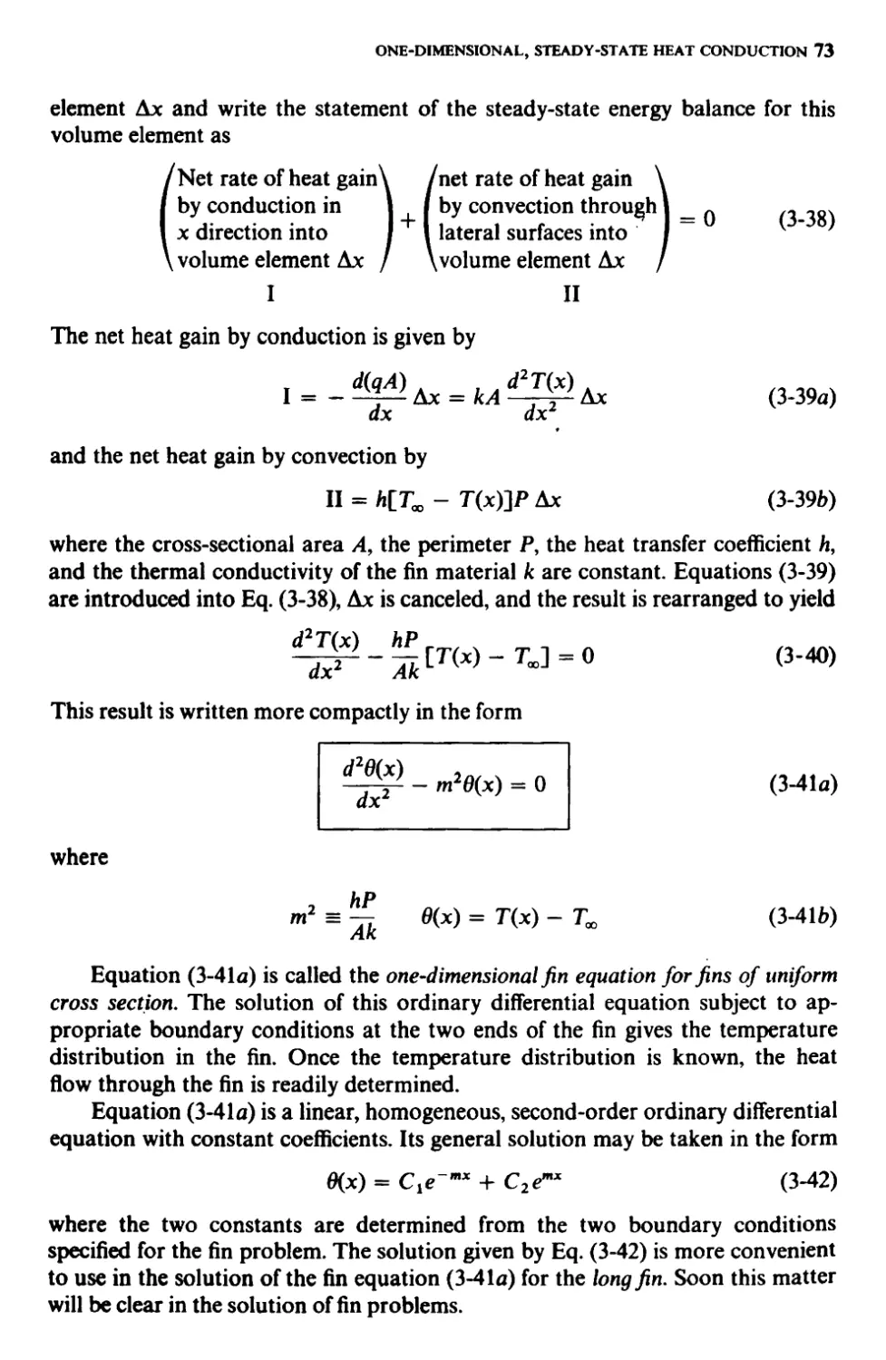
3-7	Finned Surfaces	71
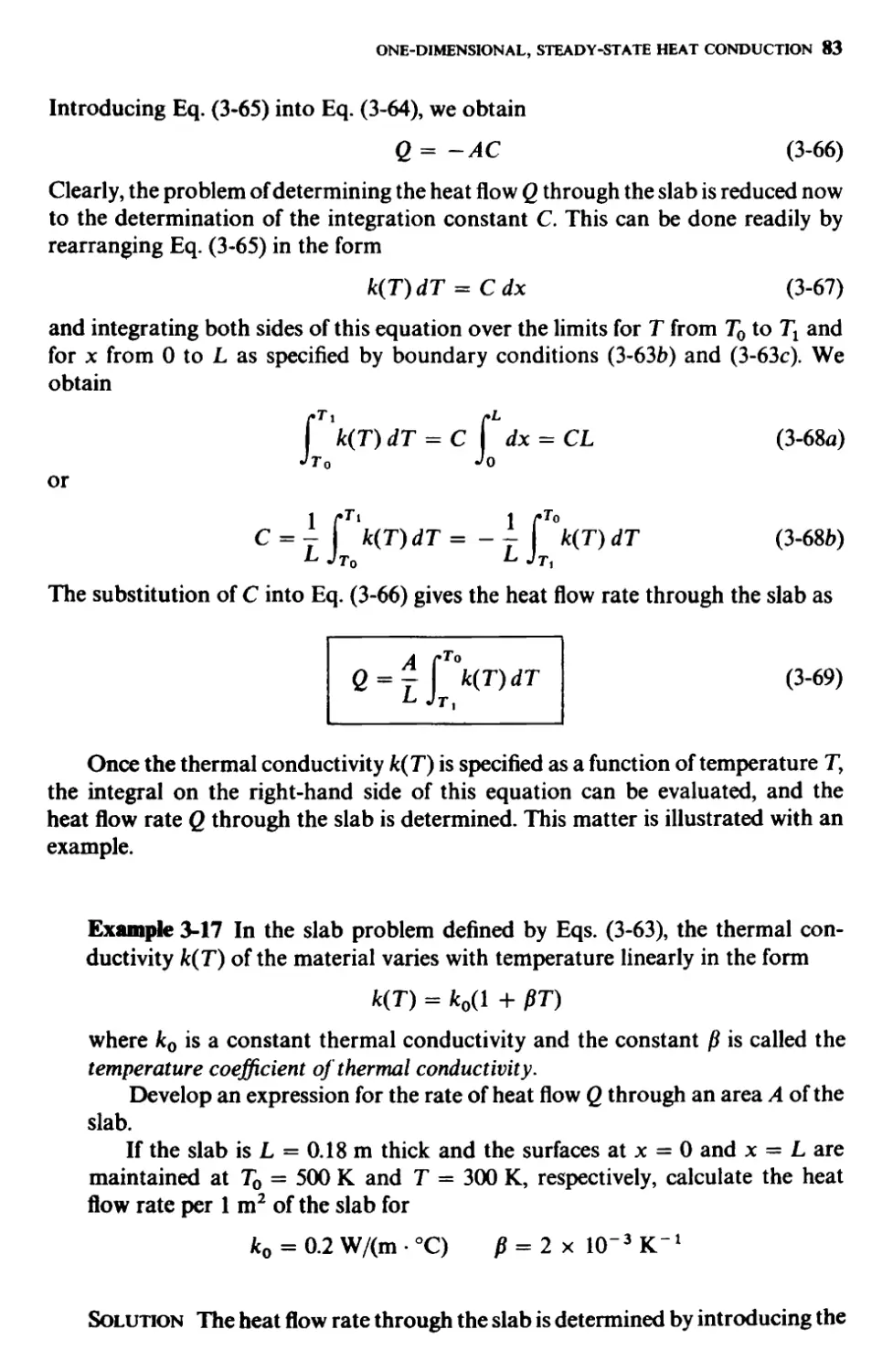
3-8	Temperature-Dependent k(T)	82
3-9	Summary of Basic Relations	85
Problems	87
References	100
Chapter 4	Transient Conduction and Use of
Temperature Charts	101
4-1	Lumped-System Analysis	101
4-2	Slab—Use of Transient-Temperature Charts	108
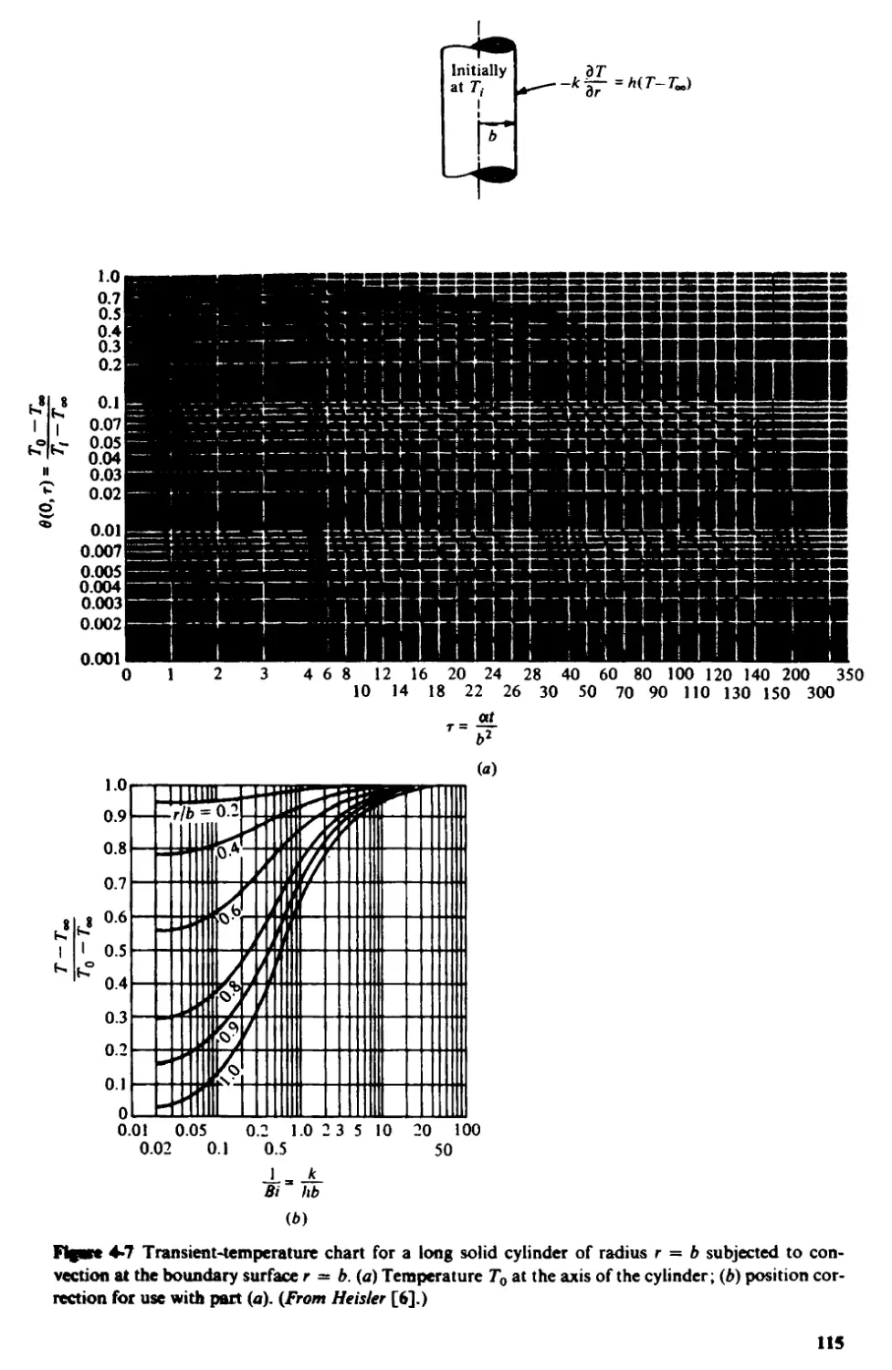
4-3	Long Cylinder and Sphere—Use of Transient-Temperature
Charts	114
4-4	Semi-infinite Solid—Use of Transient-Temperature Charts	120
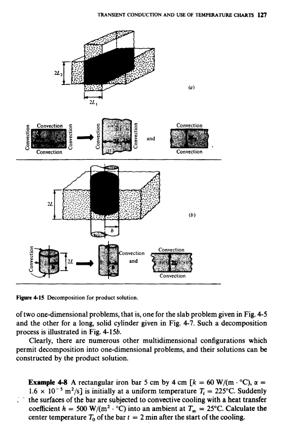
4-5	Product Solution—Use of Transient-Temperature Charts	124
4-6	Two-Dimensional, Steady-State Heat Conduction—Use	of
Conduction Shape Factors	130
4-7	Transient Heat Conduction in a Slab—Analytic Solution	134
4-8	Transient Heat Conduction in a Slab—Use of Tabulated
Solutions	141
Problems	146
References	154
Chapter 5	Finite-Difference Methods for Solving
Heat Conduction Problems	156
5-1	One-Dimensional, Steady-State Heat Conduction	157
5-2	Boundary Conditions	160
5-3	Two-Dimensional, Steady-State Heat Conduction	169
5-4	Methods of Solving Simultaneous Algebraic Equations	177
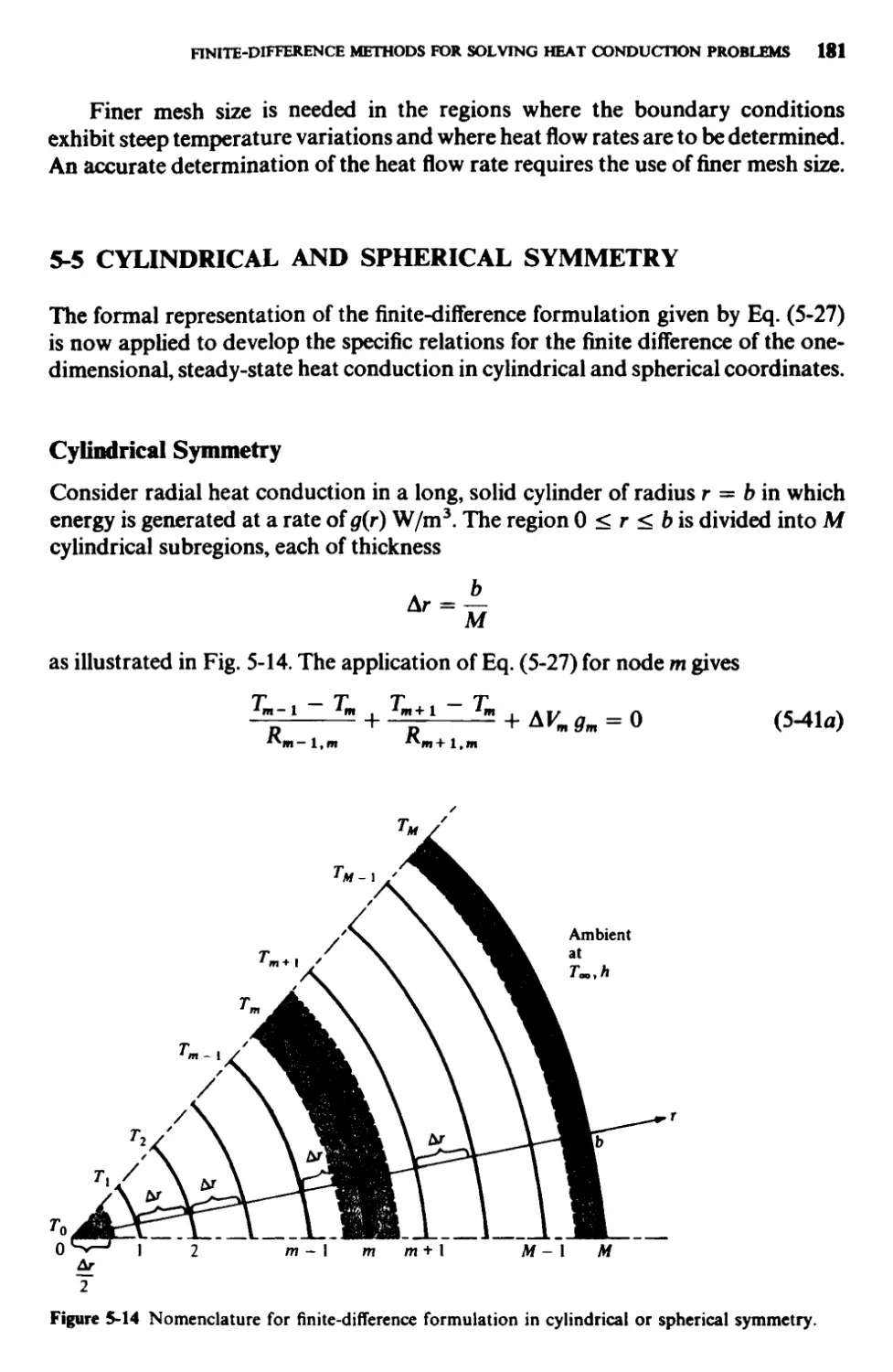
5-5	Cylindrical and Spherical Symmetry	181
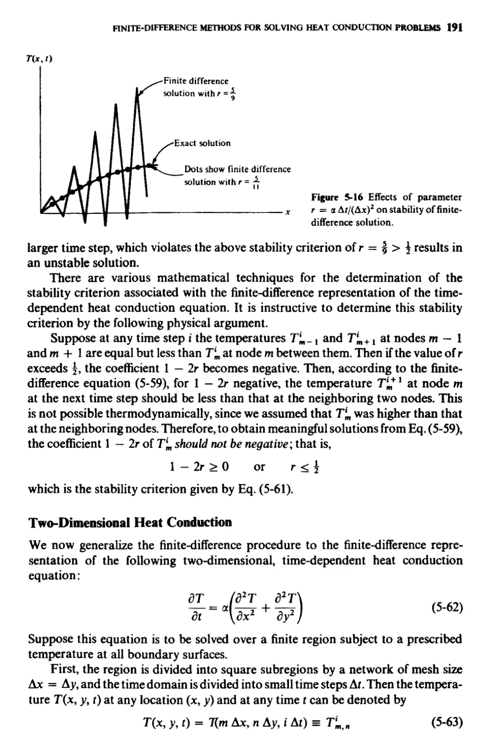
5-6	Unsteady Heat Conduction—Explicit Method	188
5-7	Unsteady Heat Conduction—Implicit Method	202
Problems	206
References	224
Chapter 6	Convection—Concepts and Basic Relations	226
6-1	Flow over a Body	227
6-2	Flow inside a Duct	238
6-3	Concepts on Turbulence	245
6-4	Equations of Motion	253
6-5	Equation of Energy	261
6-6	Dimensionless Parameters	267
6-7	Boundary-Layer Equations	270
Problems	271
References	279
CONTENTS IX
Chapter 7	Forced Convection for Flow inside Ducts	281
7-1	Hydrodynamically and Thermally Developed Laminar Flow	282
7-2	Thermally Developing, Hydrodynamically Developed Laminar Flow	299
7-3	Simultaneously Developing Laminar Flow	305
7-4	Turbulent Flow inside Ducts	310
7-5	Heat Transfer to Liquid Metals	322
7-6	Analogies between Heat and Momentum Transfer in Turbulent Flow	328
7-7	Heat Transfer Augmentation	332
7-8	Summary of Correlations	336
	Problems	339
	References	347
Chapter 8	Forced Convection for Flow over Bodies	352
8-1	Drag Coefficient for Flow over a Flat Plate	352
8-2	Heat Transfer Coefficient for Flow over a Flat Plate	361
8-3	Flow across a Single Circular Cylinder	373
8-4	Flow across a Single Noncircular Cylinder	381
8-5	Flow across a Single Sphere	382
8-6	Flow across Tube Bundles	385
8-7	Heat Transfer in High-Speed Flow over a Flat Plate	397
8-8	Summary of Correlations	404
	Problems	404
	References	410
	Notes	413
Chapter 9	Free Convection	416
9-1	Dimensionless Parameters of Free Convection	418
9-2	An Approximate Analysis of Laminar Free Convection on a Vertical Plate	422
9-3	Correlations of Free Convection on a Vertical Plate	430
9-4	Free Convection on a Horizontal Plate	436
9-5	Free Convection on an Inclined Plate	439
9-6	Free Convection on a Long Cylinder	443
9-7	Free Convection on a Sphere	447
9-8	Simplified Equations for Air	448
9-9	Mechanism of Free Convection in Enclosed Spaces	449
9-10	Correlations of Free Convection in Enclosed Spaces	452
9-11	Combined Free and Forced Convection	459
9-12	Summary of Correlations for Heat Transfer in Free Convection	462
	Problems	467
	References	472
Chapter 10	Boiling and Condensation	476
10-1	Film Condensation Theory	477
10-2	Comparison of Film Condensation Theory with Experiments	483
X CONTENTS
10-3	Film Condensation inside Horizontal Tubes	487
10-4	Dropwise Condensation	489
10-5	Condensation in the Presence of Noncondensable Gas	490
10-6	Pool Boiling Regimes	491
10-7	Pool Boiling Correlations	493
10-8	Forced-Convection Boiling inside Tubes	505
10-9	Summary of Equations	514
	Problems	516
	References	519
Chapter 11	Heat Exchangers	524
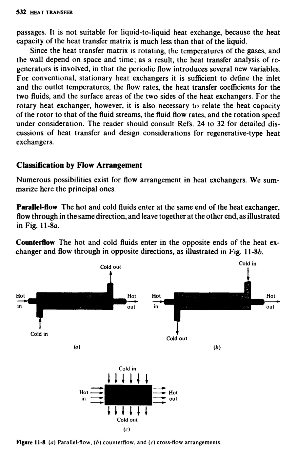
ii-i	Classification of Heat Exchangers	525
11-2	Temperature Distribution in Heat Exchangers	536
11-3	Overall Heat Transfer Coefficient	538
11-4	The LMTD Method for Heat Exchanger Analysis	545
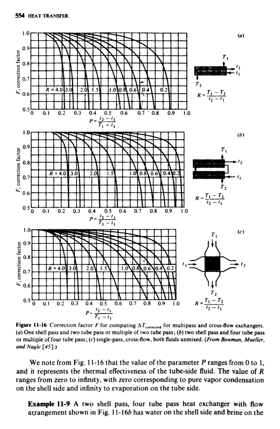
11-5	Correction for LMTD for Use with Cross-Flow and Multipass Exchangers	553
11-6	e-NTU Method for Heat Exchanger Analysis	559
11-7	Compact Heat Exchangers	571
11-8	Heat Exchanger Optimization	582
	Problems	584
	References	590
Chapter 12	Radiation among Surfaces in a Nonparticipating Medium	593
12-1	Nature of Thermal Radiation	593
12-2	Blackbody Radiation	595
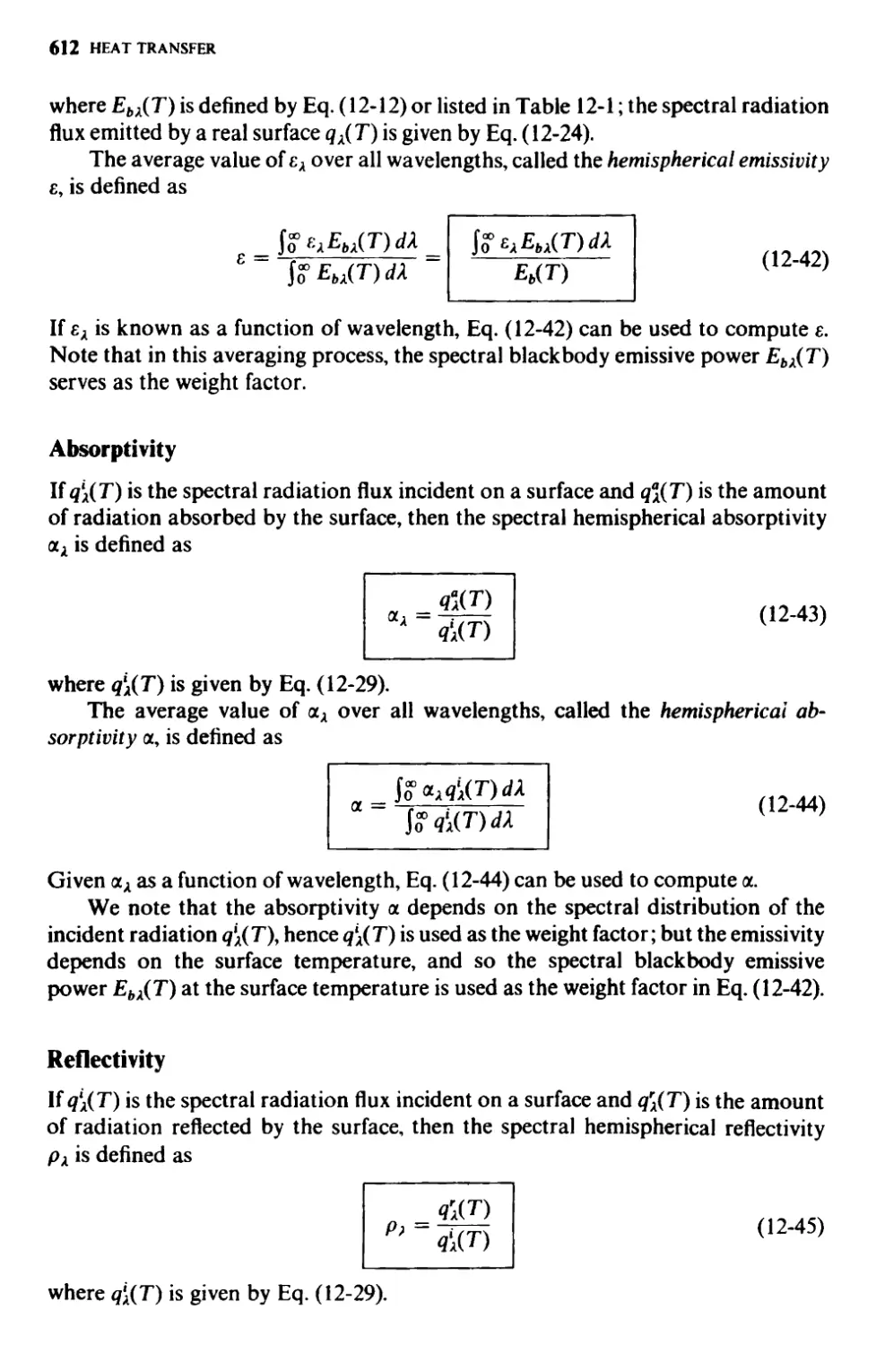
12-3	Radiation from Real Surfaces	604
12-4	Radiation Incident on a Surface	606
12-5	Radiation Properties of Surfaces	608
12-6	Solar Radiation	617
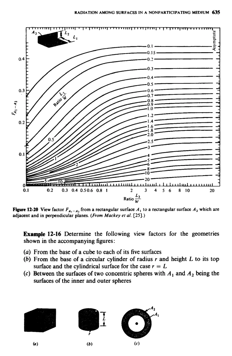
12-7	Concept of View Factor	624
12-8	Methods of Determining View Factors	631
12-9	Network Method for Radiation Exchange in an Enclosure	643
12-10	Radiosity Matrix Method for Radiation Exchange in an Enclosure	657
12-11	Correction for Radiation Effects in Temperature Measurements	667
12-12	Summary of Equations	668
	Problems	670
	References	683
Chapter 13	Radiation in Absorbing, Emitting Media	685
13-1	Equation of Radiative Transfer	685
13-2	Transmissivity, Absorptivity, and Emissivity	687
13-3	Radiation Exchange between a Gas Body and Its Black Enclosure	690
CONTENTS Xi
13-4	Radiation Flux from an Absorbing, Emitting Slab at
Uniform Temperature—An Analytic Solution	698
Problems	700
References	701
Chapter 14	Mass Transfer	702
14-1	Definitions of Mass Flux	703
14-2	Steady-State Equimodal Counterdiffusion in Gases	706
14-3	Steady-State Unidirectional Diffusion in Gases	708
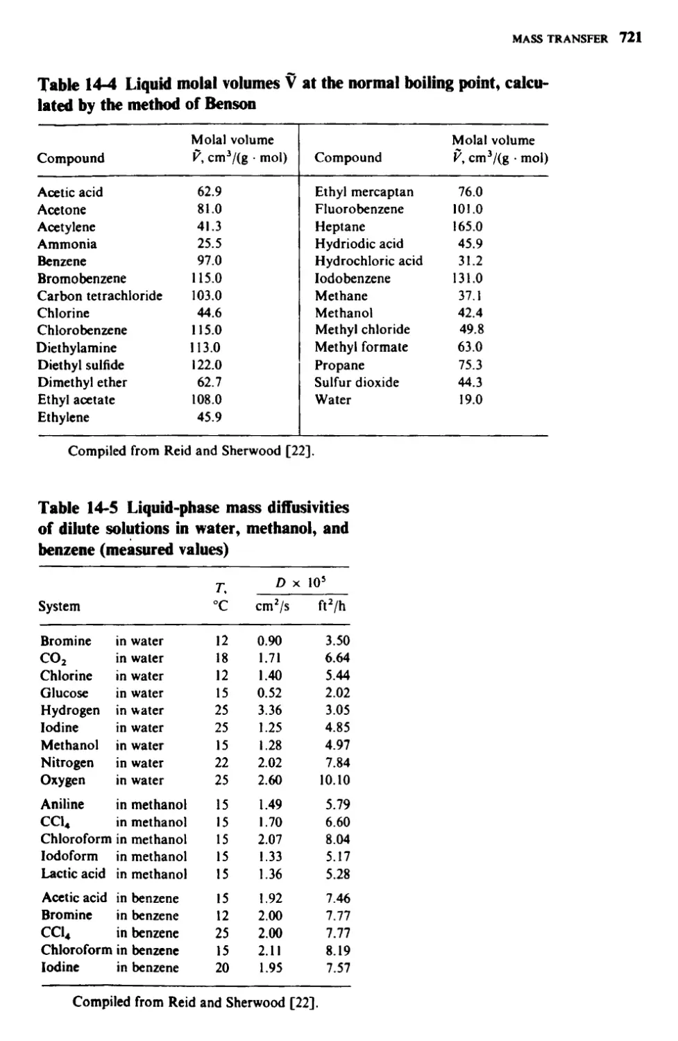
14-4	Steady-State Diffusion in Liquids	711
14-5	Unsteady Diffusion	713
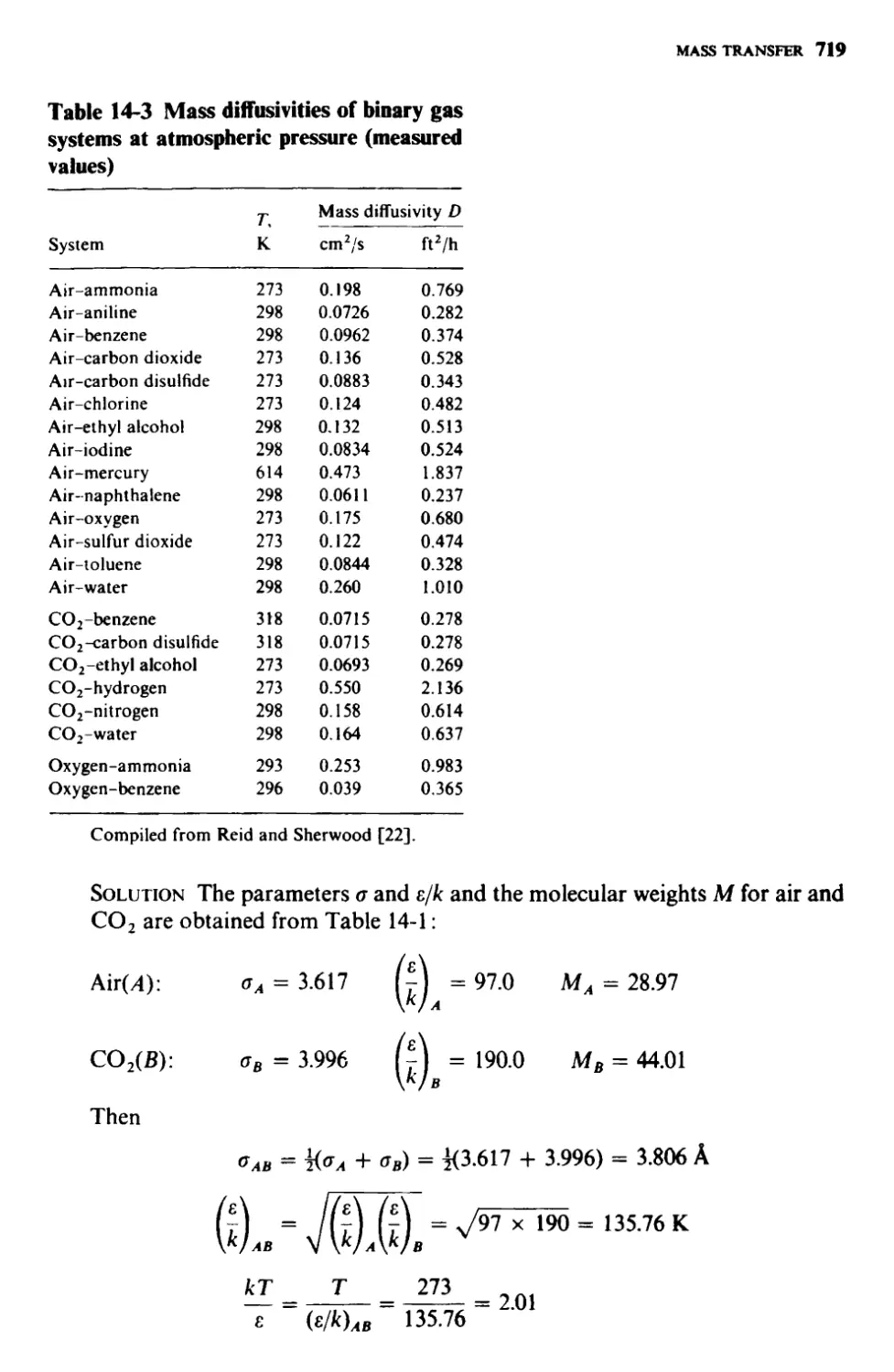
14-6	Mass Diffusivity	716
14-7	Mass Transfer in Laminar and Turbulent Flow	722
Problems	729
References	730
Appendixes	733
A	Conversion Factors	733
В	Physical Properties	736
C	Radiation Properties	756
D	Error Function, Roots of Transcendental	Equations, and
Exponential Integral Function	763
E	Dimensional Data for Tubes and	Steel Pipes	769
Indexes	771
Name Index
Subject Index
PREFACE
The field of heat transfer is so wide and diversified that an orderly presentation of
scientific facts is essential for effective teaching of this subject. In our teaching, we
should place emphasis not only to the transmission of the knowledge but also to
the laying of a strong foundation on which future knowledge can readily be
accumulated and the acquired knowledge can be fully utilized for useful purposes.
This book, although based on my 1977 book entitled Basic Heat Transfer,
is actually completely rewritten and reorganized, first by pedagogical considera-
tions, and second by providing a large number of fully worked out illustrative
examples, a large number of problems at the end of each chapter, summary tables
for ready reference, improved heat transfer charts and correlations, and com-
prehensive physical property tables to help to increase its usefulness in practical
applications.
The role of an introductory text on the subject is to establish the guidelines for
the transmission of the knowledge and serve as the catalizer in the interaction
between the teaching and learning processes. Therefore, it is not only the knowledge
contained in a book but also its organization which influences the effectiveness of
teaching. These principles have been the basic guidelines in the preparation of this
undergraduate text for the teaching of heat transfer in engineering schools for the
mechanical, chemical, and nuclear engineering students.
Our primary goal is not only to transmit the knowledge effectively but also to
provide a good understanding of the physical aspects of the subject matter and to
develop the necessary skills and background for the handling of related heat
transfer problems to be encountered later in the professional career. To achieve
such an objective, the fundamentals are systematically developed, the physical
significance of the developments are emphasized, and applications to the solution
of practical problems are illustrated with ample examples in each chapter.
There is sufficient material in this book to meet individual course objectives
at different levels, in both the junior and senior years. The spectrum of its possible
uses may range from a one-semester basic heat transfer course to a sequence of
xiii
XIV PREFACE
two-quarter or two-semester courses spread over the junior and/or senior years.
When used in a sequence course, conduction, finite differences, and radiation
should preferably be covered first, followed by convection, boiling and condensa-
tion, and heat exchangers.
The book can also serve as a source of ready reference for engineering graduates
and industry. A background in differential equations at the sophomore level and
some familiarity with fluid mechanics are all needed for following this book.
Chapter 1 introduces the basic concepts and gives a bird’s-eye view of the
mechanisms of heat transfer. A discussion of units and conversion factors is also
presented. Chapter 2 builds up the necessary background for the understanding of
the physical significance of the heat conduction equation and its boundary con-
ditions. Emphasis is placed on the development of necessary skills needed for the
mathematical formulation of practical heat conduction problems. This matter is
illustrated with numerous representative examples. Chapter 3 provides an intro-
duction to the solving of heat conduction problems and developing analytic
expressions for the determination of temperature distribution and heat flow in
solids. Only the one-dimensional steady-state heat conduction problems are con-
sidered. The thermal-resistance concept is introduced for use in the determination
of heat transfer through composite layers. The analysis and application of heat
flow through fins are presented. In Chapter 4 the concept of transient heat flow is
introduced through the use of the lumped system analysis because of its simplicity.
To develop a better understanding of the significance of temperature transients with
time and position, the temperature response and heat transfer charts are introduced
before presenting an analysis of transient conduction. The use of these charts for
predicting temperature transients in solids having shapes such as a slab, cylinder,
and sphere is illustrated with numerous examples. As a follow-up to this approach,
the use of conduction shape factors is also discussed to predict steady-state heat
flow in solids having complicated configurations. To give some idea of the analytic
methods of solving transient heat conduction problems, the method of separation
of variables is considered for the solution of one-dimensional transient heat con-
duction in a slab geometry. Chapter 5 presents the fundamentals of finite-differ-
ence methods for the solution of both steady and time-dependent heat conduction
problems. The application is illustrated with numerous examples and a computer
program is given for solving the resulting finite-difference equations.
Chapters 6 through 9 are devoted to heat transfer in forced and free con-
vection. Chapter 6 prepares the necessary background for the understanding of
the physical significance of various concepts and fundamental definitions associated
with the study of convection. The equations of motion and energy are introduced
for the case of two-dimensional constant-property incompressible flow. The
physical significance of various terms in these equations is discussed, and the use
of these equations in the formulation of forced-convection problems is illustrated
with examples. Chapter 7 presents forced-convection inside ducts. To illustrate
the use of the equations of motion and energy in the determination of friction
factor and heat transfer coefficients, simple forced-convection problems are solved
and temperature and velocity distributions are established. Such elementary
PREFACE XV
analysis of forced convection provides a good insight into the role of fluid flow in
heat transfer. In addition, it helps toward better understanding of the physical
significance of analytic and empirical correlations of friction factor and heat
transfer coefficient for complicated situations. Chapter 8 deals with forced con-
vection over bodies. To illustrate the use of boundary layer equations in the pre-
diction of drag and heat transfer coefficients, the integral method of analysis is
applied to develop analytic expressions for the drag and heat transfer coefficients
for laminar flow over a flat plate. Various correlations are then presented for flow
over bodies having other geometries. In Chapter 9 the principles of free convection
are discussed. An approximate boundary layer analysis is presented to illustrate
the use of the energy equation to predict the heat transfer coefficient for free con-
vection from a vertical plate. Correlations of free convection for other configura-
tions are then presented and their application is illustrated with examples.
Chapter 10 presents the fundamentals of boiling and condensation. Various
regimes of boiling and condensation are discussed and the heat transfer correla-
tions associated with them are presented.
Chapter 11 is devoted to the thermal analysis of heat exchangers. Various types
of heat exchangers are discussed, and the use of LMTD and E-NTU methods for
the sizing of heat exchangers are illustrated with representative examples.
Heat transfer by radiation is covered in Chapters 12 and 13. Chapter 12 deals
with radiation exchange among surfaces separated by a nonparticipating medium.
The absorption, emission, and reflection of radiation by real surfaces are dis-
cussed and the concept of blackbody radiation is developed. The analysis of
radiation exchange among surfaces is introduced first by using the network
method, because it provides a good insight into the physical nature of the problem.
However, the method is not so practicable when the system involves more than
two arbitrarily oriented surfaces. Therefore, a relatively straightforward radiosity-
matrix method, capable of handling radiation problems involving any number of
surfaces with no additional complexity, is then presented. Chapter 13 considers
radiation transfer inside a semitransparent, absorbing, emitting medium, and
radiation from hot gases.
Finally, in Chapter 14 the analysis of mass transfer is presented with an
analogy of heat transfer by diffusion and forced convection.
The SI (Systeme Internationale) system of units is used throughout this book.
Comprehensive conversion factors and physical property tables are presented in
the Appendix. To provide some feel for the relative magnitude of physical
properties in the SI and Btu units, some property tables are also included in both
system of units.
There are more than 170 fully worked-out examples to illustrate the applica-
tion of the basic theory and concepts. Over 800 problems, arranged in the same
order as the material presented in the text, are included at the ends of the chapters
with answers provided for some of the representative ones. A summary of funda-
mental equations are tabulated at the end of each chapter for ready reference.
This book is the outcome of many years of experience in teaching and writing
of textbooks in heat transfer at various levels. It is hoped that it will be helpful to
XVI PREFACE
improve the effectiveness of teaching and learning of the subject of heat transfer.
I am indebted to many of my colleagues and students for their valuable suggestions
toward achieving the objectives stated previously. I wish to thank Dr. S. Kakac
for providing useful comments on the text and Y. Cengel for thoroughly reading
the manuscript.
M. NECATI OZISIK
HEAT TRANSFER
A Basic Approach
CHAPTER
ONE
INTRODUCTION AND CONCEPTS
The concept of energy is used in thermodynamics to specify the state of a system.
It is a well-known fact that energy is neither created nor destroyed but only
changed from one form to another. The science of thermodynamics deals with
the relation between heat and other forms of energy, but the science of heat
transfer is concerned with the analysis of the rate of heat transfer taking place
in a system. The energy transfer by heat flow cannot be measured directly, but
the concept has physical meaning because it is related to the measurable quantity
called temperature. It has long been established by observations that when there
is temperature difference in a system, heat flows from the region of high tempera-
ture to that of low temperature. Since heat flow takes place whenever there is a
temperature gradient in a system, a knowledge of the temperature distribution
in a system is essential in heat transfer studies. Once the temperature distribution
is known, a quantity of practical interest, the heat flux, which is the amount of heat
transfer per unit area per unit time, is readily determined from the law relating
the heat flux to the temperature gradient.
The problem of determining temperature distribution and heat flow is of
interest in many branches of science and engineering. In the design of heat ex-
changers such as boilers, condensers, radiators, etc., for example, heat transfer
analysis is essential for sizing such equipment. In the design of nuclear-reactor
cores, a thorough heat transfer analysis of fuel elements is important for proper
sizing of fuel elements to prevent burnout. In aerospace technology, the tempera-
ture distribution and heat transfer problems are crucial because of weight limita-
tions and safety considerations. In heating and air conditioning applications for
buildings, a proper heat transfer analysis is necessary to estimate the amount of
insulation needed to prevent excessive heat losses or gains.
In the studies of heat transfer, it is customary to consider three distinct modes
of heat transfer: conduction, convection, and radiation. In reality, temperature
distribution in a medium is controlled by the combined effects of these three
modes of heat transfer; therefore, it is not actually possible to isolate entirely
one mode from interactions with the other modes. However, for simplicitv in
1
2 HEAT TRANSFER
the analysis, one can consider, for example, conduction separately whenever heat
transfer by convection and radiation is negligible. With this qualification, we
present below a brief qualitative description of these three distinct modes of heat
transfer; they are studied in great detail in the following chapters.
1-1 CONDUCTION
Conduction is the mode of heat transfer in which energy exchange takes place
from the region of high temperature to that of low temperature by the kinetic
motion or direct impact of molecules, as in the case of fluid at rest, and by the drift
of electrons, as in the case of metals. In a solid which is a good electric conductor,
a large number of free electrons move about in the lattice; hence materials that are
good electric conductors are generally good heat conductors (i.e., copper, silver,
etc.).
The empirical law of heat conduction based on experimental observations
originates from Biot but is generally named after the French mathematical
physicist Joseph Fourier [1]* who used it in his analytic theory of heat. This
law states that the rate of heat flow by conduction in a given direction is pro-
portional to the area normal to the direction of heat flow and to the gradient of
temperature in that direction. For heat flow in the x direction, for example, the
Fourier law is given as
Qx=—kA — W	(1-la)
or
Gx bdT
W/m1
where Qx is the rate of heat flow through area A in the positive x direction and
qx is called the heat flux in the positive x direction. The proportionality constant
k is called the thermal conductivity of the material and is a positive quantity.
If temperature decreases in the positive x direction, then dT/dx is negative; hence
qx (or Gx) becomes a positive quantity because of the presence of the negative sign
in Eqs. (1-la) and (1-lb). Therefore, the minus sign is included in Eqs. (1-lu) and
(1-lb) to ensure that qx (or Qx) is a positive quantity when the heat flow is in the
positive x direction. Conversely, when the right-hand side of Eqs. (1 -1 a) and (1-lb)
is negative, the heat flow is in the negative x direction.
The thermal conductivity к in Eqs. (1 -1 a) and (1-lb) must have the dimensions
W/(m • °C) or J/(m • s • °C) if the equations are dimensionally correct. There is a
wide difference in the range of thermal conductivities of various engineering
* Bracketed numbers indicate references at the end of the chapter.
INTRODUCTION AND CONCEPTS 3
Figure 1-1 Typical range of thermal
conductivity of various materials.
materials, as illustrated in Fig. 1-1. Between gases and highly conducting metals,
such as copper or silver, k varies by a factor of about 104. Thus, in Fig. 1-1 the
highest value is for highly conducting pure metals, and the lowest value is for gases
and vapors, excluding the evacuated insulating systems. The nonmetallic solids and
liquids have thermal conductivities that lie between them. Metallic single crystals
are exceptions, which may have very high thermal conductivities; for example,
with copper crystals, values of 8000 W/(m • °C) and even higher arc possible.
Thermal conductivity also varies with temperature. This variation, for some
materials over certain temperature ranges, is small enough to be neglected; but
for many cases the variation of к with temperature is significant. Especially at
very low temperatures к varies rapidly with temperature; for example, the
thermal conductivities of copper, aluminum, or silver reach values 50 to 100 times
those that occur at room temperature. Figure 1-2 illustrates how the thermal
conductivity of some engineering materials varies with temperature. Actual values
of thermal conductivity of various materials are given in Арр. B, and a compre-
hensive compilation of thermal conductivities of materials can be found in Refs.
2 to 5.
Example 1-1 Determine the heat flux q and the heat transfer rate across an
iron plate with area A = 0.5 m2 and thickness L » 0.02 m [k = 70 W/(m - °C)]
when one of its surfaces is maintained at T\ — 60°C and the other at T2 — 20°C.
4 HEAT TRANSFER
Thermal conductivity к (W/m*°C)
Figure 1-2 Effect of temperature on thermal conductivity of materials.
Solution In this problem the temperature gradient dT/dx is constant;
hence the temperature distribution T(x) through the plate is linear, as illus-
trated in Fig. 1-3. Then the heat flux q is determined by applying Eq. (1-lb) as
= _fc ZL_Zi. = —70 20 60 = 140 kW/m2
L	0.02	'
Thus the heat flow is in the positive x direction since the result is a positive
quantity. The heat flow rate Q through an area A = 0.5 m2 is computed by
applying Eq. (1-la):
Q = Aq = 0.5 x 140 = 70 kW
Example 1-2 The heat flow rate through a wood board L = 2 cm thick for a
temperature difference of AT = 25°C between the two surfaces is 150 W/m2.
Calculate the thermal conductivity of the wood.
INTRODUCTION AND CONCEPTS 5
Figure 1-3 Heat conduction through a slab.
Solution Equation (1-15) is applied as follows:
.AT
9 = fc —
150-‘<йЬ
к = 0.12 W/(m • °C)
1-2 CONVECTION
When fluid flows over a solid body or inside a channel while temperatures of the
fluid and the solid surface are different, heat transfer between the fluid and
the solid surface takes place as a consequence of the motion of fluid relative
to the surface; this mechanism of heat transfer is called convection. If the fluid mo-
tion is artificially induced, say with a pump or a fan that forces the fluid flow over
the surface, the heat transfer is said to be by forced convection. If the fluid motion
is set up by buoyancy effects resulting'from density difference caused by tempera-
ture difference in the fluid, the heat transfer is said to be by free (or natural) con-
vection. For example, a hot plate vertically suspended in stagnant cool air causes
a motion in the air layer adjacent to the plate surface because the temperature
gradient in the air gives rise to a density gradient, which in turn sets up the air
motion. As the temperature field in the fluid is influenced by the fluid motion,
the determination of temperature distribution and of heat transfer in convection
for most practical situations is a complicated matter. In engineering applications,
to simplify the heat transfer calculations between a hot surface at Tw and a cold
6 HEAT TRANSFER
fluid flowing over it at a bulk temperature Tf as illustrated in Fig. 1-4, a heat
transfer coefficient h is defined as
q = h(Tw - Tf)	(l-2a)
where q is the heat flux (in watts per square meter) from the hot wall to the cold
fluid. Alternatively, for heat transfer from the hot fluid to the cold wall, Eq. (1-2 a)
is written as
q = h(Tf - Tw)	(l-2b)
where q represents the heat flux from the hot fluid to the cold wall. Historically,
the form given by Eq. (l-2u) was first used as a law of cooling as heat is removed
from a body to a liquid flowing over it, and it is generally referred to as “Newton’s
law of cooling.” If the heat flux in Eqs. (l-2u) and (1 -2b) is given in watts per square
meter and the temperatures are in degrees Celsius (or kelvins), then the heat
transfer coefficient h in Eqs. (l-2a) and (1 -2b) must have the dimensions W/(m2 • °C)
if the equations are dimensionally correct.
The heat transfer coefficient h varies with the type of flow (i.e., laminar or
turbulent), the geometry of the body and flow passage area, the physical properties
of the fluid, the average temperature, and the position along the surface of the
body. It also depends on whether the mechanism of heat transfer is by forced
convection (i.e., the fluid motion is caused by a pump or a blower) or by natural
convection (i.e., the fluid motion is caused by the buoyancy). When h varies with the
position along the surface of the body, for convenience in engineering applications,
its average value hm over the surface is considered instead of its local value h.
Equations (l-2a) and (l-2b) are also applicable for such cases by merely replacing
h by hm; then q represents the average value of the heat flux over the region con-
sidered.
The heat transfer coefficient can be determined analytically for flow over
bodies having a simple geometry such as a flat plate or flow inside a circular tube.
INTRODUCTION AND CONCEPTS 7
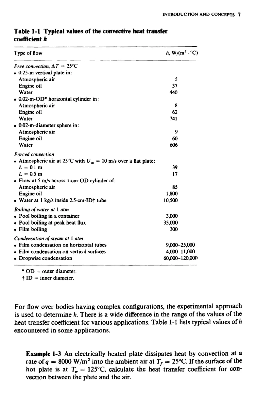
Table 1-1 Typical values of the convective heat transfer
coefficient h
Type of flow	Л, W/(m2 • °C)
Free convection, & T = 25°C	
• 0.25-m vertical plate in:	
Atmospheric air	5
Engine oil	37
Water	440
• 0.02-m-OD* horizontal cylinder in:	
Atmospheric air	8
Engine oil	62
Water	741
• 0.02-m-diameter sphere in:	
Atmospheric air	9
Engine oil	60
Water	606
Forced convection	
• Atmospheric air at 25°C with = 10 m/s over a flat plate:	
L =0.1 m	39
L = 0.5 m	17
• Flow at 5 m/s across 1-cm-OD cylinder of:	
Atmospheric air	85
Engine oil	1,800
• Water at 1 kg/s inside 2.5-cm-IDf tube	10,500
Boiling of water at 1 atm	
• Pool boiling in a container	3,000
• Pool boiling at peak heat flux	35,000
• Film boiling	300
Condensation of steam at 1 atm	
• Film condensation on horizontal tubes	9,000-25,000
• Film condensation on vertical surfaces	4,000-11,000
• Dropwise condensation	60,000-120,000
* OD = outer diameter,
t ID = inner diameter.
For flow over bodies having complex configurations, the experimental approach
is used to determine h. There is a wide difference in the range of the values of the
heat transfer coefficient for various applications. Table 1-1 lists typical values of h
encountered in some applications.
Example 1-3 An electrically heated plate dissipates heat by convection at a
rate of q = 8000 W/m2 into the ambient air at Tf = 25°C. If the surface of the
hot plate is at Tw = 125°C, calculate the heat transfer coefficient for con-
vection between the plate and the air.
8 HEAT TRANSFER
Solution Heat is being transferred from the plate to the fluid, so Eq. (l-2a) is
applied:
q = h(Tw - Tf)
8000 = h(125 - 25)
h = 80 W/(m2 • °C)
Example 1-4 Hot air at Tf = 150°C flows over a flat plate maintained at
Tw = 50°C. The forced convection heat transfer coefficient is h = 75 W/(m2 • °C).
Calculate the heat transfer rate into the plate through an area of A — 2 m2.
Solution For heat transfer from the hot fluid to the plate, Eq. (1 -2a) is applied:
q = h(Tf - Tw)
q = 75(150 - 50) = 7.5 x 103 W/m2
Q = qA = (7.5 x 103)(2) = 15 kW
1-3 RADIATION
All bodies continuously emit energy because of their temperature, and the energy
thus emitted is called thermal radiation. The radiation energy emitted by a body is
transmitted in the space in the form of electromagnetic waves according to
Maxwell’s classic electromagnetic wave theory or in the form of discrete photons
according to Planck’s hypothesis. Both concepts have been utilized in the in-
vestigation of radiative-heat transfer. The emission or absorption of radiation
energy by a body is a bulk process; that is, radiation originating from the interior
of the body is emitted through the surface. Conversely, radiation incident on the
surface of a body penetrates to the depths of the medium where it is attenuated.
When a large proportion of the incident radiation is attenuated within a very short
distance from the surface, we may speak of radiation as being absorbed or emitted
by the surface. For example, thermal radiation incident on a metal surface is
attenuated within a distance of a few angstroms from the surface; hence metals
are opaque to thermal radiation.
The solar radiation incident on a body of water is gradually attenuated by
water as the beam penetrates to the depths of water. Similarly, the solar radiation
incident on a sheet of glass is partially absorbed and partially reflected, and the
remaining is transmitted. Therefore, water and glass- are considered semitrans-
parent to the solar radiation.
It is only in a vacuum that radiation propagates with no attenuation at all.
Also the atmospheric air contained in a room is considered transparent to thermal
radiation for all practical purposes, because the attenuation of radiation by air is
insignificant unless the air layer is several kilometers thick. However, gases such as
carbon dioxide, carbon monoxide, water vapor, and ammonia absorb thermal
INTRODUCTION AND CONCEPTS 9
radiation over certain wavelength bands; therefore they are semitransparent to
thermal radiation.
It is apparent from the previous discussion that a body at a temperature T
emits radiation owing to its temperature; also a body absorbs radiation incident
on it. Here we briefly discuss the emission and absorption of radiation by a body.
Emission of Radiation
The maximum radiation flux emitted by a body at temperature T is given by the
Stefan-Boltzmann law
Eb = <tT*
W/m2
(1-3)
where T is the absolute temperature in kelvins, о is the Stefan-Boltzmann constant
[er = 5.6697 x 10“8 W/(m2 • K4)], and Eb is called the blackbody emissive power.
Only an ideal radiator or the so-called blackbody can emit radiation flux
according to Eq. (1-3). The radiation flux emitted by a real body at an absolute
temperature T is always less than that of the blackbody emissive power Eb; it is
given by
q = eEb — £tf T4
(M)
where the emissivity £ lies between zero and unity; for all real bodies it is always less
than unity.
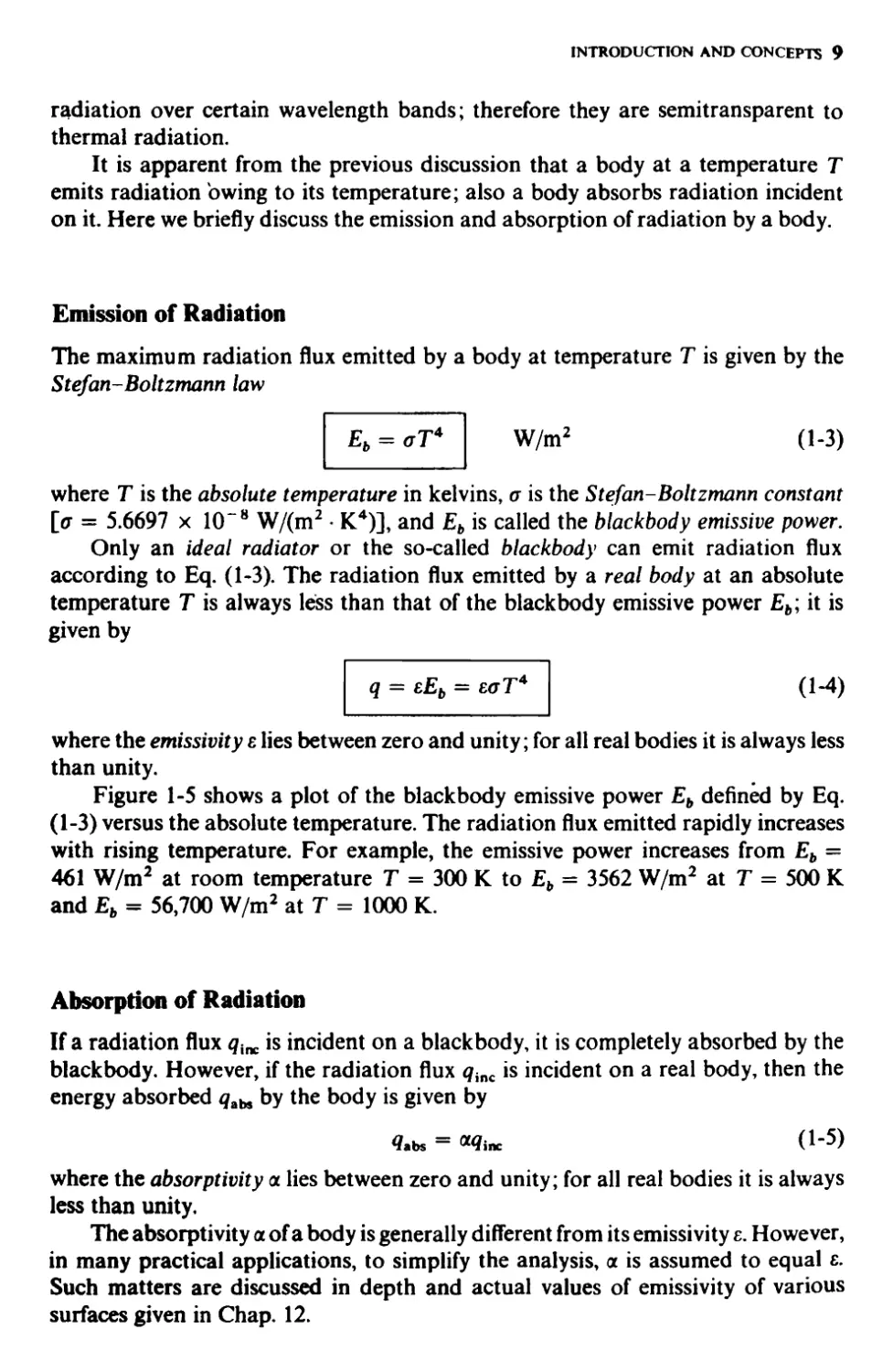
Figure 1-5 shows a plot of the blackbody emissive power Eb defined by Eq.
(1-3) versus the absolute temperature. The radiation flux emitted rapidly increases
with rising temperature. For example, the emissive power increases from Eb —
461 W/m2 at room temperature T = 300 К to Eb = 3562 W/m2 at T = 500 К
and Eb = 56,700 W/m2 at T = 1000 K.
Absorption of Radiation
If a radiation flux ginc is incident on a blackbody, it is completely absorbed by the
blackbody. However, if the radiation flux qinc is incident on a real body, then the
energy absorbed by the body is given by
4abs ®*7inc
(1-5)
where the absorptivity a lies between zero and unity; for all real bodies it is always
less than unity.
The absorptivity a of a body is generally different from its emissivity e. However,
in many practical applications, to simplify the analysis, a is assumed to equal £.
Such matters are discussed in depth and actual values of emissivity of various
surfaces given in Chap. 12.
10 HEAT TRANSFER
Figure 1-5 Blackbody emissive power Eb — aT4.
Radiation Exchange
When two bodies at different temperatures “see” each other, heat is exchanged
between them by radiation. If the intervening medium is filled with a substance
such as air which is transparent to radiation, the radiation emitted from one body
travels through the intervening medium with no attenuation and reaches the other
body, and vice versa. Then the hot body experiences a net heat loss, and the cold
body a net heat gain, as a result of the radiation heat exchange. The analysis of
radiation heat exchange among surfaces is generally a complicated matter and is
dealt with in Chap. 12. Here we examine some very special cases with illustrative
examples.
Figure 1-6 shows a small, hot, opaque plate of surface area A t and emissivity
that is maintained at an absolute temperature 7j and exposed to a large surrounding
area A2 (i.e., AJA2 -* 0) at an absolute temperature T2. The space between them
contains air which is transparent to thermal radiation. The radiation energy
emitted by the surface At is given by
A^aT*
INTRODUCTION AND CONCEPTS 11
Figure 1-6 Radiation exchange between a surface
and its surroundings.
The large surrounding area can be approximated as a blackbody in relation to the
small surface Л j. Then the radiation flux emitted by the surrounding area is aT2<
which is also the radiation flux incident on the surface Hence, the radiation
energy absorbed by the surface is
The net radiation loss at the surface A j is the difference between the energy emitted
and the energy absorbed:
Qi — AyEiffT* — Aiot1oT2
(l-6u)
For e1 = «j, this result simplifies to
6i = A1£1a(Tt - T2)	(l-6b)
which provides the expression for calculating the radiation heat exchange between
a small surface element A i and its surroundings at T2. Clearly, the positive value of
Qi implies heat loss from the surface and the negative value implies heat gain.
We now consider two finite surfaces A{ and A2 as illustrated in Fig. 1-7. The
surfaces are maintained at absolute temperatures 7\ and T2, respectively, and have
emissivities £j and e2 . The physical situation implies that part of the radiation leav-
ing surface A{ reaches surface A2 while the remaining is lost to the surroundings.
Similar considerations apply for the radiation leaving surface A2 : The analysis of
radiation heat exchange between the two surfaces for such a case should include
Figure 1-7 Radiation exchange between surfaces Ax and A2-
12 HEAT TRANSFER
the effects of the orientation of the surfaces, the contribution of radiation from the
surroundings, and the reflection of radiation at the surfaces. For the arrangement
shown in Fig. 1-7, if we assume that tne radiation flux from the surroundings is
negligible compared to those from surfaces 4X and A2, then the net radiation heat
transfer at the surface Ar can be expressed in the form
Qi =	- T*)	(1-7)
where Fx is a factor that includes the effects of the orientation of the surfaces and
their emissivities. The determination of this factor is a complicated matter, and
the analysis of radiation problems of this type is the subject of Chap. 12.
Radiation Heat Transfer Coefficient
To simplify the heat transfer calculations, it may be possible, under very restrictive
conditions, to define a radiation heat transfer coefficient hr, analogous to the con-
vection heat transfer coefficient, as
q. = MFX - T2)
(1-8)
This concept can be applied to the result given by Eq. (1-66) as now described.
Equation (1-66) is written as
Q = A^iTl + TlXT. + T2KI\ - T2)	(l-9a)
If 1Tx — T21 < Ti9 this result is linearized as
Qi s	- T2)	(l-9b)
or
= (tTUirtTi - t2)
Л1
(MO)
A comparison of Eqs. (1-8) and (1-10) reveals that for the specific case given by
Eq. (1-66), a radiation heat transfer coefficient hr can be defined as
hr = 4T|£x<t
(Ml)
Example 1-5 A heated plate of D = 0.2 m diameter has one of its surfaces
insulated, and the other is maintained at T„ = 550 K. If the hot surface has an
emissivity ew - 0.9 and is exposed to a surrounding area at Ts - 300 К with
atmospheric air being the intervening medium, calculate the heat loss by
radiation from the hot plate to the surroundings.
INTRODUCTION AND CONCEPTS 13
Solution Assuming = ab we can apply Eq. (l-6h):
Qw =	- Tt)
^(0.2)2 (0.9X5.67 x 10 8)[(5.5)4 - 34] x 10®
= 134.5 W
Example 1-6 A small hot surface at temperature 7\ = 430 К having an
emissivity =0.8 dissipates heat by radiation into a surrounding area at
T2 = 400 K. If this radiation transfer process is characterized by a radiation
heat transfer coefficient hr calculate the value of hr.
Solution For this particular case, the requirement T{ — T2 < 7\ is satisfied.
Then Eq. (1-11) is applied as follows:
hr = 4T3£1a
= 4[(4.3)3 x 106](0.8X5.67 x 10“8) = 14.4 W/(m2 • °C)
1-4 COMBINED HEAT TRANSFER MECHANISM
So far we have considered the heat transfer mechanism, conduction, convection,
and radiation separately. In many practical situations heat transfer from a surface
takes place simultaneously by convection to the ambient air and by radiation to the
surroundings. Figure 1-8 illustrates a small plate of area A and emissivity e that is
maintained at Tw and exchanges energy by convection with a fluid at with a
heat transfer coefficient hc and by radiation with the surroundings at Ts. The heat
loss per unit area of the plate, by the combined mechanism of convection and
radiation, is given by
<?» = hc(Tw - TJ + ea(Tj, - T4)
(Ы2)
Figure 1-8 Simultaneous convection and
radiation from a plate.
14 HEAT TRANSFER
If | T„ - Ts| < Tw, the second term can be linearized. We obtain
= hc(T„ - TJ + hr(T„ - Ts)	(l-13a)
where
hr = 4ectT^
(1-135)
Example 1-7 A small, thin metal plate of area A m2 is kept insulated on one
side and exposed to the sun on the other side. The plate absorbs solar energy
at a rate of 500 W/m2 and dissipates it by convection into the ambient air at
= 300 К with a convection heat transfer coefficient hc = 20 W/(m2 • °C)
and by radiation into a surrounding area which may be assumed to be a
blackbody at Tsky = 280 K. The emissivity of the surface is e — 0.9. Determine
the equilibrium temperature of the plate.
Solution The energy balance per unit area of the exposed surface is written as
KT V	1
— (2.8)4 108
1 OU /	J
or
25 = Tw - 300 + 0.255^j4 - 15.68
or
Tw = 340.68 - 0.255(^y
The solution of this equation by trial and error yields the plate temperature as
T„ = 315.5 К
1-5 UNITS, DIMENSIONS, AND CONVERSION FACTORS
In the field of heat transfer, the physical quantities such as specific heat, thermal
conductivity, heat transfer coefficient, heat flux, etc. are expressed in terms of
a few fundamental dimensions which include length, time, mass, and temperature,
and each of these dimensions is associated with a unit when it is to be expressed
numerically. For example, length is the dimension of a distance, and to express
it numerically one may use units of feet or meters or centimeters, etc. Time may
be measured in hours or seconds, mass in pounds or kilograms, temperature in
degrees Fahrenheit or Celsius, energy in British thermal units or joules, and so on.
When the dimensions of a physical quantity are to be expressed numerically, a
consistent system of units is generally preferred. In engineering the two most
commonly used systems of units are the International System of units (SI) and
the English engineering system. The basic units for length, mass, time, and tempera-
ture for each system are listed in Table 1-2. Here the symbol “Ibf” is used for
INTRODUCTION AND CONCEPTS 15
Table 1-2 Systems of units
Quantity	SI	English engineering system
Length	m	ft
Mass	kg	lb
Time	s	s
Temperature	К	R
Force	N	Ibf
Energy	J or N • m	Btu or ft • Ibf
pound-force to distinguish it from the symbol “lb” commonly used for pound-mass,
but there is no such misunderstanding in SI because the kilogram is the unit of
mass and the newton is the unit of force. The physical significance of the force
units newton and Ibf is better envisioned by considering Newton’s second law of
motion, written as
Force = — x mass x acceleration	(1-14)
9c
where gc is the gravitational conversion-factor constant. The pound-force Ibf is
defined as the force that acts on the mass of one pound at a point on the earth
where the magnitude of the gravitational acceleration is g = 32.174 ft/s2. Then,
in the English engineering system, Eq. (1-14) becomes
1 Ibf = - X 1 lb x 32.174 ft/s2	(1-15)
9c
According to this relation, one pound of force (that is, 1 Ibf) will accelerate one
pound of mass (that is, 1 lb) 32.174 ft/s2; or 1 Ibf is equal to 32.174 ft • lb/s2. The
conversion factor gc in the English engineering system is obtained from this re-
lation as
gc = 32.174 lb • ft/(lbf • s2)	(1-16)
Note that the gravitational acceleration g and the gravitational conversion factor
gc are not similar quantities; gc is constant, but g depends on the location and on the
altitude.
In SI, Eq. (1-14) becomes
1 N — — x 1 kg x 1 m/s2	(Ы7)
9c
Clearly, in SI, 1 N is a force that will accelerate a 1-kg mass 1 m/s2, or a 1-N
force is equal to 1 kg • m/s2. The conversion factor gc in SI becomes
gc = 1 kg • m/(N • s2) = 1	(1-18)
16 HEAT TRANSFER
since	1 N = 1 kg • m/s2	(1-19)
Therefore, in SI, gc is not needed.
Energy is measured in Btu or ft • Ibf in the English engineering system whereas
it is measured in joules (J) or newton-meters (N m) in SI. Note that 1 J = 1 N • m
and 1 J = 1 kg • m2/s2 since 1 N = 1 kg • m/s2.
Power is measured in Btu/h or ft • Ibf/s in the English engineering system and
in watts (IF) or kilowatts (kW) or J/s in SI. Note that
1 kW = 1000 W and 1 W = 1 J/s = 1 N • m/s = 1 kg • m2/s3
(1-20)
Pressure is measured in Ibf /in2 in the English engineering system and in bars or
N/m2 in SI. Note that
1 bar = 105 N/m2 = 105 kg/(m • s2)
and
1 atm = 0.98066 bar
In SI, when the size of units becomes too large or too small, multiples in powers
of 10 are formed with certain prefixes. The important ones are listed in Table 1-3.
For example,
1000 W = 1 kW (kilowatt)
1,000,000 W = 1 MW (megawatt)
1,000,000 N = 1 MN (meganewton)
1000 m = 1 km (kilometer)
10" 2 m = 1cm (centimeter)
and so forth.
A comprehensive table of conversion factors useful in heat transfer calculations
is presented in App. A.
Example 1-8 Convert the heat transfer coefficient h = 20 Btu/(h ♦ ft2 • °F) to
the units of J/(s • m2 • °C) or W/(m2 • °C).
Table 1-3 Prefixes for multiplying
factors
IO'12	= pico (p)	10	= deka (da)
10-’	= nano (n)	102	= hecto (h)
IO"6	= micro (д)	10'	= kilo (k)
10'2	= milli (m)	106	= mega (M)
IO’2	- centi (c)	10’	= giga (G)
10-1	= deci (d)	1012	= tera (T)
INTRODUCTION AND CONCEPTS 17
Solution From Table Al, #9, App. A we have 1 Btu/(h • ft2 • °F) ~ 5.677
W/(m2 • °C), which is written as
W/(m2 • °C)
Btu/(h • ft2 • °F)
Then the conversion is performed as
h = 20 Btu/(h • ft2 • F) = [20 Btu/(h • ft2 • °F)] 5.677
S 113.6 W/(m2 • °C) = 113.6 J/(s • m2 • °C)
since
1	W = 1 J/s
1-6 SUMMARY OF BASIC RELATIONS
We summarize in Table 1-4 the basic relations given in this chapter.
Table 1-4 Summary of basic relations
Equation number	Relation	Remarks
	Conduction:	
(Mb)	dT W/m2 ax	Conduction heat flux in the x direction
	Convection:	
(1-ЗД	q = KTW - Tf) W/m2	Convection heat flux from the wall surface to the fluid
	Radiation:	
(1-3)	Eb = oT4 W/m2	Blackbody emissive power
(M)	q = £aT4 W/m2	Radiation flux emitted by a real body
(1-66)	Ci =	- T4) W A. for	► 0 Ai	Net radiation loss from surface A t at T, to a very large medium A2 at T2
(1-8)	qi = h,(7\ - T2) W/m2 where h, =	Energy transfer by radiation for | T - T21 < T
(1-1341)	q„ = ht(Tw - TJ + h^K - T3) W/m2 where Л, = 4c<rTi	Energy transfer by combined convection and radiation for | Tw - 7J < TM.
18 HEAT TRANSFER
PROBLEMS
Conduction
1-1 A temperature difference of 500°C is applied across a fireclay brick 10 cm thick with thermal
conductivity 1.0 W/(m  °C). Determine the heat transfer rate per square meter area.
Answer: 5 kW/m2 or kJ/(m2 • s)
1-2 A temperature difference of 100°C is applied across a corkboard 5 cm thick with thermal con-
ductivity 0.04 W/(m • °C). Determine the heat transfer rate across a 3-m2 area per hour.
1-3 A fiber glass insulating board of thermal conductivity 0.05 W/(m • °C) is to be used to limit the heat
losses to 80 W/m2 for a temperature difference of 160°C across the board. Determine the thickness of
the insulating board.
Answer: 0.1 m
1-4 Glass wool of thermal conductivity 0.038 W/(m • °C) is to be used to insulate an ice box. If the maxi-
mum heat loss should not exceed 45 W/m2 for a temperature of 40°C across the walls of the ice box,
determine the thickness of the insulation.
Answer : 3.4 cm
1-5 A brick wall 15 cm thick with thermal conductivity 1.2 W/(m • °C) is maintained at 30°C at one
face and 23O°C at the other face. Determine the heat transfer rate across the 4-m2 surface area of the
wall.
Answer : 6.4 kW
1-6 Two large plates, one at 50°C and the other at 200°C, are 8 cm apart. If the space between them
is filled by loosely packed rock wool of thermal conductivity 0.08 W/(m • °C), calculate the heat transfer
rate across the plates per 1-m2 area.
1-7 The heat flow rate across an insulating material of thickness 3 cm with thermal conductivity 0.1
W/(m • °C) is 250 W/m2. If the hot surface temperature is 175°C, what is the temperature of the cold
surface?
Answer: 100°C
1-8 A 25-cm-thick concrete wall has a surface area of 40 m2. The inner surface of the wall is at 20°C,
and the outer surface is at — 10°C. Determine the rate of heat loss through the wall if the thermal
conductivity is 0.75 W/(m • °C).
Answer: 3.6 kW or kJ/s
1-9 The heat flow rate through a 4-cm-thick wood board for a temperature difference of 25°C between
the inner outer surfaces is 75 W/m2. What is the thermal conductivity of the wood?
Answer: 0.12 W/(m °C)
1-10 The inside and outside surface temperatures of a window glass are 20 and - 12°C, respectively.
If the glass is 80 cm by 40 cm, is 1.6 cm thick, and has thermal conductivity 0.78 W/(m • °C), determine
the heat loss through the glass over 3 h.
Answer: 5391 kJ
1-11 Two plates, one at a uniform temperature of 300°C and the other at 100°C, are separated by a
2-cm-thick asbestos-cement board of thermal conductivity 0.70 W/(m  °C). Determine the rate of heat
transfer across the layer per 1-m2 surface.
1-12 By conduction 2000 W is transferred through a 0.5-m2 section of a 4-cm-thick insulating material.
Determine the temperature difference across the insulating layer if the thermal conductivity is 0.2
W/(m°C).
Answer : 800°C
Convection
1-13 Water at a mean temperature of 20°C flows over a flat plate at 80°C. If the heat transfer coefficient
is 200 W/(m2 • C), determine the heat transfer per square meter of the plate over 5 h.
Answer: 216 MJ
INTRODUCTION AND CONCEPTS 19
1-14 A large surface at 50°C is exposed to air at 20°C. If the heat transfer coefficient between the surface
and the air is 15 W/(m2 • °C), determine the heat transferred from 5 m2 of the surface over 7 h.
1-15 Air at 150°C flows over a flat plate which is maintained at 50°C. If the heat transfer coefficient
for forced convection is 300 W/(m2 • °C), determine the heat transfer to the plate through 2 m2 over
lib.
Answer: 648 MJ
1-16 A 25-cm-diameter sphere at 120°C is suspended in air at 20°C. If the natural convection heat
transfer between the sphere and the air is 15 W/(m2 • C), determine the rate of heat loss from the sphere.
Answer: 294.5 W
1-17 A fluid at 10°C flows over a 2.5-cm-OD and 2-m-long tube whose surface is maintained at 100°C.
If the heat transfer coefficient between the tube and the air is 300 W/(m2 • C), determine the rate of
heat transfer from the tube to the air.
1-18 Pressurized water at 50°C flows inside a 5-cm-diameter, 1-m-long tube with surface temperature
maintained at 130°C. If the heat transfer coefficient between the water and the tube is h = 2000
W/(m • °C), determine the heat transfer rate from the tube to the water.
Answer: 25.13 kW
1-19 Heat is supplied to a plate from its back surface at a rate of 500 W/m2 and is removed from its
front surface by air flow at 30°C. If the heat transfer coefficient between the air and the plate surface is
h = 20 W/(m2 • °C), what is the temperature of the front surface of the plate?
1-20 The inside surface of an insulating layer is at 270°C, and the outside surface is dissipating heat by
convection into air at 20°C. The insulation layer is 4 cm thick and has thermal conductivity 1.2
W/(m • °C). What is the minimum value of the heat transfer coefficient at the outside surface if the
outside surface temperature should not exceed 70°C?
Answer : 120 W/(m2 - °C)
1-21 A 10-cm-diameter sphere is heated internally with a 100-W electric heater. The sphere dissipates
heat by convection from its outer surface to the ambient air. Calculate the heat transfer coefficient for
convection from the sphere if the temperature difference between the sphere surface and the ambient
air is 50°C.
1-22 A thin metallic plate is insulated at the back surface and is exposed to the sun at the front surface.
The front surface absorbs the solar radiation of900 W/m2 and dissipates it mainly by convection to the
ambient air at 25°C. If the heat transfer coefficient between the plate and the air is 15 W/(m2 • °C), what
is the temperature of the plate?
Answer: 85°C
Radiation
1-23 A thin metal plate 0.1 m by 0.1 m is placed in a large evacuated container whose walls are kept at
300 K. The bottom surface of the plate is insulated, and the top surface is maintained at 500 К as a
result of electric heating. If the emissivity of the surface of the plate is e = 0.8, what is the rate of heat
exchange between the plate and the walls of the container? Take <r = 5.67 x 10~® W/(m2 • K4).
Answer: 24.7 W
1-24 Two large parallel plates, one at a uniform temperature 500 К and the other at 1000 K, are separ-
ated by a nonparticipating gas. Assuming that the surfaces of the plates are perfect emitters and that the
convection is negligible, determine the rate of heat exchange between the surfaces per square meter.
1-25 A sphere 10 cm in diameter is suspended inside a large evacuated chamber whose walls are kept
at 300 K. If the surface of the sphere has emissivity e = 0.8 and is maintained at 500 K, determine the
rate of heat loss from the sphere to the walls of the chamber.
Answer: 77.52 W
1-26 Two very large, perfectly black parallel plates, one maintained at 1200 К and the other at 600 K,
exchange heat by radiation (i.e., convection is negligible). Determine the heat transfer rate per 1-m2
surface.
20 HEAT TRANSFER
1-27 One surface of a thin plate is exposed to a uniform heat flux of 500 W/m2, and the other side dis-
sipates heat by radiation to an environment at - 10°C. Determine the temperature of the plate. Assume
blackbody conditions for radiation.
Answer: Tj = 341.5 К
1-28 A thin metal sheet separates two large parallel plates, one at a uniform temperature of 1000 К
and the other at 400 K. Blackbody conditions can be assumed for all surfaces, and heat transfer can be
assumed to be by radiation only. Determine the temperature of the separating sheet.
Combined heat transfer mechanism
1-29 A flat plate has one surface insulated and the other surface exposed to the sun. The exposed surface
absorbs the solar radiation at a rate of 800 W/m2 and dissipates it by both convection and radiation
into the ambient air at 300 K. If the emissivity of the surface is c = 0.9 and the convection heat transfer
coefficient between the plate and air is 12 W/(m2 • °C), determine the temperature of the plate.
Answer: 342.5 К
1-30 A thin plate is exposed to an infrared radiation flux of 1500 W/m2 on one surface while the other
surface is kept insulated. The exposed surface absorbs 90 percent of the incident radiation flux and
dissipates it by convection and radiation into the ambient air at 300 K. If the heat transfer coefficient
for convection between the surface and the ambient air is 15 W/(m2 • °C), determine the temperature of
the plate. Take the emissivity of plate as e = 0.9.
1-31 A thin plate 50 cm by 50 cm is subjected to 400 W of heating on one surface and dissipates the
heat by combined convection and radiation from the other surface into the ambient air at 290 K. If
the surface of the plate has an emissivity e = 0.9 and the heat transfer coefficient between the surface
and the ambient air is 15 W/(m2 • °C), determine the temperature of the plate.
Answer : 362.2 К
1-32 The solar radiation incident on the outside surface of an aluminum shading device is 1000 W/m2.
Aluminum absorbs 12 percent of the incident solar energy and dissipates it by convection from the back
surface and by combined convection and radiation from the outside surface. The emissivity of the
aluminum is 0.10, the convection heat transfer coefficient is 15 W/(m2 • °C) for both surfaces, and
the ambient temperature can be taken 20°C for both convection and radiation. Determine the
temperature of the shade.
1-33 One surface of a thin metal sheet receives radiation from a large plate at 700°C, while the other
surface dissipates heat by convection to a coolant fluid at 20°C. The surfaces can be considered as
a perfect absorber and a perfect emitter for radiation. The heat transfer coefficient for convection
between the surface and the fluid is 120 W/(m2 • °C). Determine the temperature of the plate.
Answer : 638 К
1-34 Heat is lost by both convection and radiation from a 2-m-long uninsulated portion of 5-cm-OD
hot water pipe into an external environment at 0°C. The convection heat transfer coefficient is 20
W/(m2 * °C), and for radiation calculations blackbody conditions can be assumed. Determine the rate
of heat loss from the uninsulated portion of the pipe for a wall temperature of Tw = 125°C.
Conversion factors
1-35 Convert the heat transfer coefficient h = 50 W/(m2 • °C) to Btu/(h • ft2 • °F).
Answer: 8.807 Btu/(h • ft2 • °F)
1-36 Derive the conversion factor for converting the thermal conductivity from Btu/[(h • ft2)(°F/in)]
to W/(m °C).
1-37 Derive the following conversion factors:
Btu/(h • ft2 • °F)	Btu/(h • ft • °F)
4.882 kcal/(m2 • h • °C)'	0.0173 W/(cm • °C)
INTRODUCTION AND CONCEPTS 21
1-38 Convert the heat transfer coefficient h = 100 Btu/(h • ft2 • °F) to W/(m2 • °C).
Hnswer: 567.7 W/(m2 - °C)
1-39 Convert the generation rate g = 50 Btu/(h • ft3) to W/m3.
Answer: 517.5 W/m3
1-40 Convert the following from English units to SI units:
Cp = 0.25 Btu/(lb • °F)	to W • s/(kg • °C)
Cp = 0.25 Btu/(lb • °F)	to kJ/(kg °C)
к = 0.0263 Btu/(h • ft • °F)	to W/(m • °C)
p = 0.072 lb/(ft • h)	to kg/(m • s)
p = 62.54 lb/ft3	to kg/m3
v = 1.92 ft2/h	to m2/s
a = 2.80 ft2/h 1-41 Perform the following conversions:	to m2/s
500 Btu	to	kJ
1000 Btu	to	kcal
50 Btu/(h • °F) to	W/°C
25 Btu/(lb • °F) to	J/(kg°C)
5 Btu/(lb • °F) to	kcal/(kg  °C)
REFERENCES
1.	Fourier, J. B.: Theorie analytique de la chaleur, Paris, 1822. (English translation by A. Freeman,
Dover Publications Inc., New York, 1955.)
2.	Powell, R. W., C. Y. Ho, and P. E. Liley: Thermal Conductivity of Selected Materials. NSRDS-
NBS 8, U.S. Department of Commerce, National Bureau of Standards, 1966.
3.	Touloukian, Y. S., R. W. Powell, C. Y. Ho, and P. G. Klemens: Thermophysical Properties of
Matter, vol. 1, Thermal Conductivity—Metallic Elements and Alloys ; vol. 2, Thermal Conductivity—
Nonmetallic Solids, IFI/Plenum Data Corporation, New York, 1970.
4.	Touloukian, Y. S., P. E. Liley, and S. C. Saxena: Thermophysical Properties of Matter, vol. 3,
Thermal Conductivity—Nonmetallic Liquids and Gases, IFI/Plenum Data Corporation, New York,
1970.
5.	Ho, C. Y., R. W. Powell, and P. E. Liley: Thermal Conductivity of Elements, vol. 1, First supplement
to Journal of Physical and Chemical Reference Data (1972), American Chemical Society, Washington.
SHORT BIBLIOGRAPHY OF TEXTBOOKS IN HEAT
TRANSFER
A vast amount of information has accumulated in the heat transfer area, and the
literature continues to grow. The following short bibliography of books, selected
from the wealth of material available in the literature, may serve as a guide to
newcomers to the heat transfer area.
22 HEAT TRANSFER
General, basic heat transfer
Bayley, F. J., M. J. Owen, and A. B. Turner: Heat Transfer, Barnes & Noble, New York, 1972.
Chapman, Alan J.: Heat Transfer, Macmillan, New York, 1967.
Gebhart, B.: Heat Transfer, McGraw-Hill, New York, 1971.
Grassmann, Peter: Physikalische Grundlagen der Verfahrenstechnik, Saverlander, Aarau, 1982.
Grober, H., S. Erk, and U. Grigull: Fundamentals of Heat Transfer, McGraw-Hill, New York, 1961.
Holman, J. P.: Heat Transfer, McGraw-Hill, New York, 1981.
Incropera, Frank P., and David P. Dewitt: Fundamentals of Heat Transfer, Wiley, New York, 1981.
Kreith, F.: Principles of Heat Transfer, Intext, New York, 1973.
------and W. Z. Black : Basic Heat Transfer, Harper & Row, New York, 1979.
Lienhard, John H.: A Heat Transfer Textbook, Prentice-Hall, Englewood Cliffs, N.J., 1981.
Ozi$ik, M. N.: Basic Heat Transfer, McGraw-Hill, New York, 1977.
Thomas, Lindon D.: Fundamentals of Heat Transfer, Prentice-Hall, Englewood Cliffs, N.J., 1980.
Wolf, Helmut: Heat Transfer, Harper & Row, London, 1983.
Conduction
Arpaci, V. S.: Conduction Heat Transfer, Addison-Wesley, Reading, Mass., 1966.
Carslaw, H. S., and J. C. Jaeger: Conduction of Heat in Solids, Oxford University Press, London, 1959.
Kakac, S., and Y. Yener: Heat Conduction, Middle East Technical University, Ankara, Turkey, 1979.
Mikhailov, M. D., and M. N. Ozi$ik: Unified Analysis and Solutions of Heat and Mass Diffusion,
Wiley, New York, 1984.
Myers, Glen E.: Analytical Methods in Conduction Heat Transfer, McGraw-Hill, New York, 1971.
Ozi$ik, M. N.: Boundary Value Problems of Heat Conduction, International Textbook Company,
Scranton, Pa., 1968.
------: Heat Conduction, Wiley, New York, 1980.
Schneider, P. J.: Conduction Heat Transfer, Addison-Wesley, Reading, Mass., 1955.
Convection
Arpaci, V. S., and P. S. Larsen: Convection Heat Transfer, Prentice-Hall, Englewood Cliffs, N.J., 1984.
Cebeci, T., and P. Bradshaw: Physical and Computational Aspects of Convective Heat Transfer,
Springer, New York, 1984.
Eckert, E. R. G., and R. M. Drake: Analysis of Heat and Mass Transfer, McGraw-Hill, New York, 1972.
Kakac, S., and Y. Yener: Convective Heat Transfer, Middle East Technical University, Ankara,
Turkey, 1980.
Kays, W. M., and M. E. Crowford: Convective Heat and Mass Transfer, McGraw-Hill, New York,
1980.
Rohsenow, W. M., and H. Choi: Heat, Mass and Momentum Transfer, Prentice-Hall, Englewood
Cliffs, N.J., 1961.
Radiation
Edwards, D. K.: Radiation Heat Transfer Notes, Hemisphere, New York, 1981.
Hottel, H. C., and A. F. Sarofim: Radiative Heat Transfer, McGraw-Hill, New York, 1967.
Love, T. J.: Radiative Heat Transfer, Merrill, Columbus, Ohio, 1968.
<5zi$ik, M. N.: Radiative Transfer, Wiley, New York, 1973.
Siegel, R., and J. R. Howell: Thermal Radiative Heat Transfer, McGraw-Hill, New York, 1972.
Sparrow. E. M., and R. D. Cess: Radiation Heat Transfer, Hemisphere, New York, 1978.
Heat exchangers
Fraas, A. P., and M. N. ftzi$ik: Heat Exchanger Design, Wiley, New York, 1965.
Kays, W. M., and A. L. London: Compact Heat Exchangers, McGraw-Hill, New York, 1958.
Walker, G.: Industrial Heal Exchangers— A Basic Guide, Hemisphere, New York, 1982.
CHAPTER
TWO
CONDUCTION—BASIC EQUATIONS
This chapter is devoted to the derivation of the basic equations and the appropriate
boundary conditions that govern the temperature distribution in solids. The one-
dimensional heat conduction equation is presented in the rectangular, cylindrical,
and spherical coordinate systems. The objective of this chapter is to provide a
good understanding of the heat conduction equation and the boundary conditions
for use in the mathematical formulation of heat conduction problems.
2-1 ONE-DIMENSIONAL HEAT CONDUCTION EQUATION
The temperature distribution in solids can be determined from the solution of the
heat conduction equation subject to a set of appropriate boundary and initial
conditions. For the thermal analysis of bodies having shapes such as a slab,
rectangle, or parallelepiped, the heat conduction equation given in the rectangular
coordinate system is needed. However, to analyze heat conduction for bodies
having shapes of a cylinder and a sphere, the heat conduction equation should be
given in the cylindrical and the spherical coordinate systems, respectively. In the
analytical solution of heat conduction problems, we use different coordinate
systems to ensure that the boundary surfaces of the region coincide with the co-
ordinate surfaces. For example, in the cylindrical coordinate system, one of the
coordinate surfaces is a cylinder; hence this coordinate surface coincides with the
cylindrical surface of a body in the form of a cylinder, and so forth.
In this section we derive the one-dimensional, time-dependent heat conduction
equation in the rectangular, cylindrical, and spherical coordinate systems. Such a
derivation helps one understand the physical significance of various terms in the
heat conduction equation.
We consider a solid whose temperature T(x, t) depends on time and varies
in only one direction, say, along the x coordinate. Here we assume that the x axis
in the rectangular coordinate system refers to the usual x axis; but if the cylindrical
or the spherical coordinate system is considered, it refers to the radial coordinate r.
This matter will be clear later in the analysis.
23
24 HEAT TRANSFER
As discussed in Chap. 1, when the temperature varies in a given direction,
say, along the x axis, then there is a heat flow along the x axis given by the Fourier
law in the form
, dT(x, t)	,	/л
q= -k	W/m2	(2-1)
For generality in the analysis, we assume that there is also an external source
within the medium generating energy at a specified rate of g = g(x, t) W/m3.
In practice, such an energy source may be due to nuclear fission, as in the case of
fuel elements for nuclear reactors; or to some chemical reaction taking place
within the solid; or to the disintegration of radioactive elements present in the solid,
as in nuclear waste; or to the attenuation of gamma rays penetrating the body; or to
the passage of electric current through the solid; and so forth.
To derive the one-dimensional heat conduction equation, we consider a
volume element of thickness Ax and having an area A normal to the coordinate
axis x, as illustrated in Fig. 2-1. The energy balance equation for this volume
element is stated as
(Net rate of \	/ rate of	\	/ rate of \
heat gain by I + I energy I = I increase of I (2-2)
conduction /	\ generation/	у internal energy/
I	II	III
Each of the terms I, II, and III in this equation is evaluated as described below.
Let q be the heat flux at the location x in the positive x direction at the surface
A of the element. Then the rate of heat flow into the element through the surface
A by conduction at the location x is written as
tAq]x
Similarly, the rate of heat flowing out of the element by conduction at the location
x 4- Ax is written as
[?4<?]x + Ax
Then the net rate of heat gain by the element by conduction is the difference
between these two quantities:
I s [Л«]х - [Л4]х+Дх	(2-За)
The rate of energy generation in the element having a volume A Ax is given by
II	= A Ax g	(2-3b)
since g = <?(x, t) is the energy generation per unit volume.
The rate of increase of internal energy of the volume element resulting from
the change of temperature with time is written as
III	= Л Ax pcp	(2-3c)
ct
CONDUCTION—BASIC EQUATIONS 25
Heat
flow in
Figure 2-1 Nomenclature for the derivation of one-dimen-
sional heat conduction equation.
since for solids and liquids cp — cv. Various quantities appearing in Eqs. (2-3a) to
(2-3c) are defined as
cp = specific heat of material, J/(kg • °C)
g = energy generation rate per unit volume, W/m3
q = conduction heat flux in the x direction, W/m2
t = time, s
p = density of material, kg/m3
Equations (2-3a) to (2-3c) are introduced into Eq. (2-2), and the result is rearranged
in the form
I ЕЛ4Ъ+дх - L4«L	ат(х, t)
A-----Xie--+ 9=^-8Г~
(2-4a)
As Ax -»0, the first term on the left-hand side, by definition, becomes the deriva-
tive of with respect to x, and Eq. (2-4a) is written as
id...	ar(x, t)	..
The heat flux q, given by Eq. (2-1), is now introduced into Eq. (2-46). We obtain
1 d (ALdT\
Лк —
A ox \ ox)
+ g = pcP
ат(х, t)
dt
(2-5)
So far our analysis has been general, so we do not need to specify a particular
coordinate system; but from now on we need to know the dependence of the area A
on the coordinate axis x in order to complete the derivation of the heat conduction
equation. Therefore, we consider this matter for the rectangular, cylindrical, and
spherical coordinate systems.
Rectangular Coordinates
The area A does not vary with x, hence it is considered constant and cancels. Then
Eq. (2-5) reduces to
(2-6a)
26 HEAT TRANSFER
which is the one-dimensional, time-dependent heat conduction equation in the
rectangular coordinate system.
Cylindrical Coordinates
In cylindrical coordinates, it is customary to denote the radial variable by r instead
of x. Therefore in Eq. (2-5) we replace x by r and note that the area A is proportional
to r. Then Eq. (2-5) takes the form
(2-6b)
which is the one-dimensional, time-dependent heat conduction equation in the
cylindrical coordinate system.
Spherical Coordinates
In the spherical coordinate system, it is also customary to denote the radial variable
by r instead of x. Therefore in Eq. (2-5) we replace x by r and note that the area A
is proportional to r1 2. Then Eq. (2-5) takes the form
1 0 / 2, dT\
-у И к —
r dr \ dr )
+ g = pcP
dT(r, t)
dt
(2-6c)
which is the one-dimensional, time-dependent heat conduction equation in the
spherical coordinate system.
A Compact Equation
The one-dimensional, time-dependent heat conduction equation in the rectangular,
cylindrical, and spherical coordinate systems given above by Eqs. (2-6a) to (2-6c)
can be written more compactly in the form of a single equation as
1 d / n/ dT\
ji I r к —)
r" dr \ dr J

dT
(2-7)
where
0
1
2
n =
for rectangular coordinates
for cylindrical coordinates
for spherical coordinates
And in the rectangular coordinate system, it is customary to replace the r variable
by the x variable.
CONDUCTION—BASIC EQUATIONS 27
Special Cases
Several special cases of Eq. (2-7) are of practical interest.
For constant thermal conductivity k, Eq. (2-7) simplifies to
1 d / dT\ 1 IdT
---I r — 1 + - a —---
г1* dr \ dr J к a dt
(2-8a)
where
a = — = thermal diffusivity of material, m2/s	(2-8b)
Pcp
For steady-state heat conduction with energy sources within the medium,
Eq. (2-7) becomes
r" dr
+ 0 = 0
(2-9a)
and for the case of constant thermal conductivity, this result reduces to
(2-96)
For steady-state heat conduction with no energy sources within the medium,
Eq. (2-7) simplifies to
(2-10a)
and for constant k, this result reduces to
(2-106)
In the preceding relations n is defined as previously :
0
1
2
for rectangular coordinates
for cylindrical coordinates
for spherical coordinates
and for rectangular coordinates it is customary to replace r by x.
Example 2-1 Write the heat conduction equation for one-dimensional,
steady-state heat flow in a solid having a constant к and a constant rate of
28 HEAT TRANSFER
energy generation g0 W/m3 within the medium for (d) a slab, (b) a cylinder, and
(c) a sphere.
Solution The results are immediately obtainable from Eq. (2-9b):
(a)	By setting n = 0 and r = x,
d2T 1
j^ + fc9o = 0
(b)	By setting n = 1,
1 d / dT\
---I r — I
r dr \ dr J
+ ^o = 0
(c)	By setting n = 2,
1 A
r2 dr
+ ^»-°
Table 2-1 Thermal diffusivity of typical
materials
	Average temperature, °C	Diffusivity a x 106 m2/s
Metals		
Aluminum	0	85.9
Copper	0	114.1
Gold	20	120.8
Iron, pure	0	18.1
Cast iron (c s 4%)	20	17.0
Lead	21	25.5
Mercury	0	4.44
Nickel	0	15.5
Silver	0	170.4
Steel, mild	0	12.4
Tungsten	0	61.7
Zinc	0	41.3
Nonmetals		
Asbestos	0	0.258
Brick, fireclay	204	0.516
Cork, ground	38	0.155
Glass, Pyrex		0.594
Granite	0	1.291
Ice	0	1.187
Oak, across grain	29	0.160
Pine, across grain	29	0.152
Quartz sand, dry		0.206
Rubber, soft		0.077
Water	0	0.129
CONDUCTION—BASIC EQUATIONS 29
Table 2-2 Effect of thermal diffusivity on the rate of heat
propagation
Material	Silver	Copper	Steel	Glass
a	106 x m2/s	170	103	12.9	0.59
Time	9.5 min	16.5 min	2.2 h	2.00 days
Thermal Diffusivity
The time-dependent heat conduction equation for constant к contains a quantity a,
called the thermal diffusivity, as defined by Eq. (2-8b). It is instructive to discuss
the physical significance of a. Table 2-1 lists thermal diffusivity of typical materials.
There are orders of magnitude of difference in the values of thermal diffusivity of
different materials. For example, a varies from about 114 x 10“6 m2/s for copper
to 0.15 x 10”6 m2/s for ground cork.
The physical significance of thermal diffusivity is associated with the propaga-
tion of heat into the medium during changes of temperature with time. The higher
the thermal diffusivity, the faster the propagation of heat into the medium. Con-
sider, for example, a semi-infinite medium extending from x = 0 to x -> oo and
initially at a uniform temperature TQ = 100°C. Suddenly the temperature of the
surface at x — 0 is lowered to 0°C and maintained at that temperature. The
temperature in the interior of the solid will vary continuously with position and
time. Table 2-2 lists the time required for the temperature to be lowered to
jTQ = 50°C at a location 30 cm from the boundary surface for materials having
different thermal diffusivities. It is apparent from this table that the larger the
thermal diffusivity, the less time is required for heat to penetrate into the solid.
2-2 THREE-DIMENSIONAL HEAT CONDUCTION EQUATION
In Sec. 2-1 we derived the one-dimensional, time-dependent heat conduction
equation. By following a similar approach but allowing for heat conduction in the
three directions, the general equation can be derived also. Such derivations are ex-
plained in various texts on heat conduction [1-5]. Here we directly present the
resulting equations in the rectangular, cylindrical, and spherical coordinate
systems for the case of constant thermal conductivity.
For the rectangular coordinate system (x, y, z), the heat conduction equation
becomes
а2т a2r a2r i _iar
dx2 + dy2 + dz2 * a dt
where T = T(x, y, z, t).
(2-1 la)
30 HEAT TRANSFER
Figure 2-2 Cylindrical coordinate
system (г, ф, z).
For the cylindrical coordinate system (r, </>, z), illustrated in Fig. 2-2, it is given
by
12/1^12 82 T g_l£2\
r dr \ Sr ) г2 8ф2 + 8z2 k a StJ
(2-1 lb)
where T = T(r, ф, z, t).
Finally, for the spherical coordinate system (г, ф, 0), illustrated in Fig. 2-3, it is
given by
£2
r2 dr
1 a /. дт\ 1 д2т д_1дт
+ r2 sin в дв \1П дв) + г2 sin2 0 дф2 + к a dt
(2-11с)
where Т = Т(г, ф, 0, г).
Clearly, for the special case of temperature depending on time and only the
space variable r (or x in the rectangular coordinates), Eqs. (2-11 a) to (2-1 lc)
reduce to Eq. (2-8).
Figre 2-3 Spherical coordinate system (г, ф, в).
CONDUCTION —BASIC EQUATIONS 31
Example 2-2 By simplifying the three-dimensional equation (2-11c), obtain
the heat conduction equation for a sphere in which there is energy generation
and the temperature varies with time and the radial coordinate r only.
Solution Since the temperature depends on r and t only, we have T = T(r, t).
Then the derivatives with respect to 6 and ф vanish, and Eq. (2-11c) reduces to
r2 dr \	dr ) + к 9 a dt
which is the same as Eq. (2-8a) for n = 2.
2-3 BOUNDARY CONDITIONS
Appropriate boundary and initial conditions are needed for the analysis of heat
conduction problems. The initial condition specifies the distribution of temperature
at the origin of the time coordinate, t = 0. The boundary conditions specify the
thermal condition at the boundary surfaces of the region. For example, at a given
boundary surface, the distribution of temperature may be prescribed, or the
distribution of the heat flux may be specified, or there may be heat transfer by
convection into the ambient fluid at a specified temperature with a known heat
transfer coefficient.
Therefore, in the analysis of heat conduction problems, such physical boundary
conditions should be represented with appropriate mathematical expressions.
We now discuss the mathematical representation of three commonly used,
different types of boundary conditions, namely, the prescribed temperature,
prescribed heat flux, and convection boundary conditions.
Prescribed Temperature Boundary Condition (B.C. First Kind)
There are numerous applications in which the temperature of the boundary
surface is considered known. For example, a boundary surface in contact with
melting ice is said to be maintained at a uniform temperature 0°C, or the distribu-
tion of temperature at the boundary surface may be known as a function of time.
Consider a plate of thickness L as illustrated in Fig. 2-4. Suppose the boundary
surface at x = 0 is maintained at a uniform temperature 7\ and that at x = L at
a uniform temperature T2. The plate is said to be subjected to prescribed tempera-
ture boundary conditions at both surfaces, and these boundary conditions are
written as
T(x, t)|x=0 = T(0, t) = T,	(2-12a)
T(x, t)\^L = T(L, t) = T2	(2-12b)
In more general cases, the distribution of temperature at the boundary surface
may be specified as a function of position and time. When the value of temperature
32 HEAT TRANSFER
Figure 2-4 Prescribed temperature at the boundary (boundary
condition of the first kind).
is prescribed at the boundary surface, the boundary condition is said to be of the
first kind.
Similar considerations are applicable for boundary conditions at the surfaces
of a cylinder and sphere.
Prescribed Heat Flux Boundary Condition (B.C. Second Kind)
In some situations, the rate of heat supply to a boundary surface is considered
known. For example, on an electrically heated surface the rate of heat flow entering
the solid is known. Such boundary conditions are called prescribed heat flux
boundary conditions.
Consider a plate of thickness L as illustrated in Fig. 2-5a. Suppose there is a
heat supply into the medium at a rate of q0 W/m2 through the boundary surface
at x = 0 and another heat supply into the medium at a rate of qL W/m2 through
the boundary surface at x = L. The mathematical representation of such boundary
conditions is now described.
(a) Plate
(b) Hollow cylinder or hollow sphere
Figure 2-5 Prescribed heat flux at the boundaries (boundary condition of the second kind).
CONDUCTION—BASIC EQUATIONS 33
At the boundary surface x = 0, the external heat supply q0 W/m2 is equated to
the conduction heat flux into the solid :
-/c—	= qQ	(2-13a)
Similarly, at the boundary surface x = L, the external heat supply qL W/m2 is
equated to the conduction heat flux into the solid:
+ fc— =qL	(2-13b)
Equations (2-13a) and (2-13b) are the mathematical representation of prescribed
heat flux boundary conditions. In these equations a positive value for q0 and qL
implies heat supply into the medium. Conversely, a negative value for q0 and qL
implies heat removal from the medium.
When the heat flux is prescribed at a boundary surface, the boundary condition
is said to be of the second kind.
The results given by Eqs. (2-13a) and (2-13b) are developed with reference to a
slab geometry. Similar results are applicable at the boundary surfaces of a cylinder
or sphere as illustrated in Fig. 2-5b for a hollow cylinder or sphere. For such
cases the coordinate x is replaced by the radial variable r.
Convection Boundary Condition (B.C. Third Kind)
In most practical applications, heat transfer at the boundary surface is by con-
vection with a known heat transfer coefficient h into an ambient fluid at a prescribed
temperature. We consider again a plate of thickness L as illustrated in Fig. 2-6a.
Suppose a fluid at a temperature 7\ with a heat transfer coefficient flows over
the surface of the plate at x = 0. The mathematical formulation of this convection
boundary condition is obtained by considering an energy balance at the surface
x = 0 stated as
Convection heat flux \	/conduction heat	'
from the fluid at 7j I = I flux from the surface
to the surface at x = 0/ \at x = 0 into the plate
or
, г-r TV Al T ,5T(x, t)
hi[Tj - T(x, t)|x=0] = — k —-----------
(2-14a)
which is the convection boundary condition at the surface x = 0.
34 HEAT TRANSFER
(a) Plate
Figure 2-6 Convection at the boundaries (boundary condition of the third kind).
If a fluid at a temperature T2 with a heat transfer coefficient h2 flows over
the surface at x = L, the energy balance for this surface is stated as
Convection heat flux \ /conduction heat flux
from the fluid at T2 I = I from the surface at
to the surface at x = L/ \x = L into the plate
or
h2[.T2 - T(x, t)|x=J = +k
(2-14b)
which is the convection boundary condition at the surface x = L.
Similar expressions are applicable for convection boundary conditions at the
surfaces of a hollow cylinder or sphere, as illustrated in Fig. 2-6h. Such boundary
conditions are called of the third kind.
Summary of Boundary Conditions
Of the three different types of boundary conditions considered, the convection
boundary condition is the most general one, and the remaining two are obtainable
from this boundary condition as special cases.
Consider the convection boundary conditions for a plate given by Eqs. (2- 14a)
and (2-14h) rewritten in the form
	dx	J	= hiTl |jc»O	at x = 0
	+ k^ + h2T ex	= h2T2 x = L	at x = L
(2-15a)
(2-15b)
CONDUCTION—BASIC EQUATIONS 35
Clearly, the prescribed temperature boundary conditions (2-12a) and (2-12b) are
obtainable from these results by dividing both sides of Eqs. (2-15a) by ht and of
Eq. (2-15b) by h2 and then letting ht -► oo and h2 -► oo.
Similarly, the prescribed heat flux boundary conditions Eqs. (2-13a) and (2-13b)
are also obtainable from Eqs. (2-15a) and (2-15b) by setting
h1T1 = q0 and h2T2 = qL
on the right-hand sides of Eqs. (2-15a) and (2-15b) and then letting bx = h2 = 0
on the left-hand sides.
Finally, the convection boundary conditions for a hollow cylinder or sphere
having an inside radius a and an outside radius b are written, according to Fig.
2-6b, in the form
-k — ^h.r = ^7;
+fc^ + h2r] = й2Т2
Jr=b
at r = a	(2-16a)
at r = b	(2-16b)
Example 2-3 Consider one-dimensional, steady-state heat conduction in a
plate with constant thermal conductivity in a region 0 < x < L. Energy is
generated in the medium at a rate of goe~px W/m3, while the boundary sur-
faces at x — 0 are kept insulated and at x = L dissipate heat by convection
into a medium at temperature with a heat transfer coefficient h W/(m2 • °C).
Write the mathematical formulation of this heat conduction problem.
Solution The heat conduction equation is immediately available from Eq.
(2-6a) by setting in that equation g — gQe~px and considering к constant.
The boundary condition at x = 0 is obtainable from Eq. (2-13a) by setting
qQ = 0 and that at x = L from Eq. (2-14b). Then the mathematical formulation
is given by
d2T(x) 1	л
2- + - goe px = 0 in 0 < x < L
dx* к
dT(x) л
—— = 0	at x = 0
dx
к ~dx~ +	= at x =
Example 2-4 Consider one-dimensional, steady-state heat conduction in a
hollow cylinder with constant thermal conductivity in the region a <> r < b.
Heat is generated in the cylinder at a rate of gQ W/m3, while heat is dissipated
by convection into fluids flowing inside and outside the cylindrical tube.
36 HEAT TRANSFER
Heat transfer coefficients for the inside and outside fluids are ha and hb, re-
spectively, and temperatures of the inside and outside fluids are Ta and Th,
respectively. Write the mathematical formulation of this heat conduction
problem.
Solution The heat conduction equation is obtainable from Eq. (2-9d) by
setting n = 1 and g = g0. The boundary conditions at r = a and r = b are
convective boundary conditions and can be written according to Eqs. (2-16).
Then the formulation of the problem becomes
rdr\ dr) к
dT
-k— + haT = haTa
in a < r < b
where T = T(r).
dT
k— + hbT = hbTb
dr
at r = a
at r = b
Example 2-5 Write the mathematical formulation of one-dimensional, steady-
state heat conduction for a hollow sphere with constant thermal conductivity
in the region a < r < b, when heat is supplied to the sphere at a rate of q0
W/m2 from the boundary surface at r = a and dissipated by convection from
the boundary surface at r = b into a medium at zero temperature with a heat
transfer coefficient h.
Solution The heat conduction equation is obtained from Eq. (2-106) by
setting n = 2. Then, the mathematical formulation becomes
in a < r < b
dT
k— + hT = 0
dr
at r = a
at r = b
where T = T(r).
2-4 SUMMARY OF BASIC EQUATIONS
We summarize in Table 2-3 the basic equations given in this chapter.
Table 2-3 Summary of basic equations
Equation number	Equation		Remarks
(2-6a)	dx \	3T\	ST тх} + 9 = ре'-ъ	One-dimensional, time-dependent heat conduction equation in rectangular
(2-6b)	111 r dr	L	4-	dT :kfr)+9=pc’T	coordinates One-dimensional, time-dependent heat conduction equation in cylindrical
(2-6c)	12 r2 dr	( 2t dT\	coordinates One-dimensional, time-dependent heat conduction equation in spherical
(2-7)	12 r" dr	/ дТ\	3T ^k^ + g=p(p-	coordinates Equations (2-6a) to (2-6c) expressed compactly as a single equation
(2-8a)	wher n = < 1 d 7 dr	e 0	rectangular coordinates 1	cylindrical coordinates 2	spherical coordinates / dT\ 1 \dT Vfr) + k9 = -a^	Constant thermal conductivity
(2-9a)	1 d r" dr	/ dT\ 1 r ~T +7^ = 0 \ dr / A	Constant thermal conductivity, steady state
(2-1 la)	d2T dx2	d2T d2T 1	1 dT dy2 dz2 к at dt	Three-dimensional, time-dependent heat conduction equation with constant k,
(2-1 lb)	l£j r dr ’	f dT\ 1 d2T d2T < dr) r2 d$2 + dz2	in rectangular coordinates Three-dimensional, time-dependent heat conduction equation with constant k,
(2-11c)	+  1 d r2 dr	1 _ 1 dT k$ a dt [2dT\	1	d (	n dT\ r Sr +r4inoaJs,n%J	in cylindrical coordinates Three-dimensional, time-dependent heat conduction equation with constant k,
(2-13a)	i г2т i _ i ar + r2 sin2 0 0ф2 + кУ a dt -‘EL-’-		in spherical coordinates Prescribed heat flux boundary conditions at x = 0 and
(2-13b)	‘El	L = gL	at x = L
(2-15a)	L	dT	1 —+ л,т =л1т1 Sx	Jxs0	Convection boundary conditions at x = 0 and
(2-15b)	[+fc-	dT	1 —+ a2t =h2T2 dx	JX=L	at x = L
37
38 HEAT TRANSFER
PROBLEMS
Derivations of heat conduction equation
2-1 By writing an energy balance for a differential volume element, derive the one-dimensional, time-
dependent heat conduction equation with internal energy generation and variable thermal conductivity
in the rectangular coordinate system for the x variable.
2-2 By writing an energy balance for a differential cylindrical volume element in the r variable, derive
the one-dimensional, time-dependent heat conduction equation with internal heat generation and
variable thermal conductivity in the cylindrical coordinate system for the r variable.
2-3 By writing an energy balance for a differential spherical volume element in the r variable, derive
the one-dimensional, time-dependent heat conduction equation with internal heat generation and
constant thermal conductivity in the spherical coordinate system for the r variable.
2-4 By simplifying the three-dimensional heat conduction equations obtain the one-dimensional,
steady-state heat conduction equation with heat generation and constant thermal conductivity for
(a)	Rectangular coordinates in the x variable
(b)	Cylindrical coordinates in the r variable
(< ) Spherical coordinates in the r variable
2-5 By simplifying the three-dimensional heat conduction equation in the rectangular coordinate
system, obtain the two-dimensional, steady-state heat conduction equation in rectangular coordinates
for the x and у variables.
2-6 By simplifying the three-dimensional heat conduction equation in the cylindrical coordinate
system, obtain the two-dimensional, steady-state heat conduction equation with heat generation in the
cylindrical coordinate system for the r and z variables.
2-7 By simplifying the three-dimensional heat conduction equation for the spherical coordinate
system, obtain the one-dimensional, time-dependent heat conduction equation with heat generation
in the variables r and t in the spherical coordinate system.
2-8 Write the one-dimensional, steady-state heat conduction equation for constant thermal con-
ductivity and constant heat generation rate for
(a)	Rectangular coordinates in the x variable
(b)	Cylindrical coordinates in the r variable
(c)	Spherical coordinates in the r variable
2-9 Write the two-dimensional steady-state heat conduction equation in the x and у variables in the
rectangular coordinate system for temperature-dependent thermal conductivity and heat generation
within the medium.
2-10 Write the one-dimensional, steady-state heat conduction equation for temperature-dependent
thermal conductivity and space-dependent heat generation for
(a)	Rectangular coordinates in the r variable
(b)	Cylindrical coordinates in the r variable
(c)	Spherical coordinates in the r variable
2-11 Write the one-dimensional, time-dependent heat conduction equation with temperature-
dependent thermal conductivity and heat generation in the spherical coordinate system in the
r variable.
Formulation of boundary conditions
2-12 A plane wall, confined to the region 0 x < L, is subjected to a heat supply at a rate of q0 W/m2
at the boundary surface x = 0 and dissipates heat by convection with a heat transfer coefficient
W/(m2 • °C) into the ambient air at temperature from the boundary surface at x = L. Write the
boundary conditions at x = 0 and x = L.
CONDUCTION—BASIC EQUATIONS 39
2-13 Consider a cylindrical wall with inside radius r t and outside radius r2. The inside surface is heated
uniformly at a rate of qx W/m2, and the outside surface dissipates heat by convection with a heat transfer
coefficient h2 W/(m2 ♦ °C) into the ambient air at zero temperature. Write the boundary conditions for
the boundaries at r = rx and r - r2.
2-14 Write the mathematical formulation of the boundary conditions for heat conduction in a
rectangular region 0 < x < a. 0 < у < b for
(a) Boundary at x = 0: heat removed at a constant rate of q0 W/m2
(h) Boundary at x = a: heat dissipated by convection with a heat transfer coefficient ha into the
ambient air at constant temperature Tu
(c) Boundary at у = 0: maintained at a constant temperature To
(d) Boundary at у = b : heat supplied into the medium at a rate of qb W/m2
2-15 A spherical shell has inside radius r = rx and outside radius r = r2. At the inside surface it is
electrically heated at a rate of qx W/m2, and at the outside surface it dissipates heat by convection with
a heat transfer coefficient h2 into the ambient air at temperature T^2. Write the boundary conditions.
2-16 Consider a tube of inside radius r = rx and outside radius r ~ r2. A hot gas at a temperature T2
flows on the outside, and a cold fluid at a temperature Tx flows inside. If the heat transfer coefficients for
the inside and outside аге /ц and h2, respectively, write the boundary conditions for the inside and
outside surfaces of the tube.
2-17 The inside surface at z = 0 of a plane wall is heated by a hot gas flowing at temperature 7], and
the outside surface at z = L is cooled by a cold gas flowing at temperature T2. The heat transfer co-
efficients for the hot side and cold side are hx and h2, respectively. Write the boundary conditions for the
inside and outside surfaces.
2-18 A copper bar of radius r = a, which is heated by the passage of electric current, dissipates heat
by convection with a heat transfer coefficient from its outer surface at r = a into the ambient air at
temperature Tn. Write the appropriate boundary condition at the outer surface r = a.
2-19 Consider a solid cylinder of radius r = b and height z = c. The boundary surface at r = b is
subjected to a uniform heating electrically at a rate of q0 W/m2, the boundary surface at z = 0 is
insulated, and the boundary surface at z = c dissipates heat by convection into an ambient at zero
temperature with a heat transfer coefficient h. Write the boundary conditions.
2-20 Consider a plane wall of thickness L. The boundary at x = 0 is subjected to forced convection
with a heat transfer coefficient h into an ambient at temperature Тда. The boundary at x = L is heated
by solar radiation flux at a rate of q0 W/m2. Write the boundary conditions.
2-21 Consider a hollow cylinder with inside radius r,, outside radius r2, and height H, as illustrated in
the accompanying figure. The boundary conditions for each of the boundary surfaces are as stated:
Figure P2-21
40 HEAT TRANSFER
(a)	The inner boundary surface at r = is heated uniformly with an electric heater at a constant
rate of q0 W/m2.
(b)	The outer boundary surface at r = r2 dissipates heat by convection, with a heat transfer
coefficient h2, into an ambient at constant temperature 7^.
(c)	The lower surface at z = 0 is kept insulated.
(d)	The upper boundary surface at z = H dissipates heat by convection with a heat transfer
coefficient h3 into an ambient at temperature .
Write the mathematical formulation of each boundary condition.
Formulation of heat conduction problems
2-22 Heat is generated at a constant rate of gQ W/m3 in a copper rod of radius r = a by the passage of
electric current. The heat is dissipated by convection from the boundary surface at r = a into the ambient
air at temperature T№ with a heat transfer coefficient h^. Write the mathematical formulation of this
heat conduction problem for the determination of the one-dimensional, steady-state temperature distri-
bution T(r) within the rod.
2-23 A plane wall of thickness L and with constant thermal properties is initially at a uniform tem-
perature 7J. At time t = 0, the surface at x = Lis subjected to heating by the flow of a hot gas at
temperature Тж, while the other surface at x = 0 is kept insulated. The heat transfer coefficient between
the hot gas and the surface is . There is no heat generation within the plate. Write the mathematical
formulation of this transient heat conduction problem in order to determine the one-dimensional,
time-dependent temperature distribution T(x, t) within the plate for t > 0.
2-24 A solid bar of radius r = b is initially at a uniform temperature To. For times t > 0, it is cooled
by convection from its surface at r = b into the ambient air at temperature with a heat transfer
coefficient h^. Write the mathematical formulation of this heat conduction problem for the determina-
tion of one-dimensional, time-dependent temperature distribution T(r, t) within the rod.
2-25 A plane wall of thickness L is exposed to a uniform heat flux of q0 W/m2 on one side and dissi-
pates heat by convection with a heat transfer coefficient into the ambient air temperature on the
other side. Write the mathematical formulation of this problem for the determination of one-dimensional,
steady-state temperature distribution T(x) within the wall.
2-26 A thick-walled circular tube has inside radius /4 and outside radius r2. A hot gas at temperature
7\ flows inside the tube, and a cold gas at temperature T2 flows outside. The thermal conductivity к of
the tube is considered constant. The heat transfer coefficients for flow inside and outside the tube are
specified as and h2, respectively. Write the mathematical formulation of this heat conduction problem
in order to determine the one-dimensional, steady-state temperature distribution T(r) through the tube
wall.
2-27 Consider a solid cylinder of radius r = b and the height z — H. Heat is generated in the solid at a
rate of g0 W/m3. The boundary surface at z = 0 is kept insulated; the boundary surface at z = H
dissipates heat by convection into a medium at temperature with a heat transfer coefficient h. The
cylindrical boundary surface at r = b is maintained at a uniform temperature To. Write the mathe-
matical’formulation of this problem for the determination of two-dimensional, steady-state temperature
distribution T(r, z) within the cylinder.
2-28 Consider the two-dimensional, steady-state heat conduction problem for a rectangular region
0 < x < a, 0 < у < b for the following boundary conditions:
(a)	The	boundary surface at x	=	0 is electrically heated at a rate of q0 W/m2.
(b)	The	boundary surface at x	=	a is kept at constant temperature To.
(c)	The	boundary surface at у	—	0 is insulated.
(t/) The	boundary surface at у	=	b dissipates heat by convection into a	medium at temperature
7^ with a heat transfer coefficient h.
CONDUCTION—BASIC EQUATIONS 41
The thermal conductivity of the solid is constant, and there is no heat generation in the medium.
Write the mathematical formulation of this problem for the determination of two-dimensional, steady-
state temperature distribution T(x, y) within the region.
2-29 A copper bar of radius b is initially at a uniform temperature To. The heating of the rod begins
at time t = 0 by the passage of electric current which generates heat throughout the rod at a constant
rate of g0 W/m3. The rod dissipates heat by convection from its surface at r = b, with a heat transfer
coefficient h, into the ambient air at temperature Тф. Assuming that the thermal conductivity к of the
rod is constant and that the problem can be treated as one-dimensional transient heat conduction in the
r variable, write the mathematical formulation for the determination of the one-dimensional, time-
dependent temperature distribution T(r, t) within the solid for t > 0.
2-30 Consider a hollow sphere of inside radius r = a and outside radius r = b. The inside surface is
uniformly heated electrically at a rate of qQ W/m2, and the outside surface dissipates heat by convection
with a heat transfer coefficient h into an ambient at a constant temperature . Write the mathematical
formulation of this heat conduction problem for the determination of the one-dimensional steady-state
temperature distribution T(r) in the sphere.
2-31 Consider a long tube of inside radius r = a and outside radius r = b. Heat is generated in the tube
at a constant rate of g0 W/m3 by the passage of electric current. The inside surface is kept insulated,
and the outside surface is dissipating heat by convection into an ambient at temperature with a heat
transfer coefficient h. Write the mathematical formulation of this heat conduction problem for the
determination of the one-dimensional, steady-state temperature distribution T(r) in the solid.
REFERENCES
1.	Schneider, P. J.: Conduction Heat Transfer, Addison-Wesley, Reading, Mass., 1955.
2.	Carslaw, H. S., and J. C. Jaeger: Conduction of Heat in Solids, 2d ed., Oxford University Press,
London, 1959.
3.	Ozi^ik, M. N.: Boundary Value Problems of Heat Conduction, International Textbook, Scranton,
Pa., 1968.
4.	Myers, G. M.: Analytical Methods in Conduction Heat Transfer, McGraw-Hill, New York, 1971.
5.	Ozi$ik, M. N.: Heat Conduction, Wiley, New York, 1980.
CHAPTER
THREE
ONE-DIMENSIONAL, STEADY-STATE HEAT
CONDUCTION
In this chapter we present the application of one-dimensional, steady-state heat
conduction problems to determine temperature distribution and heat flow in
solids having geometries in the form of a slab (i.e., plane wall), cylinder, and sphere.
The one-dimensional, steady-state condition implies that the temperature gradients
exist along one coordinate direction only and that temperature within the solid
does not vary with time. Situations involving different types of boundary con-
ditions, with and without internal energy generation within the solid, are examined.
The concept of thermal resistance, analogous to electric resistance, is introduced to
solve one-dimensional, steady-state heat conduction with no internal energy
generation. The thermal resistance concept is also utilized to determine one-
dimensional, steady-state heat flow through layers of slabs, cylinders, or spheres.
Heat flow problems involving the determination of critical thickness of
insulation and the use of extended surfaces (i.e., fins) are examined.
3-1 THE SLAB
Consider a slab (i.e., plane wall) of thickness L as illustrated in Fig. 3-1. The plate
is sufficiently large in the у and z directions in comparison to its thickness L to
ensure that the temperature gradients in the у and z directions are negligible
compared with that in the x direction. The temperature within the solid does not
vary with time. Then the temperature distribution T(x) within the solid is governed
by the one-dimensional, steady-state heat conduction equation. For the case of
constant thermal conductivity к and with an energy generation at a rate of g(x)
W/m3, the heat conduction equation is given by
d2T(x)
dx2
+1 g(x) = о
(3-1)
42
ONE-DIMENSIONAL, STEADY-STATE HEAT CONDUCTION 43
MVA---+-Q
R=— T1
R kA
Figure 3-1 One-dimensional steady-state heat flow through a
slab and the equivalent thermal resistance concept.
which is valid over the domain of the slab confined to the region 0 < x < L.
Once the temperature distribution T(x) in the slab is established from the solution
of this equation, the heat flux q(x) anywhere in the slab is determined from the
definition

W/m2	(3-2)
In this section we are concerned with the solution of the heat conduction
equation (3-1) with or without energy generation for a slab of thickness L and the
determination of the temperature distribution T(x) within the slab. To illustrate
the general procedure, we consider Eq. (3-1) for the case of constant energy
generation and write it in the form
The first and the second integrations of this equation give, respectively,
=	+	(3-4a)
ax к
T(x) = - || X2 + ClX + C2	(3-46)
where and C2 are the integration constants.
Clearly, two boundary conditions are needed for the determination of these
constants. For a slab in the region 0 < x < L, one boundary condition is assigned
for the surface at x = 0 and another for the surface at x — L. These boundary
conditions can be a prescribed temperature, a prescribed heat flux, or a convection
boundary condition. The case in which both boundary surfaces are subjected to
prescribed heat flux is not considered. To illustrate the difficulties associated with
such a case, we consider a slab in which energy is generated while both boundary
surfaces are kept insulated. Then the steady-state condition can never be established,
44 HEAT TRANSFER
because the energy generated in the medium cannot escape from the slab since
both boundaries are insulated and the temperature rises continuously. Therefore,
in the analysis of the problem, we avoid such a situation.
We now illustrate with examples the determination of one-dimensional,
steady-state temperature distribution and heat flow in a slab subject to different
types of boundary conditions.
Example 3-1 Consider a slab of thickness L as illustrated in Fig. 3-1. The
boundary surfaces at x = 0 and x = L are maintained at constant, but
different, temperatures 7\ and T2, respectively. There is no energy generation
in the solid, and the thermal conductivity к is constant.
Develop an expression for the temperature distribution T(x) in the slab.
Develop an expression for heat flow Q through an area A of the slab.
Solution The mathematical formulation of this heat conduction problem is
given by
J2T(x) л o
——r- = 0	in 0 < x < L
dx2
T(x) =7] at x = 0
T(x) = T2 at x = L
Two integrations of the differential equation gives
T(x) = Ctx 4- C2
The application of the boundary condition at x = 0 gives
c2 = t;
and the application of the boundary condition at x = L results in
_T2-T\
1 L
Introducing these constants into the above expressions for T(x), we determine
the temperature distribution T(x):
T(x) = (T2 - T,
This result shows that for one-dimensional, steady-state heat conduction
through a slab having a constant thermal conductivity and no energy genera-
tion, the temperature T(x) varies linearly with x.
The heat flux q through the slab is determined by differentiating the above
solution for T(x) with respect to x and applying the definition of the heat
flux given by Eq. (3-2). We find
т — T
q = к - - - W/m2
ONE-DIMENSIONAL, STEADY-STATE HEAT CONDUCTION 45
When 7] > T2, the right-hand side of this expression is positive, hence the
heat flow is in the positive x direction.
The heat flow rate Q through an area A of the slab normal to the direction
of heat flow is
Q = Aq = Ak -1 Ti W
This result is now rearranged in the form
Q =	(3-5a)
where
R = 4	(3-5b)
Here R is called the thermal resistance of the slab for heat flow through an
area A across a temperature potential 7\ — T2. The concept is analogous to
electric resistance in Ohm’s law and is illustrated in Fig. 3-1.
Example 3-2 Consider a slab of thickness L as illustrated in Fig. 3-2. A fluid
at a temperature Tool with a heat transfer coefficient ht flows over the surface
at x = 0, and another fluid at a temperature T^2 with a heat transfer coefficient
h2 flows over the surface at x = L of the plate.
Develop an expression for the heat flow Q through an area A of the plate.
Calculate the heat transfer rate through A = 1 m2 of the slab for =
130°C, Тда1 = 30°C, h^ = 250 W/(m2 • °C), h^ = 500 W/(m2 • °C), L =
4 cm, к = 20 W/(m • °C).
Solution Since there is no energy generation in the medium and only the
heat flow rate through the plate is required, it is more convenient to utilize
Ге»!	T J
Q— » o—O-
1
Ahi
T2
— О—О — » Q
L	1
kA	Ah2
Figure 5-2 Thermal resistance concept for
heat flow through a slab with convection
at both surfaces.
46 HEAT TRANSFER
the thermal resistance concept for the solution of this problem. Refer to the
nomenclature shown in Fig. 3-2. The heat flow Q is by convection from fluid 1
to the surface of the plate at x = 0, by conduction through the plate, and by
convection from the surface at x = L to fluid 2. With this consideration we
write
Q = Aht(T„t - Tt) = Ak = Ah2(T2 - T„2)
This result is rearranged in the form
= ТЮ1 - 7] = Л - T2 = T2 - T„2
*	L/(Ak) \/{Ah2)
This is analogous to Ohm’s law, with each term in the denominator
representing the thermal resistance to heat flow of that particular layer.
By adding the numerators and the denominators of this equality, we
obtain
Q _ _________^00 1 ~ ^qo2 ______
V " 1/(4^) + L/(Ak) + l/(4h2)
The heat transfer rate Q through the area A of the slab can be calculated from
this expression, since all the quantities on the right-hand side are known.
This result can be written more compactly in the form
q =	~ To 2
where the total thermal resistance to heat flow Rtot is defined as
1	L 1
'°* “ Ah2 + Ak + Ah2
Here 1/(4/ij is the thermal resistance for convection through fluid 1, L/(Ak)
is the thermal resistance for conduction through the slab, and 1/(4/i2) is the
thermal resistance for convection through fluid 2.
The numerical part of this example is computed as
130 - 30
2	= 8 x 1^-3 = 12,500 W = 12.5 kW
Example 3-3 Consider a slab of thickness L and constant thermal conductivity
к in which energy is generated at a constant rate of gQ W/m3. The boundary
surface at x = 0 is insulated (adiabatic) and that at x - L dissipates heat by
convection with a heat transfer coefficient h into a fluid at a temperature .
ONE-DIMENSIONAL, STEADY-STATE HEAT CONDUCTION 47
Develop expressions for the temperature T(x) and the heat flux q(x) in
the slab.
Calculate the temperatures at the surfaces x = 0 and x = L under the
following conditions: L = 1 cm, к = 20 W/(m • °C), gQ = 8 x 107 W/m3,
h = 4000 W/(m2 • °C), and T* = 100°C.
Solution There is energy generation in the medium, hence the thermal
resistance concept cannot be utilized for this problem. Therefore, the heat
conduction equation should be solved to determine the temperature distri-
bution.
The mathematical formulation of this heat conduction problem is given
by
d2T{x) g0
dx2 + к ~ U
in 0 < x < L
k^
^W = o
dx
+ hT = hTx
at x = 0
at x = L
The first integration of the differential equation gives
dT(x) _ g0
~dT~~~kX + Ci
and the application of the boundary condition at x = 0 yields
=0
A second integration with CY = 0 results in
T(x)= -^-x2 + C2
and the application of the boundary condition at x = L gives
-g0L + h(-^- + C2\=hTx
or
C2
—	I	| r
2k h °
Then the temperature distribution in the slab becomes
rw-2irf1-(z
21
h
48 HEAT TRANSFER
The physical significance of each term in this solution is as follows: The
first term on the right-hand side is due to the energy generation in the solid.
The second term is due to the presence of a finite heat transfer coefficient at the
surface. For h -► oo, this term vanishes, and the boundary surface at x = L
is at the temperature .
The expression for the heat flux anywhere in the medium is determined
from its definition as
q(x) = -k—fa~ = 9ox
Finally, by using the numerical values given above, the temperatures
at the boundary surfaces x = 0 and x = L are, respectively,
8 x 107 x (0.01)2	8 x 107 x 0.01
Tm ---------27»-^ +-------------«66------+ 100 - 500 c
T(L) - 8 *	0 01 + 100 - 300-c
4<AAJ
Example 3-4 An iron plate of thickness L with thermal conductivity к is
subjected to a constant, uniform heat flux qQ W/m2 at the boundary surface
at x = 0. From the other boundary surface at x = L, heat is dissipated by
convection into a fluid at temperature with a heat transfer coefficient h.
Figure 3-3 shows the geometry and the nomenclature.
Develop expressions for the determination of the surface temperatures
7\ and T2 at the surfaces x = 0 and x = L, respectively.
Calculate the surface temperatures 7j and T2 for L = 2 cm, к = 20
W/(m • °C), qQ = 105 W/m2,	= 50°C, and h = 500 W/(m2 • °C).
Solution Since there is no energy generation in the medium and only the
temperatures of the boundary surfaces are required, it is more convenient to
utilize the thermal resistance concept as illustrated in Fig. 3-3 to solve this
problem.
J 2
-O-
Figure 3-3 Nomenclature and thermal resistance con-
cept for Example 3-4.
ONE-DIMENSIONAL, STEADY-STATE HEAT CONDUCTION 49
Using the nomenclature in this figure, we immediately apply the thermal
resistance concept:
Aa ^T^T2 _T2-T^
q° L/(Ak) l/(Ah) L/(Ak) + l/(A/i)
Here the last expression is obtained by adding the numerators and the de-
nominators of the second and third expressions. Clearly, in these equations
the area A cancels, and the surface temperatures 7] and T2 become the two
unknowns.
By equating the first and the last expression, is found:
T1 = (l+	+
and by equating the first and the third expressions, T2 is found:
T2=^+Tx
For the numerical part of this example, the temperatures Tj and T2 are
calculated by introducing the numerical values of various quantities in the
above results. We find
T‘ = S + x 105 + 50 = 350°C
105
= 500 + 50 = 250°C
3-2 THE CYLINDER
The problems of one-dimensional, radial heat flow in solids having a geometry
in the form of a cylinder have numerous engineering applications. Heat removal
from a cylindrical fuel element of a nuclear reactor by the coolant fluid, heat
dissipation from a current-carrying wire, and heat flow across a thick-walled
circular tube are typical examples.
Suppose there is an energy generation in the solid at a rate of g(r) W/m3,
and the thermal conductivity is considered constant. The temperature distribution
T(r) in the solid is governed by the following heat conduction equation:
1 d_
r dr
+ g(f) = о
(3-6)
50 HEAT TRANSFER
which is valid over the cylindrical region. Once the temperature distribute
in the cylinder is established from the solution of this equation, the radia
flux q(r) anywhere in the solid is determined from the definition

W/m2	(3-
To determine the temperature distribution T(r) in the region, Eq. (3-6) is integrated,
and the resulting integration constants are determined from the application of the
boundary conditions for the problem.
To illustrate the general procedure, we consider Eq. (3-6) for constant energy
generation gQ and write it in the form
d ( dT\
dr \ dr /
go
к
(3-8)
where gQ = constant. The first and the second integrations of Eq. (3-8) give,
respectively,
dT(r) _ _go Q
dr 2кГ r
T(r) = - fr r2 + C, In r + C2
(3-9)
(3-Ю)
Clearly, two boundary conditions are needed to determine the two integration
constants Ci and C2. In the case of a hollow cylinder illustrated in Fig. 3-46,
the boundary conditions at the inner and outer surfaces can be a prescribed
temperature, a prescribed heat flux, or a convection boundary condition. The
case in which both boundary surfaces are subjected to prescribed heat flux is not
considered in this book, because it requires special consideration. The implications
of such a situation can be envisioned if we consider a hollow cylinder in which
energy is generated while both boundary surfaces are kept insulated. The energy
Figure 3-4 Coordinate
dimensional heat conz
cylinder, (a) Solid :
hollow cylinder.
ONE-DIMENSIONAL, STEADY-STATE HEAT CONDUCTION 51
generated has no way to escape from the medium because the boundaries are
insulated; as a result, the problem has no steady-state solution.
In the case of a solid cylinder, illustrated in Fig. 3-4a, a boundary condition
can be specified for the outer surface, but another boundary condition is needed
at the center of the cylinder. Such a boundary condition is specified from the
physical consideration of the temperature distribution in the cylinder. Physically
meaningful solution requires that the temperature not be infinite at r = 0; this
condition is satisfied if
T(r) = finite at r = 0	(3-1 la)
In one-dimensional, radial heat flow in a solid cylinder, the temperature is sym-
metric about the center of the cylinder. With this consideration, an alternative
boundary condition at r = 0 can be given as
^ = 0 at r = 0	(3-llb)
dr
Either of the boundary conditions, Eq. (3-1 la) or Eq. (3-1 ib), at the center of the
cylinder can be used, and they yield the same result.
We now illustrate with examples the determination of temperature distribu-
tion and heat flow in cylindrical bodies.
Example 3-5 Consider a solid cylinder of radius r = b in which energy is
generated at a constant rate of gQ W/m3, while the boundary surface at r = b
is maintained at a constant temperature T2.
Develop an expression for the one-dimensional, radial, steady-state
temperature distribution T(r) and the heat flux q(r).
Calculate the center temperature T(0) and the heat flux at the boundary
surfacer = bforb = 1cm,g0 = 2 x 108 W/m3,fc = 20W/(m • °C),and T2 =
100°C.
Solution The mathematical formulation of this problem is given as
dT(r) л
—— =0	at r = 0
dr
T(r) =T2 at r = b
The first and the second integrations of this differential equation give, respec-
tively,
dT(f) = _ go
dr 2kГ r
T(r) — ~	In r + C2
52 HEAT TRANSFER
The application of the boundary condition at r = 0 to the first equation gives
Ci = 0
The same result also could be obtained by the application of the alternative
form of the boundary condition given by T(r) = finite at r = 0 to the second
equation. The constant C2 is determined by the application of the boundary
condition at r = b to the second of the above equations. We find
Ci~ 4k +Ti
Then the temperature distribution in the cylinder becomes
T(r) =
+ T2
and the heat flux q(r) anywhere in the^tfedium is determined from its definition
as
dT(r) gor
The center temperature T(0) is calculated from the above expression for
T(r) by setting r = 0:
The surface heat flux is calculated from the expression for q(r) by setting r = b:
q(b) = ^ = 2.x..10*x001 = i06 w/m2
Example 3-6 The inner surface at r = a and the outer surface at r = b of a
hollow cylinder are maintained at uniform temperatures 7j and T2, respectively.
The thermal conductivity k of the solid is constant.
Develop an expression for the one-dimensional, steady-state temperature
distribution T(r) in the cylinder.
Develop an expression for the radial heat flow rate Q through the cylinder
over a length H.
Develop an expression for the thermal resistance of a hollow cylinder of
length H.
Solution The mathematical formulation of this problem is given as
dr L dr J
T(r)J= Tt
T(r) = T2
in a < r < b
at r = a
at r = b
ONE-DIMENSIONAL, STEADY-STATE HEAT CONDUCTION 53
The first and the second integrations of the differential equation give, respec-
tively,
dT(r) = Cj
dr r
T(r) = Ci In r 4- C2
The boundary conditions at r = a and r = b are applied to the equation for
T(r) to give
Tj = Cj In a + C2
T2 = Cx In b -I- C2
A simultaneous solution of these two equations gives
_ 12 ~ 1
” ln(h/a)
Ina
^2 =	~ (^2 ” 7j) i / x
In (b/a)
Introducing these coefficients into the above equation for T(r), we obtain
T(r)-Tj = ln(r/q)
T2-Ti In (b/a)
The heat flow rate Q over a length H of the cylinder is determined from
л	, dT(f) ~ rr
Q = <&) ’ area = —k- 2nrH
dr
= —k2nHCx
since dT(r)/dr = (l/r)CP Now, introducing Cx into the expression Q, we find
2лкН
Q ~ In (b/a)(T1
This expression for Q is now rearranged in the form
4 R
(3-12a)
where
(3-12b)
2nkH
54 HEAT TRANSFER
Equation (3-12b) can also be rearranged in the form
In (b/a) _(b-a) In [2яЬН/(2лаЯ)]
2nHk ~ (b — a)2nHk
or
(3-12c)
(3-12J)
where
л —	~
’"''In (Л./Ао)
when	Ao = 2naH = area of inner surface of cylinder
A j = 2nbH = area of outer surface of cylinder
Am = logarithmic mean area
t = b — a = thickness of cylinder
Here, R, as defined above, is called the thermal resistance for a hollow cylinder.
Example 3-7 A hollow cylinder with inner radius r — a and outer radius
r = b is heated at the inner surface at a rate of q0 W/m2 and dissipates heat
by convection from the outer surface into a fluid at temperature with a
heat transfer coefficient h. There is no energy generation, and the thermal
conductivity of the solid is assumed to be constant.
Develop expressions for the determination of the temperatures 7\ and T2
of the inner and outer surfaces of the cylinder.
Calculate the surface temperatures 7\ and T2 for a = 3 cm, b = 5 cm,
h = 400 W/(m2 • °C), T* = 100°C, к = 15 W/(m • °C), and qQ = 105 W/m2.
Solution Since there is no energy generation in the medium, it is more
convenient to solve this problem by utilizing the thermal resistance approach.
Figure 3-5 illustrates various thermal resistances in the path of heat flow.
We therefore immediately write
, if	T'~T*	- T2 ~ T<x>
lnan*> ln	\H2nbHh)
Г, -
In (Ь/а)/(2якЯ) + 1/(2 лЬЯ/i)
Неге Я is the length of the cylinder, and the last expression is obtained by
adding the numerators and the denominators of the second and third ex-
pressions. Clearly, in these expressions 2nH cancels, and the surface tempera-
tures T, and T2 are the two unknown quantities.
ONE-DIMENSIONAL, STEADY-STATE HEAT CONDUCTION 55
2*aHq — » о----W»------о---VW—О
In (b/a)	1	Figure 3-5 Nomenclature for thermal resistance con-
2wkH	2irbHh	cept for Example 3-7.
By equating the first and the last expressions, 7j is determined to be
_ (а л b a\
Ti = \k[na + bh)q°+
and equating the first and third expressions, we find
a
T2 = tv <?o + Ta
bn
By introducing the numerical values given above into these solutions,
we find
T' - (ттln5 + осШ * '°5 + 100 - 352rc
T2 = » 0'°3 x 105 + 100 = 250°C
2	0.05 x 400
3-3 THE SPHERE
The one-dimensional, steady-state temperature distribution T(r) in a sphere in
which energy is generated at a rate of g(r) W/m3 is governed by the heat con-
duction equation
(3-13)
56 HEAT TRANSFER
This equation must be solved over the domain of the sphere subject to appropriate
boundary conditions. Once the temperature distribution T(r) is known, the heat
flux q(r) anywhere in the medium is determined from the definition
	W/m2
(3-14)
To illustrate the procedure, we consider Eq. (3-13) for the case of constant
energy generation gQ and write it in the form
d ( 2	_ 9q 2
dr \ dr J к
(3-15)
where g0 — constant. The first and second integrations of Eq. (3-15) give, re-
spectively,
dT(r) = _go Ci
dr ЗкГ r2
(3-16)
T(r)= -gr2 --1 +C2
OK r
(3-17)
Two boundary conditions are needed to determine the two integration constants
Cx and C2. In the case of a hollow sphere, illustrated in Fig. 3-66, the boundary
conditions at the inner and outer surfaces can be a prescribed temperature, a
prescribed heat flux, or a convection boundary condition. The case in which both
boundary surfaces are subjected to prescribed heat flux is not considered for the
reasons stated previously in connection with the slab and the cylinder.
In the case of a solid sphere, illustrated in Fig. 3-6a, a boundary condition can
be specified for the outer surface, but another boundary condition is needed at the
center of the sphere. As discussed in connection with the solid cylinder, the boundary
condition at the center of the sphere can be taken as
T(r) = finite at r = 0
(3-18a)
^2 = 0 at r = 0	(3-18b)
dr
Both boundary conditions lead to the same result.
(b)
Figure 3-6 Coordinates for one-
dimensional heat conduction in a
sphere, (a) Solid sphere. (6) hollow
sphere.
ONE-DIMENSIONAL, STEADY-STATE HEAT CONDUCTION 57
We now illustrate with examples the application of heat conduction in a
sphere.
Example 3-8 The inner surface at r = a and the outer surface at r = b of a
hollow sphere are maintained at uniform temperatures 7\ and T2, respectively.
The thermal conductivity к of the solid is constant.
Develop an expression for the one-dimensional, steady-state tempera-
ture distribution T(r) in the sphere.
Develop an expression for the radial heat flow rate Q through the hollow
sphere.
Develop an expression for the thermal resistance of the hollow sphere.
Solution The mathematical formulation of this problem is given as
J Г <tT(r)
4-	J-
in a < r < b
T(r) =7]	at r = a
T(r) =T2	&tr = b
The first and second integrations of the differential equation give, respectively,
dr r2
T(r) = - £1 + c2
The boundary conditions at r = a and r = b are applied to the equation for
T(r) to give
= - — + C2 and r2 = - £* + C2
a	b
A simultaneous solution of these two equations for constants and C2
gives
_ ab	_ bT2 - al\
Cx — — -—-(Tt — T2) and C2 — -	-—
b — a	b — a
Then the temperature distribution T(r) becomes
T(r) = -.
b - r b r - a
-------7\ 4------------T2
b - a r b - a
The heat flow rate Q through the hollow sphere is determined from
Q = (4лг2)Г — к = (4nr2)f—к = — 4nkCl
I dr	\ r J
58 HEAT TRANSFER
When Ci is substituted, we obtain
Q = 4nk-^-(Tl - T2)
b — a
This result is now rearranged in the form
where
(3-19a)
b — a
Ankab
(3-19h)
and R is called the thermal resistance for a hollow sphere.
Example 3-9 A hollow sphere of inside radius r = a and outside radius r = b
is electrically heated at the inner surface at a constant rate of q0 W/m2. At
the outer surface it dissipates heat by convection into a fluid at temperature
Тда with a heat transfer coefficient h. The thermal conductivity к of the solid
is constant.
Develop expressions for the determination of the inner and outer surface
temperatures Tt and T2 of the sphere.
Calculate the inner and outer surface temperatures for a = 3 cm, b — 5 cm,
h = 400 W/(m2 • °C), Too = 100°C, к = 15 W/(m • °C), and q0 = 105 W/m2.
Solution This problem can be readily solved by the thermal resistance
concept since there is no energy generated in the medium. Figure 3-7 illustrates
the thermal resistance network for this problem. We therefore write
4 2	Ti ’ T2 =T2- Too
q° (b - a)/(4nkab) l/(4nb2h)
=	Ъ~Т<°
(b - a)/(4nkab) + l/(4nb2/i)
In these equations, 7\ and T2 are the only unknowns; the last expression is
obtained by adding the numerators and denominators of the second and
third expressions.
Л	T2
4va2qQ » O----Wr  -o-----------О
b — g	1
4irkab 4*b2h Figure 3-7 Thermal resistance network for Example 3-9.
ONE-DIMENSIONAL, STEADY-STATE HEAT CONDUCTION 59
By equating the first and last expressions, 7\ is found:
a(b — a) (a\2 11
bk +	й]9° +
and by equating the first and third expressions, T2 is found:
ЛД2 1
^2 — I Z ) T 4 О + TLo
By introducing the numerical values given above, we find the surface
temperatures 7\ and T2:
0.03 x 0.02	/3\2 1 '
0.05 x 15 + V5/ 400.
x 105 + 100 = 270°C
Ti = (i)2sfc * Ю5 + 100 = 190°C
3-4 COMPOSITE MEDIUM
In many engineering applications, heat transfer takes place through a medium
composed of several different layers, each having different thermal conductivity.
Consider, for example, a hot fluid flowing inside a tube covered with a uniform
layer of thermal insulation. The thermal conductivities of the tube metal and of
insulation are different; hence the heat transfer problem from the hot fluid to the
colder, outer environment involves conduction through a composite medium
consisting of two parallel concentric cylinders. The thermal resistance concept
discussed earlier is applied now to the prediction of one-dimensional, steady-state
heat transfer rate by conduction through a composite structure.
Composite Slab
Consider a composite wall consisting of three parallel layers in perfect thermal
contact as illustrated in Fig. 3-8. Consider the heat flow rate Q through an area A
of the slab. The equivalent thermal resistance network is also shown in this figure.
By applying the thermal resistance concept, we immediately write
_ Tfl- To _ To- Tt _ 7\ - T2 _ T2-T3 _ T3 - Tb
Q Ra Ri R2	R3 Rb	}
where various thermal resistances are defined as

Ak
L2
Ak2
K3 = -^ and
R = -L
‘ Ahb
R
(3-21)
60 HEAT TRANSFER
Тй	To	T2 T3 Tb
Q-' » О—АЛЛ-О—V«A—О —	--О—О—АЛА—О—..^ Q
Ra	Л|	/?2	R3	Rb
Figure 3-8 A composite of three walls in series paths and the equivalent thermal resistance network.
By summing the numerators and the denominators of the individual ratios in
Eq. (3-20), we obtain
Q =
та-ть
R
W
(3-22a)
where
R = Ra 4- Ri 4- R2 4" R3 4- Rb
(3-22b)
Here R is the total thermal resistance in the path of heat flow through an area A
from temperature Ta to Tb, and various individual resistances are defined by Eq.
(3-21). The composite wall arrangement shown in Fig. 3-8 is a series arrangement
because the individual thermal resistances are connected in series.
Figure 3-9 A composite of two materials in
parallel paths and the equivalent thermal
resistance network.
ONE-DIMENSIONAL, STEADY-STATE HEAT CONDUCTION 61
Insulated
Insulated
Figure 3-10 Equivalent thermal resistance
network approximating heat flow through
a composite wall as one-dimensional heat
flow.
(3-23a)
(3-23b)
Figure 3-9 shows a composite of two materials combined in parallel paths
with the ends maintained at uniform temperatures Ta and Tb. The equivalent
thermal resistance network is also shown in this figure. The total heat transfer rate
Q through this parallel arrangement is given by
V R
where the equivalent parallel resistance is
= J_ 1 _L _	। ^2^2
R~ Rt R2~ L L
Figure 3-10 illustrates a composite of several different materials arranged
in parallel and series paths. An equivalent thermal resistance network shown in
this figure is based on the assumption that the heat flow path can be approximated
as one-dimensional. In reality, the heat flow through such a system is two-di-
mensional. But if all the materials have the same thermal conductivity, the heat
flow is truly one-dimensional, and the analysis becomes exact. Therefore, if the
thermal conductivities of the materials in the composite do not differ significantly,
the approximation of the problem as one-dimensional may be reasonable. Other-
wise, a two-dimensional analysis is necessary.
Example 3-10 Consider the composite of two materials combined in parallel
paths with the ends maintained at uniform temperatures as illustrated in Fig.
62 HEAT TRANSFER
3-9. Various quantities are specified:	kt = 20 W/(m • °C),
A2 = 0.4 m2, k2 = 15 W/(m • °C), L = 0.5 m, Ta = 150°C, and Tb = 30°C.
Calculate the rate of heat transfer Q across the composite medium.
Solution The equivalent parallel resistance is computed according to Eq.
(3-23b) as
1 4Л	0.2 x 20 0.4 x 15	__
R L L 0.5	0.5
Then the heat transfer rate Q is calculated by Eq. (3-23a) as
Q = т- ~ Ta = (150 - 30X20) = 2400 w
R
Composite Coaxial Cylinders
Consider a composite cylinder structure consisting of two coaxial layers in
perfect thermal contact, as illustrated in Fig. 3.11a. A hot fluid at a temperature
Ta flows inside the tube, and heat is transferred to the tube wall with a heat transfer
coefficient ha. On the outside, heat transfer takes place from the exterior surface
of the tube to a cold fluid at temperature Tb with a heat transfer coefficient hb.
The total heat transfer rate Q from the hot to the cold fluid over the length H of the
cylindrical structure is the same through each layer and is given by
n	- To	_ Го - Tj	_	~ T2	_ T2 — Th	дч
y	Ra R1 R2 Rb	}
where various thermal resistances are defined as
&a 2nr0Hha	2пНк^П rQ
R = 1 In — R =	1
2 2nHk2	b 2nr2Hhb
(3-25)
Here the thermal resistances RY and R2 for conduction through a cylindrical
layer are written in accordance with the thermal resistance expression given by
Eq. (3-126).
Summing the numerators and denominators of the individual ratios in Eq.
(3-24), we write
T — T
Q = ^-^ w
i\
(3-26a)
where
R — Ra Ri 4" Ri 4* Rb
(3-266)
Here R is the total thermal resistance in the path of heat flow through the composite
cylinder from Ta to Tb.
ONE-DIMENSIONAL, STEADY-STATE HEAT CONDUCTION 63
(b)
Figure 3-11 Thermal resistances for
radial heat flow through a hollow
composite cylinder and sphere with
layers in perfect thermal contact.
(a) Coaxial cylinder, (b) concentric
spheres.
Example 3-11 A steel tube with 5-cm ID,7.6-cm OD, and к = 15 W/(m • °C)
is covered with an insulative covering of thickness t = 2 cm and к = 0.2
W/(m • °C). A hot gas at Ta = 33O°C, ha = 400 W/(m2 • °C) flows inside the
tube. The outer surface of the insulation is exposed to cooler air at Tb = 30°C
with hb = 60 W/(m2 • °C).
Calculate the heat loss from the tube to the air for H = 10 m of the tube.
Calculate the temperature drops resulting from the thermal resistances of
the hot gas flow, the steel tube, the insulation layer, and the outside air.
Solution The radial heat flow through the tube is given by Eq. (3-26) as
Q =--------T“ ~ T------- W
Ra + Ri + R2 4- Rb
64 HEAT TRANSFER
where various thermal resistances are calculated by Eqs. (3-25) as
R° = 2xr0Hh„ * 2x x 0.025 x 10 x 400 = 159 * 10 ’ C/W
* 2ЙЙ? * 2,5H = 0,44 X 10 'CW
* - Mil,	* 2, , 10 ‘x 0.2 19 Й - 33 “ X 10’“C/W
Rb = 2nr2Hhb = In x 0.058 x 10 x 60 = 421 X 10 ’ C/W
Then the total thermal resistance becomes
r = Ra +	+ R2 + Rb = 39.89 X 10"3oC/W
and the total heat loss from the tube is
330 - 30
Q =	= 7521 W
* 39.89 x 10" 3
Given g, various temperature drops can be calculated according to Eqs. (3-24):
AThotgas = QRa = 12.0°C
A7JubewaI1 = QR. = 3.3°C
Д^и1айоп = QR2 = 253.0°C
A7^utsideair = QRb = 31.7°C
Clearly, the largest temperature drop occurs across the insulation layer and
the smallest across the tube wall.
Composite Concentric Spheres
Figure 3-1 lb shows a composite sphere consisting of two concentric layers. The
interior and exterior surfaces are subjected to heat exchange by convection with
fluids at constant temperatures Ta and Tb, with heat transfer coefficients ha and
hb, respectively. The total radial heat flow Q through the sphere is given by
n _ Ta- To _ To — Tt _ Tt - T2 _ T2 — Tb
2 Ra Rt R2 Rb	{	>
where various thermal resistances are defined as
R 1	r - 1 ri ~ ro
e 4лго^в	1 4nkt rtr0
(3-28)
R - 1 Гг~Г' R -	1
2	4л/с2 r2rt b 4nr2hb
ONE-DIMENSIONAL, STEADY-STATE HEAT CONDUCTION 65
Here the thermal resistances Rt and R2 for conduction through a hollow sphere
are written according to Eq. (3-19b).
Summing the numerators and the denominators of the individual ratios in
Eq. (3-27), we write
W
where
R = Ra + Ri + R2 + Rb
(3-29a)
(3-2%)
* R
where R is the total thermal resistance for the system.
3-5 THERMAL CONTACT RESISTANCE
Consider one-dimensional heat flow Jhrough a composite medium consisting of
two bars brought into contact with lateral surfaces insulated. As illustrated in
Fig. 3-12, the temperature profile through the solids experiences a sudden drop
across the interface between the two materials. This temperature drop across the
interface is the result of thermal contact resistance.
The physical significance of thermal contact resistance is better envisioned by
examining an enlarged view of an interface as shown in Fig. 3-12. The direct
contact between the solid surfaces takes place at a limited number of spots, and
the voids between them usually are filled with air or the surrounding fluid. Heat
transfer through the fluid filling the voids is mainly by conduction, because there
is no convection in such a thin layer of fluid and the radiation effects are negligible
Figure 3-12 Temperature drop
across a contact resistance.
66 HEAT TRANSFER
Interface pressure, atm
Figure 3-13(a) Effects of interface pressure, contact temperature, and roughness on interface conduc-
tance h.
Interface pressure, atm
Figure 3-13(6) Effects of interface pressure, contact temperature, and roughness on interface conduc-
tance Л. (Based on data from Ref. 2.)
ONE-DIMENSIONAL, STEADY-STATE HEAT CONDUCTION 67
Table 3-1 Thermal contact conductance in a vacuum
Type of interface	Contact temperature, °C	Contact roughness, дт	Contact pressure, atm	л.. W/(m2°C)
304 Stainless	25	0.25 x 0.38	0.6 to 75	300 to 11,000
steel	25	1.1 x 1.3	0.7 to 75	200 to 2100
6061-T6				
Aluminum	25	0.3	0.7 to 75	1500 to 32,000
Copper	45	0.2	0.7 to 75	6500 to 14,000
Magnesium	40	0.3	0.7 to 75	11,000 to 26,500
Based on data in Ref. 6.
at normal temperatures. Then heat transfer across the interface takes place entirely
by conduction through both the thin layer filling the voids and the spots in direct
metal-to-metal contact. If the thermal conductivity of the fluid is less than that of the
solids, the interface acts as a resistance to heat flow; this resistance is referred to as
the thermal contact resistance.
Considerable amounts of experimental and theoretical work have been re-
ported in the literature on the prediction of thermal contact resistance [1—12].
It appears that the reliable results for practical use are still those that have been
determined experimentally. To illustrate the effects of various parameters such
as the surface roughness, the interface temperature, the interface pressure, and the
type of material, we present in Fig. 3-13a and b the interface thermal contact
conductance h for stainless steel-to-stainless steel and aluminum-to-aluminum
joints. The results on these figures show that interface conductance increases with
increasing interface pressure, increasing interface temperature, and decreasing
surface roughness. The interface conductance is higher with a softer material
(aluminum) than with a harder material (stainless steel).
The smoothness of the surface is another factor that affects contact conduc-
tance; a joint with a superior surface finish may exhibit lower contact conductance
owing to waviness. The adverse effect of waviness can be overcome by introducing
between the surfaces an interface shim from a soft material such as lead.
Contact conductance also is reduced with a decrease in the ambient air
pressure, because the effective thermal conductance of the gas entrapped in the
interface is lowered. To illustrate this effect, Table 3-1 shows appropriate ranges of
contact conductance under vacuum conditions.
Example 3-12 Consider one-dimensional, steady-state heat flow along two
stainless-steel bars, each of diameter D = 2 cm, length L = 3 cm and pressed
together with a pressure of 10 atm. The surface has a roughness of about
2.5 дт. An overall temperature difference of AT = 100°C is applied across
the bars. The interface temperature is about 90°C.
Calculate the heat flow rate along the bars.
Calculate the temperature drop at the interface.
68 HEAT TRANSFER
Solution The total heat flow rate Q along the bars is determined by the
application of the thermal resistance concept as
R\ 4- Rc +
where AT — 100°C. The thermal resistance Rj for each of the steel bars is
determined as
L	0.03
n ____	__ _____________________ 77c
1 ” kA ~ 20 x n/4 x (0.02)2 “ ’
The contact conductance of the interface is obtained from Fig. 3-13a as hc =
3000 W/(m2 • °C). Then the thermal contact resistance of the interface becomes
R‘ = hA = 3000 x n/4 x (0.02)2 = 1061
So the heat flow rate is
100
Q =-----------—-----------= 9.42 W
V 4.775 + 1.061 + 4.775
The temperature drop across the interface becomes
ATf = ------~	= 77V7 x 100 = 10°C
' R, + Rc + Ri 10.61
3-6 CRITICAL THICKNESS OF INSULATION
Consider a small-diameter tube, cable, or wire the outside surface of which has
approximately constant temperature and dissipates heat by convection into the
surrounding air. Suppose the surface is covered with a layer of insulation. In some
situations the addition of insulation increases the heat loss until a critical thick-
ness of insulation at which the energy loss becomes maximum. Further addition
of insulation beyond the critical thickness starts to decrease the energy loss.
Therefore, this critical thickness can be used to increase the cooling of a cable,
wire, or tube. However, if the insulation is added to reduce the heat loss from a
tube, it is essential that the thickness of the insulation added be larger than the
critical thickness of the insulation. We now examine the critical thickness of
insulation for a cylinder and a sphere.
Cylinder
To develop a relation for the critical thickness of insulation, we consider a circular
tube of radius r: maintained at a uniform temperature 7J and covered with a layer
of insulation of radius r0, as illustrated in Fig. 3-14. Heat is dissipated by con-
vection from the outside surface of the insulation into an ambient at temperature
Tqo with a heat transfer coefficient h0.
ONE-DIMENSIONAL, STEADY-STATE HEAT CONDUCTION 69
Figure S-14 Nomenclature for the critical radius of
insulation for a tube.
The rate of heat loss Q from the tube is given by
T - T
Q = ~------w
Kins + Ro
(3-30)
If H is the tube length and к is the thermal conductivity of the insulation, the
thermal resistances Kins and Ro of the insulation and the convection at the outer
surface are
Rins 2лкН,Пг” and R° 2nr0Hho
(3-31)
Now, it is assumed that 7], 7^, к, Я, h0, and r, remain constant and r0 is
allowed to vary (i.e., r0 > rt). We note that as r0 increases, the thermal resistance
Ro decreases but Kins increases. Therefore, Q may have a maximum for a certain
value of r0 = roc. This critical value of the radius roc is determined by differentiating
Eq. (3-30) with respect to ro and setting the resulting expression equal to zero:
dQ = __	2яШ(7] - TJ Л _ к \
dr, [In (ro/r,) + k/(h0r0)]2 \ro /ior2/
(3-32)
The solution of Eq. (3-32) for r0 gives the critical radius rM of insulation at which
the heat transfer rate is a maximum; we find
к
~ ho
(3-33)
In practice, the physical significance of this result is as follows: If the radius
is greater than the critical radius defined by Eq. (3-33), any addition of insulation
on the tube surface decreases the heat loss, as one expects. But if the radius is less
than the critical radius, as in small-diameter tubes, cables, or wires, the heat loss
will increase continuously with the addition of insulation until the radius of the
outer surface of the insulation equals the critical radius. The heat loss becomes
maximum at the critical thickness of insulation and begins to decrease with the
addition of insulation beyond the critical radius.
There are numerous practical applications of the critical radius of insulation.
In electric wires or cables, the critical thickness of coating can be utilized to achieve
a maximum amount of cooling. If the insulation on a steam pipe is wetted, the
thermal conductivity of the insulation increases, which in turn increases the
70 HEAT TRANSFER
critical radius. Then it is possible that with the resulting critical radius the heat
loss from the pipe will become larger with wet insulation than with no insulation.
Sphere
In the previous analysis we discussed the critical thickness of insulation for a
cylindrical body. In the case of a sphere, by following a similar procedure we can
show that the critical radius of insulation becomes
(3-34)
where к is the thermal conductivity of insulation.
Effects of Radiation
The results given above for the critical radius do not include the effects of thermal
radiation. Suppose the heat transfer coefficient h0 at the outer surface of insulation
is approximated by the sum of a convection component hc and a radiation com-
ponent hr in the form
h0 = hc + hr	(3-35)
Then the critical radius given by Eqs. (3-33) and (3-34) becomes, respectively,
к
~ hc + hr
2k
hc + hr
for a cylinder
for a sphere
(3-36a)
(3-36fe)
Example 3-13 A tube with OD of D = 2 cm is maintained at a uniform tempera-
ture and is covered with an insulative tube covering [k = 0.18 W/(m • °C)]
in order to reduce the heat loss. Heat is dissipated from the outer surface of
the cover by natural convection with h0 = 12 W/(m2 ♦ °C) into the ambient air
at constant temperature. Determine the critical thickness of the insulation.
Calculate the ratio of the heat loss from the tube with insulation to that with-
out any insulation for (1) the thickness of insulation equal to that at the critical
thickness and (2) the thickness of insulation 2.5 cm thicker than the critical
thickness.
Solution The critical radius гж of insulation is determined by Eq. (3-32):
г* =	= 0.015 m = 1.5 cm
"o 12
Then the critical thickness of insulation is 0.5 cm.
ONE-DIMENSIONAL, STEADY-STATE HEAT CONDUCTION 71
The heat losses from the tube with and without insulation are respectively,
ewi.b = 2nroHh0 AT —(r<>ho/fc)ln(raZrj)
Cwithout = 2nrtHh0 AT
where H is the tube length and rt is the tube radius. Then the heat-loss ratio
becomes
= +^in5A	(3.37a)
Qwithout	ri \	ri)
For r0 = rK, this ratio reduces to
(1 + In —) *	(3-376)
(/without ri \	ri /
since = 1.
For the critical radius roc =1.5 cm, this result gives
~ — = ^(1 + In 1.5)-* = 1.067
{/without *
which shows that the heat loss is increased about 7 percent despite the fact
that there is an insulation of thickness 0.5 cm. If another layer of 2.5-cm-thick
insulation is added, we have ro = 1.5 + 2.5 = 4 cm, and the heat-loss ratio is
6with
(/without
0.04 x 12
0.18
= 0.85
This result implies that with a 3-cm-thick insulation layer the heat loss is
reduced by about 15 percent.
3-7 FINNED SURFACES
Heat transfer by convection between a surface and the fluid surrounding it can
be increased by attaching to the surface thin strips of metal called fins. A large
variety of fin geometries are manufactured for heat transfer applications; Fig. 3-15
shows typical examples.
When heat transfer takes place by convection from both interior and exterior
surfaces of a tube or a plate, generally fins are used on the surface where the heat
transfer coefficient is low. For example, in a car radiator the outer surface of the
tubes is finned because the heat transfer coefficient for air at the outer surface is
much smaller than that for water flow at the inner surface. The problem of de-
termination of heat flow through a fin requires a knowledge of temperature
72 HEAT TRANSFER
Figure 3-15 Types of finned tubing. {From Brown Fintube Co.)
distribution in the fin. In this section we analyze temperature distribution and heat
flow through a fin having a simple geometry. The objective is to provide the reader
a better insight to the physical significance of various parameters that affect heat
transfer through a finned surface.
To determine the temperature distribution through a fin, we must develop the
governing energy equation by performing an energy balance on a differential
volume element in the fin. Figure 3-16 illustrates the geometry, the coordinates,
and the nomenclature for the development of the one-dimensional, steady-state
energy equation for fins of uniform cross section. We consider a small volume
(a)
(/>)
Figure 3-16 Nomenclature for the derivation of one-dimensional fin equation.
ONE-DIMENSIONAL, STEADY-STATE HEAT CONDUCTION 73
element Ax and write the statement of the steady-state energy balance for this
volume element as
(Net rate of heat gain\	/net rate of heat gain	\
by conduction in	]	I by convection through I	_ q	/3	3g\
x direction into	I	I lateral surfaces into	I	~	'	'
volume element Ax	/	\volume element Ax	/
I	II
The net heat gain by conduction is given by
d(qA)	d2T(x)
I =------;— Ax = кЛ —Ax	(3-39a)
dx	dx*
and the net heat gain by convection by
II = h[T„-T(xnPAx	(3-396)
where the cross-sectional area A, the perimeter P, the heat transfer coefficient h,
and the thermal conductivity of the fin material к are constant. Equations (3-39)
are introduced into Eq. (3-38), Ax is canceled, and the result is rearranged to yield
d2T(x)
dx2
-^t[T(x)-TJ = 0
(3-40)
This result is written more compactly in the form
t/20(x)	2л. .
= 0
(3-41a)
where
m2 = —	0(x) = T(x) -
(3-416)
Equation (3-4la) is called the one-dimensional fin equation for fins of uniform
cross section. The solution of this ordinary differential equation subject to ap-
propriate boundary conditions at the two ends of the fin gives the temperature
distribution in the fin. Once the temperature distribution is known, the heat
flow through the fin is readily determined.
Equation (3-41a) is a linear, homogeneous, second-order ordinary differential
equation with constant coefficients. Its general solution may be taken in the form
0(x) = (\e~mx + C2emx	(3-42)
where the two constants are determined from the two boundary conditions
specified for the fin problem. The solution given by Eq. (3-42) is more convenient
to use in the solution of the fin equation (3-41a) for the long fin. Soon this matter
will be clear in the solution of fin problems.
74 HEAT TRANSFER
Recalling the fact that hyperbolic sine and hyperbolic cosine can be constructed
by the combination of e~mx and emx, we know it is possible to express the solution
(3-42) in the following alternative forms:
0(x) = cosh mx 4- C2 sinh mx	(3-43a)
or
6(x) = Cj cosh m(L — x) + C2 sinh m(L — x)	(3-436)
The solution given by Eqs. (3-43) is more convenient to use for the analysis of fins
of finite length, as soon will be apparent.
The temperature distribution в(х) in a fin having a uniform cross section can be
determined from Eq. (3-42) or (3-43) if the integration constants and C2 are
determined by the application of the two boundary conditions for the problem,
one specified for the fin base and the other for the fin tip. Customarily, the tempera-
ture at the fin base x = 0 is considered known; that is,
0(0) = Tq -	= 0O	(3-44)
where To is the fin base temperature. Several different physical situations are
possible at the fin tip x = L; any one of the following conditions may be con-
sidered: long fin, negligible heat loss from the fin tip, and convection at the fin tip.
To illustrate the physical significance of such conditions and the corresponding
heat transfer results, we present the solution of the fin problem for each of these
three cases.
Long Fin
For a sufficiently long fin, it is reasonable to assume that the temperature at the
fin tip approaches the temperature of the surrounding fluid. With this con-
sideration the mathematical formulation of the fin problem becomes
-	—	m20(x)	= 0	in x	> 0	(3-45a)
ax
0(x)	= To	- К = 0O	at x	= 0	(3-456)
0(x)	-* 0	as x	-► oo	(3-45c)
where m2 = Ph/(Ak). The solution is taken in the form given by Eq. (3-42):
0(x) = Cxe~mx + C2emx	(3-46)
The boundary condition (3-45c) requires that C2 — 0, and the application of the
boundary condition (3-456) gives Q = 0O. Then the solution becomes
~	"J" = e’mx	(3-47)
f'O *0 ~ Лю
which is the simplest analysis of the fin problem.
ONE-DIMENSIONAL, STEADY-STATE HEAT CONDUCTION 75
Now, since the temperature distribution is known, the heat flow through the
fin is determined either by integrating the convective heat transfer over the entire
fin surface according to the relation
6= Г hP0(x)dx	(3-48a)
Jx = O
or by evaluating the conductive heat flow at the fin base according to the relation
Q=-Ak~^	(3-48b)
«X x = 0
Equations (3-48a) and (3-486) give identical results since heat flow through the
lateral surfaces by convection is equal to heat flow at the fin base by conduction.
Here we prefer to use the relation given by Eq. (3-486). By substituting 0(x) from
Eq. (3-47) into Eq. (3-486), the heat flow rate through the fin becomes
Q = Akeom = 60y/PhkA W	(3-49)
since m = JPh/(kA).
Fins with Negligible Heat Loss at the Tip
The heat transfer area at the fin tip is generally small compared with the lateral
area of the fin for heat transfer. For such situations the heat loss from the fin tip is
negligible compared with that from the lateral surfaces, and the boundary con-
dition at the fin tip characterizing this situation is taken as dQ/dx = 0 at x = L.
Then the mathematical formulation of the fin problem becomes
-	— т2в(х) = 0	in 0 < x < L
dx
0(x) = Tq - T^ = 0O at x = 0
d6(x) л
—— = 0	at x = L
dx
Here we choose the solution in the form given by Eq. (3-436):
0(x) = cosh m(L — x) + C2 sinh m(L — x)
The reason for this choice is that the solution (3.51) is in such a form that one of the
integration constants is immediately eliminated by the application of one of the
boundary conditions. Indeed, the boundary condition (3-50c) requires that C2 = 0;
then the application of the boundary condition (3-506) gives Cj = 0o/cosh mL,
and the solution becomes
(3-50a)
(3-506)
(3-50c)
(3-51)
0(x) T(x) — cosh m(L — x)
0O TQ —	cosh mL
76 HEAT TRANSFER
If we had performed this analysis by choosing 0(x) in the form given by Eq.
(3-42), it would have required rather lengthy manipulations to bring the solution
into the form given by Eq. (3-52).
The heat flow rate Q through the fin is now determined by introducing the
solution Eq. (3-52) into Eq. (3-486)- We obtain
Q = Ak0om tanh mL = eQy/PhkA tanh mL
(3-53)
We note that this result reduces to that given by Eq. (3-49) for the long fin since
tanh mL -► 1 for sufficiently large values of mL (i.e., tanh mL is equal to 0.7616,
0.964, and 0.995, respectively, for mL = 1,2, and 3). Also, Eq. (3-52) reduces to
Eq. (3.47) for sufficiently large values of mL.
Fins with Convection at the Tip
A physically more realistic boundary condition at the fin tip is the one that in-
cludes heat transfer by convection between the fin tip and the surrounding fluid.
Then the mathematical formulation of the heat conduction problem becomes
m^-0 dx* m0(x)-O	in 0 < x < L	(3-54a)
e(x) = т0-тх = е0	at x = 0	(3-54h)
, d0(x)	, _z 4 к 7 4- he0(x) = 0	at x = L	(3-54c)
where к is the thermal conductivity of the fin and he is the heat transfer coefficient
between the fin tip and the surrounding fluid.
The solution is chosen in the form given by Eq. (3-436):
0(x) = Cx cosh m(L -x) + C2 sinh m(L — x)	(3-55)
The application of the boundary conditions (3-546) and (3-54c), respectively, gives
0Q = Ct cosh mL 4- C2 sinh mL
and
— kC2m 4- heCt = 0
(3-56a)
(3-566)
since
dx X=L
[ — Ctm sinh m(L — x) — C2m cosh m(L — x)]x=JL =
— C2m
ONE-DIMENSIONAL, STEADY-STATE HEAT CONDUCTION 77
When Cj and C2 are determined from Eqs. (3-56) and introduced into Eq. (3-55),
the temperature distribution in the fin becomes
0(x) __ T(x) —	_ cosh m(L — x) 4- (hjmk) sinh m(L — x)
0O To — К	cosh mL 4- (he/mk) sinh mL
(3-57)
The heat flow rate through the fin is obtained by introducing this result into
Eq. (3-486). We obtain
Q = 0oJPhkA
sinh mL 4- (he/mk) cosh mL
cosh mL 4- (he/mk) sinh mL
(3-58)
Clearly, the temperature distribution and the heat flow given by Eqs. (3-57)
and (3-58) are for more general situations than those derived under the assumptions
of long fin and fin with negligible heat loss from the fin tip. For example, he = 0
corresponds to no heat loss from the fin tip. Indeed, for he = 0, Eqs. (3-57) and
(3-58), respectively, reduce to the results given by Eqs. (3-52) and (3-53).
Example 3-14 A steel rod of diameter D = 2 cm, length L = 25 cm, and
thermal conductivity к = 50 W/(m • °C) is exposed to ambient air at = 20°C
with a heat transfer coefficient h = 64 W/(m2 • °C). If one end of the rod is
maintained at a temperature of 120°C, calculate the heat loss from the rod.
Solution In this problem, the condition for the other end of the rod is not
specified explicitly. By considering the length-to-diameter ratio, it appears that
the long fin assumption may be applicable, and we can use the simplest
analysis to solve this problem. First we compute the value of the parameter m:
? hP hnD	4h	4 x 64	.	_.
— ___ — ________ — ___ — _________ — A x 64
Ak	(n/4)D2k	kD	50 x 0.02
m = 16 and mL = 16 x 0.25 = 4
Therefore Eq. (3-49) can be used to calculate the heat flow rate:
Q = 0Oy/PAkh = 0
kh
= (120 - 20) V(0.02)3 x 50 x 64 = 25.1 W
If Eq. (3-53) were used, the difference in the result would be a factor of
tanh mL = tanh 4 = 0.999, which is negligible.
78 HEAT TRANSFER
Fin Efficiency
In the preceding analysis, we considered only fins of uniform cross section. In
numerous applications fins of variable cross section are used. The determination
of temperature distribution, and hence the heat flow for such cases, is rather
involved and beyond the scope of this book. However, heat transfer analysis has
been performed for a variety of fin geometries [12-14], and the results have been
presented in terms of a parameter called fin efficiency f] defined by
actual heat transfer through fin £>fin	~ m
ideal heat transfer through fin Qidcai
if entire fin surface were at
fin base temperature TQ
Here gideai is given by
fiideal = a/h0o	(3-60a)
where af = surface area of fin
h = heat transfer coefficient
0o = To —
Fin efficiency rj
Figure 3-17 Efficiency of axial fins where the fin thickness у varies with the distance' x from the root of
the fin where у = t. (From Gardner [14].)
ONE-DIMENSIONAL, STEADY-STATE HEAT CONDUCTION 79
Thus, if the fin efficiency tj is known, the heat transfer Q through the fin is de-
termined from
Qfin = »/6ideal = 4afhe0	(3-60b)
Figures 3-17 and 3-18 show the fin efficiency у plotted against the parameter
Ly/2h/(kt) for typical fin geometries. Figure 3-17 gives the efficiency of axial
fins where the fin thickness у may vary with the distance x from the fin base when
the thickness is t. Figure 3-18 is the fin efficiency for circular disk fins of constant
thickness.
In practical applications a finned heat transfer surface is composed of the fin
surfaces and the unfinned portion. Then the total heat transfer Qtotal from such
a surface is obtained by summing the heat transfer through the fins and the un-
finned portion as
Qtotal Cfin "F Qunfinned
= rjafheQ + (a - af)h0Q	(3-61)
where a = total heat transfer area (i.e., fin surface 4- unfinned surface)
af = heat transfer area of fins only
Fin efficiency r?
Figure 3-18 Efficiency of circular disk fins of constant thickness. (From Gardner [14].)
80 HEAT TRANSFER
Equation (3-61) can be written more compactly as
2io.3i = llP + (1 - fi№he0 = rfahd0	(3-62a)
where
rf = ffy + 1 - ft = area-weighted fin efficiency	(3-62b)
p =	(3-62c)
a
Although the addition of fins on a surface increases the surface area for heat
transfer, it also increases the thermal resistance over the portion of the surface
where the fins are attached. Therefore, there may be situations in which the addition
of fins does not improve heat transfer. As a practical guide, the ratio Pk/(Ah)
should be much larger than unity to justify the use of fins. In the case of plate fins,
for example, P/А s 2/t; then Pk/(Ah) becomes [2(k/t)]/h, which implies that
internal conductance of the fin should be much greater than the heat transfer
coefficient for the fins to improve the heat transfer rate.
Example 3-15 Develop an expression for the efficiency of a fin of uniform cross
section when the heat loss from the fin tip is considered negligible.
Solution The heat transfer through a fin having a uniform cross section and
negligible heat loss from the fin tip was solved, and the result given by Eq. (3-53)
as
2fin = Ooy/PhkA tanh mL
For a fin of length L and perimeter P, the heat transfer area is taken as a f = PL.
Then 0ideai is determined by Eq. (3-60a) as
Cideal ~ PLh0o
Introducing these results into the definition of rj given by Eq. (3-59), we find
0ox/PhkA tanh mL tanh mL
n= 60PLh	mL
where
I T	т
mL = L —r = L —
\ Ak yj kt
since P/А s 2/t, t being the fin thickness. We note that in Fig. 3-17 the fin
efficiency is plotted against the same parameter L^lh/fkt).
Example 3-16 Circular disk fins of constant thickness of the type shown in
Fig. 3-18 are attached on a 2.5-cm-OD tube with a spacing of 100 fins per
ONE-DIMENSIONAL, STEADY-STATE HEAT CONDUCTION 81
1-m length of tube. Fins are made of aluminum, к — 160 W/(m • °C), thickness
t = 1 mm, and length L - 1 cm. The tube wall is maintained at TQ = 170 °C,
and the heat is dissipated by convection into the ambient air at = 30°C
with a heat transfer coefficient h = 200 W/(m2 • °C). The radiation effects are
considered negligible.
Calculate the heat loss to the ambient air per 1-m length of tube.
Compare this heat loss with that if there were no fins on the tube.
Solution To determine the fin efficiency rj from Fig. 3*18, the following
parameters are calculated:
2 x 200
---------т = 0.5
160 x 10"3
Then the fin efficiency is determined as
^0.9
We now compute Д, the ratio of the heat transfer area for the fin to the total
heat transfer area, by considering a 1-cm length (i.e., one cycle of fin) along the
tube:
Fin surface per cm of tube length
= 2n(rj - rfr = 2л[(2.25)2 - (1.25)2]
= 21.99 cm2
Total heat transfer surface per cm of tube length
= 2л(г2 - r2) + 2яг,(1 - t)
= 2л[(2.25)2 - (1.25)2] + 2n(1.25)(l - 0.1)
= 29.06 cm2
Then
rf =	+ 1 - p = 0.757(0.9) + 0.243 = 0.924
The total heat transfer surface a per 1-m length of the tube is
a = 29.06 x 100 cm2 = 0.29 m2
The total heat loss per 1-m length of tube is determined according to
Eq. (3-62a):
Q = ti'ahe0 = 0.924 x 0.29 x 200(170 - 30) = 7503 W
82 HEAT TRANSFER
The heat loss per 1-m length of tube with no fins is
Cnofin = 2nrih0o = 2n X 0.0125 x 200 x (170 - 30) = 2199 W
Clearly, the addition of fins increased the heat dissipation by a factor of about
3.4.
3-8 TEMPERATURE-DEPENDENT *(T)
In many applications the thermal conductivity of the solid varies with tempera-
ture very rapidly, or the temperature differences become so large that substantial
variation occurs in the thermal conductivity. In such situations it may be necessary
to include in the analysis the variation of thermal conductivity with temperature.
In general, the solution of heat conduction problems with variable thermal
conductivity is a complicated matter; however, in the case of one-dimensional,
steady-state heat conduction in a solid subject to prescribed temperature boundary
conditions, the effects of variable thermal conductivity on heat flow can be in-
cluded in the analysis in a straightforward manner as described below.
Slab
Consider a slab in the region 0 < x < L having boundary surfaces at x = 0 and
x = L kept at uniform temperatures To and 7], respectively. The thermal con-
ductivity k(T) of the material depends strongly on temperature, and the variation
of k(T) with temperature is assumed to be specified. The rate of heat flow through
the slab is determined by including in the analysis the temperature dependence of
the thermal conductivity.
The mathematical formulation of the problem is given as
in 0 < x < L	(3-63a)
at x = 0	(3-63Z?)
at x = L	(3-63c)
The heat flow rate Q through an area A of the slab is determined from the defini-
tion
dT
Q = Aq = -Ak(T)—	(3-64)
dx
The integration of Eq. (3-63u) yields
fc(T)^ = C	(3-65)
dx |_ Jxj
T= TQ
T = 7\
ONE-DIMENSIONAL, STEADY-STATE HEAT CONDUCTION 83
Introducing Eq. (3-65) into Eq. (3-64), we obtain
Q = —AC	(3-66)
Clearly, the problem of determining the heat flow Q through the slab is reduced now
to the determination of the integration constant C. This can be done readily by
rearranging Eq. (3-65) in the form
k(T)dT = Cdx	(3-67)
and integrating both sides of this equation over the limits for T from TQ to 7\ and
for x from 0 to L as specified by boundary conditions (3-63b) and (3-63c). We
obtain
k(T) dT = C
(3-68a)
or
1 rTi	1 CT°
C = - k(T)dT = - - k(T) dT
L JTo	L JTi
(3-68h)
The substitution of C into Eq. (3-66) gives the heat flow rate through the slab as
А Гт°
e = - k(T)dr
(3-69)
Once the thermal conductivity k(T) is specified as a function of temperature T,
the integral on the right-hand side of this equation can be evaluated, and the
heat flow rate Q through the slab is determined. This matter is illustrated with an
example.
Example 3-17 In the slab problem defined by Eqs. (3-63), the thermal con-
ductivity k(T) of the material varies with temperature linearly in the form
k(T) = k0(l + PT)
where k0 is a constant thermal conductivity and the constant P is called the
temperature coefficient of thermal conductivity.
Develop an expression for the rate of heat flow Q through an area A of the
slab.
If the slab is L = 0.18 m thick and the surfaces at x = 0 and x — L are
maintained at To = 500 К and T = 300 K, respectively, calculate the heat
flow rate per 1 m2 of the slab for
kQ = 0.2 W/(m °C) p = 2 x 10"3 K“1
Solution The heat flow rate through the slab is determined by introducing the
84 HEAT TRANSFER
expression k(T) = k0(l + pT) into Eq. (3-69) and performing the integration.
We obtain
Ak
Q=~^ [(To - T.) + $0(T2O - Tf)]
= Akol 1 +
To- T,
L
= Ak
” L
(3-70a)
where the mean thermal conductivity km is defined as
km = k011 +
(3-706)
Equations (3-70) are utilized now to calculate the heat flow rate as
1+(2xl0-’)^
k,
= 0.36 W/(m • °C)
Q = Akm^-T^-=(l x 0.36) 5О°о18ЗО() = 400 W
We note that for the linear variation of к with temperature the heat flow rate
through the slab can be calculated by the simple relation given by Eq. (3-70)
in which the thermal conductivity km is evaluated at the arithmetic mean of the
boundary surface temperatures, that is, (To + 7])/2.
Hollow Cylinder
Consider a hollow cylinder in the region a < r < b with boundary surfaces at
r = a and r = b kept at uniform temperatures To and 7\, respectively. The thermal
conductivity k(T) of the material depends strongly on temperatures, and the
variation of k(T) with temperature is considered specified. The rate of heat transfer
through a length H of the cylinder is determined by including in the analysis the
variation of thermal conductivity with temperature.
The mathematical formulation of the problem is given as
rk(T) — =0	in a < r	< b	(3-7 la)
dr
T — To	atr = a	(3-716)
T=7\	at r = 6	(3-71c)
The heat flow rate Q through a length H of the cylinder is determined from its
definition:
Q — 2nrHq = — 2тигН
dT
к(Т)~г
dr
(3-72)
ONE-DIMENSIONAL, STEADY-STATE HEAT CONDUCTION 85
The integration of Eq. (3-7la) yields
rk(T)— = C
dr
(3-73)
Introducing Eq. (3-73) into Eq. (3-72), we obtain
Q = — 2nHC
(3-74)
Hence the problem of determining Q is reduced to the determination of the
integration constant C. This can be done readily by rearranging Eq. (3-73) in the
form
k(T) dT=C —
r
(3-75)
and integrating both sides over the limits for T from To to 7\ and for r from a to b
as specified by the boundary conditions Eqs. (3-7lb) and (3-71c). We obtain
(3-76a)
(3-765)
The substitution of Eq. (3-765) into Eq. (3-74) gives the heat flow rate Q through the
slab as
Once the thermal conductivity is specified as a function of temperature, the integral
in this equation can be evaluated and the heat transfer rate through the cylinder
determined.
3-9 SUMMARY OF BASIC RELATIONS
We summarize in Table 3-2 the basic relations given in this chapter.
Table 3-2 Basic relations
Equation
number Relation
Remark
Thermal resistance concept:
(3-5o)
Thermal resistance concept for heat
flow
Table 3-2 (continued)
Equation number	Relation	Remark
(3-5b)	R = — Ak	Thermal resistance for a slab
(3-12b)	д _ In (b/a} 2nkH	Thermal resistance for a hollow cylinder
(3-196)	R-b-a Ankab	Thermal resistance for a hollow sphere
	Critical radius:	
(3-33)	к	Critical radius of insulation for a cylinder
(3-34)	_ 2k	Critical radius of insulation for a sphere
	Fins of uniform cross section:	
(3-41a)	- m20(x) = 0	The fin equation
(3-416)	m2 = - Ak	
	Solution for a long fin:	
(3-47)	^0	Temperature profile
(3-49)	Q = ^JPhkA	Heat flow rate
	Solution for a fin with negligible heat loss at the fin tip:	
(3-52)	9(x) cosh m(L — x) 0Q	cosh mL	Temperature profile
(3-53)	Q = O^PhkA tanh mL Solution for a fin with convection at the fin tip:	Heat flow rate
(3-57)	0(x) cosh m(L - x) + В sinh m(L - x)	Temperature profile
	0O	cosh mL + В sinh mL	
(3-58)	л i—.— /sinh mL + В cosh mL\ Q = 0oJPhkA I	 \cosh mL + В sinh mLJ where В = mk	Heat flow rate
	Temperature-dependent k(T):	
(3-69)	A C T1 e = L Jr k(TUT	Heat flow rate for a slab
(3-77)	2nH rT‘ /П — 	 1 L/T\ JT	Heat flow rate for a hollow cylinder /
	Q - ln(*/o)	
86
ONE-DIMENSIONAL, STEADY-STATE HEAT CONDUCTION 87
PROBLEMS
Slab
3-1 Consider a slab of thickness L = 0.20 m and thermal conductivity к = 40 W/(m • °C) with no
internal heat generation. The boundary surface at x = 0 is kept at uniform temperature Tb and the
boundary surface at x = L is kept at uniform temperature T2- Determine the heat flux across this slab
under steady-state conditions for each of the cases shown:
7], °C 100	-20	-40
T2,°C	0	40	-10
Also specify the direction of the heat flow for each case.
Answer: 20 kW/m2, - 12 kW/m2, -6 kW/m2
3-2 Consider a slab of thickness L = 0.25 m. One surface is kept at 100°C and the other surface at 0°C.
Determine the heat flux across this slab if the slab is made from (a) pure copper, (b) pure aluminum,
(<•) pure iron, (d) building brick, (e) cement, and (/) loosely packed asbestos.
3-3 Determine the steady-state heat flux through a 0.20-m-thick brick wall [Л = 0.69 W/(m • °C)]
with one surface at 30°C and the other at — 20°C.
Answer: 172.5 W/m2
3-4 A pressure vessel for a nuclear reactor is approximated as a large flat plate of thickness L. The
inside surface of the plate at x = 0 is insulated, the outside surface at x - L is maintained at a uniform
temperature T2, and the gamma-ray heating of the plate can be represented as a heat generation term
in the form
g(x) = goe~* W/m3
where g0 and у are constants and x is measured from the insulated inside surface.
(a)	Develop an expression for the temperature distribution in the plate.
(b)	Develop an expression for the temperature at the insulated surface (that is, x = 0) of the
plate.
(c)	Develop*an expression for the heat flux at the outer surface x = L.
3-5 What is the total rate of heat loss per hour from a 0.5 m by 0.5 m by 1 m container having 5-cm-
thick walls made of an insulated material of thermal conductivity к = 0.04 W/(m • °C) for a temperature
(difference of 30°C between the inside and outside? Neglect the thermal resistances for the heat transfer
coefficient at the inside and outside surfaces.
Answer : 60 W
3-6 Derive an expression for one-dimensional, steady-state temperature distribution T(x) in a slab
of thickness L, with no heat generation, when the boundary surface at x = 0 is kept at a uniform tem-
perature To and the boundary surface at x = L dissipates heat by convection with a heat transfer co-
efficient h into the ambient air at temperature . Assume constant thermal conductivity.
3-7 Derive an expression for the one-dimensional, steady-state temperature distribution T(x) in a
slab of thickness L for the following conditions: Heat is generated in the slab at a constant rate of
p0 W/m3, the boundary surface at x = 0 is kept insulated, and the boundary surface at x = L is kept
at zero temperature. Assume constant thermal conductivity. Give the relation for the temperature of
the insulated boundary.
Calculate the temperature of the insulated surface for к = 40 W/(m • °C), g0 = 106 W/m3,
L = 0.1 m.
Answer: 125°C
3-8 A plane wall of thickness L, thermal conductivity к has its surface at x = 0 insulated, and the
88 HEAT TRANSFER
other surface at x = L is kept at zero temperature. Heat is generated within the wall at a rate of
g(x) = gQcos~ W/m3
where g0 is the heat generation rate per unit volume at x = 0.
(a)'Develop an expression for the one-dimensional, steady-state temperature distribution in the
wall.
(b) Develop an expression for the temperature of the insulated surface.
3-9 A solid cylindrical rod of diameter D = 1 cm and length L — 15 cm is thermally insulated on its
cylindrical surface. One of the end surfaces is kept at 0°C and the other at 200°C. Determine the heat
flow rate through this rod if the rod is made of (a) pure copper, (b) pure iron, and (c) portland cement.
3-10 A large window glass L = 0.5 cm thick with thermal conductivity к = 0.78 W/(m • °C) is exposed
to warm air at 7] = 25°C over its inner surface, and the heat transfer coefficient for the inside air is
= 15 W/(m2 • °C). The outside air is at To = - 15°C, and the heat transfer coefficient associated with
the outside surface is h0 = 50 W/(m2 • °C). What are the temperatures of the inner and outer surfaces
of the glass?
Answer: 1\ = -3.7°C, T2 = -6.4°C
3-11 Determine the relation for the steady-state temperature distribution in a slab 0 x L in
which heat is being generated at a rate of g(x) = gox2 W/m3, while the boundary surface at x — 0 is
insulated and that at x = L is maintained at zero temperature. Give the relation for the temperature of
the insulated surface at x = 0.
3-12 A steel plate of thickness L = 5 cm and thermal conductivity к = 20 W/(m • °C) is subjected to
a uniform heat flux q = 600 W/m2 on one of its surfaces and dissipates heat by convection with a heat
transfer coefficient h^ = 80 W/(m2 • °C) from the other surface into the ambient air at Тж = 25°C.
What is the temperature of the surface dissipating heat by convection?
Answer: 32.5°C
3-13 A wall of thickness L is irradiated with gamma rays at the surface x = 0. The gamma-ray attenua-
tion with the wall can be regarded as a volumetric heat generation at a rate
flW =	W/m’
where g0 and 0 are constants. The boundary surface at x - 0 is insulated, and the boundary surface
at x = L dissipates heat by convection with a heat transfer coefficient h into the ambient air at
temperature Тж.
Develop an expression for the temperature distribution in the wall and the temperature of the
insulated surface.
3-14 A concrete wall of thickness = 15 cm has thermal conductivity kt ® 0.76 W/(m-°C). The
inside surface is exposed to air at 7^ = 20°C, and the outside surface to air at To = — 20°C. The heat
transfer coefficients for the inside and outside surfaces are ht = 10 W/(m2 • °C) and h0 = 40 W/(m2 • °C).
Determine the rate of heat loss per square meter of wall surface.
3-15 A slab has a thickness L and thermal conductivity k, and its boundary surface at x = 0 is kept at
temperature 7\ and at x = L at temperature T2. Show that the heat transfer Q through an area A of
the slab is given by
where the thermal resistance R for the slab is
Cylinder
3-16 Determine the one-dimensional, steady-state temperature distribution 7\r) in a solid cylinder
of radius r — b for the following conditions: Heat is generated in the cylinder at a constant rate of
ONE-DIMENSIONAL, STEADY-STATE HEAT CONDUCTION 89
gQ W/m3, and the boundary surface at r = b is kept at zero temperature. Assume constant thermal
conductivity. Also, give the expressions defining the temperature at the center of the cylinder and the
heat flux at the surface r — b.
3-17 Repeat Problem 3-16 for the case when the heat generation rate g(r) within the cylinder is a func-
tion of the radial position in the form
- 0 w/m’
where g0 is a constant.
3-18 A long cylindrical rod of radius b = 5 cm, к = 10 W/(m • °C) contains radioactive material which
generates heat uniformly within the cylinder at a constant rate of g# — 3 x 105 W/m3. The rod is
cooled by convection from its cylindrical surface into the ambient air at = 50°C with a heat transfer
coefficient = 60 W/(m2 • °C). Determine the temperatures at the center and the outer surface of
this cylindrical rod.
Answer: 193.7°C, 175°C
3-19 A cylindrical insulation for a steam pipe has an inside radius = 6 cm, outside radius r0 = 8 cm,
and a thermal conductivity к = 0.5 W/(m • °C). The inside surface of the insulation is at a temperature
Tt — 430°C, and the outside surface at Te = 30°C. Determine the heat loss per 1-m length of this
insulation.
Answer : 4368 W/m
3-20 A thick cylindrical pipe of thermal conductivity к W/(m2 * °C) is subjected to a uniform constant
temperature 7} at the inner surface r = r, and to zero temperature at the outer surface r - ro. There is
no heat generation. Determine the steady-state temperature distribution l\r) in the cylinder. Obtain
the relation for the heat flux at the outer boundary surface r = ro.
3-21 A hollow cylindrical fuel element of inner radius and outer radius r0 is heated uniformly within
the entire volume at a constant rate of g0 W/m3 as a result of the disintegration of some radioactive
material. The inner and outer surfaces of the element are at zero temperature, and the thermal con-
ductivity of the cylinder is constant. Determine the relation for the one-dimensional, steady-state
temperature distribution T(r) within the cylinder.
3-22 A pipe of inner radius r,, outer radius r0, and thermal conductivity к is heated by passing an
electric current through the pipe. The passage of current heats the tube at a constant rate of g0 W/m3.
The outer surface of the pipe is insulated, and the inner surface is considered to be at zero temperature.
Develop an expression for the steady-state temperature distribution T(r) within the pipe and for the
temperature of the outer insulated surface.
3-23 A long, hollow cylinder with constant thermal conductivity has a constant heat supply at a rate of
W/m2 at the inner boundary surface at r = r,, while the heat is dissipated from the outer boundary
surface at r = ro by convection into a fluid at zero temperature with a heat transfer coefficient h. Develop
an expression for the steady-state temperature distribution T(r) in the cylinder.
3-24 Develop an expression for the steady-state temperature distribution T(r) in a long, hollow cylinder,
a £ r £ b, in which heat is generated at a rate of
g(r) = 0O(1 + Ar) W/m3
where g0 and A are constants, while the boundary surfaces at r = a and r = b are kept at zero tem-
perature.
3-25 An electric resistance wire of radius a = 1 x 10“3 m, with thermal conductivity к = 25W/(m-°C)
is heated by the passage of electric current which generates heat within the wire at a constant rate of
tfo = 2 x 109 W/m3. Determine the centerline temperature rise above the surface temperature of the
wire if the surface is maintained at a constant temperature.
Answer: 20°C
3-26 A 3-mm-diameter chrome-nickel wire of thermal conductivity к = 20 W/(m - °C) is heated elec-
trically by the passage of electric current which generates heat within the wire at a constant rate of
90 HEAT TRANSFER
g0 — 10’ W/m3. If the outer surface of the wire is maintained at 100°C, determine the center temperature
of the wire.
3-27 Heat is generated at a constant rate of g0 = 4 x 10® W/m3 in a copper rod of radius r = 0.5 cm
and thermal conductivity к = 386 W/(m • °C). The rod is cooled by convection from its cylindrical
surface into an ambient at 30°C with a heat transfer coefficient h = 2000 W/(m • °C). Determine the
surface temperature of the rod.
Answer: 530°C
3-28 In a cylindrical fuel element for a gas-cooled nuclear reactor, the heat generation rate within the
fuel element due to fission can be approximated by the relation
9(r) = 9o[l -	W/m3
where b is the radius of the fuel element and gQ is constant. The boundary surface at r = b is maintained
at a uniform temperature To.
(a)	Assuming one-dimensional, steady-state heat flow, develop a relation for the temperature
drop from the centerline to the surface of the fuel element.
(b)	For radius b = 2 cm, the thermal conductivity к = 10 W/(m • °C) and gQ — 4 x 107 W/m3,
calculate the temperature drop from the centerline to the surface.
Answer: 300°C
3-29 Consider a long, hollow cylinder of inner radius r = a and outer radius r = b. The inner surface is
heated uniformly at a constant rate of qQ W/m2, and the outer surface is maintained at zero temperature.
(a)	Develop an expression for the steady-state temperature distribution.
(b)	Calculate the temperature of the inner surface for к = 50 W/(m • °C), a = 10 cm, b = 20 cm,
and q0 = 1.16 x 10$ W/m2.
3-30 Consider a long, hollow cylinder of inside radius r = a and outside radius r = b. The outer surface
is heated uniformly at a constant rate of qQ W/m2 while the inner surface is maintained at zero tem-
perature.
(a)	Develop an expression for the steady-state temperature distribution T(r) in the cylinder.
(b)	Calculate the temperature of the outer surface for к = 75 W/(m ♦ °C), a - 5 cm, b = 15 cm,
and 4o - 105 W/m2.
3-31 A hollow cylinder of inner radius rt, outer radius r2, and length H has a constant thermal con-
ductivity k. If the inner surface is kept at temperature and the outer surface at temperature T2, show
that the total heat transfer rate Q through the cylinder is given by
«-V »
where the thermal resistance R of the cylinder is
R = ln
2нНк
3-32 A 10-cm-OD steam pipe maintained at 7} = 130°C is covered with asbestos insulation L - 3 cm
thick [k = 0.1 W/(m • °C)]. The ambient air temperature is = 30°C, and the heat transfer coefficient
for convection at the outer surface of the absestos insulation is h = 25 W/(m2 • ФС). By using the thermal
resistance concept calculate the rate of heat loss from the pipe per 1-m length of pipe.
Answer: 120.8 W/m
3-33 A 2.5-cm-OD pipe carrying oil at 7] = 150°C is exposed to an ambient at 7] = 25°C with a con-
vection heat transfer coefficient h = 50 W/(m2 • C). Calculate the thickness of the asbestos insulation
[k = 0.1 W/(m • °C)] required to reduce the heat loss from the pipe by 50 percent.
Answer: 0.23 cm
ONE-DIMENSIONAL, STEADY-STATE HEAT CONDUCTION 91
Sphere
3-34 Determine the steady-state temperature distribution T(r) in a solid sphere of radius r = b in
which heat is generated at a uniform rate of g0 W/m3 a id heat is dissipated from the surface by con-
vection into a medium at a temperature Тю with a heat transfer coefficient h. Determine the expressions
for the temperature at the center of the sphere and the heat flux at the boundary surface.
3-35 Develop an expression for the steady-state temperature distribution T(r) in a hollow sphere,
a < r <; 6, in which heat is generated at a uniform rate of g0 W/m3 and the boundary surfaces at r = a
and r = b are kept at the same uniform temperature To •
3-36 Develop an expression for the steady-state temperature distribution T(r) in a solid sphere of
radius r = b in which heat is generated at a rate of
«(<•) =	W/m3
where g0 is a constant and the boundary surface at r = Ms maintained at a uniform temperature To.
3-37 Determine the steady-state temperature distribution T(r) in a hollow sphere in which heat is
generated at a constant rate of g0 W/m3, while the inner surface t = a is insulated and the outer surface
r = b is kept at zero temperature. Also give the expressions for the temperature of the insulated inner
surface and the heat flux at the outer surface.
3-38 The inner surface of a hollow sphere of radius r = r, is subjected to a uniform heat flux Qi W/m2,
and the outer surface of radius r = ro is kept at zero temperature. There is no heat generation within
the cylinder, and the thermal conductivity к is constant. Develop an expression for the steady-state
temperature distribution T(f) within the sphere and for the temperature of the inner surface.
If the inner and outer radii are r4 — 4 and r0 = 8 cm, respectively, and the thermal conductivity
is к — 50 W/(m • °C), determine the heat flux required at the inner surface in order to maintain the
inner surface at 100°C, while the outer surface is at 0°C.
Answer: 250 кW/m2
3-39 Determine the heat tansfer rate through a spherical copper shell of thermal conductivity к = 386
W/(m • °C), inner radius r,< = 2 cm, and outer radius r0 = 6 cm if the inner surface is kept at 7} = 200°C
and the outer surface at To = 100°C.
Answer: 14.55 kW
3-40 A solid sphere of radius b = 5 cm and thermal conductivity к = 20 W/(m • °C) is heated uniformly
throughout the volume at a rate of 2000 W/m3, and heat is dissipated by convection from its outer
surface into ambient air at = 25°C with a heat transfer coefficient h = 20 W/(m2 ♦ °C). Determine
the steady-state temperature at the center and the outer surface of the sphere.
3-41 Consider an aluminum hollow sphere of inside radius rt = 2 cm, outside radius r2 = 6 cm, and
thermal conductivity к = 200 W/(m - °C). The inside surface is kept at a uniform temperature 7] =
100°C, and the outside surface dissipates heat by convection with a heat transfer coefficient — 80
W/(m2 • °C) into the ambient air at temperature = 20°C. Determine the outside surface temperature
of the sphere and the rate of heat transfer from the sphere.
Answer: 96.3°C, 276.3 W
3-42 A hollow sphere, rt < r < r2, is kept at a uniform temperature 7\ at the inner surface r =
and at temperature T2 at the outer surface r = r2. Show that the total heat transfer rate Q through
the sphere is given by
where the thermal resistance R of the sphere is
R =	~ A„ = y/(4nrft(4itrf) = yAjA^
kAm
and к is the thermal conductivity.
92 HEAT TRANSFER
3-43 Consider a hollow sphere of inner radius r = a and outer radius r — b. The inner surface is heated
uniformly at a constant rate of q0 W/m2 with an electric heater while the outer surface is maintained
at zero temperature.
(a)	Develop an expression for the steady-state temperature distribution T(r) in the sphere.
(b)	Calculate the temperature of the inner boundary surface for a = 10 cm, b = 20 cm, к = 40
W/(m • °C), and qQ = 1.6 x 10s W/m2.
Answer: 200°C
3-44 A hollow sphere of inside radius r = a and outside radius r = b is heated uniformly at a rate
of qQ W/m2 at the inner surface. At the outer surface, heat is dissipated by convection into an ambient
at zero temperature with a heat transfer coefficient h.
(a)	Develop an expression for the steady-state temperature distribution T(r) in the sphere.
(b)	Calculate the temperature of the inner surface for к — 50 W/(m  °C), a - 8 m, b = 16 cm,
h = 100 W/(m2 • °C), and qQ = 105 W/m2.
3-45 A sphere of outside diameter D = 10 cm maintained at a uniform temperature 7] = 225°C is
exposed to an ambient at = 25°C with a heat transfer coefficient for convection of A = 50 W/(m2 °C).
Calculate the thickness of the insulation [A - 0.08 W/(m °C)] required to reduce the rate of heat loss by
83 percent while the sphere is maintained at 7] = 225°C.
Answer: 0.5 cm
3-46 The inside and outside radii of a hollow aluminum sphere are r j =5 and r2 = 10 cm, respectively.
The inside surface is maintained at = 330°C by heating electrically, while heat is dissipated from the
outer surface by convection, with a heat transfer coefficient h = 100 W/(m2 • °C) into an ambient at
Te — 30°C. By using the thermal resistance concept, calculate the heat transfer rate across the sphere
[k = 204 W/(m °C)J.
Composite medium
3-47 A composite wall consisting of three different layers in perfect thermal contact is shown in the
sketch below. The outer surfaces to the left and right are kept at temperatures 7\ = 400°C and T2 = 50°C,
respectively. The thickness L, and the thermal conductivity k, for i = 1, 2, 3 of each layer are also
specified. Determine the heat transfer rate .per square meter across this composite layer by assuming
one-dimensional heat flow and using the thermal resistance concept.
Answer: 58.3 kW/m2
3-48 The wall for an industrial furnace consists of a fireclay brick of thickness Lt = 0.20 m of thermal
conductivity к j = 1.0 W/(m • °C), which is covered on the outer surface with a layer of insulating material
of thickness L2 = 0.03 m of thermal conductivity k2 = 0.05 W/(m ♦ °C). If the inner surface of the wall
is at temperature 7] = 83O°C and the outer surface at To = 30°C, determine the heat transfer rate per
square meter of the furnace wall. Assume one-dimensional heat flow, and use the thermal resistance
concept.
Answer: 1 к W/m2
3-49 An industrial furnace is made of fireclay brick of thickness = 0.25 m and thermal conductivity
kt = 1.0 W/(m °C). The outside surface is to be insulated with material of thermal conductivity k2
= 0.05 W/(m • °C). Determine the thickness of the insulation layer in order to limit the heat loss from the
ONE-DIMENSIONAL, STEADY-STATE HEAT CONDUCTION 93
furnace wall to q = 1000 W/m2 when the inside surface of the wall is at 1030°C and the outside surface
at 30°C.
Answer: 3.75 cm
3-50 A composite wall consists of an iron plate of thickness Lt = 3 cm and thermal conductivity
к = 60 W/(m • °C), an asbestos layer of thickness L2 = 0.5 cm and thermal conductivity k2 = 0.2
W/(m • °C), and an insulation of thickness L3 = 4 cm with thermal conductivity k3 = 0.05 W/(m • °C).
Calculate the heat flow across this composite wall per square meter of the surface for a temperature
difference of 400°C between the inner and outer surfaces.
Answer : 484.6 W/m2
3-51 A Thermopane window consists of two 6-mm-thick glasses separated by a stagnant air space of
thickness 6 mm. The thermal conductivity of the glass is ke = 0.78 W/(m • °C), and that of air can be
taken as ka ~ 0.025 W/(m • °C). The convection heat transfer coefficients for the inside and outside air
are = 10 and h0 = 60 W/(m2 • °C). Determine the rate of heat loss per square meter of the glass
surface for a temperature difference of 40°C between the inside and outside air. Compare this result
with the heat loss if the window had a single glass of thickness L = 6 mm only instead of the Thermo-
pane.
3-52 Consider a composite plane wall consisting of two layers of different materials A and B, as illus-
trated below. Layer A is in contact with a hot fluid at Тл = 250°C for which the heat transfer coefficient is
ha = 15 W/(m2 • °C), layer В is in contact with a cold fluid at Tb = 50°C for which the heat transfer
Figure P3-52
coefficient is hb = 25 W/(m2 • °C), and the contact conductance between layers A and В is he = 3
W/(m2-°C). Layer A is La — 2 cm thick and has a thermal conductivity ka = 0.1 W/(m-°C), and
layer В is Lb - 4 cm thick and has a thermal conductivity kb = 0.05 W/(m • °C). Determine the heat
transfer rate through this composite wall per square meter of the surface, and make a sketch of the
temperature distribution.
Answer: 138.9 W/m2
3-53 A composite wall consisting of four different materials is shown in the sketch below. Since the
Insulated
Insulated
L । = 4 cm
L2 = 10 cm
L3 = 5 cm
Figure P3-53
94 HEAT TRANSFER
upper and lower surfaces are insulated, the heat flow can be assumed to be one-dimensional. The di-
mensions and the thermal conductivities of each layer are also listed. Using the thermal resistance
concept, determine the heat flow rate per square meter of the exposed surface for a temperature dif-
ference of AT = 300°C between the two outer surfaces.
3-54 A composite slab consisting of three layers in perfect thermal contact, shown in the accompanying
figure, is maintained at uniform temperatures To and T3 at the outer surfaces. Here kn k2, and k3 are
the thermal conductivities, and L2, and L3 are the thicknesses of the layers. Develop the relations
for the determination of the interface temperatures Tt and T2.
3-55 Consider a composite slab consisting of two layers A and В as illustrated below. Layer A has
thermal conductivity k„ and thickness La and is in contact with a hot fluid at temperature Ta with heat
transfer coefficient ha. Layer В has thermal conductivity kb and thickness Lb and is in contact with a
cold fluid at temperature Tb with a heat transfer coefficient hb. The thermal contact conductance between
layers A and В is hc.
(a)	Develop an expression for the overall heat transfer coefficient U for this composite layer.
(b)	Develop expressions for the temperatures of layers A and В where they are in contact.
Convection
into an ambient
at Ta with a
heat transfer
coefficient
Convection into an
ambient at Tb
with a heat transfer
coefficient hb
Figure P3-55
3-56 Two 416 stainless-steel plates each L = 1 cm thick are bolted together. The thermal conductivity
of the stainless steel can be taken as к = 20 W/(m  °C). The contact pressure is approximately 10 atm.
Calculate the heat transfer rate across the plates for a temperature difference of AT = 100°C per square
meter of the surface, assuming that the contact conductance is hc = 4000 W/(m2 ♦ °C).
Answer: 80 кW/m2
3-57 The inside surface of a brick wall L = 10 cm thick [kft = 1 W/(m • °C)] is at temperature T,
= 930°C, and the outer surface is exposed to an ambient at Тда = 30°C with a heat transfer coefficient
h0 = 20 W/(m2 • °C).
(a)	What is the temperature of the outer surface?
(b)	Calculate the thickness of the insulation layer [k — 0.1 W/(m°C)J needed on the outer
surface such that the surface of the insulation layer exposed to air will not exceed 90°C.
Answer: 330°C, 6 cm
3-58 A 0.5-m-thick furnace wall [k = 1 W/(m • °C)] is to be insulated with a material [k = 0.08
W/(m • °C)]. The temperature inside the furnace is 1350°C. If the heat loss should not exceed 750 W/m2
for the outer surface temperature of 50°C, what thickness of insulation is required?
Answer: 9.9 cm
3-59 A composite wall is composed of 1-cm-thick iron [k = 60 W/(m • °C)], 4-cm-thick fiber glass
[k = 0.04 W/(m • °C)], and 0.4-cm-thick asbestos sheet [k = 0.2 W/(m • °C)].
(a)	Determine the overall heat transfer coefficient.
ONE-DIMENSIONAL, STEADY-STATE HEAT CONDUCTION 95
(b)	Determine the heat transfer rate per square meter through this composite wall for a tempera-
ture difference of 400°C.
3-60 A composite wall consists of a 10-cm-thick layer of building brick of thermal conductivity к = 0.7
W/(m • °C) and 3-cm-thick plaster of thermal conductivity к = 0.5 W/(m • °C). An insulating material
of thermal conductivity к = 0.08 is to be added to reduce the heat transfer through the wall by 70
percent. Determine the thickness of the insulating layer.
Answer: 3.8 cm
3-61 A wall is constructed of 10-cm-thick common brick [k = 0.69 W/(m°C)], 1.5-cm-thick fiber
insulating board [k = 0.048 W/(m • °C)], followed by a 5-cm layer of glass wool (k = 0.038) and 1.5-cm-
thick insulating board [k = 0.048 W/(m • °C)]. The heat transfer coefficient for both outside and inside
is 12 W/(m2 • °C). Determine the overall heat transfer coefficient U.
Answer : 0.44 W/(m2 • °C)
3-62 Sketch the electric network analog for one-dimensional heat flow through the composite wall
shown below.
Figure P3-62
3-63 A steam pipe of outside radius rt = 4 cm is covered with a layer of asbestos insulation of thickness
Li = 1 cm, thermal conductivity kt =0.15 W/(m • °C) which is covered in turn with a fiber glass
insulation of thickness L2 = 3 cm and thermal conductivity k2 = 0.05 W/(m • °C). The surface of the
steam pipe is at temperature 33O°C, and the outside surface of the fiber glass insulation is at 30°C.
(a)	Determine the interface temperature between the asbestos and fiber glass insulations.
(b)	Determine the heat transfer rate per 1-m length of pipe.
4ns wer: 173.1 W/m, 289°C
3-64 A steam pipe of outside radius rt = 4 cm is covered with a layer of asbestos cement of thickness
Lt = 1.5 cm of thermal conductivity kt =0.2 W/(m • °C) which is covered in turn with glass wool of
thickness L2 = 5 cm and thermal conductivity k2 = 0.038 W/(m • °C). If the temperature of the outer
surface of the pipe is = 300°C and that of the outer surface of the glass wool is 40°C, determine the
heat loss per 1-m length of pipe. Assume one-dimensional heat flow, and use the thermal resistance
concept. Also give the overall heat transfer coefficient Uo based on the outside surface of the insulation.
3-65 Consider a hollow steel sphere of inside radius rt = 10 cm and outside radius r2 = 20 cm. The
thermal conductivity of the steel is к = 10 W/(m • °C). The inside surface is maintained at a uniform
temperature of = 230°C, and the outside surface dissipates heat by convection with a heat transfer
coefficient h = 20 W/(m2 - °C) into an ambient at T® = 30°C. Determine the thickness of asbestos
insulation [k, = 0.5 W/(m °C)] required to reduce the heat loss by 50 percent.
Answer: 5.8 cm
96 HEAT TRANSFER
Critical radius of insulation
3-66 A tube of outside diameter D = 2.5 cm is to be insulated with a layer of asbestos of thermal
conductivity к = 0.2 W/(m • °C). The convection heat transfer coefficient from the surface of the asbestos
to the ambient air is = 12 W/(m • °C). Calculate the critical radius of the insulation. If an asbestos
later 3 mm thick were added on the tube, would the heat transfer be increased or decreased from the
tube?
Answer : rc = 1.67 cm
3-67 A wire of diameter D = 2 mm is heated as a result of passing electric current through it. The wire
dissipates heat by convection with a heat transfer coefficient h = 125 W/(m2 • °C) into the ambient air.
If the wire is covered with an insulation of thickness 0.2 mm of thermal conductivity к = 0.175 W/(m • °C),
will the heat from the wire increase or decrease?
3-68 A copper rod/of diameter D = 5 mm is heated by the passage of an electric current. The surface
of the rod is maintained at a temperature of 175°C while it is dissipating heat by convection into an
ambient at = 25°C with a heat transfer coefficient = 150 W/(m2 • °C). If the rod is to be covered
with a 1-mm-thick coating of thermal conductivity к = 0.6 W/(m • °C), will the heat loss from the
rod increase or decrease?
Answer: rc = 4 mm; the heat loss increases.
3-69 Derive an expression for the critical radius appropriate for the insulation of a sphere.
3-70 Determine the critical radius for a pipe covered with a layer of asbestos of thermal conductivity
к = 0.2 W/(m • °C) if the external convection heat transfer coefficient is hK = 10 W/(m2 • °C).
Answer: rc = 2 cm
3-71 An electric wire of diameter D = 3 mm is to be covered with a rubber insulator of thermal con-
ductivity к = 0.15 W/(m2 • °C). If the external heat transfer coefficient is кю = 50 W/(m2 • °C), what is
the optimum thickness of the rubber insulation that will produce maximum heat loss from the wire.
Answer: 1.5 mm
3-72 A conductor with D = 0.8 cm diameter carrying an electric current passes through an ambient
at = 30°C with a convection heat transfer coefficient h = 120 W/(m2 • °C). The temperature of the
conductor is to be maintained at 7] = 130°C. Calculate the rate of heat loss per 1-m length of the con-
ductor for (a) the conductor bare and (b) the conductor covered with Bakelite [k — 1.2 W/(m * °C)]
with radius corresponding to the critical radius of the insulator.
3-73 An electrically heated sphere with diameter D = 6 cm is exposed to an ambient at T„ = 25°C
with a convection heat transfer coefficient h — 20 W/(m2 • °C). The surface of the sphere is to be main-
tained at T; - 125°C. Calculate the rate of heat loss from the sphere for (a) the sphere bare (i.e., un-
insulated) and (b) the sphere covered with an insulation [k = 1.0 W/(m • °C)] having a radius cor-
responding to the critical radius of the sphere.
Xnswer: 22.6 W, 44.4 W
Fins
3-74 Heat is generated at a constant rate of g W/m3 in a thin circular rod of length L and diameter
D by the passage of electric current. The two ends at x = 0 and x = L are kept at constant temperatures
TQ and zero, respectively, while the heat is dissipated from the lateral surfaces by convection into a
medium at zero temperature with a heat transfer coefficient k.
(a)	Derive the one-dimensional, steady-state energy equation for the determination of tempera-
ture distribution T(x) in the rod.
(b)	By solving this differential equation, develop an expression for the temperature distribution
T(x) in the rod.
3-75 Derive the differential equation governing the temperature distribution T(x) in a thin fin of
uniform cross section by assuming that the thermal conductivity k, the heat transfer coefficient k, and
the ambient temperature Te remain constant.
ONE-DIMENSIONAL, STEADY-STATE HEAT CONDUCTION 97
3-76 A circular rod fin of diameter £>, length £, and thermal conductivity к is exposed to an ambient fluid
at temperature and having a heat transfer coefficient h. The fin base is maintained at temperature To,
and the heat loss from the fin tip can be considered negligible compared with that from the lateral
surfaces of the fin.
(a)	Using the fin equation derived in Chap. 3, develop an expression for temperature distribution
T(x) in the fin.
(b)	Develop an expression for the heat transfer rate through the fin.
(c)	Develop an expression for the fin efficiency ц.
3-77 Copper-plate fins of rectangular cross section having thickness t = 1 mm, height L = 10 mm, and
thermal conductivity к - 380 W/(m • °C) are attached to a plane wall maintained at a temperature
TQ = 230°C, Fins dissipate heat by convection into ambient air at T = 30°C with a heat transfer
coefficient h = 40 W/(m2 • °C). Fins are spaced at 8 mm (that is, 125 fins per meter). Assume negligible
heat loss from the fin tip.
(a)	Determine the fin efficiency.
(h)	Determine the area-weighted fin efficiency.
(c)	Determine the net rate of heat transfer per square meter of plane wall surface.
(d)	What would be the heat transfer rate from the plane wall if there were no fins attached?
Answer: (c) 26.87 kW/m2, (d) 8 kW/m2
3-78 Circular aluminum disk fins of constant rectangular profile are attached to a tube having D = 2.5
cm outside diameter with a spacing of 8 mm (that is, 125 fins per 1-m tube length). Fins have a thickness
t = 1 mm, height L = 15 mm, and thermal conductivity к = 200 W/(m • °C). The tube wall is main-
tained at a temperature To = 190°C, and the fins dissipate heat by convection into ambient air at
= 40°C with a heat transfer coefficient = 80 W/(m2 • °C).
(a)	Determine the fin efficiency.
(h)	Determine the area-weighted fin efficiency.
(c)	Determine the net heat loss per 1-m length of tube.
(d)	What would be the heat loss per 1-m length of tube if no fins were attached?
Answer: (c) 6.4 кW/m, (d) 0.94 кW/m
3-79 Aluminum fins of rectangular profile are attached on a plane wall with 5-mm spacing. The fins
have thickness t = 1 mm, length L = 10 mm, and thermal conductivity к = 200 W/(m • °C). The wall
is maintained at a temperature To = 200°C, and the fins dissipate heat by convection into the ambient
air at = 40°C with heat transfer coefficient = 50 W/(m2 • °C).
(a)	Determine the fin efficiency.
(b)	Determine the area-weighted fin efficiency.
(c)	Determine the heat loss per square meter of wall surface.
Answer: (c) 37.8 кW/m2
3-80 Aluminum fins of triangular profile are attached on a plane wall with 5-mm spacing (that is,
200 fins per meter). The fin base is t — 2 mm thick, the fin height is L = 8 mm, and the thermal con-
ductivity of the fin material is к = 200 W/(m • °C). The plane wall is maintained at To = 240°C, and
the fins dissipate heat by convection into the ambient air at Tw = 40°C with heat transfer coefficient
= 50W/(m°C).
(a)	Determine the fin efficiency.
(b)	Determine the area-weighted fin efficiency.
(c)	Determine the heat loss from the wall per square meter of wall surface.
3-81 Circular aluminum fins of constant rectangular profile are attached to a tube of outside diameter
D = 5 cm. The fins have thickness t = 2 mm, height L — 15 mm, thermal conductivity к = 200
W/(m • °C), and spacing 8 mm (that is, 125 fins per 1-m tube length). The tube surface is maintained
at a uniform temperature TQ — 200°C, and the fins dissipate heat by convection into the ambient air at
Тл » 30°C with a heat transfer coefficient = 50 W/(m2 • °C). Determine the net heat transfer
per 1-m length of tube.
Answer: 7AS кW/m
98 HEAT TRANSFER
3-82 Consider a tube having fins attached to both inside and outside surfaces. The thermal resistance
of the tube material is negligible compared with those for flow on the outside and inside. Various
quantities are given:
	Outside	Inside
Temperatures of fluids		
Heat transfer coefficients	h.	hi
Fin surface area		afi
Total heat transfer area	ato	
Tube surface areas without fins	ao	ai
Fin efficiency	По	Hi
Write the expressions for the heat transfer rate through the tube for the following cases:
(a) Fins are attached on both sides of the tube surface.
(h) Fins are attached on the outside surface of the tube only.
(c) No fins are attached to the tube surfaces.
3-83 Consider a long, slender copper rod of diameter D = 1 cm and thermal conductivity к = 380
W/(m • °C), with one end thermally attached to a wall at 200°C. Heat is dissipated from the rod by
convection with a heat transfer coefficient — 15 W/(m2 • °C). Determine the heat transfer rate from
the rod into the surrounding air at Tn = 30°C
Answer: 20.16 W
3-84 A thin rod of uniform cross section A, length L, and thermal conductivity к is thermally attached
from its ends to two walls which are maintained at temperatures 7\ and T2. The rod is dissipating heat
from its lateral surface by convection into the ambient air at with a heat transfer coefficient .
(a)	Derive the differential equation governing the one-dimensional, steady-state temperature
distribution T(x) in the rod.
(b)	By solving this equation, develop an expression for the temperature distribution T(x) in the rod.
(c) Develop an expression for the heat loss from the rod into the ambient air.
3-85 Consider a steel rod of length L — 50 cm, diameter D = 2 cm, and thermal conductivity к = 55
W/(m • °C). One end of this rod is thermally attached to a hot surface maintained at Tj = 150°C,
and the other end is attached to a cold surface maintained at T2 = 50°C. The rod dissipates heat by
convection into the ambient air at temperature Tx =* 20°C with a heat transfer coefficient = 15
W/(m2 ♦ °C). Determine the heat loss from the rod into the ambient air. What fraction of this heat loss
is from the surface maintained at 7\ = 150°C?
Answer: 19.4 W, 84.4%
3-86 A very long, slender brass rod of diameter D = 2 cm and thermal conductivity к = 60 W/(m • °C)
is thermally attached at one end to a large, hot surface maintained at To = 200°C. The rod dissipates
heat by convection with a heat transfer coefficient = 25 W/(m2 • °C) into an ambient at = 30°C.
(a) Calculate the heat loss through the rod into the ambient air.
(h) If a copper rod [k = 386 W/(m • °C)] of identical size were used in place of the brass rod,
what would be the resulting change in the heat loss through the rod?
3-87 An iron rod of length L — 30 cm, diameter D = 1 cm, and thermal conductivity к = 65 W/(m • °C)
is attached horizontally to a large tank at temperature To = 200°C. The rod is dissipating heat by
convection into the ambient air at = 20°C with a heat transfer coefficient hao= 15 W/(m2 • °C).
What is the temperature of the rod 10 and 20 cm from the tank?
Answer : 90.1°C, 50.1°C
3-88 Two very long, slender rods of the same diameter are given. One rod is of aluminum and has a
thermal conductivity к t = 200 W/(m • °C), but the thermal conductivity k2 of the other rod is not known.
To determine the thermal conductivity of the other rod, one end of each rod is thermally attached to
a metal surface which is maintained at a constant temperature To. Both rods are losing heat by con-
vection, with a heat transfer coefficient into the ambient air at T9. The surface temperature of each
rod is measured at various distances from the hot base surface. The temperature of the aluminum rod
ONE-DIMENSIONAL, STEADY-STATE HEAT CONDUCTION 99
at x, = 40 cm from the base is the same as the that of the rod of unknown thermal conductivity at
x2 — 20 cm from the base. Determine the thermal conductivity k2 of the second rod.
Answer: 50 W/(m • °C)
3-89 For a fin with convection at the fin tip, the temperature distribution in the fin is given by
T(x) — cosh m(L — x) + (hjmk) sinh m(L — x)
To - T„	cosh mL + (he/mk) sinh mL
Using this result, develop an expression for heat transfer through the fin.
Temperature-dependent k(T) and variable cross-sectional area
3-90 The lateral surface of a rod is perfectly insulated while its ends at x = 0 and x — L are kept at
constant temperatures Tx and T2, respectively. The cross-sectional area A of the rod is uniform, and the
thermal conductivity of the material varies with temperature as
k(T) = k0(l 4- aT)
where k0 and a are constants.
(a)	Develop an expression for the heat flow rate Q through the rod.
(b)	Develop an expression for the thermal resistance of the rod.
3-91 Thermal conductivity of a plane wall varies with temperature according to the relation
k(T) = k0(l 4- PT2)
where k0 and P are constants.
(a)	Develop an expression for the heat flow through the slab per unit area if the surfaces at x = 0
and x= L are maintained at uniform temperatures Tt and T2, respectively.
(b)	Develop a relation for the thermal resistance of the wall if the heat transfer surface is A.
(c)	Calculate the heat transfer rate through A ~ 0.1 m2 of the plate for Tt = 200°C, T2 = 0°C,
L = 0.4 m, ka = 60 W/(m • °C), and p = 0.25 x 10“4 °C"2.
3-92 The two faces of a slab at x = 0 and x = L are kept at uniform temperatures Tt and T2, re-
spectively, and the thermal conductivity of the material depends on temperature in the form
k(T) = k0(T2 - T2)
where k0 and To are constants.
(a)	Find an expression for the heat flow rate per unit area of the slab.
(b)	Find an expression for the average thermal conductivity for the slab.
3-93 A hollow cylinder, a £ r < b, has its boundary surfaces at r = a and r = b maintained at uniform
temperatures Tt and T2, respectively. The thermal conductivity varies with temperature in the form
k(T) ~ kQ(l + PT), where k0 and p are constants.
(a)	Develop a relation for the heat flow through the cylinder per unit length of cylinder.
(b)	Develop an expression for the thermal resistance per unit length of cylinder.
3-94 A hollow cylinder, a < r b, has its boundary surfaces at r = a and r - b maintained at tem-
peratures Tj and T2, respectively. The thermal conductivity of the material varies with temperature in
the form k(T) = k0(l 4- PT2). Develop an expression for the heat flow through a unit length of
cylinder.
3-95 The inner and outer radii of a hollow cylinder are 5 and 10 cm, respectively. The inside surface is
maintained at 300°C, and the outside surface at 100°C. The thermal conductivity varies with tempera-
ture over the range of 100 < T < 300°C as k(T) = 0.5(1 4- 10“3T), where T is in degrees Celsius.
Determine the heat flow rate per 1-m length of cylinder.
Answer: 1.088 к W/m
3-96 The inside and outside surfaces of a hollow sphere, a £ r < b, at r = a and r — b are maintained
at uniform temperatures Tt and T2, respectively. The thermal conductivity varies with temperature as
k(T) = k0(l 4- <zT 4- PT2)
100 HEAT TRANSFER
(a)	Develop an expression for the total heat flow rate Q through the sphere.
(b)	Develop a relation for the thermal resistance of the hollow sphere.
3-97 Consider a slab of thickness L in which heat is generated at a constant rate of g0 W/m3. The
boundary surfaces at x = 0 and x = Lof the slab are maintained at temperatures Tt and T2, respectively.
The thermal conductivity of the slab varies with temperature as
k(T) = Ml + PT)
where k0 and Д are constants. Develop an expression for the heat flux q(x) in the slab.
3-98 The thermal conductivity of a plane wall of thickness L varies with temperature as
k(T) = Ml + 0П
where k0 and Д are constants. The boundary surfaces at x = 0 and x = Lare maintained at temperatures
7j and T2, respectively.
(a)	Develop an expression for the heat flow rate across an area A of the plate.
(b)	Calculate the heat transfer rate for A - 0.1 m2, L — 0.4 m, 7\ = 200°C, T2 = 0°C, k0 = 60
W/(m • °C), and /7 = 0.25 x 10-4oC"3, and compare this result with that obtained in Problem 3-91.
REFERENCES
1.	Cetinkale, T. N., and M. Fishenden: Thermal Conductance of Metal Surfaces in Contact. General
Discussion on Heat Transfer. Conference of Institution of Mechanical Engineers (London) and
ASME, pp. 271-275, 1951.
2.	Barzelay, M. E., K. N. Tong, and G. F. Holloway: “Effect of Pressure on Thermal Conductance
of Contact Joints,” NACA Tech. Note 3295, May 1955.
3.	Fried, E.: Study of Interface Thermal Contact Conductance, General Electric Co. 64SD652, May
1964 (also ARS Paper No. 1690-61, April 1961).
4.	Fried, E., and F. A. Costello: “Interface Thermal Contact Resistance Problem in Space Vehicles,”
ARS Journal, 32:237-243 (1962).
5.	Fenech, H., and W. H. Rohsenow: “Prediction of Thermal Conductance of Metallic Surfaces in
Contact,” J. Heat Transfer, Trans. ASME, 85:15-24 (1963).
6.	Atkins, H. L., and E. Fried: “Thermal Interface Conductance in a Vacuum,” AlAA Paper No.
64-253,1964.
7.	Clausing, A. M., and В. T. Chao: “Thermal Contact Resistance in a Vacuum Environment,”
J. Heat Transfer, 87:243-265 (1965).
8.	Fried, E.: “Study of Interface Thermal Contact Conductance,” General Electric Co. 65SD4395,
March 1965.
9.	Moore, C. J., Jr., H. A. Blum, and H. Atkins: “Subject Classification Bibliography for Thermal
Contact Resistance Studies,” ASME Paper 6&-WAlHT-\%, December 1968.
10.	Cooper, M. G., В. B. Mikic, and M. M. Yovanovich: “Thermal Contact Conductances,” Int. J.
Heat Mass Transfer, 12:279-300 (1969).
11.	Clausing, A. M.: “ Heat Transfer at the Interface of Dissimilar Metals—The Influence of Thermal
Strain,” Int. J. Heat Mass Transfer, 9:791-801 (1966).
12.	Veziroglu, T. N.: “Correlation of Thermal Contact Conductance Experimental Results,” Prog.
Astron. Aero., 20, Academic Press, Inc., New York, 1967.
13.	Harper, W. P., and D. R. Brown: “Mathematical Equations for Heat Conduction in the Fins of
Air-Cooled Engines.” NACA Rep. 158, 1922.
14.	Gardner, K. A.: “Efficiency of Extended Surfaces,” Trans. ASME, 67:621-631 (1945).
15.	Kern, D. Q., and A. D. Kraus: Extended Surface Heat Transfer, McGraw-Hill, New York, 1972.
CHAPTER
FOUR
TRANSIENT CONDUCTION AND
USE OF TEMPERATURE CHARTS
If the surface temperature of a solid body is suddenly altered, the temperature
within the body begins to change over time. It will take some time before the
steady-state temperature distribution is reached. The determination of the
temperature distribution within the solid during temperature transients is a more
complicated matter because temperature varies with both position and time [1-9].
In many practical applications, the variation of temperature with position is
negligible during the transients, hence the temperature is considered to vary with
time only. The analysis of heat transfer under such an assumption is called the
lumped system analysis, and since the temperature is a function of time only, the
analysis becomes very simple. Therefore, in this chapter we begin with the lumped
system analysis of transient heat conduction problems.
The use of transient-temperature charts is illustrated for solving simple transient
heat conduction in a slab, cylinder, and sphere in which temperature varies with
both time and position. The method of product solution is described for the analysis
of multidimensional transient heat conduction. The use of conduction shape
factors is discussed for predicting the steady-state heat flow in two-dimensional
heat flow systems.
Finally, the analytic solution of transient heat conduction by the method of
separation of variables is presented for the case of the slab geometry, and the use of
tabulated solutions is introduced.
4-1 LUMPED SYSTEM ANALYSIS
Consider that a solid of arbitrary shape, volume V, total surface area A, thermal
conductivity ks, density p, specific heat cp, at a uniform temperature To is suddenly
immersed at the time t = 0 in a well-stirred fluid which is kept at a uniform
temperature Тю. Figure 4-1 illustrates the considered heat transfer system. Heat
transfer between the solid and liquid takes place by convection with a heat transfer
101
102 HEAT TRANSFER
Figure 4-1 Nomenclature for
lumped system analysis of tran-
sient heat flow.
coefficient h. It is assumed that the temperature distribution within the solid at any
instant is sufficiently uniform that the temperature of the solid can be considered
to be a function of time only, that is, T(t). The energy equation for heat transfer in
the solid may be stated as
(Rate of heat flow into the \	/rate of increase of	\
solid of volume V through) = I internal energy of the solid) (4-1)
boundary surfaces A J	\of volume V	/
By writing the appropriate mathematical expressions for each of these terms,
Eq. (4-1) becomes
Л1.ГТ T<tX\	I/
ЛМХ - T(t)] = pc„ V
or
—+ —- [T(t) - T<J = 0 for t > 0	(4-2a)
at pcpV
subject to the initial condition
T(t) = To for t = 0	(4-2b)
For convenience in the analysis, a new temperature 0(t) is defined as
0(t) = T(t) - T„	(4-3)
Then Eqs. (4-2) become
+ m0(t) = 0 for t > 0	(4-4u)
TRANSIENT CONDUCTION AND USE OF TEMPERATURE CHARTS 163
and
Figure 4-2 Dimensionless temperature as a
function of time.
0(t) = To - Tx = e0 for t = 0	(4-4b)
where we have defined
Ah
~ PCpV
(4-5)
Equation (4-4a) is an ordinary differential equation for the temperature 0(t), and
its general solution is given as
6(t) = Ce~mt	(4-6)
The application of the initial condition (4-46) gives the integration constant as
C = 6Q. Then the temperature of the solid as a function of time is given as
W = T(Q - Tn =
To -
(4-7)
Figure 4-2 shows a plot of the dimensionless temperature given by Eq. (4-7)
as a function of time. The temperature decays with time exponentially, and the
shape of the curve is determined by the value of the exponent m. Here m has the
dimension of (time) - \ Clearly, the curves in Fig. 4-2 become steeper as the value of
m increases. That is, any increase in m will cause the solid to respond more quickly
to a change in the ambient temperature. An examination of the parameters in the
definition of m reveals that increasing the surface area for a given volume and the
heat transfer coefficient increases m. Increasing the density, specific heat, or
volume decreases m.
Tq establish some criteria under which the temperature distribution can be
considered uniform within the solid, and hence the lumped system analysis becomes
applicable, we define a characteristic length Ls as
(4-8)
(4-9)
and the Biot number Bi as
104 HEAT TRANSFER
where ks is the thermal conductivity of the solid. For solids in the shape of a slab,
long cylinder, and sphere, the temperature distribution during transients within the
solid at any instant is uniform, with an error less than about 5 percent, if
Bi = ^ < 0.1	(4-10)
This matter is discussed further and becomes clear later in this chapter. Here we
assume that the lumped system analysis is applicable for situations in which
Bi < 0.1.
The physical significance of the Biot number is better envisioned if it is arranged
in the form
which is the ratio of the heat transfer coefficient for convection at the surface of
the solid to the specific conductance of the solid. Hence, the assumption of uniform
temperature within the solid is valid if the specific conductance of the solid is much
larger than the heat transfer coefficient for convection.
Example 4-1 An aluminum plate [k = 160 W/(m ♦ °C), p = 2790 kg/m3, cp =
0.88 kJ/(kg • °C)] of thickness L = 3 cm and at a uniform temperature of To =
225°C is suddenly immersed at time t = 0 in a well-stirred fluid maintained
at a constant temperature = 25°C. The heat transfer coefficient between
the plate and the fluid is h = 320 W/(m2 • °C). Determine the time required
for the center of the plate to reach 50°C.
Solution This problem can be solved by the lumped system analysis with
sufficient accuracy if Bi <0.1. Therefore, we need to check the magnitude of the
Biot number. The characteristic dimension Ls is determined as
_ volume LA _ L
5 area “ 2A 2
1.5 cm
Then the Biot number becomes
hL, 320 x 1.5 x 10‘2	,	,n_,
к	160
which is less than 0.1, hence the lumped system analysis is applicable. From
Eq. (4-7) we have
no - r°° = e-m,
t0-tx
where
T(t) = 50°C	= 25°C To = 225°C
and
/14 h __________________320_____________ nnnfiAQ _!
m pcpV ~ pcpLs 2790 x 880 x 1.5 x 10“2	S
TRANSIENT CONDUCTION AND USE OF TEMPERATURE CHARTS 105
Then
252°5~~255 = e-° 00869' or 0.125 = e~° °0869'
0.00869г = 2.079
t = 239 s 4 min
Example 4-2 The temperature of a gas stream is measured with a thermo-
couple. The junction may be approximated as a sphere of diameter D = 1 mm,
к = 25 W/(m • °C), p = 8400kg/m3, and cp = 0.4 kJ/(kg • °C). The heat
transfer coefficient between the junction and the gas stream is h = 560
W/(m2 • °C). How long will it take for the thermocouple to record 99 percent
of the applied temperature difference?
Solution The characteristic dimension Ls is
т	V	&tr3	r	D	1
Ls =	—	=	-—=•	= -==	—	=	- mm
A	4nr2	3	6	6
The Biot number becomes
л. hLs 560 IO’3 „	,
Bi =	= 3.7 x 10~3
к 25 6
hence the lumped system analysis is applicable. From Eq. (4-7) we have
t(Q-t
To -
When the temperature reaches 99 percent of the applied temperature dif-
ference, we have
__I___
100 ~ e
or	em' = 100
or	mt = 4.6
The value of m is
hA _ h	560 x 6
m ~ pcpV ~ pcpLs ~ 8400 x 400 x 10-3 ” 1 S
Then
t — 4.6 s
Mixed Boundary Condition
In the previous discussion we considered a situation in which all boundary surfaces
of the region were subjected to convection. The method is also applicable when
part of the boundary surface is subjected to convection and the remainder is
subjected to prescribed heat flux as now illustrated.
106 HEAT TRANSFER
Heat supply
7
W/m2
Convection
to a fluid
at Too
Figure 4-3 Nomenclature for lumped analysis of
transient heat flow in a slab.
Consider a slab of thickness L, initially at a uniform temperature TQ. For times
t > 0, heat is supplied to the slab from one of its boundary surfaces at a constant
rate of q W/m2 while heat is dissipated by convection from the other boundary
surface into a medium at a uniform temperature Tx with a heat transfer coefficient
h. Figure 4-3 shows the geometry and the boundary conditions for the problem.
We assume an equal area A for heat transfer on both sides of the plate. The
application of the energy balance equation (4-1) for this particular case gives
Aq + Ah[Tx - T(t)] = pcpAL
ОГ
q + h[T„ - T(t)] = pc,L	for t > 0
with the initial condition
T(r) = To for t = 0
For convenience in the analysis, a new temperature 0(t) is defined as
(4-12a)
(4-12h)
0(t) = T(t) -	T Л 00	(4-13)
Then Eqs. (4-12) become		
+ m0(t) = Q	for t > 0	(4-14a)
and	0(t) = To - Tx = 0O	for t = 0	(4-14b)
where we have defined		
h m =.	- and	V pc,L	(4-15)
The solution of Eq. (4-14a) is written as a sum of the solution of the homogeneous
part of Eq. (4-14a) and a particular solution in the form
= Ce~mt + 0p	(4-16)
where C is the integration constant. The particular solution 0P is given by
0, = -
p m
(4-17)
TRANSIENT CONDUCTION AND USE OF TEMPERATURE CHARTS 107
By combining Eqs. (4-16) and (4-17) we obtain
0(t) = Ce~m' + -
m
(4-18)
The integration constant C is determined by the application of the initial condition
(4-14b) as
0O = C + -
m
(4-19)
Substitution of Eq. (4-19) into (4-18) gives the solution of this heat transfer problem:
0(t) = 0ое’и' + (1 - e-"“)-
ТП
e(t) = вое~тг + (1
(4-20)
For t -» oo this solution simplifies to
0(oo) =
(4-21)
which is the steady-state temperature in the slab.
Example 4-3 A household electric iron has a steel base [p = 7840 kg/m3,
cp = 450 J/(kg • °C), and к = 70 W/(m • °C)] which weighs M = 1 kg. The
base has an ironing surface of A = 0.025 m2 and is heated from the other surface
with a 250-W heating element. Initially the iron is at a uniform temperature
of 7] = 20°C. Suddenly the heating starts, and the iron dissipates heat by
convection from the ironing surface into an ambient at = 20°C with a
heat transfer coefficient h = 50 W/(m2 • °C).
Calculate the temperature of the iron t = 5 min after the start of heating.
What would the equilibrium temperature of the iron be if the control did
not switch off the current?
Solution The thickness L of the base is determined to be
M 1
~Ap ~ 0.025 x 7840
= 0.51 x 10 2 m
Q = ?
m h
L =
The Biot number becomes
bL = 50x0.51 xl02 = 0.36xlo-,
k	70
108 HEAT TRANSFER
hence the lumped system analysis is applicable. From Eq. (4-20) we have
0(t) = 0oe~”u + (1
h
where 0O = 7] - 7^ = 20 - 20 = 0
250
« = 0^5 = 10,000 W/m3
h = 50 W/(m2 • °C)
m = рсД. = 7840 x 450 x 0.51 x 10“2 = °’278 X 10 2
Then the temperature at the end of t = 5 min is determined as
mt = 0.278 x 10"2 x 5 x 60 = 0.834
0(t) = (1 - g-o.834) 12^99 = n3=C
T(t) = 0(t) + Tx = 113 + 20 = 133°C
The equilibrium temperature becomes
T(oo) = 0(oo) + 7^ = 200 + 20 = 220°C
4-2 SLAB—Use of Transient-Temperature Charts
In many situations the temperature gradients within the solid are no longer
negligible, hence the lumped system analysis is no longer applicable. Then the
analysis of heat conduction problems involves the determination of the tempera-
ture distribution within the solid as a function of both time and position, and it is a
complicated matter. Various methods of analysis for solving such problems are
discussed in several texts [1-5] on advanced treatment of heat conduction.
Simple problems, such as one-dimensional, time-dependent heat conduction in a
slab with no internal energy generation, can be solved readily by the method of
separation of variables, as described later in this chapter. In addition, the tempera-
ture distribution for such situations has been calculated, and the results presented
in the form of transient-temperature charts in several places [6-8]. We now
present transient-temperature and heat flow charts and discuss their physical
significance and use.
Consider a slab (i.e., a plane wall) of thickness 2L that is confined to the region
— L < x < L. Initially the slab is at a uniform temperature 7]. Suddenly, at t = 0,
both boundary surfaces of the slab are subjected to convection with a heat transfer
TRANSIENT CONDUCTION AND USE OF TEMPERATURE CHARTS 109
(a)
Figure 4-4 Geometry, coordinates, and boundary conditions for transient heat conduction in a slab.
coefficient h into ambients at temperature Тл and are maintained so for times
t > 0. Figure 4-4a shows the geometry, coordinates, and boundary conditions for
this particular problem. However, in this problem there is both geometrical and
thermal symmetry about the x = 0 plane, so we need to consider the heat con-
duction problem for only half the region, say, 0 < x < L. With this consideration
the heat conduction problem for the slab of thickness 2L confined to the region
— L < x < L as illustrated in Fig. 4-4a is equivalent to that for the slab of thick-
ness L confined to the region 0 < x < L as illustrated in Fig. 4-45. Then the
mathematical formulation of this time-dependent heat conduction problem for
the geometry and boundary conditions shown in Fig. 4-45 is given as
dx2 a dt	in 0 < x < L, for t > 0	(4-22a)
dx	at x = 0, for t > 0	(4-22b)
k^ + hT = hT„ dx	at x = L, for t > 0	(4-22c)
T - Ti	for t = 0, in 0 < x < L	(4-22J)
Dimensionless Equations
The transient heat conduction problem given by Eqs. (4-22) can be expressed in the
dimensionless form by introducing the following dimensionless variables:
T(x, t) - TK 0 - ——	—— = dimensionless temperature A* * co	(4-23a)
X X — — = dimensionless coordinate	(4-23b)
« hL ' Bi = — = Biot number к /	(4-23c)
at т = —j = dimensionless time, or Fourier number Ju	(4-234)
110 HEAT TRANSFER
Then the heat conduction problem given by Eqs. (4-22) becomes		
s2e ев dX2 ~ дт	in 0 < X < 1, for т > 0	(4-24a)
ее n dx~°	at X = 0, for т > 0	(4-246)
^r+ Bi0 = O OX	at X = 1, for т > 0	(4-24c)
0 = 1	in 0 < X < 1, for т = 0	(4-24d)
The physical significance of the dimensionless time т or the Fourier number is
better envisioned if Eq. (4-23 J) is rearranged in the form
rate of heat conduction
across L in volume L3,
= ar = k(l/L)L2 = W/°C______________________
L2 pcpL3/t rate of heat storage	'
in volume L3, W/°C
Thus, the Fourier number is a measure of the rate of heat conduction in com-
parison with the rate of heat storage in a given volume element. Therefore, the
larger the Fourier number, the deeper the penetration of heat into a solid over a
given time.
The physical significance of the Biot number is better understood if Eq. (4-23c)
is rearranged in the form
heat transfer coefficient at
hL h the surface of solid	_ л
Bi = — = — = —------------1-----—--------—	(4-25Ь)
к к/L internal conductance of
solid across length L
That is, the Biot number is the ratio of the heat transfer coefficient to the unit
conductance of a solid over the characteristic dimension.
Comparing the heat conduction problems given by Eqs. (4-22) and (4-24),
we conclude that the number of independent parameters that affect the tempera-
ture distribution in the solid is reduced significantly when the problem is expressed
in the dimensionless form. In the problem given by Eqs. (4-22), the temperature
depends on the following eight physical parameters:
x, r, L, k, a, h, Ti9
However, in the dimensionless problem given by Eqs. (4-24), the temperature
depends on only the following three dimensionless parameters:
X, Bi, and т	(4-26)
Clearly, by expressing the problem in the dimensionless form, the number of
parameters affecting the temperature distribution is significantly reduced. There-
fore, it becomes feasible to solve such a problem once and for all and present the
results in the form of charts for ready reference.
TRANSIENT CONDUCTION AND USE OF TEMPERATURE CHARTS 111
9(0, т) =
1.0
0.1
0.01
0.005
0.001
0.003
0.002
0.5
0.3
0.2
0.05
0.03
0.02
4 6 8 12
16 | 20 I 24 I 28 I 40 I 60 | 80 1100| 130 1200 300 400 500 600 700
18 22 26 30 50 70 90 110	150
at
L2
(a)
Jl
Bi" hL
(b)
Figure 4-5 Transient-temperature chart for a slab of thickness 2L subjected to convection at both
boundary surfaces, (a) Temperature To at the center plane, x — 0; (b) position correction for use with
part (a). (From Heisler [6].)
112 HEAT TRANSFER
Transient-Temperature Chart for Slab
The problem defined by Eqs. (4-24) has been solved, and the results for the di-
mensionless temperature are presented in Fig. 4-5a and b. Figure 4-5a gives the
midplane temperature To or 0(0, t) at X = 0 as a function of the dimensionless
time т for several different values of the parameter 1/Bi. The curve for 1/Bi = 0
corresponds to the case h -> oo, or the surfaces of the plate are maintained at the
ambient temperature T^. For large values of 1/Bi, the Biot number is small, pr
the internal conductance of the solid is large in comparison with the heat transfer
coefficient at the surface. This, in turn, implies that the temperature distribution
within the solid is sufficiently uniform, hence the lumped system analysis becomes
applicable.
Figure 4-56 relates the temperatures at different locations within the slab to
the midplane temperature To. If we know To, temperatures at different locations
within the slab can be determined.
An examination of Fig. 4-56 reveals that for values of 1/Bi larger than 10,
or Bi < 0.1, the temperature distribution within the slab may be considered
uniform with an error less than about 5 percent. We recall that the criterion
Bi < 0.1 was used for the lumped system analysis to be applicable.
Figure 4-6 shows the dimensionless heat transferred Q/Qo as a function of di-
mensionless time for several different values of the Biot number for a slab of thick-
ness 2L. Here Q represents the total amount of energy which is lost by the plate up
to any time t during the transient heat transfer. The quantity Qo , defined as
Qo =	- TJ Ws	(4-27)
represents the initial internal energy of the slab relative to the ambient temperature.
Example 4-4 A 5-cm-thick iron plate [k = 60 W/(m • °C), cp = 460 J/(kg • °C),
p = 7850 kg/m3, and a = 1.6 x 10“5 m2/s] is initially at 7] = 225°C.
Figure 4-6 Dimensionless heat transferred Q/Qq for a slab of thickness 2L. (From Ref. 8.)
TRANSIENT CONDUCTION AND USE OF TEMPERATURE CHARTS 113
Suddenly, both surfaces are exposed to an ambient at = 25°C with a heat
transfer coefficient h = 500 W/(m2 • °C).
Calculate the center temperature at t = 2 min after the start of the cooling.
Calculate the temperature at a depth 1.0 cm from the surface at t = 2 min
after the start of the cooling.
Calculate the energy removed from the plate per square meter during this
time.
Solution The transient-temperature charts may be used to solve this problem
since the lumped system analysis is not applicable. We have
2L = 5 x 10“2 m or L = 2.5 x 10“2 m
_ at _ (1.6 x 10"5X2 x 60)
T - L1 ~	(2.5)2 x 10"4	“ 3‘
1 _	. 6Q 1S
Bi hL 500 x 2.5 x 10"2
Bi =0.21
Then, from Fig. 4-5a for т = 3.1 and 1/Bi = 4.8, the center temperature To is
0(0, r) =	= 0.58
To =	+ (7] - ТдаХ0.58)
= 25 + 200(0.58) = 141 °C
The temperature 1.0 cm from the surface is determined as
For 1/Bi = 4.8 and x/L = 0.6, from Fig. 4-5h we have
T = Т„ + (TQ - ТЛ0.95)
= 25 + (141 - 25)(0.95) = 135.2°C
The heat loss from the plate per square meter (including both sides) during the
transients up tot = 2 min is determined as follows: From Fig. 4-6, for Bi = 0.21
and Bi2 • t = 0.212 x 3 • 1 = 0.137 we find
114 HEAT TRANSFER
where Qo, by Eq. (4-27), is
Co = pc,(2L)G4)(i; - TJ
= (7850X460)(5 x 1(T2)(1X225 - 25)
= 35.33 x 106 J
Then the heat loss from the slab per square meter in 2 min becomes
Q = O.45Co = 15.9 x 106 J
4-3 LONG CYLINDER AND SPHERE-Use of
Transient-Temperature Charts
The dimensionless transient-temperature distribution and the heat transfer results
similar to those given by Figs. 4-5 and 4-6 also can be developed for a long cylinder
and sphere.
Transient-Temperature Chart for Long Cylinder
Consider one-dimensional, transient heat conduction in a long cylinder of radius
b, which is initially at a uniform temperature 7]. Suddenly, at time t = 0, the bound-
ary surface at r — b is subjected to convection with a heat transfer coefficient h
into an ambient at temperature and maintained so for t > 0. The mathematical
formulation of this heat conduction problem is given in the dimensionless form as
1 8 (n дв\ дв	. л „	, е — |=—	in 0 < R < 1, for т > 0 R<?R\ 8R) dr	(4-28a)
дв ,- = 0 at R = 0, for т > 0 dR	(4-28b)
+ Bi 0 = 0	at R = 1, for т > 0 dR	(4-28c)
0=1	in 0 < R < 1, for т = 0 where various dimensionless quantities are defined as follows:	(4-28J)
Bi = — = Biot number к	(4-29a)
at т = ^ = dimensionless time, or Fourier number	(4-2%)
T(r t) — T 0 = —		T°° = dimensionless temperature	(4-29c)
R = = dimensionless radial coordinate b	(4-29d)
1.0
Initially
at Т(
I
= Л(Г-7'ов)
V.J
0.2
0.1
0.07
0.05
0.04
0.03
0.02
0.01
0.007
0.005
0.004
0.003
0.002
0.001
0	1	2	3	4 6 8 12 16 20 24 28 40 60 80 100 120 140 200	350
10 14 18 22 26 30 50 70 90 110 130 150 300
at
r= b*
8
b
1 к
Bi hb
(b)
Film 4*7 Transient-temperature chart for a long solid cylinder of radius r = b subjected to con-
vection at the boundary surface r = b. (a) Temperature TQ at the axis of the cylinder; (b) position cor-
rection for use with part (n). (From Heisler [6].)
115
116 HEAT TRANSFER
Figure 4-8 Dimensionless heat transferred Q/0O for a long cylinder of radius d. (From Ref. 8.)
The problem given by Eq. (4-28) has been solved, and the results for the center
temperature To or 0(0, t) are shown in Fig. 4-7a as a function of the dimensionless
time т for several different values of the parameter 1/Bi. Figure 4-76 relates the
temperatures at different locations within the cylinder to the center temperature
To. Therefore, given To, temperatures at different locations within the cylinder can
be determined from Fig. 4-76.
Figure 4-8 shows the dimensionless heat transferred Q/Qo as a function of
dimensionless time for several different values of the Biot number for the cylinder
problem given by Eqs. (4-28). Here, g0 is as defined by Eq. (4-27), and Q represents
the total amount of energy which is lost by the cylinder up to any time t during the
transient heat transfer.
Transient-Temperature Chart for Sphere
For a sphere of radius b, initially at a uniform temperature Ti9 and for t > 0
subjected to convection at the boundary r = 6, with a heat transfer coefficient h
into an ambient at temperature Тда, the transient heat conduction problem is
given in the dimensionless form as
_1__6 / 2
R2 dR V 8RJ ~ dr
— = 0
dR
~ + ш e = °
dR
in 0 < R < 1, for т > 0	(4-30u)
at R = 0, for т > 0	(4-306)
at R = 1, for t > 0	(4-30c)
in 0 < R < 1, for т = 0
(4-3M)
o = i
Here, the dimensionless parameters Bi, t, 0, and R are as defined by Eqs. (4-29).
1.0
0.7
0.5
0.4
0.3
0.2
0.1
0.07
0.05
0.04
0.03
0.02
0.01
0.007
0.005
0.004
0.003
0.002
0.001
-k^-=h(T-T„)
0 0.5 1.0 1.5	2 2.5	4 5 6 7 8 910 20 30 40 50 90 130 170210250
15 25 35 45 70 ПО
at
b2
0.02	0.1	0.5
50
J_=_L
Bi hb
(h)
Figure 4-9 Transient-temperature chart for a solid sphere of radius r — b subjected to convection at
the boundary surface r = b. (a) Temperature To at the center of the sphere; (b) position correction for
use with part (a). (From Heisler [6].)
117
118 HEAT TRANSFER
Figure 4-10 Dimensionless heat transferred Q/Qq for a sphere of radius b. (From Ref. 8.)
Figure 4-9a shows the center temperature To or 0(0, t) for the sphere as a
function of dimensionless time т for several different values of the parameter 1/Bi.
Figure 4-96 relates the temperatures at different locations within the sphere to the
center temperature TQ.
Figure 4-10 shows the dimensionless heat transferred Q/Qo as a function of
dimensionless time for several different values of the Biot number. Here, Q and Qo
are as defined previously.
Example 4-5 An iron sphere [k = 60 W/(m • °C), cp = 460 J/(kg • °C), p =
7850 kg/m3, and a = 1.6 x 10“5 m2/s] of diameter D = 5 cm is initially at a
uniform temperature 7] = 225°C. Suddenly the surface of the sphere is exposed
to an ambient at = 25°C with a heat transfer coefficient h = 500 W/(m2 • °C).
Calculate the center temperature t = 2 min after the start of the cooling.
Calculate the temperature at a depth 1.0 cm from the surface t = 2 min
after the start of the cooling.
Calculate the energy removed from the sphere during this time period.
Solution This problem is identical to that considered in Example 4-4, except
here the geometry is a sphere. The transient-temperature charts can be used
to solve this problem. We have
b = 2.5 x 10"2 m
ar _(1.6 x 10“5X2 x 60)
, т " b2 ~	2.52 X KT* " 31
1 _ fc _	60	_ j.
Bi hb 500 x 2.5 x 10-1
Bi = 0.21
TRANSIENT CONDUCTION AND USE OF TEMPERATURE CHARTS 119
Then, from Fig. 4-9a, for т = 3.1 and 1/Bi = 4.8, the center temperature To is
determined as
0(0, T) =	= 0.18
*i <x>
To = Tx + (7] - T„X0.18)
= 25 + 200(0.18) = 61°C
The temperature 1.0 cm from the surface is determined as
From Fig. 4-9b, for 1/Bi = 4.8 and r/b = 0.6, we have
T = Tx + (To - T„X0.95)
= 25 + (61 - 25X0.95) = 59.2°C
The heat loss from the sphere during transients up to t = 2 min is determined
as follows: From Fig. 4-10, for Bi = 0.21, Bi2t = 0.137, we find
~ = 08
Йо
where Qo is given by Eq. (4-27) as
Йо = рср$пЬ^Ъ - TJ
= 7850(460)(fn x 2.53 x 1CT6X225 - 25)
= 47,268 J
Then the heat loss from the sphere becomes
Q = 37,814 J
The boundary and initial conditions for this problem as well as the
physical properties are the same as those for the slab problem considered in
Example 4-4. In addition, the half-thickness L of the slab is the same as the
radius b of the sphere. A comparison of the center temperatures To for the two
examples reveals that at the end of 2 min To = 14ГС for the slab whereas
To = 6ГС for the sphere. That is, the sphere loses heat at a much faster rate
than the slab. This conclusion is also apparent from the comparison of the
fractional heat loss Q/Qo> which is 0.45 for the slab and 0.8 for the sphere.
120 HEAT TRANSFER
4-4 SEMI-INFINITE SOLID-Use of Transient-Temperature Charts
The one-dimensional, transient heat conduction in a semi-infinite solid in rec-
tangular coordinates with no energy generation in the medium is another example
of simple geometry for which the temperature distribution in the solid as a function
of time and position can be presented in graphical form.
Consider a semi-infinite solid, confined to the domain 0 < x < oo, which is
initially at a uniform temperature 7], and there is no internal energy generation.
Then the temperature transient within the solid can be initiated by a change in the
thermal condition at the boundary surface x = 0, since the solid extends to in-
finity. Figure 4-11 illustrates three different possibilities at the boundary surface
x = 0 to initiate the transients within the solid. The physical significance of these
three situations is as follows:
1.	In Fig. 4-1 la, at t = 0 the surface temperature is suddenly changed to To and
is maintained at that temperature for t > 0. The applied temperature To may
be higher or lower than the initial temperature T, of the medium.
2.	In Fig. 4-1 lb, at t = 0 a constant heat flux qQ W/m2 is imposed on the boundary
surface at x = 0 and maintained for t > 0.
3.	In Fig. 4-1 \c, at t = 0 the boundary surface at x = 0 is subjected to convection
with a fluid at temperature and with a heat transfer coefficient h. This con-
dition is maintained for all t > 0. Here, the fluid temperature may be
higher or lower than the initial temperature 7] of the solid.
Clearly, the temperature response within the solid will be different for each of
these three cases.
The semi-infinite medium transient heat conduction problems have numerous
practical applications in engineering. Consider, for example, temperature transients
in a slab of finite thickness, initiated by a sudden change in the thermal condition
at the boundary surface. At very early times, the temperature transients near the
boundary surface behave similar to those of the semi-infinite medium, because
some time is required for the heat to penetrate the slab before the other boundary
condition begins to influence the transients.
The transient heat conduction problems for the three cases illustrated in Fig.
4-11 have been solved, and analytical expressions are available for the temperature
Ю	(b)	(c)
Figure 4-11 Three different boundary conditions for transient heat conduction in a semi-infinite solid.
TRANSIENT CONDUCTION AND USE OF TEMPERATURE CHARTS 121
distribution in the solid as a function of time and position. We now examine the
results obtained from such solutions for each case.
Case 1 The solid is initially at a uniform temperature 7], and for t > 0 the boundary
surface at x = 0 is maintained at a constant temperature To, as illustrated in Fig.
4-11 a. For this particular case the dimensionless temperature
is plotted against the dimensionless parameter £ = x/^^/at), as shown in Fig. 4-12.
The physical significance of this graph is as follows: For a given value of x, the
graph represents the variation in temperature with time at that particular location
x. Conversely, for a given value of t, the graph represents the variation of tempera-
ture with position within the solid at that particular time t.
In engineering applications, the heat flux at the boundary surface x = 0
is also of interest. For the case illustrated in Fig. 4-1 la, the analytic expression for
the heat flux at the boundary surface x = 0 is given by
W/m2
(4-31)
х/лаГ
Figure 4-12 Temperature distribution T(x, t) in a semi-infinite solid which is initially at Т> for r > 0
the surface at x = 0 is maintained at To.
122 HEAT TRANSFER
Clearly, when qs(t) is a positive quantity, the heat flow is into the medium, and
vice versa.
Case 2 The solid is initially at a uniform temperature 7], and for t > 0 the boundary
surface at x = 0 is subjected to a constant heat flux q0 W/mi 2, as illustrated in
Fig. 4-1 lb. For this case, the temperature distribution T(x, t) within the solid is
given by
T(x, t)=Tt + ^ (at)112
+ £erf(£)-{
(4-32a)
where
(4-32b)
Here, the function erf(<J) is called the error function of arguments and its values are
tabulated in App. D, Table D-l.
Case 3 The solid is initially at a uniform temperature 7], and for t > 0 the boundary
surface at x = 0 is subjected to convection with a fluid at temperature with a
heat transfer coefficient h9 as illustrated in Fig. 4-11c. For this case, the dimension-
less temperature
T(x, t) - 7]
К - 7]
is plotted as a function of the dimensionless parameter x/(2y/ai) for several
different values of hy/aH/k, as given in Fig. 4-13.
Note that the case h oo is equivalent to the boundary surface at x = 0
maintained at a constant temperature T^,
Example 4-6 A very thick concrete wall (a = 7 x 10“7 m2/s) is initially
at a uniform temperature 7] = 25°C. Suddenly one of its surfaces is raised
to To = 125°C and maintained at that temperature. By treating the wall as a
semi-infinite solid, calculate the temperatures at 5,10, and 15 cm from the hot
surface 30 min after the raising of the surface temperature.
Solution This problem is the same as case 1, and the temperature distribu-
tion is plotted in Fig. 4-12. For a = 7 x 10“7 m2/s and t = 30 x 60 = 1800 s,
the parameter f becomes
i = —-f= = —	——
2yfat 2^/7 x 10-7 x 1800
TRANSIENT CONDUCTION AND USE OF TEMPERATURE CHARTS 123
-е(х»о
Figure 4-13 Transient temperature Цх, z) in a semi-infinite solid subjected to convection at the boun-
dary surface. (From Ref. 9.)
For x = 0.05 m: £ = 0.7, and
T(x,t)-T0 T(x, t)-125
—----------------------= u.o /
25 - 125
Tt-T0
T(x, t) = 58°C
For x = 0.10 m: = 1.4, and
Г(х,0-Ч5 = 0.95
25 - 125
T(x, t) = 30°C
For x = 0.15 m: £ = 2.1, and
T(x, t) - 125
25 - 125
T(x, t) = 25°C
It is apparent from these calculations that the effect of heating has not pene-
trated to a depth x = 0.15 m in 30 min.
124 HEAT TRANSFER
Example 4-7 A water pipe is to be buried in soil at sufficient depth from the
surface to prevent freezing in winter. When the soil is at a uniform temperature
Ti = 10°C, the surface is subjected to a uniform temperature of To « - 15°C
continuously for 50 days. What minimum burial depth is needed to prevent the
freezing of the pipe? Assume that a = 0.2 x 10" 6 m2/s for the soil and that the
pipe surface temperature should not fall below 0°C.
Solution Figure 4-12 may be used to determine the temperature distribu-
tion in the soil. For a = 0.2 x 10~6 m2/s and t = 50 x 24 x 3600 s, the
parameter { becomes
£ = -4= = / —-  	 - -= = O.538x
2^0.2 x 10”6 x 50 x 24 x 3600
Taking = 10°C, To = — 15°C, and T(x, t) > 0°C, we obtain
0(x,t) =
T(x,t)-T0
Ti-TQ
0+15
10 + 15

From Fig. 4-12, for 6(x91) = 0.6, we determine £ = 0.6; hence
O.538x = 0.6
0.6
0.538
1.12 m
That is, the pipe should be buried at least to a depth of x = 1.12 m.
4-5 PRODUCT SOLUTION—Use of Transient-Temperature Charts
When the temperature gradients are important in not one, but, say, two dif-
ferent directions within the solid, then the problem is one of two-dimensional
transient heat conduction in a solid. When there is no internal energy generation
in the medium, it is possible to combine the solutions obtained from one-di-
mensional transient-temperature charts and to construct the solution for a two-
dimensional transient heat conduction problem. Such an approach, called the
method of product solution, is applicable if the solution of a two-dimensional, time-
dependent heat conduction problem can be shown to be equivalent to the product
of the solutions of two one-dimensional, transient heat conduction problems.
Demonstration of the Concept of Product Solution
The basis of the product solution is better envisioned with the following example.
Consider a rectangular bar of sides 2LX and 2L2, confined to the region
—Lx £x<Lt and — L2<y<L2,as illustrated in Fig. 4-14. Initially the slab
TRANSIENT CONDUCTION AND USE OF TEMPERATURE CHARTS 125
is at a uniform temperature 7]. Suddenly at t = 0 all boundary surfaces are sub-
jected to convection to an ambient at a constant temperature T^. The mathe-
matical formulation of this heat conduction problem, in terms of the dimensionless
temperature
в(х, у, t) =
T(x,y,t)-T„
Tt-Tx
is given by
d2e d2e ide	r	4
=	in -Lx <x <L„ -L2 <y <L2fort>0 (4-33a) dx2 3y2 a. 3t	1	1	2 л	2
k^- + hi6 = 0	at x = — Li	(4-336) dx
k~ + hi6 = O	at x = Li	(4-33c)
k~ + h26 = 0	at у = -L2	(4-33J) oy
к ~ 4- h26 = 0	at у = L2	(4-33e)
6 = 1	for t = 0	(4-33/)
It can be shown that the solution of this two-dimensional problem can be expressed
as a product of the solutions of two one-dimensional problems t) and 02(У> 0
in the form [5, p. 54]
9(x, y, t) = 0t(x, t)62(y, t)
126 HEAT TRANSFER
where 0/x, t) is the solution of the one-dimensional problem
d202 _ l<?£i 8x2 a dt	in -Li < x < L1? t > 0	(4-34a)
-k^ + hl0l =0 8x	at x =	(4-345)
fc^ + ЛА =°	at x = Lj	(4-34c)
0i = 1	for t = 0	(4-34J)
and 02(y, 0 is the solution of the following one-dimensional problem:		
82e2 _ 1802 8y2 a dt	in -L2 < у < L2, t > 0	(4-35a)
-k^ + h2e2 = o dy	at у — —L2	(4-355)
k~ + h202 = O dy	at у = L2	(4-35c)
02 = 1	for t = 0	(4-35Л)
The validity of the above decomposition can be verified by substituting 6 = 0^2
in the original two-dimensional problem [Eqs. (4-33)] and utilizing the above
problems, defined by Eqs. (4-34) and (4-35).
Clearly, the above one-dimensional problems for the functions t) and
02(y, 0 are exactly the same as that whose solution is given by the transient-
temperature chart in Fig. 4-5.
From the previous illustration we conclude that the solution of the two-
dimensional heat conduction problem defined by Eqs. (4-33) for a rectangular
region — Lj < x < Lv — L2<y<L2 can be constructed as the product of the
solutions of two one-dimensional, time-dependent problems for slabs, whose
solutions are obtained from the chart given in Fig. 4-5.
The concept of the product solution described above—decomposing the solu-
tion for a rectangular bar to the product of the solutions of two slab problems—
is illustrated in Fig. 4-15a.
The basic idea developed here with reference to a rectangular bar can be ex-
tended to other configurations. For example, the two-dimensional, transient-
temperature distribution T(r, z, t) in a solid cylinder of radius b and finite height 2L,
initially at temperature 7] and subjected to convection at the boundaries, can be
expressed in the dimensionless form as
* oo
Then the solution of this problem can be constructed as the product of the solutions
TRANSIENT CONDUCTION AND USE OF TEMPERATURE CHARTS 127
Convection
Convection
Figure 4-15 Decomposition for product solution.
of two one-dimensional problems, that is, one for the slab problem given in Fig. 4-5
and the other for a long, solid cylinder given in Fig. 4-7. Such a decomposition
process is illustrated in Fig. 4-156.
Clearly, there are numerous other multidimensional configurations which
permit decomposition into one-dimensional problems, and their solutions can be
constructed by the product solution.
Example 4-8 A rectangular iron bar 5 cm by 4 cm [k = 60 W/(m • °C), a =
1.6 x 10“5 m2/s] is initially at a uniform temperature Tf = 225°C. Suddenly
the surfaces of the bar are subjected to convective cooling with a heat transfer
coefficient h = 500 W/(m2 ♦ °C) into an ambient at = 25°C. Calculate the
center temperature To of the bar t = 2 min after the start of the cooling.
128 HEAT TRANSFER
Solution The dimensionless temperature 0(x, y, t) for this problem is defined
as
* oo
The solution for 0 can be constructed as a product of the solutions of two
slab problems: 0x(x, the solution for a slab of thickness 2Lr = 5 cm, and
02(y, 0, the solution for a slab of thickness 2L2 = 4 cm.
For the slab 2LX = 5 cm, we have
_ at __ (1.6 x 10-5)(2 x 60)
т “ Ц ~	2.52 x IO’4
1 _ к	60
and	Bi " hL, ~ 500 x 2.5 x IO"2-4'8
Then the center temperature for this slab problem, for т = 3.1 and 1/Bi = 4.8,
is obtained from Fig. 4-5a as
0iiO = 0.58
For the slab 2L2 = 4 cm, we have
_ at _(1.6 x 10"5)(2 x 60)
T ~ L2 "	22 x 10’4	“ 8
1 _ к	60	_
ana	Bi ~ hL2 ~ 500 x 2 x 10"2  °
The center temperature for this problem, for т = 4.8 and 1/Bi = 6, is obtained
from Fig. 4-5a as
02.o = 0.45
Then the dimensionless center temperature 0O for the two-dimensional
problem is determined by product solution:
0O =	0.02 0 = 0.58 x 0.45 = 0.26
And the center temperature To for the two-dimensional problem becomes
T —
0o = T°_ / = 0.26
*i * oo
To = тю + (7] - T^XO.26)
= 25 + 200(0.26) = 77°C
A comparison of this result with that for the slab 2Lt = 5 cm thick considered
in Example 4-4 shows that the center temperature is lower for the rectangular
bar because of increased lateral cooling.
TRANSIENT CONDUCTION AND USE OF TEMPERATURE CHARTS 129
Example 4-9 A short, iron cylinder [k = 60 W/(m • °C), a = 1.6 x 10“5
m2/s] of diameter D = 5 cm and height H = 4 cm is initially at a uniform
temperature 7] = 225°C. Suddenly the boundary surfaces are exposed to an
ambient at = 25°C with a heat transfer coefficient h — 500 W/(m2 • °C).
Calculate the center temperature TQ at t = 2 min after the start of cooling.
Solution The dimensionless temperature 0(r, z, t) for this problem is defined
as
The solution for 0 can be constructed as a product of the solutions of the
following two problems: 0x(r, t), the solution for a long cylinder of diameter
D = 5 cm, and 02(z, t), the solution for a slab of thickness 2L2 = 4 cm.
For the cylinder with D = 5 cm, we have
at _(1.6 x 10"5)(2 x 60)
T “ (D/2)2 "	2.52 x 10“	“ 3’
1 _ к	60
“	Bi “ hD/2 ~ 500(2.5 x IO-2) “ ’
The center temperature for this cylinder problem, for т = 3.1 and 1/Bi = 4.8,
is obtained from Fig. 4-7a as
0i,o = 0.31
For the slab with 2L2 = H = 4 cm, we have
_ at _(1.6 x 10“5X2 x 60)
T ~ Ll ~	(2 x IO’2)2	' 8
.	J._____к 60
Bi hL2 500(2 x 10'2)
The center temperature for this slab problem, for т = 4.8 and 1/Bi = 6, is
obtained from Fig. 4-5a as
02,o = 0.45
Then the dimensionless center temperature 0O for the two-dimensional short
cylinder problem is determined by product solution:
0O = 01,0 • 02,0 = 0.31(0.45) = 0.14
And the center temperature To becomes
T — т
60 = ~~ = 0.14
° Tf-T"
To = + (1; - T„xo.i4)
= 25 + 200(0.14) = 53°C
130 HEAT TRANSFER
4-6 TWO-DIMENSIONAL STEADY-STATE HEAT
CONDUCTION—Use of Conduction Shape Factors
An approximate, yet very simple approach to determining the steady-state heat
conduction in two-dimensional systems uses conduction shape factors. Let 7\
and T2 be the two characteristic temperature potentials in a two-dimensional,
steady-state heat flow system, and let Q be the total heat flow rate across these two
potentials. The conduction shape factor S is defined to relate the total heat flow
rate Q to the temperature difference 7\ - T2 as
Q = Sk(7\ - T2)	(4-36)
The conduction shape factors S have been computed for a variety of geometries
and the results tabulated in Refs. 10 and 11. Table 4-1 shows some of these shape
factors, and we illustrate their use with the following examples.
Example 4-10 A hot water pipe with diameter D = 10 cm and L = 8 m
long is buried horizontally in the earth [k = 0.9 W/(m - °C)] at a depth
z = 0.6 m from the surface. The pipe is at a uniform temperature 7\ = 80°C,
and the earth surface is at T2 = 10°C. Calculate the heat loss from the pipe.
Solution The physical situation and the configuration for this problem are
similar to those of case 7 in Table 4-1. By setting L = 8 m, z = 0.6 m, and
R = 0.05 m, the shape factor S' is determined as follows:
S = 2nL =	2tc(8)	= I58m
cosh i(z/R) cosh 1(O.6/O.O5)
The heat loss is calculated from Eq. (4-36) as
Q = Sk(7\ - T2) = 15.8(0.9X80 - 10) = 997 W
Example 4-11 A spherical tank of diameter D = 0.5 m containing radio-
active materials is buried in the earth [k = 0.8 W/(m • °C)] at a depth z =
1.25 m from the earth surface to the center of the sphere. The surface of the tank
is maintained at a uniform temperature of 1\ = 100°C as a result of the radio-
active decay while the earth surface is at a uniform temperature T2 — 15°C.
Calculate the rate of heat generation in the tank as a result of radioactive
disintegration.
Solution The physical situation and the configuration are similar to those
in case 5 in Table 4-1. By taking R - 0.25 m and z = 1.25 m, the shape factor
S is found:
4tcR _	4л(0.25)
5 “ 1 - R/(2z) ~ 1 - 0.25Д2 x 1.25) ~ Ш
Table 4-1 Conduction shape factors; S defined by Q » Sk(Tl — T2)
Physical situation
Shape factor S
Remark
1 One-dimensional heat conduction through
a slab
2 One-dimensional beat conduction through
a long, hollow cylinder
3 One-dimensional heat conduction through
a hollow sphere
4 An isothermal sphere at placed in an
infinite medium at T2
A
L
2nH
In (r2/r,)

4nR
See Example 3-1
See Example 3-6
See Example 3-8
5 An isothermal sphere at 7\ placed in a
semi-infinite medium having a surface
temperature T2
4яЛ
1 - */(2r)
tS Table 4-1 (continued)
k> -
Physical situation
Shape factor S
Remark
6 An isothermal sphere at 7], placed near the
insulated boundary of a semi-infinite
medium at T2
Insulated
4nR
1 + R/(2z)
7 Isothermal cylinder of length L, at Tj, placed
horizontally in a semi-infinite medium
having a surface at T2
Ti
2nL
cosh"1 (z/R)
L > R
8 Thin, circular disk at Tt placed horizontally
in a semi-infinite medium having a surface
at T2
9 Two parallel, isothermal cylinders of length
L at Tj and T2 placed in an infinite
medium
T2
8K
More accurate
8.88R
1 - R/(2.83z)
2itL
cosh^[(z2 - R2 - R22')K2RXR2')]
z>2R
L > Rx, R2
L > z
10 Isothermal cylinder of length L and at 1\
placed vertically in a semi-infinite medium
having a surface at T2
2nL
In (2L/R)
L > 2R
11 Circular hole centered in a square solid of
length L
12 Eccentric circular hole in a cylindrical solid.
of length L
2nL
In (0.54 И7Я)
L > W
cosh^RK?+ K2-z2)/(2K1R2)J
Й
134 HEAT TRANSFER
The heat loss from the sphere is calculated from Eq. (4-35) as
Q = Sk(l\ - T2) = 3.49(0.8X100 - 15) = 237.3 W
4-7 TRANSIENT HEAT CONDUCTION IN A SLAB-Analytic
Solution
There are numerous physical situations for which transient-temperature charts are
not available. Consider, for example, the slab problem with an initial temperature
that varies with the position instead of being uniform within the solid. The transient-
temperature charts given in this chapter are not applicable for such situations.
Furthermore, it is not practical to construct such charts for all possible spacial
variations of the initial temperature distribution. Therefore, it is useful to have
analytic solutions for such problems.
The solution of the transient heat conduction problem in its general form is a
very complicated matter, and various methods of analysis have been discussed in
several texts [1-5] in an advanced treatment of heat conduction. However,
simple problems involving one-dimensional transient heat conduction in a slab
with no internal energy generation can be solved readily with the method of
separation of variables.
To illustrate the basic concepts in the application of this method, we consider
the following transient heat conduction problem in a slab of thickness L, confined
to the region 0 x < L. Initially the slab has a temperature distribution F(x)
which is a prescribed function of position within the solid. Suddenly, at t = 0, the
temperatures at both boundaries at x = 0 and x = L arc lowered to zero and
maintained at that temperature for t > 0. Figure 4-16 shows the geometry, co-
ordinates, and boundary conditions for the problem. The mathematical formula-
tion of this heat conduction problem is
82T(x, t) 1 dT(x, t) dx2	a dt	in 0 < x •	< L,t:	>0	(4-37a)
subject to the boundary conditions				
T(x, o = o	at x = 0, t >	► 0		(4-37b)
T(x, 0 = 0	at x = L, t >	>0		(4-37c)
and the initial condition
T(x, t) = F(x) for t = 0, in 0 x < L	(4-374)
Figure 4-16 Boundary and initial conditions for transient
heat conduction in a slab.
TRANSIENT CONDUCTION AND USE OF TEMPERATURE CHARTS 135
Method of Solution
We now focus our attention on the solution of the heat conduction problem given
by Eqs. (4-37).
To solve such a problem, we apply the method of separation of variables. That
is, we assume that the temperature T(x, t) can be represented as a product of two
functions in the form
T(x,t) = ^(х)Г(г)	(4-38)
where <Д(х) is a function of x only and T(t) is a function of t only.
Our objective is to separate the partial differential equation of heat conduction,
Eq. (4-37a), into two ordinary differential equations—one for the function |Д(х)
and the other for the function Г(г). Then it is easier to solve the resulting ordinary
differential equations. Once the functions ф(х) and T(t) are known, the solution for
T(x, 0 is constructed by taking a linear sum of these elementary solutions, because
the problem is linear.
To achieve our first objective for separation, we substitute Eq. (4-38) into the
differential equation (4-37a) and arrange the result in the form
Id2* 1 dT
dx2 аГ dt
(4-39)
where ф = ф(х) and Г = T(t). The left-hand side of this equality is a function of x
only, whereas the right-hand side is a function of t only. Such an equality is possible
only if both sides are equal to the same constant, say, - Л2. Then Eq. (4-39) becomes
1 d^ 1 dr
ф dx2 аГ dt
(4-40)
Here, the negative sign is chosen for A2 to ensure that the section for T(t) will
decay with time. This will become apparent later.
So Eq. (4-40) results in two ordinary differential equations. One is for the
function T(t), and it yields a first-degree, ordinary differential equation in the form
+ «А2Г(0 = 0
(4-41)
The other is a second-degree, ordinary differential equation for the function ф(х).
The two boundary conditions needed for the solution of this ordinary differential
equation are determined by introducing Eq. (4-38) into the boundary conditions
(4-37a) and (4-37b) of the original heat conduction problem. Then the ordinary
differential equation and the boundary conditions defining the function ф(х)
are
+ Л2^(х) = 0 in 0 < x < L	(4-42a)
dx
ф(х) = 0	at x = 0
ф(х) = 0	at x = L
(442b)
(442c)
136 HEAT TRANSFER
We now examine the solutions of Eqs. (4-41) and (4-42) to determine the
functions Г(0 and ф(х).
Solution for Г(Г)
Equation (4-41) is an ordinary differential equation, and its solution is written as
r(t) = e^2'	(4-43)
Here we did not include the integration constant, because it will not be needed in
this problem. Clearly, because of the choice of a negative sign for A2 in Eq. (4-40),
the resulting solution for T(t) is a decaying function of time.
Solution for ф(х)
The problems of the type given by Eqs. (4-42) belong to a special class because both
the differential equation and its boundary conditions are homogeneous. Therefore,
such problems have solutions only for certain values of the constant A, and for all
other values of A it has zero solutions. Problems of this type are generally referred
to as eigenvalue problems, the values of A for which the problem has solutions are
called the eigenvalues, and the corresponding solutions ^(A, x) are called the
eigenfunctions of the problem.
The solution of Eq. (4-42a) is taken as
^(A, x) = Cx sin Ax + C2 cos Ax	(4-44)
The boundary condition (4-42b) requires
C2 = 0	(4-45)
Then the solution reduces to
^(A, x) = sin Ax	(4-46)
If this solution satisfies the boundary condition (4-42c) for Cx # 0, we should
have
sin AL = 0	(4-47a)
which establishes the permissible values of A for which the solution exists as
A„L = nn
or	=	" = 1’2,3,...	(4-47i>)
Thus we establish the solution of (4-42) and summarize the results: The eigen-
functions are given by
X) = sin
(4-48)
TRANSIENT CONDUCTION AND USE OF TEMPERATURE CHARTS 137
and the eigenvalues Л, are the roots of
sin U = 0	(4-49u)
or	4 = у «=1,2,3,...	(4-4%)
Finally, we present the following property of the functions ф(А„, x):
fL . .	.	.	(0 for A„ ± Am	ч
sin A„x sin 4x dx =	(4-50a)
Jo	{N t°r лл — Ля
This relation is called the orthogonality property of the eigenfunctions. The con-
stant N is called the normalization integral, and for this particular case it is evaluated
as
N = J (sin Л,х)2 dx =
(4-50b)
The physical significance of the orthogonality property given by Eqs. (4-50)
is as follows: If two solutions of the eigenvalue problem in (4-42), one for the eigen-
value A* and the other for A„, are multiplied and then integrated over the region
fromx = Otox = L, the resulting integral vanishes if Am An and equals a constant
N if A^ - A„. This important property will be needed in developing a solution to the
heat conduction problem in (4-37).
Solution for T(x, r)
According to the assumption in Eq. (4-38), the product of the separated solutions
T(t) and ф(Ап, x), given by
Г(0^(Л», x) = sin A„x	(4-51)
is a solution of the heat conduction equation (4-37u). However, there are numerous
such solutions, each corresponding to a consecutive value of the eigenvalues A^
for n = 1, 2, 3,... . Then the complete solution for the temperature T(x, 0 is
constructed by taking a linear sum of all individual solutions given by Eq. (4-51).
That is, each solution (4-51) is multiplied by a constant C„, and the results are
added to yield the solution for T(x, t) in the form
T(x, t)= XC”e sin
Л = 1
(4-52)
where the constants CH are yet to be determined.
The solution (4-52) satisfies the differential equation of heat conduction (4-37u)
and its two boundary conditions (4-37b) and (4-37c); but it docs not satisfy the
initial condition (4-37d). Therefore, this initial condition can be utilized to determine
the unknown coefficients C„.
138 HEAT TRANSFER
The solution (4-52) is forced to satisfy the initial condition (4-37J); that is,
in Eq. (4-52) we set T(x, t) = F(x) for t = 0 and obtain
F(x) = £ Ся sin in 0 < x < L	(4-53)
л= 1
To determine the coefficients Си, the orthogonality property of the eigenfunctions,
defined by Eq. (4-50a), is utilized.
To begin we need to generate on the right-hand side of Eq. (4-53) the integral
term given by Eq. (4-50o). To achieve this, both sides of Eq. (4-53) are multiplied
by sin Amx, and the resulting expression is integrated with respect to x from x = 0
to x = L We obtain
/•1	co
I F(x) sin Лях dx =» £ C„ sin Л* x sin Лих dx	(4-54)
Jo	n=l	JO
In view of the orthogonality relation (4-50a), all the terms of the summation on the
right-hand side of Eq. (4-54) vanish, except the term for Ли = and the integral
equals N. As a result, the summation drops out, and Eq. (4-54) reduces to
f F(x) sin Лях dx = CnN	(4-55a)
Jo
or
c„ = i f F(x) sin Л.Х dx	(4-55b)
N Jq
where the subscript m is replaced by n since m = n.
The substitution of Cn from Eq. (4-55b) into Eq. (4-52) gives the solution of the
heat conduction problem (4-37) as
T(x, t)= У	sin Л,х f F(x') sin Л,х'dx' (4-56a)
»=i N	Jo
where
S-Z	<««>
and
Л, = 7-	(4-56c)
L
Example 4-12 A slab of thickness L confined to the region 0 < x < L has an
initial temperature distribution given by
F(x) = To sin x
where To is the initial temperature at the center of the plate. Suddenly, at
time t ’ 0, both boundary surfaces of the slab are lowered to and maintained
at zero temperature for t > 0.
TRANSIENT CONDUCTION AND USE OF TEMPERATURE CHARTS 139
Develop an expression for the temperature distribution in the slab.
Develop an expression for the heat flux at the boundary surface x = 0.
Solution This problem is exactly the same as that defined by Eqs. (4-37),
except the initial temperature distribution is specified as given above. Therefore,
the solution (4-56) is applicable, by setting in that equation F(x) =
To sin[(Tc/L)x]. We find
T(x, t) = To £ е~л^ sin Л„х f sin у x' sin Л„х' dx' (4-57a)
л=1	Jo L.
where
Лп = т	(4-576)
and
To evaluate the integral, we note that according to the definition of Л„ we have
Л
1 " L
Then the integral term is written as
(sin AjX' sin ^x' dx'
о
where n = 1, 2, 3,... . This integral is similar to that given by Eq. (4-50a).
Then the integral vanishes for all values of Л„ except Л„ = Ax; and for this
particular case the integral becomes equal to zero. That is,
I =
f
0
N
sin Axx' sin Л„х' dx'
for A,, # Л1
for Л, = A,
(4-58)
Introducing this result into Eq. (4-57u), we find all the terms of the sum-
mation vanish except the term for n = 1, and the solution of the problem
reduces to
where
T(x, t) = Toe sin AjX
(4-59a)
(4-596)
Figure 4-17 illustrates the transient-temperature distribution in the slab as
given by Eq. (4-59).
Once the temperature distribution T(x, t) in the slab is known, the heat
flux q(xf t), anywhere in the medium, is determined from its definition:
q(x,t)= -k —~—-
ex
(4-60)
140 HEAT transfer
Then the heat flux at the boundary surface x = 0 is determined by introducing
the solution (4-59) into Eq. (4-60) and evaluating it at x = 0. We find
g(0, 0 = -“/cT0e-eA^A1[cos Л-1Х]х=0
q(0, t) = -kT^e-**	(4-61a)
where
= J	(4-616)
Since k, To, and are all positive quantities, the right-hand side of Eq. (4-61a)
is negative. The negative value implies that the heat flow at the boundary
surface x = 0 is in the negative x direction, or outward. This result is consistent
with the physical reality for the problem.
Example 4-13 A slab of thickness L is initially at a uniform temperature 7].
Suddenly at time t = 0 the temperatures of both boundary surfaces are
lowered to and maintained at Тда for all t > 0. Develop an expression for the
temperature distribution T(x, t) in the slab.
Solution The boundary condition for this problem is not homogeneous;
that is, the temperature at the boundaries is not zero. Therefore, a new tempera-
ture 0(x, t) is defined as
0(x,t) = T(x,t)-
Then the mathematical formulation of this problem becomes
d20(x, t)	1 S0(x, t) dx2	a dt	in 0 < x < L, t	> 0	(4-62a)
0(x, t) = 0	at x = 0		(4-626)
0(x, t) = 0	at x = L		(4-62c)
0(x, t) = т; - т„ = 0O	for t = 0		(4-624)
TRANSIENT CONDUCTION AND USE OF TEMPERATURE CHARTS 141
This problem is now in exactly the same form as (4-37) with
F(x) = 0O
Therefore, the solution (4-56) is applicable and we obtain
oo |	pL
0(x, t) = 0O £ m sin sin Anx' dx'
n=l ™	Jo
The integral is evaluated as
I = sin Anx' dx'
Jo
= - J- [cos	- cos A„L)
= 1(1 -coSwt) = l[l -(-1)"]
Лл	Лл
0	for и = even
= - 2
—	for n = odd
/л
Then 0(x, t) becomes
0(x, о=0O e -Д- e~i"> sin A"x
„ = 1,3,5.... N*n
Noting that
i _ 2	1 _ L
N~L	4 “йл
we see that the solution is written as
0(x, t) = - 0o У - e~a(nKlL)2t sin x	(4-63)
71 n= 1,3.5,... П	L
which gives the temperature distribution within the slab, in excess of the
ambient temperature , as a function of position and time.
4-8 TRANSIENT HEAT CONDUCTION IN A SLAB-Use of
Tabulated Solutions
In the last section, the analytic solution of transient heat conduction in a slab by
separation of variables was illustrated for a sample problem given by Eqs. (4-37).
In that example, for simplicity, the boundary conditions for both surfaces are
taken to be of the first kind. However, in engineering applications, other combina-
tions of boundary conditions are encountered. For the slab problem, there are
142 HEAT TRANSFER
nine different combinations of boundary conditions, and each such case requires
a separate analysis.
Therefore, in this section we develop one general formal solution for the
transient heat conduction problem in a slab. Then this solution is used in con-
junction with a table from which the eigenfunctions, eigenvalues, and normaliza-
tion integral appropriate for any given combination of the boundary conditions
can be obtained. To develop such a solution, we consider the following heat
conduction problem for a slab with convection at both boundaries.
A slab of thickness L, confined to the region 0 < x < L, initially (i.e., at t = 0)
has a specified temperature distribution f (x). Suddenly, at time t = 0, both bound-
ary surfaces are subjected to convection with a heat transfer coefficient h into an
ambient at temperature . We now solve this problem.
Let T(x, t) be the solution of this problem. We define a new temperature
0(x, t), measured in excess of the ambient temperature , as
0(x, г) = T(x, 0 - T*	(4-64)
This choice of a new temperature is made to obtain homogeneous boundary
conditions in the mathematical formulation of the problem. Then the mathematical
formulation in terms of the temperature 0(x, t) is given by
	d20(x, t) _ 1 d0(x, t) dx2	a dt	in 0 < x < L, t:	>0	(4-65a)
d0(x, t) dx	+ hf)(x, t) = 0	at x = 0		(4-65b)
,.S0(x,t) dx	+ h0(x, t) = 0	at x = L		(4-65c)
e(x, t) = j	f(x) - T„ = F(x)	for t = 0		(4-65J)
We note that the boundary conditions (4-65b) and (4-65c) are now homogeneous.
Furthermore, the heat conduction problem defined by Eqs. (4-65) is sufficiently
general to include numerous other combinations of boundary condition as
special cases.
By separating the variables as defined by Eq. (4-38), it can be shown that the
appropriate eigenvalue problem is given by
+	- о	in 0 < x < L	(4-66a)
	at x = 0	(4-66b)
	at x = L	(4-66c)
TRANSIENT CONDUCTION AND USE OF TEMPERATURE CHARTS 143
and the solution for the separated function Г(г) is again an exponential in the form
£-аЫ2Г
The heat conduction problem (4-65) can be solved by following a procedure
described previously, and the solution for 0(x, t) can be expressed in the form
00 i	pL
0(x, 0 = E jy	x) £ F(х'ЖЛ,, x') dx'	(4-67)
where
<Д(АЛ, x) =	eigenfunctions	(4-68a)
An =	eigenvalues	(4-686)
N =	normalization integral	(4-68c)
of the eigenvalue problem (4-66).
It is now apparent from the solution (4.67) that the temperature distribution
0(x, t) within the slab can be determined for any of the nine different combinations
of boundary conditions if the three quantities ^(Ля, x), A*, and N are available from
the solution of the appropriate eigenvalue problem.
Table 4-2 shows a systematic tabulation of the three quantities defined by
Eqs. (4-68) for each of the nine different combinations of boundary conditions.
For example, case 1 of this table corresponds to the situation in which the boundary
conditions at the surfaces x = 0 and x=_L are both of the first kind. For this case,
the eigenfunctions are given by
x) = sin l.„x
where the eigenvalues Л„ are the roots of sin XL — 0, or
. _ mt
n==T
and the normalization integral is given by
J__ 2
N~L
These results are indeed the same as those given by Eqs. (4-48), (4-496), and
(4-506).
Clearly, all the other cases in this table can be interpreted in a similar manner.
Therefore, the eigenfunctions, the eigenvalues, and the normalization integrals
listed in Table 4-2 can be used in conjunction with Eq. (4-67) to obtain solutions
for the transient heat conduction in a slab for any of the nine different combinations
of boundary conditions.
Example 4-14 A slab of thickness L, confined to a region 0 x < L, is
initially at a uniform temperature 7]. For t > 0, the boundary surface at x = 0
is kept insulated and the boundary surface at x = L is maintained at constant
(4-69a)
(4-696)
(4-69c)
144 HEAT TRANSFER
Table 4*2 Eigenfunctions ^(A, x), eigenvalues A, and the normalization integral TV of the eigen-
value problem
4- A2^(x) = 0 in 0 < x L
о
W///////A
subject to boundary conditions at x = 0 and x = L as shown
L
	Boundary condition at:			Eigenfunction <KM	Eigenvalues! As are positive roots of:	1=	1 t
	x — 0		x = L			N fo *) dx
1	ф = 0		ф =0'	sin Ax	sin AL = 0	2 L
2	ф = 0		^ = 0 dx	sin Ax	cos AL — 0	2 L
3	ф =0		dib k~~ + кф = 0 dx	sin Ax	A cot AL = -H	2(A2 + H2)
						Ш1 + H1') + H
4	^=0 dx		ф = 0	cos Ax	cos AL — 0	2 L
5	dx		^ = 0 dx	cos Ax	sin AL = 0	— for A 0 £ for A =
6	^=0		dф к-?- + кф = 0 dx	cos Ax	A tan AL = H	2(A2 + H2)
	dx					~Цк2 + н*) + н
7	d& ~kTx	+ кф = О	ф = 0	sin A(L — x)	Acot AL = — H	2(Аа 4- В2)
						Ш2 + И2) + Н
8	_kd± dx	+ кф = О	^ = 0	cos A(L - x)	A tan AL = H	2(Л2 + И2)
			dx			Ш2 + И2) + Н
9	dx	+ ^ = 0	dф к + Иф = 0 dx	A cos Ax + H sin Ax	,, 2ЛЯ tan А/ —			2
					tan AL -	_ H2	Щ1 + И2) + 2Н
f H is defined as H = h/k.
t A = 0 is an eigenvalue for this case.
temperature . Develop an expression for the transient-temperature distri-
bution in the slab.
Solution The boundary condition at x = L also can be made homogeneous
by defining a new temperature 0(x, t) as
S(x, t) = T(x, t) -
TRANSIENT CONDUCTION AND USE OF TEMPERATURE CHARTS 145
Then the mathematical formulation of this heat conduction problem becomes
d2e(x, t)	i dQ(x,t)
dx2	a dt
(4-70a)
^x, 0
dx
at x = 0
(4-706)
3(x, t) = 0
0(x, 0 = 7]-^ =
at x = L
(4-70c)
(4-70d)
This problem is a special case of the general problem (4-65). Therefore,
its solution can be obtained immediately from Eq. (4-67) by utilizing the results
in Table 4-2. The problem (4-70) corresponds to case 4 in this table, because
it has boundary condition of the second kind at x = 0 and of the first kind at
x = L. Therefore, we obtain
^(A„, x) = cos Ax
where the An are the roots of cos AL = 0, or
(2n - 1)71
" 2L
and the normalization integral is given by
1 _ 2
N “ L
These results are introduced into Eq. (4-67), and the initial condition is
taken as F(x) = 0(. We find
0(x, t) — у 0, £ e-eA"f cos A„x f cos Anx' dx1
L n=i	Jo
The integral is evaluated as
for t > 0
(4-71a)
(4-716)
(4-71c)
fL	1
I = cos Anx' dx' = y sin ^nx
Jo
о
= у sin A„L = у sin (2n —
А*	A_

Лл
Then the solution becomes
where
0(x, 0 = у 0i £ (-1)"+ eA*r у cos A„x
я= 1	4Л
(2п - l)7t
2L
(4-72u)
(4-726)
146 HEAT TRANSFER
Determination of Eigenvalues
In the previous examples we chose problems for which the determination of the
eigenvalues Л„ was a simple matter. However, in many other situations the de-
termination of the eigenvalues is not so straightforward.
Consider, for example, case 6 in Table 4-2. The eigenvalues Лп are given as the
roots of the transcendental equation
Л tan ЛЬ = H	(4-73)
.	„ _ h
where	H = -
к
Clearly, it is not possible to obtain an explicit solution for the eigenvalues ЛТ1 for
this case. However, the transcendental equation (4-73) can be solved by a numerical
scheme, as discussed in Refs. 12 and 13, and the Л„ can be determined. The results
a|so can be presented in tabular form if Eq. (4-73) is rearranged as
P tan P = c	(4-74)
where P = ЛЬ and c = HL = hb/k. The first six roots of this transcendental
equation are tabulated in Table D-2 from c = 0 to с = eo.
Case 4 in Table 4-2 gives the eigenvalues Лп as the roots of the transcendental
equation
Л cot ЛЬ =-H	(4-75)
This equation also can be rearranged in the form
P cot P = — c	(4-76)
where p = ЛЬ and c = Hb = hb/k. The first six roots of this transcendental
equation are tabulated in Table D-3»
PROBLEMS
Lumped system analysis
4-1 A hot metal block, initially at a uniform temperature is suddenly immersed in a well-stirred,
cold liquid bath which is maintained at a uniform temperature Тда. The heat transfer coefficient between
the block and the liquid is h W/(m2 • °C). The metal block has a weight M kg, surface area A m2, and
specific heat c9 J/(kg • °C). Assuming that the lumped system analysis is applicable, develop an ex-
pression for the determination of the temperature T(r) of the block as a function of time.
4-2 A solid copper sphere of 10-cm diameter [p = 8954 kg/m’.c,, - 383 J/(kg • °C), к = 386 W/m-°C)],
initially at a uniform temperature 7] = 250°C, is suddenly immersed in a well-stirred fluid which is
maintained at a uniform temperature = 50°C. The heat transfer coefficient between the sphere and
the fluid is h = 200 W/(m2 • °C).
(a)	Check whether the lumped system analysis is suitable.
(b)	If it is suitable, determine the temperature of the copper block at t = 5,10, and 20 min after the
immersion.
Answer: (b) 120°C, 74.5°C, 53°C
4-3 A long, cylindrical iron bar [p = 7800 kg/m\ cp = 460 J/(kg • °C), and к = 60W/(m°C)J of
diameter D = 5 cm, initially at temperature T, - 700°C. is exposed to a cool airstream at = 100°C.
TRANSIENT CONDUCTION AND USE OF TEMPERATURE CHARTS 147
The heat transfer coefficient between the airstream and the surface of the iron bar is h = 80 W/(m2 • °C).
(a)	Check whether the lumped system analysis is suitable.
(b)	If it is suitable, determine the time required for the temperature of the rod to reach 300°C.
44 Using the lumped system analysis, determine the time required for a solid steel ball of diameter
D = 5 cm [p = 7833 kg/m3, cp - 0.465 kJ/(kg • °C), and к = 54 W/(m °C)] to cool from 600 to
200°C if it is exposed to an airstream at 50°C having a heat transfer coefficient h = 100 W/(m2 • °C).
Answer : 6 min 34 s
4-5 A large aluminum plate [p = 2707 kg/m3, cp = 0.896 kJ/(kg  °C), and к = 204 W/(m • °C)] of
thickness L = 0.10 m, initially at a uniform temperature 7} = 250°C, is cooled by exposing it to an air-
stream at = 40°C. Using the lumped system analysis, determine the time required to cool the
aluminum plate from 250 to 75°C if the heat transfer coefficient between the airstream and the surface
is h = 80 W/(m2 • °C).
4-6 A 2-cm-diameter, stainless-steel ball [p = 7865 kg/m3, cp = 0.46 kJ/(kg • °C), and к - 61
W/(m • °C)] is uniformly heated to 7} = 800°C. It is to be hardened by suddenly dropping it into an
oil bath at Tm ~ 50°C. If the quenching occurs when the ball reaches 100°C and the heat transfer co-
efficient between the oil and the sphere is 300 W/(m2 • °C), how long should the ball be kept in the oil
bath?
If 100 balls are to be quenched per minute, determine the rate of heat removal from the oil bath per
minute needed to maintain its temperature at 40°C.
Answer: 1 min 6 s; 3580 kJ/min
4-7 A steel bar [p = 7800 kg/m3, c = 0.5 kJ/(kg • °C), and к = 50 W/(m - °C)] of diameter D = 5 cm
is to be annealed by slowly cooling from 7] = 800°C to 120°C in an ambient at = 50°C. If the heat
transfer coefficient between the ambient air and the surface of the bar is h = 45 W/(m2 • °C), determine
the time required for the annealing process by applying the lumped system analysis.
Answer: 42 min 49 s
4-8 A metal plate of thickness L and surface area A is initially at a uniform temperature 7J. Suddenly
one of its surfaces is subjected to a uniform heat flux q W/m2, while the other surface is exposed to a cool
.airstream at temperature . The heat transfer coefficient between the airstream and the plate’s surface
is h W/(m2 • °C). Assuming that the lumped system analysis is applicable, develop an expression for the
temperature T(t) of the plate as a function of time.
4-9 An aluminum plate [p = 2707kg/m3, cp = 0.896 kj/(kg • °C), and к = 204 W/(m • °C)] of thick-
ness L = 3 cm is initially at a uniform temperature = 50°C. Suddenly it is subjected to a uniform heat
flux q = 7500 W/m2 at one of its surfaces and is exposed to a cool airstream at — 30°C at the other
surface. The heat transfer coefficient between the airstream and the surface is h = 60 W/(m2 • °C).
By using the lumped system analysis:
(a)	Determine the temperature of the plate as a function of time, and plot it against t.
(b)	Calculate the steady-state temperature of the plate.
4-10 A household electric iron has an aluminum base [p = 2700 kg/m3, cp = 0.896 kJ/(kg °C), and
к = 204 W/(m • °C)] which weighs 1.5kg. The base has an ironing surface of 0.06 m2 and is heated from
the other side with a 500-W heating element. Initially the iron is at the same temperature as the ambient
air, = 20°C. How long will it take for the iron to reach 120°C if the heat transfer coefficient between
the iron and the ambient air is h = 20 W/(m2 • °C)2.
4-11 Consider an aluminum cube [p = 2700 kg/m3, cp = 0.896 kJ/(kg • °C), and к = 204 W/(m • °C)]
that is 5 cm by 5 cm by 5 cm, and initially at 7} = 20°C. For t > 0, two of the boundary surfaces
are kept insulated, two are subjected to uniform heating at a rate qQ W/m2, and the remaining two sur-
faces dissipate heat by convection into an ambient at = 20°C with a heat transfer coefficient h = 50
W/(m2 • °C). Assuming the lumped system analysis is applicable, develop an expression for the tempera-
ture T(t) of the aluminum block as a function of time. Calculate the equilibrium temperature of the block
for q0 = 10,000 W/m2.
Answer: 220°C
4-12 Consider a large plate of thickness L, initially at a uniform temperature To. Suddenly one of its
surfaces is exposed to convection with an ambient at temperature 7\ with a heat transfer coefficient h.
148 HEAT TRANSFER
The other surface exchanges heat by radiation with an ambient at temperature T2 which is regarded as
a blackbody. Applying the lumped system analysis, develop an expression for the temperature T(t) in the
slab as a function of time.
4-13 A thermocouple junction may be approximated as a sphere of diameter D = 2 mm, with к = 30
W/(m • °C), p - 8600 kg/m3, and cp = 0.4 kj/(kg °C). The heat transfer coefficient between the gas
stream and the junction is h = 280 W/(m2 • °C). How long will it take for the thermocouple to record
98 percent of the applied temperature difference?
Answer: 8 s
4-14 A thermocouple is to be used to measure the temperature in a gas stream. The junction may be
approximated as a sphere having thermal conductivity к = 25 W/(m • °C), p = 8400 kg/m3, and cp =
0.4 kj/(kg • °C). The heat transfer coefficient between the junction and the gas stream is h = 560
W/(m2 • °C). Calculate the diameter of the junction if the thermocouple should measure 95 percent of the
applied temperature difference in 3 s.
4-15 A 2-cm-thick copper plate [p = 8954 kg/m3, cp = 0.3830 kJ/(kg °C), and к = 386 W/(m °C)] is
initially at To = 25°C. For t > 0, it is subjected to a heat flux q = 8000 W/m2 at one of its surface and is
cooled by convection from the other surface with a heat transfer coefficient h = 200 W/(m2 • °C) into
an ambient at = 25°C. Using the lumped system analysis, develop an expression for the transient
temperature T(t) in the plate.
4-16 A 3-cm-diameter aluminum sphere [k = 204 W/(m • °C), p = 2700 kg/m3, and cp = 0.896
kJ/(kg  °C)] is initially at To = |75°C. It is suddenly immersed in a well-stirred fluid at = 25°C.
The temperature of the sphere is lowered to T(t) = 100°C in t = 42 s. Calculate the heat transfer
coefficient.
Answer: h = 200.1 W/(m2 • °C)
Use of transient-temperature charts for the slab, cylinder, and sphere
4-17 A 0.10-m-thick brick wall [a = 0.5 x 10“6m2/s, к = 0.69 W/(m  °C), and p = 2300kg/m3] is
initially at T, = 230°C. The wall is suddenly exposed to a convective environment at Тж = 30°C with
a heat transfer coefficient Л = 60 W/(m2 °C). By using the transient-temperature charts, determine:
(a)	The center temperature at 2, and 4 h after exposure to the cooler ambient
(b)	The surface temperature at | and 2 h
(c)	Energy removed from the plate per square meter during | h
4-18 A long 8-cm-diameter chrome-steel rod [a = 1.1 x 10 5 m2/s and к = 40 W/(m ♦ °C)] is initially
at a uniform temperature T\ = 225°C. It is suddenly exposed to a convective environment at = 25°C
with a surface heat transfer coefficient h = 50W/(m2 °C). By using the transient-temperature chart,
determine (a) the center temperature and (6) the surface temperature at t = уд and 1 h after exposure to
the cooler ambient.
4-19 A solid iron rod [a = 2 x 10~5 m2/s and к = 60 W/(m • °C)] of diameter D = 6 cm, initially at
temperature 7] = 800°C, is suddenly dropped into an oil bath at = 50°C. The heat transfer coefficient
between the fluid and the surface is h = 400 W/(m2 • °C).
(a)	Using the transient-temperature charts, determine the centerline temperature 10 min after
immersion in the fluid.
(b)	How long will it take the centerline temperature to reach 100°C?
Answer: (a) 54.5°C; (b) 5 min 47 s
4-20 An orange of diameter 10 cm is initially at a uniform temperature of 30°C. It is placed in a re-
frigerator in which the air temperature is 2°C. If the transfer coefficient between the air and the surface
of the orange is h = 50 W/(m2 • °C), determine the time required for the center of the orange to
reach 10°C. Assume the thermal properties of the orange are the same as those of water at the same
temperature [a = 1.4 x 10"7 m2/s and к = 0.59 W/(m °C)].
Answer: 1 h 32 min
4-21 A marble plate 3 cm thick [a = 1.3 x 10-6 m2/s and к = 3 W/(m °C)] is initially at a uniform
temperature T = 130°C. The surfaces are suddenly lowered to 30°C. Determine the center-plane
temperature 2 min after the lowering of the temperature.
TRANSIENT CONDUCTION AND USE OF TEMPERATURE CHARTS 149
4-22 A long hot dog [a = 1.6 x 10”7 m2/sand к = 0.5 W/(m °C)] of diameter D — 2 cm, initially at a
uniform temperature of 7°C, is dropped suddenly into boiling water at 7^ = 100°C. The heat transfer
coefficient between the water and the surface is h = 150 W/(m2 • °C). The hot dog is considered cooked
when its center temperature reaches 80°C. How long will it take the centerline temperature to reach
80°C?
Answer: 8 min 20 s
4-23 A 6-cm-diameter potato, initially at a uniform temperature of 20°C, is suddenly dropped into
boiling water at 100°C. The heat transfer coefficient between the water and the surface is h = 6000
W/(m2 • °C). The thermophysical properties of potato can be taken the same as those of water [a = 1.6 x
10"7 m2/s and к = 0.68 W/(m CC)]. Determine the time required for the center temperature of the potato
to reach 95°C and the energy transferred to the potato during this time.
Answer: 33 min; 37.8 kJ
4-24 A solid brass sphere [a = 1.8 x 10"5 m2/s and к = 61 W/(m- °C)] of diameter £> = 25 cm is initially
at T, = 120°C. It is cooled with an airstream at Te = 15°C. The heat transfer coefficient between the
airstream and the surface is h = 500 W/(m2 • °C). How long will it take for the center of the sphere to
cool to 30°C? What fraction of the initial energy will be removed during this time?
4-25 A steel plate [a = 1.2 x 10"5 and к = 43 W/(m °C)] of thickness 2L = 10 cm, initially at a uniform
temperature of 240cC, is suddenly immersed in an oil bath at = 40°C. The convection heat transfer
coefficient between the fluid and the surface is h = 600 W/(m2 ♦ °C). How long will it take for the center
plane to cool to 100°C? What fraction of the initial energy is removed during this time?
4-26 A solid aluminum sphere [a = 8.4 x 10"5m2/sand к = 204W/(m °C)] of diameter D — 10cm is
initially at = 250°C. Suddenly it is immersed in a well-stirred bath at = 80°C. The heat transfer
coefficient between the fluid and the surface is h = 1000 W/(m2 • °C). How long will it take for the center
of the sphere to cool to 100°C?
Answer: 80.4 s
4-27 Consider a slab of thickness 10 cm, a cylinder of diameter 10 cm, and a sphere of diameter 10 cm,
each made of steel [a = 1.6 x 10"5 m2/s and к = 61 W/(m-°C)] and initially at uniform temperature
T, = 300cC. Suddenly, they are all immersed into a well-stirred bath at Tv = 50°C. The heat transfer
coefficient between the surface and the fluid is h = 1000 W/(m2 • °C). Calculate the time required for the
centers of slab, cylinder, and sphere to cool to 80°C.
Answer: 547, 266, and 188 s
Use of transient-temperature charts for a semi-infinite medium
4-28 A thick concrete slab (a = 7 x 10"7 m2/s) is initially at a uniform temperature 7] = 60°C. One
of its surfaces is suddenly lowered to 10°C. By treating this as a one-dimensional transient heat con-
duction problem in a semi-infinite medium, determine the temperatures at depths 5 and 10 cm from the
surface 30 min after the surface temperature is lowered.
4-29 A thick stainless-steel slab [a = 1.6 x 10"5 m2/s and к = 61 W/(m • °C)] is initially at a uniform
temperature T, = 150°C. Its surface is suddenly lowered to 20°C. By treating this as a one-dimensional
transient heat conduction problem in a semi-infinite medium, determine the temperature at a depth 2 cm
from the surface and the heat flux at the surface 1 min after the surface temperature is lowered.
Answer: 65.5°C; - 144.4 кW/m2
4-30 A thick copper slab [a = 1.1 x 10"4 m2/s and к = 380 W/(m • °C)] is initially at a uniform tem-
perature 10°C. Suddenly the surface is raised to 100°C. Calculate the heat flux at the surface 5 and 10
min after the raising of the surface temperature. How long will it take the temperature at a depth 5 cm
from the surface to reach 90°C?
4-31 A thick bronze [a = 0.86 x 10’5 m2/s and к = 26 W/(m °C)] is initially at a uniform temperature
25O°C. Suddenly the surface is exposed to a coolant 25°C. Assuming that the heat transfer coefficient
for convection between the fluid and the surface is 150 W/(m2 • °C), determine the temperature 5 cm
from the surface 10 min after the exposure.
Answer: 205°C
150 HEAT TRANSFER
4-32 A thick wood wall [a = 0.82 x 10“7m2/s and к = 0.15W/(m °C)] is initially at a uniform
temperature of 20°C. The wood may ignite at 400°C. If the surface is exposed to hot gases at = 500°C
and the heat transfer coefficient between the gas and the surface is h = 45 W/(m2 • °C), how long will it
take for the surface of the wood to reach 400°C?
4-33 A thick wood wall [a = 0.8 x 10“ 7 m2/s and к =0.15 W/(m • °C)] is initially at a uniform tem-
perature Tt = 20°C. Suddenly the surface is raised to 120°C. Calculate the temperature 2 cm from the
surface at 2 and 20 min after the exposure
Answer: 20°C; 36°C
4-34 A thick concrete slab [a = 7 x 10’7m2/s and к = 1.37 W/(m °C)] is initially at a uniform
temperature 1\ = 340°C. Suddenly its surface is subjected to convective cooling with a heat transfer
coefficient h = 100 W/(m2 °C) into an ambient at Тж — 40°C. Calculate the temperature 10 cm from
the surface I h after the start of cooling.
Product solution
4-35 A rectangular aluminum bar 6 cm by 3 cm [k = 200 W/(m • °C), cp = 890 J/(kg • °C), p = 2700
kg/m3, and a = 8.4 x 10“5 m2/s] is initially at a uniform temperature 7] = 175°C. Suddenly the
surfaces are subjected to convective cooling with a heat transfer coefficient h = 250 W/(m2 • °C) into
an ambient at = 25°C as shown in Fig. P4-35. Determine the center temperature To of the bar
t = 1 min after the start of the cooling.
Figure P4-35
Answer: 107.5°C
4-36 A short, cylindrical aluminum bar [k = 200W/(m °C) and a = 8.4 x 10'5m2/s] of diameter
D = 6 cm and height L = 3 cm is initially at a uniform temperature 7} = 175°C. Suddenly the surfaces
are subjected to convective cooling with a heat transfer coefficient h = 250 W/(m2 • °C) into an ambient
at - 25°C Calculate the center temperature To of the cylinder t = 1 min after the start of the cooling.
Answer: 93.3°C
4-37 A brick column with cross section 10 cm by 10cm [k = 0.69 W/(m °C)anda = 0.5 x 10“6m2/s]
is initially at a uniform temperature 7J = 225°C. Suddenly the surfaces are subjected to convective
cooling with a heat transfer coefficient h = 60 W/(m2 ♦ °C) into an ambient at = 25°C. Calculate
the center temperature To at t = th after the start of the cooling. Compare this temperature with that of a
plane wall of thickness L = 10 cm of the same material and under the same conditions.
4-38 A semi-infinite corner, 0 < x < oo, 0 < у < oo, of concrete cinder stone [k = 1.3 W/(m • °C)
Figure P4-38
TRANSIENT CONDUCTION AND USE OF TEMPERATURE CHARTS 151
and a — 8 x 10”7 m2/s] is initially at a uniform temperature T, = 130°C. Suddenly the surfaces are sub-
jected to convective cooling, with a heat transfer coefficient h = 100 W/(m2 • °C) into an ambient at
Тю = 30°C. Determine the temperature at a point P at a location x = 10 cm, у = 10 cm, as illustrated
in Fig. P4-38, t = 2 h after the start of the cooling.
Answer: 76°C
4-39 A semi-infinite strip, 0 < x < oo, 0 < у < 10 cm, of fireclay brick = 1 W/(m • °C) and a = 5.4 x
10'7 m2/s] is initially at a uniform temperature 7] = 340°C. Suddenly all surfaces are subjected to
convection, with a heat transfer coefficient h = 100 W/(m2 • °C) into an ambient at = 40°C.
Calculate the temperature To of a point P located along the midplane at a distance L = 5 cm from the
surface, as shown in Fig. P4-39, t - 2 h after the start of the cooling.
L = 5 cm
x
Figure P4-39
Answer: 51.4°C
4-40 A semi-infinite, cylindrical iron bar [Л = 60W/(m°C) and a = 1.6 x 10'5m2/s] of diameter
D - 5 cm, confined to the region 0 < x < oo, is initially at a uniform temperature 7J — 33O°C. Suddenly
the surfaces are subjected to convection with a heat transfer coefficient h = 200 W/(m2 • °C) into an
ambient at = 30°C. Determine the temperature TQ of a point P located along the axis L = 3 cm
from the flat surface r = 2 min after the start of the cooling. See Fig. P4-40.
L = 3 cm
Figure P4-40
Conduction shape factors
4-41 An isothermal sphere of radius r = 10 cm is buried in a large body of earth. The sphere is main-
tained at a uniform temperature of 100°C while the temperature of the earth at large distances from the
sphere is 10°C. Calculate the rate of heat loss from the sphere by using the shape factor data if the
thermal conductivity of the earth is к = 1.2 W/(m • °C).
Answer: 135.8 W
4-42 A pipe carrying a hot fluid at 7} = 150°C is buried in the earth. The distance between the pipe
center and the earth’s surface is H = 1 m. The pipe has an outer radius r0 = 10 cm and is covered with
a 5-cm-thick fiberglass insulation [k = 0.04 W/(m • °C)]. The earth has a thermal conductivity к =
1.3 W/(m - °C), and the earth’s surface is at 0°C. Determine the heat loss per 10-m length of pipe.
Answer: 777 W
4-43 A spherical tank of radius r = 1 m containing a fluid maintained at 7} = 200°C is buried in the
earth. The distance between the center of the tank and the earth’s surface is H = 3 m. The tank is
covered with a 5-cm-thick insulation layer of thermal conductivity к = 0.038 W/(m • °C), and the
thermal conductivity of the earth at this location may be taken as к = 1.1 W/(m  °C). If the earth’s
surface is at 0°C, determine the rate of heat loss from the tank.
4-44 Two parallel pipes are buried in the earth with a spacing of H = 0.6 m between their centerlines.
One of the pipes has radius r, = 10 cm, and its surface is maintained at Tt = 60°C; the other pipe has
152 HEAT TRANSFER
radius r2 = 5 cm, and its surface is maintained at T2 = 150°C. Calculate the heat transfer rate between
the two pipes per 1-m length for earth conductivity к = 1.2 W/(m • °C).
4-45 A spherical tank of radius r = 1 m containing radioactive material is buried in the earth. The
distance between the earth’s surface and the tank’s center is H = 5 m. Heat release resulting from radio-
active decay in the tank is 700 W. Calculate the steady-state temperature of the tank’s surface if the
earth’s surface is at 10°C. The thermal conductivity of the earth at this location may be taken as к = 1.0
W/(m • °C).
Answer : 60°C
4-46 A cylindrical storage tank of radius r = 0.5 m and length L = 2.5 m is buried in the earth with its
axis parallel to the earth’s surface. The distance between the earth’s surface and the tank axis is H = 2 m.
If the tank’s surface is maintained at 70°C and the earth’s surface is at 20°C, determine the rate of heat
loss from the tank. The earth’s thermal conductivity may be taken as к - 1.2 W/(m • °C).
Answer : 457.5 W
4-47 A hot water pipe of outside radius ro = 2.5 cm passes through the hole at the center of a long
concrete block 40 cm by 40 cm in cross section, as shown in Fig. P4-47. The surface of the pipe is at
70°C, and the outer surface of the concrete block is at 20°C. The thermal conductivity of the concrete may
be taken as к = 0.76 W/(m • °C). Determine the heat loss from the pipe per 1-m length.
4-48 A hot water pipe of outside radius rj = 2 cm is embedded eccentrically inside a long, concrete,
cylindrical block of radius r2 = 8 cm, as in Fig. P4-48. The distance between the centers of the pipe and
of the cylinder is L = 4 cm. The surface of the hot water pipe is at 7] = 70°C, and the outside surface of
the concrete cylinder is maintained at T2 = 20°C. The thermal conductivity of concrete is к = 0.76
W/(m ♦ °C). Determine the rate of heat loss from a 1-m length of pipe.
Answer : 129.3 W
4-49 A spherical tank of radius r = 1 m containing some radioactive material is totally buried in a
large mass of earth of thermal conductivity к = 1.6 W/(m° • C). If the surface of the tank is at 150°C
TRANSIENT CONDUCTION AND USE OF TEMPERATURE CHARTS 153
and the bulk temperature of the earth is 20°C, determine the rate of energy generated by the radio-
active material in the tank that is due to radioactive decay.
Analytic solution of transient heat conduction in a slab
4-50 A slab of thickness L is initially at a uniform temperature Tt. For t > 0, the boundary surface
at x — 0 is kept insulated, and that at x = L is kept at a constant temperature TQ. The thermal properties
of the slab are constant, and there is no heat generation within the medium.
(a)	Develop an expression for the one-dimensional, time-dependent temperature distribution
T(x, t) in the slab.
(b)	Develop an expression for the temperature of the insulated surface.
(c)	Develop an expression for the heat flux at the boundary surface x = L.
4-51 A brick wall confined to the region -L < x < L, as illustrated in Fig. P4-51, is initially at a
uniform temperature 7J. For t > 0, both boundary surfaces are maintained at a uniform tempera-
ture To.
Figure P4-51
(a)	Develop an expression for the time-dependent temperature distribution T(x, t) in the slab.
(Hint: Compare this problem with Problem 4.50.)
(b)	Compute the temperature at the center plane for L = 5 cm, к = 1 W/(m * °C), a = 0.5 x
10“ 6 m2/s, 7] — 23O°C, To = 30°C at t — fa 1, and 3 h after the exposure to cooling.
4-52 Develop an expression for the one-dimensional, time-dependent temperature distribution
T(x, t)for a slab in 0 < x < L, which is initially at temperature T = F(x) and for t > 0 both boundaries
are maintained at zero temperature, as in Fig. P4-52.
(a)	Calculate the center temperature for the special case of initial distribution given by F(x) =
100 sin (nx/L) by taking L = 10 cm, a = 0.5 x 10“6 m2/s, and к = 1 W/(m • °C) at t = уд, 1, and 2 h
after the exposure to cooling.
(b)	Calculate the heat fluxes at the boundary surfaces x = 0 and x = 10 cm at t = Л>, 1, and 2 h
for the case considered in (a).
154 HEAT TRANSFER
4-53 A slab of thickness L has an initial temperature distribution 7] = To cos [zcx/(2L)]. For t > 0, the
boundary surface at x — 0 is kept insulated, and that at x = L is kept at zero temperature.
(a)	Develop an expression for the one-dimensional, time-dependent temperature distribution
T(x, t) in the slab.
(b)	Calculate the temperature of the insulated boundary at t =	1, and 2 h for a plate of thick-
ness L = 10 cm, and thermal diffusivity a = 10'7 m2/s by taking To = 200°C.
4-54 A slab in 0 < x < L has an initial temperature distribution T - F(x). For t > 0, the boundary
at x = 0 is kept at zero temperature, and that at x = L is kept insulated, as illustrated in Fig. P4-54.
(a)	Develop an expression for the one-dimensional, time-dependent temperature distribution
T(x, 0 in the slab.
(b)	Obtain a solution for the special case of initial temperature distribution given by
F(x) = To sin x
(c)	Calculate the temperature of the insulated surface for the case in (b) by setting To = 200°C,
L - 10 cm, and a = 10"7 m2/s at t =	1, and 2 h after the start of cooling.
Answer: (c) 198.2, 183, and 167.4°C
4-55 A large plate of thickness L is initially at a uniform temperature 7]. At t = 0, the temperatures at
both surfaces are suddenly lowered to a temperature Tr.
(a)	Develop an expression for the one-dimensional, time-dependent temperature distribution
T(x, r) in the slab.
(b)	Calculate the center temperature at t = and 1 h for L = 20 cm, a = 0.5 x 10"6 m2/s,
7> 250°C, and Te = 50°C.
Answer: (b) 250 and 211.7°C
4-56 A large plate of thickness L is initially at a prescribed temperature F(x). For r > 0, the boundary
surface at x = 0 is suddenly lowered to zero temperature, and the boundary surface at x « L is kept
insulated.
(a)	Develop an expression for the one-dimensional, time-dependent temperature distribution
T(x, t) in the slab.
(b)	Develop an expression for the heat flux at the boundary surface at x = 0.
4-57 A large plate of thickness L is initially at a uniform temperature 7]. For t > 0, the boundary at
x — 0 is kept insulated, and the boundary surface at x = L is dissipating heat by convection into the
ambient air at with a heat transfer coefficient h. The thermal properties of the slab are constant.
(a)	Develop an expression for the one-dimensional, time-dependent temperature distribution
T(x, r) in the slab.
(b)	Develop an expression for the temperature of the insulated surface at x = 0.
(c)	Develop an expression for the heat ffux at the boundary surface x = L.
REFERENCES
1.	Carslaw, H. S., and J. C. Jaeger: Conduction of Heat in Solids, 2d ed., Oxford University Press,
London, 1959.
TRANSIENT CONDUCTION ANE USE OF TEMPERATURE CHARTS 155
2.	Ozi$ik, M. N.: Boundary Value Problems of Heat Conduction, International Textbook, Scranton,
Pa., 1968.
3.	Arpaci, V. S.: Conduction Heat Transfer, Addison-Wesley, Reading, Mass., 1966.
4.	Mikhailov, M. D., and M. N. Ozisik, Unified Analysis and Solutions of Heat and Mass Diffusion,
Wiley, New York, 1984.
5.	Ozi$ik, M. N.: Heat Conduction, Wiley, New York, 1980.
6.	Heisler, M. P.: “Temperature Charts for Induction and Constant Temperature Heating,” Trans.
ASME, 69:227-236 (1947).
7.	Schneider, P. J.: Temperature Response Charts, Wiley, New York, 1963.
8.	Grdber, H., S. Erk, and U. Grigull: Fundamentals of Heat Transfer, McGraw-Hill, New York,
1961.
9.	Schneider, P. J.: Conduction Heat Transfer, Addison-Wesley, Reading, Mass., 1955.
10.	Sunderland, J. E., and K. R. Johnson: “Shape Factors for Heat Conduction through Bodies with
Isothermal or Convective Boundary Conditions,” Trans. ASH RAE, 70:237-241 (1964).
11.	Hahne, E., and U. Grigul: “Formfaktor und Formwiderstand der Stationaren Mehrdimen-
sionalen Warmeleitung,” Int. J. Heat Mass Transjer, 18:751-767 (1975).
12.	James, M. L., G. M. Smith, and J. C. Wolford: Applied Numerical Methods for Digital Computa-
tations with Fortran and CSMP, 2d ed., IEP, New York, 1977.
13.	Groove, W. E.: Brief Numerical Methods, Prentice-Hall, Englewood Cliffs, N.J., 1966.
CHAPTER
FIVE
FINITE-DIFFERENCE METHODS FOR SOLVING
HEAT CONDUCTION PROBLEMS
The numerical method of solution is used extensively in practical applications
to determine the temperature distribution and heat flow in solids having com-
plicated geometries, boundary conditions, and temperature-dependent thermal
properties. A commonly used numerical scheme is the finite-difference method,
described in Refs. 1 to 10. In this approach, the partial differential equation of heat
conduction is approximated by a set of algebraic equations for temperature at a
number of nodal points over the region. Therefore, the first step in the analysis is
the finite-difference representation, or the transformation into a set of algebraic
equations, of the differential equation of heat conduction. This matter is discussed
in this chapter, first, with emphasis on the finite-difference representation of one-
dimensional, steady-state heat conduction problems in rectangular, cylindrical, and
spherical coordinates; and, second, by the finite-difference representation of the
two-dimensional, steady-state heat conduction problems in rectangular coordin-
ates. Since the method transforms the analysis of the heat conduction problem to
the solution of a set of coupled algebraic equations, we briefly discuss the methods
of solving simultaneous algebraic equations. Finally, the solution of one-di-
mensional, time-dependent heat conduction problems by finite differences is
described.
In recent years, another numerical scheme called the finite-element method,
developed originally for the solution of structural problems, has been applied
to the solution of heat conduction problems. For problems with complex geo-
metries, the finite-element method offers some advantage over the finite-difference
method in the solution of heat conduction problems. The application of this method
is described in Refs. 11 to 16. In this approach, either the variational principles or,
preferably, the Galerkin method is used to transform the heat conduction problem
to a set of algebraic equations; hence some background is needed in the use of
these methods as well as the selection of finite elements. Therefore, in the limited
space available here, this method is not discussed.
156
FINITE-DIFFERENCE METHODS FOR SOLVING HEAT CONDUCTION PROBLEMS 157
5-1 ONE-DIMENSIONAL, STEADY-STATE HEAT
CONDUCTION
When a heat conduction problem is solved exactly by an analytical method, the
resulting solution satisfies the governing differential equation at every point in the
region as well as at the boundaries. However, when the problem is solved by a
numerical method, such as finite differences, the differential equation is satisfied
only at a selected number of discrete nodes within the region. Therefore, the starting
point in an analysis by the finite-difference method is the finite-difference repre-
sentation of the heat conduction equation and its boundary conditions.
The finite-difference form of the heat conduction equation can be developed by
replacing the partial derivatives of temperature in the heat conduction equation
with their equivalent finite-difference forms or by writing an energy balance for a
differential volume element. In this book, we develop the finite-difference equations
by writing an energy balance. However, it is instructive to use the former approach
to illustrate the relation between the heat conduction equation and its finite-
difference form. Therefore, we also illustrate the use of this approach in order to
provide a better understanding of the finite-difference formulations.
Finite-Difference Forms from the Differential Equation
Consider the following one-dimensional, steady-state heat conduction equation
with energy generation
(5-1)
The region 0 < x < L is divided into M equal subregions, each in size
(5-2)
and there аге M + 1 nodes for m = 0 to m = M, as illustrated in Fig. 5-1. Node
m corresponds to a location whose coordinate is x = m Ax. Let Tm be the tempera-
ture at node m; then the region contains M + 1 node temperatures for m =
0, 1, 2,..., nodes.
The second derivative of temperature d2T(x)/dx2 at a node m can be repre-
sented in finite differences. Consider the locations (m -I-1) and (m — |) as illustrated
To	Л	2
о	i
I'm - 1 m + i
X = 0
(m - 5) (m +|)
Figure 5-1 Nomenclature for finite-difference representation of derivatives.
158 HEAT TRANSFER
in Fig. 5-1. The first derivative of temperature dT(x)/dx at these two locations can
be approximated as
dT(x)
dx
~ Tm+1 - Tm
m+1/2
(5-3a)
and
dT(x) g —Tm-i	(5.3^)
dx m_I/2 Дх
Then the second derivative of temperature d2 T /dx2 at node m can be approximated
as
d2T(x) ^dT/dx\m+il2-dT/dx\m-m
dx2 „	Ax
_	- 2Tm + Tm+1
(Дх)2
Equation (5-4) is introduced into the heat conduction equation (5-1):
(Tm-. - 2T„ + Tm+I) +	= 0
(5-4)
(5-5)
ivhere gm = energy generation rate at node m
m = 1,2, 3, ...,Af - 1
Equation (5-5) is called the finite-difference form of the heat conduction equation
(5-1), and it is valid at the interior nodes, that is, m = 1,2,..., M — 1, of the region.
In this equation the energy generation term gm, thermal conductivity k, and mesh
size Ax are considered known quantities. Then the system (5-5) provides M — 1
simultaneous algebraic equations for the M + 1 unknown node temperatures
Tm, m = 0,1,2,..., M. Two additional relations are needed to make the number of
equations equal to the number of unknown node temperatures Tm. These two
additional relationships are obtained from the finite-difference representation of
the boundary conditions at nodes m — 0 and m = M, as is discussed later.
An examination of Eq. (5-5) reveals that the terms inside the parentheses
represent the sum of the temperatures of the two neighboring nodes of node m
minus twice the temperature of node m.
Finite-Difference Form by Energy Balance
Consider, again, one-dimensional, steady-state heat conduction with energy
generation at a rate of g(x) W/m3 in a finite region 0 < x < L, We divide the region
into M subregions, each Ax = L/M in size, and we denote the node temperatures
by Tm, m — 0, 1,..., M.
FINITE-DIFFERENCE METHODS FOR SOLVING HEAT CONDUCTION PROBLEMS 159
Figure 5-2 Nomenclature for energy balance at a node m.
To develop the finite-difference equation, we consider a differential volume
element Ax about node m, as illustrated in Fig. 5-2. The steady-state energy
balance equation for this volume element can be stated as
(Rate of heat	\	/rate of energy \
entering the I	/ generation	1 — 0
volume element I	I within the	I ~
by conduction /	\volume element/
Let A be the cross-sectional area of the element normal to the Ox axis and к the
thermal conductivity of the material. It is assumed that A and к may vary with
position along the x axis. By writing the appropriate mathematical expressions,
Eq. (5-6) takes the form
т ______ TT	T* ____ T
(>4fc)m_	-----= + (4k)„+	----=
(5-6)
(5-7)
By utilizing the thermal resistance concept, this expression can be written more
compactly as
where
R,
kA
т _ т т — т
~5 + -v2-------- +	= 0
= thermal resistance between nodes m — 1 and m
= thermal resistance between nodes m + 1 and m
(5-8)
(5-9a)
(5-9b)

A V — Am\x = volume of the element about node m
gm = energy generation rate at node m
Equation (5-8) is the finite-difference form of the one-dimensional, steady-state
heat conduction equation with energy generation in the rectangular coordinate
system. This equation is more general than Eq. (5-5), because it allows for the
(5-9c)
(5-9d)
160 HEAT TRANSFER
variation of thermal conductivity and cross-sectional area with position along
the Ox axis.
When к and A are constants, Eq. (5-7) reduces to
(Tm_, - 2Ta + Tm + I) + (Ax)2A" = 0
к
(5-10)
which is the same as Eq. (5-5).
5-2 BOUNDARY CONDITIONS
The boundary conditions for the heat conduction problem may be a prescribed
temperature, prescribed heat flux, or convection boundary condition. There are
others, such as the radiation boundary condition. Here we consider only the finite-
difference representation for the first three of these boundary conditions.
Prescribed Temperature
Suppose the temperatures are specified at the boundaries x — 0 and x = L as
rWL=o=/o	(5-lla)
and
T(x)\x=L=fM	(5-116)
where f0 and fM are two known temperatures. Then the temperatures TQ and TM
at the nodes m = 0 and m = M in Fig. 5-1 are taken as
Го=/о	(5-12a)
and
TM=fM	(5-126)
which provides the two additional relations needed to make the number of
equations equal the number of unknown node temperatures.
Prescribed Heat Flux
Suppose the heat fluxes qQ and qM, entering the medium through the boundaries at
x = 0 and x = L, respectively, are prescribed as illustrated in Fig. 5-3. To develop
the finite-difference form of these boundary conditions, we need to write energy
balance equations for a differential volume element Ax/2 at nodes m = 0 and
m = M. The energy balance equation for the differential volume element at the
boundary may be stated as
Rate of heat \	/ * f. A / . c \
, ,	, I / rate of heat \	/ rate of i
supp у t joug J	I entering by I + I energy 1 = 0
e oun ary I	lconduction/ I generation/
.surface /	\	/	\	/
(5-13)
FINITE-DIFFERENCE METHODS FOR SOLVING HEAT CONDUCTION PROBLEMS 161
Figure 5-3 Nomenclature for finite difference of
prescribed heat flux boundary conditions.
Applying this equation for the volume elements Ax/2 at the boundaries at x = 0 and
x = L, we obtain respectively,
, Ti - To 1 . л	, TM. - TM 1 A
q° + k —+ 2Дх0° = О Чм +	----+ 2 Зм = О
These equations are rearranged as
2Tt - 2T0 4-	+ 2-#^-o к	for m = 0	(5-14)
ТГ	IT Л1м-i £iM T	2Дхдм = 0 к	for m = M	(5-15)
2T, - 2T0 + (Ax^2go = 0
2Тм_1-2Гм + ^^ = 0
Equations (5-14) and (5-15) are the finite-difference representation of the prescribed
heat flux boundary conditions for nodes m = 0 and m — M, respectively.
For the insulated or symmetry boundary conditions, we have
<?o = 4м = 0	(5-16)
Then Eqs. (5-14) and (5-15), respectively, reduce to
(5-17)
(5-18)
We note that Eq. (5-17) can be obtained from Eq. (5-10) by setting m = 0 and
T_j = Tp Here T.j represents the mirror image of because of symmetry.
Similarly, Eq. (5-18) is also obtainable from Eq. (5-10) by setting m = M and
?m+ i = Tm- i
Convection
Suppose the boundary surfaces at x = 0 and x = L are subjected to convection
with a heat transfer coefficient h into an ambient at temperature , as illustrated
in Fig. 5-4. We consider a differential volume element Ax/2 at nodes m = 0 and
162 HEAT TRANSFER
Figure 5-4 Nomenclature for finite difference of
convection boundary conditions.
m = M. The energy balance equation for the differential volume elements at the
boundaries may be stated as
(Rate of heat \	/ A fx f \
. .,	u \ /rate oi heat \ / rate of \
gain through 1 , I A . I f	I	z_
the surface	+ еп1е™ё by I + energy 1 = 0	(5-19)
by convection/ \conduc“on/ \ generat ion/
Applying this equation for the boundaries at x = 0 and x = L, we obtain, re-
spectively,
h(Tx -T0) + k + J Ax g0 = 0
Ax 2
and	h(T„ -Tu) + k -M--‘ i Ax = 0
Ax 2
Equations (5-20) and (5-21) are the finite-difference representation of convection
boundary conditions at nodes m — 0 and m — M.
Example 5-1 Consider the steady-state heat conduction in a slab of thickness
L, in which energy is generated at a constant rate of g W/m3. The boundary
surface at x = 0 is maintained at a constant temperature fQ, while the boundary
surface at x = L dissipates heat by convection with a heat transfer coefficient
h into an ambient at temperature Тда. Dividing the region into five equal
subregions, write the finite-difference formulation of this heat conduction
problem.
FINITE-DIFFERENCE METHODS FOR SOLVING HEAT CONDUCTION PROBLEMS 163
Гр	T t r 2	r3	r4	Ts
m = 0	1'----*—' 2	3	4	5	Figure 5-5 Finite-difference nodes
x = о	Ax	X = L	for Example 5-1.
Compute the temperature at the nodes by finite differences for h = 200
W/(m2 • °C), k = 18 W/(m • °C), L = 0.01 m, = 100°C, /0 = 50°C, and
g = 7.2 x 107 W/m3. Compare the numerical solution with the exact result
obtained from the analytic solution of the problem.
Solution The mathematical formulation of this heat conduction problem is
given by
d2T(x)
dx2
T(x)=f0
. dT(x)
dx
+ hT = hT„
in 0 < x < L
at x = 0
at x = L
+l9=°
This problem can readily be solved analytically. However, to illustrate the
application of the finite-difference method, the region is divided into five
subregions of equal size, as illustrated in Fig. 5-5. There are five unknown node
temperatures Tm, m = 1 to 5; hence five equations are needed for their de-
termination.
Equation (5-10) is applicable for the four interior nodes m = 1 to 4, and
Eq. (5-21) is applicable for node m = 5 on the convection boundary. These
equations are
(Дх)2 q
Tm.t — 2T„ + Tm+l + jP = O form=lto4
2T4-
'	2 Ax h\_	(Ax)2 g 2 Ax h
2 + — )7' + Lt’ + -- r--°
for m = 5
The numerical values of various coefficients are
a L 0.01	„
Ax = j= = 2 x 10 3 m
(Ax)2 g (2 x 10’3)2(7.2 x 107) 1Г
~1^=-----------------18----------=16
2Axh 2(2 x 10-3)(200)
— =------------------------= 0.0444
= (0.0444X100) = 4.44
To = /о = 50°C
164 HEAT TRANSFER
Then these five equations take the form
— 27\ + T2 = -16 - 50
7\ — 2T2 + T3 = -16
T2 - 2T3 + T4 = -16
T3 - 2T4 + T5 = -16
2T4 - 2.044T5 = -16 - 4.44
matrix; if the problem involved more than five nodes, the banded form would
still be retained. The solution of this matrix equation yields the node tempera-
tures Tm, m = 1 to 5. A computer program for the solution of matrix algebraic
equations is discussed next.
A Computer Program for Solving Simultaneous Algebraic Equations
We present in Table 5-1 a computer program written in Fortran for solving a
system of N simultaneous algebraic equations, applied to the solution of the system
in Example 5-1 containing only N = 5 equations. This program is sufficiently
general to be used for the solution of systems of algebraic equations encountered
in this book by changing only a statement. The basic features of this program and its
application for the solution of other simultaneous algebraic equations are described
in the note below.*
* The program shown in Table 5-1 uses the International Mathematical and Statistical Libraries
(IMSL) subroutine [18] LEQT1F for solving N simultaneous algebraic equations, expressed in the
matrix form as
[Л][Х] = [В]
where [Л] is the N-by-N input coefficient matrix, [B] is the N-by-1 right-hand side vector of input data,
and [X] is the N-by-1 vector that contains the N unknown node temperatures. This program can be
used for solving N simultaneous algebraic equations as follows:
1. If N < 40: Replace in line 5 the value of 5 assigned to N by the number of equations for the new
system; and read in the matrices A and В for the new system.
2. If N > 40: In addition to the change made above, replace in lines 2 and 3 the value of 40 by the new
value of /V; also in line 2 replace the value of 1600 by a value at least equal to №.
finite-difference methods for solving heat conduction problems 165
Table 5-1 Computer program for solving a system of N simultaneous equations
applied to the solution of Example 5-1
JOB
1	IMPLICIT REAL*8 (A-H,O-Z)
2	REAL*8 A(40,40),B(40,l),WKAREA(1600)
3	NDIMEN = 40
4	IDGT=0
C
C READ THE MATRICES [A] AND [B] BY ROWS
C
5	N = 5
6	DO 50 1=1,N
7	READ, (A(I,J),J= 1,N),B(I,1)
8	50 CONTINUE
C
C PRINT THE INPUT DATA FOR CHECKING PURPOSES
C
9	DO60I = l,N
10	WRITE(3,70)(A(I,J),J= 1,N),B(I,1)
11	70	FORMAT(IX/TIO,13F9.3)
12	60	CONTINUE
13	CALL LEQT1F(A,1,N,NDIMEN,B,IDGT,WKAREA,IER)
C
C	WHEN RETURNED, THE MATRIX [B] CONTAINS THE SOLUTION.
C	THE SOLUTION IS NOW PRINTED.
C
14	WRITE(3,80)
15	80 FORMAT(1X///T30,‘NODE#’, 5X,TEMPERATURE’/)
16	DO 90 1 = 1,N
17	WRITE(3,100)1, B(I,1)
18	100	FORMAT(1X,T28,I5,7X,F9.3)
19	90	CONTINUE
20	STOP
21	END
2.000	1.000	0.000	0.000	0.000	-66.000
1.000	-2.000	1.000	0.000	0.000	-16.000
0.000	1.000	-2.000	1.000	0.000	-16.000
0.000	0.000	1.000	-2.000	1.000	-16.000
0.000	0.000	0.000	2.000	-2.044	— 20.440
NODE# TEMPERATURE
1	119.045
2	172.090
3	209.135
4	230.180
5	235.225
The exact analytic solution of the heat conduction problem in Example 5-1 is
straightforward and yields the following expression for the temperature distribu-
tion.
T(x) = 50 + 5^ + 200(1.9 4)g)
166 HEAT TRANSFER
We compare the finite-difference solution using five nodes and the exact
solution of the problem; the results are very close as shown below.
x(L	Tm	Finite difference	Exact
0.2	7\	119.05	119.00
0.4	T2	172.09	172.00
0.6	T3	209.14	209.00
0.8	T4	230.18	230.00
1.0	Л	235.22	235.00
In this particular problem, we have the exact solution to check the accuracy
of the numerical solution. When no exact solution is available, the convergence
of the numerical solution should be checked by performing further compu-
tations using finer subdivisions, until the solutions from subsequent compu-
tations satisfy a specified convergence criterion.
Example 5-2 An iron rod L = 5 cm long of diameter D — 2 cm with thermal
conductivity к = 50 W/(m • °C) protrudes from a wall and is exposed to an
ambient at — 20°C and h = 100 W/(m2 • °C). The base of the rod is at
To = 32O°C, and its tip is insulated. Assuming one-dimensional steady-state
heat flow, calculate the temperature distribution along the rod and the rate of
heat loss into the ambient by using finite differences. Compare the finite-
difference solution with the exact analytical solution of this problem.
Solution This problem is exactly like the fin problem considered in Chap. 3,
and its mathematical formulation is given by [see Eq. (3-54u) for m = N]
- N20(x) = 0 in 0 < x < L
dx
0(x) = 0q	at x = 0
—-— = 0	at x = L
dx
where 0(x) = T(x) -
Go = To - T„
2 Ph _ TiDh _ 4h
~Tk~ (n/4)D2k ~ Dk
The analytic solution of this problem for the temperature distribution 0(x)
and the heat flow rate Q is given in Chap. 3 as [see Eqs. (3-52) and (3-53) for
m = /V]
0M = 0o
cosh N(L — x)
cosh NL
FINITE-DIFFERENCE METHODS FOR SOLVING HEAT CONDUCTION PROBLEMS 167
and
Q = 0oAkN tanh NL
To solve this problem by finite differences, the finite-difference form of this
problem is needed. This can be done either by considering an energy balance
for a typical internal node of the rod or by directly writing the finite-difference
form of the above mathematical problem. We prefer the latter approach and
express the second derivative of temperature in finite differences. The resulting
finite-difference equation becomes
1	= 0
(A*)
For finite-difference calculations, the rod is divided into five subregions of
equal size, as illustrated in Fig. 5-6. In this arrangement there are five unknown
node temperatures 0m, m = 1 to 5; therefore we need five equations for their
determination. The above finite-difference equation is applicable for the four
internal nodes
— [2 + (N Ax)2]0ffl + 0m+1 =0 form = 1 to4
This equation is also applicable for the node m = 5 on the insulated (symmetry)
boundary if we set 0m_ j = 0„,+ j as discussed previously. We find
204 - [2 + (N Ax)2]05 =0 for m = 5
The numerical values of various coefficients are
L 0.05 _
- = — = 0.01 m
0O = 320 - 20 = 300°C
N2
Dk 0.02 x 50
(A Ax)2 = 0.04
Figure 5-6 Finite-difference nodes
for Example 5-2
168 HEAT TRANSFER
Then the equations become
m = 1:	-2.040! + e2 = -300
m = 2:	0, - 2.0402 + 03 = 0
m = 3:	02 - 2.0403 + 04 = 0
m = 4:	03 - 2.0404 + 05 = 0
m = 5:	204 - 2.040, = 0
These equations are arranged in matrix form as
— 2.04	1	0	0	0		01'		 -300‘
1	-2.04	1	0	0		0,		0
0	1	-2.04	1	0		03	—	0
0	0	1	-2.04	1		04		0
0	0	0	2	-2.04		05		0
We now compare the finite-difference solution with the exact results for
the above five nodes:
x/L		Exact	Finite difference
0.2	0t	260.0	260.1
0.4	02	230.5	230.6
0.6	e,	210.2	210.4
0.8		198.3	198.6
1.0	«5	194.4	194.7
Clearly, the finite-difference solution of this problem, with a five-node analysis
considered here, is sufficiently accurate.
To determine the heat flow rate, we consider an energy balance for a
differential volume element Дх/2 at node m = 0, as illustrated in Fig. 5-6:
Heat enteringX	/heat entering \	/heat entering \
the element I +	I the element I	+	I the element I	= 0
from the base /	\by conduction/	\by convection/
Q + kA + hpT(e” - 0o) = o
or
Q = ^(o0-el) + h^(o0-ej
FINITE-DIFFERENCE METHODS FOR SOLVING HEAT CONDUCTION PROBLEMS 169
The numerical values of the various coefficients are
Oo = To - T* = 300°C
0«o = К - К = o°c
kA
&x = OOl 14
— X 0.022^ = 1.571
hP Ax 100
~Y~ = — (я x 0.02)(0.01) = 0.0314
Thun the heat transfer rate is found to be
Q = 1.571(300 - 260.1) + 0.0314(300)
= 62.68 + 9.42 = 72.1 W
which is very close to the exact result Q = 71.76 W determined from the
analytic solution of the problem.
5-3 TWO-DIMENSIONAL, STEADY-STATE HEAT
CONDUCTION
Consider the two-dimensional, steady-state heat conduction equation with the
energy generation term given in the form
+ 44 +	= ° in region R	(5-22)
dxz дуг к
subject to a set of boundary conditions. To replace the region by a set of discrete
nodes, a rectangular net of mesh size Ax, Ay is constructed over the region, as
shown in Fig. 5-7a. The symbols m, n are used to denote the location of a nodal point
whose coordinates are x = m Ax, у = n Ay. Then the temperature at a node (m, n)
is denoted by Tm „. By following a procedure similar to that for the derivation of
Eq. (5-4), the finite-difference forms of the second derivatives of temperature at a
node (m, n) can be determined:
d2T ~ dT/dx|M+1;2.„ - 3T/dx\„_ l!2 „ _ TM_,,n + Tm+I,„ - 2TW,„
~	Дх	(Ax)2
and similarly,			
d2T	T 1т.п—	л-T	— 7T 1 ' fm.n + 1	‘т.п	(5-236)
	т.п	(Ду)2	
Introducing Eqs. (5-23) into Eq. (5-22), we obtain
(5-24)
In finite-difference analysis, usually a square mesh is used. For a square mesh
A.\ = Ar = /
170 HEAT TRANSFER
(a)
Figure 5-7 Rectangular net of mesh
size Ax, Ay and a node (m, n) next
(b)	to a curved boundary.
Equation (5-24) simplifies to
+ rm+1.„ +	+ T„„+i -4Tm,„) + ^ = o
(5-25)
Equation (5-25) is the finite-difference form of the heat conduction equation (5-22)
for an interior node (m, n).
It is also possible for an internal node (m, n) to be located next to a curved
boundary in such a manner that the curved boundary intersects the two strings
from the node (m, n) as illustrated in Fig. 5-7h. It is assumed that temperature
is prescribed at the curved boundary so that temperatures Tc and TD are known
at points C and D, respectively, where the boundary intersects the strings. If the
lengths of the strings from the point m, n to the points C and D are, respectively.
FINITE-DIFFERENCE METHODS FOR SOLVING HEAT CONDUCTION PROBLEMS 171
rjl and £1, where у, Q < 1, then the finite-difference equation for the node m, n is
given by [17]
2
Tc
TD Tc
Д1 + О »;(1 + n) 1 + £
/1 1
1 + U + t
9m,______ q
к
(5-26)
where
0 < £ < 1
0 < ^ < 1
We note that for £ = r/ = 1 this equation reduces to Eq. (5-25).
Thermal Resistance Concept
A more general expression for the finite-difference equation, which will allow for
the variation of thermal conductivity with position within the medium, can be
written in terms of thermal resistances. In formulating the finite-difference equa-
tion, we consider a node p and four of its neighboring nodes 1, 2, 3, and 4, as
illustrated in Fig. 5-8. The steady-state energy balance equation for the node p
contained by the volume element shown shaded in this figure is written as
4 T _ T-
Z -^ + ^Pg„=0
Kjp
(5-27)
where / = distance between nodes j and p
R,= It—) = thermal resistance between nodes j and p
\kA/ip
ЛУР = volume of the element about node p
gp = energy generation rate per unit volume at node p
In Eq. (5-27), in general, the subscript p denotes any node in the region, and the
subscript j denotes the neighboring nodes around the node p. In Fig. 5-8, there are
four neighboring nodes.
Nodes on a Boundary
Finite-difference equations (5-25) or (5-27) are valid for an interior node of the
region. When a node is on the boundary, an appropriate finite-difference equation
Figure 5-8 Nomenclature for energy balance at a node p.
172 HEAT TRANSFER
Figure 5-9 Node (m, n) on a boundary subjected to prescribed
heat flux.
can be developed by writing an energy balance equation for the node on the bound-
ary, as illustrated below.
1. Node (m, ri) on a prescribed heat flux boundary. Figure 5-9 shows a node
(m, ri) on a boundary subjected to a prescribed heat flux q0, W/m2. By writing
an energy balance equation for the volume element shown shaded, we obtain
/ T1 _____ 'T	'Г _____ rr
i . t 1 1m,n+l m,n . i i	лт,п
<?o I + к j---j-----+ kl------j-----
IT — T 1
+ k_^l—4^ + _pgmii = Q
After rearrangement,
Тт,л+1 +2Tm+1.„+ -4Tm.B + ^ + ^=0	(5-28)
к к
2. Node (m, n) at the intersection of two convection boundaries. Figure 5-10 shows
node (m, ri) at the intersection of two convection boundaries. Writing an energy
balance equation for the volume element shown shaded, we obtain
+ k l_ Tm,„ + hl{T„ _ Тт я) + л = 0
After rearrangement,
4- 2Tm_l n + 2Tm n+1 + n — ^6 +
3 /2	2й/ л _
4" 2 J	= 0 (5-29)
Figure 5-10 Node (m, n) at intersection of two con-
vection boundaries.
finite-difference methods for solving heat conduction problems 173
Figure 5-11 Boundary conditions for Example 5-3.
Example 5-3 Consider steady-state heat conduction in a square region of
side 2b, in which energy is generated at a constant rate of g W/m3. The bound-
ary conditions for the problem are shown in Fig. 5-11. Write the finite-dif-
ference equations for nodes 1, 3, and 5 in this figure.
Solution By writing energy balance equations for each of the volume elements
shown shaded in this figure, the finite-difference equations for these three
nodes are determined:
Node 1:
b , b T3 ~T\ b T2 — TY
«•>2 + l‘2^+l‘2-h-L
or
2T2 + 2T3 -4Tl+i^- +	= 0
Node3:<Job + ^2^ ++	+ 1^ = 0
2 b	b	2 b Z
or	T, + 2T4 + T5 - 4T3 +	= 0
Node 5: 9o+ Ц(Tx - T5) +	+ fc11’—+ Wg = 0
2	2	Zb Zb \ZJ
or	2T3+2T6-^4 + ^T5+^ + ^Too+^<?0=0
Example 5-4 Consider steady-state heat conduction in a rectangular region
0 < x < 3b, 0 < у < 2b, subjected to the boundary conditions shown in Fig.
Figure 5-12 The geometry and boundary con-
ditions for Example 5-4.
174 HEAT TRANSFER
5-12. Calculate the temperatures Tm, m = 1 to 6, at the six nodes shown in this
figure, and compare the finite-difference solution with the exact results.
Solution The finite-difference equations for each node are
Node 1:	2T2 + 2T3 - 4Tt = 0
Node 2:	7j + 2T4 + 100 - 4T2 = 0
Node 3:	Tt + 2T4 + T5 - 4T3 = 0
Node 4:	T2 + T3 + T6 + 86.66 - 4T4 = 0
Node 5:	T3 + 2T6 - 4TS = 0
Node 6:	T4 + Ts + 50 - 4T6 = 0
These equations can be arranged in matrix form as follows:
— 4	2	2	0	0	0		T,		0
1	-4	0	2	0	0		T2		-100
1	0	— 4	2	1	0		T3		0
0	1	1	-4	0	1		T<		-86.66
0	0	1	0	— 4	2		T5		0
0	0	0	1	1	—4		t6		-50
The solution of this matrix equation gives the six node temperatures Tm,
m = 1 to 6.
The exact analytic solution of this heat conduction problem for the
temperature distribution within the region is
cosh [лy/(6b)l	. / n \
T(xf y) = 100-----. r7 ' cosh -x
cosh [я/(ЗЬ)]	\6o /
We now compare the finite-difference solution with the exact results:
Tm	Finite difference	Exact
Л	63.6	62.4
T2	72.2	71.1
r3	55.1	54.0
r4	62.5	61.7
r5	31.8	31.2
T6	36.1	35.6
FINITE-DIFFERENCE METHODS FOR SOLVING HEAT CONDUCTION PROBLEMS 175
Figure 5-13 Boundary conditions
and the finite-difference network
for Example 5-5.
The accuracy of the finite-difference solution can be improved if a finer mesh
is used.
Example 5-5 Consider a rectangular region subdivided with a square mesh
of side / and subjected to the boundary conditions shown in Fig. 5-13. There is
energy generation in the medium at a constant rate of g W/m3. Write the
finite-difference equations for the 10 node temperatures Tm, m = 1 to 10.
Express these equations in matrix form.
Solution The finite-difference equation for the internal nodes is immediately
written by utilizing Eq. (5-25). The same equation also can be used for a node
on the insulated boundary if proper adjustment is made for the symmetry
requirement. An energy balance equation is readily written for a node on the
convection boundary. We summarize the resulting 10 equations:
Node
number Finite-difference equation
1	2T2 + 2T3 - 47\ + gl2/k = 0
2	Г, + A + 2T4 - 4T2 4- gl2jk = 0
3	Л +	T5 + 2T4 - 4T3 + gl2/k = 0
4	Л +	Л + T6 +/2 - 4T4 + gl2/k = 0
5	Л +	Г, + 2T6 - 4T, + gl2/k = 0
6	Л +	Л + Г, + f3 — 4T6 + gl2/k = 0
7	Л +	T9 + 2T, - 4T, + gl2/k = 0
8	T6 +	Ло + Л +/4 -4T, + gl2/k = 0
/	2A/\	gl2\ л
9	2Г7 + 2Г1о_(4 + т)г, + (-^ + у = 0
10
2Te + Г, +f,

0
176 HEAT TRANSFER
These 10 equations can be expressed in matrix form as
— 4	2	2	0 0 0 0 0	0	0				
1 -4	020000	0	0			T2	
10 -4	21000	0	0			T3	
011-40100	0	0			Тл	
0010-4210	0	0			Ts	
0 0 0	1	1 -4	0	1	0	0			T6	
000010 -4	2	1	0			T,	
0	0	0	0	0	1	1 -4	0	1			Te	
0 0 0 0 0 0 2 0 -(4 + Я) 2			T9	
0 0 0 0 0	0	0 2	1	- (4 + Я)			Tl0	
	-G			-
	-G		-fl	
	— G			
	-G		-fl	
	— G			
	—G		-f3	
	-G			
	-G		-f<	
	-G		-HTX	
	-G			
where we have defined				
r gl2 .	„ 2hl
G = —	and	H = -r~
к	к
Once the numerical values of the parameters G and H are specified, these
equations can be solved for the node temperatures.
It is now apparent that in the finite-difference approach, the heat conduction
equation is replaced by a set of simultaneous algebraic equations for temperatures
at the nodal points of a network constructed over the region. These equations
can be solved readily with a high-speed digital computer. The larger the number of
nodes, the closer the finite-difference approximation to the exact results; but
larger number of nodes requires more equations, hence more computer time and
may introduce some roundoff errors. However, in most practical applications, it
may not be necessary to choose a large number of nodes. The results obtained with
a small number of nodes may be sufficiently accurate in view of the uncertainties
in the determination of thermal properties of the material and the heat transfer
coefficient at the boundaries.
finite-difference methods for solving heat conduction problems 177
5-4 METHODS OF SOLVING SIMULTANEOUS ALGEBRAIC
EQUATIONS
The analytic solution of simultaneous algebraic equations of order greater than 3
is quite tedious, and it is quite prohibitive for orders such as those encountered in
the finite-difference analysis of heat conduction problems. Therefore, various
numerical schemes have been developed to solve simultaneous algebraic equations
by a digital computer. Table 5-1 shows a computer program calling a computer
subroutine that utilizes the gaussian elimination method: Here we discuss the basic
features of the gaussian elimination method as well as other methods utilizing an
iterative scheme and the matrix inversion.
Gaussian Elimination Method
The finite-difference formulation of heat conduction problems, as discussed
previously, leads to a system of algebraic equations that form a banded matrix.
The gaussian elimination method is very efficient for solving such systems of
algebraic equations. In this approach, the matrix is transformed to an upper
diagonal form.
To illustrate the basis of the gaussian elimination process, we consider a
system of algebraic equations forming a banded matrix as shown in Eqs. (5-30).
Дц #12 fl13 t)	0	0		К			
fl21 a22 a23 a24	0	0		T2		£-2	
a31 fl32 fl33 fl34	0 0	U42 fl43 u44	0		T3	=	c3	(5-30)
o 0	0	••• a„'„_2	a„'„		Л.			
The matrix in this system can be transformed to upper diagonal form. The first
equation is used to eliminate the nonzero elements a21 and a31 in the first column.
That is, the first equation is multiplied by a2i/au> and the resulting equation is
subtracted from the second equation in order to eliminate a21; then the first
equation is utilized in a similar manner to eliminate a3 P Next the second equation
is used to eliminate a32 and a42. The third equation is used to eliminate a43, and
so forth. When this process is carried out to the last equation, the resulting system
forms an upper diagonal matrix, as shown in Eqs. (5-31).
aTl fl12 fl*3 0	0
0	a22	a23	a24	0
0	0	uj3	ab
0	0	0	a{4	......
0	...... 0	0 a?-i,n-i a?-i.
0	0	0	-	0	0	0
T2
Ъ
Tn-1
Tn
178 HEAT TRANSFER
Once the upper diagonal form is obtained, the solution follows immediately.
That is, the last equation in the system (5-31) immediately gives Tn. Given T„,
the(n — l)st equation gives Tn_ and given Tn_b the (n - 2)d equation gives 7^_2;
and so forth. The calculations are carried out until 7\ is determined from the first
equation.
When the number of equations to be solved is very large, the roundoff errors
can accumulate and sometimes cause a deterioration in accuracy. Rearranging
the equations so that the coefficients which are largest in magnitude are put on the
main diagonal may improve the accuracy.
Various computer subroutines are available for solving simultaneous linear
algebraic equations by the gaussian elimination process or by the methods which
are some variation of it. The International Mathematical and Statistical Libraries
[18] gives numerous such subroutines. For example, LEQT1F and LEQT1B are
typical subroutines for solving systems of algebraic equations, while LEQT2F
and LEQT2B are the high-accuracy solution versions of these subroutines, re-
spectively.
Gauss-Seidel Iteration
When the number of equations is very large, the matrix is not sparse, and the
computer storage is critical, an iterative technique frequently is preferred for the
solution of such a system. The Gauss-Seidel iteration (often called the Liebmann
iteration) is one of the most efficient procedures for solving large systems of
equations. The procedure involves the following steps: (1) Solve each equation
for one of the unknowns. (2) Make initial guesses for all unknowns, and compute
the unknowns from the equations developed in step 1 (use the most recently
computed values for the unknowns in each equation). (3) Repeat the procedure
until a specified convergence criterion is satisfied.
To illustrate the application of the Gauss-Seidel iteration process, we consider
the following three simultaneous algebraic equations for the three unknowns
7i, 7^, and •
0ц 7] -1- a12 T2 + Un T3 = /i	(5-32a)
fl21 + a22 ^2 + a23 ^3 = /2	(5-32b)
a31	+ fl32 7*2 + 033 7з = /з	(5-32c)
The first equation is solved for 7\, the second for T2 and the third for T3:	
_ /1 “ ai2 7i —	3 7з	(5-33a)
71	— an	
T _ /2 ~ fl21Ti — 023 7з	(5-33h)
*2 —	
a22	
т — f3 ~ fl31 ~~ °32 ^2	(5-33c)
Ti 	
finite-difference methods for solving heat conduction problems 179
Let \ T(2\ and T(30) be the initial guesses for the temperatures. These values
are introduced into Eq. (5-33a) to obtain a first approximation for T, as
TV> = 71 -а»2П0,-а13П0>
*11
This most recent value of T4,1* and the initial guesses are introduced into Eq.
(5-336) to obtain T(2l}:
T?> = fi - a2iT^ - a23T^	(5.34ft)
*22
By using the initial guess or the most recent values of temperature in Eq. (5-33c),
a first approximation T(3n is obtained for temperature T3.
The above procedure is repeated until a specified convergence criterion is
satisfied. The convergence criterion may be specified as
|7?+1) _ Г(и)| < e	(5.35)
which should be satisfied for all 7J.
Another convergence criterion may be specified in the form
rT(n+ 1) _ 'р(л)
‘ -/и4. п * <£	(5-36)
rr(n+ 1)	—	v /
which should be satisfied for all 7J.
The convergence criterion given by Eq. (5-36) is the safest when the magnitudes
of the Ti cannot be guessed beforehand, but the testing process requires more
computer time than checking the criterion (5-35). If the approximate magnitudes
of the 7] are known beforehand, the convergence criterion (5-35) is useful.
Whether the solution of a system of algebraic equations with an iterative scheme
converges or diverges, does not depend on the initial guess for the unknowns; it
depends on the character of the coefficient matrix. The system of equations in
which the diagonal elements are the largest elements in each row is most suitable
for the iterative method of solution. For the example given by Eqs. (5-32), the
diagonal elements should be the largest elements in their respective rows.
Furthermore, the convergence cannot be guaranteed unless for each row i the
following criterion is satisfied:
N
laj > I |ool	(5-37)
J= !>•»
where N is the total number of equations in the system.
We illustrated the application of the iterative method of solution with a specific
example given by Eqs. (5-32). We now illustrate its application to the solution of a
180 HEAT TRANSFER
more general system of finite-difference equations (5-27). We solve Eqs. (5-27)
for the temperature Tp
т —	(Tj/Rjp)
₽“ E (W	( 8)
where p = 1, 2,..., N and N is the total number of nodes in the region.
The general procedure for iterative method of solving Eq. (5-38) is as follows:
1.	An initial guess is made for the node temperature T(p\ p = 1,2,...»N.
2.	A first approximation for the node temperatures T(p } is calculated, by introducing
the initial guess values or, if available, the most recent values of the node tempera-
tures on the right-hand side of Eq. (5-38).
3.	The procedure is repeated until a convergence criterion, such as that given by
Eq. (5-35) or (5-36), is satisfied.
Matrix Inversion
The matrix inversion is another method that can be used for solving simultaneous
algebraic equations. This method, like the gaussian elimination method, provides
an exact solution to the unknowns, instead of approaching the exact results
gradually by iteration, as in the Gauss-Seidel iteration. Consider, for example, the
matrix equations (5-30) written compactly in the form
= [В]	(5-39)
where [Л] is the coefficient matrix, [T] is the vector for the unknown temperatures,
and [B] is the known coefficient vector whose elements involve contributions due
to energy generation and/or the boundary conditions for the problem. The solution
of the problem by matrix inversion is given as
[Т] = [Л]-1[В]	(5-40)
where [Л]-1 is the inverse of matrix [Л]. The matrix inversion can be performed
readily by using the standard computer subroutine for matrix inversion.
Accuracy of Finite-Difference Solution
In the numerical examples in this chapter, we assessed the accuracy of the finite-
difference solution by comparing it with the exact analytic solutions. Therefore, if it
is available, the numerical solution should be compared with an analytical solution
for a similar problem. We stated that performing the calculations with smaller
values of mesh size would improve the accuracy of the finite-difference solution.
However, there is a limit to the use of very small mesh size, because an increase in
the number of nodes increases the number of machine calculations, which in turn
increases the computational roundoff errors. Therefore, one should start the
finite-difference calculations with a coarse mesh, gradually refining the mesh size
and observing the convergence of the solution before choosing the mesh size to
perform the final computations.
FINITE-DIFFERENCE methods for solving heat conduction problems 181
Finer mesh size is needed in the regions where the boundary conditions
exhibit steep temperature variations and where heat flow rates are to be determined.
An accurate determination of the heat flow rate requires the use of finer mesh size.
5-5 CYLINDRICAL AND SPHERICAL SYMMETRY
The formal representation of the finite-difference formulation given by Eq. (5-27)
is now applied to develop the specific relations for the finite difference of the one-
dimensional, steady-state heat conduction in cylindrical and spherical coordinates.
Cylindrical Symmetry
Consider radial heat conduction in a long, solid cylinder of radius r = b in which
energy is generated at a rate of g(r) W/m3. The region 0 < r < b is divided into M
cylindrical subregions, each of thickness
as illustrated in Fig. 5-14. The application of Eq. (5-27) for node m gives
^ + Wmgm = 0
(5-41a)
Figure 5-14 Nomenclature for finite-difference formulation in cylindrical or spherical symmetry.
182 HEAT TRANSFER
where
2n(m Ar — | &r)Hk 2тпи[1 — l/(2m)]Hfc
Ar	1
2n(m Ar + | Аг)Як = 2л<1 + 1/(2т)]Ш
АИт = 2ятАгАгН	(5-41J)
H = the length of the cylinder
Equations (5-41) can be rearranged as
1 -	-2T-+ 6 +	+	=0
J	\ zmj	к
for m = 1, 2,..M - 1
(5-42)
At the center r = 0, Eq. (5-27) yields
where
Y7"
Kl,0
R	Ar	1
10 2л(Аг/2)Я* nHk
After some rearrangement, Eqs. (5-43) yield
(A?)2 go
4(7] - To) +	= 0
(5-43u)
(5-43b)
(5-43c)
(5-44)
Equations (5-42) and (5-44) are the finite-difference form of one-dimensional,
steady-state heat conduction in cylindrical coordinates, with internal energy
generation for constant thermal conductivity. Note that for large values of m,
Eq. (5-41) reduces to Eq. (5-5) for the slab geometry.
Equations (5-42) and (5-44) are applicable for the internal nodes m =
0, 1, ..., M — 1. The equation for node M on the boundary is determined by
applying Eq. (5-27) at the boundary and by taking into consideration the boundary
condition. For example, for a convection boundary condition, the application of
Eq. (5-27) for node M gives
Tp~‘ ~ T“ + ЛЙ<Г« - Тм) +	= 0	(5-45a)
KM- l.M
FINITE-DIFFERENCE METHODS FOR SOLVING HEAT CONDUCTION PROBLEMS 183
where
d =___________________________—____________1__________ C5-45&)
2n(M Ar - | Аг)Як 2лМ[1 - l/(2M)]Hfc k 7
ЛИм = (2тгМ Ar) —Я
(5-45c)
A = (2nM Ar)H
After rearranging the terms in Eq. (5-45), we obtain
(5-46)
which is the finite-difference equation at the boundary node M which is subjected
to convection with an ambient at temperature , with a heat transfer coefficient h.
For large values of M, Eq. (5-46) reduces to Eq. (5-21) for the slab geometry.
Example 5-6 A long, cylindrical fuel element of radius b = 1 cm and thermal
conductivity к = 25 W/(m • °C) generates energy at a constant rate of
g = 5 x 108 W/m3. The boundary surface at r = b can be assumed to be
maintained at 100°C. Assuming one-dimensional, radial heat flow, calculate
the radial temperature distribution in the fuel element by using finite dif-
ferences. Compare the results with the exact solution of the problem.
Solution The region 0 < r < b is divided into M = 10 cylindrical sub-
regions, each of thickness
The finite-difference equation for the center node m = 0 is obtained from
Eq. (5-44):
4(7; - To) +	= 0 for m = 0
The equations for the remaining internal nodes are obtained from Eq. (5-42) as
1 - 27.)T- -2T-+ (‘+ i)T-'+ 'T' -0 for" =1 “9
Since the temperature for the boundary surface has been specified, for node
M = 10 we have
T10 = 100°C
184 HEAT TRANSFER
Thus the above system provides 10 simultaneous algebraic equations for the 10
unknown temperatures Tm.m = 0 to 9.
The energy generation term in these equations is evaluated as
(Лг)2д = (0.001)2(5 x 108)
к	25
The resulting system of equations is given in matrix form as
—4	4	0	0	0	0	0	0	0	0	>o‘		-20
0.5	-2	1 5	0	0	0	0	0	0	0			— 20
0	0.75	— 2	1.25	0	0	0	0	0	0	T2		-20
0	0	0.833	-2	1.167	0	0	0	0	0	r3		-20
0	0	0	0.875	— 2	1.125	0	0	0	0	r4	=	-20
0	0	0	0	0.9	-2	1.1	0	0	0	r5		-20
0	0	0	0	0	0.917	— 2	1.083	0	0			-20
0	0	0	0	0	0	0.929	-2	1.071	0	r7		-20
0	0	0	0	0	0	0	0.938	—2	1.062	T.		-20
0	0	0	0	0	0	0	0	0.944	-2	T9		-125.6
This system of equations is readily solved by the gaussian elimination pro-
cedure.
The exact solution of this problem is given by
T(r) = 100 + 500 1 -
Here we compare the finite-difference solution with the exact results:
Tm	Finite difference, °C	Exact, °C
Го	600.27	600.00
Л	595.27	595.00
T2	580.27	580.00
T3	555.27	555.00
r4	520.28	520.00
T5	475.30	475.00
T6	420.31	420.00
T7	355.28	355.00
T9	280.20	280.00
T9	195.05	195.00
The finite-difference results obtained with the 10 subdivisions of the region are
sufficiently accurate. The finite-difference calculations have also been tried with
M = 5 subdivisions, but the results were not so accurate.
finite-difference methods for solving heat conduction problems 185
Spherical Symmetry
We consider radial heat conduction in a sphere of radius r = b in which energy
is generated at a rate of g(r) W/m3. The region 0 < r < b is divided into M spherical
subregions, each of thickness
as illustrated in Fig. 5-14. The application of Eq. (5-27) for node m gives
rr 	 т* "T 	 rr m~1	" 4-	+ An <7 = о n	’	n	'	m tfm лт-1,т	лт+1.т where R 			1	 " l’m 4it(m Ar — ^r/2)2k 4nm2 Ar[l — l/(2m)]2k R = 	1	 m+1’m 4л(т Ar + Ar/2)2k 4nm2 Ar[l + l/(2m)]2k &vm = 4я(т Ar)2 Ar Equations (5-47) can be rearranged as				(5-47a) (5-476) (5-47c) (5-47d)
	(‘ - L) <t- - t->40 it- - t->+- °			(5-48)
The following approximation can be made: /	1 V	1	/	1 \2	1 1-— bl-- and 1 + — ^1+- \	2т/	m	\	2m)	m Then Eq. (5-48) reduces to				
		Д	1\~	/.	1\^	(Ar)2 gm i - -Jt^-j - 2Tm + i + - ти+1 +	;	= о \ \ *	(5-49)	
This equation is similar to Eq. (5.42) for a cylinder, except l/2m is replaced by 1/m. At the center r = 0, Eq. (5-27) yields + AK0 g0 = 0	(5-50a) K1.0 where Ar	1 ~ A i	(5-506) _ 4я(Дг/2)/с яАг/г Д*о =	= Iя (Дг)3	(5-50c)				
186 HEAT TRANSFER
After rearrangement, Eqs. (5-50) reduce to
6(T, - r0) + (Ar^2 9o = 0
(5-51)
Equations (5-49) and (5-51) are the finite-difference form of one-dimensional,
steady-state heat conduction in spherical coordinates, with internal energy
generation and constant thermal conductivity. We note that for large values of m,
Eq. (5-49) reduces to Eq. (5-5) for the slab geometry.
These equations are applicable for all the internal nodes. The equation for
node M on the boundary is determined by applying Eq. (5-27) at the boundary
and taking into consideration the boundary condition. For a convection boundary
condition at the surface, the application of Eq. (5-27) for node M gives
~ Tm + Ah(Tx - TM) + ДИМ gM = 0	(5-52e)
l.M
where
Rm~1 ’M = 4n(M &r - Лг/2)2к = 4nM2 Ar[l - l/(2M)]2k	(5‘52b)
A = 4n(M Ar)2	(5-52c)
AV„ = 4я(М Ar)2 у	(5-52J)
After rearrangement, Eqs. (5-52) yield
(Ar)2gM
2k
(5-53)
= 0
or this equation can be linearized as
(Ar)2 gM
2k
(5-54)
= 0
which is applicable for node M at the boundary. This equation is similar to Eq.
(5.46), except 1/2M is replaced by 1/M.
Example 5-7 A spherical fuel element of radius b = 1 cm and thermal
conductivity к = 25 W/(m • °C) generates energy at a constant rate of g =
7.5 x 108 W/m3. The boundary surface at r — b is maintained at 100°C.
Calculate the radial, steady-state temperature distribution in the sphere by
using finite differences, and compare the results with the exact solution.
FINITE-DIFFERENCE METHODS FOR SOLVING HEAT CONDUCTION PROBLEMS 187
Solution The region 0 < r < b is divided into M = 10 spherical shells,
each of thickness
Ar = ^=10-3m
The finite-difference equations for various nodes are determined as follows:
At the center node m — 0, Eq. (5-51) gives
6(T, - To) + ^-go = 0
For the internal nodes m = 1 to 9, Eq. (5-49) is applicable. That is,
1 - -K-! - 2Tm + (1 + -Vm+1 +	= 0
Ш/	\ mJ	к
for m = 1 to 9. Finally, node M — 10 on the boundary surface has a specified
temperature of 100°C; that is,
T10 = 100°C
This system provides 10 simultaneous algebraic equations for the unknown
node temperatures Tm, m = 0 to 9.
The energy generation term is evaluated as
(Ar)2 g = (0.001)2(7.5 x 108) =
k	25
This system of equations is written in matrix form as
-6	6	0	0	0	0	0	0	0	0		V		-30 '
0	—2	2	0	0	0	0	0	0	0		7\		-30
0	0.5	-2	1.5	0	0	0	0	0	0		T2		-30
0	0	0.667	-2	1.333	0	0	0	0	0		T3		-30
0	0	0	0.75	-2	1.25	0	0	0	0		r4	=	-30
0	0	0	0	0.8	— 2	1.2	0	0	0		T5		-30
0	0	0	0	0	0.833	—2	1.167	0	0		T6		-30
0	0	0	0	0	0	0.857	— 2	1.143	0		Л		-30
0	0	0	0	0	0	0	0.875	-2	1.125		Л		-30
0	0	0	0	0	0	0	0	0.889	— 2				— 141.1
The above system of equations is solved by the gaussian elimination procedure.
The exact solution of this problem is given by
T(r) = 100 + 500^1 -
Note that for this problem the magnitude of the generation term was chosen
so as to make the temperature distribution in the spherical region exactly
the same as that for the cylinder considered in Example 5-6.
188 HEAT TRANSFER
We compare the finite-difference solution with the exact results. The
agreement is very good.
	Finite difference, °C	Exact, °C
Го	599.9	600.0
Л	594.9	595.0
T2	579.9	580.0
	554.9	555.0
T4	519.9	520.0
T5	474.9	475.0
	419.9	420.0
T7	354.9	355.0
	280.0	280.0
T9	195.0	195.0
5-6 UNSTEADY HEAT CONDUCTION-EXPLICIT METHOD
Unsteady heat conduction problems can be solved numerically by transforming
the partial differential equation of heat conduction to finite-difference equations
in both space and time domains.
Various schemes have been developed for the finite-difference representation
of the time-dependent heat conduction equation. Here we present the explicit
method, which is very easy to apply and leads to a set of uncoupled algebraic
equations which are very easy to solve.
One-Dimensional Heat Conduction
Consider a one-dimensional, time-dependent heat conduction equation confined
to the domain 0 < x < L :
dT(x, Q _ a2T
dt a dx2
(5-55)
To obtain the finite-difference form of this differential equation, the x and t domains
are divided into small steps Ax and At, as illustrated in Fig. 5-15, so that
x = m Ax	m = 0,1, 2,..., M	(5-56a)
t = i At	i = 0,1, 2,...	(5-56h)
where
M =	(5-56c)
Ax
FINITE-DIFFERENCE METHODS FOR SOLVING HEAT CONDUCTION PROBLEMS 189
Figure 5-15 Subdivision of the xt domain into intervals of Дх and Д/ for finite-difference representation
of the one-dimensional, time-dependent heat conduction equation.
Then the temperature T(x, t) at a location x and time t is denoted by the symbol
Ti,; that is,
T(x, t) = T(m Ax, i At) = Т1М
(5.56J)
By using this formalism, various derivatives appearing in the heat conduction
equation (5-55) are represented in finite differences.
The second derivative of temperature with respect to x, at a position m Ax and
at a time i At, is represented in the finite-difference form as described previously
[see Eq. (5-4)]. We find
d2T
dx1
П-1 + n+1 -2Tj,
(Ax)2
(5-57a)
where T‘m-t and T^ + i are the two neighboring points of the node T‘m, and all
of which are evaluated at the time i At.
The first derivative of temperature with respect to the time variable t at a
position n Ax and at a time i At is represented by
дт
3t mJ At
(5-57b)
where Tl*1 is the temperature at the location m Ax at the time (i 4- 1) At. The
numerator in Eq. (5-57b) is a forward finite-difference formulation of the change
in temperature at node m from i At to (i 4- 1) At.
190 HEAT TRANSFER
By introducing Eqs. (5-57) into Eq. (5-55), the finite-difference form of the one-
dimensional, time-dependent heat conduction equation becomes
n+1 - n П-1 + rm+1 -2П
At	(Ax)2
(5-58)
This equation is rearranged in the form
П+1 =г(П_1 + П+1) + (1-2г)Т!я	(5-59)
where
i = 0,1,...
m = 1,2,...,M - 1
a At
Г ”(Ax)2
(5-60)
Equation (5-59) is called the explicit finite-difference form of the one-dimensional,
time-dependent heat conduction equation (5-55).
The method is called explicit because the temperature T*1 at node m at a
time step i -к 1 is immediately determined from Eq. (5-59) if the temperatures of
node m and its neighboring points at the previous time step i are available and the
value of the parameter r is specified.
The procedure is very simple. Starting with i = 0, which corresponds to the
initial condition, we calculate the temperatures at each subsequent step according
to Eq. (5-59) and continue the procedure until the specified time. The only dis-
advantage of this method arises from the restriction on the permissible maximum
value of r, which in turn imposes a restriction on the permissible maximum value
of the time step At. If computations are to be carried out over a long time, a very
large number of calculations are needed with very small At. We briefly discuss the
restriction imposed on the value of r.
Restriction on r The value of the parameter r in the explicit finite-difference
formula Eq. (5-59) is restricted to
a Ar
(Дх)2
(5-61a)
where
(5-616)
This restriction implies that for given values of a and Ax, the time step At cannot
exceed the limit imposed on it by Eqs. (5-61). This is called the stability criterion.
If this stability criterion is violated, numerical calculations become unstable.
Figure 5-16 illustrates what happens to the numerical results if the above stability
criterion is violated. This figure shows that the numerical results obtained with the
time step satisfying the condition r = ft < | are in good agreement with the exact
solution. However, the numerical solution of the same problem with a slightly
finite-difference methods for solving heat conduction problems 191
Figure 5-16 Effects of parameter
r = a A//(Ax)2 on stability of finite-
difference solution.
larger time step, which violates the above stability criterion of r = |	| results in
an unstable solution.
There are various mathematical techniques for the determination of the
stability criterion associated with the finite-difference representation of the time-
dependent heat conduction equation. It is instructive to determine this stability
criterion by the following physical argument.
Suppose at any time step i the temperatures T'm_ j and T'm+l at nodes m — 1
and m + 1 are equal but less than T'm at node m between them. Then if the value of r
exceeds the coefficient 1 — 2r becomes negative. Then, according to the finite-
difference equation (5-59), for 1 — 2r negative, the temperature T1*1 at node m
at the next time step should be less than that at the neighboring two nodes. This
is not possible thermodynamically, since we assumed that T'm was higher than that
at the neighboring nodes. Therefore, to obtain meaningful solutions from Eq. (5-59),
the coefficient 1 — 2r of Т'т should not be negative; that is,
1	— 2r > 0 or r < |
which is the stability criterion given by Eq. (5-61).
Two-Dimensional Heat Conduction
We now generalize the finite-difference procedure to the finite-difference repre-
sentation of the following two-dimensional, time-dependent heat conduction
equation:
dT _ (d2T d2T\
dt \dx2 + dy2/
(5-62)
Suppose this equation is to be solved over a finite region subject to a prescribed
temperature at all boundary surfaces.
First, the region is divided into square subregions by a network of mesh size
Ax = Ay, and the time domain is divided into small time steps At. Then the tempera-
ture T(x, y, t) at any location (x, y) and at any time t can be denoted by
T(x, y, t) = 7{m Ax, n Ay, i At) = Tlm „	(5-63)
192 HEAT TRANSFER
Using this notation, we can write the finite-difference form of the partial derivatives
with respect to the space variables, by Eq. (5-23), for Ax = Ay, as
p2T 32T] ^T^lin+T:+Un + T^.l + T^a+l-4T^
b? + V J„..., =----------------------<м>-------------------- (5'64“)
The partial derivative with respect to the time variable can be written as
Introducing Eqs. (5-64) into Eq. (5-62), we find that the finite-difference form
of the two-dimensional, time-dependent heat conduction equation is
n:; =	+ n+1,„ +	+ П,я+1] + (1 - 4г)П,я (5-65)
where
a At
(Ax)2
Ax = Ay
(5-66)
Equation (5-65) is the explicit finite-difference formulation of the heat conduction
equation (5-62). This equation provides a simple expression for calculating the
temperature Т^я at a node (m, ri) at the time step i + 1 if the temperatures at the
node (m, n) and at its neighboring nodes are known for the previous time step i.
Therefore, by starting with the initial condition i = 0, the node temperatures at
the subsequent time steps are calculated.
The procedure is simple, but there is a restriction on the permissible maximum
value of the parameter r.
Restriction on r By following an argument similar to that described for the one-
dimensional equation (5-59), we conclude that to obtain physically meaningful
results, the coefficient 1 — 4r of Tlm n in Eq. (5-65) should not be negative. This
requirement leads to the following stability criterion:
0 < r < |
(5-67a)
where
a At
(Ax)2
(5-67b)
This condition implies that for given values of a and Ax, the time step At cannot
exceed the upper limit imposed by the stability criterion given by Eqs. (5-67);
otherwise, the numerical calculations become unstable.
Nodes on a Boundary
The finite-difference equations (5-59) and (5-65) are developed for nodes located in
the interior of the region, and it is assumed that the temperatures are prescribed
on the boundaries.
FINITE-DIFFERENCE METHODS FOR SOLVING HEAT CONDUCTION PROBLEMS 193
When the problem involves boundaries subjected to convection or prescribed
heat flux or adiabatic conditions, the temperature at the boundaries is not known.
Therefore, when nodes are considered on such boundaries, the finite-difference
equations are needed for each node on the boundary.
We describe now two different approaches for developing finite-difference
equations for the boundary nodes.
Negligible heat capacity If the step size Ax is sufficiently small, the heat capacity
associated with the volume element at the boundary node can be neglected. Then
the finite-difference equation for the boundary node is developed by considering
a steady-state energy balance for the node, which can be stated as
Rate of heat entering\	/ rate of energy
the volume element I I generated in
A К from all its	I I the volume element
surfaces	/ \AF	?
To illustrate the application of this approach, we consider a slab of thickness
L, subjected to convection at both its boundary surfaces, as shown in Fig. 5-17,
and write the finite-difference equations for nodes m = 0 and m = M at the bound-
ary surfaces.
The steady-state energy balance for node m = 0 at the boundary surface x = 0,
at any time step i + 1, gives
уi +1   у i + 1
h0(T„ - n+1) + к 1	0 = 0
or
(5-68)
Figure 5-17 Finite-difference equations for nodes on the boundaries.
194 HEAT TRANSFER
Similarly, an energy balance for node m = M, at the boundary x = L, gives
k—+ мт. - m = о
or
(5-69)
Equations (5-68) and (5-69) provide the finite-difference equations for the nodes at
the boundaries x = 0 and x = L at the time step i + 1.
Effects of heat capacity If the step size Ax is not sufficiently small, it may be
necessary to include the effects of the heat capacitance by considering a time-
dependent energy balance for the volume element associated with the node at the
boundary. The transient energy balance for a volume element Д V can be stated as
This energy balance is applied to a volume element of thickness Ax/2, associated
with the boundary node m = 0, shown in Fig. 5-17. We obtain
h (T —	4- k ~	— nr	1 ~
^о(Тю To) + * A PCp
Solving for Tq+ l, we get
(5-70)
Similarly, the application of this transient energy balance equation to the boundary
node m = M associated with the volume element of thickness Ax/2 gives
А /т т» A -l l ^*<-1 —	A* T'm1 — T'm
МТШ -Тм) + к---------------= pcp T-------------
Solving for T'm l, we obtain
2	Ax \ Г ~ Л Д^ЛМ\1 .
T'i1 = Н2Т^_ j	+ 1 - 2Я 1 + TM
(5-71)
FINITE-DIFFERENCE METHODS FOR SOLVING HEAT CONDUCTION PROBLEMS 195
Equations (5-70) and (5-71) are the finite-difference equations for the boundary
nodes m = 0 and m = M, subjected to convection. These equations include the
effects of the heat capacity of the volume elements associated with the boundary
nodes m = 0 and m = M.
The effects of Eqs. (5-70) and (5-71) on the stability criteria associated with
the solution of the finite-difference equations should be recognized. By following
an argument similar to that described for Eq. (5-59) associated with the interior
nodes of the slab, we conclude that, to obtain physically meaningful results, the
coefficients of Tq and T'M in these equations should be positive that is,
1 - 2r(l +	> 0 for m = 0
\	* /
1 — 2r( 1 4-	) >o for m = M
\	* /
These conditions imply that the following restriction should be imposed on the
value of r:
0 < r <			 “ 2(1 + Ax h0/k)	for m = 0	(5-72)
< 1 < Г ~ 2(1 + Ax hM/k)	for m = M	(5-73)
Clearly, this restriction is more severe than that given by Eq. (5-61) for the interior
nodes in the region; only the smaller of the above two different values of r should
be considered as the stability criterion for the numerical calculations.
The finite-difference equations developed above for the boundary nodes of the
one-dimensional slab problem can be generalized readily for two-dimensional
problems by writing a time-dependent energy balance for the node on the boundary.
To illustrate, we consider the node 0 at the intersection of two boundaries in a two-
dimensional, transient heat conduction problem, as illustrated in Fig. 5-18. The
Convection
^2» ^'oo
Figure 5-18 Finite-difference equation for a corner node.
196 HEAT TRANSFER
transient energy balance equation for this node associated with the shaded volume
element is written as
- П) + h2~(T„ - T‘o) +	Ti>
2	2	2 Ax
k Дх T- - ri, _	MxV 7Г-П
2	Ax	\ 2 / At
Solving this equation for Tq+ \ we obtain
n*' -	+ ri + T. + T.'j
+ h_272 + ^ + Mj)ln (5.74)
\ к к / I
An examination of this equation reveals that the coefficient of Tl0 should not be
negative in order to obtain meaningful solutions. Hence we require
Ax h2 Ax\
2 + -д— +	1 > 0	(5-75)
or the parameter r should satisfy the following stability criterion:
0 < r <------------------------
~ 2(2 + ht Лх/к + h2 hx/k)
(5-76)
This analysis demonstrates that when there are nodal points on a convection
boundary and a time-dependent energy balance is used to obtain the finite-
difference equations for such nodes, the selection of the stability criterion is not as
simple as that for the interior nodes. In such situations, it is usually a good policy
to develop all the finite-difference equations for the system and then examine the
elements that lie along the main diagonal in the coefficient matrix. These elements
must be greater than or equal to zero for a stable system, and the smallest value of
r that satisfies this requirement among the main diagonal elements gives the upper
limit for r that satisfies the stability criterion. This matter will be apparent in
Example 5-10.
Example 5-8 Develop the finite-difference equations for the solution of
transient heat conduction in a slab of thickness L, initially with temperature
distribution F(x), when for t > 0 the boundary surfaces at x — 0 and x = L
are subjected to convection. The mathematical formulation of this problem
can be taken as
dT	d2T	. o
— = a in 0 < x < L, t > 0
dt	dx2
finite-difference methods for solving heat conduction problems 197
subject to the boundary conditions
~+ IiqT — hQТл0	at x = 0, t > 0
+ hMT = hM ox	at x = L, t > 0
and the initial condition
T = F(x) for t = 0, in 0 < x < L
Solution The region 0 < x < L is divided into M equal intervals with the
mesh size equal to Ax = L/M. as illustrated in Fig. 5-17.
The finite-difference equations for the interior nodes m = 1, 2,..., M — 1
are immediately obtained from Eqs. (5-59):
П+1 =г(П_1 + П+1) + (1 -2г)П m = 1,2,... ,Af — 1 (a)
Now we need two more equations for nodes m = 0 and m = M on the bound-
ary surfaces. If we assume that the heat capacitance of the volume element
associated with the boundary nodes is negligible, the finite-difference equations
for nodes m = 0 and m = M are obtained, respectively, from Eqs. (5-68) and
(5-69), as
Finally, the initial condition for the problem is written as
T° = F(m Ax) = Fm m = 0,1, 2,..., M for i = 0
(b)
(c)
(<D
where
__ a At
(Дх)2
Equations (a) to (d) provide the complete system of equations for the solution
of this transient heat conduction problem.
The first step in the analysis is to establish the stability criterion. Equations
(a) for the interior nodes govern the stability criterion, since the steady-state
formulation is used for nodes at the boundaries.
All the elements in the main diagonal of the system of Eqs. (a) are equal to
1 — 2r; hence the stability criterion becomes
Once the stability criterion is established and a suitable value is chosen for r
198 HEAT TRANSFER
(for this particular case, it is best to choose r — | so that the coefficients of
Tlm will become zero), the calculations are performed in the following order:
1. Calculations are started with the system of Eqs. (a) by setting i - 0. Then
the node temperatures on the right-hand side become the initial condition,
and the interior node temperatures m = 1, 2,..., M — 1, for the time
step i — 1 are determined. The temperatures Tj and for time step i = 1
at the boundary nodes m = 0 and m — M are calculated, respectively, from
Eqs. (b) and (c), because the temperatures T} and TlM _ j are now known.
2. Given the node temperatures m = 0, 1, 2,..., Af, we repeat the pro-
cedure in step 1 by setting i = 2 in order to calculate the node temperatures
T2, m = 0, 1,..., M. The node temperatures for the subsequent times are
found in a similar manner.
Example 5-9 A marble slab [k = 2 W/(m • °C), a = 1 x 10"6 m2/s] that is
L = 2 cm thick is initially at a uniform temperature 7] = 200°C. Suddenly
one of its surfaces is lowered to 0°C and is maintained at that temperature,
while the other surface is kept insulated. Develop an explicit finite-difference
scheme for the determination of the temperature distribution in the slab as a
function of position and time as well as the heat flux at the boundary surface.
Solution The mathematical formulation of this heat conduction problem
is given by
dT	d2T
— - a —in 0 < x < L, t > 0
dt	dx2
dT
— = 0 at x = 0, t > 0
dx
T — 0	at x = L, t > 0
T = 200	for t = 0
This problem is a special case of that in Example 5-8; hence its finite-difference
formulation is immediately obtained from that example by setting k0 = 0,
hM = oo, and = 0:
П+1 =rTjR_1 +(1 -2г)П + гП+1 m = 1, 2,..., Af — 1
Т10+1 =	T\+1	for node	m = 0
T'J1 =	0	for node	m = M
T° =	200	for i = 0, m = 0,1,...,	M
To solve this problem, we divide the region into M = 5	equal	parts.
Hence,
a L 2
Ax = ~~ = - = 0.4 cm
M 5
FINITE-DIFFERENCE METHODS FOR SOLVING HEAT CONDUCTION PROBLEMS 199
The value of the parameter r is taken as r = then the corresponding time
step At becomes
r (Ax)2 _ 1 (0.4 x 10-V
a 2	10"6
By setting r = |, the above set of finite-difference equations becomes
+	m	= 1,2, 3,4
Т£' =	Т\+1	m	= 0
71+1=0	m	= 5
T£ =	200	m	= 0,	1,2, 3,4, 5, / =0
Clearly, the temperature T'J1 at an interior node m at time step i + 1 is
equal to the arithmetic average of the two adjacent node temperatures at the
previous time step i.
For illustration purposes, the numerical computations are performed
by hand calculations, and the results for 10 consecutive time steps are listed in
Table 5-2. A programmable calculator or a digital computer can readily be
used to perform such calculations.
In Table 5-2, the first row, i = 0, is the initial temperature distribution.
The second, third, etc. rows are the temperatures at the end of At = 8 s,
2 At = 16 s, and so on.
The heat flux at the boundary surface x = L (that is, M = 5) can be
determined from
= W/m2
For example, the heat flux qlM at the end of time step i = 10 (i.e., t = 80 s)
becomes
Table 5-2 Finite-difference calculations for Example 5-8
i	r, s	m — 0	1	2	3	4	5
		x = 0	0.4	0.8	1.2	1.6	2.0
0	0	200	200	200	200	200	200
1	8	200	200	200	200	200	0
2	16	200	200	200	200	100	0
3	24	200	200	200	150	100	0
4	32	200	200	175	150	75	0
5	40	187.5	187.5	175	125	75	0
6	48	181.2	181.2	156.2	125	62.5	0
7	56	168.7	168.7	153.1	109.4	62.5	0
8	64	160.9	160.9	139.1	107.8	54.7	0
9	72	150.0	150.0	134.4	96.9	53.9	0
10	80	142.2	142.2	123.5	94.2	48.5	0
200 HEAT TRANSFER
The exact analytic solution of this problem for the temperature distribution is
T(x, t)
200
4 «
n 2n - 1
e cos x
(2n - 1)я
2L
Then the heat flux at the boundary surface x = L becomes

400k
L
00
Ee-‘*
The exact value of the heat flux at the boundary surface x = L at t = 80 s is
^xact = 24,890 W/m2
The finite-difference solution obtained by using a rather coarse mesh size
compares well with the exact solution.
Example 5-10 Consider two-dimensional, time-dependent heat conduction
for the region shown in the accompanying figure. The boundary conditions are
m = 4
m = 5
FINITE-DIFFERENCE METHODS FOR SOLVING HEAT CONDUCTION PROBLEMS 201
stated in this figure, and a very coarse network of mesh size Ax = Ay = I =
1 cm is used for finite-difference formulation. Develop the finite-difference
equations for each of the five nodes, m = 1 to 5, and establish the stability
criterion for the resulting system. Take h = 60 W/(m2 • °C), к — 30 W/(m • °C),
and T* = 0°C.
Solution Since the finite-difference network for this problem is very coarse,
there are only a few nodes for the entire region. Therefore, we need to use a
transient energy balance to determine the finite-difference equations for all
the nodes on the boundaries, because their thermal capacitance cannot be
neglected. The accompanying figure also shows the volume element associated
with each node used for writing the energy balance equation. The results are
summarized here:
Node m = 1:
T‘-T‘	1100-Г. P тГ -
2 I + I + 2 I ~pc»2 At
Solving for T\* \ we obtain
T\+1 = (1 - 4r)T\ + rT2 + 2rT\ + 100г	(a)
.	к I2 al2
where	r = — — = —-
pcp at at
Node m = 2:
JT‘-T‘2 , , /T‘3-r2 , , l/fr
k2 I +k2 l +А2(Га>	T1) pCp2 At
/2 T‘+1 - T\
/
Setting Tx = 0, h = 60 W/(m2 • °C), к = 30 W/(m • °C), and I = 0.01 m and
then solving for T'2+l, we obtain
T‘2+l = 2гТ\ + (1 - 4.04r)T‘2 + 2rT'3	(b)
Node m = 3:
./Т^-Т'з	,/Ti-T‘3
k 2 I +k2 I + Л (T<C Гз) ~pCp 2 At
Substituting the appropriate values for , h, and к and then solving for T3+ \
we obtain
T*3+1 = 2rT\ + (1 - 4.08r)T3 + 2rT\	(c)
Node m = 4:
l_ Т‘з - n / r, - Ti / 100 - n / r5 - n
2 I + 2 I + 2 I + 2 I
T T‘+ 1 — T*
+ hKT.-Tj = pc,-P 4 At ‘
202 HEAT TRANSFER
Substituting the appropriate values for 7^, h, and к and then solving for
\ we obtain
Ti+1= L333rT\ + 0.67rT*3 + (1 - 4.027г)Т* + 0.67rT*5 + 133.3r (d)
Node m = 5:
,J П - T-
2 I
+ kl
i2 yi + 1   у i
+ «(Гда-Г5) = рс,>--^г-
100 - T‘5
I
Substituting the appropriate values for , h, and к and then solving for Tpl,
we get
T?1 = 2rTi + (1 - 4.04r)T*5 + 200r	(e)
Equations (a) to (e) are now expressed in matrix form:
		1 - 4r	r	0	2r	0	Гт'
T‘2+i		2r 1	- 4.04г	2r	0	0	т‘2
Tf'	=	0	2r	1 - 4.08r	2r	0	T‘3
Tf'		1.333г	0	0.67r	1 - 4.027г	0.67r	T'
Tf'		0 100г ' 0 +	0 133.3г 200г	0	0	2r	1 - 4.04r	[r5
An examination of the elements in the main diagonal of the coefficient matrix
reveals that the smallest value for r is associated with
1 - 4.08г = 0
Hence the stability criterion for the system becomes
where
a/2 _ a x 10 4
At ~ At
5-7 UNSTEADY HEAT CONDUCTION—IMPLICIT METHOD
The explicit method of the finite-difference scheme discussed earlier has a re-
striction on the maximum size of the time step because of stability considerations.
If computations are to be performed for large periods of time, the number of time
steps required for the calculations can become enormous with small Ax. To
alleviate such difficulties, other methods of finite-difference schemes that are not
restricted by the stability criteria have been developed.
FINITE-DIFFERENCE METHODS FOR SOLVING HEAT CONDUCTION PROBLEMS 203
The implicit methods of finite-difference schemes, which involve the use of
backward-difference formulation in time increments, eliminate the restrictions
imposed on the size of the time step At. Numerous implicit schemes have been
reported in the literature. We describe here some of these schemes as applied to
one-dimensional, transient heat conduction in a slab.
Fully Implicit Scheme
The finite-difference formulation of the one-dimensional, time-dependent heat
conduction equation (5-55) with the fully implicit scheme is given by
yi+1 __ yi	yi+1 ____ nyi + 1 I	Ti + 1
1 m	1 m	1 m- 1	1 m '	1 m+ 1	\
—дГ“ = “------------------(£0*-----------	(5’77)
A comparison of this result with that given by Eq. (5-58) obtained by the explicit
scheme reveals that the right-hand side of Eq. (5-77) is evaluated at time step z + 1,
whereas that of Eq. (5-58) is evaluated at time step i.
The implicit schemes are advantageous in that there is no restriction on the
size of the time step At by the stability considerations. However, to determine the
node temperatures TJ,, a simultaneous solution of all the equations for the nodes
at each time step is required.
The basic idea in the use of the implicit scheme has been further developed
by numerous investigators with the objective of finding more efficient schemes that
are stable but lack restrictions on the size of the time step. We present one such
scheme which has been successful in achieving such an objective.
Crank-Nicolson Method
Crank and Nicolson [10] proposed a modified implicit form. In this formulation,
the left-hand side of the finite-difference equation (5-77) is retained, but for the
right-hand side the arithmetic average of the right-hand sides of the explicit
formulation (5-58) and the fully implicit formulation (5-77) are used.
To illustrate the Crank-Nicolson method of finite-difference representation,
we consider the following one-dimensional, time-dependent heat conduction
problem for a slab subjected to convection boundary conditions:
= a in 0 < x < L, for t > 0	(5-78)
dt dx2
subject to the boundary conditions
О у
~kJX + h'T = fl
k^+h2T = f2
at x = 0, for t > 0	(5-79a)
at x = Ц for t > 0	(5-796)
T = F(x) for t = 0 in 0 < x < L
(5-79c)
204 HEAT TRANSFER
Figure 5-19 Fictitious image nodes T_t and TM + i.
The finite-difference form of the differential equation (5-78) obtained with the
Crank-Nicolson method becomes
T^1 - Т‘т а Гт^-1! - 2Т;+1 + т;+л T‘m-i - 2Т‘т + т‘т+1
Frl	rrl	ffl X	m	m । X । тп 1	rrl  X
At = 2 [	(Ax)2	(Ax)2
which is rearranged as
-гТ^\ + (2 + 2г)П+1 - гП+Д = гГм_! + (2 - 2г)П + гГт+,	(5-80)
for т = 0, 1, 2,..., М, where
a At
Г=(А^)2
The finite-difference representations of boundary conditions (5-79a) and (5-796)
are given, respectively, as
-k T12^‘ 1 +h'T°=	(5-81a)
k T'M+\ a T— +h2T"= A	<5-81fc)
2 Ax
and the initial condition (5-79c) becomes
T° = F(m Ax) m = 0, 1, 2,..., M	(5-81c)
In Eqs. (5-81a) and (5-816), T-i and T'M+l are the fictitious temperatures at the
fictitious image nodes m = — 1 and m = M + 1, respectively, as illustrated in
Fig. 5-19. These fictitious temperatures are introduced because we use a central-
difference approximation in representing the derivatives at the boundaries
associated with the convection boundary condition.
We now summarize the results of the above finite-difference formulation:
1. Equations (5-80) provide M + 1 simultaneous algebraic equations. The
unknowns include M + 1 node temperatures \ m = 0,1, 2,..., M, and the
two fictitious image temperatures T1?/ and Therefore, two more
equations are needed.
FINITE-DIFFERENCE METHODS FOR SOLVING HEAT CONDUCTION PROBLEMS 205
2. The boundary conditions, Eqs. (5-81), provide the two additional relations
that make the number of equations equal to the number of unknowns.
For computational purposes, it is better to solve for and TlM+l (or
TlV and T'mIi) from Eqs. (5-8la) and (5-8lb) and to introduce them into Eqs.
(5-80) in order to eliminate T1?/ and TjJ+ P The resulting system provides M -F 1
simultaneous algebraic equations for the M + 1 unknown node temperatures
Tmt m = 0,1,..., M. These equations can be expressed in matrix form as
2 + 2rp.	— 2r	0	0 •••	0	0	0		n+	Г
— r	2 + 2r	— r	0 •••	0	0	0		T\+1	
0	— r	2 + 2r	— r • • •	0	0	0		ri+i	
0	0	0	0 •••	— r	2 + 2r	-r		n+1	
0	0	0	0	0	-r 2 + 2rp2			1
	‘2-2^	2r	0	0 •	•• 0	0	0	1	
	r	2 — 2r	r	0 •	•• 0	0	0	1	
—	0	r	2 - 2r	t •	•• 0	0	0	1	
	0	0	0	0 •	• • r 2 - 2r	r		
	0	0	0	0 •	•• 0 2r 2-		2гД2	
where i = 0, 1, 2, 3,..., and and ft2 are defined as
Pl = 1 +
Ax	_	, h2 Ax
— a„d h - 1 +
Once the values of the boundary condition functions j\ and f2, the heat transfer
coefficients h{ and h2, the thermal conductivity k, the space step Ax, and the
parameter r are chosen, the system of Eqs. (5-82) is solved for each time step in the
following manner:
1. The calculations are started by setting i = 0. Then the temperatures Tq,
T°, T2,..., П on the right-hand side of Eqs. (5-82) are the initial conditions
206 HEAT TRANSFER
and are known. Then M 4- 1 algebraic equations (5-82) are simultaneously
solved, and the temperatures Tq , T}, T J,..., TlM for the nodes m = 0,1,..., M
at the end of the first step are determined.
2. By setting i = 1, the temperatures To, T}, Tl2,... ,TlM on the right-hand side
of Eqs. (5-82) are known from the calculations in step 1. Then the equations are
solved simultaneously, and the temperatures To, Tj, T2,...,T^at the end of
the second time step are determined.
3. By setting i = 2, the temperatures To, Tf,..., on the right-hand side of
Eqs. (5-82) become known from step 2. Then a simultaneous solution of the
equations give the temperatures T©, Tj,..., T^ at the end of the third time
step.
The temperatures at the following time steps are computed in a similar manner.
We note that the implicit method results in a set of coupled equations to be
solved for each time step, whereas with the explicit method equations are un-
coupled. Although it is more difficult to solve a system of coupled equations.than
uncoupled equations, the implicit method has no restriction imposed on the size
of the time step At, hence has the advantage for situations where larger At may be
used to proceed with the solution more rapidly. However, At should not be chosen
so large as to cause inaccuracy in the solutions.
PROBLEMS
One-dimensional, steady-state heat conduction
5-1 Consider the following one-dimensional, steady-state heat conduction problem:
d2T(x) 1 л	. л
, 2 4- - 9 = 0	in 0 < x < L
dx1 к
^ = 0 at x = 0
dx
, dT(x)
к-----+ hT(x) = 0 at x = L
dx
Write the finite-difference formulation of this heat conduction problem by dividing the region 0 < x < L
into four equal parts.
5-2 In a parallel-plate fuel element for a gas-cooled nuclear reactor, the heat generation in the fuel
element has approximately a cosine distribution. The simplest steady-state model for the temperature
distribution in the fuel element may be taken as
d2T(x) 1	nx	.
+ г 0o cos	— = 0	in 0 <	x < L
dx* к	2L
dT
— = 0 at x = 0
dx
T = 0 at x = L
where L is the half-thickness of the fuel element. By dividing the region into four equal parts, calculate
FINITE-DIFFERENCE METHODS FOR SOLVING HEAT CONDUCTION PROBLEMS 207
the temperature distribution with finite differences for к = 12 W/(m • °C), L = 5 x 10"3 m, and
g = 6 x 108 W/m3. Compare the numerical results with the exact solution.
5-3 Consider the following one-dimensional, steady-state heat conduction problem:
, dT<x)
_	at x = 0
dx
T = 0 at x = L
(a)	Write the finite-difference formulation of this heat conduction problem by dividing the region
0 < x < L into four equal parts.
(b)	Compute the node temperatures for к = 12 W/(m • °C), L = 0.012 m, q0 = 105 W/m2, and
0O = 4 x 107 W/m3.
(c)	Compare the numerical solution at the nodes with the exact solution.
5-4 Consider an iron rod L = 10 cm long of diameter D = 1 cm with thermal conductivity к = 50
W/(m • °C). One end of the rod is maintained at To = 200°C, the other end at 0°C, while it is exposed
to convection from its lateral surfaces into ambient air at 0°C, with a heat transfer coefficient h = 200
W/(m2 * °C). If we assume one-dimensional, steady-state heat flow, the mathematical formulation of this
problem is given by
where
dx*
in 0 < x < L
T(x) = 200°C	at x = 0
T(x) = 0°C	at x = L
kA kD
By dividing the region 0 < x < L into five equal parts, calculate the temperature distribution along the
rod, using finite differences. Compare the finite-difference solution with the exact solution.
5-5 Consider a straight fin of rectangular cross section having thermal conductivity к = 40 W/(m • °C),
length L = 3.0 cm, thickness t = 0.5 cm, and a large width perpendicular to the plane of Fig. P5-5. The
Figure P5-5
fin base is at To = 130°C, and the fin tip is regarded insulated (that is, there is negligible heat loss). The
fin dissipates heat by convection with a heat transfer coefficient h = 400 W/(m2 • °C) into a fluid at
= 30°C.
(a)	By using a one-dimensional mesh of size Ax = 0.3 cm, calculate by finite differences the
temperature distribution along the fin.
(b)	Estimate the heat transfer rate through the fin per 10-cm width perpendicular to the plane of
the paper.
(c)	Compare the numerical results with those obtained from the analytic solution of the one-
dimensional fin equation.
208 HEAT TRANSFER
Two-dimensional, steady-state formulations
5-6 By writing an energy balance on a differential volume element, derive the finite-difference form of the
heat conduction equation
a2T d2T	g
дх2 + ду1+ к	°
for the nodal point A in each of the accompanying figures for the boundary conditions indicated.
Figure P5-6
5-7 Write the finite-difference formulation of the heat conduction equation
d2T d2T
+ a/-0
for the square region of side L by using a mesh size Ax = Ду = L/3 for the boundary conditions shown
in Fig. P5-7. Express the resulting equations in matrix form for the unknown node temperatures Tm,
m — 1 to 4.
FINITE-DIFFERENCE METHODS FOR SOLVING HEAT CONDUCTION PROBLEMS 209
5-0 Write the finite-difference formulation of the heat conduction equation
д2Т д2Т л
аг + г/ “°
for the rectangular region by L by using a mesh size Ax = Ay = L/3 for the boundary conditions
shown in Fig. P5-8. Also, express the resulting finite-difference equations in matrix form for the unknown
node temperatures T„, m = 1 to 6.
Figure P5-8
5-9 Write the finite-difference formulation for two-dimensional, steady-state heat conduction with no
heat generation for a square region of side L by using a mesh size Ax = Ay = L/3 for the boundary
^ + 0.57=0
dy
T-o
dy
T = 20°C
0
L
T= 200° C
Figure P5-9
210 HEAT TRANSFER
conditions shown in Fig. P5-9. Also, express the resulting finite-difference equations in matrix form for
the nine unknown node temperatures Tm, m = 1 to 9.
5-10 Write the finite-difference formulation of the steady-state, two-dimensional heat conduction
equation for constant thermal property and no heat generation in the medium, for the region shown in
Fig. P5-10 subject to the specified boundary conditions by using a mesh size Ax = Ay = 1 cm. Also,
express the resulting finite-difference equations in matrix form for the unknown node temperatures
Tm, m = 1 to 7 [A = 30 W/(m • °C)].
Figure P5-10
5-11 Write the finite-difference form of the two-dimensional, steady-state heat conduction equation
with heat generation at a constant rate g0 for a region 0.03 m by 0.03 m by using a mesh size Ax =
Ay = 0.01 m for the following case: The thermal conductivity is к = 25 W/(m • °C), the heat generation
rate is g0 = 107 W/m3, and all the boundary surfaces are maintained at 10°C. Express the finite-
difference equations in matrix form for the unknown node temperatures.
5-12 Write the finite-difference form of the two-dimensional, steady-state heat conduction equation
with no heat generation for a rectangular region 0.2 m by 0.4 m in cross section, subject to the boundary
conditions shown in Fig. P5-12. Use a mesh size Ax = Ay = 0.1 m, and take the thermal conductivity
to be к = 3 W/(m • °C). Express the finite-difference equations in matrix form for the unknown node
temperatures.
Figure P5-12
5-13 Consider two-dimensional, steady-state heat conduction in a long bar of cross section 0.02 m by
0.05 m. The material has a thermal conductivity к = 60 W/(m • °C). One surface of the rod is maintained
at 250°C (see Fig. P5-13) while the remaining coefficient h - 100 W/(m2 • °C) into an ambient at
Te = 30°C. By using a mesh size Ax = Ay = 0.01 m, write the finite-difference equations. Express
these equations in matrix form for the unknown node temperatures.
FINITE-DIFFERENCE METHODS FOR SOLVING HEAT CONDUCTION PROBLEMS 211
Figure PS-13
5-14 Write the finite-difference form of the heat conduction equation
д2Т	д2Т	g л
2	— = 0
дх2	ду2	к
for the nine nodes m = 1, 2,.... 9 at which the temperatures 7] are unknown, as shown in Fig. P5-14.
The temperatures /1У /2, and f3 are considered specified. Express these equations in matrix form for the
unknown node temperatures T„,m = 1 to 9.
at temperature T„>
Figure P5-14
5-15 Write the finite-difference formulation of the heat conduction equation
d2T d2T g
for nodes m = 1, 2,..., 12 at which the temperatures are unknown, as shown in Fig. P5-15. The
temperatures ff2, and /3 are considered specified. Express these results in matrix form for the unknown
node temperatures Tm, m - 1 to 10.
Insulated
temperature Г»
Figure P5-15
212 HEAT TRANSFER
5-16 Write the finite-difference formulation for two-dimensional, steady-state heat conduction with
energy generation at a constant rate of g0 W/m3 for a rectangular region of cross section 0.2 m by
0.3 m for the six nodes m = 1,2,..., 6 by setting Ax = Ay = 0.1 m. The boundary conditions are shown
in Fig. P5-16.
Figure P5-16
5-17 Consider one-dimensional, steady-state heat conduction in a conducting rod of radius b = 0.5 cm
in which heat is generated at a constant rate of gQ = 6 x 10® W/m3, while the boundary surface at
b = 0.5 cm is maintained at a uniform temperature Ts = 25°C. The thermal conductivity of the con-
ductor is к = 20 W/(m • °C). By dividing the region into five concentric cylinders, each with Ar =
0.1 cm, and considering a unit length Az = 1 cm, write the finite-difference form of this heat conduction
problem. Express the resulting equations in matrix form for the node temperature Tm, m = 0 to 4.
5-18 Consider two-dimensional, steady-state heat conduction in a rectangular region 4L by 3L, as
shown in Fig. P5-18. The boundary surface at x = 0 is insulated; the boundary surface at x - 4L
dissipates heat by both convection and radiation into an ambient at 300 K., which is regarded as a black-
body; and boundary surfaces at у = 0 and у = 3L are maintained at 1000 and 500 K, respectively. The
heat transfer coefficient for convection is h = 70 W/(m2 • °C), and the thermal conductivity of the
material is к = 4 W/(m • °C). By using a mesh size Ax = Ay = 0.1 m, write the finite-difference form of
this heat conduction problem for nodes Tw, m — 1 to 10.
Figure P5-18
5-19 Consider a solid sphere of radius b = 3 cm in which heat is generated at a uniform, constant rate
of g0 - 2 x 106 W/m3 owing to radioactive decay and the boundary surface is maintained at 20°C.
The thermal conductivity of the sphere is к = 3 W/(m • °C). By dividing the region into six concentric
spheres with Ar = 0.5 cm, write the finite-difference form of this heat conduction problem. Express the
resulting equation in matrix form for the unknown node equations m = 0 to 5.
5-20 Consider two-dimensional, steady-state heat conduction for a region L by L subject to the
boundary conditions illustrated in Fig. P5-20.
FINITE-DIFFERENCE METHODS FOR SOLVING HEAT CONDUCTION PROBLEMS 213
1.	The boundary at x = 0 is insulated.
2.	The boundary at x = L exchanges heat by convection with an ambient at = 300 К with a heat
transfer coefficient h = 50 W/(m2 • °C).
3.	The boundary at у — 0 is kept at 500 K.
4.	The boundary at у = L dissipates heat by convection into an ambient at 300 К with a heat transfer
coefficient h = 100 W/(m2 °C).
By using a mesh size Ax = Ay = L/3, write the finite-difference form of this heat conduction problem
for nodes Tm, m — 1 to 12.
Two-dimensional steady-state solutions
5-21 Consider two-dimensional, steady-state heat conduction in a region L by L subject to the boundary
conditions shown in Fig. P5-21. By using a coarse mesh Ax = Ay = L/3, write the finite-difference
formulation of this heat conduction problem, and calculate the node temperatures Tm, m = 1 to 4.
Repeat the analysis by refining the mesh size to Ax - Ay = L/6, and compare the results with those
obtained by Ax = Ay = L/3.
Figure P5-21
5-22 Consider two-dimensional, steady-state heat conduction in a rectangular region of cross section
2L by 3L subject to the boundary conditions shown in Fig. P5-22. By using a mesh size Ax = Ay = L,
write the finite-difference formulation of this heat conduction problem, and calculate the node tempera-
tures Tm, m - 1 to 4. Repeat the analysis by refining the mesh size to Ax = Ay = L/2, and compare the
node temperatures with those obtained by Ax = Ay = L.
214 HEAT TRANSFER
5-23 Consider two-dimensional, steady-state heat conduction in a square region of side L subject to
the boundary conditions shown in Fig. P5-23. By using a mesh size Ax = Ay = L/3, write the finite-
difference formulation of this heat conduction problem. Repeat the analysis by refining the mesh size
to Ax = Ay = L/6, and compare the results with those obtained by Ax = Ay = L/3. Calculate the heat
transfer rate through the boundary surface at у — 0 per 1-m length perpendicular to the plane of the
figure for L = 0.10 m by taking the thermal conductivity as к = 20 W/(m • °C).
5-24 Solve by finite differences the steady-state temperature distribution in a rectangular region subject
to the boundary conditions shown in Fig. P5-24 by setting L - 4 cm and To = 200°C and using a mesh
size Ax = Ay = 1 cm.
T = 0°C
Figwre P5-24
finite-difference methods for solving heat conduction problems 215
5-25 Solve by finite differences the steady-state temperature distribution in the rectangular region
subject to the boundary conditions shown in Fig. P5-25 by setting L = 4 cm and TQ = 100°C and using
a mesh size Ax = Ay = 1 cm.
5-26 Solve by finite differences the steady-state temperature distribution in a rectangular region subject
to the boundary conditions shown in Fig. P5-26 by setting a = 6 cm, 6 = 4 cm, and To — 200°C and
using a mesh size Ax = Ay = 1 cm.
У
Figure P5-26
5-27 Consider two-dimensional, steady-state heat conduction in a region subject to the boundary
conditions shown in Fig. P5-27. The material has a thermal conductivity к = 60 W/(m * °C). By using
a finite-difference mesh Ax = Ay = 0.3 cm, develop the matrix equation for the unknown node tempera-
tures. By solving these equations, calculate the node temperatures.
216 HEAT TRANSFER
5-28 Consider two-dimensional, steady-state heat conduction in a region 5 cm by 5 cm subject to the
boundary conditions shown in Fig. P5-28. The thermal conductivity of the material is к = 60 W/(m • °C),
and there is heat generation in the medium at a rate of = 107 W/m3. By using a mesh size Ax = Ay =
1 cm, develop a finite-difference formulation of this heat conduction problem, and calculate the unknown
node temperatures.
5-29 Consider two-dimensional, steady-state heat conduction in a 3 cm by 5 cm rectangular region
subject to the boundary conditions shown in Fig. P5-29. By using a mesh size Ax = Ay = 1 cm, de-
FINITE-DIFFERENCE METHODS FOR SOLVING HEAT CONDUCTION PROBLEMS 217
velop a finite-difference formulation of this heat conduction problem, and calculate the node tempera-
tures.
Figure P5-29
5-30 Heat transfer through the walls of a furnace can be represented as a two-dimensional, steady-
state heat conduction problem for a geometry illustrated in Fig. P5-30 subject to the boundary con-
ditions indicated. The thermal conductivity of the brick walls is к = 1.2 W/(m • °C); the convection
heat transfer coefficient and the temperature for the external ambient are h = 100 W/(m2 • °C) and
Te = 30°C, respectively. By using a mesh size Дх = Ay = 5 cm, develop a finite-difference formulation
of this heat conduction problem; by solving the finite-difference equations, calculate the node tempera-
tures.
Figure P5-30
5-31 Consider a tapered rod L = 8 cm long having its radius r varying in the x direction according to
the relation r = 0.2(10 — x) cm, as in Fig. P5-31. The base at x = 0 is maintained at To = 230°C, and
the tip at x = 8 cm is assumed to be insulated. The rod dissipates heat by convection with a heat transfer
Maintained
at 230°C
Figure P5-31
218 HEAT TRANSFER
coefficient h = 100 W/(mz • °C) from its lateral surfaces into an ambient at = 30°C. By approximat-
ing this problem as a one-dimensional one and using a one-dimensional finite-difference method along
the x axis with a mesh size Ax = 1 cm, develop a finite-difference form of this heat conduction equation.
Solving these equations, calculate the temperature distribution along the rod and the heat transfer
rate through the rod base.
5-32 Consider two-dimensional, steady-state heat conduction in a 4 cm by 5 cm rectangular composite
region consisting of two different materials and subject to the boundary conditions illustrated in
Fig. P5-32. The thermal conductivities of materials A and В are = 1 W/(m • °C) and = 15
W/(m • °C), respectively. By using a mesh size Ax = Ay = 1 cm, develop a finite-difference formula-
tion of this heat conduction problem. By solving the resulting equations, calculate the temperatures at
the nodes. Take к = 15 W/(m • °C).
5-33 Consider two-dimensional, steady-state heat conduction in a 3 cm by 6 cm rectangular composite
FINITE-DIFFERENCE METHODS FOR SOLVING HEAT CONDUCTION PROBLEMS 219
region consisting of three different materials A, B, and C, subject to the boundary conditions illustrated
in Fig. P5-33. Materials A, B, and C have thermal conductivities kA = l,kB = 2,andkc = 15 W/(m • °C).
By using a mesh size Ax = Ay = 1 cm, develop the finite-difference formulation of this heat conduction
problem, and calculate the node temperatures.
5-34 Consider two-dimensional, steady-state heat conduction in a 3 cm by 3 cm composite region
consisting of two different materials and subjected to the boundary conditions as shown in Fig. P5-34.
Materials A and В have thermal conductivities kA = 60 and kB = 20 W/(m • °CX respectively. By
using a mesh Ax = Ay = 1 cm, develop a finite-different formulation of this heat conduction problem,
and calculate the node temperatures.
Figure P5-34
Cylindrical and spherical symmetry
5-35 (a) Consider one-dimensional, steady-state, radial heat conduction in a rod of radius b = 2 cm,
thermal conductivity к = 350 W/(m • °C), in which energy is generated at a rate of h = 1.4 x 109 W/m3.
The boundary surface at b = 0 is kept at zero temperature. By dividing the region 0 < r < b into five
equal parts, calculate the radial temperature distribution in the rod by finite differences. Compare the
finite-difference calculations with the exact solution. (6) Repeat the solution by dividing the region
0 < r < b into 10 equal parts, if the accuracy is not good.
5-36 (a) Consider one-dimensional, steady-state, radial heat conduction in a solid sphere of radius
b = 2 cm. thermal conductivity к = 350 W/(m • °C), in which energy is generated at a rate of g = 1.4 x
109 W/m3. The boundary surface at b = 0 is kept at zero temperature. By dividing the region 0 < r < b
into five equal parts, calculate the radial temperature distribution in the sphere by finite differences.
Compare the finite-difference calculations with the exact solution. (6) Repeat the solution by dividing
the region 0 < r < b into 10 equal parts, if the accuracy is not good.
5-37 A 0.5-cm-diameter, long copper rod of thermal conductivity к = 380 W/(m  °C) has heat genera-
tion at a rate of gQ = 108 W/m3 as a result of the passage of electric current. The rod dissipates heat from
its outer surface by convection with a heat transfer coefficient h — 150 W/(m2 • °C) into an ambient at
= 25°C. The axial variation of temperature is neglected. Calculate the radial distribution of steady-
state temperature by finite differences by dividing the region into five circular elements, each of radial
thickness Ar = 0.05 cm, and taking Az = 1 cm.
5-38 A 0.5-cm-diameter, solid-copper sphere of thermal conductivity к = 380 W/(m • °C) has energy
generation at a rate of g0 = 10” W/m3. The sphere dissipates heat from its outer suiface by convection
with a heat transfer coefficient h = 150 W/(m2 • °C) into an ambient at = 25°C. Calculate the radial
distribution of steady-state temperature by finite differences by dividing the region into five elements,
each of radial thickness Ar = 0.05 cm.
220 HEAT TRANSFER
Unsteady heat conduction formulations
5-39 Consider the following one-dimensional, time-dependent heat conduction problem for a semi-
infinite region x > 0:	d2T 1 dT —у = - —-	x > 0, t > 0 dx2 a dt T =	To	x = 0, t > 0 T ->	Th	as x -► oo, t > 0 T =	Th	for t = 0, in x >	0
By using the explicit finite-difference scheme, develop a finite-difference formulation of this time-
dependent heat conduction problem, and discuss the stability criteria.
5-40 Consider the following one-dimensional, time-dependent heat conduction problem for a semi-
infinite region x < 0:	d2T 1 dT x > 0, t > 0 dx2 a dt dT —k — + hT = hT^	at x = 0, t > 0 dx T -*Th	at x oo, t > 0 T = Th	for t = 0, in x	0
By using the explicit finite-difference scheme, develop a finite-difference formulation of this heat
conduction problem, and discuss the stability criteria.
5-41 Consider the following one-dimensional, time-dependent heat conduction problem for a slab of
thickness L:	d2T 1 dT —y = - —	in 0 < x < L, f > 0 dx2 a dt ЭТ — k — + hT = hTL	at x = 0, t > 0 dx T = TL	at x = L, t > 0 T = 0	for r = 0 in 0 < x < L
By using the explicit finite-difference scheme, develop a finite-difference formulation of this heat con-
duction problem, and discuss the stability criteria.
5-42 By using the implicit finite-difference scheme, develop the finite-difference formulation of Problem
5-41, and discuss the stability criteria.
5-43 By using the Crank-Nicolson finite-difference scheme, develop the finite-difference formulation
of Problem 5-41, and discuss the stability criteria.
5-44 By using the explicit finite-difference scheme, develop the finite-difference formulation of the
following heat conduction problem:
	, агт	гт	. „ * -z-2 + з =	mO<x<L dx2	dt dT — = 0	at x = 0 dx dT k~— + hT = 0	at x = L dx T = To	for t = 0
finite-difference methods for solving heat conduction problems 221
5-45 By using the explicit finite-difference scheme, develop a finite-difference formulation for the
following time-dependent heat conduction equation:
, (d2T d2T\	dT
Discuss the stability criteria.
5-46 Consider one-dimensional, time-dependent heat conduction in a slab of thickness L, which is
initially at a uniform temperature To. For t > 0, the boundary surface at x = 0 is kept insulated and the
boundary surface at x = L dissipates heat by natural convection and radiation into an ambient which
is at a temperature К and can be regarded as a blackbody. Heat transfer by radiation and con-
vection at the boundary surface x = L can be calculated from
= <rM(T4 - Ti)	W
tf = C.AiT - TJ514	W
where e is the emissivity and Ct = 1.92 is a constant for free convection. By using a mesh size Ax = L/4
and the explicit scheme, develop the finite-difference formulation of this heat conduction problem.
5-47 Consider two-dimensional, time-dependent heat conduction in a region L by L which is initially
at a uniform temperature To and for t > 0 is subjected to the boundary conditions shown in Fig. P5-47.
By using an explicit scheme and a mesh size Ax = Ay = L/3, develop the finite-difference formulation
of this time-dependent heat conduction problem.
Figure P5-47
5-48 Consider two-dimensional, time-dependent heat conduction in a region 3 cm by 5 cm, which is
initially at a uniform temperature To = 300°C and for t > 0 is subjected to the boundary conditions
shown in Fig. P5-48. By using an explicit scheme and a mesh size Ax = Ay = 1 cm, develop the finite-
difference representation of this heat conduction problem.
Figure P5-48
222 HEAT TRANSFER
5-49 Consider two-dimensional, time-dependent heat conduction in a region which is initially at a
uniform temperature To and for t > 0 is subjected to the boundary conditions illustrated in Fig. P5-49.
By using an explicit scheme and a mesh size Ax = Ay = 1 cm, develop the finite-difference formulation
of this heat conduction problem.
Figure P5-49
5-50 Consider one-dimensional, time-dependent heat conduction in a sphere of radius b = 3 cm, in
which heat is generated at a rate of g0 W/m3. Initially, the sphere is at a uniform temperature To, and
for t > 0 the boundary surface at r = b is maintained at 0°C. By using an explicit method of the finite-
difference scheme and dividing the region into six concentric spheres with Ar = 0.5 cm, develop the
finite-difference formulation of this heat conduction problem.
5-51 Consider one-dimensional, time-dependent heat conduction in a conducting rod of radius r = h,
which is initially at a uniform temperature To. Suddenly heat is generated in the rod at a constant rate of
g0 W/m3 by the passage of electric current while the boundary surface at r = b is maintained at tempera-
ture To. The thermal conductivity к of the rod remains constant, and the temperature varies only in the
radial (r) direction (that is, variation of temperature in the z direction is negligible). By dividing the rod
into five concentric cylinders with equal increments in radius (that is, Ar = h/5), taking Az = 1, and
using the explicit scheme, develop a finite-difference formulation of this one-dimensional, time-de-
pendent heat conduction problem.
Unsteady heat conduction solutions
5-52 A large and very thick brick wall (a = 5 x 10"7 m2/s) which is initially at a uniform temperature
T, = 125°C is suddenly exposed to cooling by maintaining its surface at x = 0 at To = 25°C. To calculate
the temperature transients at depths small in comparison to the thickness, the wall can be regarded as a
semi-infinite medium confined to the region x > 0. By using an explicit scheme and a mesh size Ax =
0.3 cm, calculate the temperature x = 1.2 cm from the surface t = 1 and 5 min after the exposure.
5-53 Repeat Problem 5-52 for the case when the boundary surface at x = 0 is exposed to convection
into an ambient at Ta = 25°C with a heat transfer coefficient h = 5 W/(m2 - CC). The thermal con-
ductivity of the brick wall can be taken as к = 0.7 W/(m • °C).
5-54 A thick concrete wall [a — 8 x 10“ 7 m2/s, к = 0.8 W/(m • °C)] is initially at a uniform tempera-
ture 7] - 60°C. Suddenly it is exposed to a cool airstream at = 5°C. The heat transfer coefficient
between the airstream and the surface is h = 10 W/(m2 • °C). The wall can be regarded as a semi-
infinite medium confined to the region x > 0 with the surface at x ~ 0 subjected to convection. By
using an explicit finite-difference scheme, calculate the wall temperature at a depth x — 10 cm from the
surface /=10 min and 1 h after the start of cooling, by taking Ax = 2 cm.
5-55 A very thick copper slab [a = 11 x 10"5m2/s, к = 386 W/(m • °C)J, initially at 325°C, is
suddenly exposed to cooling, and its surface temperature is lowered to To = 25°C. For short times, the
copper slab can be treated as a semi-infinite medium confined to the region x > 0, while its boundary at
x = 0 is kept at 25°C. By using a mesh size Ax = 1 cm and an explicit finite-difference scheme, calculate
the temperature x = 6 cm from the surface 2 min after the lowering of the surface temperature.
5-56 A thick copper plate [a = 11 x 10"5 m2/s, к = 386 W/(m • °C)] is initially at a uniform tempera-
ture Tt = 25°C. Suddenly one of its surfaces is exposed to a constant heat flux q0 = 2 x 105 W/m2. For
FINITE-DIFFERENCE METHODS FOR SOLVING HEAT CONDUCTION PROBLEMS 223
short times the copper plate can be treated as a semi-infinite medium confined to the region x > 0,
subjected to a constant heat flux at the boundary surface x = 0. By using a mesh size Дх = 2 cm and an
explicit finite-difference scheme, calculate the temperature x = 10 cm from the surface t = 5 min
after the start of surface heating.
5-57 A very thick, nickel-steel plate [a = 0.5 x 10-5 m2/s, к = 20 W/(m °C)J, initially at a uniform
temperature Г, = 280°C, is suddenly exposed to a cool airstream at = 30°C. The heat transfer co-
efficient between the airstream and the surface is h = 60 W/(m2 • °C). For short times, the plate can be
treated as a semi-infinite medium confined to the region x > 0 with surface at x = 0 subjected to
convective cooling. By using a mesh size Ax = 1 cm and an explicit finite-difference scheme, calculate
the temperature at a depth x = 4 cm at t = 2 and 5 min after the start of cooling.
5-58 An 8-cm-thick chrome-steel plate [a = 1.6 x 10"5 m2/s, к - 61 W/(m °C)], initially at a uni-
form temperature T, = 325°C, is suddenly exposed to a cool airstream at = 25°C at both of its
surfaces. The heat transfer coefficient between the air and the surface is h = 400 W/(m2 • °C). By using an
explicit finite-difference scheme and a mesh size Дх = 1 cm, determine the center plane temperature
t - 5 and 15 min after the start of cooling.
5-59 A slab of thickness L = 12 cm and thermal diffusivity a = 2 x 10"5 m2/s has an initial temper-
ature distribution Tf = 100 sin (nx/L). For / > 0, both boundaries are kept at zero temperature.
By using an explicit finite-difference scheme and a mesh size Дх = 2 cm, calculate the center temperature
t = 1,5, and 15 min after the start of cooling.
5-60 A slab of thickness L = 6 cm and thermal diffusivity a = 8 x 10 '5 m2/s has an initial temperature
distribution T, = 100 cos [(n/2)(x/£)]. For t > 0, the boundary surface at x = 0 is kept insulated,
and that at x = 6 cm is kept at zero temperature. By using an explicit finite-difference scheme and a
mesh size Дх = 1 cm, calculate the temperature of the insulated boundary t — 1 and 10 min after
the start of cooling.
5-61 A slab of thickness L = 6 cm and thermal diffusivity a = 8 x 10“5 m2/s has an initial tempera-
ture distribution T, = 100 sin [(n/2)(x/£)]. For t > 0, the boundary surface at x = 0 is kept at zero
temperature, and that at x = 6 cm is kept insulated. By using an explicit finite-difference scheme and a
mesh size Дх = 1 cm, calculate the temperature of the insulated boundary t = 1 and 5 min after the
start of cooling.
5-62 An aluminum plate (a = 8 x 10'5 m2/s) L = 4 cm thick is initially at a uniform temperature
= 20°C. Suddenly one of its surfaces is raised to To = 220°C while the other surface is kept insulated.
By using an explicit finite-difference scheme and a mesh size Дх = 1 cm. calculate the temperature of the
insulated surface at 1 and 3 min after the other surface is exposed to high temperature.
5-63 Repeat Problem 5-56 for a slab of thickness L = 10 cm for the case when one of the boundary
surfaces is exposed to hot air at Тл = 220°C with a heat transfer coefficient h = 50 W/(m2 °C) while
the other surface is kept insulated. The thermal conductivity of aluminum is к — 204 W/(m • °C).
5-64 A carbon-steel bar of 4 cm by 4 cm cross section [a = 1 x IO-5 m2/s, к = 35 W/(m • °C)] is
initially at a uniform temperature 7] = 425°C. Suddenly all its surfaces are exposed to cooling by an
Figure P5-64
224 HEAT TRANSFER
airstream at = 25°C with a heat transfer coefficient h = 100 W/(m2 • °C). By using an explicit
finite-difference scheme and mesh size Ax = Ay = 1 cm, calculate the center temperature t = 1 and
5 min after the start of cooling. Because of symmetry consider only one-quarter of the cross section,
as illustrated in Fig. P5-64.
5-65 A chrome-steel bar of 6 cm by 3 cm cross section [a = 1.6 x 10" 5 m2/s, к = 60 W/(m • °C)] is
initially at a uniform temperature T, = 20°C. Suddenly one of its surfaces having 6-cm width is exposed
to hot air at T^ = 22O°C with a heat transfer coefficient h = 350 W/(m2 • °C), while the remaining
surfaces are kept insulated, as illustrated in Fig. P5-65. By using an explicit finite-difference scheme and
mesh size Ax = Ay = 1 cm, calculate how long it will take for the midpoint of the insulated surface of
width L = 6 cm to reach 120°C.
REFERENCES
1.	Fox, L.: Numerical Solution of Ordinary and Partial Differential Equations, Addison-Wesley,
Reading, Mass., 1962.
2.	Smith, G. D.: Numerical Solution of Partial Differential Equations with Exercises and Worked
Solutions, Oxford University Press, London, 1965.
3.	Richtmeyer, R. D.: Difference Methods for Initial Value Problems, Interscience, New York, 1957.
4.	Dusinberre, G. M.: Heat Transfer Calculations by Finite Differences, International Textbook,
Scranton, Pa., 1961.
5.	Forsythe, G. E., and W. R. Wasow: Finite Differences Method for Partial Differential Equations,
Wiley, New York, 1960.
6.	Larkin, В. K.: “Some Finite Difference Methods for Problems in Transient Heat Flow,” Chem.
Eng. Prog., Symp. Ser. 59, 61 (1965).
7.	Macon, N.: Numerical Analysis, Wiley, New York, 1963.
8.	Southwell, R. V.: Relaxation Methods in Engineering Science, Oxford University Press, New York,
1940.
9.	Ames, W. F.: Nonlinear Partial Differential Equations in Engineering, Academic, New York, 1965,
pp. 365-389.
10.	Crank, J., and P. Nicolson: “A Practical Method for Numerical Evaluation of Solutions of P.D.E.
of the Heat Conduction Type,” Proc. Cambridge Philos. Soc., 43:50-67 (1947).
11.	Nickell, R. E., and E. Wilson: “Application of the Finite Element Method to Heat Conduction
Analysis,” Nucl. Eng. Des., 4:276-286 (1966).
12.	Oktay, Ural: Finite Element Method: Basic Concepts and Applications, International Textbook,
Scranton, Pa., 1973.
13.	Zienkiewicz, О. C., and I. K. Cheung: The Finite Element Method in Engineering Science, McGraw-
Hill, New York, 1971.
FINITE-DIFFERENCE METHODS FOR SOLVING HEAT CONDUCTION PROBLEMS 225
14.	Martin, H. C., and G. F. Carey: Introduction to Finite Element Analysis, McGraw-Hill, New York,
1973.
15.	Huebner, К. H.: Finite Element Method for Engineers, Wiley, New York, 1975.
16.	Segerlind, L. J.: Applied Finite Element Analysis, Wiley, New York, 1976.
17.	Ozi$ik, M. N.: Heat Conduction, Wiley, New York, 1980.
18.	International Mathematical and Statistical Libraries, 7th ed.: GNB Bldg., 7500 Ballaire Blvd.,
Houston, TX 77036, 1979.
CHAPTER
SIX
CONVECTION-CONCEPTS AND
BASIC RELATIONS
So far we considered heat transfer by conduction in solids in which no motion of the
medium was involved. In conduction problems, the convection entered the analysis
merely as a boundary condition in the form of a heat transfer coefficient.
Our objective in this and the following chapters on convection is to establish the
physical and mathematical basis for the understanding of convective transport and
to reveal various heat transfer correlations.
In engineering applications, the pressure drop or the drag force associated with
flow inside ducts or over bodies is also of interest. Therefore, appropriate cor-
relations are presented to predict pressure drop or drag force in flow.
The analysis of convection is complicated, because the fluid motion affects the
pressure drop, the drag force, and the heat transfer. To determine the drag force or
the pressure drop, the velocity field in the immediate vicinity of the surface must be
known. To determine the heat transfer by convection, the velocity distribution in
the flow also is needed, because the velocity enters the energy equation; the solution
of the energy equation yields the temperature distribution in the flow field.
The literature on convection heat transfer is overhelming and ever-growing.
In recent years, with the availability of high-speed, large-capacity digital computers,
great advances have been made in the analysis of very complicated heat transfer
problems in great detail. Nonetheless, a large number of simpler engineering
problems can be handled with the use of standard heat transfer correlations.
Therefore, we focus our attention on such situations. To achieve this objective, in
this chapter we present a coherent view of the subject of convection in order to
provide a firm basis for applications. Basic concepts associated with flow over a
body, flow inside a duct, and turbulence are discussed. The role of temperature and
velocity distribution in flow on heat transfer and drag force is illustrated.
The velocity and temperature distributions in flow are determined from the
solution of the equations of motion and energy. Therefore, such equations are
presented for the case of two-dimensional, constant-property, incompressible flow
226
CONVECTION—CONCEPTS AND BASIC RELATIONS 227
in rectangular and cylindrical coordinate systems. The simplification of these
equations is illustrated in order to obtain the governing equations for the analysis
of simpler heat transfer problems.
Finally, the physical significance of dimensionless parameters is discussed, and
the boundary-layer equations are presented.
6-1 FLOW OVER A BODY
When a fluid flows over a body, the velocity and temperature distribution at the
immediate vicinity of the surface strongly influence the heat transfer by convection.
The boundary-layer concept frequently is introduced to model the velocity and
temperature fields near the solid surface in order to simplify the analysis of con-
vective heat transfer. So we are concerned with two different kinds of boundary
layers, the velocity boundary layer and the thermal boundary layer.
Velocity Boundary Layer
To illustrate the concept of the velocity boundary layer, we consider the flow of a
fluid over a flat plate, as illustrated in Fig. 6-1. The fluid at the leading edge of the
plate (i.e., at x = 0) has a velocity u^ which is parallel to the plate surface. As the
fluid moves in the x direction along the plate, those fluid particles that make contact
with the plate surface assume zero velocity (i.e., no slip at the wall). Therefore,
starting from the plate surface there will be a retardation in the x direction com-
ponent of the velocity u(x, y) = u. That is, at the plate surface у = 0, the axial
velocity component is zero, or и = 0. The retardation effect is reduced when the
fluid is moving at a location away from the plate surfaces at distances sufficiently
far from the plate the retardation effect is considered zero, that is, и = for large y.
Therefore, at each location x along the plate, one considers a distance у = £(x)
from the surface of the plate where the axial velocity component и equals 99 percent
of the free-stream velocity that is, и = 0.99u^. The locus of such points where
и = 0.99 is called the velocity boundary layer d(x). With the boundary-layer
concept thus introduced for flow over a flat plate, the flow field can be separated
Figure 6-1 Boundary-layer concept for flow along a flat plate.
228 HEAT TRANSFER
into two distinct regions. (1) In the boundary-layer region, the axial velocity com-
ponent u(x, y) varies rapidly with the distance у from the plate; hence the velocity
gradients and the shear stress are considered large. (2) In the region outside the
boundary layer, called the potential-flow region, the velocity gradients and shear
stresses are negligible.
Referring to the illustration in Fig. 6-1, we now examine the behavior of flow
in the boundary layer with the distance x from the leading edge of the plate. The
characteristic of the flow is governed by the magnitude of the quantity called the
Reynolds number. For flow over a flat plate as illustrated in Fig. 6-1, it is defined as
(6-1)
where u^ = free-stream velocity
x = distance from leading edge
v = kinematic viscosity of fluid
The boundary layer starts at the leading edge (that is, x = 0) of the plate as a
laminar boundary layer, in which the flow remains orderly and fluid particles move
along streamlines. This orderly motion continues along the plate until a critical
distance is reached or the Reynolds number attains a critical value. After this
critical Reynolds number is attained, the small disturbances in the flow begin to be
amplified and fluid fluctuations begin to develop, which characterize the end of the
laminar boundary layer and the beginning of transition from the laminar to
turbulent boundary layer. For flow along a flat plate, the critical Reynolds number
at which the transition from laminar to turbulent flow takes place is generally
taken, for most analytical purposes, as
Rex =	5 x 105
v
(6-2)
However, this critical value is strongly dependent on the surface roughness and
the turbulence level of the free stream. For example, with very large disturbances in
the free stream, the transition may begin at a Reynolds number as low as 105, and
for flows which are free from disturbances, it may not start until a Reynolds
number of IO6 or more. But for flow along a flat plate, the boundary layer is always
turbulent for Rex > 4 x 106. In the turbulent boundary layer next to the wall, there
is a very thin layer, called the viscous sublayer, where the flow retains its viscous-flow
character. Adjacent to the viscous sublayer is a region called the buffer layer in
which there is fine-grained turbulence, and the mean axial velocity rapidly in-
creases with the distance from the wall. The buffer layer is followed by the turbulent
layer in which there is larger-scale turbulence, and the velocity changes relatively
little with the distance from the wall.
Figure 6-2 shows the boundary-layer concept for flow over a curved body. In
this case, the x coordinate is measured along the curved surface of the body; by
CONVECTION—CONCEPTS AND BASIC RELATIONS 229
Figure 6-2 Boundary-layer concept
for flow along a curved body and
the flow separation.
starting from the stagnation point and at each x location, the у coordinate is
measured normal to the surface of the body. The free-stream velocity is not
constant, but varies with distance along the curved surface. The boundary-layer
concept discussed above also applies to this particular situation. The boundary-
layer thickness <5(x) increases with the distance x along the surface. However,
because of the curvature of the surface, after some distance x, the velocity profile
u(x, y) exhibits a point of inflection; that is, du/dy becomes zero at the wall surface.
Beyond the point of inflection, the flow reversal takes place, and the boundary layer
is said to be detached from the wall surface. Beyond the point of flow reversal, the
flow patterns are very complicated and the boundary-layer analysis is no longer
applicable.
Drag Coefficient and Drag Force
Suppose the velocity profile u(x, y) in the boundary layer is known. The viscous
shear stress tx acting on the wall at any location x is determined from its definition
by
du(x, y)
ay
y=0
(6-3)
Here, the constant of proportionality д is the viscosity of the fluid. Thus, knowing
the velocity distribution in the boundary layer, one can determine the shear force
acting on the wall owing to the flow. The definition of shear stress as given by
Eq. (6-3), however, is not practical in engineering applications. In practice, the
shear stress or the local drag force tx per unit area is related to the local drag
coefficient cx by the relation
т
x 2
(6-4)
where p is the density of the fluid and is the free-stream velocity. Thus, knowing
the drag coefficient, we can calculate the drag force exerted by the fluid flowing over
the flat plate. Equating Eqs. (6-3) and (6-4), we obtain
c.
2v du(x, y)
Sy
(6-5)
y = Q
230 HEAT TRANSFER
Thus, the local drag coefficient can be determined from Eq. (6-5) if the velocity
profile u(x, y) in the boundary layer is known.
The mean value of the drag coefficient cm over x = 0 to x = L is defined as
(6-6)
Knowing the mean drag coefficient cm, we can find the drag force F acting on the
plate from x = 0 to x — L and for width w from
Г , PU™ XT
F = wLc„	N
(6-7)
Example 6-1 The velocity profile u(x, y) for boundary-layer flow over a flat
plate is given by
u(x, y)
where the boundary-layer thickness <5(x) is
<5(x) =
ILlT
2
(a)
'280 vx
13
(&)
- Гy
2
Develop an expression for the local drag coefficient cx.
Develop an expression for the average drag coefficient cm over a distance
x = L from the leading edge of the plate.
Solution The local drag coefficient cx is related to the velocity profile by
Eq. (6-5) as
2v du(x, y)
cx =	—x------
Woo	y = 0
For the velocity profile given above, by Eq. (a) we have
ди(х, у) = 3ц
dy y=o 2^(x)
Then
3v
Cl ~
Introducing the above expression for <5(x) into this relation, we find
= 3v /13	/117 v
Cx ux yj 280 vx \ 280 uxx
_ 0.646
" Re!2
CONVECTION—CONCEPTS AND BASIC RELATIONS 231
The average cm over 0 < x < L is defined by Eq. (6-6) as
1 fL A
= 7 1 Cxdx
Jx = O
Introducing Eq. (c) into this expression, we obtain
_ i /HTV	_ [ггТГ ^0.646
m l728°“-oJox x 2V28°«»l 2Rei/2
= 2<xlx=t
Thus, the mean value of the drag coefficient over 0 < x < L is equal to twice
the value of the local drag coefficient at x = L.
Note that the expression for the drag coefficient developed here is an
approximate one, because the velocity profile used in the analysis is approxi-
mate.
Example 6-2 The exact expression for the local drag coefficient cx for laminar
flow over a flat plate is given by
0.664
Cx ~ Re?2
Air at atmospheric pressure and at — 300 К flows with a velocity of
= 1.5 m/s along the plate. Determine the distance from the leading edge
of the plate where transition begins from laminar to turbulent flow. Calculate
the drag force F acting per 1-m width of the plate over the distance from x = 0
to where the transition starts.
Solution The physical properties of atmospheric air at 300 К are
p = 1.177 kg/m3 v = 0.168 x 10’4 m2/s
The transition is assumed to occur at a distance x = L, where ReL — 5 x 105.
Then the distance L is
L = 5.6 m
The average drag coefficient	over the length x = Otox = Lis determined by
Eq. (6-6) as
232 HEAT TRANSFER
That is, the average value of the drag coefficient over the length x = 0 to x = L
is twice the value of the local drag coefficient at x = L. By introducing the
numerical values, cm becomes
0.664
Cm = 2 (5 x IO5)1'2 = 188 X 10
Then the drag force acting on the plate is determined by Eq. (6-7) as
F = wLca^ = (1)(5.6)(1.88 x 10~3) 1 77 * L-
= 2.09 x 10"2N
Thermal Boundary Layer
Analogous to the concept of velocity boundary layer, one can envision the develop-
ment of a thermal boundary layer along the flat plate associated with the temperature
profile in the fluid. To illustrate the concept, we consider that a fluid at a uniform
temperature flows along a flat plate maintained at a constant temperature Tw.
Let x and у be the coordinate axes along and perpendicular to the plate surface,
respectively, as illustrated in Fig. 6-3. We define the dimensionless temperature
0(x, y) as
nz x T{x, y) - Tw
У) = T _ T—	(6-8)
* 00
where T(x, y) is the local temperature in the fluid. At the wall surface, the fluid
temperature is equal to the wall temperature, hence
0(x, у) = 0 at у = 0 (wall surface)	(6-9a)
At distances sufficiently far from the wall, the fluid temperature remains the same
as T^; then
0(x, y) -► J as у —► oo	(6-9b)
Therefore, at each location x along the plate, one envisions a location у = <5t(x) in
the fluid where 0(x, y) equals 0.99. The locus of such points where 0(x, y) = 0.99
is called the thermal boundary layer bt(x).
boundary-
layer thickness
Figure 6-3 Thermal boundary-layer concept for the flow of a hot fluid over a cold wall.
CONVECTION—CONCEPTS AND BASIC RELATIONS 233
The relative thicknesses of the thermal boundary layer <5f(x) and the velocity
boundary layer d(x) depend on the magnitude of the Prandtl number for the fluid.
For fluids having a Prandtl number equal to unity, such as gases, 6Д) = <5(x).
The thermal boundary layer is much thicker than the velocity boundary layer for
fluids having Pr < 1, such as liquid metals, and is much thinner than the velocity
boundary layer for fluids having Pr 1.
Heat Transfer Coefficient
Suppose the temperature distribution T(x, y) in the thermal boundary layer is
known. Then the heat flux q(x) from the fluid to the wall is determined from
g(x) = к
dT(x,y)
ду
(6-10a)
y = 0
where к is the thermal conductivity of the fluid. However, in engineering applica-
tions it is not practical to use Eq. (6-1 Ou) to calculate the heat transfer rate between
the fluid and the wall. In practice, a local heat transfer coefficient h(x) is defined to
calculate the heat flux between the fluid and the wall:
q(x) = Кх)(Т„ - Tw)	(6-106)
Equating (6-10a) and (6-106), we obtain
h(x) = к [ar/y!r0	(6-1 la)
* oo *w
This expression is now written in terms of the dimensionless temperature 0(x, y) as
ay
(6-И6)
Thus, Eqs. (6-11) provide the relation for the determination of the local heat
transfer coefficient 6(x) from the knowledge of the dimensionless temperature
distribution 0(x, y) in the thermal boundary layer.
The mean heat transfer coefficient hm over the distance x = 0 to x = L along
the plate surface is determined from
(6-12)
Knowing the mean heat transfer coefficient 6m, we can find the heat transfer rate Q
from the fluid to the wall from x = 0 to x = L and for the width w:
Q = wLh^T* - TH.)	(6-13)
Example 6-3 An approximate expression for the temperature profile in the
thermal layer is given by
0(Х,У^Т^У)_~К
* oo	* w
3^y______1 Г у ~|3
2 5,(x)	2 [<5,(x)_
234 HEAT TRANSFER
and the thickness of the thermal boundary layer bt(x) is given by
^) = 4.53^L_
where Pr is the Prandtl number. Develop an expression for the local heat
transfer coefficient h(x).
Solution The local heat transfer coefficient is related to 0(x, y) by Eq. (6-1 lb)
as
«.<) - *
Sy y=o
For the temperature profile given above, we have
dO(x,y)	3
Sy ,=o	2<5,(x)
Then
Introducing the above relation for <5r(x), we find
k
h(x) = 0.331 - Pr1/3 Rei/2
This expression is arranged in the dimensionless form as
Nux =	= 0.331 Pr1'3 Re"2
к
where NuA is called the local Nusselt number. We note that the Nusselt number
is a function of the Prandtl and Reynolds numbers.
Example 6-4 The exact expression for the local Nusselt number for laminar
flow along a flat plate is given by
Nu = Цх)х = 0J32 prl/3 Rej/2
к
Develop a relation for the average heat transfer coefficient h(x) from x = 0 to
x = L.
Atmospheric air at = 400 К with a velocity = 1.5 m/s flows over
a flat plate L = 2 m long maintained at a uniform temperature T„ = 300 K.
Calculate the average heat transfer coefficient hm from x = 0 to x =
L = 2 m. Calculate the heat transfer rate from the airstream to the plate
from x = 0 to x = L = 2 m for w = 0.5 m.
CONVECTION—CONCEPTS AND BASIC RELATIONS 235
Solution The average heat transfer coefficient hm from x = 0 to x = L is
determined by Eq. (6-12) as
hm = Y J dx = Z 0332k Pr‘/3("oo v)1/2 f ^T7idx
/	Re1/2\
= 2f 0.332k Pr1/3-^-j = 2[h(x)]x=L
That is, the average heat transfer coefficient hm from x = 0 to x = L is twice the
value of the local heat transfer coefficient h(x) evaluated at x = L.
The physical properties of atmospheric air evaluated at the arithmetic
average of the free-stream and wall temperatures, 350 K, are v = 0.21 x
10"4 m2/s, к = 0.03 W/(m • °C), and Pr = 0.697. Then, at L = 2 m,
hm = 2|0.332fc Pr,/3 5^-) = 2^0.332 x 0.03 x 0.887 x
\	L /	\	2 /
= 3.34 W/(m2 • °C)
Then the heat transfer rate Q is determined by Eq. (6-13) as
Q = wLVToo - TJ = 0.5 x 2 x 3.34 (400 - 300)
= 334 W
Relation between cx and Л(х)
In Example 6-1 we showed that if the velocity profile and the boundary-layer
thickness are known, then an expression can be developed for the local drag coef-
ficient cx for laminar flow along a flat plate. Similarly, in Example 6-3 we showed
that if the temperature profile and the thermal boundary-layer thickness are
available, an expression can be developed for the local heat transfer coefficient for
laminar flow along a flat plate.
Now we seek a relation between the heat transfer and drag coefficients.
We consider the exact expressions for the local drag coefficient and the local
Nusselt number for laminar flow along a flat plate given, respectively, by
^ = 0.332 Re;,/2
2
(6-14a)
Nux = 0.332 Pr1/3 Rex/2
(6-14b)
236 HEAT TRANSFER
We define the local Stanton number Stx as
Stx
h(x)
which can be rearranged in the form
= h(x)x/k = Nux
1 (v/a)(uex/v) Pr Rex
Then the expression (6-146) for the local Nusselt number can be rewritten as
Stx = 0.332 Pr"2/3 Re;1/2	(6-14c)
From Eqs. (6-14a) and (6-14c), the following relation is obtained between the
Stanton number and the drag coefficient:
Stx Pr2'3 =
x 2
(6-15a)
This expression is referred to as the Reynolds-Colburn analogy that relates the local
drag coefficient cx to the local Stanton number Stx for laminar flow along a flat
plate. Thus, by making frictional drag measurements for laminar flow along a flat
plate with no heat transfer involved, the corresponding heat transfer coefficient can
be determined by Eq. (6-15a). It is much easier to make drag measurements than
heat transfer measurements.
Equation (6-15a) is also applicable for turbulent flow along a flat plate, but it
does not apply to laminar flow inside a tube.
In the case of the average values, Eq. (6-15a) is written as
Stm Pr2/3 =
(6-156)
where Stm and cm are, respectively, the mean Stanton number and the mean drag
coefficient.
Example 6-5 Atmospheric air at 300 К flows with a velocity of u* = 5 m/s
along a flat plate L = 1 m long. The plate has a width w = 0.5 m. The total
drag force acting on the plate is determined to be F = 18 x 10“3 N. By using
the Reynolds-Colburn analogy, estimate the corresponding average heat
transfer coefficient hm for flow of air over the plate.
Solution The total force acting on the plate is related to the mean drag coef-
ficient by Eq. (6-7) as
2
г т PU«>
F = wLcm ——
CONVECTION—CONCEPTS AND BASIC RELATIONS 237
and the average heat transfer coefficient is related to the average drag coefficient
by the Reynolds-Colburn analogy, given by Eq. (6-156), as
h	c
pr2/3 _ ™
рсриш	2
The physical properties of atmospheric air at 300 К are taken as p =
1.177 kg/m3, cp = 1.006 x 103 J/(kg • °C), and Pr = 0.708. Then the mean
drag coefficient cm is determined from the first of these equations as
1 177 x 52
18 x IO’3 = (0.5)(l)cw-—---------
or	cm = 2.447 x IO-3
Knowing cm, we can find the mean heat transfer coefficient hm from the second
equation as
(07Q8)2/3 = 1447 x IO'3
(1.177)(l.OO6 x 103)(5)1	’	2
or	hm = 9.12 W/(m2 oC)
Example 6-6 Atmospheric air at = 400 К flows with a velocity of = 4
m/s along a flat plate L = 1 m long maintained at a uniform temperature
Tw = 300 K. The average heat transfer coefficient is determined to be hm =
7.75 W/(m2 • °C). Using the Reynolds-Colburn analogy, estimate the drag
force exerted on the plate per 1-m width.
Solution The Reynolds-Colburn analogy is given by Eq. (6-156) as
hm pf2/3 _
pCpU^	2
The physical properties of atmospheric air at the mean film temperature
Tm = (400 + 300)/2 = 350 К are given by
p = 0.998 kg/m3 cp = 1009 J/(kg • °C) Pr = 0.697
Then the drag coefficient cm is
7 75	c
-------—-------(0.697)2/3 = —
0.998 x 1009 x 4 v 7	2
or	cm = 3.03 x 10“3
The drag force F is given by Eq. (6-7) as
r	r
F = vvLcm
- (1X1X3.03 x io-)<°"82><41>
= 24.2 x 10" 3 N
238 HEAT TRANSFER
6-2 FLOW INSIDE A DUCT
The basic concepts discussed in the last section on the development of velocity and
thermal boundary layers for flow along a flat plate also apply to flow at the entrance
region of ducts. We illustrate this matter by considering flow inside a circular tube.
Velocity Boundary Layer
Consider the flow inside a circular tube, as illustrated in Fig. 6-4. The fluid has a
uniform velocity u0 at the tube inlet. As the fluid enters the tube, a velocity boundary
layer starts to develop along the wall surface. The velocity of fluid particles at the
wall surface becomes zero, and that at the vicinity of the wall is retarded; as a result,
the velocity in the central portion of the tube increases to satisfy the requirement of
the continuity of flow. The thickness of the velocity boundary layer 6(z) continuously
grows along the tube surface until it fills the entire tube. The region from the tube
inlet to little beyond the hypothetical location where the boundary layer reaches
the tube center is called the hydrodynamic entry region. In this region the shape of the
velocity profile changes in both the axial and radial direction. The region beyond
the hydrodynamic entry length is called the hydrodynamically developed region,
because in this region the velocity profile is invariant with distance along the tube.
If the boundary layer remains laminar until it fills the tube, fully developed
laminar flow of parabolic velocity profile prevails in the hydrodynamically
developed region. However, if the boundary layer changes to turbulent before its
thickness reaches the tube center, fully developed turbulent flow is experienced in
the hydrodynamically developed region. When the flow is turbulent, the velocity
profile is flatter than the parabolic velocity profile of laminar flow.
For flow inside a circular tube, the Reynolds number, defined as
Res
V
(6-16)
is used as a criterion for change from laminar to turbulent flow. In this definition,
um is the mean flow velocity, D is the tube’s inside diameter, and v is the kinematic
CONVECTION—CONCEPTS AND BASIC RELATIONS 239
viscosity of fluid. For flow inside a circular tube, the turbulent flow is usually
observed for
Re = — > 2300
V
(6-17)
However, this critical value is strongly dependent on the surface roughness, the
inlet conditions, and the fluctuations in the flow. In general, the transition may occur
in the range 2000 < Re < 4000.
Friction Factor and Pressure Drop
In engineering applications, the pressure gradient dP/dz associated with the flow
is a quantity of interest, because the pressure drop along a given length of tube can
be determined by the integration of dP/dz over the length. To develop an expression
defining dP/dz, we consider a force balance over a differential length dz of the tube.
By equating the pressure force to the shear force at the wall, we obtain (see Fig. 6-5)
(PA)Z — (PA)z+Sz = S Az
dP S	nD	4
d? ~ “ A Tw - “ (n/4)D2	“ DTw	(6"18a)
where A is the cross-sectional area and S the perimeter.
The shear stress tw at the wall is related to the velocity gradient by
du
Tw — M
иУ wall
(6-185)
since r = D/2 - y. Then from Eqs. (6-18a) and (6-185), we have
dP
dz
4ц du
~D~dr
wall
(6-18c)
In engineering applications Eq. (6-18c) is not practical for the determination of
dP/dz, because it requires the evaluation of the velocity gradient at the wall. To
(Л4)
(Я4)2 + Дг
5 dz r.
Figure 6-5 A force balance on a differential volume
element.
240 HEAT TRANSFER
calculate the pressure drop in engineering applications, a friction factor /is defined
as
where um is the mean velocity of flow inside the tube and p is the density of the fluid.
By equating (6-18c) and (6-18 J), the following expression is obtained for the
friction factor:
Thus, given the velocity distribution и for the flow inside the tube, the friction
factor /can be determined from Eq. (6-18e).
Given the friction factor, the pressure drop Pi — P2 = ЛР over the length
z2 — Zj = L of the tube is determined by the integration of Eq. (6-185):
or the pressure drop ДР becomes
(6-19a)
If M is the flow rate in cubic meters per second through the pipe, the pumping
power required to get the fluid through the pipe against the pressure drop ДР
becomes
Pumping power = IM — JI ДР —
t _ гм • m
Pumping power = M ДР -----or W
(6-195)
Example 6-7 The velocity profile for hydrodynamically developed laminar
flow inside a circular tube is given by
/ г \2
u(r) = 2u„ 1 - (-)
\K /
where R is the inside radius of the tube and um is the mean flow velocity.
Develop an expression for the friction factor / for flow inside the tube.
Solution Equation (6-18e) gives the friction factor in terms of the velocity
gradient at the wall. For the velocity profile given above, we have
du(r)
dr
4um _	8»m
R D
CONVECTION—CONCEPTS AND BASIC RELATIONS 241
where D is the inside diameter of the tube. By introducing this expression into
Eq. (6-18e), the friction factor f for hydrodynamically developed laminar
flow inside a circular tube is determined as
_ 64p _ 64
pumD Re
where the Reynolds number is defined as
Da _ ^U'"D _ “’"D
IxC — ---- — ---
Д	V
Example 6-8 Engine oil (p = 868 kg/m3, v = 0.75 x 10"4 m2/s) flows with
a mean velocity of um = 0.15 m/s inside a circular tube having an inside
diameter D = 2.5 cm. Calculate the friction factor and the pressure drop over
the length L = 100 m of the tube.
Solution First we calculate the Reynolds number in order to establish
whether the flow is laminar or turbulent.
umD 0.15x0.025
Re = ~ = 0.75 “10-* = 50
The flow is laminar, hence the expression developed in Example 6-7 for the
friction factor is applicable. We find
64	64
f = — = — = 1.28
J Re 50
The pressure drop is calculated by Eq. (6-19a) as
_ ,	100 \ (868 kg/m2)(0.152 m2/s2)
0.025/	2
50,000 N/m2
Thermal Boundary Layer
In the case of temperature distribution in flow inside a circular tube, it is more
difficult to visualize the development of the thermal boundary layer and the
existence of a thermally developed region. However, under certain heating or
cooling conditions, such as constant heat flux or uniform temperature at the tube
wall, such a concept is possible.
Consider a laminar flow inside a circular tube subjected to uniform heat flux
242 HEAT TRANSFER
at the wall. Let r and z be the radial and axial coordinates, respectively. A di-
mensionless temperature 0(r, z) is defined as
where Tw(z) = tube wall temperature
Tm(z) — bulk mean fluid temperature over cross-sectional area of tube at z
T(r, z) = local fluid temperature
Clearly, 0(r, z) is zero at the tube wall surface and attains some finite value at the
tube center. Then, one envisions the development of a thermal boundary layer
along the wall surface. The thickness of the thermal boundary layer dt(z) con-
tinuously grows along the tube surface until it fills the entire tube. The region from
the tube inlet to the hypothetical location where the thermal boundary-layer
thickness reaches the tube center is called the thermal entry region. In this region, the
shape of the dimensionless temperature profile 0(r, z) changes in both the axial and
radial direction. The region beyond the thermal entry length is called the thermally
developed region, because in this region the dimensionless temperature profile
remains invariant with the distance along the tube, that is,
= T(r, z) - T„(z)
Tm(z) - Tw(z)
It is difficult to explain qualitatively why 0(r) should be independent of the z
variable while the temperatures on the right-hand side of Eq. (6-206) depend on
both r and z. However, it can be shown mathematically that for either constant
temperature or constant heat flux at the wall the dimensionless temperature 0(r)
depends on only r for sufficiently large values of z.
(6-20a)
(6-206)
Heat Transfer Coefficient
In engineering applications involving fluid flow in a tube, the heat transfer rate
between the fluid and the tube is of interest. Here we discuss the concept of heat
transfer coefficient that is frequently used in engineering applications for the
determination of heat transfer between the fluid and the wall surface.
Consider a fluid flowing inside a circular tube of inside radius R. Let T(r, z)
be the temperature distribution in the fluid, where r and z are the radial and
axial coordinates, respectively. The heat flux from the fluid to the tube wall is
determined from its definition
<?(z) =
t dT(r, z)
dr
wall
(6-21a)
where k is the thermal conductivity of fluid.
In engineering applications, it is not practical to use Eq. (6-2la) to determine
the heat transfer between the fluid and the tube wall because it involves the evalua-
CONVECTION—CONCEPTS AND BASIC RELATIONS 243
ation of the derivative of temperature at the wall. To avoid this difficulty, a local
heat transfer coefficient h(z) is defined as
q(z) = h(z)[Tm(z) - Tw(z)]	(6-216)
where Tm(z) = bulk mean fluid temperature over the tube cross-sectional area at
location z
Tw(z) = tube wall temperature at z
Clearly, if the heat transfer coefficient is available, it is a very simple matter to
determine the heat flux at the wall for a given temperature difference between the
mean fluid and the tube wall. Therefore, the use of heat transfer coefficient is very
convenient in engineering applications, and its determination under various flow
conditions has been the subject of numerous experimental and analytical investiga-
tions. Here we treat the relation between the heat transfer coefficient h(z) and the
fluid temperature T(r, z), in order to determine h(z) from T(r, z).
By equating (6-21a) and (6-2lb), we obtain
к dT(r, z)
~ ~ Tm(z) - T„(z) dr	(6’22a)
where Tm(z) and Tw(z), for a circular tube of radius Л, are determined from
T / X fo u(r)T(r, z)2nr dr fg u(r)T(r, z)2nr dr
W = ftu(r)2nrdr = ' umnR2-----------------------	(6'22Ь)
Tw(z) = T(r, z)|r=Rwall	(6-22c)
The mean fluid temperature Tm(z) is a definition based on the thermal energy
transport with the bulk motion of the fluid as it passes through the cross section,
because the quantity “pcpuT” represents energy flux per unit area. For incom-
pressible, constant-property fluid, the pcp term is canceled.
Equation (6-22a) can be written in terms of the dimensionless temperature
0(r, z), defined by Eq. (6-20a), as
. z x	. de(r, z) h(z) = к	r-R wall	(6-23a)
In the thermally developed region, the dimensionless temperature 0(r) is
independent of z. Then Eq. (6-23a) reduces to
h = — к—-— dr	r = Rwall
(6-236)
where 0(r) is defined by Eq. (6-206). This result implies that in the thermally de-
veloped region the heat transfer coefficient does not vary with the distance along
the tube; and it is valid for heat transfer under conditions of constant wall heat flux
or constant wall temperature.
244 HEAT TRANSFER
The definitions given by Eqs. (6-23) can be used to develop relations for the
heat transfer coefficient if the dimensionless temperature distribution in the fluid,
defined by Eq. (6-206), is available.
Example 6-9 Consider laminar forced convection inside a circular tube of
inside radius R and subjected to a uniform heat flux at the tube wall. In the
region where the velocity and temperature profiles are fully developed, the
dimensionless temperature 0(r), defined by Eq. (6-206), is given in the form
T(r, z) - Tw(z) = 96 p	1 /A4
Tm(z)-Tw(z) 11 [16 16 VV
1 /r \2'
4 \K/
Develop an expression for the heat transfer coefficient.
Solution The heat transfer coefficient can be determined by Eq. (6-23). In
the thermally developed region, the dimensionless temperature does not
depend on the axial coordinate. Hence by Eq. (6-236) we write
h = —k —:—
dr
For the temperature profile given above, we have
d8(r)	_ 96 /1__M	_ 24 _ _ Л
dr r—R “ И \4R	2RJ UK “ T1D	( }
where D is the diameter. Introducing this result in expression (a), we
obtain the heat transfer coefficient in the thermally developed region of
laminar flow inside a circular tube subjected to uniform heat flux at the wall as
,	48 к
*’П5
This expression is arranged in the dimensionless form as
M) 48
Nu = — = —
к 11
where Nu is the Nusselt number.
Example 6-10 Engine oil [v = 0.8 x 10"4 m2/s, к = 0.14 W/(m • °C)] flows
with a mean velocity of vm = 0.2 m/s inside a 1.25-cm-diameter tube which
is electrically heated at the wall at a uniform rate of q = 2450 W/m2. The
heat transfer is taking place in the thermally developed region. Calculate the
temperature difference between the tube wall surface and the mean flow
temperatures.
CONVECTION—CONCEPTS AND BASIC RELATIONS 245
Solution To ensure that the flow is laminar, we check the Reynolds number:
„ u„D 0.2 x 0.0125	,, „„
Re =	= 777.--= 31.25
v 0.8 x 10 4
Thus the flow is laminar.
The heat transfer coefficient for laminar in the thermally developed region
subjected to a uniform heat flux at the wall is determined in Example 6-9 as
,	48 к
h=UD
For this problem, h becomes
‘-Пб^- 48-87 **”’4’
Then the temperature difference AT between the wall surface and the mean
fluid temperatures is
= l =	= 50.1°C
h 48.87
6-3 CONCEPTS ON TURBULENCE
Osborne Reynolds [1], in his classic experiment of injecting dye into the water
flowing through a transparent pipe, showed that at low flow rates the flow was
streamlined; but as the flow rate was increased, the streamlines became unstable
and the laminar motion changed to turbulent flow. The term turbulent is used to
denote that the motion of the fluid is chaotic in nature and involves crosswise
mixing or eddying superimposed on the motion of the mainstream.
The eddying or crosswise mixing in turbulent flow is advantageous in that
it assists greatly in improving the heat transfer in flow, but it has the disadvantage
of increasing the resistance to flow. The flow patterns in turbulent flow are so
complex that they consist of a spectrum of coexisting vortices varying in size from
the larger ones down to those of microscopic dimension. For example, in turbulent
flow inside a circular tube, the size of the vortices varies from a significant fraction
of tube radius in the central region to microscopic sizes near the wall where the
velocity approaches zero.
In turbulent flow, the properties such as velocity, temperature, and pressure
are subject to fluctuations both with location in the fluid and with time. Therefore,
the instantaneous values of these properties can be represented as a sum of a time-
averaged mean part and a fluctuating part in the form
щ = t/4- u'
Vi = v + v'
7] = T + T
Pi = p + P'
(6-24)
246 HEAT TRANSFER
Figure 6-6 Temperature fluctua-
tions with time in turbulent flow.
where uh viy Tt. and P( are the instantaneous values; u, v, T, and P are the time-
averaged values; and u', v, T, and P' are the fluctuations. For example, if a thermo-
couple with a sufficiently small time constant is placed in a given location in
turbulent flow and the instantaneous value of temperature 7] is recorded as a
function of time, temperature may exhibit fluctuations, as illustrated in Fig. 6-6.
In turbulent flow, the fluctuations are considered superimposed on local average
flow. For example, the time-averaged value T of temperature is defined as
1 Гг+Д‘
T = — Ti dt	(6-25)
where At is a very small time interval which is large enough for recording the
turbulent fluctuations but sufficiently small for the temperature to be unaffected
by the external disturbances on the system. The averaging process similar to that
defined by Eq. (6-25) is applicable for the averaging of velocity, pressure, etc.
The effects of these fluctuations occurring in velocity and temperature in
turbulent flow are to increase heat transfer and resistance to flow (drag).
Consider turbulent flow along a flat plate, as illustrated in Fig. 6-1. The у
coordinate is measured normal to the plate surface. Let w,, viy and 7] be the in-
stantaneous values of the axial and normal components of velocity and tempera-
ture; and let u, v', and T denote the corresponding fluctuations from the average
values u, vy and T, respectively. We now examine the effects of turbulence on the
shear stress and heat flux in the fluid.
Let т be the shear stress in the fluid in the x direction at a location у from the
wall surface. This shear stress can be considered to be composed of two parts:
viscous shear stress resulting from the mean flow velocity и and turbulent shear
stress resulting from the velocity fluctuations u' and v' from the mean values.
With this consideration we write
^viscous “h ^turbulent
where
^viscous P
du
(6-26a)
(6-266)
^turbulent — — pH V
(6-26c)
CONVECTION—CONCEPTS AND BASIC RELATIONS 247
Here the viscous shear stress term given by Eq. (6-266) is similar to the one en-
countered in laminar flow. The physical significance of the turbulent shear stress
term given by Eq. (6-26c) is not quite apparent, but it can readily be derived by
introducing the instantaneous velocities u, and v, as defined by Eqs. (6-24) into the
x momentum equations and by applying the rules of averaging to the terms in-
volving the cross products of the fluctuations. See Refs. 2 to 7 for a more compre-
hensive discussion of turbulence.
Now, let q be the heat flux in the fluid in the у direction. This heat flux can be
considered as composed of two parts: the diffusive or conductive heat flux due to
the gradient of the mean temperature T in the у direction and the turbulent heat
flux resulting from the temperature fluctuations T' and the velocity fluctuations
v' in the у direction. With this consideration, we write
Я ^diffusive "F ^turbulent	(6-27fl)
where
^diffusive = — ЧТ	(6-276)
dy
^turbulent = PCpV T	(6-27c)
Here the diffusive heat flux given by Eq. (6-276) is similar to that encountered in
conduction, but the significance of the turbulent heat flux component given by
Eq. (6-27c) is not quite apparent. It is derived by introducing u,, vb and 7^ as
defined by Eqs. (6-24) into the energy equation for forced convection and manipulat-
ing by utilizing the rules of averaging.
The relations given by Eqs. (6-26c) and (6-27c) for the turbulent shear stress
and the turbulent heat flux are not useful for computational purposes unless they
are related to the mean quantities и and T. Because of the complexity of turbulence,
attempts have been made to develop such relations by semiempirical hypothesis.
For example, Prandtl [3] and von Karman [4] proposed the mixing-length concept
that has been used extensively and successively in relating turbulent stress and
turbulent heat flux to the gradients of average velocity and average temperature.
Mixing-Length Concept
The basic idea is analogous to the mean-free-path concept for molecules in the
kinetic theory of gases. The main difference is that in turbulent motion macroscopic
lumps are envisioned. That is, for turbulent flow in the x direction along the surface,
it is postulated that fluid particles a distance у from the wall surface coalesce into
macroscopic lumps and then travel, on the average, a distance / in the direction
normal to the main flow while retaining their x direction momentum before they
are dispersed. Thus, if the slow-moving lumps enter the fast-moving layer, they
act as a drag on it, and the momentum is transferred between layers as a result of
transverse mixing. Of course, I is an unknown quantity, and in reality there is no
such clearly defined distance. Although the concept lacks generality, it has been
found useful in the study of turbulent exchange in most engineering applications.
248 HEAT TRANSFER
Prandtl postulated that the velocity fluctuations can be related to du/dy by
т v' = l2^~	(6-28u, b)
dy	dy
where и and v' are of opposite sign and f and l2 are the mixing lengths for mo-
mentum transport.
A similar approach can be applied to relate T' to dT/dy as
Г	S I	dT 3 Sy	(6-28c)
where l3 is the mixing length for energy transport.			
We now define			
/л e		Мз — ft	(6-29)
In view of these relations, we write			
	du	du _	du	(6-30a)
= -%	Sy	dy ~ £fn dy	
	du	dT = dT	(6-30fe)
ёг = — I*	Sy	dy	dy	
Introducing Eqs. (6-30) into Eqs. (6-26) and (6-27), we obtain the relations for the
shear stress and heat flux in turbulent flow:
t = (6-31a)
dT dT
where Em = eddy diffusivity of momentum
= eddy diffusivity of heat (or eddy conductivity)
Equations (6-31) can be rearranged as
T	du	
p	-(v + e-)s	(6-32a)
q	dT	
PCP	= -(a + e*)aF	(6-326)
where v = kinematic viscosity and a — thermal diffusivity. Equations (6-32)
clearly demonstrate the effects of turbulent flow in enhancing both the shear stress
(drag) and the heat flux. Depending on the level of turbulence, the turbulent
transport properties ew and eh may be an order of magnitude larger than the
diffusive properties v and a.
CONVECTION—CONCEPTS AND BASIC RELATIONS 249
The eddy diffusivity of momentum em and the eddy diffusivity of heat eh
are not necessarily the same. Their ratio is defined as
— = Prr = turbulent Prandtl number	(6-33)
eh
This definition is analogous to the definition of the Prandtl number:
v
- = Pr = Prandtl number	(6-34)
a
The physical significance of Pr, and Pr should be distinguished. The Prandtl
number is a physical property of the fluid, and it varies from about unity for gases
to very large values for ordinary liquids and oils. However, the turbulent Prandtl
number is a property of the flow field more than of the fluid. Various models have
been developed for the determination of Pr,. The simplest is due to Reynolds
who assumed Pr, = 1, which implies that heat and momentum transfer in turbulent
flow takes place exactly by the same process. The numerical values of Prf may
well vary between 1 and 2.
Although the mixing-length and the eddy diffusivity concepts have been used
extensively and successfully to solve many problems in engineering applications,
the very basis of the method and the empirical constants associated with it are not
universal. Thus, their scope is very limited with respect to the geometries and flow
conditions experimentally investigated. Hence the results cannot be readily
extrapolated to other, more complicated flow situations. To overcome these
deficiencies, new approaches have been tried in recent years to determine the
transport properties for turbulent flow by solving a system of partial differential
equations similar in form to the conservation equations; a number of constants
associated with such equations are determined experimentally. Although such
equations for determining the turbulent flow properties have existed since the
middle 1940s and early 1950s, renewed interest in this area has been generated in
recent years with the availability of high-speed, large-memory digital computers.
Launder and Spalding [8,9] have summarized the governing equations for the
calculation of transport properties for turbulent flow.
Velocity Distribution in Turbulent Flow
Velocity distribution in turbulent flow has been investigated extensively because
of its importance in practice, but no fundamental theory is yet available to de-
termine this velocity distribution rigorously by purely theoretical approaches.
Therefore, empirical and semiempirical relations are used to correlate the velocity
field in turbulent flow.
Nikuradse [10a,b] was an early investigator who presented careful measure-
ment of velocity distribution in turbulent flow through a smooth pipe. Later,
experiments were performed by other investigators for turbulent flow along a
flat plate [11,12] and inside a pipe [13]. Attempts were then made to develop
empirical relations that would fit the velocity distribution in turbulent flow
250 HEAT TRANSFER
[5,7,14,15]. Here we discuss the velocity distribution law based on the concept
of separating the flow field into three distinct layers as illustrated in Fig. 6-1.
That is, (1) a very thin layer immediately adjacent to the wall in which laminar
or viscous shear stress is dominant is called the viscous sublayer ; (2) adjacent to
this layer is the buffer layer in which viscous and turbulent shear stresses are
equally important; and (3) the third layer that follows the buffer layer is called
the turbulent layer in which turbulent shear stress is dominant. We now examine
the velocity distribution laws for each layer for the steady, turbulent flow of an
incompressible, constant-property fluid over a smooth surface.
In the study of velocity distribution for turbulent flow, the following two
dimensionless quantities are introduced:
4-	u	.
и = - t_ = dimensionless velocity
s/чГр
V /Тл
y+ = - — = dimensionless distance
v V P
where p is the density, t0 is the shear stress at the wall, v is the kinematic viscosity,
and и is the velocity component parallel to the wall surface.
Experiments have shown that the viscous sublayer is maintained in the region
y+ < 5, where the laminar shear stress is dominant and the turbulent shear stress
is virtually zero. Therefore, the shear stress is taken in the form т0 = P ди/dy. The
integration of this expression for constant t0 with и = 0 for у = 0 leads to the
following result for the velocity distribution in this layer:
u+ = y+ for viscous sublayer, 0 < y+ <5	(6-35)
The buffer layer is considered to extend from y+ =5 to y+ =30, and a
logarithmic velocity distribution law in the form u+ = Л In y+ + В is assumed.
The constants A and В are determined from the requirement that the velocity и +
be equal to that of viscous sublayer and of the turbulent layer at y+ = 5 and
y+ =30, respectively. The resulting velocity distribution becomes
u+ =5.0 In y+ - 3.05 for buffer layer, 5 < y+ < 30	(6-36)
The region y+ > 30 is considered to be the turbulent layer where the
laminar shear stress is negligible in comparison to the turbulent shear stress. By
utilizing the mixing-length concept and assuming that the mixing length varies
linearly with the distance from the wall in the form I = ку, it can be shown that
the velocity distribution in the turbulent layer has a logarithmic profile in the
form
u+=llny+4-C	(6-37)
where к is called the universal constant. Experiments have shown that к = 0.4,
and the constant C has been determined by the correlation of Eq. (6-37) with the
measured velocity profile. For turbulent flow inside a smooth pipe, C = 5.5.
CONVECTION—CONCEPTS AND BASIC 4ELATIONS 251
Then the velocity distribution in the turbulent layer is given as
= 2.5 In у+ + 5.5 for turbulent layer, y+ > 30
(6-38)
We now summarize the foregoing velocity distribution laws for turbulent flow
along a smooth surface:
u+ = y+	for viscous sublayer, 0 <	<5	
u+ = 5.0 in y+ - 3.05	for buffer layer, 5 < y+	< 30
u+ = 2.5 In y+ + 5.5	for turbulent layer, y+ :	> 30
(6-39u)
(6-396)
(6-39c)
where
(6-39J)
and t0 is the total wall shear stress.
Figure 6-7 shows a correlation of the velocity distribution law given by
Eqs. (6-39) with Nikuradse’s [10a] measured velocity distribution for turbulent
flow inside smooth pipes.
Although the velocity distribution law obtained by separating the flow held
into three distinct layers appears to be in reasonably good agreement with the
experimental data, the transition from a viscous to a turbulent flow regime in
reality takes place gradually. Therefore, the representation of velocity distribution
by three different curves having discontinuous slopes at locations where they
join is not realistic. A more serious inconsistency of the logarithmic velocity
distribution law Eq. (6-39c) is that it does not give zero velocity gradient at the
tube center. For this reason, the average velocity for flow inside a pipe as determined
by using the above equations overestimates the velocity. Despite these short-
comings, the velocity distribution laws given by Eqs. (6-39) have been used ex-
tensively in the literature to study the relation between momentum and heat
transfer.
[10a] experimental data for tur-
bulent flow inside smooth pipes.
252 HEAT TRANSFER
Effects of Surface Roughness on Velocity Distribution
The velocity distribution relations discussed earlier are applicable to turbulent
flow over surfaces which are hydrodynamically smooth. A surface is considered
hydrodynamically smooth if the heights Л of the protrusions are much smaller
than the thickness of the viscous sublayer. Surfaces encountered in engineering
applications generally are not perfectly smooth, and since for most cases the
viscous sublayer is very thin, the protrusions may penetrate it. Varied geometric
forms of roughness and the variety of ways that the protrusions may be distributed
over the surface make it difficult to analyze the effects of roughness on velocity
distribution. Nikuradse [10b] made extensive experiments with turbulent flow
inside artificially roughened pipes over a wide range of relative roughness Л/D
(i.e., protrusion height-to-diameter ratio) from about тотш to jo- The sand-grain
roughness used in these experiments has been adopted as a standard for the
effects of roughness. These experiments showed that to study the effects of rough-
ness, it is desirable to introduce a roughness Reynolds number ЛЛ (i.e., a dimension-
less protrusion height) defined as
<6-*>
and when is less than about 5, the roughness has no effect on the friction due to
flow. With this consideration three distinct situations are envisioned for the effects
of roughness:
Hydrodynamically smooth: 0 < Л+ <5
Transitional:	0 <	< 70	(6-41)
Fully rough:	Л+ > 70
For the hydrodynamically smooth case, the heights of roughness are so small
that all protrusions are covered by the viscous sublayer; hence roughness has
no effect. For the transitional case, the protrusions are partly outside the viscous
sublayer and cause some additional resistance to flow. For the fully rough case,
the heights of the protrusions are so large that all protrusions penetrate the viscous
sublayer; hence the viscous sublayer no longer exists, and protrusions influence the
turbulent mixing.
For the fully rough regime, the logarithmic velocity distribution relation given
by Eq. (6-37) is applicable if у + is replaced by у/Л; then the velocity profile takes the
form
u+=-lny+C	(6-42)
where к = 0.4 as in the case of smooth wall but the constant C is different. A
correlation of this relation with Nikuradse’s [10b] experiments for the sand-
roughened wall surface conditions has shown that C = 8.5. Then Eq. (6-42) takes
the form
u+ =2.5 In j + 8.5	(6-43)
CONVECTION—CONCEPTS AND BASIC RELATIONS 253
where
. и
U =
\Ло/Р
which is called the logarithmic velocity distribution law for turbulent flow in rough
pipes in the fully rough region.
A significant difference between laminar and turbulent flow is in the fact that
in turbulent flow the velocity profile is affected by the surface roughness, whereas in
laminar flow the roughness has no effect. As the velocity distribution affects the
shear stress at the wall, and hence the friction factor, it is expected that in turbulent
flow the friction factor will depend not only on the Reynolds number but also on
the surface roughness. This matter is discussed further in the following chapter.
6-4 EQUATIONS OF MOTION
We showed that to determine the drag and the friction coefficients, the velocity
distribution in the flow was needed. The velocity distribution can be determined
from the solution of the equations of motion subject to appropriate boundary
conditions. The problem of velocity distribution in flow for general flow conditions
is a very complicated matter, but there are several very simple, yet physically
meaningful and practical situations for which the velocity distribution can be
determined readily. Our understanding of the physical significance bf various
parameters in influencing the friction factor and the drag coefficient can be
improved if we have some knowledge of the equations governing the fluid motion.
With this objective, we present here the equations of continuity and momentum for
the two-dimensional, steady motion of constant-property, incompressible newton-
ian fluid in the two-dimensional, rectangular coordinate system for the x and у
variables. We also present the equivalent equations in the cylindrical coordinate
system for the (r, z) variables, and we illustrate the simplification of these equations
for simpler flow conditions.
Continuity Equation
The continuity equation is essentially the equation for the conservation of mass;
it is derived by a mass balance on the fluid entering and leaving a volume element
taken in the flow field. Consider a differential volume element Ax Ay 1 about a
point (x, y) in the flow field, as illustrated in Fig. 6-8. The equation for the con-
servation of mass for two-dimensional steady flow may be stated as
(Net rate of mass flow entering\	/net rate of mass flow entering\ _
volume element in x direction I I volume element in у direction j \ ~ )
Let и = u(x, y) and v = v(x, y) be the velocity components in the flow in the x and у
directions, respectively. If Mx = pu Ay 1 is the mass flow rate into the element in
254 HEAT TRANSFER
Figure 6-8 Nomenclature for the derivation of the con-
tinuity equation.
the x direction through the surface at x, then Mx 4- (dMJdx) Ax is the mass flow
rate leaving the element in the x direction through the surface at x + Ax. The net
rate of mass flow into the element in the x direction is the difference between the
entering and leaving flow rates, given by
(Net rate of mass flow enteringX	dMx . d(pu) A a «
1	♦ * л *	= ~	=------5— А*	1 (6~45a)
element in x direction ) dx	dx
Similarly, for the у direction, we write
(Net rate of mass flow enteringX d(pv) ж л .
| =-------— Дх Ду 1
element in у direction / dy
Substituting Eqs. (6-45) into Eq. (6-44), we obtain
d(pa) d(pv) =
dx dy
When density p is treated as a constant, Eq. (6-46a) simplifies to
(6-456)
(6-46a)
du dv
----h — = 0
dx dy
(6-466)
Equation (6-466) is the continuity equation in rectangular coordinates for the
steady, two-dimensional flow of an incompressible fluid.
For problems of flow inside a circular tube, the continuity equation in the
cylindrical coordinate system is needed. Such an equation can be obtained from
Eq. (6-466) by the standard coordinate transformation.
Let и = u(r, z) and v = v(r, z) denote the velocity components in the axial
z and the radial r directions, respectively. Then the continuity equation for steady,
two-dimensional flow of incompressible fluid in the (r, z) cylindrical coordinates
becomes
1 d z ч ди л
-T-(rv) + y- = 0
r dr dz
(6-47)
CONVECTION—CONCEPTS AND BASIC RELATIONS 255
Momentum Equations
The momentum equations are derived from Newtons second law of motion, which
states that mass times the acceleration in a given direction is equal to the external
forces acting on the body in the same direction. The external forces acting on a
volume element in a flow field are considered to consist of the body forces and
the surface forces. The body forces may result from such effects as the gravitational,
electric, and magnetic fields acting on the body of the fluid, and the surface forces
result from the stresses acting on the surface of the volume element. With this
consideration Newton’s second law may be stated for flow in direction i as
/ i .•	• \ /L j г	\ /surface forceX
/acceleration in\	/body forces	acting\	/	i
(Mass)l	)	=	I. ,.	.	)	+	I acting	in	I	(6-48)
\ direction i /	\in direction	i I	\	/
\direction i J
for a three-dimensional flow, for example, in the rectangular coordinate system
i = x, y, and z; hence Eq. (6-48) provides three independent momentum equations.
In this analysis, we consider two-dimensional, steady, incompressible, constant-
property flow in the (x, y) rectangular coordinate system. Therefore, for i = x
and y, Eq. (6-48) will provide two momentum equations, one for the x direction
and the other for the у direction.
Let и = u(x, y) and v = v(x, y) be the velocity components in the x and у
directions, respectively. We consider a volume element Ax Ду 1 about a point
(x, y) in the flow field. Various terms in Eq. (6-48) are determined as follows:
First, if p is the density of the fluid, the mass term in this equation is given by
(Mass)= (Ax Ay l)p	(6-49)
Second, Eq. (6-48) contains a term called acceleration. Commonly, accelera-
tion implies time rate of change of velocity, but for the steady flow considered here,
there is an acceleration associated with the convective motion of fluid in other
directions, because we have a two-dimensional flow. Consider, for example,
motion of the fluid in the x direction. If и = u(x, y) is the velocity component in
the x direction, there is an acceleration of the fluid in the x direction associated
with the motion of the fluid in other directions, given by*
Acceleration X	du	du	.
..	. =u — + У-	(6-50u)
in x direction/	dx	dy
♦ The derivation of Eq. (6-50a) is as follows:
Consider и = u(x, y) for the two-dimensional steady flow. The total derivative of и is
, du du t
du = — dx + ~ dy
dx dy
Dividing both sides by dt, we have
du	du dx	du dy	du	du
— —-------I--------= и------F v —
dt dx dt dy dt	dx	dy
which is the same as Eq. (6-50a). Similarly, one obtains Eq. (6-50b) by considering the total derivative
of г н v(x, y).
256 HEAT TRANSFER
Similarly, if v = v(x, y) is the velocity component in the у direction, the accelera-
tion of the fluid in the у direction associated with the motion of the fluid in other
directions is given by
(Acceleration X	dv	dv
A. e = u + v	(6-506)
in у direction)	dx	dy
Third, Eq. (6-48) contains a term called body forces acting on the fluid. Let
Fx and Fy be the body forces acting per unit volume of the fluid in the x and у direc-
tions, respectively (that is, pg denotes the gravitational force acting per unit
volume). Then
/Body forces actingX
□	I = Fx Ax &У О	(6-51a)
yin x direction /
/Body forces actingX z . A	4
•	 •	) = Fy(Ax Ay 1)	(6-516)
\in у direction / y
Fourth, Eq. (6-48) contains a term called the surface forces acting on the fluid.
The surface forces acting per unit area are called stresses. When the stress acts
normal to the surface, it is called the normal stress : when it acts along the surface,
it is called the shear stress.
Figure 6-9 shows various stresses acting on the surfaces of a differential volume
element. In this figure ox and oy denote the normal stresses in the x and у directions,
respectively. The shear stresses are denoted by тху and тух, where the first subscript
indicates the axis to which the surface is perpendicular and the second subscript
indicates the direction of the shear stress. Thus, тху is the shear stress acting on the
surface Ay 1 (i.e., the surface perpendicular to the x axis) at x in the direction y.
Then the net normal surface force acting on the element in the positive x direction
is (d/dy\ox Ay 1) Ax, and the net shear force acting on the element in the positive x
direction is (d/dy)fcyx Ax 1) Ay. Hence, the net surface forces acting on the element
in the positive x direction becomes
/Net surface forces actingX (дах
.. ..	= I -г" + ~£~ |(Л* by 1)	(6-52a)
\in x direction	/	\ dx dy J
Figure 6-9 Nomenclature for the various
stresses acting on the surfaces of the volume
element.
0
CONVECTION—CONCEPTS AND BASIC RELATIONS 257
Similarly, the net surface force acting in the у direction is
/Net surface forces actingX fdov дтхЛ . . .. zx _ 4
(in , direction	) ~ (^’ + a?/4*	,fr52'”
When Eqs. (6-49) to (6-52) are introduced into Eq. (6-48) and Ax Ay terms are
canceled, the x momentum and the у momentum equations, respectively, become
x Momentum:
у Momentum:
(6-53^)
(6-536)
The final stage in the analysis involves the determination of the expressions for
various stresses appearing in these equations. Such relations depend on the type of
fluid considered, and a discussion of this matter can be found in several references
[16-18]. For the two-dimensional, incompressible, constant-property flow and
the newtonian fluid considered here, various stresses are related to the velocity
components by [16]
T — T
xy cyx
(6-54a)
„	„ du
ffx = -p + 2(1 —
OX
_ л
= -P + 2д —
ay
(6-546)
(6-54c)
where P is the pressure and д is the viscosity in the flow field.
When Eqs (6-54) are introduced into Eqs. (6-53), after some manipulation,
one obtains
/ du du\	dP (d2u d2u\
x Momentum: pl и — + v — | = Fx - — + д| + т-у I (6-55)
dx dy) x dx \dx2 dy2) v 7
/ dv dv\ dP (d2v d2v\
у Momentum: ри — + v — | = F- — + д	I (6-56)
\ dx dy) y dy \dxz dy1)
where Fx and Fy are the body forces per unit volume acting in the x and у di-
rections, respectively. Equations (6-55a) and (6-556) are called, respectively, the
x and у momentum equations for the steady, two-dimensional flow of an incom-
pressible, constant-property, newtonian fluid in the rectangular coordinate
system.
The physical significance of the various terms in Eqs. (6-55) is as follows: The
terms on the left-hand side represent the inertia forces, the first term on the right-
hand side is the body force, the second term is the pressure force, and the last term
in the parentheses is the viscous forces acting on the fluid element.
258 HEAT TRANSFER
If the body forces Fx and Fy are known, the continuity equation (6-46b) and
the two momentum equations (6-55) provide three independent equations for the
determination of the three unknown quantities u, v, and P for the steady, two-
dimensional flow of an incompressible fluid. The analytical solution of these
equations is extremely difficult except for very simple situations.
For problems of flow inside a circular tube, for example, the momentum
equations are needed in the cylindrical coordinate system. Let и = u(r, z) and
v = v(r, z) be the velocity components in the axial z and the radial r directions,
respectively. Then in the two-dimensional, (r, z) cylindrical coordinate system, the
equivalent of the momentum equations (6-55) and (6-56) is given by
_ _	(Sv	dv\	_	SP
r Momentum:	pl v —	+	u — 1	=	F.	——
\ dr	dz)	dr
(d2v	1 Sv	v	d2v\
\dr2	r dr r	dz2)
.	( du $u\ r* d?
z Momentum: pit?—- + u — I = F - —
\ dr dz)	dz
(d2u 1 du d2u\
+ \dr2 + r dr + dz2)
(6-57)
(6-58)
Here Fr and F2 are, respectively, the body forces acting on the fluid in the r and z
directions. For simplicity in the nomenclature we used the symbols и and v to
denote the velocity components in the z and r directions, instead of the commonly
used notations vz and vT, respectively.
Example 6-11 An incompressible, constant-property, newtonian fluid is in
steady forced flow between two parallel plates separated by a distance 2L.
The x and у coordinates are chosen along and normal to the main flow, as
illustrated in Fig. 6-10. There are no body forces acting on the fluid. Develop
the differential equation governing the velocity distribution in the flow in the
hydrodynamically developed region by simplifying the equations of motion
given above.
Figure 6-10 Laminar flow between two parallel plates.
CONVECTION—CONCEPTS AND BASIC RELATIONS 2S9
Solution In the hydrodynamically developed region, all fluid particles move
in the direction parallel to the plates. Therefore, in this region, the velocity
component normal to the wall v must be zero:
v(x, у) = 0
Then the continuity equation (6-466) reduces to
which implies that the axial velocity component и does not depend on x, or we
have
и = u(y)
The у momentum equation (6-56), subject to the requirements v = OandF, = 0,
simplifies to
which implies that the pressure P does not depend on y, or we have
P = P(x)
Finally, the x momentum equation (6-55)—subject to the requirements v = 0,
и = u(y\ P = P(x), and Fx = 0—reduces to
d2u(y) _ 1 dP(x)
dy2 д dx
(6-59)
This is a simple, ordinary differential equation for the axial velocity component
in the hydrodynamically developed region, and its solution subject to ap-
propriate boundary conditions gives u(y).
Example 6-12 An incompressible, constant-property, newtonian fluid is in
steady forced flow inside a circular tube of radius R. The z and r coordinates
are chosen along and normal to the direction of main flow, as illustrated in
Fig. 6-11. There are no body forces acting on the fluid. Develop the differential
r
I
Inlet u0
HI* HH
Figure 6-11 Laminar flow inside a circular tube.
260 HEAT TRANSFER
equation governing the velocity distribution in the flow in the hydrodynamic-
ally developed region by simplifying the equations of motion in cylindrical
coordinates.
Solution In the hydrodynamically developed region, all fluid particles move
parallel to the z axis. Therefore, in this region, the velocity component v
normal to the direction of main flow must be zero:
v(r, z) = 0
Then the continuity equation (6-47) reduces to
dz
which implies that the axial velocity component и does not depend on z, or
we have
и = u(r)
The rmomentum equation (6-57), subject to the requirement v = 0 and Fr = 0,
simplifies to
which implies that the pressure P does not depend on r, or we have
P = P(z)
Thus, the r momentum equation is no longer needed.
The z momentum equation (6-58)—subject to the requirement v = 0,
и = u(r), P = P(z), and Fx — 0—reduces to
d2u ldu_ldP
dr2 r dr ц dz
or
(6-60)
Equation (6-60) is a simple ordinary differential equation for u(r), since the
pressure gradient term dP/dz is considered constant for flow inside a circular
tube. The solution of Eq. (6-60) subject to appropriate boundary conditions
gives the velocity distribution u(r) in the hydrodynamically developed region.
This matter is discussed further in Chap. 7.
Example 6-13 Consider the flow problem described in Example 6-12. De-
velop the differential equation governing the velocity distribution u(r) in the
CONVECTION—CONCEPTS AND BASIC RELATIONS 261
Figure 6-12 Force balance on an annular control
volume.
hydrodynamically developed region by writing a force balance equation for an
annular control volume.
Solution Figure 6-12 shows an annular control volume of thickness Ar about
r and length Az about z in the fluid. For the hydrodynamically developed
flow, the axial velocity component и depends only on r, that is, u(r, z) = u(r).
A force balance on the annular volume element shown in Fig. 6-12 gives
(2лг Ar P)z — (2/rr Ar P)z+Az = (2nr Az т)г+Дг — (2nr &z z)r
P|z + Az~P|z = _ 1 (ГТ)Г + ДГ - (ri).
Az	r Ar
For the limit (Ar, Az) -> 0, we obtain
dP
dz
~r(rT)
For the newtonian fluid, the shear stress т is given by [see Eq. (6-186)]
du(r)
Introducing this into the above expression, we obtain the differential equation
governing the velocity distribution u(r) as
(6-61)
where we assumed constant д. We note that this equation is exactly the same
as developed in Example 6-12 by the simplification of the more general equa-
tions of motion.
6-5 EQUATION OF ENERGY
The temperature distribution in the flow field is governed by the energy equation,
which can be derived by writing an energy balance according to the first law of
thermodynamics for a differential volume element in the flow field. If radiation is
262 HEAT TRANSFER
absent and there are no distributed energy sources in the fluid, the energy balance
on a differential volume element may be stated as
Rate of energy \	/rate of energy input \	/	rate of energy input'
input due to I + I due to work done by I + I due to work done
conduction J \ body forces /	\	by surface stresses ?
(rate of increase of\ 4
.	, (6-62a)
energy in element I
To derive the energy equation, each term in this expression should be evaluated.
Here we consider the energy equation in the rectangular coordinate system for
steady, two-dimensional (x, y) flow of an incompressible, constant-property,
newtonian fluid. Let Ax Ду 1 be the differential volume element about a point (x, y)
in the flow field. Various terms in Eq. (6-62a) are evaluated now.
First, the heat addition into the element Дх Ay 1 by conduction occurs in the
x and у directions. Referring to the nomenclature	shown in Fig. 6-13, we write
(Rate of energyX	/лп	\	\
addition by | =	- [ ~- Дх +	—- Ay ]	=	-	(] Ах Ay	1
conduction /	Vх	/	\Sx	5у)
Ах Ду 1
(6-62Ь)
. дТ .	.дТ
since	qx = — к ——	and qv = —к —
дх	у ду
Second, if Fx and Fy are the body forces acting per unit volume of the element
and и and у are the velocity components in the x and у directions, respectively,
the energy input into the volume element Ax Ay 1 resulting from the increase
in potential energy becomes
Rate of energy input
by body forces
= (uFx -I- vFy) Ax Ду 1
(6-63)
Figure 6-13 Nomenclature for heat addition by con-
duction.
CONVECTION—CONCEPTS AND BASIC RELATIONS 263
Figure 6-14 Nomenclature for frictional work
done by the surface forces.
Third, the rate of energy input to the volume element Ax Ay 1 due to surface
stresses consists of the contributions from the stresses ax, ay, тух, and rxy. By
referring to the illustration and nomenclature in Fig. 6-14, the energy input due to
the normal stress ax is given by
d ,	'
Utrx + — (u<rx) Ax
Ay 1 = Ax Ay 1 (uax)
dx
and, due to the normal stress ay, is given by
— vffy +
d	”11	d
vay + — (ver) Ay > Ax 1 = Ax Ay 1 — (va )
dy	JJ	dy
Similarly, the energy input due to the stresses тух and тху are given, respectively, by
VTxy + dx	Ay 1 = Ax Ay 1 — (vzxy)
The total rate of energy input into the element due to the stresses is obtained by
summing the above four quantities:
~^xy +
Rate of energy A
input by surface
.stresses <
l(uffx)^±{vffy) + l(UTyx) + ±(vtIy)
Ax Ay 1
(6-64)
Fourth the energy contained in the volume element is considered to consist of
the specific internal energy e per unit mass and the kinetic energy %u2 + v2) per
unit mass of the fluid. Then the energy content of the volume element Ax Ay 1
becomes
p[e +	+ r2)] Ax Ay 1
264 HEAT TRANSFER
The rate of increase of this energy is obtained by taking its total derivative, that is,
Rate of increase
of energy of
element >
De 1 D / 2	2x1 A A 1
= P + 2 (“ + v ) Л* &У 1
(6-65a)
where the total derivative D/Dt for the two-dimensional, steady flow considered
here is defined as
D d d
Dt ~ U dx + V dy
Finally, Eqs. (6-62b) to (6-65) are introduced to the energy balance equation
(6-62a), and the resulting expression is simplified by combining it with the mo-
mentum equations (6-55) and (6-56) and introducing the definition of various
stress terms given by Eqs. (6-54). After quite lengthy manipulations, the energy
equation in the rectangular coordinate system for steady, two-dimensional (x, y)
flow of an incompressible, constant-property, newtonian fluid is determined as
(6-66a)
where the viscous-energy-dissipation function Ф is defined as
(6-66h)
The physical significance of various terms in Eq. (6-66a) is as follows: The left-
hand side represents the net energy transfer due to mass transfer; on the right-
hand side the terms in parentheses represent conductive heat transfer; and the
last term on the right-hand side is the viscous-energy dissipation in the fluid due
to internal fluid friction.
For most engineering applications, the flow velocities are moderate; hence the
viscous-energy dissipation term can be neglected. Then, the energy equation (6-66)
simplifies to
1 / dT	dT\	d2T d2T
- W + V-- = —у +
a\dx	dy /	dx	dy
(6-67)
where a = k/(pc^. For the case of no flow (that is, и = v = 0), the energy equation
simplifies to the two-dimensional, steady-state heat conduction equation with no
heat generation.
For forced convection inside a circular tube, the energy equation is needed in
the cylindrical coordinate system. Let и = u(r, z) and v = v(r, z) be the velocity
components in the axial z and the radial r directions, respectively. Then in the
CONVECTION—CONCEPTS AND BASIC RELATIONS 265
two-dimensional (r, z) cylindrical coordinate system, the equivalent of the energy
equation (6-66) is given by
/ дТ дТ\	, (дгТ	1 дТ	д2Т\
Pct>\ v + и З- J =	М ТТ	+	“ ~Т~	+	~Т~2 I
р\ dr dz )	\ dr*	г dr	dz* /
4- дФ
(6-68a)
where the viscous-dissipation function is defined as
(6-686)
The physical significance of various terms in these equations is the same as given
above for the rectangular coordinate system.
For moderate flow velocities, the viscous-energy dissipation term Ф is
negligible, and Eq. (6-68) reduces to
1 / dT dT\ d2T 1 dT d2T
~	+ u I = TF + “T—ТГ
a \ dr	dz J dr* r dr dz*
(6-69)
Example 6-14 An incompressible, constant-property fluid is in steady forced
flow between two parallel plates. The x and у coordinate axes are chosen
along and normal to the plate surface, respectively. By simplifying Eq.
(6-66), obtain the energy equation for the region where the flow is hydro-
dynamically developed.
Solution In the hydrodynamically developed region, v = 0 and и = u(y).
Then the energy equation (6-66a) reduces to
dT , (d2T d2T\
and the viscous-energy-dissipation function Ф, defined by Eq. (6-666), simplifies
to
ф = г^т
L dy.
Hence the energy equation becomes
dT	/d2T	d2T\	[du(y)l2
dx	\dx*	dy)	[ dy
(6-70)
which is valid in the hydrodynamically developed region, and u(y) is the fully
developed velocity profile.
Example 6-15 An incompressible, constant-property fluid is in steady forced
flow inside a circular tube. The coordinate axes z and r are chosen along the
266 HEAT TRANSFER
tube axis and radially, respectively. The flow velocity is moderate, hence the
viscous-energy dissipation in the fluid can be neglected. Give the energy
equation valid for the region where the flow is hydrodynamically developed.
Solution The energy equation for flow inside a circular tube with negligible
viscous-energy dissipation is given by Eq. (6-69). In the hydrodynamically
developed region, we have v - 0 and и = u(r). Then the energy equation (6-69)
simplifies to
1	дТ	d2T	1 дТ	d2T
- u(r)	+ - — + ~2
a	dz	dr	г dr	dz
or
1	дТ	1 d	/	dT\	d2T
a	dz	r dr	\	dr /	dz2

Example 6-16 Consider the forced convection problem described in Example
6-15 with the additional assumption that the heat conduction in the axial
direction is negligible in comparison to that in the radial direction. Develop
the energy equation governing the temperature distribution T(r) in the fluid
by writing an energy balance equation for an annular control volume.
Solution Figure 6-15 shows an annular control volume of thickness Ar
about r and length Az about z in the fluid. The energy convected out must be
balanced by the net heat conducted in radially, because there is no axial
conduction or viscous-energy dissipation.
The energy balance equation for the annular volume element shown in
Fig. 6-15 can be written as
(Net energy convected out) = (net heat conducted in)
or
(2nr &r)[(pcpuT)2 + ^ - (pcpuT)2] = (2лг Az q)r - (2nr &z q\+Ar
(2nr bz q)r<. ь
Figure 6-15 An annular control
volume for energy balance on fluid
in fully developed laminar flow
inside a circular tube.
CONVECTION—CONCEPTS AND BASIC RELATIONS 267
1 ("?),+a, - (rq)r
r Ar
1 S
where q is the conduction heat flux in the r direction. This expression is re-
arranged as
(П+Дх - (П
pc'u-----a7—‘
For the limit (Ar, Az) -► 0, we obtain
dT
The conduction heat flux in the radial direction is given by
Then the energy equation takes the form
1 ,. dT Id
(6-71b)
where we assumed constant k. We note that this equation is similar to the
energy equation (6-7la) except the axial conduction term has been neglected.
6-6 DIMENSIONLESS PARAMETERS
In this chapter dimensionless parameters, such as the Reynolds, Prandtl, Nusselt,
and Stanton numbers, are introduced and the physical significance of these di-
mensionless parameters in the interpretation of the conditions associated with
fluid flow or heat transfer is discussed.
We consider the Reynolds number based on a characteristic length L, re-
arranged in the form
u„L	u2JL	inertia force
Re =------=------—7 = —------------ (o-72a)
v	vuJL	viscous force
Then the Reynolds number represents the ratio of the inertia to viscous force.
This result implies that viscous forces are dominant for small Reynolds numbers and
inertia forces are dominant for large Reynolds numbers. Recall that the Reynolds
number was used as the criterion to determine the change from laminar to turbulent
flow. As the Reynolds number is increased, the inertia forces become dominant
and small disturbances in the fluid may be amplified to cause the transition from
laminar to turbulent flow.
The Prandtl number can be arranged in the form
_ pp _ v _ molecular diffusivity of momentum
к k/(pc^ & molecular diffusivity of heat
268 HEAT TRANSFER
Thus it represents the relative importance of momentum and energy transport
by the diffusion process. Hence for gases with Pr 1, the transfer of momentum
and energy by the diffusion process is comparable. For oils, Pr > 1, hence the
momentum diffusion is much greater than the energy diffusion; but for liquid
metals, Pr < 1 and the situation is reversed. We recall that in discussing the
development of velocity and thermal boundary layers for flow along a flat plate,
the relative thickness of velocity and thermal boundary layers depended on the
magnitude of the Prandtl number.
Consider the Nusselt number, based on a characteristic length L, rearranged in
the form
_ T hL h NT	.r __
Nu = v = 7-^77-	(6-73a)
к k NT/L
where AT is the reference temperature difference between the wall surface and
fluid temperatures. Then the Nusselt number may be interpreted as the ratio of
heat transfer by convection to conduction across the fluid layer of thickness L.
Based on this interpretation, the value of the Nusselt number equal to unity
implies that there is no convection—the heat transfer is by pure conduction.
A larger value of the Nusselt number implies enhanced heat transfer by convection.
The Stanton number can be rearranged as
h _ h NT
pcpum pcpum NT
(6-736)
where AT is a reference temperature difference between the wall surface and the
fluid. The numerator represents heat flux to the fluid, and the denominator repre-
sents the heat transfer capacity of the fluid flow.
The dimensionless parameter, the Eckert number, defined as E = и£>/(ср AT),
frequently arises in high-speed, heat transfer problems. The Eckert number can be
rearranged as
_ u^/cp _ dynamic temperature due to fluid motion
cp AT AT	temperature difference
Here u^/(2Cp) represents an ideal temperature rise if an ideal gas with a velocity
ил is slowed down adiabatically to zero velocity. This definition implies that if the
Eckert number is small, the viscous-energy generation effects due to the motion
of the fluid can be neglected in comparison with the temperature differences in-
volved in the heat transfer process. We recall that the viscous-energy-dissipation
term appeared in the energy equation, and the magnitude of the Eckert number
becomes the criterion in deciding whether the viscous-energy-dissipation effects
should be considered in the heat transfer analysis.
Our understanding of the physical significance of the dimensionless parameters
is further improved if we examine how these dimensionless parameters enter
the equations of motion and energy. If the equations of momentum and energy
are expressed in the dimensionless form, the dimensionless parameters Re, Pr, and
CONVECTION—CONCEPTS AND BASIC RELATIONS 269
E appear in these equations. To illustrate this matter we consider the x momentum
equation (6-55) by neglecting the body forces:
dp (d2u d2u\
dx + ^\dx2 + dy2)
(6-75)
To nondimensionalize this equation, we select a characteristic length L and a
reference velocity and we introduce the following dimensionless variables:
U	V
U = — V = —	(6-76)
Woo	Woo
Here the quantity pu2^ represents the double of the dynamic head (that is, jpu^ is
called the dynamic head). By introducing these dimensionless variables into the
above momentum equation, the dimensionless form of the x momentum equation
becomes
£(/	1 (<FU_ d2U\
U 8X+ V 8Y~ dX + Re ^X2 + 8Y2}
(6-77)
The left-hand side of this equation represents the inertial forces, and on the right-
hand side the terms in the parentheses represent the viscous forces. Increasing
the Reynolds number decreases the relative importance of the viscous forces in
the system.
We now consider the energy equation (6-66) written as
/ dT	dT\	t(d2T	d2T\	\Jdu\2	Jdv\2	(dv	du\2~
dx	dy)	\dx2	dy )	[ \dx) \dy)	\dx	dy)
(6-78)
and we define a dimensionless temperature в as
0 =
T-T*
&T
(6-79)
where is a reference temperature and AT is a reference temperature difference.
The dimensionless variables (6-76) and (6-79) are introduced to Eq. (6-78). We
obtain
do do __ i /d2e a20\
U SX + V dY ~ Re Pr \5X2 + ЗГ2/
Here the Eckert number appears as a multiplier, to the viscous-energy-dissipation
term. Thus, the viscous-energy dissipation can be neglected if the Eckert number
is small.
270 HEAT TRANSFER
6-7 BOUNDARY-LAYER EQUATIONS
The analysis of convection heat transfer is complicated by the fact that it requires
the solution of equations of motion and energy. For example, the two-dimensional,
steady-state formulation considered in Sec. 6-6 involves one continuity, two
momentum, and one energy equation, which should be solved over the entire
flow field. If the flow field is separated into a boundary-layer region where the
velocity and temperature gradients are steep and the potential-flow region,
significant simplifications can be achieved in the analysis of convection heat
transfer. The reason is that the analysis of flow for the potential-flow region is
relatively easy and simplifications occur in the momentum and energy equations
when they are restricted to only the boundary-layer region.
For the two-dimensional, steady flow, the boundary-layer equations are
obtainable from the continuity, momentum, and energy equations given previously,
with the simplification of these equations by an order-of-magnitude study. The
basic assumption made in the boundary-layer simplification is that the velocity
and the thermal boundary-layer thicknesses are small compared with a character-
istic dimension of the body. The reader should consult Ref. 16 for a detailed dis-
cussion of such an order-of-magnitude study. Here we present only the results of
the simplification of the continuity equation (6-54b), the momentum equations
(6-55) and (6-56), and the energy equation (6-66). If we assume no body forces are
acting on the fluid, the resulting bound ar у-la yer equations are given by
Continuity:	du dv 		h = dx dy	0	(6-81)
x Momentum:	/ du	du\ P	+ VT~ = \ dx	dy)	dP d2u dx + dy2	(6-82)
Energy:	/ dT dT\ pc J и —- 4- v — = dx	dy)	t d2T (du\2 k V + "w	(6-83)
We note that the continuity equation remains unchanged. The у momentum
equation is no longer needed, because since the boundary layer is thin, it reduces
to dP/dy = 0, which merely implies that the pressure across the boundary layer is
practically constant. The x momentum equation no longer contains the term
jj. d2v!dx2. In the energy equation, the axial conduction term к d2T/dx2 is dropped,
and the viscous-energy-dissipation term is drastically reduced. Clearly, this is a
significant simplification of the governing equations.
The momentum equation (6-82) contains the pressure-gradient term dP/dx.
If Eq. (6-82) is evaluated at the edge of the velocity boundary layer where u(x, y)
becomes equal to the external stream velocity и^(х), then Eq. (6-82) reduces to
dP z ч du-Xx)
~d^ = pu-(x)^r	(6-М)
CONVECTION — CONCEPTS AND BASIC RELATIONS 271
This equation relates the pressure-gradient term to the external stream velocity
Woo(x), which is assumed to be available from the solution of the potential flow
problem. Thus dP/dx term in Eq. (6-82) is a known quantity.
In the case of flow over a flat plate, the external flow velocity un is constant;
then
^ = °
dx
(6-85)
and the pressure-gradient term in Eq. (6-82) vanishes.
Example 6-17 The drag coefficient for laminar flow along a flat plate is to
be determined. Write the governing differential equations needed to solve
this problem.
Solution If the velocity distribution u(x, y) in the flow is known, the shear
stress at the wall and hence the drag coefficient can be established. The govern-
ing equations for the determination of the velocity distribution in laminar
flow along a flat plate are obtained from Eqs. (6-81) and (6-82) as
du dv л
~ “h = 0
dx dy
du	du	d2u
dx	dy	dyr
These equations should be solved subject to appropriate boundary conditions
for the flow.
PROBLEMS
Flow over a body
6-1 Compare the distance from the leading edge of a flat plate at which the transition occurs from
laminar to turbulent flow for atmospheric air at 27°C with (a) 2, (b) 10, and (c) 20 m/s. (Assume transi-
tion takes place at Rec = 5 x 105.)
Answer: (a) 4.21 m, (b) 0.842 m, (e) 0.421 m.
6-2 In a low-speed wind tunnel, air flows at 1 atm and 27°C with a velocity of 40 m/s. How long must the
length of a flat-plate test section be to produce a transition Reynolds number of 5 x 105?
6-3 Determine the distances from the leading edge of a flat plate at which transition occurs from
laminar to turbulent for the flow of air at 77°C with a velocity of % = 20 m/s at pressure of 0.5,1, and
4 atm. (Assume Rer = 5 x 105.)
Answer: 0.519 m for the case of 1 atm.
6-4 Assuming the transition from laminar to turbulent flow takes place at a Reynolds number 5 x 105,
determine the distance from the leading edge of a flat plate at which transition occurs for the flow of
each of the following fluids with a velocity of = 2 m/s at 40°C: air at atmospheric pressure; hydrogen
at atmospheric pressure; water; ethylene glycol, engine oil, and mercury.
272 HEAT TRANSFER
6-5 An approximate expression for the velocity profile u(x, y) for laminar boundary-layer flow along a
flat plate is given by
^ = 2Л-2Ш3 + ГлТ
». ад [ад] [ад]
where the boundary-layer thickness <5(x) is
<5(x)	5.83
x Rep2
(a)	Develop an expression for the local drag coefficient cx.
(b)	Develop an expression for the average drag coefficient cm over a distance x = L from the
leading edge of the plate.
(c)	Determine the drag force F acting on a plate 2 m by 2 m for the flow of air at atmospheric
pressure and at Тл — 350 К with a velocity of ux = 4 m/s.
6-6 An approximate expression for the velocity profile u(x, y) for laminar boundary-layer flow along
a flat plate is given by
where the boundary-layer thickness <5(x) is
5(x) _ 4.8
x Re*/2
(a) Develop an expression for the local drag coefficient cx.
(6) Develop an expression for the average drag coefficient cm over a distance x = L from the
leading edge of the plate.
6-7 The exact expression for the local drag coefficient cx for laminar flow over a flat plate is given by
0.664
Cx ~ Rep2
Air at atmospheric pressure and at = 350 К flows with a velocity of 30 m/s over a flat plate L = 0.2 m
long. Determine the drag force acting per 1-m width ot the plate.
Answer : 0.222 N.
6-8 The local heat transfer coefficient h(x) for laminar boundary-layer flow over a flat plate is given by
— = 0.332 Pr1'’ Re"2
К
Develop an expression for the average heat transfer coefficient hm over a distance x = L from the leading
edge of the plate.
6-9 An approximate expression for temperature profile 0(x, y) in the thermal boundary layer is given by
and the thermal boundary-layer thickness <5r(x) is
<5,(x) =	5.5
x Rel/2 Pr,/3
Develop an expression for the local heat transfer coefficient hx.
CONVECTION—CONCEPTS AND BASIC RELATIONS 273
6-10 The following expressions are given for the velocity boundary-layer thickness 3(x) and the thermal
boundary-layer thickness <5,00:
<Xx) _ 4.96	<5,(x) _	4.53
x Re*/2	x Re]/2 Pr1/3
Determine the velocity and thermal boundary-layer thickness at L = 0.8 m from the leading edge of a
flat plate for flow at = 40°C with a velocity of = 1.5 m/s of (a) air at atmospheric pressure,
(6) water, (c) ethylene glycol.
6-11 Atmospheric air at = 375 К flows with a velocity of ию = 4 m/s along a flat plate L = 1 m
long, maintained at a uniform temperature Tw = 325 K. The average heat transfer coefficient is de-
termined to be — 8 W/(m2 • °C). Using the Colburn-Reynolds analogy, estimate the drag force
acting on the plate over the width w = 2 m.
Answer: 0.05 N
6-12 Atmospheric air at T*, = 350 K. flows with a velocity of ux = 5 m/s along a flat plate L = 1 m
long. The drag force acting on the plate per 1-m width is F = 4 x 10“2 N. By using the Reynolds-
Colburn analogy, estimate the corresponding average heat transfer coefficient hm.
Answer: 10.25 W/(m2 • °C)
Flow inside a duct
6-13 The velocity profile u(y) for hydrodynamically developed laminar flow between two parallel
plates a distance 2L apart is given by
['-©]
where um is the mean flow velocity and the coordinate axis is shown in Fig. P6-13.
(a)	Develop an expression for the friction factor f.
(b)	Write the expression for calculating pressure drop ДР over a length H of the channel.
6-14 The friction factor f for hydrodynamically developed laminar flow inside a circular tube is given
by
,64 L л umD
f = — where Re =-----------
Re	v
Water at a mean temperature T„ = 60°C and a mean velocity um = 0.1 m/s flows inside a 1-cm-ID
circular tube. Calculate the pressure drop over H = 10 m of the tube. Also determine the pumping
power required.
6-15 Repeat Problem 6-14 for the flow of engine oil [p = 868 kg/m3, д = 65 x 10“3 kg/(m s)]. Com-
pare the results for the water and engine oil; explain the reason for the big difference in pressure drops.
Answer : 4166.4 N/m3; 0.0654 N • m/s.
274 HEAT TRANSFER
6-16 Engine oil at a mean temperature Tm = 80°C(p = 852 kg/m3, v = 0.375 x 10'4 m2/s) flows with a
velocity of 0.02 m/s inside a 1-cm-ID circular tube. The flow is hydrodynamically developed, and the
friction factor is
_	64	umD
f — — where Re =------------
Re	v
Calculate the pressure drop over L - 25 m of the tube.
6-17 Engine oil [v = 0.8 x 10"4 m2/s, к = 0.14 W/(m • °C)] is in laminar flow between two parallel
plates a distance 2L = 3 cm apart and subjected to a constant heat flux qw = 2500 W/m2. The mean
heat transfer coefficient for the hydrodynamically and thermally developed region is given by
Nu„ =	= 8.235
к
Calculate the temperature difference between the wall surface and the mean fluid temperatures.
Answer: 130.2°C
Concepts on turbulence
6-18 What is the magnitude of the critical Reynolds number for transition from laminar to turbulent
flow for (a) flow inside a circular tube, (b) flow over a flat plate?
6-19 Define viscous shear stress and turbulent shear stress.
6-20 Define diffusive heat flux and turbulent heat flux.
6-21 Discuss the eddy viscosity of momentum (or turbulent diffusivity of momentum) and the eddy con-
ductivity (or turbulent diffusivity of heat) based on the mixing-length concept suggested by Prandtl.
6-22 Define turbulent shear stress and turbulent heat flux in terms of eddy viscosity, respectively.
6-23 Define the turbulent Prandtl number.
6-24 Discuss the basic concepts in separating the turbulent boundary layer into three layers.
6-25 Starting with the definition of the total shear stress in turbulent flow given by
du _______ ______ ,(du\2
t0 = p------pu'v u'v' = — r| — I and I = ку
dy	\dy/
derive the logarithmic velocity distribution
+	1 i +
и = -iny + C
к
for the fully turbulent flow region.
6-26 Show that the velocity distribution in the viscous sublayer is given by и + = у+.
6-27 Write the velocity distribution in the viscous sublayer, buffer layer, and turbulent core in turbulent
flow.
6-28 Discuss the effect of surface roughness on the velocity distribution in turbulent flow.
Equations of motion
6-29 By writing a mass balance on a differential volume element, derive the steady, two-dimensional
continuity equation in (x and y) the rectangular coordinate system.
6-38 By writing a mass balance on a differential volume element, derive the steady, three-dimensional
continuity equation in (x, y, and z) the rectangular coordinate system. Denote the velocity components
in the x, y, and z directions by u, i>, and w, respectively.
6-31 By writing a mass balance on a differential volume element, derive the steady, two-dimensional
continuity equation in (r, z) the cylindrical coordinate system. Denote the velocity components in
the r and z directions by vr and vz, respectively.
CONVECTION—CONCEPTS AND BASIC RELATIONS 275
6-32 Consider the x momentum equation for the two-dimensional, incompressible, constant-property
fluid in (x, y) the rectangular coordinate system. Describe briefly the physical significance of each
term in the equation.
6-33 Consider the z direction momentum equation for the two-dimensional, constant-property fluid
in (r, z) the cylindrical coordinate system. Discuss the physical significance of each term in this equation
with regard to flow inside a circular tube with vr and v2 referring to the velocity components in the radial
and axial directions, respectively.
6-34 The continuity equation for flow between two parallel plates with the main flow velocity и being
in the axial x direction may be simplified to
^ = 0
dx
Discuss the assumptions made in simplifying the continuity equation du/dx 4- dv/dy = 0 to the above
form. Also discuss the physical significance of the equation du/dx = 0, regarding the dependence of и
on x and y.
6-35 Consider the steady flow of an incompressible, constant-property flow between two parallel
plates. Let и denote the main flow velocity in the axial x direction and v the velocity component in the
у direction normal to the wall. The flow is called fully developed if v = 0 everywhere in the flow. The
following assumptions are made: (1) The flow is fully developed (y = 0). (2) No body forces are acting
on the fluid. By utilizing these assumptions, simplify the continuity and x and у momentum equations
for flow between two parallel plates. Discuss the physical significance of each term in the simplified
equations.
6-36 The continuity equation for flow inside a circular tube with the main flow velocity и being in the
axial z direction may be simplified to
^ = 0
dz
Discuss the assumptions made in simplifying the continuity equation
1 d	du
- — (re) + — = 0
r dr	dz
to the above form. Also discuss the physical significance of the equation du/dz = 0, regarding the
dependence of и on r and z.
6-37 Consider the steady flow of an incompressible, constant-property flow inside a circular tube.
Let vr and vt be the velocity components in the radial r and the axial z directions, respectively. The flow
is called fully developed if vr = 0 everywhere in the flow.
Assuming that the flow is fully developed and there are no body forces acting on the fluid, simplify
the continuity and r and z direction momentum equations for flow inside a circular tube. Discuss the
physical significance of each term in the simplified equation.
6-38 For the fully developed flow in the axial x direction between two parallel plates, the momentum
equation can be simplified to
d2u	1 dp
dy2	у dx
where и is the velocity component in the x direction. Discuss the assumptions made in simplifying the
continuity and momentum equations given in this chapter to this form.
6-39 For the fully developed flow inside a circular tube, the momentum equation can be simplified to
d2vx	1 dvz	l dp
dr2	r dr	pdz
where vT is the axial velocity component. Discuss the assumptions made in simplifying the continuity
and momentum equations given in this chapter in the cylindrical coordinate system to this form.
276 HEAT TRANSFER
Equation of energy
6-40 The energy equation in the rectangular coordinate system can be used to find the temperature
distribution for flow between parallel plates. Consider the steady flow between two parallel plates with
u and v being the flow velocities in the axial x and the normal у directions, respectively. Discuss the
physical significance of each term in the energy equation for flow between two parallel plates.
6-41 The energy equation in the cylindrical coordinate system can be used to determine the temperature
distribution for flow inside a circular tube. Consider the steady flow inside a circular tube with vz
and v, being the flow velocities in the axial z and the radial r directions, respectively. Discuss the physical
significance of each term in the energy equation for flow inside a circular tube.
6-42 Consider steady flow of a fluid between two parallel plates with и and v being the velocity com-
ponents in the axial x and the normal у directions, respectively. Simplify the energy equation given in
rectangular coordinates in this chapter for flow between two parallel plates under the following assump-
tions.
(a)	The flow is fully developed.
(b)	The heat conduction in the x direction is negligible in comparison with heat conduction in the
у direction and convection in the x direction.
6-43 Further simplify the energy equation obtained in Problem 6-42 by assuming that the viscous-
energy dissipation is negligible. Discuss the physical significance of each term in the simplified equation.
What kind of equation results if the flow velocity becomes zero?
6-44 Consider the steady flow of a fluid inside a circular tube with vt and vr being the velocity components
in the axial z and radial r directions, respectively. Simplify the energy equation in the cylindrical co-
ordinate system given in this chapter for flow inside a circular tube under the following assumptions.
(a)	The flow is fully developed.
(b)	The heat conduction in the z direction is negligible in comparison with heat conduction in the
r direction and convection in the z direction.
6-45 Further simplify the energy equation obtained in Problem 6-44 by assuming that the viscous-
energy dissipation is negligible. Discuss the physical significance of each term in the simplified equation.
What kind of equation results in the flow velocity becomes zero? Discuss under which conditions the
viscous-energy-dissipation term is negligible.
6-46 Consider steady flow of a fluid between two parallel plates with и and v being the velocity com-
ponents in the axial x and the normal у directions, respectively. Simplify the energy equation in the
rectangular coordinates given in this chapter for flow between two parallel plates under the following
assumptions.
(a)	The flow is fully developed.
(b)	The temperature gradients in the axial x direction are negligible.
Discuss the physical significance of each term in the resulting energy equation.
6-47 The steady-state energy equation for flow between two parallel plates is taken as
дт	, а2т	fdu\2
PCpU — = к —T 4- /Ц-
dx dy2	\dyj
where и is the flow velocity in the axial x direction. Discuss the assumptions made to simplify the energy
equation to this form.
6-48 The steady-state energy equation for flow between two parallel plates is given in the form
dT , d2T
Pcpu — = k—Y
p dx dy2
where и is the flow velocity in the axial x direction. Discuss the assumptions made to simplify the energy
equation to this form.
6-49 The steady-state energy equation for flow between two parallel plates is given in the form
dT
pc’ute
CONVECTION—CONCEPTS AND BASIC RELATIONS 277
where u is the flow velocity in the axial x direction. Discuss the assumptions made to simplify the energy
equation to this form.
6-50 The steady-state energy equation for flow inside a circular tube is given in the form
dT	(d2T	1 dT\	/dvt\2
PCpVz~~ = И-Г2 + --Z-) +
dz	\dr2	r dr /	\dr/
where v2 is the flow velocity in the axial z direction. Discuss the assumptions made to simplify the energy
equation to this form. Explain the physical significance of each term in this equation.
Dimensionless parameters
6-51 Consider the x direction momentum equation given by
dp
dx
Re = ^
p

v = —
X = L
By introducing the following dimensionless variables
-
L pUi
where L is a reference length and is a reference velocity, express this momentum equation in the
dimensionless form.
6-52 Consider the у direction momentum equation given in the form
/ dv	dv\	dP	(d2v	d2v\
\ dx	dy/	dy	\dx2	dy2/
Express this equation in the dimensionless form by utilizing the dimensionless variables defined in
Problem 6-51.
6-53 Consider the z direction momentum equation in the cylindrical coordinates given by
/ du du\ dp [id / du\ d2u]
By introducing the following dimensionless variables
Re = ^
R = — Z = -
L L
V = —
V.
u = —
pu1»
where L is a reference length and is a reference velocity, express this momentum equation in the
dimensionless form.
6-54 The energy equation for flow between two parallel plates is
dT(x,y) d2T(x,y)
pc„u(y)—^-------к
dy
T(x,y)-T0
9------
ax
* =
and the following dimensionless variables are defined:
U=^ Y = —
«0	L
where L, u0, To, and ДТ are, respectively, a reference length (i.e., the spacing between the plates),
velocity, temperature, and temperature difference, and a is the thermal diffusivity.
By utilizing these dimensionless variables, express the above energy equation in dimensionless
form.
6-55 The energy equation for flow inside a circular tube is
рс^г}—гГ = к-г
278 HEAT TRANSFER
and the following dimensionless variables are defined:
u(r)	r	az
V = — R = - Z =--------------------
Mo	L	UqL>
T(r,z)—T0
в =----
where L, u0, To, and AT are, respectively, a reference length, velocity, temperature, and temperature
difference, and a is the thermal diffusivity.
By utilizing these dimensionless variables, express the above energy equation in the dimension*
less form.
6-56 The energy equation for flow between two parallel plates is
aT(x, у) a2T(x, у) pu(y)T
рсри(у) —z-----= к —— + Д -г—
dx	dy2 L dy J
By utilizing the dimensionless variables defined in Problem 6-54, express this energy equation in
dimensionless form and show that the following two dimensionless groups will appear in the equation:
E =--------= Eckert number
cpAT
CnP V
Pr = —- = - = Prandtl number
к a
Discuss the physical significance of the Eckert number in relation to the relative importance of the
viscous-energy-dissipation term in the energy equation.
6-57 The energy equation for flow inside a circular tube is given in the form
tBT(r,z)	i г ( гтх	r</U(r)l2
pcPu(r)—-------= к - — I Г— I + д ——
dz	r dr \ dr /	|_ dr J
By utilizing the dimensionless variables defined in Problem 6-55, express this energy equation in
dimensionless form and show that the following two dimensionless groups will appear in the equation:
E = —= Eckert number
срЛТ
CdP v
Pr —	= - = Prandtl number
к a
Discuss the physical significance of the Eckert number.
Boundary-layer equations
6-58 Discuss the physical significance of the velocity and thermal boundary layers.
6-59 Discuss the physical significance of the dimensionless groups Prandtl, Reynolds, and Eckert
numbers.
6-60 Discuss the approximations and the simplifying assumptions made in obtaining the boundary-
layer equations from the general momentum and energy equations.
6-61 Discuss the physical significance of each term in the boundary-layer x momentum equation given
in this chapter.
6-62 Discuss the physical significance of each term in the boundary-layer energy equation given in this
chapter.
6-63 Explain why the pressure-gradient term d$(x)ldx will vanish in the boundary-layer x momentum
equation for flow along a flat plate.
6-64 Consider the boundary-layer energy equation without the viscous-energy dissipation and the
CONVECTION—CONCEPTS AND BASIC RELATIONS 279
x momentum equation for flow along a flat plate. Explain under which condition these two equations
have the same form, so that the heat and momentum transfer analogy applies.
6-65 Consider heat transfer in boundary-layer flow over a flat plate in which heat transfer starts at the
leading edge of the plate. Sketch the velocity and thermal boundary layers, and illustrate their relative
thicknesses for Pr > 1, Pr = 1, and Pr 1.
REFERENCES
1.	Reynolds, O.: “On the Experimental Investigation of the Circumstances Which Determine
Whether the Motion of Water Shall Be Direct or Sinuous, and the Law of Resistance in Parallel
Channels,” Philos. Trans. R. Soc. London, Ser. A, 174:935 (1883).
2.	Burgess, J. M.: “The Motion of Fluid in the Boundary Layer along a Plane Smooth Surface,”
Proc. First Int. Congr. Appl. Meeh., Delf, 1924.
3.	Prandtl, L.: Z. Angew. Math. Meeh., 5:136(1925); NACA Tech. Memo. 1231, 1949; Proc. Second
int. Congr. Appl. Meeh., Zurich, 1926, pp. 62-75.
4.	Von Karman, Th.: Nach. Ges. Wiss. Gottingen, Math.-Phys. Klasse, 1930, p. 58. NACA Tech.
Memo. 611, 1931.
5.	Schlichting, H.: Boundary Layer Theory, 6th ed., McGraw-Hill, New York, 1968.
6.	Hinze, J. O.: Turbulence, McGraw-Hill, New York, 1959.
7.	Cebeci, T., and A. M. O. Smith: Analysis of Turbulent Boundary Layers, Academic, New York,
1974.
8.	Launder, В. E., and D. B. Spalding: Mathematical Models of Turbulence, Academic, New York,
1972.
9.	Launder, В. E., and D. B. Spalding: Heat and Fluid Flow, 2:43-54 (1972).
10a. Nikuradse, J.: Forsch. Arb. Ing. Wes., no. 346, 1932.
10b. Nikuradse, J.: Forsch. Arb. Ing. Wes., no. 361, 1933; also, “Laws of Flow in Rough Pipes”
(translation), NACA Tech. Memo. 1292, 1950.
11.	Wieghardt, K.: Zum Reibungswiderstand rauher Platten, Kaiser-Wilhelm-Institut fur Stromuns-
forschung, Gottingen, UM-6612, 1944.
12.	Klebanoff, P. S.: “Characteristics of Turbulence in a Boundary Layer with Zero Pressure
Gradient,” NACA Tech. Note 3178, 1954.
13.	Laufer, J.: “The Structure of Turbulence in Fully Developed Pipe Flow,” NACA Tech. Note
1174, 1954.
14.	Coles, D.: “The Law of Wake in the Turbulent Boundary Layers,” J. Fluid Meeh., 1:191-226
(1956).
15.	Spalding, D. B.: “Heat Transfer to a Turbulent Stream from a Surface with a Step-wise Dis-
continuity in Wall Temperature,” Conf. Int. Dev. Heat Transfer, ASME, Boulder, Colo., pt. II,
1961, pp. 439-446.
16.	Schlichting, H. : Boundary Layer Theory, 6th ed., McGraw-Hill, New York, 1968.
17.	Bird, R. B., W. E. Stewart, and E. N. Lightfoot: Transport Phenomena, Wiley, New York, 1960.
18.	Pai, S. I.: Viscous Flow Theory, Van Nostrand, New York, 1956.
19.	Eckert, E. R. G., and R. M. Drake: Analysis of Heat and Mass Transfer, McGraw-Hill, New
York, 1972.
20.	Kays, W. M., and M. E. Crowford.: Convective Heat and Mass Transfer, McGraw-Hill, New
York, 1980.
21.	Knudsen, J. G., and D. L. Katz: Fluid Dynamics and Heat Transfer, McGraw-Hill, New York,
1958.
22.	Jischa, Michael: “Konvektiver Impuls-, Warme- und Stoflaustausch,” Friedr. Vieweg & Sohn,
Braunschweig/Wiesbaden, 1982.
23.	Welty, J. R., R. E. Wilson, and С. E. Wicks: Fundamentals of Momentum, Heat and Mass Transfer,
Wiley, New York, 1976.
280 HEAT TRANSFER
24.	Patankar, S. V., and D. B. Spalding: Heal and Mass Transfer in Boundary Layers, Intertext,
London, 1970.
25.	Rohsenow, W. M., and H. Choi: Heat, Mass, and Momentum Transfer, Prentice-Hall, Englewood
Cliffs, N.J., 1961.
26.	Hinze, J. O.: Turbulence, 2d ed., McGraw-Hill, New York, 1975.
27.	Cebeci, T., and P. Bradshaw; Momentum Transfer in Boundary Layers. Hemisphere Publishing,
Washington, 1977.
28.	White, F. M.: Viscous Fluid Flow, McGraw-Hill, New York, 1974.
CHAPTER
SEVEN
FORCED CONVECTION FOR FLOW
INSIDE DUCTS
This chapter is devoted to heat transfer and pressure drop in forced convection
inside ducts under both laminar and turbulent flow. Turbulent pipe flow is used
widely in various industrial applications, and the available correlations of heat
transfer and friction factor are mostly of empirical or semiempirical nature.
We present such correlations with particular emphasis on their ranges of validity.
Laminar pipe flow is encountered generally in compact heat exchangers, cryogenic
coolant systems, the heating or cooling of heavy fluids such as oils, and in many
other applications. Numerous analytic expressions are available for the prediction
of the friction factor and heat transfer coefficient in laminar tube flow. We present
some of these results and discuss their range of validity.
Heat transfer correlations developed for ordinary fluids break down when they
are applied to liquid metals, because the Prandtl number for liquid metals is very
low. Therefore, heat transfer to liquid metals has been the subject of numerous
investigations, but reliable correlations are still rather limited. We discuss some
of the available correlations of heat transfer for the flow of liquid metals in tubes.
The experimental determination of pressure drop, and hence the friction
factor for flow inside a conduit, is much easier than the determination of the heat
transfer coefficient. So when the heat transfer correlation is not available for a
certain flow condition inside a conduit, it may be possible to estimate the heat
transfer coefficient for turbulent flow from the friction factor data by utilizing the
analogies between heat and momentum transfer. We briefly discuss the analogies
between heat and momentum transfer in turbulent flow.
In recent years, energy- and material-saving considerations have increased the
emphasis on efforts to produce more efficient heat exchange equipment through
the augmentation of heat transfer in the flow. The work in this area is progressing
rapidly. To familiarize the reader with such developments, we briefly discuss the
principles of heat transfer augmentation for flow inside conduits.
281
282 HEAT TRANSFER
7-1 HYDRODYNAMICALLY AND THERMALLY
DEVELOPED LAMINAR FLOW
We now consider the determination of the friction factor and the heat transfer
coefficient for laminar flow inside conduits in the region where the velocity and
temperature profiles are fully developed in the sense discussed in Chap. 6. The
velocity and temperature distributions in the flow are needed for the solution of
such problems. For geometries such as a circular tube and a parallel-plate channel,
the analysis of this problem is very simple. Therefore, our understanding of the
physical significance of the parameters governing the velocity and temperature
distribution in the flow will be greatly improved if we analyze the problem for
simple geometries such as a circular tube and a parallel-plate channel. The friction
factor and heat transfer results for flow inside ducts having more complicated
geometries are also presented.
Couette Flow
Couette flow provides the simplest model for the analysis of heat transfer for
flow between parallel plates. Figure 7-1 illustrates the geometry and the coordinates.
The space between the two infinite parallel plates separated by a distance L is
filled with a liquid having viscosity p, density p, and thermal conductivity k.
The upper plate at у = L moves with a constant velocity and sets the fluid
particles moving in the direction parallel to the plates while the lower plate re-
mains stationary. The lower and upper plates are kept at uniform temperatures
To and respectively. The heat transfer problem characterized with this simple
model is important for a journal and its bearing in which one surface is stationary
while the other is rotating and the clearance between them is filled with a lubricant
oil of high viscosity. When the clearance is small in comparison with the radius of
the bearing, the geometry can be considered as two parallel plates. The oil being
viscous, the temperature rise in the fluid due to friction (i.e., viscous energy dis-
sipation) may become considerable even at moderate flow velocities. Therefore,
the temperature rise in the fluid and the amount of heat transfer through the walls
are of interest in engineering applications. In solving this heat transfer problem,
Figure 7-1 Heat transfer in Couette flow.
FORCED CONVECTION FOR FLOW INSIDE DUCTS 283
we determine first the velocity distribution in the flow and then the temperature
distribution, since the velocity profile is needed in the energy equation.
The flow is fully developed since all the fluid particles move in the direction
parallel to the plates. The simplification of the momentum equations for such a
case is discussed in Example 6-11, and the resulting momentum equation is Eq.
(6-59). In Couette flow, this equation is further simplified because the fluid motion
is set by simple shear flow due to viscosity, and no pressure gradient is involved in
the direction of motion. With this consideration, the pressure-gradient term dP/dx
is zero, and Eq. (6-59) reduces to
d2u
in 0 < у < L
(7-D
The boundary conditions for this equation are taken as velocity и equal to zero
at the surface of the lower plate at у = 0 and equal to at the surface of the upper
plate at у = L; that is,
и =
0
.ui
at у = 0
at у = L
(7-26)
The solution of Eq. (7-1) subject to the boundary conditions (7-2) gives the
velocity distribution in the Couette flow as
u(y) =Y,U‘
(7-3)
The temperature distribution in the flow is governed by the energy equation.
In Example 6-14, the energy equation for laminar flow between parallel plates in
the hydrodynamically developed region was obtained by the simplification of the
general energy equation, and the result was Eq. (6-70). For this present problem,
the temperature varies in the у direction only, that is T = У(у). Then the deriva-
tives with respect to x vanish, and Eq. (6-70) reduces to
d2T(y)	/2 (du\2
dy2	к \dy)
(7-4)
The velocity profile u(y) is needed to determine the temperature distribution
from this energy equation. By introducing the velocity profile given by Eq. (7-3)
into Eq. (7-4), the energy equation takes the form
d2T(y)	/zu2
dy2	kL2
in 0 < у < L
subject to the boundary conditions
T(y) = №
(11
at у = 0
at у = L
(7-5)
(7-6a)
(7-66)
284 HEAT TRANSFER
This system is just like the steady-state heat conduction problem with internal
energy generation for a slab; the viscous-energy-dissipation term represents the
energy generation. The solution is straightforward and is given as
T(y) -T0 = y-
(Tt - To) +
(7-7)
We now examine the physical significance of this solution and heat flow at the wall
for To / 7] and To = TP
First, when the upper and lower plate temperatures are not equal, that is,
Tq Tp both sides of Eq. (7-7) are divided by (7\ — To) to yield
T(y) - To
T\ - To
у Г. £ ди!
l[ 2ед-Т0)
(7-8)
which is written more compactly in the form
У --° = 7 [1 +4 Pr - т)1	(7-9)
Ti - To L [	2	\ L/J
where
Pr = C~^ ~ Prandtl number к	(7-10a)
n	U1	n 1	u E — —	— — Eckert number c/Tj - To)	(7-106)
Figure 7-2 shows a plot of [T(y) — T0]/(Tt — To) as a function ofy/L for several
different values of the parameter Pr • E. The case Pr • E = 0 corresponds to no
flow condition; hence there is no viscous dissipation in the medium, and the
temperature distribution is a straight line, which characterizes pure conduction
across the fluid layer. The physical significance of other curves is envisioned better
FORCED CONVECTION FOR FLOW INSIDE DUCTS 285
if heat transfer at the wall, say at the upper wall, is considered. The heat flux at the
upper wall is determined from its definition

y=t dy
(7-11)
The derivative is obtained from Eq. (7-9):
dT(y)
(7-12)
Then the heat flux at the upper wall becomes
=	-lPr-E)
(7-13)
This result implies that the direction of heat flow at the upper wall—that is, whether
the heat flow is into the fluid or the wall for 7\ > To—depends on the magnitude
of the parameter Pr * E.
For Pr • E > 2, the right-hand side of Eq. (7-13) is positive; hence the heat
flows in the positive у direction, or from the liquid into the wall, even though the
upper wall is at a higher temperature than the lower wall.
For Pr • E < 2, the right-hand side of Eq. (7-13) is negative; hence the heat
flows is in the negative у direction, or from the upper wall into the fluid.
For Pr • E = 2, the right-hand side of Eq. (7-13) vanishes; hence there is no
heat flow at the upper wall.
Second, when To = Ть both plates are at the same temperature, and (7-7)
reduces to
(7-14)
The maximum temperature in the fluid occurs at the midpoint between the plates;
by setting у = L/2, Eq. (7-14) becomes

max -*0 gi
(7-15)
By combining Eqs. (7-14) and (7-15) the temperature distribution in the fluid is
expressed as
Example 7-1 A heavy lubricating oil [д = 0.25 kg/(m s), к=0.125 W/(m °C)]
at room temperature flows in the clearance between a journal and its bearing.
Assuming both the bearing and the journal are at the same temperature,
determine the maximum temperature rise in the fluid for a velocity of Ui =
6 m/s.
286 HEAT TRANSFER
Solution The maximum temperature rise ATmax, for To = 7\, is obtained
from Eq. (7-15) as
дт =/d
max 8k
Introducing the numerical values, we obtain
ATmax
- 1 /n ?S kg m2U 1 m °C\
-8V m s/V s2/\0.125 W )
= 9°C
since 1 kg • m2/s2 = 1 N • m = 1 W • s.
Flow Inside a Circular Tube
The problems of steady-state heat transfer and pressure drop in laminar forced
convection inside a circular tube in regions away from the inlet where the velocity
and temperature profiles are fully developed are of interest in numerous engineer-
ing applications. The friction factor and the heat transfer coefficient for the flow
are determined, respectively, from the knowledge of the velocity and temperature
distributions in the fluid.
Friction factor Consider an incompressible, constant-property fluid in laminar
forced convection inside a circular tube of radius R in the region where the flow is
hydrodynamically developed. The friction factor for flow inside a circular tube
is related to the velocity gradient at the wall by Eq. (6-18*0 as
8/z du
r = R
(7-17)
The velocity distribution u(r) can be determined from the solutions of the equations
of motion. In Example 6-12, it is shown that for hydrodynamically developed
laminar flow inside a circular tube, the equations of motion reduce to a simple
equation given by Eq. (6-60), which is written in the form
in 0 < r < R
(7-18)
subject to the boundary conditions
Ju
— = 0 at r = 0
dr
(7-19a)
и - 0 at r = R
(7-196)
The first boundary condition is the symmetry of the velocity profile about the
tube axis, and the second is that the velocity vanishes at the wall.
FORCED CONVECTION FOR FLOW INSIDE DUCTS 287
For steady fully developed laminar flow inside a circular tube, the pressure
gradient dP/dz is constant. Then the solution of Eq. (7-18) for constant dP/dz,
subject to the boundary conditions (7-19), gives the fully developed velocity
profile u(r) as
Here the velocity i/(r) is always a positive quantity because for flow in the positive
z direction, but the pressure gradient dP/dz is a negative quantity.
The mean flow velocity um over the tube cross section is determined from the
definition as
I z X J R2 dP
I'm = -^2 2ЛГИ(Г) dr =
7iK JQ	ъц dz
(7-21)
since u(r) is given by Eq. (7-20).
The physical significance of the mean velocity um implies that the flow rate
through the tube is determined from
Flow rate = (area cross section) um = nR2um
Now from Eqs. (7-20) and (7-21) we obtain
(7-22)
This relation shows that the velocity profile u(r)/um in the hydrodynamically
developed region is parabolic. The velocity u0 at the tube axis is obtained from
Eq. (7-20) by setting r = 0;
R2 dP
uo= ~ T~ ~T~
4ц dz
(7-23)
A comparison of the results given by Eqs. (7-21) and (7-23) shows that the velocity
at the tube axis is equal to twice the mean flow velocity;
«о = 2uw
(7-24)
The friction factor / for laminar flow inside a circular tube in the hydrodynamically
developed region is determined by obtaining the velocity gradient from Eq. (7-22)
as
du(r)	4um =	8u„
dr r=R	R D
(7-25)
and introducing this result into Eq. (7-17). We find
64д _ 64
Pu»D ~ Re
(7-26a)
288 HEAT TRANSFER
where D is the tube inside radius and
_ pumD _ umD
1x6 -	—
P V
(7-266)
is the Reynolds number.
In the literature, the friction factor also has been defined on the basis of
hydraulic radius. If fr denotes the friction factor based on the hydraulic radius, it is
related to the friction factor f defined by Eq. (7-26a) by f = 4fr. That is, Eq. (7-26a),
on the basis of fr, would be fr = 16/Re, where Re = pumD/ii. This result is some-
times referred to as the Hagen-Poiseuille relation for friction factor in tubes,
because Hagen’s [1] experimental data were later verified theoretically by Poiseuille
[2].
Heat transfer coefficient The heat transfer coefficient for flow inside a circular
tube in the thermally developed region is related to the dimensionless temperature
gradient at the wall by Eq, (6-236) as

(7-27)
where 0(r) is defined by Eq. (6-206) as
0(r) =
T(rt z) - 7\£z)
Tm(z) - Tw(z)
(7-28)
To determine 6, the temperature distribution in the flow is needed, and it can be
established from the solution of the energy equation.
In the hydrodynamically developed region, the energy equation for laminar
flow of an incompressible fluid inside a circular tube with negligible viscous-energy
dissipation is discussed in Example 6-15 and given by Eq. (6-7la) as
In general, this is a partial differential equation for the determination of tempera-
ture distribution in the flow, and its solution is rather involved. However, for forced
convection inside a circular tube in the thermally developed region, with constant
wall temperature or constant wall heat flux, it can be shown [3,4] that the axial
temperature-gradient term in Eq. (7-29) becomes a constant; that is,
dT
—- = constant
dz
Then the partial differential equation (7-29) reduces to an ordinary differential
equation for the fully developed temperature profile T(r), because the term
d2 T/dz2 vanishes for constant d T/dz. We now examine such a heat transfer problem
for the constant wall heat flux and constant wall temperature boundary conditions
for forced convection inside a circular tube.
FORCED CONVECTION FOR FLOW INSIDE DUCTS 289
Constant wall heat flux In Ref. 3 it has been shown that under constant wall heat
flux conditions, the temperature gradient in the direction of flow anywhere in the
flow is constant and equal to the axial gradient of the mean temperature of the
fluid. That is,
ar(r, z) dTm{z)
—= —7— = constant
dz dz
(7-30)
This result implies that under constant wall heat flux, the mean fluid temperature
Tm(z\ in the thermally developed region, increases linearly with the distance z
along the tube.
When Eq. (7-30) is introduced into Eq. (7-29), the term d2T/dz2 vanishes for
constant dT/dz, and the following ordinary differential equation is obtained for
T(r):
rdr\drj a dz
(7-31)
This equation is written in terms of the dimensionless temperature 0(r), defined by
Eq. (7-28), as
- T (r ?) = - “W	- r-(z)] ’ ‘	(7-32a)
r dr \ dr) a dz
where the fully developed velocity profile u(r) is given by Eq. (7-22) as
Г	/ r\2
u(r) = 2uJl- -	(7-326)
I	\** /
Equations (7-32a) and (7-326) are combined and written more compactly as
d_
dr
' d0\
Г dr)
= Ar 1 —
in 0 < r < R
where the constant A is defined as
2um dTw(z)
Л = rrT, . .---— z - —-— = constant
a[Tm(z) - Tw(z)] dz
The boundary conditions for Eq. (7-33) are taken as
d0
— = 0
dr
at r = 0
0 = 0 at r = R
(7-33a)
(7-336)
(7-34a)
(7-346)
The first boundary condition states that 0 has symmetry about the tube axis, and
the second results from the definition of 0 given by Eq. (7-28) that 0 must be zero
at the wall.
290 HEAT TRANSFER
Equation (7-33a) is similar to the steady-state heat conduction equation in
cylindrical coordinates, and it can readily be integrated subject to the boundary
conditions in Eqs. (7-34) to give
0(r) = — AR2
16 + 16
1 / r\2
4 1Д/
(7-35)
The unknown constant A appearing in this equation can be determined by utilizing
the definition of the bulk mean fluid temperature.
According to the definition of the bulk mean fluid temperature given by Eq.
(6-226), we write
д _ fo «(r)0(O2nr dr
Um7lR2
(7-36)
where the fully developed velocity profile u(r) is given by Eq. (7-326), that is,
u(f) = 2um 1 -
(7-37)
Equations (7-35) and (7-37) are introduced into Eq. (7-36), and the integrations
are performed. We obtain
0m = -&AR2	(7-38a)
Also, from the definition of 0(r) given by Eq. (7-28), we write
T„(z) — Tw(z)
m Tm(z) - Tw(z)
Equating (7-38a) and (7-386), we find
AR2 = -ff
Introducing this result for AR2 into Eq. (7-35), we obtain
4	96 Г 3	1 /г\4	1 /r\2‘
11 [16 + 16 (r)	4W.
(7-386)
(7-39)
(7-40)
Equation (7-40) is the dimensionless temperature profile for forced convection in a
circular tube in the hydrodynamically and thermally developed region under the
constant wall heat flux boundary condition. We recall that this temperature profile
was used in Example 6-9 to determine the heat transfer coefficient.
Given the temperature profile in the fluid, the heat transfer coefficient h is
immediately obtained from its definition given by Eq. (7-27):
, 48 к ‘"ПЬ		
or	vr	hD Nu = — = К	48 Й=4364
(7-41a)
(7-416)
where D is the tube’s inside diameter and Nu is the Nusselt number.
FORCED CONVECTION FOR FLOW INSIDE DUCTS 291
The result given by Eqs. (7-41) represents the heat transfer coefficient for
laminarforced convection inside a circular tube in the hydrodynamically and thermally
developed region under constant wall heat flux boundary condition.
Constant wall temperature The heat transfer problem described above for the
hydrodynamically and thermally developed region also can be solved under con-
stant wall temperature boundary condition; but the analysis is more involved
and is not presented here. The result is
Nu ==
hD
к
3.66
(7-42)
which represents the Nusselt number (or the heat transfer coefficient) for laminar
forced convection inside a circular tube in the hydrodynamically and thermally
developed region under constant wall temperature boundary condition.
Evaluation of physical properties In the results given by Eqs. (7-41) and (7-42),
the thermal conductivity of the fluid к depends on temperature. When the fluid
temperature varies along the tube, к may be evaluated at the fluid bulk mean
temperature Tb, defined as
Tb = № + To)
(7-43)
where = bulk fluid temperature at the inlet and To = bulk fluid temperature
at the outlet.
(7-44a)
(7-446)
The logarithmic and arithmetic mean temperature differences The logarithmic mean
(LMTD) of the two quantities A7\ and AT2 is defined as
= ATt - AT2
ln ^(АТ^ДТг)
whereas the arithmetic mean (AM) of A7\ and AT2 is defined as
ATam = %Д7\ + AT2)
In Chap. 11 we show that for the heating or cooling of fluid flowing inside a duct,
the appropriate mean temperature difference between the fluid and the tube wall
is the LMTD, where
A7j = Tw - Tin = inlet temperature difference
AT2 = Tw - Tout = outlet temperature difference
Note that ATln is always less than ATam. If the ratio of A7\ and AT2 is not greater
than 50 percent, then A7]n can be approximated by the arithmetic mean difference
within about 1.4 percent.
292 HEAT TRANSFER
Example 7-2 Engine oil is pumped with a mean velocity of um = 0.6 m/s
through a bundle of n = 80 tubes each of inside diameter D = 2.5 cm and
length L = 10 m. The physical properties of the oil are v = 0.75 x 10“4 m2/s
and p = 868 kg/m3. Calculate the pressure drop across each tube and the
total power required for pumping the oil through 80 tubes to overcome the
fluid friction to flow.
Solution The Reynolds number for the flow is
_ umD _ (0.6X0.025)
Re~ v ~ 0.75xl0-4 = 200
The flow is laminar, hence the friction factor f is computed by Eq. (7-26):
/ = Й = ^ = °-32
The pressure drop across a tube, according to Eq. (6-19a), becomes
J D 2
(868 kg/m3)(0.62 m2/s2)
2
2 x 104 N/m2
The flow rate through the 80 tubes is
M =	D2)u,
\4 J
= 80 (0.025 m2X0.6 m/s) = 2.356 x 10’2 m3/s
The pumping power requirement is determined by (6-19h):
W = ЬРМ =\2x 104 ДУ2.З56 x 10’2—
\ m /\	S J
= 471.2
s
= Л712— V 1 hps
I s Д 745.7 N m
Example 7-3 Consider the heating of atmospheric air flowing with a velocity
of um = 0.5 m/s inside a thin-walled tube 2.5 cm in diameter in the hydro-
dynamically and thermally developed region. Heating can be done either by
condensing steam on the outer surface of the tube, thus maintaining a uniform
surface temperature, or by electric resistance heating, thus maintaining a
FORCED CONVECTION FOR FLOW INSIDE DUCTS 293
uniform surface heat flux. Calculate the heat transfer coefficient for both of
these heating conditions by assuming air properties can be evaluated at 350 K.
Solution The air properties at 350 К are
v = 20.76 x 10~6 m2/s к = 0.03 W/(m  s)
The Reynolds number for the flow is
Rc = sp= (0:5X0.025)	2
v 20.76 x 10 6
Hence the flow is laminar. The Nusselt number for laminar flow inside a
circular tube in the hydrodynamically and thermally developed region is given
by Eqs. (7-41) and (7-42), respectively, for the constant wall heat flux and
constant wall temperature boundary conditions. Therefore, the heat transfer
coefficients for these two cases are determined as follows:
Heating by condensing steam:
,	0.03W/(m-s)
h = 3.66 — = 3.66 —---------
D	0.025 m
= 4.39 W/(m2 • °C)
Electric resistance heating:
U A^Ak A^003W/<m S)
h = 4.364 — = 4.364 ————----
D	0.025 m
= 5.24 W/(m2 • °C)
Flow Inside Ducts of Various Cross Sections
The Nusselt number and the friction factor for laminar flow in ducts of various
cross sections have been determined in the region where velocity and temperature
profiles are fully developed. If the duct cross section for flow is not circular, then the
heat transfer and friction factor, for many cases of practical interest, can be based
on the hydraulic diameter Dh, defined as
4Ac
Dh~
(7-45)
where Ac = cross-sectional area for flow and P = the wetted perimeter. Then the
Nusselt and Reynolds numbers for such cases are
xt hD*
Nu = —-
к
о Um&h
Re =	-
v
(7-46a)
(7-46h)
294 HEAT TRANSFER
The basis for choosing Dh as in Eq. (7-44) is that for a circular tube Dh becomes the
tube diameter D, since Ac = (л/4)£)2 and P = nD.
The Nusselt number in the hydrodynamically and thermally developed region
for laminar flow inside a circular tube was given earlier for two different boundary
conditions, namely, the constant surface temperature and the constant wall heat
flux. However, for geometries other than the circular tube and parallel plates,
the constant wall heat flux boundary condition can involve two distinct limiting
cases.
First, the surface heat flux in the flow direction is uniform while the surface
temperature remains uniform around the periphery at a flow cross section. This
situation arises in ducts having highly conductive materials resulting in a negligible
wall thermal resistance. The reason is that highly conductive material tends to make
the temperature around the perimeter at any cross section uniform. Except for a
circular tube and a parallel-plate duct, the flow resistance around the duct is not
uniform.
Second, the surface heat flux both in the flow direction and around the periphery
is uniform. This situation arises in the ducts having walls of very low conducting
material.
To distinguish the Nusselt number for the three different cases—the ducts
subjected to uniform surface temperature and the ducts subjected to two different
cases of uniform heat flux boundary conditions—we adopt the following notation:
Nur = Nusselt number for uniform surface temperature
NuH1 = Nusselt number for uniform surface heat flux in the flow direction while
the surface temperature remains uniform around the periphery
NuH2 — Nusselt number for uniform surface heat flux both in the flow direction
and around the periphery
Shah and London [5] have compiled these three different types of Nusselt
number and the quantity f • Re (i.e., the product of the friction factor and the
Reynolds number) for laminar flow through ducts of various cross sections in the
hydrodynamically and thermally developed region. Their results are listed in
Table 7-1. We note that only for flow inside a circular tube and a parallel-plate
geometry are NuH1 and NuH2 the same. These results are strictly applicable in the
region where the velocity and temperature profiles are fully developed. The
determination of hydrodynamic and thermal entry lengths is discussed next.
Example 7-4 Air at atmospheric pressure and with a mean velocity of um =
0.5 m/s flows inside thin-walled, square cross-section ducts of sides b = 2.5 cm.
The air is heated from the walls of the duct, which are maintained at a uniform
temperature by condensing steam on the outside surface. Calculate the friction
factor and the heat transfer coefficient in the hydrodynamically and thermally
developed region. Air properties can be evaluated at 350 K.
Solution The air properties at 350 К are
v = 20.76 x 10" 6 m2/s к = 0.03 W/(m • s)
FORCED CONVECTION FOR FLOW INSIDE DUCTS 295
Table 7-1 Nusselt number and friction factor for
hydrodynamically and thermally developed laminar
flow in ducts of various cross sections*
Geometry
NuT NuH, Niijf2 f Re
2Л= i
3.657	4.364	4.364	64.00
3.34	4.002	3.862	60.22
2.47	3.111	1.892	53.33
2.976	3.608	3.091	56.91
3.391	4.123	3.017	62.20
3.66	5.099	4.35	74.8
Insulated
5.597	6.490	2.904	82.34
7.541	8.235	8.235	96.00
4.861	5.385		96.00
(L/Dfc > 100)
* From Shah and London [5].
The hydraulic diameter of the duct is
= b = 2.5 cm
4b
and the Reynolds number becomes
o. - (0-5X0-025) _
v 20.76 x 10“6
296 HEAT TRANSFER
From Table 7-1, for a square duct we obtain
f Re = 56.91
602
and
NuT = 2.976
b
h = 2.976 — = 2.976
Dh
0.03 W/(m  °C)
0.025 m
3.57
W
m^C
Hydrodynamic and Thermal Entry Lengths
It is of practical interest to know the hydrodynamic entrance length Lh and the
thermal entrance length Lt for flow inside ducts.
The hydrodynamic entrance length Lh is defined, somewhat arbitrarily,
as the length required from the duct inlet to achieve a maximum velocity of 99
percent of the corresponding fully developed magnitude.
The thermal entrance length Lt is defined, somewhat arbitrarily, as the length
required from the beginning of the heat transfer section to achieve a local Nusselt
number Nux equal to 1.05 times the corresponding fully developed value.
Figure 7-3 Hydrodynamic and thermal entrance lengths: (a) heat transfer starts at the duct inlet, (b)
heat transfer starts after an isothermal section.
FORCED CONVECTION FOR FLOW INSIDE DUCTS 297
If heat transfer to the fluid starts as soon as fluid enters the duct, both the
velocity and thermal boundary layers begin to develop immediately, and Lh
and Lt are both measured from the tube inlet, as illustrated in Fig. 7-3a.
In some situations the heat transfer to the fluid begins after an isothermal
calming section, as illustrated in Fig. 7-3h. For such a case, Lh is measured from the
duct inlet because the velocity boundary layer begins to develop as soon as the
fluid enters the duct, but Lt is measured from the location where the heat transfer
starts, because the thermal boundary layer begins to develop in the heat transfer
section.
The hydrodynamic and thermal entrance lengths for laminar flow inside
conduits have been given by various authors [3, 5-8]. We present in Table 7-2
the. hydrodynamic entrance length Lh for laminar flow inside conduits of various
cross sections based on the definition discussed previously. Included in this table
are the thermal entrance lengths for constant wall temperature and constant
wall heat flux boundary conditions for thermally developing, hydrodynamically
developed flow. In this table, Dh is the hydraulic diameter, and the Reynolds
number is based on the hydraulic diameter.
We note from Table 7-2 that for a given geometry, the hydrodynamic entry
length Lh depends on the Reynolds number only, whereas the thermal entry length
Table 7-2 Hydrodynamic entrance length Lk and thermal
entrance length Lt for laminar flow inside ducts*
QPh
Pe
Ph/Ph Constant wall Constant wall
Geometry
Re temperature heat flux
M I
2b
- = 0.25 b	0.075	0.054	0.042
0.50	0.085	0.049	0.057
1.0	0.09	0.041	0.066
♦ Based on the results reported in Refs. 5 to 8. The thermal entry
lengths are for the hydrodynamically developed, thermally developing
flow conditions.
298 HEAT TRANSFER
Lt depends on the Peclet number Pe which is equal to the product of the Reynolds
and Prandtl numbers. Therefore, for liquids having a Prandtl number of the order
of unity, Lh and Lt are of comparable magnitude. For fluids, such as oils, which have
a large Prandtl number, Lt > Lh; and for liquid metals which have small Prandtl
number, Lt < Lv
The thermal entry lengths given in Table 7-2 are for hydrodynamically de-
veloped, thermally developing flow. As we discuss later, in many cases the velocity
and temperature profiles develop simultaneously at the entrance region. Such a flow
is called the simultaneously developing flow. The thermal entry lengths for a
simultaneously developing flow also depend separately on the Prandtl number.
For example, for simultaneously developing flow inside a circular tube, under
constant wall temperature, the thermal entry length Lt is
= 0.037 for Pr = 0.7
DPe
which should be compared with
= 0.033 for Pr —» oo
DPe
which corresponds to that given in Table 7-2 for the hydrodynamically developed,
thermally developing flow. Thus Lt increases with decreasing Prandtl number
and a weak function of the Prandtl number for Pr > 0.07.
Example 7-5 Determine the hydrodynamic and the thermal entrance lengths
in terms of the tube inside diameter D for flow at a mean temperature Tm =
60°C and Re = 200 inside a circular tube for mercury, air, water, ethylene
glycol, and engine oil, under constant wall heat flux boundary condition.
Solution The hydrodynamic entrance length Lh, for laminar flow inside a
circular tube, is obtained from Table 7-2 as
Lh = 0.056 Re D
= (0.056X200)D	11D
Thus, Lh is approximately 11 diameters from the tube inlet for all the fluids
considered here.
The thermal entrance length, given heat transfer under the constant wall
heat flux boundary condition, is obtained from Table 7-2 as
Lt = 0.043 Re Pr D
= (0.043X200) Pr D = 8.6 Pr D
FORCED CONVECTION FOR FLOW INSIDE DUCTS 299
Here Lt depends on the Prandtl number, and for the fluids considered in this
example it is determined as follows:
Fluid	Pr	ч IQ
Mercury	0.02	0.17
Air	0.7	6
Water	3	26
Ethylene glycol	50	430
Engine oil	1050	9030
We note that for flow at Re = 200 the thermal entrance length varies from a
fraction of the tube diameter for mercury to about 9000 diameters for engine
oil, while the hydrodynamic entrance length is about 11 diameters for all the
fluids considered here.
7-2 THERMALLY DEVELOPING, HYDRODYNAMICALLY
DEVELOPED LAMINAR FLOW
Consider the flow of a fluid inside a duct, as illustrated in Fig. 7-3b, in which there
is an isothermal section to allow for the velocity development before the fluid
enters the heat transfer zone. As illustrated in Example 7-5, for fluids having a
large Prandtl number such as oils, the hydrodynamic entrance length is very small
in comparison with the thermal entrance length. In the analysis of heat transfer
for such situations, it is reasonable to assume a thermally developing but hydro-
dynamically developed flow. For flow inside a circular tube, for example, if one
neglects the axial heat conduction and viscous-energy dissipation in the fluid, the
governing energy equation is obtained from Eq. (6-71u) of Example 6-15 [or
Eq. (6-71b) of Example 6-16] as
1	aT(r,z)	ld(dT\
- u(r) —-----= - — r —	(7-47u)
a dz	r dr \ dr J
and u(r) is the fully developed velocity distribution in flow and is given by Eq. (7-22)
as
w(r) =	1 -
(7-47b)
where R is the inside radius of the tube.
The solution of the partial differential equation (7-47) subject to appropriate
boundary conditions at the tube inlet and wall surface gives the temperature
distribution T(r, z) in the flow. Given the temperature distribution, the local heat
300 HEAT TRANSFER
transfer coefficient h(z) and the local Nusselt number Nuz can be determined.
Once h(z) and Nuz are available, their average values hm and Num from z — 0 to
z = L along the conduit can be computed readily.
A classic solution of laminar forced convection inside a circular tube subject
to uniform wall surface temperature was given by Graetz [9] in 1885 and later
quite independently by Nusselt [10] in 1910. The reader should consult Refs.
3 and 11 to 13 for a discussion of the original Graetz problem. A vast amount of
literature [14-32] now exists on the extensions of the Graetz problem for boundary
conditions other than the uniform surface temperature, geometries other than a
circular tube, the effects of energy generation, and viscous dissipation in the fluid.
An extensive compilation of literature on the subject of forced convection inside
ducts is given in a monograph by Shah and London [5].
Figure 7-4 shows the local and average Nusselt numbers for thermally de-
veloping, hydrodynamically developed laminar flow inside a circular tube plotted
against the dimensionless parameter (x/D)/(Re Pr), where x is the axial distance
along the conduit measured from the beginning of the heated section. The inverse
of this dimensionless parameter is called the Graetz number Gz:
In this figure, the Nusselt numbers are given for both constant wall temperature
and constant wall heat flux boundary conditions. We note that the asymptotic
values of the Nusselt numbers for the constant wall heat flux and constant wall
temperatures are, respectively, 4.364 and 3.66. These values are the same as those
given previously by Eqs. (7-4lb) and (7-42) for the region where the flow is both
hydrodynamically and thermally developed.
Figure 7-5 gives the local and average Nusselt numbers for thermally de-
veloping, hydrodynamically developed laminar flow between parallel plates
plotted against the dimensionless parameter (x/DA)/(Re Pr), where Dh is the hy-
draulic diameter and x is the distance along the plate measured from the beginning
of the heating section in the direction of flow. The Nusselt numbers are given for
both constant wall heat flux and constant wall temperatures. The asymptotic
values of the Nusselt numbers 8.235 and 7.541 for constant wall heat flux and
constant wall temperature, respectively, are the same as those given in Table 7-1
for the hydrodynamically and thermally developed region.
Figure 7-6 shows the mean Nusselt numbers for thermally developing, hydro-
dynamically developed laminar flow inside a square duct plotted against the
dimensionless parameter (x/DA)/(Re Pr). The asypmtotic values 3.608 and 2.976
for the constant wall heat flux and constant wall temperature, respectively, are the
same as those NuH1 and Nur given in Table 7-1.
Example 7-6 Ethylene glycol at 60°C, with a velocity of um — 4 cm/s, enters the
6-m-long, heated section of a thin-walled, 2.5-cm-ID tube, after passing through
an isothermal calming section. In the heated part, the tube wall is maintained
at a uniform temperature Tw = 100°C by condensing steam on the outer
surface of the tube. Calculate the exit temperature of ethylene glycol.
Local or mean Nusselt number Nu =
(Gz)‘1=(x/Z))/Re-Pr
Figure 7-4 Mean and local Nusselt numbers for thermally developing, hydrodynamically developed laminar flow inside a circular tube.
Local or mean Nusselt number Nu =
(Gz)-‘ = (x/DA)/Re-Pr
Figure 7-5 Mean and local Nusselt numbers for thermally developing, hydrodynamically developed laminar flow between parallel plates.
FORCED CONVECTION FOR FLOW INSIDE DUCTS 303
Local or mean Nusselt number Nu
(Gz)-'=W£>A)/Re-Pr
Figure 7-6 Mean and local Nusselt numbers for thermally developing, hydrodynamically developed
laminar flow inside a square duct. (From the data by Chandrupatla and Sastri [52].)
Solution The Reynolds number should be determined to establish whether
the flow is laminar or turbulent. The mean fluid temperature inside the tube
cannot be calculated yet because the fluid exit temperature is not known.
Therefore, we start by evaluating the physical properties of the fluid at the
inlet temperature 60°C. We obtain
cp = 2562 J/(kg °C) p = 1088 kg/m3
v = 4.75 x 10“6 m2/s к = 0.26 W/(m • °C) Pr = 51
Then
umD (0.04X0.025)
Re = — = 4.75 x TO-= 210
and the flow is laminar. In the heat transfer section, the flow can be regarded
as thermally developing but hydrodynamically developed, because there is an
isothermal calming section, and for fluids with high Prandtl number the
hydrodynamic entrance length is short compared with the thermodynamic
entrance length, as illustrated in Example 7-4. Therefore, Fig. 7-4 can be used
to calculate the mean Nusselt number.
304 HEAT TRANSFER
First, we calculate the parameter
x/D 600/2.?
Re Pr “ (210)^51)
= 0.0224
Second, the mean Nusselt number for constant wall temperature, with
(x/D)/(Re Pr) = 0.0224, is determined from Fig. 7-4 as
NuM =	5.5
‘--5-55-5-5S-57'2w/(,n‘'’C)
To calculate the outlet temperature Tout, we consider an overall energy balance
for the length L of the tube, stated as
(Heat supplied to\ _ /energy removed by\
fluid from wall J - I fluid by convectionj
hm(nDL) Л.Тт = D2kmpCpXToul - 7T„)	(a)
Here ATm is taken as the logarithmic mean temperature difference discussed
previously. That is, let
ATj = Tw - Tin = inlet temperature difference
and	AT2 = Tw — Tout = outlet temperature difference
Then the logarithmic mean temperature difference becomes
дг = ATt - AT2 = Tout - 7jn
m In (A^/ATJ In [(Tw - Tin)/(TW - Tout)]
as A Tm is introduced into Eq. (a).
or	In	= 7^=-
7^, Tout P^p
7^ut	\Dumpc p/
(b)
The numerical values are substituted:
100 - 60	/	4 x 6 x 57.2
100 - Toul " eXP\0.025 X 0.04 x 1088 x 2562
Tout = 75.6°C
The results can be improved by computing the physical properties at the bulk
fluid temperature (7;n -I- Tout)/2 = (60 -I- 75.6)/2 = 68°C, but the improve-
ment would be very little, that is, Tout = 75.4°C.
FORCED CONVECTION FOR FLOW INSIDE DUCTS 305
7-3 SIMULTANEOUSLY DEVELOPING LAMINAR FLOW
When heat transfer starts as soon as a fluid enters a duct, as illustrated in Fig. 7-3a,
the velocity and temperature profiles start developing simultaneously. The
analysis of temperature distribution in the flow, and hence of heat transfer between
the fluid and the walls, for such situations is more involved because the velocity
distribution varies in the axial direction as well as normal to it. For example,
for simultaneously developing flow inside a circular tube, the velocity distribution
in the energy equation (7-47a) is a function of both r and z, that is, и = u(r, z).
Heat transfer problems of simultaneously developing flow have been solved
mostly by numerical methods for flow inside a circular tube [33-39], a parallel-
plate channel [40-49], and a rectangular duct [50, 51].
Figure 7-7 shows the mean Nusselt number for simultaneously developing
laminar flow inside a circular tube subject to constant wall temperature. The results
are given for the Prandtl numbers 0.7, 2, 5, and oo and are plotted against the di-
mensionless parameter (x/D)/(Re • Pr). The case for Pr = oo corresponds to the
thermally developing but hydrodynamically developed flow discussed earlier.
Clearly, the Nusselt number for simultaneously developing flow is higher than that
for the hydrodynamically developed flow. It is also apparent from this figure that
for fluids having a large Prandtl number, the Nusselt number for simultaneously
developing flow is very close to that for thermally developing, hydrodynamically
developed flow. The asymptotic Nusselt number for all the cases shown in this
figure is equal to the fully developed value 3.66.
(Gz)-1 = (jc/D)/Re-Pr
Figere 7-7 Mean Nusselt numbers for simultaneously developing laminar flow inside a circular tube
subjected to constant wall temperature. (Based on the results from Refs. 8 and 35.)
(Gz)'1 = (x/Z)A)/Re-Pr
Figure 7-8 Mean Nusselt number for simultaneously developing laminar flow between parallel plates subjected to constant and the same temperature at both
walls. (Based on the results of C. L. Hwang given in Ref 8.)
FORCED CONVECTION FOR FLOW INSIDE DUCTS 307
Figure 7-8 shows the mean Nusselt number for simultaneously developing
flow inside a parallel-plate channel subjected to a constant and the same tempera-
ture at both walls. The results are given for the Prandtl numbers 0.72, 10, and oo
and are plotted against the dimensionless parameter (x/Dh)/(Re • Pr). Here, the
case for Pr = oo corresponds to thermally developing, but hydrodynamically
developed flow.
Empirical Correlations
Empirical relations also have been developed for predicting the mean Nusselt
number for laminar flow in the entrance region of a circular tube. One such
correlation for the mean Nusselt number for laminar flow in a circular tube at
constant wall temperature is given by Hausen [52] as
		x,	«	0.0668 Gz Nu~ = 3.66 4	ТГ5- m	1 + 0.04(Gz)2'3	(7-49)	
where		Nu-“		(7-50a)
		Gz = ^ L/D		(7-505)
	Re =	 £ = distance from the inlet V			(7-50c)
This relation is recommended for Gz < 100 (see Table 7-3) and all properties
are evaluated at the fluid bulk mean temperature. Clearly, as the length L increases,
the Nusselt number approaches the asymptotic value 3.66.
A rather simple empirical correlation has been proposed by Sieder and Tate
[53] to predict the mean Nusselt number for laminar flow in a circular tube at
constant wall temperature:
	/	\0.14 Num = 1.86(Gz)1/3| —1 \M w/			(7-51)
And it is recommended for				
	0.48 <	: Pr	< 16,700	(7-52a)
	0.0044 <	‘ Ди-	< 9.75	(7-525)
	(Gz)1/3(	\Дм-/	0.14 1	> 2	(7-52c)
All physical properties are evaluated at the fluid bulk mean temperature, except
pw, which is evaluated at the wall temperature. The Graetz number Gz is defined
308 HEAT TRANSFER
Table 7-3 A comparison of empirical and theoretical correlations for the
mean Nusselt number for simultaneously developing laminar flow inside a
circular tube
(Gz)’1	/.. \0.14					
	-	Num [Hausen], Eq. (7-49)	XT 1	1 NuJ — 1 \/w [Sieder-Tate], Eq. (7-51)	Num from Fig. 7-7		
				Pr = 0.7 Pr = 5		Pr = oo
	“ Re Pr					
0.1		4.22	4.0			4.16
0.02		5.82	6.85	6.8	5.8	5.8
0.01		7.25	8.63	8.7	7.2	7.2
0.001		17.0	18.60	22.2	16.9	15.4
0.0001		30.0	31.80	44.1	30.3	26.7
by Eq. (7-506). The last restriction implies that this equation cannot be used for
extremely long tubes, because as Gz -► 0 with increasing length, the equation has
no provision to yield the correct asymptotic value, as in the case of Hausen equation.
In Table 7-3, we compare the mean Nusselt numbers calculated from Eqs.
(7-49) and (7-51) and obtained from Fig. 7-7. The Sieder and Tate equation under-
estimates Num for Gz > 10, which is consistent with the restriction Eq. (7.52c).
The results given in Table 7-3 show that the theoretical prediction of the Nusselt
number for simultaneously developing flow given in Fig. 7-7 is reasonably accurate
and includes the effects of the Prandtl number.
Example 7-7 Engine oil is cooled from 7^n = 120°C to 7^ut = 80°C while it is
flowing with a mean velocity of um = 0.04 m/s through a circular tube of
inside diameter 2.5 cm. The tube wall is maintained at a uniform temperature
Tw = 40°C. Determine the tube length L.
Solution The physical properties of oil at the bulk mean temperature
T _ Tin + Tout _ 120 + 80 _
-----------~	— 1UU Vz
m 2	2
are taken as
cr = 2200 J/(kg °C) p = 840 kg/m3 Pr = 276
v = 0.2 x 10’4 m2/s к = 0.137 W/(m • °C)
Then the Reynolds number becomes
umD (0.04X0.025)
v 0.2 x 10"4
hence the flow is laminar.
We treat this problem as an entrance region heat transfer problem of
simultaneously developing flow. Figure 7-7 or Eq. (7-49) or (7-51) can be used
FORCED CONVECTION FOR FLOW INSIDE DUCTS 309
to determine the Nusselt number. However, to perform these calculations, we
need the Gratz number
Re * Pr (50)(276)	13,800
GZ = ~LiD- = ~LiD- = ~LjD	(a)
Here, since the tube length L is unknown, Gz cannot be determined.
Another relation is obtained by writing an overall energy balance for L as
D2)(pumCpX7]„ - Tout) = hm(nDL) ЛТт	(b)
We take ATm as the logarithmic means of 7]n - Tw and Tout — Tw; that is,
Arp _ (7jn ~ Tw) ~ (Tout ~ Tw) _ _________^in ~ Tout_______ Z \
m ' In [(7]n - Tw)/(Tout - TJ] " In [(7]n - TJ/(Tout - TJ] 1 }
Equation (b) is rearranged in terms of dimensionless parameters:
Re Рг(Ш„ - Toul) = Num &Tm	(d)
The numerical values are
(5O)(276)(i)(12O - 80) = Nu„^ ATm
where
120 - 80
m ~ In [(120 - 40)/(80 - 40)] “ ’
Or, solving for Num, we obtain
2391.3
Nu- = MT	(e)
Equations (a) and (e) can be used in conjunction with the appropriate cor-
relation for the Nusselt number, and the two unknowns L/D and Num can
be found.
We use the Sieder and Tate equations (7-51) for this purpose. Introducing
Eqs. (a) and (e) into Eq. (7-51), we obtain
23913 i O£/13,800\v70.17\° 14
------= l.ooi-------1 f-------1
L/D \ L/D ) \0.21/
where д = 0.17 and = 0.21 are the viscosities evaluated at the fluid bulk
mean and the wall temperatures, respectively.
Solving for L/D, we obtain
= 410.2 or L = (410.2X0.025) = 10.3 m
An iterative solution is needed if Fig. 7-7 is used.
310 HEAT TRANSFER
7-4 TURBULENT FLOW INSIDE DUCTS
Turbulent flow is important in engineering applications because it is involved in
the vast majority of fluid flow and heat transfer problems encountered in engineer-
ing practice. Here we show how to determine the friction factor and heat transfer in
turbulent flow inside conduits.
Friction Factor and Pressure Drop
Consider fully developed turbulent flow at a mean velocity of um through a circular
tube of inside diameter D. The pressure drop ЛР over the length L of the tube can
be determined according to the relation given by Eq. (6-19a):

(7-53)
where f is the friction factor for turbulent flow. The friction factor for laminar flow
inside a circular tube can be found by a purely theoretical approach and has been
shown to be f = 64/Re. In the case of turbulent flow, however, some empiricism is
introduced in its derivation because a semiempirical velocity profile is used in the
analysis. It is instructive to describe here the development of the relation defining
the friction factor in turbulent flow.
A force balance over the length L of a circular tube, shown in Fig. 7-9, is written
as
. itD2
TtDl/Tq =- Ap —~
or
Ap=-^*o	(7-54)
where t0 is the total shear stress at the wall. Combining Eqs. (7-53) and (7-54), we
obtain
PU" (ujy/ч/р)2
Figure 7-9 A force balance over length L of a
tube.
FORCED CONVECTION FOR FLOW INSIDE DUCTS 311
where
u„ =	— dimensionless mean velocity
VTo/P
We assume that the velocity distribution for turbulent flow is given by Eq. (6-39c),
that is,
u+ = 2.5 In у+ + 5.5	(7-56)
where
y+ = - /— = dimensionless distance measured from tube wall
v V P
The average value of u+ over the cross section of the flow through the tube is
determined as
= 2.5 In	+ 1.75	(7-57)
where R is the tube radius. The term yjtjp appearing in this expression is obtained
from Eq. (7-55) as
(7-58)
Equation (7-58) is introduced into Eq. (7-57):
u.
= 2.25 In
+ 1.75
= 2.5 In (Re v7) - 2.5 In
+ 1.75
= 5.756 log (Re Jf) - 2.582
(7-59)
Equation (7-59) is substituted into Eq. (7-55). The following expression results for
the friction factor f:
~4= = 2.035 log (Re Jf) - 0.91	(7-60)
V7
where Re = um D/v = Reynolds number. Equation (7-60) is derived by utilizing a
semiempirical velocity profile. A comparison with experiments suggests that Eq.
(7-60) should be modified as follows:
(7-61a)
312 HEAT TRANSFER
This relation agrees well with the experiments and is used for the determination of
the friction factor for turbulent flow inside smooth pipes. Figure 7-10 shows a
comparison of Eq. (7-6la) with the experiments of various investigators; here
Nikuradse’s [54] experiments cover a range of Reynolds numbers up to 3.4 x 106.
The implicit equation (7-6la) is closely approximated by the following explicit
expression:
f = (1.82 log Re - 1.64)'2	(7-616)
Nikuradse [55] also made extensive experiments with turbulent flow inside
artificially roughened pipes over a wide range of relative roughness X/D (i.e.,
protrusion height-to-diameter ratio) from about тотш t0 To- The sand-grain rough-
ness used in these experiments has been adopted as a standard for the effects of
roughness. A friction factor correlation also has been developed for turbulent
flow inside rough pipes based on experiments performed with rough pipes.
Figure 7-11 shows the friction factor chart, originally presented by Moody [57],
for turbulent flow inside smooth and rough pipes. The curve for the smooth pipe
is based on Eq. (7-61). Included on this figure is the friction factor f = 64/Re for
laminar flow inside circular pipes. It is apparent that for laminar flow the surface
roughness has no effect on the friction factor; for turbulent flow, however, the
friction factor is a minimum for a smooth pipe. The laminar flow is confined to the
region Re < 2000. The transitional turbulence occurs in the region 2000 < Re <
10,000. The fully turbulent flow occurs in the region Re > 104.
For smooth pipes, simpler but approximate analytic expressions have been
given for the friction factor in the form
/= 0.316 Re’0 25	for Re < 2 x	104	(7-62)
/ = 0.184 Re*0 2	for 2 x 104 <	Re < 3 x 105	(7-63)
These results apply to hydrodynamically developed turbulent flow. The hydro-
dynamic development for turbulent flow occurs for x/D much shorter than that
for laminar flow. For example, hydrodynamically developed flow conditions
occur for x/D greater than about 10 to 20.
Friction factor f
0.07
0.05
0.04
0.03
0.02
0.015
0.01
0.008
6	104
10s	2
Re = um Div
107	2	4	6 IO8
0.03
0.02
0.015
0.01
0.006
0.004
0.002
0.001
0.0006
0.0004
0.0002
0.0001
0.000 05
0.000 01
Relative roughness
Figure 7-И Friction factor for use in the relation ДР = f{LjD) {pU2mH} for pressure drop for flow inside circular pipes. {From Moody [57].)
314 HEAT TRANSFER
Example 7-8 Atmospheric air at Tm = 300 К and a bulk stream velocity of
um = 10 m/s flows through a tube with D = 2.5 inside diameter. Calculate
the pressure drop per 100-m length of the tube for (a) a smooth tube and (b) a
commercial steel tube.
Solution The physical properties of atmospheric air at 300 К are
p = 1.1774 kg/m3 v = 16.84 x 10‘6 m2/s
Then the Reynolds number is
Re =
“mV
V
(10)(0.025)
16.84 x 10"6
= 14,846
The flow is turbulent. The relative roughness of the commercial steel tube is
D
0.0045
2.5
= 0.0018
The friction factors f at Re = 14,846 for the smooth and commercial steel
tubes are determined from Fig. 7-11 as
_ (0.028 for smooth tube
10.0315^ for commercial steel tube
(a)	The pressure drop for the smooth tube is
ДР =/4^ = 0.028
J D 2
100 (1.1774ХЮ2)
0.025	2
kN
= 6.59 —у
m2
(b)	The pressure drop for the commercial steel tube is
ап ЛА.,, W (1.1774ХЮ2) kN
AP - 0.0315 ——  -------~~—- = 7.42
0.025	2	m2
Heat Transfer Coefficient
Since the analysis of heat transfer for turbulent flow is much more involved than
that for laminar flow, a large number of empirical correlations have been developed
to determine the heat transfer coefficient. We present some of these correlations.
The Colburn equation [58] The Nusselt number for fully developed turbulent
flow inside smooth tubes can be determined by recalling the Reynolds-Colburn
analogy given by Eq. (6-15a) as
St, Pr2/3 =
(7-64)
FORCED CONVECTION FOR FLOW INSIDE DUCTS 315
and the definitions of cx and /, given by Eqs. (6-4) and (7-55), respectively, as
From Eqs. (7-65a) and (7-656) we conclude that f /8 for flow inside a circular tube is
analogous to cx/2 for flow along a flat plate.
With this consideration, the analogue of Eq. (7-64) can be written for turbulent
flow inside a circular tube as
St Pr2/3 = £
(7-66)
We substitute the friction factor from Eq. (7-63) into Eq. (7-66):
St Pr23 = 0.023 Re’0 2
(7-67a)
where
(7-676)
Equations (7-67) are rearranged to yield the Colburn equation for turbulent flow
inside a smooth tube:
Nu = 0.023 Re08 Рг1/3
(7-68)
where Nu = hD/k, Re = umD/v, and Pr = v/a. Equation (7-68) is applicable for:
0.7 < Pr < 160 Re > 10,000
smooth pipes
and small to moderate temperature differences. Fluid properties are evaluated at
the bulk mean temperature Tb.
Dittus-Boelter [59] equation A slightly different form of Eq. (7-68) is given
by Dittus and Boelter:
Nu = 0.023 Re08 Pr"
(7-69)
where n = 0.4 for heating (Tw > Tb) and n = 0.3 for cooling (Tw < Tb) of the fluid.
The range of applicability is the same as for the Colburn equation.
316 HEAT TRANSFER
Sieder and Tate [53] equation For situations involving a large property varia-
tion, the Sieder and Tate equation is recommended:
Nu = 0.027 Re0 8 Pr1/3f^A°
\l^w/
(7-70)
This equation is applicable for
0.7 < Pr < 16,700 Re > 10,000
L
— > 60 smooth pipes
All properties are evaluated at the bulk mean temperature Tb, except which is
evaluated at the wall temperature.
Petukhov [61] equation The previous relations are relatively simple, but they
give maximum errors of ±25 percent in the range of 0.67 < Pr < 100 and apply
to turbulent flow in smooth ducts. A more accurate correlation, which is also
applicable for rough ducts, has been developed by Petukhov and coworkers at the
Moscow Institute for High Temperature:
	-TO	(7-71a)
where	Zf\1/2 X = 1.07 + 12.7(Pr2/3 - 1)151 \ О /	(7-7lb)
f0.ll
and
n = 0.25
heating with uniform Tw (Tw > Tb)
cooling with uniform Tw (Tw < Tb)
uniform wall heat flux or gases
0
Equations (7-71) are applicable for fully developed turbulent flow in the range
10* < Re < 5 x 106
0.5 < Pr < 200
with 5 to 6 percent error
0.5 < Pr < 2000 with 10 percent error
0.08 < — < 40
We note that pJnb < 1 when a liquid is heated and Дн-/Дь > 1 when the liquid is
cooled. All physical properties, except are evaluated at the bulk temperature.
The friction factor f in Eqs. (7-71) can be evaluated by Eq. (7-61b) for smooth
tubes or obtained from the Moody chart (Fig. 7-11) for both smooth and rough
tubes.
FORCED CONVECTION FOR FLOW INSIDE DUCTS 317
We have given four different equations for the determination of the Nusselt
number for turbulent flow inside circular tubes. The Petukhov equation (7’71)
is the most up-to-date correlation that is applicable for both smooth and rough
tubes, and it appears to correlate with the experimental data very well over a wide
range of parameters. Therefore, it should be preferred to the other correlations.
Nusselt [62] equation The previous relations apply to the region L/D > 60.
Nusselt studied the experimental data for L/D from 10 to 100 and concluded that /1,
in this region, is approximately proportional to (£>/L)1/8. Hence, he replaced
Eq. (7-70) by
Zrj\ 0.055	L
Nu = 0.036 Re0 8 Pr1/3 (-)	for 10 < < 400
where L is the length measured from the beginning of the heat transfer section, and
the fluid properties are evaluated at the bulk mean fluid temperature.
Notter and Sleicher [63] equation The Nusselt number is determined theoretic-
ally from the solution of the energy equation by using an appropriate velocity
profile for turbulent flow. The resulting Nusselt number for the hydrodynamically
and thermally developed region was expressed in the form
Nu = 5 + 0.016 Re* Pr*	(7-73)
where
0 24
a = 0.88 -	and b = 0.33 + 0.5e-°*6Pr
4 + Pr
which is applicable for
0.1 < Pr < 104
104 < Re < 106
s>25
Equation (7-73) correlates well with experimental data and provides a more
accurate representation of the effect of the Prandtl number. It may be preferred to
Eq. (7-72).
Noncircular Ducts
So far, discussion of the friction factor and heat transfer coefficient for turbulent
flow has been restricted to flow inside circular tubes. Numerous engineering
applications involve turbulent forced convection inside ducts of noncircular
cross section. The friction factor for a circular tube given by the Moody chart
318 HEAT TRANSFER
(Fig. 7-11) applies to turbulent flow inside noncircular ducts if the tube diameter D
is replaced by the hydraulic diameter of the noncircular duct, defined by Eq.
(7-44), as
Dh =	(7-74)
where Ac is the cross-sectional area for flow and P is the wetted perimeter.
For noncircular ducts, the turbulent flow also occurs for Re > 2300, where the
Reynolds number is based on the hydraulic diameter.
With noncircular ducts, the heat transfer coefficient varies around the perimeter
and approaches zero near the sharp corners. Therefore, for certain situations
difficulties may arise in applying the circular-tube results to a noncircular duct by
using the hydraulic diameter concept. Irvine [64] discusses some problems of heat
transfer in noncircular ducts.
Effects of Surface Roughness
The heat transfer coefficient for turbulent flow in rough-walled tubes is higher
than that for smooth-walled tubes because roughness disturbs the viscous sub-
layer. The increased heat transfer due to roughness is achieved at the expense
of increased friction to fluid flow. The correlation of heat transfer for turbulent
flow in rough-walled tubes is very sparse in the literature. The Petukhov equation
(7-71) can be recommended for predicting the heat transfer coefficient in hydro-
dynamically and thermally developed turbulent flow in rough pipes, because the
friction factor f can be obtained from the Moody chart (Fig. 7-11) once the relative
roughness of the pipe is known.
Effects of Property Variation
When heat transfer takes place to or from a fluid flowing inside a duct, the tempera-
ture varies over the flow cross section of the duct. For most liquids, although the
specific heat and thermal conductivity are rather insensitive to temperature, the
viscosity decreases significantly with temperature. For gases, the viscosity and
thermal conductivity increase approximately by 0.8 power of the temperature.
Therefore, the property variation affects both the heat transfer coefficient and the
friction factor.
To compensate for the effects of nonisothermal conditions in the fluid, the
Sieder and Tate equation (7-70) and the Petukhov equation (7-71) included a
viscosity correction term in the form (gb/gw)n.
The variation of the transport properties with temperature changes both the
velocity and temperature profiles within the fluid, and an accurate determination
of the effects of such changes on the friction factor and the heat transfer coefficient
is a very complicated matter. Here we discuss some of the recommended simple
correlations, used in engineering applications, in order to adjust the analytic
or experimental correlations for constant-property conditions for the effects of
property variation.
FORCED CONVECTION FOR FLOW INSIDE DUCTS 319
For liquids, the variation of viscosity is responsible for the property effects.
Therefore, viscosity corrections of the following power-law form are found to be
sufficiently good approximations:
Nu _ /МьЛ"
Nuiso
f = /Дь?
/iso \Я*/
where jib = viscosity evaluated at bulk mean temperature
gw = viscosity evaluated at wall temperature
Nuiso, Nu = Nusselt number under isothermal and nonisothermal conditions,
respectively
/iso,/ = friction factor under isothermal and nonisothermal conditions,
respectively
(7-75a)
(7-75b)
In the case of gases, the viscosity, thermal conductivity, and density depend on
the absolute temperature. Therefore, temperature corrections of the following
form are found to be adequate for most practical applications:
Nu _ /Tb
Nuiso \TW
(7-76a)
F	(7-766)
J iso \
where Tb and Tw are the absolute bulk mean and wall temperatures, respectively.
A number of experimental investigations and variable-property analyses have
been reported in the literature to determine the values of the exponents n and к
appearing in Eqs. (7-75) and (7-76). We present in Table 7-4 recommended values
of these exponents. Thus, by using the corrections given by Eqs. (7-75) and (7-76),
the Nusselt number and the friction factor for ideal isothermal conditions can be
adjusted for the effects of property variations, if no viscosity correction is included
in the equation.
Table 7-4 The exponents n and m associated with Eqs. (7-75) and
(7-76)
Type of flow	Fluid	Tw = constant condition	и	к	Reference
Laminar	Liquid	Cooling or heating	0.14		[53]
	Gas	Cooling or heating	0	-1	[3]
Turbulent	Liquid	Cooling	0.25		[61]
	Liquid	Heating	0.11		[61]
	Liquid	Cooling or heating		-0.25	[3]
	Gas	Cooling	0	0.1	[3]
	Gas	Heating	0.5	0.1	[3]
320 HEAT TRANSFER
Example 7-9 Water flows with a mean velocity of um = 2 m/s inside a circular
pipe of inside diameter D = 5 cm. The pipe is of commercial steel, and its
wall is maintained at a uniform temperature Tw = 100°C by condensing
steam on its outer surface. At a location where the fluid is hydrodynamically
and thermally developed, the bulk mean temperature of water is Tb = 60°C.
Calculate the heat transfer coefficient h by using the Petukhov equation (7-71).
Solution Various properties for water at Tb - 60°C are taken as
p = 985 kg/m3	pb = 4.71 x 10 ~4 kg/(m • s)
к = 0.651 W/(m • °C) Pr = 3.02
and the viscosity at the tube wall temperature Tw = 100°C is
pw = 2.82 x 10’4 kg/(m • s)
Then
Re =	= (985X2X005)
P 4.71 x 10“4
For the heating problem, we set n = 0.11, and the viscosity ratio becomes
/Яь\011 = /4.71\° 11
J ' \2.82
The relative roughness of the tube wall for commercial steel is
Л 0.0045
- =-------= 0.0009
D 5
= 1.06
The friction factor f is determined from Fig. 7-11 as
f = 0.0205
We now apply the Petukhov equation (7-71):
Nu = (2.04 x 105)(3.02) /0Ю205У
X \ 8 /
where
Then
and
X = 1.07 + 12.7(3.022/3 -
Nu = 945.28
h = Nu 4 = 945.28	= 12,307 W/(m2 • °C)
D	0.05
Example 7-10 Solve the problem considered in Example 7-9 for a smooth
pipe by using the following correlations:
(a)	The Notter and Sleicher equation (7-73).
FORCED CONVECTION FOR FLOW INSIDE DUCTS 321
(b)	The Petukhov equation (7-71).
(c)	The Sieder and Tate equation (7-70).
(d)	The Dittus and Boelter equation (7-69).
Solution The physical properties at Tb = 60°C are taken as
к = 0.651 W/(m • °C) Pr = 3.02 Re = 2.04 x 105
= 4.71 x 10"4 kg/(m • s) ди. = 2.82 x 10’4 kg/(m • s)
The friction factor for smooth pipe at Re = 2.04 x 105 is obtained from
Fig. 7-11 as
f = 0.0152
(a)	The Notter and Sleicher Eq. (7-73) gives
b = 0.33 + 0.5e-°-6Pr = 0.412
Nu = 5 + 0.016(2.04 x 105)°*846(3.02)° 412
= 788
h = 788 7ГЯГ = ,0’267 W/<m2 • °C)
(6)	The Petukhov equation (7-71) gives
XT (2.04 x 1O5)(3.O2) /O.O152\/4.71\011
Nu = ------------------1-----II----1
X \ % J\2.82j
/00152V/2
where X = 1.07 + 12.7(3.022/3 - 1) ——
Then	Nu = 741.65
h = 741,65 тгзг= 9656 w/(m2 ’ °C)
(c)	The Sieder and Tate equation (7-70) gives
/4 71\014
Nu = 0.027(2.04 x IO5)0 8(З.О2)1/3 —
\ 2.82 /
Then Nu = 704
Л = 704	= 9166 W/(m2 • °C)
322 HEAT TRANSFER
(d)	The Dittus and Boelter equation (7-69) gives
Nu = 0.023(2.04 x 105)O8(3.02)°-4
= 633
h = 633 7Г5Г = 8242 W/(I”2' °C)
7-5 HEAT TRANSFER TO LIQUID METALS
The liquid metals are characterized by their very low Prandtl number, varying
from about 0.02 to 0.003. Therefore, the heat transfer correlations in previous
sections do not apply to liquid metals, because their range of validity does not
extend to such low values of the Prandtl number.
Lithium, sodium, potassium, bismuth, and sodium-potassium are among the
common low-melting metals which are suitable for heat transfer purposes as
liquid metals. There has been interest in liquid-metal heat transfer in engineering
applications, because large amounts of heat can be transferred at high temperatures
with a relatively low temperature difference between the fluid and the tube wall
surface. The high heat transfer rates result from the high thermal conductivity of
liquid metals compared with that of ordinary liquids and gases. Therefore, they are
particularly attractive as heat transfer media in nuclear reactors and many other
high-temperature, high-heat-flux applications. The major difficulty in their use lies
in handling them. They are corrosive, and some may cause violent reactions when
they come into contact with water or air.
As discussed in Chap. 6 and schematically illustrated in Fig. 6-4, when Pr < 1,
as in liquid metals, the thermal boundary layer is much thicker than the velocity
boundary layer. This implies that the temperature profile, and hence the heat
transfer for liquid metals, is not influenced by the velocity sublayer or viscosity.
So in such cases one expects rather weak dependence of heat transfer on the Prandtl
number. Thus most empirical correlations of liquid-metal heat transfer have been
made by plotting the Nusselt number against the Peclet number, Pe = Re Pr.
This situation, discussed earlier with reference to flow along a flat plate, also
applies to flow inside a circular tube, as illustrated in Fig. 7-12. There the Nusselt
numbers from various sources for the heating of liquid metals in long tubes sub-
jected to constant wall heat flux are compiled by Lubarsky and Kaufman [65] and
plotted against the Peclet numbers. The data appear to correlate reasonably well,
but there is also the scatter of the data. The reason has been attributed to difficulties
inherent in liquid-metal experiments, namely, having to deal with high tempera-
tures and very small temperature differences. The nonwetting of some liquid
metals on solid surfaces also has been considered as a possible explanation why
some measured values of the Nusselt number are lower than the theoretical
predictions. The reader should consult Refs. 66 and 67 for extensive data on liquid-
metal heat transfer and the heat transfer characteristics of liquid metals.
FORCED CONVECTION FOR FLOW INSIDE DUCTS 323
Figure 7-12 Measured Nusselt number for the heating of liquid metals in long, round tubes with
constant wall heat flux. (From Ref. 65.)
We summarize now some empirical and theoretical correlations for heat
transfer to liquid metals in fully developed turbulent flow inside a circular tube
under uniform wall heat flux and uniform wall temperature boundary conditions.
Uniform Wall Heat Flux
Lubarsky and Kaufman [65] proposed the following empirical relation for calcu-
lating the Nusselt number in fully developed turbulent flow of liquid metals in
smooth pipes:
Nu = 0.625 Pe° 4	(7-77)
where
Peclet number = Pe = Re Pr
for 102 < Ре < 104, L/D > 60, and properties evaluated at the bulk mean fluid
temperature.
Skupinski, Tortel, and Vautrey [68], based on heat transfer experiments with
sodium-potassium mixtures, recommended the following expression for liquid
metals in fully developed turbulent flow in smooth pipes:
Nu = 4.82 + 0.0185 Pe0 827	(7-78)
for 3.6 x 103 < Re < 9.05 x 105, 102 < Ре < 104, and L/D > 60. The physical
properties are evaluated at the bulk mean fluid temperature.
Equation (7-77) predicts the Nusselt number lower than Eq. (7-78); therefore
it is on the conservative side.
324 HEAT TRANSFER
Uniform Wall Temperature
Seban and Shimazaki [69] utilized the analogy between momentum and heat
transfer and proposed the following expression for liquid metals in smooth pipes
under uniform wall temperature:
Nu = 5.0 + 0.025 Pe0,8
(7-79)
for Pe > 100, L/D > 60, and physical properties evaluated at the bulk mean fluid
temperature.
The expressions also have been developed for the Nusselt number in fully
developed turbulent flow of liquid metals in smooth pipes subject to uniform
wall temperature boundary conditions by empirical fits to the results of the theo-
retical solutions. We present now the results of such solutions:
Sleicher and Tribus [70]:
Nu = 4.8 + 0.015 Pe0 91 Pr0*30 for Pr < 0.05
(7-80)
Azer and Chao [71]:
Nu = 5.0 + 0.05 Pe° 77 Pr0 25 for Pr < 0.1, Pe < 15,000	(7-81)
Notter and Sleicher [63]:
Nu = 4.8 + 0.0156 Pe0 85 Pr0 08 for 0.004 < Pr < 0.1, Re < 500,000
(7-82)
The physical properties in calculating Nu, Pe, and Pr in these expressions are
evaluated at the bulk mean fluid temperature; the expressions are applicable for
L/D > 60.
Figure 7-13 shows a comparison of the Nusselt number under uniform tube
wall temperature determined from Eqs. (7-79) to (7-82) with the experimental data
of Sleicher, Awad, and Notter [72] for heat transfer to NaK in turbulent flow inside
a circular tube with uniform wall temperature. It appears that Eq. (7-82) agrees well
with the experimental data.
Thermal Entry Region
The previous relations for liquid metals in turbulent flow are applicable in the fully
developed region. Sleicher, Awad, and Notter [72] examined the heat transfer
calculations of Notter and Sleicher [63] in the thermal entry region for both uni-
form wall heat flux and uniform wall temperature. They noted that the local
FORCED CONVECTION FOR FLOW INSIDE DUCTS 325
Figure 7-13 Comparison of Nusselt
number from various correlations
and the experimental results for
heat transfer to NaK in turbulent
flow inside a circular tube with
uniform wall temperature. (From
Sleicher et al. [72].)
Nusselt number for the thermal entrance region can be correlated within 20
percent with
Nux - Nu[ 1
for£>4
(7-83)
2 \
+ */£/
where
Nu = 6.3 + 0.0167 Pe085 Pr008 for uniform wall heat flux (7-84)
Nu = 4.8 + 0.0156 Pe0 85 Pr008 for uniform wall temperature (7-85)
and applies in the range 0.004 < Pr < 0.1.
Effects of Axial Heat Conduction in Liquid Metals
Liquid metals have very high thermal conductivity. Therefore, in the thermal
entrance region where the temperature gradient in the axial direction is high, the
heat conduction in the fluid in the axial direction may become important. In
general, the effect of axial conduction in the fluid is negligible for Pe > 50; this
condition implies that the axial heat conduction in liquid metals may become
important for laminar flow.
Heat transfer in laminar forced convection in circular tubes with axial heat
conduction in the fluid has been investigated theoretically [73-80]. Figure 7-14
shows the effects of axial heat conduction in the fluid on the local Nusselt number
Nux at the thermal entrance region for laminar flow inside a circular tube subject
to uniform wall heat flux in the downstream region (i.e., x > 0) while the upstream
region (i.e., x < 0) is insulated. The axial heat conduction becomes important for
Pe < 50, and its effect is to reduce the local Nusselt number in the thermal entrance
region; but the length of the thermal entrance region is very short (i.e., about 1
diameter).
326 HEAT TRANSFER
Figure 7-14 Effects of axial heat conduction in fluid on the local Nusselt number for laminar flow in a
circular tube with uniform wall heat flux. {From Vick and Ozi^ik [50].)
Example 7-11 Liquid NaK (56 percent Na) flows with a mean velocity of
um = 3 m/s inside a smooth tube of inside diameter D = 2.5 cm and is heated
by the tube wall maintained at a uniform temperature = 120°C. Determine
the heat transfer coefficient at a location where the bulk mean fluid tempera-
ture is Tb = 95°C and the flow is fully developed by using Eqs. (7-79), (7-80),
and (7-82). Compare the results.
Solution The physical properties of NaK (56 percent Na) are taken as
p = 887 kg/m3	p = 0.58 x 10"3 kg/(m • s)
к = 25.6 W/(m  °C) Pr = 0.026
Then
Re = PJ^ = (88^^=115t000
д 0.58 x 10'3
and
Pe = Re Pr = (115,000X0 026) = 2990
Hence Eqs. (7-79), (7-80), and (7-82) are applicable.
FORCED CONVECTION FOR FLOW INSIDE DUCTS 327
Using Eq. (7-79), we find
Nu = 5.0 + 0.025 Pe° 8
= 5.0 + 0.025(2990)° 8 = 20.1
h = Nu £ = 20.1	= 20,582 W/(m2 • °C)
D 0.025	/v ’
Using Eq. (7-80) yields
Nu = 4.8 + 0.015 Pe° 91 Pr° 30
= 4.8 + 0.015(2990)° 9 *(0.026)° 30 = 12.1
h = Nu £ = 12.1	= 12,877 W/(m2  °C)
Using Eq. (7-82), we find
Nu = 4.8 + 0.0156 Pe° 85 Pr0 08
= 4.8 + 0.0156(2990)°-85(0.026)°°8 = 15.3
h = Nu £ = 15.3	= 15,667 W/(m2 • °C)
Equation (7-82) gives the heat transfer coefficient somewhere between those
obtained from Eqs. (7-79) and (7-80). A comparison of these three equations
with the experimental results for NaK, given in Fig. 7-13, shows that the result
from Eq. (7-82) is closer to the experimental data. So, of the three results
calculated, the one from Eq. (7-82) is preferred.
Example 7-12 By using the heat transfer coefficient for the fully developed
flow determined as case 3 in Example 7-11, calculate the heat transfer co-
efficient for the thermal entry region at locations 5 and 10 diameters from the
inlet.
Solution Equation (7-83) can be used to determine the thermal entrance
hx:
where h for the fully developed region is determined in case 3, of Example
7-11, as
h = 15,667 W/(m2 • °C)
328 HEAT TRANSFER
Then
At	= 5:	/ix = (1 + |)(15,667) = 21,934 W/(m2  °C)
At	= 10:	hx = (1 + i%)(l5,667) = 18,800 W/(m2 • °C)
7-6 ANALOGIES BETWEEN HEAT AND MOMENTUM
TRANSFER IN TURBULENT FLOW
In Chap. 6, based on the analysis of laminar flow along a flat plate, we developed
a relation between the local heat transfer coefficient hx and the local drag coefficient
cx, given by Eq. (6-15a) as
Stx • Рг2/3 = у
(7-86a)
where
Nux Rex hx
Pr	pcPux
(7-86b)
For turbulent flow inside a circular tube a similar expression is given by Eq.
(7-66):
St-Pr2/3
(7-87a)
where
Nu  Re_ h
Pr pcpum
(7-Mb)
Equations (7-86) and (7-87) are the relations between heat and momentum transfer
for turbulent flow along a flat plate and a circular tube, respectively. Given the
drag coefficient or the friction factor, the heat transfer coefficient can be found
from these equations. It is instructive to examine how equivalent expressions can
be developed for turbulent flow along a flat plate or inside a circular tube, by
making use of the analogies between heat and momentum transfer. Here we
consider only the flow inside a circular tube.
The first and simplest such relation for turbulent flow was developed by
Reynolds and is now known as the Reynolds analogy for momentum and heat
transfer. More refined analogies were developed later by Prandtl [81], von Karman
[82], Martinelli [83], Deissler [60, 84], and many others. The development of all
these analogies is based on the solution, with various degrees of approximation,
of the relations for the shear stress and the heat flow in turbulent flow given by
FORCED CONVECTION FOR FLOW INSIDE DUCTS 329
Eqs. (6-32). If we assume fully developed turbulent flow, hence и = u(y) and
T = T(y), Eqs. (6-32) become
- = (v + Em)J	(7-88)
P	dy
where у is the distance measured from the tube wall.
To provide some insight into the nature of the approximations involved in the
development of such analogies, we now derive the Reynolds analogy.
Reynolds Analogy
Reynolds assumed that the entire flow field consisted of a single zone of highly
turbulent region. That is, he neglected the presence of the viscous sublayer and
the buffer layer. In such a turbulent core, the molecular diffusivities of heat a
and of momentum v are negligible in comparison with turbulent diffusivities. That
is,
and
(7-90a)
In addition, he assumed that the turbulent diffusivities are equal:
(7-906)
tm = Ъ = «
With the assumptions in Eqs. (7-90), the expressions given by Eqs. (7-88) and
(7-89) simplify, respectively, to
du
" dy
dT
£ dy
(7-91)
Q
Pcp
By combining these two equations, we find
dT = -±du
tcp
(7-92)
(7-93)
t
- = e —
P <
The integration of Eq. (7-93) from the wall conditions T = Tw, и = 0 to the
mean bulk stream conditions T = Tm, и = um with the assumption that q/т
remains constant results in
p Jo
or
T - T
1 w ‘ft
Wm
tcb
(7-94)
330 HEAT TRANSFER
Now, the heat transfer coefficient h and the friction factor f for flow inside a tube
are defined as
<1 = h(Tw - Tm)
[see Eq. (7-55)]
The substitution of Eqs. (7-95) into (7-94) yields
Tzrzr
pcpum 8
(7-95a)
(7-95b)
(7-96)
This result is known as the Reynolds analogy for momentum and heat transfer in
fully developed turbulent flow in a pipe. It is valid for Pr £ 1.
Prandtl Analogy
Prandtl assumed that the flow field consisted of rwo layers, a viscous sublayer where
the molecular diffusivities are dominant, that is,
and < a
(7-97)
and a turbulent zone where the turbulent diffusivities are dominant, that is
v < a < Eh and Em = £h = e	(7-98)
These assumptions are utilized to simplify Eqs. (7-88) and (7-89) for each layer,
the equations are integrated, and the definitions of the friction factor and the heat
transfer coefficient are introduced. The following result is obtained:
pcpum 8 1 + 5V//8(Pr- 1)
(7-99)
This relationship is known as the Prandtl analogy for momentum and heat transfer
for fully developed turbulent flow in a pipe. We note that for Pr = 1 the Prandtl
analogy reduces to the Reynolds analogy.
Von Karman Analogy
Von Karman extended Prandtl’s analogy by separating the flow field into three
distinct layers: a viscous sublayer, a buffer layer, and a turbulent core. He made
assumptions about the relative magnitudes of the molecular and turbulent
diffusivities of heat and momentum in the viscous sublayer and the turbulent core
similar to those made by Prandtl, but in addition he included the effects of the
FORCED CONVECTION FOR FLOW INSIDE DUCTS 331
buffer layer by assuming that the molecular and eddy diffusivities in this layer
were of the same order of magnitude. The following result is obtained:
pc„um 8 1 + 5jfii {(Pr - 1) + In [(5 Pr + 1 )/6]}
(7-100)
which is known as the von Karman analogy for momentum and heat transfer for
fully developed turbulent flow in a pipe. We note that for Pr = 1 this result also
reduces to the Reynolds analogy. This relation appears to be good for a Prandtl
number up to about 30.
The previous relations are given in terms of the Stanton number. They also
can be expressed in terms of the Nusselt number by noting that
St =
Nu
Re Pr
(7-101)
where Nu = hD/k and Re = umD/v. The effect of the property variation can be
included by utilizing Eq. (7-75), that is,
Nu = Nuis0|
(7-102)
With these considerations, we write the von Karman analogy in the alternative
form as
Nu =
Re-Pry/8/дЛ"
Z V4
(7-103a)
where
Z = 1 + 5
(Pr - 1) + In
(7-103h)
and the exponent n may be determined from Table 7-4.
Note that the von Karman analogy, expressed in the alternative form Eq.
(7-103), resembles the Petukhov equation (7-71) except for the definition of the Z
term in the denominator. However, Eq. (7-71) should be preferred to predict the
heat transfer coefficient, because the denominator has been adjusted to closely
correlate with the experimental data over a wide range of the parameters. For
example, for Pr = 1, in the von Karman analogy Z = 1 and the corresponding
term in the Petukhov equation becomes X = 1.07, which is about a 7 percent
difference.
Example 7-13 Solve the problem considered in Example 7-9 by using the
alternative form of the von Karman analogy, Eqs. (7-103). Compare the result-
ing heat transfer coefficient h with that obtained by the Petukhov equation
(7-71).
332 HEAT TRANSFER
Solution The physical properties for water from Example 7-9 are:
к = 0.651 W/(m2 • °C) Re = 2.04 x 105 Pr = 3.02
nb = 4.71 x 10-* kg/(m • s) = 2.82 x 10’4 kg/s
and the friction factor is
f = 0.0205
For the heating problem we set n = 0.11. We now apply Eq. (7-103):
Nu =
RePr
Z
_ (2.04 x 105X3.02) /O.O2O5\/4.71\011 _ 1763.42
“ Z	8 ) ^182/	~ Z
where
Nu = 950.27
Then
and
h = 950.27	= 12,372 W/(m2 • °C)
This result is very close to 12,307 given by the Petukhov equation (7-71) in
Example 7-9. However, the deviation may increase at larger Prandtl numbers.
7-7 HEAT TRANSFER AUGMENTATION
In recent years, energy and material saving considerations have prompted an
expansion of the efforts aimed at producing more efficient heat exchange equip-
ment through the augmentation of heat transfer. The potentials of heat trans-
fer augmentation in engineering applications are numerous. For example, the heat
exchanger for a projected ocean thermal energy conversion (OTEC) plant [85]
requires a heat transfer surface area on the order of 10,000 m2/MW(e). Clearly,
an increase in the efficiency of the heat exchanger through augmentation may result
in considerable savings in the material need.
Desalinization is another application in which large heat transfer surfaces are
required and possibilities exist for the use of augmented systems [86, 87]. Numerous
other examples can be cited for the application of heat transfer augmentation.
A vast amount of literature exists on this subject, and a comprehensive survey
on heat transfer augmentation is available [88-90]. Here we briefly discuss
FORCED CONVECTION FOR FLOW INSIDE DUCTS 333
principal augmentation techniques for single-phase forced flow in ducts, and we
cite the pertinent references that present data on heat transfer and friction factor
characteristics of various augmentation systems.
Augmentation Techniques
We recall from our discussion of the analogies between momentum and heat
transfer that increasing the friction factor increases the heat transfer coefficient.
The Moody chart (Fig. 7-11), for example, shows that in turbulent flow increasing
the relative roughness of the surface increases the friction factor. This chart is
based on the random sand-grain type of surface roughness. Other types of surface
roughness have been produced, and their friction factors and heat transfer character-
istics have been tested for possible use in heat transfer augmentation. We discuss
some of these enhancement techniques.
Roughened surfaces Surface roughnesses can be produced by the machining of
the surface as well as by casting, forming, and welding processes. Clearly, an infinite
number of geometric configurations are possible, each having its own heat trans-
fer and pressure-drop characteristics. Experimental techniques generally are used
to determine the heat transfer coefficient and friction factor for flow, since no
unified analysis is yet available for predicting them by purely theoretical means.
Bergles and Jensen [91] and Webb, Eckert, and Goldstein [92, 93] presented heat
transfer and friction factor data for various surface roughnesses.
Extended surfaces The use of fins on the outer surface of tubes to enhance heat
transfer is well known. Internally finned tubes have been used also to enhance heat
transfer to fluids flowing inside tubes. Heat transfer and friction factor correlations
have been presented for internally finned tubes under laminar flow [94] and turbu-
lent flow [95-97] conditions. A theoretical approach has been applied to predict
the effects of internal fins on the turbulent flow of air [98].
Enhancement devices Enhancement devices such as twisted tapes have been
employed in the form of inserts into the tubes, to promote increased heat transfer
for the laminar and turbulent flow of viscous fluids [99, 100].
Coiled tubes Coiled tubes can serve as a heat transfer enhancement device
because the secondary flow produced by the curvature causes an increase in the
heat transfer coefficient. Effects of curvature in enhancing heat transfer in curved
pipes have been reported [101-103].
Optimization Methods
The increase in heat transfer with augmentation is accompanied by an increase in
the friction factor. For example, in some situations the heat transfer coefficients
are increased at most about 4 times while the friction factors are increased as much
334 HEAT TRANSFER
as 50 times or more [91]. An increased friction factor implies an increased power
for pumping the fluid. So the results of augmentation, when it is applied to produce
more efficient heat exchange equipment, should be weighed against the increased
power requirement for pumping the fluid.
Studies have been conducted to develop methodologies for assessing heat
transfer, pumping power, and surface area for a system resulting from enhance-
ment versus those for the unenhanced system [104-108]. For a given enhancement
technique, if the heat transfer and the friction factor data are available as a function
of the Reynolds number, it may be possible to optimize the system to reduce the
heat transfer surface, to obtain increased heat transfer capacity, or to reduce the
power required for pumping the fluid.
No unified correlation of heat transfer and friction factor characteristics of
enhancement techniques is yet available. Each specific enhancement method has
its own correlation. For this reason, we do not present here various correlations for
specific cases; instead, pertinent references have been cited. However, we give now
an example, to illustrate a typical data set on heat transfer augmentation and its
use in the optimization processes as a means to reduce the heat transfer surface
area for a heat exchanger. In an actual optimization study, numerous other
questions arise in connection with the area reduction resulting from heat transfer
enhancement. For example, the manufacturing procedure, manufacturing cost,
material, and many other factors associated with the augmentation technique used
should be considered before a final decision is made.
Example 7-14 Heat transfer augmentation is applied on the inner surface of a
circular tube subjected to uniform wall temperature by condensing vapor
on the outer surface. Figure 7-15 shows heat transfer and friction factor data
for different types of enhancement on the inner surface of the tube for experi-
Re	Re
Figure 7-15 Heat transfer and friction factor data for water flowing in internally roughened tubes.
(From Ref. 91.)
FORCED CONVECTION FOR FLOW INSIDE DUCTS 335
ments performed with water flow. Examine the effectiveness of each enhance-
ment method in reducing the heat transfer surface area while the total heat
transfer rate, the pumping power requirement, and the tube length remain the
same as for the unaugmented, smooth tubes.
Solution This example is based on the optimization study [91] performed
in connection with the inside augmentation of a proposed shell-and-tube
heat exchanger for an ocean thermal energy conversion power plant, described
in Ref. 17. The total heat transfer rate Q is considered to remain the same for
both the augmented and the reference (unaugmented) systems.
As a first approximation, we write
Q = AQh0 AT = AahaAT
where the subscripts 0 and a refer, respectively, to the reference and the
augmented cases. Here we assume that the temperature difference AT does not
change for the augmented and the reference systems. And we use h instead of the
overall heat transfer coefficient и because our analysis is an approximate one.
The area ratio is obtained from the above heat transfer relation and rearranged
as
Aa = h0 = Nu0/Pr° 4 = 0.023 Reg 8
Ao ha NUfl/Pr04 NU<I/Pr0 4	W
where the correlation Nu0 = 0.023 Re08 Pr° 4 is used for the reference case.
The pumping power requirement W for both systems is the same and can
be expressed as
W = cfoAoUo = cf0Aau*
since the constant c is defined as
W = (flow rate)(pressure drop)
= (nu^D2}(f у;-—) = cfAu3
\ 4 J\D 2 /
where A is the surface area, и is the flow velocity, n is the number of tubes in the
bundle, and f is the friction factor.
The area ratio is now obtained from the above pumping power relation-
ship as
_ /owo _ fo Reg _ 0.184 Reg'8
~A0~faS.~fe Re] " “Л Re]
where the correlation f0 = 0.184 Re0 0 2 is used for the smooth tube.
From Eqs. (a) and (b) we obtain
0.023 Reg 8 _ 0.184 Reg 8
Nu„/Pr°‘4 “	/„Re]
336 HEAT TRANSFER
Re0
Figure 7-16 Ratio of the heat transfer surface
area of augmented heat exchanger to the reference
one. (Derivedfrom data given in Fig. 7-15.)
or
Re0 = 0.3535
' /.Rea3 \
Nua/Pr04/
(c)
Now the calculation procedure is as follows:
1.	Choose Ree.
2.	Determine from Fig. 7-15 the corresponding values of Nufl/Pr° 4 and /a;
then calculate from Eq. (c) the corresponding value of Re0.
3.	Given Re0, calculate the area ratio Aa/AQ from Eq. (a).
Figure 7-16 shows the area ratio Aa/AQ plotted against Re0 for each of the
various enhancement techniques. The results suggest that the enhancement
with the low transverse ribs is most efficient, and such tubes are also acceptable
with manufacturing considerations.
For more accurate results, the calculations should be performed with
variable temperature differences and by using the overall heat transfer co-
efficient instead of the h values. The reduction in the heat transfer surface
area obtained with such calculations will be less than that shown in Fig. 7-16.
However, the area reduction—even with the inclusion of outside resistance
for condensation and the tube resistance—may amount to about 30 percent.
This is a considerable savings when large surface areas are involved.
7-8 SUMMARY OF CORRELATIONS
We summarize in Table 7-5 the correlations of the heat transfer coefficient and the
friction factor for forced convection inside ducts presented in this chapter.
FORCED CONVECTION FOR FLOW INSIDE DUCTS 337
Table 7-5 Summary of correlations for forced convection inside ducts*
Equation or table number	Correlation	Flow regime	Remarks
(7-26) (7-41) (7-42) Table 7-1 Table 7-2 (7-49) (7-51) (7-616) (7-62) (7-63) (7-68) (7-69) (7-70) (7-71)	/=* J Re Nu = 48/11 Nu = 3.66 Nu and f Lh and Lt 0.0668 Gz Num = 3.66 +	z-r 1 + 0.04(Gz)2'3 Nu„ = 1.86(Gz)';3| — | /= (1.82 log Re - 1.64) ~2 /= 0.316 Re 025 /= 0.184 Re-0 2 Nu = 0.023 Re08 Pr1'3 Nu = 0.023 Re08 Pr" n = 0.4 for heating n = 0.3 for cooling Nu = 0.027 Re° 8 Pr1 3| — ) \K / Mu-RePrPY4	Laminar Laminar Laminar Laminar Laminar Laminar Laminar Turbulent Turbulent Turbulent Turbulent Turbulent Turbulent Turbulent	Fully developed flow in a circular tube Fully developed flow in a circular tube, constant wall heat flux Fully developed flow in a circular tube, constant wall temperature Fully developed flow in ducts of various cross section Hydrodynamic and thermal entry lengths for ducts of various cross sections Entrance region, circular tube, constant wall temperature Entrance region, circular tube, constant wall temperature, 0.48 < Pr < 16,700 and /.. \°-14 (Gz)l/3| — ]	>2 Smooth tubes. Re > 104 Smooth tubes, Re < 2 x 104 Smooth tubes, 2 x 104 < Re < 3 x 105 0.7 < Pr < 160; Re > 10,000; LiD > 60; smooth pipes 0.7 < Pr < 160; Re > 10,000; LiD > 60; smooth pipes 0.7 < Pr < 16,700; Re > 10,000; L/D > 60; smooth pipes Smooth or rough pipes
	* MJ where X = 1.07 + 12.7(Pr2 3 - 1) n = 0.11 heating with uniform T„ n = 0.2 cooling with uniform TH n = 0 uniform wall heat flux or gases		I04 < Re < 5 x 106 0.5 < Pr < 200 with 5 to 6°o error 0.5 < Pr < 2000 with 10°o error Properties, except , are evaluated at bulk mean temperature
(7-72)	/d\0 055 Nu « 0.036 Re0 8 Pr1 3I-1	Turbulent	L 10 < - < 400 D
338 HEAT TRANSFER
Table 7-5 (Continued)
Equation or table number	Correlation	Flow regime	Remarks
(7-73)	Nu = 5 + 0.016 Re“ Prb 0.24 where a = 0.88	 4 + Pr b = 0.33 + 0.5<° 6Pr	Turbulent	0.1 < Pr < I04 104 < Re < 106 - > 25 D
(7-75a, b)		Liquids laminar or turbulent	See Table 7-4 for recommended values of n, к
(7-76a, b)	z ' c II z c I 		4. II 8 	- ж-	Gases laminar or turbulent	See Table 7-4 for recommended values of и, к
(7-77)	Nu - 0.625 Pe° 4	Turbulent	Liquid metals; uniform wall heat flux;LID > 60; 102< Pe< 104
(7-78)	Nu = 4.82 + 0.0185 Pe° 827	Turbulent	Liquid metals; uniform wall heat flux; LfD > 60; 3.6 x 103 < Re < 9.05 x I05; 102 < Pe < 104
(7-79)	Nu =* 5.0 + 0.025 Pe° 8	Turbulent	Liquid metals; uniform wall temperature; LjD > 60; Pe > 100
(7-80)	Nu = 4.8 + 0.015 Pe° 91 Pr° 30	Turbulent	Liquid metals; uniform wall temperature; L/D > 60; Pr < 0.05
(7-81)	Nu = 5.0 -1- 0.05 Pe° 77 Pr° 25	Turbulent	Liquid metals; uniform wall temperature; L/D > 60; Pr < 0.1; Pe > 15,000
(7-82)	Nu = 4.8 + 0.0156 Pe° 85 Pr° 08	Turbulent	Liquid metals; uniform wall temperature; L/D > 60; Re < 500,000; 0.004 < Pr < 0.1
(7-83)	Nux = Null + —— | for x/D > 4 where Nu is determined from. Eq. (7-84) for uniform wall heat flux Eq. (7-85) for uniform wall temperature	Turbulent	Liquid metals; entrance region; 0.004 < Pr < 0.1
* Unless otherwise stated, fluid properties are evaluated at the bulk mean fluid temperature
Tb = (Ttn + 7^u,)/2. The film temperature Tf is defined as Tf = (T„. + TJ/2. In the viscosity ratio
nb ’s the viscosity at bulk mean fluid temperature and at rhe wall temperature. Also Re =
w^Dfc/v, Gz = (Re Pr )/(L/D), and Pe = Re Pr.
FORCED CONVECTION FOR FLOW INSIDE DUCTS 339
PROBLEMS
Couette flow
7-1 A lubricating oil of viscosity д and thermal conductivity к fills the clearance L between two rotating
cylinders, which can be regarded as two parallel plates in motion for the purpose of the analysis. Let
u0 and be the velocities of the inner and outer cylinders, respectively. Develop a relation for the
velocity distribution in the oil layer for (a) the inner and outer cylinders rotating in the same direction
but Ui > u0 and (b) the inner and outer cylinders rotating in opposite directions. Also develop a relation
for the shear stress in the fluid resulting from the rotation.
7-2 A lubricating oil of viscosity д and thermal conductivity к is contained in the clearance L between
the journal and the bearing, which can be regarded as two parallel plates. Let Uj be the velocity of the
upper plate while the lower plate is considered stationary. Heat is generated in the oil layer during
rotation as a result of viscous-energy dissipation. Develop expressions for the temperature distribution
in the fluid for the following cases:
(a)	The lower plate is maintained at a temperature To and the upper plate at a temperature Tt,
with Tt > To.
(b)	The lower plate is kept at a temperature To while the upper plate is insulated. Also develop an
expression for the temperature of the insulated surface.
7-3 Develop an expression for the maximum temperature rise in a lubricating oil contained between a
journal and its bearing if the velocity of the rotating surface is U] m/s and the journal and the bearing are
both maintained at the same temperature To. Calculate the maximum temperature rise for a rotation
velocity of Ui = 10 m/s and To = 20°C. The viscosity of the oil is given as д = 0.21 kg/(m • s) at 40°C,
д = 0.45 at 30°C, and д = 0.8 at 20°C. The viscosity can be taken at the mean fluid temperature. The
thermal conductivity of oil is к = 0.14 W/(m • °C).
7-4 Consider Couette flow with heat transfer between two parallel plates separated by a distance L.
The spacing between the plates is filled with a fluid of viscosity д and thermal conductivity k. The lower
plate is stationary, and the upper plate is moving with a velocity u, and maintained at a temperature
Ti, with Ti > To where To is the temperature of the lower plate. Establish the criteria under which
there will be no heat transfer in the upper plate. Also develop an expression for heat transfer rate at
the lower plate.
7-5 Two large parallel plates separated by a distance L = 0.2 cm are maintained at T = 20°C. The
upper plate is moving with a speed u, = 100 m/s, while the lower plate is stationary. In one case the
fluid between the plates is water; in the other case, it is air. For each fluid determine the following: (д) the
maximum temperature rise in the fluid, (b) the shear stress in the fluid, and (c) the heat flux at the plate
surface.
Answer: (a) 0.93 and 2.1°C; (b) 0.957 and 50.33 N/m2; (c) 47.85 and 2516 W/m2.
7-6 Consider Couette flow between two parallel plates with the lower plate at у = 0 stationary and the
upper plate at у = L moving with a velocity и = и P Develop a solution for the velocity distribution u(y)
for the case dP/dx = C # 0.
Hydrodynamically and thermally developed flow inside circular tubes
7-7 Determine the friction factor and the pressure drop for fully developed laminar flow of ethylene
glycol at 40°C [д = 0.96 x 10“2 kg/(m • s), p = 1101 kg/m3] through a 5-cm-diameter, 50-m-long
tube at a rate of 0.1 kg/s.
Answers: 0.242; 286 N/m2.
7-8 Engine oil at 40°C [д = 0.21 kg/(m • s), p = 875 kg/m3] flows inside a 2.5-cm-diameter, 50-m-long
tube with a mean velocity of 1 m/s. Determine the pressure drop for flow through the tube.
Answer: 538 kN/m2.
7-^Mfcrmine the friction factor and the pressure drop for fully developed laminar flow of water at
2«W = 9.8 x 10 4 kg/(m • s), p = 997.4 kg/m3] through a 2.5-cm-diameter, 100-m-long tube at a
rate of 0.015 kg/s. What are the mean and the maximum velocities of flow inside the tube?
340 HEAT TRANSFER
7-10 Determine the friction factor, the pressure drop, the mean, and the maximum flow velocities for
the fully developed laminar flow of mercury at 20°C [д = 1.55 x 10" 3 kg/(m • s), p = 13,579 kg/m3]
through a 2.5-cm-diameter, 50-m-long tube at a rate of 0.05 kg/s.
Answer: f = 0.039; AP = 29.8 N/m2; um — 0.0075 m/s; = 0.015 m/s.
7-11 Compare the mean velocities, friction factors, and pressure drops for fully developed laminar flow
of Freon at 20°C [д = 2.63 x 10-4kg/(m-s), p = 1330kg/m3], ethylene glycol [д = 2.24 x 10-2
kg/(m • s), p — 1117 kg/m3], and engine oil [д = 0.8 kg/(m • s), p = 888 kg/m3] through a 2.5-cm-
diameter, 100-m-long tube at a rate of 0.01 kg/s.
7-12 Consider hydrodynamically fully developed laminar flow inside a circular tube. Let z be the co-
ordinate measured axially in the direction of flow and r the radial coordinate. By writing a force balance
equation for the pressure and the viscous shear forces acting on an annular element of radius r, radial
thickness Ar, and axial thickness Az in the fluid, show that the z momentum equation is
1_£ Г du(r)~l 1 dP
r dr L dr J p dz
where p is the viscosity, dP/dz is the pressure gradient, and u(r) is the axial flow velocity.
7-13 By solving the z momentum equation
1Я du(r)~l _£dP
r dr L dr J p dz
for constant p and dP/dz, develop an expression for the velocity distribution u(r) for fully developed
laminar flow inside a circular tube of radius R. Then utilize this velocity distribution to:
(a)	Develop a relation for the mean flow velocity um.
(b)	Develop an expression for the friction factor /, defined as
dP/dz
ipui/D
where p is the density of fluid and D is the inside diameter of the tube.
(c)	Determine the ratio u0/um, where u0 is the centerline velocity and um is the mean flow velocity.
7-14 By solving the z momentum equation for constant p and dP/dz, develop an expression for the
velocity distribution in fully developed laminar flow inside a circular annulus of inside radius rt and
outside radius r2.
Hydrodynamically and thermally developed flow inside noncircular ducts
7-15 Determine the friction factor for flow of ethylene glycol at 20°C (v = 19.2 x 10“ 6 m2/s) through a
parallel-plate channel having a spacing of L - 5 cm between the plates with a velocity of um = 0.25 m/s.
Assume the flow is laminar and fully developed.
Answer: 0.0737
7-16 Consider the fully developed laminar flow of a viscous fluid through a parallel-plate channel of
spacing L and a circular tube of diameter D. Determine the ratio L/D for which the friction factors for
flow between a parallel-plate channel and circular tube are equal.
7-17 Compare the friction factors associated with the fully developed laminar flow of engine oil at 40°C
(v = 0.84 x 10"* m2/s) through a parallel-plate channel of spacing L = 1.5 cm and a circular tube of
diameter D — 2 cm with a velocity of 0.5 m/s.
7-18 Consider hydrodynamically fully developed laminar flow between two parallel plates. Let x be the
coordinate measured axially in the direction of flow and у be the coordinates normal to the walls. By
writing a force balance equation for the pressure and the viscous shear forces acting on a differential
volume element of sides Ax and Ay and length unity in the fluid, show that the x momentum equation is
d2u(y) _ 1 dP
dy2 p dx
where p is the viscosity, dP/dx is the pressure gradient in the flow, and u(y) is the axial flow velocity.
FORCED CONVECTION FC» FLOW INSIDE DUCTS 341
7-19 Consider fully developed laminar flow between two parallel plates separated by a distance 2L. Let
the Ox axis be taken along the center plane in the direction of flow and the Oy axis be normal to the
walls. The x momentum equation is given by
d2u(y) _ 1 dP(x)
dy2 д dx
(a)	By solving this momentum equation for constant p and dP(x)/dx, develop a relation for the
fully developed velocity profile u(y).
(b)	Develop a relation for the mean velocity um.
(c)	If the friction factor is defined by
dP/dx
where p is the density and Dh = 4L the hydraulic diameter, develop a relation for the friction factor f.
(d)	Determine the ratio u0/u„, where u0 is the flow velocity at the midplane of the channel and uw
is the mean flow velocity.
7-20 Consider the flow of water at a rate of 0.015 kg/s through a square duct 2 cm by 2 cm whose walls
are maintained at a uniform temperature 100°C. Assume that the flow is hydrodynamically and therm-
ally developed. Determine the duct length required to heat the water from 30 to 70°C.
Answer : L = 7 m
7-21 Consider the flow of water at a rate of 0.01 kg/s through an equilateral triangular duct of sides 2 cm
and whose walls are kept at a uniform temperature 100°C. Assume that the flow is hydrodynamically
and thermally developed. Determine the duct length required to heat the water from 20 to 70°C.
Answer: 5 m
7-22 Engine oil at 50°C with a flow rate of 10" 3 kg/s enters a 1-m-long, equilateral triangular duct of
sides 0.5 cm whose walls are maintained at a uniform temperature 120°C. Assuming hydrodynamically
and thermally fully developed flow, determine the outlet temperature of the oil.
7-23 Oil at 50°C enters a 4-m-long conduit whose cross section can be approximated as two parallel
plates with a spacing of 1 cm. The flow rate of oil is 5 kg/(m2 • s). The walls are subjected to a uniform
heating at rate of 1000 W/m2. Assuming hydrodynamically and thermally fully developed flow, de-
termine the average heat transfer coefficient, the temperature rise of the oil for flow through the con-
duit, and the wall temperature. [Properties of oil may be taken at the anticipated mean temperature of
80°Casjt = 0.032 kg/(m s), cp = 2130 W • s/(kg °C), k = 0.14 W/(m • °C), p = 850 kg/m3, and Pr =
487.]
7-24 Consider hydrodynamically developed laminar flow of velocity u(y) in the x direction between two
parallel plates. Let у be the coordinate axis normal to the plates. Consider a differential volume element
Ax Ду 1. By writing an energy balance equation for heat conducted in the у direction and heat convected
in the x direction for this volume element, show that the energy equation is
I	ar(x,y) a2T(x,y)
- »(>’) —; = —2—
a ox dy2
where a is the thermal diffusivity of the fluid, T(x, y) is the temperature, and u(y) is the laminar velocity
profile.
7-25 Water at 20°C with a flow rate of 0.015 kg/s enters a 2.5-cm-ID tube which is maintained at a
uniform temperature of 90°C.
(a)	Determine the thermal entry length.
(b)	Assuming hydrodynamically and thermally fully developed flow, determine the heat transfer
coefficient and the tube length required to heat the water to 70°C.
(c)	Determine the heat transfer rate to the water.
(d)	Determine the friction factor and the pressure drop.
Answer : (a) 4.4 m; (b) 92.7 W/(m2 • °C) and 10.8 m; (c) 3.14 kW; (J) 10.4 N/m2.
7-26 Determine the friction factor f for the fully developed laminar flow of engine oil at 60°C with a
flow rate of 0.1 kg/s through (a) a circular tube of 1-cm diameter, (b) a square duct 1 cm by 1 cm,
342 HEAT TRANSFER
(c) a rectangular duct 0.5 cm by 2 cm, and (d) an equilateral-triangle duct of sides 1 cm and having sharp
corners.
7-27 Determine the pressure drops over the length L = 10 m for each of the cases considered in
Prob. 7-26.
Hydrodynamic and thermal entry lengths
7-28 Determine the hydrodynamic entry lengths for flow at 60°C and at a rate of 0.015 kg/s of water,
ethylene glycol, and engine oil through a circular tube of inside diameter 2.5 cm.
Answer; 2.27, 0.207,0.015 m
7-29 Determine the thermal entry lengths for laminar flow at 60°C at a rate of 0.015 kg/s of water,
ethylene glycol, and engine oil through a circular tube of inside diameter 2.5 cm and subjected to uni-
form wall temperature.
Answer: 4.04,6.2,9.1 m
7-30 Determine the thermal entry lengths for hydrodynamically developed laminar flow at 40°C
with a flow rate of 50 kg/(m2 • s) of water, glycerin, ethylene glycol, and engine oil through a parallel-
plate channel having a spacing of 1 cm and subjected to uniform wall temperature.
7-31 Repeat Prob. 7-30 for uniform wall heat flux.
7-32 Repeat Probs. 7-30 and 7-31 for a flow rate of 20 kg/(m2 • s).
7-33 Compare the thermal entry lengths for hydrodynamically developed laminar flow of the same
fluid at a rate of Q kg/s through the following ducts subjected to uniform wall temperature: (a) a circular
duct of diameter D, (b) a square duct of side D, and (c) a rectangular duct of sides |D and 2D.
7-34 Determine the hydrodynamic entry length, thermal entry length, and heat transfer coefficient
for fully developed flow for engine oil at 60°C flowing at 0.01 kg/s through a square duct 1 cm by 1 cm
in cross section and subjected to a uniform wall temperature. [Physical properties of engine oil at 60°C
may be taken as p = 864 kg/m3, cp = 2047 W • s/(kg • °C), к = 0.140 W/(m °C), д = 0.0725 kg/(m • s),
Pr = 1050.]
7-35 Repeat Prob. 7-34 for a flow through a rectangular duct 0.5 cm by 1 cm in cross section and
subjected to uniform wall temperature.
7-36 Glycerin at 20°C enters a square duct 1 cm by 1 cm in cross section with a flow rate of 0.01 kg/s.
The walls of the duct are subjected to uniform heal flux everywhere (that is, NuH2 condition of
Table 7-1).
(a)	Determine the hydrodynamic entry length.
(b)	Determine the thermal entry length.
(c)	Determine the heat transfer coefficient for the region where the velocity and temperature
profiles are fully developed.
Answer; (a) 0.0006 m; (b) 5.6 m; (c) 103 W/(m2 °C).
7-37 Repeat Prob. 7-36 for a rectangular duct having a cross section 0.5 cm by 2 cm.
7-38 Engine oil at 20°C enters a 0.3-cm-diameter, 15-m-long tube with a flow rate of 0.01 kg/s. The tube
wall is maintained at 100 C by condensing steam outside the tube surface.
(a)	Determine the thermal entry length.
(b)	Determine the hydrodynamic entry length.
(c)	Assuming hydrodynamically and thermally fully developed flow, determine the heat transfer
coefficient and the outlet temperature of the fluid.
7-39 Glycerin at 20°C with a flow rate of 0.01 kg/s enters a 1-cm-ID tube which is maintained at a
uniform temperature of 80°C.
(a)	Determine the thermal entry length.
(b)	Assuming hydrodynamically and thermally fully developed flow, determine the heat transfer
coefficient and the tube length required to heat the glycerin to 50°C.
Answer: (a) 3.5 m; (b) 5.2 m.
FORCED CONVECTION FOR FLOW INSIDE DUCTS 343
7-40 Determine the hydrodynamic and thermal entry lengths for fully developed laminar flow of engine
oil at 60°C with a flow rate of 0.1 kg/s through (a) a circular tube of 1-cm diameter, (b) a square duct
1 cm by 1 cm, and (c) a rectangular duct 0.5 cm by 2 cm.
7-41 Repeat Prob. 7-40 for the case when the ducts are subjected to uniform wall heat flux.
Thermally developing, hydrodynamically developed laminar flow
7-42 By writing an energy balance for heat conducted radially and energy converted axially in the
z direction on an annular element of radius r, radial thickness Ar, and axial thickness Az in the fluid,
show that the energy equation associated with the hydrodynamically developed flow in a circular tube
is given by
1	dT(r,z) 1 d / dT\
~u(r)—------= - — (r — I
a dz	r dr \ dr /
where u(r) is the velocity distribution in flow, a is the thermal diffusivity, and T(r, z) is the temperature.
7-43 Water at 15°C with a flow rate of 0.01 kg/s enters a 2.5-cm-diameter, 3-m-long tube maintained at
a uniform temperature of 100°C by condensing steam on the outer surface of the tube. Assume the flow
is hydrodynamically developed. Determine the thermal entry length, the average heat transfer co-
efficient, and the outlet temperature of water.
Answer: Lt = 3 m; < = 95 W/(m2 • °C); T2 = 5O.3°C.
7-44 Water at 30°C with a flow rate of 0.01 kg/s enters a 2.5-cm-diameter tube which is maintained at a
uniform temperature of 100°C. Assuming hydrodynamically developed flow, determine the tube length
to heat the water to 65°C.
7-45 Engine oil at 30°C with a flow rate of 0.2 kg/s enters a 1-cm-diameter tube which is maintained at a
uniform temperature of 120°C. Assuming hydrodynamically developed flow, determine the tube
length to heat the oil to 70°C.
7-46 Engine oil at 40°C with a flow rate of 0.3 kg/s enters a 2.5-cm-diameter, 40-m-long tube maintained
at a uniform temperature of 100°C. The flow is hydrodynamically developed. Determine (a) the average
heat transfer coefficient, (b) the outlet temperature of the oil, (c) the total heat transfer rate to the oil, and
(d) the thermal entry length.
7-47 Water at an average temperature of 60°C and with a flow rate of 0.02 kg/s flows through a square
duct 2.5 cm by 2.5 cm in cross section which is maintained at a uniform temperature.
(a)	Assuming a fully developed velocity profile, determine the average heat transfer coefficients
over L = 1,2, and 3 m from the inlet.
(b)	Determine the average heat transfer coefficient for the hydrodynamically and thermally
developed region.
. * Answer: (a) 185,146, ano 128 W/(m2 • °C); (b) 77.5 W/(m2 • °C).
7-48 Repeat Prob. 7-47 for the case when the walls are subjected to uniform heat flux.
7-49 Water at 30°C with a flow rate of 0.02 kg/s enters a square duct 2.5 cm by 2.5 cm whose walls are
maintained at a uniform temperature 100°C. Assuming hydrodynamically developed flow, determine
the length of the duct needed to heat the water to 70°C.
7-50 Engine oil at 20°C with a flow rate of 0.2 kg/s enters a 30-m-long, square duct 1 cm by 1 cm in
cross section whose walls are maintained at a uniform temperature of 120°C. Assuming hydrodynami-
cally developed flow, determine the outlet temperature of the oil.
Answer : 45°C
7-51 Engine oil at 20°C with a flow rate of 0.1 kg/s enters a square duct 1 cm by 1 cm whose walls are
maintained at a uniform temperature of 100°C. Assuming hydrodynamically developed flow, determine
the duct length required to heat the oil to 60°C.
Answer : 29 m
7-52 Water at 20°C with a flow rate of 0.02 kg/s enters a square duct 2.5 cm by 2.5 cm, which is main-
tained at a uniform temperature of 90°C. Assuming hydrodynamically developed flow, determine the
thermal entry length. Calculate the duct length required to heat the water to 70°C.
344 HEAT TRANSFER
7-53 Engine oil at 30°C with a flow rate of 0.002 kg/s enters a 4-m-long, rectangular duct of sides 0.4 cm
by 0.8 cm whose walls are maintained at a uniform temperature of 100°С. Assuming hydrodynamically
developed flow, determine the outlet temperature of the oil.
7-54 Water at a mean temperature of 60°C with a flow rate of 0.01 kg/s flows through a 1-m-long,
rectangular duct maintained at a uniform temperature. Assuming hydrodynamically developed flow,
determine the local heat transfer coefficient 1 m from the inlet. Also calculate the average heat transfer
coefficient over the 1-m length of duct having a square cross section 2 cm by 2 cm.
7-55 Repeat Prob. 7-54 for the flow of engine oil at a mean temperature of 60°C.
Simultaneously developing laminar flow
7-56 Repeat Prob. 7-46 for the case when both the velocity and the temperature profiles are simul-
taneously developing.
7-57 Repeat Prob. 7-43 for the case when both the velocity and the temperature profiles are developing
simultaneously.
7-58 Water at an average temperature of 60°C and with a flow rate of 0.015 kg/s flows through a 2.5-cm-
diameter tube which is maintained at a uniform temperature.
(a)	Assuming a fully developed velocity profile, determine the average heat transfer coefficients
1,2, and 3 m from the tube inlet.
(6)	Assuming simultaneously developing velocity and temperature profiles, determine the average
heat transfer coefficients over a distance 1, 2, and 3 m from the tube inlet.
(c)	Determine the heat transfer coefficient for the case of hydrodynamically and thermally fully
developed flow.
Answer: (a) 195,156, and 143 W/(m2 • °C); (b) 203,161, and 146 W/(m2 • °C); (c) 95.3 W/(m2 °C).
7-59 Water at an average temperature of 60°C with a flow rate of 0.015 kg/s flows through a 2.5-cm-
diameter tube which is maintained at a uniform temperature.
(a)	Assuming a fully developed velocity profile, determine the local heat transfer coefficients 1,2,
and 3 m from the inlet.
(6)	Assuming simultaneously developing velocity and temperature, determine the mean heat
transfer coefficients over a distance 1, 2, and 3 m from the inlet.
7-60 Repeat Prob. 7-59a for the case when the tube wall is subjected to uniform wall heat flux.
Friction factor and pressure drop in turbulent flow
7-61 Oil having a kinematic viscosity v = 1 x 10" 4 m2/s and density p = 890 kg/m3 flows through a
0.75-m-diameter commercial-steel pipe with a velocity of 1.5 m/s. The pumping stations are 100 km
apart. Determine the pressure drop, hence the pumping power, required for pumping to overcome the
friction losses for flow between the pumping stations.
Answer: 3200 hp
7-62 Water at 20°C flows with a velocity of и = 1.5 m/s inside a 20-cm-diameter clean cast-iron tube.
(a)	Determine the friction factor.
(b)	Determine the pressure drop over L = 1500 m of the pipe.
(c)	Determine the pumping power required to pump the water over L = 1500 m of the pipe.
Answer: (a) 0.0215; (b) 181.5 kN/m2; (c) 11.4hp.
7-63 After a few years of service, field tests indicate that the roughness of the pipe in Prob. 7-62 increased
by 15 percent. What increase in the friction factor, pressure drop, and pumping power is required to
pump the water over the same distance with the same velocity?
7-64 Consider hydrodynamically fully developed turbulent flow of water in a circular tube of inside
diameter D and length L with a mass flow rate M kg/s. Compare the pressure drops over the length L
of the tube if the tube diameter is reduced from D to D/2 while the mass flow rate remains the same.
FORCED CONVECTION FOR FLOW INSIDE DUCTS 345
7-65 Water at 20°C is to be pumped through a 15-cm-diameter commercial-steel pipe over L = 2000 m.
The available head (or the pressure difference) is 450,000 N/m2. Determine the velocity of the water
through the pipe.
Answer : 2.15 m/s
7-66 Determine the friction factor, pressure drop, and pumping power required for the flow of water
at 20°C at a rate of 6 kg/s through a 5-cm-diameter, 200-m-long commercial-steel pipe.
7-67 Compare the friction factor, pressure drop, and pumping power required for the flow of air at
20°C at Q = 0.1 kg/s through a 2.5-cm-diameter, 100-m-long tube at 1,2, and 3 atm.
7-68 Compare the friction factors and the pressure drops associated with the flow of water at a mean
temperature of 60°C with a mass flow rate of 2 kg/s through 10-m-long, smooth tubes having inside
diameters D = 1.25, 2.5, and 5 cm.
7-69 Compare the friction factor, pressure drop, and pumping power required for the flow of air,
hydrogen, and helium at 80°C at M = 0.05 kg/s through a 2.5-cm-diameter, 100-m-long tube at 1 atm
pressure.
7-70 Compare the friction factor and pressure drop for the flow of water and engine oil at 40°C at
5 kg/s through a 5-cm-diameter 60-m-long commercial-steel pipe.
7-71 Determine the friction factor, pressure drop, and pumping power required for the flow of water at
40°C at 0.5 kg/s through a square duct of cross section 2 cm by 2 cm and L = 12 m long. The surface
of the duct is assumed smooth.
7-72 Determine the friction factor, pressure drop, and pumping power required for the flow of water at
40°C at 0.5 kg/s through an equilateral-triangular cross-sectional duct of sides 2 cm and length L = 5 m.
The surface is assumed smooth.
7-73 Compare the friction factor and the pressure drop for the flow of water at 20°C at a rate of 1 kg/s
through a 2.5-cm-diameter, 5-m-long tube made of (a) drawn tubing, (b) commercial steel, (c) galvanized
iron, and (d) cast iron.
Heat transfer in turbulent flow
7-74 Water at a mean temperature of 60°C flows inside a 5-cm-ID tube with a velocity и = 3 m/s.
Determine the heat transfer coefficient for the fully developed turbulent flow.
Answer : 10,816 W/(m2 • °C)
7-75 Water at 2(FC with a mass flow rate of 5 kg/s enters a 5-cm-ID, 10-m-long tube whose surface is
maintained at a uniform temperature of 80°C. Calculate the outlet temperature of water.
7.76 Water at a mean temperature of 40°C flows inside a 2.5-cm-diameter. 10-m-long tube with a
velocity of 6 m/s. The tube wall is maintained at a uniform temperature of 100°C by condensing steam.
Determine the heat transfer rate to the water. Assume an inlet temperature of 20°C.
7-77 A fluid at a mean temperature of 40°C flows with a velocity of 10 m/s inside a 5-cm-diameter tube.
Assuming fully developed turbulent flow, determine the average heat transfer coefficient for the flow of
(a) helium at 1 atm, (b) air at 1 atm, (c) water, and (d) glycerin.
7-78 Water at 30°C with a mass flow rate of 2 kg/s enters a 2.5-cm-ID tube whose wail is maintained at
a uniform temperature of 90°C. Calculate the tube length required to heat the water to 70°C.
7-79 Air at 27°C with a flow rate of M = 0.01 kg/s enters a rectangular tube 0.6 cm by 1.0 cm in cross
section and 2 m long. The duct wall is subjected to a uniform heat flux of q = 5 kW/m2. Determine the
outlet temperature of the air and the duct surface temperature at the tube outlet. (Assume hydro-
dynamically and thermally developed flow.)
7-80 Air at atmospheric pressure and 27°C enters a 12-m-long, 1.5-cm-ID tube with a mass flow rate
of 0.1 kg/s. The tube surface is maintained at a uniform temperature of 90°C. Calculate the average heat
transfer coefficient and the rate of heat transfer to the air.
Answer 842 W/(mx • °C)j 6.276 kW
346 HEAT TRANSFER
7-81 Consider hydrodynamically and thermally developed turbulent flow of water with a mass flow
rate of M kg/s inside a circular tube of diameter D. The Dittus-Boelter equation can be used to determine
the heat transfer coefficient. If the tube’s inside diameter is changed from D to D/2 while the mass flow
rate M remains the same, determine the resulting change in the heat transfer coefficient.
7-82 Air at 1 atm and 27°C mean temperature flows with a velocity of 20 m/s through a 5-cm-diameter,
2-m-long tube. Flow is hydrodynamically developed and thermally developing. Determine the average
heat transfer coefficient over the entire length of the tube.
7-83 The pressurized water at a mean temperature of 300°C flows with a velocity of 15 m/s between
parallel-plate fuel elements in a nuclear reactor. Assuming fully developed turbulent flow and a spacing
of 0.25 cm between the plates, determine the average heat transfer coefficient.
7-84 Cooling water at 20°C and with a velocity of 2 m/s enters a condenser tube and leaves the tube at
30°C. The inside diameter of the tube is D = 1.7 cm. Assuming a fully developed turbulent flow, de-
termine the average heat transfer coefficient.
Heat transfer to liquid metals in turbulent flow
7-85 Mercury at 20°C with a mass flow rate of 5 kg/s enters a 5-cm-ID tube whose surface is maintained
at 100°C. Calculate the required tube length to raise the temperature of the mercury to 80°C.
Answer: 2.77 m
7-86 Mercury at an average temperature of 100°C flows with a velocity of 0.5 m/s inside a 2.5-cm-
diameter tube. The flow is hydrodynamically developed but thermally developing. Determine the entry
region heat transfer coefficient under both uniform wall heat flux and uniform wall temperature
conditions over x/D = 20,40, and 60.
7-87 Repeat Prob. 7-85 for the hydrodynamically and the thermally developed region for the flow of
NaK (56 percent Na, 44 percent K) at a mean temperature of 93°C.
7-88 Repeat Prob. 7-86 for the flow of liquid NaK (56 percent Na, 44 percent K) at a mean temperature
of204°C.
7-89 Mercury at a temperature of 100°C and with a velocity of 1 m/s enters a 1.25-cm-diameter tube
which is maintained at a uniform temperature of 250°C. Determine the length of the tube required to
raise the temperature of mercury to 200°C.
7-90 Liquid sodium at 180°C with a mass flow rate of 3 kg/s enters a 2.5-cm-ID tube whose wall is
maintained at a uniform temperature of 240°C. Calculate the tube length required to heat sodium to
23O°C.
Answer: 2.18 m
7-91 Liquid bismuth at 500°C and with a velocity of и = 1 m/s enters a 1.25-cm-diameter tube which is
maintained at a uniform temperature of 600°C. Determine the length of the tube required to raise the
temperature of the liquid bismuth to 580°C.
Analogies between heat and momentum transfer
7-92 Explain the basic assumption s made in the Reynolds, Prandtl, and von Karman analogies between
heat and momentum transfer in turbulent flow. Discuss their range of applicability to determine the heat
transfer coefficient given the friction factor.
7-93 Using the Reynolds analogy, develop an expression for the heat transfer coefficient for turbulent
flow over a flat plate in terms of the drag coefficient.
7-94 Water at a mean temperature of 60°C flows inside a 5-cm-diameter tube with a velocity of 4 m/s.
By obtaining the corresponding friction factor from the friction factor chart, determine the heat trans-
fer coefficients by using both the Reynolds and Prandtl analogies. Compare the heat transfer coefficient
thus obtained with that determined from the Dittus-Boelter equation.
7-95 By using the von Karman analogy, determine the heat transfer coefficient for hydrodynamically
and thermally developed flow of water at a mean temperature of 40°C at a rate of 15 kg/s through a
10-cm-diameter, galvanized iron pipe by utilizing the friction factor data.
FORCED CONVECTION FOR FLOW INSIDE DUCTS 347
7-96 For turbulent flow inside a smooth pipe, the friction factor f is approximately represented by
f = 0.184 Re“° 2 for 20,000 < Re < 300,000
Colburn, by making use of Reynolds analogy, proposed the following correlation:
st Pr2'3 = -
8
By utilizing these relations, develop a correlation for the Nusselt number and compare it with the
Dittus-Boelter equation.
7-97 The measured pressure drop for the flow of water at 20°C with a velocity of и = 3 m/s through a
2.5-cm-diameter, 5-m-long tube is 1.8 x 104 N/m2. Using the Colburn analogy, determine the heat
transfer coefficient.
Answer: 8560 W/(m2 • °C)
7-98 Compare the Nusselt numbers for the flow of water at a mean temperature of 20°C inside a
5-cm-ID smooth pipe at Re = 40,000 calculated by using (a) the Dittus-Boelter equation, (6) the
Prandtl analogy, and (c) the Colburn analogy.
REFERENCES
1.	Hagen, G.: Uber die Bewegung des Wassers in engen zylindrischen Rohren, Pogg. Ann , 46 :423
(1839).
2.	Poiseuille, J.: Recherches experimentelles sur le mouvement des Liquids dans les tubes de tres
petits diametres, C. R., 11:961 (1840).
3.	Kays, W. M., and M. E. Crowford: Convective Heat and Mass Transfer, McGraw-Hill, New York,
1980.
4.	Jischa, M.: Konvektiver Impuls-, War me- und Stoffaustausch, Friedr. Vieweg & Sohn,
Braunschweig/Wiesbaden, 1982.
5.	Shah, R. K., and A. L. London: Laminar Flow: Forced Convection in Ducts, Academic, New York,
1978.
6.	Hornbeck, R. W.: “Laminar Flow in the Entrance Region of a Pipe,” Appl. Sci. Res., Sec. A,
13:224-232(1964).
7.	Wiginton, C. L., and C. Dolton: “Incompressible Laminar Flow in the Entrance Region of a
Rectangular Duct,” J. Appl. Meeh., 37:854-856 (1970).
8.	Shah, R. K.: “Thermal Entry Length Solutions for a Circular Tube and Parallel Plates,” Proc.
Nat. Heat. Mass Transfer Conf, 3d, Indian Inst. Technol., Bombay, vol. 1, Paper no. HMT-11-75
(1975).
9.	Graetz, L.: “Uber die Warmeleitungsfahigkeit von Fliissigkeiten (On the thermal conductivity
of liquids). Part 1.” Ann. Phys. Chem., 18:79-94 (1883); Part 2. Ann. Phys. Chem., 25:337-357
(1885).
10.	Nusselt, W.: “Die Abhangigkeit der Warmeiibergangszahl von der Rohrlange (The Dependence
of the Heat-Transfer Coefficient on the Tube Length),” VDIZ., 54:1154-1158 (1910).
11.	Jakob, M.: Heat Transfer, vol. 1, Wiley, New York, 1949.
12.	Knudsen, J. G., and D. L. Katz: Fluid Dynamics and Heat Transfer, McGraw-Hill, New York,
1958.
13.	Eckert, E. R. G., and R. M. Drake, Jr. : Analysis of Heat and Mass Transfer, McGraw-Hill,
New York, 1972.
14.	Sellars, S. R., M. Tribus, and J. S. Klein: “Heat Transfer to Laminar Flow in a Round Tube or
Flat Plate—The Graetz Problem Extended,” Trans. ASME, 78:441-448 (1956).
15.	Norris, R. H., and D. D. Streid: “Laminar-Flow Heat-Transfer Coefficient for Ducts,” Trans.
ASME, 62:525-533 (1940).
16.	Reynolds, W. C.: “Heat Transfer to Fully Deveoped Laminar Flow in a Circular Tube with
Arbitrary Circumferential Heat Flux,” J. Heat Transfer, 82:108-112 (1960).
348 HEAT TRANSFER
17.	Brown, G. M.: “ Heat or Mass Transfer in a Fluid in Laminar Flow in a Circular or Flat Conduit,”
AIChE J.. 6:179-183 (1960).
18.	Tao, L. N.: “On Some Laminar Force-Convection Problems.” J. Heat Transfer, 83:466-472
(1961).
19.	Madejski, J.: “Temperature Distribution in Channel Flow with Friction,” Int. J. Heat Mass
Transfer, 6:49-51 (1963).
20.	Chen, J. C.: “Laminar Heat Transfer in Tube with Nonlinear Radiant Heat-Flux Boundary
Condition,” Int. J. Heat Mass Transfer, 9:433-440 (1966).
21.	Hasegawa, S., and Y. Fujita: “Nusselt Numbers for Fully Developed Flow in a Tube with
Exponentially Varying Heat Flux,” Mem. Fac. Eng., Kyushu Unir., 27 (1):77-80 (1967).
22.	Chandler, R. D., J. N. Panaia, R. B. Stevens, and G. E. Zinsmeister: “The Solution of Steady
State Convection Problems by the Fixed Random Walk Method,” J. Heat Transfer, 90:361-363
(1968).
23.	Graber, H.: “Heat Transfer in Smooth Tubes, between Parallel Plates, in Annuli and Tube
Bundles with Exponential Heat Flux Distributions in Forced Laminar or Turbulent Flow (in
German), "Int. J. Heat Mass Transfer, 13:1645-1703 (1970).
24.	Tay, A. O., and G. De Vahl Davis: “Application of the Finite Element Method to Convection
Heat Transfer between Parallel Planes,” Int. J. Heat Mass Transfer, 14:1057-1069 (1971).
25.	McKillop, A. A., J. C. Harper, and H. J. Bader: “Transfer in Entrance-Region Flow with
External Resistance,” Int. J. Heat Mass Transfer, 14:863-866 (1971).
26.	Swearingen, T. W., and D. M. McEligot: “Internal Laminar Heat Transfer with Gas-Property
Variation,” J. Heat Transfer, 93C: 432-440 (1971).
27.	Kadaner, Y. S., Y. P. Rassadkin, and E. L. Spektor: “Heat Transfer during Laminar Fluid
Flow in a Pipe with Radiative Heat Removal,” J. Eng. Phys. (USSR), 20:20-24 (1971); also in
Heat Transfer-Sot\ Res., 3 (5): 182-188 (1971).
28.	Ou, J. W., and К. C. Cheng: “Effects of Pressure Work and Viscous Dissipation on Graetz
Problem for Gas Flows in Parallel-Plate Channels,” Waerme- Stoffuebertrag., 6:191-198 (1973).
29.	Ou, J. W., and К. C. Cheng: “Viscous Dissipation Effects on Thermal Entrance Region Heat
Transfer in Pipes with Uniform Wall Heat Flux,” Appl. Sci. Res., 28:289-301 (1973).
30.	Ou, J. W., and К. C. Cheng: “Viscous Dissipation Effects on Thermal Entrance Heat Transfer
in Laminar and Turbulent Pipe Flows with Uniform Wall Temperature,” Am. Inst. Aeronaut.
Astron. Pap., 74-743 or Am. Soc. Meeh. Eng., Pap., 74-HT-50 (1974).
31.	Hong, S. W., and A. E. Bergles: “Laminar Flow Heat Transfer in the Entrance Region of Semi-
circular Tubes with Uniform Heat Flux,” Int. J. Heat Mass Transfer, 19:123-124 (1976).
32.	Chandrupatla, A. R., and V. M. K. Sastri: “Laminar Forced Convection Heat Transfer of a
Non-Newtonian Fluid in a Square Duct,” Int. J. Heat Mass Transfer, 20:1315-1324 (1977).
33.	Kays, W. M.: “Numerical Solutions for Laminar Flow Heat Transfer in Circular Tubes,”
Trans. ASME, 77:1265-1274 (1955).
34.	Ulrichson, D. L., and R. A. Schmitz: “Laminar-Flow Heat Transfer in the Entrance Region of
Circular Tubes,” Int. J. Heat Mass Transfer, 8:253-258 (1965).
35.	Hornbeck, R. W.: “An All-Numerical Method for Heat Transfer in the Inlet of a Tube,” ASME
paper No. 65-WA/HT-36 (1965).
36.	Bender, F., “ Warmeubergang bei ausgebildeter und nicht ausgebildeter laminarer Rohrstromung
mit temperatureabhangigen Stoffwerten,” Waerme- Stoffuebertrag, 1:159-168 (1968).
37.	Manohar, R. “Analysis of Laminar-Flow Heat Transfer in the Entrance Region of Circular
Tubes,” Int. J. Heat Mass Transfer, 12:15-22 (1969).
38.	Bankston, C. A., and D. M. McEligot: “Turbulent and Laminar Heat Transfer to Gases with
Varying Properties in the Entry Region of Circular Ducts,” Int. J. Heat Mass Transfer, 13:319-344
(1970).
39.	Hwang, G. J., and J.-P. Sheu: “Effect of Radial Velocity Component on Laminar Forced Con-
vection in Entrance Region of a Circular Tube,” Int. J. Heat Mass Transfer, 17:372-375 (1974).
40.	Sparrow, E. M.: “Analysis of Laminar Forced-Convection Heat Transfer in Entrance Region
of Flat Rectangular Ducts,” NACA Tech. Notes. TN 3331 (1955).
FORCED CONVECTION FOR FLOW INSIDE DUCTS 349
41.	Siegel, R., and E. M. Sparrow: “Simultaneous Development of Velocity and Temperature
Distributions in a Flat Duct with Uniform Wall Heating.” AIChE J., 5:73-75 (1959).
42.	Slezkin, N. A.: “On the Development of the Flow of a Viscous Heat-Conducting Gas in a Pipe,”
T~Appl. Math. Meeh., 23:473-489(1959).
43.	Stephan, K.: “ Warmeiibergang und druckabfall bei nicht ausgebildeter Laminarstromung in
Rohren und in ebenen Spalten,” Chem.-lng.-Tech., 31:773-778 (1959).
44.	Bodoia, J. R., and J. F. Osterle, “ Finite Difference Analysis of Plane Poiseuille and Couette Flow
Developments,” Appl. Sci. Res., Sec. A, 10:265-276 (1961).
45.	Hwang, C. L., and L. T. Fan: “Finite Difference Analysis of Forced-Convection Heat Transfer
in Entrance Region of a Flat Rectangular Duct,” Appl. Sei. Res., Sec. A, 13:401-422 (1964).
46.	Miller, J. A., and D. D. Lundberg: “Laminar Convective Heat Transfer in the Entrance Region
Bounded by Parallel Flat Plates at Constant Temperature,” Am. Soc. Meeh. Eng., Pap. 67-HT-48
(1967); condensed from TR No. 54, U.S. Naval Postgrad. Sch., Monterey, Calif., 1965.
47.	Mercer, W. E., W. M. Pearce, and J. E. Hitchcock: “ Laminar Forced Convection in the Entrance
Region between Parallel Flat Plates,” J. Heat Transfer, 89:251-257 (1967).
48.	Kiya, M., S. Fukusako, and M. Arie: “Effect of Non-uniform Inlet Velocity Profile on the
Development of a Laminar Flow between Parallel Plates,” Bull. JSME, 15(81): 324-336 (1972).
49.	Bhatti, M. S., and C. W. Savery: “Heat Transfer in the Entrance Region of a Straight Channel:
Laminar Flow with Uniform Wall Heat Flux,” Am. Soc. Meeh. Eng., Pap. 76-HT-20 (1976);
also in a condensed form in J. Heat Transfer, 99:142-144 (1977).
50.	Montgomery, S. R., and P. Wibulswas: “Laminar Flow Heat Transfer for Simultaneously
Developing Velocity and Temperature Profiles in Ducts of Rectangular Cross Section,” Appl.
Sei. Res., 18:247-259(1967).
51.	Wibulswas, P.: “Laminar-Flow Heat-Transfer in Non-Circular Ducts,” Ph.D. thesis. London
University, London, 1966.
52.	Hausen, H.: “Darstellung des Warmeiiberganges in Rohren durch verallgemeinerte Potenz-
beziehungen, VDI Z,4:9\ (1943).
53.	Sieder, E. N., and G. E. Tate: “Heat Transfer and Pressure Drop of Liquids in Tubes,” Ind. Eng.
Chem., 28:1429-1435 (1936).
54.	Nikruadse, J.: Forsch. Arb. Ing. Wes. no. 346 (1932).
55.	Nikuradse, J.: Forsch. Arb. Ing. Wes. no. 361 (1933); also, “Laws of Flow in Rough Pipes”
(trans.), NACA Tech. Memo. 1292, 1950.
56.	Schlichting, H.: Boundary Layer Theory, 6th ed., McGraw-Hill, New York, 1968.
57.	Moody, L. F.: “Friction Factor for Pipe Flow,” Trans. ASME, 66:671-684 (1944).
58.	Colburn, A. P.: “A Method of Correlating Forced Convection Heat Transfer Data and a Com-
parison with Liquid Frictions,” Trans. AIChE, 29:174-210 (1933).
59.	Dittus, F. W., and L. M. К Boelter: Univ. Calif, Berkeley, Publ. Eng., 2:443 (1930).
60.	Deissler, R. G.: “ Investigation of Turbulent Flow and Heat Transfer in Smooth Tubes Including
the Effects of Variable Properties,” Trans. ASME, 73:101 (1951).
61.	Petukhov, B. S.: “Heat Transfer and Friction in Turbulent Pipe Flow with Variable Physical
Properties,” in J. P. Hartnett and T. F. Irvine (eds.). Advances in Heat Transfer, Academic, New
York, 1970, pp. 504-564.
62.	Nusselt, W.: “Der Warmeaustausch Zwischen Wand und Wasser im Rohr,” Forsch. Geb.
Ingenieurwes, 2:309 (1931).
63.	Notter, R. H., and C. A. Sleicher: “A Solution to the Turbulent Graetz Problem. Ill. Fully
Developed and Entry Heat Transfer Rates,” Chem. Eng. Sci., 27:2073-2093 (1972).
64.	Irvine, T. R.: “Noncircular Convective Heat Transfer,” in W. Ible (ed.), Modern Developments
in Heat Transfer, Academic, New York, 1963.
65.	Lubarsky, B., and S. J. Kaufman: “ Review of Experimental Investigation of Liquid Metal Heat
Transfer,” NACA Tech. Note 3336, 1955.
66.	Lyon, R. D. (ed.): Liquid Metals Handbook, 3d ed., U.S. Atomic Energy Commission and
Department of the Navy, Washington, 1952.
67.	Stein. R.: “Liquid Metal Heat Transfer,” Adv. Heat Transfer, 3:(1966).
350 HEAT TRANSFER
68.	Skupinski, E. S., J. Tortel, and L. Vautrey: “Determination des coefficients de convection d’un
alltage sodium-potassium dans un tube circulaire," Int. J. Heat Mass Transfer, 8:937 (1965).
69.	Seban, R. A., and T. T. Shimazaki: “Heat Transfer to Fluid Flowing Turbulently in a Smooth
Pipe with Walls of Constant Temperature," Trans. ASME, 73:803-808 (1951).
70.	Sleicher, C. A., Jr., and M. Tribus: “Heat Transfer in a Pipe with Turbulent Flow and Arbitrary
Wall-Temperature Distribution," Trans. ASME, 79:789-797 (1957).
71.	Azer, N. Z., and В. T. Chao: “Turbulent Heat Transfer in Liquid Metals—Fully Developed Pipe
Flow with Constant Wall Temperature," Int. Heat Mass Transfer, 3:77-83 (1961).
72.	Sleicher, C. A., A. S. Awad, and R. H. Notter: “Temperature and Eddy Diffusivity Profiles in
NaK," Int. J. Heat Mass Transfer, 16:1565-1575 (1973).
73.	Hennecke, D. K.: “ Heat Transfer by Hagen-Poiseuille Flow in the Thermal Development Region
with Axial Conduction,” Warme-Stoffubetragung Bd., 1:177-184 (1968).
74.	Hsu, Chia-Jung: “Theoretical Solutions for Low-Peclet-Number Thermal-Entry-Region Heat
Transfer in Laminar Flow through Concentric Annuli," Int. J. Heat Mass Transfer, 13:1907-1924
(1970).
75.	Hsu, Chia-Jung: “An Exact Analysis of Low-Peclet-Number Thermal-Entry-Region Heat
Transfer in Transversely Nonuniform Velocity Fields,” AIChE J., 17 (3)1732-740 (May 1971).
76.	Verhoff, F. H., and D. P. Fisher.: “A Numerical Solution of the Graetz Problem with Axial
Conduction," ASME J. Heat Transfer, 95:132-134 (1973).
77.	Campo, A., and J. C. Auguste.: “Axial Conduction in Laminar Pipe Flows with Nonlinear Wall
Heat Fluxes," Int. J. Heat Mass Transfer, 21:1597-1607 (1978).
78.	Vick, В., M. N. 6zi$ik, and Y. Bayazitoglu: “A Method of Analysis of Low Peclet Number
Thermal Entry Region Problems with Axial Conduction," Letters in Heat Mass Transfer,! :235-
248 (1980).
79.	Vick, B., and M. N. Ozi$ik: “ An Exact Analysis of Low Peclet Number Heat Transfer in Laminar
Flow with Axial Conduction," Letters in Heat Mass Transfer, 8:1-10 (1981).
80.	Vick, B., and M. N. 6zi§ik: “Effects of Axial Conduction and Convective Boundary Conditions
in Slug Flow inside a Circular Tube," J. Heat Transfer, 103:436-440, 1981.
81.	Prandtl, L : Z. Phys., 11:1072 (1910).
82.	Von Karman, Th.: “The Analogy between Fluid Friction and Heat Transfer," Trans. ASME,
61:705-711 (1939).
83.	Martinelli, R. C.: “Heat Transfer in Molten Metals," Trans. ASME, 69:947-959 (1947).
84.	Deissler, R. G.: “Analysis of Turbulent Heat Transfer, Mass Transfer and Friction in Smooth
Tubes at High Prandtl and Schmidt Numbers," NACA Tech. Note 3145, 1954.
85.	Trimble, L. C. et al.: “Ocean Thermal Energy Conversion System Study Report," Proc. Third
Workshop on Ocean Thermal Energy Conversion, APL/JHU SR 75-2, August 1975, pp. 3-21.
86.	Alexander, L. G., and H. W. Hoffman: “Performance Characteristics of Corrugated Tubes for
Vertical Tube Evaporators," ASME paper no. 71-HT-30, 1971.
87.	Thomas, D. G.: “Prospects for Further Improvements in Enhanced Heat Transfer Surfaces,”
Desalination, 12:189-215 (1973).
88.	Shah, R. K.: “Perforated Heat Exchanger Surfaces. Part 2—Heat Transfer and Fluid Flow
Characteristics," ASME paper no. 75-WA/HT-9, 1975.
89.	Bergles, A E., R L. Webb, G. H. Junkhan, and M. K. Jensen: “Bibliography on Augmentation
of Convective Heat and Mass Transfer,” HTL-19, ISU-ERI-Ames-79206, Iowa State University,
1979.
90.	Bergles, A. E., and R. L. Webb: “Bibliography on Augmentation of Convective Heat and Mass
Transfer—Part 1 to Part 6," Previews of Heat and Mass Transfer, 4 (2):6\-13 (1978) to 6(3): 242-
313 (1980).
91.	Bergles, A. E., and M. L. Jensen: “Enhanced Single-Phase Heat Transfer for OTEC Systems,”
Proc. Fourth Annual Conference on Ocean Thermal Energy Conversion, New Orleans, March
1977, pp. VI-41-VI-54.
92.	Webb, R. L., E. R. G. Eckert, and R. J. Goldstein: “Heat Transfer and Friction in Tubes with
Repeated Rib Roughness," Int. J. Heat Mass Transfer, 14:601-618 (1971).
FORCED CONVECTION FOR FLOW INSIDE DUCTS 351
93.	Webb, R. L., E. R. G. Eckert, and R. J. Goldstein: “Generalized Heat Transfer and Friction
Correlations for Tubes with Repeated-Rib Roughness,” Int. J. Heat Mass Transfer, 15:180-184
(1972).
94.	Watkinson, A. P., D. C. Miletti, and G. R. Kubanek: “Heat Transfer and Pressure Drop of
Internally Finned Tubes in Laminar Oil Flow,” ASME paper no. 75-HT-41, 1975.
95.	Carnavos, T. C.: “Cooling Air in Turbulent Flow with Multipassage Internally Finned Tubes,”
ASME paper no. 78-WA/HT-52, 1978.
96.	Carnavos, T. C.: “Heat Transfer Performance of Internally Finned Tubes in Turbulent Flow,”
in Advances in Enhanced Heat Transfer, ASME, 1979, pp. 61-67.
97.	Carnavos, T. C.: “Cooling Air in Turbulent Flow with Internally Finned Tubes,” Heat Transfer
Engineering, 1 (2): 41 -46 (1979).
98.	Patankar, S. V., M. Ivanovic, and E. M. Sparrow: “Analysis of Turbulent Flow and Heat Transfer
in Internally Finned Tubes and Annuli,” J. Heat Transfer, 101:29-37 (1979).
99.	Marner, W. J., and A. E. Bergles: “Augmentation of Tubeside Laminar Flow Heat Transfer by
Means of Twisted-Tape Inserts, Static-Mixer Inserts, and Internally Finned Tubes,” Heat
Transfer 1978, vol. 2, Hemisphere, Washington, 1978, pp. 583-588.
100.	Hong, S. W., and A. E. Bergles: “Augmentation of Laminar Flow Heat Transfer by Means of
Twisted-Tape Inserts,” J. Heat Transfer, 98:251-256 (1976).
101.	Ozi$ik, M. N., and H. Topakoglu: “Heat Transfer for Laminar Flow in a Curved Pipe,” J. Heat
Transfer, 90:313-381 (1968).
102.	Schmidt, E. F.: “ Waermeuebergang and Druckverlust in Rohrschlangen,” Chem.-Ing.-Tech.,
39:781-789(1967).
103.	AbuLHamayel, M. A., and K. J. Bell: “Heat Transfer in Helically-Coiled Tubes with Laminar
Flow,” ASME paper no. 79-WA/HT-l 1, 1979.
104.	Webb, R. L., and E. R. G. Eckert: “Application of Rough Surfaces to Heat Exchanger Design,”
Int. J. Heat Mass Transfer, 15:1647-1658 (1972).
105.	Bergles, A. E., A. R. Blumenkrantz, and J. Taborek: “Performance Evaluation Criteria for
Enhanced Heat Transfer Surfaces,” AIChE Preprint 9 for 13th National Heat Transfer Conf.,
Denver, Colo., August 1972.
106.	Bergles, A. E., R. L. Bunn, and G. H. Junkhan: “Extended Performance Evaluation Criteria for
Enhanced Heat Transfer Surfaces,” Letters in Heat and Mass Transfer, 1:113-120 (1974).
107.	Webb, R. L., and M. J. Scott: “A Parametric Analysis of the Performance of Internally Finned
Tubes for Heat Exchanger Applications,” J. Heat Transfer, 102:38-43 (1980).
108.	Webb, R. L., and J. T. Hong: “ Water-Side Enhancement for OTEC Shell and Tube Evaporators,”
Paper III 13/4, presented at 7th Ocean Energy Conference, June 1980.
CHAPTER
EIGHT
FORCED CONVECTION FOR FLOW
OVER BODIES
In Chap. 7 we discussed the determination of the friction factor and heat transfer
coefficient for flow inside ducts. There are numerous important engineering
applications in which heat transfer and pressure drop for flow over bodies such
as a flat plate, a sphere, a circular tube, or a tube bundle are needed. This chapter
is devoted to the discussion and presentation of various correlations of heat trans-
fer and drag coefficients for flow in such situations. To provide better insight into
the mechanism of heat transfer and pressure drop for flow over bodies, a simple
approximate method of analysis is discussed for the determination of drag and
heat transfer coefficients for laminar flow along a flat plate before the exact results
are presented. Recommended correlations are given for the drag and heat transfer
coefficients for flow over bodies of various geometries for both laminar and
turbulent flow conditions. Heat transfer at high speeds also is discussed briefly.
8-1 DRAG COEFFICIENT FOR FLOW OVER A FLAT PLATE
As discussed in Chap. 6, flow over a flat plate remains laminar until the critical
Reynolds number (that is, Rec = 5 x 105) is reached, and then the transition into
turbulent begins. The correlations for the drag coefficient in the laminar and
turbulent flow regimes are different. Therefore, the determination of the drag
coefficients for these two regimes is considered separately.
Laminar Boundary Layer
Consider two-dimensional, steady flow of an incompressible, constant-property
fluid along a flat plate, as illustrated in Fig. 8-1.
352
FORCED CONVECTION FOR FLOW OVER BODIES 353
Figure 8-1 Coordinates for the
velocity problem for forced laminar
flow along a flat plate.
The x axis is chosen along the plate with the origin x = 0 at the leading edge
and the у axis perpendicular to the plate surface. Let u(x4 y) and v(x, y) be the
velocity components in the x and у directions, respectively, i/x the free-stream
velocity, and <5(x) the thickness of the velocity boundary layer. The velocity
components u(x, y) and v(x, y) satisfy the continuity and momentum equations for
a boundary layer given in Chap. 6 [see Eqs. (6-81) and (6-82)]:
Continuity:	— + — = 0	(8-1)
dx dy
du	du	d2u
x Momentum:	и — 4- v — = v —(8-2)
dx	dy	dy
The pressure term dP/dx in the momentum equation vanishes for flow along a
flat plate, as discussed in Chap. 6, hence is not included in Eq. (8-2).
The boundary conditions for these equations are
и = 0 v = 0 at у = 0	(8-3a)
и иф	at у = <5(x)	(8-36)
The boundary conditions (8-3a) state that the velocity components are zero at
the wall surface (i.e., wall surface is impermeable to flow), and the boundary
condition (8-36) implies that the axial velocity component is almost equal to the
external flow velocity ux at the edge of the velocity boundary layer at у — <5(x).
Equations (8-1) to (8-3) give the complete mathematical formulation of the
velocity problem for laminar flow along a flat plate. If this system of equations is
solved and the axial velocity component u(x, y) is determined, the local drag
coefficient cx can be determined readily from its definition, given by Eq. (6-5),
that is,
2v du(x, y)
2	□
dy y=0
(8-4)
The first exact analysis of the above velocity problem is due to Blasius [1],
who transformed the system to a third-order ordinary differential equation and
solved it by a series expansion method. Later, the resulting ordinary differential
equation was solved by Howarth [2] more accurately by using a numerical
technique. A discussion of the exact solution of this velocity problem can be found
in several sources [3-6].
354 HEAT TRANSFER
In this section we present an approximate analysis of the above velocity
problem by the integral method originally developed by von Karman [7]. This
method transforms the above system of equations to the solution of a simple
first-order ordinary differential equation for the determination of the velocity
boundary-layer thickness <5(x). Once <5(x) is known, an approximate expression
becomes available for the velocity profile, hence the drag coefficient is determined
by Eq. (8-4). It is instructive to analyze the velocity problem by the integral method
and develop an approximate expression for the drag coefficient for laminar flow
along a flat plate before the exact results are presented.
The basic steps in the analysis with this method are as follows:
1.	The x momentum equation (8-2) is integrated with respect to у over the bound-
ary-layer thickness <5(x), and the velocity component v(x, y) appearing in this
equation is eliminated by means of the continuity equation (8-1). The resulting
equation, called the momentum integral equation, is given (see Note 1 at the end
of this chapter for the derivation).
du
Sy y=o
in 0 < у < <5
(8-5)
where 3 = <5(x) and и = u(x, y). So far the analysis and Eq. (8-5) are exact, but
this equation cannot be solved because it involves two unknowns, namely,
<5(x) and w(x, y). Therefore, an additional relationship is needed between <5 and u.
2.	At this stage an approximation is introduced to the analysis. To obtain a
relationship between 6 and u, an assumption is made regarding the functional
form of the velocity profile u(x, y) within the boundary layer 0 < у < <5(x).
A polynomial form is generally chosen. A second-, a third-, or a fourth-degree
polynomial approximation generally is chosen for this purpose. Experience
has shown that there is no significant improvement in the accuracy of the
solution by choosing a polynomial greater than the fourth degree.
Suppose a cubic approximation is chosen for u(x, y) in the form
u(x, y) = a0 + fljy + a2y2 4- u3y3 in 0 < у < 6(x)	(8-6)
where the coefficients a, are a function of x. The four conditions needed to
determine these four coefficients a0,	a2, and a3 are taken as
= 0 and ~	=0 (8-7)
Sy y=o
Clearly, the first two relations are the boundary conditions for the problem,
the third one results from the boundary-layer concept, and the last one is the
derived condition obtained by evaluating the x momentum equation (8-2)
at у = 0, where и = v = 0. The application of these four conditions given by
Eqs. (8-7) to Eq. (8-6) results in a velocity profile in the form
y) = 3 /y\
%	2 ^<5/
1 M3
2 W
(8-8)
FORCED CONVECTION FOR FLOW OVER BODIES 355
3.	The velocity profile given by Eq. (8-8) is introduced to the momentum integral
equation (8-5), that is,
2	+W
2 V/ JL 2(5 2 VV
3
™00 2<5
(8-9)
where the right-hand side of this equation results from the relation du/dy |y = 0 =
31^7(2(5). When the integration with respect to у is performed, Eq. (8-9) becomes

d_
dx
3v
2^00 <5(x)
or
140 v
ddd = — — dx	(8-10)
13
Thus, we transformed the velocity problem given by Eqs. (8-1) to (8-3) to the
solution of a simple ordinary differential equation (8-10) for the boundary-layer
thickness (5(x). The physical situation illustrated in Fig. 8-1 implies that the
boundary-layer thickness is zero at x = 0. Therefore, the boundary condition
for Eq. (8-10) is taken as
(5(x) = 0 at x = 0
(8-11)
The integration of Eq. (8-10) subject to the boundary condition (8-11) yields
^00 = ^- 13 Then the boundary-layer thickness becomes	(8-12)
AZ t	/280 VX V 13 «00 which can be rearranged in the dimensionless form as	(8-13)
6(x) I 280	4.64 x ~ а/ 13 Rex " Re}2 where the local Reynolds number Rex is defined by	(8-14)
	(8-15)
4.	The velocity gradient at the wall, for the cubic velocity profile given by Eq. (8-8),
becomes
ди _ 3ц
dy y=0 ~ 2(5(x)
(8-16)
356 HEAT TRANSFER
Introducing S(x) from Eq. (8-13) to Eq. (8-16), we obtain
du
dy
3u^ /13 u^
2 V 280 vx
(8-17)
The substitution of Eq. (8-17) into Eq. (8-4) yields the local drag coefficient cx :
ИЗ v 0.646
280
(8-18)
The simple method of analysis just described is approximate because of the
approximation introduced in step 2. We summarize in Table 8-1 the boundary-
layer thickness d(x) and the local drag coefficient cx obtained by the integral method
using second-, third- and fourth-degree polynomial approximations, together
with the exact solution for the problem. Note that the result obtained above by a
cubic polynomial approximation is within 2.7 percent of the exact value of the
local drag coefficient given by
0.664
Cx = Rep (eXaCt)
(8-19)
which is valid for laminar flow, that is, Re < 5 x 105. We note that the local drag
coefficient cx ~ x~1/2, The average drag coefficient cm, over the length x = 0 to
x = L, can be determined from the definition [see Eq. (6-6)]:
cm = 7 cxdx = 2c x
Ь Jx=0	x = L
(8-20)
Table 8-1 Comparison of exact and approxi-
mate solutions for boundary-layer thickness
and the local drag coefficient for laminar
flow along a flat plate
Velocity profile	flx) X	
	4.96	0.664
Exact		Rep
Approximate:	5.5	0.727
Second-degree polynomial	Rep	Re]/2
Approximate:	4.64	0.646
Cubic polynomial	Rep2	iup
Approximate:	5.83	0.686
Fourth-degree polynomial	Re’2	Rep
y = 0
FORCED CONVECTION FOR FLOW OVER BODIES 357
We find
1.328
Cm = Re]/2 (eXaC°
(8-21)
and the boundary-layer thickness is given by
<5(x)	4.96
----= Гш (exact)
x Re*
(8-22)
The results given by Eqs. (8-21) and (8-22) are valid for laminar flow, (that is,
Re < 5 x 105).
Once the average drag coefficient cm is known, the drag force F acting on the
plate over the length x = 0 to x = L and for a width w is determined from [see
Eq. (6-7)]
F = wLcm N
(8-23)
Example 8-1 Atmospheric air at 300 К at a velocity of 1 m/s flows over a
flat plate. Calculate the boundary-layer thickness d(x) and the local drag
coefficient cx at x = 0.75 m from the leading edge of the plate. What is the drag
force F acting on the plate over the length x = 0 to x — 0.75 m and width
w = 0.5 m of the plate?
Solution The physical properties of atmospheric air at 7да = 300 К are
p = 1.177 kg/m3 v = 0.168 x 10’4 m2/s
The Reynolds number at x = 0.75 m is
= (D(0.75^ =
x v 0.168 x 10“4
The boundary-layer thickness <5(x) and the local drag coefficient cx at x =
0.75 m are
лг a _ 4'96x _ (4-96)(0.75) _
<5(x) Rel 2	(44,640)1/2	0 0176 m
and
3.14x10-
Re*2
358 HEAT TRANSFER
The mean drag coefficient over the length x = 0 to x = 0.75 m is
Cm = 2cX
= 6.28 x 10-3
x = 0.75
The drag force acting on the plate becomes
= (0.5 mX0.75 mX6.28 x 10-3)(M77 kg/rn^P т^)
= 1.39 x 10“ 3N
since
1 N = 1 kg • m/s2
Example 8-2 Calculate the boundary-layer thickness <5(x) at x = 0.5 m from
the leading edge of a flat plate for flow at Tf = 20°C, ux = 1 m/s, and atmos-
pheric pressure of hydrogen, ethylene glycol, air, and water.
Solution The boundary-layer thickness is given by Eq. (8-22) as
4.96x
£(x) —	I/? valid for Rex < 5 x 105
7 ReJ/2
The results are listed here for x = 0.5 m, = 1 m/s, Тх = 20°C, and atmos-
pheric pressure:
Fluid:	Hydrogen	Ethylene glycol	Air	Water
r, m2/s:	1 x 10’4	0.19 x 10“4	0.15 x 10"4	1 x 10’6
Rer	0.5 x 104	2.63 x 104	3.33 x 104	5 x 10s
<5(x), m:	0.035	0.0153	0.0136	0.0035
Turbulent Boundary Layer
In the study of turbulent flow over bodies, the local drag coefficient cx and the
thickness of the turbulent boundary layer <5(x) are quantities of practical interest.
The drag coefficient cx cannot be determined by purely theoretical means as was
the case for laminar boundary-layer flow over a flat plate. Also, an experimentally
determined velocity profile is used for the determination of the boundary-layer
thickness. Here we present the relations for the determination of cx and <5(x) for
turbulent flow over a flat plate.
FORCED CONVECTION FOR FLOW OVER BODIES 359
Local drag coefficient Schlichting [3] examined the experimental data and
recommended the following correlation for local drag coefficient cx for turbulent
flow over a flat plate:
cx = 0.0592 Rex"° 2
(8-24)
valid for 5 x 105 < Rex < 107.
At higher Reynolds numbers, the following correlation is recommended by
Schultz-Grunow [8]:
cx = 0.370(log Rex)’2 584
(8-25)
valid for 107 < Rex < 109.
We now consider a boundary-layer flow along a flat plate such that the flow is
laminar over the region 0 < x < xc and turbulent over the region xc < x < L. The
local drag coefficients for each of the two regions are taken as
cx = 0.664 Re;0 5
c'x = 0.0592 Rex"° 2
in 0 < x < xc (laminar)
in xc < x < L (turbulent)
The average drag coefficient cm over the entire region 0 < x < L is
1
L
After performing the integration, we obtain
cm = 0.074 Re£° 2
0.074 Re?8 - 1.328 Re0 5
Re,
(8-25a)
valid for Rec < ReL < 107, where ReL = u^L/v and Rec is the critical Reynolds
number for transition to turbulent flow.
Clearly, the mean drag coefficient cm, over the region where the flow is partly
laminar and partly turbulent, depends on the value of the critical Reynolds number
Rec. Therefore, for ready reference, Eq. (8-25д) can be written more compactly
in the form
D
cm = 0.074 Re£° 2------for Rec < Ret < 107
n	L ReL	c
(8-25fe)
360 HEAT TRANSFER
valid over the laminar and turbulent regions. The value of В depends on the
choice of the value of Ref	and is given		as			
		' 700	for Rec =	2	X	105
		1050	for Rec =	3	X	105
В		1740	for Rec =	5	X	10s
		3340	for Rec =	1	X	106
We note that В = 0 corresponds to the case of turbulent flow starting from x = 0.
Boundary-layer thickness The momentum integral equation (8-5) can be used
to determine the turbulent boundary-layer thickness because the laminar sub-
layer is very thin. Calculations have been performed by assuming that the velocity
profile и appearing on the left-hand side of this equation can be represented with
a power-law velocity distribution determined experimentally in the form u/u^ =
(y/<5)1/7, where 5 is the boundary-layer thickness and is the free-stream velocity.
This velocity profile, however, cannot be used on the right-hand side of Eq. (8-5),
because its derivative becomes infinite at у = 0. To alleviate this difficulty, an
empirical relation for the wall shear stress, given in the form
du
у
Sy
/ v V'5
= 0.0296 ---- puL
y = 0	\^oo^/
can be used for the right-hand side of this equation. The results of such analysis
yield the following expressions for the thickness of turbulent boundary layer over
a flat plate:
1. The boundary layer is completely turbulent, starting from the leading edge
у = 0 of the plate. The boundary-layer thickness becomes
= 0.381 Re;1/5
x
(Z-lba)
2. The boundary-layer thickness is laminar up to the location where Rec —
5 x 105, and then it becomes fully turbulent. For such a case, <5(x) is given by
— = 0.381 Re;1'5 - 10,256 Re;1
(8-266)
valid for 5 x 105 < Rex < 107.
Example 8-3 Water at = 20°C and a velocity of ut = 1.5 m/s flows over
a flat plate L = 1.2 m long. Calculate the mean drag coefficient cm and the
drag force F acting over the length L = 1.2 m and width w = 1 m of the plate.
Assume the transition from laminar to turbulent flow occurs at Ref = 5 x 105.
FORCED CONVECTION FOR FLOW OVER BODIES 361
Solution The physical properties of water at T(JD = 20°C are
p = 998 kg/m3 v = 1 x 10 6 m2/s
The Reynolds number at L = 1.2 m is
Ret^ = (L№)=i.8xioe
L v 10 6
Thus the flow regime includes both laminar and turbulent flow; cm is obtained
from Eq. (8-25b) for Ref = 5 x 105 as
Cm = 0.074 Re£° 2 -	= 3.18 x 10’3
Ret
The drag force F is determined by Eq. (8-23)
F = WLcm^
= (1X1.2X3.18 x io-3)<-998^152> = 4.28 N
8-2 HEAT TRANSFER COEFFICIENT FOR FLOW OVER
A FLAT PLATE
We now consider heat transfer to or from a fluid flowing over a flat plate. Suppose
heat transfer starts at the leading edge of the plate. As discussed in Chap. 6, the
velocity and thermal boundary layers start to develop simultaneously, and their
relative thicknesses depend on the magnitude of the Prandtl number. If the
temperature distribution T(x, y) in the boundary layer is known, the local heat
transfer coefficient h(x) can be determined from its definition, given in Eq. (6-1 la) as
Л(х) = к [аГ/^°	(8-27)
* 00	* w
where and Tw are the fluid free-stream and the wall temperatures, respectively.
Here, first we present an approximate analysis of determining the temperature
distribution in the thermal boundary layer, hence the heat transfer coefficient for
the special case of Pr < 1, that is, liquid metals. The reason for considering the
liquid metals first is the simplicity of the analysis for this particular case; yet,
it will help improve our understanding of the role of the thermal boundary layer
in heat transfer. The case of Pr = 1 (gases), which involves a more elaborate
analysis, is considered afterward.
Liquid Metals in Laminar Flow
The Prandtl number is very low for liquid metals; therefore, the thermal boundary
layer is much thicker than the velocity boundary layer (that is, <5r > <5). Figure 8-2
362 HEAT TRANSFER
Figure 8-2 Velocity and thermal
boundary layers for liquid-metal
heat transfer, Pr <$ 1.
illustrates the velocity and the thermal boundary layers when both start to de-
velop from the leading edge of the flat plate. Let and be the temperature and
the velocity of the fluid, respectively, outside the boundary layers; Tw is the surface
temperature of the plate. We assume incompressible, constant-property fluid in
two-dimensional, steady flow with negligible viscous dissipation. The energy
equation governing the temperature distribution T(x, y) in the thermal boundary
layer is obtained from Eq. (6-83) by neglecting the viscous-dissipation term:
dT	dT	d1 2T
u— 4- и— = a-~y
dx	dy	dy
(8-28)
For convenience in the analysis, we define a dimensionless temperature 0(x, y) as
0(x,y)=T^y)_ T”	(8-29)
*00	* H>
where 0(x, y) varies from zero at the wall surface to unity at the edge of the thermal
boundary layer. Then the energy equation is written in terms of 0(x, y) as
00	ая	a2G	f
+	=	for x > 0	(8-30)
dx	dy	dy2
and the boundary conditions are taken as
0 = 0	at у = 0	(8-31а)
0=1	at у = <5t(x)	(8-3 lb)
where Eqs. (8-3la) and (8-3lb) are, respectively, the statements of temperatures
equal to Tw at the wall surface and Tx at the edge of the thermal boundary-layer
thickness <5f(x).
The exact analysis of this temperature problem is quite involved, because the
velocity components и and v should be determined from the velocity problem
given by Eqs. (8-1) to (8-3), before the energy equation (8-30) can be solved.
However, an approximate solution of this problem with the integral method
is a relatively easy matter. The basic steps are as follows:
1. The energy equation (8-30) is integrated with respect to у over the thermal
boundary layer, and the velocity component v(x. y) is eliminated by means of
FORCED CONVECTION FOR FLOW OVER BODIES 363
the continuity equation (8-1). The resulting equation, called the energy integral
equation, is given by (see Note 2 at the end of this chapter for the derivation)
d Г Cdt 1
de
dy y=Q
in 0 < у < dt
(8-32)
where <5r = <5r(x), и = u(x, y), and 6 = 6(x, y). So far, the analysis and Eq. (8-32)
are exact, but this equation cannot be solved because it involves three unknowns,
namely, <5f(x), u(x, y), and 0(x, y). Therefore, additional relationships are needed.
2. Approximations are introduced at this stage to develop simple analytic ex-
pressions for u(x, y) and 0(x, y) consistent with the physical reality. Since the
velocity boundary layer is very thin, the flow velocity over the large portion of
the thermal boundary layer is uniform and equal to u*, as illustrated in Fig. 8-2.
Therefore, as a first approximation, the velocity profile is taken as
u(x, у) = и = constant	(8-33)
The temperature profile 0(x, y) can be represented with a polynomial approxi-
mation within the thermal boundary layer. Suppose a cubic approximation is
chosen for 0(x, y) in the form
в(х, у) = c0 + Cj(x)y + c2(x)y2 + c3(x)y3 in 0 < у < <5r(jf)	(8-34)
and the four conditions needed to determine the four coefficients are taken as
0 = 0	at у = 0	(8-35a)
0 = 1	at у = dt	(8-35h)
? = o Sy	at у = 5,	(8-35c)
д2в		
ap	at у = 0	(8-35J)
We note that the first two conditions are the boundary conditions for the
problem given by Eqs. (8-31), the third condition is based on the definition
of the thermal boundary layer, and the last condition is obtained by evaluating
the energy equation (8-30) at у — 0 and noting that и = v = 0 at the wall
surface. The application of conditions (8-35) to Eq. (8-34) gives the temperature
profile in the form
Q(x,= I (f)
2 \OtJ
i /zV
2 Ц/
(8-36)
3. The velocity and temperature profiles given by Eqs. (8-33) and (8-36) are
introduced to the energy integral equation (8-32). We obtain
A 1	3
2<V 2Ц/
(«-37)
364 HEAT TRANSFER
where the right-hand side of this equation has resulted from the relation
[00/dy]y=o = 3/(2<5f). When the integration with respect to у is performed,
Eq. (8-37) reduces to the following ordinary differential equation for the thermal
boundary-layer thickness <5f:
3d^ _ 3a
"°° 8 dx ~ 26,
or
4a
6tddt = — dx	(8-38)
Wqo
The integration of Eq. (8-38) with the condition = 0 for x = 0 gives the
thermal boundary-layer thickness as
<5,2= — x	(8-39a)
or
e /8ax
= /------- (8-39b)
V «00
4.	The temperature gradient at the wall for the cubic temperature profile. Eq.
(8-36), becomes
h(x) = k~
dy
and the heat transfer coefficient defined by Eq. (8-27) is written in terms of
0(x, y) as
(8-41)
y=0
From Eqs. (8-40) and (8-41), we have
=	(8-42)
z dr
By introducing 6t from Eq. (8-39b) to Eq. (8-42), the local heat transfer co-
efficient h(x) is determined as
The local Nusselt number Nux for the laminar flow of liquid metals over a flat
plate maintained at a uniform temperature becomes
_ h(x)x _ 3
Nux
0.530 Pe'/2
(8-44)
FORCED CONVECTION FOR FLOW OVER BODIES 365
U X
where Rex = —— = local Reynolds number
v
Pr = - = Prandtl number
a
Pex = Rex Pr = — * = local Peclet number
The solution given by Eq. (8-44) is obtained by an approximate analysis. This
result should be compared with Pohlhausen’s [9] exact solution of this heat
transfer problem for the limiting case of Pr -► 0, given by
Nux = 0.564 Pex/2 (exact) for Pr -> 0	(8-45)
This equation was derived under the assumption Pr -► 0; in practice, this assump-
tion implies liquid metals (that is, Pr < 0.05). The approximate solution given by
Eq. (8-44), is reasonably close to the above exact result.
At the beginning of this analysis we stated that for liquid metals the velocity
boundary layer is much smaller than the thermal boundary layer. To check the
validity of this statement, the velocity boundary-layer thickness <5(x) given by
Eq. (8-13) is divided by the thermal boundary-layer thickness dt(x) given by
Eq. (8-39h). We obtain
<5(x)	/280 vx /Й7 p
777 = /-77- — /0— = V2.692 Pr
<5,(x)	\/ 13 ида \ 8ax
For liquid metals with Pr 0.01, we find
7'- 0.164
(8-46)
which shows that for liquid metals <5(x)	<5r(x).
Ordinary Fluids n Laminar Flow
We now examine the determination of the heat transfer coefficient for laminar
flow of ordinary fluids having Pr > 1 over a flat plate maintained at a uniform
temperature. It is assumed that a fluid at a temperature flows with a velocity
over a flat plate. The x axis is chosen along the plate in the direction of flow with
the origin x = 0 at the leading edge, and the у axis is perpendicular to the plate
in the outward direction. The plate is maintained at a temperature in the region
0 < x < x0 and at a uniform temperature Tw in the region x > x0. That is, heat
transfer between the plate and the fluid does not start until the location x = x0.
Figure 8-3 illustrates the velocity and thermal boundary layers for the physical
situation just described. We note that the velocity boundary layer is thicker than
366 HEAT TRANSFER
Figure 8-3 Velocity and thermal
boundary layers for a fluid having
Pr > 1.
the thermal boundary layer because Pr > 1; and <5(x) starts to develop at the
leading edge of the plate, while <\(x) starts to develop at x = x0 where the heat
transfer section begins. Again we assume incompressible, constant-property fluid
in two-dimensional, steady laminar flow with negligible viscous dissipation. The
boundary-layer energy equation is taken as
d0	d0	d20
п +р =а	for X > XQ
dx	dy	dy
and the boundary conditions are taken as
0 = 0 at у = 0
0=1 at у = <5r(x)
where 0 is defined by Eq. (8-29).
Since the exact analysis of this temperature problem is rather involved, again
we consider its solution by the integral method:
1.	The energy equation (8-47) is integrated with respect to у over the thermal
boundary layer, and the velocity component v(x, y) is eliminated by means
of the continuity equation (8-1). The energy integral equation is determined as
(8-47)
(8-48a)
(8-48b)
М[\1 -0)Jyl = a^
dx LJ0	J dy
in 0 < у < dt
(8-49)
which is the same as Eq. (8-32). This equation cannot be solved because it
involves three unknowns, namely, <5r(x), n(x, y), and 0(x, y). Therefore, additional
relationships are needed.
2.	Approximations are introduced to develop analytic expressions for i/(x, y) and
0(x, y). For the velocity profile и(х, у), we choose a cubic polynomial approxima-
tion as given by Eq. (8-8) and take it in the form
u(x, у) = 3 /y\ _ 1 /y\3
2	2
(8-50)
FORCED CONVECTION FOR FLOW OVER BODIES 367
For the temperature profile 0(x, y), we also choose a cubic profile and im-
mediately obtain the resulting expression from Eq. (8-36) as
0(-vy) = I
1M3
2 \<M
(8-51)
3.	The velocity and temperature profiles given by Eqs. (8-50) and (8-51) are
introduced to the energy integral equation (8-49). We obtain
</ГГ*73	9 ,	3	.	1 ,	3	.	1 Л '
</х[]0\2дУ 4дд,У + 4д$У 2дзУ + 463д,У 463дзУ ) У
3a
2^
(8-52b)
The integration with respect to у is performed:
£/3^_3<>f	_ 1	3 <5*
4~& + 20T - 8^ + 2055
28 J3}
3a
2^Z
(8-53)
A new variable A(x) is now defined as the ratio of the thermal boundary-layer
thickness to the velocity boundary-layer thickness:
л/ v
A(x) =
<5(x)
(8-54)
Then Eq. (8-53) becomes
fX^2
~ 28oA4)]
3a
2<5AUq0
(8-55)
We now consider the situation in which the thermal boundary-layer thick-
ness is smaller than the velocity boundary-layer thickness 6, as illustrated in
Fig. 8-3, for Pr > 1. Then A < 1, and in Eq. (8-55) the term A4 can be
neglected in comparison to 2ь A2. Equation (8-55) simplifies to
<5A	(<5A2) = —	(8-56)
dx
Differentiation with respect to x is performed as
2а.д.'“ + д>а".^
dx dx ux
or
^4^4=
dx dx
10a
Woo
(8-57)
368 HEAT TRANSFER
since
д2 JA _ 1 JA3
dx 3 dx
The velocity boundary-layer thickness 8 was previously determined as [see
Eq. (8-12)]:
2 _ 280 vx
and by differentiating we obtain
3d8 _ 140 v
dx 13 Woo
(8-58a)
(8-58b)
The substitution of Eqs. (8-58) into Eq. (8-57) yields
JA3 , ,	39 a
x —+ |Д3 = — -
dx	56 v
(8-59)
This is an ordinary differential equation of the first order in A3, and its general
solution is written as (see Note 3 at the end of this chapter for derivation)
Д3(х) = Сх-3/4 + ^“	(8-60)
14 v
The integration constant C is determined by the application of the boundary
condition (5f = 0 for x = x0, which is equivalent to
A(x) = 0 for x = x0	(8-61)
We find
A3(x) = HPr
(8-62)
where
v
Pr — - = Prandtl number
a
If it is assumed that the heat transfer to the fluid starts at the leading edge of the
plate, we set x0 -► 0 and Eq. (8-62) simplifies to
Д(х) = ^ = ({j)1'3 Pr"1/3 = 0.976 Pr“1/3	(8-63)
This relation shows that the ratio of the thermal to velocity boundary-layer
thickness for laminar flow along a flat plate is inversely proportional to the cube
root of the Prandtl number.
FORCED CONVECTION FOR FLOW OVER BODIES 369
The substitution of <5(x) from Eq. (8-58a) into Eq. (8-63) gives the thermal
boundary-layer thickness as
5l(x) = 4-53R^F¥r^
where
Rex = ^
v
4.	For the cubic polynomial approximation considered here for 0(x, y), the local
heat transfer coefficient h(x) has been related to the thermal boundary-layer
thickness 6t(x) previously, by Eq. (8-42), as
3 к
hW = 5TT\	(8-65)
2 <5r(x)
By introducing <5t(x) from Eq. (8-64) into Eq. (8-65), the local Nusselt number
Nux is found:
Nux =	= 0.331 Pr,/3 Re‘/2 for Rex < 5 x 105	(8-66)
This approximate solution is remarkably close to the exact solution of this
problem given by Pohlhausen [9] as
Nux = 0.332 Pr13 Re{2 (exact) for Rex < 5 x 105	(8-67)
Note that the heat transfer relation given by Eq. (8-66) was derived by an
approximate analysis on the assumption <5r < 6 or Pr > 1. However, its com-
parison with the exact results shows that it is valid in the range of 0.6 < Pr < 10,
which covers most gases and liquids.
For very large values of the Prandtl number, Pohlhausen’s exact calculations
show that the local Nusselt number Nux is given by
Nux — 0.339 Pr1/3 Rej/2 (exact) for Pr -► oo and Rex < 5 x 105	(8-68)
To calculate the heat transfer coefficient from the above relations, it is recom-
mended that the fluid properties be evaluated at the arithmetic mean of the wall
temperature Tw and the external-flow temperature that is, at Tf = |(TH. 4- T^),
which is called the film temperature.
In engineering applications, an average heat transfer coefficient hm over the
length of the plate from x = 0 to x = L is defined as
hm = 7 f h(x) dx	(8-69)
b Jo
370 HEAT TRANSFER
Noting that hx ~ x 1/2, we find the average heat transfer coefficient for laminar
flow along a flat plate, over the length x = 0 to x = L, as
(8-70)
Then the average Nusselt numbers for laminar flow along a flat plate are given by
Num = 0.664 Pr1/3 Re[/2 (exact) 0.6 < Pr < 10	(8-7 la)
Num = 0.678 Pr,/3 Re}/2 (exact) Pr oo	(8-716)
where
and the properties are evaluated at the film temperature. Equation (8-716), derived
for the limiting case of Pr oo, is applicable for fluids having large Prandtl
number, such as oils.
Turbulent Flow
A transition takes place from laminar to turbulent flow in the range of Reynolds
numbers from 2 x 105 to 5 x 105 for flow over a flat plate. Heat transfer cor-
relations can be developed for turbulent flow over a flat plate by utilizing the
relationship between the heat transfer and the drag coefficients given by Eq. (6-15a):
Stx Pr2/3 =	(8-72)
For example, if cx is obtained from Eq. (8-24), we find
	Stx Pr2/3 = 0.0296 Rex-0 2 for 5 x 105 < Rex < 107	(8-73a)
or cx is obtained from Eq. (8-25) to yield		
	Stx Pr23 = O.185(log Rex)’2 584 for 107 < Rex < 109	(8-736)
and all properties are evaluated at the film temperature.
More recently, Whitaker [10] used the experimental data of Zukauskas and
Ambrazyavichyus [11] and modified the Colburn [12] expression Eq. (7-68) to
develop the following correlation for turbulent boundary layer along a flat plate:
Nux = 0.029 Re? 8 Pr° 43	(8-74)
FORCED CONVECTION FOR FLOW OVER BODIES 371
valid for Rex >2 x 105 to 5 x 105; and all properties are evaluated at the film
temperature.
In practical applications, the average heat transfer coefficient hm over the
distance 0 < x < L of the plate is of interest. When the flow is turbulent, it is
always preceded by a laminar boundary layer in which the equation governing the
heat transfer is different from that for turbulent flow. Therefore, the averaging must
be performed over both regions as now described.
Let the flow be laminar over the region 0 < x < c and turbulent over the region
c < x < L. The local heat transfer coefficients for these two regions are obtained
from Eqs. (8-67) and (8-74), respectively, as
hlx = O.332^|^—Pr1/3 in 0 < x < c (laminar)
hx = 0.029Pr° 43 inc < x < L (turbulent)
The average heat transfer coefficient hm over the region 0 < x < L is defined as
‘40лл<+.1/л‘)
1 Г	/и \°'5	(*
hn = - 0.332*1 — 1	Pr1/3 x~°5 dx
L L	\v J	Jo
(8-75a)
and the average Nusselt number Num over the region 0 < x < L as
h L
Num =	(8-756)
After the integrations are performed, the average Nusselt number over the laminar
and turbulent flow regions is
Num = 0.036 Pr°-43(Re° 8 - Rec08) + 0.664 Pr1/3 Rec°‘5 (8-76)
valid for ReL > Rec, where ReL = u^L/v and Rec = critical Reynolds number for
transition.
Clearly, Num, as given by Eq. (8-76), depends on the value of the critical
Reynolds number for transition from laminar to turbulent flow. The free-stream
turbulence level affects the transition. When high-intensity turbulence is generated
in the free stream, the transition to turbulent flow takes place at a lower critical
Reynolds number. However, if care is taken to eliminate free-stream turbulence,
the transition to turbulent flow is delayed.
For a critical Reynolds number Rer = 2 x 105, Eq. (8-76) yields
Num = 0.036 Pr0 43(Re° 8 - 17,400) + 297 Pr1/3	(8-77)
372 HEAT TRANSFER
The last term on the right-hand side can be approximated as
297 Рг1/3	297 Pr° 43
and the viscosity correction can be introduced by multiplying the right-hand side of
the resulting expression by (ДаУ^н-)0,25. Then the following equation is obtained:
/	\V.
Nu„ = 0.036 Pr°-43(Re£-8 - 9200)1 —	(8-78)
All physical properties are evaluated at the free-stream temperature except
which is evaluated at the wall temperature. For gases, the viscosity correction is
neglected, and for such a case the physical properties are evaluated at the film
temperature.
Equation (8-78) gives the average Nusselt number over the laminar and
turbulent boundary layers over a flat plate for ReL > 2 x 105. It has been proposed
by Whitaker [10] and used to correlate the experimental data of several investiga-
tors [11, 13, 14] for air, water, and oil covering the following ranges:
2 x 105 < ReL < 5.5 x 106
0.70 < Pr < 380
0.26 < — <3.5
Pw
Equation (8-78) correlates the experimental data reasonably well when the free-
stream turbulence is small. If high-level turbulence is present in the free stream,
Eq. (8-78) without the constant 9200 correlates the data reasonably well.
Example 8-4 Atmospheric air at = 275 К and a free-stream velocity
= 20 m/s flows over a flat plate L = 1.5 m long that is maintained at a
uniform temperature Tw = 325 K.
(a)	Calculate the average heat transfer coefficient hm over the region where the
boundary layer is laminar.
(b)	Find the average heat transfer coefficient over the entire length L = 1.5 m
of the plate.
(c)	Calculate the total heat transfer rate Q from the plate to the air over the
length L - 1.5 m and width w = 1 m.
Assume transition occurs at Rec = 2 x 105.
Solution The physical properties of atmospheric air are taken as follows at
(Tw + TJ/2 = 300 K:
к = 0.026 W/(m • °C) Pr = 0.708
v = 16.8 x 10“6 m2/s
= 1.98 x 10“5 kg/(m • s)
FORCED CONVECTION FOR FLOW OVER BODIES 373
ForRec = 2 x 105, the location xc where the transition occurs is determined as
vRe, (16.8 x 10“6X2 x 105)
Xc ~	~	20
= 0.168 m
(a)	The average heat transfer coefficient for the laminar boundary layer, if we
neglect the viscosity correction, is determined by Eq. (8-71a):
(/A
- Pr1/3 Re]2
xj
/0.026Х	,,, c i
= 0.664 —-(0.708)1/3(2 x 105)1/2
\ 0.168/
= 41.0 W/(m2  s) for 0 < x < 0.168 m
(b)	The Reynolds number at L = 1.5 m is
Then the average heat transfer coefficient over L = 1.5 m, if we neglect the
viscosity correction, is determined by Eq. (8*78) as
/ k\
hm = 0.0361- IPr0 43(Re2 8 - 9200)
= 0.036^(^|^^(0.708)°'43[(1.79 x IO6)0 8 - 9200]
= 49.1 W/(m2  °C)
(c)	The heat transfer rate is
Q = wLhm(Tw - TJ
= (1)(1.5)(49.1)(325 - 275) = 3683 W
8-3 FLOW ACROSS A SINGLE CIRCULAR CYLINDER
Flow across a single circular cylinder frequently is encountered in practice, but
the determination of the drag and heat transfer coefficients is a very complicated
matter because of the complexity of the flow patterns around the cylinder. Figure
8-4 illustrates with sketches the flow characteristics around a circular cylinder;
clearly they depend on the Reynolds number, defined as
Re =	(8-79)
V
374 HEAT TRANSFER
Re <4
Unseparated flow
4 < Re < 60
Pair of vortices
in the wake
60 < Re < 5000
Periodic vortices
Figure 8-4 Flow around a circular cylinder at various Reynolds numbers.
Re > 5000
Highly turbulent
wake
where D is the cylinder diameter and is the free-stream velocity. For a Reynolds
number less than about 4, the flow remains unseparated and the velocity field can
be analyzed by the solution of equations of motion [15]. For Reynolds numbers
above about 4, the vortices start in the wake region and the analysis of velocity and
temperature distribution around the cylinder for Re > 4 becomes very complicated
[16].
Drag Coefficient
Consider flow at a velocity across a circular cylinder of diameter D, and let
F be the drag force acting on the length L of the cylinder. A drag coefficient cD
is defined as
F „ Р"»
LD D 2
(8-80)
Here LD represents the area normal to the flow. The drag coefficient cD defined by
Eq. (8-80) is the average value of the local drag coefficient over the circumference
of the cylinder. Thus, given cD, the drag force F acting over the length L of the
cylinder can be calculated according to Eq. (8-80).
Figure 8-5 shows the drag coefficient cD for flow across a single cylinder. The
physical significance of the variation of cD with the Reynolds number is better
envisioned if we examine the results in Fig. 8-5 in relation to the sketches in Fig.
8-4. For Re < 4, the drag is caused by viscous forces only since the boundary layer
remains attached to the cylinder. In the region 4 < Re < 5000, vortices are formed
in the wake; therefore, the drag is partly due to the viscous forces and partly due
to the wake formation, that is, the low pressure caused by the flow separation. In
the region 5 x 103 < Re < 3.5 x 105, the drag is caused predominantly by the
highly turbulent eddies in the wake. The sudden reduction in drag at Re = 3.5 x 105
is caused because the boundary layer changes to turbulent, thus causing the point of
flow separation to move toward the rear of the cylinder, which in turn reduces the
size of the wake, hence the drag.
Heat Transfer Coefficient
Figure 8-6 shows McAdams’ [17] correlation of the average heat transfer co-
efficient hm for the cooling or heating of air flowing across a single circular cylinder.
The properties are to be evaluated at (Ta 4- TM.)/2. This correlation for gases does
FORCED CONVECTION FOR FLOW OVER BODIES 375
Re = ~
Figure 8-5 Drag coefficient for flow across a single circular cylinder. (From Schlichting [3].)
not show explicitly the dependence of the results on the Prandtl number, because
gases have a Prandtl number of about unity. Therefore, more elaborate correla-
tions have been developed by several investigators [18-20] in order to include
the effects of the Prandtl number and hence extend the applicability of the results
to fluids other than gases.
Whitaker [18] correlated the average heat transfer coefficient hm for the flow
of gases or liquids across a single cylinder by
h D	lu \025
Num =	= (0.4 Re0 5 + 0.06 Re2/3) Pr° 4| —
к	\pw/
(8-81)
which agrees with the experimental data [21-26] within ±25 percent in the range
of variables
40 < Re < 105
0.67 < Pr < 300
0.25 < — <5.2
P-w
where the physical properties are evaluated at the free-stream temperature except
for which is evaluated at the wall temperature. For gases, the viscosity correc-
tion is neglected, and for such a case properties are evaluated at the film tempera-
ture. We note that Eq. (8-81) involves two different functional dependences of the
Nusselt number on the Reynolds number. The functional dependence Re0 5
characterizes the contribution from the undetached laminar boundary region, and
376
Figure 8-6 Average Nusselt number for heating or cooling of air flowing across a single circular cylinder. (From McAdams [/7].)
FORCED CONVECTION FOR FLOW OVER BODIES 377
Re2/3 characterizes the contribution from the wake region around the cylinder.
Figure 8-7 shows the correlation of Eq. (8-81) with the experimental data of various
investigators [21-26] for different fluids.
A more elaborate but more general correlation is given by Churchill and
Bernstein [19] for the average heat transfer coefficient hm for flow across a single
cylinder as
VT _	0.62 Re1/2 Рг1/3
Um “ ’ + [1 + (0.4/Pr)2/3]1/4
' Re \5/8l4/5
282,000/
(8-82)
1 +
which is applicable for 102 < Re < 107 and Pe = Re • Pr > 0.2.
Equation (8-82) underpredicts most data by about 20 percent in the range
20,000 < Re < 400,000. Therefore, for this particular range of Reynolds number,
the following modified form of Eq. (8-82) is recommended:
_	0.62 Re1/2 Pr1/3
Um “  + [1 + (0.4/Pr)2/3]1/4
' Re V'2’
282,000/
(8-83)
1 +
for 20,000 < Re < 400,000.
In Eqs. (8-82) and (8-83), all properties are evaluated at the film temperature.
Equations (8-82) and (8-83) were developed by correlating the experimental data
of many investigators, and the fluids included air, water, and liquid sodium with
both constant wall temperature and constant wall heat flux.
378 HEAT TRANSFER
For the range of Peclet number less than 0.2, Nakai and Okazaki [20] proposed
the correlation
Num = (0.8237 - in Pe1/2)‘ 1 for Pe < 0.2
(8-84)
Properties are to be evaluated at the film temperature.
Variation of Л(0) around the Cylinder
In the above discussion we focused our attention on the determination of the
average value of the heat transfer coefficient for the cylinder. Actually the local
value of the heat transfer coefficient h(9) varies with the angle в around the cylinder.
It has a fairly high value at the stagnation point 0 = 0 and decreases around the
cylinder as the boundary layer thickens. The decrease of the heat transfer co-
efficient is continuous until the boundary layer separates from the wall surface or
the laminar boundary layer changes into turbulent; then an increase occurs with
the distance around the cylinder. The variation of the local heat transfer coefficient
/i(0) with angle 0 around a circular cylinder has been investigated by Eckert and
Soehngen [27] for low Reynolds numbers and by Giedt [28] for high Reynolds
numbers. To illustrate the complicated heat transfer mechanism around the
cylinder, we present in Fig. 8-8 Giedt’s data. At high Reynolds numbers, the heat
transfer coefficient exhibits two minima around the cylinder. For example, in the
curve for Re = 140,000, the first minimum occurs at the transition from laminar
to turbulent boundary layer at an angle 0 = 80°; the second minimum occurs at
0 = 130°, where the flow separation takes place.
Example 8-5 Atmospheric air at = 250 К and a free-stream velocity
= 30 m/s flows across a circular cylinder of diameter D = 2.5 cm. The
surface of the cylinder is maintained at a uniform temperature Tw = 350 K.
(a) Calculate the average heat transfer coefficient h„.
(b)	Determine the heat transfer rate Q per 1-m length of the cylinder.
(c)	Find the average drag coefficient cD.
(d)	Calculate the drag force F acting per 1-m length of the cylinder.
Solution Equation (8-81) is	used to calculate the heat	transfer	coefficient.
The physical properties of air	at the film temperature Tf =	300 К	are
к = 0.0262 W/(m • °C) v	= 16.84 x 10"6 m2/s
Pr = 0.708	p	= 1.983 x 10-5 kg/(m • s)	p= 1.177 kg/m3
The Reynolds number becomes
Rc_«»P_ (30X0-025)
v 16.84 x 10'6
FORCED CONVECTION FOR FLOW OVER BODIES 379
Figure 8-8 Variation of the local
heat transfer coefficient h(0)
around a circular cylinder for
flow of air. (From Giedt [25].)
(a)	Equation (8-81) is applied to calculate h„ :
Num = (0.4 Re0 5 + 0.06 Re2'3) Pr° *
= [0.4(44,537)05 + 0.06(44,537)2/3](0.708)°“
= 139.2
hm = Num =	(139.2) = 145.9 W/(m2 • °C)
If Eq. (8-83) were used, the heat transfer coefficient would be hm = 143.7
W/(m2 • °C); the two results are very close.
380 HEAT TRANSFER
(b)	The heat transfer rate Q becomes
Q = hm(nDL)(Tw - TJ
= (145.9ХЛ x 0.025 x 1 )(35O - 250)
= 1146 W/m
(c)	With Re = 44,537, the average drag coefficient cD is determined from
Fig. 8-5;
cD = 1.1
(J) The drag force F is determined by using Eq. (8-80):
F = cdLD
= (1.1)(1XO.O25)^^3°2)
= 14.6 N
Example 8-6 Atmospheric air at Ta = 275 К flows across a 1-mm-diameter
electric wire that is maintained at a uniform temperature Tw = 325 K. If the
wire dissipates 70 W/m, calculate the free-stream velocity u.x of the air.
Solution Since the Reynolds number is not known, it is more convenient to
use the heat transfer data given in Fig. 8-7. The physical properties of air at
the film temperature 7} = 300 К are
к = 0.0262 W/(m • °C)
Pr = 0.708
The heat transfer coefficient hm is
V = 16.84 X 10’6 m2/s
p. = 1.983 x 10"5 kg/(m • s)
hm nDL &T
Then
ti x 10 3 x 1 x 50
_ hmD _ 445.6 x 10’3 _
к 0.0262
Pr° 4 = (0.708)° 4 = 0.871
or
FORCED CONVECTION FOR FLOW OVER BODIES 381
From Fig. 8-7 we obtain
Re S 103
or
= 5103 = 16'8ю-3° 6(1°3) = 16’84m/s
8-4 FLOW ACROSS A SINGLE NONCIRCULAR CYLINDER
The results of experiments for the average heat transfer coefficient hm for the flow
of gases across a single, noncircular, long cylinder of various geometries have been
correlated by Jakob [29] with the following simple relationship:
Num
hmD.
к
«oo De
V
(8-85)
Table 8-2 Constants c and n of Eq. (8-85)
Flow direction and geometry	V	n	c
П t J	5,000-100,000	0.588	0.222
Noo 	►	De	2,500-15,000	0.612	0.224
и °o —►	| De	2,500-7500	0.624	0.261
	5,000-100,000	0.638	0.138
oT о t JI	5,000-19,500	0.638	0.144
□ J."'	5,000-100,000	0.675	0.092
			
1 1	2,500-8,000	0.699	0.160
lioo 	►	|	| De	4,000-15,000	0.731	0.205
h°° —**	0	19,500-100,000	0.782	0.035
— OZb	3,000-15,000	0.804	0.085
Source: Jakob [29].
382 HEAT TRANSFER
where the constant c, the exponent n, and the characteristic dimension De for
various geometries are presented in Table 8-2. The physical properties of the
fluid are evaluated at the arithmetic mean of the free-stream and the wall tempera-
tures.
8-5 FLOW ACROSS A SINGLE SPHERE
The flow characteristics across a single sphere are somewhat similar to those shown
in Fig. 8-4 for a single cylinder. Therefore, the dependence of the drag and heat
transfer coefficients on the Reynolds number for a sphere is expected to be of the
same form as that for a single cylinder.
Drag Coefficient
If F is the total drag force due to flow across a single sphere, the average drag
coefficient cD is defined by the relation
A
(8-86)
where A is the frontal area (that is, A = tiD2/4) and is the free-stream velocity.
We note that F/A is the drag force per unit frontal area of the sphere. Figure
8-9 shows the average drag coefficient cD for flow across a single sphere. A com-
parison of the drag coefficient curves in Figs. 8-5 and 8-9 for a single cylinder and
Figure 8-9 Drag coefficient for flow over a single sphere. (From Schlichting [3].)
FORCED CONVECTION FOR FLOW OVER BODIES 383
sphere, respectively, reveals that the two curves have similar general character-
istics.
Heat Transfer Coefficient
For the flow of gases across a single sphere, McAdams [17] recommends the simple
correlation
NuM = ^ = 0.37 Re0 6 for 17 < Re < 70,000
К
(8-87)
where hm is the mean heat transfer coefficient over the entire surface of the sphere.
The properties are evaluated at (T^ + Tw)/2.
A more general correlation for the flow of gases and liquids across a single
sphere is presented by Whitaker [18] in the form
!u \° 25
Num = 2 4- (0.4 Re0 5 + 0.06 Re2/3) Pr0 4
(8-88)
which is valid over the ranges
3.5 < Re < 8 x 104
0.7 < Pr < 380
1 < ^ < 3.2
Ди1
and the physical properties are evaluated at the free-stream temperature, except
which is evaluated at the wall temperature. For gases the viscosity correction is
neglected, but the physical properties are evaluated at the film temperature.
Equation (8-88) for a sphere and Eq. (8-81) for a cylinder have the same
functional dependence of the Nusselt number on the Reynolds number, except for
the constant 2 in Eq. (8-88). As Re -► 0 (i.e., no flow), Eq. (8-88) assumes a
limiting value Nu = 2, which represents the steady-state heat conduction from a
sphere at a uniform temperature into the surrounding infinite medium.
Figure 8-10 shows a correlation of Eq. (8-88) with the experimental data of
Refs. 30 to 32 for air, water, and oil. Equation (8-88) represents the data reasonably
well.
Example 8-7 Atmospheric air at T(r = 250 К and a free-stream velocity
ип = 30 m/s flows across a sphere of diameter D = 2.5 cm. The surface of
the sphere is maintained at a uniform temperature Tw = 350 К by electric
heating.
(a)	Calculate the average heat transfer coefficient hm.
(b)	Find the heat transfer rate Q from the sphere.
384 HEAT TRANSFER
- *nN)
Figure 8-10 Nusselt number for flow across a single sphere. (From Whitaker [/5].)
(c)	Find the average drag coefficient cD.
(J) Determine the drag force F acting on the sphere.
Solution Equation (8-88) can be used to calculate the average heat transfer
coefficient hm. The physical properties of air are the same as in Example 8-5.
Therefore,
(30X0-025) =
v 16.84 x 10’6
va) Equation (8-88) is the same as Eq. (8-81), used in Example 8-5, except for
the constant of 2. Then Num is obtained immediately from Example 8-5 as
Num = 139.2 + 2 = 141.2
and
= 148 W/(m2 • °C)
(b)	The heat transfer rate becomes
Q = hm(nD2)(Tw - TJ
= (148)(n x 0.0252)(350 - 250)
= 29 W
FORCED CONVECTION FOR FLOW OVER BODIES 385
(c)	The mean drag coefficient cD for Re = 44,537 is determined from Fig. 8-9 as
cD = 0.45
(d)	The drag force F is determined from Eq. (8-86) as
F = cD(±nD2)^
= (0.45Х|яХ0.0252) (1 17?X302) = 0 1]7 N
8-6 FLOW ACROSS TUBE BUNDLES
Heat transfer and pressure drop characteristics of tube bundles have numerous
applications in the design of heat exchangers and industrial heat transfer equip-
ment. For example, a common type of heat exchanger consists of a tube bundle with
one fluid passing through the tubes and the other passing across the tubes. Fre-
quently used tube bundle arrangements include the in-line and the staggered
arrangements, illustrated in Fig. 8-11 a and b respectively. The tube bundle geometry
is characterized by tfie transverse pitch ST and the longitudinal pitch SL between the
tube centers; the diagonal pitch SD between the centers of the tubes in the diagonal
row sometimes is used for the staggered arrangement. To define the Reynolds
number for flow through the tube bank, the flow velocity is based on the minimum
free-flow area available for flow, whether the minimum area occurs between the
Figure 8-11 Definitions of longitudinal, transverse, and diagonal pitches for in-line and staggered tube
bundle arrangements, (a) In-line arrangement, (6) staggered arrangement.
386 HEAT TRANSFER
tubes in a transverse row or in a diagonal row. Then the Reynolds number for
flow across a tube bank is defined as
Re =	(8-89)
where
Gmax = pumax = maximum mass flow velocity	(8’90)
is the mass flow rate per unit area where the flow velocity is maximum, and D
is the outside diameter of the tube, p is the density, and umax the maximum velocity
based on the minimum free-flow area available for fluid flow. If is the flow
velocity measured at a point in the heat exchanger before the fluid enters the tube
bank (or the flow velocity based on flow inside the heat exchanger shell without
the tubes), then the maximum flow velocity umax for the in-line arrangement shown
in Fig. 8-1 la is determined from
_ ST _ ST/D
«max - "» St _ D ~ St/D _ 1	<8’91)
where ST is the transverse pitch and D is the outer diameter of the tube. Clearly,
for the in-line arrangement, ST — D is the minimum free-flow area between the
adjacent tubes in a transverse row per unit length of the tube.
For the staggered arrangement shown in Fig. 8-1 lh the minimum free-flow
area may occur between adjacent tubes either in a transverse row or in a diagonal
row. In the former case, is determined as given above; in the latter case, it is
determined from
ST , St/D
“max = 2(Sd - D) = 5““ Sd/D - 1	(8‘92)
The maximum mass flow rate Gmax, defined by Eq. (8-90), also can be calcu-
lated from
Gm.x =	(8-93)
*4 min
where M = total mass flow rate through the bundle in kilograms per second and
^min = total minimum free-flow area.
The flow patterns through a tube bundle are so complicated that it is virtually
impossible to predict heat transfer and pressure drop for flow across tube banks
by pure analysis. Therefore, an experimental approach is the only alternative,
and a wealth of experimental data are available in the literature [33-45].
Experimental investigations indicate that for tube bundles having more than
about N = 10 to 20 rows of tubes in the direction of flow, and the tube length
large compared to the tube diameter, the entrance, exit, and edge effects are
FORCED CONVECTION FOR FLOW OVER BODIES 387
negligible. For such cases, the Nusselt number for flow across the bundle depends
on the following parameters:
Sr	ST
Re Pr	-r
D	D
and the geometric arrangement of the tubes, namely, whether the tubes are aligned
or staggered.
We now present the heat transfer and pressure drop correlations for flow
across the tube bundles.
Heat Transfer Correlations
Grimison [34] correlated heat transfer data for air reported by several investi-
gators for both in-line and staggered tube arrangements, for tube bundles having
10 or more transverse rows in the direction of flow with an expression in the form
_ /DGmax
,	— co|
k \ Я ,
(8-94)
for air in the range 2000 < Re < 40,000.
This expression has been generalized to fluids other than air by including the
Prandtl number effect in the form
h D
= 1.13c0 Re" Prl/3
(8-95a)
for 2000 < Re < 40,000, Pr > 0.7, and A > 10. Here Re is defined as
Re =
DG
max
(8-956)

The values of constant c0 and the exponent n are listed in Table 8-3. All physical
properties in Eq. (8-95a) are evaluated at the mean film temperature.
Kays, London, and Lo [39] examined experimentally the effects of the row
number on the heat transfer coefficient for a variety of tube arrangements. For
tube bundles having less than /V = 10 transverse rows in the direction of flow,
there was some reduction in the heat transfer coefficient. Based on the results of
their experiments, the heat transfer coefficient hN for N < 10 could be determined
by utilizing the following relation:
hN =	for 1 < /V < 10
(8-96)
Table 8-4 lists the values of the correction factor Cj for both in-line and staggered
tube arrangements, with N varying from 1 to 9. The results depend only slightly
on the Reynolds number.
388 HEAT TRANSFER
Table 8-3 Constants cQ and n of Eq. (8-95)
Arrangement	D	5/ D							
		1.25		1.50		2.0		3.0	
		co	n	Co	n	c0	n	c0	n
	0.6	—	—	—	—	—	—	0.213	0.636
	0.9	—	—	—	—	0.446	0.571	0.401	0.581
	1.0	—	—	0.497	0.588	—	—	—	—
Staggered	1.125	—	—	—	—	0.478	0.565	0.518	0.560
	1.250	0.518	0.556	0.505	0.554	0.519	0.556	0.522	0.562
	1.50	0.451	0.568	0.460	0.562	0.452	0.568	0.488	0.568
	2.0	0.404	0.572	0.416	0.568	0.482	0.556	0.449	0.570
	3.0	0.310	0.592	0.356	0.580	0.440	0.562	0.421	0.574
	1.25	0.348	0.592	0.275	0.608	0.100	0.704	0.0633	0.752
In-line	1.50	0.367	0.586	0.250	0.620	0.101	0.702	0.0678	0.744
	2.0	0.418	0.570	0.299	0.602	0.229	0.632	0.198	0.648
	3.0	0.290	0.601	0.357	0.584	0.374	0.581	0.286	0.608
Source: Grimison [34].
More recently, Zukauskas [47] reviewed the work of various investigators and
proposed the following correlation for the heat transfer coefficient for flow across
tube bundles:
h D	/ Pr \"
~^=c2 Re" Pr°
k	^PrJ
(8-97)
where Prw is the Prandtl number evaluated at the wall temperature, and
n =
for gases
for liquids
which is valid for 0.7 < Pr < 500 and N > 20. For liquids, the physical properties
are evaluated at the bulk mean temperature, since the viscosity correction term is
included through the Prandtl number ratio. For gases, the properties are evaluated
at the film temperature and the viscosity correction term (Pr/Prw)" is omitted.
Table 8-4 Correction factor for Eq. (8-96)
N	1		2	3	4	5	6	7	8	9
In-line	0.64	0.80	0.87	0.90	0.92	0.94	0.96	0.98	0.99
Staggered	0.68	0.75	0.83	0.89	0.92	0.95	0.97	0.98	0.99
Source: Kays, London, and Lo [39].
FORCED CONVECTION FOR FLOW OVER BODIES 389
Table 8-5 Constant c2 and exponent m of Eq. (8-97)
Geometry	Re			Cl	m	Remarks
In-line	2 x	10 to 102 102 to 10’ 10’to 2 x 10’ to 106	105	0.8	0.40 Large and moderate longitudinal pitch, can be regarded as a single tube 0.27	0.63 0.21	0.84		
Staggered		10 to 102 102 to 10’ 103 to 2 x	10s	0.9	0.40 About 20 percent higher than that for single tube		^<2
	2 x	103 to 2 x 105 to 106	10s	0.40 0.022	0.60 0.84	— >2 St
Source: Zukauskas [47].
The coefficient c2 and the exponent m were determined by correlating the
experimental data for air, water, and oil reported by numerous investigators.
Table 8-5 lists the recommended values of c2 and m of Eq. (8-97).
Equation (8-97) correlates the experimental data very well for tube bundles
having N = 20 or more rows in the direction of flow. For bundles having less than
N = 20 rows, the Nusselt number can be found from
Nu/y — c3 Nu/y>2o	(8-98)
where the correction factor c3 is given in Fig. 8-12 for both in-line and staggered
tube arrangements.
In the previous discussion we considered two correlations, given by Eqs.
(8-95) and (8-97), for the heat transfer coefficient for flow across tube bundles.
The latter equation is a more recent correlation which has been developed as a
result of comparison with the experimental data over a wide range of flow rates,
Figure 8-12 Correction factor c3
of Eq. (8-98). (From Zukauskas
[47].)
390 HEAT TRANSFER
Figure 8-13 Friction factor / and the correction factor Z for use in Eq. (8-99) for in-line tube arrange-
ment. {From Rej. 47.)
Prandtl numbers, and tube arrangements. The agreement with the experimental
data was shown to be very good; therefore, it should be preferred.
Pressure Drop Correlations
Zukauskas [47] correlated the pressure drop due to fluid friction for flow across
tube bundles by
ДР = f z
2p
(8-99)
where f = friction factor
G = Pumax = maximum mass flow velocity, kg/(m2 • s)
N = number of tube rows in direction of flow
Z = correction factor for effects of tube bundle configuration (Z = 1 for a
square or equilateral triangle tube arrangements)
Figures 8-13 and 8-14 show the friction factor /for in-line arrangement with square
tube and staggered arrangement with equilateral triangular tube, respectively. In
these figures xT = ST/D, xL = SJD, and xD = Sd/D denote, respectively, the
dimensionless transverse pitch, longitudinal pitch, and diagonal pitch. The cor-
rection factor Z is plotted as an insert in these figures. Note that Z = 1 for the
square arrangement in Fig. 8-13 and for the equilateral triangular arrangement in
Fig. 8-14. For tube arrangements with ST ± SL or SD, appropriate correction
factors should be obtained from these figures and included in the pressure drop
expression, Eq. (8-99).
FORCED CONVECTION FOR FLOW OVER BODIES 391
Figure 8-14 Friction factor / and the correction factor Z for use in Eq. (8-99) for staggered tube
arrangement. {From Ref. 47.)
Liquid Metals
The previous heat transfer correlations are not applicable to fluids having very
low Prandtl number, such as liquid metals. Hoe, Dropkin, and Dwyer [48] and
Richards, Dwyer, and Dropkin [49] reported experimental data on heat transfer
rates for mercury flowing across staggered tube banks. In these experiments the
mercury flow was across a tube bank 60 to 70 rows deep and consisting of f-in
tubes arranged in equilateral-triangle array having a pitch-to-diameter ratio of
1.375. The average heat transfer coefficient for these experiments were correlated by
Num =	= 4.03 + 0.228 (Re Pr)° 67
(8-100)
where Re = DGmax/g. for 20,000 < Re < 80,000. The physical properties are
evaluated at the arithmetic average of the bulk fluid and wall surface temperatures.
Kalish and Dwyer [50] give heat transfer data for NaK flowing through tube
bundles.
Example 8-8 Water at 7\ = 24°C is to be heated to T2 = 74°C by passing
it through a tube bundle in staggered tube arrangement. Tubes have an outside
diameter D = 2.5 cm and are maintained at a uniform surface temperature
392 HEAT TRANSFER
Tw = 100°C. The longitudinal and the transverse pitches for the staggered
arrangement are given by
= 1.5 and = 2.0
D	D
The velocity of water just before entering the tube bundle is ux = 0.3 m/s.
(a) Calculate the average heat transfer coefficient hm.
(h) Calculate the number of tube rows N in the direction of flow needed to
achieve the above temperature rise of water.
Solution The physical properties of water at the bulk mean fluid tempera-
ture (24 + 74)/2 = 49°C are
Cp = 4174 J/(kg - °C)	p = 989 kg/m3
к = 0.644 W/(m • °C)	p = 5.62 x 10’4kg/(ms)
Pr = 3.64
At Tw = 100°C, Prw = 1.74. The maximum velocity i/max for a tube bundle with
staggered tube arrangement is determined by either Eq. (8-92) or Eq. (8-91),
depending on which gives the greater value for wmax. For the particular
geometry, Eq. (8-91) gives greater wmax; hence, from Eq. (8-91)
ST/D	2
“ma. = И» ^7^----j- = 0.3 ----- = 0.6 m/s
The maximum mass-flow velocity Gmax becomes
Gn.ax = P«max = (989)(0.6) = 593.4 kg/(m2 • s)
Then the Reynolds number is
Ke	.2,« xl0.
/z 5.62 x 10
(a)	Equation (8-97) now can be used to determine the heat transfer co-
efficient hm with the assumption that N > 20. For the staggered tube
arrangement, with ST/D = 2.0, SJD = 1.5, or ST/SL = 2.0/1.5 < 2, and
Re — 2.64 x 104, the constant c2 and the exponent m of Eq. (8-97) are
obtained from Table 8-5:
m = 0.6
FORCED CONVECTION FOR FLOW OVER BODIES 393
h Г)
= 0.371 Re0 6 Pr°36
к
Then Eq. (8-97) becomes
±lY/4
PrJ
h (00251	/3 64\1/4
7 = 0.371(26,400)° 6(3.64)° 361
0.644	\1.74/
hm = 8230 W/(m2 • °C)
[If Eq. (8-95a) were used, the resulting heat transfer coefficient would be
6570 W/(m2 • °C), which is within 20 percent.]
(b)	The accompanying figure illustrates the definition of various quantities
that we now use to write an energy balance to determine the number of
transverse rows N needed:
Heat transferred from\ /heat carried away
tube surface to water / \by water
AchmATm = McP(T2 - 7])	(a)
where M = A^u^p = total mass flow rate, kg/s
= free-flow area just before entry to tube bundle
= LmST
As = total heat transfer surface
= (surface area per tube)(number of rows)(number of tubes per
row)
= (nDLmm)
m = number of tubes per row
N = number of rows
L = tube length
ST = transverse pitch
ATm = difference between fluid and wall surface temperatures
7\, T2 = inlet and outlet temperatures of water, respectively
N = number of rows
О О О О
ю о о о
О ООО
О О О Ол
о о о о
о о о о
о о о о
о°ооооо
т =
number of
tubes per row
394 HEAT TRANSFER
The logarithmic mean temperature difference is used to determine ATm:
AT = (т* ~ T1) ~~ T?) = T2~T1
- In [(Tw - T,)/(TW - T2)] In [(Tw - Tt)/(TW - T2)J
Now, Ax, As, and ДГ„, as defined above, are introduced into the energy
balance equation (a):
(nDLNrn)hm Ti ~Jl-------------— = (LmS^pc^ - T,)
fflLUw“ h//Uw“ *2) J
Solving for N yields
_ 1 ST u^pcp Tw - Tj
nD hm Tw-T2
1	(0.3X989X4174)	100 - 24
71( '	8230	100 - 74
= 102.7	103
Thus, 103 rows are needed.
Example 8-9 Air at atmospheric pressure and temperature T\ = 325 К flows
through a tube bundle in in-line tube arrangement, as shown in Fig. 8-1 la.
Tubes have an outside diameter D = 1.9 cm and are maintained at a uniform
temperature Tw = 375 K. The longitudinal and transverse pitches for the
bundle are given by
Sr _ $l _ ?
D D
The bundle consists of tubes L = 0.75 m long tubes, N = 15 tube rows in the
direction of flow, and m — 20 tubes per row. The air velocity just before the
tube bank is = 8 m/s.
(a)	Find the pressure drop AP across the tube bundle.
(b)	Determine the heat transfer coefficient hm.
(c)	Find the exit temperature T2 of the air.
(d)	Determine the total heat transfer rate Q.
Solution The exit temperature of the air is not known; therefore, the bulk
fluid temperature cannot be determined. To start the calculations, the physical
properties of atmospheric air are evaluated at the mean temperature, taken as
TM. + 7\	375 + 325
-------- — ---------- — JJV
FORCED CONVECTION FOR FLOW OVER BODIES 395
Then
Cp = 1009 J/(kg °C)	p = 0.998 kg/m3
к = 0.03 W/(m °C)	p = 2.075 x 10“5 kg/(m  s)
Pr = 0.697
The maximum flow velocity um„ is determined by Eq. (8-91):
ST/D о 2	,
«max = «00	----7 = 8 ---7 = 16 m/S
— 1	Z	1
The maximum mass flow velocity G^ becomes
Gm.x = P«nux = 0.998 X 16 = 15.97 kg/(m2 • s)
Then
Re = £^ = ^X15^= 14 623
fi 2.075 x 10 5
(a)	Equation (8-99) is used now to determine the pressure drop:
NG2
2p
The friction factor f is obtained from Fig. 8-13, for Re = 14,623 and
XL = SJD = 2, as
f = 0.22
The correction factor is Z - 1, since XT = XL. Then
= 0.22 ^5X1nl7^ 422 N/m2
2 x 0.998	7
(b)	The heat transfer coefficient hm is determined by using Eq. (8-97). For the
in-line arrangement with Re = 14,623, the coefficients c2 and m are
obtained from Table 8-5:
c2 = 0.27 m = 0.63
and for gas we set n = 0. Then Eq. (8-97) becomes
= 0.27 Re0 63 Pr° 36
к
= 0.27(14,623)°-63(0.697)° 36
hm = 157.5 W/(m2 • °C)
396 HEAT TRANSFER
(c)	To calculate the exit temperature T2, we consider an energy balance
(Heat transferred from\ _ /heat carried\
tube surface to air I — I away by air I
Q = Ashm &Tm = Mcp{T2 — 7\)	(a)
where M = A^u^p = total mass flow rate, kg/s
= free-flow area just before tube bundle
= LmST
As = total heat transfer surface
= (surface area per tube)(number of rows)(number of tubes per
row)
= (nDL)(N)(m)
ATm = difference between wall surface and air temperatures
7], T2 = inlet and outlet temperatures of air, respectively
The logarithmic mean temperature difference is used to determine &Tm :
&Tm =_______________________
In [(Tw - 70/(7; - T2)]
Now А As, and ATm are introduced into the energy balance equation (a):
(nDLNm)hm T1 _ тп = (LmS^u^pCp^ - T,)
In l(^v m)/(Tw T2)j
Solving for the logarithmic term yields
~ KJ D hnt
In —------- = nN ----------
TW~T2 Sru^pc-p
1 375 - 325	1	157.5
375 - T2 W } 2 (8X0.998)(1009)
T2 = 343.5 К
(d)	Given the exit temperature T2, the heat transfer rate is calculated from
Eq. {a\
Q = ВД - 7])
= Л7(1ОО9)(343.5 - 325)
= 18,666.57V/
where
M = A^u^p
= {LmST)u^p
= (0.75X20)(2 x 0.019X8)(0.998)
= 4.551 kg/s
FORCED CONVECTION FOR FLOW OVER BODIES 397
Then
Q = (18,666.5X4.551) = 84.95 kW
Calculations can be repeated by evaluating the air properties at
= 325 + 343.5 = 3343 K
2	2
but the improvement would be negligible.
8-7 HEAT TRANSFER IN HIGH-SPEED FLOW
OVER A FLAT PLATE
At flow velocities approaching or exceeding the velocity of sound encountered
in applications such as high-speed aircraft, missiles, and reentry vehicles, the
effects of compressibility, viscous dissipation, and property variation with tempera-
ture become important. The general analysis of such problems is very involved.
However, the heat transfer rate in high-speed flow along a flat plate at a uniform
temperature Tw can be predicted, for most practical purposes, by using the low-
speed heat transfer coefficient hx for flow along a flat plate with the temperature
difference Tw — Taw. That is, at high-speed flow along a flat plate, the local heat
flux qx at the wall can be computed from
qx = hx(Tw - Taw)	(8-101)
where Tw = wall temperature
Taw = adiabatic wall temperature
hx = local, low-speed heat transfer coefficient
Note that in Eq. (8-101) the adiabatic wall temperature Taw replaces the fluid free-
stream temperature Тда commonly used in low-speed heat transfer.
To use Eq. (8-101) for high-speed heat transfer calculations, the local heat
transfer coefficient hx is obtained from the low-speed heat transfer correlations for
flow along a flat plate presented earlier. For example, for laminar boundary-la у er
flow, hx is obtained from the Pohlhausen equation (8-67), that is
Nux = ^ = 0.332 Pr1/3 Re‘/2 for Rex < 5 x 105	(8-102)
For turbulent boundary-layer flow, it can be obtained from Eqs. (8-73a), (8-736),
and (8-74); that is,
—= 0.0296 Re;0 2 Pr"2/3 for 5 x 105 < Rex < 107	(8-103)
Puxcp
= O.185(log Rex)'2 584Pr~2/3 for 107 < Rex < 109 (8-104)
Pu^cp
= 0.029 Re? 8 Pr° 43 for Rex > 2 x 105 to 5 x 105, (8-105)
к
398 HEAT TRANSFER
The adiabatic wall temperature Taw is determined from
u^
Ta„=TXl + r-^	(8-106)
4
where Tf and ux are the free-stream temperature and velocity, respectively. The
parameter r is called the recovery factor, and it is related to the Prandtl number as
follows: For the laminar boundary layer:
r	Pr1/2	0.6 < Pr	< 15 [3,	51]	(8-107)
r	1.9 Pr1/3	for Pr —>	oo [52]	(8-108)
For the turbulent boundary layer [53]:
r	Pr1/3	(8-109)
The physical significance of the recovery factor is better envisioned by consider-
ing an ideal gas at a temperature Тда with a velocity that is slowed down adi-
abatically to zero velocity. The conversion of kinetic energy in the gas to internal
energy will result in a gas temperature To given by
u2
r0 = t; + -^	(s-ио)
where To is called the stagnation temperature. A comparison of Eqs. (8-106) and
(8-110) reveals that for r = 1, Taw is equivalent to the stagnation temperature To.
Note that r = 1 for Pr = 1; thus for a gas (Pr = 1) flowing at high speed along a
flat plate, the adiabatic wall temperature is the same as the stagnation temperature.
For fluids with Pr > 1, the recovery factor r is greater than unity, and the adiabatic
wall temperature exceeds the stagnation temperature. For a fluid with Pr < 1,
the recovery factor r is less than unity, and the adiabatic wall temperature is less
than the stagnation temperature.
In high-speed flow, temperature gradients in the boundary layer are generally
large; hence the properties of the fluid vary significantly with temperature. Al-
though the exact analysis of such problems is very involved, the effects of variation
of properties may be approximately included in the heat transfer relations given
above by Eqs. (8-103) to (8-105) if the properties of the fluid are evaluated at the
following reference temperature [54]:
Tr =	+ 0.5(TH, - TJ + 0.22(Taw - TJ	(8-111)
Readers should consult Refs. 55 to 58 for further details of high-speed heat transfer.
Example 8-10 Air at a pressure P = so temperature Tf = 250 K, and
velocity = 600 m/s flows over a flat plate L = 0.80 m long and w = 0.30 m
wide. Calculate the amount of cooling needed to maintain the plate surface at
a uniform temperature Tw = 300 K.
FORCED CONVECTION FOR FLOW OVER BODIES 399
Solution This is a high-speed flow problem, and if it involves both laminar
and turbulent regions, the heat transfer analysis for each region should be
considered separately because the recovery factor, and hence the adiabatic
wall temperatures, is different for each flow regime.
Laminar Flow Region
To start the calculations, we evaluate Pr and cp at 300 К:
Pr = 0.708 cp = 1006 J/(kg • °C)
Then the recovery factor r is determined by Eq. (8-107):
r = pr1/2 = (0.708)1/2 = 0.841
and the adiabatic wall temperature Taw is by Eq. (8-106),
Taw =	= 250 + 0.841	= 400.5 К
2c„	2 x 1006
The reference temperature Tr is determined by Eq. (8-111):
Tr = T„ + 0.5(Ти, - TJ + O.22(TeH, - TJ
= 250 + 0.5(300 - 250) + 0.22(400.5 - 250)
= 308.1 К
The physical properties of air at Tr = 308 К and at P = jq atm are taken as
p = LH75 = 0.0383 kg/m3 к = 0.0269 W/(m  °C)
p = 1.998 x 10“5 kg/(m • s) Pr = 0.710
cp = 1007 J/(kg • °C)
Note that the Prandtl number and cp at Tr are sufficiently close to the values
used above to compute the recovery factor; therefore, there is not need to
repeat the calculations.
Assuming that the tibnsition takes place at a critical Reynolds number
Rec = 5 x 105, we can find the distance xc:
xc =Rec =
PWao
1.998 x 10"5
0.0383 x 600
(5 x 105) - 0.43 m
The average heat transfer coefficient for laminar boundary-layer flow over
0 < x < 0.43 m is determined by Eq. (8-7la):
k
hm = -0.664 Rec12 Pr13
xc
=	(0.664X5 X 105)1/2(0.710)1/3 = 26.2 W/(m2 • °C)
0.43
400 HEAT TRANSFER
The heat transfer rate Ql over the laminar flow region is determined by Eq.
(8-101):
Q' = wxchm(Tw - Taw)
= 0.3(0.43X26.2X300 - 400.5)
= -340 W
Turbulent Flow Region
To start the calculations, we evaluate Pr and cp again at 300 К:
Pr = 0.708 cp = 1006 J/(kg • °C)
Then the recovery factor r is determined by Eq. (8-109):
r = Pt113 = (0.708)1/3 = 0.891
And Taw is found by Eq. (8-106):
и2	6002
Tav =	+ r = 250 + 0.891 ——- = 409.4 К
Z(lWo)
The reference temperature Tr is determined by Eq. (8-111):
Tr = Т„ + 0.5(T„ - TJ + 0.22(TeH, - T„)
= 250 + 0.5(300 - 250) + 0.22(409.4 - 250)
= 310 К
The physical properties of air at 310 К can be taken the same as those given
above for the laminar flow region.
The local heat transfer coefficient for the turbulent flow region can be
determined from Eq. (8-103);
hx = 0.0296pu(JOcp Pr 2/3 Rex 0 2
= (O.O296)(O.O383)(6OO)( 1007)(0.71) ’ 2/3
'0.0383 x 600\
J.998 x IO’5/
-0.2
-0.2
= 52.8x-0,2
The average value of hx over the region 0.43 < x < 0.8 is
1	p0.8
/1" = 0J^43jo.43^^ = 58-4W/(m2°C)
The heat transfer rate Ql over the turbulent flow region is
Q, = hmw(L- XC)(TW - Taw)
= 58.4(0.3X0.8 - 0.43X300 - 409.4)
= -709.2 W
Table 8-6 Summary of correlations for forced convection over bodies*
Equation number	Correlation	Flow regime	Remarks
(8-19)	0664 a n C* = Rep (,OCa,)	Laminar	Flow over a flat plate for Rex £ 5 x 105
(8-21)	1.328 C" = Rep <avera8«)	Laminar	Flow over a flat plate for ReL < 5 x 103
(8-22)	<5(x) _ 4.96 ~~ Rep*	Laminar	Flow over a flat plate for Rex < 5 x 103
(8-24)	c, = 0.0592 Re;0 2 (local)	Turbulent	Flow over a flat plate for 5 x 105 < Rex < 107
(8-25)	c, = 0.370(log Re,)'2”4 (local)	Turbulent	Flow over a flat plate for 107 < Rex’ 109
(8-256)	c„ = 0.074 Re; 02 — r—- (average) Ret	Laminar and turbulent	Flow over a flat plate for Rer < ReL < 107
(8-266)	— = 0.381 Re; 1/5 - 10,256 Re;1 X	Laminar and turbulent	Flow over a flat plate for 5 x 103 < Rex < 107
(8-45)	Nu, = 0.564 Pe]'2 (local)	Laminar	Flow over a flat plate, constant wall temperatures, Pr « 1
(8-67)	Nu, = 0.332 Pr1'3 Rel'2 (local)	Laminar	Flow over a flat plate, constant wall temperature,
(8-73a)	St, Pr2'3 = 0.0296 Re; ° 2 (local)	Turbulent	Flow over a flat plate for 5 x 103 < Rex < 107 Rex £ 5 x 103;0.6 < Pr < 10
(8-68)	Nu, = 0.339 Pr1'3 Rel'2 (local)	Laminar	Flow over a flat plate, constant wall temperature, Rex 5 x 103, Pr > 1
(8-71o)	Nu„ = 0.664 Pr1'3 Re['2 (average)	Laminar	Flow over a flat plate, constant wall temperature, Ret < 5 x 103; 0.6 < Pr < 10
* Fluid properties are evaluated at the film temperature Tf - (Tw + T^/2 if no viscosity correction is included.
Table 8-6 (Continued)
Equation number	Correlation	Flow regime	Remarks
(8-716)	Num = 0.678 Pr*'3 Re['2 (average)	Laminar	Flow over a flat plate, constant wall temperature, Ret 5 x 103, Pr > 1
(8-73*)	St, Pr/3 = 0.0296 Re;0 2 (local)	Turbulent	Flow over a flat plate for 5 x IO5 > Rev > 107
(8-736)	St, Pr2'3 = 0.185(log Re,)’2 584 (local)	Turbulent	Flow over a flat plate for 107 < Rex < 109
(8-74)	Nu., = 0.029 Re,8 Pr° 43 (local)	Turbulent	Flow over a flat plate for Re, > 2 x 103 to 5 x 103
(8-78)	/u \°25 Nu„ = 0.036 Pr0 43  (Re? 8 - 9200)1—) \Я»7 (average)	Laminar and turbulent	Flow over a flat plate, small free-stream turbulence, for 2 x 10s < Ret < 5.5 x IO6 0.70 < Pr < 380
(8-81) Num = (0.4 Re0 5 + 0.06 Re2/3) • Pr° 4 •
(8-82)
(8-84)
(8-85)
Kr _	0.62 Re1/2 Рг,/3 Г /Re \3'814'5
U" “ ' + [1 + (0.4/Pr)2/3],/4 * L1 + \282,000/ J
Num = (0.8237 - In Pe1/2)-1
Num - j constant c and n are given in Table 8-2
0.26 < — <3.5
Flow across a single cylinder, for
40 < Re < 103
0.67 < Pr < 300
0.25 < — < 5.2
Flow across a single cylinder, for 102 < Re < 107 and
Pe = Re Pr > 0.2
Flow across a single cylinder for Pe < 0.2
Flow across a single noncircular cylinder
(8-87) Nu„ = 0.37 Re06
(8-88) Nuw = 2 + (0.4 Re0 5 4- 0.06 Re2/3) • Pr°
(8-95o)
(8-96)
(8-97)
(8-98)
(8-99)
(8-100)
—- = 1.13c0 Re" Pr1/3
к
where Re = DGmax//<; coefficients c0 and n given in
Table 8-3
/iN = CihN^ia
Correction factor q is given in Table 8-4.
{0	for gases
i	for liquids
c2 and m given in Table 8-5
NUtf = Cj Nuw^2o
Correction factor c3 is given in Fig. 8-12.
NG2
Ap = f_^z
2p
/and Z are given in Figs. 8-13 and 8-14.
Nu„ = 4.03 + 0.228 (Re Pr)06’
403
Flow of gases across a single sphere for 17 < Re <
70,000
Flow across a single sphere for
3.5 < Re < 8 x 104
0.7 < Pr < 380
1 < — < 3.2
Flow across tube bundles having 10 or more
transverse rows in direction of flow and for
2000 < Re < 40.000, Pr > 0.7, N к 10
To correct hm given by Eq. (8-95a) for tube bundles
having 1 < N < 10
Flow across tube bundles for 0.7 < Pr < 500 and
N > 20
To correct Num given by Eq. (8-97) for tube bundles
having 1 < N < 20
Pressure drop for flow across tube bundles
Mercury flow across a staggered, equilateral tube
arrangement; 20,000 < Re < 80,000
404 HEAT TRANSFER
The total amount of cooling is determined by adding the heat transfers for the
laminar and turbulent regions:
Total cooling = 340 + 709 = 1049 W
8-8 SUMMARY OF CORRELATIONS
In Table 8-6 we summarize the correlations of heat transfer and drag coefficients for
forced convection over bodies presented in this chapter.
PROBLEMS
Drag force for laminar flow over a flat plate
8-1 Atmospheric air at 27°C flows along a flat plate with a velocity of и = 8 m/s. The critical Reynolds
number for transition from laminar to turbulent flow is Ref = 5 x IO5.
(a)	At what distance from the leading edge of the plate does transition occur?
(b)	Determine the velocity boundary-layer thickness and the local drag coefficient at the location
where the transition occurs.
(c)	Determine the average drag coefficient over the distance where the flow is laminar.
Answer: (a) 0.98 m; (b) 7 mm, 0.00094; (c) 0.00188
8-2 Atmospheric air at 77°C flows over a flat plate with a velocity of u^ = 10 m/s. Plot the variation of
the thickness of the velocity boundary layer d(x) and the local drag coefficient as a function of the
distance along the plate up to the location where the transition takes place from laminar to turbulent
flow at Re = 5 x 105.
8-3 Determine the thickness of the velocity boundary layer <5(x) and the local shear stress tx at x = 2 m
from the leading edge of a flat plate for the boundary-layer flow of air and hydrogen at atmospheric
pressure and 80°C with a velocity of = 2 m/s.
8-4 Determine the thickness of the velocity boundary layer b(x) and the local shear stress rx at x = 0.5 m
from the leading edge of a flat plate for the boundary-layer flow of engine oil and ethylene glycol at 80°C
with a velocity of = 2 m/s.
8-5 Determine the thickness of the velocity boundary layer b(x), the local drag coefficient cx, and the
local shear stress rx at a distance x = 0.5 m from the leading edge of a flat plate for the boundary-layer
flow of air at Te = 77°C with a velocity of uw — 2 m/s at (a) 0.5, (b) 1, and (c) 2 atm.
8-6 Consider a flat plate of length L = 1 m in the x direction and width w = 3 m in the у direction.
Air at Te = 27°C and atmospheric pressure flows along this plate in the x direction with a velocity of
ue = 2 m/s. Calculate the total drag force exerted on the plate. What would the drag force be if the air
flow were in the у direction?
Answer: 0.0263 N, 0.0152 N
8-7 Determine the drag force exerted on a 2-m-long flat plate per 1-m width for the flow of the following
fluids at atmospheric pressure and 350 К with a velocity of ида = 5 m/s: (a) air, (b) hydrogen, and (c)
helium.
8-8 Show that the second-degree polynomial representation of the velocity profile for flow along a flat
plate subject to the conditions
I	I	du I
u =0 u I = ue and —	=0
ly = o	l> = <5	dy |y=a
FORCED CONVECTION FOR FLOW OVER BODIES 405
is given by
it
11 n

8-9 Show that the fourth-degree polynomial representation of the velocity profile for flow along a flat
plate is given by
8-10 Using the momentum integral equation given by
d Г f*x’	1	du\
~r O'x - u)udy = v —
dxtJo	J	dy|y=0
and a velocity profile represented by a sinusoidal expression in the form
и(х,у) . (ny\
for laminar boundary-layer flow along a flat plate, derive expressions for the boundary-layer thickness
<5(x), the local drag coefficient cx, and the average drag coefficient cL over the length 0 < x < L.
8-11 Repeat Prob. 8-10, using a linear velocity profile given in the form
y) = у
&
8-12 Repeat Prob. 8-10, using a second-degree polynomial representation of the velocity profile given
in the form
»(*, У) = 2У
<5
Drag force for turbulent flow over a flat plate
8-13 Atmospheric air at 27°C flows with a free-stream velocity of = 10 m/s along a flat plate
L = 4 m long. Compute the drag coefficient at 2 and 4 m from the leading edge. Assuming an all-turbulent
boundary layer, determine the drag force exerted per 1-m width of the plate.
Answer: 3.56 x 10 3, 3.1 x 10"3;0.91 N
8-14 A fluid at 80°C flows with a free-stream velocity of = 8 m/s along a flat plate L = 5 m long.
Compute the local drag coefficient and the shear stress at the trailing edge (that is, L = 5 m) of the plate
for (a) air, (b) CO2, (c) water, and (d) ethylene glycol.
8-15 Air at 27°C flows with a free-stream velocity of = 40 m/s along a flat plate L = 2 m long.
Calculate the boundary-layer thickness at the end of the plate for air at (a) (b) 1, and (c) 2 atm.
Answer : (a) 3.18, (b) 3.07, (c) 2.82 cm
8-16 In a low-speed wind tunnel, air at 1 atm and 300 К flows over a flat plate with a free-stream velocity
of 50 m/s. Determine the length of the plate to study boundary layers at Reynolds numbers up to 2 x 107.
What is the boundary-layer thickness at the trailing edge of the plate?
8-17 Air at a pressure = 0.6 atm and temperature Te = - 15°C flows with a free-stream velocity
ux - 120 m/s over the wing of an airplane. The wing is L — 2 m long in the direction of flow and can be
regarded as a flat plate. Determine the local drag coefficient and the shear stress at the trailing edge of the
wing. What is the drag force per meter width of the wing?
Heat transfer for laminar flow over a flat plate
8-18 Determine the velocity and the thermal boundary-layer thicknesses at L = 0.5 m from the leading
edge of a plate at 50°C for flow at Tx = 30°C, velocity uT = 0.5 m/s of (a) air at atmospheric pres-
sure, (b) water, and (c) engine oil. Compare the ratio <5,/<5 of thermal to velocity boundary-lay^r thickness.
406 HEAT TRANSFER
8-19 Determine the velocity and the thermal boundary-layer thicknesses L — 0.5 m from the leading
edge of a flat plate at 74°C for flow at = 80cC and atmospheric pressure with a velocity of ux = 3 m/s
of air. hydrogen, and helium, respectively. Compare the ratio dt/6.
Answer-. 6 = 9.2, 24.1, 25.8 mm; df = 9.5, 24.8, 26.4 mm
8-20 Engine oil at 40°C flows with a velocity of ux = 1 m/s over a 2-m-long flat plate whose surface
is maintained at a uniform temperature of 80 C. Determine the average heat transfer coefficient over the
2-m length of the plate.
Answer: 74.4 W/(m2 - °C)
8-21 Air at atmospheric pressure and 40°C flows with a velocity of = 5 m/s over a 2-m-long flat
plate whose surface is kept at a uniform temperature of 120°C. Determine the average heat transfer
coefficient over the 2-m length of the plate. Also find the rate of heat transfer between the plate and the
air per 1-m width of the plate.
8-22 Air at atmospheric pressure and = 54°C flows with a velocity of = 10 m/s over a 1-m-long
flat plate maintained at Tw = 200°C. Calculate the average drag and heat transfer coefficiefits over the
1-m length of the plate. Determine the rate of heat transfer between the plate and air per meter width of
the plate.
8-23 Mercury at T® - 80°C flows with a velocity of =0.1 m/s over a flat plate maintained at
Tw = 120°C. Assuming that the transition from laminar to turbulent flow takes place at Rec = 5 x 105,
determine the average heat transfer coefficient over the length of the plate where the flow is laminar.
Answer: 2300 W/(m2 • °C)
8-24 The following information is given:
Pr >	1	for	oils
Pr s	0.7	for	gases
Pr <	1	for	liquid metals
Sketch the velocity and thermal boundary-layer thicknesses with distance from the leading edge of a
flat plate for laminar flow of each of the above fluids.
8-25 The local heat transfer coefficient hx for laminar flow along a flat plate varies as x-1/2, with x
being the distance measured from the leading edge of the plate. Develop an expression for the average
value of the heat transfer coefficient hm over the distance L from the leading edge of the plate.
8-26 Determine the ratio of the average Nusselt number Nuw over the length L of a flat plate to the
local value of the Nusselt number NuL at the location L if the local heat transfer coefficient hx varies
as x J/2, where x is the distance from the leading edge of the plate.
8-27 Atmospheric air at = 24°C flows with a velocity of = 4 m/s along a flat plate L = 2 m long
that is maintained at a uniform temperature of 130°C.
(a)	Determine the thermal boundary-layer thickness £( and the local heat transfer coefficient h
at the trailing edge (that is, L = 2 m) of the plate.
(6)	Find the average heat transfer coefficient over the entire length of the plate.
(c)	Calculate the heat transfer rate from the plate to the air per meter width of the plate.
8-28 Consider the flow of air, hydrogen, and helium at atmospheric pressure and 77°C with a velocity
of = 4 m/s along a flat plate L = 2 m long. Determine the thicknesses of the velocity and the thermal
boundary layers and the value of the local heat transfer coefficient 1 m from the leading edge of the plate.
8-29 Determine the thickness of the thermal boundary layer dt and the local heat transfer coefficient
hx a distance L = 1 m from the leading edge of a flat plate for the flow of air at 77°C with velocity
of = 4 m/s at pressures 0.5, 1.0, and 2 atm.
8-30 Air at atmospheric pressure at a mean temperature of 77CC flows over a flat plate L — 2 m long with
a velocity of um = 4 m/s. Plot the local and average heat transfer coefficients as a function of the distance
from the leading edge of the plate.
8-31 Ethylene glycol at a mean temperature of 80°C flows over a 0.5-m-long flat plate with a velocity of
ил = 2 m/s. Calculate the average heat transfer coefficient over the entire length of the plate.
Answer: 640 W/(m2 °C).
FORCED CONVECTION FOR FLOW OVER BODIES 407
8-32 Helium at atmospheric pressure and 20°C flows with a velocity of 10 m/s over a flat plate L = 2 m
long that is maintained at a uniform temperature of 140°C. Calculate the rate of heat loss from the plate
per meter width of the plate. What is the drag force exerted on the plate?
8-33 Atmospheric air at 20°C flows with a velocity of 2 m/s over the 3 m by 3 m surface of a wall which
absorbs solar energy flux at a rate of 500 W/m2 and dissipates heat by convection into the airstream.
Assuming that the other surface of the wall has negligible heat loss, determine the average temperature
of the wall under equilibrium conditions.
Answer: 180°C
8-34 Atmospheric air at 27°C flows with a speed of 4 m/s over a 0.5 m by 0.5 m flat plate which is
uniformly heated with an electric heater at a rate of 2000 W/m2. Calculate the average temperature of
the plate.
8-35 Consider the laminar boundary-layer flow of a liquid metal with velocity and temperature
Tm along a flat plate kept at a uniform temperature Tw. Derive the expressions for the thermal boundary-
layer thickness 3,(x) and the local Nusselt number Nux = hx/k by using a linear profile for the tempera-
ture distribution given in the form
У) ~ К = __y_
К - Tw <5,(x)
8-36 Repeat Prob. 8-35, using a second-degree polynomial representation for the temperature profile.
8-37 Consider laminar boundary-layer flow of a fluid having a Prandtl number Pr = 1 with a velocity
and themperature Тда along a flat plate kept at a uniform temperature Tw. Derive the expressions for
the thermal boundary-layer thickness <5/x) and the local Nusselt number Nux = hx/k by using a linear
velocity profile for the velocity distribution and a second-degree polynomial representation for the
temperature distribution. Compare this result with those derived in this chapter by using cubic velocity
and temperature profiles.
8-38 Consider the laminar boundary-layer flow of a liquid metal with velocity ив and temperature
over a flat plate maintained at a uniform temperature Тж. Taking the temperature profile in the form
„ ч T(x,y)-Tw (ny\
where Tw is the wall temperature and <5, is the thermal boundary-layer thickness, develop an expression
for the local heat transfer coefficient hx.
Heat transfer for turbulent flow over a flat plate
8-39 Air at atmospheric pressure and 24°C flows with a velocity of = 10 m/s along a flat plate
L = 4 m which is maintained at a uniform temperature of I30°C. Assume Ref = 2 x 105.
(a)	Calculate the local heat transfer coefficient at x = 2, 3, and 4 m from the leading edge of the
plate.
(b)	Find the average heat transfer coefficient over L = 4 m.
(c)	Determine the heat transfer rate from the plate to the air per meter width of the plate.
Answer: (a) 22.8, 21.1, 19.9 W/(m2 • °C); (b) 23.3 W/(m2 • °C); (c) 9880 W/m
8-40 The local heat transfer coefficient for turbulent flow along a flat plate can be determined from
Stx Pr23 = 0.0296 Re;1/5 for 5 x 105 < Rex < 107
Assuming that this relation is valid from the leading edge of a flat plate, develop an expression for the
average value of the heat transfer coefficient over the length L of a flat plate.
8-41 A fluid at Тж = 40°C flows with a velocity = 8 m/s along a flat plate L = 3 m long which is
maintained at a uniform temperature of 100°C. Calculate the local heat transfer coefficient at the end of
the plate and the average heat transfer coefficient over the entire length of the plate for (a) air at atmos-
pheric pressure and (b) ethylene glycol. Assume Ref = 2 x 105.
408 HEAT TRANSFER
8-42 Helium at 1 atm, = 30 m/s, and 300 К flows over a flat plate L = 5 m long and w = 1 m wide
which is maintained at a uniform temperature of 600 K. Calculate the average heat transfer coefficient
and the total heat transfer rate. (Assume Rec = 2 x 105.)
8-43 Air at Тда = 24°C flows along a flat plate L = 4 m which is maintained at a uniform temperature
of 130°C. Calculate the average heat transfer coefficient over the entire length of the plate and the heat
transfer rate per meter width of the plate for (a)	= 5, (b)	= 10, and (с) мл = 20 m/s. (Assume
Ref = 2 x 105.)
8-44 A highly conducting thin wall L = 2 m long separates the hot and cold airstreams flowing on
both sides parallel to the plate surface. The hot stream is at the atmospheric pressure and has a tempera-
ture Th = 25O°C and a velocity uh = 50 m/s. The cold airstream is also at atmospheric pressure and has
temperature Tc = 50°C and velocity uc = 15 m/s. Calculate the average heat transfer coefficients for
both airstreams and the total heat transfer rate between the streams per meter width of the separating
plate. (Assume the wall at the arithmetic mean of Th and Tc for the calculation of physical properties, and
take Ret = 2 x 105.)
Flow across a single cylinder
8-45 A fluid at 27°C flows with a velocity of 10 m/s across a 5-cm-OD tube whose surface is kept at a
uniform temperature of 120°C. Determine the average heat transfer coefficients and the heat transfer
rates per meter length of the tube for (a) air at atmospheric pressure, (b) water, (c) ethylene glycol.
Answer: (a) 58.3, (b) 31,800, (c) 10,628 W/(m2 • °C)
8-46 Consider the flow of air at 27°C with a velocity of = 20 m/s across a single cylinder of
outside diameter D — 2.5 cm. The surface of the cylinder is maintained at a uniform temperature of
Ts = 120°C. Determine the average heat transfer coefficient and the heat transfer rate from the tube to
the air per meter length of the tube for (a) 1, (b) 2, and (c) 4 atm.
8-47 A fluid at 80°C flows with a free-stream velocity of 10 m/s across a tube with D = 5 cm OD.
Determine average drag coefficient and the drag force per meter length of the tube for (a) air at 1 atm,
(b) CO2 at 1 atm, (c) water, (d) ethylene glycol, and (e) engine oil.
8-48 Consider the flow of air at 77°C and with a mass flow rate of = 25 kg/(m2 s) across a single
cylinder of outside diameter D = 2.5 cm. Determine the drag force exerted per meter length of the tube
for air flowing at (a) 1, (b) 2, and (c) 4 atm.
8-49 Engine oil at 20°C flows with a velocity of 1 m/s across a 2.5-cm-diameter tube which is maintained
at a uniform temperature Ts = 100°C. Determine the average heat transfer coefficient and the heat
transfer rate between the tube surface and the oil per meter length of the tube.
Answer: 3206 W/(m2 • °C), 20.14 kW/m
8-50 The thermal insulation is removed from the 1-m-length section of a steam pipe of outside diameter
D = 25 cm and carrying high-pressure, high-temperature steam at 180°C. Air at — 5°C is flowing across
the exposed section with a velocity of = 6 m/s. Determine the average heat transfer coefficient and
the rate of heat loss from the 1-m-length exposed section of the tube into the air.
8-51 Atmospheric air at 27°C flows with a velocity of = 10 m/s across a single duct whose surface is
kept at a uniform temperature Tw = 100°C. Determine the average heat transfer coefficient and the heat
transfer rate per meter length of the duct having the following dimension and configuration:
(a)	A circular tube with D = 1.25 cm OD
(b)	A square duct of 1.2 cm by 1.2 cm cross section oriented such that one of its lateral surfaces is
perpendicular to the direction of flow
8-52 Water at Тж = 20°C with a free-stream velocity = 1.5 m/s flows across a single circular tube
of outside diameter D = 2.5 cm. The tube surface is maintained at a uniform temperature Tu, = 80°C.
Calculate the average heat transfer coefficient hm and the heat transfer rate per meter length of the tube.
8-53 Atmospheric air at = 300 К and with a free-stream velocity of ux = 30 m/s flows across a
single cylinder of outside diameter D = 2.5 cm. The cylinder's surface is at a uniform temperature of
Tw - 400 K. Calculate the mean heat transfer coefficient hm and the heat transfer rate per meter length
of the cylinder.
FORCED CONVECTION FOR FLOW OVER BODIES 409
Flow across a single sphere
8-54 Consider the flow of a fluid at 80°C and with a mass flow rate of = 50 kg/(m2 • s) across a
single sphere of diameter D = 5 cm. Compute the average drag coefficient and the drag force exerted
on the sphere for (a) air at 1 atm, (b) CO2 at 1 atm, (c) water, (d) ethylene glycol, and (e) engine oil.
8-55 A fluid at 80°C flows with a free-stream velocity of 10 m/s across a 5-cm-diameter single sphere.
Compute the average drag coefficient and the total drag force exerted on the sphere for (a) air at 1 atm,
(b) CO2 at 1 atm, (c) water, (d) ethylene glycol, and (e) engine oil.
8-56 A fluid at 40°C flows with a velocity of 2 m/s across a 2.5-cm-diameter sphere. The surface of the
sphere is maintained at a uniform temperature of 100°C. Compute the average heat transfer coefficient
and the rate of heat transfer from the sphere to the fluid for (a) air at 1 atm, (b) CO2 at 1 atm, (c) water,
(d) ethylene glycol, and (e) engine oil.
8-57 Atmospheric air at 20°C flows with a free-stream velocity и e = 5 m/s over a 2-m-diameter spherical
tank which is maintained at 80°C. Compute the average heat transfer coefficient and the heat transfer
rate from the sphere to the air.
Answer: 63.2 W/(m2 °C), 29.8 W
8-58 Water at 20°C flows with a free-stream velocity of 1 m/s over a 2.5-cm-diameter sphere whose
surface is maintained,at a uniform temperature of 140°C. Determine the average heat transfer coefficient
and the rate of heat loss from the sphere to the air.
Flow across tube bundles
8-59 Air at atmospheric pressure and 27°C flows over a tube bank consisting of D = 1-cm-diameter
tubes 10 rows deep. The flow velocity before the air enters the tube bundle is 1 m/s. Determine the
average heat transfer coefficient for the following two cases:
(a)	Tubes are in equilateral-triangular arrangement with ST/D = Sd/D = 1.25.
(b)	Tubes are in square arrangement with ST/D = SJD = 1.25.
Answer : (a) 106, (b) 101 W/(m2 °C)
8-60 Air at atmospheric pressure and 27°C flows over a tube bank consisting of D = 1-cm-diameter
tubes 10 rows deep. The flow velocity before the air enters the tube bank is = 1.5 m/s. Determine the
average friction factor and the pressure drop for the following configurations:
(a)	Tubes are in equilateral-triangular arrangement with ST/D = Sd/D = 1.25.
(b)	Tubes are in a square arrangement with ST/D = SJD = 1.25.
Answer: (a) f = 0.6, ДР = 198.7 N/m2; (b) f = 0.53, ЬР = 175.5 N/m2
8-61 Air at 227°C and 1.5 atm pressure flows over a tube bank consisting of 1.25-cm-OD tubes 10 rows
deep in the direction of flow and forming a stack 40 tubes high. Tubes are in in-line arrangement with
SJD - ST/D = 2. The air velocity before entering the tube bank is ux = 4 m/s. Determine the friction
factor and the pressure drop for flows across this tube bank.
8-62 Repeat Prob. 8-61 for the staggered arrangement with SJD = ST/D = 2.
8-63 Air at 27°C flows over a tube bank consisting of 2.5-cm-OD, 2-m-long tubes in in-line arrangement
with SJD = 1.5 and ST/D - 2. The tube bank is 10 rows deep, forming a stack 20 tubes high. The air
velocity before entering the tube bank is = 10 m/s. Tubes are maintained at a uniform temperature
of 100°C. Determine the average friction factor and the pressure drop for flow across the tube bank.
Answer: 0.3; 410 N/m2
8-64 Air at 100°C and 5 atm pressure flows over a tube bank consisting of 2.5-cm-OD tubes 40 rows
deep in the direction of flow; Gmax for the flow is 20 kg/(m2 • s). Determine the average heat transfer
coefficient for a staggered arrangement with SJD =1.5 and ST/D = 2.0.
8-65 Hot flue gases at 375°C flow across a tube bank consisting of 1.25-cm-OD tubes which are main-
tained at a uniform temperature of 30°C by flowing water through the tubes. The tube bundle is 10 rows
deep in the direction of flow and contains 40 tubes in each row. The tubes are L = 1 m tong and have
an in-line arrangement with SJD = SJD = 2. The velocity of flue gases before entering the tube
410 HEAT TRANSFER
matrix is иж = 7 m/s. Determine the average heat transfer coefficient and the total heat transfer rate in
the tube matrix. (Treat flue gases as air.)
Answer'. 155.3 W/(m2 • QC); 96.9 kW
8-66 Air at atmospheric pressure and 20°C enters a tube bank consisting of 1.25-cm-OD tubes 14 rows
deep in the direction of flow and containing 20 tubes in each row. The tubes are L = 2 m long and have an
in-line arrangement with SJD = Sr/D - 1.5. The velocity of air before entering the* tube bank is
= 6 m/s. Determine the average heat transfer coefficient and the total heat transfer rate for the tube
matrix. Assume a wall temperature Tw - 134°C.
8-67 Mercury at 200°C flows over a tube bank consisting of 1.25-cm-OD tubes arranged in equilateral-
triangular arrangement with a pitch-lo-diameter ratio of 1.375. There are 60 rows in the direction of flow,
and the flow velocity just before the fluid enters the tube bank is ue = 0.07 m/s. Determine the friction
factor and the pressure drop for flow across this tube bank.
Answer: 0.25; 6.5 kN/m2
8-68 Mercury at 25O°C flows over a tube bank consisting of 1.25-cm-OD. 1-m-long tubes in equi-
lateral-triangular arrangement with a pitch-to-diameter ratio of 1.375. The matrix has 60 rows in the di-
rection of flow and 30 tubes in each row. The velocity of mercury before entering the matrix is =
0.05 m/s, and the tubes are maintained at a uniform temperature of 160°C. Determine the average heat
transfer coefficient and the total heat transfer rate through the matrix.
8-69 Liquid sodium at 425°C flows across a tube bank consisting of 1.25-cm-OD tubes 50 rows deep in
the direction of flow and having an equilateral-triangular arrangement with a pitch-to-diameter ratio of
1.5. The flow velocity before the liquid enters the tube bank is 0.3 m/s, and the tubes are at a uniform
temperature of 200°C. Determine the average heat transfer coefficient.
Answer: 62.84 kW/(m2 • °C)
High-speed flow over a flat plate
8-70 Air at atm and 300 К flows over a flat plate with a free-stream velocity of 600 m/s. The plate
surface is to be maintained at a uniform temperature of 340 К. Determine the amount of cooling needed
per meter width of the plate over the region where the flow is laminar. (Assume the critical Reynolds
number 5 x 10s.)
8-71 Air at atm and 275 К flows over a flat plate with a free-stream velocity of 700 m/s. The surface
of the plate is to be maintained at 325 K. Determine the amount of cooling needed per meter width of the
plate over the region where the flow is laminar. (Assume Ref = 5 x 105.)
Answer: 1.923 к W/m
8-72 Air at atm and at 250 К flows over a 0.25-m-long flat plate with a free-stream velocity of800 m/s.
How much cooling is needed per meter width of the plate to keep the plate at 300 К over the portion
where the flow is laminar?
8-73 Repeat Prob. 8-72 for air pressures of 73 and atm.
8-74 In a wind-tunnel test, air at atm and 250 К flows with a free-stream velocity of = 900 m/s
over a flat plate L = 1.0 m long. If the plate surface is to be maintained at a uniform temperature of
300 K, determine the amount of cooling needed when the plate width is и’ — 0.5 m.
8-75 Air at Jb atm and 275 К flows with a free-stream velocity of = 700 m/s over a flat plate L =
1.2 m long. If the surface of the plate is to be maintained at 325 K, determine the amount of cooling
needed per meter width of the plate.
Answer: 14.384 кW/m
8-76 Repeat Prob. 8-75 for air pressures of n and yj atm.
REFERENCES
I.	Blasius, H.: ‘Grenzschleten in Flussigkeiten mit kleiner Reibung,” Z. Angew. Math. Phys..
56:1(1908).
FORCED CONVECTION FOR FLOW OVER BODIES 411
2.	Howarth, L.: “On the Solution of the Laminar Boundary Layer Equations/' Proc. R. Soc.
(London), A164:546 (1938).
3.	Schlichting, H.: Boundary Layer Theory, 7th ed., McGraw-Hill, New York, 1979.
4.	Rosenhead, L.: Laminar Boundary Layers, Clarendon Press, Oxford, 1963.
5.	White, F. M.: Viscous Fluid Flows, McGraw-Hill, New York, 1974.
6.	Ozi$ik, M. N.: Basic Heat Transfer, 1st ed., McGraw-Hill, New York, 1977, chap. 8.
7.	Von Karman,T.: “Ober laminare und turbulente Reibung,” Z. Angew. Math. Meeh., 1:233(1912);
also (trans.) NACA Tech. Memo. 1092, 1946.
8.	Schultz-Grunow, F.: “Neues Widerstandsgesetz fur glatte Flatten,“ Luftfahrtforschung, 17:239
(1940); also NACA Tech. Memo. 986, 1941.
9.	Pohlhausen, E.: Z. Angew. Math. Meeh., 1:115 (1921).
10.	Whitaker, S.: Elementary Heat Transfer Analysis, Pergamon, New York, 1976.
11.	Zukauskas, A. A., and A. B. Ambrazyavichyus: “Heat Transfer of a Plate in a Liquid Flow,”
Int. J. Heat Mass Transfer, 3:305 (1961).
12.	Colburn, A. P.: “A Method of Correlating Forced Convection Heat Transfer Data with Fluid
Friction,’’ Trans. AlChE, 29:174 (1933).
13.	Edwards, A., and B. N. Furber, “The Influence of Free-Stream Turbulence on Heat Transfer by
Convection from an Isolated Region of a Plane Surface in Parallel Air Flow,” Proc. Inst. Meeh.
Engrs. (London), 170:941 (1956).
4.	Parmelee, G. V., and R. G. Huebscher: “Heat Transfer by Forced Convection along a Smooth
Flat Surface,” Heating, Piping, and Air Conditioning, 19(8): 115 (Aug. 1947).
15.	Thom, A.: “The Flow Past Circular Cylinders at Low Speeds,” Proc. Roy. Soc., A141:651 (1933).
16.	Acrivos, A., D. D. Snowden, A. S. Grove, and E. E. Petersen: “The Steady Separated Flow past a
Circular Cylinder at Large Reynolds Numbers,” J. Fluid Meeh., 21:737 (1965).
17.	McAdams, W. H.: Heat Transmission, 3d ed., McGraw-Hill, New York, 1954.
18.	Whitaker, S.: “ Forced Convection Heat Transfer Calculations for Flow in Pipes, past Flat Plates,
Single Cylinders, and for Flow in Packed Beds and Tube Bundles,” AIChE J., 18:361-371 (1972).
19.	Churchill, S. W., and M. Bernstein: “A Correlating Equation for Forced Convection from Gases
and Liquids to a Circular Cylinder in Cross Flow,” J. Heat Transfer, 99:300-306 (1977).
20.	Nakai, S., and T. Okazaki: “Heat Transfer from a Horizontal Circular Wire at Small Reynolds
and Grashof Numbers—1. Pure Convection,” Int. J. Heat Mass Transfer, 18:387 (1975).
21.	King, L. V.: “ On the Convection of Heat from Small Cylinders in a Stream of Fluid,” Phil. Trans.
Roy. Soc. (London), 214:373 (1914).
22.	Davis, A. H.: “Convective Cooling of Wires in Streams of Viscous Liquids,” Phil. Mag., 47:1057
(1924).
23.	Hilpert, Von R.: “Warmeabgabe von Geheizten Drahten und Rohren im Luftstrom,” Forsch.
Gebiete Ingenieurw., 4:215 (1933).
24.	Piret, E. L., W. James, and M. Stacy: “Heat Transmission from Fine Wires to Water,” I&EC,
39:1098(1947).
25.	Perkins, H. C., and G. Leppert: “Forced Convection Heat Transfer from Uniformly Heated
Cylinder,” J. Heat Transfer, Trans. ASME, Series C 84:257 (1962).
26.	Fand R. M.: “Heat Transfer by Forced Convection from a Cylinder to Water in Crossflow,”
Int. J. Heat Mass Transfer, 8:995 (1965).
27.	Eckert, E. R. G., and E. Soehngen: “Distributions of Heat-Transfer Coefficients around Circular
Cylinders in Cross Flow at Reynolds Numbers from 20 to 500,” Trans. ASME, 74:343-347 (1952).
28.	Giedt, W. H.: “Investigation of Variation of Point Unit-Heat-Transfer Coefficient around a
Cylinder Normal to an Air Stream,” Trans. ASME, 71:375-381 (1949).
29.	Jakob, Max: Heat Transfer, vol. 1, Wiley, New York, 1949.
30.	Kramers, H.: “Heat Transfer from Spheres to a Flowing Media,” Physica, 12:61 (1946).
31.	Vliet, G. C., and G. Leppert: “Forced Convection Heat Transfer from an Isothermal Sphere to
Water,” Trans. ASME, 83C: 163 (1961).
32.	Yuge, T.: “ Experiments on Heat Transfer from Spheres Including Combined Natural and Forced
Convection,” Trans. ASME, 82C:214 (1960).
412 HEAT TRANSFER
33.	Pierson, O. L.: “ Experimental Investigation of the Influence of Tube Arrangement on Convection
Heat Transfer and Flow Resistance in Cross Flow of Gases Over Tube Banks,” Trans. ASME,
59:563-572(1937).
34.	Grimison, E. D.: “Correlation and Utilization of New Data on Flow Resistance and Heat Transfer
for Cross Flow of Gases over Tube Banks,” Trans. ASME, 59:583-594 (1937).
35.	Jakob, M.: “Heat Transfer and Flow Resistance in Cross-Flow of Gases over Tube Banks,”
Trans. ASME, 60:384-368 (1938).
36.	Bergelin, О. P., A. P. Colburn, and H. L. Hull: Heat Transfer and Pressure Drop During Viscous
Flow across Unbaffled Tube Banks, Bulletin no. 2, University of Delaware Engineering Experiment
Station, June 1950.
37.	Bergelin, О. P., G. A. Brown, and S. C. Doberstein: “Heat Transfer and Fluid Friction during
Flow across Banks of Tubes,” Trans. ASME, 74:953-960 (1952).
38.	Kays, W. M., and R. K. Lo: “ Basic Heat Transfer and Fluid Friction Data for Gas Flow Normal
to Banks of Staggered Tubes—Use of Transient Technique,” Stanford Univ. Dep. Meeh. Eng.,
Tech. Rep. 15, Navy Contract NG-ONR-251, T.O. 6, 1952.
39.	Kays, W. M., A. L. London, and R. K. Lo: “Heat Transfer and Friction Characteristics for Gas
Flow Normal to Tube Banks—Use of a Transient Test Technique,” Trans. ASME, 76:387 (1954).
40.	Zukauskas, A. A., R. V. Ulinskas, and C. S. J. Sipavicius: “Heat Transfer and Pressure Drop in
Cross-Flow of Viscous Fluids Over Tube Bundles at Low Re,” Heat Transfer-Soviet Research,
10:90-101 (1978).
41.	Hoe, R. J., D. Dropkin, and О. E. Dwyer: “Heat Transfer Rates to Cross Flowing Mercury in a
Staggered Tube Bank, I,” Trans. ASME, 79:899-908 (1957).
42.	Kays, W. M., and A. L. London: Compact Heat Exchanger Design, McGraw-Hill, New York, 1958.
43.	Bergelin, О. P., M. D. Leighton, W. L. Lafferty, and R. L. Pigford: Heat Transfer and Pressure Drop
during Viscous and Turbulent Flow across Baffled and Unbaffled Tube Banks, Bulletin no. 4, University
of Delaware Engineering Experiment Station, April, 1958.
44.	Fairchild, H. N., and С. P. Welch: “Convection Heat Transfer and Pressure Drop of Air-Flowing
across In-Line Tube Banks at Close Back Spacings,” Paper no. 61-WA-250, presented at ASME
annual winter meeting, 1961.
45.	Masliyah, J. H.: “Viscous Flow Across Banks of Circular and Elliptical Cylinders: Momentum
and Heat Transfer,” Can. J. Chem. Engr., 61:550-555 (1973).
46.	(a) Jakob, Max: Heat Transfer, vol. 1, Wiley, New York, 1949.
(b) Jakob, Max: “Heat Transfer and Flow Resistance in Cross Flow of Gases over Tube Banks,”
Trans. ASME, 60:384-386 (1938).
47.	Zukauskas, A.: “Heat Transfer from Tubes in Cross Flow,” Adv. Heat Transfer, 8:93-160 (1972).
48.	Hoe, R. J, D. Dropkin, and О. E. Dwyer: “Heat Transfer Rates to Cross Flowing Mercury in a
Staggered Tube Bank, I,” Trans. ASME, 79:899-908 (1957).
49.	Richards, C. L., О. E. Dwyer, and D. Dropkin: “Heat Transfer Rates to Cross Flowing Mercury
in a Staggered Tube Bank, II,” ASME-AIChE Heat Transfer Conf. Paper 57-HT-ll, 1957.
50.	Kalish, S., and О. E. Dwyer: “Heat Transfer to NaK Flowing through Unbaffled Rod Bundles,”
Int. J. Heat Mass Transfer, 10:1533-1558 (1967).
51.	Eckert, E., and O. Drewitz: Forsch. Geb. Ingenieurwes., 7:116 (1940); (trins.) NACA Tech. Memo.
1045, 1943.
52.	Meksyn, D.: “Plate Thermometer,” Z. Angew. Math. Phys., 11:63-68 (1960).
53.	Kaye, J.: “Survey of Friction Coefficients, Recovery Factors, and Heat Transfer Coefficients for
Supersonic Flow,” J. Appl. Sci., 21:117-119 (1954).
54.	Eckert, E. R. G.: “ Engineering Relations for Heat Transfer and Friction in High-Velocity Laminar
and Turbulent Boundary Layer Flow over Surface with Constant Pressure and Temperature,”
Trans. ASME, 78:1273-1284 (1956).
55.	Eckert, E. R. G.: “Engineering Relations for Friction and Heat Transfer to Surfaces in High-
Velocity Flow,” J. Appl. Sci., 22:585-587 (1955).
56.	Lin, С. C. (ed.): “Turbulent Flows and Heat Transfer,” in High Speed Aerodynamics and Jet
Propulsion, vol. 5, Princeton University Press, Princeton, N.J., 1954.
57.	Eckert, E. R. G.: “ Survey of Boundary Layer Heat Transfer at High Velocities and High Tempera-
tures,” WADC Tech. Rep. 59-624, 1960.
FORCED CONVECTION FOR FLOW OVER BODIES 413
NOTES
1. The derivation of the momentum integral equation (8-5). The momentum
equation (8-2) is integrated with respect to the у variable over the boundary-
layer thickness <5(x); we obtain
><Их) du . fd(x) du J (du
u^-dy + v — dy = v| —
0 dx Jo Sy \Sy y=i
du
Sy
du
V Sy
(1)
y=0
since du/dy\y=i = 0 by the boundary-layer concept. The velocity component v
appearing in Eq. (1) is eliminated by making use of the continuity equation (8-1).
The second integral on the left-hand side is evaluated by parts as
f* Su	4
v — dy = uv
Jo Sy	о
f* dV A	f4 8v A
- u — dy = ux v - u — dy
Jo Sy t Jo Sy
(2)
since и = u^ at у = <5 and и = 0 at у = 0. The terms on the right-hand side of
this relation are now determined in the following manner: dv/dy is immediately
obtained from the continuity equation (8-1) as
dv _ du
dy dx
(3)
and v |a is determined by integrating Eq. (3) from у = 0 to d as
or
since r|y=o 0. The substitution of Eqs. (3) and (4) into Eq. (2) yields
“Woo
Jo
Г3 du
1“
(4)
(5)
When this result is substituted into Eq. (1), we find
or
or
du J	f3 du ,
l2"
^(uuj	du
—----dy = -v —
dx	dy
du
V Sy y=0
du
dy
— V
y = O
y = O
which is the momentum integral equation given by Eq. (8-5).
414 HEAT TRANSFER
2. The derivation of the energy integral equation (8-32). The energy equation (8-30)
is integrated with respect to у over a distance H that exceeds the thicknesses of
both boundary layers
d0
— OL —
dy
(1)
y = 0
since de/dy\y=H — 0 by the definition of the boundary layer. The velocity
component v appearing in Eq. (1) is eliminated by making use of the continuity
equation (8-1).
The second integral on the left-hand side of this equation is evaluated by
parts as
-	0 — dy = v
o Jo dy
dy
(2)
Jo
since г(у=0 = 0 and 0|у=я = 1. The terms p|y=H and dv/dy appearing in Eq. (2)
are obtained from the continuity equation (8-1) as
dv	du
— = - T- and v
dy	dx
y=H
(3)
The substitution of Eqs. (3) into Eq. (2) yields
fH dO J	[" du J
•Л/'1	ЬЛ* I,.
Substituting Eq. (4) into Eq. (1), we obtain
ndO du
U dx + dx
de
— a
dy y=o
or
- T- Uy =
dx
de
—<* —
dy
y=Q
or
d
dx
pH = dt
u(l-ff)dy
Jo
de
dy y = o
(4)
(5)
y = H
0
which is the energy integral equation given by Eq. (8-32).
3. The derivation of equation (8-60). The differential equation (8-59) is of the
following form:
x^ + Ay = B	(1)
where A and В are constants. A particular solution Yp of this equation is given
as
r- -" ®
FORCED CONVECTION FOR FLOW OVER BODIES 415
and the homogeneous solution YH that satisfies the homogeneous part of this
equation is given as
YH = x~A	(3)
Then the complete solution becomes
Y = Cx~A +	(4)
A
where C is the integration constant. This solution is of the same form as that
given by Eq. (8-60).
CHAPTER
NINE
FREE CONVECTION
In Chaps. 7 and 8, we considered heat transfer in forced convection, in which the
fluid motion was imposed externally by a fan, a blower, or a pump. Also in some
situations convective motion is set up within the fluid without a forced velocity.
Consider, for example, a hot plate placed vertically in a body of fluid at rest, which
is at a uniform temperature lower than that of the plate. Heat transfer will take place
first by pure conduction, and a temperature gradient will be established in the fluid.
The temperature variation within the fluid will generate a density gradient which,
in a gravitational field, will give rise, in turn, to a convective motion as a result of
buoyancy forces. The fluid motion set up as a result of the buoyancy force is called
free convection, or natural convection.
The flow velocity in free convection is much smaller than that encountered in
forced convection; therefore, heat transfer by free convection is much smaller than
that by forced convection. Figure 9-la illustrates the development of the velocity
field in front of a hot vertical plate owing to the buoyancy force. The heated fluid
in front of the hot plate rises, entraining fluid from the quiescent outer region.
Figure 9-16 shows a cold vertical plate in a hot fluid. In this case, the direction of
motion is reversed; namely, the fluid in front of the cold plate moves vertically down,
again entraining fluid from the quiescent outer region. In both cases a velocity
boundary layer is developed, with the peak velocity occurring somewhere
within the boundary layer. The velocity is zero at both the plate surface and the
edge of the boundary layer. Furthermore, in the regions near the leading edge
of the plate, the boundary-layer development is laminar, but, at a certain distance
from the leading edge of the plate, transition to a turbulent boundary layer begins.
Eventually, a fully developed turbulent boundary layer is established.
We now consider a fluid contained in a cavity or between two parallel plates
arranged horizontally as illustrated in Fig. 9-2a. Suppose the lower plate is main-
tained at a temperature higher than that of the upper plate (that is, 7\ > T2).
416
FREE CONVECTION 417
0)
Cold wall
(a) Hot wall
Figure 9-1 The laminar and turbulent velocity
boundary layer for free convection on a vertical
plate.
A temperature gradient will be established in the vertical direction. The layer will
be top-heavy, since the density of the cold fluid at the top is higher than that of the
hot fluid at the bottom. If the temperature difference is increased beyond a certain
critical value, the viscous forces within the fluid can no longer sustain the buoyancy
forces, and a convective motion is set up, giving rise to circulation patterns. Thus
again we have natural convection in the fluid.
Suppose, in Fig. 9-2b, the lower plate is cold and the upper plate is hot (that is,
Ti < T2). In such a case, the density of the top layer is less than that of the bottom
1 Temperature	— — Density
(a) Lower plate hot
Tj > T2,p2 > Pl
Figure 9-2 Fluid contained between two horizontal plates.
(b) Upper plate hot
7*2 > Л' Pl >02
418 HEAT TRANSFER
layer; then the fluid is always stable, and no natural convection currents can be
set up.
Energy transfer by free convection arises in many engineering applications,
such as a hot steam radiator for heating a room, refrigeration coils, transmission
lines, electric transformers, and heating elements. Free-con vection currents also
can be set up at high-speed rotation in which temperature gradients alter the density
in the presence of centrifugal body forces. This results because the magnitude of the
body force due to centrifugal effects is proportional to the fluid density.
Buoyancy-induced flows in water are in evidence in nature also. For example,
short-term circulations of water due to the solar heating and the seasonal thermal
inversion of lakes are buoyancy-induced free-convection motions.
In this chapter we examine the energy transfer by free convection for situations
in which the convection currents are set up by the buoyancy forces. The analysis
of free convection is a complicated matter. To provide some insight to the physical
significance of the factors affecting heat transfer by free convection, we briefly
discuss the dimensionless parameters of free convection, and we present a simple,
approximate analysis of laminar free convection on a vertical surface. Various
empirical and semiempirical correlations of free convection are then given.
9-1 DIMENSIONLESS PARAMETERS OF FREE CONVECTION
To develop the principal dimensionless parameters of free convection, we consider
free convection on a vertical plate, as illustrated in Fig. 9-1. For simplicity in the
analysis, we assume the boundary-layer flow is steady and laminar; the viscous-
energy dissipation term in the energy equation can be neglected because of the
small flow velocities associated with free convection. Then the governing continuity,
momentum, and energy equations are obtained from the boundary-layer equations
(6-81), (6-82), and (6-83), respectively, by introducing the appropriate buoyancy
term into the momentum equation:
Continuity:
du dv
~—Ь —
dx dy
x Momentum:
Energy:
Pcp
dT
+ u —
dy,
(9-1)
(9-2)
(9-3)
Here the term — pg on the right-hand side of the momentum equation represents
the body force exerted on the fluid element in the negative x direction. For small
temperature differences, the density p in the buoyancy term is considered to vary
with temperature whereas the density appearing elsewhere in these equations is
considered constant.
FREE CONVECTION 419
To determine the pressure gradient term dP/дх, the x momentum equation
(9-2) is evaluated at the edge of the velocity boundary layer, where и -► 0 and
p -> px. We obtain
= -p*,g	(9-4)
OX
where p^ denotes the fluid density outside the boundary layer. Then the term
— pg — dP/dx appearing in the momentum equation (9-2) becomes
dP
-pg t = (p. - p)g	(9-5)
OX
If P is the volumetric coefficient of thermal expansion of the fluid, the change of
density with temperature is related to P by
= P	(9-6)
P yoTJp
By expressing the derivative term in this relation with finite difference, Eq. (9-6)
is approximated by
Ap = -pp AT
or	(9-7)
p« - p = -ML, - T)
Then Eq. (9-5) becomes
-PP - ~ = -РрСЪ - T)g	(9-8)
Equation (9-8) is substituted into the momentum equation (9-2). We summarize
the resulting equations for free convection on a vertical plate:
du dv -—Ь v” — 0 dx dy	(9-9)
dU	Г 4	(9-10)
дТ	дТ	д2Т dx	dy	dy	(9-11)
If the fluid is considered to be an ideal gas, we have	
P =	(9-12)
420 HEAT TRANSFER
Then the coefficient of expansion p in Eq. (9-7) becomes
B = (Poo/p) - 1 = (T/TJ - 1 = J
P T-	T- Tn T
(9-13)
For liquids, the value of p can be obtained from the property tables in Арр. B-2.
To determine the dimensionless parameters that govern heat transfer in free
convection, we need to nondimensionalize the above governing equations. The
following dimensionless parameters are defined:
Here L is a characteristic length, Uo is a reference velocity, Tw is the wall surface
temperature, and Tn is the fluid temperature at a far distance from the hot plate.
When these new variables are introduced into Eqs. (9-9) to (9-11), the resulting
nondimensional equations become
dU
dX
dV л
+ ar
3X
du = gfi(Tw - TJL
3Y Ul Rear2
,,30	„30	1 320
T J   4- у  —----------
3X 3Y Re Pray2
Here the Reynolds and Prandtl numbers are defined as
Re = ^ Pr = *
v	a
(9-15)
(9-16)
(9-17)
(9-18)
The dimensionless group in the momentum equation can be rearranged as
gp(Tw - TJL дРЬ\Т„ - T„)/v2 _ Gr
U20	(LU0/v)2 Re2
where the Grashof number Gr is defined as
Qr gpLXTw-T„)
v2
(9-19)
(9-20)
The Grashof number represents the ratio of the buoyancy force to the viscous
force acting on the fluid. We recall that in forced convection, the Reynolds number
represents the ratio of the inertial to viscous forces acting on the fluid. Therefore,
the Grashof number in free convection plays the same role as the Reynolds number
in forced convection. For example, in forced convection the transition from
laminar to turbulent flow is governed by the critical value of the Reynolds number.
FREE CONVECTION 421
Similarly, in free convection, the transition from laminar to turbulent flow is
governed by the critical value of the Grashof number.
Equations (9-15) to (9-17) imply that when the effects of free and forced
convection are of comparable magnitude, the Nusselt number depends on Re, Pr,
and Gr:
Nu = /(Re, Gr, Pr)	(9-21)
The parameter Gr/Re2, defined by Eq. (9-19), is a measure of the relative importance
of free convection in relation to forced convection. When Gr/Re2 as 1, free and
forced convection are of the same order of magnitude, hence both must be con-
sidered.
If (Gr/Re2) <£ 1, flow is primarily by forced convection. If (Gr/Re2) > 1, free
convection becomes dominant and the Nusselt number depends on Gr and Pr
only:
Nu = /(Gr, Pr)	(9-22)
In free convection flow velocities are produced by the buoyancy forces only,
hence there are no externally induced flow velocities. As a result, the Nusselt
number does not depend on the Reynolds number.
For gases, Pr = 1; hence the Nusselt number for free convection is a function
of the Grashof number only:
Nu = /(Gr)	for gases	(9-23)
Sometimes another dimensionless parameter, called the Rayleigh number (Ra),
which is defined as
Ra = Gr Pr = &PL3(K ~ Pr = 9Р1ЛТ” ~
v2	va
is used instead of the Grashof number to correlate heat transfer in free convection.
For such cases, Eq. (9-22) takes the form
Nu = /(Ra, Pr)	(9-25)
Example 9-1 Examine the dimension of each term in the momentum equation
(9-2).
Solution We write Eq. (9-2) and show below the dimension of each term:
du	du	1	dP	d2u
+ __ + v —
dx	dy	p	dx	dy
m	m	m3 N	m2 m
s2	s2	kg	m2 • m	s	s ♦ m2
N	m
kg	s2
422 HEAT TRANSFER
Here,
m _ kg • m _ N
s2 kg • s2 kg
Thus, each term in the momentum equation has the dimension of newtons per
kilogram.
9-2 AN APPROXIMATE ANALYSIS OF LAMINAR
FREE CONVECTION ON A VERTICAL PLATE
Heat transfer by free convection on a vertical or an inclined plate has been the
subject of numerous investigations [1-26]. To provide better insight into heat
transfer by free convection, we consider here the simplest situation involving a
vertical plate under isothermal conditions (i.e., subjected to uniform surface
temperature) placed in a large body of fluid at rest, as illustrated in Fig. 9-1 or 9-3.
Let Tw and	be, respectively, the temperature of the wall surface and the bulk
temperature of the fluid. The fluid moves upward along the plate for Tw >
Figure 9-3 Temperature and velocity profiles for free
convection on a hot vertical plate.
FREE CONVECTION 423
and flows downward for Tw < Tx, as illustrated in Fig. 9-1. The following analysis
is applicable for both cases.
Mathematical Formulation of Problem
The buoyancy-induced flow problem, as illustrated in Fig. 9-1, is considered a
boundary-layer type of flow, and the governing equations of motion and energy
are obtained from Eqs. (9-9) to (9-11):
		1" T- = 0 dx dy	(9-26)
du	du	4	d2u	(9-27)
dT	dT	d2T dx	dy	dy2	(9-28)
The physical boundary conditions for the problem include zero velocity com-
ponents at the wall surface, no axial velocity outside the boundary layer, tempera-
tures Tw at the wall and outside the boundary layer. These boundary conditions
are stated as follows:
U = 0 г = О T =TW at у = 0 (wall)
и — 0 T =	as у -► oo (or outside boundary layer)
The heat transfer problem posed here yields itself to exact solution, but the analysis
is more involved. Here we describe a simple, approximate method of analysis by
using the integral method, considered in Chap. 8 for the solution of heat transfer in
laminar forced convection over a flat plate.
For simplicity, we assume the Prandtl number for the fluid is close to unity,
hence the thicknesses of the velocity and the thermal boundary layers are almost
equal or <5	<5r. The basic steps in the analysis are described.
The Momentum and Energy Integral Equations
The first step in the analysis by the integral method is the development of the mo-
mentum and the energy integral equations. The momentum integral equation is
developed by integrating the momentum equation (9-27) over the velocity bound-
ary-layer thickness <5, utilizing the continuity equation to eliminate the velocity
component v, and making use of the boundary conditions for the velocity com-
ponent u. If we omit the details of such a development, the resulting momentum
integral equation can be expressed in the form
+ g0 f(T - TJdy
y~Q Jo
(9-30)
424 HEAT TRANSFER
The energy integral equation is developed by integrating the energy equation
(9-28) over the boundary layer <5, = <5, utilizing the continuity equation to eliminate
the velocity component v, and employing the boundary conditions imposed on
the temperature. Omitting the details of this development, we find the energy
integral equation to be
TJdy
dT
dy
(9-31)
y = Q
As expected, Eqs. (9-30) and (9-31) are coupled because и and T appear in both;
hence they should be solved simultaneously.
The next step in the analysis is the determination of suitable profiles for the
distribution of velocity and temperature in the boundary layers.
Choice of Velocity and Temperature Profiles
A suitable choice should be made for the velocity and temperature profiles, con-
sistent with the physical reality. For free convection on a vertical plate, say for
Tw >	, the physical nature of the problem gives rise to the velocity and tempera-
ture profiles as illustrated in Fig. 9-3. Polynomial representations can be used to
approximate these profiles.
The temperature profile is represented by a second-degree polynomial in the
form
T(x, y) = a0 + boy + c0y2
(9-32)
The following three conditions can be applied to determine the three coefficients
aQ, b0, and c0 in terms of the boundary-layer thickness:
T — T 1	*w	at у = 0	(9-33)
T = T 1	1 oo	at у = <5	(9-34)
dT ~		
	at у = d	(9-35)
The resulting temperature profile becomes
T(x,y)-T„
(9-36)
Here we assume 6	<5r.
The determination of a suitable velocity profile, however, is more involved. An
examination of the velocity profile in Fig. 9-3 implies that the velocity component
u(x, y) is zero both at the wall surface and at the edge of the velocity boundary
layer, but has a peak inside the boundary layer. To represent such a situation, we
choose a cubic polynomial in the form
u(x, y) = «$(«! + bxy + Cty2 + <Цу3)	(9-37)
FREE CONVECTION 425
where the coefficients	and a reference velocity u* are considered to be
functions of x and are yet to be determined. Four conditions are needed on the
velocity to determine the four coefficients. Three of these conditions are taken as
u = 0	at у = 0	(9-38)
w = 0	at у = <5	(9-39)
ay	at у = a	(9-40)
where <5 is the edge of the velocity boundary layer. A fourth condition is obtained
by evaluating the momentum equation (9-27) at у = 0 and noting that и = v = 0
and T = Tw at у = 0. We find
d2u gB
_=_^(TW_TJ	(9-41)
With the application of the conditions given by Eqs. (9-38) to (9-41), the velocity
profile, Eq. (9-37), becomes
u(x, = f«S ~ TJ1 7 6 - 7?	(9-42)
4v J о \ o)
which can be written more compactly as
u(x,y) = u* (1 -	(9-43)
о у о)
where u0 - no(*) = wJ0<520(Tw - Т^/Щу) is an arbitrary function of x with the
dimension of velocity.
By differentiating Eq. (9-43) with respect to y, it can be shown that the maxi-
mum velocity u(x, y) occurs at a distance у = 5/3.
Solution of Equations
The temperature profile equation (9-36) and the velocity profile equation (9-43)
are introduced into the momentum integral equation (9-30) and the energy integral
equation (9-31), and the indicated operations are performed. The momentum and
the energy integral equations, respectively, become
lUs Tx {u° = 19(1(т" ~	~ v 7	(9'44)
(Tw - T„) M = 2a T-b	(9-45)
30	ах	о
To solve these equations, we assume that u0(x) and 5(x) depend on x in the form
u0(x) ~	and 5(x) = c2xn	(9-46u, b)
426 HEAT TRANSFER
where c2, m, and n are constants. Equations (9-46) are substituted into Eqs.
(9-44) and (9-45) to yield
— t "k—	19KTW - TJc2x' -	л"’"	(9-47)
105	3	c2
+ (Mg)
30	c2
To make this system of equations invariant of x, we equate the exponents of x
on both sides of Eqs. (9-47) and (9-48), and obtain
2т + л-1 = п = т- и	(9-49)
m + n — 1 = — и	(9-50)
which yields
m = | and n = j	(9-51)
When these values of m and n are introduced into Eqs. (9-47) and (9-48), the x
variable cancels. A simultaneous solution of the resulting equations gives сг
and c2 as
ci =
V/ L v* J
,л,/20 *
\21 a
v2
- 1/2
(9-52)
(9-53)
c2 =

These values of n and c2 are introduced into Eq. (9~46b); the boundary-layer
thickness <5(x) becomes
VaB(T - T П’1/4
<5(x) = 3.93(0.952 + Pr)1/4	Pr’1/2 xl/4 (9-54)
v I
or
— = 3.93 Pr~1/2(0.952 + Pr)1/4 Gr;1/4
(9-55)
where the local Grashof number Grx is defined as
Gr gp(Tw - TJx3
x	v2
(9-56)
Given 5(jc), the temperature profile T(x, y) can be determined from Eq. (9-36), and
the local Nusselt number can be obtained as described below.
FREE CONVECTION 427
Local Nusselt Number
The local Nusselt number Nux is related to the temperature gradient of the fluid
at the wall surface by
_ /»xx _	X = -к(дТ/ду)\„=0 x = x dT
x ~ к Tw-T„k Tw-T„ к Tw — dy y=0 ' '
Here the temperature gradient is determined from Eq. (9-36):
ат	(9.58)
иУ y = 0	0
Introducing Eq. (9-58) into Eq. (9-57), the local Nusselt number is related to the
boundary-layer thickness.
Nux = 2 *	(9-59)
0
From Eqs. (9-55) and (9-59), the local Nusselt number for laminar free convection
on a vertical wall subjected to uniform surface temperature is
Nu, = у = 0.508 Pr1/2(0.952 + Pr)“1/4 Gr]/4	(9-60)
This result can be expressed in the alternative form as
/ Pr V/4
Nux = 0.508 Ra]/4	-——	(9-61)
x	x \0.952 + Pr/	v ’
where the local Grashof and Rayleigh numbers, respectively, are defined as
=	- Tac)x3
V
Rax = GrxPr = -^Tw ~ Г°°)х3	(9-63)
va
The results developed above for Tw > also apply for > Tw. For the latter
case, the temperature difference should be replaced by — Tw.
Note that functional forms of Eqs. (9-60) and (9-61) are, respectively, Nux =
/(Grx, Pr) and Nux = /(Rax, Pr). These forms are consistent with those given by
Eqs. (9-22) and (9-25), which were developed from the examination of the di-
mensionless form of the governing equations.
Mean Nusselt Number
In engineering applications, the mean Nusselt number Nuw over a distance x = 0
to x = L along the plate is also of interest. To determine Num, we consider the
average heat transfer coefficient hm, defined as
h„ = y f hxdx	(9-64a)
b Jo
428 HEAT TRANSFER
According to Eq. (9-61), hx is proportional to x 1/4; then hm becomes
= njx=t
The average Nusselt number Num is
Num = f[NuJx=I
(9-646)
(9-64c)
Note that the mean Nusselt number given by Eq. (9-64c) is developed for the case
when hx is proportional to x~1/4.
Suppose the local heat transfer coefficient hx depends on x in the form
hx = cx’n	(9-65a)
Then the mean heat transfer coefficients hm over x = 0 to x — L becomes
c rL	1	1
hm = - X-" dx = —- CL-' =	[6JX=L (9-656)
L Jq	1 — П	1 — П
and the average Nusselt number becomes
Nu„=r-^[NuJx=I.	(9-65c)
Clearly, for n — | Eq. (9-65c) reduces to Eq. (9-64c). The relation given by Eq.
(9-64c) can be used now to determine the corresponding average value of the
local Nusselt number given by Eq. (9-61). Introducing Eq. (9-61) into Eq. (9-64c),
we obtain
/ Pr \1/4
Nu. - 0.677	<9-66)
where
	жТ	hmL N“--T	(9-67a)
and	Rat. GriPr. <MT- - VOL	(9-676)
The results for Nux and Num given by Eqs. (9-61) and (9-66) are applicable for
laminar free convection on a vertical plate maintained at a uniform temperature.
The fluid properties are evaluated at the film temperature Tf = (Tw -I- T^/2.
Under the present circumstances, the transition from laminar to turbulent
flow has been observed [4, 15, 16] to take place in the range
108 < Rax < 109
Therefore, the above laminar-flow solution is restricted to the range RaL < 109.
FREE CONVECTION 429
Table 9-1 Exact solutions
of the mean Nusselt number
for laminar free convection
on a vertical plate*
Nuw
(Gl Pr)1'4
0.003	0.182
0.008	0.228
0.01	0.242
0.02	0.280
0.03	0.305
0.72	0.516
0.73	0.518
1	0.535
2	0.568
10	0.620
100	0.653
1000	0.665
00	0.670
• Valid for GrL Pr < 109.
Source: Schlichting [14].
Results of Exact Analysis
The previous analysis, even though approximate, helps to envision the implications
of heat transfer in free convection and the physical significance of various di-
mensionless parameters.
The exact analysis of free convection on a vertical plate subject to uniform wall
temperature has been performed over a wide range of Prandtl numbers by various
investigators. Schlichting [14] compiled the mean Nusselt number obtained by
several investigators [1, 3,6,13]. We present in Table 9-1 the resulting expressions
for the mean Nusselt number; in this table, Num and GrL are defined as follows:
Num = Grt = gP(Tw ~ Г<р)£3	(9-68)
and they are applicable for GrLPr < 109.
Example 9-2 A square plate 0.4 by 0.4 m, maintained at a uniform tempera-
ture of Tw = 400 K, is suspended vertically in quiescent atmospheric air at
= 300 K.
(a)	Determine the boundary-layer thickness <5(x) at the trailing edge of the
plate (at x = 0.4 m).
(b)	Calculate the average heat transfer coefficient h over the entire length of
the plate by using the results of the exact analysis listed in Table 9-1.
430 HEAT TRANSFER
Solution The physical properties of air at atmospheric pressure and 7} =
(300 + 400)/2 = 350 К are
V = 20.75 X 10’6 m2/s	Pr = 0.697
к = 0.03 W/(m • °C)	= 2.86 x 10’3 K’1
Tr
The Grashof number at L = 0.4 m becomes
_ (9.8X2.86 x 10’3)(400 - Э00Х0.4)3
“	(20.76 x 10’6)2
= 4.16 x 108
Thus the boundary layer is laminar, and the approximate analysis is applicable.
(a)	The boundary-layer thickness <5(x) is determined from Eq. (9-55):
<5|l=o.4 = 3.93 Pr’ 1/2(0.952 + Pr)1'* Grt’1/4 L
3 93	04
-(0W^(°-952 + 0693)1/4 (4.16 x 108)1'4
= 1.5 x 10' 2 m = 1.5 cm
(b)	The average Nusselt number is determined from Table 9-1:
Num = y =0.518(GrLPr)I/4
h = 0.518(4.16 x IO8 x 0.697)’/4^
= 5.07 W/(m2  °C)
9-3 CORRELATIONS OF FREE CONVECTION ON A
VERTICAL PLATE
The analysis of free convection is complicated, and experimental data are often
desirable in order to develop reliable heat transfer relations. Here we present some
of the recommended empirical correlations of free convection on a vertical wall
in laminar and turbulent flow, for both uniform wall temperature (i.e., isothermal
surface) and the uniform wall heat flux boundary conditions.
FREE CONVECTION 431
Table 9-2 Constant c and the exponent n of Eq. (9-69)
Type of flow	Range of GrL Pr	c	n	Reference^)
Laminar	104 to 109	0.59	i	[8]
Turbulent	109 to 1013	0.10	i	[9, 17]
Uniform Wall Temperature
McAdams [8] correlated the average Nusselt number with an expression in the
form
Num = c(GrL - Рг)" = c Ra"L	(9-69)
where L is the height of the vertical plate and GrL and Num are defined by Eq. (9-68).
The recommended values of the constant c and the exponent n are listed in Table
9-2. The physical properties are evaluated at
Tf = &TW + TJ
An examination of the values of the exponent n given in this table reveals that in
turbulent flow hm is independent of the plate height L, since GrL — L3 and hm ~~
(l/LXGrL)1/3.
More recently, Churchill and Chu [25] proposed two equations for correlat-
ing free convection on a vertical plate under isothermal surface conditions. One
expression, which applies to only laminar flow and holds for all values of the
Prandtl number, is given by
0 67 Ra1''4
Nu- = 068 + f°r 10“1 < Ra^ < 109 (9'70)
The other expression, which applies to both laminar and turbulent flow, is given by
л iqi Do 1/6
Nu”2 = °*825 + [1 + (0.492/Pr)9/16]8/27 f°r l°’1 < RaL < 1012
(9-71)
In Eqs. (9-70) and (9-71), the Rayleigh number is defined by Eq. (9-67h). The
physical properties are evaluated at Tf = (Tw +
Although Eq. (9-71) is applicable over both laminar and turbulent flow regimes,
Eq. (9-70) yields slightly more accurate results for laminar flow.
Example 9-3 A square plate 0.4 m by 0.4 m, maintained at a uniform tempera-
ture Tw = 400 K, is suspended vertically in quiescent atmospheric air at
— 300 K. Calculate the average heat transfer coefficient hm over the entire
432 HEAT TRANSFER
length of the plate by using both correlations given by Eqs. (9-69) and (9-70).
Compare these results with that obtained in Example 9-2.
Solution The Grashof number at L = 0.4 m is found in Example 9-2:
Gr|t=04 = 4.16 x 108
We also have к = 0.03 W/(m • °C) and Pr = 0.697. Equation (9-69) gives
Num = у = 0.59(GrL Pr)1/4
,	„	(0.03X4.16 x 10" x 0.697)l/4
so h = 0.59	= 5.77 w/(m2 . oC)
Equation (9-70) gives
_ M-	0.67(4.16 x 10s x 0.697)1'4
Um- к ' + [1 + (0.492/0.697)9/16]4/9
so	h = | (72.61) = ^7^6^ = 5.45 W/(m2 rC)
Note that the results obtained from Eqs. (9-69) and (9-70) are close. The
result obtained from the purely theoretical solution in Example 9-2, h =
5.07 W/(m2 • °C), underestimates the heat transfer coefficient.
Example 9-4 A vertical plate L = 5 m high and w = 1.5 m wide has one of
its surfaces insulated; the other surface, maintained at a uniform temperature
Tw = 400 K, is exposed to quiescent atmospheric air at = 300 K. Calculate
the total rate of heat loss from the plate.
Solution The physical properties of atmospheric air at Tf = (300 + 400)/2 =
350 К are
v = 20.75 x 10"6 m2/s	Pr = 0.697
к = 0.03 W/(m - °C)	0 =	= 2.86 x 10~3 K~1
Tf
The Grashof number for L = 5 m is
_ gp(Tw - T„)L3
Gr —	2
L=5m	V
(9.8)(2.86 x 10- 3)(400 - ЗООХ53)	,
=---------(mtsTIo^V 8137 x 10
FREE CONVECTION 433
Since the Grashof number (hence the Rayleigh number) is beyond the range
of Eq. (9-70), we use Eq. (9-71) to calculate Num or the average heat transfer
coefficient h:
к (
h = — <0.825 +
0.387(GrL Рг)1/6 I2
[1 + (0.492/Pr)9/16]8/27J
0.03 j 0.387(8.137 x 1011 x 0.697)1/6)2
"V [°825 + [1 + (0.492/0.697)9/16]8/27J
= 5.51 W/(m2  °C)
The total heat transfer rate becomes
Q = hA(Tw - TJ
= (5.51X5 x 1.5X400 - 300)
= 4.133 kW
Uniform Wall Heat Flux
Free convection on a vertical plate subject to uniform heat flux at the wall surface
has been investigated by Sparrow and Gregg [11], Vliet and Liu [19], and Vliet
[20]. Based on the experimental data of Ref. 20 for air and water and of Ref. 19
for water, the following correlations are proposed for the local Nusselt number
under uniform wall heat flux:
Nux = 0.60(GrJ Pr)1/5 for 105 < GrJ Pr < 1011 (laminar) (9-72)
Nux = O.568(GrJ Pr)° 22 for 2 x 1013 < GrJ Pr < IO16 (turbulent)
(9-73)
where the modified Grashof number GrJ is defined as
GrJ = Grx Nux = 9^Tw	q"X =	(9-14a)
v2 T„. - T* kv
and the local Nusselt number as
x/ix

к
(9-74b)
And qw is the constant wall heat flux.
434 HEAT TRANSFER
To determine the average Nusselt number Num, we need to establish the
dependence of hx on x in the form given by Eq. (9-65a). From Eqs. (9-72) and (9-73)
we have, respectively,
hx~^ (Gr*)02 ~ | (x4)02 ~ x“° 2	(9-74c)
hx ~ - (Gr?)022 ~ - (x4)022 ~ x'012	(9-74J)
X	X
Then Eq. (9-65c) is used to determine the average Nusselt number. Therefore, the
average Nusselt numbers for Eqs. (9-72) and (9-73) are, respectively,
Num = Г^02	= 125[NuJ-t for 105 < Gr* Pr < 10“
(9-74e)
Num = t Jo n [NuJx=l = 1.136[NuJI=t for 2 x 1013 < Gr? Pr < 1016
(9-74/)
All physical properties are evaluated at the film temperature.
When the wall heat flux qw is prescribed instead of the wall temperature Tw,
the temperature difference Tw — T^, and hence the film temperature, is unknown
at the onset of the problem. In such situations, an initial guess is made for the film
temperature, and the calculations are performed. If the guess and the calculated
values are different enough to affect the results, the calculations are repeated with
the new value of the film temperature.
In Refs. 19 and 20 the transition from laminar to turbulent regime begins in the
range 3 x 1012 < Gr* Pr < 4 x 1013 and ends in the range 2 x 1013<GrJPr<
1014. Therefore, the fully turbulent regime is considered to occur at Gr* Pr = 1014,
but this value may be as low as 2 x 1013.
Churchill and Chu [25] also correlated some of the available experimental data
under uniform wall heat flux conditions with Eq. (9-70), which was developed
strictly for the uniform wall surface temperature. The two problems, because of the
boundary conditions (i.e., one is uniform heat flux, the other is uniform wall
temperature), are different from a mathematical point of view. Therefore, rigorously
speaking, the heat transfer results are not expected to be the same. However, they
found that Eq. (9-70) correlated the data well; hence they concluded that Eq.
(9-70) also can be used to correlate free convection on a vertical wall subjected to
uniform wall heat flux. Similarly, they propose Eq. (9-71) for use with the uniform
wall heat flux condition.
If Eq. (9-70) is to be used for uniform wall heat flux condition, it is desirable to
express the right-hand side in terms of the modified Grashof number Gr*. This
can be done by noting that
RaL = Grt Pr and GrJ = GrL Nuw
FREE CONVECTION 435
Then
Introducing this result for RaL on the right-hand side of Eq. (9-70) and rearranging,
we obtain
(9-75)
for laminar free convection on a vertical plate subjected to uniform wall heat flux.
Example 9-5 A thin vertical panel L = 3 m high and w = 1.5 m wide is
thermally insulated on one side and exposed to a solar radiation flux of
qs = 750 W/m2 on the other side. The exposed surface has an absorptivity
of as = 0.8 for solar radiation. Assuming that the energy absorbed by the
plate is dissipated by free convection into the surrounding quiescent air at
atmospheric pressure and - 300 K, calculate the surface temperature of
the panel.
Solution The problem is one of constant wall heat flux, hence the surface
temperature is not known and Tf cannot be determined to evaluate the
physical properties of air. To determine a film temperature to evaluate
properties, we choose an approximate value for h in free convection, namely,
h = 6 W/(m2 • °C). The solar energy absorbed by the wall is
= 0.8 x 750 = 600 W/m2
Then a first approximation to the wall temperature Tw is
h(Tw - TJ = qw
Tw = Tx 4-	= 300 +	= 400 К
h	6
Hence,	Tf = %TW + TJ = |(400 + 300) = 350 К
The physical properties of atmospheric air at 7} = 350 К are taken as
v = 2.076 x 10“5 m2/s к = 0.03 W/(m  °C)
Pr = 0.697	p =	= 2.86 x 10’3 K’1
z?
Then the modified Grashof number at x = 3 m is determined by Eq. (9-74u):
r „ =	= (9.8X2.86 x 1Q-3X600X34)
°Гх kv2 (0.03X2.076 x 10’5)2
= 1.05 x 1014 at x = 3 m
436 HEAT TRANSFER
Therefore, Eq. (9-73) can be used to determined the local hx at x = 3 m:
hz = - (0.568XGr? Pr)° 22
X
= ^(0.568X1.05 x 1014 x O.697)0 22
= 6.38 W/(m2 °C) at x = 3 m
The average heat transfer coefficient over 0 < x < 3 m is determined from
Eq. (9-74/):
hm = 1.136[AJx=3m = 7.25 W/(m2 • °C)
Given hm, the wall surface temperature Tw is
Tw =	= 300 + ™ = 382.8 К
hm	7.25
To improve the result, a new film temperature 7} is calculated:
Tf = |(300 + 382.8)	341 К
Then these calculations are repeated by evaluating the physical properties of
air at this new film temperature.
However, another iteration is not warranted, since the film temperature
Tf = 350 К used in the above calculations is sufficiently close to Tf = 341 К
and the resulting change in the physical properties will be negligible.
9-4 FREE CONVECTION ON A HORIZONTAL PLATE
The average Nusselt number for free convection on a horizontal plate depends on
whether the surface is facing up or down and whether the plate surface is warmer
or cooler than the surrounding fluid. Again we consider the cases for uniform wall
temperature and uniform wall heat flux separately.
Uniform Wall Temperature
The mean Nusselt number for free convection on a horizontal plate is correlated
by McAdams [8] with an expression in the form
Num = c(Gr • Pr)”	(9-76a)
where
FREE CONVECTION 437
Table 9-3 Constant c and exponent л of Eq. (9-76a) for free convection on a hori-
zontal plate at uniform temperature
Orientation of plate	Range of Grt Pr	c	n Flow regime
Hot surface facing up or cold surface facing down	105 to 2 x 107	0.54	J	Laminar 2 x IO7 to 3 x IO10	0.14	J	Turbulent
Hot surface facing down or cold surface facing up "	3 x 105 to 3 x IO10 0.27	{ Laminar
Source: McAdams [8].
The coefficient c and the exponent n are listed in Table 9-3. The characteristic length
L of the plate can be taken as the length of a side for a square, the arithmetic mean
of the two dimensions for a rectangular surface, and 0.9D for a circular disk of
diameter D, as suggested by McAdams [8]. We note that for turbulent flow Num
is independent of the characteristic length. For the case of a hot surface facing down
or a cold surface facing up, the turbulent flow regime is not reached even at
GrL Pr 3 x IO10.
Recent correlations [24, 27] suggest that improved accuracy may be obtained
if the characteristic length L for the plate is defined as
L	(9-77)
where A is the surface area of the plate and P is the perimeter, which encompasses
the area. Equation (9-77) is similar to the definition of the equivalent diameter
except for a factor of 4.
Uniform Wall Heat Flux
Free convection under uniform wall heat flux has been studied extensively in
Ref. 23 for an electrically heated plate in vertical, horizontal, and inclined positions.
We present here only the results for the horizontal plate.
For the horizontal plate with the heated surface facing upward:
Nuw = 0.13(GrL Pr)1/3	for GrL Pr < 2 x 108
Num = 0.16(GrL Pr)1/3	for 5 x 108 < Grr Pr < 1011
(9-78)
(9-79)
Here, the | power suggests that the heat transfer coefficient does not change locally
or depend on the plate length. These two results have been developed by using 30-
and 5-cm-long heated plates, respectively. Equation (9-79) developed with the
smaller plate shows higher heat transfer than Eq. (9-78) developed with the larger
plate. It appears that the edge effect becomes negligibly small with the larger plate.
438 HEAT TRANSFER
For the horizontal plate with the heated surface facing downward :
Num = 0.58(GrL Pr)1/5 for 106 < GrL Pr < 1011	(9-80)
Here the | power suggests that the flow regime remains laminar. The physical
properties in Eqs. (9-78) to (9-80) are to be evaluated at a mean temperature,
defined as
Tm = Tw - 0.25(Tw - TJ	(9-81)
and the thermal expansion coefficient p at (Tw + T^y/2, In these expressions, the
Grashof number is defined as
GrL = 9^Tw ~ T^L3	(9-82a)
and the mean Nusselt number over the length L as
Num = — =---------,	(9-826)
к (Tw - TJk
Example 9-6 Consider a square plate 0.5 m by 0.5 m with one surface in-
sulated and the other surface maintained at a uniform temperature of T„ =
385 К which is placed in quiescent air at atmospheric pressure and = 315 K.
Calculate the average heat transfer coefficient for free convection for the follow-
ing three orientations of the hot surface:
(a)	The plate is horizontal, and the hot surface faces up.
(b)	The plate is vertical.
(c)	The plate is horizontal, and the hot surface faces down.
Solution The physical properties of atmospheric air at Tf = |(385 + 315) =
350 К are taken as
v = 2.076 x 10'5 m2/s	Pr = 0.697
к = 0.03 W/(m °C)	p =	= 2.86 x 10“3 K~1
Tr
Then the Grashof number for L = 0.5 m becomes
„ gP(T„ - tjl3
GfL = ---------2-------
_ (9.8)(2.86 x 1O’3X385 - 315X0.5)3
(2.076 x 10 5)2
= 5.7 x 108
FREE CONVECTION 439
(a)	For the horizontal plate with the hot surface up, the average Nusselt
number is determined from Eq. (9-76a) and Table 9-3. For the turbulent
flow condition, we obtain
Nu„ =	= 0.14(Grt Pr)1'3
к
/im = z(0.14XGriPr)1'3
=	(0.14X5.7 x 10* x 0.697)1'3
= 6.18 W/(m2  °C)
(6)	For the vertical plate; the average Nusselt number is determined from
Eq. (9-69) and Table 9-2. For the laminar flow condition we have
Num = ^ = 0.59(GrL Pr)1'4
h„ = 2^ (0.59X5.7 x 108 x 0.697)1'4
= 5.0 W/(m2 • °C)
(c)	For the horizontal plate with the hot surface facing down, the average
Nusselt number is determined from Eq. (9-76a) and Table 9-3:
Num = ^ = 0.27(GrL Pr)1'4
hm =	(0.27X5.7 x 108 x 0.697)1'4
= 2.29 W/(m2 • °C)
These results show that of the three orientations considered with a square
plate, the highest and lowest values of the free-convection heat transfer
coefficient occur with the horizontal position, the hot surface facing up-
ward and downward, respectively.
9-5 FREE CONVECTION ON AN INCLINED PLATE
Rich [7] pointed out that the heat transfer coefficient for free convection on an
inclined plate can be predicted by the vertical plate formulas if the gravitational
term in the Grashof number is adjusted to accommodate the effect of the inclina-
tion. Since then, free convection on inclined surfaces has been studied by several
investigators [20, 23, 25, 26]. The orientation of the inclined surface, whether the
440 HEAT TRANSFER
Hot surface |
facing upward I
Hot surface
facing upward
Hot surface
facing downward
Figure 9-4 The concept of positive and negative inclination angles from the vertical to define the
orientation of the hot surface.
surface is facing upward or downward, is also a factor that affects the Nusselt
number. To make a distinction in the orientation of the surface, by following Fujii
and Imura [23], we designate the sign of the angle 0 that the surface makes with
the vertical as follows:
1. The angle 0 is considered negative if the hot surface is facing up, as illustrated
in Fig. 9-4д.
2. The angle 0 is considered positive if the hot surface is facing down, as illustrated
in Fig. 9-4c.
Figure 9-4b illustrates the limiting cases of 0 -► — 90°, the horizontal plate with
hot surface facing upward, and 0 -► +90°, the horizontal plate with hot surface
facing downward.
Uniform Wail Heat Flux
Here we present the heat transfer correlations based on the extensive experimental
investigations of Fujii and Imura [23] for free convection from an inclined plate
subjected to approximately uniform wall flux to water.
For an inclined plate with the heated surface facing downward:
Num = 0.56(GrL Pr cos 0)114 for +0 < 88°, 105 < GrL Pr < 10l 1
(9-83)
For the plate slightly inclined with the horizontal (that is, 88° < 0 < 90°) and the
heated surface facing downward, Eq. (9-80) is applicable. The | power in Eq. (9-83)
implies that the flow is always in the laminar regime.
For the inclined plate with the heated surface facing upward, the heat transfer
correlation has been developed with the following considerations [23]. It is assumed
that Eq. (9-83) is applicable in the laminar flow regime of GrL Pr < Grf Pr,
where Grf is the critical Grashof number at which the transition from laminar to
turbulent flow takes place. In the turbulent regime, it is assumed that Eq. (9-78) or
(9-79) is applicable if GrL Pr is replaced by GrL Pr cos 0. With this consideration,
FREE CONVECTION 441
Table 9-4 Transition Grashof
number (see Fig. 9-4a for the
definition of 0)
0, degrees	Grf
-15	5 x 10’
-30	10’
-60	10"
-75	10‘
From the experimental data of Fujii
and Imura [23].
two expressions can be developed, one involving the coefficient 0.13 based on the
results of experiments with the 30-cm test plate and the other involving the co-
efficient 0.16 based on a 5-cm test plate. Here we present the average of these two
results and give the correlation of free convection on an inclined plate with the
heated surface facing upward as
Num = 0.145[(GrL Pr)1/3 - (Grc Pr)1/3] + 0.56(Grc Pr cos 0)1/4	(9-84)
for GrL Pr < 1011, GrL > Grc, and -15° < 6 < -75°. Here, the value of the
transition Grashof number Grf depends on the angle of inclination 0, as listed in
Table 9-4.
In Eqs. (9-83) and (9-84), all physical properties are evaluated at the mean
temperature
Tm = Tw - 0.25(Ти, - TJ
and P is evaluated at Tf + 0.25(TH, - 7^).
Example 9-7 A square plate | m by | m is thermally insulated on one side and
subjected to a solar radiation flux q = 600 W/m2 on the other side which is
considered a black surface. The plate makes an angle 0 = —60° with the
vertical, as illustrated in Fig. 9-4a, so that the hot surface is facing upward.
The heated surface dissipates heat by free convection into quiescent atmos-
pheric air at = 300 K. Calculate the equilibrium temperature of the plate.
Solution This is a problem of constant wall heat flux. Therefore, the surface
temperature is not known, and the mean temperature at which physical
properties are to be evaluated cannot be determined. To start the calculations,
we choose an approximate value for h. From our previous experience we take
h = 6 W/(m2 • °C). Then a first approximation to the wall temperature Tw is
h(Jw -Ta3) = q
q	600
tw= 7; + ± = 3oo + — = 4oo к
n	о
442 HEAT TRANSFER
We plan to use Eq. (9-84) for which the physical properties are evaluated at a
mean temperature
Tm = Tw - 0.25(Tw - T„)
= 400 - 0.25(400 - 300) = 375 К
and ft is evaluated at
T,„ + 0.25(Tw - TJ = 300 + 0.25(400 - 300) = 325 К
Then the physical properties of air are taken as
v = 2.33 x 10"5 m2/s к = 0.032 W/(m  °C)
Pr = 0.693	0= 3^5 = 3.08 x 10'3
The transition Grashof number for в = - 60° is obtained from Table 9-4 as
Grc = 10«
The Grashof number GrL is
gp(Tw - T„)L3
Gfl =--------
_ (9.8X3.08 x 10’3X400 - ЗООХ0.5)3
(2.33 x IO’5)2
= 6.95 x 10"
Equation (9-84) is given as
Num = у = 0.145[(GrL Pr),/3 - (Grc Pr),/3] + O.56(Grc Pr cos 0)1/4
or
h = ?^(0.145)[(6.95 x 108 x 0.693)1/3 - (108 x 0.693)1'3]
0 032
4-	(0.56ХЮ8 x 0.693 x 0.5)1/4
= 6.21 W/(m2 • °C)
Given h, the wall surface temperature Tw can be determined from
q	600
Tw = T„ + I = 300 + — = 396.6 К
h	6.21
Another iteration is not warranted, because the mean temperature used in
the above calculations is sufficiently close to the mean temperature obtained
by taking Tw = 396.6 K.
FREE CONVECTION 443
94 FREE CONVECTION ON A LONG CYLINDER
We now examine free convection on a long cylinder for both vertical and horizontal
cylinders.
Vertical Cylinder
The average Nusselt number for free convection on a vertical cylinder is the same
as that for a vertical plate if the thickness of the thermal boundary layer is much
smaller than the cylinder radius, namely, if the curvature effects are negligible.
Therefore, for an isothermal vertical cylinder, the average Nusselt number can be
found from vertical plate relation, Eq. (9-69), with the coefficients c and n given in
Table 9-2. For such cases, the length L in the definition of the Grashof or the Ray-
leigh number represents the height of the cylinder.
For fluids having a Prandtl number 0.7 and higher, a vertical cylinder may be
treated as a vertical flat plate when
L/D
(G^
< 0.025
where D is the diameter of the cylinder. The physical significance of this criterion
and the error associated with it are better envisioned by referring to Fig. 9-5h
In the case of vertical, slender, circular cylinders, the above criterion is not
satisfied; hence a vertical cylinder can no longer be treated as a vertical plate.
This matter was studied by Sparrow and Gregg [29], Minkowycz and Sparrow
[30], and Cebeci [31]. Figure 9-5a shows a plot of the ratio of the local Nusselt
number for a vertical cylinder to that for a flat plate as a function of the parameter
£ = (2^/2/Gr ^l4r)(x/R) for several different values of the Prandtl number. Here R
is the radius of the cylinder, Nux = hx/k is the local number, and Grx =
gfi(Tw ~ Тф)х3/у2 is the local Grashof number. Similarly, Fig. 9-5h shows a plot
of the ratio of the average Nusselt number for a vertical cylinder to that for a vertical
plate. Note that the deviation increases when the Grashof number or the Prandtl
number decreases.
For the case of a vertical cylinder subjected to uniform wall heat flux, the
local Nusselt number may be determined from Eqs. (9-72) and (9-73).
Horizontal Cylinder
Churchill and Chu [32] correlated the existing data for the average Nusselt number
for free convection on an isothermal horizontal cylinder with an equation of the
same form as Eq. (9-71) and proposed the following correlation:
Nu^/2 = 0.60 +
0.387 Rap6
[1 4- (0.559/Pr)9/16]8/27
for 10"4 < RaD < 1012
(9-85)
444 HEAT TRANSFER
(a) Local Nusselt number
(b) Mean Nusselt number
Figure 9-5 The ratio of the Nusselt number for a vertical plate to that for a vertical cylinder (From
Cebeci [5/J.)
where Num and RaD are based on the cylinder diameter, namely,
Num =	(9-86a)
Po _ Cr Pr - 9^T"’ ~ T^°3 Pr	iO OAM
RaD — Or^ Pr —	2 Pг	(9-86o)
Figure 9-6 shows a comparison of Eq. (9-85) correlating the experimental data for
heat transfer with air, water, and mass transfer. The correlation appears to provide
a smooth transition from the laminar to the turbulent regime, despite the fact that
the actual transition is known to occur in discrete steps.
The experimental data by Parsons and Mulligan [22] with 0.127-mm-
diameter wire correlated well with Eq. (9-85) for Rayleigh numbers above 10“ 3,
but Eq. (9-85) was overpredicting the Nusselt number for Rayleigh numbers
below about 10"4. A similar trend is also apparent from the correlation shown in
Fig. 9-6. Equation (9-85) overpredicts the Nusselt number for RaD < 10~4 and so
FREE CONVECTION 445
1------1-----1-----1-----1------1-----1-----1-----1-----1------1-----1-----1-----1------1-----1-----1-----1------г
10-2l-----1----1----1----1---1----1----1----1----1----1----1----1----1----1---1----1----1----1----1----
IO-7 IO'5 IO'3 10-’	101 IO2 103 104 IO5 106 107 IO8 109 1010 1 Ol 1 1012 10‘3
io-6 IO4 IO2 10°
RaD/[ 1 + (O.559/Pr)9/16l16/9
Figure 9-6 Comparison of Eq. (9-85) with the experimental data (Ref. 32).
should not be used for Rayleigh numbers below about 10 “4. The range RaD <
10 ~ 4 has numerous important applications in free convection from small-diameter
wires, especially for heat transfer in microelectronic circuits.
Recently, Farouk and Gu^eri [34b] numerically solved free convection from
an isothermal horizontal cylinder for the turbulent flow regime. Their results
closely agreed with the empirical correlation given by Kuehn and Goldstein [36].
The correlation given by Eq. (9-85) waHrttJe above the theoretical predictions in
the range of Rayleigh number 107 < Ra < 10*
Morgan [33] presented a simple correlation for free convection from a hori-
zontal isothermal cylinder, covering the range 10“10 < RaD < 1012. It is given in
the form
Num = — = c Ra"D	(9-87)
к
where the constant c and the exponent n are listed in Table 9-5.
For example, for RaD = 10~5 and Pr = 1, the Nusselt numbers obtained from
Eqs. (9-85) and (9-87) are, respectively, 0.420 and 0.346. The latter is closer to the
experimental data.
Table 9-5 Constant c and exponent n
of Eq. (9-87) for free convection on a
horizontal cylinder
RaD		c	n
10-'°-	IO*2	0.675	0.058
10‘2-	IO2	1.02	0.148
102-	104	0.850	0.188
104-	107	0.480	0.250
107-	IO12	0.125	0.333
Source: Morgan [33].
446 HEAT TRANSFER
Example 9-8 A tube 3.6 cm OD and 0.4 m long, maintained at a uniform
temperature Tw — 400 K, is placed vertically in quiescent air at atmospheric
pressure and = 300 K. Calculate the average heat transfer coefficient for
free convection and the rate of heat loss into the air.
Solution The physical properties of atmospheric air at the film temperature
7} = 1(Л + T'oo) = 350 К are taken as
v = 2.076 x 10"5 m2/s Pr = 0.697
к = 0.03 W/(m °C)	0 = 4- = 2 86 x 10’3 K"1
‘f
Then the Grashof number for L ~ 0.4 m becomes
Gr =	- TX)L3 = 4 16 x 1()g
1=0.4	V2
The tube diameter is small compared with the tube length. Therefore, the
problem may not be treated as a vertical plate; we need to use the correlation
given in Fig. 9-56 to establish the effect of slenderness on the Nusselt number.
The parameter f of Fig. 9-56 is determined for x = L — 0.4 m:
2^/2 (L\ _	2^/2	/40 \
“° “ Gr,/4\«/ “ (4.16 x 108)1/4 \L8/
= 0.44
Then, from Fig. 9-56, for £ = 0.44 and Pr = 0.697, we obtain
(^t^ni)cyl _ (^m)cyl _ 1 |
Thus, the mean heat transfer coefficient for the cylindrical tube considered here
is 1.1 times that for a vertical plate. In Example 9-3, we calculated the mean
heat transfer coefficient for a vertical plate under the same conditions and
found that	*
(hm)fp = 5.77 W/(m2 - °C)
Then the mean heat transfer coefficient for the vertical, slender cylinder
considered in this example becomes
(hm)cyl = 5.77 x 1.1 = 6.4 W/(m2 • °C)
The heat transfer rate Q becomes
Q = nDUhm)c^T„ - TJ
= л(0.036)(0.4)(6.4)(400 - 300)
= 29 W
FREE CONVECTION 447
Example 9-9 Compare the average Nusselt number for free convection from
an isothermal horizontal cylinder for air as obtained from the correlations
given by Eqs. (9-85) and (9-87) at Rayleigh numbers RaD = 103,105, and IO10.
Nuw = 0.850(103)° 188 = 3.15
Num = O.480(105)0-250 = 8.54
Num = 0.125(10*°)0 333 = 269.1
= 103:
= 105:
= IO10:
Num = 2.61
Num = 7.76
Num = 240.1
Solution We calculate Num as obtained from the simple expression given by
Eq. (9-87) with the coefficients c and n obtained from Table 9-5:
Rao = Ю3:
Ra„ = Ю5:
Ra0 = IO10:
We now calculate these results from Eq. (9-85), by taking the Prandtl number
for air as Pr = 0.70, and obtain
RaD
RaD
RaD
A comparison of these two sets of results reveals that the more elaborate
correlation given by Eq. (9-85) gives a Nusselt value about 17 to 10 percent
lower than that predicted by the simpler correlation given by Eq. (9-87).
9-7 FREE CONVECTION ON A SPHERE
The average Nusselt number for free convection on a single isothermal sphere,
for fluids having Prandtl number close to unity, has been correlated by Yuge [35]
with the following expression:
Num = ^ = 2 + 0.43 Ra^'4
к
(9-8861)
for 1 < RaD < 105 and Pr = 1.
Amato and Tien [37], based on experimental data for free convection on a
single isothermal sphere in water, proposed the following correlation:
Num = 2 + 0.50 Ra*/
(9-885)
for 3 x 105 < RaD < 8 x 108 and 10 < Num < 90. Here the Rayleigh number,
based on the sphere diameters, is defined as
p r p	- TJ
RaD = GrD Pr =
(9-88c)
v2
Properties are evaluated at the film temperature. Note that as RaD -♦ 0, Eqs.
(9-88a) and (9-885) reduce to Num -► 2, which is the limiting value for heat con-
duction from an isothermal sphere in an infinite medium.
448 HEAT TRANSFER
9-8 SIMPLIFIED EQUATIONS FOR AIR
We present in Table 9-6 simplified expressions for rapid but approximate estimation
of the average heat transfer coefficient from isothermal surfaces in air at
atmospheric pressure and moderate temperatures. For more accurate results,
previously given, more exact expressions should be used. The correlations given
in this table apply to air from about 20 to 800°C as well as to CO, CO2, O2, N2,
and flue gases. The Grashof number is defined as
gfl&TL3
GrL=~V—
where L is the characteristic dimension of the body and ДТ is the temperature
difference between the surface and the ambient air, that is, ДТ = Tw —	.
The correlations given in Table 9-6 for air at atmospheric pressure can be
extended to higher or lower pressures by multiplying by the following factors:
P1/2	for laminar regime
P2/3	for turbulent regime
where P is the pressure in atmospheres.
We reiterate that the expressions given in Table 9-6 are merely approxima-
tions ; care must be exercised in their use.
Example 9-10 Calculate the free-convection heat transfer coefficients on a
square plate 0.5 m by 0.5 m considered in Example 9-6 by using the simplified
relations given in Table 9-6.
Table 9-6 Simplified equations for free convection to air at atmospheric pressure
and moderate temperatures
Geometry	Characteristic dimension, L	Type of flow	Range of GrL Pr	Heat transfer coefficient A.,W/(m2°C)
Vertical plates and	Height	Laminar	10“to 10’	/>„ = 1.42(AT/L)‘'4
cylinders		Turbulent	10’to 1013	h„ = 1.31 AT1'3
Horizontal	Outside	Laminar	104 to 109	h„ = 1.32(AT/D)1/4
cylinders	diameter	Turbulent	109 to 1012	h„ = 1.24 AT”'3
Horizontal plates (a) Upper surface	As defined in	Laminar	105 to 2 X 107	hm = 1.32(AT/L)*'4
hot or lower surface cold	the text	Turbulent	2 x 107 to 3 x IO10	h„ = 1.52 AT1'3
(b) Lower surface	As defined in	Laminar	3 x 10s to 3 x 10'°	h„ = 0.59(AT/L)l/4
hot or upper surface cold	the text			
From McAdams [8]
FREE CONVECTION 449
Solution In Example 9-6, the Grashof number was Gr = 5.7 x 108, the
temperature difference was AT = 385 — 315 = 70°C, and the characteristic
dimension of the plate was L = 0.5 m. We now use the simplified expressions
given in Table 9-6 to determine the free-convection heat transfer coefficients
and compare the results with those obtained in Example 9-6.
For the horizontal plate with the hot surface facing up, from Table 9-6
we have
hm = 1.52 AT1/3 = 1.52 x 701/3 = 6.26 W/(m2 • °C)
which is within 1.5 percent of the result obtained in Example 9-6 by using
Eq. (9-76a).
For the vertical plate, from Table 9-6 we have
(AT\1/4	/70\1/4
it) = 142( 05) = 488 w/(m2 * °C)
which is within 2.3 percent of the result obtained in Example 9-6 by using
Eq. (9-69).
For the horizontal plate with the hot surface facing down, from Table 9-6
we have
/AT\1/4	/70 \1/4
hm = °’59hr)	= °-59(o5)	= 203w/(m '°C)
which is about 11 percent less than that obtained in Example 9-6 by using
Eq. (9-76a).
9-9 MECHANISM OF FREE CONVECTION IN
ENCLOSED SPACES
Heat transfer by free convection in enclosed spaces has numerous engineering
applications. For example, free convection in wall cavities, between window
glazing, in the annulus between concentric cylinders or spheres, and in flat-plate
solar collectors are typical examples. Before we discuss the correlations of heat
transfer in Sec. 9-10, it is instructive to provide some insight into the physical
nature of the problem and give a qualitative discussion of the onset of free con-
vection in enclosed spaces.
Consider a fluid contained in a horizontal enclosed space, as illustrated
in Fig. 9-7a. Let the lower plate be maintained at a uniform temperature Th which
is higher than the temperature Tc of the upper colder plate. Then there is a heat
flow through the fluid layer in the upward direction, and a temperature profile,
decreasing upward, is established. The denser, cold fluid layers lie above the lighter,
warm layers. For sufficiently small values of the temperature difference Th — Tc
between the plates, the viscous forces overcome the buoyancy forces and the fluid
450 HEAT TRANSFER
(b)
Figure 9-7 Free convection in enclosed spaces: (o) Horizontal layer with Benard cells, (b) vertical
layer, (c) inclined layer.
remains motionless; as a result, heat transfer across the fluid layer is by pure
conduction, and a Nusselt number can be defined as
T _ T
k-^^=h(Tk-Tc)
or
where b is the thickness of the fluid layer.
Suppose the temperature difference Th — Tc is increased beyond a value such
that the buoyancy forces overcome the viscous forces. Then some kind of con-
vective motion takes place in the fluid. Theoretical and experimental investiga-
tions have verified that for a horizontal enclosure if Th — Tc is increased beyond a
value corresponding to the critical Rayleigh number
Ra = Gr4 Pr =	~ T— Pr = 1708	(9-89)
V
FREE CONVECTION 451
then the horizontal fluid layer becomes unstable, giving rise to the formation of
flow patterns in the form of hexagonal cells as illustrated in Fig. 9-7a. These cells
are called Benard cells, after Benard who observed this phenomenon first in 1900.
If the temperature difference Th— Tc is further increased beyond a value cor-
responding to about Ra = 50,000, then turbulent free convection sets in, destroying
the regular cellular flow patterns.
It is apparent from the previous discussion that the heating of a horizontal
layer of fluid from below is associated with three distinct heat transfer regimes:
the conduction, the cellular convection, and the turbulent convection regimes. A
knowledge of the Nusselt number for such situations is of interest in engineering
applications in order to predict heat transfer across the fluid layer.
We now consider a fluid layer contained between two vertical, isothermal
plates maintained at two different temperatures, as illustrated in Fig. 9-7b. Let
Th and Tc be the temperatures of the hot and cold surfaces, respectively.
For small temperature differences Th — Tc, the energy is transmitted across
the fluid layer by pure conduction, because viscous forces overcome the buoyancy
forces and the fluid remain stationary. For such a situation, the Nusselt number is
unity:
where 6 is the spacing between the plates.
For larger temperature differences Th — Tc, a moderate circulatory flow starts,
and cells are formed. In these cells, the circulatory flow is symmetric with respect
to the cell center, and the velocity distribution is invariant with height over the
fluid layer. The heat transfer through the central portion of the layer is by con-
duction, while there is a complex flow pattern at the ends.
Further increase of the temperature difference Th — Tc beyond about Ra > 104
gives rise to a semiboundary-layer type of flow. Namely, fluid moves upward as a
boundary-layer flow along the hot wall and downward along the cold wall. The
central layer between the plates, however, remains stationary as a result of a
balance between the buoyancy and viscous forces. In this regime, the heat is
transferred primarily by convection in the boundary-layer region and by con-
duction through the stationary, central region of the layer.
Further increase of the temperature difference beyond about Ra > 105
gives rise to the vertical row of vortices with horizontal axes. The number of vortices
increases with increasing Grashof number.
Finally, at much larger Grashof numbers turbulence sets in.
In the case of vertical layers, the aspect ratio H/д is another factor which
governs the end effects and the transition from one regime to another.
For an inclined layer, as illustrated in Fig. 9-7c, with the cold plate above
the hot plate, free-convection flow patterns set in when a critical Grashof number is
exceeded, but the mechanism of heat transfer in various flow regimes is much
more complicated than that of free convection in horizontal or vertical layers.
452 HEAT TRANSFER
Figure 9-8 Free convection in horizontal cylindrical annulus or
spherical annulus.
Therefore, one expects that the heat transfer correlations for free convection in
inclined layers to be more complicated than those for vertical and horizontal
layers.
In the case of fluid contained in the annulus between two horizontal cylinders
or two concentric spheres, as illustrated in Fig. 9-8, free-convection flow patterns
start when the temperature difference 7] — To between the surfaces is increased,
hence a critical Grashof number is exceeded.
The preceding qualitative discussion of free convection in enclosed spaces is
intended to illustrate the complexity of the mechanism of flow, hence of heat
transfer and the physical significance of various heat transfer regimes. Next we
present some of the correlations of heat transfer in free convection in enclosed
spaces.
9-10 CORRELATIONS OF FREE CONVECTION IN
ENCLOSED SPACES
The determination of the onset of free convection and the heat transfer coefficient
associated with free convection has been the subject of numerous investigations
[38-53]. Despite the vast amount of experimental and analytic studies of free
convection in enclosed spaces, the heat transfer correlations covering all ranges of
parameters are still not available.
Here we consider some specific situations and present some recommended
correlations, but such results should not be used beyond the ranges of param-
eters for which they are tested against the experimental data.
Simple Empirical Correlations
As discussed previously, the mechanism of heat transfer in free convection in
enclosed spaces is so complicated that the correlation of heat transfer with simple
expressions is not expected to be very accurate. However, simple correlations are
useful for a quick estimate of the approximate magnitude of the free-convection
heat transfer coefficient. Therefore, before presenting more accurate but more
FREE CONVECTION 453
elaborate expressions, we consider a very simple correlation of the free-convection
heat transfer coefficient for enclosures given in the form
Nu, = c(Ra,)'
(9-90a)
up r Pr ^(Th-Tc)d3
where Ra, = Gr, Pr =--
d = thickness of fluid layers; in an annulus, it is (Do — D^/2
H = height of fluid layer
Table 9-7 lists the values of the constants c, n, and m for vertical and horizontal
enclosures formed by two parallel plates, a horizontal cylindrical annulus, and a
spherical annulus. Once the Nusselt number is computed from Eq. (9-90), the mean
heat transfer coefficient hm is determined from its definition
к
hm = Nu, K	(9-905)
о
Given hm, the total heat transfer rate Q across the fluid layer is
Q = Amhm(T„ - Tc)	(9-90c)
where the mean area Am depends on the geometry:
Plane layer:	Am
Cylindrical annulus:	Am
Spherical annulus:	Am
The vertical cylindrical annulus can be treated as a plane layer for determining the
constants c, n, and m in Eq. (9-90), but the logarithmic mean area as defined above
is used for calculating Am.
Ao — Aj
In (Ло/Л.)
= s/M-
More Accurate Empirical Correlations for Free Convection in Enclosures
We now present some of the more accurate, and consequently more elaborate,
correlations of free convection in vertical, horizontal, and inclined enclosed
layers; a horizontal cylindrical annulus; and a spherical annulus.
Vertical layer Consider a vertical layer of fluid contained between two parallel
plates of height H and separated by a distance <5, as illustrated in Fig. 9-75. The
plates are maintained at uniform temperatures Th and Tc. Let a = H/8 be the
aspect ratio. Heat transfer across such a gap by free convection has been experi-
mentally investigated [53] for air, covering the range of aspect ratios from a = 5
to 110 and the range of Rayleigh numbers from Ra, = 102 to 2 x 107. Based on the
Table 9-7 Coefficients с, л, and m of Eq. (9-90)
Geometry	Type of heating	Type of fluid	Range ofPr	Range of Raa	H 6	c	n	m	Reference(s)
Vertical layer or vertical	Isothermal	Gas		<2000	—	1	0	0	[40,41,43]
cylindrical annulus		Gas	0.5-2	2 x 103-2 x 103	11-42	0.197	1 4	-i	
		Gas	0.5-2	2 x 105-107 *	11-42	0.073	J		
	Isothermal	Liquid	1-2 x 104	104-107	10-40	0.42 Pr0 012	i	-0.3	[15, 39]
	or uniform	Liquid	1-20	106-10*	1-40	0.046		0	
”*Ир“ ь	heat flux								
Horizontal layer		Gas		<1700	—	1	0	0	[40,41,43, 44, 48]
		Gas	0.5-2	1.7 x 103-7 x 103	—	0.059	0.4	0	
f cold 1	Isothermal	Gas	0.5-2	7 x 103-3.2 x 10$	—	0.212	1	0	
	lower	Gas	0.5-2	>3.2 x 105	—	0.061	i	0	
	plate hot	Liquid		<1700	—	1	0	0	
hot		Liquid	1-5000	1.7 x 103-6 x 103	—	0.012	0.6	0	[41,45, 48, 49]
		Liquid	1-5000	6 x 103-3.7 x 104	—	0.375	0.2	0	
		Liquid	1-20	3.7 x 104-108	—	0.13	0.3	0	
		Liquid	1-20	>108	—	0.057	i	0	
Horizontal cylindrical	Isothermal	Gas or liquid	1-5000	6 X 10’-10‘	—	0.11	0.29	0	[56]
annulus			1-5000	10‘-108	—	0.40	0.20	0	

Spherical annulus	Isothermal	Gas or liquid 0.7-4000	102-109	-	0.228	0.226	0	[57]
0							
FREE CONVECTION 455
results of these experiments, the following correlation equation is proposed for
free convection in vertical layers:
Nu90. = [Nuj, Nu2, Nu3]mix
(9-91)
which implies that one should select the maximum of the three Nusselts numbers
Nub Nu2, and Nu3, which are defined as
Nu, = 0.0605 Ra1'3
0.104 Ra° 293 I3)173
1 + (6310/Ra)136J J
/Ra\0 272
Nu, = 0.242 —
\ a I
Nu2
(9-92a)
(9-926)
(9-92c)
where
H
a = — — aspect ratio
о
and
Ra^Pr-^^Pr
v2
The Nusselt number can be defined as
KI
U’° - k(Tk - Tc)
since q = h(Th - Tc)
and all physical properties are evaluated at (Th + Tc)/2. The experimental data
for air agree with Eq. (9-91) to within 9 percent. Therefore, knowing the Nusselt
number, the heat flux q is determined.
Example 9-11 Air at atmospheric pressure is contained in a vertical enclosure
consisting of two square parallel plates 0.6 m by 0.6 m separated by a distance
d = 0.05 m. The temperatures of the hot and cold plates are, respectively,
Th = 380 and Tc — 320 K. Calculate the rate of heat transfer by free con-
vection across the airspace by using the heat transfer correlation given by
Eqs. (9-91) and (9-92). Compare the Nusselt number determined from this
more accurate correlation with that obtainable from the approximate cor-
relation given by Eq. (9-90).
Solution The physical properties of air at Tm = (380 + 320)/2 = 350 К are
v = 2.076 x 10’5 m2/s	a = 2.983 x 10"5 m2/s
p =	= 2.86 x IO'3 K"1	к = 0.03 W/(m • °C)
456 HEAT TRANSFER
Noting that Pr = v/a, we know the Rayleigh number is written as
gp(Th - T')d3
к a =-----------------------------
va
which becomes
= (9.8X2.86 x 10"3X380 - 320X0.05)3
a -	(2.07 x 10'5)(2.983 x IO’5)
= 3.4 x 105
The aspect ratio is
H _ 0.60
7 “ 005
12
The correlations given by Eqs. (9-91) and (9-92) are used now to calculate the
Nusselt number. From Eqs. (9-92) we have
Nu, = 0.0605 Ra1/3 = 0.0605(3.4 x 105)1/3 = 4.22
0.104 Ra° 293 I3)1/3
1 + (6310/Ra)136
''Ra\0-272
Nu3 = 0.242( —I =3.93
\ a )
Hence the largest of these three values is taken as the Nusselt number for the
problem.
Nu2 =
= 4.36
qd
Nu90o =	*	= 4.36
90 k(Th - Tc)
or
4.36k(T, - T)
Q =
6
= (4.36)(O.O3Xq38O-32O) =
The total heat transfer rate across the gap is thus
Q = q • area = (157X0.6 x 0.6) = 56.5 W
We now calculate the Nusselt number for this problem by using the
approximate correlation given by Eq. (9-90). We obtain the constants from
Table 9-7 and write
Nu,0. = 0.073(Ra)1/3
= 0.073(3.4 x 105)*'3(12~1/9) = 3.86
which is about 12 percent below the value predicted by Eq. (9-91).
FREE CONVECTION 457
Inclined layer (90° < ф < 60°) Figure 9-7c shows a fluid contained between
two inclined parallel plates, separated by a distance d and maintained at uniform
temperatures Th and Tc. The plates make an angle ф with the horizontal, and the
cold plate is above the hot plate. We consider here the inclinations 90° < ф < 60°,
since the inclinations below ф = 60° require a different type of correlation.
The experimental data with air for a layer making ф = 60° with the horizontal
have been correlated with the following expression [53]:
Nu60> = [NU1,Nu2]max	(9-93)
where one should select the maximum of Nuj and Nu2, defined as
and
NUi =
'0.093 Ra° 314VT/7
< 1 + G / J
Nu2 = (0.104 + Ra° 283
\ a /
[1 + (Ra/316O)20'6]01
(9-94a)
(9-94h)
(9-94c)
and the Nusselt number is defined as
Nu
60’
KTh - Tc)
To determine the Nusselt number for inclinations in the range 60° < ф < 90°,
a straight-line interpolation is used between Eqs. (9-91) and (9-93), namely,
(90° _ 0°)Nu6Oo + (ф° - 60°)NuQOo
Nu, =	—60	-------<—9-±	for 60° < ф < 90° (9-95)
The experimental data with air agree with Eq. (9-95) to within 6.5 percent.
Inclined layer (0° < ф < 60°) Based on the experimental investigations with
air, the following correlating equation has been proposed [42] for free convection
in inclined layers lying in the range 0° < ф < 60°:
Nu, = 1 + 1.44 1
1708 TT _ 1708 (sin 1.8ф)16
Ra cos ф]	Ra cos ф
KRa cos ф\1/3
5830 /
for 0° < ф < 60°
(9-96a)
.	XT	Ф5
where	NuA =	----—
* k(T„ - Tc)
q = heat flux across layer, W/m2
458 HEAT TRANSFER
and the notation [ ]* is used to denote that if the quantity in the bracket is negative,
it should be set equal to zero.
Equation (9-96a) is recommended for 0° < ф < 60° and for high aspect
ratios in the range of 0 < Ra < 105.
The experimental data with air agree with Eq. (9-96a) to within 5 percent.
Horizontal layer (ф = 0°) Equation (9-96) includes the horizontal layer as a
special case. By setting ф - 0° in Eq. (9-96a), the Nusselt number for the horizontal
layer is
Nu,=0. = 1 + 1.44	i _1708 Ra	* 4-	7 Ra \1/3 _ 1‘ \5830/	J
(9-96fc)
Note that for Ra < 1708, Eq. (9-966) reduces to
Nu,=0 =1 for Ra < 1708	(9-96c)
which is consistent with our previous discussion that the free-convection flow
sets up at a critical Rayleigh number 1708, and for Ra < 1708 the conduction
regime prevails. [See Eq. (9-89).]
Horizontal cylindrical annulus Theoretical and experimental work on free con-
vection on a horizontal cylindrical annulus and a spherical annulus is rather
limited. A comprehensive discussion of the pertinent literature can be found in
Refs. 54 and 55.
Consider a fluid contained in a long, horizontal cylindrical annulus, having a
gap spacing <5 = |(D0 — Df), where Do and £>, are, respectively, the diameters of the
outer and inner cylinders, as illustrated in Fig. 9-8.
Raithby and Hollands [54] proposed the following correlation for the heat
transfer rate Q for the length H of a cylindrical annulus:
’ЧХ'’'-'-' w
where
(RacV'4 =	Raj'4	(9-98fe)
H = length of cylindrical annulus
p,	(,.98c)
i - ЦО. - D,)	(9-98J>
This correlation is applicable over the range 102 < Ra*, < 107.
FREE CONVECTION 459
Spherical annulus We now consider a fluid contained between two concentric
spheres of inner and outer diameters and £>0, respectively, as illustrated in Fig.
9-8. The surfaces are maintained at uniform temperatures 7] and To. Raithby and
Hollands [54] proposed the following correlation for the total heat transfer rate
from the spheres :
О
W
(9-99)
where
' Pr \1/4
0.861 + Pr) (Ra*pl>)
(9- 100a)
and
Raj'4
£!/4
СРя* V'4 -__________________________________
D D° (D_ 7/5 + D_ 7/5)5/4
(9-1006)
where Ra^ and <5 are defined by Eqs. (9-98c) and (9-98J), respectively. The cor-
relation equation (9-99) is applicable over the range 102 < Ra*ph < 104.
9-11 COMBINED FREE AND FORCED CONVECTION
Earlier we considered free convection resulting from unstable density gradients
caused by the temperature gradients within the fluid. In Chaps. 7 and 8 we com-
pletely neglected the free convection and considered forced convection in which the
fluid motion was imposed externally by a fan, a blower, or a pump.
We know from our examination of the dimensionless form of the governing
equations that the relative magnitude of the dimensionless parameter Gr/Re2
governs the relative importance of free convection in relation to forced convection.
We recall from Eq. (9-19) that this dimensionless group can be expressed in terms
of the physical parameters as
Gr gP(Tw - TJL
Re2 U20
(9-101)
which represents the ratio of the buoyancy forces to inertial forces. When this
ratio is of the order of unity, that is, Gr £ Re2, the free and forced convection are of
comparable magnitude; hence they should be analyzed simultaneously. Therefore,
460 HEAT TRANSFER
this parameter can be used as a criterion to establish the dominant regions of free
and forced convection:
Gr
Re2
Gr
Re2
Free convection dominates
Free and forced convection
are of comparable magnitude
Forced convection dominates
(9-102u)
(9-1026)
(9-102c)
In this section we examine the effects of free convection on forced convection.
Vertical and Horizontal Plates
Combined free and forced convection has been studied by various investigators
for flow over vertical [58, 59] and horizontal [60-67] plates.
Figure 9-9 Local Nusselt number for combined free and forced convection from an isothermal vertical
plate. (From Lloyd and Sparrow [55].)
FREE CONVECTION 461
Table 9-8 Threshold values of Grx/Re* for
5 percent deviation of the Nusselt number
resulting from neglecting free convection in
forced flow along a vertical plate for
Tw > Тш when is upward
Pr	100	10	0.72	О.ОЗ-О.ООЗ
Gr«/Re*	0.24	0.13	0.08	0.056-0.05
Based on data from Lloyd and Sparrow [58].
Figure 9-9 illustrates the role of the dimensionless group Grx/Rex on the effects
of free convection on forced convection on a vertical, heated (that is, T„ > 7^),
isothermal flat plate subjected to upward forced flow with a free-stream velocity и*.
The results also apply for a cold plate (that is, Tw < T^) when the forced flow
velocity ux is downward. In such cases, the effect of free convection is to enhance
the total heat transfer.
In Fig. 9-9, the solid lines represent the theoretical predictions of the local
Nusselt number when heat transfer by combined free and forced convection is
considered. The horizontal and the slanted chain dotted lines are for the cases of
pure forced and free convection, respectively. For larger values of Grx/Re2, the
solid lines asymptotically join the lines for pure free convection. For smaller
values of Grx/Rex, the solid lines join the lines for pure forced convection. Included
on this figure are the experimental data for Pr = 0.72. The agreement between
the experiment and the analysis is very good. The theoretical results indicate
that the effects of free convection on forced convection become pronounced
at low Prandtl numbers. The results shown in Fig. 9-9 can be utilized to establish
a threshold for the effects of free convection on force convection. Table 9-8 gives
the threshold values of Grx/Rex for 5^ percent deviation of the local Nusselt
number caused by neglecting free-convection effects in forced flow over a hot,
isothermal vertical plate. For example, if the forced convection correlation
Nux = 0.332 Re]/2 Pr1/3	(9-103)
is used for forced convection of air (that is, Pr = 0.72), it underestimates the local
Nusselt number by 5 percent at the threshold value Grx/Rex = 0.08.
In the case of forced convection over a horizontal, isothermal flat plate,
Mori’s [60] results show that for air the effect of free convection on the local heat
transfer coefficient on either side of the plate is less than about 10 percent if
St £ 0 08
Re*5
(9-104)
462 HEAT TRANSFER
Flow across a Horizontal Cylinder and Sphere
A number of investigators have reported on combined free and forced convection
in external flow over a sphere [68] and a horizontal cylinder [69-71]. A review of
the pertinent literature is given in Ref. 70. It is shown that the results depend
strongly on the orientation of the flow velocity relative to the gravitational field.
Flow inside Tubes
Combined free and forced convection for laminar flow inside circular tubes has
been the subject of numerous investigations [72-82]. The results depend on a
number of parameters, including the Reynolds and Prandtl numbers, Rayleigh
numbers, and the orientation of the forced flow relative to the gravitational field.
In general, for large Reynolds numbers and small Rayleigh numbers, the
effects of free convection on forced convection are negligible.
Metais and Eckert [72] discuss various regimes that characterize the relative
importance of free and forced convection for flow inside a horizontal tube. The
free and forced convections are of comparable magnitude when
Sh1 (9-105)
where Gr0 and ReD are the Grashof and Reynolds numbers, respectively, based on
the tube diameter. For combined free and forced convection in the laminar flow
regime inside a circular tube, Brown and Gauvin [73] recommend the following
correlation for the Nusselt number:
\014
NuD = 1.75[Gz + 0.012(Gz Gr*>/3)4/3]1/3( —	(9-106)
where Gz is the Graetz number, defined as
Gz = ReD Pr/=J	(9-107)
and GrD and ReD are the Grashof and Reynolds numbers, respectively, based on the
tube’s inside diameter. The temperature difference in the Grashof number is
taken as AT = TH — Tb, where Tw and Tb are the tube wall and fluid bulk tempera-
tures, respectively.
9-12 SUMMARY OF CORRELATIONS FOR HEAT
TRANSFER IN FREE CONVECTION
In Table 9-9 we summarize correlations for heat transfer in free convection.
Table 9-9 Summary of free convection correlations
Equation number		Geometry	Correlation!	Remarks
(9-69)		Vertical isothermal plate	Num = c(GrL Pr)"	c and n from Table 9-2
(9-70)	Г1	Vertical isothermal plate	Nu -O66,	°-67Rai'4	10'1 < Rat < 10’
	£ 1 l_l		N ” " 068	[1 + (0.492/Pr)9'16]4'9	
(9-71)		Vertical isothermal plate	Nu1'2 0825 1	0387 Raj'6 " “	[1 + (0.492/Pr)9/16.]8/27	IO'1 < Rat < 10“
(9-72) (9-73)	1	Vertical plate, uniform wall heat flux	Nu, = 0.60(Gr? Pr)1'5 Nu, = 0.568(Gr* Pr)°12	10s < Gr» Pr < 10“ 2 x 1013 < Gr» Pr < 10“
			where Gr£ = ——5— kv*	
(9-76)		Hot	7/777777 Hot	Num = c(GrL Pr)"	c and n from Table 9-3
		Horizontal isothermal plate	where L is characteristic dimension	
(9-78)		Horizontal plate, uniform wall heat flux	Heated surface facing upward: Nu„ = 0.13(Grt Pr)1'3 Nu„ = 0.16(Grt Pr)1'3	GrL Pr < 2 x 10’
(9-79)		Hot-^	77777777 Hot	Heated surface facing downward:	5 x 10’ < GrtPr < 10“
(9-80)			Nu„ = 0.58(Grt Pr)1'3	106 < GrtPr < 10"
Table 9-9 (Continued)
Equation number	Geometry	Correlation!	Remarks
(9-83)	Inclined plate, uniform heat flux,	Num = 0.56(GrL Pr cos 0)1/4	105 < GrL Pr < 1011 heated surface facing downward	в < 88° i x К Hot
(9-84)	Inclined plate, uniform heat flux,	Nuw - 0.145[(GrL Pr)1/3 - (Gre Pr)1/3] 4- 0.56(Grf Pr cos 0)1/4	GrL Pr < 10*1 heated surface facing upward 6 H	for -15° < e < -75°	GrL > Gre '^Se E4 (9-83) for GrL < Gr,	and Gr, from Table 9-4
ГП L lrtrD	2)	Vertical isothermal	Can be treated as an isothermal vertical plate. For a slender 1	cylinder	cylinder, use the chart in Fig. 9-5. t , „	0.387 RaA/6
(9-85)	Horizontal isothermal cylinder	Nui'2 = 0.60 +	(O559/pr)’'16]s'2’	10	* Ra° < 10
(9-87)	Num = c Raj	c and n from Table 9-5
(9-88a)	Isothermal sphere	Num = 2 + 0.43 Ra}/4	1 < Rao < 103; Pr s 1
(9-88b)	Num = 2 + 0.50 Ra}/4	3 x 103 < RaD < 8 x 108 v x—'	10 <. Num £ 90
(9-90а)
Vertical or horizontal plane layer;
vertical annulus; horizontal
cylindrical annulus; spherical
Nuj = c(Ra4y

constants ct n, and m from Table 9-7
465
annulus
(9-91)	Vertical isothermal parallel pla*e	uL
	enclosure	I>U90> —	? ту ~ LINU1» 1>iU2» ™и3-1тах
	^.hot	where
(9-92a)	T	Nu, = 0.0605 Ra1/J
	J1 H	
(9-926)	я “ = L	( Г 0.104 Ra0-2” 1’1 “2 _ c + [1 + (6310/Ra)‘ 3‘J J
(9-92c)		/Ra\0,272 Nu3 = 0-2421 — 1
(9-93)	Inclined isothermal parallel plate enclosure	ф = 60Q: Nu60. = [Nun Nu2]ra„ where
(9-94e)	\Ф (hot)	Г /0.093 Ra°-314\7T/7 Nui = L1 + ( 1+g )]
	Horizontal	
(9-946)	я ° ~ L	Nu2 = (o.lO4 +	Ra0 2”
(9-94c)		G_ °-5
		[1 + (Ra/316O)2O‘]°l
gj Table 9-9 (Continued)
Equation number	Geometry	Correlation!	Remarks		
(9-95)	Inclined, isothermal parallel-plate enclosure	60° < ф £ 90°: (90° - ^°)Nu60. + (ф° - 60°)Nu9o.			
		Nu*	JO”			
		0° < ф < 60°:			
(9-96a)		к. . . , л J. 1708 Г Г, 1708(sin 1-8‘A)“1			
		L Ra cos ф] L	Ra co$ Ф J			
		r/RacoscM13	"I + L\ 5830 )	J			
		where [ ]* implies that if the quantity in the bracket is negative, it should be set equal to zero.			
(9-97)	Horizontal cylindrical annulus or spherical annulus.	Horizontal cylindrical annulus: w	102 	c Ra*yl <	: 10’
	1	r")	keff is defined by Eq. (9-98).			
	\ D,	/	Spherical annulus:			
(9-99)		Q =	n w <)	102 <	Ra?Ph *	c 10‘
		keff is defined by Eq. (9-100) and <5 by Eq. (9-98d)			
+ Physical properties are evaluated at the film temperature unless otherwise stated.
FREE CONVECTION 467
PROBLEMS
Boundary-layer concept
9-1 A large, vertical plate at a uniform temperature of Tw = 120°C is exposed to atmospheric air at
= 24°C. It is assumed that the transition from laminar to turbulent boundary layer takes place at a
critical Grashof number 4 x 108.
(a)	Determine the location from the lower edge of the plate where the transition from laminar
to turbulent flow takes place.
(b)	Determine the thickness of the velocity boundary layer at that location.
Answer: (a) 0.392 m; (b) 1.48 cm
9-2 A large, vertical plate at a uniform temperature Tw = 125°C is suspended in a large body of fluid
at T*> = 29°C. The transition from laminar to turbulent boundary-layer flow takes place at a critical
Grashof number 4 x 108. Determine the location from the lower edge of the plate where the transition
occurs and the thickness of the velocity boundary layer at that location for (a) hydrogen, (b) air, and
(c) carbon dioxide at atmospheric pressure.
9-3 Two plates each at a uniform temperature of Tw = 80°C are immersed vertically and parallel to
each other into a large tank containing water at = 20°C. The plates are 10 cm high. Determine the
minimum spacing between the plates to prevent the touching of the velocity boundary layers.
Answer: 0.446 cm
9-4 By utilizing the expression for the velocity component w(x, y) given by
in this chapter, show that the maximum velocity occurs at a distance у = Jb from the surface of the
plate, where d is the thickness of the laminar boundary layer at location y.
9-5 The local heat transfer coefficient hx for laminar free cpnvection from a vertical plate can be ex-
pressed as
bx = cx-1/4
where x is the distance from the leading edge of the plate and c is a constant which depends on fluid
properties. Develop an expression for the average value of the heat transfer coefficient hm over a distance
L from the leading edge of the plate.
9-6 A vertical plate, maintained at a uniform temperature of Tw = 90°C, is exposed to queiscent atmos-
pheric air at Tn = 25°C.
(a)	Compute the thickness of the velocity boundary layer at locations L = 15 and 30 cm from the
bottom of the plate.
(b)	Plot the velocity profiles within the boundary layer at these two locations.
Flat plate
9-7 A vertical plate 0.3 rtt high and 1 m wide; maintained at a uniform temperature 124°C, is exposed to
quiescent atmospheric air at 30°C.
(a)	Calculate the average heat transfer coefficient for free convection.
(b)	Find the total heat transfer rate from both surfaces of the plate by free convection into the air.
Answer: (a) 5.38 W/(m2 • °C); (b) 303.4 W
9-8 Calculate the heat transfer rates by free convection from a 0.3-m-high vertical plate maintained at a
uniform temperature Tw = 80°C to an ambient at = 24°C containing air at 1.0,2.0, and 3.0 atm.
9-9 Determine the heat transfer rates by free convection from a plate 0.3 m by 0.3 m whose one surface
is insulated and whose other surface is maintained at T„ — 100°C and exposed to quiescent atmospheric
air at Tn = 30°C for the following conditions:
(a)	The plate is vertical.
468 HEAT TRANSFER
(b)	The plate is horizontal with the heated surface facing up.
(c)	The plate is horizontal with the heated surface facing down.
Answer: (a) 36.2, (h) 39.8, (c) 16.5 W
9-10 Consider a rectangular plate 0.15 m by 0.3 m maintained at a uniform temperature Tw = 80°C
placed vertically in quiescent atmospheric air at = 24°C. Compare the heat transfer rates from the
plate when 0.15 and 0.3 m are the vertical heights.
9-11 A circular disk heater of diameter D = 0.2 m is exposed to atmospheric air at 25°C. If its surface
temperature should not exceed 130°C, estimate the amount of heat it can deliver when it is horizontal
and (a) faces downward, (b) faces upward, and (c) vertical.
9-12 The south-facing wall of a building is 7 m high and 10 m wide. The wall absorbs the incident solar
energy at a rate of 600 W/m2. It is assumed that about 200 W/m2 of the absorbed energy is conducted
through the wall into the interior of the wall, and the remaining energy is dissipated by free convection
into the surrounding quiescent atmospheric air at 30°C. Calculate the temperature of the outside
surface of the wall.
9-13 An electrically heated vertical plate 0.25 m by 0.25 m is insulated on one side and dissipates heat
from the other surface at a constant rate of 600 W/m2 by free convection into quiescent atmospheric air
at 30°C. Determine the surface temperature of the plate.
Answer: 120.5°C
9-14 A cube 5 cm by 5 cm by 5 cm is suspended with one of its surfaces in horizontal position in quiescent
atmospheric air at 20°C. AH surfaces of the cube are maintained at a uniform temperature 100°C.
Determine the heat loss by free convection from the cube into the atmosphere.
9-15 A circular hot plate D = 25 cm in diameter with both surfaces maintained at a uniform tempera-
ture of 100°C is suspended in the horizontal position in atmospheric air at 30°C. Determine the heat
transfer rate by free convection from the plate into the atmosphere.
9-16 Consider an electrically heated plate 25 cm by 25 cm in which one surface is thermally insulated
and the other is dissipating heat by free convection into atmospheric air at 30°C. The heat flux over the
surface of the plate is uniform and results in a mean surface temperature of 50°C. The plate is inclined,
making an angle of 50° from the vertical. Determine the heat loss from the plate for (a) the heated
surface facing up and (b) the heated surface facing down.
9-17 A thin electric strip heater of width Я - 20 cm is placed with its width oriented vertically. It
dissipates heat by free convection from both of its surfaces into atmospheric air at = 20°C. If the
surface of the heater should not exceed 225°C, determine the length of the strip in order to dissipate
1000 W of energy into the room.
Answer : L = 1.73 m
9-18 A hot iron block at 425°C of sides 10 cm by 15 cm by 20 cm is placed on an asbestos sheet with
its 10-cm side oriented vertically. There is negligible heat loss from its surface which is in contact
with the asbestos sheet. Calculate the rate of heat loss from its five boundary surfaces by free convection
into the surrounding quiescent air at atmospheric pressure and 25°C.
9-19 A plate 0.75 m by 0.75 m is thermally insulated on one side and subjected to a solar radiation flux
q, = 800 W/m2 on the other surface, which has an absorptivity as = 0.9 for the solar radiation. The
plate makes an angle в = — 60° with the vertical, as illustrated in Fig. 9-4a, so that the hot surface is
facing upward. If the surface is exposed to quiescent atmospheric air at = 300 К and the heat transfer
is by pure free convection only, calculate the equilibrium temperature of the plate.
Answer: 126°C
Cylinder
9-20 A 5-cm-OD, 1.5-m-long vertical tube at a uniform temperature Tw = 100°C is exposed to quiescent
atmospheric air at = 20°C. Calculate the rate of heat loss from the tube to the surrounding air.
Answer: 101.8 W
FREE CONVECTION 469
9-21 Compare the heat transfer rates by free convection from a 5-cm-OD, 1.5-m-long vertical cylindrical
tube maintained at a uniform temperature Tw = 80°C into a quiescent surrounding at = 24°C
containing (a) atmospheric air, (b) air at 2 atm, (c) carbon dioxide at 1 atm, and (d) water.
9-22 An electric heater of outside diameter D = 2.5 cm and length L = 1 m is immersed horizontally
inside a large tank containing engine oil at 20°C. If the surface temperature of the heater is 140°C,
determine the rate of heat transfer to the oil.
Answer'. 1.614 kW
9-23 A horizontal electric heater of outside diameter D - 2.5 cm and length L = 2 m dissipates heat
by free convection into atmospheric air at Tx = 20°C. If the surface temperature of the heater is 230°C,
calculate the rate of heat transfer from the heater to the air.
9-24 A cylindrical electric heater of outside diameter D = 2.5 cm and length L = 2 m is immersed
horizontally into a pool of mercury at 100°C. If the surface of the heaters is maintained at an average
temperature of 300°C, calculate the rate of heat transfer to the mercury.
9-25 A hot gas at 220°C flows through a horizontal pipe of outside diameter D = 1.5 cm. The pipe has
an uninsulated portion of length L = 3 m which is exposed to atmospheric air at temperature =
30°C. Assuming the outside surface of the pipe is also at 220°C, determine the rate of heat loss into the
atmosphere.
Answer'. 296.5 W
9-26 An uninsulated, horizontal duct of diameter D = 20 cm carrying cold air at 10°C is exposed to
quiescent atmospheric air at 35°C. Determine heat gain by free convection per 1-m length of the duct.
9-27 A 5-cm-diameter horizontal pipe with outer surface at 225°C is exposed to atmospheric air at
25°C. Calculate the heat transfer rate per meter length of the pipe by free convection.
9-28 A 2.5-cm-diameter, 1.5-m-long vertical cylinder maintained at a uniform temperature of 140°C
is exposed to atmospheric air at 15°C. Determine the free-convection heat transfer coefficient and the
heat transfer rate.
/Inswr: 6.69 W/(m2 °C), 98.5 W
9-29 A tube with D — 4 cm OD and L = 36 cm, maintained at a uniform temperature Tw = 390 K, is
placed vertically in quiescent air at atmospheric pressure and Тж = 310 К. Calculate the average free-
convection heat transfer coefficient and the rate of heat loss from the tube to the air.
9-30 Compare the average heat transfer coefficient hm from an isothermal, horizontal cylinder of
diameter D — 5 cm at Tw = 400 К to quiescent air at atmospheric pressure and Tm = 300 К obtained
from Eqs. (9-85) and (9-87).
Sphere
9-31 A 5-cm-diameter sphere whose surface is maintained at a uniform temperature of 120°C is sub-
merged into quiescent water at 30°C. Determine the heat transfer rate by free convection from the sphere
to the water.
4nswer: 642.2 W
9-32 Compare the heat transfer rate by free convection from a 20-cm-diameter sphere whose surface
is maintained at 140°C with the surrounding fluid at 20°C if the fluid is (a) air at 1 atm, (6) air at 2 atm,
(c) carbon dioxide at 1 atm, and (J) engine oil.
9-33 A sphere of diameter D = 0.5 cm, maintained at a uniform temperature of 60°C, is immersed in
water at 20°C. Calculate the rate of heat loss by free convection.
9-34 Compare the heat loss by free convection from a spherical body of diameter D = 0.2m,
maintained at a uniform temperature 30°C, to the ambient air at — 10°C at 1 and 3 atm.
9-35 A 1.5-cm-diameter, electrically heated sphere is placed in a quiescent body of air at 20°C. Calculate
the amount of heat to be supplied by the electric heater in order to keep the surface temperature of the
sphere at 100°C.
Answer: 0.74 W
470 HEAT TRANSFER
Simplified equations for air
9-36 A vertical plate 0.3 m high and 0.5 m wide at a uniform temperature of 115°C is exposed to
atmospheric air at 30°C. Compare the heat transfer coefficient for free convection with that obtainable
by the simplified expression for free convection at atmospheric pressure [Eq. (9-70); Eq. (9.69) with
Table 9-2; and Table 9-6].
Answer: 5.28, 5.99, 5.83 W/(m2 ♦ °C), respectively.
9-37 A 0.3-m-high vertical plate maintained at a uniform temperature of 70°C is exposed to cold air at
10°C. Calculate the free-convection heat transfer coefficient, and compare it with that obtainable from
the simplified expressions for free convection to air [Eq. (9-70); Eq. (9-69) with Table 9-2; and Table
9-6] for air at (a) 0.25, (6) 1, and (c) 4 atm.
9-38 A square plate 0.2 m by 0.2 m and at a uniform temperature of 140°C is exposed to atmospheric
air at 15°C. Calculate the free-convection heat transfer coefficient, and compare the results with those
obtainable from the simplified expressions for air at atmospheric pressure for (a) the plate vertical,
(6) the plate horizontal with the heated surface facing up, and (c) the plate horizontal with the heated
surface facing down.
9-39 A 1-m-high vertical plate at a uniform temperature of 23СГС is exposed to atmospheric air at 25°C.
Determine the free-convection heat transfer coefficient, and compare it with that obtainable from the
simplified expressions for free convection to air at atmospheric pressure [Eqs. (9-71) and (9-69) and
Table 9-6].
Answer: 6.87, 5.82, 7.72 W/(m2 • °C), respectively
9-40 A block 10 cm by 10 cm by 10 cm is suspended with one of its surfaces in horizontal position in
atmospheric air at 10°C. All surfaces of the block are maintained at 150°C. Determine the free-con-
vection heat transfer coefficient for all the surfaces of the block, and compare these results with those
obtainable from the simplified expressions for air at atmospheric pressure [use Eq. (9-69) with Table
9-3; and Table 9-6].
9-41 A horizontal cylinder 5 cm in diameter and 1 m long, maintained at a uniform temperature 140°C,
is exposed to atmospheric air at 10°C. Calculate the free-convection heat transfer coefficient, and compare
it with that obtainable from the simplified expression for air at atmospheric pressure [Eqs. (9-85) and
(9-87) and Table 9-6].
Answer: 7.24, 7.67, 9.43 W/(m2 • °C), respectively
9-42 A horizontal electric heater of outside diameter 2.5 cm and length 0.5 m is exposed to atmospheric
air at 15°C. If the surface of the heater is at 130°C, determine the heat transfer coefficient for free con-
vection, and compare it with that obtainable from the simplified expression for air at atmospheric
pressure [Eqs. (9-85) and (9-87) and Table 9-6].
9-43 Calculate the heat transfer coefficient for free convection from a 2.5-cm-diameter horizontal
cylinder maintained at a uniform temperature of 325°C into air at 30°C at (a) 0.25, (b) 1, and (c) 3 atm.
Compare these results with those obtainable from the simplified expression for free convection in air
[Eqs. (9-85) and (9-87) and Table 9-6].
9-44 A thin, square vertical plate with sides H by H m long, thickness d m, density p kg/m3, and specific
heat cp J/(kg • °C) is initially at a uniform temperature 7]. At t = 0, it is exposed to quiescent atmospheric
air at . Heat transfer from the plate to the air takes place by laminar free convection. Using the simpli-
fied correlations for free convection in air and assuming that the lumped-system analysis is applicable,
develop an expression for the temperature T(t) of the plate as a function of time.
Enclosure between parallel plates
9-45 Atmospheric air is contained between two large, horizontal parallel plates separated by 5 cm.
The lower plate is maintained at 100°C and the upper plate at 30°C. Determine the heat transfer rate
between the plates by free convection per square meter of the plate surface. Use Eq. (9-96a).
Answer: 233 W/m2
FREE CONVECTION 471
9*44 Two vertical parallel plates, each 0.5 m by 0.5 m, are separated by 3 cm, and the space is filled with
atmospheric air. One of the plates is maintained at a uniform temperature of 250°C and the other at
100°C. Calculate the heat transfer rate by free convection between the plates.
9-47 Two parallel horizontal plates are separated by 2 cm. The lower plate is at a uniform temperature
of 220°C and the upper plate at 35°C. Determine the heat transfer rate between the plates per square
meter of the plate surface when the fluid between the plates is atmospheric air.
Answer: 1006 W/m2
9-48 The 2-cm space between two parallel horizontal plates is filled with water. The lower plate is at a
uniform temperature of 130°C and the upper plate at 30°C. Determine the heat transfer rate between the
plate per meter square of the plate surface.
9-49 Two parallel vertical plates each 2 m high are separated by a 6-cm airspace. One plate is maintained
at a uniform temperature of 130°C, and the other at 25°C. Determine the free-convection heat transfer
coefficient between the two plates.
9-50 A double-glass window consists of two vertical parallel glasses each 1.6 m by 1.6 m and separated
by 1.5-cm airspace at atmospheric pressure. Calculate the free-convection heat transfer coefficient for
the airspace for a temperature difference of 35°C. Assume a mean temperature for the air of 27°C. Use
Eq. (9-91).
Answer: 2.36 W/(m2 °C)
9-51 Consider an enclosure formed by two parallel plates, 1.2 m by 1.2 m, and separated by a 3-cm
airspace at atmospheric pressure. The lateral boundary of the enclosure is insulated. One of the plates
is hot and maintained at a uniform temperature of 120°C; the other plate is at 35°C. Calculate the heat
transfer rate across the gap when (a) the enclosure is vertical and (b) the enclosure is' horizontal with the
hot plate at the bottom.
9-52 In a horizontal flat-plate solar collector, the absorber plate and the glass cover are separated by
an air gap at atmospheric pressure. Estimate the heat transfer coefficient for free convection across the
air gap for spacings 1.5 and 3.0 cm, assuming that the absorber plate is at 60°C and the glass cover at
30°C.
9-53 A vertical, double window glass 50 cm by 50 cm is constructed of two glass plates separated by a
2-cm air gap at atmospheric pressure. If the outer and inner glasses are at —15 and 20pC, respectively,
calculate the heat transfer rate across the gap.
Enclosures between coaxial horizontal cylinders or concentric spheres
9-54 The annular space between two horizontal, thin-walled coaxial cylinders contains air at atmo-
spheric pressure. The inner cylinder has a diameter = 8 cm and is maintained at a uniform tempera-
ture Г, — 100°C, while the outer cylinder has a diameter D2 = 12 cm and is maintained at a uniform
temperature T2 = 50°C. Calculate the heat transfer rate by free convection across the airspace per
meter length of the cylinders.
Answer: 42.9 W/m
9-55 The annular space between two horizontal, thin-walled coaxial cylinders contains air. The
diameters of the inner and outer cylinders are =8 and D2 = 12 cm, respectively. The temperature
difference between the cylinders is 50°C, and the mean temperature of air in the annular space is 27°C.
Calculate the heat transfer rate by free convection across the airspace per meter length of the tube for
(a) air at 1 atm, (b) air at 3 atm, and (c) air at 5 atm.
9-56 The annular space between two horizontal, thin-walled coaxial cylinders is filled with water.
The inner and outer cylinders have diameters £>t = 10 and D2 = 13 cm, respectively. Calculate heat
transfer by free convection across the water space per meter length of the cylinder for a temperature
difference of 60°C and a mean temperature of 40°C for the water.
9-57 The annular space between two thin-walled, horizontal coaxial cylinders with diameters — 7
and D2 = 10 cm contains water. Calculate the heat transfer rate across the annulus by free convection
when the inside and outside cylinders are maintained at 70 and 50°C, respectively.
472 HEAT TRANSFER
9-58 The space between two concentric, thin-wailed spheres of diameters D, = 10 and D2 = 14 cm
contains air at atmospheric pressure. Calculate the heat transfer rate across the spheres by free convection
for a temperature difference of 50°C and a mean air temperature of 27°C.
9-59 Repeat Prob. 9-58 for water at a mean temperature of 40°C contained in the space between the
spheres.
9-60 The space between two concentric, thin-walled spheres contains air. The inner and outer spheres
have diameters D} = 8 and D2 = 10 cm, respectively, and the temperature difference between the
surfaces is 50°C. Calculate the heat transfer rate across the space by free convection for air at a mean
temperature of 27°C and at (a) I, (6) 3, and (<•) 5 atm.
9-61 A spherical storage tank of diameter £>( = 1.5 m contains a cold liquid at 1\ = 15°C. To reduce
the heat losses, this storage tank is enclosed inside another spherical shell, and the gap spacing is 3 cm.
The temperature of the outer sphere is 25°C. Determine the rate of heat loss by free convection across
the gap filled with air at (a) (b) pg, and (с) 1 atm.
Combined free and forced convection
9-62 Atmospheric air at 27°C flows upward with a velocity of 2 m/s over a 0.5-m-long vertical plate.
Determine the plate temperature for which the effect of free convection on heat transfer will be less than 5
percent.
Answer: 46.6°C
9-63 Air at atmospheric pressure at 77°C flows upwards along a 0.5-m-long vertical plate which is
maintained at a uniform temperature of 110°C. Determine the minimum flow velocity below which the
effect of free convection on the heat transfer is more than 5 percent.
9-64 Ethylene glycol at 40°C flows along a heated vertical plate L = 0.5 m long and is maintained
at a uniform temperature of 80°C. Determine the minimum flow velocity below which the effect of free
convection on heat transfer becomes more than 5 percent. (For ethylene glycol take Pr = 50.)
REFERENCES
1.	Pohlhausen, E.: “Der Warmeaustrausch zwishen festen Кdrpen und Fliissigkeiten mit kleiner
Reiburg and kleiner Warmeleitung,” Z. Angew. Math. Meeh., 1:115 (1921).
2.	Schmidt, E., and W. Beckmann: Das Temperatur und Geschwindigkeitsfeld von einer licher
Wandtemperatur,” Forsch. Geb. Ingenieures., 1:391 (1930).
3.	Schuh, H.: Einige Probleme bei Freirer Stromung Zaher Fliissigkeiten,” Gbttinger Monogr. Bd. B.,
Grenzschichten, 1946.
4.	Eckert, E. R. G., and E. Soehngen: “Interferometric Studies on the Stability and Transition to
Turbulence of a Free Convection Boundary Layer,” Proc. Gen. Discuss. Heat Transfer ASME-
IME. London, 1951.
5.	Eckert, E. R. G., and T. W. Jackson: “Analysis of Turbulent Free Convection Boundary Layer on
a Flat Plate,” NACA Rep. 1015, 1951.
6.	Ostrach, S.: “An Analysis of Laminar Free Convection Flow and Heat Transfer about a Flat
Plate Parallel to the Direction of the Generating Body Force,” NACA Rep. 1111, 1953.
7.	Rich, B. R.: “An Investigation of Heat Transfer from an Inclined Flat Plate in Free Convection,”
Trans. ASME, 75:489-499 (1953).
8.	McAdams, W. H.: Heat Transmission, 3d ed., McGraw-Hill, New York, 1954.
9.	Bayley, F. J.: “An Analysis of Turbulent Free Convection Heat Transfer,” Proc., Inst. Meeh.
Eng., London, 169:361 (1955).
10.	LeFevre, E. J.: “Laminar Free Convection from a Vertical Surface.” Meeh. Eng. Res. Lab., Heat.
113 (Gt. Britain), 1956.
II.	Sparrow, E. M., and J. L. Gregg: “Laminar Free Convection from a Vertical Plate,” Trans.
ASME, 78:435-440 (1956).
FREE CONVECTION 473
12.	Sparrow, E. M.: NACA Tech. Note 3508, 1955; also. E. M. Sparrow and J. L. Gregg, Trans.
ASME, 78:435-440 (1956).
13.	Sparrow, E. M., and J. L. Gregg: “Details of Exact Low Prandtl Number Boundary Layer
Solutions for Forced and Free Convection,1’ NACA Tech. Memo. 2-27-59E, 1959.
14.	Schlichting, H.: Boundary Layer Theory, McGraw-Hill, New York, 1968.
15.	MacGregor, R. K., and A. P. Emery: “Free Convection through Vertical Plane Layers: Moderate
and High Prandtl Number Fluids,’* J. Heat Transfer, 91:391 (1969).
16.	Cheesewright, R.: “Turbulent Natural Convection from a Vertical Plane Surface,” J. Heat
Transfer, 90:1 (Feb. 1968).
17.	Warner, C. Y., and V. S. Arpaci: “An Investigation of Turbulent Natural Convection in Air at
Low Pressure along a Vertical Heated Flat Plate,” Int. J. Heat Mass Transfer, 11:397-406 (1968).
18.	Warner, C. Y., and V. S. Arpaci: “An Experimental Investigation of Turbulent Natural Convec-
tion in Air at Low Pressure for a Vertical Heated Flat Plate,” Int. J. Heat Mass Transfer, 11:397
• (1968).
19.	Vliet, G. C., and С. K. Liu: “An Experimental Study of Natural Convection Boundary Layers,”
J. Heat Transfer, 9IC:517-531 (1969).
20.	Vliet, G. C.: “ Natural Convection Local Heat Transfer on Constant-Heat-Flux Inclined Surfaces.”
J. Heat Tracer 91C:511-516 (1969).
21.	Muntasser, M. A., and J. C. Mulligan: “A Local Nonsimilarity Analysis of Free Convection from a
Horizontal Cylindrical Surface.” J. Heat Transfer, 100C: 165-167 (1978).
22.	Parsons, J. R., and J. C. Mulligan : “Transient Free Convection from a Suddenly Heated Hori-
zontal Wire,” J. Heat Transfer, 100C:423-428, 1978.
23.	Fujii, T. and H. Imura: “Natural Convection Heat Transfer from a Plate with Arbitrary Inclina-
tion,” Inf. J. Heat Mass Transfer, 15:755 (1972).
24.	Goldstein, R. J., E. M. Sparrow, and D. C. Jones.: “Natural Convection Mass Transfer Adjacent
to Horizontal Plates,” Int. J. Heat Mass Transfer, 16:1025 (1973).
25.	Churchill, S. W. and H. H. S. Chu: “Correlating Equations for Laminar and Turbulent Free
Convection from a Vertical Plate,” Int. J. Heat Mass Transfer, 18:1323 (1975).
26.	Emery. A. F., A. Yang, and J. R. Wilson: “Free Convection Heat Transfer to Newtonian and
Non-Newtonian High Prandtl Number Fluids from Vertical and Inclined Surfaces,” ASME
Prepr. 76-HT-46, 1976.
27.	Lloyd, J. R., and W. R. Moran: “Natural Convection Adjacent to Horizontal Surfaces of Various
Platforms,” ASME Paper 74-WA/HT-66, 1974.
28.	Moran, W. R., and J. R. Lloyd: “Natural Convection Mass Transfer Adjacent to Vertical and
Downward-Facing Surfaces,” J. Heat Transfer, 97C:472 (1975).
29.	Sparrow, E. M., and J. L. Gregg: “Laminar-Free-Convection Heat Transfer from the Outer
Surface of a Vertical Cylinder,” Trans. ASME, 78 :1823 (1956).
30.	Minkowycz, W. J., and E. M. Sparrow: “Local Nonsimilar Solutions for Natural Convection on a
Vertical Cylinder,” J. Heat Transfer, 96C:78 (1974).
31.	Cebeci, T: “Laminar-Free-Convective-Heat Transfer from the Outer Surface of a Vertical Slender
Circular Cylinder,” Fifth Int. Heat Transfer Conf., vol. 3, NC 1.4, pp. 15-19, 1974.
32.	Churchill, S. W., and H. H. S. Chu: “Correlating Equations for Laminar and Turbulent Free
Convection from a Horizontal Cylinder,” Int. J. Heat Mass Transfer, 18:1049-1053 (1975).
33.	Morgan, V. T.: “The Overall Convective Heat Transfer from Smooth Circular Cylinders,” in
in T. F. Irvine and J. P. Hartnett (eds), Advances in Heat Transfer, vol. 16 Academic, New York,
1975. pp. 199-264.
34.	Farouk, B., and S. I. Giicjeri: “ Natural Convection from a Horizontal Cylinder
(a)—Laminar Regime,” J. Heat Transfer, 1O3C:522-527 (1981).
(b)—Turbulent Regime,” J. Heat Transfer, IO4C:228-235 (1982).
35.	Yuge, T.: “Experiments on Heat Transfer from Spheres Including Combined Natural and Free
Convection,” J. Heat Transfer, 82C:214-220 (1960).
36.	Kuehn, T. H., and R. J. Goldstein: “Correlating Equations for Natural Convection Heat Transfer
Between Circular Cylinders,” Int. J. Heat Mass Transfer, 19:1127-1134 (1976).
474 HEAT TRANSFER
37.	Amato, W. S., and C. Tien: “Free Convection Heat Transfer from Isothermal Spheres in Water,”
Int. J. Heat Mass Transfer, 15:327-339 (1972).
38.	Dropkin, D., and E. Somerscales: “Heat Transfer by Natural Convection in Liquids Confined by
Parallel Plates Which Are Inclined at Various Angles with Respect to the Horizontal,” J. Heat
Transfer, 87C: 77-84 (1965).
39.	Emery, A.,andN.C. Chu: “Heat Transfer across Vertical Layers,” J. Heat Transferable: 100-116
(1965).
40.	Jacob, M.: “Free Convection through Enclosed Gas Layers,” Trans. ASME, 68:189 (1946).
41.	Jacob, M.: Heat Transfer, vol. 1, Wiley, New York, 1949.
42.	Hollands, K. G. T.,T. E. tinny, G. D. Raithby, and L. Konicek: “Free Convective Heat Transfer
across Inclined Air Layers,” J. Heat Transfer, 98C: 189-193 (1976).
43.	Graff, J. G. A., and E. F. M. Van der Held: “The Relation between the Heat Transfer and Con-
vection Phenomena in Enclosed Air Layers,” Appl. Sei. Res., 3:393 (1952).
44.	O’Toole, J., and P. L. Silveston: “Correlation of Convective Heat Transfer in Confined Horizontal
Layers,” Chem. Eng. Progr. Symp., 57:81 (196).
45.	Schmidt, E.: “Free Convection in Horizontal Fluid Spaces Heated from Below,” Proc. Int. Heat
Transfer Conf., ASME, Boulder, 1961.
46.	Yiicel, A., and Y. Bayazitoglu: “Onset of Convection in Fluid Layers with Nonuniform Volu-
metric Energy Sources,” J. Heat Transfer, 101C:666-671 (1979).
47.	Ozi$ik, M. N., and M. A. Hassab: “Effects of Convective Boundary Conditions on the Stability
of Conductions Regime in an Inclined Slender Slot,” Int. J. burner. Heat Transfer, 2:251-260
(1979).
48.	Globe, S., and D. Dropkin: “Natural-Convection Heat Transfer in Liquids Confined by Two
Horizontal Plates and Heated from Below,” J. Heat Transfer, 81:24-28 (1959).
49.	Goldstein, R. J., and T. Y. Chu: “Thermal Convection in a Horizontal Layer of Air,” Progr. Heat
Mass Transfer, 2:55 (1969).
50.	Ruth, D. W., K. G. T. Holland, and G. D. Raithby: “On Free Convection Experiments in In-
clined Air Layers Heated from Below,” J. Fluid Mechanics, 96:459-479 (1980).
51.	Shaaban, A. H., and M. N. Ozi$ik: “The Effect of Nonlinear Density Stratification on the Stability
of a Vertical Water Layer in the Conduction Regime,” J. Heat Transfer, 105CJ30-137 (1983).
52.	Hassab, M. A., and M. N. Ozi§ik: “Effects of Thermal Wall Resistance on the Stability of Con-
duction Regime in an Inclined Narrow Slot,” Int. J. Heat Mass Transfer, 24:739-747 (1981).
53.	El Sherbiny, S. M., G. D. Raithby, and K. G. T. Hollands: “ Heat Transfer by Natural Convection
across Vertical and Inclined Air Layers.” J. Heat Transfer, 104C:96-102 (1982).
54.	Raithby, G. D., and K. G. T. Hollands: “ A General Method of Obtaining Approximate Solutions
to Laminar and Turbulent Free Convection Problems,” in T. F. Irvine and J. P. Hartnett (eds.).
Advances in Heat Transfer, vol. 11, Academic, New York, 1975, pp. 265-315.
55.	Buchberg, H., I. Catton, and D. K. Edwards: “Natural Convection in Enclosed Spaces: A Review
of Application to Solar Energy Collection,” ASME Paper 74-WA/HT/12, 1974.
56.	Liu, C. Y., W. K. Mueller, and F. Landis: “ Natural Convection Heat Transfer in Long Horizontal
Annuli,” Int. Der. Heat Transfer, 5:976(1976).
57.	Scanlan, J. A, E. H. Bishop, and R. E. Powe: “Natural Convection Heat Transfer between Con-
centric Spheres,” Int. J. Heat Mass Transfer, 13:1857 (1970).
58.	Lloyd, J. R., and E. M. Sparrow: “Combined Forced and Free Convection Flow on Vertical
Surfaces, Int. J. Heat Mass Transfer, 13:434-438 (1970).
59.	Wilks, G. “Combined Forced and Free Convection Flow on Vertical Surfaces,” Int. J. Heat Mass
Transfer, 16: 1958-1964(1973).
60.	Mori, Y.: “Buoyancy Effects in Forced Laminar Convection Flow over a Horizontal Flat Plate,”
J. Heat Transfer, 83C:479-482 (1961).
61.	Sparrow, E. M., and W. J. Minkowycz: “Buoyancy Effects on Horizontal Boundary-Layer Flow
and Heal Transfer,” Int. J. Heat Mass Transfer, 5:505-155 (1962).
62.	Hauptmann, E. G.: “Laminar Boundary Layer Flows with Small Buoyancy Effects.” Int. J. Heat
Mass Transfer. 8:289-295 (1965).
FREE CONVECTION 475
63.	Redekopp, L. G., and A. F. Charwatt: “Role of Buoyancy and the Boussinesq Approximation in
Horizontal Boundary Layers,” J. Hydronautics, 6:34-39 (1972).
64.	Leal, L. G.: “Combined Forced and Free Convection Heat Transfer from a Horizontal Flat
Plate,” J. Appl. Math. Phys. (ZAMP), 24:20-42 (1973).
65.	Hieber, C. A.: “Mixed Convection above a Heated Horizontal Surface,” Im. J. Heat Mass
Transfer, 16:769-785 (1973).
66.	Robertson, G. E., J. H. Seinfeld, and G. E. Leal: “Combined Forced and Free Convection Flow
Passed a Horizontal Flat Plate,” AIChE J., 19:998-1008 (1973).
67.	Chen, T. S., E. M. Sparrow, and A. Mucoglu: “ Mixed Convection in Boundary Layer Flow on a
Horizontal Plate,” J. Heat Transfer, 99C: 66-71 (1977).
68.	Yuge, T.: “Experiments on Heat Transfer from Spheres Including Combined Natural and Free
Convection,” J. Heat Transfer, 82C:214-220 (1960).
69.	Oosthuizen, P. H., and S. Madan: “Combined Convective Heat Transfer from Horizontal
Cylinders in Air,” J. Heat Transfer, 92C:194-196 (1970).
70.	Fand, R. M., and К. K. Keswani: “Combined Natural and Forced Convection Heat Transfer from
Horizontal Cylinders to Water,” Int. J. Heat Mass Transfer, 16:1175 (1973).
71.	Mucoglu, A., and T. S. Chen: “Mixed Convection across a Horizontal Cylinder with Uniform
Surface Heat Flux,” J. Heat Transfer, 99C:679-682 (1977).
72.	Metais, B., and E. R. G. Eckert: “ Forced, Mixed and Free Convection Regimes,” J. Heat Transfer,
86C:295-296(1964).
73.	Brown, С. K., and W. H. Gauvin: “Combined Free and Forced Convection, Pts. I and II, Can. J.
Chem. Eng., 43:306, 313 (1965).
74.	Del Casal, E., and W. N. Gill: “A Note on Natural Convection Effects in Fully Developed
Horizontal Tube Flow,” AIChE J., 8:570-574 (1962).
75.	Faris, G. N., and R. Viskanta: “An Analysis of Laminar Combined Forced and Free Convection
Heat Transfer in a Horizontal Tube,” Int. J. Heat Mass Transfer, 12:1295-1309 (1969).
76.	Newell, P. H., and A. E. Bergles: “Analysis of Combined Free and Forced Convection for Fully
Developed Laminar Flow in Horizontal Tubes,” J. Heat Transfer, 9OC:83-93 (1970).
77.	Bergles, A. E., and R. R. Simonds: “Combined Forced and Free Convection for Laminar Flow in
Horizontal Tubes with Uniform Heat Flux,” Int. J. Heat Mass Transfer, 14:1989-2000 (1971).
78.	Sabbagh, J. A., A. Aziz, A. S. El-Ariny, and G. Hamad: “Combined Free and Forced Convection
in Circular Tubes,” J. Heat Transfer, 98C:322-324 (1976).
79.	Patankar, S. V., S. Ramadhyani, and E. M. Sparrow: “Effect of Circumferentially Nonuniform
Heating on Laminar Combined Convection in a Horizontal Tube,” J. Heat Transfer, 1OOC:63-7O
(1978).
80.	Cheng, К. C., and S. W. Hong: “Combined Free and Forced Laminar Convection in Inclined
Tubes,” Appl. Sci. Res., 27:19-38 (1972).
81.	Hieber, C. A., and S. K. Sreenivasan: “Mixed Convection in an Isothermally Heated Pipe,” Int.
J. Heat Mass Transfer, 70:1337-1348 (1974).
82.	Depew, C. A., J. L. Franklin, and С. H. Ito: “Combined Free and Forced Convection in Hori-
zontal, Unformly Heated Tubes,” ASME Paper 75-HT-19, August 1975.
CHAPTER
TEN
BOILING AND CONDENSATION
Condensers and boilers constitute an important and widely used type of heat
exchanger with unique characteristics of heat transfer mechanism on the con-
densing and boiling side. If a vapor strikes a surface that is at a temperature
below the corresponding saturation temperature, the vapor will immediately
condense into the liquid phase. If the condensation takes place continuously
over the surface which is kept cooled by some cooling process and the condensed
liquid is removed from the surface by the motion resulting from gravity, then the
condensing surface is usually covered with a thin layer of liquid, and the situation
is known as filmwise condensation. Under certain conditions, for example, if traces
of oil are present during the condensation of steam on a highly polished surface,
the film of condensate is broken into droplets, and the situation is known as
dropwise condensation. The presence of condensate acts as a barrier to heat
transfer from the vapor to the metal surface, and the dropwise condensation
offers much less resistance to heat flow on the vapor side than the filmwise con-
densation. If vapor contains some noncondensable gas, this gas will collect
on the condensing side while condensation takes place. The presence of non-
condensable gas acts as resistance to heat flow on the condensing side because
the vapor must diffuse through the noncondensable gas before it comes into
contact with the cool surface of the condensate. Therefore, an understanding of
the mechanism of heat transfer and an accurate prediction of the heat transfer
coefficient for condensing vapors with and without the presence of noncondens-
able gas are important in the design of condensers.
When a liquid is in contact with a surface maintained at a temperature above
the saturation temperature of the liquid, boiling may occur. The phenomenon of
heat transfer in boiling is extremely complicated because of a large number of
variables involved and very complex hydrodynamic developments occurring in
the process. Therefore, considerable work has been directed toward gaining a
better understanding of the boiling mechanism, but most of the heat transfer
correlations in boiling still remain of empirical and semiempirical nature.
476
BOILING AND CONDENSATION 477
In this chapter we present a simple analysis for the determination of the heat
transfer coefficient during filmwise condensation on a plane, vertical surface;
we discuss the effects of noncondensable gas on heat transfer; and we give various
correlations of the heat transfer coefficient during condensation of vapor. Dif-
ferent boiling regimes and their heat transfer characteristics are described, and
pertinent heat transfer relations are presented.
10-1 FILM CONDENSATION THEORY
When the temperature of a vapor is reduced below its saturation temperature,
the vapor condenses. In engineering applications, the vapor is condensed by
bringing it into contact with a cold surface. The steam condensers for power plants
are typical examples of the application of condensing of steam. If the liquid wets
the surface, the condensation occurs in the form of a smooth film, which flows down
the surface under the action of the gravity. The presence of a liquid film over the
surface constitutes a thermal resistance to heat flow. Therefore, numerous ex-
perimental and theoretical investigations have been conducted to determine the
heat transfer coefficient for film condensation over surfaces [1-34]. The first
fundamental analysis leading to the determination of the heat transfer coefficient
during filmwise condensation of pure vapors (i.e., without the presence of non-
condensable gas) on a flat plate and a circular tube was given by Nusselt [1] in
1916. Over the years, improvements have been made on Nusselt’s theory of
film condensation. But with the exception of the condensation of liquid metals,
Nusselt’s original theory has been successful and still is widely used. Here we
present Nusselt’s theory of film condensation of pure vapors on a vertical plate,
because it serves as a basis to better understand heat transfer during condensation.
Condensation on Vertical Surfaces
Consider the condensation of a vapor on a vertical plate, as illustrated in Fig. 10-1.
Here x is the axial coordinate, measured downward along the plate, and у is the
coordinate normal to the condensing surface. The condensate thickness is repre-
sented by <5 = d(x). This condensation problem was first analyzed by Nusselt [1]
under the following assumptions:
1.	The plate is maintained at a uniform temperature Tw that is less than the satura-
tion temperature Tv of the vapor.
2.	The vapor is stationary or has low velocity, and so it exerts no drag on the motion
of the condensate.
3.	The downward flow of condensate under the action of gravity is laminar.
4.	The flow velocity associated with the condensate film is low; as a result, the flow
acceleration in the condensate layer is negligible.
5.	Fluid properties are constant.
6.	Heat transfer across the condensate layer is by pure conduction, hence the liquid
temperature distribution is linear.
478 HEAT TRANSFER
Figure 10-1 Nomenclature for filmwise condensation
on a vertical plane surface.
The velocity distribution u(y) at any location x across the condensate layer is
determined by writing a force balance on a volume element, shown by the shaded
area in Fig. 10-1. Equating the shear force acting upward to the buoyancy force
acting downward, we write
du
P,dydx = (Pl ~ P"^ ~ dx
or
where <5 = <5(x) is the thickness of the condensate layer at the position x, ц is
viscosity, and the subscripts / and v refer to the liquid and vapor phases, respectively.
Here we assume zero shear stress at the liquid-vapor interface, because the vapor
is considered almost stationary by assumption 2.
At the wall surface, the liquid velocity is zero:
и = 0 at у = 0
(10-2)
The integration of Eq. (10-1) subject to the boundary condition Eq. (10-2) gives the
velocity distribution in the condensate layer:

y2 j
(10-3)
BOILING AND CONDENSATION 479
The mass flow rate of condensate m(x) through any axial position x per unit
width of the plate is given by
m(x) = I* ptudy	(10-4)
Jo
Introducing и from Eq. (10-3) into Eq. (10-4) and performing the integration yield
, x gpiipi - Pv)^3	,in ,,
m(x) =---------------- (10-5)
Зд(
and differentiation with respect to 6 gives
dm = gpfpi - pX> d5	(1(K6)
Pi
Here dm represents the rate of condensation over the distance dx per unit width
of the plate, since the condensate thickness increases by dd over the differential
length dx.
The rate of heat released dQ associated with the rate of condensation dm is
dQ = hfgdm	(10-7)
where hfg is the latent heat of condensation. The amount of heat released dQ qncx
the area dx • 1 must be transferred across the condensate layer of thickness d by
conduction, according to assumption 6. Therefore,
dQ = k, Tv ~-Tw dx  1	(10-8)
О
where kt is the thermal conductivity of liquid and Tv and Tw are the vapor satura-
tion and wall surface temperatures, respectively.
Introducing Eqs. (10-6) and (10-8) into Eq. (10-7), we obtain the following
differential equation for the thickness of the condensate layer:
dd	i
dx gpfpi - pv)hfg 83
The integration of Eq. (10-9) with the condition <5 = Oforx = 0 yields the thickness
of the condensate layer as a function of the position x along the plate:
<5(x) =	'^PikfTv - Tw)x _g(Pl - Pv)Plhfg_	1/4
(10-10)
Since we have established the relation for the thickness of the condensate layer, the
local heat transfer coefficient hx for condensation is determined from the definition
hx(Tv - T„) = k,
8(x)
L
or	=	(10-11)
480 HEAT TRANSFER
Introducing <5(x) from Eq. (10-10) into Eq. (10-11), we obtain
hx
'gpi(pi - Pv)hfekr
. 4д,(Г„ - TJx
1/4
(10-12)
and the local Nusselt number Nux is expressed as
Nux
ki
gpkpi - р.ЛлЛ3Т/4
- Тж)х
(10-13)
We note from Eq. (10-12) that the local heat transfer coefficient hx varies with the
distance as x-1/4. Then the average heat transfer coefficient hm over the length
0 < x < L of the plate is
1 CL	4
hm = — hx dx = - h.
L Jq	3
(10-14)
Or, introducing Eq. (10-12) into Eq. (10-14), we obtain
hm = 0.943	gPi(A ~ Pv)hfskl' Pi(Tv - T„)L	1/4
W/(m2 • °C)	(10-15)
The physical properties in Eqs. (10-12) and (10-15), including hfg, should be
evaluated at the film temperature
Tf = &TW + Tv)	(10-16)
The additional energy needed to cool the condensate film below saturation tempera-
ture is accommodated approximately by evaluating hfg at the film temperature
instead of the saturation temperature. The heat transfer coefficient derived above
for a vertical plate is also applicable for condensation on the outside or inside
surface of a vertical tube, provided that the tube radius is large compared with the
thickness of the condensate film.
Condensation on Inclined Surfaces
Nusselt’s analysis of film wise condensation given above for a vertical surface can
readily be extended for condensation on an inclined plane surface making an angle
cp with the horizontal, as illustrated in Fig. 10-2. The results for the local and the
average heat transfer coefficients are given, respectively, as
К
9Pt(Pi ~ Pv)hfgkf $.
.	- TJx
(10-17)
and
[dP^-P^L3incp
hm °‘943L Pi(Tv-Tw)L
(10-18)
BOILING AND CONDENSATION 481
Ж
Figure 10-2 Nomenclature for filmwise condensation on an inclined
plane surface.
Condensation on a Horizontal Tube
The analysis of heat transfer for condensation on the outside surface of a hori-
zontal tube is more complicated than that for a vertical surface. Nusselt’s analysis
for laminar filmwise condensation on the surface of a horizontal tube gives the
average heat transfer coefficient as
hm = 0.725
9Pi(Pi - P„)WiT/4
- TW)D
(10-19)
where D is the outside diameter of the tube.
A comparison of Eqs. (10-15) and (10-19), for condensation on a vertical tube
of length L and a horizontal tube of diameter D, yields
This result implies that for a given Tv — Tw, the average heat transfer coefficients
for a vertical tube of length L and a horizontal tube of diameter D become equal
when L - 2&1D. For example, when L = 100D, theoretically hmhor2 would be
2.44 times hm vcrl. With this consideration, horizontal tube arrangements are
generally preferred to vertical tube arrangements in condenser design.
Condensation on Horizontal Tube Banks
Condenser design generally involves horizontal tubes arranged in vertical tiers,
as illustrated in Fig. 10-3, in such a way that the condensate from one tube drains
onto the tube just below. If it is assumed that the drainage from one tube flows
smoothly onto the tube below, then for a vertical tier of N tubes each of diameter £>,
the average heat transfer coefficient hm for the N tubes is given by
= 0.725
gpXPi - pjhfekf]'1*
P,(TV - TW)ND
N tubes
(10-20)
482 HEAT TRANSFER

Figure 10-3 Film condensation on horizontal tubes arranged in a vertical tier.
This relation generally yields a conservative result since some turbulence and
disturbance of condensate film are unavoidable during drainage and increase the
heat transfer coefficient.
Reynolds Number for Condensate Flow
Although the flow hardly changes to turbulent during condensation on a single
horizontal tube, turbulence may start at the lower portions of a vertical tube.
When turbulence occurs in the condensate film, the average heat transfer co-
efficient begins to increase with the length of the tube in contrast to its decrease
with the length for laminar film condensation. To establish a criterion for transition
from laminar to turbulent flow, a Reynolds number for condensate flow is defined as
Re~D‘“^
(10-21)
where um is the average velocity of condensate film and Dh is the hydraulic diameter
for condensate flow, given by
4Л 4 x cross-sectional area for condensate flow
wetted perimeter
From Eqs. (10-21) and (10-22), the Reynolds number for condensate flow becomes

(10-23)
where A = cross-sectional area for condensate flow and P = wetted perimeter.
BOILING AND CONDENSATION 483
The Reynolds number at the lowest part of the condensing surface can be expressed
in a more convenient form as
Re = —-
Pi?
(10-24)
where M = mass flow rate of condensate at the lowest part of the condensing
surface, in kilograms per second. The wetted perimeter depends on the geometry;
it is given as
	nD	for vertical tube of outside diameter D	(10-25a)
p =	2L	for horizontal tube of length L	(10-255)
	w	for vertical or inclined plate of width w	(10-25c)
Experiments have shown that the transition from laminar to turbulent condensa-
tion takes place at a Reynolds number of about 1800.
10-2 COMPARISON OF FILM CONDENSATION THEORY
WITH EXPERIMENTS
A comparison of the average heat transfer coefficient for vertical surfaces given
by Eq. (10-15) with that found by experiments has shown that the measured
heat transfer coefficient is about 20 percent higher than theory would suggest.
Therefore, McAdams [20] recommends that Nusselt’s equation for hm on a vertical
surface be multiplied by a factor of 1.2; hence Eq. (10-15) should be replaced by
	1/4
(10-26)
Generally, pv < pt; hence Eq. (10-26) reduces to
gpfhfek} T;4
- TH.)Lj
h„ =
(10-27a)
which can be rearranged in the form
(10-276)
which is valid for Re < 1800, and the Reynolds number is defined by Eqs. (10-24)
and (10-25).
In the case of condensation on a single horizontal tube, Eq. (10-19) is recom-
mended.
484 HEAT TRANSFER
Turbulent Film Condensation
The previous results for film condensation are applicable if condensate flow is
laminar. Kirk bride [21] proposed the following empirical correlation for film
condensation on a vertical plate after the start of turbulence:
' ri V3
k/Pig)
= 0.0077(Re)° 4
(10-28)
valid for Re > 1800.
Figure 10-4 shows a plot of Eq. (10-276) and (10-28) as a function of the
Reynolds numbe’* for condensate flow in the laminar and turbulent regimes,
respectively. Included in this figure, shown by the dashed line, is the original co-
efficient of Nusselfs theory, which lies about 20 percent below the recommended
correlation.
In Eq. (10-28), the physical properties of the condensate should be evaluated at
Tf = &TW + TJ
A more accurate analysis of laminar film wise condensation of vapors on verti-
cal surfaces has been performed by various investigators [6-10] by using the
mathematical techniques of boundary-layer theory. The results show that the
Prandtl number of the condensing vapor is a factor that influences the condensa-
tion heat transfer coefficient. The Prandtl numbers for steam and other common
engineering fluids lie between 1 and 10; in this range, the effect for practical pur-
poses appears to be negligible for laminar film condensation. At low Prandtl
numbers in the range of 0.003 to 0.03, which embrace the currently important
liquid metals, these analyses show that the heat transfer coefficient drops below
the Nusselt prediction as the parameter cp(Tv — Tw)/hfg increases (i.e., relatively
thicker condensate flow). This matter is discussed further later in this chapter.
Example 10-1 Air-free saturated steam at Tv = 65°C (P = 25.03 kPa) con-
denses on the outer surface of a 2.5-cm-OD, 3-m-long vertical tube maintained
at a uniform temperature TH. = 35°C by the flow of cooling water through the
Figure 10-4 Average heat transfer coefficient for filmwise condensation on a vertical surface for laminar
and turbulent flow regions.
BOILING AND CONDENSATION 485
tube. Assuming film condensation, calculate the average heat transfer co-
efficient over the entire length of the tube and the rate of condensate flow at the
bottom of the tube.
Solution The physical properties of condensate (i.e., water) at the film
temperature 7} = |(65 -I- 35) = 50°C are
k, = 0.640 W/(m • °C)	= 0.562 x 10’ 3 kg/(m • s)
p, = 990 kg/m3	hfe = 2382 kJ/kg
and g = 9.8 m2/s under normal conditions. The average heat transfer co-
efficient hm for laminar film condensation on a vertical surface is determined
from Eq. (10-26). For pv < pt, Eq. (10-26) becomes
/i„= 1.13
~ 9P?hfgkt ~11/4
_p,(Tv - TJL
The numerical values are now substituted:
hm = 1.13
[9.8 x 9902 x (2382 x 103) x 0.6403"p =
(0.562 x 10“3)(65 - 35)(3.0)
The mass flow rate of condensate M at the bottom of the tube is
nDLhm(Tv - 7J
hfg
(nX0.025X3.0)(3729)(65 - 35)
2346 x 103
= 11.23 x 10"3 kg/s
In the previous calculations we assumed that the condensate flow was in
the laminar regime. To check the validity of this assumption, we calculate the
Reynolds number at the bottom of the tube from Eqs. (10-24) and (10-25):
_ 4M _	4	11.23 x 10~3
ptitD 0.562 x 10"3 n x 0.025
which is less than 1800. Hence the condensate flow is laminar, and the above
calculations are valid.
Example 10-2 Determine the average heat transfer coefficient hm and the total
condensation rate for Example 10-1 when the tube is horizontal.
Solution The average heat transfer coefficient for condensation on a hori-
zontal tube is given by Eq. (10-19). For pv < pf, this equation reduces to
hm = 0.725
' 9P?hfgkt I1'4
Pi(Tv - TJD.
486 HEAT TRANSFER
The numerical values are introduced:
Г9.8 x 9902 x 2382 x 103 x 0.6403T/4
= 0.725
= 7918 W/(m2  °C)
(0.562 x 10-3)(65 - 35X0.025)
The mass flow rate of condensate M for the tube is
M = nDLhm(Tv - Tw)
hfg
= 23.86 x IO-3 kg/s
The condensate flow rate with the horizontal tube is higher than that with the
vertical tube.
Example 10-3 Air-free saturated steam at Tv = 65°C condenses on the surface
of a vertical tube with an OD of D — 2.5 cm which is maintained at a uniform
temperature Tw = 35°C. Determine the tube length L for a condensate flow
rate of M = 6.0 x 10" 3 kg/s per tube.
Solution This problem is the inverse of Example 10-1. The physical properties
of the condensate are the same as those given previously. We start the calcula-
tion by checking the Reynolds number for the condensate:
_ 4M _	4	6.0x IO"3 _
fanD 0.562 x 10"3 я x 0.025
Hence the condensate flow is in the laminar range. It is more convenient to use
Eq. (10-276) to calculate the average heat transfer coefficient:
/ЬЗЛ2Л\ 1/3
Re"1/3
hm = 1.761
Substituting the numerical values, we obtain
Г0.6403 x 9902 x 9.8Т/3/ 1 \1/3
= L76[-(a562^T-J (ш) =^W/(m2-C)
The tube length L is determined from
Mhf9 = (nDL)hm(Tv - Tw)
or
L  Mbf,
nDhm(Tv - T„)
The numerical values are substituted:
= (6.0 x 10’3X2382 x 103) _
я(0.025Х4307Х65 - 35) ~ ‘ m
BOILING AND CONDENSATION 487
Example 10-4 Air-free saturated steam at Tv — 85°C (P = 57.83 kPa) con-
denses on the outer surface of 225 horizontal tubes of 1.27-cm-OD arranged
in a 15-by-15 array. Tube surfaces are maintained at a uniform temperature
Tv = 75°C. Calculate the total condensation rate per 1-m length of the tube
bundle.
Solution The physical properties of water at Tf ~ ^<85 + 75) = 80°C are
kt = 0.668 W/(m  °C) д, = 0.355 x IO"3 kg/(m • s)
Pl = 974 kg/m3	hfg = 2309 kJ/kg
The average heat transfer coefficient hm is determined from Eq. (10-20):
hm = 0.725
Pl(Tv - TJND
In this equation pv can be neglected in comparison to Pl since Pv < Pl. The
numerical values are introduced:
(9.8)(9742)(2309 x 103)(0.6683) T/4
hm = 0.725
(0.355 x 10’3X85 - 75)( 15X0.0127)
= 7150 W/(m2 • °C)
The total heat transfer surface per meter length of the tube array is
у = (number of tubes)7iD - (225Хя)(0.0127) = 9.76 m2/m
Lt
and the heat flow rate becomes
L =	~	= <715°X9.76)(85 - 75)
= 697.84 kW/m
The total mass flow rate of condensate per meter length of the tube bundle is
then
M Q/L 697.84 x 103 л f /z
L=^-12967kF-03W(s"”
10-3 FILM CONDENSATION INSIDE HORIZONTAL TUBES
In the previous analysis and correlations of film condensation, it is assumed that
the vapor is stationary or has a negligible velocity. In practical applications, such
as condensers in refrigeration and air conditioning systems, vapor condenses
488 HEAT TRANSFER
inside the tubes and so has a significant velocity. In such situations the condensa-
tion phenomenon is very complicated, and a simple analytical treatment is not
possible. Consider, for example, the film condensation on the inside surface of a
long vertical tube. The upward flow of vapor retards the condensate flow and causes
the thickening of the condensate layer, which in turn decreases the condensation
heat transfer coefficient. Conversely, the downward flow of vapor decreases the
thickness of the condensate film, hence increases the heat transfer coefficient.
The effect of vapor velocity on the heat transfer coefficient for film condensation
inside tubes has been studied [4, 5, 22-27], and more complete information on the
subject is given in Ref. 32. Because of the complexity of the problem, we consider
here only film condensation on the inside surface of horizontal tubes.
Chato [33] recommends the following correlation for condensation at low
vapor velocities inside horizontal tubes:
hm = 0.555	9Pi(Pi - Pv)klh'fe' Pi(Tsal - TS)D	1/4
(10-29u)
where
h'fg = hfg + lcpJ(Tv - TJ	(10-296)
This result has been developed for the condensation of refrigerants at low-vapor
Reynolds numbers such that
Re, =	< 35,000
Pv
(10-30)
where Re, should be evaluated at the inlet conditions and D is the inside diameter
of the tube.
For higher flow rates, Akers, Deans, and Grosser [34] propose the following
approximate empirical correlation for the average condensation heat transfer
coefficient hm on the inside surface of a horizontal tube of diameter D:
h D = 0.026 Рг,1/3 к,	Г	/рЛ1/21 Re( + ReJ —) \Pv/	0.8
(10-31)
where
4M1
Ref =
Rek
nDPv
Here Mt and Mv are, respectively, the mass flow rate of liquid and vapor, respectively,
in kilograms per second. Equation (10-31) correlates experimental data within
about 50 percent for the range
Re, > 20,000 and Re, > 5000
BOILING AND CONDENSATION 489
10-4 DROPWISE CONDENSATION
Since the original observation of dropwise condensation by Schmidt, Schurig, and
Sellschopp [35], numerous investigations of dropwise condensation have been
reported [36-50]. In experiments, if traces of oil are present in steam and the con-
densing surface is highly polished, the condensate film breaks into droplets. This
type of condensation is called dropwise condensation. Figure 10-5 shows an ideal
dropwise condensation of steam on a vertical surface. The droplets grow, coalesce,
and run off the surface, leaving a greater portion of the condensing surface freely
exposed to incoming steam. Since the entire condensing surface is not covered
with a continuous layer of liquid film, the heat transfer for ideal dropwise con-
densation of steam is much higher than that for filmwise condensation of steam.
The heat transfer coefficients may be 5 to 10 times greater, but the overall heat
transfer coefficient between the steam and the coolant in a typical surface con-
denser may be about 2 to 3 times greater for dropwise than for filmwise condensa-
tion. Therefore, considerable research has been done with the objective of pro-
ducing long-lasting dropwise condensation. Various types of promoters such as
oleic, stearic, and linoleic acids, benzyl mercaptan, and many other chemicals
have been used to promote dropwise condensation. Continuous dropwise con-
ditions obtainable with different promoters vary between 100 and 300 h with pure
steam and are shorter with industrial steam or intermittent operations. Failure
occurs because of fouling or oxidation of the surface, or by the gradual removal of
the promoter on the surface by the flow of condensate, or by a combination of these
effects.
To prevent the failure of dropwise condensation due to the oxidation, noble-
metal coating of the condensing surface has been tried, and coatings of gold,
silver, rhodium, palladium, and platinum have been used. Although some of
these coated surfaces could produce dropwise condensation under laboratory
Figure 10-5 Dropwise condensation of steam under ideal conditions. (From Hampson anddzi$ik [36].)
490 HEAT TRANSFER
conditions for more than 10,000 h of continuous operation, the cost of coating
the condensing surface with noble materials is so high that the economics of
such an approach for industrial applications has yet to be proved.
It is unlikely that long-lasting dropwise condensation can be produced
under practical conditions by a single treatment of any of the promoters cur-
rently available. Although it may be possible to produce dropwise condensation
for up to a year by the injection of a small quantity of promoter into the steam at
regular intervals, the successful operation depends on the amount and the cost of
the promoter and to what extent the cumulative effect of the injected promoter can
be tolerated in the rest of the plant. Therefore, in the analysis of a heat exchanger
involving the condensation of steam, it is recommended that filmwise condensation
be assumed for the condensing surface.
10-5 CONDENSATION IN THE PRESENCE OF
NONCONDENSABLE GAS
Earlier we considered the heat transfer coefficient for condensing vapors that did
not contain any noncondensable gas. If noncondensable gas such as air is present
in the vapor, even in very small amounts, the heat transfer coefficient for con-
densation is greatly reduced. The reason is that when a vapor containing non-
condensable gas condenses, the noncondensable gas is left at the surface and the
incoming condensable vapor must diffuse through this body of vapor-gas mixture
collected in the vicinity of the condensate surface before the vapor reaches the
cold surface to condense. Therefore, the presence of noncondensable gas adjacent
to the condensate surface acts as a thermal resistance to heat transfer. The resistance
to this diffusion process causes a drop in the partial pressure of the condensing
vapor, which in turn drops the saturation temperature; that is, the temperature of
the outside surface of the condensate layer is lower than the saturation temperature
at the bulk mixture. A simple condensation theory as discussed earlier is not
applicable because the condensate surface temperature is not known; the analysis
is complicated in that heat, mass, and momentum transfer problems in the liquid
and the vapor-gas mixture should be solved simultaneously.
The prediction of the condensation heat transfer coefficient in the presence
of noncondensable gas has been the subject of numerous theoretical and experi-
mental investigations [51-60]. Both analytical and experimental results have
shown that the heat transfer coefficient is very much dependent on the vapor
flow patterns in the vicinity of the condensing surface. For example, high velocities
over the condensing surface tend to reduce the accumulation of the noncondensable
gas and to alleviate the adverse effect of noncondensable gas on the heat transfer.
If the noncondensable gas can accumulate over the condensing surface, a significant
reduction in the heat transfer coefficient can result. Depending on the vapor flow
patterns in the vicinity of the condensing surface and the magnitude of the non-
condensable gas in the bulk mixture, the condensation heat transfer coefficient
can be reduced by many folds. For example, 0.5 percent by mass of air in the steam
BOILING AND CONDENSATION 491
can reduce the filmwise condensation heat transfer coefficient by a factor of 2,
or a 5 percent by mass of air can easily cut h by a factor of 5.
In steam condensers for industrial applications, however, the vapor flow
patterns are so complicated that neither an analysis performed under idealized
conditions nor the data obtained from simple laboratory experiments can repre-
sent the actual situations, but they help to demonstrate the importance of various
factors. Therefore, the general practice in condenser design still is to vent non-
condensable gas as much as possible.
10-6 POOL BOILING REGIMES
Pool boiling provides a convenient starting point for the discussion of the mechanism
of heat transfer in boiling systems. Despite the fact that it has been extensively
studied and its mechanism is reasonably well understood, it is not possible to
predict theoretically the heat transfer characteristics of this apparently most
simple boiling system.
Nukiyama [61] was the first investigator who established experimentally
the characteristics of pool boiling phenomena. He immersed an electric resistance
wire into a body of saturated water and initiated boiling on the surface of the wire
by passing current through it. He determined both the heat flux and the tempera-
ture from the measurements of current and voltage. Since the original work of
Nukiyama, numerous investigations of the pool boiling phenomenon have been
reported [62-90]. Figure 10-6 illustrates the characteristics of pool boiling for
water at atmospheric pressure. This boiling curve illustrates the variation of the
heat transfer coefficient or the heat flux as a function of the temperature difference
between the wire and water saturation temperatures.
Free-convection regime In this regime, the energy transfer from the heater surface
to the saturated liquid takes place by free convection and can be predicted by the
methods discussed in Chap. 9. The surface is only a few degrees above the satura-
tion temperature of the liquid, but the free-convection currents produced in the
liquid are sufficient to remove the heat from the surface.
Nucleate boiling regime The nucleate boiling regime in which the bubbles are
formed on the surface of the heater can be separated into two distinct regions. In
the region designated II, bubbles start to form at the favored sites on the heater
surface, but as soon as the bubbles are detached from the surface, they are dis-
sipated in the liquid. In region III, the nucleation sites are numerous and the bubble
generation rate is so high that continuous columns of vapor appear. As a result,
very high heat fluxes are obtainable in this region. In practical applications, the
nucleata boiling regime is most desirable, because large heat fluxes are obtainable
with small temperature differences. In the nucleata boiling regime, the heat flux
492 HEAT TRANSFER
ДГ= Tw - Tt,°C
Figure 10-6 Principal boiling regimes in pool boiling of water at atmospheric pressure and saturation
temperature Тл from an electrically heated platinum wire. (From Farber and Scorah [62].)
increases rapidly with increasing temperature difference until the peak heat flux
is reached. The location of this peak heat flux is called the burnout point, or de-
parture from nucleata boiling (DNB), or the critical heat flux (CHF). The reason for
calling the peak heat flux the burnout point is apparent from Fig. 10-6. As soon as
the peak heat flux is exceeded, an extremely large temperature difference is needed
to realize the resulting heat flux. Such high temperature differences may cause the
burning up, or melting away, of the heating element.
Film boiling regime Figure 10-6 shows that after the peak heat flux is reached,
any further increase in the temperature difference causes a reduction in the heat
flux. The reason for this curious phenomenon is the blanketing of the heater
surface with a vapor film which restricts liquid flow to the surface and has a low
thermal conductivity. The film boiling regime can be separated into three distinct
regions. The region designated IV is called the unstable film boiling region, where
the vapor film is unstable, collapsing and reforming under the influence of con-
vective currents and the surface tension. Here the heat flux decreases as the surface
temperature increases, because the average wetted area of the heater surface
decreases. In region V, the heat flux drops to a minimum, because a continuous vapor
BOILING AND CONDENSATION 493
film covers the heater surface. This is called the stable film boiling region. In region
VI, the heat flux begins to increase as the temperature difference increases, be-
cause the temperature at the heater surface is sufficiently high for thermal radiation
effects to augment heat transfer through the vapor film.
10-7 POOL BOILING CORRELATIONS
In Sec. 10-6 we discussed qualitatively the physical mechanisms characterizing the
different regimes in pool boiling. In this section we present some of the correlations
for predicting heat transfer in free-convection, nucleata boiling, and film boiling
regimes as well as the magnitude of the peak heat flux.
Free-Convection Regime
In this region, the heat transfer takes place by free convection, and heat transfer
correlations, as discussed in Chap. 9, are in the form
Nu = /(Gr, Pr)	(10-32)
Once the heat transfer coefficient h is obtained, the heat flux for the free-convection
regime is determined from
q = h(Tw - Tsal)	(10-33)
Various correlations are given in Chap. 9 to determine the free-convection
heat transfer coefficient h for various geometries, such as vertical, inclined, and
horizontal plates; vertical and horizontal cylinders; and many others.
Nucleata Boiling Regime
The nucleata boiling regime involves two separate processes: the formation of
bubbles on the surface, which is referred to as the nucleation, and the subsequent
growth and motion of these bubbles.
The process of nucleation is very complicated. Several theories have been
proposed as to exactly how the bubbles first form on the surface. Still there is
controversy on this subject. The distribution of active nucleation sites on the surface
also must be known for the development of theoretical models of nucleata boiling.
Once the nucleation process is complete, further heat transfer from the surface
to the bubble promotes bubble growth. Therefore, considerable effort has been
expended to understand the mechanism of bubble growth. The bubble departure
size is also another important parameter that affects heat transfer in the nucleata
boiling regime.
Clearly the heat transfer in the nucleata boiling regime is affected by the
nucleation process, the distribution of active nucleation sites on the surface, and
494 HEAT TRANSFER
Figure 10-7 Heat flux for boiling of
saturated water on a horizontal,
0.61-mm-diameter platinum wire.
(From Addoms [7/].)
the growth and departure of bubbles. If the number of active nucleation sites
increases, the interaction between the bubbles may become important. In addition
to these variables, the state of the fluid (i.e., the fluid properties) and the surface
condition (i.e., the mechanical and material properties of the surface) are among
the factors that affect heat transfer in the nucleata boiling regime.
Numerous experimental investigations have been reported [89,90], and
various attempts have been made to correlate that portion of the boiling curve
characterizing heat transfer in the nucleata boiling regime. For example, Fig. 10-7
shows typical experimental data for the heat flux q plotted as a function of AT at
various pressure levels for boiling of water on a horizontal, 0.061-cm-diameter,
electrically heated platinum wire. The dashed lines denote the location of the peak
heat flux in nucleata boiling. Heat flux correlations of the form shown in Fig. 10-7
were used by numerous early investigators for each different liquid by plotting q
versus AT Later, attempts were made to obtain more general empirical correlations
between q and AT that could be applicable to a group of liquids over a wide range
of pressure levels. A discussion of such attempts is given in Refs. 66 and 72. The basic
concept behind such correlations was the fact that the principal mechanism of
heat transfer in nucleate boiling is forced convection caused by the agitation
produced by bubbles. The most successful and widely used correlation was de-
veloped by Rohsenow [73]. By analyzing the significance of various parameters in
BOILING AND CONDENSATION 495
relation to forced-convection effects, he proposed the following empirical relation
to correlate the heat flux in the entire nucleata boiling regime:
cpi^T _ h/e Pr? sf	4	/ у g(pt - pv)_	0.33
(10-34)
where cpl = specific heat of saturated liquid, J/(kg • °C) or Btu/(lb • °F)
Csf = constant to be determined from experimental data depending on
heating surface-fluid combination
hfg = latent heat of vaporization, J/kg or Btu/lb
g = gravitational acceleration m/s2 or ft/h2
gc = gravitational acceleration conversion factor, 1 kg • m/(N • s2) or
lb • ft/(lbf • h2); it is not needed in the SI system.
Pr, — CpiHi/l^ = Prandtl number of saturated liquid
q = boiling heat flux, W/m2 or Btu/(h • ft2)
AT = Tw — Ts, temperature difference between wall and saturation tempera-
ture, °C or °F
Pi = viscosity of saturated liquid, kg/(m • s) or lb/(ft • h)
Pi, pv = density of liquid and saturated vapor, respectively, kg/m3 or lb/ft3
a* = surface tension of liquid-vapor interface, N/m or Ibf/ft
In Eq. (10-34) the exponent n and the coefficient Csf are the two provisions to
adjust the correlation for the liquid-surface combination. Table 10-1 lists the
Table 10-1 Values of the coefficient Csf of Eq. (10-34) for
various liquid-surface combinations
Liquid-surface combination	c./	Reference
Water-copper	0.0130	[75]
Water-scored copper	0.0068	[74]
Water-emergy-polished copper	0.0128	[74]
Water-emery-polished, paraffin-treated copper	0.0147	[74]
Water-chemically etched stainless steel	0.0133	[74]
Water-mechanically polished stainless steel	0.0132	[74]
Water-ground and polished stainless steel	0.0080	[74]
Water-Teflon pitted stainless steel	0.0058	[74]
Water-platinum	0.0130	[71]
Water-brass	0.0060	[74]
Benzene-chromium	0.0100	[70]
Ethyl alcohol-chromium	0.0027	. [70]
Carbon tetrachk ide-copper	0.0130	[75]
Carbon tetrac. ide-emery-polished copper	0.0070	[74]
n-Pentane-emery-polished copper	0.0154	[74]
n-Pentane-emergy-polished nickel	0.0127	[74]
л-Pentane-emery-rubber copper	0.0074	[74]
n-Pentane -lapped copper	0.0049	[74]
496 HEAT TRANSFER
Table 10-2 Values of liquid-vapor surface tension <7 for
various liquids
Liquid	Saturation temperature		Surface tension	
			ст* x 104 Ibf/ft	CT* X 103 N/m
	°F	°C		
Water	32	0	51.8	75.6
Water	60	15.56	50.2	73.2
Water	100	37.78	47.8	69.7
Water	200	93.34	41.2	60.1
Water	212	100	40.3	58.8
Water	320	160	31.6	46.1
Water	440	226.7	21.9	31.9
Water	560	293.3	11.1	16.2
Water	680	360	1.0	1.46
Water	705.4	374.11	0.0	0
Sodium	1618	881.1	77	11.2
Potassium	1400	760	43	62.7
Rubidium	1270	687.8	30	43.8
Cesium	1260	682.2	20	29.2
Mercury	675	357.2	27	39.4
Benzene (C6H6)	176	80	19	27.7
Ethyl alcohol (C2H6O)	173	78.3	15	21.9
Freon 11	112	44.4	5.8	8.5
experimentally determined values Csf for a variety of liquid-surface combina-
tions. The value of n should be taken as 1 for water and 1.7for all the other liquids
shown in Table 10-1.
Table 10-2 gives the values of the vapor-liquid surface tension for a variety
of liquids.
Figure 10-8 shows the correlation of Addoms’ experimental data given in
Fig. 10-7 with Eq. (10-34) for water with Csf = 0.013 over a wide range of con-
ditions. It shows a deviation in heat flux as much as 100 percent, but the typical
error in AT is about 25 percent. The reason is that according to Eq. (10-34), we
have q AT3; as a result, a large error in q corresponds to a small error in AT.
A vast amount of experimental data has been accumulated in the literature
on heat transfer in the nucleata boiling regime. So one may question whether
it is possible to develop a correlation by purely statistical means. In a recent work
by Stephan and Abdelsalam [88], this matter was investigated. And for water,
for example, their correlation was in excellent agreement with Rohsenow’s
correlation given by Eq. (10-34).
Example 10-5 Saturated water at Tv = 100°C is boiled with a copper heating
element having a heating surface A — 4 x 10” 2 m2 which is maintained at a
BOILING AND CONDENSATION 497
(“с/ _ >d)8
Figure 10-8 Rohsenow’s [73] correlation of Addoms’
[71] data for boiling of water using Eq. (10-34).
uniform temperature Tw — 115°C. Calculate the surface heat flux and the rate
of evaporation.
Solution An examination of the heat transfer data in Fig. 10-7 for the boiling
of water implies that the boiling is in the nucleata boiling regime. Equation
(10-34) can be used to determine the boiling heat flux q:
cpl^T
In this equation the gravitational conversion factor gc is omitted because the
SI system of units will be used in the calculations.
For water, the exponent n is taken as 1, and for water-copper the coefficient
Csf is obtained from Table 10-1 as 0.013. The physical properties of saturated
water and vapor are taken as
cpl = 4216 J/(kg • °C)	hfg = 2257 x 103 J/kg
pt = 960.6 kg/m3 pv = 0.60 kg/m3
Pr, = 1.74 pt = 0.282 x 10 3 kg/(m • s) a* = 58.8 x 10~3 N/m
and
AT = Tw - Tv = 15°C
498 HEAT TRANSFER
These numerical values are substituted:
.0013
(2257 x 103X1.74)
_____________4_____________
(0.282 x 103)(2257 x IO3;
“10.33
I 58.8 x 10“3
x V (9.8X960.6 - 0.60)_
Then the heat flux becomes
q = 4.84 x 105 W/m2
The total rate of heat transfer is
Q = area x q = (4 x 10’2)(4.84 x 105) = 19.36 kW or kJ/s
The rate of evaporation becomes
Q 19.36 x 103
Ж“г''
Example 10-6 In Example 10-5, if the heating element were made of brass
instead of copper, what would be the heat flux at the surface of the heater?
Solution The problem is exactly the same as that in Example 10-5, except
that Csf = 0.013 should be replaced by Csf = 0.006 according to Table 10-1.
Then from Eq. (10-34) we write
Qwater—brass   / E sf, water—copper \
^water—copper \ ^sf, water—brass /
Substituting the numerical values yields
/0013\3
<?„(.г-ьИЙ = (4-84 x 105) —	= 4.93 x 106 W/m2
Example 10-7 During the boiling of saturated water at Tv — 100°C with an
electric heating element, a heat flux of q = 5 x 105 W/m2 is achieved with a
temperature difference of Tw — Tv = 9.3°C. What is the value of the coefficient
Csf for the heater surface?
Solution The physical properties of saturated water and vapor at 100°C
are given in Example 10-5. Introducing these properties into Eq. (10-34)
and taking n — 1, ДТ = 9.3°C, and q = 5 x 105 W/m2, we obtain
4216 x 9.3	Г 5 x 105
(2257 x 103X1.74) “ s/|_(0.282 x 10’3)(2257 x 103)
0.33
I 59.8 X 10"3
x V (9.8) (960.6 - 0.6)
BOILING AND CONDENSATION 499
Solving for Cs/, we obtain
C5f = 0.008
Peak Heat Flux
The correlation given by Eq. (10-34) provides information for the heat flux in
nucleate boiling, but it cannot predict the peak heat flux. The determination of
peak heat flux in nucleate boiling is of interest because of burnout considerations;
that is, if the applied heat flux exceeds the peak heat flux, the transition takes place
from the nucleate to the stable film boiling regime in which, depending on the kind
of fluid, boiling may occur at temperature differences well above the melting point
of the heating surface. Equations have been developed for the prediction of the
peak heat flux [76-79]. Kutateladze [76] treated the failure of nucleate boiling as a
purely hydrodynamic problem and developed an expression for <7max that is valid
for an infinite horizontal plate, but the equation needed a constant. He then
suggested the value of the constant as 0.131 on the basis of data for geometries
other than an infinite plate.
Zuber [77] and Zuber and Tribus [78] developed a similar expression for the
peak heat flux by the stability requirement of the liquid-vapor interface, given in
the form
n ~ — nh ~ ^T'Vi , M1/2 now
^max Pvkfg 2 I 1 + I	(10-35)
** L Pv J \ Pl)
where a* = surface tension of liquid-vapor interface, N/m or Ibf/ft
g — gravitational acceleration, m/s2 or ft/h2
gc = gravitational acceleration conversion factor, 1 kg • m/(N • s2) or
lb • ft/(lbf • h2); not needed in the SI system
pb pv = density of liquid and vapor, respectively, kg/m3 or lb/ft3
hfg = latent heat of vaporization, J/kg or Btu/lb
<7max = peak heat flux, W/m2 or Btu/(h • ft2)
In Eq. (10-35), the constant n/24 = 0.131 is the same as that proposed by
Kutateladze. However, the correlation of Eq. (10-35) with experimental results
reveals that n/24 is low; the value of 0.18 has been recommended by Rohsenow
[94]. It is apparent from this equation that large values of hfg, pv, g, and a* are
desirable for a large value of the peak heat flux. For example, water has a large
value of hfg ; hence the peak heat flux obtainable with the boiling of water is high.
This equation also shows that a reduced gravitational field decreases the peak
heat flux.
Although Eq. (10-35) correlates well selected sets of data, it is not so accurate
for all systems. For example, in the case of boiling of liquid oxygen, Eq. (10-35)
underestimates the peak heat flux [93]. Also the heater geometry is another
parameter that affects the peak heat flux.
500 HEAT TRANSFER
Table 10-3 Correction factor F(L) for use in Eq. (10-36)
Heater geometry	F(L')	Remarks
1. Infinite flat plate facing up	1.14	L' > 2.7; L is the heater width or diameter
2. Horizontal cylinder	0.89 4- 2.27e”3 44717	L' > 0.15; L is the cylinder radius
3. Large sphere	0.84	L' > 4.26; L is the sphere radius
4. Small sphere	1.734 (TF	0.15 < L’ < 4.26; L is the sphere radius
5. Large finite body	-0.90	volume j ' •> 4. I — 	
		L->	*», La —	~ surface area
Based on Refs. 86,87,91, and 92.
Lienhard and coworkers [86, 87, 91, 92] reexamined the correlation (10-35)
given by Zuber in order to accommodate the effects of heater geometry and size.
For the peak heat flux they proposed the following modified form of Eq. (10-35):
«max =	* 0.131p‘/2/i/9[<7*ggc(P( - A,)]1/4
(10-36)
where the quantities are defined previously except F(L'\ which is a correction
factor for the effects of heater geometry and size. The factor F(L') depends on the
dimensionless characteristic length L' of the heater, defined as

(10-37)
where L is the characteristic dimension of the heater and the other quantities are as
defined previously.
In Eqs. (10-35) and (10-36), the physical properties of the vapor should be
evaluated at
Tf =	+ Ts)
The enthalpy of evaporation hfg and the liquid properties should be evaluated
at the saturated temperature of the liquid.
We present in Table 10-3 the recommended values of the factor F(L') for
heater geometries such as an infinite flat plate, a horizontal cylinder, and a sphere.
Equation (10-36), with the F(L') values as specified in Table 10-3, correlates the
experimental data within ±20 percent. Equation (10-36) may be preferred to
Eq. (10-35).
Example 10-8 Water at atmospheric pressure and saturation temperature is
boiled in a 25-cm-diameter, electrically heated, mechanically polished,
BOILING AND CONDENSATION 501
stainless-steel pan. The heated surface of the pan is maintained at a uniform
temperature Tw = 116°C.
(a) Calculate the surface heat flux.
(h) Calculate the rate of evaporation from the pan.
(c) Calculate the peak heat flux.
Solution The physical properties of saturated water and vapor are taken as
cpl = 4216 J/(kg • °C)
Pi = 960.6 kg/m3
hfg = 2257 x 103 J/kg
pv = 0.60 kg/m3
д, = 0.282 x 10“3 kg/(m • s)
AT = Tw - Tv = 16°C
Pq = 1.74
c* = 58.8 x 10“3 N/m
(a)	Equation (10-34) is used to calculate the surface heat flux;
" 0.33
Q
g(Pi - Pv)_
For water, n = 1; for water-mechanically polished stainless steel, from
Table 10-1 Csf = 0.0132. The numerical values of various quantities are
introduced into the above equation. We obtain
4216x16
(2257 x 103X1.74) “ ’
hfsPr1 sf
___________<?__________
(0.282 x 10’3X2257 x IO3;
0.33
58.8 x 10'3
V (9.8X960.6 - 0.60)
Then the surface heat flux becomes
q = 5.61 x 105 W/m2
(b)	The total rate of heat transfer is
Q = area x q =
(5.61 x 105
a
= 0.275 x 105 W or J/s
The rate of evaporation becomes
M=V~=	X 3600 = 43.9 kg/h
hfg 22.57 x 10э
(c) To calculate the peak heat flux, we use Eq. (10-36) with the factor F(L')
taken from Table 10-3, case 1. That is,
= 1.14 x O.131^%[a*0(P/ - pv)]1*
502 HEAT TRANSFER
which is valid for
L' = L J^P‘~* Pv) > 2.7
For L = 0.25 m and other quantities as given above, we have L' = 100,
which is larger than the specified lower bound 2.7. Hence, the above
equation for qmax is applicable. Introducing the numerical values yields
the peak heat flux:
4™ = (1.14)(0.131X0.6)1/2(2257 x 103)
x [58.8 x IO’3 x 9.8(960.6 - 0.6)]1/4
= 1.27 x 106 W/m2 = 1.27 MW/m2
We note that the surface heat flux q = 5.61 x 105 W/m2 is well below the
peak heat flux qmax = 1.27 x 106 W/m2 or J/(s • m2).
Film Boiling Regime
As illustrated in Fig. 10-6, the nucleate boiling region ends and the unstable
film boiling region begins after the peak heat flux is reached. No analysis is available
for the prediction of heat flux as a function of the temperature difference Tw — Ts
in this unstable region until the minimum point in the boiling curve is reached
and the stable film boiling region starts. In stable film boiling regions V and VI,
the heating surface is separated from the liquid by a vapor layer across which
heat must be transferred. Since the thermal conductivity of the vapor is low,
large temperature differences are needed for heat transfer in this region; therefore,
heat transfer in this region is generally avoided when high temperatures are
involved. However, stable film boiling has numerous applications in the boiling
of cryogenic fluids. A theory was developed by Bromley [81] for the prediction of
the heat transfer coefficient for stable film boiling on the outside of a horizontal
cylinder. The basic approach in the analysis is similar to Nusselfs theory for film-
wise condensation on a horizontal tube. The resulting equation for the average
heat transfer coefficient hQ for stable film boiling on the outside of a horizontal
cylinder in the absence of radiation is given by
h0 = 0.62pc3pp(Pln~ (1 +	(10-38)
L p.vDokT \ hfg
where hQ = average boiling heat transfer coefficient in absence of radiation,
W/(m2 • °C) or Btu/(h • ft2 • °F)
= specific heat of saturated vapor, J/(kg  °C) or Btu/(lb • °F)
Do = outside diameter of tube, m or ft
g = gravitational acceleration, m/s2 or ft/h2
hfg = latent heat of vaporization, J/kg or Btu/lb
kv = thermal conductivity of saturated vapor, W/(m • °C) or Btu/(h • ft • °F)
AT = Tw — Ts, temperature difference between wall and saturation tempera-
tures, °C or °F
BOILING AND CONDENSATION 503
In Eq. (10-38), the physical properties of vapor should be evaluated at Tf ~
$(TW -h Ts), and the enthalpy of evaporation hfg and the liquid density pt should be
evaluated at the saturation temperature Ts of the liquid.
Equation (10-38) has been derived by assuming that heat transfer across the
vapor film is by pure conduction; therefore, it does not include the radiation
effects. Bromley [81] suggested that when the surface temperature is sufficiently
high for the radiation effects to be important, the average heat transfer coefficient
hm can be determined from the following empirical relation:
(10-39a)
where h0 is the boiling heat transfer coefficient given by Eq. (10-38) without the
radiation effects and hr is the radiation heat transfer coefficient which can be
estimated approximately from
h =	1	- Tt)
r 1/e + 1/a - 1 Tw - T5
(10-396)
where a = absorptivity of liquid
£ = emissivity of hot tube
a = Stefan-Boltzmann constant
Tw — wall temperature
Ts = saturation temperature of liquid
Equation (10-39) is difficult to use because a trial-and-error approach is needed
to determine hm. When hr is smaller than 60, Eq. (10-39a) may be replaced by
hm = h0 + lhr
(10-40)
To check the validity of the above theory, Bromley [81] used Eqs. (10-38) and
(10-40) to correlate film boiling data at atmospheric pressure for a number of
liquids such as water, benzene, carbon tetrachloride, и-pentane, and nitrogen
boiling on carbon tubes of various diameters over a wide range of Tw — Ts up to
1400°C. Figure 10-9 shows the comparison of calculated and experimental
heat transfer coefficients for nitrogen boiling on a 0.89-cm-diameter tube. The
agreement between the theory and experiment is fairly good. However, the
correlation of film boiling data for water on very small-diameter wires (i.e., from
0.01 to 0.06 cm) showed that the theory predicted lower values, the deviation
ranging from 30 to 100 percent as the wire size decreased from 0.06 to 0.01 cm.
Therefore, the above correlation for the effects of radiation should be used with
caution for small-diameter wires.
504 HEAT TRANSFER
ДТ,°С
ДТ. °F
Figure 10-9 Heat transfer co-
efficient for stable film boiling of
liquid nitrogen on an electrically
heated, 0.89-cm-diameter carbon
tube. (From Bromley [£/].)
Example 10-9 Water at saturation temperature and atmospheric pressure is
boiled with an electrically heated, horizontal platinum wire of 0.127-cm di-
ameter. Determine the boiling heat transfer coefficient hm and the heat flux
for a temperature difference Tw — Ts = 650°C.
Solution The heat transfer coefficient for stable film boiling without the
radiation effects is given by Eq. (10-38):
h0 = 0.62
- Pv)ghfg
pJhbT
0.4с„Л.Т\]и*
hf.
The physical properties of vapor evaluated at Tf = |(TW + Ts) = |(750 4- 100)
= 425°C are taken as
cpv = 2085 J/(kg • °C)	kv = 0.0505 W/(m • °C)
= 24.26 x 10“ 6 kg/(m • s) pv = 0.314 kg/m3
The liquid density and hfg are evaluated at the saturation temperature Ts:
pt = 960.6 kg/m3 hfg = 2257 x 103 J/kg
The wire diameter is
Do = 0.127 x 10"2 m
and the temperature difference is given by
AT = Tw - Ts = 650°C
BOILING AND CONDENSATION 505
Substituting these numerical values into the above equation, we find the
heat transfer coefficient h0 as:
(0.05053X0.314)(960.6 - 0.3X9.8X2257 x 103)
(24.26 x 10'6)(0.127 x 10"2X650)
1 +
X
0.4 x 2085 x 650\
2257 x 103 /
1/4
= 297.8 W/(m2 • °C)
To include the radiation effect, the radiation heat transfer coefficient hr is
determined from Eq. (10-396):
.	1 q(Tt -
r 1/e + 1/a - 1 Tw - T5
We assume г — a = 1 and take the Stefan-Boltzmann constant as a= 5.667 x
10"8 W/(m2 • K4) and the absolute temperatures as
Tw = 750 4- 273 = 1023 К
T5 = 100 + 273 = 373 К
Then hr becomes
h, = 5.667 x 10~*(10234 - 3734) =	. 0Q
The linearized equation (10-40) is now used to calculate the total heat transfer
coefficient resulting from the combined effect of film boiling and radiation:
hm = hQ + X = 297.8 + K93.8) = 368.2 W/(m2 • °C)
80.9% 19.1%
Then the net heat flux becomes
q = hm ЛТ = 368.2 x 650 = 239.33 kW/m2
Thus, the net heat transfer by radiation counts for 19.1 percent of the total heat
transfer.
10-8 FORCED-CONVECTION BOILING INSIDE TUBES
In previous sections we considered boiling on a heated surface immersed in a
quiescent mass of liquid. If boiling takes place on the inside surface of a heated
tube through which the liquid flows with some velocity, boiling is called forced-
convection boiling. Boiling of liquids in forced flow inside heated tubes has numer-
ous applications in the design of steam generators for nuclear power plants, space
506 HEAT TRANSFER
power plants, and various advanced power generation systems. Since the velocity
inside the tube affects the bubble growth and separation, the mechanism and
hydrodynamics of boiling in forced convection are much more complex than in the
pool boiling of a quiescent liquid. In addition to the various boiling regimes
considered in pool boiling, there are many other boiling regimes in forced-con-
vection boiling inside tubes. The problem is complicated further by the fact that
the transition between the regimes should be understood as well. Numerous
experimental investigations of this subject, aimed at the understanding of the
complex heat transfer mechanism, have been reported [95-106]. An excellent
discussion of the problems of forced-convection boiling is given by Collier [97],
and an overview of the convective boiling is given in Ref. 106.
To illustrate various flow regimes involved in forced-convection boiling
inside tubes, we consider upward flow of water in a long, vertical tube uniformly
heated over its length. We examine separately the cases involving a low heat flux
and a progressively increasing heat flux.
Low Heat Flux
Figure 10-10 illustrates, at least qualitatively, various flow patterns and the cor-
responding heat transfer regimes associated with the upward flow of a subcooled
liquid in a vertical tube subjected to a uniform low heat flux over its length.
The subcooled liquid entering the tube is first heated by the mechanism of
forced-convection heat transfer to single-phase liquid, in region A. In this region,
the difference between the wall and the bulk fluid temperatures remains relatively
constant.
Region A is followed by the subcooled nucleata boiling regime, region B.
In the subcooled nucleata boiling regime, the bubbles form and collapse; therefore,
the vapor quality remains zero (that is, x = 0) until the end of region B. In this
region, the temperature difference between the wall and the bulk fluid decreases
linearly up to the point where x = 0. This implies a gradual increase in the heat
transfer coefficient, since the wall heat flux is constant.
In the saturated nucleata boiling regime, regions C and D, the temperature
difference and therefore the heat transfer coefficient, remains constant.
In the two-phase forced-convection regime, regions E and F, the temperature
difference decreases and the heat transfer coefficient increases with the distance
along the tube. The reason is the reducing thickness of the liquid film as the vapor
velocity increases.
At the dryout point, there is a sudden rise in the temperature difference with a
corresponding decrease in the heat transfer coefficient. Beyond the dryout point,
the heat transfer coefficient is equal to that expected for heat transfer by forced
convection to saturated steam.
In the liquid-deficient regime, region G, the vapor quality continuously increases
and the temperature difference decreases with the corresponding increase in the
heat transfer coefficient.
BOILING AND CONDENSATION 507
Flow
patterns
Single-phase
vapor
Drop flow
Annular
flow with
entrainment
Heat transfer
regions
Convective
heat transfer
to vapor
Liquid deficient
region
Dryout
point
Annular
flow
Slug flow
Bubbly
flow
Single-
phase
liquid
Two-phase
forced
convective heat
transfer through
liquid film
Saturated
nucleate
boiling
Subcooled boiling
Convective
heat transfer
to liquid
Figure 10-10 Various flow and heat transfer regimes in forced convection inside a vertical tube sub-
jected to uniform heat flux.
High Surface Heat Flux
In the previous discussion, we considered flow in a tube with a relatively low heat
flux at the wall. Suppose the flow rate of liquid in the tube remains constant, but
higher heat fluxes are applied to the wall surface. Figure 10-11, provided by Collier,
illustrates various other heat transfer regimes that are encountered as the surface
heat flux is increased progressively. In this figure, the axial coordinate represents
the distance along the tube length; and the transverse coordinate, the wall heat
508 HEAT TRANSFER
Heat flux
Figure 10-11 Effects of increasing heat ffux on heat transfer regimes in forced convection inside a
vertical tube subjected to uniform heat flux.
flux. The heat transfer regime encountered along the tube at low heat fluxes is
similar to that illustrated in Fig. 10-10. As the heat flux is progressively increased,
other heat transfer regimes can occur at a given location. For example, with high
surface heat fluxes, the departure from the nucleata boiling occurs even in the
subcooled region.
Heat Transfer Relations
Clearly the analysis of heat transfer for forced-convection boiling inside a circular
tube is a very complicated matter because it involves numerous heat transfer
regimes and the transitions between them.
Region A in Fig. 10-11, corresponding to forced-convection heat transfer to
liquid only, can be handled with a very simple correlation. In this region, the flow
of subcooled liquid in the tube may be laminar or turbulent. In either case, the
heat transfer coefficient can be calculated by the well-established methods discussed
in Chap. 7. For example, for fully developed turbulent flow, the Dittus-Boelter
equation may be used:
h D
Nu = -^— = 0.023 Re0 8 Pr° 4
к
(10-41)
which is valid for L/D > 60 and Re > 10,000; various quantities are defined in
BOILING AND CONDENSATION 509
Chap. 7. Given the heat transfer coefficient, the heat flux in the tube for the heat
transfer regime A is determined from
q = hm(Tw - 7])
where Tw is the tube surface temperature and 7j is the bulk fluid temperature.
After the boiling is initiated, the whole surface eventually becomes covered
with bubbles, and the boiling becomes fully developed. In the subcooled, fully
developed boiling, the surface temperature is essentially a function of the surface
heat flux and the system pressure for a given fluid. With this consideration, equa-
tions of the same form as that used for pool boiling can be suitable for correlating
forced-convection fully developed, subcooled boiling data.
Therefore, heat transfer for the subcooled boiling regime B, the forced-con-
vection, fully developed boiling, as discussed by Collier (Chap. 8, Ref. 106), can be
correlated by
(10-42)
where n = 1 for water, n = 1.7 for other liquids, and all other quantities are as
defined for Eq. (10-34) except the coefficient Csf. The recommended values of Csf
for forced- (and natural-) convection subcooled boiling in circular tubes, de-
termined by various investigations [107-110], are listed in Table 10-4. The
subcooled boiling of water flowing in heated tubes has been investigated by
others [111,112], and alternative correlations have been proposed. However,
AT calculated from such correlations does not seem to be much different from that
obtained by the pool boiling correlation considered above.
Table 10-4 Values of Csf of Eq. (10-42) for forced- (natural-)
convection boiling
Geometry	Liquid-surface combination	c./	Reference
Horizontal tube (14.9-mm ID)	Water-stainless steel	0.015	[Ю7]
Horizontal tube (2.39-mm ID)	Water-stainless steel	0.020	[HO]
Vertical tube (4.56-mm ID)	Water-nickel	0.006	[108]
Vertical tube (27.1-mm ID)	Water-copper Carbon tetrachloride-copper Isopropyl alcohol-copper л-Butyl alcohol-copper 50 percent K2CO3-copper 35 percent K2C03-copper	0.013 0.013 0.0022 0.0030 0.00275 0.0054	[109]
510 HEAT TRANSFER
X"
Figure 10-12 Convective boiling factor f.
Chen [96] proposed a correlation that covers both the saturated nucleata boiling
regions C and D and the two-phase forced-convection regions E and F, illustrated
in Fig. 10-11. The analysis is rather complex. Here we present a summary of Chen’s
results for the determination of the two-phase heat transfer coefficient hTP for these
regions.
It is assumed that in these regions heat transfer takes place by both nucleation
and convection. Therefore, the two-phase heat transfer coefficient hTP is con-
sidered to be composed of the contributions made by these two different me-
chanisms:
hTP — hNB -f- hc
(10-43)
where hNB = contribution from nucleata boiling and hc = contribution from the
forced convection. It is assumed that the forced-convection contribution hc
can be determined from the modified Dittus-Boelter equation, given in the form
hc = 0.023 nA Re? 8 Pr? 4 F
(10-44)
BOILING AND CONDENSATION 511
where Re, =
G(1 - x)D
Pi
G = mass flow rate through tube , ,z ?
-------------------------, kg/(m2 • s)
Aube
D = tube inside diameter, m
F — convective boiling factor
x = vapor mass quality
Here the subscript / refers to the liquid phase. Figure 10-12 gives the convective
boiling factor F plotted as a function of the Martinelli parameter Xtl.
The nucleata boiling heat transfer coefficient hNB is taken as the modified
Forster-Zuber [113] equation in the form
(/z0.79 ,,0.45 „0.49	\
1 Cpl Fl________ I AT0,24 • АР0'75 • S'
*0.5 ..0.29l0.24 _0.24 P' sat ^rsat
° Fl nfg Pv /
(10-45)
where ATsat = Tw - Tsat, °C
A^sat ^satatTw — ^sat at Tsat ’ N/lTl
a* = surface tension, N/m
S = suppression factor
The subscripts / and v refer, respectively, to the liquid and the vapor phases.
Figure 10-13 gives the empirical factor 5 plotted against the two-phase
Reynolds number RerP, defined as
RerP = Fl 25 Re, = F1 25Г—---
(10-46)
512 HEAT TRANSFER
The Martinelli parameter Xri appearing in Fig. 10-12 is defined as
(10-47)
Finally, the heat flux at the wall is related to the two-phase heat transfer coefficient
hTp by
q = hTP ATsal = hTP(Tw - Tsat)	(10-48)
Here we note that hTP is a function of ATsat because of Eq. (10-45). Therefore, an
iterative scheme may be needed to calculate hTP for a specified wall heat flux.
We summarize now the basic steps to calculate hTP from the above relations
for a specified wall heat flux qw, vapor mass quality x, tube inside diameter D, mass
flow velocity G, and saturation temperature :
1.	Calculate УГ1 from Eq. (10-47).
2.	Given Xtt, determine F from Fig. 10-12.
3.	Calculate hc from Eq. (10-44).
4.	Calculate Rer/> from Eq. (10-46)
5.	Determine S from Fig. 10-13.
6.	Calculate hNB from Eq. (10-45), and express it in the form
Л^ = СДТ^4ДР°,75	(10-49)
7.	Use Eq. (10-43) to determine hTP:
hTP = hNB + hc
hTP = c ATs°a24 APs°at75 + hc	(10-50)
8.	Use Eq. (10-48) for the wall heat flux qw:
Qw = hTp ATsat
qw = с ATsat24 APs°at75 + hc AT^	(10-51)
where	ATsat = Tw - Tsat	(10-52a)
APsat = Psat( at TJ - PMl(at Tsat)	(10-526)
When the wall heat flux qw is specified, an iterative scheme is needed to calculate
APsat from Eq. (10-51), because APsat depends on A7^at.
One way to perform the iterations is as follows: Make a guess for A7^t, and
calculate Tw from Eq. (10-52a), since Tsat is known. Determine Psat at the tempera-
tures Tw and Tsat from the physical property table. Then ATsat and APsat are avail-
able, and the right-hand side of Eq. (10-51) can be computed. If the right-hand side
value is different from the specified value of qw of the left-hand side, repeat the
calculations with different values of ATsat until the equality is satisfied.
Given АТ^^ the two-phase heat transfer coefficient hTP can be determined
from Eq. (10-48):
hTF =	(10-53)
'sat
BOILING AND CONDENSATION 513
Example 10-10 Saturated water at Tsal = 180°C flows with a mass flow rate of
M = 0.1 kg/s through a 2.5-cm-ID tube, subjected to a uniform wall heat
flux of qw =135 кW/m2. Calculate the tube wall temperature Tw and the two-
phase heat transfer coefficient hTP at the location where the vapor mass
quality is x = 0.25.
д, = 0.154 x 10 3 kg/(m • s)
Pr, = 1.004
hfg = 2015 x 103 J/kg
pv = 5.15 kg/m3
Psat(at 180°C) = 1.002 x 106 N/m2
Solution The physical properties of saturated water and steam at 7^at =
180°C are taken as
kt = 0.675 W/(m • °C)
pv = 0.1525 x 10"4kg/(ms)
cp, = 4417 J/(kg • °C)
pt = 889 kg/m3
= 41.8 x 10"3N/m
This problem is now solved by following the calculation procedure just
described:
1.	Calculate Xlt from Eq. (10-47):
_ /1 - 0.25\°-9/5.15\°-5/0.154 x 10“3 \° 1 _
"	\ 0.25 / \889/ \0.1525 x 10’4/	“ ’
2.	Determine F from Fig. 10-12:
F = 6.5
3.	Calculate hc from Eq. (10-44):
G =	= 203 7 k8/(m2's)
^tub. (tt/4X0.025)
_ G(1 - x)D _ 203.7(1 - 0.25X0.025) _
Re' "	“	0.154 x 10-3	" 24’8Ш
hc = 0.023^^(24,801)oli(1.004)® 6(6.5)
= 13,230
4.	Calculate RerP from Eq. (10-46):
Rerp = F1-25 Re, = (6.5)1 25(24,801) = 257,400
5.	Determine 5 from Fig. 10-13:
5 = 0.17
6.	Calculate hNB from Eq. (10-45):
_ППП1??Г	(0.675)° 79(4417)° 45(889)° 49
NB~ '	22|_(0.0418)° 5(0.154 x 10“ 3)° 29(2015 x 103)° 24(5.15)° 24
x ДТ®,24ДР»а,750.17
= 0.239 ДТ®,24 ДР® ,75
514 HEAT TRANSFER
7.	Calculate hTP from Eq. (10-43):
hTP = hNB + hc = 0.239 AT®,24 APs°at75 + 13,230
8.	Represent qw according to Eq. (10-48):
4w = hTP ATsal
135,000 = 0.239 AT^24APs°al75 + 13,230 AT^
We now use this equation to calculate A7^t by iteration. Let ATsat = 10°C.
Then
Tw = 180 + 10 = 190°C
Psal(at 190°C) = 1.2544 x 106 N/m2
PMt(at 180°C) = 1.0021 x 106 N/m2
APsat = 0.2523 x 106 N/m2
These results are introduced into the above expression:
135,000 0.239(10)' 24(0.2523 x IO6)0*75 + (13,23O)(1O)
135,000 # 179,056
They are not equal. We try ATMt = 8°C and obtain
135,000	135,390
which is sufficiently close. Then
ATsat = 8°C Tw = 188°C
and	hTP = 135’00° = 16,875 W/(m2 • °C)
О
10-9 SUMMARY OF EQUATIONS
In Table 10-5 we summarize the equations given in this chapter.
Table 10-5 Summary of equations
Equation number	Correlation	Remarks
(10-10)	Г4д(к|(7; — Tw)xl,/4	Thickness of condensate film *X) " L9(Pi - PJM/J	on a vertical P,ate for laminar 61m condensation
(10-27a)	_ T gpih/ekf I1'4	Average heat transfer ** “ *	- TW)LJ	coefficient for laminar film condensation on a vertical surface or
(10-276)	4^_y'’ = 1.76Re-'’	P^Pl \k>Pi9/	Re <1800
Table 10-5 (Continued)
Equation number	Correlation	Remarks
	( я? V'3	„^„„04	Average heat transfer
(10-28)	AJtA-J =0.0077 Re0 4 wptgj	coefficient on a vertical surface for turbulent film condensation
		pv < pi Re > 1800
(10-29a)	, П	“ A)*’*//! 1/4	Film condensation inside
	hM = 0.555 ——			— L - w J	horizontal tubes at low vapor velocities
		
(10-296)	where	h'fg = hu 4- |ср/Тр - Tw)	Re„ =	< 35,000 №
	6„D	_ л тГ	ZaV'T8	Film condensation inside
(10-31)	= 0.026 Pr,*'3| Re, + Re.P) I	horizontal tubes at higher flow rates
(10-34)	= c Г_Л_ / Г”	Heat flux in nucleata pool
	*/, Pr7	Sf L h/e yj g(pt - p„) J	boiling; coefficient Ctf is given in Table 10-1; и = 1 for water, n = 1.7 for other liquids
		
		
(10-35)	*	Г**0&(а - pjT/4/f рЛ1/2 ^ = 24рЛ.[ pi J (1 + J	Maximum heat flux in pool boiling
		Maximum heat flux in pool
(10-36)	9^ = F(i') x 0.131P;'%(a*99c(p, - p,)]1'4	boiling; factor F(L') is for effects of heater geometry and is given in Table 10-3
(10-38)	,	А 4,Гк^е(Р. - p^ht, (, o.4c„ ДТ\1*'4	Heat transfer coefficient for
	h0 = 062 	r\ A rT~t	1 + 	Г	 I I P.D.&T \	hfl /J	stable film boiling without radiation effects
		
(10-39a)		Heat transfer coefficient for
		stable film boiling with radiation effects
		
(10-396)	u	.	1	«(Ti-T4)	
	wnere	4	
	l/c + 1/a - 1 Tw - T„	
		Subcooled boiling inside tubes; Csf is given in Table 10-4; n = 1 for water,
(10-42)	СцЬТ c Г Я 1 9.0* ]° 33	
	Pr;	v s(Pi - pJJ	
		n = 1.7 for other liquids
(10-43)	6TF = = hNB + hc	Two-phase heat transfer
	where h, = 0.023( -) Re,08 Pr° 4 F	coefficient hTP for boiling in
(10-44)		forced-convection regime inside circular tubes; F and S obtained from Figs. 10-12
	\D) I k° f9 QA5 0.49	\ ho - 0.00122(	0 29 0 24 0 24|AT$at APMl S \ff 111 nfe p„ /	
(10-45)		and 10-13, respectively
515
516 HEAT TRANSFER
PROBLEMS
Laminar film condensation
10-1 The condensation heat transfer coefficient for inclined plane surfaces includes sin ф, as shown in
Eqs. (10-17) and (10-18), where ф is the angle with the horizontal. By going through the derivation of the
heat transfer coefficient for film condensation, show at which stage of the analysis the term 44 sin ф"
enters the problem, and explain the reason.
10-2 Show that the condensation heat transfer coefficient given by Eq. (10-27a) also can be arranged
in the form given by Eq. (10-27b).
10-3 Show that the average of the local heat transfer coefficient hx given by Eq. (10-17) over the distance
0 < x < L is as given by Eq. (10-18).
10-4 Air-free saturated steam at Tv = 90°C (P = 70.14 kPa) condenses on the outer surface of a 1.5-m-
long, 2.5-cm-OD vertical tube maintained at a uniform temperature Tw = 70°C. Assuming film con-
densation, calculate (a) the local heat transfer coefficient at the bottom of the tube, (b) the average heat
transfer coefficient over the entire length of the tube, (c) the condensate thickness at the bottom of the
tube, (d) the total rate of condensation at the tube surface, and (e) the condensate Reynolds number at
the bottom of the tube.
10-5 Air-free saturated steam at Tv = 50°C (P = 12.35 kPa) condenses on the outside surface of a
2.5-cm-OD, 2-m-long vertical tube maintained at a uniform temperature Tw = 30°C by the flow of cool-
ing water through the tube. Assuming film condensation, calculate (a) the average condensation heat
transfer coefficient over the entire length of the tube, (6) the rate of condensate flow at the bottom of the
tube, and (c) the condensate thickness b(X) at the bottom of the tube.
Answer: (a) 4356 W/(m2 • °C), (b) 5.69 x 10“ 3 kg/s. (c) 0.23 mm
10-6 Calculate the average heat transfer coefficient hm and the total condensation rate at the tube
surface for Prob. 10-5 when the tube is in the horizontal position.
10-7 Repeat Prob. 10-5 for a tube of length L = 1 m.
Answer: (a) 5180 W/(m2 • °C), (b) 3.383 x 10"3 kg/s, (c) 0.19 mm
10-8 Saturated air-free steam at Tv = 65°C (P = 25.03 kPa) condenses on the outer surface of a 2.5-cm-
OD vertical tube whose surface is maintained at uniform temperature Tw = 35°C. Determine the tube
length needed to condense 30 kg/h of steam.
10-9 Saturated air-free steam at temperature - 80°C (P = 47.39 kPa) condenses on the outer
surface of a 1.2-m-long, 0.1-m-diameter vertical tube which is maintained at a uniform temperature
Tw = 40°C. Calculate (a) the average heat transfer coefficient hm for film condensation over the entire
tube length, (b) the total rate of steam condensation at the tube surface, and (c) the condensate thickness
at the bottom of the tube.
10-10 Saturated air-free steam at Tt = 75°C (P = 38.58 kPa) condenses on a 0.5 m-by-0.5 m vertical
plate maintained at a uniform temperature Tw - 45°C. Calculate (a) the average film condensation heat
transfer coefficient hm over the entire length of the plate, (b) the total rate of condensation over the entire
surface of the plate, and (<•) the condensate thickness at the bottom of the plate.
Answer: (a) 6142 W/(m2 • °C), (b) 1.953 x 10"2 kg/s, (c) 0.17 mm
10-11 Repeat Prob. 10-10 for the cases when the plate makes an angle (а) ф = 45° with the horizontal
and (b) ф = 5° with the horizontal.
10-12 Saturated air-free steam at Tv — 50°C (P = 12.35 kPa) condenses on the outer surface of a
1-m-long, 2.5-cm-OD vertical tube maintained at a uniform temperature of Tw = 30°C. Assuming film
condensation, calculate the average condensation heat transfer coefficient hm over the entire length of the
tube and the total rate of condensation at the surface of the tube.
10-13 Air-free saturated steam at Tv = 90°C (P = 70.14 kPa) condenses on the outer surface of a
2.54-cm-OD vertical tube maintained at a uniform temperature T„ = 70°C. Determine the tube length
in order to condense 20 kg/h of steam.
Answer: 1.5 m
BOILING AND CONDENSATION 517
10-14 Saturated ammonia vapor at Tv = - 5°C (P = 0.3528 MPa) condenses on the outer surface of a
0.75-m-long, 1.27-cm-OD vertical tube maintained at a uniform temperature Tw = — 15°C. Calculate the
average condensation heat transfer coefficient and the total rate of condensation of ammonia over the
entire length of the tube. (Take hf9 - 1280 kJ/kg for ammonia.)
10-15 Saturated air-free steam at Tv = 170°C (P = 0.8 MPa) condenses on the outer surface of a
2.5-cm-OD 1.2-m-long vertical tube maintained at a uniform temperature of Tw = 150°C. Calculate
(a) the local film condensation heat transfer coefficient at the bottom of the tube, (b) the average con-
densation heat transfer coefficient over the entire length of the tube, and (<•) the total condensation rate
at the tube surface.
10-16 Saturated Frcon-12 vapor at Tv = -5°C (P = 0.26 MPa) condenses on the outer surface of a
1.2-m-Iong, 1.27-cm-OD vertical tube maintained at a uniform temperature of Tw = - 15°C. Calculate
(a) the average condensation heat transfer coefficient over the entire length of the tube, (b) the total heat
transfer rate, and (c) the mass rate of condensation at the tube surface. (Take hf9 = 154 kJ/kg for
Freon-12.)
Answer: (a) 848 W/(m2 • °C), (h) 406 W, (c) 2.635 x 10“3 kg/s
Condensation on horizontal tube banks
10-17 Air-free saturated steam at 7\. = 60°C (P = 19.94 kPa) condenses on the outer surface of 100
horizontal tubes with 2.5-cm OD and 2 m long, arranged in a 10 by 10 square array. The surface of the
tubes is maintained at a uniform temperature Tw = 40°C. Calculate the average condensation heat
transfer coefficient for the entire tube bundle, the total rate of heat transfer, and the rate of condensation
at the surface of the tubes in the bundle.
10-18 Consider N horizontal tubes arranged in a vertical tier. What number of tubes will produce an
average condensation heat transfer coefficient for the vertical tier equal to half that for the single hori-
zontal tube at the top?
10-19 A steam condenser consists of625 horizontal tubes, with 1.25-cm OD and 3 m long, arranged in a
25-by-25 array. Saturated steam at Tv — 50°C (P = 12.35 kPa) condenses on the outer surface of the
tubes which are maintained at a uniform temperature Tw = 30°C. Calculate (a) the average heat transfer
coefficient hm, (b) the total rate of heat transfer, and (c) the condensation in the condenser.
Answer: (a) 4445 W/(m2  °C), (b) 6546 kW, (c) 2.72 kg/s
10-20 Compare the average condensation heat transfer coefficient for filmwise condensation of air-
free steam at atmospheric pressure on a single 1-m-long. 2.5-cm OD vertical tube and on N = 40
horizontal tubes with 2.5-cm OD, tubes arranged in a vertical tier.
10-21 Saturated air-free steam at Tv - 50°C (P = 12.35 kPa) condenses on the outer surface of a
2.5-cm-OD horizontal tube maintained at a uniform temperature Tw = 30°C. Calculate the tube length
required to condense Л/ = 50 kg/h of steam.
10-22 Air-free saturated steam at Tv = 85°C (P = 57.83 kPa) condenses on the outer surface of 196
horizontal tubes with 1.27-cm OD arranged in a 14-by-14 array. The tube surfaces are maintained at a
uniform temperature Tw = 75°C. Calculate the length of the matrix to condense M = 0.7 kg/s of
steam.
Answer: 2.84 m
10-23 Some 400 tubes, each with 1.27-cm OD and 2 m long, arranged in a 2O-by-2O array, are maintaned
at a uniform temperature Tw = 55°C. Saturated steam at Tv — 65°C (P = 25.03 kPa) condenses at the
outer surface of the tubes. Calculate the average film condensation heat transfer coefficient and the total
rate of condensation of steam at the surfaces of the tube bank.
Turbulent film condensation
10-24 Air-free saturated steam at Tt = 70°C (P = 31.19 kPa) condenses on the outer surface of a
2.5-cm-OD vertical tube maintained at a uniform temperature Tw = 50°C. What length of tube would
produce a turbulent film condensation?
518 HEAT TRANSFER
10-25 Air-free saturated steam at Tv = 90°C (P = 70.14 kPa) condenses on the outer surface of a
2.5-cm-OD, 6-m-long vertical tube maintained at a uniform temperature Tw = 30°C. Calculate (a) the
average heat transfer coefficient over the entire length of the tube and (b) the total rate of condensation
of steam at the tube surface.
Answer : (a) 6539 W/(m2 - °C), (b) 0.0784 kg/s
10-26 Air-free steam at Tv = 100°C (P =0.1013 MPa) condenses on a 2-m-long vertical plate. What is
the temperature Tw of the plate below which the condensing film at the bottom of the plate will become
turbulent?
10-27 Air-free saturated steam at Tv = 50°C (P = 12.35 kPa) condenses on the outer surface of a
2.5-cm-OD vertical tube maintained at a uniform temperature Tw - 30°C. Calculate the tube length L
that would produce turbulent film condensation at the bottom of the tube and the total condensation
rate at the tube surface.
Pool boiling
10-28 Saturated water at Ts = 100°C is boiled inside a copper pan having a heating surface A = 5 x
10“ 2 m2 which is maintained at a uniform temperature Tw = 1IO°C. Calculate (a) the surface heat flux
and (b) the rate of evaporation.
Answer : (a) 144 kW/m2, (b) 11.48 kg/h
10-29 Repeat Prob. 10-28 for a pan made of brass.
10-30 During the boiling of saturated water at Ts = 100°C with an electric heating element, a heat flux
of q = 7 x 105 W/m2 is achieved with a temperature difference of AT = Tw - Ts = 10.4°C. What is
the value of C5/ for the heater surface?
10-31 Saturated water at Tv = 55°C (P = 15.76 kPa) is boiled with a copper heating element having a
heating surface A = 5 x 10“ 3 m2 and is maintained at a uniform temperature Tw = 65°C. Calculate
the rate of evaporation.
Answer: 0.235 kg/h
10-32 A brass heating element of surface area A - 0.04 m2, maintained at a uniform temperature
Tw = 112°C, is immersed into saturated water at atmospheric pressure at temperature Ts = 100°C.
Calculate the rate of evaporation.
10-33 Saturated water at T5 = 100°C is boiled in a 20-cm-diameter pan with a temperature difference
of Tw — Ts = 10°C. Calculate the rate of evaporation for (a) copper and (b) Teflon-pitted stainless steel.
10-34 Saturated water at Ts = 100°C is boiled with a copper heating element. If the surface heat flux is
q = 400 kW/m2, calculate the surface temperature.
Answer: 114. ГС
10-35 An electrically heated copper plate of heating surface A — 0.2 m2, maintained at a uniform
temperature Tw = 108°C, is immersed in a water tank at Тя = 100°C and atmospheric pressure. Calcu-
late the rate of evaporation.
10-36 Water at a saturation temperature Ts = 160°C(P = 0.6178 MPa) is boiled by using an electrically
heated copper element with a temperature difference of Tw - Ts = 10°C.
(a)	Calculate the surface heat flux.
(b)	Compare this heat flux with that obtainable with water at saturation temperature, atmospheric
pressure, and with the same temperature difference.
10-37 An electrically heated copper kettle with a flat bottom of diameter D = 25 cm is to boil water at
atmospheric pressure at a rate of 2.5 kg/h. What is the temperature of the bottom surface of the kettle?
Answer: 106.1 °C
10-38 If the coefficient Csf in Eq. (10-34) is increased by a factor of 2, what is the change in the heat
flux q while all other quantities remain the same?
Peak heat flux
10-39 Water at atmospheric pressure and saturation temperature is boiled by using an electrically
heated, circular disk of diameter D = 20 cm with the heated surface facing up. The surface of the element
BOILING AND CONDENSATION 519
is maintained at a uniform temperature Tw = 110°C. Calculate (a) the surface heat flux, (b) the rate of
evaporation, and (c) the peak heat flux.
10-40 Saturated water is boiled in the nucleata boiling regime with a large-plate heating element.
Calculate the peak heat flux obtainable at (a) P = 1 and (b) P = 10 atm.
Answer: (a) 1.27, (b) 2.98 MW/m2
10-41 Determine the peak heat flux obtainable with nucleata boiling of saturated water at 1 atm in a
gravitational held equal to one-eighth that of the earth. Compare this result with that obtainable at
earth’s gravitational field. Assume large heating element.
10-42 An electrically heated, copper, spherical heating element of diameter D = 10 cm is immersed
in water at atmospheric pressure and saturation temperature. The surface of the element is maintained
at a uniform temperature Tw = 115°C. Calculate (a) the surface heat flux (b) the rate of evaporation,
and (c) the peak heat flux.
Answer: (a) 484 kW/m2, (b) 24.3 kg/h, (c) 0.933 MW/m2
10-43 Repeat Prob. 10-42 for a horizontal cylindrical heating element of diameter D = 5 cm and
length H = 20 cm.
Film boiling
10*44 Water at saturation temperature and atmospheric pressure is boiled with an electrically heated
platinum wire of diameter Do — 0.2 cm, £ = 1 in the stable film boiling regime with a temperature
difference Tw - Ts = 654°C. Calculate the film boiling heat transfer coefficient hm and the heat flux.
10-45 Repeat Prob. 10-44 for a heating element of diameter Do = 0.6 cm.
Answer: 272.7 W/(m2 • °C), 178.4 kW/m2
10-46 Water at saturation temperature and atmospheric pressure is boiled with an electrically heated,
horizontal platinum wire of diameter D = 0.2 cm. Boiling takes place with a temperature difference of
Tw - Tt = 454°C in the stable film boiling regime. Calculate the film boiling heat transfer coefficient
and the heat flux. Assume £ = 1.
10-47 Water at saturation temperature and atmospheric pressure is boiled in the stable film boiling
regime with an electrically heated, horizontal platinum wire of diameter d = 0.127 cm. Calculate the
surface temperature necessary to produce a heat flux q = 150 кW/m2.
Forced-convection boiling
10-48 Saturated water at T№t = 150°C flows with a mass flow rate of M = 0.05 kg/s through a 2.5-cm-ID
tube subjected to a uniform wall heat flux qw ~ 100 кW/m2. Calculate the tube wall temperature
and the two-phase heat transfer coefficient hrp at the location where the vapor mass quality is x = 0.20.
Answer: 158°C
10-49 Saturated water at = 120°C flows with a mass flow rate of M - 0.10 kg/s th rough a 2.5-cm-ID
tube subjected to a uniform wall heat flux qw = 120 кW/m2. Calculate the tube wall temperature Tw
and the two-phase heat transfer coefficient hrp at the location where the vapor mass quality is x = 0.15.
REFERENCES
1.	Nusselt, W.: “ Die Oberflachenkondensation des Wasserdampfes,” Z. Ver. Deut. Ing. 60:541-569
(1916).
2.	Colburn, A. P.: “The Calculation of Condensation Where a Portion of the Condensate Layer Is
the Turbulent Flow,” Trans. AIChEM-.W-W (1933).
3.	Kirkbride, C. G.: “Heat Transfer by Condensing Vapors,” Trans. AIChE30:170-186 (1934).
4.	Carpenter, E. F., and A. P. Colburn: “The Effect of Vapor Velocity on Condensation inside
tubes,” Inst. Meeh. Eng.-ASME, Proc. General Discussion Heat Transfer, pp. 20-26, 1951.
5.	Rohsenow, W. M., J. M. Weber, and A. T. Ling: “Effect of Vapor Velocity on Laminar and
Turbulent Film Condensation,” Trans. A SME 19:1637-1644 (1956).
6.	Sparrow, E. M., and J. L. Gregg: “A Boundary Layer Treatment of Laminar Film Condensation,”
J. Heat Transfer 81C: 13-18 (1959).
520 HEAT TRANSFER
7.	Chen, M. M.: “An Analytical Study of Laminar Film Condensation: Pt. I, Flat Plates,” J. Heat
Transjer 83C: 48-54 (1961).
8.	Koh, J. C. YE. M. Sparrow, and J. P. Hartnett: “The Two Phase Boundary Layer in Laminar
Film Condensation,” Int. J. Heat Mass Transfer 2:69-82 (1961).
9.	Koh, J. C. Y.: “ Film Condensation in a Forced-Convection Boundary Layer Flow,” Int. J. Heat
Mass Transjer 5:941-954 (1962).
10.	Koh, J. C. Y.: “An Integral Treatment of Two-Phase Boundary Layer in Film Condensation,”
J. Heat Transjer 83C: 359-362 (1961).
11.	Chung, P. M.: “Unsteady Laminar Film Condensation on Vertical Plate,” J. Heat Transfer
85C: 63-70 (1963).
12.	Madejski, J.: “ The Effect of Molecular-Kinetic Resistances on Heat Transfer in Condensation,”
Int. J. Heat Mass Transfer 9:35-39 (1966).
13.	Jones, W. P., and U. Renz: “Condensation from a Turbulent Stream onto a Vertical Surface,”
Int. J. Heat Mass Transfer 17:1019-1028 (1974).
14.	Tamir, A., and I. Rachmilev: “Direct Contact Condensation of an Immiscible Vapor on a Thin
Film of Water,” Int. J. Heat Mass Transfer 17:1241-1251 (1974).
15.	Colburn, A. P., and T. B. Drew: “The Condensation of Mixed Vapors,” Trans. AIChE33:197-
208 (1937).
16.	Sparrow, E. M., and E. R. G. Eckert: “Effects of Superheated Vapor and Noncondensable Gas
on Laminar Film Condensation,” AIChEJ. 7:473-477 (1961).
17.	Sparrow, E. M., and S. H. Lin: “Condensation Heat Transfer in the Presence of Noncondensable
Gas,” J. Heat Transfer 86C:430-436 (1964).
18.	Modlem, D., and S. Siedman: “Theoretical Analysis of Horizontal Condenser-Evaporator
Tube,” Int. J. Heat Mass Transjer 19: 259-270 (1976).
19.	Epstein, M., and D. H. Cho: “Laminar Film Condensation with Heat Generation,” J. Heat
Transferee, 141-143 (1975).
20.	McAdams, W. H.: Heat Transmission, 3d ed., McGraw-Hill, New York, 1954.
21.	Kirkbride, C. G.: “Heat Transfer by Condensing Vapors,” Trans. AIChE3Q: 170-186 (1934)
22.	Colburn, A. P.: “Problems in Design and Research on Condensers of Vapors and Mixtures,”
Int. Meeh. Eng-ASME Proc. General Discussions Heat Transfer, pp. 1-11, 1951.
23.	Tepe, J. B., and A. C. Mueller: “Condensation and Subcooling inside an Inclined Tube,” Chem.
Eng. Prog. 43:267 (1947).
24.	Altman, M., F. W. Staub, and R. H. Norris: “Local Heat Transfer and Pressure Drop for
Refrigerant-22 Condensing in Horizontal Tubes,” ASME-AIChE Storrs, Conn., August 1959.
25.	Goodykoontz, J. H., and R. G. Dorsch: “Local Heat-Transfer Coefficients and Static Pres-
sures for Condensation of High-Velocity Steam with a Tube,” NASA Tech. Note D-3953, May
1967.
26.	Goodykoontz, J. H., and W. F. Brown: “Local Heat Transfer and Pressure Distribution for
Freon-113 Condensing Downward Flow in a Vertical Tube,” NASA Tech. Note D-3952, May
1967.
27.	Soliman, M., J. R. Schuster, and P. J. Berenson: “A General Heat Transfer Correlation for
Annular Flow Condensation,” J. Heat Transfer 90C: 267-276 (1968).
28.	Carpenter, F. G.: “ Heat Transfer and Pressure Drop for Condensing Pure Vapors inside Vertical
Tubes at High Vapor Velocities,” Ph.D. dissertation, University of Delaware, Newark, 1948.
Also available as American Documentation Institute, Document 3274, Washington.
29.	Dhir, V. K.: “Quasi-Steady Laminar Film Condensation of Steam on Copper Spheres,” J. Heat
Transjer 97C:347-351 (1975).
30.	Popiel, Cz. O., and L. Boguslawski: “Heat Transfer by Laminar Film Condensation on Sphere
Surfaces,” Int. J. Heat Mass Transfer 18:1486-1488 (1975).
31.	Karimi, A.: “Laminar Film Condensation on Helical Reflux Condensers and Related Con-
figurations,” Int. J. Heat Mass Transfer 20:1137-1144 (1977).
32.	Rohsenow, W. M.: Handbook of Heat Transfer, McGraw-Hill, New York, 1973, chap. 12.
33.	Chato, J. C.: “Laminar Condensation inside Horizontal and Inclined Tubes,” J. Am. Soc.
Heating Rejrig. Aircond, Engrs. 4:52 (1962).
BOILING AND CONDENSATION 521
34.	Akers, W. W., H. A. Deans, and О. K. Grosser: “Condensing Heat Transfer within Horizontal
Tubes,” Chem. Eng. Prog. Symp. Ser. 55:171 (1958).
35.	Schmidt, E., W. Schurig, and W. Sellschopp: “Versuche fiber die Kondensation von Wasser-
dampf in Film- und Tropfenform,” Tech. Meeh. u. Thermodynam. 1:53 (1930).
36.	Hampson, H., and N. 6zi§ik: “An Investigation into the Condensation of Steam,” Proc. Inst.
Meeh. Eng., London, IB:282-294 (1952).
37.	Blackman, L. C. F., and M. J. S. Dewar: “Promoters for Dropwise Condensation of Steam,
Pts. I-IV,” J. Chem. Soc. pp. 162-176, January-March 1957.
38.	Blackman, L. C. F., M. J. S. Dewar, and H. Hampson: “An Investigation of Compounds Pro-
moting Dropwise Condensation of Steam,” J. Appl. Chem. 7:160-171 (1957).
39.	Osment, B. D. J., D. Tudor, R. M. M. Speirs, and W. Rugman: “Promoters for the Dropwise
Condensation of Steam,” Trans. Inst. Chem. Eng. 40:152-160 (1962).
40.	Erb. R. A., and E. Thelen: “Promoting Permanent Dropwise Condensation,” Ind. Eng. Chem.
57:49-52(1965).
41.	Umur, A., and P. Griffith: “ Mechanism of Dropwise Condensation,” ASME Paper 64-WA/HT-3,
1964.
42.	Lefevre, E. S., and J. Rose: “A Theory of Dropwise Condensation of Steam,” Proc. ASME-Inst.
Meeh. Eng. Heat Transfer Conf., 1966.
43.	Qtakoglu, E., and J. W. Rose: “Dropwise Condensation—Some Factors Influencing the
Validity of Heat Transfer Measurements,” Int. J. Heat Mass Transjer 11:523-537 (1968).
44.	Glicksman, L., and A. Hunt: “Numerical Simulation of Dropwise Condensation,” Int. J. Heat
Mass Transfer 15:2251-2269 (1972).
45.	Tanasawa, I., and J. Ochiai: “Experimental Study of the Dropwise Condensation Process,”
Trans. J.S.M.E. 38:3193 (1972).
46.	Aksan, S., and J. Rose: “Dropwise Condensation—The Effect of Thermal Properties of the
Condenser Material,” Int. J Heat Mass Transfer 16:461-467 (1973).
47.	Graham, C., and P. Griffith: “Dropsize Distribution and Heat Transfer in Dropwise Con-
densation,” Int. J. Heat Mass Transfer 16:337-346 (1973).
48.	Tanasawa, I., F. Tachibana, and J. Ochiai: “A Study of the Process of Drop Growth by Coales-
cence during Dropwise Condensation,” Bull. J.S.M.E. 16:1367 (1973).
49.	Hannemann, R. J., and В. B. Mikic : “An Analysis of the Effect of Surface Thermal Conductivity
on the Rate of Heat Transfer in Dropwise Condensation,” Int. J. Heat Mass Transfer 19:1299-
1307(1976).
50.	Brodowicz, K., and A. Czaplicki: “Effect of Droplet Coalescence in Dropwise Condensation,”
Proc. 7th Int. Heat Transfer Conf. vol. 5, pp. 3-7, Munich 1982.
51.	Othmer, D. F.: “The Condensation of Steam.” Ind. Eng. Chem. 21:576-583 (1929).
52.	Colburn, A. P., and T. B. Drew: “The Condensation of Mixed Vapors,” Trans. AIChE 33:197—
208 (1937).
53.	Meisenburg, S. J., R. M. Boarts, and W. L. Badger: Trans. Л/С//Е31:622-637 (1935).
54.	Hampson, H.: “The Condensation of Steam on a Metal Surface,” Int. Meeh. Eng.-ASME,
Proc. General Discussion Heat Transfer, pp. 58-61, 1951.
55.	Sparrow, E. M., and E. R. G. Eckert: “Effects of Superheated Vapor and Noncondensable Gas
on Laminar Film Condensation,” AIChE J. 7:473-477 (1961).
56.	Sparrow, E. M., and S. H. Lin: “Condensation Heat Transfer in the Presence of Noncondensable
Gas,” J. Heat Transfer 86C:430-436 (1964).
57.	Mihkowycz, W. J., and E. M. Sparrow: “Condensation Heat Transfer in the Presence of Non-
condensables, Interfacial Resistance, Superheating, Variable Properties, and Diffusion,” Int. J.
Heat Mass Transfer 9:1125-1144 (1966).
58.	Mori, Y., and K. Hijikata: “Free Convective Condensation Heat Transfer with Noncondensable
Gas on a Vertical Surface,” Int. J. Heat Mass Transfer 16:2229-2240 (1973).
59.	Turner, R. H., A. F. Mills, and V. E. Denny: “The Effect of Noncondensable Gas on Laminar
Film Condensation of Liquid Metals,” J. Heat Transfer 95C:6-11 (1973).
60.	Denny, V. E., and V. J. Jusionis: “Effects of Noncondensable Gas on Forced Flow on Laminar
Film Condensation,” Int. J. Heat Mass Transfer 15:315-326 C1972).
522 HEAT TRANSFER
61.	Nukiyama, S.: “The Maximum and Minimum Values of the Heat Q Transmitted from Metal
to Boiling Water under Atmospheric Pressure,” J. Jap. Soc. Meeh. £^.37:367-374 (1934).
[Transl: Int. J. Heat Mass Transfer 9:1419-1433 (1966).]
62.	Farber, E. A., and R. L. Scorah: “Heat Transfer to Water Boiling under Pressure,” Trans.
ASME 79:369-384 (1948).
63.	Jens, W. H., and G. Leppert: “ Recent Developments in Boiling Research, Pts, 1, П,” J. Am. Soc.
Nav. Eng. 67:137-155 (1955); 66:437-456 (1955).
64.	Rohsenow, W. M.: “Boiling Heat Transfer,” in W. M. Rohsenow (ed.), Developments in Heat
Transfer," M.I.T. Press, Cambridge, Mass., 1964.
65.	Leppert, G., and С. C. Pitt: “Boiling,” in T. F. Irvine, Jr., and J. P. Hartnett (eds), Advances in
Heat Transfer, vol. 1, Academic, New York, 1964.
66.	Tong, L. S.: Boiling Heat Transfer and Two-Phase Flow, Wiley, New York, 1966.
67.	Jordan, D. P.: “Film and Transition Boiling,” in T. F. Irvine, Jr., and J. P. Hartnett (eds.),
Advances in Heat Transfer, vol. 5, Academic, New York, 1968.
68.	Wallis, G. B.: One-Dimensional Two-Phase Flow, McGraw-Hill, New York, 1969.
69.	Cryder, D. S., and A. C. Finalbargo: “Heat Transmission from Metal Surfaces to Boiling
Liquids: Effects of Temperature of the Liquid on Film Coefficient,” Trans. AIChE 33:346-362
(1937).
70.	Chichelli, M. T., and C. F. Bonilla: “Heat Transfer to Liquids Boiling under Pressure,” Trans.
AIChE 4\: 755-787 (1945).
71.	Addoms, J. N.: “ Heat Transfer at High Rates to Water Boiling outside Cylinders.” D. Sc. thesis,
M.I.T., Cambridge, Mass., 1948.
72.	Rohsenow, W. M., and H. Y. Choi: Heat, Mass and Momentum Transfer, Prentice-Hall, Engle-
wood Cliffs, N. J., 1961.
73.	Rohsenow, W. M.: “A Method of Correlating Heat Transfer Data for Surface Boiling Liquids,”
Trans. ASME 74:969-975 (1952).
74.	Vahon, R. I., G. H. Nix, and G. E. Tanger: “Evaluation of Constants for the Rohsenow Pool-
Boiling Correlation,” J. Heat Transfer 90C: 239-247 (1968).
75.	Piret, E. L., and H. S. Isbin: “Natural Circulation Evaporation Two-Phase Heat Transfer,”
Chem. Eng. Prog. 50:305-311 (1954).
76.	Kutateladze, S. S.: “A Hydrodynamic Theory of Changes in Boiling Process under Free Con-
vection,” Iz. Akad. Nauk SSSR, Otd. Tekh. Nauk (4): 524(1951).
77.	Zuber, N.: “On the Stability of Boiling Heat Transfer,” J. Heat Transfer 80C:711 (1958).
78.	Zuber, N., and M. Tribus: “Further Remarks on the Stability of Boiling Heat Transfer,” Univ.
Calif, Los Angeles, Dept. Eng., Rep. 58-5, 1958.
79.	Moissis, R., and P. J. Berenson: “On the Hydrodynamic Transitions in Nucleata Boiling,” J.
Heat Transfer 85C: 221 -229 (1963).
80.	Usiskin, С. M., and R. Siegel: “An Experimental Study of Boiling in Reduced and Zero Gravity
Fields,” Trans. ASME33C:243-253 (1961).
81.	Bromley, L. A., “Heat Transfer in Stable Film Boiling,” Chem. Eng. Prog. 46:221-227 (1950).
82.	Breen, В. P., and J. W. Westwater: “Effect of Diameter of Horizontal Tubes on Film Boiling
Heat Transfer,” Chem. Eng. Prog. 58:67-72 (1962).
83.	Berenson, P. J.: “Film-Boiling Heat Transfer from a Horizontal Surface,” Trans. ASME
83C; 351-356 (1961).
84.	Hsu, Y. Y., and J. W. Westwater: “Approximate Theory for Film Boiling on Vertical Surfaces,”
Chem. Eng. Prog., Symp. Ser., AIChE Heat Transfer Conf., Storrs, Conn., 56:15-22 (1959).
85.	Bankoff, S. G.: “Discussion of Approximate Theory for Film Boiling on Vertical Surfaces,”
Chem. Eng. Prog., Symp. Ser., AIChE Heat Transfer Conf., Storrs, Conn., pp. 22-24, 1959.
86.	Lienhard, J. H., V. K. Dhir, and D. M. Riherd: “Peak Pool Boiling Heat-Flux Measurements on
Finite Horizontal Flat Plates,” J. Heat Transfer 95C:152-158 (1973).
87.	Sun, К. H., and J. H. Lienhard: “The Peak Boiling Heat Flux on Horizontal Cylinders,” bit. J.
Heat Mass Transfer 13:1425-1439 (1970).
88.	Stephan, K., and M. Abdelsalam: “ Heat-Transfer Correlations for Natural Convection Boiling,”
Int. J. Heat Mass Transfer 23:73-87 (1980).
BOILING AND CONDENSATION 523
89.	Jakob, M., and W. Fritz: “ Versuche uber den Verdampfungsvorgang,” Forsch. Geb. Ingenieurs.
2:435-447(1931).
90.	Berenson, P. J.: “Experiments on Pool Boiling Heat Transfer,” Int. J. Heat Mass Transfer
5:985-999(1962).
91.	Lienhard, J. H., and V. K. Dhir: “Hydrodynamic Prediction of Peak Pool-Boiling Heat Fluxes
from Finite Bodies,” J. Heat Transjer 95C: 152-158 (1973).
92.	Ded, J. S., and J. H. Lienhard: “The Peak Boiling Heat Flux from a Sphere,” AIChEJ. 18:337-
342(1972).
93.	Bergles, A. E.: “Burnout in Boiling Heat Transfer, Part 1: Pool-Boiling Systems,” Nuclear
Safety 16:29-42 (1975).
94.	Rohsenow, W. M.: “Boiling,” in Handbook of Heat Transfer, McGraw-Hill, New York, 1973,
pp. 13-28.
95.	Chen, J. C.: “ A Correlation for Boiling Heat Transfer to Saturated Fluids in Convective Flow,”
ASME Prepr. 63-HT-34, 6th ASME-AIChE Heat Transfer Conf., Boston, August 1963.
96.	Chen, J. C.: “Correlation for Boiling Heat Transfer to Saturated Liquids in Convective Flow,”
Int. Eng. Chem. Process Des. Develop. 5:322 (1966).
97.	Collier, J. G.: Convective Boiling and Condensation, McGraw-Hill, New York, 1972.
98.	Collier, J. G., and D. J. Pulling: “Heat Transfer to Two-phase Gas-Liquid Systems. Pt. II:
Further Data on Steam/Water Mixtures in the Liquid Dispersed Region in an Annulus,” AERE-
R3809, 1962.
99.	Davis, E. J., and G. H. Anderson: “The Incipience of Nucleate Boiling in Forced Convection
Flow,” AIChEJ. 12(4): 774-780 (1966).
100.	Dengler, С. E., and J. N. Addoms: “Heat Transfer Mechanism for Vaporisation of Water in a
Vertical Tube,” Chem. Eng. Prog. Symp. Ser. 52:95-103 (1956).
101.	Guerrieri, S. A., and R. D. Talty: “A Study of Heat Transfer to Organic Liquids in Single Tube
Natural Circulation Vertical Tube Boilers,” Chem. Eng. Prog. Symp. Ser., Heat Transfer,
Louisville, 52:69-77 (1956).
102.	Berenson, P. J., and R. A. Stone: “A Photographic Study of the Mechanism of Forced-Convec-
tion Evaporation,” Symposium on heat transfer, San Juan, Puerto Rico, AIChE Reprint 21,1963.
103.	Konmutsos, K., R. Moissis, and A. Spyridonos: “A Study of Bubble Departure in Forced
Convection Boiling,” J. Heat Transjer 90C: 223-230 (1968).
104.	Polomik, E. E.,S. Levy, and S. G. Sawochka. “Film Boiling of Steam-Water Mixtures in Annular
Flow at 800, 1100, and 1400 Psi,” J. Heat Transjer 86C:81-88 (1964).
105.	Katto, Y.: “A Generalized Correlation of Critical Heat Flux for the Forced Convection Boiling
in Vertical Uniformly Heated Round Tubes,” Int. J. Heat Mass Transfer 21:1527-1542 (1978).
106.	Bergles, A. E., J. G. Collier, J. M. Delhaye, G. F. Hewitt, and F. Mayinger: Two-Phase Flow and
Heat Transfer in the Power and Process Industries, Hemisphere, New York, 1981.
107.	Krieth, F., and M. Summerfield: “Heat Transfer to Water and High Flux Densities with and
without Surface Boiling,” Trans. ASME71:805—815 (1949).
108.	Rohsenow, W. M., and J. A. Clarke: “Heat Transfer and Pressure Drop Data for High Heat
Flux Densities to Water at High Sub-critical Pressure,” 1951 Heat Transfer and Fluid Mechanics
Institute, Stanford University Press, Stanford, Calif., 1951.
109.	Piret, E. L., and H. S. Isbin: “Two-phase Heat Transfer in Natural Circulation Evaporators,”
AIChE Heat Transfer Symp., St. Louis, Chem. Eng. Prog. Symp. Ser. 50:305 (1953).
110.	Bergles, A. E., and W. M. Rohsenow: “The Determination of Forced Convection Surface
Boiling Heat Transfer,” Trans. ASME, J. of Heat Transfer, 86C:365 (1964).
ill.	Jens, W. H., and P. A. Lottes: “Analysis of Heat Transfer Burnout, Pressure Drop and Density
Data for High Pressure Water,” ANL-4627, 1951.
112.	Thom, J. R. S., W. M. Walker, T. A. Fallon, and G. F. S. Reising: “ Boiling in Subcooled Water
during Flow up Heated Tubes or Annuli,” Paper presented at the Symposium on Boiling Heat
Transfer in Steam Generating Units and Heat Exchangers, 15-16 September 1965 by Inst, of
Meeh. Engrs. (London), no. 6, 1965.
113.	Forster, H. K. and N. Zuber: “Dynamics of Vapour Bubbles and Boiling Heat Transfer,”
AIChEJ. 1:531-535 (1955).
CHAPTER
ELEVEN
HEAT EXCHANGERS
Heat exchangers are devices that facilitate heat transfer between two or more
fluids at different temperatures. Many types of heat exchangers have been de-
veloped for use at such varied levels of technological sophistication and sizes as
steam power plants, chemical processing plants, building heating and air con-
ditioning, household refrigerators, car radiators, radiators for space vehicles, and
so on. In the common types, such as shell-and-tube heat exchangers and car
radiators, heat transfer is primarily by conduction and convection from a hot to a
cold fluid, which are separated by a metal wall. In boilers and condensers, heat
transfer by boiling and condensation is of primary importance. In certain types of
heat exchangers, such as cooling towers, hot fluid (i.e., water) is cooled by direct
mixing with the cold fluid (i.e., air); that is, the water sprayed or falling down into
an induced air draft is cooled by both convection and vaporization. In radiators
for space applications, the waste heat carried by the coolant fluid is transported
by convection and conduction to the fin surface and from there by thermal radia-
tion into the atmosphere-free space.
The design of heat exchangers is a complicated matter. Heat transfer and
pressure drop analysis, sizing and performance estimation, and the economic
aspects play important roles in the final design. For example, although the cost
considerations are very important for applications in large installations such as
power plants and chemical processing plants, the weight and size considerations
become the dominant factor in the choice of design for space and aeronautical
applications. A comprehensive treatment of heat exchanger design is, therefore,
beyond the scope of this chapter. The reader should consult Refs. 1 to 17 for the
general theory and design of heat exchangers.
In this chapter we discuss the classification of heat exchangers, the determina-
tion of the overall heat transfer coefficient and the logarithmic mean temperature
difference, and the methods of rating and sizing of heat exchangers.
524
HEAT EXCHANGERS 525
11-1 CLASSIFICATION OF HEAT EXCHANGERS
Heat exchangers are made in so many sizes, types, configurations, and flow arrange-
ments that some kind of classification, even though arbitrary, is necessary for
the study of heat exchangers. Fraas and Ozi^ik [11], Walker [16], and Kaka^,
Shah, and Bergles [15] broadly classify the heat exchangers. In the following dis-
cussion we consider classifications based on (1) the transfer process, (2) compact-
ness, (3) construction type, (4) flow arrangement, and (5) heat transfer mechanism.
Classification by Transfer Process
Heat exchangers can be classified as direct contact and indirect contact. In the
direct-contact type, heat transfer takes place between two inmiscible fluids, such as
a gas and a liquid, coming into direct contact. For example, cooling towers, jet
condensers for water vapor, and other vapors utilizing water spray are typical
examples of direct-contact exchangers.
Cooling towers have been widely used to dispose of waste heat from industrial
processes by rejecting heat into the atmosphere rather than to water in a river,
lake, or ocean. The most common types include the natural-convection and forced-
convection cooling towers. In the natural-convection type of cooling tower
shown in Fig. 11-1, the water is sprayed directly into the airstream that moves
Figure 11-1 Section through a
natural-convection cooling tower
with “fill” to increase the effective
water-droplet surface area by
multiple splashing.
Air out
Figure 11-2 Forced-convection cooling tower with draft induced by a fan.
HEAT EXCHANGERS 527
through the cooling tower by thermal convection. The falling water droplets are
cooled both by ordinary convection and by the evaporation of water. The deck of
fills positioned inside the cooling tower reduces the average velocity of the falling
droplets and thus increases the time that droplets are exposed to the cooling
airstream in falling through the tower. Large natural-convection-type cooling
towers over 100 m high have been built to cool waste heat from power plants.
In a forced-convection type of cooling tower, the water is sprayed into the air-
stream circulated through the tower by a fan which can be mounted either on top
of the tower so that it draws air upward or just outside the base so that air flows
directly inward. Figure 11-2 shows a section through a forced-circulation cooling
tower with draft induced by a fan. The increased air circulation increases the heat
transfer capacity of the cooling tower. The reader should consult Refs. 18 to 23
for information about the characteristics and performance of cooling towers.
In the indirect-contact type of heat exchangers, such as automobile radiators,
the hot and cold fluids are separated by an impervious surface, and they are referred
to as surface heat exchangers. There is no mixing of the two fluids.
Classification according to Compactness
The definition of compactness is quite an arbitrary matter. The ratio of the heat
transfer surface area on one side of the heat exchanger to the volume can be used
as a measure of the compactness of heat exchangers. A heat exchanger having a
surface area density on any one side greater than about 700 m2/m3 quite
arbitrarily is referred to as a compact heat exchanger regardless of its structural
design. For example, automobile radiators having an area density on the order of
1100 m2/m3 and the glass ceramic heat exchangers for some vehicular gas-turbine
engines having an area density on the order of 6600 m2/m3 are compact heat
exchangers. The human lungs, with an area density of about 20,000 m2/m3, are
the most compact heat-and-mass exchanger. The very fine matrix regenerator for
the Stirling engine has an area density approaching that of the human lung.
On the other extreme of the compactness scale, plane tubular and shell-
and-tube type exchangers, having an area density in the range of 70 to 500 m2/m3,
are not considered compact.
The incentive for using compact heat exchangers lies in the fact that a high value
of compactness reduces the volume for a specified heat exchanger performance.
When heat exchangers are to be employed for automobiles, marine uses, aircraft,
aerospace vehicles, cryogenic systems, and refrigeration and air conditioning, the
weight and size—hence the compactness—become important. To increase the
effectiveness or the compactness of heat exchangers, fins are used. In a gas-to-
liquid heat exchanger, for example, the heat transfer coefficient on the gas side
is an order of magnitude lower than that for the liquid side. Therefore, fins are
used on the gas side to obtain a balanced design; the heat transfer surface on the
gas side becomes much more compact. Figure 11-3 show a typical automotive
radiator.
528 HEAT TRANSFER
Figure 11-3 An automobile radiator.
(Courtesy oj Harrison Radiator Division of
Genera! Motors Corporation.)
Classification by Construction Type
Heat exchangers also can be classified according to their construction features.
For example, there are tubular, plate, plate-fin, tube-fin, and regenerative ex-
changers.
Tubular heat exchangers Tubular exchangers are widely used, and they are manu-
factured in many sizes, flow arrangements, and types. They can accommodate
a wide range of operating pressures and temperatures. The ease of manufacturing
and their relatively low cost have been the principal reason for their widespread
use in engineering applications. A commonly used design, called the shell-and-tube
exchanger, consists of round tubes mounted on a cylindrical shell with their axes
parallel to that of the shell. Figure 11-4 illustrates the main features of a shell-and
tube exchanger having one fluid flowing inside the tubes and the other flowing
outside the tubes. The principal components of this type of heat exchanger are
the tube bundle, shell, front and rear end headers, and baffles. The baffles are used
to support the tubes, to direct the fluid flow approximately normal to the tubes,
and to increase the tubulence of the shell fluid. There are various types of baffles,
and the choice of baffle type, spacing, and geometry depends on the flow rate,
HEAT EXCHANGERS 529
Figure 11-4 A shell-and-tube heat exchanger; one shell pass and one tube pass.
allowable shell-side pressure drop, tube support requirement, and the flow-
induced vibrations. Many variations of shell-and-tube exchanger are available;
the differences lie in the arrangement of flow configurations and in the details of
construction. We discuss this matter further in connection with the classification
of heat exchangers by flow arrangement.
The character of the fluids may be liquid-to-liquid, liquid-to-gas, or gas-to-gas.
Liquid-to-liquid exchangers have the most common applications. Both fluids are
pumped through the exchanger ; hence the heat transfer on both the tube side and
the shell side is by forced convection. Since the heat transfer coefficient is high with
the liquid flow, generally there is no need to use fins.
The liquid-to-gas arrangement is also commonly used; in such cases, the fins
usually are added on the gas side of the tubes, where the heat transfer coefficient
is low.
Gas-to-gas exchangers are used in the exhaust-gas and air preheating re-
cuperators for gas-turbine systems, cryogenic gas-liquefaction systems, and steel
furnaces. Internal and external fins generally are used in the tubes to enhance heat
transfer.
Plate heat exchangers As the name implies, plate heat exchangers usually are
constructed of thin plates. The plates may be smooth or may have some form of
corrugation. Since the plate geometry cannot accommodate as high pressure and/or
temperature differentials as a circular tube, they are generally designed for moderate
temperature and/or pressure. The compactness factor for plate exchangers ranges
from 120 to 230 m2/m3.
Plate-fin heat exchangers The compactness factor can be significantly improved
(i.e., up to about 6000 m2/m3) by using the plate-fin type of heat exchanger.
Figure 11-5 illustrates typical plate-fin configurations. Louvered or corrugated
fins are separated by flat plates. Cross-flow, counterflow, or parallel-flow arrange-
ments can be obtained readily by properly arranging the fins on each side of the
plate. Plate-fin exchangers are generally used for gas-to-gas applications, but
they are used for low-pressure applications not exceeding about 10 atm (that is,
1000 kPa). The maximum operating temperatures are limited to about 800°C.
Plate-fin heat exchangers also have been used for cryogenic applications.
530 HEAT TRANSFER
Figure 11-5 Plate-fin heat exchangers. (Courtesy of Harrison Radiator Division of General Motors
Corporation.}
Tube-fin heat exchangers When a high operating pressure or an extended surface
is needed on one side, tube-fin exchangers are used. Figure 11-6 illustrates two
typical configurations, one with round tubes and the other with flat tubes. Tube-fin
exchangers can be used for a wide range of tube fluid operating pressures not
exceeding about 30 atm and operating temperatures from low cryogenic applica-
tions to about 870°C. The maximum compactness ratio of about 330 m2/m3 is
less than that obtainable with plate-fin exchangers.
The tube-fin heat exchangers are used in gas-turbine, nuclear, fuel cell, auto-
mobile, airplane, heat pump, refrigeration, electronics, cryogenics, air conditioning,
and many other applications.
(a) Round tube and fin
(b) Flat tube and fin
Figure 11-6 Tube-fin heat exchangers. (Courtesy of Harrison Radiator Division of General Motors
Corporation.}
HEAT EXCHANGERS 531
Regenerative heat exchangers Regenerative heat exchangers can be either static
or dynamic. The static type has no moving parts and consists of a porous mass (i.e.,
balls, pebbles, powders, etc.) through which hot and cold fluids pass alternately.
A flow-switching device regulates the periodic flowing of the two fluids. During the
flow of the hot fluid, the heat is transferred from the hot fluid to the matrix of the
regenerative exchanger. Then the hot fluid flow is switched off, and the cold fluid
flow is switched on. During the passage of the cold fluid, heat is transferred from the
matrix to the cold fluid. Static-type regenerators can be noncompact for use in
high-temperature applications (that is, 900 to 1500°C), such as air preheaters for
coke manufacturing and glass melting tanks. Also they can be compact regenera-
tors for use in refrigeration, the Stirling engine.
In dynamic-type regenerators, the matrix is arranged in the form of a drum
which rotates about an axis so that a given portion of the matrix passes periodically
through the hot stream and then through the cold stream. The heat stored in the
matrix during its contact with the hot gas is transferred to the cold gas during its
contact with the cold stream. A typical example of the rotary regenerator is the
Ljungstrom regenerative air preheater shown in Fig. 11-7. The rotary regenerators
have been designed for a surface area density up to 6500 m2/m3. The metal rotary
regenerators can operate at temperatures up to 870°C; ceramic matrices are used
for higher temperatures. Rotary-type regenerators are suitable only for gas-to-gas
heat exchange, because only for gases is the heat capacity of the heat transfer
matrix much greater than the heat capacity of the gas contained in the flow
Figure 11-7 Ljungstrom air preheater. (By permission from С. E. Air Preheater, Combustion Engineering,
Inc.)
532 HEAT TRANSFER
passages. It is not suitable for liquid-to-liquid heat exchange, because the heat
capacity of the heat transfer matrix is much less than that of the liquid.
Since the heat transfer matrix is rotating, the temperatures of the gases, and
the wall depend on space and time; as a result, the heat transfer analysis of re-
generators is involved, in that the periodic flow introduces several new variables.
For conventional, stationary heat exchangers it is sufficient to define the inlet
and the outlet temperatures, the flow rates, the heat transfer coefficients for the
two fluids, and the surface areas of the two sides of the heat exchangers. For the
rotary heat exchanger, however, it is also necessary to relate the heat capacity
of the rotor to that of the fluid streams, the fluid flow rates, and the rotation speed
under consideration. The reader should consult Refs. 24 to 32 for detailed dis-
cussions of heat transfer and design considerations for regenerative-type heat
exchangers.
Classification by Flow Arrangement
Numerous possibilities exist for flow arrangement in heat exchangers. We sum-
marize here the principal ones.
Parallel-flow The hot and cold fluids enter at the same end of the heat exchanger,
flow through in the same direction, and leave together at the other end, as illustrated
in Fig. ll-8a.
Counterflow The hot and cold fluids enter in the opposite ends of the heat ex-
changer and flow through in opposite directions, as illustrated in Fig. 11-86.
(a)	(d)
Cold in
Figure 11-8 (a) Parallel-flow, (b) counterflow, and (c) cross-flow arrangements.
Cold out
(c)
HEAT EXCHANGERS 533
Cross-flow In the cross-flow exchanger, the two fluids usually flow at right angles
to each other, as illustrated in Fig. 1 l-8c. In the cross-flow arrangement, the flow
may be called mixed or unmixed, depending on the design.
Figure 11 -9a shows an arrangement in which both hot and cold fluids flow
through individual channels formed by corrugation; therefore the fluids are
not free to move in the transverse direction. Then each fluid stream is said to be
unmixed. Figure 11 -9b illustrates a typical temperature profile for the outlet
temperatures when both fluids are unmixed, as shown in Fig. 11 -9a. The inlet
temperatures for both fluids are assumed to be uniform, but the outlet temperatures
exhibit variation transverse to the flow.
In the flow arrangement shown in Fig. 11-9c, the cold fluid flows inside the
tubes and so is not free to move in the transverse direction. Therefore, the cold
fluid is said to be unmixed. However, the hot fluid flows over the tubes and is free
to move in the transverse direction. Therefore, the hot fluid stream is said to be
mixed. The mixing tends to make the fluid temperature uniform in the transverse
direction; therefore, the exit temperature of a mixed stream exhibits negligible
variation in the crosswise direction.
Figure 11-9 Cross-flow arrangements: (a) both fluids unmixed; (b) temperature profile when both
fluids are unmixed; (c) cold fluid unmixed, hot fluid mixed.
534 HEAT TRANSFER
Figure 11-10 Multipass flow arrangements, (a) one shell pass, two tube pass; (b) two shell pass, four
tube pass; and (c) three shell pass, six tube pass.
In general, in a cross-flow exchanger, three idealized flow arrangements are
possible: (1) Both fluids are unmixed; (2) one fluid is mixed, and the other is un-
mixed; and (3) both fluids are mixed. The last arrangement is not commonly
used.
In a shell-and-tube exchanger, the presence of a large number of baffles serves
to “mix” the shell-side fluid in a sense discussed above; that is, its temperature
tends to be uniform at any cross section.
Multipass flow The multipass flow arrangements are frequently used in heat
exchanger design, because multipassing increases the overall effectiveness over
individual effectiveness. A wide variety of multipass flow arrangements are possible.
Figure 11-10 illustrates typical arrangements. The heat exchanger in Fig. ll-10a
is a “one shell pass, two tube pass” arrangement, which is also referred to as a
“one-two” heat exchanger. Figure 11-10/? shows a “two shell pass, four tube pass”
arrangement, and Fig. ll-10c shows a “three shell pass, six tube pass” arrange-
ment.
Classification by Heat Transfer Mechanism
The possibilities for the heat transfer mechanism include a combination of any two
of the following:
1.	Single-phase forced or free convection
2.	Phase change (boiling or condensation)
3.	Radiation or combined convection and radiation
HEAT EXCHANGERS 535
For all the cases discussed earlier we considered single-phase forced convection
on both sides of the heat exchanger. Condensers, boilers, and radiators for space
power plants include the mechanisms of condensation, boiling, and radiation,
respectively, on one of the surfaces of the heat exchanger.
Condensers Condensers are used for such varied applications as steam power
plants, chemical processing plants, and nuclear electric plants for space vehicles.
The major types include the surface condensers, jet condensers, and evaporative
condensers. The most common type is the surface condenser, which has the
advantage that the condensate is returned to the boiler through the feedwater
system. Figure 11-11 shows a section through a typical two-pass surface condenser
for a large steam turbine in a power plant. Since the steam pressure at the turbine
exit is only 1.0 to 2.0 inHg abs, the steam density is very low and the volume rate
of flow is extremely large. To minimize the pressure loss in transferring steam
from the turbine to the condenser, the condenser is normally mounted beneath
and attached to the turbine. Cooling water flows horizontally inside the tubes,
while the steam flows vertically downward from the large opening at the top and
passes transversely over the tubes. Note that provision is made to aspirate cool
air from the regions just above the center of the hot well. This is important because
the presence of noncondensable gas in the steam reduces the heat transfer co-
efficient for condensation.
Steam inlet
Figure 11-11 Section through a typical two-pass surface condenser for a large steam power plant.
(From Allis-Chalmers Manufacturing Company.)
536 HEAT TRANSFER
Boilers Steam boilers are one of the earliest applications of heat exchangers.
The term steam generator is often applied to boilers in which the heat source is a
hot fluid stream rather than the product of combustion.
An enormous variety of boiler types exist, ranging from small units for house
heating applications to huge, complex, expensive units for modern power stations.
Radiators for space power plants The rejection of waste heat from the condenser
of a power plant intended to produce electricity for the propulsion, guidance,
or the communication equipment of a space vehicle poses serious problems
even for a power plant producing only a few kilowatts of electricity. The only
way the waste heat can be dissipated from a space vehicle is by thermal radiation
by taking advantage of the fourth-power relationship between the absolute
temperature of the surface and the radiative-heat flux. Thus, in the operation of
some power plants for space vehicles, the thermodynamic cycle is at such high
temperatures that the radiator runs red-hot. Even so, it is difficult to keep the
radiator size within a reasonable envelope for launch vehicles.
11-2 TEMPERATURE DISTRIBUTION IN HEAT EXCHANGERS
In stationary-type heat exchangers, the heat transfer from the hot to the cold
fluid causes a change in temperature of one or both fluids flowing through the heat
exchanger. Figure 11-12 illustrates how temperature of the fluid varies along the
path of the heat exchanger for a number of typical single-pass heat transfer matrices.
In each instant, the temperature distribution is plotted as a function of the distance
from the cold-fluid inlet end. Figure 11.12u, for example, characterizes a pure
counter-flow heat exchanger in which the temperature rise in the cold fluid is equal
to the temperature drop in the hot fluid; thus the temperature difference AT
between the hot and cold fluids is constant throughout. However, in all other cases
(i.e., Fig. 11-126 to e), the temperature difference AT between the hot and cold
fluids varies with position along the path of flow. Figure 11-126 corresponds to a
situation in which the hot fluid condenses and heat is transferred to the cold fluid,
causing its temperature to rise along the path of flow.
In Fig. 1 l-12c, cold liquid is evaporating and cooling the hot fluid along its
path of flow.
Figure 11-12d shows a parallel-flow arrangement in which both fluids flow
in the same direction, with the cold fluid experiencing a temperature rise and the
hot fluid a temperature drop. The outlet temperature of the cold fluid cannot
exceed that of the hot fluid. Therefore, the temperature effectiveness of parallel-
flow exchangers is limited. Because of this limitation, generally they are not
considered for heat recovery. However, since the metal temperature lies approxi-
mately midway between the hot and cold fluid temperatures, the wall is almost at
a uniform temperature.
Figure 1 l-12e shows a counterflow arrangement in which fluids flow in
opposite directions. The exit temperature of the cold fluid can be higher than that of
the hot fluid. Theoretically, the exit temperature of one fluid may approach the
HEAT EXCHANGERS 537
Temperature
(a) Uniform temperature	(b) Uniform surface	(c) Uniform surface
difference or uniform	temperature	temperature (as in
heat flux	(as in a condensor)	boiling)
(d) Parallel flow heat	(e) Counterflow heat
exchanger	exchanger
Figure 11-12 Axial temperature distribution in typical single-pass heat transfer matrices.
Shell-side fluid
in
Figure 11-13 Axial temperature distribu-
tion in a one shell pass, two tube pass heat
exchanger.
538 HEAT TRANSFER
Figure 11-14 Temperature distribution
in a cross-flow heat exchanger. Both
fluids are unmixed.
inlet temperature of the other. Therefore, the thermal capacity of the counterflow
heat exchanger can be twice that of the parallel-flow heat exchanger. The high
heat recovery and temperature effectiveness of this exchanger makes it preferable
to the parallel-flow exchanger whenever the design requirements permit such a
choice. The metal temperature in the counterflow exchanger, in contrast to that of
the parallel-flow one, involves a steep gradient along the path of flow.
In multipass and cross-flow arrangements, the temperature distributions
in the heat exchanger exhibit a more complicated pattern. For example, Fig. 11-13
shows the temperature distribution in a one shell pass, two tube pass heat ex-
changer. Figure 11-14 shows a typical temperature profile in a cross-flow heat
exchanger when both fluids are unmixed. In this arrangement, the hot and cold
fluids enter the heat transfer matrix at uniform temperatures, but since there are
channels in the flow path to prevent mixing, the temperatures are not constant
across any cross section perpendicular to the direction of flow, hence the exit
temperatures are not uniform. If channels were not present for one of the fluids,
that fluid could become mixed along the path of flow and the exit temperature
for the mixed fluid would become nearly uniform.
11-3 OVERALL HEAT TRANSFER COEFFICIENT
In the heat transfer analysis of heat exchangers, various thermal resistances in the
path of heat flow from the hot to the cold fluid are combined into an overall heat
transfer coefficient U by a procedure discussed in Chap. 3.
Consider that the total thermal resistance R to heat flow across a tube, between
the inside and the outside flow, is composed of the following thermal resistances:
thermal \	/thermal	\	/thermal
resistance I	I resistance	I	I resistance
of inside I	I of tube	I	I of outside
flow /	\ material	/	\flow ,
(IM)
HEAT EXCHANGERS 539
and the various terms are given by
1 t 1
4,Л, + kA„ + Aoho
(П-2)
A,
where Ло, = outside and inside surface areas of tube, respectively, m2
Л — Л
= i A , A = logarithmic mean area, m2 [see Eq. (3-12 J)]
In (Ao/Ai)
hi, ho = heat transfer coefficients for inside and outside flow, respectively,
W/(m2 • °C)
к = thermal conductivity of tube material, W/(m • °C)
R = total thermal resistance from inside to outside flow °C/W
t = thickness of tube, m
The thermal resistance R given by Eq. (11-2) can be expressed as an overall heat
transfer coefficient based on either the inside or the outside surface of the tube.
It does not matter on which area it is based as long as it is specified in its definition.
For example, the overall heat transfer coefficient Uo based on the outside surface
of the tube is defined as
since
(H-3)
(U-4)
u. = — = -____________________-___________________
° A„R (AJA^/h.) + (Ао/Ат\Чк) + 1/h.
1
(DJDWIht) + [l/(2fc)]Z>0 ln(Z>./D.) + 1Д,
£ = £'"5;
and D, and Do are the inside and outside diameters of the tube, respectively.
Similarly, the overall heat transfer coefficient based on the inside surface
of the tube is defined as
(ll-5d)
u, = — =____________________!________________
' A.R \/ht + (AJAMk) +
= 1/h, + [l/(2fc)]D( In (De/O,) + (D./D.Xl/ft.)	° Ь5)
When the wall thickness is small and its thermal conductivity is high, the tube
resistance can be neglected and Eq. (11-5) reduces to
U‘ = i/ht + l/ft(
In heat exchanger applications, the heat transfer surface is fouled with the
accumulation of deposits, which is turn introduces additional thermal resistance
in the path of heat flow. The effect of fouling is generally introduced in the form
540 HEAT TRANSFER
of a fouling factor F which has the dimensions m1 2 3 4 • °C/W; this is discussed further
later.
We now consider heat transfer across a tube, which is fouled by deposit forma-
tion on both the inside and outside surfaces. The thermal resistance R in the path
of heat flow for this case is given by
1 Fi t Fo 1
-------1----- 4------1----- H-----
Afii kAm A, Aoht
(И-6)
where F, and Fo are the fouling factors (i.e., unit fouling resistances) at the inside
and outside surfaces of the tube, respectively and the other quantities are as defined
previously.
In heat exchanger applications, the overall heat transfer coefficient is usually
based on the outer tube surface. Then (11-6) can be represented in terms of the
overall heat transfer coefficient based on the outside surface of the tube as
U° (D./D.X W + (ЛЛМЛ + IA/(2fc)] In (Do/D,) + F„ + 1/Л.	° ’'7)
The values of overall heat transfer coefficients for different types of applica-
tions vary widely. Typical ranges of Uo are as follows:
Water-to-oil exchangers:
Gas-to-gas exchangers:
Air condensers:
Ammonia condensers:
Steam condensers:
60 to 350 W/(m2 • °C)
60 to 600 W/(m2 • °C)
350 to 800 W/(m2 • °C)
800 to 1400 W/(m2  °C)
1500 to 5000 W/(m2 • °C)
It is apparent that Uo is generally low for fluids having low thermal conductivity,
such as gases or oils.
Fouling Factor
Considerable effort has been directed during the past decade toward the under-
standing of fouling [33-44]. During operation, heat exchangers become fouled
with an accumulation of deposits of one kind or another on heat transfer surfaces.
As a result, the thermal resistance in the path of heat flow increases, which reduces
the heat transfer rate. The economic penalty for fouling can be attributed to
1. Higher capital expenditure through oversized units
2. Energy losses due to thermal inefficiencies
3. Costs associated with periodic cleaning of heat exchangers
4. Loss of production during shutdown for cleaning
HEAT EXCHANGERS 541
Epstein [41] has delineated the following six categories of fouling:
1.	Scaling or precipitation fouling, the crystallization from solution of dissolved
substance onto the heat transfer surface
2.	Particulate fouling, the accumulation of finely divided solids suspended in the
process fluid onto the heat transfer surface
3.	Chemical reaction fouling, the deposit formation on the heat transfer surface by
’ chemical reaction
4.	Corrosion fouling, the accumulation of corrosion products on the heat transfer
surface
5.	Biological fouling, the attachment of microorganisms to a heat transfer surface
6. Solidification fouling, the crystallization of a pure liquid or one component from
the liquid phase on a subcooled heat transfer surface
Clearly the mechanism of fouling is very complicated, and no reliable techniques
are yet available for its prediction.
When a new heat exchanger is put into service, its performance deteriorates
progressively as a result of the buildup of fouling resistance. The fluid velocity and
the fluid temperature appear to be among the factors that affect the rate of fouling
on a given surface. An increase in the velocity decreases both the rate of deposit
and the ultimate amount of deposit on the surface. Increasing the fluid bulk
temperature increases both the rate of buildup of fouling and its ultimate stable
level.
Based on the experience of manufacturers and users, the Tubular Equipment
Manufacturers Association (ТЕМА) prepared tables of fouling factors as a guide
in heat transfer calculations. We present in Table 11-1 some of their results.
Fouling is very complicated, and its representation with such a simple listing is
highly questionable. But in the absence of anything better, it remains the only
reference for estimating the effects of fouling in reducing heat transfer.
Example 11-1 Determine the overall heat transfer coefficient Uo based on the
outer surface ofa steel pipe with an ID off), = 2.5 cm and an OD of Do = 3.34
cm [£ = 54 W/(m • °C)] for the following flow and fouling conditions:
/i,. = 1800 W/(m2 • °C) h0 = 1250 W/(m2 • °C)
F, = Fo = 0.00018 m2 • °C/W
Solution Equation (11-7) can be used to determine Uo:
(DO/D,X1 A) + (Do/Df)Ff + [D0/(2kJ] In (DJDJ + Fo + \/ho
542 HEAT TRANSFER
Table 11-1 Unit fouling resistance F for heat transfer
equipment
	Water temperature 52°C or less	
	Water velocity 1 m/s and less m2 • C/W	Water velocity over 1 m/s m2 C/W
Types of Water :		
Seawater	0.000088	0.000088
Distilled	O.OOOO88	0.000088
Treated boiler feedwater	0.00018	O.OOOO88
Engine jacket	0.00018	0.00018
Great Lakes	0.00018	0.00018
Cooling tower and spray pond		
Treated makeup	0.00018	0.00018
Untreated	0.00053	0.00053
Boiler blowdown	0.00035	0.00035
Brackish water	O.OOO35	0.00018
River water		
Minimum	0.00036	0.00018
Mississippi	0.00053	O.OOO35
Delaware, Schuylkill	O.OOO53	O.OOO35
East River and New York Bay	0.00053	0.00035
Chicago sanitary canal	0.00141	0.00106
Muddy or silty	O.OOO53	O.OOO35
Hard (over 15 grains/gal)	0.00053	0.00053
Types of Fluid: Industrial oils		
Clean recirculating oil	0.00018	
Machinery and transformer oils	0.00018	
Vegetable oils	O.OOO53	
Quenching oil	0.00070	
Fuel oil	0.00088	
Industrial gases and vapors		
Organic vapors	0.000088	
Steam (non-oil bearing)	0.000088	
Alcohol vapors	0.000088	
Steam, exhaust	0.00018	
Refrigerating vapors	0.00035	
Air	0.00035	
Industrial liquids		
Organic	0.00018	
Refrigerating liquids	0.00018	
Brine (cooling)	0.00018	
Source: Tubular Exchanger Manufacturers Association [4].
HEAT EXCHANGERS 543
Introducing the numerical values, we obtain
U° = (0.742 + 0.241 + 0.090 + 0.18 4- 0.800) x 10“3
= 487.1 W/(m2 • °C)
Example 11-2 Water at a mean temperature of Tm - 80°C and a mean
velocity of um = 0.15 m/s flows inside a 2.5-cm-ID, thin-walled copper tube.
Atmospheric air at = 20°C and a velocity of = 10 m/s flows across the
tube. Neglecting the tube wall resistance, calculate the overall heat transfer
coefficient and the rate of heat loss per 1-m length of the tube.
Solution The physical properties of water at Tm - 80°C are
v = 0.364 x 10“6 m2/s к = 0.668 W/(m • °C) Pr = 2.22
The Reynolds number for water flow is
uD 0.15x0.025
Dp — m — ______________
v 0.364 x 10'6
= 10,300
We use the Dittus-Boelter equation to determine hi for water flow;
Nu = 0.023 Re0 8 Pr0 3
= 0.023(10,300)°'8(2.22)°‘3
= 47.4
к 0.668
= Nu — = 47.4 —- = 1267 W/(m2 • °C)
* Di 0.025	z 7
To evaluate the physical properties of air at the film temperature, the closest
approximation for the film temperature is taken as 7} = (80 -I- 20)/2 = 50°C.
Then
v = 18.22 x 10'6m2/s к = 0.0281 W/(m • °C) Pr = 0.703
The Reynolds number for the air flow becomes
Re_“»B_ (10X0.025)
Re““" 18.22 x IO'6-13’721
544 HEAT TRANSFER
The Nusselt number for the air flow is determined by Eq. (8-81):
Nu = (0.4 Re° 5 + 0.06 Re2/3) Pr0 4
= [0.4(13,721)° 5 + 0.06(13,721)2/3](0.703)° 4
= 70.52
and
к
h0 = Nu - = 70.52 —— = 79.3 W/(m2 • °C)
By neglecting the tube wall resistance to heat flow and the curvature effect
(i.e., assume Do = DJ, the overall heat transfer coefficient becomes
u = WHA = 1/1267 ?1/79?3 = 7463 W/(m2 • °C)
The heat loss per meter length of tube is
Q = AU &T
= nDUa ~ To)
= (rcX0.025)(74.63X80 - 20)
= 351.7 W/m
Example 11-3 Engine oil at a mean temperature 7J = 80°C and mean velocity
и = 0.1 m/s flows inside a thin-walled, horizontal copper tube with an ID of
D = 2.5 cm. The outer surface of the tube dissipates heat by free convection
into atmospheric air at = 20°C. Calculate the temperature of the tube wall,
the overall heat transfer coefficient, and the heat loss per meter length of tube.
Solution The physical properties of engine oil at 80°C are
v = 0.375 x 10“4 m2/s k = 0.138 W/(m • °C)
The Reynolds number is
The flow is laminar. By assuming fully developed flow and a constant tube wall
temperature, the Nusselt number for oil flow is given by
Nu = 3.66
and
к 0.138
ht = 3.66 - = 3.66 —- = 20.2 W/(m2 • °C)	(a)
We assume that the thermal resistance for a thin-walled copper tube is
negligible.
HEAT EXCHANGERS 545
The free-convection heat transfer coefficient ho at the outer surface of the
tube can be calculated from the following simplified expression:
= 3.32(TW - 2O)025	(b)
The tube wall temperature Tw is not known. We consider an overall energy
balance equation with the assumption that Л- =
- Tw) = h0(Tw - TJ	(c)
We introduce the above values of /1, and h0 and T and Тх into Eq. (c):
20.2(80 - TJ = 3.32(TW - 20)125	(J)
The tube wall temperature Tw can now be determined from this equation by
iteration. We find
Tw = 62.28°C
Then h0 is calculated from Eq. (b):
h0 = 8.47 W/(m2 • °C)
and the overall heat transfer coefficient becomes
v - WnA  1/20.2 I ./8.47 - 5 97 W/(m’' ’c>
The heat loss per meter length of tube is
Q = nDUtT; - TJ
= (ЛХ0.025Х5.97Х80 - 20) = 28.13 W/m
11-4 THE LMTD METHOD FOR HEAT EXCHANGER
ANALYSIS
In the thermal analysis of heat exchangers, the total heat transfer rate Q through
the heat exchanger is a quantity of primary interest. Here we turn our attention to
single-pass heat exchangers having flow arrangements of the type illustrated in
Fig. 11-15. It is apparent from this figure that the temperature difference AT
between the hot and the cold fluids, in general, is not constant; it varies with
distance along the heat exchanger.
In the heat transfer analysis of heat exchangers, it is convenient to establish
A7^ between the hot and cold fluids such that the total heat transfer rate Q between
the fluids can be determined from the following simple expression:
Q = >WATM	(11-8)
546 HEAT TRANSFER
Figure 11-15 Nomenclature for the
derivation of logarithmic mean
temperature difference ATln.
where A is the total heat transfer area and U is the average overall heat transfer
coefficient based on that area.
In the following analysis we develop an expression for such a mean tempera-
ture difference by utilizing the single-pass parallel-flow arrangement shown in
Fig. 11-15. But the result developed here is applicable for all the single-flow
arrangements shown in Fig. 11-12.
Refer to Fig. 11-15. Let
A = heat transfer area measured from inlet, m2
mc, mh = mass flow rate of cold and hot fluids, respectively, kg/h
ДТ = Th - Tc = local temperature difference between hot and cold fluids, °C
U = local overall heat transfer coefficient between two fluids, W/(m2 • °C)
The rate of heat transfer dQ from the hot to the cold fluid through an elemental
area dA about the location A is given by
dQ=UdAAT	(11-9)
However, dQ should equal the heat given up by the hot fluid or gained by the cold
fluid flowing from position A to A + dA; with this consideration, we write
dQ = — mhcphdTh	(hot fluid)	(11-lOa)
dQ = mccpcdTc	(cold fluid)	(ll-10b)
where and cph are the specific heats and dTc and dTh are the changes in the
temperatures of the cold and hot fluids, respectively. We note that
AT=Th-Tf	(11-1 It?)
or
d(£T) = dTh - dTc	(11-1 lb)
HEAT EXCHANGERS 547
Combining Eqs. (11-10) and utilizing Eq. (11-1 lb), we obtain
mhCph т€Срс	VWPh Wpc/
which can be written more compactly as
J(AT) = -BdQ
where
rWph Wpc
The elimination of dQ between Eqs. (11-9) and (11-13a) yields
(1Ы2)
(1l-13a)
(11-136)
(11-14)
The integration of Eq. (11-14) over the entire length of the heat exchanger gives
B r%jA
or
JaT0	At
where At is the total heat transfer area of the heat exchanger. We now define the
average overall heat transfer coefficient Um for the entire heat exchanger as
um = J,cu<lA	(11-16)
Then Eq. (11-15) is integrated to yield
ln^ = BGm4,	(11-17)
&TL
The total heat transfer rate Q through the heat exchanger is determined by
integrating Eq. (11-13d) over the entire length:
fATt	pQ
d(bT)=-B\dQ
*ATo	*0
AT0 - ATL = BQ
or
Q = ^Г? в Ar~	(1148)
The elimination of В between Eqs. (11-17) and (11-18) results in
Q = /t,t/"ln(AT/AT)	(1149)
In (AT0/ATL)
548 HEAT TRANSFER
Our objective in this analysis was to express the total heat transfer rate through the
heat exchanger in terms of a mean temperature difference A7jn in the form
Q = AtUm ATIn
(11-20)
A comparison of the results given by Eqs. (11-19) and (11-20) reveals that the mean
temperature difference A7jn between the hot and cold fluids, over the entire length
of the heat exchanger, is given by
AT0 - ATl
In (AT0/ATl)
(11-21)
The mean temperature difference A7]n, defined by Eq. (11-21), is called the log-
arithmic mean temperature difference (LMTD).
Thus, the total heat transfer rate between the hot and cold fluids for all the
single-pass flow arrangements shown in Fig. 11-12 is determined from
e = Л1/Д7]п
(11-22)
where A 7]n is defined by Eq. (11-21). We note that for the special case of AT0 = ATL,
Eq. (11-21) leads to A7jn = 0/0 = indeterminate. But by the application of
L’Hospital’s rule [i.e., by differentiating the numerator and denominator of
Eq. (11-21) with respect to AT0], it can be shown that for this particular case
A7jn = AT0 = ATl.
It is of interest to compare the LMTD of AT0 and ATt with their arithmetic
mean:
AT0 + ATl
ATe =----------
(H-23)
We present in Table 11-2 a comparison of the logarithmic and the arithmetic
means of the two quantities AT0 and ATL. We note that the arithmetic and log-
arithmic means are equal for AT0 = ATt. When AT0 ATL, the LMTD is
always less than the arithmetic mean; if AT0 is not more than 50 percent greater
than ATL, the LMTD can be approximated by the arithmetic mean within about
1.4 percent.
Table 11-2 Comparison of logarithmic
and arithmetic means of AT0 and ATt
ДТ0 1	1-2	1.5 ATl	1.7	2
дта —“	1	1.0028	1.0137 AT)n	1.023	1.04
HEAT EXCHANGERS 549
Example 11-4 In a single-pass shell-and-tube heat exchanger, the inlet and
outlet temperatures for the hot fluid are, respectively, Th ti = 260°C and Th 0 =
140°C; for the cold fluid they are Tcl = 70°C and Tc o — 125°C. Calculate
the logarithmic mean temperature difference for (a) counterflow and (b)
parallel-flow arrangements.
Solution The temperature profiles for the counterflow and parallel-flow
arrangements are illustrated in the sketch.
(a) For the counterflow

135 - 70 _
v ,3^99
(b) For the parallel flow:

190 - 15
= 68.9
Example 11-5 A counterflow shell-and-tube heat exchanger is used to heat
water at a rate of m - 0.8 kg/s from 7^ = 30°C to To = 80°C, with hot oil
entering at 120°C and leaving at 85°C. The overall heat transfer coefficient is
U = 125 W/(m2 • °C). Calculate the heat transfer area required.
Solution If we take the specific heat of water as cp = 4180 J/(kg • °C), the total
heat load for the exchanger is
Q = mcp(To - 7]) = (0.8X4180X80 - 30)
= 167,200 W
The temperature profiles in the exchanger are illustrated in the sketch. The
logarithmic mean temperature difference becomes
Д7 -	~ 40 - 47 1 °C
A7,n~ inFo "
550 HEAT TRANSFER
The total heat transfer area required is
A =
Q 167,200
I/A7Jn ~ 125(47.1)
= 28.4 m2
Example 11-6 An oil cooler for a large diesel engine is to cool engine oil from
60 to 45°C, using seawater at an inlet temperature of 20°C with a temperature
rise of 15°C. The design heat load is Q = 140 kW, and the mean overall heat
transfer coefficient based on the outer surface area of the tubes is 70 W/(m2 • °C).
Calculate the heat transfer surface area for single-pass (a) counterflow and
(b) parallel-flow arrangements.
Solution The temperature profiles for the counterflow and parallel-flow
arrangements are shown in the figure. The heat transfer area for each arrange-
ment is now evaluated.
(a) Counterflow:
AT0 = bTL = 25°C A7]n = 25°C
л = _е_ =
140,000
25(70)
= 80 m2
(b) Parallel flow:
AT0 = 40°C
ATl = 10°C
л = _е_ =
A7]n Vm 21.64(70)
40—10
4r“ -	«-c
“•“° . 92.42 m=
We note that less area is required with the counterflow arrangement.
HEAT EXCHANGERS 551
Example 11-7 Engine oil is to be cooled from 80 to 50°C by using a single-pass,
counterflow, concentric-tube heat exchanger with cooling water available at
20°C. Water flows inside a tube with an ID of D, = 2.5 cm at a rate of mw = 0.08
kg/s, and oil flows through the annulus at a rate of moiI = 0.16 kg/s. The heat
transfer coefficients for the water side and oil side are, respectively, hw =
1000 W/(m2 • °C) and hoil = 80 W/(m2 • °C); the fouling factors are Fw =
0.00018 m2 • °C/W and Foil = 0.00018 m2 • °C/W; and the tube wall re-
sistance is negligible. Calculate the tube length required.
Solution The specific heats of water and oil can be taken as
cw = 4180 J/(kg • °C) coil = 2090 J/(kg • °C)
The outlet temperature of water can be calculated from an overall energy
balance:
Q = moilcoi|(rK( - rh>0) = mwc„(T€0 - Tc i)
Q = 0.16(2090X80 - 50) = 0.08(4180)(TC(, - 20)
so	Tco = 50°C and Q = 10,032 W
The temperature profiles for the hot and cold fluids are shown in the figure.
We note that the temperature difference between the hot and cold fluids
is constant (ДТ = 30°C) throughout the heat exchanger. The reason is the
equal heat capacity rates for the hot and cold fluids, that is cwmw = co,,moil.
The overall heat transfer coefficient U is determined from Eq. (11-4), by
neglecting the thermal resistance of the tube and the curvature effects. We
obtain
l//iw + Fw + Foil + 1/Aioil
+ 0.00018 + 0.00018 + & 72 2 W^m
For ДТ0 = ДТЬ = 30°C, we have ДЦП = 30°C. The total heat transfer area
required becomes
A =
Q 10,032
ДTin U “ 30(72.2)
= 4.63 m2
552 HEAT TRANSFER
Then the tube length L
i A 4-63
” nDi ~ Tt(0.025) S 6 m
Example 11-8 A shell-and-tube steam condenser is to be constructed of
2.5-cm-OD, 2.2-cm-ID, single-pass horizontal tubes with steam condensing
at Ts — 54°C outside the tubes. The cooling water enters each tube at = 18°C,
with a flow rate of m = 0.7 kg/s per tube and leaves at To = 36°C. The heat
transfer coefficient for the condensation of steam is hs = 8000 W/(m2 • °C).
Calculate the tube length L. Calculate the condensation rate per tube.
Solution The physical properties of water are taken at (18 4- 36)/2 = 27°C
as
cp = 4180 J/(kg  °C) д =0.86 x 10"3kg/(ms)
Pr = 5.9	к = 0.61 W/(m • °C)
The Reynolds number for flow inside the tube is
nDp л(0.022)(0.86 x IO’3)
The Dittus-Boelter equation can be used to determine the heat transfer
coefficient for the water side:
Nu = 0.023 Re0 8 Pr0 4
= 0.023(47,107)° 8(5.9)°*4 = 256.2
ht = Nu £ = 256.2	7104 W/(m2 • °C)
‘ D 0.022	'
The overall heat transfer coefficient based on the outer surface of the tube can
be determined from Eq. (11-7). Neglecting the tube wall resistance, we have
U =---------------------=---------------!-------------
’ (Оо/О()(1/Л() + 1/Лс (0.025/0.022X7^) + (^
= 3509 W/(m2 • °C)
The logarithmic mean temperature difference is
(54 - 18) - (54 - 36)
ln In [(54 - 18)/(54 - 36)]
The tube length L is determined by writing an overall energy balance for a tube:
c,ube = (nDeL)U. Д7]„ = mcp(T0 - T.)
e.ub« = л(0.025)(Т)(3509)(25.97) = 0.7(4180)(36 - 18)
L = 7.4 m
HEAT EXCHANGERS 553
The heat transfer rate per tube is
e,ube = 52,668 W
The condensation rate per tube is
= ^ = ySSo = 2 22 X ‘°’2 k*/S
11-5 CORRECTION FOR LMTD FOR USE WITH CROSS-FLOW
AND MULTIPASS EXCHANGERS
The LMTD developed in Sec. 11-4 is not applicable for the heat transfer analysis
of cross-flow and multipass exchangers. The effective temperature differences have
been determined for cross-flow and multipass arrangements also, but the resulting
expressions are very complicated. Therefore, for such situations, it is customary to
introduce a correction factor F [45-47] so that the simple LMTD can be adjusted
to represent the effective temperature difference ATcorr for the cross-flow and
multipass arrangements as
ATcorr = F(A7]n for counterflow)	(11-24)
where A7jn should be computed on the basis of counterflow conditions. Namely,
AT0 and ATl appearing in the definition of LMTD given by Eq. (11-21) should be
taken as (see Fig. 1 l-12e)
ДГ0 = T„.out - Tc.in	(11-25*)
&TL = ТМп - Tc.oul	(11-25*)
where the subscripts c and h refer, respectively, to the cold and the hot fluids.
Figure 11-16 shows the correction factor F for some commonly used heat exchanger
configurations. In these figures, the abscissa is a dimensionless ratio P, defined as
P = ~~	(И-26П)
*1 “ rl
where T refers to the shell-side temperature, t to the tube-side temperature, and
subscripts 1 and 2, respectively, to the inlet and outlet conditions. The parameter
R appearing on the curves is defined as
__ ^1 Tt   (^Cp)tube side	(ц -266)
^2	(^^ p)shcil side
Note that the correction factors in Fig. 11-16 are applicable whether the hot fluid
is in the shell side or the tube side. Correction-factor charts for several other flow
arrangements are available in Ref. 45.
Generally F is less than unity for cross-flow and multipass arrangements;
it is unity for true counterflow heat exchanger. It represents the degree of depar-
ture of the true mean temperature difference from the LMTD for the counterflow.
554 HEAT TRANSFER
Figure 11-16 Correction factor Ffor computing Д Гсоггес(е<| for multipass and cross-flow exchangers.
(a) One shell pass and two tube pass or multiple of two tube pass; (b) two shell pass and four tube pass
or multiple of four tube pass; (c) single-pass, cross-flow, both fluids unmixed. (From Bowman, Mueller,
and Nagle [45].)
We note from Fig. 11-16 that the value of the parameter P ranges from 0 to 1,
and it represents the thermal effectiveness of the tube-side fluid. The value of R
ranges from zero to infinity, with zero corresponding to pure vapor condensation
on the shell side and infinity to evaporation on the tube side.
Example 11-9 A two shell pass, four tube pass heat exchanger with flow
arrangement shown in Fig. 11-166 has water on the shell side and brine on the
HEAT EXCHANGERS 555
tube side. Water is cooled from 1\ — 18°C to T2 = 6°C with brine entering at
= — 1°C and leaving at t2 — 3°C. The overall heat transfer coefficient is
U = 600 W/(m2 • °C). Calculate the heiat transfer area required for a design
heat load ofQ = 24,000 W.
Solution This is a multipass heat exchanger. Therefore, the LMTD based on
a counterflow arrangement should be corrected by using the correction factor
given in Fig. 11-16b. The counterflow arrangement is illustrated in the figure.
The counterflow LMTD becomes
15-7
Д7^^=1О-5°С
The parameters P and R are
_ T, - T2 _ 18-6 _ 12
" r2-'i "3-(-l)~ 4
Then, from Fig. 11-165, the correction factor F is
F = 0.98
and the corrected temperature difference becomes
ДТСОГГ = 0.98(10.5) = 10.29°C
The heat transfer area required is then
Q = 24,000	2
U ATcorr 600(10.29)
Example 11-10 A one shell pass, two tube pass heat exchanger with flow
arrangement shown in Fig. 11-16a has water on the tube side and engine oil
on the shell side. It must be designed to heat 1.5 kg/s water from = 30°C
to t2 — 80°C, with hot oil entering at T\ = 120°C and leaving at T2 = 80°C.
The overall heat transfer coefficient is U = 250 W/(m2 • °C). Calculate the
heat transfer area required.
556 HEAT TRANSFER
Solution Taking the specific heat of water as cp = 4180 J/(kg ♦ °C), we find
the total heat load:
Q = mcp(t2 - G) = 1.5(4180X80 - 30)
= 313,500 W
Since the exchanger is a multipass type, the LMTD should be calculated on
the counterflow basis and corrected by utilizing the correction factor from
Fig. 1 l-16a. The accompanying figure shows the temperature profiles on the
counterflow basis.
Since AT0 = ATL = 50°C, we have ATta = 50°C. Then
1\ - f, 130 - 30
R __ T\ - T2 _ 130 - 80 _ t
” t2 - fl ~ 80 - 30 ~
From Fig. 11-16я we find the correction factor F :
F = 0.8
and the corrected temperature difference becomes
ATcorr = 0.8(50) = 40°C
The heat transfer area required is
A - Q
^ATcorr
313,500
250(40)
31.35 m2
Example 11-11 A one shell pass, two tube pass heat exchanger of flow arrange-
ment shown in Fig. 11-16a is to be designed to heat mc — 2.0 kg/s of pres-
surized water from Ц — 40°C to t2 = 120°C flowing on the tube side, by using
hot water entering the shell side at Tj = 300°C with a flow rate of mh - 1.03
kg/s. The overall heat transfer coefficient is U = 1250 W/(m2 • °C). Calculate
the heat transfer area required.
HEAT EXCHANGERS 557
Solution The outlet temperature of hot water is calculated from an overall
heat balance:
^^2 “ M	- Ti) = Q
2.0(4200X120 - 40) = l.O3(466O)(3OO - T2)
T2 = 160°C
and the total heat transfer rate Q becomes
Q = 672 kW
The exchanger is multipass, so the mean temperature difference should be
evaluated by appropriate correction to the counterflow LMTD. The ac-
companying figure shows the counterflow temperature profiles.
So P and R are
120 - 40 _ 80
7\ - t, 300 - 40	260
7\ - T2 = 300 - 160 = 140 =
t2 - G 120 - 40	80
The correction factor F is determined from Fig. 11-16a as
F = 0.90
Then the corrected temperature difference becomes
ATcorr = 0.9(148) = 133.2°C
The heat transfer area required is
A _	6	672,000 =	2
V ATcorr 1250(133.2) “ m
558 HEAT TRANSFER
Example 11-12 A heat exchanger is to be designed to cool mh = 8.7 kg/s an
ethyl alcohol solution [cph = 3840 J/(kg °C)] from 7\ = 75°C to T2 = 45°C
with cooling water [Cp,. = 4180 J/(kg -°C)] entering the tube side at = 15°C
at a rate of mc = 9.6 kg/s. The overall heat transfer coefficient based on the
outer tube surface is Uo = 500 W/(m2 • °C). Calculate the heat transfer area
for each of the following flow arrangements:
(a)	Parallel flow, shell and tube
(b)	Counterflow, shell and tube
(c)	One shell pass and two tube pass (Fig. 11-16a)
(J) Cross-flow, both fluids unmixed (Fig. 11-16c)
Solution The outlet temperature t2 of the cooling water is determined by an
overall energy balance
- T2) = щ.с^з -	= Q
8.7(3840)(75 - 45) = 9.6(4180Xt2 - 15) = Q
So
t2 = 40°C and Q 1003 kW
The accompanying figure shows the temperature profiles for the parallel-
flow and counterflow arrangements.
(a) Parallel flow: The LMTD becomes
iT- -- 23-4>c
and the heat transfer area is
A U^Tln
1,003,000
500(23.4)
85.73 m2
(h) Counterflow: The LMTD is
A7jn = 35°C
and the heat transfer area becomes
л Q 1,003,000
~ U A7Jn “ 500(35) ~ ' m
HEAT EXCHANGERS 559
(c) One shell pass, two tube pass: The parameters P and R are
t2-fl _ 40- 10	30
T, - tj 75 - 10	65	°’
R _ T1 ~ T2 _ 75 - 45 _ 30 _
- t2 - ti ~ 40 - 10 ~ 30 ”
The correction factor F is found from Fig. 11-16л:
F = 0.87
The corrected temperature difference becomes
ATcorr = 0.87(35) = 30.45°C
The heat transfer area is
1,003,000
500(30.45)
65.88 m2
(d) Cross-flow: For P = 0.46 and R = 1, the correction factor F from Fig.
11.16c is
F = 0.93
The corrected temperature difference becomes
ATcorr = 0.93(35) = 32.55°C
The heat transfer area is
A =
1,003,000
500(32.55)
= 61.63 m2
11-6 e-NTU METHOD FOR HEAT EXCHANGER ANALYSIS
The rating and sizing of heat exchangers are the two important problems en-
countered in the thermal analysis of heat exchangers. The rating problem is
concerned with the determination of the heat transfer rate, the fluid outlet tempera-
tures, and the pressure drops for an existing heat exchanger or the one which is
already sized; hence the heat transfer surface area and the flow passage dimensions
are available. The sizing problem is concerned with the determination of the matrix
dimensions to meet the specified heat transfer and pressure drop requirements.
If we are not concerned with the pressure drop, the rating problem involves the
determination of the total heat transfer rate for an existing heat exchanger; and
the sizing problem involves the determination of the total heat transfer surface
required to meet a specified heat transfer rate.
If the inlet and outlet temperatures of the hot and the cold fluid and the overall
heat transfer coefficient are specified, the LMTD method, with or without the
correction, can be used to solve the rating or sizing problem.
560 HEAT TRANSFER
In some situations only the inlet temperatures and flow rates of the hot and
cold fluids are given, and the overall heat transfer coefficient can be estimated. For
such cases, the logarithmic mean temperature cannot be determined because the
outlet temperatures are not known. Therefore, the use of LMTD method for the
thermal analysis of heat exchangers will involve tedious iterations in order to
determine the proper value of LMTD which will satisfy the requirement that
heat transferred in the heat exchanger be equal to the heat carried out by the fluid.
To illustrate the tedious iteration process involved in such a calculation,
we consider a rating problem for the following conditions:
Given: Physical properties of hot and cold fluids
Inlet temperatures Tc in and 7J, in
Flow rates mc and mh, kg/s
Overall heat transfer coefficient Um
Total heat transfer surface A
Appropriate LMTD correction chart
Determine: Total heat transfer rate Q
The following steps can be followed to solve this problem:
1.	Assume an outlet temperature, and determine P and R according to Eqs.
(11-26a) and (11-266), respectively; also find the LMTD correction factor F
from the chart.
2.	Calculate ATln for counterflow conditions.
3.	Determine Q from
Q = AUmFM]n
4.	Calculate the outlet temperatures from the knowledge of Q and the flow rates.
5. Compare the outlet temperatures determined in step 4 with the values assumed
step 1.
6.	If the assumed and computed values of the outlet temperatures are different,
repeat the calculations until a specified convergence is achieved.
Clearly, such a computation is very tedious. The analysis can be simplified sig-
nificantly by using the v-NTU method or the effectiveness method, developed origi-
nally by Kays and London [10].
In this method, effectiveness e is defined as
Q	actual heat transfer rate
Qmax maximum possible heat transfer rate from one stream to the other
The maximum possible heat transfer rate gmax is obtained with a counterflow
exchanger if the temperature change of the fluid having the minimum value of
mcp equals the difference in the inlet temperatures of the hot and cold fluids. Here
we consider (mcp)rnin, because the energy given up by one fluid should equal that
HEAT EXCHANGERS 561
received by the other fluid. If we consider (mcp)max, then the other fluid should
undergo a temperature change greater than the maximum available temperature
difference; that is, AT for the other fluid should be greater than Th>in — Tc in. This
is not possible. With this consideration, Qmax is chosen as
emax = (mcp)min(Thtin - TGin)	(11-27)
Then, given г and Qmaxj, the actual heat transfer rate Q is
e = ^cp)min(Th,in~Tc>in)	.	(11-28)
Неге (тсДйп is the smaller of mhcph and mccpc for the hot and cold fluids; Th in
and in are the inlet temperatures of the hot and cold fluids, respectively.
Clearly, if the effectiveness e of the exchanger is known, Eq. (11-28) provides
an explicit expression for the determination of Q through the exchanger. We now
describe the derivation of the expressions for the effectiveness e.
Determination of s The relation for the effectiveness depends on the heat exchanger
geometry and the flow arrangement. To illustrate the general procedure for the
derivation of e, we again consider the parallel-flow arrangement shown in Fig. 11 -15.
From Eq. (11.28) we write
£ = ИДЛ, - Tc,in)	° b29)
The actual heat transfer rate Q is given by
Q = ™hcph(Thtin - ThtOUt) =	- TGin) (11-30)
The substitution of Eq. (11-30) into (11-29) yields
G»(7Jl,in ~ ^h.out)	/11	x £ =	;	(11 -31 a) Cnin(7/i.in ~	in) or ЭДОШ — 7^ in) C~ (T -T 1	(11’31b) v'min\ in	*c, in/ where we defined Ch = mhcph	(11-32) and Cmin = smaller of Ch and Cc. Now, our objective is to eliminate the tempera- ture ratio, say, in Eq. (11-31b). The procedure is as follows: We consider Eq. (11-17)	
In	= BUm^ &TL	(И-33)
where, for the parallel-flow arrangement, we have
^^0 — ^i,in“ rc,in	(ll-34a)
=	out “ ?C.out	(ll-34t>)
562 HEAT TRANSFER
Equation (11-33) is exponentiated, and the results of Eq. (11-34) are utilized:
4»u. 7 Tc.out =	(Ц.35)
in *e, in
Equation (11-31) is solved for Th>oul:
Ti.out = TMn - ^(TCtQM - TMn)	(11-36)
This result is introduced into Eq. (11-35) to eliminate Th>oul:
T — T . / C \
i _ c»out c>in I 1 I c I _ e~BAUm
Th,in-TCtin \ ^Ch)
or
T — T 1 —
c-™'—= *— --------------- (11-37)
TMn - TttiK i+Cc/C„	’
This result is introduced into Eq. (11-316), and the temperature ratio is eliminated.
The effectiveness г is determined as
1 _ e-BAUrn
6 _ cmin/ce + cmin/c„	(11’38a)
where В is defined by Eq. (11-136) as
B = ^ + ^-	(11-386)
Clearly, if we consider a different flow arrangement, we should have a different
expression for the effectiveness.
e-NTU Relation
For convenience in practical applications, a dimensionless parameter called the
number of (heat) transfer units (NTU) is defined as
AU
NTU = —-	(ll-39a)
^min
For simplicity in the notation, we adopt the following abbreviation:
NTU = N	(11-396)
Then Eq. (11-38) is written as
1 - exp [ - N(C.JC, + C. JC,)3
“-----------c.jc, + c.jch------------	|1|-40>
HEAT EXCHANGERS 363
We now define
C
^min
c
vmax
C =
(U-41)
where Cmin and Cmax are, respectively, the smaller and the larger of the two quanti-
ties Ch and Cc. Then Eq. (11-40) is written more compactly as
1 -exp[-N(l + C)] zr 111Л ч
с =------p ------- (for parallel flow)
(11-42)
This equation gives the relation between the effectiveness e and the number of
heat transfer units N for a parallel-flow heat exchanger, regardless of whether
Cmin occurs on the hot or the cold side.
Similar calculations can be performed and s-NTU relations can be developed
for heat exchangers having other flow arrangements, such as counterflow, cross-
flow, multipass, etc. The reader should consult Ref. 10 for the effectiveness charts
of various flow arrangements.
In Figs. 11-17 to 11-21 we present some effectiveness charts for typical flow
arrangements. Also we list in Table 11-3 some of the functional relationships for
ready reference.
Condensers and boilers In the case of condensers and boilers, the fluid tempera-
ture on the boiling or the condensing side remains essentially constant. Recall
Eqs. (11-31) for the definition of effectiveness. If the effectiveness should remain
2V=/4t/m/CmiR
Ш' ШШ
Figure 11-17 Effectiveness for a parallel-flow heat
exchanger. (From Kays and London [70].)
Figure 11-18 Effectiveness for a counterflow heat
exchanger. (From Kays and London [/0].)
Figure 11-19 Effectiveness for a cross-flow heat
exchanger* both fluids unmixed. (From Kays and
London [/0].)
Figure 11-20 Effectiveness for a single shell pass
heat exchanger with two, four, six, etc. tube passes.
(From Kays and London [/0].)
*
Figure 11-21 Effectiveness of a two shell pass heat
exchanger with four, eight, twelve, etc. tube passes.
(From Kays and London [/□].)
566 HEAT TRANSFER
Table 11-3 Heat exchanger effectiveness formulas;
UA	C
N = NTU = C =
QiB	C..x
Flow arrangement
c formula
Parallel flow
Counterflow
Cross-flow: One fluid mixed,
other unmixed
1 - exp [-N(l + C)]
£ = ----------------
1 -exp[-N(l - C)]
1	- Cexpf —N(l - C)]
Cross-flow: Both fluids unmixed The exact formula is complex. Approximate formula is:
(1) Cmin mixed, Cmax unmixed:
e = I - exp [-1(1
(	2) Cmin unmixed, Cmax mixed:
* = ^{1 -exp[-C(l - с’")]}
finite, Cc or Ch on the phase-change side should behave as an infinite specific heat
since 7]n - Tout for that side is practically zero. This requirement implies that for a
boiler or condenser we must have Cmax -► oo, and as a result,
C = |^->0	(11-43)
max
And for such situations the expressions given in Table 11-3 simplify to
c=l-eN forC-0	(11-44)
where N = AU„/Cmi„ .
HEAT EXCHANGERS 567
Physical significance of NTU The physical significance of the dimensionless
parameter NTU can be viewed as follows:
NTU =	= heat capacity of exchanger, W/°C
Cmin heat capacity of flow, W/°C	'
For a specified value of Um/Cmin, the NTU is a measure of the actual heat transfer
area Л, or the “physical size” of the exchanger. The higher the NTU, the larger the
physical size.
An examination of the results presented in Figs. 11-17 to 11-21 reveals that for
e < 40 percent, the capacity ratio C = Cmin/Cmax does not have much effect on
the effectiveness £.
A counterflow exchanger has the highest £ for specified values of NTU and C
compared with that for other flow arrangements. Therefore, for a given NTU and C,
a counterflow arrangement yields maximum heat transfer performance.
Use of e-NTU Relations
The £-NTU relations can be readily used for the solution of both rating and sizing
problems.
Rating problem Suppose the inlet temperatures Tc in and Th in, the flow rates mc
and the physical properties of both fluids, the overall heat transfer coefficient
Um, and the total heat transfer area A are all given. The type and the flow arrange-
ment for the exchanger are specified. We wish to determine the total heat flow rate
Q and the outlet temperatures Th oul and 7^ou(. The calculation is as follows:
1.	Calculate C = Cmin/Cmax and N = NTU = UmA/Cmin from the specified
input data.
2.	Knowing N and C, determine £ from the chart or the equation for the specific
geometry and flow arrangement.
3.	Knowing e, compute the total heat transfer rate Q from
Q = eCmin(Thtin - Tcin)
4.	Calculate the outlet temperatures from
у = T___________—
11Л, out	* h, in
T = T • + —
c, out *<?, in ' £
The preceding discussion of the e-NTU method clearly illustrates that the
rating problem, when the outlet temperatures are not given, can readily be solved
with the £-NTU method, but, a tedious iteration procedure would be required to
solve it with the LMTD method, and the convergence might not be easy.
568 HEAT TRANSFER
Sizing problem Suppose the inlet and outlet temperatures, the flow rate, the overall
heat transfer coefficient, and the total heat transfer rate are given; also the flow
arrangement is specified. We wish to determine the total heat transfer surface A,
1.	Knowing the outlet and inlet temperatures, calculate e according to Eqs. (11-31).
2.	Calculate C = Cmin/Cmax.
3.	Knowing £ and C, determine NTU from the appropriate e-NTU chart.
4.	Knowing NTU, calculate the heat transfer surface A from Eq. (1l-39a):
(NTU)Cmin
A = -----------
The use of the e-NTU method is generally preferred in the design of compact
heat exchangers for automotive, aircraft, air-conditioning, and other industrial
applications where the inlet temperatures of the hot and cold fluids are specified
and the heat transfer rates are to be determined. In the process, power, and petro-
chemical industries, both the inlet and outlet temperatures of the hot and cold
fluids are specified; hence the LMTD method is generally used.
Example 11-13 A counterflow heat exchanger of heat transfer area A —
12.5 m2 is to cool oil [срЛ = 2000 J/(kg • s)] with water [c^ = 4170 J/(kg • s)].
The oil enters at Th in = 100°C and mh — 2 kg/s, while the water enters at
Tc in = 20°C and mc = 0.48 kg/s. The overall heat transfer coefficient is
Um = 400 W/(m2 • °C). Calculate the exit temperature of water 7^O1H and
the total heat transfer rate Q.
Solution In this problem the exit temperatures are not known; therefore an
iterative solution is required if the LMTD method is to be used. However,
the problem can be solved directly without an iteration by using the effective-
ness method:
Ch = mhcph = 2(2000) = 4000 W/°C
Cc = mccpc^ 0.48(4170) = 2002 W/°C
Then
Cmin _ 2002 _
Cmax 4000
12.5(400)
cmi„ 2002
From Fig. 11-18, we obtain
£ = 0.82
HEAT EXCHANGERS 569
From Eq. (11-3lb), by setting Cc = Cmin, we obtain
Tc,oUt - 20
100 - 20
TGOUt = 85.6°C
The total heat transfer rate is now
Q = ЛТС = 0.48(4170)(85.6 - 20)
= 131.3 kW
Example 11-14 A cross-flow heat exchanger with the flow arrangement shown
in Fig. 11-19 and having a heat transfer area A = 8.4 m2 is to heat air [c^ =
1005 J/(kg • °C)] with water [cph = 4180 J/(kg • °C)]. Air enters at Tc in =
15°Candmc = 2.0 kg/s, while water enters at Th in = 90°Candwh = 0.25 kg/s.
The overall heat transfer coefficient is Um = 250 W/(m2 ♦ °C). Calculate the
exit temperatures of both air and water as well as the total heat transfer rate Q.
Solution The effectiveness method should be used to solve this problem
since the exit temperatures are not known. We have
Cc = cpcmc = 1005(2.0) = 2010 W/°C
Ch = cphmh = 4180(0.25) = 1045 W/°C
Then
and
^ = -^ = 0.52
2010
N = ^ = M<250) = 2.0
Cmin 1045
From Fig. 11-19, we obtain
£ = 0.72
From Eq. (11-3la), by setting = Cmin, we obtain
т — т
?h, in “
072 - '
= 36°C
570 HEAT TRANSFER
From Eq. (11-3la), by setting Ch = Cmin, we obtain
c _ C<(Tt.TO, - Tc,in)
“ Tcin)
0 2010(Tcout - 15)
1045(90 - 15)
Tc, out = 43.1°C
The total heat transfer rate is
Q = mhcph ==	~out)
= 1045(90 - 36) = 56.43 kW
Example 11-15 A two shell pass, four tube pass heat exchanger of flow arrange-
ment shown in Fig. 11-21 is to cool at mh — 1.5 kg/s oil [cph = 2100 J/(kg • °C)]
from TMn = 90°C to Тл,О|а = 40°C with water [c^ = 4180 J/(kg • °C)]
entering at 7^in = 19°C and mc = 1 kg/s. The overall heat transfer coefficient
is Um = 250 W/(m2 • °C). Calculate the heat transfer area required.
Solution The effectiveness method can be used to solve this problem. We
have
Cc =	= 1(4180) = 4180 W/°C
Ch = mhcph = 1.5(2100) = 3150 W/°C
The effectiveness can be calculated from Eq. (11.31a) by setting Ch = Cmin.
We obtain
p Thtin-ThtOut 90-40
Then, from Fig. 11-21, we obtain
Therefore,
2.0(Cmin) 2(3150)
A = —r;------= —— = 25.2 m
250
Example 11-16 A shell-and-tube steam condenser is constructed with 2.5-
cm-OD, single-pass horizontal tubes with steam condensing at Th = 54°C.
The cooling water enters the tubes at Tc in = 18°C with a flow rate of mc — 0.7
HEAT EXCHANGERS 571
kg/s per tube and leaves at 7^out = 36°C. The overall heat transfer coefficient
based on the outer surface of the tube is Um = 3509 W/(m2 • °C). Calculate
the tube length L and the heat transfer rate Q.
Solution This is exactly the same problem as that in Example 11-8. Here, we
solve it with the effectiveness method.
From Eq. (ll-31b), by setting Cmin = Cc, we obtain
, . r-.-- T-.-_ 36-18,
T,.,. - T,.„	54 - 18
For a condenser, from Eq. (11-44), we have
c = 1 — e~N or 0.5 = 1 — e~N
Then,	N = 0.693
By definition
t-'min
where Cmin = mcCpc = 0.7(4180) = 2926 W/°C
A = nDL = rc(0.025XL) m2
Um = 3509 W/(m2 • °C)
Then
= (7Q(0.025LX3509)
2926
or	L = 7.4 m
which is the same as that in Example 11-8.
The heat transfer rate per tube is determined by Eq. (11-29) as
Q = ^Cmin(Th/m - TCtin)
= (0.5)(2926)(54 - 18) = 52,668 W
11-7 COMPACT HEAT EXCHANGERS
A heat exchanger having a surface area density greater than about 700 m2/m3
is quite arbitrarily referred to as a compact heat exchanger. These heat exchangers
are generally used for applications where gas flows. Hence the heat transfer co-
efficient is low, and the smallness of weight and size is important. They are available
in a wide variety of configurations of the heat transfer matrix, and their heat
transfer and pressure drop characteristics have been studied extensively by Kays
572 HEAT TRANSFER
Figure 11-22 Typical heat transfer matrices for compact heat exchangers, (a) Circular finned-tube
matrix; (6) plain plate-fin matrix; (c) finned flat-tube matrix.
and London [10]. Figure 11-22 shows typical heat transfer matrices for compact
heat exchangers. Figure 11.22a shows a circular finned-tube array with fins on
individual tubes; Fig. 1 l-22b shows a plain plate fin matrix formed by corrugation,
and Fig. 1 l-22c shows a finned flat-tube matrix.
The heat transfer and pressure drop characteristics of such configurations for
use as compact heat exchangers are determined experimentally. For example,
Figs. 11-23 to 11-25 show typical heat transfer and friction factor data for three
£
(3
0.060
402 in
0.040
0.030
0.020
0.010
0.008
0.006
0.004
Г||1|7н111П1111Ийн1
.00 in
0.866 in
= 0.013 in
8.0 10.0
Re X 10 3
llllllllllllllllllllllll
llllllllllllllllllllllll
0.3	0.4
0.6	0.8
Figure 11-23 Heat transfer and friction factor for flow across plate-finned circular tube matrix. (From
Kays and London [70].)
IIIIILilllllLUIIJjllllJ
Tube OD = 1.02 cm
Fin pitch = 3.15/cm	“
Fin thickness = 0.033 cm
Fin area/total area =0.839
Hydraulic diameter Dh - 0.3633 cm
Minimum free-flow area/frontal area, a = 0.534“
Heat transfer area/total volume = 587 m2/m3 “
HEAT EXCHANGERS 573
Figure 11-24 Heat transfer and friction factor for flow across finned flat-tube matrix. (From Kays and
London [/(?].)
different configurations. Note that the principal dimensionless groups governing
these correlations include the Stanton, Prandtl, and Reynolds numbers
St = -A- Pr = ^ Re = GI)*	(11-46)
Here G is the mass velocity defined as
G = kg/(m2 • s)	(11-47)
^min
where m = total mass flow rate of fluid (kg/s) and >lmin = minimum free-flow
cross-sectional area (m2) regardless of where this minimum occurs.
The magnitude of the hydraulic diameter Dh for each configuration is specified
on Figs. 11-23 to 11-25. The hydraulic diameter Dh is defined as
D(j = 4£^nln	(Ц-48)
A
574 HEAT TRANSFER
Re X IO“3
A	В
Hydraulic diameter DA	= 0.5477	1.1674 cm
Minimum free-flow area/frontai area, a = 0.443	0.628
Heat transfer area/total volume = 323.8	215.6m2/m3
Figure 11-25 Heat transfer and friction factor for flow across circular finned-tube matrix. (From Kays
and London [/0].)
where A is the total heat transfer area and the quantity Lv4min can be regarded as
the minimum free-flow passage volume, since L is the flow length of the heat
exchanger matrix.
Thus, once the heat transfer and the friction factor charts such as those shown
in Fig. 11-23 are available for a specified matrix and the Reynolds number Re
for the flow is given, the heat transfer coefficient h and the friction factor f for flow
across the matrix can be evaluated. Then the rating and sizing problem associated
with the heat exchanger matrix can be performed by utilizing either the LMTD
or the effectiveness method of analysis. We now describe the pressure drop analysis
for compact heat exchangers.
The pressure drop associated with flow through a compact heat exchanger
matrix consists of three components: the core friction, the core acceleration, and the
entrance and exit losses.
We now present the pressure drop analysis for plate-fin and tube-fin heat
exchangers.
HEAT EXCHANGERS 575
Pressure Drop for Plate-Fin Exchangers
Consider a plate-fin exchanger matrix as illustrated in Fig. 11-226. As the fluid
enters the passage, it experiences pressure losses owing to contraction resulting
from an area change and an irreversible free expansion after a sudden contraction.
As the fluid passes through the heat exchanger matrix (i.e., core), it experiences
pressure loss because of fluid friction. Also, depending on whether heating or
cooling takes place, a pressure change results from flow acceleration or decelera-
tion. Finally, as the fluid leaves the heat exchanger matrix, there are pressure losses
associated with the area change and the flow separation.
Then the total pressure drop for flow of fluid across the heat exchanger matrix
is given by [10]
entrance	flow	core
effect acceleration friction
(1 -Ke-a2)J
____________Po\
exit
effect
(11-49)
, Лт;п minimum free-flow area
where a = —=---------------------------------
Afr	frontal area
A	4L	total heat transfer area
y4min	Dh	minimum free-flow area
G _ P.Ua°Afr =	= mass velocity, kg/(m2 • s)
^min
Kc, Ke = flow contraction and expansion coefficients, respectively
piy p0 = density at inlet and exit, respectively
1 _ 1
Pm 2
Equation (11-49) is for the pressure drop associated with flow across the heat
exchanger matrix. One may consider also the relation for flow inside the tubes of
the heat exchanger. Therefore, the total pressure drop through the heat exchanger
is equal to the sum of the pressure drops for flow across the tubes and for flow
inside the tubes.
In Eq. (11-49), the frictional pressure drop generally dominates and accounts
for about 90 percent or more of the total pressure drop across the core. The entrance
and exit losses become important for short cores (i.e., small L), small values of a,
high values of the Reynolds number, and gases. For liquids they are negligible.
The reader should consult Kays and London [10, pp. 45-46] for typical values
ofKcandKe.
576 HEAT TRANSFER
Pressure Drop for Finned-Tube Exchangers
For flow normal to finned-tube banks, such as that illustrated in Fig. ll-22a,
the entrance and exit losses are generally accounted for in the friction factor,
hence Kc = Ke = 0. Then, by setting Kc - Ke = 0 in Eq. (11-49), the total pressure
drop for flow across the tube bank becomes
(11-50)
flow	core
acceleration friction
Example 11-17 Air at 1 atm and 400 К and with a velocity of u* = 10 m/s
flows across a compact heat exchanger matrix having the configuration shown
in Fig. 11-23.
(a)	Calculate the heat transfer coefficient.
(b)	Find the ratio of the frictional pressure drop to the inlet pressure drop
for the flow of air across the exchanger. The geometry is shown in the
figure
Solution Physical properties of atmospheric air at = 400 К are
p = 0.8826 kg/m3	cp = 1014 J(kg • °C)
p = 2.286 x 10“5 kg/(m • s) Pr = 0.689
From Fig. 11-23 we have
= a = 0.534 Dh = 0.3633 cm
Af'
Then
G	= P^ = (0.8826X10) = 16 53 k 2 . s)
4min a 0.534
and
GD„ (16.53X0.3633 x IO"2)
Re = V = --------2.286 x IO’’------= 2630
HEAT EXCHANGERS 577
(a) From Fig. 11-23, for Re = 2630, we obtain
к
— Pr23 = 0.0071
Gcp
Then the heat transfer coefficient is
h = 0.0071	= 0.0071
Pr2/3
16.53(1014)
(0.689)2'3
= 152.6 W/(m2 • °C)
(h) The frictional pressure drop for flow across the heat exchanger matrix
is determined from Eq. (11-49):
where
A _ 4 x length _	4 x 0.6	_	*
A~ =	= 0.3633 x IO'2 =	’
Also, for Re = 2630, from Fig. 11-23 we have
f = 0.025
Then
ДР, = 0.025	660.6 = 2556 N
1	2(0.8826)
The inlet pressure is
P = 1 atm = 1.01132 x 105 N
Then the ratio of APZ to P becomes
APf 2556
—= — -------------yr - 2.52 percent
P 1.0132 x 105
Thus, the frictional pressure drop is 2.5 percent of the inlet pressure.
Example 11-18 This example is intended to illustrate the solution of a com-
plete rating problem for a compact heat exchanger.
Hot air at Pa = 2 atm and Ta = 147°C with a flow rate of ma = 10 kg/s
flows across a finned flat-tube matrix of configuration shown in Fig. 11-24.
Water at Tw = 15°C and a flow rate of m„ = 40 kg/s flows inside the flat tubes.
The overall dimensions of the heat exchanger matrix are shown in the figure.
578 HEAT TRANSFER
Water side:
Dh = 0.373 cm
Minimum free-flow area _	=0179
Frontal area	*
Water-side heat transfer area	7
Total volume---------------138m’/m>
Air side;
Data are given in Fig. 11-24. Additional data are:
t = plate thickness = 0.01 cm
L = effective plate length as a fin = 0.572 cm
finarea = o.845
total area
(a)	Calculate the heat transfer coefficients ha and h„ for the air and water
sides, respectively.
(b)	Find the overall heat transfer coefficient Ua based on the air-side surface.
(c)	Determine the total heat transfer rate Q.
(d)	Calculate the outlet temperature of air and water.
Solution To start the calculations, the physical properties of air and water
at their respective mean temperatures are needed. The mean temperatures
cannot be calculated because the outlet temperatures are not known. Calcula-
tions may be started by evaluating the physical properties at the inlet tempera-
tures, and then the calculations are repeated. We prefer to choose suitable
mean temperatures which are to be checked at the end of the calculation.
For the air side we assume a mean temperature 77°C and determine the
physical properties of air at Pa = 2 atm:
pa = 1.996 kg/m3	cpa = 1009 J/(kg  °C)
дв = 2.075 x 10“ 5 kg/(m • s) Pre = 0.697
Assuming an average temperature of 20°C for the water, we take the physical
properties as
pw = 1000 kg/m3	cp„ = 4182 J/(kg • °C)
vK = 1 x IO'6 m2/s Pr„ = 7.02 k„ = 0.597 W/(m • °C)
(a) Heat transfer coefficients:
Air side:	Ga =	= —~т~ ma = Ю kg/s
^min ^a^fr
Aft = 0.6(0.5) = 0.3 m2 (specified on figure)
aa = 0.78 Dh = 0.351 cm (from Fig. 11-24)
HEAT EXCHANGERS 579
Then,
G“ = 07ib) = 42-74kg/(m2s)
_ GaDh _ (42.74)(0.351 x 10'2
ta ~	“	2.075 x 10’5
= 7230
Gacpa
Pr2'3
42.74(1009)
From Fig. 11-24 for Ree = 7230, we find
-Д- Pr2/3 = 0.005
Then	ha = 0.005
= 0.005
= 274.3 W/(m2 • °C)
Water side: um„ = —-— =---------— m„ = 40 kg/s
Pw^rnin Pw^w^fr
= 0.129 Dh = 0373 (specified for water side)
Afr = 0.6(0.4) = 0.24 m2 (from figure)
40
Then, ““« - 10э(0 129)(o.24) = 1292 m/S
Rp	1.292(0.373 x IO’2)
w - vw “ lx 10-6
= 4819
The water side can be treated as a fully developed turbulent flow inside a
long duct since L/Dh = 50/0373 = 134. Using the Sieder and Tate equa-
tion (7-69), we have
Nu = 0.023 Re08 Pr0’4
so
к
hw = 0.023 — Re0*8 Pr04
De
-W303,*”7|0,,(48l9>»4W^^
= 7094 W/(m2 • °C)
(ft) Overall heat transfer coefficient Ua. To determine Ua, based on the air-side
surface, the fin efficiency q should be determined. The reason is that the
580 HEAT TRANSFER
effective temperature difference between the fluid and the fin surface is
lower than that between the fluid and the fin base. Only the air side has
extended surfaces which can be regarded as plate fins; the thermal con-
ductivity and dimensions are given on the figure as
к = 170 W/(m °C) t = thickness = 0.01 cm
L = effective fin length = 0.572 cm
n fin area л n _
P =--------:--= 0.845
total area
The fin efficiency r/ for a plate fin can be calculated, as discussed in Example
3-15, from the relation
tanh mL
.	[2ha
\ kt
Then mL = JnonTIO-^(0-572 x 10- 2) = 10275
,	tanh mL
and	rj =-------— = 0.752
mL
The area-weighted fin efficiency is determined by Eq. (3-62b) as
rf = prj + 1 - p
= 0.845(0.752) + 1 - 0.845
= 0.79
The overall heat transfer coefficient Ua, based on the air-side surface, is
11 1
U. " V'ha + (Aw/Aa)hw
Here the ratio of the water-side to air-side heat transfer surfaces is found
to be
Aw	water-side heat transfer area/total volume	138 m2/m3
Aa air-side heat transfer area/total volume	886 m2/m3
Then
— =--------?----+-------i-----= 5.52 x 10'3
Ua 0.79(274.3) 0.156(7094)
(83.6 percent) (16.4 percent)
Ua = 181.2 W/(m2 • °C)
HEAT EXCHANGERS 581
(c) Total heat transfer rate Q. We apply the e-NTU method.
Air-side capacity rate = Ca = macpa = 10,090 W/°C
Water-side capacity rate = Cw = mwcpw = 167,280 W/°C
Total volume of matrix = V - 0.6(0.5)(0.4) = 0.12 m3
у = 886 (from Fig. 11-24)
Then	Aa = 886F = 886(0.12) = 106.32 m2
NSNTU = ^=10613^1-2)=1.91
cmin 10,090
£- = JW=0.06
Cmax 167,280
From Fig. 11-19, for a cross-flow heat exchanger with both fluids unmixed,
for N = 1.91 and Cmin/Cmax = 0.06, we obtain
e = 0.86
Then the total heat transfer rate Q, by Eq. (11-29), becomes
Q = cCmin(TMn - TGin)
= 0.86(10,090X147 - 15)
= 1145.4 к W
(J) Outlet temperatures.
Q = tnacpa(Tatin - Tfl>oul)
1,145,400 = 10(1009)(147 - Tfl 0Ut)
So
Ta ош = 33.5°C for air outlet temperature
Q	out U
1,145,400 = 40(4182)(TW>OUI - 15)
So
Tw out = 21.8°C for water outlet temperature
We now check the mean temperatures for the air and water sides:
= 15+ 21.8
*m, water
18.4°C
582 HEAT TRANSFER
The mean temperatures chosen to evaluate the physical properties of air
and water are sufficiently close to these values. If the differences were large,
it would be necessary to repeat the calculations by using the above average
temperatures to determine the physical properties.
11-8 HEAT EXCHANGER OPTIMIZATION
Although the standard heat exchanger designs may satisfy the need for most small,
simple units operating at moderate temperatures and pressures, individually
designed units may be needed for numerous special applications.
The heat exchangers are designed for a vast variety of applications; therefore,
the criteria for optimization depend on the type of application. For example, the
optimization criteria may require minimum weight, minimum volume or heat
transfer surface, minimum initial cost, minimum initial and operating costs,
maximum heat transfer rate, minimum pressure drop for a specified heat transfer
rate, minimum mean temperature difference, and so on.
Therefore, to conduct an optimization study, the thermal design of the heat
exchanger should be performed and the calculations should be repeated for each
design variable until the optimization criterion is satisfied. Computer programs
have been prepared for the thermal design of heat exchangers.
Bell [14, pp. 559-579] describes a computer-aided design procedure for the
thermal design of shell-and-tube heat exchangers. Shah [15, pp. 537-566] discusses
the basic features of a computer-aided thermal design and optimization process
for compact heat exchangers. Spalding [15, pp. 641-655] outlines the general
features of a numerical approach for computing fluid dynamics and heat transfer
performance of heat exchangers.
To illustrate the basic logical structure of the optimization of heat exchangers,
we focus our attention on the compact heat exchangers.
The first step in the optimization process is the solution of the rating and the
sizing problems. The rating problem is concerned with the determination of the
heat transfer rate, the outlet temperatures, and the pressure drop on each side.
The following quantities are generally specified in the rating problem: type of
heat exchanger, surface geometries, flow arrangement, flow rates, inlet tempera-
tures, and overall dimensions of the matrix.
The sizing problem is concerned with the determination of the matrix di-
mensions to meet the specified heat transfer and pressure drop requirements. The
designer’s task is to select the type of construction, flow arrangement, and surface
geometries on both sides. The following quantities are generally specified: fluid
inlet and outlet temperatures, flow rates, pressure drops, and heat transfer rate.
Shah [15, pp. 537-566] describes the highlight of major computer subroutines
needed to perform the sizing and rating calculations. They include the following.
1.	Design specifications. Complete design specifications should be available as a
computer subroutine. The information should include heat exchanger type;
HEAT EXCHANGERS 583
flow arrangement; surface geometries; operating conditions, such as inlet
temperatures, pressures, flow rates, types of fluids, etc.; overall dimensions.
2.	Fluid properties. The physical properties of the fluids, such as specific heat,
density, viscosity, thermal conductivity, and the Prandtl number, should be
included as a function of temperature in the form of correlations.
3.	Matrix geometry. The information characterizing the matrix geometry should
be provided for each side of the exchanger, including the minimum free flow
area, hydraulic diameter, fin dimensions needed for the calculation of fin
efficiency, etc.
4.	e-NTU relation. Since the e-NTU method is used in the thermal design of
compact heat exchangers, formulas defining the e-NTU relation should be
provided. The relations should be sufficiently general to permit the determination
of £ when NTU and C = Cmin/Cmax are available, and to calculate NTU when
E and C are available.
5.	h and f relations. The heat transfer and flow friction characteristics of compact
heat exchangers are generally given in the form of j and f charts plotted as a
function of the Reynolds number. These data should be provided in the form
of correlations.
6.	Fin efficiency. When extended surfaces are used in the heat transfer matrix,
the fin efficiency rj and the area-weighted fin efficiency rf are needed in the heat
transfer calculations. Therefore the formulas defining the fin efficiency q and the
information needed for the computation of tf should be given.
7.	Pressure drop relations. The pressure drop for flow through the matrix is due to
flow friction, acceleration or deceleration resulting from heat transfer, con-
traction and expansion at the matrix inlet and outlet. Appropriate relations
should be given for the calculation of the pressure drop due to such causes. Also,
provision must be made for the calculation of pressure drop in bends, turns,
headers, manifolds, etc.
Rating problem If the prolem involves the optimization associated with the heat
transfer rate or the pressure drop, then the rating problem is solved and the resulting
heat transfer rate and the pressure drop are calculated. The solution of the rating
problem follows a procedure similar to that illustrated in Example 11-18, except
the computations are performed with the computer.
Sizing problem If the problem involves optimization associated with the size,
weight, or heat transfer surface, and hence the cost, then the sizing problem is
solved and the dimensions of the core matrix and the heat transfer surface are
calculated.
Optimization problem As discussed earlier the criterion for optimization depends
on the specific application. Therefore, the quantity optimized (i.e., maximized or
minimized) should be stated. Also there may be some additional constraints.
A variety of approaches may be used to arrive at an optimized design; but what-
ever approach is adopted, in each case it involves the solution of the rating or the
sizing problem.
584 HEAT TRANSFER
Suppose the heat exchanger is to be optimized for a minimum total cost.
The problem involves explicit constraints, such as a fixed frontal area and the
ranges of heat exchanger dimensions, and implicit constraints specifying the
minimum heat transfer rate and maximum pressure drops. Once the surface
geometry is selected, the designer has the option of imposing additional constraints,
such as minimum and maximum values of fin height, fin thickness, fin pitch, fin
thermal conductivity, fin length, gas flow rate, etc. Then the problem reduces to
that of solvmg the rating problem within the ranges of variables specified.
PROBLEMS
Classification of heat exchangers
11-1 Illustrate with sketches the flow path arrangement for the following types of shell-and-tube heat
exchangers:
(a)	Single shell pass, two tube pass, counterflow
(b)	Two shell pass, four tube pass, counterflow
(c)	Three shell pass, six tube pass counterflow
11-2 Illustrate with sketches the temperature profiles for hot and cold fluids as a function of the distance
along the flow path for (a) parallel-flow heat exchangers, (b) counterflow exchangers, (c) condenser, and
(d) gas-heated boiler.
11-3 Consider a cross-flow heat exchanger with hot and cold fluids entering at uniform temperatures.
Illustrate with sketches the exit temperature distribution for the following cases:
(a)	Both fluids are unmixed.
(b)	Cold fluid is unmixed, hot fluid is mixed.
Overall heat transfer coefficient
11-4 Water at 7] = 25°C and a velocity of um = 1.5 m/s enters a brass condenser tube L = 6 m
long, 1.34-cm ID, 1.58-cm OD, and к = 110 W/(m • °C). The heat transfer for condensation at the outer
surface of the tube is h0 = 12,000 W/(m2 • °C). Calculate the overall heat transfer coefficient Uo based
on the outer surface.
Answer: 3600 W/(m2 ♦ °C)
11-5 Hot water at a mean temperature Tm = 80°C and with a mean velocity um = 0.4 m/s flows inside
a 3.8-cm-ID, 4.8-cm-OD steel tube [k = 50 W/(m • °C)]. The flow is considered hydrodynamically and
thermally developed. The outside surface is exposed to atmospheric air at Te = 20°C, flowing with a
velocity of = 3 m/s normal to the tube. Calculate the overall heat transfer coefficient Uo based on the
outer surface of the tube.
11-6 Engine oil at 7jn = 50°C and a mean velocity of = 0.25 m/s enters a brass [k = 110 W/(m • °C)]
horizontal tube with D, = 2.22 cm ID and t =0.17 cm thick. Heat is dissipated from the outer surface
by free convection into an ambient at = 20°C. Calculate the overall heat transfer coefficient Uo based
on the tube’s outer surface.
11-7 Determine the overall heat transfer coefficient Uo based on the outer surface of a brass tube with
D, = 2.5 cm and Do = 3.34 cm [k = 110 W/(m • °C)] for the following conditions: The inside and out-
side heat transfer coefficients are, respectively, ht = 1200 and h0 = 2000 W/(m2 • °C); the fouling factors
for the inside and outside surfaces are F, — Fo = 0.00018 m2 °C/W.
Answer: 481.3 W/m2
HEAT EXCHANGERS 585
LMTD method
11-8 Engine oil at Tt = 40°C at a rate of m = 0.2 kg/s enters a tube with D, = 2.5 cm ID which is main-
tained at a uniform temperature Tw = 100°C by condensing steam outside. Calculate the tube length
required to have an outlet temperature To = 80°C.
11-9 A counterflow heat exchanger is to be used to heat mc = 2.5 kg/s of water from Tc in = 20°C to
Te >oul = 80°C by using hot exhaust gas [cp = 1000 J/(kg • °C)] entering at Th in = 220°C and leaving at
Tfc „„I = 90°C. The overall heat transfer coefficient is Um = 250 W/(m2 • °C). Calculate the heat trans-
fer surface required.
Answer: 5.94 m2
11-10 A single-pass, counterflow, shell-and-tube heat exchanger is used to heat water from TCt in = 15°C
to ^.out = 80°C at a rate of mc = 1.5 kg/s by oil entering the shell side at Th in = 140°C and leaving at
Th oul = 90°C. The overall heat transfer coefficient is U„ = 250 W/(m2 • °C). Calculate the heat transfer
surface required.
11-11 A shell-and-tube heat exchanger is to cool m = 6 kg/s of oil [cp = 2000 J/(kg • °C)] from TA in =
65°C to 7i>oul = 35°C by using mc = 10 kg/s of water at an inlet temperature of Tc in = 20°C. The
average heat transfer coefficient is U„ = 600 W/(m2 °C). Calculate the heat transfer surface required
for a (a) parallel-flow heat exchanger and (b) a counterflow heat exchanger. [Water: Cp = 4200 J/kg • °C]
11-12 A counterflow heat exchanger is to be designed to cool mh = 0.5 kg/s of oil [cp = 2000 J/(kg • °C)]
from Th in = 60°C to Tfc>0MI = 40°C with cooling water entering at Tc in = 20°C and leaving at Tc out =
30°C. The overall heat transfer coefficient is Um — 200 W/(m2 • °C). Calculate the heat transfer surface
required.
11-13 Engine oil at a mean temperature 7] = 80°C and mean velocity um = 0.2 m/s flows inside a
thin-walled, horizontal copper tube with an ID of D = 1.9, cm. At the outer surface, atmospheric air
at = 15°C and a velocity of кю = 5 m/s flows across the tube. Neglecting the tube wall resistance,
calculate the overall heat transfer coefficient and the rate of heat loss to the air per meter length of tube.
Answer: 18.5 W/(m2 • °C), 71.8 W/m
11-14 Water at a mean temperature = 80°C and a mean velocity um = 0.15 m/s flows inside a
thin-walled, horizontal copper tube with D = 2.5 cm ID. At the outer surface of the tube, heat is
dissipated by free convection into atmospheric air at T® = 15°C. Assuming that the tube wall resistance
is negligible, calculate (o) the tube wall temperature, (6) the overall heat transfer coefficient, and (c) the
heat loss per meter length of tube.
11-15 The design heat load for an oil cooler is Q = 500 кW. Calculate the heat transfer surface A
required if the inlet and outlet temperature differences are, respectively, AT0 = 40°C and ATt = 15°C
and the average value of the overall heat transfer coefficient is Um = 500 W/(m2 • °C).
11-16 A counterflow shell-and-tube heat exchanger is to be used to cool water from Th. jn — 22°C to
Tfc.oui = 6°C by using brine entering at 7^in = -2°C and leaving at Tc ou, = 3°C. The overall heat trans-
fer coefficient is estimated to be Um = 500 W/(m2 • °C). Calculate the heat transfer surface area for a
design heat load of Q = 10 kW.
11-17 A counterflow shell-and-tube heat exchanger is to be used to heat water from Tc in = 10°C to
Tf,om = 70°C with oil [cp = 2100 J/(kg • °C)] entering at Th in = 120°C and leaving at Th ou, = 60°C at
a rate of mh = 1 kg/s. The overall heat transfer coefficient is UK = 200 W/(m2 • °C). Calculate the heat
transfer surface required.
11-18 A counterflow heat exchanger is to cool mh = 1 kg/s of water from 65 to 5°C by using a refrigerant
[Cjt = 920 J/(kg • °C)] entering at Tc in = -20°C with a flow rate of mc — 8 kg/s. The overall heat
transfer coefficient is Vm = 1500 W/(m2 • °C). Calculate the heat transfer surface required. [cpw =
4180 J/(kg -O’)]
11-19 Steam condenses at Th = 60°C on the shell side of a steam condenser while cooling water flows
inside the tubes at a rate of mc = 3 kg/s. The inlet and outlet temperatures of the water are Tc in = 20°C
586 HEAT TRANSFER
and Tt out = 50°C, respectively. The overall heat transfer coefficient is 17 w = 2000 W(m2 • CC). Calculate
the surface area required.
Answer: 8.7 m2
Correction to LMTD
11-20 A one shell pass, two tube pass exchanger is to be designed to heat mc = 0.5 kg/s of water entering
the shell side at Tc |B = 10°C. The hot fluid, oil, enters the tube at Th in = 80°C at = 0.3 kg/s and
leaves the exchanger at ou, = 30°C. The overall heat transfer coefficient is U„ = 250 W/(m2 • °C).
Calculate the total heat transfer area A required [c^ = 2000 J/(kg • °C), c* = 4180 J(kg • °C)].
11-21 Air flowing at a rate of mc = 1 kg/s is to be heated from Tc in = 20°C to Tc out = 50°C with hot
water entering at Thin = 90°C and leaving at Th oul = 60°C. The overall heat transfer coefficient is
Um = 400 W/(m2 * °C). Determine the surface area required by using a heat exchanger (a) shown in
Fig. 11-16a and (6) shown in Fig. 11-166.
11-22 A two shell pass, four tube pass heat exchanger of flow arrangement shown in Fig. 11-166 is to
be used to heat water with oil. Water enters the tubes at a flow rate of mc = 2 kg/s and temperature
tx = 20°C and leaves at t2 - 80°C. Oil enters the shell side at 7\ = 140°C and leaves at T2 = 90°C.
Calculate the heat transfer area required for an overall heat transfer coefficient of Um - 300 W/(m2 • °C)
[cpc = 4180J/(kg°C)].
Answer: 26.6 m2
11-23 A cross-flow heat exchanger having the flow arrangement shown in Fig. 1 1 - 16c is to heat mc =
2 kg/s of air from 7^ = 10°C to T2 = 50°C flowing on the shell side, with hot water entering the tube side
at tj = 806C and leaving at t2 = 45°C. The overall heat transfer coefficient is t7m = 250 W/(m2 • °C).
Calculate the heat transfer surface A required.
11-24 A one shell pass, two tube pass heat exchanger of flow arrangement shown in Fig. 1 l-16d is used
to heat water from 7j = 25°C to T2 = 80°C at a rate of mc - 1.5 kg/s with pressurized water entering
the tubes at r, = 200°C and leaving at t2 = 100°C. The overall heat transfer coefficient is [7m = 1250
W/(m2 ♦ °C). Calculate the heat transfer surface A required [c^ = 4180 J/(kg • °C)].
Answer: 7.45 m2
11-25 A single-pass, cross-flow heat exchanger of flow arrangement shown in Fig. 11-16c is used to
heat water from T\ — 25°C to T2 = 80°C at a rate of me = 0.5 kg/s by using oil [cp = 2100 J/(kg °C)].
Oil enters the tubes at t, = I75°C at a rate of m* = 0.5 kg/s. The overall, heat transfer coefficient is
= 300 W/(m2 • °C). Calculate the heat transfer surface A required.
11-26 A one shell pass, two tube pass heat exchanger of flow arrangement shown in Fig. 11-16a is to
heat water with ethylene glycol. Water enters the shell side at 1\ = 30°C and leaves at T2 = 70°C with a
flow rate of me = 1 kg/s, while ethylene glycol enters the tube at t, = 100°C and leaves at t2 = 60°C.
The overall heat transfer coefficient is Um = 200 W/(m2 • °C). Calculate the heat transfer surface A
required [cpc = 4180 J/(kg °C)].
11-27 Repeat Prob. 11-26 with the flow arrangement shown in Fig. 11-166.
11-28 A finned-tube, single-pass, cross-flow heat exchanger, with both fluids unmixed as shown in
Fig. 11 -16c, is to heat air with hot water. The total heat transfer rate is 200 к W. The water enters the tubes
at tj = 85°C and leaves at t2 = 30°C, while the air enters the shell side at 7\ = 15°C and leaves at T2 =
50°C. The overall heat transfer coefficient is Um = 75 W/(m2 • °C). Calculate the heat transfer surface A
required.
Answer: 150.7 m2
11-29 A two shell pass, four tube pass heat exchanger of flow arrangement shown in Fig. 11-166 is
used to heat water with hot exhaust gases. Water enters the tubes at t j = 50°C and leaves at t2 = I25°C
with a flow rate of mc = 10 kg/s, while the hot exhaust gas enters the shell side at T\ = 300°C and leaves
at T2 = 125°C. The total heat transfer surface is A - 800 m2. Calculate the overall heat transfer
coefficient [c^ = 4180 J/(kg • °C)].
11-30 A cross-flow heat exchanger of flow arrangement shown in Fig. 11 - 16c is to heat water with hot
exhaust gas. The exhaust gas enters the exchanger at Tfc in = 250°C and leaves at Th Oll, = 110°C. The
HEAT EXCHANGERS 587
cold water enters at tf ie = 25°C and leaves at tc out = 100°C with a flow rate of = 2 kg/s. The overall
heat transfer coefficient is estimated to be Um = 150 W/(m2 • °C). Calculate the heat transfer surface
A required.
Answer: 40.2 m2
e-NTU method
11-31 A two shell pass, four tube pass heat exchanger of flow arrangement shown in Fig. 11-165 is
used to cool processed water from = 75°C to t2 = 25°C on the tube side at a rate of mk = 5 kg/s,
with cold water entering the shell side at 7\ = 10°C at a rate of mc = 6 kg/s. The overall heat transfer
coefficient is Um = 750 W/(m2 • °C). Calculate the heat transfer surface and the outlet temperature
of the coolant water.
Answer: 125 m2, 5I.7°C
11-32 A counterflow heat exchanger of flow arrangement shown in Fig. 11-18 is used to cool hot
mercury [cp = 1370 J/(kg • °C)] from Tk in = 110°C to Thoul = 70°C at a rate of mh = 1 kg/s, with
water entering at Tc in = 30°C at a rate of mc = 0.2 kg/s. The overall heat transfer coefficient is Um =
250 W/(m2 • °C). Calculate the heat transfer surface required and the exit temperature of water.
11-33 Hot chemical products [cph = 2500 J/(kg °C)] at Th>in = 600°C and at a flow rate of =
30 kg/s are used to heat chemical products at mc = 30 kg/s = 4200 J/(kg - CC)] at Tc jn = 100°C.
The total heat transfer surface is A = 50 m2. Calculate the outlet temperatures of the hot and cold
products for the following two cases:
(a) A parallel-flow exchanger shown in Fig. 11-17 is used.
(5) A counterflow exchanger shown in Fig. 11-18 is used. Take Um = 1500 W/(m2 ♦ °C).
11-34 A cross-flow heat exchanger of flow arrangement shown in Fig. 11 -19 is used to heat water with an
engine oil. Water enters at Tc in = 30°C and leaves at 7^ou( = 85°C at a rate of mc = 1.5 kg/s, while the
engine oil [cp = 2300 J/(kg • °C)] enters at 7^in = I20°C at a flow rate of mh = 3.5 kg/s. The heat
transfer surface is A = 30 m2. Calculate the overall heat transfer coefficient Um by using the e-NTU
method.
Answer: 334 W/(m2 • °C)
11-35 A counterflow shell-and-tube exchanger of flow arrangement shown in Fig. 11-18 is used to
heat water with hot exhaust gases. The water [cp = 4180 J/(kg • °C)] enters at Tc in = 25°C and leaves
at Tf,out = 80°C at a rate of mc = 2 kg/s. Exhaust gases [cp = 1030 J/(kg ♦ °C)] enters at Th in = 175°C
and ieaves at Th ou, = 90°C. The overall heat transfer coefficient is Vm = 200 W/(m2 °C). Calculate the
heat transfer surface A required.
11-36 A single shell pass, two tube pass heat exchanger of flow arrangement shown in Fig. 11-20 is used
to heat water entering at Tc in = 15°C and mc = 2 kg/s with ethylene glycol [cp = 2600 J/(kg • °C)]
entering at Thin = 85°C and mh = 1 kg/s. The overall heat transfer coefficient is Um = 500 W/(m2 • °C).
Calculate the rate of heat transfer Q and the outlet temperatures of water and ethylene glycol. The
heat transfer area is A = 10 m2.
11-37 A cross-flow heat exchanger of flow arrangement shown in Fig. 11-19 is used to heat pressur-
ized water with a hot exhaust gas. The hot gas [cph = 1050 J/(kg • °C)] enters the exchanger at Th in =
300°C and a flow rate of = 1 kg/s, while the pressurized water enters at Tc in = 30°C and leaves at
^.out = 130°C with a flow rate of mc = 0.25 kg/s. The heat transfer surface area is A = 3 m2. Calculate
the overall transfer coefficient Um.
11-38 A two shell pass, four tube pass heat exchanger shown in Fig. 11-21 is to be used to heat mc =
1.2 kg/s of water from T( in = 20°C to Tc OIU = 80°C by using = 2.2 kg/s of oil entering at Th in =
160°C. The overall heat transfer coefficient is Um = 300 W/(m2 • °C), and the specific heat of oil is
= 2100 J/(kg • °C). Determine the heat transfer surface required.
Answer: 13.9 m2
11-39 A counterflow heat exchanger of flow arrangement shown in Fig. 11-18 is to heat cold fluid
entering at Te in = 30°C and = 15,000 W/°C with the hot fluid entering at Th in = 120°C with
588 HEAT TRANSFER
mhcp* = 10,000 W/°C. The overall heat transfer coefficient is Vm = 400 W/(m2 • °C), and the total heat
transfer surface is A = 20 m2. Calculate the total heat transfer rate Q and the outlet temperatures of the
hot and cold fluids.
Answer; 430.2 kW, 77°C, 58.7°C
11-40 A one shell pass, two tube pass heat exchanger of flow arrangement shown in Fig. 11-20 is to
heat pressurized cold water from Tc m = 40°C to T( out = 140°C flowing at mc =2 kg/s with pressurized
hot water entering at TA in = 300°C with mh = 2 kg/s. The overall heat transfer coefficient is Vm = 1250
W/(m2 • °C). Calculate the heat transfer surface A required and the outlet temperature of the pres-
surized water.
11-41 A single shell pass, two tube pass condenser of flow arrangement shown in Fig. 11 -20 is to condense
steam at T = 55°C with the cooling water entering at Tc in = 20°C and mc = 600 kg/s. The total heat
transfer rate is given by Q = 14,000 к W. The overall heat transfer coefficient is Um = 3500 W/(m2 • °C).
Calculate the total heat transfer surface A and the outlet temperature Tc ou, of the cooling water.
11-42 A cross-flow heat exchanger of flow arrangement shown in Fig. 11-19 is to heat water with hot
exhaust gas. The exhaust gas enters at 7^ j0 = 200°C and = 2.5 kg/s while the water enters at
Tc in = 30°C and mc = 1.5 kg/s. The overall heat transfer coefficient is V„ = 150 W/(m2 • °C). Calcu-
late the total heat transfer rate and the outlet temperatures of water and exhaust gas. Take heat transfer
area A = 17.5 m2, cph = 1050 J/(kg • °C), and cpf = 4180 J/(kg • °C).
Answer: 214 kW, 11’8.4°C, 64.2°C
11-43 A two shell pass, four tube pass heat exchanger of flow arrangement shown in Fig. 11-21 is to
cool mh = 3 kg/s of oil [cph = 2100 J/(kg • °C)] from Th in = 85°C to Th oul = 35°C with water [c^ =
4180 J/(kg • °C)] entering the exchanger at Tc>in = 14°C and mc = 2 kg/s. The overall heat transfer
coefficient is Um = 400 W/(m2 • °C). Calculate the total heat transfer surface A required.
11-44 A cross-flow heat exchanger of flow arrangement shown in Fig. 11-19 has a heat transfer surface
/4 = 12 m2. It will be used to heat air entering at Tc in = 10°C and mc = 3 kg/s, with hot water entering
at Tht in = 80°C and = 0.4 kg/s. The overall heat transfer coefficient can be taken as Vm = 300
W/(m2 • °C). Calculate the total heat transfer rate Q and the outlet temperatures of the air and water.
11-45 A counterflow heat exchanger of flow arrangement of Fig. 11-17 is to heat air with the exhaust
gas from the turbine. Air enters the exchanger at 7^in = 300°C and leaves at Tc 0UI = 500°C and mt =
4 kg/s; the exhaust gas enters at Th in = 650°C and mh = 4 kg/s. The overall heat transfer coefficient is
Um = 80 W/(m2 - °C). The specific heat for both air and the exhaust gas can be taken as cph =	=
1100 J/(kg • °C). Calculate the heat transfer surface A required and the outlet temperature of the exhaust
gas.
Answer: 77 m2, 450.5^C
11-46 Examine the surface area requirement in Prob. 11-45 if the counterflow arrangement is replaced
with the cross-flow arrangement in Fig. 11-19.
11-47 A cross-flow heat exchanger of flow arrangement shown in Fig. 11-19 is to heat water with hot
exhaust gas. The water enters the tubes at T( in = 25°C and mc = 1 kg/s, while the exhaust gas enters the
exchanger at Th in = 200°C and mh = 2 kg/s. The total heat transfer surface is A = 30 m2, and the
overall heat transfer coefficient is Um = 120 W/(m2 • °C). The specific heat for the exhaust gas may be
taken as = 1100 J/(kg °C). Calculate the total heat transfer rate Q and the outlet temperatures
7^>out and Th ou, of the water and the exhaust gas.
11-48 A counterflow exchanger is to heat air entering at Tc jn = 400°C and mc = 6 kg/s with an exhaust
gas entering at Th in = 800°C and mh = 4 kg/s. The overall heat transfer coefficient is Um = 100
W/(m2 • °C), and the specific heat for both air and the exhaust gas may be taken as cph =	= 1100
J/(kg • °C). Calculate the heat transfer surface A required and the outlet temperatures of both the air
and the hot exhaust gas, for a heat transfer rate of Q = 1000 к W.
11-49 A single-pass, counterflow, tube-and-shell heat exchanger has a heat transfer area A = 20 m2
based on the outer surface of the tubes. Hot oil [cp = 2000 J/(kg °C)] entering the tubes at Th in =
120°C and = 3 kg/s is to be cooled with water entering the shell side at Tc in = 20°C and mc = 0.75
HEAT EXCHANGERS 589
kg/s. The overall heat transfer coefficient is l/w = 350 W/(m2 °C). Calculate the heat transfer rate Q
and the exit temperatures of the oil and water.
Answer: 250.8 kW, 78.2°C, 100°C
Compact heat exchangers
11-50 Air at 2 atm and 500 К with a velocity of = 20 m/s flows across a compact heat exchanger
matrix having a configuration shown in Fig. 11-23. Calculate the heat transfer coefficient.
Answer: 330 W/(m2 • °C)
11-51 Repeat Prob. 11-50 for the heat exchanger matrix configuration shown in Fig. 11-24a, and
calculate h.
11-52 Repeat Prob. 11-50 for the heat exchanger matrix configuration shown in Fig. 11-25, and
calculate h.
11-53 Hot air at P = 3 atm and 500 К and at a rate of m = 20 kg/s flows across a plain plate-fin matrix
configuration shown in Fig. 11-24. The dimensions of the heat exchanger matrix are given in the
accompanying figure. Calculate (a) the heat transfer coefficient, (b) the friction factor, and (c) the ratio of
the pressure drop due to core friction APZ to the inlet pressure P.
Figure Pl 1-53
11-54 Repeat Prob. 11-53 for a finned circular-tube matrix shown in Fig. 11-23.
Answer: h = 237 W/(m2 • °C), f = 0.022, APZ/P = 1.5 percent
11-55 Hot air at P = 2 atm and 500 К and at a rate of m = 12 kg/s flows across a circular finned-tube
matrix configuration shown in Fig. 11-25. The dimensions of the heat exchanger matrix are given in the
accompanying figure. Calculate (a) the heat transfer coefficient, (b) the friction factor, and (c) the ratio
of the pressure drop due to core friction AP^ to the inlet pressure. (Consider case A.)
Figure Pl 1-55
11-56 Repeat Prob. 11-55 for a finned flat-tube matrix configuration shown in Fig. 11-24.
Answer: h = 287 W/(m2 • °C), / = 0.022, ДР/Р = 3.9 percent
11-57 Air at P = 1 atm and 500 К and at a rate of m = 5 kg/s flows across a plain plate-fin matrix of
configuration shown in Fig. 11-24. The dimensions of the heat exchanger matrix are given in the
accompanying figure. Calculate (a) the heat transfer coefficient, (b) the friction factor, and (c) the ratio
of the pressure drop due to core friction APZ to the inlet pressure.
590 HEAT TRANSFER
Figure Pl 1-57
11-58 Repeat Example 11-18 for hot air at a flow rate of ma = 20 kg/s, while everything else remains the
same.
REFERENCES
General theory and design
1.	Kern, D. Q.: Process Heat Transfer, McGraw-Hill, New York, 1950.
2.	Fax, D. H., and R. R. Mills, Jr.: “General Optimal Heat Exchanger Design,” Trans. ASME
79:653-661 (1957).
3.	Hyrnisak, W.: Heat Exchangers, Academic, New York, 1958.
4.	Tubular Exchanger Manufacturers Association, Standards, ТЕМА, New York, 1959.
5.	Heat Exchangers, The Patterson-Kelley Co., East Stroudsburg, Pa., 1960.
6.	Chilton, С. H. (ed.): Cost Engineering in the Process Industries, McGraw-Hill, New York, I960.
7.	Shields, C. D.: Boilers: Types, Characteristics, and Functions, McGraw-Hill, New York, 1961.
8.	Berman, L. D.: Evaporative Cooling of Circulating Water, Pergamon, New York, 1961.
9.	Fraas, A. P., and M. N. Ozi§ik: Steam Generators for High Temperature Gas-Cooled Reactors,
ORNL-3208. Oak Ridge National Laboratory, Oak Ridge, Tenn., April 1963.
10.	Kays, W. M., and A. L. London: Compact Heat Exchangers, 2d ed., McGraw-Hill, New York,
1964.
11.	Fraas, A. P., and M. N. Ozi$ik: Heat Exchanger Design, Wiley, New York, 1965.
12.	Mueller, A. C.: “Heat Exchangers,” W. M. Rohsenow and J. P. Hartnett (eds.), Handbook of
Heat Transfer, McGraw-Hill, New York, 1973, chap. 18.
13.	Afgan, N. H., and E. U. Schliinder: Heat Exchangers: Design and Theory, McGraw-Hill, New
York, 1974.
14.	Kakacj, S., A. E. Bergles, and F. Mayinger (eds.): Heat Exchangers: Thermal-Hydraulic Funda-
mentals and Design, Hemisphere, Washington, 1981.
15.	Kakap, S., R. K. Shah, and A. E. Bergles (eds.): Low Reynolds Number Flow Heat Exchangers,
Hemisphere, Washington, 1982.
16.	Walker, G.: Industrial Heat Exchangers, Hemisphere, Washington, 1982.
17.	Schliinder, E. (J.: Heat Exchanger Design Handbook, Hemisphere, Washington, 1982.
Cooling towers
18.	Nance, G. R.: “Fundamental Relationships in the Design of Cooling Towers,” Trans. ASME
61:721-725 (1939).
19.	London, A. L., W. E. Mason, and L. M. K. Boelter: “Performance Characteristics of Mechanically
Induced Draft Counterflow Packed Cooling Towers,” Trans. ЛЗЛ/Е’62:41-50 (1940).
20.	Lichtenstein, J.: “Performance and Selection of Mechanical Draft Cooling Towers,” Trans.
ASME65:779-787 (1943).
HEAT EXCHANGERS 591
21.	Kelly, N. W., and L. K. Swenson: “Comparative Performance of Cooling Tower Packing Arrange-
ments,” Chem. Eng. Prog. 52:263-268 (1956).
22.	Moore, F. K.: “On the Minimum Size of Large Dry Cooling Towers with Combined Mechanical
and Natural Draft,” J. Heat Transfer 95C: 383-389 (1973).
23.	Webb, R. L., and R. E. Barry (eds.): Dry and Wet} Dry Cooling Towers for Power Plants, ASME,
New York, 1973.
Regenerative heat exchangers
24.	Hausen, H.: “On the Theory of Heat Exchange in Regenerators,” Z. Angew. Math. Meeh.
9:193-200(1929).
25.	Karlsson, H., and S. Holm: “Heat Transfer and Fluid Resistance in Ljungstrom-Type Air Pre-
heaters,” Trans. ASME 65:61-72 (1943).
26.	Coppage, J. E., and A. L. London: “The Periodic Flow Regenerator—A Summary of Design
Theory,” Trans. Л5Л/Е 75:779-787 (1953).
27.	Harper, D. B.,and W. M. Rohsenow: “Effect of Rotary Regenerator Performance on Gas-Turbine-
Plant Performance,” Trans. ASME 75:759-765 (1953).
28.	Lambertson, T. J.: “Performance Factors of a Periodic Flow Heat Exchanger,” Trans. ASME
80:586-592 (1953).
29.	Harper, D. B.: “Seal Leakage in the Rotary Regenerator and Its Effect on Rotary Regenerator
Design for Gas Turbines,” Trans. ASME 79:233-245 (1957).
30.	Jakob, M.: Heat Transfer, vol. 2, Wiley, New York, 1957.
31.	Fingold, J. G., and R. H. Sterrett: “Stirling Engine Regenerator Review,” Jet. Prop. Lab. Rept.
5030-230, California Institute of Technology, Pasadena, 1978.
32.	Grossman, D. G., and L. G. Laming: “Aluminuous Keatie Ceramic Regenerators,” Bull. Am.
Ceram. Soc. 56:474-477 (1977).
Fouling
33.	Watkinson, A. P., and N. Epstein: “Gas Oil Fouling in a Sensible Heat Exchanger,” Chem. Eng.
Prog. Symp. Ser. 65(92): 84-90 (1969).
34.	Bott, R. R., and R. A. Walker: “Fouling in Heat Transfer Equipment,” Chem. Eng., 255:391-93
(1971).
35.	Taborek, J., T. Aoki, R. Ritter, J. Pallen, and J. Knudsen: “Predictive Methods for Fouling
Behaviour,” Chem. Eng. Prog. 68(7):69 (1972).
36.	Watkinson, A. P., and O. Martinez: “Scaling of Heat Exchanger Tubes by Calcium Carbonate,”
J. Heat Transfer Trans. ASME, 76-HT-8 (1976).
37.	Suitor, J. W., W. J. Marner, and R. B. Ritter: “The History and Status of Research in Fouling of
Heat Exchangers in Cooling Water Service,” Can. J. Chem. 55:374-380 (1977).
38.	Suitor, J., W. Marner, and R. B. Ritter: “The History and Status of Research in Fouling of Heat
Exchangers in Water Service,” Can. J. Chem. Eng. 35:347 (1977).
39.	Epstein, N.: “Fouling in Heat Exchangers,” Proc. Sixth int. Heat Transfer Conf. 6:235-253
(1978).
40.	Pritchard, A. M.: “Heat Exchanger Fouling in British Industry,” Fouling Prevention Res. Dig.
1(1—4):iv—vi (1979).
41.	Epstein, N.: “Fouling in Heat Exchangers.” Keynote paper KS-18 in 6th International Heat
Transfer Conference, Toronto, Canada, August 7-11, 1978, vol. 6 of Proceedings.
42.	Epstein, N.: “Fouling in Heat Exchangers and Fouling: Technical Aspects,” in E. F. C. Somer-
scales and J. G. Knudsen (eds.), Fouling of Heat Transfer Equipment, Hemisphere, New York,
1981, pp. 701-734, 31-53.
43.	Somerscales, E. F. C., and J. G. Knudsen: Fouling of Heat Transfer Equipment, Hemisphere,
Washington, 1980.
44.	Ma, R. S. T., and N. Epstein: “Optimum Cycles for Falling Rate Processes,” Can. J. Chem. Eng.
in press, 1981.
592 HEAT TRANSFER
LMTD correction charts
45.	Bowman, R. A., A. C. Mueller, and W. M. Nagle: “Mean Temperature Difference in Design,”
Trans. ASME 62 -.283-294(1940).
46.	Gardner, K. A.: “Variable Heat Transfer Rate Correction in Multipass Exchangers, Shell-Side
Film Controlling,” Trans. ASME G7:3\-3% (1945).
47.	Stevens, R. A., J. Fernandes, and J. R. Woolf : “Mean Temperature Difference in One, Two and
Three-Pass Cross Flow Heat Exchangers,” Trans. ASME 79:287-297 (1957).
CHAPTER
TWELVE
RADIATION AMONG SURFACES IN
A NONPARTICIPATING MEDIUM
12-1 NATURE OF THERMAL RADIATION
Thermal radiation refers to radiation energy emitted by bodies because of their
temperature. All bodies at a temperature above absolute zero emit thermal
radiation. Consider, for example, a hot object at temperature Th placed in a vacuum
chamber having cold walls at temperature Tc, as illustrated in Fig. 12-1. Since the
hot object is separated from the cold walls by a vacuum, heat transfer by conduc-
tion or convection is not possible. Instead, the hot object cools as a result of heat
exchange by thermal radiation.
Another example is the transfer of energy from the sun to the earth; the thermal
energy emitted from the sun travels through space and reaches the earth’s surface.
The energy transport by radiation does not require an intervening medium between
the hot and cold surfaces. The actual mechanism of radiation propagation is not
fully understood, but theories are proposed to explain the propagation process.
According to Maxwell’s electromagnetic theory, radiation is treated as electro-
magnetic waves, while Max Planck’s concept treats radiation as photons, or
quanta, of energy. Both concepts have been utilized to describe the emission and
propagation of radiation. For example, the results obtained from the electro-
magnetic theory have been used to predict radiation properties of materials, while
results from Planck’s concept have been employed to predict the magnitude of
radiation energy emitted by a body at a given temperature.
When radiation is treated as an electromagnetic wave, the radiation from a
body at temperature T is considered emitted at all wavelengths from Я = 0 to
Л = oo. At temperatures encountered in most engineering applications, the bulk of
the thermal energy emitted by a body lies in wavelengths between Л = 0.1 and
Л = 100 дт. For this reason, the portion of the wavelength spectrum between
Л = 0.1 and Л = 100 pm is generally referred to as the thermal radiation. The sun
593
594 HEAT TRANSFER
Figure 12-1 Radiation heat exchange.
emits thermal radiation at an effective surface temperature of about 5760 K, and
the bulk of this energy lies in wavelengths between A 0.1 and A = 3 дт; there-
fore, this portion of the spectrum is generally known as the solar radiation. The
radiation emitted by the sun in wavelengths between A = 0.4 and A = 0.7 дт is
visible to the eye; therefore, this portion of the spectrum is called visible radiation
(i.e., light). Figure 12-2 illustrates such subdivisions on the electromagnetic
wave spectrum.
The wave nature of thermal radiation implies that the wavelength A should be
associated with the frequency v of radiation. The relation between A and v is given by
A =	(12-1)
where c is the speed of propagation in the medium. If the medium in which radiation
travels is a vacuum, the speed of propagation is equal to the speed of light, that is,
c0 = 2.9979 x 108 m/s	(12-2)
By utilizing this relationship between A and v, we included in Fig. 12-2 the cor-
responding frequency spectrum.
Other types of radiation, such as x-rays, gamma rays, microwaves, etc., are well
known and utilized in various branches of science and engineering. The x-rays
are produced by the bombardment of a metal with high-frequency electrons, and
the bulk of the energy is in the range between A = 10“ 4 and Л = 10“ 2 дт. Gamma
Thermal radiation
V?/'nTm ~0.4 - 10-2 дт
~0.4—0.7дт
Figure 12-2 Typical spectrum of electromagnetic radiation due to temperature of a body.
Wavelength (jun)
Frequency (a”*1)
RADIATION AMONG SURFACES IN A NONPARTICIPATING MEDIUM 595
rays are produced by the fission of nuclei or by radioactive disintegration, and the
bulk of the energy is concentrated in the range of wavelengths shorter than that of
x-rays. In this book, we are not concerned with such radiation; our interest is only
the thermal radiation as a mechanism of energy transport between objects at
different temperatures.
In the study of radiation transfer, a distinction should be made between bodies
which are semitransparent to radiation and those which are opaque. If the material
is semitransparent to radiation, such as glass, salt crystals, and gases at elevated
temperatures, then the radiation leaving the body from its outer surfaces results
from emissions at all depths within the material. The emission of radiation for
such cases is a bulk, or a volumetric phenomenon. If the material is opaque to
thermal radiation, such as metals, wood, rocks, etc., then the radiation emitted
by the interior regions of the material cannot reach the surface. In such cases, the
radiation emitted by the body originates from the material at the immediate
vicinity of the surface (i.e., within about 1 /im), and the emission is regarded as a
surface phenomenon. Also note that a material may behave as a semitransparent
medium for certain temperature ranges and as opaque for other temperatures.
Glass is a typical example of such behavior; it is semitransparent to thermal radia-
tion at elevated temperatures and opaque at intermediate and low temperatures.
In this chapter we consider radiation transfer only for situations in which
radiation can be regarded as a surface phenomenon. Radiation as a bulk or
volumetric phenomenon is the subject of the next chapter. The reader interested
in a more comprehensive treatment of the subject is referred to Hottel and Sarofim
[1], Love [2], Ozi^ik [3], Siegel and Howell [4], and Sparrow and Cess [5].
12-2 BLACKBODY RADIATION
A body at any temperature above absolute zero emits thermal radiation in all
wavelengths in all possible directions into space. The concepts of blackbody
is an idealized situation that serves to compare the emission and absorption
characteristics of real bodies.
A blackbody is considered to absorb all incident radiation from all directions
at all wavelengths without reflecting, transmitting, or scattering it. For a given
temperature and wavelength, no other body at the same temperature can emit more
radiation than a blackbody. The radiation emission by a blackbody at any tem-
perature T is the maximum possible emission at that temperature.
The term black should be distinguished from its common usage regarding the
blackness of a surface to visual observations. The human eye can detect blackness
only in the visible range of the spectrum. For example, an object such as ice is
bright to the eye but is almost black for long-wave thermal radiation. However,
a blackbody is perfectly black to thermal radiation for all wavelengths from A = 0
to A = oo.
Radiation is emitted by a body in all directions. It is of interest to know the
amount of radiation emitted by a blackbody streaming into a given direction. The
596 HEAT TRANSFER
fundamental quantity that specifies the magnitude of the radiation energy emitted
by a blackbody at an absolute temperature T, at a wavelength A, in any given di-
rection is called the spectral blackbody radiation intensity IbJL(T). Here the term
spectral is used to denote the wavelength dependence of the radiation intensity,
and the subscript b refers to the blackbody.
The magnitude of lbx(T) for emission into a vacuum was first determined by
Planck [6] and is given by
2hc2
lb^T) = A5{exp [Лс/и*Т)] - 1}	(12’3)
where h ( = 6.6256 x 10“34 J s) and к ( = 1.38054 x 10"23 J • K) are the Planck
and Boltzmann constants, respectively, c ( = 2.9979 x 108 m/s) is the speed of
light in a vacuum, T in kelvins is the absolute temperature, and A is the wave-
length. Here 1ЬЛ(Т) represents the radiation energy emitted by a blackbody at
temperature T, streaming through a unit area perpendicular to the direction of propa-
gation, per unit wavelength about the wavelength A per unit solid angle about the
direction of propagation of the beam. Based on this definition, the units of /ЬЛ(Т)
can be written as
Energy
(AreaXwavelength)(solid angle)
(12-4a)
where the area is measured perpendicular to the direction of propagation.
If energy is measured in watts, area in square meters, wavelength in micro-
meters, and the solid angle in steradian (sr), then Eq. (12-4a) has the dimension
W
m2 • pm ♦ sr
(12-4b)
The physical significance of the solid angle is better envisioned by referring to
Fig. 12-3. Let ft be the direction of propagation and О the reference location.
Figure 12-3 Definition of solid angle.
RADIATION AMONG SURFACES IN A NONPARTICIPATING MEDIUM 597
We consider a small area dA at a distance r from О and normal to the direction ft.
The solid angle da) subtended by dA from О is defined as
da) = -^	(12-5)
Based on this definition, we can readily infer that the solid angle subtended by a
hemisphere from its center is 2n (that is, 2nr2/r2) and by a full sphere from its center
is 4л (that is, 4яг2/г2).
In Eq. (12-3), 1ЬЛ(Т) is the blackbody radiation intensity per unit wavelength
about the wavelength Л. However, the radiation is emitted at all wavelengths.
To determine the blackbody radiation intensity Ib(T) emitted by a blackbody at
temperature T over all wavelengths, we integrate 1ЬЛ(Т) from Л = 0 to Л = oo:
Ib(T) = Г IbX(T) dЛ W/(m2 • sr)	(12-6)
Here, Ib(T) is called the blackbody radiation intensity.
Example 12-1 Determine the solid angles subtended by the surfaces dAY
and dA2, when they are viewed from the point О for the dimensions and the
geometric arrangement shown in the accompanying figure.
Solution The solid angle da) is defined by Eq. (12-5) as
where dA is the area normal to the direction r. This definition is now applied to
the areas dA j and dA 2, in order to determine the solid angles.
d/ljcos#! 4(0.707)
1 =	= “50^
= 1.13 x 10"3 sr
10(0.5)
802
= 0.78 x 10'3sr
.	dA2 cos в2
d<D2 = ------j----
r2
598 HEAT TRANSFER
Figure 12-4 Nomenclature for (a) emission of radiation from a surface dA, (b) definition of the solid
angle du in terms of (0, ф).
Blackbody Emissive Power
It is of practical interest to know the amount of radiation energy emitted per unit
area of a blackbody at an absolute temperature Tin all directions into hemispherical
space. To evaluate this quantity, we consider an elemental area dA at temperature
T, as illustrated in Fig. 12-4<j. Let ft be the normal to this surface, 0 be the polar
angle measured from this normal, and ф be the azimuthal angle. The surface emits
radiation of spectral intensity 1ЬЛ(Т) in all directions. According to the definition,
this intensity, given by Eq. (12-3), is independent of direction. The quantity
IbX(J)dA cos 0 da)	(12-7)
represents the spectral radiation energy emitted by the surface element dA,
streaming through an elemental solid angle dco in any given direction Q. In this
expression, the term dA cos 0 is the projection of dA on a plane normal to the
direction Q; the use of projected area is necessary because 1ЛЬ(Т), by definition, is
based on the area normal to the direction of propagation.
Dividing Eq. (12-7) by dA, we obtain
1ЬЛ(Т) cos Odo	(12-8)
which represents the spectral blackbody radiation energy emitted by a unit
surface area, streaming through a differential solid angle do in any direction Q.
Refer to Fig. 12-46. A differential solid angle do can be related to the polar angle
0 and the azimuth angle ф by
dAv (r d0)(r dф sin 0)	.
do = —у- =-----------2------= sin ^0 d</>	(12-9)
Then Eq. (12-8) becomes
IbA(T) cos 0 sin 0 d0 dф
(12-10)
RADIATION AMONG SURFACES IN A NONPARTICIPATING MEDIUM 599
The spectral blackbody radiation emitted per unit surface area in all directions into
the hemispherical space is obtained by integrating Eq. (12-10) over 0 < ф < 2n
and 0 < 0 < n/2. We obtain
£W(T) = /W(T) f f cos 0 sin 0 de d<f>
J^=oJe=o
pn/2
= 2п!ьл(Т) cos 0 sin 0 d0
Л=о
= 2n/bA(T)[|sin2
= п1ьл(Т)
W/(m2 • дт)
(12-11)
Here ЕЬЛ(Т) is called the spectral blackbody emissive power. It represents the radia-
tion energy emitted by a blackbody at an absolute temperature T per unit area
per unit time per unit wavelength about A in all directions into the hemispherical
space. Actually, it is the spectral blackbody radiation flux.
The Planck function defined by Eq. (12-3) is now introduced into Eq. (12-11).
We obtain
£-(Г) = W/(m2 • (12’12)
where <4 = 2nhc2 = 3.743 x 108 W • дт4/т2
hc
c2 = y = 1.4387 x 104 дт К
T = absolute temperature, К
A = wavelength, дт
Equation (12-12) can be used to compute ЕЬЛ(Т) for any given A and T. Figure 12-5
shows a plot of ЕЬЛ(Т) as a function of A at various T. We note from this figure that
at any given wavelength, the emitted radiation increases with increasing tempera-
ture, and at any given temperature, the emitted radiation varies with wavelength
and shows a peak. These peaks tend to shift toward smaller wavelengths as the
temperature increases. The locus of these peaks is given by Wien's displacement
law as
(AT)max = 2897.6 дт • К	(12-13)
The locations of the peaks are shown in Fig. 12-5 by the dashed line.
600 HEAT TRANSFER
X, wavelength, дт
Figure 12-5 Spectral blackbody emissive power at different temperatures.
Stefan-Boltzmann Law
The radiation energy emitted by a blackbody at an absolute temperature T over all
wavelengths per unit time per unit area is determined by integrating Eq. (12-12)
from A = 0 to A = oo:
Eb(T} Lo A5{exp [с2/(ЛТ)] - 1} Л
The integration variable is changed from A to AT = x:
Eb(T) = T4 f “°	---- dx
J*=o x [exp (c2/x) - 1]
The integration can be performed. The result is expressed as
Eb(J) = oT4
W/m2
(12-14)
(12-15)
where T is in kelvins and a is called the Stefan-Boltzmann constant, which has the
numerical value
a = 5.67 x 10'8	W/(m2  K4)
(12-16)
RADIATION AMONG SURFACES IN A NON PARTICIPATING MEDIUM 601
Here Eb(T) is called the blackbody emissive power, and the result given by Eq.
(12-15) is called the Stefan-Boltzmann law. The physical significance of Eb(T) is
that it is the blackbody radiation flux emitted from a surface at an absolute
temperature T.
A relation can be established between Eb(T) and Ib(T) by integrating Eq. (12-11)
over all wavelengths. We obtain
£b(T) = nIb(T)
W/m2
(12-17)
and from Eqs. (12-15) and (12-17) we write
1ь(Т) = -аТ*
n
W/(m2 ♦ sr)
(12-18)
Blackbody Radiation Functions
In numerous applications, one is interested in the emission of radiation by a
blackbody over the wavelength interval from Л = 0 to Л as a function of the total
emission from Л = 0 to Л = oo. This quantity is determined from its definition,
given by
Jo-Al )
(12-19)
And EbX(T) is introduced from Eq. (12-12) into Eq. (12-19):
aT dx
к=о^5[ехр(с2/х) - 1]
(12-20)
where the integration variable is changed from Л to ЛТ = x. The integral in Eq.
(12-20) can be performed and /0_A(T) calculated for a given ЛТ. Table 12-1 gives
the blackbody radiation function f0_x(T), as a function of ЛТ, originally computed
by Dunkle [7]. In this table, the first and second columns give ЛТ in pm • К and
pm • °R, respectively. The third column is useful to compute the spectral blackbody
emissive power Ebx(T) for a specified temperature and wavelength.
So far we discussed the blackbody radiation intensity and the emissive power,
which are useful for the comparison of radiation energy from real surfaces. A
perfect blackbody does not exist in reality; however, it can be closely approximated.
Consider, for example, a hollow sphere whose interior surface is maintained at a
uniform temperature T with a small opening provided at the surface of the sphere.
The radiation coming out of such a hole is the closest approximation to blackbody
radiation at temperature T.
Table 12-1 Blackbody radiation functions
		Ebi				Ен	
		T5				T5	
		W				W	
AT,	AT,	m2 • K5 fan		at	AT,	m2 • K5 • fan	
fan - К	fan  °R	x 1011	/о-л(Т)	fan  К	fan °R	4- 1011	fo-AT)
555.6	1,000	0.400 x 10"5	0.00000	5,777.8	10,400	0.52517	0.71806
666.7	1,200	0.120 x 10“3	0.00000	5,888.9	10,600	0.50261	0.72813
777.8	1,400	0.00122	0.00000	6,000.0	10,800	0.48107	0.73777
888.9	1,600	0.00630	0.00007	6,111.1	11,000	0.46051	0.74700
1,000.0	1,800	0.02111	0.00032	6,222.2	11,200	0.44089	0.75583
1,111.1	2,000	0.05254	0.00101	6,333.3	11.400	0.42218	0.76429
1,222.2	2,200	0.10587	0.00252	6,444.4	11,600	0.40434	0.77238
1,333.3	2,400	0.18275	0.00531	6,555.6	11,800	0.38732	0.78014
1,444.4	2,600	0.28091	0.00983	6,666.7	12,000	0.37111	0.78757
1,555.6	2,800	0.39505	0.01643	6,777.8	12,200	0.35565	0.79469
1,666.7	3,000	0.51841	0.02537	6,888.9	12,400	0.34091	0.80152
1,777.8	3,200	0.64404	0.03677	7,000.0	12,600	0.32687	0.80806
1,888.9	3,400	0.76578	0.05059	7,111.1	12,800	0.31348	0.81433
2,000.0	3,600	0.87878	0.06672	7,222.2	13,000	0.30071	0.82035
2,111.1	3,800	0.97963	0.08496	7,333.3	13,200	0.28855	0.82612
2,222.2	4,000	1.0663	0.10503	7,444.4	13,400	0.27695	0.83166
2,333.3	4,200	1.1378	0.12665	7,555.6	13,600	0.26589	0.83698
2,444.4	4,400	1.1942	0.14953	7,666.7	13,800	0.25534	0.84209
2,555.6	4,600	1.2361	0.17337	7,777.8	14,000	0.24527	0.84699
2,666.7	4,800	1.2645	0.19789	7,888.9	14,200	0.23567	0.85171
2,777.8	5,000	1.2808	0.22285	8,000.0	14,400	0.22651	0.85624
2,888.9	5,200	1.2864	0.24803	8,111.1	14,600	0.21777	0.86059
3,000.0	5,400	1,2827	0.27322	8,222.2	14,800	0.20942	0.86477
3,111.1	5,600	1,2713	0.29825	8,333.3	15,000	0.20145	0.86880
3,222.2	5,800	1.2532	0.32300	8,888.9	16,000	0.16662	0.88677
3,333.3	6,000	1.2299	0.34734	9,444.4	17,000	0.13877	0.90168
3,444.4	6,200	1.2023	0.37118	10,000.0	18,000	0.11635	0.91414
3,555.6	6,400	1.1714	0.39445	10,555.6	19,000	0.09817	0.92462
3,666.7	6,600	1.1380	0.41708	11,111.1	20,000	0.08334	0.93349
3,777.8	6,800	1.1029	0.43905	11,666.7	21,000	0.07116	0.94104
3,888.9	7,000	1.0665	0.46031	12,222.2	22,000	0.06109	0.94751
4,000.0	7,200	1.0295	0.48085	12,777.8	23,000	0.05272	0.95307
4,111.1	7,400	0.99221	0.50066	13,333.3	24,000	0.04572	0.95788
4,222.2	7,600	0.95499	0.51974	13,888.9	25,000	0.03982	0.96207
4,333.3	7,800	0.91813	0.53809	14,444.4	26.000	0.03484	0.96572
4,444.4	8,000	0.88184	0.55573	15,000.0	27,000	0.03061	0.96892
4,555.6	8,200	0.84629	0.57267	15,555.6	28,000	0.02699	0.97174
4,666.7	8,400	0.81163	0.58891	16,111.1	29,000	0.02389	0.97423
4,777.8	8,600	0.77796	0.60449	16,666.7	30,000	0.02122	0.97644
4,888.9	8,800	0.74534	0.61941	22,222.2	40,000	0.00758	0.98915
5,000.0	9,000	0.71383	0.63371	27,777.8	50,000	0.00333	0.99414
5,111.1	9,200	0.68346	0.64740	33,333.3	60,000	0.00168	0.99649
5,222.2	9,400	0.65423	0.66051	38,888.9	70,000	0.940 x 10"3	0.99773
5,333.3	9,600	0.62617	0.67305	44,444.4	80,000	0.564 x 10“3	0.99845
5,444.4	9,800	0.59925	0.68506	50,000.0	90.000	0.359 x 10"3	0.99889
5,555.6	10,000	0.57346	0.69655	55,555.6	100,000	0.239 x 10"3	0.99918
5,666.7	10,200	0.54877	0.70754	□0	00	0.	1.00000
602
RADIATION AMONG SURFACES IN A NONPARTICIPATING MEDIUM 603
Example 12*2 A hole of area dA =2 cm2 is opened on the surface of a large
spherical cavity whose inside is maintained at T = 800 K.
(a)	Calculate the radiation energy streaming through the hole in all directions
into space.
(6)	Find the radiation energy streaming per unit solid angle in the direction
making a 60° angle with the normal to the surface of the opening.
Solution Radiation from the opening can be approximated as a blackbody
radiation at 800 K.
(a)	Radiation energy streaming through the hole is
Q = dA aT* = (2 x 10"4 m2)( 5.67 x 10" 8 —(8004 K4)
\	m tv /
= 4.64 W
(6)	Radiation energy streaming through a solid angle unity in the direction
0 = 60° with the normal to the surface of the hole is [see Eq. (12-7)]
Q = l„(T) dA cos 0 = dA cos 0
_^7>.0-X800)-(2 x	0.74w
71
Example 12*3 The emission of radiation from a surface can be approximated
as a blackbody radiation at T = 1000 K.
(o) What fraction of the total energy emitted is below Л = 5 дт?
(6) What is the wavelength below which the emission is 10.5 percent of the
total emission at 1000 K?
(c) What is the wavelength at which the maximum spectral emission occurs at
T- 1000 K?
Solution
(a)	From Table 12-1, for ЛТ = 5(1000) = 5000, we obtain /О_Л(Т) = 0.6337.
Then 63.37 percent of the total emission occurs below Л = 5 дт.
(6)	From Table 12-1, for /0_A(T) = 0.105, we find XT = 2222. Then
X = 2.222 дт.
(c)	From Wien’s displacement law, Eq. (12-13), we have
(AT)max = 2897.6 дт • К
Then for T = 1000 K, we obtain X = 2.8976 дт.
604 HEAT TRANSFER
Example 12-4 A surface with A = 2 cm2 emits radiation as a blackbody at
T= 1000 K.
(a)	Calculate the radiation emitted into a solid angle subtended by 0 < ф < 2л
and 0 < в < л/6.
(b)	What fraction is the energy emitted into the above solid angle of that
emitted into the entire hemispherical space?
Solution
(a)	The radiation energy emitted by an area A streaming through a differential
solid angle do = sin 0 dO dф in any direction is given by [see Eq. (12-7)]
AIb(T) cos 0 sin 0 dO dф
The energy into the solid angle subtended by the angles 0 < ф < 2л and
0 < 0 < л/6 is obtained by the integration of this quantity:
Q = AIb(T) f f cos 0 sin 0 d0 dф
J</> = oJe=o
/•Я/6
= 2л AIb(T)	cos0sin0J0
Je = Q
= 2nAl„(T)[_ism20yo16
= AI„(T) = iAaT*
= K2 x 1(T4)(5.67 x 10’8X1000)4
= 2.835 W
(b)	The energy emitted into the entire hemispherical space is
Qo= AoT4
Then
Q _ %AcT4 _ 1
Go  X<tT4 " 4
That is, 25 percent of the total energy is emitted into the solid angle
0 < </> < 2л, 0 < 0 < л/6.
12-3 RADIATION FROM REAL SURFACES
The spectral radiation intensity emitted by a real surface at temperature T of
wavelength A is always less than that emitted by a blackbody at the same tempera-
ture and wavelength. Furthermore, radiation intensity from a real surface depends
RADIATION AMONG SURFACES IN A NONPARTICIPATING MEDIUM 605
on direction, whereas the blackbody radiation intensity is independent of direction.
To distinguish these two cases, we use the symbol
Ш ф) W/(m2 • дт • sr)	(12-21)
to denote the spectral radiation intensity from a real surface. In fact, this intensity
may vary with the position along the surface, but for simplicity of notation we
omitted the space variable to appear as a separate variable in the symbol.
The radiation is emitted from a surface at all wavelengths. The integration of
Л(0, Ф) fr°m 2 = 0 to 2 = oo gives
1(0, ф) = Г Ц(0,ф)аЛ	(12-22)
Ja = o
Here 1(0, ф) is called the radiation intensity.
In engineering applications, the radiation energy leaving a real surface per
unit area per unit tiine in all directions into the hemispherical space above it is a
quantity of practical interest. It is called the radiation flux from a surface. An
expression defining this quantity in terms of the radiation intensity can be developed
by a procedure similar to the derivation of blackbody emissive power.
We refer to the nomenclature in Fig. 12-4. Let Iff), ф) be the spectral radiation
intensity leaving the surface element in any given direction Q. The spectral radia-
tion energy leaving a unit surface area, streaming through a differential solid
angle dco = sin 0 d0 dф in any direction, is written in analogy to Eq. (12-10) as
If0, ф) cos 0 sin 0 d0 dф	(12-23)
The spectral radiation energy leaving a unit surface area in all directions into the
hemispherical space is obtained by integrating Eq. (12-23) over the angles 0 <
ф < 2n and 0 < 0 < rc/2:
/*я/2
Ял =	If О, ф) cos 0 sin 0 d0 Лф
(12-24)
Here qk is called the spectral radiation flux from a surface, and it has the dimensions
of W/(m2 • дт).
The integration of Eq. (12-24) from Л = 0 to 2 = oo gives
W/m2	(12-25)
where q is called the radiation flux from a surface.
Radiation Intensity Independent of Direction
When the spectral radiation intensity I f0, ф) = Iл is independent of direction,
Eq. (12-24) is integrated, to yield
Qa =	W/(m2 • дт)	(12-26)
where qx is the spectral radiation flux.
606 HEAT TRANSFER
The integration of Eq. (12-26) from Л = 0 to Л = oo yields
<7 = л[	W/m2	(12-27)
Thus, given the spectral distribution of the radiation leaving a surface, the radiation
flux q from the surface can be calculated from Eq. (12-27).
12-4 RADIATION INCIDENT ON A SURFACE
In the preceding discussions, we focused our attention on the determination of the
radiation energy emitted from a blackbody and that from a real surface. In engineer-
ing applications, radiation flux incident on a surface is also of interest.
We refer to the nomenclature shown in Fig. 12-6 for the discussion of radiation
flux incident on a surface. Let 7/0, ф) be the spectral radiation intensity incident on
a surface element dA in any given direction Q. Here we use the superscript i to
distinguish 7/0, ф) from the spectral radiation intensity 7Л(0, ф) leaving the surface.
Then
7/0, ф) cos 0 da)	(12-28a)
or
7/0, ф) cos 0 sin 0 dO dф	(12-285)
represents the radiation energy incident per unit area of the surface from an
irradiation through a differential solid angle d<o = sin 0 dO dф in a given direction
П. The cos 0 term appearing in Eq. (12-28) results from the fact that the irradiation
energy on the surface is based on the actual area, whereas 7/0, ф) is based on the
area normal to the direction of propagation.
The spectral radiation flux incident per unit area of the surface due to irradia-
tion from all directions in the hemispherical space above it is determined by
integrating Eq. (12-285) over the angles 0 < ф < 2 л and 0 < 0 < л/2. We obtain
ля/2
=	7/0, 0) cos 0 sin 0 d0	(12-29)
J<A = oJe = O
Here q\ is called the spectral incident radiation flux on a surface, and it has the
dimensions of W/(m2 • pm).
Figure 12-6 Nomenclature for radiation flux
incident on a surface.
RADIATION AMONG SURFACES IN A NONPARTICIPATING MEDIUM 607
The integration of Eq. (12-29) from 1 = 0 to Л = oo gives
<?' =
W/m2
(12-30)
where ql is called the incident radiation flux.
Radiation Intensity Independent of Direction
When the incident spectral radiation I\(0, ф) = I\ is independent of direction,
Eqs. (12-29) is integrated to yield
•d = яЛ w/(m2 • дт)	(12-31)
where q\ is the incident spectral radiation flux.
The integration of Eq. (12-31) from Л = 0 to Л = oo gives
ql = n f °° /1Л W/m2	(12-32)
Ja = o
Given the spectral distribution of the incident radiation, radiation flux ql incident
on a surface can be calculated.
Example 12-5 A small surface of area A = 5 cm2 is subjected to irradiation
of constant intensity Г = 1.8 x 104 W/(m2 • sr) over the solid angle sub-
tended by 0 < ф < 2я, 0 < 6 < 7t/6. Calculate the radiation energy incident
on the surface.
Solution The radiation energy incident on the surface through a differential
solid angle do = sin 0 dO defy is given by [see Eq. (12-28)]
АГ cos 0 sin 0 d0 dф
The total radiation energy (Г incident on the surface is determined by integrat-
ing this quantity over the solid angle of incidence, that is, over the angles
0 < ф < 2n and 0 < 0 < 7t/6. We obtain
f»2n pn/6
Ql = АГ	cos 0 sin 0 d0 dф
J<^ = oJfl = 6
Г1	1я/6	n
= ЛГ(2л) - sin2 0	= ~АГ
|_2	Jo	4
Substituting the numerical values, we obtain
C‘ = ^(5 x 10’4Х1-8 X 104) = 7.07 W
608 HEAT TRANSFER
Example 12-6 A surface is irradiated uniformly from all directions in the
hemispherical space. The spectral distribution of the incident radiation intensity
Л is
0 < Л < 1 дт
1 < Л < 2 дт
2 < Л < 4 дт
4 < А < 8 дт
Л = 0
Л = 2000 W/(m2 • дт)
Гл = 8000 W/(m2 • дт)
Л = 4000 W/(m2 • дт)
Л > 8 дт
Л = о
Calculate the radiation flux ql incident on the surface.
Solution Since the intensity of the incident radiation is independent of
direction, the incident radiation flux q' can be calculated by Eq. (12-32):
q* = я I dA
W/m2
For the stepwise spectral distribution given above, the integral is broken into
parts as
/•2	л4	p8
qi = 2000 dA + 8000 dA + 4000 dA
Ji	Ji	J4
= 2000(2 - 1) + 8000(4 - 2) + 4000(8 - 4)
= 34,000 W/m2
12-5 RADIATION PROPERTIES OF SURFACES
The radiation emitted by a real body at a temperature T and wavelength A is
always less than that of the blackbody. Therefore, the blackbody emission is
chosen as a reference, and a quantity called the emissivity of a surface is defined
as the ratio of the energy emitted by a real surface to that by a blackbody at the
same temperature; it has a value between zero and unity. Clearly, numerous
possibilities exist for making such a comparison; for example, the comparison can
be made at a given wavelength, over all wavelengths, for the energy emitted in a
specified direction, or for the energy emitted into the hemispherical space. Here we
consider the comparison only for the energy emitted into the hemispherical space
for both a given wavelength and an average over all wavelengths. With this con-
sideration, the following symbols are used; £л = spectral hemispherical emissivity
and £ = hemispherical emissivity.
A blackbody absorbs all radiation incident upon it at all wavelengths, whereas
a real surface absorbs only part of it and the amount of absorption varies with the
RADIATION AMONG SURFACES IN A NONPARTICIPATING MEDIUM 609
wavelength of radiation as well as the temperature at which the radiation is emitted.
Therefore, a quantity called the absorptivity of a surface is defined as the fraction of
the incident radiation absorbed by the surface. Clearly, numerous possibilities
exist for such a definition; for example, the absorption can be considered at a given
wavelength, over all wavelengths, for the energy incident in a given direction, or
for the energy incident over all directions in the hemispherical space. Here, we
consider only the situation in which the radiation is incident on the surface from
all directions in the hemispherical space for a given wavelength and for the average
over all wavelengths. With this consideration, the following symbols are used:
aA = spectral hemispherical absorptivity and a = hemispherical absorptivity.
When radiation is incident on a real surface, a fraction of it is reflected by the
surface. If the surface is perfectly smooth, that is, the roughness of the surface is
much smaller than the wavelength of the radiation, the incident and the reflected
rays lie symmetric with respect to the normal at the point of incidence, as illustrated
in Fig. 12-7a. This mirrorlike reflection is called specular reflection. If the surface
has some roughness, the incident radiation is scattered in all directions. An
idealized reflection under such a situation is to assume that the intensity of the
reflected radiation is constant for all angles of reflection and independent of the
direction of the incident radiation, and it is called diffuse reflection. Figure 12-76
illustrates a diffuse reflection from a surface. Real surfaces encountered in engineer-
ing applications are neither perfectly diffuse nor perfectly specular. However, the
concept is useful to study the effects of the two limiting cases on radiation transfer.
The reflectivity of a surface is defined as the fraction of the incident radiation re-
flected by a surface. Numerous possibilities exist for the definition of reflectivity;
for example, the reflection can be considered at a given wavelength, over all
wavelengths, for the energy incident in a given direction, or for the energy incident
over all directions in the hemispherical space. There is also the possibility of
reflection being specular or diffuse. Here we consider only the diffuse reflection
for situations in which the radiation is incident on the surface from all directions in
the hemispherical space, for both a given wavelength and the average over all
wavelengths. With this consideration, the following symbols are used: pA =
spectral hemispherical reflectivity and p = hemispherical reflectivity.
Figure 12-7 Reflection from surfaces, (a) Specular reflection, (b) diffuse reflection.
610 HEAT TRANSFER
Figure 12-8 Reflection, absorption, and transmission of incident
radiation by a semitransparent material.
Finally, if the body is opaque to radiation, the sum of the reflectivity and ab-
sorptivity of the body should equal unity:
«Л + Pi = 1	(12-33a)
a + p = 1	(12-33&)
If the body is semitransparent to radiation, the sum of absorptivity and reflectivity
is less than unity, and the difference is called the transmissivity of the body. With
this consideration we write
+ Рл + Ъ = 1	(12-34л)
a + p 4- т = 1	(12-345)
where we defined тл = the spectral transmissivity and т = the transmissivity.
Figure 12-8 shows that a radiation beam incident on a semitransparent body
of finite thickness, such as a glass plate, is partly reflected and absorbed, and the
remainder is transmitted through the glass.
Kirchhoff’s Law
The absorptivity and the emissivity of a body can be related by Kirchhoff’s law
of radiation. The reader should consult Ref. 6 for a rigorous derivation of this law.
Consider a body placed inside a perfectly black, closed container whose walls
are maintained at a uniform temperature T and allowed to reach an equilibrium
with the walls of the container. Let be the spectral radiative-heat flux
from the walls at temperature T incident upon the body. The spectral radiative-
heat flux qk(T) absorbed by the body at the wavelength Л is
<7л(Л = ал(Т)^(Т)	(12-35)
where ал(Т) is the spectral absorptivity of the body. The quantity qA(T) also
represents the spectral radiative flux emitted by the body at the wavelength Я
since the body is in radiative equilibrium. We note that the incident radiation
q'i(T) is coming from the perfectly black walls of the enclosure at temperature T
and the emission by the walls is unaffected whether the body introduced into the
enclosure is a blackbody. With this consideration, we have
(12-36)
RADIATION AMONG SURFACES IN A NON PARTICIPATING MEDIUM 611
where q^T) is the spectral blackbody emissive flux at temperature T. From
Eqs. (12-35) and (12-36) we write
= «л(Т)	(12-37)
The spectral emissivity cA(T) of the body for radiation at temperature T is defined
as the ratio of the spectral emissive flux <jA(T) of the body to the spectral black-
body emissive flux ^(T) at the same temperature, that is,
= £a(T)	(12-38)
From Eqs. (12-37) and (12-38) we obtain
*a(T) = aA(T)	(12-39)
which is the Kirchhoff law of radiation stating that spectral emissivity for the
emission of radiation at temperature T is equal to the spectral absorptivity for
radiation coming from a blackbody at the same temperature T.
Care must be exercised in the generalization of Eq. (12-39) to the averaged
values of a and e, over the entire wavelength, that is, to the case
e(T) = a(T)	(12-40)
Equation (12-39) is always valid, but Eq. (12-40) is applicable when the incident
and emitted radiation have the same spectral distribution or when the body is
gray, that is, the radiative properties are independent of wavelength.
The application of Eq. (12-40) greatly simplifies the calculation of radiation
heat exchange between the surfaces, as will be apparent later in this chapter.
Graybody
To simplify the analysis of radiative-heat transfer, the graybody assumption is
frequently made in many applications; that is, the radiative properties aA, and
Px are assumed to be uniform over the entire wavelength spectrum. Such bodies
are referred to as graybodies, and under the graybody assumption the absorp-
tivity and the emissivity are related by the Kirchhoff law as a = £.
Emissivity
If is the spectral radiation flux emitted from a real surface at a temperature T
and Ehx(T) is the blackbody emissive power (i.e., flux) at the same temperature T,
then the spectral hemispherical emissivity of the surface is defined as
e = -^zl
Л EM(T)
(12-41)
612 HEAT TRANSFER
where EbX(T) is defined by Eq. (12-12) or listed in Table 12-1; the spectral radiation
flux emitted by a real surface <?A(T) is given by Eq. (12-24).
The average value of over all wavelengths, called the hemispherical emissivity
г, is defined as
^^Ebx(T)dA
ftEbx(T)<U
Eb(T)
(12-42)
If is known as a function of wavelength, Eq. (12-42) can be used to compute e.
Note that in this averaging process, the spectral blackbody emissive power EbJL(T)
serves as the weight factor.
Absorptivity
If q^CT) is the spectral radiation flux incident on a surface and qai(T) is the amount
of radiation absorbed by the surface, then the spectral hemispherical absorptivity
aA is defined as
£(T)
(12-43)
where q^T) is given by Eq. (12-29).
The average value of aA over all wavelengths, called the hemispherical ab-
sorptivity a, is defined as
^Q\(T)dX
(12-44)
Given ал as a function of wavelength, Eq. (12-44) can be used to compute a.
We note that the absorptivity a depends on the spectral distribution of the
incident radiation <?*А(Т), hence q\(T) is used as the weight factor; but the emissivity
depends on the surface temperature, and so the spectral blackbody emissive
power ЕЬЛ(Т) at the surface temperature is used as the weight factor in Eq. (12-42).
Reflectivity
If ^l(T) is the spectral radiation flux incident on a surface and q\(T) is the amount
of radiation reflected by the surface, then the spectral hemispherical reflectivity
Pi is defined as
_ <ЫТ)
p>
(12-45)
where q'i(T) is given by Eq. (12-29).
RADIATION AMONG SURFACES IN A NONPARTICIPATING MEDIUM 613
The average value of px over all wavelengths, called the hemispherical reflectivity
p, is defined as
_№pMT)<u
P ftqXndl
(12-46)
Given pt as a function of the wavelength, Eq. (12-46) can be used to compute p.
In this averaging process, the incident spectral radiation flux q\(T) serves as the
weight factor.
Transmissivity
The analysis of transmissivity of a semitransparent body is, in general, a compli-
cated matter, because radiation incident upon a semitransparent body pene-
trates into the depth of the medium where it is attenuated as a result of absorption
and in some cases scattering by the material. Therefore, transmissivity depends on
the radiation properties of the material, its thickness, and the conditions at the
outer surfaces [1-5]. However, in engineering applications there are many
situations, such as the transmission of radiation through a sheet of glass, in which
the spectral hemispherical transmissivity тл is defined as
Ъ q\(T)
(12-47)
where q\(T) and q"(T) are the incident and the transmitted radiation fluxes,
respectively.
Given the spectral distribution of ta, the hemispherical transmissivity т is
determined from
tfq\(T)dX
(12-48)
Data on Radiation Properties
There is a vast amount of data on radiation properties of opaque surfaces [8-14].
In Appendix Table C-2, we tabulate the hemispherical emissity £ of various
opaque surfaces. To illustrate the effects of various parameters on emissivity, we
present some typical experimental data.
Figure 12-9 illustrates the effects of temperature and oxidation on the hemi-
spherical emissivity of opaque surfaces. Clearly, oxidation increases the emissivity.
The temperature of the surface also has an effect on the emissivity, but it is less
pronounced for highly polished metallic surfaces.
614 HEAT TRANSFER
Figure 12-9 Effects of temperature and oxidation on hemispherical emissivity of metals. (Based on
data from Gubarejf, Janssen, and Torborg [5].)
Figure 12-10 shows the effect of the source temperature of the incident radia-
tion (i.e., temperature at which the incident radiation is emitted) on the hemi-
spherical absorptivity of various common materials at room temperature. We
note that the absorptivity of nonmetallic substances significantly changes with the
source temperature of the incident radiation. Relatively little data are available in
the literature on the effects of source temperature on the absorptivity of surfaces,
except for the case of solar radiation.
Figure 12-11 shows the spectral emissivity as a function of wavelength
for several materials.
RADIATION AMONG SURFACES IN A NONPARTICIPATING MEDIUM 615
1.0
Absorptivity a
0.8
0.6
0.4
0.2
0
300 400	600	1000	2000	4000 6000
Source temperature. К
Figure 12-10 Variation of absorp-
tivity with source temperature of
incident radiation for various com-
mon materials at room tempera-
ture. (From Sieber [/4].)
Example 12-7 The spectral hemispherical emissivity of firebrick at T = 750 К
as a function of wavelength is approximated in stepwise variation as follows:
= 0.1
£2 = 0.6
£3 = 0.8
for Ло = 0 to At < 2 pm
for Ai = 2 to Л2 < 14 pm
for Л2 = 14 to A3 -► 00
Calculate the hemispherical emissivity £ over all wavelengths.
Solution The spectral distribution of emissivity is given in stepwise variations.
Therefore, in applying Eq. (12-42) we break the integral into parts as
E^T)
= £
ЕьАТ)
Eb(T)
E„AT)
Eb(T)
dA + £3
Г ЕЬ>,(Г)
•L EJT)
dA
— е1/о-Л| + £z(/o-A2 — fo-Ai) + £з(/о-® — /0-Л2)
where/0_ л are listed in Table 12-1. We have
T = 2(750) = 1500	.'./0_Л1 = 0.013
Аг T = 14(750) = 10,500	f0.l2 = 0.924
23T-*oo	/0_ю=1
616 HEAT TRANSFER
Spectral emissivity
Figure 12-11 Spectral emissivity of materials.
Then
a = 0.1(0.013) + 0.6(0.924 - 0.013) + 0.8(1 - 0.924)
= 0.609
Example 12-8 The spectral transmissivity of plate glass for incident solar
radiation is approximated in stepwise variation as
T! =	0	for 20	=	0 to Aj < 0.4 /лп
т2 =	0.8	for	=	0.4 to Л2 3.0 цт
t3 =	0	for A2	=	3.0 to A3 —> oo
Calculate the transmissivity of the glass over all wavelengths.
Solution We apply Eq. (12-48) by noting that the incident radiation is a
blackbody radiation at the effective surface temperature of the sun (that is,
T 5700 K). Therefore, Eq. (12-48) is written as
T E„(T)
RADIATION AMONG SURFACES IN A NONPARTICIPATING MEDIUM 617
The spectral distribution of тл is given in a stepwise variation, so we break this
integral into parts as
Ek,(T)
Eb(T)
EOT)
Ek(T)
Eb(T)
For — t3 = 0, this relation reduces to
T — ЪС/о-Аг ~ /о-Ai)
Taking the sun’s surface temperature as T s 5760 K, we obtain
T = 0.4(5760) = 2304	,/o-Ai = 0.125
A2 T = 3.0(5760) = 17,280	/0-л2 = 0.977
Then
т = 0.8(0.977 - 0.125)	0.68
Example 12-9 The filament of a light bulb is assumed to emit radiation as a
blackbody at T = 2400 K. If the bulb glass has a transmissivity of т = 0.90
for the radiation emitted by the filament in the visible range, calculate the
percentage of the total energy emitted by the filament that reaches the ambient
as visible light.
Solution The visible range of the spectrum is taken from = 0.38 to
,.2 = 0.76 дт. The fraction F of the total energy emitted by the filament that
reaches the ambient as light becomes
F = т
ftEbl(T)<U. = p EM(T) _ fA‘ ЕЫ(Т)
Eb(T) Jo Eb(T) Jo Eb(T)
— T(/o-A2 ~ ./o-Ai)
and
T = 0.38(2400) = 912
X2 T = 0.76(2400) = 1824
Then
/0_Л1 s 0.0002
fo^2 = 0.0436
F = 0.9(0.0436 - 0.0002) = 0.039
Only 3.9 percent of the total energy enters the ambient as light; the remaining
energy produces heating.
12-6 SOLAR RADIATION
The sun’s energy is created in the interior regions of the sun as a result of a con-
tinuous fusion reaction. Almost 90 percent of this energy is generated in a region
0.23 times the radius of the sun and then transferred by radiation up to a distance
618 HEAT TRANSFER
Figure 12-12 Solar constant Gs and
extraterrestrial solar irradiation Go.
about 0.7 times the radius of the sun. Outside this region there is the convective
zone where the temperature is in the range of 6000 K. The relative coolness of the
outer surface of the sun is an indication that the energy created in the interior is
dissipated by radiation from the outer surface of the sun. Thus, the sun with its
radius R s 6.96 x 105 km and weight M s 1.99 x IO30 kg is almost an in-
exhaustible source of energy for the earth. Only a small fraction of the sun’s energy
reaches the earth’s surface because of the large distance between them. The in-
tensity of solar radiation reaching the earth’s atmosphere has been determined
more accurately by a series of high-altitude measurements made by using balloons,
aircraft, and spacecraft from 1967 to 1970. The resulting energy, known as the
solar constant Gs, is established as [15]
Gs = 1353 W/m2	(12-49)
This quantity represents the incident solar radiation flux on a plane normal to
the sun’s rays, just outside the earth’s atmosphere when the earth is at its mean
distance from the sun. As the earth moves around the sun in a slightly elliptical
orbit, the distance between them varies from 98.3 percent of the mean distance when
the earth is closest to the sun to 101.7 percent of the mean distance when the earth-
sun distance is maximum. Therefore, the actual value of Gs varies approximately
by ±3.4 percent, that is, from a maximum of 1399 W/m2 on December 21 to a
minimum of 1310 W/m2 on June 21. However, for practical purposes, such a
variation in actual Gs is neglected, and it is taken as a constant equal to 1353 W/m2.
Then the solar energy Go incident normal to the outer surface of the earth’s
atmosphere becomes
Go = GS cos 0 W/m2	(12-50)
where Go is called the extraterrestrial solar irradiation. Figure 12-12 illustrates the
physical significance of Gs and Go in relation to the direction of the solar beam.
The value of Gs can be utilized in the blackbody radiation law to establish an
effective temperature Ts for the sun’s surface:
Zr\2
c’=	(12-51)
\ IV /
RADIATION AMONG SURFACES IN A NONPARTICIPATING MEDIUM 619
where Gs = 1353 W/m2
r = 6.9598 x 108 m, radius of solar disk
R = 1.496 x 1011 m, mean earth-sun distance
о = 5.6697 x 10“8 W/(m2 • K4) Stefan-Boltzmann constant
Then the effective temperature of the sun’s surface is determined as Ts = 5762 K.
The solar radiation impinging on the upper surface of the earth’s atmosphere
must propagate through the earth’s atmosphere before reaching the surface.
Approximately 99 percent of the atmosphere is contained within a distance of
about 30 km from the earth’s surface. As the solar radiation passes through the
atmosphere, it is absorbed and scattered by the atmospheric material. Figure 12-13
shows the spectral distribution of the solar radiation GsX just outside the earth’s
atmosphere and on the ground level under clear atmosphere. We note that the
total energy contained under the Gs* curve represents the solar radiation flux
just outside the earth’s atmosphere, that is,
[ GskdX = GS= 1353 W/m2	(12-52)
Jo
The spectral distribution curve for the solar radiation reaching the earth’s surface
lies below the GsA curve and exhibits several dips. The reason for this is the ab-
sorption of the solar radiation by O3,02, CQ2, and H2O at various wavelengths.
The ozone (O3), which is concentrated in a layer 10 to 30 km from the earth’s
surface, strongly absorbs the ultraviolet radiation in the range from A = 0.2 to
A = 0.29 дт and relatively strongly in the range from 0.29 to 0.34 дт. As a result,
negligible solar radiation with wavelengths less than about 0.3 дт reaches the
earth’s surface. Thus the biological systems on the earth are protected from the
damaging ultraviolet radiation. The oxygen absorption occurs in a very narrow
line centered at A = 0.76 дт. The absorption bands due to water vapor are dis-
tinctly visible in the range 0.7 to 2.2 дт. Carbon dioxide and water vapor strongly
absorb the thermal radiation in wavelengths larger than about 2.2 дт. As a result,
the solar radiation reaching the earth’s surface is essentially contained in the
wavelengths between 0.29 and 2.5 дт. The total energy contained under the curve
Wavelength, дт
Figure 12-13 Effects of atmospheric attenuation on
the spectral distribution of the solar radiation. (From
Thekaekara [/5].)
620 HEAT TRANSFER
for the solar spectrum on the earth’s surface under a clear atmosphere is about
956 W/m2. This is considerably less than the solar constant 1353 W/m2 just out-
side the earth’s atmosphere.
In addition to the absorption of the solar radiation, there is the scattering of the
solar radiation by air molecules, water droplets contained in the clouds, and
aerosols or dust particles as it passes through the atmosphere. The air molecules
scatter the solar radiation in very short wavelengths comparable to the size of
molecules, and such scattering is called the Rayleigh scattering. Water droplets,
aerosols, and other atmospheric turbidity scatter radiation in wavelengths com-
parable to the diameter of such particles.
The part of the solar radiation that is neither scattered nor absorbed by the
atmosphere and that reaches the earth’s surface as a beam is called direct solar
radiation. The scattered part of the radiation that reaches the earth’s surface from
all directions over the sky is called diffuse solar radiation. Thus the solar radiation
received by the earth’s surface is composed of direct and diffuse components. The
diffuse part varies from about 10 percent of the total on a clear day to almost 100
percent on a totally cloudy day.
Solar Radiation Striking the Earth
The amount of solar energy received by a surface on the ground level depends on
the orientation of the surface in relation to the sun, the hour of the day, the day of
the year, the latitude of the point of observation, and the atmospheric conditions.
In the early morning or late afternoon, the solar radiation reaching the earth’s
surface follows an oblique, longer path through the atmosphere; as a result, the
atmospheric attenuation is greater and the intensity is significantly reduced.
The total solar energy flux qt received per unit area of a surface at ground
level consists of direct and diffuse components. Let qdf (in watts per square meter)
be the diffuse solar radiation incident on a horizontal surface due to irradiation
from the entire hemispherical space and qD be the direct solar radiation flux per
unit area normal to the direction of the solar beam on ground level. Let 0 be the
angle of incidence, that is, the angle between the sun’s ray and the normal to a
surface, as illustrated in Fig. 12-14. Then the total solar energy flux qt received
per unit area of the surface on ground level is
qt = qD cos 0 + qdf W/m2	(12-53)
Thus, to calculate the total solar energy flux received by a surface, one needs to
know the diffuse solar radiation flux, the direct solar radiation flux on a plane
normal to the direction of the beam, and the angle of incidence 0.
The angle of incidence 0 can be related to the tilt angle of the surface (i.e., the
angle between the horizontal and the surface), the latitude (i.e., the angular distance
from the equator), and the declination (i.e., the angle between the sun’s ray and the
equatorial plane at solar noon). The reader should consult Refs. 16, 17, and 18
for a detailed discussion of this subject.
RADIATION AMONG SURFACES IN A NONPARTICIPATING MEDIUM 621
Figure 12*14 Solar radiation received
at the earth's surface.
The solar energy striking an opaque surface is partly absorbed by the surface,
and the remainder is reflected. In Appendix Table C-2 we present the solar ab-
sorptivity of various surfaces.
Solar Radiation Measurements
The daily and hourly records of the amount of solar radiation received at any given
location over the earth’s surface are essential for the design and optimization of heat
transfer systems utilizing solar energy. Such information is also useful for archi-
tectural, agricultural, biological, and other purposes. Therefore, solar radiation
measurements are continuously made from radiation-monitoring networks
located at different parts of the world. Such measurements generally include
1.	The direct solar radiation flux qD at normal incidence
2.	The diffuse solar radiation flux qdf from the entire sky on a horizontal surface
3. The total (or global) solar radiation flux qt, which is the sum of direct and diffuse
solar radiation received by a horizontal surface
4.	The total solar radiation flux on an inclined surface having a specified orienta-
tion
In addition, the spectral distribution of solar radiation over certain wavelength
bands and the amount of solar radiation reflected from the ground are of interest
in certain situations.
Therefore, the solar radiation measurements are made continuously by a
system of national and international solar radiation measuring centers at different
parts of the world. The reader should consult Refs. 19 to 21 for a discussion of
available solar radiation instruments and observing practices.
To illustrate the effects of weather conditions and time of the day on the total
(i.e., global) solar radiation flux qt received by a horizontal surface, we present in
Figs. 12-15 and 12-16 the measurements made for a clear and cloudy day, re-
spectively, at Greenbelt, Maryland, reported in Ref. 22. The clear-day record in
Fig. 12-15 shows that the peak radiation flux of 1000 W/m2 occurs near noon,
and the sharp dips on the curve are due to occasional clouds blocking the sun.
A similar record for a cloudy day is shown in Fig. 12-16. The sharp peaks in mid-
afternoon results from the sun coming out briefly. We note that the occasional
622 HEAT TRANSFER
Time, h
Figure 12-15 Total solar radiation on a horizontal surface, measured at Greenbelt, Maryland, on
May 14, 1971. (From Ref. 22.)
maximum near 1200 W/m2, just after 14:00, is 30 percent higher than the clear-sky
maximum of 900 W/m2 for that time of the day. This is due to reflection from the
clouds.
Atmospheric Emission
The solar radiation passing through the atmosphere is attenuated owing to
absorption by certain atmospheric constituents. Therefore, the atmosphere should
emit thermal radiation due to the temperature of such constituents. Also CO2 and
Time, h
Figure 12-16 Total solar radiation on a horizontal surface, measured at Greenbelt, Maryland, on
May 14, 1971. (From Ref 22.)
RADIATION AMONG SURFACES IN A NONPARTICIPATING MEDIUM 623
H2O are the two principal constituents that give rise to emission over bands in the
regions of 5 to 8 дт and above 13 дт. Although such an emission is not a black-
body emission, for convenience in the analysis, an effective sky temperature ТЛу
has been introduced. The emission of the atmosphere to the earth’s surface is
represented by
<7sky =	W/m2	(12-54)
The magnitude of this fictitious temperature 7^y depends on the atmospheric
conditions. The values assigned to it vary from 230 К for cold, clear-sky conditions
to about 285 К for warm, cloudy-sky conditions.
Example 12-10 A thin layer of water is exposed to a clear sky in a desert at
night. The effective sky temperature is ТАу = 255 К, the ambient air is at
= 278 K, the heat transfer coefficient for convection is h = 5 W/(m2 • °C),
and the emissivity and absorptivity of water to long-wave radiation are
£ = a = 0.95. Calculate the equilibrium temperature of water.
Solution An energy balance on the water surface can be stated as
(Heat loss \ /heat loss \ _ /heat gain from\
by emission j I by convection j ~ I sky radiation j
гаТ4 + h(T - T„) = aaT4y
MT4 - T4y) = h(T„ - T)
since £ = a. Substituting the numerical values, we obtain
0.95 x 5.67 x 10‘8(T4 - 2554) = 5(278 - T)
The solution yields the equilibrium temperature of water as
T = 268 К
This result implies that the water will freeze, even though the ambient air
temperature Тл is above the freezing temperature of water.
Example 12-11 A flat-plate solar collector without a cover receives direct
solar radiation flux qD = 700 W/m2 at an incidence angle 0 — 30° while the
diffuse solar radiation flux is qdf = 100 W/m2. The collector surface tempera-
ture is T5 = 370 K, the effective sky temperature is ТАу = 280 К, and the
ambient air temperature is = 300 K. The collector plate has an absorptivity
for solar radiation as = 0.95, while it has a selective absorber surface with
emissivity and absorptivity for the long-wave radiation of a = £ = 0.2. The
heat transfer coefficient for convection is h = 4 W/(m2 ♦ °C). Calculate the
rate of heat removal per square meter of collector surface.
624 HEAT TRANSFER
Solution The heat removal rate Q by the collector is
0 _ /Solar energy\	/sky radiationX	/radiationX	/convection toX
I absorbed J	(absorbed I	I emitted j	I ambient air J
= *s(<?d cos e +	+ а<тТ*ку - eoT* - h(Ts - Tx)
Substituting the numerical values, we obtain
Q = 0.95(700 cos 30° + 100) + 0.2(5.67 x 10 " 8)(2804 - 3704) - 4(370 - 300)
= 670.9 - 142.8 - 280
= 248.1 W/m2
12-7 CONCEPT OF VIEW FACTOR
So far we discussed radiation to or from a single surface. However, in engineering
applications, problems of practical interest involve radiation exchange between
two or more surfaces. When the surfaces are separated by a nonparticipating
medium that does not absorb, emit, or scatter radiation, then the radiation
exchange among the surfaces is unaffected by the medium. A vacuum, for example,
is a perfect nonparticipating medium; however, air and many gases closely approxi-
mate this condition. For any two given surfaces, the orientation between them affects
the fraction of the radiation energy leaving one surface that strikes the other
surface directly. Therefore, the orientation of the surfaces plays an important role
in radiation heat exchange.
To formalize the effects of orientation in the analysis of radiation heat ex-
change among the surfaces, the concept of view factor has been adopted. The terms
shape factor, angle factor, and configuration factor also have been used in the
literature. A distinction should be made between a diffuse view factor and a specular
view factor. The former refers to the situation in which the surfaces are diffuse
reflectors and diffuse emitters, whereas the latter refers to the situation in which the
surfaces are diffuse emitters and specular reflectors. In this book we consider only
the cases in which the surfaces are diffuse emitters and diffuse reflectors; therefore,
we do not need such a distinction. We use simply the term view factor, and it will
imply the diffuse view factor.
The physical significance of the view factor between two surfaces is that it
represents the fraction of the radiative energy leaving one surface that strikes
the other surface directly.
View Factor Between Two Elemental Surfaces
To provide some insight to the development of the relations defining the view
factors, we derive the expression defining the view factor between two elemental
surfaces.
Consider two elemental surfaces dA{ and dA2, as illustrated in Fig. 12-17.
Let r be the distance between these two surfaces, be the polar angle between the
RADIATION AMONG SURFACES IN A NONPARTICIPATING MEDIUM 625
Figure 12-17 Coordinates for the definition of view factor.
normal fii to the surface element dA} and the line r joining dAx to dA2i and 62
be the polar angle between the normal n2 to the surface element dA2 and the line r.
Let da)l2 be the solid angle under which an observer at dAx sees the surface
element dA2 and Ц be the intensity of radiation leaving the surface element
diffusely in all directions in hemispherical space. The rate of radiative energy dQx
leaving dAx that strikes dA2 is
dQi = dAt 11 cosda)l2	(12-55)
where the solid angle dcol2 is given by
,	<L42cos02
t/to 12 = ——2------	(12-56)
r
The substitution of Eq. (12-56) into Eq. (12-55) results in
/Л	z COS01 cos02<M2
dQi = dAt I! —-------2-------	(12-57)
r
The rate of radiation energy Qx leaving the surface element dAx in all directions
over hemispherical space is
Qi = dAi f f IY cos Oi sin 0! J0j d(j>	(12-58)
where ф is the azimuthal angle. For a diffusively reflecting and diffusely emitting
surface, the radiation intensity leaving the surface is independent of direction.
Then, for constant Eq. (12-58) is integrated to give
Q^nl.dAi	(12-59)
The elemental view factor dFdAi_dA2, by definition, is the ratio of the radiative
energy leaving dA} that strikes dA2 directly to the radiative energy leaving dAx
626 HEAT TRANSFER
in all directions into the hemispherical space. Hence, it is obtained by dividing
Eq. (12-57) by Eq. (12-59) to yield
_ dQl _ cos 0t cos 02 dA2
dFdAi-dA2 - — -	—2
(12-60)
The elemental view factor dFdA^dAi from dA2 to dAx is now immediately ob-
tained from Eq. (12-60) by interchanging subscripts 1 and 2. We find
_ cos cos 02 dA{
"FdAi-dAi —	2-------
7tr
(12-61)
The reciprocity relation between the view factors dFdAi_dA1 and dFdA2_dAl follows
from Eqs. (12-60) and (12-61) as
t/Л j dFdA
i~dA2 - dA2 dFdA2
-dAi
(12-62)
This relation implies that for two elemental surfaces dAx and dA2, when one of
the view factors is known, the other is readily computed by the reciprocity re-
lation.
View Factor for Finite Surfaces
We developed the view factor between two elemental surfaces dA j and dA 2. These
results are now generalized to obtain view factors between an elemental surface
dAt and a finite surface A2 or between two finite surfaces A j and A2.
The view factor FdAx_A2, from dAr to Л2, is immediately determined by
integrating the elemental view factor dFdAt.dA2 given by Eq. (12-60) over the
area A2 as
cos 0j cos 02
2	"^2
nrz
(12-63)
The view factor FA2-dAx from A2 to dAx is obtained by integrating Eq. (12-61) over
the area A2 and dividing it by A2:
dA{ f cos 0! cos 02 ,
(12-64)
The division by A 2 on the right-hand side makes the energy striking dA x a fraction
of that emitted by A2 into the entire hemispherical space. From Eqs. (12-63) and
RADIATION AMONG SURFACES IN A NONPARTICIPATING MEDIUM 627
(12-64) we write the reciprocity relation between the view factors FdAl_A2 and
Fa,-u, as
^.F^-,, =	(12-65)
The view factor from A2 to At is obtained by integrating Eq. (12-64) over At
Л2-А1
COS 01 COS 02 J л , .
5	dAiuA2
TtT
(12-66)
And the view factor from At to A2 is obtained by integrating Eq. (12-63) over AY
and dividing by A!:
cos 0i cos 02 J л
------5----aA2 a A
ПГ
(12-67)
The division by Ai on the right-hand side makes the energy striking A2 a fraction
of that emitted by A j into the entire hemispherical space.
From Eqs. (12-66) and (12-67), the reciprocity relation between the view factors
^At-A2 and FA2_Al is
A\ —A2 ~
(12-68)
The reciprocity relations given above are useful to determine one of the view
factors given knowledge of the other.
Properties of View Factors
We now consider an enclosure consisting of N zones, each of surface area Ah
i = 1, 2,..., N, as illustrated in Fig. 12-18. It is assumed that each zone is iso-
thermal, diffuse emitter, and diffuse reflector. The surface of each zone may be
plane, convex, or concave. The view factors between surfaces Л, and Aj of the
enclosure obey the following reciprocity relation:
Ai^A.-Aj — AjpAj-Ai
(12-69)
Zone
Figure 12-18 An /V-zone enclosure.
628 HEAT TRANSFER
The view factors from the surface, say Ah of the enclosure to all surfaces of the
enclosure, including to itself, when summed, should be equal to unity by the
definition of the view factor. This is called the summation relation among the view
factors for an enclosure, and it is written
= 1
k= 1
(12-70)
where N is the number of zones in the enclosure. In this summation the term
FAi_Ai the view factor from the surface to itself; it represents the fraction
of radiative energy leaving the surface Д that strikes itself directly. Clearly,
FA._A. vanishes if At is flat or convex, and it is nonzero if Л, is concave; this is
stated as
FAi-A. — 0 if A^ plane or convex
FA._A. 0 tf Л concave
(12-71a)
(12-716)
The reciprocity and summation rules given are useful in providing additional
simple relations to calculate view factors for an enclosure from the knowledge
of others. That is, to determine all possible view factors for an enclosure, one need
not compute every one of them directly but should make use of the reciprocity
and summation relations whenever possible. This situation is envisioned better
if all possible view factors for an N-zone enclosure are expressed in matrix no-
tation as
		Fl2	 FiN	
	f21	F22 	 f2N	(12-72)
	fni	Fn2	Fnn_	
Clearly there are N2 view factors to be determined for an N-zone enclosure.
However, the reciprocity rule provides N(N — l)/2 relations, and the summation
rule provides N additional relations among the view factors. Then the total number
of view factors that are to be calculated for an N-zone enclosure from the view
factor expressions becomes
N2 - |N(N - 1) - N =	- 1)	(12-73)
If the surfaces are convex or flat, N of these view factors, from a surface to itself,
vanish and the total number of view factors to be calculated directly from the
geometric arrangement of surfaces reduces to
'2N(N -l)- N = N(N~ 3-	(12-74)
RADIATION AMONG SURFACES IN A NONPARTICIPATING MEDIUM 629
For example, for an enclosure with N = 5 zones with a flat surface at each zone, out
of all the possible N2 = 25 view factors, the number of view factors to be de-
termined from the geometric arrangement of surfaces is only |N(N — 3) = 5.
If the geometry possesses symmetry, some view factors are known from the
symmetry condition, thus reducing further the number of view factors to be
calculated.
Example 12-12 Two small surfaces dAY = 6 cm2 and dA2 — 12 cm2 are
separated by r = 60 cm and oriented as illustrated in the accompanying figure.
Calculate the view factors between the surfaces.

Solution Both surfaces can be approximated as differential surfaces because
dA-Jr2 < 1 (i = 1, 2). From Eq. (12-60) we have
cos 01 cos 02 dA2
“F dAj-dAi =	2------
(cos 60°Xcos 3O°)(12)
---------W----------- °*x 10
By the reciprocity relation (12-62) we write
dA
dFdA^dA, =^dFdAx_dA2 = A x 046 x 10~3 = 0.23 x 10~3
Example 12-13 View factors are to be determined for all possible combinations
of the surfaces of an enclosure consisting of six different zones, each having a
flat surface. If the system does not possess symmetry, how many of these view
factors are to be computed from the individual view factor relations?
Solution The enclosure contains N = 6 zones; hence the maximum possible
combination of view factors is N2 = 36. However, the reciprocity relation
between view factors provides |/V(W - 1) = (6 x 5)/2 = 15 relations, the
summation rule Ft_j = 1 provides six additional relations, and the fact
that surfaces are flat, hence Ft j = 0 (i = 1 to 6), provides another additional
630 HEAT TRANSFER
six relations. Then the number of individual view factors to be evaluated from
the view factor relations becomes
36-15- 6- 6 = 9
This result could also be obtained by Eq. (12-74) as
N(N -3) 6x3
2	2
Example 12-14 Determine analytically the view factors from an elemental
surface to a circular disk A2 of radius R which are parallel to each other
and positioned at a distance L, as shown in the accompanying figure.
Solution The view factor FdAi_A2 from an elemental surface dAx tp a finite
surface 42 is given by Eq. (12-63) as
„	f cos cos 02 .,
----—2-----dA2
By referring to the geometric arrangement of the accompanying figure, the
elemental area dA j is expressed in the p and ф coordinates as
dA2 = p dф dp
where ф is the azimuthal angle. The distance r between the elemental surfaces
dA j and dA2 is given by
r2 = p2 + L2
and the angles 0 j and 02 are equal to the angle 0 shown in the figure and given by
L L
COS 01 = COS 02 = COS 0 = - = —5---
r (p2 + L2y/2
RADIATION AMONG SURFACES IN A NONPARTICIPATING MEDIUM 631
Substituting the above expressions for dA 2, r, and 0 into the above definition of
view factor and performing the integration over the limits 0 < p < R and
0 < ф < 2я, we obtain the view factor
। r>R p2n £^2
F<lAl-A2 = -]	, 2x2 P dP d$
It Jp=oJ« = o (p +	)
R	£2	J _ R2
=0 (p2 - L2)2pdp~ R2 + L2
12-8 METHODS OF DETERMINING VIEW FACTORS
The computation of the view factor between two elemental surfaces, defined by
Eqs. (12-60) and (12-61), poses no problem, but the determination of the view
factor for finite surfaces involves integration over the surfaces, which is difficult
to perform analytically except for simple geometries. Readers should consult
Refs. 1 to 5 for a discussion of various analytical techniques for the determination
of view factors and Refs. 4 and 23 to 26 for a compilation of view factors. Par-
ticularly, Refs. 4 and 23 give comprehensive compilations of the results.
We present in Table 12-2 analytical expressions for view factors for several
different simple configurations. Some of the view factor results are presented
in graphical form in Figs. 12-19 to 12-23.
We now illustrate with examples the determination of view factors for simple
configurations by using both the analytical expressions given in Table 12-2 and the
results presented in graphical form. The use of the reciprocity relation and the
summation rule also are discussed.
Example 12-15 Determine the view factor FdAy_A2 fr°m an elemental area
dA! = 2 cm2 to an area A2 for the configuration shown as case 1 in Table 12-2
by taking Lr = L2 = D = 10 cm. Compare this result with-thatpresented in
graphical form in Fig. 12-19. Also determine the view factor FA2_dA1 from the
surface A2 to dA{.
Solution In this example the surface dAx can be*assumed to be an elemental
area because dAJD2 = 2/102 < 1; then the formula given in case 1 of Table
12-2 is applicable. The parameters X and У become
X = = r = ^ = ^=i
D 10	D 10
and the view factor becomes
= 0.1385
632 HEAT TRANSFER
Table 12-2 Analytical expressions for view factors for simple geometric arrange-
ments
Geometric arrangement
Analytical expression for view factor
dAt
1 ( X . У
। a = — I ——	tan 1	-
' 1 2" V1 + X2 + Хг
у x \
d—, - tan , I
71 + У2 71 + Y2/
Differential surface parallel
to a finite rectangular
surface
where X = LJD and Y = L2/D are in radians.
where X = D/L and Y = H/L are in radians.
Differential surface
perpendicular to a
rectangular finite surface
1	XY
— sin 1	. -=
**	^/1 4- X2 4- У2 4- Х2У2
A differential spherical
surface and a finite
rectangular surface
where X = LJD and Y = LJD are in radians.
1 + В2 + C’ - 7(1 + B2 + C1)2 - 4B2C2
2B1
Plane circular surfaces with
a common central normal
where В — b/a and C = c/a.
RADIATION AMONG SURFACES IN A NONPARTICIPATING MEDIUM 633
Geometrical arrangement
Analytical expression for the view factor
Area dAt of differential width and any length, to infinitely long strip
dA2 of differential width and with parallel generating line to dAlf
cos d>
= —y- d<f> = Jd(sin ф)
Area dAt of differential width and any length to any cylindrical
surface A2 generated by a line of infinite length moving parallel
to itself and parallel to the plane of dAt.
^x.-x^Ksin ф2 - sin фО
Plane element dA j to sphere of radius r2; normal to center of element
passes through center of sphere
Plane element dAt to sphere of radius r2; tangent to element passes
through center of sphere.
7H2 - 1
where H = h/r2.
Spherical point source to a sphere of radius r2.
= ki - - f.1)
where R = r2/h.
From Refs. 4,25, and 26.
634 HEAT TRANSFER
Figure 12-19 View factor FdAt_* from an elemental surface dA, to a rectangular surface A2. (From
Mackey et al. [25].)
The physical significance of this result in radiation problems means that
13.85 percent of the radiation leaving surface dAt diffusely in all directions in
hemispherical space strikes surface A 2.
The same result is also obtainable from Fig. 12-19 within the accuracy of
readability.
The view factor from A2 to dAr is determined by the reciprocity relation
for the view factors:
^2^A2-dAt = FdAl-A2
dA	2
F^. = -T-F„,_A1 = —y (0.1385) = 0.277 x 10‘2
/>2	1U
RADIATION AMONG SURFACES IN A NONPARTICIPATING MEDIUM 635
^1-^2
0.1	0.2	0.3 0.4 0.50.6 0.8 1	2	3	4 5 6	8 10	20
Ratio —
Figure 12-20 View factor FAi _A1 from a rectangular surface A t to a rectangular surface A2 which are
adjacent and in perpendicular planes. {From Mackey et al. [25].)
li 1 ill I iL ill iL JiL 1 Ji 111J I ti. J। л. . 111	> Л p
Example 12-16 Determine the following view factors for the geometries
shown in the accompanying figures:
(a)	From the base of a cube to each of its five surfaces
(b)	From the base of a circular cylinder of radius r and height L to its top
surface and the cylindrical surface for the case r = L
(c)	Between the surfaces of two concentric spheres with At and A2 being the
surfaces of the inner and outer spheres
(fr)	(c)
636 HEAT TRANSFER
Figure 12-21 View factor FAi . Ai from a rectangular surface At to a rectangular surface A2 which are
parallel to and directly opposite each other. (From Mackey el al. [25].)
Solution For abbreviations, the following notation is used for the view
factors:
= Fij
(a)	For the cube, let 1 and 2 denote the base and top surface, respectively, and
3, 4, 5, and 6 the remaining four lateral surfaces. The view factor F12 is
determined from Fig. 12-21 as
F12 = 0.2
The summation rule requires
6
J=1
where Fn = 0, Fi2 = 0.2, and by symmetry F13 = F14 = F15 = F16.
RADIATION AMONG SURFACES IN A NONPARTICIPATING MEDIUM 637
Then we obtain
Fij = 0.2 for j = 2 to 6
(b)	For the cylinder, let 1,2, and 3 denote the base, the top, and the cylindrical
surfaces, respectively. For the special case r = L, from Fig. 12-22 we obtain
F12 = 0.4
tai	(b)
Figure 12-23 View factors FA1-A, and FA1_A2 for concentric cylinders of finite length,
(a) Outer cylinder to inner cylinder, (b) outer cylinder to itself.
638 HEAT TRANSFER
The summation rule requires
+ Fu + F is = 1
where F} r = 0 and Fl2 = 0.4. Then
Fi3 = 0.6
and F31 is determined by the reciprocity relation
f31 =7ifl3 = Szf,3 = l(zk13 = 03
/43	2. ух-i J
(<?) For the concentric spheres we have
Fn =0
because the inner surface is convex. The summation rule requires
^11 + Fl2 = 1	or	Fi2 = 1
The reciprocity relation gives
4iF12 = A2F2l	or	F21=^
Then F22 is determined by the summation rule:
F21 + F22 = l or F22 = l-4i
A2
View Factor Algebra
The standard view factor charts are available for only a limited number of simple
configurations. However, it may be possible to split up the configuration of a
complicated geometric arrangement into a number of simple configurations in such
a manner that the view can be determined from the standard view factor charts.
Then it may be possible to determine the view factor for the original, complicated
configuration by the algebraic sum of the view factors for the separate, simpler
configurations. Such an approach is known as view factor algebra. It provides a
powerful method for determining the view factors for many complicated con-
figurations.
No standard set of rules can be stated for this method, but appropriate use of
the reciprocity relations and the summation rules is the key for the success of this
technique.
To illustrate how the summation rule and the reciprocity relation can be
applied, we consider the view factor from an area A j to an area A 2, which is divided
into two areas A3 and A4 as
A2 — A3 4- A4
(12-75)
RADIATION AMONG SURFACES IN A NONPARTICIPATING MEDIUM 639
as illustrated in the accompanying sketch. Then the view factor from A r to A2 can
be written as
F1_2 = Fi_^Fl_4	(12-76)
which is consistent with the definition of the view factor. That is, the fraction of the
total energy leaving A! that strikes Л 3 and A4 is equal to the fraction that strikes Л2.
л2=л3 +a4
Additional relationships can be obtained among these view factors. For
example, both sides of Eq. (12-76) are multiplied by A i:
= AXFt_3 4- AXF
Then the reciprocity relation is applied to each term:
^2^2-1 — A3F 3_i + A4F 4-!
or
ЛзF3-1 4- Л4Т4 1 _ A3F3 i 4- A4F4 t
a2	a3 4- A4
(12-77)
Suppose the area A2 is divided into more parts as
A2 — A3 4- A4 4- • • 4* Л/у	(12-78)
Then the corresponding form of Eq. (12-73) becomes
Л3^з-1 + ^4^4-1 + ••• 4- AnFn-!
Л3 4- A4 4- • • • 4* Л/у
(12-79)
Clearly, similar manipulations can be applied to Eq. (12-77), and other relations
can be obtained among the view factors.
Example 12-17 Two parallel surfaces dAt and A2 are arranged as shown in
the accompanying figure. Show that by a suitable application of view factor
algebra, the view factor for this configuration can be constructed by the
algebraic sum of view factors, which can be determined from the standard
charts as shown in Fig. 12-19.
640 HEAT TRANSFER
Solution The area A2 can be expressed as the algebraic sum of the four
areas A3, A4, A 5, and A6, as illustrated in the following geometric arrangement,
where>12 = A3 — Л4 — A5 4- Л6. Then the view factor FdAi_A2 is constructed
by the algebraic sum of the view factors for the divided arrangement:
^dAi — A2 ^dAi — Aj F^Ai-A* FjAi — As ^dAt — Ae
Each view factor on the right-hand side can be obtained from Fig. 12-19; hence
FdAi _A1 can be determined.
Example 12-18 Determine the view factors Ft _2 and F2-\ between areas Aj
and A2, which are perpendicular rectangles, as illustrated in the accompanying
configuration.
Solution The area A2 can be written as
Л2 = (A2 4- Л3) — Л3
Then the view factor from AY to Л2 becomes
F1-2 ~ F 1_(2 + 3) — F !-3
RADIATION AMONG SURFACES IN A NONPARTICIPATING MEDIUM 641
Figure 12-24 Determination of view factor between the
surfaces and A3 of a long enclosure.
Each of the view factors on the right-hand side can be obtained from Fig. 12-20.
That is, F1_(2 + 3) = 0.37 and F{~3 = 0.25. Then
Fi_2 = 0.37 - 0.27 = 0.10
The reciprocity relation is used to determine F2 _ i:
F2_,= 4^1-2 = 1(010) = 0.05
л2
Crossed-String Method
Consider an enclosure, as shown in Fig. 12-24, consisting of four surfaces which
are very long in the direction perpendicular to the plane of the figure. The surfaces
can be flat, convex, or concave. Suppose we wish to find the view factor F{_3
between the surfaces At and A3. We assume imaginary strings, shown by dashed
lines in Fig. 12-24, are tightly stretched among the four corners 4, В, C, and D of
the enclosure. Let L, (i = 1, 2, 3, 4, 5, 6) denote the lengths of the strings joining
the corners, as illustrated in this figure. Hottel [27] has shown that the view factor
F1 _ з can be expressed as
(Ls + L6) - (L2 + L4)
Here we note that the term L5 -I- L6 is the sum of the lengths of the cross strings,
and Li + L2 is the sum of the lengths of the uncrossed strings. Equation (12-80)
is useful for determining the view factor between the surfaces of a long enclosure,
such as a groove, which can be characterized as a two-dimensional geometry of the
form illustrated in Fig. 12-24.
Example 12-19 An infinitely long semicylindrical surface Ar of radius b
and an infinitely long flat plate A3 of half-width c are located a distance d
apart, as illustrated in the accompanying figure. Determine the view factor
Fj-з between surfaces A t and A3 for b = 5, c = 10, and d = 8 cm.
642 HEAT TRANSFER
Solution The dashed lines in this figure show the imaginary strings stretched
among the four corners of the geometry. The view factor Fi-3 between
surfaces Ar and A3 is given by Eq. (12-80) as
_ (L5 + L6) - (L2 + L4)
i-3 —-----------2-----------
Because of symmetry, we have Ls = L6 and L2 = L4; so
F _ ^6 — ^4
For the geometry of this example, we have
La = [(c - b)2 + d1^2
L6 = [(c + b)2 + d2?12
Li = 2b
Substituting these results into the expression for _ 3, we obtain
_	[(c + b)2 + d2]112 - [(c - b)2 + J2]1/2
Fi-з -	2b
For the numerical values given, we find
[(c + b)2 + d2]1'2 = [(10 + 5)2 4- 82]1/2 = 17
[(c - b)2 4- J2]1/2 = [(10 - 5)2 4- 82]1/2 = 9.434
2b = 10
Then
17 - 9.434
10
= 0.757
RADIATION AMONG SURFACES IN A NONPARTICIPATING MEDIUM 643
12-9 NETWORK METHOD FOR RADIATION EXCHANGE
IN AN ENCLOSURE
The analysis of radiation exchange among the surfaces of an enclosure is compli-
cated by the fact that when the surfaces are not black, radiation leaving a surface
may be reflected back and forth several times among the surfaces, with partial
absorption occurring at each reflection. Therefore, a proper analysis of the problem
must include the effects of these multiple reflections. To simplify the analysis, we
assume that a given enclosure can be divided into several zones, as illustrated in
Fig. 12-25, in such a manner that the following conditions are assumed to hold for
each of the zones i = 1, 2,..., N:
1.	Radiative properties (i.e., reflectivity, emissivity, absorptivity) are uniform
and independent of direction and frequency.
2.	Surfaces are diffuse emitters and diffuse reflectors.
3.	The radiative-heat flux leaving the surface is uniform over the surface of each
zone.
4.	The irradiation is uniform over the surface of each zone.
5.	Surfaces are opaque (that is, a 4- p = 1).
6.	Either a uniform temperature or a uniform heat flux is prescribed over the
surface of each zone.
7.	The enclosure is filled with a nonparticipating medium.
Assumptions 3 and 4 are generally not correct, but the analysis becomes very
complicated without them.
The objective of the analysis of radiation heat exchange in an enclosure is the
determination of net radiation heat flux at the zones for which the temperature is
prescribed. Several different methods of analysis have been reported for the solution
of radiation heat exchange in an enclosure under the simplifying assumptions
stated above [27-33]. However, a close scrutiny of all these methods reveals that
there is no significant difference among them, since all utilize the same simplifying
assumptions. In this section we present the network method originally introduced
by Oppenheim [31]. The method is relatively easy to apply for simple problems
7/, ei» Pi
(b)
Figure 12-25 (a) An enclosure filled with a
nonparticipating medium; (b) an energy
balance per unit area of zone i.
644 HEAT TRANSFER
which do not involve too many surfaces. Furthermore, it provides good insight to
the physical concepts in radiation exchange between surfaces. When many heat
transfer surfaces are involved, the method is not so practical. Therefore, in the next
section we present the matrix formulation of radiation exchange for enclosures.
The first step in the analysis of radiation exchange by the network method is
the development of the concept of surface resistance to radiation.
Surface Resistance to Radiation
Consider zone i of an enclosure, as illustrated in Fig. 12-25. We define the following
quantities:
G, = irradiation at zone z; it represents the radiation flux incident on surface
Aif W/m2
Ji = Radiosity at zone i; it represents the radiation flux leaving surface Ai9
W/m2
qt = Net radiation flux leaving surface Ah W/m2
A distinction should be made between J, and qi. The radiosity Jt is the radia-
tion energy leaving the surface as observed immediately outside the surface of
zone i, at a location illustrated symbolically by the dashed line in Fig. 12-256. The
net radiation heat flux qt leaving surface Л, , however, is based on the net energy
balance in the interior of surface Therefore, by definition, q^ is equal to the
difference between and G,:
q. = j. - Gi W/m2	(12-81)
The radiosity, however, is composed of the following components:
(radiation \	/radiation \
emitted by I + I reflected by |	(12-82a)
surface J	\ surface	J
Let Ebi be the blackbody emissive power, e, the emissivity, p, the reflectivity, and
Gi the incident radiation flux at zone i. Then Eq. (12-82a) becomes
Ji = £iEbi + PiGi = £iEbi + (1 - £i)Gi	(12-82b)
where we assumed p, = 1 — a, = 1 — £,. Equation (12-82b) is substituted into
Eq. (12-81) to eliminate J, :
qi = £i(Ebi - G^	(12-83)
Equation (12-826) is solved for Gf:
G. =	(12-84)
RADIATION AMONG SURFACES IN A NONPARTICIPATING MEDIUM 645
Equation (12-84) is introduced into Eq. (12-83):
=	W/m2
1 — ei
(12-85)
The total net radiation heat flow leaving surface 4t becomes
which is rearranged as
1 ~ £I
Еы ~ Л
where
(12-86a)
4,6/
(12-866)
Clearly, Eq. (12-86) is analogous to Ohm’s law, where R, represents the surface
resistance to radiation. Equation (12-86) is also analogous to the concept of
thermal resistance (or the skin resistance) that we discussed in connection with
convective heat transfer over a surface. That is, the total heat transfer rate is equal
to the potential difference across the surface divided by the thermal resistance to
heat flow over the surface.
When the surface is black, we have = 1, which implies that R, = 0. Then
Eq. (12-86a) reduces to
Ji = Ebi = aT* for = 1 or black surface
(12-87)
Thus, for a black surface, the radiosity is equal to the blackbody emissive power of
the surface.
Figure 12-26 illustrates the concept of surface thermal resistance to radiation
between the potentials Ebi and J,.
Imaginary plane
Actual surface
Еы
Figure 12-26 Surface resistance to radiation.
646 HEAT TRANSFER
Figure 12-27 Two-zone enclosure and the equivalent radiation network.
Two-Zone Enclosure
Having established the formalism for defining the surface resistance to radiation,
we can analyze the simplest enclosure problem, involving heat exchange in an
enclosure containing only two zones. Typical examples of such a physical situation
include radiation exchange between the surfaces of two large parallel plates, two
long coaxial cylinders, or two concentric spheres. For generality, we consider
a two-zone enclosure as illustrated in Fig. 12-27. Zone 1 has a surface area
and emissivity and is maintained at a uniform temperature Tt. Zone 2 has a
surface area 42 and emissivity t2 and is maintained at a uniform temperature T2.
Both surfaces are opaque. Heat exchange takes place between the surfaces because
they are at different temperatures. Let
Qi_2 = net radiation heat transfer from zone 1 to zone 2
Then the energy balance for radiation heat exchange between the two zones can be
stated as
(radiation energyX	/radiation energyX
leaving A{ that I — I leaving A2 that I	(12-88)
strikes A 2	/	\strikes Ax	/
The mathematical expressions for each term on the right-hand side are written as
Q1-2 = J.A.F^2 - J2A2F2.X	(12-89)
where f7 is the view factor between the surfaces and Jx and J2 are the radiosities.
We apply the reciprocity relation to the second term on the right-hand side:
Qi-2 = J^A^F !_2 — J2A iFi _2 = 4jF i _2(J i — J2)	(12-90)
RADIATION AMONG SURFACES IN A NONPARTICIPATING MEDIUM 647
Equation (12-90) is now rearranged in the form
Ql 2 = J-L^1
2	«1-2
(12-91)
where
(12-92)
Thus, Eq. (12-92) establishes the resistance to radiation between the potentials
and J2- Then the thermal radiation network for radiation exchange between
zones 1 and 2 is constructed as illustrated in Fig. 12-27. By utilizing this network,
the net radiation heat exchange Qv _2 between zones 1 and 2 is
Ki +	+ ^2
(12-93)
or
0	=____________________- aT4_________________________
1-2	(1 - £1)/(41C1) + l/M.F.-J + (1 - е2)/(Л2е2)
The heat flow rates _2, and Q2 must be related by
Ql = ~(?2 = 61-2
since there are only two surfaces.
(12-94)
Example 12-20 Consider an enclosure consisting of two parallel, infinite
opaque plates. Surfaces 1 and 2 are gray, are kept at uniform temperatures
Tj and T2, and have emissivities £j and e2 an(^ reflectivities pj and p2, re-
spectively.
(a)	Develop an expression for radiation exchange between the surfaces.
(b)	Calculate the net radiation flux leaving plate 1 for 7\ = 800 K,
T2 = 600 K, and Ej = e2 = 0.8.
Solution This is a problem of radiation exchange in a two-zone enclosure.
(a)	The expression for net radiation exchange is immediately obtained from
Eq. (12-94) by setting A, = A2 = A and £^2 = 1. We obtain
_ Q._2 _ art - aTl	2
2 A l/£t + l/£2 - 1	/
(b)	The net radiation flux q^2 leaving zone 1 for the condition specified
becomes
(5.67 x 10-8)(8004 - 6004)	2
*-------1Д8 + 1/0.8 - 1-------‘ 1M53 W/m
648 HEAT TRANSFER
Example 12-21 Consider a small convex object of surface area and
emissivity £, that is maintained at a uniform temperature 7\ and placed inside
a large cavity of area A 2 with emissivity e2 and temperature T2. The accompany-
ing figure illustrates the configuration.
(a)	Develop an expression for the radiation loss Qt-2 from the small object
to the surrounding, assuming AJA2 -► 0.
(b)	Calculate the radiation loss Qv-2 from the small object for T\ — 600 K,
T2 = 300 K, = 0.9, and A{ = 20 cm2.
Solution This problem is also a special case of the two-zone analysis.
(a)	The expression for the heat loss Qi-2 is immediately obtained from Eq.
(12-94) by setting A JA2 -► 0 and _ 2 = 1 and assuming that s2 # 0. We
find
Qi-2 = Л1£1а(П-П) W
(b)	The radiation loss for the conditions stated becomes
Q{.2 = (20 x 10'4X0.9)(5.67 x 10~8)(6004 - 3004)
= 12.4 W
Three-Zone Enclosure
The radiation network approach just described can be readily generalized to
enclosures involving three or more zones. However, when the problem involves
more than three zones, it is preferable to use the more direct matrix approach
which lends itself to solution with a digital computer, as will be discussed in the next
section. For this reason, we restrict the use of the radiation network method for
enclosures up to three zones.
The results given by Eqs. (12-91) and (12-92) can be applied to any two zones
i and j of the enclosure as
Qi-j
J. - Jj
R;-;
(12-95a)
RADIATION AMONG SURFACES IN A NONPARTICIPATING MEDIUM 649
where
and the total net radiation heat flow leaving the zone i becomes [see Eqs.
(12-86)]
p ____ r
Qi =	(12-96a)
where
1 — F-
R, =	(12-96*)
The results given by Eqs. (12-95) and (12-96) when applied to a three-zone enclosure
shown in Fig. 12-28a yields the radiation network illustrated in Fig. 12-286.
Figure 12-28 (a) A three-zone enclosure and (b) the corresponding radiation network.
650 HEAT TRANSFER
Reradiating
(23=O
(a)
Л = £b3
(b)
Figure 12-29 (a) A three-zone enclosure with one reradiating zone and (b) the corresponding radiation
network.
Reradiating Surface
There are many engineering applications in which a zone is thermally insulated.
In such a case, the net radiation heat flux in that particular zone is zero, because the
surface emits as much energy as it receives by radiation from the surrounding
zones. Such a zone is called a reradiating, or an adiabatic, zone.
Figure 12-29a illustrates a three-zone enclosure, with zones 1 and 2 having
prescribed temperatures 7\ and T2, respectively, and the third zone being re-
radiating, that is,
бз = 0	(12-97a)
As a consequence, by Eq. (12-96a) we have
Eb3 = (f°r reradiating zone)	(12-976)
This condition implies that, given the radiosity J3 of the reradiating surface,
its temperature can be determined. Furthermore, the equilibrium temperature
T3 of a reradiating zone is independent of its emissivity (or reflectivity), because
the emissivity does not enter into the analysis.
An examination of the three-zone network shown in Fig. 12-296 also reveals
that when one of the zones is reradiating, the network simplifies a series-parallel
arrangement. The solution for the net heat flow rates is
Qi = -Qi =	(12-98a)
IX
RADIATION AMONG SURFACES IN A NONPARTICIPATING MEDIUM 651
where
R = Ri
1
*13 + *23,
+ R2
1	I"1 1 -
A'F^ + 1/zj f x  .//j p x + -ГГ (12-98b)
1/G41F13) 4- 1/(A2F23)J	^2£2
Example 12-22 The configuration of a furnace can be approximated as an
equilateral triangular duct which is sufficiently long that the end effects are
negligible. The hot wall is maintained at 7\ = 900 К and has an emissivity
= 0.8. The cold wall is at T2 = 400 К and has an emissivity e2 = 0.8. The
third wall is a reradiating zone for which Q3 = 0. The accompanying sketch
illustrates the configuration. Calculate the net radiation heat flux leaving the
hot wall.
Reradiating
Solution This is a three-zone enclosure problem with one of the zones being a
reradiating surface. Therefore, the solution is obtainable from the result given
by Eq. (12-98). Various quantities are taken as
A^ — A2 = A £i = £2 = 0.8
F! - 2 = F i-3 = F2-3 ~ 0-5
Ebi - Eb2 = <r(T4i - ?!) = (5-67 x 10 ' 8)(9004 - 4004)
= 35.749 kW/m2
Introducing these numerical values into Eq. (12-98a), we obtain
6i _ °(T4 - T4) __ 35.749
A AR AR
kW/m2
where AR is determined from Eq. (12-986) as

652 HEAT TRANSFER
So the net radiation heat flux leaving the hot wall is
35 749
= Гктп = 195 kw/m2
1 .о ЛЭЭ
Example 12-23 Two square plates, each 1 m by 1 m, are parallel to and directly
opposite each other at a distance 1 m. The hot plate is at 7\ = 800 К and has
an emissivity £i = 0.8. The colder plate is at T2 = 600 К and also has an
emissivity e2 = 0.8. The radiation heat exchange takes place between the plates
as well as with a large ambient at T3 = 300 К through the opening between
the plates. The configuration is illustrated in the accompanying sketch.
Calculate the net heat transfer rate by radiation at each plate and to the ambient.
Solution This is a three-zone enclosure problem, and the radiation network
is similar to that shown in Fig. 12-28, with various quantities given by
A3
£i = «2 = 0.8
Fi-2 = 0.2	F1_3 = F2_3 = 0.8
Ri =
1 - £i
=	= 0.25
1(0.8)
R2 =
1 ~ e2
A2S2
0.2
1(0.8)
= 0.25
R3 = ^-^-0	. . J3 = Eb3
A3e3
AiFt-2	AiFt_3 A2F2_3	0.8
T, = 800 К T2 = 600 К T3 = 300 К
£M = aT\ = (5.67 x 10'8X800“) = 23.224 kW/tn2
Eb2 = aT2 = 7.348 kW/m2
E„ = aT* = 0.459 kW/m2
RADIATION AMONG SURFACES IN A NONPARTICIPATING MEDIUM 653
These quantities are introduced into the radiation network shown in Fig.
12-28. The results are presented in the accompanying network.
Ebi ~	Eb2
23.224 J\ Л1.2=5 J2 7.348
<2э
The problem is now reduced to that of determining the radiosities J x and
J2 . By setting the algebraic sum of the currents at the nodes and J2 equal to
zero we obtain
At j .	23.224 - Ji	J2 -	0.459 - Ji л
At Jj.	----------L _|_	-----L j----------L _ q
0.25	5	1.25
At J2:	h-h 7.348 - J2 0.459 - J2 =
5	0.25	1.25
A simultaneous solution of these equations yields
Ji = 18.921 кW/m2 J2 = 6.709 кW/m2
The net rate of heat leaving plate 1 becomes
2i = ^~-‘ = 23 224 ~ 18 921 = 17.212 kW
ix. i	U.Z3
The net rate of heat leaving plate 2 is
Eb2 — J2 7.348 - 6.709
Q‘ ' —ЯГ~ - “025------------------ 2 557 kW
The net rate of heat leaving the ambient is
n _ ^b3 “A Eb3 ~~ 7 2
0.459 - 18.921	0.459 - 6.709
~	L25	+	1.25
= -19.769 kW
654 HEAT TRANSFER
Clearly, plates 1 and 2 are losing heat, and the ambient is gaining heat; and
the algebraic sum of these three quantities should be equal to zero:
Qi + (?2 + 6з = 0
or
17.212 + 2.557 - 19.769 = 0
which satisfies the requirement.
Radiation Shields
The radiation heat transfer between two surfaces can be reduced significantly if
a radiation shield made of a low-emissivity material is placed between them. The
reason for this reduction in heat transfer can be envisioned better by recalling the
definition of surface resistance to radiation given by Eq. (12-866). That is, the role of
the radiation shield is to increase the thermal resistance to radiation, hence to
reduce the heat transfer rate. The lower the emissivity of the shield, the higher the
thermal resistance.
To illustrate this matter, we first consider radiation heat transfer between two
large, opaque parallel plates. Let 7\ and T2 be the temperatures and and e2
the emissivities of the surfaces. Then the heat transfer rate Qo across an area A
through the plates is determined from Example 12-20 as
А<т(Т* - Tl)
1/£1 + l/e2 - 1
W
(12-99)
We now consider a radiation shield placed between the plates. Let s3t i and s3> 2 be
the emissivities of the shield at the surfaces facing plates 1 and 2, respectively. The
radiation network for the assembly with one shield can be constructed by utilizing
Eqs. (12-95) and (12-96). Figure 12-30 shows the radiation network for a parallel-
plate assembly with one shield between the plates. By utilizing this network and
Figure 12-30 Plate-shield
assembly and the corresponding
radiation network.
RADIATION AMONG SURFACES IN A NONPARTICIPATING MEDIUM 655
noting that Fl 3 = F32 = 1 for large parallel plates, the heat transfer rate
across the system with one shield becomes
Q =____________________- Tf)_________________________
V«1 3" 0	£3, 1)Аэ, 1 "f" (1	^3,з)Аз,2 3" V®2
A<r(Tt - T4)
61	(1/s, + l/e2 - 1) + (1/£зл + 1/£зл - 1)
W (12-100)
A comparison of Eq. (12-100) with Eq. (12-99) shows that the effect of the radiation
shield is to increase the thermal resistance of the system.
If the emissivities of all surfaces are equal, Eq. (12-100) reduces to
= A^-
41	2(2/e - 1)
For a parallel-plate system containing N shields and having the emissivities of
all surfaces equal, Eq. (12-101) is generalized as
__ Ao(T4-lb
(N + 1)(2/e - 1)
The ratio of heat transfer rates for parallel-plate systems having N shields and no
shield, when all emissivities are equal, is determined from Eq. (12-102):
Qn =	1
Co N+ 1
(12-101)
(12-102)
(12-103)
Concentric Spheres and Long Cylinders
We now consider two concentric spheres or long cylinders with opaque surfaces.
Let Ar and A2 be the surface areas, 7\ and T2 the temperatures, and £1 and e2 the
emissivities of the inner and outer surfaces, respectively. The radiation heat
transfer across these surfaces can be determined by utilizing Eq. (12-94) and noting
that Fi _ 2 — 1- Wc obtain
О =	~ T2)	W	(12-104)
Qo 1/£1 + (AJAJWb - 1)	(	’
For Xj = A2 = Л, this result reduces to Eq. (12-99) for parallel plates.
We now consider the situation in which a radiation shield is placed between
the surfaces. Let e3 x and e3 2 be the emissivities of the shield at the surfaces facing
the inner and outer surfaces of the assembly, respectively. The rate of heat transfer
across this system containing a shield is determined by utilizing the radiation net-
work shown in Fig. 12-30, using the proper area relations and noting that Flt3 =
F3 2 = 1 according to the Example 12-16, case 3. After some manipulation we
obtain
_________________A^fJ* - Tj)________________
1/£1 + (AJA2\l/82 - 1) + (^МзХ!/^,! + 1/e3,2 - 1)
656 HEAT TRANSFER
A comparison of Eq. (12-105) with Eq. (12-104) clearly shows the contribution of
the radiation shield to the thermal resistance to radiation.
For A{ = A2 = A3 = A, Eq. (12-105) reduces to Eq. (12-100) for parallel
plates.
Example 12-24 Two large parallel plates at = 800 К and T2 = 600 К
have emissivities q =0.5 and e2 = 0.8, respectively. A radiation shield having
an emissivity e3 { = 0.1 on one side and an emissivity e3> 2 = 0.05 on the other
side is placed between the plates. Calculate the heat transfer rate by radiation
per square meter with and without the radiation shield.
Solution The heat transfer rate without the shield is determined by Eq.
(12-99):
Co <7(Tt - П)
A	1/e, + l/e2 - 1
The numerical values are introduced:
Qo _ (5.67 x 10~8X8004 - 6004)
A 1/0.5 + 1/0.8 - 1
15,876
2.25
= 7056 W/m2
The heat transfer rate with the shield is determined by Eq. (12-100):
Ci =________________<7(T4 - T4)__________________
A (1/£1 + l/£2 - 1) + (l/£3,, + 1/E3,2 - 1)
The numerical values are introduced:
Qi	(5.67 x 10~8)(8004 - 6004)	= 15,876 =	2
A (1/0.5 + 1/0.8 - 1) + (1/0.1 + 1/0.05 - 1)	31.24	/m
The presence of the radiation shield reduces the heat transfer rate significantly.
Example 12-25 A spherical tank with diameter = 40 cm filled with a
cryogenic fluid at 7] = 100 К is placed inside a spherical container of diameter
D2 = 60 cm and is maintained T2 = 300 K. The emissivities of the inner and
outer tanks are =0.15 and e2 = 0.2, respectively. A spherical radiation
shield of diameter D3 = 50 cm and having an emissivity £3 = 0.05 on both
surfaces is placed between the spheres.
Calculate the rate of heat loss from the system by radiation. Then find
the rate of evaporation of the cryogenic liquid for hfg = 2.1 x 105 W • s/kg.
Solution The rate of heat transfer for the system is determined by Eq. (12-105):
0 =______________________^(T4 - Tt)_______________________
1/e, + (А3/Аг)(Д/е2 - 1) + (А,/А3)(1/е3.. + 1/£э,2 - 1)
RADIATION AMONG SURFACES IN A NONPARTICIPATING MEDIUM 657
The numerical values are introduced:
n(O.4)2(5.67 x 1(Г8М1004 - 3004)
Ql ~ 1/0.15 + (;)2(l/0.2 - 1) + (f)2(l/0.05 + 1/0.05 - 1)
= Z||? = —6.83 W
33.4
The evaporation rate M becomes
M = Г1 = TI—6.^5 T7 = 3 25 x 10"5 ks/s
hfg 2.1 x 105 W • s/kg
Example 12-26 Two parallel plates are at temperatures 7\ and T2 and have
emissivities = 0.8 and e2 = 0.5. A radiation shield having the same emis-
sivity e3 on both sides is placed between the plates. Calculate the emissivity
e3 of the shield in order to reduce the radiation loss from the system to one-
tenth of that without the shield.
Solution The heat transfer ratio for the cases with and without the shield
is obtained from Eqs. (12-99) and (12-100):
01 = _______________i/б! + 1/^2 - 1_______________
Go (1Д1 + l/e2 - 1) + (1/ез, 1 + 1Дз,2 - 1)
The numerical values are introduced:
1 _	1/0.8 + 1/0.5 - 1
10 ” (1/0.8 + 1/0.5 - 1) + (l/£3 + l/£3 - 1)
The solution is
e3 = 0.094
12-10 RADIOSITY MATRIX METHOD FOR RADIATION
EXCHANGE IN AN ENCLOSURE
The network method is quite easy to apply for determining the radiation exchange
in simple enclosures ; as the number of zones increases, the manipulations involved
to solve the problem becomes enormous, and the method is not so practical. A
more direct and simple approach is to transform the problem to the solution of an
algebraic matrix equation for the unknown radiosities JL (i - 1,2,..., N). Once
the resulting matrix equation is solved with a digital computer by using any of the
standard solution techniques and the radiosities are known, then the net radiation
heat flux or the surface temperature at any one of the N zones is immediately
determined from its definition.
Figure 12-31 illustrates an enclosure separated into N zones, each having a
surface area Ah i = 1,2,3,..., N. Let a,, e,, p(, and 7] be the absorptivity, emissivity,
658 HEAT TRANSFER
Figure 12-31 (V-zone enclosure.
reflectivity, and temperature, respectively, of zone 4,. The assumptions made in
connection with the network method of analysis are considered valid. For the
graybody assumption made we have e, = af, and for opaque surfaces we can write
pi = 1 — a, = 1 — 8i. As discussed previously, we define
Gi = irradiation at zone i, W/m2
Ji = radiosity at zone i, W/m2
qt = net radiation heat flux leaving zone i, W/m2
As discussed previously, from Eqs. (12-81) and (12-826), we write respectively,
qi = Ji - Gi	(12-106)
Ji = 8iEbi + (1 - eJG,	(12-107)
For an N-zone enclosure illustrated in Fig. 12-31, the incident radiation G, is
related to the radiosities as now described.
The radiation energy leaving the surface Aj that strikes the surface 4, is
or by the reciprocity relation
Jj4,F,._.
Then the radiation from all the zones, including i, that strikes surface 4t is de-
termined by summing this expression for j = 1 to N. We obtain
N
>=i
When this expression is divided by 4it is equal to G,; thus we have
G, =	(12-108)
RADIATION AMONG SURFACES IN A NONPARTICIPATING MEDIUM 659
Substituting Gi from Eq. (12-108) into Eqs. (12-106) and (12-107), we find
N
=	(12-109)
J=1
1 1 - £  N
Ebi = ~Ji---------i=l,2,...,N	(12-110)
e. £. ;= i
By eliminating the summation term between these two equations, a simpler
expression is obtained for qt:
p.
(12-111)
Equations (12-109) and (12-110) provide the fundamental relations for obtaining a
system of N algebraic equations for the determination of the N unknown radiosities
Jj, j = 1, 2,..., N. Once the radiosities are known, the net radiation heat flux q,
at any of zone i is computed either from Eq. (12-109) or from Eq. (12-111).
We now examine the applications of Eqs. (12-109) and (12-110) for the solu-
tion of radiation exchange in an N-zone enclosure. Two situations are of particular
interest:
1. Temperatures are prescribed for each of the N zones.
2. Temperatures are prescribed for some of the zones, and the net radiation heat
fluxes are prescribed for the remaining zones.
We consider these two situations separately.
Temperatures Prescribed for All Zones
Consider an N-zone enclosure in which the temperatures 7] (i = 1, 2,..., N) are
prescribed for all the surfaces 4, (i = 1, 2,..., N). Also, the emissivities and
surface areas 4f are known, and the view factors Ft-_; between the zones are given.
Our objective in this problem is the determination of the net radiation heat fluxes
q, for each zone.
To solve this problem, we consider Eq. (12-110), that is,
1 1 — £. N
-Ji---------‘ YJjFi-j^ Ebi 1=1,2,....N	(12-112)
et	j=i
where Ebi = aT* is known because the temperatures T are prescribed. Then
the system (12-112) provides N simultaneous algebraic equations for the N unknown
radiosities Jh i = 1,2,..., N, Once the are obtained from the solution of this
system, the net radiation heat flux for any zone i is determined from either
Eq. (12-109) or Eq. (12-111).
660 HEAT TRANSFER
For convenience in the computations, it is desirable to express Eq. (12-112)
in matrix form as
= [5]
(12-113)
where [M] is the N x N coefficient matrix, defined as
		mi2	Ш13	Win	
	m2i	m22	m23	m2N	(12-114a)
		mN2	mN3 •	• mNN	
with its elements m0 given by
- (1 - eJF.-
----------------
ei
(12-114b)
and 3^ is the kronecker delta, defined as
JI
d,i ~ |0
for i — j
for i j
(12-114c)
The radiosity vector [J] and the surface-input vector [5] are defined as
	J 1 J 2	and [S] =	.. ъ to' 	1	=	°Т*г	(12-115a, b)
	J N		.EbN.		.'Tt.	
For this particular case, the vector [S] contains only the surface temperatures,
because we consider an enclosure problem in which the temperatures at the zones
are specified.
The matrix algebraic equation (12-113) for the unknown radiosities can be
solved by a variety of standard computer subroutines available for the solution of a
system of algebraic equations. For example, the programmable calculators can
readily handle the solution of up to six equations. For a system involving more
surfaces, the gaussian elimination procedure discussed in Chap. 5 can be used.
The matrix inversion method, well documented in computational practice,
also can be used to solve such a system of equations. Suppose the matrix inversion
method is used. The solution of the system of Eqs. (12-113) is formally written as
[Л =	(12-116)
where [Af] '1 is the inverse of the coefficient matrix [М]. The computer computes
[M]"1 for a given [Af] and stores it. Standard matrix inversion subroutines
are available at every computer installation.
RADIATION AMONG SURFACES IN A NONPARTICIPATING MEDIUM 661
Once the radiosities J, are known from the solution of the system of Eqs.
(12-113), the net radiation heat flux qh for any zone i for which the temperature is
prescribed, is determined from Eq. (12-109) or (12-111). We obtain, respectively,
N
=	(12-117)
7=1
or
£.
4i = ~-(Ebi-Ji)	(12-118)
1 — ei
The basic steps in the solution of the enclosure problem by the radiosity matrix
method when the temperatures are prescribed for all zones can be summarized
as follows:
1.	Construct the radiosity matrix equations by using either system (12-112) or
(12-113). The system (12-113) is more convenient for computational purposes.
2.	Evaluate the view factors Ft_; and the blackbody emissive power Ebi = oTf,
and specify the emissivities for all zones of the enclosure.
3.	With the information available in step 2, solve the radiosity matrix equations
and determine the radiosities J, for all the zones.
4.	Knowing the radiosities, calculate the net radiation heat flux for any of the
zones, using Eq. (12-117) or (12-118).
Example 12-27 Two large, opaque, gray, diffusely emitting, diffusely reflecting
parallel plates have emissivities q =0.8 and e2 == 0-5 and are maintained at
uniform temperatures 7\ = 800 К and T2 = 600 K. Using the radiosity
matrix method, calculate the net radiation heat fluxes q{ and q2 at the surfaces
of the plates.
Solution This is a two-zone enclosure problem with temperatures prescribed
for both zones. The radiosity matrix equations are obtained by using Eqs.
(12-113) and (12-114). We find
i -d -^i)Fu o - (i - eQfJ L Г r
£1 £, 1 ’
0-(l-£2)F21 1—(1—e2)F22	, =	_4
--------------- --------------- J 2 ff 1 2
£2 J L J
where the view factors are given by
Fn = F 22 = 0	F12 = F21 = 1
Then the matrix equations reduce to
1	1				
1 - ^2	1 £2		J 2		aT2
662 HEAT TRANSFER
where
£, = 0.8 e2 = 0.5
Ebl = aT* = (5.67 X 10-8)(8004) = 23.224 кW/m2
£b2 = *71 = (5.67 x 10‘8X6004) = 7.348 kW/m2
These numerical values are introduced into the above system. We obtain
1.25 -0.251ГУЯ _ Г23.224
-1	2 JLj2] ‘L 7-348.
and the solution gives the radiosities as
Jx = 21.460 кW/m2	J2 = 14.404 кW/m2
Equation (12-118) is now used to calculate the net radiation heat fluxes qt
and q2 at the surfaces of the plates:
qt = (Ebi - Jt) =	(23.224 - 21.460) = 7.056 kW/m2
1 — £j	1—0.8
q2 = —(Eb2 - J2) =	(7.348 - 14.404) = -7.056 kW/m2
1 — £2	1 — 0.Э
As expected, qr = —q2-
Example 12-28 An equilateral-triangle enclosure, illustrated in the ac-
companying figure, is sufficiently long in the direction perpendicular to the
plane of the figure that the end effects can be neglected. Surfaces are opaque,
gray, diffuse emitters, and diffuse reflectors and have emissivities
£i = £2 = 0.9	£3 = 0.5
and are maintained at temperatures
7; = 800 К T2 = 600 К T3 = 300 К
Calculate the net radiation heat fluxes qt (i = 1,2,3) for each of the three zones.
RADIATION AMONG SURFACES IN A NONPARTICIPATING MEDIUM 663
Solution This is a three-zone enclosure problem with prescribed temperature
for each zone. The governing matrix equation for the radiosities is written
from Eqs. (12-113) and (12-114) as
A
J 2 =
A
where
Л1 = F22 = F33 = 0 Ftj = 0-5 for i * j
ei = e2 = 0-8	£3 = 0.5
aTj = 23.224 aT42 = 7.348	= 0.459 kW/m2
Introducing these values into the above matrix equation, we obtain
1 -d -ei)Fn 0 ~ (1 ~ eQFu 0 - d ~ q)F,3
£1 £1 £1
o-d -^21 1 - d - ^F22 0 — (1 — e2)F23
e2	E2	e2
0 — (1 — e3)F31 0 - d ~ e3)^32 1 - d ~ EJF33
£3	£3	£3
0T3
	1.25	-0.125	— 0.125			’23.224'	
	-0.125	1.25	-0.125	7 2	—	7.348	
	-0.5	-0.5	2	Уз.		0.459	
The solution gives							
J \	= 20.187	J 2 =	8.641	J3 -	= 7.436 к W/m2		
Equation (12-111) is now used to determine the net radiation heat fluxes:
Qi =	Si 1 - £i	0 8 (Ebl - J,) = ~ (23.224 - 20.187) = 12.148 kW/m2	
Q2 =	E2 1 - E2	(£>2=	(7-348 - 8.641) =	-5.172 к W/m2
Q3 =	£3 1 - e3	(£ьз-Л) = ^ (0-459 - 7.436) =	-6.977
Since the surface areas for each zone are equal, we should have
Qi + Q2 + Яз = 0
The numerical results check this equality.
Temperature Prescribed for Some Zones and Net Heat Flux Prescribed
for Others
In many practical applications, temperatures are prescribed for some of the zones
and the net heat fluxes for the remaining zones of an enclosure. In such problems,
664 HEAT TRANSFER
the interest lies in the determination of net radiation heat fluxes for the surfaces
for which temperatures are prescribed and the determination of the temperatures
of the surfaces for which the net heat fluxes are specified. This problem also can
be solved by utilizing Eqs. (12-109) and (12-110) as now described.
We consider again an N-zone enclosure and assume
1. Temperatures 7J are prescribed for zones i = 1, 2, 3,..., k.
2. The net heat fluxes q-t are prescribed for the remaining zones i = к 4- 1,
к + 2,..., N.
We need N equations for the determination of N unknown radiosities Jt,
i = 1,2,..., N. These equations are obtained from Eqs. (12-109) and (12-110) with
the following considerations.
For the zones i =' 1, 2, 3,..., к with prescribed surface temperatures 7], we
use Eqs. (12-110), that is,
1 1 — £. N
-Ji----------'^JjFi-i = Ebi i=l,2,...,k	(12-119)
E;	£j	j = i
And for zones i = к + 1, к + 2,..., N with prescribed net heat flux qh we use
Eqs. (12-109), that is,
JV
Ji- 'LJjFi-j = 4i i = k+l,k + 2,...,N	(12-120)
J=1
Equations (12-119) and (12-120) provide N simultaneous algebraic equations for
the determination of N unknown radiosities Jhi = 1, 2,..., N.
For computational purposes, it is more convenient to express Eqs. (12-119)
and (12-120) in matrix form as
= [S]	(12-121)
where [M] is the N x N coefficient matrix, defined as
	’"hi	M12	Ж13	"Un	
[mj =	"hi	m22	m23 •	• m2N	(12-122a)
		™n2		 ’ mNN	
with its elements mtJ given by
.	- (1 - eJF,-,-
e
Wljj d[j ^i-j
for i = 1,2,...,к	(12-1226)
for i = к + l,k 4- 2,...,N (12-122c)
where is the kronecker delta, defined as
1
0

for i = j
for i * j
(12-122J)
RADIATION AMONG SURFACES IN A NONPARTICIPATING MEDIUM 665
The radiosity vector [J] and the surface-input vector [S] are defined as
	JI			’ Ebl'		aTf'	
	J2						
[Л =		and	[S] =	Ebk 4k+i	=	<h+1	(12-122e, /)
				4n			
We note that the elements of the surface input vector contain prescribed surface
temperatures and the prescribed net surface heat fluxes. Similarly, the elements т1}
of the coefficient matrix contain those appropriate for the prescribed surface
temperature for i = 1, 2,..., к and those appropriate for the prescribed net surface
heat flux for i = к + 1,..., N. Now the problem is reduced to that of solving the
matrix equation (12-121) and determining the radiosities Ji (i = 1, 2,, N). The
matrix equation can be solved by a variety of methods discussed previously.
Given the radiosities Jh the net radiation heat flux qt for any zone with pre-
scribed temperature 7] is determined from Eq. (12-109) or (12-111), that is,
N
= USi-J	(12-123a)
j= i
or
£•
qi = ~-(Ebi-Ji)	(12-123*)
1 — С,
for i = 1, 2,... ,k.
The temperature 7] for a zone with a prescribed heat flux is determined
from either Eq. (12-110) or Eq. (12-111), that is, from
1 1 - £. N
=	(12‘124a)
or
oTf = J, + —- qt	(12-124b)
for i = к + 1, к + 2,..., N.
For a reradiating surface, the net heat flux qt on that surface is zero. Then
Eq. (12-124b) requires that
aTf = Ji (for reradiating surface)	(12-125)
We now summarize the computational procedure for the problem in which
some surfaces have prescribed temperature and others have prescribed net heat
flux.
1.	Construct the radiosity matrix equations by using system (12-121).
2.	Evaluate the view factors for all the zones and the blackbody emissive
power Ebi = aT* for the zones with prescribed temperature. Specify the qt
for the zones with prescribed heat flux and the emissivities e, for all the zones.
666 HEAT TRANSFER
3.	With the information available in step 2, solve the matrix equations (12-121)
and determine the radiosities for all the zones.
4.	Knowing the radiosities, calculate the net radiation heat fluxes from Eq.
(12-123a) or Eq. (12-1236) for zones i = 1, 2,... ,k with prescribed surface
temperature. Then calculate the surface temperatures from Eq. (12-124a) or
Eq. (12-1246) for zones i = к + 1, к + 2,..., N with prescribed heat flux.
Example 12-29 In a cubical oven, the top wall is maintained at 7} = 800 К
and has an emissivity = 0.8, the floor is at T2 = 600 К and has an emissivity
e2 — 0.8, and the four lateral walls are reradiating surfaces. Calculate the net
radiation heat flux leaving the top surface.
Solution This is a three-zone problem with two of the zones having pre-
scribed surface temperatures and the third zone having a zero net radiation
heat flux. The governing equations for the radiosities are obtained from
Eq. (12-121) with к = 2 and N = 3. We find
1-(1-C1)FU
0 ~ (1 ~ £2)F21
e2
0 — F3l
where
Fji —F22 —0	F12 — F21 — 0.2	F13 — F23 — 0.8
F3l =F»= ^23 = 0.2	F33 = 1 — F31 — F32 = 0.6
aT* = (5.67 x 10'8X8004) = 23.224 кW/m2
aTt = (5.67 x 10*8X6004) = 7.348 кW/m2
<h = 0
RADIATION AMONG SURFACES IN A NONPARTICIPATING MEDIUM 667
= 21.392
J2 = 9.179
J3 = 15.286 кW/m2
Equation (12-1236) is used to determine the net radiation fluxes at surfaces
1 and 2:

Я1 =
0 8
, (aTf -	'	(23.224 - 21.392) = 7.33 kW/m2
1 —	1 — 0.8
<12 =
—— (oT4 - J2) = V- (7.348 - 9.179) = -7.33 kW/m2
1	£2	1 — 0.8
The temperature of the reradiating zone is determined from
aT* = J,
/ 15,286 V/4
= 720K
We note that q^ = — q2, as expected.
12-11 CORRECTION FOR RADIATION EFFECTS IN
TEMPERATURE MEASUREMENTS
When a thermometer or thermocouple is used to measure the temperature of a
fluid surrounded by an ambient at a temperature different from that of the fluid
itself, then the temperature reading is affected by convection to the fluid and radia-
tion to the surrounding ambient. The true temperature of the fluid can be de-
termined only after the measured reading is corrected for the radiation effects
with an energy balance at the thermocouple (or thermometer) junction. By
assuming that the surrounding is much larger than the size of the measuring device
and that thermal equilibrium is established, the energy balance equation can be
written as
(Rate of heat loss by\ , /rate of heat loss by \ л	4
.	. a -j I + I j- .	 4	j |=0 (12-126a)
convection to fluid /	1 radiation into surrounding /
h(Tt - TJ + £<7? - 7?) = 0 (12-1266)
where h = heat transfer coefficient
Tt = thermocouple reading (measured value)
= true temperature of fluid
T5 = temperature of surrounding
£ = emissivity of thermocouple
668 HEAT TRANSFER
Then the true temperature of the fluid can be calculated from Eq. (12-126),
since all the other quantities are considered known.
Example 12-30 Hot air flows inside a duct whose walls are maintained at
Ts = 300 K. The thermocouple inserted into the gas stream reads Tt = 500 K.
Assuming e = 0.9 and h = 300 W/(m2 • °C), calculate the true air tempera-
ture
Solution We apply the energy balance given by Eq. (12-1266):
h(Tt - TJ +	= 0
300(500 - TJ + (0.9)(5.67 x 10’8X5004 - 3004) = 0
Then
Tx = 509.25 К
That is, the radiation effect on the thermocouple reading is 9.25°C.
12-12 SUMMARY OF EQUATIONS
We summarize in Table 12-3 the fundamental relations presented in this chapter.
Table 12-3 Summary of equations
Equation number	Description	Equation
(12-5)	Solid angle	
(12-11)	Spectral blackbody emissive power	£M(T) = я/ы(Т) W/(m2 pm)
(12-13)	Wien’s displacement law	(/ГЦ = 2897.6 pm • К
(12-15)	Blackbody emissive power	Eb(T) = aT4 W/m2
(12-18)	Blackbody radiation intensity	Zt(T) = -aT4 W/(m2sr) It
(12-41)	Spectral hemispherical emissivity	ЕьАТ)
(12-42)	Hemispherical emissivity	_ fo" ®aEW(T) Eb(T)
RADIATION AMONG SURFACES IN A NONPARTICIPATING MEDIUM 669
Equation number	Description	Equation	
(12-43)	Spectral hemispherical absorptivity	_ &T) “д <?i(D	
(12-44)	Hemispherical absorptivity	fcd(T)dA	
(12-45)	Spectral hemispherical reflectivity	<A(T)	
(12-46)	Hemispherical reflectivity	SZpmtha P jM(T)dA	
(12-47)	Spectral hemispherical transmissivity	q"(T)	
(12-48)	Hemispherical transmissivity	t _ f?	dA frq‘>(T)dA	
(12-60)	Elemental view factor from	cos cos 02 dA2	
	area dAi to dA2	nr2	
(12-69)	Reciprocity relation	A,Fa.-Aj =	
(12-70)	Summation relation	k = 1	
(12-86a)	Total net radiation heat fl6w leaving surface A,	w	
(12-866)		»	1 “ £i where R, =	 Л,£,	
(12-87)	Radiation flux leaving a black surface	J, = Eti = aT* W/m2	
(12-99)	Radiation heat transfer rate Qo across an area A through parallel plates	Vo l/e, + l/e2 - 1	
(12-104)	Radiation heat transfer rate	- Tp	
	Qo across concentric cylinders or spheres	Vo 1/e, + (4,/Л2Х1/с2 - 1)	
(12-109) (12-110)	Fundamental equations of radiosity matrix method of analysis for an N-zone enclosure	t4	_ г	S» II	II -л 1	> 1 1 4; § 1м*	i = 1, 2	N i = 1, 2,.... N
(12-111)		9. = r~~~~ (Еы - Jt) 1 -	
670 HEAT TRANSFER
PROBLEMS
Blackbody radiation
12-1 The sun radiates as a blackbody at an effective surface temperature T = 5762 K. What fraction
of the total energy is in the (a) ultraviolet (that is, Л = 0.01 to 0.4 дт), (b) visible (that is, Л = 0.4 to
0.7 дт), and (c) infrared (that is, X = 0.7 to 1000 дт) regions?
Answer: (a) 12.11, (b) 36.57, (c) 51.32 percent
12-2 A tungsten filament is heated to 2500 K. What is the maximum radiative-heat flux from the
filament, and what fraction of this energy is in the visible range (that is, X = 0.4 to 0.7 дт)?
12-3 A red-hot surface is at 2000 K. What fraction of the total radiation emitted is in the following wave-
length bands? (Assume blackbody radiation.)
AAt = 1 to 5 дт	ДЛ3 = 10 to 15 дт
ДЛ2 = 5 to 10 дт	ДЛ4 = 15 to 20 дт
12-4 Determine the radiative energy emitted between 2- and 10-дт wavelengths by a 1 m by 1 m gray
surface at 600 К which has an emissivity e = 0.8.
Answer: 4309 W
12-5 Calculate the blackbody emissive power Eb(T) and the blackbody radiation intensity Ib(T) at
(a) 500, (b) 1000, (c) 3000, and (J) 5762 K.
12-6 The spectral emissive power Ел for a diffusely emitting surface is
0
150 W/(m2 • дт)
300 W/(m2 • дт)
0
for X < 3 дт
for 3 < X < 12 дт
for 12 < X < 25 дт
for X > 25 дт
(a)	Calculate the total emissive power of the surface over the entire wavelengths.
(b)	Calculate the intensity of radiation, assuming I is independent of direction.
12-7 There is a 0.25-cm-diameter hole on a large spherical enclosure whose inner surface is maintained
at 600 K. Determine the rate of emission of radiative energy through this opening.
Answer: 3.61 x 10"2 W
12-8 A tungsten filament is Jieated to 2300 K. What fraction of the total energy is emitted in the wave-
length range X = 0.4 to 0.8 дт?
12-9 A laboratory black enclosure at 900 К has a small opening into the atmosphere. Calculate (a)
the blackbody radiation intensity emerging from the opening and (b) the blackbody radiation heat flux
from the enclosure.
12-10 A blackbody radiation from a source at T К is incident on a quartz sheet which transmits 90
percent of the incident radiation in the wavelength range X = 0.2 to 4 дт and is opaque for other
wavelengths. Calculate the percentages of the incident radiation transmitted through the quartz sheet
for each of the blackbody radiation sources at 600, 1200, and 2500 K.
12-11 Calculate the spectral blackbody emissive power Ец,(Т), in W/(m2 • дт), at X = 2,5, and 10 дт
for a surface at 1000 K.
12-12 Consider a blackbody at 1449 K. emitting into air.
(a)	Determine the wavelength at which the blackbody spectral emissive power £ib( T) is maximum.
(b)	Calculate the corresponding spectral emissive power and the spectral blackbody radiation
intensity.
12-13 A blackbody at 1111 К is emitting into air.
(a)	Calculate the wavelength at which the blackbody emissive power is maximum.
(b)	Calculate the energy emitted over the wavelength X = 1 to 10 дт and X = 10 to 20 дт.
Answer: (a) 2.61 дт; (b) 80,554 and 4810 W/m2
RADIATION AMONG SURFACES IN A NONPARTICIPATING MEDIUM 671
12-14 A blackbody irradiates such that the maximum spectral emissive power occurs at A — 3 дт.
(a)	What is the temperature of the surface.
(b)	What is the magnitude of the spectral emissive power E^(T) at this temperature?
12-15 What is the temperature of a blackbody such that 50 percent of the energy emitted should lie in the
wavelength spectrum A = 0 to 10 дт?
12-16 Consider a blackbody emitting at a temperature T K. What fraction of the total hemispherical
emissive power is irradiated into a solid angle subtended by 0° < 0 < 30° and 0 < ф < 2л?
Answer: 25 percent.
12-17 A large blackbody enclosure has a small opening of area Ao = 1 cm2. The radiant energy emitted
by the opening is 5.67 W. Determine the temperature of the blackbody enclosure.
12-18 Calculate the wavelengths at which the emission of radiation is maximum by a blackbody at the
following temperatures:
(a)	The effective surface temperature of the sun, 5762 К
(b)	A tungsten filament at 2300 К
(<) A body at room temperature, 300 К
(d) A body at 100 К
12-19 Consider a blackbody enclosure at 800 К having an opening 4 = 2 cm2. Calculate (a) the
amount of radiant energy emitted through the opening and (b) the intensity of blackbody radiation.
Answer: (a) 4.64 W, (b) 7392 W/(m2 • sr)
12-20 Consider a surface emitting as blackbody at 2000 K.
(a)	Calculate the rate of emission per unit area through a solid angle subtended by 0° < 0 < 30°,
0 < ф < 2л, over all wavelengths.
(b)	Find the rate of emission per unit area through a solid angle subtended by 0° 0 < 30°,
0 < ф < 2n over 0 < Л < 3 дт.
12-21 Calculate the fraction of the total radiation energy emitted in the range of wavelengths from
A = 5 to 20 дт by a graybody at 500 K.
12-22 A small surface of area 4 = 8 cm2 is subjected to radiation of constant intensity I = 105
W/(m2 ♦ sr) over the solid angle subtended by 0 < ф < 2л, 0 < 0 < л/3. Calculate the radiation energy
received by the surface.
Answer: 188.5 W
12-23 A surface is subjected to irradiation of spectral distribution given by
0 < A 1 дт	Л = о
1 < A < 1.5 дт	Л = 3000 W/(m2 • pm)
1.5 < A < 5 дт	1\ = 8000 W/(m2 • pm)
5 < A 10 дт	Гд = 2000 W/(m2 • pm)
10 < A < oo дт	Л = о
Calculate the radiation energy incident on the surface per unit area over a solid angle subtended by
0 < ф < 2л and 0 < 0 < л/3.
Absorptivity, emissivity, reflectivity, and transmissivity
12-24 The transmissivity of plate glass for incident solar radiation (that is, 5762 K) for various wave-
length bands is	T; = 0	for	= 0 to Aj = 0.5 дт r2 = 0.7	for Aj = 0.5 to A2 = 2.8 дт
t3 = 0 for A2 = 2.8 дт to A3 oo
Determine the average hemispherical transmissivity of the glass over the entire wavelengths.
Answer: 0.51
672 HEAT TRANSFER
12-25 Fused quartz transmits 85 percent of thermal radiation at 1700 К in the wavelength band At =
0.3 to A2 = 3 pm and is opaque to radiation outside this range. If a blackbody radiation source at 1700 К
is placed in front of this fused quartz sheet, what is the rate of energy.transmitted through a 0.1-m2
area of the quartz sheet ?
12-26 A plain glass has transmissivity т = 0.90 in the range A = 0.2 to 3 pm and zero transmissivity
for other wavelengths. A tinted glass has transmissivity r = 0.90 in the range A = 0,5 to 1 pm and zero
transmissivity for all other wavelengths. If the solar energy is incident on both glasses, compare the
energy transmitted through each glass.
12-27 The spectral emissivity of a filament at 3000 К is given by
£i = 0.5	for Ло = 0 to Aj = 0.5 pm
s2 =0.1	for Aj = 0.5 pm to A2 —» oo
Determine the average emissivity of the filament over the entire wavelengths.
Answer: 0.105
12-28 The spectral emissivity of an opaque surface at 1500 К is
(0.3	for Ao = 0 to Ai = 1.0 pm
(0.8	for Ax = 1.0 pm to A2 -> oo
Determine the average emissivity over the entire wavelengths and the emissive power of the material
at 1500 K.
12-29 The spectral emissivity of an opaque surface at 1000 К is
0.1	for Ao = 0 to At = 0.5 pm
0.5	for Ai = 0.5 to A2 = 6 pm
Ea 0.7 for A2 = 6 to A3 = 15 pm
0.8 for A3 > 15 pm
Determine the average emissivity of the surface over the entire wavelengths.
12-30 The spectral distribution of a radiation flux incident on a surface is
500 W/(m2 • pm)
2500 W/(m2 • pm)
300 W/m2 pm
0
for 0 < A < 1 pm
for 1 < A < 5 pm
for 5 < A < 10 pm
for A > 10 pm
and the spectral absorptivity of the surface for the above incident radiant is
0
0.8
0.2

for 0 < A < 1 pm
for 1 < A < 5 pm
for A > 5 pm
Determine the average absorptivity a of the surface over the entire, wavelength spectrum.
Answer: 0.69
12-31 The spectral hemispherical absorptivity of an opaque surface for solar radiation is
=	0	for	Ao	=	0 to Ai = 0.2 pm
a2 =	0.85	for	Aj	=	0.2 to A2 = 2 pm
a3 =	0	for	A2	=	2 pm to A3 -> ao
Determine the average absorptivity	of the surface for solar radiation. What is the rate of absorption of
the solar energy by the surface if the incident solar radiation flux is 1000 W/m2?
RADIATION AMONG SURFACES IN A NONPARTICIPATING MEDIUM 673
12-32 The spectral absorptivity and reflectivity of a surface to solar radiation are
«j = 0.15	pi ~ 0.1	for Ao = 0 to Ai = 1.2 дт
a2 = 0.7	p2 = 0.2	for	= 1.2 дт to Л2 -» co
Determine the average absorptivity, reflectivity, and transmissivity of the surface over the entire wave-
lengths. Calculate the amount of solar radiation absorbed, reflected, and transmitted for a solar radiation
flux of 900 W/m2.
12-33 The interior walls of a furnace are maintained at 1300 К and can be regarded as black. The
furnace has a 10 cm by 10 cm glass window which has a spectral transmissivity to radiation at 1300 К
given by
tj = 0.7	in 0 < A < 2.5 дт
r2 = 0	in 2.5 < X < 7Э
Calculate the average transmissivity of the glass for radiation emitted at 1300 K. Determine the amount
of radiant energy transmitted through the window into the surrounding environment.
Answer: 0.23, 373 W
Solar radiation
12-34 The surface of a satellite receives solar radiation at a rate of 1100 W/m2. The surface has an
absorptivity of a = 0.8 for solar radiation and an emissivity of e = 0.9. Assuming no heat losses into the
satellite and a heat dissipation by thermal radiation into the space at absolute zero, calculate the
equilibrium temperature of the surface.
Answer: 362.4 К
12-35 A surface receives solar radiation at a rate of900 W/m2 while the other side is kept insulated. The
absorptivity of the surface to solar radiation is a = 0.9, and its emissivity is e = 0.5. Assuming the
surface loses heat by radiation into a clear sky at an effective temperature of 40°C, determine the equi-
librium temperature of the surface. The absorptivity for long-wave radiation from the sky can be taken
as o*y — 0.5.
12-36 Repeat Prob. 12-35 for an aluminum surface which has a solar absorptivity a = 0.15 and emis-
sivity £ = 0.1.
12-37 A space radiator dissipates 9 x 104 W/m2 by thermal radiation into an environment at absolute
zero temperature. If the surface has an emissivity £ - 0.9, determine the equilibrium temperature of the
radiator surface.
12-38 A space radiator is to dissipate heat by thermal radiation into an environment at absolute zero
temperature. If the maximum allowable surface temperature is 1500 K, what is the maximum heat
transfer rate per square meter of surface fc * a surface emissivity of e = 0.8?
Answer: 2.3 x 105 W/m2
12-39 A hot plate 0.3 m by 0.3 m and insulated on the back side dissipates 1.5 к W of heat by convection
and radiation from the front surface. The heater is placed outside in a clear night. The effective radiation
temperature of the sky on a clear night can be taken as Tsky = 200 K, the temperature of the air is Ta =
280 K, the convection heat transfer coefficient at the heater surface is h = 30 W/(m2 • °C), and the
emissivity of the heater surface is e = 0.9. What is the surface temperature of the heater? Assume a = e.
12-40 The outer surface of a spaceship receives radiation heat flux from the sun at a rate of 1380 W/m2.
Assuming the inside surface is perfectly insulated and that the outer surface dissipates heat by radiation
into the outer space at 0 K, determine the equilibrium temperature of the surface. Assume as = 0.9
and c = 0.8.
12-41 A window has a heat-absorbing glass with an average absorptivity a = 0.5 for the solar radiation
over the entire wavelength. A solar radiation flux of 800 W/m2 is incident on the glass. The inside and
outside air temperatures are 7] = 25°C and To = 20°C, respectively. The inside and outside heat
transfer coefficients for convection аге Л, = 10 W/(m2 • °C) and ho = 15 W/(m2 • °C), respectively. By
neglecting the emission of energy by radiation, determine the equilibrium temperature of the glass.
Answer: 38°C
674 HEAT TRANSFER
12-42 An opaque surface which is insulated at the back side has an absorptivity of a, = 0.8 for solar
radiation and an emissivity e = 0.2 for long-wave radiation. A solar radiation flux of 800 W/m2 is
incident on this surface. If the surface is exposed to the ambient air at = 300 К and the convective
heat transfer coefficient is h = 15 W/(m2  °C), determine the equilibrium temperature of the surface.
Neglect the sky radiation.
1243 Radiation from a blackbody source at 3000 К strikes one of the surfaces of a thin, opaque
plate at a rate of q = 3500 W/m2. The surface has a spectral absorptivity for this incident radiation
given by
= 0.5	0 < Л < 3 дт
a2 — 0.2	3 дт < A < oo
The plate dissipates heat by convection from both its surfaces into an ambient at = 290 К with a
heat transfer coefficient h = 20 W/(m2 • °C). Calculate the equilibrium temperature of the plate.
Answer: 330.1 К
1244 Determine the average absorptivities for the solar radiation of two surfaces A and В having the
following spectral absorptivities:
аЛ1 = 0.9	<хЯ1 =0.1	for 0 < Л < 3 дт
aA1 = 0-1	ав2 = 0-9	for 3 дт < Л ао
Explain why the average absorptivity of surface A is higher than that of surface B. Which surface would
be desirable for use as an absorber in a flat-plate solar collector?
View factors
1245 A radiation detector is aimed at a small horizontal surface a distance L = 5 m away. The line
joining the detector axis to the hot object makes в = 45° with the normal to the surface of the hot object.
The aperture has an area of 0.1 cm2.
(a)	Determine the solid angle subtended by the aperture with respect to the point on the surface
of the hot object.
(b)	If the hot object is a blackbody of area dAt = 100 cm2 at temperature 1000 K, determine the
energy intercepted by the aperture.
Answer: (a) 4 x 10‘7 sr, (b) 5.1 x 10"3 W
1246 Consider three small surfaces each of area dAt = dA2 — dA3 = 2 cm2 as shown in the
accompanying figure. Calculate (a) the solid angle da) l2 subtended by area dA2 with respect to the point
on dAlt (b) the solid angle daj13 subtended by area dA3 with respect to the point on dAu and (c) the
elemental diffuse view factors dF4Al_^a and dFdAi^dAi.
Figure P1246
1247 Determine the view factor Ft^2 between an elemental surface dAt and the finite rectangular
surface A2 for the geometric arrangements shown in the accompanying figure.
RADIATION AMONG SURFACES IN A NONPARTICIPATING MEDIUM 675
12-48 Determine the view factor Ft_2 between two rectangular surfaces At and A2 for the geometric
arrangement shown in the accompanying figure.
Answer: 0.2275
5 m
Figure Pl 2-48
12-49 In a cubical enclosure there are 36 individual view factors between the six surfaces of the enclosure.
How many different view factors are to be computed?
12-50 Determine the view factors between the surfaces shown below by view factor algebra:
(a) A long, semicylindrical duct:
Determine F12, F21, and F22.
(ft) A sphere on a large plane
surface: Determine F12 and F13.
A semicircular groove and the
surrounding: Determine F12 and
^21-
Figure P12-50
676 HEAT TRANSFER
12-51 The view factor Fj _ 3 between the base and the top surface of a cylinder shown in the accompany-
ing figure is available from the charts. Develop a relation for the view factors F, _2 and F2-i between
the base and the lateral cylindrical surface in terms of Ft _ 3. Calculate Ft _ 2 and F2 _ д for H = R, that is,
when Fj_3 = 0.39.
Figure P12-51
12-52 Consider two parallel-plane circular surfaces with a common central normal, as illustrated in
the accompanying figure. We assume dA} is very small in comparison to the disk A2. Also the distance
between the disks is much larger than the diameter D2 of the large disk (that is, H > D2). Determine
(a) the solid angle subtended by area A2 with respect to the point on dAt and (b) the view factor F12.

dAj
Figure P12-52
12-53 How many view factors are involved in an enclosure in the shape of a rectangular parallelepiped ?
(a)	How many of these can be calculated by the reciprocity and summation rules?
(b)	How many of these view factors become zero because the surfaces are fiat?
(c)	How many of the remaining possess symmetry?
(d)	Finally, how many view factors need to be calculated?
12-54 A small circular disk of diameter d is placed centrally at the base of a hemisphere of diameter D,
as illustrated in the accompanying figure. Determine the view factors F3_j and F3_2 by view factor
algebra.
Figure P12-54
RADIATION AMONG SURFACES IN A NONPARTICIPATING MEDIUM 677
12-55 Consider two concentric spheres. The inner sphere has a radius Ri = 10 cm. Determine the
radius К 2 of the outer sphere such that F2l = 0.64, where the subscript 1 refers to the inner sphere.
Answer: 12.5 cm
12-56 Consider two very long coaxial cylinders. The outer cylinder has a radius R2 = 10 cm. De-
termine the radius Ri of the inner cylinder such that F2l = 0.75.
12-57 Consider two coaxial cylinders with diameters = 0.25 m and D2 = 0.5 m and equal lengths
L = 0.5 m. Calculate the view factors between the open ends of annular space between the cylinder.
12-58 The configuration shown in the accompanying figure is very long in the direction perpendicular
to the plane of the figure. Calculate the view factor between surfaces A t and A 2.
7.5-m
Figure Pl2-58
Network method
12-59 Calculate the heat dissipated by radiation through a 0.2-m2 opening of a furnace at 1100 К into
an ambient at 300 K. Assume both the furnace and the ambient are blackbodies.
Answer: 16.5 kW
12-60 Two black rectangular surfaces At and Л2, arranged as shown in the accompanying figure, are
located in a large room whose walls are black and kept at 300 K. Determine the net radiative-heat
exchange between these two surfaces when A t is kept at 1000 К and A 2 at 500 K. (Neglect the radiation
from the room.)
Answer: 17 kW
12-61 Two aligned, parallel square plates 0.6 m by 0.6 m are separated by L = 0.3 m, as illustrated in
the accompanying figure. Plate 1 is maintained at 7\ = 1000 К and has an emissivity gj = 0.7. Plate 2
is maintained at T2 = 500 К and has an emissivity e2 = 0.5. The plates are exposed through the
opening between them into an ambient which can be regarded as a black medium at = 300 K.
Sketch the radiation network for the two surfaces and the ambient. Calculate the heat transfer between
the plate and the heat loss to the ambient.
Figure P12-61
678 HEAT TRANSFER
12-62 Two rectangular plates 0.5 m by 1.0 m are arranged perpendicular to each other with a common
edge, as illustrated in the accompanying figure. Plate 1 is at 7\ == 1000 К and has an emissivity = 0.8.
Plate 2 is at T2 = 500 К and has an emissivity e2 = 0.6. The surrounding ambient can be regarded
a blackbody at = 300 K. Sketch the radiation network, and calculate the heat transfer rate between
the plates.
Answer: 3.375 kW
Figure P12-62
12-63 Two parallel circular disks of equal diameter D = 0.5 m separated by L = 0.25 m have a common
central normal, as illustrated in the accompanying figure. One disk is maintained at 7\ = 800 К and
has an emissivity = 0.9. The other is at T2 = 500 К and has an emissivity e2 = 0.7. The disks are
exposed through the opening between them into an environment which can be regarded as a black
medium at — 300 K. Sketch the radiation network. Calculate the radiation heat transfer between
the two disks and the total heat loss into the ambient.
Figure Pl 2-63
12-64 Consider a long equilateral-triangle-shaped duct, shown in the accompanying figure. The
radiation properties and the surface conditions for each of the three surfaces are as given. Sketch the
radiation network, and calculate the heat transfer rates per unit area at surfaces 2 and 3.
Surface Surface conditions
1	Tj = 300 K, ej = 1
2 T2 = 500K,€2 =0.5
3 T3 = 700 K, e3 = 0.4
Figure P12-64
12-65 Consider a long, equilateral-triangle-shaped oven, as illustrated in the accompanying figure.
The radiation properties and the surface conditions are as given.
(a)	Sketch the radiation network.
(b)	Calculate the temperature T3 of the adiabatic surface and the net radiation heat flux at the hot
surface.
RADIATION AMONG SURFACES IN A NONPARTICIPATING MEDIUM 679
Surface Surface conditions
1	Tj = 500 K, €j = 0.7
2	T2 = 1000 K, e2 =0.9
3	Insulated
Figure P12-65
12-66 A 10-cm-OD, 5-m-long steam pipe whose surface is at 110°C passes through a room whose
walls are at 10°C. Assuming the emissivity of the pipe is £ = 0.9, determine the rate of heat loss from the
pipe by radiation.
Answer: 1.211 kW
12-67 In a test room 3 m by 3 m by 3 m the ceiling is kept at 70°C while the walls and the floor are at
10°C. Assuming that all surfaces have an emissivity s = 0.8, determine the rate of heat loss from the ceiling
by radiation.
12-68 A cubical test room 3 m by 3 m by 3 m is heated through the floor by maintaining it at a uniform
temperature Tt =310 K. Since the side walls are well insulated, the heat loss through them can be
considered negligible. The heat loss takes place through the ceiling, which is maintained at 280 K.
All surfaces has an emissivity £ = 0.85. Sketch the radiation network, and calculate the rate of heat loss
by radiation through the ceiling.
Radiation shields (network method)
12-69 Consider two large parallel plates, one at 7\ К with emissivity £t = 0.8 and the other at T2 К
with emissivity e2 = 0.4. An aluminum radiation shield with an emissivity e3 = 0.05 is placed between
the plates. Sketch the radiation network for the systems with and without the radiation shield. Calculate
the percentage reduction in heat transfer rate resulting from the radiation shield.
Answer: 93.4 percent
12-70 A radiation shield (plate 3) is placed between two parallel plates, 1 and 2, as illustrated in the
accompanying figure. The radiation properties and the surface conditions for each of these plates are
as follows: plate 1: 7\ = 1000 K, £j = 0.8; plate 2: T2 = 500 K, e2 = 0.5; plate 3: radiation shield,
£ = 0.05. Sketch the radiation network. Determine the net radiative-heat transfer per unit area between
the plates 1 and 2, and calculate the equilibrium temperature of plate 3.
Figure P12-70
12-71 Consider two large parallel plates, one at 7\ = 1000 К with emissivity Ei = 0.8 and the other at
T2 = 300 К with emissivity e2 = 0.6. A radiation shield is placed between them. The shield has
an emissivity e31 = 0.1 on the side facing the hot plate and an emissivity e32 = 0.3 on the side facing
the cold plate. Sketch the radiation network. Calculate the reduction in the heat transfer rate be-
tween the hot and cold plates as a result of the radiation shield, and And the equilibrium temperature
of the radiation shield.
680 HEAT TRANSFER
12-72 Consider two large parallel plates, one at 7] = 800 К with emissivity Ej =0.9 and the other at
T2 = 300 К with emissivity e2 = 0.5. A radiation shield having an equal emissivity £3 on both sides is
placed between these two plates. Calculate the emissivity of the radiation shield in order to reduce the
radiative heat transfer between the two plates to 10 percent of that without the shield.
Answer: 0.1
12-73 A long tube with an OD of D = 5 cm that is maintained at T, = 450 К and has an emissivity
Ej =0.9 is exposed to an ambient which can be regarded as a blackbody at T2 = 300 K. Calculate the
reduction in heat loss from the tube by radiation if a radiation shield of diameter D3 = 10 cm with
emissivity c3 = 0.1 on both surfaces is placed coaxially around the tube.
12-74 In a spaceship, a radiation shield is installed on the exposed surface of a cryogenic tank in order
to protect it from the solar radiation flux. The tank surface is at 7j = 100 К and has an emissivity
с, = 0.15. The radiation shield has an emissivity of 0.05 for both surfaces. The exposed surface of the
radiation shield receives a solar energy flux G = 1300 W/m2 and faces the space surrounding which is
regarded a blackbody at 0 K. The tank surface and the radiation shield can be treated as two parallel
plates for the analysis. Calculate (a) the temperature of the radiation shield and (b) the heat flux received
by the tank surface.
12-75 A radiation shield having an equal emissivity e3 on both its surfaces is placed between two large
parallel plates at 7\ and T2 К with emissivities £t =0.8 and £2 = 0.5. Sketch the radiation network.
Calculate the emissivity of the radiation shield in order to reduce the heat transfer between the plates to
8 percent of that without the radiation shield.
Answer 0.0744
12-76 A tube with Dt = 3 cm OD carrying a cryogenic fluid is maintained at 7j — 100 К and has an
emissivity e, = 0.15. A radiation shield of diameter D3 = 5 cm with emissivity £3 = 0.05 at both its
surfaces is installed coaxially over the tube, and the space between them is evacuated. The outer surface
of the radiation shield is exposed to an ambient, which can be regarded a blackbody at T2 = 300 K.
Sketch the radiation network. Calculate (a) the temperature of the radiation shield and (b) the reduction
in the heat gain by the pipe due to the presence of the radiation shield.
12-77 Consider three large parallel plates. The two outer plates are maintained at 7\ = 1000 К and
T2 = 200 К and have emissivities e, =0.4 and e2 = 0.8, respectively. Calculate the equilibrium
temperature T3 of the middle plate if it has an emissivity £3 =0.1 on both sides. Determine the heat
transfer rate per square meter across the plates. (Neglect heat transfer by convection.)
Answer: 828.9 K, 2.6 к W/m2
12-78 Consider two coaxial cylinders of radii = 5 cm and r2 = 15 cm which are maintained at
7\ = 1000 К and T2 = 300 K, respectively. The emissivity for the surfaces are = 0.6 and e2 = 0.9,
respectively.
(a)	Calculate the radiation exchange between the cylinders per meter length of the cylinder.
(h) A radiation shield of radius r3 = 10 cm having an emissivity £3 = 0.1 is placed coaxially
between the two cylinders. Sketch the radiation network. Calculate the heat transfer rate between
cylinders 1 and 2 with the shield present, and determine the equilibrium temperature T3 of the shield.
Radiosity matrix method
12-79 In a cubical furnace 1.5 m by 1.5 m by 1.5 m, the ceiling is at 1100 K, the floor is at 550 K, and the
walls are refractory (reradiating) surfaces. Assuming that both the ceiling and the floor are black,
determine the net radiative-heat exchange between the ceiling and the floor.
Answer: 105 kW
12-80 Repeat Prob. 12-79 for the following surface emissivities:
(«) Veiling = 1A «floor = 0.8
(b)	Veiling = 0.8, £f|oor = 0.8
12-81 Consider an equilateral-triangle-shaped enclosure which is infinitely long in the direction
perpendicular to the plane of the accompanying figure. Surfaces 1 and 2 are kept at prescribed uniform
heat fluxes and q2„ respectively, while surface 3 is kept at a uniform temperature T3. Write the
equations for the determination of the radiosities J J2, and J3. (Emissivities are £,, £2, £3.)
RADIATION AMONG SURFACES IN A NONPARTICIPATING MEDIUM 681
12-82 The radiation properties and surface conditions for a long, equilateral-triangle-shaped duct,
shown in the accompanying figure, are as follows: Surface 1:	= 600 W/m2, e, = 0.6; surface 2:
T2 = 800 K, c2 = 0.8; surface 3: T3 = 500 K, c3 = 0.7. Calculate the temperature for surface 1 and the
heat fluxes for the surfaces 2 and 3.
Figure Pl2-82
12-83 A 2.5-cm-OD hot pipe at 7\ = 1000 К is enclosed inside a 7.5-cm-ID pipe at T2 = 350 K.
Determine the rate of heat loss by radiation per meter length from the hot to the cold pipe for the
following three different surface conditions.
(a)	£j = fi2 = 1
(6)	Ei = 1, e2 =0.1
(c)	q = 0.1, e2 = 0.1
Answer: (a) 4386, (6) 1097, (c) 337 W/m
12-84 Consider two parallel, circular plate disks of equal diameter D = 0.6 m separated by a distance
L = 0.3 m and having a common central normal. One of the disks is at Tt = 600 К and the other at
T2 — 400 K, while their outer surfaces are insulated. The disks are exposed through the opening between
them into an environment at T3 = 300 K. Determine the net radiation exchange between the disks as
well as heat loss by radiation into the surrounding environment for the following cases:
(a)	Ei = e2 — 1 and the surrounding is black.
(6)	£j = aj = e2 = a2 = 0.8 and the surrounding is black.
12-85 Two aligned, parallel plates 0.8 m by 0.8 m separated by a distance L = 0.4 m are maintained at
7\ = 800 К and T2 = 400 K., respectively. The plates are exposed through the opening between them
into an ambient which can be regarded as a blackbody at = 300 K. Calculate the heat transfer
rate between the plates and the rate of heat loss through the opening into the surrounding ambient
when the emissivities of the plates are (a) e, = e2 = 1, (h) £i = c2 = 0.7, (c) £, = e2 =0.1.
12-86 Consider two long concentric cylinders. The inner cylinder has radius Rr = 8 cm and emis-
sivity £> =0.8 and is maintained at a uniform temperature 1\. The outer cylinder has radius R2 = 12 cm
and emissivity e2 = 0.8 and is maintained at uniform temperature T2. What change is needed in the
emissivity q of the inner cylinder in order to reduce the heat transfer rate between the cylinders to
70 percent of the original heat transfer rate.
Answer: £l new = 0.538
12-87 Repeat Prob. 12-86 for the case of two concentric spheres.
12-88 A copper rod with Dt =2 cm diameter dissipates 50 W per meter length as a result of the passage
of electric current. The rod is coaxial inside a tube with D2 = 5 cm ID that is maintained at a uniform
temperature 300 K. The space inside the tube is evacuated so that the heat transfer is by radiation only.
The surfaces have emissivity Et = e2 = 0.8. Calculate the surface temperature of the rod.
Answer: 405.5 К
12-89 A spherical tank with = 1 m diameter containing liquid oxygen is enclosed inside a spherical
container of inside diameter D2 = 1.25 m. The space between the tanks is evacuated to reduce the heat
transfer to the oxygen. The surfaces have an emissivity e = 0.1. Calculate the heat transfer rate to the
oxygen by radiation when the oxygen tank is at Tj = 100 К and the outer tank at T2 = 300 K. De-
termine the rate of evaporation of oxygen for h/e = 2.1 x 105 W s/kg.
682 HEAT TRANSFER
12-90 Consider two concentric spheres. The inner sphere has diameter D} = 0.4 m and is maintained
at 7j = 600 K; the outer sphere has diameter D2 = 0.6 m and is maintained at T2 = 400 K. The
space between the surfaces is evacuated. Determine the total heat transfer rate between the spheres
when the emissivities £, and e2 f°r the inner and outer spheres, respectively, are
(a)	£, = g2 = 1,
(b)	£, = 0.1, £2 = 1
(<?) £t = 1, £2 = 0.1
(d) £j = £2 = 0.1
12-91 Helium at T, = 80 K. flows inside a tube with Dt = 3 cm OD which is coaxial with a larger tube
of inside diameter D2 = 6 cm and is maintained at T2 = 300 K. The space between the tubes is evacuat-
ed to reduce the heat transfer. Calculate the heat transfer rate to the helium per meter length of the tube
if the emissivities of the inner and outer tubes, respectively, are = f.2 = 0.05.
12-92 Consider a cubical furnace 0.5 m by 0.5 m by 0.5 m. The ceiling is at 7\ = 1200 К and has an
emissivity £, = 0.9, the floor is at T2 = 600 К and has an emissivity e2 = 0.8, and the four side walls are
reradiating (i.e., no net radiation flux) surfaces. Calculate the radiation heat transfer between the ceiling
and the floor as well as the equilibrium temperature of the reradiating side walls.
12-93 Consider a cylindrical enclosure of diameter D = 1 m and height L = 1 m. The top surface is
maintained at 7\ = 700 K, is opaque, and has an emissivity £j — 0.9. The bottom surface is maintained
at T2 = 400 K, is opaque, and has an emissivity e2 = 0.8. The lateral cylindrical surface is insulated and
so behaves as a reradiating surface. Neglecting the convection losses, determine the rate of heat transfer
between the top and bottom surfaces and calculate the equilibrium temperature of the reradiating
cylindrical surface. (The view factor between the top and bottom surfaces can be taken as Fj _ 2 = 0.4.)
12-94 The radiation properties and the surface conditions for a four-zone enclosure with all sides equal,
shown in the accompanying figure, are as follows: Surface 1: 1\ = 800 K, = 1; surface 2: T2 = 500 K,
£2 = 0.8; surface 3: T3 = 400 K, e3 = 0.8; surface 4: insulated (reradiating). Determine the heat fluxes
for zones 1,2, and 3. Calculate the equilibrium temperature for the reradiating zone 4.
Figure P12-94
12-95 A copper conductor with D = 1 cm diameter with surface emissivity e = 0.8 dissipates 500 W
per meter length in an ambient at Тл = 300 К which can be regarded as black. Assuming that the heat
dissipation is by radiation only, determine the surface temperature of the conductor.
Answer: 774 К
12-96 A spherical tank of diameter = 0.5 m containing liquid oxygen is enclosed inside another
spherical tank of diameter D2 = 0.8 m, and the space between them is evacuated. The inner and outer
spheres are maintained at Tj = 90 К and T2 = 280 K, respectively. Both spheres have an emissivity
e = 0.05. Calculate the rate of heat transfer to the inner sphere and the rate of evaporation of oxygen
for h/9 = 2.1 x 105 W • s/kg for oxygen.
12-97 Consider two concentric spheres 2.5 and 5 cm in diameter. The inner sphere is black and kept at a
temperature 7\ - 1100 К while the outer sphere has an emissivity e2 = 0.8 and is kept at T2 = 500 K.
Determine the rate of radiative-heat exchange between the two spheres.
Radiation effect on temperature reading
12-98 A thermocouple is used to measure the temperature of a hot gas flowing in a large duct whose
wails are at Tw = 300 K.. The thermocouple shows a temperature Tt = 600 K. Assuming that the emis-
RADIATION AMONG SURFACES IN A NONPARTICIPATING MEDIUM 683
sivity of the thermocouple is e = 0.8 and the convection heat transfer coefficient is h = 100 W/(m1 2 3 4 5 6 7 8 9 10 11 12 • °C),
calculate the true air temperature
Answer: 655.1 К
12-99 Air with a true temperature Ta = 400 К flows through a large duct whose walls are at = 300 K.
If a thermocouple having an emissivity e = 0.9 is inserted into the gas stream and the convection heat
transfer coefficient is h - 150 W/(m2 • °C), what temperature will the thermocouple indicate?
12-100 In a room the true air temperature is Ta = 300 K, and the walls are at Tw = 280 K. A thermo-
couple having an emissivity e = 0.85 and subjected to a convective heat transfer coefficient of h = 15
W/(m2 • °C) is placed in the room. What temperature will it show?
Answer: 295.3 К
12-101 A shielded thermocouple shows a temperature Tt = 600 К for the hot gas in a large duct whose
walls are at Tw = 400 K. The shield has an emissivity es = 0.2 for both sides and a diameter 5 times
larger than that of the thermocouple wire. The convection heat transfer coefficient for both sides of the
shield and for the thermocouple is ht = 400 W/(m2 • °C). The emissivity of the thermocouple is e, = 0.9.
Calculate the true temperature of the hot air.
12-102 Hot air is circulated in a room with large glass windows. A thermometer shows 23°C while the
average temperature of the walls and the windows is 10°C. The emissivity of the thermometer is e = 0.92,
and the convection heat transfer coefficient for the thermometer is 20 W/(m2 • °C). Calculate the actual
air temperature.
12-103 A thermocouple shows Tt = 1100 К in a combustion chamber whose walls are at Tw = 750 K.
Assuming all black surfaces and a convection heat transfer coefficient h = 500 W/(m2 • °C), calculate the
true temperature of the hot gases in the combustion chamber.
Answer: 1230 К
12-104 Find the temperature reading of a thermocouple placed in a large duct with walls at Tw =
600 К and air flowing at Ta = 1100 К when the emissivity of the thermocouple is Et = 0.7 and the heat
transfer coefficient for convection is h = 120 W/(m2 • °C).
12-105 An electrically heated hot plate of diameter D - 0.3 m, placed on the floor in a large room, is
insulated on the back side and dissipates heat by convection and radiation from the upper surface into
the room. The room air is at Ta = 300 K, the ceiling and the walls are at Tw = 290 K, the convection
heat transfer coefficient at the heater surface is h = 27 W/(m2 • °C), and the emissivity of the heater
surface is e = 0.9. If the plate surface temperature should not exceed 600 K, calculate the maximum
allowable heat input into the plate.
REFERENCES
1. Hottel, H. C., and A. F. Sarofim: Radiative Transfer, McGraw-Hill, New York, 1967.
2. Love, T. J.: Radiative Heat Transfer, Merrill, Columbus, Ohio, 1968.
3. Ozi$ik, M. N.: Radiative Transfer and interactions with Conduction and Convection, Wiley, New
York, 1973.
4. Siegel, R., and R. Howell: Thermal Radiation Heat Transfer, Hemisphere, New York, 1981.
5. Sparrow, E. M., and R. D. Cess: Radiation Heat Transfer, Brooks/Cole, Belmont, Calif., 1970.
6. Planck, M.: The Theory of Heat Radiation, Dover, New York, 1959.
7. Dunkle, R. V.: “Thermal Radiation Tables and Applications,” Trans. ASME76:549-552 (1954).
8. Gubareff, G. G., J. E. Janssen, and R. H. Torborg: Thermal Radiation Properties Survey, Honeywell
Research Center, Honeywell Regulator Company, Minneapolis, 1960.
9. Singham, J. R.: “Tables of Emissivity of Surfaces,” Int. J. Heat Mass Transfer 5:67-76 (1962).
10. Touloukian, Y. S., and D. P. DeWitt: “Nonmctallic Solids,” in Thermal Radiative Properties,
vol. 8, IFI/Plenum, New York, 1970.
11. Svet, D. Y.: Thermal Radiation, Metals, Semiconductors, Ceramics, Partly Transparent Bodies and
Films, Consultants Bureau, New York, 1965.
12. Wood, D. H., H. W. Deem, and C. F. Lucks: Thermal Radiative Properties, vol. 3, Plenum, New
York, 1964.
684 HEAT TRANSFER
13.	Touloukian, Y. S., and D. P. DeWitt: “Metallic Elements and Alloys,” m Thermal Radiative
Properties, vol. 7, IFI/Plenum, New York, 1970.
14.	Sieber, W.: Z Tech. Phys. 22:130-135 (1941).
15.	Thekaekara, M. P.: “Data on Incident Solar Radiation,” Suppl. Proc. 20th Ann. Meeting Inst.
Environ. Sci. 21, 1974.
16.	Duffie, J. A., and W. A. Beckman: Solar Energy Thermal Process, Wiley, New York, 1974.
17.	Meinel, A. B., and M. P. Meinel: Applied Solar Energy, Addison-Wesley, Reading, Mass., 1976.
18.	Sayigh, A. A. M. (ed.): Solar Energy Engineering, Academic, New York, 1977.
19.	Hoyt, D. V.: “A Review of Presently Available Solar Radiation Instruments,” report and recom-
Jncndations of Solar Energy Data Workshop, National Science Foundation (RANN Grant No.
AG-495), Washington, 1974.
20.	Guide to Meteorological Instrumentation and Observing Practices, Secretariat of the World
Meteorological Organization, 4th ed., Geneva, Switzerland. 1971.
21.	Coulson, K. L.: Solar and Terrestrial Radiation: Methods and Measurement, Academic, New York,
1975.
22.	Thekaekara, M. P.: “Solar Radiation Techniques and Instrumentation,” Solar Energy 18:309-325
(1976).
23.	Hamilton, D. C., and W. R. Morgan: “Radiant Interchange Configuration Factors,” NACA
Tech. Note 2836, 1952.
24.	Leuenberger, H., and R. A. Pearson: “Compilation of Radiant Shape Factors for Cylindrical
Assemblies,” ASME Paper 56-A-144, 1956.
25.	Mackey, С. O., L. T. Wright, R. E. Clark, and N. R. Gray: “Radiant Heating and Cooling,
Pt. I,” Cornell Univ., Eng. Exp. Sta. Bull. 22, 1943.
26.	Jakob, M.: Heat Transjer vol. 2, Wiley, New York, 1957.
27.	Hottel, H. C.: “Radiant Heat Transmission,” in W. H. McAdams (ed.), Heat Transmission,
3d ed., McGraw-Hill, New York, 1954, chap. 4.
28.	Eckert, E. R. G., and R. M. Drake: Analysis of Heat and Mass Transfer, McGraw-Hill, New York,
1972, pp. 619-646.
29.	Gebhart, B.: “A New Method for Calculating Radiant Exchanges,” Heat. Piping!Air Cond.
30:131-135 (July 1958).
30.	Gebhart, B.: “Surface Temperature Calculations in Radiant Surroundings of Arbitrary Com-
plexity for Gray, Diffuse Radiation,” Int. J. Heat Mass Transfer 3:341-346 (1961).
31.	Oppenheim, A. K.: “Radiation Analysis by the Network Method,” Trans. ASME 13:725-735
(1956).
32.	Sparrow, E. M.: “Radiation Heat Transfer between Surfaces,” in James P. Hartnett and T. F.
Irvine, Jr. (eds), Advances in Heat Transfer, Academic, New York, 1965, pp. 407-411.
33.	Clark, J. A., and E. Korybalski: “ Radiation Heat Transfer in an Enclosure Having Surfaces Which
Are Adiabatic or of Known Temperature,” First. Natl. Heat Mass Transfer Conf, Madras, India,
December 1971.
CHAPTER
____________THIRTEEN
RADIATION IN ABSORBING
EMITTING MEDIA
In Chap. 12 we discussed radiation exchange among surfaces when the medium
separating them was transparent. Radiation propagating through such a medium
remains unchanged. For example, atmospheric air, in general, is transparent to
radiation. However, gases such as CO, NO, CO2, SO2, H2O, and various hydro-
carbons absorb and emit radiation over certain wavelength regions called absorp-
tion bands. A body of water and a sheet of glass absorb the solar radiation passing
through them. Radiation emitted in the interior regions of molten glass passes
through the body of the glass and helps to augment cooling. As a result, during the
cooling of molten glass, the temperature distribution within the body is more
uniform than that expected from heat transfer by conduction alone.
In numerous other applications, engineers must concern themselves with the
absorption and emission of radiation within the body. In general, the analysis
of such heat transfer problems is a very complicated matter. In this chapter we
present a very simple analysis of radiation exchange in an absorbing and emitting
medium, and we discuss the use of some radiation charts for predicting the radia-
tion heat exchange between a body of hot gas and its black enclosure.
The reader should consult Chandrasekhar [1], Hottel and Sarofim [2],
KourganofT[3], Love [4], Ozi§ik [5], Siegel and Howell [6], Sobolev [7], Sparrow
and Cess [8], Viskanta [9], and Edwards [10] for detailed discussions of the
problems of radiation transfer in participating media.
13-1 EQUATION OF RADIATIVE TRANSFER
As discussed earlier, a beam of radiation traveling through a participating medium
is attenuated as a result of absorption. Radiation emitted in the interior of a hot,
semitransparent body can pass through the medium and leave the body through the
bounding surfaces.
685
686 HEAT TRANSFER
Figure 13-1 Nomenclature for the absorption
of radiation in a semitransparent medium.
The distribution of radiation intensity within the body of a semi-infinite medium
is governed by the equation of radiative transfer. Here we present the development
of the equation of radiative transfer for the specific case of an absorbing, emitting
medium. The results obtained will help to improve our understanding of the
mechanism of radiation transfer in a participating medium.
Figure 13-1 illustrates an absorbing, emitting, semitransparent plate of thick-
ness L that is maintained at a uniform temperature T. A beam of thermal radiation
of spectral intensity /л(0) propagating along a path s normal to the plate is incident
on one of the boundary surfaces. When the incident radiation travels through the
plate, its intensity is attenuated as a result of absorption by the medium and
augmented as a result of emission of radiation owing to the temperature of the
plate.
Let 7a(s) be the intensity of radiation along the path s at the location s and
Ix(s) + dIA(s) be the intensity after traveling a distance ds along the path s in the
medium. Then the quantity

ds
(13-1)
represents the increase in the intensity of radiation per unit length along the
direction of propagation. This increase in intensity must be the result of a balance
between the augmentation due to emission and the attenuation due to absorption
by the medium. Therefore, we state the energy balance in the form
ds
emission per
unit volume
(absorption per
unit volume
(13-2)
The absorption per unit volume is given by
(Absorption per\ _
unit volume ) ~
(13-3)
where кл is called the spectral absorption coefficient for the medium and has the
dimension m" \
Assuming that the medium is in local thermodynamic equilibrium and that
Kirchhoff’s law is valid, к, also represents the emission coefficient for the medium.
RADIATION IN ABSORBING, EMITTING MEDIA 687
Then the emission per unit volume is
/Emission рег\=к ^(Г)	(i3.4)
\unit volume /
where IbJi(T) is the spectral blackbody radiation intensity at the medium tempera-
ture T.
Introducing Eqs. (13-3) and (13-4) into Eq. (13-2), we obtain
~ + кл/д(5) = кл/н(Т)	(13-5)
as
which is called the equation of radiative transfer for an absorbing, emitting medium.
The boundary condition for this equation at s = 0 may be specified as
/A(s) = /A(0) at s = 0	(13-6)
This boundary condition implies that there is no reflection of radiation at the
boundary surface.
13-2 TRANSMISSIVITY, ABSORPTIVITY, AND EMISSIVITY
The spectral radiation intensity /A(s) along the path s in the absorbing and emitting
layer can be determined from the solution of the equation of radiative transfer (13-5)
subject to the boundary condition (13-6). Based on the result of such a solution,
the relations defining the transmissivity, absorptivity, and emissivity along the
path of propagation can be developed.
The solution of Eq. (13-5) subject to the boundary condition (13-6), with the
assumption that кл and IbA(T) are constant everywhere in the medium, gives
/A(s) = /A(0)e'^ + (1 - e~™)Ibk(T)	(13-7)
The physical significance of various terms in this equation is as follows: The first
term on the right-hand side is the contribution to the intensity from the beam
entering the medium at the boundary surface s = 0. The second term is the contri-
bution to the intensity from the emission along the path 5 — 0 to s. We note that
the radiation entering the medium is attenuated exponentially along the path of
propagation.
The radiation intensity /A(L) at the boundary surface 5 = L is obtained by
setting s = L in Eq. (13-7):
Л(Ь) = /л(0)е-^ + (1 -	(13-8)
This relation implies that the radiation intensity IA(L) reaching the boundary
surface at s = L is made up of two contributions: The first term on the right-hand
side is due to the externally incident radiation, and the second term is due to the
emission of radiation from the medium itself because of its temperature.
We now examine two special cases of Eq. (13-8).
688 HEAT TRANSFER
Negligible emission If the emission of radiation by the medium is negligible
in comparison to the contribution of the externally incident radiation, we set
ZbA(T) = and then Eq. (13-8) reduces to
	I^L) = /л(0)е-^	(13-9)
Then the spectral transmissivity ta over the path L can be defined as		
	A /л(0)	(13-10)
If the medium is nonreflecting, we must have		
	Ч + «А = 1	(13-11)
and the spectral absorptivity	over the path L is	
	aA = 1 - e~K*L	(13-12)
When Kirchhoff's law is applicable, the spectral absorptivity aA is equal to the
spectral emissivity ea. Hence we write
eA = 1 - e~K*L	(13-13)
No externally incident radiation If there is no externally incident radiation but
the contribution is due to the emission by the medium only, then Eq. (13-8) reduces
to
Za(L) = (1 - e-**L)Ibi(T)	(13-14)
This equation implies that the term in the parentheses on the right-hand side is like
the spectral emissivity 8Л over the path L.
Absorption and Emission Properties of Materials
The absorption and emission characteristics of gases are quite different from those
of solids. The absorption (or emission) of radiation by gases does not take place
continuously over the entire wavelength spectrum; rather, it occurs over a large
number of relatively narrow strips of intense absorption (or emission). Figure
13-2a shows the absorption spectrum for carbon dioxide from the data by Edwards
[11] for which the density times the thickness (that is, pL) of the gas layer was
pL = 2.44 kg/m2. The spectrum is composed of four absorption bands approxi-
mately positioned at wavelengths 15, 4.3, 2.7, and 1.9 дт.
In semitransparent solids, the absorption spectrum is not in the form of several
discrete absorption bands, but it is more or less continuous. For example, Fig. 13-2b
shows the spectral absorption coefficient for ordinary window glass as a function of
wavelength for several different temperatures as obtained from measurements by
Neuroth [12]. It is apparent from this figure that ordinary window glass trans-
RADIATION IN ABSORBING, EMITTING MEDIA 689
500	1000	1500	2000	2500	3000	3500	4000	4500	5000	5500 5800
Wavenumber = (cm-1)
Figure 13-2 (a) Spectral absorptivity of CO2 layer having pL = 2.441 kg/m2 (0.5 lb/ft2). (From
Edwards [11].)
Figure 13-2 (b) Spectral absorption coefficient of window glass. (From Neuroth [12].)
mits radiation well in the visible range of the spectrum, but in the infrared range
(i.e., beyond about 2.6 /лп) it is considered opaque to radiation. This behavior
of transmittance is the reason for the so-called greenhouse effect, that is, the
trapping of solar radiation by a glass enclosure.
690 HEAT TRANSFER
13-3 RADIATION EXCHANGE BETWEEN A GAS BODY AND
ITS BLACK ENCLOSURE
Radiation exchange between a hot gas and the walls of its enclosure is of interest in
numerous engineering applications. Examples include radiation from hot furnace
gases to walls or radiation in an engine combustion chamber. In such cases there is
sufficient mixing that the entire gas body can be assumed to be isothermal. Further-
more, the walls, in the case of furnaces, are rough and soot-covered so that they are
essentially nonreflecting and hence can be considered black. Even under such
simplifying assumptions, the analysis of radiation heat exchange between a gas
body and its surrounding walls is very complicated.
Here we describe a relatively simple, semiempirical approximate approach
for determining the radiation heat exchange between a body of absorbing, emitting
hot gas at a uniform temperature Tg and the walls of its enclosure, which are
assumed to be black and maintained at a uniform temperature T„.
To illustrate the basic concept in this approach, we consider a hemispherical
body of gas at a uniform temperature Tg and examine the radiation energy emitted
by this gas body and striking a surface element at the center of its base. Figure 13-3
illustrates the geometry. Let L be the radius of the hemisphere, dA the elemental
surface at the center of the base, Tg the gas temperature, and ka the spectral ab-
sorption coefficient of the gas.
The intensity of the spectral radiation /A(L) striking the surface element dA
as a result of the emission of radiation by the gas along the path L is determined
from Eq. (13-14):
Za(L) = 1ь,(Тд)(1 -	(13-15)
The spectral radiation heat flux q> striking the surface element dA owing to the
emission of radiation by the entire hemispherical gas body is determined by
integrating Eq. (13-15):
= Г" f" 2 IX(L) cos 3 sin 0 d0 d<t>	(13-16)
J <I> = qJ e = o
The integration can be performed since fA(L) is independent of direction. We
obtain
= я/ЬА(Тд)(1 - е~клЬ)	(13-17«)
or
= £ьл(7;)(1 - e-^L)	(13-176)
where Еьл(Тд) is the spectral blackbody emissive power at Tg.
From Eq. (13-13), the quantity (1 - e~**L) is the spectral emissivity of the gas
fiA for the path length L. Then Eq. (13-176) is written as
q. = rMTg)	(13-18*)
where	sA = 1 — e~K*L	(13-186)
RADIATION IN ABSORBING, EMITTING MEDIA 691
Equations (13-18) are a very simple expression for the spectral radiation flux from
a hemispherical gas body at uniform temperature Tg of radius L to a surface
element at the center of the base. The incident energy depends on the optical
radius of the hemisphere.
The simple form for the incident radiation flux as given by Eqs. (13-18) is not
applicable for other geometries. Consider, for example, a body of isothermal gas
contained inside a full sphere of diameter D. The radiation energy emitted by the gas
striking a spot on the inner surface of the sphere must result from the contributions
of beams varying in length from zero to D at normal incidence. If all the contribu-
tions due to the varying beam lengths could be approximated by an equivalent
path length L, related to the diameter D of the sphere, then a simple expression
would result for the radiation heat flux from the gas body to the surface.
Similar arguments can be made for the radiation flux from a gas body of any
other shape striking all or part of the surface of its enclosure. That is, if one can
define an equivalent path length L related to the characteristic dimension of the gas
volume, then the spectral emissivity of the gas body for the radiation flux incident
on a particular surface can be expressed in the form given by Eq. (13-18b). Table
13-1 lists such equivalent path lengths L for several different geometries. In the
absence of information for the equivalent path length, one can estimate it approxi-
mately from
V
L = 3.5 —	(13-19)
A
where A = total surface area of the enclosure and V = total volume of the gas.
Emissivity Charts
Hottel [13,14] and Hottel and Egbert [15] measured gas emissivity eg and
presented emissivity charts for gases such as CO2, H2O, CO, ammonia, SO2,
etc., as a function of temperature and a product term PtL, where P, is the partial
pressure (in atmospheres) of gas i in the gas mass and L is the beam length. Most
of the experiments are conducted at a total pressure of 1 atm. However, as the total
pressure is increased, the absorption lines are broadened, hence the gas emissivity
692 HEAT TRANSFER
Table 13-1 Equivalent path length L for radiation from a gas body for various
geometries
Case	Geometry	L
1	Sphere: Radiating to inside surface	0.65 x diameter
2	Hemisphere: Radiating to an element at the center of the base	0.5 x diameter
3	Circular cylinder of infinite height: Radiating to inside cylindrical surface	0.95 x diameter
4	Circular cylinder of semi-infinite height: Radiating to:	
	Element at the center of base	0.90 x diameter
	Entire base	0.65 x diameter
5	Circular cylinder of height equal to two diameters radiating to:	
	Plane end	0.60 x diameter
	Cylindrical surface	0.76 x diameter
	Entire surface	0.73 x diameter
6	Circular cylinder of height equal to | diameter radiating to:	
	Plane end	0.43 x diameter
	Cylindrical surface	0.46 x diameter
	Entire surface	0.45 x diameter
7	Volume between two parallel plates radiating to an element	1.8 x spacing
	on one face	between plates
8	Cube radiating to any face	0.6 x edge
9	Gas volume outside infinite bank of tubes radiating to a single tube. Let 5 = center-to-center spacing between the tubes. Equilateral-triangle array:	
	S = 2D	3.0(5 - D)
	S = 3D	3.8(5 - D)
	Square array: S = 2D	3.5(5 - D)
From [2, 6].
is affected. Therefore, approximate correction factors also are presented to adjust
such emissivity data for a total pressure differing from 1 atm. To generalize the
utility of these charts for the prediction of gas emissivities for gas masses having
shapes other than a hemisphere, corrections are applied by introducing the
equivalent mean path length which are determined by graphical or analytical means.
We now present some of these charts and discuss their application in the prediction
of radiative-heat exchange between a gas mass and a surface element.
Figure 13-4a gives the emissivity ec for carbon dioxide in a gas mass at a total
pressure of 1 atm, plotted as a function of gas temperature Tg for several different
values of the product PCL, where Pc is the partial pressure in atmospheres of
carbon dioxide and L is the radius in feet or meters of the hemispherical gas mass.
Figure 13-46 gives an approximate correction factor Cc to adjust the emissivity data
of Fig. 13-4a for a total pressure of gas mass differing from 1 atm; that is, the
emissivity of carbon dioxide ec read from Fig. 13-4a is multiplied by the factor Cc
from the correction chart, Fig. 13-46, to adjust the emissivity for other total
pressures.
Figure 13-5a shows the emissivity	for water vapor in a gas mass at a total
pressure of 1 atm plotted as a function of gas temperature Tg for several different
Temperature, К
250	500	750	1000	1250	1500	1750	2000	2250	2500	2750
Gas emissivity et
m • atm
1.52
0.91
0.61
0 46
0.30
0.24
0.18
0.12
0.091
0.061
0.046
0.030
0.024
0.018
0.012
0.0091
0.0061
0.0046
0.0030
0.0024
500	1000	1500	2000	2500	3000	3500	4000	4500	5000
°R
Figure 13-4 (a) Emissivity ec of carbon dioxide at a total pressure of PT = i atm. (From Hottel [14].)
P-f, total pressure, atm
Figure 13-4 (b) Correction factor Cc for converting the emissivity of CO2 at 1 atm to emissivity at
PT atm. (From Hottel [14].)
693
694 HEAT TRANSFER
values of PWL. The data presented in this figure were obtained by Hottel and
Egbert [15] by reducing ail measured gas emissivities to values corresponding
to an idealized case of Pw -► 0. By this procedure they were able to correlate the
data of various other experiments at a total pressure of 1 atm. Figure 13-5b gives
an approximate correction factor Cw for converting the emissivity of water vapor
to values of Pw other than almost zero and to values of total pressure PT other
than 1 atm. That is, the emissivity of water vapor from Fig. 13-5o is multiplied
by the correction factor Cw from Fig. 13-56 to adjust it to values of Pw and PT
other than 0 and 1 atm, respectively.
When carbon dioxide and water vapor are present together in a gas mass, the
emissivity of the gas mixture is somewhat less by an amount Ac than that
°R
Figure 13-5 (a) Emissivity ew of water vapor at a total pressure of PT — 1 atm and corresponding to an
idealized case of Pw -» 0. (From Hottel and Egbert [15].)
RADIATION IN ABSORBING, EMITTING MEDIA 695
Figure 13-5 (b) Correction factor Cw for converting emissivity of H2O to values of Pw and PT other
than 0 and 1 atm, respectively. (From Hottel [14].)
determined by adding separately calculated emissivities cc and for carbon dioxide
and water vapor from Figs. 13-4 and 13-5, respectively. The reason is the mutual
absorption of radiation. The emissivity of the mixture of carbon dioxide and
water vapor can be determined approximately from
= Sc + £n. - Af	(13-20)
where e,c and cM> are emissivities of carbon dioxide and water vapor given in Figs.
13-4 and 13-5, respectively, and the emissivity correction Ac for mutual absorption
can be obtained from Fig. 13-6. In this figure Pc and Pw denote, respectively, the
Figure 13-6 Emissivity correction Ac for mutual absorption when water vapor and carbon dioxide are
present in the gas. (From Hottel [14].)
696 HEAT TRANSFER
The reader should consult Ref. 14 for similar emissivity charts for various other
gases.
Calculation of Radiation Exchange between a Gas Body and
Its Enclosure
Having established the formalism for the determination of the average radiation
flux from a gas body to the surface of its enclosure, we can proceed to the determina-
tion of the net radiation heat exchange between a gas and its enclosure.
Consider an absorbing and emitting gas at a constant temperature Tg that is
contained in a black enclosure whose walls are maintained at a uniform tempera-
ture Tw. Let £g be the emissivity of the gas mass for the considered geometry, partial
pressure, total pressure, and temperature. The radiation emitted Qe by the gas
mass to the surrounding black walls of the container is
Qe = АгдаТ4д (13-21)
where A is the surface area of the walls. The radiation emitted by the surrounding
black walls of temperature Tw is AcT*; if ag is the absorptivity of the gas for radia-
tion emitted at temperature Tw, then the radiation absorbed Qa by the gas mass is
Qa = AagaT*	(13-22)
The net radiative-heat exchange Q between the gas mass at temperature Tg and
its black surroundings at temperature Tw is then determined from
Q = Qe-Qa = ^(8gT^g-agTi) W	(13-23)
or
я = % = ottf - «Л*)
W/m2	(13-24)
where the gas emissivity eg of the gas mass is obtained from the emissivity chart for
the gas temperature Tg and the gas absorptivity ag is obtained from the same chart
for the wall temperature Tw.
Example 13-1 Calculate the emissivity of a gas mass at Tg = 600 К at a total
pressure of PT = 1.5 atm that contains 10 percent water vapor over a path
length L = 0.8 m.
Solution The partial pressure of water vapor in the gas mass is
pw = (0.1 )(1.5) = 0.15 atm
Then PWL for water vapor becomes
PWL = (0.15X0.8) = 0.12 m • atm
RADIATION IN ABSORBING, EMITTING MEDIA 697
From Fig. 13-5a, for Tg = 600 К and PWL = 0.12, the emissivity of water
vapor at a total pressure of 1 atm is eg = 0.19. This result must be corrected
for the desired total pressure and the partial pressure for the problem by
utilizing the correction chart in Fig. 13-56. Thus for
the correction factor is determined from Fig. 13-56 as Cw £ 1.35. The corrected
emissivity of the gas mass over the path L = 0.8 m becomes zg corr = (0.19)(1.35)
= 0.256.
Example 13-2 A flue gas at Tg = 1000 К and total pressure PT = 2 atm
containing 10 percent water vapor by volume flows over a tube bank arranged
in an equilateral-triangle array, having a tube with diameter D = 7.6 cm and
a spacing S = 2D. The tubes are maintained at a uniform temperature Tw =
500 К and considered black. Calculate the net radiation-heat exchange between
the gas and the tubes per square meter of tube wall surface.
Solution The equivalent path length L, for the considered gas mass geometry,
for radiation to the tube surface is obtained from Table 13-1, case 9:
L = 3.0(S — £>) = (3.0)(0.076) = 0.228 m
The partial pressure of water vapor in the gas mass is Pw = (0.2X1 atm) =
0.2 atm, and PWL = (0.2X0.228) = 0.0456 m • atm. Then, from Fig. 13-5a,
the emissivity of the gas for Tg = 1000 К and Pw L = 0.0456 m • atm is
Eg = 0.08.
The absorptivity of the gas also is obtained from Fig. 13-5a for PWL =
0.0456, but by using TH, = 500 К since the energy absorbed originates from a
surface at 500 K. We find a.g = 0.12.
Figure 13-56 is now used to correct these results for the effects of pressure.
We have
+	= 0.2 + 2 _ , j t	d p L = 0 0456
2	2
and the correction factor is obtained from Fig. 13-55 as Cw = 1.58. Then
£,,co„ = 0.08(1.58) = 0.126 ag,cOrr = 0.12(1.58) = 0.19
The net radiation heat flux at the wall is determined from Eq. (13-24):
9 = ^(^g. corr ^g	^g. Corr 2*и.)
= (5.67 X 10’8X0.126 x 10004 - 0.19 x 5004)
= 6471 W/m2
698 HEAT TRANSFER
13-4 RADIATION FLUX FROM AN ABSORBING, EMITTING
SLAB AT UNIFORM TEMPERATURE—AN ANALYTIC
SOLUTION
Consider an absorbing, emitting, semitransparent medium confined to a space
between two parallel plates at x = 0 and x = L, as illustrated in Fig. 13-7. The
plates are black and are maintained at uniform temperatures 7\ and T2. The
medium between them is gray and has an absorption coefficient к and at a constant
temperature To. Problems of this type are encountered in heat transfer from a hot
gas or fluid between two parallel plates when the fluid temperature is so high that
radiation is the dominant mode of heat transfer. In such problems the radiation
heat flux at the walls is of interest, because it governs the amount of cooling needed
at the walls to keep them at the specified temperatures.
The net radiation heat flux at the walls can be determined analytically from
the equation of radiative transfer, as described in Refs. 3 to 8. Here we present
only the resulting expressions for the net radiation heat flux anywhere in the medium
and at the boundary surfaces. The reader should consult the original references
for the derivation of these results.
In radiation transfer problems of the absorbing, emitting medium, the co-
ordinate is generally measured in the optical variable t, defined as
т = kx	(13-25)
Then the optical thickness of the medium becomes
t0 = kL	(13-26)
The net radiation heat flux q(r) at any location т in the medium is given by
4(t) = 2[ffT*E3(r) - аТ1Е3(т0 - г)] + 2ffT*[E3(t0 - t) - E3(t)] (13-27)
where TQ = temperature of medium, К
T>, T2 = temperatures of boundary surfaces at т = Oandr = t0 , respectively, K.
Е3(т) = exponential integral function, tabulated in App. D.
a == Stefan-Boltzmann constant
Figure 13-7 Geometry and coordinate.
RADIATION IN ABSORBING, EMITTING MEDIA 699
In Eq. (13-27) the first expression in brackets is the contribution of the boundary
surface temperatures to the net radiation flux; the second term in brackets is the
contribution of the medium temperature To to the net radiation heat flux.
The net radiation heat flux at the boundary surfaces is immediately obtained
from Eq. (13-27) by setting т = 0 and т = т0. The net radiation heat flux at the
boundary surface т = 0 becomes
<?(0) = 2[|aT4 - <тТ4Е3(т0)] + 2aT4[E3(t0) - ft
and the net radiation heat flux at the boundary surface т = т0 becomes
<7(t0) = 2|>Т*Е3(г0) -	- £3(i0)]
(13-28)
(13-29)
To obtain these expressions, we made use of the fact that E3(0) =
In the above expressions the heat flow is in the positive т direction if q is a
positive quantity, whereas in the expressions given in Chap. 12 for the nonparticipat-
ing medium, the heat flow is from the surface into the medium (i.e., the enclosure) if
q is positive.
If the medium between the plates is transparent to radiation, we have к = 0,
hence the optical thickness of the medium is t0 = 0. For this special case, we set
t0 = 0 in Eqs. (13-28) and (13-29) and obtain
q(Q) = aT* - aT*
(13-30)
We note that this result is the same as that given in Chap. 12 for the net radiation
heat flux between two black parallel plates at temperatures T\ and T2 that are
separated by a nonparticipating medium.
Example 13-3 An absorbing, emitting, gray gas at To = 1000 К flows between
two parallel, black plates maintained at 7\ = T2 = 500 K. Calculate the net
radiation heat flux at the walls for an optical thickness r0 = 0.5 of the gas
between the plates.
Solution The net radiation heat flux at the walls can be evaluated from Eq.
(13-28):
<7(0) = 2[jaT4 - аПЕ3(г0)] + 2<rT4[E3(t0) - j]
and because of symmetry, the magnitude of the radiation heat flux at both
boundaries is the same.
The numerical values are as follows:
aTj = aT* = (5.67 x 10'8X5004) = 3544 W/m2
aTj = (5.67 x 10-8X10004) = 56,700 W/m2
700 HEAT TRANSFER
From Table D-4, E3(0.5) = 0.2216. Introducing these values in the above ex-
pression, we obtain
q(0) = 2(3544X1 ~ 0.2216) + 2(56,700)(0.2216 - j)
= — 29.6 к W/m2
Here, since q(O) is negative, heat flows from the gas to the plate at r = 0.
PROBLEMS
Use of emissivity charts
13-1 A gas mass at a uniform temperature T9 = 1100 К and a total pressure PT = 2 atm contains
5 percent water vapor by volume. Determine the emissivity of the gas over a path length L = 1.5 m.
Answer: 0.235
13-2 Determine the emissivity of a gas mass at Te = 800 К with a total pressure PT = 3 atm that
contains 15 percent water vapor by volume over a path length L = 3 m.
13-3 A gas body at Te = 1100 К and total pressure PT = 2 atm, containing 15 percent water vapor by
volume, flows over a tube bank in a square array. The spacing between the tube centers is S = 2D, and
the tube diameter is D = 5 cm. The tube surface is maintained at a uniform temperature Tw = 500 К
and can be considered black. Calculate the net radiation heat flux between the gas and the tube surface.
13-4 A gas at a uniform temperature Te = 1000 К and total pressure PT = 3 atm, having 10 percent
water vapor by volume, is contained inside a sphere of diameter D = 0.3 m. The surface of the sphere is
maintained at a uniform temperature Tw = 500 К and is considered black. Determine the net radiation
heat exchange between the gas and the wall of the sphere.
Answer: 1.85 кW
13-5 A cubical furnace with sides a = 0.75 m long has black interior walls which are maintained at a
uniform temperature = 600 K. It contains hot gases at Tg = 1400 К and a total pressure of PT =
1 atm that consist of 22 percent CO2 and 78 percent nitrogen by volume. Calculate the net radiation
heat flux and the total radiation heat transfer rate at the walls.
13-6 A hot gas at Te = 1500 К and total pressure PT = 1 atm. consisting of 20 percent CO2 and 80
percent nitrogen by volume, is contained in the space between two black, parallel plates maintained at a
uniform temperature Tw = 600 K. The spacing between the plates is H = 0.8 m. Calculate the net
radiation heat flux between the hot gas and the wall surface.
Answer: 39.1 kW/m2
13-7 A cubical furnace of sides о = 2m has interior walls which are maintained at a uniform tempera-
ture Tw = 500 К and considered black. The furnace is filled with combustion products at Tg = 1800 K,
at a total pressure PT = 2 atm, which contains 40 percent CO2 and 60 percent nitrogen by volume.
Calculate the net radiation heat flux and the total heat transfer rate at the walls.
13-8 A cylindrical tank with diameter D - 2m and height H = 4 m contains a hot gas at Te — 1000 К
and a total pressure PT = 1 atm consisting of 25 percent CO2 and 75 percent nitrogen by volume. The
walls of the tank are sufficiently cool so that radiation from them is negligible. Calculate the radiation
energy needed to be removed from the tank to keep the walls sufficiently cool (i.e., Tw < T9).
13-9 A hot gas at Te - 1000 К and total pressure PT = 4 atm, consisting of 50 percent CO2 and 50
percent nitrogen by volume, is contained between two parallel plates H = 15 cm apart. The plate surfaces
are maintained at a uniform temperature Tw = 500 К and are considered black. Calculate the net
radiation heat flux at the surface of the plates.
Answer: 11.6kW/m2
13-10 A cylindrical tank with diameter D = 4 m and height H = 2 m contains a hot gas at Te = 1200 К
and a total pressure PT = 1 atm. The gas is composed of 30 percent CO2 and 70 percent nitrogen by
volume. The walls of the tank are sufficiently cool so that the radiation from the wall is negligible in
comparison to that from the hot gas. Calculate the heat removal rate from the tank necessary to keep
the walls sufficiently cool.
RAD'ATION IN ABSORBING, EMITTING MEDIA 701
Analytic solutions
13-11 A gray gas at a uniform temperature To = 800 К flows between two black parallel plates, each
maintained at a uniform temperature of T, = T2 = 400 K. The spacing between the plates is L = 0.8 m,
and the absorption coefficient of the gas is к = 0.5 m “1. Calculate the net radiation heat flux at the walls.
13-12 An absorbing, emitting, gray gas at a uniform temperature To = 1000 К flows between two
parallel plates which are regarded as black and are maintained at a uniform temperature Tt = T2 =
400 K. The spacing between the plates is L = 1.2 m. Calculate the absorption coefficient к for the gas if
the amount of cooling needed at each wall surface is q = 30 kW/m2.
Answer: 0.4 m1
13-13 An absorbing, emitting, gray gas having an absorption coefficient к = 0.1 m_ 1 that is maintained
at a uniform temperature To = 900 К flows between two parallel plates separated by a distance L =
0.6 m. The plates are considered black and are maintained at uniform, but different, temperatures
Tx = 400 К and T2 = 600 K. Calculate the rate of cooling necessary at each wall.
Answer: 9.07 kW/m2 at surface I; 2.09 kW/m2 at surface 2
13-14 An absorbing, emitting, gray gas at To = 1200 К flows between two black parallel plates main-
tained at 7j = 500 К and T2 = 700 K. Calculate the net radiation heat flux at both surfaces for the
following optical thicknesses of the gas: r0 = 0, 0.1, and 1.0.
REFERENCES
1.	Chandrasekhar, S.: Radiative Transjer, Oxford University Press, London, 1950; also, Dover,
New York, 1960.
2.	Hottel, H. C., and A. F. Sarofim: Radiative Transfer, McGraw-Hill, New York, 1967.
3.	Kourganoff, V.: Basic Methods in Transfer Problems, Dover, New York, 1963.
4.	Love, T. J.: Radiation Heat Transfer, Merrill, Columbus, Ohio, 1968.
5.	Ozi^ik, M. N.: Radiative Transfer and Interactions with Conduction and Convection, Wiley, New
York, 1973.
6.	Siegel, R., and R. Howell: Thermal Radiation Heat Transfer, 2d ed., Hemisphere, New York, 1981.
7.	Sobolev, V. V.: A Treatise on Radiative Transfer, Van Nostrand, Princeton, N.J., 1963.
8.	Sparrow, E. M., and R. D. Cess: Radiation Heat Transfer, Brooks/Cole, Belmont, Calif., 1970.
9.	Viskanta, R.: “ Radiation Transfer and Interaction of Convection with Radiation Heat Transfer,”
in T. F. Irvine and J. P. Hartnett (eds.), Advances in Heat Transfer, Academic, New York, 1966.
10.	Edwards, D. K.: Radiation Heat Transfer Notes, Hemisphere, New York, 1981.
II.	Edwards, D. K.: “Radiation Interchange in a Nongray Enclosure Containing an Isothermal
Carbon Dioxide-Nitrogen Gas Mixture,” J. Heat Transfer 84C: 1-11 (1962).
12.	Neuroth, N.: “Das Einfluss der Temperatur auf die Spektrale Absorption von Blasern in Ultra-
roter, I,” Glastech Ber. 25:242-249 (1952).
13.	Hottel, H. C.: “Heat Transmission by Radiation from Non-luminous Gases,” Trans. AIChE
19:173-205 (1927).
14.	Hottel, H. C.: “Radiant Heat Transmission,” in W. H. McAdams (ed.), Heat Transmission,
McGraw-Hill, New York, 1954.
15.	Hottel, H. C., and R. B. Egbert: “Radiant Heat Transmission from Water Vapor,” Trans. AIChE
38:531-565 (1942).
CHAPTER
FOURTEEN
MASS TRANSFER
Mass transfer processes occur in a variety of applications in mechanical, chemical,
and aerospace engineering; physics; chemistry; and biology. Typical examples
include the transpiration cooling of jet engines and rocket motors, the ablative
cooling of space vehicles during reentry into the atmosphere, the mass transfer
from laminar and turbulent streams onto the surfaces of a conduit, and evap-
oration or condensation on the surface of a tube or plate. Processes such as
absorption, desorption, distillation, solvent extraction, drying, humidification,
sublimation, and many others involve mass transfer. In absorption, a gas is
brought into direct contact with a liquid solvent in order to remove the soluble
components of the gas. The reverse process occurs in desorption; that is, the transfer
of solute takes place from the liquid to the gas. In solvent extraction, one or more
components of a liquid mixture are extracted by solution in a selective solvent.
In humidification, water is transferred from the liquid to the air. The biological
applications include oxygenation of blood, food and drug assimilation, respira-
tion mechanism, and numerous others. The theory and application of mass
transfer is such a widespread field that numerous books have been written on
the subject [1-16]. Here, in the one chapter devoted to mass transfer we only
introduce this subject, with emphasis on the similarity between heat and mass
transfer processes. When mass transfer takes place in a fluid at fest, the mass is
transferred by purely molecular diffusion resulting from concentration gradients;
the process is analogous to heat diffusion resulting from temperature gradients.
When the fluid is in motion, mass transfer takes place by both molecular diffusion
and convective motion of the bulk fluid; then a knowledge of the velocity field is
needed to solve the mass transfer problem. For low concentrations of the mass in
the fluid and low mass transfer rates, the convective heat and mass transfer pro-
cesses are analogous, and many of the results derived in connection with convective
heat transfer are applicable to convective mass transfer. Therefore, the mass transfer
equations and coefficients presented in this chapter are obtained by analogy directly
from the corresponding heat transfer equations. However, under high-mass-
flux conditions and with chemical reactions there are significant differences
702
MASS TRANSFER 703
between heat and mass transfer processes; such situations are not considered
here. The reader should consult Refs. 7 and 8 for a discussion of mass transfer in
chemically reacting systems and Ref. 1 for mass transfer at high mass flux and
high concentrations.
14-1 DEFINITIONS OF MASS FLUX
We consider a fluid mixture of two components, say A and B, the composition
of which is characterized by the molal concentration of the components. The molal
concentration cA of component A is defined as the number of molecules of com-
ponent A per unit volume of the mixture and may be given in the units lb • mol/ft3
or kg • mol/m3. Various other definitions are also in use in the literature for ex-
pressing the composition. For example, the mole fraction Xa of component A is
defined as Xa = ca/c> where c is the total molal concentration of the mixture.
The mass concentration pA of component A is the mass of component A per unit
volume and may be given in the units lb/ft3 or kg/m3. The mass fraction of
component A is defined as wA = pA/p, where p is the total mass density of the
mixture.
Various Velocities in the Mixture
Consider a two-component mixture whose concentration varies in the x direction
and the fluid undergoes a bulk motion in the same direction. Let uA and uB be
the statistical mean velocities of components A and B, respectively, in the x di-
rection with respect to the stationary coordinate. The molal average velocity U
of the mixture in the x direction is defined by
=	+	(14-1)
c
where cA and cB are the molal concentrations of species A and B, respectively, and
c is the total molal concentration of the mixture.
The diffusion velocities of species A and В with respect to the molal average
velocity U are defined as
uA — U = diffusion velocity of species A
uB — U = diffusion velocity of species В
Thus, the diffusion velocity indicates the motion of a species relative to the local
average motion of the mixture.
Various Fluxes in the Mixture
The molal fluxes NA and NB of species A and B, respectively, relative to stationary
coordinates in the x direction are given by
na = CAUA and NB = cbub	(14-3)
704 HEAT TRANSFER
That is, NA and NB characterize the moles of species A and B, respectively, that
pass through a unit area perpendicular to the x axis per unit time.
The molal fluxes J A and JB of species A and B, respectively, relative to the molal
average velocity U are defined as
J a = cA(uA - U) and JB = cB(uB - U)	(14-4)
That is, the molal fluxes JA and JB are the measure of the diffusion rates of species
A and B, respectively, in the mixture.
Relationship among Various Fluxes
The relationship among various molal fluxes is now derived by combining the
above results. We substitute U from Eq. (14-1) into Eqs. (14-4) to obtain
jл = cAuA - — (uAcA + uBcB)	(14-5a)
c
J в = свив - — (uAcA + uBCg)	(14-5i>)
c
When the definition of NA and NB as given by Eqs. (14-3) is introduced into
Eqs. (14-5), we obtain the relations among various fluxes:
Ja = NA-^(NA + NB)	(14-6a)
c
JB = Nb-~(Na + NB)	(14-6h)
c
These results show that the molal diffusion flux of species i is equal to the dif-
ference between the molal flux and the bulk flow in the mixture of species i.
It is apparent from Eqs. (14-6) that the sum of JA and JB is zero, that is,
J a + J в = 0 or J a = ~Jb	(14-7)
since c = cA + cB. This result implies that in a binary mixture the diffusion fluxes
J A and JB of the two components are of equal magnitude and in opposite directions.
Fick’s First Law
In a binary mixture in which composition varies in the x direction and molecular
diffusion occurs within the fluid due to the nonuniformity of composition, the molal
fluxes JA and JB in the x direction of species A and В are related to the concentra-
tion gradients by Fick's first law :
ja=-dab^	(14-8a)
JB=-DBAd-^	(14-8b)
MASS TRANSFER 705
where DAB is the mass diffusivity (or the diffusion coefficient) of A in В and DBA
is the mass diffusivity of Bin A; they are equal to each other:
Dab = Dba^D	(14-9)
Because mass diffusion takes place in the direction of decreasing concentration,
a minus sign is included in Eqs. (14-8) to make the mass flux in the positive x
direction a positive quantity when the concentration decreases in the positive x
direction. Thus, when JA is positive, the mass flux of species A is in the positive
x direction, and vice versa. To give some idea on the units of various quantities
in Eqs. (14-8), we list the units:
Ci = concentration of component i in mixture, i = A or B, kg • mol/m3 or
(lb • mol/ft3)
D = mass diffusivity, or diffusion coefficient, m2/s or (ft2/h)
Ji = molal flux of component i in x direction, i = A or B, kg • mol/(m2 • s) or
lb • mol/(ft2 • h)
x = distance in x direction, m or ft
We note that the mass flux relation given above by Fick’s first law is similar to
the heat flux expression given by the Fourier law as
dT	d
q=-k— = — a.—~(pcpT)	(14-10)
dx	dx	F
and to the momentum flux expression given by
Clearly, the mass diffusivity D, the heat diffusivity a, and the momentum dif-
fusivity v have the same units, ft2/h or m2/s, and Eqs. (14-8), (14-10), and (14-11)
are of the same form.
If the mixture is considered to be a perfect gas, the molal concentrations cA
and cB are related to the partial pressures pA and pB of the species A and В in the
mixture by
Pi = Ci#T i = A or В	(14-12)
where q = molal concentration of component i in mixture, kg • mol/m3 or
(lb • mol/ft3)
р, = partial pressure of component i in mixture, atm
& = gas constant
= 0.730 ft3 • atm/(lb • mol • °R) = 0.08205 m3 • atm/(kg • mol • K)
Then Eqs. (14-8) can be written as
Л = - ~~ i = A or В kg • mol/(m2 • s)[lb • mol/(ft2 • h)] (14-13)
Various relations given in this section for the definition of mass fluxes are
applied in the next sections in the analysis of mass diffusion problems for binary
mixtures.
706 HEAT TRANSFER
14-2 STEADY-STATE EQUIMOLAL COUNTERDIFFUSION
IN GASES
Consideration is now given to the application of the previous relations for flux
in the prediction of concentration distribution for the steady-state equimolal
counterdiffusion in a binary gas mixture composed of components A and B. In
this mass transfer process, gases A and В diffuse simultaneously in opposite
directions through each other. That is, component A diffuses through compo-
nent B, and vice versa, and they diffuse at the same molal rate but in opposite
directions. This process is approximated in the distillation of a binary system.
Consider that two large vessels containing uniform mixtures of A and В at
different concentrations are suddenly connected by a small pipe. It is assumed
that both vessels are at the same total pressure p and uniform temperature T.
Component A will diffuse from the higher concentration to the lower concentra-
tion, and component В will diffuse at the same rate but in the opposite direction
through the connecting pipe. Since the vessels are sufficiently large, steady-state
equimolal counterdiffusion takes place in the connecting pipe; that is, the total
molal flux with respect to stationary coordinates is zero, and we have
NA + NB = 0 or NA = -NB	(14-14)
For this type of mass diffusion process, the molal fluxes of species A and В relative
to stationary coordinates are equal and in the opposite directions. The substitu-
tion of Eqs. (14-14) into Eqs. (14-6) yields
J a = Na =	= -Jb	(14-15)
Substitution of this result into Eq. (14-13) for i = A gives
At steady state NA and NB are constant. Then, Eq. (14-16) for constant D implies
that the distribution of the partial pressure pA of component A along the con-
necting pipe is linear with the distance. A similar conclusion can be drawn for
the distribution of pB either by writing an equation for NB analogous to Eq.
(14-15) or by the fact that the sum of the partial pressures pA and pB is equal to the
total pressure p, which remains constant, i.e.,
Pa + Рв = P = const	(14-17)
Let pAi and pA2 be the partial pressures of component A at the two ends of the
connecting pipe x = Xj and x = x2, respectively. The integration of Eq. (14-16)
from x = Xi to x = x2 gives
Na = -	kg • mol/(m2 • s) or [lb - mol/(ft2 * h)] (14-18)
x2 — Xj
MASS TRANSFER 707
Figure 14-1 Distribution of partial
pressures pA and pB in equimolal
counterdiffusion of a binary gas
mixture.
A similar relation can be written for NB. If it is assumed that pAl > pA1, then
for component В we must have pB1 > pBl, where pBx and pB1 are the partial pressures
of component В at x = Xi and x = x2, respectively. Figure 14-1 shows schematic-
ally the distribution of partial pressures of the two components as a function of
distance for pAi > рАг. Clearly, component A diffuses in the direction from Xj
to x2, and component В in the opposite direction.
Example 14-1 Consider two large vessels, each containing uniform mixtures of
nitrogen (i.e., component A) and carbon dioxide (i.e., component B) at 1 atm,
T = 288.9 K, but at different concentrations. Vessel 1 contains 90 mole percent
N2 and 10 mole percent CO2, whereas vessel 2 contains 20 mole percent N2
and 80 mole percent CO2. The two vessels are connected by a duct of d —
0.1524 m inside diameter and L = 1.22 m long. Determine the rate of transfer
of nitrogen between the two vessels by assuming that steady-state transfer
takes place in view of the large capacity of the two reservoirs. The mass
diffusivity for the N2-CO2 mixture at 1 atm and 2^8.9 К can be taken as
D = 0.16 x 10"4 m2/s.
Solution In this mass transfer process, nitrogen (component Л) is transferred
from vessel 1 containing a higher concentration of nitrogen to vessel 2 con-
taining a lower concentration of nitrogen. In the early stages of the mass trans-
fer, the partial pressure of nitrogen in both vessels is considered to remain
constant, hence a steady-state transfer can be assumed. Then the mass transfer
process can be characterized as an equimolal counterdiffusion as described above,
and the mass flux of nitrogen through the connecting duct can be determined by
using Eq. (14-18):
P£ _ Px*2 kg • mol/(m2 • s)
708 HEAT TRANSFER
The total mass transfer rate QA of nitrogen is given by
Qa = area x NA
1 D Рлг ~ РЛ|
4	/ x2 — Xi
kg • mol/s
The numerical values of various quantities in this equation are
d = 0.1524 m
T = 288.9 К
D = 0.16 x 10’4m2/s
x2 - Xj = L - 1.22 m
= 0.08205 m3 • atm/(kg • mol • K)
pAl ~ 0.9 x 1 atm = 0.9 atm	pA1 = 0.2 x 1 atm - 0.2 atm
Then the mass transfer rate QA is determined:
Qa
n	0.16 x 10’4 0.9 -0.2
— x 0 15242_________________________
4	’	0.08205 x 288.9 1.22
= 0.71 x 10 8 kg mol/s
14-3 STEADY-STATE UNIDIRECTIONAL DIFFUSION
IN GASES
An application of various flux relations discussed previously is now given in rela-
tion to the steady-state unidirectional diffusion in a binary gas mixture of com-
ponents A and B. In this process one of the components, say A, diffuses through
component B, which remains motionless relative to the stationary coordinates; i.e.,
the molal flux NB of component В relative to the stationary coordinates is zero.
The situation is better envisioned if we consider a medium containing gas com-
ponents A and В in which component A is supplied at x = Xj at a steady rate and
diffuses in the x direction through gas В to an interface at x = x2 where gas A is
absorbed but В is not. This type of diffusion process is approximated in gas
absorption, desorption, and adsorption. The determination of the distribution of
concentrations of gases A and В in the medium is of interest.
Since in this mass transfer process the net molal flux of component В relative
to the stationary coordinates is zero, we set
NB = 0	(14-19)
and the molal diffusion flux JA of component A due to molecular diffusion is
given by
Ja=~^	(14-20)
where D is the mass diffusivity of A in B. The mass flux JA is now obtained from
Eq. (14-6a) as
J A = Na -C-±(Na + NB)	(14-21)
c
MASS TRANSFER 709
When the results in Eqs. (14-19) and (14-20) are substituted into Eq. (14-21),
we obtain
-D^= NA-^NA	(14-22)
dx	c
Assuming perfect gas, we replace cA = pAi/(^T), and Eq. (14-22) becomes
&T dx д p
or
NAdx =
Dp ‘IPa
p- pA
(14-23)
where p is the total pressure of the mixture, which is assumed to be constant, and
pA is the partial pressure of A in the mixture. Then
Рл + Рв - P = const
(14-24)
The integration of Eq. (14-23) for constant D, p, T, NA with x varying from Xj
to x2 and pA varying from pAi to pA1 gives
Na f dx = -
DP
ГЯг dp л
L, P - Pa
or
N, - д Л , 1»	DP , I" <1«5)
«Г(х2 - X,) p - рЯ1 >TlX; - X,) pB1
since
P. - Рл, = Pb, and p - рАг = pB1	(14-26)
We note from Eqs. (14-26) that the following relation holds :pB1 — Pb, — Pa{ ~ Pa2-
Equation (14-25) can be arranged as
Dp	Dp
= 4m?	?~ь (p*2 ~ Рв>) =	?”bi—	~ Pa^ <14“27fl)
УГ/ (x2 “ xl)Pein	9tT(X2 — XjpBln
where the logarithmic mean partial pressure pB ln of component В is defined as
Pb2 ~ Pbi
In (РВг/Рв,)
(14-276)
Figure 14-2 illustrates the distribution of partial pressures (or the concentra-
tion) of species A and В with distance x in the medium; clearly the distribution is
not linear with the position. Also note that there is a diffusion of species В in the
medium due to the presence of the concentration gradient set up; but the net flux
of В remains zero because species В is supplied by the bulk movement at the same
ate as it diffuses away.
710 HEAT TRANSFER
Figure 14-2 Distribution of partial pressures pA and pB for unidirectional diffusion of gas A through
gas B.
Example 14-2 A deep, narrow cylindrical vessel which is open at the top
contains some toluene at the bottom. The air within the vessel is considered
motionless, but there is sufficient air current at the top surface of the vessel
that any toluene vapor arriving at the top surface is immediately removed to
ensure zero toluene concentration at the top surface. The entire system is at
atmospheric pressure and 18.7°C. Under these conditions the diffusivity of
air-toluene vapor is D = 0.826 x 10"5 m2/s (see Table 14-3), and the saturated
vapor pressure of toluene at the liquid surface in the vessel is 0.026 atm. De-
termine the rate of evaporation of toluene into the air per unit area of the
liquid surface if the distance between the liquid toluene surface and the top
of the vessel is 1.524 m.
Solution Here toluene vapor is supplied to the air inside the vessel as a
result of evaporation from the liquid surface. The toluene vapor diffuses
through the stagnant air layer to the top of the vessel where it is immediately
removed as a result of air currents, but there is no net removal of air from the
vessel. Therefore, the process can be characterized as the steady-state uni-
directional diffusion of toluene (component A) through the stationary air
(component B) layer of thickness x2 — = 1-524 m. Equations (14-27) can be
used to determine the rate of evaporation of toluene into the air, that is,
Na = <ЯТ(х2 - xl)pBtn(l>A' " PA1)
where
= Рвз ~ PBi
PBln In
MASS TRANSFER 711
and the numerical values of various quantities are given as
D = 0.826 x 10“5 m2/s T = 291.7 К
x2 -	= 1.524 m
& — 0.08205 m3 • atm/(kg • mol • K)
p - 1 atm pAx = 0.026 atm pA1 = 0 atm
pBl — 1 — pAi = 1 — 0.026 = 0.974 atm
Then
1 - 0.974
Рв,п ~ In (1/0.974) ~ °‘ 8
The rate of evaporation of toluene into the air per unit area of the liquid surface
is now determined by substituting these numerical values into the above
equation.
Ua
(0.826 x 10’5) x 1 x (0.026 - 0)
0.08205 x 291.7 x 1.524 x 0.987
= 0.597 x 10 8 kg • mol/(m2 • s)
14-4 STEADY-STATE DIFFUSION IN LIQUIDS
In the last two sections, we considered steady-state equimolal counterdiffusion and
unidirectional diffusion in binary gas mixtures. We now examine the same dif-
fusion processes for binary mixtures of liquids.
Steady-State Equimolal Counterdiffusion in Liquids
The analysis follows the same approach as that for gases. Equation (14-16) is
now written in terms of the molal concentration cA as
J л =	= -D	(14-28)
The integration of the equation from x = Xj to x = x2 with cA varying from cAl
to cAl gives
Na = D Ca' ~ Cjt2	(14-29)
X2 - Xj
where сЛ1, cA1 = molal concentration of species A at x, and x2, respectively,
kg • mol/m3
D = mass diffusivity for liquid-to-liquid diffusion in binary liquid
mixture, m2/s
Na = molal flux of species A, kg • mol/(m2 • s)
x = distance, m
712 HEAT TRANSFER
Clearly, Eq. (14-29) is analogous to Eq. (14-18). In the analysis of diffusion in
liquids, the mole fraction Xi is sometimes defined as
C:
Xi = - = mole fraction of component i i = A or В	(14-30л)
where
cA + cb = c = total molal concentration of mixture, kg • mol/m3 (14-306)
Then, in terms of the mole fraction, Eq. (14-29) is written
ЛГЛ = DC Xa‘ ~ X'2 kg • mol/(m2  s)	(14-31)
X2 ~ X1
Steady-State Unidirectional Diffusion in Liquids
The analysis for the determination of the concentration distribution is exactly the
same as that for gases. Therefore, Eqs. (14-27) derived previously for gases in terms
of partial pressures are now written for liquids in terms of the molal concentra-
tions cA and cB :
Na = D —-— CBi ~ CB1 = D —-— Ca‘	Cjt2	(14-32д)
*2 ~ xi cBin x2 - Xi cBln
where the logarithmic mean concentration cBin of component В is defined as
— Cb2 ~ CBl
Св,а ~ In (cB2/cei)
and we note that c = cA + cB and cB2 - cBl = cAl - сАг.
Equations (14-32) can also be written in terms of mole fractions:
N = D	Xb2 XBi ______ D	%Aj Xa2
X2 ~ X1 Zflln ” X2 “ X1 Zfi In
where the logarithmic mean mole fraction /Bln of component В is defined as
(14-326)
(14-33a)
Xb2 ~ Zb,
In (Zb2/Zbi)
(14-336)
In Eqs. (14-32) and (14-33), the units of various quantities may be taken as
с^ = molal concentration, i = Л, B, or Bln, kg • mol/m3
Xi = eje = mole fraction
c = total molal concentration of mixture, kg • mol/m3
D = mass diffusivity, m2/s
Na — molal flux of species 4, kg • mol/(m2  s)
x = distance, m
MASS TRANSFER 713
14-5 UNSTEADY DIFFUSION
In the previous sections we considered mass transfer problems in which the con-
centration distribution is a function of one space variable only. In many engineer-
ing applications the concentration distribution in the medium varies with both
time and position. The mathematical analysis of such unsteady mass transfer
problems is complicated because they involve the solution of differential equations
with more than one independent variable. However, a large number of unsteady
mass transfer problems can be expressed in a form analogous to the one-di-
mensional, time-dependent heat conduction problems considered in a previous
chapter. Therefore, the same mathematical techniques discussed for the solution
of a time-dependent heat conduction equation become applicable to the solution
of one-dimensional, unsteady mass diffusion problems. In this section we present
the mathematical formulation of the one-dimensional, unsteady mass diffusion
equation in the rectangular coordinate system and discuss its solution for typical
applications.
When there are no mass sources, sinks, or chemical reactions in the medium
and the mass transfer takes place as a result of pure molecular diffusion, the mass
conservation equation for a given species may be stated as
(Net rate of diffusion^	/rate of increase of\
of species A into I = I species A in I (14-34)
medium	/ \medium /
We now consider a one-dimensional mass diffusion in the x direction for a dif-
ferential volume element of thickness Ax and area a, as illustrated in Fig. 14-3,
and we write the mathematical expressions for various terms in the mass conserva-
tion equation (14-34) as
(Л1х--/л1х+лх)« = «Ах^	(14-35)
ot
where JA = molal diffusion flux
cA = molal concentration of component A
t = time
Figure 14-3 Nomenclature for the derivation of the one-
dimensional, unsteady mass diffusion equation.
'4 HEAT TRANSFER
)
Equation (14-35) is written (as Ax -»0)
_ dcA
dx dt
(14-36)
By Fick’s law of diffusion, the diffusion flux JA is related to the concentration
gradient by [see Eqs. (14-8)]
Г	dCA
JA =
dx
(14-37)
Substituting Eq. (14-37) into Eq. (14-36) and assuming a constant £>, we obtain
d2cA _ 1 dcA
dx2 D dt
(14-38)
where cA — molal concentration of component 4, kg • mol/m3
D — mass diffusivity for diffusion of component A in medium, m2/s
t = time, s
x = distance, m
Equation (14-38) is called the one-dimensional, time-dependent mass diffusion
equation in the rectangular coordinate system for constant mass diffusivity. It is
analogous to the heat conduction (or diffusion) equation given previously in the
form
d2T _ 1 dT
dx2 a. dt
(14-39)
We note that in the mass diffusion equation the mass concentration cA replaces
temperature T, and the mass diffusivity D replaces the heat diffusivity a. Equation
(14-38) can readily be generalized to the three-dimensional case:
V2c
1 dcA
D dt
(14-40u)
where V2 is the laplacian operator and in the rectangular coordinate system is
given as
2
V2 = -r~2 +	+ T~2
dx2 dy dz2
(14-406)
Again Eq. (14-40a) is analogous to the three-dimensional, time-dependent heat
conduction equation, with no energy generation and constant thermal diffusivity.
The mass transfer problems characterized by the mass diffusion equation as
given above are encountered in processes such as drying, vapor penetration
through porous media, and numerous other applications. The analytical solution
of the resulting partial differential equation subject to a given set of boundary
and initial conditions can be obtained for simple geometries such as slabs, cylinders,
and spheres. The reader should consult Refs. 5, 6, 16, 17, and 18 for analytical
MASS TRANSFER 715
methods of solution of the diffusion equation and for solutions under different
boundary conditions. In Example 14-3 we illustrate the solution of the above one-
dimensional, unsteady mass diffusion equation for drying of a slab. Since the mass
conservation equation (14-39) is of exactly the same form as the one-dimensional,
time-dependent heat conduction equation, the same mathematical techniques described
previously for the solution of heat conduction problems are applicable.
Example 14-3 A large slab of clay of thickness L initially contains c0 mass
percent of water distributed uniformly over the volume. The surface of the slab
at x = 0 is impermeable to moisture flow. The clay is subjected to drying by
blowing a stream of low-humidity air over the boundary surface at x = L.
It is assumed that the drying takes place by the process of moisture diffusion
through the clay, and the mass diffusivity D for the diffusion of water vapor
through the medium is uniform everywhere. The concentration of water
vapor at the boundary surface x = L may be taken as zero since dry air is
swept over the surface. Determine a relation for the concentration of water
vapor in the clay as a function of time and position. Also give a relation for the
concentration of water vapor at the impermeable boundary as a function of
time.
Solution The partial differential equation and appropriate boundary and
initial conditions for the determination of distribution of concentration
c(x, t) = c in mass percent of water in the slab are given as
de _ 1 de dx2 D dt	in 0	< x < L, t > 0	(14-41a)
£.0 dx	at x	= 0, t > 0	(14-416)
c = 0	at x	= L, t > 0	(14-41C)
c = c0	in 0	< x < L, t = 0	(14-41J)
Clearly, boundary condition (14-416) implies that the boundary surface at
x = 0 is impermeable to moisture, and boundary condition (14-41c) states
that the vapor concentration is zero at the surface x = L. The mass transfer
problem described above by Eqs. (14-41) is a special case of the transient heat
conduction problem given in Chap. 4. Therefore, the same technique de-
scribed in Chap. 4 to solve transient heat conduction problems can be used
to solve Eqs. (14-41). The solution of Eqs. (14-41) is given as
c(x, t) - У e"D^\cos A„x f c0 cos Лпх'dx' (14-42a)
n=i N	Jo
where
1 _ 2
N ~ L
(14-426)
716 HEAT TRANSFER
and the 1„ are the roots of cos AL = 0, or
Ъ = -n2L 1 к	(14-42c)
The integration in Eq. (14-42a) is readily performed since c0 is constant, and
the resulting expression for the distribution of water concentration in the slab
becomes
c(x, t) 2 £ _DJi2t sin
-----  = у Xе " cos *nx —j----------	(14-43a)
co Ln=1	A„
where
= 2r*2L 1 Л	(14-436)
The concentration of water at the impermeable boundary x = 0 becomes
— = T I e~D*	(14-44)
co ^n=i	An
14-6 MASS DIFFUSIVITY
The prediction of mass diffusivity D has been the subject of extensive investi-
gations, and the mass diffusivity for gases, liquids, and solids requires different
considerations. Here we briefly discuss the methods of determination of mass
diffusivities.
Mass Diffusivity in Gases
Various models have been proposed for the determination of mass diffusivity
DAB ~ &ba f°r a binary mixture of gases A and B. The reader should consult
Refs. 15, 19, and 20 for detailed discussion of various mathematical models. Here
we present the pertinent result for the mass diffusivity of a binary mixture of
gas, obtained from the kinetic theory derivation by considering the gas molecules
as rigid spheres experiencing elastic collisions and assuming an ideal-gas behavior.
According to this model, the mass diffusivity DAB = DBA for a mixture of two
gases composed of species A and B, for pressures below 20 atm, can be predicted
from
1.8583 x 10~3 Ti/2 l_L + _L
PaAB^D,AB У]	MB
(14-45)
where DAB = mass diffusivity, cm2/s
p = pressure, atm
T = absolute temperature, К
MA, MB = molecular weights of components A and B, respectively
oAB = collision diameter, A
QDAB — collision integral or a dimensionless function depending on tempera-
ture and intermolecular forces
MASS TRANSFER 717
The parameters aAB and C1D AB for a mixture of two gases composed of components
A and В can be determined from Tables 14-1 and 14-2 for the species shown in
Table 14-1.
We obtain from Table 14-1 the values of aA, (e/k)A and aBi (s/k)B for com-
ponents A and B, respectively. Then aAB is given by
Oab = fax + ° в)
(14-46)
Table 14-2 lists the values of AB as a function of kTfa which actually implies
kT _ T
(14-47a)
and the value of (e/k)AB for the mixture is taken as
(14-476)
g
Table 14-1 Parameter <r and for substances*
Substance		Molecular weight M	<r, A	e/£, К
Air	Air	28.97	3.617	97.0
Argon	A	39.94	3.418	124.0
Benzene	C6H6	78.11	5.270	440.0
Bromine	Br2	159.83	4.268	520.0
Carbon dioxide	CO2	44.01	3.996	190.0
Carbon disulfide	cs2	76.14	4.438	488.0
Carbon monoxide	CO	28.01	3.590	110.0
Carbon tetrachloride	CCl4	153.84	5.881	327.0
Chlorine	Cl2 .	70.91	4.115	357.0
Ethane	C2H6	30.07	4.418	230.0
Ethylene	c2h4	28.05	4.232	205.0
Fluorine	f2	38.00	3.653	112.0
Helium	He	4.003	2.576	10.2
Hydrogen	H2	2.016	2.915	38.0
Iodine	I2	253.82	4.982	550.0
Krypton	Kr	83.80	3.61	190.0
Methane	CH4	16.04	3.822	137.0
Methyl chloride	CH3Cl	50.49	3.375	855.0
Neon	Ne	20.183	2.789	35.7
Nitric oxide	NO	30.01	3.470	119.0
Nitrogen	n2	28.02	3.681	91.5
Nitrous oxide	n2o	44.02	3.879	220.0
Oxygen	O2	32.00	3.433	113.0
Sulfur dioxide	so2	64.07	4.290	252.0
Waterf	H2O	18.0	2.641	809.1
Xenon	Xe	131.3	4.055	229.0
* From Hirschfelder, Curtiss, and Bird [20].
t From Svehla [21].
718 HEAT TRANSFER
Table 14-2 Values of collision integral
kT/et		kT/E	&D,AB	kT/E	
0.30	2.662	1.65	1.153	4.0	0.8836
0.35	2.476	1.70	1.140	4.1	0.8788
0.40	2.318	1.75	1.128	4.2	0.8740
0.45	2.184	1.80	1.116	4.3	0.8694
0.50	2.066	1.85	1.105	4.4	0.8652
0.55	1.966	1.90	1.094	4.5	0.8610
0.60	1.877	1.95	1.084	4.6	0.8568
0.65	1.798	2.00	1.075	4.7	0.8530
0.70	1.729	2.1	1.057	4.8	0.8492
0.75	1.667	2.2	1.041	4.9	0.8456
0.80	1.612	2.3	1.026	5.0	0.8422
0.85	1.562	2.4	1.012	6	0.8124
0.90	1.517	2.5	0.9996	7	0.7896
0.95	1.476	2.6	0.9878	8	0.7712
1.00	1.439	2.7	0.9770	9	0.7556
1.05	1.406	2.8	0.9672	10	0.7424
1.10	1.375	2.9	0.9576	20	0.6640
1.15	1.346	3.0	0.9490	30	0.6232
1.20	1.320	3.1	0.9406	40	0.5960
1.25	1.296	3.2	0.9328	50	0.5756
1.30	1.273	3.3	0.9256	60	0.5596
1.35	1.253	3.4	0.9186	70	0.5464
1.40	1.233	3.5	0.9120	80	0.5352
1.45	1.215	3.6	0.9058	90	0.5256
1.50	1.198	3.7	0.8998	100	0.5130
1.55	1.182	3.8	0.8942	200	0.4644
1.60	1.167	3.9	0.8888	400	0.4170
t From Hirschfelder, Curtiss, and Bird [20].
J Reference 20 uses the symbol T* for kT/E and Q(1, °*
in place of QD AB.
where (s/k)A and (e/k)B for components A and В are readily obtainable from Table
14-1. Thus, given the value of fcT/c, the corresponding value of AB is obtained
from Table 14-2.
We present in Table 14-3 measured values of mass diffusivities for typical
binary gas systems at 1 atm. Clearly, according to Eq. (14-45), if the experimental
value of mass diffusivity at temperature 7\ is available, the mass diffusivity
D2 at temperature T2 may be estimated from
(Qd,Ab)t!
(^D, Лв)г2
(14-48)
Example 14-4 Determine the mass diffusivity of the binary mixture of air-CO2
at 273 К and 1 atm from Eq. (14-45). Compare the result with the experimental
value given by Table 14-3.
MASS TRANSFER 719
Table 14-3 Mass diffusivities of binary gas
systems at atmospheric pressure (measured
values)
System	T, К	Mass diffusivity D	
		cm2/s	ft2/h
Air-ammonia	273	0.198	0.769
Air-aniline	298	0.0726	0.282
Air-benzene	298	0.0962	0.374
Air-carbon dioxide	273	0.136	0.528
Air-carbon disulfide	273	0.0883	0.343
Air-chlorine	273	0.124	0.482
Air-ethyl alcohol	298	0,132	0.513
Air-iodine	298	0.0834	0.524
Air-mercury	614	0.473	1.837
Air- naphthalene	298	0.0611	0.237
Air-oxygen	273	0.175	0.680
Air-sulfur dioxide	273	0.122	0.474
Air-loluene	298	0.0844	0.328
Air-water	298	0.260	1.010
CO2-benzene	318	0.0715	0.278
CO2-carbon disulfide	318	0.0715	0.278
CO2-ethyl alcohol	273	0.0693	0.269
CO2-hydrogen	273	0.550	2.136
CO2-nitrogen	298	0.158	0.614
CO2-water	298	0.164	0.637
Oxygen-ammonia	293	0.253	0.983
Oxygen-benzene	296	0.039	0.365
Compiled from Reid and Sherwood [22].
Solution The parameters a and z/k and the molecular weights M for air and
CO2 are obtained from Table 14-1:
Air(4):	aA = 3.617 [Я = 97.0 MA = 28.97 VV A
CO2(B):	aB = 3.996	(J) = 190.0 MB = 44.01 \К/ В
Then	оAB = fcA + aB) = |(3.617 + 3.996) = 3.806 A G)..  MG). 797 x 190 13576 к kT	T	273 — =	=	= 2.01 e (E/k)AB 135.76
720 HEAT TRANSFER
and the value of the collision integral for кТ/г = 2.01 is obtained from Table
14-2 as ClDAB = 1.073
Various quantities as given above, the mass diffusivity for p = 1 atm, and
T = 273 К are determined from Eq. (14-45) as
1.8583 x IO"3 ,/2 Л Г
£)	— ___________________ ’J'3/2	/__ _i_____
P X &AB X &D,AB V MA
1.8583 x 10"3	,/2 l~i Г“
1 x 3.8062 x 1.073	V28-97 44-01
= 0.129 cm2/s
This result should be compared with the measured value DAB = 0.136 cm2/s
given in Table 14-3.
Mass Diffusivity in Liquids
A rigorous theory is yet to be developed for the prediction of mass diffusivity
in liquids. The existing approximate theories lack agreement with experiments;
therefore, a number of semiempirical relations have been proposed for the de-
termination of mass diffusivity in liquids. The reader should consult Refs. 1 and 22
for a collection of such expressions. One of these relations, developed by Wilke
and Chang [23], gives the mass diffusivity DAB for small concentrations of A in В
(that is, A is the solute, В is the solvent) as
Dab = (7.4 X 10-«)	(14-49)
Д y A
where DAB = mass diffusivity (4 is solute, В is solvent), cm2/s
MB = molecular weight of solvent В
T = absolute temperature, К
VA = molal volume of solute A as liquid at its normal boiling point,
cm3/(g • mol)
p = viscosity of solution, cP
£B = “association” factor for solvent В (recommended values are 2.6
for water, 1.9 for methanol, 1.5 for ethanol, and 1.0 for benzene,
ether, heptane, and other unassociating solvents)
The liquid molal volumes V at the normal boiling point are given in Table 14-4
for a number of liquids; the reader is referred to Reid and Sherwood [22] for
a discussion of various methods of estimating the liquid molal volumes R Equation
(14-49) is good within +10 percent for the prediction of mass diffusivity of dilute
solutions of nondissociating solutes. In Table 14-5 we present the measured
values of mass diffusivities for dilute solutions of various liquids in water, methanol,
and benzene.
MASS TRANSFER 721
Table 14-4 Liquid molal volumes V at the normal boiling point, calcu-
lated by the method of Benson
Compound	Molal volume P, cm3/(g • mol)	Compound	Molal volume P, cm3/(g • mol)
Acetic acid	62.9	Ethyl mercaptan	76.0
Acetone	81.0	Fluorobenzene	101.0
Acetylene	41.3	Heptane	165.0
Ammonia	25.5	Hydriodic acid	45.9
Benzene	97.0	Hydrochloric acid	31.2
Bromobenzene	115.0	lodobenzene	131.0
Carbon tetrachloride	103.0	Methane	37.1
Chlorine	44.6	Methanol	42.4
Chlorobenzene	115.0	Methyl chloride	49.8
Diethylamine	113.0	Methyl formate	63.0
Diethyl sulfide	122.0	Propane	75.3
Dimethyl ether	62.7	Sulfur dioxide	44.3
Ethyl acetate	108.0	Water	19.0
Ethylene	45.9		
Compiled from Reid and Sherwood [22].
Table 14-5 Liquid-phase mass diffusivities
of dilute solutions in water, methanol, and
benzene (measured values)
System		°C	D x 105	
			cm2/s	ft2/h
Bromine	in water	12	0.90	3.50
CO2	in water	18	1.71	6.64
Chlorine	in water	12	1.40	5.44
Glucose	in water	15	0.52	2.02
Hydrogen	in water	25	3.36	3.05
Iodine	in water	25	1.25	4.85
Methanol	in water	15	1.28	4.97
Nitrogen	in water	22	2.02	7.84
Oxygen	in water	25	2.60	10.10
Aniline	in methanol	15	1.49	5.79
CC14	in methanol	15	1.70	6.60
Chloroform	in methanol	15	2.07	8.04
Iodoform	in methanol	15	1.33	5.17
Lactic acid	in methanol	15	1.36	5.28
Acetic acid	in benzene	15	1.92	7.46
Bromine	in benzene	12	2.00	7.77
CC14	in benzene	25	2.00	7.77
Chloroform	in benzene	15	2.11	8.19
Iodine	in benzene	20	1.95	7.57
Compiled from Reid and Sherwood [22].
112 HEAT TRANSFER
Example 14-5 Determine the mass diffusivity DAB for a dilute solution of
CC14 (i.e., component Л, the solute) in benzene (i.e., component B, the solvent)
at 25°C. Compare the predicted value with the measured value given in Table
14-5.
Solution Equation (14-49) can be used to determine the mass diffusivity, and
the values of various quantities in this equation are taken as
MB = 78.10 VA = 103 (from Table 14-4) T = 298 К
£B = 1 (for benzene) and /1 = 0.6 cP
Then Eq. (14-49) gives
= (7.4 x 10“ 8)
(1 x 78.1)1/2 x 298
0.6 x 103° 6
= 2.01 x 10 5 cm2/s
which should be compared with the measured value DAB = 2.00 x 10“5
cm2/s given in Table 14-5.
Mass Diffusivity in Solids
The theoretical prediction of mass diffusivity in solids containing pores and
capillaries is an extremely complicated matter, and no fundamental theory is
yet available on the subject. When a solid contains capillaries and pores, in some
situations the capillary forces are opposed to the concentration gradient; as a
result, the mass flux may not even be proportional to the concentration gradient.
Describing diffusion inside the tortuous void passages in such a medium by taking
into consideration the interaction between different mechanisms of transport
appears not to be possible analytically. Therefore, an experimental approach is
the only means to determine an effective mass diffusivity for a given solid structure
and fluid combination. The effective mass diffusivity determined in this manner
can be used in the equation of mass conservation (14-38) or (14-40) to predict the
mass diffusion in solids. Note that for solids which are not so porous, the mass
diffusivity is several orders of magnitude smaller than that for liquids.
14-7 MASS TRANSFER IN LAMINAR
AND TURBULENT FLOW
In many engineering applications, mass transfer takes place through a fluid stream
that is in laminar or turbulent flow. For example, in transpiration cooling, a cold
fluid is injected into the hot gas stream through the perforations in the plate or duct
surface to protect the duct surfaces from the hot gas. In high-temperature, gas-
MASS TRANSFER 723
cooled nuclear reactors, the fission products that are released into the coolant gas
stream are transported by molecular and eddy diffusion from the gas stream to the
surfaces of the conduits and the heat exchanger tubes. When the concentration of
mass in the fluid stream is very small, the mass transfer to and from the fluid stream
is governed by the mass conservation equation, which is similar to the energy
equation with no viscous dissipation. For example, the steady-state mass conserva-
tion equation for incompressible laminar flow inside a circular tube with cylindrical
symmetry in the distribution of mass concentration is given as
dcA dcA JS2ca 1 dcA d2cA
u~3---v~z~ = D *--------Й--VT
dx or \ dr* r or dx*
(14-50)
where cA = cA(r, x) is the concentration of mass, D is the mass diffusivity, x and
r are the axial and radial coordinate, respectively, and и and v are the velocity
components in the axial and radial directions, respectively. The velocity com-
ponents и and v are to be determined from the solution of the continuity and
momentum equations.
If the axial diffusion is neglected, Eq. (14-50) simplifies to
dcA	dcA	/ d2cA	1 dcA
u~ + v—A=D 1*+--^
dx	dr	\ dr	r dr
(14-51)
In the case of fully developed flow, v = 0 and Eq. (14-51) is further simplified as
0CA п(д2сл л. 1
u ~л~ ~ ^1 "5T -----I
dx \ dr* r dr J
(14-52)
The solution of these equations subject to appropriate boundary conditions
gives the distribution of mass concentration in the flow field. Then the mass
flux to and from the conduit surface, in the absence of fluid injection or suction
at the wall, is determined from
Na
wall
~ ^CA
-D
dr
wall
(14-53)
(Note that q = — к dT/dx for heat flux.)
Clearly, the mathematical formulation of the mass transfer problem to and
from fluid streams is analogous to heat transfer problems to and from fluid
streams. In mass transfer, the mass concentration cA replaces the temperature T,
and the mass diffusivity D replaces the heat diffusivity a. The similarity between
heat and mass transfer illustrated above for laminar flow is also valid for turbulent
flow. Therefore, when the concentration of mass in the fluid stream is very small,
various expressions given in the previous chapters for heat transfer from laminar
and turbulent streams become applicable to mass transfer by proper modification.
The reader should consult Ref. 1 for mass transfer at high mass flux and high
concentration and Refs. 7 and 8 for mass transfer in chemically reacting systems.
724 HEAT TRANSFER
A mass transfer coefficient km for the transfer of a species A between the fluid
stream and the wall surface is defined, in analogy with the heat transfer coefficient,
as
^A
(14-54)
where cAm = mean concentration of species A in bulk fluid, kg • mol/m3
caw = concentration of species A at immediate vicinity of wall surface,
kg • mol/m3
NA = mass flux of species A to the wall, kg • mol/(m2 • s)
km = mass transfer coefficient for species Л, m/s
In heat transfer problems, the Nusselt number is defined as
hd
Nu = —
к
Nux
hx
T
for flow inside tube
for boundary-layer flow
(14-55u)
(15-556)
In an analogous manner in
defined as
mass transfer problems the Sherwood number Sh is
Sh = for mass transfer inside tube
(14-56a)
к x
Shx = for mass transfer in boundary-layer flow (14-56b)
where d = tube diameter
D = mass diffusivity
x = distance along plate
In previous chapters on forced-convection heat transfer, we recall that the
Nusselt number for heat transfer in incompressible flows is a function of Reynolds
and Prandtl numbers, that is,
Nu = /(Re, Pr)	(14-57)
A similar dimensional analysis of the governing equations for mass transfer
from an incompressible flow shows that the Sherwood number is a function of
Reynolds and Schmidt numbers, that is,
Sh = /(Re, Sc)
Where the Schmidt number is defined as
Sc = —
D
(14-58a)
(14-586)
and the Reynolds and Prandtl numbers have their usual definitions.
MASS TRANSFER 725
We reiterate that the foregoing similarity between heat and mass transfer
processes is valid if the concentration of the species in the fluid stream is small.
For such situations, the mass transfer coefficient km is obtained from the analogous
heat transfer coefficient by replacing the Nusselt number by the Sherwood number
and the Prandtl number by the Schmidt number. We illustrate the procedure for
typical cases.
Mass Transfer in Laminar Flow with Fully Developed Velocity
and Concentration Distributions inside Ducts
In Chap. 7 we discussed heat transfer for hydrodynamically and thermally de-
veloped flow in circular tubes under constant wall temperature and constant
wall heat flux boundary conditions. The solution of the mass transfer problem
for laminar flow with fully developed velocity and concentration distribution
yields analogous results, except the Nusselt number is replaced by the Sherwood
number. That is,
к d
Sh =	- = 3.66	for uniform wall mass concentration	(14-59o)
= 4.36	for uniform wall mass flux	(14-596)
The Sherwood number for mass transfer in laminar flow inside conduits having
noncircular cross section can be obtained from those given in Table 7-1 for heat
transfer.
Mass Transfer in Turbulent Flow inside Pipes
The heat transfer relation for turbulent flow inside a pipe was given in Chap. 7
[Eq. (7-68)] as
Nu = 0.023 Re0 8 Pr1/3 for 0.7 < Pr < 100 Re > 10,000 (14-60)
In the case of mass transfer, experiments performed with a wetted-wall column
have shown that the analogous relation is in the form
Sh = 0.023 Re0 83Sc1/3 for 0.6 < Sc < 2500	2000 < Re < 35,000 (14-61)
The slight increase in the exponent of the Reynolds number may be justified
under the experimental conditions leading to this expression. That is, a wetted-
wall column is an experimental vertical tube in which liquid flows in a thin film
down the inside surface and a gas flows upward in the tube. Mass transfer takes
place from the liquid to the gas, or vice versa. Under these conditions, the presence
of rippling and wave formation on the liquid surface increases the interface
available for mass transfer, which is characterized by slightly stronger dependence
of the mass transfer coefficient on Reynolds number. In the case of mass transfer
experiments with liquids flowing in turbulent flow inside soluble tubes so that mass
is transferred from the inside surface of the tube to the fluid stream, the surface
726 HEAT TRANSFER
remains smooth and the mass transfer relation takes a form analogous to Eq.
(14-60), that is,
Sh = 0.023 Re0 8 Sc1/3	(14-62)
Other mass transfer relations are obtainable from the heat transfer relations in
a similar manner. For example, the results of analogies between heat and mo-
mentum transfer can be recast as analogies between mass and momentum transfer.
That is, by replacing the Nusselt number by the Sherwood number and the Prandtl
number by the Schmidt number, the Reynolds, Prandtl, and von Karman analogies
become analogies between mass and momentum transfer. Then once the friction
factor or the'drag coefficient is known, the mass transfer coefficient km for turbulent
flow inside a pipe or along a flat plate can be determined.
Example 14-6 Air at atmospheric pressure and 25°C containing small
quantities of iodine flows with a velocity of и = 5.18 m/s inside a tube with an
ID of d = 3.048 x 10“ 2 m. Determine the mass transfer coefficient for iodine
transfer from the gas stream to the wall surface. If cm is the mean concentration
of iodine in kg • mol/m3 in the airstream, determine the rate of deposition of
iodine on the tube surface by assuming that the wall surface is a perfect sink
for iodine deposition (i.e., the iodine concentration at the immediate vicinity
of the wall is assumed to be zero).
Solution The kinematic viscosity of air is v — 1.58 x 10“5 m2/s, and the
mass diffusivity for the air-iodine system at 1 atm and 25°C is obtained from
Table 14-3 as D = 0.0834 cm2/s. The Reynolds number for the flow is
„ ud 5.18(3.048 x 10“2)
Re-V- l.SS x 10~*	-'°
The flow is turbulent, and the mass transfer coefficient can be determined by
Eq. (14-62):
Sh = 0.023 Re0 8 Sc1/3
where
V 1.58 x 10~5
D 0.0834 x 10’4
M = M3-O48 x 10~2) = km
D 0.0384 x 10‘4	1.26 x 10~4
к
1 26~xT0-~* = 0-023(10*)° »(1.89)>'3
km = 0.57 x 10’2 m/s
The rate of decomposition of iodine on the tube surface is determined from
N = km(cm - cw) kg • mol/(m2 • s)
MASS TRANSFER 727
For the perfect sink condition at the wail, cw = 0; then
N = kmcm = (0.57 x IO’ 2)em kg • mol/(m2 • s)
where cm is the mean iodine concentration in kg * mol/m3 in the airstream.
Mass Transfer in Boundary Layer Flow over a Flat Plate
The heat transfer correlations for laminar and turbulent boundary-layer flow
over a flat plate presented in Chap. 8 can be recast as mass transfer correlations by
changing the Nusselt number to the Sherwood number and the Prandtl number
to the Schmidt number.
For example, for mass transfer from laminar boundary-layer flow over a flat
plate, the Pohlhausen equation (8-67) can be written as a mass transfer correlation
equation in the form
Shx = 0.332 Scl/3 Rei/2 for Rex < 5 x 105	(14-63a)
or this expression can be rearranged as
k
— Sc2/3 = 0.332 Re;1/2 for Rex < 5 x 105	(14-63h)
^oo
where km = local mass transfer coefficient at x
к x
Shx =	= local Sherwood number
Sc = — = Schmidt number
The average value of the mass transfer coefficient over the distance 0 < x < L is
determined from the definition given by Eq. (8-70) as
= 2[km]x=L	(14-64)
In mass transfer from turbulent boundary-layer flow over a flat plate, Eq.
(8-73a) can be written as mass transfer correlation in the form
к
— Sc2/3 = 0.0296 Re;0 2 for 5 x 105 < Rex < 107	(14-65)
“oc
Since
St = NUx _ Sh* = kmX v = —
x Rex Pr Rex Sc D u*x v
where km is the local mass transfer coefficient.
When heat transfer and mass transfer take place simultaneously, the ratio of
the heat transfer coefficient hx to the mass transfer coefficient km can be of interest.
Such a relation can be obtained from Eqs. (8-67) and (14-63a) for laminar flow and
728 HEAT TRANSFER
from Eqs. (8-73a) and (14-65) for turbulent flow. We note that for both cases it
leads to
hx /Sc\2/3	2/3
(14-66)
where the Lewis number Le is defined as
Sc
Pr
(14-67)
The same relation is also applicable for the ratio of the average values of the heat
and mass transfer coefficients, namely,
h	/ a\2/3
F = ^Le2/3 = 45
(14-68)
Example 14-7 Atmospheric air at = 40°C flows over a wet-bulb thermom-
eter (i.e., a thermometer which is wrapped in a damp cloth). The reading of the
thermometer, which is called the wet-bulb reading, is Tw = 20°C. Calculate the
concentration of water vapor cx in the free stream. Also determine the relative
humidity of the airstream (i.e., the ratio of the concentration of water vapor
in the free stream to the saturation concentration at the free-stream tempera-
ture = 40°C obtained from the steam table).
Solution We assume that the steady-state conditions are established so that
no net heat exchange takes place at the thermometer. Therefore, heat trans-
ferred from the airstream to the wet cloth must be balanced to evaporate the
water. Therefore, we state the energy balance as
Rate of heat \	/heat removed
transfer from]/ by evaporation
air to wet I I of water from
.cover / \ cover	.
or
- Tw) = Akm(c„ -	(a)
or
Tw) = (c„ - сш)йл	(b)
The ratio hm/km is obtained from Eq. (14-68):
/ a \ '
рСр\в) “ Tw> =	~
(c)
MASS TRANSFER 729
The properties are evaluated at the film temperature 7} = (40 + 20)/2 =
30°C. We find
Air:	p = 1.132 kg/m3 c„ = 1.007 kJ/(kg • °C) a = 0.241 x 10~4 m2/s D = 0.26 x 10’4 m/s (from Table 14-3)	£ = 0.927
Water:
hfg = 2407 kJ/kg
The saturation concentration of water vapor cw at Tw = 20°C measured by the
wet-bulb thermometers is determined from
=
Cw
where Mw =18, molecular weight of water
Tw = 293 K, wet-bulb temperature
Pw = 2.339 kPa = 2.339 kN/m2, from saturated steam tables at
= 20°C
& = 8314 N - m/(kg • mol • K), universal gas constant
Then Cw is determined as
(2339X18)
(8314X293)
= 0.01728 kg/m3
These quantities are now introduced into Eq. (c):
(1.132)(1007)(0.927)2/3(40 - 20) = (0.01728 - С.Д2407 x 103)
Then the concentration of water vapor in the free stream is determined as
c* = 0.0083 kg/m3
The saturation concentration at = 40°C from the steam table is
csal = 0.0512 kg/m3
Then the relative humidity becomes
RH
0.0083
0.0512
= 16.2%
PROBLEMS
14-1 Two large vessels contain uniform mixtures of air (component A) and sulfur dioxide (component B)
at 1 atm and 273 К but at different concentrations. Vessel 1 contains 80 mole percent air and 20 mole
percent sulfur dioxide, while vessel 2 contains 30 mole percent air and 70 mole percent sulfur dioxide.
The vessels are connected by a 10-cm-ID, 1.8-m-long pipe. Determine the rate of transfer of air between
these two vessels by assuming a steady-state transfer takes place.
14-2 Repeat Prob. 14-1 for an air and ammonia mixture.
14-3 An open tank contains benzene at atmospheric pressure and 298 K. The distance from the surface
of the benzene layer'to the top of the tank is 3 m. It is assumed that the air in the vessel is motionless
730 HEAT TRANSFER
while there is sufficient air motion outside to remove the benzene vapor arriving at the top surface.
Determine the rate of evaporation of benzene per square foot of the benzene surface (pAt ~ 0.01 atm).
14-4 Repeat Prob. 14-3 for naphthalene inside the tank (pAi — 0.001 atm).
14-5 Calculate the mass diffusivity of the binary gas mixture of air-iodine at 273 К and 1 atm, and
compare the result with that given in Table 14-3.
14-6 Repeat Prob. 15-4 for pressures of 5 and 10 atm.
14-7 Repeat Prob. 14-5 for a temperature of 819 К by using Eq. (14-48).
14-8 Calculate the mass diffusivity DAB for a dilute solution of methanol (component A, the solute) in
water (component B, the solvent) at 18°C, and compare the result with that given in Table 14-5.
14-9 Determine the mass diffusivity DAB for a dilute solution of acetone (component A, the solute) and
benzene (component B, the solvent) at 15°C.
14-10 Repeat Prob. 14-9 for acetic acid (component A) in benzene (component B) at 15°C (VA = 64).
14-11 A slab of clay of thickness 2L initially contains c0 mass percent of water distributed uniformly
over the entire volume. The slab is subjected to drying by blowing a stream of low-humidity air over both
of its surfaces. The mass diffusivity of water vapor through the clay is D.
(a)	Give the mathematical formulation of this mass diffusion problem. (Note that this problem can
be expressed in the same form as that given by Example 14-3).
(b)	Derive an expression for the concentration of water vapor as a function of time and position in
the slab.
(c)	Derive an expression for the rate of removal of water vapor per unit area of the surface of the
slab.
14-12 Air at 10°C and atmospheric pressure flows over a plane surface covered with naphthalene. The
flow velocity is such that the Reynolds number at a distance of 0.6 m from the leading edge of the plate is
Re = 9 x 104 Determine the average mass transfer coefficient for the transfer of naphthalene over the
0.6 m length of the surface by making use of the analogy between heat and mass transfer in laminar flow
along a flat plate.
14-13 Air at atmospheric pressure and 25°C, containing small quantities of iodine, flows along a flat
plate. The flow velocity is such that the Reynolds number at a distance x = 1.2 m from the leading edge
of the plate is Re = 9 x 104. Determine the average mass transfer coefficient for the transfer of iodine
from the airstream into the wall surface over the 1.2-m length of the plate.
14-14 In Prob. 14-13, let c0 be the mass concentration of iodine in the main airstream. It is assumed
that the plate surface is a perfect sink for iodine so that the mass concentration of iodine in the gas at
the immediate vicinity of the plate surface is zero. Write the expression for the rate of transfer of iodine
from the gas stream to the plate surface per foot width over the 1.2-m length of the plate.
14-15 Air at 25°C and atmospheric pressure flows with a velocity of 7.6 m/s inside a 2.5-cm-ID pipe.
The inside surface of the tube contains a deposit of naphthalene. Determine the mass transfer coefficient
for the transfer of naphthalene from the pipe surface into the air in regions away from the inlet.
14-16 Dry air at atmospheric pressure and 10°C flows over a flat plate with a velocity of 1 m/s. The plate
is covered with a him of water which evaporates into the airstream. Determine the average mass transfer
coefficient for the transfer of water vapor over a distance of 0.6 m from the leading edge of the plate.
14-17 Atmospheric air at T^ = 30°C flows over a wet-bulb thermometer, which reads Tw = 20°C.
Calculate the concentration of water vapor in the airstream and the relative humidity of the airstream.
REFERENCES
1.	Skelland, A. H. P.: Diffusional Mass Transfer, Wiley, New York, 1974.
2.	Sawistowski, H., and W. Smith: Mass Transfer Process Calculations, Interscience, New York,
1963.
MASS TRANSFER 731
3.	Hobler, T.: Mass Transfer and Absorbers (trans, from Polish by J. Bandrowski), Pergamon, New
York, 1966.
4.	Spalding, D. B.: Convective Mass Transfer, Edward Arnold (Publishers), London, 1963.
5.	Jost, W.: Diffusion in Solids, Liquids, and Gases, Academic, New York, 1960.
6.	Crank, J. : The Mathematics of Diffusion, Oxford University Press, London, 1956.
7.	Astarita, G.: Mass Transfer with Chemical Reaction, Elsevier, Amsterdam, 1967.
8.	Danckwerts, P. V.: Gas-Liquid Reactions, McGraw-Hill, New York, 1970.
9.	Barter, R. M.: Diffusion in and through Solids, Cambridge University Press, New York, 1941.
10.	Tr^ybal, R. E.: Mass Transfer Operations, McGraw-Hill, New York, 1955.
11.	Brian, P. L. T.: Staged Cascades in Chemical Processing, Prentice-Hall, Englewood Cliffs, N.J.,
1972.
12.	Henley, E. J-, and H. K. Staffin: Stagewise Process Design, Wiley, New York, 1963.
13.	Smith, Buford D.: Design of Equilibrium Stage Processes, McGraw-Hill, New York, 1963.
14.	Sherwood, T. K., and R. L. Pigford: Absorption and Extraction, McGraw-Hill, New York, 1952.
15.	Bird, R. B., W. E. Stewart, and E. N. Lightfoot: Transport Phenomena, Wiley, New York, 1960.
16.	Mikhailov, M. D., and M. N. Ozisik: Unified Analysis and Solutions of Heat and Mass Diffusion,
Wiley. New York, 1984.
17.	Carslaw, H. S., and J. C. Jaeger: Conduction of Heat in Solids, Oxford University Press, London,
1959.
18.	6zi§ik, M. N.: Heat Conduction, Wiley, New York, 1980.
19.	Present, R. D.: Kinetic Theory of Gases, McGraw-Hill, New York, 1958.
20.	Hirschfelder, J. О., C. F. Curtiss, and R. B. Bird: Molecular Theory of Gases and Liquids, Wiley,
New York, 1954.
21.	Svehla, R. A. : NACA Tech. Rep. R-132, Lewis Research Center, Cleveland, Ohio, 1962.
22.	Reid, R. C., and T. K. Sherwood: The Properties of Gases and Liquids, McGraw-Hill, New York,
1966, chap. 11.
23.	Wilke, C. R., and P. Chang: “Correlations of Diffusion Coefficients in Dilute Solutions,” AIChE
J. 1:264-270(1955).
APPENDIX
A
CONVERSION FACTORS
Table A-l Conversion factors
1.	Acceleration
1	ft/s2 = 03048 m/s2
1	m/s2 = 3.2808 ft/s2
2.	Area
1 in2 = 6.4516 cm2
1 in2 = 6.4516 x 10-4 m2
1 ft2 = 929 cm2
1 ft2 = 0.0929 m2
1 m2 = 10.764 ft2
3.	Density
1 lb/in3 = 27.680 g/cm3
1 lb/in3 = 27.680 x 103 kg/m3
1 lb/ft3 = 16.019 kg/m3
1 kg/m3 = 0.06243 lb/ft3
1 slug/ft3 = 515.38 kg/m3
1 lb-mol/ft3 = 16.019 kg-mol/m3
1 kg-mol/m3 = 0.06243 lb-mol/ft3
4.	Diffusivity (heat, mass, momentum)
1 ft2/s = 0.0929 m2/s
1 ft2/h = 0.2581 cm2/s
1 ft2/h = 0.2581 x 10"4 m2/s
1 m2/s = 10.7639 ft2/s
1 cm2/s = 3.8745 ft2/h
5. Energy, heat, power
13=1 W-s = 1 N-m
1 J = 105 * 7 erg
1 Btu = 1055.04 J
1 Btu = 1055.04 W-s
1 Btu = 1055.04 N-m
1 Btu = 252 cal
1 Btu = 0.252 kcal
1 Btu = 778.161 ft-lbf
1 Btu/h = 0.2931 W
1 Btu/h = 0.2931 x 10"3kW
1 Btu/h = 3.93 x 10"4 hp
1 cal = 4.1868 J (or W-s or N-m)
1 cal = 3.968 x 10"3 Btu
1 kcal = 3.968 Btu
1 hp = 550 ft Ibf/s
1 hp = 745.7 W = 745.7 N -m/s
1 Wh = 3.413 Btu
1 kWh = 3413 Btu
6.	Heat capacity, heat per unit mass, specific
heat
1 Btu/(h-°F) = 0.5274 W/°C
1 W/°C = 1.8961 Btu/(h-°F)
1 Btu/lb = 2325.9 J/kg
1 Btu/lb = 2.3259 kJ/kg
1 Btu/(lb - °F) = 4186.69 J/(kg - °C)
1 Btu/(lb-°F) = 4.18669 kJ/(kg-°C)
[orJ/(g-°C)]
1 Btu/(lb-°F) = 1 cal/(g-°C) = 1 kcal/(kg-°C)
7.	Heat flux
1 Btu/(h-ft2) = 3.1537 W/m2
1 Btu/(h-ft2) = 3.1537 x 10“3 kW/m2
1 W/m2 = 031709 Btu/(h-ft2)
8.	Heat generation rate
1 Btu/(h-ft3) = 1035 W/m3
1 Btu/(h-ft3) = 8.9 kcal/(h-m3)
1 W/m3 = 0.0966 Btu/(h-ft3)
733
734 HEAT TRANSFER
Table A-l (continued)
9.	Heat transfer coefficient
I Btu/(h ft2 °F) = 5.677 W/(m2 °C)
1 Btu/(h ft2 °F) = 5.677 x 10“4 W/(cm2 °C)
1 W/(m2 °C) = 0.1761 Btu/(h-ft2-°F)
1 Btu/(h-ft2-°F) = 4.882 kcal/(h-m2- °C)'
10.	Length
1 A = 10-8 cm
1 A = 10~10m
1 дт = 10"3 mm
1 дт = 10~4 cm
1 дт = 10-6 m
1 in = 2.54 cm
1 in = 2.54 x 10"2 m
1 ft = 0.3048 m
1-m = 3.2808 ft
1 mi = 1609.34 m
1 mi = 5280 ft
1 light year = 9.46 x 1015 m
11.	Mass
1 oz = 28.35 g
1 lb = 16 oz
1 lb = 453.6 g
1 lb = 0.4536 kg
1 kg = 2.2046 lb
1 g = 15.432 g
1 slug = 32.1739 lb
1 t (metric) = 1000 kg
1 t (metric) = 2205 lb
1 ton (short) = 2000 lb
1 ton (long) = 2240 lb
12.	Mass flux
1 lb-mol/(ft2-h)
= 1.3563 x 10~3 kg-mol/(m2-s)
1 kg • mol/(m2 • s) = 737.3 lb • mol/(ft2 • h)
1 lb/(ft2 h) = 1.3563 x 10“3 kg/(m2-s)
1 lb/(ft2 s) = 4.882 kg/(m2 s)
1 kg/(m2-s) = 737.3 lb/(ft2 • h)
1 kg/(m2s) = 0.2048 lb/(ft2 -s)
13.	Pressure, force
1N = 1 kg-m/s2
1 N = 0.22481 Ibf
1 N = 7.2333 pdl
1 N = 105 dyn
1 Ibf = 32.174 ft lb/s2
1 Ibf = 4.4482 N
1 Ibf = 4.4482 kg m/s2
1 Ibf = 32.1739 pdl
1 lbf/in2 = 1 psi = 6894.76 N/m2
1 Ibf/ft2 = 47.880 N/m2
I bar = 105 N/m2 = 105 Pa
1 atm = 14.696 lbf/in2
1 atm = 2116.2 Ibf/ft2
1 atm = 1.0132 x 105 N/m2
1 atm = 1.0132 bar
1 Pa = 1 N/m2
14.	Specific heat
1 Btu/(lb-°F) = 1 kcal/(kg-°C) = 1 cal/(g-°C)
1 Btu/(lb-°F) = 4186.69 J/(kg-°C)
[or W -s/(kg-°C)]
1 Btu/(lb-°F) = 4.18669 J/(g-K)
[or W-s/(g °C)]
1 J/(g °C) = 0.23885 Btu/(lb-°F)
[cal/(g-°C) or kcal/(kg-°C)J
15.	Speed
1 ft/s = 0.3048 m/s
1 m/s = 3.2808 ft/s
1 mi/h = 1.4667 ft/s
1 mi /h = 0.44704 m/s
16.	Surface tension
1	Ibf/ft = 14.5937 N/m
1	N/m = 0.068529 Ibf/ft
17.	Temperature
1 К = 1.8°R
T(°F) = 1.8(K - 273) + 32
T(K) = J-(°F - 32) + 273
1 .o
T(°C) =	(°R - 492)
AT(°C) = AT(°F)/1.8
18.	Thermal conductivity
1 Btu/(h-ft-°F) = 1.7303 W/(m- °C)
1 Btu/(h• ft• °F) = 1.7303 x 10’2W/(cm-°C)
1 Btu/(h-ft-°F) = 0.4132 cal/(s-m-°C)
1 W/(m-°C) = 0.5779 Btu/(h-ft-°F)
1 W/(cm-°C) = 57.79 Btu/(h-ft-°F)
19.	Thermal resistance
1 h-°F/Btu = 1.896°C/W
1°C/W = 0.528 h °F/Btu
20.	Viscosity
1 P = 1 g/(cm-s)
1 P = 102 cP
1 P = 241.9 lb/(ft • h)
1 cP = 2.419 lb/(ft -h) *
CONVERSION FACTORS 735
Table A-l (continued)
1 lb/(ft s) = 1.4882 kg/(m s) 1 lb/(ft s) = 14.882 P 1 lb/(ft s) = 1488.2 cP 1 lb/(ft h) = 0.4134 x 10'3 kg/(ms) I lb/(ft h) = 0.4134 x IO'2 P 1 lb/(ft-h) = 0.4134 cP	1 cm3 = 0.06102 in3 1 oz (U.S. fluid) = 29.573 cm3 1 ft3 = 0.0283168 m3 1 ft3 = 28.3168 liters 1 ft3 = 7.4805 gal (U.S.) 1 m3 = 35.315 ft3 1 gal (U.S.) = 3.7854 liters
21. Volume 1 in3 = 16.387 cm3	1 gal (U.S.) = 3.7854 x 10'3 m3 1 gal (U.S.) = 0.13368 ft3
Constants
gc = gravitational acceleration conversion factor = 32.1739 ft - lb/(lbf s2)
	= 4.1697 x 108 ftlb/(lbfh2) = 1 gcm/(dyns2) = 1 kgm/(Ns2) = 1 lbft/(pdls2) = 1 slugft/(lbf-s2)
J = mechanical equivalent of heat £ = gas constant	= 778.16 ft Ibf/Btu = 1544 ft -lbf/(lb mol °R) = 0.730 ft3 atm/(lb- mol °R) = 0.08205 m3atm/(kgmol-K) = 8.314 J/(g. mol K) = 8.314 N m/(g mol K) = 8314 N m/(kg-mol -K.) = 1.987 cal/(g -mol-K)
a = Stefan-Boltzmann constant	= 0.1714 x 10'8 Btu/(h-ft2-°R4) = 5.6697 x 10'8 W/(m2 K4)
APPENDIX
В
PHYSICAL PROPERTIES
Table B-l Physical properties of gases at atmospheric pressure
T, к	P< kg m3	eP> kJ kg °C	M. leg . m - s	V, m2 s X IO6	k, W mJC	Л, m2 s xlO4	Pr
Air							
100	3.6010	1.0266	0.6924 x 10“5	1.923	0.009246	0.02501	0.770
150	2.3675	1.0099	1.0283	4.343	0.013735	0.05745	0.753
200	1.7684	1.0061	1.3289	7.490	0.01809	0.10165	0.739
250	1.4128	1.0053	1.488	9.49	0.02227	0.13161	0.722
300	ЧД774..	1.0057	1.983	15.68	0.02624	0.22160	0.708
350	a9980	1.0090	2.075	20.76	0.03003 "	0.2983	0.697
400	0.8826	1.0140	2.286	25.90	0.03365	0.3760	0.689
450	0.7833	1.0207	2.484	28.86	0.03707	0.4222	0.683
500	0.7048	1.0295	2.671	37.90	0.04038	0.5564	0.680
550	0.6423	1.0392	2.848	44.34	0.04360	0.6532	0.680
600	0.5879	1.0551	3.018	51.34	0.04659	0.7512	0.680
650	0.5430	1.0635	3.177	58.51	0.04953	0.8578	0.682
700	0.5030	1.0752	3.332	66.25	0.05230	0.9672	0.684
750	0.4709	1.0856	3.481	73.91	0.05509	1.0774	0.686
800	0.4405	1.0978	3.625	82.29	0.05779	1.1951	0.689
850	0.4149	1.1095	3.765	90.75	0.06028	1.3097	0.692
900	0.3925	1.1212	3.899	99.3	0.06279	1.4271	0.696
950	0.3716	1.1321	4.023	108.2	0.06525	1.5510	0.699
1000	0.3524	1.1417	4.152	117.8	0.06752	1.6779	0.702
1100	0.3204	1.160	4.44	138.6	0.0732	1.969	0.704
1200	0.2947	1.179	4.69	159.1	0.0782	2.251	0.707
1300	0.2707	1.197	4.93	182.1	0.0837	2.583	0.705
1400	0.2515	1.214	5.17	205.^	0.0891	2.920	0.705
1500	0.2355	1.230	5.40	229.1	0.0946	3.262	0.705
1600	0.2211	1.248	5.63	254.5	0.100	3.609	0.705
1700	0.2082	1.267	5.85	280.5	0.105	3.977	0.705
736
PHYSICAL PROPERTIES 737
Table B-l {continued)
	p*		p,	V,	k,	a,	
	kg	kJ	kg	m2	W	m2	
T.K	m3	kg °C	m • s	s	m • К	s	Pr
				X 106		x 104	
Air
1800	0.1970	1.287	6.07	308.1	0.111	4.379	0.704
1900	0.1858	1.309	6.29	338.5	0.117	4.811	0.704
2000	0.1762	1.338	6.50	369.0	0.124	5.260	0.702
2100	0.1682	1.372	6.72	399.6	0.131	5.715	0.700
2200	0.1602	1.419	6.93	432.6	0.139	6.120	0.707
2300	0.1538	1.482	7.14	464.0	0.149	6.540	0.710
2400	0.1458	1.574	7.35	504.0	0.161	7.020	0.718
2500	0.1394	1.688	7.57	543.5	0.175	7.441	0.730
Helium							
3		5.200	8.42 x 10'7		0.0106		
33	1.4657	5.200	50.2.	3.42	0.0353	0.04625	0.74
144	3.3799	5.200	125.5	37.11	0.0928	0.5275	0.70
200	0.2435	5.200	156.6	64.38	0.1177	0.9288	0.694
255	0.1906	5.200	181.7	95.50	0.1357	1.3675	0.70
366	0.13280	5.200	230.5	173.6	0.1691	2.449	0.71
477	0.10204	5.200	275.0	269.3	0.197	3.716	0.72
589	0.08282	5.200	311.3	375.8	0.225	5.215	0.72
700	0.07032	5.200	347.5	494.2	0.251	6.661	0.72
800	0.06023	5.200	381.7	634.1	0.275	8.774	0.72
900	0.05286	5.200	413.6	781.3	0.298	10.834	0.72
Carbon dioxide
220	2.4733	0.783	11.105 x IO’6	4.490	O.O1O8O5	0.05920	0.818
250	2.1657	0.804	12.590	5.813	0.012884	0.07401	0.793
300	1.7973	0.871	14.958	8.321	0.016572	0.10588	0.770
350	1.5362	0.900	17.205	11.19	0.02047	0.14808	0.755
400	1.3424	0.942	19.32	14.39	0.02461	0.19463	0.738
450	1.1918	0.980	21.34	17.90	0.02897	0.24813	0.721
500	1.0732	1.013	23.26	21.67	0.03352	0.3084	0.702
550	0.9739	1.047	25.08	25.74	0.03821	0.3750	0.685
600	0.8938	1.076	26.83	30.02	0.04311	0.4483	0.668
Carbon monoxide
220	1.55363	1.0429	13.832 x 10’6	8.903	0.01906	0.11760	0.758
250	1.3649	1.0425	15.40	11.28	0.02144	0.15063	0.750
300	1.13876	1.0421	17.843	15.67	0.02525	0.21280	0.737
350	0.97425	1.0434	20.09	20.62	0.02883	0.2836	0.728
400	0.85363	1.0484	22.19	25.99	0.03226	0.3605	0.722
450	0.75848	1.0551	24.18	31.88	0.0436	0.4439	0.718
738 HEAT TRANSFER
Table B-l (continued)
				V,	k.	a,	
	kg	kj	kg	m2	W	m2	
	-	1 	—	— -			 -		
T, к	m3	kg-°C	m • s	s	m К	s	Pr
				X 10*		X 104	
Carbon monoxide							
500	0.68223	1.0635	26.06	38.19	0.03863	0.5324	0.718
550	0.62024	1.0756	27.89	44.97	0.04162	0.6240	0.721
600	0.56850	1.0877	29.60	52.06	0.04446	0.7190	0.724
Ammonia, NH3
220	0.9304	2.198	7.255 x 10’6	7.8	0.0171	0.2054	0.93
273	0.7929	2.177	9.353	11.8	0.0220	0.1308	0.90
323	0.6487	2.177	11.035	17.0	0.0270	0.1920	0.88
373	0.5590	2.236	12.886	23.0	0.0327	0.2619	0.87
423	0.4934	2.315	14.672	29.7	0.0391	0.3432	0.87
473	0.4405	2.395	16.49	37.4	0.0467	0.4421	0.84
Steam (H2O vapor)
380	0.5863	2.060	12.71 x 10’6	21.6	0.0246	0.2036	1.060
400	0.5542	2.014	13.44	24.2	0.0261	0.2338	1.040
450	0.4902	1.980	15.25	31.1	0.0299	0.307	1.010
500	0.4405	1.985	17.04	38.6	0.0339	0.387	0.996
550	0.4005	1.997	18.84	47.0	0.0379	0.475	0.991
600	0.3652	2.026	20.67	56.6	0.0422	0.573	0.986
650	0.3380	2.056	22.47	64.4	0.0464	0.666	0.995
700	0.3140	2.085	24.26	112	0.0505	0.772	1.000
750	0.2931	2.119	26.04	88.8	0.0549	0.883	1.005
800	0.2739	2.152	27.86	102.0	0.0592	1.001	1.010
850	0.2579	2.186	29.69	115.2	0.0637	1.130	1.019
Hydrogen
30	0.84722	10.840	1.606 x 10’6	1.895	0.0228	0.02493	0.759
50	0.50955	10.501	2.516	4.880	0.0362	0.0676	0.721
100	0.24572	11.229	4.212	17.14	0.0665	0.2408	0.712
150	0.16371	12.602	5.595	34.18	0.0981	0.475	0.718
200	0.12270	13.540	6.813	55.53	0.1282	0.772	0.719
250	0.09819	14.059	7.919	80.64	0.1561	1.130	0.713
300	0.08185	14.314	8.963	109.5	0.182	1.554	0.706
350	0.07016	14.436	9.954	141.9	0.206	2.031	0.697
400	0.06135	14.491	10.864	177.1	0.228	2.568	0.690
450	0.05462	14.499	11.779	215.6	0.251	3 164	0.682
500	0.04918	14.507	12.636	257.0	0.272.	3.817	0.675
550	0.04469	14.532	13.475	301.6	0.292	4.516	0.668
600	0.04085	14.537	14.285	349.7	0.315	5.306	0.664
700	0.03492	14.574	15.89	455.1	0.351	6.903	0.659
800	0.03060	14.675	17.40	569	0.384	8.563	0.664
PHYSICAL PROPERTIES 7Э9
Table B-l (continued)
	p-		&	V,	k.	a.	
	kg	kJ	kg	m2	W	m2	
T к	m3	kg °C	ms	s	m-K	s	Pr
				X 106		x 10*	
Hydrogen
900	0.02723	14.821	18.78	690	0.412	10.217	0.676
1000	0.02451	14.968	20.16	822	0.440	11.997	0.686
1100	0.02227	15.165	21.46	965	0.464	13.726	0.703
1200	0.02050	15.366	22.75	1107	0.488	15.484	0.715
1300	0.01890	15.575	24.08	1273	0.512	17.394	0.733
1333	0.01842	15.638	24.44	1328	0.519	18.013	0.736
Oxygen							
100	3.9918	0.9479	7.768 x 10’6	1.946	0.00903	0.023876	0.815
150	2.6190	0.9178	11.490	4.387	0.01367	0.05688	0.773
200	1.9559	0.9131	14.850	7.593	0.01824	0.10214	0.745
250	1.5618	0.9157	17.87	11.45	0.02259	0.15794	0.725
300	1.3007	0.9203	20.63	15.86	0.02676	0.22353	0.709
350	1.1133	0.9291	23.16	20.80	0.03070	0.2968	0.702
400	0.9755	0.9420	25.54	26.18	0.03461	0.3768	0.695
450	0.8682	0.9567	27.77	31.99	0.03828	0.4609	0.694
500	0.7801	0.9722	29.91	38.34	0.04173	0.5502	0.697
550	0.7096	0.9881	31.97	45.05	0.04517	0.6441	0.700
600	0.6504	1.0044	33.92	52.15	0.04832	0.7399	0.704
Nitrogen							
100	3.4808	1.0722	6.862 x 10"6	1.971	0.009450	0.025319	0.786
200	1.7108	1.0429	12.947	7.568	0.01824	0.10224	0.747
300	1.1421	1.0408	17.84	15.63	0.02620	0.22044	0.713
400	0.8538	1.0459	21.98	25.74	0.03335	0.3734	0.691
500	0.6824	1.0555	25.70	37.66	0.03984	0.5530	0.684
600	0.5687	1.0756	29.11	51.19	0.04580	0.7486	0.686
700	0.4934	1.0969	32.13	65.13	0.05123	0.9466	0.691
800	0.4277	1.1225	34.84	81.46	0.05609	1.1685	0.700
900	0.3796	1.1464	37.49	91.06	0.06070	1.3946	0.711
1000	0.3412	1.1677	40.00	117.2	0.06475	1.6250	0.724
1100	0.3108	1.1857	42.28	136.0	0.06850	1.8591	0.736
1200	0.2851	1.2037	44.50	156.1	0.07184	2.0932	0.748
From E. R. G. Eckert and R. M. Drake, Analysis of Heat Mass Transfer, McGraw-Hill, New York,
1972.
740 HEAT TRANSFER
Table B-2 Physical properties of saturated liquids
t,C	kg m3	kJ kg °C	V, m2 s	A-, W m-K	a, m2 s x 107	Pr	P. K"‘
Ammonia, NH3							
-50	703.69	4.463	0.435 x 10"6	0.547	1.742	2.60	
-40	691.68	4.467	0.406	0.547	1.775	2.28	
-30	679.34	4.476	0.387	0.549	1.801	2.15	
-20	666.69	4.509	0.381	0.547	1.819	2.09	
-10	653.55	4.564	0.378	0.543	1.825	2.07	
0	640.10	4.635	0.373	0.540	1.819	2.05	
10	626.16	4.714	0.368	0.531	1.801	2.04	
20	611.75	4.798	0.359	0.521	1.775	2.02	2.45 x 10“3
30	596.37	4.890	0.349	0.507	1.742	2.01	
40	580.99	4.999	0.340	0.493	1.701	2.00	
50	564.33	5.116	0.330	0.476	1.654	1.99	
Carbon	dioxide, CO2						
-50	1,156.34	1.84	0.119 x 10"6	0.0855	0.4021	2.96	
-40	1,117.77	1.88	0.118	0.1011	0.4810	2.46	
-30	1,076.76	1.97	0.117	0.1116	0.5272	2.22	
-20	1,032.39	2.05	0.115	0.1151	0.5445	2.12	
-10	983.38	2.18	0.113	0.1099	0.5133	2.20	
0	926.99	2.47	0.108	0.1045	0.4578	2.38	
10	860.03	3.14	0.101	0.0971	0.3608	2.80	
20	772.57	5.0	0.091	0.0872	0.2219	4.10	14.00 x 10“3
30	597.81	36.4	0.080	0.0703	0.0279	28.7	
Dichlorodifluoromethane (Freon-12), CC12F2							
-50	1,546.75	0.8750	0.310 x 10“6	0.067	0.501	6.2	2.63 x 10“3
-40	1,518.71	0.8847	0.279	0.069	0.514	5.4	
-30	1,489.56	0.8956	0.253	0.069	0.526	4.8	
-20	1,460.57	0.9073	0.235	0.071	0.539	4.4	
-10	1,429.49	0.9203	0.221	0.073	0.550	4.0	
0	1,397.45	0.9345	0.214	0.073	0.557	3.8	
10	1,364.30	0.9496	0.203	0.073	0.560	3.6	
20	1,330.18	0.9659	0.198	0.073	0.560	3.5	
30	1,295.10	0.9835	0.194	0.071	0.560	3.5	
40	1,257.13	1.0019	0.191	0.069	0.555	3.5	
50	1,215.96	1.0216	0.190	0.067	0.545	3.5	
Engine oil (unused)
0	899.12	1.796	0.00428	0.147	0.911	47,100	
20	888.23	1.880	0.00090	0.145	0.872	10,400	0.70 x 10"3
PHYSICAL PROPERTIES 741
Table B-2 (continued)
	p'		V,	k,	a,
	kg	kJ	m2	W	m2
r,C	m3	kg^°C	s	m-K	s
					x 10'
0, K’1
Engine oil (unused)
40	876.05	1.964	0.00024	0.144	0.834	2,870
60	864.04	2.047	0.839 x 10"*	0.140	0.800	1,050
80	852.02	2.131	0.375	0.138	0.769	490
100	840.01	2.219	0.203	0.137	0.738	276
120	828.96	2.307	0.124	0.135	0.710	175
140	816.94	2.395	0.080	0.133	0.686	116
160	805.89	2.483	0.056	0.132	0.663	84
Ethylene glycol, C2H4(OH2)
0	1,130.75	2.294	57.53 x 10"6	0.242	0.934	615
20	1,116.65	2.382	19.18	0.249	0.939	204	0.65 x IO’3
40	1,101.43	2.474	8.69	0.256	0.939	93
60	1,087.66	2.562	4.75	0.260	0.932	51
80	1,077.56	2.650	2.98	0.261	0.921	32.4
100	1,058.50	2.742	2.03	0.263	0.908	22.4
Eutectic calcium chloride solution, 29.9% CaCl2
-50	1,319.76	2.608	36.35 x 10~6	0.402	1.166	312
-40	1,314.96	2.6356	24.97	0.415	1.200	208
-30	1,310.15	2.66L1	17.18	0.429	1.234	139
-20	1,305.51	2.688	11.04	0.445.	1.267	87.1
-10	1,300.70	2.713	6.96	0.459	1.300	53.6
0	1,296.06	2.738	4.39	0.472	1.332	33.0
10	1,291.41	2.763	3.35	0.485	1.363	24.6
20	1,286.61	2.788	2.72	0.498	1.394	19.6
30	1,281.96	2.814	2.27	0.511	1.419	16.0
40	1,277.16	2.839	1.92	0.523	1.445	13.3
50	1,272.51	2.868	1.65	0.535	1.468	11.3
Glycerin, C3H5(OH)3
0	1,276.03	2.261	0.00831	0.282	0.983	84.7 x 103
10	1,270.11	2.319	0.00300	0.284	0.965	31.0
20	1,264.02	2.386	0.00118	0.286	0.947	12.5	0.50 x 10" 3
30	1,258.09	2.445	0.00050	0.286	0.929	5.38
40	1,252.01	2.512	0.00022	0.286	0.914	2.45
50	1,244.96	2.583	0.00015	0.287	0.893	1.63
742 HEAT TRANSFER
Table B-2 (continued)
t,C	kg m3	cr, kJ kg °C	V, m2 s	k, W mJC	a, m2 s x 107	Pr	Д K-‘
Mercury, Hg							
0	13,628.22	0.1403	0.124 x IO"6	8.20	42.99	0.0288	
20	13,579.04	0.1394	0.114	8.69	46.06	0.0249	1.82 x 10’*
50	13,505.84	0.1386	0.104	9.40	50.22	0.0207	
100	13,384.58	0.1373	0.0928	10.51	57.16	0.0162	
150	13,264.28	0.1365	0.0853	11.49	63.54	0.0134	
200	13,144.94	0.1360	0.0802	12.34	69.08	0.0116	
250	13,025.60	0.1357	0.0765	13.07	74.06	0.0103	
315.5	12,847	0.134	0.0673	14.02	8.15	0.0083	
Methyl chloride, CH3C1
-50	1,052.58	1.4759	0.320 x 10’6	0.215	1.388	2.31
-40	1,033.35	1.4826	0.318	0.209	1.368	2.32
-30	1,016.53	1.4922	0.314	0.202	1.337	2.35
-20	999.39	1.5043	0.309	0.196	1.301	2.38
-10	981.45	1.5194	0.306	0.187	1.257	2.43
0	962.39	1.5378	0.302	0.178	1.213	2.49
10	942.36	1.5600	0.297	0.171	1.166	2.55
20	923.31	1.5860	0.293	0.163	1.112	2.63
30	903.12	1.6161	0.288	0.154	1.058	2.72
40	883.10	1.6504	0.281	0.144	0.996	2.83
50	861.15	1.6890	0.274	0.133	0.921	2.97
Sulfur dioxide, SO2
-50	1,560.84	1.3595	0.484 x	10"6	0.242	1.141	4.24
-40	1,536.81	1.3607	0.424		0.235	1.130	3.74
-30	1,520.64	1.3616	0.371		0.230	1.117	3.31
-20	1,488.60	1.3624	0.324		0.225	1.107	2.93
-10	1,463.61	1.3628	0.288		0.218	1.097	2.62
0	1,438.46	1.3636	0.257		0.211	1.081	2.38
10	1,412.51	1.3645	0.232		0.204	1.066	2.18
20	1,386.40	1.3653	0.210		0.199	1.050	2.00	1.94 x 10" 3
30	1,359.33	1.3662	0.190		0.192	1.035	1.83
40	1,329.22	1.3674	0.173		0.185	1.019	1.70
50	1,299.10	1.3683	0.162		0.177	0.999	1.61
Water, H2O							
0 '	1,002.28	4.2178	1.788 x	10-6	0.552	1.308	13.6
20	1,000.52	4.1818	1.006		0.597	1.430	7.02	0.18 x IO"3
40	994.59	4.1784	0.658		0.628	1.512	4.34
PHYSICAL PROPERTIES 743
Table B-2 (continued)
r,C	kg m3	cp, kJ kg °C	V, m2 s	W пГк	a, m2 s x 107	Pr	/>, K’1
Water, H2O							
60	985.46	4.1843	0.478	0.651	1.554	3.02	
80	974.08	4.1964	0.364	0.668	1.636	2.22	
100	960.63	4.2161	0.294	0.680	1.680	1.74	
120	945.25	4.250	0.247	0.685	1.708	1.446	
140	928.27	4.283	0.214	0.684	1.724	1.241	
160	909.69	4.342	0.190	0.680	1.729	1.099	
180	889.03	4.417	0.173	0.675	1.724	1.004	
200	866.76	4.505	0.160	0.665	1.706	0.937	
220	842.41	4.610	0.150	0.652	1.680	0.891	
240	815.66	4.756	0.143	0.635	1.639	0.871	
260	785.87	4.949	0.137	0.611	1.577	0.874	
280.6	752.55	5.208	0.135	0.580	1.481	0.910	
300	714.26	5.728	0.135	0.540	1.324	1.019	
From E. R. G. Eckert and R. M. Drake, Analysis of Heat Mass Transfer, McGraw-Hill, New York,
1972.
Table B-3 Physical properties of liquid metals
Metal	Melting point, °C	Boiling point, °C	T, °C	kg m3	kJ kg °C	fi x 104, kg ms	v x 106, m2 s	k, W m°C	a x 106, m2 s	Pr
Bismuth	271	1477	315	10,011	0.144	16.2	0.160	16.4	11.25	0.0142
			538	9,739	0.155	11.0	0.113	15.6	10.34	0.0110
			760	9,467	0.165,	7.9	0.083	15.6	9.98	0.0083
Lead	327	1737	371	10,540	0.159	2.40	0.023	16.1	9.61	0.024
			704	10,140	0.155	1.37	0.014	14.9	9.48	0.0143
Lithium	179	1317	204.4	509.2	4.365	5.416	1.1098	46.37	20.96	0.051
			315.6	498.8	4.270	4.465	0.8982	43.08	20.32	0.0443
			426.7	489.1	4.211	3.927	0.8053	38.24	18.65	0.0432
			537.8	476.3	4.171	3.473	0.7304	30.45	15.40	0.0476
Mercury	-38.9	357	-17.8	13,707.1	0.1415	18.334	0.1342	9.76	5.038	0.0266
			100	13,384.5	0.1373	12.420	0.0928	10.51	5.716	0.0162
			200	13,144.9	0.1570	10.541	0.0802	12.34	6.908	0.0116
Sodium	97.8	883	93.3	,931.6	1.384	7.131	0.7689	84.96	56.29	0.0116
			204.4	907.5	1.339	4.521	0.5010	80.81	66.80	0.0075
			315.6	878.5	1.304	3.294	0.3766	75.78	66.47	0.00567
			426.7	852.8	1.277	2.522	0.2968	69.39	64.05	0.00464
			537.8	823.8	1.264	2.315	0.2821	64.37	62.09	0.00455
			648.9	790.0	1.261	1.964	0.2496	60.56	61.10	0.00408
			760.0	767.5	1.270	1.716	0.2245	56.58	58.34	0.00385
Potassium	63.9	760	426.7	741.7	0.766	2.108	0.2839	39.45	69.74	0.0041
			537.8	714.4	0.762	1.711	0.2400	36.51	67.39	0.0036
			648.9	690.3	0.766	1.463	0.2116	33.74	64.10	0.0033
			760.0	667.7	0.783	1.331	0.1987	31.15	59.86	0.0033
NaK	-11.1	784	93.3	889.8	1.130	5.622	0.6347	25.78	27.76	0.0246
(56% Na,			204.4	865.6	1.089	3.803	0.4414	26.47	28.23	0.0155
44 % K)			315.6	838.3	1.068	2.935	0.3515	27.17	30.50	0.0115
			426.7	814.2	1.051	2.150	0.2652	27.68	32.52	0.0081
			537.8	788.4	1.047	2.026	0.2581	27.68	33.71	0.0076
			648.9	759.5	1.051	1.695	0.2240	27.68	34.86	0.0064