STUDIES EDIT0RS
E.VANGROESEN E.M.DEJAGER
A IN V
PHYSICS
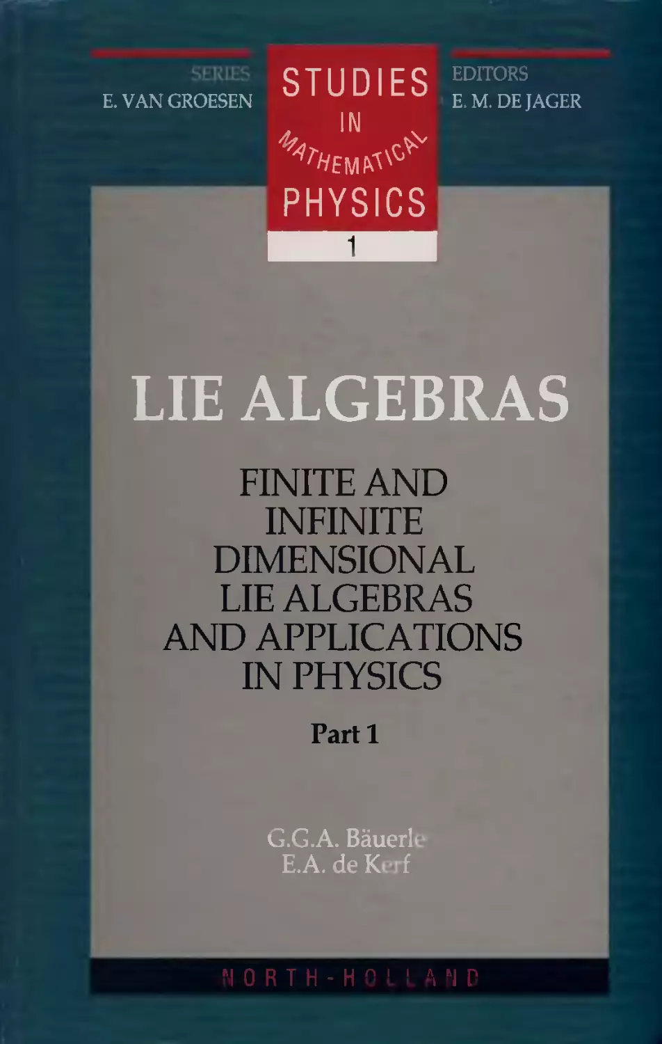
LIE ALGEBRAS
FINITE AND
INFINITE
DIMENSIONAL
LIE ALGEBRAS
AND APPLICATIONS
IN PHYSICS
Parti
G.G.A. Bauerl-
E.A.deK f
"I 0 R T H - H " ' ' VI P

LIE ALGEBRAS
PARTI
FINITE AND INFINITE DIMENSIONAL LIE ALGEBRAS
AND APPLICATIONS IN PHYSICS

STUDIES IN
MATHEMATICAL PHYSICS
VOLUME 1
EDITORS:
E. van GROESEN
Technical University of Twente, Enschede, The Netherlands
E.M. de JAGER
Emeritus, University of Amsterdam, Amsterdam, The Netherlands
ELSEVIER
Amsterdam - Lausanne - New York - Oxford - Shannon - Singapore - Tokyo

LIE ALGEBRAS
PART 1
FINITE AND INFINITE DIMENSIONAL
LIE ALGEBRAS
AND APPLICATIONS IN PHYSICS
G.G.A. BAUERLE
E.A. DE KERF
Institute for Theoretical Physics, University of Amsterdam
Amsterdam, The Netherlands
m
ELSEVIER
Amsterdam - Lausanne - New York - Oxford - Shannon - Singapore - Tokyo

ELSEVIER SCIENCE B.V.
Sara Burgerhartstraat 25
P.O. Box 211, 1000 AE Amsterdam, The Netherlands
© 1990 Elsevier Science B.V. All rights reserved.
This work and the individual contributions contained in it are protected under copyright by Elsevier Science
B.V.jand the following terms and conditions apply to its use:
Photocopying
Single photocopies of single chapters may be made for personal use as allowed by national copyright laws.
Permission of the publisher and payment of a fee is required for all other photocopying, including multiple or
systematic copying, copying for advertising or promotional purposes, resale, and ail forms of document delivery.
Special rates are available for educational institutions that wish to make photocopies for non-profit educational
classroom use.
Permissions may be sought directly from Elsevier Science Rights & Permissions Department, PO Box 800, Oxford
OX5 1DX, UK; phone: (+44) 1865 843830, fax: (+44) 1865 853333, e-mail: permissionstaelsevier.co.uk. You may
also contact Rights & Permissions directly through Elsevier's home page (http://www.elsevier.nl), selecting first
'Customer Support', then 'General Information', then 'Permissions Query Form'.
In the USA. users may clear permissions and make payments through the Copyright Clearance Center, Inc., 222
Rosewood Drive, Danvers, MA 01923, USA; phone: (978) 7508400, fax: (978) 7504744, and in the UK through the
Copyright Licensing Agency Rapid Clearance Service (CLARCS), 90 Tottenham Court Road, London W1P 0LP,
UK; phone: ( + 44) 171 436 5931; fax: (+44) 171 436 3986. Other countries may have a local reprographic rights
agency for payments.
Derivative Works
Subscribers may reproduce tables of contents for internal circulation within their institutions. Permission of the
publisher is required for resale or distribution of such material outside the institution.
Permission of the publisher is required for all other derivative works, including compilations and translations.
Electronic Storage or Usage
Permission of the publisher is required to store or use electronically any material contained in this work,
including any chapter or part of a chapter. Contact the publisher at the address indicated.
Except as outlined above, no part of this work may be reproduced, stored in a retrieval system or transmitted in
any form or by any means, electronic, mechanical, photocopying, recording or otherwise, without prior written
permission of the publisher.
Address permissions requests to: Elsevier Science Rights & Permissions Department, at the mail, fax and e-mail
addresses noted above.
Notice
No responsibility is assumed by the Publisher for any injury and/or damage to persons or property as a matter of
products liability, negligence or otherwise, or from any use or operation of any methods, products, instructions or
ideas contained in the material herein. Because of rapid advances in the medical sciences, in particular,
independent verification of diagnoses and drug dosages should be made.
First edition 1990
Second impression 1999
Library of Congress Cataloging in Publication Data
A catalog record from the Library of Congress has been applied for.
ISBN: 0 444 88776 8
@ The paper used in this publication meets the requirements of ANSI/NISO Z39.48-1992
(Permanence of Paper).
Printed in The Netherlands.

Dedicated to
Riet and Margaretha Jacoba
(E. de K.)
Hennie and Paula
(G.B.)

Preface from the Editors
The second half of our century has shown a very rapid and broad
expansion of mathematics and theoretical physics in all of its
specializations. Much is achieved, on the one hand in algebra, geometry, analysis
and stochastics, on the other hand in quantum field theory, statistical
mechanics and dynamical systems.
Although these developments occurred in many instances separately
in mathematics and physics there has been a strong interaction
between the two disciplines. To be more specific we mention: infinite
dimensional algebras, integrable systems and solitons and strings; group
theory and quasi crystals; algebraic geometry and solid state physics;
differential geometry, in particular fibre bundles and non-abelian gauge
theories; symplectic geometry and mechanics; non-linear analysis,
dynamical systems, chaos ind fluid mechanics and dynamics of high
dimensional systems; stochasic processes, operator algebras and
statistical mechanics and quantum field theory.
The fact that sometimes research in mathematics and physics has
been carried out independently from each other may bring about a
lack of mathematical rigour in theoretical physics and a loss of fruitful
sources of inspiration in mathematics.
Another problem is posed by the amount of literature in
mathematical physics which is overwhelming and scattered in many periodicals.
The editors strongly believe that it is important for researchers to be
able to get acquainted to a new field rapidly. It is the aim of the
editors to stimulate with the series 'Studies in Mathematical Physics'
actual developments in physics, sound mathematics and high
didactical quality. The emphasis lies on techniques, ideas and methods that
are fundamental, interesting and innovating in both mathematics and
physics, herewith building a bridge between the two disciplines.
We think that the authors of the present volume, which is the first in
the series, have succeeded in writing a lucid text on finite and infinite
dimensional Lie algebras and applications; more applications will be
given in a forthcoming volume. We want to express our hope that the
treatment in both volumes provides a good insight in the mathemati-
vii

Vlll
Preface from the Editors
cal and physical aspects of the subject, and students as well as more
experienced researchers will be motivated to study the mathematical
and physical aspects of conformal fields theory, sigma models, string
theories and integrable systems.
E. van Groesen
E.M. de Jager

Preface
This book is the first volume of a series on finite and
infinite-dimensional Lie algebras and their applications in mathematical physics. It
covers roughly two thirds of the material treated in a one-year, two
hours a week, course for undergraduates studying theoretical physics
or applied mathematics. In this volume we treat mainly the
mathematics of complex finite-dimensional Lie algebras, in particular semisimple
Lie algebras, and Kac-Moody algebras. The prerequisites for this
volume are very modest, an introductory course in linear algebra will be
sufficient.
In the literature on Lie algebras one can observe a
physics-mathematics dichotomy. Whereas mathematical literature sticks to a safe
environment of definitions, theorems and proofs, in physics one is
usually less precise in the statements of definitions and theorems. In the
physics literature proofs are often conducted by referring to an
analogous special case and one hardly, if ever, bothers about the existence
of certain mathematical entities. This may be tolerable when one uses
well-known mathematics as a tool for the description and
investigation of equally well-known physical theories. However, the theory of
Kac-Moody and Virasoro algebras and their applications are still in a
state of development and intuition is here less developed. This alone
is sufficient reason to adhere to a more mathematical treatment of
the subject. Equally important is the fact that a more mathematical
treatment of the subject gives physicists an easier access to the
mathematical literature.
There is yet another reason which in our view justifies a
mathematical approach as an introduction to the subject. The physics literature,
aiming mostly at applications, uses various concepts from relativis-
tic field theory, current algebra, integrable systems, string theory, etc.
These topics are not common knowledge at the undergraduate level.
We have, however, tried not to push the mathematics too far: the
emphasis lies on comprehension.
The main subject of this volume is the theory of affine Kac-Moody
algebras. Many of the concepts which appear in Kac-Moody
algebras are already present in the theory of finite-dimensional complex
ix

X
Preface
semisimple Lie algebras. The first intermediate goal is an elaborate
discussion of these Lie algebras. Chapters 1-5 give the general
background material on Lie algebras. In these chapters the important
concepts are those of solvable, nilpotent, semisimple and simple Lie
algebras. Chapter 6 deals with the general structure of finite-dimensional
complex semisimple Lie algebras. This general structure is essentially
a decomposition of such a Lie algebra into a direct sum of eigenspaces
with respect to a set of commuting diagonalizable operators. These
eigenspaces are labelled by so-called roots and are called root spaces.
For finite-dimensional complex semisimple Lie algebras roots are very
simple objects, they are vectors in a euclidean vector space. Chapters 7,
8 and 9 give a step by step investigation of the properties of roots and
root spaces culminating in the classification of all finite-dimensional
complex (semi)simple Lie algebras. These Lie algebras can be
completely characterized by their so-called Cartan matrix or, equivalently,
by their Dynkin diagram. Throughout chapters 1-9 we use the simple
Lie algebra sl(n, C), the Lie algebra of traceless n x n matrices, to
illustrate the various properties of simple Lie algebras.
The rest of this volume is devoted to Kac-Moody algebras.
Similar to the fact that a finite-dimensional complex semisimple Lie
algebra is determined by its Cartan matrix, a Kac-Moody algebra is
determined by a so-called generalized Cartan matrix. Chapter 10
describes the construction of a Kac-Moody algebra from a generalized
Cartan matrix. This is in fact a generalization of Serre's construction
of Lie algebras from generators and relations. Chapters 11, 12 and
13 deal with general properties of Kac-Moody algebras such as
gradations, the center, generalized Cartan-Killing form, the Weyl group
and properties of root chains. Chapter 14 deals with the
classification of Kac-Moody algebras. They can be divided into three classes.
The first class are the finite-dimensional complex simple Lie algebras,
which were already fully classified in chapter 9. The other two classes
are infinite-dimensional Kac-Moody algebras, namely the afHne Kac-
Moody algebras and the indefinite Kac-Moody algebras. Almost all
attention will be given to the afHne Kac-Moody algebras. The root
system of these algebras is investigated in detail in chapters 15 and 16.
Chapter 17, the final chapter of this volume, is of a somewhat different
nature. In this chapter we discuss a few applications of Lie algebras in
physics.
The main topics of the second volume are representation theory and
the applications of Kac-Moody algebras in mathematical physics. To
make contact with the physicist's approach to Kac-Moody algebras,

Preface
XI
see for instance Goddard and Olive (1986), we treat the realization
of affine Kac-Moody algebras as loop algebras with central extension
and a derivation. Besides Kac-Moody algebras we also discuss the Vi-
rasoro algebra. As for applications we will discuss sigma models, string
theory, conformal field theory and examples of integrable systems, in
particular the K-P hierarchy associated to the representations of the
infinite matrix algebra gl(oo).
To the insiders it will be immediately clear that this first volume is
considerably influenced by two of the standard works on Lie algebras,
notably Humphreys (1972) and Kac (1985). Although we have tried
to stay as close as possible to Kac, the construction of Kac-Moody
algebras from generators and relations is based on Serre (1966) and
Moody (1967). In our lectures we have tried to bridge the gap between
the level of these works and a first year course in linear algebra. The
simple observation that students who attended the course were
immediately able to do research in the domains of string theory, conformal
field theory and integrable systems has convinced us of the fact that
these lectures served their purpose.
Acknowledgements. We wish to acknowledge several people. In
particular we like to thank Dr Fons ten Kroode1 who, in collaboration
with Dr Maarten Bergvelt2, initiated the study of Kac-Moody
algebras and their applications to integrable systems at the University of
Amsterdam. Ten Kroode's unpublished notes on the subject have been
our initial guide in the field of Kac-Moody algebras. We also owe
gratitude to Professor Eduard de Jager3 who expressed his confidence in
our enterprise by encouraging his students to follow our lectures and
to Professor Michiel Hazewinkel4 for letting us profit from his
unpublished lecture notes on Kac-Moody algebras. One of the authors (E.
A. de K.) wants to thank Professor Gustavo Castelo Branco and Dr
Juca da Silva Marcos from the Instituto Fi'sica e Matematica of the
University of Lisbon for their kind invitation to present a first 'try
out' of these lectures in the summer of 1987, and Drs Fulco Bohle
for his help in preparing the Lisbon notes. We also want to thank
1 Department of Mathematics and Computer Science of the University of
Amsterdam
2 Assistant Professor in the Department of Mathematics, University of Illinois at
Urbana-Champaign
3 Professor of pure and applied mathematics at the Department of Mathematics
and Computer Science of the University of Amsterdam
4 Professor of mathematics at the Centre for Mathematics and Computer Science,
Amsterdam

Xll
Preface
Drs Peter van Driel and Drs Koos de Vos who managed to translate
our original Microsoft® Word™ file into lATgX on the Macintosh®
computer, and Drs Bart Wage whose print-technical and substantial
remarks have much improved this volume. Drs Mark Eligh and Drs
Hans Oosterom from North-Holland are acknowledged for their
cooperation and support during the preparation of the typescript. We thank
the students attending our lectures for the many critical remarks and
questions which have improved these notes, Miss Zoritza Hilgeman,
Miss Elvire Smeets and Mr. Taco Tichelaar for their part in the typing
job. Last but not least we thank the editors Professor Eduard de Jager
and Professor Brennie van Groesen 5 for their stimulating remarks and
the Staff of the Instituut voor Theoretische Fysica of the Universiteit
van Amsterdam for providing the appropriate computer facilities.
Amsterdam, July 1990
G.G.A. Bauerle
E.A. de Kerf
Professor of mathematics at the Department of Mathematics of the Technical
University of Twente

xiii
Contents
Preface from the Editors vii
Preface ix
1 Generalities on Lie algebras 1
1.1 Lie algebras 2
1.2 Quotient Lie algebras 8
1.3 Solvable and nilpotent Lie algebras 10
1.4 Simple and semisimple Lie algebras 14
1.5 Levi's theorem 15
1.6 Idealizer and centralizer 16
1.7 Derivations of a Lie algebra 17
1.8 Structure constants of a Lie algebra 18
1.9 Special linear Lie algebra 20
1.10 Lie groups and Lie algebras 25
1.11 Classical groups and their Lie algebras 29
1.11.1 The special linear group SL(n, C) 29
1.11.2 The orthogonal group 0(n,C) 30
1.11.3 The Lie algebra so(2k, C) . 34
1.11.4 The Lie algebra so(2k + 1, C) 37
1.11.5 The symplectic group Sp(k, C) 40
2 Representations of Lie algebras 44
2.1 Lie algebra homomorphisms 45
2.2 Representations and modules of Lie algebras 46
2.3 Quotient Lie modules 48
2.4 Tensor product and direct sum of Lie modules 49
2.5 Homomorphisms between Lie modules 50
2.6 The adjoint representation 52
2.7 Automorphisms 56
2.8 Finite-dimensional representations of sl(2, C) 58
3 Nilpotent and solvable Lie algebras 64
3.1 Nilpotent Lie algebras 64

xiv Contents
3.2 Solvable Lie algebras 68
4 Jordan—Chevalley decomposition 71
4.1 Jordan-Chevalley theorem 71
4.2 Proof of the Jordan-Chevalley theorem 74
4.3 Invariant subspaces of a semisimple operator 79
5 Cartan—Killing form on a Lie algebra 82
5.1 Cartan-Killing form 82
5.2 Semisimple Lie algebras 85
5.3 Jordan-Chevalley decomposition for a semisimple Lie
algebra 90
5.4 Simple and semisimple Lie algebras 91
1
6 General structure of finite-dimensional complex semi-
simple Lie algebras 95
6.1 Toral subalgebras 95
6.2 Root space decomposition of a semisimple Lie algebra . 98
6.3 Root system of sl(k + 1, C) 100
7 Properties of root spaces 106
7.1 General properties of root spaces 106
7.2 Properties of roots 110
7.3 More about roots 114
7.4 Root chains 116
7.5 Euclidean subspace of H* 120
7.6 Properties of the roots of sl(k + 1,C) 125
8 Weyl group of a root system 129
8.1 Weyl reflections 129
8.2 Weyl reflections for sl(k+ 1,C) 132
9 Classification of finite-dimensional complex semisimple
Lie algebras 133
9.1 Angle and norm restrictions 134
9.2 Restrictions on root chains 136
9.3 Simple roots and ordering of roots 137
9.4 Cartan matrix 143
9.5 Commutation relations and structure constants 145

Contents xv
9.6 Root diagrams 149
9.6.1 Rank L = 1 149
9.6.2 Rank L = 2 150
9.7 Dynkin diagrams 153
9.8 Classification of simple complex Lie algebras 156
9.9 Root systems of classical Lie algebras 174
9.9.1 Root system of so(2k, C) 175
9.9.2 Root system of so(2k + 1, C) 179
9.9.3 Root system of sp(k, C) 182
9.10 Some general properties of simple complex Lie algebras 184
9.11 Real and complex Lie algebras 189
10 Kac—Moody algebras and Serre's construction 201
10.1 Universal structures 203
10.2 Generalized Cartan matrix 209
10.3 Serre's construction 213
10.4 Root chain conditions 222
11 Gradations of a Lie algebra and center of a Kac—Moody
algebra 230
11.1 Gradations of vector spaces and Lie algebras 230
11.2 Center of a Kac-Moody algebra 233
12 Generalized Cartan-Killing form 238
12.1 Symmetric bilinear form on if 238
12.2 Generalized Cartan-Killing form 245
13 Weyl group and root properties of a Kac-Moody
algebra 251
13.1 Weyl group of a Kac-Moody algebra 251
13.2 Properties of the root system of a Kac-Moody algebra . 254
14 Classification of Kac—Moody algebras 264
14.1 Inequalities 265
14.2 Classification of matrices 271
14.3 Graphs and symmetrizability of generalized Cartan
matrices 279
14.4 Positivity properties of generalized Cartan matrices of
finite and affine type 288

xvi Contents
14.5 Dynkin diagrams of generalized Cartan matrices .... 289
14.6 Classification of affine Kac-Moody algebras 298
15 Real and imaginary roots of Kac-Moody algebras of
affine type 305
15.1 Real roots 306
15.2 Imaginary roots 309
15.3 Long and short roots 313
16 Root system of untwisted affine Kac-Moody algebras 318
16.1 Dynkin diagrams and Coxeter numbers 318
16.2 Bases for H and H* 321
16.3 Root system of affine algebras 324
16.4 Root 0 326
17 Applications in physics — a preview 328
17.1 General principles of quantum physics 329
17.2 Symmetry 341
17.3 Relativistic quantum theory 349
17.4 Gauge theories 370
17.5 Current algebras 379
References 388
Subject index 391

1. Generalities on Lie algebras
This chapter is a compilation of many basic notions and some
examples from the theory of Lie algebras. In section 1.1 we begin with the
definitions of a Lie algebra L, a Lie subalgebra and a Lie ideal I. These
definitions are then illustrated by the so-called linear Lie algebras, i.e.
Lie algebras the elements of which are linear operators or matrices.
In section 1.2 we treat the construction of the quotient algebra L/I of
a Lie algebra L with respect to an ideal I. The construction of quotient
algebras is one of the cornerstones for the construction of Lie algebras,
and more in particular Kac-Moody algebras, from a set of generators.
This construction is discussed in considerable detail.
In section 1.3 two classes of Lie algebras are studied, viz. the nilpo-
tent and solvable Lie algebras. Both classes are characterized by a
sequence of ideals constructed from the Lie algebra itself. The prototype
of nilpotent Lie algebras is the matrix Lie algebra of strictly upper
triangular n x n matrices. These matrices have zeros on the diagonal
and below the diagonal. The prototype of solvable Lie algebras is the
matrix Lie algebra of upper triangular n x n matrices, i.e. matrices
with zeros below the diagonal.
In section 1.4 we introduce two more classes of Lie algebras, namely
the simple and semisimple Lie algebras. The key concept is again that
of an ideal. Since these algebras will be discussed in great detail in the
sequel only their definitions are given in this chapter.
In section 1.5 we discuss briefly Levi's theorem. It says that every Lie
algebra can be decomposed into the sum of a solvable and a semisimple
subalgebra.
In section 1.6 two more basic concepts are introduced: the idealizer
and the centralizer of a subalgebra of a Lie algebra.
In section 1.7 we define the concept of derivations of a Lie algebra.
An important example is the so-called adjoint action.
In section 1.8 we restrict ourselves to finite-dimensional Lie algebras.
Choosing a basis, we define the structure constants of a Lie algebra.
We explain the simplification which occurs in the structure constants
if the Lie algebra has an ideal and a basis adjusted to this ideal.
In section 1.9 we give a detailed description of the structure of the
special linear Lie algebra. This is the Lie algebra of traceless n x n
l

2
Generalities on Lie algebras
matrices. Introducing its so-called standard basis we show that this
Lie algebra decomposes into the direct sum of three subalgebras, viz.
a nilpotent subalgebra of strictly lower triangular matrices, a subalge-
bra of diagonal matrices and a nilpotent subalgebra of strictly upper
triangular matrices. Finally, we show that the standard basis can be
obtained from a certain subset of basis elements, the so-called Cartan-
Chevalley generators. The structure of the special linear Lie algebra is
rather typical for all simple Lie algebras.
In section 1.10 we discuss briefly the relation between Lie groups
and Lie algebras. The discussion is based on the general linear group
GL(n, C), the group of linear automorphisms of a complex n-dimen-
sional vector space V. We define the notion of an invariant bilinear form
on V and we show that such a form defines a subgroup of GL(n,C).
In section 1.11 we discuss the so-called classical Lie groups, i.e. the
special linear group SL(n, C), the orthogonal group 0(n, C) and the
symplectic group Sp(n, C). We give a detailed description of the Lie
algebras corresponding to these groups.
1.1. Lie algebras
The definition of a Lie algebra consists essentially of two parts
revealing its structure. A Lie algebra L is firstly a vector space (linear
space), secondly there is defined on L a particular kind of binary
operation, i.e., a mapping L x L —> L, denoted by [. , .]. The axioms
characterizing the so-called Lie bracket [. , .] are given in definition
1.1.1 below. The dimension of a Lie algebra is by definition the
dimension of its vector space. It may be finite or infinite. The vector space is
taken either over the real numbers R or the complex numbers C. We
will use F to denote either R or C.
Definition 1.1.1 A Lie algebra L is a vector space with a binary
operation
(x,y)eLx L^[x,y]e L (1.1.1)
called Lie bracket or commutator, which satisfies
L.l For all x, y € L one has
[x, y] = -[y, x] (antisymmetry)
L.2 The binary operation is linear in each of its entries:
[ax+/3y,z] = a[x,z] + 0[y,z] (1.1.3)
(1.1.2)

Lie algebras 3
and
[x, ay + fiz] = a[x, y] + fi{x, z] (bilinearity) (1-1-4)
for all x,y € L and all a, (3 € F.
L.3 For all x,y,z € L one has
[x, [y, z]] + [y, [z, x]] + [z, [x, y]] = 0 (Jacobi identity) (1.1.5)
A Lie algebra is called real or complex when its vector space is
respectively real (F = R) or complex (F = C).
Notice that (1.1.4) follows from (1.1.2) and (1.1.3).
Some Lie algebras differ only in the names of their elements,
everything else being the same. Such Lie algebras are called isomorphic.
Definition 1.1.2 Let L and M be Lie algebras and
$: L -> M (1.1.6)
a bijection such that for all a, ft € F and all x,y € L
$(ax + (3y) = a$(x) + (3$(y) (1.1.7)
and
#([!,»]) = [#(*),#(»)] (1-1-8)
then $ is called an isomorphism and the Lie algebras L and M are
called isomorphic.
The mapping $ clearly preserves the linear structure and the Lie
bracket.
Definition 1.1.3 A Lie algebra L is called abelian or commutative
if [x, y] = 0 for all x and y in L.
In order to investigate the structure of Lie algebras it is useful to
introduce the notion of subalgebra. A subalgebra K of a Lie algebra L
is a subspace of L which is closed under the Lie bracket operation of L
restricted to K. More explicitly one has the following definition.
Definition 1.1.4 A subset K of a Lie algebra L is called a
subalgebra of L if for all x,y € K and all a, (3 € F one has
ax+(3yeK, [x,y]eK (1.1.9)

4
Generalities on Lie algebras
Obviously a subalgebra K of a Lie algebra L is also a Lie algebra. A
special type of subalgebra is a so-called ideal. As we will see ideals
play a crucial role in the investigation of the structure of Lie algebras.
Before giving the definition we need some more notation.
Definition 1.1.5 Let M and N be subsets of L which are not
necessarily subspaces. Then the commutator [M, N] of M and N is defined
to be the linear span of the set of elements of the form [x, y] with x € M
and y € AT, i.e.
[M,N]: =
<z e L z = ^^-[ij.yj]; Xi,yj e L; a0- € F I (1.1.
10)
Definition 1.1.6 An ideal J of a Lie algebra L is a subalgebra of L
with the property
[I,L] C I (1.1.11)
i.e. for all £ € J and all y € L one has
[x,y] e I (1.1-12)
Every (non-zero) Lie algebra has at least two ideals, namely the Lie
algebra L itself and the subalgebra 0 consisting of the zero element
only
0 = {0} (1.1.13)
Both these ideals are called trivial. All non-trivial ideals are called
proper.
We will now determine the structure of some low-dimensional Lie
algebras.
Example 1.1.7 One-dimensional Lie algebras. There exists, up to
isomorphisms, only one one-dimensional Lie algebra. Indeed, all
elements of a one-dimensional vector space are proportional to one
another, and consequently all commutators are equal to zero. Hence a
one-dimensional Lie algebra is abelian.
Example 1.1.8 Two-dimensional Lie algebras. There exist only two
non-isomorphic two-dimensional Lie algebras. Let x and y span a two-
dimensional Lie algebra. Then their commutator is either zero or [x, y]
= z ^ 0. In the first case we have a two-dimensional abelian Lie
algebra. In the second case one has [x,y] = z — ax + (3y (q,/3 € F)

Lie algebras
5
and not both a and (3 are zero. Let us suppose a ^ 0, then one has
[z,a_1J/] = z. Hence for all non-abelian two-dimensional Lie algebras
one can choose a basis {z,u} such that [z,u] = z. Consequently all
non-abelian two-dimensional Lie algebras are isomorphic. Notice that
the one-dimensional subalgebra spanned by z is an ideal.
Example 1.1.9 Three-dimensional Lie algebras. An important tool
in the classification of the three-dimensional Lie algebras is the so-
called derived algebra L1. The latter is defined to be the Lie algebra
L1 .= [L,L] (compare definition 1.1.5). In order to classify all three-
dimensional Lie algebras we consider the different possibilities for the
dimension of L1.
Case dim L J= 0. For dim L1 = 0 the Lie algebra L is clearly the
abelian three-dimensional Lie algebra.
Case dim L J= 1. If dim L1 = 1 then there exists a fixed element
z £ L1 such that for all x and y in L one has [x, y] = ui(x, y)z where u>
is a skew-symmetric bilinear form. There arise two possibilities for w.
— either ui(x,z) = 0 for all x € L
— or there exists anigl such that ui(x, z) = 1.
In the first case we extend z € L1 to a basis {x,y,z} of L. One
then has ui(x,z) = 0 and ui(y,z) = 0. Consequently ui(x, y) ^ 0 since
otherwise all commutators would be equal to zero, which contradicts
dim L1 = 1. By rescaling (for instance) x one can achieve that ui(x, y) =
1. Hence one arrives in the first case at the commutation relations
[x, y] = z, [x,z] = [i/, z] = 0 for a suitably chosen basis {x,y,z}- This
Lie algebra is often called the three-dimensional Heisenberg algebra. Its
infinite-dimensional analogue, i.e., the algebra with basis {x{,yt,z \ i €
Z} and commutation relations
[xi,yj] = SijZ, [xi, z] = [yi,z] = 0
plays an important role in the representation theory of Kac-Moody
algebras.
In the second case one has [x, z] = 2. Let us extend {a;, 2} to a basis
{a;,u, 2} of L. Then [x,u] = az and [u, z] = bz (a, b e F). Defining
y := u — bx — az gives the commutation relations [x,y] = [y,z] =
0, [1, 2] = 2. Hence for dim L1 = 1 there exist two non-isomorphic
three-dimensional Lie algebras.
Case dim LJ= 2. The case dim L1 = 2 will not be considered in any
detail. Its analysis can be based on the fact that all two-dimensional
Lie algebras are determined in example 1.1.8.

6
Generalities on Lie algebras
Case dim L'= 3. Finally in the case dim L1 = 3, that is L = L1,
there exist two non-isomorphic Lie algebras for F = R. By a suitable
choice of a basis {x, y, z} their commutation relations read respectively
[x,y]=z, [y,z] = x, [z,x] = y (1.1.14)
and
[x, y] = 2y, [x, z] = -22, [y, z] = x (1.1.15)
Considered as complex Lie algebras, the Lie algebras corresponding to
(1.1.14) and (1.1.15) are isomorphic. Hence the classifications of Lie
algebras over R and over C are in general different [see section 9.10].
The classification of the real three-dimensional Lie algebras is known
in physics as the Bianchi classification. It gives, for example, a
classification of the spatially-homogeneous anisotropic cosmological models
[see, for instance, section 116 of Landau (1975)]. We will now treat some
examples of Lie algebras, which we will use frequently to illustrate new
concepts.
Example 1.1.10 In this example we introduce a prototype of Lie
algebras, the so-called general linear Lie algebra. Let L( V) be the set of
all linear operators on a vector space V. This vector space V will often
be a finite-dimensional one. Multiplication and addition of these linear
operators as well as the product of a linear operator and a number is
defined in the usual way. Thus denoting operators of L(V) by capitals,
we have for all a,(3eF and all v € V
(aA + PB)v = a(Av) + (3(Bv) (1.1.16)
and
(AB)v = A(Bv) (1.1.17)
These properties allow us to regard L(V) as an associative algebra
with unit element 1; the latter being defined by lv = v for all v in V.
Defining on L(V) a bracket operation by
[A,B}:= AB-BA (1.1.18)
turns L(V) into a Lie algebra. This Lie algebra is called the general
linear Lie algebra gl(V).
Example 1.1.11 In this example the matrix form of the general linear
Lie algebra is introduced. Choosing a basis {ei, e2, • •., en} in the n-
dimensional vector space V, every linear operator A can be represented
by a matrix M(A) = (a,j) with respect to this basis by means of

Lie algebras
7
Ae% = ]T
efcafct
(1.1.19)
fc=i
The set ofnxn matrices obtained in this way is an n2-dimensional
vector space Mn = M(n, F). Taking matrix multiplication as the product
on this vector space it becomes, similar to example 1.1.10, an
associative algebra with unit element. Defining a commutator on Mn
analogous to (1.1.18) one obtains the Lie algebra of all n x n matrices. The
latter is denoted by gl(n) = gl(n,F). It is easily verified that gl(n)
and gl(V) are isomorphic. The former is said to represent the latter
faithfully, that is, bijectively.
Taking a different basis {di,d,2, ■■■^dn} in V, causes the operator A
to be represented by a different matrix M'(A) = (aj-) defined by
Adi = ]P dka'ki
(1.1.20)
fc=i
The representations M and M' are called equivalent.
Exercise 1.1.12 Define in the context of example 1.1.11 a linear
operator 5 by d{ = Se{ (i = 1,..., n) and show that
M\A) = M(S~1)M(A)M(S)
(1.1.21)
Example 1.1.13 Consider in gl(n) the subset t+(n) of upper
triangular matrices
Kj) =
/ an
0
0
0
ai2
<*22
0
0
ai3
^23
^33
0
ai4
a24
A34
044
V o
0 0
0 0
O-in
O-nn )
(1.1.22)
i.e. a,-j = 0 for i > j. Linear combinations and commutators of such
matrices are again of this type. Hence it follows that t+(n) is a Lie
algebra. Moreover, it is a Lie subalgebra of gl(n).
Exercise 1.1.14 Show that the commutator of matrices in t+(n)
yields matrices with all diagonal elements equal to zero.
Example 1.1.15 The matrices (a,-j) with a,ij = 0 for i > j are called
strictly upper triangular. These matrices form a Lie algebra
denoted by t++(n). Notice that t++(n) is a Lie subalgebra of t+(n).
Moreover t++(n) is the derived algebra of t+(n) [see example 1.1.9]:

8
Generalities on Lie algebras
t++(n) = [t+(n),t+(n)} (1.1.23)
Prove this using the results of exercises 1.1.14 and 1.8.2.
Example 1.1.16 The subset d(n) of diagonal matiices in gl(n) is a
Lie algebra.
Example 1.1.17 Consider in gl(n) the subset of matrices with trace
equal to zero. This is a Lie algebra called the special linear algebra
sl(n).
Exercise 1.1.18 Show that t++(n) constitutes an ideal in t+(n), that
is, show that
[t+(n),t++(n)}ct++(n) (1.1.24)
In the next section we discuss an important construction which is
frequently used to obtain from a given Lie algebra L with ideal I a
'smaller' Lie algebra, the quotient Lie algebra L/I.
1.2. Quotient Lie algebras
Starting with a Lie algebra L which contains an ideal I we define
on L an equivalence relation. Elements x and y in L are said to be
equivalent if their difference x — y lies in the ideal I. The equivalence
of the elements x and y is denoted by x ~ y. Recall that a relation ~
between elements of an arbitrary set is called an equivalence relation
if for all x, y and z in this set one has
E. 1 x ~ x (reflexivity)
E. 2 x ~ y => y ~ x (symmetry)
E. 3 (x ~ y & y~z) => x ~ z (transitivity)
One easily verifies that these conditions are satisfied for the relation
defined above using an ideal I of the Lie algebra L. Having such an
equivalence relation, the Lie algebra L can be partitioned into disjoint
classes of mutually equivalent elements. These classes are called
equivalence classes. More explicitly, let x be in L then we define the class
x of elements equivalent with x by
x:= {z <EL\x ~ z} = {z <E L \(x- z) el} (1-2.1)
Alternative notations are
x = x + I = x (modi) (1.2.2)

Quotient Lie algebras
9
Notice that 0 = {z £ L | (0 - z) £ 7} = I. Due to the fact that 7 is
an ideal we can define a Lie algebra structure on the set of equivalence
classes. Let x and y be two equivalence classes. Using the linear
structure and the bracket in L we define for all a, /3 £ F linear combinations
of x and y by
ax + (3y := ax + fiy
and the Lie bracket of x and y by
(1.2.3)
[x,y] := [x,y]
(1.2.4)
The right-hand sides of (1.2.3) and (1.2.4) contain representatives x
and y of x and y respectively. Due to the fact that 7 is an ideal these
right-hand sides are independent of the choice of the representatives x
and y in x and y respectively. With the definitions (1.2.3) and (1.2.4)
the set of equivalence classes becomes a Lie algebra. The latter is called
a quotient Lie algebra. It is denoted by
L = L/I= L (mod 7)
(1.2.5)
Forming the quotient algebra by means of an equivalence relation can
also be described by the so-called canonical projection II defined by
II: x £ L >-> n(a;) = x£L
This projection has the properties [see (1.2.3) and (1.2.4)]
n(az: + 0y) = ~ax + 0y = all(x) + 0U(y)
and
n[x,y} = [x,y} = [x,y} = [n(x),n(y)}
(1.2.6)
(1.2.7)
(1.2.8)
In section 2.1 we will see that the map II is an example of a Lie algebra
homomorphism.
Example 1.2.1 The Lie algebra of strictly upper triangular matrices
t++(n) is an ideal in the Lie algebra of upper triangular matrices t+(n).
The equivalence relation applied to this case says that two matrices of
the form
(<*.->) =
/ an
0
0
0
an
022
0
0
ai3
a23
033
0
an
a-u
a34
a44
ain \
02n
03n
a4n
V o
(1.2.9)
0 0 ann J

10
Generalities on Lie algebras
belong to the same equivalence class iff all corresponding diagonal
elements are equal. Consequently the quotient algebra t+(n)/t++(n) has
the structure of d(n), that is to say, this quotient algebra is isomorphic
to d(n) [see example 1.1.16].
1.3. Solvable and nilpotent Lie algebras
In this section we consider two special types of Lie algebras, namely
the solvable and the nilpotent Lie algebras. These algebras play a
crucial role in the classification of all Lie algebras. To define these algebras
we need to know a little bit more about ideals. We begin with an easy
construction to obtain a particular ideal from a given Lie algebra L.
Consider in L the set L1 := [L,L] (see definition 1.1.6). Recall that
this is the set of elements of the form [a;, y] (x, y € L) and all possible
linear combinations of such elements. It is called the derived algebra
of L. The derived algebra L1 is an ideal in L, although it may be a
trivial one. We put this in a lemma.
Lemma 1.3.1 Let
Ll:=[L,L] (1.3.1)
then this is an ideal in L.
Proof The derived algebra Ll is by definition a subspace of L. Since
Ll<zL (1.3.2)
we have [L1, L1] C [L, L} = L1. Thus L1 is a subalgebra of L. We must
finally show that [i1,^] C Ll in order to prove that L1 is an ideal.
However, from (1.3.2) it follows also immediately that
[L\L]c[L,L} = L1 (1.3.3)
Notice that for an abelian Lie algebra Ll = [L,L] = 0. A simple
example is provided by d(n).
Remark 1.3.2 Recall that the derived algebra of t+(n) is t++(n)
[compare example 1.1.15].
Ideals in a Lie algebra can be combined in various ways to give new
ideals. We first define for subsets V and W of L the sum V + W by
V + W := {z € L | z = v + w; v £ V; w £ W} (1.3.4)

Solvable and nilpotent Lie algebras
11
Lemma 1.3.3 Let I and K be ideals in L. Then the sum I + K, the
intersection I n K and the commutator [7, K] are ideals in L.
Exercise 1.3.4 Prove the above lemma.
We now come to the notions of solvable and nilpotent Lie algebras.
These concepts are denned by means of sequences of ideals which are
obtained from L using the commutator. Starting with a Lie algebra
L one defines the so-called descending central sequence and derived
sequence. The descending central sequence consists of repeated
commutators of the Lie algebra L.
Definition 1.3.5 Let L be a Lie algebra. The sequence L°, L1,..., Ln,
.. . defined by
L°:=L, Ll:=[L,L], L2 := [L,L% ...,
Ln :=[L,Ln-1},... (1.3.5)
is called the descending central sequence.
Notice that Ln is the (n + l)th power of L with respect to the Lie
bracket as multiplication operation.
Exercise 1.3.6 Prove that
L° D L1 D L2 D ... D Ln D ... (1.3.6)
and that L°, L1 ,L2,... are ideals in L.
Another descending sequence of ideals figures in the following
definition.
Definition 1.3.7 Let L be a Lie algebra. The sequence L0, Lx, ■ ■ ■, Ln,
...defined by
L0 := L, Li := [7vo,7v0], • • •, Ln := [Ln_i,Lr,-i],... (1.3.7)
is called the derived sequence.
Exercise 1.3.8 Prove that
L0D Li D L2 D ... D Ln D ... (1.3.8)
and that Lj (i = 0,1, 2,...) are ideals in L.

12
Generalities on Lie algebras
Notice that for an arbitrary finite-dimensional Lie algebra both
sequences become constant from a certain term on. Indeed the
dimensions of the successive Lie algebras cannot continue to decrease
indefinitely since dimensions are non-negative. Hence the dimensions of the
Lie algebras in the sequences become constant from a certain term on.
However, when a subspace W of a vector space V has the same
dimension as V (dim W = dim V), then V = W. Consequently the sequences
(1.3.5) and (1.3.7) become constant from a certain term on. There are
two noteworthy cases for both sequences. These are L = L1 = L\ [see
section 1.4] and Ln — 0 or Ln — 0.
Definition 1.3.9 A Lie algebra L is called nilpotent if there exists
an n £ N such that Ln = 0.
Remark 1.3.10 If Ln = 0 then of course Lq = 0 for q > n. Let
L ^ 0 and let p be the smallest integer for which Lp = 0. Then we
have [L,Lp~l] = 0 and Lp~l / 0. This means that Lp~l is an abelian
ideal in L. Hence each nilpotent Lie algebra L ^ 0 contains an abelian
ideal unequal to 0.
Example 1.3.11 The Lie algebra t++{n) of strictly upper triangular
matrices is the prototype of nilpotent algebras.
Exercise 1.3.12 Show that t++(n) is nilpotent.
Nilpotent Lie algebras have nice properties which will be discussed in
relation with Engel's theorem in chapter 3. Actually Engel's theorem
gives a more tangible characterization of nilpotent Lie algebras. The
case Ln — 0 figures in the following definition.
Definition 1.3.13 A Lie algebra L is called solvable if Ln = 0 for
some n g N.
Exercise 1.3.14 Show that
L'DLi (1.3.9)
From this we obtains the following theorem.
Theorem 1.3.15 Nilpotent Lie algebras are solvable.
The converse need not be true as the following example shows.
Example 1.3.16 The upper triangular algebras t+(n) are the
prototypes of solvable algebras. The derived algebra t+in)1 is t+ + (n).
Moreover t+(n) is not nilpotent for n > 1 since [see (1.1.23)]

Solvable and nilpotent Lie algebras
13
[t+(n),t+(n)} =<++(") (1-3-10)
and
[t+(n),t++(n)}=t+ + (n) (1.3.11)
One part of the verification of (1.3.11) is given by (1.1.24). The proof
of
[t+{n),t++{n)} D t++{n)
can be given by means of (1.8.10). Hence solvable Lie algebras are in
general not nilpotent.
We will have more to say about solvable Lie algebras in chapter 3 in
connection with Lie's theorem. We now come to a lemma on solvable
ideals in a Lie algebra.
Lemma 1.3.17 Every finite-dimensional Lie algebra L has a unique
maximal solvable ideal R. Of course R may be trivial.
Proof Let / and J be solvable ideals in L. Then the sum I + J is
an ideal in L [see lemma 1.3.3]. Moreover it can be shown to be a
solvable ideal [see section 3.1 of Humphreys (1972) or section 1.4 of
Goto (1978)]. Let R be the linear span of all solvable ideals in L. Since
L is finite-dimensional there exists a finite number of solvable ideals
which span R. Their sum R is a maximal solvable ideal.
Definition 1.3.18 The maximal solvable ideal of a Lie algebra L is
called the radical of L and it is denoted by R = rad L.
Remark 1.3.19 Equation (1.3.9) can be extended in the following
way
U D L2' D Li (1.3.12)
Remark 1.3.20 Similar to remark 1.3.10 one has the following
assertion. Every solvable Lie algebra L / 0 has an abelian ideal 1^0.
Indeed for 1^0 there exists an n £ N such that Ln = [£„_i, £n-i] = 0
and .Ln_i ^ 0. Hence Xn_i is the abelian ideal we are looking for.
In the next section we consider two other important classes of Lie
algebras. They are again characterized by ideals.

14
Generalities on Lie algebras
1.4. Simple and semisimple Lie algebras
Simple and semisimple Lie algebras are non-abelian Lie algebras
without proper ideals and without abelian ideals, respectively.
Definition 1.4.1 A Lie algebra L is called simple if L is non-abelian
and has no proper ideals.
Corollary 1.4.2 For a simple Lie algebra L the derived algebra L1 =r
[L,L] is equal to L:
Ll=L (1.4.1)
Proof The derived algebra L1 is an ideal (see lemma 1.3.1). Since L is
simple, Ll has to be a trivial ideal. One has only two alternatives: either
L1 = 0 or L1 = L. The first option is ruled out since L is non-abelian.
Hence (1.4.1) follows.
Example 1.4.3 The algebra sl(n) (see example 1.1.17) is simple [see
example 5.2.8].
Definition 1.4.4 A Lie algebra L is called semisimple if L / 0 and
L has no abelian ideals ^ 0.
Remark 1.4.5 It is immediately clear that simple algebras are also
semisimple.
For finite-dimensional Lie algebras the definition of semisimple can be
given in a different, but equivalent way, by using the notion of the
radical of a Lie algebra. We put this in a lemma.
Lemma 1.4.6 A finite-dimensional Lie algebra L is semisimple if and
only if rad L = 0.
Proof We first prove that radi = 0 implies that L is semisimple.
Assume that A ^ 0 is an abelian ideal in L. Then A is a solvable ideal
and we have
rad L D A / 0
[see definition 1.3.18]. This contradicts radX = 0. Hence A — 0 and
L is semisimple. In order to prove the other implication L is taken to
be semisimple. Let us assume that R = radX ^ 0. Since R is solvable
there exists in its derived sequence an ideal Rn-\ / 0 such that
Rn = [Rn_uRn_1] = 0 (1.4.2)

Levi's theorem
15
From (1.4.2) one sees that Rn-\ ^ 0 is abelian. This contradicts the
semisimplicity of L. The result of the next exercise will be used in the
following section.
Exercise 1.4.7 Let Ibea Lie algebra and R = rad L ^ L its radical.
Show that the quotient algebra L/R is semisimple.
1.5. Levi's theorem
Now that we have introduced various types of Lie algebras we can
say something about the relation between these types. We have already
noticed that nilpotency implies solvability. Moreover we have seen
(remark 1.3.20) that a solvable Lie algebra ^ 0 has an abelian ideal ^
0. Hence such a solvable algebra is not semisimple and consequently
not simple. We will now quote without proof a famous theorem which
makes clear why solvable and semisimple Lie algebras are important
for the classification of Lie algebras.
Theorem 1.5.1 (Levi's theorem) Let L be a finite-dimensional Lie
algebra and R = rad L its radical. Then there exists a semisimple sub-
algebra S of L such that L is the direct sum of its linear subspaces R
and S
L=R®S (1.5.1)
Fig. 1.5.1. Illustration of the inclusions of various types of Lie algebras.

16
Generalities on Lie algebras
A proof can be found in chapter III.9 of Jacobson (1979).
Remark 1.5.2 The direct sum in (1.5.1) is with respect to the vector
space structure. It is not a direct sum of the Lie algebras R and 5 [see
remark 2.6.6].
Remark 1.5.3 The theorem says that a Lie algebra L is either
solvable or the sum of a solvable Lie algebra R and a semisimple Lie
algebra 5.
Figure 1.5.1 illustrates the inclusion of various types of Lie algebras.
1.6. Idealizer and centralizer
In this section we define some concepts related to a subalgebra K of
a Lie algebra L. Considering a subalgebra K of a Lie algebra L, it is
obvious that K is a trivial ideal of K. It may happen that L contains
a larger subalgebra N in which K is a proper ideal. This is formalized
in the following definition.
Definition 1.6.1 Let K be a subalgebra of a Lie algebra L. The
idealizer Ni(K) of K in L is defined as
NL(K) :={xGL\Wy€K: [x, y] £ K) (1.6.1)
Exercise 1.6.2 Verify that the idealizer is a subalgebra of L. It is the
largest subalgebra in which K is an ideal. An idealizer is also called a
normalizer.
Definition 1.6.3 A subalgebra K is called self-idealizing in L if
NL{K) = K (1.6.2)
Example 1.6.4 Both the subalgebras t+(n) of upper triangular
matrices [see example 1.1.13] and d(n) of diagonal matrices [see example
1.1.16] are self-idealizing in the general linear Lie algebra gl(n).
In the next definition we consider, for a given subalgebra K in L, all
elements in L which commute with K.
Definition 1.6.5 Let K be a subalgebra of L. The centralizer Cl{K)
of K is defined by
CL(K) :={x£L\Vy€ K: [x,y] = 0} (1.6.3)

Derivations of a Lie algebra
17
Exercise 1.6.6 Prove that Cl(K) is a subalgebra of L.
Considering the set of all elements in L which commute with L, one
arrives at the following definition.
Definition 1.6.7 The centralizer Ci{L) of L itself is called the center
of L. It is usually denoted by Z(L) = Cl{L) and it is given by
Z(L) := {ar G L | V» G L: [x, y] = 0} (1.6.4)
Exercise 1.6.8 Prove that Z(L) is an abelian ideal in L.
Remark 1.6.9 It follows from the statement in exercise 1.6.8 that the
center of a semisimple Lie algebra L contains only the zero vector, that
is Z(L) = 0.
Exercise 1.6.10 Prove that the center of gl{n) is the set of all
multiples of the unit matrix. Hint: use the basis of gl(n) defined in (1.8.8)
and the commutation relations of exercise 1.8.2.
1.7. Derivations of a Lie algebra
A derivation 6 of a Lie algebra L is a linear map L —> L satisfying
Leibniz's rule with respect to the Lie bracket.
Definition 1.7.1 A derivation 6 of a Lie algebra L is a linear map
6: L —> L satisfying
6[x., y] = [6x, y] + [x,6y] (Leibniz) (1-7-1)
The collection of all derivations of L is denoted by Der L.
Example 1.7.2 A simple and useful example is obtained by taking
an arbitrary but fixed element x G L and defining the map 6X: L t-> L
by using the Lie bracket of L:
Sx:y -»«,(»):= [x,y] (1.7.2)
This clearly defines a linear map. Invoking the Jacobi identity and
the anti-symmetry of the commutator, it follows that 6X (x £ I) is a
derivation since
6X [y, z] = [x, [y,z}} = [y, [x, z}} + [[x, y], z]
= [Sxy,z} + [y,6xz] (1.7.3)

18
Generalities on Lie algebras
Hence 6X € Der L. The derivations ^(a; e L) defined in (1.7.2) are
called inner derivations. The action on L defined in (1.7.2) is called
the adjoint action of x. This action is denoted by 6X = ad x. Hence
(ad x){y) = [x, y] (1.7.4)
Exercise 1.7.3 Since Der L consists of linear maps L —> L, linear
combinations and products of derivations can be defined in the usual
way. One has for all a, (3 e F and 6,6' € Der L
(a6 + 06'){z) := a6(z) + /36'(z) (1.7.5)
and
(66')(z):=6(6'(z)) (1.7.6)
Show that 66' is in general not a derivation. Show also that
[6, 6'}:= 66'-6'6 (1.7.7)
is a derivation. Notice that Der L is a Lie subalgebra of the Lie algebra
1.8. Structure constants of a Lie algebra
In this section we restrict ourselves to a finite-dimensional Lie
algebra L. Let n be the dimension of L. By taking a basis {ej, e2,..., en}
in L, every element x of L has an expansion
x =
^x'ei (1.8.1)
Notice that the commutator [a;, y] of any two elements x and y in L
is completely determined by the Lie brackets [e,',ej,] of pairs of basis
elements because
n
[*,»]= E zV[^efc] (1.8.2)
;,fc=i
Since [e;,efc] € L the commutator [e;,efc] can also be expanded with
respect to the basis {ei, e2, • •., en}:
n
[ei.e*]=]C<Vei (j,ft = l,...,n) (1.8.3)

Structure constants of a Lie algebra
19
The numbers Cjkl are called the structure constants with respect
to the basis {ei, ei,..., en}. From the definition of these quantities [see
(1.8.3)], the anti-symmetry of the commutator and the Jacobi identity
we obtain the relations
Cjk> = -CV (1.8.4)
n
]T {Cjk'Cimp + Ckm'Ctjp + Cmj'Clkp) = 0 (1.8.5)
i=i
A Lie algebra is completely determined by its structure constants: a
set of numbers {Cjk'} satisfying (1.8.4) and (1.8.5). One could think
of a program of classifying all Lie algebras by considering (1.8.4) and
(1.8.5) as equations to be solved for unknown structure constants. This
turns out to be a very complicated problem because of the
non-linearity of (1.8.5). As the structure constants depend on the basis it is
expedient to find a basis for which one has a maximum number of the
structure constants equal to zero. We now show that zeros arise quite
naturally if the algebra under consideration has ideals. Suppose / is
an ideal of dimension i in a Lie algebra L of dimension n. Since / is a
linear subspace of L there exists a basis {ei, e2,..., e„} in L such that
{ei, e2,..., e,} is a basis for /. Let 1 < j < i and k = 1,..., n then we
obtain from the fact that / is an ideal that the commutators [ey,efc]
are again elements of /, or
i
fo,efc] = ]TCjfcpep (1.8.6)
P=i
Hence
Cjkm = 0 (1 < j < i; 1 < k < n; i + 1 < m < n) (1.8.7)
Ideals are basic tools for unravelling Lie algebras into nilpotent,
solvable and (semi)simple Lie algebras. We give some exercises in which
structure constants are calculated.
Remark 1.8.1 The vector space formed by the set ofnxn matrices
is n2-dimensional. A basis for this vector space is provided by the
collection of matrices {e,j} (i,j = 1,..., n) defined by
(eij)ki = Slk6ji (1.8.8)
Thus the matrix e^ has all entries zero except on the the intersection
of the ith row and jth. column where it has a one. Every n x n matrix

20
Generalities on Lie algebras
A — (o,ij) can of course be expanded with respect to this basis. The
expansion coefficients are just the matrix elements of A since one has
A = ^aijeij (1.8.9)
'J
Exercise 1.8.2 Verify the commutation relations
Exercise 1.8.3 The complex three-dimensional Lie algebra sl(2, C)
has a basis {e, /, h} denned by
•=(:;)• »=(;-;)• >-(!;) <-»>
Verify the commutation relations
[h,e] = 2e, [h,f] = -2f, {e,f} = h (1.8.12)
Determine the structure constants of s/(2, C) with respect to this basis
Remark 1.8.4 The simple Lie algebra s/(2,C) (simple in both senses)
will play a crucial role in the structure theory of semisimple Lie algebras
and Kac-Moody algebras.
Exercise 1.8.5 Prove that s/(2, C) is a simple Lie algebra.
1.9. Special linear Lie algebra
In this section we investigate in detail the structure of the special
linear Lie algebra sl(n,C). Firstly we do this because it is relatively
easy to unravel the structure of sl(n, C). Secondly, because we will
frequently return to this Lie algebra as an example to elucidate abstract
notions and results. We want to emphasize that the Lie algebra sl(n, C)
(n > 1) is simple. The proof will be given in example 5.2.8. We start
by recalling the definition of the special linear Lie algebra.
Definition 1.9.1 The special linear Lie algebra sl(n, C) is the set
of complex n x n matrices with trace zero. The Lie bracket of elements
of sl(n, C) is the commutator of these matrices. The dimension of this
algebra, being the number of independent traceless n x n matrices, is
given by
dim sl(n, C) = n2 — 1
(1.9.1)

Special linear Lie algebra
21
Remark 1.9.2 The cases of interest clearly have n > 2. One usually
puts n = k + 1 with k > 1. Henceforth we will follow this convention
and denote the special linear Lie algebras by sl(k + l, C). An alternative
symbol for sl(k + 1, C) is Ak- The dimension of Ak is
dim s/(fc + l,C) = k(k + 2)
(1.9.2)
To define a basis for sl(k + 1, C) we consider first the general form of
a matrix (a,j) in s/(fc + 1, C):
(1.9.3)
A = (aij) =
^ an
«21
^31
\ Onl
with
n
Tr A = ^2 «■
,- = o
ai2
a.22
«32
«n2
(n
ai3 •
a-23 ■
^33 •
0-n3 ■
= fc + l)
ain ^
CL2n
fl3n
Ann /
(1.9.4)
It is clear that the matrix A can be split uniquely in a diagonal part
j4j, a strictly lower triangular part j4_ and a strictly upper triangular
part A+, that is
A = A_ + Ad + A ,
(1.9.5)
For the strictly upper triangular part j4+ of j4 we take the basis
matrices epq with l<p<<ji<fc+l. Recall [see (1.8.8)] that the matrices
epq are defined by
(er
SpiS„
(1.9.6)
These matrices have the number one on the intersection of the pth
row and the qth column, all other matrix elements being zero. For the
strictly lower triangular part A- of A we take the basis matrices epq
with 1 < q <p < fc + 1. This gives altogether (fc + 1)2-(fc + 1) = fc(fc + l)
matrices. For the diagonal part of A we need k traceless diagonal basis
matrices. We define these matrices by
*^p •— *~pp
ep+i,P+i (p - 1,2, ...,fc)
(1.9.7)
Definition 1.9.3 The matrices epq with p / q and hp given in (1.9.6)
and (1.9.7) form the so-called standard basis of sl(k + 1, C).

22
Generalities on Lie algebras
The matrices epq with p < q are strictly upper triangular matrices.
They are the basis elements for a k(k + l)/2-dimensional nilpotent
subalgebra of sl(k + 1, C). This subalgebra is called N+. Likewise, the
matrices epq with p > q are strictly lower triangular matrices. The
nilpotent subalgebra with this basis is denoted by JV_. Finally the
matrices hp are the elements of a fc-dimensional abelian subalgebra of
diagonal traceless matrices. This subalgebra is denoted by H. As every
matrix A in sl(k + l, C) has a unique decomposition of the form (1.9.5),
the Lie algebra sl(k + 1,C) considered as a vector space is the direct
sum of three subspaces
sl(k + l,C) = N-@H@N+ (1.9.8)
This is called the triangular decomposition of the Lie algebra.
Remark 1.9.4 This structure, which is almost trivial for sl(k + 1, C),
will turn out to be the general structure of simple Lie algebras. We will
see that all simple Lie algebras have a triangular decomposition into
an abelian subalgebra H and two nilpotent subalgebras N_ and N+.
Before going on with the general theory, we give an explicit example
to illustrate the diagonal matrices in sl(k + 1,C).
Example 1.9.5 Let us consider for this purpose the 4x4 diagonal
matrix A — dia,g(an, 0,22,0,33,0,44)- The condition of zero trace implies
a44 = -(an + a22 + 0,33) (1.9.9)
A basis for the traceless diagonal matrices is given by
fci =diag(l,-1,0,0), A2 =diag(0,1,-1,0),
A3 =diag(0, 0,1,-1) (1.9.10)
The expansion of A with respect to this basis reads
A = auhi + (an + a22)A2 + (an + a22 + a33)A3 (1.9.11)
The case of arbitrary k should be clear from this.
We discuss one more general concept in the context of sl(k + 1,C),
namely the concept of Cartan-Chevalley generators. It turns out to be
possible to obtain all basis elements epq and hp and therefore the
algebra sl(k +1, C) from a subset of 3k basis elements. The elements of this
subset of the standard basis are called Cartan-Chevalley generators.

Special linear Lie algebra
23
Definition 1.9.6 The basis elements
ei=ei2, e2 = e23,..., ek — efcjfc+1
/i = C2i, /2=e32,-.., fk = ek+i,k
hi, h2,..., hk (1.9.12)
are called the Cartan—Chevalley generators of .A*. = s/(A; 4- 1, C).
A simple calculation yields the following set of commutation relations
between these basis elements:
[hi,hj] =0
[hi,ei] = 2e,
[hi,ei+i] = -e,:+i
[ft,-,e,-_i] = -ei_i
[fc«,/i] = -2/f
[^ii /i+l] = /i' + l
[fti,/i-l] = fi-1
[e., /,•] = 5yftj
(1.9.13)
(1.9.14)
(1.9.15)
(1.9.16)
(1.9.17)
(1.9.18)
1.9.19)
(1.9.20)
where i,j = l,...,fc. Notice that commutators of type [e,,ej] and
[/,-, fj] are not in this set. In chapter 10 we will study extensively the
construction of a Lie algebra from generators and relations.
Exercise 1.9.7 Verify the commutation relations given above.
Remark 1.9.8 The commutation relations (1.9.13)-(1.9.19) can be
cast in the form of eigenvalue equations for the operators ad ft,-:
a.d hi(hj) = 0 (1.9.21)
adhi(ej) = (26,3 - Si-lyj - Si+1J) e, (1.9.22)
ad hi {fj) = -(26,j - 6i-u - 6i+1<j) fj (1.9.23)
We. consider [ep, ep+i] in order to show that the basis elements of the
Lie algebra Ak which are not contained in the set of Cartan-Chevalley

24 Generalities on Lie algebras
generators can be obtained from the generators. A simple calculation
yields
[ep, ep+1] = eP)P+2 (1.9.24)
Exercise 1.9.9 Show that one obtains for the multiple commutators
[[[• • • [eP> ep+i]> ep+2]> ep+3]> • • •]> ep+,-i] = ePiP+, (1.9.25)
[/„+,_„ [..., [/p+3, ifp+2, [/p+i, /P] • • •]]] = fp+q<P (1-9.26)
This exercise makes clear that all basis elements epq with p < q of
.A*, can be obtained by taking repeated commutators of the elements
ei, e2,..., efc. In a similar way one obtains epq with p > q from the
elements /i, /2, • • • i /fc- It is for this reason that elements ei, e2,..., e*.
and f\ifti ■ ■ -,fk are called generators.
Remark 1.9.10 The commutation relations (1.9.20) show that the
elements h\,hi,...,hk are also obtained from the subset {ei,...,ej,,
/i, •••)/*}• This means that one could have started with an even
smaller set of generators by defining hj as the commutator [ej, fj].
We finish this digression on the structure of sl(k + 1, C) by giving two
explicit examples.
Example 1.9.11 The Lie algebra */(2,C) has dimension 3. The
matrices
«-(:;). »=(;.;)• /-(:;) <—»
form the standard basis.
Example 1.9.12 The Lie algebra sl(Z, C) has dimension 8. The
standard basis is given by
ftj = 0 -1 0 , h2 = 0 1 0 (1.9.28
d = 0 0 0 , e2 = 0 0 1 (1.9.29
(1.9.30)

Lie groups and Lie algebras
25
ri3
(1.9.31)
The commutation relations for these basis elements are summarized
in table 1.9.1.
hi
h2
ei
e2
ei3
/i
h
/is
hi
C
h2
0
0
ei
2ei
~ei
0
e2
-e2
2e2
ei3
0
ei3
ei3
ei3
0
0
0
/i
-2/i
h
hi
0
-e2
0
h
h
-2/2
0
/>2
ei
-/is
0
fci
/l3
~/l3
-/l3
~/2
/l
+ /l2
0
0
0
Table 1.9.1. Commutation relations of «I(3,C).
1.10. Lie groups and Lie algebras
In this section we discuss briefly the relationship between Lie groups
and Lie algebras. We will use the results in the next section of this
chapter to discuss the so-called classical Lie groups and their
corresponding Lie algebras. Since we will be dealing with linear Lie groups,
i.e. groups the elements of which are linear operators on some
vector space, we need not go into the general theory of Lie groups and
their Lie algebras. We will, however, use some results from the
general theory. Our discussion is based on the complex general linear Lie
group GL(V), the group of bijective linear operators on a complex
n-dimensional vector space V. Denoting the group elements by
capitals A, B, etc. we define a matrix representation of these operators by
taking a basis in the vector space V and by considering the action of
the operators on the basis vectors. Let {ei,...,en} be a basis in V.
Then the matrix (ajj) representing the operator A is defined by [recall
(1.1.19)]
Aei=Yleiaii (*' = 1>'
(1.10.1)

26
Generalities on Lie algebras
In this way we obtain the isomorphism A £ GL(V) i—» {dij) £ GL(n, C)
where GL(n, C) is the group of all invertible complex n x n
matrices. Next we indicate why both groups, GL(V) and GL(n, C), are n2-
dimensional complex Lie groups. For this we give a chart (coordinate
system) on these groups. Let M(n, C) be the set of all complex n x n
matrices, then the map
k: (cnj) £ M(n,C) >-> (au,a12,.. .,ann) £ Cn
is a bijection. From the fact that the map
det: (dij) >-> det (atj) e C (1.10.2)
is a continuous function of the matrix elements it follows that GL (n, C)
= {A e M (n, C) | det A / 0} is an open set in Cn . This implies that
the restriction n\GL(n, C) maps the open set GL(n, C) bijectively onto
the open set Cn \ K where
2
£ := {(an,ai2,•••,Ann) G Cn |det(a,-j) = 0}
Remark 1.10.1 In the applications of Lie groups in physics one deals
mainly with real Lie groups. We will nevertheless stick to complex
groups and complex Lie algebras. The reason for doing so is the fact
that the classification of real semisimple Lie algebras is based on that
of complex Lie algebras [see section 9.10].
Remark 1.10.2 In the sequel we will not distinguish between linear
operators and their matrix representations. One should be aware of the
fact that a matrix representation of a linear operator depends on the
basis.
We now turn to the Lie algebra of GL(n, C). In the general theory
of Lie groups it is shown that the vector space structure of the Lie
algebra of a Lie group is isomorphic with the tangent space at the unit
element of the group manifold. For a linear Lie group the tangent space
is readily obtained. Consider in GL(n, C) a subset of operators A(t)
depending smoothly on a real parameter t and such that A(0) = 1,
where 1 is the identity operator on V. Such a subset is called a curve
through the unit element. The tangent vector at t — 0 is obtained by
making the Taylor expansion of A(t) up to the first order term
A(t) = A(0) + Mt + 0(t2)
(1.10.3)

Lie groups and Lie algebras
27
with M the derivative of A(t) at t = 0:
M = i(0) (1.10.4)
The linear operators M obtained in this way are elements of the Lie
algebra of GL(n, C). With respect to the basis {ei,...,en} the
operators M are represented by complex n x n matrices (m^) without
any restrictions whatsoever. Considering all possible smooth curves
through the unit element of the group one obtains for the vector space
structure of the Lie algebra the n2-dimensional space of complex n x n
matrices. This is the vector space M(n,C). To obtain the Lie bracket
of elements M,N £ M(n,C) one considers the group commutator
C(t) := i4(0B(<)i4"1(<)B-1(0 of two smooth curves A(t) and B(t).
If A(0) = M and B(0) = N then the Lie bracket of M and N is
denned as the tangent vector at t = 0 of C(t). A simple calculation
yields (7(0) = MN — iVAf, i.e. the Lie bracket is the commutator
[M, N] = MN - NM of the matrices M and N. Comparing this result
with the examples 1.1.10 and 1.1.11 of the general linear Lie algebra
gl(n, C) shows that gl(n, C) is the Lie algebra of the group GL(n, C).
The procedure sketched above applies to Lie subgroups as well.
Subgroups of GL(n, C) are obtained by imposing restrictions on the group
elements. These restrictions lead to restrictions on the tangent
vectors, that is, to restrictions on the elements of the Lie algebra. The Lie
bracket is always the matrix commutator.
We discuss briefly another topic from the theory of Lie groups and
Lie algebras, viz. the exponential mapping. We explain this notion
in the context of GL(n,C). Let M £ gl(n,C), then A(t) := expM<
(t £ R) is a non-singular linear operator (matrix), i.e. expMi is a
matrix in GL(n, C). This is obvious from the property det(expMi) =
exp(TrM<) / 0 [see exercise 1.10.3 below]. Clearly A(0) = M, i.e. M
is the tangent vector to the path A(t). The map
exp: M e gl(n,C) ^expMe GL(n,C) (1.10.5)
is called the exponential map.
Exercise 1.10.3 Prove that
det(expM<) = exp(TrM<) (1.10.6)
Hint: for a diagonal matrix M = diag(mi,..., mn)
expM = diag(expm!,.. .,expmn)
(1.10.7)

28 Generalities on Lie algebras
and
n
det(expM) = JJexpm, =exp(TrM) (1.10.8)
1 = 1
For a strictly upper triangular matrix M
(° T\
M = i (1.10.9)
\0 ... 0/
one has
1 , 1
expM = 1 +M + —M2 + ■■■ + —Mp= 1+B (1.10.10)
2! p]
with B a strictly upper triangular matrix. This yields
det(expM) = l (1.10.11)
Using the Jordan-Chevalley decomposition [see chapter 4] the reader
can complete the proof.
In the next section we define subgroups of GL(n,C) by considering
a subset of elements in GL(n, C) that leave a specific non-degenerate
bilinear form on the vector space V invariant. We first explain these
notions.
A bilinear form, denoted by (. , .) is a map
(.,.): VxV-> C (1.10.12)
such that for all q,/3 € C and all x,y, z € V one has
(ax+(3y,z) = a(x,z)+(3{y,z) (1.10.13)
and
(ar, ay + 0z) = a(x, y) + /3(x, z) (1.10.14)
A bilinear form is called symmetric if for all x, y € V
[x,y] = [y,x] (1.10.15)
A bilinear form is called skew-symmetric if for all x, y £ V
[x,y} = -[y,x] (1.10.16)

Classical groups and their Lie algebras
29
A (skew-)symmetric form (. , .) is called non-degenerate if (a;, y) = 0
for all y € V implies x = 0.
We will now point out that a bilinear form (. , .) on a vector space V
can be used to define a subgroup of GL(n, C). Consider in GL(n, C) the
subset 5 of elements which leave invariant the form (. , .). An element
A £ GL(n, C) is said to leave the form (. , .) invariant if we have for
all x, y € V
(Ax,Ay) = (x,y) (1.10.17)
We argue that the subset 5 is a subgroup of GL(n, C). Let A, B e 5
then
(ABx, ABy) = (Bx, By) = (x, y) (1.10.18)
This means that the product AB e 5. From the fact that the unit
operator 1 belongs to S one obtains as follows that AGS implies
A'1 6 5:
(x,y) = (lx,ly) = {AA'lx,AA~ly) = (A~lx,A-ly) (1.10.19)
We conclude that the set 5 is a subgroup of GL{n, C).
The condition of invariance (1.10.17) on the group can be translated
to a condition on the Lie algebra. Taking instead of A a curve A(t) =
exp Mt, one has
(A(t)x,A(t)y) = {x,y) (1.10.20)
Differentation of this expression with respect to t and taking t = 0
gives
(Mx,y) + (x,My) = 0 (1.10.21)
We will use these results in the next section to define the orthogonal
group 0(n,C) and the symplectic group Sp(n,C).
1.11. Classical groups and their Lie algebras
The special linear group SL(n, C), the orthogonal group 0(n, C) and
the symplectic group Sp(n, C) are called classical Lie groups. They are
subgroups of the general linear group GL(n,C). We will define these
groups and their Lie algebras.
1.11.1. The special linear group SL(n,C)
The subset of linear operators A £ GL(n,C) with det A = 1
constitutes by definition the special linear group SL(n, C). The condition

30 Generalities on Lie algebras
on the group elements leads to a condition on the tangent vectors. Let
A(t) = expMt be a smooth path in GL(n, C). Imposing the condition
det A(t) = 1 yields according to (1.10.6)
1 = det A(t) = det(expM<) = exp(TrM<) (1.11.1)
This gives the restriction
TrM = 0 (1.11.2)
on the Lie algebra elements. Since the trace of a commutator is
identically zero
Tr[M,JV] = 0 (1.11.3)
we have obtained the following result. The Lie algebra sl(n, C) of the
Lie group SL(n, C) is given by the subalgebra of traceless matrices in
gl(n,C):
sl{n, C) = {M e gl(n, C) | TrM = 0} (1.11.4)
The condition on the trace could have been obtained in a more
pedestrian way using the Taylor expansion of A(t)
A{t) = l+Mt + 0{t2) (1.11.5)
The condition det A(t) = 1 applied to (1.11.5) yields
det A(t) = l + (TrM)< + 0(<2) (1.11.6)
This gives again (1.11.2). The Lie algebra of traceless complex matrices
with n = k + 1 has been discussed in great detail in section 1.9.
1.11.2. The orthogonal group 0(n,C)
The definition of the orthogonal group requires a bigger effort than
the previous case. We first define on the vector space V a particular
non-degenerate symmetric bilinear form (. , .). Let {ei,...,en} be a
basis of V. Then we define the bilinear form (. , .) on this basis by
(ei,ej)=6ij (i,j = l,...,n) (1.11.7)
Vectors x, y £ V have with respect to the basis the decomposition
n n
z = X^.e„ y = ^2y.e, (1.11.8)
1=1 1=1

Classical groups and their Lie algebras
31
and the requirement of bilinearity yields
n
(x,y) = '^2xiyi = xTy = yTx (1.11.9)
i=i
where xT = (xi,..., xn). One easily verifies that this is a
non-degenerate bilinear form.
We now consider in GL(n, C) the subset of operators which leave
invariant the form (1.11.9). According to the considerations of section
1.10 this subset is a group. This is by definition the complex orthogonal
group 0(n, C). To get more familiar with this group we consider the
matrix representation with respect to the basis {ei,...,en} which is
according to (1.11.7) orthonormal with respect to the invariant form
(. , .). The matrix representation of the linear operators A £ 0(n,C)
is again defined by the action on this basis [see (1.10.1)]. Let the action
of A on an arbitrary vector x be denoted by
x':=Ax (1.11.10)
Then one has for the components of x' and x the relation
n
*i=ZMi*** (1.11.11)
t=l
The condition of invariance of the bilinear form (1.11.9) under the
transformations of 0(n,C) leads for the matrices to the condition
ATA = 1. Indeed
(x,y) = {Ax,Ay) (1.11.12)
implies
xTy = (AxfAy = xTAT(Ay) = xT(ATA)y
Since this holds for all x, y £ V one concludes
ATA = l (1.11.14)
Matrices having this property are called orthogonal matrices. From
(1.11.14) follows 1 = detylTdetyl = (det j4)2. Hence the determinant
of orthogonal matrices equals ±1.
The subset of matrices in 0(n, C) having determinant equal to one
is easily seen to be a subgroup of 0(n,C). This subgroup is called
the special orthogonal group SO(n, C). We will now discuss this
(1.11.13)

32
Generalities on Lie algebras
subgroup somewhat further. To find the Lie algebra of the matrix
representation of SO(n,C) we consider again smooth curves through the
unit element of the group. Let A(t) be such a path. Condition (1.11.14)
of orthogonality of the matrices leads to
1 = AT(t) A(t) = (1 + MTt + ■ ■ -)(1 + Mt + ■ ■ •)
= 1 + (MT + M)t + 0(t2) (1.11.15)
From this follows that the tangent vectors M are restricted by the
condition MT + M = 0 or, equivalently
MT = -M (1.11.16)
Hence, the tangent vectors are in the orthogonal basis (1.11.7)
represented by anti-symmetric matrices. Since the commutator of two
anti-symmetric matrices is again an anti-symmetric matrix we have
a characterization of the Lie algebra of SO(n, C). Denoting this Lie
algebra by so(n, C) we have
so(n, C) = {M € gl{n, C) | MT = -M} (1.11.17)
Notice that the condition TrM = 0 following from the condition det A
= 1 (A £ SO(n,C)) is automatically fulfilled for anti-symmetric
matrices. The dimension of this Lie algebra follows simply by counting
the number of independent anti-symmetric matrices. This yields
dimso(n,C) = \n{n - 1) (1.11.18)
The basis for so(n, C) is given by the anti-symmetric matrices
£pi '•= epq ~ eip (1<P<9<«) (1.11.19)
with the matrices epq defined in (1.8.8). The oasis epq is called the
standard basis of so(n, C).
The commutation relatior •, of the matrices epq can easily be
calculated. Using the commutation relations of the matrices epq [see (1.8.10)]
one finds
1. P91 ^rsj "ps^-qr i Oqr^ps Opr^-qs "qs^-pr yl.ll.ZUJ
Remark 1.11.1 The basis {£p9}1<p<„<„ is not suited to investigate
the structure of so(n, C) in a way similar to sl(k + 1, C). If one wants
to analyze this Lie algebra in the way we analyzed sl(k + 1,C) one

Classical groups and their Lie algebras
33
must look for a basis which contains a manifestly abelian subalgebra.
To obtain such a basis we consider in more detail the matrices epq.
A simple investigation shows that the n x n matrices epq have
eigenvalues i, —i,0,.. .,0. We show this by considering the secular equation
for £12, i.e.
0 =det(ei2 - Al)
-A
-1
0
1
-A
0
0 ..
0 ..
-A
0
0
0
0
0
-A
(1.11.21)
or (-A)n_2(A2 +1) = 0. This yields the eigenvalues A = i,-i, 0,.. .,0.
Since all other matrices epq can be obtained from £12 by suitable
simultaneous permutations of rows and columns, i.e. by similarity
transformations, it follows that all epq have the same eigenvalues. The matrix of
£12 is clearly diagonal if one takes in the vector space V a basis of
eigenvectors of £12. That these eigenvectors are easily found is explained by
a simple example. Let £12 be represented by the 2x2 matrix
£12
0 1
-1 0
(1.11.22)
Its eigenvalues are i and —i and the corresponding eigenvectors are
1
«i =
and
«2 =
V2
V2
= 7/=(ei +ie2<)
y/2
(ei -ie2)
(1.11.23)
(1.11.24)
Defining the transformation matrix S relating the basis {ei,e2} and
the basis {1*1,112} by
Se, (» = 1,2)
one has
J_/l 1
V2Vi ~i
(1.11.25)
(1.11.26)
Notice that 5 is a unitary matrix since

34
Generalities on Lie algebras
s,-^(i "l)-s"' (L1L27)
The matrix e'12 := S~1£i2S is the diagonalized form of £12. Indeed
i/l-iWolWl l\ (\ 0
The reason why we have gone through this trivial calculation is that it
shows the way to diagonalize epq in the general case. An easy
calculation shows that the action of the matrix epq [see (1.8.8)] on a basisvector
ej yields
ePq(ej)=Sqjep (1.11.29)
This gives for the action of epq on ej
epq (ej) = (eP1 - eqp) (ej) = 6qJep ~ 6pJeq (1.11.30)
Taking respectively j = q and j — p (p ^ q) in (1.11.30) yields
epq(eq) = ep (1.11.31)
and
£p,(ep) = -e, (1.11.32)
From these relations one obtains the eigenvectors of epq belonging to
the eigenvalues i and —i. The vectors
' ~ (1.11.33)
(1.11.34)
-\vq (1.11.35)
From (1.11.35) and (1.11.30) one concludes that the matrix epq has
eigenvectors vp,vq and Vj := ej with j ^ p,q. In this basis epq is
diagonal. We now look for a maximal abelian subset of matrices epq.
From the commutation relations (1.11.20) one sees that epq and eTS
commute if and only if all labels are different. For instance the set
vp: =
and
», : =
satisfy
£pqVp
7!(ep
7!(ep
= it'pi
+ ie,)
-ie,)
epqvq

Classical groups and their Lie algebras
35
£121 £34i £56i ••• is a set of mutually commuting diagonalizable matrices.
Hence all matrices of this set can be diagonalized simultaneously. For
a systematic approach it is convenient to treat separately the cases
where n = dim V is odd respectively even. We discuss first the case n
is even. Putting n — 2A;, k = 1, 2,... we consider so(2k, C).
1.11.3. The Lie algebra so(2k,C)
The standard basis is given by {ePq}1< < <2k- For *ne maximal
abelian subalgebra we take
H := span {ePtP+k \ p = 1,. .., k} (1.11.36)
Clearly we have dim if = k. From (1.11.30)-(1.11.35) one sees that the
set of vectors {up,up+k} =1 defined by
up:= —=(ep + iep+k) (p=l,...,fe) (1.11.37)
up+k := —hMp " ieP+fc) (P=l> •••,*;) (1.11.38)
is a set of simultaneous eigenvectors of H. The eigenvectors up and
Up+fc are eigenvectors of £p,p+k with eigenvalues i and —i respectively.
The vectors Uj and Uj+k with j -£ p belong to the zero eigenvalues of
£p,P+fc-
The matrix 5 which relates the standard basis {ei,..., e2k) to the
new basis {up,up+k} x, i.e. Uj = 5e;, is given by
where 1 is the k x k unit matrix. Notice that 5 is a unitary matrix
since
S^±(\ -«)=5- (1.11.40,
The similarity transformation
e'^-S-h^S (l<p<q<2k) (1.11.41)
gives a new basis for so(2k,C). In this new basis the matrices in the
abelian subalgebra H [see (1.11.36)] are traceless diagonal matrices.
Instead of carrying out the similarity transformation (1.11.41) we go

36 Generalities on Lie algebras
back to the invariant bilinear from {x,y) — xTy on the vector space
V and we express this in coordinates with respect to the new basis
(1.11.38).
From (1.11.16) and (1.11.38) one obtains
(wp, V) = («P+fc,V+fc) =° (P'P' = 1i---ifc) (1.11.42)
(up,up. + k) = 6pp< (p,p' = l,...,fc) (1.11.43)
Denoting the components of x, y € V with respect to the basis
{up, up+k}p=1 by {y'p, y'p+k}p=i respectively one obtains for the bilinear
form expressed in the primed coordinates
fc fc
(z,2/) = ]>>p2/p+fc+]>>p+fc2/p (1.11.44)
P=i P=i
or equivalently
(x, y) = xTy = (S-'xf ST S (S^y) = x'T9y' (1.11.45)
where
;T c _ / Ofcxfc lfcxfc
Uxfc Ofcxfc
g:= SLS = "fcxfc ;fcxfc (1.11.46)
The condition (Mx, y) + (x, My) = 0 [see (1.10.21)] for the Lie algebra
expressed in basis {up,up+fc} =1 takes the form
{M'x')Tgy' = -x'TM'Tgy' (1.11.47)
Since this holds for all x,y £ V we have found the condition for M'
being an element of so(2k, C)
M'Tg = -gM' (1.11.48)
From now on we will characterize the Lie algebra by condition (1.11.48).
Omitting the prime on M we have
so(2k,C) = {Me gl(2k,C) \MTg = -gM} (1.11.49)
The general form of matrices M satisfying MTg = — gM is readily
obtained by partitioning M in a block form similar to the block structure
of g in (1.11.46). We write
M-(c d) (1-11-5°)

Classical groups and their Lie algebras
37
where A, B,C and D are k x k matrices. Condition (1.11.48) leads to
the following restrictions on A, B, C and D
D = -AT, BT = -B, CT = -C (1.11.51)
The general form of M £ so(2k, C) is thus given by
M=(c -A*) (1-n-52)
with B and C anti-symmetric matrices. It is now an easy job to obtain
a set of basis matrices for this Lie algebra. To account for the blocks
A and — AT we take
Vpq := epq - eq+k,P+k (p,q = I,.. .,k) (1.11.53)
For the block B we take the anti-symmetric matrices
vpq ■ = ep,,+fc - e,iP+fc (1 < p < q < k) (1.11.54)
Finally, for the block C we take the anti-symmetric matrices
Ppq ■= ep+fc,, - e,+fc,p (l<p<q<k) (1.11.55)
This gives altogether k(2k~ 1) independent basis matrices for so(2k, C).
In this basis one easily recognizes a subalgebra H of traceless diagonal
matrices:
H := I h(a) := ]T] apnpp = diag(ai,...,ak, -ai,..., ~ak) \
<• P=i >
(1.11.56)
Clearly
dimtf = fc (1.11.57)
Using the commutation relations for the matrices epq one can show that
the matrices npq, vpq and ppq are eigenvectors of the operators ad h(a).
We give the results
ad h (a) npq = [h (a), npq] = (ap - aq) npq
(p,q = l,...,k) (1.11.58)
ad h (a) vpq - [h (a), vpq\ = (ap + aq) vpq

38
Generalities on Lie algebras
{l<p<q<k) (1.11.59)
ad h (a) ppq = [h (a), ppq] = - (ap + aq) ppq
(l<p<q<k) (1.11.60)
This is as far as we want go with the Lie algebra so(2k,C). We will
take up its investigation again in chapter 9. The next topic we want to
discuss is the case dim V is odd, i.e. n = 2k + 1.
1.11.4. The Lie algebra so(2k + 1,C)
The approach we are going to use is basically the same as for the
previous case. Starting with the basis {el5..., e2k+i} in V we define
a new basis such that the matrix representation of the Lie algebra
has a manifestly abelian subalgebra of traceless diagonal matrices. The
definition of the new basis is almost the same as for the case dim V
even. The only difference is that we need one more basis vector. We
define
(1.11.61)
(p=l,...,fc) (1.11.62)
Cp+n, (p = l,...,fc) (1.11.63)
Using (e;,ej) = 6ij one obtains for p,q = 1,...,fc
(up,uq) = (up+fc,u,+fc) = (up,u0) - {up+%,u0) - 0 (1.11.64)
(up,uq+k) =6pq (1.11.65)
(m0,«o) = 1 (1.11.66)
The matrix 5 relating the basis {uoi ^i,..., it*, uk+1,..., u2fc} with the
basis {ei,.. .,e2k} can be read off from (1.11.61)—(1.11.63):
V2 0lxfe 0lxfc\
Ofcxi Uxfc Uxfe (1.11.67)
Ofcxi ilfcxfc —ilfcxfc/
The matrix 5 is unitary since
V2 0lxfc 0lxfe\
Ofcxi lfexfc -ilfcxfc = S~l (1.11.68)
Ifcxfc ilfcxfc /
u0 : =
up : =
uP+k
e2fc+i
7f(ep +
:= 7!(ep
iep+fc
- iep

Classical groups and their Lie algebras 39
With respect to the basis {uo, «i, • • • 5 «*, «fc+i>..., «2fc} one has
fc fc
x = x'0u0 + ^2x'pup + ^xp+kup+k (1.11.69)
p=i P=i
when the components of the vector x with respect to this basis are
given primes. The bilinear form (. , .) on V then takes the form
fc k
(x,y) = x'0y'0+^2x'py'p+k+^2x'p+ky'p
p=i P=i
= x'Tgy' (1.11.70)
where the matrix g is now given by
1
1 0lxfc 0i
x k
5 = 5T5=-^= I 0fcxl 0fcxfc lfcxfc | (1.11.71)
\0fcxl lfcxfc Ofc
To obtain the matrix representation of so(2k + 1,C) with respect to
the u-basis we partition M in a block form similar to g
(O-O O-l xfc &lxfc \
Cfcxi lfcxfc Bfcxfc (1.11.72)
4x1 Cfc x fc Dk xfc/
The condition for M to be an element of the Lie algebra is so(2k + l, C)
reads
MTg = -gM (1.11.73)
with g given by (1.11.71). A simple calculation yields the following
conditions on the entries of M
o-o =-a0, d~-aT, c — -bT (1.11.74)
D = -AT, B=-BT, C =-CT (1.11.75)
Notice that the conditions on the second line are identical to those
given in (1.11.51). From (1.11.75) we obtain the general form of M e
«o(2fe + l,C).
/ 0 a b \
M= -6T A B (1.11.76)
\-aT C -AT

40 Generalities on Lie algebras
This form of M leads to the following set of basis matrices
£oP == e0p ~ ep+fc,0 (p = l,...,fc) (1.11.77)
£o,P+fc := e0,p+fc - ep0 (p=l,...,k) (1.11.78)
e,+fc,p+fc (p,g = l,...,fc) (1.11.79)
{l<p<q<k) (1.11.80)
ppq := ep+k:q - eq+k,p (1 < p < q < k) (1.11.81)
Just as in the previous case this basis is suitable to obtain an abelian
subalgebra H of diagonal matrices. The subalgebra H is obviously given
by
H= lh{a) = ^Tapfipp ap e C i (1.11.82)
<• P=i >
Notice that h(a) = diag(0, a,i,..., a*., — ai,..., — afc). Furthermore we
have again
dimH = k (1.11.83)
Considering the action of ad if on the basis elements (1.11.81) and
noticing that only £op and £o,p+fc are new, one arrives at the following
relations
ad h(a)£0p = [h(a), £0p] — ap£0p (1.11.84)
ad h(a)e:0,p+k = [h(a),£0tP+k] = -ap£0p (1.11.85)
ad h (a) fipq = [h (a), fipq] = (ap - aq) fipq
(p,q = l,...,k) (1.11.86)
&&h{a)vpq = [ft (a), vpq] = (ap + aq)vpq
{\<p<q<k) (1.11.87)
ad ft (a) ppq - [ft (a), ppq] = - (ap + aq) ppq
{l<p<q<k) (1.11.88)
This is as far as we will go for the moment with so(2k + 1, C). We now
turn to the last member of the family of classical groups: the sympletic
group Sp(k, C).

Classical groups and their Lie algebras 41
1.11.5. The symplectic group Sp(k,C)
To define the sympletic group we start with a 2fc-dimensional
complex vector space V, equipped with a non-degenerate bilinear skew-
symmetric form. Denoting this form by (.,.) the requirement of skew-
symmetry means that one has for all x,y eV
(x,y) = -{y,x) (1.11.89)
One can prove that V has a basis {ej ..., e2k} such that
{ei,eJ + k) = 6ij (i,j = l,...,k) (1.11.90)
Notice that skew-symmetry implies
(ei+fc,e,) = -Sij {i,j = l,...,k) (1.11.91)
A vector space equipped with a non-degenerate skew-symmetric
bilinear form is called a sympletic vector space. Let vectors x,y £ V
have, with respect to the basis satisfying (1.11.90) and (1.11.91), the
decomposition
k k
x - ^2 x'e' + 5Z Xi+kei+k (1.11.92)
1=1 i=i
and likewise for y. Then the bilinear form can be expressed in the
coordinates
k
(X>V) = ^(xiVi+k - Xi+kyi) = xTJy (1.11.93)
i=i
or
(x,y) = xTJy (1.11.94)
where the matrix J is given by
J= ( °fcxfc lkxk) (1.11.95)
V^lfcxfc 0fcxfc/
With this structure on V we can now define the symplectic group
Sp(fc,C):
Sp(k, C) -.= {A € GL(2k, C) | Va, y e V: (Ax, Ay) = (x, y)}
(1.11.96)

42 Generalities on Lie algebras
Using the basis {e;}i=1 introduced above we have a matrix
representation of the symplectic group with matrices satisfying
{Ax)TJ{Ay) = xTJy (1.11.97)
From (1.11.97) we obtain
ATJA = J (1.11.98)
Exercise 1.11.2 Prove that the matrices satisfying (1.11.98) form a
group.
To obtain the Lie algebra of the symplectic group one considers again
smooth curves A(t) = exp Mt through the unit element of the group.
We leave it to the reader to show the Lie algebra elements must satisfy
MTJ = -JM (1.11.99)
The structure of matrices M obeying (1.11.99) is made explicit by
partitioning M in a block form
M=(£ BD) (1.11.100)
with A,B, C and D being k x k matrices. Substitution of (1.11.100) to
(1.11.99) yields the following conditions
BT=B, CT=C, D = -AT (1.11.101)
and M takes the form
M=(c -1T) (1.11.102)
with B and C symmetric matrices. Experience with the previous cases
tells us how to obtain a basis for the Lie algebra sp(k, C). The basis is
given by
fipq = epq - eq+ktP+k (p,q=l,...,k) (1.11.103)
<rp,q+k = ep,,+fc + e,,p+fc (1 < p < q < k) (1.11.104)
ffp+fc,, - ep+fc,, + e,+fc,p (l<p<q<k) (1.11.105)
From the general form (1.11.102) we obtain a fc-dimensional abelian
subalgebra H

Classical groups and their Lie algebras 43
H := {h(a) = diag(a!,.. .,ak, -ai,..., -ak \at e C} (1.11.106)
Considering again the adjoint action of ad H on the basis elements one
obtains the following relations for (1 < p < q < k)
a.dh{a){ap,q+k) = [h(a),aPtq+k] - {ap +aq)ap>q+k (1.11.107)
a.dh(a)(ap>q+k) = [h(a),ap+k,q] = -{ap + aq)ap+k,q (1.11.108)
and for {p,q — \,..., k)
ad h(a) (/xp>,) = [h{a), fipq] - {ap - aq)fipq (1.11.109)
This ends our discussion on the classical Lie algebras. We will take up
this topic again in section 9.9.

2. Representations of Lie algebras
In applications of Lie algebras in physics and mathematics one does
not work with the Lie algebra as such, but with linear representations
of the algebra. It is even so that the investigation of the structure of
Lie algebras is done by means of representations. We start this chapter
by briefly reviewing the concept of Lie algebra homomorphisms. We
need this because a representation of a Lie algebra is in fact a Lie
algebra homomorphism between the given Lie algebra and a linear Lie
algebra, i.e. a Lie algebra consisting of linear operators. The question
of the existence of representations is settled by treating the so-called
adjoint representation of a Lie algebra. Moreover, there exists a famous
theorem by Ado which says that every finite-dimensional Lie algebra
is isomorphic to a linear Lie algebra [see Bourbaki(1975)].
In section 2.1 we start with the definition of Lie algebra
homomorphisms and we review briefly some relevant notions and theorems.
In section 2.2 we define representations, Lie modules, Lie submod-
ules, reducibility and irreducibility.
Section 2.3 treats the construction of the quotient module from a Lie
module with a submodule.
In section 2.4 we define the direct sum and the tensor product of
modules.
In section 2.5 we consider homomorphisms between modules and
we show that the quotient module constructed in section 2.3 yields
an example of a module homomorphism. We state Schur's lemma on
irreducibility, and Weyl's theorem on complete reducibility of finite-
dimensional representations of a semisimple Lie algebra.
In section 2.6 we treat in detail the so-called adjoint representation.
We give some examples and we stress the importance of the adjoint
representation for semisimple and simple Lie algebras.
In section 2.7 we consider automorphisms of a Lie algebra and inner
automorphisms generated by so-called ad-nilpotent elements.
Finally section 2.8 contains a detailed treatment of the
finite-dimensional representations of the simple Lie algebra sl(2,C). These
representations are central in the structure theory of simple Lie algebras.
44

Lie algebra homomorphisms 45
2.1. Lie algebra homomorphisms
Definition 2.1.1 A mapping $: K —» L from a Lie algebra K to a
Lie algebra L is called a Lie algebra homomorphism if $ satisfies
H.l The map $ is a linear map, i.e. for all a,0 £ F and all x,y £ K
$: ax +Py •-> $(az +/3j/) = a$(z) +/3$(j/) (2.1.1)
H.2 For all x,y £ K
*([*,»]) = [*(*),*(»)] (2.1.2)
In short, the map $ respects both structures of the Lie algebra K.
The following definition is a slightly modified version of definition 1.1.2.
Definition 2.1.2 A homomorphism $: K —» L which is bijective, that
is, onto and one-to-one, is called an isomorphism. If $ is an
isomorphism between K and L, the Lie algebras K and L are called
isomorphic. This is denoted by K = L.
Definition 2.1.3 An isomorphism $: L —» L is called an
automorphism.
We define now the notions of the kernel ker$ and the image im $ of
a homomorphism. These notions figure in the lemmas following the
definition.
Definition 2.1.4 Let $: K —» L be a Lie algebra homomorphism.
Then, $ being a linear map, one defines as usual the following concepts.
The kernel ker$ is the set of elements of K which are mapped onto
the zero element in L:
ker$:= {x£ K | ${x) = Q} (2.1.3)
The image im $ is the set of elements in L which are images of elements
of K:
im$ := {u £ L | 3x £ K: u = *(x)} (2.1.4)
We quote a simple lemma and two theorems concerning
homomorphisms.
Lemma 2.1.5 Let $: K —» L be a Lie algebra homomorphism. Then
the kernel ker $ is an ideal in K and the image ini $ is a subalgebra
ofL.

46
Representations of Lie algebras
Exercise 2.1.6 Prove this lemma.
Theorem 2.1.7 Let $: K —» L be a Lie algebra homomorphism. Then
the quotient algebra K/ker$ is isomorphic with im$:
Kj ker $ ^ im $
(2.1.5)
Moreover, the isomorphism $: Kj ker $ —» im $ which satisfies $ =
* o II is unique.
Recall that the quotient algebra and the canonical projection II are
defined in section 1.2. Notice that im$ = $(K) need not be equal
to L. We illustrate theorem 2.1.7 in figure 2.1.1.
There exists a unique isomorphism $ such that the diagram in figure
2.1.1 is commutative, i.e. $ = $ o n. A slight generalization of this
theorem reads as follows.
Theorem 2.1.8 Let $: K —» L be a Lie algebra homomorphism. Let
I be an ideal contained in ker$. Then there exists a unique
homomorphism \P from the quotient algebra K/I to L such that * = $oII.
2.2. Representations and modules of Lie algebras
In this section the concept of a representation of a Lie algebra is
defined in terms of a Lie algebra homomorphism.
Fig. 2.1.1. Isomorphism * between Kj ker * and $(K).

Representations and modules of Lie algebras
47
Definition 2.2.1 A (linear) representation p of a Lie algebra L is
a homomorphism p of L into the Lie algebra <?i(V) of linear operators
on a vector space V. A matrix representation M is a homomorphism
M of L into a Lie algebra gl(n,F) of n x n-matrices. A representation
is called faithful when it is a one-to-one map (injection).
Let p be a representation of L. Then every element x of L is mapped
to (represented by) a linear operator p(x) acting on V and the
homomorphism p satisfies H.l and H.2 of definition 2.1.1. Hence, for all
x,y £ L and all a, P 6 F
p: x £ L h-» p(x) £ gl(V) (2.2.1)
with
p{ax+(3y) = ap(x)+0p(y) (2.2.2)
and
p([x,y}) = [p(x),p(y)} (2.2.3)
When the operators p(x) (x e L) are matrices the representation is a
matrix representation. So a matrix representation is a map
M:i£Lh M(z) e gl{n, F) (2.2.4)
for which the analogues of (2.2.2) and (2.2.3), obtained by replacing p
by M, hold. When V is finite-dimensional, choosing a basis in V turns
a representation into a matrix representation and vice versa [compare
example 1.1.11]. Instead of p(x) one often denotes the linear operator
corresponding to a; by an a; followed by a dot, that is
p{x)=x- (2.2.5)
A slightly different look at representations is presented in the next
definition.
Definition 2.2.2 A Lie module (V,L, •) is a vector space V, a Lie
algebra L and a mapping L x V —» V, denoted by (x,v) h-> x-v, which
satisfies for all x,y £ L, all a,0 £ F and all u, u> £ V
x-(av +(3w) - a(x-v) + (3{x-w) (2.2.6)
(ax + (3y)-v = a(x-v) + (3(yv) (2.2.7)
and

48
Representations of Lie algebras
[x, y]-v = x-yv — yx-v (2.2.8)
A Lie module (V, K, •) with Lie algebra K is also called a .ST-module.
The dimension of V is called the dimension of the Lie module.
It is to be stressed that (2.2.5) turns a Lie module into a linear
representation and vice versa. It may happen that the space V has a subspace
W which is invariant or stable under the action of L, i.e. w £ W
implies x-w € W for all x £ L. In such a case W itself is a module.
Definition 2.2.3 A Lie module (W, L, •) is called a Lie submodule
of a Lie module {V,L, •) if W is a subspace of V and W is invariant
under the action of L.
A Lie module V which has no submodules except the trivial ones 0
and V is called irreducible.
Definition 2.2.4 A Lie module V is called reducible if V has a
proper Lie submodule. A Lie module which is not reducible is called
irreducible.
If a Lie module V is reducible, it contains by definition a proper sub-
module, say W. One can then define a 'smaller' Lie module called the
quotient Lie module V/W. This is explained in the next section.
2.3. Quotient Lie modules
Let V be a Lie module and W a proper Lie submodule of V. We
define on V an equivalence relation. Vectors u and v in V are called
equivalent if u — v belongs to W. This equivalence is denoted by
u ~ c. One easily verifies that this is indeed an equivalence relation
(compare section 1.2). Using this equivalence relation, the vector space
V can be partitioned into disjoint equivalence classes. Let us denote
these equivalence classes by u, v,... where for instance
u:=u + W {ueV) (2.3.1)
Notice that 0 = W. The set of equivalence classes can be given a vector
space structure. Analogous to (1.2.3) one defines au + (3v = au + fiv
for all u, v £ V and all a, (3 £ F. Again this definition is independent
of the choice of representatives. The resulting vector space is called the
quotient vector space and we will denote it by Q = V/W.
The map II: V -» Q = V/W denned by

Tensor product and direct sum of Lie modules
49
II: v h-> II(i>) = v (2.3.2)
is a linear map, called the canonical projection. Notice that all
elements of W C V are mapped onto the zero element 0 of the quotient
space Q. Using the action of L on V we can now define an action of
x £ L on the quotient space Q. This action is denoted by a;o. For x £ L
one defines this action by
xou = x-u (2.3.3)
for some u £ u. This definition is independent of the choice of the
representative u £ u. Indeed, since W is a Lie submodule, one has for
u, u' G u, i.e. (u — u') £ W, that x-(u — u') € W or x-(u — u') = 0.
Hence
x-u = x-(u' + (u — u1)) = x-u1 + x-(u — u') = x-u1 (2.3.4)
Moreover, one easily verifies
[x,y]ou = [x,y]-u=[xo,yo]u (2.3.5)
Anti-symmetry of [a;, y]o and the Jacobi identity for the actions a;o on
Q follow immediately.
Definition 2.3.1 The space Q — V/W with the action zo defined by
(2.3.3) for all x e L is a Lie algebra module. It is called the quotient
Lie module.
It may happen that the quotient Lie module Q has again a submodule.
The procedure outlined above can then be repeated until eventually it
stops. For finite-dimensional Lie modules this procedure will, of course,
stop.
A Lie algebra L may have several representations. One can use these
to construct new representations. This is the subject of the next
section.
2.4. Tensor product and direct sum of Lie modules
Suppose a Lie algebra L has two Lie modules (V, L, •) and (W, L, o).
We have denoted the action of L on V and W by x- and a;o respectively.
The difference in notation stresses the difference between these two
actions. The tensor product of these modules is constructed by defining
an action of L on the tensor product V ® W of the vector spaces V
and W.

50
Representations of Lie algebras
Definition 2.4.1 Let for all x £ L the linear operator x» be denned
on the tensor product V ® W of the vector spaces V and W by
x» (v ® w) := (a>u) ® 10 + v ® (a;o «j) (2.4.1)
for all w £ V and w £ W. It is defined on all of V <g> W by linear
extension. Then (V ® W, L, •) is called the tensor product of the Lie
modules V and W.
Exercise 2.4.2 Check that the action (2.4.1) of L on V ® W defines
indeed a Lie module.
From the Lie modules (V, L, •) and (W,L,o) one can construct yet
another Lie module by defining an action of L on the direct sum V©W
of the vector spaces V and W. Let u be an element of V © W, then
there exist unique elements v £ V and w £ W such that
u = v + w (2-4.2)
The action of x e L on V © W is now defined by
x() u := X'V-\-xo w (2.4.3)
It is easily verified that (V © W, L, 0) is Lie module.
Definition 2.4.3 Let (V,L,-) and (W,L,o) be Lie modules and x(}
the action of x £ L on the direct sum V © W of vector spaces defined
by (2.4.3). Then (V © W, L, 0) is called the direct sum module of V
and W.
In the next section we consider homomorphisms between Lie modules.
2.5. Homomorphisms between Lie modules
Two modules V and W of a Lie algebra L are said to be homomorphic
if there exists a linear map $ from V to W which commutes, in the
sense stated below, with the action of L on V and W. Denoting the
action of x £ L on V and W by a> and xo respectively, we give the
following definition.
Definition 2.5.1 A linear map $: V —» W is called a Lie module
homomorphism if the diagram in figure 2.5.1 commutes, i.e. if for all
v £ V and all x £ L one has
${X'V) = XO $((>)
(2.5.1)

Homomorphisms between Lie modules
51
*
w
xo
V
*
w
Fig. 2.5.1. A commuting diagram.
If a Lie module homomorphism $: V —» W is bijective, it is a called a
Lie module isomorphism.
Definition 2.5.2 Lie modules V and W are called isomorphic or
equivalent if there exists a Lie module isomorphism $: V —» W.
We will now give an interesting and useful example of a Lie module
homomorphism. Consider a Lie module V which has a Lie submodule
W. As we have explained in section 2.3 one can define the Lie quotient
module Q = V/W. Let us denote the canonical projection from the
vector space V to the quotient space Q by II
U-.veV^ U{v) =veQ = V/W
(2.5.2)
[see (2.3.1) and (2.3.2)]. In (2.3.3) we have denned the action xo of
x e L on Q. It is straightforward to prove the following lemma.
Lemma 2.5.3 Let V be a Lie module with Lie submodule W. The
canonical projection II: V —» V/W is a Lie module homomorphism:
H(x-v) = xo II(v) for all x e L and all v £ V [compare (2.5.1)].
It will not be too surprising that there are a number of lemmas on Lie
modules which are very similar to those treated in section 2.1. We give
one example. Suppose $: V —> W is a Lie module homomorphism.
Defining ker $ as the set of vectors in V which are mapped to the
zero vector of W one can consider the quotient space V/ ker $ with its
appropriate Lie module structure. This Lie module is then isomorphic
to the Lie module $(V). Now that we have discussed the language of
Lie modules we come back to the the key problem of representation
theory, i.e. the determination of the Lie modules of a given algebra
which can serve as the building blocks for other Lie modules. We will
not go far into this subject, but merely state a number of important

52
Representations of Lie algebras
results. We have already seen that a Lie module V which has a proper
Lie submodule W allows the construction of the quotient Lie module.
This process is called reduction of V. It may happen that there exists
a subspace W complementary to W, that is V = W © W with W
also a Lie submodule. This leads to the following definition.
Definition 2.5.4 A Lie module V is called completely reducible if
V is isomorphic to a direct sum of irreducible Lie submodules.
A criterion for irreducibility is provided by Schur's lemma.
Lemma 2.5.5 (Schur's lemma) Let V be a Lie module and A / 0
a linear operator on V satisfying for all x £ I
x-A = Ax- (2.5.3)
Then the Lie module V is irreducible if and only if (2.5.3) holding for
all x £ L implies that A is a multiple of the unit operator 1;
j4 = A1 (AeC\{0}) (2.5.4)
For semisimple Lie algebras there is an extremely important theorem
by H.Weyl, which we quote without proof.
Theorem 2.5.6 (Weyl's theorem) Let L be a semisimple Lie
algebra and V be a finite-dimensional module of L. Then V is completely
reducible, i.e.
V = ®Vk (2.5.5)
k
with T4 irreducible Lie submodules.
Up to now we have not yet questioned the existence of representations
of Lie algebras. Of course every linear Lie algebra gl{V) has a
representation given by the linear operators of the algebra itself. This is called
the defining representation. In the next section we explain that every
Lie algebra has a Lie module which arises in a natural way, namely,
the adjoint module.
2.6. The adjoint representation
We have already denned for every x £ L a linear operator adz on
the vector space L by means of the Lie bracket on L, namely
adx(y) := [x,y]
(2.6.1)

The adjoint representation
53
for all y £ L. It is easily checked that the map
(x,y) £ L x L^> a.dx{y) £ L (2.6.2)
meets the requirements (2.2.6) and (2.2.7) of definition 2.2.2 with V =
L. For (2.2.8) we must prove
ad [a;, y] = [ad a;, ad y] (2.6.3)
Using (2.6.1) and the Jacobi identity one obtains for all z £ L
ad[x, y]{z) = [[x, y], z] = [x, [y, z]] - [y, [x, z]]
= (a.d x a.d y)(z) — (a.dy a,dx)(z)
= [a.dx,a.dy]{z) (2.6.4)
and (2.6.3) follows. Hence
ad: x £ L h-> ad a; e gl(L) (2.6.5)
is a representation of L with representation space L. This
representation is called the adjoint representation of L. Defining an action of
L on L by x £ L —» x- = ad a; £ gl(L) makes L a Lie module (L,L,-).
This is called the adjoint module of L. For a finite-dimensional Lie
algebra one can, using a basis in L, easily obtain a matrix
representation of the adjoint representation. Let {ej, e-i-, • •., en} be a basis for L.
It suffices to determine ad e; for i = 1,2,..., n. Recalling the results of
section 1.8 we have
adeI(eJ) = [eI,eJ] = ^CI/efc (2.6.6)
k
This yields a matrix representation of ad e;. The matrix elements of e,-
are obtained from (2.6.6). They are given by
(ade;)fcj-=C;/ (2.6.7)
Exercise 2.6.1 Show that (2.6.7) defines indeed a matrix
representation of the adjoint representation ad e; by inserting (2.6.7) into
[ad e;, ad e,] = ^ Chk ad ek (2.6.8)
k
Why does (2.6.8) hold true?

54 Representations of Lie algebras
Example 2.6.2 The algebra sl(2,C) considered in exercise 1.8.3 has
the basis
ei = e, e2 = h, e3 = / (2.6.9)
with
[e2,e1] = 2ei (2.6.10)
[e2,e3] = -2e3 (2.6.11)
[ei,e3] = e2 (2.6.12)
This gives the three-dimensional matrix representation for the adjoint
action
ade2 h-» 0 0 0 , adej
ade3 •-» -1 0 0 (2.6.13)
We now come to the theorem which states that for semisimple Lie
algebras the adjoint representation is faithful. That is, for semisimple Lie
algebras L is isomorphic to ad(L). This is a very important result
because one can now study these algebras via the adjoint representation.
Theorem 2.6.3 The adjoint representation of a semisimple Lie
algebra is faithful.
Proof We must show that the map ad: madi [see (2.6.5)] is bi-
jective. This is effected by showing that the kernel of ad contains only
the zero element. Notice that
ker(ad) := {x € L | adz = 0} (2.6.14)
This means that z £ ker(ad) if and only if for all y £ L
0 = ad z(y) = [z,y] (2.6.15)
that is, if and only if z £ Z(L). Hence the kernel ker(ad) coincides with
the center Z(L):
ker(ad) = Z(L) (2.6.16)

The adjoint representation
55
We know that Z(L) is an abelian ideal in L (see exercise 1.6.8). But a
semisimple L has no abelian ideals unequal 0. Hence ker(ad) = Z(L) =
0.
Since a simple Lie algebra is also semisimple the adjoint
representation of a simple Lie algebra is faithful too.
Lemma 2.6.4 The adjoint representation of a simple Lie algebra L is
irreducible.
Proof Suppose that the adjoint module of L has a proper Lie sub-
module M. This means that for all x e L
a.dx{M) = [x,M]cM (2.6.17)
This means that M is a proper ideal of the Lie algebra L. This is
a contradiction, since a simple Lie algebra has no proper ideals. We
conclude that L does not contain proper Lie submodules. Hence, the
adjoint module is irreducible.
We close this section by quoting a theorem on the structure of
semisimple Lie algebras.
Theorem 2.6.5 For a finite-dimensional semisimple Lie algebra L
there exist simple ideals Li such that L is a direct sum of Lie
algebras:
L = ®Lt (2.6.18)
i
This direct sum contains all simple ideals of L and is unique up to
ordering.
Remark 2.6.6 Let us digress somewhat on direct sums. Direct sums
of vector spaces were encountered already several times. Now we turn
to direct sums of Lie algebras. Let {£,:} (i ~ 1, • • •, n) be a finite set of
Lie algebras and let
L = ©L, (2.6.19)
be the direct sum of the Lj's considered as vector spaces. A direct
sum of Lie algebras presupposes a further requirement on all x,y £ L.
Notice that x,y € L means x = (x\,..., a;„) and y = (j/i, • • • i J/n) f°r
all Xi, y,; e Li (i = 1,..., n). The above mentioned requirement that L
is a direct sum of Lie algebras reads
n
[x,y] = ]T \xi,yi] (2.6.20)
i=l

56 Representations of Lie algebras
for all x,y e L. This is equivalent with [£,-,.£,•] = 0 for all i / j.
Consequently the L,'s are ideals of L.
For finite-dimensional Lie algebras the assertion of theorem 2.6.5 is
sometimes taken as the definition of semisimple Lie algebras. Theorem
2.6.5 has the following corollary.
Corollary 2.6.7 The adjoint representation of a finite-dimensional
semisimple Lie algebra is completely reducible.
Using the adjoint action we can, within certain restrictions to be
discussed below, construct automorphisms of a Lie algebra.
2.7. Automorphisms
By means of an adjoint action ad(a;) one can construct an
automorphism of the Lie algebra if x £ L is a so-called ad-nilpotent element.
We first define the concept of nilpotent linear operators.
Definition 2.7.1 A linear operator A on a vector space V is called
nilpotent if An = 0 for some n £ N.
One wants to define the exponential of a linear operator by
°° 1
exp^ = V-^" (2.7.1)
In general this gives rise to convergence problems. However, nilpotent
linear operators on a finite-dimensional vector space V can be
exponentiated without convergence problems at all. In this case we have
only a finite number of terms unequal zero. Consequently the sum is
well-defined.
Definition 2.7.2 Let L be a Lie algebra. An element x e L is called
ad-nilpotent if the linear operator ad x is nilpotent.
Example 2.7.3 The elements e and / in sl(2,C) are ad-nilpotent,
(ade)3 = (ad/)3 = 0 [compare (2.6.13)].
We now give a lemma which can be proven by doing the exercises
following this lemma.
Lemma 2.7.4 Let x be an ad-nilpotent element in a Lie algebra L.
Then

Automorphisms
57
ix :— exp(ada:)
(2.7.2)
is an automorphism of L. This means that it is a linear one-to-one
map of L onto itself, which respects the bracket. That is
,[y,z] = [ix{y),ix{~)}
(2.7.3)
Remark 2.7.5 An automorphism of the form (2.7.2) is an example
of a so-called inner automorphism.
Exercise 2.7.6 Let 6 be a nilpotent derivation of a Lie algebra L.
More in particular let 8k — 0 for all k > n. Then
es[x,y] = [e\x),es(v)\
(2.7.4)
Show this by means of the following hints. Prove by mathematical
induction, using Leibniz' rule for derivations,
i=0 ^l'
t=0
6'(x) 6r"(y)
il ' (r-t)!
6{(x) 6>(yy
(2.7.5)
n n
(2.7.6)
Verify
[eW(0)]=U2J
i=0 j = 0
Prove (2.7.4) using (2.7.5) and (2.7.6).
Exercise 2.7.7 Verify (2.7.3) using (2.7.4).
Exercise 2.7.8 Let A be a linear operator on a finite-dimensional
vector space, then eA is well-defined. Furthermore
(2.7.7)
(eA)~1=e-A
This means that eA is invertible, i.e. eA is a one-to-one map. Prove
(2.7.7) with the following him
that B(0) = 1 and dB/dt = 0.
(2.7.7) with the following hints. Consider B(t) = e tAetA and note
Exercise 2.7.9 Complete the proof of lemma 2.7.4 using the results
of the preceding exercises.

58
Representations of Lie algebras
Example 2.7.10 For the adjoint representation of the generators of
the Lie algebra sl(2, C) we obtain
(2.7.8)
(2.7.9)
(2.7.10)
Notice that, although h is not ad-nilpotent, ad h can be exponentiated
anyway since it is diagonal.
Example 2.7.11 The matrices
are nilpotent and one has
expe = (J J), exp/ = (j J) (2.7.12)
Furthermore for
^0 -lf
which is not nilpotent but diagonal, one finds
exph=(l e°^ (2.7.14)
For future use we will now derive the finite-dimensional irreducible
representations of the simple Lie algebra sl(2,C). We will see later
that this Lie algebra and its irreducible representations play a crucial
role in the structure theory of the semisimple Lie algebras and of the
Kac-Moody algebras.
2.8. Finite-dimensional representations of 5/(2, C)
In this section we construct the finite-dimensional representations o
sl(2, C) on a complex vector space V. To obtain a representation of;

Finite-dimensional representations of sl(2,C)
59
Lie algebra it is sufficient to construct a representation for a basis in
this Lie algebra. For sl(2,C) we take the basis given by [see (1.8.11)]
-(xi> »-(;:)• '-(is) <"■"
Their commutation relations read [see (1.8.12)]
[ft,e] = 2e, [ft,/] = -2/, [e, /] = ft (2.8.2)
Let V be a finite-dimensional sl(2, C)-module. Denoting the linear
operators representing the action of e, / and ft by e- , /• and ft-, we have
in view of the definition of a representation
[ft,e]- = h-e--e-h- = 2e- (2.8.3)
[h,f]- = h.f.-f.h. = -2f. (2.8.4)
[e,/]- = e./.-/.e. = ft. (2.8.5)
It has to be stressed that e-, /• and ft- are linear operators on the vector
space V, Now a linear operator on a finite-dimensional complex vector
space has at least one eigenvector. Let v £ V be an eigenvector of the
operator ft-, then v / 0 and
h-v = Xv (A e C) (2.8.6)
From (2.8.3) we obtain
h-{e-v) = e-h-v + 2e-v (2.8.7)
or equivalently
ft-(e-v) = (A + 2)e-t> (2.8.8)
Likewise one has
h-(f-v) = f-h-v - 2f-v (2.8.9)
or
ft.(/.j.) = (A-2)/-t> (2.8.10)
From (2.8.8) one sees; When e-v ^ 0, then it is an eigenvector of ft-
and its eigenvalue, compared to the eigenvalue of v, is raised by 2.
Likewise [see (2.8.10)] if /•■!> / 0 then it is an eigenvector of ft- and its
eigenvalue, compared to the eigenvalue of v, is lowered by 2. Hence,

60
Representations of Lie algebras
e- acts as a raising operator and /• as a lowering operator when
they act on the eigenvectors of h-. Repeating these actions we get a
chain of independent eigenvectors of h-. This chain must be finite since
the dimension of V is finite. This breaking-off of the chain occurs in
the following way. The action of e- or /• on an eigenvector of v gives
either a new eigenvector of h- or the zero vector. In the latter case
the chain breaks, that is, one obtains only zero vectors from this point
on. To formalize this procedure we first give the commutation relations
between (e-)fc, (/-)fc and h-
[h;(e-)k) = 2k{e-)k (2.8.11)
[h;(f.)k] = -2k(f-)k (2.8.12)
[e-, (/•)*] = -*(* - l)(/-)fc_1 + Kf-)k~lh- (2.8.13)
Exercise 2.8.1 Prove these relations by mathematical induction.
Let us consider again the procedure outlined above. Suppose v\ / 0 in
V is an eigenvector of h- with eigenvalue A
h-vx = Xvx (2.8.14)
The repeated action of e« on vx gives a chain of eigenvectors and from
a certain point on zero vectors. These eigenvectors are linearly
independent since they have different eigenvalues [see exercise 2.8.5]. One
has
Chain of vectors vx e-vx (e-)2vx ... (e-)pvx
Possible eigenvalues A A + 2 A + 4 ... X + 2p
Since V is a finite-dimensional vector space the chain of eigenvectors
is finite, i.e. there must exist an integer n such that (e-)nvx / 0 and
(e-)pvx — 0 for p > n. Setting
wo := (e-)nvx # 0 (2.8.15)
we obtain
h-v0 = h-(e-)nvx = (A + 2n)v0 =: fiv0 (2.8.16)
and
e-v0 = 0 (2.8.17)
The vector i>o is now taken to be the starting point for the construction
of a basis of the representation space of an irreducible representation.

Finite-dimensionaJ representations of sl(2,C)
61
This is achieved by repeated application of the lowering operator /• on
vo- We explain this construction in the proof of the following lemma.
Lemma 2.8.2 Let V be a sl(2,C)-module and Vo / 0 a vector in V
satisfying
h-vo = fivo (fi e C) (2.8.18)
e-v0 = 0 (2.8.19)
Let the vector Vj be defined by
Vj := (/-)J'wo (2.8.20)
then the following relations hold
h-Vj = ((i - 2j)Vj (2.8.21)
e-wj^j^-j + ljwj.i (2.8.22)
f-vj = vj+1 (2.8.23)
Proof The first two statements [(2.8.21) and (2.8.22)] follow directly
from (2.8.12) and (2.8.13) and the fact that e-vo = 0. Indeed one has
h-Vj = h-if-Yvo = {f-)jh'v0 - 2j{f-yv0
= fi(f-)jv0 - 2j(f-Yv0 (2.8.24)
and
e-vj = e-{f-)3va = (f')3e-v0
-jti ~ l)(/')J'_1«o +j(f')j-1h'V0 (2.8.25)
Finally (2.8.23) follows from (2.8.20). We have again obtained the chain
consisting of eigenvectors of h- and zero vectors. It reads
Chain of vectors vo V\ V2 • • • vp
Possible eigenvalues fi fi — 2 fi — 4 ... fi — 2p ...
In view of the finite-dimensionality of the representation space this
chain must give zero after a finite number of steps. Suppose Vk / 0
and 0 = Vk+i = /•'!'&. Using (2.8.22) we obtain from this assumption
0 = e-vh+i = {k + l){n - k)vk (2.8.26)

62
Representations of Lie algebras
This yields for the as yet unknown number fj, the condition
H = k > 0 (2.8.27)
Hence fi is a non-negative integer. The vector space spanned by the
chain of eigenvectors vo, v\,..., v^ is invariant under the actions of e-, /•
and h-. Since these vectors are linearly independent the chain is a basis
for this (k + l)-dimensional submodule of V. Calling the eigenvalues
of h- the weights of the representation we have a descending series of
weights. The eigenvectors corresponding to weights are called weight
vectors. The weight vector vo is called a highest weight vector. The
highest weight equals k, the lowest weight is — k. We give once again
the chain of eigenvectors and their corresponding eigenvalues:
Chain of eigenvectors ti0 «i V2 ... vp
Possible eigenvalues k k — 2 k — 4 ... — k
The (k + l)-dimensional sl(2, C)-module V spanned by {vo, Vi,v2,...,
Vk} is irreducible. In order to prove this we have to show that W = V
when W / 0 is a Lie submodule of V. Now this follows from the fact
(see below) that an arbitrary non-zero vector w 6 W can be mapped
to an arbitrary vector v £ V by means of repeated application of e-
and /•. Indeed, the vector w is a linear combination of u,'s. Hence
acting on w with a suitable power of e- gives a non-zero multiple of vo-
Repeated application of /• on vo gives all the eigenvectors of the chain.
A suitable linear combination thereof gives the vector v £ V.
We summarize all this in the following lemma.
Lemma 2.8.3 For each integer k > 0 there exists, unique up to
isomorphism, an irreducible (k + 1)-dimensional sl(2,C)-module. Such
a (k + 1)-dimensional sl(2, C)-module is realized by a complex vector
space V with basis vo, «i,i>2, • • ■-, *>fc and the action ofsl(2,C) on V is
determined by the action of its basis elements e-, /• and h- given by
(2.8.21), (2.8.22) and (2.8.23).
Remark 2.8.4 The construction of the above chain is similar to the
construction of representations of the angular momentum operators in
quantum theory. One difference is the normalization of the generators.
Another difference is the use of j instead of k:
k = 2j (j = 0,i,l,§, 2, f,...) (2.8.28)

Finite-dimensional representations of sf(2, C)
63
Exercise 2.8.5 Let A be a linear operator on a finite-dimensional
vector space V. Then a set of eigenvectors with different eigenvalues is
linearly independent. Prove this statement by using the fact that
JV
£>i»i=0 (2.8.29)
where Vj is an eigenvector of A with eigenvalue Xj , implies
JV
'%2cj\Jvj=0 {n = 0,l,...,N-l) (2.8.30)
Also note that
det((Ai)B) = II(Ai-A'-) (2-8-31)
(i,j = 1,...,N; n = 0,...,JV-l)
[Vandermonde's determinant].

3. Nilpotent and solvable Lie algebras
Nilpotent and solvable Lie algebras were already denned in section
3 of chapter 1. The definitions given there are perhaps somewhat
unappealing. The main goal of this chapter is to give a more manageable
description of such algebras. We discuss the classical theorems of Lie
and Engel. These theorems are in fact criteria for solvability and nilpo-
tency. We will not prove these theorems. However, we will stress their
importance by giving the prototypes of nilpotent and solvable algebras
and some very interesting corollaries of these theorems.
From Levi's theorem we have learned that solvable algebras are
important to understand the structure of Lie algebras. Nilpotent algebras
are important too. They occur for instance as subalgebras of simple Lie
algebras (see remark 1.9.4) and as ideals of solvable Lie algebras (see
e.g. exercise 1.1.18). We have already seen that a nilpotent Lie algebra
is also solvable. The converse is in general not true.
In section 3.1 we recall the definition of nilpotent Lie algebras by
means of the central descending series. The larger part of this section
is devoted to the so-called concrete version of Engel's theorem. This
theorem results in a statement for a linear Lie algebra, i.e. a subalge-
bra of gl(V). Namely, that for a linear Lie algebra consisting of
nilpotent elements, there exists a basis in V such that all operators have
simultaneously a strictly upper triangular matrix representation.
Section 3.2 on solvable Lie algebras more or less parallels the
previous section. We discuss Lie's theorem for solvable linear Lie algebras.
This theorem results in the statement that for a solvable linear Lie
algebra there is a basis in V such that all operators have simultaneously
an upper triangular matrix representation. We prove that the derived
algebra of a solvable Lie algebra is a nilpotent algebra.
3.1. Nilpotent Lie algebras
Nilpotent Lie. algebras were introduced in definition 1.3.9. We
consider again the central descending series of ideals in L = L°
L° D L1 D L2 D ...DLn D ... (3.1.1)
with
64

Nilpotent Lie algebras
65
Ln = [L,Ln~l] (n = l,2,...) (3.1.2)
Recall that L / 0 is nilpotent means that Lr = 0 for some r while
Lr~l / 0 [see remark 1.3.10]. This implies
0=Lr = [L,Lr'1} (3.1.3)
This means that Lr~l is a non-trivial abelian ideal. Recalling the
definition of semisimple Lie algebras we see that a nilpotent Lie algebra
is not semisimple. Although the definition of nilpotent algebras is
perhaps somewhat unappealing at first sight, it is quite easy to translate
it into a more manageable form. The first step in this direction is the
following lemma.
Lemma 3.1.1 Let L be a nilpotent Lie algebra. Then the linear
operator ad x is nilpotent for all x in L.
Proof Consider the operator ad x applied k times to an arbitrary
element y of L. Using the definition of adz, this gives
(ad x)k{y) = (ad x)k~l [x, y] = (ad x)k~2{x, [x, y}}
= [x,[x,...,[x,y]...]]eLk (3.1.4)
As Lk = 0 for some k we obtain (a,dx)k(y) = 0 for all y £ L.
Consequently there exists a positive integer k such that
(adz)fc=0 (3.1.5)
Hence ad x is nilpotent for all x £ L.
The converse of the statement in lemma 3.1.1 is also true. This is in
fact Engel's theorem. Below we will also discuss the so-called concrete
forms of this theorem. These theorems are the central results in the
theory of nilpotent Lie algebras.
Theorem 3.1.2 (Engel's theorem) If all elements of a Lie algebra
L are ad-nilpotent, then L is a nilpotent algebra.
Remark 3.1.3 Recall that a linear operator A is called nilpotent if
Ar ■= 0 for some positive integer r [see definition 2.7.1]. Also recall that
ad-nilpotency of x £ L means that ad a;, viewed as a linear operator,
is nilpotent [see definition 2.7.2]. The proof of Engel's theorem follows
simply from theorem 3.1.6 below. We will not reproduce the proof here.
A clear proof can be found in section 3.3 of Humphreys (1972).

66
Nilpotent and solvable Lie algebras
Lemma 3.1.4 Let A be a nilpotent linear operator on a
finite-dimensional vector space V. Then ad A is nilpotent.
Proof Recall that ad A is denned on the linear Lie algebra gl{V) by
(ad A)(B) := AB - BA (3.1.6)
To prove that the operator ad A is nilpotent we use the following
formula for linear operators A and B on V
(ad A)nB = ^ (-l)n_fc (Uk ) AkBAn'k (3.1.7)
We now take n = 2r in (3.1.7) where r is a positive integer such that
Ar = 0 (3.1.8)
We see that for k = 0,..., 2r either k > r or n— k > r and we conclude
[see (3.1.8)] that each term in the right-hand side of (3.1.7) is zero.
This holds for all B in gl(V). Hence
(ad^)2r = 0 (3.1.9)
This proves the ad-nilpotency of A.
Remark 3.1.5 The converse of this lemma is not true. Let us for
instance take the identity operator 1 in gl{V). This operator is obviously
ad-nilpotent
ad 1(A) = 1A - Al = 0 (3.1.10)
Clearly, however, the identity operator itself is not nilpotent. We will
now give two theorems, namely the concrete versions of Engel's
theorem. These express the fundamental properties of linear Lie algebras
consisting of nilpotent operators.
Theorem 3.1.6 (Engel's theorem) Let L be a Lie algebra
consisting of nilpotent linear operators on a vector space V / 0. Then V
contains a non-zero vector v which is an eigenvector with eigenvalue
zero of all operators A £ L. In other words, for all A e L one has
Av = 0 (7>€V\0) (3.1.11)
Remark 3.1.7 For a proof of this theorem we refer to Humphreys
(1972) again. The crucial point of theorem 3.1.6 is the assertion of the

Nilpotent Lie algebras
67
existence of a vector v / 0 which is a simultaneous eigenvector of all
operators in the algebra since all eigenvalues of a nilpotent operator
are zero. Indeed, suppose A is an eigenvalue of A, i.e. Aw = Xw. Then
An = 0 implies An = 0. Hence A = 0. Once one has proven theorem
3.1.6, theorem 3.1.2 follows relatively easily.
From theorem 3.1.6 we obtain the following theorem.
Theorem 3.1.8 Let L be a nilpotent subalgebra of gl(V). Then there
exists in V a chain of subspaces
0 = V0 C Vi C V2 C ... C Vn = V (3.1.12)
with
dimVk=k (fc =0, l,...,n) (3.1.13)
such that for all A e L and all k = 1, 2,..., n one has
AVk C Vh-! (3.1.14)
Remark 3.1.9 A chain of subspaces of a vector space V satisfying
(3.1.12) and (3.1.13) is called a flag. A linear operator with the
property AVk C Vfc for all k = 1, 2,..., n is said to stabilize the flag or to
leave it invariant. From (3.1.14) one sees that all A e L stabilize the
flag (3.1.12).
We will now give the prototypes of nilpotent linear Lie algebras.
Remark 3.1.10 The prototypes of nilpotent linear Lie algebras are
subalgebras of t++(n). Indeed, theorem 3.1.8 allows us to choose a basis
{ei, e2,..., en} of the vector space V, adapted to a given flag, invariant
under all elements A of L. Such a basis is obtained in the following way.
We start by taking a non-zero vector e-^ £ V\ (dim V\ = 1). In V-i we
can take e-i linearly independent of e\ since dim Vi = 2. Likewise we
can choose e; € Vi but e2 £ Vj for all j < i. From (3.1.14) we find the
following interesting result
n
Aei = '^ekAki&Vi-l (3.1.15)
This means, however, that the matrix (Am) corresponding to the linear
operator A has A^i = 0 for k > i. Hence this matrix is strictly upper
triangular. This holds of course for all operators in the algebra and

68
Nilpotent and solvable Lie algebras
we conclude that all operators of the nilpotent linear Lie algebra are
represented, with respect to the basis {ej, e2, ■ ■ ■ ,en} adapted to the
flag, by strictly upper triangular matrices, i.e. matrices from t++(n).
We conclude that every nilpotent linear Lie algebra is a subalgebra of
some t++(n). Conversely, it is immediately clear that every subalgebra
of t++(n) is nilpotent.
3.2. Solvable Lie algebras
The definition of solvable Lie algebras by means of the derived series
of ideals is at least as unappealing as the definition of nilpotent algebras
by means of the central descending series. For linear Lie algebras things
become much more transparent. We will quote some theorems and
elaborate a little bit on the consequences of these theorems. One will
certainly notice the striking similarity with the theorems of section 3.1.
Theorem 3.2.1 Let L be a solvable subalgebra of gl(V), that is, L is
assumed to be a solvable linear Lie algebra. Then there exists in V a
vector v ^ 0 which is a common eigenvector for all linear operators
in L.
Theorem 3.2.2 (Lie's Theorem) Let L be a solvable subalgebra of
gl{V). Then V has a flag of subspaces
0 = V0 C Vi C V2 C ...C Vn = V (3.2.1)
with
dimVfc=it (ft = 0,l,...,n) (3.2.2)
such that for all A in L and for k — 0,1,..., n one has
AVk C Vk (3.2.3)
Notice that this flag of subspaces Vk is stable. From Lie's theorem we
obtain the prototype of solvable linear Lie algebras.
Remark 3.2.3 The vector space V has again a basis {ei, e2, ■ ■ ■, en}
adapted to the flag of subspaces, i.e. a basis satisfying e2 € Vi and
e,- ^ Vj for j < i [see remark 3.1.10]. For the matrix representation of
the operators A of L with respect to this basis one has
n
Aei = Y^ekAki&Vi (3.2.4)

Solvable Lie algebras
69
Taking into account the stability of the flag one finds Aki = 0 for k > i.
Hence, all matrices representing the elements of a solvable linear Lie
algebra with respect to a basis adapted to the flag [see (3.2.1)-(3.2.3)]
are upper triangular. This implies that the subalgebras of t+(n) are
the prototypes of the solvable linear Lie algebras.
Remark 3.2.4 It is known from linear algebra that every linear
operator A on a vector space V can be represented by an upper
triangular matrix. The special thing about solvable linear Lie algebras is of
course the existence of a basis in V such that all of its operators take
simultaneously the upper triangular form. We discuss two important
consequences of Lie's theorem.
Remark 3.2.5 Let L be a solvable Lie algebra and p a representation
of L. Then, obviously, p{L) is solvable. Consider now in particular the
adjoint representation ad L of L. Invoking Lie's theorem, we know that
the representation space L has a chain of sub spaces
0 = L0 C Li c L2 C ... C Ln = L (3.2.5)
with
dimL{=i (3.2.6)
Furthermore for all x € L we have [see (3.2.3)]
(ada;)(Ii)cL, (3.2.7)
This means that L, is an ideal in L. In other words L has a flag of
ideals Lq, Li, L2, ■ ■ ■, Ln with dimL; — i (i = 0,1,..., n).
Corollary 3.2.6 Let L be a solvable Lie algebra and L1 = [L, L] its
derived algebra. Then ad x: L —> L is a nilpotent operator for all x € L1
and the derived algebra L1 is a nilpotent Lie algebra.
Proof From corollary 3.2.5 we know that L has a flag L0, L\,L2,...,
Ln of ideals. Taking a basis {ej^,..., en} adapted to this flag we
obtain for all x € L [compare (3.2.7)]
n
(a,dx)et=J2ek(a,dx)k,€Li (3.2.8)
k = i
Hence for k>i
{&dx)ki = 0
(3.2.9)

70
Nilpotent and solvable Lie algebras
With respect to this basis the matrix ((ad x)ki) is clearly upper
triangular. Now take x € L1 = [L,L]. Then a; is a linear combination of
commutators of elements of L [see (1.1.10)]
* = I>w [»p. *«] (3-2-10)
P,9
Hence
adz = ^Qp?ad[2/p,2?] = ^ apq[a.dyp, adz,] (3.2.11)
P,9 P.9
Now [adj/p,adz?] is the commutator of two upper triangular matrices
and therefore this is a strictly upper triangular matrix. Hence ad x
is a strictly upper triangular matrix [see (1.1.23)]. Consequently adx
is nilpotent. Invoking Engel's theorem we conclude that the derived
algebra L1 of a solvable algebra is nilpotent.
After this digression on the classical theorems of Lie and Engel on
solvable and nilpotent Lie algebras we want to discuss simple and
semisimple Lie algebras. Cartan has given a criterion for a Lie algebra
to be solvable or semisimple in terms of a bilinear form, the so-called
Cartan-Killing form. Again the adjoint representation plays the key
role in all this. Before going into this subject we need one more
result from linear algebra, namely the Jordan-Chevalley decomposition
of linear operators on a vector space.

4. Jordan-Chevalley decomposition
In this chapter we consider an important property of linear
operators on a vector space V. It is a well-known fact that every matrix is
equivalent to an upper triangular matrix. This means that every
matrix can, with respect to an appropriate basis, be written as the sum of
a diagonal matrix and a strictly upper triangular matrix. Hence every
linear operator can be decomposed into two parts, one being diagonal-
izable and the other one being nilpotent. In general these parts do not
commute.
The Jordan-Chevalley theorem, however, states that every linear
operator can be decomposed uniquely as a the sum of two commuting
operators, one being diagonalizable and the other one being nilpotent.
The important part in the theorem is the commutativity. This theorem
plays a crucial role in the structure theory of semisimple Lie algebras.
Diagonalizable operators are also called semisimple operators.
In section 4.1 we formulate the Jordan-Chevalley theorem and look
at implications for the adjoint ad A of a linear operator A. We also
give some simple examples to illustrate the theorem. The proof of the
Jordan-Chevalley theorem is given in section 4.2.
In section 4.3 we elaborate on invariant subspaces of semisimple
operators.
4.1. Jordan-Chevalley theorem
A linear operator A on a. vector space V is called diagonalizable if
there exists a basis of V such that the matrix representation of A, with
respect to this basis, is a diagonal matrix. Diagonalizable operators are
also called semisimple operators. Examples of semisimple operators
are ubiquitous. For instance hermitian operators and unitary operators
on finite-dimensional vector spaces are semisimple.
Theorem 4.1.1 (Jordan-Chevalley decomposition theorem)
Let A be a linear operator on a finite-dimensional vector space V. Then
there exist a semisimple operator As and a nilpotent operator An such
that
A = AS + An (4.1.1)
71

72
Joidan-Chevalley decomposition
and
[As,An}=0 (4.1.2)
The operators As and An are uniquely determined by the requirements
(4-1.1) and (4-1-2).
A decomposition (4.1.1) of a linear operator A satisfying (4.1.2) is
called a Jordan-Chevalley decomposition. The proof of this
important theorem is given in section 4.2. It can be skipped without any
serious inhibitions. We stress that the commutativity property (4.1.2)
is the crucial restriction in this decomposition. Starting with a simple
lemma we discuss some consequences of the theorem.
Lemma 4.1.2 Let A be a semisimple linear operator in gl{V). Then
ad A is semisimple.
Proof If A is semisimple then V has a basis {ei, e2,..., en} such that
(i4,-i) = diag(A1,A2,...,A„) (4.1.3)
with respect to this basis. We show that the operator ad A is diagonal
with respect to the basis {e,j} of the linear Lie algebra gl{V) where
e2j is defined by
(eij)ki = 6ik6ji (4.1.4)
[see remark 1.8.1]. One has
n
e'j(ek) = X! em(eij)mk = <5jfce; (4.1.5)
m=l
Calculating the action of ad A on the basis {e^} one finds for all ek
{&d A(eij)}{ek) = [A,eij](ek) = Aeij{ek) - eijJ4(efc)
= 6jkA(et) - Xkei}{ek) = (A,- - Xj)etj{ek) (4.1.6)
This yields
ad^(eij) = [A,eij] = (A, - \j)eij (4.1.7)
Hence ad A is a diagonal matrix with respect to the basis {e,>} in the
space of linear operators on V. This means that ad A is a semisimple
linear operator.

Jordan-Chevalley theorem
73
We know already that a nilpotent operator A leads to a nilpotent
operator ad A (see lemma 3.1.4). Combining this with lemma 4.1.2 we
are led to the following lemma.
Lemma 4.1.3 Let A be a linear operator on V and
A = AS+An (4.1.8)
its Jordan-Chevalley decomposition. Then
a,d A = a.d(As + An) = a,d As + a,d An (4.1.9)
is the Jordan-Chevalley decomposition of the operator ad A.
Proof From As semisimple follows ad As semisimple. Likewise An
nilpotent implies that ad An is nilpotent. Finally [As, An] = 0 gives
[adA^ad^n] =0 (4.1.10)
The uniqueness property in theorem 4.1.1 completes the proof.
The concepts of semisimple and nilpotent parts of a linear operator
will be used very frequently in the structure theory of solvable and
semisimple Lie algebras. Criteria for a Lie algebra to be solvable or
semisimple have been developed by Cartan. To explain these criteria
we need a bilinear form on a Lie algebra, the so-called Cartan-Killing
form. This will be the subject of the next chapter. However, first we
give some simple examples of the Jordan-Chevalley decomposition.
Example 4.1.4 The 2x2 matrix
^=(o -1) (4-L11>
can be decomposed as
A = A1+A2 (4.1.12)
with
The splitting of A in the diagonal matrix Ax and the nilpotent matrix
A2 is however not the Jordan-Chevalley decomposition of A. One easily
verifies that Ax and A2 do not commute. In fact the matrix A, having
two different eigenvalues, is diagonalizable. Hence A = As.

74 Jordan-Chevalley decomposition
Example 4.1.5 The 2x2 matrix
Hi 1) <4-li4>
can be decomposed as (4.1.1) where
This is the Jordan-Chevalley decomposition of A.
Exercise 4.1.6 Verify that the matrix
An=(~l "J) (4.1.16)
is nilpotent.
Example 4.1.7 The Jordan-Chevalley decomposition of the matrix
(4.1.17)
A =
is given
A.=
2
°
\°
by
1 2
0
V o
i
2
0
0
2
0
1
1
1
0
1
1
An = 0 0 0 (4.1.18)
Exercise 4.1.8 Find the similarity transformation which diagonalizes
the matrix ^4S in (4.1.18).
4.2. Proof of the Jordan-Chevalley theorem
The proof of the Jordan-Chevalley theorem presented in this section
is an elaborated version of the proof given in chapter IV, section 3.3 of
Tits (1983).
Proof Let Ai, A2,..., Ar be the different eigenvalues of A with
multiplicities ni, 712, •.., nr respectively. The characteristic polynomial,
which is defined by
x(A):=det(i4-Al) (A e C) (4.2.1)

Proof of the Jordan-Chevalley theorem 75
then has the form
x(A) = (A-A1r...(A-Ar)n- (4.2.2)
Consequently the polynomials
^A) := (A !(a,V. (i = l,2,...,r) (4.2.3)
are relatively prime. This implies that there exist polynomials $;(A)
such that
r
£$,(A)Ml(A) = l (4.2.4)
;=i
[see for instance Chapter XII, sect. 2 of Lang (1980)]. Defining now the
polynomials P,(A) by
P,(A) := $,.(A)m,(A) (»=l,...,r) (4.2.5)
we obtain for i ^ j, using (4.2.2) and (4.2.3),
PiWPjW = *iW*jWdiWdjW = 2(A)*(A) (4.2.6)
with Q{\) a polynomial in A [compare (4.2.3)]. Moreover, from (4.2.4)
and (4.2.5) one gets
r
]TP,(A) = 1 (4.2.7)
Next we define linear operators P; on the vector space V by replacing
A € C in the polynomial P;(A) by the linear operator A. Hence
Pi = Pi(A) = *i(A)ni(A) (» = l,2,...,r) (4.2.8)
Notice that Pi (A) is a polynomial in A since P;(A) is a polynomial in
A. We investigate the properties of these operators. The theorem of
Hamilton and Cayley states
X(A)=0 (4.2.9)
where 0 is the zero operator in the vector space V. This has interesting
consequences for the operator products P{Pj. From (4.2.6) follows
PtPj = ^l{A)nl{A)^>}{A)n}{A) = X(A)Q(A) (4.2.10)

76
Joidan-Chevalley decomposition
Using now (4.2.9) we obtain
PiPj=0 (i^j) (4.2.11)
From (4.2.7) we obtain for the linear operators P{
r
Multiplication of (4.2.12) with Pj and using (4.2.11) gives
r
Pj=J2PjPi = Pf (4.2.13)
i = l
or
P?=Pi (» = l,...,r) (4.2.14)
Operators P£ (i = l,...,r) satisfying (4.2.11), (4.2.12) and (4.2.14)
are called projection operators. According to (4.2.12) the space V
decomposes into a direct sum of subspaces
V = Pi(V)®P2(V)®...®PP(V) (4.2.15)
where we define
Pj[V) := {to € V | to = P^w)^ € F} (4.2.16)
Notice that (4.2.11) and (4.2.14) imply for to € Pj(V) and i ^ j
Pto = 0 (4.2.17)
and for to € Pi(V)
PiW = w (4.2.18)
We now define a linear operator As associated to a given linear operator
A by using its eigenvalues Xi and projection operators Pi:
r
As:=J2^Pi (4.2.19)
Next we will prove that this operator is semisimple. The first step is
to point out that the projection operators P; map the vector space V
onto the subspaces

Proof of the Jordan-Chevalley theorem 77
VXi := {v e V I (A - Atl)n'u = 0} (4.2.20)
From (4.2.3), (4.2.8) and (4.2.9) we obtain
(A - Xtl)n'Pt = *i(A)(A - \il)n<Hi(A) = *i(A)x(A) = 0 (4.2.21)
This implies that the subspace Pi(V) is contained in the subspace VXi
[see (4.2.16) and (4.2.20)]
Pi{V) C VXi (4.2.22)
Thus one has for their dimensions dimP;(V) < dimV*'. Noting in
particular that ^dimP,-(V) = dimV [see (4.2.15)] one can show that
dimPi{V) = dimVXi (4.2.23)
From (4.2.22) and (4.2.23) follows
Pi(V) = VXi (4.2.24)
Hence the projection operator P, maps V onto VXi Choosing a basis
{ek }k in each of the subspaces P,-(V) gives a basis {ek},-,* for V [see
(4.2.15)]. One has
Pitf = 4° (4-2.25)
[see (4.2.18)] and
Pj^]=0 (i¥=j) (4-2.26)
[see (4.2.17)]. This implies that the linear operator As is diagonal with
respect to this basis of V. Namely, using [see (4.2.19)] and [see (4.2.26)]
successively, we obtain
^^E^i"^'^1 (4-2-27)
or, using (4.2.25),
Aj? = A.e^ (4.2.28)
Hence the matrix of As with respect to the basis {e^ } is a diagonal
matrix. Consequently As is diagonalizable (semisimple).
We now define the operator An as the difference between A and As
An := A - A. (4.2.29)

78
Jordan-Chevalley decomposition
and we prove that An is a nilpotent operator. Since As is a polynomial
in A [see (4.2.8) and (4.2.19)] the operator An is also a polynomial
in A. The subspaces VXi defined in (4.2.20) are invariant under the
operator A because A .commutes with (A—Ail)™1. Then these subspaces
are also invariant under the action of polynomials in A. Hence VXi is
invariant under the operators As and An. The operator As is completely
determined by its restrictions As |y>, and one has [see (4.2.15), (4.2.19)
and (4.2.24)]
At\v^=Xili (4.2.30)
where lt- is the unit operator on VXi. Combining this with (4.2.29)
yields for An
Avlyx—iA-Xil)^, (4.2.31)
Comparing this with the definition of VXi in (4.2.20) gives
(An)n< \v>i=(A - Ail)Bi \vm= °\v». (4-2.32)
Since An is completely determined by its restriction to the respective
subspaces VXi one concludes from (4.2.32)
(An)N = 0 (4.2.33)
where N :— max; n;. This means that An is a nilpotent operator. The
semisimple operator As and the nilpotent operator An commute
because both operators are polynomials in A. Hence
[A„An] = 0 (4.2.34)
The uniqueness of the Jordan-Chevalley decomposition is shown as
follows. Suppose one has another Jordan-Chevalley decomposition
A = Bs + Bn (4.2.35)
with Bs semisimple and Bn nilpotent and
[Bs,Bn}=0 (4.2.36)
Then
As-Bs = Bn- An (4.2.37)
The linear operators Bs and Bn commute with A since
[Bt,A] = [BS,BS] + [B„BU] = 0 (4.2.38)

Invariant subspaces of a semisimple operator
79
and
[Bn,A] = [Bn,Bs] + [Bn,Bn] = 0 (4.2.39)
The linear operators As and An are polynomials in A and together with
(4.2.38) and (4.2.39) this gives
[Bs,As] = 0 = [Bs,An] (4.2.40)
and
[Bn,As] = 0 = [Bn,An] (4.2.41)
Now As and Bs are commuting diagonalizable linear operators and
consequently As — Bs is diagonalizable (semisimple). For the nilpotent
linear operators An and Bn there exist positive integers K and L such
that A% = 0 and B% = 0. Using also (4.2.41) one gets
(Bn - An)K+L =it(K^L) (BnV(-An)K+L-" = 0 (4.2.42)
P=o V P /
Hence the linear operator in (4.2.37) is both semisimple and nilpotent.
This implies that it is the zero operator since it can be represented
by a diagonal matrix which has all its diagonal elements (eigenvalues)
equal to zero [compare remark 3.1.7]. Hence
At = B„ An = Bn (4.2.43)
This settles the question regarding the uniqueness of the Jordan-
Chevalley decomposition.
4.3. Invariant subspaces of a semisimple operator
We first elaborate a little on the meaning of semisimplicity (diagonal-
izability) of a linear operator A on a. vector space V. Let Alt A2,..., Aj.
be the different eigenvalues of the operator A and Vi,V2,...,Vfc the
respective eigenspaces, that is
Vt = {v e V | Av = Kv} (4.3.1)
If the dimension of V; is larger than one we call the eigenvalue A;
degenerate. For a semisimple operator the degree of degeneracy, or
multiplicity, of an eigenvalue A; is equal to the dimension of the eigenspace
V-, i.e.

80
Jordan-Chevalley decomposition
multAt = dimV; (4.3.2)
Choosing in each eigenspace Vj a basis {e* } -™ ' one obtains a basis
of V. The operator A is, with respect to this basis, represented by a
diagonal matrix. Since Vi fl Vj =0 for i ^ j the space V decomposes
into a direct sum of eigenspaces of the operator A
V = ® V, (4.3.3)
t=i
In the following lemma we consider the restriction A \w of a semisimple
operator A on a. vector space V where W is a subspace of V.
Lemma 4.3.1 Let A be a semisimple operator on a vector space V and
W a subspace of V which is invariant under A. Then the restriction
A\w is a semisimple operator on W.
Proof We prove this lemma by constructing a basis of W consisting
of eigenvectors of the restriction A\w- From (4.3.3) follows that every
vector w € W C V is a sum of m vectors Vj € Vj
m
w - ^T vi (4.3.4)
jes
where the set of indices 5 is defined by
5 := {j e {1, • •., k} | Vj # 0} = {n,..., »ra} (4.3.5)
We next prove that Vj € W for j € S. Since W is an invariant subspace
of A the vectors
w,Aw,A2w,...,Am-1w (4.3.6)
are elements of the subspace W. For the sake of convenience we relabel
the set 5 such that ip = p (p = 1,..., m). Since the vectors Vj in the
right-hand side of (4.3.4) are eigenvectors of A we obtain [see (4.3.1)]
W = Vi +V2~\ h Vm
Aw = Xyi'i + X2v2 H h Ami>m
A2w = Afn + \\v2 + ••■ + X2mvm
i-i
to = XT~'vi +X2n~1v2 + -.- + X™-lvm (4.3.7)

invariant subspaces of a semisimple operator
81
The matrix of this system has the form
/
M
1
Ai
A?
1
A2
A2
A2
V XT
as
i
Am
A2
\
a:
(4.3.8)
/
Notice that det M is the determinant of Vandermonde and one has
det M ^ 0 if Ai ^ Xj for i ^ j [see exercise 2.8.5]. Hence the system of
linear equations (4.3.7) has a unique solution V\,.. .,vm and the vectors
v\, t'2, ■ ■ ■, Vm are linear combinations of the vectors to, Aw, A2w,...,
Am-lwiTL (4.3.4).
The above construction depends on the vector to. This fact is now
incorporated in the notation. Summarizing, one has for every vector
to € W a set of eigenvectors Vj = v ?K,j = J (to) € 5 = 5'*"' with
j7w) e ^ an(* (4-3.4) now reads
j(w)es^-
"(;\
j(">)
(4.3.9)
.»
When w runs through all of W one gets the set of vectors {V(u\ | to €
W} which spans the subspace W. This set contains a (linearly
independent) basis of W. Since every vector of this basis is an eigenvector of
A the operator A \w is represented (with respect to this basis) by a
diagonal matrix.

5. Cartan-Killing form on a Lie algebra
In this chapter we restrict ourselves to finite-dimensional Lie
algebras. We define a bilinear form, called the Cartan-Killing form, on a
Lie algebra L. We will point out how this form provides criteria for Lie
algebras to be solvable or semisimple.
In section 5.1 we define the Cartan-Killing form and we calculate it
for linear Lie algebras. We point out that the Cartan-Killing form can
be used to give a criterion for solvability of a Lie algebra.
Section 5.2 is rather technical. It contains the proof of Cartan's
criterion for semisimplicity of a Lie algebra. As an example we prove that
the linear Lie algebra sl(k + l, C) is semisimple.
In section 5.3 we discuss the Jordan-Chevalley decomposition for
elements of semisimple Lie algebras.
In section 5.4 we come back to the relationship between simple and
semisimple Lie algebras given in theorem 2.6.5.
5.1. Cartan-Killing form
We start with the definition of the Cartan-Killing form. The trace
of a matrix A is denoted by Tr A.
Definition 5.1.1 Let L be a Lie algebra. The map K: L x L —» F
given by
K(x,y) = Tr(adz a.dy) (5.1.1)
is called the Cartan-Killing form or Killing form of L.
From this definition we obtain some very useful properties of K, on
which we want to put some emphasis.
Lemma 5.1.2 Let x,y,z € L and a,/3 € F. Then the Cartan-Killing
form on a Lie algebra has the following properties
K.l K(ax+0y,z) = aK(x,z)+l3K(y,z),
K(x, ay + j3z) = aK(x, y) + 0K(x, z) (bilinearity)
K.2 K{x,y) = K{y,x) (symmetry)
82

Cartan-Killing form 83
K.3 K([x, y],z) = K(x, [y, z]) (associativity)
Property K.3 can be rewritten as — K((&dy)x,z) = K(x,(a.dy)z) or
K.4 K((ad(y))x,z) + K(x, (ad(»))z) = 0
This is called the invariance of K.
Before continuing with the general theory we calculate the Cartan-
Killing form for the general linear Lie algebra gl(n, C) [see example
1.1.11] and for a basis {el5 e2, • • •, e„} of an abstract Lie algebra L.
The elements of gl(n, C) are complex nxn matrices. A basis of this n2-
dimensional vector space consists of n2 matrices epq (p,q = 1,..., n)
given by
{epq)km = SpkSqm (5.1.2)
[see also remark 1.8.1]. Every matrix A € gl{n, C) is a linear
combination of these basis elements [compare (1.8.9)]
A~^2apqepq (5.1.3)
p. i
Recall that the commutation relations between the basis elements are
easily determined [compare exercise 1.8.2]
I P9' rsJ ^qr^p5 Op$erq ^D.l.riJ
To calculate the Cartan-Killing form
K(A,B) = Tr{(a.dA)(a.dB)} (5.1.5)
we first determine the action of adB on a basis element er„. A simple
calculation yields, using (5.1.3) and (5.1.4),
(ad B)(erl) = ]P bpq[epq, ers] = ]P(6preps - 6sperp) (5.1.6)
P,9 P
Repeating this operation for ad A gives
{(ad^l)(adB)}(ers) = ]T{6pr(ad A)eps - 6sp(ad A)erp) (5.1.7)
p
= / j\Ar5)qTeqS + 2_/\BA),qeTq — y ^ opraSqepq + y ^ ospaqreqP

84
Cartan-Killing form on a Lie algebra
To calculate the trace of the operator (ad A)(a.d B) we must determine
its diagonal elements, i.e. the coefficient of ers in the right-hand side
of (5.1.7). This coefficient is
(AB)rr + {BA)SS - brrass - bssarr (5.1.8)
The value of the Cartan-Killing form on (A,B) is obtained by
summation over r and s from 1 to n of (5.1.8). We put the result in a
lemma.
Lemma 5.1.3 The Cartan-Killing form of the linear Lie algebra gl(n,
C) is given by
K{A,B) = Tr{{&d A){&dB)} = 2nTr{AB) - 2{Tr A)(Tr B) (5.1.9)
The next problem is the calculation of the values of the Cartan-Killing
form for a pair of elements of a basis of a Lie algebra L. Let {ej, e2,...,
en} be a basis in L. Then we want to determine K(ei,ej). To this end
we consider the action of (ade,)(adej) on a basis element e*. Using
the definition of structure constants given in (1.8.3) one easily obtains
{(adet)(adei)}(efc) = ]T CiJtmCimp ep (5.1.10)
To calculate the trace of the operator (ade,- adey) we must select the
diagonal term on the right hand-side of (5.1.10), i.e. the coefficient of
ek and perform the summation of these coefficients. This results in
^(ei,ei)=Tr{(adei)(adej)} = ^Cim'!Cifcm (5.1.11)
For future use we put this result in a lemma.
Lemma 5.1.4 Let {e1,e2,.. .,en} be a basis of a Lie algebra L. Let
Cijk be the structure constants corresponding to this basis [see (1.8.3)J.
Then the value of the Cartan-Killing form for the basis elements reads
9ij := K{ei,ej) =Tr{{a.dei){a.dej)} = J2Ci™kCjkm (5.1.12)
ktm
We will now explain why traces are important for the classification of
Lie algebras. We do this by considering an almost trivial trace property
for solvable linear Lie algebras. Let L C gl{V) be a solvable linear Lie
algebra. By Lie's theorem the vector space V has a basis such that
all operators in L are represented by matrices which have the upper

Semisimple Lie algebras
85
triangular form with respect to this basis [compare remark 3.2.3]. Now
take an operator A in the derived algebra of L, that is A € [L, L]. The
matrix M(A) representing the operator A is a strictly upper triangular
matrix, i.e. M(A) € t++. Taking finally the product of A € [L,L] with
B € L, that is M(A) € t++ and M(B) € t+, one readily verifies that
M(AB) is a matrix with all diagonal elements zero. Hence Tr AB — 0.
Cartan has proved that the converse is also true.
Theorem 5.1.5 Let L be a linear Lie algebra with Tr AB = 0 for all
A € [L, L] and B € L. Then L is solvable.
The proof is not really complicated. The Jordan-Chevalley
decomposition plays an essential role in it. The proof can for instance be found in
section 4.3 of Humphreys (1972). The theorem given above for linear
Lie algebras has the following pendant for abstract Lie algebras.
Theorem 5.1.6 Let L be a Lie algebra such that K(x, y) — 0 for all
x € [L, L] and all y € L. Then L is solvable.
Proof The premises of the theorem can be rewritten as Tr(ad x a.dy) =
0 for all adz € ad[L,L] = [adL, adL] and all ad y € adL. Applying
theorem 5.1.5 to the adjoint representation ad L we find that the linear
Lie algebra adL is solvable. Moreover the kernel ker(ad) = Z(L) is a
solvable ideal in L. With these ingredients one can prove the statement
of theorem 5.1.6 [see again section 4.3 of Humphreys (1972)].
We are now ready for the semisimple Lie algebras.
5.2. Semisimple Lie algebras
Before giving Cartan's criterion for semisimplicity of Lie algebras,
we have to discuss the notion of (non)degeneracy of a bilinear form
on a Lie algebra. Let B(. , .) be a symmetric bilinear form on a Lie
algebra L. We define the radical of B as follows.
Definition 5.2.1 The radical 5 of a symmetric bilinear form Bona
Lie algebra L is the subset 5 of L given by
S :={x€L\Vy €L: B(x,y)=0} (5.2.1)
An alternative notation reads
5 = rad B
(5.2.2)

86
Cartan-Killing form on a Lie algebra
Definition 5.2.2 A bilinear form Bona Lie algebra is called non-
degenerate if its radical S is zero
5 = radB = 0 (5.2.3)
This means of course: if for all y in L one has B(x, y) = 0 then x = 0.
Remark 5.2.3 Taking a basis in the Lie algebra L, a bilinear form B
can be represented by a matrix. Let {ei, e2,... ,en} be a basis for L,
then the matrix (-Bjj) defined by
Bij=B(euej) (*, j = 1, 2,..., n) (5.2.4)
is the representation of the bilinear form B with respect to this basis.
If x and y are elements of L, then we have
B{x,y) = J2Bijxiyj (5.2.5)
•J
where {x{} and {?/,•} are the components of £ and y with respect to
the basis {ei, e2,..., en}.
Remark 5.2.4 A matrix (Bij) is called non-singular if det B ^ 0.
The bilinear form B is non-degenerate if and only if the matrix (Bij)
is non-singular.
We now show that the radical rad K of the Cartan-Killing form K
is an ideal in L. The associativity of K is essential in this proof.
Lemma 5.2.5 Let K be the Cartan-Killing form on a Lie algebraL.
Then the radical rad K of K is an ideal in L.
Proof By definition we have
rad if = {x € L | Wy € L: K{x,y) = 0} (5.2.6)
Taking z € rad K we have to show that for all x in L one has [z,x] €
rad K. Using the invariance of the Cartan-Killing form [see property
K.3 of lemma 5.1.2] one obtains for z € radiiT and for all x,y € L that
K([z,x],y) — K(z, [x,y]). Since K([z,x], y) — 0 for all y € L we have
[z,x] € rad K for all x € L and all z € rad K. Hence rad K is an ideal.
We now come to a cornerstone of semisimple Lie algebras: Cartan's
criterion for semisimplicity of Lie algebras.

Semisimple Lie algebras 87
Theorem 5.2.6 (Cartan's theorem) A Lie algebra L is semisimple
if and only if its Cartan-Killing form K( , ) is non-degenerate.
Proof We first prove that the non-degeneracy of K, i.e.
radiiT = 0 (5.2.7)
implies that L is semisimple. Suppose that L has an abelian ideal J.
First we show that then I C radiiT. Take x e I and y € L. Then the
linear operator {(ad a;)(ad y)} maps L into I because for all z in L one
has
{(&dx)(Ady)}(z) = [x,[y,z]] € I (5.2.8)
This implies
{(adz)(ady)}2L C {(ad x)(&dy)}I C (ad a:)J C [1,1] (5.2.9)
Since I is supposed to be abelian one has [1,1] = 0 and (5.2.9) gives
then {(ad x)(a.dy)}2 = 0. Consequently {(ad x)(a.dy)} is a nilpotent
operator. Since the trace of a nilpotent operator is zero [see remark
5.2.9] one has
K(x,y) =Tr{(a,dx)(a,dy)} = 0 (5.2.10)
for all a; € I and all y € L. In conclusion, (5.2.10) states that x £ I
leads to £ € rad K. Hence
Id radiiT (5.2.11)
From (5.2.7) and (5.2.11) it follows that 1=0. This expresses the
semisimplicity of L.
In order to prove that the semisimplicity of L implies the non-
degeneracy of the Cartan-Killing form K oi L we need a property of
the restriction of iiT to an ideal. Recall that a Lie algebra M determines
its Cartan-Killing form iiT uniquely. This dependence of iiT on the Lie
algebra M will be made notationally explicit by setting iiT = Km- This
means
KM{x, V) = Tr{(adM z)(adM »)} (5.2.12)
where
(a.dMx): ze M ^[x,z]e M (5.2.13)

88
Cartan-Killing form on a Lie algebra
Lemma 5.2.7 Let L be a Lie algebra and I an ideal in L. Let us
denote the Killing form of L by K and the Killing form of I by Kj
then
Ki = K\IxI (5.2.14)
where K \jxj is the restriction of K to the cartesian product Ixl.
Proof The proof uses the following simple property of traces. Let V
be a linear space with a subspace W and A a linear operator mapping
V into W
A: V-+W (5.2.15)
Then the trace of the operator A is just the trace of the restriction
A \w of the operator A to the subspace W
TiA = TtA\w (5.2.16)
To see this, just take a basis {ei,...,er} of W and extend this to
a basis {ei,...,en} of V. Then [see (5.2.15)] Aki = 0 for k > r and
i = 1,..., n. Hence in particular Akk = 0 for k > r and (5.2.16) follows.
Let y € I then ad/ y = ad/, y\j. This implies for x,y £ I
{(ad7 z)(ad7 y)} = {(adL z)(adL y)} |, (5.2.17)
Hence for x,y € I we find, using successively (5.2.12), (5.2.17) and
(5.2.16),
K,{x,y) = Tr{(adLz)(adL2/)}|7
= Tr{(adL z)(adL y)} = K\lxI (x, y) (5.2.18)
Continuation of the proof of theorem 5.2.6 We are now ready to
prove that the semisimplicity of L implies the non-degeneracy of the
Killing form of L. From lemma 1.4.6 we know that semisimplicity of L
means that the maximal solvable ideal, called rad L, is the zero vector
space
radL = 0 (5.2.19)
We must prove that rad-ftT = 0. Suppose x € rad K, then we have by
definition [see (5.2.6)] for all y € L
0 = K{x, y) = Tr{(ad z)(ad y)} (5.2.20)

Semisimple Lie algebras
89
By means of theorem 5.1.6 we point out that the ideal rad K is solvable
[see lemma 5.2.5]. To this end we assume that z € [rad K, rad K] and
x € radiiT and show that Kt!U± K(z, x) = 0. From (5.2.14) and (5.2.20)
follows for x € rad K and z € [rad K, rad K] C rad K that
KTsldK{z,x) = # | rad it X rad if {z,x) = K{z,x) = 0 (5.2.21)
So the premises of theorem 5.1.6 are fulfilled. We conclude that the ideal
rad K is solvable. This means that rad K is contained in the maximal
solvable ideal R = rad L
ra,dKcR (5.2.22)
The latter is zero for semisimple Lie algebras, i.e. R = 0. Hence rad K =
0. Consequently the Cartan-Killing form is non-degenerate.
To conclude this rather abstract section we give an important
example of an application of Cartan's theorem.
Example 5.2.8 The Lie algebra sl(k + l, C) is semisimple.
Proof The elements of this Lie algebra are traceless matrices.
Applying lemma 5.1.3 to the subalgebra sl(k + l, C) of gl(k+l, C) we obtain
for the Cartan-Killing form of sl(k+l, C)
K{A,B) = 2{k + l)Tr{AB) {A,B € sl{k + l, C)) (5.2.23)
To show that K is non-degenerate we must verify the implication: if
Tt(AB) = 0 for all B then A = 0. It suffices of course to take for B
the elements of the standard basis of sl(k + l, C) [see definition 1.9.3].
In summary, we have to show that for A € sl(k + l, C)
Tr(4ep,) = 0 (p^q; p,q=l,...,k + l) (5.2.24)
and
Tr{Ahr) = 0 (r = l,...,k) (5.2.25)
imply A = 0. Insertion of (1.9.6) into (5.1.24) gives aqp = 0 (q ^ p).
Insertion of (1.9.7) in (5.1.25) leads to arr = ar+iir+i (r — l,...,fc).
Since A has zero trace this gives app — 0 (p = 1,..., k + 1). Hence
A = 0 follows indeed and this in turn asserts the non-degeneracy of
the Cartan-Killing form of sl(k+l, C). Finally Cartan's theorem asserts
the semisimplicity of sl(k + l, C).

90
Cartan-Killing form on a Lie algebra
Remark 5.2.9 In order not to interrupt the flow of the proof of
theorem 5.2.6 we have there omitted the proof of the statement 'the trace
of a nilpotent operator is zero'. Its proof runs as follows. Firstly, any
operator A can be represented by an upper triangular matrix M(A)
[see Lang (1980)]. The diagonal elements of M(A) are eigenvalues of
M(A). If A is a nilpotent operator then all eigenvalues of A are zero
[see remark 3.1.7]. Hence the trace of A is zero.
In chapter 4 we have considered the Jordan-Chevalley decomposition
of linear operators into their semisimple and nilpotent parts. In the
following chapter we need these notions for the elements of a
semisimple Lie algebra which are not necessarily linear operators. In the next
section we will show that the notions of semisimple and nilpotent
elements can be defined for semisimple Lie algebras with the help of the
adjoint action.
5.3. Jordan-Chevalley decomposition for a
semisimple Lie algebra
Let I be a semisimple Lie algebra and x an element in L. We want
to define a decomposition x ~ xs + xn. This cannot be done directly
because the notions of semisimplicity and nilpotency have been defined
only for linear operators. The way out is again offered by the adjoint
representation. We know from theorem 2.6.3 that ad L is isomorphic
to L for a semisimple Lie algebra L. We could call an element x €
L semisimple if ad x is semisimple and likewise x € L nilpotent if
ad x is nilpotent. There is however a slight problem. Taking x € Land
considering the corresponding linear operator ad x € ad L we have of
course the Jordan-Chevalley decomposition for this operator
adz = (ad x)s + (ad x)n (5.3.1)
with
[(adz)s,(adz)n] = 0 (5.3.2)
It is not clear that the operators (adz)s and (adx)n are the ad-
representatives of elements in L. In other words it is not clear that
(adz)s and (adx)n belong to the linear Lie algebra adL. However,
for semisimple Lie algebras ad L contains the semisimple and
nilpotent parts of all its elements. To prove this, one first shows that the
algebra of derivations DerL (see definition 1.7.1) of any Lie algebra
contains the semisimple and nilpotent parts of its elements. Secondly, one

Simple and semisimple Lie algebras
91
proves that for semisimple Lie algebras DerL = adL [see section 5.3
of Humphreys (1972)]. Using this property we can now unambiguously
define the concepts of semisiinplicity and nilpotency for the elements
of a semisimple Lie algebra.
Definition 5.3.1 Let L be a semisimple Lie algebra. Then x € L
is called semisimple if ad x is semisimple. Likewise x € L is called
nilpotent if ad x is nilpotent.
With this definition and the preceding remarks we have for every x in
L the decomposition
x = xs + xn (xs,xneL) (5.3.3)
where x& is semisimple, xn is nilpotent and
[zs,zn]=0 (5.3.4)
To verify this, take x € L. In ad L we have (5.3.1) and (5.3.2). Since
(ada;)s and (ada;)n are elements of adL, the isomorphism between L
and ad L guarantees the existence of unique elements xs and xn in L
such that
ad: xs h-► ad xs = (ada;)s (5.3.5)
ad: xn h-> ad xn = (ada;)n (5.3.6)
and
ad xs + ad xn — (ad x)s + (ad x)n — ad x (5.3.7)
This yields the desired results (5.3.3) and (5.3.4).
The decomposition given by (5.3.3) and (5.3.4) is called the abstract
Jordan decomposition. The analysis of the structure of semisimple
Lie algebras is based upon this decomposition.
5.4. Simple and semisimple Lie algebras
In this section we come back to theorem 2.6.5 which states that
a finite-dimensional semisimple Lie algebra is a direct sum of simple
ideals. The proof of this theorem is based on the properties of the
Cartan-Killing form. Using the Cartan-Killing form of L we give the
definition of the orthogonal complement of an ideal J of the semisimple
Lie algebra.

92
Cartan-Killing form on a Lie algebra
Definition 5.4.1 Let L be a semisimple Lie algebra and J an ideal
of L. The orthogonal complement I1 of J with respect to the
Cartan-Killing form is defined by
I1- :={xeL\Vy€l:K(x,y) = 0}
The following lemma expresses an important property of I1.
Lemma 5.4.2 Let L be a semisimple Lie algebra, I an ideal of L and
IL the orthogonal complement of I. Then I1 is an ideal of L and
lnl±=0 (5.4.2)
Proof Since K is linear in each of its entries it follows immediately
that I1- is a subspace of L. To prove that this subspace is an ideal we
show that for all 2 € IL,x € L one has [z,x] € IL or equivalently
K([z,x], y) = 0 for all z € IL, x <E L and y € I. Using the associativity
of K one obtains indeed
K([z,x},y) = K(z,[x,y}) = 0 (5.4.3)
since z € I1 and [x, y] € J. Hence
[z,x] &IL {z&IL,x&L) (5.4.4)
In order to prove that the intersection J n IL contains only the zero
element first of all notice that the intersection of ideals is again an ideal
[compare lemma 1.3.3]. Using the non-degeneracy and the invariance
of the Cartan-Killing form, we show that the intersection I n I1 is an
abelian ideal of L. Indeed associativity reads
K{[x,y],z) = K{x,[y,z]) {x,y,z£L) (5.4.5)
Furthermore for x, y € / n I1 and z € L the right-hand side of (5.4.5)
is zero for all z £ L because [j/, z] € I and x € I1. Hence
K([x,y],z) = 0 (5.4.6)
for all z in L. Invoking the non-degeneracy of K we conclude from
(5.4.6) that
[x,y] = 0 (5.4.7)
for all x, y e I n I1. Hence I n I1 is an abelian ideal. Since L has no
proper abelian ideals the intersection I CM1 is the zero vector space 0.
(5.4.1)

Simple and semisimple Lie algebras
93
The next lemma is essential for the proof of theorem 2.6.5.
Lemma 5.4.3 Let L be a semisimple Lie algebra, I an ideal in L and
IL the orthogonal complement of I with respect to the Cartan-Killing
form. Then L is the Lie algebra direct sum of I and IL [see remark
2.6.6]
L = I®IL (5.4.8)
and
[I,IA-] = 0 (5.4.9)
Moreover I and IL are semisimple.
Proof From the non-degeneracy of K and the finite-dimensionality of
L it follows that
dim L = dim J + dim IL (5.4.10)
Combining this with (5.4.2) asserts (5.4.8). Statement (5.4.9) follows
from [I,IL] C I n IL =0 [see (5.4.2)]. In order to prove that J is
semisimple assume that / contains an abelian ideal K, that is, [K,I] C
K and [K,K] = 0. Then (5.4.8) and (5.4.9) imply [K,L] C K, that is,
K is an abelian ideal of L. This contradicts the semisimplicity of L.
For IL the proof runs similarly.
Finally we come to the proof of theorem 2.6.5. This theorem states
that a finite-dimensional semisimple Lie algebra L has simple ideals L,-
such that L is a direct sum of Lie algebras L{. That is
L = ®Li (5.4.11)
i
and
[L„L,] = 0 (5.4.12)
Proof of theorem 2.6.5 Let J be a non-trivial ideal in L. If such an
ideal does not exist the Lie algebra L is simple and we are ready. In
the other case lemma 5.4.3 gives the decomposition (5.4.8) of L as the
Lie algebra direct sum of two semisimple ideals J and IL. We can now
apply the same procedure to J and IL, and so on. This repeated
splitting into direct sums must come to an end since L is finite-dimensional.
Hence we end up with a decomposition of L into a direct sum of simple
ideals. The last few steps are now made entirely convincing by means of

94
Caitan-Killing form on a Lie algebra
mathematical induction on the dimension n = dim L. From the
examples 1.1.7-1.1.9 we know that there are no (semi)simple Lie algebras of
dimension one and two and that there exists a (semi)simple Lie algebra
of dimension three. For n = 3 each semisimple Lie algebra L is simple.
This is proved as follows. Suppose a three-dimensional semisimple Lie
algebra L is not simple. Then there exists a decomposition of L into a
direct sum of two proper semisimple ideals. One of them is then
necessarily one-dimensional, and consequently is abelian. This contradicts
the semisimplicity of these ideals. Let us now assume that the
proposition holds for dim L = 3,..., N. Let us consider a Lie algebra with
dim.L — N + 1. Then either L is simple, and then we are ready, or
one has L — I © I1 with / and IL semisimple and dim I < N and
dim I1 < N, since dim I > 2 and dim I1 > 2. Hence one can apply
the induction hypothesis to / and IL:
7 = L1®---®La, I1 = La+1 ® ■■■®Lb (5.4.13)
with
[Li,Lj]=0 (t,j = l,...,o,o + l,...,6) (5.4.14)
From (5.4.9) and (5.4.14) follows (5.4.12).

6. General structure of finite-dimensional
complex semisimple Lie algebras
We have now at our disposal all the equipment needed to investigate
the general structure of complex semisimple Lie algebras. We first
explain the strategy which is followed below. Using the abstract Jordan
decomposition discussed in section 5.3 we first point out that a
semisimple Lie algebra L has a non-zero subalgebra consisting of semisimple
elements. Such a subalgebra is called a toral subalgebra and it will be
denoted by H. We show that H is an abelian subalgebra. Next we
consider the adjoint action adl{H) of ad(iJ) on L. In other words we look
at L as an ad(H )-module. From the fact that H is abelian it follows
that {ad(/i) | h € H} is a commuting set of semisimple operators on
L. It is a well-known fact from linear algebra that such a collection
of operators can be simultaneously diagonalized. In other words, the
vector space L has a basis such that all operators ad h with h € H are
diagonal.
In section 6.1 we argue that non-trivial toral subalgebras exist in a
semisimple Lie algebra and we prove that such subalgebras are abelian.
In section 6.2 we introduce the notion of roots of a semisimple Lie
algebra and we discuss the root space decomposition of a semisimple
Lie algebra.
In section 6.3 we illustrate these abstract notions by a concrete
example. We determine the roots and the root space decomposition of
the special linear Lie algebra sl(k + 1, C).
6.1. Toral subalgebras
We first argue that a complex semisimple Lie algebra L must have
non-zero semisimple elements. Suppose that L has no non-zero
semisimple elements. Each element x € L can be decomposed [see (5.3.8)] into
a semisimple part xs and a nilpotent part xn, both belonging to L. In
view of the assumption we have xs = 0. Hence x ~ xn for all x € L,
i.e. all elements in L are nilpotent. Then ad a; is nilpotent for all x in
L and Engel's theorem (see theorem 3.1.2) asserts that L is a
nilpotent Lie algebra. Since i ^ 0, the semisimple Lie algebra L contains
95

96 General structure of finite-dimensional complex semisimple Lie algebras
then an abelian ideal ^ 0 [see remark 1.3.10]. This contradicts the
semisimplicity of L [see definition 1.4.4].
Definition 6.1.1 A subalgebra of a Lie algebra consisting of
semisimple elements is called a toral subalgebra.
Notice that every semisimple Lie algebra has a non-zero toral
subalgebra [e.g. a one-dimensional toral subalgebra]. For toral subalgebras we
have the following important lemma.
Lemma 6.1.2 Let T be a toral subalgebra of L. Then T is abelian.
Proof We must show that for all x and y in T one has [a;, y] = 0 or
equivalently
&dx{y) = 0 (6.1.1)
The linear operator &dx (x € T) is semisimple on L. Since T is an
invariant subspace of this operator the restriction ad a; |y (x € T) is
also semisimple [see lemma 4.3.1]. Hence we have to show that for x € T
all eigenvalues of the operator ad x |y are equal to zero and then (6.1.1)
follows. Let y ^ 0 in T be an eigenvector of ad a; with eigenvalue A:
Xy = ad x(y) = - ad y(x) (x, y € T) (6.1.2)
We show that A — 0. Taking in T a basis {ei,e2,.. .,en} consisting of
eigenvectors of ad y one has
ad 2/(0 = mei (6.1.3)
Expressing both x and y in this basis we have
a: = ^a1ei, t^^T&e; (6.1.4)
Using (6.1.3) and (6.1.4) one obtains
ad y(x) = ad y ( ]P o^e; j = ]P a^e; (6.1.5)
» i
Furthermore one has [see (6.1.2) and (6.1.4)]
ad2/(a;) = -A2/ = -^A/31e? (6.1.6)
From (6.1.5) and (6.1.6) one gets

Total subalgebras
97
aifn = -\0i (» = l,...,n) (6.1.7)
From (6.1.3) and (6.1.4) one finds
0 = ad y(y) = ad y fa foeA = ]T(/31^)ei (6.1.8)
^ » i
and this yields
0ilH = 0 (6.1.9)
Not all 0i are equal to zero since y ^ 0 [see (6.1.4)]. We conclude
that m — 0 if fa ^ 0. Confronting this statement with (6.1.7) gives
A = 0. Hence the diagonalizable operator ad x |y (x € T) has indeed all
eigenvalues equal to zero. Hence [x, y] — 0 for x, y € T and we conclude
that T is an abelian subalgebra.
Remark 6.1.3 A Lie algebra L may contain several toral
subalgebras. Some may be contained in other ones. A toral subalgebra is called
maximal if it is not a proper subalgebra of any other toral subalgebra.
Since the Lie algebra L is finite-dimensional such a maximal toral
subalgebra exists. We choose in L a maximal toral subalgebra which
we shall call H. Notice that H ^ L, otherwise L would be abelian.
Now that we have argued that a maximal toral subalgebra exists in
a semisimple Lie algebra one might wonder whether such a subalgebra
is unique. The following remark answers this question.
Remark 6.1.4 A maximal toral subalgebra H is not unique. A semi-
simple Lie algebra has always non-trivial automorphisms, e.g. the inner
automorphisms corresponding to the ad-nilpotent elements [see lemma
2.7.4]. If a is an automorphism of L the subalgebra cr(H) is also a
maximal toral subalgebra of L. One can prove that all maximal toral
subalgebras of a semisimple Lie algebra L are related by
automorphisms. This implies that all maximal toral subalgebras have the same
dimension. This justifies the following definition.
Definition 6.1.5 Let L be a semisimple Lie algebra and H a maximal
toral subalgebra. Then
r —dimtf (6.1.10)
is called the rank of L.

98 General structure of finite-dimensional complex semisimple Lie algebras
Remark 6.1.6 In almost all literature on Lie algebras one encounters
instead of toral subalgebras the concept of the so-called Cartan subal-
gebra. If L is a Lie algebra, not necessarily semisimple, a Cartan sub-
algebra C is a selfidealizing nilpotent subalgebra [see definition 1.6.3].
This concept is more general than that of a toral subalgebra. It is also
more difficult to prove that Cartan subalgebras exist. For semisimple
Lie algebras, however, a maximal toral subalgebra is a Cartan
subalgebra. We refer to section 15 of Humphreys (1972) for a detailed
exposition of this topic.
6.2. Root space decomposition of a semisimple Lie
algebra
Let H be a maximal toral subalgebra of L. The linear Lie algebra
ad^H is a commuting set of diagonalizable linear operators on the
vector space L. So L has a basis consisting of the simultaneous
eigenvectors of the set of operators {ad h | h € H}. This means that L
decomposes into a direct sum of subspaces. These subspaces, which
will be denoted by LQ (the meaning of the label a will be explained
in a short while), arise as follows. The vectors x ^ 0 in La C L are
by definition eigenvectors of ad/i for all h € H. We must of course
distinguish the eigenvalues of the various operators ad h. Denoting the
eigenvalue of ad h by a(h) one has for all h in H
&dh{x) = a{h)x (6.2.1)
Clearly the label a is the function a: h £ H —> a(h) £ C which
associates the eigenvalue a(h) of the eigenvector x to the element h.
Summarizing one has
Definition 6.2.1 Let H be a maximal toral subalgebra of a
finite-dimensional complex semisimple Lie algebra L. The eigenvalues of the
linear operator ad h will be denoted by a(h) [see (6.2.1)] and one defines
the subspace La of L by
La := {x e L | Vft e H: ad h(x) = a{h)x} (6.2.2)
Then the Lie algebra L is a vector space direct sum of the subspaces
La:
L = ®La (6.2.3)
Ct
This is called the root space decomposition of L with respect to H.

Root space decomposition of a semisimple Lie algebra 99
The function a: H —» C is in fact a linear function on H and as such
it is an element of the dual space H* of H. Indeed, for all h\ and h2
in H and all A, \x £ C one has for x £ La
{&d{\hi + nh2)}{x) = a(Xhi + /j.h2)x (6.2.4)
and
{ad(A/ii + /j,h2)}(x) = [(A/i! + /u/12), a:] = A[/ii, x] + n[h2, x]
= A{ad hi}(x) + /u{ad /12K2:)
= {\a{h!) + fia(h2)}x (6.2.5)
Since (6.2.4) and (6.2.5) hold for all x / 0 it follows that
a{\hi + nh2) = Xa{hi) + na{h2) (6.2.6)
This shows that a is indeed a linear function on the vector space H.
With this in mind we change the notation and denote the eigenvalues
a(h) by
a{h) = (a,h) (6.2.7)
the so-called (dual) contraction between a £ H* and h £ H. With
these conventions we can now define the notion of roots.
Definition 6.2.2 A non-zero element a £ H* for which La / 0, i.e.
dimLQ > 1, is called a root of the Lie algebra L. A subspace La ^ 0
with q ^ 0 is called a root space.
All non-zero elements in LQ are eigenvectors of ad h for all h £ H. A
root q is said to be degenerate if dimLQ > 1. In the sequel we will see
that for a semisimple Lie algebra all root spaces are one-dimensional.
This will be shown to be a direct consequence of the non-degeneracy of
the Cartan-Killing form. Before stating the main result of this section,
we consider the eigenvalue zero. As H is an abelian algebra ^ 0 the
eigenvalue zero occurs; namely
ad h{h') = [h, ti] = 0 {h, ti £ H) (6.2.8)
The subspace of L consisting of all eigenvectors with eigenvalue zero
for all elements in H is of course given by [see (6.2.2)]
L0 = {x £ L j Vfc £ H: ad h(x) = [h, x] = 0} (6.2.9)

100 General structure of finite-dimensional complex semisimple Lie algebras
The subspace L0 is equal to the centralizer Cl(H) of H in L [see
(1.6.3)], i.e.
L0 = CL{H) (6.2.10)
Notice that [see (6.2.8)]
H C L0 (6.2.11)
From (6.2.10) and (6.2.11) we obtain
HcCL{H) (6.2.12)
We have now gathered almost all ingredients to give the main result.
We need, however, one more definition.
Definition 6.2.3 The subset A of H* consisting of all roots of L is
called the root system of L.
Theorem 6.2.4 Let L be a finite-dimensional complex semisimple Lie
algebra and H a maximal toral subalgebra. Then L has with respect to
&&lH the structure
L=CL{H)®( 0 Laj (6.2.13)
This is called the root space decomposition
This theorem is an immediate consequence of (6.2.3) and (6.2.10).
Since we are considering finite-dimensional Lie algebras the number
of roots is finite. Cartan has proved that all semisimple Lie algebras
can be classified by means of their root system A. This classification
reduces to the classification of the simple Lie algebras. We will see
that there are only four different families and five so-called exceptional
simple Lie algebras. They are conveniently characterized by their so-
called Cartan matrix or equivalently by Dynkin diagrams. In order
to explain these notions we must further investigate the properties of
roots and root spaces.
Remark 6.2.5 Recall that the root spaces LQ and Lp with a / (3 are
linearly independent [see exercise 2.8.5].
6.3. Root system of sl(k + 1, C)
To obtain some insight in the structure of the root system of sl(k +
1,C) we consider first the Lie algebra sl(3, C). From this example we

Root system of sl{k + 1, C)
101
will see that roots which are initially defined in a rather abstract way
are directly related to linear functions on the Lie algebra of traceless
diagonal matrices.
Example 6.3.1 In this example we consider the root system of sl(3,
C). The structure of the Lie algebra sl(3, C) is already given in example
1.9'. 12. For the toral subalgebra H we take the subalgebra spanned by
the diagonal matrices hi and ft2 [see (1.9.28)]. The root spaces are the
one-dimensional subalgebras spanned by the elements e\, e2, ei3, f\, /2
and /13 [see (1.9.29)-(1.9.31)]. This can be immediately read off from
the first two rows of table 1.9.1. More in particular, let us consider the
root space spanned by the element e\. Denoting the corresponding root
by Qi, we obtain using table 1.9.1
[fci,ei] = (ai,fci)e! =2e! (6.3.1)
and
[fc2,ei] = (ai,fc2)ei = -ei (6.3.2)
This means that the linear function Qj g H* maps h\,h2 € H to
the numbers 2 and —1 respectively. Although this is the general way
of introducing roots, it would be more convenient if the roots could
somehow be related to the matrix structure of the toral subalgebra.
This is indeed possible. The toral subalgebra H consists of traceless
3x3 diagonal matrices. Denoting a generic element of H by
h = diag(ai, a2,a3) (6.3.3)
with
0 = a1+a2 + a3 (6.3.4)
we define elements Ai, A2 and A3 in H* by
(Ai,diag(oi,02,o3)) = a, (6.3.5)
The linear functions A^ (i = 1,2,3) are not independent. From (6.3.4)
and (6.3.5) follows that they satisfy
0 = A!+A2+A3 (6.3.6)
From (6.3.5) it is clear that A, is the linear function on H which picks
the ith entry from the diagonal matrix h e H. It is now straightforward
to express the root a.\ which occurs in (6.3.1) and (6.3.2) in terms of

102 General structure of finite-dimensional complex semisimple Lie algebras
the linear functions A^. To this end we calculate (A;, hj). Using (6.3.5)
and the explicit form of the matrices h\ and h2 [see (1.9.23)] we obtain
(Ai,fci) = l, (A2,fci) = -1, (A3,fci)=0 (6.3.7)
and
(Ai, h2) = 0, {X2,h2) = 1, (A3, h2) = -1 (6.3.8)
From these results, together with (6.3.1) and (6.3.2), we obtain
[fci,ei] = 2ei = (Ai-A2,fei)ei (6.3.9)
[h2,ei] = -ei =(Ai-A2,fc2)ei (6.3.10)
Comparison with (6.3.1) and (6.3.2) gives an expression of the root a.\,
in terms of the functions A,:
qi = Ai - A2 (6.3.11)
A similar calculation for the root space spanned by e2 yields
[h2, e2] = (q2, h2)e2 = 2e2 = (A2 - A3, h2)e2 (6.3.12)
and
[fti,e2] = (a2,fti)e2 = -e2 = (A2 - A3,fti)e2 (6.3.13)
where a2 is the root of e2. Hence
a2 = A2 - A3 (6.3.14)
The roots qj and q2 are independent elements in the two-dimensional
vector space H*. Hence they are a basis of H* and the remaining
roots can therefore be expressed in these two roots. As an example we
consider the root space Cei3. Since the element ei3 = [ei,e2] (see table
1.9.1) we can use the Jacobi identity, (6.3.9) and (6.3.12) to calculate
the root q13 of the root space Cei3. One has, using (6.3.1) and (6.3.13),
[fti,ei3] = [fti, [ei,e2]] = [e1,[/ii,e2]] + [[fti,ei],e2]
= (qi+Q2,/ii)e13 (6.3.15)
This yields [see (6.3.11) and (6.3.14)]
c*i3 = Qi + Q2 = Ai - A3 (6.3.16)

Root system of sl(k + 1, C)
103
The remaining roots are of course — a.\, —a2 and — [pt\ +02)- Hence
the root system A for the Lie algebra sl(3, C) is given by
A = {qi, -qi,q2,-Q2, Qi +a2,-{a1 +q2)} (6.3.17)
This root system has a basis
n = {Q!,Q2} (6.3.18)
With this example in mind we consider the general case.
Example 6.3.2 In this example we discuss the root system of sl(k +
1, C). The Lie algebra sl(k + 1, C) has already been discussed in great
detail in section 1.9. To determine the root system we take for the
toral subalgebra H the subalgebra of traceless diagonal matrices [see
(1.9.7)]. Denoting the generic element h in H by
h = diag(ai,a2,.. .,ak+i) (a,- e C) (6.3.19)
with
Jt+i
^at=0 (6.3.20)
t=i
we define [compare (6.3.5)] elements A; in H* by
(Xi,h) = (A,-,diag(oi,o2,.. .,ofc+i)) = a{ (&.3.21)
Summing this equation over i gives
fc+i
^A,; = 0 (6.3.22)
t=i
To obtain the roots we consider the commutator of h [see (6.3.19)] with
the basis elements epq (p / q) [see (1.9.6)]. A simple calculation yields
\h,epq] = (ap - aq)epq (6.3.23)
Using now (6.3.21) we can rewrite this in the form
[h,epq] = {\p-\„h)epq (6.3.24)
From this result we. conclude that Cepq is a root space with root Xp — Xq.
In other words
LXp_Xq=Cepq {p,q = 1,2,...,k + l;p^q) (6.3.25)

104 General structure of finite-dimensional complex semisimple Lie algebras
Just as in the previous example we can find a basis II for the root
system A. To this end we consider the Cartan-Chevalley generators
{et-, fi, hi | i = 1,..., k} of sl(k + 1, C) [see definition 1.9.6]. Denoting
the root belonging to the subspace Cet- = Ce^+i [see (1.9.12)] by Qi
we have
[h,ei]={ai,h)ei (6.3.26)
From (6.3.24) we get
[h,ei] = {\i-\i+1,h)ei (6.3.27)
Hence
ai=A,--A,-+i (» = 1,2,...,*) (6.3.28)
The subset II given by
n = {a1,Q2,...,QJb} (6.3.29)
is a basis for the root system A of the Lie algebra sl(k + 1,C). The
roots Qt- are called the simple roots of sl(k + 1, C). We will encounter
simple roots also for an arbitrary complex semisimple Lie algebra. For
p < q the root (Ap — Aq) corresponding to the root space Cepq can be
expressed in roots of the basis II. Namely
Ap — Aq = (Ap — Ap+i) + (Ap+i — Ap+2) + • • • + (Aq_! — \q)
= ap + ap+x-\ hQ,_i (6.3.30)
Exercise 6.3.3 Give an alternative verification of relation (6.3.30) by
using (1.9.25) of exercise 1.9.9 together with the Jacobi identity.
The results obtained so far are summarized in the following lemma.
Lemma 6.3.4 The root system of the Lie algebra sl(k + 1,C) is given
by
A = {±(ap + ap+1 +--- + aq)\l<p<q} (6.3.31)
with a,- given by (6.3.28). A basis for A is provided by
II = {a1,a2,...,afc} (6.3.32)
Remark 6.3.5 The element ei^+i corresponds to the root Aj — \k+i-
Let us denote this root by

Root system of sl{k + 1,C)
105
6 = \i-\k+i (6.3.33)
Using (6.3.30) to express 6 in the basis II gives
6 = a1+a2+--- + ak (6.3.34)
The root 6 is called the highest root of sl(k + 1, C). Like the simple
roots, we will encounter this concept of a highest root also for arbitrary
complex semisimple Lie algebras.

7. Properties of root spaces
The complex Lie algebra L considered in this chapter is assumed
to be semisimple, although some results hold in a more general
setting. The main tools for a further investigation of the root spaces are
the Jacobi identity, the non-degenerate Cartan-Killing form and the
irreducible representations of the Lie algebra sl(2,C).
In section 7.1 we investigate the general structure of root spaces. We
prove that the restriction of the Killing form to a toral subalgebra H
is non-degenerate and we establish a natural isomorphism between the
space H and its dual H*.
In section 7.2 we consider in more detail the properties of roots. We
prove that to every root a is associated a three-dimensional subalgebra
of L which is isomorphic to sl(2, C).
In section 7.3 we prove that the roots of a semisimple Lie algebra L
are non-degenerate. In other words the root spaces are one-dimensional
subalgebras of L.
In section 7.4 we apply the representation theory of sl(2, C) to so-
called root chains. This leads to the important result that the dual
contractions (j3, ha) of roots j3 with special elements ha in H are
integers.
In section 7.5 we define, using the Cartan-Killing form, a
non-degenerate bilinear form on the space H*. We introduce the IJ.-span E of the
root system A and we prove that the restriction to E of the bilinear
form on H* is non-degenerate and positive-definite, i.e. it is an inner
product.
In section 7.6 we illustrate some of the results obtained in this chapter
by considering their explicit form for the Lie algebra sl(k + 1, C).
7.1. General properties of root spaces
We start with some important general properties of root spaces which
we present in the form of lemmas.
Lemma 7.1.1 Let L be a Lie algebra. For any pair of elements a and
(3 in H* the spaces La and Lp satisfy
[La,Lp}cLa+0 (7.1.1)
106

General properties of root spaces
107
Proof Taking x € La , y € Lp and h € H gives, using the Jacobi
identity,
(ad h)([x, y]) = [ft, [x, y}} = [[ft, x], y] + [x, [ft, y}}
= {a,h)[x,y] + {(3,h)[x,y]= (a+(3,h)[x,y] (7.1.2)
where we have used for instance [see (6.2.1) and (6.2.7)]
[h,x] = (a,h)x (7.1.3)
Hence for x e La and y £ Lp
[x,y]eLa+p (7.1.4)
This implies (7.1.1).
Remark 7.1.2 Notice that in this lemma a, (3 or a + /3 need not be
roots. Of course, if a is not a root and a ^ 0, then La = 0.
Lemma 7.1.3 Let L be a complex semisimple Lie algebra and a € H*.
For a ^ 0 and x £ La the operator ad x is nilpotent.
Proof From the preceding lemma we obtain for x <E La and y € Lp
(&dx)k(y)€Lka+p (* = 0,1,...) (7.1.5)
In this way one obtains from Lp new root spaces Lka+/3- Since root
spaces with different roots are linearly independent and the algebra
L is finite-dimensional, this process of creating new root spaces must
stop. Hence there exists a positive integer Np such that for x £ La one
has for all y £ Lp
(adx)Ng(y) = 0 (7.1.6)
Letting y run through all of L one gets from the finiteness of A
(adx)JV(2/) = 0 (yeL) (7.1.7)
where
N = ma.xNp (7.1.8)
From (7.1.7) we see that ad a: is nilpotent.
Remark 7.1.4 The operator ad a: with x <E Lp maps La into La+p.
In physics such an operator is called a step operator.

108
Properties of root spaces
Lemma 7.1.5 Let L be a complex semisimple Lie algebra. For a and
/3 in H* such that (3 ^ — a the subspaces La and Lp are mutually
orthogonal with respect to the Killing form. That is, for x £ La and
y € Lp one has
K(x,y) = 0 (7.1.9)
or
K(La,Lp)=0 (a#-0) (7.1.10)
Proof Using successively the symmetry and the associativity of the
Killing form one gets for all x e LQ, y £ Lp and h e H
K([h,x],y) = K(y,[h,x]) = K([y,h],x) = -K(x,[h,y]) (7.1.11)
or [see (7.1.3)]
(a,h)K(x,y) = -0,h)K(x,y) (7.1.12)
For q + /3 / 0 there exists an h in H such that (a + /3,h) / 0. With
this choice of h relation (7.1.12) gives
K{x,y) = 0 (x£La,y£Lp) (7.1.13)
This lemma leads directly to an important property of the restriction
of the Killing form on L to the centralizer Cl{H) occurring in the root
space decomposition of L [see (6.2.13)].
Lemma 7.1.6 Let L be a complex semisimple Lie algebra. The
restriction of the Killing form on L to the subalgebra Cl{H) — Lq is non-
degenerate.
Proof Suppose that the restriction of K to Lq is degenerate. Then
there exists an element z ^ 0 in L0 such that K(z, y) = 0 for all y € Lq
or
K(z,L0) = 0 (z^0,z£L0) (7.1.14)
Since z £ Lq we have for all a € A
K(z,La)=0 (7.1.15)
because a ^ 0 [see lemma 7.1.5]. From (6.2.13), (7.1.14) and (7.1.15)
follows
K(z,L) = 0 (7.1.16)

General properties of root spaces
109
Since z ^ 0 this implies that K is degenerate on L. This is a
contradiction [see theorem 5.2.6], since L is semisimple.
The next topic to be discussed is the structure of the centralizer
Cl{H) — Lq. One can prove that Cl{H) is equal to H. A subalgebra
M of L is called selfcentralizing if Cl(M) — M. Hence the maximal
toral subalgebra is selfcentralizing. The proof of this property is not
very difficult. It will however not be reproduced here [see section 8.2
of Humphreys (1972)]. Using this result, lemma 7.1.6 says that the
restriction of the Cartan-Killing form to H is non-degenerate. These
statements are now collected in the following lemma.
Lemma 7.1.7 The toral subalgebra of a complex semisimple Lie
algebra is selfcentralizing, that is
CL{H)=H (7.1.17)
The restriction of the Killing form K to H is non-degenerate.
Remark 7.1.8 Combining this lemma with theorem 6.2.4 we rewrite
the root space decomposition of L in the form
L = H®( 0 Laj (7.1.18)
Using the non-degeneracy of the restriction of the Killing form to H
one can establish a natural isomorphism v between the space H and
its dual H*. This isomorphism will be used repeatedly in the sequel.
Definition 7.1.9 Let H be a maximal toral subalgebra of a complex
semisimple Lie algebra L and H* its dual space. Then the map
v:h£H^v{h)£H* (7.1.19)
is defined by specifying v (h) as follows:
(v(h), h') := K{h, h') {ti e H) (7.1.20)
Lemma 7.1.10 Let H be a maximal toral subalgebra of a complex
semisimple Lie algebra L and H* its dual space. The map v. H —* H*
defined in (7.1.20) is a vector space isomorphism.
Proof The linearity of v is obvious from (7.1.20) and the linearity
of the Killing form K in its first entry. Furthermore v(h) = 0 implies
K(h, h!) = 0 for all h! £ H. Since the Killing form K is non-degenerate

110
Properties of root spaces
on H this implies in turn that h = 0. In summary v[h) = 0 implies
h = 0. Hence v is a bijection and thus a vector space isomorphism. The
fact that v establishes an isomorphism means that to every element
q £ H* there corresponds a unique element v"1{o) in H.
Definition 7.1.11 Let Hbea maximal toral subalgebra of a complex
semisimple Lie algebra L and let H* be the dual space of H. The
element
ta:=u~\a)£H {a£H") (7.1.21)
is called the star vector associated to a. Since
a = u{ta) (7.1.22)
it satisfies [see (7.1.18)]
(a, h) = (u{ta), h) = K{ta,h) {h £ H) (7.1.23)
In the next section we consider the root system A in more detail. Up
to now the only thing we know about A is that it is a finite non-empty
subset of H* .
7.2. Properties of roots
This section consists of one rather long lemma. It summarizes a
number of properties of roots which are important to the understanding
of the structure of semisimple Lie algebras. Again the Killing form is
crucial to prove the assertions of the lemma.
Lemma 7.2.1 Let H be a maximal toral subalgebra of a complex semi-
simple Lie algebra L. Let H* be the dual space of H.
a The root system A spans the dual space H*.
b Let q € A, that is a / 0 and LQ / 0. Then — a is also a root.
Hence a £ A implies — a £ A.
c For a £ A, x £ La and y £ L_a the commutator is given by
[x,y] = K{x,y)v-\a) = K(x,y)ta (7.2.1)
d For a £ A the subspace [La,L-a] is one-dimensional and it is
spanned by the star vector ta.
e Let a be a root. Then
K{ta,ta) = (v-l(ta),ta) = (a,ta) ± 0 (7.2.2)

Properties of roots
111
f Let a € A and ea an arbitrary non-zero element in the root space
La. Then there exists a non-zero element fa in L_Q such that the set
{eai fa,ha}, where ha is defined by
ha:=[ea,fa] (7.2.3)
spans a three-dimensional simple Lie algebra denoted by Sa. The Lie
algebra Sa is isomorphic to the Lie algebra sl(2,C).
g The vector ha defined in (7.2.3) satisfies
ha = 2ta x (7.2.4)
K(ta,ta) K
and
ha = -h-a (7.2.5)
This is a large number of statements. Almost all properties given
above will also come back in the theory of Kac-Moody algebras.
Proof
a Assume that A does not span H*. Then the set {ta \ a £ A} of
star vectors do not span H [see lemma 7.1.10 and formula (7.1.21)],
that is, the linear span S of {ta | Q € A} is a proper subspace of H.
Hence the orthogonal complement (with respect to the Killing form)
S1- is not trivial: S1- ^ 0. Hence there exists an element h € H, h ^ 0
which is orthogonal to all star vectors ta. That is, for all a € A one
has
K{ta,h) = 0 (7.2.6)
or
{a,h) = 0 (7.2.7)
This gives for all a £ A [see (6.2.2)]
[h,La]=0 (7.2.8)
Combining this with the obvious statement [h, H} = 0 and using
remark 7.1.8 we arrive at
[h,L} = 0 (7.2.9)
This means that the element h belongs to the center Z(L) of L [see
definition 1.6.7 ]. For semisimple Lie algebras the center is zero [see
remark 1.6.9]. Hence h = 0 and we have a contradiction.

112
Properties of root spaces
b We have a € A. Suppose now — a ^ A, then by definition L_Q =
0. Consequently K(La, L~a) = 0. Lemma 7.1.5 now asserts that K(La,
Lp) = 0 for all /3 e H*. Using remark 7.1.8 this leads to K{La, L) = 0.
Hence the Killing form is degenerate since LQ / 0. This is a
contradiction. Hence — a £ A.
c Let a € A, x € La and y € L-a. Then
z:=[x,y}-K{x,y)v-\a) € H (7.2.10)
Using the bilinearity and associativity of K [see lemma 5.1.2] this yields
for all h € H [see also (7.1.3) and (7.1.23)]
K{h,z) = K{h,[x,y])-K{x,y)K{h,v-1{a))
= K([h,x},y)-K(x,y)K(tQ,h)
= {a, h)K(x, y) - (a, h)K(x, y) = 0 (7.2.11)
The non-degeneracy of the Killing form K on H gives z = 0. In view
of (7.2.10) this proves (7.2.1).
d From (7.2.1) it is clear that [LQ,L-Q] is either equal to 0 or
equal to the one-dimensional subspace CtQ. If [La,L-a] = 0 then
iir(LQ,L_a) = 0 [see (7.2.1)]. Consequently K{La,L0) = 0 for all 0
[see again lemma 7.1.5]. Hence K(LQ,L) = 0 [see (7.1.18)] and this
implies the degeneracy of the Killing form. This is again a
contradiction. Hence
[La,L_a} = Cta (7.2.12)
e Assume that for a € A one has K(ta,ta) = 0. Then [see (7.1.21)]
{a,ta) = K(ta,ta) = 0 (7.2.13)
We show that this leads to ta = 0. This is of course a contradiction.
Since ta £ H we obtain from the assumption (7.2.13) for all x € La
and all y e L_Q
[ta,x] = (a,ta)x = 0 (7.2.14)
and
[ta,y] = -{a,ta)y = 0 (7.2.15)
The elements x £ La,y € L-a and ta e H [compare c of lemma 7.2,1]
generate a subalgebra S of L, This algebra S has the properties

Properties of roots
113
S1 = [S,S] = Cta, S2 = [S1,S1]=0 (7.2.16)
This means that S is solvable. But then adi, 5 is a solvable subalgebra
of gl{L). Using corollary 3.2.6 it follows that adx, s is nilpotent for
s € Si. Since Si C H the linear operator adi, s is also semisimple.
An operator which is both nilpotent and semisimple is zero and so we
conclude that adx, s = 0, or equivalently [L, s] = 0 for all s in Si. This
gives SiCZ(L). Since Z(L) = 0 we find Si = 0. Hence (7.2.16) gives
ta = 0. This is the contradiction we were after.
f For q € A and elements x £ LQ, and y £ L_a (7.2.1) holds. For
x ^ 0 and 2/^0 one has
K(x,y)?0 (7.2.17)
since otherwise [LQ,L_Q] = 0. The assertion [La,L-a] = 0 is in
contradiction with dim [La,L-a] — 1 [see d of lemma 7.2.1]. The
elements x, y and ta have commutation relations
[ta,x] = (a,ta)x = iiT(<Q,<Q)x / 0 (7.2.18)
[ta,y] = {-a,ta)y = — K{ta,ta)y # 0 (7.2.19)
and
[x,2/] = ^(x,2/)<Q/0 (7.2.20)
Hence the elements x, y and ta span a subalgebra of L. This subalgebra
will be denoted by Sa. It is now simply a matter of rescaling to get the
desired result. Let
ea:=x (7.2.21)
f° '■= Wi—\vlt * \* (7-2-22)
K(x,y)K{ta,ta)
and
ha := [ea, fa] (7-2.23)
Then it follows from (7.2.1) and (7.2.21)-(7.2.23) that
From (7.2.18), (7.2.19) and (7.2.24) one gets
[ha,ea} = (a,ha}ea = 2eQ (7.2.25)

114
Properties of root spaces
and
K, fa] = (-a, ha)fa = -2/„ (7.2.26)
From (7.2.23), (7.2.25) and (7.2.26) follows that the subalgebra Sa is
isomorphic to sl(2, C) [compare exercise 1.8.3].
g The element ha denned in (7.2.23) indeed satisfies (7.2.4). For
q € A we have — a e A [see b of lemma 7.2.1] and
t-a=v-l{-a) = -ta €H (7.2.27)
Furthermore
K(t-a,t„a)=K(-ta,-ta) (7.2.28)
or
K(t-a,t-a) = K{ta,ta) (7.2.29)
This gives, using (7.2.23), (7.2.27) and (7.2.29)
h — "•-<* _ ~"-a _ , i~ „ oq\
K(t-a,t-a) K(ta,ta)
This completes the proof of the lemma.
7.3. More about roots
From lemma 7.2.1 fit is clear that every root a £ A labels a three-
dimensional subalgebra Sa. This algebra is generated by eQ, fa and ha.
It is isomorphic to sl(2, C). In this section we derive a number of
properties of roots and root spaces which follow from the representation
theory of the algebra sl(2, C).
Lemma 7.3.1 Let L be a complex semisimple Lie algebra.
a Let a be a root. Then \a (A € C) is a root iff either A = 1 or
A = — 1. In other words the only multiples of a root a which are again
roots are a and —a. For a € A one has dim La = 1, that is, roots are
non-degenerate.
b Let a, (1 and a + (3 be roots. Then
[La,L0]=La+/3 (7.3.1)
Proof
a Let q be a fixed root. We define

More about roots
115
M:=H®((B LA (7.3.2)
Since a finite-dimensional semisimple Lie algebra has only a finite
number of root spaces the direct sum (7.3.2) has only a finite number of
the spaces L\a / 0. Using (6.2.2) and (7.1.1), one easily verifies that
M is invariant under the action of ad Sa. This means that M is the
representation space of a finite-dimensional representation of sl{2,C).
Weyl's theorem [see theorem 2.5.6] asserts that this representation is
completely reducible:
M = 0 M{k'ak) (7.3.3)
where M^'afe' is a (k + l)-dimensional irreducible sl(2, C)-submodule.
The label aj. accounts for the fact that a (fc + l)-dimensional irreducible
sl(2, C)-submodule may occur several times in the direct sum. From
section 2.8 we know that the eigenvalues of ha in an irreducible sub-
module M^'afe' are integers. From (7.3.3) one sees that the eigenvalues
of ad ha acting on M are integers. From (7.3.2) follows that ad ha
acting on M has eigenvalues {0, (Aa, hQ}} = {0,2A} [see (7.2.24)]. Hence
2A is an integer. Let us set A = |n with n € Z. We consider two cases,
the case n is even and the case n is odd.
For n even we have A € Z and we consider the subspace V of L given
by
V = C/Q0C/iQ0L+Q0L+2a0 • • • ®L+Na (7.3.4)
where TV is the largest natural number for which Na is a root. This
is again a subspace of L which is invariant under the action of adSQ.
The operator ad ha acts diagonally on V and we can easily calculate
the trace of ad hQ on V:
Tr(ad/iQ|y) = -(a, ha) + 0 + (a, ha) dimLa
+ {2a, hQ) dimL2a + • • • + (Na, ha) dimLjvQ
Ha,/iQ)(-l + ^ndimLnQJ (7-3.5)
^ n=l '
From (7.2.26) and the invariance of V under the action of ad ea and
ad fa we see that
a,dhQ \v= [adeQ,ad fQ] \v= [adeQ |y,ad fa \v] (7.3.6)

116
Properties of root spaces
Since the trace of a commutator of linear operators is zero we have
TradftQ|y=0 (7.3.7)
From (7.3.5) and (7.3.7) we obtain an interesting result, namely
- 1 + dim La + 2 dim L2a H \-N dim LNa = 0 (7.3.8)
Since dim Lna > 0 the only solution of (7.3.8) is
dimLQ = l, dimLnQ = 0 (2 < n < N) (7.3.9)
Taking — a instead of a in the definition of V one obtains in an
analogous way
dimL_Q = l, dimL_nQ = 0 (2 < n < N) (7.3.10)
As a special case it follows from (7.3.9) that twice a root is not a root.
We now consider the case that n is odd. Then A € |Z. From the
case of even n we know that if a is a root |a cannot be a root. Similar
to the case with n even one finds that the only multiples of a root a
which are again roots are a and — a.
b From lemma 7.1.1 we have
[La,Lfi]cLa+fi (7.3.11)
Notice that
dimLQ+/3 = l (7.3.12)
and we have two alternatives: either dim[La,La] ~ 0 or
dim[La,L0] = l (7.3.13)
The first alternative means that (ad ea)e^ — 0. In the context of section
2.8.3 one sees that vq ■— ep is a highest weight vector of an irreducible
representation of adSQ. From ad/iQ(e/g) = (B,ha)e0 follows for the
highest k = (3,ha). Hence k + 2 = (a + 0, ha) [see (7.2.25)] is not
an eigenvalue. Hence a + B is not a root. This is a contradiction. This
asserts the second alternative (7.3.13).
From (7.3.11), (7.3.12) and (7.3.13) follows (7.3.1).
7.4. Root chains
In this section we consider an important application of lemma 7.3.1.
Let q and B ^ ±q be roots. Repeated application of the linear operator

Root chains
117
adeQ on eg yields a sequence of non-zero vectors eg, es+a,..., e/3+qa,
of course after deleting the zero vectors. Likewise repeated application
of the linear operator ad fQ (fQ £ L_Q) on e^ yields also a sequence of
non-zero vectors e^, ep-a, e/g_2Q, • • •, e^-pQ- In this way we obtain the
following sequence of roots
'0-pa,...,0-2a,0-a,0,0 + a,0 + 2a,...,0 + qa (7.4.1)
Applying the properties of the irreducible representations of sl(2, C)
on this sequence we derive in the following lemma some important
properties of the root system A.
Lemma 7.4.1 Let L be a complex semisimple Lie algebra. Let a and
0 ^ ±q be roots and let M be the set of integers {t} such that 0 + ta
is a root, i.e.
M:={t € Z \0 + ta€ A} (7.4.2)
a Then M is a closed interval [—p, q] of integers
M = [-p,q] HZ (7.4.3)
with p and q non-negative integers. Moreover one has
p-q={0,ha) (7.4.4)
In particular (0,ha) is an integer:
(0,ha)€Z (7.4.5)
The sequence of roots
0-pa,...,0-a,0,0 + a,...,0 + qa (7.4.6)
is called the a-chain through 0.
b As a special result we mention that 0 — (0, ha)a is a root, i.e.
0-{0,ha)a£A (7.4.7)
Proof
a Let us consider the subspace V of L spanned by the
one-dimensional root spaces L/3+iQ (t £ M), i.e.
V = 0 Lp + ta
(EM
Under the adjoint action of the subalgebra Sa this finite-dimensional
subspace V is a 5Q-module. Hence V is a direct sum of irreducible
SQ-modules (Weyl's theorem)

118
Properties of root spaces
V= 0 U{k'ak)
k,ak
where k refers to the irreducible (2k + l)-dimensional 5Q-module and
the label aj. accounts for the fact that such an irreducible 5Q-module
may occur several times. Next we show that this direct sum contains
only one irreducible 5Q-module, that is, the original 5Q-module V is
irreducible. First we note that the direct sum can be rewritten as
V=( 0 U(-k'ak) ) 0 ( 0 t7(fc'afe))
\k even,afc J \k odd,a*. /
All J/(fc'afe) (k even) contain an eigenvector of ad/iQ with eigenvalue
zero
ad ha (sJ^/J) = ({0, ha) + 2s) x^ = 0
where Xq^J £ f/C*.0*). Since root spaces are one-dimensional, only
one subspace U^k,ak^ (k even) occurs in the direct sum.
For k odd one can proceed similarly by considering an eigenvector
of ad ha with eigenvalue 1. Hence the direct sum contains at most one
even and one odd value of k. We next show that they do not appear
simultaneously. Let us assume that the direct sum contains one even
and one odd value of k simultaneously. Then there exists an eigenvector
X/3+ia of ad ha with eigenvalue 0 and an eigenvector X/3+ja of ad ha with
eigenvalue 1. Hence
0, ha) + 2» = 0
and
<J3,ha) + 2j = l
This implies 2(j — i) = 1. This is a contradiction, since i, j € Z.
Consequently the Sa-module V is irreducible.
Taking e^ € Lp we have
adha{ep) = {l3,ha)ep (7.4.8)
The repeated action with adeQ on e^ gives according to lemma 7.3.1 b
a sequence of vectors
e^,e^+Q,...,e^+,Q,... (7.4.9)
These are either eigenvectors of &dha or the zero vector. Since L is
finite-dimensional this sequence must stop, that is, from a certain point

Root chains
119
on its vectors are zero. Repeated action with ad fa on eg gives also a
sequence of vectors
■01 e/3-2o
,eg-
(7.4.10)
This sequence must also stop due to the fact that L is
finite-dimensional. All non-zero vectors in this chain are also eigenvectors of ad ha.
The eigenvalues of ad ha are referred to as weights [see section 2.8].
The eigenvectors of both sequences and their corresponding weights
are tabulated as follows:
vectors weights
ef3+qc, (P,ha) + 2q
eg-
el3 + c,
eg
eg-a
(P,ha)+2
{P,ha}
<j3,ha)-2
P,hc
2p
The eigenvectors {eg-pa,..., eg+qa} span an irreducible sl(2, C)-mod-
ule. Such modules are characterized by non-negative integers k [see
section 2.8]. The highest and the lowest weight are denoted by It and
—k respectively. Hence
{P,ha)+2q = k (7.4.11)
and
(0,ha)-2p=-k (7.4.12)
Addition and subtraction of (7.4.11) and (7.4.12) gives
(AU=?-?eZ (7.4.13)
and
p + q=k (7.4.14)
respectively. All fi + ta with t e [-p,g] n Z occur in the chain {eg-pQ,
■ ■ -,eg+qa} and are roots. This proves part a.

120
Properties of root spaces
b Since p, q > 0 one has — p < q — p < q or q — p £ [—p, q\.
Furthermore q — p £ Z. Hence
q-p&M (7.4.15)
This means that
(3+(q-p)a=(3-((3,ha)a (7.4.16)
is in the a-chain through j3. This result is important in the discussion
of the Weyl group of root systems [see section 8.1].
Remark 7.4.2 Relation (7.4.13) is an extremely important result. It
shows that all numbers (j3, ha) occurring in the commutation relations
[ha,ep] = lj3,ha)ep (7.4.17)
are integers if a and (3 are roots. We have seen where this comes from. It
is just representation theory of sl[2,C). The numbers (/3, ha) appearing
in the commutation relation (7.4.17) are called Cartan integers.
7.5. Euclidean subspace of H*
We are going to show that the properties obtained so far allow for
the definition of a bilinear form on the R-span of the root system A of
a semisimple Lie algebra L. This form has the nice property of being
positive definite. The main ingredients are the non-degeneracy of the
Cartan-Killing form restricted to the maximal toral subalgebra H and
a result obtained in the previous lemma, namely (j3, ha) £ Z for roots
q and /3 / ±a. Recall that the isomorphism v between H and H*
given by
(v{h),h') = K{h,ti) {h,h'GH) (7.5.1)
led to
ta = v-1{a) (7.5.2)
[see definition 7.1.11]. Using this and
ha = 2t° x (7.5.3)
K(ta,ta) V
[see (7.2.24)] we obtain for the roots a and /3 ^ ±q the following
expressions for the Cartan integers:

Euclidean subspace of H*
121
(AM = %.M = |r7TeZ (7.5.4)
Furthermore [see (7.2.2)]
{a,ta) = K(ta,ta)?0 (7.5.5)
We now define a symmetric bilinear form on H*.
Definition 7.5.1 For a, (3 in H* we define
(a\{3) := K{V-l{a),V-\p)) = K(ta,tfi) (7.5.6)
Remark 7.5.2 The form (. | .) is non-degenerate on H* since K is
non-degenerate on H and v is an isomorphism. Special results are given
by [see (7.5.5) and (7.5.6)]
(a\a) = K(ta,ta)^0 (qGA) (7.5.7)
Furthermore [see (7.5.4) and (7.5.6)] the Cartan integers can be
expressed by means of the form (. | .). Namely
</U«} = y4^reZ (Q,/3eA) (7.5.8)
(q|q)
In lemma 7.2.1 a we stated that A spans the space H*. We can
therefore choose in H* a basis {0i,/32,... ,/3j.} consisting of roots and every
q £ hi* can be decomposed with respect to this basis, i.e.
k
a = Y,*& (7-5-9)
We obtain an important result if we take a e A. Using the fact that
the Cartan integers (0,ha) are indeed integer for a and (3 in A [see
(7.5.8)] we will now prove that the coefficients g, in (7.5.9) are rational
numbers.
Lemma 7.5.3 Let (3i,(32, ■ ■ ■ ,Pk be independent roots which span hi*.
Then the expansion coefficients g, in (7.5.9) are rational numbers.
Proof Consider for a e A the decomposition (7.5.9) and take the dual
contraction with hp {j = l,...,fc). This gives a system of inhomo-
geneous linear equations for g,:
A:
<a,/%)=£></3;,/^) (j = l,2,...,k) (7.5.10)

122 Properties of root spaces
where (a, hp.) and (Pi, hp.) are (Cartan) integers. Moreover the matrix
with matrix elements {/3i,hp.} is non-singular. Solving (7.5.10), with
for instance Cramer's rule, yields
5,€Q (» = l,...,fc) (7.5.11)
where Q denotes the set of rational numbers.
Exercise 7.5.4 Prove that the fcxfc-matrix ((/3,-, hp.)) is non-singular.
Inspired by this result we consider the Q-span .Eq of the root system
A. This is a subspace of H* defined by
£Q:=j^rQa rQ € Q j (7.5.12)
Now the following lemma holds.
Lemma 7.5.5
a The dimension of Eq considered as a vector space over Q is equal
to k = dim if*.
b The values of the restriction of the bilinear form (. | .) to Eq are
rational numbers, i.e. for A,/u £ .Eq one has (A|/u) £ Q.
c On Eq the bilinear form (. | .) is non-degenerate and positive-
definite.
Proof
a Let A e Eq. Then one has [see (7.5.9), (7.5.11) and (7.5.12)]
A=5>«a = W£p«*)/3*' (7.5.13)
where ra,qi € Q. Hence YlaeAr°Qi e Q an<^ {&' | i = 1, • • •, A;} is a
basis of .Eq . This proves part a.
b For the proof of this item we need an expression for
{\\li) = Tr{{*dtx){adtll)} (7.5.14)
with X,n € H* [see (5.1.1) and (7.5.6)]. To obtain this expression we
consider the action of the operator (ad<x)(ad t^) on the decomposition
of the Lie algebra L:
L = H®( 0 La\ (7.5.15)

Euclidean subspace of H* 123
Since t^ e H we get for h £ H
{(adtA)(ad^)}(fc) = [tx, [tp,h]] = 0 (7.5.16)
For x e LQ we have
{(ad<x)(ad<^)}(x) = (ad **)[*,,, a;] = (adij^a,*,,)!
= (q,^)[<a,x] = {a,th){a,tx)x (7.5.17)
The operator {(a.dt\)(&dtfJ)} is represented by a diagonal matrix with
respect a basis adapted to the decomposition (7.5.15). As all root spaces
are one-dimensional the trace is given by
Tr{(ad<A)(ad^)} = ^(q,^)(q,<a) (7.5.18)
Hence [see (7.1.23) and (7.5.6)]
(A|/i)=5^(Q|/i)(Q|A) (7.5.19)
This gives in particular for (3 € A
(P\P) = ^2(a\(3)2 (7.5.20)
Dividing both sides of (7.5.20) by {/3\/3)2 gives
W) = (m) (7-5-21)
Since 2(q|/3)/(/3|/3) € Z for a,/3 e A, we conclude that the right-hand
side of (7.5.21) is a positive rational number. Hence {/3\/3) is a positive
rational number. This implies that (a|/3) is a rational number since
{a\/3)=y^{a,hf))€Q (7.5.22)
[see (7.5.8)]. We have now proven that {a\j3) is a rational number for
all roots q and p\ This property extends to the values of the bilinear
form on Eq. In order to show this we take a basis {/31?/32,.. .,/3j.} in
A . Then A, \x £ Eq means
k k
A = Y, ViPi, V = 5Z r<& («"r' e Q) (7.5.23)

124
Properties of root spaces
and we have (0i\/3j) € Q. This gives
(%) = X>rv(ft|/3;)eQ (7.5.24)
So the restriction of the bilinear form to Eq takes only rational values.
c Although the proof of this point may perhaps be already clear
from that of b, we give it explicitly. From (7.5.19) follows
(A|A)=£(a|A)2 (7.5.25)
This is a sum of squares of non-negative rational numbers, hence
(A|A) > 0 (7.5.26)
Furthermore (A|A) = 0 iff (q|A) = (X,ta) = 0 for all a € A. This
means that (A|A) = 0 iff (A,iQ) = 0 for all q £ A and this implies
A = 0. Consequently (. | .) is positive-definite. This in turn implies
that (. | .) is non-degenerate.
The final step of this section is the extension of the subspace .Eq of
H* to a real vector space E. This is possible because the real numbers
R are the completion of Q. This means that we can consider the R-
span of A [compare (7.5.12)]:
£R) (7.5.27)
The positive definite non-degenerate bilinear form .Eq has an obvious
extension to E. It is the restriction of (. | .) to E. In this way one obtains
a euclidean subspace E in H*. For its dimension one has dim^ E =
dimc H* = k.
Let us summarize these results in a theorem.
Theorem 7.5.6 Let L be a semisimple Lie algebra, H a maximal toral
subalgebra of L and A the root system of L. Then
a The dual space H* is spanned by A.
b H* contains a real euclidean subspace E spanned by A. Its
dimension is given by
dimR E = dimc H* ~ k (7.5.28)
and H* is the complexification of the euclidean subspace E.

Properties of the roots of sl{k + 1,C)
125
c The restriction of the non-degenerate form (. | .) on H* to the eu-
clidean subspace E is positive definite. This means that this restriction
to E is an inner product.
d Ifa,/3e A, then t^T ^ z
(q|q)
e If a,/3 € A, then j3-2^pP~a € A.
(q|q)
With the results obtained in this chapter we can define mappings on
H* and E which can be interpreted as reflections. This will lead to the
Weyl group of a root system [see chapter 8].
7.6. Properties of the roots of $l(k + 1, C)
In this section we investigate properties of the Killing form and of
roots and root spaces discussed in chapters 5, 6 and 7 for the special
case of the linear Lie algebra sl(k + 1,C). Throughout this section
we use the results of sections 1.9 and 6.3 where we discussed this Lie
algebra. We begin with the Killing form for the elements epq. From
example 5.2.8 and the explicit form of the matrices epq [see (1.9.6)] we
obtain for p ^ q and r ^ s
K{epq,ers) = 2{k + l)Tr(ep,ers) = 2{k + l)6qr6ps (7.6.1)
Using this result we calculate the Killing form on the set of Cartan-
Chevalley generators [see definition 1.9.6]
K{ei,ej) = K{ei,i+1,ejJ+1) = 0
K(fl,fJ) = K(et+1,t,ej+1J) = 0
K{ei,fj) = K(eltl+1,ej+1J) = 2(* + 1)^
K(hi,ej) = K{eitl - e,+M+i, ejJ+1) = 0
K{hi, fj) = if(e,,, - e,+lil+1,eJ + liJ) = 0
K(hi,hj) = K(eiti - e1+lti+1,ejtj - ej+1j+1)
(7.6.2)
(7.6.3)
(7.6.4)
(7.6.5)
(7.6.6)
= 2(* + l)(28,j - 6i+1,j -6i,j+1) (7.6.7)
Defining the bilinear form K. by K = 2(k + 1)/C one obtains from (7.6.7)

126
Properties of root spaces
K.(hi, hj) =
I
\
2
-1
0
0
0
-1
2
-1
0
0
0
-1
2
0
0
0
0
0
2
. -1
0 \
0
0
-1
2 /
(7.6.8)
One easily verifies that matrices of this type are non-singular. This
expresses the non-degeneracy of the Killing form on H.
Exercise 7.6.1 Denoting the determinant of the k x k matrix K.(hi, hj)
by Kk show that /Cj. satisfies
fCk — 2/Cjfc_i — K.k-2
(7.6.9)
For k > 2 this relation is satisfied by Kk = k + 1.
From the non-degeneracy of the Killing form on H we obtained an
isomorphism v between H and H*. For h £ H we defined v{h) by [see
definition 7.1.9)1
{v{h),ti) = K{h,h')
(7.6.10)
while the star vector ta — v 1(a) £ H associated to a £ H* satisfies
[see (7.1.18)]
(v{ta),h) = (a,h) = K{ta,h)
(7.6.11)
We now determine the star vector associated to the root at- = A; — A^+i.
Taking h = diag(oi,02,.. .,Ofc+i) we obtain, using (6.3.21), (6.3.28)
and (5.2.24),
{v(tai), h) = (a,-, h) = a; - ai+1
= K{tai,h) = 2{k + l)Ti{taih)
A simple calculation yields
1
tai =v-\ai) =
2(fc + 1
-hi
(» = !,...,*)
(7.6.12)
(7.6.13)
with hi a Cartan-Chevalley generator. For the diagonal element K(ta.,
tai) of the Killing form one finds, using (7.6.7) and (7.6.13),
K{tc,i, tai) —
k+ 1
(» = 1,...,*)
(7.6.14)

Properties of the roots ol sl(k+ 1,C)
127
This is clearly non-zero [see lemma 7.2.1]. For the element hQi [see
(7.2.4)] one obtains using the above results
2
h°i=l?r* Z-^t°i=hi (» = 1,...,*) (7.6.15)
-fM<ai> '■Oil
According to (7.2.26) this element must be equal to the commutator
[eQ,->/<»,■] where eQ, = e.i [see (6.3.26)] and fai = fi = e_Q;. One easily
verifies that this is indeed the case.
We now turn to the bilinear form on H* introduced in definition
7.5.1. Restricting to the roots q^ we consider (a,-|aj). Using the
definition of the bilinear form and (7.6.14) one finds that all roots at- have
the length
{ai\ai)=K{tai,tai) = -j^-j (i=l,...,k) (7.6.16)
1 ^2
and for i ^ j one has
(ai\aj) =K(tai,taj) = [2{k + 1)j K{hi,hj) (7-6.17)
From (7.6.7) and i / j one sees that the right hand side of (7.6.17)
differs from zero only if i = j ± 1. This gives
{oLi\aj)
0 l»-j|>l
1 (7.6.18)
2(* + l)
From (7.6.16), (7.6.18) and the structure of the root system of sl(k +
1, C) [see (6.3.31)] follows that all roots have the same length.
Exercise 7.6.2 Show that the root apq — ap + ap+\ + ■ ■ ■ + Q,_i [see
(6.3.30)] associated to the element epq satisfies
JtTl
(<*pqKq) = 7TTT (7-6-19)
From (7.6.16) and (7.6.18) we can also obtain the angle between the
roots Qi and q7. Defining this angle (/>tJ by
(«i|«i) = Il«.-Il Il«il|cos0o- (7.6.20)
one finds from (7.6.18) that the angle between adjacent roots a, and
Qi+i is obtuse, more precisely 0,,,+i = 27r/3, while non-adjacent roots
are orthogonal.

128
Properties of root spaces
We end this section with the calculation of the Cartan
(ai,ha.) [see remark 7.4.2 for their definition and formula
From the relations (7.6.16) and (7.6.17) we obtain
(Qi,ftQ.) = 2-—;—r = 2
integers
(7.5.8)].
{ai,haj) = 2
(a^Qi)
(ai\aj)
= 0 (|»-j|>l)
iaj\aj
(a{,hai + 1) = -1 = (Qj+1,ftQi)
The Cartan integers are the entries of the so-called Cartan
{Aij) which is defined by
Aij = {aj,hai) = 2
(aj\ai)
{<Xi\Oii)
One finds [see (7.6.7), (7.6.16) and (7.6.17)]
Aij = 26ij — Si+ij — 8i,j+i
or
(-^ij;
(7.6.21)
(7.6.22)
(7.6.23)
matrix
(7.6.24)
(7.6.25)
(
{
2
-1
0
0
0
-1
2
-1
0
0
0
-1
2
0
0
0
0
0
2
. -1
°\
0
0
-1
2/
(7.6.26)
Notice that A = K [see (7.6.8)].

8. Weyl group of a root system
In this chapter we consider again a complex semisimple Lie algebra
L. Using the isomorphism between a maximal toral subalgebra H of
L and its dual space H* we define for every root a of L a linear map
ra from H* to H*. We show that the bilinear form on H* is invariant
under these maps. The restriction of the maps ra to the subspace E
can be interpreted geometrically as reflections. The group generated
by these reflections is called the Weyl group. We show that the root
system A of L is invariant under this group.
In section 8.1 we define the maps ra and we prove the statements
mentioned above.
In section 8.2 we apply these definitions to the Lie algebra sl(k +
1,C).
8.1. Weyl reflections
For every root a of L we define a map ra: H* —> H*.
Definition 8.1.1 Let a be a root and
(q|q) (t*|Qj
[see (7.2.4)]. We define the map ra (a € A) by
r0:Aeff*H rQ(A) := A - (A, ha)a £ H* (8.1.2)
The maps ra (a £ A) are bijective. To see this we calculate the square
{rQ)2. One gets
ra{ra{\)) = ra{\ - (\,ha)a) = rQ(A) - (A, ha)ra{a)
= A- (X,ha)a - (\,ha)a + (\,ha)(a,ha)a (8.1.3)
Since (a,hQ) — 2 we obtain for all A e H* that (rQ)2(A) = A or
(rQ)2 = l (8.1.4)
Hence
129

130 Weyl group of a root system
ra = {ra)~1 (8.1.5)
Consequently ra is a bijection.
For a g A and A e H* one has [see (7.5.1), (7.5.3) and (7.5.6) and
compare the special case (7.5.8)]
(8.1.6)
(\ha)
Hence
r«(A) =
-2(A|Q)
(q|q)
A — I-—:—- Q
(8.1.7)
yut\u.)
One easily shows that the bilinear form (. | .) on H* is invariant under
the transformations ra.
Exercise 8.1.2 Show that the bilinear form on H* is invariant under
the maps (8.1.2), that is
(r„(/3)|r„(7)) = 09|7) (a € A; /3,7 € #*) (8.1.8)
We now consider the restriction of the map ra to the euclidean subspace
E of H*. This leads to a simple geometrical interpretation of ra since
(. | .) is an inner product on E [see theorem 7.5.6 c]. Denoting as usual
the norm of a by
\\a\\ = sMa) (8.1.9)
and defining the angle <f> between A and a by
(A|q) = ||A|| \\a\\cos<t> (8.1.10)
the map rQ: E —» E can be rewritten as
ra(A) = A-(2||A||cos0)la (8.1.11)
where 1Q := a/||a|| is the unit vector in the direction of a. Hence the
map rQ is the reflection of A in the hyperplane Pa perpendicular to a
[see figure 8.1.1].
We summarize these results in the following definition.
Definition 8.1.3 Let a be a root. The map ra: E —» E given in
(8.1.11) is called a Weyl reflection.
By taking all possible products of Weyl reflections we obtain a group.

Weyl reflections
131
Fig. 8.1.1. The Weyl reflection ra on E.
Definition 8.1.4 The group of transformations E —► E generated by
the Weyl reflections rQ (a £ A) is called the Weyl group W of the
Lie algebra L.
Using the properties obtained in the construction of root chains in
section 7.4 we now make an important statement concerning the root
system A.
Lemma 8.1.5 The root system A of a complex semisimple Lie algebra
L is invariant under the Weyl group W.
Proof Since W is generated by the reflections {rQ | a € A} it is
sufficient to prove the invariance of A under these transformations. Taking
A e A in (8.1.2) we obtain from (7.4.7) that rQ(A) is a root.
Remark 8.1.6 We know already that the root system A contains only
a finite number of roots. Weyl reflections applied to the root system give
permutations of this system. Hence the Weyl group is a subgroup of the
group of all permutations 5(A) of A. Hence W is a finite group. The
invariance of the bilinear form on H* [see (8.1.8)] holds in particular
for the root system. This means that for all w G W
(w(a)\w((3)) = (q|/3) (q,/3gA) (8.1.12)
Remark 8.1.7 The root system A has no fixed points under the Weyl
group. That is, there are no roots a G A such that w(a) = a for all
w s W. To see this suppose a s A is a fixed point. Then the Weyl
reflection r^ applied to a gives rp(a) — a — (a, hf})f3 — a. This means
that we have (a, hp) = 0 for all j3 e A. Since H is spanned by the
set {fyaJ^gAi this gives a = 0. Since a — 0 is not a root this is a
contradiction.
We have now reached the point where almost all that can be said
about the general structure of semisimple Lie algebras has been said.

132
Weyl group of a root system
The properties obtained in chapters 6, 7 and 8 provide the tools for a
complete classification of all finite-dimensional complex semisimple Lie
algebras. In the next chapter we will use these tools to establish the
complete classification of these Lie algebras.
8.2. Weyl reflections for sl(k + 1,C)
With the results of section 7.6 the Weyl reflections of the Lie algebra
sl(k + 1,C) can be cast in an explicit form. Prom (8.1.7) we obtain for
a = cm and A = atj
rQt(a]) = a]-2^p±al (8.2.1)
Using the definition of the Cartan matrix [see (7.6.24)] one obtains
rai(aj) = aj - AijOi (8.2.2)
We consider some special cases.
For i = j one has [see (8.2.1)]
Taj{aj) = -aj (8.2.3)
For \i — j\ = 1 one obtains using (7.6.23)
ra.(ai+1) = ai+l + ai (8.2.4)
For \i - j\ > 1 one has [see (7.6.22)]
rai(aj) = aj (8.2.5)
From (8.2.4) one derives an interesting result: every root apq — ap +
ap+i + • • • + otq-\ can be obtained from the root basis {qi, Q2, • • • ,ajt}
by successive Weyl reflections. From ap we obtain ap + ap+\:
rap+1{ap) = ap + ap+1 (8.2.6)
Applying the reflection ra +2 to the above expression one finds, using
(7.6.18) and (7.6.19),
rap+2(ap + ap+1) = ap + ap+i + ap+2 (8.2.7)
Continuing this procedure one ends up with apq.

9. Classification of finite-dimensional
complex semisimple Lie algebras
The main issue of this chapter is the classification of
finite-dimensional complex semisimple Lie algebras. This classification is based
completely on the properties of the root system summarized in theorem
7.5.6. Before treating the problem of classification we derive a number
of properties of the root system.
In section 9.1 we prove that the angles between roots and the ratios
of root lengths are restricted to the values given in table 9.1.1.
In section 9.2 we show that the number of roots occurring in a root
chain is at most equal to four.
In section 9.3 we introduce a new concept, the ordering of roots.
This is achieved by defining a so-called lexicographical ordering in the
euclidean subspace E of H*. Having an ordering of roots means that
one can say whether a root is positive or negative. Next we define the
notion of simple roots. We prove that the simple roots provide a basis
for the euclidean subspace E. Moreover we prove that every positive
root is a linear combination of simple roots with non-negative integral
coefficients.
In section 9.4 we define the Cartan matrix for semisimple Lie
algebras. This matrix plays a crucial role in the structure theory of these
Lie algebras. It embodies all properties of the root system, e.g. the
angle and norm restrictions and the number of roots in a root chain.
In section 9.5 we give the so-called basic commutation relations of
semisimple Lie algebras and we introduce the notion of the height
(level) of a root. Using this notion we can answer the question: 'which
linear combinations of simple roots are roots?' In doing so we find that
all roots in a root chain are either positive or negative.
In section 9.6 we discuss briefly the idea of root diagrams. These
diagrams are useful for Lie algebras of low dimension, dim H < 2 since
in these cases the root diagrams can be drawn in the plane.
In section 9.7 we define the notion of the Dynkin diagram associated
to a semisimple Lie algebra. The Dynkin diagram is a diagrammatic
representation of the Cartan matrix. We illustrate this concept by a
few simple examples.
Section 9.8 is completely devoted to the classification of complex
133

134 Classification of finite-dimensional complex semisimple Lie algebras
semisimple Lie algebras. The Cartan matrix plays a dominant role in
the determination of all possible root systems. The result of the analysis
is given in figure 9.8.13.
In section 9.9 we calculate the root systems of the classical Lie
algebras. Since the structure of these algebras has been discussed already
in detail in section 1.11 the calculation is meant also to show how these
Lie algebras fit in the general structure of simple Lie algebras. We
obtain an explicit description of the root systems in terms of a set of
independent linear funtionals in H*.
In section 9.10 we discuss some important properties of root systems.
As has been remarked above the Cartan matrix is central in the theory
of complex simple Lie algebras. Now from the very definition of a
Cartan matrix it is clear that if A is a Cartan matrix then its transpose
j4t is a Cartan matrix too. We discuss the relation between the simple
Lie algebras associated to A and AT. The next topic concerns the Weyl
group of a root system. We show that every root of a finite-dimensional
complex simple Lie algebra can be obtained from a simple root by a
Weyl transformation. This is a very important property. Not only
because it determines the length of roots in terms of the length of simple
roots, but also, because it serves as the definition of the concept of
so-called real roots in Kac-Moody algebras. Finally we introduce the
notion of dual root systems. The leads to an important property of the
so-called coroots.
In section 9.11 we look at the relationship between complex simple
Lie algebras and real simple Lie algebras. We have added this section
because in the investigation of symmetries in physics one often
encounters real Lie groups and their Lie algebras. It is worthwhile noticing
that every complex simple Lie algebra has a basis, the Chevalley basis,
in which the structure constants are not only real numbers, they are
integers.
9.1. Angle and norm restrictions
In section 7.4 we have derived, using the representation theory of
sl(2, C), the following important property of roots: if a and (3 are roots
then (/3, ha) is an integer. In section 7.5 we have shown that the vector
space H* can be equipped with a bilinear form (. | .) such that for all
a, (3 € A
mi, \- 2(q|/3)
(9.1.1)

Angle and norm restrictions
135
Moreover we have shown that the non-degenerate bilinear form is an
inner product on the euclidean subspace E oi H* [see theorem 7.5.6 c].
From this we can derive restrictions on the angles between roots and
on the ratios of their norms.
Considering two roots a and j3 with j3 ^ ±q we define in the usual
way the angle <f>ap between these vectors by
(a|/3) = |Nll0l|cos0a/J (9.1.2)
To obtain the restrictions just mentioned we define integers M and TV
by
(q|q) (/3|/3)
Notice that for (a\j3) ^ 0 the integers M and TV have the same sign.
Taking the product of M and TV yields, using (9.1.2),
4 cos2 <t>afi = MTV e N = {0,1, 2,...} (9.1.4)
From (9.1.4) we obtain the following restrictions (recall that j3 ^ ±a)
cos2 4>a0 e {0, i, |, f} (9.1.5)
and from (9.1.4) and (9.1.5)
\MN\ < 3 (9.1.6)
Hence
|M|,|TV|G {0,1,2,3} (9.1.7)
For the ratio of the norms of the roots a and j3 we find for (q|/3) ^ 0
M (W\\
, , (9.1.8)
TV ' "-" ' v '
So the ratio of M and TV determines for non-orthogonal roots the ratio
of the lengths of these roots. From (9.1.2) and (9.1.3) follows
cos^^TV^i (9.1.9)
2,\\a\\
The possible values of cos(j)aa, <paa and the ratios ||/3||/||q|| are given
in table 9.1.1. Without loss of generality it is assumed therein that

136 Classification of finite-dimensional complex semisimple Lie algebras
11/311 > ||q||, or equivalently \M\ > \N\. We will use these results to
derive further restrictions on the root system.
M
0
1
-1
2
-2
3
-3
cos2 <f>a/3
0
1/4
1/4
1/2
1/2
3/4
3/4
COS (f>ap
0
1/2
-1/2
72/2
-72/2
73/2
-73/2
<Pc,0
tt/2
tt/3
2tt/3
tt/4
3tt/4
tt/6
5tt/6
ll/3||/l|a||
undetermined
1
1
72
72
73
73
Table 9.1.1 The angles and ratios of lengths for pairs of roots.
9.2. Restrictions on root chains
In this section we use the results of preceding section to derive a
restriction on the number of roots in a root chain. The result is given
in the following lemma.
Lemma 9.2.1 Let a and (3 ^ -a be roots. Then the a-chain through
P contains at most four roots.
Proof Consider the chain [see (7.4.6)]
/3-pa,...,/3-a,/3,/3 + a,/3 + 2a,...,/3 + qa (9.2.1)
The numbers p and q depend on a and f3. More explicitly p — /(q,/3)
and q = g(a,@) and they satisfy [see (7.4.13) and (7.5.8)]
p-q = (P,ha} = 2j^l = M (9.2.2)
(q|q)
We now apply this result to the Q-chain through 7 := j3 + qa. This is
the same chain as (9.2.1), but rewritten as
7 - (p + g)a,...,7 -a,7 (9.2.3)
For this chain one has
/(a,7)=p + g, g{an) = 0 (9.2.4)
Similar to (9.2.2) one has

Simple roots and ordering of roots
137
0(-v|/v1
(a|a)
where M' e {0,1,2,3} [compare (9.1.7)]. The number of roots in the
chain is equal top + q+l = M' + l [see (9.2.1), (9.2.3) and (9.2.5)].
Since the maximal value of M' is three, the maximal numbers of roots
in a chain is four.
9.3. Simple roots and ordering of roots
In this section we consider again the euclidean subspace E spanned
by the root system A. The dimension of E is given by dimn.E = k
[see theorem 7.5.6]. To investigate in more detail the structure of the
root system we define on the vector space E a so-called vector space
ordering. To explain how this is achieved we first define a certain type
of ordering on a set S.
Definition 9.3.1 A set S is said to be ordered by > if for any pair
of elements x,y s S one and only one of the following relations holds:
x > y or y > x or x = y (9.3.1)
and furthermore
(x > y & y > z) => x> z (9.3.2)
Once one has a set with a relation > one defines the relation < by
x < y «=> y > x (9.3.3)
We use the relation > to define the notion of an ordered real vector
space.
Definition 9.3.2 A finite-dimensional real vector space V is called an
ordered vector space if V is ordered by > and if for all x,y,z G V
and all positive a s R one has
(x > 0 & y > 0) => x + y > 0 (9.3.4)
x > y => x + z > y + z (9.3.5)
x > 0 => ax > 0 (a > 0) (9.3.6)
Remark 9.3.3 Let V be an ordered vector space. A vector x e V is
called positive if x > 0 and negative if —x > 0. Given finite sets of

138 Classification of finite-dimensional complex semisimple Lie algebras
positive vectors {xi} and positive numbers {c,} then [see (9.3.4) and
(9.3.6)]
^2ciXi>0 (9.3.7)
i
It turns out that it is quite easy to equip a real vector space with an
ordering. Taking a basis {ei, e^, ■ ■., en} in V one defines, relative to
such a basis, a so-called lexicographical ordering of V.
Definition 9.3.4 Let V be a finite-dimensional real vector space and
let {ei, e2,..., en} be a basis for V. For x, y s V one has
n n
x = ^2 a>'e>'> V = 5Z6,e' (9.3.8)
i=l z=l
and
n
;=i
The relation > on the vector space V is now defined as follows. One
has x > y if the first non-vanishing coefficient in the sum on the right
hand side of (9.3.9) is positive. More precisely this means that x > y
if ai — b\ — ... — aj_i — bj-i — 0 and a,j — bj > 0 for j < n. With this
definition the vector space V is said to be lexicographically ordered
with respect to the basis {ei, e^, ■ ■ ■, en}.
Exercise 9.3.5 Show that a lexicographically ordered vector space is
an ordered vector space in the sense of definition 9.3.2.
Exercise 9.3.6 Show that from z = x+y with x and y positive vectors
follows z > x and z > y.
An example of positive vectors is given in figure 9.3.1. We will use
the concept of lexicographical ordering to introduce an ordering on the
real vector space E. To this end we take in the root system A C E a
basis of roots, i.e. a set of linearly independent roots
{ft.Av.Wci (9.3.10)
with k — dim^i?. With respect to this basis the vector space E is
equipped with a lexicographical ordering [see definition 9.3.4].
According to exercise 9.3.5 this is a vector space ordering. Hence every
nonzero vector x G E is either positive or negative or zero. Since a = 0

Simple roots and ordering of roots
Fig. 9.3.1. The vector space ordering in the above plane is defined with respect to
the basis {ex,e2}, and {(Aex,^e2) | A > 0}U{(0, Ae2) | A > 0} is the set of positive
vectors.
is not a root, the root system A can be partitioned into a subset A+,
containing the positive roots and a subset A_, containing the negative
roots. One easily verifies the following properties
A+ = -A_ (9.3.11)
A+nA_=0 (9.3.12)
A+UA_=A (9.3.13)
From (9.3.4) we obtain yet another property of roots, which is worth
mentioning. If
q,/3g A+ & a+/3 e A (9.3.14)
then
a+/3eA+ (9.3.15)
Remark 9.3.7 The roots /3i,/32, • ■ • ,0k of the basis (9.3.10) are by
definition positive roots. Moreover they are ordered according to
0i >(32 > ... > (3k > 0 (9.3.16)
In order to fully explore the structure of a root system we need the
notion of simple roots.

140 Classification of finite-dimensional complex semisimple Lie algebras
Definition 9.3.8 A positive root a is called a simple root if a is not
the sum of two positive roots.
Although it is obvious from this definition we nevertheless make the
following remark.
Remark 9.3.9 A positive root a € A+ which is not simple can be
written as a = j3 + 7 with j3,7 e A+.
We will now consider in A+ the subset of simple roots. This subset is
not empty. Indeed, the root /3k in (9.3.10) is a simple root, since it is
the smallest positive root [see (9.3.16) and lemma 7.3.1 a]. Let us for
the time being denote the set of simple roots by
n = {ai,a2,...,a,} (9.3.17)
The importance of simple roots is perhaps already clear from the next
theorem.
Theorem 9.3.10 Let U be the set of simple roots in a root system A.
a Let a,- and aj be simple roots. Then the difference a* — aj is not
a root. Moreover the angle between a; and aj is either a right angle or
an obtuse angle, i.e.
(ai\aj)<0 (i^j) (9.3.18)
b Simple roots are linearly independent.
c Every positive root is a linear combination of simple roots with
non-negative integral coefficients
V
a e A+ => a = ^n,a;, m <E {0,1,2,...} (9.3.19)
Likewise every negative root is a linear combination of simple roots
with non-positive integral coefficients.
d The simple roots constitute a basis for the euclidean vector space
E. Hence the number of elements of 11 is given by
r = Jfc=dimR£ (9.3.20)
Proof Part a is easy to prove. The statement is trivial for at- = aj. For
a,- ^ Qj we have either q,- > Qj or Qj > a,-. Without loss of generality
we only consider the case a, > aj. We have the decomposition
Q; = (a,- - Qj) + aj
(9.3.21)

Simple roots and ordering of roots
141
Suppose a,- — Qj is a root, then (9.3.21) is a decomposition of Q; into
two positive roots. Since a, is a simple root this is a contradiction.
Hence the difference a, — Qj is not a root.
To prove that the angle between the root vectors a,- and Qj is obtuse
we consider the Qj-chain through a,-. Since a,- — Qj is not a root, this
chain takes the form
a,-, a,- + aj,ai + 2a,,..., a, + qcij (9.3.22)
From (9.2.2) follows
2(a,-|a,-)
(9.3.23)
(qjIqj)
where q is a non-negative integer. Consequently
||q,|| KHcosc^- = (q.Iqj) < 0 (9.3.24)
Hence the angle <pij is a right angle or obtuse. This completes the proof
of part a.
Part b will be shown to be a direct consequence of this property of
the angles between simple root vectors. We prove that the simple roots
are linearly independent by showing that the assumption
r
^a;Q,=0 (a,- e R) (9.3.25)
z=i
implies a, = 0 (i = 1,.. .,r). To see how this comes about we divide
the coefficients ai, <i2,. --,ar in (9.3.25) into the subset 1+ containing
the a,'s with a,- > 0 and J_ containing the negative coefficients. We will
denote the coefficients in J+ by bi, bi, ■ ■ ■ and those in J_ by C\, c^,....
Equation (9.3.25) can then be rewritten as
(9.3.26)
(9.3.27)
(9.3.28)
where
bi > 0,
+ Yl cia3= °
cj€I-
Cj <0
Defining now the vectors j3 and 7 in E by

142 Classification of finite-dimensional complex semisimple Lie algebras
we obtain from (9.3.26)
i3= ^2 biai = ^2 ic>iQj= 7
f>i6/+ cj€I-
Calculating the norm of (3 gives
{0\0) = {0h) = ^2bi\cj\(ai\aj) (9.3.30)
Notice that all coefficients 6,|cj| in this sum are non-negative real
numbers. Using (9.3.24) we obtain
((3\P) = (/3|7) < 0 (9.3.31)
Since (. | .) is an inner product on E we have {(3\(3) > 0 and with
(9.3.31) this gives
((3\(3) = 0 (9.3.32)
This yields f3 = 0. Hence [see (9.3.29)]
It follows that J_ = 0. Indeed if J_ ^ 0 then there exists a \cj\ > 0
and 7 > 0 follows [see (9.3.7)]. This contradicts 7 = 0. Similarly, when
there exists a coefficient 6, > 0 then (3 > 0. Again contradicting (3 = 0.
Hence all coefficients a,- in (9.3.25) are zero. This completes the proof
of the linear independence of the simple re Dts.
We now turn to part c. Recall that the subset A+ is ordered with
respect to the basis given in (9.3.10). Clearly (3k is the smallest root
with respect to this ordering. Hence (3k is simple. Considering a root
q € A+ there are two possibilities. Either a is simple, in which case
we are done, or a is not simple. In the latter case a > (3k and a can
be decomposed as
q = /3 + 7 (9.3.34)
with (3 and 7 two (different) positive roots. From the statement in
exercise 9.3.6 we obtain that (3 and 7 are strictly smaller than a, that
is (3 < a and 7 < a. Now either (3 is simple or it can be decomposed
into two positive roots. These roots are strictly smaller than (3. For
7 the same statement holds. This procedure of decomposing the
resulting roots has to stop after a finite number of steps. Indeed, if this
(9.3.29)

Cartan matrix
143
procedure would not stop one would obtain a strictly descending
sequence of positive roots. Thus one would obtain an infinite number of
different positive roots. This contradicts the fact that the number of
roots is finite. Hence a can be decomposed in a finite number of simple
roots. The number of times that a particular simple root occurs in this
decomposition is of course 0,1,2,... . Hence
a = J2ni<*i (n,-e {0,1,2,...}) (9.3.35)
i
This completes the proof of part c.
Finally we have to prove part d. Going back to the set of basis
vectors 0i, 02, ■ ■ ■, 0k ln (9.3.10) and recalling remark 9.3.7 we know
that the vector space E is spanned by the positive roots 0i, 02, ■ ■ ■ ,0k-
From part c of this theorem we know that each 0t (i = 1,..., k) is is a
linear combination of simple roots Qi,..., ar. Hence, we conclude that
E is spanned by the set n of simple roots. This means that there are
precisely r = k = dim^i? simple roots.
Remark 9.3.11 Theorem 9.3.10 c states that every positive root is
a linear combination of simple roots. The question yet to be answered
is: 'Which linear combinations of simple roots are indeed roots'. In the
case of sl(k + 1,C) we know the answer to this question. The root
system is then given by [see lemma 6.3.4]
A = {±{ap + ap+l + ... + a„)} {l<p<q<k) (9.3.36)
For the general case we refer to section 9.5.
9.4. Cartan matrix
In the preceding section we have seen that the root system A contains
a subset n = {qi, ... , a*} of simple roots with k = dimc# = dim^i?
[see theorem 9.3.10]. To every simple root a* corresponds a vector hai €
H defined by
K, - 5C^> (9.4.i)
From now on we will also use the alternative notation
hai = av% (9.4.2)
and we will call this vector a coroot. Corresponding to the n-system
we have the coroot system

144 Classification of finite-dimensional complex semisimple Lie algebras
n":=K,^--^}cH (9.4.3)
which is a basis of H. Using the simple roots and the corresponding
coroots we define the so-called Cartan matrix A of a semisimple Lie
algebra.
Definition 9.4.1 The Cartan matrix (j4,j)*.=1 of a semisimple Lie
algebra is defined by means of the dual contraction between II and 11^:
{Oti\OCi)
Notice that the matrix elements of the Cartan matrix are the
Cartan integers of simple roots [see remark 7.4.2 and formula (9.4.2)]. An
immediate consequence of (9.4.4) is a relation between the ratios of
lengths of simple roots and matrix elements of the Cartan matrix
An = K
Aji ||a,-
We list some properties of the Cartan matrix which follow directly from
theorem 9.3.10 parts a and b and table 9.1.1.
Theorem 9.4.2 Let A be the Cartan matrix of a finite-dimensional
complex semisimple Lie algebra. Then
C.l det.4^0
C.2 An =2 (i=l,...,Jk)
C.3 ^£{0,-1,-2,-3} (i^j)
C.4 Aij =0 <* A^ = 0
C.5 A{j =-2 => Aji = -1
C.6 Aij = -Z => Aji = -1
Exercise 9.4.3 Verify the properties C.1-C.6.
We discuss one more property of the Cartan matrix. This property will
turn out to be of utmost importance for a so-called generalized Cartan-
Killing form which appears in the theory of Kac-Moody algebras.
The Cartan-Killing form is symmetric whereas the Cartan matrix is
not so in general. The reason for this can be seen from its definition
and table 9.1.1, namely not all roots have equal length. However, it is
not difficult to extract from the Cartan matrix A a symmetric matrix.
Just define
(9.4.4)
(9.4.5)

Commutation relations and structure constants
145
£>:=diag(ei,e2, ••-,£*) (9-4-6)
where
e,-:=7—^-r>0 (i = l,...,*) (9.4.7)
Then
,4=£>B (9.4.8)
with
Bij=(q1-|qj) = (qj|q1-) = Bji (9.4.9)
Hence the Cartan matrix A is the product of a diagonal matrix £>,
defined by (9.4.6) and (9.4.7), and a symmetric matrix B, defined
by (9.4.9). This property of the Cartan matrix A is called its sym-
metrizability. Although this property is trivial here, it is crucial for
the definition of the Cartan-Killing form of a Kac-Moody algebra.
9.5. Commutation relations and structure
constants
A complex semisimple Lie algebra L has the decomposition
L=H®1 © Laj (9.5.1)
The root system A has a basis n of simple roots
n = {ai,a2,...,a*} (9.5.2)
Corresponding to n we have a basis for H consisting of coroots
Uv = {alal...,al} (9.5.3)
such that the dual contractions
(a;|a,-)
give the matrix elements of the Cartan matrix.
Roots are either positive or negative. A positive root a has with
respect to II an expansion [see (9.3.19)]

146 Classification of finite-dimensional complex semisimple Lie algebras
n
q = 2_.niai (9.5.5)
1=1
with ri; s N, i.e. the coefficients n* are non-negative integers. Since
q = 0 is not a root, not all n;'s can be zero. The sum of the coefficients
n,- will often be used in the sequel.
Definition 9.5.1 Let a be a root and (9.5.5) its expansion with
respect to II. Then the sum of the coefficients ti; is denoted by
k
hta:=^n, (9.5.6)
i=i
and it is called the height of a.
Since the root system is finite there must be a root in A with maximal
height. Without proof we give the following lemma about the
uniqueness of this root.
Lemma 9.5.2 The root system A of a finite-dimensional complex
semisimple Lie algebra contains a unique root
n
0 = 53^ (9.5.7)
i=i
with ht# > ht q for all a ^ 6 in A. The root 6 is called the highest
root.
With all these results we can now give the basic commutation
relations of a semisimple Lie algebra. For every root a we have in the Lie
algebra L an sl(2, C)-subalgebra Sa with basis elements ea, fa and
ha = [e„, /„]. Let us denote the Lie algebra elements corresponding to
the simple roots ot\, a^,..., a* by
e; = eQi (i = l,...,fc) (9.5.8)
and the elements corresponding to —a\, — a.2, ■ ■ ■, —O-k by
/,-=e_„t (i = l,...,*) (9.5.9)
then we can state the following result.
Lemma 9.5.3 Let L be a finite-dimensional complex semisimple Lie
algebra. Then L has the following so-called basic commutation
relations

Commutation relations and structure constants
147
[a?,aj] = 0
lahei] = (ai,ai)ei = Aaei
[avi,fj] = {-aj,ay)fj = -Aijfj
[ei,/>]=*y«;
[e^efl] = 0
(9.5.10)
(9.5.11)
(9.5.12)
(9.5.13)
(9.5.14)
Proof Formulae (9.5.10)-(9.5.12) are by now well-known results. The
commutation relation (9.5.13) follows from theorem 9.3.10 a which
states that the difference of two simple roots ai — aj is not a root. Hence
for i ^ j one has [e$, fj] = 0, since then Lai-aj — 0. Furthermore, for
the case i = j follows from (7.2.3) and (9.4.2)
[e„ fi]=a] (9.5.15)
Finally (9.5.14) follows from lemma 9.5.2. Indeed suppose [ej,e#] ^ 0
then a.j + 6 would be a root and a3■ + 6 > 6. Then 6 is not the highest
root and we have a contradiction.
Remark 9.5.4 The commutation relations (9.5.10)-(9.5.14) show
part of the structure constants of a semisimple Lie algebra. There are
of course other commutation relations e.g. if a^ + olj is a root we have
[ei,ej] = e(i,j)eai+aj. The structure constants e(i,j) are submitted
to severe restrictions which follow from the Jacobi identity. For the
moment we will not go into their analysis.
We conclude this section with an interesting property of the
operators ad e; and ad /;. From the construction of root chains [lemma 7.4.1]
which is based on [La,L/3] = La+/3 we know already that ad ea and
ad fa are nilpotent operators. We can give a more precise description
of this property for the operators ad e^ and ad fi corresponding to the
simple roots. We will see that the Cartan matrix appears again.
Lemma 9.5.5 The operators ade^ and ad fi are nilpotent operators
satisfying
(ade^-^e^O (i ^ j) (9.5.16)
and
(ad/>)1"^/i=0 (iti)
(9.5.17)

148 Classification of finite-dimensional complex semisimple Lie algebras
Proof Since a; — Qj is not a root, one has starting with the root a,
a one-way Qj-chain
root Q{ Q; + Qj Q; + 2a j ... Q; + qQj
element e< [e^e*] [ej, [ej,e,-]] ... [ej, [..., [ej, e<] ...]
The number q follows from (9.3.23)
This means that (ad ej)9e; 7^ 0 corresponds to the highest weight in the
chain. Hence (adej),+1e,- = 0 and insertion of (9.5.18) yields (9.5.16).
The proof of (9.5.17) goes along similar lines.
We now come back to the question raised in remark 9.3.11. Which
of the linear combinations of simple roots are roots? With the notions
introduced in this section this question can be answered. The idea
behind the discussion given below is quite simple. Using the notion
of the height of a root, one starts by looking for the roots of height
one, next one looks for the roots of height two, and so on. Since there
are only a finite number of roots, the procedure involves only a finite
number of steps. We give the result in the following remark.
Remark 9.5.6 The root system A of a finite-dimensional complex
simple Lie algebra is completely determined by the system of simple
roots II and the Cartan matrix A. In order to show this we can restrict
ourselves to the positive part A+ of the root system since A_ = — A+.
From the definition of height of a root (see definition 9.5.1) one sees
that a root is simple iff it has height one, i.e. q; G II iff ht a; = 1 (i =
1,2, ...,fc). Roots of height two are of the form a; + a,-. To check
whether a; + aj is a root we consider the Qj-chain through a,. Since
a; — Qj is not a root this chain has the form
a,-, a; + Qj, ..., a; + qaj (9.5.19)
with — q = {(ai,a^)} = Aji. From this follows that a% + aj is a root
if and only if q = — Aji > 1. Having found the roots of height two,
we continue by looking for the roots of height three. These roots have
the form a, + aj + am = 8 + am, with 8 := a,■ + aj a root of height
two. Notice that the simple roots a,;, aj and am are not necessarily
different. To see whether 8 + am is a root we consider the am-chain
through 8. This chain has the form
8 - pam,..., 8 - am, 8, 8 + am, ..., 8 + qam (9.5.20)

Root diagrams
149
with
p-q = (0,0 = (Q„ O + {aj:avm} = Ami + Amj (9.5.21)
The number p must be either one or zero. We show that this follows
from theorem 9.3.10 c. This theorem states that the coefficients n{ in
the expansion of a root a — J] n^cci G A+ are non-negative. For p
larger than one, say p = 2, one would obtain (3 — 2am = Q; +Qj — 2am.
In this expansion a negative coefficient nm can only be avoided by
choosing Q; = Qj = am. However then one gets (3 — 2am = 0 which is
not a root. For p > 2 a negative coefficient in f3 — pam is unavoidable
and in these cases one does not get a root either. Likewise one sees that
the roots in a root chain are either all positive or all negative.
For the case p = 1 follows am = Q; or am = aj and j3 — am is a
simple root (height one). If this is not the case then p = 0 and the
chain (9.5.20) starts with (3. For (3 + am to be a root of height three we
must have q > 1. From (9.5.21) follows that this condition is satisfied
iff
-(j4rai + i4rai) = g>l (9.5.22)
In this way one obtains all the roots of height three. Continuing this
procedure one ends up, after a finite number of steps, with the highest
root 6 (see lemma 9.5.2). The negative roots are obtained from the
positive ones by multiplication with — 1.
For the semisimple Lie algebras with dim if* < 2 the root system A
can be depicted in the euclidean plane by a so-called root diagram. In
the next section we give some examples.
9.6. Root diagrams
In this section we show by some examples that the root system of
complex finite-dimensional semisimple Lie algebras L with rank L =
r < 2, i.e. dim if < 2, can be depicted in the euclidean plane by a
so-called root diagram.
9.6.1. Rank L = 1
The simplest case is of course dim H* = 1. There is only one simple
root, namely a = a\\
n = {a}
(9.6.1)

150 Classification of finite-dimensional complex semisimple Lie algebras
-(Xi < • > (Xi
Fig. 9.6.1. Root diagram of */(2,C) s A\.
The complete root system is
A = {q,-q} (9.6.2)
This is just the root system of sl(2, C) = Ai. The root diagram is
depicted in figure 9.6.1.
9.6.2. Rank L = 2
For dim H* = 2 there are more possibilities. There are two simple
roots Qi and a2:
II = {<*!,a2} (9.6.3)
From theorem 9.3.10 a we know that the angle between a\ and a2 is
either a right angle or an obtuse one, i.e. (a.\ \a2) < 0. From table 9.1.1
we see that there are only four possibilities:
a
b
c
d
<f>aia2 - 7T/2
(fic.tc.i = 27T/3
<Ao,o2 = 37T/4
<Ao,o2 = 57T/6
In case a the ratio of the norms of the roots is undetermined. The
Cartan matrix reads
This Lie algebra is in fact Ai © Ai [see figure 9.6.2]. In case b the roots
have equal length [see table 9.1.1]. The Cartan matrix is
-1 1) <9-6-5)
From the chain construction and (9.5.16) we obtain from Qi and ai
the root 6 = oc\ + ai- This is the highest root, since -412 = A^ = — 1.
Notice that this root is also obtained by means of a Weyl reflection:
rai(«2) = a2 - {Q2,Qi)Qi = a2 - A12ai = a2 + a\ (9.6.6)

Root diagrams
151
(X2
-04 <-
-^-aj
-a.
Fig. 9.6.2. Root diagram of Ax ffi A\.
The root space Lg is given by
L, = C[ei,e2] = {A[ei,e2]|AeC}
Since 6 is the highest root we have
[ei,ee] = 0, [e2,ee] = 0
(9.6.7)
(9.6.8)
The Lie algebra with the Cartan matrix (9.6.5) is called A2 = sl(3, C).
Its root diagram is depicted in figure 9.6.3. The dimension of the Lie
algebra sl(3, C) is eight. From the root diagram it is clear that the root
system is invariant under Weyl reflections. For case c with <paia2 —
Zk/4 there are two different root lengths. Choosing ||0:211 > llQi|| the
Cartan matrix reads
A =
(9.6.9)
Hence [see (9.5.16)]
(Xj + <X2
-CXj <■
-(o^ + o^) -oc2
Fig. 9.6.3. Root diagram of A2 = s/(3,C).

152 Classification of finite-dimensional complex semisimple Lie algebras
a2+2a!
>• 04
Fig. 9.6.4. Root diagram of B2.
(ade!)3e2=0, (ade2)2e!=0
From Qi and a2 we construct the chain
Q2, a2 + Qi, a2 + 2qi
The ratio between the roots lengths is given by [see (9.4.5)
llQill
lQ2|
A21 = 1
An y/2
(9.6.10)
(9.6.11)
(9.6,12)
The Lie algebra with this root system is called B%. The root diagram is
given in figure 9.6.4. The dimension of this algebra is 10. The highest
root is 8 = q2 + 2qj. It can also obtained by means of a Weyl reflection:
^,("2) = Q2 - (q2, Qi)qi = Q2 - An<X\ = a2 + 2qj
In case d one has <f>aia2 — 57r/6 and the ratio ||qi||/||q2|| is either
equal to y3 or to l/y/3. Let us take again q2 to be the longest root.
Then ||q2||/||qi|| = y/3 and the Cartan matrix is given by
(9.6.13)
Then [see (9.5.16)]
(adei)4e2 = 0, (ade2)2ei=0 (9.6.14)
Prom Qi and q2 we can construct the a\ chain through q2
q2, q2 + Qi, q2 + 2qi, q2 + 3qi (9.6.15)

Dynkin diagrams
153
<x1+3a2 2<xi+3<x2
\ I /
<*2 \ /
-* ^3K^ *- aj
"
Fig. 9.6.5. Root diagram of G2.
We leave it to the reader to complete the root system by means of Weyl
reflections. The Lie algebra corresponding to this root system is called
G^. The dimension of G% is 14. Its root diagram is depicted in figure
9.6.5.
9.7. Dynkin diagrams
This section serves as an introduction to section 9.8 in which we
treat the classification of finite-dimensional complex semisimple Lie
algebras. Semisimple Lie algebras may be represented by diagrams,
called Dynkin diagrams. Conversely, Dynkin diagrams determine the
Cartan matrix. The latter determines in its turn, via Serre's
construction [see chapter 10], a semisimple Lie algebra. Hence there is a one-
to-one correspondence between Dynkin diagrams and complex finite-
dimensional semisimple Lie algebras.
A Dynkin diagram consists of vertices representing the simple roots
of the Lie algebra, and (oriented) lines connecting the vertices. The
number of lines connecting a pair of vertices Q; and Qj and their
possible orientation is determined by the matrix elements A{j and Aji of
the Cartan matrix. In this section we give the definition of Dynkin
diagrams and we illustrate the one-to-one correspondence between a
Cartan matrix and its Dynkin diagram by some examples.
Definition 9.7.1 Let A(L) be a k x k Cartan matrix of a semisimple
Lie algebra L. The Dynkin diagram D(A) of the Lie algebra L is

154 Classification of finite-dimensional complex semisimple Lie algebras
constructed using the following rules:
D.l Draw k vertices, one for each simple root, vertex i (i — 1,..., k)
corresponding to the simple root a,.
D.2 Connect the vertices i and j with n,j lines (bonds), where
riij = Aij x Aji (i,j = l,...,fc) (9.7.1)
D.3 If \Aij\ > 1 draw an arrow pointing from vertex j to vertex i.
A diagram which is obtained from a Cartan matrix A only by means
of the rules D.l and D.2 is called a Coxeter diagram. This diagram
is denoted by C(A).
Whereas a Dynkin diagram determines a unique Cartan matrix, this
is in general not true for a Coxeter diagram. Nevertheless in the
classification of all simple Lie algebras we will concentrate first on a
classification of Coxeter diagrams. In the last step of the classification the
Dynkin diagrams will be obtained from the Coxeter diagrams by adding
possibly arrows to the bonds.
Remark 9.7.2 From theorem 9.4.2 follows firstly that the number of
bonds between two vertices is also given by
nii^maxUAijllAjil} (9-7-2)
Secondly, it follows that |.Ay| > 1 implies \Aj{\ = 1. Combining this
with (9.4.5) one obtains from D.3 that the arrow points to the root
with the smallest norm.
From theorem 9.4.2 one also sees that the number of bonds between
two vertices is
nij =0,1,2,3 (9.7.3)
When the number of bonds between the vertices i and j is unequal to
zero (riij ■£ 0) then this pair is called linked. Hence a pair of roots is
linked iff(a,-|aj) ^ 0.
In section 9.6 we have given the Cartan matrices of the Lie algebras
Ai © j4j, j42, i?2 and G<i- Using the rules given in definition 9.7.1 one
easily obtains the corresponding Dynkin diagrams, see figures 9.7.1-
9.7.5.
A summary of the possible bonds between a pair of vertices and
further numerical information is given in figure 9.7.6.

Dynkin diagrams
155
al Oil
• •
Fig. 9.7.1. Dynkin diagram of Ai®Ai. It has two vertices and no bond.
a! <X2
Fig. 9.7.2. Dynkin diagram of A2. It has two vertices with one bond connecting
them.
<Xl <X2
Fig. 9.7.3. Dynkin diagram of Bi- It has two vertices and two bonds connecting
them.
<Xl _ <X2
Fig. 9.7.4. Dynkin diagram of G2. It has two vertices and three bonds connecting
them.
<Xl (X2 (Xk-1 ak
Fig. 9.7.5. Dynkin diagram of Ak. It has k vertices. From (7.6.25) one sees that the
pairs of vertices of successive roots in the sequence ai,. • • ,£>& are connected by a
single bond.
a;
(Xi
"ij *ai(Xj A;j A,-; llojll/llaill
• 0 7t/2 0 0 undetermined
a;
«j
#4 ™
ai
•4
—ij
1 27t/3 -1 -1 l
2 3ti/4 -2 -1 V2
3 57t/6 -3 -1 V3
Fig. 9.7.6. Pairs of vertices, their number of connecting bonds and related numerical
information.

156 Classification of finite-dimensional complex semisimple Lie algebras
As shown by the examples, Dynkin diagrams of semisimple Lie
algebras may be connected or disconnected. We will see, however, that for
simple Lie algebras the diagrams are connected.
9.8. Classification of simple complex Lie algebras
In this section we treat in considerable detail the classification of the
finite-dimensional simple Lie algebras. In view of theorem 2.6.5 [see
also section 5.4] this gives also a classification of the finite-dimensional
semisimple Lie algebras.
The classification of the simple Lie algebras draws heavily on
euclidean geometry in n dimensions. Indeed, finite-dimensional simple
Lie algebras are determined uniquely, up to isomorphisms, by their
system of simple roots
n = {ai,...,a4} (9.8.1)
which constitute a basis for the euclidean vector space E [see theorem
9.3.10 d]. Recall that the Cartan matrix corresponding to II reads [see
(9.4.1)]
A, = 2pM (9.8.2)
The matrix elements .4,j of a Cartan matrix are actually submitted to
severe restrictions [see C.1-C.6 of theorem 9.4.2]. These are obtained
from restrictions on the ratios of the norms of simple roots and the
angles between simple roots [see section 9.1].
In order to classify all simple Lie algebras we determine all possible
systems of simple roots. However, in a more general setting we will
first classify all systems of linearly independent vectors {a\,..., a*} in
a fc-dimensional euclidean vector space E such that 2(aJ|ai)/(ai|ai) is
a non-positive integer for i -£ j.
Definition 9.8.1 Let £ be a fc-dimensional euclidean vector space.
Then a subset S = {qi, ..., an..} in E is called a scheme if:
a For all ai,aj G S with a* -£ otj one has
_ 2(a>i) rQ _j _2 ,
b The set of vectors S is linearly independent, that is det (j4,j) ^ 0.
A pair of different vectors {a>i,aj} in a scheme S is called linked if
(9.8.3)

Classification of simple complex Lie algebras
157
{*{<*]) *0 (9-8.4)
The number of vectors in S is called the rank of the scheme S.
Clearly a system of simple roots is a scheme. Rescaling all vectors of
a scheme by a common non-zero factor gives again a scheme. Schemes
related in this way will be considered to be equivalent. Our immediate
goal is the determination of all possible schemes for all ranks k € Z+ =
{1,2,...}.
From (9.8.3) follows for i ^ j
0 < Al]A]l = 4KIQ')(Q»I^) = 4cos2 ^ < 4 (i # •) (9.8.5)
(q1|q1)(qj|qj)
This product cannot be equal to four because a; and aj are linearly
independent. Hence
ni3■:=AijAji € {0,1,2,3} (i jL j) (9.8.6)
Remark 9.8.2 The angle and norm restrictions given in table 9.1.1
apply also to the vectors in a scheme. There is however one extra
condition. From (9.8.3) follows that the angle between two vectors in
a scheme is either 7r/2 or obtuse. The allowed angles are therefore
tt/2, 2tt/3, 3tt/4 and 5tt/6.
A subset S' C S of a scheme S also satisfies the requirements of
definition 9.8.1. Hence a subset S' of a scheme S is also a scheme. It
is called a subscheme of S. This simple remark will be at the heart
of the classification of all possible schemes. Indeed the determination
of all schemes proceeds to a large extent^ by showing which sets of
vectors {qi ,..., ak} in E are not a scheme. This is sometimes effected
by showing that they contain a subset which is not a scheme.
A scheme S will be represented by a diagram C(S) analogous to the
Coxeter diagrams of the preceding section. Hence a Coxeter diagram
of a scheme S is obtained by imposing rules similar to D.l and D.2 of
definition 9.7.1:
D.l Draw k vertices (points), one for each vector in S. Vertex i
corresponding to the vector a*.
D.2 Connect the vertices i and j with n^ = AijAji bonds (lines).
Definition 9.8.3 A scheme S is called decomposable if there exist
subsets Si and 52 of S such that

158 Classification of finite-dimensional complex semisimple Lie algebras
S=S1US2, SUS2^<& (9.8.7)
and
aeSl:j3eS2 => (q|/3) = 0 (9.8.8)
that is, Si and S2 are orthogonal. A scheme which is not decomposable
is called indecomposable.
From (9.8.8) follows S1nS2 = 0.
Definition 9.8.4 A diagram C(S) of a scheme S is called connected
if for each pair a,/3 € S (a -£ (3) one can find a subset
S' = {7o,7i,---,7n+i}cS (9.8.9)
with
a = 70, /3 = 7n+i (9.8.10)
such that all pairs {7;, 7i+i} with i = 0,..., n are linked.
Remark 9.8.5 A scheme S is indecomposable iff its diagram C(S)
is connected. Prom now on we can concentrate, without loss of
generality, on the connected diagrams C(S) associated to indecomposable
schemes S.
As an interlude we determine the indecomposable schemes with k =
1, 2 and 3 vertices respectively.
— For k = 1 one has only one vertex and the corresponding diagram is
trivial.
— For k = 2 one has two vertices with respectively 1, 2 and 3 bonds
[see figures 9.7.2-9.7.4]. In the last two of these diagrams one has to
delete the arrow in order to obtain the Coxeter diagrams from the
corresponding Dynkin diagrams.
— For k = 3 the only possible connected diagrams C(S) of schemes
{ai, 02,03} are given in figure 9.8.1.
In order to prove this we note that the sum of the angles between
three linearly independent vectors is smaller than 2k. Denoting the
angle between q^ and Qj by fa, this gives
Fig. 9.8.1. The two diagrams C(S) of schemes S with three vertices.

Classification of simple complex Lie algebras
159
A ~
Fig. 9.8.2. Diagrams for triples of coplanar vectors.
012 +023+031 < 27T (9.8.11)
Indeed this sum is equal to 2k iff the three vectors are coplanar. The
only possible angles are [see remark 9.8.2]
<j>ij = it/2, 2tt/3, 3tt/4, 5tt/6 (9.8.12)
At least one of the angles in the left-hand side of (9.8.11) has to be k/2
since otherwise this inequality is violated. On the other hand at most
one of the angles in (9.8.11) can be equal to ir/2. Indeed let for instance
012 = 023 = k/2. Then it follows that Si = {qi,q3} is orthogonal
to 52 = {a^}- This contradicts the assumed indecomposability of S.
Hence precisely one of the angles is equal to tt/2. In view of (9.8.11)
the values of the two remaining angles can be either 27r/3 and 27r/3
or 27r/3 and 3k/4. The corresponding diagrams are the ones given in
figure 9.8.1. All other choices violate (9.8.11).
In passing we note that each diagram of figure 9.8.2 represents three
coplanar vectors and in all three cases the sum of the angles between
the vectors is equal to 2k. This violates requirement b of definition
9.8.1.
Any subset of three connected vertices in a diagram of a scheme is
the diagram of a (sub)scheme. Consequently such a subset of three
vertices is one of the configurations given in figure 9.8.1. In particular
there does not appear a triple bond in this figure. Hence diagrams of
schemes with three or more vertices do not contain triple bonds.
Lemma 9.8.6 Let S be an indecomposable scheme of rank k > 3.
Then its diagram C(S) does not contain a triple bond.
The only possibility for a triple bond in the diagram of a scheme is
the one of figure 9.7.4. Hence in the classification of indecomposable
schemes with rank k > 3 one has only to deal with diagrams with
single and double bonds. Below we will see that there appears at most
one double bond in a connected diagram C(S). Furthermore we will
show that the links in diagrams C(S) do not form loops. All this is

160 Classification of finite-dimensional complex semisimple Lie algebras
n
m
Fig. 9.8.3. Three classes of diagrams of indecomposable schemes.
embodied in the following theorem which we are going to prove by a
series of lemmas and corollaries.
Theorem 9.8.7 Let S be an indecomposable scheme of order k > 3.
Then its diagram C(S) belongs to one of the three classes I, II or III
depicted in figure 9.8.3. The dots in the diagrams of these classes stand
for possible additional vertices connected by single bonds.
However, we first prove via some intermediate steps that loops are
absent in diagrams of schemes.
Lemma 9.8.8 Let S be a scheme of rank k. Then the number of links
p of S is smaller than k:
p<k (9.8.13)
Hence the number of links in a scheme is at most equal to k — 1.
Proof Let S = {qi, ..., a*} and
*:=E-7rH (9-8-14)
Then £ ^ 0 [see requirement b of definition 9.8.1] and one gets
0 < (£|£) = k + 2^2cos<f>ij (9.8.15)
«j
or

Classification of simple complex Lie algebras 161
k > ^2-2 cos<j>ij (9.8.16)
«i
Now the number of links is equal to the number of times that cos faj ^
0. However cos (pij ^ 0 implies — 2cos<^,j > 1 [see table 9.1.1]. Hence
the sum in the right-hand side of (9.8.16) is at least equal to p and we
have'proven (9.8.13).
Definition 9.8.9 A closed circuit in a scheme 5 is a subset S' =
{li, ■■■ ,1m} of S (m > 3) such that the pairs {71,72}, ■ ■■, {li,li+i},
■■•,{7m,7i} (»'= l,...,m- 1) are linked.
Clearly this subset S' is a (sub)scheme. To a closed circuit in a scheme
S corresponds in its diagram C(S) a loop formed by its links.
Lemma 9.8.10 Schemes do not contain closed circuits.
Proof Suppose that S has a closed circuit
S' = {71,..., 7m} (9-8.17)
Then the number p' of linked pairs in S' is larger than or equal to m,
i.e.
p' > m (9.8.18)
Since S' is a scheme, lemma 9.8.8 ascertains
p' < m (9.8.19)
This contradicts (9.8.18).
Corollary 9.8.11 Let S' be a connected subscheme of a scheme S ^
S'. Then any a £ S with a &" S' is linked with at most one element
in S'.
Proof Assume that there exist links {qi,q} and {02,0} with Qi,Q2 €
S' and Qi 7^ Q2. Then in view of the connectedness of S' [see
definition 9.8.3] there exists a subset {70, ■ ■ ■ ,7n+i} C S' such that 70 =
Qi,7n+i = Q2 and all pairs {7;,7;+i} (t = 0, ...,n) linked. Hence the
scheme {a, 70,... ,7n+i} is a closed circuit. This is a contradiction [see
lemma 9.8.10].
Diagrams which do not contain loops are called tree diagrams.
Hence our quest for diagrams C(S) of schemes S can be restricted
to connected tree diagrams. These tree diagrams can be restricted still

162 Classification of finite-dimensional complex semisimple Lie algebras
further by looking at their nodes and the number of their doubly linked
pairs of vertices. A vertex is called a node if more than two lines are
attached to it. We will show that a connected diagram of a scheme
contains at most one node. The case with one node leads to the
diagrams of class III of theorem 9.8.7 and the case with no node leads to
the classes I and II. We will also see that there is at most one
doubly linked pair of vertices. Furthermore it will become clear that when
there is a node in C(S) there is no doubly linked pair of vertices and if
there is a doubly linked pair of vertices then there is no node in C(S).
This is more or less the way in which we will arrive at theorem 9.8.7.
Lemma 9.8.12 The number of lines emanating from a vertex of a
scheme is at most equal to three.
Proof Let Q; € 5 and let {/3i, ...,/3m} € S\{a;} be the set of vectors
which are linked with a;. Hence
(/3>,-)^0 (9.8.20)
Then the number N of lines attached to a,- is given by
m
*:=l>tf (9-8-21)
j=i
where
(ailfrXftlaQ (7>,)2 (9822)
where ■yj := j3j/\\j3j\\. Vectors Pj and /3p are not linked, since otherwise
{q;,/3j,/3p} would be a closed circuit. Hence
(7,"l7p) = 0 (j^p) (9.8.23)
Since S is linearly independent the subset {a,-,/?i,.. -,0m} is also
linearly independent. Hence there exists a unit vector 70 in the linear
span of {a;, /3lr .., j3m} which is orthogonal to all (3j but which is not
orthogonal to a,:
Kl7o)^0 (9.8.24)
Clearly {70,71, ■ ■ ■, 7m} is an orthonormal set. Hence
m
J=0

Classification of simple complex Lie algebras
163
and
(QilaO^^lQi)2 (9.8.26)
i=o
With (9.8.21) and (9.8.22) one finally gets
^ = 4^(^_4(^)! = 4_4(7oko2 <4 (9827)
Remark 9.8.13 The connected tree diagrams we are after, are further
restricted by this lemma: the only nodes these diagrams can contain
are the ones with three lines attached to them. Lemma 9.8.6 is also an
immediate consequence of lemma 9.8.12. Indeed a pair of vertices with
a triple bond cannot be linked to any other vertex, since all the lines
attached to them are already used.
Definition 9.8.14 A subset C = {6\,..., 6m | m > 2} of a scheme S
such that the pairs {61,62}, ■ ■ ■, {<5;,<5j+i},..., {6m-i,6m} are linked is
called a chain. When all the bonds of these pairs are single it is called
homogeneous. The homogeneity of the chain means that [see (9.8.6)]
1 = ni)i+1 = Ai.i+iAi+u (9.8.28)
or [see (9.8.3)]
Ai<i+1 = Ai+1<i = -1 (9.8.29)
where the subscripts refer to the vectors <5; and <5;+i. Relation (9.8.29)
means that
2(6l+1\6,) 2(Si\6i+1)
~mr ~ w^^) - ( }
Hence
(6^) = (6l+1\6l+1) (i = l,...,m-l) (9.8.31)
From lemma 9.8.10 follows that there are no other bonds between the
vertices 6i,...,6m besides the ones of the pairs {61, 62 }, ■ ■ ■, {<$,•, <$<+1},
• • -i {6m-i, 6m}. Hence for j ^ i, i ± 1 one has
(^|^)-0 (|j-t|>l) (9.8.32)
By definition a chain C is connected. From corollary 9.8.11 follows that
any a G S with a ^ C is linked with at most one element in the chain
C. Hence for a e S \C one has

164 Classification of finite-dimensional complex semisimpje Lie algebras
(a\6j) = 6jp(a\6p) (j = l,...,m} (9.8.33)
where p is a fixed index from {1,..., m).
In the following theorem a scheme S is changed by replacing a
homogeneous chain in 5 by a given vector. The question is whether
the resulting diagram corresponds to a scheme.
Theorem 9.8.15 Let S = {qj ,..., a*} be a scheme and C = {Si,...,
6m} C S a homogeneous chain in S. Then
S' := (S \C) U {6} (9.8.34)
where
m
8:=^8j (9.8.35)
is a scheme.
Proof In order to show that S' is a scheme we have to verify the
linear independence of S' and we must prove that the matrix elements
(9.8.3) corresponding to different vectors of S' are non-positive
integers. Since S = (S\C)U{61:62, ■ ■ -,<5m} is linearly independent, the set
(S \C) U {6,62, ■ ■ ■, 6m} with 61 replaced by 6 is also linearly
independent [see (9.8.35)]. Because S' is a subset of this linearly independent
set, it is also linearly independent. In order to verify requirement a of
definition 9.8.1 we have only to consider the matrix elements
corresponding to the pairs of vectors {6, Q;} where a; € S\C, since all other
pairs of different vectors belong to the scheme S. So we have to
calculate the matrix elements given by 2(<5|a;)/(a;|al) and 2(<5|al)/(<5|<5)
where Q; € S\C. From (9.8.33) and (9.8.35) follows
2(6\ai) =y2(6J\al) =2(Sp\a,) Q)
(ai\ai) 4ri (QilQ') (q.Iq.)
The right-hand side is a non-positive integer since 6p,a.i € S and Sp ^
Q;. Finally we consider the matrix element 2(<5|al)/(<5|<5). Since a, is
linked to at most one vector of the chain, we have, calling this vector
again 6P [see (9.8.33)]
(t*i\6j) = 6jp(ai\6p) (j = l,...,m) (9.8.37)
Hence [see (9.8.35)]

Classification of simple complex Lie algebras
165
Oh
>
a.
82
a.
a.
S':
>
a.
a„
«i
Fig. 9.8.4. Shrinking of a chain in a Coxeter diagram.
(6\ai) = (6p\ai)
Furthermore [see (9.8.30)-(9.8.32)]
m-l
(S\S) = (Sm\Sm)+Yi{(6j\6j) + 2(Sj\6j+1)}
m-l
= (6m\6m) + £{(*il*>) - (6^)} = (6P\6P)
i=i
Using (9.8.38) and (9.8.39) we get
2(tf|a,-) 2(6p\aj)
(6\6) (6P\6P)
(9.8.38)
(9.8.39)
(9.8.40)
The right-hand side of (9.8.40) is a non-positive integer since 6p,a.i €
S and 6p ^ a;. This completes the verification of requirement a of
definition 9.8.1.
Figure 9.8.4 is intended to illustrate theorem 9.8.15. Notice that the
diagram C(S') is obtained from C(S) by shrinking the chain C to one
vertex 6. We now use theorem 9.8.15 to show that certain subdiagrams
do not appear in the diagrams C(S) of schemes S.
Lemma 9.8.16 The diagram C(S) of a scheme S does not contain a
subdiagram of the classes A, B and C depicted in figure 9.8.5.
Proof Suppose that such a subdiagram occurs in the diagram C{S)
of a scheme S. Then this subdiagram is the diagram of a scheme S'

166 Classification of finiie-dimensionaJ complex semisimple Lie algebras
>
Fig. 9.8.5. Diagrams of the classes A, B and C.
A'
B'
C
Fig. 9.8.6. The diagrams A', B' and C.
[see remark 9.8.2]. Replacing the homogeneous chain in these diagrams
by 6 [see (9.8.34)] gives the diagrams A', B' and C in figure 9.8.6.
Theorem 9.8.15 asserts that A',B' and C are diagrams of schemes.
This is a contradiction [see lemma 9.8.12].
Let us summarize the results obtained so far. Diagrams C(S) of
schemes S are tree diagrams. For rank k > 3 only single or double
bonds occur. At most three lines emanate from a node. One easily
sees that a diagram C(S) cannot contain a double bond together with

Classification of simple complex Lie algebras
167
a node. Indeed, when a diagram would contain both a double bond
and a node it would have a subdiagram of class B. This contradicts
lemma 9.8.16. A tree diagram C(S) with more than one double bonds
contains a subdiagram of class A. A tree diagram C(S) with more than
one node contains a subdiagram of class C. Both situations contradict
lemma 9.8.16. Hence any connected diagram C(S) of a scheme 5 is a
tree diagram with one of the following alternatives:
(i) It has no double bonds, that is single bonds only, and no nodes
[see class I of theorem 9.8.7].
(ii) It has one double bond. Then it has no node [see class II of
theorem 9.8.7].
(iii) It has one node. Then it has no double bond [see class III of
theorem 9.8.7].
So we have finally proved theorem 9.8.7.
Now we turn to an analysis of the classes I, II and III. This will
finally result in a complete classification of all simple Lie algebras.
Lemma 9.8.17 To each diagram C(S) of class I with k vertices (k =
1,2,...) corresponds a scheme {ai,...,afc}. The Lie algebra
corresponding to this scheme via its Cartan matrix [see (9.8.2) and Serre's
theorem in section 10.3] is denoted by Ak-
Proof Let us enumerate the vertices in a diagram of class I as depicted
in figure 9.8.7. Then
i !or !i_j! = ; (9-8.41)
0 for |t- j\ > 1 K '
From this the Cartan matrix can be reconstructed. One has [see (9.8.28)
and (9.8.29)]
-Ai.i-i =i4i_,,i = -l, Ait = 2 (9.8.42)
and all other elements of the Cartan matrix are equal to zero [see also
C.4 of theorem 9.4.2].
Next we turn to class II. In contradistinction to class I we will see that
in this case there does not correspond a scheme to each of the diagrams.
In the discussion of the classes II and III we need the following lemma.
Oil «2 ak-l ak
Fig. 9.8.7. Coxeter diagram of A^.

168 Classification of finite-dimensional complex semisimple Lie algebras
(M<5i) = a
and let
m
* = £#;
Then
Fig. 9.8.8. Coxeter diagrams of schemes of class II.
Lemma 9.8.18 Let {6i,.. .,6m} be a homogeneous chain with
(9.8.43)
(9.8.44)
(6\6) = \am{m+ 1) (9.8.45)
Proof From (9.8.30)-(9.8.32) and (9.8.43) follows
m m— 1
(6\6) = £J2{6i\6j) + £ 2j(j + l)(6j\6j+1)
771 771— 1 / 771— 1 -v
= a^P - a £ J'(i + 1) = «(«2 - £ J) (9-8-46)
This implies (9.8.45).
We now consider the diagrams of class II.
Lemma 9.8.19 All the diagrams C(S) of class II which correspond to
schemes S are given by the diagrams in figure 9.8.8.
With Serre's theorem these diagrams give rise, via their Cartan
matrices, to a Lie algebra. The Lie algebra corresponding to the first diagram
is called F4. To each one of the last Coxeter diagrams correspond two
Dynkin diagrams, that is, two Cartan matrices. This is due to the fact
that the arrow in the double bond can be taken in two different ways
[see D.3 of definition 9.7.1]. The corresponding Lie algebras are called
Bk (k > 2) and Ck (fc > 3).
Proof Let us number the vertices of a diagram of class II as indicated
in figure 9.8.9. Then one has

Classification of simple complex Lie algebras
169
on a2
a„
Otpfl ajM-2
Pq Pq-1
ap+q
pi
Fig. 9.8.9. Labeling of vertices of a class II diagram.
np,p+i — -4p,P+i-<4p+i,p — 2
Hence we have either
or
W+i
*p,p+i
-2, Ap+lp
1> -^p+i,p — _ 2
(9.8.47)
(9.8.48)
(9.8.49)
Consequently [see (9.8.2)] (ap\ap)/(ap+1\ap+1) = Ap+l,p/Ap,p+l =
1/2 or 2 respectively. Without loss of generality we choose the labeling
such that
(Pq\0q) = {<Xp + l\ap+l) = 2(Qp|Qp)
Setting
(qi|qi) = a
and denning a and f3 by
v
a := 2_. iai
and
j = i
gives by means of lemma 9.8.18 and (9.8.50)
(q|q) = |ap(p+ 1)
and
(010) = *«(« + !)
Furthermore [see (9.4.4)]
(9.8.50)
(9.8.51)
(9.8.52)
(9.8.53)
(9.8.54)
(9.8.55)

170 Classification of finite-dimensional complex semisimple Lie algebras
Fig. 9.8.10. Coxeter diagram of B2 = C2.
{a\(3)=pq{ap\(3q)=pq{^^{ap\ap)=\pqAp,p+la (9.8.56)
\ap\ap)
or, using (9.8.48),
(a\(3) = -apq (9.8.57)
Since a and /3 are linearly independent we have
(a\0)2 < (a\a)(0\0) (9.8.58)
This yields, using (9.8.54), (9.8.55) and (9.8.57), p2q2 < pq(p + l)(q +
l)/2 or Ipq < (p + l)(q + 1). Hence
(p-l)(g-l)<2 (9.8.59)
Consequently we have only three possibilities since p,q> 1:
p=l, g = l,2,... (9.8.60)
q = l, p = l,2,... (9.8.61)
and
p,q = 2 (9.8.62)
The corresponding Lie algebras are called Bq+i, Cp+\ and F4
respectively. Notice that (9.8.60) and (9.8.61) have one member in common,
namely the one with p = q = 1. Its diagram is given in figure 9.8.10.
Now that we have found all diagrams of class II we finally consider
the diagrams of class III.
Lemma 9.8.20 All diagrams of class III which correspond to a scheme
S are given in figure 9.8.11. The corresponding Lie algebras are called
Dp+s (p > 1) and Ep+4 (p — 2, 3,4) respectively.
Proof Let us label the vertices in a diagram C(S) of class III as
depicted in figure 9.8.12. Defining a, j3 by (9.8.52), (9.8.53) and 7 by
r
7~I>7* (9-8.63)

Classification of simple complex Lie algebras
171
-<
"T^
Fig. 9.8.11. Coxeter diagrams of schemes of class III.
a,
1 «2
Pi
y2
Fig. 9.8.12. Labeling of vertices of a class III diagram.
one gets from (a.l/3/) = (0j\-)k) = (7*|a.) = 0 for t = 1,... ,p; j
1,. .., q and k = 1,..., r
(a\0) = (0h) = (7|a) = 0
(9.8.64)
Since {^,0^,^,6 \ i = l,...,p;j = l,...,q;k= 1,..., r} is a linearly
independent set, the vector 6 does not belong to the linear span of a.,0,
and 7. Hence
{cos2 l(a, S) + cos2 1(0, S) + cos2 l(-y, 6)} < 1 (9.8.65)
Next we calculate the cosines in this formula. One has
(a,\at) = (03\03) = (lk\lk) = (6\6) = a (9.8.66)
and
(a\S) = p(ap\6) = Ip^|^l(«5|«5) = -\pa (9.8.67)
Similarly
(/?|*)=-|ga, (7|<5) = -§ra (9.8.68)

172 Classification of finite-dimensional complex semisimple Lie algebras
Hence [see (9.8.54), (9.8.66) and (9.8.67)]
cos2 Z(a,<5) = i-?-= \(l- -1—) (9.8.69)
■p+1 z\ p + 1
and similarly
cos2Z(/9,rf)=i(l--iTj
cos2 1(^,6) = ±(l--^\ (9.8.70)
Insertion in (9.8.65) gives
(1 +P)-1 + (1 + q)-1 + (1 + r)-1 > 1 (9.8.71)
Without loss of generality one can choose p > q > r and this implies
(1+pr1 < (1+9)"1 <(l+f)_1 (9.8.72)
From (9.8.71) and (9.8.72) follows
3
> 1 9.8.73
1+r V '
Hence
r = 1 (9.8.74)
Substitution into (9.8.71) gives (1 +p)-1 + (1 + q)"1 > 1/2. Using
(9.8.72) this gives 2(1 + q)-1 > 1/2. Hence
q < 3 (9.8.75)
Hence, either q = 1 or q — 2. When q = 1 (9.8.71) gives no further
restriction on p [see also (9.8.74)] and we thus have in this case
p=l,2,...; q = r = l (9.8.76)
This corresponds to the diagram Dp+^-
For q = 2 and r = 1 formula (9.8.71) gives (1 +p)_1 > 1/6 orp < 5.
The possibility p — 1 is already accounted for in D5 and we are left
with
p = 2,3,4; q = 2; r = l (9.8.77)

Classification of simple complex Lie algebras
173
Fig. 9.8.13. Dynkin diagrams of simple Lie algebras.

174 Classification of finite-dimensional complex semisimple Lie algebras
The diagrams corresponding to (9.8.77) are those of the Lie algebras
Ep+i where p = 2,3,4.
This completes the classification of all possible Coxeter diagrams,
that is, of all possible schemes. Adding arrows to the double bonds
according to D.3 of definition 9.7.1 one obtains a classification all possible
Dynkin diagrams. Figure 9.8.13 gives a list of all Dynkin diagrams of
simple Lie algebras. The dots (vertices) represent the simple roots,
labeled from 1 to k. The numbers below the vertices are the components
of the highest root 9 with respect to the basis II of simple roots.
Remark 9.8.21 Connected Dynkin diagrams with only single bonds
are called simply-laced. The corresponding Lie algebras are called
simply-laced Lie algebras. From figure 9.8.13 one sees that the
algebras Ak,Dk,EQ,E-! and E% are simply-laced.
From the Dynkin diagram one can reconstruct the Cartan matrix. As
an example we consider the algebra F4. The diagonal elements are of
course equal to 2. The non-zero off-diagonal elements are A\2 = A21 =
A23 = ^34 = ^43 = -1 and A32 = -2. Hence
/ 2 -1 0 0 \
A(Ft) =
2
1
0
0
-1
2
-2
0
0
-1
2
-1
0
0
-1
2
(9.8.78)
\ 0 0-1 2 /
The Lie algebras Ak,Bk, Ck and Dk are the Lie algebras of well-known
simple Lie groups. In the next section we show that these Lie algebras
are in fact the classical Lie algebras discussed in section 9.11. The
algebras E$, E-j,E%^F\ and G2 are called exceptional and correspond
to the so-called exceptional groups. In section 9.9 we discuss in detail
the matrix representations of the Lie algebras Ak,Bk,Ck and Dk- These
four classes of Lie algebras are called the classical Lie algebras.
9.9. Root systems of classical Lie algebras
In sections 1.9 and 1.11 we have given a very detailed description
of the classical Lie algebras sl(k + 1,C), so(2k,C), so(2k + 1,C) and
sp(k, C). The reason why this has been done will become clear in this
section. We will show that these Lie algebras are in fact the algebras
Ak, Dk, Bk and Ck occurring in figure 9.8.13. Before starting the
calculation of the root systems and the Cartan matrices of the classical
Lie algebras one should of course convince oneself of the fact that these
Lie algebras are semisimple. We leave this as an exercise to the reader.

Root systems of classical Lie algebras
175
Exercise 9-9.1 Prove that the Cartan-Killing form of the classical
Lie algebras is non-degenerate. Hint: use the results of section 1.11 and
formula (5.1.9) for the Cartan-Killing form of matrix Lie algebras.
The Lie algebra sl(k + 1, C) has already been investigated in detail
in sections 1.9, 6.3 and 7.6. Comparing the Cartan matrix given in
(7.6.25) with the Cartan matrix of Ak obtained from figure 9.8.13 shows
that sl(k + 1, C) is indeed Ak- We will now successively determine the
root systems of the orthogonal Lie algebras and of the symplectic Lie
algebra.
9.9.1. Root system of so(2k,C)
We will show that the basis elements given in (1.11.58)—(1.11.60)
are root spaces of so(2k,C) with respect to the subalgebra H given
in (1.11.61). This follows almost immediately from the commutation
relations (1.11.63) of these basis elements with the matrices h(a)
belonging to the abelian subalgebra. To determine the roots we consider
the dual H* of H and we define k independent elements Ai,..., A*, in
H*bj
{\p,h(a)):= ap (p=l,...,fc) (9.9.1)
Using these linear functionals and relations (1.11.63) we can
immediately write down the following eigenvalue equations
&Ah{a)iipq = (Ap - \q,h(a))iivq (p ^ q) (9.9.2)
ad h{a)vpq = (Ap + A„ h(a))upq (1 < p < q < k) (9.9.3)
ad h(a)ppq = -<Ap + A,, h(a))ppq (1 < p < q < k) (9.9.4)
This shows that the basis elements are indeed root vectors. From these
equations one sees that the root system A of so(2k, C) is given by
A = {±(AP-A,)|l<p<9< k}
U{±(Ap + A,)|l <p< q< k} (9.9.5)
Looking at (9.9.5) one inevitably arrives at the conclusion that the
system II := {qi, ..., a*} of simple roots is given by
ap:=Ap-Ap+i (p = l,...,fc-l) (9.9.6)
and

176 Classification of finite-dimensional complex semisimple Lie algebras
a* := A*.! + Afc (9.9.7)
Using these definitions one readily shows that II is indeed a basis for
the root system A. A simple calculation yields
Ap - A, = qp + ap+1 H h q,_! (9.9.8)
Ap + A, = Qp + ap+i -\ 1- Qa._2 + Q, + Q,+1 H \-ak (9.9.9)
where 1 < p < q < k.
Exercise 9.9.2 Verify (9.9.9). Hint: use
^P = (^P — ^p+i) + ■ ■ ■ + (Afc_2 - ^k-i) + Afc_!
= ap + ■ ■ ■ + ak-2 + {(ak-i + ak) (p < k - 1) (9.9.10)
From (9.9.9) one sees that the highest root 0 of so(2k, C) is given by
0 = Aj + A2 = a, + 2q2 + ■ ■ • + 2afc_2 + ak-i + ak (9.9.11)
To obtain the Cartan matrix we need the system Hv of coroots. Recall
that the coroot a" is related to the star vector t; = i/_1(q;) by
aV = -?£- (9.9.12)
The star vector t; itself is defined by
(ahh) :=K(ti,h) =Trad<;ad/i (9.9.13)
From this relation we obtain we obtain for p = 1,..., k — 1
{ap, h(a)) = (Ap - Ap+1, h(a)) = ap - ap+1 = K(tp, h(a)) (9.9.14)
and
(ak,h(a)) = (Xk + \k+l,h(a)) = ak + ak+1 = K(tk,h(a)) (9.9.15)
In order to solve tp (p = 1,..., k) from these equations we first calculate
the Cartan-Killing form of so(2k, C) for the elements of H:
K(h(a), h(a')) = Trad h(a) ad h(a') (9.9.16)
Since the operator figuring in the trace acts diagonally on the basis
given in (1.11.53)-(l.11.55) one obtains using (1.11.58)-(l. 11.60)

Root systems of classical Lie algebras
177
K(h(a),h(a'))= Y, K ~ aq)(a'p - a'q)
P.«=1,P^«
+ 2 ^ (ap + aq)(a'p + a'q) (9.9.17)
l<p<q<k
where the first sum on the right hand side is the contribution from the
subspace spanned by the basis elements fipq. Notice that the restriction
p ^ q can be dropped since the terms with p = q do not contribute to
this sum. The second sum originates from the subspaces spanned by
vpq and ppq. The restriction on the summation indices p and q can be
dealt with by noticing that the summand is symmetric in p and q. This
means that we can drop the restriction p < q and use
k
53 (aP + aq)(a'p + a'q)
V, 9=1
k
= 2 ^ (ap + a,)(a;+a;) + 53(2ap)(2a;) (9.9.18)
l<p<q<k p=l
Combining (9.9.18) with (9.9.17) yields
k
K(h(a),h(a')) = 4(k- l)53aPaP (9.9.19)
P=i
From (9.9.14), (9.9.15) and (9.9.19) one obtains the star vectors
tp = v~\ap) = _ (fipp - MP+i,P+i)
(l<p<fc-l) (9.9.20)
and
ft=i/-1(at)=4(fe1_1)(Mt-i,t-i+/i*0 (9-9-21)
We can now calculate the inner products of the simple roots. From the
general definition
(a\p) = K{v-\a),v-\f3)) = K(ta,t0) (9.9.22)
one obtains for p, q = 1,..., k — 1

178 Classification of finite-dimensional complex semisimple Lie algebras
1
(qp|q,) =
(ap\ak) =
;Wv
1
°P+l,q
-6.
P.1+1
4(fc-l)
!)«'•
fc-i
>+l,fc~l
"P+1
>)
and
(Qfc|Qfc) =
(9.9.23)
(9.9.24)
(9.9.25)
4(fc - 1)
From these results we can then calculate the Cartan matrix of so(2k, C)
,(ag\ap)
*p*~N"""p/~>p|ap)
Avq = {a„Qp) = 2-
Notice that (9.9.23) and (9.9.26) imply
(ap\ap) = (ak\ak) (p = 1,..., fc - 1)
This means that the Cartan matrix is symmetric.
The explicit form of the Cartan matrix reads for k = 3,4,.
(9.9.26)
(9.9.27)
/ 2
-1
0
V
\
-l
0
2/
(9.9.28)
The case k = 2 yields the matrix [see (9.9.23)-(9.9.25)]
A=(l °) (9.9.29)
The Lie algebra associated to this Cartan matrix is Ai © A^.
For k = 3 one obtains the Cartan matrix
(9.9.30)
The Dynkin diagram belonging to this matrix is given in figure 9.9.1.
For k > 4 we obtain from (9.9.28) the Dynkin diagram given in
figure 9.9.2. The numbers below the vertices are the components of the
2
-1
-1
-1
2
0
~l\
o
2
1
-
\
2
-1
o
-1
2
-1
0
-1
2

Root systems of classical Lie algebras
179
a3 aj a2 o^ o^ a3
• • • <=> • • •
Fig. 9.9.1. Dynkin diagram of the Cartan matrix (9.9.30).
"l «2
12 2 1
Fig. 9.9.2. Dynkin diagram of the ft x ft Cartan matrix (9.9.28) with ft > 4.
highest weight vector 0 given in (9.9.11). Comparison of the diagram
in figure 9.9.2 with the diagram of Dk in figure 9.8.13 shows that Dk
is indeed the Dynkin diagram of the classical Lie algebra so(2k, C)
(k > 4). This proves also that so{2k, C) with k > 3 is a simple Lie
algebra.
9.9.2. Root system of so(2k + 1, C)
To determine the roots of so(2k + 1, C) we fix, using (1.11.76), a set
of k linear functionals in H*. Denoting these functionals by {Ap} =1
we define Ap by
(A„, A(a)> := a„ (p = 1,..., k) (9.9.31)
The equations (1.11.78)—(1.11.82) can now be rewritten as
ad h(a)e0p = <Ap, h(a))e0p (p =
ad h(a)e0,p+k = ~{Ap, h(a))e0,p+k
sAh(a)npq = (Ap - Xq,h(a))fipq
ad h{a)vpq = <Ap + A,, h{a))vpq
ad h(a)ppq = - (Ap + A,, h(a))ppq
From these equations one sees that the basis elements are root vectors
of the Lie algebra. The positive part of the root system is obviously
given by
A+ = {Ap 11 < p < k} U {Ap - A, 11 < p < q < k}
U{Ap + A, |1 <p<q < k} (9.9.37)
l,...,fe)
(p = l,...,fc)
(P^q)
(1 <p< q < k)
(1 <p < q < k)
(9.9.32)
(9.9.33)
(9.9.34)
(9.9.35)
(9.9.36)

180 Classification of finiie-dimensionaJ complex semisimpJe Lie aigebras
Considering this system one easily discovers a set of k simple roots.
Taking
ap:=Ap-Ap+1 (p = l,...,fc-l) (9.9.38)
ak := \k (9.9.39)
one readily verifies that the roots in A+ can be expressed in {qj, ...,
ak} in the following way
Ap - A, = ap + ap+1 +--- + q,_! (l<p<q<fc) (9.9.40)
Ap =qp + qp+i +--- + Qfc (l<p<&) (9.9.41)
Ap + A, = ap+ ■■■ + <** +aq + ---+ak (1 < p < q < k) (9.9.42)
From (9.9.42) one obtains the root 0 of maximal height
0 = \1 + A2 = Qj +2q2 + ■■■ + 2ak (9.9.43)
The system of simple roots is given by
n = {ai,...,ah} (9.9.44)
To obtain the Cart an matrix we proceed as in the case of so(2k,C).
We first calculate the Cartan-Killing form for elements in the abelian
subalgebra H. Using (1.11.78)-(1.11.82) one obtains
k
K(h(a),h(a')) = 2Yt"p"'P+ I] (ap - aq)(a'p - a'q)
p=1 p,q,p^<i
+ 2 53 (ap+a9)(a;+a'9) (9.9.45)
l<p<q<k
From the discussion of (9.9.17) one readily sees that the summations
in (9.9.45) can be simplified and one finds
k
K(h{a),h(a')) = 2(2k - l)]Tapap (9.9.46)
p-i
We can now determine the star vectors tp corresponding to the simple
roots qp. From the isomorphism between the spaces H and H* one
obtains for p — 1,..., k — 1
(ap,h(a)) = (Ap - Ap+i,ft(a))= ap - ap+1 = K(tp,h(a)) (9.9.47)

Root systems of classical Lie algebras
181
and
{ak, h(a)) = (Afc, A(a)> = ak = #(<*, ft(a)) (9.9.48)
Using (9.9.46) these equations can be solved and one finds
1
tp = 2(2fc - i)^Mpp ~ Mp+i,p+i) (l<P<fc-l)
(9.9.49)
and
tk
1
-^kk
2(2k - 1
Using (9.9.22) one obtains the inner products of the simple roots
(9.9.50)
(Qp'Q«) = 2(2fc- l)^™ ~~ *p+1'« ~ <5P'9+1)
1
(Qp|Q*) = 2(2fc-l)Mp+M)
where p, q = 1,..., k — 1 and
(a.u\a.u) = —
v ' ' 2(2fc- 1)
Notice that (9.9.51) yields
1
(ap\ap) =
2fc- 1
(p=l,...,fc-l)
(9.9.51)
(9.9.52)
(9.9.53)
(9.9.54)
This means that the roots ax,..., q^_ i have equal length and are larger
than ak. From (9.9.46)-(9.9.54) we can calculate the Cartan matrix of
«o(2fc + l,C)
A =
/ 2 -1 0
-1 2 -1
-1
\
2 -1
-1 2 -1
-2 2/
(9.9.55)
From this Cartan matrix one obtains the Dynkin diagram given in
figure 9.9.3. The numbers below the vertices are the components of the

182 Classification of finite-dimensional complex semisimple Lie algebras
«i «2 «k-i ak
12 2 2
Fig. 9.9.3. Dynkin diagram of so(2k + 1,C).
vector 0 [see (9.9.43)]. For k = 1 one obtains the Dynkin diagram of
the Lie algebra Ax. For k = 2 one has the Cartan matrix
\ ~\) (9-9.56)
The Lie algebra corresponding to this Cartan matrix is isomorphic with
the Lie algebra C^. By comparing the diagram in figure 9.9.3 with the
Dynkin diagram of Bk in figure 9.8.13 one sees that Bk (k > 2) is in
fact the classical Lie algebra so(2k + 1,C). Since the Dynkin diagram
is connected the Lie algebra so(2k + 1,C) (k > 2) is simple.
We finally consider the symplectic Lie algebra sp(k,C)
9.9.3. Root system of sp(k,C)
In section 1.11 we have found a basis of the symplectic Lie algebra
which has a manifestly abelian subalgebra H [see (1.11.106)]. To obtain
the roots we define again linear functionals Ap on H by
(A„, A(a)) = a„ (p=l,...,fc) (9.9.57)
Using these functionals equations (1.11.107)—(1.11.109) can be written
in the form
ad ft(a)<Tp>,+fc = <Ap + A,, h(a))ap<q+k (9.9.58)
ad h(a)ap+k>q = -(Ap + A,, h(a))ap+k<q (9.9.59)
adft(a)/xp, = (Ap - Xq,h(a))fipq (9.9.60)
where 1 < p < q < ft. This show that the basis elements of the Lie
algebra are root vectors. The system of positive roots is given by
A+ ={Ap-A,|l <p<q< k}
U {Ap + A,|l < p < q < k} U {2Ap|l < p < k} (9.9.61)
This looks very similar to (9.9.5). In section 9.10 we will show that the
root systems of Bk and Ck are indeed strongly related to each other.
From (9.9.61) one obtains the following set of simple roots

Root systems of classical Lie algebras
183
qp = Ap-Ap+1 (l<p<fc-l) (9.9.62)
ak = 2Xk (9.9.63)
The roots in A+ can be expressed in the roots al5... ,qj
Xp - A, = ap +ap+i +--- + a,_! (1<P<9<A;) (9.9.64)
Ap + A, = ap + ■ ■ ■ + afc_i + a, + ■ ■ ■ + ak
(l<P<q<k) (9.9.65)
The root 0 with maximal height is given by
0 = 2Ai = 2qj + 2q2 H h 2a;t_i + ak (9.9.66)
To determine the star vectors tp = v'1(ap) we calculate again the
Cartan-Killing form
K{h{a), h(a')) = TV ad h(a) ad h(a') (9.9.67)
Using (1.11.107)-(1.11.109) one obtains
K(h(a),h(a'))= £ K-«,)K-<)
l<p<q<k
+ 2 £ K+«*)« + <) (9.9.68)
i<p<,<jt
Notice the difference with (9.9.17). Working out the summations in
(9.9.66) yields
k
K(h(a), h(a')) = 4(fc + 1) ]T (ap - a'p) (9.9.69)
p=i
Using (9.9.7) we can obtain the star vectors tp corresponding to the
simple roots ap. Since the method used to determine tp has been
explained in detail for the cases so(2k, C) and so(2k + 1, C) we will leave
the calculation to the reader. The result is
<p = 4(fc + l)(Mpp"Mp+1'p+l) (^P^*"1) (9-9-70)

184 Classification of finite-dimensional complex semisimple Lie algebras
gl %> "k^ «k
2 2 2 1
Fig. 9.9.4. Dynkin diagram of sp(k,C).
From (9.9.67)-(9.9.69) one can, using (a\/3) = K(ta,tp), calculate the
inner products of the simple roots
^Qp'Q^ = 4(k + l)^26pq ~ 6p+Uq ~ 6p'q+^
(ap\ak) ■=
(ak\ak) =
-2 ,
4(fc + l)*p+1'*
1
(p> q = i>-
(P = i,..
..,fc-i)
.,fc-i)
(9.9.72)
(9.9.73)
^Q Q 7A\
(fe + 1)
Notice that one has for p ^ A;: ||Qfc|| = -\/2"||qp||, i.e. the algebra has
one long root and fc — 1 short roots.
From the inner products between the simple roots we obtain the
Cart an matrix
/ 2
-1
-1
2
-1
\
-1
2
-1
\
-1
2
-1
-2
2/
(9.9.75)
The Dynkin diagram corresponding to this matrix is depicted in figure
9.9.4. The numbers below the vertices are the components of 0 [see
(9.9.66)]. Comparing this diagram with the diagram Ck in figure 9.8.13
shows that the Lie algebra Ck is in fact the symplectic Lie algebra
sp(k, C). This completes our discussion of the classical Lie algebras.
9.10. Some general properties of simple complex
Lie algebras
In this section we consider a number of properties of complex simple
Lie algebras which not only give a deeper insight in the structure of

Some general properties of simple complex Lie algebras 185
these algebras, but which are also important for the structure of Kac-
Moody algebras.
The first topic concerns the Cartan matrix A of a simple Lie algebra
and its transpose AT.
From the definition of a Cartan matrix and the properties given
in theorem 9.4.2 one sees that if A is a Cartan matrix, then AT is a
Cartan matrix too. This leads to the question: 'What is the Lie algebra
corresponding to ATT From the expression of the matrix elements
of A in terms of the simple roots: Aij = 2 (qj|q,) / (q;|q,) follows
(AT)ij = Aji = 2 (q;|qj) / (qj|qj). This means that the Cartan matrix
is symmetric for those Lie algebras for which all simple roots have the
same length. This is the case for the simply-laced Lie algebras Ak,
Dk and £6,7,8- For the Lie algebras Bk, C*, F4 and G2 there are two
kinds of simple roots called long roots and short roots respectively [see
definition 9.10.3]. From the expressions for A^ and (A )tj one sees that
short (long) simple roots for the Lie algebra corresponding to A become
long (short) roots simple for the Lie algebra corresponding to AT. The
Dynkin diagram D(AT) corresponding to AT may be obtained from the
diagram D(A) by keeping the enumeration of the vertices the same and
by reversing the arrows. Considering in particular the Dynkin diagrams
of Bk and C*, one sees that the Cartan matrices of these Lie algebras
are each others transpose. [See also (9.9.55) and (9.9.75)]. We will see
later in this section that this entails a close relationship between the
root systems of these Lie algebras. The Lie algebra F4 has two short
simple roots and two long simple roots. Interchanging these roots gives
a Lie algebra isomorphic to F4. A similar statement applies to G?..
The next topic concerns the Weyl group of a simple Lie algebra.
We will show that every root a € A can be obtained from a simple
root by a transformation of the Weyl group. To prove this we need the
following lemma.
Lemma 9.10.1 Let A be the root system of a complex simple Lie
algebra and let II = {qj, .. .,(**} be a system of simple roots for A.
Let r{ be the Weyl reflection corresponding to the simple root a;. Then
a € A+ => ri(a) € A+ unless a = on. In other words,
rx{ai) = -a, (9.10.1)
and
ae(A+\{a,}) => r,(a)€(A+\{a;}) (9.10.2)
Proof For a £ A+ we have a = 5Z>=imjQj w^^ Tni e ^ an<^
ht q > 0. From the definition of ?•, follows

186 Classification of finite-dimensional complex semisimple Lie algebras
k
= 5Z"»iQJ--(^(QJ-,Q?)-mijQi (9.10.3)
Supposing that r;(a) € A_ one has m.j < 0 and we conclude from
(9.10.3) and m,j € N that mj = 0 for j ^ i. This means that we
are left with a = mi<Xi which is only possible if m; = 1. This gives
ri(ai) = -q;.
Using this lemma we derive a very important relation beween a root
system A and a system of simple roots II.
Lemma 9.10.2 Every root a £ A can be obtained from a simple root
by a Weyl transformation. In other words,
A= (J W(ai) (9.10.4)
l<i<k
Proof Since W>; = W one has W>;(a;) = -W(a;). Hence, it
suffices to prove that A+ C U^=1W (a,-). To show that a € A+ => a €
ujLjW (a;) we use induction on hta. For hta = 1 we have a = a; for
some i and the statement is trivial since the unit element e of W does
the job. We therefore proceed with hta > 1. Let us asume that the
statement holds true for all (3 € A+ with ht/3 < hta. Now 0 € A+
means a = £) lj=1njaj with n} € N . Calculating the norm of a we
have
k
(q|q) = ^^(qIqj) > 0
j=i
This means that there must be an index i € {l,...,fc} such that
(q|q;) > 0. For this i we consider the Weyl reflection r; on a. Defining
P by P = ?';(a) we have
. . 2(010,)
P = n (a) = a - -—:—-Q; = a- mta,
(a,\ai)
Here lemma 9.10.1 comes into play. We have taken a € A+ \ {qi, ...,
Qfc}. Hence, P = ri(a) € (A+ — {a;}) and we conlude that m; is a
positive integer. This gives ht/3 = hta — mi < hta and we have,

Some generaJ properties of simple complex Lie algebras 187
by our induction hypothesis, j3 € Uy=1W (Qj)- Since rj = e we obtain
q = r, (/?) C u£_! (r,-W) (ay) = U*=1 W (ay). This completes the proof.
Lemma 9.10.2 has important consequences for the length of roots a
ocurring in a root system A. In remark 8.1.6 we have argued that the
inner products of roots are invariant under Weyl transformations, i.e.
(w(a) | w(P)) = (q|/3). Since every root is of the form a = w(ai) for
w € W and some simple root a, we conclude that (w(a) \ w(a)) —
(a,'|a,'). Looking at the Dynkin diagrams of figure 9.8.13 one sees that
for simply-laced Lie algebras all roots have the same length. The
remaining Lie algebras have two root lengths. For later use we now define
the notion of short and long roots.
Definition 9.10.3 A root a € A is called a short root if
(q|q) = min (q,-|q,-)
i=l,...,k
A root q € A is called a long root if
(q|q) = max (q,-|q,-) (9.10.6)
The notion of long roots and short roots plays a role in the investigation
of the properties of so-called dual root systems. Since we need the
concept of dual roots for a better understanding of the properties of
coroots we will define this concepts.
Definition 9.10.4 Let A be the root system of a complex simple Lie
algebra. Then
A = {a = 2q/(q|q) I q € A}
is called the dual root system of A.
To show that A is the root system of a simple Lie algebra we consider
the set {di,..., a* } corresponding to a set II = {qi ,..., a*} of simple
roots for the root system A. A simple calculation yields
2pM = pM=AtJ (9.10.7)
Confronting this expression with the expression of the matrix elements
of the Cartan matrix Atj = 2(aj|ai)/(a,-|a,-) one sees that the set
{qi, ..., c^} can be considered as a set of simple roots with Cartan
matrix ylT. This means that A is a root system with the set of simple
(9.10.5)

188 Classification of finite-dimensional complex semisimple Lie algebras
roots given by II = {di,.. .,dj.}. Notice that long (short) roots in
A become short (long) roots in A. An important consequence of this
result we have that every q 6 A is a linear combination with integral
coefficients of elements of II = {di, ..., d*}. This leads to an important
property of coroots.
Lemma 9.10.5 Let A be the root system of a simple Lie algebra and
let II = {ai,...,Qfc} be a system of simple roots for A. Then every
coroot a" is a linear combination with integral coefficients of elements
0/n^={Qj,...,Q«}.
Proof Recall that a" is denned as
aV:=%^r = v~1W (9-10-8)
(q|q)
In particular we have
a}=v~1(ai) (9.10.9)
As has been shown above A is a root system with simple roots II =
{di,...,dfc}. The proof is completed by using the fact that v~l is a
linear isomorphism. This gives for d = YL)=\ni<*i tne resu^
k k
av = i/_1(d) = ^riju^i&j) = J^Tij-aJ
The final topic to be discussed is the classification of simple Lie
algebras which has been treated in great detail in section 9.8. Although
we have obtained all indecomposable systems of simple roots, it is by
no means clear how one gets from this a clear-cut description of the
complete root systems. One can of course use Weyl reflections and chain
constructions but this is all very elaborate. Considering the classical
Lie algebras discussed in section 9.9 one sees that the roots of these
Lie algebras are very simple expressions in terms of the functionals
Aj,..., A*, and it would be very convenient if one could calculate the
properties, i.e. the inner products and norms, of the roots from these
functionals. That this can indeed be done will be shown for the Lie
algebra so(2k + 1, C). The positive part of the root system of this Lie
algebra is given in (9.9.37). Looking at the inner products and norms of
the simple roots (9.9.51)-(9.9.54) one readily sees these expressions can,
apart from the irrelevant normalization factor 1/2(2A — 1), be obtained

Real and complex Lie algebras
189
by considering Ai,..., A* as a set of orthonormal vectors in the k-
dimensional euclidean subspace E of H*. Indeed assuming (Ap, A,) =
6pq one obtains for p, q = 1,..., k — 1
26v
— 6V
(Ap — Ap+l \\q ~ A?+l) — LOpq — Op+\tq — Op,9+l
(•Ap - Ap+1|Afc) = -6p+itk
(A*|Afc) = 1
Using these relations one obtains for the roots in (9.9.37)
(Ap|Ap) = l (p=l,...,fc)
(Ap-A,|Ap-A,) = 2 (l<p<q<fc)
(Ap + A,|Ap + A,) = 2 (l<p<q<k)
The simple roots Qi,..., a*, satisfy in this normalisation
(Qp|Qp) = 2 (1<P<«!-1)
(ak\ak) = 1
Applying these considerations to the Lie algebra Ck = sp(k
obtains
(AP
A,|Ap
A,)
(Ap + A,|Ap+A,) = 2
(1 < P < q < k)
(1 < P < q < k)
(2Ap|2Ap)
(p = l,...,fc)
9.10.10)
9.10.11)
9.10.12)
9.10.13)
9.10.14)
9.10.15)
9.10.16)
9.10.17)
, C) one
9.10.18)
9.10.19)
9.10.20)
From the discussion on dual root systems and the fact that the Cartan
matrices of Bk and Ck are each others transposed follows that the root
systems of Bk and Ck are each others duals. Since we have at our
disposal the roots systems of these Lie algebras and the norms of the
roots we can check the relationship by calculation. Calculating the dual
roots of Bk one obtains the roots of Ck. We conclude this section by
remarking that the root systems of the exceptional Lie algebras can also
be expressed in terms of an orthonormal system of linear functionals.
For a concise presentation we refer to Carter (1972).
9.11. Real and complex Lie algebras
Up to this point we have been dealing almost exclusively with
complex Lie algebras. However, many applications of Lie groups and Lie

190 Classification offinite-dimensionai complex setnisimple Lie algebras
algebras in physics are based on real Lie groups and real Lie
algebras. One might wonder whether the theory of complex Lie algebras,
especially the classification of complex simple Lie algebras, has any
relevance for real Lie algebras. The answer to this question is affirmative.
As has been shown by Cartan as early as 1914 the classification of the
finite-dimensional complex simple Lie algebras entails the classification
of the real simple Lie algebras.
In this section we point out how one obtains real Lie algebras from
complex ones and vice versa. We will not give an elaborate treatment
of the classification of real simple Lie algebras. We will, however, define
the relevant concepts needed to understand how things work. All this
is preceeded by a lot of explicit examples.
The definition of a real Lie algebra has already been given in section
1.11. Taking F = R in definition 1.1.1 one obtains the definition of a
real Lie algebra L.
It is important to notice that a real Lie algebra has necessarily real
structure constants. From section 1.18 we know that the structure
constants depend on the basis and it may well happen that a complex Lie
algebra has a basis in which all structure constants a real. This is in
fact the case for all finite-dimensional complex simple Lie algebras. We
quote an important theorem which states that every finite-dimensional
complex simple Lie algebra has a basis, the so-called Chevalley basis
in which all structure constants are integers. This theorem makes it
possible to obtain at least one simple real Lie algebra from a complex
one. In general a complex simple Lie algebra gives rise to a number of
non-isom orphic real simple Lie algebras.
Theorem 9.11.1 Let L be a finite-dimensional complex simple Lie
algebra with root space decomposition
L = H®( © Laj (9.11.1)
Let II = {qj, ... ,ak} be a system of simple roots andHv= {qj, ... ,a£}
the corresponding system of coroots. Then L is spanned by
{ea, ae A; a?,...,aft (9.11.2)
such that
[<*?,<*]] =0 (i,j = l,...,k) (9.11.3)
[a»,eQ} = {a,a»)eQ (a e A, i = 1,..., k) (9.11.4)

Real and complex Lie algebras
191
[ea,e-a] = av (9.11.5)
Let for a, (3 G A (/3 / ±q) <fte a-string through (3 given by
(3-pa,...,(3,...,(3 + qa (9.11.6)
Then
[cq,c^] = 0 if g = 0
[eQ,e„] = ±(p+l)eQ+0 if(Q+/3)GA (9.11.7)
The basis (9.11.2) with these commutation relations is called the
Chevalley basis. In this basis all structure constants are integers.
Remark 9.11.2 From (a, a") = ^ ■ nj(ctj,a") = £). njAij one
immediately sees that (a, a") is an integer. Furthermore, from lemma
9.10.5 follows that a" is a Z-linear combination of a"'s. Hence the
remaining and crucial point in the proof of theorem 9.11.1 is the
determination of the structure constants in the commutators [eQ,e^]. In
general one has
[ea,e/j] = Cafiea+0 {a,(3, a + (3 € A)
Using the convention CQ ^ — —C_Q)_0 one proves that C\ „ = (p+1)2.
For the proof of the existence of a Chevalley basis we refer to section
25.1 and 25.2 of Humphreys (1972).
Taking the Chevalley basis one obtains for F = C the complex simple
Lie algebra L. Restricting the scalars to F = R on obtains a simple
real Lie algebra. In this way e.g. sl(k + 1,C) gives sl(k + 1,R) and
so(2k, C) yields so(2fc,R). These real Lie algebras are called real forms
of the corresponding complex Lie algebras.
A simple complex Lie algebra L may have, in fact has in general,
various non-isomorphic real forms. Before giving the definition of a
real form we consider an example.
Example 9.11.3 The complex simple Lie algebra sl(2, C) has the
Chevalley basis
with commutation relations
[h, e] = 2e, [h, f] = -2/, [e, /] = h (9.11.9)

192 Classification of finite-dimensionai complex semisimple Lie algebras
Considering (9.11.9) as the basis of a Lie algebra over R, i.e. taking only-
real linear combinations of e, / and h we obtain the real Lie algebra
s/(2,R). This is a real form of s/(2,C).
The complex Lie algebra has however another real form. Taking the
following linearly independent combinations of the basis elements
ii=+ii(c + /) = +^, = |i(5 j) (9.11.10)
z2=+|(e-/) = +V2 = fi(° ~l) (9.11.11)
«s=-|ifc = -^s = -|i(j _J) (9.11.12)
one obtains a basis {xi, X2, x$} with commutation relations
3
[xj,xk] = "Y^^jkix, (9.11.13)
1=1
Here <Ji (i = 1,2,3) are the Pauli matrices and tjki is the Levi-Civita
symbol with 6^3 = 1. Clearly the structure constants are real.
Considering x\,X2,x$ as the basis for a Lie algebra over R one obtains the
real Lie algebra su(2). This is again a real form of sl(2, C). The real Lie
algebras s/(2,R) and su(2) have already appeared in example 1.1.9.
Remark 9.11.4 The Lie algebra su(2) is the Lie algebra of the Lie
group SU{2). This is the group of complex 2x2 matrices U with
det U = 1. One easily sees that elements of SU(2) are matrices of the
form
u=( % t) MeC) (9.11.14)
-(3* q*
with
detU= \a\2 + \(3\2 = l (9.11.15)
Since SU(2) is a compact Lie group the Lie algebra su(2) is also called
a compact Lie algebra. The Lie algebra su(2) is called a compact real
form of sl(2, C). We will see that every complex simple Lie algebra has
a compact real form.

Real and complex Lie algebras
193
Remark 9.11.5 The real Lie algebras s/(2,R) and su(2) are not
isomorphic, i.e. there is no real Lie algebra isomorphism $ : s/(2,R) —»
su{2). We leave the proof of this statement to the reader.
There is yet another way to obtain a real Lie algebra from a complex
one. It is based on the simple observation that a complex number a
is determined by two real numbers, namely Rea and Im a. Stated in
an other way the construction we have in mind boils down to the fact
that the one-dimensional complex vector space C can be considered as
a two-dimensional real vector space with for instance the basis {l,i}-
As an illustration we consider again s/(2,C).
Example 9.11.6 We consider now the Lie algebra sl(2, C) with the
basis given in equations (9.11.10)—(9.11.13). An arbitrary element z G
sl(2, C) is a linear combination
3
z = Y^XjXj (A,-eC) (9.11.16)
i=i
Putting Xj — a,j + ibj with a_,- = Re Xj and bj = Im Xj then equation
(9.11.16) can be rewritten as
3 3
* = '52aJxi + '52bAixj) (9.11.17)
i=\ j=\
Now Xj and ixj are linearly dependent elements of sl(2, C). They are,
however, linearly independent as basis elements of a real vector space.
Indeed, let a, b G R and
axj+b(ixj)-0 (9.11.18)
Then (a + ib)xj = 0 and we have a = — ib. Since a,b £ H. a = b = 0
follows.
In conclusion, the complex Lie algebra sl(2, C) with dime s'(2, C) =
3 yields a 6-dimensional real Lie algebra with basis
{xi,X2,x3,1x1,1x2,1x3} (9.11.19)
Defining Uj :— ixj (j = 1, 2, 3) one obtains for the real Lie algebra the
commutation relations
3
[xj,xh] = ^2^uxi (9.11.20)
1=1

194 Classification of finite-dimensional complex semisimple Lie algebras
[Uj,ufc] =-]Tejfc,z, (9.11.21)
[Xj,uk]=YleJi"u> - (9.11.22)
i=i
where the commutators [uj,uk] and [sj,u/i] have been obtained
simply by using the commutators in sl(2, C). For instance, [uj,Ufc] =
[ixj,ixk] = -[xj,xk].
The real Lie algebra obtained in this way is called the realification
of sl(2, C). This realification of s/(2, C) is well-known in physics. It
is the real Lie algebra of the 6-dimensional real Lie group SL(2, C),
the group of complex 2x2 matrices A with det A = 1. There exists a
homomorphism from 5L(2,C) onto the restricted Lorentz group L+.
The latter is the group of real 4x4 matrices A = (A£)^>1/=0 with
det A — 1 and sgn Aq > 0 which leave invariant the bilinear form
(x, y) = xTgy (x,yeK4) (9.11.23)
with
S = diag(l,-1,-1,-1) (9.11.24)
On the Lie algebra level the invariance of (9.11.23) leads to the
condition
MTg=-gM (9.11.25)
We leave it to the reader to obtain from (9.11.25) a basis for the Lie
algebra of L+ and to show that this Lie algebra is isomorphic to the
Lie algebra given in (9.11.20)-(9.11.22).
Remark 9.11.7 In mathematical literature the group L'+ is often
denoted by 50(1,3)T. This is a special case of the following. One defines
the so-called pseudo-orthogonal group SO(p, q) with p + q = n as
the group of real n x n matrices A with det A = 1, leaving invariant
the bilinear form
(z, y) := xTg{Ptq)y (z, y e Rn) (9.11.26)
with
^)=(JP _°la) (9-H.27)

Real and complex Lie algebras
195
The Lie algebra of SO(p,q) is denoted by so(p,q). In a similar way
one defines the pseudo-unitary groups SU(p,q) with p + q = n as the
group of n x n matrices U with det U — 1, which leave invariant the
pseudo-hermitian form
{x,y):=xig(p<q)y (x,yeCn) (9.11.28)
The Lie algebra of SU(p, q) is denoted by su(p, q).
After these examples it will be clear that a complex Lie algebra gives
rise to various non-isomorphic real Lie algebras which are either of the
same dimension as the complex algebra or of larger dimension.
The problem to be faced yet is the construction of all simple real
Lie algebras from the simple complex Lie algebras. It would really lead
us to far to show how this problem has been solved. We will however
discuss the relevant concepts needed to tackle the problem. We start
wish the definiton of the so-called realification of a complex Lie algebra.
Definition 9.11.8 Let L be an n-dimensional complex Lie algebra
and let us choose a basis of L denoted by {ei,..., en}. The
realification LR of L is the Lie algebra over R with basis
{ci,...,cn,ici,...,icn} (9.11.29)
The dimension of LR is dimR LR = 2n.
In example 9.11.6 the 6-dimensional Lie algebra A+ = so(l, 3)T is a
realification of sl(2, C). Notice that we have not required that the
structure constants in the basis {ei,..., en} are real.
Exercise 9.11.9 Let L be a complex Lie algebra with basis {ei,...,
en} and commutation relations
n
[ej,eb] = '52cjkle, (9.11.30)
Find the commutation relations and real structure constants of LR.
The next topic concerns the complexification of a real Lie algebra L.
Starting with L we consider firstly the real vector space C <8>r. L
obtained by considering C as the 2-dimensional real vector space with
basis {l,i}- Notice that
dimR (C ®R L) = 2 dim L

196 Classification of finite-dimensional complex semisimple Lie algebras
Elements of this vector space have the form 1 ® x + i ® y with x, y G L.
Simplifying the notation by writing x instead of 1 ® x and iy instead
of i ® y we have
C®RL = {x + iy | x,y G L} (9.11.31)
This real vector space is the starting for the notion of complexification.
Definition 9.11.10 Let L be a real Lie algebra and C ®n L the real
vector space (9.11.31). Defining multiplication of an element x + iy of
C ®n L with a complex number a = a + ib (a = Re a, b = Im a) by
(a + i&)(z + iy) := (ax - by) + i(bx + ay) (9.11.32)
and the commutator of the elements x+iy and x' + iy1 by
[x + iy, x' + iy1} = [x, x'} - [y, y'} + i ([x, y1} + [y, x']) (9.11.33)
one obtains a complex Lie algebra Lq, called the complexification
of the real Lie algebra L. One writes
Lc = L + iL
Exercise 9.11.11 Verify the Jacobi-identity on Lq.
Examples of complexification are already given. The complexifications
of su(2) and sl(2, R) are the complex Lie algebra s/(2, C). The real Lie
algebras su(2) and s/(2,R) are called real forms of s/(2, C). We now
give the definition of a real form of a complex Lie algebra.
Definition 9.11.12 Let L be a complex Lie algebra and Lr its real-
ification. A real subalgebra K of Lj^ is called a real form of L if the
complexification Kq = K + iK is equal to L, that is, if
L = KC
Remark 9.11.13 One also encounters a somewhat more general
definition. K is called a real form of L if there exists a complex Lie algebra
isomorphism $: L —> Kq such that $(s) = x for all x G K.
For the systematic investigation of real forms of complex simple Lie
algebras one needs the notion of conjugations of a complex Lie algebra.
Definition 9.11.14 Let L be a complex Lie algebra. A mapping a :
L —> L satisfying for all x, y G L and all a G C

Real and complex Lie algebras
197
a([x,y}) = [a(x),a(y)} (9.11.34)
<r{x + y) = <r{x) + a(y) (9.11.35)
<r(Qz)=aV(i) (9.11.36)
and
a2 = 1 (9.11.37)
is called a conjugation of L.
Examples of conjugations are easily found. For instance, if L is a real Lie
algebra and Lq = L+iL its complexification the mapping a: Lq —» Lq
defined by
a(x + iy) := x - iy (x,y € L) (9.11.38)
is a conjugation of Lq. To see whether (9.11.34)-(9.11.37) are satisfied
we calculate first the action of cr on a commutator. From (9.11.33) and
(9.11.38) one obtains
a{[x + iy,x' + iy'}) = [x,x'] - [y,y']-i{[x,y'] + [y,x'])
= [x- iy, x' - iy'} = [a{x + iy), a{x' + iy')} (9.11.39)
Herewith (9.11.34) is verified. Condition (9.11.35) is easily seen to
follow directly from (9.11.38). As for the verification of (9.11.36) we
consider for q = a + ib (a, b e R)
cr((a + ib)(x + iy)) = a(ax — by + i(bx + ay))
= ax — by — i(bx + ay)
= (a - ib){x - iy) = a*a{x + iy) (9.11.40)
Hence a satisfies (9.11.36). Finally a2(x + iy) = a(x — iy) = x + iy. In
other words a2 = 1.
Notice that this conjugation acts trivially on the real subalgebra L,
i.e. cr(x) = x for x G L. This simple observation lies at the heart of
the construction of real forms of a complex Lie algebra. In fact every
conjugation gives rise to a real form and conversely every real form
yields a conjugation.
Lemma 9.11.15 Let L be a complex Lie algebra and let a be a
conjugation of L. Then

198 Classification of finite-dimensional complex semisimple Lie algebras
K := {x e L | cr(x) = x}
is a real form of L.
Proof Let Lr be the realification of L. Then K is a real subalgebra
of Lr. It remains to be shown that the complexification Kq is equal
to L. The proof runs as follows. Every element z G L can be written as
with
J+..= (I±^-, .-=.(1^). ("1.42)
From this and a2 = 1 follows
a(z+) = z+, *(*_) =-z_ (9.11.43)
This means that K is given by
K = {±{l+a)z\zeL} (9.11.44)
Since a is anti-linear we have also
K={{\/2i)(l-a)z\zeL} (9.11.45)
This yields for the complexification of K
KC=K + iK
= {i(l+<0*+i((l/2i)(l-<0z) \zeL} = L (9.11.46)
According to definition 9.11.12 the subalgebra K is a real form of L.
Remark 9.11.16 Operators with properties (9.11.35) and (9.11.36)
are called anti-linear operators. We want to draw attention to a
peculiar property of anti-linear operators. According to (9.11.43) z+ and
2_ are eigenvectors of a belonging to different eigenvalues 1 and -1
respectively. For a linear operator eigenvectors belonging to different
eigenvalues are linearly independent. For anti-linear operators
eigenvectors belonging to different eigenvalues may be linearly dependent.
Indeed, the eigenvector ~_ = |(1 — cr)z of a has the eigenvalue —1.
However, iz_ is also an eigenvector of cr with eigenvalue +1 and iz_ is
clearly proportional to Z-.

Real and complex Lie algebras
199
To show the relevancy of the concepts of realification, complexifica-
tion, real form and conjugation for the classification of real simple Lie
algebra we quote without proofs two theorems.
Theorem 9.11.17 Let L be a simple real Lie algebra. Then L is either
isomorphic to the realification of a simple complex Lie algebra, or L is
isomorphic to a real form of a simple complex Lie algebra.
Theorem 9.11.18 Every realification of a simple complex Lie algebra
is a simple real Lie algebra.
The real simple Lie algebras have been classified. From the preceding
two theorems one sees that there are two types of real simple Lie
algebras. Either one has a realification of an n-dimensional complex simple
Lie algebra, i.e. one has then an 2n-dimensional simple real Lie algebra,
or one has an (n-dimensional) real form of an n-dimensional complex
Lie algebra. The realifications are easily obtained. The determination
of all real forms is much more involved. An elaborate discussion can
be found in e.g. Hausner (1968). The real forms of the classical simple
complex Lie algebras An, Bn, Cn, and Dn are nicely discussed in e.g.
Naimark (1982). Useful tables can be found in Tits (1967).
Finally we want to say a word on so-called compact real forms
because they are fundamental for the structure of compact real Lie
groups. A Lie group is called compact if its manifold is a compact
topological space. To show the relationship between compact real forms
we quote Weyl's theorem.
Theorem 9.11.19 (Weyl's theorem). A real Lie group is compact
if and only if the Killing form of its Lie algebra is negative definite.
Because of this theorem a real Lie algebra is called compact if its Killing
form is negative-definite.
Using the Chevalley basis of a complex simple Lie algebra [see
theorem 9.11.1] one can show that a complex simple Lie algebra has a
compact real form.
Theorem 9.11.20 Every (semi)-simple complex Lie algebra L has a
compact real form.
Proof Starting with the Chevalley basis
{ea, a e A; a\,...,avk}
of L we define a new basis in L given by

200 Classification of finite-dimensional complex semisimple Lie algebras
{xQ := eQ -e_Q; ya := i(eQ + e_Q); iaj,...,ia£} (9.11.47)
The commutation relations of the new basis elements are easily
calculated. One obtains for a, (3, a ± (3 £ A
K,iaj;]=0 (9.11.48)
[iavJ,xa}=(a,avJ)ya (9.11.49)
[iavjtya]=-{a,avj)xa (9.11.50)
[xa,x0] - Cajiixa+ii + Ca^px-a+p (9.11.51)
[ycVp] = -Ca,pxa+i3 +Cat-px-a+p (9.11.52)
[xcVp] =Ca^ya+l3 +CQ^/3ya_i3 (9.11.53)
In the calculation of (9.11.51)—(9.11.53) we have used Ca$ = —C_aj_^
[see remark 9.11.2]. The structure constants in the basis (9.11.47) are
again integers. By restricting the scalars in linear combinations of basis
elements (9.11.47) to the real numbers R we obtain a real Lie algebra
K associated to the simple complex Lie algebra L. It remains to be
shown that the Killing form of the Lie algebra K is negative definite.
This is left to the reader [see e.g. lemma 4.11.8 in Varadarajan (1984)].

10. Kac—Moody algebras and Serre's
construction
In chapter 9 we have seen that the structure and properties of a
semisimple Lie algebra are incorporated in its Cartan matrix. In this
chapter we discuss, following Serre, an interesting formalism for the
construction of a Lie algebra from a Cartan matrix. Serre has shown
that a matrix with the properties of a Cartan matrix leads to a finite-
dimensional semisimple Lie algebra [see Serre (1966)]. In, for instance,
Moody (1967) the very definition of a Kac-Moody algebra is a copy of
Serre's construction applied to a so-called generalized Cartan matrix.
To explain the construction we need some general concepts.
In section 10.1 we start with the definition of the universal tensor
algebra T(V) generated by a vector space V. The universal tensor
algebra is an associative algebra with unit element. We need this concept
to construct the universal enveloping algebra U(L) associated to a Lie
algebra L and the Lie algebra L(X) generated by a set X.
In section 10.2 the so-called generalized Cartan matrices are
introduced. The main difference with the Cartan matrix is the greater
freedom in the choice of the off-diagonal elements. The only restriction on
these elements is that they must be non-positive integers. This allows
for the possibility of singular matrices. To explain Serre's construction
we define, following Kac, the notion of the realization of a matrix. This
is a vector space with certain properties depending on the matrix one
starts with. This notion is useful in the case of singular generalized
Cartan matrices.
In section 10.3 we treat Serre's construction of a Lie algebra. The
starting point is the realization of a generalized Cartan matrix and a
set of generators. From these ingredients one constructs a Lie algebra
along the lines explained in section 10.1. Taking the quotient of this Lie
algebra with respect to a certain ideal one obtains a Lie algebra with
specific commutation relations between the generating elements. The
properties of this Lie algebra are investigated by means of a particular
representation. It turns out that the quotient algebra has a structure
which is similar to finite-dimensional simple Lie algebras. The result is
however far more general due the greater freedom in the off-diagonal
elements of the generalized Cartan matrix.
201

202
Kac-Moody algebras and Serre's construction
In section 10.4 we define ideals in the Lie algebra obtained in section
10.3 which are such that the quotient algebra obtained by successively
factoring out these ideals is a Lie algebra with finite root chains. One
obtains in this way the general form of a Kac-Moody algebra.
The main topic of this chapter is to give the definition of a Kac-Moody
algebra. Since the road to this definition shows many technical
preliminaries we consider it suitable to give an outline of the things to come
without going into technical details. We will see that a Kac-Moody
algebra is a clever generalization of a simple Lie algebra. The
definition of a Kac-Moody algebra has as input an n x n matrix A = (Aij)
which is a generalization of a Cartan matrix. It is this so-called
generalized Cartan matrix A which gives rise to a Lie algebra g(A): the
Kac-Moody algebra corresponding to A. Important elements of g{A)
are the elements of the sets {e;, /;}"=1 and H, where H is an abelian
Lie subalgebra of g(A) with dim H >n. The Kac-Moody algebra g{A)
has a so-called triangular decomposition
g(A) = iV_ @H ®N+
where iV_ is the linear span of {/;}"=1 and their (repeated)
commutators and N+ is the linear span of {e;}"=1 and their (repeated)
commutators. Since it is the generalized Cartan matrix A which gives rise
to the Lie algebra g(A) it also determines the 'structure constants' of
g(A). There exists, for instance, a set of n independent elements in H,
denoted by {a\, a£,..., a£}, and one has the commutation relations
[<*i,ej] = Aijd
[<*lfj] = -Aiifi
[eufj] =6ijavi
[q?,qJ]=0
The last relation is obvious, since H is abelian. The number of repeated
commutators of /;'s and e,'s is kept within bounds by the requirements
(ade.,)1^''^;) = 0 {i /j; i,j = l,...,n}
and
(ad/j)1-A-(/i) = 0 {i^j- i,j = l,...,n}
From this one sees why the off-diagonal matrix elements of a
generalized Cartan matrix A are taken to be non-negative integers.

Universal structures
203
In the construction of the Kac-Moody algebra g(A) out of a
generalized Cartan matrix A one can distinguish three main issues.
— Starting with the generalized Cartan matrix A one constructs a triple
(H,IL,ILV) where H := C2"-r (r := rank4), Uv is the subset of H
we already encountered above:
nv:= {<*!,<*!,..., ai}
and II is a set of linear functionals {qj, Q2,..., an} on H such that
(on, a]) = -4^
— Out of a set S one can construct a Lie algebra generated by this
set. In order to do so one firstly constructs a vector space V(S) out of
the set S by taking all formal linear combinations of the elements of
S and defining the vector space operations on this collection of linear
combinations in the obvious way. Thereafter the tensor algebra T(S) of
the vector space V(S) is introduced. The tensor algebra T(S) gives rise
to a Lie algebra Tl{S) by defining the Lie bracket in an obvious way.
Finally, the intersection L(S) of all Lie subalgebras of Tl(S) which
include 5 as a subset is the Lie algebra generated by the set S. In the
present chapter 5 is taken to be the union of an arbitrary set of In
elements {e,-,/,-}"_! and H.
— Finally, one arrives at a Lie algebra with the desired commutation
relations and restrictions on repeated commutators by considering the
appropriate ideals in the Lie algebra L(S) and taking quotient Lie
algebras.
The initial development of the theory of Kac-Moody algebras can
be traced from Kac (1967, 1868, 1985), Moody (1967, 1968, 1969) and
Kantor (1968).
10.1. Universal structures
In this section we discuss briefly the notions of the tensor algebra
T(V) generated by a vector space, the universal enveloping algebra
U(L) of a Lie algebra L and finally the algebra L(X) generated by a
set X. We start with the definition of the tensor algebra T(V).
Definition 10.1.1 Let V be a complex vector space. Denoting its
multiple tensor products by
T°V:=C, TlV:=V, T2V:=V®V,..., (10.1.1)
TnV := V<S>Tn'1V (10.1.2)

204 Kac-Moody algebras and Serre's construction
one defines the vector space T(V) as the direct sum
oo
T(V)= ® TV (10.1.3)
i = 0
Elements t £ T{V) have the form
oo
t = 5Z 5Z fl;.-.4».-. ® • • • ® i\„ (10.1.4)
fc=0 i'i "-ifc
where u,-,,...,«,-,_ are vectors in V and ffli,...,-,, £ C. Recall that by
definition only a finite number of terms in the right-hand side of (10.1.4)
are unequal to zero. The vector space T(V) can be given the structure
of an algebra by defining a product between vectors in T(V). Let u,-, ®
•••<B>vim e TmV, vh ® • • • ® vjn e TnV and a € C. Then
(«,-, ® u,-2 • • • ® v,-m) ® (w)jj ® wJ2 ■ ■ ■ ® wjn )
:= u,-, ® vi2 ■ ■ ■ ® vim ® wh <B>Wj2---<B) wjn € rm+"vr (10.1.5)
and
a® (u,-, ®u,-2 •••® u,-m) := (aw,-,)® (u,-2 ® •••® u,-m) (10.1.6)
with «ij,..., u,-m, w)jj,..., w)jn vectors in V and a G T°V = C. This is
extended linearly to all of T(V). The vector space T(V) equipped with
this multiplication is called the tensor algebra generated by the
vector space V. Elements of the subspace TnV are called homogeneous
of degree n.
Remark 10.1.2 The multiplication in T(V) is clearly associative.
Furthermore 1 € C is the unit element of T(V). In view of this T(V)
is an associative algebra with unit element. For completeness sake we
define this concept.
Definition 10.1.3 A vector space A over a field F = R or C is called
an algebra if for all pairs of vectors u,v £ A there is defined a product
uv € A such that for all u, v, w e A and all A G F one has
u(v + w) = uv + uw (10.1.7)
(u + v)w = uw + vw (10.1.8)
\{uv) = u(Xv) = (Xu)v (10.1.9)
An algebra A is called an associative algebra if for all u, v,w G A

Universal structures
205
{uv)w = u{vw) (10.1.10)
This algebra is said to have a unit element e if eu — ue = u for all u
in A.
Remark 10.1.4 From an associative algebra A one obtains in a
natural way a Lie algebra A^ by defining the Lie bracket as follows
[u, v] := uv — vu (10.1.11)
for all u, v £ A. The associativity of A leads to the Jacobi identity of
this bracket.
Remark 10.1.5 The tensor algebra T(V) is universal in the following
sense. Let
$:V~*U (10.1.12)
be a linear map from a vector space V to an associative algebra U.
Then there exists a unique (associative algebra) homomorphism
*:T(Vr)->t/ (10.1.13)
such that the diagram in figure 10.1.1 is commutative, i.e. $ = $ o j,
where i is the canonical embedding of V in T^F). This embedding is
given by
^t1) — *1 {t1 e V) (10.1.14)
where for t £ T{V) one has [see (10.1.4)]
t = t°+t*+--- + tk+ ■■■ (tkeTkV) (10.1.15)
The definition of * is simply given by
0>
T(V)
Fig. 10.1.1. Universality of T(V).

206
Kac-Moody algebras and Serre's construction
^k=0 ii—ih
oo
= E £ Om-.u*K)® •••»*(».-») (10.1.16)
k = 0 ii '"ifc
Notice that the products in the right-hand side are those of the
associative algebra U.
The next topic is the definition and construction of the universal
enveloping algebra (U(L),i) of a Lie algebra L. We will see that the
notion of an associative tensor algebra discussed above is used in the
construction of U(L).
Definition 10.1.6 Let L be a Lie algebra. A universal enveloping
algebra of L is a pair (U(L), i) with U(L) an associative algebra with
unit element and i a Lie algebra homomorphism
i:L~+U(L) (10.1.17)
where U(L) is considered as a Lie algebra [see remark 10.1.4], i.e. i is
a linear map satisfying
i{[x, y]) = i{x)i(y) - i{y)i(x) (x, y e L) (10.1.18)
Furthermore the pair (U(L),i) is such that for any other pair (W,j)
with W an associative algebra with unit element and j a Lie
algebra homomorphism j: L —> W there exists a unique homomorphism
*: U(L) —> W, mapping the identity of U(L) to the identity of W,
and such that the diagram in figure 10.1.2 is commutative, i.e.
j=*oi (10.1.19)
Remark 10.1.7 The universal character of (U(L), i) is now clear. All
other pairs (W, j) are related to U(L) by homomorphisms. A universal
enveloping algebra is unique up to isomorphisms. We now explain how
U(L) and i are obtained from L.
We start with the Lie algebra L. Forgetting for the moment about the
algebraic structure of L we have a linear space L and we can construct
the tensor algebra T(L) with unit element,
T(L) = C © L ® T2L © T3L © • • •
(10.1.20)

Universal structures
207
U(L)
w
Fig. 10.1.2. Universal enveloping algebra.
The next step is the construction of a certain ideal I in T(L). Using
the Lie bracket in L we consider in L © T2L C T(L) elements of the
form
*>y
x <B> y - y ® x - [x,y] {x,yeL)
(10.1.21)
From elements of this form we construct in T(L) the two-sided ideal I
by multiplying such elements from the left and the right with elements
of T{L). This gives
I :-
'I„,y ®*'
t,t' eT(L); x,yeL\ (10.1.22)
With the two-sided ideal I one can define the quotient algebra
U(L):=T(L)/I (10.1.23)
and the canonical projection
II: t e T(L) — n(t) e U(L) = T(L)/I (10.1.24)
By definition one has
U{I) = 0eU{L) (10.1.25)
In particular
n((z® y - y®x) - [x,y])
= U(x)U(y) - U(y)U(x) - U([x, y]) = 0 (10.1.26)
The restriction of II to the subspace L of T(L) gives the homomorphism
i = TL\L:L-+U{L) (10.1.27)

208
Kac-Moody algebras and Serre's construction
Indeed we have for x and y in L [see (10.1.26)]
i([x, y}) = U([x, y}) = n(x)n(y) - U{y)U{x)
= i{x)i{y) - i{y)i{x) (10.1.28)
Remark 10.1.8 We will not prove that (U(L), i) is indeed a universal
enveloping algebra [see e.g. Humphreys (1980)]. The technique used
here to obtain certain relations such as (10.1.28) will be employed over
and over again. If one wants a certain set of relations to be fulfilled,
i.e. one wants certain combinations of elements to be zero, one starts
with the construction of an ideal generated by these combinations of
elements. One then looks at the quotient space. The ideal is mapped on
the zero element of the quotient space and one has the desired relations
in the quotient space.
Remark 10.1.9 For the ideal I [see (10.1.22)] one has
I C ® TkL (10.1.29)
fc>i
This means that C survives the projection II. Hence the subspace C =
T°L is mapped injectively from T(L) into U(L). One can prove that
the subspace L = TlL is also mapped injectively from T(L) into U(L)
[see sections 17.2 and 17.3 of Humphreys (1972)].
The final structure we need is the notion of a Lie algebra generated by
a set X. Here one starts with a set X which has no structure at all.
It is just a set, and one ends up with a Lie algebra. The first step in
the construction is to consider the elements of X as basis elements of
a complex vector space denoted by V = V(X). That is, one considers
the set V(X) of formal sums
V(X):=(Y,c(x)x
c(x) eC; x eX\ (10.1.30)
Then one defines addition of such expressions and multiplication by a
complex number A in the usual way by
]T c{x)x + ]T d(x)x := ]T (c(z) + d(x))x (10.1.31)
x€X xex xex
and
A ]T c(x)x := ]T {Xc{x))x (10.1.32)
xex xex

Generalized Cartan matrix
209
The next step is the construction of the tensor algebra T(V) = T(V(X))
from the vector space V. From the tensor algebra T(V) one obtains a
Lie algebra T(V)l by defining a Lie bracket
[u,v] :- u<8> v- v ®u (u,veT(V)) (10.1.33)
The-procedure above yields a Lie algebra T(V)i. One can however
obtain a smaller Lie algebra from X. Consider in T(V)i Lie subalgebras
containing the set X. The 'smallest' subalgebra containing X is of
course the intersection of all subalgebras of T{V)i containing X. This
intersection is a Lie algebra denoted by L(X). It is called the Lie
algebra generated by X.
Remark 10.1.10 Suppose we have a map $ from the set X to a Lie
algebra U:
$:X^U (10.1.34)
Then $ has a unique extension
*: L(X) — U (10.1.35)
where * is a Lie algebra homomorphism. As an application we consider
a set X and a map $ from X into the linear Lie algebra gl(W) of a
vector space W
$:X^gl(W) (10.1.36)
Then this map has a unique extension to a Lie algebra homomorphism
*: L(X) -» gl(W) (10.1.37)
Hence $ is a representation of L(X).
10.2. Generalized Cartan matrix
In this section we discuss the notions of a generalized Cartan matrix
and its so-called realization. Both concepts will be used in section 10.3
where we treat the construction of a Lie algebra from a generalized
Cartan matrix. The Cartan matrix for a semisimple Lie algebra was
introduced in definition 9.4.1. It has the properties [see theorem 9.4.2]
C.l AetA^Q
C2 An = 2 (i = !,...,*)

210
Kac-Moody algebras and Serre's construction
C.3 Atj€ {0,-1,-2,-3} (i^j)
C.4 Aij = 0 <s> Aji = 0
C.5 A^ = -2 => i4ji = -1
C.6 A^ = -3 => A,-; = -1
Moreover a Cartan matrix A is symmetrizable (see section 9.4). Serre
has shown that one can construct a finite-dimensional complex semi-
simple Lie algebra using all the properties C.1-C.6 of a Cartan matrix
and the restrictions which lead to finite root chains [see lemma 9.5.5].
Below we will apply Serre's construction in the setting of a so-called
generalized Cartan matrix. In the definition below figures the concept
of decomposability. This notion will be explained immediately after the
definition.
Definition 10.2.1 Let A be an n x n matrix with the following
properties
GC.l An = 2 (t = l,...,n)
GC.2 Atj€ {0,-1,-2,...} (i^j)
GC.3 A^ = 0 <s> Aji = 0
GC.4 A is indecomposable
Then A is a generalized Cartan matrix.
Definition 10.2.2 Anxn matrix A — (A^) is called decomposable
if by permutating its row and column indices by one and the same
permutation it it takes the form
(^(•>o))=(o c) (10"2-1)
where B and C are square matrices. An n x n matrix which is not
decomposable is called indecomposable.
Notice that GC.2 is a generalization of C.3 and that A may be
singular. The analogue of requirement GC.4 does not appear in GC.l—
GC.6 holding for a Cartan matrix. It is made for convenience's sake
only.
We need yet another notion, called a realization of an n x n matrix.
We give the definition and explain how a realization is obtained. We
will see that a realization is an extremely useful idea in the case of a
singular generalized Cartan matrix.

Generalized Cartan matrix
211
Definition 10.2.3 Let A be an n x n matrix with rank .4 = r. Then
a realization of this matrix A is a triple {H, II, 11^} with:
R.l if is a complex vector space with dimension (2n — r).
R.2 11^ = {qj, c*2, ■ ■ ■, a£} is a set of n independent elements in H.
R.3 II = {qi, Q2,..., Qn} is a set of n independent elements in the
dual space H* of H.
R.4 The dual contraction between H* and H is such that
Aij = (<*;,<*!) (10.2.2)
Notice that dim H = In — r > n. Hence 11^ is a basis in H iff rank A =
n, i.e. iff A is a non-singular matrix.
For every square matrix one can construct a realization along the
following lines. The n x n matrix A having rank A — r has a r x r
submatrix denoted by A(r) which is not singular. By a permutation
of the rows and columns we can rearrange A such that A(r) is in the
upper left corner. We assume that this has been done. The matrix A
then takes the form
*={V d) (»«)
We now extend this matrix to a (2n — r) x (2n — r) matrix E given by
(A{r) B 0 \
E=[ C D ln_„ (10.2.4)
\ 0 ln_„ 0 /
where ln_r is the (n — r) x (n - r) unit matrix. One readily verifies
that the matrix E is non-singular, since
detE = ±detA{r)^0 (10.2.5)
This means that the rows of E are 2n — r independent vectors in a
(2n — r)-dimensional vector space. With the help of the matrix E we
now define the triple {H, II, Ilv}. For H we take C2n_r. Elements of
H are rows of 2n — r complex numbers. The rows of the matrix E
provide a basis for H. They are independent and their number equals
the dimension of H. The system 11^ = {a\,..., a£} C H is defined as
the set of the first n rows of E:
a\ := (Au,A12,...,Aln,0,...,0)
a% -.= (A2i,A22,...,A2n,0,...,0)

212 Kac-Moody algebras and Serre's construction
o°r := (.4,1, .4r2,..., .4m, 0, ...,0)
q"+1 := (Ar+iti, Ar+i,2, ■ ■ ■ ,Ar+itn, 1,0,.. .,0)
o£ :={Anl,An2,...,Ann,0,0,...,l) (10.2.6)
The space H", the dual of H, is the (2n — r)-dimensional space of
linear functionals on H. The system II = {qi,Q2, ... ,an} of linear
functionals on H has to be defined in such a way that
(aua^^Aji (t,j = l,...,n) (10.2.7)
[see R.4]. This is easily achieved. For a,- we take the linear functional
which assigns to every vector v = (v\, v2, ■ ■ ■, V2n-r) in H the ith
component of this vector. That is
{ai,v) = Vi (i = l,...,n) (10.2.8)
Applying a; to the vector a"- one obtains the ith component of qJ .
This is precisely the matrix element Aji of the matrix A.
This completes the construction of a realization of the n x n matrix
A of rank r.
Remark 10.2.4 In the case of a non-singular matrix A one has rank A
= n and dim H = n. The system 11^ provides a basis for H and II is a
basis for H*. In the case of a singular matrix A the dimension of H is
(2n — r)>n and 11^ is not a basis. It is of course quite easy to obtain a
basis for H. Just take all rows of the matrix E. The so-called affine Kac-
Moody algebras [see chapter 14] have a singular generalized Cartan
matrix A with rank r = n — 1. This gives dim H = 2n — r = n + l = r + 2
and dim 11^ = n = r +1. In that case one needs just one additional row
and column to define the matrix E. We give some simple examples.
Example 10.2.5 The Cartan matrix of .42 reads
A=(J1 "J) (10.2.9)
It has rank A = 2. Consequently one has H = C2 and
at =(2,-1), a; = (-1,2) (10.2.10)

Serre's construction
213
Example 10.2.6 The generalized Cartan matrix
^=(-2 ID (1°-2-n)
has rank A = 1 . Hence H = C3 and the matrix E [see (10.2.4)] reads
2 -2 0\
£= | -2 2 1 (10.2.12)
0 1 0/
This gives
qJ = (2,-2,0), qJ = (-2,2,1) (10.2.13)
Example 10.2.7 In example 6.3.2 and section 7.6 we have
investigated the root system of the Lie algebra sl(k + 1,C). The system of
simple roots given in (6.3.32) and (6.3.28) [see also (6.3.21)] and the
set of elements given in (7.6.15) provide a realization of the Cartan
matrix (7.6.24).
10.3. Serre's construction
We have now all the equipment we need to start the construction
of a Kac-Moody algebra. We will use the realization of a generalized
Cartan matrix A [see definition 10.2.3]. However, for the time being we
will denote this realization by {H,U.,U.V}.
The starting point of the construction is the set X given by
X = {eiJi}?=1UH (10.3.1)
where H = C2n~r and {e,-, /,}"=1 is merely a set of In unspecified
elements. Along the lines discussed in section 10.1 we construct the Lie
algebra L(X) generated by X. This Lie algebra will be denoted by
g(A) = L(X) (10.3.2)
Notice that we deviate here from our habit of denoting a Lie algebra
by capitals such as L,K, The Lie algebra g(A) generated by the
set X has no relations at all between its elements. Elements of g(A)
are first of all the generators themselves and their linear combinations.
Secondly there are all kinds of (multiple) commutators between the
generators e.g.
[ft, e,-] = h <g> e, - i, ® h (10.3.3)

214 Kac-Moody algebras and Serre's construction
[ii, f] = ii ® f - f ® ii (10.3.4)
[e,-, [ft, ij}} = ii ® [ft, ij] - [ft, ij] ® ii
= ii ® ft ® ij - ii ® ij ® ft - ft ® ej ® e; + e,- ® ft ® e; (10.3.5)
and linear combinations of such elements.
We will impose relations between elements of g(A) by defining an
ideal I in g(A). Consider in g(A) the subset Y of elements
[ft, ft'] {h,h'eH) (10.3.6)
[h,ii]-(&i,h)ii (i = l,...,n) (10.3.7)
[h,fi} + (auh)fi (i = l,...,n) (10.3.8)
[e,-,/i]-«o-a? (i,j = l,...,n) (10.3.9)
Let I be the ideal in g{A) generated by this subset Y. This means that
I is the intersection of all ideals in g(A) containing Y. From g(A) and
this ideal I we define the quotient algebra
g(A):=g(A)/i (10.3.10)
Denoting the canonical projection from g(A) onto g(A) by II we have
H: x e g(A) ^ x := n{x) e g{A) (10.3.11)
Recall that II is a Lie algebra homomorphism [see section 1.2]. In the
Lie algebra g(A) we have now the commutation relations
[ft,ft'] = 0 (h,tieH) (10.3.12)
[ft,e,-] = (a,-,ft)e,- (i = l,...,n) (10.3.13)
[h,fi] = -(cti,h)fi (i = l,...,n) (10.3.14)
{ei,fj}=8ijavi (i,j = l,...,n) (10.3.15)
Notice that there does not appear a caret on a; and qJ' in (10.3.13)-
(10.3.15) [see remark 10.3.6].
As yet we know very little about the Lie algebra g{A). As it stands
g(A) might be trivial. We will show that this is not the case by
constructing a particular representation of g(A). More specifically, in order
to investigate the structure of the Lie algebra g(A) we go back to the
generating set X [see (10.3.1)]. For each of its elements ft, ii, /,; we

Serre's construction
215
will define corresponding linear operators h-, ii-, fi- which act on a
tensor algebra T(V) where V is an n-dimensional vector space with
basis {vi, V2, ■ ■ ■, vn}. This defines a map
*: X — gl(T{V)) (10.3.16)
According to remark 10.1.10 this map has a unique extension to a
representation * of the algebra g(A) on the space T(V). To simplify
the notation we will denote elements of the tensor algebra T(V) by
v^v^ ... vik = «,•, <8» V{2 ■ ■ ■ <8» vik (10.3.17)
for k — 1, 2,.... For k — 0 we take as basis element 1 G C.
Definition 10.3.1 Let X be the generating set (10.3.1) and T(V) the
tensor algebra associated to an n-dimensional vector space V. Then the
action of X on T(V), for an arbitrary but fixed A G H*, is defined by
ft-l:=(A,ft)l (10.3.18)
h-vh ... vjk := -{ah +--- + ajk, h)vh ... vjh + (A, h)vh ... vjk
(10.3.19)
fi-1 := Vi (10.3.20)
fi-vjl .. . vjk := ViVh ... vjk (10.3.21)
e;-l:=0 (10.3.22)
ei-Vji ■ ■■vik ■= vJ^i-{vh ...vjk) + Sihavr(vJ2 . ..vjk) (10.3.23)
The action of X on T(V) can be extended to a Lie algebra homomor-
phism * from g(A) to the linear Lie algebra gl(T(V))
*: x e g{A) — *(£) e gl{T(V)) (10.3.24)
where,of course, we have
4?{[x,y}) =x-y- - y-x- (10.3.25)
Remark 10.3.2 The representation defined above is an example of a
so-called highest weight representation. Highest weight representations
will be seen to play a prominent role in the representation theory of
simple Lie algebras, affine Kac-Moody algebras and the Virasoro
algebra and their applications. The element 1 € T(V) has the properties
of a so-called highest weight vector, i.e.

216
Kac-Moody algebras and Serre's construction
ft-l=(A,ft)l, e-l = 0 (10.3.26)
Furthermore ft acts diagonally on the elements (10.3.17) [see (10.3.19)].
We now come back to the ideal I in the Lie algebra g(A) and the
quotient algebra g(A) = g(A)/I. We want to show that we can obtain a
representation of g(A), the algebra in which we have the commutation
relations (10.3.12)-(10.3.15). To this end we need one more theorem
from representation theory.
Theorem 10.3.3 Let \t be a Lie algebra homomorphism from a Lie
algebra K to a Lie algebra L and let I be an ideal in K contained in the
kernel o/\t, i.e. I C ker\t. Then there exists a unique homomorphism
$ from K/I to L such that
#=*oII (10.3.27)
where II: JtT —» K/I is the canonical projection.
If we want to apply this theorem to the representation \t of g(A)
on T(V) we have to check that the ideal I is indeed contained in the
kernel ker\t. We will be content with verifying a few examples.
Firstly consider the commutator [ft, ft']. From the definition of ft- one
obtains, noticing in particular the fact that ft- and ft • act diagonally
on the basis (10.3.17),
*([ft,ft']) = ft-ft'- - ft'-ft- = 0 (10.3.28)
Hence
[ft,ft']eker* (10.3.29)
The next example is [ft, fj}. One has
*([hjj]) = h-jr-jrh- (10.3.30)
We show that the right-hand side equals <f>( — {c\j, ft)/j) by applying the
operator (10.3.30) to vh ...vik £ T{V). Using (10.3.19) and (10.3.21)
we find
(h-fj-- frh-)vix ...vik =h-vjvil...vik
+ fj-{(6<ii +--- + aik,h}vil ...vik - (A,ft)^vtl ...vlk
= -(dj +d;j H hd.^ft)^,! ...vik + {X/tyvjVit ...vilt

Serre's construction
217
+ (d,-, H Va^iKjVjV^ . ..vik - (A, &)«,■«,■, .. .vik
= ~(&j,h)fj-vil ...vik
= 9(-(aj,~h)jj)vil...vik (10.3.31)
From (10.3.30) and (10.3.31) we obtain
9{[h,fj] + (aj,~h)fj) = 0 (10.3.32)
Hence
{[h,fj] + (aj,h)fj) Gker* (10.3.33)
We leave it to the reader to check the remaining assertions
([ft,e,-] + (d,-,ft)e;) Gker*
([ci./j-J-^-dneker* (10.3.34)
Thus one finds that all generating elements of the ideal I are in ker *
and we conclude I C ker*.
We can now apply theorem 10.3.3 to the homomorphism \t [see
(10.3.24)] with K = g(A) and L = gl(T(V)). This yields the
representation * of g(A) [see (10.3.10)]:
*:g(A) = g/i-+gl(T(V)) (10.3.35)
Using the notation x — H(x) [see (10.3.11)] we have of course
$(a;)=*(i) (10.3.36)
[compare (10.3.27)]. The following theorem summarizes the structure
of the Lie algebra g{A).
Theorem 10.3.4 The Lie algebra g(A) defined by (10.3.10) has the
following properties:
a The Lie algebra g(A) is generated by
X = {ei,fl}?=1UH (10.3.37)
b In g(A) the following commutation relations hold:
[h,ei} = (ai,ft)c,- (i=l,...,n) (10.3.38)
[h,f,} = -(aifh)fi (i = l,...,n) (10.3.39)

218
Kac-Moody algebras and Serre's construction
[ei, fi] = SijCti {i,j = 1, ...,n)
[h,h'] = 0 {h,h'eH)
Special cases of (10.3.38) and (10.3.39) read
[Q.Vj] = {aj,ai)ej = A{jej
and
[alf]} = -(aj,a°)fj = -Aijfj
(10.3.40)
(10.3.41)
(10.3.42)
(10.3.43)
c The Lie algebra g(A) has the triangular decomposition [compare
(1.9.8) for the Lie algebra sl{2, C)/
g(A) = N-®H @N+
(10.3.44)
where N+ is generated by {e\,.. .,en} and iV_ is generated by {/i,...,
/»}■
d Considering g(A) as an ad if module we have the root space
decomposition
(10.3.45)
g(A) = © g-Q ®if ® I © g+c
\a^O,aeQ+ J \aj±0,aeQ +
with
Q+ := I ]T kai k{ e Z, k, > 01
The root lattice Q is defined by
Q:=<Y,kiai ft,-ezl
The spaces gQ occurring in (10.3.J5) are defined by
gQ := {x e g{A) | Vft € if: ad h{x) = (a, h)x}
(10.3.46)
(10.3.47)
(10.3.48)
V 9a 7^ 0 then ga is called a root space and a a root. They satisfy
for ±q e Q+ and a / 0
ffa C N±
and
dimga < oo
(10.3.49)
(10.3.50)

Serre's construction
219
The name 'root' lattice for the set Q may be considered to be a
misnomer since the elements of Q are not necessarily roots. Before proving
the theorem we make two remarks.
Remark 10.3.5 To prove this theorem we must at least check that
the generating set H U {<?;, /i}"=1 survives the canonical projection
II: g(A) - g(A) (10.3.51)
This means that we must convince ourselves of the fact that H and
{^iifi}?=i are nc,t in the ideal I. However, one can prove even more.
Neither H nor the e;'s and /;'s are in ker *. For H this is rather simple
to prove. Taking h € H and supposing h € ker* we have *(ft) = 0.
From (10.3.18) then follows
*(ft)-l = h-1 = (A, h)l = 0 (10.3.52)
Consequently (A, h) — 0 with A arbitrary but fixed in H*. However, if
h € ker * then we have (A, h) = 0 for all A € H*. So we conclude h = 0.
Hence H = 0 and this is a contradiction. Consequently H n ker * = 0.
This is an important result. We know now that the subspace H of the
Lie algebra g(A) is mapped injectively into <?(.A). That is
U.:H->H (10.3.53)
is a bijection. Hence dim H = dim H.
In order to prove that the generating elements ei, e-i,..., en and
f\i fii- ■ -i fn are not in ker* we use the fact that the map *: g(A) —>
gl(T(V)) is a Lie algebra homomorphism. The elements (10.3.6)-
(10.3.9) in g(A) are mapped by * to the zero element of gl(T(V))
[see for instance (10.3.34)]. Choosing h = q" gives
[irJi-] = &Vi- (10.3.54)
[avi;ii-] = 2ei- (10.3.55)
[d?-,/i-] = -2/r (10.3.56)
This means that we have in gl(T(V)) a representation of sl(2, C). Since
sl(2, C) is a simple Lie algebra its representations are either faithful or
identically zero. From the discussion following (10.3.52) we have seen
that *(q") = £*"• # 0. Hence we have a faithful representation and
consequently *(e;) = ei- / 0 and *(/i) = /,•• # 0. We conclude that
ii and /; are not in ker*.

220
Kac-Moody algebras and Serre's construction
Remark 10.3.6 With the notation introduced in (10.3.11) and using
the previous remark we conclude
U(e{) = eh n(/;) = /„ U(h) = h
{he H; i = l,...,n) (10.3.57)
Corresponding to II: H —> H we have the projection II* between their
dual spaces:
IT: 7 € H* -♦ 7 € H* (10.3.58)
It is defined in such a way that the dual contraction is invariant. That
is, for all 7 € H* one has
<7,fc) = <7,*> (10.3.59)
with
II(ft) = h (10.3.60)
and
n*(7) = 7 (10.3.61)
In this way we obtain the triple {H, II , II} [II and II are printed
italic to distinguish them from the projection II] with
(ai,a})=i4ji (10.3.62)
This triple is the realization of the generalized Cartan matrix {Aij).
Proof of theorem 10.3.4 Part a has been discussed in remark
(10.3.5). Part b just reflects the construction of the quotient algebra
g(A)/I. For the proof of part c we refer to Humphreys (1972). We
also note that the elements of N+ are just the generating elements
ei,e2,..., en, together with all possible multiple commutators of these
elements and their linear combinations. The subalgebra iV_ has a
similar structure with e, replaced by /;. Part d is a direct consequence of b
and c. We show this by considering a homogeneous element in N+, i.e.
a multiple commutator in which e\ occurs k\ times, e^ occurs &2 times,
etc. We denote this element by
[ei,ei,...,ei,e2,e2,...,en, e„] (10.3.63)
Using now the basic commutation relations

Serre's construction
221
adft(ey) = [h,ej] = (aj,ft)e_,- (10.3.64)
one easily proves, using the Jacobi identity and mathematical
induction, that
adft([e1,e1,...,e1,e2,...,en])
= {h<*i + kzocz + ... + fcnQn, ft)[ei,ei,.. .,ei,e2,.. .,e„]
(10.3.65)
For example for all ft € if one has
adft([ei,e2]) = [ft, [e1,e2]] = -[ei,[e2,ft]] - [e2,[ft,ei]]
= {a2+a1,h)[e1,e2] (10.3.66)
This shows that the homogeneous elements in N+ are simultaneous
eigenvectors of ad ft (ft € H). The eigenvalues are (a, ft) with a given
by
a = ^fc,-a,- (V=0,1,...; £*,•#<>) (10.3.67)
This is precisely what is meant in d.
A subspace ga with a^0,a€<5+isa simultaneous eigenspace
of ad ft (ft € H) with the eigenvalues (q, ft). For arbitrary a it can of
course happen that ga = 0.
Notice that we never have q's of the form fca,- with k € Z and k / ±1
because the corresponding Lie algebra element is [e,, [e,-, [..., e,]]] = 0.
The only multiples of a,- occurring as roots are just a,- and —a,-.
The dimension of ga is finite. It is in fact bound by
dim3a<nhta (10.3.68)
To arrive at Kac-Moody algebras we need one more restriction. This
should not come as a surprise. We know from the simple Lie algebras
that the length of a root chain is restricted. The restriction is there
expressed by
(ade>)1-^i(eI-) = 0, {adfj)1-A''(fi) = 0 (i # j) (10.3.69)
[see lemma 9.5.5]. We are going to impose restrictions on g{A) such
that similar relations hold in a Kac-Moody algebra. To obtain these
restrictions we will proceed in the usual way. First we define in g{A) an

222
Kac-Moody algebras and Serre's construction
ideal K generated by the elements in the left-hand sides of (10.3.69).
Then the relations (10.3.69) hold in the quotient algebra g(A)/K.
Instrumental in the construction of the ideal K are subsets S+ and 5_.
The next section starts with a definition and an analysis of these sets.
10.4. Root chain conditions
We consider two subsets in the algebra g{A) called S+ and 5_. They
are defined by
S+ = {Xij = (ade,-)1"^^) I M i; i,j = !,...,«} (10.4.1)
5_ = {Vij = (ad &?-*<>&) | i # j; i, j = 1, • •.,«} (10.4.2)
By now we know how to obtain relations in a Lie algebra. Just define
an ideal and take the quotient space. We consider in the subalgebra
N+ the ideal I+ generated by the subset S+. This ideal intersects the
abelian subalgebra H trivially, i.e.
Hnl+=0 (10.4.3)
In iV_ we define the ideal I_ generated by 5_. This ideal also intersects
the abelian subalgebra H trivially. That is
ifnl_=0 (10.4.4)
Moreover
/+ fl L = 0 (10.4.5)
The next step is to show that I+ and J_ are ideals in the algebra g(A).
Recall that we want to take the quotient of g{A) by a suitable ideal
such that relations similar to (10.3.69) hold. In order to prove that 1+
is an ideal in §{A) we first prove the following lemma.
Lemma 10.4.1 Let S+ and 5_ be the subsets in g(A) defined by
(10.4.1) and (10.4.2). Then
a.dek(yij) = 0 (k = 1, 2,..., n)
and
adfh(xij) = 0 (fc = l,2,...,n) (10.4.7)
Proof We prove only the first statement of the lemma since the proof
of the second one goes along similar lines. We distinguish two cases,
namely k = i and k / i. For k = i we prove that
(10.4.6)

Root chain conditions
223
adei(ad/01-Jl,'(/i) = 0 (i # j) (10.4.8)
In order to show this we can use the commutation relations (2.8.13),
which hold in a representation of the Lie algebra sl(2, C). To see why
this is appropriate here we recall that the triple {ei,fi,a*} spans a
sl(2, C)-subalgebra of g(A). Considering g{A) as a sl(2, C)-module the
operators ade* and ad/i satisfy according to (2.8.13) the following
commutation relation
[ade;, (ad/;)"1]
= -m(m-lMad/i)"*-1 + r^ad/i)"1"1 ada" (10.4.9)
We will use this relation to commute the operators ade* and ad/i in
(10.4.8). Since i / j we have (ad ej)(/j) = 0 and we obtain after putting
m :=(1 -Aij)
ad aisidfiTifj)
= {-m(m - l)(ad/i)m_1 + m(ad/i)m~1 ad <*?}(£) (10.4.10)
To proceed we use (10.3.43) in the form
adaV(/j) = -Aijfj =(m- l)fj (10.4.11)
Substitution of (10.4.11) in (10.4.10) yields
ad ei (ad/i )"*(/,■)
= {-m{m - 1) + m{m - l)}(ad/i)m"1(/J) = 0 (10.4.12)
This settles the case k = i. For k / i, k / j the elements e*., /i and /,
commute. Hence
adefc(2/ij) = (ad/i)1^-adefc(/j) = (ad/i)1-^-[efc,/j]
= 0 (10.4.13)
We finally must consider the case k ^ i, k — j. Using the commutation
relations between the elements ej,/i and q^ we arrive at
adejfoy) = (ad/i)1-^ ade^/,) = (ad/i)1"^ (q))
= (ad/,)-*" [/»<*?] =^i(ad/,)^'J(/0 (10.4.14)
For A^ / 0 (z / j) we have, according to the definition of the
generalized Cartan matrix, -A.j < 0. Then the right hand side of (10.4.14)

224
Kac-Moody algebras and Serre's construction
is a (multiple) commutator of /,'s. Consequently it is zero. If Aij = 0
then the transposed element Ajt = 0 and we have again zero for the
right-hand side of (10.4.14). This completes the proof of the lemma.
We now prove that I+ is an ideal in g(A). To this end we consider an
arbitrary element u € g{A). By part c of theorem 10.3.4 this element
has a unique decomposition
u=x+h+y (10.4.15)
with
x e N+, he H, y e iV_ (10.4.16)
We must show that for all u € ga
[u, 1+] = [x, 1+] + [h, I+] + [y, I+] C 1+ (10.4.17)
The first term [x,I+] is no problem. This term belongs to 1+ since 1+
is an ideal in N+. For the second term we need the Jacobi identity.
Elements of 1+ are of the form [z, xij] with z € N+ and linear
combinations of such objects, because 1+ is the ideal generated by S+. Using
the Jacobi identity we obtain
[h, [z, xij}} = [z, [h, x^}} + [[h, z], Xij] (10.4.18)
As h acts diagonally on g(A) one has
[h,Xij} = Xxij, [h,z]=fiz (z € <jM) (10.4.19)
We conclude that both terms are in I+.
The term [y, I+] requires a bigger effort. These elements are of the
form
[y, [z,Xij]] = [z, [y,xij]] + [XiJ, [z,y]} (10.4.20)
The simplest example of such elements is obtained by taking z and y
equal to generating elements, say y = /*. and z = em. This yields
[fk, [em, Xij]] = [em, [fk, x^]] + [x^, [em, /*]] (10.4.21)
The first term in the right-hand side is zero [see lemma 10.4.1]. Since
[em,/i] € H the second term on the right-hand side is of the form
[xij,h] = KXij (k € C). Hence I+ and similarly I_ are ideals in g{A).
The final step is to consider the ideal
K := 1+ + J_
(10.4.22)

Root chain conditions
225
It has the property that it intersects H trivially
K(1H = 0 (10.4.23)
We have now all we need to define a Kac-Moody algebra.
Definition 10.4.2 Let g{A) be the Lie algebra of theorem 10.3.4 and
K the ideal defined in (10.4.22). Then the quotient algebra
g(A):=g(A)/K (10.4.24)
is by definition the Kac-Moody algebra corresponding to the
generalized Cartan matrix A.
This is the definition given in Moody (1967). In Kac (1985) a different
condition is given.
For convenience's sake we will denote corresponding elements in g(A)
and g(A) by the same symbol. The properties of such algebras are
summarized in the following theorem.
Theorem 10.4.3 Let g(A) be the Kac-Moody algebra belonging to the
generalized Cartan matrix A = (Aij). Then g{A) has the following
properties:
a It has a triangular decomposition
g{A) = JV_ © H © N+ (10.4.25)
where iV_ is generated by /i,..., /„ and N+ is generated by ei,..., en.
b It has a root space decomposition
g(A)=[ © <?_„©#© © g+a) (10.4.26)
where
ga := {x eg(A)\\/he H: ad h{x) = (a, h)x} (10.4.27)
When ga / 0 then a is called a root and ga a root space.
For ±q € Q + ,a / 0 one has
ga C N± (10.4.28)
and
dimga < oo (10.4.29)

226
Kac-Moody algebras and Serre's construction
c In the Kac-Moody algebra g(A) the following commutation
relations hold
[ft,e,-] - {ai,h)ei
[h,fi] = -(ai,h)fi
\eufj] =tijcxvi
[h,h'} =0
d Furthermore one has
(adej-)1-^)^ {i^j;
(ad/i)1-^'(/i) = 0 {i^j;
i,3
i,3
= !,••
= 1,..
.,n}
.,n}
(10.4.30)
(10.4.31)
(10.4.32)
(10.4.33)
(10.4.34)
(10.4.35)
Proof We must again convince ourselves of the fact that H and {e*,
fi}"=1 survive the canonical projection II from g(A) to g{A) = g(A)/K.
For H this is easy because K n H = 0. So H is mapped injectively by
II. We call the image II(if) also H. For {e*, /i}"=1 the reasoning is the
same as in the proof of remark 10.3.5. The rest of the theorem will be
clear from theorem 10.3.4.
Remark 10.4.4 The set of generalized Cartan matrices contains in
particular the matrices which have all the properties of indecomposable
Cartan matrices. Restricting oneself to these matrices one can prove
that one obtains a finite-dimensional simple Lie algebra whose Cartan
matrix is just the matrix one starts with. This is in fact Serre's theorem.
For the proof we refer to Humphreys (1972).
Before ending this chapter we want to fix some conventions and
notation.
Definition 10.4.5 Recall that the elements a / 0 in the root lattice
Q [see (10.3.47)] for which ga / 0 are called roots. The set of all roots
is called the root system and it is again denoted by A. The roots Q;
(i = 1,2,...) are called simple. The set of simple roots is denoted by
n = {ai,a2,...,a„} (10.4.36)
and they constitute a basis for A. The roots fall into two subsets defined
by
A+:=AnQ + , A_:=AnQ_ (10.4.37)

Root chain conditions
227
and one has
A = A+UA._, A+nA_=0 (10.4.38)
For a € A+ one has
n
a = Y,kiai (Jfci€N = {0,1,2,...}) (10.4.39)
i=i
with
n
hta = ^ki> 0 (10.4.40)
i=i
These roots are called positive.
For a € A_ one has
n
a = ^kiai (*,•€ -N = {-0,-1,-2,...}) (10.4.41)
i=i
where
n
hta = ^fci<0 (10.4.42)
i=i
These roots are called negative.
The multiplicity of a root a is defined by
mult a := dim ga (10.4.43)
We have already stated that dim <?a < oo. For the simple roots one has
gai = Ce„ <?_ai = Cfi (10.4.44)
and
mult a, = dimpa. = 1 (10.4.45)
Furthermore the only multiples kai of a; which are roots are a,- and
-a,.
In a Kac-Moody algebra one can define the so-called Chevalley
involution.
Definition 10.4.6 Let g(A) be a Kac-Moody algebra. The
Chevalley involution is the map u>: g(A) —> g{A) which is defined as follows.

228
Kac-Moody algebras and Serre's construction
Firstly, its action on the elements {e;,/; \ i = 1,,...,«} of g(A) is
given by
w(e4) = -fi (10.4.46)
iv{fi) = -ei (10.4.47)
Secondly it is extended to all of g{A) by requiring it to be a Lie algebra
isomorphism.
Notice that application of u on the commutators [e;, /;] gives
w(h) = -h (10.4.48)
Furthermore one easily checks that v is an automorphism satisfying
J = id \a(A) (10.4.49)
Example 10.4.7 According to example 10.2.7 the sets
n = {Q1,Q2,...,a„} (10.4.50)
nv = {ftai,ftaa,...,ftaJ (10.4.51)
provide a realization of the Cartan matrix of the Lie algebra sl(k+l, C).
In section 1.9 [definition 1.9.6 and exercise 1.9.9] we have shown that
the sets {eu e2,.. .,efc}, {/i, /2,..., fk} and H = span{fti, ft2,..., hk)
are the generators of this Lie algebra. Hence, the Lie algebra sl(k+l, C)
is an example of a Kac-Moody algebra.
In this chapter we have described how one constructs from a
generalized Cartan matrix a Lie algebra, which shares many features with
the finite-dimensional simple Lie algebras treated in chapter 9. There
are however many questions to be answered. The analysis of the finite-
dimensional (semi-)simple Lie algebras is based on the non-degenerate
Cartan-Killing form. The classification of the finite-dimensional simple
Lie algebras given in section 9.8 exhausts all possible simple Lie
algebras. Their Dynkin diagrams contain all information which is necessary
to construct the root systems and the corresponding algebras.
As yet we know very little about the root system of a Kac-Moody
algebra. We have a very general structure, a set of commutation relations
for the generators and the conditions of finite root chains. The
chapters to come will reveal much of the structure of Kac-Moody algebras.
We will show that many concepts, known from the finite-dimensional
case, can be generalized for Kac-Moody algebras. Although we will not

Root chain conditions
229
restrict ourselves to specific cases with regard to the rank of the
generalized Cartan matrix A, our ultimate goal will be the affine Kac-Moody
algebras. These algebras have a generalized Cartan matrix A with
rank A — n— 1. Affine Kac-Moody algebras are infinite-dimensional Lie
algebras, which are not simple. They have a one-dimensional center.
This is due to the fact that rank .A = n — 1.
For the finite-dimensional simple complex Lie algebras the space H*
has a real euclidian subspace E, spanned by the roots of the algebra. On
E there is an inner product (positive-definite bilinear form). For affine
Kac-Moody algebras one has instead of E a Minkowski-like space M.
This space contains a root 6 with zero norm, that is, (6 \ 6) — 0. This
root is orthogonal to the simple roots Q;, i.e. (6 | Q;) = 0. A remarkable
property of this root is the fact that all non-zero integral multiples nS
(n € Z \ {0}) are roots. This is why affine Kac-Moody algebras are
infinite-dimensional Lie algebras. An investigation of the root system
is given in chapters 13, 15 and 16.
In chapter 11 we introduce the concept of gradation of a Lie algebra.
This turns out to be an extremely useful concept to investigate the
structure of Kac-Moody algebras and their representations. The root
space decomposition (10.4.26) is an example of a Lie algebra gradation.
The notion of gradation is used to prove that Kac-Moody algebras
have a center Z [see definition 1.6.7] with dim .A = n — r. For affine
Kac-Moody algebras r = n — 1 and hence dimZ — 1.
In chapter 12 we show, using again the concept of a gradation, that a
generalization of a Cartan-Killing form for Kac-Moody algebras exists.
This generalized Cartan-Killing form is non-degenerate on the abelian
subalgebra H. One can define, just as in the finite-dimensional case, a
natural isomorphism between the spaces H and H*. This isomorphism
is used to define a bilinear form on the space H*.

11. Gradations of a Lie algebra and
center of a Kac—Moody algebra
In this chapter we introduce the concept of gradation for vector
spaces and Lie algebras. A vector space with a gradation is a direct sum
of subspaces such that each subspace consists of elements homogeneous
of a certain degree. A simple example of a vector space with a gradation
is the infinite-dimensional vector space of Laurent polynomials in one
variable. In this example it will be clear what is meant by elements
homogeneous of a certain degree. The concept of gradation makes it
possible to deal with infinite-dimensional vector spaces without running
into convergence problems.
In section 11.1 we define the concept of gradation for vector spaces
and Lie algebras. We point out that a Kac-Moody algebra can be
equipped with various gradations. Among these is a special one, called
the principal gradation.
In section 11.2 we use the principal gradation to investigate whether
a Kac-Moody algebra has a non-trivial center. We will show that the
existence of a non-trivial center depends on the rank of the generalized
n x n Cartan matrix A. More in particular let rank A = r then the
Kac-Moody algebra g(A) has a center Z with dimension equal to n — r.
Noteworthy are the special cases r = n and r = n — 1. For r = n there
is no non-trivial center. For r — n — 1 the center is a one-dimensional
subalgebra and g{A) is a so-called affine Kac-Moody algebra. Notice
that Z / 0 implies that affine Kac-Moody algebras are not simple.
11.1. Gradations of vector spaces and Lie algebras
Definition 11.1.1 Let V be vector space and G an additive abelian
group. The vector space V is said to have a G-gradation if V is a
direct sum of subspaces labeled by the elements of the group G, i.e.
V = © Va (11.1.1)
a£G
Elements in Va are called homogeneous of degree a.
A simple example is provided by the vector space V of Laurent
polynomials in one variable A
230

Gradations of vector spaces and Lie algebras
231
f N
V := £ cnA"
cn € C; N, M e Z, AT > M } (11.1.2)
The abelian group in question is G = Z and we have
V = ® Vk (11.1.3)
with
Vk:=C\k (11.1.4)
The notion of gradation on a Lie algebra is a little bit more involved.
In a Lie algebra we have the Lie bracket and we want the Lie bracket
of elements with degrees a and b to yield an element of degree a + b.
It is here that the abelian nature of the group G comes into play.
Definition 11.1.2 Let L be a Lie algebra and G an abelian group.
The algebra has a G-gradation if there exist subspaces La in L such
that
L= © La (11.1.5)
aeG
considered as a direct sum of vector spaces La and if for all a,b € G
[La,Lb]cLa+b (11.1.6)
Elements in La are called homogeneous of degree a.
A Kac-Moody algebra can be equipped with various types of
gradations. Going back to theorem 10.4.3 b we see that the Kac-Moody
algebra g{A) has a Q-gradation
9(A) = © ga (11.1.7)
c,eQ
where the root lattice Q plays the role of the additive abelian group G.
We now define via a number of intermediate steps the so-called s-
gradations on g{A). This is actually a G-gradation with G = Z and
consequently the name s-gradation is somewhat misleading. Hence the
degree of a homogeneous element is in the s-gradation an integer. This
degree is introduced by assigning a specific (integer) degree to each of
the Chevalley generators of g(A).
Definition 11.1.3 Let s be a sequence of n integers

232 Gradations of a Lie algebra and center of a Kac-Moody algebra
«:=(«i,«2,-.-,«») («i€Z) (11.1.8)
The s-degree of the generators of g(A) is defined by
dege,:=s,, deg/,:=-s, (i = l,...,n) (11.1.9)
and
degft:=0 (ft € if) (11.1.10)
Consider now the subset <y(s) (j € Z) of <?(.4) defined by
9j{') ■= © 9c (11.1.11)
[see (10.4.27)] where
Qj: = [a € Q a = ^t;Qi, £*;«,■ = J, *i € ZJ (11.1.12)
*• 1=1 1=1 '
The s-degree of (non-zero) elements in gj(s) is defined to be equal to
j. The Kac-Moody algebra g(A) can now be rewritten as
g(A)~ ® g3(s) (11.1.13)
It is a simple exercise to verify that
[9j(s),gk(s)}Cgj+k(s) (11.1.14)
and consequently we have here a Lie algebra gradation. This gradation
is called the s-gradation.
A special case of s-gradation is the so-called principal gradation.
Definition 11.1.4 Let
p:=(l,l,...,l) (11.1.15)
Then gradation obtained from s = p is called the principal
gradation.
For the principal gradation we obtain [compare (11.1.11) and (11.1.12)]
9j(p): = © 9a (11.1.16)
ht a=j
and [compare (11.1.13)]

Center of a Kac-Moody algebra 233
9(A) := © 0y(p) (11.1.17)
jeZ
Remark 11.1.5 In the principal gradation elements of if have degree
zero
H = go(p) (11.1.18)
All generators e; (i = 1,..., n) have degree one and
9i(p) =span{e,,...,en} (11.1.19)
All /, have degree minus one and
9_1(p)=Bpan{/i,...,/B} (11.1.20)
We will use the principal gradation to determine the center of a Kac-
Moody algebra.
Remark 11.1.6 It is useful to notice that if one has a gradation on
g(A) every element x € g(A) is a finite sum of homogeneous elements.
11.2. Center of a Kac-Moody algebra
The center Z of a Kac-Moody algebra g(A) is defined by
Z := {x e 9(A) | Vy e g(A): [x,y] = 0} (11.2.1)
We first explain, using the principal gradation, that the center is
a subspace of H. Let c be an element of the center. With respect to
the principal gradation c can be written as the sum of homogeneous
elements c,
c = J> (11.2.2)
i
with
c, e 9i(p) (11.2.3)
We argue that only terms of degree zero are present in the sum, that
is c = Co- This has the desired consequence c € H. Considering the
commutator of c € Z with g\(p) we obtain [see (11.2.1)]
O = [c,0i(p)]=5>»0i(P)l (11.2.4)

234 Gradations of a Lie algebra and center of a Kac-Moody algebra
All terms on the right-hand side of (11.2.4) have different degree and
consequently they are linearly independent [see (11.1.17)]. Hence each
of these terms must be zero, i.e. for all i
[ci,si(p)]=0 (11.2.5)
Consider now the case i < 0. Then c; is an an element of the subalge-
bra AL. From (11.2.5) one sees that it commutes with all generators
ei, e2,..., en. One can show that the ideal generated by c; is contained
in AL. It is of the type J_ and one has II(J_) = 0 [see section 10.4].
Hence c; = 0 for i < 0. A similar reasoning shows that c; = 0 for i > 0.
Hence the assumption c € Z implies c = cq € H. Consequently
ZcH (11.2.6)
With this we can now prove the following lemma which gives more
details about the center of a Kac-Moody algebra.
Lemma 11.2.1 The center Z of the Kac-Moody algebra g{A) has the
following properties:
a Z is given by
Z = {he H\ (Qi,ft) = 0; i = l,...,n} (11.2.7)
b The dimension of the center is given by
dimZ = dimif - n = (2n - r) - n ~ n - r (11.2.8)
where
r:=rank4 (11.2.9)
c The center is contained in the linear span ofHv.
Proof The proof of part a runs as follows. Since the elements of Z
belong to H we have for each c € Z C H
0 = [c,ei] = (Qi,c)e) (11.2.10)
Hence
(Qi,c) = 0 (i = l,...,n) (11.2.11)
Consequently the center is contained in the set given by the right-hand
side of (11.2.7). Next we show that the latter set is contained in the
center, thus proving (11.2.7). Indeed, let ft € if and (a*, ft) = 0 for

Center of a Kac-Moody algebra
235
all i = 1, ...,n. Then these elements ft commute with all generators
from {e,-,/,-,/» | ft € if} [see (10.4.30), (10.4.31) and (10.4.33)]. Hence
ft commutes with g(A) [see theorem 10.4.3 a] and we have ft € Z.
The proof of part b uses the fact that the dimension of H is In — r [see
R.l of definition 10.2.3]. From (11.2.7) one sees that Z is the subspace
of H satisfying the n conditions
(a;,ft}=0 (i = l,...,n) (11.2.12)
Since {qi,...,q„} is a linearly independent set these conditions are
linearly independent [see R.3 of definition 10.2.3]. Hence
dimZ= dim if - n = n - r (11.2.13)
Finally, in order to prove that Z is contained in the linear span of Hv
we go back to the matrix E [see (10.2.4)]. The rows of E are denoted
by
Qj,QS,...,Q»,Q»+1,...,Q5„_r (11.2.14)
and they form a basis of H. Since Z C H [see (11.2.6)] every element
c € Z can be decomposed with respect to this basis:
2n-r
c=EciQi (11.2.15)
Imposing now the conditions
(Qi,c)=0 (i = l,...,n) (11.2.16)
[compare (11.2.7)] one obtains n linearly independent homogeneous
equations for the 2n — r coefficients Cj in (11.2.15). From the fact that
A has rank r one easily deduces that
.. = c2n_,.=0 (11.2.17)
(11.2.18)
and the center is contained in the linear span of IIV.
Remark 11.2.2 In (11.2.8) it is stated that dim Z = n-r. This shows
that a Kac-Moody algebra g(A) has a non-trivial center if r < n. For
c,
sn
c
i + l — cn
ice
n
= £<,
i + 2
a]

236 Gradations of a Lie algebra and center of a Kac-Moody algebra
affine Kac-Moody algebras one has by definition r = n — 1, hence they
are not simple Lie algebras. The center of an affine Kac-Moody algebra
is one-dimensional.
Remark 11.2.3 From (11.2.7) and (11.2.18) we obtain an important
property of the components Cj occurring in (11.2.18). Since c commutes
with the generators ei,..., en we have
n n
(i = l,...,n) (11.2.19)
Since the set {ei,...,en} is linearly independent and (q,,Qj} = Aji
this yields
n
£^■,• = 0 (11.2.20)
or
n
X)UT)«Ci=0 (11.2.21)
Hence the column vector c := (ci,..., cn)T belongs to the kernel of the
matrix .AT.
We now give a simple example in which we calculate explicitly the
center.
Example 11.2.4 The matrix
A=(-l ~2) (1L2-22)
is a generalized Cartan matrix with rank .A = 1. The matrix E
associated to A a reads
/ 2 -4 0 \
E = -1 2 1 (11.2.23)
V 0 1 0 /
This yields the following basis vectors for H — C3
qJ = (2,-4,0), at =(-1,2,1), qJ =(0,1,0) (11.2.24)

Center of a Kac-Moody algebra 237
For the vector c which spans the kernel of AT we can take
The central element c [see (11.2.15) and (11.2.17)] of the Kac-Moody
algebra g{A) is then given by
c = a\ +2a% = (0,0,2) (11.2.26)
For the dual contractions of c with c^ and a2 one finds as expected
(ai,c) = (ai,aj) + 2(a1,a2'} = i4n +2A2i = 0 (11.2.27)
and
(q2,c) = (q2,q5;) + 2(q2,q2") = Al2 + 2A22 = 0 (11.2.28)
One can also calculate the dual contraction of c with the element Q3 €
H*. Using the definition of a; [see (10.2.8)] one finds
(q3,c) = (q3,qI) + 2(q3,q2") = 0 + 2 = 2 (11.2.29)
This is, as it should be, different from zero.

12. Generalized Cart an—Killing form
In chapters 6, 7, 8 and 9 we have seen that the structure theory of
semisimple Lie algebras is largely based on the non-degenerate Cartan-
Killing form. It is precisely this form which leads to the inner product
on the euclidean subspace E.
In this chapter we show that a Kac-Moody algebra g{A) with A
symmetrizable can be equipped with a non-degenerate symmetric
associative bilinear form which can be considered as a generalization of the
Cartan-Killing form. Since g(A) is not necessarily finite-dimensional
its definition by means of a trace is no longer feasible.
In section 12.1 we show that for a symmetrizable generalized Car-
tan matrix it is possible to define a non-degenerate symmetric bilinear
form on the subalgebra H. Using this bilinear form we establish,
similar to the finite-dimensional case, a natural isomorphism between the
subspace H and its dual H*. This in turn allows for the definition of a
bilinear form on H* and ipso facto on the root system. Although this
looks all very similar to the finite-dimensional case there are important
differences. The bilinear form is not positive-definite when the
generalized Cartan matrix is singular. We show by a simple example that
for a 2 x 2 generalized Cartan matrix A with rank A = 1 there exists a
root with norm zero. Hence we are no longer dealing with a euclidean
subspace in this case.
In section 12.2 we extend, using the principal gradation of a Kac-
Moody algebra g{A), the bilinear form defined on if to a
non-degenerate bilinear form on g{A).
12.1. Symmetric bilinear form on H
In this chapter we always assume that the generalized Cartan matrix
is symmetrizable, i.e.
A = DB (12.1.1)
with
D = diag(ei, £2,. •-,£„), (e,->0; i = l,2,...,n) (12.1.2)
and
238

Symmetric bilinear form on H 239
B = BT (12.1.3)
[compare section 10.2]. Notice that by means of a rescaling of D and B
one of the e, 's can be set equal to one. We will use symmetrizability
to define a bilinear form on the (2n — r)-dimensional subalgebra if.
To define the bilinear form we need a basis for if. Recall that we have
already given an explicit description of a basis in (10.2.6). It contains
the subset
Uv = {qJ,qS,...,q»} (12.1.4)
The complete basis is given by
{aJ,QS,...,Q»,Q» + 1,...,Q2B_r} (12.1.5)
Hence H can be written as a direct sum of two subspaces:
H = if(1)©if<2) (12.1.6)
where
/r<1>:=spanllv, ff(2) := span{a"n+1,.. ., a2V,} (12.1.7)
We now define, using the dual contraction of H and if*, a symmetric
bilinear form K on if.
Definition 12.1.1 Let g{A) be a Kac-Moody algebra with the sub-
space H satisfying (12.1.6) and (12.1.7). A bilinear form if on if is
defined for all h € if by
K(a!,h):=ei(ai,h)=:K(h,a?) (i = l,...,n) (12.1.8)
and for all h,h' 6 if<2) by
K{h,h')=0 (12.1.9)
Requiring bilinearity of K: if x if —> C defines it on all of if.
Remark 12.1.2 From (12.1.8) we obtain for i,j — 1, ...,n
K(a»,a*) = £i{au a]) = e^ = e,-£j-B0- (12.1.10)
[see also (12.1.1) and (12.1.2)]. This is clearly symmetric in the indices
i and j [see (12.1.3)].
We discuss two properties of the bilinear form K. For this we need the
concept of the kernel (radical) of a symmetric bilinear form Bona
vector space V. Recall that it is defined by

240 Generalized Cartan-KHIing form
kerB :={v e V | V»' € V : B{v, v') = 0} (12.1.11)
Lemma 12.1.3 £e< K be the bilinear form on H of definition 12.1.1.
Then
a The kernel of the restriction of K to if*1' [see (12.1.7)] is the
center Z of g{A) [see (11.2.1)]:
ker(Jir|H,„xH,„) = Z (12.1.12)
b K is non-degenerate on H.
Proof Let
heker(K\HWxHm) (12.1.13)
then K(h, ft') = 0 for ft' € if*1'. As a special case we have
K{h,avi) = ei{ai,h) =0 (i = l,...,n) (12.1.14)
Since £j / 0 this yields (qj, ft) = 0 for i = 1,..., n. Using (11.2.7) gives
he Z (12.1.15)
Hence
ker{K\Bn)xBW)cZ (12.1.16)
Using (11.2.7) again, ft € Z gives (12.1.14). And this implies (12.1.13)
or
ker(K\HWxHW) D Z (12.1.17)
From (12.1.16) and (12.1.17) follows (12.1.12). In order to prove part b
we take ft € if and suppose K(h, ft') = 0 for all ft' e if. We will show
that this implies ft = 0. Taking ft' = a" we have for i = 1,..., n
0 = K(h,a*) = ci(ai,h) (12.1.18)
Hence ft e Z [see (11.2.7)] and lemma 11.2.1 c asserts
n
ft = ^a;a)' (12.1.19)
i=l
Hence our assumption now states that for all ft' € if
K^a.Q^ft'j =0 (12.1.20)

Symmetric bilinear form on H
241
or [see (12.1.8)]
^ a.-e.-Q,-, ft') = 0 (12.1.21)
vt=l
Hence
^(ai£>.- = 0 (12.1.22)
i=i
Since Qi,Q2,. • -,Q„ are linearly independent it follows that a;£; = 0
for i = 1,..., n. As e; /Owe conclude that a* = 0 for i — 1, 2,..., n
and (12.1.19) yields the desired result: ft = 0. Hence we have shown
that K is non-degenerate on if.
This is an important result. Just as in the finite-dimensional case
[see definition 7.1.9], we can now establish a natural isomorphism v
between H and its dual if*. We introduce again the mapping
v.heH >-n/(ft) e if* (12.1.23)
with v(h) defined by
(v(h),h'):=K(h,h') (ft, ft' € if) (12.1.24)
As a special case we obtain for ft = a"
{v(avi),h'):=K(avi,h') = ei{auh') (ft' € H) (12.1.25)
This implies
1/(0 = ^0,- (i = l,...,n) (12.1.26)
or
a^^-Vi) (i=l,...,n) (12.1.27)
Using this isomorphism and the bilinear form if we can, again in
complete analogy with the finite-dimensional case, define a bilinear form
(. | .) on if*. For q,/3 € if* we define
(a\p):=K{v-\a),v-\p)) (12.1.28)
For Q.-.Qj € n this gives [see (12.1.27)]
(a,\aj) = Kiv-1^),*-1^)) = —K(a»,a]) (12.1.29)

242
Generalized Cartan-KUIing form
or, using also (12.1.10)
{oilaj) = —Aji = Bi3 (12.1.30)
£j
In particular for i = j we have
1 2
(Qi|Q;) = —i4;; = - > 0 (12.1.31)
£{ £{
because e{ > 0. From (12.1.27) and (12.1.31) we obtain the relation
between q" and v~l(oti) which we have also met in the finite-dimensional
case [see (9.4.1) and (9.4.2)]:
<*\=2V, l^ (i=l,...,n) (12.1.32)
(qj|q,-)
Remark 12.1.4 The bilinear form (. | .) defined on H* [see (12.1.28)]
need not be positive definite on the root system. We demonstrate this
by a simple example. The Kac-Moody algebra associated to the
generalized Cartan matrix
^=(J "a) (12-L33)
has two simple roots, a.\ and a2. Since this matrix is symmetric we can
take D = diag(l, 1). Hence A = B and (12.1.30) gives
(ai|ai) = 2, (a2|a2) = 2, (qi|q2) = -2 (12.1.34)
The Q2-chain through a.\ reads
Qi,Qi +Q2,.. .,Qi + qa2 (12.1.35)
with -q = (qi,q2) = A2X = -2 [see (10.4.34)]. This shows that 6 :=
Qi + q2 is a root of the Kac-Moody algebra g(A). Calculating the norm
of the root 6 one finds, using (12.1.34),
{6\6) = (qi +q2 |qi +q2) = 0 (12.1.36)
This means that the real subspace spanned by the roots is, in contrast
to the finite-dimensional simple Lie algebras, not a euclidean space.
Instead of the euclidean space E we have a Minkowski-like space. This
is a general result for affine Kac-Moody algebras [see chapter 14].
Example 12.1.5 We calculate the bilinear forms K on H and (. | .)
on H* for the generalized Cartan matrix

Symmetric bilinear form on H 243
2 -4>
_! 2' (12.1.37)
This matrix is symmetrizable. One has A — DB with for example
*-('.■'.)-GO
and
*=(_2 ~J) (».1.39)
Notice that rank .A = 1 and consequently dimH = 3. The set
qJ =(2,-4,0), a\ = (-1,2,1), qJ = (0,1,0) (12.1.40)
are basis vectors for H [see (10.2.4) and (11.2.13)]. This gives according
to (12.1.6) and (12.1.7)
if(1) = spw{a\,av2}, H{2) = span{a£} (12.1.41)
Applying the definition of if [see definition 12.1.1] to this case yields
K(av1,h) = e1{a1,h), K(a"2,h) = e2(a2,h) (12.1.42)
K(alal) = 0 (12.1.43)
Taking successively h = a\, a2 and a\ in (12.1.42) one obtains for the
matrix {Kij) with Ktj := K(a?,a?)
K11:=K(av1,a\)=e1A11=i
K12:=K(a\,aZ)=e1A21=-2
K13 := K(a^,Q^) = e,(a„a5) = 0 (12.1.44)
In a similar way one finds
if 22 = ^2-^22 = 1
K2s=e2(a2,al) = $ (12.1.45)
Hence
(12.1.46)

244
Generalized Cartan-KHIing form
The matrix (if,j) is not singular, in fact det(Kij) — —1. This reflects
the non-degeneracy of the bilinear form on H.
In order to obtain the bilinear form on H* we calculate first for
i = 1,2,3 the elements v~1(ai) in H. From (12.1.27) and (12.1.38) we
get
i/-1(a1) = -Q^ = ^, v-\a2) = -al = 1a\ (12.1.47)
Since Q3 is not a root we need (12.1.24) with h = Q3 to find v~l{a.z).
It reads
(u(al),h'}^K(al,h') (12.1.48)
Taking h' = qJ, a£ and Q3 yields [see (12.1.46)]
(V(aZ),a\)=K(aZ,a\) = K13 = 0
(v{al),al) = K(q^,q2") = K23 = f
(i/(q5), qJ) = *(<*;, qJ) = K33 = 0 (12.1.49)
From these relations we conclude, recalling that for v € H one has
(0:3,») := t>3 and using (12.1.40), that
v(al) = |q3 (12.1.50)
or
i/"1(Q3) = 2Q3 (12.1.51)
We can now calculate the matrix ((qj|qj)) of the bilinear form (. | .)
on H*. From (12.1.28) and the expressions for i/_1(q,-) one obtains
(q1|q1) = 1, (q1|q2) = -2, (q1|q3)=0
(q2|q2)=4, (q2|q3) = 2, (q3|q3)=0 (12.1.52)
This gives the matrix
/ 1 -2 0\
((QilQ,))^ -2 4 2 (12.1.53)
\ 0 2 0 /
In example 11.2.4 we have found the central element c of the Kac-
Moody algebra g(A) associated to the matrix A in (12.1.37)

Generalized Cartan-Killing form
245
c = a\+2av2 (12.1.54)
Using (12.1.47) we can now calculate the element S := v(c) € H*
corresponding to the central element. One gets
6 ~ „(c) = u(a\) + 2v{a%) = 2qj + q2 (12.1.55)
Setting
6 =: aiQj +a2a2 (12.1.56)
and
0-2
one sees that
(12.1.57)
Aa = 0, a = K J (12.1.58)
We will see later that all affine Kac-Moody algebras g{A) have a root
with properties similar to 6.
In the next section we discuss the definition of a bilinear form on
g(A), namely the generalized Cartan-Killing form.
12.2. Generalized Cartan-Killing form
In this section we will point out how one can construct on g{A) a
non-degenerate symmetric associative bilinear form.
Theorem 12.2.1 Let g(A) be a Kac-Moody algebra. Then there exists
on g(A) a non-degenerate symmetric bilinear form
K: (x, y) e g(A) x g(A) -> K(x, y) € C (12.2.1)
such that
a The restriction K\h*h of K coincides with a bilinear form K on
H [see definition 12.1.1]
b K is associative, i.e. for all x,y,z € g{A) one has
K(x,[y,z]) = K(ix,y],z) (12.2.2)
Before proving this theorem we first give a definition and state another
theorem.

246
Generalized Cartan-Killing form
Definition 12.2.2 A bilinear form K on g(A) introduced in theorem
12.2.1 is called the generalized Cartan-Killing form.
It satisfies the properties stated in the next theorem.
Theorem 12.2.3 Let K be the generalized Cartan-Killing form on
g{A). Then
a For x € ga and y € g@ with 0 / — a one has [see (10.4-27)]
K(x,y)=0 (12.2.3)
or
K(ga,g0) = O (0 #-a) (12.2.4)
b For a / 0 and a € A the restriction of K to the subspace ga®g-a
is non-degenerate,
c For x e ga and y € g-a one has
[x,y] = K(x,y)u-1(a) (12.2.5)
Proofs of theorems 12.2.1 and 12.2.3 The proof of theorem 12.2.1
boils down to the construction of the form K in such a way that it meets
the statements in this theorem. Starting with the form K defined on H
[see definition 12.1.1] we extend this form, using the principal gradation
on g(A), to the subspace <?_i(p) © if © 9i{p) such that it satisfies
(12.2.2). Then we enlarge this subspace with elements of degree 2 and
— 2, and so on. To formalize this procedure we define subspaces
g(N):= © 9j(p) (N = 0,1,...) (12.2.6)
j = -N
This gives for instance
g(0)=H = g°(p) (12.2.7)
5(1) = 0_,(p) © g0(p) © g+1(p) (12.2.8)
5(2) = <?_2(p) © 0_,(p) © g0(p) © 9+1{p) © g+2(p) (12.2.9)
and so on. On <?(0) = if we take the form K as in definition 12.1.1.
Since if is abelian the proof of the associativity on if is trivial. We
now extend K to g(\) in such a way that it satisfies the properties a
and b of the theorem 12.2.1. Since every element in <?(1) is a
linear combination of its generating elements it is sufficient to consider
K(/i,e)),K(/i,/i),K(e),/J),K(ei,ej) and K(ft,fj).

Generalized Cartan-Killing form 247
From [ft, e,] = (a;, h)e{ ^ 0 we see that there is at least one ft € H
such that (q;, h) -£ 0. Denoting this particular element by ft' we have
e, = 7T^TW [h\e{] (12.2.10)
{(*i,h')
Imposing now linearity, symmetry and associativity we obtain from
this for all ft € if
K(e,, ft) = K(ft, a) = —. — = — — = 0 (12.2.11)
(a;, ft') (a;, ft)
since [ft, ft'] = 0. In a similar way we obtain
K(ft,/i) = K(/„ft) = 0 (12.2.12)
The next step is to consider K(e,-, fj). Taking again the expression for
e{ given in (12.2.10) we have, imposing linearity
K{[h\ei],fj)
13' (a,-,ft')
g(e,-,/j)= u; ,,;J (i2-2-13)
Imposing again associativity and linearity we obtain
*<„.,,) = S£-Md> = *,,^(/.',a?) (12.2.14)
This yields, using (12.1.8)
K(ei,fj) = ^—^e^ti) = e^ (12.2.15)
(Qi,ft')
Finally we show that
K(e„eJ)=0, K(fi,fj) = 0 (12.2.16)
For this purpose we consider the more general case of K(x, y) with
x e ga and y € gp- Imposing again the by now usual requirements on
K we have
K(h, [x, y}) = K([h, x], y) = (a, h)K(x, y) (12.2.17)
and
K(h, [x, y}) = K([x, y], ft) = K(z, [y, ft]) = -</3, &)#(*, y) (12.2.18)
This yields

248
Generalized Cartan-Killing form
(a+/3,h)K{x,y) = 0 (12.2.19)
Hence if a + j3 / 0 then
K(9c9p) = 0 (12.2.20)
With (12.2.20) we have in fact proven part a of theorem 12.2.3. For
a / 0 and j3 = 0 (12.2.20) gives
K{H,9a)=0 (12.2.21)
Taking either a = a; and /3 = Qj or a = —q,- and /3 = — aj in
(12.2.20) asserts (12.2.16). Likewise, (12.2.11) and (12.2.12) follow also
from (12.2.21). Collecting all results we have for all ft € if and i =
l,...,n
K{ei,h) = K{h, e{) = 0 (12.2.22)
K(fi,h) =K(h,fi) = 0 (12.2.23)
Kiei.fi) =eiSij (12.2.24)
K(ei,ej)=K(fi,fj)=0 (12.2.25)
We have now obtained a symmetric bilinear form on the subspace
<?(1). By inspection it follows that this form is associative and non-
degenerate. Furthermore notice that the assertion in part b of theorem
12.2.3 is satisfied.
Exercise 12.2.4 Show that K is non-degenerate on <?(1).
We now enlarge <?(1) to obtain <?(2). Recall that
<?(2) = <?_2(p) ©<?_!(?)© <?0(p) © <?+i(p)©<?+2(p) (12.2.26)
Remark 12.2.5 The proof of theorem 12.2.3 c is completely
analogous to the proof of lemma 7.2.1 c. We will not repeat it here.
Continuation of the proofs of theorems 12.2.1 and 12.2.3
Returning to 0(2) and using (12.2.20) and (12.2.21) we have K{x,y) = 0
for x € <?(1) and y € g+2{p) U <?~2(p)- This leaves us only to consider
the case x € 5+2(p) and y e <?_2(p)- According to the definition of
<?+2(p), its elements x have the form
x = J2aiAe^ej] (12.2.27)

Generalized Cartan-KHIing form 249
with e, and ej in <?+i(p) and we have
K(x, y) = K(j2 flute» ej]> 2/) (12.2.28)
Imposing again the requirements of bilinearity and associativity we
obtain
K(x, V) = J2 aHK(e» [ej, 2/1) (12.2.29)
Now the important observation is that [ej,y] € <?(1) since y € <?-2(p)
and e, € <?+i(p)- This means that the right-hand side of (12.2.29) is
already determined by its restriction to <?(1) x <?(1).
To complete the proof of the theorem one uses mathematical
induction and the observations just made. Indeed, assume that K is defined
on g(N) x g(N) such that it satisfies a and b of the theorem 2.2.1.
Consider then
g(N + 1) = 0_(w+1)(p) © g(N) © g+{N+1)(p) (12.2.30)
For x e g±(N+i){p) and V € fl(-W) we have again [see (12.2.20)]
A"(i,j/)=0 (12.2.31)
The value of K(x, y) has still to be defined for the case x € g+(N+i){p)
and y € g_(jv+i)(p)- Elements £ € g+(^+1j(p) are of the form
^Eouk";] (12.2.32)
with «, and «, homogeneous elements in g{N). This yields
#(*,!,) =^atiK([«),i;i],2/) = ^aijK(«)-,[i,J,2/]) (12.2.33)
'J >J
where we have once again imposed bilinearity and associativity of K.
Since the commutators [vj, y] are elements in g(N) the right-hand side
of (12.2.32) is already determined by its value on g{N) x g{N). The
form K now has the required properties on g(N + 1).
Remark 12.2.6 One must of course prove that the result does not
depend on the expressions one takes for x and y. We refer to Kac
(1985) for this point.

250
Generalized Caitan-Killing form
Exercise 12.2.7 Show that K is non-degenerate on <?-2(p) © 9+2{p)-
Hint: show first that
K([ei,ej],[/m,/n]) = ei(ai,Qj)(*,-m*J-„ -SinSjm) (12.2.34)
We will come back to the generalized Cartan-Killing form after a
treatment of so-called realizations of untwisted affine Kac-Moody algebras.
For the realizations of these algebras a concrete expression for the
generalized Cartan-Killing form can be given.

13. Weyl group and root properties of a
Kac-Moody algebra
In this chapter we discuss the Weyl group and the construction of
root chains in Kac-Moody algebras.
In section 13.1 we define the Weyl group ^(.A) of a Kac-Moody
algebra g{A). This is the group generated by the Weyl reflections
associated to the simple roots of g{A). We prove that the bilinear form
defined on H* is invariant under the Weyl group. In the case of finite-
dimensional semisimple Lie algebras Weyl reflections can be interpreted
geometrically as reflections in the euclidian subspace E of H*. Such an
interpretation is in general not possible for Kac-Moody algebras
associated to generalized Cartan matrices.
In section 13.2 we investigate the properties of root chains in Kac-
Moody algebras. Since Kac-Moody algebras associated to generalized
Cartan matrices are in general infinite-dimensional algebras [see chap^
ter 15] it not obvious that the root chains have finite length. To prove
that the chains do have finite length we need the notion of locally nilpo-
tent operators on a vector space. Having defined this notion we prove
that adjoint operators associated to the generators e, and /, are locally
nilpotent operators on a Kac-Moody algebra. This property and the
fact that the root spaces have finite dimension lead to finite chains. As
an important by-product of the root chain construction we obtain the
invariance of the root system under the Weyl group.
We conclude this chapter with an important theorem on
automorphisms, generated by the operators ade, and ad/;, of a Kac-Moody
algebra. We give an explicit proof of the fact that the root spaces
belonging to a root and its Weyl reflected root have the same dimension-
13.1. Weyl group of a Kac-Moody algebra
In analogy with the definition of Weyl reflections in a
finite-dimensional semisimple Lie algebra, we define now Weyl reflections in a Kac-
Moody algebra. In contrast to the finite-diinensional case we. restrict
the definition to Weyl reflections corresponding to simple roots.
251

252 Weyl group and root properties of a Kac-Moody algebra
Definition 13.1.1 Let g{A) be a Kac-Moody algebra and II = {qi,
q2i • • -,ctk} its system of simple roots. For every a, € II we define a
linear map rai from H* to H* by
raj: Aef/'M r„.(A) := (A - (A,a|>;) € H" (13.1.1)
The map rQj is called a Weyl reflection.
Clearly the map rai is linear. It is also a bijective map. This follows
immediately from the observation that
(rai)2=idH- (13.1.2)
The proof of (13.1.2) runs as follows
(rQj)2(A)=7-Qj(A-(A,a>>)
= (A - (A,QV)Qi) - ((A - (A,Q,v)at-),a?)a,-
= A - 2(A,a|>,- + (A,Q?)(Qi,Q?)Qi (13.1.3)
Since (a;, a") = An = 2, we have for all A e H*
(raj)2(A) = A (13.1.4)
implying (13.1.2).
The Weyl group W = VF(.A) is again constructed from the Weyl
reflections rai (i = 1,..., n).
Definition 13.1.2 The Weyl group W of g(A) is the group of maps
from H* onto if* generated by the Weyl reflections ra. (a, € II).
Notice the slight differences in the definitions 13.1.1 and 13.1.2 with
the definitions 8.1.3 and 8.1.4. In the former we have maps H* —> H*,
whereas we have in the latter E —> E.
Since we do not yet know the properties of the root system of g(A)
we can not say whether the Weyl group is finite or infinite. It is of
course a finite group if A is a Cartan matrix.
Using the bilinear form on H* defined in section 12.1 we can rewrite
the Weyl reflections in the form known from the finite-dimensional case
[see (8.1.6)]. Recall that (12.1.32) reads
iz-'K) (» = l,...,n) (13.1.5)
(q.Iq.)
Using (12.1.28) and (12.1.24) yields

Weyl group of a Kac-Moody algebra
253
(a|/3) = K(V-l(a), v~\l3)) = (a,!/"1^))
From (13.1.5) and (13.1.6) follows
lx v\ 2 _j 2(A|Q;)
Substituting this in (13.1.1) gives for the Weyl reflection
rai(<M - A - -—■—-an
(a.K
(13.1.6)
(13.1.7)
(13.1.8)
This simple result enables us to prove that the bilinear form on H* is
invariant under the Weyl group.
Lemma 13.1.3 The bilinear form on H* is invariant under the Weyl
group W. That is for all w € W one has
(w(a) \w(P)) = (a\0) (a,0€H')
(13.1.9)
Proof Since the Weyl group W is generated by the Weyl reflections
ra. the elements of W are products of these reflections. Hence it suffices
to show that the form (. | .) is invariant under the Weyl reflections.
This is demonstrated by the following simple calculation
(ra»|rQi(/3))
2(q|q,)
q — -—;—r £*;
(q,|q,)
Hence
(rai(a)\rai(0)) = (a\0)
(q.|q.)
, 2(q|q;;
' 2(/3|q,)
P - 7 i TQi
(<*;|Q;)
(a, |/3) +
(Q,:|Qi)
i(a\ai)(0\ai)
{OLi\OLi)
(13.1.10)
(13.1.11)
Remark 13.1.4 In definition 13.1.1 of the Weyl reflections we have
restricted ourselves to the reflections associated to the simple roots.
The reason for this stems from the fact that we do not yet know the
properties of the root system A of a Kac-Moody algebra. In particular
we do not know whether every root a has a coroot a1'. The
following example shows that peculiar things may happen in a Kac-Moody
algebra.

254 Weyl group and root properties of a Kac-Moody algebra
Example 13.1.5 The Weyl group W of the root system of a finite-
dimensional simple Lie algebra has no fixed points, i.e. there are no
roots which are invariant under W [see remark 8.1.7]. For Kac-Moody
algebras things are different. In remark 12.1.4 we have seen that the
root system contains a root 6 = d\ + c*2. This root is orthogonal to the
simple roots Qj and Q2:
(%,-)= 0 (13.1.12)
For instance [see (12.1.34)]
(«|a,) = (a1|a1) + (a2|a1) = 0 (13.1.13)
From (13.1.12) one obtains
r*t{6) = 6-f$2\=6 (13.1.14)
Hence, 6 is a fixed point under the action of the Weyl group.
The Weyl reflections rai, applied to the simple roots, can be cast in a
form in which the generalized Cartan matrix appears explicitly
ra;(Qj) = ctj - <Qj'iQi'>Q. = aj - Aijai (13.1.15)
13.2. Properties of the root system of a
Kac-Moody algebra
We will now formulate a theorem which reveals a number of
important properties of the root system. These properties will look very
familiar. We have seen most of them in the finite-dimensional case.
Before stating the theorem we introduce the concept, of locally nilpotent
operators.
Definition 13.2.1 Let V be a vector space and A a linear operator
on V. This operator A is called locally nilpotent if for every v £ V
there is a non-negative integer N(v) such that
AN{v)v=0 (13.2.1)
It is easily seen, by choosing a basis, that for a finite-dimensional vector
space V a locally nilpotent operator is nilpotent. Returning to the Kac-
Moody algebra g{A), which is a vector space, we can easily find locally
nilpotent operators.

Properties of the root system of a Kac-Moody algebra 255
Lemma 13.2.2 In a Kac-Moody algebra g{A) the operators ade; and
ad fi (i = 1,..., n) are locally nilpotent.
Proof Since every element in g(A) is constructed from the generating
elements [see theorem 10.4.3] one can convince oneself that it suffices
to prove the statement for the action on these generators.
For ad e; we must prove that there are non-negative integers iVi, N2
and N3 such that for i,j = 1,..., n and all h € H
(ade,-)Wl(ei)=0, (ad eif'Uj) = 0, (ad e,-)w,W = 0 (13.2.2)
The first relation in (13.2.2) is trivial for i = j. For i / j it follows
from (10.4.34). The second and third relation in (13.2.2) follow from
(10.4.34) and the basic commutation relations (10.4.30)-(10.4.33). The
proof of the local ad-nilpotency of ad /; is similar.
These properties of ad e, and ad /; are used to prove the following
theorem.
Theorem 13.2.3 Let g{A) be a Kac-Moody algebra and A its root
system. For a € A and a € II we define the subset of integers
M :={t t Z I a + ta, e A} (13.2.3)
Then
a M is a closed interval of integers, that is
M = [-p,q}nZ (13.2.4)
with p, q £ N = {0,1,...} and
p-q = {a,al) (13.2.5)
b The operator ade; maps ga+ta. into ga+((+1)a.
ad e,: : ga+ta, >-> 3a+(<+i)a, (13.2.6)
This map is injective for t e [—p, —|(q, a")).
c Let us define
m(t) ~ mult(a + ta,) = dimga+tc<t (13.2.7)
Then the function t 1—» m(t) is non-decreasing for t € [—p, —|(q,q")).
d The function m(t) is a symmetric function with respect to the
point
t0 = -i(a,aV)

256 Weyl group and root properties of a Kae-Moody algebra
Before giving the proof we make a number of remarks stressing the
importance of the theorem.
Remark 13.2.4 This theorem is in fact a special case of a general
theorem on integrable representations of Kac-Moody algebra [see
proposition 3.6 in Kac (1985)].
Remark 13.2.5 Let q be a root. From theorem 13.2.3 a we obtain,
because of the fact that — p < (q — p) < q, i.e. q — p € M, the following
result:
Q + (5-p)Qi = o-(o,a°)aj€A (13.2.8)
The left-hand side is, however, the Weyl reflection rai applied to a [see
(13.1.1). Hence
a € A => ra({a) € A (13.2.9)
Corollary 13.2.6 The root system A of g{A) is invariant under the
Weyl group.
Remark 13.2.7 Let us consider the chain of roots {a + tfa,}<eM, i.e.
Q - pat,a - (p+ l)Qi,...,Q - Qj,Q, Q + Q;,...,Q + <Q;, . . . , Q + qa{
(13.2.10)
We state that the Weyl reflection ra. is an inversion of this chain with
respect to the point
(q + <„<*;) = a- |(a, a- K € H* (13.2.11)
Notice that to = —\{a,a") and that (a + <oa;) need not be an element
of the chain. In order to prove the statement we first calculate the Weyl
reflections of the elements of the chain (13.2.11):
ra.{a+tat) = q- {t + (a,^))^ (13.2.12)
Inversion of (a + (a,-) with respect to (a + <oQi) yields the map
(q + tat) H-+ (q + tat) - 2 [(a + tat) - (a + t0at)\
= a-(t+{ayal;))a, (13.2.13)
Comparison of (13.2.12) and (13.2.13) asserts that the Weyl reflection
?'a. is an inversion of the chain (13.2.10). Clearly the end points of the
chain are interchanged. Indeed, using (13.2.5) gives

Properties of the root system of a Kac-Moody algebra 257
i'ai(a + qoLi) = a - (q+ {a,av{))ai = a - pat (13.2.14)
Combining (13.2.14) with theorem 13.2.3 c and d yields the important
result
dimga = dini3rct.(ct) (13.2.15)
From this we obtain
Corollary 13.2.8 Let a be a root andw an element of the Weyl group.
Then
dimga = dimgw(a) (13.2.16)
Proof of theorem 13.2.3 As has been remarked before some of the
statements in the theorem look very familiar in view of our experience
with finite-dimensional semisimple complex Lie algebras. The new
elements are in the parts b, c and d. In the finite-dimensional semisimple
case these are trivial because there all root spaces are one-dimensional.
For Kac-Moody algebras we do not yet know the dimensions of the
subspaces ga. We will not prove the theorem in full detail. To start we
take an element x in ga and consider the subspace U of g{A) defined
by
U := span{(ad /,-)*(ad e,)mi \k,m = 0,1,2,...} (13.2.17)
Notice that
(adfi)k(*dei)mx€ga+nai (13.2.18)
for n = 77i — k. Vectors in ga+nai will be denoted below by xa+nai. The
subspace U in g{A) is finite-dimensional since ad e,- and ad /; are locally
nilpotent operators. We. next consider the adjoint action of the sl(2, C)-
subalgebra Sa. on U. Recall that Sa. is the subalgebra generated by e;,
/, and a)'. Furthermore the subspace U is invariant under the action
of ade;, ad/, and adaj'. From Weyl's theorem [see theorem 2.5.6] we
know that the subspace U considered as an Sai-module is completely
reducible and U is isomorphic with a direct sum of irreducible Sai-
modules which will be denoted by [/(fc>afc>:
U =* 0 U(k-ak) (13.2.19)
k,at,
k>0
Here k refers to the irreducible (k + l)-dimensional sl(2, C)-modules
C/(fc) and the label ak accounts for the fact that a (k + l)-dimensional

258 Weyl group and root properties of a Kac-Moody algebra
subspace may occur several times in the reduction of U. For the
analysis of (13.2.19) it is important to realize that U and the individual
subspaces TJ(-k'ak^ are invariant under the action of ad-ff. For U this is
trivial because adi? acts diagonally on g(A), For the subspaces U^k'ak^
it needs some explanation. Indeed, let us take an irreducible subspace
jj(k,ak) jn (13.2.19). It has a basis of eigenvectors, yo, y\,. ■ ■, 2/t, of
ad a". For the highest weight vector y0 [see section 2.8] we have
ada?(y0) = ky0 (13.2.20)
Now yo € U has the general form
n€Z «
In this expression the label s accounts for a possible degeneracy of the
weight (q + ncii). Applying ad a" to (13.2.21) we obtain
ada^o) = ky0 = ]T ]T C^{a + na^a^x^^ (13.2.22)
n€Z «
On the left-hand side of (13.2.20) we have yo, an eigenvector of ad a"
with eigenvalue k. On the right-hand side we have eigenvectors
belonging to different eigenvalues ((a, a?) + 2n) of ad a". We conclude that
there is only one value of n which contributes to the right-hand side.
Let us call it r. We then have
yo = £CJ')a4'-L< (13-2.23)
s
Notice that yo is now an eigenvector of ad h for all h € H:
&dh(y0) = J2CrS)^dh^lrai)=(a + ra:,h)y0 (13.2.24)
5
The reader will have no problems in showing that this ensures the
invariance of £/C!'afc' under adiJ. It is now also clear where p and q
in theorem 13.2.3 a come from. In every irreducible submodule U^k'ak'
we have a basis yoiVii ■ ■ -iVk with
adavi(yo)=ky0 (13.2.25)
adaUVk) =-hk (13.2.26)
On the other hand yo is in ga+qa. for some integer q and y^ is in ga-pai
for some integer p. This leads to
(13.2.21)

Properties of the root system of a Kac-Moody algebra 259
adavi(y0)=ky0 = {a + qa^a^yo (13.2.27)
adavi(yk) = -kyk = {a - pai,a°)yk (13.2.28)
Hence
(a + qai,avi) = {a,avi) + 2q = k
(q - pati, a]) = (a, avt) - 2p = -k
This implies
p-q = {a,a})
and
p+q = k (13.2.32)
These p and q need not yet be the integers of the theorem 13.2.3. If
(13.2.19) contains different &'s we can take the largest one. Moreover
if the dimension of the root space ga is larger than one we can take as
the starting point for U an element y linearly independent of x. This
may lead to a larger chain. In the theorem we mean the largest p and
q obtained in this way. Recall that dimga < oo.
After this digression on parts a and b of the theorem its further
proof is left to the reader.
Remark 13.2.9 From corollary 13.2.6 follows that the right-hand side
of (13.1.15) is a root. Since -AtJ < 0 for i / j one sees that it is a positive
root.
The following lemma is analogous to lemma 9.10.1.
Lemma 13.2.10 Let a be a positive root. Then rai(a) is a positive
root, unless a = a,.
Proof The positive root a is a linear combination of simple roots with
non-negative integral coefficients:
n
a = ]T kjcij {kj e N) (13.2.33)
i=i
Applying rai to this root yields
(13.2.29)
(13.2.30)
(13.2.31)

260 Weyl group and root properties of a Kac-Moody algebra
rd(a) = YlkJaJ ~ [YlAiJkj)ai
7 = 1 \ = 1 '
= -ban + Y^kjaj + (]T \Aij\kAan (13.2.34)
Suppose that ra.(a) is a negative root. Then the coefficients kj with
j ^ i occurring in (13.2.34) must be non-positive integral numbers.
Hence kj = 0 for j / i [see also (13.2.33)]. Consequently it follows
from (13.2.34) that a = &;£*;. Since a = kiOti is a positive root one has
ki = 1. Hence the assumption that ra.(a) is a negative root leads to
a — en and we have proven the lemma.
In the proof of theorem 13.1.3 we have seen that a Weyl reflection
r; = ra. yields a permutation of the root system. If a is a root then
ri{a) is a root. Moreover, according to (13.2.15) the root spaces
belonging to these roots have the same dimensionality. We now give an
alternative proof of this property. We will show that every Weyl
reflection Ti entails an automorphism t; of g{A) which maps ga bijectively
On flr.-(a)-
Theorem 13.2.11 Let ga be a root space of g(A) and let Ti be the
Weyl reflection corresponding to the simple root a,. Then
Ti =eade"e"ad/"eadei (13.2.35)
is an automorphism of g(A). Moreover
Ti{9a) =9ri(a) (13.2.36)
To prove this theorem we use the following lemma.
Lemma 13.2.12 Let A be a locally nilpotent linear operator on a
vector space V and let B be an arbitrary linear operator on V. Then
eABe'A = B + [A,B] + ~[A,[A,B]\ + ■ ■ ■ = ead AB (13.2.37)
Notice that there are only a finite number of terms in the summation.
The proof of this lemma is left to the reader [see also exercise 13.2.14].
Proof of theorem 13.2.11 The first statement of this theorem is
trivial. Indeed, since ad e, and ad /, are locally nilpotent operators on
g(A) the exponentials in (13.2.35) are well-defined automorphisms on
g{A) [see also (2.7.2) for the finite-dimensional case].

Properties of the root system of a Kac-Moody algebra 261
To prove the second statement we must show that the vectors in
Ti{9a) are eigenvectors of ad ft for all ft £ H with eigenvalues (ri(a), ft).
In other words for all xa in ga
a,dhTi(x0) - (ri{a),h)ri{xa) = (a - (a,avi)ai, h)ri(xa) (13.2.38)
The proof of (13.2.38) can be considerably simplified by the
following observation. Every h £ H can be decomposed into a component
'orthogonal' to Q; and a component 'parallel' to a;. Putting
ft = ft'+ ft" (13.2.39)
with ft' and ft" given by
ft' :=h- \(ai,h)avi, h" := \(a{, h)av{ (13.2.40)
one has
(q;,/i')=0, <a;,/i") = (a,-, ft) (13.2.41)
Using this observation one sees that it suffices to prove (13.2.38) for
the two distinct cases
(i) ft / qV and (a;, ft) =0
(ii) ft = <
For case (i) we must prove that [see (13.2.38)]
a,d hri(xa) = (a, h)n(xa) = Tia.dh(xa) for all xa & ga (13.2.42)
i.e.
TvfadfcjTf1 =adft (13.2.43)
For case (ii) we must show that
ada?r,-(ar0) = -(a,a*)n(xa) = -r,ada?(^) (13.2.44)
i.e.
TYadaJV,-1 =-ada? (13.2.45)
To prove equations (13.2.43) and (13.2.45) we use lemma 13.2.12 and
the properties of the adjoint representation.
We first sketch the proof of (13.2.43). Applying lemma 13.2.12 to the
expression
eade"adfte-ade- (13.2.46)

262 Weyl group and root properties of a Kac-Moody algebra
one obtains
ead ei ad ft e~ ad ei = ad ft + [ad eh ad ft]
= ad ft - (a*, ft) ad e* (13.2.47)
Since we are considering the case (a;, ft) = 0 the right-hand side of
(13.2.47) is equal to ad ft. The same result, holds if ade* is replaced by
ad/;. This proves (13.2.43).
We now consider case (ii). Replacing ad ft by ad a1- in (13.2.47) yields
e"deiada7e-"dei = ad a*1 + [ad e*, ad a*1]
= ad a*"-2 ad e* (13.2.48)
Here we used (a{,a") = 2. A similar calculation yiels
e~ad/i(ada? - 2adei)ead/i = -adaj" -2adei (13.2.49)
Finally
eadei(-adQ,t'-2ade,)e"adei =-adaj" (13.2.50)
This completes the proof of the theorem.
Remark 13.2.13 Equation (13.2.45) holds in the defining
representation of the Lie algebra sl(2,C). Indeed taking
o oj' /=(? oj' ft=(o -l
one easily obtains
T:=eee-fee=(^_V ^ (13.2.51)
and
rhT~l = -ft (13.2.52)
It holds therefore in any representation II of sl(2, C) in which 11(e)
and II(/) are nilpotent operators. The adjoint representation figuring
in the foregoing theorem is merely a special case.
Exercise 13.2.14 Prove lemma 13.2.12. Hint: consider the operator
C{t) defined by

Properties of the root system of a Kac-Moody algebra 263
C(t):=etABe~tA (13.2.53)
and show that
dn
dtn K '
= {&dA)n(B) (13.2.54)
The Taylor expansion of C(t)
C(t) = C(0) + tC{0) + -}t2C{0) + --- (13.2.55)
calculated for t = 1 gives the desired result.
This ends the chapter on the Weyl group and root chains in g(A).
In the next chapter we discuss the classification of generalized Cartan
matrices and Kac-Moody algebras.

14. Classification of Kac—Moody algebras
In this chapter we investigate the classification of Kac-Moody
algebras. We will see that these algebras fall into three disjoint classes
which can be fully characterized by specific properties of the
generalized Cartan matrix. These classes are:
(i) finite-dimensional simple Lie algebras,
(ii) affine Kac-Moody algebras,
(iii) indefinite Kac-Moody algebras.
In chapter 9 we have treated in great detail the classification of finite-
dimensional semisimple Lie algebras. This classification boils down to
the determination of all indecomposable Cartan matrices, or equiva-
lently, to the construction of all their connected Dynkin diagrams.
In this chapter we tackle the classification of the so-called affine Kac-
Moody algebras. Our approach differs from the one used by Kac (1985).
We will use the Dynkin diagrams of the finite-dimensional simple Lie
algebras to construct the affine Kac-Moody algebras. The strategy is
as follows. First we show that a Dynkin diagram of finite type gives rise
to one or more diagrams of affine type. Then we give tables of affine
diagrams and we prove that these tables exhaust all possible diagrams
of affine type. About the class of indefinite Kac-Moody algebras little
can be said. Although some of them, the so-called hyperbolic type,
have nice properties, they seem as yet to play no major role in physics.
Before reaching the final section of this chapter a lot of work has to
be done.
In section 14.1 we consider the class of indecomposable real n x n
matrices with non-positive off-diagonal elements with Aij = 0 implying
Aji = 0. This class is much larger than the class of generalized Cartan
matrices. They appear frequently in this chapter and they will be called
here semi-Cartan matrices. Their diagonal elements need not be equal
to two and the non-zero off-diagonal elements need not be negative
integers. Introducing the concepts of positive and non-zero vectors in
Rn we prove two lemmas on inequalities involving such vectors and
matrices.
In section 14.2 we use these inequalities and we prove that the semi-
Cartan matrices fall into three disjoint classes, called the finite, affine
and indefinite type respectively. Since the generalized Cartan matrices
264

Inequalities
265
form a subset of the semi-Cartan matrices they fall in these classes
too. We also define the notions of principal submatrices and principal
minors of a matrix. In this section we also prove a theorem which is of
great importance for the classification of affine Kac-Moody algebras.
Every proper principal submatrix of a matrix of finite or affine type is
of finite type.
In section 14.3 we consider the problem of symmetrizability of
generalized Cartan matrices. As we know from chapter 12, symmetrizability
is important for the construction of a generalized Cartan-Killing form.
To tackle the problem of symmetrizability we introduce the concept of
the graph T(A) of a semi-Cartan matrix A. This turns out to be a
useful concept. It leads to a criterion for symmetrizability of semi-Cartan
matrices. Applying this criterion to generalized Cartan matrices we
see that generalized Cartan matrices of finite or affine type are sym-
metrizable. This means that the results of chapter 12 apply to the
Kac-Moody algebra g(A) associated to generalized Cartan matrices A
of affine type. This section heavily draws on unpublished lecture notes
of Prof. M. Hazewinkel.
In section 14.4 we give a further characterization of generalized
Cartan matrices. Using symmetrizability we prove that all proper minors
of generalized Cartan matrices of finite or affine type are positive.
In section 14.5 we define Dynkin diagrams for generalized Cartan
matrices. Specializing to matrices of finite and affine type we construct
all Dynkin diagrams with two vertices. Next we explain how one obtains
Dynkin diagrams of affine type from diagrams of finite type. Several
examples illustrate the procedure. The section ends with a table of
three types of affine Dynkin diagrams.
In section 14.6 we prove, using some simple but useful lemmas, that
the table just mentioned contains all affine Dynkin diagrams. From a
Dynkin diagram S(A) one reads off the number of simple roots and the
non-zero structure constants of the basic commutation relations of the
Kac-Moody algebra g(A). The deeper structure of the algebra, i.e. the
complete root system has yet to be determined. This is the subject of
the following chapters.
14.1. Inequalities
To explain where the three classes, mentioned in the introduction,
come from, we start by studying real n x n matrices A = (Aij) having
the properties

266
Classification of Kac-Moody algebras
M.l A is indecomposable
M.2 Aij < 0 for i / j
M.3 A^ = 0 implies Aji = 0
These matrices are called here semi-Cartan matrices. Clearly
generalized Cartan matrices are semi-Cartan matrices. To proceed we need
the notions of positive vectors and non-negative vectors in Rn.
Definition 14.1.1 Let u = («i, «2, • • • i un) be a vector in Rn. Then
u is called positive, u > 0, if
Ui > 0 (t = l,...,n) (14.1.1)
A vector u is called non-negative, u > 0, if
Ui > 0 (t = l,...,n) (14.1.2)
In this section we state two lemmas which will enable us to derive the
above mentioned three classes of generalized Cartan matrices.
Lemma 14.1.2 Let A be a semi-Cartan matrix. Then Au > 0 and
u > 0 together imply that either u > 0 or u = 0.
Proof Let us assume that the statement (u > 0 or u = 0) is false.
Then u is not positive and u / 0. Together with u > 0 one sees that
the vector u has positive components as well as components equal to
zero. If necessary we reorder the components of u in such a way that
Ui = 0 for i = 1, 2,..., s and «,- > 0 for i > s. Notice that 1 < s < n.
From Au > 0 we then obtain
n n
(Au), = YlA'JuJ= J2 A'JUJ>° (» = l,2,...,n) (14.1.3)
Consider now i < s and j > s, then i / j, and according to the
property M.2 we have Aij < 0. Hence
n
{Au)i = ]T AijUj < 0 (i < s) (14.1.4)
j = s + l
We conclude from (14.1.3) and (14.1.4) that
]T AljU] = 0 (14.1.5)
j = s+l

In equalities
267
for i < s. Since in the sum in the left-hand side of (14.1.5) all Uj > 0
and all Aij < 0 it follows that Aij = 0 for i < s and j > s. With
property M.3 one concludes that A^ = Aji = 0 for i < s and j > s.
This is in contradiction with the indecomposability of A [see property
M.l]. Thus our assumption is false and we have either u > 0 or u = 0.
That is, either all components of u are zero or they are all positive.
We also need the following lemma from the theory of inequalities.
Lemma 14.1.3 Let A = {Aij) be an arbitrary real nxm matrix, then
one has the following two alternatives:
Either there exists a vector u > 0, u ^ 0 such that A u > 0
or there exists a vector u > 0 such that Au < 0.
In the proof of this lemma we will use the following lemma.
Lemma 14.1.4 Let A = (A^) be a real nxm matrix and let
^•:=(^-1,^2,...,^n)eRra (i = l,...,n) (14.1.6)
be points in Rm. The convex hull of these points is defined by
C = C(A1,...,An)
:=ja£Rra a = ^2niAn ni>0;^2ni = l\ (14.1.7)
It is now stated that
0=(0,...,0)?C(A1,A2,...,An) (14.1.8)
iff there exist s; € R(i = l,...,m) such that for all a = (ai,.. .,am) e
C
siai+ hsmom>0 (14.1.9)
Notice that the components of a € C are given by
n
aj=Yl^AiJ (j=l,...,m) (14.1.10)
t=i
Remark 14.1.5 For n = 4 and m = 2 the statement is heuristically
clear from figure 14.1.1. In this figure s = {s\,-. -,sm) is the point in
C(Ai,..., Ai) with the minimal distance to the origin. Indeed s ■ a > 0
for all a £ C(A\,.. .,Ai). Furthermore s ■ a = s^ + \- smam.

268
Classification of Kac-Moody algebras
Fig. 14.1.1. Illustration of a particular case of lemma 14.1.4.
Proof of lemma 14.1.4 We first show that the existence of s,- (?' =
1,.. .,m) such that for all (oi,.. .,om) £ C with s^a^ +■ ■ ■+smam > 0
implies (14.1.8). This is equivalent with the statement: if
0€C(A1,...,An) (14.1.11)
then there do not exist s; such that for all (oi,..., am) £ C
Sidi +
+smam >0
(14.1.12)
That this is true is clear from the choice a = 0, i.e. a,j = 0 for all
j = l,...,m.
Next we show that (14.1.8) implies that there exist s; such that for
all (oi,..., am) € C the inequality (14.1.9) holds.
Let s be the unique point in C which has minimal distance to the
origin, i.e.
s = (su...,sm)eC(Au...,An) (14.1.13)
and Ylj sj is minimal. Hence, 0 ^ C(Ax,..., An) iff
]TSj2>0 (14.1.14)
In summary one has
o^c(^1,...,^n)^^*J2 >o
(14.1.15)
oeC(ii, ii„) => J2s2j =0
^Sj=o (j = i,.
(14.1.16)

Inequalities
269
We now show that for all a £ C one has
j i
Since C is convex and a,s £ C one gets [<a + (l —<)s] € C for 0 < t < 1.
Since s is the unique point in C with the minimal distance to the origin,
the distance to the origin of [ta + (1 — t)s] is certainly not smaller:
^[<aJ+(l-<)^]2 >£«; (0<<<1) (14.1.18)
j J
or
t'£i[t(aj-aj)2 + 2sj(aj-8j)]>0 (0 < / < 1) (14.1.19)
j
Hence for t > 0 one has
£[<(aj -Sj)2 + 2Sj(a}-,-sj)] > 0 (0<<<1) (14.1.20)
j
Taking the limit t —> 0 gives
£2<j(ai-»i)>0 (14.1.21)
From this result (14.1.17) follows immediately.
Finally from (14.1.15) and (14.1.17) it follows that 0 £ C(At,. ..,An)
implies ^ Sjdj > XI sj > 0.
Proof of lemma 14.1.3 Given the matrix j4 = (Ajj) we introduce
the points
Bi:={Bn,Bi2,...,Bim)£B.m (» = l,...,n) (14.1.22)
where
B17 := -^ (14.1.23)
and points
Ej:=(0,...,l,...,0) (14.1.24)
where the 1 in the right-hand side is in the jth entry (j = 1,..., m).
The convex hull of these points is denoted by
C{B1,...,Bn,Ei,...,Em) = C (14.1.25)

270
Classification of Kac-Moody algebras
There exist two alternatives:
i OeC
ii 0 £ C
Clearly these alternatives exclude one another.
ad i. 0 £ C iff there exist \xj (j = 1,..., m + n) with \Xj > 0 and
HTLi" Vj = 1 such that
0 = mBi +■■■ + nnBn + Hn+iEx +■■■ + Hn+mEm (14.1.26)
or equivalently
HiBij + ■ ■ ■ + iinBni + nn+j = Q (j = l,...,m) (14.1.27)
or again equivalently
H\Bij-\ h VnBnj - ~Vn+j (j = l,...,J7l) (14.1.28)
Not all /ii,..., /xn are equal to zero, since /x\ = ... = fxn = 0 implies
Hn+j = 0 for all j — 1,..., m [see (14.1.28)] and this contradicts
m+n
$>,- = 1 (14.1.29)
Hence
H :=(ni,...,n„) > 0 and ix / 0 (14.1.30)
Since iXn+j > 0 one also concludes from (14.1.28)
HiBij + ■ ■ ■ + nnBn} < 0 (14.1.31)
or equivalently
BTn < 0 (14.1.32)
Summarizing: (14.1.28) implies that there exists a vector zx with zx > 0
and zx / 0, such that (14.1.31) or its equivalent (14.1.32) holds. On the
other hand, assuming that there exists a vector fx with fx > 0 and fx / 0
satisfying (14.1.31), one defines the zxn+j (j = l,...,m) via (14.1.28).
Consequently 0 £ C is equivalent with the statement that there exists
a vector jx with fx > 0 and zx ^ 0 such that
BTzx < 0 (14.1.33)
or in view of (14.1.23)

Classification of matrices
271
ATn > 0 (14.1.34)
Denoting fx by u one sees that the case 0 € C is equivalent with the
property of the matrix (Aij) which states:
There exists a vector u with u > 0 and u / 0 such that j4tw > 0.
ad ii. This is the case 0 # C. According to lemma 14.1.4 this is
equivalent, with the statement that there exist S\,..., sm such that for
all a £ C one has
sjaj + hsmom>0 (14.1.35)
From this follows, taking the point a equal to B, and Ej respectively,
m
^sjBij>0 (14.1.36)
and
m
sj = E 'i'6H > ° (14.1.37)
Conversely, since a point a € C is a convex linear combination of B;
(t = l,...,n) and Ej (j = l,...,m), (14.1.36) and (14.1.37) imply
(14.1.35). Denoting s by v, and using B{j = — A^ [cf. (14.1.23)], we see
that (14.1.36) and (14.1.37) are equivalent with respectively
Av < 0 (14.1.38)
and
v > 0 (14.1.39)
Summarizing, the alternative 0 ^ C is equivalent with the following
statement about the matrix A:
There exists a vector v > 0 such that .Av < 0.
This completes the proof of lemma 14.1.3.
14.2. Classification of matrices
We will now formulate a theorem which states that semi-Cartan
matrices [see section 14.1] fall into three disjoint classes. Then the
generalized Cartan matrices also fall into these three classes. This entails
a division of Kac-Moody algebras into three types.

272
Classification of Kac-Moody algebras
Theorem 14.2.1 Let A be a semi-Cartan matrix. Then A belongs to
one and only one of the following three classes:
Finite type
Affinetype
Indefinite type
The set of matrices A satisfying:
detA =/= 0,
3w > 0 such that Au > 0,
Au > 0 => (w > 0 or u = 0).
This set is denoted by Fin.
The set of matrices A satisfying:
detA = 0,
corankj4 = 1,
3w > 0 such that Au = 0,
Au > 0 => Au = 0.
This set is denoted by Aff.
The set of matrices A satisfying:
3w > 0 such that Au < 0,
Au > 0, u > 0 => u = 0.
This set is denoted by Ind.
Proof These three classes are mutually disjoint. We only show this
for one case. Suppose A e Aff Hind. Then A € Ind gives 3w > 0 such
that Au < 0. Let v = — u. Then 3v < 0 such that Av > 0, hence one
has also Av > 0. However from A € Aff follows that Av > 0 implies
Av = 0. This is in contradiction with Av > 0.
We now turn to the proof of the existence of these classes. This
boils down to the investigation of the geometrical properties of linear
operators satisfying M.l, M.2 and M.3. Let us define the cone
KA ■= {u | Au > 0} (14.2.1)
One easily sees that
C.l ker4 := {u \ Au = 0} C KA
C.2 u& KA => Aw e KA for A > 0
C.3 u, v € KA => Aw + (1 - X)v e KA for 0 < A < 1
The third property means that the cone Ka is convex. We consider the
intersection of the cone Ka with the set Q defined by
Q := {u | u > 0}
(14.2.2)

Classification of matrices
u
273
Fig. 14.2.1. A hypothetical intersection Ka n Q of the cone Ka and the first
quadrant Q.
We will call this set the first quadrant. For the intersection we have,
using lemma 14.1.2,
KAnQ = {u\Au>Q}n{u\u> 0}
C {u | u > 0} U{w = 0}
(14.2.3)
From this one sees that the cone Ka crosses the boundary OQ of Q
only at u ~ 0 [see also figure 14.2.1], since one has for this boundary
dQ = U {u € Rn | u,: = 0 and (Vj + i:uj> 0)}
i
We distinguish two cases:
Case 1 KAnQ ^ {0}
Case 2 i^ n Q = {0}
In the first case we have the two possibilities:
Case la KA C Q
Case lb K^ <£ Q
(14.2.4)
(14.2.5)
(14.2.6)
(14.2.7)
(14.2.8)
We will consider in detail the cases la and lb. For case 2, which leads
to matrices of indefinite type, we refer to Kac (1985).

274
Classification of Kac-Moody algebras
"1
Fig. 14.2.2. Illustration of the case la: KA C Q-
Case la [Ka C Q]- In this case we have [see (14.2.3)]
KA C [{u I u > 0} U {0}]
(14.2.9)
This means that the cone Ka is entirely in the first quadrant Q (see also
figure 14.2.2). Moreover, apart from u = 0, the cone Ka lies entirely in
the interior of the first quadrant. Hence Ka does not contain a linear
subspace except 0. Since ker.A C Ka we conclude ker.A = 0, and we
have det^4 ^ 0. Furthermore there are u > 0 such that Au > 0 and
finally Au > 0 => (u > 0 or u = 0). Hence in case la the matrices A
are of the finite type, i.e. A € Fin.
Case lb [Ka <£- Q)- Since in this case the cone Ka is not completely
contained in Q, the cone Ka has points outside the first quadrant [see
figure 14.2.3]. However, the cone Ka crosses the boundary of Q only
at u = 0.
Let v be a point of Ka in the interior of Q and w a point of Ka
outside Q. Since Ka is convex [see property C.3] it contains the segment
of the straight line I connecting w and v. As this segment must cross
the boundary of Q at u = 0 the points v, w and the origin are collinear
[see figure 14.2.4]. From property C.2 we see that the whole line I
belongs to Ka- We now show that I — Ka- Indeed assume that there is a
point p € Ka, p € Q and p $ I. Then the line segment connecting p and
w has to lie entirely in Ka [see C.3]. This is a contradiction, since this
line does not cross dQ at the origin. Hence Ka is a one-dimensional
subspace in Rn.
In particular u € Ka implies —u € Ka- Comparison with the
definition of Ka gives [see (14.2.1)]

Classification of matrices
275
Fig. 14.2.3. A hypothetical illustration of case lb.
Fig. 14.2.4. Illustration of the case lb: KA (2 Q.
KA = {u\ Au = 0} =ker A (14.2.10)
Hence dim if ^ = 1 gives
det^^O (14.2.11)
and
rank 4 = 71-1 (14.2.12)
Furthermore there exists a vector « > 0 with Au = 0 and Au > 0
implies Au — 0. Hence in case lb the matrices A are of afEne type, i.e.
Ae AS.

276
Classification of Kac-Moody algebras
"1
Fig. 14.2.5. The class with KA n Q = 0.
Case 2 [Ka n Q = 0], This case is illustrated in figure 14.2.5. Clearly
we have here that Au > 0 and u > 0 imply u = 0. We will not analyze
this case any further. It leads to the class of matrices of indefinite type.
Using theorem 14.2.1 one can prove that the various classes can be
distinguished even simpler. This is expressed by the following corollary.
Corollary 14.2.2 Let A be a semi-Cartan matrix. Then:
A e Fin «=> 3w > 0 such that Au > 0
A e AfF «=> 3w > 0 such that Au = 0
A e Ind «=> 3w > 0 such that Au < 0
The proof is left to the reader.
Remark 14.2.3 The sets Fin, AfF and Ind are not empty as can be
seen from the following examples.
e Fin
G AfF
(14.2.13)
(14.2.14)

Classification of matrices
277
l_3 2)Elnd (14.2.15)
These generalized Cartan matrices are symmetric. It is to be stressed
that symmetrizability of a semi-Cartan matrix does not belong to the
requirements M.1-M.3. Notice that the vector u given by
u = f M > 0 (14.2.16)
can play the role of the vector u from corollary 14.2.2.
If A is a semi-Cartan matrix then its transpose AT is also a semi-
Cartan matrix.
Theorem 14.2.4 Let A be a semi-Cartan matrix. Then both A and
A belong to the same class Fin, Aff or Ind.
Proof Here we need lemma 14.1.3. Let A e FinU Aff. Suppose that
there exists a vector u > 0 such that Au < 0. This is impossible for A G
FinU Aff [see corollary 14.2.2]. This means that the first alternative of
lemma 14.1.3 applies. That is, there exists a vector u > 0,« / 0 such
that ATu > 0. This implies for the intersection of the cone K^t and the
quadrant Q that KAi P\Q / 0 and we conclude that AT E FinU Aff.
The cases Fin and Aff are distinguished by the value of det A. Hence
A e Fin implies AT e Fin and likewise for A E Aff. We omit the
discussion of the case A G Ind.
Remark 14.2.5 The Kac-Moody algebra obtained from a generalized
Cartan matrix of finite, affine or indefinite type by means of Serre's
construction is also called finite, affine and indefinite, respectively. The
question yet to be answered is whether the finite Kac-Moody algebras
are indeed the finite-dimensional simple complex Lie algebras. Recall
that the latter correspond to indecomposable Cartan matrices.
We will now discuss a property for matrices of finite and affine type
which is of utmost importance for the classification of affine Kac-
Moody algebras. To formulate this property we need the concepts of
principal submatrix and principal minor of a matrix.
Definition 14.2.6 Let A be a n x n matrix and S a subset of the
set {l,..., n}. The matrix As obtained from A by restricting the row-
and column labels to the set S is called a principal submatrix of

278
Classification of Kac-Moody algebras
A. The determinant of a principal submatrix is called principal
minor. A principal submatrix is called proper if 5 is a proper subset of
{l,2,...,n}.
The next theorem states a special property of matrices which are of
finite or affine type.
Theorem 14.2.7 Let A be of finite or affine type, then any proper
principal submatrix of A decomposes into a direct sum of matrices of
finite type.
Proof Consider A E Fin U Aff. Then there exists a vector u > 0 such
that Au > 0. Let As be a proper principal submatrix of A and us
the vector obtained from u by taking only the components U{ with
i G S. Then us > 0. We will prove that AsUs > 0. If As happens
to be indecomposable corollary 14.2.2 applies and As £ Fin. If As is
decomposable it is a direct sum of matrices of finite type. To prove the
assertion AsUs > 0 we calculate the components with i 6 5 of AsUs
(Asus)i = J2 AiJuJ = (E AM + E(-^"i)) (14.2.17)
The first term on the right-hand side is non-negative because Au > 0.
In the second term we have i / j because the label i is in S while j
is not. But then Aij < 0, so the second term is non-negative too. This
yields for i'e5
n n
(Asus)i = Y, AiJuJ + E(-^"j) ^ E AHui ^ ° (14.2.18)
Now suppose (Asus)i = 0, then the inequality in (14.2.18) gives for
i e S
n
Y,Ai]U]=Q (14.2.19)
and consequently also
£j4ijUj=0 (14.2.20)
as
Since u > 0 we conclude A;j = 0 for i e S and j g S. Hence the
matrix A would be decomposable. This is excluded by M.l and we

Graphs and symmetrizability of generalized Cartan matrices 279
have proved that there exists a vector us > 0 with A$us > 0. The
matrix As must therefore be of finite type or it decomposes into a sum
of matrices of finite type.
In section 14.5 this theorem will be used in the construction of
Dynkin diagrams for affine Kac-Moody algebras. In particular we will
use the fact that each (n — 1) x (n — 1) (proper) principal submatrix
of an n x n affine matrix is a matrix of finite type. We will construct
affine matrices by adding in a suitable way one row and one column to
a matrix of finite type.
Example 14.2.8 The matrix A given by
(14.2.21)
A =
i 2 -1
-1 2
0 -1
V-l 0
is of affine type [see exercise 14.2.9 below]. Taking S = {1, 3} we obtain
the principle submatrix
o 2) <14-2-22)
This matrix is trivially decomposable into two matrices of finite type.
Exercise 14.2.9 Check that the matrix given in (14.2.21) maps the
vector u defined by wT = (1,1,1,1) to zero.
14.3. Graphs and symmetrizability of generalized
Cartan matrices
In chapter 12 we have shown that a Kac-Moody algebra g(A)
associated to a symmetrizable generalized Cartan matrix allows for the
construction of a generalized Cartan-Killing form. In the previous
section we have shown that semi-Cartan matrices [see section 14.1] fall
into three disjoint classes. Since symmetrizability is not required for
semi-Cartan matrices, it plays no role in the classification of such
matrices. Generalized Cartan matrices are semi-Cartan matrices, so they
fall into these classes too. In this section we will prove that generalized
Cartan matrices of finite or affine type are symmetrizable. We will do
this by first deriving a criterion for symmetrizability for semi-Cartan
matrices. Next we prove that generalized Cartan matrices of finite or

280
Classification of Kac-Moody algebras
affine type satisfy this criterion. To derive the criterion we use the
concepts of the graph T(A) associated to a matrix A and of paths in a
graph r(j4).
Definition 14.3.1 Let ibeanxn matrix. The graph T(A) of A =
(Aij) is a set of n points, called the vertices of T and single lines
connecting vertices i and j if the matrix element Aij / 0.
Definition 14.3.2 Let 7 — (i'i, ?2,..., u) be an ordered subset of A;
vertices of the graph T(A) and let pairs of adjacent vertices {in, i„+i}
(1 < n < k - 1) be connected by a single line, i.e. Ainin+l / 0 for
1 < n < k — 1. Then the subgraph of T(A) formed by the ordered subset
7 of vertices and the single lines between pairs of adjacent vertices is
called a path. The path 7 is said to start at the vertex i\ and to end
at ik- For a path 7 one defines a (non-zero) number a7 by
a7:=AilhAhi3...Aik_lik^0 (14.3.1)
Since semi-Cartan matrices are indecomposable, the graphs of these
matrices are connected. This means that any pair of vertices i and j in
a graph can be connected by a path.
For a path 7 = (?i, it, • • •, ik) starting with the vertex i'i and ending
in ik, we define the reverse path 7_1 as being the same set of vertices
and single lines, however, now the starting point is ik and the end
point of the path is i\. That is 7_1 = (ik, ik-i, ■■■, «2, h)- Property
M.2 guarantees that
"7-1 •■=Aihi„_1Aih_lih_a...Aiii1 /0 (14.3.2)
Notice that the expressions for a7 and a7~i have the same number of
factors moreover all these factors are negative [see M.2]. Hence the
quotient <77 of a7 and a7 -1 is a positive number:
q1 := a7/a7-i > 0 (14.3.3)
It may happen that the vertices i\ and ik can be connected by more
than one path. The quotient q7 will in general depend on the path 7.
Two paths 71 and 72 can be combined to a path 73 if the end point
of 7i is the starting point of 72. Indeed let 71 — (i'i,i2, • ■-,i*) and
72 — (ik, ■ ■ ■, i-m) (m > k) then one defines
7s = 7i72 := (ii,i2,...,ifc,---,im) (14.3.4)
Of course we have

Graphs and symmetiizability of generalized Cartan matrices 281
Fig. 14.3.1. Graph of the semi-Cartan matrix (14.3.6).
a7l72 = alta12 (14.3.5)
The starting point and end point of a path may coincide.
Definition 14.3.3 A path 7 in a graph T(A) is called a loop if
7 = (h,«2.- • -,ik,h)
Notice that for a loop 7 one also has
a7 := -^iii2-^i2i3 • • •Aih_1ikAiki1 7= U
Remark 14.3.4 If the vertices i and j in T are connected by paths
71 and 72 the composite path 7 = (7i)_172 is a loop. Of course 7~1 =
(72) X7i is also a loop. In general one has a7-i / a7.
Example 14.3.5 The matrix A
A =
\
1
2
0
0
1
-1
1
-4
0
0
0
-1
1
-5
-1
0
0
-1
1
0
"M
0
-2
0
0 /
(14.3.6)
is a semi-Cartan matrix. Its graph is given in figure 14.3.1. Each pair
of vertices can be connected by a path. The path 7 = (1,2,3,5,1) is
a loop. Notice that a loop can be factorized in several ways. Taking
for instance 7X = (1,2) and 72 = (2, 3, 5,1) we have 7 = 7i72- Taking
pi = (1, 2, 3) and P2 = (3, 5,1) we obtain 7 = PiP2-
Semi-Cartan matrices are not necessarily symmetrizable. However,
symmetrizability leads to an interesting property of the corresponding
graphs. For convenience's sake we recall the definition of
symmetrizability. A semi-Cartan matrix A is called symmetrizable if it can be
written as a product
A =DB
(14.3.7)

282 Classification of Kac-Moody algebras
where D = diag(ei,£2) • •-t^n) with e, > 0 (i = 1,2, ...,n) and B
is a symmetric matrix. Notice that the matrices D and B are not
unique. For A > 0 the matrices D' = XD and B' = A_1B give another
factorization of A meeting the requirements. This gives the possibility
to make one of the e,-'s equal to one. Taking for instance A = \/ej yields
d'jj = 1. For a symmetrizable semi-Cartan matrix A we will assign to
each vertex i (i = 1, 2,..., n) of the graph a positive number £;.
Let us now consider a symmetrizable matrix A and its graph T(A).
Let 7 = («'i,«2,.. -,ik) be a path in T. Then a7 := Aiji3Ai3h ...Aik_lik
/ 0. From the factorization (14.3.7) we obtain
B = D~lA, Bij = — A{j (14.3.8)
To the path 7 we also assign the number &7 defined by
^ :=Bhi2Bi2i3...Bik_lik =a1{£hei3...eik_1)-1 (14.3.9)
From the symmetry of the matrix B follows that the number b7-i
assigned to the reverse path 7""1 is equal to
67- =Bikik_lBik_lik_2...Bhil =67 (14.3.10)
On the other hand (14.3.9) gives
67-i =a7-i(e,-]te,-k_1 ...e,-3)_1 (14.3.11)
From (14.3.9)-(14.3.11) we obtain an expression for the quotient q7
q-r = ^-=£jL (14.3.12)
a7-i £,-„
This is an interesting result. For a symmetrizable matrix the number <77
is independent of the path connecting the vertices i\ and «'*., it depends
only on the e-factors of both end points of the path. If the path 7 is a
loop, i.e. if 7 = («'i, «2,. •., ifc, i'i) the quotient equals one. We put this
in a lemma.
Lemma 14.3.6 Let A be a symmetrizable semi-Cartan matrix. Then
a7 = a7-i for each loop 7 e T(j4).
We consider yet another property for symmetrizable semi-Cartan
matrices. Since the graph of such a matrix is connected, we can fix a
particular vertex i in T and any other vertex k in T is then connected
with the vertex i via a path. Let 7 = (i, «i,..., ij, k) be a path
connecting i and k and let m g 7 be a vertex such that Akm / 0. Then

Graphs and symmetrizability of generalized Cartan matrices 283
p = («', «i,..., ij, k, m) is a path connecting i and m. From (14.3.12)
applied to the paths p and 7 we obtain
(14.3.13)
£t
£m
Hence
-Amfc
9p =
ap-i
"fcm
a7
ft7-i
-"■fern
-"■mfe
^t -"-fern
£*; ^.m*;
(14.3.14)
Notice that this is also true if A^m = 0, because then Amk = 0. These
considerations and results which are more or less trivial lead
nevertheless to a criterion for symmetrizability.
Theorem 14.3.7 Let A be a semi-Cartan matrix. Then A is sym-
metrizable iff ft7 — a7-i for every loop 7 G F(A).
Corollary 14.3.8 A semi-Cartan matrix A is symmetrizable if its
graph T(A) is a tree graph, i.e. ifF(A) has no loops.
Proof of theorem 14.3.7 and corollary 14.3.8 Let A be
symmetrizable. Then lemma 14.3.6 applies and we have for every loop 7
that a1 = a7-i.
We now turn to the proof of the converse statement, i.e. suppose
a7 = a7-i for every loop 7 in T(A). Since T(A) is connected we can
fix a vertex i G T(A) and any other vertex k G T(A) is then connected
with i via a path in T(A). Let 7 = («', i'i,..., ij, k) be such a path. If
this is the only path connecting the vertex k with the vertex i we define
£k by
— :=g7 = —i- (14.3.15)
ek a1-i
Next we show that ej. does not depend on the path connecting the
vertices i and k. Let p be another path connecting i and k then the
path a := 7P-1 is a loop and we have by our assumption
a1ap-i = aa — aa-i — apa7 1 (14.3.16)
This yields
a~ a„ ,
<Z7 = ^- = — =<Z„ (14.3.17)
a7-i ftp 1
This says that in case there are different paths from i to k, the quotient
<77 is independent of the path 7 connecting i and k. Hence e*. [see
(14.3.15)] is independent of the path 7 connecting i and k.

284
Classification of Kac~Moody algebras
We can now repeat the argument which led to (14.3.14). Defining
the matrices D~l and B by
D
and
-1 := diag (—,—,...,—
(14.3.18)
'km
Hkm
'mJ
(14.3.19)
respectively, we have the factorization B — D lA of the symmetric
matrix B. This completes the proof of the theorem.
If there are no loops in T(A) (14.3.15), (14.3.18) and (14.3.19) still
hold true. Hence A is symmetrizable.
We now turn to the symmetrizability of generalized Cartan matrices.
We will prove that generalized Cartan matrices of finite or affine type
are symmetrizable. The idea behind the proof is quite simple. Using
theorem 14.2.7 we investigate the graphs of the generalized Cartan
matrices in the subset FinU Aff. Apart from a class of affine matrices
called Ak we will find that all graphs are tree graphs. For a matrix in
the class Ak the graph T is a single loop which satisfies ap = ap-i.
Theorem 14.3.7 and corollary 14.3.8 guarantee the symmetrizability of
these generalized Cartan matrices.
Theorem 14.3.9 Let A be a generalized Cartan matrix of finite or
affine type. Then the graph T(A) is either a tree graph or a single loop
with ap = ap-i. In the case of the single loop the matrix A has the
form
t
A =
\
2
1
0
0
1
-1
2
-1
0
0
0
-1
2
0
0
0
0
0
2
-1
-1 \
0
0
-1
2 J
(14.3.20)
Proof Suppose that the graph T(A) contains a loop 7 = (ii,i2,...,
ik, h) (3 < k < n). Furthermore we assume that this loop has been
chosen in such a way that it contains a minimal number of vertices.
Hence, in particular 7 does not contain a proper subloop. We have
:— Aiti2Ai2i3 ... Aik likAil!il ^ 0. From the subset of vertices S =
{h,
»2)
,ik} we obtain the submatrix (-*4,>)m)j m=1 of A. By means

Graphs and symmetrizability of generalized Cartan matrices 285
of a suitable permutation -k of rows and columns of A this submatrix
can be brought in the form
US =
( 2
«2l
0
0
V Ukl
«12
2
"32
0
0
0
"23
2
0
0
0
0
0
2
Uk,k-1
«i*
0
0
Uk-l,k
2
\
(14.3.21)
/
where the non-zero off-diagonal matrix elements of Us are given by
(Us)jm = ujm = Aijim < -1 (14.3.22)
The matrix Us is a principal submatrix of the matrix A. From
theorem 14.2.7 follows that Us is of finite type if it is a proper principal
submatrix. If Us is not proper we have Us = A. This means that Us is
either of finite type or of affine type. The latter case occurs if Us = A
and A 6 Aff. In that case k = n > 3 and Us = A is an affine matrix.
We can now apply theorem 14.2.1 to the matrix Us- There is a vector
x > 0 such that U$x > 0. This gives
(Usx)i = uiti-iXi-i + 2xi + uiti+ixi+i > 0
(14.3.23)
where the label i is meant to be modulo k. This means «io = Wi*. and
uk,k+i = uki- Summation over i of (14.3.23) yields
^2 (2 + u,-it-_i + u,-_iit-)x,- > 0
(14.3.24)
t=i
Since A is a generalized Cartan matrix the non-zero off-diagonal matrix
elements of Us are negative integers [see (14.3.22)]. This yields
2 + «,-,i-i +«i-i,i < 0 (14.3.25)
Since x,- > 0 for i = 1, 2,..., Jfe, we obtain from (14.3.24) and (14.3.25)
2+ uM_i +u,-_1>i = 0 (i= 1,2,...,*) (14.3.26)
From (14.3.22) and (14.3.26) follows
w.,,-1 =«,-i,i = -1 (14.3.27)
Hence the matrix t/5 takes the form given in (14.3.20).

286
Classification of Kac-Moody algebras
Notice that Us is a symmetric matrix. Moreover Us maps the
vector x defined by xT :— (1,1,..., 1) to zero. This means that Us is of
affine type. According to theorem 14.2.7 the matrix Us is not a proper
principal submatrix. Hence Us = A G Aff. In conclusion, the set of
matrices Fin U Aff contains a subset of affine matrices called Ak for
which the graph is a single loop with ap = a^-i. For all other
matrices A the graph T(A) is a tree graph. This completes the proof.
Combining theorem 14.3.9 with theorem 14.3.7 and corollary 14.3.8
yields the important result that generalized Cartan matrices of finite
and affine type are symmetrizable. The importance of symmetrizabil-
ity lies in the fact that the corresponding Kac-Moody algebras have a
generalized Cartan-Killing form [see chapter 12].
Theorem 14.3.10 Generalized Cartan matrices of finite and affine
type are symmetrizable.
Remark 14.3.11 Generalized Cartan matrices of indefinite type may
be symmetrizable. The matrix given in (14.2.15) provides an example.
Before discussing some specific properties of generalized Cartan
matrices of finite and affine type, we consider a new concept, namely the
support of an element of the root lattice. This is important for the
investigation of root systems. Let A = (Aij) be a generalized
Cartan matrix. Let g(A) be the Kac-Moody algebra and A(j4) the root
system corresponding to A. The graph T(A) is connected since A is
indecomposable. Consider now in the root lattice Q(A) a point
n
a = ^Jfc,-Qi (kteZ) (14.3.28)
t=i
The subset S of the row and column indices of A is defined by
S:={ie{l,...,n}|jt^0} (14.3.29)
This determines a principal submatrix As of the Cartan matrix A.
Associated to As we have the subgraph T(.As), which is obtained from
T(A) by deleting the vertices j with j $ S.
Example 14.3.12 Consider the graph T(A) given in figure 14.3.2.
Taking the point a = Qj + a3 + a4 of the root lattice gives rise to
the set S = {1,3,4}. The corresponding subgraph r(.As) is depicted
in figure 14.3.3. Notice that the subgraph r(.As) is not connected.
We now define the support of a point a in the root lattice Q(A).

Graphs and symmetrizability of generalized Cartan matrices 287
Fig. 14.3.2. Example of a graph T(A).
Fig. 14.3.3. Subgraph T(AS).
Definition 14.3.13 Let g(A) be a Kac-Moody algebra, r(j4) the
graph of the generalized Cartan matrix A and Q(A) the root lattice.
Let q e Q(A) have the form (14.3.28) and let S be given by (14.3.29)
then the support of a is the graph r(.A,s) belonging to the principal
submatrix As, i.e.
suppa :=r(,4s) (14.3.30)
We will now prove a lemma which states that suppa is connected if a
is a root.
Lemma 14.3.14 Let g(A) be a Kac-Moody algebra and let a € Q{A)
be a root of g(A). Then suppa is connected.
Proof Denote by A(A$) the root system of the Kac-Moody algebra
g(A$) belonging to the principal submatrix A$- The root a € A(A)
is a root of g(As). Suppose that T(.As) is not connected. Then the
principal submatrix A$ is decomposable:
This means however that the Kac-Moody algebra g(A$) is the direct
sum of the Lie algebras associated to the matrices A$j and A$2:
g(As) = g(ASl) (B g(AS2) (14.3.32)
where in particular
g(ASl)ng(As,)=0 (14.3.33)
and
[g(ASl),g(ASa)]=0 (14.3.34)
Let a e A(AS) and

288
Classification of Kac-Moody algebras
a=(31+(32 (Pieg(ASl),f32eg(AS2)) (14.3.35)
then either 0i = 0 or fo = 0 [see (14.3.34)]. Hence ga is either in g{A$l)
or in g(As2). This means that suppa is either r(j4sj) or T(As2) which
are both different from T(.As). This contradicts suppa = T(.As).
Exercise 14.3.15 Let a be a root of a Kac-Moody algebra g{A) and
let g(A$) be the principal submatrix related to a by (14.3.28) and
(14.3.29). Then q is a root of the Kac-Moody algebra g{As). Hint:
consider the generators {e;,/,}7=1 of the generalized Cartan matrix A
and the subset {e;,/,},£$ corresponding to As-
14.4. Positivity properties of generalized Cartan
matrices of finite and affine type
In the previous section we have shown that generalized Cartan
matrices of affine or finite type are symmetrizable. Combining this with
the property that every proper principal submatrix As of a generalized
Cartan matrix is of finite type or decomposable into matrices of finite
type, one can prove that every proper principal minor is positive.
Lemma 14.4.1 For a generalized Cartan matrix A of finite type all
principal minors, in particular A itself, are positive.
Lemma 14.4.2 For generalized Cartan matrix of affine type all proper
principal minors are positive.
Proof The proof of these lemmas is based on the symmetrizability
of the generalized Cartan matrix A of finite or affine type and on
theorem 14.2.7. Let A = DB be the factorization of A [see (14.3.8)
and (14.3.9)]. For A 6 FinU Aff there exists a vector u > 0 such that
Au > 0. Since D is a diagonal matrix with positive entries it follows
that Bu = D~1(Au) > 0. This means that B is a matrix of affine
or finite type. Notice that B is not necessarily a generalized Cartan
matrix. It is however a semi-Cartan matrix [see (14.3.9)]. From u > 0
and Bu > 0 follows for all A > 0
(B + Al)u>0 (14.4.1)
This means that the semi-Cartan matrix (B + Al) is of finite type,
hence [see theorem 14.2.1] for all A > 0
det(S + Al) ^ 0
(14.4.2)

Dynkin diagrams of generalized Cartan matrices
289
Since B is a real symmetric matrix its eigenvalues are real. The secular
equation for B reads
det(B-fil) = 0 (14.4.3)
From (14.4.2) and (14.4.3) follows that all eigenvalues of B are non-
negative real numbers, fj, > 0. If the matrix A is of finite type then
det B = (det £>)_1 det A / 0. Hence all eigenvalues of B are positive.
This yields det B > 0 and consequently det A > 0. Herewith the
particular case of lemma 14.4.1 is proved.
Consider now a proper principal submatrix A$ for A 6 FinUAff.
From the symmetrizability of A and the form of D follows As = D$B$
with Bs a symmetric matrix. Since A$ is a proper principal submatrix
the matrix A$ is of finite type or a direct sum of matrices of finite type
[see theorem 14.2.7]. The same holds for the symmetric matrix Bs-
Hence det 5$ > 0. This yields det As > 0. This completes the proof of
both lemmas.
From the proof of these lemmas one gets the following corollary.
Corollary 14.4.3 Let A be a generalized Cartan matrix of finite or
affine type. Then the matrices Bs corresponding to proper principal
submatrices are positive definite.
14.5. Dynkin diagrams of generalized Cartan
matrices
In the following definition we give the rules for the construction of
the Dynkin diagram D(A) associated to a generalized Cartan matrix A.
Definition 14.5.1 Let A be a generalized Cartan matrix. Then the
Dynkin diagram D(A) belonging to a nxn generalized Cartan matrix
A = {Aij) is the diagram constructed according to of the following
rules:
DD.l The diagram has n vertices, numbered l,2,...,n. These
vertices correspond to the n simple roots Qi,Q2,.. .,q„ £ll [see (10.2.7)].
DD.2 When 0 < A^Aji < 4 the vertices i and j are connected by
n,j =max(\A,j\,\Ajl\)
bonds (lines). If \A,j\ > \Aji\ and |j4,-j| > 1 the nij bonds are equipped
with an arrow pointing from j to i.

290 Classification of Kac-Moody algebras
Generalized Cartan matrix A Dynkin diagram D(A)
V 1)
(-? 1)
U 1)
U 1)
<*i a2
w—
ai
A4=
<*i
A4=
ai
<*i
a2
—%
a2
a2
a2
■y—
a2
Fig. 14.5.1. Some generalized Cartan matrices and their corresponding Dynkin
diagrams.
DD.3 If AijAji > 4 the vertices i and j are connected by a thick line.
It is useful to compare this with definition 9.7.1 of the Dynkin
diagram of a Cartan matrix. Recall that in the present case [see GC.2 of
definition 10.2.1]
i4y =0,-1,-2,-3,... (i^j) (14.5.1)
We give some examples to illustrate definition 14.5.1.
Example 14.5.2 In figure 14.5.1 some generalized Cartan matrices
and their corresponding Dynkin diagrams are given.
Applying the rules DD.1-DD.3 to the generalized Cartan matrices
A of finite type one eventually arrives at the Dynkin diagrams of the
simple Lie algebras [see figure 9.8.13].

Dynkin diagrams of generalized Cartan matrices 291
For generalized Cartan matrices of finite and affine type one does not
need rule DD.3 in view of the following lemma. For the generalized
Cartan matrices of finite type this is also clear from figure 9.8.13.
Lemma 14.5.3 Let A be a generalized Cartan matrix of finite or
affine type. Then for all pairs i,j one has
0 < ily^ < 4 (i^j) (14.5.2)
Proof From the lemmas 14.4.1 and 14.4.2 follows for the (not
necessarily) proper 2x2 principal minor
2 Aij
Aji 2
or
4 - An Ai{ > 0 (14.5.4)
Since i / j we have from (14.5.1) A^ Aji > 0. This leads together with
(14.5.4) to (14.5.2).
Remark 14.5.4 Notice that the equality in (14.5.3) only holds when
A is a 2 x 2-matrix of affine type.
Remark 14.5.5 It is easily verified that the possible links between
the vertices i and j (i / j) are restricted by (14.5.1) and (14.5.2) to
the possibilities in the table in figure 14.5.2. From this table it becomes
clear that the Dynkin diagram D(A) determines the generalized Cartan
matrix uniquely if A is of finite or affine type. The Dynkin diagrams
corresponding to generalized Cartan matrices of finite and affine type
are also called finite and affine respectively.
In section 9.8 we classified all simple Lie algebras, or equivalently, all
Dynkin diagrams of finite type. In the next section we classify all affine
Kac-Moody algebras by classifying all generalized Cartan matrices of
affine type. In the present section some examples of the construction
of such matrices are given. It is concluded with a table of generalized
Cartan matrices and the nomenclature of the corresponding affine Kac-
Moody algebras. In the next section it is shown that this table exhausts
all possible affine Kac-Moody algebras (affine generalized Cartan
matrices).
To obtain the diagrams D(A) for the matrices of affine type one can
use theorem 14.2.7. One starts with the Dynkin diagrams of finite type
> 0
(14.5.3)

292 Classification of Kac-Moody algebras
lAijI
0
1
1
2
1
3
1
2
4
lAjil
0
1
2
1
3
1
4
2
1
Fig. 14.5.2. Possible links between pairs of vertices for generalized Cartan matrices
of finite or affine type.
Fig. 14.5.3. Dynkin diagram of A\.
with k vertices corresponding to a basis of simple roots oci,oci, ... ,(**..
One then adds one vertex which gets the label zero and a number of
links (bonds) in such a way that the new diagram is connected and,
furthermore, such that the (k + l)x(k + l) matrix obtained from the k x
k matrix by extending it with one row and one column is a generalized
Cartan matrix which has determinant equal to zero, rank k and satisfies
theorem 14.2.7. The diagram so obtained describes an affine algebra
with k + 1 simple roots Qo, Qi, Q2,..., a*.. One conventionally puts the
new vertex corresponding to q0 to the left of the finite type diagram
one starts with. It may happen that one obtains two or more essentially
different types of affine algebras from one finite algebra. We now give
some examples of this construction.
Example 14.5.6 From the Lie algebra A^ with the Dynkin diagram
given in figure 14.5.3 one obtains the Dynkin diagrams of figure 14.5.4.
1 J
•4 •

Dynkin diagrams of generalized Cartan matrices
293
«0
<*1
«0
<*l
Fig. 14.5.4. Dynkin diagram of A\ ' and A^ .
<*1 Oz
"k-l °k
Fig. 14.5.5. Dynkin diagram of Ak.
Fig. 14.5.6. Dynkin diagram of yl'1'.
<*1 Oz
<Vl <*k
Fig. 14.5.7. Dynkin diagram of the Lie algebra Bk-
The generalized Cartan matrices corresponding to these Dynkin
diagrams read
41' =
and
A[2) =
2 -2
-2 2
2 -4
-1 2
det^1' =0
det A[2) = 0
(14.5.5)
(14.5.6)
Example 14.5.7 From the Lie algebra Ak (k > 1) with the diagram
of figure 14.5.5 one obtains the Lie algebra Ak with the Dynkin
diagram of figure 14.5.6.
Example 14.5.8 From the Lie algebra B^ with the Dynkin diagram
of figure 14.5.7 one finds for instance the Lie algebra Bk [see figure
14.5.8] and also the Lie algebra D^^ [see figure 14.5.9].
Example 14.5.9 From the Dynkin diagram of the Lie algebra E§
[see figure 9.8.13] one obtains the Dynkin diagram of E\ [see figure
14.5.10].

294
Classification ofKac-Moody algebras
Oq Oz
aic-i ak
Fig. 14.5.8. Dynkin diagram of the Lie algebra B,
(1)
Of) <*!
"ic-i ak
(2)
Fig. 14.5.9. Dynkin diagram of the Lie algebra Dk '
1"
OO °6
a3 (X4 as
.(1)
Fig. 14.5.10. Dynkin diagram of the Lie algebra £(
Example 14.5.10 From the Lie algebra Gi one finds two different
Lie algebras denoted by G2 and D\ . Indeed one can start with
A(G2) =
(14.5.7)
A =
2 -3
v-l 2,
They give rise to the generalized Cartan matrices
MG^) =
and
A(D,
(3)^
2-10
-1 2 -1
0-3 2
2-1 0
-1 2 -3
0-1 2
(14.5.8)
(14.5.9)
(14.5.10)

Dynkin diagrams of generalized Cartan matrices
295
a0 <*ia2
Fig. 14.5.11. Dynkin diagram of the Lie algebra Gi .
a0 aj a2
Fig. 14.5.12. Dynkin diagram of the Lie algebra D^ '.
Their Dynkin diagrams are given in the figures 14.5.11 and 14.5.12.
We will not proceed here with the construction of affine Dynkin
diagrams any further. We will, however, collect the above affine Dynkin
diagrams and many more in a long table, see fgure 14.5.13.
We end this section with some remarks. Looking at the table of
the affine algebras one notices that there are in fact three different
types called Aff(1), Aff(2) and Aff(3). The algebras in Aff(1) are called
untwisted affine Lie algebras. The algebras AfT2' and AfT ' are called
twisted affine Lie algebras. We do not explain these notions.
The positive numbers under the vertices of the diagrams are
important for the structure of the root systems of the affine algebras. We
explain what these numbers mean.
Remark 14.5.11 From theorem 14.2.1 we know that for a generalized
Cartan matrix A of affine type there exists a positive vector u such that
Au = 0. Since the entries of the matrix A are integers the components
of the vector u are rational numbers. From such a vector we can make
a unique vector called a with components (ao,ai, •.., a*.) such that
these components are positive integers and relatively prime, i.e. their
greatest common divisor is one. The numbers underneath the vertices
are just the components of the vector a = (a0,ai,... ,a*.). This vector
satisfies
k
53i4yaj-=0 (i = 0,...,k) (14.5.11)
j=o
It may come as a surprise but we have already met the components
ai,..., a*, of a. These numbers are just the components of the highest
root.
6 = aiQi + a2Q2 + ... + akak
(14.5.12)

296
Class Aff
Classification of Kac-Moody algebras
(1)
,(1)
.0)
,(D
.(1)
M)
1
1
<*i
1
f1
1
02
(k>2)
(k^3)
(k>2)
(k>4)
D(D
c(D
1
<*i
-•-
2
a2
-•-
3
2
a3
(X4
-#-
3
<*5
2
<*6
-#
1
Fig. 14.5.13. Table of affine Dynkin diagrams.

3(1)
p(l)
h4
Dynkin diagrams of generalized Cartan matrices
f
3
(Xi 02 03 04
• "
2
297
<#
•-
1
ai
2
a2
3
Qass Aff
(2)
»(2>
«0
2
«l
1
A(22k} (kS2)
A2k-l (k>3)
4+1 (ks2)
3(2)
Fig. 14.5.13. Continued.

298
Classification of Kac-Moody algebras
iff
Class Aff(3)
«0 «i «2
1 2 1
Fig. 14.5.13. Continued.
of the finite-dimensional simple Lie algebra on top of which the affine
algebra is constructed. We will meet both a and 6 in the analysis of
the root systems.
The verification of (14.5.11) for the diagrams in figure 14.5.13 is
somewhat simplified by rewriting it as
k
2ai=53|j4,-j|aj (14.5.13)
j=o
and by noticing that |j4jj| equals the number of bonds between the
vertices i and j when there is an arrow pointing from j towards i and 1
otherwise [see figure 14.5.2]. In this way (14.5.13), and thus (14.5.11),
can be verified by means of the Dynkin diagram S(A) of the generalized
Cartan matrix of affine type.
14.6. Classification of affine Kac-Moody algebras
In this section all affine Kac-Moody algebras are classified. Although
the table in figure 14.5.13 displays a long list of Dynkin diagrams of
affine Kac-Moody algebras there might be more of them. The next
theorem states that the table is exhaustive, that is, there are no other
affine Kac-Moody algebras.
Theorem 14.6.1 All connected affine Dynkin diagrams are listed in
figure 14-5.13.
This means that all corresponding affine Kac-Moody algebras are also
classified.
The proof of this theorem is given by means of a considerable number
of intermediate results. We first determine all connected affine Dynkin
diagrams with n = 1,2 and 3 vertices and then proceed to the case
n > 3.

Classification of affine Kac-Moody algebras
299
•4;
=►•
Fig. 14.6.1. Connected Dynkin diagrams with two vertices.
n = 1. There exists only one Dynkin diagram with one vertex. This
is the Dynkin diagram of A^ which is of finite type. Obviously there is
no affine Dynkin diagram with one vertex.
n = 2. All connected Dynkin diagrams with two vertices are
enumerated in figure 14.5.2. They are repeated in figure 14.6.1 together
with their labels (ao,ai) in case they represent an affine Dynkin
diagram. The Dynkin diagrams -A2, C2 and Gz are of finite type [see figure
9.8.13]. Hence the only affine Dynkin diagrams with two vertices are
A[l) and 42).
n = 3. In this case a Dynkin diagram is either a tree diagram or a
single loop [see theorem 14.3.9]. In the latter case it is necessarily A2 ■
If it is a tree then the generalized Cartan matrix reads
2
b
0
-a
2
-d
0
— c
2
A = I -b 2 -c (14.6.1)
\ 0 -d 2 /
The numbers a,b,c and d are of course positive integers and they satisfy
[see lemma 14.4.2]
ab < 3, cd < 3 (14.6.2)
and, since A is of affine type,
0 = detA = 8 - 2(ab + cd) (14.6.3)
or equivalently
ab + cd = 4 (14.6.4)
Since the integers a, b, c and d are positive, this leads to the following
possibilities:
(i) ab=l, cd = 3
(ii) ab = 2, cd = 2

300
Classification of Kac-Moody algebras
III.
a
1
1
1
1
2
2
1
3
b
1
1
2
2
1
1
3
1
c
1
3
1
2
1
2
1
1
d
3
1
2
1
2
1
1
1
D(A)
Fig. 14.6.2. Table of matrix elements of (14.6.1) and Dynkin diagrams.
(iii) ab — 3, cd — 1
Clearly (14.6.2) is also satisfied. The possible values for a,b,c and d
and the corresponding Dynkin diagrams are given in the table in figure
14.6.2. Some of the cases differ only by a renumbering of the vertices.
All this amounts to the determination of all affine Dynkin diagrams
with three vertices [see figure 14.6.3].
So far we have determined all affine Dynkin diagrams with less than
four vertices. We proceed with the determination of all affine Dynkin
diagrams for which the number of vertices n satisfies
n > 4 (14.6.5)
In the next step we use theorem 14.3.9 applied to Dynkin diagrams. It
states that an affine Dynkin diagram is either a tree graph or a single
loop. In the latter case it corresponds to a Lie algebra Ak (k > 2) [see
figure 14.5.13 for its Dynkin diagram]. Consequently we can restrict
ourselves to the search of tree Dynkin diagrams with n > 4. Let us
denote these Dynkin diagrams for the time being by T(A), where A is
their generalized Cartan matrix. In this quest the following implication
of theorem 14.2.7, which is readily seen to hold true, is very useful.
Lemma 14.6.2 If an affine Dynkin diagram D(A) has a subdiagram
D(B) which is affine too, then D(A) ~ D(B).

Classification of affine Kac-Moody algebras
301
A(1)
A2
c2
G2
A<2>
A4
n(2)
D3
D?
Fig. 14.6.3. Table of all affine Dynkin diagrams with three vertices.
We will now use this result to show the following lemma.
Lemma 14.6.3 All multiple bonds in a Dynkin tree diagram T(A) are
double bonds.
Proof We first show that T(A) does not contain quadruple bonds.
Indeed let us assume that T(A) contains a quadruple bond. Then it
has A2 as a subdiagram. This subdiagram is affine and lemma 14.6.2
(2)
asserts then T(A) = A2 • However, then the number of vertices of
T(A) is equal to two and this contradicts (14.6.5). Hence a Dynkin
diagram T(A) does not contain quadruple bonds.
Next we show that a Dynkin diagram T(A) does not contain triple
bonds. Let us assume that T(A) contains a triple bond between two
of its vertices. At least one of these vertices has to be connected to a
third vertex. The subdiagram of these three vertices is not finite [see
figure 9.8.13]. Hence it is affine. Lemma 14.6.2 then implies that this
subdiagram is equal to T(A) and consequently T(A) has three vertices.
This contradicts (14.6.4). Hence T(A) does not have triple bonds.

302
Classification of Kac-Moody algebras
Since all triple and quadruple bonds are absent from a diagram T(A)
the only multiple bonds in a Dynkin diagram are double bonds.
Lemma 14.6.4 A Dynkin diagram T(A) has at most two double
bonds. The only Dynkin diagrams of type T(A) with two double bonds
are those of the Lie algebras Ck ,A2k and D^K.
Proof Let us assume that T(A) has two or more double bonds.
Since T(A) is connected it has a subdiagram containing two of these
double bonds connected by a chain of 0,1,2,... single bonds. These
subdiagrams are not of finite type [see figure 9.8.13]. Hence they are
affine. Lemma 14.6.2 asserts that this subdiagram containing two
double bonds at its end is equal to T(A). For a fixed number of vertices
these diagrams can only differ in the directions of the arrows in the
double bonds. All possibilities are exhausted by the diagrams of Ck ,A2k
and Dk+1. Hence T(A) is equal to one of them.
Remark 14.6.5 In view of the preceding lemma we are left with the
problem to determine all Dynkin diagrams T(A) with no double bond
or one double bond. From these we consider first Dynkin diagrams T(A)
with no multiple bond, i.e. the simply-laced ones. These are analyzed
by means of their number of branch points.
Lemma 14.6.6 The only simply-laced Dynkin diagrams T(A) with
more than one branch point are those of Dk (k > 5) [see figure
14.5.13].
Proof We first argue that a simply-laced Dynkin diagram T(A) with
more than one branch point has to contain a Dk (k > 5) as a
subdiagram. Indeed, going from one branch point to a next one, one traces
out the chain between these branch points. Besides this chain to each
of the branch points are attached two single bonds. Hence Dk is a
subdiagram of T(A). Since Dk (k > 5) is an affine subdiagram, one
has T{A) = Dk1].
The only simply-laced Dynkin diagrams without a branch point are
Ak, and these are of finite type. Hence we can finally restrict ourselves
to simply- laced affine Dynkin diagrams, which are trees, have one
branch point and have more than three vertices. Let us denote such
diagrams for the time being by U(A). We analyze those diagrams by
considering the number of links m attached to this branch point.

Classification of affine Kac-Moody algebras
303
Fig. 14.6.4. Dynkin diagram of D^1'.
Fig. 14.6.5. Dynkin diagrams U(A).
Lemma 14.6.7 The only Dynkin diagram U(A) with more than three
links attached to its branch point, i.e. m > 4, is D\ [see figure 14-6.4].
Proof The proof of this lemma contains no surprises at all. A Dynkin
diagram U(A) with m > 4 has the Dynkin diagram D\ as a subdia-
gram. Since the subdiagram Di is affine one has U(A) — D\ .
For the classification of Dynkin diagrams U(A) we are now only left
with the possibility of three links attached to the branch point.
Lemma 14.6.8 The only Dynkin diagrams U{A) with three links
attached to its branch point are those of the Lie algebras EQ , Ej and
Proof Dynkin diagrams U(A) have the form shown in figure 14.6.5.
The number of vertices in its branches are denoted by p, q and r and
chosen such that
1 <P < q < r (14.6.6)
Notice that p + q + r + 1 = n where n is the number of vertices of
U(A). If p > 2 then U(A) contains the affine subdiagram Eq1 [see
figure 14.5.13] and hence
U(A) = E[l) (14.6.7)

304
Classification of Kac-Moody algebras
Thus we can restrict from now on to investigate the case p = 1. If p = 1
and q > 3 then U(A) contains the affine subdiagram E\ [see again
figure 14.5.13]. Hence
U{A) = E(71] (14.6.8)
The only remaining cases to be studied are p = 1, q = 2 and p = 1,
q = 1. If p — 1, q = 2 and r > 5 then U(A) contains the affine sub-
diagram E8 . Hence
U{A)=Eis1) (14.6.9)
In the remaining cases one gets a Dynkin diagram of finite type.
Namely: p = 1, q = 2 and r = 2,3,4 give E6, E-i and E% respectively and
p = 1, q = 1 and r > 1 gives D$+T.
This completes the analysis of the simply-laced Dynkin diagrams
T{A). In view of remark 14.6.5 we complete the classification of all
Dynkin diagrams by considering diagrams T(A) with one double bond.
Lemma 14.6.9 All Dynkin diagrams of type T(A) with no branch
point and with one double bond are given by F4 and Eg .
Proof In this case the Dynkin diagram is linear. Let p be the number
of vertices to one side of the double bond and q the number of vertices
to the other side of the double bond and let this be arranged in such
a way that p > q. We take q > 1, since otherwise we have the Dynkin
diagrams Bk or Ck which are of finite type. For q = 1, p > 2 the Dynkin
diagram T(A) contains F4 or Eg as an affine subdiagram. Hence
T{A) = F4(1), E(%2) (14.6.10)
Having considered q = 1, we turn to q > 2. For q > 2 the Dynkin
diagram T(A) contains either F4 or Eg as a proper affine subdiagram.
This contradicts theorem 14.2.7 and it follows that there do not exist
Dynkin diagrams T(A) with p > q > 2.
We have finally obtained all connected affine Dynkin diagrams and
we see that they all occur in figure 14.5.13. Since all Dynkin diagrams
in figure 14.5.13 are affine, we have herewith proved theorem 14.6.1.

15. Real and imaginary roots of
Kac-Moody algebras of affine type
In this chapter we investigate in detail the general properties of the
root system A of an affine Kac-Moody algebra g{A).
Following Kac (1985) we divide the root system into two disjoint
subsets denoted by Are and Alm respectively. Roots in A" are called
real, roots in Aim are called imaginary. The set Are contains, by
definition, the simple roots and all roots obtained from simple roots by Weyl
transformations, i.e. elements of the Weyl group W^-A). This makes Are
automatically invariant under the Weyl group. We will show that Are
is in many respects similar to the root system of a finite-dimensional
simple Lie algebra: real roots are non-degenerate, they have positive
length, every real root has its corresponding coroot, and it makes sense
to define Weyl reflections for real roots.
Roots which are not real are, by definition, imaginary. The complete
root system is therefore the union A = Are U Aim with A" n Aim = 0.
Imaginary roots have quite different properties. We show that the
imaginary part of the root system is generated by a single root, called 8.
This root is the linear combination of simple roots given by 8 = Yl fl«<*,-,
where the coefficients ao, a\,.. ■, a*, are the numbers below the vertices
of the Dynkin diagram S(A) in figure 14.5.13. Recalling that these
numbers are the components of the vector a which is annihilated by
the Cartan matrix A [see (14.5.11)] one easily shows that the root 8 is
orthogonal to all simple roots and {8\8) — 0. The subset Alm consists
of all non-zero integral multiples of 8.
In section 15.1 we define real roots and investigate their properties.
In section 15.2 we consider imaginary roots. In its main theorem we
prove that Aim = 0 for A of finite type, and Aim = { n8 | n e Z \ {0} }
if A is of affine type.
In section 15.3 we introduce the notion of short and long real roots.
This section culminates in a theorem which says which points of the
root lattice are indeed roots.
305

306 Real and imaginary roots of Kac-Moody algebras of affine type
15.1. Real roots
In this section we define the notions of real roots and dual real roots.
We will show that real roots have many properties in common with
simple roots [see section 9.10].
Definition 15.1.1 A root a € A is called real if there exists a Weyl
transformation w € W and a simple root a* € II such that
Q = U)(Qi) (15.1.1)
Since the identity is an element of the Weyl group W it follows that
simple roots are real.
Remark 15.1.2 The set of real roots is denoted by Are. From the
above definition it is clear that the set of real roots Are is invariant
under the Weyl group W^-A). Moreover we have from the invariance of
the bilinear form on H* under the Weyl group [see lemma 13.1.3]
(q|q) = {w{ai)\w{ai)) = {a^) > 0 (15.1.2)
Hence real roots have positive length.
Formula (12.1.32) gives, using the generalized Cartan-Killing form, the
relationship between a simple root a* and its corresponding coroot a\
Q,; = -; : — (15.1.3)
(<Xi\ai)
We point out that there is a similar relation for real roots. To this end
we define an action of the Weyl group on H. For w € W we have the
mapping
w: X e H* k-> w{\) e H* (15.1.4)
Using the dual contraction
(A, h) e H* x H h-> (A, h) € C (15.1.5)
we define corresponding to w € W the mapping w: H —> H by
{w(\),w{h)) := (A, ft.) (15.1.6)
for all A t H* and all h € H. We now introduce the coroot a"
corresponding to the real root a.

Real roots
307
Definition 15.1.3 Let q be a real root related to a,- by a = u>(at)
where w is a Weyl transformation. Then the coroot (dual real root)
av is defined by
av:=w{av{) (15.1.7)
As a direct corollary of (15.1.6) and (15.1.7) we have
(q,q") = (tu(a,-),«>(a?)> = (ana!) = 2 (15.1.8)
Using the isomorphism v between H* and H one easily proves
w o v — v o w (15.1.9)
Applying the mapping w to (15.1.1) one obtains, using (15.1.9) and
remark 15.1.2, the corresponding relation between a and av
(q|q)
Exercise 15.1.4 Prove (15.1.9) and (15.1.10). Verify
fa(h) = h-{a,h)av
For the simple roots we have defined Weyl reflections. We can generalize
this for real roots.
Definition 15.1.5 Let a be a real root and av the corresponding co-
root. The Weyl reflection ra is defined by
ra{\)=\-{\,av)a (a € A") (15.1.11)
for all A e H*.
Using (15.1.10) and (13.1.6) we can rewrite (15.1.11) as
Po(A)=--A-2^Q (15.1.12)
(q|q)
The relationship between a and at is also reflected in the following
relationship between ra and r,.
Lemma 15.1.6 If a € Are and a — io(a,-) then
ra = wi'iW'1 (15.1.13)
This follows immediately from the definitions.

308 Real and imaginary roots of Kac-Moody algebras of affine type
We summarize the properties of real roots in the following theorem.
Theorem 15.1.7 Let a be a real root, i.e. a = u>(at) (a* € II, w €
W). Then
1. mult a = dim<7Q = 1
2. ka is a root if and only if k = 1 or k = — 1
3'. Let (3 be an arbitrary root in A. Considering the a-root chain
through ft and defining the set of integers M by
M :={t £ Z \(3 + tae (AUO)}
the following statements hold:
(i) M = [—p,q] H Z with p, q integer and p,q> 0.
(ii) {(3,av) = P - q, in particular, {0,av) € Z.
4. (q|q) = (w{ai)\w(cei)) = (a,-|ai) > 0
Proof The statement in part 1 follows directly from the invariance of
dimga under the Weyl group [see corollary 13.2.8]. We have a = w(cti),
hence dim<7Q = dim^(ai) = 1.
The proposition in part 2 is a direct consequence of this property for
the simple roots a*.
Part 3 needs some more explanation. From theorem 13.2.3 we see
that the statement holds true for the Q;-chain through a root 7. Taking
7 = w~l((3) we have for the a,-chain through 7
P-q= (7, <*?)) = M7),t5(a?)> = (frO (15.1.14)
Part 4 is already made clear in remark 15.1.2. The important thing to
notice is that real roots have positive length.
Remark 15.1.8 If a is a real root then av is by definition a dual real
root. Corresponding to Are we have A" re. The isomorphism v. H —>
H* gives rise to the bilinear form K on A"re by [see (12.1.28)]
K{y-\a),V-\P)) := (a\(3) (15.1.15)
With (15.1.10) this gives
Ma\8)
This yields as a special case
K{a°,av) = 1£i2 (15.1.17)

Imaginary roots
309
In the next section we start the investigation of imaginary roots.
15.2. Imaginary roots
Before proving the existence of imaginary roots we derive a number
of properties of imaginary roots. In doing so we assume, of course, that
such roots do indeed exist. Then we introduce a certain subset K of
the positive part Q+ of the root lattice. This subset K will play a
important role in the characterization of imaginary roots. In the main
theorem of this section we prove the existence of imaginary roots for
affine Kac-Moody algebras.
In order to discover the properties of imaginary roots it is clearly
sufficient to discuss the positive part A™ of Aim.
We start with an important property of A™. We know already that
the complete root system is invariant under the Weyl group. In the
preceding section we have seen that Are is invariant under the Weyl
group. Hence Aim is invariant under this group. The following lemma
contains an even stronger statement.
Lemma 15.2.1 The set A™ is invariant under the Weyl group.
Proof We use lemma 13.2.10. Let a be a positive root. Then ?";(a)
is positive, unless a = a;. Taking a € A™ we have a ^ a;. Hence
7-;(a) e A™. Since W is generated by the reflections we conclude that
w(a) e A™ for all w € W and all a € A™.
With this lemma in mind we consider the so-called Weyl orbit Oa
through q defined by
Oa := {w{a) | w e W,a€ A™} (15.2.1)
Since A™ is invariant under the Weyl group, this orbit lies entirely
in A™. One can prove that the orbit Oa contains a unique root of
minimal height. The prove requires the knowledge of the geometrical
properties of the Weyl group, e.g. the notions of Weyl chambers and
the Tits cone. Since it would lead us to far from our goal to discuss
these topics, we refer to the propositions 3.12b and 5.2b in Kac (1985).
We summarize the above and its corollary in the following lemma.
Lemma 15.2.2 For each root a € A™ there exists a unique root (3
in the Weyl orbit Oa with minimal height. For this root the dual
contractions with the simple coroots are non-positive:
(/3,<)<0 (« = 0,1 fc)
(15.2.2)

310 Real and imaginary roots of Kac-Moody algebras of affine type
or, equivalently
(/3|a,-)<0 (i = 0,1 fe) (15.2.3)
Proof Assuming the existence of the root (3 with minimal height, we
calculate the action of Weyl reflection r, on (3. This gives
ri(f3) = 0-i^^i)ai=f3-f^lai (15.2.4)
(<Xi\aii)
and
htniP) = ht/J - (£,<) = ht/J - ^4 ^ ht^ (15-2-5)
("i|"i)
Hence (/?, a?) < 0 and also (/3|a,-) < 0 for i = 0,..., k.
Using this lemma we can prove that (q|q) is non-positive for
imaginary roots.
Lemma 15.2.3 Imaginary roots have non-positive length:
(q|q) < 0 (a € A™) (15.2.6)
Proof For a € A™ we have the unique root with minimal height
(3 e Oa C Aif" such that (/3|aj) < 0 for i = 0,1,..., fc. Using the
invariance of the bilinear form on H* under W we find
(Q|Q)=(tU(Q)|tU(Q)) = (/3|/3)
= (p X]fc.-(/8)a,-) =J]fc,-(/3)(/3|Qi) (15.2.7)
Using Jfej(/8) > 0 and (15.2.3), one obtains (a\a) < 0.
The next topic concerns the subset K of the positive part Q+ of the
root lattice Q defined by
K := {a e Q+ \ 0 | (q,q-') < 0 (i = 0,1,...) & supp a connected}
(15.2.8)
The notion of supp a has been discussed in section 14.3 where we have
proven [see lemma 14.3.14] that supp a is a connected subgraph of the
graph r(.A) associated with the generalized Cartan matrix A if a v
a root. Since the difference between the graph T(A) and the Dynki:

Imaginary roots
311
diagram D(A) lies only in the eventual presence of multiple bonds,
lemma 14.3.14 applies also to Dynkin diagrams.
The subset K plays an important role in proving the existence of
imaginary roots. One can prove the following lemma about K.
Lemma 15.2.4 The subset K is contained in A™.
Proof The proof requires a lot of technicalities. Taking a € K, one
proves first that a is a positive root. Next one shows that a is an
imaginary root. Writing a = 5Z»=o k«'(Q)Q« and using (a, a*) < 0 and
obtains (q|q) < 0. Hence, a € A™. We refer to the proof of lemma 5.3
in Kac (1985) for more details.
Using the set K we can characterize A™ completely.
Lemma 15.2.5 The positive part of the imaginary root system is
obtained by the action of the Weyl group on K, i.e.
A;+m= U w(K) (15.2.9)
u;£ W
Proof From lemma 15.2.4 we have K C A™. From lemma 15.2.1 we
know that A™ is invariant under the Weyl group. Hence
w{K) C w{A{™) c A™ {w e W) (15.2.10)
Taking the union over the group W we obtain
U w{K) C A'™ (15.2.11)
As for the other inclusion, we use lemma 15.2.2. For every root a € A™
there is a root (3 — w(a) in the Weyl orbit of a such that {(3, a") < 0
(i = 0,1,..., k). Since (3 is a root, supp/3 is connected and we conclude
that (3 € K. Hence a = w~1((3) £ w~1(K). This completes the proof.
We will now give a lemma which expresses a property of imaginary
roots which distinguishes them also from real roots.
Lemma 15.2.6 Let a be an element of Aif". Then na € Aim for
n= ±1,±2,±3,....
Proof Let a e Alm then there is a f3 = w{a) in the Weyl orbit of a
which meets all the requirements for being an element of the set K [see
lemma 15.2.5]. Then n(3 {n — 1,2,...) meets these requirements too
[see (15.2.8)]. We conclude that n/3 (n = 1,2,...) is in K. From this we

312 Real and imaginary roots of Kac-Moody algebras of a/fine type
obtain for n = 1,2,... that u)_1(n/8) = no € A™ C Aim. This implies
-net € A™ C Aim for n = 1,2,.... Hence no € Aim for n € Z \ {0}.
After all these preparations we can finally give an explicit description
of A1™. Although we are discussing affine Kac-Moody algebras, the
following theorem applies also to Lie algebras of finite type.
Theorem 15.2.7 Let A be a generalized Cartan matrix of finite or
affine type, then
(i) Aim = 0 if A is of finite type.
(ii) A™ = {n6 | n = 1,2,...} if A is of affine type. The root 6 is
given by
k
^ = ^a,Q, (15.2.12)
i=0
The numbers a,- are the components of the vector a which satisfies
Aa — 0. Recall that these numbers are integers and relatively prime.
They are given in figure 14.5.13.
Proof We know already that the matrices A of finite type lead to finite-
dimensional simple Lie algebras and for such algebras the complete
root system is obtained from the simple roots by the operations of the
Weyl group. This means that all roots are real. Now that we have a
characterization for imaginary roots by means of the set K and the
Weyl group we can prove that Alm = 0 by proving that K = 0.
Consider once again the set K [see (15.2.8)]. Let a € Q+ \ 0, a =
Y^i kiCti with ki > 0 and hta > 0. Suppose (a, a") < 0 for all i. Then
(a,0 = ]T>(<*,■,<*?) = Y^Aakj < 0 (15.2.13)
i i
and we have a vector k > 0, k ^ 0 such that Ak < 0. According
to theorem 14.2.1 this is impossible for A of finite type. We give the
arguments once more. Suppose we have k as above, taking v — —k,
then v < 0 and Av > 0. However for A € Fin the inequality Av > 0
implies v > 0 or v = 0. Hence K = 0. This finally implies Alm = 0 for
matrices A of finite type.
To prove the second statement consider a = J^t £,0^ in K with non-
negative components ki and ht a > 0. The condition (a, a") < 0 gives
Ak < 0. Taking v = -kwe have Av > 0. For the affine case this implies
Av = 0. This means that v is in the kernel of A. Hence v = Aa, where
a is the vector discussed at the end of section 14.5 in connection with

Long and short roots
313
Dynkin diagrams. As the components kj must be integers we must take
A an integer, i.e. k = na. We conclude that
{a€Q+\O|(a,a:)<0}
= la = n6 i = ^fljQj, n€l,2,...l (15.2.14)
^ j=o '
Since the components of 6 are all positive one has supp^ = D(A).
Hence D(A) is connected. The same holds for n6. We conclude that
K = {n6 \ne 1,2,...} (15.2.15)
Let us now consider the action of the Weyl group on K. Denoting the
Weyl reflection associated to q_, by r_, we obtain
i i
= 6~ (Y,AJ'ai)ai=6 (15.2.16)
This says that 6 is a fixed point under the action of the Weyl group.
That is, for all w € W one has w6 = 8. Invoking lemma 15.2.5 we
obtain A™ = K.
The imaginary part of the root system is now completely known. The
hard problem is the determination of the real part of the root system.
This may come as a bit of a surprise because the characterization of
real roots as roots being obtained from II = (ao,ai,Q2,... ,Q/t) by
operations of the Weyl group is so simple. In the next chapter we
will give a much more explicit description of the real roots for the
affine algebras of type k = 1, the algebras of the class Aflr '. For this
description we need a criterion to decide which points of the root lattice
are indeed roots of the affine algebra. This is the subject of the next
section.
15.3. Long and short roots
Looking at the Dynkin diagrams in figure 14.5.13 we see that there
are algebras for which all simple roots have the same length, viz. the
algebras of type A[1] {k > 1), d[1] {k > 4) and of type E^] {k =
6,7,8). The same holds for the underlying finite-dimensional algebras.

314 Real and imaginary roots of Kac-Moody algebras of affine type
These algebras are called simply-laced. All other types have roots of
different length.
Since the matrices A € Aff are symmetrizable we have [see (12.1.30)
and (12.1.31)]
(<*>,-)=-,• (ai\aj) = Bij (15.3.1)
The ratio of the root lengths is therefore given by
Klttj) _ £j _ £jBij _ \Aji\
(Qj|q_,) £i EiBij \Aij\
(15.3.2)
With the convention of drawing arrows in the diagram [see definition
14.5.1] we see that the arrow between the vertices i and j points to the
smallest of the roots a* and q_,. The ratio follows from the diagram.
For finite-dimensional simple Lie. algebras and affine algebras with the
exception of A2k there are only two different root lengths. This holds of
course for all real roots and it thus makes sense to distinguish between
long and short real roots [compare definitions 9.10.3 and 9.10.4].
Definition 15.3.1 A root a € Are is called a short root if
(q|q) = min {aAaA (15.3.3)
ie{o,i,...,/t}
A root q € Are is called a long root if
(q|q) = max (aJoi) (15.3.4)
ie{o,i,...,k)
We now want to prove a criterion which gives an explicit prescription
for points in the root lattice to be short respectively long roots. To
arrive at this criterion we need one more lemma.
By an appropriate choice of Bij the bilinear form has the property
(a;|a_,) € Z. We assume that this is the case. Then ||a||2 is an integer
for all q € Q and the number a defined by
a := min ||q|| (15.3.5)
q6<?,||q||2>0
is a positive integer.
The number a plays an important role. Points in the root lattice
have the general form
a=Y^kJaJ (15.3.6)

Long and short roots 315
However if ||q||2 < a the coefficients kj in (15.3.6) are either in N or
in -N.
Lemma 15.3.2 Let A £ FinUAff. Then a € Q k \\a\\2 < a implies
either a € Q+ or a € Q_.
Proof Assume a 0 Q+ and a 0 Q_. Points in the root lattice have
the decomposition (15.3.6). Then some of the coefficients are positive
and some are negative. Let (3 be the positive and —7 the negative part
of q, i.e. a — (3 — 7 with j3,"f € Q+ \0. The supports Pi := supp/9
and P2 :— supp7 are of course disjoint subdiagrams of the Dynkin
diagram D(A). If both subdiagrams are proper theyare of finite type or
decomposable in matrices of finite type. Then the principal submatrices
B and B' defined by
(B{j) := ((q.Iq,)),. jePi , (B'{j) := ((a.-lQ,-)),-,,-^ (15-3.7)
are of finite type or decomposable into matrices of finite type.
According to corollary 14.4.3 the matrices B and B' are positive definite. This
yields
P||2= Y, kiBijkj>0 (15.3.8)
i,l€Pi
and likewise ||7||2 > 0. Hence [see (15.3.5)], ||,9||2 > a and ||7||2 > a.
Moreover,
(£17) = I>KK)fc; = X! Ma.-|aj)*j < 0 (15-3-9)
&j iePiJePz
Combining these results with the assumption ||q||2 < awe have
a > \\a\\2 = \\(3\\2 + ||7||2 + 2(0 I - 7) > 2a (15.3.10)
This is a contradiction. It means that the assumption (a 0 Q+ & a 0
Q-) is false. Hence a £ Q+ or a € Q-.
With this lemma at hand we can give a criterion for points in the
root lattice to be long or short roots respectively.
Theorem 15.3.3 Let A € Fin U Aff and let the set of short and long
roots be denoted by A" and A" respectively. Then
a Ar/ = {q e Q I ||q||2 = a}
b AJe = {q = Ei kiOi € Q I ||q||2 = max||Q,||2 ; Vj: k^-^f € Z}

316 Real and imaginary roots of Kac-Moody algebras of affine type
c Aim = {ae Q\0 | ||a||2 = 0}
Proof Take a e Q and ||q||2 = a. Then ||u>(a)||2 = a for all w € W.
From lemma 15.3.2 we have either a € Q+ or a e Q-. Without loss of
generality we can take a € Q+. Consider now the intersection Oa C\Q+
of Q+ and the Weyl orbit through a. Let (3 = £\ Jfej(/3)aj £ OanQ+
be an element of minimal height. Since
P|2 = £MWIQi) = a>0 (15.3.11)
i
there exists an index j for which (/3\ctj) > 0. We will show that j3 = a,-.
Assume (3 ^ ctj. Then rJ(/3) € Q+ [ see lemma 13.2.10] and
htr-jCS) = ht0 - {/3\aj) < ht/3 (15.3.12)
This contradiction shows that our assumption is false. Hence j3 = a,-.
Since /9 = w(a) for some u> € W we obtain a = w~1(ctj) € Are.
To see that a is a short root we notice that ||a||2 — ||Qj||2 = a-
Moreover
minllaJI2 > min ||a||2 = a (15.3.13)
i aeQ,||a|P>0
Here we have ||qj||2 = a. Hence ||q||2 = min; ||a;||2 = a and we have
proven a € A" [see definition 15.3.1]. We conclude that
{q e Q | ||q||2 = a} C Arse (15.3.14)
From the above also follows min; ||Qi||2 = a . This means
Ar/ C {q e Q I ||q||2 = a} (15.3.15)
This completes the proof of part a.
To prove part b we consider the relation between real roots and
coroots given in (15.1.8). Let a £ A", then av € A"re. The norm of
av is given by [see remark 15.1.8]
(av\a»):=K(av,a»)=-^ (15.3.16)
This shows that a € A" yields av € A" re and vice versa. Taking
q = Ylj kjCtj one obtains from (15.1.8)
a..^ = £?!CM = E«^ (I5.3.17)
(q|q) ^ (q|q) *-? ||a||2 3

Long and short roots
317
Hence [see also lemma 9.10.5 for the finite-dimensional case]
\, ,f,"- € Z (15.3.18)
llQll
The proof is completed by using the result of part a.
We finally have to consider c. Let a be in Q and ||q||2 = 0. From
lemma 15.3.2 follows a € Q+ or a £ Q_. We consider the case a € Q+.
Since ||u>(a)||2 = ||a||2 = 0, the intersection of the Weyl orbit Oa with
II = (a0,.. -,Q/i) is the void set and we conclude, using again lemma
13.2.10, that Oa € Q+. Taking in Oa an element j3 with minimal height
and considering rj((3) we obtain
htrji/3) =ht/8- (/8,aJ) >ht/3 (15.3,19)
From this follows that for all values of j one has
(/3,aJ)<0 (15.3.20)
It remains to be shown that supp/3 is connected. We leave this to the
reader [see exercise 15.3,4 below]. Gathering the above results we now
have
(5 e Q+, {(3,a)) < 0, supp0 is connected (15.3.21)
This means that (3 € K C A1™ [see (15.2.8)].
Exercise 15.3.4 Prove that supp,9 is connected. Hint: assume (3 =
7i + 72, with supp7i n supp72 = 0. Prove that this gives \\(3\\2 =
||7i||2 + ll72||2 >0.

16. Root system of untwisted affine
Kac-Moody algebras
In this chapter we investigate in detail the description of the root
system of untwisted Kac-Moody algebras Aflr .
In section 16.1 we consider the rules for Dynkin diagrams D(A) and
D(AT) and vectors a and av belonging to the symmetrizable
generalized Cartan matrices A and AT respectively. The components of these
vectors are important for the definition of the standard bilinear form
on the Kac-Moody algebra g(A).
In section 16.2 we define the so-called canonical central element c and
the scaling (dilatation) element d, both in the subalgebra H. Moreover
we fix standard bases in H and H*. Using these standard bases we
define the standard bilinear form on H and, using the isomorphism v,
the standard bilinear form on H*.
In section 16.3 we investigate, using some results of chapter 15, the
real part of the root system of the algebras of type Aff^1'.
16.1. Dynkin diagrams and Coxeter numbers
From now on we will restrict ourselves to the Kac-Moody algebras
Aff(1) [see figure 14.5.13]. The generalized Cartan matrices are (fc + 1) x
(k + 1) A matrices with rank A — k. The Dynkin diagram has k + 1
vertices which are labeled 0,1,..., fc. The vertex on the left has the
label 0. The vertices of the diagram D(A) \ {0} are labeled according
to the corresponding diagram in figure 9.8.13.
«l
«2
aoo^ a3 a4 as
Fig. 16.1.1. The Dynkin diagram of E^1'.
318

Dynkin diagrams and Coxeter numbers
319
Fig. 16.1.2. Deleting the vertex 0 from D(E{e^)
For example the Dynkin diagram for E% has seven vertices [see
figure 16.1.1]. Deleting the vertex 0 we obtain the Dynkin diagram in
figure 16.1.2. This is of course just another way of drawing the diagram
for the Lie algebra E6. The numbers below the vertices of the diagrams
in figure 14.5.13 are the components of the vector a = (ao, oi, ..., a^).
We note that for the algebras under consideration the first component
ao is equal to one, ao = 1.
We now consider the Dynkin diagrams D(AT) belonging to the
matrices AT. Recall that AT is of the same type as A [see section 9.10
for the finite-dimensional case].The diagram D(AT) is obtained from
the diagram D(A) by keeping the labeling of the vertices the same and
reversing the directions of the arrows. This means that long and short
roots are interchanged. Let the vector av be the analogue for AT of
the vector a corresponding to A [see remark 14.5.11].
o" = (aS,aJ,...,aj;)
one can convince oneself of the fact that
(16.1.1)
av0 = l
(16.1.2)
[see also example 16.1.1]
Definition 16.1.1 The Coxeter number h of a Dynkin diagram is
defined by
h = ^2 a>
(16.1.3)
The dual Coxeter number g is defined by
* = !>?
(16.1.4)
;=o

320 Root system of untwisted affine Kac-Moody algebras
Anticipating the definition of the standard bilinear form on a Kac-
Moody algebra in Aflr1' we show that the matrix elements of the matrix
D = diag(eo,£i,..., £k) in the relation A = DB can be expressed in
terms of a, and a? (i = 0,..., k). For a we have Aa = 0 and for o" we
have ATav = 0. This gives
{DByav = 0 =» B{Da°)
0
Since the matrix D is non-singular we also have
0 = Aa = D{Ba) => Ba = 0
(16.1.5)
(16.1.6)
Now the matrix A, just like the matrix B, has corank 1 and we conclude
from (16.1.5) and (16.1.6) that
Dav = Xa (A^O) (16.1.7)
Taking A = 1 we find for the diagonal elements of the matrix D
4 o' = o,i,...,fe)
(16.1.8)
We will use this convention for D in the definition of the standard
bilinear form on the Kac-Moody algebra g{A).
Example 16.1.2 The Dynkin diagram of -B^ is shown in fig. 16.1.3.
The generalized Cartan matrix following from this diagram is given by
/ 2 0-1 0 0 \
0 2-100
-1 -1 2-1 0
0 0-1 2-1
\ 0 0 0-2 2 /
From the diagram one sees that
o = (l,l,2,2,2)
(16.1.9)
(16.1.10)
f
"0 l«2
pa a3
2
«4
2
Fig. 16.1.3. Dynkin diagram of B^.

Bases for H and H'
321
f
a3
2
04
1
1 2
Fig. 16.1.4. Dynkin diagram of AT.
and Aa = 0.
The transposed matrix AT reads
A1 =
/ 2 0-1 0 0 \
0 2-100
-1 -1 2-1 0
0 0-1 2-2
\ 0 0 0-1 2 /
(16.1.11)
Inspection of this matrix yields
o" = (1,1,2,2,1)
(16.1.12)
Indeed ATav = 0.
The Dynkin diagram corresponding to the generalized Cartan matrix
AT is given in figure 16.1.4. It is the diagram A7
16.2. Bases for H and H*
We start this section by recalling some facts concerning symmetriz-
able affine generalized Cartan matrices A and related notions.The
matrix A is (k + 1) x (k + 1) and rank A — 1. The set of simple roots
II = {a0,ai,.. .,Q/i} is linearly independent in H*. The set of simple
coroots Uv = {ao,ctj',.. .,a£} is linearly independent in H. For the
dimensions of H and the center Z one has dim H = 2 dim A — rank A =
k + 2 and dim Z = dim A — rank A = 1. The central element c satisfies
(q,,c) =0 for i = 0,. ..,Jk [see (11.2.10)].
The canonical central element c is defined in the following way:
c==£<Q?
(16.2.1)
;=o
One easily verifies that (a,-, c) = 0. This is a consequence of ATav = 0.
The elements Qq,q\', ... ,qJ| are independent in H. We will now fix a

322 Root system of untwisted affine Kac-Moody algebras
basis in H by selecting one more element called the scaling element
which is denoted by d. We fix this element partly by fixing the dual
contraction with the simple roots by
(aJ,d) = S]0 (j = 0,1,2,...,fc) (16.2.2)
Notice that d is only partly determined since one can still add a
multiple of the canonical central element c to it. We now have a basis for
H. Indeed the elements
K,a?,...,aj;,d} (16.2.3)
are independent elements in the space H. To see this suppose that
k
Y^^ja] + fid = 0 (16.2.4)
i=o
Taking the dual contraction with the generator of imaginary roots [see
(15.2.12)]
k
3=0
one obtains from (6,av-) = 0
(6,d) = a0fi = 0 => ^ = 0 (16.2.6)
Insertion of fi = 0 in (16.2.4) and noting that the coroots qJ,Qj, ... ,a\
are linearly independent we get A_, = 0. This shows the linear
independence of the set (16.2.3). The basis of H serves as the starting point for
the definition of a basis for H*. The set II = {qo,Qi,. . -,otk} consists
of independent elements in H*. To fix a basis in H* we introduce one
more element in H* denoted by Ao- We fix this element by imposing
the following conditions:
{A0,avi)=6i0 (16.2.7)
(A0,d)=0 (16.2.8)
The set of elements {ao, Qi,... ,Q/t, Ao} is a basis for H*. In order to
prove that these elements are indeed linearly independent suppose that
k
^AJQJ+MA0=0 (16.2.9)
3=0

Bases for H and H"
323
Taking the dual contraction of this expression with the element c one
easily arrives at fia^ = 0 or ft = 0. Insertion in (16.2.9) leads to Aj = 0
since {qo, al5.. . ,<*&} is a linearly independent set. This shows the
linear independence of the set {qo , a\,..., a*., Ao}.
Now that we have bases for H and H* we can define, using (16.1.8),
the standard bilinear forms on these spaces. Recall that we have
denoted the generalized Cartan-Killing form on the algebra by K. For
the standard bilinear form on the algebra we will adopt the notation
(. , .). For the bilinear form on H* we keep the original notation (. | .).
Definition 16.2.1 The standard bilinear form on H is fixed as
follows:
(qJ.q?) := £>,-,<) - ejAij = ^Ar] (16.2.10)
a3
(aj,d) := Ej{aj,d) = Ej6j0 = 6j0 (16.2.11)
(d,d):=0 (16.2.12)
where i,j = 0,1,...,fc. The bilinear form on the algebra <?(.A)
obtained from (16.2.10)-(16.2.12) is called the standard bilinear form
ong(A).
Using the isomorphism between H and H* one easily derives the
following results for the inner product on H*:
(aJ|a?) = X4y (16.2.13)
(aj|A0) = tfjo (16.2.14)
(A0|A0)=0 (16.2.15)
We list some useful formulae. First we recall once more the isomorphism
v. h e H i-+ v(h) € H* with v(h) defined with the help of the bilinear
form on if
{v(h),h') = {h,h') (16.2.16)
We now calculate v(a]j), v{d) and i'(c). One has
Map, A) =(qJ,A):=£j-(qj,A) (16.2.17)
This gives

324 Root system of untwisted affine Kac-Moody algebras
v{a]) = ejaj = ^aj (16.2.18)
Furthermore
(v(c\a)) = (qJ,c) = ej{ajtc) = 0 (16.2.19)
Mc),d) = (c,d) = £a>;,d) = a? = 1 (16.2.20)
j=o
<i/(d),/») = (d,aj) = £j6j0 = tfjo (16.2.21)
(i/(d),d) = (d,d) = 0 (16.2.22)
From the definition of c and (16.2.18) one easily obtains
v(c) = 6 (16.2.23)
Comparing (16.2.21) and (16.2.22) with the definition of A0 [see (16.2.7)
and (16.2.8)] we obtain the following relationship between i'(d) and Ao:
i/(d) = A0 (16.2.24)
We continue our list of useful formulae. It reads
(c,qJ) = 0 (16.2.25)
(c,c) = 0 (16.2.26)
(c,d) = l (16.2.27)
(6\aj) = 0 (16.2.28)
(6\6) = 0 (16.2.29)
{6\A0) = 1 (16.2.30)
The next section deals with the determination of the root systems of
the Kac-Moody algebras of type Aff(1).
16.3. Root system of affine algebras
In this section we show that the root system A of an affine Kac-
Moody algebra <?(.A) is determined by the imaginary root 6 and the root
o
system A of the finite-dimensional algebra associated with the Cartan
o
matrix A ■ This matrix is obtained from the matrix A by deleting the

Root system of a/fine algebras
325
zeroth row and the zeroth column. Before giving the main theorem we
repeat some facts about the construction of Kac-Moody algebras. Let
g{A) be the affine Kac-Moody algebra generated by {eo, el5..., ek, /o,
/i i • • • i /fc} and H. Deleting the zeroth row and column of A we obtain
o ... °
the Cartan matrix A of a finite-dimensional algebra g generated by
o
{ei,..., e/t,/i,.. .,fk}- We call g the finite-dimensional Lie algebra
associated with g{A). We give the following results for the structure of
o
9:
o o o
H = 9 n H is the toral subalgebra of g .
o t o
II = {ct\,..., a£} is the coroot basis of g .
II = {qi , • • •, ctk } is the root basis of g .
o o o
A = A n H * is the root system of g .
o o o
A = A.UAi.
Theorem 16.3.1 Let A be a generalized Cartan matrix. Then the real
part of the root system of a Kac-Moody algebra of class Aff^1' is given
by
A" = {a + n6 \ a € A ; n€ Z} (16.3.1)
Furthermore
Ar+e = {a + n6 \ a € A ; n = 1,2,...} U A + (16.3.2)
The real part of the root system of a Kac-Moody algebra in
(Aff(2)uAff(3))\4r
is given by
A" = {a + n6\a € A, ; n € Z} U {a + nk6 | a € A; ; n € Z}
(16.3.3)
if A € A(k^. The real part of the root system of the Kac-Moody algebra
■&2k ls 9iven by
A" = {\[a + {2n - 1)6] \ ae A, ; n€ Z}
U {q + n6 | a € A , ; n £ Z} U {a + 2n6 \ a € A; ; n € Z}
(16.3.4)

326 Root system of untwisted affine Kac-Moody algebras
With the imaginary part given by Alm = {n6 \ n € Z} we have an
explicit description for the total root system A = Are U Alm.
Proof We only consider here the class Aff^ . Let a be a real and
positive root. Since Are is the union of A" and A" [definition 15.3.1]
we can consider separately the cases where a is a short root or a long
root. We treat only the case where a is a short root. The root a is given
by a = Ylj=o^jaj and we know from definition 15.3.1 that ||q||2 =
min ||qj||2 where j runs from zero to k. Consider now (3 := a — ko6 =
V =1 kjOtj. Recall that ao = 1 for the algebras from the table Aflr .
o
This shows that (3 = a — ko6 is in the root lattice Q of the finite-
o
dimensional Lie algebra g. Since the imaginary root is orthogonal to
all roots we obtain [see the class Aff^1' in figure 14.5.13]
P|2 = ||a||2= . min \\a31|2 = min 1^ ||2 (16.3.5)
J=0,1,...,K J = l,...,k
and we conclude
(3 = a-k06eA, (16.3.6)
This shows that a e A" has indeed the form a = j3 + k6 with (3 in the
o
root system A of the finite-dimensional algebra. We leave the case of
the long roots as well as the cases Aff(2) and Aff(3) to the reader see
Kac (1985)].
16.4. Root 6
In the next volume we consider the realization of the affine Kac-
Moody algebras of class Aff^1' by means of so-called loop algebras.
To make the connection between the realization and the underlying
abstract Kac-Moody algebra we need to know the properties of the
element 6 e A given by [see (14.5.12)]
k
0 = 6 — a0ao = yj ajai (16.4.1)
i=i
As we have not yet shown that 6 is a root we start by proving this
o
now. Indeed 6 is a point of the root lattice Q . The length of 6 is easily
found to be ||0||2 = 2ao- Inspection of the class Aff^1 in figure 14.5.13
shows that ||0||2 = max ||qj||2 (j = 0,1,..., k). Hence 8 is in A" [see

Root e
327
theorem 15.3.3]. We now quote without proof a lemma which gives an
important property of 6 [see proposition 6.4 in Kac (1985)].
Lemma 16.4.1 For the affine Kac-Moody algebras of class AST1' and
the algebra A2k the root 6 is the unique root in (A+); with maximal
height:
k
ht9 = ht6 -a0=Y^ai (16.4.2)
Since the root 6 is a real root it has a coroot 6V related to 6 by
„.=2!^ffl = 2iL!W (16.4.3)
This gives for the norm of 6V[see (15.1.17)]
\\ev\\2 = — (16.4.4)
a0
To make the connection between the abstract algebra and the
realization it is useful to rewrite the root basis and the coroot basis in a form
which uses the special elements #,d,c and 6V. One has
n=|^,Q1,...,Qfc| (16.4.5)
Since a$ = 1 for the algebras of class Aflr1' one has for these algebras
n = {tf-fl,Q1,...,Qfc} (16.4.6)
From the definition of 9 we obtain [see (16.4.1), (16.2.23), (16.2.18) and
(16.1.2)]
v-\0) = p"\6) - aov-^ao) = c - av0 (16.4.7)
This gives with (16.4.3)
a06v=c-al (16.4.8)
and the coroot system takes the form
Uv = {c-aoe\a\,...,al} (16.4.9)
For algebras of the class AflP1' this reads
nv = {c-B\al...,al} (16.4.10)
We end this chapter with the remark that the root 6 also plays an
important role for the investigation of the Weyl group of Kac-Moody
algebras.

17. Applications in physics — a preview
Applications of Lie algebras draw heavily on the representation
theory of these algebras. Since representation theory will be discussed in
part II we are faced with a problem in treating an application of Lie
algebras in physics at his stage. Nevertheless we will try to indicate
already at this point why Lie algebras play an important role in physics.
In the following sections we will see how symmetries of a quantum
system S can give rise to a unitary representation of Lie group G. The
Lie algebra L(G) of the unitary representation of the Lie group G is
spanned by conserved observables corresponding to the symmetries in
question. Moreover the representation space of the the unitary
representation of the Lie group G is the state vector space Ji of the system S.
These general observations give a nice point of departure for the set-up
of relative quantum field theory, i.e. the language of elementary particle
physics. Relativistic quantum field theory is an amalgamation of the
general principles of both quantum mechanics and the theory of special
relativity. Here we will only concentrate on the symmetries of the latter
theory an we will merge these with the general principles of quantum
mechanics. Actually we will use the fact that the theory of special
relativity has a group of symmetries: the Poincare group or inhomogeneous
Lorentz group. The classification of all relativistic one-particle systems
amounts to the determination of a subset of the irreducible unitary
representations of the Poincare group or its Lie algebras.
In section 17.1 the general principles of quantum physics are
discussed. All the fundamental postulates on which quantum theory is
based are explained. This section ends with a discussion of Fock space,
a concept which lies at the base of relativistic quantum theory and
many-particle theory.
Section 17.2 is about symmetry in a quantum theoretical setting.
Symmetry is the root for many recent developments in physics.
Section 17.3 deals with relativistic quantum field theory. In this
section it is sketched how relativistic quantum field theory can be
developed starting with the representation theory of the Poincare group.
This approach has the advantage that it is rather 'physical'. Its first
goal is the description of one-particle systems in a way which is
consistent with special relativity and quantum theory. Wigner made it clear
328

General principles of quantum physics
329
in 1939 that all this boils down to representation theory of the Poincare
group.
In section 17.4 gauge theories are discussed. These theories give an
excellent description of the electromagnetic, weak and strong
interaction of elementary particles. A gauge theory is constructed by means
of a Lie group acting as a local symmetry group. This group is a
product of Lie groups. Its possible factors are the abelian group C/(l) and
real compact simple Lie groups. The classification of the latter groups
greatly restricts of course the number of possible gauge theories.
Section 17.5 gives an impression of another chapter of quantum field
theory: current algebra. Current algebras are closely related to Kac-
Moody algebras. This is illustrated for a simple current algebra in
two-dimensional spacetime.
17.1. General principles of quantum physics
A physical system is described either classically or quantum
mechanically. Symmetries play an important role in both descriptions. Here we
will consider symmetries in a quantum mechanical setting. This is a
beautiful subject which was mainly developed by E.P. Wigner [see e.g.
Wigner (1939), Wigner (1959)]. Wigner's work is the basis for rela-
tivistic quantum field theory and the so-called internal symmetries of
the theory of elementary particles. In this section we summarize the
general principles of quantum theory. An elementary introduction can
be found in de Kerf (1984). In the description of a physical system
the observables and the states of the physical system are fundamental
concepts. These observables and states are, of course, represented by
mathematical entities. Examples of physical systems are:
— a non-relative particle with mass m in a given external force field
with potential energy V(r).
— an electromagnetic field in a cavity.
In classical mechanics the state of the first system at a certain time
to can be described by a pair of vectors {r(to),p(t0)) where r(to) is
the position and p(to) the linear momentum of the particle at time to-
Examples of observables (measurable quantities) are in this case: the
position r, the linear momentum p, the angular momentum L = r A p
and the total energy
H =p2/2m + V{r)
The evolution in time is determined by Newton's equations.

330
Applications in physics - a preview
The state of the second system is described in Maxwell's theory by a
pair of vector fields (E{x,t), B(x,t)) where E(x,t) is the electric field
strength and B(x,t) is the magnetic induction at the position x and
at time t. Examples of observables are: the electric field strength, the
magnetic induction, the energy density and the Poynting vector. The
evolution in time of this system is determined by Maxwell's equations.
Classical mechanics and Maxwell's theory of electromagnetism are
examples of non-quantal, i.e. classical theories. We now turn to
quantum theory. The general principles of quantum mechanics are supposed
to be valid for the quantum mechanical description of every physical
system. The first two postulates indicate how the states and the
observables of the system are represented in quantum theory. This is followed
by a postulate about the physical interpretation. Finally we consider
the description of the evolution in time of the physical system.
Postulate 17.1.1 (states) A pure state of a physical system S is
represented by a non-zero vector in a complex separable Hilbert space
Ji. The vectors ip £ H {ip ^ 0) and A^ (A € C, A ^ 0) represent the
same state of the system.
It follows immediately that a state of the system S can always be
represented by a unit vector. However, even then there is a certain
arbitrariness. The unit vectors ip and eiaip (a € R) represent the same
state. The complex number ela (a € R) is called a phase factor.
To every pure state corresponds a non-zero vector of Ji. Conversely,
for simple physical systems, there corresponds to every non-zero vector
of Ji a physically realizable state of the system. This is however not
true in general. If these exists a superselection rule [Bogoliubov (1975),
Wick (1952)] for the system S then there are vectors in Ji which do not
correspond to physically realizable states. For example the
superposition of state vectors corresponding to states with different electrical
charge does not represent a physically realizable state. More explicitly,
if ipn is a vector describing a state of the system with total electrical
charge ne, where n € Z and e is the elementary unit charge, then the
vector ipo + V'i does not correspond to a physically realizable state of
the system.
The inner product of two state vectors ip, \ € Ji is denoted by {ip, x)-
According to the convention in quantum mechanics it is anti-linear in
its first entry. The norm ||V'|| := \/{i'W') induced by the inner product
is, of course, positive definite. So we exclude in our discussion
quantum mechanical formalisms with a vector space with indefinite metric

General principles of quantum physics
331
[see e.g. Nagy (1966)], like the Gupta-Bleuler formalism of quantum
electrodynamics.
Postulate 17.1.2 (observables) An observable A of a physical
system S is represented by a self-adjoint operator A with a domain T>a C
H. The domain V^ is dense in 7i, i.e. V\ = H.
In particular the total energy of the system S is an observable. Hence,
the total energy is represented by a self-adjoint operator. This operator
is denoted by H and is called the hamiltonian of the system.
Self-adjoint operators have a spectral decomposition and a
resolution of the identity. For a self-adjoint operator on a finite-dimensional
inner product space this is a quite elementary result. Following Halmos
(1958) it can be stated as follows.
Theorem 17.1.3 For every self-adjoint linear transformation A on
a finite-dimensional inner product space V there exist real numbers
Ai,..., AP with 0 < r < dim V and Ai < A2 < ... < AP and self-adjoint
projection operators P\,..., Pr such that
a. PiPj = 0 for i / j and Pt ^ 0 (t = l,...,r) (17.1.1)
r
b. ^2pi = 1 (resolution of the identity) (17.1.2)
j=i
r
c. A = 2^^jPj (spectral decomposition) (17.1.3)
j=i
As a preliminary to theorem 17.1.4 below we define the projection
operators Ei {i — 0,..., r) by
£0=0 (17.1.4)
and
>=i
These operators have the following properties
E{ < Ej for A; < Xj (17.1.6)

332
Applications in physics - a preview
ET = 1 (17.1.7)
r
i=i
For bound self-ad .nt operators B and C on a Hilbert space fi one
has by definition B < C if (V>, B^) < (Vs CV) for all ip € W.
Notice that a non-zero vector in the subspace PiV of V is an
eigenvector of A with eigenvalue A;.
Theorem 17.1.3 holds for a finite-dimensional inner product space.
Its analogue for a Hilbert space fi is called the spectral theorem
for a self-adjoint operator [see e.g. Helmberg (1969)]. This theorem
is needed for a precise formulation of the physical interpretation of
the postulates 17.1.1 and 17.1.2 about the description of states and
observables in quantum mechanics.
Theorem 17.1.4 For every self-adjoint operator A on a Hilbert space
fi there exists a family of projection operators {E(X)\X € R}, called
the spectral family of A, with the following properties:
E{\)<E{\') for A<A' (17.1.9)
lim £(A) = 0 (17.1.10)
A—* — oo
lim E(X) = 1 (17.1.11)
A—» + oo
limE{n) = E(\) for all AeR (17.1.12)
oo
xpeVAcfi iff / A2d||£(A)V>||2 < oo (17.1.13)
OO
Arp = I XdE{\)iP forall ip<EVA. (17.1.14)
— oo
where lim means the strong limit, i.e. if B and Bn (n = 1,2,...) are
bound operators on Ji then limJ5n = B means lim ||J5n^ — Bip\\ — 0
n—»oo
for all tp £ fi.
The above description of states and observables is now linked via the
spectral theorem to the outcome of measurements by means of the

General principles of quantum physics
333
following postulate on the probability interpretation of quantum
mechanics.
Postulate 17.1.5 (probability interpretation) The outcome of a
measurement of the observable A, represented by the self-adjoint
operator A with spectral family {E(A)}, on the system in the state
represented by a unit vector ip € 7i is a real number in the spectrum of
A. The probability Wy(a € A) of finding the value a in the interval
A := (0:1,0:2] is given by
Wi,{a<EA) = (ip,EA{A)xP) (17.1.15)
where
EA{&) := E(a2) - E{ai) (17.1.16)
We now state two immediate consequences of postulate 17.1.4.
Remark 17.1.6 Let A be a self-adjoint operator with a discrete and
non-degenerate spectrum of eigenvalues Ai, A2,..., A„,... and a
spectral decomposition
A = ^XkPk (17.1.17)
k
The probability W^(a € A) is then given by
Wi,(a&A)= Y, (1>>Pn1>)= Y, (P^'PniP) (17.1.18)
An€A An€A
with II^H = 1. Immediate consequences of (17.1.18) are the following.
Let A be an interval which does not contain any eigenvalue A„, then the
sum in the right-hand side of (17.1.18) is empty. Hence W^,(a € A) = 0
if A„ ^ A for all n. Let Wn denote the probability that the result of the
measurement of the observable A will be its (non-degenerate)
eigenvalue A„. Then (17.1.18) gives
Wn = (ip,PnTp) = \(4>n,Tp}\2 (17.1.19)
since Pntp = (<j>n,tp)(l>n where <j>n is a unit eigenvector of A with
eigenvalue A„ {A(j>n = Xn(f>n). The probability Wn is called the transition
probability. We stress that transition probabilities are independent
of the phase factors of state vectors. Indeed if tp := elaxp and <j> := e^(f>
then
K^)|2 = lto,ifr>|2
(17.1.20)

334
Applications in physics — a preview
A similar remark applies to the probability given in (17.1.15), i.e.
^(oe A) = Wi,{ae A) (17.1.21)
Remark 17.1.7 Let W(a') be the probability that a measurement of
the observable A gives a result in the interval A := (—oo,a'] if the
system is in the state represented by the unit vector ip € 7i, i.e.
W{a!) :=W^(a€ A) (17.1.22)
The mean value (expectation value) (A)^ of the observable A is,
as usual, defined by
oo
(A)i, := / a'dW(a') (17.1.23)
— oo
With (17.1.15) and (17.1.16) this gives
OO
(A) + = (ip, f a'dE{a')ip\ (17.1.24)
— oo
By means of the spectral theorem we get the following simple and very
important formula for the expectation value
(A)i=(tl>,Atl>) (|H| = 1) (17.1.25)
Postulate 17.1.4 gives the connection between measurable quantities
(like transition probabilities and expectation values) on the one hand
and the concepts introduced in the postulates 17.1.1 and 17.1.2
(description of a state by means of a vector and an observable by means
of a self-adjoint operator) on the other hand.
In quantum mechanics the evolution in time can be expressed in
various ways. There are two extremes: the Schrodinger picture and the
Heisenberg picture. In the Schrodinger picture the dynamical time-
dependence occurs via the state vectors, and the self-adjoint operators
representing observables have no dynamical time-dependence. In the
Heisenberg picture it is just the other way around. More specifically
one has
Postulate 17.1.8 (Schrodinger picture) Let rp(t) be the state
vector representing the state of a system at time t, then the change of
this state vector in the course of time is determined by the first order
differential equation

General principles of quantum physics
335
ih^(t) = H(t)^P(t) (17.1.26)
where h := h/2ir with h Planck's constant and H(t) is the
hamiltonian of the system at time t. The self-adjoint operators representing
observables like position, momentum, angular momentum etc. are time-
independent. Equation (17.1.26) is called the Schrodinger equation.
Actually there may occur time-dependent self-adjoint operators
representing observables in the Schrodinger picture. The potential energy of
a particle in a time-dependent external field is an example of such an
observable. Such a time-dependence is, however, explicitly given.
The evolution of a system can be conveniently described by the so-
called evolution operator U(t2,ti) in the Schrodinger picture. This is
the operator which maps the state vector ip(t\) representing the state
of the system at time <i to the state vector ip{t2) representing the state
of the system at time t2 where it is assumed that ip(t) satisfies the
Schrodinger equation (17.1.26) for all times t. Hence
U{t2,ti): tKh) £«h 0(<2) = U{t2MHh) € n (17.1.27)
One easily verifies that
U(t,t) = l (17.1.28)
U(t3,t2)U(t2,ti) = U{t3,h) (17.1.29)
and
U{tut2)=U{t2,h)-1 (17.1.30)
Using the self-adjointness of the hamiltonian and the invertibility of
U(h,t2) [see (17.1.30)] one can show that U(ti,t2) is a unitary
operator, that is
U(h,t2)-1 =U{tu *2)t (17.1.31)
We now discuss the various other ways of describing the dynamics
of a system.
Remark 17.1.9 Using the Schrodinger picture let ip(t) denote the
state vector of the system at time t and let the operator A represent
the observable A. Let V(t) be a differentiate family of time-dependent
unitary operators on H. We define
V>'(t) := V(t)i>(t)
(17.1.32)

336
Applications in physics - a preview
and
A'{t) :=V{t)A{t)V-\t) (17.1.33)
where the eventual time-dependence of A(t) is only an explicitly given
time-dependence. Then the expectation value (17.1.25) can be written
as
(A) 4 = (V, Atl>) = <ifr\ A'rp1} = (A%. (17.1.34)
This transformation of state vectors and operators leaves the
expectation values invariant. Transition probabilities are left invariant too,
i.e.
Ktf,lfr)|2=Ktf\l&')|2 (17.1.35)
The description with primed vectors and primed operators is physically
equivalent to the description with unprimed vectors and unprimed
operators, because it gives the same values to the directly observable
quantities such as expectation values and transition probabilities. The
expectation values (A)^, and (A')^,i are equal. Consequently they have
the same time-dependence. However ip and ip' have in general a
different time-dependence. Likewise A and A' have in general a different
time-dependence. Hence the equations of motion of state vectors and
operators representing observables in the primed and unprimed
description are different too.
The Heisenberg picture is obtained from the Schrodinger picture by a
particular choice of the family of unitary operators V(t). The
Heisenberg picture is by definition a description of the dynamics of the system
S where the state vectors are time-independent. This description can
be obtained in the following way. Let <o be an arbitrary but fixed time.
Then
i,(t) = U(t,t0)iP(t0) (17.1.36)
From this we see at once that the choice
V(0 = tf(Mo)_1 (17.1.37)
gives rise to time-independent primed state vectors [see (17.1.32)].
However, even if one has an operator A without explicit time-dependence,
then the corresponding primed operator will now be in general time-
dependent [see equation (17.1.33)]. We have the following definition
[compare (17.1.32), (17.1.33) and (17.1.37)].

General principles of quantum physics
337
Definition 17.1.10 (Heisenberg picture) Let xp(t) denote the state
vector of the system at time t and let the operator A(t) represent the
observable A at time t (explicitly given time-dependence only!) in the
Schrodinger picture. Then the state vector of the system at time t in
the Heisenberg picture is denned by
Vh:=V(<o) (17.1.38)
The operator representing the observable A at time t in the Heisenberg
picture is denned by [compare (17.1.33) and (17.1.37)]
AH(t) := U(t,t0)-lA{t)U(t,t0) (17.1.39)
Notice that An(t) is self-adjoint since A(t) is self-adjoint and U(t,to)
is unitary.
In comparison to the other pictures the Heisenberg picture is very
convenient for a description of symmetries. For a further discussion of
the Heisenberg picture, see e.g., Messiah (1961).
Exercise 17.1.11 Show that the time-dependence of a state vector
and an operator in the Heisenberg picture is determined respectively
by
4^H=0 (17.1.40)
dt
and
ift^i4H = [^H,HH]+^) (17.1.41)
where Hn is the hamiltonian in the Heisenberg picture. Eq. (17.1.41)
is called the Heisenberg equation.
Remark 17.1.12 An observable A with a time-independent
Heisenberg operator An is called a constant of the motion or a conserved
quantity. Hence, the observable A is a conserved quantity if the right-
hand side of (17.1.41) is zero. For an operator which has no explicit
time-dependence this leads to
0 = [AH,HH} = [A,H}H (17.1.42)
In other words, an operator which has no explicit time-dependence and
which commutes with the hamiltonian is a conserved quantity.
Consequently the total energy of a system is conserved if the hamiltonian has

338
Applications in physics - a preview
no explicit time-dependence since the commutator [Hr, Hh] = [H, H]h
is equal to zero.
In section 17.3 we need two further postulates of quantum
mechanics. These postulates have to do with composite systems and identical
particles. If a system S can be considered to be a set of two
(possibly interacting) subsystems Si and 52 and their respective state vector
spaces are 7i, Hi and H.2 then the state vector space of the total system
S is the tensor product of the state vector spaces of the subsystems S\
and «S2, i.e.
H:=nl^H2 (17.1.43)
This leads to the following generalization.
Postulate 17.1.13 (composite systems) If a system S can be
considered to consist of (possibly interacting) subsystems 5; (i = 1, 2,..., n)
and their respective state vector spaces are Ji and Hi (i — 1, 2,..., n),
then the state vector space of the total system S is the tensor product
of the state vector spaces of the subsystems S{, i.e.
H := ® Hi (17.1.44)
If all the subsystems 5, are identical, then all Hi are equal and we
will denote this state vector space by
HW :='Hl = ... = Hi =... = W„ (17.1.45)
An example is a system «S consisting of n identical particles, e.g.
electrons. Then W'1' is the state vector space of one electron. In quantum
mechanics there arises the following pecularity: if two identical
subsystems, or in particular two identical particles, are interchanged the state
of the system remains the same. Consequently the state vector changes
only by a phase factor. Examples of state vectors with this property
are the symmetric state vector
IVi,^2>. ~ IV'i) ® IV'2> + 1^2) ® |^i) (17.1.46)
and the anti-symmetric state vector
I^M^HiM®!^}-!^}®!^} (17.1.47)
These state vectors behave under interchange of the two subsystems as
IV'l.lfc). = + |V'2,tfl)., hfrl,^2>a = -|^2,^l)a (17.1.48)

General principles of quantum physics
339
This leads us to introduce the following permutation operators for a
system consisting of n > 2 identical subsystems. Let P be a
permutation of (1, 2,..., n) and let K, denote a Hilbert space. Then we define
the permutation operator crP: /C®/C®...®/C—>/C®/C®...®/Con the
n-fold tensor product of /C by means of its action on the basis vectors
V>i ® ^2 ® • • • ® ipn [ipi € K (i = 1,.. ., n)]:
<rp{ipi ® ^2 ® • • • ® ipn) == rpp(i) ® ^P(2) ® • • • ® V'Pfn) (17.1.49)
With these permutation operators the symmetrization operator Sn
is defined by
n\
, ^<JP (17.1.50)
1
i.
p
and the anti-symmetrization operator An is defined by
An:=-Y]e{P)cTP (17.1.51)
p
where e(P) is the parity of the permutation P, i.e.
<p) -={*\ p !^TriTw-r (17.1.52)
P even permutation
P odd permutation
We now consider a system 5 consisting of n identical subsystems 5'1',
each having a state vector space W'1'. In order to keep terminology
simple we will call a subsystem 5'1' a particle and 5 a system of n
identical particles. It is a very remarkable fact of nature that all state
vectors of a system of n identical particles are either totally symmetric
or totally anti-symmetric under the interchange of their particles. The
symmetric state vector space is defined by
n(sn) •.= sn{n{l) ® n(l) ®...® n{1)) (17.1.53)
and the anti-symmetric state vector space is defined by
H[n) := An{H(1) ® H{1) ® ... ® H{1)) (17.1.54)
where in the right-hand sides appear n copies of W'1'.
Postulate 17.1.14 (identical particles) The state vector space of
a system of n identical particles is either the symmetric state vector
space HI" or the anti-symmetric state vector space Hi" ■

340
Applications in physics - a preview
Particles which have for their systems of identical particles a symmetric
state vector space are called bosons and those which have an
antisymmetric state vector space are called fermions.
Finally we consider a system Sjr of identical particles for which the
number of particles is unknown, i.e. the number of particles has not
been measured. The state vector space of this system will be denoted
by Ts for bosons and by T* for fermions. One calls Ts and .Fa Fock
spaces. The number of particles is an observable, and consequently
we have a self-adjoint operator N, called the number operator,
describing this observable. The eigenvalues of the number operator are
0,1, 2,.... The Fock spaces have the following decomposition into eigen-
spaces of the number operator N
Ts = © n[n) (17.1.55)
n = 0
and
r* = e n[n) (i7.i.56)
n = 0
where Hs and Hi are the one-particle state vector space W'1' we
started with and Hi = Hi =: W'0' is the state vector space of the
system without any particle at all. The latter system is the vacuum.
If the vacuum is non-degenerate we have dim H^0' = 1 and
H{0) = C (17.1.57)
In this case one often choses a normalized state vector
|0) € H{0\ (0|0) = 1 (17.1.58)
called the vacuum state vector.
If we have a system S consisting of several types of bosons (e.g.
photons, pions, gravitons,...) and several types of fermions (e.g. electrons,
muons, neutrinos, protons, quarks,...) then each type of particle has
its own Fock space. Denoting these Fock spaces of the different types
of bosons by .F'fc'5 (k = 1,2,...) and of the different types of fermions
by T^\ (I = 1, 2,...) then the state vector space H of the system 5 is
given by
H= (®T[k]A ® (®T[l]A (17.1.59)

Symmetry
341
17.2. Symmetry
In this section we tacitly assume that we are using the Heisenberg
picture. The first topic to be discussed are symmetry transformations.
The vectors rp £ H {rp ^ 0) and \ip € H (A € C, A / 0) describe
the same state of physical system [see postulate 17.1.1]. Even if we
represent the state of the system by the unit vector ip := ||V'||~1V' where
IIV'II = v (V')V') then there is no uniqueness since the unit vectors ip
and elaxp (a € R) represent the same state. We define the ray rp as the
set of vectors
rp_:={eiaip\a€ R} (17.2.1)
The ray ip with ||0|| = 1 is called a unit ray.
A pure state of a system can be represented by a unit ray. Working
with rays has certain drawbacks. For instance, the quantum
mechanical superposition principle, which is embodied in the Hilbert space
description, is lost. Rays are elements of a projective space and an
expression like flip + \<p {fi,\ € C) does not give rise to a unique ray.
Nevertheless we will use rays to introduce the concept of a
symmetry transformation. However, by means of Wigner's theorem we will
recover the Hilbert space description of symmetry transformations.
In the following we disregard a minor complication which arises
if there exists a (commutative) super-selection rule [see Bogoliubov
(1975), Wick (1952)] and we simply assume that every vector of H
represents a physically realizable state. Then there is a one-to-one
correspondence between the states of the system and the unit rays in the
Hilbert space H.
Before giving the definition of a symmetry transformation we give
some examples. A first example of a symmetry transformation is the
translation over a certain distance of a physical system in a
homogeneous external environment. Another example is that of a fixed rotation
of a physical system in an isotropic environment. A transformation of
a physical system is expressed be specifying the transformation of the
states of the system. So in quantum mechanics a transformation of a
physical system gives rise to a bijective transformation of the unit rays
T:KHHf' = TKH' (17.2.2)
The map T is called ray transformation.
In many instances TV is equal to H. An example where TV and H
may be unequal occurs in charge conjugation. For instance let H be

342
Applications in physics - a preview
the state vector space of a free electron and let TV be the state vector
space of a free positron. Let \tp, —e) be a state vector of the electron
(charge — e) and let \tp,+e) be the state vector of the positron (charge
+e) where the states of the positron and the electron are the same
except for their charges. In this case charge conjugation is the map
C: |V, -e) £Hh |V, +e) € TL'
where H and TV are different.
Intuitively a symmetry is a transformation of the system in which
'nothing' changes. By this we mean in particular that every transition
probability between an arbitrary pair of states in the original
situation is equal to the transition probability between the corresponding
transformed states of the transformed system. This is the object of the
following definitions.
Definition 17.2.1 For all rays <p, rp C H and (p € (p,ip G ip the ray
product of <p and rp is defined by
£.£:=K0,1&)| (17.2.3)
Notice that the ray product is independent of the choice of the phase
factors of the representatives (p € (j> and ip € ip.
Definition 17.2.2 A ray transformation T is called a symmetry
transformation if for all <p, ip C TL.
*-±={T4).(T±) (17.2.4)
So symmetry transformations are transformations which preserve the
transition probabilities. Symmetry transformations are induced in a
simple way by unitary and by anti-unitary transformations. Recall that
a transformation U: H —> TV is called unitary if the domain of U is
TL and the range of U is TV and if for all <p,%p € TL
(U<P,UtP) = (<P,iP) (17.2.5)
It can be proved [see e.g. Achieser (1954)] that a unitary operator U is
a linear operator. Moreover, the inverse U~1 exists and U~l is unitary.
Definition 17.2.3 A transformation A: TL —> TV is called
anti-unitary if the domain of A is TL and the range of A is TV and if for all
4>,ipe TL
(A<P,AtP) = (<P,-iPY =(i,,<p) (17.2.6)

Symmetry
343
Remark 17.2.4 For an anti-unitary operator A it can be proved
analogously that A"1 exists and that A'1 is anti-unitary. Furthermore A
is anti-linear, i.e.
A{\i> + fi(t>) = \*AxP +n'Acp (17.2.7)
for all </>, V' € H and A, fi € C.
If U: H —> W is a unitary transformation then the ray transformation
£/: £ = {eiaip | a € R} ■-» £' = {elPUtp \ f3 € R} (17.2.8)
is a symmetry transformation, since
£V = |(eiaC/<A,e^C/V')l = 1(0,^)1 = £•£ (17.2.9)
Analogously, if A: H —> W is an anti-unitary transformation, then the
ray transformation
A;. ± = {eiaip | a e R} « ^' = {& Aip |/3eR} (17.2.10)
is also a symmetry transformation, since
£.£ = \(eiaA<p,el^Ai>)\ = \(ip,cfr)\ = £-± (17.2.11)
In these two cases it is possible to replace the ray transformation by a
transformation of vectors. The operators U and A are called compatible
with the ray transformations JJ_ and A respectively.
Definition 17.2.5 A transformation T: ip £ H i-» %p' € W is called
compatible with the ray transformation T: ip >—> rp' if for all ip € H
T±={eiaTTp\a<ER} (17.2.12)
Above we have seen that a unitary or an anti-unitary transformation
gives rise to a compatible symmetry transformation. Wigner's theorem
[Wigner (1959)] asserts that the converse is also true, i.e. every
symmetry transformation has a compatible unitary or anti-unitary
transformation.
Theorem 17.2.6 (Wigner's theorem) If H and W are Hilbert
spaces and if
TiKHnf'cH1 (17.2.13)
is a symmetry transformation, then there exists a transformation T: H
—> TV which is compatible with T and such that T is either unitary or

344
Applications in physics - a preview
anti-unitary ifd.im.Ti > 2. If dimTi = 1 there exists a unitary
transformation T\: Ti —> TV and an anti-unitary transformation T^'-Ti —> TV
which are both compatible with T.
This theorem will not be proved here. A beautiful proof of Wigner's
theorem is given in Bargmann (1964). An elaboration of Bargmann's
proof can be found in Bauerle (1979). Neither will we prove the
following theorem which deals with the non-uniqueness of the vector
transformations compatible with a given symmetry transformation. In the
statement of this theorem figures the notion of additive
transformations. These are defined as follows. A transformation T:TL —> Ti is
called additive if for all <f>,ip € Ti one has T(<j> + tp) = T(j> + Tip.
Theorem 17.2.7 Let T\ and T% be additive transformations from Ti
onto TV which are both compatible with the ray transformation T and
let dimW > 2, then T2 - eaTx (a € R).
Remark 17.2.8 We now look somewhat closer at an additive
transformation T:Ti—*TV compatible with a symmetry transformation T.
For such a transformation T one has for all tp, 4> € Ti
Kifr,1& + <t>)\2 = \(TrP, T(4> + <j>))\2 = \(Tip,TrP + T4>)\2 (17.2.14)
This gives
«ifr,i&) + <<M))«tfM&) + <iM))*
= ((Ttl>,Til>) + (TtP,T<j>)){(TiP,TtP) + (Tip,T<t>))* (17.2.15)
or
(V, 4>) + (V, 4>Y = (^, T4>) + (Tip,T4>y (17.2.16)
Hence one has for the real parts of the inner products
Re(V',0) = Re(Tip,T<f>) (17.2.17)
From (17.2.3) and (17.2.4) follows
(Re<V,0))2+(Im<^M))2
= (Re(T^,T0))2 + (Im(T4',T(t>})2 (17.2.18)
where Im denotes the imaginary part. From (17.2.17) and (17.2.18) one
gets Im(ip,4>) = ±Im{Tip,T4>). Hence one has

Symmetry
345
(iP,<t>) = (TiP,T<t>) (17.2.19)
or
{il>,<l>) = (Ttl>,T<l>y (17.2.20)
It remains to be shown that either (17.2.19) or (17.2.20) holds for all
pairs (ip,(j>).
We summarize now the main results obtained so far in this section. A
symmetry transformation is a transformation of the states of a system.
A state is represented by (unit) ray. Hence a symmetry transformation
is a ray transformation. Moreover the ray product is by definition
invariant under a symmetry transformation. In quantum mechanics one
uses state vectors very often whereas rays are seldom used. In view of
this it is very gratifying that every symmetry transformation can be
replaced by a unitary or an anti-unitary transformation on H. These
(anti-)unitary transformations are unique up to a phase factor. For
convenience's sake we restrict ourselves now to symmetry transformations
with H = H'. One easily verifies the following facts.
— The product of two symmetry transformations is a symmetry
transformation.
— This product is associative.
— The identity ray transformations E: ip —> tp_ is a symmetry
transformation.
— The inverse of a symmetry transformation exists and is a symmetry
transformation.
Thus a set of symmetry transformations forms a group if it is closed
under multiplication and taking the inverse. This group is called a
symmetry group of the system. Symmetry groups play a very
important role in physics. We mention the important roles of the rotation
group and the permutation group in atomic physics and that of the
Poincare group (inhomogeneous Lorentz group) in relativistic physics.
In elementary particle physics we come across the so-called internal
symmetries, for instance the isospin group SU(2) and SU(Z). In the
following we will only consider symmetry groups which are Lie groups.
Let G be a symmetry group, then to every element g € G there
corresponds a unitary or anti-unitary transformation U(g) on H which
is compatible with the ray transformation U_{g)- If 9i92 = 93 where
9i.92.93 € G then
U(9i)U(92) = U(9s) (17.2.21)

346
Applications in physics - a preview
Hence the ray transformations give a realization U: g € G >—> U_{g)
of the group G. A homomorphism is called a realization if its image
consists of maps S —> S for some set S. Now theorem 17.2.7 says that
U(g) is determined by U_(g) up to an arbitrary phase factor. Hence
(17.2.21) implies
U(gi)U(g2) = w{glt92) U(gl92) (17.2.22)
where u{gi,g2) is a phase factor. A map g € G i—> U(g) satisfying
(17.2.22) for all gi,g2 € G is called a projective representation or
a ray representation. We choose U always in such a way that one
has U(e) = 1 for the unit element e € G.
Remark 17.2.9 The operators U(g) one encounters in applications
are very often unitary. This is due to the following. If for g € G there
exists an element h £ G such that g = h2, then U(g) = w{h,h)~lU{h)2.
This implies that U(g) is unitary. Indeed, if U(h) is unitary this is clear
because the product of two unitary operators is unitary. On the other
hand, if U(h) is anti-unitary then U(g) is unitary since the product of
two anti-unitary operators is unitary.
Let us restrict ourselves to the case of unitary operators U. We define
£(0i,02) by
w(fli,S2)=e{«»1'«) (17.2.23)
Then (17.2.22) reads
U(gi)U(g2) = J«'^U(9lg2) (17.2.24)
Furthermore £(e,e) = 0 and
£(01,02) +£(0102,03) = £(01,0203) + £(02,03) (mod27r) (17.2.25)
because of the associativity of group multiplications. If we shift the
phases of the operators U(g) by
U(g) -> 0(0) = e^U(g) (17.2.26)
then
£(0i,02) - £(01,02) = £(01,02) + C(0i)C(02) - C(0i02) (17.2.27)
where £ is defined by
U(9i)U(92)=^gi'l»)U(gi92)
(17.2.28)

Symmetry
347
Notice that (17.2.26) is just the non-uniqueness of the operators
compatible with the ray transformation U{g). Thus the phase factors in the
multiplication rule of the projective representations are not uniquely
determined either.
The freedom contained in (17.2.27) can sometimes be used to
simplify the phase factors in (17.2.22). For the projective representations of
the group of proper rotations SO(3), one can make shifts of the phases
of the unitary operators U(g) such that w = ±1. For the universal
covering group 517(2) of 50(3) it is even possible to choose w = 1.
Among the symmetry groups which play a prominent role in physics
are the real linear Lie groups. These are Lie groups with elements from
the general linear group GL(n,R). On a suitable neighbourhood of the
identity 1 of a real linear Lie group G one has a coordinate system.
Denoting the coordinates by (a1,..., aT) (r < n) the group element in
this neighbourhood with these coordinates is denoted by g{al,.. .,aT).
We assume furthermore that the coordinate system is choosen such that
g(0,..., 0) = 1. A curve in the manifold of the Lie group G through the
identity 1 has the coordinate representation a' = a'(t) with q'(0) = 0
(i = 1,..., r). Since the group elements are nxn matrices one can easily
define the derivative at t = 0 [compare (1.10.4) for G = GL(n,C)}
d5(Q1(<),---,ar(0)
M : =
dt
= 9(0) (17.2.29)
<=o
These tangent vectors at t = 0 form the Lie algebra L(G) of the Lie
group G. The Lie bracket in L(G) is obtained from the group
commutator as follows. Let us denote two curves through t = 0 by gk{t) :=
g{al{t),...,al{t)) {k = 1,2) then SiW^Wsf1^^) is a group
commutator. Its tangent vector at t = 0 gives the Lie bracket, namely
[fli(0),fl2(0)] := ^(SiW^Wsr'W^'W)
(17.2.30)
<=o
A basis of the Lie algebra L(G) can be obtained as follows
d5(0,...,<,...,0)
T, : =
dt
(17.2.31)
<=o
where the t is in the ith entry in the right-hand side of (17.2.31). In the
physics literature these basis elements are often called infinitesimal
generators. Their commutation relations are given by
r
[Tf-,T>]=5ZC«">mTm (17.2.32)

348
Applications in physics - a preview
where C;_,m are the structure constants. We now consider the Lie
algebra corresponding to a unitary representation
U:g<EG~U(g)
of the Lie group G. Its elements are obtained by
dU{g{a\t\...^{t)))
U(g)(0) :--
dt
(17.2.33)
(17.2.34)
<=o
For the group commutator in U(G) one gets
U(9i(t))U(g2(t))U(g-l(t))U(g^(t))
= U{g1{t)g2{t)g^{t)g^1(t))
(17.2.35)
and its tangent vector at t = 0 gives the Lie bracket in the Lie algebra
L{U{G)) of U{G)
[U(9i)(0),U(92)(0)] =
dU(9l(t)g2(t)g-\t)g^(t))
dt
(17.2.36)
<=o
A basis of the Lie algebra L(U(G)) corresponding to (17.2.31) is given
by
F,: =
dU(g(0,...,t,...,0))
dt
(17.2.37)
<=o
The commutation relations of these infinitesimal generators of L(U(G))
read [compare (17.2.32)]
[F^FA^^C^Fn
(17.2.38)
m=l
Notice that the group representation U gives rise to a Lie algebra
representation
$:
dfl(o1(0,...,op(0)
dt
dt/^aHO, ••-,«'(<)))
<=o
dt
(=0
(17.2.39)
where in particular $(T;) = F,-.
We now look at the case where U is a projective representation [see
(17.2.24)]. Also in this case the infinitesimal generators and the Lie

Relativistic quantum theory
349
bracket are defined by (17.2.34) and (17.2.36). However the image
under U of the group commutator is now different [compare (17.2.35)]
U(gi(t))U(g2(t))U(g;l(t))U(g;l(t))
= ei[«(9i.92) + «(9f1>92-1)+«(9i92.9rV1)]
x C/tsiW^Wsr'W^V)) (17.2.40)
Introducing the abbreviation
fi(fli,fl2) ■.T=^si,S2)+i(si1,S21)+i(gi92,9[1S21)] (17.2.41)
one sees that the Lie bracket is now given by [compare (17.2.36)]
[U(9l)(0),U(92)(0)}
= d£/(gi(%2(<)gr1(<)g2"1(<))
dt
More in particular the analogue of (17.2.38) gets the form
r
[FuFj] = Y, CijmFm + Dijl (17.2.43)
In the next volume the second terms in the right-hand sides of the last
two equations will be seen to play a very important role (see: central
extensions and 2-cocycles).
17.3. Relativistic quantum theory
In this section we will treat the amalgamation of quantum mechanics
and the theory of a special relativity. In this way we obtain some of the
fundamentals of relativistic quantum theory. The general principles of
quantum mechanics are already discussed in section 17.1. We now turn
to some fundamentals of the theory of relativity.
The key concept of the theory of relativity is that of an event.
Everything that happens and for which its extension in space and its
duration in time can be neglected for the problem in question is called
an event. This state of affair is similar to the application of euclidean
geometry to the physical space around us wherein e.g. particles are
sometimes represented by points of euclidean three-dimensional space.
The collection of all possible events is called spacetime.
+
t=n
dfl(fli,fl2)
dt
(17.2.42)
*=n

350
Applications in physics - a preview
Common experience tells us that we need four real numbers as the
coordinates of an event, namely three real numbers for its spatial
position and one real number for its instant in time. These coordinates are
necessarily chosen quite arbitrary since at this stage we do not have
any metrical structure on space and time. One only requires that the
coordinates arise through a bijection of a subset of spacetime and an
open subset of R4. The following postulate gives a mathematical model
of spacetime.
Postulate 17.3.1 Spacetime is a four-dimensional differentiable
manifold.
This is not the place to delve into a precise definition of differentiable
manifolds [see e.g. Kobayashi (1963), Choquet-Bruhat (1982) or O'Neill
(1983)]. Postulate 17.3.1 is not only valid in special relativity but also
in the general theory of relativity and in most of the more recent
developments. However, in the latter the dimension of spacetime may be
unequal four. One actually puts some further topological restrictions
on the differentiable manifold of spacetime, e.g. the Hausdorff property
and paracompactness [see Hawking (1973)].
A classical, i.e. non-quantum mechanical, particle has at each instant
a definite position. Hence in the course of its history it traces a curve in
spacetime. This is called the worldline of the particle. In many
situations the concept of a free particle is very useful. Verbal definitions
of this concept have a tendency to contain a vicious circle. Here we
will be content with a mathematical characterization of this concept.
Intuitively a free particle is a particle with a constant velocity, that
is, zero acceleration. Thus one contends that the worldline of a free
particle is a straight line. However, without further structure on space-
time, the concept of a straight line is not available in the differentiable
manifold of spacetime. On the other hand, the notion of a free particle
is a key concept in special relativity. This leads to the following
postulate wherein the necessary additional structure of special relativistic
spacetime is postulated.
Postulate 17.3.2 Spacetime of special relativity is a
four-dimensional affine space M.
The definition of an affine space can be found, for instance, in Kuiper
(1963). Affine spaces have many similarities with vector spaces. One of
the main differences being that a vector space has a preferred origin
(the zero vector), whereas this is not the case for an affine space. Since

Relativistic quantum theory
351
spacetime does not have a preferred origin postulate 17.3.2 does not
read 'spacetime of special relativity is a four-dimensional real vector
space'. Some of the highlights in the definition of an affine space are the
following. An n-dimensional affine space An has a family A of bijections
{(f>a | q € 1} (I being an index set)
J>a:An^V (17.3.1)
where V is a real n-dimensional vector space. For the n-dimensional
vector space V one can equally well take Rn. The bijections in A are
called charts. The maps nap : = <pa o <p^1 (a,/? € I) are bijections
V —> V or R™ —> R™. An affine space gets its linear structure by the
requirement that all maps Kap: V —> V are (inhomogeneous) linear
maps, i.e.
Kaf}:v€V^Lv + a€V (17.3.2)
where L is a (bijective) linear map V —> V and a is a vector in V. The
maps nap = 4>ao<j)Zl are called affine coordinate transformations.
The set A of charts is called an affine atlas. The vector space V is
called the standard vector space of the affine space An.
Finally we give the definition of a straight line in an affine space An.
A subset I in An is called a straight line if <t>a(l) is a straight line in
V, i.e. 4>a(l) is given by
4>a(l) = {x <EV\x = M + x0; t,x0<EV,\£lL} (17.3.3)
Notice that this definition is independent of the choice of the chart.
A map x € An i—> y € An is called a translation if <j)a{y) = 4>a{x) + a
(a € V). Notice again that this definition is independent of the choice
of the chart.
Vectors arise very naturally from an affine space. First, by extending
the affine atlas of An with new charts by means of differentiate
coordinate transformations turns An into a differentiable manifold. And this
gives rise to its tangent vectors. An ordered pair of points in an affine
space can be depicted by an arrow. Ordered pairs of points which can
be transformed into one another by means of a translation are said to
be equivalent. In this way a vector in An arises as an equivalence class
of ordered pairs of points.
Spacetime of special relativity has even more structure: it is equipped
with the so-called Minkowski metric. The Minkowski metric on M
is a symmetric bilinear form r\ with the signature ( + ,—,—,—) on the
vector spaces of the affine space M, e.g. the standard vector space of

352
Applications in physics - a preview
M. Following Robb (1936) the Minkowski metric can be introduced in
an operational way by means of a so-called radar procedure. An affine
space with the Minkowski metric is called a Minkowski space.
Postulate 17.3.3 Spacetime of special relativity is a four-dimensional
Minkowski space.
A Minkowski space has an important set of isometries, the Poincare
transformations. We define the concept of an isometry in a more general
setting. A differentiable manifold M with a metric tensor field g, i.e. a
symmetric non-degenerate tensor field of constant signature on M, is
called a semi-riemannian manifold. A transformation 4>: M —> M
of a semi-riemannian manifold M which leaves the metric tensor field
g invariant, i.e. <p*g = g is called an isometry. Here <j>* is the
transformation acting on covariant tensors induced by <j) [see e.g. Hawking
(1973)].
We now turn to the isometries of Minkowski spacetime, where g = r\.
Let {eo,Ci,e^,e$} be an orthononnal set of vectors at a fixed point O
of Minkowski spacetime, called the origin. Orthonormal means here
V{elt,ev) = riltv {n,u = 0,..., 3) (17.3.4)
where
r,^ :=diag (1,-1, -1,-1) (17.3.5)
A point x gives together with the origin O rise to an ordered pair
of points (0,x), i.e. a vector x pointing from O to x. For a fixed
origin O one gets a bijection x € M i—> x € V. The decomposition
of the vector x with respect to the orthonormal basis is denoted by
x^e^ = x°eo + x1ei + x2e2 + x3es (Einstein's summation convention is
assumed here and below). In this way a point x € M gets coordinates
(z0,^1,^2,^3) = (a;"). The map
xe M-+(z")€R4 (17.3.6)
is called a Lorentz coordinate system. Let us denote the vector
pointing from a point X\ to a point x-i by Ax = x-i — X\ and the
vector pointing from a point y\ to a point i/2 by Ay = y2 — j/j. An
affine transformation (f>: x t M i—> x' — <j){x) € M induces a map of
the vectors $ : x t V i—> x' = $(sb) € V. An affine transformation
4> : M —> M is called a Poincare transformation if for all vectors
Ax and Ay in V one has

Relativistic quantum theory
353
j/(#(Aas),#(Ay)) =r)(Ax,Ay) (17.3.7)
The coordinate representation of a Poincare transformation reads
x"1 = k11 uxv + a» (17.3.8)
where
j^A^A", = VplT (17.3.9)
Indeed, (17.3.8) holds because a Poincare transformation is an affine
transformation and (17.3.9) follows by insertion of (17.3.8) in (17.3.7).
Poincare transformations form a group. The group multiplication
being the composition of the Poincare transformations. This group is
called the Poincare group. It is denoted by V■ Poincare
transformations with a14 = 0 (fi — 0, ...,3) are called Lorentz
transformations. They form a subgroup of V called the Lorentz group £.
The particular Poincare transformations x^ i—> a:'14 = x^ + a14 (i.e.
A*4,, = S^v) are called translations. They form a subgroup of V called
the translation group T. Denoting the Poincare transformation (17.3.8)
by x' = (a,A)x, where a = (a0,a1,a2,a3) and A = (A*4,,), the
composition of Poincare transformations is given by
(o2,A2)(o1,A1) = (o2 +A2a1,A2A1) (17.3.10)
The Poincare group V is the semidirect product of the Lorentz group £
and the translation group T. Both the Lorentz group and the Poincare
group are Lie groups. Both groups consist of four connected
components. The connected components of £ and V containing the unit
element of these groups are characterized by
detA = l, A°0 > 1 (17.3.11)
These connected components are denoted by V\ and C+ respectively.
In the sequel we restrict ourselves to the connected subgroups V\ and
C'+ of the Poincare group V. The group V\ is called the proper (i.e.
det A = 1) orthochronous (i.e. A°0 > 1) Poincare group.
In relativistic quantum theory one has the following postulate.
Postulate 17.3.4 The Poincare group V\ is a symmetry group.
This innocently looking postulate has far reaching consequences.
Indeed from (17.2.22) follows that the V\. gives rise to a projective
representation

354
Applications in physics - a preview
(a, A) € V\ >-> U(a,A) (17.3.12)
that is
C/(a2,A2)C/(a1,A1)
= w(a1,a2,A1,A2)C/(a2 +A2a1,A1A2) (17.3.13)
Wigner's theorem asserts that the operators U(a,A) can be chosen
to be unitary or anti-unitary. By means of remark 17.2.9 it is then
easily verified that they are unitary. Hence the Poincare group V+ gives
rise to a unitary projective representation. The representation space is
the state vector space Ji of the system in question. It can be shown
by means of a transformation (17.2.26) [compare also (17.2.28)] that
projective representations of V\ can be turned into a representation
up to a sign, i.e.
w(o1,o2,A1,A2) = ±l (17.3.14)
[see Wigner (1939), Bargmann (1954)]. The possibility of a minus sign
in (17.3.14) can be illustrated with the following example. A spin-|
particle is described in non-relativistic quantum mechanics by a 2-
component spinor wave function. Rotation over an angle 2ir changes
the sign of such a wave function. Consequently this representation of
the rotation group 50(3,R) for a spin-| particle is a representation
up to a sign, i.e. a projective representation with w = ±1. In non-
relativistic quantum mechanics one can deal in an elegant way with
this situation. One considers instead of the rotation group the covering
group SU{2) of 50(3,R):
±u eSU{2) ^>R{u) € 50(3,R) (17.3.15)
In the quantum theory of spin-| particles one clearly needs to
distinguish between a rotation over an angle 0 and over an angle 27r. This is
what the covering group SU(2) does. The group SU(2) is sometimes
called the quantum mechanical rotation group. An analogous
situation occurs in relativistic quantum theory. We therefore introduce the
universal covering group of the proper orthochronous Poincare group
V\. We recall the well-known homomorphism of the unimodular group
SL(2,C) and the proper Lorentz group C+:
AeSL{2,R)^>A=:A{A)eCl (17.3.16)
with

Relativistic quantum theory 355
A(i4)"„:=iTY(6r'1i4«TI,i4t) {fi,v = 0,1,2,3) (17.3.17)
where a^ := a^, a^ := r]llva1' and a1, a2,a3 are the Pauli matrices
defined by
and a-0 = 1 is the 2x2 unit matrix. This homomorphism is constructed
as follows. For a given (a;'') one first defines a hermitian 2x2 matrix
Next one transforms this matrix as follows with A € SL(2,C)
X:=AXA^ (17.3.20)
Finally one defines (f) with
3
X = ^2x'xalx (17.3.21)
n=a
The map (a;'') i—> (i*4) is denoted by
x,1=k{Afvxv (17.3.22)
It is easily seen to be a Lorentz transformation since
■q^x" = det X = det X = n^xTx" (17.3.23)
implies
ntlvk{AYpt,{A)\=n^ (17.3.24)
The homomorphism (17.3.16) gives rise to the universal covering group
iSL{2, C) of the Poincare group.
Definition 17.3.5 The inhomogeneous SL(2,C) group is a group
consisting of a set of pairs {a, A) where a £ R4, A £ SL(2,C) and
the group multiplication is defined by
(ai,j4i).(a2lj42) = (oi + A(i4i)o2, AXA2) (17.3.25)
The inhomogeneous SL(2,C) group is denoted by iSL(2,C).

356
Applications in physics - a preview
From (17.3.25) follows
(a,^)-1 ={-A{A-1)a,A-1) (17.3.26)
The inhomogeneous SL(2,C) group is sometimes called the quantum
mechanical Poincare group. We will now turn to a theorem, theorem
17.3.8, which states how the Poincare group, being a symmetry group,
gives rise to a representation of its universal covering group iSL(2, C)
on the state vector space H. This theorem is preceded by a definition
and a theorem of a somewhat more technical nature. In this definition
the notions of continuity and unitarity of a realization of a group by
means of ray transformations are introduced.
Definition 17.3.6 Let G be a Lie group and let g i—> U_(g) be a
realization of the group G by means of ray transformations. Then g >—> U_(g)
is called continuous if g g G >—> V> ■ (iZ(s)V') 6 C is continuous for all
ip £ H. The realization g i—> U_(g) is called unitary if for all g £ G the
ray transformation E/(<?) is a symmetry transformation.
Next we state the somewhat technical theorem [see Wigner (1939)].
Theorem 17.3.7 IfU{g) is a continuous unitary realization of a
symmetry group G, then there exists a neighbourhood No of the identity
e € G and there exist unitary operators U(g) compatible withU_(g) for
g € No such that U(g) is strongly continuous on No, i.e. for all e > 0,
and for all ip € 7i there exists a neighbourhood Ne(g) C No such that
\\U(9')il> - U(g)xP\\ < e for all g' 6 Ne(g).
We are finally in the position to state the theorem which is crucial for
the classification and description of relativistic quantum systems.
Theorem 17.3.8 If {a, A) € V\ >-> C/(a,A) is a continuous unitary
realization of the proper Poincare group V+ by ray transformations,
then there exists a strongly continuous unitary representation (a, A) i—>
U(a, A) of iSL(2,C) such that U(a, A) is compatible with U_(a, A(A))
for all (a, A) 6 iSL(2,C).
See in addition to Wigner (1939) also Bargmann (1954) and Varadara-
jan (1970). Notice that the statement that U is a representation means
that [compare (17.3.25)]
U{al,A1) U{a2,A2) = U{a1+A{Al)a2,A1A2) (17.3.27)
Due to this theorem the classification of relativistic quantum systems
reduces to the determination of (a subset of) the unitary
representations of iSL(2,C).

Relativistic quantum theory
357
Relativistic quantum field theory can be introduced in a variety of
ways. One of the more gratifying ways rests on the above mentioned
results of Wigner. We give here only a bare outline of this approach.
Relativistic quantum field theory describes systems of particles. Since
these particles may have high energies interaction between these
particles may lead to annihilation or creation of particles. All this requires
a relativistic description. For the sake of simplicity one uses the
theory of special relativity for this purpose. For an adequate description
of matter one needs the principles of quantum mechanics. Relativistic
quantum field theory emerges through the following steps:
- A system of interacting particles is described by means of a
corresponding system of free particles. The latter system can be thought to
be obtained from the former by switching off all interactions between
the particles. Technically this is performed as follows. The system of
interacting particles has a hainiltonian H and the corresponding system
of free particles has a hamiltonian Ho, called the free hamiltonian.
Now one interpolates between these two cases by considering a system
with a hamiltonian
H{g) := H0 + gH^ (0 < g < 1) (17.3.28)
where
H^ := H- H0 (17.3.29)
is called the interaction hamiltonian. Notice that H(0) = Ho and
H(l) = H. Since problems with the total hamiltonian H [or with
a hamiltonian H(g)] are in general too difficult to solve one turns
to perturbation theory. That is, one calculates physical quantities in
the theory with hamiltonian H(g). The outcome of such a
calculation depends on the coupling constant g. Hence when the calculated
quantity is called Q then Q = Q{g)- Now only the first few terms
Qn{g) ■■= Q{0) + S<?(1) +92Q(2) + \-gnQ(n) in a power series
expansion of Q{g) in the coupling parameter g are calculated. Setting 3 = 1
one considers Qn(l) to be a suitable approximation of the quantity
Q = Q(1).
- So the problem is reduced to the description of a system of free
particles. From postulate 17.1.13 one sees that the problem reduces still
further since the state vector space of a system of an arbitrary number
of particles can be obtained from one-particle state vector spaces by
means of the Fock construction.
- Hence all this reduces to the construction of one-particle state
vector spaces. The latters are, however, the representation spaces of irre-

358
Applications in physics - a preview
ducible unitary representations of the group iSL{2, C). Thus the
determination of the irreducible unitary representations lies in this approach
at the basis of the formalism of relativistic quantum field theory.
Thus we turn to the determination of the unitary representations
of iSL{2, C). Their corresponding Lie algebras will be seen to play an
important role in all this. From (17.3.25) follows
{a, A) = {a,l)-{0,A) (17.3.30)
and (17.3.26) gives
U{a,A) = U{a,l)U{0,A) (17.3.31)
Here a € R4 i—> U(a, 1) is a unitary representation of the
four-dimensional translation group T and (0,^4) € SL(2,C) i—> U(0,A) is a
unitary representation of SL(2, C). Recall that a Lie algebra gives rise to
(a neighbourhood of the identity of) a Lie group by means of
exponentiation. Conversely, the tangent vectors to the Lie group at the identity
give the Lie algebra of this Lie group. For the translation group T we
get in this way
U{a, 1) = exp(ia^P") (17.3.32)
where P14 (fi = 0,..., 3) are the infinitesimal generators of the
translations, i.e.
JM, = _.«^1)| (17333)
Actually the exponential in the right-hand side of equation (17.3.32)
reads ia^P^/h. However, from this point on we will use a system of
units where h = c = 1. In case the representation space of the
representation U is the state vector space of a particle then the observable
corresponding to P14 is the four-momentum, i.e. cP° is the energy
of the particle (c speed of light) and P := (P1 ,P2,P3) is the
momentum of the particle. The group SL(2,C) considered as a real
Lie group can be coordinatized by six real parameters lj^v = —ll>vii
(fi, v = 0,..., 3) such that
i4 = exp(-|iw#1„<T'u') (17.3.34)
where {io-*4" | (/i, v — 0,...,3)} spans the Lie algebra s/(2,C)
considered as a real Lie algebra. Recall that 5L(2,C) gives rise to the

Relativistic quantum theory
359
Lorentz group C+ via the homomorphism A = A(j4). An arbitrary
Lorentz transformation A can be written as the product
A = KR (17.3.35)
where the matrix {R?„) is orthogonal and the matrix (if „) is
symmetric. A factorization such as (17.3.35) is an example of a polar
decomposition. A symmetric Lorentz transformation K — (if „) is
called a pure Lorentz transformation. The elements of the covering
group SL(2, C) have also a polar decomposition. This reads
A = HV, A€SL{2,C) (17.3.36)
where H is a hermitian 2x2 matrix and V 6 SU(2, C). With (17.3.17)
one can show that the homomorphism SL(2, C) —> C+ maps a
hermitian matrix if to a pure Lorentz transformation K, i.e. A(iJ) = K and
a unitary matrix V to a rotation R, i.e. A(V) = R. If the hermitian
matrix H is written in the form H = exp(—iM) and the unitary matrix
V in the form V = exp(-iiV) then M is anti-hermitian (M = —M*)
and N is hermitian. The matrices {fie*} [k = 1,2,3) form a basis
for the subspace of the anti-hermitian 2x2 matrices. The matrices
{|c''} (k = 1,2,3) form a basis for the subspace of the hermitian 2x2
matrices. We write
H = exP(-iJ2xk~) (17-3.37)
F = exp(-i^^y) (17.3.38)
For the unitary representation U of SL(2,C) one has
£/(0,4(uv))=exp(-|iuv„J'"') (17.3.39)
where the self-adjoint operators {J*4" | fi, v = 0,..., 3} span a
representation of sl(2, C). One has
J"" =i
.dtf(0,j4(uv))
dulnv
(17.3.40)
The factor 'i' in the exponentials in (17.3.32) and (17.3.39) is
conventional in physics. It makes the infinitesimal generators P*4 and J14"
self-adjoint operators. In case that the representation space of the
representation U is the state vector space of a particle then the observable

360
Applications in physics - a preview
corresponding to J^v is the relativistic total angular momentum.
The operators J1 := J23, J2 := J31 and J3 := J12 are the infinitesimal
generators for rotations around the x1-, x2- and £3-axis respectively.
The vector operator J :— (J1 ,J2,J3) is the total angular
momentum. The operator J0t (i = 1,2,3) is the infinitesimal generator of a
pure Lorentz transformation in the direction of the z'-axis. The
operators {i-"\ J*4" | fi, v = 0, ...,3} span a representation of the Lie
algebra L(iSL(2,C)). The commutation relations of the infinitesimal
generators are given by:
[P",Pl'] = 0 (17.3.41)
[JK\ J""] = i(77K" JA" + vx» JKV - if»JXv - i)Xv JK") (17.3.42)
and
[JK\ P"] = -i(77K"PA - tix"Pk) (17.3.43)
From (17.3.42) follow the commutation relations of the components of
the total angular momentum
[j\j2]=iJ3, [J2,J3] = ij\ [J3,J1]=iJ2 (17.3.44)
In the enveloping algebra of L(iSL(2,C)) we have the elements
W„ := ie^KAP"JKA (17.3.45)
where e^„KA is the Levi-Civita symbol, i.e. e^„KA is completely
antisymmetric and eoi23 = +1- The four-vector W^ is called the Pauli-
Lyubanski spin vector. One readily derives the following relations
W^P" = 0 (17.3.46)
[Wr#1,P"] = 0 (17.3.47)
[W„ W„] = -i^„KxWKPx (17.3.48)
Furthermore we have in the enveloping algebra the elements
P2 ~ V^P^P" (17.3.49)
and
f2:=vrr (17.3.50)
From (17.3.41)-(17.3.50) follows that P2 and W2 commute with P"
and JkX . Hence P2 and W2 commute with every element of the Lie

Relativistic quantum theory
361
algebra L(iSL(2,C)) = isl(2,C). Because of this property the
operators P2 and W2 are called Casimir operators. Schur's lemma asserts
that in an irreducible representation of isl(2,C) the Casimir operators
are multiples of the unit operator 1. In an irreducible representation
we set
P2=m2l, W2 =-m2 s{s + 1)1 (17.3.51)
Since P2 and W2 are self-adjoint operators the numbers m2 and s are
real. Hence an irreducible representation is characterized by two
numbers m and s and its representation space will be denoted by Wtm>5l. In
physics m is interpreted as the mass of the particle with state vector
space Wm's'. One uses in physics only the representations with real
m > 0. In order to determine these irreducible representations one
distinguishes two cases
m > 0 (massive particles)
m = 0 (inassless particles)
These irreducible representations were already obtained in Wigner
(1939), a beautiful review is given in Wightman (1960). A lot of
technical difficulties in the determination of these irreducible representations
are bypassed by enlarging the Hilbert space 7^im'sl to a rigged Hilbert
space [see Bogoliubov(1975), Bohm (1967), Bohm (1978) and De Kerf
(1979)]. The technical advantage gained by enlarging the Hilbert space
to a rigged Hilbert space is that the simultaneous eigenvectors of P^
are elements of the rigged Hilbert space, whereas there are no
eigenvectors in the 'ordinary' Hilbert space. Dirac's bra and ket formalism
[see e.g. Messiah (1961)] is the physicist's way of dealing with rigged
Hilbert spaces. We now shortly comment on the determination of the
irreducible reprentations with m > 0. This problem is solved if we have
found a (rigged) Hilbert space and the action of the operators U(a, A)
on this Hilbert space. Actually we will construct a basis in this Hilbert
space and give the. action of the operators U(a, A) on this basis. The
simultaneous eigenvalue p = (p1*) of the commuting operators P1* may
be degenerate. We choose an orthogonal basis in the eigenspace Hp
with eigenvalue p s (p1*). The elements of this basis are indexed by
q. An eigenvector in this basis will be denoted by Ip^a). Eigenspaces
Hp and Hv< with different eigenvalues p ^ p' are orthogonal. Below we
will introduce a relation between the bases chosen in Hp and Hp<. The
eigenvalue equation reads
P"|p",a)=p"|p",a)
(17.3.52)

362
Applications in physics - a preview
With (17.3.51) this gives m2 = rj^p^p" or
p° = ±vV+ m2 (17.3.53)
Particles have a non-negative energy E and only the case with the plus
sign represents a physical particle:
E=p° = VP2 + m2 (17.3.54)
Consequently the momentum p determines the four-momentum p1*
uniquely. Because of this one also writes I;/1, a) = |p, a). It is
sometimes desirable to normalize these eigenvectors. A normalization which
is often convenient is given by
(p'q'Ipq) = 2(27r)V(5(3)(p' - p)Sa.a (17.3.55)
Notice that the vectors \pa) do not have a finite norm. Consequently
they are not elements of the original Hilbert space ftlm's'. The factor
2(27r)3 in the right-hand side is to a large extend a matter of taste. For
the factor p°S^(p' — p) this is also the case, however, the nice thing
about this factor is that it is relativistically invariant. This means that
for Lorentz transformed four-momenta p :— Ap and p' := Ap' it is the
same, i.e.
p°(5(3)(p' - p) = p°(5(3)(p' - p) (17.3.56)
The subset M.m determined by equation (17.3.54) in the vector space
R4 spanned by the four-momenta is called the mass shell. The mass
shell is transitive under the action of the Lorentz group. More in
particular each four-momentum vector p = (p1*) can be obtained from
o
the special four-momentum vector P:= (m,0) of the particle at rest,
i.e. p = 0. We contend that the basis vector |p",a) can be obtained
from the one of the particle at rest by means of a suitable Lorentz
transformation. There is, however, no unique Lorentz transformation
o o ~ o
which maps P to p. Indeed if Ap = p then Ap = p where A := AR and
R = {R* v) is a Lorentz transformation with iZ°, = R'0 = 0. Notice that
the Lorentz transformation R gives rise to a rotation in three
dimensions. For the Lorentz transformation R the matrix R — (■R'V) is
orthogonal. Let H o denote a hermitian 2x2 matrix for which the pure
P'-p
o
Lorentz transformation A(H ) maps P to p. Since ±^4 € 5L(2,C)
p^p
are mapped both to the same Lorentz transformation there exist two
such hermitian 2x2 matrices. We take

Relativistic quantum theory
363
h ,,-v+"i+a—y (I7.3.57)
p^p V2m(p° + m)
One easily verifies, using the hermiticity of the Pauli matrices and
tr'o-7 + (tV =6ij, that
Pl+J\ Pl0-^)=H J™ °)H J (17.3.58)
p1 + \pl pu - ps ) p^P \0 m) p^p x '
Notice that the choice (17.3.57) entails Ho o = 1. We now come back
p^p
to the construction of the basis (Ip^a)}. We define
\p»,a):=U{H o)\p",a) (17.3.59)
p-p
It is easily verified that the left-hand side is indeed a simultaneous
eigenvector of the four-momentum P*4 with eigenvalue p^. The
representation space H{m'si is decomposed into mutually orthogonal eigen-
spaces Hp (p £ Mm) and (17.3.59) gives an isomorphism between
each such eigenspace and W». We will see below that, due to (17.3.59),
p
we can limit the further analysis to the subspace Ho. The elements V G
p
SL(2, C) for which one has A(V)p = P form the subgroup 5C/(2, C) of
5L(2,C). The corresponding elements {A{V) | V 6 5C/(2,C)} in C\
form the rotation group 50(3,R) 6 C\. This is as expected, a rotation
transforms a particle in rest into a particle in rest. The groups SU(2, C)
and 50(3, R) are called little groups in physical literature. Inhomoge-
neous SL(2, C) is a semidirect product of the translation group T, an
abelian group, and SL(2, C). The method which is used here to
determine representations of inhomogeneous SL(2,C) can also be applied
to other semidirect products of an abelian group and another group.
In physical literature this method is called the little group method, in
mathematical literature it is called the method of induced
representations.
Notice that a parametrization of the unitary 2x2 matrices V was
given in (17.3.38). For their corresponding action by U(0,V) on the
representation space Wm's> we have
U{0,V)=exp(-i^r<f>kJk} (17.3.60)
^ k=i '
o
We see that the vector space H spanned by the vectors {\p, a}} is the
representation space of SU(2, C). We are interested in the restriction
of £7(0, V) to H which will be denoted by

364
Applications in physics - a preview
D(V) := U(0,V)\n (17.3.61)
p
The representation of V £ SU(2,C) i—> D(V) has to be irreducible
since otherwise the resulting representation of iSL(2, C) would be
reducible. It is a unitary representation, because it is the restriction of
the unitary representation of iSL(2, C). From (17.3.60) and (17.3.61)
follows
D{V)=exp(~i^2<pki:k^\ (17.3.62)
^ i.—i '
where
fc=i
Jh\n^ (17.3.63)
The Lie algebra spanned by {Sfc|fc = 1,2,3} is a representation of
su(2, C). The determination of these irreducible representations is
similar to the determination of the irreducible finite-dimensional
representations of the Lie algebra s/(2,C) [see section 2.8]. The Lie algebra
sl(2, C) has su(2, C) as compact real form. In order to characterize
this representation let us look at the restriction of the Casimir
operator to Wc The restriction of the Pauli-Lyubanski spin vector W is
given by
(17.3.64)
w°\
and this
W2\
= °'
p
gives
. - W„
wk\
p
W"\n, =
= mE*
-m2]
(Efc) (17.3.65)
" " fc=i
Hence the Casimir operator E2 := 5Zt=i (^*) °f s'(^> *-") nas tne va^~
ues s{s + 1). The infinitesimal generators Sfc are then denoted by £*,)•
From (17.3.44) and (17.3.63) follows for their commutation relations
[S(s)>S(s)] =iS(s)' [S(s)'S(s)] =iS(s)> [S(s)>S(s)] = lS(s)
(17.3.66)
Defining
E(s) :- E(s) ±iE(s)
(17.3.67)

Relativistic quantum theory
365
these commutation rules get the form
[S(s)'S(s)] = S(S)> [S(s)'S(s)] = ~S(s)> IS(S)'S(s)] = 2S(»)
(17.3.68)
The similarity of the commutation relations of the matrices E,*), E? .,
E.~. and the matrices e, h, f of the standard basis of sl{2, C) is to be
noted. More precisely one has the correspondence
K)~l2e> eu ~^> Eu)~y (i7-3-69)
The dimension of their representation space is 2s + 1 where s = 0, |, 1,
|,.... The matrices E(+s), E? )( E,"~s) are then (2s + l) x (2s + l) matrices.
In the so-called standard representation they have the form
(Ef,,) _ =*6... (17.3.70)
where the row and column indices run through the 2s +1 values a', a =
— s, —s+1,..., s —1, s. Notice that E,1 . and E?s> are now easily obtained
by means of (17.3.67):
K) = KE(+S, + E("s,)' Sfs) = (V2i)(E(+, - E-„) (17.3.71)
A short, calculation shows that for s = | the matrices EJ . (i = 1, 2, 3)
are the Pauli matrices, i.e. E!i> = cr'.
We are now finally in the position to introduce a particular basis for
the representation space ftl"''sl and to specify the action of the unitary
operators U(a, A) on this basis.
First we choose an orthogonal basis {\P ,a) \ a = —s,—s + 1,...,
s - l,s} of eigenvectors of E? . in the subspace H ■, i.e.
^s)\p\a)=a\h\c7) (17.3.72)
and
P"\p',(r)=pl\pl,(r) (17.3.73)

366 Applications in physics - a preview
Analogous to (17.3.59) we define the following basis of ftlm's'
\pu,a):=U{H o)|pV) (17.3.74)
This basis is called the canonical basis. It is normalized according to
[compare (17.3.55)]
(p'a'\pa) = 2(2tt)3p°6(3)(p' - p)^v (17.3.75)
Next we consider the action of U(0,A) on a vector |pM, cr) = \pa). For
o
the particular case where A = V £ SU(2,C) and p — P this action
is known since W« is the representation space of S£/(2,C) and [see
(17.3.61)]
S
U(0,V)\p,a}=D(V)\p,a}= £ |P,<t'}WW (17.3.76)
and [see (17.3.62)]
D{V)...= (exp(-i£0fcEfs,)) = exp(-iX>fc (e*.,)^)
(17.3.77)
We now come to the following crucial observation regarding the action
of C/(0, A) on the canonical basis. First we have
U(0,A)\p,cr) = U(0,A)U(0,H ,)\°P,a) = U(0, AH „)\°p,a)
p*—P P*—P
(17.3.78)
and the Lorentz transformation corresponding to AH .- [see right-
p^p
o
hand side of (17.3.78)] maps P to A(^4)p. If the pure Lorentz
transformation corresponding to (H ■)~1 is applied to A(A)p we get
A(A)p'—P
o
back the four-momentum P. Thus we get a Lorentz transformation
o o
which maps P to P, i.e. a rotation. Hence we can use (17.3.76). We have
U(0,A)\p,a) = U(0,H )U(0,(H A'1 AH )\p,a)
A(A)p<—p A(A)p'—P p>—P
(17.3.79)

Relativistic quantum theory 367
Defining the so-called Wigner rotation by
K(p,A):=(H or'AH „ (17.3.80)
A(A)p>-P p<—P '
we obtain from (17.3.79)
£7(0, A)\p, a) = £7(0, H „) £7(0, H(p, A)\°P,a)
A(A)p*—P
= E7(0,H .) V |pV)iWpM)W (17.3.81)
A(A)p<-p ^—'
(7' = — S
or [compare (17.3.74)]
s
U(0,A)\p,a} = Y, \MA)p,a')D(n(p,A))<T,<T (17.3.82)
(T' — -S
Using (17.3.31) and (17.3.32) we get finally the formula for the action
of U{a, A) on an arbitrary vector of the canonical basis
s
U(a,A)\p,a} = exp(^(A(A)Pr) £ \k{A)p,a')D{n{p,A))(r,(r
<r' = — s
(17.3.83)
Now we return from the rigged Hilbert space description to the genuine
Hilbert space 7vm'^ of vectors with finite norm. The covariant
amplitude (in momentum representation) of a vector |^>) of this Hilbert
space is defined as the inner product
^(p):=(P,^> (17.3.84)
The covariant amplitudes span a Hilbert space with the inner product
<*M = £ / 2(2^P *'(P»(P> (17-3.85)
where one has to recall that p° = ^/p2 + m2. The map
|0) ,-> |V>) = U{a, A)\ip) (17.3.86)
induces a map of the corresponding covariant amplitudes. Namely,
using the unitarity of U(a,A) and (17.3.26)

368
Applications in physics - a preview
Mp) = (p,cr\U(a,A)\xp} = {i,\U(a,A)^\p,a)'
= MUi-AiA-^A-1)^,*)* (17.3.87)
From (17.3.83) one gets
Ui-AiA-^A-1)^*)
s
= exp(-ia„p") J2 mA-ifaa'WKfaA-1)),,.,, (17.3.88)
Insertion in (17.3.87) gives
s
^(p)=exp(ia^) J2 WHA-^PyrDCIlfaA-1));,,,
(17.3.89)
Since the matrix D(TZ(p, A~1)) is unitary one obtains
Vv(p) = exp(ia„p") £ D(7e(p,^-1))„.^(A(^-1)p) (17.3.90)
<r' = — s
or
s
j>„(A(A)p) = exp(ial>(A(A)p)>) £ D(7l(A(A)p,A-1))^xP,l(p)
<r' — — s
(17.3.91)
The only unitary representations of inhomogeneous 5L(2,C) which are
suitable for the description of the one-particle states of the elementary
particles of nature are those of the massive particles, having a
representation space Wm's' (m > 0, s = 0, |, 1, |,...), and the massless
particles, having a representation space •ftl,n=0'A] (^ = 0, |, 1, |,...).
The label A appearing in the massless representations is called the he-
licity. Recall that for massive particles the extra label besides mass m
is the spin s. It arises in the following way. Spin, considered as a vector,
is by definition the total angular momentum of a particle at rest [see
(17.3.63]. The label s is define by setting the eigenvalue of the Casimir
operator E2 := ^2^=1 i^k) eQual *° sis + !)• For massless particles
such a procedure is out of the question since there does not exist a
restframe for these particles. For massless particles the label A is
introduced as an eigenvalue of the component of the angular momentum

Relativistic quantum theory
369
along the momentum of the particle. This observable h is also called
helicity and it is defined by
J-P
h:=—— (17.3.92)
The one-particle state vector spaces ftlm's' and ft[m=0>A] are an
excellent starting point for an introduction to quantum field theory. This
approach is the subject of some beautiful articles by S. Weinberg [e.g.
Weinberg (1964) three references, and (1965)]. We only mention some
of the highlights. First one constructs from the one-particle state vector
spaces a Fock space H [see 17.1.59]. In H one defines creation and
annihilation operators. Let us consider for convenience's sake only one type
of (massive) particles. Starting with the canonical basis \p, u) one
constructs the (anti-)symmetric n-particle states [see (17.1.49)-(17.1.54)]
|pi,<7l,. . .,Pi,(Ti,. . .,pn,<Tn)s
■= S„(|pi, <ti) ® • • • \pu <?i} ® • • • ® |p„, *„}) e n{n) (17.3.93)
and
|pi,(7l, . . .,Pi,(Ti, . . .,pn,0-n)a
■= An(\Pl, ax) ® • • • \p„ a{) ® • • • ® \pn, an)) 6 H[n) (17.3.94)
Suppressing the subscripts s and a, the creation operator a(p, a)>:
y(n) _> W(n+i) is defined by
= |P, <r,Pi,<ri,. .. ,pi,cn,.. .,pn,crn} (17.3.95)
The annihilation operator a(p, a): H(n) —> ft("_1) is defined as the
hermitian adjoint, of a(p, ay . One has in particular for action on the
vacuum state a(p, a)H^ = 0 or taking a normalized vector |0) £ H*-0'
a(p, <t)|0)=0, <0|0> = 1 (17.3.96)
One easily verifies that creation and annihilation operators satisfy the
following (anti-Commutation relations
[a(p)(r),a(p>')]-f =0 (17.3.97)
[a(p,a)la(p',a')^-e = 0 (17.3.98)

370
Applications in physics - a preview
[o(p, a), a(p', *')*]-« = 2(27r)3p°«(p' - P)<W (17.3.99)
All observables can be expressed by means of creation and annihilation
operators. From the creation and annihilation operators one constructs
the covariant operator fields (quantum fields) on spacetime. Perhaps
the most tangible quantum field is the electromagnetic field. Indeed
the electric field strength and the magnetic induction are observable
quantities in consequently they are represented in quantum theory by
means of self-adjoint operators E(x,t) and E(x,t) depending on the
space and time coordinates x and t. The quantum field which is most
easily constructed in the above formalism is the one corresponding
to massive spinless (s = 0) particles. Denoting the annihilation and
creation operators in this case by a(p,a) and a(p,a') this quantum
field is given by
4>(x) = J 2{2f)3p0 (a(p)e-ip-x + a(p)te+ipI) (17.3.100)
where x = {ct,x),p — {p°,p), p° — \Jp2 + m2 and p- x = p°x° — px.
One easily verifies that the operator field <f>(x) satisfies the field
equation
{0 + m2)<t>{x) =0 (17.3.101)
where D is the d'Alembertian, i.e. D := So2 — A. Equation (17.3.101)
is called the Klein-Gordon equation.
17.4. Gauge theories
In this section we shortly discuss the role played by the Cartan-
Killing form in the theory of non-abelian gauge theories [some
elementary background material can be found for instance in De Kerf (1984),
Bauerle (1984) and (1985)]. Gauge fields give an excellent description
of the electromagnetic, weak and strong interaction of the elementary
constituents of matter. It is a remarkable fact that the Cartan-Killing
form plays a crucial role in the theory of Lie algebras and the theory
of gauge fields. To the main ingredients of a gauge theory belong a
Lie group and its corresponding Lie algebra. We want to indicate here
in particular why these Lie algebras are (semi)simple in the case of
non-abelian gauge theories.
Gauge theories are a particular kind of field theories. As a warming-
up let us look at the simpliest field theory: the Klein-Gordon field. It

Gauge theories
371
is to be stressed that we start here with a classical, i.e. non-quantum
mechanical, field theory. The Klein-Gordon field is a real- or complex-
valued scalar field (f>(x^) on Minkowski spacetime. The real-valued
Klein-Gordon field is e.g. fully characterized by the lagrangian
(density)
£=i(j;',,'0#100„0-mV) (17.4.1)
where d^ := d/dx^ and Einstein's summation convention is used. The
equation of motion follows from the Euler-Lagrange equation
n dC dC ,
It reads
(Q + m2)^!") = 0 (17.4.3)
and it is also called Klein-Gordon equation [compare (17.3.101)]. The
left-hand side of (17.4.2) is called the Lagrange derivative of C. The
conjugate momentum of <f> is the field defined by
9C (17.4.4)
d{da<j>)
The quantized theory corresponding to this classical field theory can be
obtained by replacing the fields <f> and 7r by operator-valued fields. In
the so-called canonical quantization these fields are replaced by self-
adjoint operator fields, for convenience's sake also denoted by <f> and 7r,
and they are characterized by the equal-time commutation relations
{<f>(t,x),4>(t,x')}=0 (17.4.5)
[■K{t,x),x(t,x')]=0 (17.4.6)
and
[n{t, x), <f>{t, x')} = -i6{3){x - x') (17.4.7)
From this we see that the operator fields are actually operator-valued
distributions [see Bogoliubov (1975) and Bongaarts (1988)]. We will,
however, not pay any further attention to this complication here.
Solutions of the operator form of the Klein-Gordon equation can be written
as [compare (17.3.100)]
4>{x)
/2(2^V(a(P)e"iP'I+a(P)te+iP'I) (ir'4'8)

372
Applications in physics - a preview
Insertion in (17.4.5)-(17.4.7) gives [compare (17.3.97)-(17.3.99)]
[o(p),o(p')]=0 (17.4.9)
[a(p)t,a(p')t]=0 (17.4.10)
and
[o(p),o(p')t] = 2(2tt)3 p°6(p'-p) (17.4.11)
Hence we get back the Fock space description of a system of spinless
identical particles of mass m [see section 17.3]. We now calculate for
the one-particle state vector
IV'):=/2(2^V'(p)a(p)t|0> (17-4-12)
the inner product {ip\ip}. One obtains, using (17.3.96) and (17.4.11),
m) = / 2(2^ / 27MV* ^(P)>(p')(0|a(p')a(p)t|0)
= /2l2W^(P)^(P) (1T-4-13)
or
<^>=/2(2WIWP)l12 (1T-4-14)
Notice that this inner product is non-negative. This is a very desirable
thing in view of the quantum mechanical probability interpretation.
If we would have, however, chosen an overall minus sign in the right-
hand side of (17.4.1) we would have ended up with a minus sign in the
right-hand side of (17.4.13). In the present case this could be remedied
for instance by changing the conventional sign in the definition of the
conjugate momentum. In general this way out is not available if one
has a field with more than one component. For example a field theory
with real-valued scalar fields <j>\ and <p2 and lagrangian

Gauge theories 373
C=±Wdli<l>1dl,<l>1-m2<l>12)
~ \{v^d^2dv<j>2 -m2022) (17.4.15)
has necessarily state vectors with a negative 'norm'. Such state vectors
will be called ghosts.
In order to indicate how this kind of ghosts are avoided in gauge
theory we first give a short sketch of the construction of such a theory.
Input for this construction is a lagrangian which is invariant under a
real Lie group G. Let the (real) coordinates in a suitable neighbourhood
of the identity of this r-dimensional real Lie group G be denoted by
(a1,..., ar). The N fields of the theory are put in a column vector $.
The lagrangian one starts with is denoted by
£o = £o($,0„$) (17.4.16)
It is assumed that the fields $ form at each fixed point {x^) the
representation space of an iV-dimensional unitary representation U(G) of
the Lie group G, i.e.
U{aj): $(x») >-> $(£") := U(aj)$(x») (17.4.17)
Invariance of the lagrangian £0 means that
£o(*,^*) = £o(*,M) (17.4.18)
for all U € U{G). Notice that (17.4.17) implies that derivatives of fields
transform in the same way as the fields:
^(as") := U{o^){dlti{x'i)) (17.4.19)
In a suitable neighbourhood of the identity one can write
U{al,... ,Qr) = exp(-i^2akFk\ (17.4.20)
where the infinitesimal generators Fk span the Lie algebra L(U(G)) of
the unitary representation of the Lie group U(G). Their commutation
relations read
r
[4Fj=i^Cta"F„ (17.4.21)
n = l
where Ckmn are the structure constants. We have followed here the
physical convention of putting an 'i' in the right-hand sides of (17.4.20)

374
Applications in physics - a preview
and (17.4.21). An important step in the construction of a gauge
theory is to enlarge the invariance (17.4.18) of the lagrangian £0 under
'global' transformations to an invariance under so-called 'local'
transformations. Here 'global' means that the parameters a3 in (17.4.17)
are independent of spacetime coordinates (a;''). 'Local' means that the
parameters a3 in (17.4.17) are functions of the spacetime coordinates
{x^). That is, instead of (17.4.17) one considers transformations
$(1") .-» $'(35") := U{a3\x'l))^{x'x) (17.4.22)
Invariance of the lagrangian £o under (17.4.22) means
£o(*,0„*) = 4>(*\0„*') (17.4.23)
There is, however, an obstruction to this invariance. If derivatives are
present in the lagrangian, and they usually are, then the local
invariance (17.4.18) does not imply the global invariance (17.4.23) since the
derivatives transform in an inhomogeneous way. More precisely, one
has [see (17.4,22)]
d„$'(z") = U{aj(x"))dlti(x't) + [d^U{aj{x'x))}^{x>x) (17.4.24)
The second term in the right-hand side of (17.4.24) generally gives
rise to the non-invariance of the lagrangian. There exists, however,
a modified derivative where the inhomogeneous term, i.e. the second
term in the right-hand side of (17.4.24), is absent. Using this modified
derivative in £o makes it invariant under local transformations if it
is invariant under global transformations. This modified derivative is
called the gauge-covariant derivative and it is defined by
£>„$ :=0„$-L4„$ (17.4.25)
where A^ — AfX(xx) is a Lie algebra-valued field, i.e. AfX(xx) is an
element of the Lie algebra of the representation U(G) of the group G.
The field AfX(xx) is called the gauge potential. This object also arises
in the theory of fibre bundles. There it is called a connection. Since
the gauge-covariant derivative D^ depends on AK we will also denote
it by Dp(AK). The homogeneous transformation rule alluded to above
is the requirement that the transformation rule of D^Q has the same
form as the transformation rule of the ordinary derivative under global
transformations [see (17.4.19)]. Thus it. reads
lUO*' = McSix"))] (D„(AK)$) (17.4.26)
An immediate consequence of (17.4.25) and (17.4.26) is

Gauge theories
375
4, = UA^U'1 + {\li){d„U)U-1 (17.4.27)
Replacement of the ordinary derivative d^ by the gauge-covariant
derivative D^(AK) in the lagrangian £o is called minimal coupling.
Hence by minimal coupling the lagrangian £0 is changed into
£($, d^, j4„) := £„(*, D^AJi) (17.4.28)
So we have now a theory with the fields ($,A^) and lagrangian £. A
transformation
($,^)~($',4J (17.4.29)
satisfying (17.4.22) and (17.4.27) is called a gauge transformation.
The lagrangian £ is invariant under gauge transformations, i.e.
£($,d„$,^) = £($\0#1$\41) (17.4.30)
The requirement of local invariance (gauge-invariance) leads to the
appearance of the gauge potential in (17.4.28). This lagrangian has
terms which contain the $-field and the gauge potential. Such terms
are called interaction terms of the gauge field and the $-field. The
gauge idea is a general method to introduce interactions in a field
theory with a global symmetry Lie group. The Lie algebra-valued field
AfX(xx) can be decomposed with respect to the basis {F/,} of the Lie
algebra L(U(G))
Alx{xx) = Aklx{xx)Fk (17.4.31)
The lagrangian £ does not give field equations, i.e. partial differential
equations, for the gauge potentials AkfX(xx) by means of the Euler-
Lagrange equations since £ does not contain spacetime derivatives of
the gauge potentials. In the theory with lagrangian £ the field A^ has
to be given. It is therefore called an external field. In order to obtain
field equations for A^ a kinetic energy term Cg = Cg(Ak ^^d^A11^) is
added to £. The lagrangian of the system is then
£ = £ + £g (17.4.32)
and with this lagrangian the gauge potentials AkfX(xx) are dynamical
variables if Cg is suitably chosen. The choice of Cg is restricted by the
requirements that it has to be a Lorentz scalar and a gauge
invariant. The gauge field strength tensor G^v of the gauge potential is
defined by

376
Applications in physics - a preview
[D^(AK), DU{A.)\ = -iGW (17.4.33)
In bundle theory it is called the curvature tensor. Like AK the field
G^v is an element of the Lie algebra L(U(G)). Its components Gk^v
with respect to the basis {Fk} are given by
r
G^ = Y,G\»Fk (17.4.34)
From (17.4.21), (17.4.33) and (17.4.34) follows
r
G\v = dltAhv - d„A\ + J2 C-jA^AK (17.4.35)
i,j=i
If the group G is non-abelian then Gk^v contains terms quadratic in
the gauge potentials. From (17.4.26) and (17.4.33) follows the
transformation rule under gauge transformations
<?;„ = UG^U-1 (17.4.36)
A kinetic energy has to be quadratic in the derivatives d^Ak^. The two
expressions G^C" and t^p„G^vC" are quadratic in the derivatives
dvAkp and invariant under Lorentz transformations, but they are not
gauge invariant. Their traces
J1:=Tr(G#1„G'"') (17.4.37)
and
h--=e^^Tr(G^Gfin (17.4.38)
are, however, gauge invariant. The invariant li is a four-divergence and
consequently its Lagrange derivative is zero. Hence this term does not
contribute to the equations of motion. Thus we arrive at the following
lagrangian of the gauge fields
1
4<?2T(£/)
C9 = -,.2,T,„rxT*(GWG""') (17.4.39)
where T(U) is a constant depending on the representation U of G and
g is a coupling constant.
Let. us now consider for a moment the abelian gauge theory with
G = E/(l). The elements g € E/(l) are phase factors

Gauge theories
377
g=e~la (a€R) (17.4.40)
The (unitary) representations of £7(1) are completely reducible and its
irreducible representations are one-dimensionnal. Hence, they can be
given the form
C/(9) = C/(Q)=diag(e-i9,Q,e-i^Q,...,e-iwQ) (9i 6 Z) (17.4.41)
Introducing
Q:=diag(9l,92,...,gjv) (17.4.42)
the gauge-covariant derivative can be written as [see (17.4.25) and
(17.4.31)]
D^ — d^-iQA^ (17.4.43)
where A^ is a real-valued field. The field strength tensor G^v is in this
case denoted by F^v and it reads [compare (17.4.35)]
F^ = d»Av - duAp (17.4.44)
The lagrangian of the gauge field is given by [compare (17.4.39)]
In order to quantize the theory with this lagrangian one has to choose
a gauge. Due to the indefiniteness of the Minkowski metric appearing
in (17.4.45) this gives in general rise to ghosts. However, these are
innocent, since they can be dealt with by means of the gauge invariance
in such a way that they do not destroy the probability interpretation.
The first succesful quantum field theory was quantum
electrodynamics. This theory describes a system of electrons, positrons and
photons with their electromagnetic interaction. This theory is an
example of a C/(l) gauge theory. Its gauge field lagrangian has the form
(17.4.45). The electrons and positrons are described by a Dirac field
which plays the role of the $-field.
We now consider the non-abelian case. Substitution of (17.4.34) in
(17.4.39) gives
Cg = -—FltvF1"' = -—^n^F^F^ (17.4.45)
1
£* = -4^W)^f ""G ^^ (17-4-46)
The symmetric matrix

378
Applications in physics - a preview
gM := TriFuFt) (17.4.47)
appearing in (17.4.46) has to be positive-definite. Indeed, if it is diago-
nalized negative diagonal elements are not admitted because they give
rise to harmful ghosts. Zero diagonal elements are excluded since
otherwise the corresponding gauge field would not have a kinetic energy.
One assumes in gauge theory that the lagrangian Cg of the gauge fields
only depends on the gauge group G and is independent of the further
details of the 'matter' fields $. In particular Cg has to be
independent of the representation U of G. This implies that we can take the
adjoint representation for U. However then gki gives, up to a factor,
the Cartan-Killing form with respect to the basis {ad(Fjt)}. Since the
Cartan-Killing form has to be negative-definite we have to use simple
compact Lie algebras and simple compact Lie groups in the
construction of non-abelian gauge theories. By chosing a basis {Fk} of the Lie
algebra L(U(G)) of a simple compact Lie group G with
Tr(FkF,)=T(U)6k, (17.4.48)
one gets
In the general case a gauge theory has a gauge group
G = Gj xG2...xG; x ...xG, (17.4.50)
where G; is either a simple compact group or C/(l). To each factor in
(17.4.50) corresponds a gauge field lagrangian with a coupling constant
gi (i = 1,..., a). The total lagrangian reads in the general case
£ = E(-i) EffliFG*"l£,(*,i),(i)*) (17.4.51)
I=i ^ a' ' kt=\
where [compare (17.4.25)]
£>„$:= 0„$ - L4„$ (17.4.52)
and
An = Y,A'kiF^ (17.4.53)

Current ajgebras
379
with {Fik{} {i fixed) spanning the Lie algebra L(E/(G;)). By rescaling
the gauge fields
Aiki :=9iAiki, Qiki := giGiki (17.4.54)
one obtains the more usual form of the lagrangian
£ = ~\ E E SikiltvSik''"' + £o(#,X>„*) (17.4.55)
i = l Jfej = l
where
£>„$:= fl#l$-i5]fl.-fe4fci-F*)* (17.4.56)
The standard model of elementary particle physics is a gauge theory
which describes matter and its electromagnetic, weak and strong
interactions at the experimentally accessible energies very well. This model
is based on the Lie group
G = U(\) x SU{2) x SU{Z) (17.4.57)
Its matter fields $ are those of fermions with spin ^ (quarks and lep-
tons) and bosons with spin zero (Higgs particles).
17.5. Current algebras
Current algebra is part of relativistic quantum field theory. It deals
with operator fields on spacetime, called currents, which satisfy certain
commutation relations [see e.g. Jackiw (1985)]. An example is the
electromagnetic current in quantum electrodynamics. At the end of this
section we will introduce a simple example of a current algebra. This
simple current algebra is a Kac-Moody algebra in disguise.
Conserved currents arise in classical lagrangian field theory with Lie
group G of global symmetry transformations. This is actually the
contents of Noether's theorem. Since we consider here only an elementary
example we do not state the general form of this theorem. Let <p be a
column vector consisting of N complex scalar fields 0i,...,0n,...,0jy
on Minkowski spacetime and let their lagrangian be given by
C = d^d>x(p~m24>^4> (17.5.1)
The Euler-Lagrange equation reads

380
Applications in physics - a preview
The lagrangian C is invariant under the transformations
(t>{x») ^expf-i^QaFaJ0(a:'') (17.5.3)
where {Fa \ a = 1,..., r} are a set of hermitian N x N matrices
generating the group U(N) or a subgroup of U(N). Noether's theorem
asserts that the currents
are conserved, that is
d„J2 = 0 (17.5.5)
The minus sign in the right-hand side of (17.5.4) is conventional. It is
easy to verify this statement directly in this particular case. The zeroth
component J° is called charge density and
Qa(t):= [j°adx (17.5.6)
is called a charge. From (17.5.5) follows that the charges Qa{t) are
time-independent if the fields fall off rapidly at spacial infinity.
This classical theory is quantized by replacing the fields <pk and their
conjugate momenta [compare the second formula in (17.5.4)]
by operator fields satisfying the canonical commutation relations
[4>k{ct, x), 7Tl(ct, y)] = ihS(x - y)S'h (17.5.8)
[4>k{ct, x), 0,(c<, y)] = 0 = [nk{ct, x), nl{ct, y)] (17.5.9)
In order to obtain the operator fields for the currents one replaces the
classical fields <pk and nl in J£ [see (17.5.4)] by their corresponding
operator fields. However, this prescription does not give a unique result
since the classical fields commute whereas the corresponding operator
fields do not commute. So the result depends on the (irrelevant)
ordering one starts with. In order to obtain a unique result one usually takes

Current algebras 381
the so-called normal ordered product. This ensures that the currents
have vacuum expectation values equal to zero. We will ignore this issue
for the time being and procede in a pragmatic and naive way. A
formal calculation of the equal-time commutation relations of the charge
densities gives, using the commutation relations (17.5.8)-(17.5.9)
[Ja°(rf,*),J6°(rf,»)]
= 7rfc(rf, x) i(Fa)j>,(rf, x) 7rm(ct, y) \{Fb)nm4>u{ct, y)
- 7rm(ct, y) i(Fb)^<pn(ct, y) 7rk(ct, x) i(Fa)lk4>i(^ *)
= 7rfc(rf,*)i(Fa),fc[7rra(rf,»)^(rf,*)
+ M(x - y)6r}i(Fb)l<pn(ct,y)
- nm{ct,y)i{Fbrm [7rk(ct,x)<pn(ct,y)
+ ih6(x-y)6kn}i(Fa)lkMct,x)
= -7rk(ct,x)7rm(ct,y)<pl(ct,x)<pn(ct,y)(Fa)'k(Fb)n
+ 7rk(ct,x)7rm(ct, y)<t>,{<*> *)<Pn(ct, y)(Fa)'h(Fb)^
- ih6{x - y)[nk{ct,x) {FaFb)nk4>n{ct,x)
-nm{ct,x){FbFa)lm4>l{ct,x)]
= -7tk(ct,x) {[FaiFb])Wn(ct,x)ih6(x - y) (17.5.10)
By means of
[Fa,Fb] = Y,CateFe (17.5.11)
C
and definition (17.5.4) this gives
[J°a(ct,x),J°(cUy)} = ih6(x - y)CabcJ°(ct,x) (17.5.12)
From now on we will use agaiii units with c = h = 1. Integration of
the charge densities in the left-hand side of (17.5.12) over x and y
respectively gives
[Qa,Q6]=i£Ca6cQc (17.5.13)
c
Hence the charges Qa are the generators of a Lie algebra. This Lie
algebra is isomorphic to the Lie algebra of the generators Fa. The latter

382
Appiications in physics - a preview
is the Lie algebra of the Lie group G of symmetry transformations.
Another consequence of (17.5.12) reads
[Q™ J%(t,y)} = iCabcJ°c(t,y) (17.5.14)
This is obtained by integrating (17.5.12) with respect to x. Under
Lorentz transformations Qa is a scalar operator and J£ a vector
operator field. Hence, it follows from (17.5.13) that one has for the spatial
components of the current operator
[Qa,4{t>v)] =iCabcrc(t,y) (17.5.15)
We now turn to the calculation of the commutator [J®{t,x), Jlb(t, y)}.
Once the answer is known, integration of the charge density in this
commutator has to give back (17.5.15). One might actually guess the
answer. However, at this point one has to be careful. In view of this
we first discuss a crucial property of quantum field theories: micro-
causality. Microcausality springs from a less severe restriction which
is sometimes called Einstein causality. From quantum mechanics it
is known that observables which can be measured simultaneously are
represented by commuting self-adjoint operators and vice versa. The
corresponding measurements are called compatible. In the theory of
special relativity one comes to the conclusion that spacelike separated
events cannot influence one another. Recall that the events x and y are
called spacelike separated if
(a;o-0o)2-(*-V)2<O (17.5.16)
All this leads to the following assertion. Let fij and il2 De two spacelike
separated regions in Minkowski spacetime. This means that for all x
in fii and all y in il2 the events x and y are spacelike separated. Let
j4(fii) be a local observable restricted to the region fii and B(£l2) a
local observable restricted to f^- Since the spacelike separated regions
fii and £l2 cannot influence one another, the measurements of A(£li)
and B(£l2) are compatible. Hence
[A{fl1),B{fl2)] = 0 (17.5.17)
for il\ and il2 spacelike separated regions. This property is called
Einstein causality. It leads in particular to
[A(x),B(y)]=0 (17.5.18)
for x and y spacelike separated events. The fields A(x) and B(y) can
be thought of as observables like a current, charge density or energy
density. Einstein causality is implied by the postulate:

Current algebras
383
[tffc(a:),0z(0)]=O (17.5.19)
for x and y spacelike separated. This postulate is called microcausal-
ity. One immediately sees that microcausality implies Einstein
causality since A(ili) then only consists of fields 0jt(a;) and their
derivatives with x belonging to S71 and B(il2) consists of fields 4>k{y) and
their derivative with y belonging to il2- From (17.5.19) follows that
all fields 4>u{x) and their derivatives commute with all fields 4>k(y)
and their derivatives for spacelike separated events x and y. Hence
(17.5.18) follows. Microcausality determines the commutator between
time-components and space-components of currents to a large extend.
It says that
iJ0a(t,x),J'b(t,y)}=0 (17.5.20)
for x ^ y. Indeed, for x ^ y the events {t,x) and (t,y) are spacelike
separated. Hence this commutator is a distribution with support x = y.
But such a distribution is a finite linear combination of 6(x — y) and
its spatial derivatives. Consequently
[J°a(t,x),4(t,y)} = iCabcJ'c(t,x)6(x -y) + S^dj6(x - y) + ■ ■ ■
(17.5.21)
The first term in the right-hand side of (17.5.21) is fixed by the
requirement that integration of (17.5.21) with respect to x has to give
(17.5.15). The terms in (17.5.21) containing spatial derivatives are
called Schwinger terms. Their integrals with respect to x are equal
zero. Of course they could all be zero themselves. We now show that
this is not true in general. Let us consider a conserved current J^, i.e.
d0J° + d;J'=0 (17.5.22)
[summation convention ranging over 1,2,3 for roman indices] with a
Schwinger term C" defined by
iJ°(t,x),J'(t,y)}=Ui(t,x)6(x-y)+Ci(x,y) (17.5.23)
Assuming that the vacuum expectation value of the currents is zero:
(0|J^|0) = 0 (17.5.24)
we obtain from (17.5.23) and (17.5.24)
(0\C<(x,y)\0) = (0\lJ°(t,x),J'(t,y)}\0)
(17.5.25)

384 Applications in physics - a preview
Hence, using (17.5.22),
(Ol^C'Or.iOlO) = <0|[J°(*,*), ^J''(<,»)]|0)
= -(0\[J°(t,x),~J°(t,y)}\0) (17.5.26)
Application of the Heisenberg equation, which reads
i—A{t,y) = [A{t,y),H] (17.5.27)
gives
<o|Ac;(iC,y)|o) =i(o\[j°{t,x),[j°{t,y),H]]\o)
= -i(0| J°{t,x)HJ°{t,y) + J°{t,y)HJ°{t,x)\0) (17.5.28)
since the energy of the vacuum is zero:
H\0)=0 = {0\H (17.5.29)
Let / = f(x) be a real-valued function which vanishes for |z| —> oo.
Then partial integration gives
-iJJdxdyiOl&iXtyMfix^fiy)
= i JJdxdy (0\-£Lc>(x,y)\0)f(x)f(y) (17.5.30)
Defining
F= f J°{t,x)f{x)dx (17.5.31)
and using (17.5.28) gives
-i J J dxdy{G\C\x,y)\G) f{x)-^f{y)
= 2<0|F.ffF|0) (17.5.32)
From the hermiticity of J° and the real-valuedness of / follows that F
is herniitian. Finally, we show that
{0\FHF\0) >0 (17.5.33)

Current algebras
385
Taking J°(t,x) i=- 0, not all matrix elements (0|F|n) can be equal to
zero. Notice however that (0|F|0) = 0 [see (17.5.24)]. Furthermore, we
assume that the energy eigenvalues En of the hamiltonian H are non-
negative. Denoting the corresponding normalized energy eigenvectors
by \n) one has
H\n)=En\n) (17.5.34)
(m\n)=6mn (17.5.35)
and
53|n)(n| = l (17.5.36)
n
where 1 stands for the unit operator on the Hilbert space of the state
vectors. Only the vacuum state, denoted by |0), has energy eigenvalue
Eq = 0 and all other energy eigenstates are positive. The proof of
(17.5.33) runs as follows:
(0\FHF\0) = Y,(0\F\m)(m\H\n)(n\F\0)
rnyn
= ^(0\F\m)En6mn(n\F\0)
TTi,n
= ^(0|F|n)Fn(n|F|0) (17.5.37)
The hermiticity of F implies
(0|F|n)* = (n|F|0) (17.5.38)
Hence
(0 \FHF\ 0) = ^ |(0 \F\ n)\2 En > 0 (17.5.39)
since all En occurring in the right-hand side are positive and not all
|(0|F|n)|2 are zero. This implies indeed that the right-hand side of
(17.5.39) is in general positive. Hence (17.5.33) holds and it asserts that
the right-hand side of (17.5.32) is unequal zero. Hence the Schwinger
term C, appearing in its left-hand side has to be unequal zero. Thus
from general assumptions like microcausality, Lorentz invariance and
positivity of the energy spectrum one finds that Schwinger terms are

386
Applications in physics - a preview
in general unequal zero. However, in calculations based on a formal
application of canonical commutation relations Schwinger terms are
often lost.
We now discuss a current algebra in two-dimensional spacetime. This
algebra is actually a non-twisted affine Kac-Moody algebra in disguise.
A non-twisted affine Kac-Moody algebra g can be loosely described as
follows. Let {Cabc | a,b,c = l,...,r} be the structure constants of a
simple Lie algebra. Then g is the Lie algebra spanned by the elements
{Tam, Jfe, d I a, b, c = 1,..., r; m € Z} (17.5.40)
The commutation relations of g are given by
[T?,Tbn] = iCa6cTcm+" + m6ab6m,-nk (17.5.41)
[T?,k] = 0, [ktk] = 0 (17.5.42)
[d,T:\ = nT: (17.5.43)
[d,k] = 0t [d,d] = 0 (17.5.44)
Notice that k is the central element and d the scaling element. From
this Kac-Moody algebra we now construct a current algebra. Let x be
a real number then we define a current Ja = Ja{x) by
h °°
Ja{x) = T V T-nexp{2irinx/L) (17.5.45)
n—— 00
Notice that we have momentarily reinstated the constant h. The
current Ja is actually defined on a circle since
Ja(x) = Ja(x + L) (17.5.46)
We now calculate the commutation relations of these currents using
those of the generators of the Kac-Moody algebra. One has
[Ja{x),Jb{0)]= , L
h^2
l6
J2 Ta-"exp(2ninx/L), £ Tb
— — 00 m = — 00
) J2^P(^inx/L)[Tr,Tb-m] (17.5.47)
^2
Insertion of (17.5.41) gives

Current algebras 387
[Ja(x),Jb(0)}
I y^ exp{2mmx/L) y^ exp(2nilx/L) T~l\Cabc
- ( 7 ) kSab "^2 exp(2mnx/L) 6m^nm
— [jj ^ exp(27rima:/X) Jc{x)iCabc
m
-(7) kSab'^2exp{2mmx/L)m (17.5.48)
By differentiating Poisson's summation formula, which reads
j ^2 exp(-2mmx/L) = ^ 6(x + mL) = 6(x) (17.5.49)
TTl TTl
for x in the interval (0,i), one gets
- yj 5Z exp(-27rima;/JL) = 6'{x) (17.5.50)
m
Insertion of (17.5.49) and (17.5.50) into (17.5.48) gives
•*2
[Ja(x), Jb{0)} = ihCabcJc{0)6{x) + ~k6ab6' {x) (17.5.51)
Hence the current (17.5.45) constructed from the infinitesimal
generators of a Kac-Moody algebra satisfies a current algebra commutation
relation with a Schwinger term. On the other hand, one easily derives
from the current algebra commutator (17.5.51) the commutation
relation (17.5.41) of the Kac-Moody algebra g.

References
Achieser, N.I. and I.M. Glasmann, Theorie der linearen Operatoren im
Hilbert Raum (Akademie-Verlag, Berlin, 1954).
Bargmann, V., On unitary ray representations of continuous groups,
Annals of Math. 59 (1954) 1-46.
Bargmann, V., Note on Wigner's theorem on symmetry operations,
J. Mathematical Physics 5 (1964) 862-868.
Bauerle, G.G.A., Quantum mechanics and symmetry, in:
'Representations of locally compact groups with applications', ed. T.H. Koorn-
winder (Mathematical Centre, Amsterdam, 1979).
Bauerle, G.G.A., Elements of gauge theory and theory of gravity, in:
'Proceedings seminar 1981-1982 mathematical structures in field
theories', eds. E.M. de Jager and H.G.J. Pijls, Centre for
mathematics and computer science, Amsterdam, 1984.
Bauerle, G.G.A., Gauge fields, gravitation and Kaluza-Klein theory, in:
'Geometric aspects of the Einstein equations and integrable systems',
Proceedings, Scheveningen, The Netherlands, 1984, ed. R. Martini
(Springer, Berlin, 1985).
Bohm, A., Rigged Hilbert space and mathematical description of
physical systems, in: Boulder Lectures 1966 (Gordon and Breach, New
York, 1967).
Bohm, A., The rigged Hilbert space and quantum mechancs (Springer,
Berlin, 1978).
Bogoliubov, N.N., A.A. Logunov and I.T. Todorov, Introduction to
axiomatic quantum field theory (Benjamin, New York, 1975).
Bongaarts, P.J.M., The mathematical structure of free quantum fields.
Gaussian systems, in: P.J.M. Bongaarts, E.A. de Kerf and P.H.M.
Kersten, 'Proceedings seminar 1984-1986 mathematical structures
in field theories, Vol.1', eds. E.A. de Kerf and H.G.J. Pijls, Centre
for mathematics and computer science, Amsterdam, 1988.
Bourbaki, N., Elements of mathematics, Lie groups and Lie algebras,
Part I (Addison-Wesley, Reading, MA, 1975).
Cahn, R.N., Semi-simple Lie algebras and their representations
(Benjamin-Cummings, Menlo Park, 1984).
Carter, R.W., Simple groups of Lie type (Wiley, New York, 1972).
Choquet-Bruhat, Y., C. DeWitt-Morette and M. Dillard-Bleick,
388

References
389
Analysis, manifolds and physics (North-Holland, Amsterdam, 1982).
De Kerf, E.A., Unitary irreducible representations of the continuous
Poincare group V\, in: 'Representations of locally compact groups
with applications', ed. T.H. Koornwinder (Mathematical Centre,
Amsterdam, 1979).
De Kerf, E.A., Elements of quantum theory and field theory, in:
'Proceedings seminar 1981-1982 mathematical structures in field
theories', eds. E.M. de Jager and H.G.J. Pijls, Centre for mathematics
and computer science, Amsterdam, 1984.
Georgi, H., Lie algebras in particle physics (Benjamin-Cummings,
Menlo Park, 1982).
Goddard, P. and D. Olive, Kac-Moody and Virasoro algebras in
relation to quantum physics, Int. J. Mod. Phys. Al (1986) 313-414.
Goto, M. and F.D. Grosshans, Semisimple Lie algebras (Marcel
Dekker, New York, 1978).
Halmos, P.R., Finite-dimensional vector spaces (Van Nostrand,
Princeton, 1958).
Hausner, M. and J.T. Schwartz, Lie groups; Lie algebras (Gordon and
Breach, New York, 1968).
Hawking, S.W. and G.F.R. Ellis, The large scale structure of space-
time (Cambridge Univ. Press, Cambridge, 1973).
Helmberg, G., Introduction to spectral theory in Hilbert space (North-
Holland, Amsterdam, 1969).
Humphreys, J.E., Introduction to Lie algebras and representation
theory (Springer, Berlin, 1972).
Jackiw, R., Field theoretic investigations in current algebra, in:
'Current algebras and anomalies', eds. S.B. Treiman, R. Jackiw, B. Zu-
mino and E. Witten (World Scientific, Singapore, 1985).
Jacobson, N., Lie algebras (Dover, New York, 1979).
Kac, V.G., Infinite dimensional Lie algebras (second edition)
(Cambridge Univ. Press, Cambridge, 1985).
Kirillov, A.A., Elements of the theory of representations (Springer,
Berlin, 1976).
Kobayashi, S. and K. Nomizu, Foundations of differential geometry,
Vol. I (Interscience, New York, 1963).
Kuiper, N.H., Linear algebra and geometry (North-Holland,
Amsterdam, 1963).
Lang, S., Linear algebra (second edition) (Addison-Wesley, Reading,
MA, 1980).
Landau, L.D. and E.M. Lifshitz, The classical theory of fields (Perga-
mon Press, New York, 1975).

390
References
MacDonald, I.G., Affine Lie algebras and modular forms, in: Seminaire
Bourbaki, Vol. 1980/81, Exposes 561-578 (Springer, Berlin, 1981).
Messiah, A., Quantum mechanics, Vol. I (North-Holland, Amsterdam,
1961).
Moody, R.V., Lie algebras associated with generalized Cartan matrices,
Bull. Am. Math. Soc. 73 (1967) 217-221.
Naimark, M.A. and A.I. Stern, Theory of group representations
(Springer, Berlin, 1982).
O'Neill, B., Semi-riemannian geometry (Academic Press, New York,
1983).
Robb, A. A., Geometry of space and time (Cambridge Univ. Press,
Cambridge, 1936).
Sagle, A.A. and R.E. Walde, Introduction to Lie groups and Lie
algebras (Academic Press, New York, 1973).
Stewart, I., Lie algebras (Springer, Berlin, 1970).
Tits, J., Lieschen Gruppen und Algebren (Springer, Berlin, 1983).
Tits, J., Tabellen zu den einfachen Lieschen Gruppen und ihren Dar-
stellungen (Springer, Berlin, 1967).
Varadarajan, V.S., Lie groups, Lie algebras, and their representations
(Springer, Berlin, 1984).
Weinberg, S., Feynman rules for any spin, Phys. Rev. 133 (1964)
B1318-B1331.
Weinberg, S., Feynman rules for any spin II. Massless particles, Phys.
Rev. 134 (1964) B882-B896.
Weinberg, S., Photons and gravitons in S-matrix theory: Derivation of
charge conservation and equality of gravitational and inertial mass,
Phys. Rev. 135 (1964) B1049-B1056.
Weinberg, S., The quantum theory of massless particles, in: 'Lectures
on particle and field theory, Vol. II', Brandeis summer institute in
theoretical physics, 1964, eds. S. Deser and K.W. Ford (Prentice-
Hall, Englewood Cliffs, NJ, 1965).
Wightman, A.S., L'Invariance dans la mecanique quantique relativiste,
in: 'Relations de dispersision et Particules elementaires' (Wiley, New
York, 1960).

Subject index
abelian 3
abstract Jordan decomposition 91
additive 344
adjoint action 18
adjoint module 52
adjoint representation 52
ad-nilpotent 55
Aff 272
affine coordinate transformation
351
affine type 272
annihilation operator 369
anti-linear 343
anti-symmetric state vector space
339
anti-symmetrization operator 339
anti-unitary 342
associativity 83
basic commutation relations 146
bilinear form 28
bilinearity 82
boson 340
canonical basis 366
canonical central element 321
canonical projection 9, 48
canonical quantization 371
Cartan-Chevalley generators 23
Cart an integers 120
Cartan-Killing form 82
Cart an matrix 128, 144
Cart an's theorem 87
Cart an subalgebra 98
Casimir operator 361
center 17
centralizer 16
chain 163
charge conjugation 341
charts 351
Chevalley basis 191
classical Lie algebras 174
closed circuit 161
commutative 3
commutator 2, 4
compact 199
compatible 343
compatible measurements 382
completely reducible 51
complexification 196
complex Lie algebra 3
composite system 338
conjugate momentum 371
conjugation 197
connected 158
connection 374
conserved current 380
conserved quantity 337
constant of the motion 337
continuous 356
contraction 99
coroot 143, 307
coroot system 143
covariant amplitude 367
Coxeter diagram 154
Coxeter number 319
creation operator 369
current 380
curvature tensor 376
decomposable 157
degeneracy 79
degenerate 79
derivation 17
derived algebra 10
derived sequence 11
descending central sequence 11
diagonalizable 71
direct sum module 49
dual contraction 99
dual Coxeter number 319
dual real root 307
Dynkin diagram 153, 289

392
Subject index
Einstein causality 382, 382
energy 358
equivalence classes 8
equivalence relation 8
equivalent 7, 47, 50
exceptional 174
expectation value 334
exponential map 27
external field 375
faithful 46
fermion 340
Fin 272
finite type 272
flag 67
Fock space 340
four-momentum 358
free hamiltonian 357
gauge-covariant derivative 374
gauge field strength tensor 375
gauge potential 374
gauge transformation 375
ghost 373
graph 280
hamiltonian 331
height 146
Heisenberg equation 337
Heisenberg picture 337
helicity 368
highest root 105, 146
highest weight vector 61
homogeneous 163
ideal 4
idealizer 16
identical particles 339
Ind 272
indecomposable 158
indefinite type 272
infinitesimal generators 347
inner derivations 18
inner product of E 125
interaction hamiltonian 357
invariance 83
invariant 29, 47, 67
irreducible 47
isometry 352
isomorphic 3, 44, 50
isomorphism 3, 44
Jordan-Chevalley decomposition
72
Jordan-Chevalley decomposition
theorem 71
Killing form 82
Klein-Gordon equation 370
Lagrange derivative 371
lexicographically ordered 138
Lie algebra 2
Lie algebra, general linear 6
Lie algebra homomorphism 44
Lie bracket 2
Lie module 46
Lie module homomorphism 49
Lie module isomorphism 50
Lie submodule 47
linear representation 46
linked 154, 156
little group 363
long root 314
loop 281
Lorentz coordinate system 352
Lorentz group 353
Lorentz transformations 353
lowering operator 59
mass shell 362
matrix representation 46
maximal toral subalgebra 97
mean value 334
microcausality 382, 383
minimal coupling 375
minimal height 309
Minkowski metric 351
Minkowski space 352
momentum 358
multiplicity 79
negative 137
nilpotent 12, 55, 91
node 162
non-degenerate 28, 86
non-negative vector 266
norm 130
normalizer 16
number operator 340

Subject index
393
observable 331
ordered 137
ordered vector space 137
orthochronous 353
orthogonal complement 92
orthogonal matrices 31
path 280
Pauli-Lyubanski spin vector 360
phase factor 330
Poincare group 353
Poincare transformation 352
polar decomposition 359
positive 137
positive vector 266
principal minor 278
principal submatrix 277
projection operators 76
projective representation 346
proper 4, 278, 353
pseudo-orthogonal group 194
pure Lorentz transformation 359
quantum electrodynamics 377
quotient Lie algebra 9
quotient Lie module 48
radical 13, 85
raising operator 59
rank 97, 157
ray 341
ray product 342
ray representation 346
ray transformation 341
real form 196
realification 195
realization 346
real Lie algebra 3
real root 306
reducible 47
relativistic total angular momentum
360
representation 46
resolution of the identity 331
root 99
root, highest 146
root space 99
root space decomposition 100
root system 100
scheme 156
Schrodinger equation 335
Schrodinger picture 334
Schwinger terms 383
selfcentralizing 109
self-idealizing 16
semi-Cartan matrix 266
semi-riemannian manifold 352
semisimple 14, 71, 91
short root 314
simple 14
simple root 140
simply-laced 174, 314
single lines 280
skew-symmetric 28
solvable 12
spacelike separated 382
special linear algebra 8
special linear group 29
special linear Lie algebra 20
special orthogonal group 31
spectral decomposition 331
spectral family 332
spectral theorem 332
stabilize 67
stable 47
standard basis 32
standard model 379
standard vector space 351
state 330
step operator 107
straight line 351
strictly upper triangular 7
strong limit 332
structure constants 19
subalgebra 3
subscheme 157
sum 10
support 287
symmetric 28
symmetric state vector space 339
symmetrizability 145
symmetrization operator 339
symmetry 82
symmetry group 345
symmetry transformation 342
sympletic vector space 41
scaling element 322
tensor product 49

394
Subject index
toral 96
total angular momentum 360
transition probability 333
translation 351, 353
tree diagrams 161
triangular decomposition 22
trivial 4
twisted 295
unitary 342, 356
unit ray 341
untwisted 295
upper triangular 7
vacuum 340
vacuum state vector 340
Vandermonde's determinant 62
vertices 280
weight 61
weight vector 61
Weyl group 131
Weyl orbit 309
Weyl reflection 130, 307
Weyl's theorem 199
Wigner rotation 367

About this volume:
Symmetry makes the world go round! The structure
of the laws in physics is largely based on symmetries
This book on Lie algebras, the mathematics of
symmetry, has grown from lectures for
undergraduates in theoretical and mathematical
physics. It gives a thorough mathematical treatment
of finite dimensional Lie algebras and Kac-Moody
algebras. Concepts such as Cartan matrix, root system
and Serre's construction are carefully introduced.
Although the book can be read by the undergraduate
who has only an elementary knowledge of linear
algebra, it will also be of use to the experienced
researcher for whom finite dimensional Lie algebras
have no secrets but who still thinks that a Kac-Moody
algebra is a somewhat exotic animal. Experience has
shown that students who followed the lectures were
well prepared to tackle research in the realms of string
theory, conformal field theory and integrable systems.
'SBN 0*44-88776-8
9 780444,l887764"