AMC PAMPHLET	АМСР 706-248
(THIS IS A REPRINT OF ORDP 20-248, WHICH WAS REDESIGNATED AMCP 706-248.)
ENGINEERING DESIGN
HANDBOOK
AMMUNITION SERIES
SECTION 5
INSPECTION ASPECTS OF ARTILLERY
AMMUNITION DESIGN
STATEMENT -2 UNCLASSIFIED
Tills document is subject to special export
c on t rtds -ind each t г i ns m it t a i to foreign
gOVl i iiin nt -
nnlv u- It ’ pt
(' ammarr: .	' t
or foreign nationals may be made
Lor approval of: Army Materiel
tn AMCRD-TV, Washington, D.C.
20 t! 5
шлицилп I L?.J,
U.0. nnmi IHNliniLL uu MMAND
MARCH 1966
BLANK PAGE
HEADQUARTERS
UNITED STATES ARMY MATERIEL COMMAND
WASHINGTON, D. C. 20315
10 March 1966
AMCP 706-248, Section Inspection Aspects of Artillery Ammu-
nition Design, forming part of the Ammunition Series of the Army
Materiel Command Engineering Design Handbook Series, is published
for the information and guidance of all concerned.
(AMCRD)
FOR THE COMMANDER: г;' < J; ' i OFFICIAL: rSAWI CKI	i Qi	. ( У 9* Colonel, GS	1 //1 -I 9 Chief, Administrative bffic^	| DISTRIBUTION: Special	4	SELWYN D. SMITH, JR. *	Major General, USA Chief of Staff
PREFACE
The Engineering Design Handbook Series of the Army Materiel
Command is a coordinated series of handbooks containing basic in-
formation and fundamental data useful in the design and develop-
ment of Army materiel and systems. The handbooks are authorita-
tive reference books of practical information and quantitative
facts helpful in the design and development of Army materiel so
that it will meet the tactical and the technical needs of the
Armed Forces.
This handbook 1s the fifth of six handbooks on artillery
ammunition and forms a part of the Engineering Design Handbook
Series of the Army Materiel Command. Information concerning
the other handbooks on artillery ammunition, together with the
Table of Contents, Glossary and Index, will be found in AMCP
706-244, Section lt Artillery Ammunition—General.
The material for this series was prepared by the Technical
Writing Service of the McGraw-HillBook Co., based on technical
information and data furnished principally by Picatinny Arsenal.
Final preparation for publication was accomplished by the Engi-
neering Handbook Office of Duke University, Prime Contractor to
the Army Research Office-Durham for the Engineering Design Hand-
book Series.
Elements of the U. S. Army Materiel Command having need for
handbooks may submit requisitions or official requests directly
to Publications and Reproduction Agency, Letterkenny Army Depot,
Chambersburg, Pennsylvania 17201. Contractors should submit
such requisitions or requests to their contracting officers.
Comments and suggestions on this handbook are welcome and
should be addressed to Army Research Office-Durham, Box CM,
Duke Station, Durham, North Carolina 27706.
1
TABLE OF CONTENTS
lection I - Incpoctlon Aspect* off Artillery Ammunition Do*i«n
	Page	Paragraph
Quality Auurance Aspects of Ammunition Design	5-1	
Quality Assurance	5-1	5-1
Amount of Inspection	5-1	5-2
Definition of Lot*	5-1	5-3
Sampling Risks		5-4
Operating Characteristic Curve	i	5-5
The Average Outgoing Quality (AOQ)	5-3	5-6
Establishing the Acceptable Quality Level (AQL)	5-4	5-7
Classification of Defect*	5-5	5-8
Inspection by Attributes	5-5	5-9
Single-Sampling	5-5	5-10
Double-Sampling	5-5	5-11
Multiple-Sampling	5-6	5-12
ОС Curve* for Comparable Single-, Double-,		
and Multiple-Sampling Plans	5-6	5-13
Relationship of Sample Site to Lot Sire	5-6	5-14
Acceptable Quality Level as Basis for		
Inspection	5-8	5-15
Resubmission and Retest	5-10	5-16
Continuous-Sampling Plans	5-10	5-17
Statistical Aspect of Parallel Design	5-11	5-18
Relationship Between Sampling Plan, Tolerance		
Limits, and Safety Factor	5-11	5-19
Sampling Plans Based on Variables	5-12	5-20
Variables Inspection Compared with Attribute		
Inspection	5-12	5-21
References and Bibliography	5-12	
Effect of Dimensioning and Tolerancing on		
Inspection	5-13	
Introduction	5-13	5-22
Locational Tolerance Symbols	5-13	5-23
Independent Locational Tolerance	5-13	5-24
Dependent Locational Tolerance	5-15	5-25
Centrality of Holev	5-22	5-26
Basic Angle Dimensioning	5-23	5-27
Effect of Gage Tolerance on Component Tolerance	5-24	5-28
SECTION К
INSPECTION	d
ASPECTS OF ARTILLERY AMMUNITION DESIGN
QUALITY ASSURANCE ASPECTS OF AMMUNITION DESIGN
5-1. Quality Assurance It is necessary not
only to state the dimensions to which an item
must be produced, and the nature and propertigs
of the materials of which the item must be
made, but also to state methods for determining
whether these requirements have been met to
an extent which will be satisfactory to the Gov-
ernment.
The term "quality assurance" embraces the
techniques used in the determination of the ac-
ceptability of products. Th-'se techniques in-
clude*.
1.* Establishment of homogeneity criteria
(lot definition)
3.	Establishment of acceptance criteria (in-
spection plans, sampling plans)
3.	Determination of methods of inspection
(gaging, testing, visual inspection)
4.	Classification of defects.
The specification provisions for quality assur-
ance must be formulated with care in order that
maximum assurance of satisfactory quality may
be obtained at the minimum cost that is consis-
tent with the requirements of safety and effi-
ciency of the end item. Incorrect classification
of defects, unrealistic or ambiguous acceptance
criteria, incomplete analysis of quality desired,
and wrong methods of inspection may result in
unreliable, costly, or hazardous ammunition,
and render difficult the satisfactory fulfillment
of a contract.
5-2. Amount of Inspection. The design engineer,
unfamiliar with the practical aspects of inspec-
tion, may reach the conclusion that in order to
obtain materiel of satisfactory quality, accept-
ance must be based on 100 percent inspection
for every defect which is likely to occur. Ac-
tually, this is not the case, unless it is essen-
tial that there be no defective pieces accepted.
Four factors militate against the performance
of 100 percent acceptance inspection of Ord-
nance materiel.
a.	The cost of 100 percent inspection (or
"screening") of all materiel would be prohibi-
tive, unless suitable automatic machines of
proven reliability are available.
b.	Biecnuse of the extent of human fatigue
associated with the inspection of large lots, 100
percent inspection by other than automatic ma-
chines is seldom 100 percent effective.
c.	The contractor would tend to rely on the
Ordnance inspection to screen out defectives,
and would fall to inspect his product adequately;
yet, inspection, is properly his own responsi-
bility.
d.	When inspection testing is destructive,
100 percent inspection obviously is impossible.
In most cases, adequate quality control may be
obtained by a lot-by-lot sampling inspection;
that is, a predetermined number of units of the
product are selected from a lot in such a man-
ner that the quality of the sample will represent
as accurately as possible the quality of the lot.
Normally, every effort should be made to select
a sample consisting of units of product selected
at random from the lot.
5-3. Definition of Lots. A lot is an aggregation
of objects that are essentially of the same kind,
size, form, and composition.
A homogeneous lot is one in which the units of
product are so thoroughly mixed that all por-
tions of the lot are essentially alike. A lot may
be homogeneous, but the units of which it is
composed may not be identical. For example,
a lot produced on an automatic machine may
be homogeneous, but not all the units will be
identical. On the other hand, the ingots poured
from one heat of steel may be considered iden-
tical in their chemical composition.
5-1
Homogeneity at lot and randomness of sample
are closely related. If a lot of units is thor-
oughly mixed, that is, homogeneous, each unit
has an equal chance of being located in a cer-
tain part of the lot. By randomness of sample
is meant the selection of sample units in such
a manner that each unit of the lot has an equal
chance of being selected. It follows, therefore,
that any sample drawn from a homogeneous lot
is equivalent to a random sample drawn from a
heterogeneous lot.
The purpose of restricting lot size in the speci-
fication is to assure homogeneity or uniformity
by controlling the material which goes into the
product, and the conditions under which the pro-
duct is produced. However, if all variables
which may make for some degree of nonuni-
formity are strictly controlled, the resulting
lot may be so small that the cost of inspection,
subsequent handling, and use is disproportion-
ately high. It follows, then, that only the major
sources of variation, with respect to the specific
product requirements, ought to be controlled.
In practice, it is often difficult, if not impos-
sible, to select perfectly random samples. For
example, if a lot of 20,000 components is of-
fered for inspection on trays containing 100
components in each tray, for practical reasons
it may be necessary to treat each tray as a sub-
lot, and select one sample unit drawn at ran-
dom from each tray. Thus, the lack of complete
assurance of homogeneity (a result of control-
ling only major sources of variation) is
counterbalanced by partial randomness of
sampling.
5-4. Sampling Risks. In any form of accept-
ance sampling, there is the inherent risk that a
lot of acceptable quality will be rejected, while
a lot of rejectable quality will be accepted.
Fundamentally, there are three criteria by
which a sampling plan should be judged to en-
sure that the plan selected is the correct one
to use. These criteria are:
a.	How the plan will operate with respect
to lots of acceptable quality;
b.	How it will operate on lots which should
be rejected;
c.	How it will affect the cost of inspection.
The first two criteria may be determined by
calculations involving the probabilities of ac-
ceptance. In general, the risks of making a
wrong decision, that is, accepting a bad lot or
rejecting a good lot, may be reduced by increas-
ing the sample size. However, in so doing, the
costs of inspection are increased.
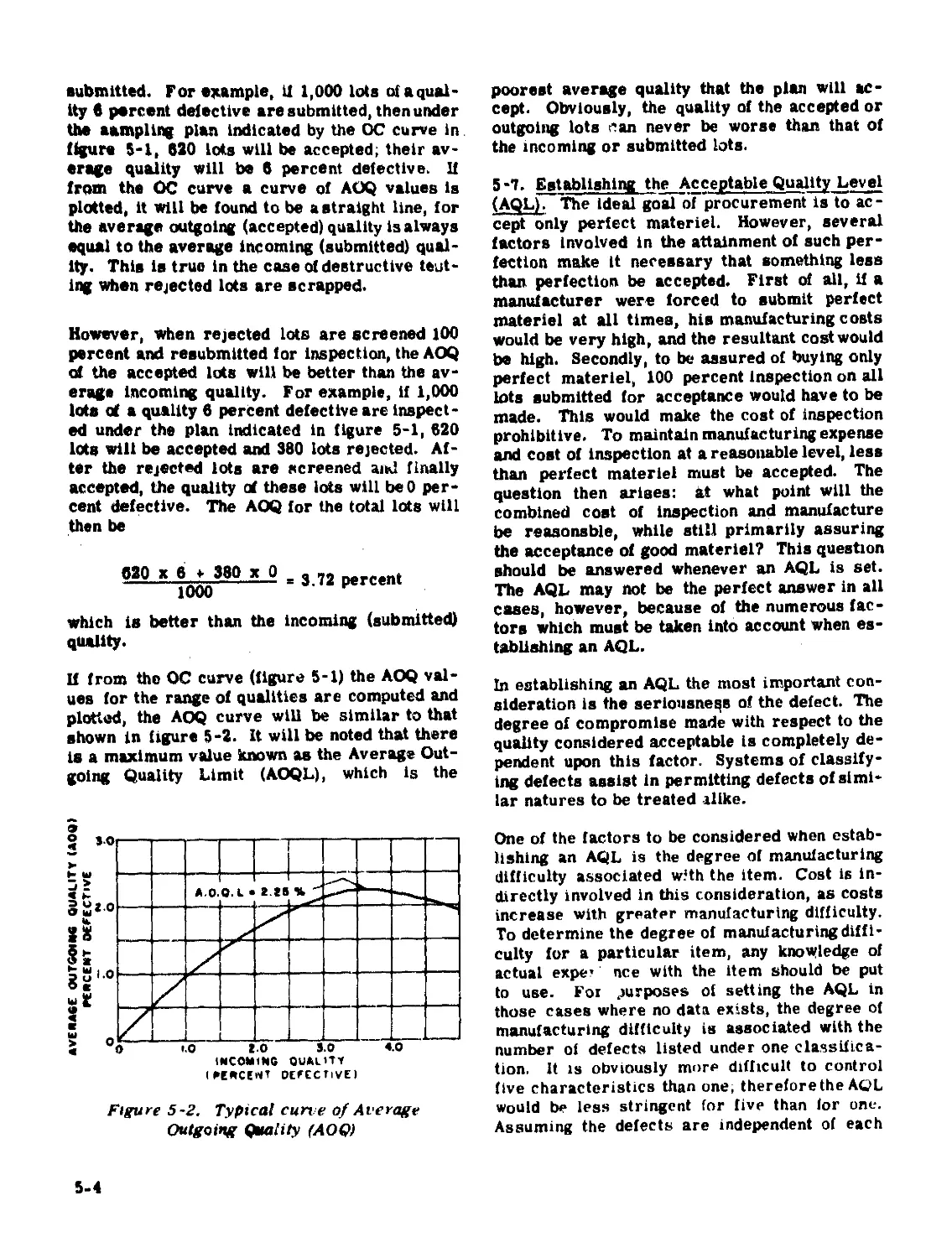
5-5. Operating Characteristic Curve. Four im-
portant curves tell how any specific sampling
plan operates with respect to lots that are de-
tective in various percentages. Of these, the
operating characteristic (ОС) curve is the most
important because it gives an adequate picture
of the plan's severity anddiscriminatory power.
It pictures the probability of acceptance Pa for
lots of various qualities, p' percent defective.
The exact probability of finding d defectives Jn
a sample of n pieces drawn from a lot of N
pieces containing D defects is determined by
the hypergeometric distribution, and is given
by the formula
_ N-Dcn-d Dcd
О . a -------------
The first factor of the numerator is the number
of ways in which (n — d) good pieces may be
drawn from (N — D) good pieces in the lot, and
the second factor is the number of ways in which
d defectives may be drawn from D defectives in
the lot. The denominator is the number of ways
in which n pieces in the sample may be drawn
from N pieces in the lot.
The use of this hypergeometric formula is te-
dious. For example, in a sampling plan where
n * 150, and c (the acceptance number) - 4
defectives, applied to a lot of N  3,000 pieces
of p' я 1 percent defective, gives a probability
of acceptance
p = 2970C150 + 2970C149 ' 30Cl +
3000C150	3000C150
297QC146 ' 30^4	(1)
+	3000C150
Where n £ 0.1N, the binomial approximation to
the hypergeometric distribution may be used.
Thus, fcr the above plan
₽a - i50e0(°-M)150+ 15OC1(°	14в<0 01> *
. . . + 150C4(0.99)146(0.01)4	(2)
However, this is still a somewhat complicated
calculation, unless a set of "Tables of the Bi-
5-2
nomial Probability Distribution" is available.
Whenever n £ 0.1N and 2» 20 and p' 5 5 per-
cent, use is made of the Poisson distribution,
which may be used as a distribution in its own
right, or as a good approximation of the bi-
nomial.
Using the Poisson distribution, the probability
of acceptance is given by
Pa s e’1*8	e’1,s1.5 + e"1B1.52/2
< e-l-W/e + e-b51.54/24
This is much easier to calculate. Also, tables
of probabilities of accentance for various values
of np' are to be found in any standard text on
quality control. (The tables use p' as the frac-
tion defective.)
It should be noted that the hypergeometric and
binomial probabilities are based on a fixed lot
size, while use of the Poisson distribution as-
sumes an infinite lot size. Since in most ap-
plications in Ordnance the actual size of the lot
is indeterminate at the time the sampling plan
is developed, the Poisson is nearly always used.
For further study, reference is made to "Sta-
tistical Quality Control" by Grantor "Engineer-
ing Statistics and Quality Control" by Burr.
The ОС curve is a plot of percent defective ver-
sus probability of acceptance for a given sample
of n size and acceptance number of c defectives.
Thus, for any given percent defective (normal-
ly the abscissa), the probability that a lot of
this quality will be accepted may be found. Fig-
ure 5-1 is a plot of a typical ОС curve.
Terms frequently used to indicate the charac-
teristics of a plan, or used as an index to a
series of plans, can best be indicated by ref-
erence to the ОС curve. The term used most
often is Acceptance Quality Level (AQL). The
AQL represents that quality, expressed in terms
of percent defective, which is considered ac-
ceptable and which will be accepted most of the
time. The probability of not accepting material
of this level of quality is called the producer's
risk (a). In standard practice it is customary
to base the AQL on a probability oi acceptance
of 95 percent, with a producer's risk of rejec-
tion of 5 percent. However, these figures are
Figure 5-1. Typical Operating Characteristic
(ОС) curve
purely arbitrary. Plans outlined in MIL-STD-
105A are based on acceptance of AQL product
of quality from 88 percent to 99 percent of the
time, with corresponding producer's risks of
12 percent and 1 percent.
On the other hand, the Lot Tolerance Percent
Defective (LTPD) is the quality, expressed in
terms of percent defective, that is considered
unacceptable and which will be rejected most of
the time. The consumer's risk {p) is the prob-
ability of accepting material LTPD quality. In
practice, p usually is given a value of 0.1, or
10 percent, but other values may be given if
considered desirable.
The discriminatory power of a plan cannot be
determined merely by knowing the AQL. The
proximity of the AQL and LTPD of a plan in-
dicates its ability to distinguish between good
and bad quality. This is reflected by a steep
ОС curve. A tight AQL may not offer sufficient
protection if the LTPD is poor.
5-6. The Average Outgoing Quality (AOQ) is the
average quality of a succession of lots which
have been accepted. U the rejected lots are
not resubmitted for inspection, then, disre-
garding the removal of defectives found in the
samples, the average quality of the lots ac-
cepted is the same as the quality of the lots
5-3
submitted. For example, if 1,000 lots of equal-
ity 6 percent defective are submitted, then under
the sampling plan Indicated by the ОС curve in
figure 5-1, 620 lots will be accepted; their av-
erage quality will be в percent defective. If
from the ОС curve a curve of AOQ values is
plotted, it will be found to be a straight line, for
the average outgoing (accepted) quality is always
equal to the average incoming (submitted) qual-
ity. This is true in the case of destructive tout-
ing when rejected lots are scrapped.
However, when rejected lots are screened 100
percent and resubmitted for inspection, the AOQ
of the accepted lots will be better than the av-
erage incoming quality. For example, if 1,000
lots of a quality в percent defective are inspect-
ed under the plan indicated in figure 5-1, 620
lets will be accepted and 380 lots rejected. Af-
ter the rejected lots are screened and finally
accepted, the quality of these lots will beO per-
cent defective. The AOQ for the total lots will
then be
020 *	° * ° = 3 72 Percent
1000
which is better than the incoming (submitted)
quality.
If from the ОС curve (figure 5-1) the AOQ val-
ues for the range of qualities are computed and
plotted, the AOQ curve will be similar to that
shown in figure 5-2. it will be noted that there
is a maximum value known as the Average Out-
going Quality Limit (AOQL), which is the
(«ecewT DEFECTIVE)
Figure 5-2. Typical сип е of Average
Outgoing Quality (AOQ)
poorest average quality that the plan will ac-
cept. Obviously, the quality of the accepted or
outgoing lots can never be worse than that of
the incoming or submitted lots.
5 -7. Establishing the Acceptable Quality Level
(AQL). The ideal goal of procurement is to ac-
cept only perfect materiel. However, several
factors involved in the attainment of such per-
fection make it necessary that something less
than perfection be accepted. First of all, if a
manufacturer were forced to submit perfect
materiel at all times, his manufacturing costs
would be very high, and the resultant cost would
be high. Secondly, to be assured of buying only
perfect materiel, 100 percent inspection on all
lots submitted for acceptance would have to be
made. This would make the cost of inspection
prohibitive. To maintain manufacturing expense
and cost of inspection at a reasonable level, less
than perfect materiel must be accepted. The
question then arises: kt what point will the
combined cost of inspection and manufacture
be reasonable, while still primarily assuring
the acceptance of good materiel? This question
should be answered whenever an AQL is set.
The AQL may not be the perfect answer in all
cases, however, because of the numerous fac-
tors which must be taken into account when es-
tablishing an AQL.
In establishing an AQL the most important con-
sideration is the seriousness of the defect. The
degree of compromise made with respect to the
quality considered acceptable is completely de-
pendent upon this factor. Systems of classify-
ing defects assist in permitting defects of simi-
lar natures to be treated alike.
One of the factors to be considered when estab-
lishing an AQL is the degree of manufacturing
difficulty associated with the item. Cost is in-
directly involved in this consideration, as costs
increase with greater manufacturing difficulty.
To determine the degree of manufacturing diffi-
culty for a particular item, any knowledge of
actual expe* nee with the item should be put
to use. For purposes of setting the AQL in
those cases where no data exists, the degree of
manufacturing difficulty is associated with the
number of defects listed under one classifica-
tion. It is obviously more difficult to control
five characteristics than one, thereforethe AQL
would be less stringent for five than for one.
Assuming the defects are independent of each
5-4
other, as the number of defects listed under one
classification increases, the probability that all
of them will occur with the same frequency de-
creases.
When setting an AQL for a component part it is
important to view the item as a whole, in order
that the importance of different features can be
seen in proper perspective. For example, con-
sider the case of a squib that is to be a com-
ponent of a rocket. The AQL for the functioning
test of the rocket is determined to be 2.5 per-
cent. This means that the AQL must be more
stringent for the functioning test of the igniter
(1.5 percent) and still more stringent for the
functioning test of the squib (0.65 percent). This
must be done in order to avoid penalizing the
manufacturer of the igniter (the functioning of
which depends on the squib) and the manufac-
turer of the rocket (the functioning of which de-
pends on the squib and the igniter). However,
if xt is known that the same squib is to be used
in a J A TO unit, for which the functioning test
has an AQL of 0.25 percent, the AQL for the
squib in this case should be about 0.10 percent.
Obviously, the same squib cannot have two
AQL's; therefore, the squib intended for the
rocket also must have an AQL of 0.10 percent,
unless a method of grading squibs can be de-
vised. In all cases the component snould be
given the most stringent AQL required for any
use.
5-8. Classification of Defects. Defects of simi-
lar importance are treated alike. To accom-
plish this it is necessary to classify them into
groups, the number of which is a compromise
between the degree of selectivity desired and
the administrative complexity. The following
excerpts taken from MIL-STD-105 reflect the
prevalent classes and definitions for the
classes.
a.	Method of Classifying Defects. A classi-
fication of defects is the enumeration of pos-
sible defects of the unit of product classifie ’
according to their importance. A defect is ai
deviation of the unit of product from require-
ments of the specifications, drawings, purchase
descriptions, and any changes thereto in the
contract or order. Defects are normally
grouped into one or more of the following
classes; however, the Government reserves
the right to group defects into other classes.
b.	Critical Defects. A critical defect is one
that judgment and experience indicate could
result in hazardous or unsafe conditions for in-
dividuals using or maintaining the product; or,
for major end-item units .uf product, such as
ships, aircraft, or tanks, a defect that could
prevent performance of their tactical function.
c.	Major Defects. A major defect is a de-
fect, other than critical, thst could result in
failure, or materially reduce the usability of
the unit of product for its intended purpose.
d.	Minor Defects. A minor defect is one that
does not materially reduce the usability of the
unit of product for its intended purpose, or is a
departure from established standards having no
significant bearing on the effective use or op-
eration of the unit.
5-9. Inspection by Attributes is the grading of a
unit of product as defective or nondefective, with
respect to a given requirement, by sampling in-
spection. When attributes inspection is per-
formed, the decision to accept or reject is based
on the number of sample units found defective.
The extent of deviation from the requirement is
not considered in.this form of inspection. This
form is simple to administrate, normally is
simple and rapid to perform, is not dependent
upon a particular distribution of product to pro-
vide a desired assurance, and involves no math-
ematics to determine lot acceptability. It is al-
ways possible to use attributes inspection, and
in many instances, such as in GO and NOT GO
gaging, it is the only type possible.
5-10. Single-Sampling is a technique in which
only one sample of n items isinspectedto reach
a decision on the disposition of the lot. A sam-
pling plan is best described by the sample size
(n) and rcceptance number (c). When the num-
ber of defectives found in this sample equals,
or is less than, the acceptance number pre-
scribed by the sampling plan, the lot is accepted.
U the number of defectives exceeds the accept-
ance number, the lot is rejected. Anexampleof
a single plan is as follows. Select a sample of
100 units. If 3 or fewer defectives are found,
accept the lot; if more than 3 are found, re-
ject the lot.
Single plans may be summarized as follows:
Sample size Acceptance no. Rejection no.
100	3	4
5-11. Double-Sampling is a technique in which
a second sample of n items is inspected when
Um results of the first sampling do not accept
or reject the lot. Depending on what is found
in the first sample, there are three possible
courses of action. The lot may be accepted, it
may be rejected, or the decision may be defer-
red until the results of a second sampling are
obtained. A decision is sure to be made on the
basis of a second sample, inasmuch as the re-
jection number of a second sample is one more
than the acceptance number.
An example of a double plan is as follows. A
sample of 75 units is selected. If the sample
Contains 4 or fewer defectives, the lot is ac-
cepted. If the sample contains 9 or more de-
fectives, the lot is rejected. If more than 4
defectives, but fewer than 9, are found, a second
sample of 150 units is selected and inspected.
If In the combined sample of 255 units fewer
than 9 defectives are found, the lot is accepted;
but if 9 or more defectives are found, the lot is
rejected. Double-sampling plans are sum-
marized as follows:
Cumulative
sample Acceptance no. Rejection no.
75	4	9
225	8	9
5-12. Multiple-Sampling is a procedure in
which a final decision to accept or reject the
specific lot need not be riade after one or two
samples, but ma^ require the drawing of sev-
eral samples. An example of a multiple-sam-
pling plan is as follows:
Cumulative sample	Acceptance no.	Rejection no.
30	2	8
60	8	13
90	12	18
120	17	22
150	21	27
180	27	32
210	35	36
The inspector selects a sample of 30 from a
lot of 4,000 items. If the first sample contains
2 or fewer defectives, the lot is accepted; if 8
or more defectives appear in the sample, the
lot is rejected. If more than 2 but fewer than
8 defectives appear in the sample, the inspector
draws a second sample of 30 items. If, in the
total sample of 60 units, 8 or fewer defectives
are found, the lot is accepted. If 13 or more
defectives are found, then the lot is rejected.
If more than 8 but fewer than 13 defectives are
found, a third sample of 30 is inspected. This
process Is continued, until a decision is reach-
ed, which in this case will be not later than the
seventh sample.
It is a common misconception that a compar-
able double- or multiple-sampling plan is less
stringent than a single plan. This is not true,
since the acceptance and rejection numbers are
selected to make them equivalent. The ОС
curves for equivalent single, double, and mul-
tiple plans are shown in figure 5-3.
5-13. ОС Curves for Comparable Single-,
Double-, and Multiple-Sampling Plans. It will
be noted that the ОС curves of the three plans
almost coincide, showing little difference in
their severity and discriminatory power. How-
ever, there is a great difference among the
plans in the average number of pieces per lot
that will be inspected before a decision is
reached. Figure 5-4 shows the ASN (Average
Sample Number) curves for the same plans.
In the single-sampling plan the sample is al-
ways completely inspected, regardless of a
possible earlier decision. The ASN curve for
the single-sampling plan is, therefore, a
straight line.
In the double-sampling plan the first sample is
completely inspected, ^ut inspection of the
second sample ceases as soon as the number of
defectives found in the combined samples
equals the rejection number. Since lots of
very good quality will be accepted, and lots of
very bad qu ility will be rejected on the first
sample, and inspection of the second sample is
curtailed, the average amount of inspection will
be less for a double-sampling plan than for a
single-sampling plan. As will be seen, mul-
tiple-sampling reduces still further the amount
of inspection.
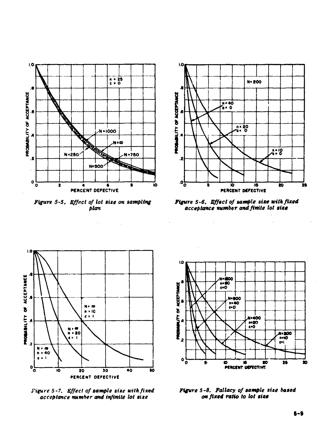
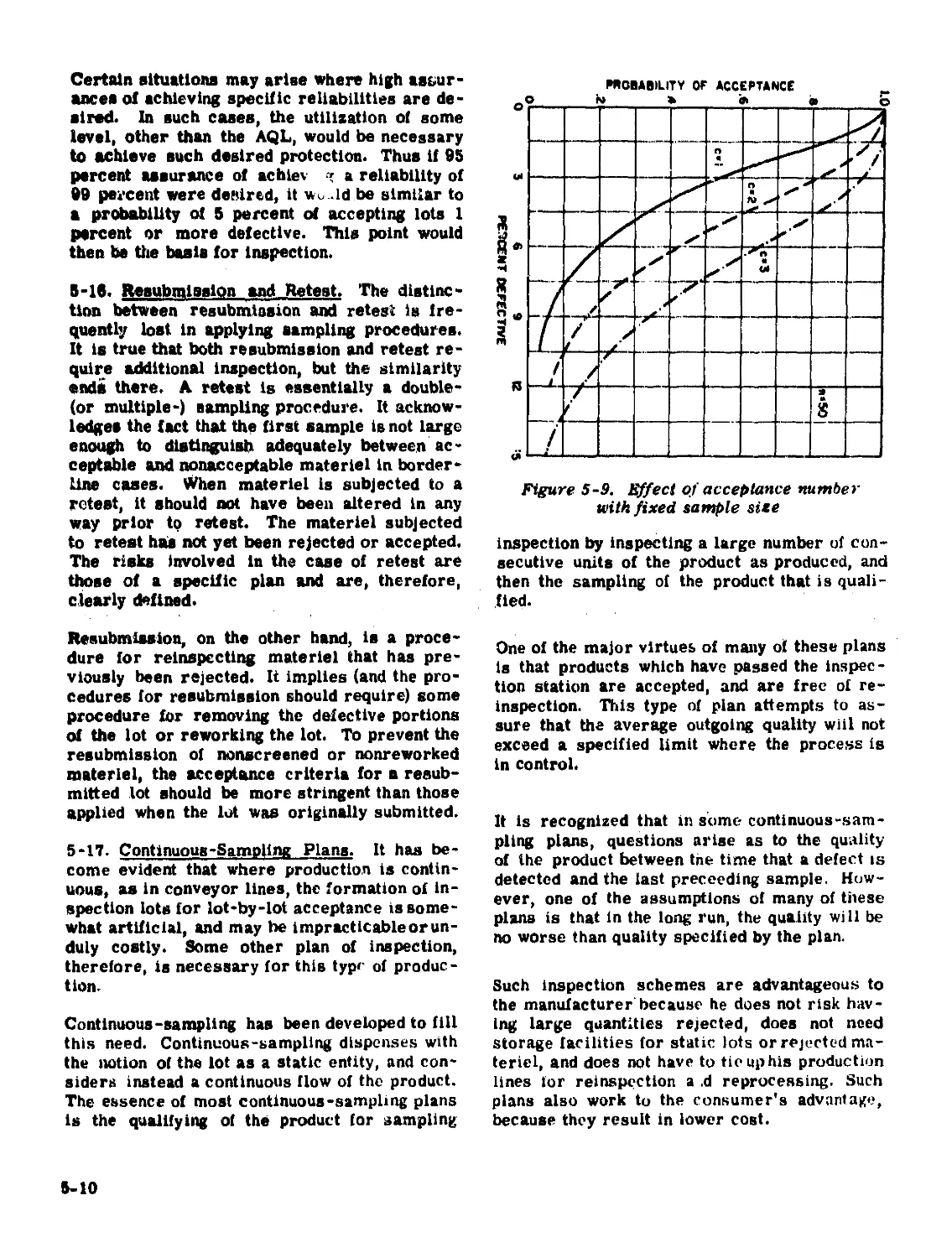
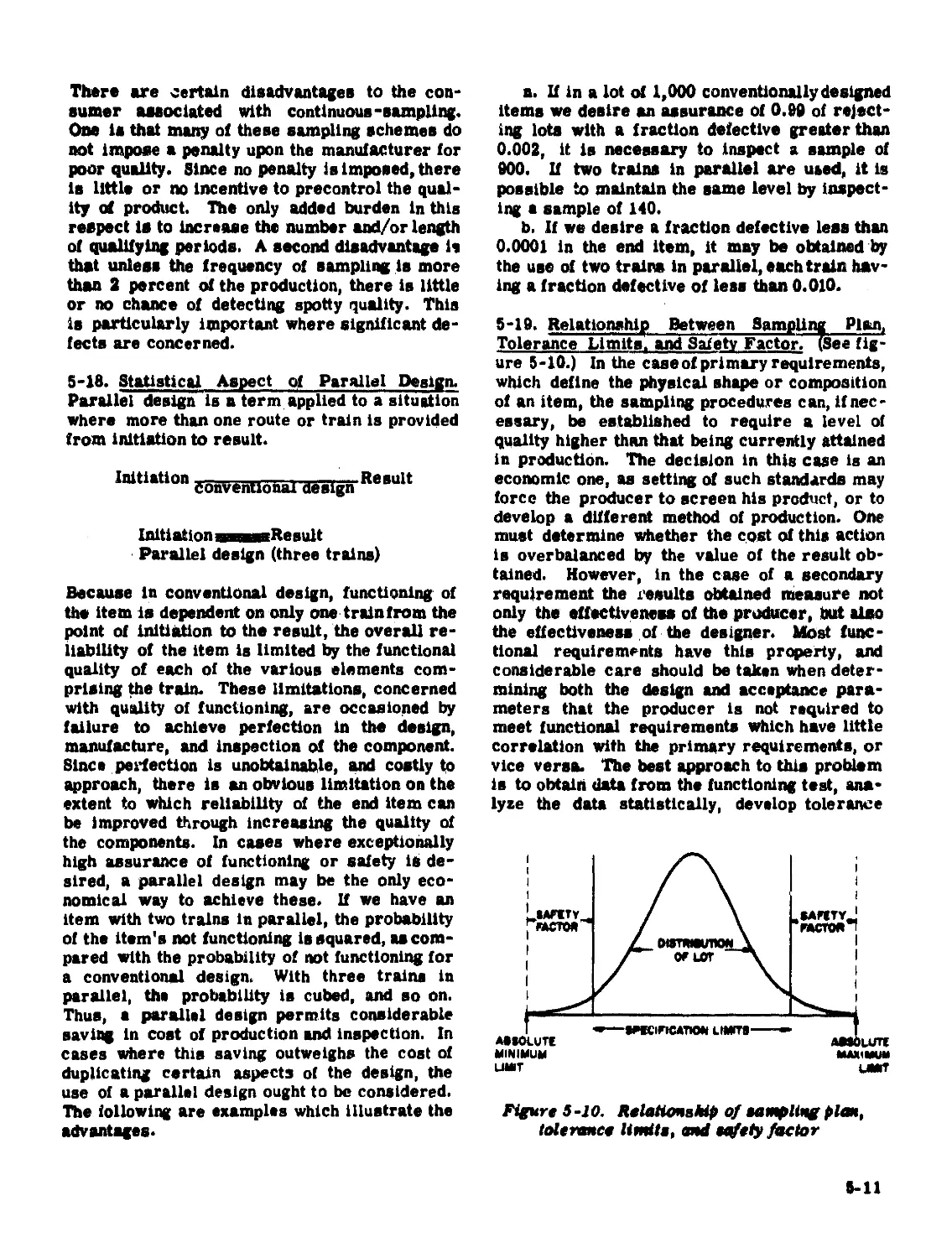
5-14. Relationship of Sample Size to Lot Size.
The sample size is of considerably more sig-
nificance, with respect to severity and dis-
criminating power, than the lot size from which
it is taken. Figure 5-5 is composed of ОС
curves, all having the same sample size and
acceptance numbers, but different lot sizes.
5-6
Figure 5-3. Operating Characteristic (ОС) curves for single-, double-, and
multiple-sampling plans
It is readily observed that the ОС curves for lot
sizes of 1,000 and over aro virtually equivalent
to that for a lot size of infinity. Thus it is often
said that the lot size has almost no effect on
the sampling plan. This statement holds, pro-
vided the sample size is a small fraction of the
lot size (normally less than 10 percent). Fig-
ures 5-6 and 5-7 demonstrate the effect of
varying sample size for finite and infinite lot
aize, respectively.
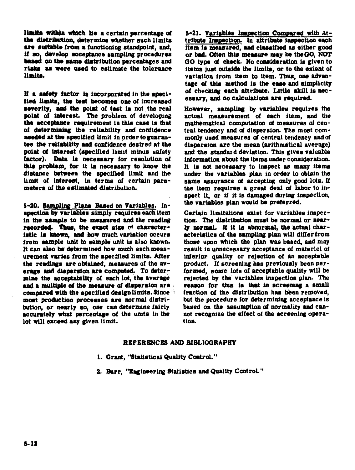
Although percent sampling appears logicalfrom
a cost or time aspect, it is decidedly not so with
respect to the degree of protection offered. The
absolute size of the sample, it has been noted,
affects the characteristics of a plan more sig-
nificantly than the lot size. A proportional
change in both the sample and lot size, there-
fore, will result in different degrees ot pro-
tection. Figure 5-8 is an illustration of this
phenomenon.
b-7
100
					SINGLE SAMPLING	
ou V» Ulb-						
OF PIECI TIOM LO" » >				DOUBLE^ SAMPLING		
BE NUMBER PER INSPEG h	« >	<	“T1		MULTIPLE SAMPLING			
ASN «AVER Al INSPECTED »	4 5	<						
«V 0						
c	>	2	3	d	1	6
p'l PERCENT DEFECTIVE
Figure 5-4. Average Sample Number (ASN) curves for plans shown in figure 5-3
The effect of varying the sample size can be
observed by noting figures 5-6 and 5-7. Ob-
viously the greater the sample size, the more
stringent and more discriminating will the plan
be for a fixed acceptance number. Similarly,
for a fixed sample size, the severity of the plan
increases as the acceptance number decreases
(figure 3-9).
5-15. Acceptable Quality Level as Basis for
Ingpectign. Usually, the effect of a sampling
plan for acceptance Inspection is to force man-
ufacturers to supply materiel of such good qual-
ity that only a very small proportion of the lots
is rejected. The manufacturer, when given the
AQL, knows the major piece of inf or mat ion per-
taining to the sampling plans, which will affect
the disposition of his lots. The manufacturer
will know that by submitting products as good
as, or better than, the AQL, rejections can be
kept to an absolute minimum. Й the manufac-
turer produces worse than AQL level, many
inspection lots will be rejected, with increased
costs necessary to screen or to scrap the lots.
On the other hand, a production quality level
better than the AQL may involve higher pro-
duction costs than are necessary. The know-
ledge of the AQL level will enable the producer
to manufacture most efficiently.
If some point other than the AQL is set as a
basis for inspection, the acceptable quality level
will differ among manufacturers, depending on
the particular sampling plan used.
5-9
Figure 5-5. Effect of lot size on sampling
plan
Figure 5-6. Effect of sample site with fixed
acceptance number and finite lot size
Figure 5-7. Effect of sample size with fixed
acceptance number and infinite lot size
Figure 5 -8. Fallacy of sample size based
on fixed ratio to lot size
8-9
Certain situations may arise where high assur-
ances of achieving specific reliabilities are de-
sired. In such cases, the utilization of some
level, other than the AQL, would be necessary
to achieve such desired protection. Thus if 85
percent assurance of achlev ' a reliability of
BB percent were denired, it wo .id be similar to
a probability of 5 percent at accepting lots 1
percent or more defective. This point would
then be the basis for inspection.
5-16. Resubmlsslpn and Retest. The distinc-
tion between resubmlnsion and retest is fre-
quently lost in applying sampling procedures.
It is true that both resubmission and retest re-
quire additional inspection, but the similarity
ends there. A retest is essentially a double -
(or multiple-) sampling procedure. It acknow-
ledges the fact that the first sample is not large
enough to distinguish adequately between ac-
ceptable and nonacceptable materiel in border-
line cases. When materiel is subjected to a
retest, it should not have been altered in any
way prior to retest. The materiel subjected
to retest has not yet been rejected or accepted.
The risks involved in the case of retest are
those of a specific plan and are, therefore,
clearly defined.
Resubmlssion, on the other hand, is a proce-
dure for reinspccting materiel that has pre-
viously been rejected. It implies (and the pro-
cedures for resubmlssion should require) some
procedure for removing the defective portions
of the lot or reworking the lot. To prevent the
resubmission of nonscreened or nonreworked
materiel, the acceptance criteria for n resub-
mitted lot should be more stringent than those
applied when the lot was originally submitted.
5-17. Continuous-Sampling Plans. It has be-
come evident that where production is contin-
uous, as in conveyor lines, the formation of in-
spection lots for lot-by-lOt acceptance is some-
what artificial, and may be impracticable or un-
duly costly. Some other plan of inspection,
therefore, is necessary for this type of produc-
tion.
Continuous-sampling has been developed to fill
this need. Continuous-sampling dispenses with
the notion of the lot as a static entity, and con-
siders instead a continuous flow of the product.
The essence of most continuous-sampling plans
is the qualifying of the product for sampling
Figure 5-9. Effect of acceptance number
with fixed sample site
inspection by inspecting a large number of con-
secutive units of the product as produced, and
then the sampling of the product that is quali-
fied.
One of the major virtues of many of these plans
is that products which have passed the inspec-
tion station are accepted, and are free of re-
inspection. This type of plan attempts to as-
sure that the average outgoing quality will not
exceed a specified limit where the process is
in control.
It is recognized that in some- continuous-sam-
pling plans, questions arise as to the quality
of the product between tne time that a defect is
detected and the last preceeding sample. How-
ever, one of the assumptions of many of these
plans is that in the long run, the quality will be
no worse than quality specified by the plan.
Such inspection schemes are advantageous to
the manufacturer because he does not risk hav-
ing large quantities rejected, does not need
storage facilities for static lots or rejected ma-
teriel, and does not have to tie up his production
lines tor reinspection a .d reprocessing. Such
plans also work to the consumer's advantage,
because they result in lower cost.
5-10
There are certain disadvantages to the con-
sumer associated with continuous-sampling.
One is that many of these sampling schemes do
not impose a penalty upon the manufacturer for
poor quality. Since no penalty is imposed, there
is little or no incentive to precontrol the qual-
ity of product. The only added burden in this
respect is to increase the number and/or length
of qualifying periods. A second disadvantage is
that unless the frequency of sampling is more
than 2 percent of the production, there is little
or no chance of detecting spotty quality. This
is particularly important where significant de-
fects are concerned.
5-18. Statistical Aspect of Parallel Design.
Parallel design is a term applied to a situation
where more than one route or train is provided
from initiation to result.
Initiation asamsaResult
Parallel design (three trains)
Because in conventional design, functioning of
the item is dependent on only one train from the
point of initiation to the result, the overall re-
liability of the item is limited by the functional
quality of each of the various elements com-
prising the train. These limitations, concerned
with quality of functioning, are occasioned by
failure to achieve perfection in the design,
manufacture, and inspection of the component.
Since perfection is unobtainable, and costly to
approach, there is an obvious limitation on the
extent to which reliability of the end item can
be improved through increasing the quality of
the components. In cases where exceptionally
high assurance of functioning or safety is de-
sired, a parallel design may be the only eco-
nomical way to achieve these. If we have an
item with two trains in parallel, the probability
of the item's not functioning is squared, as com-
pared with the probability of not functioning for
a conventional design. With three trains in
parallel, the probability is cubed, and so on.
Thus, a parallel design permits considerable
saving in cost of production and inspection. In
cases where this saving outweighs the cost of
duplicating certain aspects of the design, the
use of a parallel design ought to bo considered.
The following are examples which illustrate the
advantages.
a.	If in a lot of 1,000 conventionally designed
items we desire an assurance of 0.09 of reject-
ing lots with a fraction defective greater than
0.002, it is necessary to inspect a sample of
900. If two trains in parallel are used, it is
possible to maintain the same level by inspect-
ing a sample of 140.
b.	If we desire a fraction defective less than
0.0001 in the end item, it may be obtained by
the use of two trains in parallel, each train hav-
ing a fraction defective of less than 0.010.
5-19. Relationship Between Sampling Plan,
Tolerance Limits, and Safety Factor. (See fig-
ure 5-10.) In the caseof primary requirements,
which define the physical shape or composition
of an item, the sampling procedures can, if nec-
essary, be established to require a level of
quality higher than that being currently attained
in production. The decision in this case is an
economic one, as setting of such standards may
force the producer to screen his product, or to
develop a different method of production. One
must determine whether the cost of this action
is overbalanced by the value of the result ob-
tained. However, in the case of a secondary
requirement the results obtained measure not
only the effectiveness of the producer, but also
the effectiveness of the designer. Most func-
tional requirements have this property, and
considerable care should be taken when deter-
mining both the design and acceptance para-
meters that the producer is not required to
meet functional requirements which have little
correlation with the primary requirements, or
vice versa. The best approach to thia problem
is to obtain data from the functioning test, ana-
lyze the data statistically, develop tolerance
Figure 5 -10. Relationship of eatnpling plan,
tolerance linrite, and egfety factor
5-11
limit* within which lie a certain percentage ct
the distribution, determine whether such limits
are suitable from a functioning standpoint, and,
if so, develop acceptance sampling procedures
baaed on the same distribution percentages and
risks as were used to estimate the tolerance
limits.
И a safety factor is incorporated in the speci-
fied limits, the test becomes one of increased
severity, and the point of test is not the real
point of interest. The problem of developing
the acceptance requirement in this case is that
of determining the reliability and confidence
needed at the specified limit in order to guaran-
tee the reliability and confidence desired at the
point of interest (specified limit minus safety
factor). Data is necessary for resolution of
thia problem, for it is necessary to know the
distance between the specified limit and the
limit of interest, in terms of certain para-
meters of the estimated distribution.
5-20. Sampling Plans Based on Variables. In-
spection by variables simply requires each item
in the sample to be measured and the reading
recorded. Thue, the exact also c* character-
istic is Imown, and how much variation occurs
from sample unit to sample unit is also known.
It can also be determined how much each meas-
urement varies from the specified limits. After
the readings are obtained, measures of the av-
erage and dispersion are computed. To deter-
mine the acceptability of each lot, the average
and. a multiple of the measure of dispersion are >
compared with the specified design limits. Since ;
most production processes are normal distri-
bution, or nearly so, one can determine fairly
accurately what percentage of the units in the
lot will exceed any given limit.
5-21. Variables Inspection Compared with At-
tribute Inspection. In attribute inspection each
item is measured^ and classified as either good
or bad. Often this measure may be the GO, NOT
GO type of check. No consideration is given to
items just outside the limits, or to the extent of
variation from item to item. Thus, one advan-
tage of this method is the ease and simplicity
of checking each attribute. Little skill is nec-
essary, and no calculations are required.
However, sampling by variables requires the
actual measurement of each item, and the
mathematical computation of measures of cen-
tral tendency and of dispersion. The most com-
monly used measures of central tendency and of
dispersion are the mean (arithmetical average)
and the standard deviation. This gives valuable
information about the items under consideration.
It is not necessary to inspect as many items
under the variables plan in order to obtain the
same assurance of accepting only good lots. If
the item requires a great deal pf labor to in-
spect it, or if it is damaged during inspection,
the variables plan would be preferred.
Certain limitations exist for variables inspec-
tion. The distribution must be normal or near-
ly normal. If it Is abnormal, the actual char-
acteristics of the sampling plan will differ from
those upon which the plan was based, and may
result in unnecessary acceptance of materiel of
inferior quality or rejection of an acceptable
product. If screening has previously been per-
formed, some lots of acceptable quality will be
rejected by the variables inspection plan. The
reason for this is that in screening a small
fraction of the distribution has been removed,
but the procedure for determining acceptance is
based on the assumption of normality and can-
not recognize the effect of the screening opera-
tion.
REFERENCES AND BIBLIOGRAPHY
1. Grant, "Statistical Quality Control."
2. Burr, "engineering Statistics and Quality Control."
5-12
EFFECT OF DIMENSIONING AND TOLERANCING ON INSPECTION
5*22. Introduction. When an Ordnance item
leaves the design and engineering phases and
goes into production, dimensional control is
exercised by inspectors who determine, by gag-
ing and, when necessary, measurement, that the
items and components conform dimensionally to
the requirements specified by the design en-
gineer. The dimensioning and tolerancing of an
item impose difficulties on production and in-
spection, unless presented in a proper manner.
Department of Ordnance Drawing 30-1-7,
"Standard for Dimensioning and Tolerancing,"
has been established as a standard for dimen-
sioning and tolerancing of ammunition items,
and the design engineer should understand thor-
oughly the methods outlined therein and their
practical application, in order that difficulties
may be avoided in the production and inspection
stages. The application of an incorrect symbol
or requirement may result in the manufacture
of a component that is not what the designer in-
tended, but which the inspector must accept,
since it complies with the drawing.
The definition a dimensioning terms is clearly
stated on page 2 of Drawing 30-1-7. The en-
gineer should bear in mind that a basic dimen-
sion, although exercising control, is not checked
directly by the inspector. A reference dimen-
sion, being informative only, is not a control
dimension, and is not checked by the inspector.
Generally speaking, only toleranced and datum
dimensions are checked by the inspector.
5-23. Locational Tolerance Symbols. There are
two classes of locational tolerance symbols
permitted, independent and dependent, and the
difference between them is of great importance.
5-24. An Independent Locational Tolerance is a
fixed tolerance to whi^h the manufacturer must
adhere, whether the part produced is of maxi-
mum permitted size or minimum permitted
size. (See paragraph 5-25, on dependent loca-
tional tolerances, for comparison.) Independent
locational tolerance requirements are specifi-
cally checked by the Inspector independently of
other requirements, normally by the use of dial
indicating gages. The application of the various
symbols, and the implications of their use,
should be thoroughly understood.
The use of the datum surface symbol I- P -I in
conjunction with the tolerancing symbols, must
be carefully studied to assure that what is speci-
fied on the drawing is in fact the requirement
which is needed. Examples of the requirements
and use of the symbols follow.
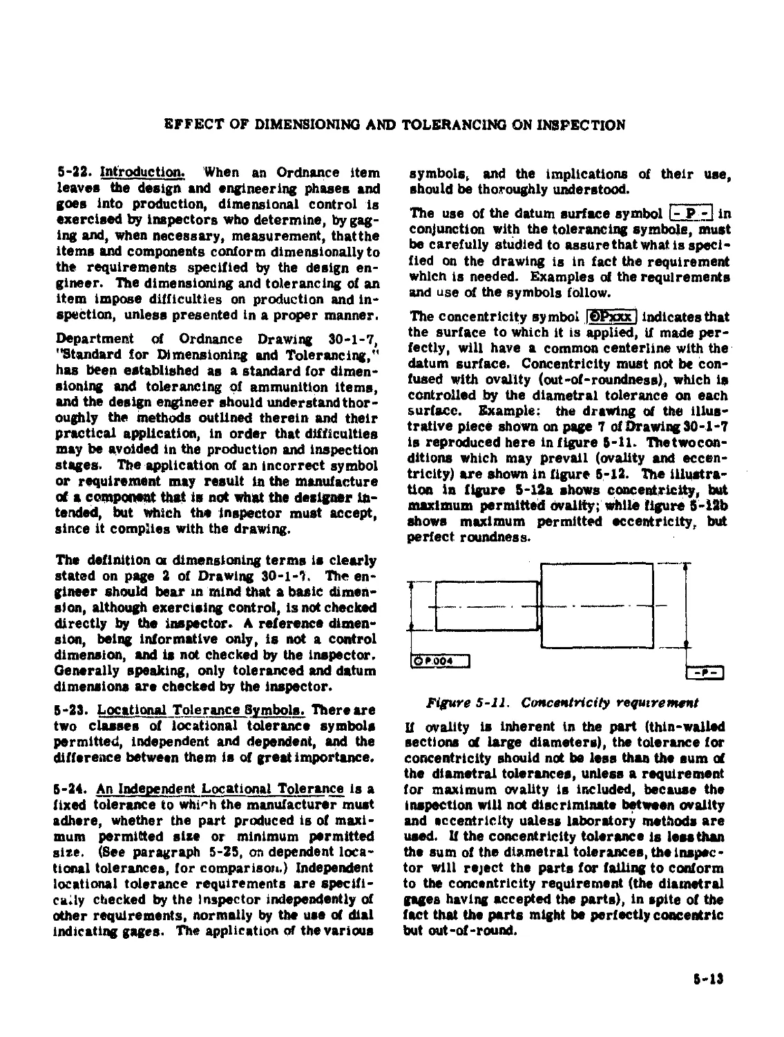
The concentricity symbol |6Pxxx| indicates that
the surface to which it is applied, if made per-
fectly, will have a common centerline with the
datum surface. Concentricity must not be con-
fused with ovality (out-of-roundness), which ip
controlled by the diametral tolerance on each
surface. Example; the drawing of the illus-
trative piece shown on page 7 of Drawing 30-1-7
is reproduced here in figure 5-11. The two con-
ditions which may prevail (ovality and eccen-
tricity) are shown in figure 5-12. The illustra-
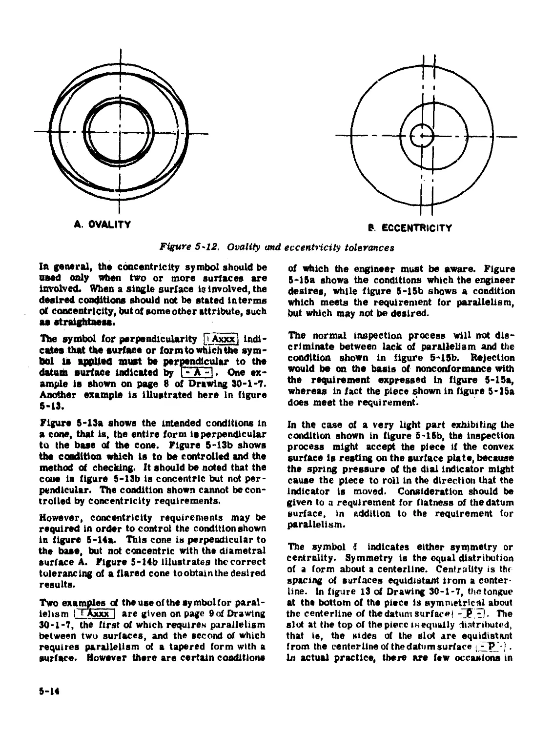
tion in figure 5-12a shows concentricity, but
maximum permitted ovality; while figure 5-12b
shows maximum permitted eccentricity, but
perfect roundness.
OR 004	1
Figure 5-11. Concentricity requirement
If ovality is inherent in the part (thin-walled
sections of large diameters), the tolerance for
concentricity should not be less than the sum of
the diametral tolerances, unless a requirement
for maximum ovality is included, because the
inspection will not discriminate between ovality
and eccentricity ualess laboratory methods are
used. If the concentricity tolerance is less than
the sum of the diametral tolerances, the inspec -
tor will reject the parts for falling to conform
to the concentricity requirement (the diametral
gages having accepted the parts), in spite of the
fact that the parts might be perfectly concentric
but out-of-round.
5-13
A. OVALITY
Figure 5-12. Ovality and eccentricity tolerances
In general, the concentricity symbol should be
used only when two or more surfaces are
Involved. When a single surface is involved, the
desired conditions should not be stated in terms
of concentricity, but of some other attribute, such
as straightness.
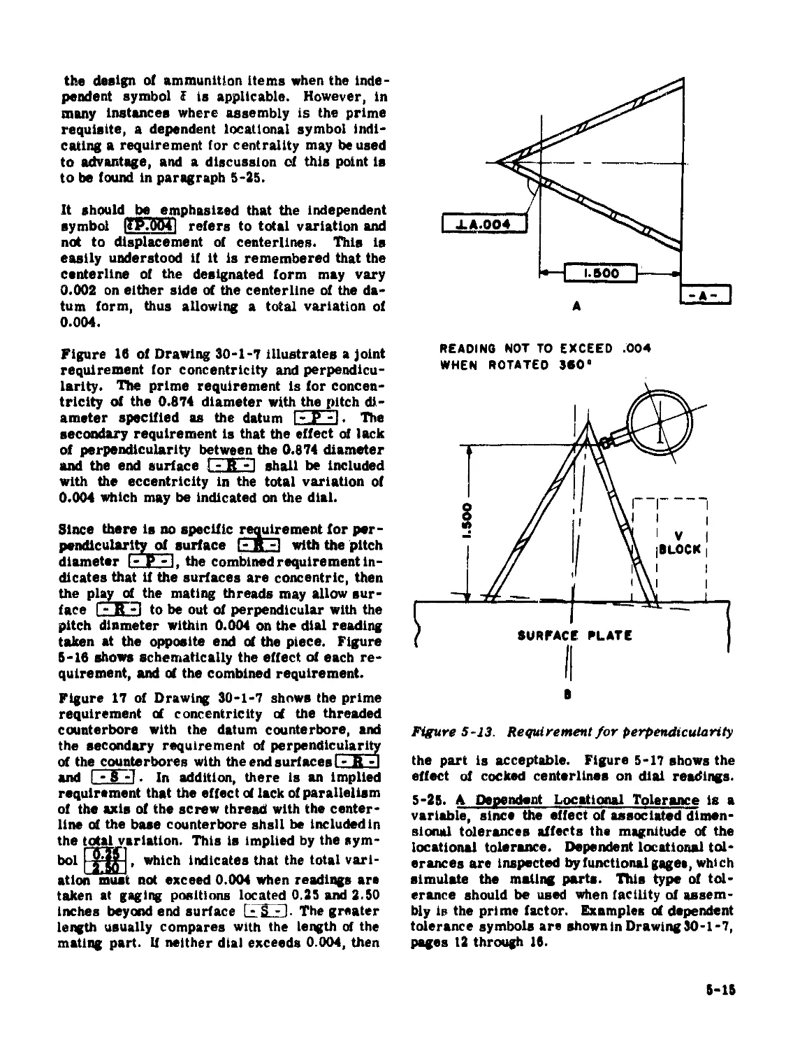
The symbol for perpendicularity | i Axxx| indi-
cates that the surface or form to which the sym-
bol is applied must be perpendicular to the
datum surface indicated by Г-'А. One ex-
ample is shown on page 8 of Drawing 30-1-7.
Another example is illustrated here in figure
6-13.
Figure 5-13a shows the intended conditions in
a cone, that is, the entire form is perpendicular
to the base of the cone. Figure 5-13b shows
the condition which is to be controlled and the
method of checking. It should be noted that the
cone in figure 5-13b is concentric but not per-
pendicular. The condition shown cannot be con-
trolled by concentricity requirements.
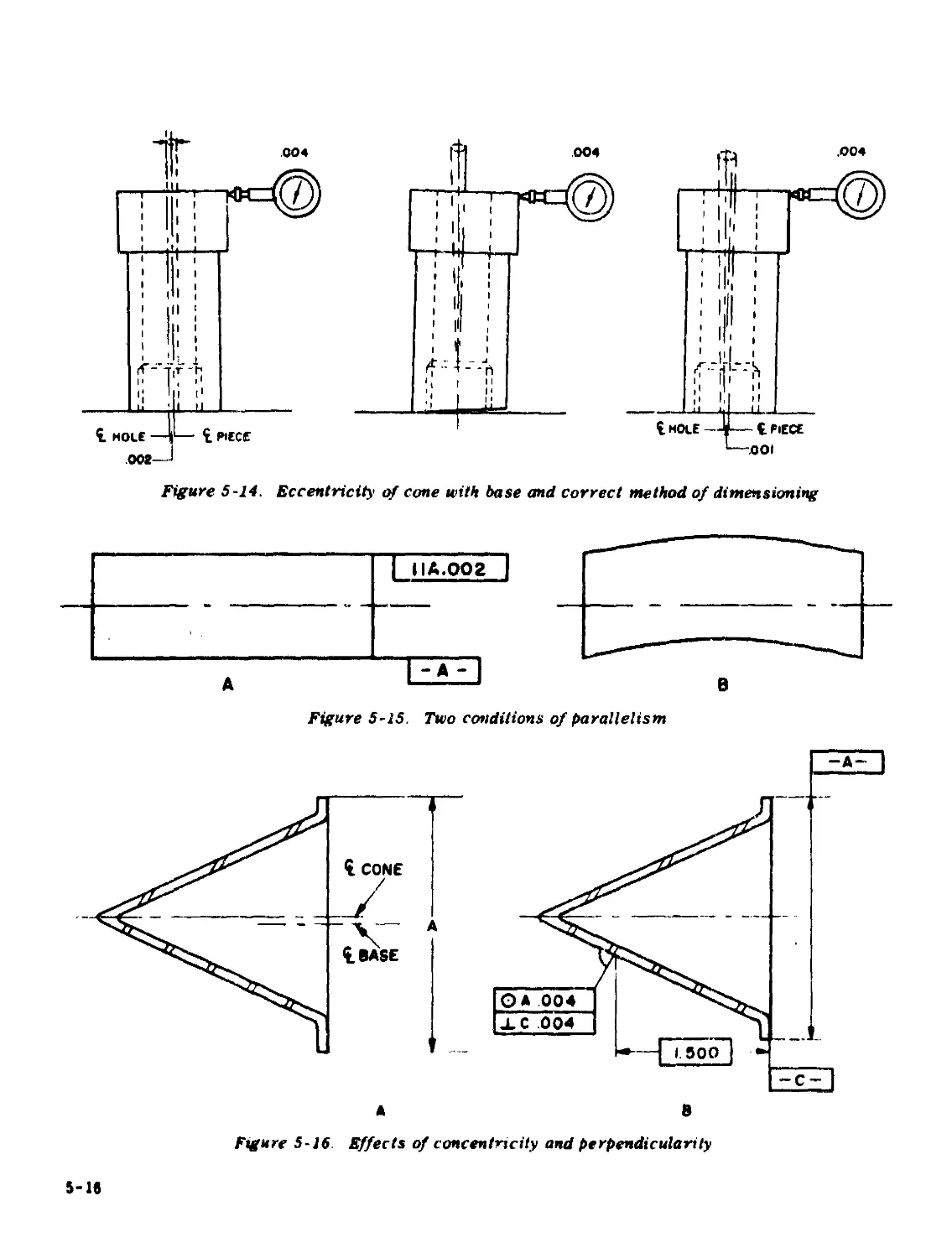
However, concentricity requirements may be
required in order to control the condition shown
in figure 5-14a. This cone is perpendicular to
the base, but not concentric with the diametral
surface A. Figure 5-14b illustrates the correct
toleranclng of a flared cone to obtain the desired
results.
Two examples of the use of the symbol for paral-
lelism I И Axxx I are given on page 9 of Drawing
30-1-7, the first of which requires parallelism
between two surfaces, and the second of which
requires parallelism of a tapered form with a
surface. However there are certain conditions
of which the engineer must be aware. Figure
5-15a shows the conditions which the engineer
desires, while figure 5-15b shows a condition
which meets the requirement for parallelism,
but which may not be desired.
The normal inspection process will not dis-
criminate between lack of parallelism and the
condition shown in figure 5-15b. Rejection
would be on the basis of nonconformance with
the requirement expressed in figure 5-15a,
whereas in fact the piece shown in figure 5-15a
does meet the requirement*.
In the case of a very light part exhibiting the
condition shown in figure 5-15b, the inspection
process might accept the piece if the convex
surface is resting on the surface plate, because
the spring pressure of the dial indicator might
cause the piece to roll in the direction that the
indicator is moved. Consideration should be
given to a requirement for flatness of the datum
surface, in addition to the requirement for
parallelism.
The symbol t indicates either symmetry or
centrality. Symmetry is the equal distribution
of a form about a centerline. Centrality is the
spacing of surfaces equidistant irom a center-
line. In figure 13 of Drawing 30-1-7, the tongue
at the bottom of the piece is symmetrical about
the centerline of the datum surface I -5,41. The
slot at the top of the piece is equally distributed,
that ie, the sides of the slot are equidistant
from the centerline of thedatum surface •
In actual practice, there are few occasions in
5-14
the design of ammunition items when the inde-
pendent symbol I is applicable. However, in
many instances where assembly is the prime
requisite, a dependent locational symbol indi-
cating a requirement for centrality may be used
to advantage, and a discussion of this point is
to be found in paragraph 5-25.
It should be emphasised that the independent
symbol itP.OOil refers to total variation and
not to displacement of centerlines. This is
easily understood if it is remembered that the
centerline of the designated form may vary
0.002 on either side of the centerline of the da-
tum form, thus allowing a total variation of
0.004.
READING NOT TO EXCEED .004
WHEN ROTATED 380'
Figure 16 of Drawing 30-1-7 illustrates a joint
requirement for concentricity and perpendicu-
larity. The prime requirement is for concen-
tricity of the 0.874 diameter with the pitch di-
ameter specified as the datum I- F -I. The
secondary requirement is that the effect of lack
of perpendicularity between the 0.874 diameter
and the end surface ! - Й -П shall be included
with the eccentricity in the total variation of
0.004 which may be indicated on the dial.
Since there is no specific requirement for per-
pendicularity^ surface I- R -] with the pitch
diameter I- P - lf the combined requirement in-
dicates that if the surfaces are concentric, then
the play of the mating threads may allow sur-
face Г- R A to be out of perpendicular with the
pitch dinmeter within 0.004 on the dial reading
taken at the opposite end of the piece. Figure
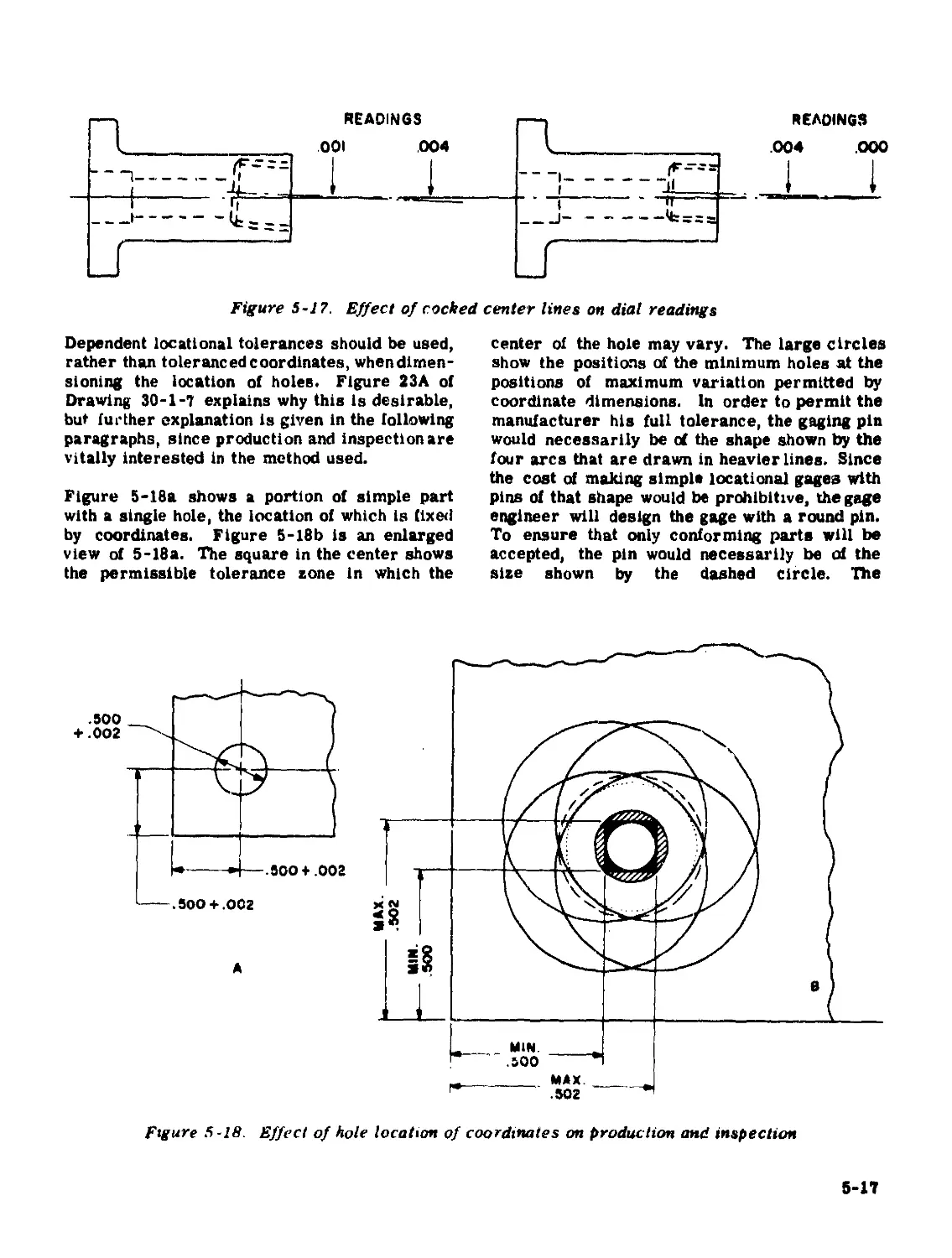
5-18 shows schematically the effect of each re-
quirement, and of the combined requirement.
Figure 17 of Drawing 30-1-7 shows the prime
requirement of concentricity of the threaded
counterbore with the datum counterbore, and
the secondary requirement of perpendicularity
of the counterbores with the end surfaces - I
and I - 8 -I. In addition, there is an implied
requirement that the effect of lack of parallelism
of the axis of the screw thread with the center-
line of the base counterbore shell be included in
the total variation. This is implied by the sym-
bol , which indicates that the total vari-
ation must not exceed 0.004 when readings are
taken at gaging positions located 0.25 and 2.50
inches beyond end surface Г- 8 Я. The greater
length usually compares with the length ol the
mating part. If neither dial exceeds 0.004, then
8
Figure 5-i3. Requirement for perpendicularity
the part is acceptable. Figure 5-17 shows the
effect of cocked centerlines on dial readings.
5-25. A Dependent Locational Tolerance is a
variable, since the effect of associated dimen-
sional tolerances affects the magnitude of the
locational tolerance. Dependent locational tol-
erances are inspected by functionalgagee, which
simulate the mating parts. This type of tol-
erance should be used when facility of assem-
bly is the prime factor. Examples of dependent
tolerance symbols are shown in Drawing 30-1-7,
pages 12 through 16.
5-15
Figure 5-14. Eccentricity of cone with base and correct method of dimensioning
Figure 5-15. Two conditions of parallelism
Figure 5-16 Effects of concentricity and perpendicularity
5-16
Figure 5-17. Effect of cocked center lines on dial readings
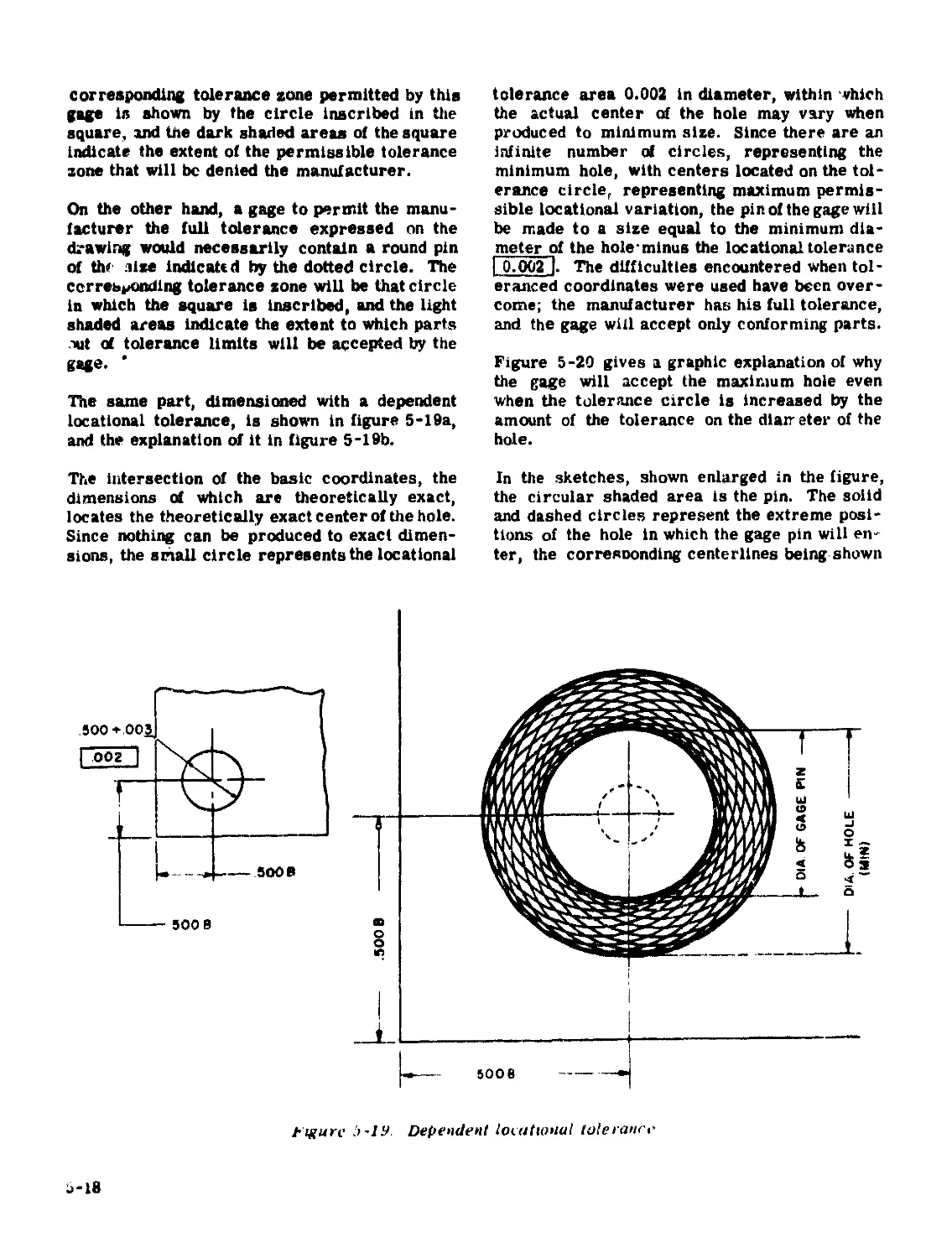
Dependent locational tolerances should be used,
rather than toleranced coordinates, whendimen-
sioning the location of holes. Figure 23A of
Drawing 30-1-7 explains why this is desirable,
but further explanation is given in the following
paragraphs, since production and inspection are
vitally interested in the method used.
Figure 5-18a shows a portion of simple part
with a single hole, the location of which is fixed
by coordinates. Figure 5-18b is an enlarged
view of 5-18a. The square in the center shows
the permissible tolerance zone in which the
center of the hole may vary. The large circles
show the positions of the minimum holes at the
positions of maximum variation permitted by
coordinate dimensions. In order to permit the
manufacturer his full tolerance, the gaging pin
would necessarily be of the shape shown by the
four arcs that are drawn in heavier lines. Since
the cost of making simple locational gages with
pins of that shape would be prohibitive, the gage
engineer will design the gage with a round pin.
To ensure that only conforming parts will be
accepted, the pin would necessarily be of the
size shown by the dashed circle. The
Figure 5-18. Effect of hole location of coordinates on production and inspection
5-17
corresponding tolerance zone permitted by this
gage is shown by the circle inscribed in the
square, and the dark shaded areas of the square
indicate the extent of the permissible tolerance
zone that will be denied the manufacturer.
On the other hand, a gage to permit the manu-
facturer the full tolerance expressed on the
drawing would necessarily contain a round pin
of th* iize indicated by the dotted circle. The
cerrebnonding tolerance zone will be that circle
in which the square is inscribed, and the light
shaded areas indicate the extent to which parts
xit of tolerance limits will be accepted by the
gage. *
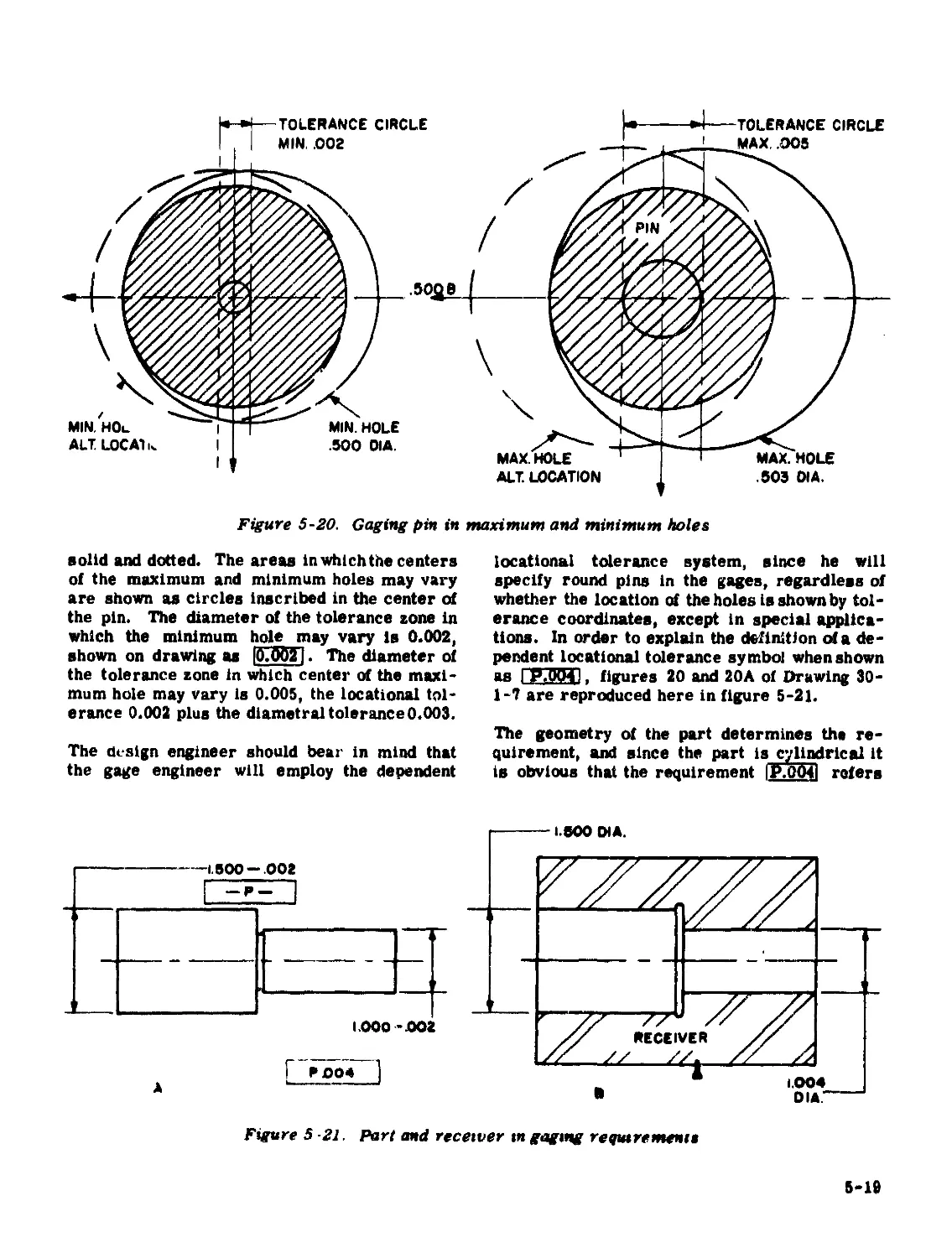
The same part, dimensioned with a dependent
locational tolerance, is shown in figure 5-19a,
and the explanation of it in figure 5-19b.
The intersection of the basic coordinates, the
dimensions of which are theoretically exact,
locates the theoretically exact center of the hole.
Since nothing can be produced to exact dimen-
sions, the small circle represents the locational
tolerance area 0.002 in diameter, within which
the actual center of the hole may vary when
produced to minimum size. Since there are an
infinite number of circles, representing the
minimum hole, with centers located on the tol-
erance circle, representing maximum permis-
sible locational variation, the pin of the gage will
be made to a size equal to the minimum dia-
meter of the hole*minus the locational tolerance
I 0.002 ). The difficulties encountered when tol-
eranced coordinates were used have been over-
come; the manufacturer has his full tolerance,
and the gage will accept only conforming parts.
Figure 5-20 gives a graphic explanation of why
the gage will accept the maximum hole even
when the tolerance circle is increased by the
amount of the tolerance on the diair eter of the
hole.
In the sketches, shown enlarged in the figure,
the circular shaded area is the pin. The solid
and dashed circles represent the extreme posi-
tions of the hole in which the gage pin will eiv
ter, the corresnonding centerlines being shown
figure l>-19 Dependent locational tolerance
5-18
Figure 5-20. Gaging pin in maximum and minimum holes
solid and dotted. The areas In which the centers
of the maximum and minimum holes may vary
are shown as circles inscribed in the center at
the pin. The diameter of the tolerance zone in
which the minimum hole may vary is 0.002,
shown on drawing as |0.QQ21. The diameter of
the tolerance zone in which center of the maxi-
mum hole may vary is 0.005, the locational tol-
erance 0.002 plus the diametral tolerance 0.003.
The design engineer should bear in mind that
the gage engineer will employ the dependent
locational tolerance system, since he will
specify round pins in the gages, regardless of
whether the location of the holes is shown by tol-
erance coordinates, except in special applica-
tions. In order to explain the definition cd a de-
pendent locational tolerance symbol when shown
as I P.0041, figures 20 and 20A of Drawing 30-
1-7 are reproduced here in figure 5-21.
The geometry of the part determines the re-
quirement, and since the part is cylindrical it
is obvious that the requirement IP.0d4l refers
Г ₽J004
A	--------
Figure 5 -21. Part and receiver tn gaging requirements
5-19
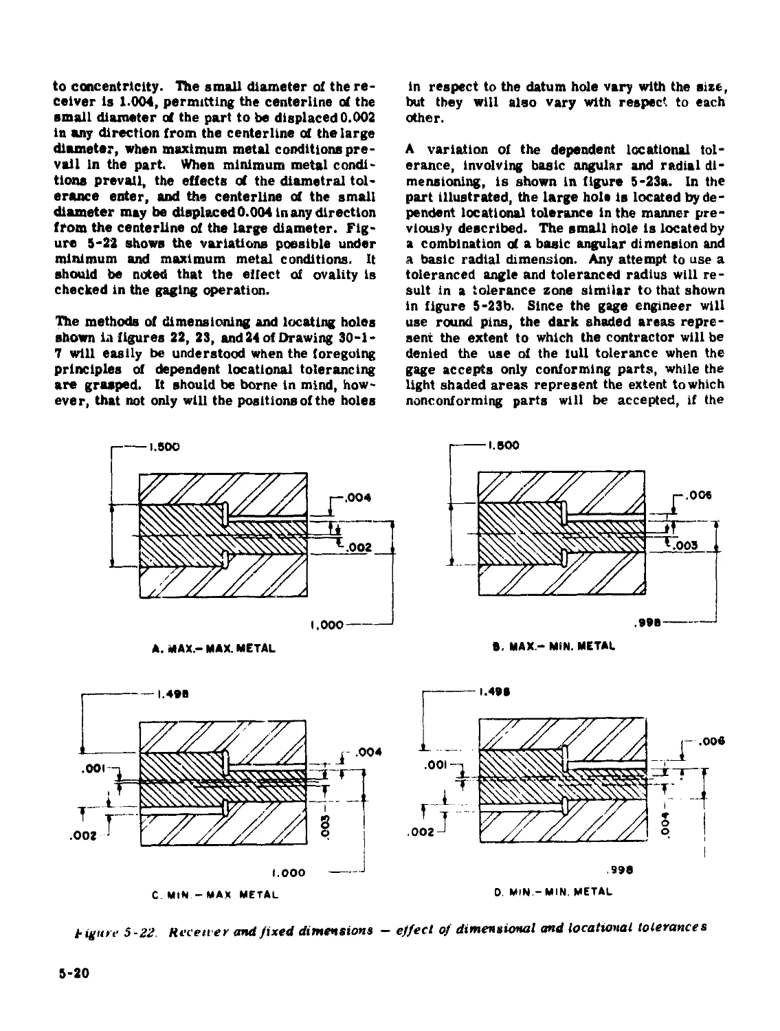
to concentricity. The small diameter of the re-
ceiver is 1.004, permitting the centerline of the
small diameter of the part to be displaced 0.002
in any direction from the centerline of the large
diameter, when maximum metal conditions pre-
vail In the part. When minimum metal condi-
tions prevail, the effects of the diametral tol-
erance enter, and the centerline of the small
diameter may be displaced 0.004 In any direction
from the centerline of the large diameter. Fig-
ure 5-22 shows the variations possible under
minimum and maximum metal conditions. It
should be noted that the effect of ovality is
checked in the gaging operation.
The methods of dimensioning and locating holes
shown la figures 22, 23, and 24 of Drawing 30-1-
7 will easily be understood when the foregoing
principles of dependent locational tolerancing
are grasped. It should be borne in mind, how-
ever, that not only will the positions of the holes
in respect to the datum hole vary with the size,
but they will also vary with respect to each
other.
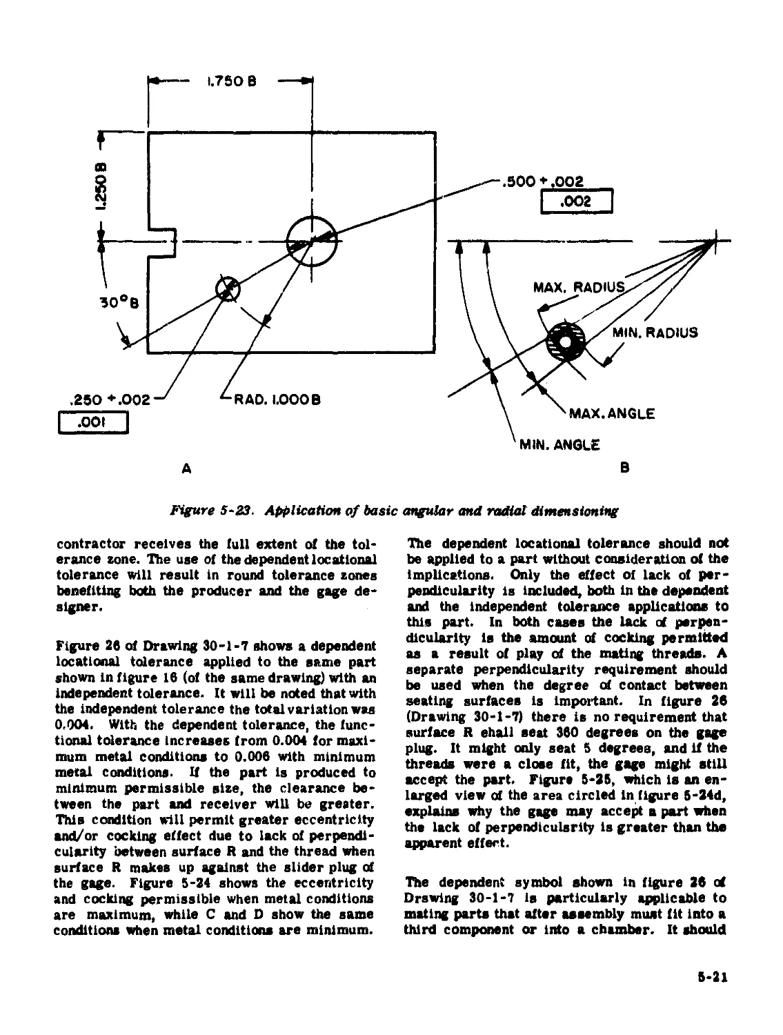
A variation of the dependent locational tol-
erance, involving basic angular and radial di-
mensioning, is shown in figure 5-23a. In the
part illustrated, the large hols is located by de-
pendent locational tolerance in the manner pre-
viously described. The small hole is located by
a combination of a basic angular dimension and
a basic radial dimension. Any attempt to use a
toleranced angle and toleranced radius will re-
sult in a tolerance zone similar to that shown
in figure 5-23b. Since the gage engineer will
use round pins, the dark shaded areas repre-
sent the extent to which the contractor will be
denied the use of the full tolerance when the
gage accepts only conforming parts, while the
light shaded areas represent the extent to which
nonconforming parts will be accepted, if the
figure 5-22. Receiver and fixed dimensions — effect of dimensional and locational tolerances
5-20
Figure 5-23. Application of basic angular and radial dimensioning
contractor receives the full extent of the tol-
erance zone. The use of the dependent locational
tolerance will result in round tolerance zones
benefiting both the producer and the gage de-
signer.
Figure 26 of Drawing 30-1-7 shows a dependent
locational tolerance applied to the same part
shown in figure 16 (of the same drawing) with an
independent tolerance. It will be noted that with
the independent tolerance the total variation was
0,004. With the dependent tolerance, the func-
tional tolerance increases from 0.004 for maxi-
mum metal conditions to 0.006 with minimum
metal conditions. If the part is produced to
minimum permissible size, the clearance be-
tween the part and receiver will be greater.
This condition will permit greater eccentricity
and/or cocking effect due to lack of perpendi-
cularity between surface R and the thread when
surface R makes up against the slider plug of
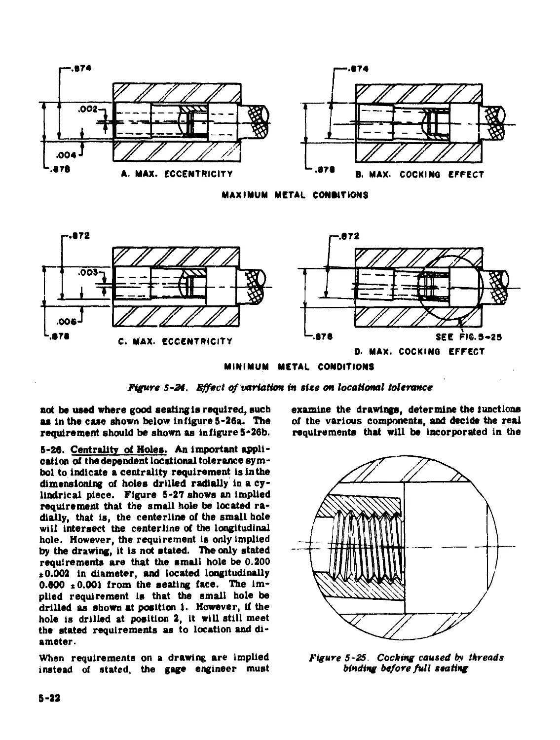
the gage. Figure 5-24 shows the eccentricity
and cocking permissible when metal conditions
are maximum, while C and D show the same
conditions when metal conditions are minimum.
The dependent locational tolerance should not
be applied to a part without consideration of the
implications. Only the effect of lack of per-
pendicularity is included, both in the dependent
and the independent tolerance applications to
this part. In both cases the lack of perpen-
dicularity is the amount of cocking permitted
as a result of play of the mating threads. A
separate perpendicularity requirement should
be used when the degree of contact between
seating surfaces is important. In figure 26
(Drawing 30-1-7) there is no requirement that
surface R ehall seat 360 degrees on the gage
plug. It might only seat 5 degrees, and if the
threads were a close fit, the gage might still
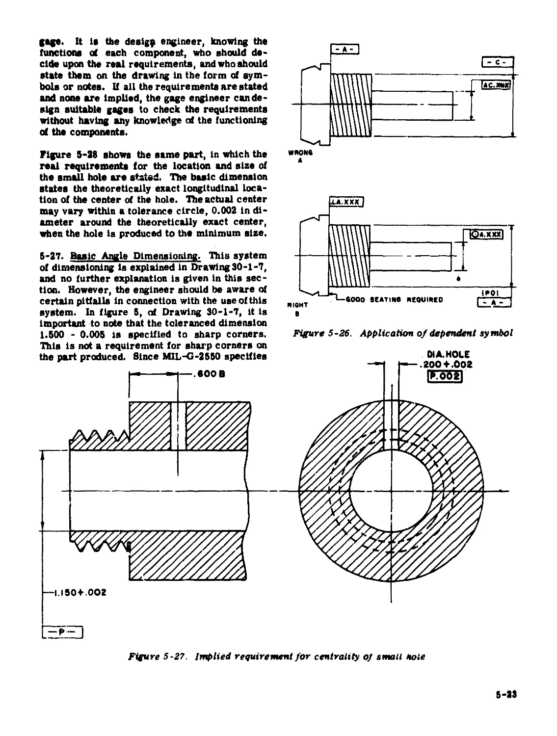
accept the part. Figure 5-25, which is an en-
larged view of the area circled in figure 5-24d,
explains why the gage may accept a part when
the lack of perpendicularity is greater than the
apparent effect.
The dependent symbol shown in figure 26 of
Drswing 30-1-7 is particularly applicable to
mating parts that after assembly must fit into a
third component or into a chamber. It should
5-21
A. MAX. ECCENTRICITY
[ LZZZZZI
•87в B. MAX. C0CKIN6 EFFECT
MAXIMUM METAL CONDITIONS
Г-.872
.003-^
I T
FZZZZ
OOS
T\ZZZZZ
C. MAX. ECCENTRICITY
0. MAX. C0CKIN6 EFFECT
MINIMUM METAL CONDITIONS
Figure 5-24. Effect of variation in site on locational tolerance
not be used where good seating Is required, such
as in the case shown below infigure 5-26a. The
requirement should be shown as in figure 5-26b.
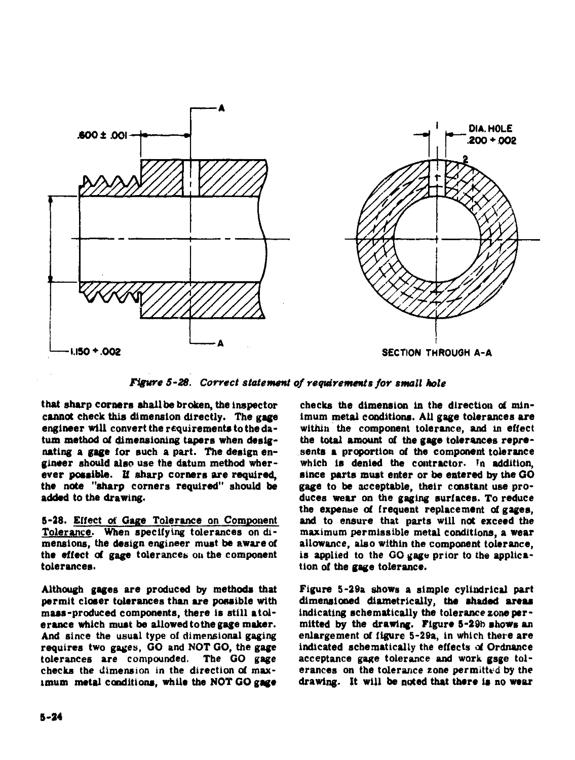
5-26. Centrality of Holes. An important appli-
cation of the dependent locational tolerance sym-
bol to indicate a centrality requirement isinthe
dimensioning of holes drilled radially in a cy-
lindrical piece. Figure 5-27 shows an implied
requirement that the small hole be located ra-
dially, that is, the centerline of the small hole
will intersect the centerline of the longitudinal
hole. However, the requirement is only implied
by the drawing, it is not stated. The only stated
requirements are that the small hole be 0.200
±0.002 in diameter, and located longitudinally
0.600 ±0.001 from the seating face. The im-
plied requirement is that the small hole be
drilled as shown at position 1. However, if the
hole is drilled at position 2, it will still meet
the stated requirements as to location and di-
ameter.
When requirements on a drawing are implied
instead of stated, the gage engineer must
examine the drawings, determine the functions
of the various components, and decide the real
requirements that will be incorporated in the
Figure 5-25. Cocking caused by threads
binding before full seating
5-22
gage. It is the desigp engineer, knowing the
functions at each component, who should de-
cide upon the real requirements, and who should
state them on the drawing in the form of sym-
bols or notes. If all the requirements are stated
and none are implied, the gage engineer can de-
sign suitable gages to check the requirements
without having any knowledge of the functioning
of the components.
Figure 5-28 shows the same part, in which the
real requirements for the location and size of
the small hole are stated. The basic dimension
states the theoretically exact longitudinal loca-
tion of the center of the hole. The actual center
may vary within a tolerance circle, 0.002 in di-
ameter around the theoretically exact center,
when the hole is produced to the minimum size.
5-27. Basic Angle Dimensioning. This system
of dimensioning is explained in Drawing 30-1-7,
and no further explanation is given in this sec-
tion. However, the engineer should be aware of
certain pitfalls in connection with the use of this
system. In figure 5, of Drawing 30-1-7, it is
important to note that the toleranced dimension
1.500 - 0.005 is specified to sharp corners.
This is not a requirement for sharp corners on
the part produced. Since MIL-G-2550 specifies
WRONG
XA.XXX |
Figure 5-26. Application of dependent symbol
Figure 5-27. Implied requirement for centrality oj small Hole
5-23
Figure 5-28. Correct statement of requirements for small hole
that sharp corners shall be broken, the inspector
cannot check this dimension directly. The gage
engineer will convert the requirements to the da-
tum method of dimensioning tapers when desig-
nating a gage for such a part. The design en-
gineer should also use the datum method wher-
ever possible. И sharp corners are required,
the note "sharp corners required" should be
added to the drawing.
5-28. Effect <Л Gage Tolerance on Component
Tolerance. When specifying tolerances on di-
mensions, the design engineer must be aware of
the effect of gage tolerances on the component
tolerances.
Although gages are produced by methods that
permit closer tolerances than are possible with
mass-produced components, there is still atol-
e rance which must be allowed to the gage maker.
And since the usual type of dimensional gaging
requires two gages, GO and NOT GO, the gage
tolerances are compounded. The GO gage
checks the dimension in the direction of max-
imum metal conditions, while the NOT GO gage
checks the dimension in the direction of min-
imum metal conditions. All gage tolerances are
within the component tolerance, and in effect
the total amount al the gage tolerances repre-
sents a proportion of the component tolerance
which is denied the contractor. Tn addition,
since parts must enter or be entered by the GO
gage to be acceptable, their constant use pro-
duces wear on the gaging surfaces. To reduce
the expense of frequent replacement of gages,
and to ensure that parts will not exceed the
maximum permissible metal conditions, a wear
allowance, also within the component tolerance,
is applied to the GO gage prior to the applica-
tion of the gage tolerance.
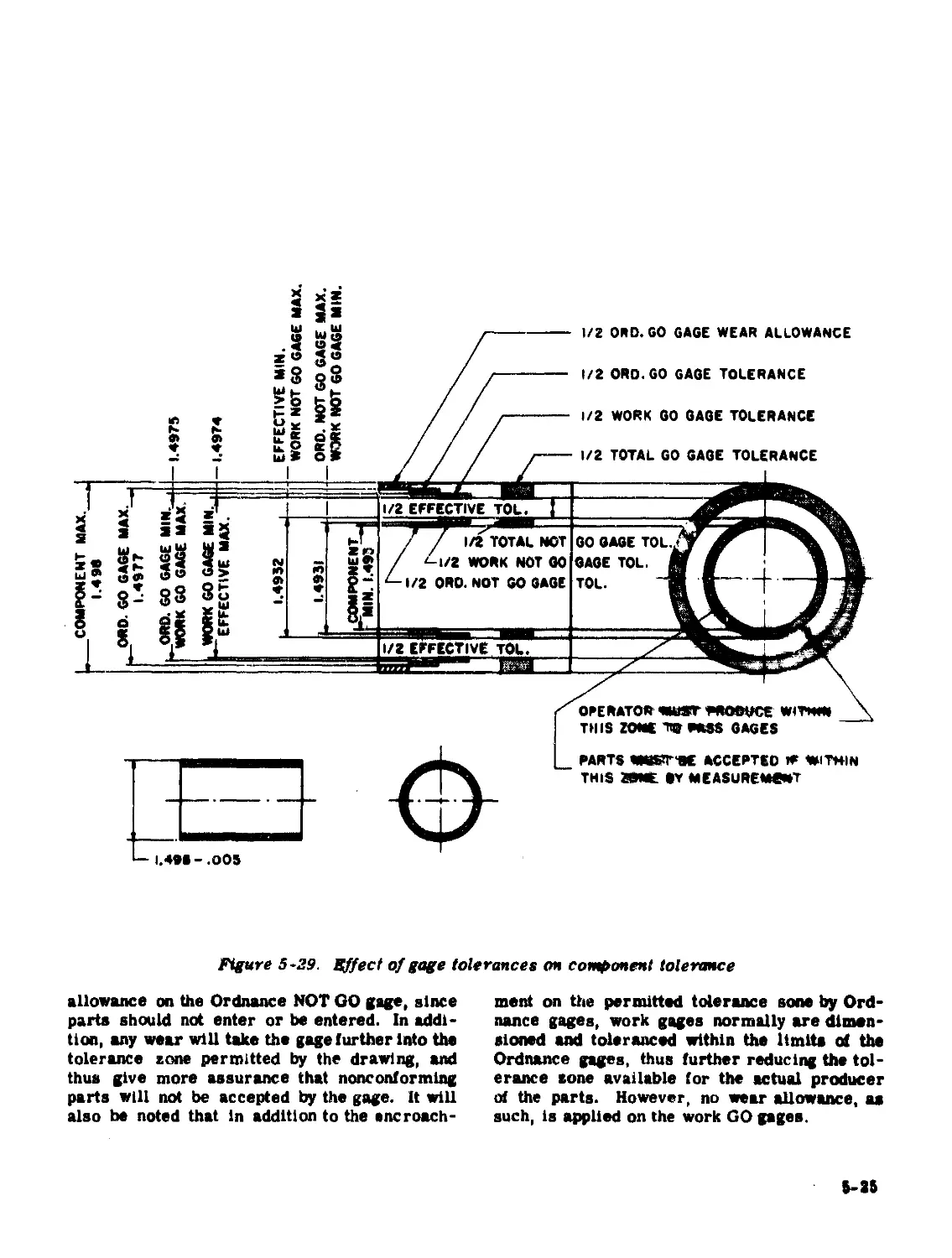
Figure 5-29a shows a simple cylindrical part
dimensioned diametrically, the shaded areas
Indicating schematically the tolerance zone per-
mitted by the drawing. Figure 5-29b shows an
enlargement of figure 5-29a, in which there are
indicated schematically the effects of Ordnance
acceptance gage tolerance and work gsge tol-
erances on the tolerance zone permitted by the
drawing. It will be noted that there is no wear
5-34
Ul
as
8s
1/2 EFFECTIVE TOL.
1/2
1/2
1/2
ORD. GO GAGE WEAR ALLOWANCE
ORD.GO GAGE TOLERANCE
WORK GO GAGE TOLERANCE
TOTAL GO GAGE TOLERANCE
1/2
1/2 EFFECTIVE TOL. i
1/2 TOTAL NOT
*-1/2 WORK NOT GO
1/2 ORD. NOT GO GAGE
OPERATOR ШДТ FRODVCE WITH*
THIS ZONE TO GNSS GAGES
PARTS Ш1ГГОЕ ACCEPTED * WITHIN
THIS ZWE GY MEASUREMENT
GO GAGE TOL.f
GAGE TOL.
TOL.
Figure 5-29. Effect of gage tolerances on component tolerance
allowance on the Ordnance NOT GO gage, since
parts should not enter or be entered. In addi-
tion, any wear will take the gage further Into the
tolerance zone permitted by the drawing, and
thus give more assurance that nonconforming
parts will not be accepted by the gage. It will
also be noted that in addition to the encroach-
ment on the permitted tolerance sone by Ord-
nance gages, work gages normally are dimen-
sioned and toleranced within the limits of the
Ordnance gages, thus further reducing the tol-
erance aone available for the actual producer
of the parts. However, no wear allowance, as
such, is applied on the work GO gages.

ENGINEERING DESIGN HANDBOOK SERIES
Listed below ere the Handbook! which have bean published or submitted for publication. Handbooks with publica-
tion dates prior to 1 August 1962 wars published as 20-seriee Ordnance Corps pamphlets. AMC Circular 310-38, 19
July 1963, redesignated those publications as 706-series AMC pamphlets (i.s., ORDP 20-138 was redesignated AMCP
706-138). All now, reprinted, or revised Handbooks are being published as 706-series AMC pamphlets.
General and Miscellaneous Subjects
No.	Tide
106 Elements of Armament Engineering. Part One,
Sources of Energy
107 Elements of Armament Engineering, Part Two,
Ballistics
100 Elements of Armament Engineering, Part
Three, Weapon Systems and Componsnts
110 Experimental Statistics, Section 1, Basic Con-
cepts and Analysis of Measurement Data
111 Experimental Statistics, Section 2, Analysis of
Enumerative and Claseificatory Data
112 Experimental Sts tie ties, Section 3, Planning
and Analysis of Comparative Experiments
113 Experimental Statistics, Section 4, Special
Topics
114	Experimental Statistics, Section 5, Tables
121	Packaging and Pack Engineering
134 Maintenance Engineering Guido for Ordnance
Design
135 Inventions, Patents, and Related Matters
(Revised)
136 Servomechanisms, Section 1, Theory
13? Servomechanisms, Section 2. Msasur ament
and Signal Converters
13S	Servomechanisms, Section 3, Amplification
139	Servomechanisms, Section 4, Power Elements
and System Desipi
170(G) Armor and Its Application to Vehicles (U)
250	Guns --General (Guns Series)
252	Gun Tubss (Guns Series)
270	Propellant Actuated Devices
290(C)	Warheada--General (U)
331	Compensating Elements (Fire Control Series)
355 The Automotive Assembly (Automotive Seriss)
(Revised)
Ammunitisn and Explosive. Series
175	Solid Propellants, PartOns
176(C)	Solid Propellants, Part Two (U)
177 Propertiss of Explosives of Military Interest,
Section 1
178(C) Properties of Explosives of Military Interest,
Section 2 (U)
179	Explcsivs Trains
210	Fuses, General and Mechanical
211(C)	Fuses,	Proximity,	Electrical,	Part	One (U)
212(3)	Fusee,	Proximity,	Electrical.	Part	Two (U)
213(8)	Fuses, Proximity, Electrical, Part	Three (U)
214(S)	Fuses,	Proximity.	Electrical	Part	Four (U)
215(C)	Fuses,	Proximity,	Electrical.	Part	Five (U)
244	Section I. Artillery Ammunition--General,
with Table of Contente, Glossary and
Index for Series
245(C)	Section 2, Design for Terminal Effects (U)
246	Section 3, Design for Control of Flight
Characteristics
247 Section 4, Design for Projection
248 Section 5, Inspection Aspscts of Artillery
Ammunition Design
249 Section 6, Manufacture of Metallic Components
' of Artillery Ammunition
Ballistic Missile Series
No.	Title
281(B-RD)	Weapon System Effectiveness (U)
282	Propulsion and Propellants
283	Aerodynamics
284(C)	Trajectories (U)
286	Structures
Ballistics Series	
140	Trajectories, Differential Effects, and
	Data for Projectiles
150	Interior Ballistics of Gone
160(S)	Elements of Terminal Ballistics, Part
	One, Introduction, Kill Mechanisms, and Vulnerability (U)
161(3)	Elements of Terminal B^allistics, Part
	Two, Collection and Analysis of Data Concerning Targets (U)
162(8-RD)	Elements of Terminal Ballistics, Part
	Three, Application to Missile and Space Targets (U)
Carriage*	i and Mounts Series
340	Carriages and Mounts—General
341	Cradles
342	Recoil Systems
343	Top Carriages
344	Bottom Carriages
345	Equilibrators
346	Elevating Mechanisms
347	Traversing Mechanisms
Military Pyrotechnics Series	
1»6	Part Two, Safety, Procedures and
	Glossary
187	Part Three. Properties of Materials
	Used in Pyrotechnic Compositions
Surfac»to-Air Missile Series	
291	Part One, System Integration
292	Part Two, Weapon Control
293	Part Three, Computers
294(3)	Part Four, Missile Armament (U)
295(d)	Part Five, Countermeasures (U)
296	Part Six, Structures and Power Sources
297(8)	Part Seven, Sample Problem (U)
Materials	Series»
149	Rubber and Rubber-Like Materials
212	Gasket Materials (Nonmetallic)
691	Adhesives
692	Guide to Selection of Rubber O-Rings
693	Magnesium and Magnesium Alloys
694	Aluminum and Aluminum Alloys
697	Titanium and Titanium Allots
698	Copper and Copper Aiioye
699	Guide to Specifications for Flexible Rubbe
	Products
700	Plastics
721	Corrosion and Corrosion Protection of
	Metals
7 22	Glass
•The Materials Series is being published as Military Handbooks (MIL-HDBK-) which are available to Department of
Defense Agencies from the Naval Supply Depot, 5801 Tabor Avenue. Philadelphia. Pennsylvania 19120.