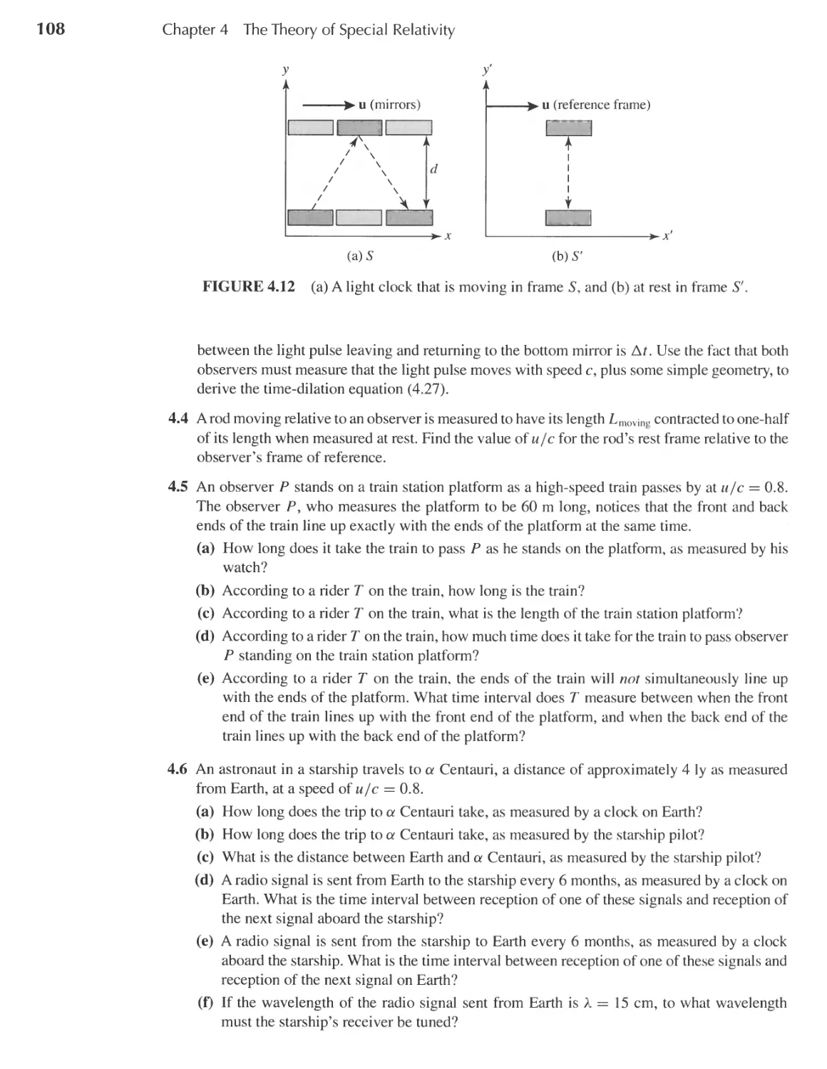
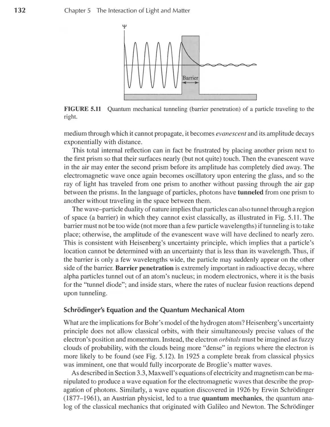
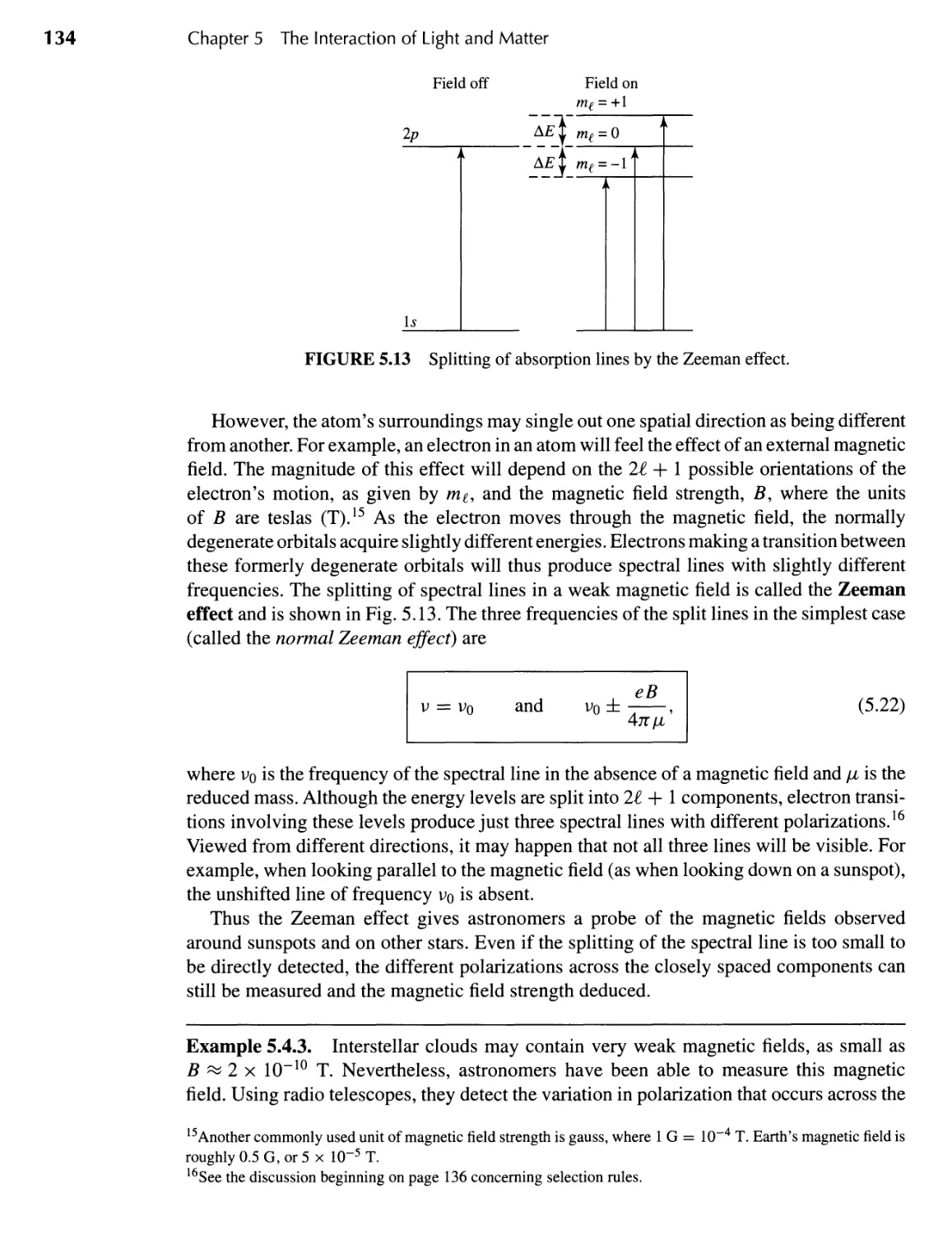
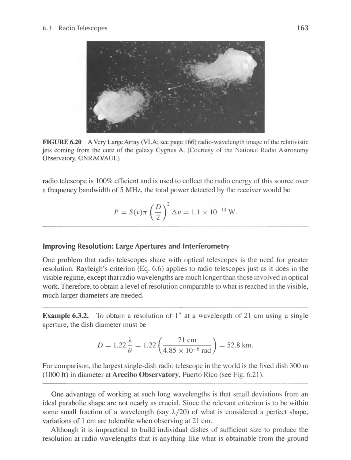
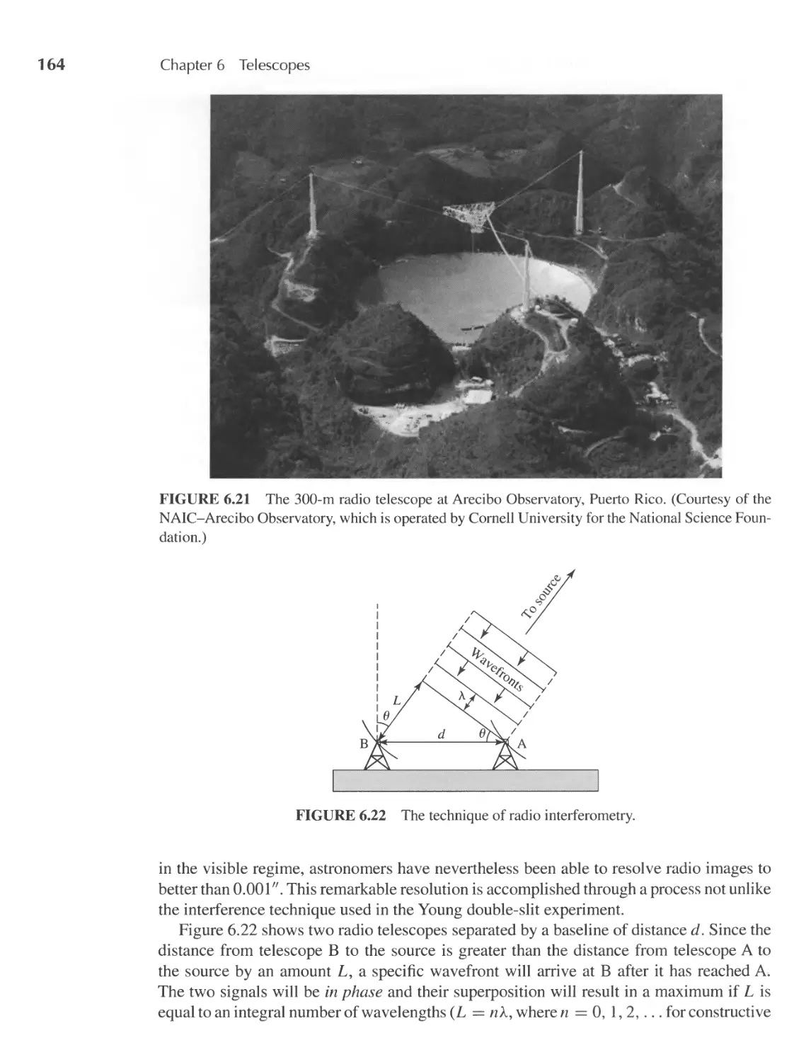
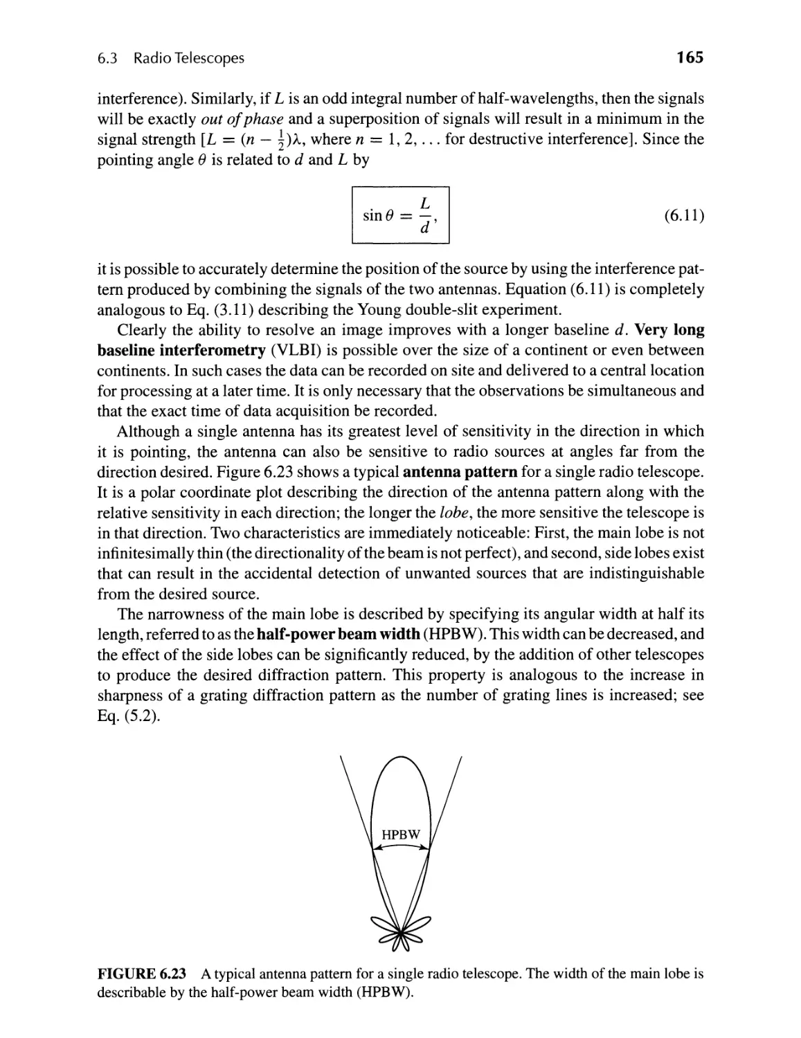
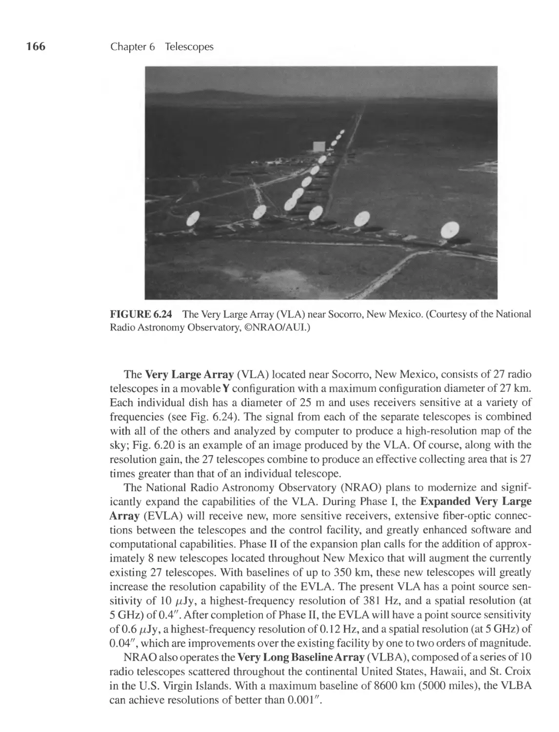
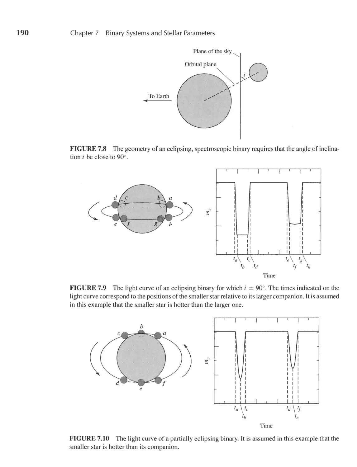
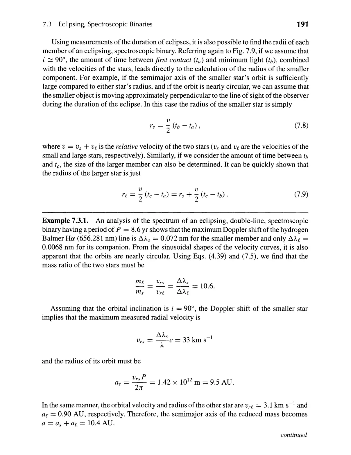
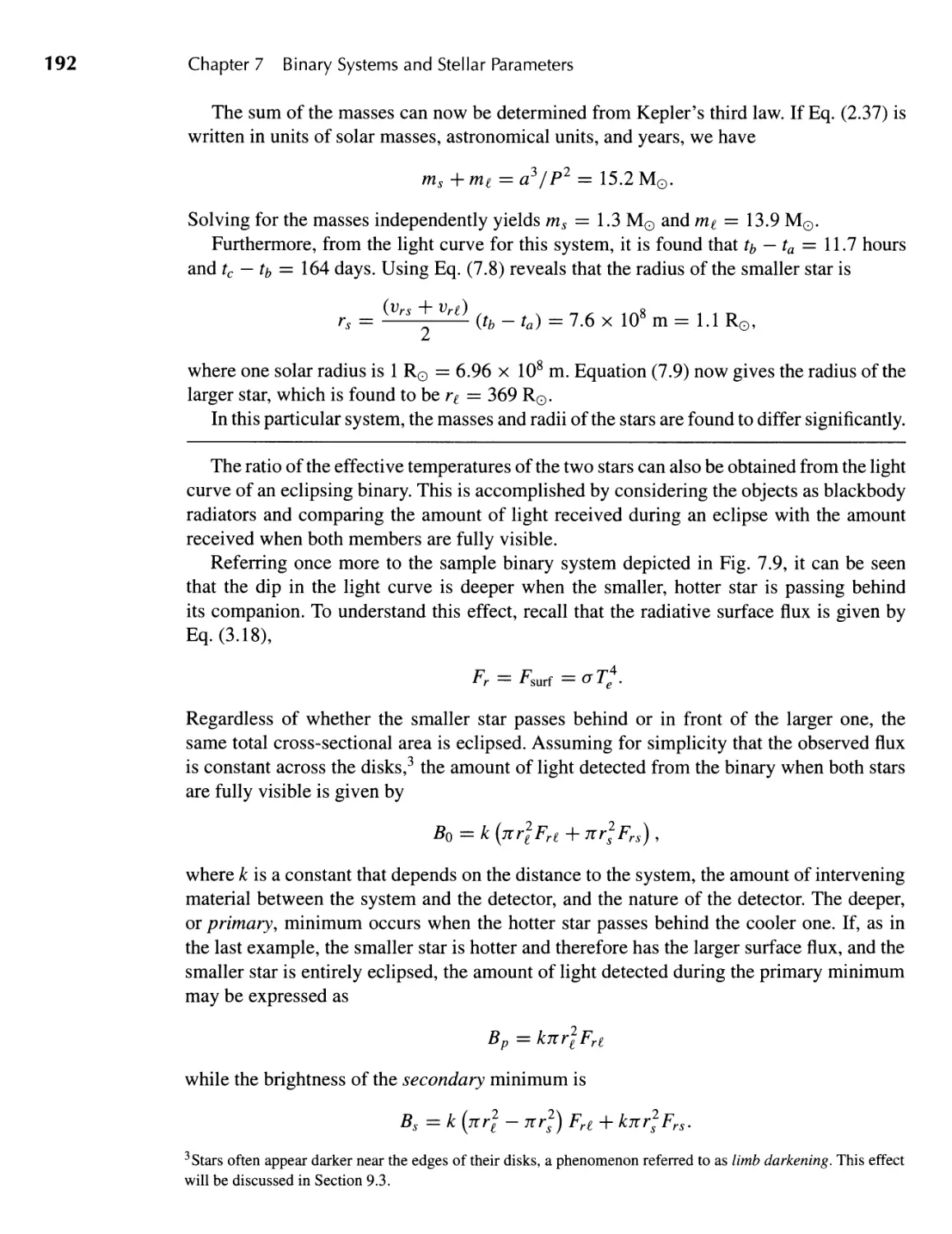
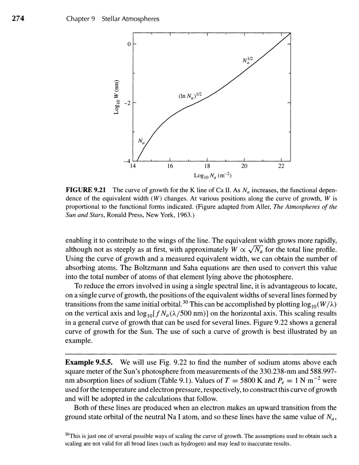
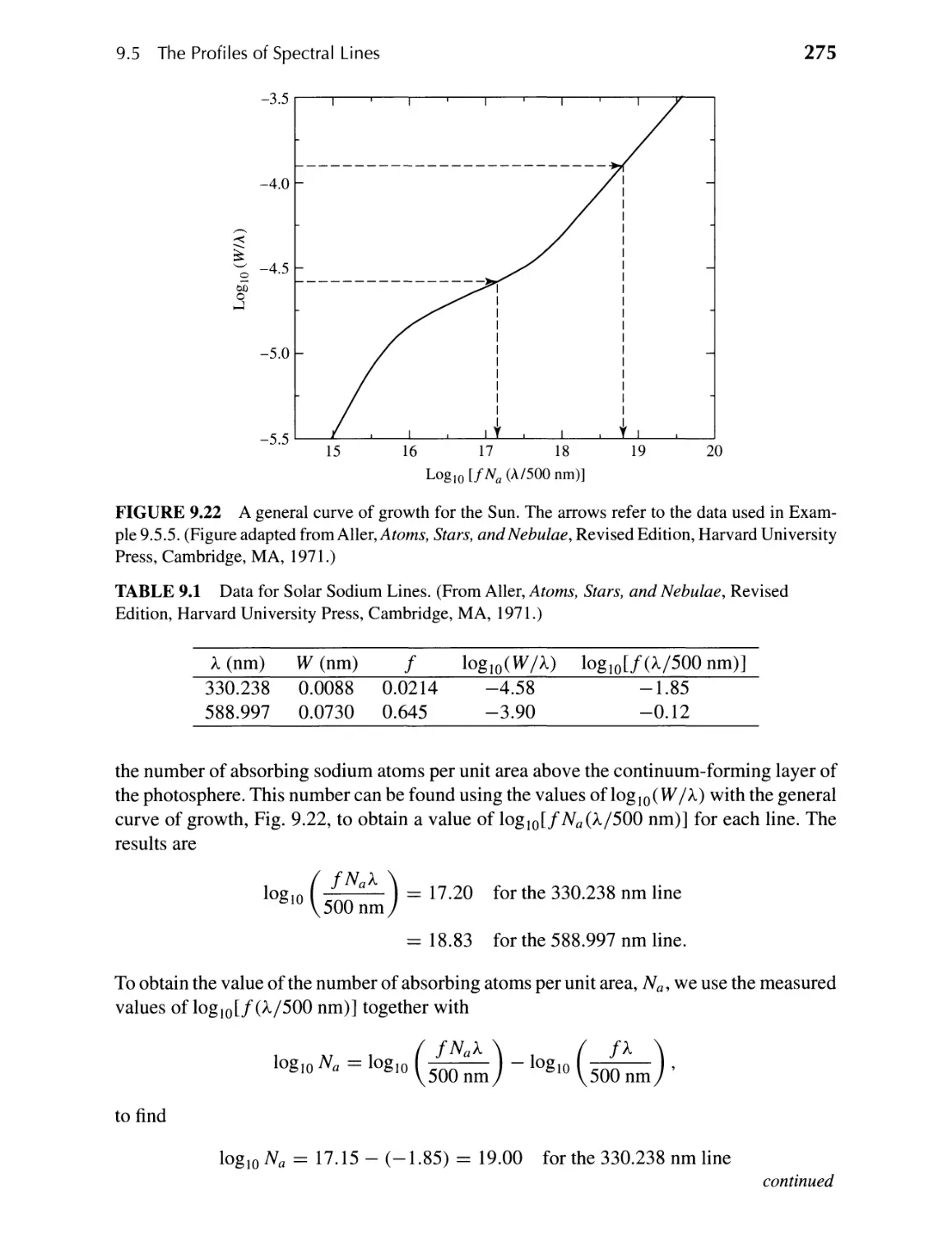
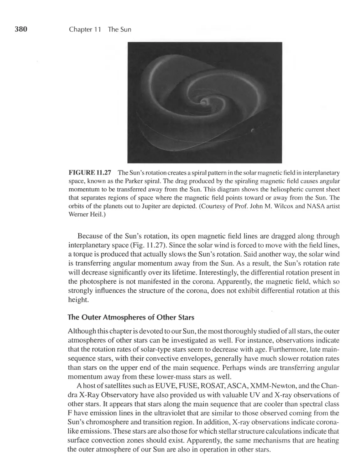
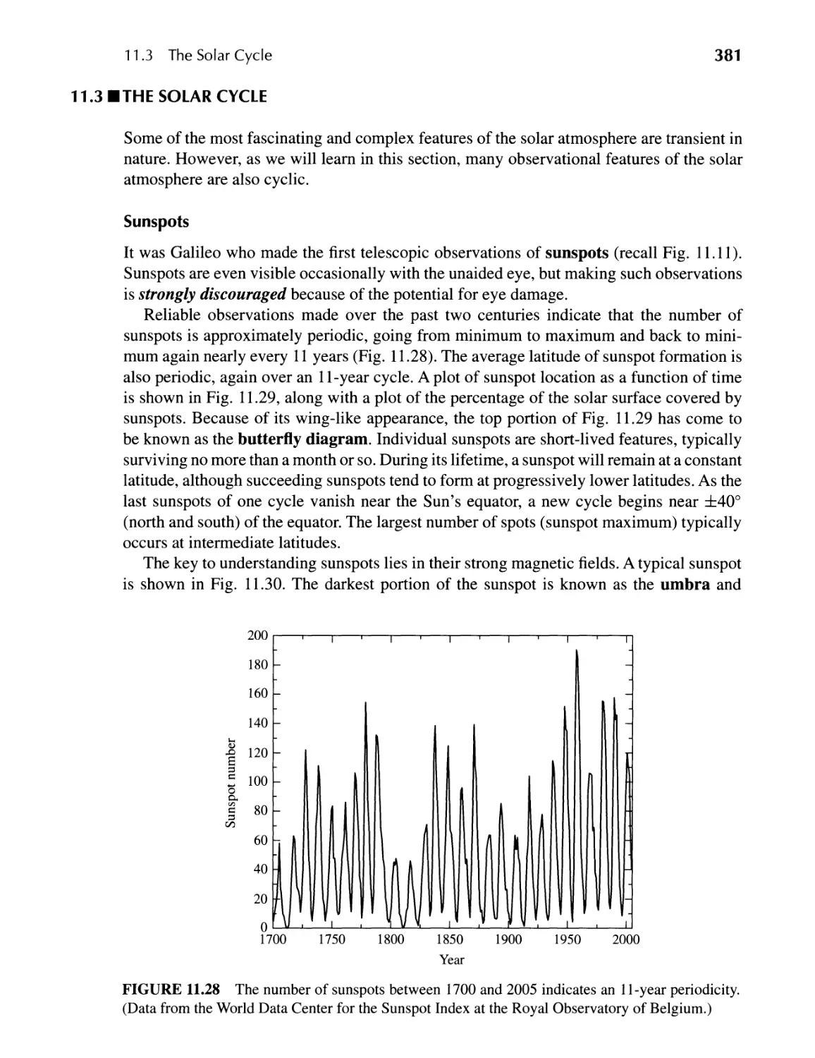
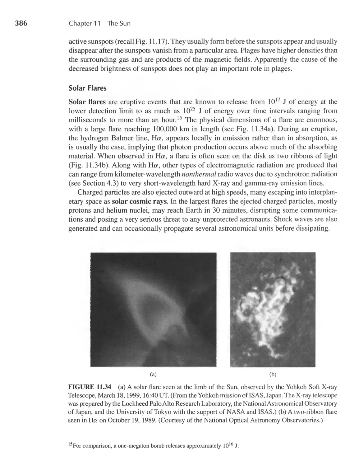
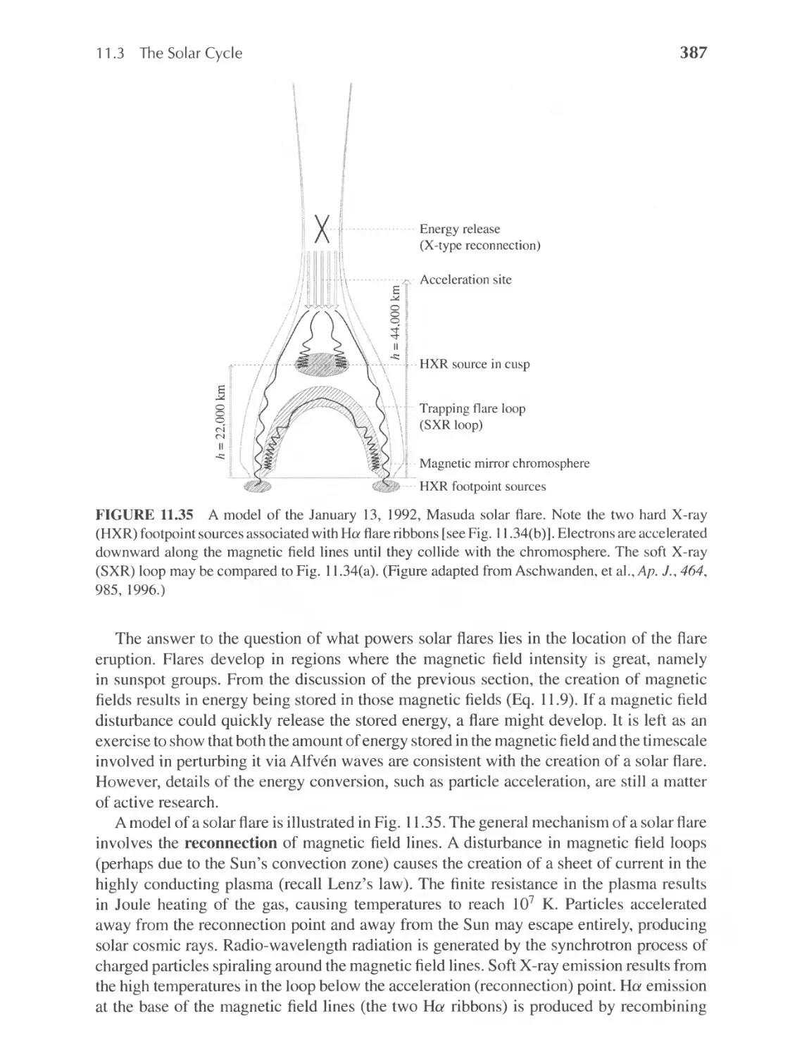
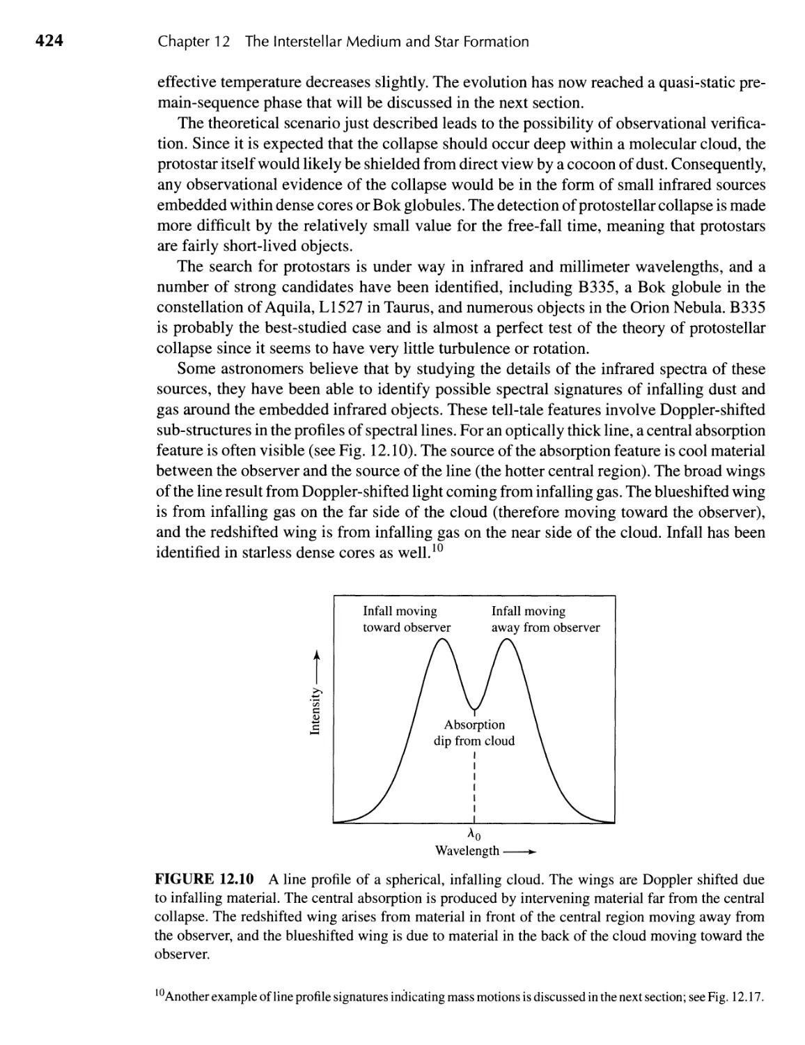
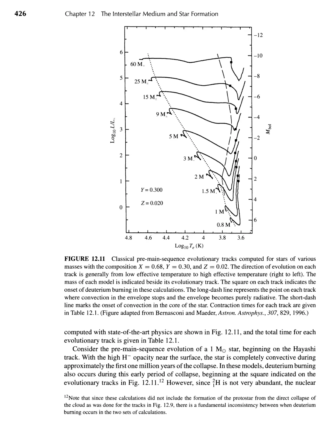
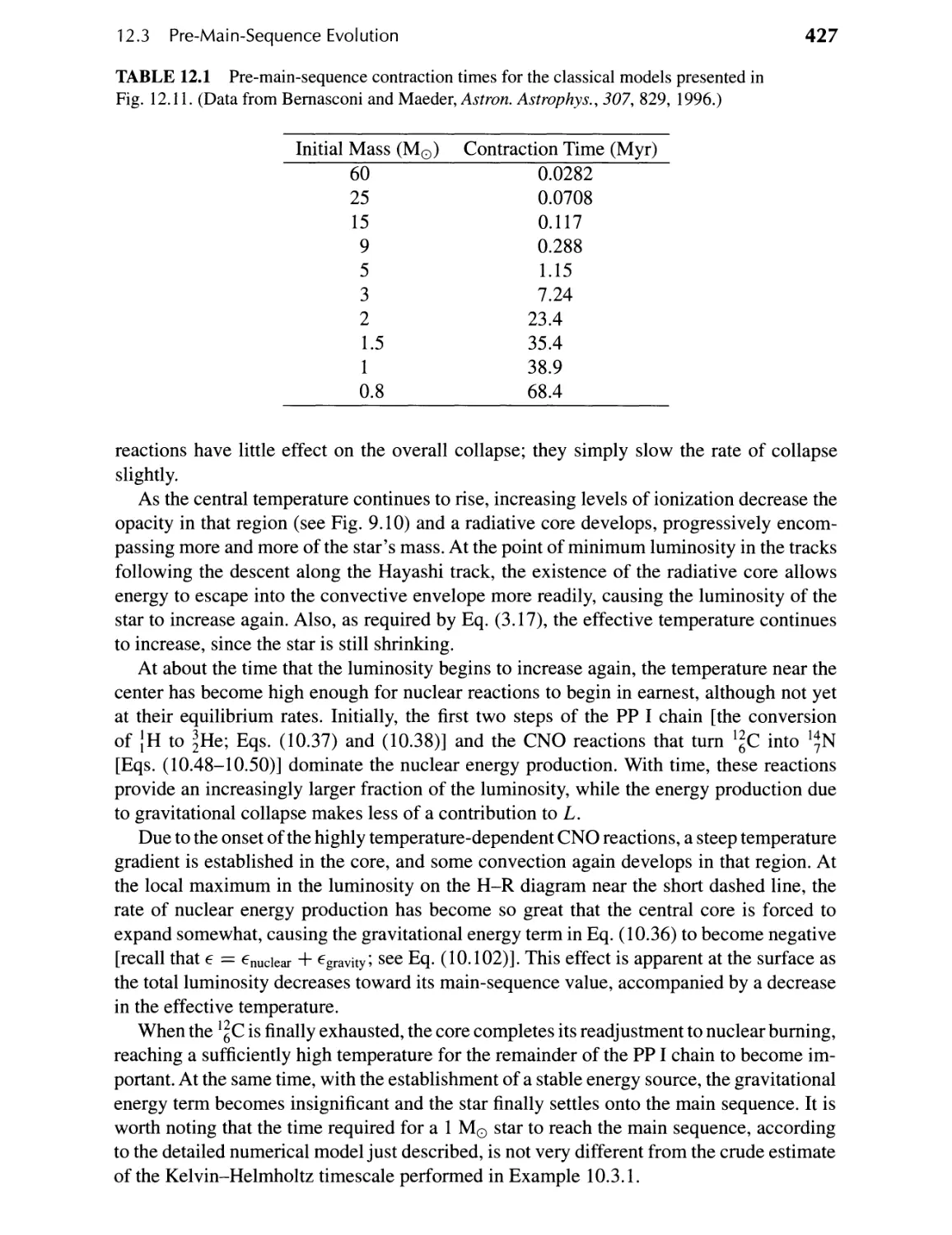
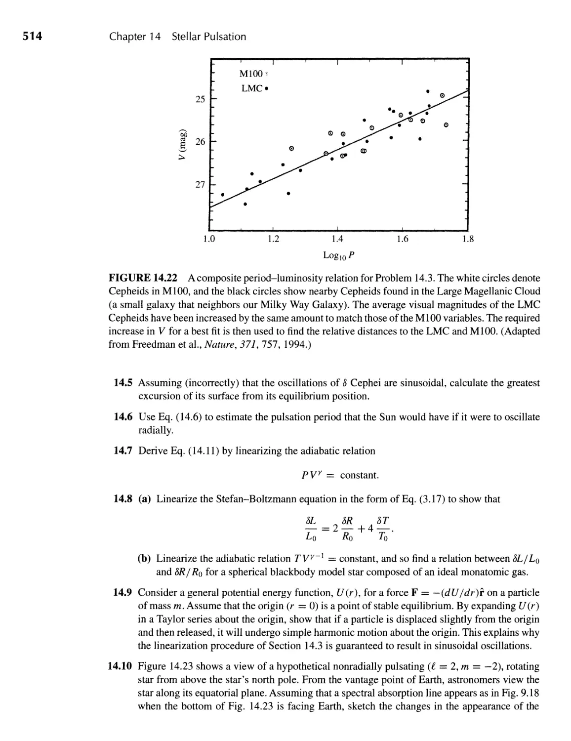
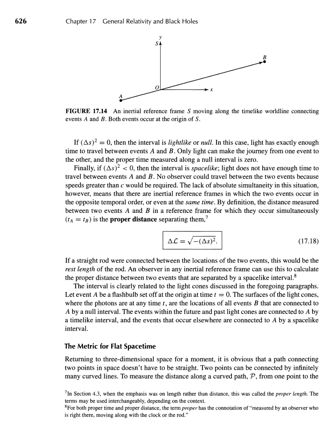
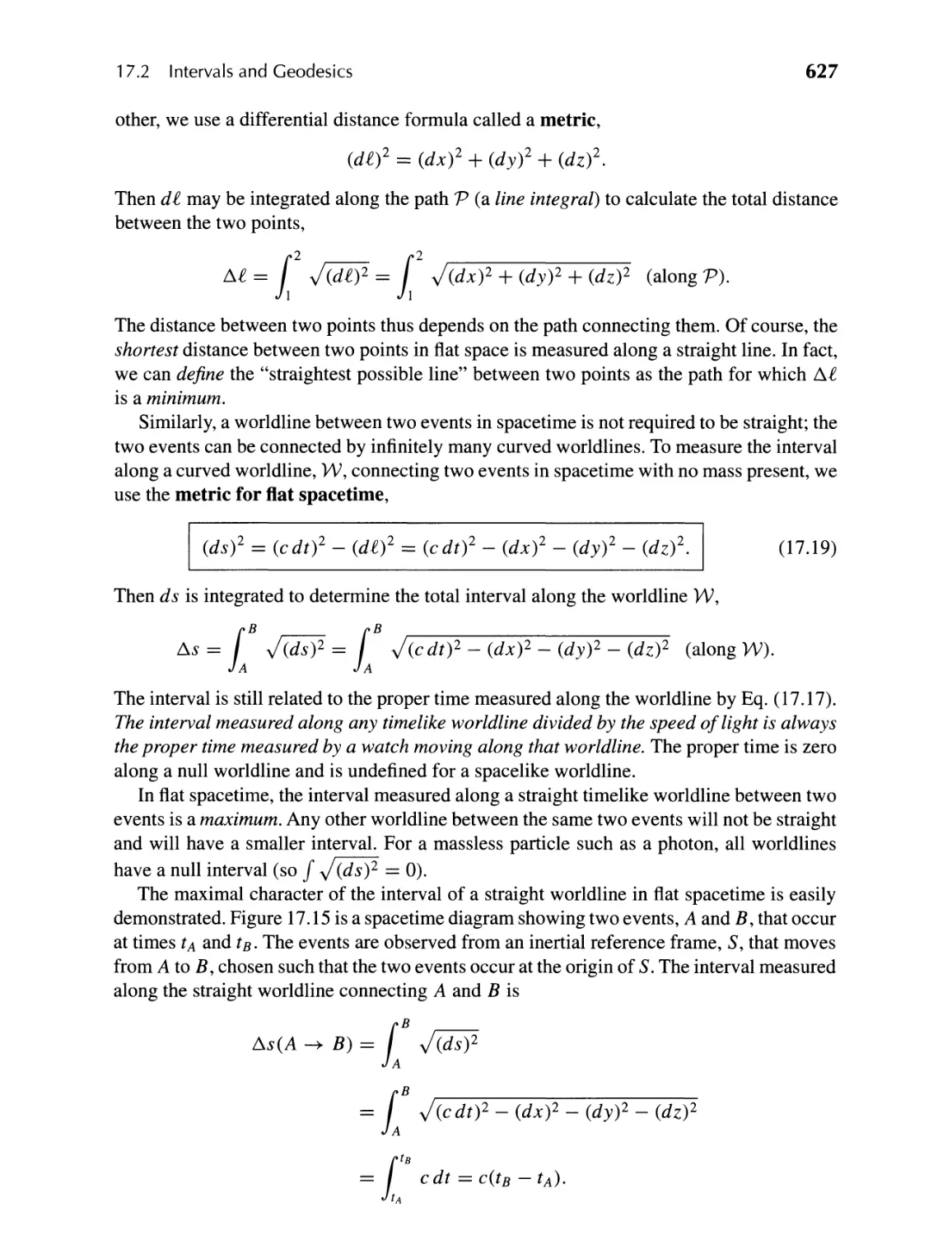
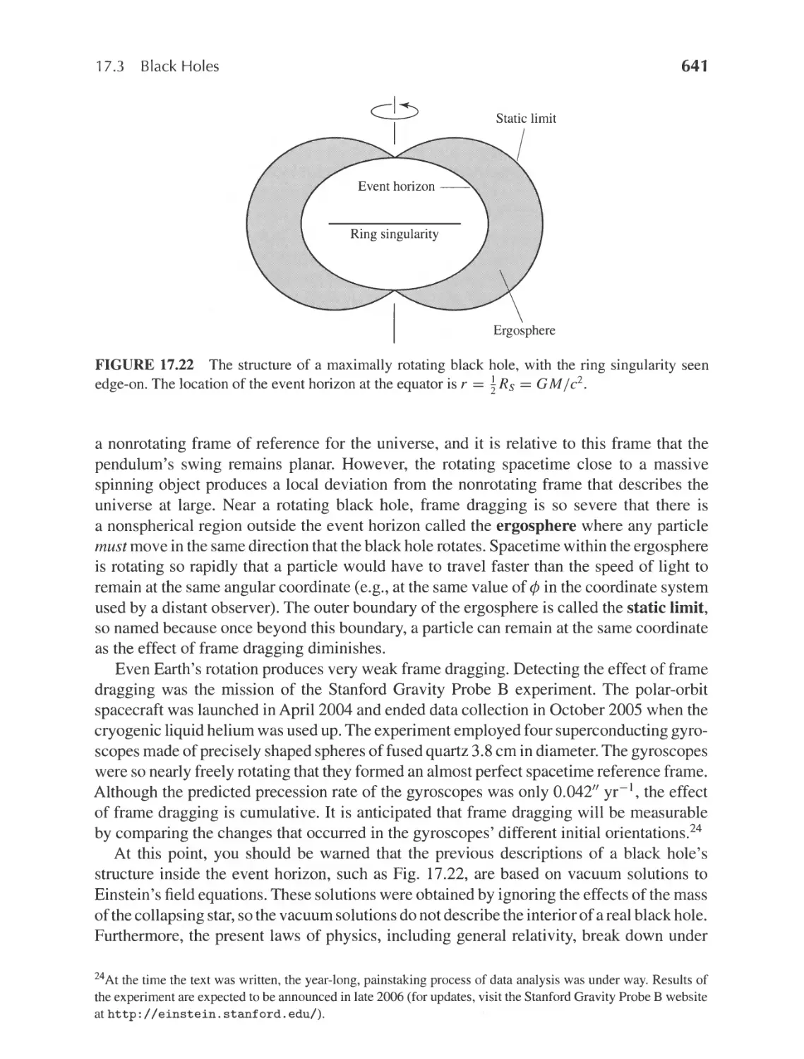
/


Текст
.
.
I
Astronomical Constants
1 Mo 1.9891 X 10 30 kg
S 1.365(2) X 10 3 W m- 2
1 Lo 3.839(5) x 10 26 W
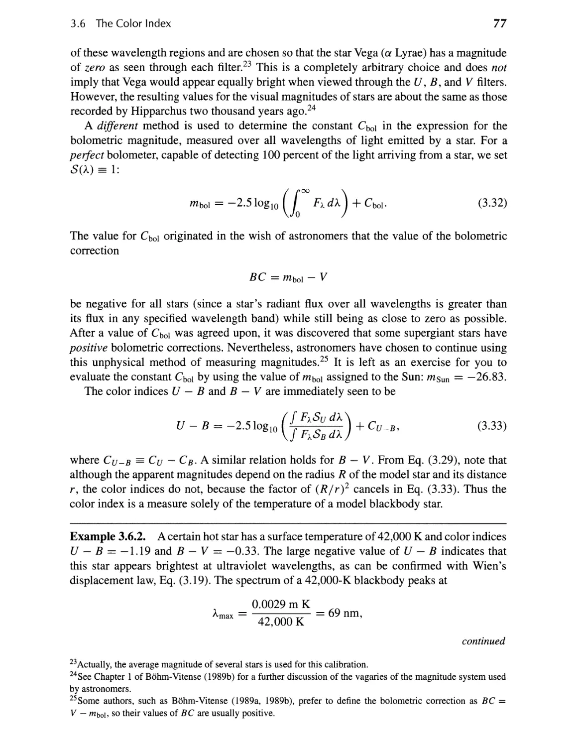
1 Ro 6.95508(26) x 10 8 m
Te,o L o /(4Jra R )1/4
5777(2) K
Solar mass
Solar irradiance
Solar luminosity
Solar radius
Solar effecti ve temperature
Solar absolute bolometric magnitdue
Solar apparent bolometric magnitude
Solar apparent ultraviolet magnitude
Solar apparent blue magnitude
Solar apparent visual magnitude
Solar bolometric correction
Earth mass
Earth radius (equatorial)
Astronomical uni t
Light (Julian) year
Parsec
Sidereal day
Solar day
Sidereal year
Tropical year
Julian year
Gregorian year
Mbol
mbol
U
B
V
BC
1 M EB
1 R EB
1 AU
1ly
1 pc
4.74
- 26.83
- 25 . 91
-26.10
-26.75
-0.08
5.9736 X 10 24 kg
6.378136 x 1 0 6 m
1.4959787066 X 10¹¹ m
9.460730472 x 10 15 m
206264.806 AU
3.0856776 x 10 16 m
3.2615638 ly (Julian)
23 h 56 ffi 04.0905309 s
86400 s
3.15581450 x 10 7 s
365.256308 d
3.155692519 x 10 7 s
365.2421897 d
3. 1557600 x 1 0 7 s
365.25 d
3.1556952 x 10 7 S
365.2425 d
Note: Uncertainties in the last digits are indicated in parentheses. For instance,
the solar radius, 1 Ro, has an uncertainty of :i:0.00026 x 10 8 ffi.
I
Gravitational constant
Speed of light (exact)
Permeability of free space
Permittivity of free space
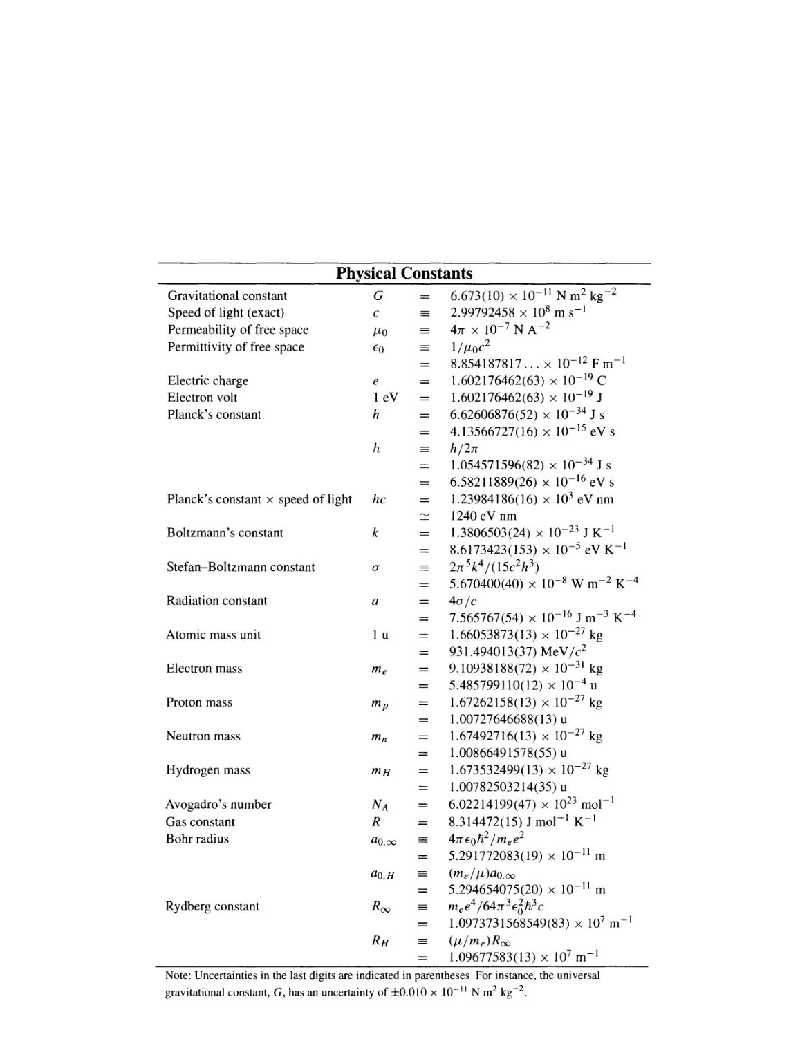
Physical Constants
G 6.673(10) x 10- 11 N m 2 kg- 2
e 2.99792458 x 10 8 m s-l
JLo 4Jr X 10- 7 N A- 2
EO 1 I JLOC 2
8.854187817... x 10- 12 F m- 1
1.602176462(63) x 10- 19 C
1.602176462(63) x 10- 19 J
6.62606876(52) x 10- 34 J s
4.13566727(16) X 10- 15 eV s
hl2Jr
1.054571596(82) X 10- 34 J s
6.58211889(26) X 10- 16 eV s
1.23984186(16) x 10 3 eV om
1240 eV nm
1.3806503 (24) x 10- 23 J K- 1
8.6173423(153) X 10- 5 eV K- 1
2Jr 5 k 4 1(15c 2 h 3 )
5.670400(40) x 10- 8 W m- 2 K- 4
4ale
7.565767(54) x 10- 16 J m- 3 K- 4
1.66053873(13) x 10- 27 kg
931.494013(37) MeV Ic 2
9.10938188(72) x 10- 31 kg
5.485799110(12) X 10- 4 U
1.67262158(13) X 10- 27 kg
1.00727646688(13) u
1.67492716(13) x 10- 27 kg
1.00866491578(55) u
1.673532499(13) x 10- 27 kg
1.00782503214(35) u
6.02214199(47) x 10 23 mol- I
8.314472(15) J mol- 1 K- I
4Jr EO li 2 Im e e 2
5.291772083(19) x 10- 11 m
(mel JL)ao,oo
5.294654075(20) x 10- 11 m
m e e 4 /64Jr3E5li 3 c
1.0973731568549(83) x 10 7 m- I
(JLI me ) Roo
1.09677583(13) x 10 7 m- I
Electric charge
Electron volt
Planck's constant
e
leV
h
Ii
Planck's constant x speed of light
he
Boltzmann's constant
k
Stefan-Boltzmann constant
a
Radiation constant
a
Atomic mass unit
1 u
Electron mass
me
Proton mass
mp
N eu tron mass
m n
Hydrogen mass
mH
Avogadro's number
Gas constant
Bohr radi us
NA
R
ao,oo
aO,H
Rydberg constant
Roo
RH
Note: Uncertainties in the last digits are indicated in parentheses For instance, the universal
gravitational constant, G, has an uncertainty of :i:0.0 lOx 10- 11 N m 2 kg -2 .
.
.
I
I
Quantity
Distance
Mass
Time
current b
chargeC
S I U ni t
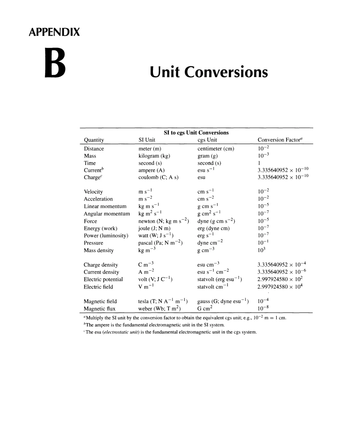
SI to cgs Unit Conversions
cgs Unit
centimeter (cm)
gram (g)
second (s)
esu s-l
Conversion Factofl
10- 2
10- 3
1
3.335640952 x 10- 10
3.335640952 X 10- 10
meter (m)
kilogram (kg)
second (s)
ampere (A)
coulomb (c; As)
esu
Velocity
Acceleration
Linear momentum
Angular momentum
Force
Energy (work)
Power (luminosity)
Pressure
Mass density
m s-l
m s-2
kg m s-l
kg m 2 s-l
newton (N; kg m s-2)
joule (J; N m)
watt (W; J s-I)
pascal (Pa; N m- 2 )
kg m- 3
10- 2
10- 2
10- 5
10- 7
10- 5
10- 7
10- 7
10- 1
10 3
cm s-1
cm s-2
g cm S-l
g cm 2 s-I
dyne (g cm s-2)
erg (dyne em)
erg s-l
dyne cm- 2
g cm- 3
Charge densi ty
Current densi ty
Electric potential
Electric field
cm- 3
Am- 2
volt (V; J c- I )
V m- I
3.335640952 X 10- 4
3.335640952 X 10- 6
2.997924580 X 10 2
2.997924580 X 10 4
esu cm- 3
esu s-l cm- 2
statvolt (erg esu -I )
statvolt cm- I
.
Magnetic field tesla (T; N A -I m -I ) gauss (G; dyne esu -I ) 1 0- 4
Magnetic flux weber (Wb; T m 2 ) G cm 2 10- 8
aMultiply the SI unit by the conversion factor to obtain the equivalent cgs unit; e.g., 10- 2 m = 1 cm.
bThe ampere is the fundamental electromagnetic unit in the SI system.
(The esu (electrostatic unit) is the fundamental electromagnetic unit in the cgs system.
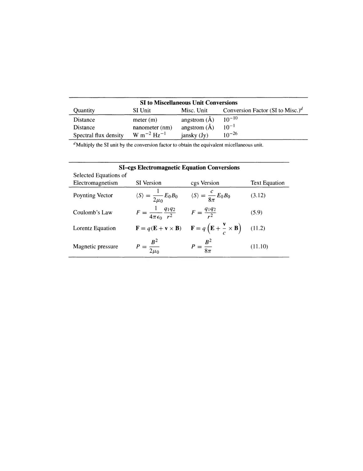
SI to Miscellaneous Unit Conversions
Quantity SI Unit Misc. Unit Conversion Factor (SI to Misc.)d
Distance meter (m) angstrom (A) 10- 10
Distance nanometer (nm) angstrom (A) 10- 1
S t I fl d t W m -2 Hz -l J - ansky (Jy) 10 -26
pec ra ux ensi y
dMultiply the SI unit by the conversion factor to obtain the equivalent micellaneous unit.
SI-cgs Electromagnetic Equation Conversions
Selected Equations of
Electromagnetism
Poynting Vector
SI Version
1
(5) EoBo
2JLo
F 1 q I q2
4Jr EO r 2
cgs Version
Text Equation
(5)
e
EoBo
8Jr
qlq2
r 2
(3.12)
Coulomb's Law
F
(5.9)
Lorentz Equation
F q(E+vxB)
F
v
q E+ - x B
e
( 11.2)
Magnetic pressure
B 2
P
2JLO
p
B 2
8Jr
( 11.1 0)
San Francisco Boston New York
Cape Town Hong Kong London Madrid Mexico City
Montreal Munich Paris Singapore Sydney Tokyo Toronto
econ E ition
Bradley W. Carroll
Weber State University
Dale A. 05tl ie
Weber State University
Editor-in-Chief: Adam R. S. Black
Senior Acquisitions Editor: Lothl6rien Hornet
Assistant Editor: Deb Greco
Editorial Assistant: Ashley Taylor Anderson
Executive Marketing Manager: Christy Lawrence
Managing Editor: Corinne Benson
Production Supervisor: Shannon Tozier
Manufacturing Manager: Stacey Weinberger
Project Management and Composition: Techsetters, Inc.
Illustration: Techsetters, Inc.
Cover Illustration: Kenneth Xavier Probst
Cover Design: Seventeenth Street Studios
Text Printer: R. R. Donnelley, Crawfordsville
Cover Printer: Phoenix Color
If you purchased this book within the United States or Canada you should be aware that it has been
wrongfully imported without the approval of the Publisher or the Author.
ISBN 0-321-44284-9
Copyright @ 2007 Pearson Education, Inc., publishing as Addison-Wesley, 1301 Sansome St., San
Francisco, CA 94111. All rights reserved. Manufactured in the United States of America. This
publication is protected by Copyright and permission should be obtained from the publisher prior to
any prohibited reproduction, storage in a retrieval system, or transmission in any form or by any
means, electronic, mechanical, photocopying, recording, or likewise. To obtain permission(s) to use
material from this work, please submit a written request to Pearson Education, Inc., Permissions
Department, 1900 E. Lake Ave., Glenview, IL 60025. For information regarding permissions, call
(847) 486-2635.
Many of the designations used by manufacturers and sellers to distinguish their products are
claimed as trademarks. Where those designations appear in this book, and the publisher was aware
of a trademark claim, the designations have been printed in initial caps or all caps.
2 3 4 5 6 7 8 9 1 0 DOC 0 9 08 07
www.aw-bc.com/astrophysics
For Lynn,
and
Candy, Michael, and Megan
with love
Preface
Since the first edition of An Introduction to Modern Astrophysics and its abbreviated com-
panion text, An Introduction to Modern Stellar Astrophysics, first appeared in 1996, there
has been an incredible explosion in our knowledge of the heavens. It was just two months
before the printing of the first editions that Michel Mayor and Didier Queloz announced
the discovery of an extrasolar planet around 51 Pegasi, the first planet found orbiting a
main-sequence star. In the next eleven years, the number of known extrasolar planets has
grown to over 193. Not only do these discoveries shed new light on how stars and planetary
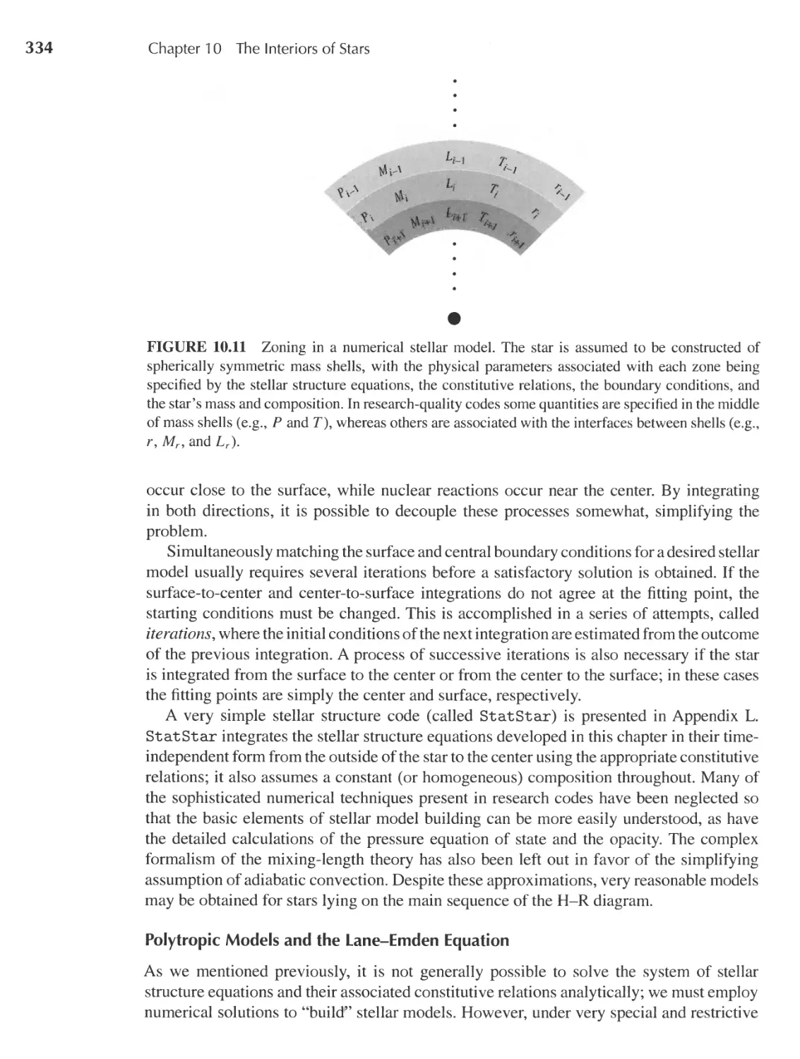
systems form, but they also inform us about formation and planetary evolution in our own
Solar System.
In addition, within the past decade important discoveries have been made of objects,
within our Solar System but beyond Pluto, that are similar in size to that diminutive planet.
In fact, one of the newly discovered Kuiper belt objects, currently referred to as 2003 UB313
(until the International Astronomical Union makes an official determination), appears to be
larger than Pluto, challenging our definition of what a planet is and how many planets our
Solar System is home to.
Explorations by robotic spacecraft and landers throughout our Solar System have also
yielded a tremendous amount of new information about our celestial neighborhood. The
armada of orbiters, along with the remarkable rovers, Spirit and Opportunity, have confirmed
that liquid water has existed on the surface of Mars in the past. We have also had robotic
emissaries visit Jupiter and Saturn, touch down on the surfaces of Titan and asteroids, crash
into cometary nuclei, and even return cometary dust to Earth.
Missions such as Swift have enabled us to close in on the solutions to the mysterious
gamma-ray bursts that were such an enigma at the time An Introduction to Modern Astro-
physics first appeared. We now know that one class of gamma-ray bursts is associated with
core-collapse supernovae and that the other class is probably associated with the merger of
two neutron stars, or a neutron star and a black hole, in a binary system.
Remarkably precise observations of the center of our Milky Way Galaxy and other
galaxies, since the publication of the first editions, have revealed that a great many, perhaps
most, spiral and large elliptical galaxies are home to one or more supermassive black holes
at their centers. It also appears likely that galactic mergers help to grow these monsters in
their centers. Furthermore, it now seems almost certain that supermassive black holes are the
central engines responsible for the exotic and remarkably energetic phenomena associated
with radio galaxies, Seyfert galaxies, blazars, and quasars.
The past decade has also witnessed the startling discovery that the expansion of the uni-
verse is not slowing down but, rather, is actually accelerating! This remarkable observation
suggests that we currently live in a dark-energy-dominated universe, in which Einstein's
vi
Preface
cosmological constant (once considered his "greatest blunder") plays an important role
in our understanding of cosmology. Dark energy was not even imagined in cosmological
models at the time the first editions were published.
Indeed, since the publication of the first editions, cosmology has entered into a new era of
precision measurements. With the release of the remarkable data obtained by the Wilkinson
Microwave Anisotropy Probe (WMAP), previously large uncertainties in the age of the
universe have been reduced to less than 2% (13.7:1: 0.2 Gyr). At the same time, stellar
evolution theory and observations have led to the determination that the ages of the oldest
globular clusters are in full agreement with the upper limit of the age of the universe.
We opened the preface to the first editions with the sentence ''There has never been
a more exciting time to study modem astrophysics"; this has certainly been borne out in
the tremendous advances that have occurred over the past decade. It is also clear that this
incredible decade of discovery is only a prelude to further advances to come. Joining the
Hubble Space Telescope in its high-resolution study of the heavens have been the Chandra
X-ray Observatory and the Spitzer Infrared Space Telescope. From the ground, 8-m and
larger telescopes have also joined the search for new information about our remarkable
universe. Tremendously ambitious sky surveys have generated a previously unimagined
wealth of data that provide critically important statistical data sets; the Sloan Digital Sky
Survey, the Two-Micron All Sky Survey, the 2dF redshift survey, the Hubble Deep Fields
and Ultradeep Fields, and others have become indispensable tools for hosts of studies. We
also anticipate the first observations from new observatories and spacecraft, including the
high-altitude (5000 m) Atacama Large Millimeter Array and high-precision astrometric
missions such as Gaia and SIM PlanetQuest. Of course, studies of our own Solar System
also continue; just the day before this preface was written, the Mars Recounaissance Orbiter
entered orbit around the red planet.
When the first editions were written, even the World Wide Web was in its infancy. Today
it is hard to imagine a world in which virtually any information you might want is only
a search engine and a mouse click away. With enormous data sets available online, along
with fully searchable journal and preprint archives, the ability to access critical infonnation
very rapidly has been truly revolutionary.
Needless to say, a second edition of BOB (the "Big Orange Book," as An Introduction
to Modern Astrophysics has come to be known by many students) and its associated text
is long overdue. In addition to an abbreviated version focusing on stellar astrophysics (An
Introduction to Modern Stellar Astrophysics), a second abbreviated version (An Introduction
to Modern Galactic Astrophysics and Cosmology) is being published. We are confident that
BOB and its smaller siblings will serve the needs of a range of introductory astrophysics
courses and that they will instill some of the excitement felt by the authors and hosts of
astronomers and astrophysicists worldwide.
We have switched from cgs to SI units in the second edition. Although we are personally
more comfortable quoting luminosities in ergs s-l rather than watts, our students are not.
We do not want students to feel exasperated by a new system of units during their first
encounter with the concepts of modem astrophysics. However, we have retained the natural
units of parsecs and solar units (Mo and La) because they provide a comparative context
for numerical values. An appendix of unit conversions (see back endpapers) is included for
Preface
vii
those who delve into the professional literature and discover the world of angstroms, ergs,
and esu.
Our goal in writing these texts was to open the entire field of modem astrophysics to
you by using only the basic tools of physics. Nothing is more satisfying than appreciating
the drama of the universe through an understanding of its underlying physical principles.
The advantages of a mathematical approach to understanding the heavenly spectacle were
obvious to Plato, as manifested in his Epinomis:
Are you unaware that the true astronomer must be a person of great wisdom?
Hence there will be a need for several sciences. The first and most important
is that which treats of pure numbers. To those who pursue their studies in
the proper way, all geometric constructions, all systems of numbers, all duly
constituted melodic progressions, the single ordered scheme of all celestial
revolutions should disclose themselves. And, believe me, no one will ever
behold that spectacle without the studies we have described, and so be able to
boast that they have won it by an easy route.
Now, 24 centuries later, the application of a little physics and mathematics still leads to
deep insights.
These texts were also born of the frustration we encountered while teaching our junior-
level astrophysics course. Most of the available astronomy texts seemed more descriptive
than mathematical. Students who were learning about Schrodinger's equation, partition
functions, and multipole expansions in other courses felt handicapped because their astro-
physics text did not take advantage of their physics background. It seemed a double shame to
us because a course in astrophysics offers students the unique opportunity of actually using
the physics they have learned to appreciate many of astronomy's fascinating phenomena.
Furthermore, as a discipline, astrophysics draws on virtually every aspect of physics. Thus
astrophysics gives students the chance to review and extend their knowledge.
Anyone who has had an introductory calculus-based physics course is ready to under-
stand nearly all the major concepts of modem astrophysics. The amount of modem physics
covered in such a course varies widely, so we have included a chapter on the theory of
special relativity and one on quantum physics which will provide the necessary background
in these areas. Everything else in the text is self-contained and generously cross-referenced,
so you will not lose sight of the chain of reasoning that leads to some of the most astounding
ideas in all of science. I
Although we have attempted to be fairly rigorous, we have tended to favor the sort of
back-of-the-envelope calculation that uses a simple model of the system being studied.
The payoff-to-effort ratio is so high, yielding 80% of the understanding for 20% of the
effort, that these quick calculations should be a part of every astrophysicist's toolkit. In
fact, while writing this book we were constantly surprised by the number of phenomena
that could be described in this way. Above all, we have tried to be honest with you; we
remained determined not to simplify the material beyond recognition. Stellar interiors,
1 Footnotes are used when we don't want to interrupt the main flow of a paragraph.
viii
Preface
stellar atmospheres, general relativity, and cosmology-all are described with a depth that
is more satisfying than mere hand-waving description.
Computational astrophysics is today as fundamental to the advance in our understanding
of astronomy as observation and traditional theory, and so we have developed numerous
computer problems, as well as several complete codes, that are integrated with the text
material. You can calculate your own planetary orbits, compute observed features of binary
star systems, make your own models of stars, and reproduce the gravitational interactions
between galaxies. These codes favor simplicity over sophistication for pedagogical rea-
sons; you can easily expand on the conceptually transparent codes that we have provided.
Astrophysicists have traditionally led the way in large-scale computation and visualization,
and we have tried to provide a gentle introduction to this blend of science and art.
Instructors can use these texts to create courses tailored to their particular needs by
approaching the content as an astrophysical smorgasbord. By judiciously selecting topics,
we have used BOB to teach a semester-long course in stellar astrophysics. (Of course,
much was omitted from the first 18 chapters, but the text is designed to accommodate such
surgery.) Interested students have then gone on to take an additional course in cosmology.
On the other hand, using the entire text would nicely fill a year-long survey course (and then
some) covering all of modem astrophysics. To facilitate the selection of topics, as well as
identify important topics within sections, we have added subsection headings to the second
editions. Instructors may choose to skim, or even omit, subsections in accordance with their
own as well as their students' interests-and thereby design a course to their liking.
An extensive website at http://www.aw-bc.com/astrophysics is associated with
these texts. It contains downloadable versions of the computer codes in various languages,
including Fortran, C++, and, in some cases, Java. There are also links to some of the
many important websites in astronomy. In addition, links are provided to public domain
images found in the texts, as well as to line art that can be used for instructor presentations.
Instructors may also obtain a detailed solutions manual directly from the publisher.
Throughout the process of the extensive revisions for the second editions, our editors have
maintained a positive and supportive attitude that has sustained us throughout. Although we
must have sorely tried their patience, Adam R. S. Black, Lothl6rien Hornet, Ashley Taylor
Anderson, Deb Greco, Stacie Kent, Shannon Tozier, and Carol Sawyer (at Techsetters) have
been truly wonderful to work with.
We have certainly been fortunate in our professional associations throughout the years.
We want to express our gratitude and appreciation to Art Cox, John Cox (1926-1984),
Carl Hansen, Hugh Van Horn, and Lee Anne Willson, whose profound influence on us has
remained and, we hope, shines through the pages ahead.
Our good fortune has been extended to include the many expert reviewers who cast
a merciless eye on our chapters and gave us invaluable advice on how to improve them.
For their careful reading of the first editions, we owe a great debt to Robert Antonucci,
Martin Burkhead, Peter Foukal, David Friend, Carl Hansen, H. Lawrence Helfer, Steven
D. Kawaler, William Keel, J. Ward Moody, Tobias Owen, Judith Pipher, Lawrence Pinsky,
Joseph Silk, J. Allyn Smith, and Rosemary Wyse. Additionally, the extensive revisions to
the second editions have been carefully reviewed by Bryon D. Anderson, Markus J. As-
chwanden, Andrew Blain, Donald J. Bord, Jean-Pierre Caillault, Richard Crowe, Manfred
A. Cuntz, Daniel Dale, Constantine Deliyannis, Kathy DeGioia Eastwood, J. C. Evans,
Preface
.
IX
Debra Fischer, Kim Griest, Triston Guillot, Fred Hamann, Jason Harlow, Peter Hauschildt,
Lynne A. Hillenbrand, Philip Hughes, William H. Ingham, David J ewitt, Steven D. Kawaler,
John Kielkopf, Jeremy King, John Kolena, Matthew Lister, Donald G. Luttermoser, Geoff
Marcy, Norman Markworth, Pedro Marronetti, C. R. O'Dell, Frederik Paerels, Eric S. Perl-
man, Bradley M. Peterson, Slawomir Piatek, Lawrence Pinsky, Martin Pohl, Eric Preston,
Irving K. Robbins, Andrew Robinson, Gary D. Schmidt, Steven Stahler, Richard D. Sydora,
Paula Szkody, Henry Throop, Michael T. Vaughn, Dan Watson, Joel Weisberg, Gregory G
Wood, MattA. Wood, Kausar Yasmin, Andrew Youdin, Esther Zirbel, E. J. Zita, and others.
Over the past decade, we have received valuable input from users of the first-edition texts
that has shaped many of the revisions and corrections to the second editions. Several gener-
ations of students have provided us with a different and extremely valuable perspective as
well. Unfortunately, no matter how fine the sieve, some mistakes are sure to slip through,
and some arguments and derivations may be less than perfectly clear. The responsibility for
the remaining errors is entirely ours, and we invite you to submit comments and corrections
to us at our e-mail address: modastro@weber. edu.
Unfortunately, the burden of writing has not been confined to the authors but was un-
avoidably shared by family and friends. We wish to thank our parents, Wayne and Marjorie
Carroll, and Dean and Dorothy Ostlie, for raising us to be intellectual explorers of this fas-
cinating universe. Finally, it is to those people who make our universe so wondrous that we
dedicate this book: our wives, Lynn Carroll and Candy Ostlie, and Dale's terrific children,
Michael and Megan. Without their love, patience, encouragement, and constant support,
this project would never have been completed.
And now it is time to get up into Utah's beautiful mountains for some skiing, hiking,
mountain biking, fishing, and camping and share those down-to-Earth joys with our families!
Bradley W. Carroll
Dale A. Ostlie
Weber State University
Ogden, UT
modastro@weber.edu
I
Preface
v
I THE TOOLS OF ASTRONOMY
1
1 _ The Celestial Sphere
1.1 The Greek Tradition 2
1.2 The Copernican Revolution 5
1.3 Positions on the Celestial Sphere 8
1.4 Physics and Astronomy 19
2
2 _ Celestial Mechanics
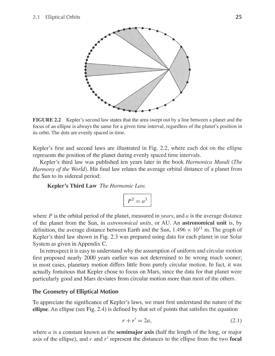
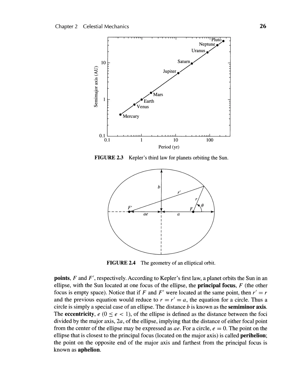
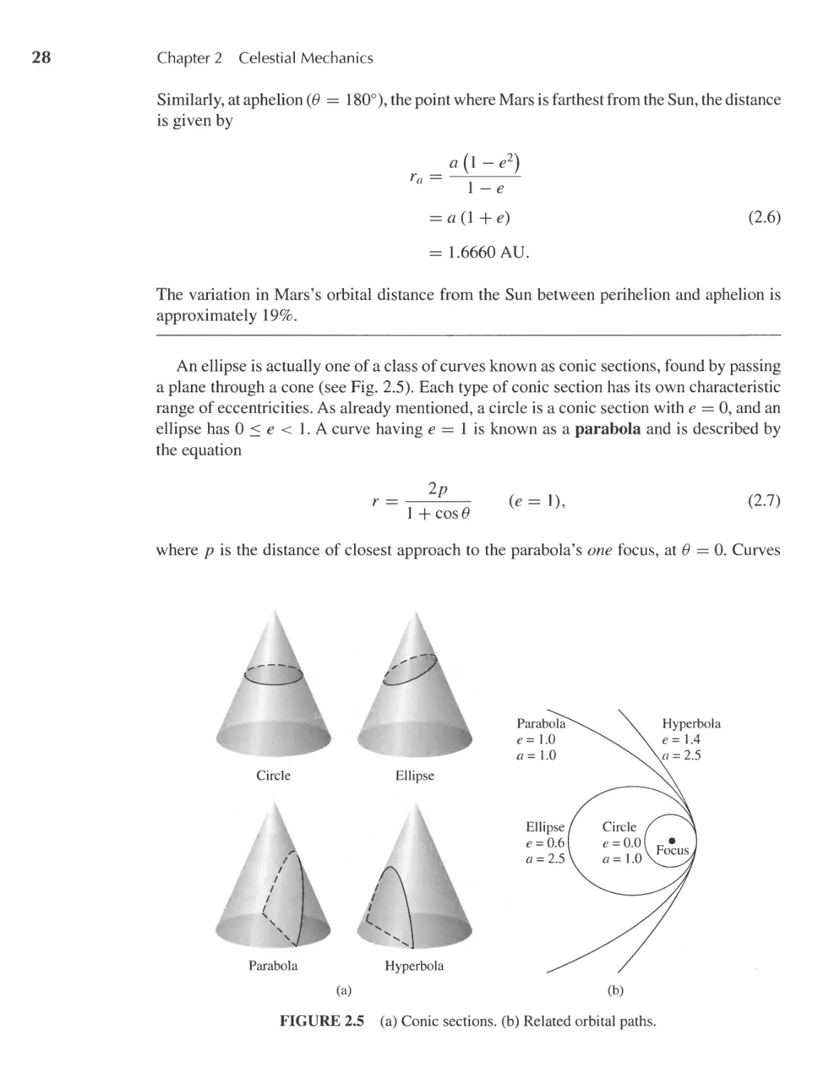
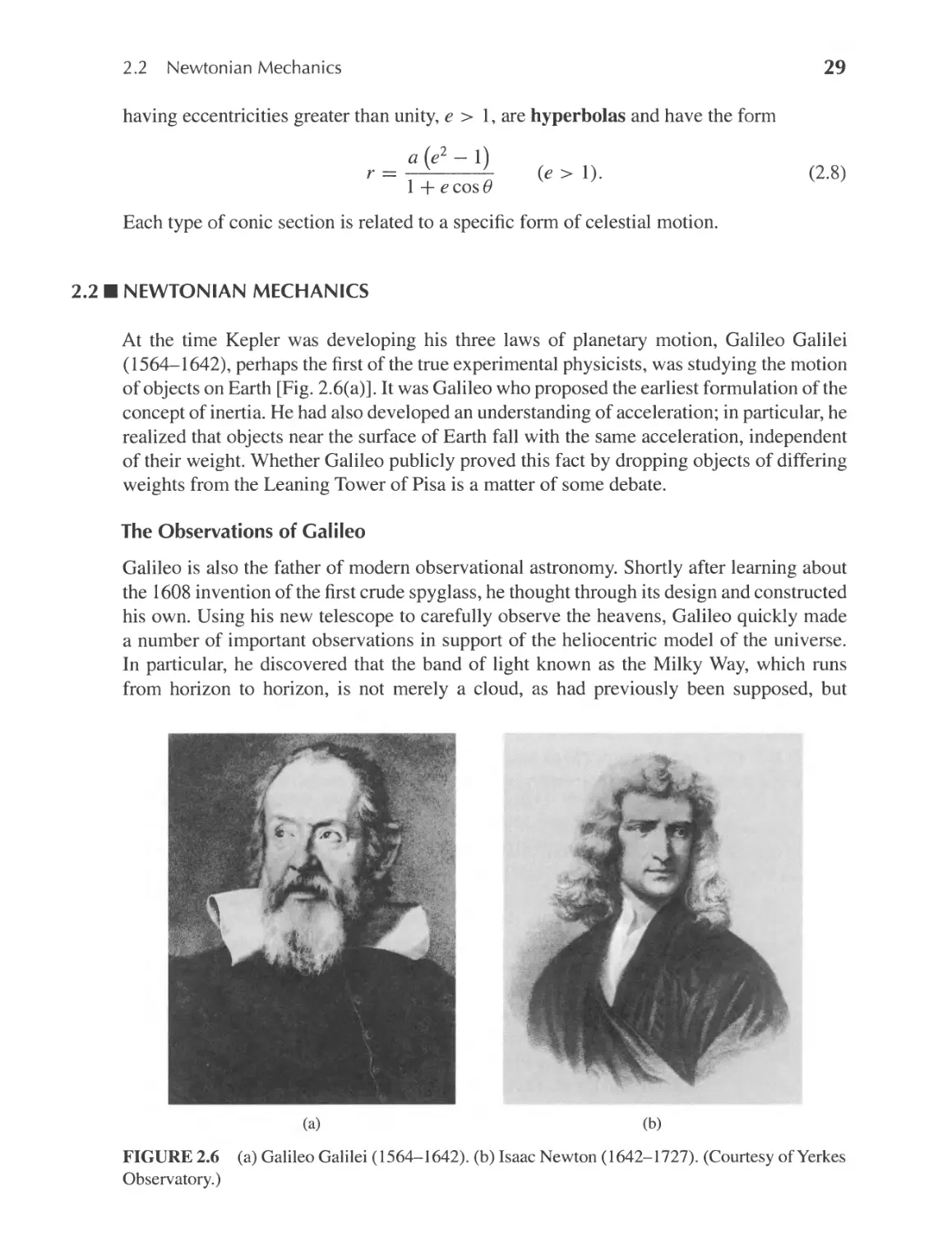
2.1 Elliptical Orbits 23
2.2 Newtonian Mechanics 29
2.3 Kepler's Laws Derived 39
2.4 The Virial Theorem 50
23
3 - The Continuous Spectrum of Light
3.1 Stellar Parallax 57
3.2 The Magnitude Scale 60
3.3 The Wave Nature of Light 63
3.4 Blackbody Radiation 68
3.5 The Quantization of Energy 71
3.6 The Color Index 75
57
4 _ The Theory of Special Relativity
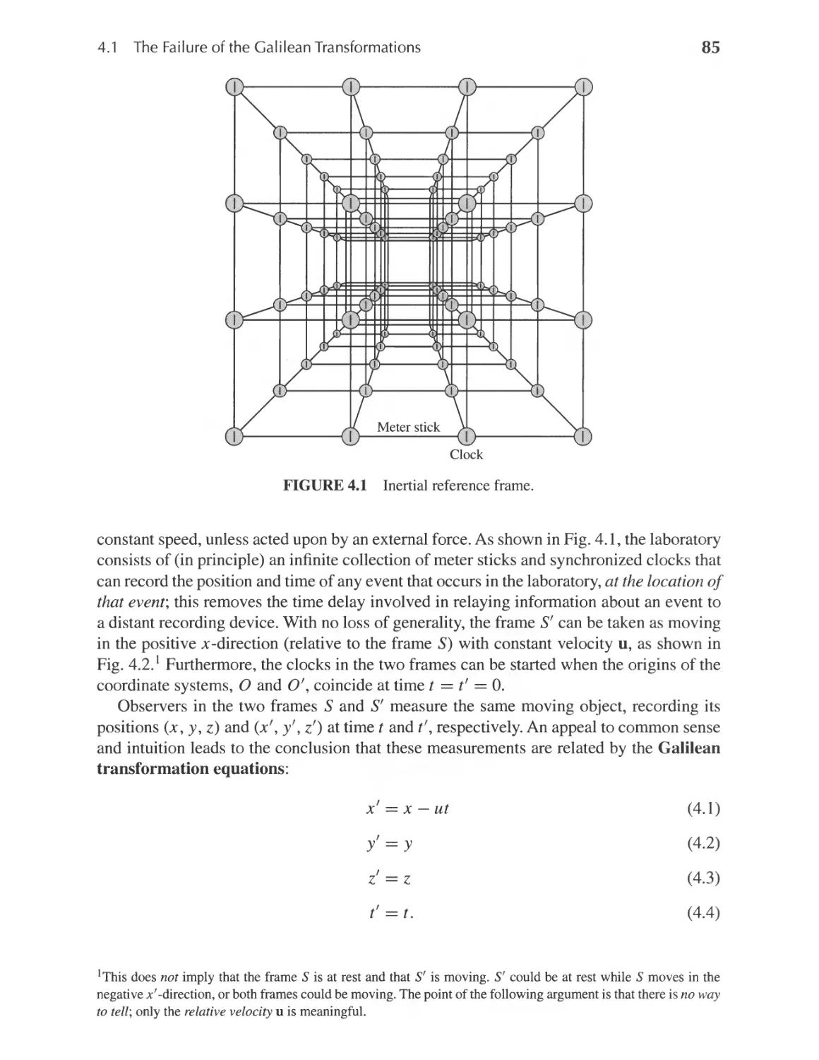
4.1 The Failure of the Galilean Transformations 84
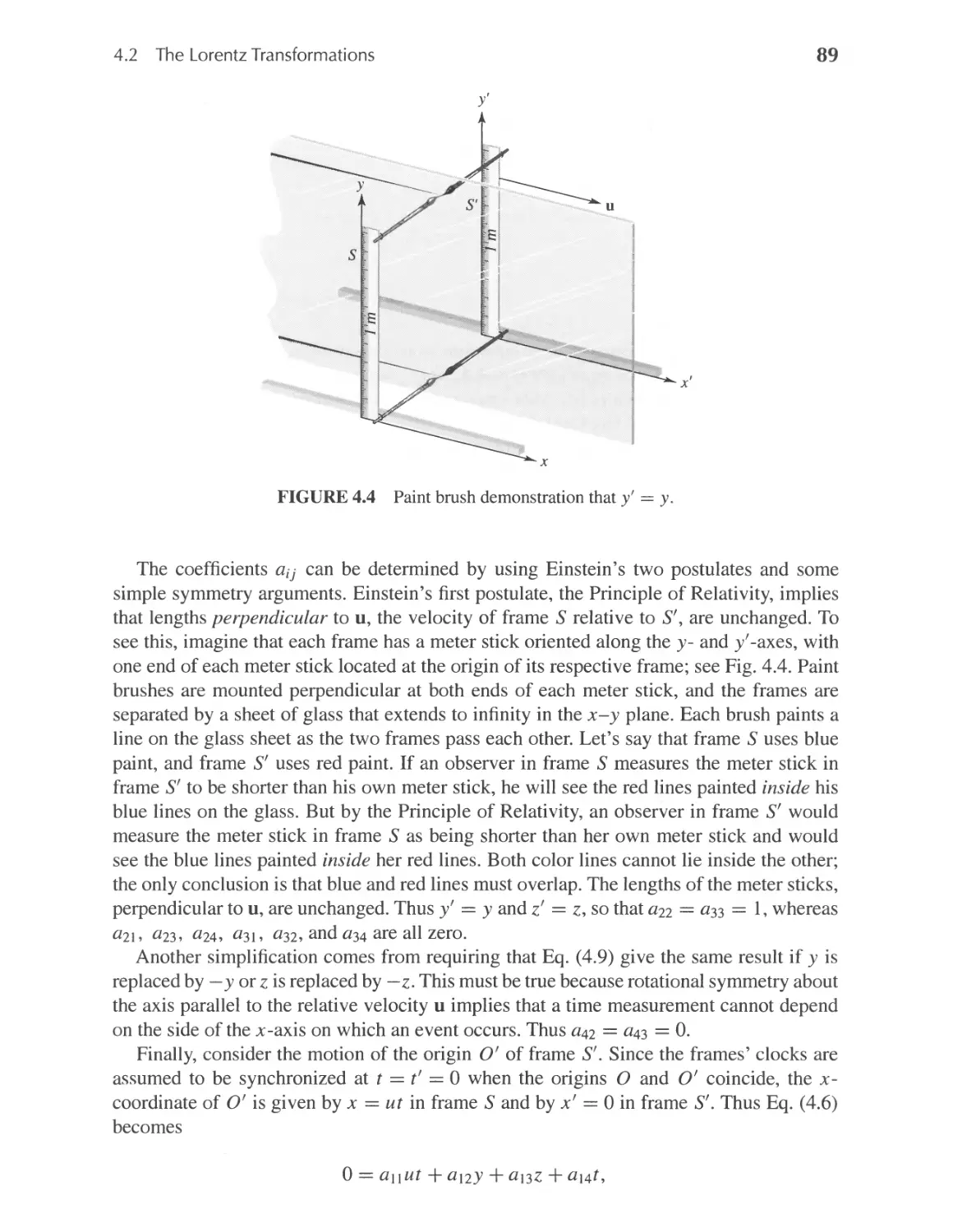
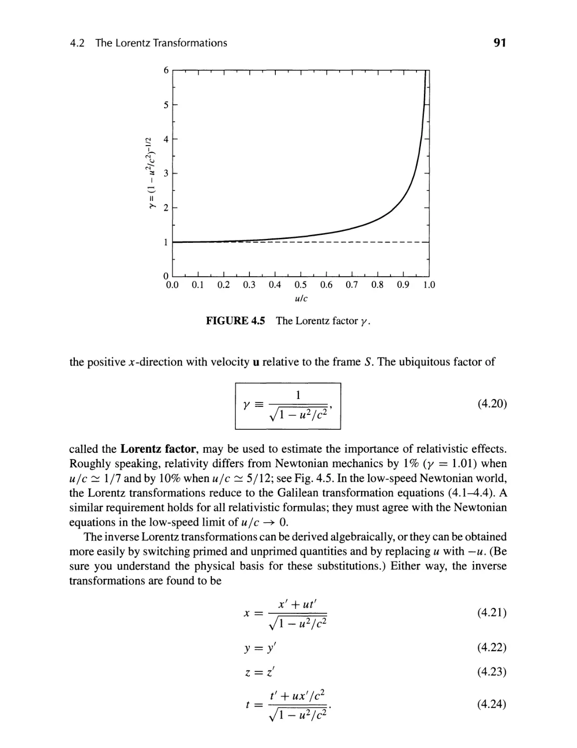
4.2 The Lorentz Transformations 87
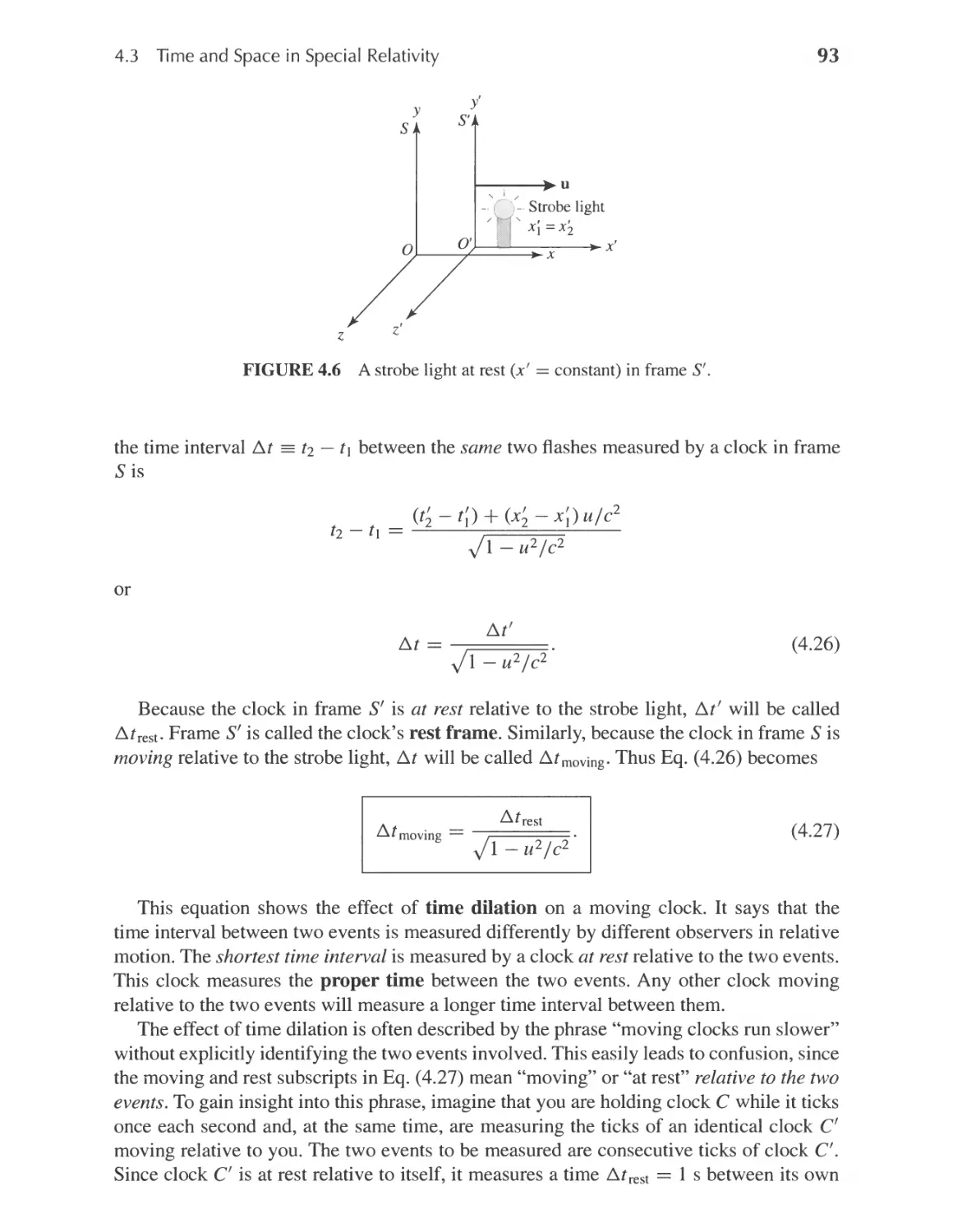
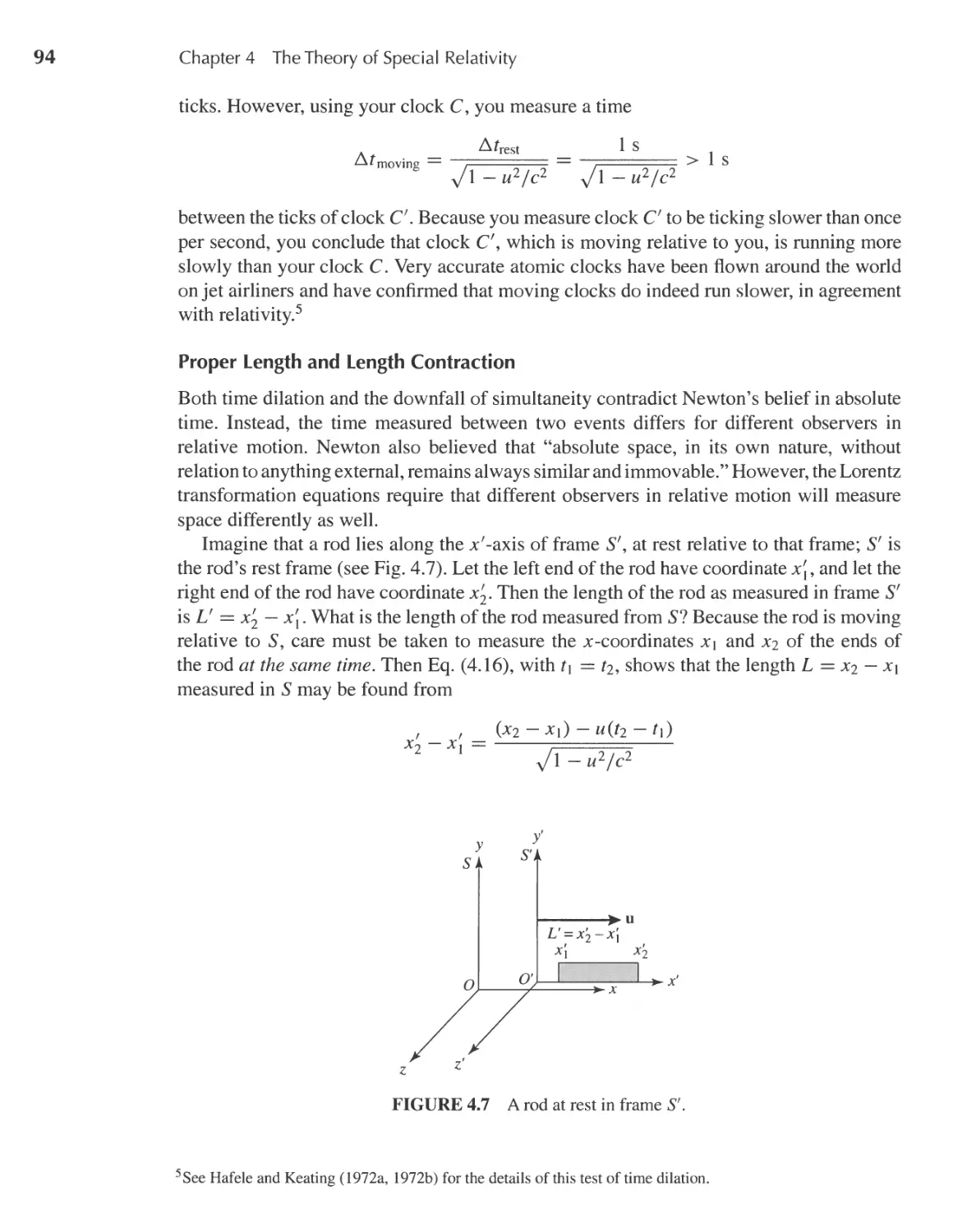
4.3 Time and Space in Special Relativity 92
4.4 Relativistic Momentum and Energy 102
84
.
XI
XII
Contents
5 _ The Interaction of Light and Matter
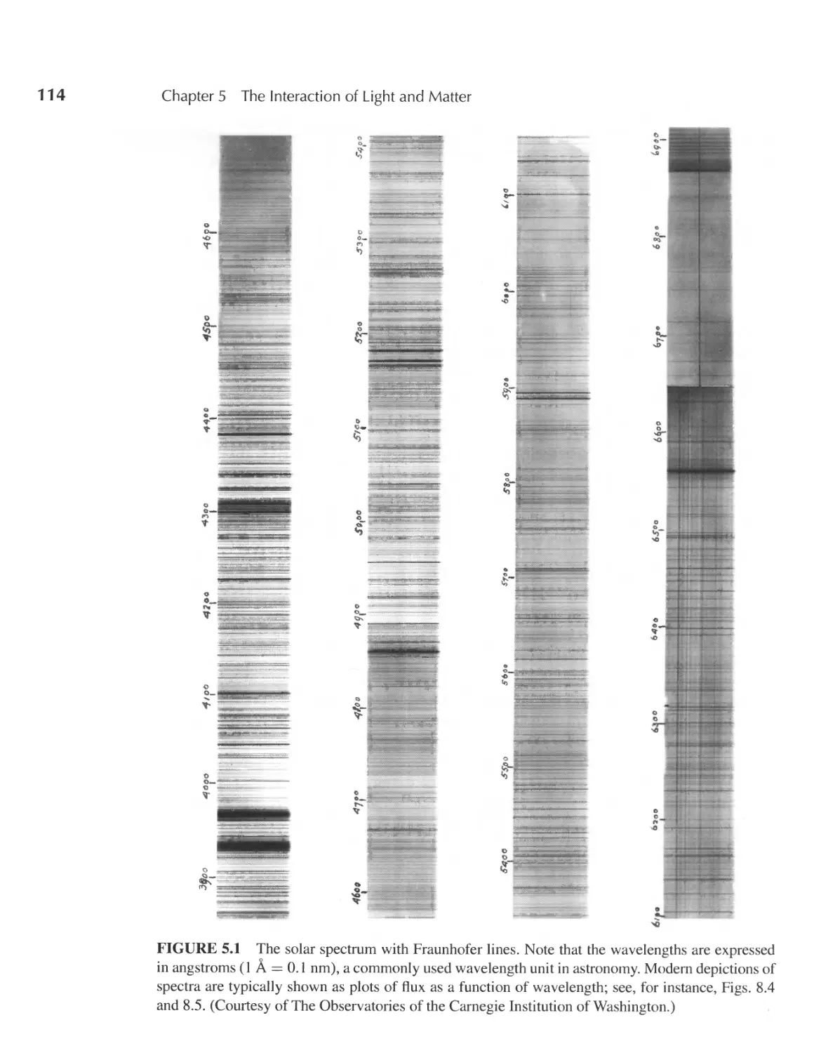
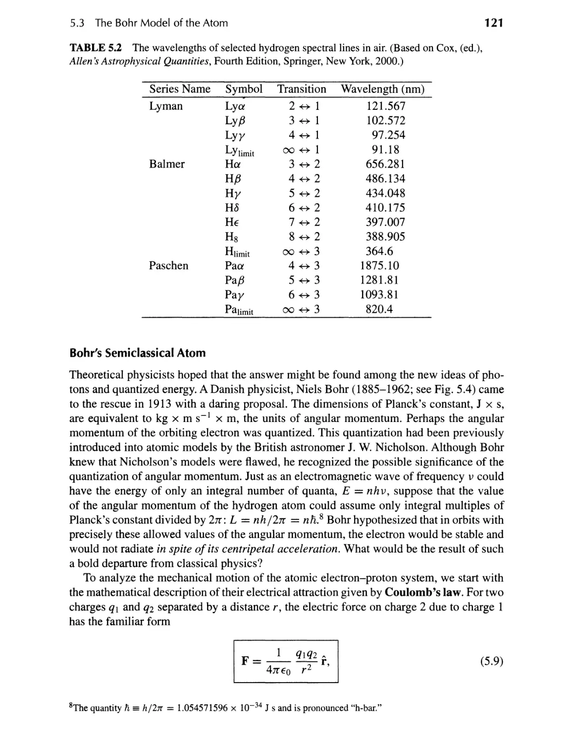
5.1 Spectral Lines 111
5.2 Photons 116
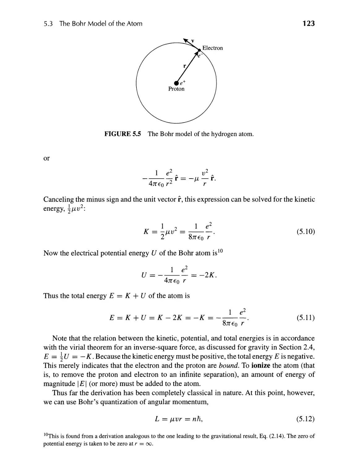
5.3 The Bohr Model of the Atom 119
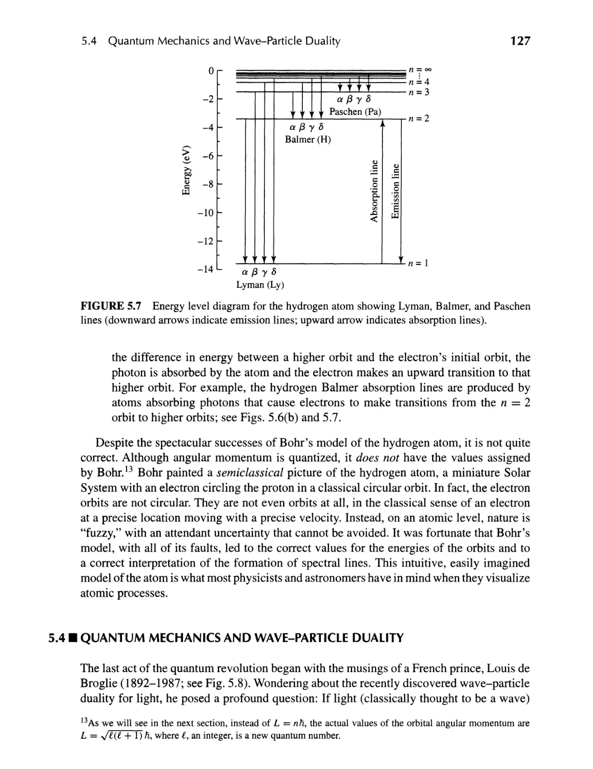
5.4 Quantum Mechanics and Wave Particle Duality 127
111
6 _ Telescopes
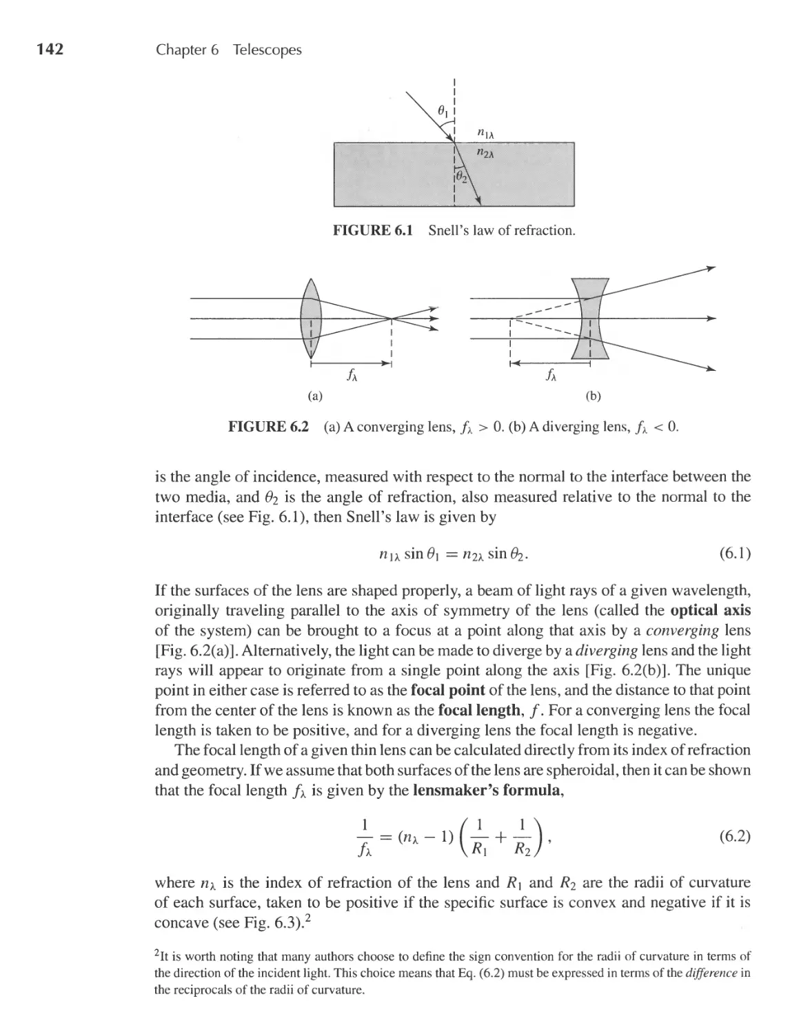
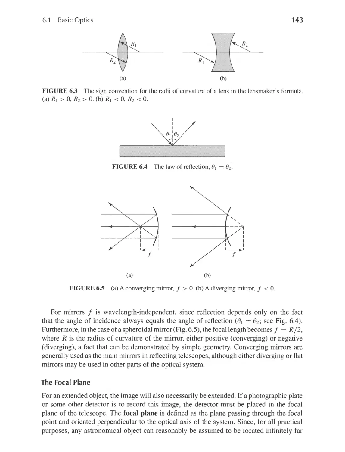
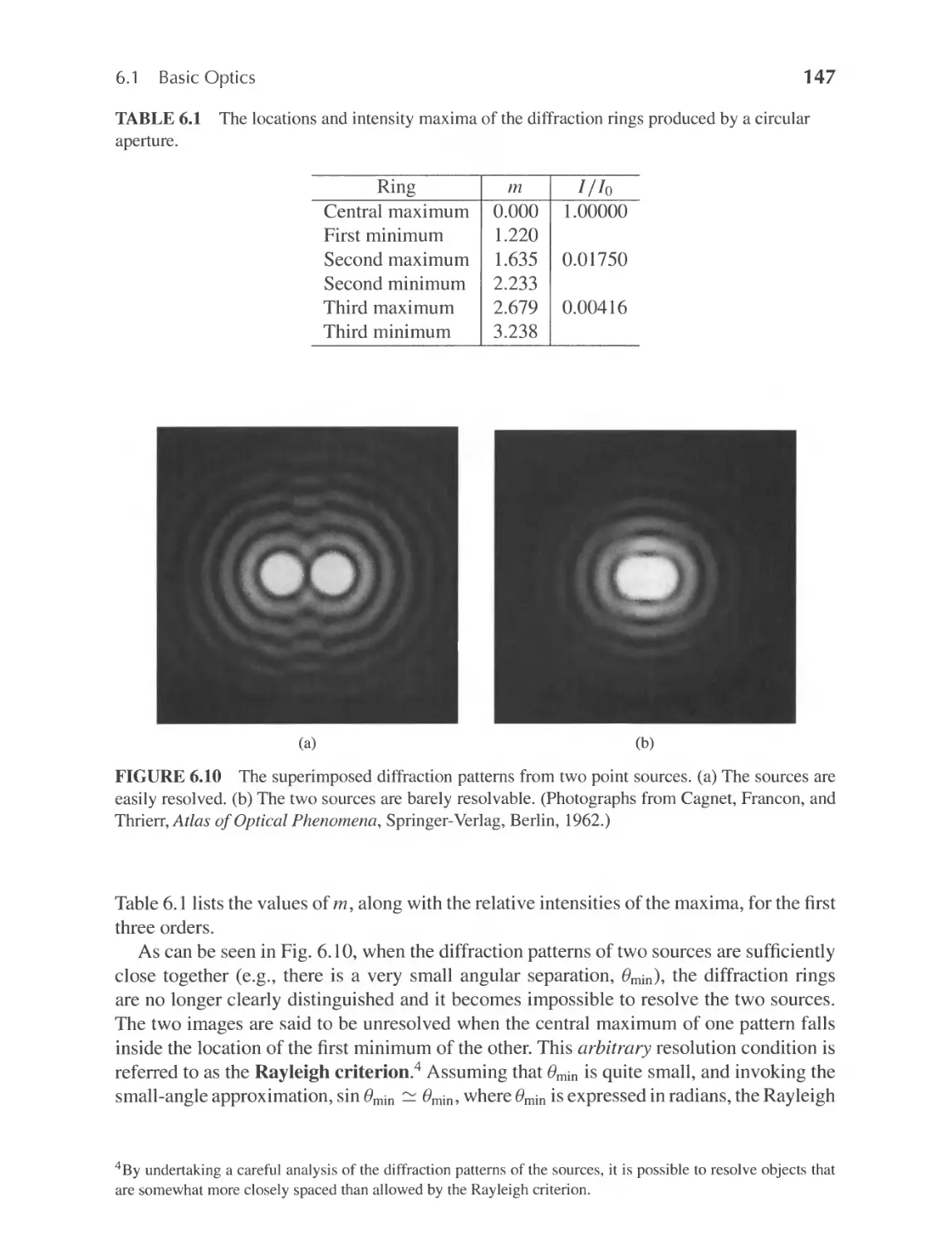
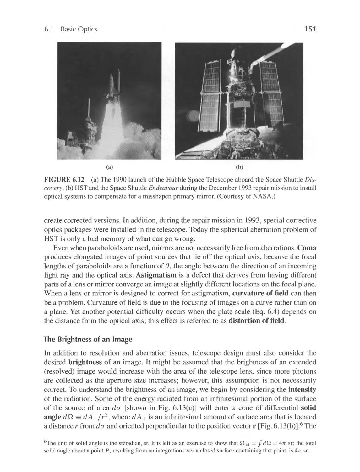
6.1 Basic Optics 141
6.2 Optical Telescopes 154
6.3 Radio Telescopes 161
6.4 Infrared, Ultraviolet, X-ray, and Gamma-Ray Astronomy 167
6.5 All-Sky Surveys and Virtual Observatories 170
141
II THE NATURE OF STARS
179
7 _ Binary Systems and Stellar Parameters
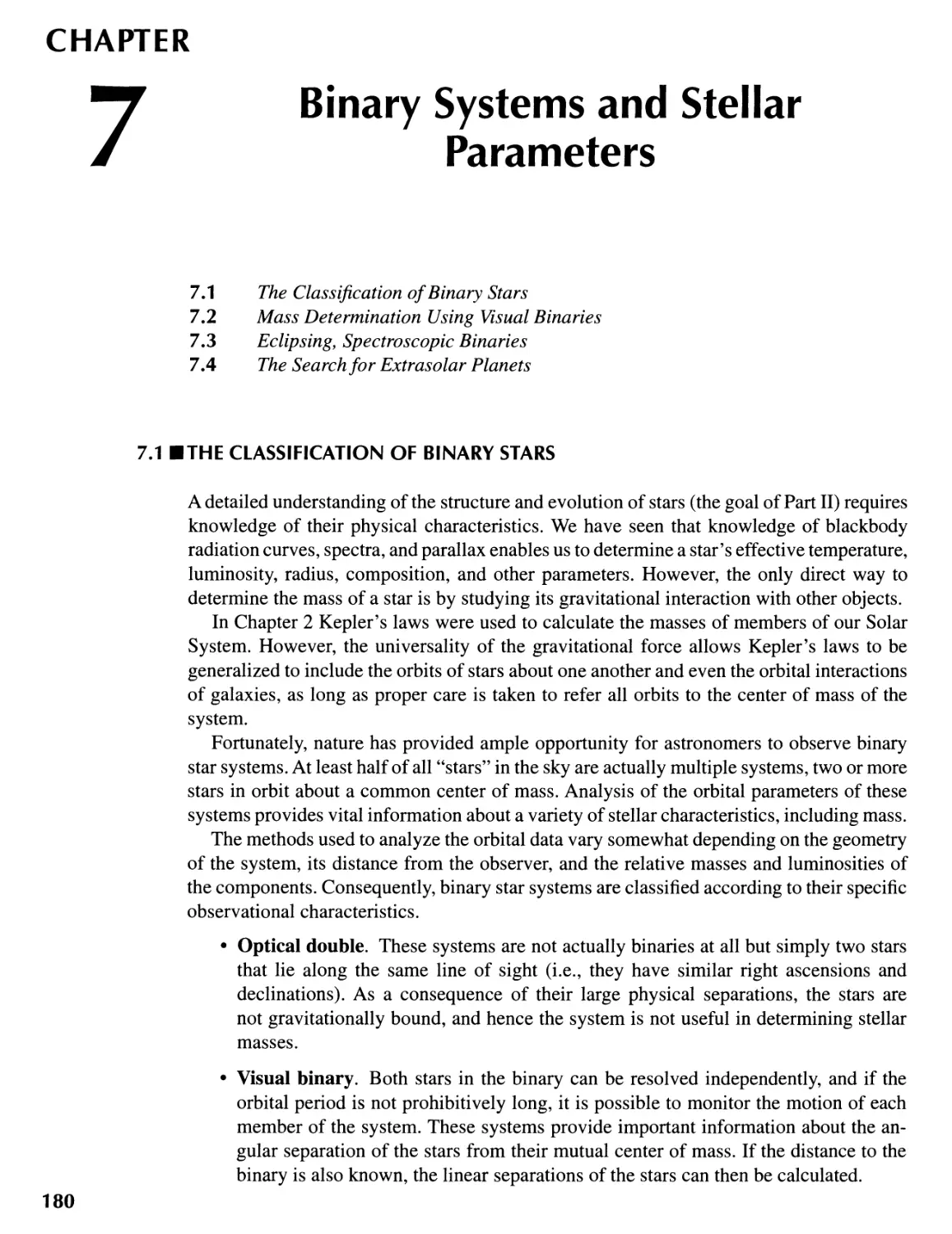
7 .1 The Classification of Binary Stars 180
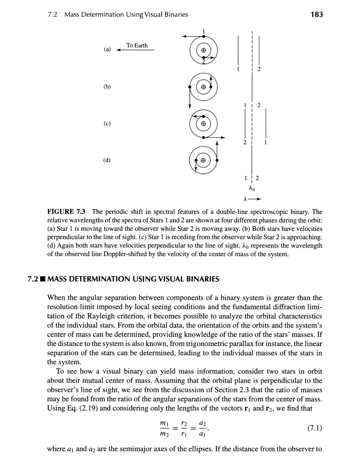
7 .2 Mass Determination Using Visual Binaries 183
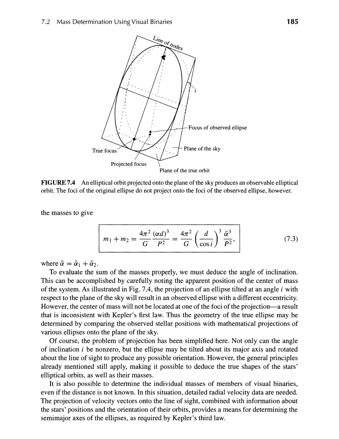
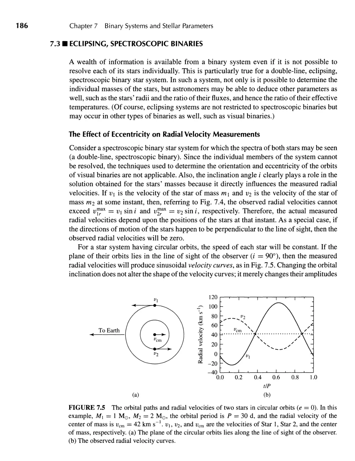
7 .3 Eclipsing, Spectroscopic Binaries 186
7.4 The Search for Extrasolar Planets 195
180
8 _ The Classification of Stellar Spectra
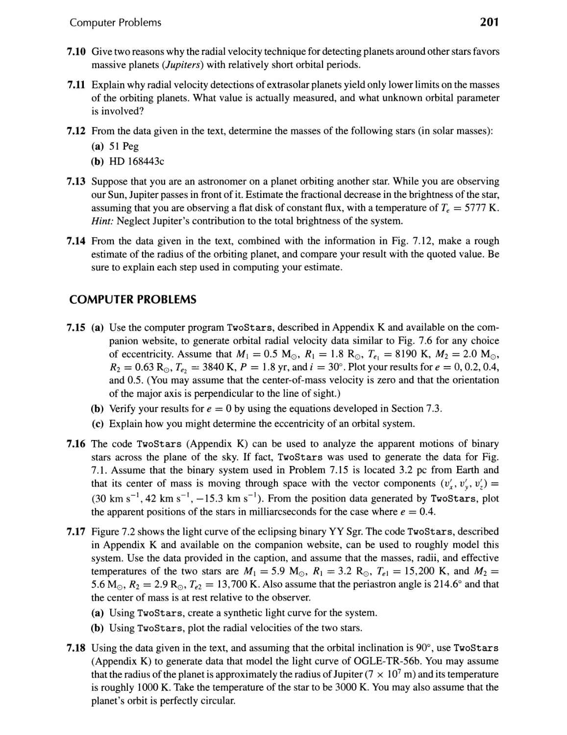
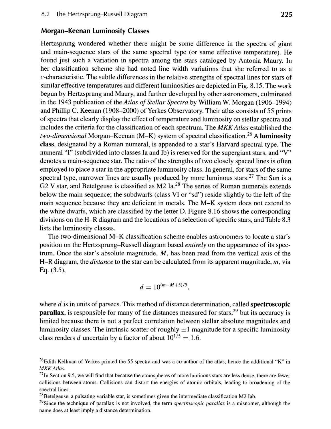
8.1 The Formation of Spectral Lines 202
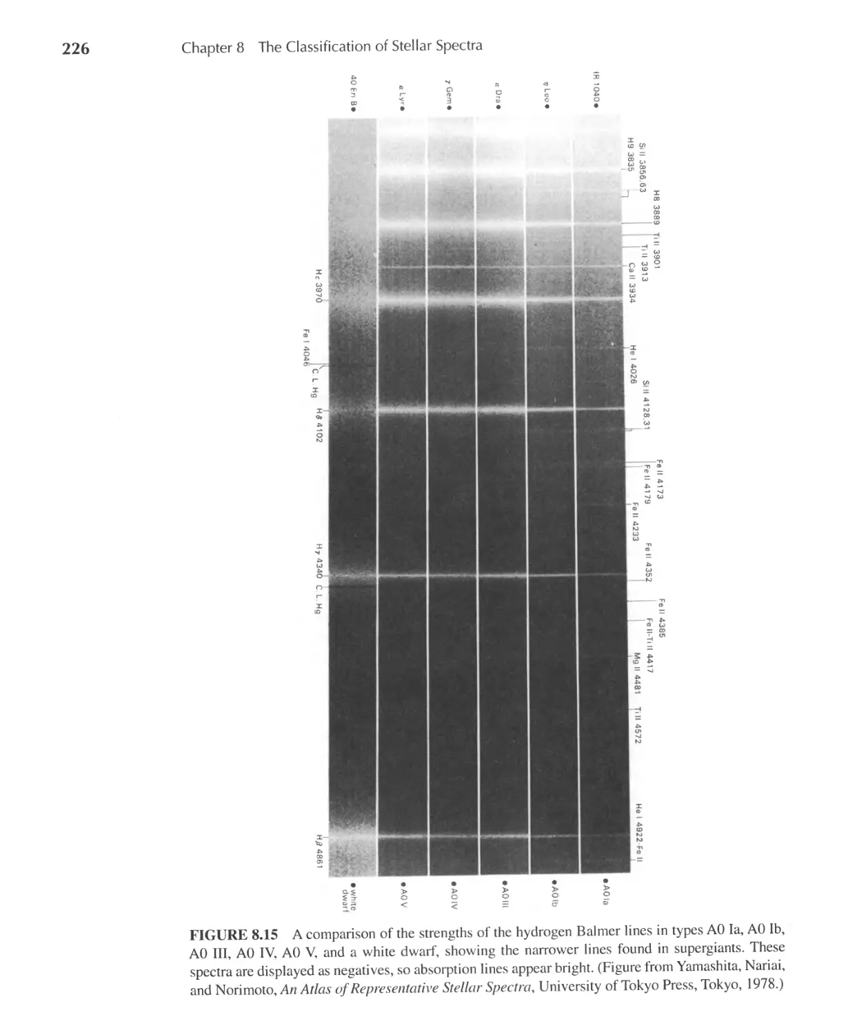
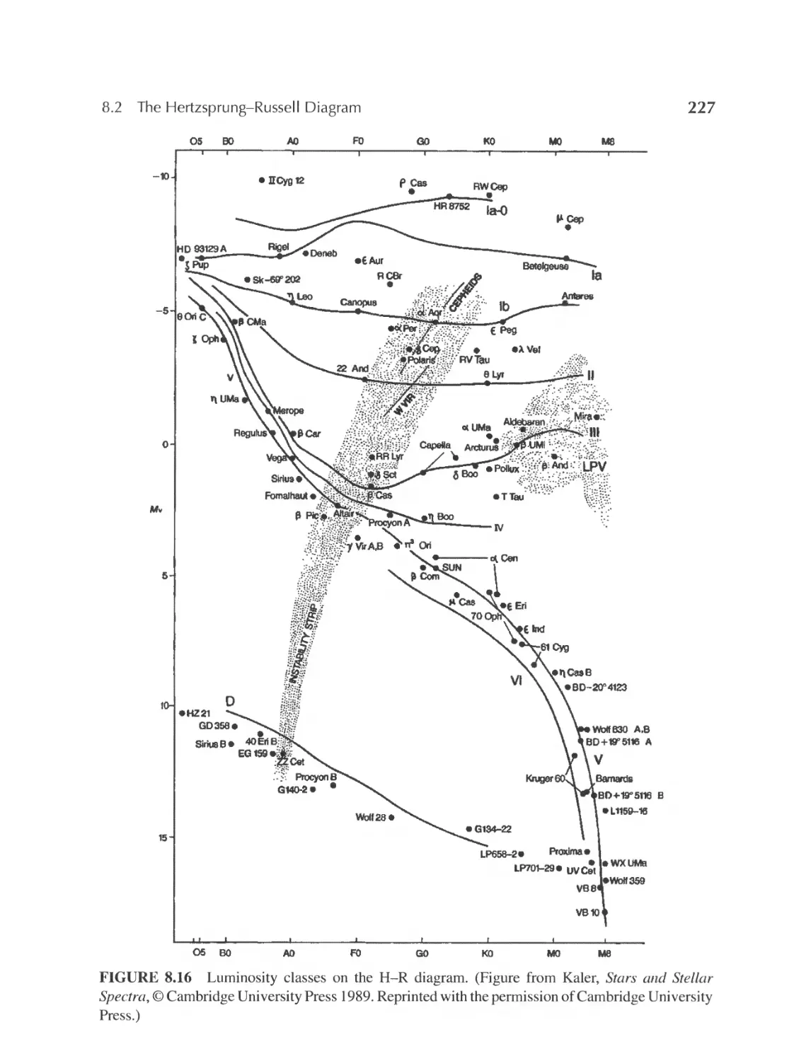
8.2 The Hertzsprung Russell Diagram 219
202
9 _ Stellar Atmospheres
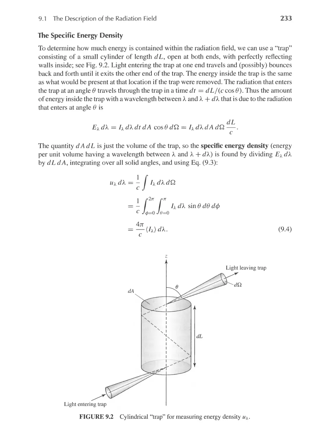
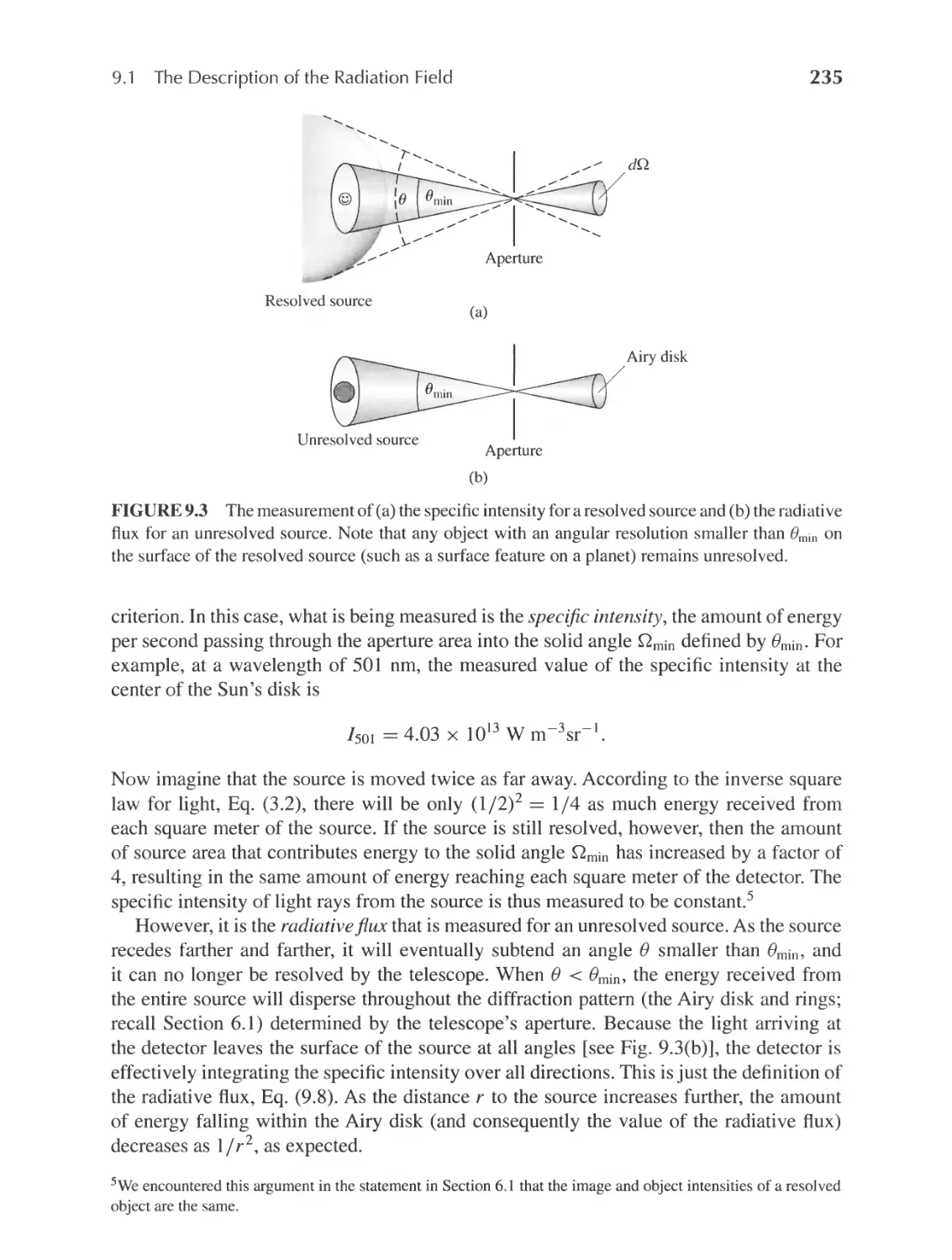
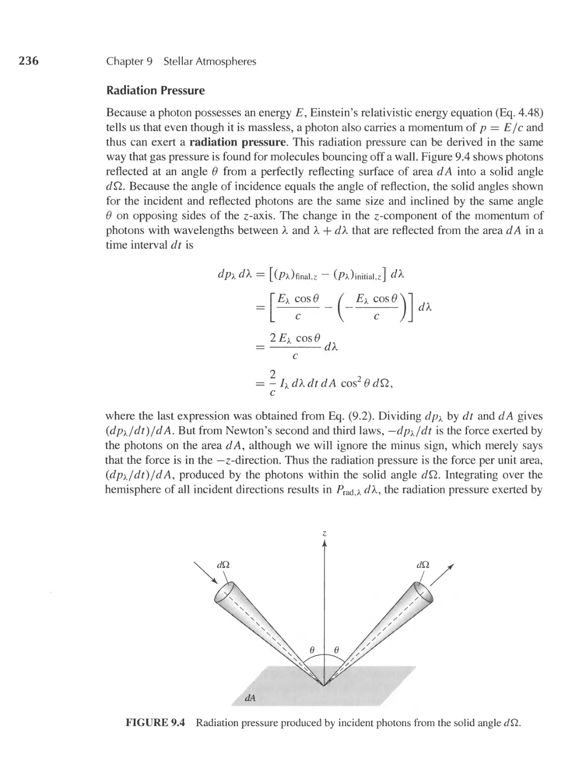
9.1 The Description of the Radiation Field 231
9.2 Stellar Opacity 238
9.3 Radiative Transfer 251
9.4 The Transfer Equation 255
9.5 The Profiles of Spectral Lines 267
231
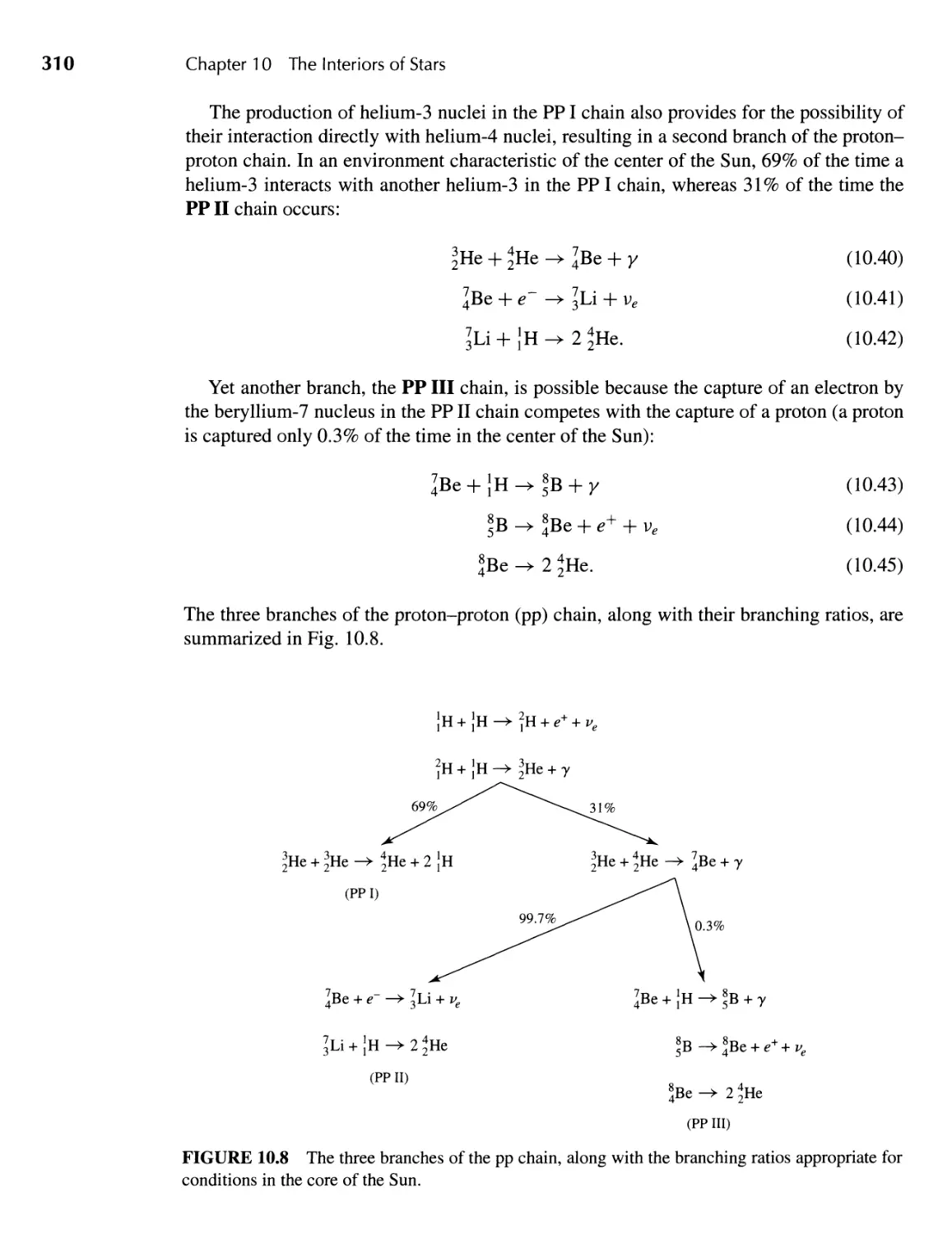
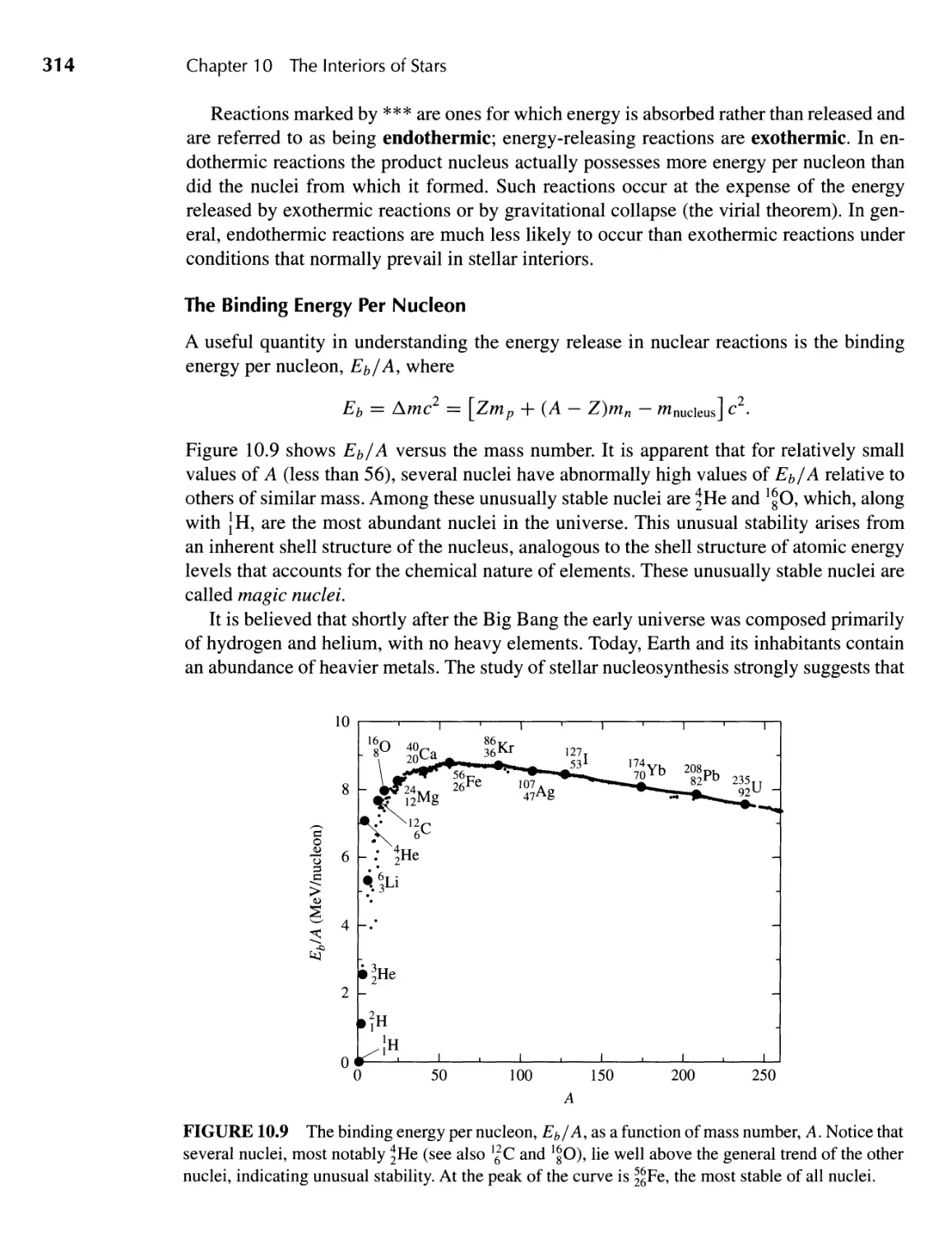
1 0 _ The Interiors of Stars
10.1 Hydrostatic Equilibrium 284
10.2 Pressure Equation of State 288
1 0.3 Stellar Energy Sources 296
1 0.4 Energy Transport and Thermodynamics 315
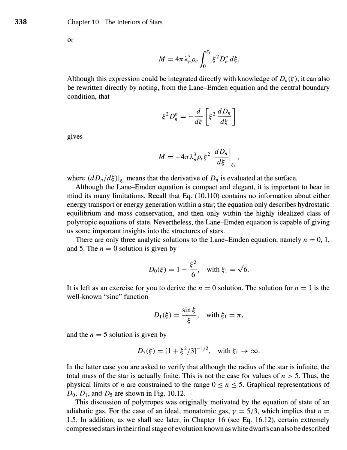
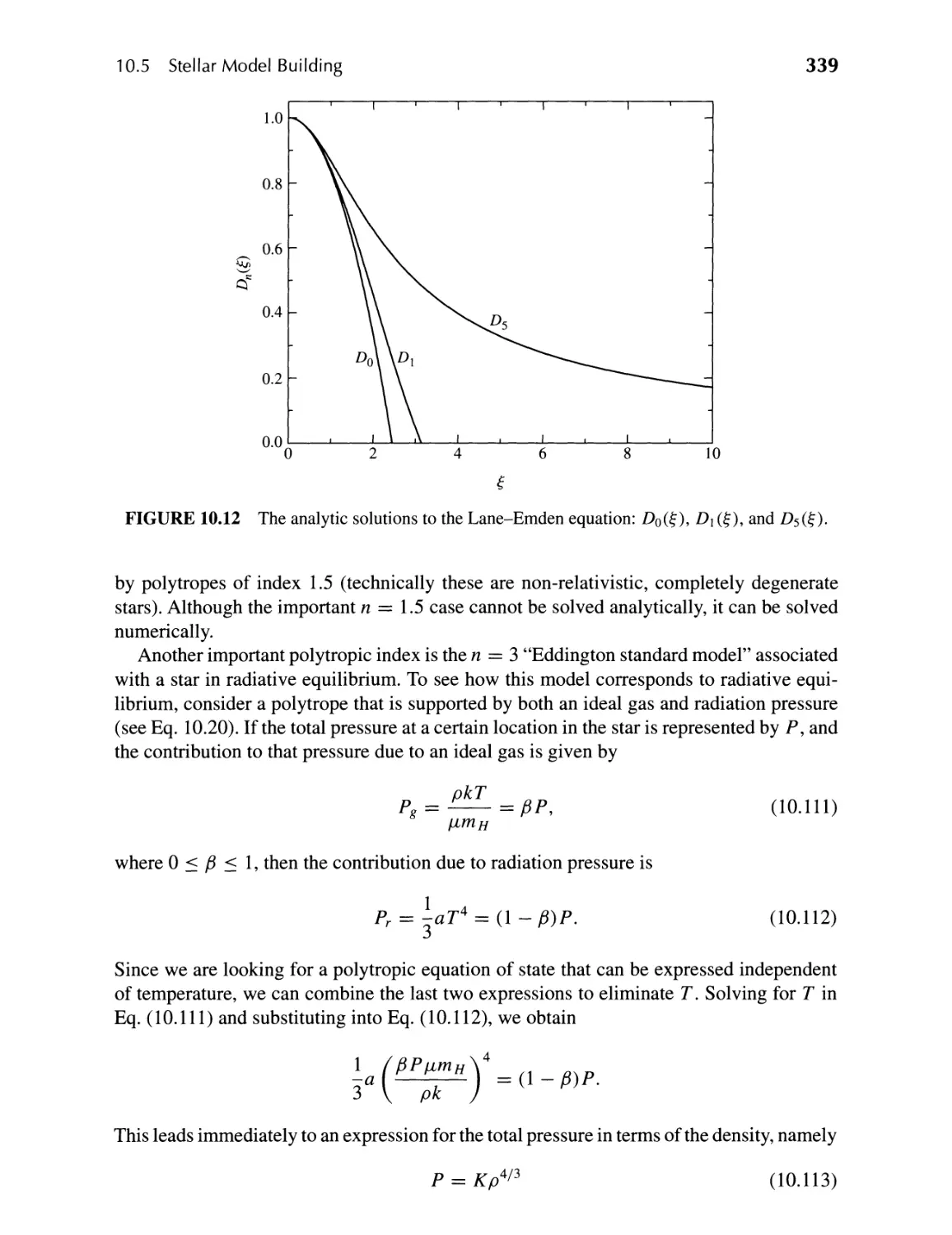
10.5 Stellar Model Building 329
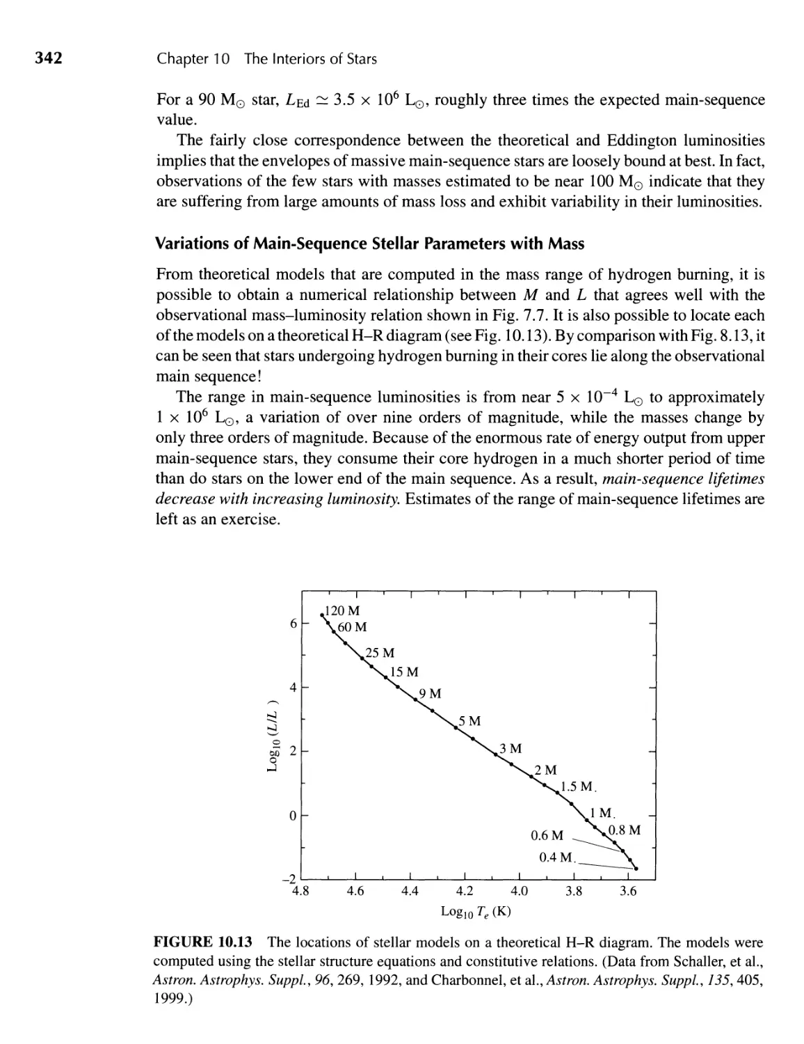
10.6 The Main Sequence 340
284
Contents
...
XIII
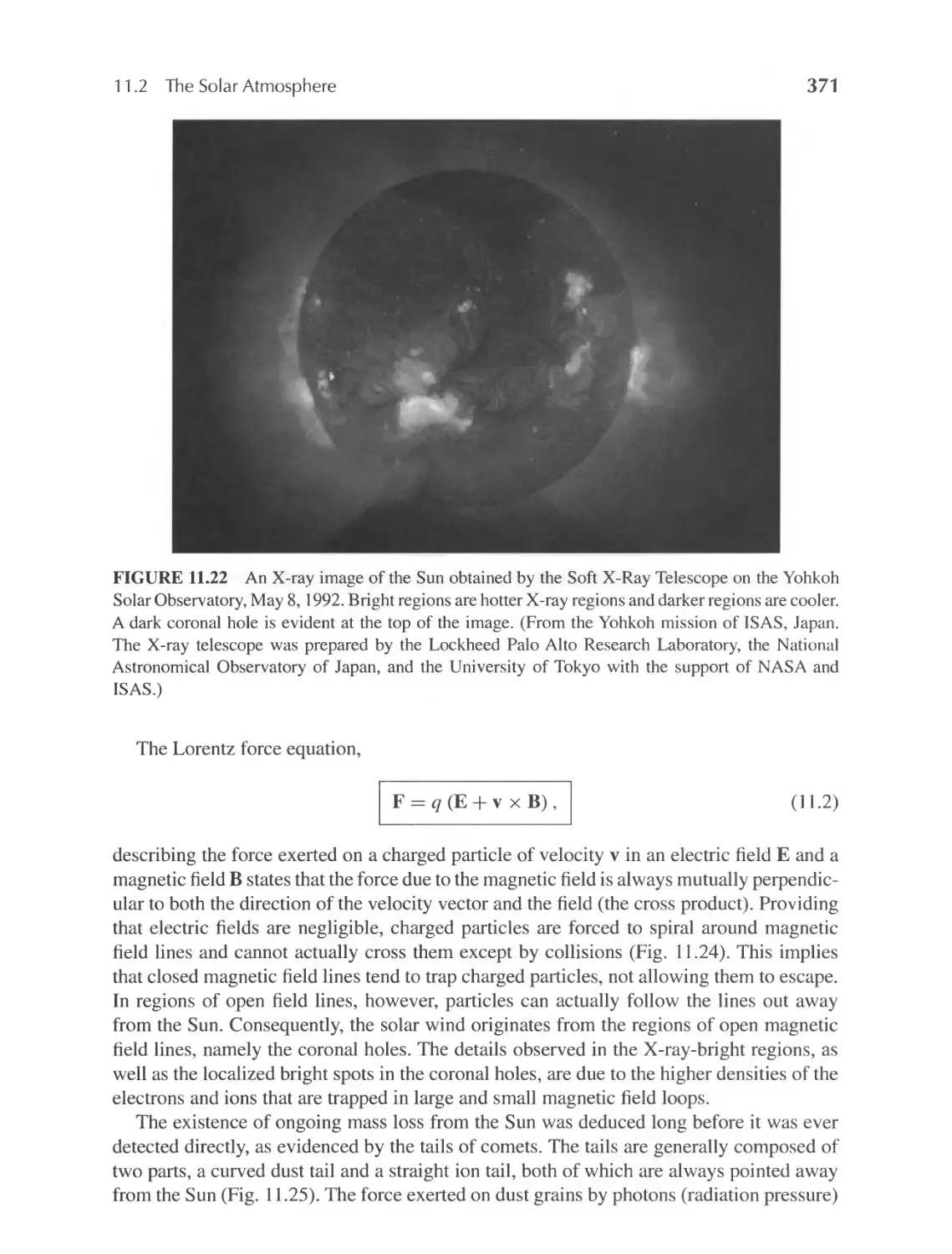
11 _ The Sun
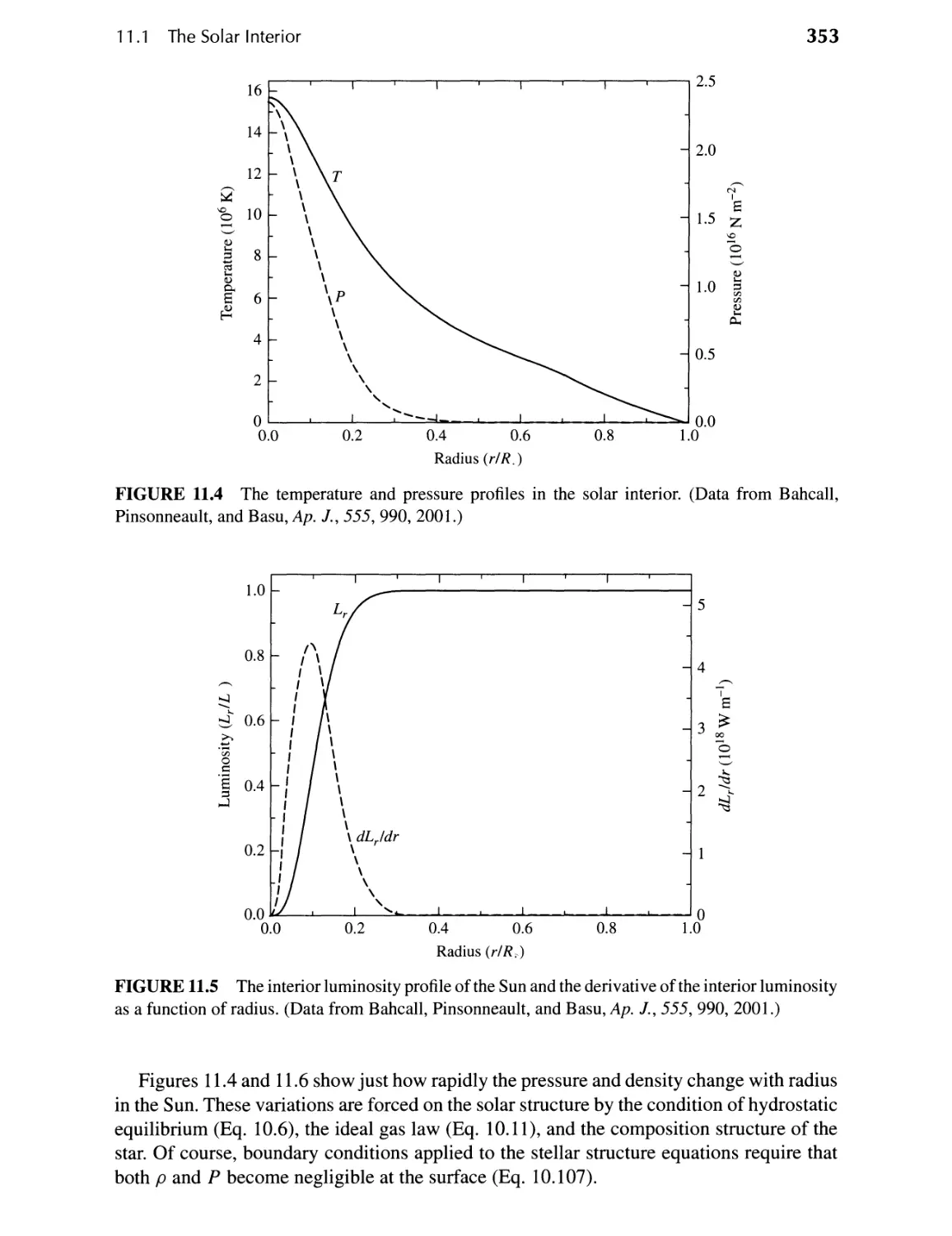
11.1 The Solar Interior 349
11.2 The Solar Atmosphere 360
11.3 The Solar Cycle 381
349
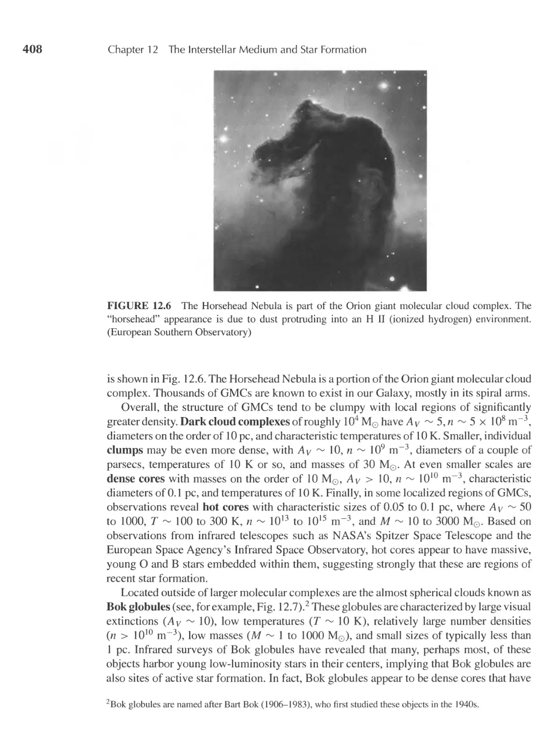
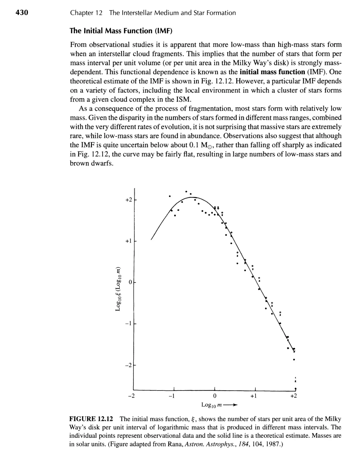
12 _ The Interstellar Medium and Star Formation
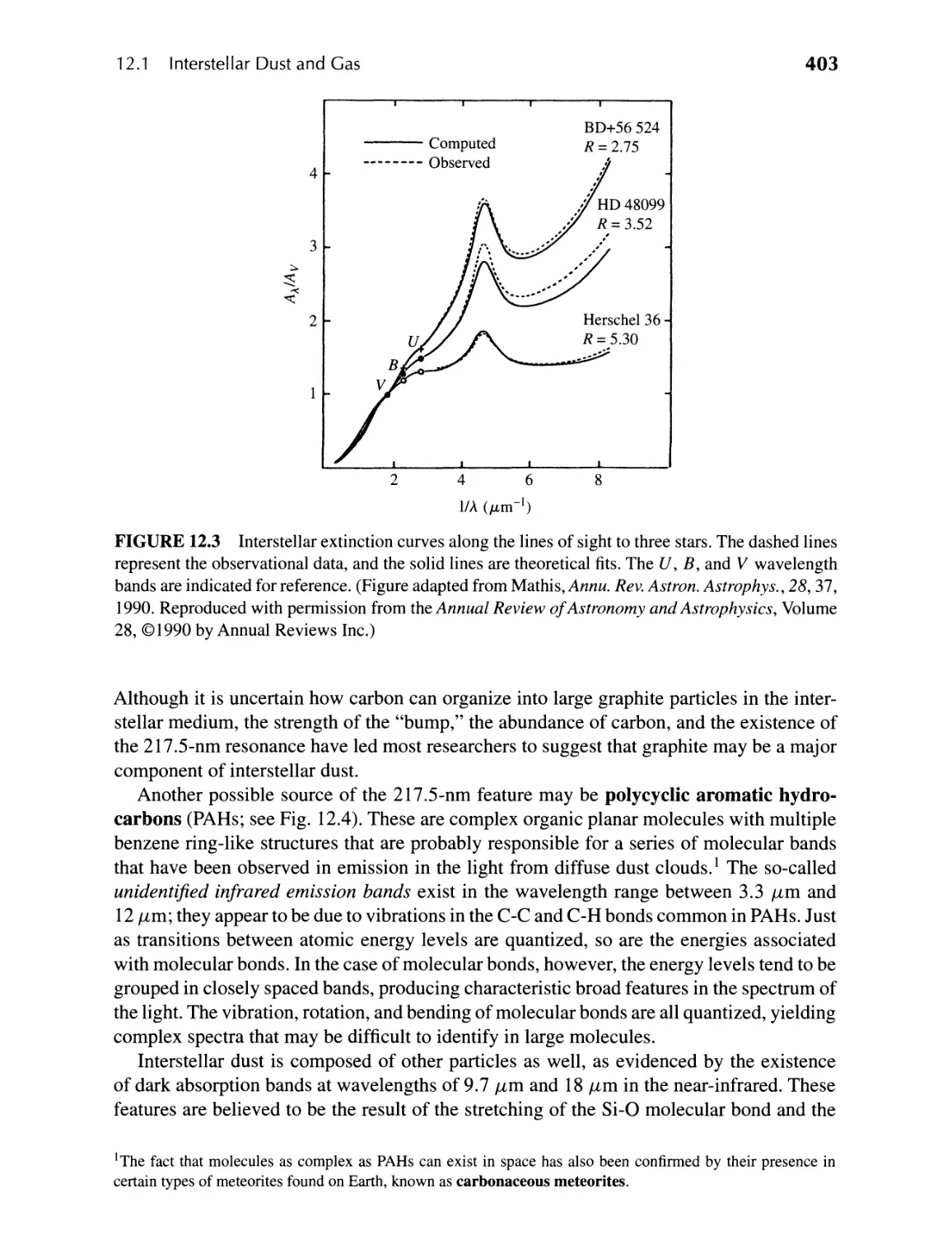
12.1 Interstellar Dust and Gas 398
12.2 The Formation of Protostars 412
12.3 Pre-Main-Sequence Evolution 425
398
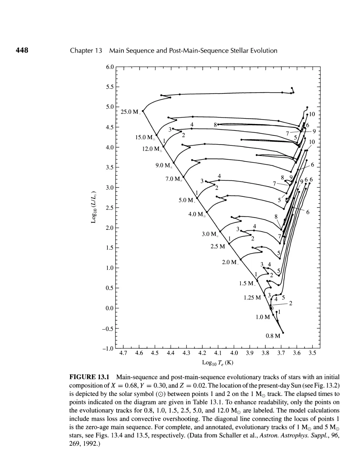
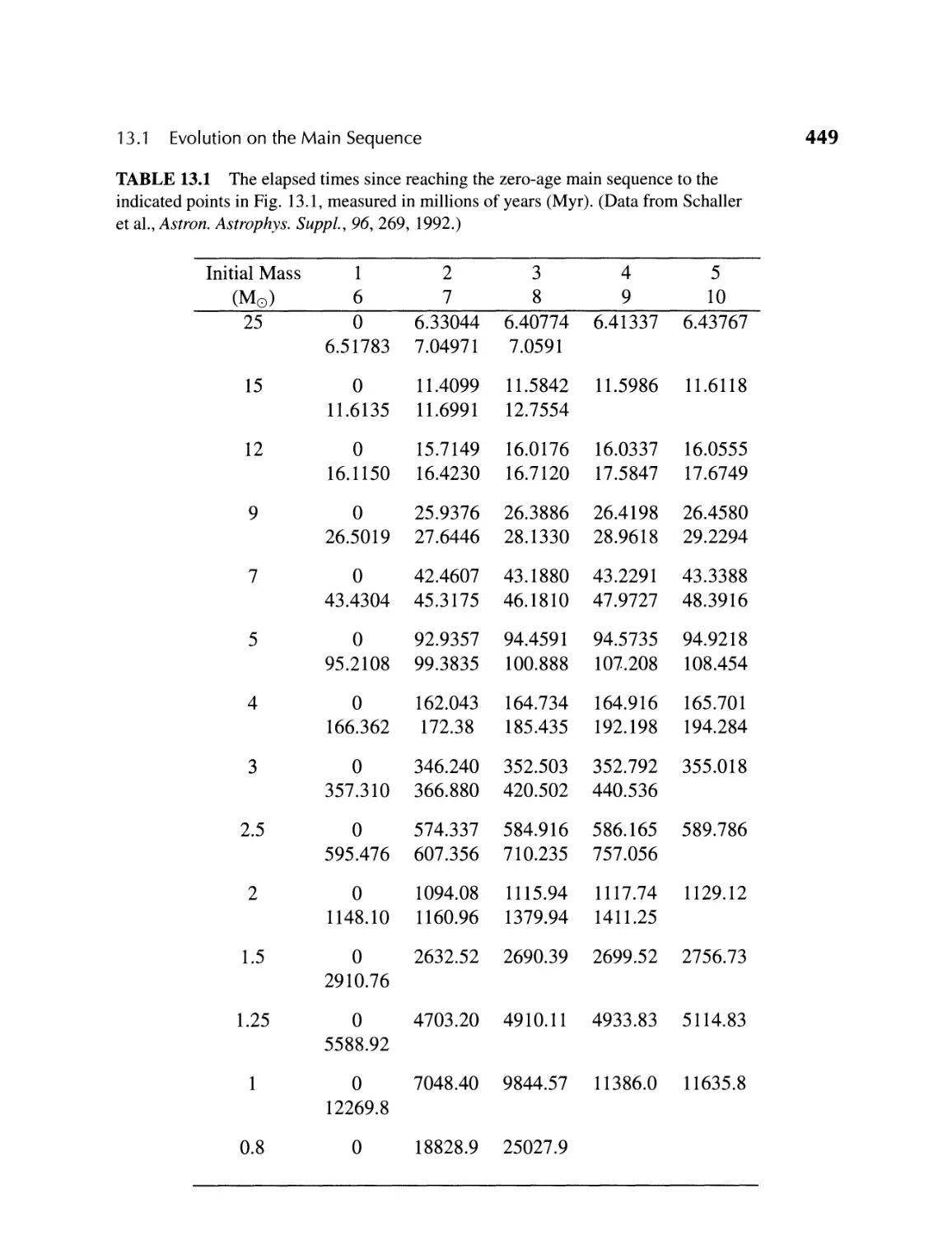
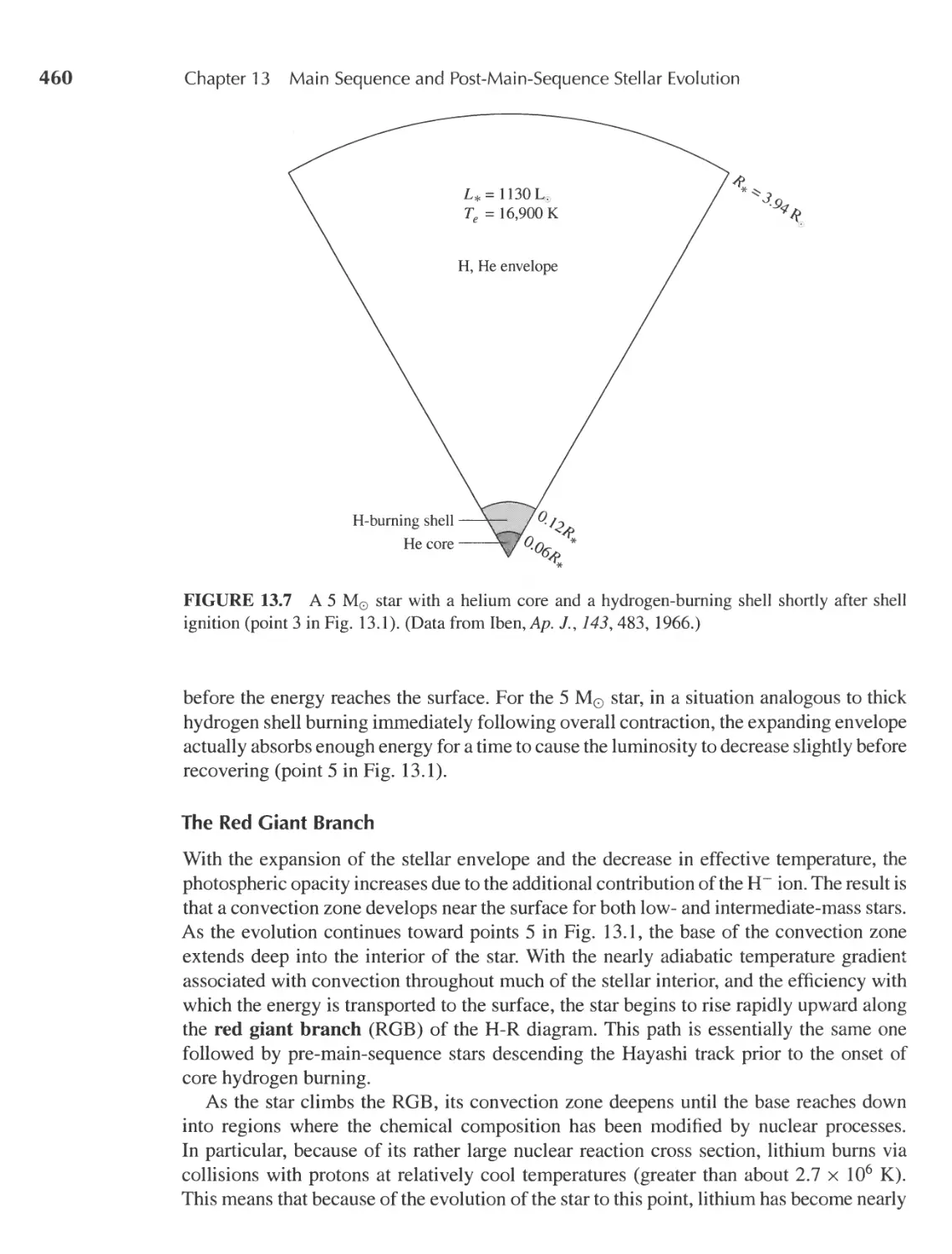
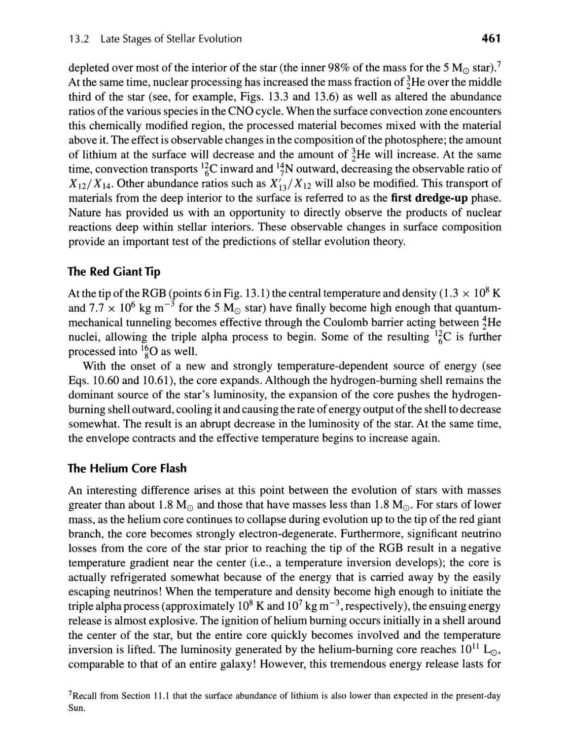
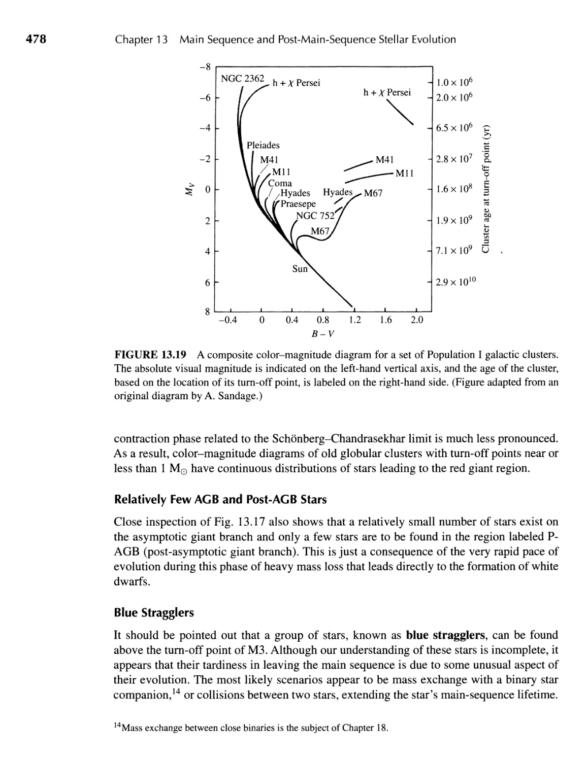
13 II Main Sequence and Post-Main-Sequence Stellar Evolution
13.1 Evolution on the Main Sequence 446
13.2 Late Stages of Stellar Evolution 457
13.3 Stellar Clusters 474
446
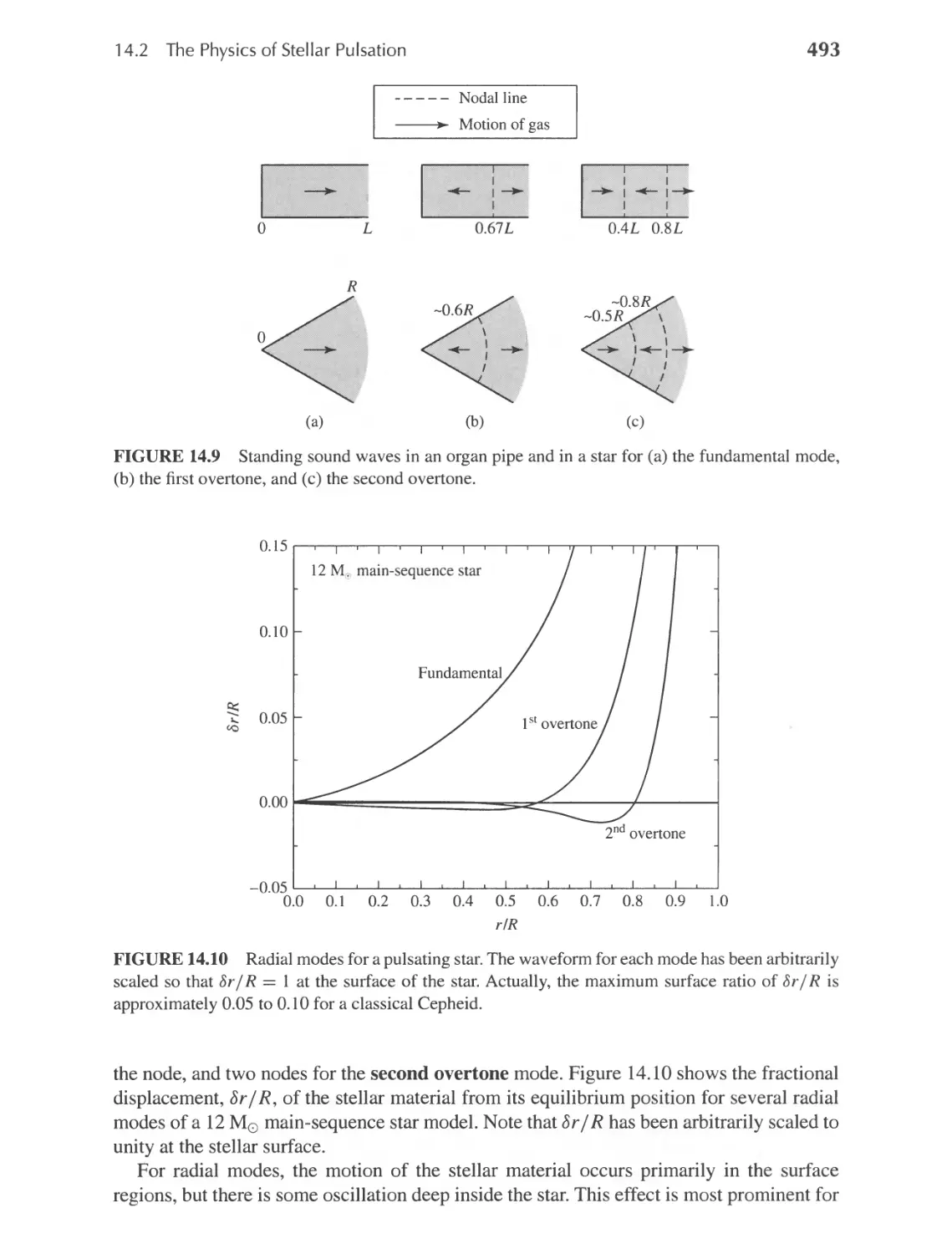
14 II Stellar Pulsation
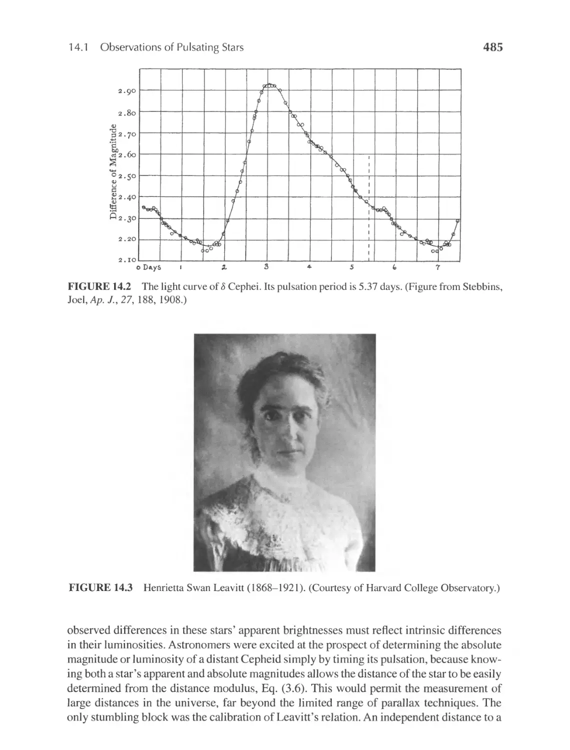
14.1 Observations of Pulsating Stars 483
14.2 The Physics of Stellar Pulsation 491
14.3 Modeling Stellar Pulsation 499
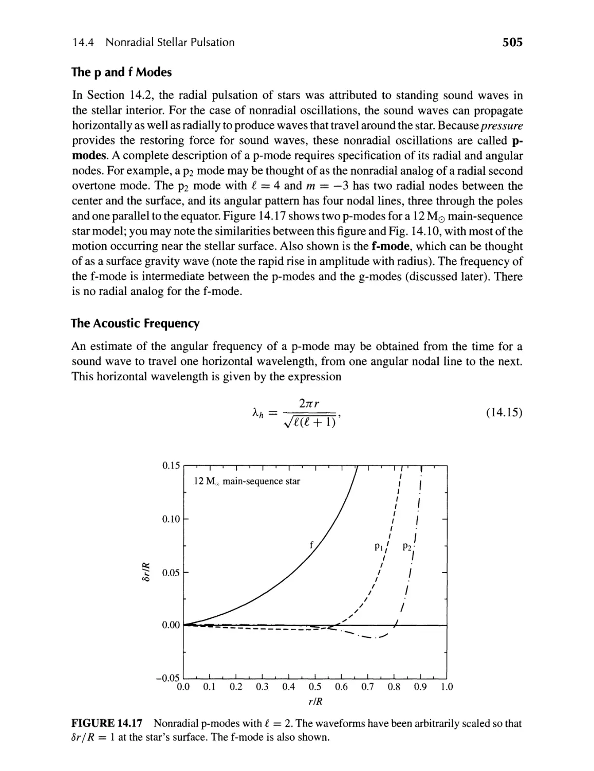
14.4 N onradial Stellar Pulsation 503
14.5 Helioseismology and Asteroseismology 509
483
15 _ The Fate of Massive Stars
15.1 Post-Main-Sequence Evolution of Massive S rs 518
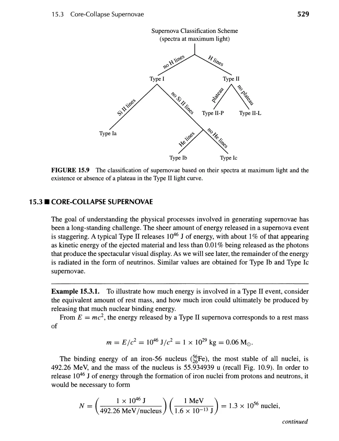
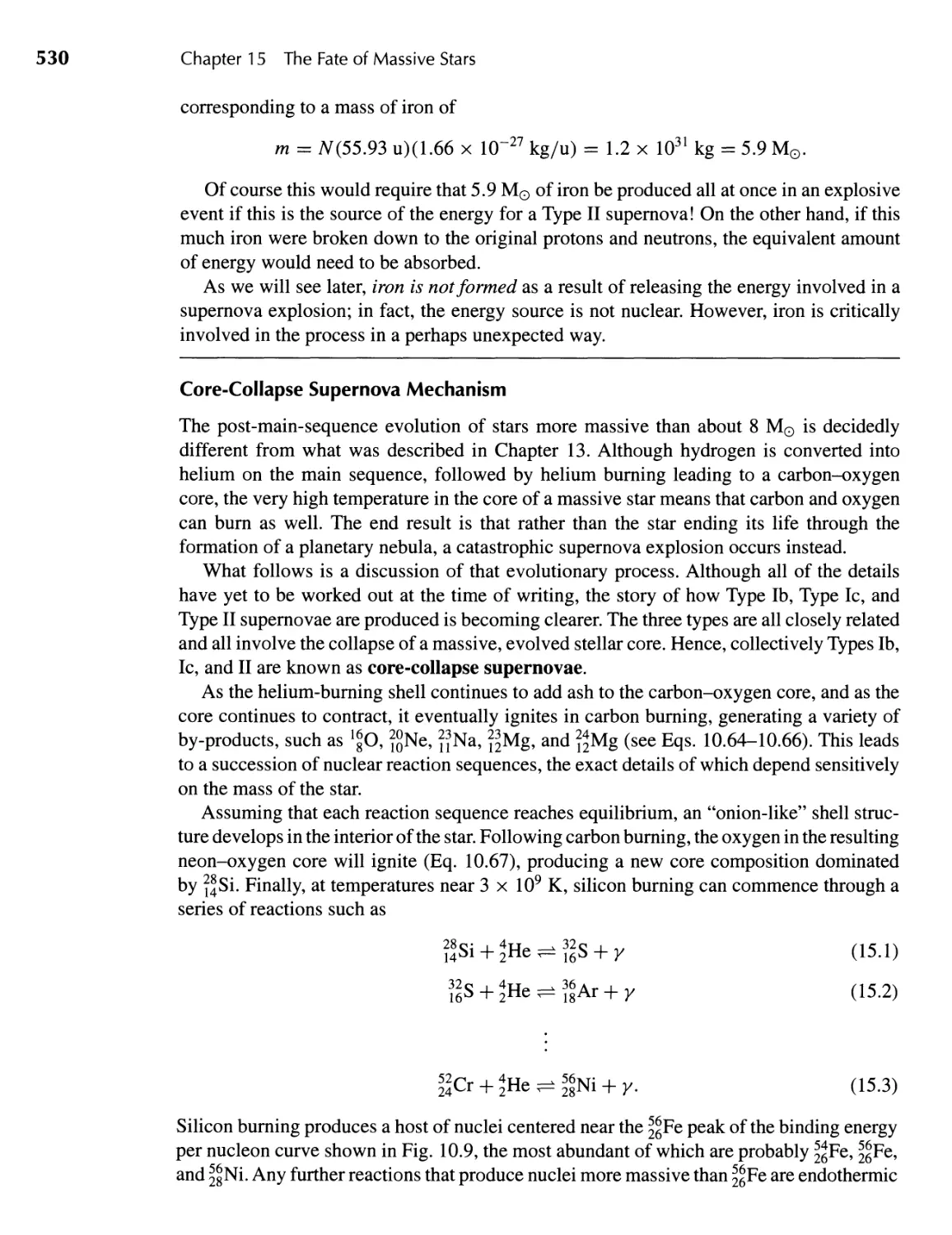
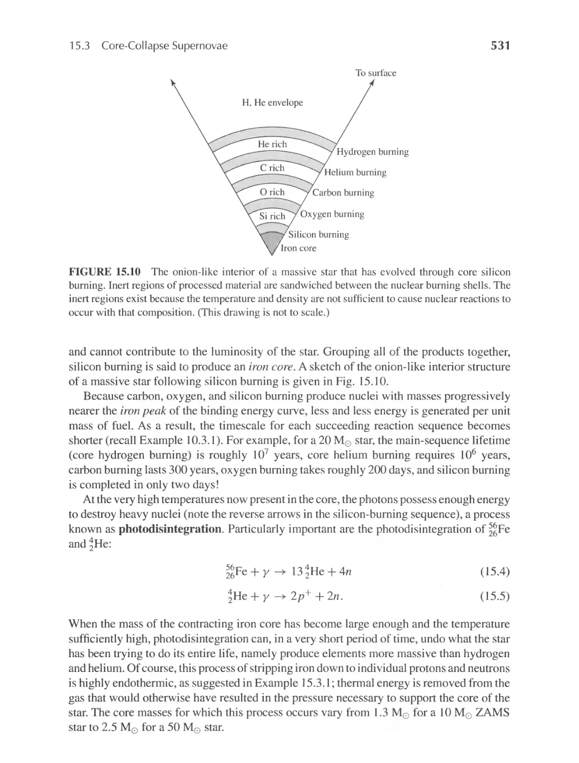
15.2 The Classification of Supernovae 524
15.3 Core-Collapse Supernovae 529
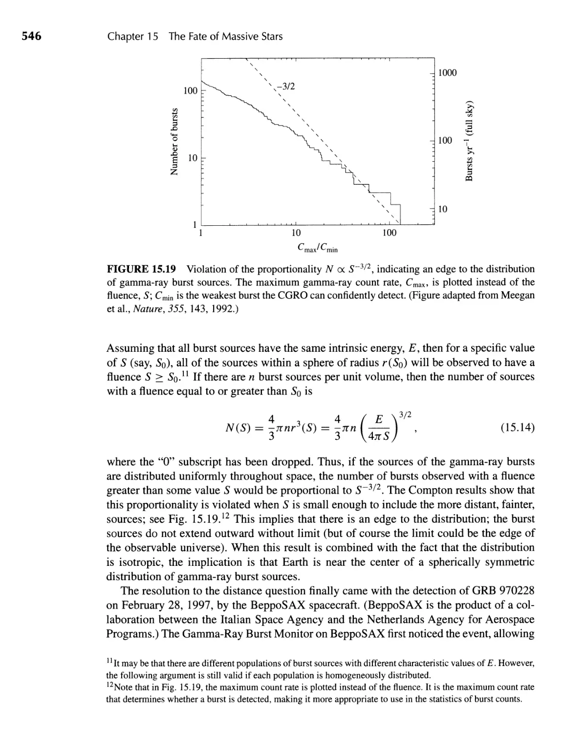
15.4 Gamma-Ray Bursts 543
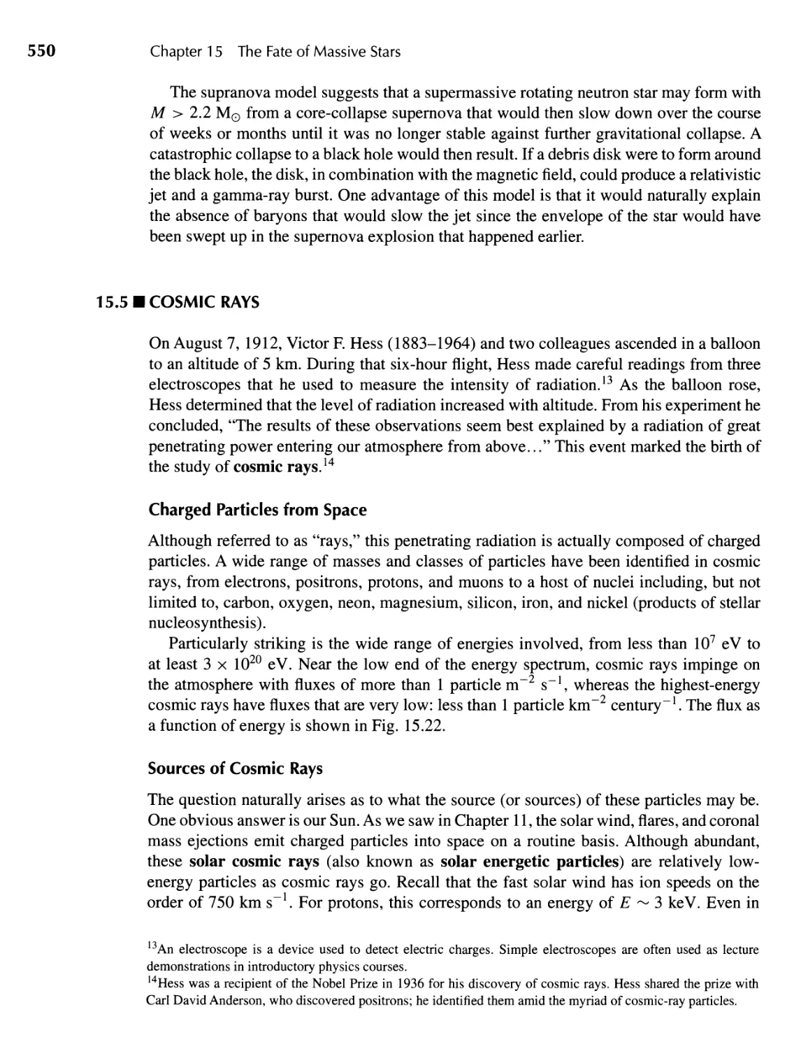
15.5 Cosmic Rays 550
518
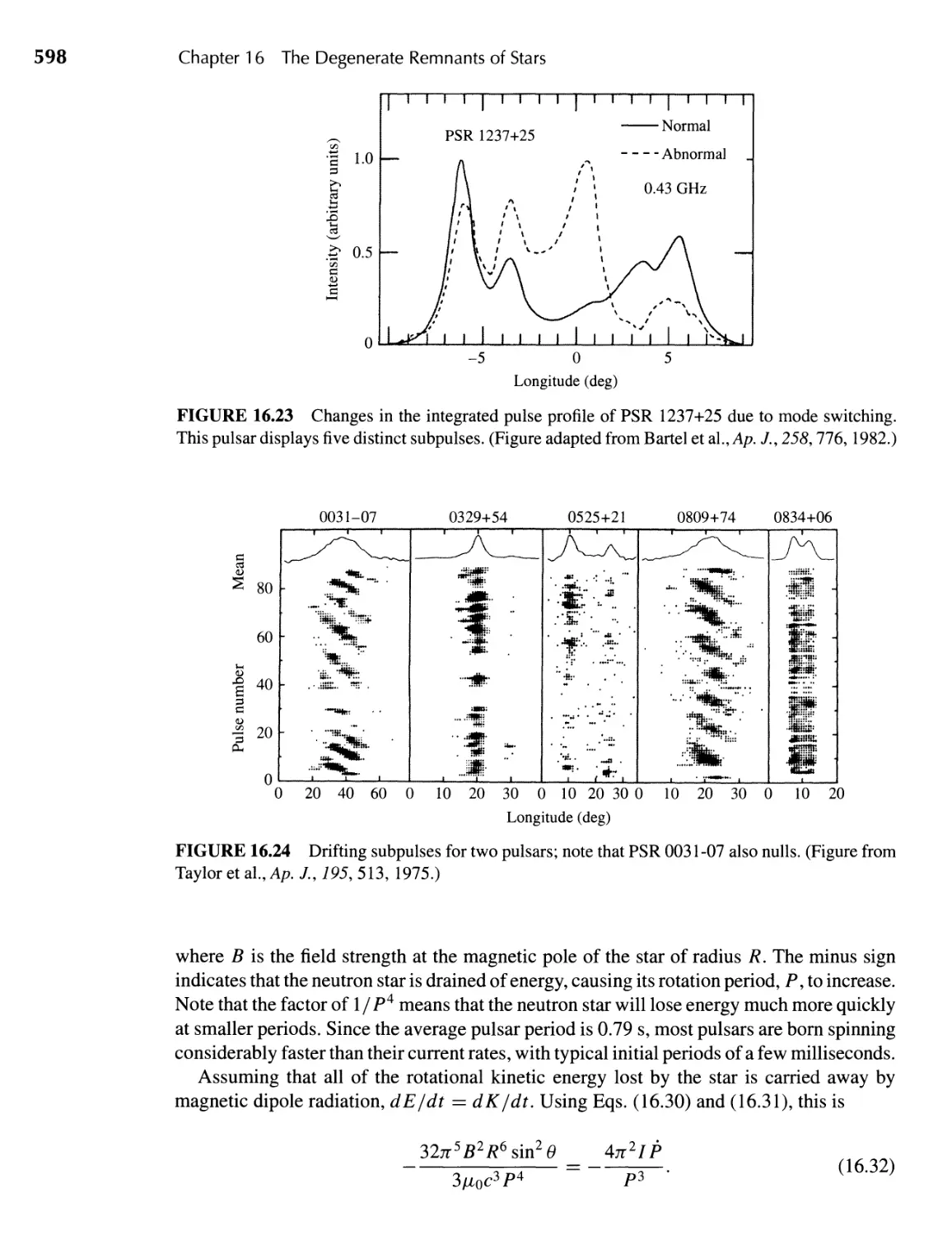
16 II The Degenerate Remnants of Stars
16.1 The Discovery of Sirius B 557
16.2 White Dwarfs 559
16.3 The Physics of Degenerate Matter 563
16.4 The Chandrasekhar Limit 569
16.5 The Cooling of White Dwarfs 572
16.6 Neutron Stars 578
16.7 Pulsars 586
557
.
XIV
Contents
17 II General Relativity and Black Holes
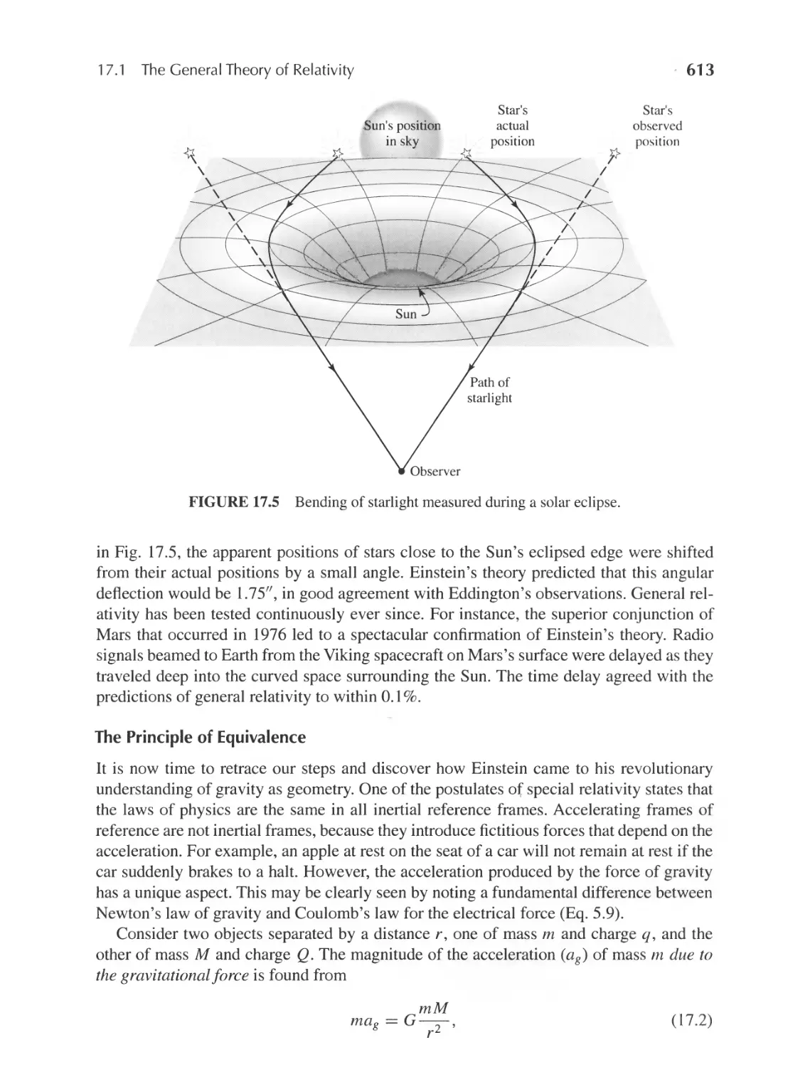
17 .1 The General Theory of Relativity 609
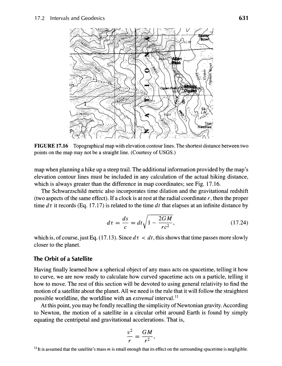
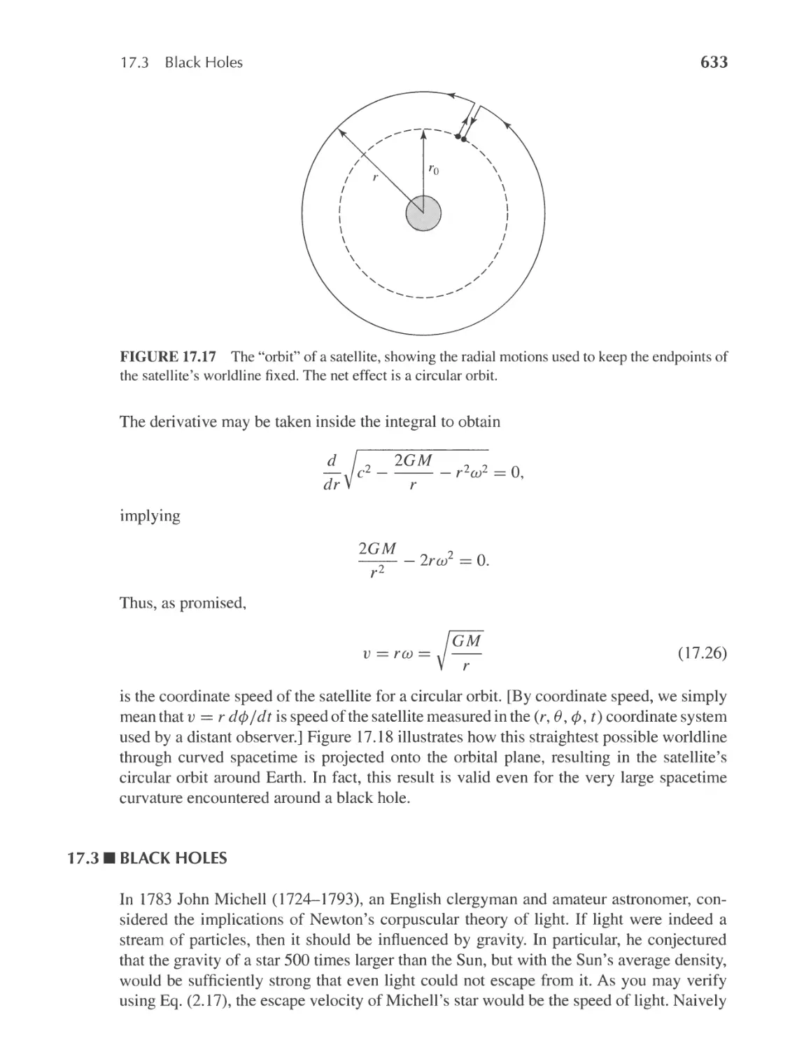
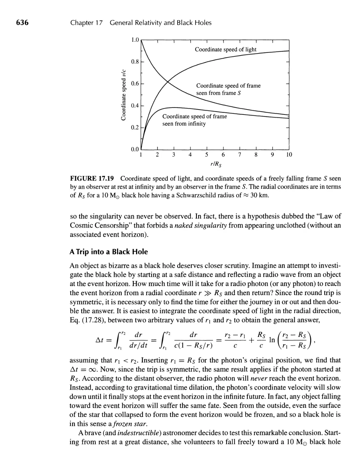
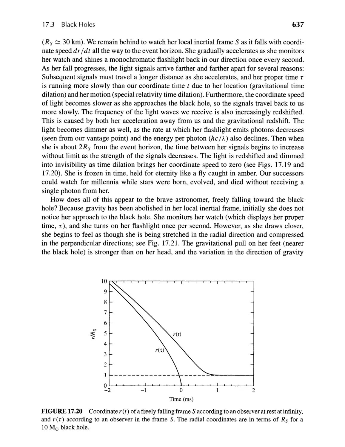
17 .2 Intervals and Geodesics 622
17.3 Black Holes 633
609
653
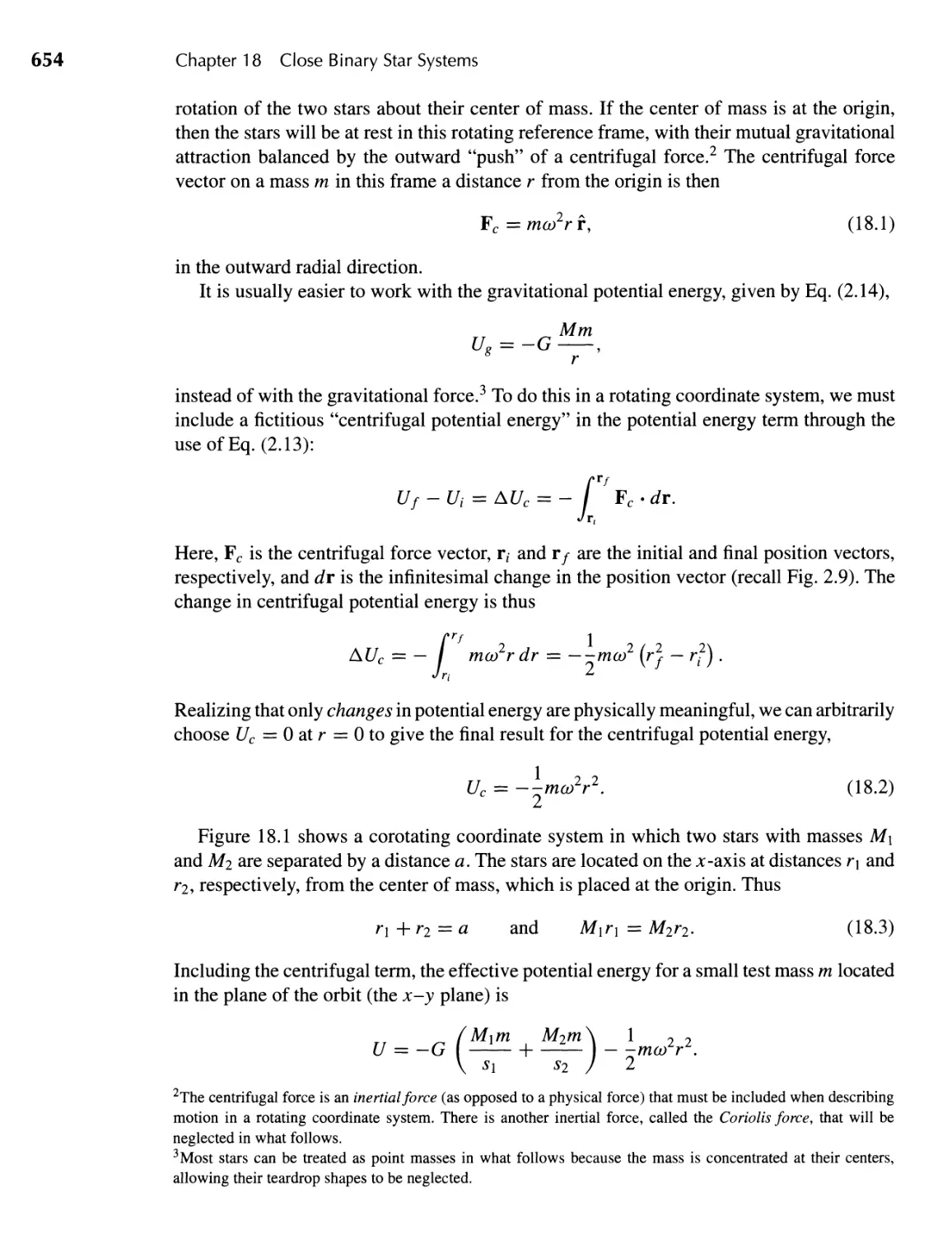
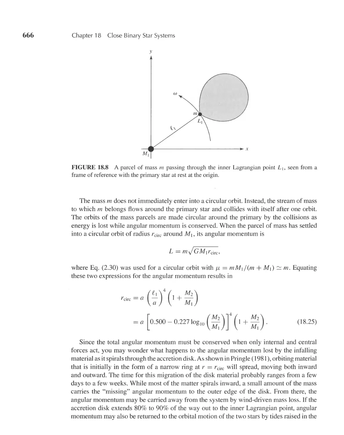
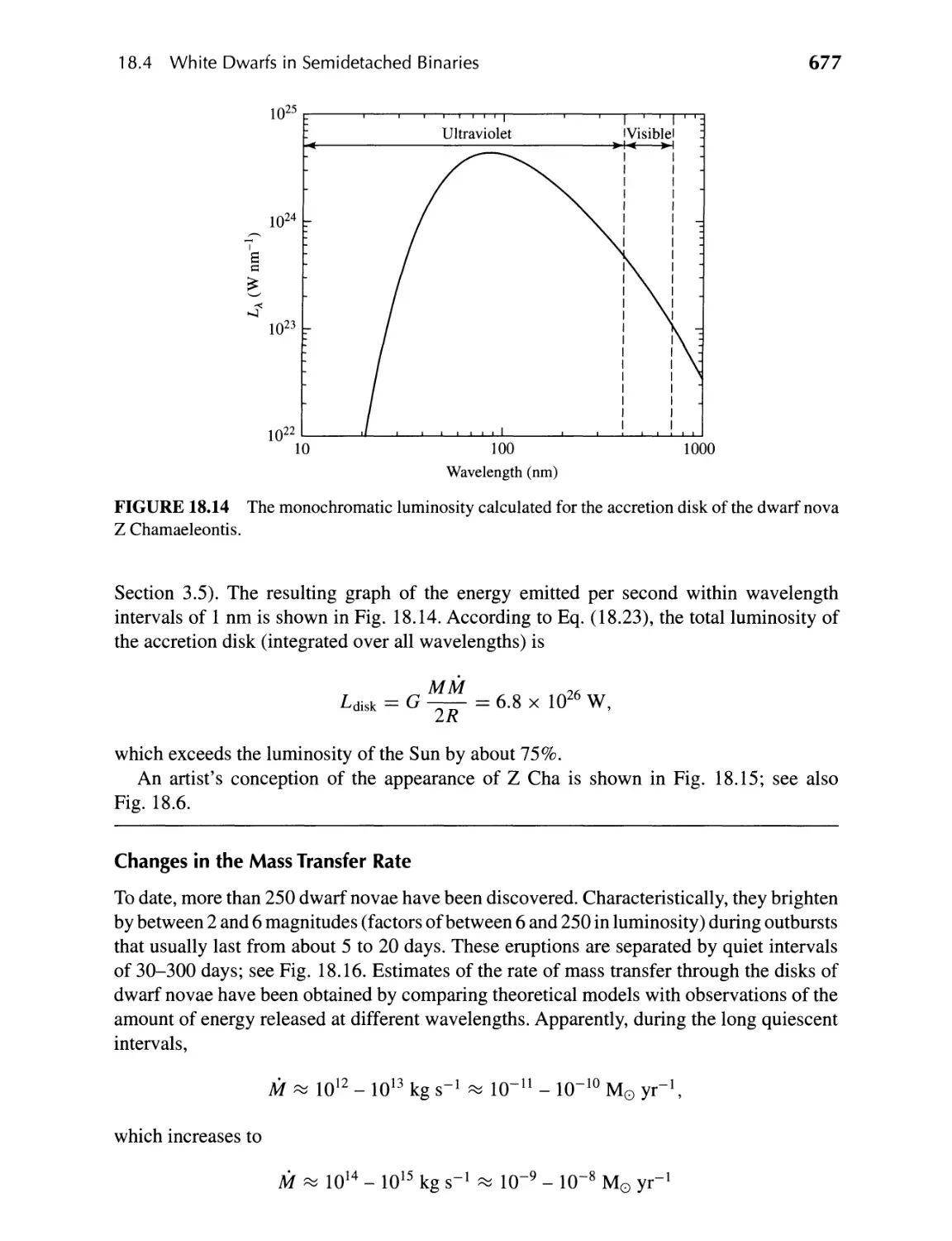
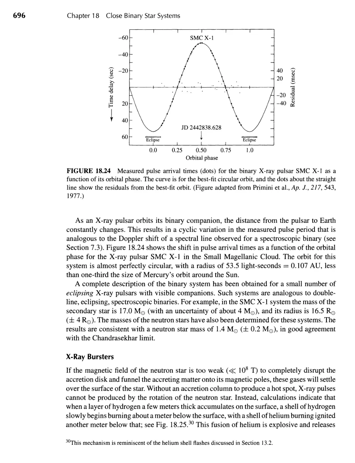
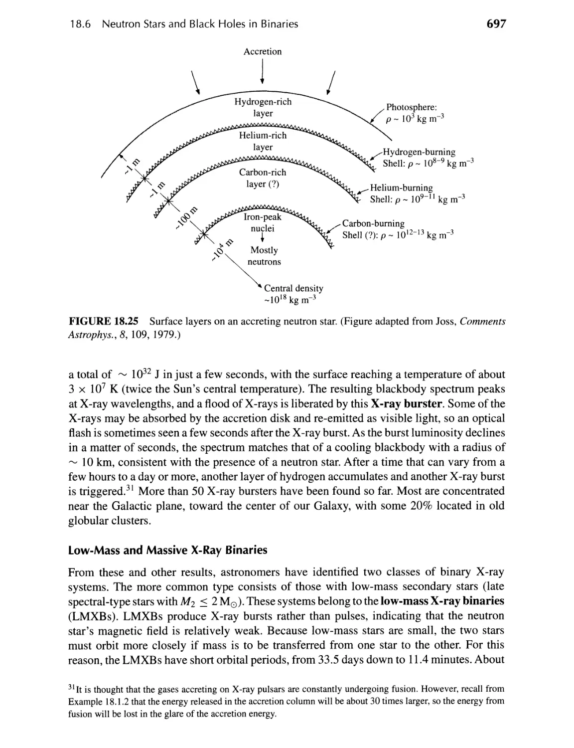
18.1 Gravity in a Close Binary Star System 653
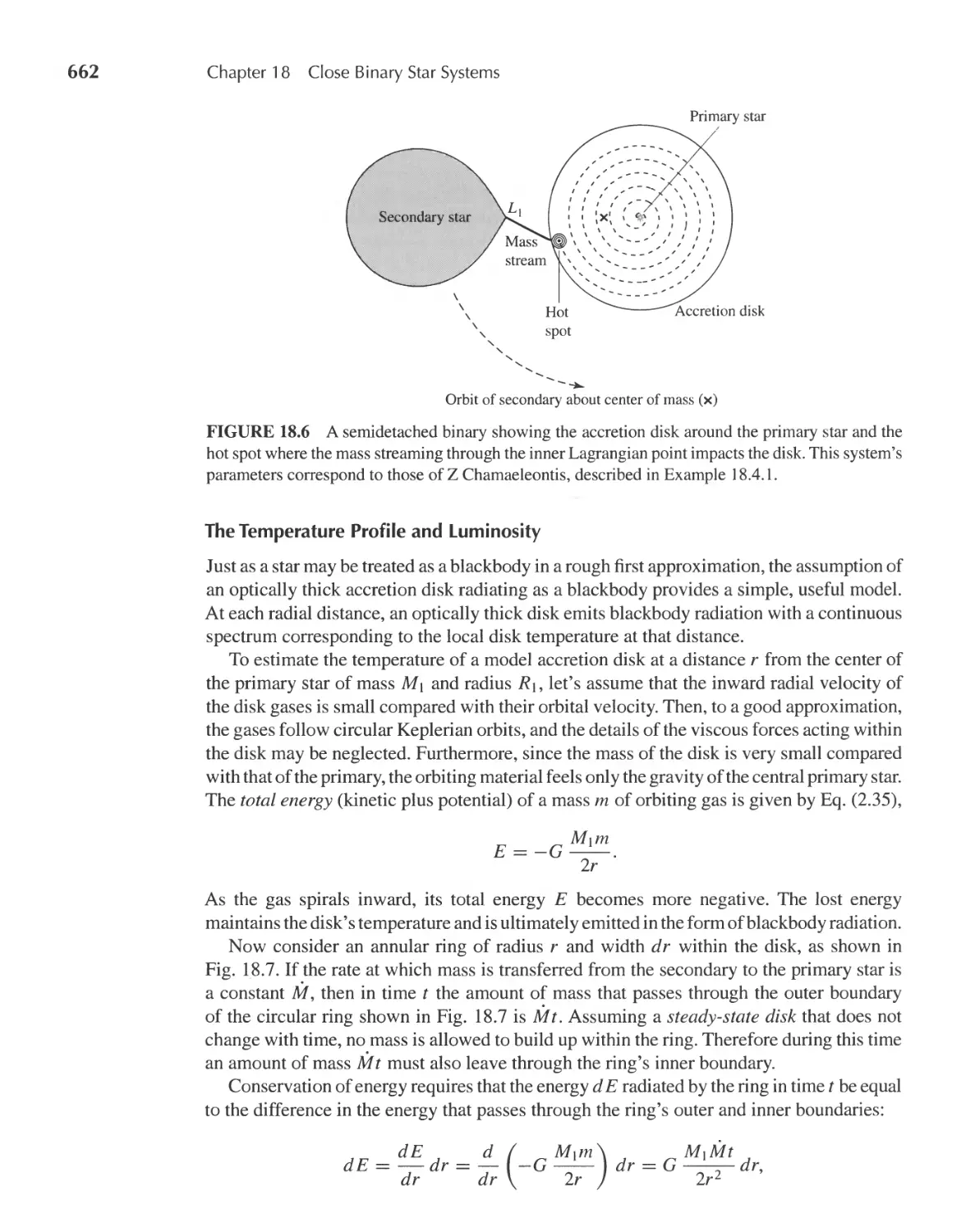
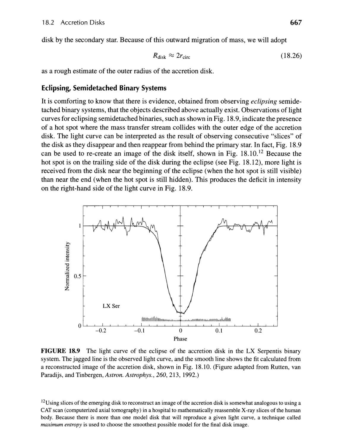
18.2 Accretion Disks 661
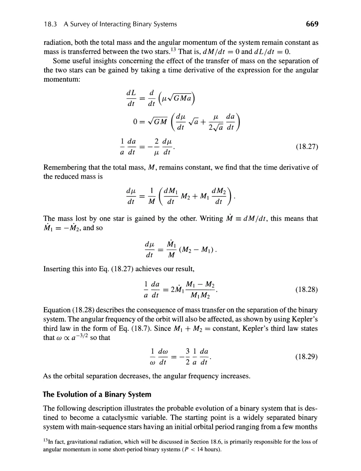
18.3 A Survey of Interacting Binary Systems 668
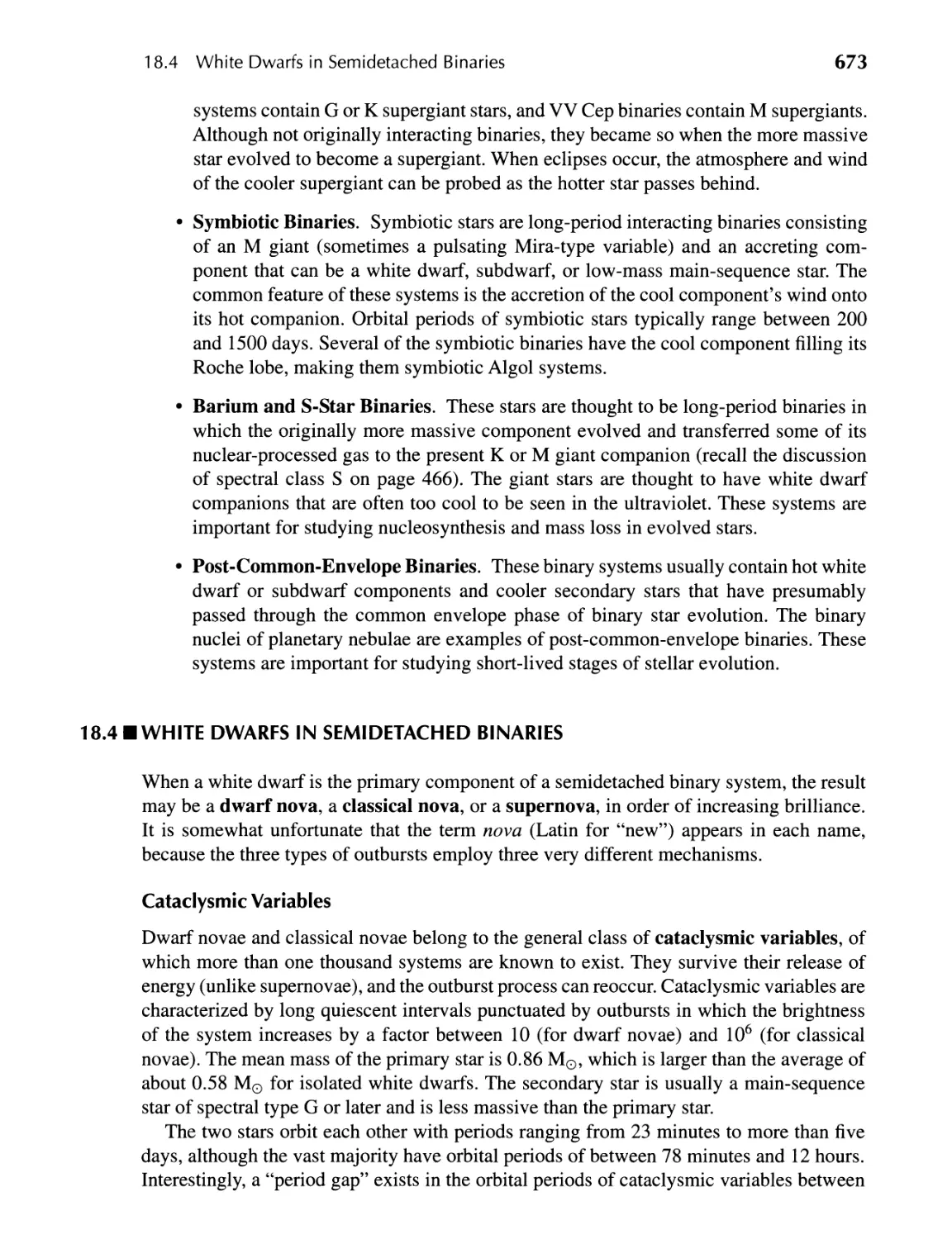
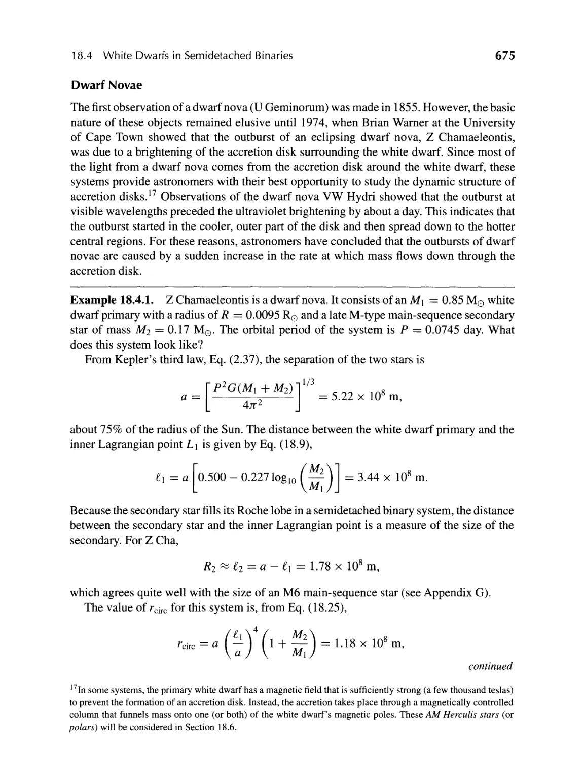
18.4 White Dwarfs in Semidetached Binaries 673
18.5 Type Ia Supernovae 686
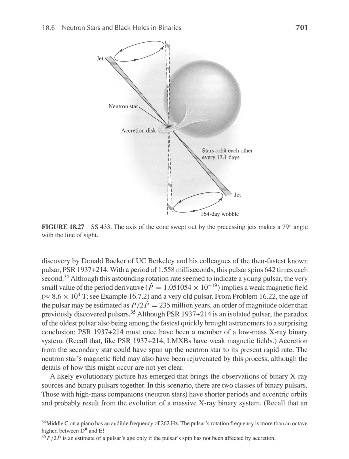
18.6 Neutron Stars and Black Holes in Binaries 689
III THE SOLAR SYSTEM
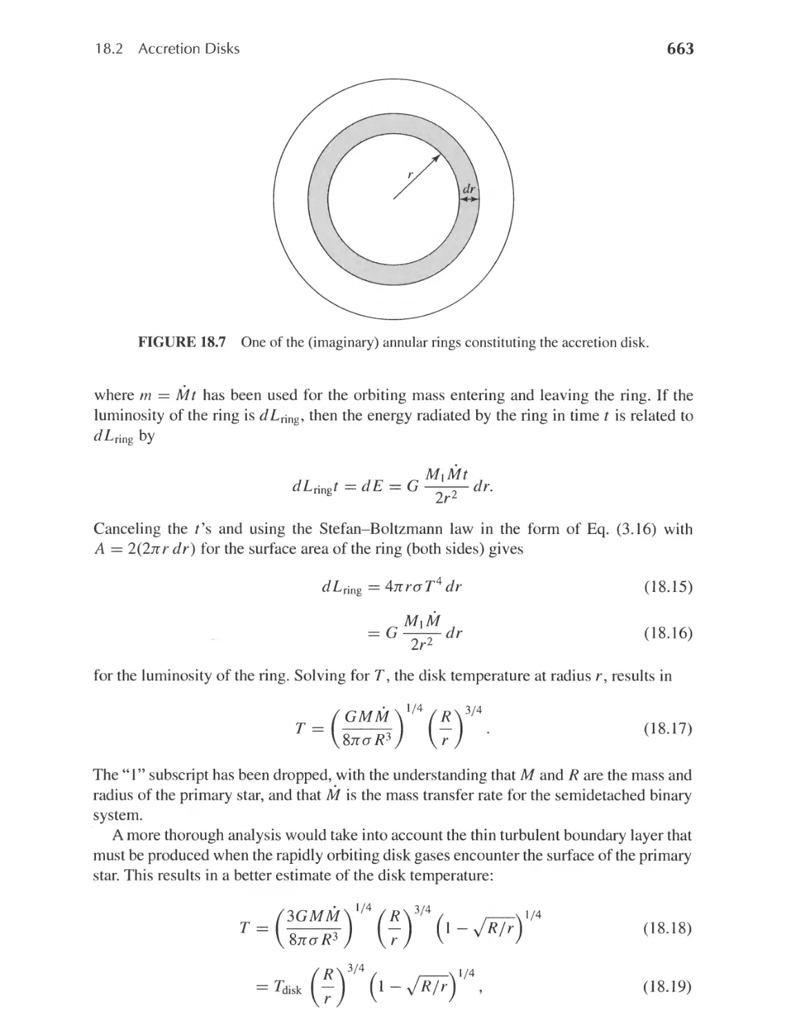
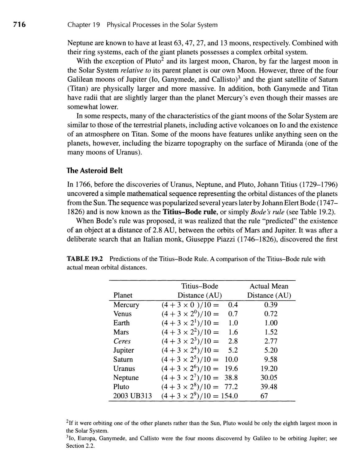
713
19 II Physical Processes in the Solar System
19.1 A Brief Survey 714
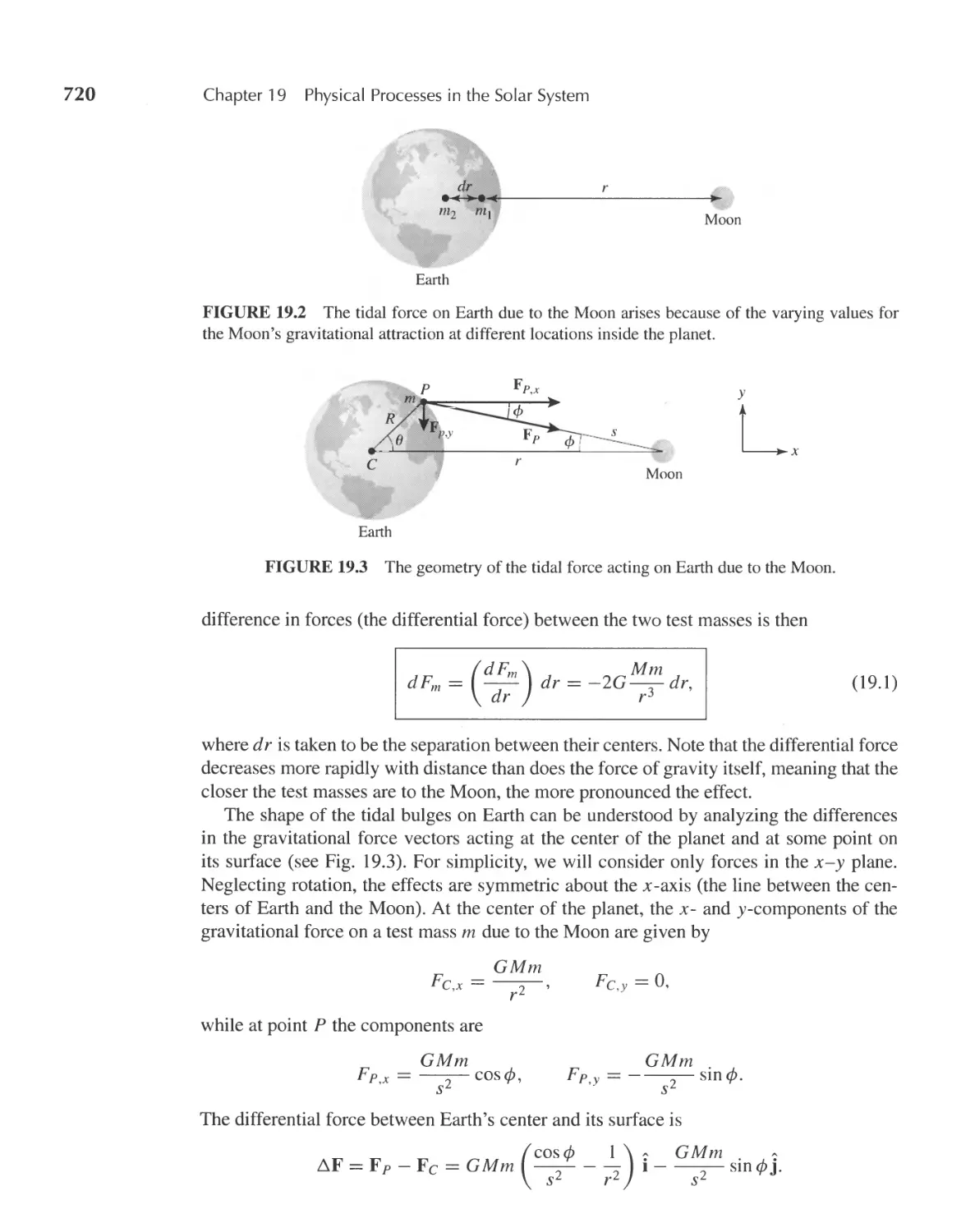
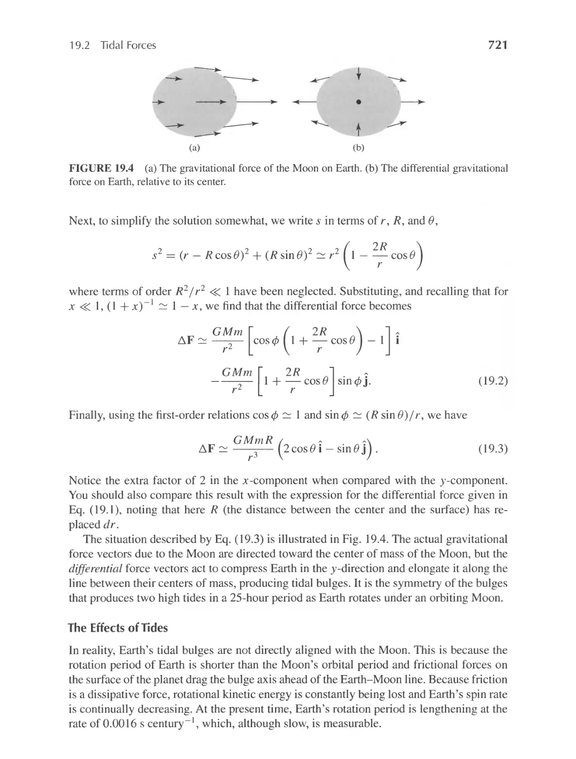
19.2 Tidal Forces 719
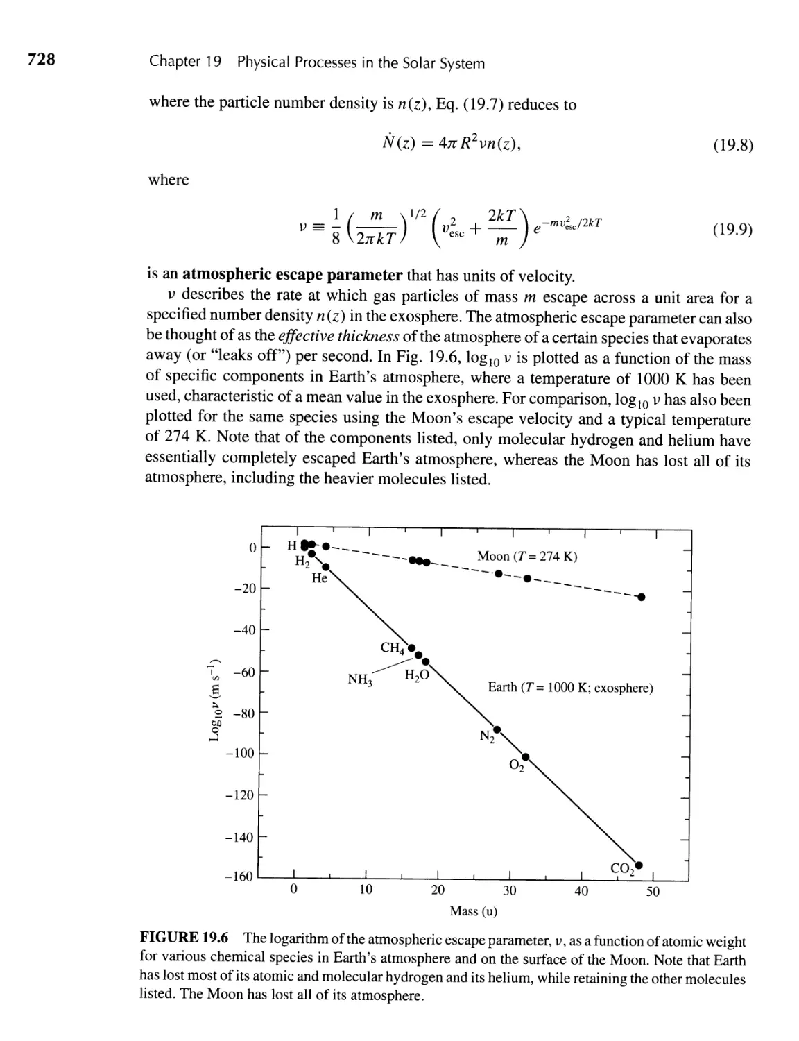
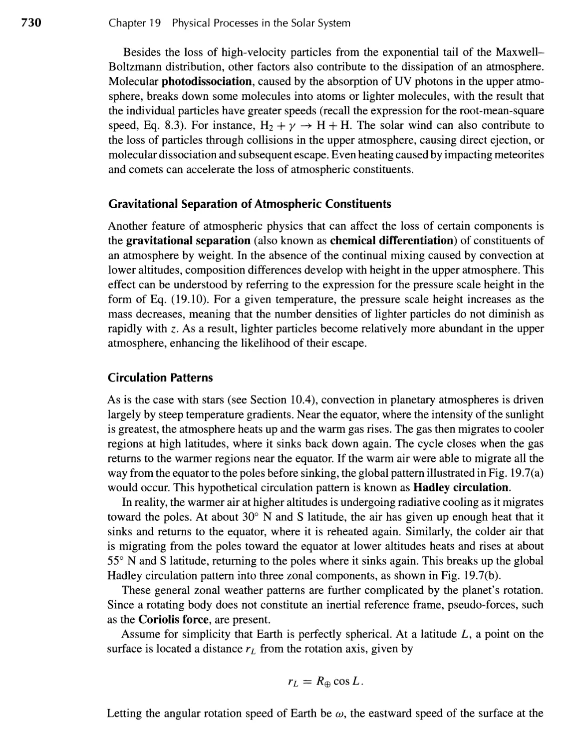
19.3 The Physics of Atmospheres 724
714
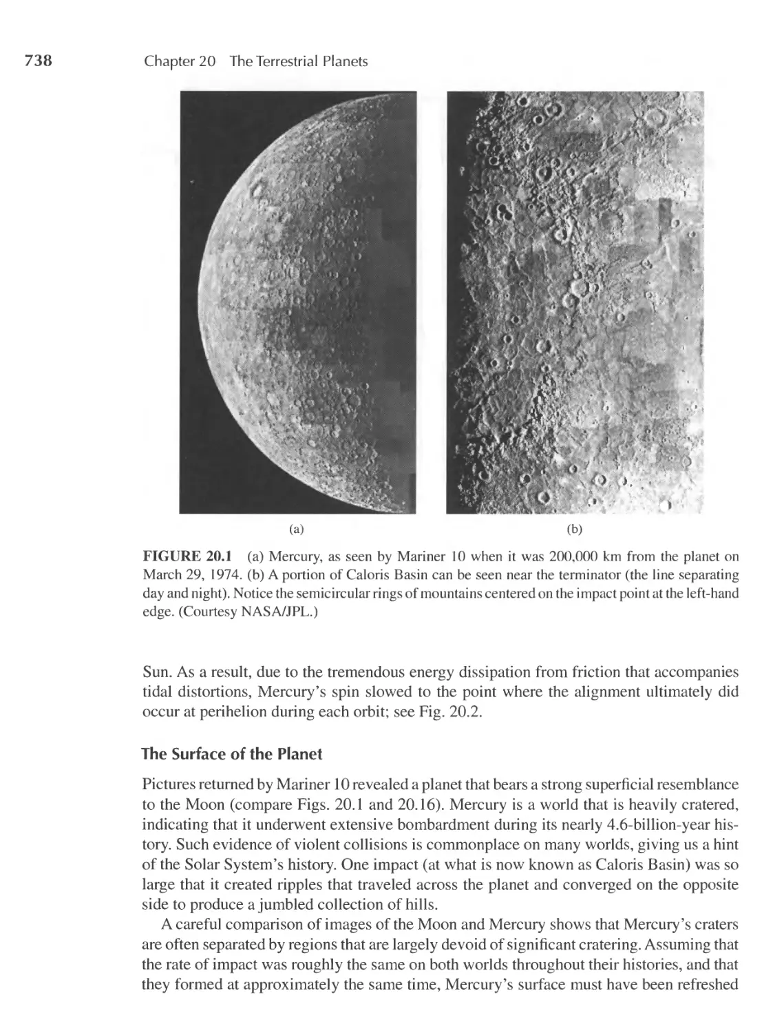
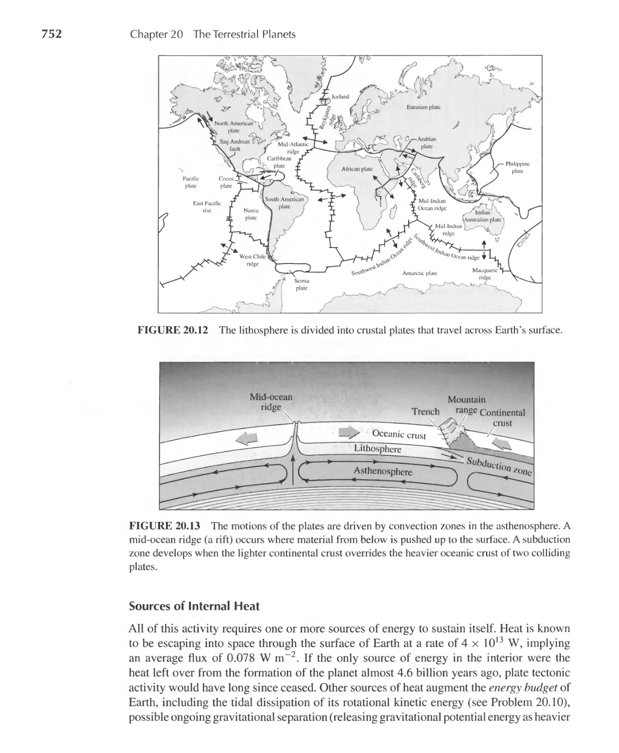
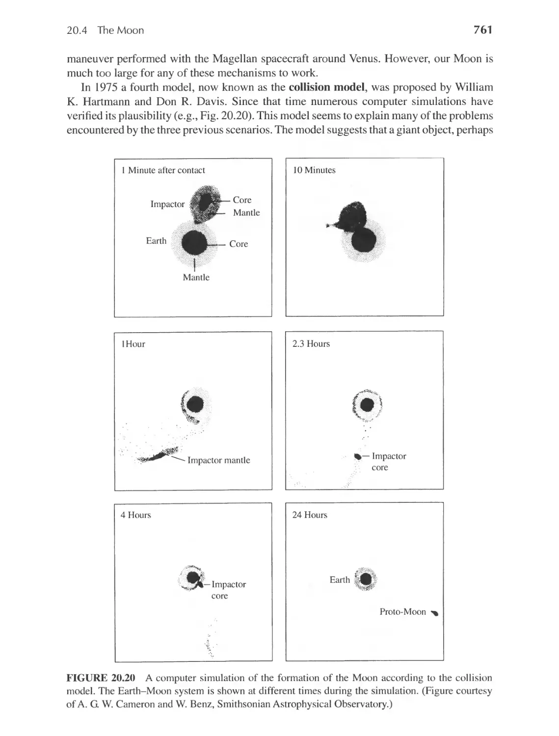
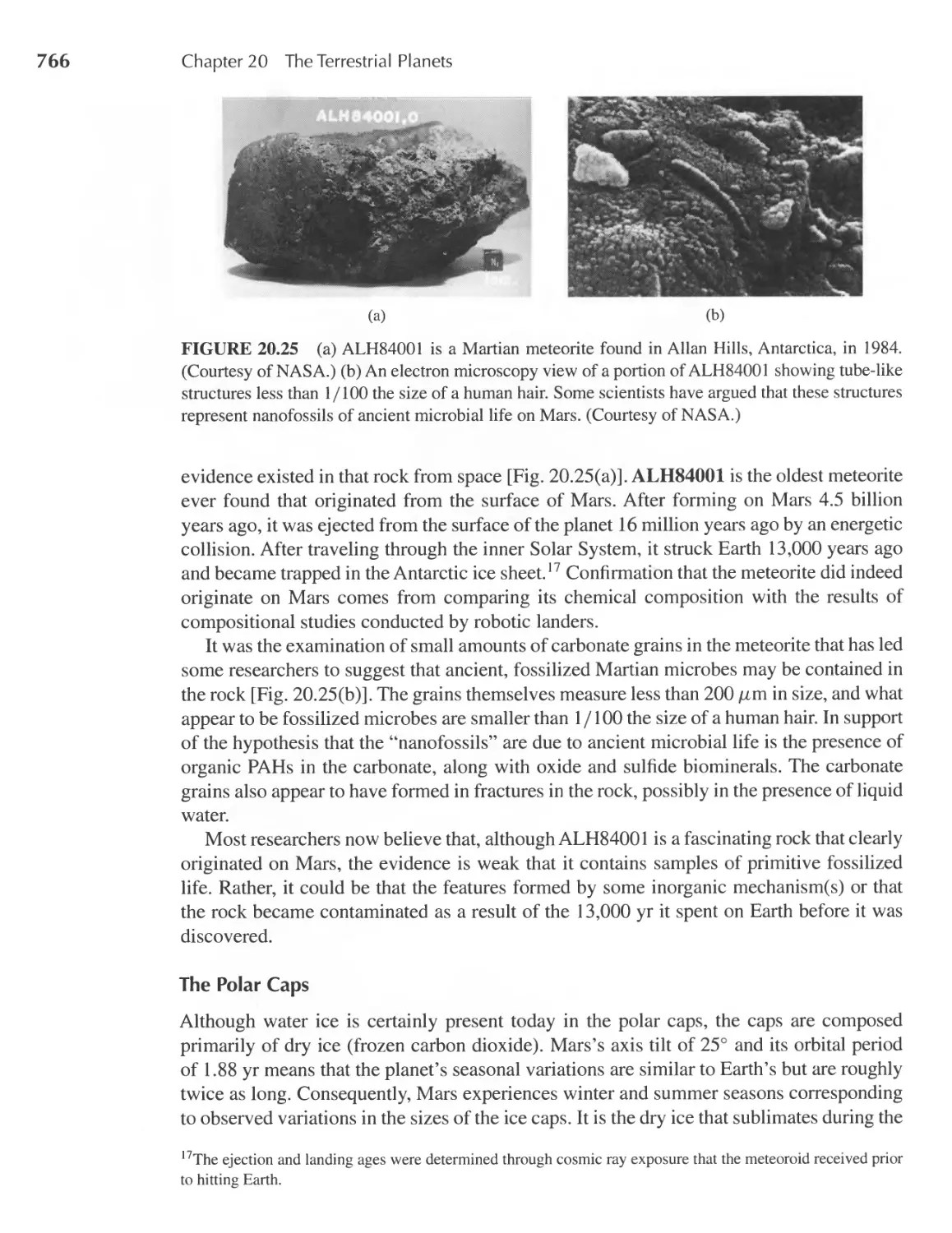
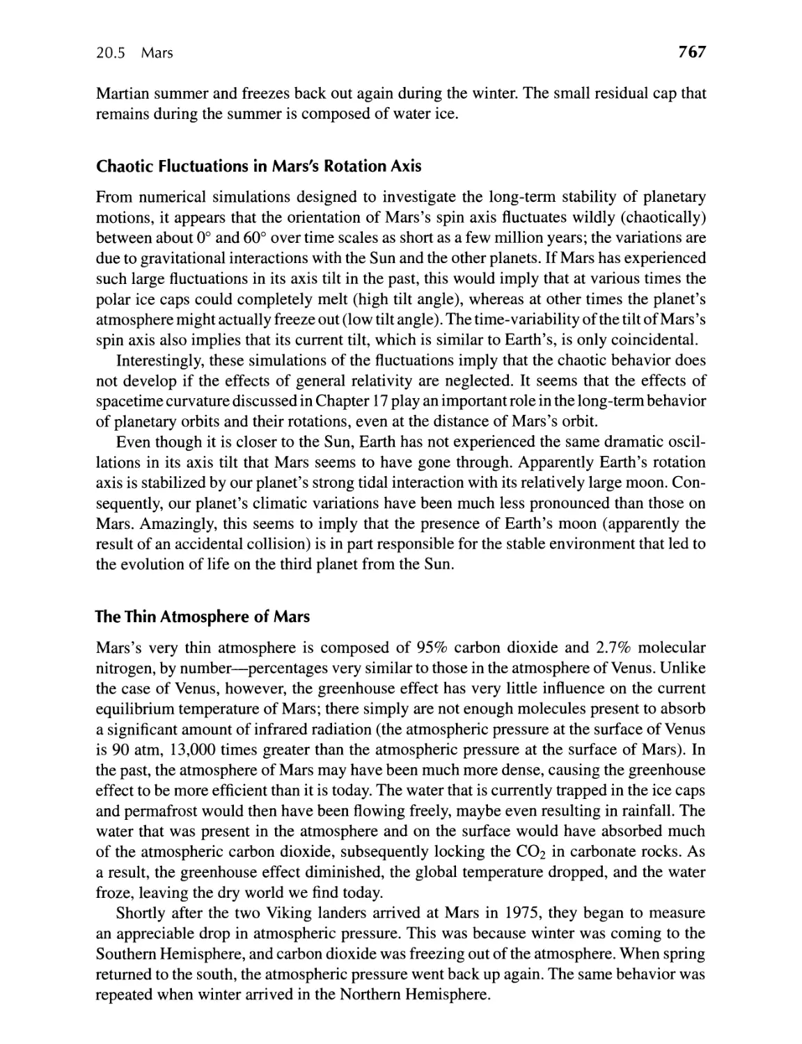
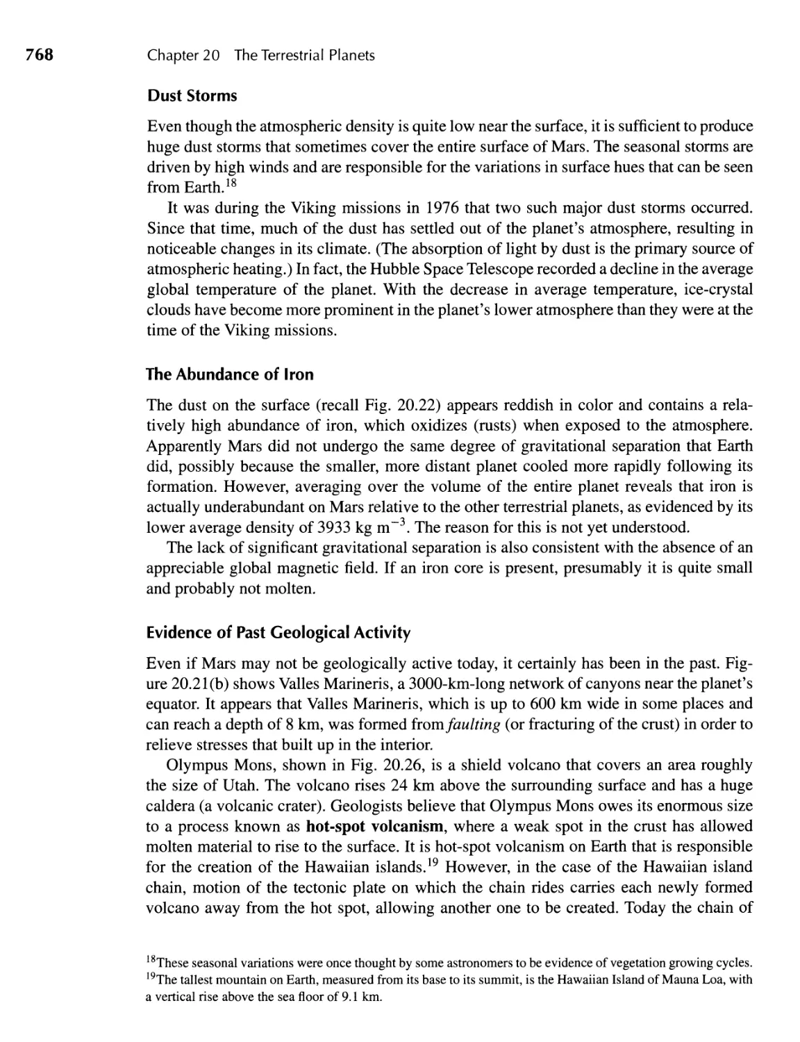
20 II The Terrestrial Planets
20.1 Mercury 737
20.2 Venus 740
20.3 Earth 745
20.4 The Moon 754
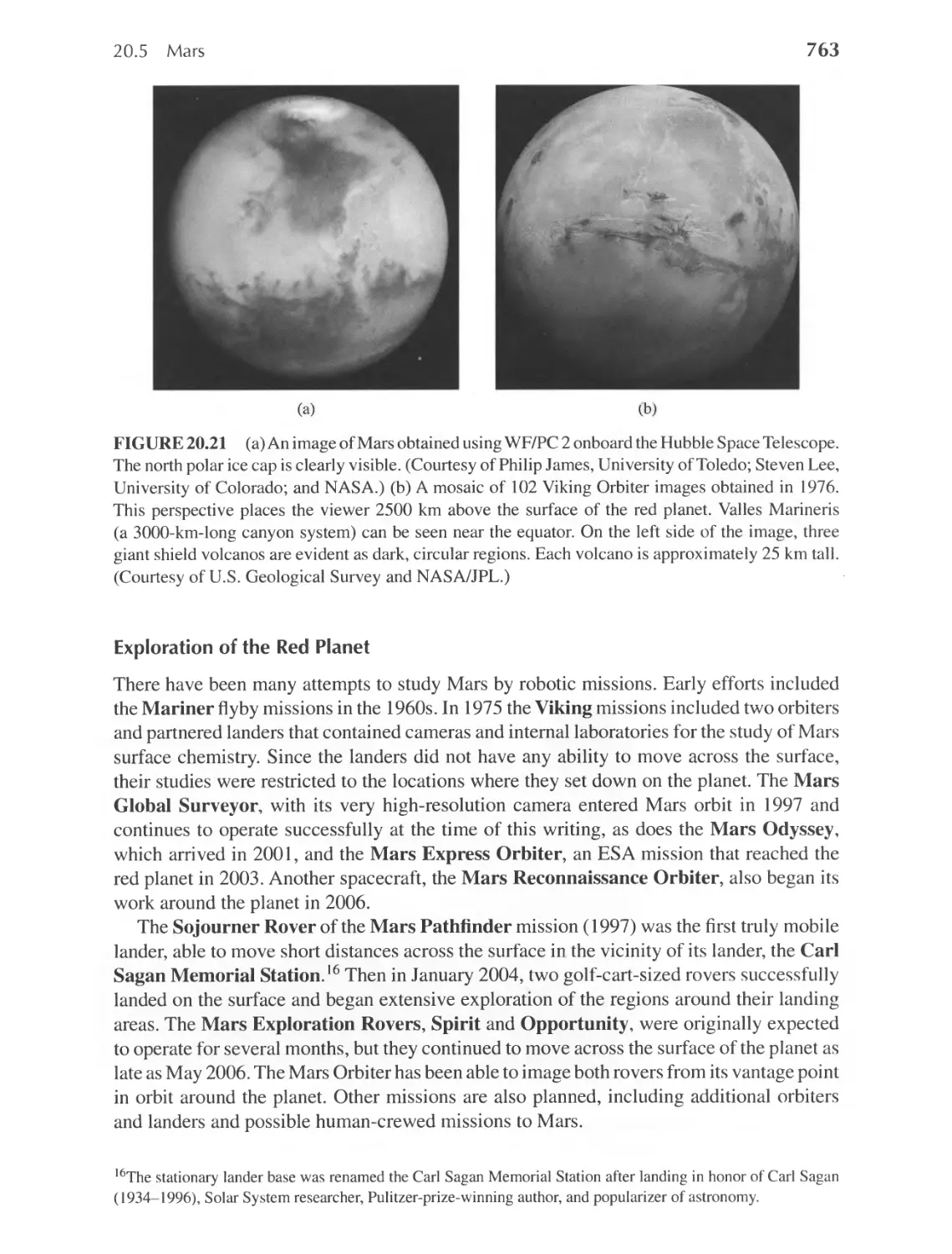
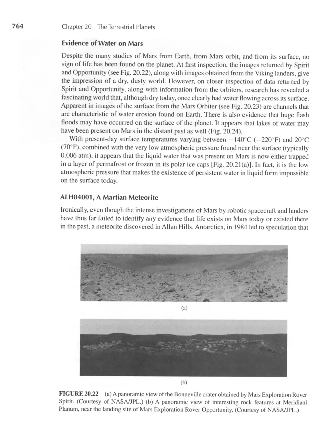
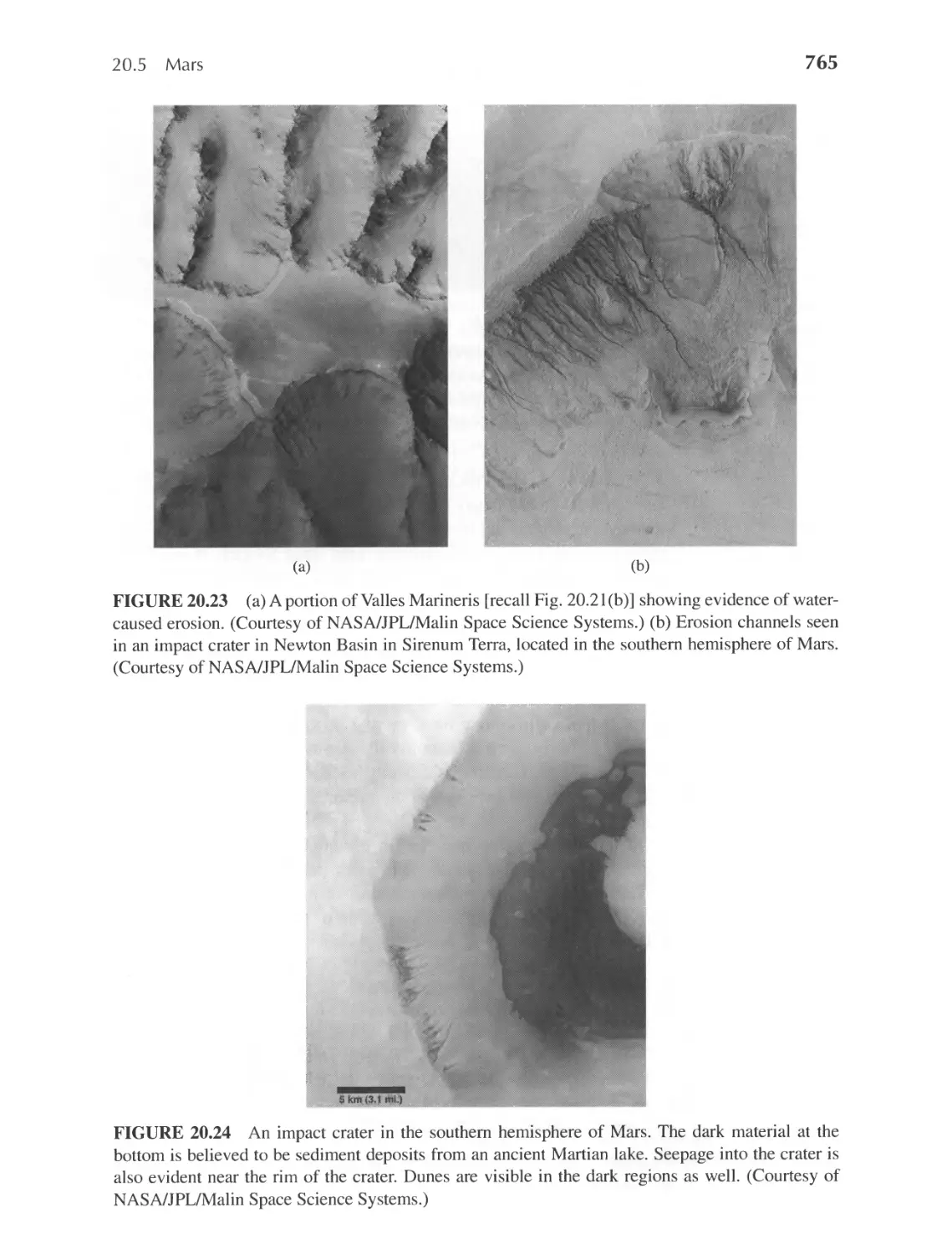
20.5 Mars 762
737
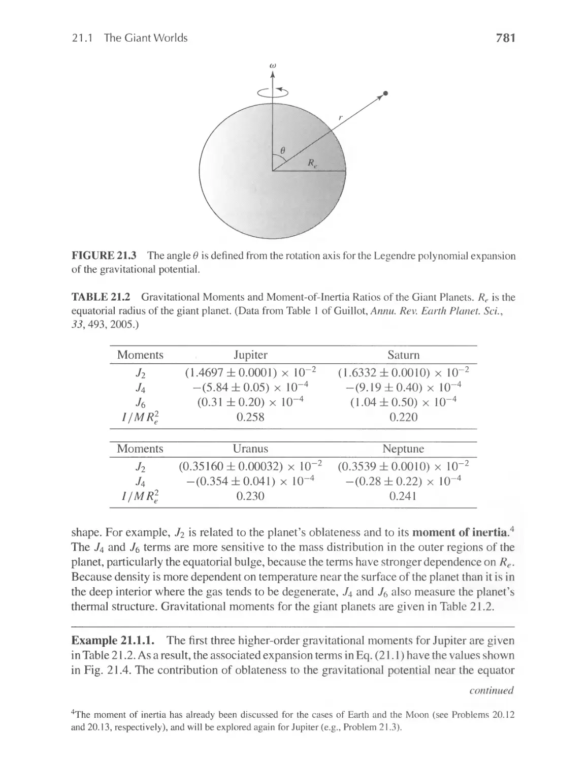
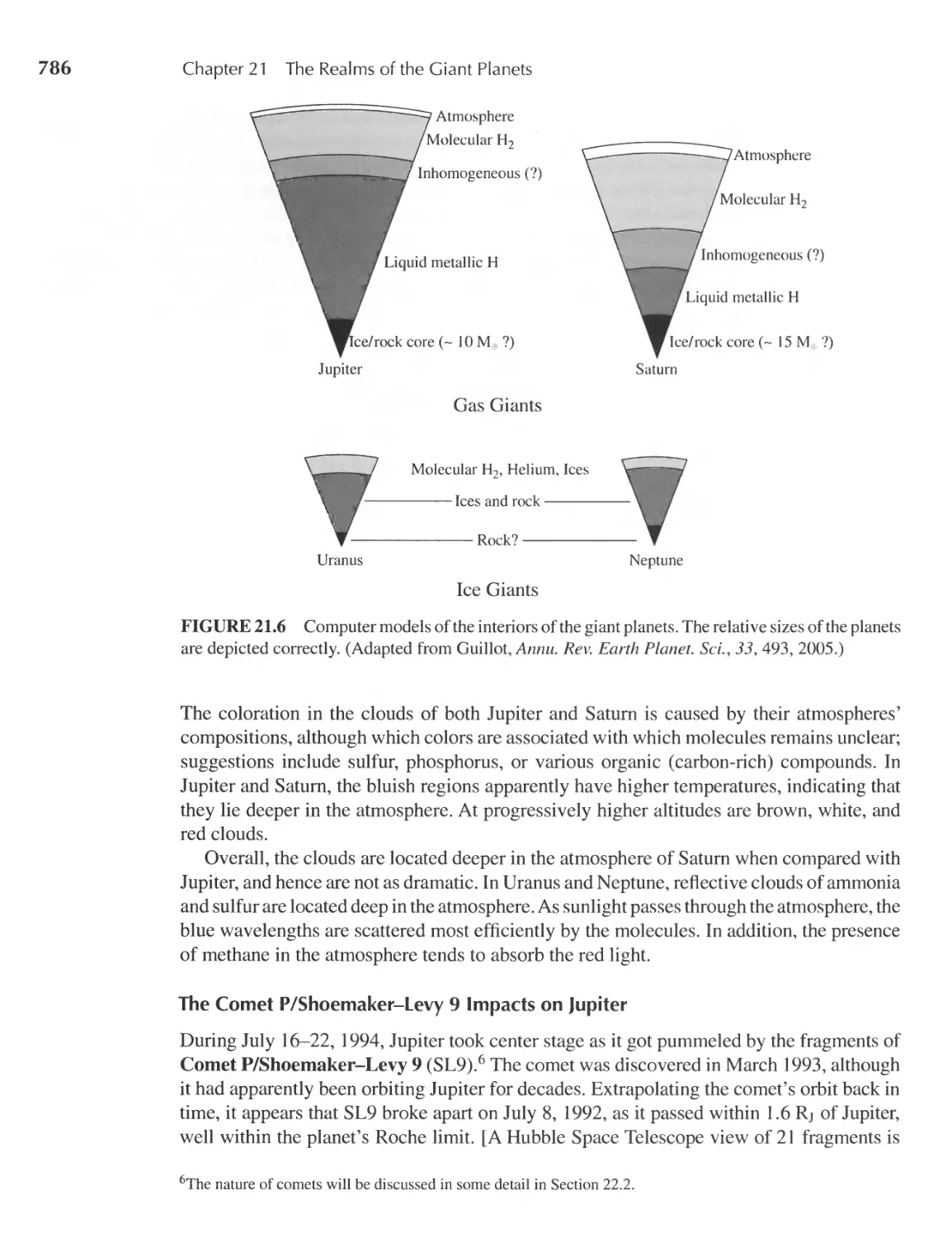
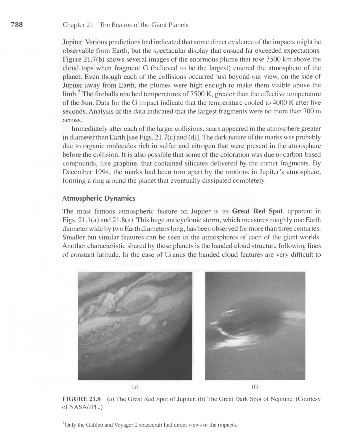
21 II The Realms of the Giant Planets
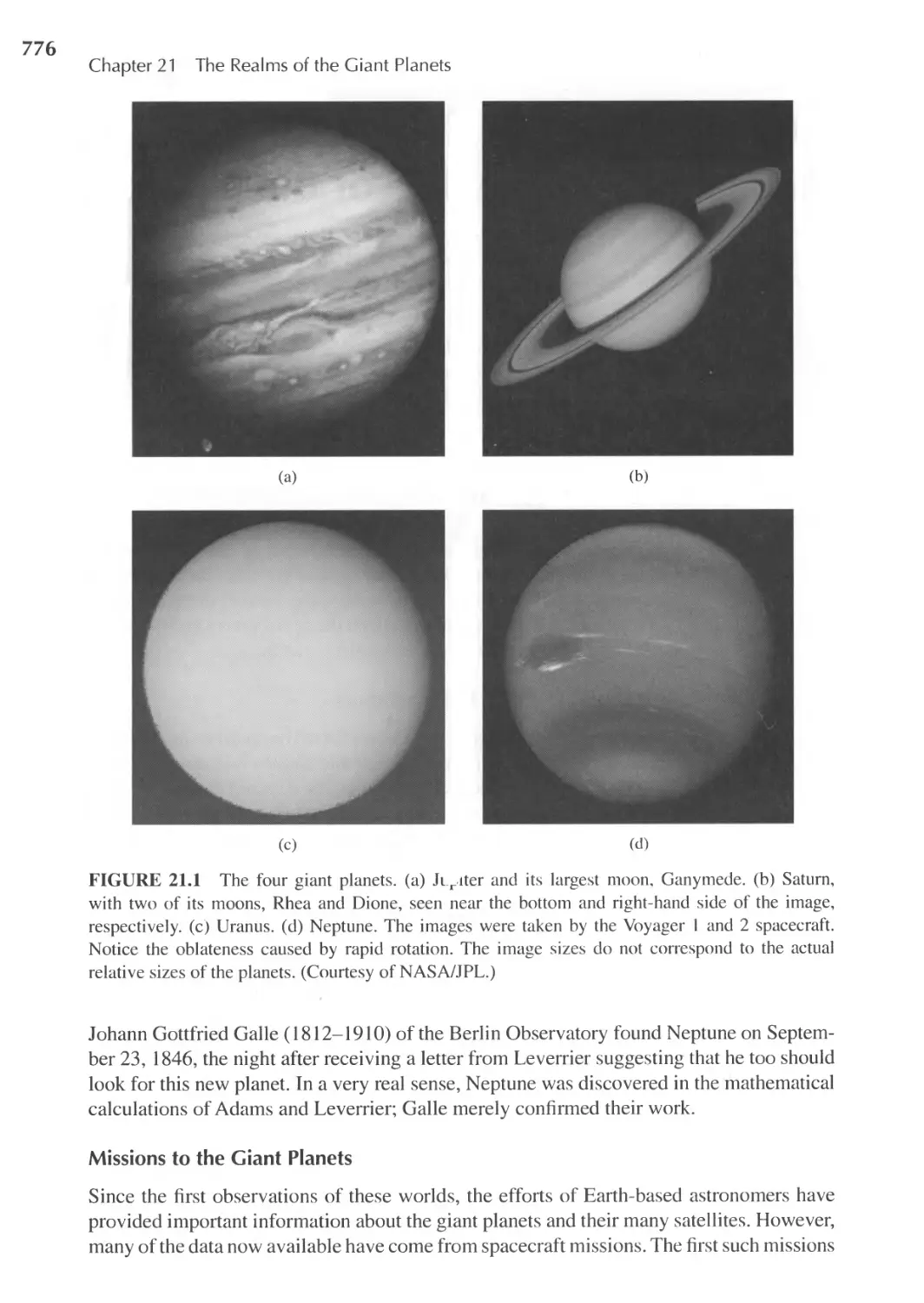
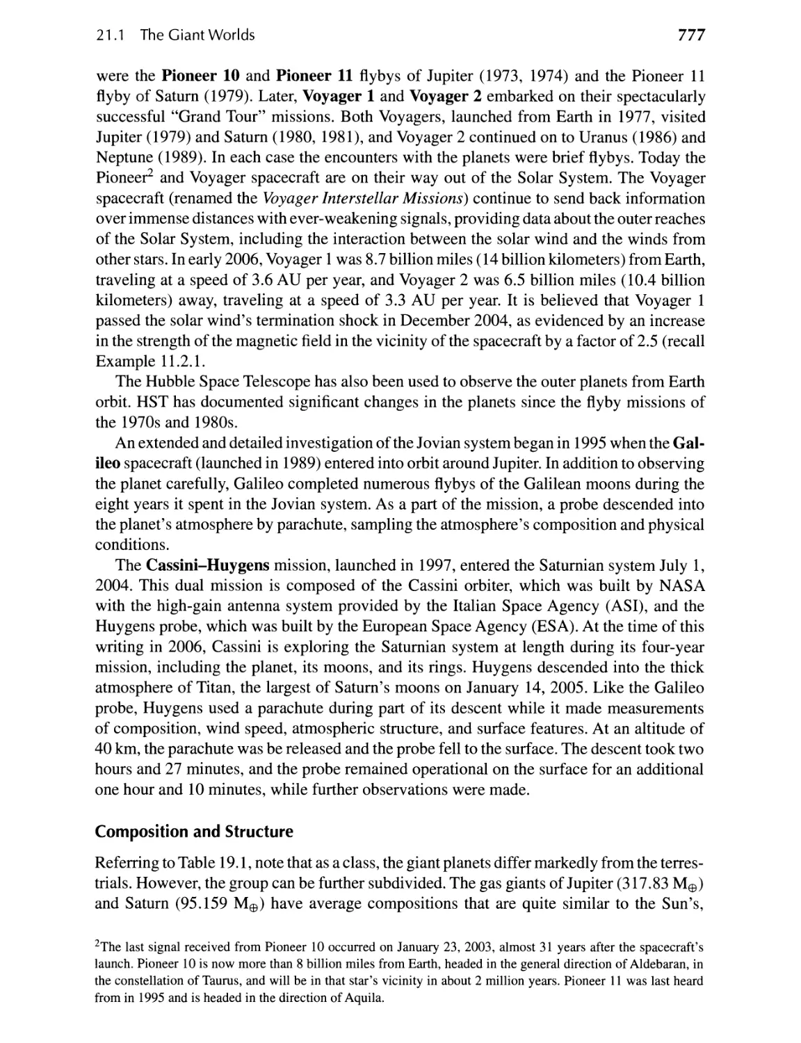
21.1 The Giant Worlds 775
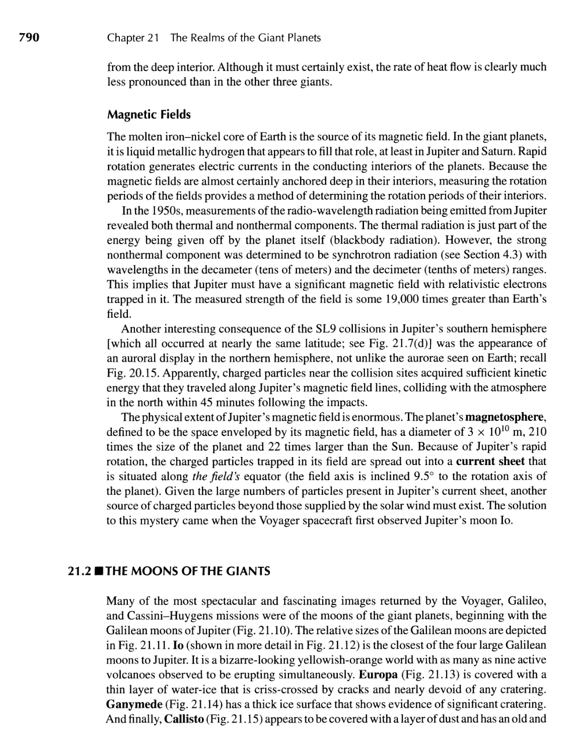
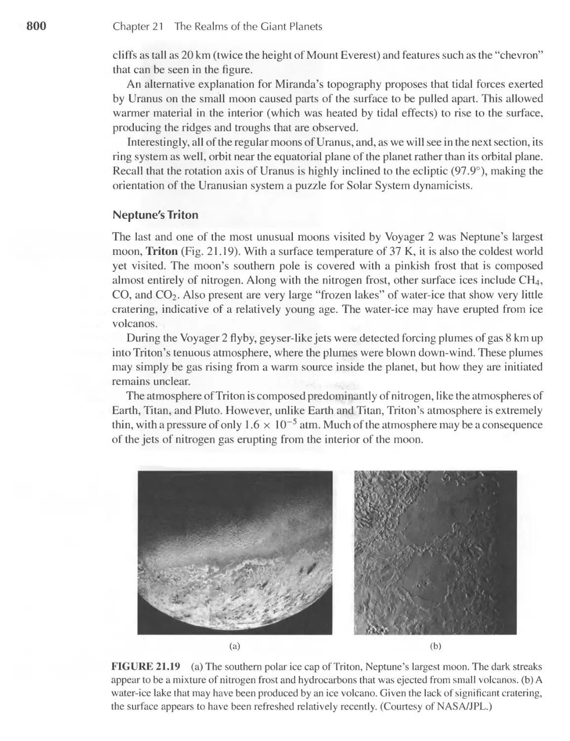
21.2 The Moons of the Giants 790
21.3 Planetary Ring Systems 801
775
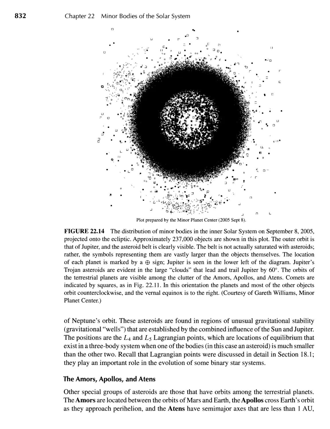
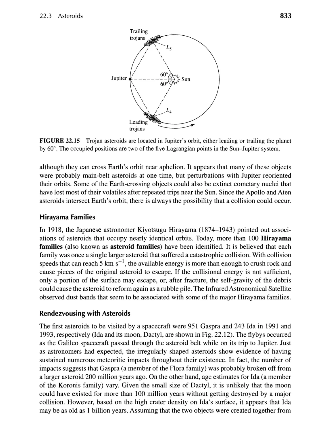
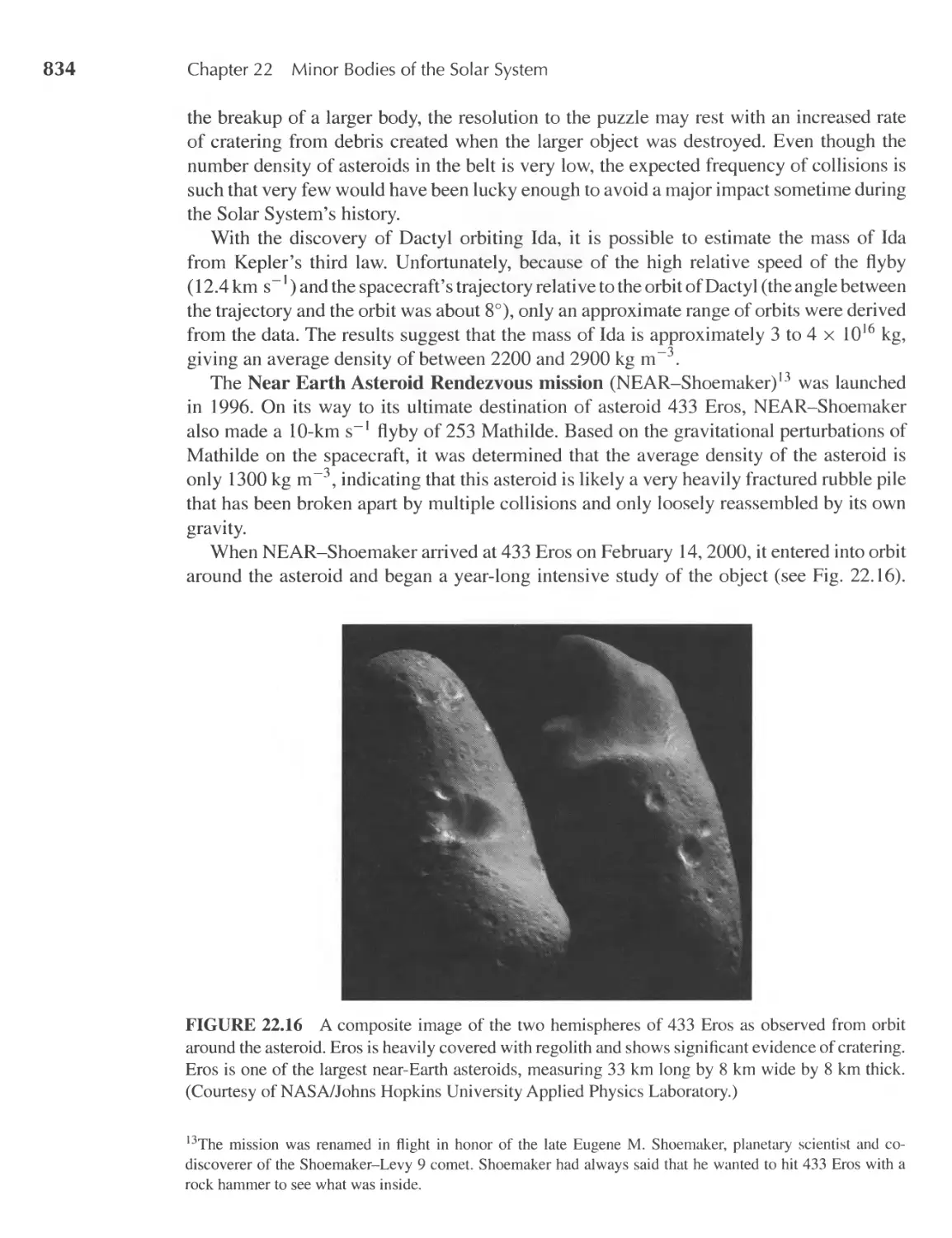
22 II Minor Bodies of the Solar System
22.1 Pluto and Charon 813
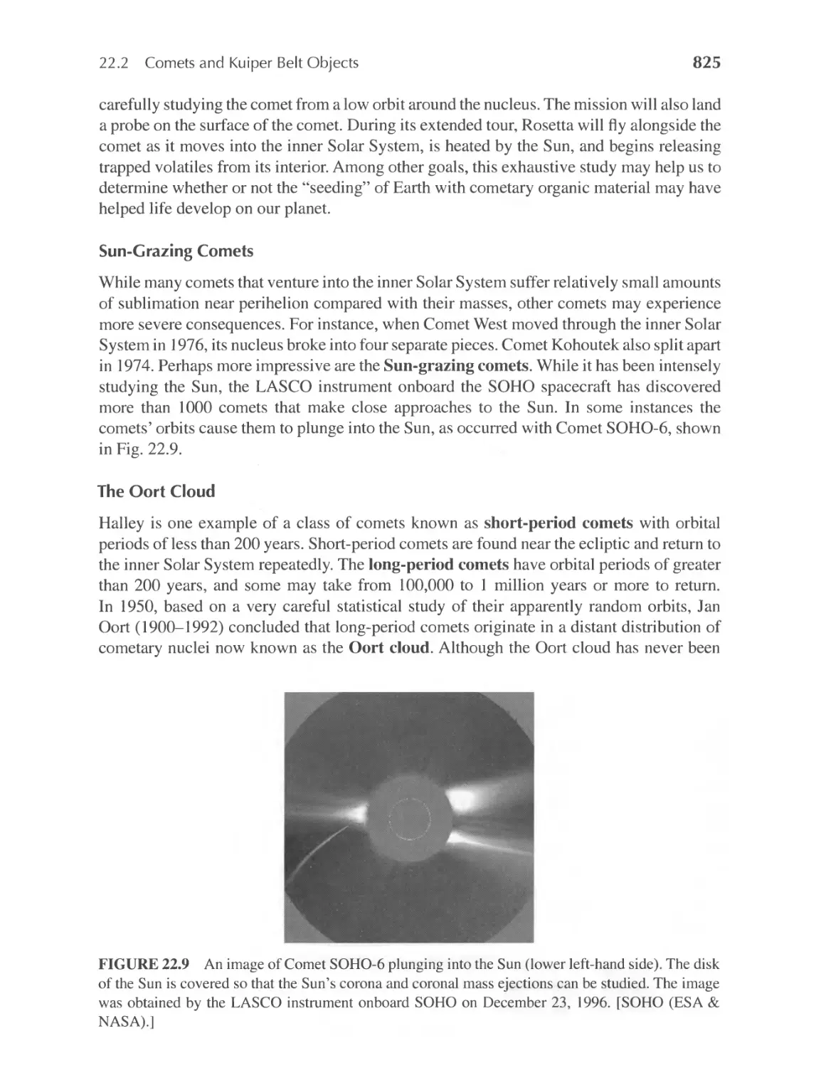
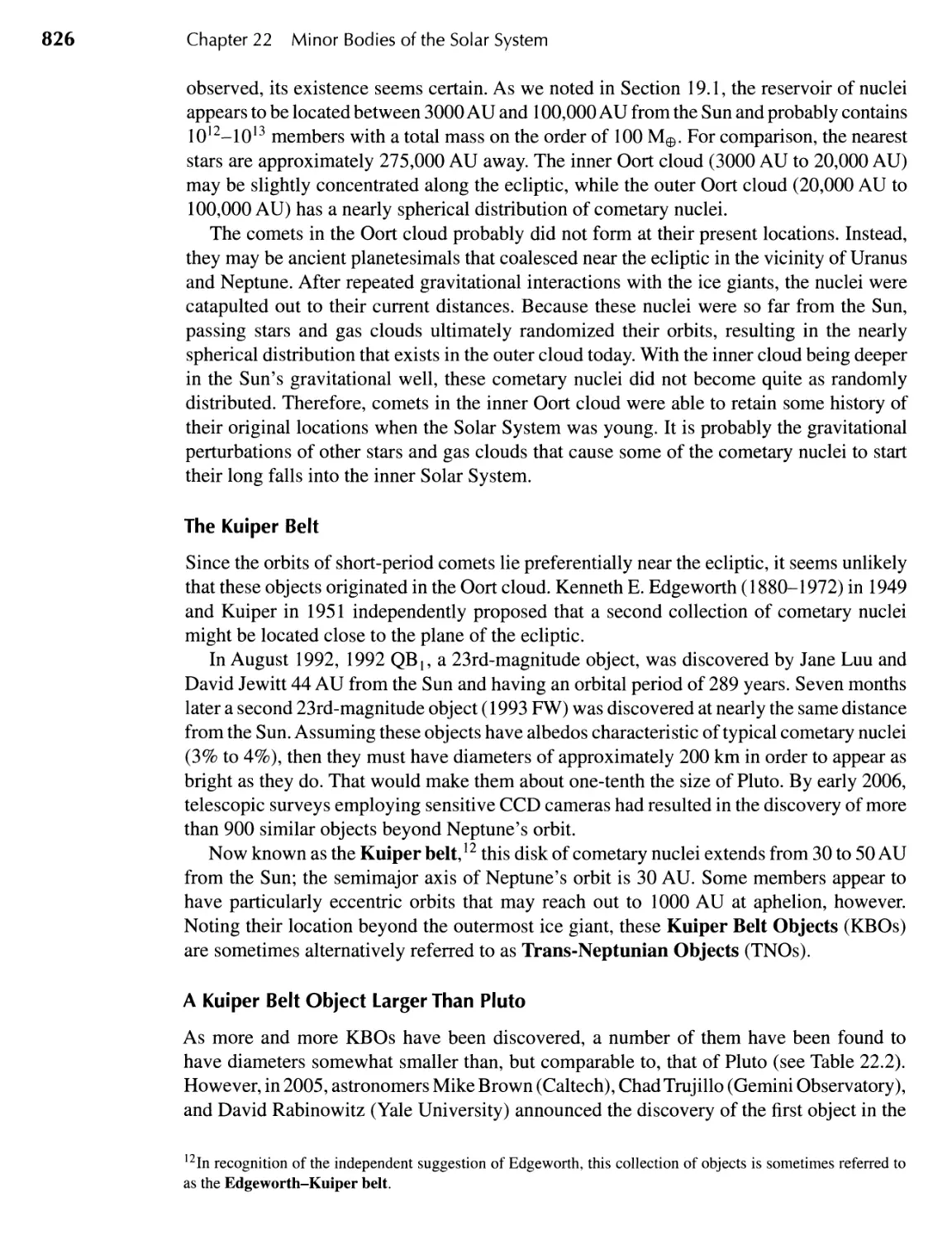
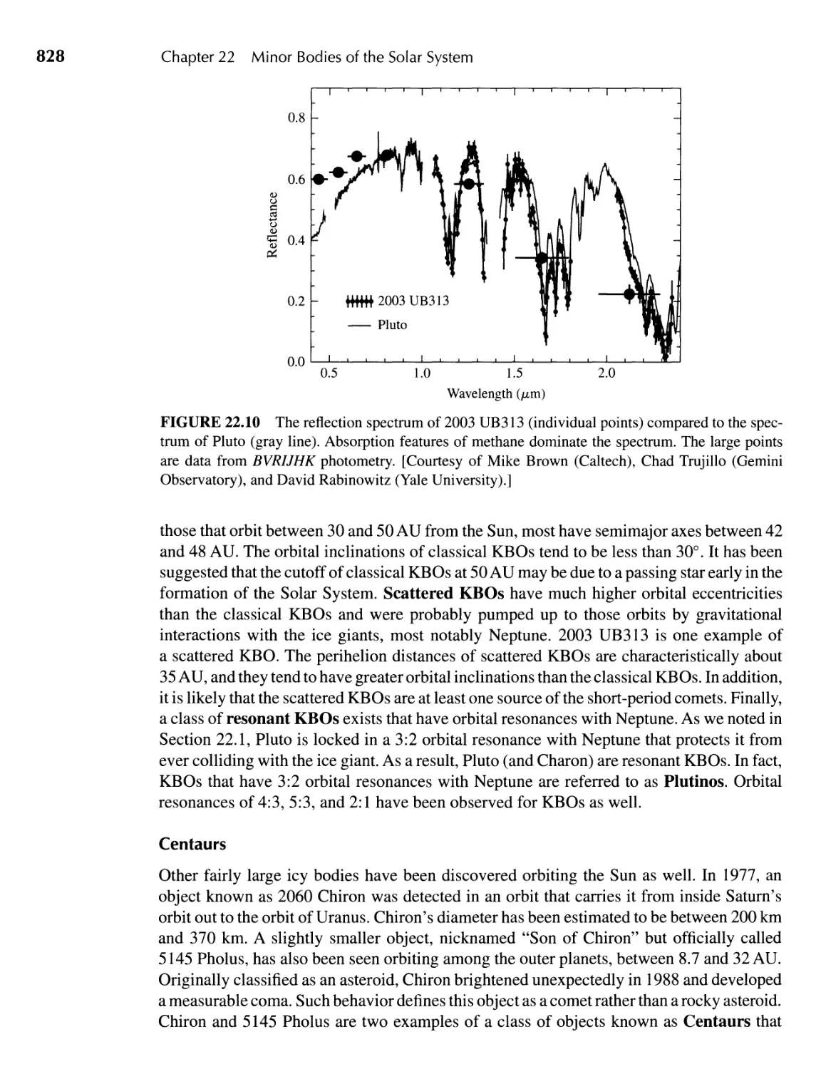
22.2 Comets and Kuiper Belt Objects 816
22.3 Asteroids 830
22.4 Meteorites 838
813
Contents
xv
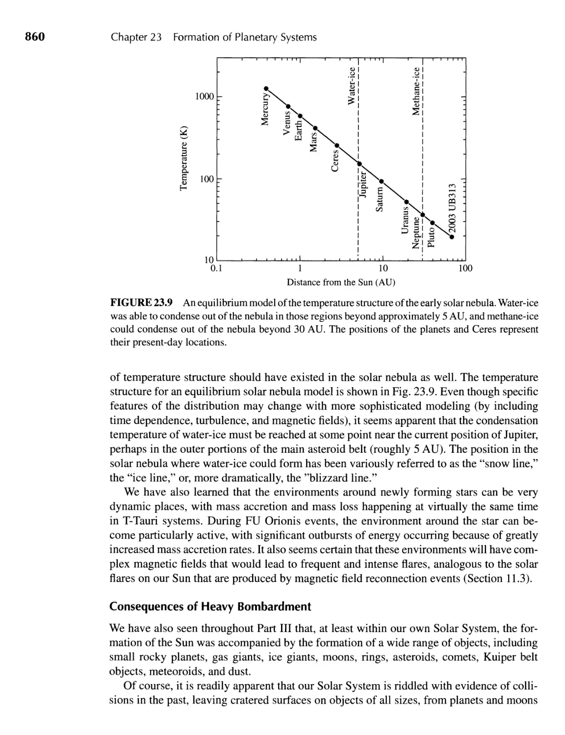
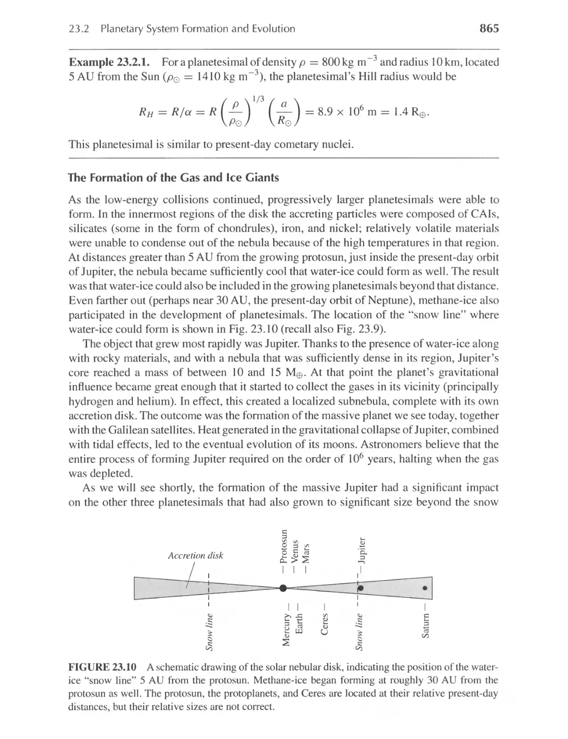
23 II Formation of Planetary Systems
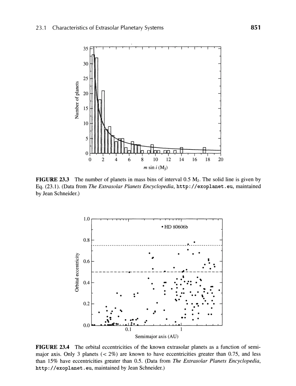
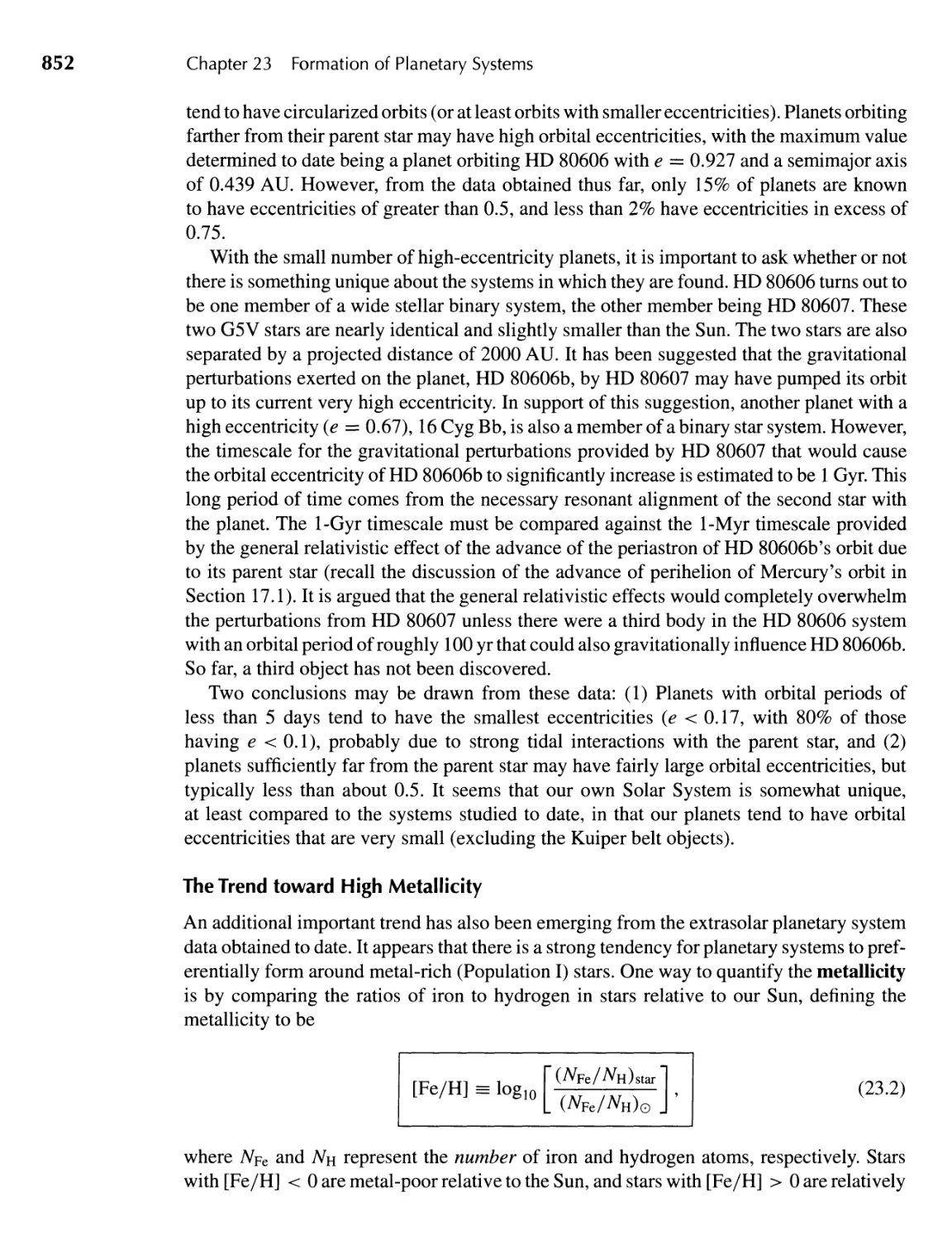
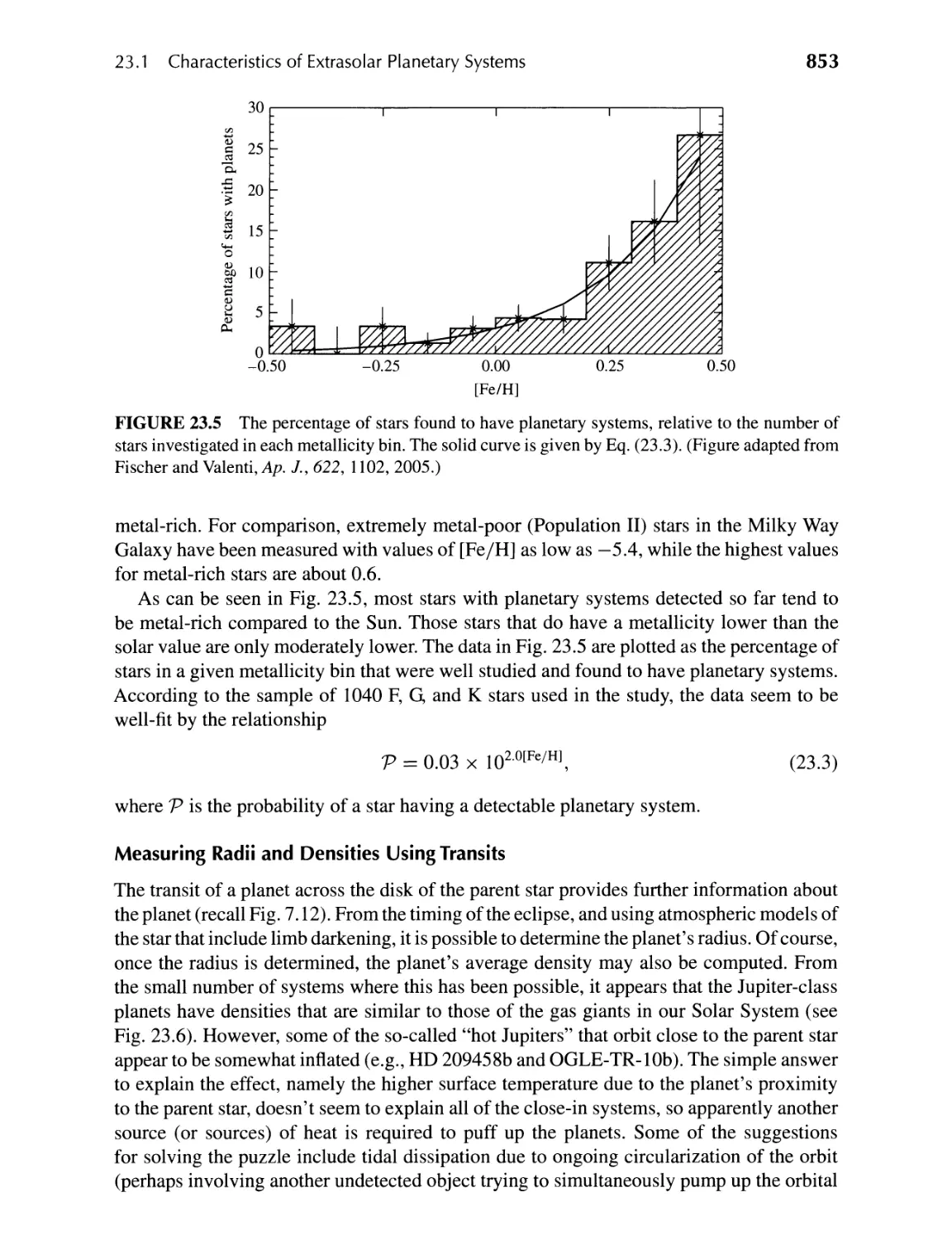
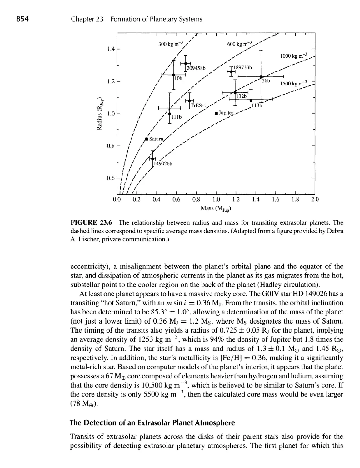
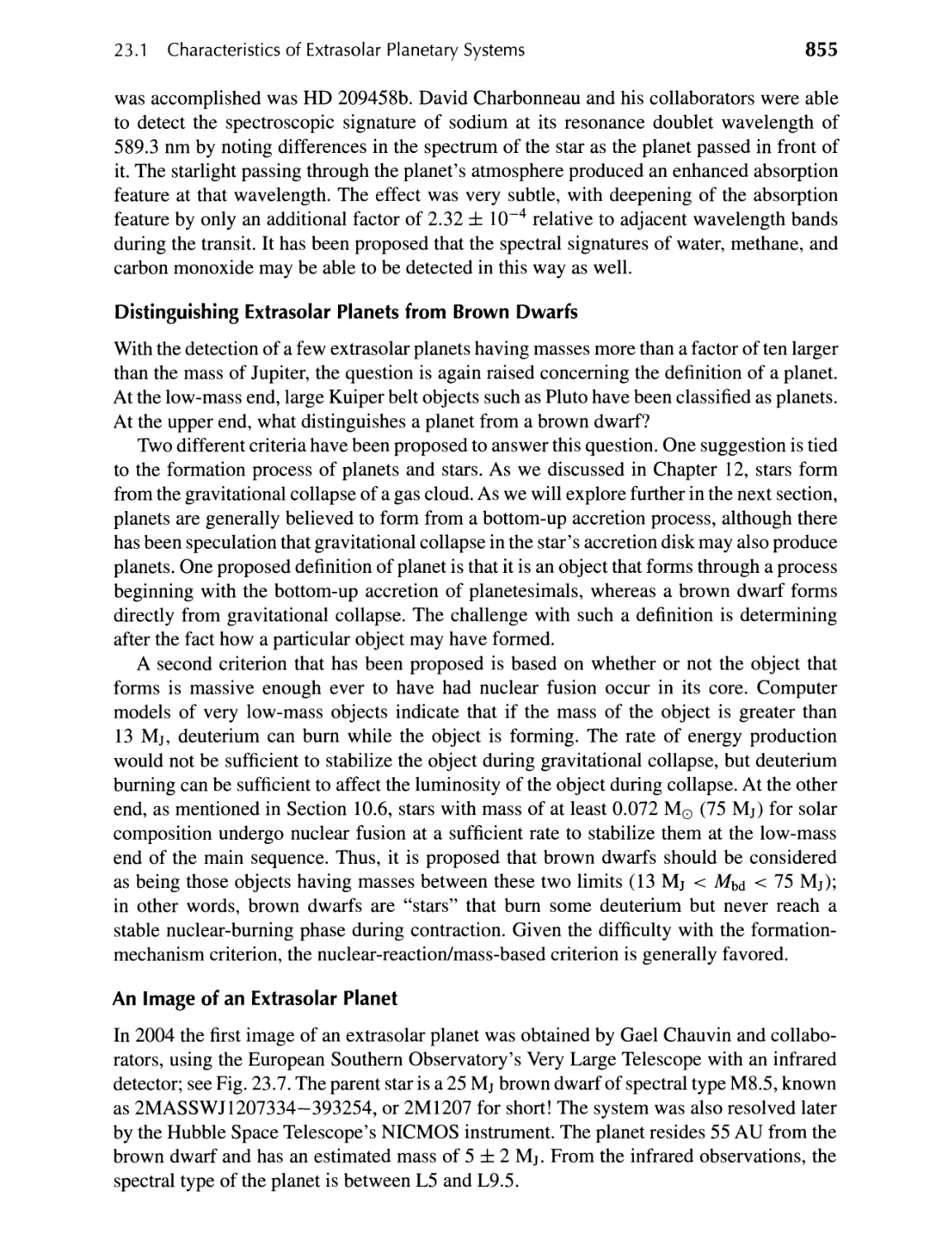
23.1 Characteristics of Extrasolar Planetary Systems 848
23.2 Planetary System Formation and Evolution 857
848
IV GALAXIES AND THE UNIVERSE
873
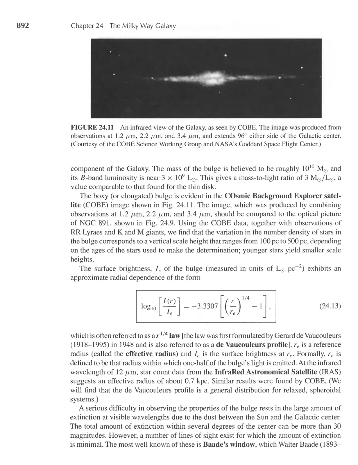
24 II The Mil Way Galaxy
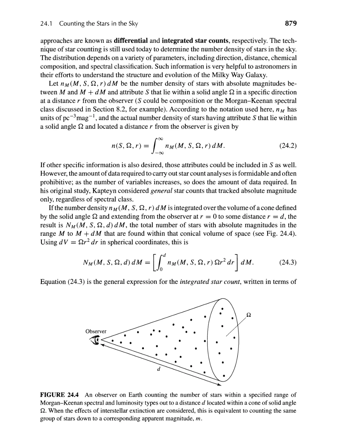
24.1 Counting the Stars in the Sky 874
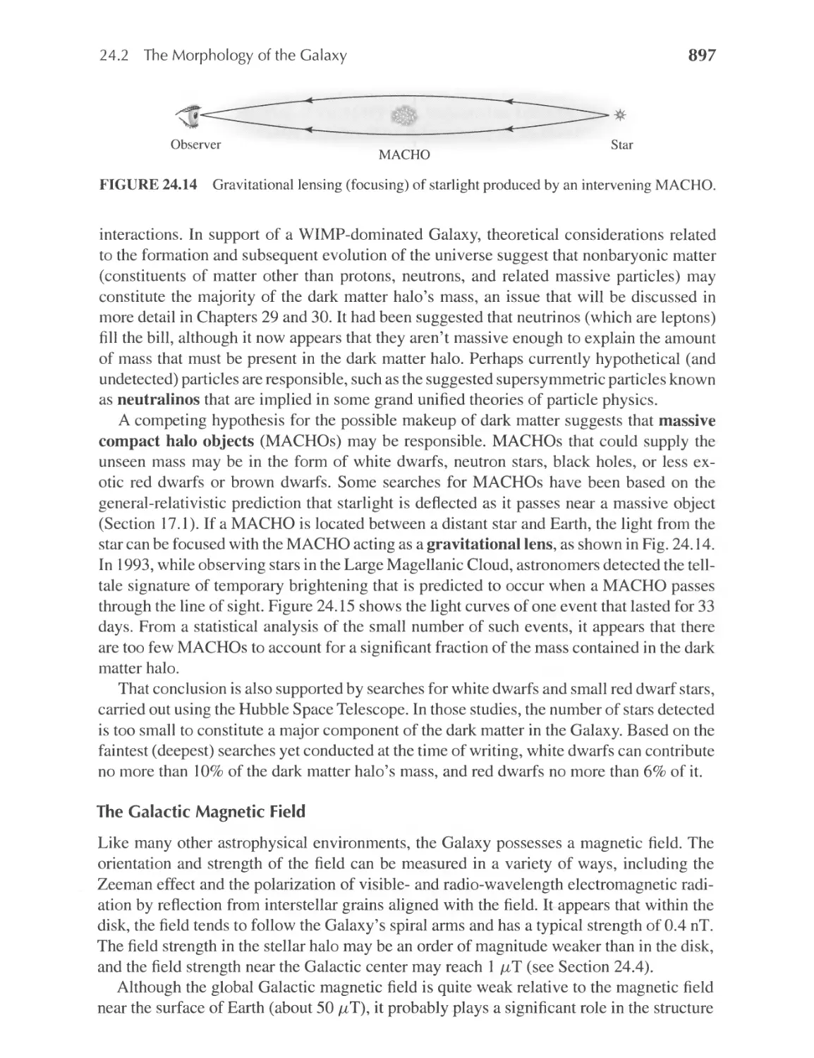
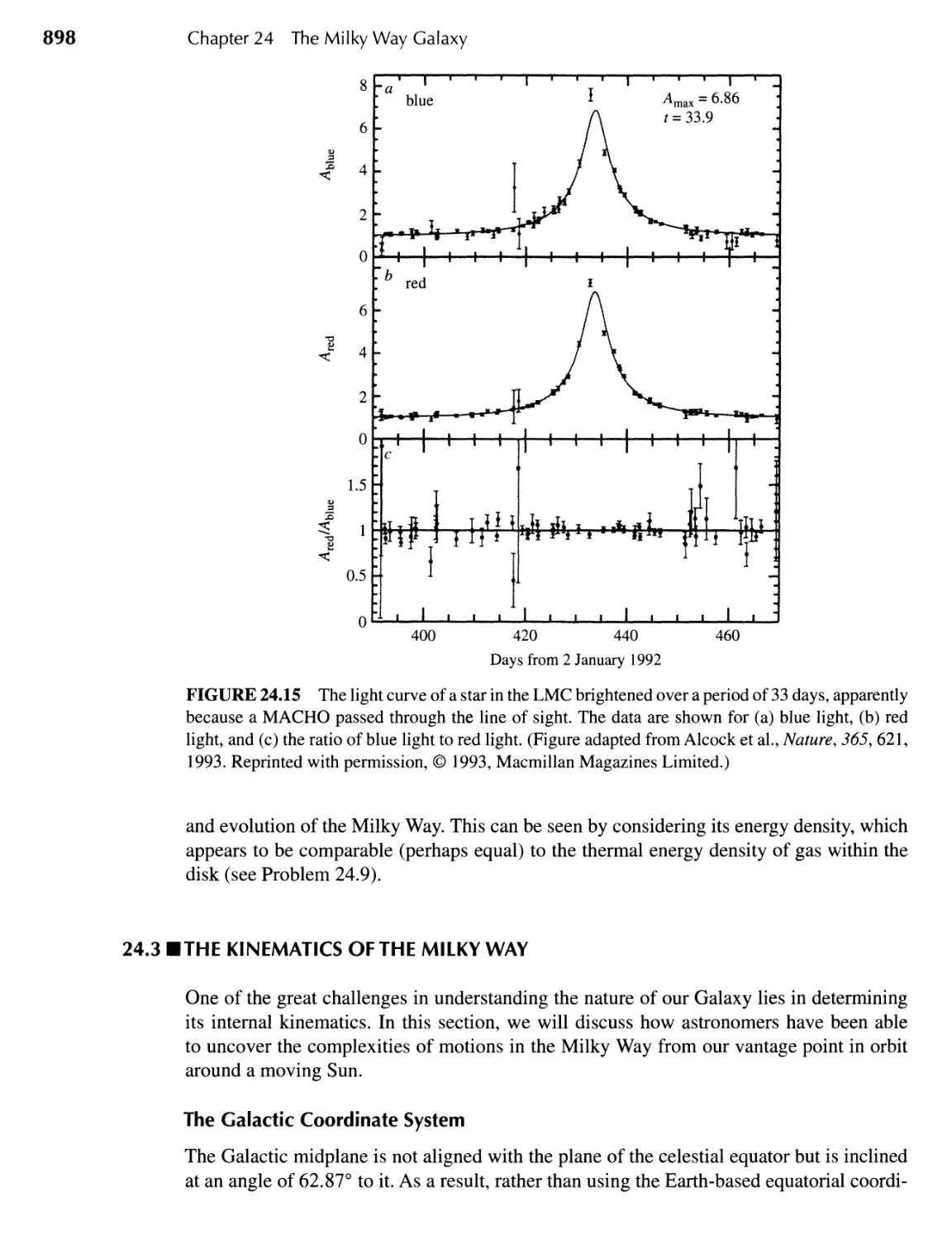
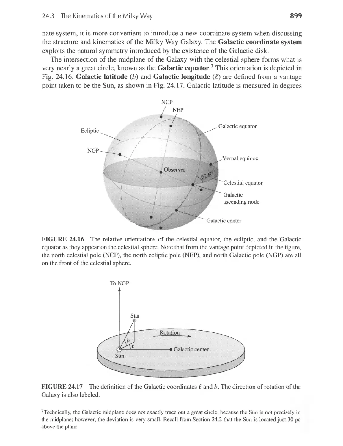
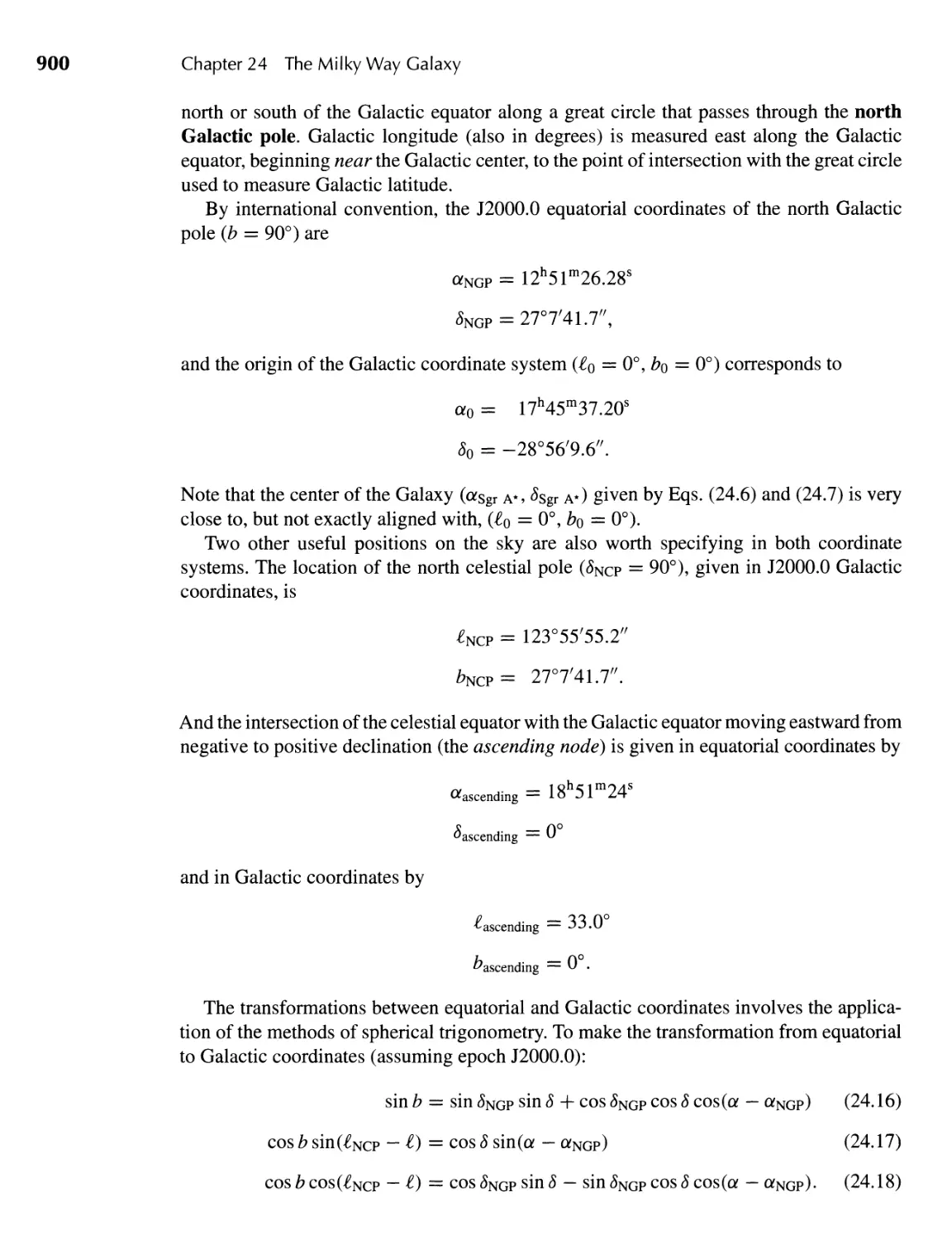
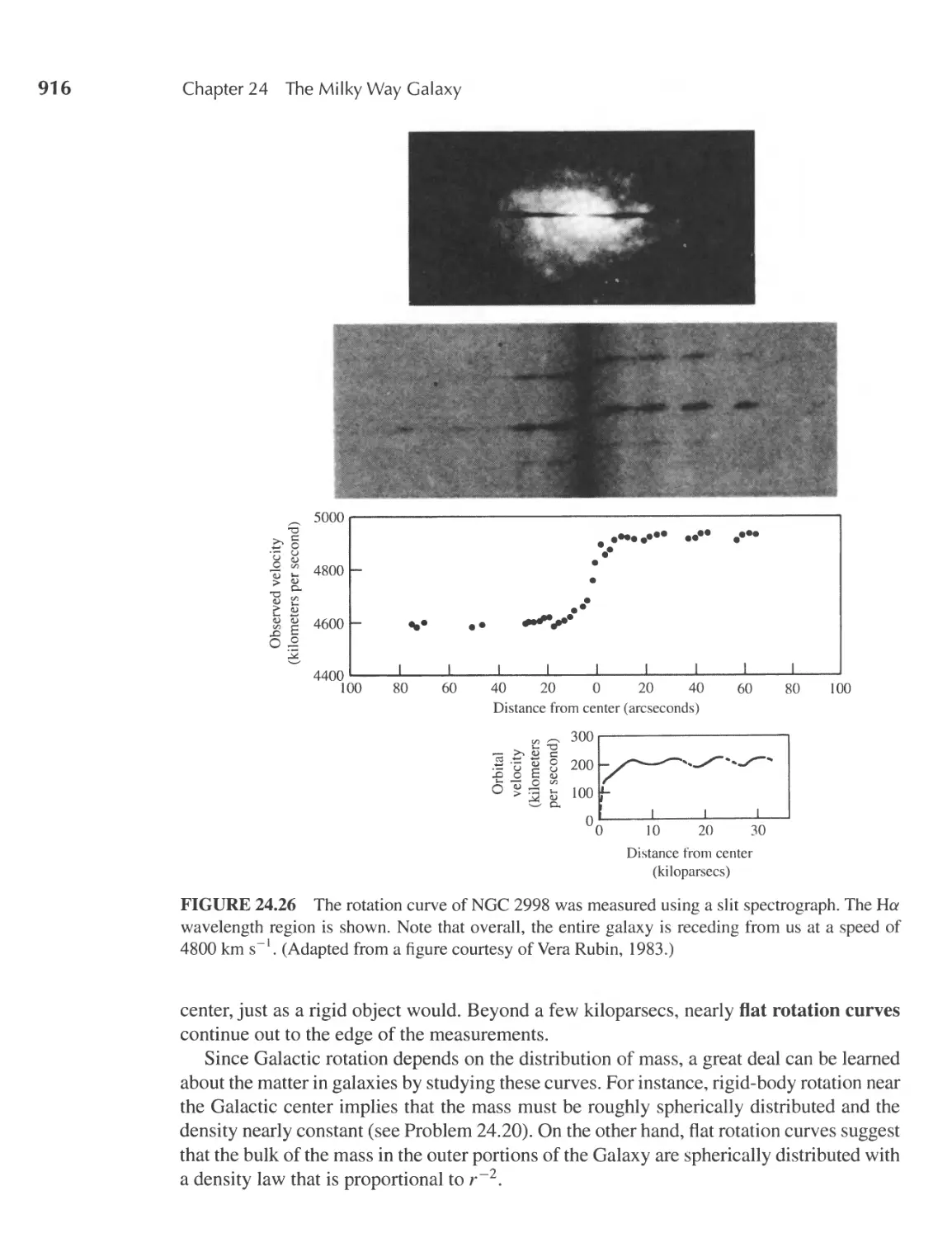
24.2 The Morphology of the Galaxy 881
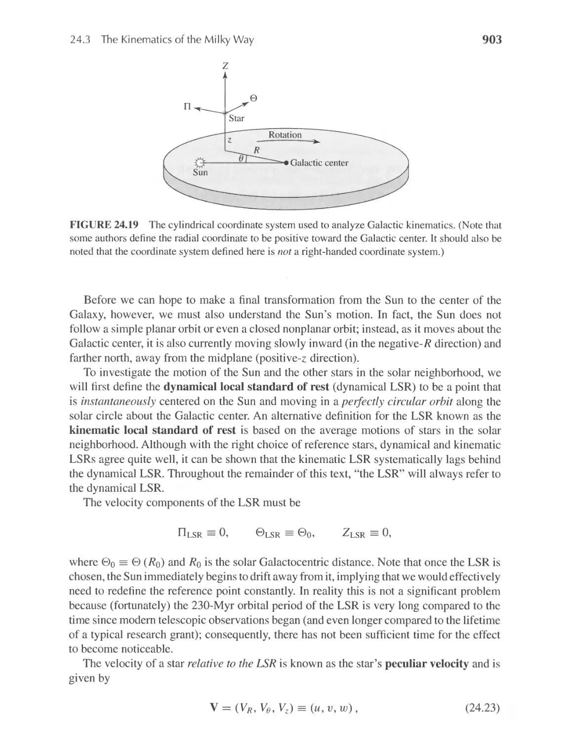
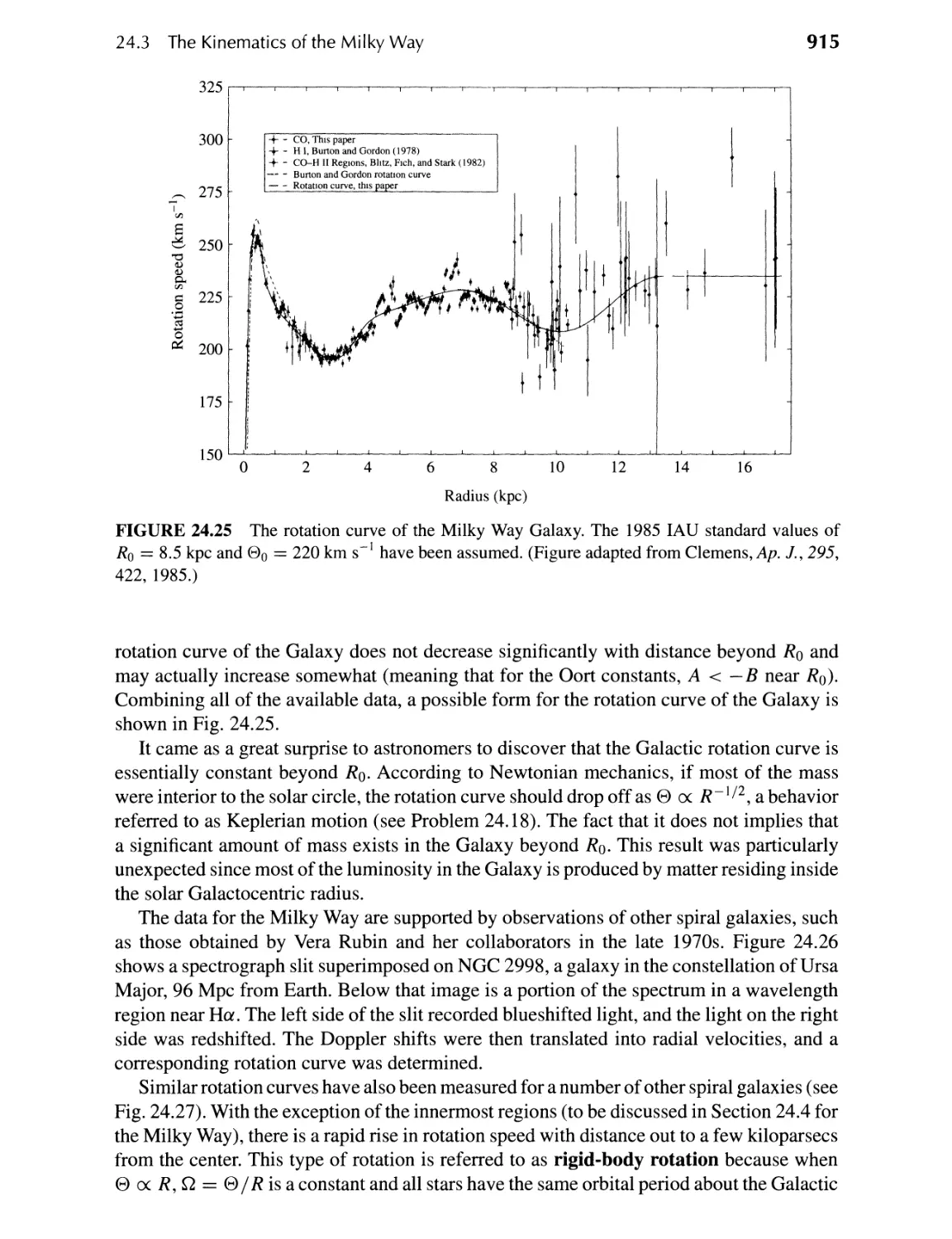
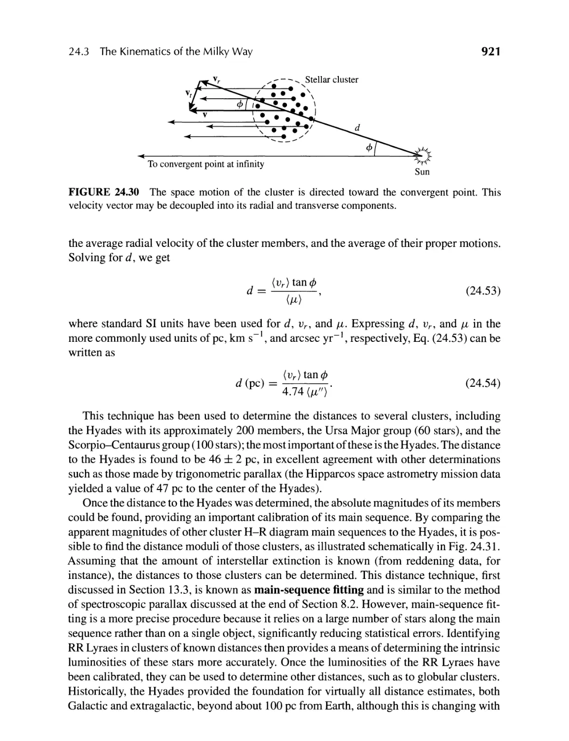
24.3 The Kinematics of the Milky Way 898
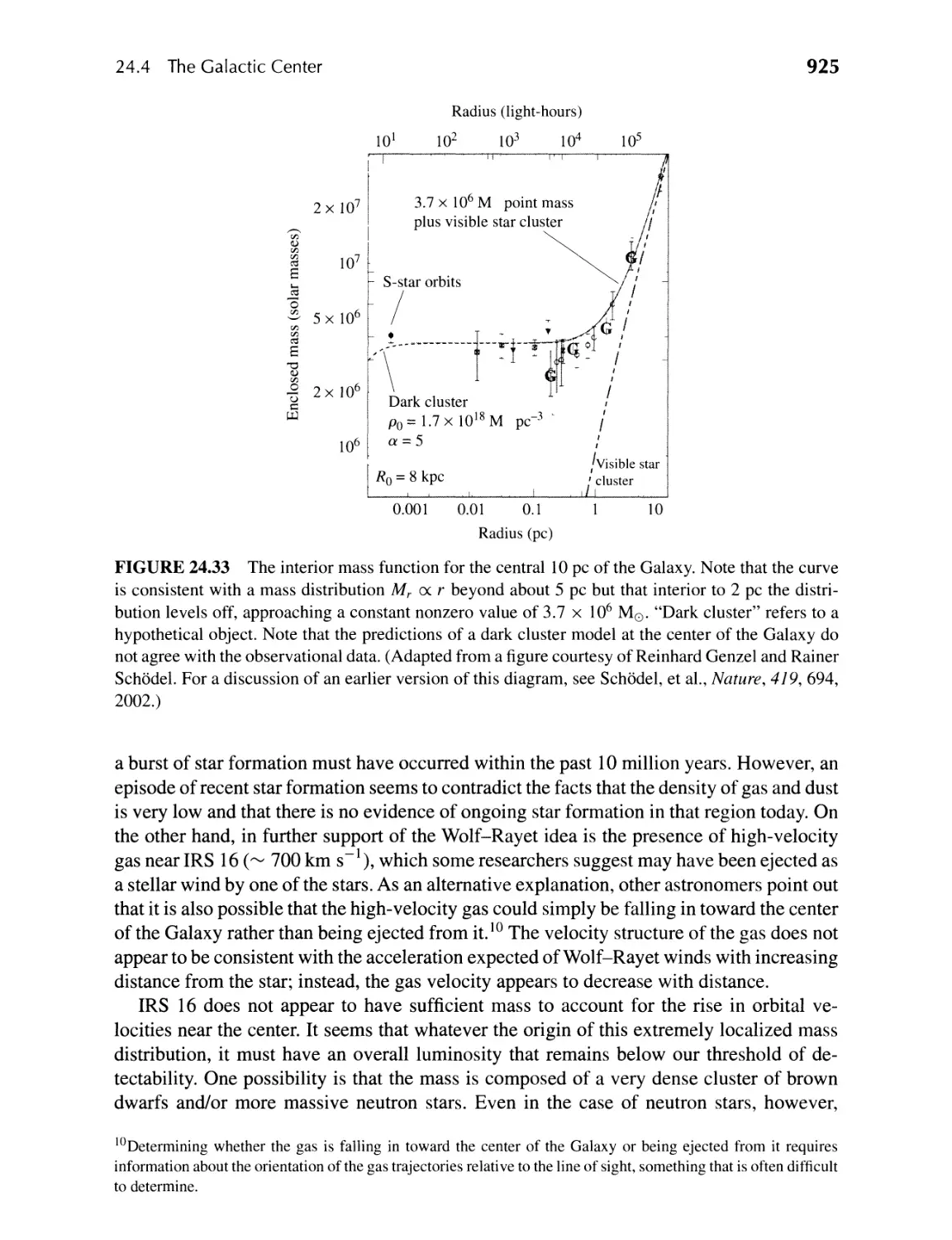
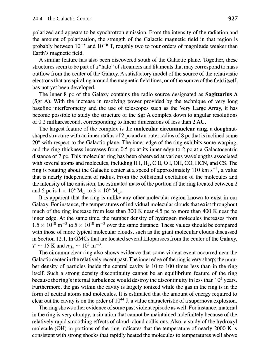
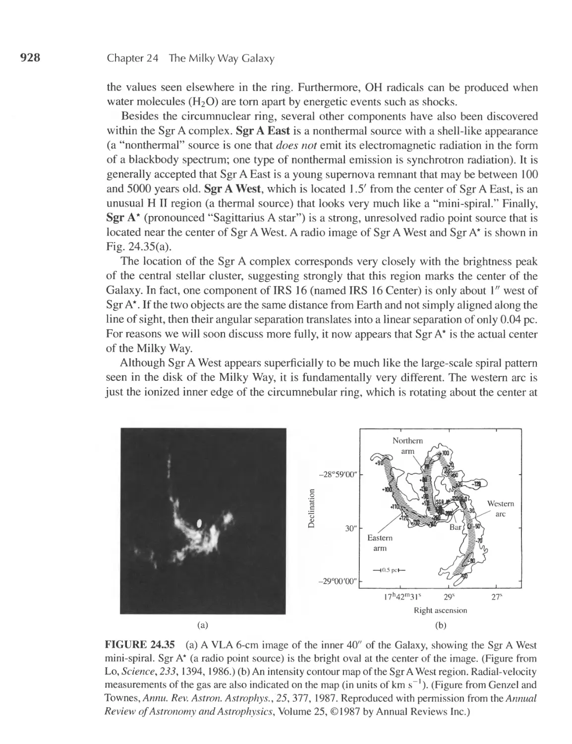
24.4 The Galactic Center 922
874
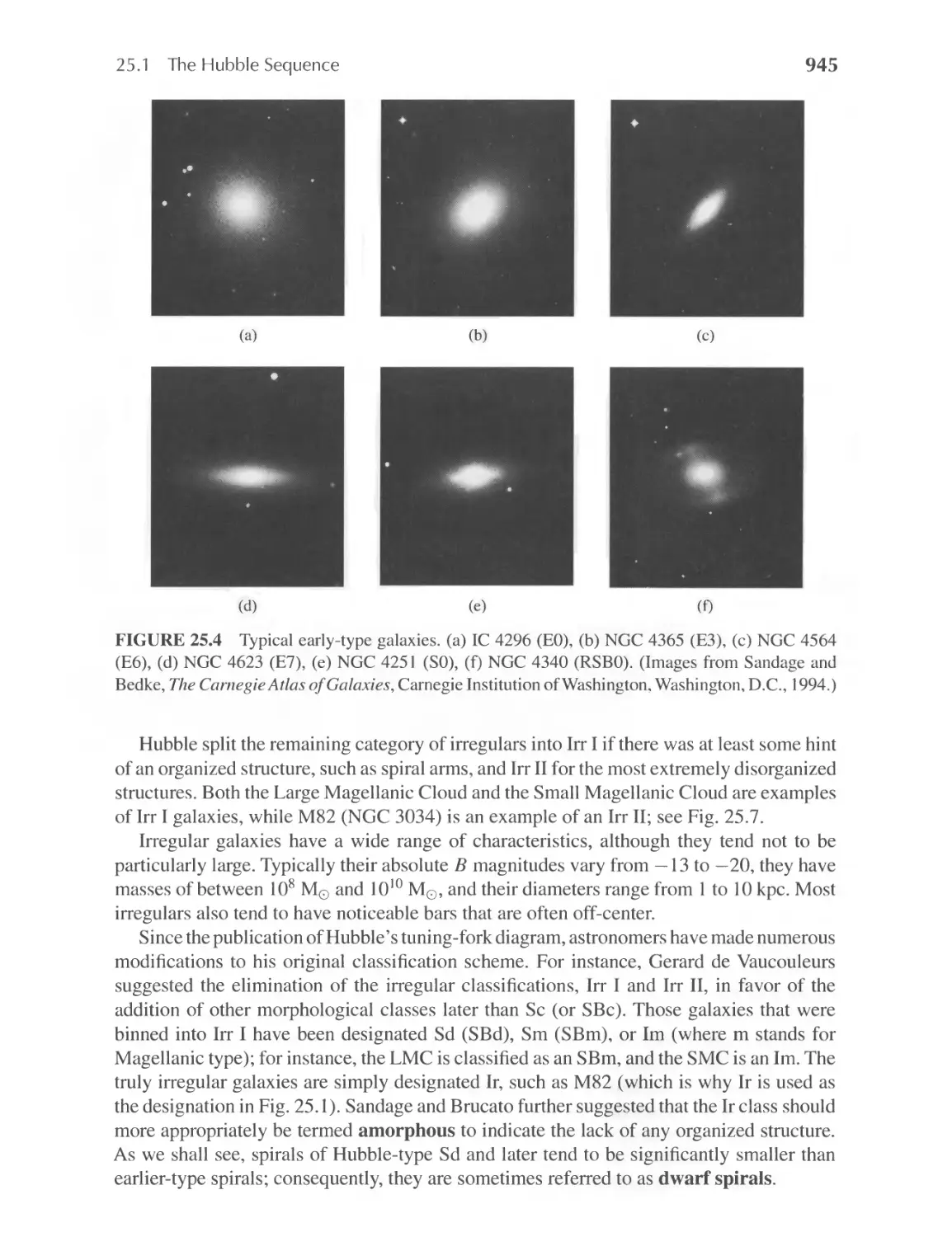
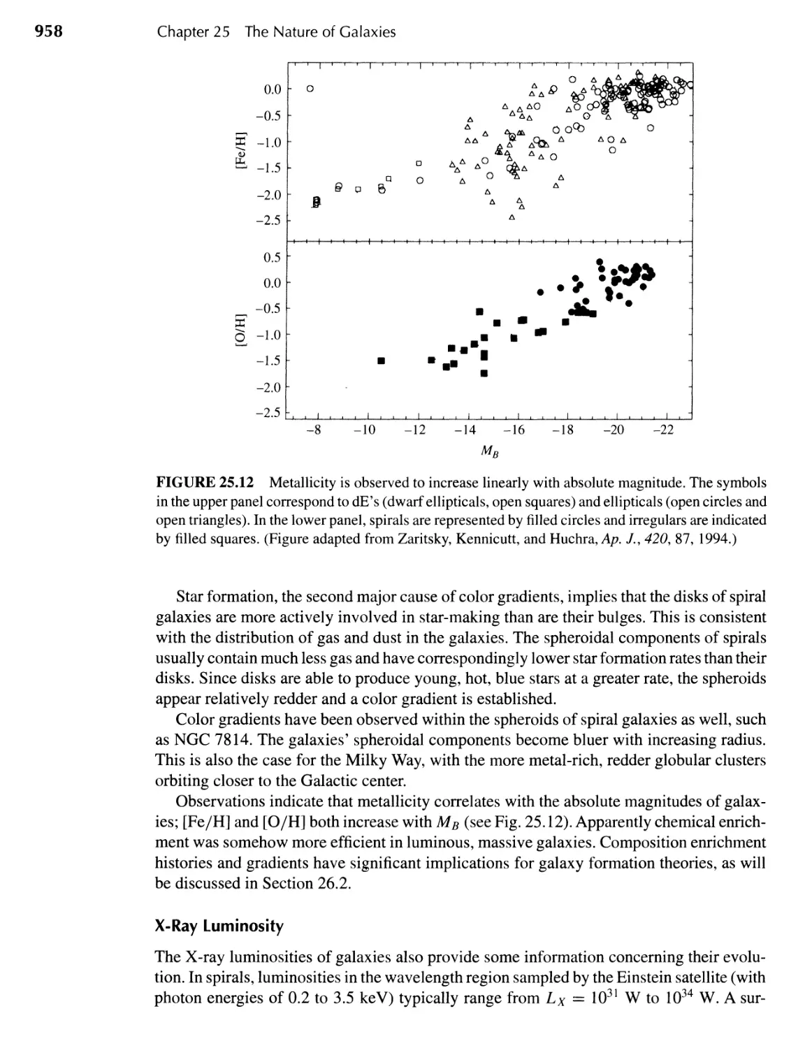
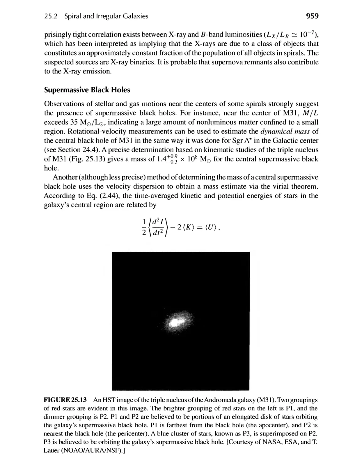
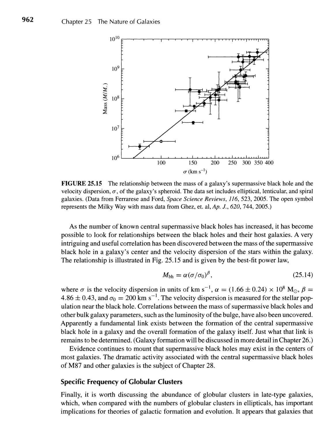
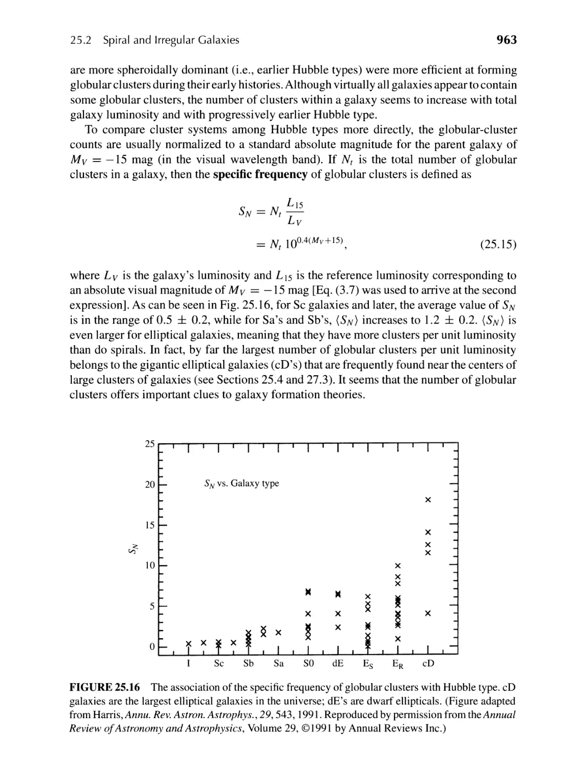
25 II The Nature of Galaxies
25.1 The Hubble Sequence 940
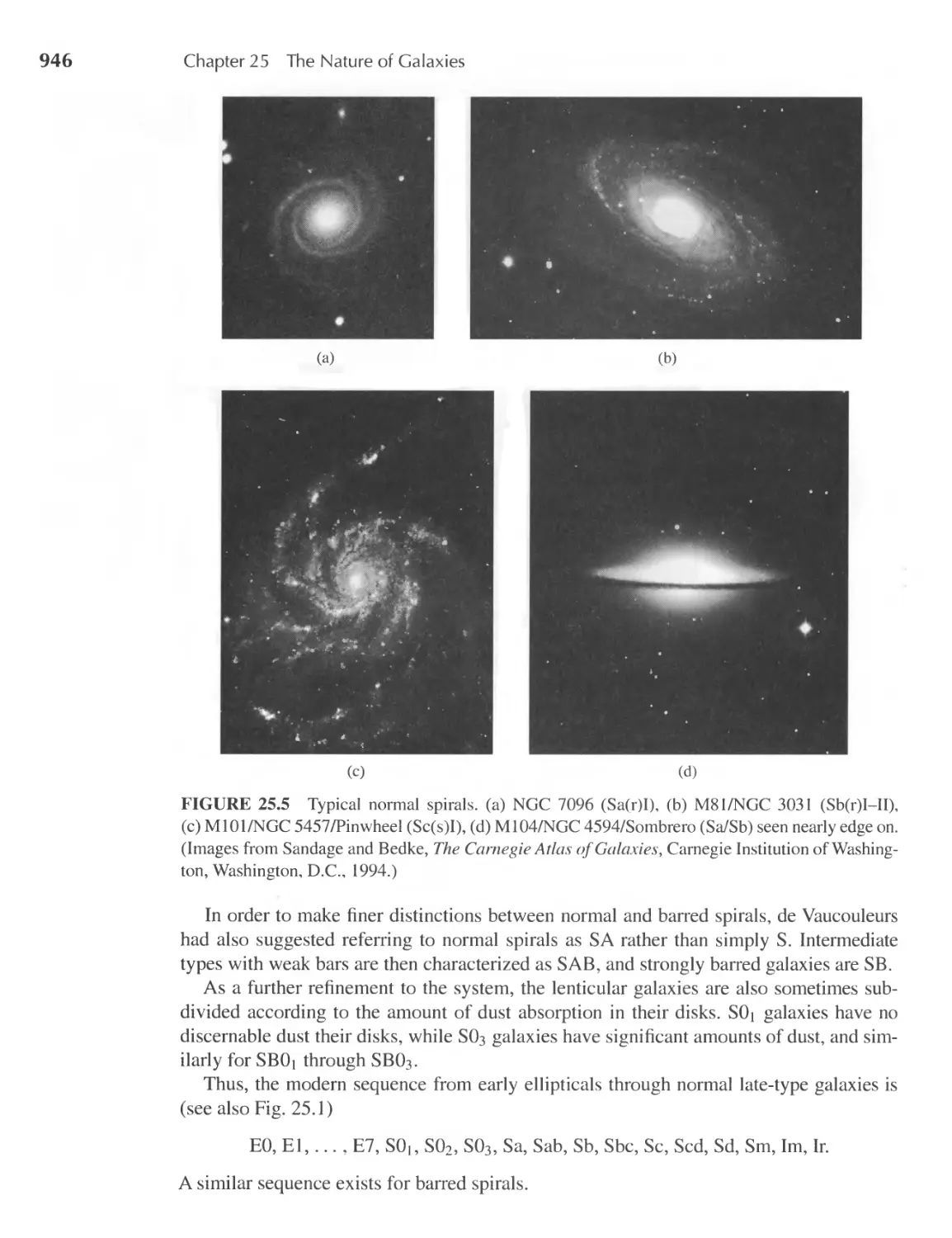
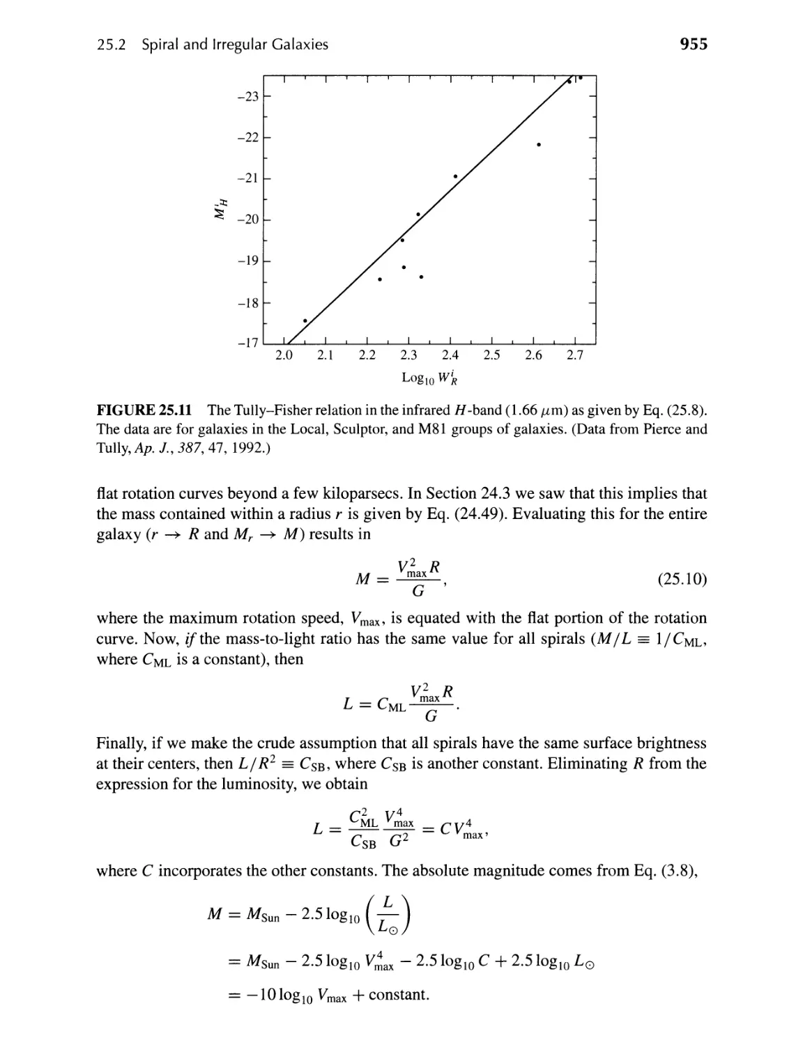
25.2 Spiral and Irregular Galaxies 948
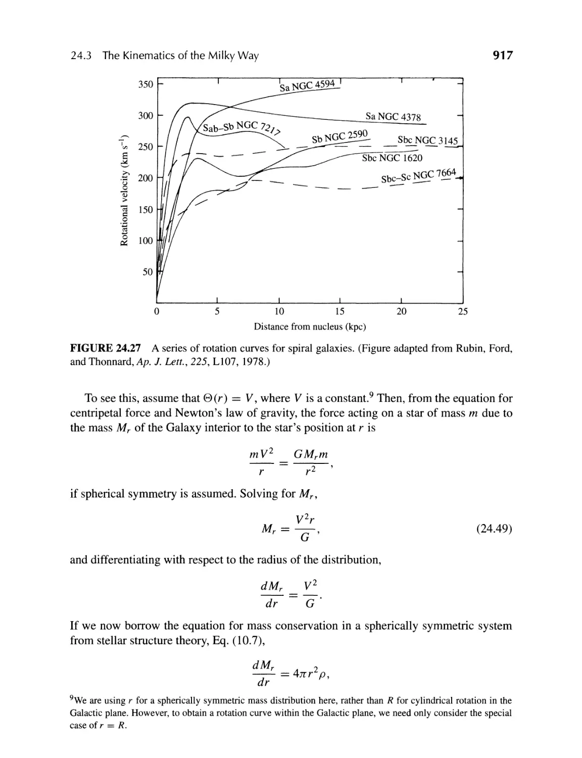
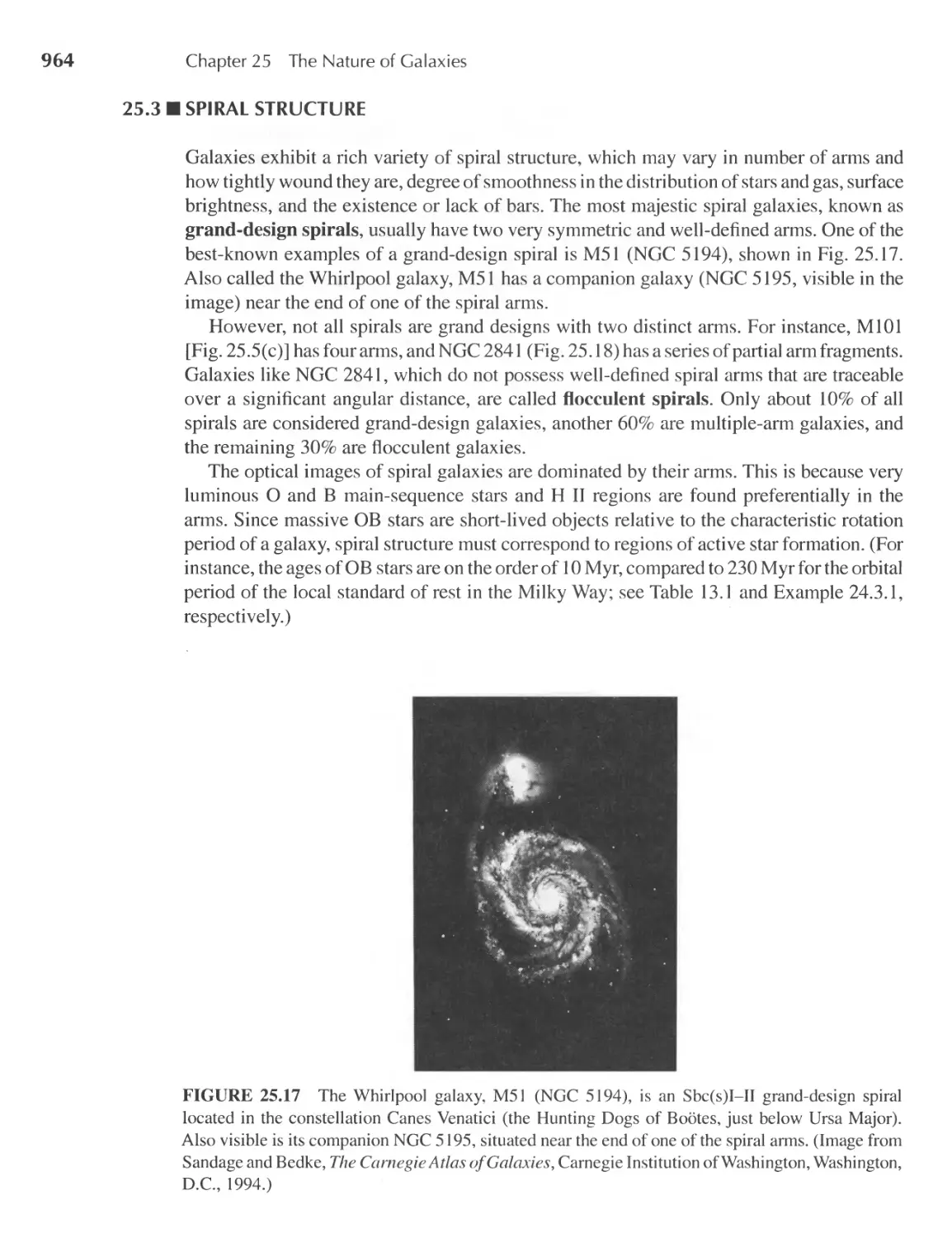
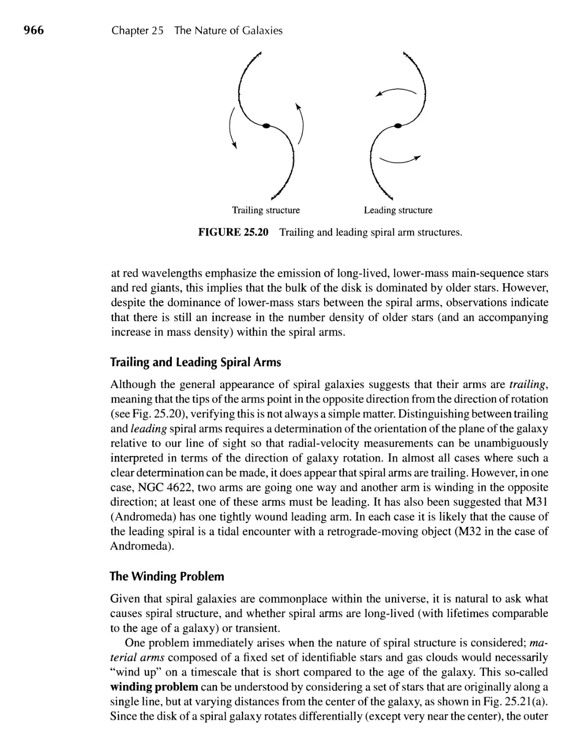
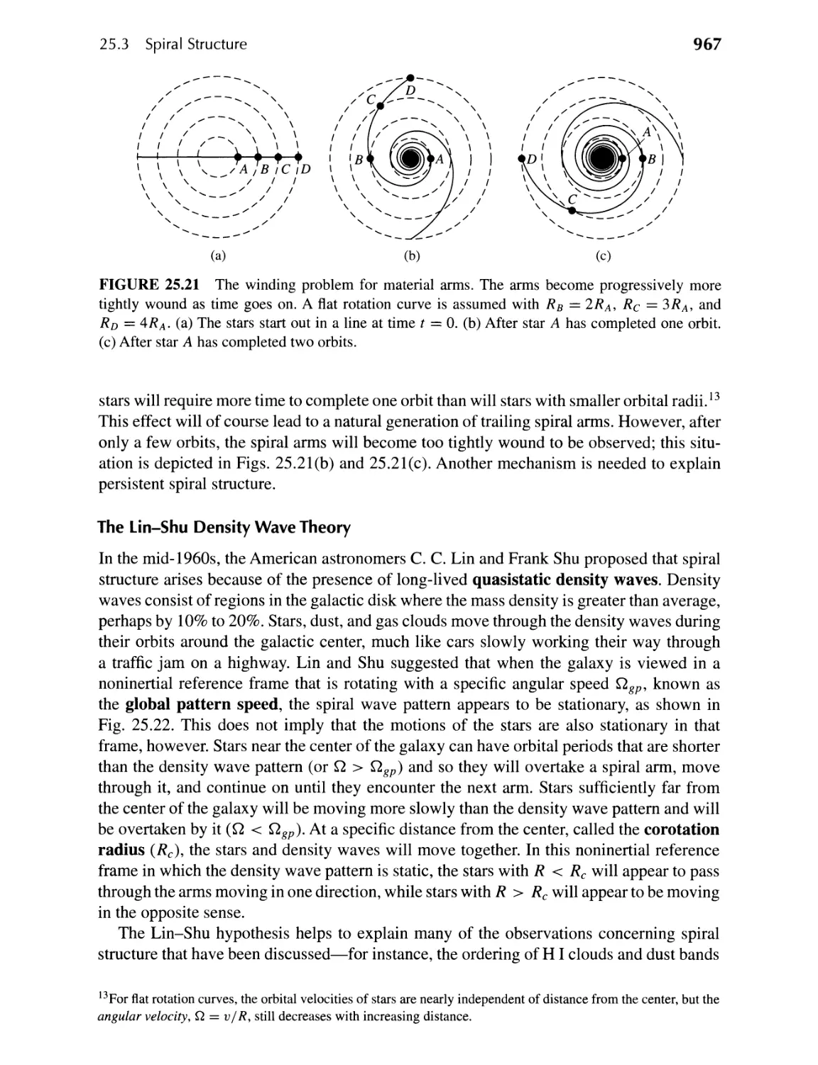
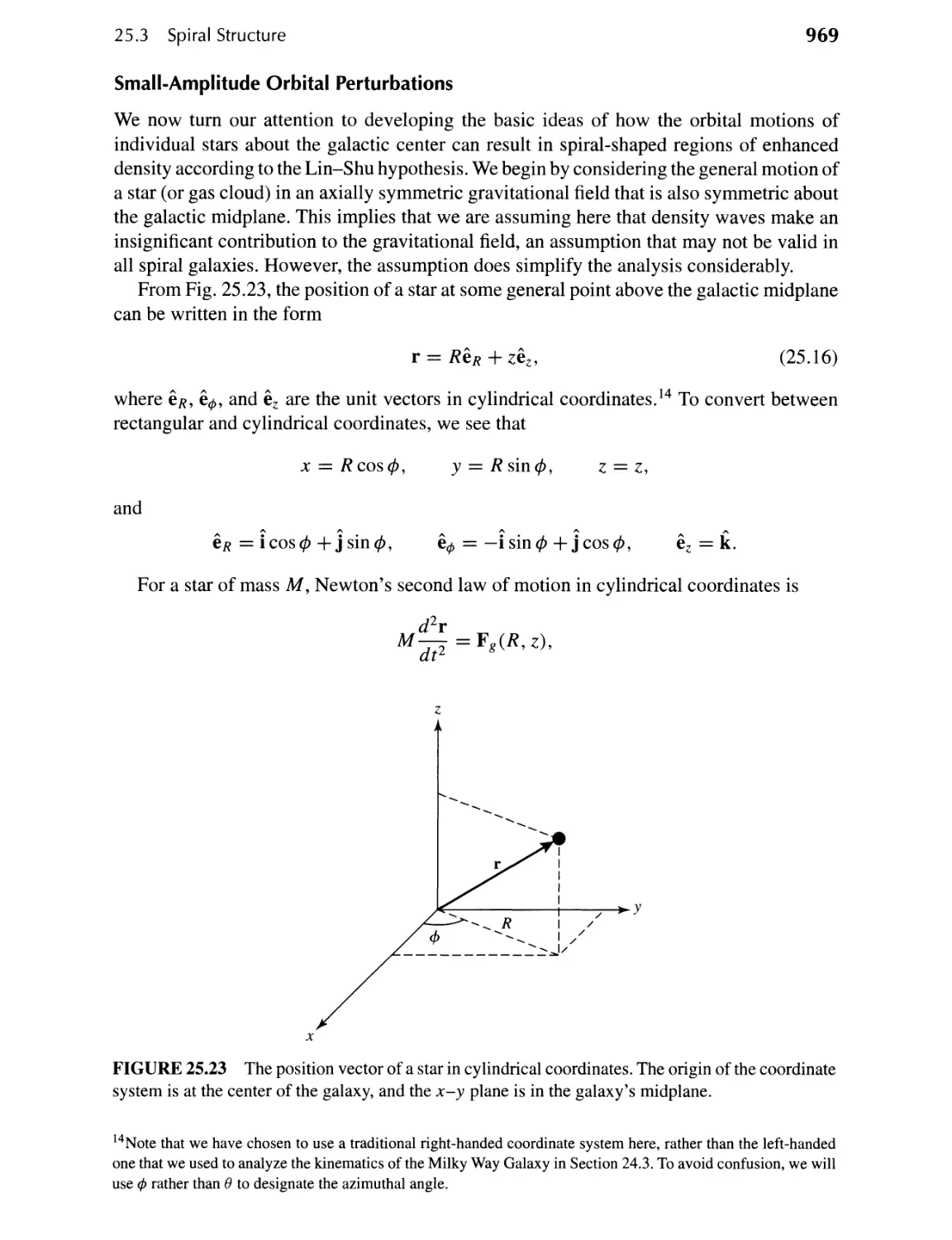
25.3 Spiral Structure 964
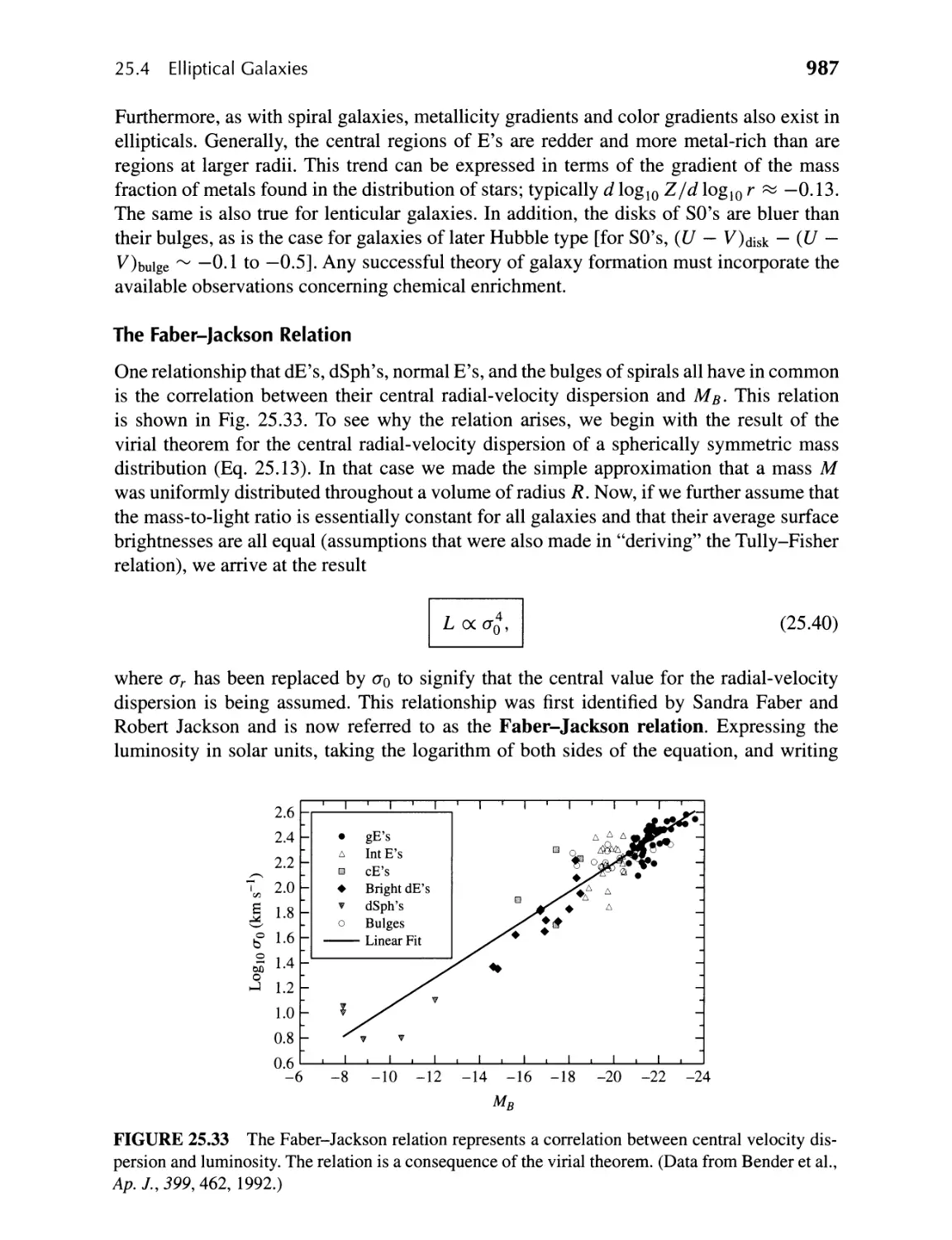
25.4 Elliptical Galaxies 983
940
26 II Galactic Evolution
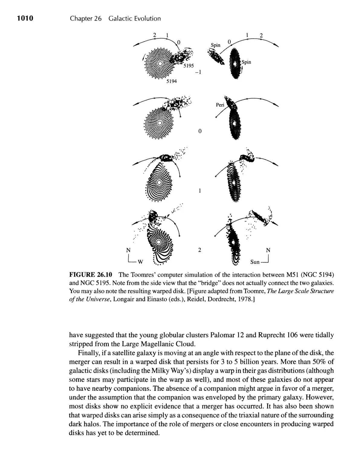
26.1 Interactions of Galaxies 999
26.2 The Formation of Galaxies 1016
999
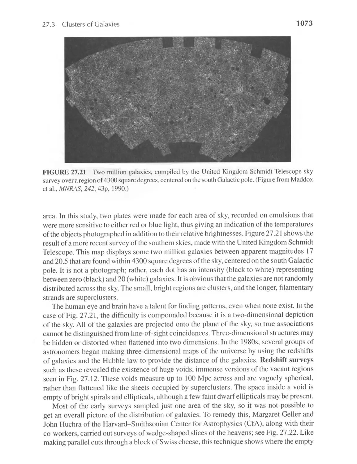
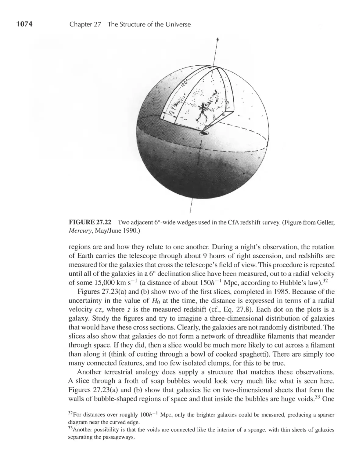
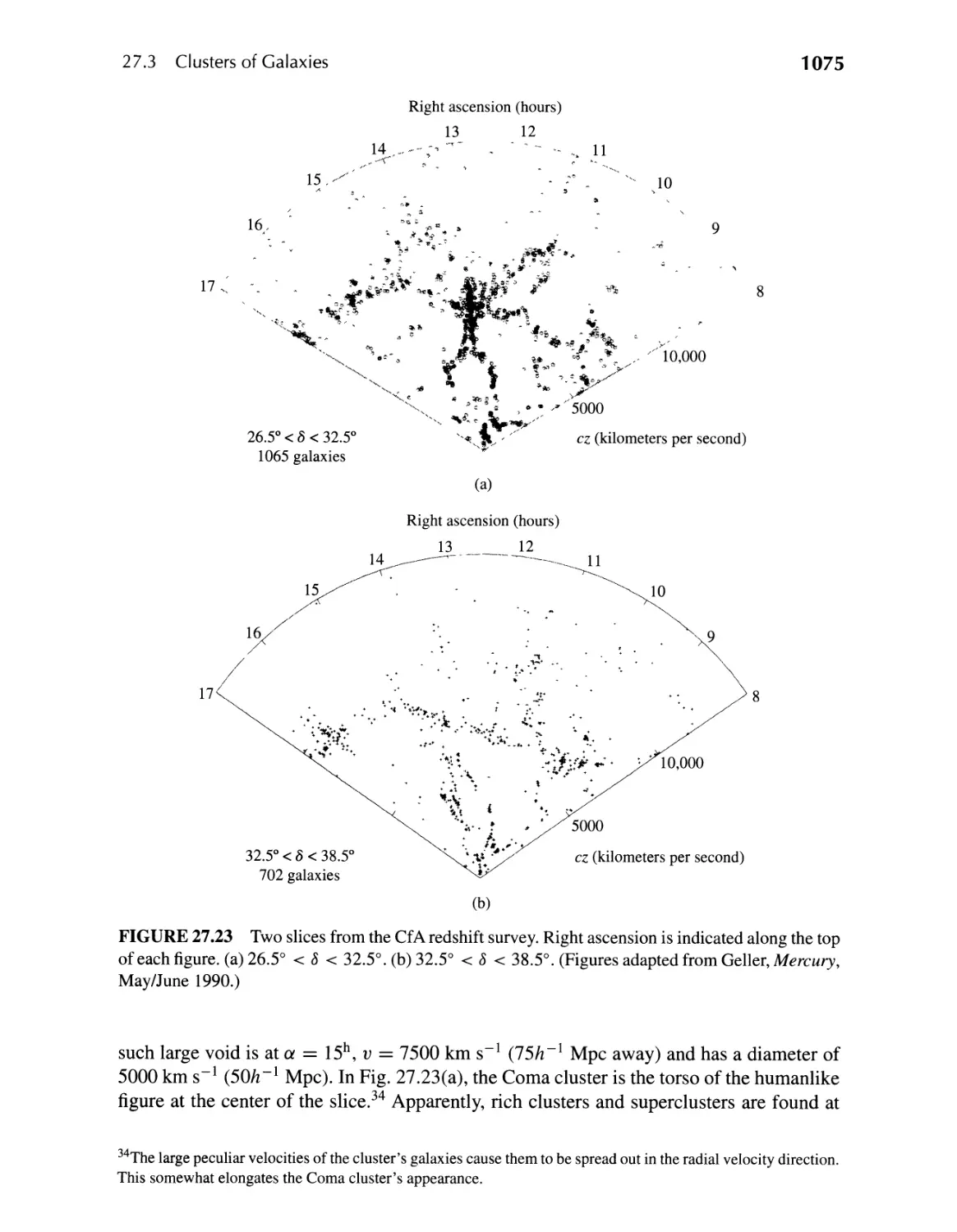
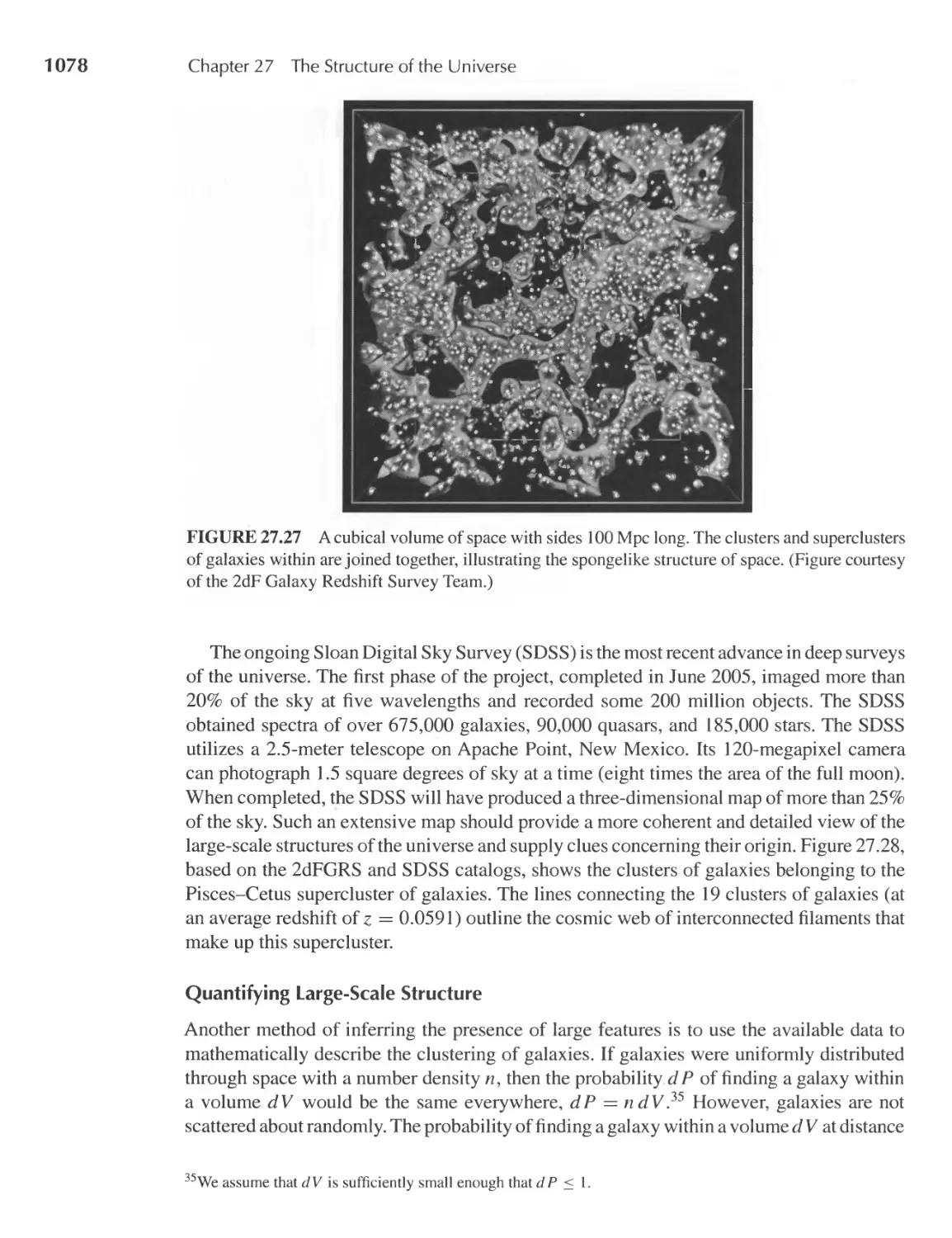
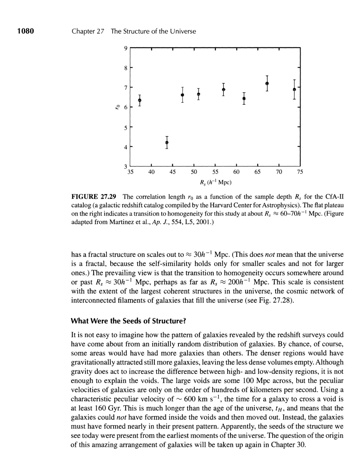
27 II The Structure of the Universe
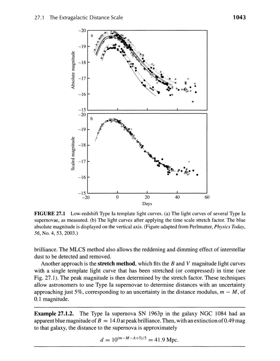
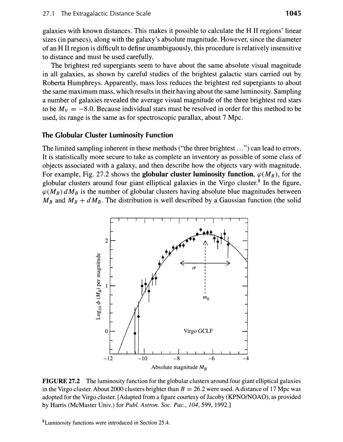
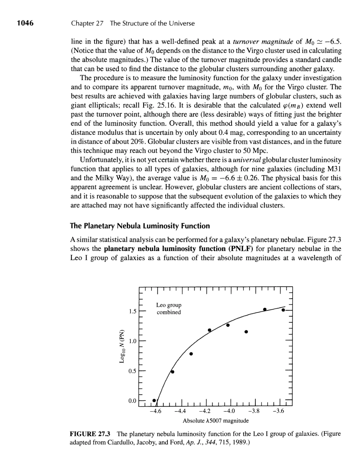
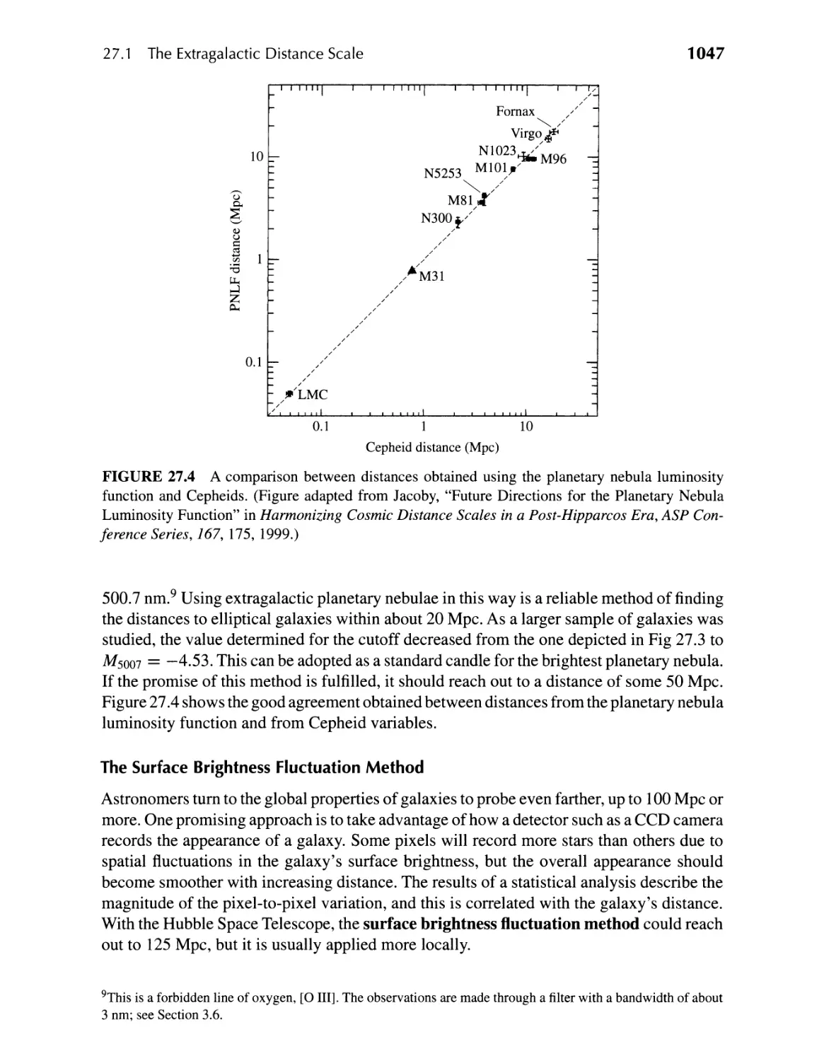
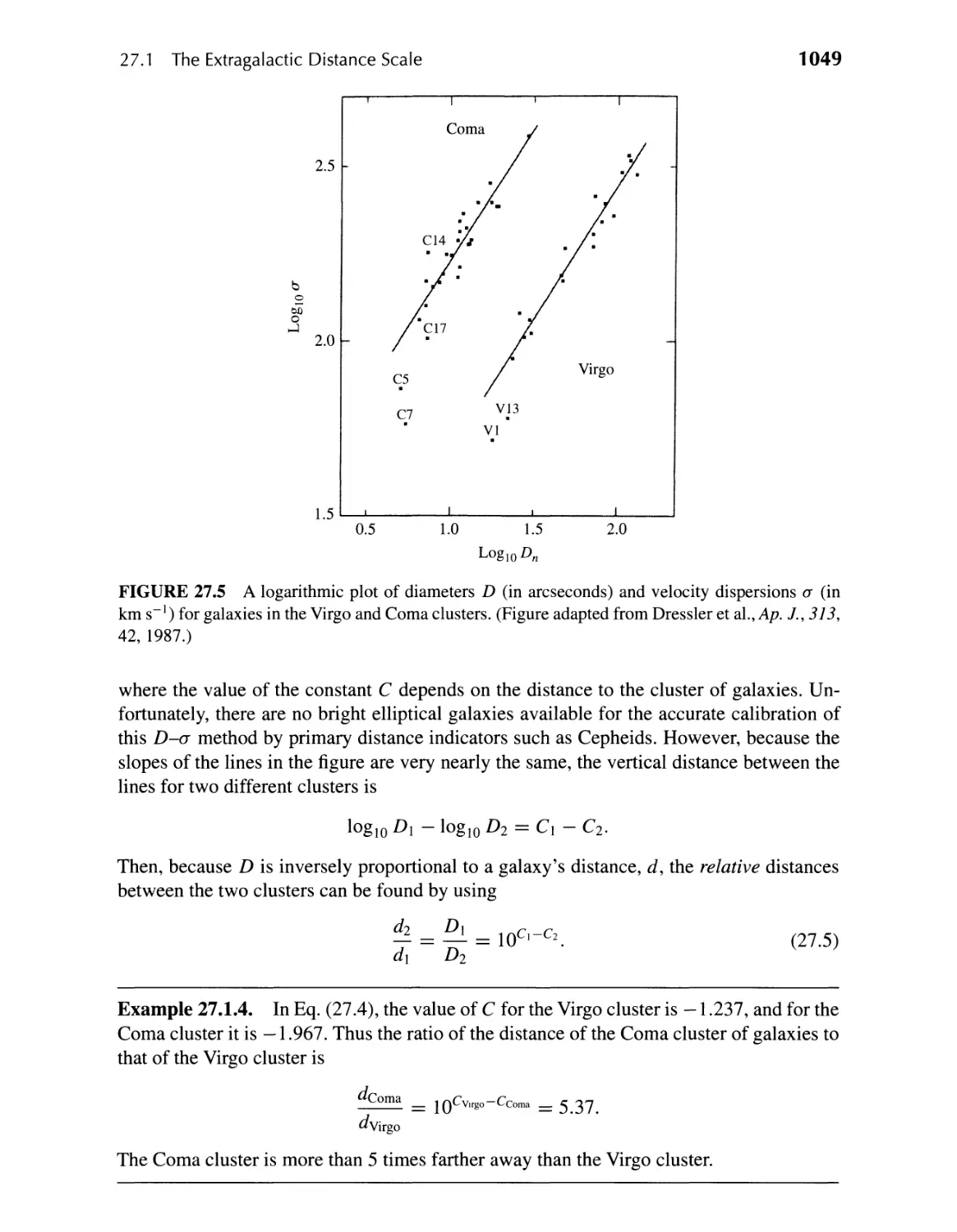
27 .1 The Extragalactic Distance Scale 1 038
27.2 The Expansion of the Universe 1052
27.3 Clusters of Galaxies 1058
1038
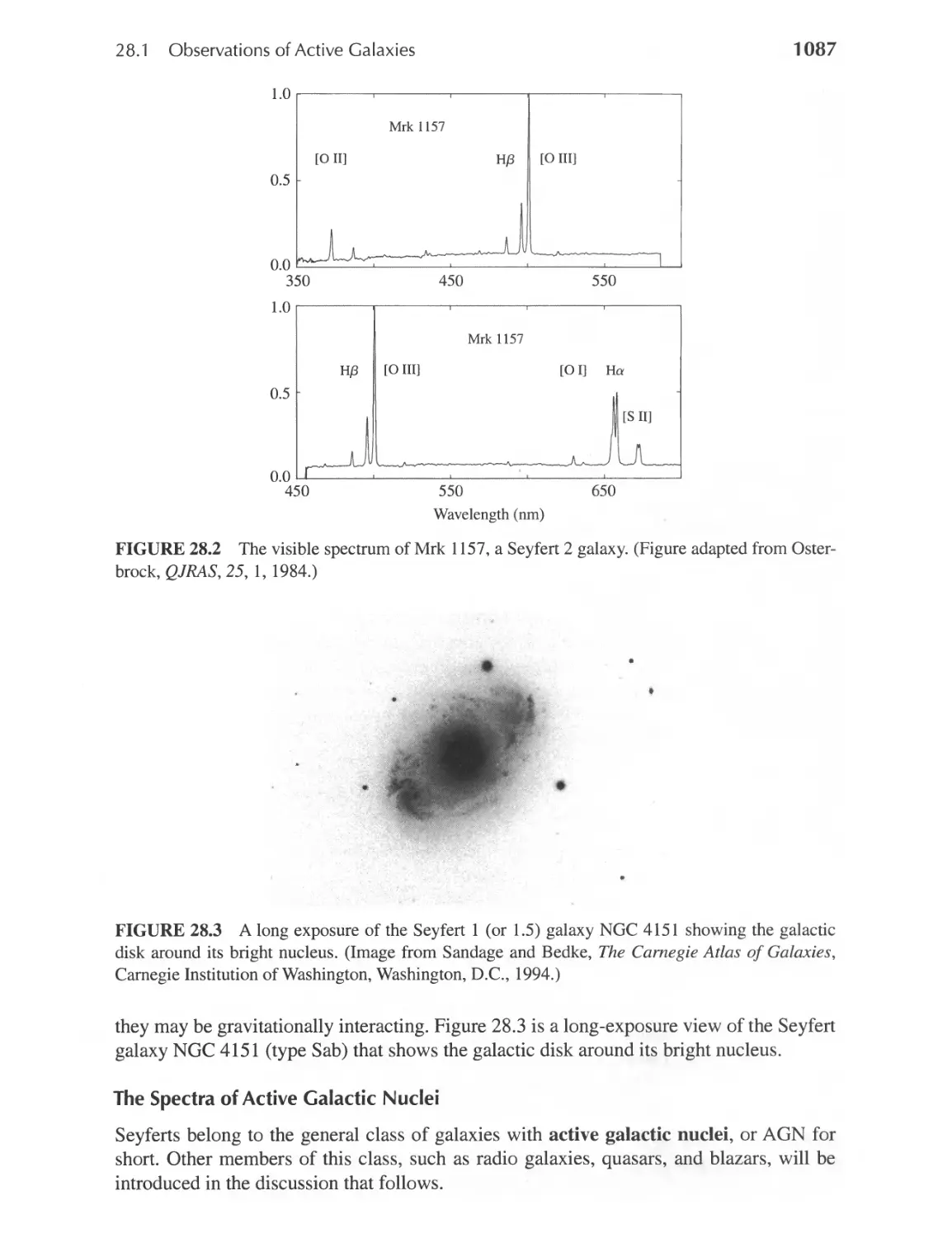
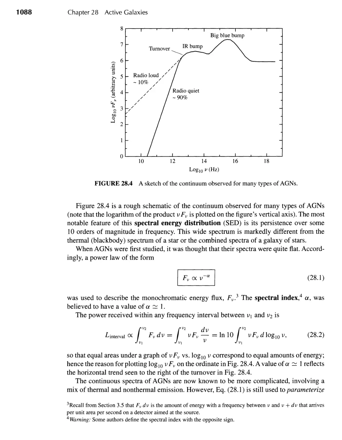
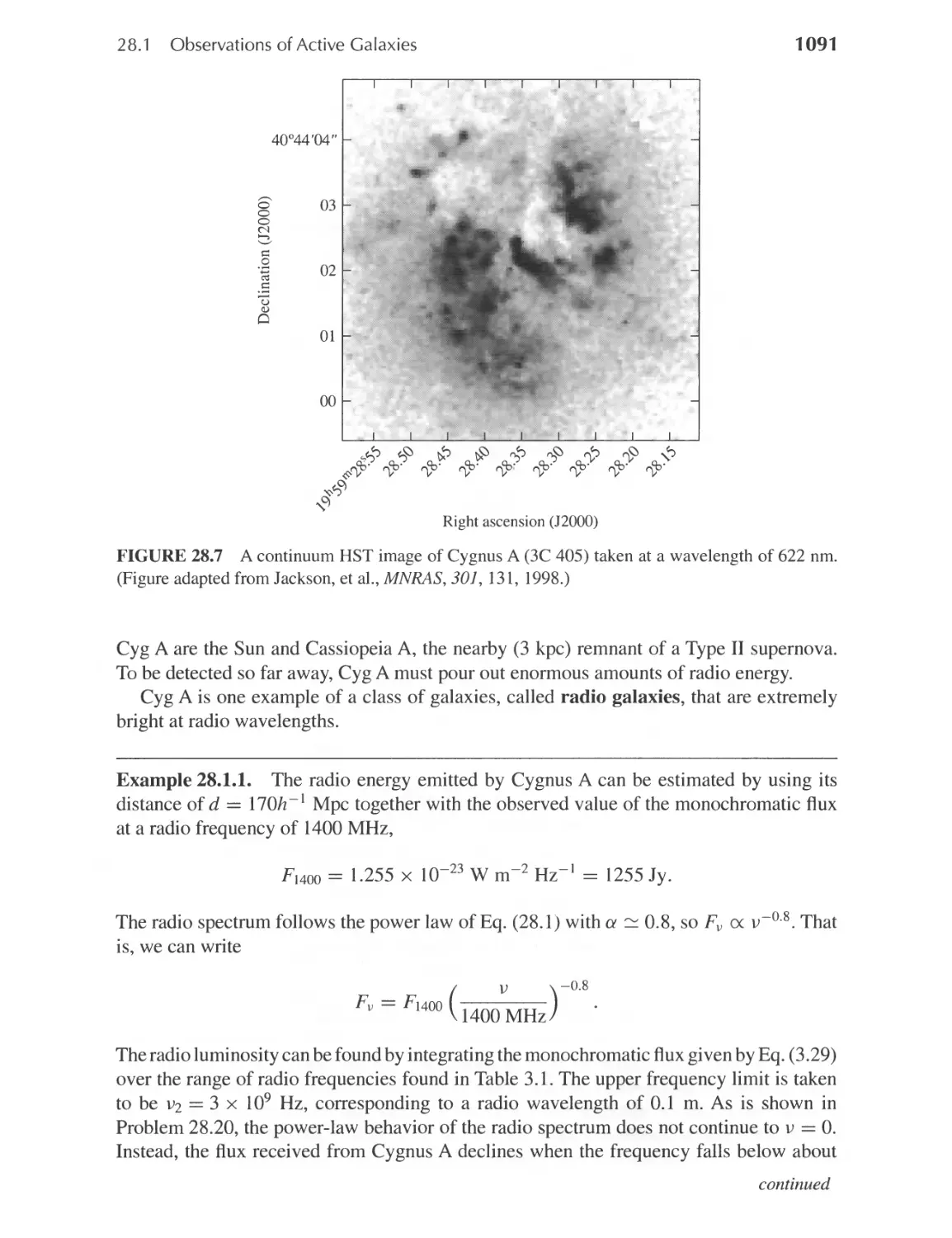
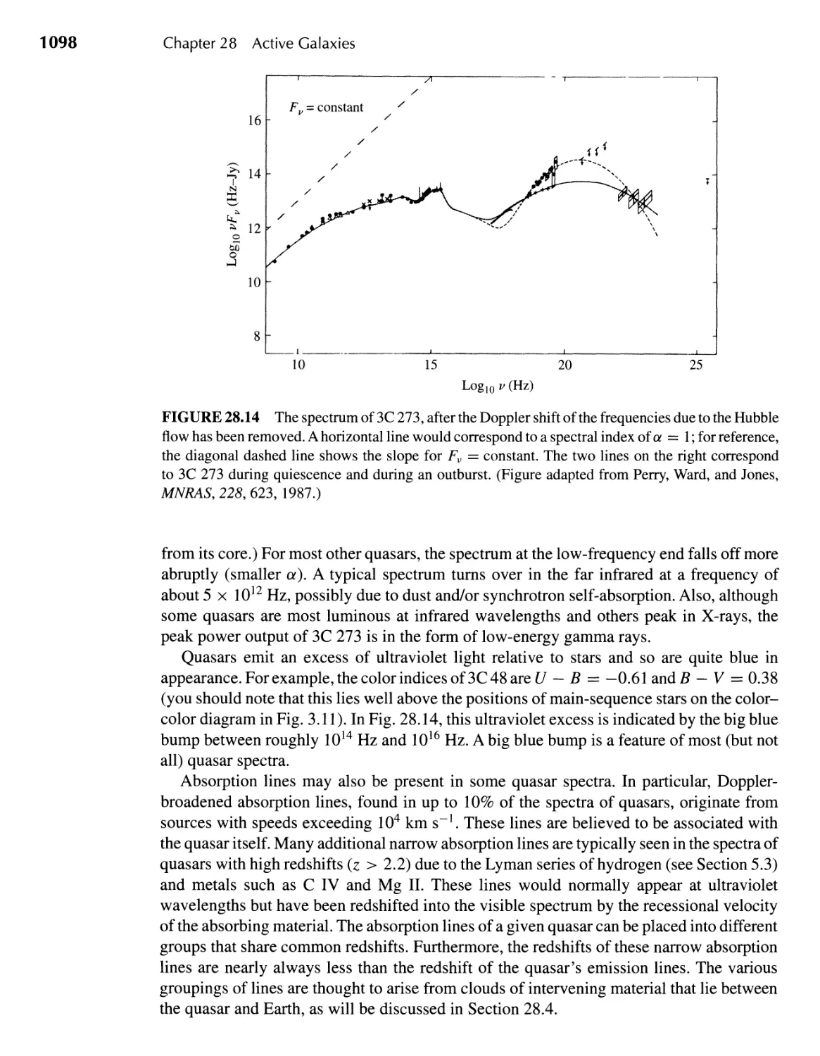
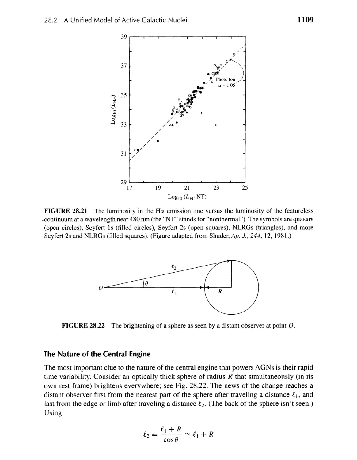
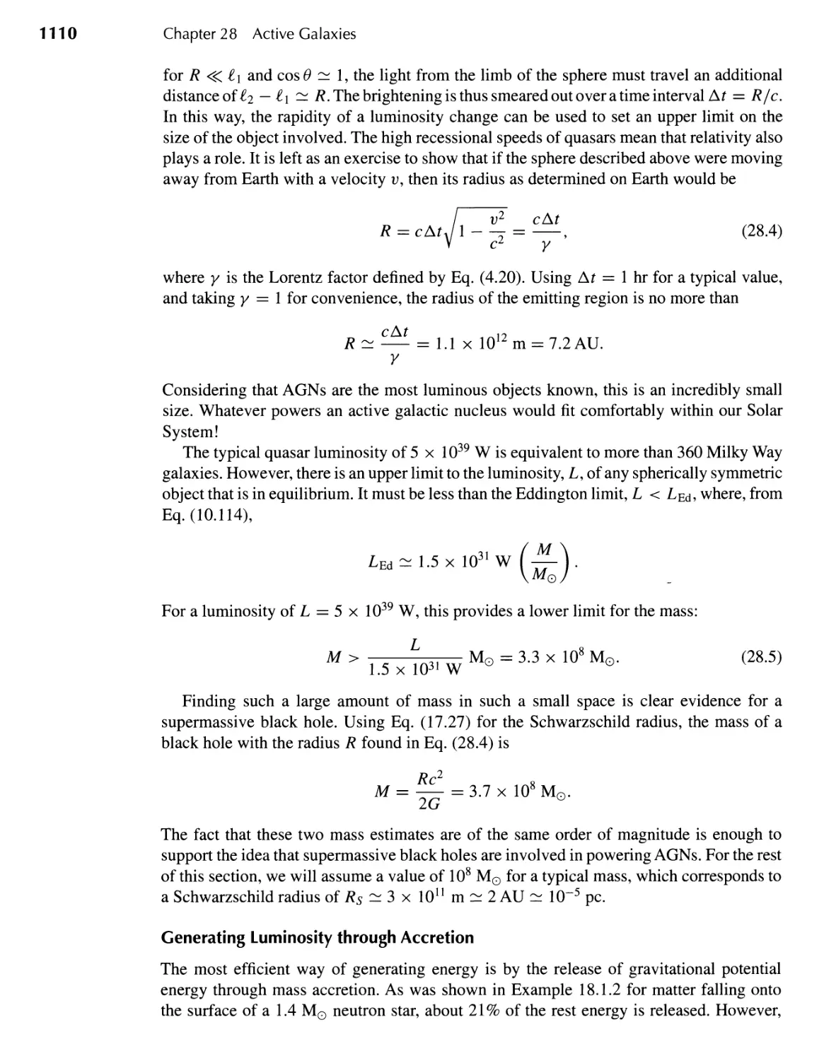
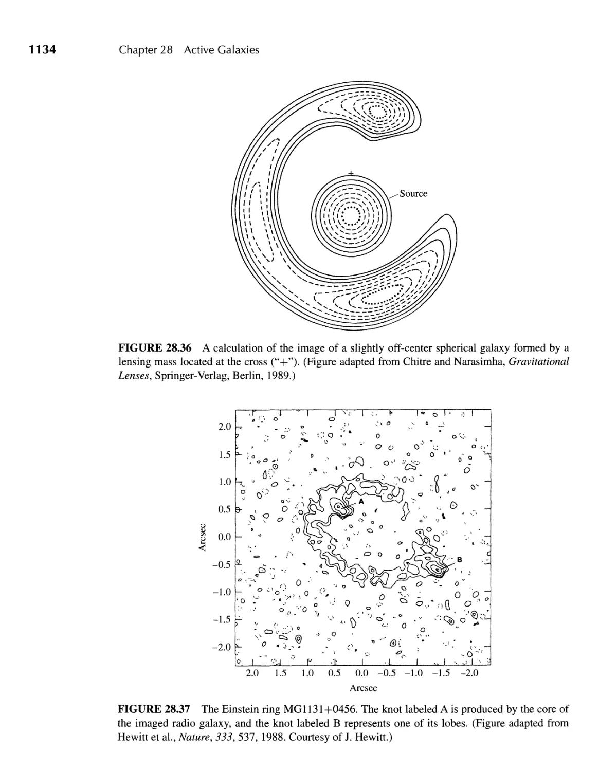
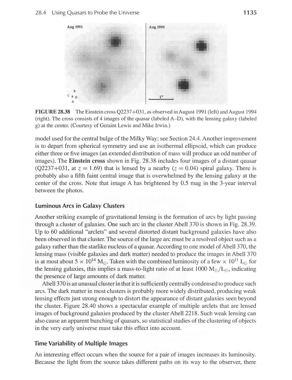
28 II Active Galaxies
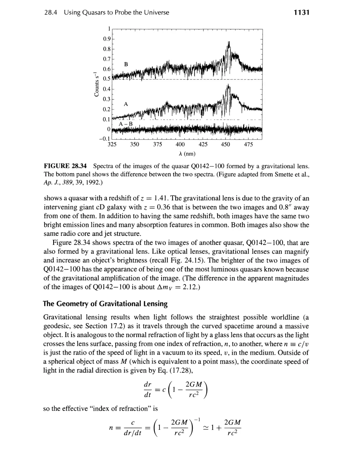
28.1 Observations of Active Galaxies 1 085
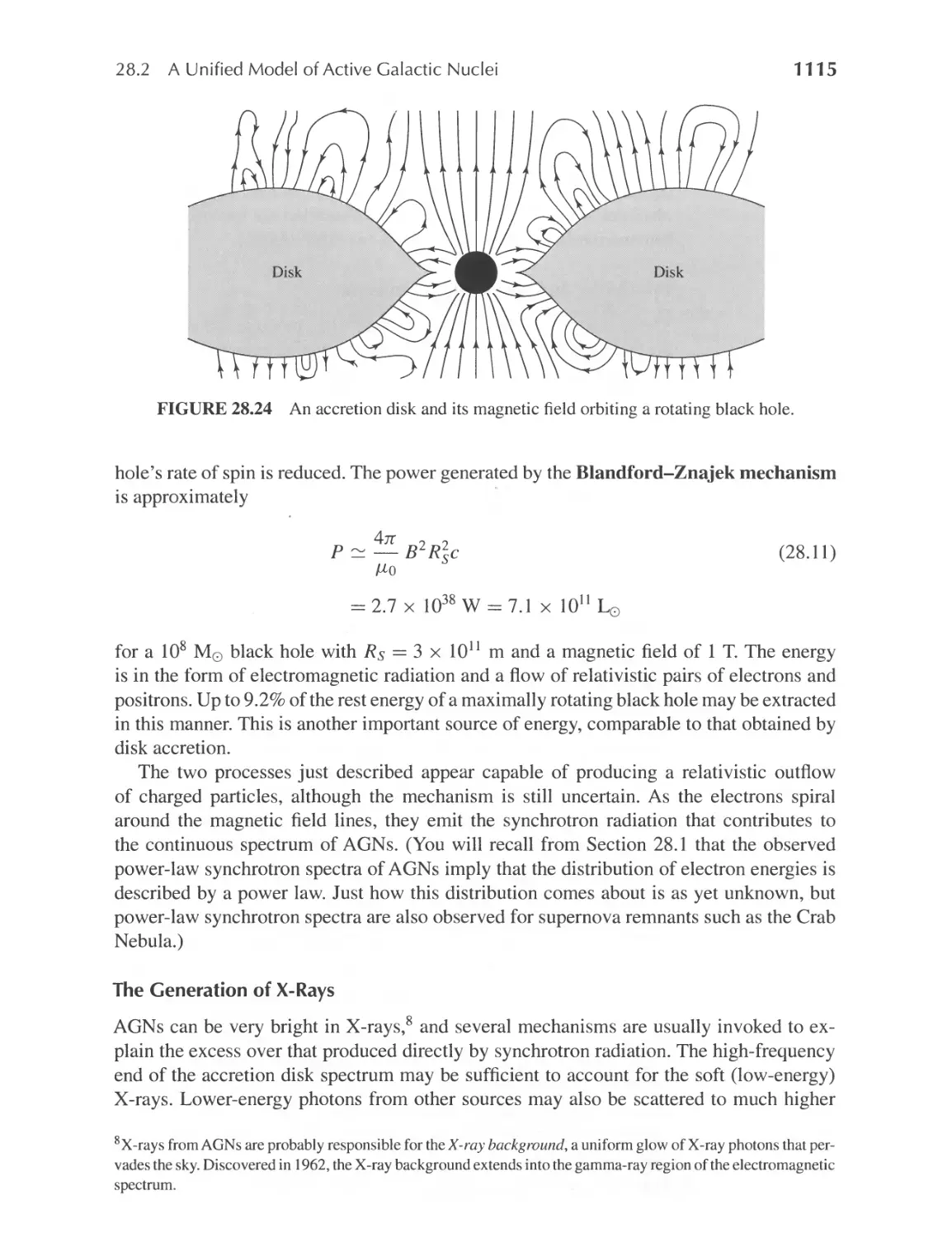
28.2 A Unified Model of Active Galactic Nuclei 1108
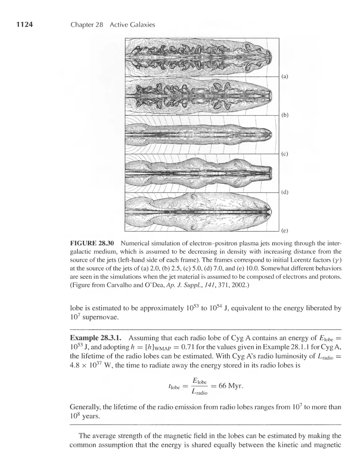
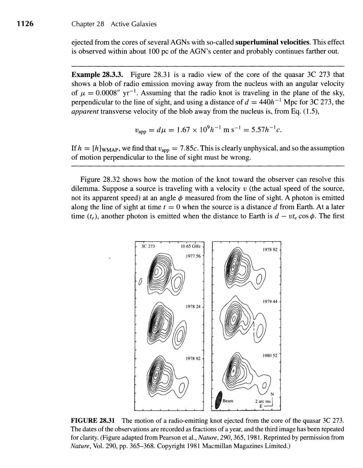
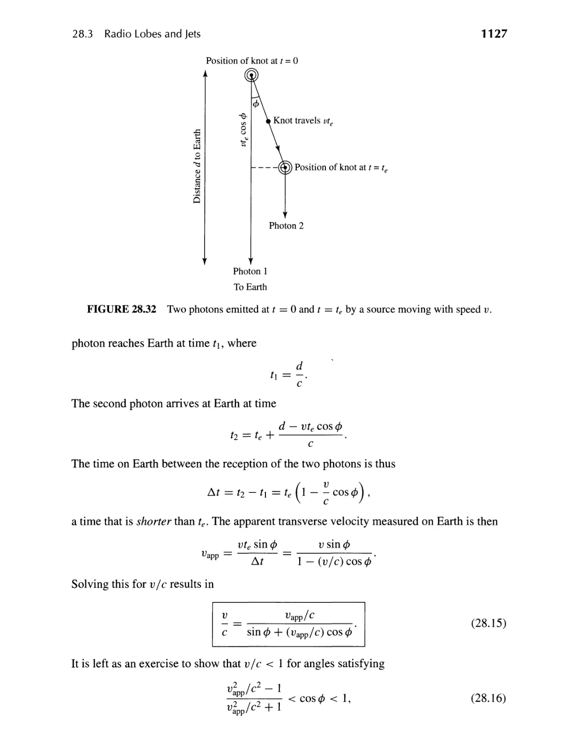
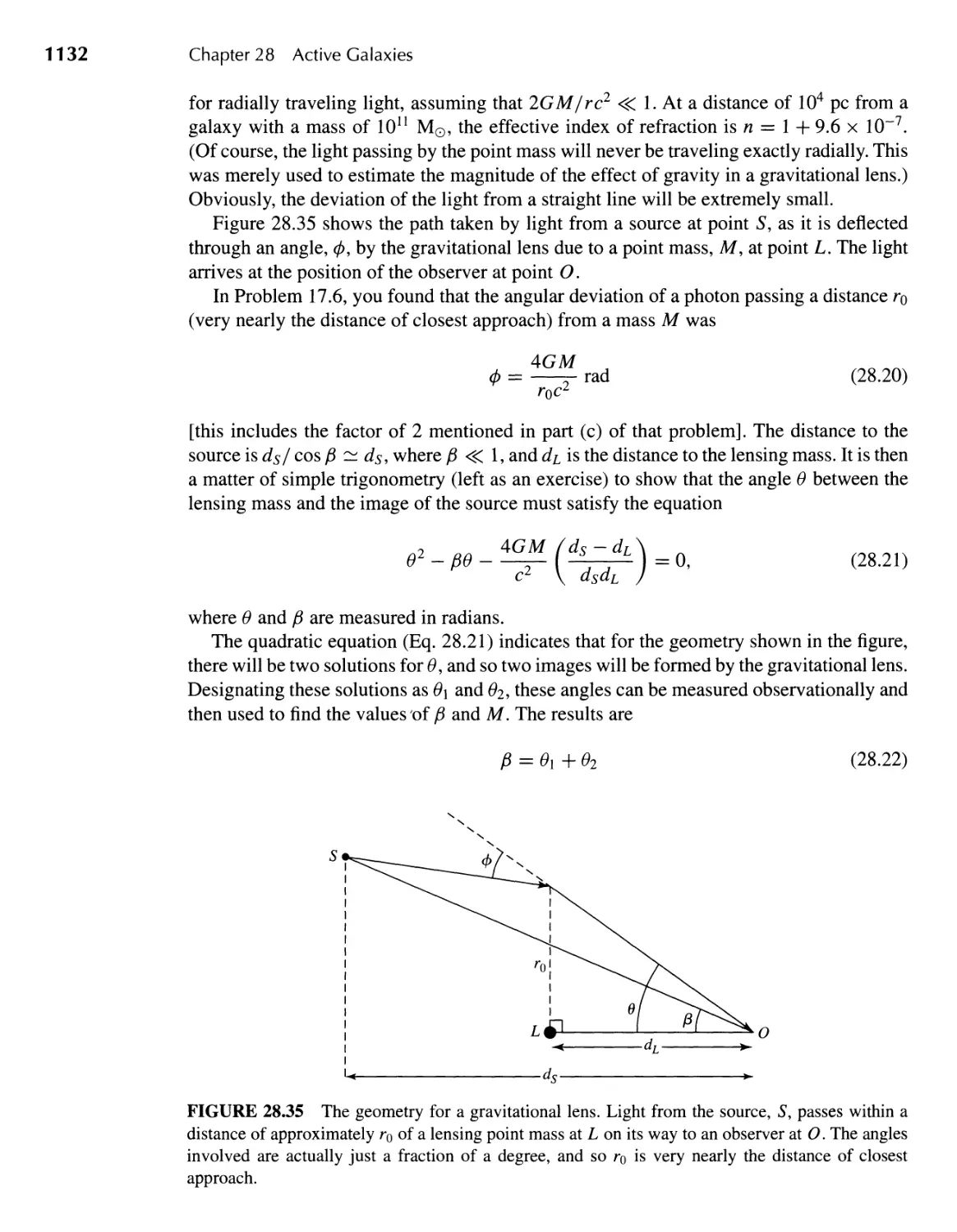
28.3 Radio Lobes and Jets 1122
28.4 Using Quasars to Probe the Universe 1130
1085
29 II Cosmology
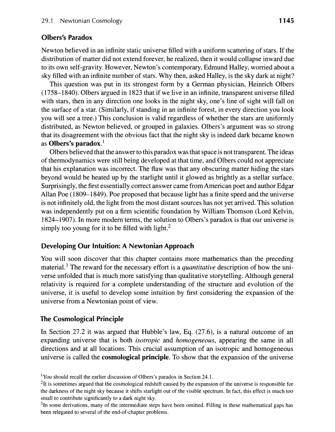
29.1 Newtonian Cosmology 1144
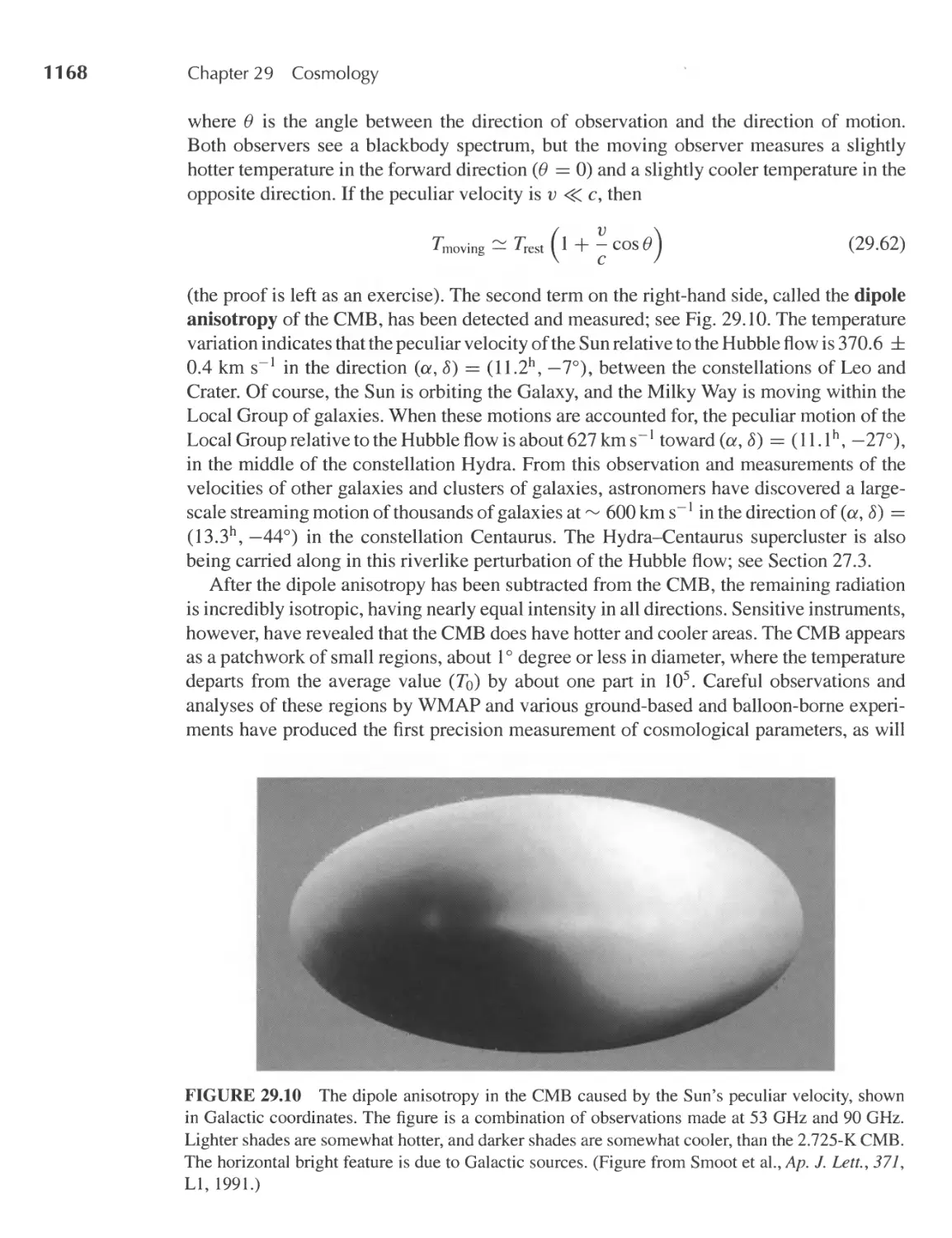
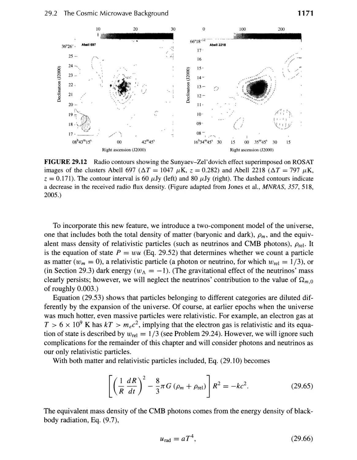
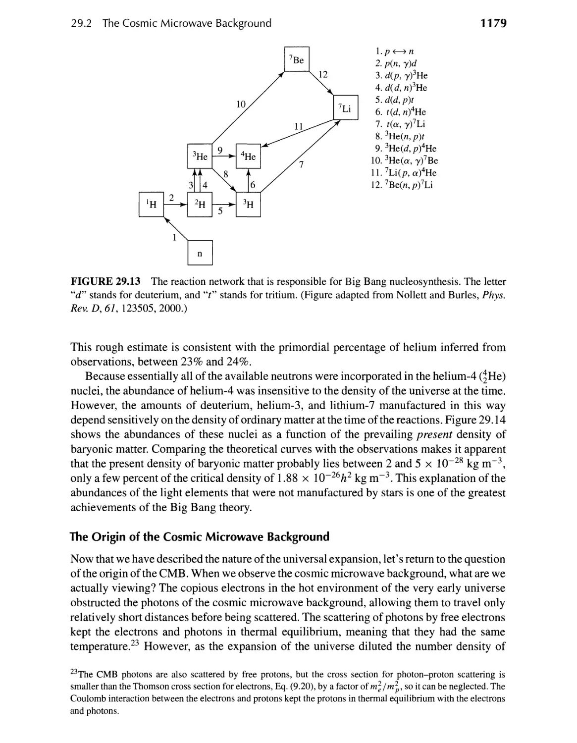
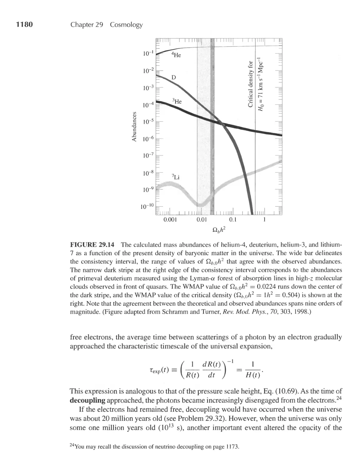
29.2 The Cosmic Microwave Background 1162
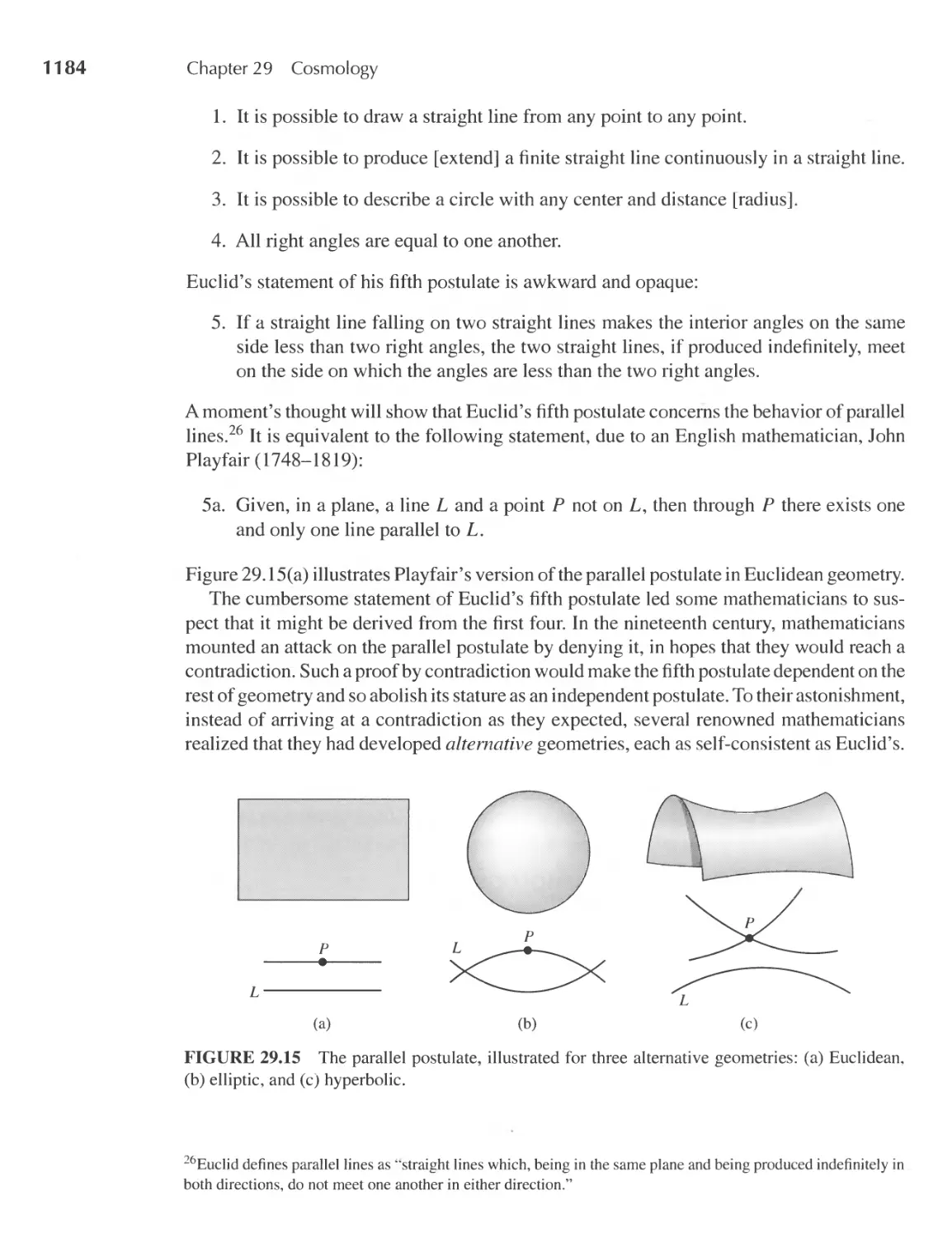
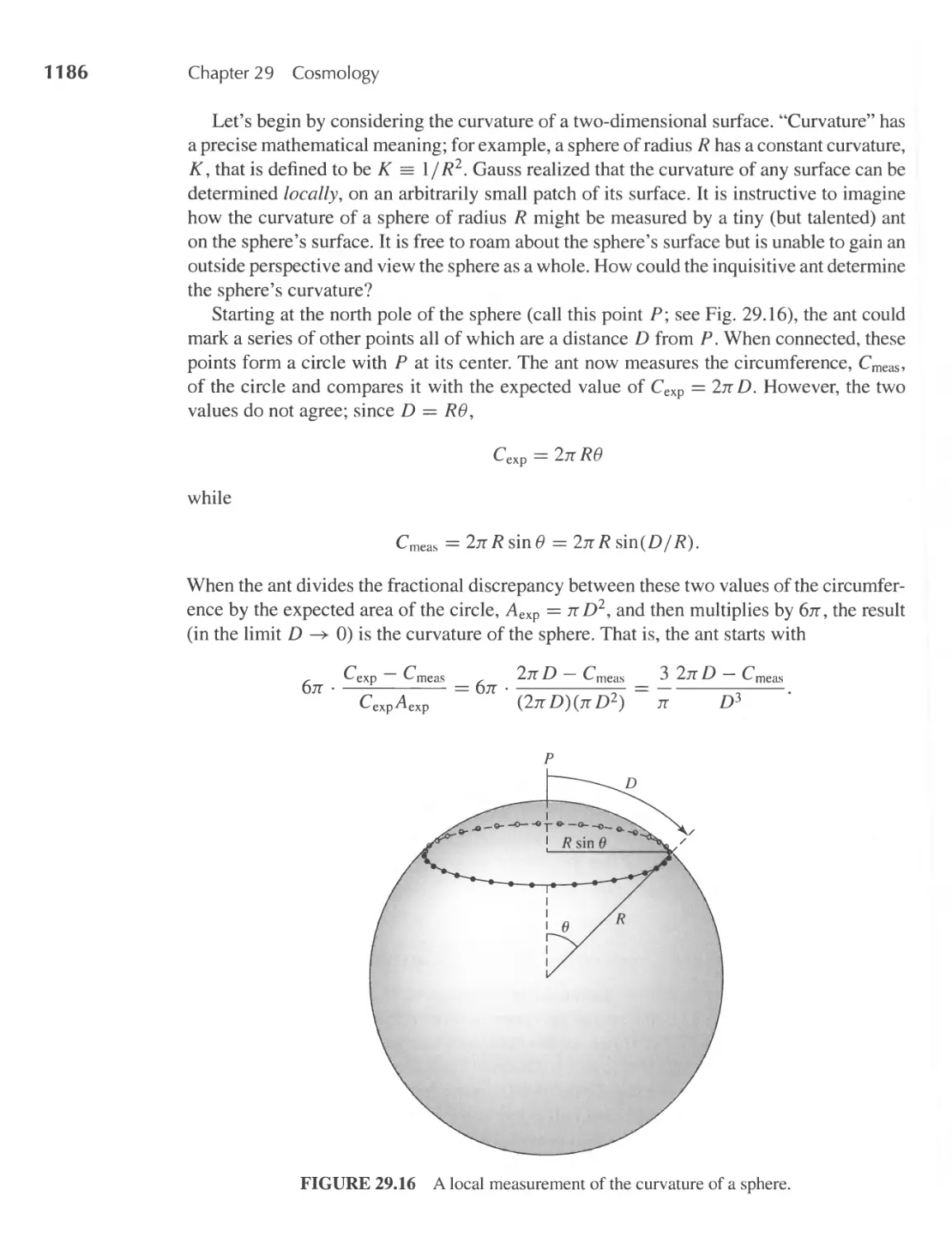
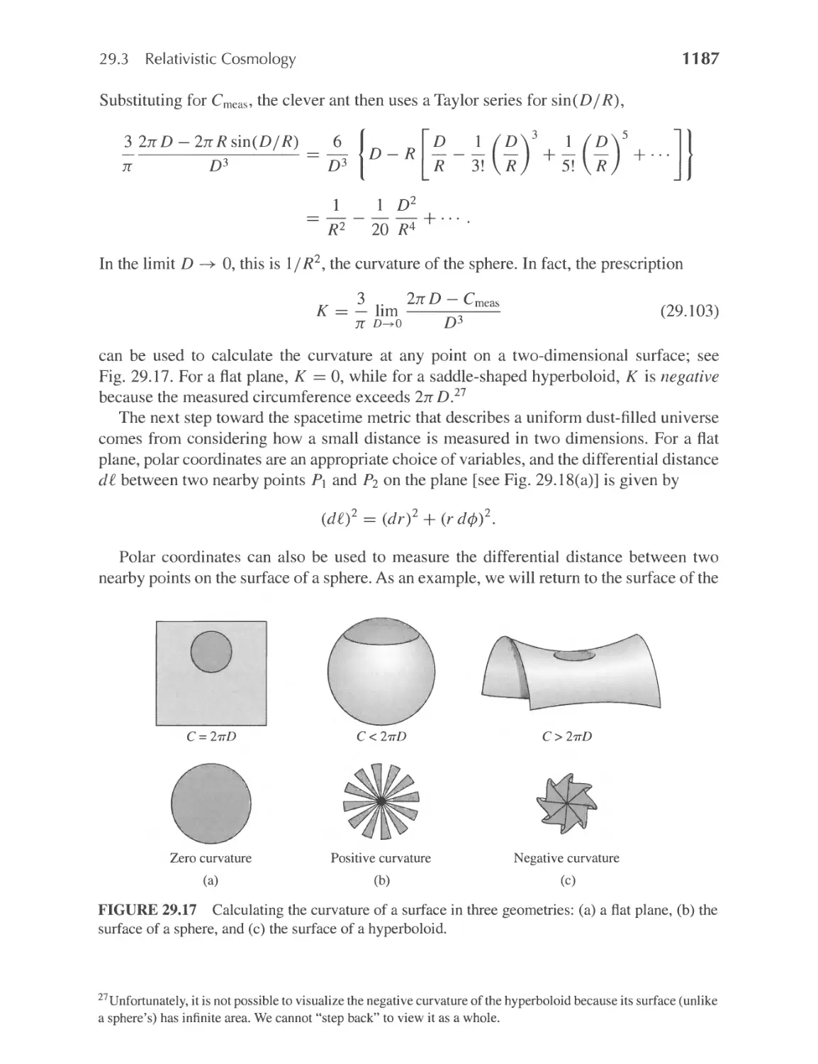
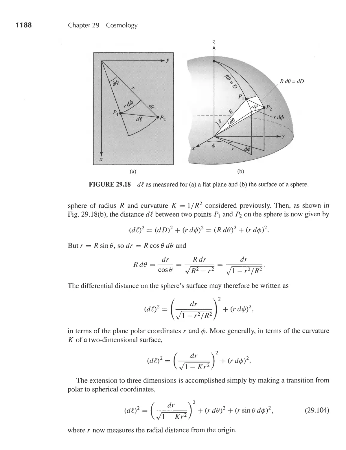
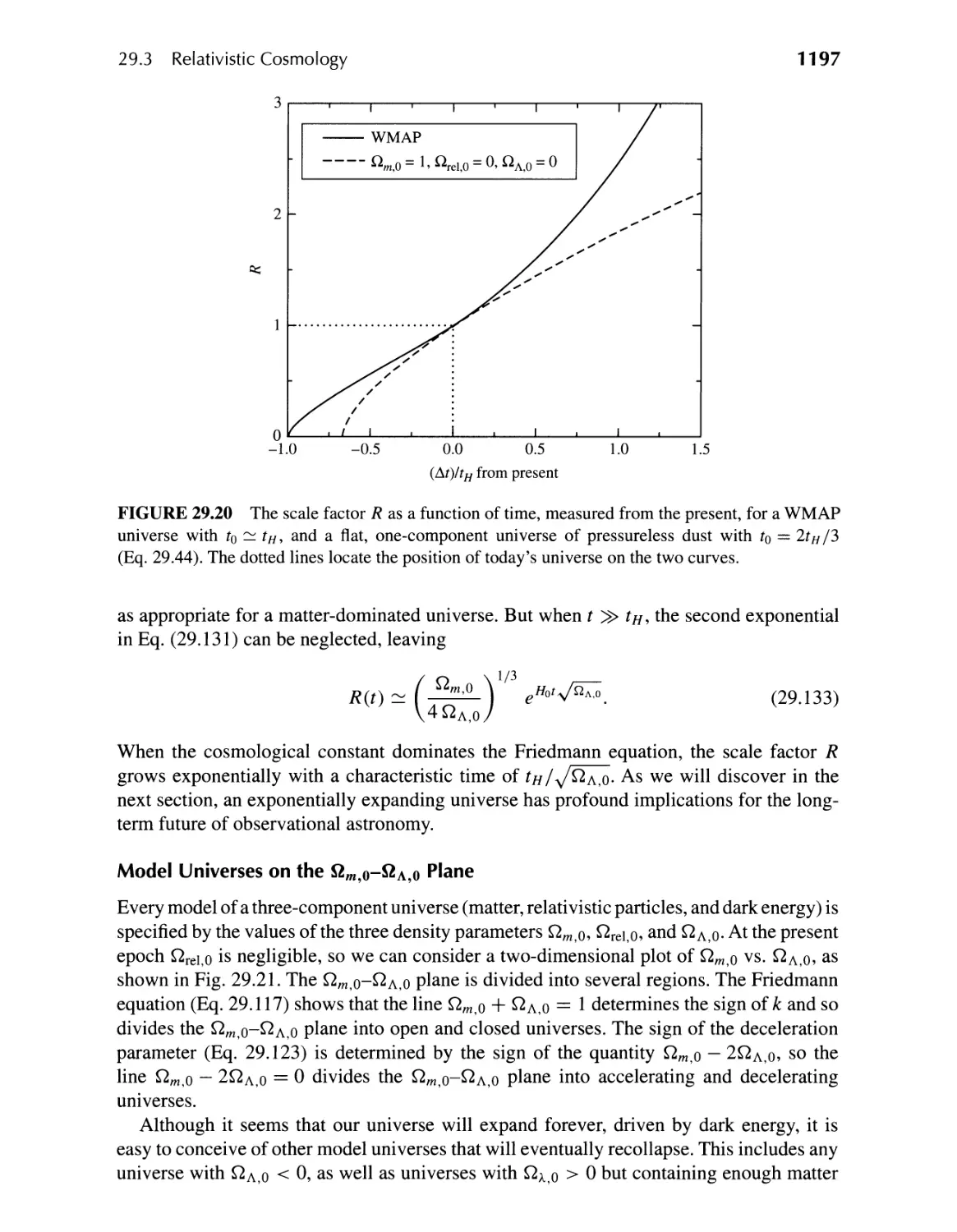
29.3 Relativistic Cosmology 1183
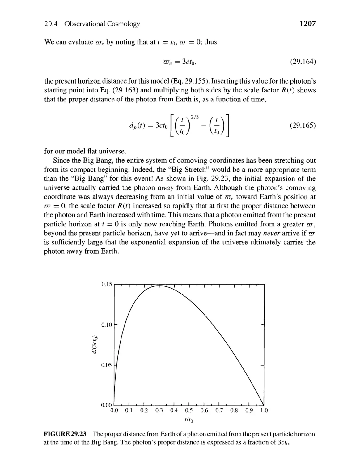
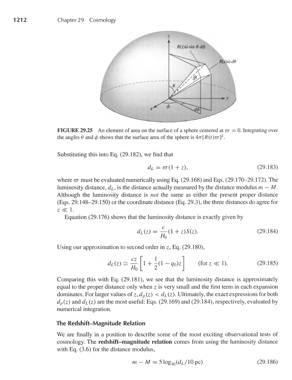
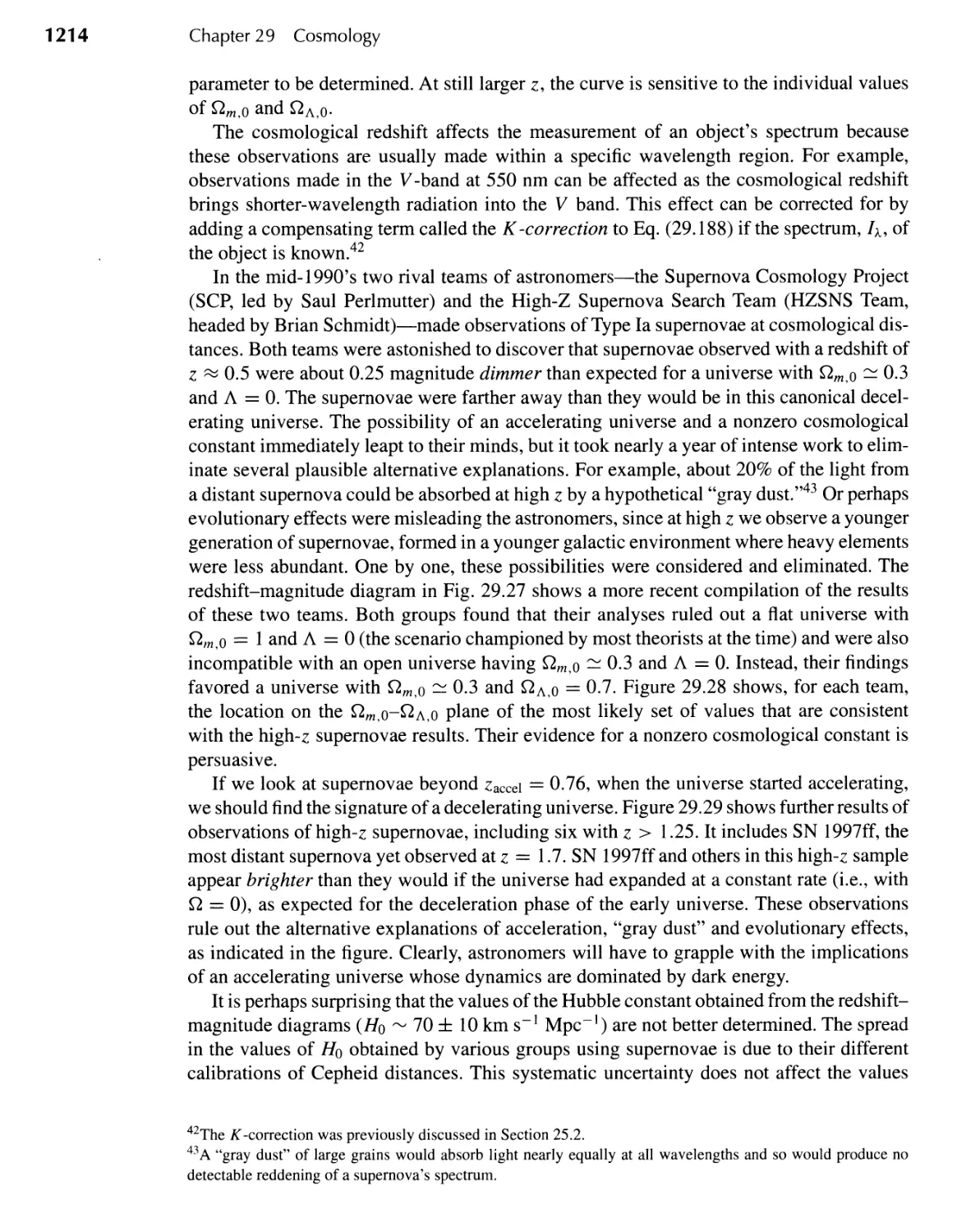
29.4 Observational Cosmology 1199
1144
XVI
Contents
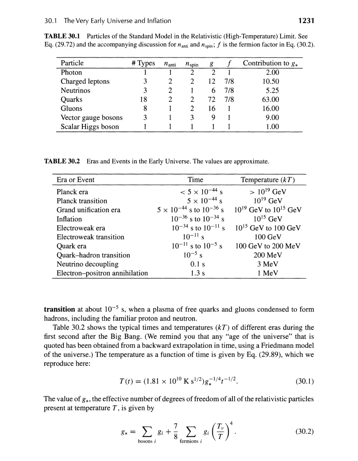
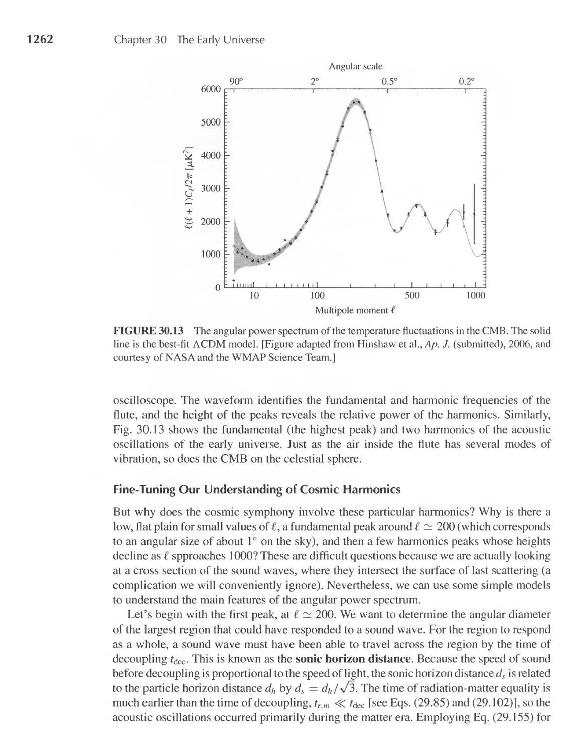
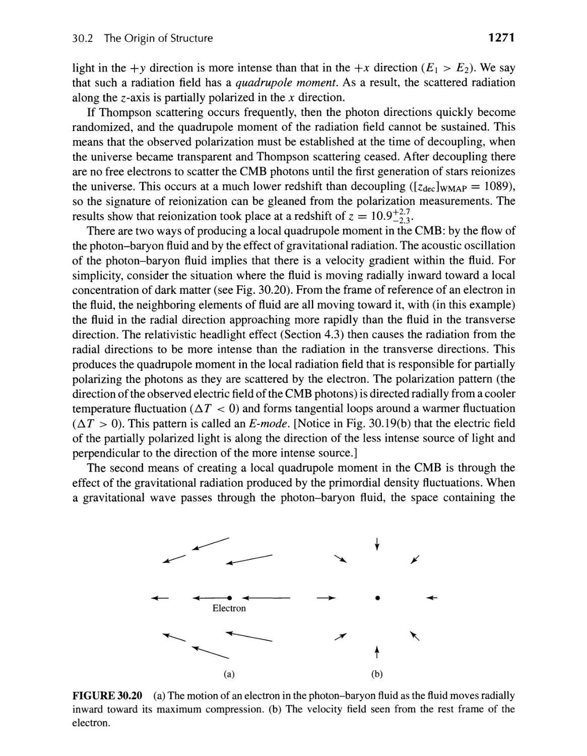
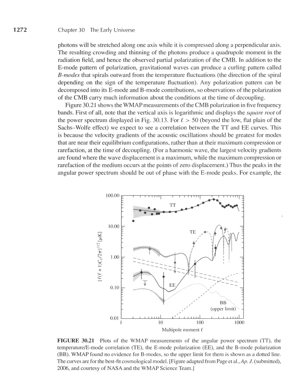
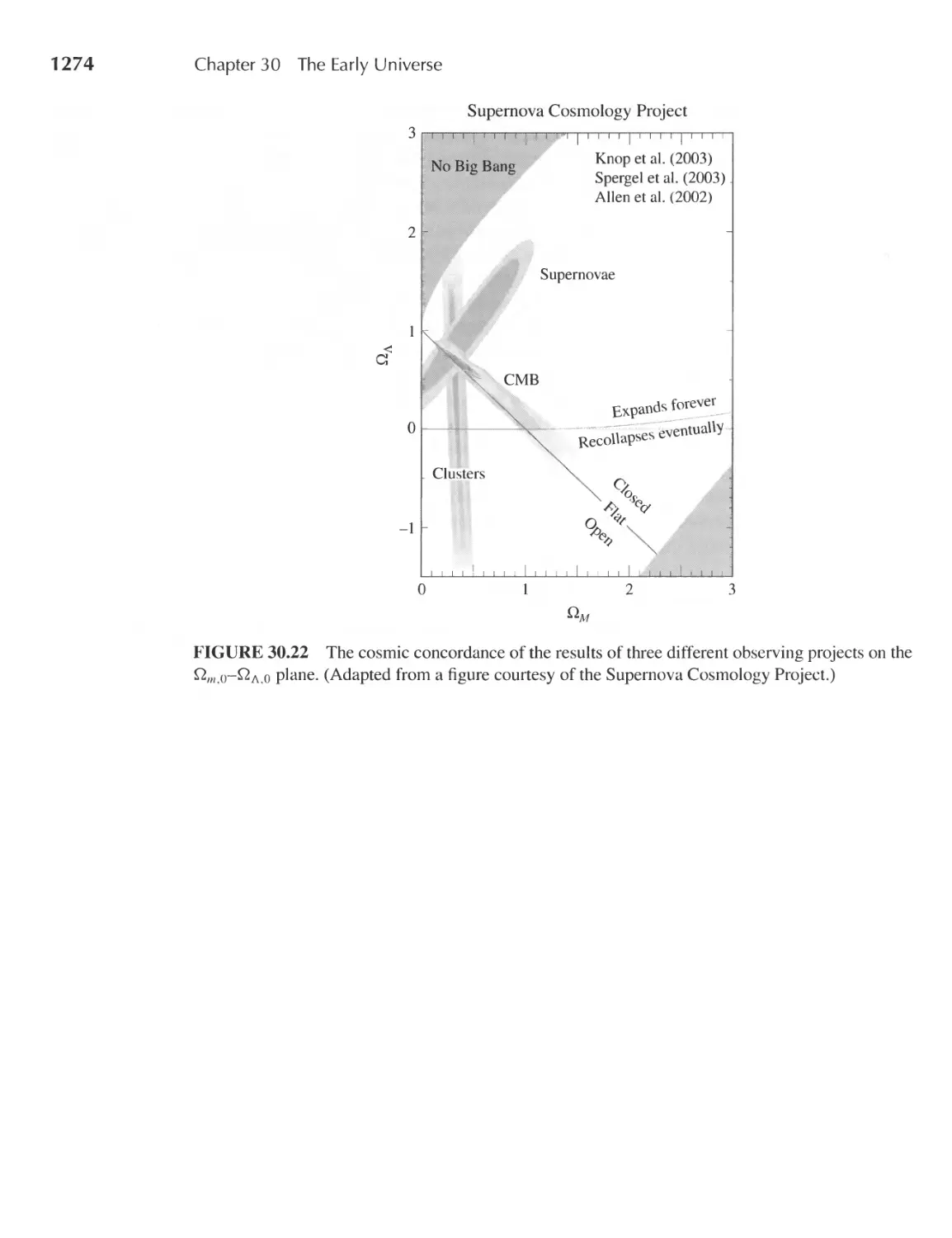
30 II The Early Universe
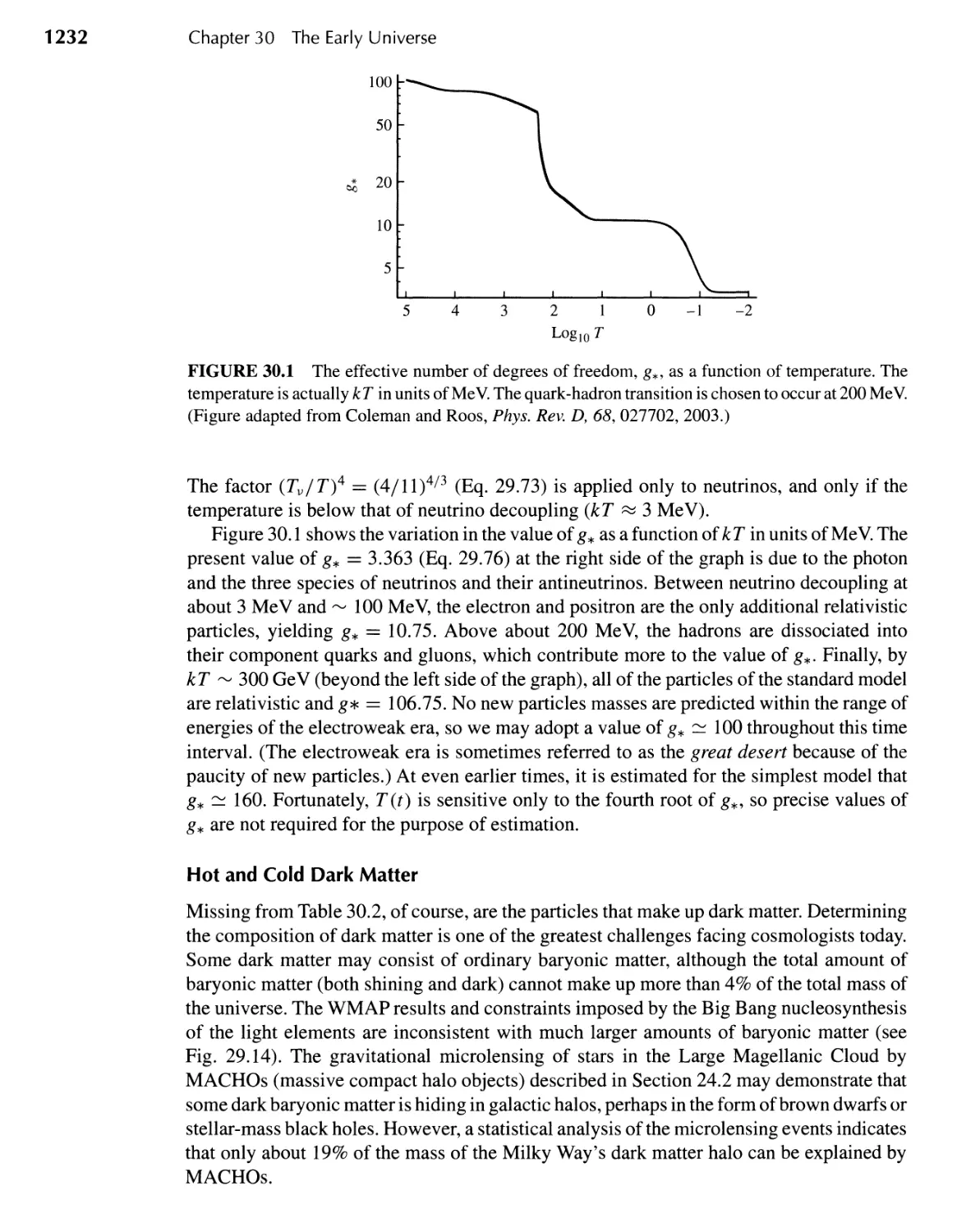
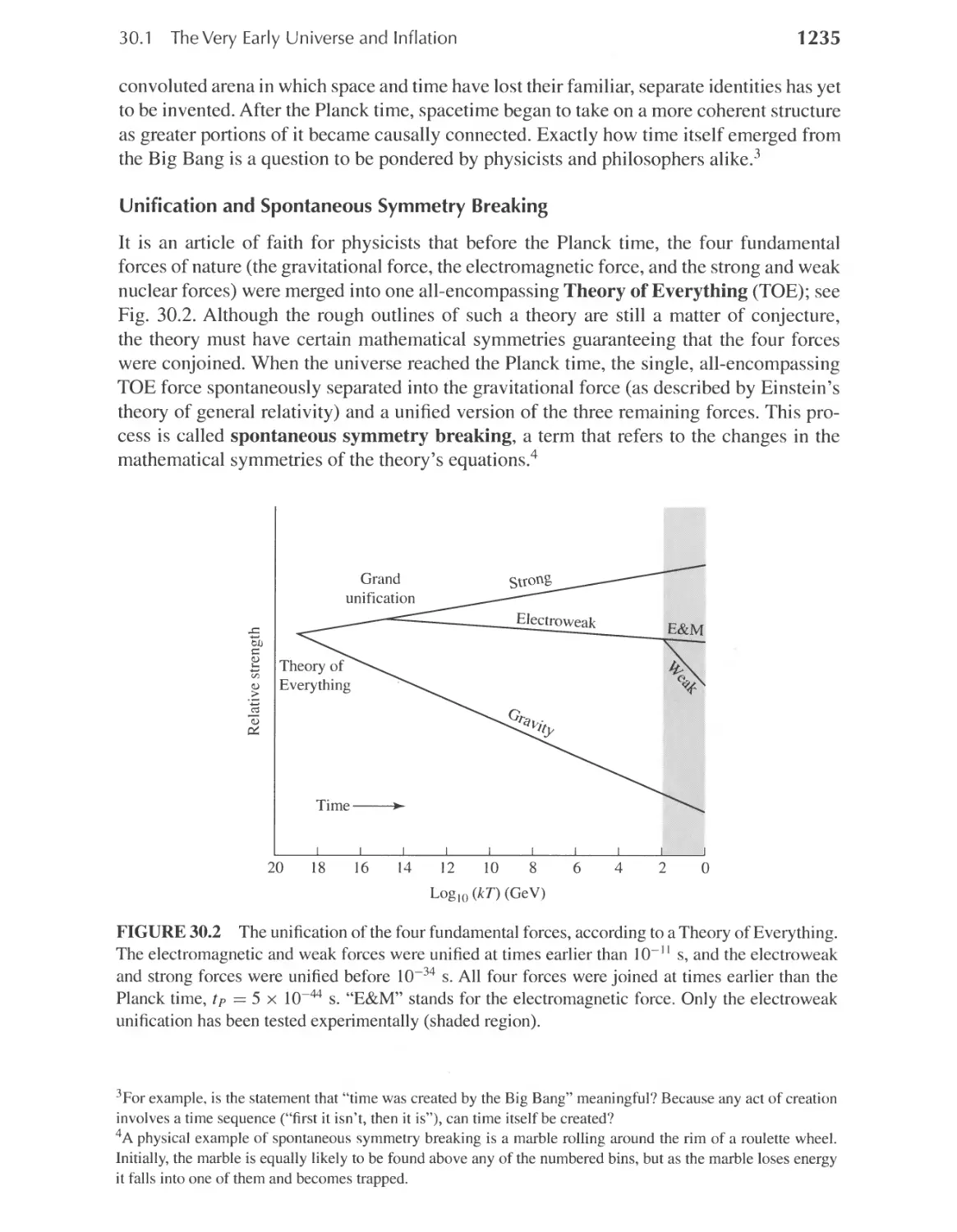
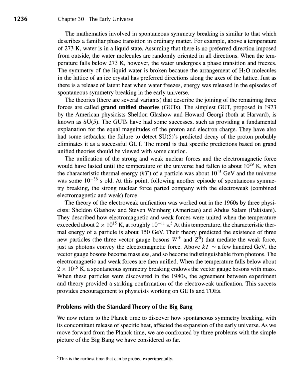
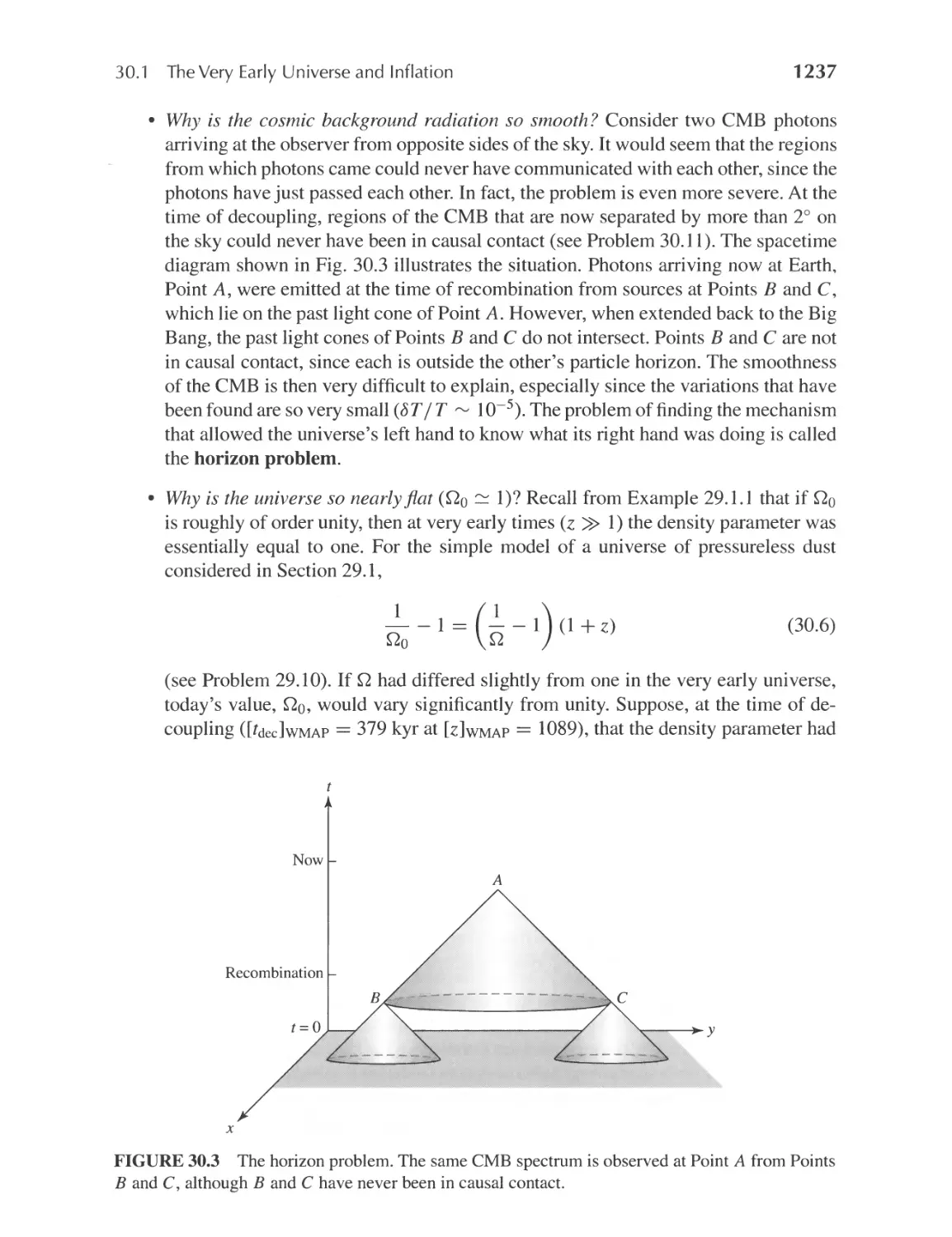
30.1 The Very Early Universe and Inflation 1230
30.2 The Origin of Structure 1247
1230
A II Astronomical and Physical Constants
Inside Front Cover
B II Unit Conversions
I nside Back Cover
C II Solar System Data
A-1
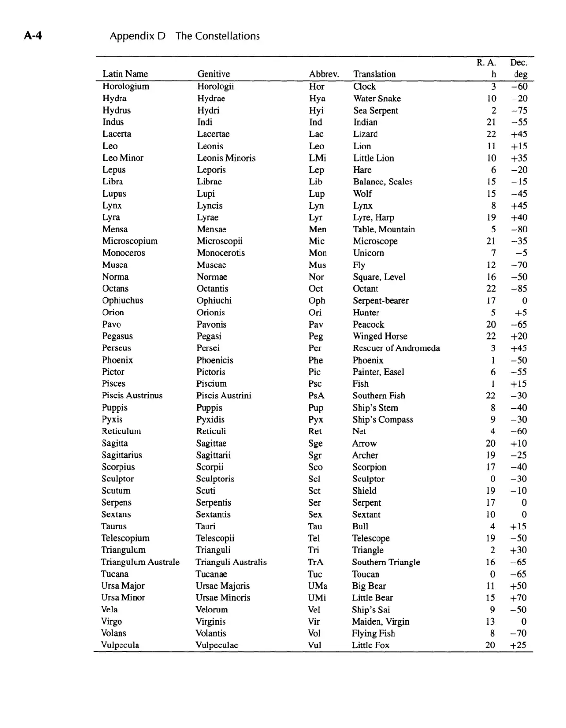
D II The Constellations
A-3
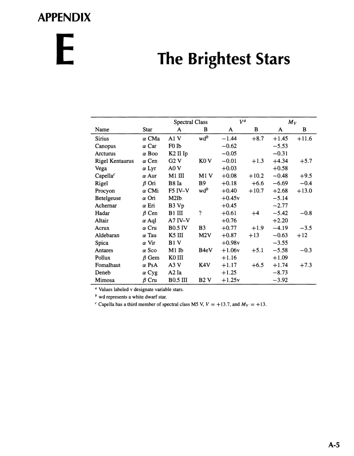
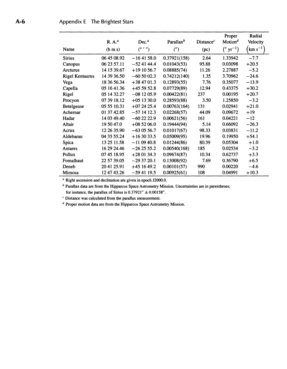
A-5
F II The N earest Stars
A-7
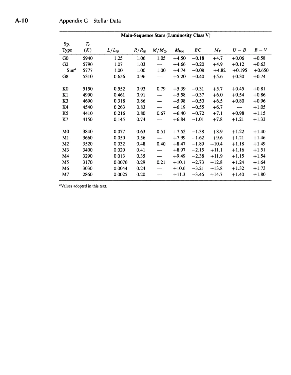
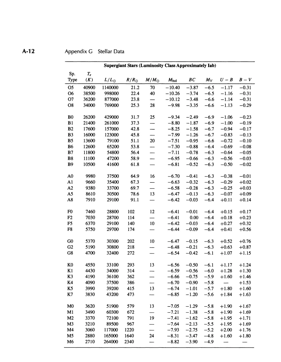
G II Stellar Data
A-9
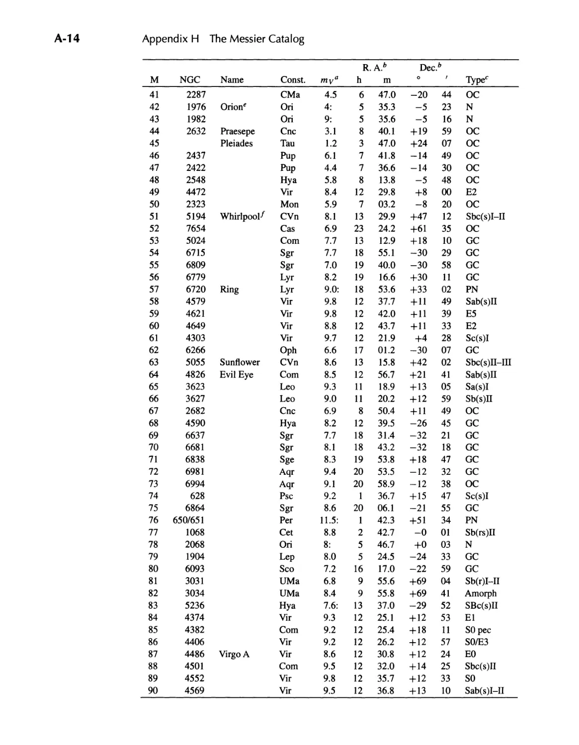
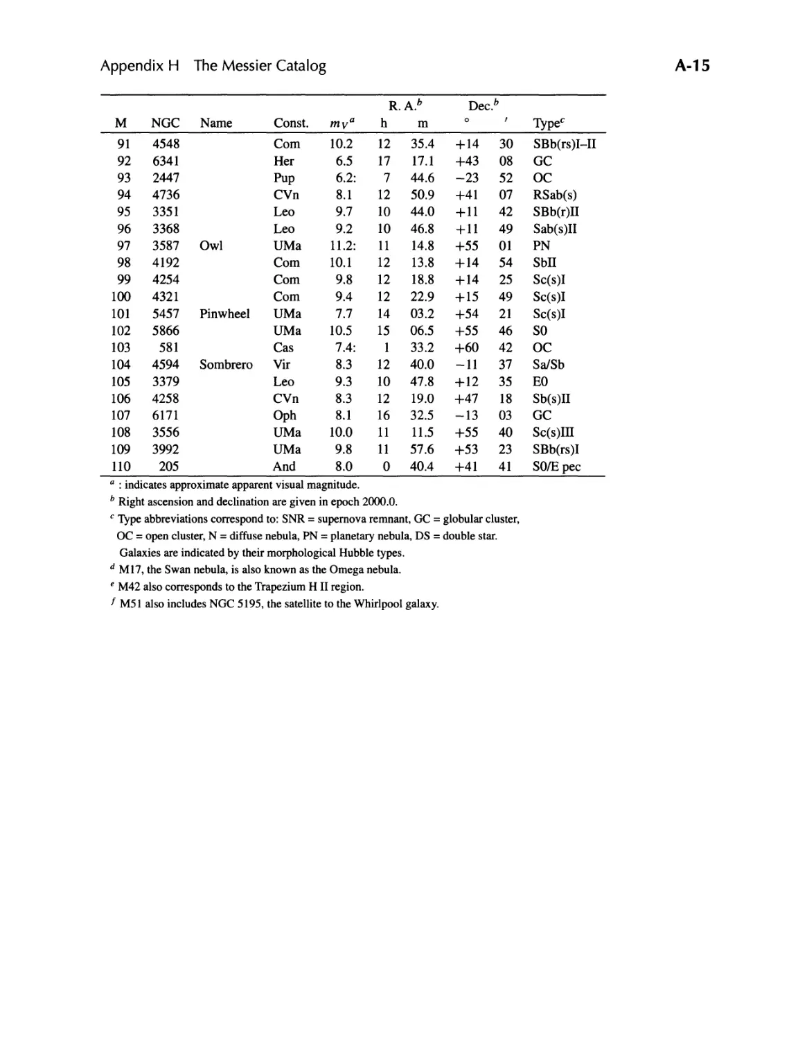
H II The Messier Catalog
A-13
I II Constants, A Programming Module
A-16
A-17
K II TwoStars, A Binary Star Code
A-18
L II StatStar, A Stellar Structure Code
A-23
M II Galaxy, A Tidal I nteraction Code
A-26
N II WMAP Data
A-29
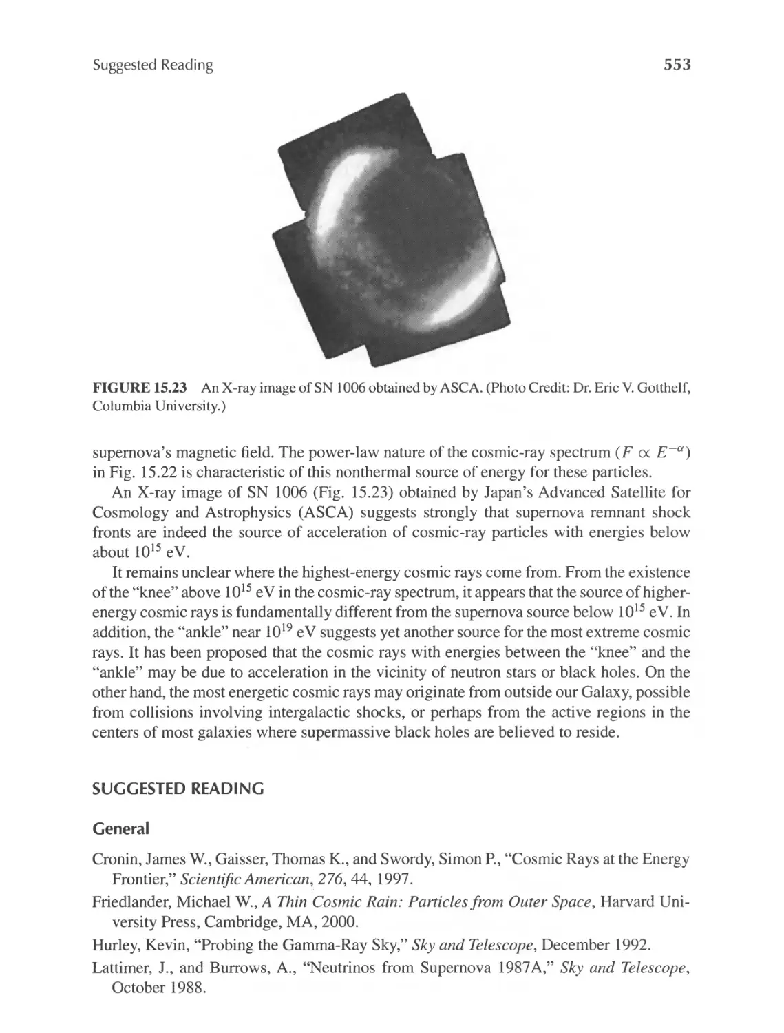
Suggested Reading
A-30
Index
1-1
PART
I
The Tools of Astronomy
CHAPTER
1
The Celestial Sphere
1.1
1.2
1.3
1.4
The Greek Tradition
The Copernican Revolution
Positions on the Celestial Sphere
Physics and Astronomy
1.1 .THE GREEK TRADITION
Human beings have long looked up at the sky and pondered its mysteries. Evidence of the
long struggle to understand its secrets may be seen in remnants of cultures around the world:
the great Stonehenge monument in England, the structures and the writings of the Maya and
Aztecs, and the medicine wheels of the Native Americans. However, our modern scientific
view of the universe traces its beginnings to the ancient Greek tradition of natural philosophy.
Pythagoras (ca. 550 B.C.) first demonstrated the fundamental relationship between numbers
and nature through his study of musical intervals and through his investigation of the
geometry of the right angle. The Greeks continued their study of the universe for hundreds
of years using the natural language of mathematics employed by Pythagoras. The modem
discipline of astronomy depends heavily on a mathematical formulation of its physical
theories, following the process begun by the ancient Greeks.
In an initial investigation of the night sky, perhaps its most obvious feature to a careful
observer is the fact that it is constantly changing. Not only do the stars move steadily from
east to west during the course of a night, but different stars are visible in the evening sky,
depending upon the season. Of course the Moon also changes, both in its position in the
sky and in its phase. More subtle and more complex are the movements of the planets, or
"wandering stars."
The Geocentric Universe
Plato (ca. 350 B.C.) suggested that to understand the motions of the heavens, one must first
begin with a set of workable assumptions, or hypotheses. It seemed obvious that the stars
of the night sky revolved about a fixed Earth and that the heavens ought to obey the purest
possible form of motion. Plato therefore proposed that celestial bodies should move about
Earth with a uniform (or constant) speed and follow a circular motion with Earth at the
center of that motion. This concept of a geocentric universe was a natural consequence of
the apparently unchanging relationship of the stars to one another in fixed constellations.
2
1.1 The Greek Tradition
3
North celestial pole Celestial sphere
"'"
North pole (Earth) -d- -{ ',----
* -
-*
* * -*
..: )Ie : , --- Equator (Earth)
.
)¥
... /
Celestial equator
South pole (Earth)
South celestial pole /
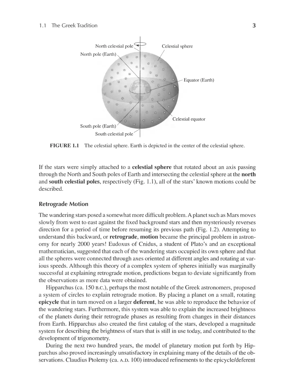
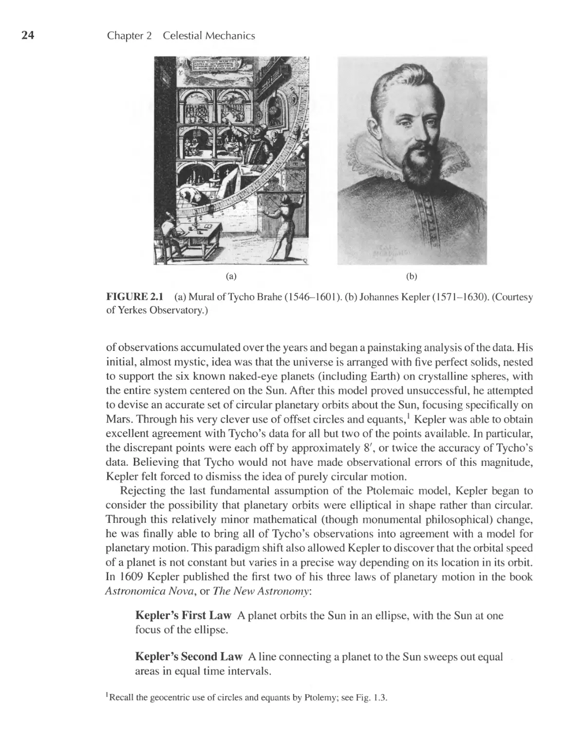
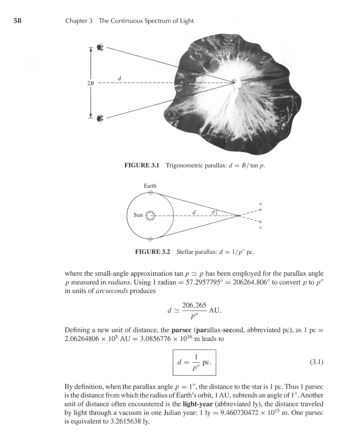
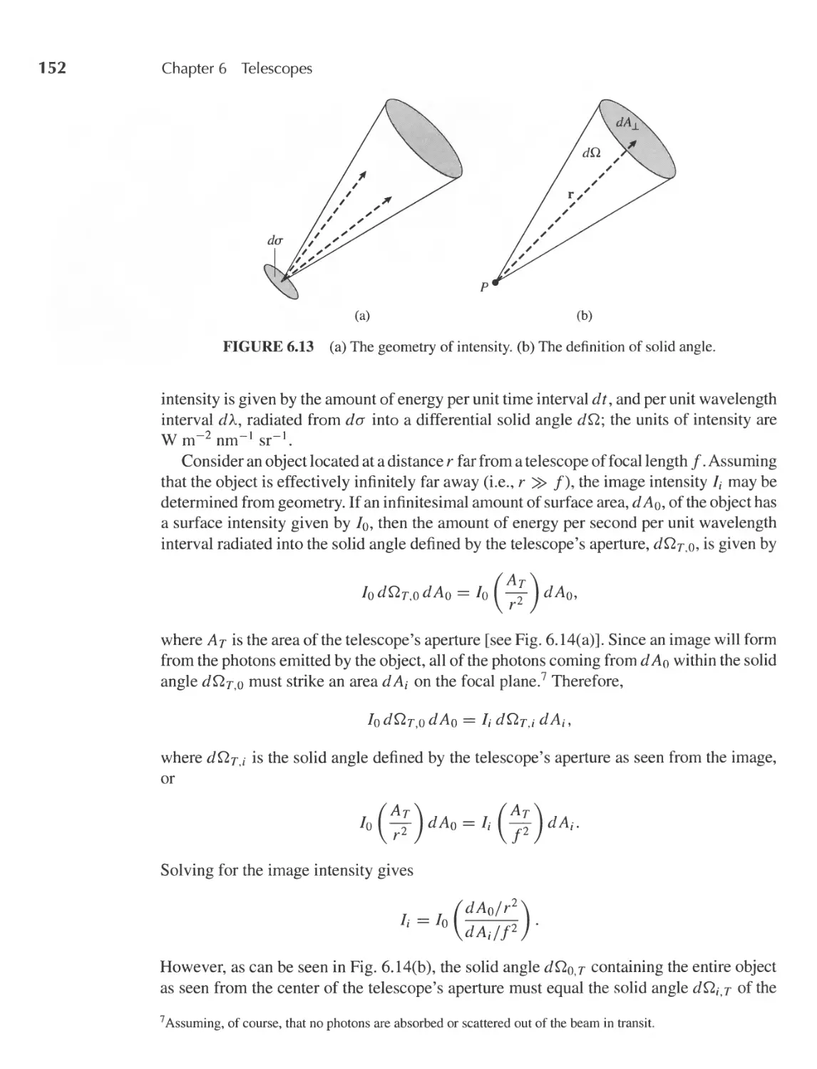
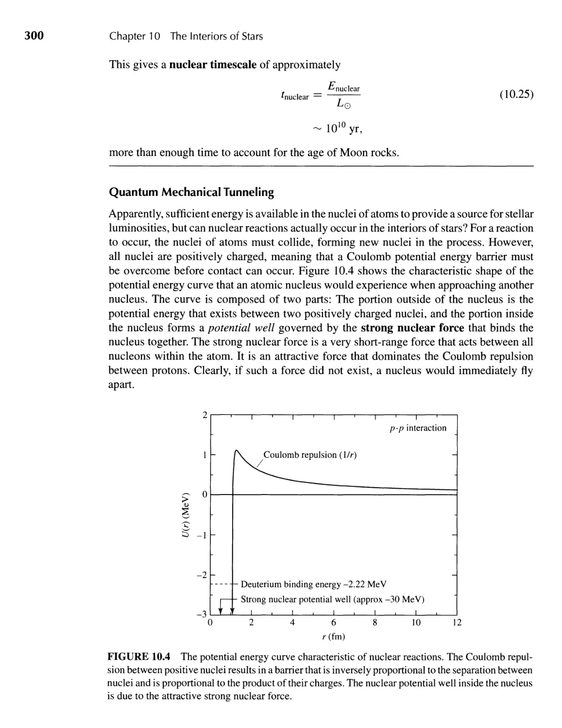
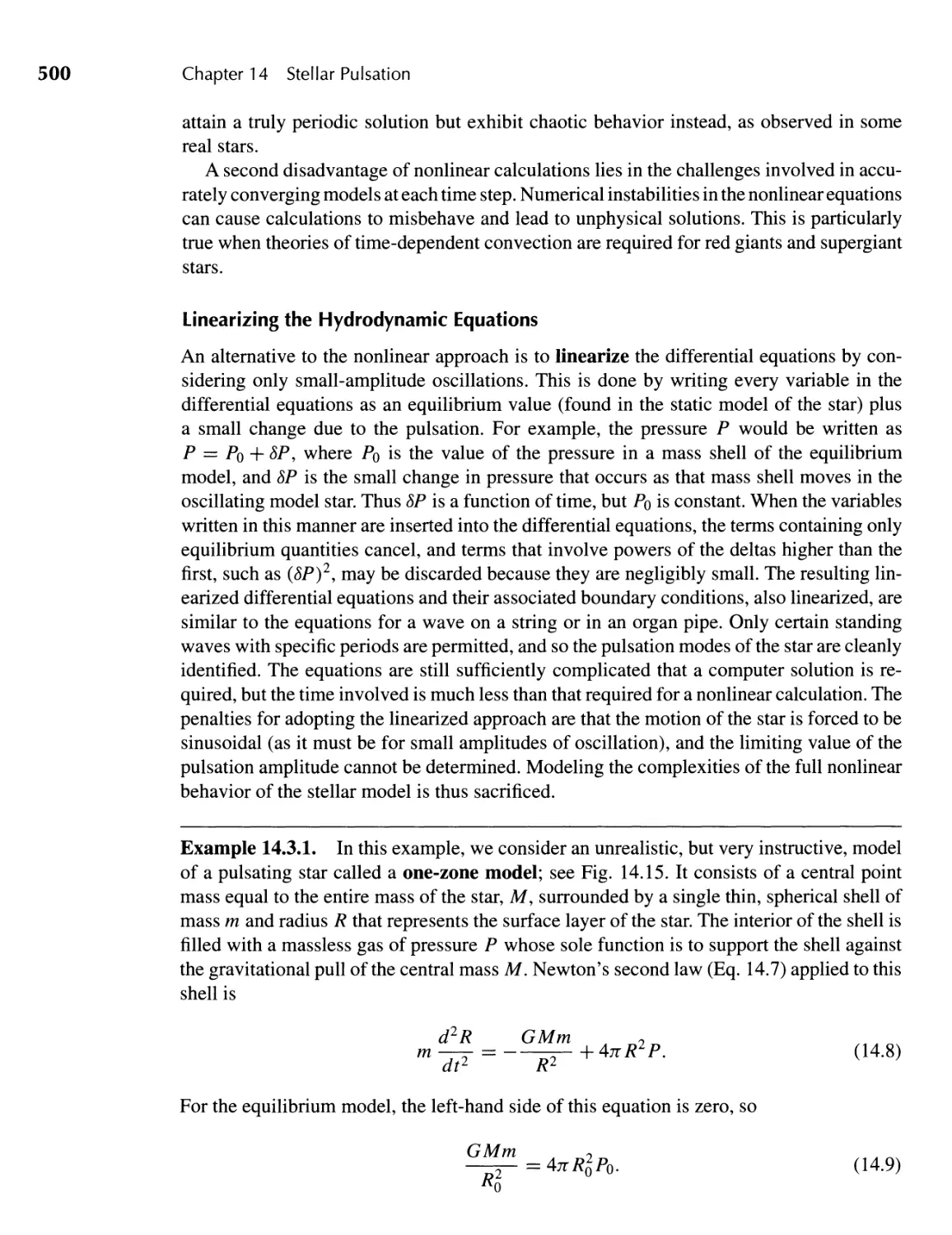
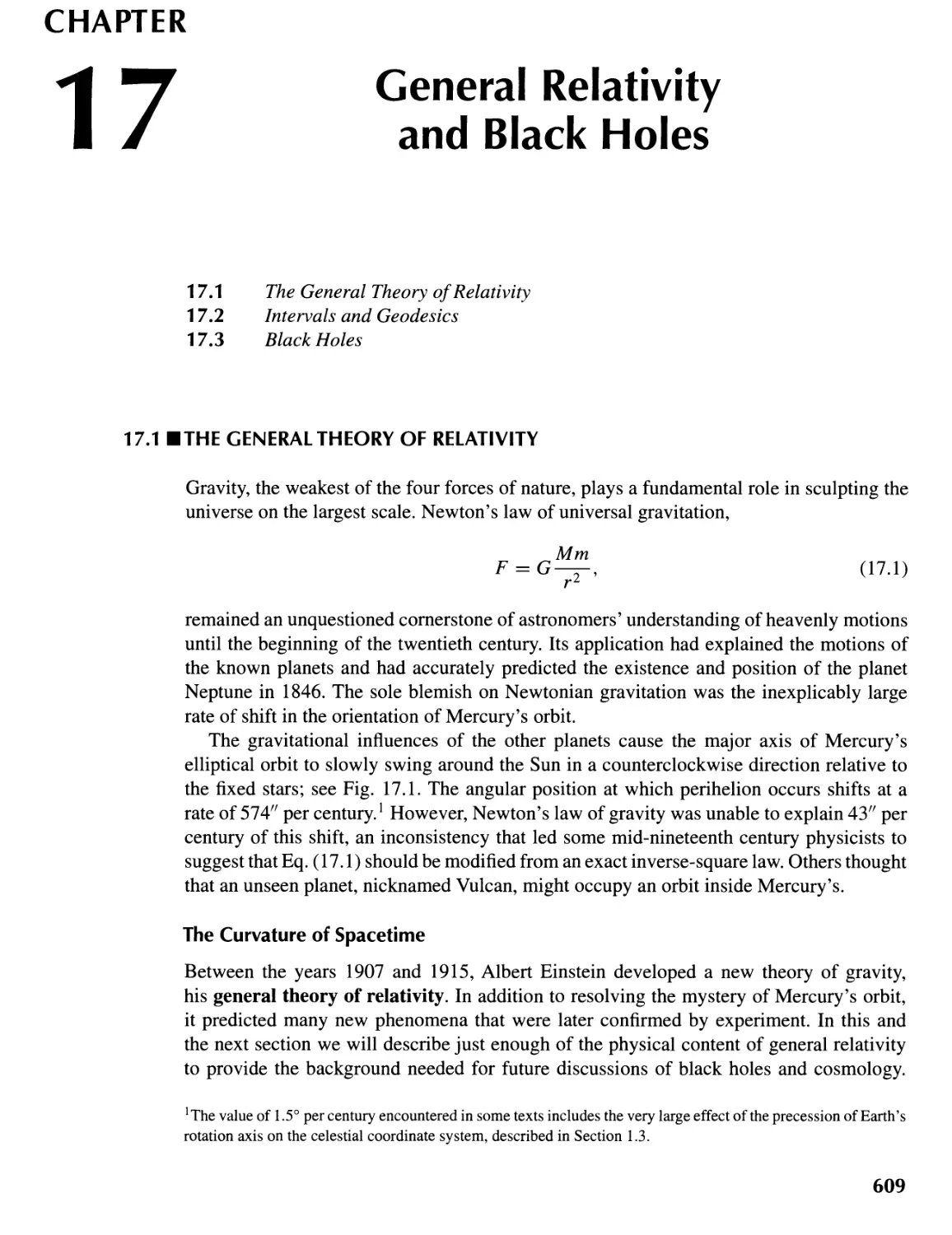
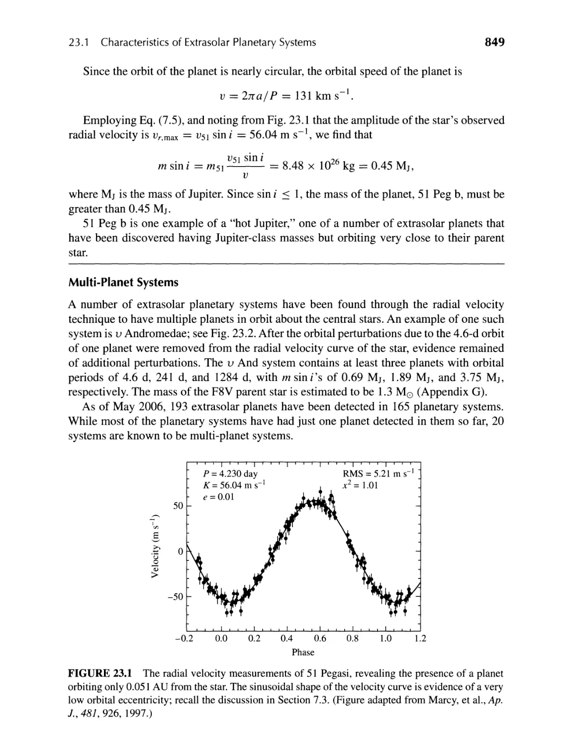
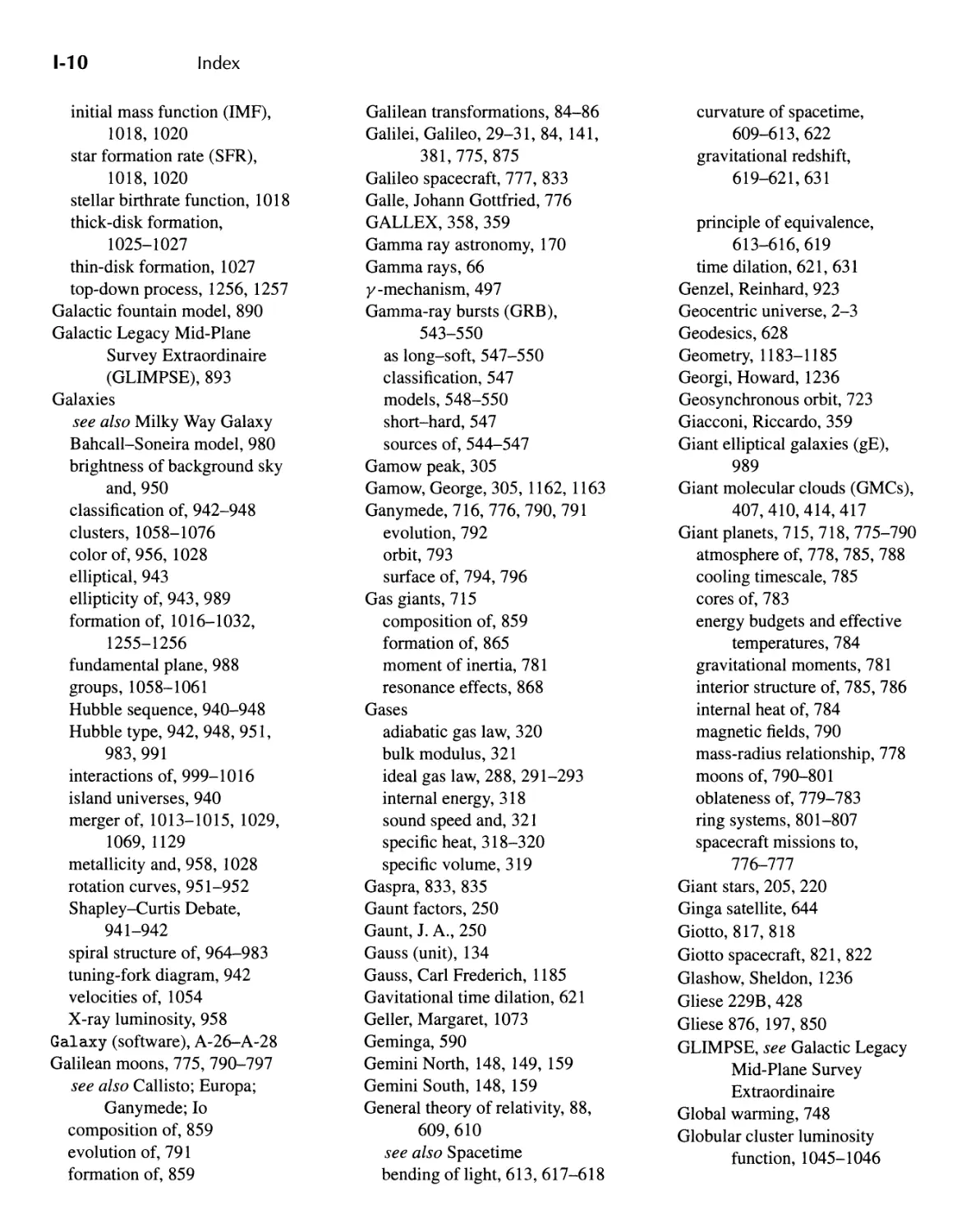
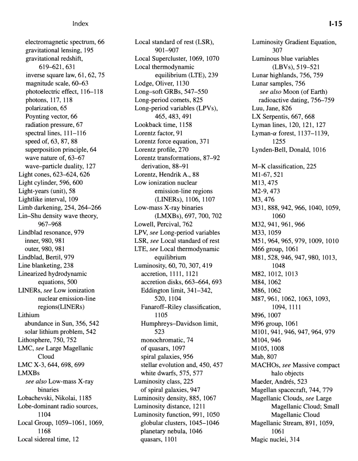
FIGURE 1.1 The celestial sphere. Earth is depicted in the center of the celestial sphere.
If the stars were simply attached to a celestial sphere that rotated about an axis passing
through the North and South poles of Earth and intersecting the celestial sphere at the north
and south celestial poles, respectively (Fig. 1.1), all of the stars' known motions could be
described.
Retrograde Motion
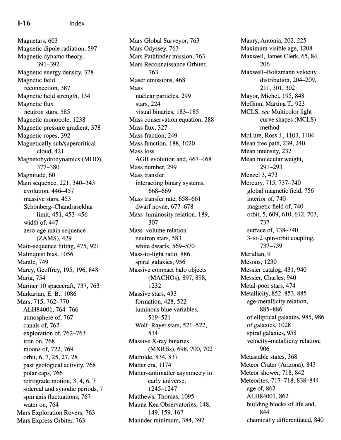
The wandering stars posed a somewhat more difficult problem. A planet such as Mars moves
slowly from west to east against the fixed background stars and then mysteriously reverses
direction for a period of time before resuming its previous path (Fig. 1.2). Attempting to
understand this backward, or retrograde, motion became the principal problem in astron-
omy for nearly 2000 years! Eudoxus of Cnidus, a student of Plato's and an exceptional
mathematician, suggested that each of the wandering stars occupied its own sphere and that
aIJ the spheres were connected through axes oriented at different angles and rotating at var-
ious speeds. Although this theory of a complex system of spheres initially was marginally
successful at explaining retrograde motion, predictions began to deviate significantly from
the observations as more data were obtained.
Hipparchus (ca. 150 B.C.), perhaps the most notable of the Greek astronomers, proposed
a system of circles to explain retrograde motion. By placing a planet on a small, rotating
epicycle that in turn moved on a larger deferent, he was able to reproduce the behavior of
the wandering stars. Furthermore, this system was able to explain the increased brightness
of the planets during their retrograde phases as resulting from changes in their distances
from Earth. Hipparchus also created the first catalog of the stars, developed a magnitude
system for describing the brightness of stars that is stilJ in use today, and contributed to the
development of trigonometry.
During the next two hundred years, the model of planetary motion put forth by Hip-
parchus also proved increasingly unsatisfactory in explaining many of the details of the ob-
servations. Claudius Ptolemy (ca. A.D. 100) introduced refinements to the epicycle/deferent
4
Chapter 1 The Celestial Sphere
.
r "- 25
rJ.j .. .
.
(1,) April 15, 2006 . . . . .
. e.
(1,) .
J.-c . February 28, 2006 . .
20 .
0.0 . . .
January 1, 2006 · .
(1,) .. November 4, 2005 :::---.....
"'0 . .
.
.
"-"" . f" October 1, 2005
15 . .
c:: . . December 10,2005
. . .
.
0 .
. August 30, 2005
. ...... "
10
.t . . e. .
. .
c:: . . . .
.
.
. ...... . .
. I ..
u 5 . , .
(1,) . July 15, 2005
. .
0 . . .
.
. . .
0 .
6 5 4 3 2 1
Right ascension (hours)
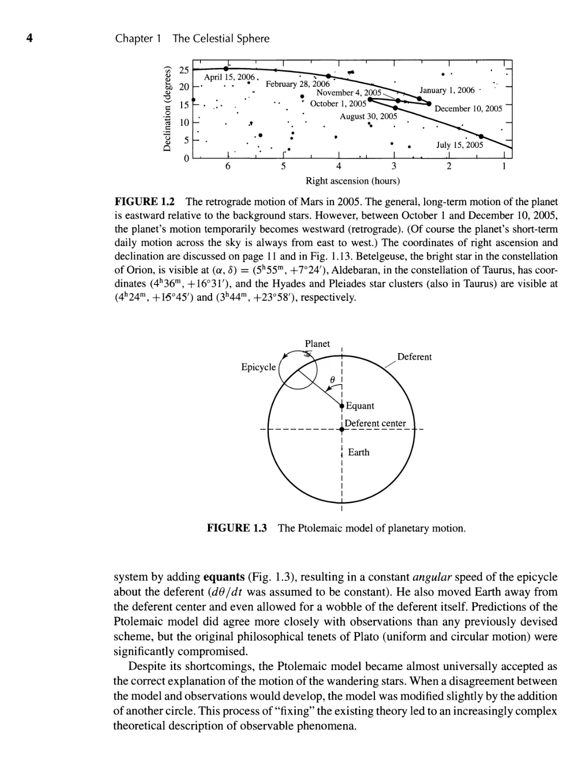
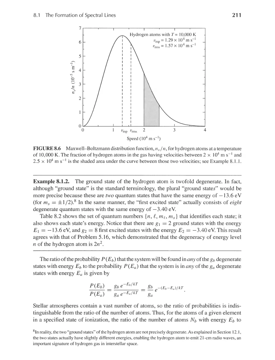
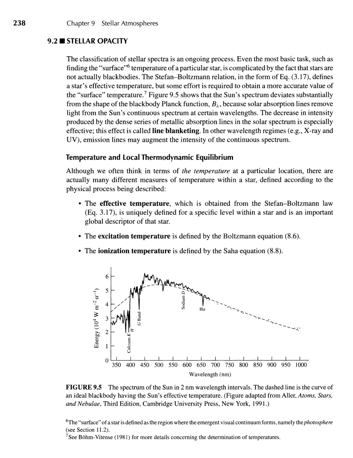
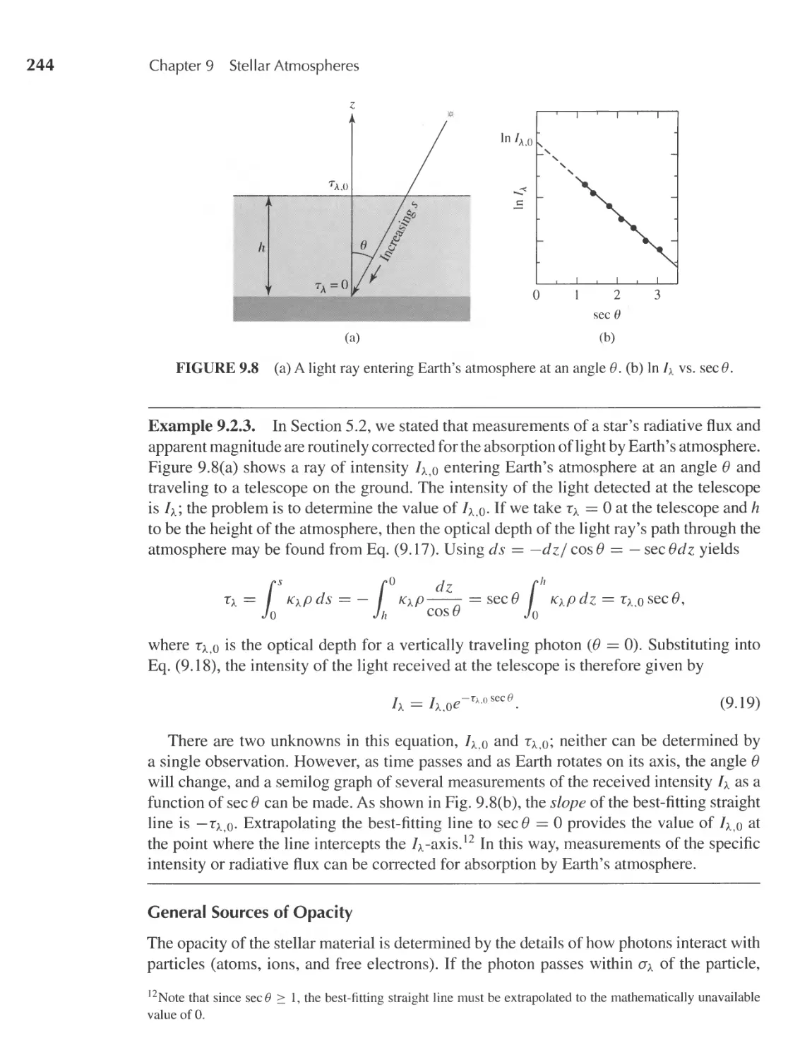
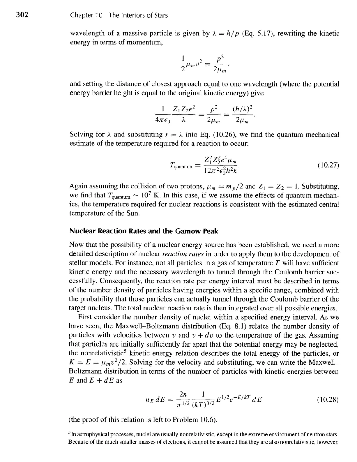
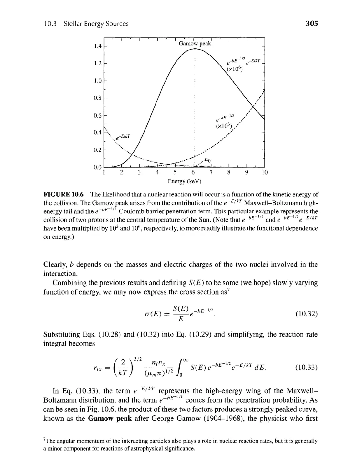
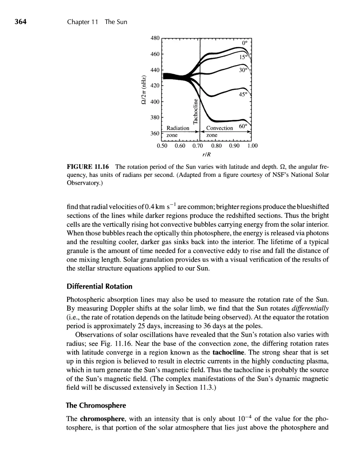
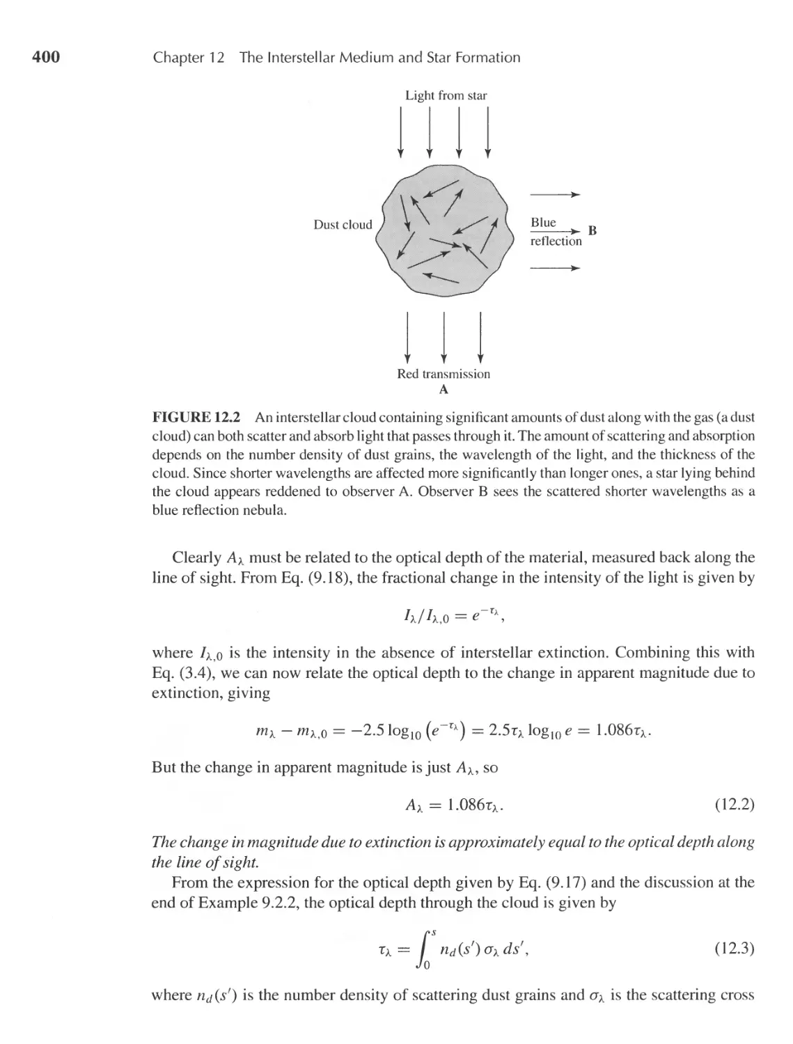
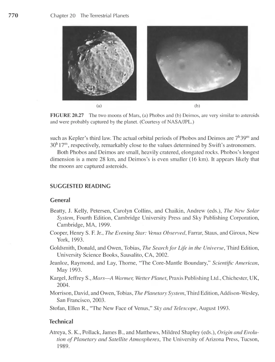
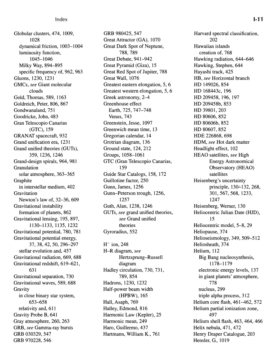
FIGURE 1.2 The retrograde motion of Mars in 200S. The general, long-term motion of the planet
is eastward relative to the background stars. However, between October 1 and December 10, 2OOS,
the planet's motion temporarily becomes westward (retrograde). (Of course the planet's short-term
daily motion across the sky is always from east to west.) The coordinates of right ascension and
declination are discussed on page 11 and in Fig. 1.13. Betelgeuse, the bright star in the constellation
of Orion, is visible at (a, 8) (shssm, + 7°24'), Aldebaran, in the constellation of Taurus, has coor-
dinates (4 h 36 m , +16°31'), and the Hyades and Pleiades star clusters (also in Taurus) are visible at
(4 h 24 m , + 16°4S') and (3 h 44 m , +23°58'), respectively.
Epicycle
Planet
«.x-
I
I
I
() I
I
Equant
I
Deferent center
Deferent
/
........ --.-.----- ...-...-..-..-...-----
I
Earth
I
I
I
I
I
I
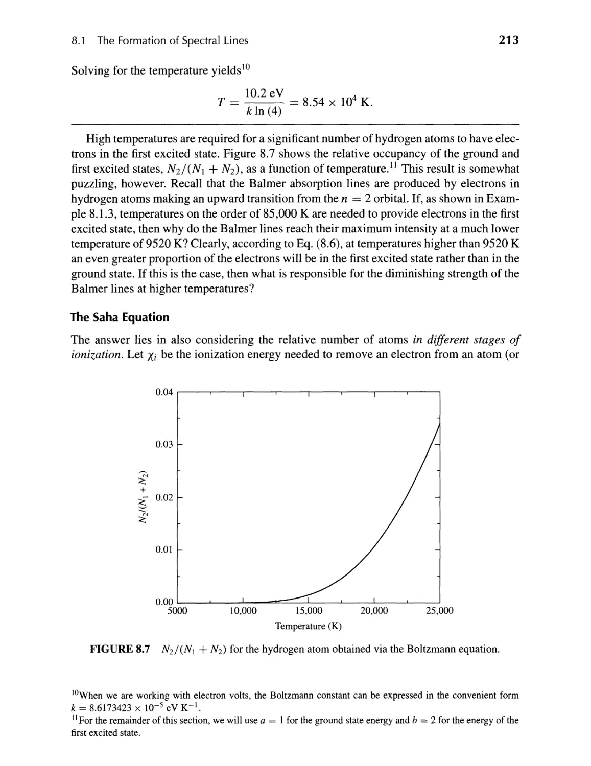
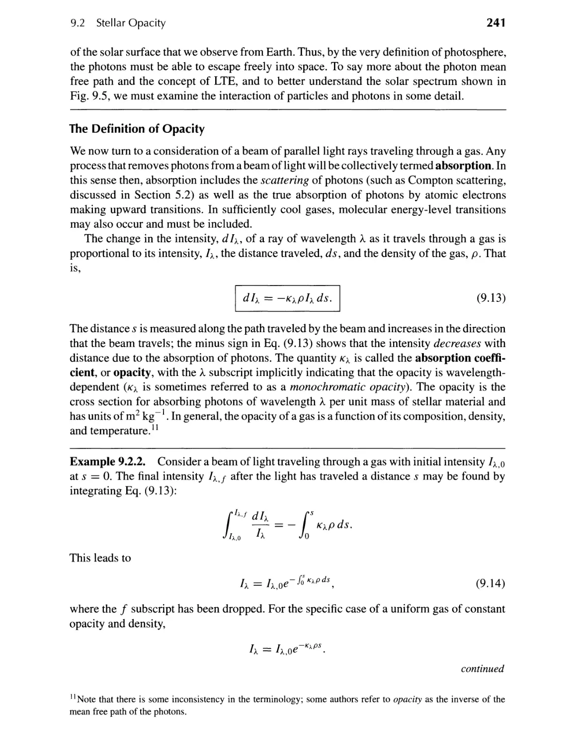
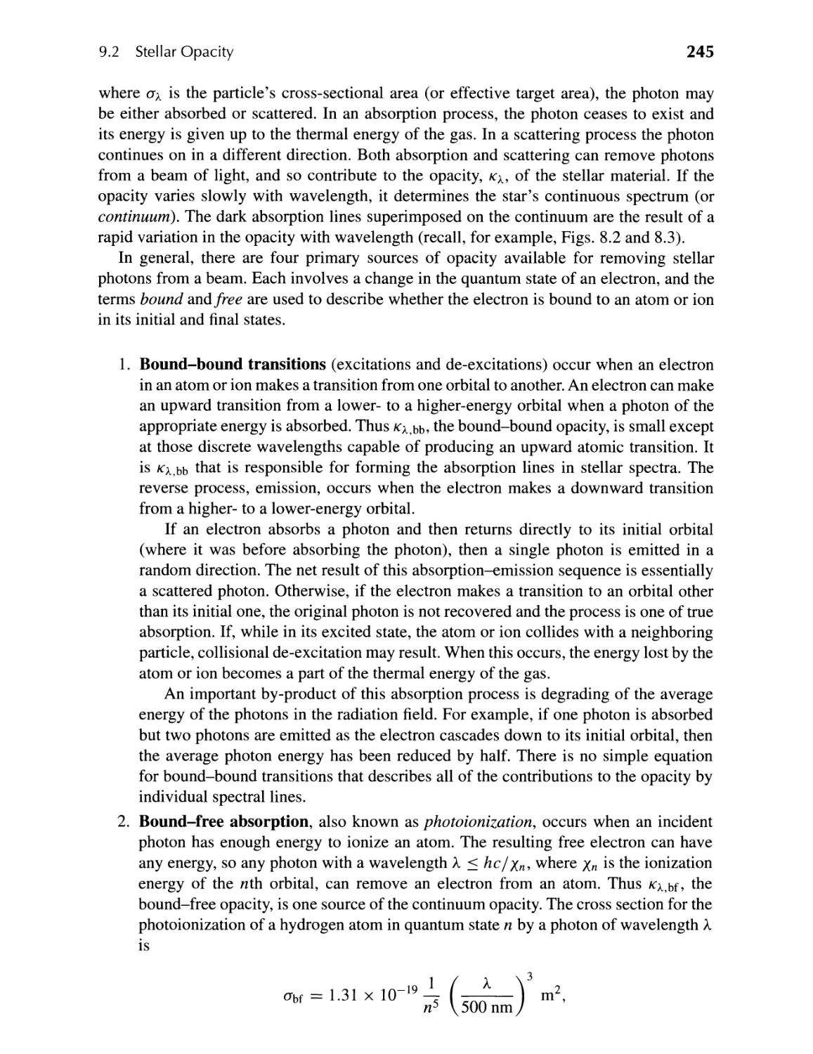
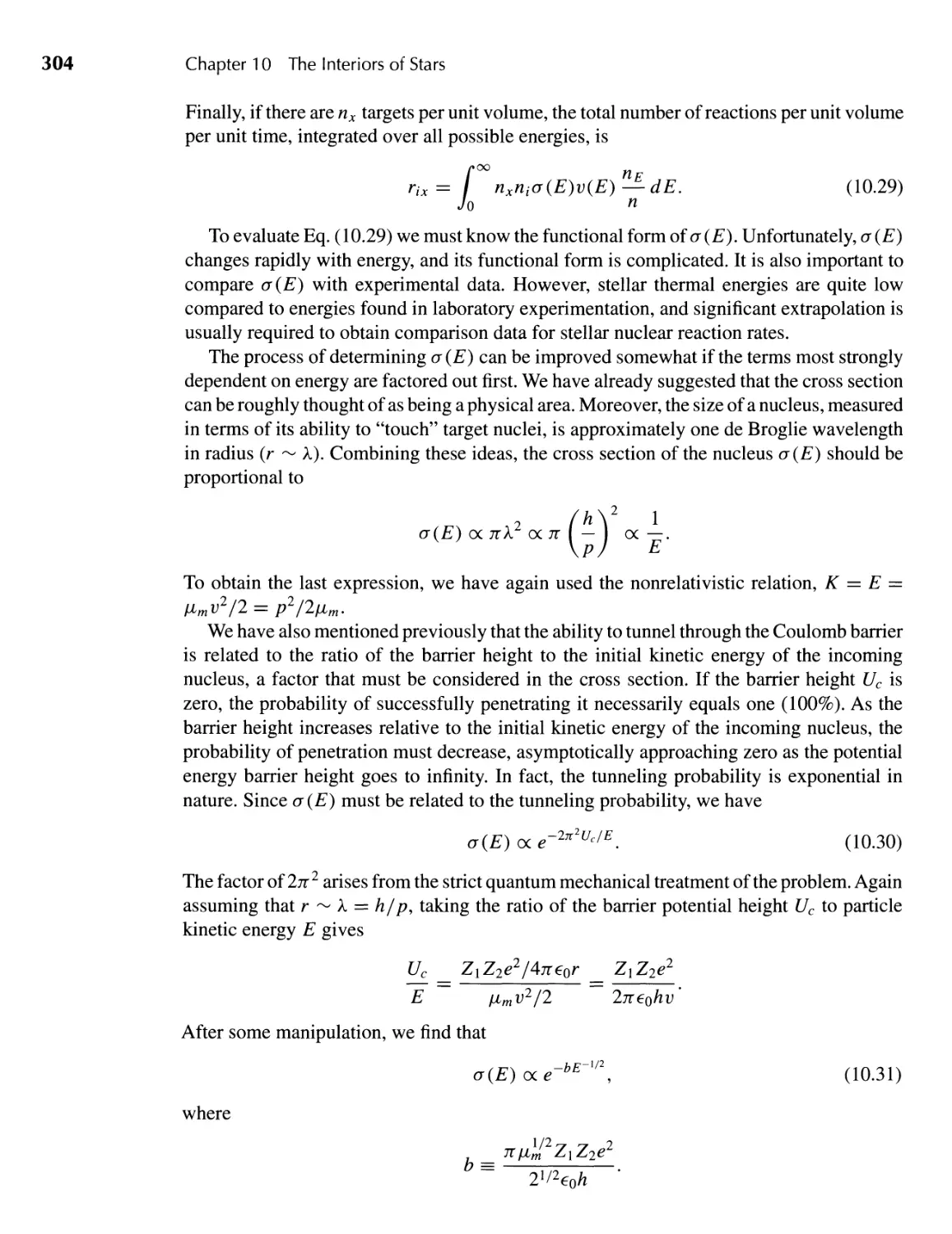
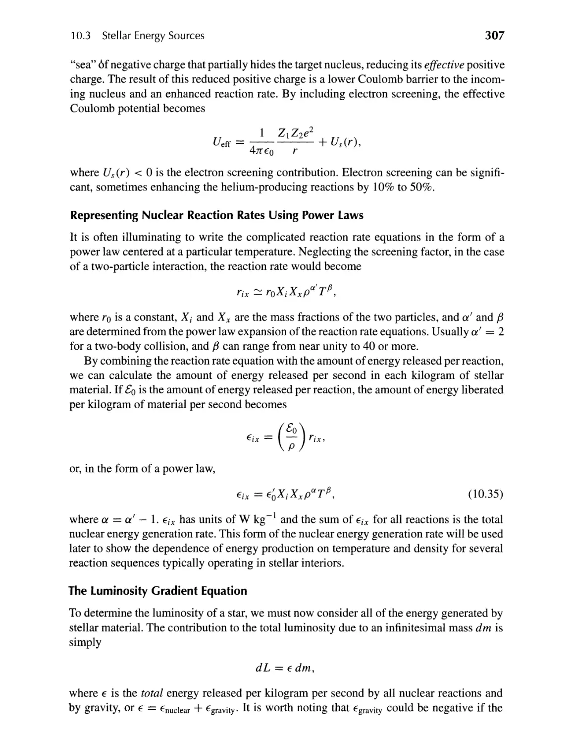
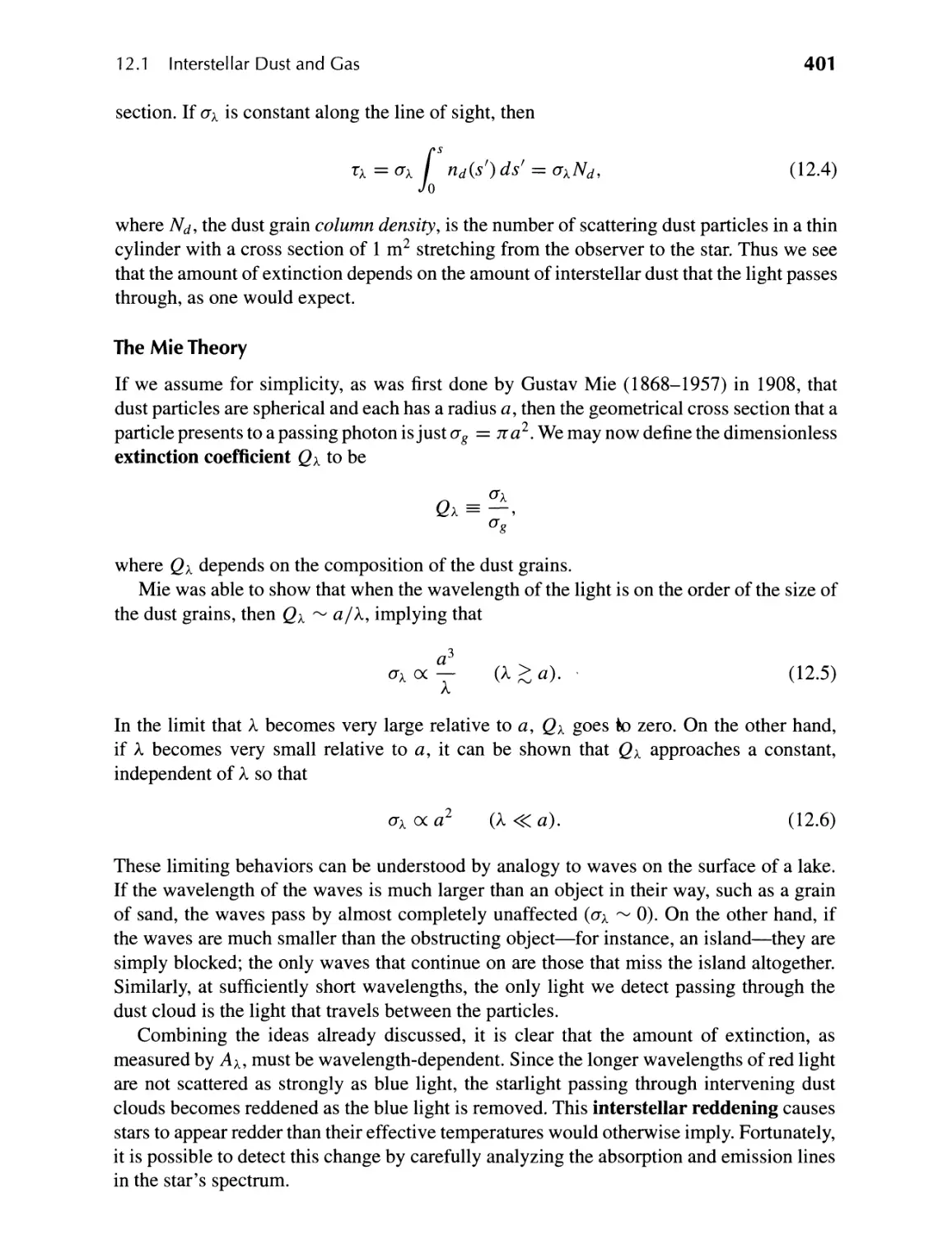
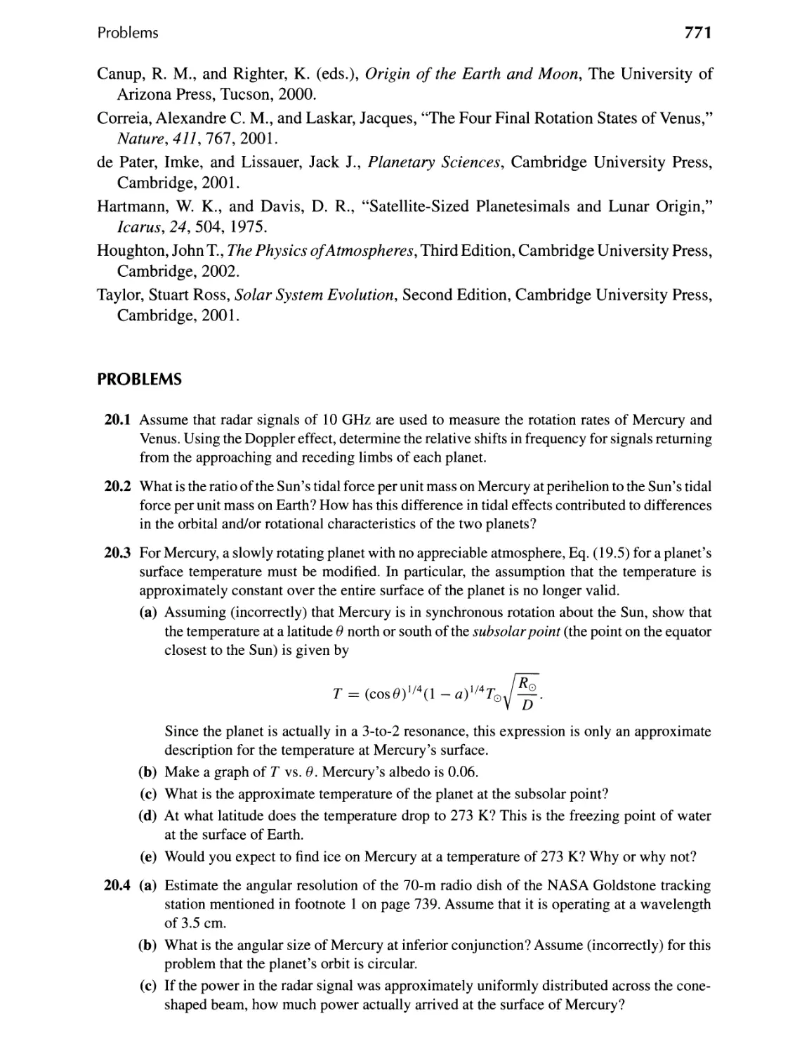
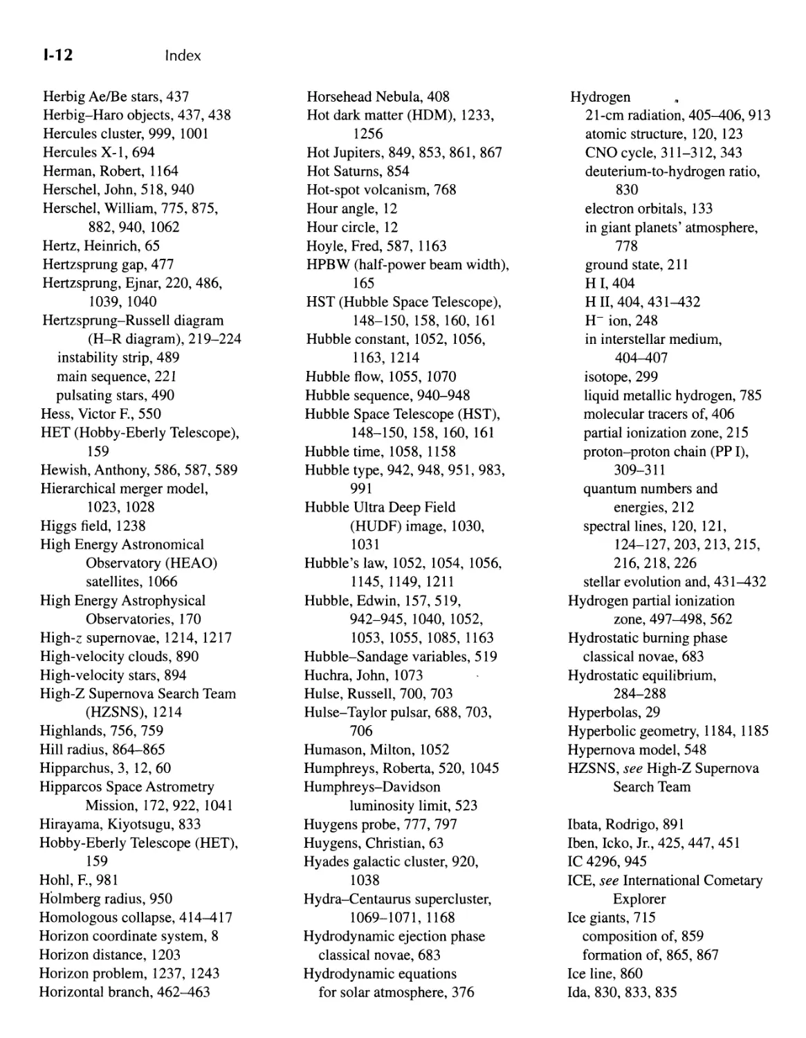
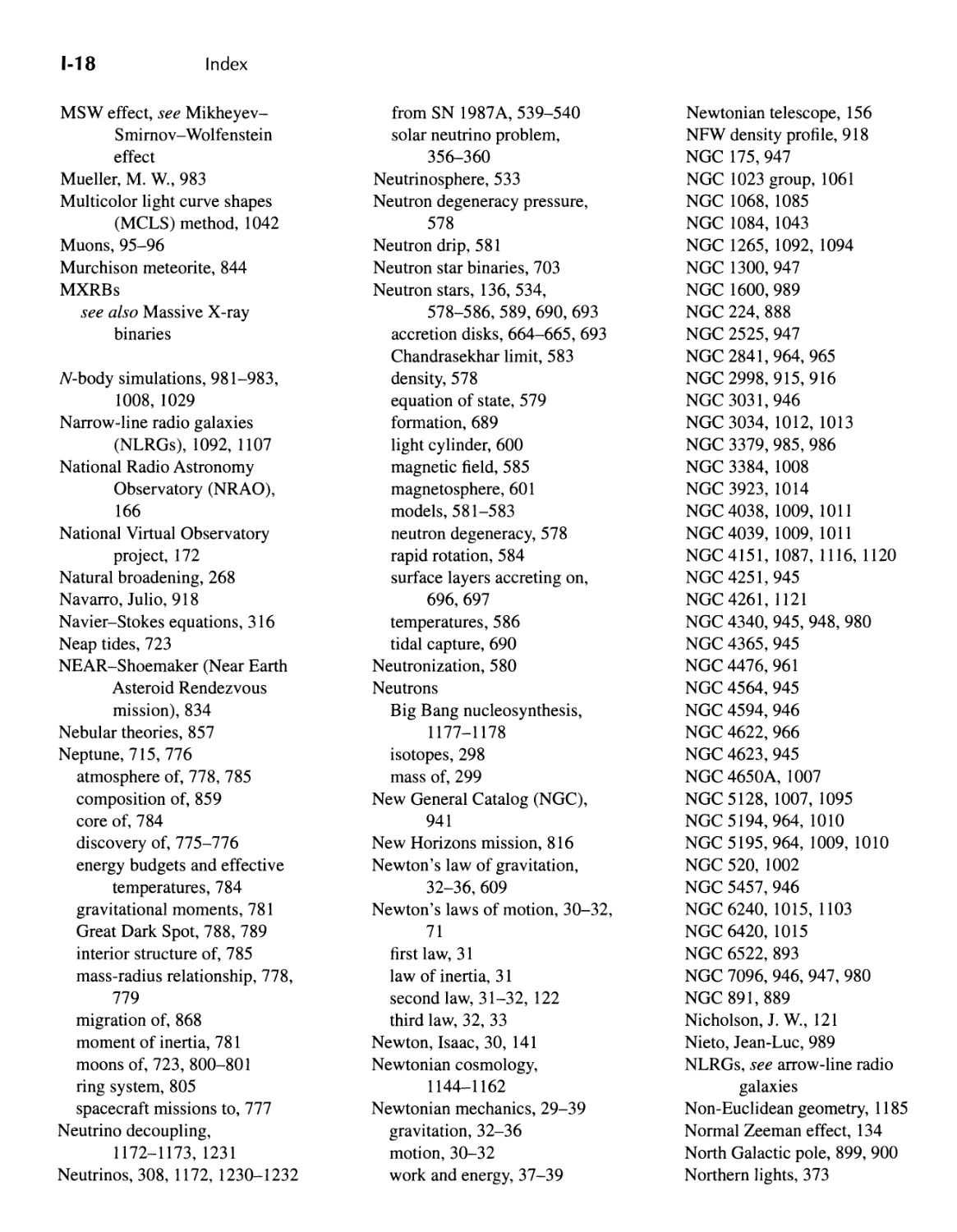
FIGURE 1.3 The Ptolemaic model of planetary motion.
system by adding equants (Fig. 1.3), resulting in a constant angular speed of the epicycle
about the deferent (dO / dt was assumed to be constant). He also moved Earth away from
the deferent center and even allowed for a wobble of the deferent itself. Predictions of the
Ptolemaic model did agree more closely with observations than any previously devised
scheme, but the original philosophical tenets of Plato (uniform and circular motion) were
significantly compromised.
Despite its shortcomings, the Ptolemaic model became almost universally accepted as
the correct explanation of the motion of the wandering stars. When a disagreement between
the model and observations would develop, the model was modified slightly by the addition
of another circle. This process of "fixing" the existing theory led to an increasingly complex
theoretical description of observable phenomena.
1.2 The Copernican Revolution
5
"'jIh .._.
.:{ /'." . :. {:
t
t::'<f;>O
: :, )" ..
",'
"',":' ,,! , ,\"\
,..-..
"$ -
. . .; .. .. '«'
.. , ""
" .--.. , ....,
." . .".
.: :.. ."" . .." .
. ...
.". .
'.n .._ .
, ' --;..
'. ." , t,__' ':: .' ' :'?' ,.'
, ,
.... . ,. . Y..-
". ".". "." '. : "::" -' '-:
, "", I
, - C",:', '" \
":,'" ,'. ) ; !':1
.- ',,"'-- "
-:a.: : ....
Tl-->'f (:r
?" :
'/ -', ',,..,"
(a)
(b)
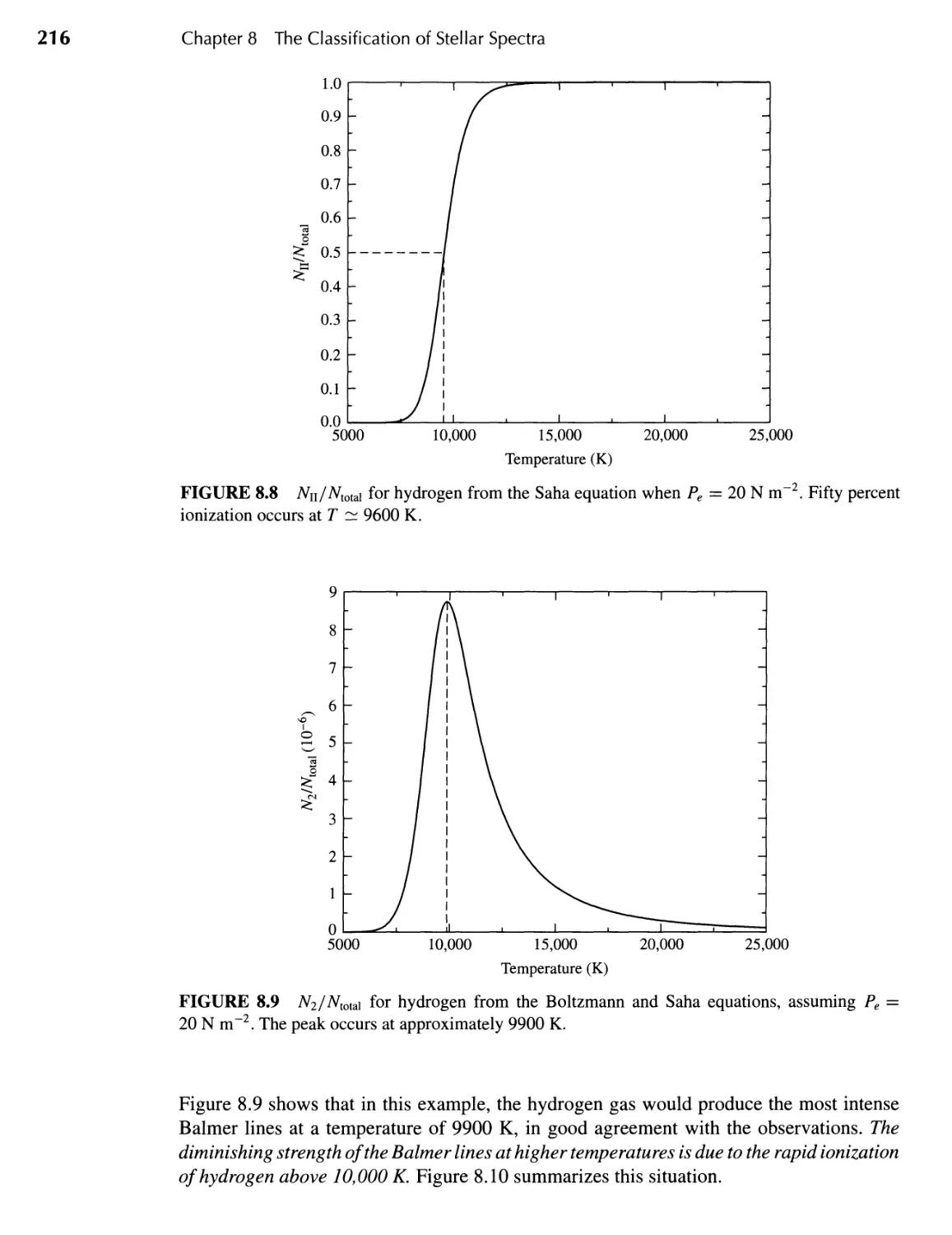
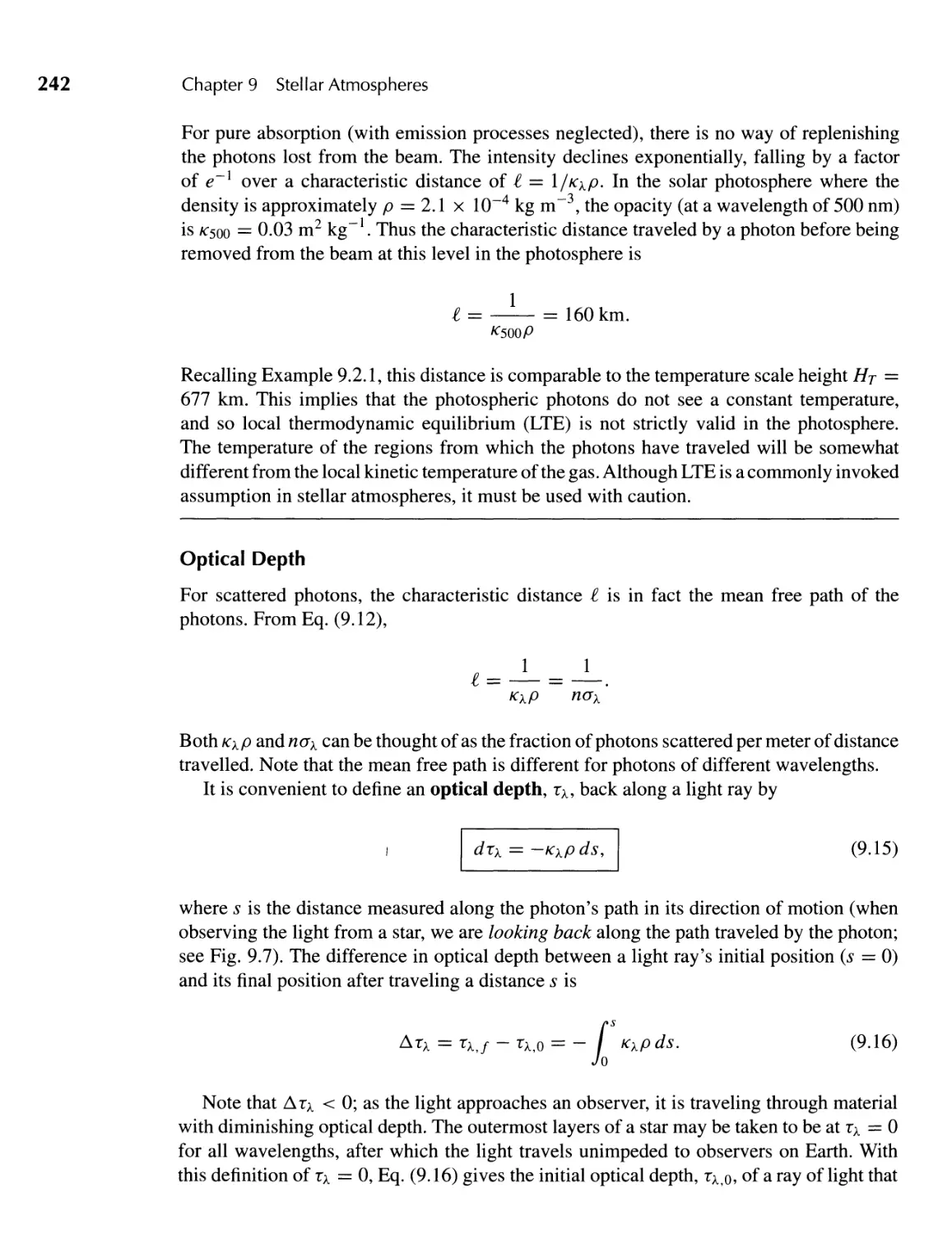
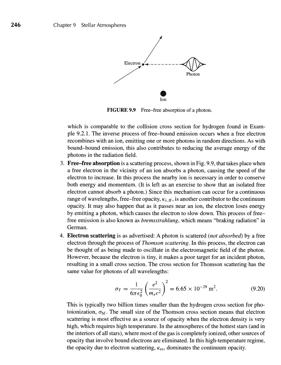
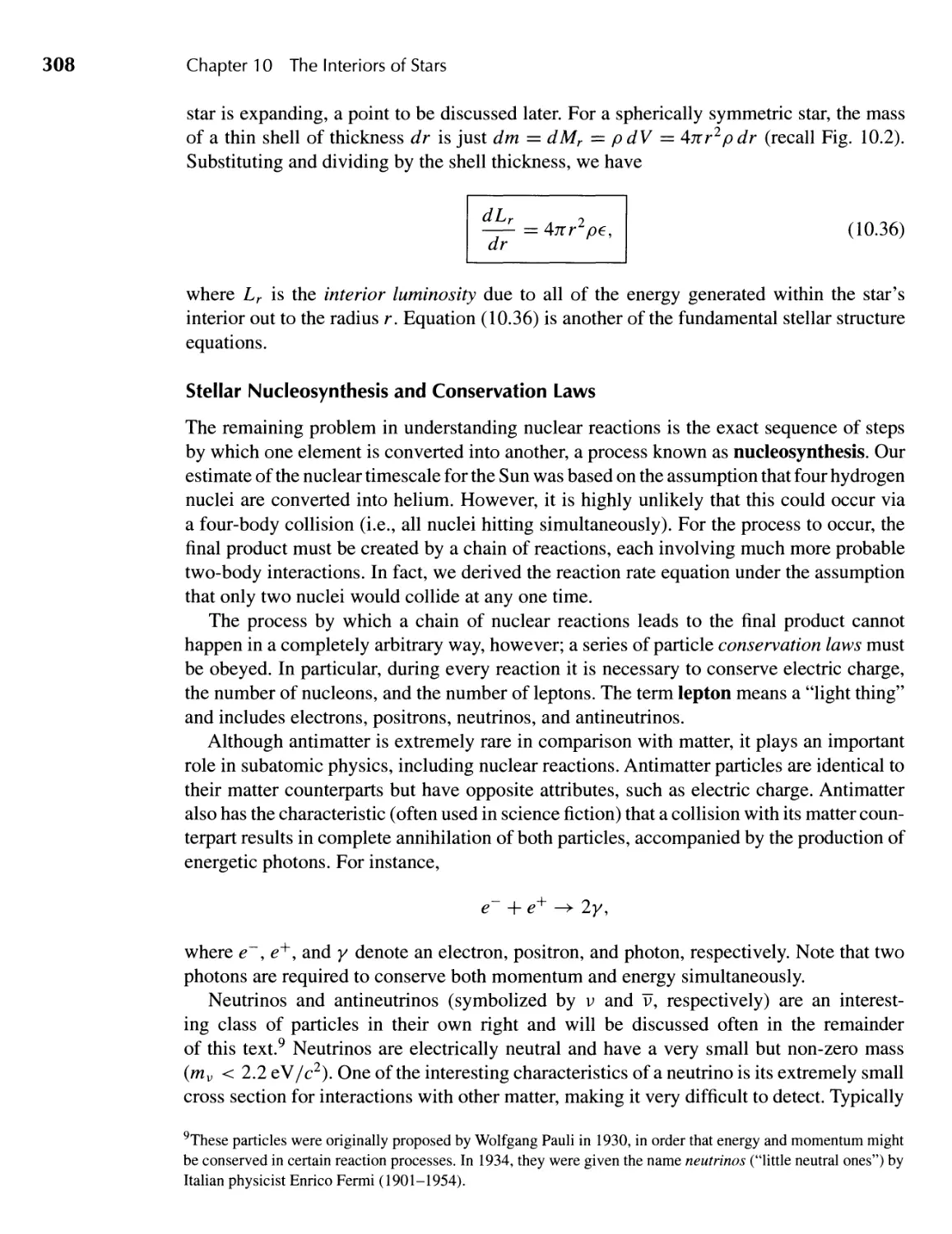
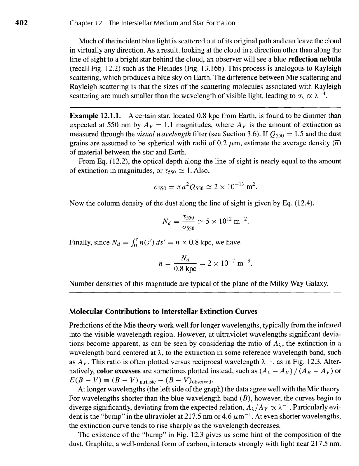
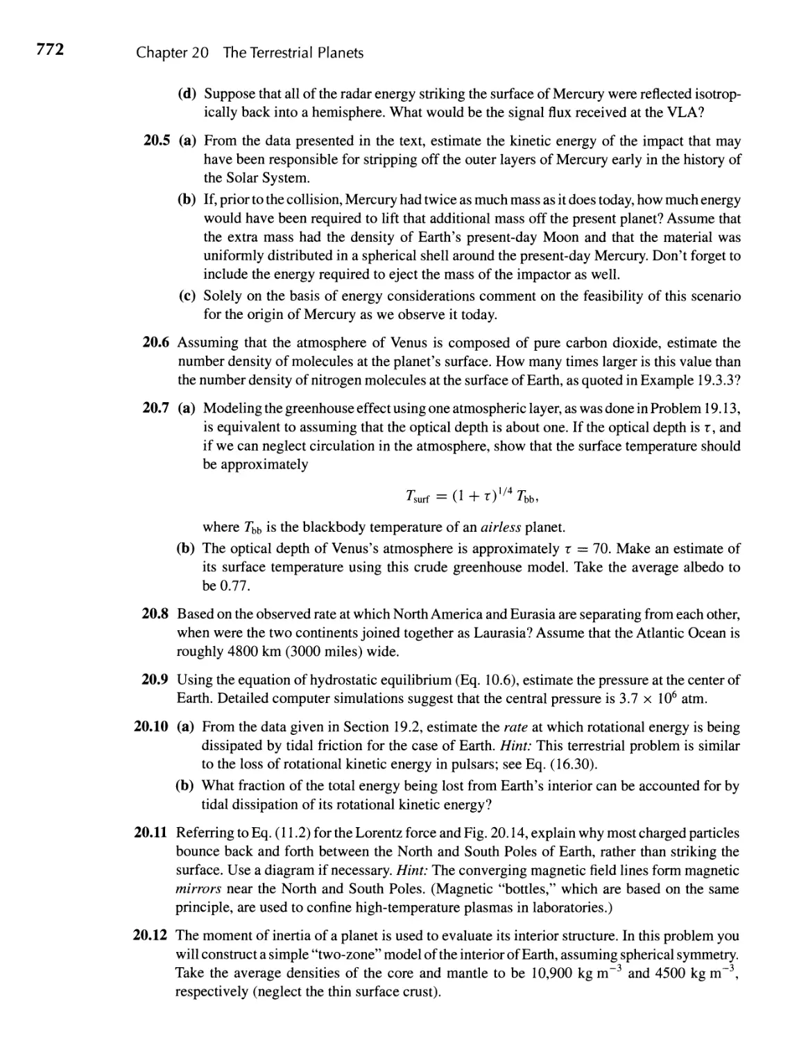
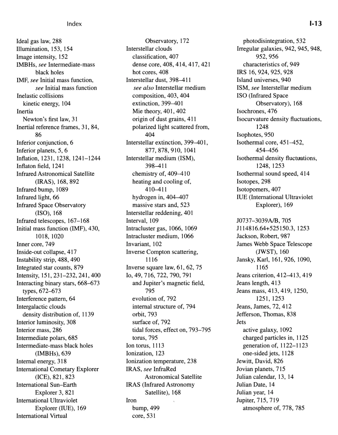
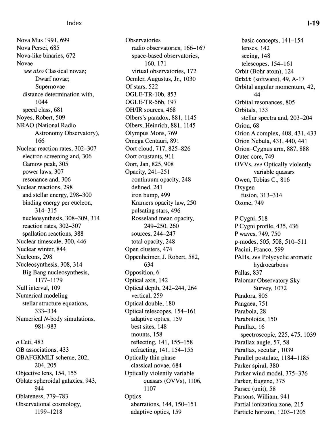
FIGURE 1.4 (a) Nicolaus Copernicus (J473-1543). (b)TheCopemican model of planetary motion:
Planets travel in circles with the Sun at the center of motion. (Courtesy of Yerkes Observatory.)
1.2 .THE COPERNICAN REVOLUTION
By the sixteenth century the inherent simplicity of the Ptolemaic model was gone. Polish-
born astronomer Nicolaus Copernicus (1473-1543), hoping to return the science to a less
cumbersome, more elegant view of the universe, suggested a heliocentric (Sun-centered)
model of planetary motion (Fig. 1.4). 1 His bold proposal led immediately to a much less
complicated description of the relationships between the planets and the stars. Fearing
severe criticism from the Catholic Church, whose doctrine then declared that Earth was
the center of the universe, Copernicus postponed publication of his ideas until late in life.
De Revo/utionibus Orbium Coelestium (On the Revolution of the Celestial Sphere) first
appeared in the year of his death. Faced with a radical new view of the universe, along
with Earth's location in it, even some supporters of Copernicus argued that the heliocentric
model merely represented a mathematical improvement in calculating planetary positions
but did not actually reflect the true geometry of the universe. In fact, a preface to that effect
was added by Osiander, the priest who acted as the book's publisher.
Bringing Order to the Planets
One immediate consequence of the Copernican model was the ability to establish the order
of all of the planets from the Sun, along with their relative distances and orbital periods.
The fact that Mercury and Venus are never seen more than 28° and 47°, respectively, east
or west of the Sun clearly establishes that their orbits are located inside the orbit of Earth.
These planets are referred to as inferior planets, and their maximum angular separations
east or west of the Sun are known as greatest eastern elongation and greatest western
I Actually, Aristarchus proposed a heliocentric model of the universe in 280 B.c. At that time, however, there was
no compelling evidence to suggest that Earth itself was in motion.
6
Chapter 1 The Celestial Sphere
Orbit of
inferior planet
Superior
conjunction
Orbit of
superior planet
/
Greatest
eastern
elongation
Greatest
western
elongation
Opposition
Inferior
conjunction
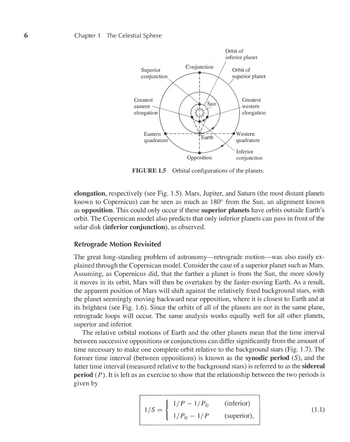
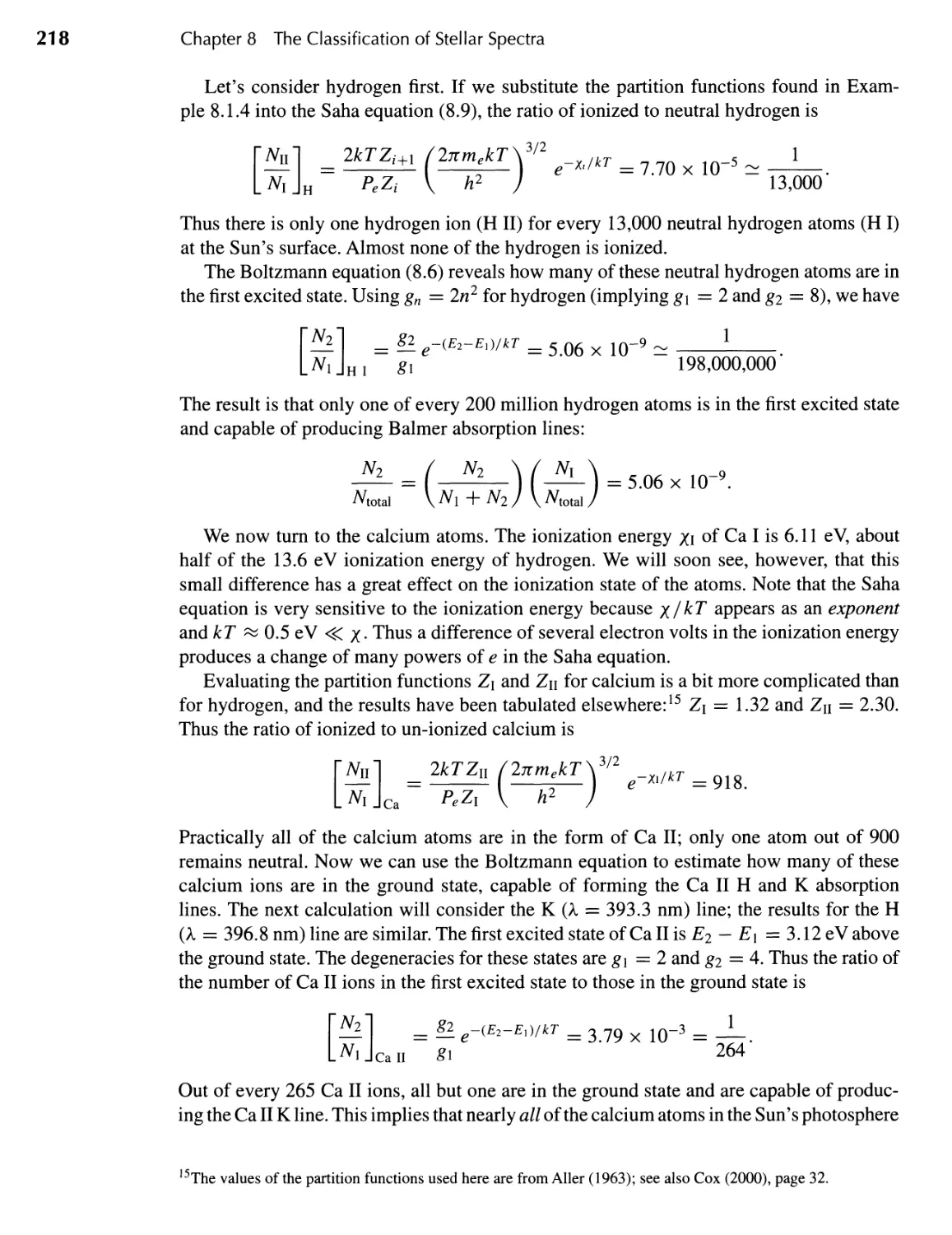
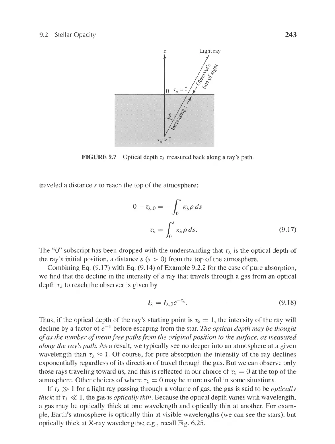
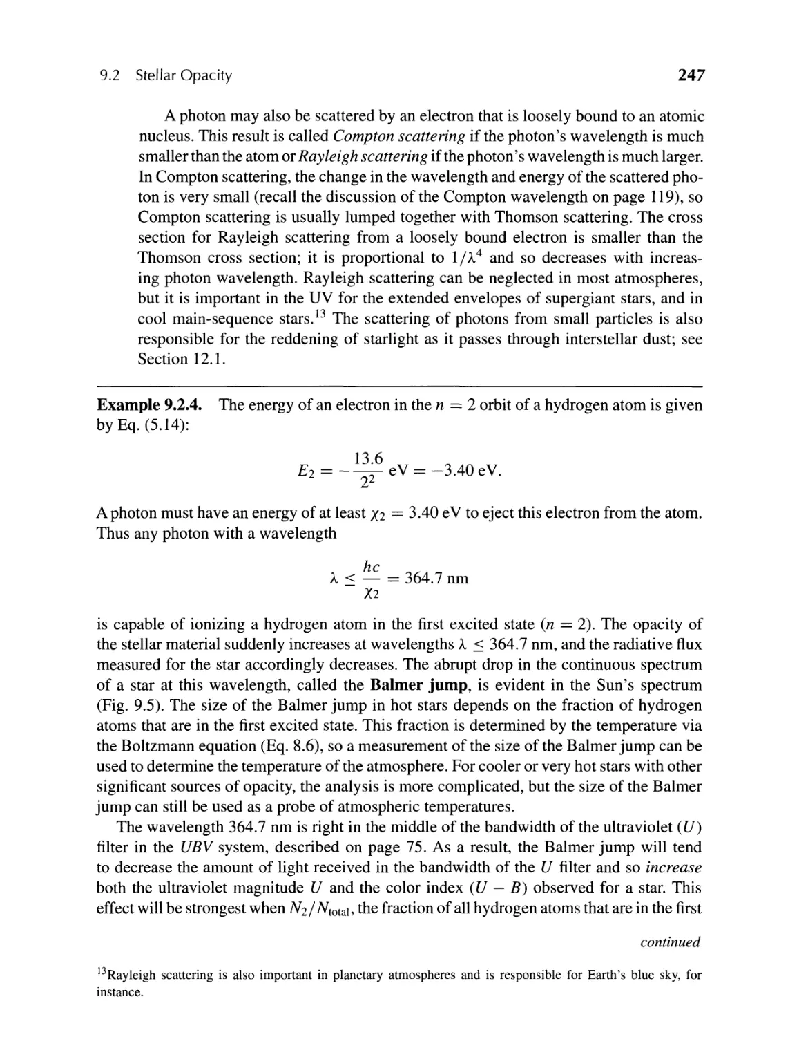
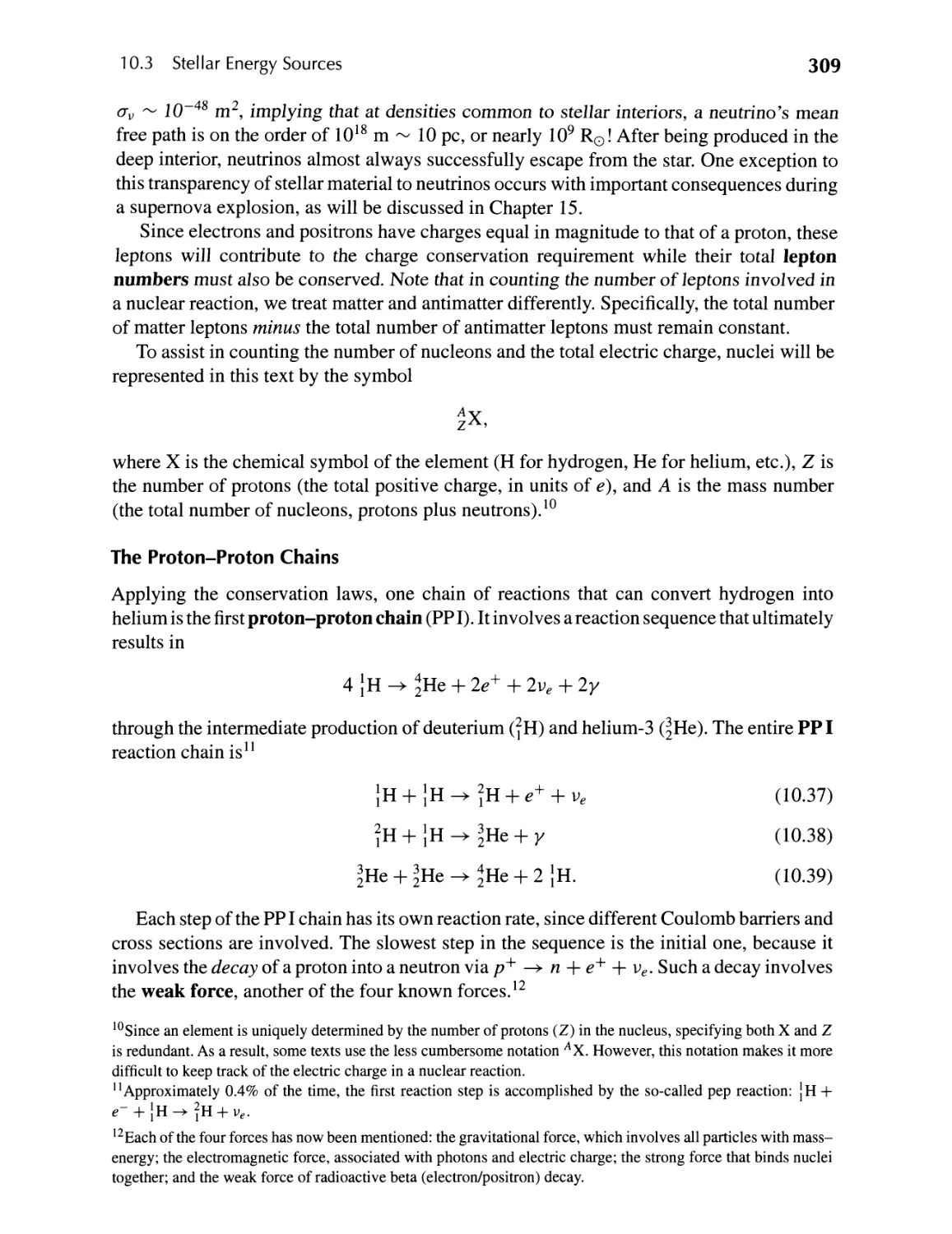
FIGURE 1.5 Orbital configurations of the planets.
elongation, respectively (see Fig. 1.5). Mars, Jupiter, and Saturn (the most distant planets
known to Copernicus) can be seen as much as 180 0 from the Sun, an alignment known
as opposition. This could only occur if these superior planets have orbits outside Earth's
orbit. The Copernican model also predicts that only inferior planets can pass in front of the
solar disk (inferior conjunction), as observed.
Retrograde Motion Revisited
The great long-standing problem of astronomy-retrograde motion-was also easily ex-
plained through the Copernican model. Consider the case of a superior planet such as Mars.
Assuming, as Copernicus did, that the farther a planet is from the Sun, the more slowly
it moves in its orbit, Mars will then be overtaken by the faster-moving Earth. As a result,
the apparent position of Mars will shift against the relatively fixed background stars, with
the planet seemingly moving backward near opposition, where it is closest to Earth and at
its brightest (see Fig. 1.6). Since the orbits of all of the planets are no in the same plane,
retrograde loops will occur. The same analysis works equally well for all other planets,
superior and inferior.
The relative orbital motions of Earth and the other planets mean that the time interval
between successive oppositions or conjunctions can differ significantly from the amount of
time necessary to make one complete orbit relati ve to the background stars (Fig. 1.7). The
former time interval (between oppositions) is known as the synodic period (S), and the
latter time interval (measured relative to the background stars) is referred to as the sidereal
period (P). It is left as an exercise to show that the relationship between the two periods is
given by
[ l/P-l/PEfj
1/ S ==
l/PEfj-l/P
(inferior)
(superior),
(1.1)
1.2 The Copernican Revolution
7
7
6
3
4
5
2
Mars orbit
FIGURE 1.6 The retrograde motion of Mars as described by the Copernican model. Note that the
lines of sight from Earth to Mars cross for positions 3,4, and 5. This effect, combined with the slightly
differing planes of the two orbits result in retrograde paths near opposition. Recall the retrograde (or
westward) motion of Mars between October 1,2005, and December 10,2005, as illustrated in Fig. 1.2.
.--------.
. c<::-
.
c
O S
q
\
....-
."
."
./
/
/
/
/
I
/
I
I
I
,
I
,
\
,
\
\
\
\
,
,
,
"
.......
.......
......
........-----.---
FIGURE 1.7 The relationship between the sidereal and synodic periods of Mars. The two periods
do not agree due to the motion of Earth. The numbers represent the elapsed time in sidereal years
since Mars was initially at opposition. Note that Earth completes more than two orbits in a synodic
period of S = 2.135 yr, whereas Mars completes slightly more than one orbit during one synodic
period from opposition to opposition.
when perfectly circular orbits and constant speeds are assumed; P(J) is the sidereal period
of Earth's orbit (365.256308 d).
Although the Copernican model did represent a simpler, more elegant model of planetary
motion, it was not successful in predicting positions any more accurately than the Ptolemaic
model. This lack of improvement was due to Copernicus's inability to relinquish the 2000-
year-old concept that planetary motion required circles, the human notion of perfection. As
a consequence, Copernicus was forced (as were the Greeks) to introduce the concept of
epicycles to "fix" his model.
8
Chapter 1 The Celestial Sphere
Perhaps the quintessential example of a scientific revolution was the revolution begun
by Copernicus. What we think of today as the obvious solution to the problem of planetary
motion a heliocentric universe was perceived as a very strange and even rebellious
notion during a time of major upheaval, when Columbus had recently sailed to the "new
world" and Martin Luther had proposed radical revisions in Christianity. Thomas Kuhn
has suggested that an established scientific theory is much more than just a framework for
guiding the study of natural phenomena. The present paradigm (or prevailing scientific
theory) is actually a way of seeing the universe around us. We ask questions, pose new
research problems, and interpret the results of experiments and observations in the context
of the paradigm. Viewing the universe in any other way requires a complete shift from the
current paradigm. To suggest that Earth actually orbits the Sun instead of believing that the
Sun inexorably rises and sets about a fixed Earth is to argue for a change in the very structure
of the universe, a structure that was believed to be correct and beyond question for nearly
2000 years. Not until the complexity of the old Ptolemaic scheme became too unwieldy
could the intellectual environment reach a point where the concept of a heliocentric universe
was even possible.
1.3 . POSITIONS ON THE CELESTIAL SPHERE
The Copernican revolution has shown us that the notion of a geocentric universe is incorrect.
Nevertheless, with the exception of a small number of planetary probes, our observations
of the heavens are still based on a reference frame centered on Earth. The daily (or diurnal)
rotation of Earth, coupled with its annual motion around the Sun and the slow wobble of its
rotation axis, together with relative motions of the stars, planets, and other objects, results
in the constantly changing positions of celestial objects. To catalog the locations of objects
such as the Crab supernova remnant in Taurus or the great spiral galaxy of Andromeda,
coordinates must be specified. Moreover, the coordinate system should not be sensitive to
the short-term manifestations of Earth's motions; otherwise the specified coordinates would
constantly change.
The Altitude Azimuth Coordinate System
Viewing objects in the night sky requires only directions to them, not their distances. We
can imagine that all objects are located on a celestial sphere, just as the ancient Greeks
believed. It then becomes sufficient to specify only two coordinates. The most straight-
forward coordinate system one might devise is based on the observer's local horizon. The
altitude azimuth (or horizon) coordinate system is based on the measurement of the az-
imuth angle along the horizon together with the altitude angle above the horizon (Fig. 1.8).
The altitude h is defined as that angle measured from the horizon to the object along a great
circle 2 that passes through that object and the point on the celestial sphere directly above
the observer, a point known as the zenith. Equivalently, the zenith distance z is the angle
measured from the zenith to the object, so z + h 90°. The azimuth A is simply the angle
2A great circle is the curve resulting from the intersection of a sphere with a plane passing through the center of
that sphere.
1 .3 Positions on the Celestial Sphere
9
Zenith
t,
f ,:_ Star,;
$- ,,-
-' -
* '*
..*
-
: . -
n
South
West
> h O
-
A
East
w
North
FIGURE 1.8 The altitude-azimuth coordinate system. h, z, and A are the altitude, zenith distance,
and azimuth, respectively.
measured along the horizon eastward from north to the great circle used for the measure
of altitude. (The meridian is another frequently used great circle; it is defined as passing
through the observer's zenith and intersecting the horizon due north and south.)
Although simple to define, the altitude-azimuth system is difficult to use in practice.
Coordinates of celestial objects in this system are specific to the local latitude and longitude
of the observer and are difficult to transform to other locations on Earth. Also, since Earth
is rotating, stars appear to move constantly across the sky, meaning that the coordinates of
each object are constantly changing, even for the local observer. Complicating the problem
still further, the stars rise approximately 4 minutes earlier on each successive night, so that
even when viewed from the same location at a specified time, the coordinates change from
day to day.
Daily and Seasonal Changes in the Sky
To understand the problem of these day-to-day changes in altitude-azimuth coordinates, we
must consider the orbital motion of Earth about the Sun (see Fig. 1.9). As Earth orbits the
Sun, our view of the distant stars is constantly changing. Our line of sight to the Sun sweeps
through the constellations during the seasons; consequently, we see the Sun apparently
move through those constellations along a path referred to as the ecliptic. 3 During the
spring the Sun appears to travel across the constellation of Virgo, in the summer it moves
through Orion, during the autumn months it enters Aquarius, and in the winter the Sun is
located near Scorpius. As a consequence, those constellations become obscured in the glare
of daylight, and other constellations appear in our night sky. This seasonal change in the
constellations is directly related to the fact that a given star rises approximately 4 minutes
earlier each day. Since Earth completes one sidereal period in approximately 365.26 days,
it moves slightly less than 1 0 around its orbit in 24 hours. Thus Earth must actually rotate
nearly 361 0 to bring the Sun to the meridian on two successive days (Fig. 1.10). Because of
the much greater distances to the stars, they do not shift their positions significantly as Earth
orbits the Sun. As a result, placing a star on the meridian on successive nights requires only
a 360 0 rotation. It takes approximately 4 minutes for Earth to rotate the extra 1 0 . Therefore a
given star rises 4 minutes earlier each night. Solar time is defined as an average interval of
3The term ecliptic is derived from the observation of eclipses along that path through the heavens.
10
Chapter 1 The Celestial Sphere
23.5 0
I
........
Earth........ ....
(Jun 21)
"$\,JJ
.::-'/",\"
Sun
Equatorial
plane
To NCP
To
Scorpius 11(
........
........
........
Ecliptic plane
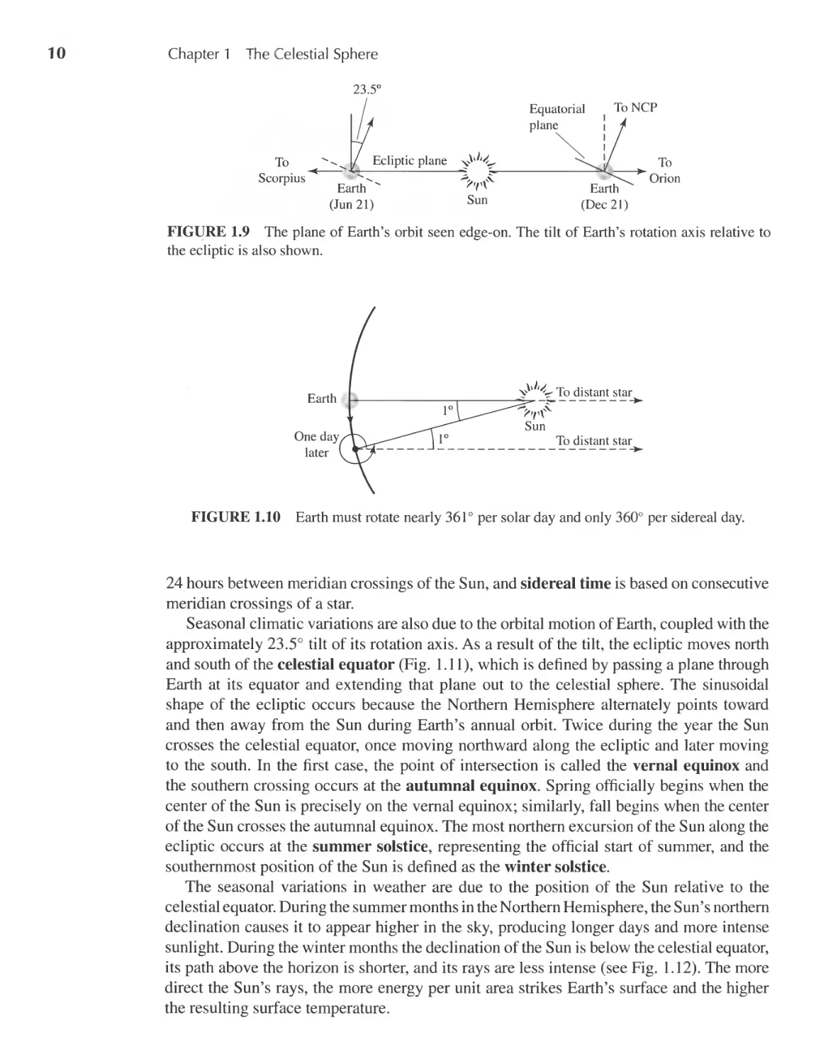
FIGURE 1.9 The plane of Earth's orbit seen edge-on. The tilt of Earth's rotation axis relative to
the ecliptic is also shown.
Earth
\\JJ __ To distant star
- - -------
,/",,$...
Sun
1 0 To distant star
-------------------
One day
later
FIGURE 1.10 Earth must rotate nearly 361 0 per solar day and only 360 0 per sidereal day.
24 hours between meridian crossings of the Sun, and sidereal time is based on consecutive
meridian crossings of a star.
Seasonal climatic variations are also due to the orbital motion of Earth, coupled with the
approximately 23.5° tilt of its rotation axis. As a result of the tilt, the ecliptic moves north
and south of the celestial equator (Fig. 1.11), which is defined by passing a plane through
Earth at its equator and extending that plane out to the celestial sphere. The sinusoidal
shape of the ecliptic occurs because the Northern Hemisphere alternately points toward
and then away from the Sun during Earth's annual orbit. Twice during the year the Sun
crosses the celestial equator, once moving northward along the ecliptic and later moving
to the south. In the first case, the point of intersection is called the vernal equinox and
the southern crossing occurs at the autumnal equinox. Spring officially begins when the
center of the Sun is precisely on the vernal equinox; similarly, fall begins when the center
of the Sun crosses the autumnal equinox. The most northern excursion of the Sun along the
ecliptic occurs at the summer solstice, representing the official start of summer, and the
southernmost position of the Sun is defined as the winter solstice.
The seasonal variations in weather are due to the position of the Sun relative to the
celestial equator. During the summer months in the Northern Hemisphere, the Sun's northern
declination causes it to appear higher in the sky, producing longer days and more intense
sunlight. During the winter months the declination of the Sun is below the celestial equator,
its path above the horizon is shorter, and its rays are less intense (see Fig. 1.12). The more
direct the Sun's rays, the more energy per unit area strikes Earth's surface and the higher
the resulting surface temperature.
1 .3 Positions on the Celestial Sphere
11
18
30
20
---
OI)
Q) 10
'-'
c
.9 0
ro
.5
U -10
Q)
0
-20
-30
Dec 21
12
Right ascension (hr)
6
o
18
Summer solstice
Winter solstice
Sep 23
J un 21
(Approximate dates)
Mar 20
Dec 21
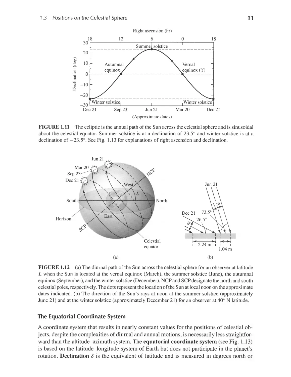
FIGURE 1.11 The ecliptic is the annual path of the Sun across the celestial sphere and is sinusoidal
about the celestial equator. Summer solstice is at a declination of 23.5° and winter solstice is at a
declination of - 23.5°. See Fig. 1.13 for explanations of right ascension and declination.
Horizon
"-
"-
"
"
'\.
South \
North
/
. "
u"
SG
Celestial
equator
I I I I
Ie .1
I 2.24m I I I
1.04 m
(a)
(b)
FIGURE 1.12 (a) The diurnal path of the Sun across the celestial sphere for an observer at latitude
L when the Sun is located at the vernal equinox (March), the summer solstice (June), the autumnal
equinox (September), and the winter solstice (December). NCP and SCPdesignate the north and south
celestial poles, respectively. The dots represent the location of the Sun at local noon on the approximate
dates indicated. (b) The direction of the Sun's rays at noon at the summer solstice (approximately
June 21) and at the winter solstice (approximately December 21) for an observer at 40° N latitude.
The Equatorial Coordinate System
A coordinate system that results in nearly constant values for the positions of celestial ob-
jects, despite the complexities of diurnal and annual motions, is necessarily less straightfor-
ward than the altitude-azimuth system. The equatorial coordinate system (see Fig. 1.13)
is based on the latitude-longitude system of Earth but does not participate in the planet's
rotation. Declination 8 is the equivalent of latitude and is measured in degrees north or
12
Chapter 1 The Celestial Sphere
Celestial NCP
SPhere *
. .I * .
. I.
* .fir.
Earth . .., : -%
.. w I
* 't\. I
Star
.
. I
'j
a
8
.
$
.,
.
."
.J
I
I
. I
I
I
I
I
Celestial
eq uator
SCP
FIGURE 1.13 The equatorial coordinate system. a, 8, and Y designate right ascension, declination,
and the position of the vernal equinox, respectively.
south of the celestial equator. Right ascension ex is analogous to longitude and is measured
eastward along the celestial equator from the vernal equinox (I) to its intersection with
the object's hour circle (the great circle passing through the object being considered and
through the north celestial pole). Right ascension is traditionally measured in hours, min-
utes, and seconds; 24 hours of right ascension is equivalent to 360°, or 1 hour == 15°. The
rationale for this unit of measure is based on the 24 hours (sidereal time) necessary for an
object to make two successive crossings of the observer's local meridian. The coordinates
of right ascension and declination are also indicated in Figs. 1.2 and 1.11. Since the equa-
torial coordinate system is based on the celestial equator and the vernal equinox, changes
in the latitude and longitude of the observer do not affect the values of right ascension and
declination. Values of ex and 8 are similarly unaffected by the annual motion of Earth around
the Sun.
The local sidereal time of the observer is defined as the amount of time that has elapsed
since the vernal equinox last traversed the meridian. Local sidereal time is also equivalent to
the hour angle H of the vernal equinox, where hour angle is defined as the angle between
a celestial object and the observer's meridian, measured in the direction of the object's
motion around the celestial sphere.
Precession
Despite referencing the equatorial coordinate system to the celestial equator and its inter-
section with the ecliptic (the vernal equinox), precession causes the right ascension and
declination of celestial objects to change, albeit very slowly. Precession is the slow wobble
of Earth's rotation axis due to our planet's nonspherical shape and its gravitational inter-
action with the Sun and the Moon. It was Hipparchus who first observed the effects of
precession. Although we will not discuss the physical cause of this phenomenon in detail,
it is completely analogous to the well-known precession of a child's toy top. Earth's pre-
cession period is 25,770 years and causes the north celestial pole to make a slow circle
through the heavens. Although Polaris (the North Star) is currently within 1 ° of the north
1 .3 Positions on the Celestial Sphere
13
celestial pole, in 13,000 years it will be nearly 47° away from that point. The same effect
also causes a 50.26" yr- 1 westward motion of the vernal equinox along the ecliptic. 4 An
additional precession effect due to Earth planet interactions results in an eastward motion
of the vernal equinox of 0.12" yr- 1 .
Because precession alters the position of the vernal equinox along the ecliptic, it is
necessary to refer to a specific epoch (or reference date) when listing the right ascension
and declination of a celestial object. The current values of ex and 8 may then be calculated,
based on the amount of time elapsed since the reference epoch. The epoch commonly used
today for astronomical catalogs of stars, galaxies, and other celestial phenomena refers to
an object's position at noon in Greenwich, England (universal time, UT) on January 1,
2000. 5 A catalog using this reference date is designated as J2000.0. The prefix, J, in the
designation J2000.0 refers to the Julian calendar, which was introduced by Julius Caesar
in 46 B.C.
Approximate expressions for the changes in the coordinates relative to J2000.0 are
ex M + N sin ex tan 0
8 N cosex,
( 1.2)
(1.3 )
where M and N are given by
M 1 2812323T + 0 0003879T2 + 0 0000101T3
N 0 5567530T 0 0001185T2 0 0000116T3
and T is defined as
T (t 2000.0)/100
(1.4 )
where t is the current date, specified in fractions of a year.
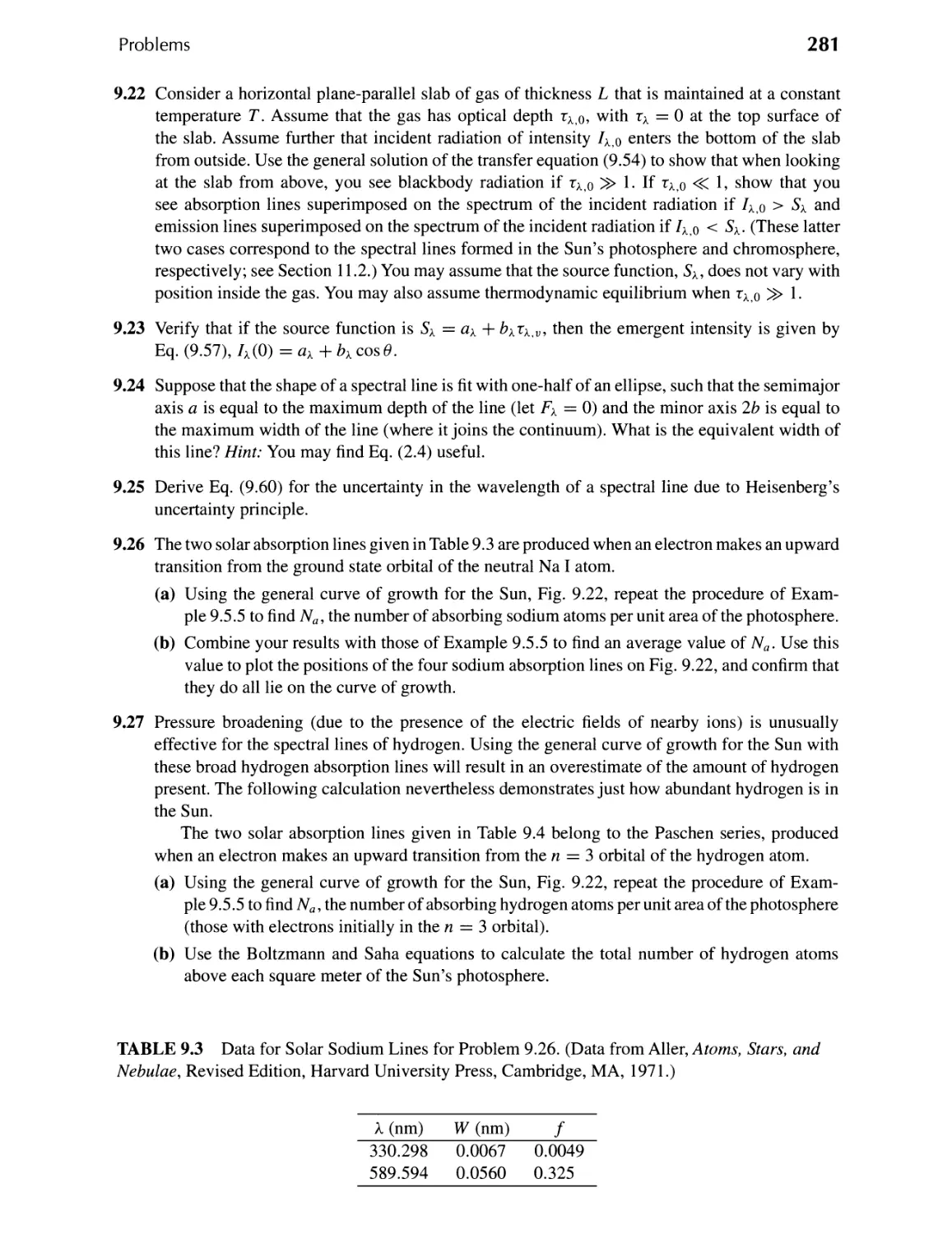
Example 1.3.1. Altair, the brightest star in the summer constellation of Aquila, has the
following J2000.0 coordinates: ex 19 h 50 ffi 47.0 s , 8 +08°52'06.0". Using Eqs. (1.2) and
(1.3), we may precess the star's coordinates to noon Greenwich mean time on July 30,2005.
Writing the date as t 2005.575, we have that T 0.05575. This implies that
M 0.071430° and N 0.031039°. From the relations between time and the angular
continued
41 arcminute = I' = 1/60 degree; 1 arcsecond = I" = 1/60 arcminute.
5Universal time is also sometimes referred to as Greenwich mean time. Technically there are two forms of
universal time; UTI is based on Earth's rotation rate, and UTC (coordinated universal time) is the basis of the
worldwide system of civil time and is measured by atomic clocks. Because Earth's rotation rate is less regular
than the time kept by atomic clocks, it is necessary to adjust UTe clocks by about one second (a leap second)
roughly every year to year and a half. Among other effects contributing to the difference between UTI and UTe
is the slowing of Earth's rotation rate due to tidal effects.
14
Chapter 1 The Celestial Sphere
measure of right ascension,
I h 15°
1 m 15'
IS 15//
the corrections to the coordinates are
a 0.071430° + (0.031039°) sin 297.696° tan 8.86833°
0.067142° rv 16.11 S
and
8 (0.031039°) cos 297.696°
0.014426° rv 51.93".
Thus Altair's precessed coordinates are a 19 h 51 m 03.1 sand 8 +08°52'57.9//.
Measurements of Time
The civic calendar commonly used in most countries today is the Gregorian calendar. The
Gregorian calendar, introduced by Pope Gregory XIII in 1582, carefully specifies which
years are to be considered leap years. Although leap years are useful for many purposes,
astronomers are generally interested in the number of days (or seconds) between events,
not in worrying about the complexities of leap years. Consequently, astronomers typically
refer to the times when observations were made in terms of the elapsed time since some
specified zero time. The time that is universally used is noon on January 1, 4713 B.C., as
specified by the Julian calendar. This time is designated as JD 0.0, where JD indicates
Julian Date. 6 The Julian date of J2000.0 is JD 2451545.0. Times other than noon universal
time are specified as fractions of a day; for example, 6 PM January 1, 2000 UT would be
designated JD 2451545.25. Referring to Julian date, the parameter T defined by Eq. (1.4)
can also be written as
T (JD 2451545.0)/36525,
where the constant 36,525 is taken from the Julian year, which is defined to be exactly
365.25 days.
Another commonly-used designation is the Modified Julian Date (MJD), defined as
MJD JD 2400000.5, where JD refers to the Julian date. Thus a MJD day begins at
midnight, universal time, rather than at noon.
6The Julian date JD 0.0 was proposed by Joseph Justus Scaliger (1540-1609) in 1583. His choice was based on
the convergence of three calendar cycles; the 28 years required for the Julian calendar dates to fall on the same
days of the week, the 19 years required for the phases of the Moon to nearly fall on the same dates of the year, and
the IS-year Roman tax cycle. 28 x 19 x 15 7980 means that the three calendars align once every 7980 years.
JD 0.0 corresponds to the last time the three calendars all started their cycles together.
1 .3 Positions on the Celestial Sphere
15
Because of the need to measure events very precisely in astronomy, various high-
precision time measurements are used. For instance, Heliocentric Julian Date (HJD) is
the Julian Date of an event as measured from the center of the Sun. In order to determine
the heliocentric Julian date, astronomers must consider the time it would take light to travel
from a celestial object to the center of the Sun rather than to Earth. Terrestrial Time (TT)
is time measured on the surface of Earth, taking into consideration the effects of special and
general relativity as Earth moves around the Sun and rotates on its own axis (for discussions
of special and general relativity, refer to Chapter 4 and Section 17.1, respectively).
Archaeoastronomy
An interesting application of the ideas discussed above is in the interdisciplinary field of
archaeoastronomy, a merger of archaeology and astronomy. Archaeoastronomy is a field
of study that relies heavily on historical adjustments that must be made to the positions of
objects in the sky resulting from precession. It is the goal of archaeoastronomy to study
the astronomy of past cultures, the investigation of which relies heavily on the alignments
of ancient structures with celestial objects. Because of the long periods of time since con-
struction, care must be given to the proper precession of celestial coordinates if any proposed
alignments are to be meaningful. The Great Pyramid at Giza (Fig. 1.14), one of the Hseven
wonders of the world," is an example of such a structure. Believed to have been erected
about 2600 B.C., the Great Pyramid has long been the subject of speculation. Although many
of the proposals concerning this amazing monument are more than somewhat fanciful, there
can be no doubt about its careful orientation with the four cardinal positions, north, south,
east, and west. The greatest misalignment of any side from a .true cardinal direction is no
more than 51'. Equally astounding is the nearly perfect square formed by its base; no two
sides differ in length by more than 20 cm.
Perhaps the most demanding alignments discovered so far are associated with the "air
shafts" leading from the King's Chamber (the main chamber of the pyramid) to the outside.
These air shafts seem too poorly designed to circulate fresh air into the tomb of Pharaoh, and
To Orion's belt
To Thuban
/
FIGURE 1.14 The astronomical alignments of the Great Pyramid at Giza. (Adaptation of a figure
from Griffith Observatory.)
16
Chapter 1 The Celestial Sphere
it is now thought that they served another function. The Egyptians believed that when their
pharaohs died, their souls would travel to the sky to join Osiris, the god of life, death, and
rebirth. Osiris was associated with the constellation we now know as Orion. Allowing for
over one-sixth of a precession period since the construction of the Great Pyramid, Virginia
Trimble has shown that one of the air shafts pointed directly to Orion's belt. The other air
shaft pointed toward Thuban, the star that was then closest to the north celestial pole, the
point in the sky about which all else turns.
As a modern scientific culture, we trace our study of astronomy to the ancient Greeks, but
it has become apparent that many cultures carefully studied the sky and its mysterious points
of light. Archaeological structures worldwide apparently exhibit astronomical alignments.
Although some of these alignments may be coincidental, it is clear that many of them were
by design.
The Effects of Motions Through the Heavens
Another effect contributing to the change in equatorial coordinates is due to the intrinsic
velocities of the objects themselves. 7 As we have already discussed, the Sun, the Moon,
and the planets exhibit relatively rapid and complex motions through the heavens. The stars
also move with respect to one another. Even though their actual speeds may be very large,
the apparent relative motions of stars are generally very difficult to measure because of their
enormous distances.
Consider the velocity of a star relative to an observer (Fig. 1.15). The velocity vector
may be decomposed into two mutually perpendicular components, one lying along the
line of sight and the other perpendicular to it. The line-of-sight component is the star's
radial velocity, v r , and will be discussed in Section 4.3; the second component is the star's
V r
/'
/'
./
./
/'
./
/'
./
;; :,,- . ..../'.//'/'
I "
rr
FIGURE 1.15 The components of velocity. V r is the star's radial velocity and Ve is the star's
transverse velocity.
7Parallax, an important periodic motion of the stars resulting from the motion of Earth about the Sun will be
discussed in detail in Section 3.1.
1 .3 Positions on the Celestial Sphere
17
transverse or tangential velocity, Ve, along the celestial sphere. This transverse velocity
appears as a slow, angular change in its equatorial coordinates, known as proper motion
(usually expressed in seconds of arc per year). In a time interval f:1t, the star will have
moved in a direction perpendicular to the observer's line of sight a distance
f:1d Ve f:1t .
If the distance from the observer to the star is r, then the angular change in its position
along the celestial sphere is given by
f:1()
f:1d
Ve
f:1t .
r
r
Thus the star's proper motion, J-l, is related to its transverse velocity by
J-l
d()
dt
Ve
.
( 1.5)
r
An Application of Spherical Trigonometry
The laws of spherical trigonometry must be employed in order to find the relationship
between f:1() and changes in the equatorial coordinates, f:1a and f:18, on the celestial sphere.
A spherical triangle such as the one depicted in Fig. 1.16 is composed of three intersecting
segments of great circles. For a spherical triangle the following relationships hold (with all
sides measured in arc length, e.g., degrees):
Law of sines
.
SIn a
sin A
sinb
sin B
.
Sin c
-
sinC
Law of cosines for sides
cosa
cos b cos c + sin b sin c cos A
Law of cosines for angles
cos A cos B cos C + sin B sin C cosa.
Figure ] .17 shows the motion of a star on the celestial sphere from point A to point B.
The angular distance traveled is f:1(). Let point P be located at the north celestial pole so
that the arcs A P, A B, and BP form segments of great circles. The star is then said to be
moving in the direction of the position angle f/J (LPAB), measured from the north celestial
pole. Now, construct a segment of a circle NB such that N is at the same declination as B
and L PNB 90° . If the coordinates of the star at point A are (a, 8) and its ne w co ord ina tes
at point B are (a + f:1a, 8 + f:18), then LAPB f:1a, AP 90° 8, and NP BP
90° (8 + f:18). Using the law of sines,
sin (f:1()
sin (f:1a)
sin [90° (8 + f:18)]
sin f/J
,
18
Chapter 1 The Celestial Sphere
I
,
\
\
\
, /
',/
/......
/ ......
I
J
.
FIGURE 1.16 A spherical triangle. Each leg is a segment of a great circle on the surface of a sphere.
and all angles are less than 180 0 . a, b, and c are in angular units (e.g., degrees).
p
-
."
"
--
Celestial equator
,
FIGURE 1.17 The proper motion of a star across the celestial sphere. The star is assumed to be
moving from A to B along the position angle cp.
or
sin ( a) cos (8 + 8) = sin ( e) sin fjJ.
Assuming that the changes in position are much less than one radian, we may use the small-
angle approximations sin E E and cos E 1. Employing the appropriate trigonometric
identity and neglecting all terms of second order or higher, the previous equation reduces
to
sin fjJ
a = e-.
cos8
( 1.6)
1 .4 Physics and Astronomy
19
The law of cosines for sides may also be used to find an expression for the change in the
declination:
cos [90 0 (8 + 8)] cos (90 0 8) cos ( ()) + sin (90 0 8) sin ( ()) cos 4J.
Again using small-angle approximations and trigonometric identities, this expression re-
duces to
8 () cos 4J.
(1.7)
(Note that this is the same result that would be obtained if we had used plane trigonometry.
This should be expected, however, since we have assumed that the triangle being considered
has an area much smaller than the total area of the sphere and should therefore appear
essentially flat.) Combining Eqs. (1.6) and (1.7), we arrive at the expression for the angular
distance traveled in terms of the changes in right ascension and declination:
( e)2 ( a cos 8)2 + ( 8)2 .
( 1.8)
1.4 . PHYSICS AND ASTRONOMY
The mathematical view of nature first proposed by Pythagoras and the Greeks led ultimately
to the Copernican revolution. The inability of astronomers to accurately fit the observed
positions of the "wandering stars" with mathematical models resulted in a dramatic change
in our perception of Earth's location in the universe. However, an equally important step
still remained in the development of science: the search for physical causes of observable
phenomena. As we will see constantly throughout this book, the modern study of astronomy
relies heavily on an understanding of the physical nature of the universe. The application of
physics to astronomy, astrophysics, has proved very successful in explaining a wide range
of observations, including strange and exotic objects and events, such as pulsating stars,
supernovae, variable X-ray sources, black holes, quasars, gamma-ray bursts, and the Big
Bang.
As a part of our investigation of the science of astronomy, it will be necessary to study
the details of celestial motions, the nature of light, the structure of the atom, and the shape
of space itself. Rapid advances in astronomy over the past several decades have occurred
because of advances in our understanding of fundamental physics and because of improve-
ments in the tools we use to study the heavens: telescopes and computers.
Essentially every area of physics plays an important role in some aspect of astronomy.
Particle physics and astrophysics merge in the study of the Big Bang; the basic question
of the origin of the zoo of elementary particles, as well as the very nature of the fundamental
forces, is intimately linked to how the universe was formed. Nuclear physics provides
information about the types of reactions that are possible in the interiors of stars, and atomic
physics describes how individual atoms interact with one another and with light, processes
that are basic to a great many astrophysical phenomena. Condensed-matter physics plays a
20
Chapter 1 The Celestial Sphere
role in the crusts of neutron stars and in the center of Jupiter. Thermodynamics is involved
everywhere from the Big Bang to the interiors of stars. Even electronics plays an important
role in the development of new detectors capable of giving a clearer view of the universe
around us.
With the advent of modern technology and the space age, telescopes have been built to
study the heavens with ever-increasing sensitivity. No longer limited to detecting visible
light, telescopes are now capable of "seeing" gamma rays, X-rays, ultraviolet light, infrared
radiation, and radio signals. Many of these telescopes require operation above Earth's
atmosphere to carry out their missions. Other types of telescopes, very different in nature,
detect elementary particles instead of light and are often placed below ground to study the
heavens.
Computers have provided us with the power to carry out the enormous number of calcu-
lations necessary to build mathematical models from fundamental physical principles. The
birth of high-speed computing machines has enabled astronomers to calculate the evolution
of a star and compare those calculations with observations; it is also possible to study the
rotation of a galaxy and its interaction with neighboring galaxies. Processes that require
billions of years (significantly longer than any National Science Foundation grant) cannot
possibly be observed directly but may be investigated using the modern supercomputer.
All of these tools and related disciplines are used to look at the heavens with a probing
eye. The study of astronomy is a natural extension of human curiosity in its purest form. Just
as a small child is always asking why this or that is the way it is, the goal of an astronomer
is to attempt to understand the nature of the universe in all of its complexity, simply for the
sake of understanding the ultimate end of any intellectual adventure. In a very real sense,
the true beauty of the heavens lies not only in observing the stars on a dark night but also
in considering the delicate interplay between the physical processes that cause the stars to
exist at all.
The most incomprehensible thing about the universe is that it is
comprehensible. Albert Einstein
SUGGESTED READING
General
Aveni, Anthony, Skywatchers of Ancient Mexico, The University of Texas Press, Austin,
1980.
Bronowski, J., The Ascent of Man, Little, Brown, Boston, 1973.
Casper, Barry M., and Noer, Richard J., Revolutions in Physics, W. W. Norton, New York,
1972.
Hadingham, Evan, Early Man and the Cosmos, Walker and Company, New York, 1984.
pp, E. C., Echos of the Ancient Skies: The Astronomy of Lost Civilizations, Harper &
Row, New York, 1983.
Problems
21
Kuhn, Thomas S., The Structure of Scientific Revolutions, Third Edition, The University of
Chicago Press, Chicago, 1996.
Ruggles, Clive L. N., Astronomy in Prehistoric Britain and Ireland, Yale University Press,
New Haven, 1999.
Sagan, Carl, Cosmos, Random House, New York, 1980.
SIMBAD Astronomical Database, http: / / simbad. u-strasbg. ir /
Sky and Telescope Sky Chart,
http://skyandtelescope.com/observing/skychart/
Technical
Acker, Agnes, and Jaschek, Carlos, Astronomical Methods and Calculations, John Wiley
and Sons, Chichester, 1986.
Astronomical Almanac, United States Government Printing Office, Washington, D.C.
Cox, Arthur N. (ed.), Allen s Astrophysical Quantities, Fourth Edition, Springer-Verlag,
New York, 2000.
Lang, Kenneth R., Astrophysical Formulae, Third Edition, Springer- Verlag, New York,
1999.
Smart, W. M., and Green, Robin Michael, Textbook on Spherical Astronomy, Sixth Edition,
Cambridge University Press, Cambridge, 1977.
PROBLEMS
1.1 Derive the relationship between a planet's synodic period and its sidereal period (Eq. 1.1).
Consider both inferior and superior planets.
1.2 Devise methods to determine the relative distances of each of the planets from the Sun given
.
the information available to Copernicus (observable angles between the planets and the Sun,
orbital configurations, and synodic periods).
1.3 (a) The observed orbital synodic periods of Venus and Mars are 583.9 days and 779.9 days,
respectively. Calculate their sidereal periods.
(b) Which one of the superior planets has the shortest synodic period? Why?
1.4 List the right ascension and declination of the Sun when it is located at the vernal equinox, the
summer solstice, the autumnal equinox, and the winter solstice.
1.5 (a) Referring to Fig. 1.12(a), calculate the altitude of the Sun along the meridian on the first
day of summer for an observer at a latitude of 42° north.
(b) What is the maximum altitude of the Sun on the first day of winter at the same latitude?
1.6 (a) Circumpolar stars are stars that never set below the horizon of the local observer or stars
that are never visible above the horizon. After sketching a diagram similar to Fig. 1.12( a),
calculate the range of declinations for these two groups of stars for an observer at the
latitude L.
(b) At what latitude(s) on Earth will the Sun never set when it is at the summer solstice?
22
Chapter 1 The Celestial Sphere
(c) Is there any latitude on Earth where the Sun will never set when it is at the vernal equinox?
If so, where?
1.7 (a) Determine the Julian date for 16: 15 UT on July 14,2006. (Hint: Be sure to include any leap
years in your calculation.)
(b) What is the corresponding modified Julian date?
1.8 Proxima Centauri (ex Centauri C) is the closest star to the Sun and is a part of a triple star system.
It has the epoch J2000.0 coordinates (ex, 8) = (14 h 29 ffi 42.95 s , -62°40'46.1/1). The brightest
member of the system, Alpha Centauri (ex Centauri A) has J2000.0 coordinates of (ex, 8) =
(14 h 39 ffi 36.50 s , -60°50'02.3/1).
(a) What is the angular separation of Proxima Centauri and Alpha Centauri?
(b) If the distance to Proxima Centauri is 4.0 x 10 16 m, how far is the star from Alpha Centauri?
1.9 (a) Using the information in Problem 1.8, precess the coordinates of Proxima Centauri to epoch
J20 1 0.0.
(b) The proper motion of Proxima Centauri is 3.84/1 yr- 1 with the position angle 282°. Calculate
the.. change in ex and 8 due to proper motion between 2000.0 and 2010.0.
( c) Which effect makes the largest contribution to changes in the coordinates of Proxima Cen-
tauri: precession or proper motion?
1.10 Which values of right ascension would be best for viewing by an observer at a latitude of 40°
in January?
1.11 Verify that Eq. (1.7) follows directly from the expression immediately preceding it.
.
.
2.1 Elliptical Orbits
2.2 Newtonian Mechanics
2.3 Kepler s Laws Derived
2.4 The Virial Theorem
2.1 . ELLIPTICAL ORBITS
Although the inherent simplicity of the Copernican model was aesthetically pleasing, the
idea of a heliocentric universe was not immediately accepted; it lacked the support of
observations capable of unambiguously demonstrating that a geocentric model was wrong.
Tycho Brahe: The Great Naked-Eye Observer
After the death of Copernicus, Tycho Brahe (1546 1601), the foremost naked-eye observer,
carefully followed the motions of the "wandering stars" and other celestial objects. He
carried out his work at the observatory, Uraniborg, on the island of Hveen (a facility provided
for him by King Frederick II of Denmark). To improve the accuracy of his observations,
Tycho used large measuring instruments, such as the quadrant depicted in the mural in
Fig. 2.1 (a). Tycho' s observations were so meticulous that lie was able to measure the position
of an object in the heavens to an accuracy of better than 4', approximately one-eighth the
angular diameter of a full moon. Through the accuracy of his observations he demonstrated
for the first time that comets must be much farther away than the Moon, rather than being
some form of atmospheric phenomenon. Tycho is also credited with observing the supernova
of 1572, which clearly demonstrated that the heavens were not unchanging as Church
doctrine held. (This observation prompted King Frederick to build Uraniborg.) Despite the
great care with which he carried out his work, Tycho was not able to find any clear evidence
of the motion of Earth through the heavens, and he therefore concluded that the Copernican
model must be false (see Section 3.1).
Kepler's Laws of Planetary Motion
At Tycho's invitation, Johannes Kepler (1571 1630), a German mathematician, joined him
later in Prague [Fig. 2.1(b)]. Unlike Tycho, Kepler was a heliocentrist, and it was his
desire to find a geometrical model of the universe that would be consistent with the best
observations then available, namely Tycho' s. After Tycho' s death, Kepler inherited the mass
23
24
Chapter 2 Celestial Meehan ies
}' ':'? {.; f
- _ 1 - .. , <' i' i _ I
_ I r n h :- - ,j, tilf- 1! < . :..; :'* 7
e '11 zC< '! ':: G' I -",
_ , a. 1 f' " f: . .. I :: II
.-.. .c .' '\\. - t .
, ;. _. . ; ".( lr - '{.r_
I " !)1 1 f1A. 7:"" .. $J' '..'
.Il'"", ' . ,', .,: fSttl
- .H:i Y "'-:J %.\gj" it 'J' IJ '" "
' .. .: / >ilt;J
I /11 t.'..!l " , .. . ,
_I t I'':. . ".. 't
.. - - . . __' .r..t. , .. .
e , ..'tt'. m' '-)'1."<I . . .. .I"'" ---::t.
, ., ..Y:." ' ' , !!/- . .
, - _"' _ ",p .. '" ., ,
. . "\ ." . . ;.:- - ,. i . .\. .
. ". " D f" .
<.. , :i\ . ':' :-:: . -;. ."c"i'if):j/;:.'.;;c, .' '?
: : -. .t /.:
Q
., 'J' ;
;.< ",' . ..:t
tJ
.
,X.-'
-
b
L
,,:T ? \"I' ,. .'
.,. .'
. .
..;t..
t< .
) , ') .
..., .
.
"',
. ",..;,9
. . .,
t"<" .. ..
.i
i.
;. <J
(a)
(b)
FIGURE 2.1 (a) Mural of Tycho Brahe (1546-160 I). (b) Johannes Kepler (1571-1630). (Courtesy
of Yerkes Observatory.)
of observations accumulated over the years and began a painstaking analysis of the data. His
initial, almost mystic, idea was that the universe is arranged with five perfect solids, nested
to support the six known naked-eye planets (including Earth) on crystalline spheres, with
the entire system centered on the Sun. After this model proved unsuccessful, he attempted
to devise an accurate set of circular planetary orbits about the Sun, focusing specifically on
Mars. Through his very clever use of offset circles and equants,] Kepler was able to obtain
excellent agreement with Tycho's data for all but two of the points available. In particular,
the discrepant points were each off by approximately 8', or twice the accuracy of Tycho's
data. Believing that Tycho would not have made observational errors of this magnitude,
Kepler felt forced to dismiss the idea of purely circular motion.
Rejecting the last fundamental assumption of the Ptolemaic model, Kepler began to
consider the possibility that planetary orbits were elliptical in shape rather than circular.
Through this relatively minor mathematical (though monumental philosophical) change,
he was finally able to bring all of Tycho's observations into agreement with a model for
planetary motion. This paradigm shift also allowed Kepler to discover that the orbital speed
of a planet is not constant but varies in a precise way depending on its location in its orbit.
In 1609 Kepler published the first two of his three laws of planetary motion in the book
Astronomica Nova, or The New Astronomy:
Kepler's First Law A planet orbits the Sun in an ellipse, with the Sun at one
focus of the ellipse.
Kepler's Second Law A line connecting a planet to the Sun sweeps out equal
areas in equal time intervals.
1 Recall the geocentric use of circles and equants by Ptolemy; see Fig. 1.3.
2.1 Elliptical Orbits
25
FIGURE 2.2 Kepler's second law states that the area swept out by a line between a planet and the
focus of an ellipse is always the same for a given time interval, regardless of the planet's position in
its orbit. The dots are evenly spaced in time.
Kepler's first and second laws are illustrated in Fig. 2.2, where each dot on the ellipse
represents the position of the planet during evenly spaced time intervals.
Kepler's third law was published ten years later in the book Harmonica Mundi (The
Harmony of the World). His final law relates the average orbital distance of a planet from
the Sun to its sidereal period:
Kepler's Third Law The Harm onic Law.
I p2 = a 3
where P is the orbital period of the planet, measured in years, and a is the average distance
of the planet from the Sun, in astronomical units, or AU. An astronomical unit is, by
definition, the average distance between Earth and the Sun, 1.496 x 10¹¹ m. The graph of
Kepler's third law shown in Fig. 2.3 was prepared using data for each planet in our Solar
System as given in Appendix C.
In retrospect it is easy to understand why the assumption of uniform and circular motion
first proposed nearly 2000 years earlier was not determined to be wrong much sooner;
in most cases, planetary motion differs little from purely circular motion. In fact, it was
actually fortuitous that Kepler chose to focus on Mars, since the data for that planet were
particularly good and Mars deviates from circular motion more than most of the others.
The Geometry of Elliptical Motion
To appreciate the significance of Kepler's laws, we must first understand the nature of the
ellipse. An ellipse (see Fig. 2.4) is defined by that set of points that satisfies the equation
r + r' == 2a,
(2.1 )
where a is a constant known as the semimajor axis (half the length of the long, or major
axis of the ellipse), and rand r' represent the distances to the ellipse from the two focal
Chapter 2 Celestial Meehan ies
26
10
r "'
<
""--"
rJ:J
. ...-4
><
cd
o
. . .
cd
e
.s 1
Q)
en
· Mercury
0.1
0.1
1
10
Period (yr)
100
FIGURE 2.3 Kepler's third law for planets orbiting the Sun.
b
F'
--.----
ae
I
I
I
r
I
I
I
I
I
I
a
FIGURE 2.4 The geometry of an elliptical orbit.
points, F and F', respectively. According to Kepler's first law, a planet orbits the Sun in an
ellipse, with the Sun located at one focus of the ellipse, the principal focus, F (the other
focus is empty space). Notice that if F and F' were located at the same point, then r' r
and the previous equation would reduce to r r' a, the equation for a circle. Thus a
circle is simply a special case of an ellipse. The distance b is known as the semiminor axis.
The eccentricity, e (0 < e < 1), of the ellipse is defined as the distance between the foci
divided by the major axis, 2a, of the ellipse, implying that the distance of either focal point
from the center of the ellipse may be expressed as ae. For a circle, e O. The point on the
ellipse that is closest to the principal focus (located on the major axis) is called perihelion;
the point on the opposite end of the major axis and farthest from the principal focus is
known as aphelion.
2.1 Ell iptical Orbits
27
A convenient relationship among a, b, and e may be determined geometrically. Consider
one of the two points at either end of the semiminor axis of an ellipse, where r r' .
In this case, r a and, by the Pythagorean theorem, r 2 b 2 + a 2 e 2 . Substitution leads
immediately to the expression
b 2
a 2 'I
,
2'
e .
)
(2.2)
Kepler's second law states that the orbital speed of a planet depends on its location in
that orbit. To describe in detail the orbital behavior of a planet, it is necessary to specify
where that planet is (its position vector) as well as how fast, and in what direction, the
planet is moving (its velocity vector). It is often most convenient to express a planet's orbit
in polar coordinates, indicating its distance r from the principal focus in terms of an angle ()
measured counterclockwise from the major axis of the ellipse beginning with the direction
toward perihelion (see Fig. 2.4). Using the Pythagorean theorem, we have
r,2 r 2 sin 2 () + (2ae + r cos ())2 ,
which reduces to
r,2 r 2 + 4ae(ae + r cos ()) .
U sing the definition of an ellipse, r + r' 2a, we find that
r
a '1 e 2 '
, )
(0 < e < 1).
(2.3)
1 + e cos ()
It is left as an exercise to show that the total area of an ellipse is given by
A nab.
(2.4)
Example 2.1.1. Using Eq. (2.3), it is possible to determine the variation in distance of
a planet from the principal focus throughout its orbit. The semimajor axis of Mars's orbit
is 1.5237 AU (or 2.2794 x 10¹¹ m) and the planet's orbital eccentricity is 0.0934. When
() 0°, the planet is at perihelion and is at a distance given by
rp
a 1 e 2
l+e
a (1 e)
1.3814 AU.
(2.5)
continued
28
Chapter 2 Celestial Mechanics
Similarly, at aphelion (8 = 180°), the point where Mars is farthest from the Sun, the distance
is given by
a (1 - e 2 )
ra =
1 - e
= a (1 + e)
= 1.6660 AU.
(2.6)
The variation in Mars's orbital distance from the Sun between perihelion and aphelion is
approximately 19%.
An ellipse is actually one of a class of curves known as conic sections, found by passing
a plane through a cone (see Fig. 2.5). Each type of conic section has its own characteristic
range of eccentricities. As already mentioned, a circle is a conic section with e = 0, and an
ellipse has 0 < e < 1. A curve having e = 1 is known as a parabola and is described by
the equation
2p
r=
1 + cos 8
(e = 1),
(2.7)
where p is the distance of closest approach to the parabola's one focus, at 8 = O. Curves
c=>
0 :.
.",. ., ....
'" .0.
./
/
Circle
Ellipse
Hyperbola
e=l.4
a = 2.5
r
/
I
I
I
I
I
"
"
"
"
I
I
I
l
"
"
.....
.....
Parabola
Hyperbola
(a)
(b)
FIGURE 2.5 (a) Conic sections. (b) Related orbital paths.
2.2 Newtonian Mechanics
29
having eccentricities greater than unity, e > 1, are hyperbolas and have the form
a (e 2 - 1)
r=
1 + e cos e
Each type of conic section is related to a specific form of celestial motion.
(e > 1).
(2.8)
2.2 . NEWTONIAN MECHANICS
At the time Kepler was developing his three laws of planetary motion, Galileo Galilei
(1564-] 642), perhaps the first of the true experimental physicists, was studying the motion
of objects on Earth [Fig. 2.6(a)]. It was Galileo who proposed the earliest formulation of the
concept of inertia. He had also developed an understanding of acceleration; in particular, he
realized that objects near the surface of Earth fall with the same acceleration, independent
of their weight. Whether Galileo publicly proved this fact by dropping objects of differing
weights from the Leaning Tower of Pisa is a matter of some debate.
The Observations of Galileo
Galileo is also the father of modern observational astronomy. Shortly after learning about
the 1608 invention of the first crude spyglass, he thought through its design and constructed
his own. Using his new telescope to carefully observe the heavens, Galileo quickly made
a number of important observations in support of the heliocentric model of the universe.
In particular, he discovered that the band of light known as the Milky Way, which runs
from horizon to horizon, is not merely a cloud, as had previously been supposed, but
<.".
, ::
,'",.' :.,-
.. . .
. .
. i: ,
,.. At) , .i ,"
...':." ,, :.'/
.#
..Ut .
. ..
,
. !
,..
. ;. f . S;'
-:..f , ,.." '
t Y M :.
tt,. ., "
. ::.. .
: ..... ......-
(a)
(b)
FIGURE 2.6 (a) Galileo Galilei (1564-1642). (b) Isaac Newton (1642-1727). (Courtesy of Yerkes
Observatory. )
30
Chapter 2 Celestial Meehan ies
actually contains an enormous number of individual stars not resolvable by the naked eye.
Galileo also observed that the Moon possesses craters and therefore is not a perfect sphere.
Observations of the varying phases of Venus implied that the planet does not shine by its own
power, but must be reflecting sunlight from constantly changing angles relative to the Sun
and Earth while it orbits the Sun. He also discovered that the Sun itself is blemished, having
sunspots that vary in number and location. But perhaps the most damaging observation for
the geocentric model, a model still strongly supported by the Church, was the discovery of
four moons in orbit about Jupiter, indicating the existence of at least one other center of
motion in the universe.
Many of Galileo's first observations were published in his book Sidereus Nuncius (The
Starry Messenger) in 1610. By 1616 the Church forced him to withdraw his support of the
Copernican model, although he was able to continue his study of astronomy for some years.
In 1632 Galileo published another work, The Dialogue on the Two Chief World Systems, in
which a three-character play was staged. In the play Salviati was the proponent of Galileo's
views, Simplicio believed in the old Aristotelian view, and Sagredo acted as the neutral third
party who was invariably swayed by Salviati's arguments. In a strong reaction, Galileo was
called before the Roman Inquisition and his book was heavily censored. The book was then
placed on the Index of banned books, a collection of titles that included works of Copernicus
and Kepler. Galileo was put under house arrest for the remainder of his life, serving out his
term at his home in Florence.
In 1992, after a 13-year study by Vatican experts, Pope John Paul II officially announced
that, because of a "tragic mutual incomprehension," the Roman Catholic Church had erred
in its condemnation of Galileo some 360 years earlier. By reevaluating its position, the
Church demonstrated that, at least on this issue, there is room for the philosophical views
of both science and religion.
Newton's Three Laws of Motion
Isaac Newton (1642 1727), arguably the greatest of any scientific mind in history
[Fig. 2.6(b)], was born on Christmas Day in the year of Galileo's death. At age 18, Newton
enrolled at Cambridge University and subsequently obtained his bachelor's degree. In the
two years following the completion of his formal studies, and while living at home in Wool-
sthorpe, in rural England, away from the immediate dangers of the Plague, Newton engaged
in what was likely the most productive period of scientific work ever carried out by one
individual. During that interval, he made significant discoveries and theoretical advances
in understanding motion, astronomy, optics, and mathematics. Although his work was not
published immediately, the Philosophiae Naturalis Principia Mathematica (Mathematical
Principles of Natural Philosophy), now simply known as the Principia, finally appeared
in 1687 and contained much of his work on mechanics, gravitation, and the calculus. The
publication of the Principia came about largely as a result of the urging of Edmond Halley,
who paid for its printing. Another book, Optiks, appeared separately in 1704 and contained
Newton's ideas about the nature of light and some of his early experiments in optics.
Although many of his ideas concerning the particle nature of light were later shown to be
in error (see Section 3.3), much of Newton's other work is still used extensively today.
Newton's great intellect is evidenced in his solution of the so-called brachistochrone
problem posed by Johann Bernoulli, the Swiss mathematician, as a challenge to his col-
2.2 Newtonian Mechanics
31
leagues. The brachistochrone problem amounts to finding the curve along which a bead
could slide over a frictionless wire in the least amount of time while under the influence
only of gravity. The deadline for finding a solution was set at a year and a half. The problem
was presented to Newton late one afternoon; by the next morning he had found the answer
by inventing a new area of mathematics known as the calculus of variations. Although the
solution was published anonymously at Newton's request, Bernoulli commented, "By the
claw, the lion is revealed."
Concerning the successes of his own career, Newton wrote:
I do not know what I may appear to the world; but to myself I seem to have
been only like a boy, playing on the seashore, and diverting myself, in now and
then finding a smoother pebble or a prettier shell than ordinary, while the great
ocean of truth lay all undiscovered before me.
Today, classical mechanics is described by Newton's three laws of motion, along with his
universal law of gravity. Outside of the realms of atomic dimensions, velocities approaching
the speed of light, or extreme gravitational forces, Newtonian physics has proved very
successful in explaining the results of observations and experiments. Those regimes where
Newtonian mechanics have been shown to be unsatisfactory will be discussed in later
chapters.
Newton's first law of motion may be stated as follows:
Newton's First Law The Law of Inertia. An object at rest will remain at rest
and an object in motion will remain in motion in a straight line at a constant
speed unless acted upon by an external force.
To establish whether an object is actually moving, a reference frame must be established. In
later chapters we will refer to reference frames that have the special property that the first
law is valid; all such frames are known as inertial reference frames. Noninertial reference
frames are accelerated with respect to inertial frames. ·
The first law may be restated in terms of the momentum of an object, p my, where
m and v are mass and velocity, respectively.2 Thus Newton's first law may be expressed as
"the momentum of an object remains constant unless it experiences an external force. ,,3
The second law is actually a definition of the concept of force:
Newton's Second Law The net force (the sum of all forces) acting on an object
is proportional to the object's mass and its resultant acceleration.
If an object is experiencing n forces, then the net force is given by
n
Fnet
F i ma.
(2.9)
i=l
2 Hereafter, all vectors will be indicated by boldface type. Vectors are quantities described by both a magnitude
and a direction. Some texts use alternate notations for vectors, expressing them either as v or v.
3The law of inertia is an extension of the original concept developed by Galileo.
32
Chapter 2 Celestial Mechanics
r'
In} -
F21
m2
FIGURE 2.7 Newton's third law.
However, assuming that the mass is constant and using the definition a = dv / dt Newton's
second law may also be expressed as
dv d(mv)
Fnet == m- ==
dt dt
dp
dt'
(2.10)
the net force on an object is equal to the time rate of change of its momentum p. F net ==
dp / d t actually represents the most general statement of the second law, allowing for a time
variation in the mass of the object such as occurs with rocket propulsion.
The third law of motion is generally expressed as follows:
Newton's Third Law For every action there is an equal and opposite reaction.
In this law, action and reaction are to be interpreted as forces acting on different objects.
Consider the force exerted on one object (object 1) by a second object (object 2), F i2 .
Newton's third law states that the force exerted on object 2 by object 1, F 2i , must necessarily
be of the same magnitude but in the opposite direction (see Fig. 2.7). Mathematically, the
third law can be represented as
F 12 == -F 21 .
Newton's Law of Universal Gravitation
Using his three laws of motion along with Kepler's third law, Newton was able to find an
expression describing the force that holds planets in their orbits. Consider the special case
of circular orbital motion of a mass m about a much larger mass M (M » In). Allowing
for a system of units other than years and astronomical units, Kepler's third law may be
written as
p2 == kr3,
where r is the distance between the two objects and k is a constant of proportionality. Writing
the period of the orbit in terms of the orbit's circumference and the constant velocity of m
yields
2nr
p == -,
v
and substituting into the prior equation gives
4n 2 r 2
== kr 3 .
v 2
2.2 Newtonian Mechanics
33
Rearranging terms and multiplying both sides by m lead to the expression
v 2
m
4Jl" 2 m
kr 2 ·
r
The left-hand side of the equation may be recognized as the centripetal force for circular
.
motIon, so
F
4Jl" 2 m
kr 2
must be the gravitational force keeping m in its orbit about M. However, Newton's third
law states that the magnitude of the force exerted on M by m must equal the magnitude of
the force exerted on m by M. Therefore, the form of the equation ought to be symmetric
with respect to exchange of m and M, implying
F
4Jl"2 M
k'r 2 ·
Expressing this symmetry explicitly and grouping the remaining constants into a new con-
stant, we have
F
4Jl"2 Mm
k"r 2 '
where k k" / M and k' kIf / m. Finally, introducing a new constant, G 4Jl"2/ k", we
arrive at the form of the Law of Universal Gravitation found by Newton,
Mm
F G 2 '
r
(2.11 )
where G 6.673 x 10- 11 N m 2 kg- 2 (the Universal Gravitational Constant).4
Newton's law of gravity applies to any two objects having mass. In particular, for an
extended object (as opposed to a point mass), the force exerted by that object on another
extended object may be found by integrating over each of their mass distributions.
Example 2.2.1. The force exerted by a spherically symmetric object of mass M on a point
mass m may be found by integrating over rings centered along a line connecting the point
mass to the center of the extended object (see Fig. 2.8). In this way all points on a specific
ring are located at the same distance from m. Furthermore, because of the symmetry of
the ring, the gravitational force vector associated with it is oriented along the ring's central
axis. Once a general description of the force due to one ring is determined, it is possible to
add up the individual contributions from all such rings throughout the entire volume of the
mass M. The result will be the force on m due to M.
continued
4At the time this text was written, the uncertainty in G was :f:O.Ol0 x 10- 11 N m 2 kg- 2 .
34
Chapter 2 Celestial Meehan ies
Ro
..
/'
'"
(
....-
r
m
dM ring
M
FIGURE 2.8 The gravitational effect of a spherically symmetric mass distribution.
Let r be the distance between the centers of the two masses, M and m. Ro is the radius
of the large mass, and s is the distance from the point mass to a point on the ring. Because
of the symmetry of the problem, only the component of the gravitational force vector along
the line connecting the centers of the two objects needs to be calculated; the perpendicular
components will cancel. If d M ring is the mass of the ring being considered, the force exerted
by that ring on m is gi ven by .
m dM ring
d F ring = G 2 cos 4J.
S
Assuming that the mass density, peR), of the extended object is a function of radius only
and that the volume of the ring of thickness d R is d V ring , we find that
dM ring = peR) dVring
= peR) 2n R sine R de dR
= 2n R 2 p(R) sin e dR de.
The cosine is given by
r - R cos e
cos 4J =
s
where s may be found by the Pythagorean theorem:
s = J (r - R CDS e)2 + R2 sin 2 e = J r 2 - 2r R CDS e + R2.
Substituting into the expression for d Fring, summing over all rings located at a distance R
from the center of the mass M (i.e., integrating over all e from 0 to n for constant R), and
then summing over all resultant shells of radius R from R = 0 to R = Ro give the total
2.2 Newtonian Mechanics
35
force of gravity acting on the small mass m along the system's line of symmetry:
F
Gm
Ro
o
7r (r
R cos 0) p (R)2n R 2 sin 0
3 dO dR
s
o
2nGm
Ro j(
r R 2 p(R) sin 0
3/2 dO dR
r 2 + R2 2rRcosO
o 0
Ro j(
2nGm
o 0
R 3 p(R) sin 0 cos 0
3 /2 d 0 dR.
r 2 + R2 2r R cos 0
The integrations over 0 may be carried out by making the change of variable, u s2
r 2 + R 2 2rRcosO. Then cosO (r 2 + R 2 u)/2rR and sinO dO duj2rR.Afterthe
appropriate substitutions and integration over the new variable u, the equation for the force
becomes
F
Gm
r 2
Ro
4n R 2 p(R) dR.
o
Notice that the integrand is just the mass of a shell of thickness dR, having a volume d V shell ,
or
dMshell 4n R 2 p(R) dR p(R) dVshell.
Therefore, the integrand gives the force on m due to a spherically symmetric mass shell of
mass dMshell as
d Fshell
Gm dMshell
r 2
.
The shell acts gravitationally as if its mass were located entirely at its center. Finally,
integrating over the mass shells, we have that the force exerted on m by an extended,
spherically symmetric mass distribution is directed along"the line of symmetry between the
two objects and is given by
Mm
F G 2 '
r
just the equation for the force of gravity between two point masses.
When an object is dropped near the surface of Earth, it accelerates toward the center of
Earth at the rate g 9.80 m s-2, the local acceleration of gravity. Using Newton's second
law and his law of gravity, an expression for the acceleration of gravity may be found. If m
is the mass of the falling object, Mffi and Rffi are the mass and radius of Earth, respectively,
and h is the height of the object above Earth, then the force of gravity on m due to Earth is
given by
F
Mffim
G 2 .
(Rffi +h)
36
Chapter 2 Celestial Meehan ies
Assuming that m is near Earth's surface, then h « Rffi and
Mm
Rffi
However, F ma mg; thus
g
Mffi
G 2 .
Rffi
(2.12)
Substituting the values M ffi 5.9736 x 1 0 24 kg and Rffi 6.378136 x 1 0 6 m gives a value
for g in agreement with the measured value.
The Orbit of the Moon
The famous story that an apple falling on Newton's head allowed him to immediately
1P
realize that gravity holds the Moon in its orbit is probably somewhat fanciful and inaccurate.
However, he did demonstrate that, along with the acceleration of the falling apple, gravity
was responsible for the motion of Earth's closest neighbor.
Example 2.2.2. Assuming for simplicity that the Moon's orbit is exactly circular, we
can calculate the centripetal acceleration of the Moon rapidly. Recall that the centripetal
acceleration of an object moving in a perfect circle is given by
v 2
a c
.
r
In this case, r is the distance from the center of Earth to the center of the Moon, r
3.84401 x 10 8 m, and v is the Moon's orbital velocity, given by
v
2nr
p'
where P 27.3 days 2.36 x 10 6 s is the sidereal orbital period of the Moon. Finding
v 1.02 Ian S-l gives a value for the centripetal acceleration of
a c 0.0027 m s-2.
The acceleration of the Moon caused by Earth's gravitational pull may also be calculated
directly from
a g
Mffi
G 2
r
0.0027 m s-2,
in agreement with the value for the centripetal acceleration.
2.2 Newtonian Mechanics
37
Work and Energy
In astrophysics, as in any area of physics, it is often very helpful to have some understand-
ing of the energetics of specific physical phenomena in order to determine whether these
processes are important in certain systems. Some models may be ruled out immediately
if they are incapable of producing the amount of energy observed. Energy arguments also
often result in simpler solutions to particular problems. For example, in the evolution of a
planetary atmosphere, the possibility of a particular component of the atmosphere escaping
must be considered. Such a consideration is based on a calculation of the escape speed of
the gas particles.
The amount of energy (the work) necessary to raise an object of mass m a height h
against a gravitational force is equal to the change in the potential energy of the system.
Generally, the change in potential energy resulting from a change in position between two
points is gi ven by
rf
F.dr
,
(2.13 )
V f Vi V
r ,
where F is the force vector, ri and r f are the initial and final position vectors, respectively,
and dr is the infinitesimal change in the position vector for some general coordinate system
(see Fig. 2.9). If the gravitational force on m is due to a mass M located at the origin, then
F is directed inward toward M, dr is directed outward, F · dr F dr, and the change in
potential energy becomes
V
rf Mm
G 2 dr.
r
r 1
Evaluating the integral, we have
Uf Vi
GMm
1 1
.
rf
ri
z
m
----- dr
\
\
I
r.
l
F
rf
y
x
FIGURE 2.9 Gravitational potential energy. The amount of work done depends on the direction of
motion relative to the direction of the force vector.
38
Chapter 2 Celestial Mechanics
Since only relative changes in potential energy are physically meaningful, a reference
position where the potential energy is defined as being identically zero may be chosen. If,
for a specific gravitational system, it is assumed that the potential energy goes to zero at
infinity, letting r f approach infinity (r f 00) and dropping the subscripts for simplicity
.
gIve
u
Mm
G
.
(2.14)
r
Of course, the process can be reversed: The force may be found by differentiating the
gravitational potential energy. For forces that depend only on r,
au
ar
.
(2.15)
F
In a genera! three-dimensional description, F
of U. In rectangular coordinates this becomes
V' U, where V' U represents the gradient
F
aUA
.
I
ax
aUA
.
au A
k.
az
Work must be performed on a massive object if its speed, lvi, is to be changed. This can
be seen by rewriting the work integral, first in terms of time, then speed:
w U
rf
F.dr
r 1
tf dp
· (v dt)
t , dt
tf dv
m · (v dt)
t , dt
tf
m v.
dv
dt
dt
ti
tf d Iv 2
m 2
dt
dt
t z
Vf 1 2
md v
2
V,
1
mv 2
2 f
1 2
mV i ·
2
2.3 Kepler's Laws Derived
39
We may now identify the quantity
1
K mv 2
2
(2.16)
as the kinetic energy of the object. Thus work done on the particle results in an equiva-
lent change in the particle's kinetic energy. This statement is simply one example of the
conservation of energy, a concept that is encountered frequently in all areas of physics.
Consider a particle of mass m that has an initial velocity v and is at a distance r from
the center of a larger mass M, such as Earth. How fast must the mass be moving upward to
completely escape the pull of gravity? To calculate the escape speed, energy conservation
may be used directly. The total initial mechanical energy of the particle (both kinetic and
potential) is given by
1
mv 2
2
Mm
G
E
.
r
Assume that, in the critical case, the final velocity of the mass will be zero at a position
infinitely far from M, implying that both the kinetic and potential energy will become zero.
Clearly, by conservation of energy, the total energy of the particle must be identically zero
at all times. Thus
1
mv 2
2
Mm
G
,
r
which may be solved immediately for the initial speed of m to give
V esc
2G M / r .
(2.17)
Notice that the mass of the escaping object does not enter into the final expression for the
escape speed. Near the surface of Earth, V esc 11.2 Ian S-l.
2.3 . KEPLER'S LAWS DERIVED
Although Kepler did finally determine that the geometry of planetary motion was in the more
general form of an ellipse rather than circular motion, he was unable to explain the nature
of the force that kept the planets moving in their precise patterns. Not only was Newton
successful in quantifying that force, he was also able to generalize Kepler's work, deriving
the empirical laws of planetary motion from the gravitational force law. The derivation of
Kepler's laws represented a crucial step in the development of modem astrophysics.
The Center-of-Mass Reference Frame
However, before proceeding onward to derive Kepler's laws, it will be useful to examine
more closely the dynamics of orbital motion. An interacting two-body problem, such as
40
Chapter 2 Celestial Mechanics
z'
r
m2
M
r2
ml
r'
1
y'
X'
FIGURE 2.10 A general Cartesian coordinate system indicating the positions of m I, m2, and the
center of mass (located at M).
1r
binary orbits, or the more general many-body problem (often called the N -body problem),
is most easily done in the reference frame of the center of mass.
Figure 2.10 shows two objects of masses m 1 and m2 at positions r; and r;, respectively,
with the displacement vector from r to r; given by
r
r ' r '
2 1-
Define a position vector R to be a weighted average of the position vectors of the individual
masses,
R
, + '
mlr 1 m2 r 2
ml + m2
.
(2.18)
Of course, this definition can be immediately generalized to the case of n objects,
R
n ,
· 1 m z .r.
1= I
n
i=l mi
.
Rewriting the equation, we have
n n
mi R ,
mi r i .
i=l i=l
Then, if we define M to be the total mass of the system, M
becomes
7=1 mi, the previous equation
n
MR
,
mi r i .
i=l
Assuming that the individual masses do not change, differentiating both sides with respect
2.3 Kepler's Laws Derived
41
to time gi ves
dR
M
dt
n d '
r.
m. I
I dt
i=l
or
n
MV
,
mi v i ·
i=l
The right-hand side is the sum of the linear momenta of every particle in the system,
so the total linear momentum of the system may be treated as though all of the mass were
located at R, moving with a velocity V. Thus R is the position of the center of mass of the
system, and V is the center-of-mass velocity. Letting P MV be the linear momentum of
the center of mass and P miv; be the linear momentum of an individual particle i, and
again differentiating both sides with respect to time, yields
dP
dt
n d '
Pi
dt
;=1
.
If we assume that all of the forces acting on individual particles in the system are due to
other particles contained within the system, Newton's third law requires that the total force
must be zero. This constraint exists because of the equal magnitudes and opposite directions
of action reaction pairs. Of course, the momentum of individual masses may change. Using
center-of-mass quantities, we find that the total (or net) force on the system is
F
dP
dt
d 2 R
M
dt 2
o.
Therefore, the center of mass will not accelerate if no external forces exist. This implies
..
that a reference frame associated with the center of mass must be an inertial reference frame
and that the N -body problem may be simplified by choosing a coordinate system for which
the center of mass is at rest at R O.
If we choose a center-of-mass reference frame for a binary system, depicted in Fig. 2.11
(R 0), Eq. (2.18) becomes
ml r l + m2 r 2
m 1 + m2
0,
(2.19)
where the primes have been dropped, indicating center-of-mass coordinates. Both rl and
r2 may now be rewritten in terms of the displacement vector, r. Substituting r2 rl + r
.
gl ves
m2
(2.20)
r
m 1 + m2
rl
m1
(2.21)
r2
r.
ml + m2
42
Chapter 2 Celestial Mechanics
z
r2
m2
rl
y
ml
x
FIGURE 2.11 The center-of-mass reference frame for a binary orbit, with the center of mass fixed
at the origin of the coordinate system.
Next, define the reduced mass to be
m}m2
.
(2.22)
JL
ml + m2
Then rl and r2 become
r}
JL
r
ml
(2.23)
r2
JL
r.
m2
(2.24 )
The convenience of the center-of-mass reference frame becomes evident when the total
energy and orbital angular momentum of the system are considered. Including the necessary
kinetic energy and gravitational potential energy terms, the total energy may be expressed
as
E
1 2 1 2
mlm2
G .
I r2 rll
Substituting the relations for rl and r2, along with the expression for the total mass of the
system and the definition for the reduced mass, gives
E
1
JLV 2
2
MJL
G ,
r
(2.25)
where v Ivi and v dr / dt. We have also used the notation r I r 2 rll. The total
energy of the system is equal to the kinetic energy of the reduced mass, plus the potential
energy of the reduced mass moving about a mass M, assumed to be located and fixed at
the origin. The distance between JL and M is equal to the separation between the objects of
masses ml and m2.
Similarly, the total orbital angular momentum,
L ml r l x VI + m2 r 2 x V2
2.3 Kepler's Laws Derived
43
z
JL
y
x
FIGURE 2.12 A binary orbit may be reduced to the equivalent problem of calculating the motion
of the reduced mass, jL, about the total mass, M, located at the origin.
becomes
L JLr x v r x p,
(2.26)
where P JL v. The total orbital angular momentum equals the angular momentum of the
reduced mass only. In general, the two-body problem may be treated as an equivalent one-
body problem with the reduced mass JL moving about a ed mass M at a distance r (see
Fig. 2.12).
The Derivation of Kepler's First Law
To obtain Kepler's laws, we begin by considering the effect of gravitation on the orbital
angular momentum of a planet. Using center-of-mass coordinates and evaluating the time
derivative of the orbital angular momentum of the reduced mass (Eq. 2.26) give
;
dL dr dp
· x p + r x v x p + r x F,
dt dt dt
the second expression arising from the definition of velocity and Newton's second law.
Notice that because v and p are in the same direction, their cross product is identically zero.
Similarly, since F is a central force directed inward along r, the cross product of rand F is
also zero. The result is an important general statement concerning angular momentum:
dL
dt
0,
(2.27)
the angular momentum of a system is a constant for a central force law. Equation (2.26)
further shows that the position vector r is always perpendicular to the constant angular
momentum vector L, meaning that the orbit of the reduced mass lies in a plane perpendicular
to L.
Using the radial unit vector r (so r rr), we can write the angular momentum vector
in an alternative form as
L JLr x v
A d A
JLrr x (rr)
dt
44
Chapter 2 Celestial Mechanics
dr " d "
r+ r r
dt dt
2" d "
j,tr r x dt r.
A
j,trr x
(The last result comes from the fact that r x r 0.) In vector form, the acceleration of the
reduced mass due to the gravitational force exerted by M is
GM "
a 2 r.
r
Taking the vector cross product of the acceleration of the reduced mass with its own orbital
angular momentum gi ves
A
GMj,trx
A.
rx
d "
r .
dt
GM "
2 r x
r
2" d"
j,tr r x r
dt
axL
Applying the vector identity A x (B x C) (A · C)B (A · B)C results in
GMj,t
" d" "
r. r r
dt
A A.
r.r
d "
r .
dt
axL
Because r is a unit vector, r. r 1 and
d " "
(r · r)
dt
" d"
2 r · r O.
dt
As a result,
axL
d "
GMj,t r
dt
or, by referring to Eq. (2.27),
d
(v x L)
dt
d "
(GMj,tr).
dt
Integrating with respect to time then yields
vxL GMj,tr+D,
(2.28)
where D is a constant vector. Because v x Land r both lie in the orbital plane, so must
D. Furthermore, the magnitude of the left-hand side will be greatest at perihelion when the
velocity of the reduced mass is a maximum. Moreover, the magnitude of the right-hand
side is greatest when rand D point in the same direction. Therefore, D is directed toward
perihelion. As shown below, the magnitude of D determines the eccentricity of the orbit.
We next take the vector dot product of Eq. (2.28) with the position vector r r r:
r · (v xL) G M j,tr r · r + r · D.
2.3 Kepler's Laws Derived 45
Invoking the vector identity A · (B x C) (A x B) · C gives
(r x v) · L G M J,tr + r D cos ().
Finally, recalling the definition of angular momentum (Eq. 2.26), we obtain
L 2
J,t
D cos ()
G M J,tr 1 +
GMJ,t
,
where () is the angle of the reduced mass as measured from the direction to perihelion.
Defining e D j G M J,t and solving for r, we find
Kepler's First Law (revisited)
r
L2jJ,t2
GM(1 + ecos())
.
(2.29)
This is exactly the equation of a conic section, as may be seen by comparing Eq. (2.29)
with Eqs. (2.3), (2.7), and (2.8) for an ellipse, parabola, and hyperbola, respectively. The
path of the reduced mass about the center of mass under the influence of gravity (or any
other inverse-square force) is a conic section. Elliptical orbits result from an attractive r- 2
central-force law such as gravity when the total energy of the system is less than zero (a
bound system), parabolic trajectories are obtained when the energy is identically zero, and
hyperbolic paths result from an unbounded system with an energy that is greater than zero.
When Eq. (2.29) is translated back to a physical reference frame on the sky, we find
that Kepler's first law for bound planetary orbits may be stated as: Both objects in a binary
orbit move about the center of mass in ellipses, with the center of mass occupying one
focus of each ellipse. Newton was able to demonstrate the elliptical behavior of planetary
motion and found that Kepler's first law must be generalized somewhat: The center of mass
of the system, rather than the exact center of the Sun, is actually located at the focus of
the ellipse. For our Solar System, such a mistake is understandable, since the largest of
the planets, Jupiter, has only 1/1000 the mass of the Sun. This places the center of mass
of the Sun Jupiter system near the surface of the Sun. Having used the naked-eye data of
Tycho, Kepler can be forgiven for not realizing his error.
For the case of closed planetary orbits, comparing Eqs. (2.3) and (2.29) shows that the
total orbital angular momentum of the system is
L J,t G Mal e 2 .
(2.30)
Note that L is a maximum for purely circular motion (e 0) and goes to zero as the
eccentricity approaches unity, as expected.
The Derivation of Kepler's Second Law
To derive Kepler's second law, which relates the area of a section of an ellipse to a time
interval, we begin by considering the infinitesimal area element in polar coordinates, as
46
Chapter 2 Celestial Mechanics
dA = r dr dO
FIGURE 2.13 The infinitesimal area element in polar coordinates.
shown in Fig. 2.13:
dA = dr (rde) = rdrde.
If we integrate from the principal focus of the ellipse to a specific distance, r, the area swept
out by an infinitesimal change in e becomes
1
dA = _r 2 de.
2
Therefore, the time rate of change in area swept out by a line joining a point on the ellipse
to the focus becomes
dA 1 2de
- - -r -
dt - 2 dt.
(2.31 )
N ow the orbital velocity, v, may be expressed in two components, one directed along rand
the other perpendicular to r. Letting rand 6 be the unit vectors along r and its normal,
respectively, v may be written as (see Fig. 2.14)
dr "- de "-
v = V r + Ve = -r + r-6.
dt dt
Substituting Ve into Eg. (2.31) gives
dA ]
- = -rVe.
dt 2
Since r and Ve are perpendicular,
rVe = Ir x vi =
L L
jJ. jJ.
Finally, the time derivative of the area becomes
Kepler's Second Law (revisited)
dA 1 L
- - --
-
dt 2jJ.
(2.32)
2.3 Kepler's Laws Derived
47
V(J
" V r
F
FIGURE 2.14 The velocity vector for elliptical motion in polar coordinates.
It has already been shown that the orbital angular momentum is a constant, so the time rate
of change of the area swept out by a line connecting a planet to the focus of an ellipse is
a constant, one-half of the orbital angular momentum per unit mass. This is just Kepler's
second law.
Expressions for the speed of the reduced mass at perihelion (0 0) and aphelion (0
7r /2) may be easily obtained from Eq. (2.29). Since at both perihelion and aphelion, r and v
are perpendicular, the magnitude of the angular momentum at these points simply becomes
L fvtrv.
Eq. (2.29) at perihelion may thus be written as
rp
(fvtr p v p )2 / fvt2
GM(l + e) ,
whereas at aphelion
ra
(fvtr a v a )2 / fvt2
GM(1 e)
.
Recalling from Example 2.1.1 that r p a ( 1 e) at perihelion and r a a (1 + e) at aphe-
lion, we immediately obtain
GM l+e
ale
v 2
p
GM(1 + e)
(2.33)
rp
at perihelion and
v 2
a
GM(l
e)
GM
ra
a
1 e
l+e
.
(2.34)
at aphelion.
48
Chapter 2 Celestial Mechanics
The total orbital energy may be found as well:
1
JLV 2
2 p
MJL
G .
rp
E
Making the appropriate substitutions, and after some rearrangement,
E
MJL
mlm2
G .
2a
(2.35)
The total energy of a binary orbit depends only on the semimajor axis a and is exactly
one-half the time-averaged potential energy of the system,
1
E
where (U)"'denotes an average over one orbital period. 5 This is one example of the virial
theorem, a general property of gravitationally bound systems. The virial theorem will be
discussed in detail in Section 2.4.
A useful expression for the velocity of the reduced mass (or the relative velocity of m 1
and m2) may be found directly by using the conservation of energy and equating the total
orbital energy to the sum of the kinetic and potential energies:
MJL
G
2a
1
JLV 2
2
MJL
G .
r
Using the identity M ml + m2, this simplifies to give
v 2
2
1
G (m 1 + m2)
.
(2.36)
r a
This expression could also have been obtained directly by adding the vector components
of orbital velocity. Calculating v r, V (), and v 2 will be left as exercises.
The Derivation of Kepler's Third Law
We are finally in a position to derive the last of Kepler's laws. Integrating the mathematical
expression for Kepler's second law (Eq. 2.32) over one orbital period, P, gives the result
lL
A P.
2JL
Here the mass m orbiting about a much larger fixed mass M has been replaced by the more
general reduced mass JL orbiting about the center of mass. Substituting the area of an ellipse,
5The proof that (U) -GMJL/a is left as an exercise. Note that the time average, (l/r), is equal to l/a, but
(r) 1= a.
2.3 Kepler's Laws Derived
49
A nab, squaring the equation, and rearranging, we obtain the expression
4n 2 a 2 b 2 JL2
L2
p2
.
Finally, using Eq. (2.2) and the expression for the total orbital angular momentum (Eq. 2.30),
the last equation simplifies to become
Kepler's Third Law (revisited)
p2
4n 2
a 3 .
G (m 1 + m2)
(2.37)
This is the general form of Kepler's third law. Not only did Newton demonstrate the re-
lationship between the semimajor axis of an elliptical orbit and the orbital period, he also
found a term not discovered empirically by Kepler, the square of the orbital period is in-
versely proportional to the total mass of the system. Once again Kepler can be forgiven
for not noticing the effect. Tycho's data were for our Solar System only, and because the
Sun's mass Mo is so much greater than the mass of any of the planets, Mo + mplanet rv Mo.
Expressing P in years and a in astronomical units gives a value of unity for the collection
of constants (including the Sun's mass).6
The importance to astronomy of Newton's form of Kepler's third law cannot be over-
stated. This law provides the most direct way of obtaining masses of celestial objects, a
critical parameter in understanding a wide range of phenomena. Kepler's laws, as derived
by Newton, apply equally well to planets orbiting the Sun, moons orbiting planets, stars
in orbit about one another, and galaxy galaxy orbits. Knowledge of the period of an orbit
and the semimajor axis of the ellipse yields the total mass of the system. If relative dis-
tances to the center of mass are also known, the individual masses may be determined using
Eq. (2.19).
...
Example 2.3.1. The orbital sidereal period of 10, one of the four Galilean moons of Jupiter,
is 1.77 days 1.53 x 10 5 s and the semimajor axis of its orbit is 4.22 x 10 8 m. Assuming
that the mass of 10 is insignificant compared to that of Jupiter, the mass of the planet may
be estimated using Kepler's third law:
4n 2 a 3
G p2
MJupiter
1.90 X 10 27 kg
318 M EB .
Appendix J describes a simple computer program that makes use of many of the ideas
discussed in this chapter. Orbi t will calculate, as a function of time, the location of a small
mass that is orbiting about a much larger star (or it may be thought of as calculating the
motion of the reduced mass about the total mass). Data generated by Orbi t were used to
produce Fig. 2.2.
6In 1621 Kepler was able to demonstrate that the four Galilean moons also obeyed his third law in the fonn
p2 ka 3 , where the constant k differed from unity. He did not attribute the fact that k i= 1 to mass, however.
so
Chapter 2 Celestial Mechanics
2.4 .THE VI RIAL THEOREM
In the last section we found that the total energy of the binary orbit was just one-half of
the time-averaged gravitational potential energy (Eq. 2.35), or E (U) /2. Since the total
energy of the system is negati ve, the system is necessarily bound. For gravitationally bound
systems in equilibrium, it can be shown that the total energy is always one-half of the
time-averaged potential energy; this is known as the virial theorem.
To prove the virial theorem, begin by considering the quantity
Q
P . · r.
I l ,
.
I
where Pi and ri are the linear momentum and position vectors for particle i in some inertial
reference frame, and the sum is taken to be over all particles in the system. The time
deri vati ve of Q is
dQ
dt
dPi dri
· r. + P . ·
dt l l dt
.
(2.38)
.
I
Now, the left-hand side of the expression is just
dQ
dt
d
dt
.
I
dri
m. · r.
l dt l
d
dt
1 d
2 dt
.
I
2
mi r i
1 d 2 [
2 dt 2 '
where
[
2
mi r i
.
l
is the moment of inertia of the collection of particles. Substituting back into Eq. (2.38),
1 d 2 [
2 dt 2
.
l
dri
Pi. dt
dPi
· r .
I ·
dt
(2.39)
.
I
The second term on the left-hand side is just
.
I
dr.
I
p' .
l dt
m. v . . v .
III
2
1 2
m i . v.
2 l
2K,
.
I
.
l
twice the negative of the total kinetic energy of the system. If we use Newton's second law,
Eq. (2.39) becomes
1 d 2 [
2 dt 2
2K
F i · ri ·
(2.40 )
.
I
The right-hand side of this expression is known as the virial of Clausius, named after the
physicist who first found this important energy relation.
2.4 The Vi rial Theorem
51
If Fij represents the force of interaction between two particles in the system (actually
the force on i due to j), then, considering all of the possible forces acting on i,
F i · ri
Fij
· r .
I ·
.
I
.
l
.
J
Ji-l
Rewriting the position vector of particle i as ri
!(ri + rj) + !(ri rj), we find
1 1
F. · r. F. · . ri + rj Fij . ri r.
I I 2 IJ J .
. . .
l I J l J
J¥=l Ji-'
From Newton's third law, Fij F ji , implying that the first term on the right-hand side is
zero, by symmetry. Thus the virial of Clausius may be expressed as
F i · ri
1
2
Fij. ri r j .
(2.41 )
.
I
.
I J
Ji-I
If it is assumed that the only contribution to the force is the result of the gravitational
interaction between massive particles included in the system, then F ij is
Fij
mi m j "
G 2 rij ,
r. ·
IJ
where rij Irj ri I is the separation between particles i and j, and rij is the unit vector
directed from i to j:
"
r. ·
lJ
r.
J
ri
.
rij
Substituting the gravitational force into Eq. (2.41) gives
1 m.m · 2
F. · r. G I J
r. ri
l I 2 3 J
r. ·
. . IJ
l l J
J¥=l
1
2
.
I
J
J¥=l
m.m ·
G l J .
rij
(2.42)
The quantity
m.m ·
G l J
rij
is just the potential energy Uij between particles i and j. Note, however, that
m.m.
G J l
r · ·
Jl
52
Chapter 2 Celestial Mechanics
also represents the same potential energy term and is included in the double sum as well,
so the right-hand side of Eq. (2.42) includes the potential interaction between each pair of
particles twice. Considering the factor of 1/2, Eq. (2.42) simply becomes
1 m.m. 1
L F i · ri = -2 L L G ;.] = 2 L L Uij = U,
i i j lJ i j
j j
(2.43)
the total potential energy of the system of particles. Finally, substituting into Eq. (2.40) and
taking the average with respect to time give
1 ( d2 I )
- - - 2 (K) = (U) .
2 dt 2
(2.44)
The average of d 2 I I d t 2 over some time interval i is just
J d 2 I ) = r d 2 [ dt
\ dt 2 i Jo dt 2
(2.45)
= ( dI dI )
i dt T - dt 0 .
If the system is periodic, as in the case for orbital motion, then
dI dI
-
dt T dt 0
and the average over one period will be zero. Even if the system being considered is not
strictly periodic, the average will still approach zero when evaluated over a sufficiently
long period of time (Le., i -+ (0), assuming of course that d I I dt is bounded. This would
describe, for example, a system that has reached an equilibrium or steady-state configuration.
In either case, we now have (d 2 Ildt 2 ) = 0, so
I -2 (K) = (U). I
(2.46)
This result is one form of the virial theorem. The theorem may also be expressed in terms
of the total energy of the system by using the relation (E) = (K) + (U). Thus
1
(E) = - (U) ,
2
(2.47)
just what we found for the binary orbit problem.
The virial theorem applies to a wide variety of systems, from an ideal gas to a cluster
of galaxies. For instance, consider the case of a static star. In equilibrium a star must obey
the virial theorem, implying that its total energy is negative, one-half of the total potential
energy. Assuming that the star formed as a result of the gravitational collapse of a large
Problems
53
cloud (a nebula), the potential energy of the system must have changed from an initial value
of nearly zero to its negative static value. This implies that the star must have lost energy in
the process, meaning that gravitational energy must have been radiated into space during
the collapse. Applications of the virial theorem will be described in more detail in later
chapters.
SUGGESTED READING
General
Kuhn, Thomas S., The Structure of Scientific Revolutions, Third Edition, University of
Chicago Press, Chicago, 1996.
Westfall, Richard S., Never at Rest: A Biography of Isaac Newton, Cambridge University
Press, Cambridge, 1980.
Technical
Arya, Atam P., Introduction to Classical Mechanics, Second Edition, Prentice Hall, Upper
Saddle River, NJ, 1998.
Clayton, Donald D., Principles of Stellar Evolution and Nucleosynthesis, University of
Chicago Press, New York, 1983.
Fowles, Grant R., and Cassiday, George L., Analytical Mechanics, Seventh Edition, Thom-
son Brooks/Cole, Belmont, CA, 2005.
Marion, Jerry B., and Thornton, Stephen T., Classical Dynamics of Particles and Systems,
Fourth Edition, Saunders College Publishing, Fort Worth, 1995.
PROBLEMS
2.1 Assume that a rectangular coordinate system has its origin at the center of an elliptical planetary
orbit and that the coordinate system's x axis lies along the major axis of the ellipse. Show that
the equation for the ellipse is given by
x2 y2
+ 1,
a 2 b 2
where a and b are the lengths of the semimajor axis and the semiminor axis, respectively.
2.2 Using the result of Problem 2.1, prove that the area of an ellipse is given by A nab.
2.3 (a) Beginning with Eq. (2.3) and Kepler's second law, derive general expressions for V r and V()
for a mass ml in an elliptical orbit about a second mass m2. Your final answers should be
functions of P, e, a, and () only.
(b) Using the expressions for V r and V() that you derived in part (a), verify Eq. (2.36) directly
from v 2 v; + v .
2.4 Derive Eq. (2.25) from the sum of the kinetic and potential energy terms for the masses ml
and m2.
54
Chapter 2 Celestial Mechanics
2.5 Derive Eq. (2.26) from the total angular momentum of the masses ml and m2.
2.6 (a) Assuming that the Sun interacts only with Jupiter, calculate the total orbital angular mo-
mentum of the Sun-Jupiter system. The semimajor axis of Jupiter's orbit is a 5.2 AU,
its orbital eccentricity is e 0.048, and its orbital period is P 11.86 yr.
(b) Estimate the contribution the Sun makes to the total orbital angular momentum of the Sun-
Jupiter system. For simplicity, assume that the Sun's orbital eccentricity is e 0, rather
than e 0.048. Hint: First find the distance of the center of the Sun from the center of
mas s.
(c) Making the approximation that the orbit of Jupiter is a perfect circle, estimate the contri-
bution it makes to the total orbital angular momentum of the Sun-Jupiter system. Compare
your answer with the difference between the two values found in parts (a) and (b).
(d) Recall that the moment of inertia of a solid sphere of mass m and radius r is given by
I mr 2 when the sphere spins on an axis passing through its center. Furthennore, its
rotational angular momentum may be written as
L Iw,
where w is the angular frequency measured in rad S-I. Assuming (incorrectly) that both
the Sun and Jupiter rotate as solid spheres, calculate approximate values for the rotational
angular momenta of the Sun and Jupiter. Take the rotation periods of the Sun and Jupiter
to be 26 days and 10 hours, respectively. The radius of the Sun is 6.96 x 10 8 m, and the
radius of Jupiter is 6.9 x 10 7 m.
(e) What part of the Sun-Jupiter system makes the largest contribution to the total angular
momentum?
2.7 (a) Using data contained in Problem 2.6 and in the chapter, calculate the escape speed at the
surface of Jupiter.
(b) Calculate the escape speed from the Solar System, starting from Earth's orbit. Assume that
the Sun constitutes all of the mass of the Solar System.
2.8 (a) The Hubble Space Telescope is in a nearly circular orbit, approximately 610 Ian (380 miles)
above the surface of Earth. Estimate its orbital period.
(b) Communications and weather satellites are often placed in geosynchronous "parking" orbits
above Earth. These are orbits where satellites can remain fixed above a specific point on
the surface of Earth. At what altitude must these satellites be located?
(c) Is it possible for a satellite in a geosynchronous orbit to remain "parked" over any location
on the surface of Earth? Why or why not?
2.9 In general, an integral average of some continuous function f(t) over an interval T is given by
(f (t))
1
T
f(t) dt.
T 0
Beginning with an expression for the integral average, prove that
MJ1-
G ,
a
(U)
a binary system's gravitational potential energy, averaged over one period, equals the value
of the instantaneous potential energy of the system when the two masses are separated by the
Computer Problems
55
distance a, the semimajor axis of the orbit of the reduced mass about the center of mass. Hint:
You may find the following definite integral useful:
2Jr
dO
2n
1 + e cos 0
.
o
v' 1
e 2
2.10 Using the definition of the integral average given in Problem 2.9, prove that
(r) 1= a
for the orbit of the reduced mass about the center of mass.
2.11 Given that a geocentric universe is (mathematically) only a matter of the choice of a reference
frame, explain why the Ptolemaic model of the universe was able to survive scrutiny for such
a long period of time.
2.12 Verify that Kepler's third law in the form of Eq. (2.37) applies to the four moons that Galileo
discovered orbiting Jupiter (the Galilean moons: 10, Europa, Ganymede, and Callisto).
(a) Using the data available in Appendix C, create a graph of log 10 P vs. log 10 a.
(b) From the graph, show that the slope of the best-fit straight line through the data is 3/2.
(e) Calculate the mass of Jupiter from the value of the y-intercept.
2.13 An alternative derivation of the total orbital angular momentum can be obtained by applying
the conservation laws of angular momentum and energy.
(a) From conservation of angular momentum, show that the ratio of orbital speeds at perihelion
and aphelion is given by
l+e
1 e
.
V p
Va
(b) By equating the orbital mechanical energies at perihelion and aphelion, derive Eqs. (2.33)
and (2.34) for the perihelion and aphelion speeds, respectively.
(e) Obtain Eq. (2.30) directly from the expression for v p (or va)'
2.14 Cometary orbits usually have very large eccentricities, often approaching (or even exceeding)
unity. Halley's comet has an orbital period of 76 yr and an orbital eccentricity of e 0.9673.
(a) What is the semimajor axis of Comet Halley's orbit?
(b) Use the orbital data of Comet Halley to estimate the mass of the Sun.
(e) Calculate the distance of Comet Halley from the Sun at perihelion and aphelion.
(d) Determine the orbital speed of the comet when at perihelion, at aphelion, and on the semimi-
nor axis of its orbit.
( e) How many times larger is the kinetic energy of Halley's comet at perihelion than at aphelion?
COMPUTER PROBLEMS
2.15 Using Orbi t (the program is described in Appendix J and available on the companion website)
together with the data given in Problem 2.14, estimate the amount of time required for Halley's
comet to move from perihelion to a distance of 1 AU away from the principal focus.
56
Chapter 2 Celestial Mechanics
2.16 The code Orbi t (Appendix J) can be used to generate orbital positions, given the mass of
the central star, the semimajor axis of the orbit, and the orbital eccentricity. Using Orbi t to
generate the data, plot the orbits for three hypothetical objects orbiting our Sun. Assume that
the semimajor axis of each orbit is 1 AU and that the orbital eccentricities are:
(a) 0.0.
(b) 0.4.
(c) 0.9.
Note: Plot all three orbits on a common coordinate system and indicate the principal focus,
located at x 0.0, y 0.0.
2.17 (a) From the data given in Example 2.1.1, use Orbi t (Appendix J) to generate an orbit for
Mars. Plot at least 25 points, evenly spaced in time, on a sheet of graph paper and clearly
indicate the principal focus.
(b) U sing a compass, draw a perfect circle on top of the elliptical orbit for Mars, choosing the
radius of the circle and its center carefully in order to make the best possible approximation
of the orbit. Be sure to mark the center of the circle you chose (note that it will not correspond
to tJle principal focus of the elliptical orbit).
(c) What can you conclude about the merit of Kepler's first attempts to use offset circles and
equants to model the orbit of Mars?
2.18 Figure 1.7 was drawn assuming perfectly circular motion and constant orbital speeds for Earth
and Mars. By making very slight modifications to Orbi t (Appendix J), a more realistic diagram
can be created.
(a) Begin by assuming that Mars is initially at opposition and that Earth and Mars happen to be at
their closest possible approach (aphelion and perihelion, respectively). Use your modified
version of Orbi t to calculate the positions of Earth and Mars between two successive
oppositions of Mars. Graph the results.
(b) How much time (in years) elapsed between the two oppositions?
(c) Does your answer in part (b) agree precisely with the results obtained from Eq. (1. I)? Why
or why not?
(d) Would you have obtained the same answer to part (b) if you had started the calculation with
Earth at perihelion and Mars at aphelion? Explain your answer.
(e) From the results of your numerical experiment, explain why Mars appears brighter in the
night sky during certain oppositions than during others.
.
.
I
3.1 Stellar Parallax
3.2 The Magnitude Scale
3.3 The Wave Nature of Light
3.4 Blackbody Radiation
3.5 The Quantization of Energy
3.6 The Color Index
3.1 . STELLAR PARALLAX
Measuring the intrinsic brightness of stars is inextricably linked with determining their
distances. This chapter on the light emitted by stars therefore begins with the problem of
finding the distance to astronomical objects, one of the most important and most difficult
tasks faced by astronomers. Kepler's laws in their original form describe the relative sizes
of the planets' orbits in terms of astronomical units; their actual dimensions were unknown
to Kepler and his contemporaries. The true scale of the Solar System was first revealed
in 1761 when the distance to Venus was measured as it crossed the disk of the Sun in
a rare transit during inferior conjunction. The method used was trigonometric parallax,
the familiar surveyor's technique of triangulation. On Earth, the distance to the peak of
.
a remote mountain can be determined by measuring that peak's angular position from
two observation points separated by a known baseline distance. Simple trigonometry then
supplies the distance to the peak; see Fig. 3.1. Similarly, the distances to the planets can be
measured from two widely separated observation sites on Earth.
Finding the distance even to the nearest stars requires a longer baseline than Earth's
diameter. As Earth orbits the Sun, two observations of the same star made 6 months apart
employ a baseline equal to the diameter of Earth's orbit. These measurements reveal that a
nearby star exhibits an annual back-and-forth change in its position against the stationary
background of much more distant stars. (As mentioned in Section 1.3, a star may also
change its position as a consequence of its own motion through space. However, this proper
motion, seen from Earth, is not periodic and so can be distinguished from the star's periodic
displacement caused by Earth's orbital motion.) As shown in Fig. 3.2, a measurement of
the parallax angle p (one-half of the maximum change in angular position) allows the
calculation of the distance d to the star.
d
1 AU
1
AU,
p
tanp
57
58
Chapter 3 The Continuous Spectrum of Light
; ....
m----
. :"0-
....o .
.":'.: (...
-..;.w .)...
: .. '. ":::t-.
d
2B ------------------
.) ..
""'!It:: ... .... --------
.:
J
'.'.0.
.0:.'..
<"
. .
... : .,
\'.
" . \ . .', '\..
\u :"
FIGURE 3.1 Trigonometric parallax: d = B / tan p.
Earth
*
-
*
FIGURE 3.2 Stellar parallax: d = ] / p" pc.
where the small-angle approximation tan p p has been employed for the parallax angle
p measured in radians. Using 1 radian == 57.2957795° == 206264.806" to convert p to p"
in units of arcseconds produces
206,265
d AU.
p"
Defining a new unit of distance, the parsec (parallax-second, abbreviated pc), as 1 pc ==
2.06264806 X 10 5 AU == 3.0856776 X 10 16 m leads to
1
d == - pc.
p"
(3.1 )
By definition, when the parallax angle p == 1", the distance to the star is 1 pc. Thus 1 parsec
is the distance from which the radius of Earth's orbit, 1 AU, subtends an angle of 1". Another
unit of distance often encountered is the light-year (abbreviated ly), the distance traveled
by light through a vacuum in one Julian year: Ily == 9.460730472 x 10 15 m. One parsec
is equivalent to 3.2615638 lYe
3.1 Stellar Parallax
59
Even Proxima Centauri, the nearest star other than the Sun, has a parallax angle of less
than 1". (Proxima Centauri is a member of the triple star system ex Centauri, and has a
parallax angle of 0.77". If Earth's orbit around the Sun were represented by a dime, then
Proxima Centauri would be located 2.4 Ian away!) In fact, this cyclic change in a star's
position is so difficult to detect that it was not until 1838 that it was first measured, by
Friedrich Wilhelm Bessel (1784 1846), a German mathematician and astronomer. 1
Example 3.1.1. In 1838, after 4 years of observing 61 Cygni, Bessel announced his mea-
surement of a parallax angle of 0.316" for that star. This corresponds to a distance of
1
II pc
P
1
10.3Iy,
d
within 10% of the modem value 3.48 pc. 61 Cygni is one of the Sun's nearest neighbors.
From 1989 to 1993, the European Space Agency's (ESA's) Hipparcos Space Astrometry
Mission operated high above Earth's distorting atmosphere. 2 The spacecraft was able to
measure parallax angles with accuracies approaching 0.001" for over 118,000 stars, cor-
responding to a distance of 1000 pc 1 kpc (kiloparsec). Along with the high-precision
Hipparcos experiment aboard the spacecraft, the lower-precision Tycho experiment pro-
duced a catalog of more than 1 million stars with parallaxes down to 0.02" 0.03". The
two catalogs were published in 1997 and are available on CD-ROMs and the World Wide
Web. Despite the impressive accuracy of the Hipparcos mission, the distances that were
obtained are still quite small compared to the 8-kpc distance to the center of our Milky Way
Galaxy, so stellar trigonometric parallax is currently useful only for surveying the local
neighborhood of the Sun.
However, within the next decade, NASA plans to launch the Space Interferometry Mis-
sion (SIM PlanetQuest). This observatory will be able t6 determine positions, distances,
and proper motions of stars with parallax angles as small as 4 microarcseconds (0.000004"),
leading to the direct determination of distances of objects up to 250 kpc away, assuming that
the objects are bright enough. In addition, ESA will launch the Gaia mission within the next
decade as well, which will catalog the brightest 1 billion stars with parallax angles as small
as 10 microarcseconds. With the anticipated levels of accuracy, these missions will be able
to catalog stars and other objects across the Milky Way Galaxy and even in nearby galaxies.
Clearly these ambitious projects will provide an amazing wealth of new information about
the three-dimensional structure of our Galaxy and the nature of its constituents.
I Tycho Brahe had searched for stellar parallax 250 years earlier, but his instruments were too imprecise to find it.
Tycho concluded that Earth does not move through space, and he was thus unable to accept Copernicus's model
of a heliocentric Solar System.
2 Astrometry is the subdiscipline of astronomy that is concerned with the three-dimensional positions of celestial
objects.
60
Chapter 3 The Conti nuous Spectrum of Light
3.2 .THE MAGNITUDE SCALE
Nearly all of the information astronomers have received about the universe beyond our
Solar System has come from the careful study of the light emitted by stars, galaxies, and
interstellar clouds of gas and dust. Our modern understanding of the universe has been made
possible by the quantitative measurement of the intensity and polarization of light in every
part of the electromagnetic spectrum.
Apparent Magnitude
The Greek astronomer Hipparchus was one of the first sky watchers to catalog the stars
that he saw. In addition to compiling a list of the positions of some 850 stars, Hipparchus
invented a numerical scale to describe how bright each star appeared in the sky. He assigned
an apparent magnitude m 1 to the brightest stars in the sky, and he gave the dimmest
stars visible to the naked eye an apparent magnitude of m 6. Note that a smaller apparent
magnitude means a brighter-appearing star.
Since Hipparchus' s time, astronomers have extended and refined his apparent magnitude
scale. In the nineteenth century, it was thought that the human eye responded to the difference
in the logarithms of the brightness of two luminous objects. This theory led to a scale in
which a difference of 1 mag itude between two stars implies a constant ratio between their
brightnesses. By the modem definition, a difference of 5 magnitudes corresponds exactly
to a factor of 100 in brightness, so a difference of 1 magnitude corresponds exactly to a
brightness ratio of 100 1 / 5 r-v 2.512. Thus a first-magnitude star appears 2.512 times brighter
than a second-magnitude star, 2.512 2 6.310 times brighter than a third-magnitude star,
and 1 00 times brighter than a sixth- magnitude star.
Using sensitive detectors, astronomers can measure the apparent magnitude of an object
with an accuracy of ::i:O.Ol magnitude, and differences in magnitudes with an accuracy of
::i:0.002 magnitude. Hipparchus's scale has been extended in both directions, from m
26.83 for the Sun to approximately m 30 for the faintest object detectable. 3 The total
range of nearly 57 magnitudes corresponds to over 1 00 57 /5 ( 1 0 2 ) 11.4 r-v 1 0 23 for the ratio
of the apparent brightness of the Sun to that of the faintest star or galaxy yet observed.
Flux, Luminosity, and the Inverse Square Law
The "brightness" of a star is actually measured in terms of the radiant flux F received from
the star. The radiant flux is the total amount of light energy of all wavelengths that crosses
a unit area oriented perpendicular to the direction of the light's travel per unit time; that is,
it is the number of joules of starlight energy per second (i.e., the number of watts) received
by one square meter of a detector aimed at the star. Of course, the radiant flux received
from an object depends on both its intrinsic luminosity (energy emitted per second) and its
distance from the observer. The same star, if located farther from Earth, would appear less
bright in the sky.
3The magnitudes discussed in this section are actually bolometric magnitudes, measured over all wavelengths of
light; see Section 3.6 for a discussion of magnitudes measured by detectors over a finite wavelength region.
3.2 The Magnitude Scale
61
Imagine a star of luminosity L surrounded by a huge spherical shell of radius r. Then,
assuming that no light is absorbed during its journey out to the shell, the radiant flux, F,
measured at distance r is related to the star's luminosity by
F
L
41l'r 2 '
(3.2)
the denominator being simply the area of the sphere. Since L does not depend on r, the
radiant flux is inversely proportional to the square of the distance from the star. This is the
well-known inverse square law for light. 4
Example 3.2.1. The luminosity of the Sun is L0 3.839 X 10 26 W. At a distance of
1 AU 1.496 X lOll m, Earth receives a radiant flux above its absorbing atmosphere of
F
L
41l'r 2
1365 W m- 2 .
This value of the solar flux is known as the solar irradiance, sometimes also called the
solar constant. At a distance of 10 pc 2.063 X 10 6 AU, an observer would measure the
radiant flux to be only 1/(2.063 x 106)2 as large. That is, the radiant flux from the Sun
would be 3.208 x 10- 10 W m- 2 at a distance of 10 pc.
Absolute Magnitude
Using the inverse square law, astronomers can assign an absolute magnitude, M, to each
star. This is defined to be the apparent magnitude a star would have if it were located at a
distance of 10 pc. Recall that a difference of 5 magnitudes between the apparent magnitudes
of two stars corresponds to the smaller-magnitude star being 100 times brighter than the
larger-magnitude star. This allows us to specify their flux ratio as
F2
F 1
1 oo(m 1 -m2) 15 .
(3.3)
Taking the logarithm of both sides leads to the alternative form:
F 1
F 2
2.510g 10
.
(3.4)
ml
m2
The Distance Modulus
The connection between a star's apparent and absolute magnitudes and its distance may be
found by combining Eqs. (3.2) and (3.3):
100(m-M)/5
F 10
F
d
10 pc
2
,
4If the star is moving with a speed near that of light, the inverse square law must be modified slightly.
62
Chapter 3 The Continuous Spectrum of Light
where F 10 is the flux that would be received if the star were at a distance of 10 pc, and d is
the star's distance, measured in parsecs. Solving for d gives
d 10(m-M+5)/5 pc.
(3.5)
The quantity m M is therefore a measure of the distance to a star and is called the star's
distance modulus:
m
M
5Iog 10 (d)
5
5 log 10
d
lOpe
.
(3.6)
Example 3.2.2. The apparent magnitude of the Sun is mS un 26.83, and its distance is
1 AU 4.848 X 10- 6 pc. Equation (3.6) shows that the absolute magnitude of the Sun is
M sun mS un 5Iog 10 (d) + 5 +4.74,
as already given. The Sun's distance modulus is thus mS un M Sun
31.57. 5
For two stars at the same distance, Eq. (3.2) shows that the ratio of their radiant fluxes
is equal to the ratio of their luminosities. Thus Eq. (3.3) for absolute magnitudes becomes
100(M 1 -M 2 )/5
L2
L 1
.
(3.7)
Letting one of these stars be the Sun reveals the direct relation between a star's absolute
magnitude and its luminosity:
L
L0
,
(3.8)
M
M sun
2.51og 10
where the absolute magnitude and luminosity of the Sun are MS un +4.74 and L0
3.839 x 10 26 W, respectively. It is left as an exercise for you to show that a star's apparent
magnitude m is related to the radiant flux F received from the star by
F
F 10 ,0
,
(3.9)
m
MS un
2.51og 10
where F 10 ,0 is the radiant flux received from the Sun at a distance of 10 pc (see Exam-
ple 3.2.1).
The inverse square law for light, Eq. (3.2), relates the intrinsic properties of a star
(luminosity L and absolute magnitude M) to the quantities measured at a distance from
5The magnitudes m and M for the Sun have a "Sun" subscript (instead of "0") to avoid confusion with Mo, the
standard symbol for the Sun's mass.
3.3 The Wave Nature of Light
63
that star (radiant flux F and apparent magnitude m). At first glance, it may seem that
astronomers must start with the measurable quantities F and m and then use the distance
to the star (if known) to determine the star's intrinsic properties. However, if the star
belongs to an important class of objects known as pulsating variable stars, its intrinsic
luminosity L and absolute magnitude M can be determined without any knowledge of its
distance. Equation (3.5) then gives the distance to the variable star. As will be discussed in
Section 14.1, these stars act as beacons that illuminate the fundamental distance scale of
the universe.
3.3 .THE WAVE NATURE OF LIGHT
Much of the history of physics is concerned with the evolution of our ideas about the nature
of light.
The Speed of Light
The speed of light was first measured with some accuracy in 1675, by the Danish astronomer
Ole Roemer (1644 1710). Roemer observed the moons of Jupiter as they passed into the
giant planet's shadow, and he was able to calculate when future eclipses of the moons should
occur by using Kepler's laws. However, Roemer discovered that when Earth was moving
closer to Jupiter, the eclipses occurred earlier than expected. Similarly, when Earth was
moving away from Jupiter, the eclipses occurred behind schedule. Roemer realized that
the discrepancy was caused by the differing amounts of time it took for light to travel the
changing distance between the two planets, and he concluded that 22 minutes was required
for light to cross the diameter of Earth's orbit. 6 The resulting value of 2.2 x 10 8 m s -1 was
close to the modem value of the speed of light. In 1983 the speed of light in vacuo was
formally defined to be c 2.99792458 x 10 8 m s-l, and the unit of length (the meter) is
now derived from this value. 7
Young's Double-Slit Experiment
Even the fundamental nature of light has long been debated. Isaac Newton, for example,
believed that light must consist of a rectilinear stream of particles, because only such a
stream could account for the sharpness of shadows. Christian Huygens (1629 1695), a
contemporary of Newton, advanced the idea that light must consist of waves. According
to Huygens, light is described by the usual quantities appropriate for a wave. The distance
between two successive wave crests is the wavelength A, and the number of waves per
second that pass a point in space is the frequency v of the wave. Then the speed of the light
wave is given by
C AV.
(3.10)
6We now know that it takes light about 16.5 minutes to travel 2 AU.
7In 1905 Albert Einstein realized that the speed of light is a universal constant of nature whose value is independent
of the observer (see page 88). This realization plays a central role in his Special Theory of Relativity (Chapter 4).
64
Chapter 3 The Conti nuous Spectrum of Light
.......
.......
.......
.......
0_ - - i-
..............
.......
.......
.......
.......
.......
Slit
d
(1)
(1)
u
r/.)
L
Slit \
Path difference = d sin ()
FIGURE 3.3 Double-slit experiment.
+
+
(a)
(b)
FIGURE 3.4 Superposition principle for light waves. (a) Constructive interference. (b) Destructive
interference.
Both the particle and wave models could explain the familiar phenomena of the reflection
and refraction of light. However, the particle model prevailed, primarily on the strength
of Newton's reputation, until the wave nature of light was conclusively demonstrated by
Thomas Young's (1773 1829) famous double-slit experiment.
In a double-slit experiment, monochromatic light of wavelength A from a single source
passes through two narrow, parallel slits that are separated by a distance d. The light then
falls upon a screen a distance L beyond the two slits (see Fig. 3.3). The series of light
and dark interference fringes that Young observed on the screen could be explained only
by a wave model of light. As the light waves pass through the narrow slits, 8 they spread
out (diffract) radially in a succession of crests and troughs. Light obeys a superposition
principle, so when two waves meet, they add algebraically; see Fig. 3.4. At the screen, if a
wave crest from one slit meets a wave crest from the other slit, a bright fringe or maximum is
produced by the resulting constructive interference. But if a wave crest from one slit meets
a wave trough from the other slit, they cancel each other, and a dark fringe or minimum
results from this destructive interference.
The interference pattern observed thus depends on the difference in the lengths of the
paths traveled by the light waves from the two slits to the screen. As shown in Fig. 3.3,
if L » d, then to a good approximation this path difference is d sin (). The light waves
will arrive at the screen in phase if the path difference is equal to an integral number of
wavelengths. On the other hand, the light waves will arrive 180 0 out of phase if the path
difference is equal to an odd integral number of half-wavelengths. So for L »d, the angular
8 Actually, Young used pinholes in his original experiment.
3.3 The Wave Nature of Light
65
positions of the bright and dark fringes for double-slit interference are given by
n
! A
2
(n 0, 1, 2, ... for bright fringes)
(n 1, 2, 3, ... for dark fringes).
(3.11 )
nA
d sin ()
In either case, n is called the order of the maximum or minimum. From the measured
positions of the light and dark fringes on the screen, Young was able to determine the
wavelength of the light. At the short-wavelength end, Young found that violet light has
a wavelength of approximately 400 nm, while at the long-wavelength end, red light has
a wavelength of only 700 nm. 9 The diffraction of light goes unnoticed under everyday
conditions for these short wavelengths, thus explaining Newton's sharp shadows.
Maxwell's Electromagnetic Wave Theory
The nature of these waves of light remained elusive until the early 1860s, when the Scottish
mathematical physicist James Clerk Maxwell (1831 1879) succeeded in condensing every-
thing known about electric and magnetic fields into the four equations that today bear his
name. Maxwell found that his equations could be manipulated to produce wave equations
for the electric and magnetic field vectors E and B. These wave equations predicted the
existence of electromagnetic waves that travel through a vacuum with speed v 1/ EolLo,
where EO and ILo are fundamental constants associated with the electric and magnetic fields,
respectively. Upon inserting the values of EO and ILo, Maxwell was amazed to discover
that electromagnetic waves travel at the speed of light. Furthermore, these equations im-
plied that electromagnetic waves are transverse waves, with the oscillatory electric and
magnetic fields perpendicular to each other and to the direction of the wave's propagation
(see Fig. 3.5); such waves could exhibit the polarization 10 known to occur for light. Max-
well wrote that "we can scarcely avoid the inference that light consists in the transverse
modulations of the same medium which is the cause of electric and magnetic phenomena."
Maxwell did not live to see the experimental verification of his prediction of electro-
magnetic waves. Ten years after Maxwell's death, the German physicist Heinrich Hertz
(1857-1894) succeeded in producing radio waves in his laboratory. Hertz determined that
these electromagnetic waves do indeed travel at the speed of light, and he confirmed their
reflection, refraction, and polarization properties. In 1889, Hertz wrote:
What is light? Since the time of Young and Fresnel we know that it is wave
motion. We know the velocity of the waves, we know their lengths, and we know
that they are transverse; in short, our knowledge of the geometrical conditions
of the motion is complete. A doubt about these things is no longer possible; a
refutation of these views is inconceivable to the physicist. The wave theory of
light is, from the point of view of human beings, certainty.
9 Another commonly used lneasure of the wavelength of light is the angstrom; 1 A. 0.1 nm. In these units, violet
light has a wavelength of 4000 A. and red light has a wavelength of 7000 A..
lOThe electromagnetic wave shown in Fig. 3.5 is plane-polarized, with its electric and magnetic fields oscillating
in planes. Because E and B are always perpendicular, their respective planes of polarization are perpendicular as
well.
66
Chapter 3 The Continuous Spectrum of Light
E
v=c
FIGURE 3.5 Electromagnetic wave.
TABLE 3.1 The Electromagnetic Spectrum.
Region Wavelength
Gamma ray A < Inm
X-ray 1 nm < A < 10 nm
Ultraviolet 10 nm < A < 400 nm
Visible 400 nm < A < 700 nm
Infrared 700 nm < A < Imm
Microwave 1 mm< A < IOcm
Radio 10 cm < A
The Electromagnetic Spectrum
Today, astronomers utilize light from every part of the electromagnetic spectrum. The total
spectrum of light consists of electromagnetic waves of alJ wavelengths, ranging from very
short-wavelength gamma rays to very long-wavelength radio waves. Table 3. I shows how
the electromagnetic spectrum has been arbitrarily divided into various wavelength regions.
The Poynting Vector and Radiation Pressure
Like all waves, electromagnetic waves carry both energy and momentum in the direction
of propagation. The rate at which energy is carried by a light wave is described by the
Poynting vector, 11
1
S == -E x B,
J-lo
where S has units of W m -2. The Poynting vector points in the direction of the electro-
magnetic wave's propagation and has a magnitude equal to the amount of energy per unit
time that crosses a unit area oriented perpendicular to the direction of the propagation of
11 The Poynting vector is named after John Henry Poynting (1852-1914), the physicist who first described it.
3.3 The Wave Nature of Light
67
Reflected
light path
Area A (edge on)
Frad (absorption)
Light
wave
Frad (reflection)
FIGURE 3.6 Radiation pressure force. The surface area A is seen edge on.
the wave. Because the magnitudes of the fields E and B vary harmonically with time, the
quantity of practical interest is the time-averaged value of the Poynting vector over one cy-
cle of the electromagnetic wave. In a vacuum the magnitude of the time-averaged Poynting
vector, (S), is
1
EoBo,
2 0
where Eo and Bo are the maximum magnitudes (amplitudes) of the electric and magnetic
fields, respectively. (For an electromagnetic wave in a vacuum, Eo and Bo are related by
Eo cBo.) The time-averaged Poynting vector thus provides a description of the radiant
flux in terms of the electric and magnetic fields of the light waves. However, it should be
remembered that the radiant flux discussed in Section 3.2 involves the amount of energy
received at all wavelengths from a star, whereas Eo and Bo describe an electromagnetic
wave of a specified wavelength.
Because an electromagnetic wave carries momentum, it can exert a force on a surface
hit by the light. The resulting radiation pressure depends on whether the light is reflected
from or absorbed by the surface. Referring to Fig. 3.6, if the light is completely absorbed,
then the force due to radiation pressure is in the direction of the light's propagation and has
magnitude
(S)
(3.12)
Frad
(S)A
cose
c
(absorption),
(3.13)
where e is the angle of incidence of the light as measured from the direction perpendicular
to the surface of area A. Alternatively, if the light is completely reflected, then the radiation
pressure force must act in a direction perpendicular to the surface; the reflected light cannot
exert a force parallel to the surface. Then the magnitude of the force is
2(S)A 2
cos e
c
(reflection).
(3.14 )
Frad
Radiation pressure has a negligible effect on physical systems under everyday conditions.
However, radiation pressure may playa dominant role in determining some aspects of the
behavior of extremely luminous objects such as early main-sequence stars, red supergiants,
and accreting compact stars. It may also have a significant effect on the small particles of
dust found throughout the interstellar medium.
68
Chapter 3 The Continuous Spectrum of Light
3.4 . BLACKBODY RADIATION
Anyone who has looked at the constellation of Orion on a clear winter night has noticed the
strikingly different colors of red Betelgeuse (in Orion's northeast shoulder) and blue-white
Rigel (in the southwest leg); see Fig. 3.7. These colors betray the difference in the surface
temperatures of the two stars. Betelgeuse has a surface temperature of roughly 3600 K,
significantly cooler than the 13,000-K surface of Rigel. 12
The Connection between Color and Temperature
The connection between the color of light emitted by a hot object and its temperature was
first noticed in 1792 by the English maker of fine porcelain Thomas Wedgewood. All of
his ovens became red-hot at the same temperature, independent of their size, shape, and
construction. Subsequent investigations by many physicists revealed that any object with
a temperature above absolute zero emits light of all wavelengths with varying degrees of
efficiency; an ideal emitter is an object that absorbs all of the light energy incident upon
it and reradiates this energy with the characteristic spectrum shown in Fig. 3.8. Because
an ideal emitter reflects no light, it is known as a blackbody, and the radiation it emits
is called blackbody radiation. Stars and planets are blackbodies, at least to a rough first
approximation.
Figure 3.8 shows that a blackbody of temperature T emits a continuous spectrum with
some energy at all wavelengths and that this blackbody spectrum peaks at a wavelength
Amax, which becomes shorter with increasing temperature. The relation between Amax and
10 .
. . .
. . .
8 Betelgeuse . .
.
6 .
.
.
r "'" 4 .
.
OI.) .
.
(1) .
.
.
"'0 2
"'-' . .
.
0 .
0
. .
.
.
-2
.
. I .
U . .
(1)
0 -4
.
.
. .
.
-6 ...
.
. . .
-8 .
.
.
..
-10 · Rigel
.
6 5
Right ascension (hr)
FIGURE 3.7 The constellation of Orion.
12Both of these stars are pulsating variables (Chapter 14), so the values quoted are average temperatures. Estimates
of the surface temperature of Betelgeuse actually range quite widely, from about 3100 K to 3900 K. Similarly,
estimates of the surface temperature of Rigel range from 8000 K to 13,000 K.
3.4 Blackbody Radiation 69
7
6
--..
'I 5
\-,
en
'I
E
c: 4
C"1
I
E
3
"1"
0
-
"-"
--..
fo... 2
"-"
-<
co
o
200
400
600
800
1000 1200 1400
Wavelength A (nm)
FIGURE 3.8 Blackbody spectrum [Planck function B).(T)].
T is known as Wien's displacement law: 13
I Amax T = 0.002897755 ill K.
(3.15)
Example 3.4.1. Betelgeuse has a surface temperature of 3600 K. If we treat Betelgeuse
as a blackbody, Wien's displacement law shows that its continuous spectrum peaks at a
wavelength of
Amax
0.0029 m K
== 8.05 X 10- 7 rn == 805 nm,
3600 K
which is in the infrared region of the electromagnetic spectrum. Rigel, with a surface
temperature of 13,000 K, has a continuous spectrum that peaks at a wavelength of
Amax
0.0029 m K
== 2.23 X 10- 7 m == 223 nm,
13,000 K
in the ultraviolet region.
The Stefan-Boltzmann Equation
Figure 3.8 also shows that as the temperature of a blackbody increases, it emits more
energy per second at all wavelengths. Experiments performed by the Austrian physicist
] 3 In 1911, the German physicist Wilhelm Wien (1864-1928) received the Nobel Prize in 1911 for his theoretical
contributions to understanding the blackbody spectrum.
70
Chapter 3 The Continuous Spectrum of Light
Josef Stefan (1835 1893) in 1879 showed that the luminosity, L, of a blackbody of area A
and temperature T (in kelvins) is given by
L Aa T 4 .
(3.16)
Five years later another Austrian physicist, Ludwig Boltzmann (1844-1906), derived this
equation, now called the Stefan Boltzmann equation, using the laws of thermodynamics
and Maxwell's formula for radiation pressure. The Stefan Boltzmann constant, a, has the
value
a 5.670400 x 10- 8 W m- 2 K- 4 .
For a spherical star of radius R and surface area A 4n R 2 , the Stefan Boltzmann equation
takes the form
L 4nR 2 aT e 4 .
(3.17)
Since stars are not perfect blackbodies, we use this equation to define the effective temper-
ature Te of a star's surface. Combining this with the inverse square law, Eq. (3.2), shows
that at the surface of the star (r R), the surface flux is
F surf a Te 4 .
(3.18)
Example 3.4.2. The luminosity of the Sun is L0 3.839 X 10 26 Wand its radius is
R0 6.95508 X 10 8 m. The effective temperature of the Sun's surface is then
L0
4n R a
The radiant flux at the solar surface is
1
-
4
T0
5777 K.
Fsurf aT 6.316 x 10 7 Wm- 2 .
According to Wien's displacement law, the Sun's continuous spectrum peaks at a wave-
length of
0.0029 m K
5777 K
This wavelength falls in the green region (491 nm < A < 575 nm) of the spectrum of
visible light. However, the Sun emits a continuum of wavelengths both shorter and longer
than Amax, and the human eye perceives the Sun's color as yellow. Because the Sun emits
most of its energy at visible wavelengths (see Fig. 3.8), and because Earth's atmosphere is
transparent at these wavelengths, the evolutionary process of natural selection has produced
a human eye sensitive to this wavelength region of the electromagnetic spectrum.
Rounding off Amax and T0 to the values of 500 nm and 5800 K, respectively, permits
Wien's displacement law to be written in the approximate form
-
A max r....,
5.016 X 10- 7 m
501.6 nm.
AmaxT (500 nm)(5800 K).
(3.19)
3.5 The Quantization of Energy
71
The Eve of a New World View
This section draws to a close at the end of the nineteenth century. The physicists and
astronomers of the time believed that all of the principles that govern the physical world
had finally been discovered. Their scientific world view, the Newtonian paradigm, was the
culmination of the heroic, golden age of classical physics that had flourished for over three
hundred years. The construction of this paradigm began with the brilliant observations of
Galileo and the subtle insights of Newton. Its architecture was framed by Newton's laws,
supported by the twin pillars of the conservation of energy and momentum and illuminated
by Maxwell's electromagnetic waves. Its legacy was a deterministic description of a universe
that ran like clockwork, with wheels turning inside of wheels, all of its gears perfectly
meshed. Physics was in danger of becoming a victim of its own success. There were no
challenges remaining. All of the great discoveries apparently had been made, and the only
task remaining for men and women of science at the end of the nineteenth century was
filling in the details.
However, as the twentieth century opened, it became increasingly apparent that a crisis
was brewing. Physicists were frustrated by their inability to answer some of the simplest
questions concerning light. What is the medium through which light waves travel the vast
distances between the stars, and what is Earth's speed through this medium? What deter-
mines the continuous spectrum of blackbody radiation and the characteristic, discrete colors
of tubes filled with hot glowing gases? Astronomers were tantalized by hints of a treasure
of knowledge just beyond their grasp.
It took a physicist of the stature of Albert Einstein to topple the Newtonian paradigm
and bring about two revolutions in physics. One transformed our ideas about space and
time, and the other changed our basic concepts of matter and energy. The rigid clockwork
universe of the golden era was found to be an illusion and was replaced by a random
universe governed by the laws of probability and statistics. The following four lines aptly
summarize the situation. The first two lines were written by the English poet Alexander Pope
(1688 1744), a contemporary of Newton; the last two, by Sir J. C. Squire (1884-1958),
were penned in 1926.
Nature and Nature's laws lay hid in night:
God said, Let Newton be! and all was light.
It did not last: the Devil how ling "Ho!
Let Einstein be!" restored the status quo.
3.5 .THE QUANTIZATION OF ENERGY
One of the problems haunting physicists at the end of the nineteenth century was their
inability to derive from fundamental physical principles the blackbody radiation curve de-
picted in Fig. 3.8. Lord Rayleigh 14 (1842 1919) had attempted to arrive at the expression by
applying Maxwell's equations of classical electromagnetic theory together with the results
14Lord Rayleigh, as he is commonly known, was born John William Strutt but succeeded to the title of third Baron
Rayleigh of Terling Place, Witham, in the county of Essex, when he was thirty years old.
72
Chapter 3 The Continuous Spectrum of Light
from thermal physics. His strategy was to consider a cavity of temperature T filled with
blackbody radiation. This may be thought of as a hot oven filled with standing waves of
electromagnetic radiation. If L is the distance between the oven's walls, then the permitted
wavelengths of the radiation areA == 2L,L,2L/3,2L/4,2L/5,... , extending forever to in-
creasingly shorter wavelengths. 15 According to classical physics, each of these wavelengths
should receive an amount of energy equal to kT, where k == 1.3806503 X 10- 23 J K- I is
Boltzmann's constant, familiar from the ideal gas law P V == N kT. The result of Rayleigh's
derivation gave
2ckT
BA(T) A 4 '
(valid only if A is long)
(3.20 )
which agrees well with the long-wavelength tail of the blackbody radiation curve. However,
a severe problem with Rayleigh's result was recognized immediately; his solution for B A (T)
grows without limit as A ---+ O. The source of the problem is that according to classical
physics, an infinite number of infinitesimally short wavelengths implied that an unlimited
amount of blackbody radiation energy was contained in the oven, a theoretical result so
absurd it was dubbed the "ultraviolet catastrophe." Equation (3.20) is known today as the
Rayleigh-Jeans law. I6
Wien was also working on developing the correct mathematical expression for the black-
body radiation curve. Guided by the Stefan-Boltzmann law (Eq. 3.16) and classical thermal
physics, Wien was able to develop an empirical law that described the curve at short wave-
lengths but failed at longer wavelengths:
B A (T) aA -5 e- b / AT ,
(valid only if A is short)
(3.21)
where a and b were constants chosen to provide the best fit to the experimental data.
Planck's Function for the Blackbody Radiation Curve
By late 1900 the German physicist Max Planck (1858-1947) had discovered that a modi-
fication of Wien's expression could be made to fit the blackbody spectra shown in Fig. 3.8
while simultaneously replicating the long-wavelength success of the Rayleigh-Jeans law
and avoiding the ultraviolet catastrophe:
a/A 5
B A (T) == e b / AT _ 1 '
In order to determine the constants a and b while circumventing the ultraviolet catas-
trophe, Planck employed a clever mathematical trick. He assumed that a standing electro-
magnetic wave of wavelength A and frequency v == c / A could not acquire just any arbitrary
amount of energy. Instead, the wave could have only specific allowed energy values that
15This is analogous to standing waves on a string of length L that is held fixed at both ends. The permitted
wavelengths are the same as those of the standing electromagnetic waves.
16James Jeans (1877-1946), a British astronomer, found a numerical error in Rayleigh's original work; the corrected
result now bears the names of both men.
3.5 The Quantization of Energy
73
were integral multiples of a minimum wave energy. 17 This minimum energy, a quantum of
energy, is given by h v or he /)..., where h is a constant. Thus the energy of an electromagnetic
wave is nhv or nhe/)..., where n (an integer) is the number of quanta in the wave. Given this
assumption of quantized wave energy with a minimum energy proportional to the frequency
of the wave, the entire oven could not contain enough energy to supply even one quantum
of energy for the short-wavelength, high-frequency waves. Thus the ultraviolet catastrophe
would be avoided. Planck hoped that at the end of his derivation, the constant h could be
set to zero; certainly, an artificial constant should not remain in his final result for B A (T).
Planck's stratagem worked! His formula, now known as the Planck function, agreed
wonderfully with experiment, but only if the constant h remained in the equation: 18
B A (T)
2he 2 /)...5
ehcjAkT 1 ·
(3.22)
Planck's constant has the value h 6.62606876 x 10- 34 J s.
The Planck Function and Astrophysics
Finally armed with the correct expression for the blackbody spectrum, we can apply Planck's
function to astrophysical systems. In spherical coordinates, the amount of radiant energy per
unit time having wavelengths between)... and)", + d)... emitted by a blackbody of temperature
T and surface area dA into a solid angle dQ sin e de d</J is given by
BA(T)d)"'dA cosedQ BA(T)d)"'dA cose sine de d</J;
(3.23)
see Fig. 3.9. 19 The units of B A are therefore W m- 3 sr- 1 . Unfortunately, these units can
be misleading. You should note that "W m- 3 " indicates power (energy per unit time) per
unit area per unit wavelength interval, W m- 2 m- 1 , not energy per unit time per unit
volume. To help avoid confusion, the units of the wavelength interval d)... are sometimes
expressed in nanometers rather than meters, so the units of the Planck function become
W m- 2 nm- 1 sr- 1 , as in Fig. 3.8. 20
At times it is more convenient to deal with frequency intervals dv than with wavelength
intervals d).... In this case the Planck function has the form
Bv (T)
2hv 3 /e 2
e h v j k T 1 ·
(3.24 )
17 Actually, Planck restricted the possible energies of hypothetical electromagnetic oscillators in the oven walls
that emit the electromagnetic radiation.
18H is left for you to show that the Planck function reduces to the Rayleigh-Jeans law at long wavelengths
(Problem 3.10) and to Wien's expression at short wavelengths (Problem 3.11).
19Note that dA cos () is the area dA projected onto a plane perpendicular to the direction in which the radiation is
traveling. The concept of a solid angle will be fully described in Section 6.1.
20The value of the Planck function thus depends on the units of the wavelength interval. The conversion of d'A
from meters to nanometers means that the values of B>.. obtained by evaluating Eq. (3.22) must be divided by 10 9 .
74
Chapter 3 The Continuous Spectrum of Light
z
BACT)
y
x
FIGURE 3.9 Blackbody radiation from an element of surface area dA.
Thus, in spherical coordinates,
BvdvdA cosedQ = BvdvdA cose sinededifJ
is the amount of energy per unit time of blackbody radiation having frequency between v
and v + d v emitted by a blackbody of temperature T and surface area d A into a solid angle
dQ = sin e de difJ.
The Planck function can be used to make the connection between the observed properties
of a star (radiant flux, apparent magnitude) and its intrinsic properties (radius, temperature).
Consider a model star consisting of a spherical blackbody of radi us R and temperature T.
Assuming that each small patch of surface area d A emits blackbody radiation isotropically
(equally in all directions) over the outward hemisphere, the energy per second having
wavelengths between "A and "A + d"A emitted by the star is
LAd"A = 1 21T r/2 r B>.d>'dA cosB sinBdBdifJ.
4>=0 Je=o J A
The angular integration yields a factor of n:, and the integral over the area of the sphere
produces a factor of 4n: R 2 . The result is
(3.25)
LA d"A = 4n: 2 R 2 B A d"A
8n: 2 R 2 hc 2 /"A 5
= ehc/AkT _ 1 d"A.
LA d"A is known as the monochromatic luminosity. Comparing the Stefan-Boltzmann
equation (3.17) with the result of integrating Eq. (3.26) over all wavelengths shows that
(3.26)
(3.27)
1 00 aT4
BA(T) d"A = -.
o n:
(3.28)
3.6 The Color Index
75
In Problem 3.14, you will use Eq. (3.27) to express the Stefan Boltzmann constant, a, in
terms of the fundamental constants c, h, and k. The monochromatic luminosity is related
to the monochromatic flux, FA dJ...., by the inverse square law for light, Eq. (3.2):
FA dJ....
L
A dJ....
4Jl'r 2
2Jl'hc 2 /J.... 5
ehC/AkT 1
R 2
dJ....,
(3.29)
r
where r is the distance to the model star. Thus FA dJ.... is the number of joules of starlight
energy with wavelengths between J.... and J.... + dJ.... that arrive per second at one square meter
of a detector aimed at the model star, assuming that no light has been absorbed or scattered
during its journey from the star to the detector. Of course, Earth's atmosphere absorbs some
starlight, but measurements of fluxes and apparent magnitudes can be corrected to account
for this absorption; see Section 9.2. The values of these quantities usually quoted for stars are
in fact corrected values and would be the results of measurements above Earth's absorbing
atmosphere.
3.6 .THE COLOR INDEX
The apparent and absolute magnitudes discussed in Section 3.2, measured over all wave-
lengths of light emitted by a star, are known as bolometric magnitudes and are denoted by
mbol and M bol , respectively.21 In practice, however, detectors measure the radiant flux of a
star only within a certain wavelength region defined by the sensitivity of the detector.
UBV Wavelength Filters
The color of a star may be precisely determined by using filters that transmit the star's light
only within certain narrow wavelength bands. In the standard UB V system, a star's apparent
magnitude is measured through three filters and is designated by three capital letters:
· U, the star's ultraviolet magnitude, is measured through a filter centered at 365 nm
with an effective bandwidth of 68 nm.
· B, the star's blue magnitude, is measured through a filter centered at 440 nm with an
effective bandwidth of 98 nm.
· V, the star's visual magnitude, is measured through a filter centered at 550 nm with
an effective bandwidth of 89 nm.
Color Indices and the Bolometric Correction
Using Eq. (3.6), a star's absolute color magnitudes Mu, M B , and Mv may be determined if
its distance d is known. 22 A star's U B color index is the difference between its ultraviolet
21 A bolometer is an instrument that measures the increase in temperature caused by the radiant flux it receives at
all wavelengths.
22Note that although apparent magnitude is not denoted by a subscripted "m" in the UBV system, the absolute
magnitude is denoted by a subscripted "M."
76
Chapter 3 The Continuous Spectrum of Light
and blue magnitudes, and a star's B V color index is the difference between its blue and
visual magnitudes:
U B Mu M B
and
B V M B Mv.
Stellar magnitudes decrease with increasing brightness; consequently, a star with a smaller
B V color index is bluer than a star with a larger value of B V. Because a color index
is the difference between two magnitudes, Eq. (3.6) shows that it is independent of the star's
distance. The difference between a star's bolometric magnitude and its visual magnitude is
its bolometric correction BC:
BC mbol V M bo1 Mv.
(3.30)
Example 3.6.1. Sirius, the brightest-appearing star in the sky, has U, B, and V apparent
magnitudes of U 1.47, B 1.43, and V 1.44. Thus for Sirius,
U B
1.47 ( 1.43)
0.04
and
1.43 (1.44) 0.01.
B V
Sirius is brightest at ultraviolet wavelengths, as expected for a star with an effective tem-
perature of Te 9970 K. For this surface temperature,
Amax
0.0029 m K
9970 K
291 nm,
which is in the ultraviolet portion of the electromagnetic spectrum. The bolometric correc-
tion for Sirius is BC 0.09, so its apparent bolometric magnitude is
1.44 + ( 0.09)
1.53.
mbol V + BC
The relation between apparent magnitude and radiant flux, Eq. (3.4), can be used to
derive expressions for the ultraviolet, blue, and visual magnitudes measured (above Earth's
atmosphere) for a star. A sensitivity function S(A) is used to describe the fraction of the
star's flux that is detected at wavelength A. S depends on the reflectivity of the telescope
mirrors, the bandwidth of the U, B, and V filters, and the response of the photometer. Thus,
for example, a star's ultraviolet magnitude U is given by
U
2.510g 10
00
F}.Su dA +C u ,
(3.31)
o
where C u is a constant. Similar expressions are used for a star's apparent magnitude within
other wavelength bands. The constants C in the equations for U, B, and V differ for each
3.6 The Color Index
77
of these wavelength regions and are chosen so that the star Vega (a Lyrae) has a magnitude
of zero as seen through each filter. 23 This is a completely arbitrary choice and does not
imply that Vega would appear equally bright when viewed through the U, B, and V filters.
However, the resulting values for the visual magnitudes of stars are about the same as those
recorded by Hipparchus two thousand years ago. 24
A different method is used to determine the constant Cbol in the expression for the
bolometric magnitude, measured over all wavelengths of light emitted by a star. For a
perfect bolometer, capable of detecting 100 percent of the light arriving from a star, we set
SeA) 1:
00
2.51og 10
FA dA + C bol .
(3.32)
mbol
o
The value for C bol originated in the wish of astronomers that the value of the bolometric
correction
BC mbol V
be negative for all stars (since a star's radiant flux over all wavelengths is greater than
its flux in any specified wavelength band) while still being as close to zero as possible.
After a value of Cbol was agreed upon, it was discovered that some supergiant stars have
positive bolometric corrections. Nevertheless, astronomers have chosen to continue using
this unphysical method of measuring magnitudes. 25 It is left as an exercise for you to
evaluate the constant Cbol by using the value of mbol assigned to the Sun: mS un 26.83.
The color indices U Band B V are immediately seen to be
FAS u dA
FAS B dA
+ C U - B ,
(3.33)
2.5 log 10
U
B
where C u - B C U C B. A similar relation holds for B V. From Eq. (3.29), note that
although the apparent magnitudes depend on the radius R of the model star and its distance
r, the color indices do not, because the factor of (R/r)2 cancels in Eq. (3.33). Thus the
color index is a measure solely of the temperature of a model blackbody star.
Example 3.6.2. A certain hot star has a surface temperature of 42,000 K and color indices
U B 1.19 and B V 0.33. The large negative value of U B indicates that
this star appears brightest at ultraviolet wavelengths, as can be confirmed with Wien's
displacement law, Eq. (3.19). The spectrum of a 42,000-K blackbody peaks at
0.0029 m K
42,000 K
Amax
69 nm,
continued
23 Actually, the average magnitude of several stars is used for this calibration.
24See Chapter 1 of Bohm-Vitense (1989b) for a further discussion of the vagaries of the magnitude system used
by astronomers.
25Some authors, such as Bohm-Vitense (1989a, 1989b), prefer to define the bolometric correction as BC
V - mbol, so their values of BC are usually positive.
78
Chapter 3 The Continuous Spectrum of Light
1.0
u
B
v
0.8
CIJ
s:::
0
.
u 0.6
s=
c.2
.
;>
. 0.4
.
00
s=
Q.)
en
0.2
0.0
300
400
500 600
Wavelength (nm)
700
FIGURE 3.10 Sensitivity functions SeA) for U, B, and V filters. (Data from Johnson, Ap. J., 141,
923, 1965.)
in the ultraviolet region of the electromagnetic spectrum. This wavelength is much shorter
than the wavelengths transmitted by the U, B, and V filters (see Fig. 3.10), so we will be
dealing with the smoothly declining long-wavelength "tail" of the Planck function B).. (T).
We can use the values of the color indices to estimate the constant C U - B in Eq. (3.33),
and C B - v in a similar equation for the color index B V. In this estimate, we will use a
step function to represent the sensitivity function: SeA) 1 inside the filter's bandwidth,
and SeA) 0 otherwise. The integrals in Eq. (3.33) may then be approximated by the value
of the Planck function B).. at the center of the filter bandwidth, multiplied by that bandwidth.
Thus, for the wavelengths and bandwidths A listed on page 75,
B365 !:lAU
B440 AB
2.5 log 10
+ C U - B
U
B
1.19
0.32 + C U - B
0.87,
C U - B
and
B 44 0 !:lAB
B 55 0 !:lA V
0.33 0.98 + CB-v
2.5 log 10
+ C B - V
B
V
C B - V 0.65.
It is left as an exercise for you to use these values of C U - B and C B - V to estimate the
color indices for a model blackbody Sun with a surface temperature of 5777 K. Although
3.6 The Color Index
79
the resulting value of B V +0.57 is in fair agreement with the measured value of
B V +0.650 for the Sun, the estimate of U B 0.22 is quite different from the
measured value of U B +0.195. The reason for this large discrepancy at ultraviolet
wavelengths will be discussed in Example 9.2.4.
The Color Color Diagram
Figure 3.11 is a color-color diagram showing the relation between the U Band B V
color indices for main-sequence stars. 26 Astronomers face the difficult task of connecting
a star's position on a color-color diagram with the physical properties of the star itself. If
stars actually behaved as blackbodies, the color-color diagram would be the straight dashed
line shown in Fig. 3.11. However, stars are not true blackbodies. As will be discussed in
detail in Chapter 9, some light is absorbed as it travels through a star's atmosphere, and the
amount of light absorbed depends on both the wavelength of the light and the temperature
of the star. Other factors also playa role, causing the color indices of main-sequence and
supergiant stars of the same temperature to be slightly different. The color-color diagram
in Fig. 3.11 shows that the agreement between actual stars and model blackbody stars is
best for very hot stars.
-1.0 BO
0.0
AO
,
,
,
,
,
,
,
,
,
,
,
,
,
,
,
,
',
FO GO ' qc
" Q
',
,
,
,
,
,
,
,
,
,
,
,
,
,
,
,
,
,
-0.5
I
::::;
0.5
KO
MO
1.0
1.5
-0.5
0.0
0.5 1.0
B-V
1.5
2.0
FIGURE 3.11 Color-color diagram for main-sequence stars. The dashed line is for a blackbody.
(The data are taken from Appendix G.)
26 As will be discussed in Section 10.6, main-sequence stars are powered by the nuclear fusion of hydrogen nuclei
in their centers. Approximately 80% to 90% of all stars are main-sequence stars. The letter labels in Fig. 3.11 are
spectral types; see Section 8.1.
80
Chapter 3 The Continuous Spectrum of Light
SUGGESTED READING
General
Ferris, Timothy, Coming of Age in the Milky Way, William Morrow, New York, 1988.
Griffin, Roger, "The Radial-Velocity Revolution," Sky and Telescope, September 1989.
Heamshaw, John B., "Origins of the Stellar Magnitude Scale," Sky and Telescope, November
1992.
Herrmann, Dieter B., The History of Astronomy from Hershel to Hertzsprung, Cambridge
University Press, Cambridge, 1984.
Perryman, Michael, "Hipparcos: The Stars in Three Dimensions," Sky and Telescope, June
1999 .
Segre, Emilio, From Falling Bodies to Radio Waves, W. H. Freeman and Company, New
York, 1984.
Technical
Arp, Halton, "U Band B V Colors of Black Bodies," The Astrophysical Journal, 133,
874, 1961.
Bohm- Vitense, Erika, Introduction to Stellar Astrophysics, Volume 1: Basic Stellar Obser-
vations and Data, Cambridge University Press, Cambridge, 1989a.
Bohm- Vitense, Erika, Introduction to Stellar Astrophysics, Volume 2: Stellar Atmospheres,
Cambridge University Press, Cambridge, 1989b.
Cox, Arthur N. (ed.), Allen Astrophysical Quantities, Fourth Edition, Springer- Verlag,
New York, 2000.
Harwit, Martin, Astrophysical Concepts, Third Edition, Springer-Verlag, New York, 1998.
Hipparcos Space Astrometry Mission, European Space Agency,
http://astro.estec.esa.nl/Hipparcos/.
Lang, Kenneth R., Astrophysical Formulae, Third Edition, Springer-Verlag, New York,
1999 .
Van HeIden, Albert, Measuring the Universe, The University of Chicago Press, Chicago,
1985.
PROBLEMS
3.1 In 1672, an international effort was made to measure the parallax angle of Mars at the time of
opposition, when it was closest to Earth; see Fig. 1.6.
(a) Consider two observers who are separated by a baseline equal to Earth's diameter. If the
difference in their measurements of Mars's angular position is 33.6", what is the distance
between Earth and Mars at the time of opposition? Express your answer both in units of m
and in AU.
(b) If the distance to Mars is to be measured to within 10%, how closely must the clocks used by
the two observers be synchronized? Hint: Ignore the rotation of Earth. The average orbital
velocities of Earth and Mars are 29.79 km S-1 and 24.13 km S-I, respectively.
Problems
81
3.2 At what distance from a 100- W light bulb is the radiant flux equal to the solar irradiance?
3.3 The parallax angle for Sirius is 0.379".
(a) Find the distance to Sirius in units of (i) parsecs; (ii) light-years; (iii) AU; (iv) m.
(b) Determine the distance modulus for Sirius.
3.4 Using the information in Example 3.6.1 and Problem 3.3, determine the absolute bolometric
magnitude of Sirius and compare it with that of the Sun. What is the ratio of Sirius's luminosity
to that of the Sun?
3.5 (a) The Hipparcos Space Astrometry Mission was able to measure parallax angles down to
nearly 0.001". To get a sense of that level of resolution, how far from a dime would you need
to be to observe it subtending an angle ofO.001"? (The diameter of a dime is approximately
1.9 cm.)
(b) Assume that grass grows at the rate of 5 cm per week.
i. How much does grass grow in one second?
ii. How far from the grass would you need to be to see it grow at an angular rate of
0.000004" (4 microarcseconds) per second? Four microarcseconds is the estimated
angular resolution of SIM, NASA's planned astrometric mission; see page 59.
3.6 Derive the relation
m
M Sun
2.5 log 10
F
FIO,o
.
3.7 A 1.2 x 10 4 kg spacecraft is launched from Earth and is to be accelerated radially away from the
Sun using a circular solar sail. The initial acceleration of the spacecraft is to be 19. Assuming a
flat sail, determine the radius of the sail if it is
(a) black, so it absorbs the Sun's light.
(b) shiny, so it reflects the Sun's light.
Hint: The spacecraft, like Earth, is orbiting the Sun. Should you include the Sun's gravity in
your calculation?
3.8 The average person has 1.4 m 2 of skin at a skin temperature of roughly 306 K (92°F). Consider
the average person to be an ideal radiator standing in a room at a temperature of 293 K (68°F).
(a) Calculate the energy per second radiated by the average person in the form of blackbody
radiation. Express your answer in watts.
(b) Determine the peak wavelength Amax of the blackbody radiation emitted by the average
person. In what region of the electromagnetic spectrum is this wavelength found?
(c) A blackbody also absorbs energy from its environment, in this case from the 293-K room.
The equation describing the absorption is the same as the equation describing the emission
of blackbody radiation, Eq. (3.16). Calculate the energy per second absorbed by the average
person, expressed in watts.
(d) Calculate the net energy per second lost by the average person via blackbody radiation.
3.9 Consider a model of the star Dschubba (8 Sco), the center star in the head of the constellation
Scorpius. Assume that Dschubba is a spherical blackbody with a surface temperature of28,000 K
and a radius of 5.16 x 10 9 m. Let this model star be located at a distance of 123 pc from Earth.
Determine the following for the star:
(a) Luminosity.
82
Chapter 3 The Continuous Spectrum of Light
(b) Absolute bolometric magnitude.
( c) Apparent bolometric magnitude.
(d) Distance modulus.
(e) Radiant flux at the star's surface.
(0 Radiant flux at Earth's surface (compare this with the solar irradiance).
(g) Peak wavelength Arnax.
3.10 (a) Show that the Rayleigh-Jeans law (Eq. 3.20) is an approximation of the Planck function
B A in the limit of A» hc/kT. (The first-order expansion eX 1 +x for x« 1 will be
useful.) Notice that Planck's constant is not present in your answer. The Rayleigh-Jeans
law is a classical result, so the "ultraviolet catastrophe" at short wavelengths, produced by
the A 4 in the denominator, cannot be avoided.
(b) Plot the Planck function B A and the Rayleigh-Jeans law for the Sun (To 5777 K) on the
same graph. At roughly what wavelength is the Rayleigh-Jeans value twice as large as the
Planck function?
3.11 Show that Wien's expression for blackbody radiation (Eq. 3.21) follows directly from Planck's
function at short wavelengths.
3.12 Derive Wien's displacement law, Eq. (3.15), by setting dBA/dA O. Hint: You will encounter
an equation that must be solved numerically, not algebraically.
3.13 (a) Use Eq. (3.24) to find an expression for the frequency V rnax at which the Planck function Bv
attains its maximum value. (Warning: V rnax :F C/Arnax.)
(b) What is the value of V rnax for the Sun?
(c) Find the wavelength of a light wave having frequency v rnax . In what region of the electro-
magnetic spectrum is this wavelength found?
3.14 (a) Integrate Eq. (3.27) over all wavelengths to obtain an expression for the total luminosity of
a blackbody model star. Hint:
00 u 3 du Jl'4
o
e U
1
15
.
(b) Compare your result with the Stefan-Boltzmann equation (3.17), and show that the Stefan-
Boltzmann constant a is given by
a
2n 5 k 4
15c 2 h 3 ·
(c) Calculate the value of a from this expression, and compare with the value listed in Ap-
pendix A.
3.15 Use the data in Appendix G to answer the following questions.
(a) Calculate the absolute and apparent visual magnitudes, Mv and V, for the Sun.
(b) Determine the magnitudes M B , B, Mu, and U for the Sun.
(c) Locate the Sun and Sirius on the color-color diagram in Fig. 3.11. Refer to Example 3.6.1
for the data on Sirius.
3.16 Use the filter bandwidths for the U B V system on page 75 and the effective temperature of
9600 K for Vega to determine through which filter Vega would appear brightest to a photometer
Problems 83
[i.e., ignore the constant C in Eq. (3.31)]. Assume that SeA) 1 inside the filter bandwidth and
that SeA) 0 outside the filter bandwidth.
3.17 Evaluate the constant C bol in Eq. (3.32) by using mS un 26.83.
3.18 Use the values of the constants C U - B and C B - V found in Example 3.6.2 to estimate the color
indices U Band B V for the Sun.
3.19 Shaula (A Scorpii) is a bright (V 1.62) blue-white subgiant star located at the tip of the
scorpion's tail. Its surface temperature is about 22,000 K.
(a) Use the values of the constants C U - B and C B-V found in Example 3.6.2 to estimate the color
indices U Band B V for Shaula. Compare your answers with the measured values of
U B 0.90 and B V 0.23.
(b) The Hipparcos Space Astrometry Mission measured the parallax angle for Shaula to be
0.00464". Determine the absolute visual magnitude of the star.
(Shaula is a pulsating star, belonging to the class of Beta Cephei variables; see Section 14.2. As
its magnitude varies between V 1.59 and V 1.65 with a period of 5 hours 8 minutes, its
color indices also change slightly.)
CHAPTER
4
84
The Theory of Special Relativity
4.1
4.2
4.3
4.4
The Failure of the Galilean Transformations
The Lorentz Transformations
Time and Space in Special Relativity
Relativistic Momentum and Energy
4.1 .THE FAILURE OFTHE GALILEAN TRANSFORMATIONS
A wave is a disturbance that travels through a medium. Water waves are disturbances
traveling through water, and sound waves are disturbances traveling through air. James
Clerk Maxwell predicted that light consists of "modulations of the same medium which is
the cause of electric and magnetic phenomena," but what was the medium through which
light waves traveled? At the time, physicists believed that light waves moved through a
medium called the luminiferous ether. This idea of an all-pervading ether had its roots in
the science of early Greece. In addition to the four earthly elements of earth, air, fire, and
water, the Greeks believed that the heavens were composed of a fifth perfect element: the
ether. Maxwell echoed their ancient belief when he wrote:
There can be no doubt that the interplanetary and interstellar spaces are not
empty, but are occupied by a material substance or body, which is certainly the
largest, and probably the most uniform body of which we have any knowledge.
This modem reincarnation of the ether had been proposed for the sole purpose of transporting
light waves; an object moving through the ether would experience no mechanical resistance,
so Earth's velocity through the ether could not be directly measured.
The Galilean Transformations
In fact, no mechanical experiment is capable of determining the absolute velocity of an ob-
server. It is impossible to tell whether you are at rest or in uniform motion (not accelerating).
This general principle was recognized very early. Galileo described a laboratory completely
enclosed below the deck of a smoothly sailing ship and argued that no experiment done in
this uniformly moving laboratory could measure the ship's velocity. To see why, consider
two inertial reference frames, S and Sf. As discussed in Section 2.2, an inertial reference
frame may be thought of as a laboratory in which Newton's first law is valid: An object at
rest will remain at rest, and an object in motion will remain in motion in a straight line at
4.1 The Failure of the Galilean Transformations
85
Meter stick
FIGURE 4.1 Inertial reference frame.
constant speed, unless acted upon by an external force. As shown in Fig. 4.1, the laboratory
consists of (in principle) an infinite collection of meter sticks and synchronized clocks that
can record the position and time of any event that occurs in the laboratory, at the location of
that event; this removes the time delay involved in relaying information about an event to
a distant recording device. With no loss of generality, the frame S' can be taken as moving
in the positive x-direction (relative to the frame S) with constant velocity u, as shown in
Fig. 4.2. 1 Furthermore, the clocks in the two frames can be started when the origins of the
coordinate systems, 0 and 0', coincide at time t == t' == O.
Observers in the two frames Sand S' measure the same moving object, recording its
positions (x, y, z) and (x', y', z') at time t and t', respectively. An appeal to common sense
and intuition leads to the conclusion that these measurements are related by the Galilean
transformation equations:
, (4.1 )
x == x - ut
, (4.2)
y == y
, ( 4.3)
z == z
t' == t. (4.4)
1 This does not imply that the frame S is at rest and that Sf is moving. S' could be at rest while S moves in the
negative x'-direction, or both frames could be moving. The point of the following argument is that there is no way
to tell; only the relative velocity u is meaningful.
86
Chapter 4 The Theory of Special Relativity
y
s
y'
s'
u
o
0'
x
x'
z
z'
FIGURE 4.2 Inertial reference frames S and Sf.
Taking time derivatives with respect to either t or t' (since they are always equal) shows
how the components of the object's velocity v and v' measured in the two frames are related:
V , V
x x U
v' v
y y
v , V
z z,
or, in vector form,
v' v u.
(4.5)
Since u is constant, another time derivative shows that the same acceleration is obtained
for the object as measured in both reference frames:
a' a.
Thus F ma ma' for the object of mass m; Newton's laws are obeyed in both reference
frames. Whether a laboratory is located in the hold of Galileo's ship or anywhere else in
the universe, no mechanical experiment can be done to measure the laboratory's absolute
velocity.
The Michelson Morley Experiment
Maxwell's discovery that electromagnetic waves move through the ether with a speed of
c 3 X 10 8 m S-1 seemed to open the possibility of detecting Earth's absolute motion
through the ether by measuring the speed of light from Earth's frame of reference and
comparing it with Maxwell's theoretical value of c. In 1887 two Americans, the physicist
Albert A. Michelson (1852 1931) and his chemist colleague Edward W. Morley (1838-
1923), performed a classic experiment that attempted this measurement of Earth's absolute
velocity. Although Earth orbits the Sun at approximately 30 kIn s -1, the results of the
Michelson Morley experiment were consistent with a velocity of Earth through the ether
4.2 The Lorentz Transformations
87
of zero!2 Furthermore, as Earth spins on its axis and orbits the Sun, a laboratory's speed
through the ether should be constantly changing. The constantly shifting "ether wind"
should easily be detected. However, all of the many physicists who have since repeated
the Michelson-Morley experiment with increasing precision have reported the same null
result. Everyone measures exactly the same value for the speed of light, regardless of the
velocity of the laboratory on Earth or the velocity of the source of the light.
On the other hand, Eq. (4.5) implies that two observers moving with a relative veloc-
ity u should obtain different values for the speed of light. The contradiction between the
commonsense expectation of Eq. (4.5) and the experimentally determined constancy of
the speed of light means that this equation, and the equations from which it was derived
(the Galilean transformation equations, 4.1-4.4), cannot be correct. Although the Galilean
transformations adequately describe the familiar low-speed world of everyday life where
v / c « 1, they are in sharp disagreement with the results of experiments involving velocities
near the speed of light. A crisis in the Newtonian paradigm was developing.
4.2 .THE LORENTZ TRANSFORMATIONS
The young Albert Einstein (1875-1955; see Fig. 4.3) enjoyed discussing a puzzle with his
friends: What would you see if you looked in a mirror while moving at the speed of light?
Would you see your image in the mirror, or not? This was the beginning of Einstein's search
for a simple, consistent picture of the universe, a quest that would culminate in his theories
.. . ." )
-..
\.
-- ."\ .... .,.-
')
FIGURE 4.3 Albert Einstein (1875-1955). (Courtesy of Yerkes Observatory.)
2 StrictI y speaking, a laboratory on Earth is not in an inertial frame of reference, because Earth both spins on its axis
and accelerates as it orbits the Sun. However, these noninertial effects are unimportant for the Michelson-Morley
experiment.
88
Chapter 4 The Theory of Special Relativity
of relativity. After much reflection, Einstein finally rejected the notion of an all-pervading
ether.
Einstein's Postulates
In 1905 Einstein introduced his two postulates of special relativi ty 3 in a remarkable paper,
"On the Electrodynamics of Moving Bodies."
-
The phenomena of electrodynamics as well as of mechanics possess no prop-
erties corresponding to the idea of absolute rest. They suggest rather that ...
the same laws of electrodynamics and optics will be valid for all frames of
reference for which the equations of mechanics hold good. We will raise this
conjecture (the purport of which will hereafter be called the "Principle of Rela-
tivity") to the status of a postulate, and also introduce another postulate, which
is only apparently irreconcilable to the former, namely, that light is always
propagated in empty space with a definite speed c which is independent of the
state of motion of the emitting body.
In other words, Einstein's postulates are
The Principle of Relativity The laws of physics are the same in all inertial
reference frames.
The Constancy of the Speed of Light Light moves through a vacuum at a
constant speed c that is independent of the motion of the light source.
The Derivation of the Lorentz Transformations
Einstein then went on to derive the equations that lie at the heart of his theory of special
relativity, the Lorentz transformations. 4 For the two inertial reference frames shown in
Fig. 4.2, the most general set of linear transformation equations between the space and time
coordinates (x, y, z, t) and (x', y', Z', t ' ) of the same event measured from Sand S' are
x' all X + a12Y + a13Z + a14 t
y' a21 X + a22Y + a23Z + a24 t
Z' a31 X + a32Y + a33Z + a34 t
t ' a41 x + a42Y + a43Z + a44 t .
(4.6)
(4.7)
(4.8)
(4.9)
If the transformation equations were not linear, then the length of a moving object or the
time interval between two events would depend on the choice of origin for the frames S
and S'. This is unacceptable, since the laws of physics cannot depend on the numerical
coordinates of an arbitrarily chosen coordinate system.
3The theory of special relativity deals only with inertial reference frames, whereas the general theory includes
accelerating frames.
4These equations were first derived by HendrikA. Lorentz (1853-1928) of the Netherlands but were applied to a
different situation involving a reference frame at absolute rest with respect to the ether.
4.2 The Lorentz Transformations
89
"- "
y'
1
S' r r------ u
'1-. I
s
e
r-----
--
------ '
x
x
FIGURE 4.4 Paint brush demonstration that y' = y.
The coefficients aij can be determined by using Einstein's two postulates and some
simple symmetry arguments. Einstein's first postulate, the Principle of Relativity, implies
that lengths perpendicular to u, the velocity of frame S relative to S', are unchanged. To
see this, imagine that each frame has a meter stick oriented along the y- and y' -axes, with
one end of each meter stick located at the origin of its respective frame; see Fig. 4.4. Paint
brushes are mounted perpendicular at both ends of each meter stick, and the frames are
separated by a sheet of glass that extends to infinity in the x- y plane. Each brush paints a
line on the glass sheet as the two frames pass each other. Let's say that frame S uses blue
paint, and frame S' uses red paint. If an observer in frame S measures the meter stick in
frame S' to be shorter than his own meter stick, he will see the red lines painted inside his
blue lines on the glass. But by the Principle of Relativity, an observer in frame S' would
measure the meter stick in frame S as being shorter than her own meter stick and would
see the blue lines painted inside her red lines. Both color lines cannot lie inside the other;
the only conclusion is that blue and red lines must overlap. The lengths of the meter sticks,
perpendicular to u, are unchanged. Thus y' = y and z' = z, so that a22 = a33 = 1, whereas
a21, a23, a24, a31, a32, and a34 are all zero.
Another simplification comes from requiring that Eq. (4.9) give the same result if y is
replaced by - y or Z is replaced by - z. This must be true because rotational symmetry about
the axis parallel to the relative velocity u implies that a time measurement cannot depend
on the side of the x-axis on which an event occurs. Thus a42 = a43 = o.
Finally, consider the motion of the origin 0' of frame S'. Since the frames' clocks are
assumed to be synchronized at t = t' = 0 when the origins 0 and 0' coincide, the x-
coordinate of 0' is given by x = ut in frame S and by x' = 0 in frame S'. Thus Eq. (4.6)
becomes
o = allut + al2Y + al3Z + al4 t ,
90
Chapter 4 The Theory of Special Relativity
which implies that a12 a13 0 and allU a14. Collecting the results found thus far
reveals that Eqs. (4.6-4.9) have been reduced to
x' all (x ut)
t' a41 X + a44t.
(4.10)
(4.11 )
( 4.12)
(4.13)
y' y
z' z
At this point, these equations would be consistent with the commonsense Galilean transfor-
mation equations (4.1-4.4) if all a44 1 and a41 O. However, only one of Einstein's
postulates has been employed in the derivation thus far: the Principle of Relativity cham-
pioned by Galileo himself.
Now the argument introduces the second of Einstein's postulates: Everyone measures
exactly the same value for the speed of light. Suppose that when the origins 0 and 0'
coincide at time t t' 0, a flashbulb is set off at the common origins. At a later time t,
an observer in frame S will measure a spherical wavefront of light with radius et, moving
away from the origin 0 with speed e and satisfying
X 2 +y2+Z2 (et)2.
(4.14)
Similarly, at a time t', an observer in frame S' will measure a spherical wavefront of light
with radius et', moving away from the origin 0' with speed e and satisfying
,2 + ,2 + ,2
x Y z
2
et' .
( 4.15)
Inserting Eqs. (4.1 .13) into Eq. (4.15) and comparing the result with Eq. (4.14) reveal that
all a44 1 1 u 2 je 2 and a41 uallje2. Thus the Lorentz transformation equa-
tions linking the space and time coordinates (x, y, Z, t) and (x', y', z', t') of the same event
measured from Sand S' are
x'
x ut
1 u 2 j e 2
(4.16)
y' y
z' z
( 4.17)
( 4.18)
1
ux j e 2
u 2 je 2
.
( 4.19)
t'
t
Whenever the Lorentz transformations are used, you should be certain that the situation is
consistent with the geometry of Fig. 4.2, where the inertial reference frame S' is moving in
4.2 The Lorentz Transformations
91
6
5
N 4
.........
I
r ""
N
<..J
............
N 3
I
, t
'-"""
I I
2
1
--- --_.- --_..- ........_------
o
0.0 0.1 0.2 0.3 0.4 0.5 0.6 0.7 0.8 0.9 1.0
u/c
FIGURE 4.5 The Lorentz factor y .
the positive x-direction with velocity u relative to the frame S. The ubiquitous factor of
y
1
,
1 u 2 I c 2
( 4.20)
called the Lorentz factor, may be used to estimate the importance of relativistic effects.
Roughly speaking, relativity differs from Newtonian mechanics by 1 % (y 1.01) when
ujc rv 1/7 and by 10% when ulc rv 5/12; see Fig. 4.5. In the low-speed Newtonian world,
the Lorentz transformations reduce to the Galilean transformation equations (4.1-4.4). A
similar requirement holds for all relativistic formulas; they must agree with the Newtonian
equations in the low-speed limit of u I c )- o.
The inverse Lorentz transformations can be derived algebraically, or they can be obtained
more easily by switching primed and unprimed quantities and by replacing u with u. (Be
sure you understand the physical basis for these substitutions.) Either way, the inverse
transformations are found to be
x' + ut'
1 u 2 I c 2
(4.21)
x
Y y'
,
z Z
t ' + ux ' lc 2
1 u 2 I c 2
( 4.22)
(4.23)
.
( 4.24 )
t
92
Chapter 4 The Theory of Special Relativity
Four-Dimensional Spacetime .
The Lorentz transformation equations form the core of the theory of special relativity, and
they have many surprising and unusual implications. The most obvious surprise is the
intertwining roles of spatial and temporal coordinates in the transformations. In the words
of Einstein's professor, Hermann Minkowski (1864-1909), "Henceforth space by itself,
and time by itself, are doomed to fade away into mere shadows, and only a kind of union
between the two will preserve an independent reality." The drama of the physical world
unfolds on the stage of a four-dimensional spacetime, where events are identified by their
spacetime coordinates (x, y, z, t).
4.3 .TIME AND SPACE IN SPECIAL RELATIVITY
Suppose an observer in frame S measures two flashbulbs going off at the same time t but
at different x-coordinates Xl and X2. Then an observer in frame S' would measure the time
interval t - t between the flashbulbs going off to be (see Eq. 4.19)
, , (X2 - Xl) ujc 2
t 1 - t 2 = )1 _ u 2 jc 2 .
( 4.25)
According to the observer in frame S', if Xl i= X2, then the flashbulbs do not go off at the
same time! Events that occur simultaneously in one inertial reference frame do not occur
simultaneously in all other inertial reference frames. There is no such thing as two events
that occur at different locations happening absolutely at the same time. Equation (4.25)
shows that if Xl < X2, then t - t > 0 for positive u; flashbulb 1 is measured to go off after
flashbulb 2. An observer moving at the same speed in the opposite direction (u changed
to -u) will come to the opposite conclusion: Flashbulb 2 goes off after flashbulb 1. The
situation is symmetric; an observer in frame S' will conclude that the flashbulb he or she
passes first goes off after the other flashbulb. It is tempting to ask, "Which observer is
really correct?" However, this question is meaningless and is equivalent to asking, "Which
observer is really moving?" Neither question has an answer because "really" has no meaning
in this situation. There is no absolute simultaneity, just as there is no absolute motion. Each
observer's measurement is correct, as made from his or her own frame of reference.
The implications of this downfall of universal simultaneity are far-reaching. The ab-
sence of a universal simultaneity means that clocks in relative motion will not stay syn-
chronized. Newton's idea of an absolute universal time that "of itself and from its own
nature flows equably without regard to anything external" has been overthrown. Different
observers in relative motion will measure different time intervals between the same two
events!
Proper Time and Time Dilation
Imagine that a strobe light located at rest relative to frame S' produces a flash of light every
t' seconds; see Fig. 4.6. If one flash is emitted at time t , then the next flash will be emitted
at time t = t + t', as measured by a clock in frame S'. Using Eq. (4.24) with x = x ,
4.3 Time and Space in Special Relativity
93
Y
5
y'
5'
" i /
- \-d - S rob light
r! xl = x2
0' X'
X
u
z
FIGURE 4.6 A strobe light at rest (x' = constant) in frame S'.
the time interval t = t2 - t] between the same two flashes measured by a clock in frame
S is
(t - t ) + (x - x ) ujc 2
t2 - tl ==
) 1 - u 2 jc 2
or
t'
(4.26)
t==
V I - u 2 jc 2
Because the clock in frame S' is at rest relative to the strobe light, b.t' will be called
trest. Frame S' is called the clock's rest frame. Similarly, because the clock in frame S is
moving relative to the strobe light, b.t will be called b.tmoving. Thus Eq. (4.26) becomes
t rest
t moving == .
V I - u 2 jC 2
( 4.27)
This equation shows the effect of time dilation on a moving clock. It says that the
time interval between two events is measured differently by different observers in relative
motion. The shortest time interval is measured by a clock at rest relative to the two events.
This clock measures the proper time between the two events. Any other clock moving
relati ve to the two events will measure a longer time interval between them.
The effect of time dilation is often described by the phrase "moving clocks run slower"
without explicitly identifying the two events involved. This easily leads to confusion, since
the moving and rest subscripts in Eq. (4.27) mean "moving" or "at rest" relative to the two
events. To gain insight into this phrase, imagine that you are holding clock C while it ticks
once each second and, at the same time, are measuring the ticks of an identical clock C'
moving relative to you. The two events to be measured are consecutive ticks of clock C'.
Since clock C' is at rest relative to itself, it measures a time t rest == 1 s between its own
94
Chapter 4 The Theory of Special Relativity
ticks. However, using your clock C, you measure a time
l::1 t rest
l::1 t moving ==
J l-u Z jc Z
1 s
> 1 s
J I -uZjc Z
between the ticks of clock C'. Because you measure clock C' to be ticking slower than once
per second, you conclude that clock C', which is moving relative to you, is running more
slowly than your clock C. Very accurate atomic clocks have been flown around the world
on jet airliners and have confirmed that moving clocks do indeed run slower, in agreement
with relativity.5
Proper Length and Length Contraction
Both time dilation and the downfall of simultaneity contradict Newton's belief in absolute
time. Instead, the time measured between two events differs for different observers in
relative motion. Newton also believed that "absolute space, in its own nature, without
relation to anything external, remains always similar and immovable." However, the Lorentz
transformation equations require that different observers in relative motion will measure
space differently as well.
Imagine that a rod lies along the x'-axis of frame S', at rest relative to that frame; S' is
the rod's rest frame (see Fig. 4.7). Let the left end of the rod have coordinate x , and let the
right end of the rod have coordinate x . Then the length of the rod as measured in frame S'
is L' == x - x . What is the length of the rod measured from S? Because the rod is moving
relative to S, care must be taken to measure the x-coordinates Xl and Xz of the ends of
the rod at the same time. Then Eq. (4.16), with tl == tz, shows that the length L == Xz - Xl
measured in S may be found from
, ,
Xz - xl ==
(XZ - Xl) - u(tz - tI)
J l - uZjc Z
y
S
y'
s'
u
L'=xz-xi
xi Xz
x
x'
z
FIGURE 4.7 A rod at rest in frame Sf.
5 See Hafele and Keating (1972a, 1972b) for the details of this test of time dilation.
4.3 Time and Space in Special Relativity
95
or
L'
L
.
( 4.28)
1 u 2 j c 2
Because the rod is at rest relative to S', L' will be called Lrest. Similarly, because the rod is
moving relative to S, L will be called Lmoving. Thus Eq. (4.28) becomes
L L 1 U 2 jc 2 .
moving rest
( 4.29)
This equation shows the effect of length contraction on a moving rod. It says that length
or distance is measured differently by two observers in relative motion. If a rod is moving
relative to an observer, that observer will measure a shorter rod than will an observer at
rest relative to it. The longest length, called the rod's proper length, is measured in the
rod's rest frame. Only lengths or distances parallel to the direction of the relative motion
are affected by length contraction; distances perpendicular to the direction of the relative
motion are unchanged (cf. Eqs. 4.17-4.18).
Time Dilation and Length Contraction Are Complementary
Time dilation and length contraction are not independent effects of Einstien's new way of
looking at the universe. Rather, they are complementary; the magnitude of either effect
depends on the motion of the event being observed relative to the observer.
Example 4.3.1. Cosmic rays from space collide with the nuclei of atoms in Earth's upper
atmosphere, producing elementary particles called muons. Muons are unstable and decay
after an average lifetime T 2.20 Jvts, as measured in a laboratory where the muons are at
rest. That is, the number of muons in a given sample should decrease with time according
to N(t) No e-t/r:, where No is the number of muons originally in the sample at time
t O. At the top ofMt. Washington in New Hampshire, a detector counted 563 muons hr- 1
moving downward at a speed u 0.9952c. At sea level, 1907 m below the first detector,
another detector counted 408 muons hr -1 . 6
The muons take (1907 m)j(0.9952c) 6.39 JvtS to travel from the top ofMt. Washington
to sea level. Thus it might be expected that the number of muons detected per hour at sea
level would have been
N No e-t/r: (563 muons hr-I) e-(6.39 jJ-s)/(2.20 jJ-S) 31 muons hr- I .
This is much less than the 408 muons hr- 1 actually measured at sea level! How did the
muons live long enough to reach the lower detector? The problem with the preceding
calculation is that the lifetime of2.20 J-tS is measured in the muon's rest frame as dt resb but
the experimenter's clocks on Mt. Washington and below are moving relative to the muons.
continued
6Details of this experiment can be found in Frisch and Smith (1963).
96
Chapter 4 The Theory of Special Relativity
t
Muon
)
(a) (b)
FIGURE 4.8 Muons moving downward past Mt. Washington. (a) Mountain frame. (b) Muon frame.
They measure the muon's lifetime to be
t rest
t moving ==
J l-u 2 jc 2
2.20 {LS
== 22.5 {LS,
J l - (0.9952)2
more than ten times a muon's lifetime when measured in its own rest frame. The moving
muons' clocks run slower, so more of them survive long enough to reach sea level. Repeating
the preceding calculation using the muon lifetime as measured by the experimenters gives
N == No e-t/,r == (563 muons hr- 1 ) e-(6.39 fLS)/(22.5 fLS) == 424 muons hr- 1 .
When the effects of time dilation are included, the theoretical prediction is in excellent
agreement with the experimental result.
From a muon's rest frame, its lifetime is only 2.20 {LS. How would an observer riding
along with the muons, as shown in Fig. 4.8, explain their ability to reach sea level? The
observer would measure a severely length-contracted Mt. Washington (in the direction of
the relative motion only). The distance traveled by the muons would not be Lrest == 1907 m
but, rather, would be
Lmoving == L rest J l - u 2 jc 2 == (1907 m) J l - (0.9952)2 == 186.6 m.
Thus it would take (186.6 m)j(0.9952c) == 0.625 {LS for the muons to travel the length-
contracted distance to the detector at sea level, as measured by an observer in the muons'
rest frame. That observer would then calculate the number of muons reaching the lower
detector to be
N == No e- t / T == (563 muons hr- l ) e-(O.625 I1 S )/(2.20 J1-S) == 424 muons hr- 1 ,
in agreement with the previous result. This shows that an effect due to time dilation as
measured in one frame may instead be attributed to length contraction as measured in
another frame.
4.3 Time and Space in Special Relativity
97
The effects of time dilation and length contraction are both symmetric between two
observers in relative motion. Imagine two identical spaceships that move in opposite direc-
tions, passing each other at some relativistic speed. Observers aboard each spaceship will
measure the other ship's length as being shorter than their own, and the other ship's clocks
as running slower. Both observers are right, having made correct measurements from their
respective frames of reference.
You should not think of these effects as being due to some sort of "optical illusion" caused
by light taking different amounts of time to reach an observer from different parts of a moving
object. The language used in the preceding discussions has involved the measurement of
an event's spacetime coordinates (x, y, z, t) using meter sticks and clocks located at that
event, so there is no time delay. Of course, no actual laboratory has an infinite collection
of meter sticks and clocks, and the time delays caused by finite light-travel times must be
taken into consideration. This will be important in determining the relativistic Doppler shift
formula, which follows.
The Relativistic Doppler Shift
In 1842 the Austrian physicist Christian Doppler showed that as a source of sound moves
through a medium (such as air), the wavelength is compressed in the forward direction and
expanded in the backward direction. This change in wavelength of any type of wave caused
by the motion of the source or the observer is called a Doppler shift. Doppler deduced that
the difference between the wavelength Aobs observed for a moving source of sound and the
wavelength Arest measured in the laboratory for a reference source at rest is related to the
radial velocity V r (the component of the velocity directly toward or away from the observer;
see Fig. 1.15) of the source through the medium by
AObs Arest
Arest
dA
V r
,
( 4.30)
Arest
V s
where V s is the speed of sound in the medium. However, this expression cannot be pre-
cisely correct for light. Experimental results such as those of Michelson and Morley led
Einstein to abandon the ether concept, and they demonstrated that no medium is involved
in the propagation of light waves. The Doppler shift for light is a qualitatively different
phenomenon from its counterpart for sound waves.
Consider a distant source of light that emits a light signal at time trest, 1 and another signal
at time t rest ,2 trest, 1 + dt rest as measured by a clock at rest relative to the source. If this
light source is moving relative to an observer with velocity u, as shown in Fig. 4.9, then the
time between receiving the light signals at the observer's location will depend on both the
effect of time dilation and the different distances traveled by the signals from the source to
the observer. (The light source is assumed to be sufficiently far away that the signals travel
along parallel paths to the observer.) Using Eq. (4.27), we find that the time between the
emission of the light signals as measured in the observer's frame is dt rest 1 u 2 / c 2 . In
this time, the observer determines that the distance to the light source has changed by an
amount u dt rest cos () 1 u 2 / c 2 . Thus the time interval dtobs between the arrival of the
98
Chapter 4 The Theory of Special Relativity
/
/ u trest
/
" 1 - u 2 /c 2
6(;
'"
&
c
6(;
ry
u
"
"
"
"
"
"
"
"
u trest cos ()
" 1 - u 2 /c 2
FIGURE 4.9 Relativistic Doppler shift.
two light signals at the observer's location is
t rest
[1 + (u I c) cos 0] .
1 u 2 I c 2
(4.31 )
tobs
If trest is taken to be the time between the emission of the light wave crests, and if tobs
is the time between their arrival, then the frequencies of the light wave are Vrest 1 I trest
and Vobs II tobs' The equation describing the relativistic Doppler shift is thus
Vobs
V 1 U 2 /c 2
rest
1 + (ulc) cos e
V 1 U 2 /c 2
rest
1 + vrlc
,
( 4.32)
where V r U cos 0 is the radial velocity of the light source. If the light source is moving
directly away from the observer (0 0°, V r u) or toward the observer (0 180°, V r
u), then the relativistic Doppler shift reduces to
Vobs
Vrest
1 vrlc
1 + V r I c
(radial motion).
( 4.33)
There is also a transverse Doppler shift for motion perpendicular to the observer's line of
sight (0 90°, V r 0). This transverse shift is entirely due to the effect of time dilation.
Note that, unlike formulas describing the Doppler shift for sound, Eqs. (4.32) and (4.33)
do not distinguish between the velocity of the source and the velocity of the observer. Only
the relative velocity is important.
When astronomers observe a star or galaxy moving away from or toward Earth, the wave-
length of the light they receive is shifted toward longer or shorter wavelengths, respectively.
If the source of light is moving away from the observer (v r > 0), then Aobs > Arest. This
shift to a longer wavelength is called a redshift. Similarly, if the source is moving toward
the observer (v r < 0), then there is a shift to a shorter wavelength, a blueshift. 7 Because
7Doppler himself maintained that all stars would be white if they were at rest and that the different colors of
the stars were due to their Doppler shifts. However, the stars move much too slowly for their Doppler shifts to
significantly change their colors.
4.3 Time and Space in Special Relativity
99
most of the objects in the universe outside of our own Milky Way Galaxy are moving away
from us, redshifts are commonly measured by astronomers. A redshift parameter z is used
to describe the change in wavelength; it is defined as
z
Aobs Arest
Arest
A
.
(4.34)
Arest
The observed wavelength Aobs is obtained from Eq. (4.33) and c AV,
AObs
Arest
1 + vrlc
1 vrlc
(radial motion),
( 4.35)
and the redshift parameter becomes
,
z
1 + V r I c
1 1 V r I C
1
(radial motion).
( 4.36)
In general, Eq. (4.34), together with A c I v, shows that
z+l
tobs
t rest
.
( 4.37)
This expression indicates that if the luminosity of an astrophysical source with redshift
parameter z > 0 (receding) is observed to vary during a time tobs, then the change in
luminosity occurred over a shorter time trest tobsl (z + 1) in the rest frame of the
source.
Example 4.3.2. In its rest frame, the quasar SDSS 1030+0524 produces a hydrogen emis-
sion line of wavelength Arest 121.6 nm. On Earth, this emission line is observed to have
a wavelength of Aobs 885.2 nm. The redshift parameter for this quasar is thus
z
AObs Arest
Arest
6.28.
Using Eq. (4.36), we may calculate the speed of recession of the quasar:
1 + vrlc
1 vrlc
1
z
(z + 1)2 1
(z + 1)2 + 1
0.963.
( 4.38)
V r
c
continued
100
Chapter 4 The Theory of Special Relativity
Quasar SDSS 1030+0524 appears to be moving away from us at more than 96% of the speed
of light! However, objects that are enormously distant from us, such as quasars, have large
apparent recessional speeds due to the overall expansion of the universe. In these cases the
increase in the observed wavelength is actually due to the expansion of space itself (which
stretches the wavelength of light) rather than being due to the motion of the object through
space! This cosmological redshift is a consequence of the Big Bang.
This quasar was discovered as a product of the massive Sloan Digital Sky Survey; see
Becker, et al. (2001) for further information about this object.
Suppose the speed u of the light source is small compared to that of light (ujc « 1).
Using the expansion (to first order)
together with Eqs. (4.34) and (4.35) for radial motion, then shows that for low speeds,
A
V r
,
( 4.39)
z
f"""-I
Arest
c
where V r > 0 for a receding source ( A > 0) and V r < 0 for an approaching source ( A <
0). Although this equation is similar to Eq. (4.30), you should bear in mind that Eq. (4.39)
is an approximation, valid only for low speeds. Misapplying this equation to the relativistic
quasar SDS S 1030+0524 discussed in Example 4.3.2 would lead to the erroneous conclusion
that the quasar is moving away from us at 6.28 times the speed of light!
The Relativistic Velocity Transformation
Because space and time intervals are measured differently by different observers in relative
motion, velocities must be transformed as well. The equations describing the relati vistic
transformation of velocities may be easily found from the Lorentz transformation equations
(4.1 .19) by writing them as differentials. Then dividing the dX', dy', and dz ' equations
by the dt ' equation gives the relativistic velocity transformations:
v'
x
V x u
1 uv x /c 2
( 4.40)
v'
y
V y 1
1
U 2 /C 2
U V x / c 2
(4.41)
v'
z
V z 1
1
u 2 jc 2
uv x /c 2 ·
( 4.42)
As with the inverse Lorentz transformations, the inverse velocity transformations may be
obtained by switching primed and unprimed quantities and by replacing u with u. It is left
as an exercise to show that these equations do satisfy the second of Einstein's postulates:
Light travels through a vacuum at a constant speed that is independent of the motion of the
light source. From Eqs. (4.40-4.42), if v has a magnitude of c, so does v' (see Problem 4.12).
4.3 Time and Space in Special Relativity
101
Example 4.3.3. As measured in the reference frame S' , a light source is at rest and radiates
light equally in all directions. In particular, half of the light is emitted into the forward
(positive x') hemisphere. Is this situation any different when viewed from frame S, which
measures the light source traveling in the positive x-direction with a relativistic speed u?
Consider a light ray whose velocity components measured in S' are v 0, v c, and
v O. This ray travels along the boundary between the forward and backward hemispheres
of light as measured in S'. However, as measured in frame S, this light ray has the velocity
components given by the inverse transformations of Eqs. (4.4 .42):
v' + u
x
1 + uv jc2
V x
u
V y
v 1 u 2 jc 2
1 + uv jc2
c 1 u 2 j c 2
v 1 u 2 jc 2
1 + UV /c2
As measured in frame S, the light ray is not traveling perpendicular to the x-axis; see
Fig. 4.10.
In fact, for u / c close to 1, the angle e measured between the light ray and the x -axis may
be found from sin e vyjv, where
V z
O.
v 2 + v 2 + v 2 C
x y z
v
is the speed of the light ray measured in frame S. Thus
sin e
v y
v
1 u 2 / c 2
-1
Y ,
( 4.43)
y
y'
x
./
f)
x'
sin () = ,,-1 .....
(a) S
(b) S'
FIGURE 4.10 Relativistic headlight effect. (a) Frame S. (b) Frame S'.
continued
102
Chapter 4 The Theory of Special Relativity
where y is the Lorentz factor defined by Eq. (4.20). For relativistic speeds u c, implying
that y is very large, so sin e (and hence e) becomes very small. All of the light emitted into the
forward hemisphere, as measured in S', is concentrated into a narrow cone in the direction
of the light source's motion when measured in frame S. Called the headlight effect, this
result plays an important role in many areas of astrophysics. For example, as relativistic
electrons spiral around magnetic field lines, they emit light in the form of synchrotron
radiation. The radiation is concentrated in the direction of the electron's motion and is
strongly plane-polarized. Synchrotron radiation is an important electromagnetic radiation
process in the Sun, Jupiter's magnetosphere, pulsars, and active galaxies.
4.4 . RELATIVISTIC MOMENTUM AND ENERGY
Up to this point, only relativistic kinematics has been considered. Einstein's theory of
special relativity also requires new definitions for the concepts of momentum and energy.
The ideas of conservation of linear momentum and energy are two of the cornerstones of
physics. According to the Principle of Relativity, if momentum is conserved in one inertial
frame of reference, then it must be conserved in all inertial frames. At the end of this
section, it is shown that this requirement leads to a definition of the relativistic momentum
vector p:
mv
p
1 v 2 jc 2
ymv,
(4.44 )
where y is the Lorentz factor defined by Eq. (4.20). Warning: Some authors prefer to separate
the "m" and the "v" in this formula by defining a "relativistic mass," m 1 v 2 j c 2 . There
is no compelling reason for this separation, and it can be misleading. In this text, the mass
m of a particle is taken to be the same value in all inertial reference frames; it is invariant
under a Lorentz transformation, and so there is no reason to qualify the term as a "rest mass."
Thus the mass of a moving particle does not increase with increasing speed, although its
momentum approaches infinity as v c. Also note that the "v" in the denominator is the
magnitude of the particle's velocity relative to the observer, not the relative velocity u
between two arbitrary frames of reference.
The Derivation of f me?
Using Eq. (4.44) and the relation between kinetic energy and work from Section 2.2, we
can derive an expression for the relativistic kinetic energy. The starting point is Newton's
second law, F dp j d t, applied to a particle of mass m that is initially at rest. 8 Consider a
force of magnitude F that acts on the particle in the x-direction. The particle's final kinetic
energy K equals the total work done by the force on the particle as it travels from its initial
8It is left as an exercise to show that F ma is not correct, since at relativistic speeds the force and the acceleration
need not be in the same direction!
4.4 Relativistic Momentum and Energy
103
position Xi to its final position X f :
K
XI
Fdx
XI dp
dx
x, dt
PI dx
PI
vdp,
X,
P,
p,
where Pi and p f are the initial and final momenta of the particle, respectively. Integrating
the last expression by parts and using the initial condition Pi 0 give
K Pfvf
VI
pdv
o
mv 2
f
1
VI
mv
dv
v 2 jc 2
o
1
mv 2
f + mc 2
1
1
1 .
If we drop the f subscript, the expression for the relativistic kinetic energy becomes
1
1 v 2 jc 2
K mc 2
1
mc 2 (y 1).
( 4.45)
Although it is not apparent that this formula for the kinetic energy reduces to either of the
familiar forms K m v 2 or K p2 j2m in the low-speed Newtonian limit, both forms
must be true if Eq. (4.45) is to be correct. The proofs will be left as exercises.
The right-hand side of this expression for the kinetic energy consists of the difference
between two energy terms. The first is identified as the total relativistic energy E,
mc 2
ymc 2 .
( 4.46)
E
1 v 2 jc 2
The second term is an energy that does not depend on the speed of the particle; the particle
has this energy even when it is at rest. The term mc 2 is called the rest energy of the particle:
E mc 2 .
rest
( 4.47)
The particle's kinetic energy is its total energy minus its rest energy. When the energy of a
particle is given as (for example) 40 MeV, the implicit meaning is that the particle's kinetic
energy is 40 MeV; the rest energy is not included. Finally, there is a very useful expression
relating a particle's total energy E, the magnitude of its momentum p, and its rest energy
mc 2 . It states that
E 2 p 2 c 2 + m 2 c 4 .
( 4.48)
104
Chapter 4 The Theory of Special Relativity
As we will discuss in Section 5.2, this equation is valid even for particles that have no mass,
such as photons.
For a system of n particles, the total energy Esys of the system is the sum of the total
energies E i of the individual particles: Esys 7=1 E i . Similarly, the vector momentum
Psys of the system is the sum of the momenta Pi of the individual particles: Psys 7 = 1 Pi. If
the momentum of the system of particles is conserved, then the total energy is also conserved,
even for inelastic collisions in which the kinetic energy of the system, Ksys 7=1 K i , is
reduced. The kinetic energy lost in the inelastic collisions goes into increasing the rest
energy, and hence the mass, of the particles. This increase in rest energy allows the total
energy of the system to be conserved. Mass and energy are two sides of the same coin; one
can be transformed into the other.
Example 4.4.1. In a one-dimensional completely inelastic collision, two identical parti-
cles of mass m and speed v approach each other, collide head-on, and merge to form a single
particle of mass M. The initial energy of the system of particles is
2mc 2
E sys,i
.
1 v 2 jc 2
Since the initial momenta of the particles are equal in magnitude and opposite in direction,
the momentum of the system Psys 0 before and after the collision. Thus after the collision,
the particle is at rest and its final energy is
Esys,f M c 2 .
Equating the initial and final energies of the system shows that the mass M of the conglom-
erate particle is
2m
M
.
1
v 2 jc 2
Thus the particle mass has increased by an amount
2m
1 v 2 jc 2
2m
2m
1
1 v 2 jc 2
1 .
m
M 2m
The origin of this mass increase may be found by comparing the initial and final values of
the kinetic energy. The initial kinetic energy of the system is
K 2mc 2
sys, i
1
1 v 2 jc 2
1
and the final kinetic energy Ksys,f O. Dividing the kinetic energy lost in this inelastic
collision by c 2 equals the particle mass increase, m.
4.4 Relativistic Momentum and Energy
105
The Derivation of Relativistic Momentum (Eq. 4.44)
To justify Eq. (4.44) for the relativistic momentum, we will consider a glancing elastic
collision between two identical particles of mass m. This collision will be observed from
three carefully chosen inertial reference frames, as shown in Fig. 4.11. When measured in
an inertial reference frame S", the two particles A and B have velocities and momenta that
are equal in magnitude and opposite in direction, both before and after the collision. As a
result, the total momentum must be zero both before and after the collision; momentum
is conserved. This collision can also be measured from two other reference frames, Sand
S'. From Fig. 4.11, if S moves in the negative x" -direction with a velocity equal to the
x" -component of particle A in S", then as measured from frame S, the velocity of particle
A has only a y-component. Similarly, if S' moves in the positive x" -direction with a velocity
equal to the x" -component of particle B in S", then as measured from frame S', the velocity
of particle B has only a y-component. Actually, the figures for frames Sand S' would be
identical if the figures for one of these frames were rotated by 180 0 and the A and B labels
were reversed. This means that the change in the y-component of particle A's momentum
as measured in frame S is the same as the change in the y' -component of particle B's
momentum as measured in the frame S', except for a change in sign (due to the 180 0
rotation): D.PA,y D.P ,y. On the other hand, momentum must be conserved in frames S
and S' , just as it is in frame S". This means that, measured in frame S' , the sum of the changes
in the y' -components of particle A's and B's momenta must be zero: D.P ,y + D.P ,y o.
Combining these results gives
D.P ,y D.p A,y.
( 4.49)
y
y"
y'
A
A
A
B
x
x"
x'
y
y"
y'
t o;
.
JL
.
. .....
. ..
.
x
x"
x'
y
y"
y'
Time
x
x"
x'
(a) S
(b) S"
(c) S'
FIGURE 4.11 An elastic collision measured in frames (a) S, (b) S", and (c) S'. As observed from
frame S", frame S moves in the negative x" -direction, along with particle A, and frame S' moves in
the positive x" -direction, along with particle B . For each reference frame, a vertical sequence of three
figures shows the situation before (top), during, and after the collision.
106
Chapter 4 The Theory of Special Relativity
So far, the argument has been independent of a specific formula for the relativistic
momentum vector p. Let's assume that the relativistic momentum vector has the form
p Imv, where I is a relativistic factor that depends on the magnitude of the particle's
velocity, but not its direction. As the particle's speed v > 0, it is required that the factor
f > 1 to obtain agreement with the Newtonian result. 9
A second assumption allows the relativistic factor I to be determined: The y- and y'-
components of each particle's velocity are chosen to be arbitrarily small compared to the
speed of light. Thus the y- and y' -components of particle A's velocity in frames Sand S'
are extremely small, and the x' -component of particle A's velocity in frame S' is taken to
be relativistic. Since
v' V,2 + V,2 C
A A,x A,y
in frame S', the relativistic factor I' for particle A in frame S' is not equal to 1, whereas
in frame S, I is arbitrarily close to unity. If v A,y is the final y-component of particle A's
velocity, and similarly for V ,y, then Eq. (4.49) becomes
2 I' m v'
A,y
2m v A,y.
( 4.50)
The relative velocity u offrames Sand S' is needed to relate V ,y and VA,y using Eq. (4.41).
Because v A,x 0 in frame S, Eq. (4.40) shows that u v ,x; that is, the relative velocity
u of frame S' relative to frame S is just the negative of the x'-component of particle A's
velocity in frame S'. Furthermore, because the y' -component of particle A's velocity is
arbitrarily small, we can set v ,x v , the magnitude of particle A's velocity as measured
in frame S', and so use u v . Inserting this into Eq. (4.41) with VA,x 0 gives
I
V A, y V A , y 1 V 2 j c 2 .
Finally, inserting this relation between V ,y and VA,y into Eq. (4.50) and canceling terms
reveals the relativistic factor I to be
I
1
,
1
V 2 j c 2
as measured in frame S'. Dropping the prime superscript and the A subscript (which merely
identify the reference frame and particle involved) gives
I
1
.
1 v 2 jc 2
The formula for the relativistic momentum vector p Imv is thus
mv
p
ymv.
1 v 2 jc 2
9There is no requirement that relativistic formulas appear similar to their low-speed Newtonian counterparts (cf.
Eq. 4.45). However, this simple argument produces the correct result.
Prob I ems
107
SUGGESTED READING
General
French, A. P. (ed.), Einstein: A Centenary Volume, Harvard University Press, Cambridge,
MA, 1979.
Gardner, Martin, The Relativity Explosion, Vintage Books, New York, 1976.
Technical
Becker, Robert H. et aI., "Evidence for Reionization at Z 6: Detection of a Gunn Peterson
Trough in a Z 6.28 Quasar," The Astronomical Journal, preprint, 2001.
Bregman, Joel N. et aI., "Multifrequency Observations of the Optically Violent Variable
Quasar 3C 446," The Astrophysical Journal, 331, 746, 1988.
Frisch, David H., and Smith, James H., "Measurement of the Relativistic Time Dilation
Using jL-Mesons," American Journal of Physics, 31,342,1963.
Hafele, J. C., and Keating, Richard E., "Around-the-World Atomic Clocks: Predicted Rel-
ativistic Time Gains," Science, 177, 166, 1972a.
Hafele, J. C., and Keating, Richard E., "Around-the-World Atomic Clocks: Observed
Relativistic Time Gains," Science, 177, 168, 1972b.
McCarthy, Patrick J. et aI., "Serendipitous Discovery of a Redshift 4.4 QSO," The Astro-
physical Journal Letters, 328, L29, 1988.
Sloan Digital Sky Survey, http://www . sdss. org
Resnick, Robert, and Halliday, David, Basic Concepts in Relativity and Early Quantum
Theory, Second Edition, John Wiley and Sons, New York, 1985.
Taylor, Edwin F., and Wheeler, JohnA., Spacetime Physics, Second Edition, W. H. Freeman,
San Francisco, 1992.
PROBLEMS
4.1 Use Eqs. (4.14) and (4.15) to derive the Lorentz transformation equations from Eqs. (4.10-4.13).
4.2 Because there is no such thing as absolute simultaneity, two observers in relative motion may
disagree on which of two events A and B occurred first. Suppose, however, that an observer in
reference frame S measures that event A occurred first and caused event B. For example, event
A might be pushing a light switch, and event B might be a light bulb turning on. Prove that
an observer in another frame S' cannot measure event B (the effect) occurring before event A
(the cause). The temporal order of cause and effect is preserved by the Lorentz transformation
equations. Hint: For event A to cause event B, information must have traveled from A to B,
and the fastest that anything can travel is the speed of light.
4.3 Consider the special light clock shown in Fig. 4.12. The light clock is at rest in frame S' and
consists of two perfectly reflecting mirrors separated by a vertical distance d. As measured by
an observer in frame S', a light pulse bounces vertically back and forth between the two mirrors;
the time interval between the pulse leaving and subsequently returning to the bottom mirror is
t'. However, an observer in frame S sees a moving clock and determines that the time interval
108
Chapter 4 The Theory of Special Relativity
y
y'
u (mirrors)
u (reference frame)
II .. . 1
-"
/ \
/ \\
/ \ d
/ \
/11 I
9
I
I
I
I
t
1....1
x
X'
(a) 5
(b) 5'
FIGURE 4.12 (a) A light clock that is moving in frame S. and (b) at rest in frame 5'.
between the light pulse leaving and returning to the bottom mirror is /).t. Use the fact that both
observers must measure that the light pulse moves with speed c, plus some simple geometry, to
deri ve the time-dilation equation (4.27).
4.4 A rod moving relative to an observer is measured to have its length Lmoving contracted to one-half
of its length when measured at rest. Find the value of u / c for the rod's rest frame relative to the
observer's frame of reference.
4.5 An observer P stands on a train station platform as a high-speed train passes by at u / c = 0.8.
The observer P, who measures the platform to be 60 m long, notices that the front and back
ends of the train line up exactly with the ends of the platform at the same time.
(a) How long does it take the train to pass P as he stands on the platform, as measured by his
watch?
(b) According to a rider T on the train, how long is the train?
(c) According to a rider T on the train, what is the length of the train station platform?
(d) According to a rider T on the train, how much time does it take for the train to pass observer
P standing on the train station platform?
(e) According to a rider T on the train. the ends of the train will not simultaneously line up
with the ends of the platform. What time interval does T measure between when the front
end of the train lines up with the front end of the platform, and when the back end of the
train lines up with the back end of the platform?
4.6 An astronaut in a starship travels to a Centauri, a distance of approximately 4 Iy as measured
from Earth, at a speed of u/c = 0.8.
(a) How long does the trip to a Centauri take, as measured by a clock on Earth?
(b) How long does the trip to a Centauri take, as measured by the starship pilot?
(c) What is the distance between Earth and a Centauri, as measured by the starship pilot?
(d) A radio signal is sent from Earth to the starship every 6 months, as measured by a clock on
Earth. What is the time interval between reception of one of these signals and reception of
the next signal aboard the starship?
(e) A radio signal is sent from the starship to Earth every 6 months, as measured by a clock
aboard the starship. What is the time interval between reception of one of these signals and
reception of the next signal on Earth?
(I) If the wavelength of the radio signa] sent from Earth is A = 15 cm, to what wavelength
must the starship's receiver be tuned?
Problems
109
4.7 Upon reaching ex Centauri, the starship in Problem 4.6 immediately reverses direction and travels
back to Earth at a speed of ujc 0.8. (Assume that the turnaround itself takes zero time.) Both
Earth and the starship continue to emit radio signals at 6-month intervals, as measured by their
respective clocks. Make a table for the entire trip showing at what times Earth receives the
signals from the starship. Do the same for the times when the starship receives the signals from
Earth. Thus an Earth observer and the starship pilot will agree that the pilot has aged 4 years
less than the Earth observer during the round-trip voyage to ex Centauri.
4.8 In its rest frame, quasar Q2203+ 29 produces a hydrogen emission line of wavelength 121.6 nm.
Astronomers on Earth measure a wavelength of 656.8 nm for this line. Determine the redshift
parameter and the apparent speed of recession for this quasar. (For more information about this
quasar, see McCarthy et al. 1988.)
4.9 Quasar 3C 446 is violently variable; its luminosity at optical wavelengths has been observed to
change by a factor of 40 in as little as 1 0 days. Using the redshift parameter z 1.404 measured
for 3C 446, determine the time for the luminosity variation as measured in the quasar's rest
frame. (For more details, see Bregman et al. 1988.)
4.10 Use the Lorentz transformation equations (4.16-4.19) to derive the velocity transformation
equations (4.40-4.42).
4.11 The spacetime interval, /).s, between two events with coordinates
(XI, Yl, ZI, td
and
(X2, Y2, Z2, t2)
is defined by
(/).S)2 (C/).t)2 (/).X)2 (/).y)2 (/).Z)2.
(a) Use the Lorentz transformation equations (4.16-4.19) to show that /).S has the same value
in all reference frames. The spacetime interval is said to be invariant under a Lorentz
transformation.
(b) If (/).s)2 > 0, then the interval is time like . Show that in this case,
/).s
/).T
c
is the proper time between the two events. Assuming that tl < t2, could the first event
possibly have caused the second event?
(c) If (/).S)2 0, then the interval is lightlike or null. Show that only light could have traveled
between the two events. Could the first event possibly have caused the second event?
(d) If (/).S)2 < 0, then the interval is spacelike. What is the physical significance of (/).S)2?
Could the first event possibly have caused the second event?
The concept of a spacetime interval will playa key role in the discussion of general relativity
in Chapter 17.
4.12 General expressions for the components of a light ray's velocity as measured in reference frame
S are
V x c sin () cos <P
V y - c sin () sin l/J
v z c cos () ,
where () and <p are the angular coordinates in a spherical coordinate system.
110
Chapter 4 The Theory of Special Relativity
(a) Show that
v
v 2 + V 2 + V 2 e .
x y z
(b) Use the velocity transformation equations to show that, as measured in reference frame S',
v'
V ,2 + V ,2 + V ,2 C
x y z '
and so confirm that the speed of light has the constant value e in all frames of reference.
4.13 Starship A moves away from Earth with a speed of vAle 0.8. Starship B moves away from
Earth in the opposite direction with a speed of v B Ie 0.6. What is the speed of starship A as
measured by starship B? What is the speed of starship B as measured by starship A?
4.14 Use Newton's second law, F dpldt, and the formula for relativistic momentum, Eq. (4.44),
to show that the acceleration vector a dv I d t produced by a force F acting on a particle of
.
mass m IS
a
F
ym
v
(F · v) ,
yme 2
where F · v is the vector dot product between the force F and the particle velocity v. Thus the
acceleration depends on the particle's velocity and is not in general in the same direction as the
force.
4.15 Suppose a constant force of magnitude F acts on a particle of mass m initially at rest.
(a) Integrate the formula for the acceleration found in Problem 4.14 to show that the speed of
the particle after time t is given by
c
(F Im)t
(F Im)2t 2 + e 2
.
v
-
(b) Rearrange this equation to express the time t as a function of vie. If the particle's initial
acceleration at time t 0 is a g 9.80 m S-2, how much time is required for the particle
to reach a speed of vie 0.9? vie 0.99? vie 0.999? vie 0.9999? vie I?
4.16 Find the value of v I e when a particle's kinetic energy equals its rest energy.
4.17 Prove that in the low-speed Newtonian limit of vie « 1, Eq. (4.45) does reduce to the familiar
form K !mv 2 .
4.18 Show that the relativistic kinetic energy of a particle can be written as
K
p2
,
(1 + y)m
where p is the magnitude of the particle's relativistic momentum. This demonstrates that in the
low-speed Newtonian limit of v Ie « 1, K p2/2m (as expected).
4.19 Derive Eq. (4.48).
.
.
I
,
.
5.1 Spectral Lines
5.2 Photons
5.3 The Bohr Model of the Atom
5.4 Quantum Mechanics and Wave Particle Duality
5.1 . SPECTRAL LINES
In 1835 a French philosopher, Auguste Comte (1798 1857), considered the limits of human
knowledge. In his book Positive Philosophy, Comte wrote of the stars, "We see how we
may determine their forms, their distances, their bulk, their motions, but we can never know
anything of their chemical or mineralogical structure." Thirty-three years earlier, however,
William Wollaston (1766 1828), like Newton before him, passed sunlight through a prism
to produce a rainbow-like spectrum. He discovered that a number of dark spectral lines
were superimposed on the continuous spectrum where the Sun's light had been absorbed
at certain discrete wavelengths. By 1814, the German optician Joseph von Fraunhofer
(1787-1826) had cataloged 475 of these dark lines (today called Fraunhofer lines) in the
solar spectrum. While measuring the wavelengths of these lines, Fraunhofer made the first
observation capable of proving Comte wrong. Fraunhofer determined that the wavelength
of one prominent dark line in the Sun's spectrum corresponds to the wavelength of the
yellow light emitted when salt is sprinkled in a flame. The new science of spectroscopy was
born with the identification of this sodium line.
Kirchhoff's Laws
The foundations of spectroscopy were established by Robert Bunsen (1811 1899), a Ger-
man chemist, and by Gustav Kirchhoff (1824 1887), a Prussian theoretical physicist. B un-
sen's burner produced a colorless flame that was ideal for studying the spectra of heated
substances. He and Kirchhoff then designed a spectroscope that passed the light of a flame
spectrum through a prism to be analyzed. The wavelengths of light absorbed and emitted
by an element were found to be the same; Kirchhoff determined that 70 dark lines in the
solar spectrum correspond to 70 bright lines emitted by iron vapor. In 1860 Kirchhoff and
Bunsen published their classic work Chemical Analysis by Spectral Observations, in which
they developed the idea that every element produces its own pattern of spectral lines and
thus may be identified by its unique spectral line "fingerprint." Kirchhoff summarized the
production of spectral lines in three laws, which are now known as Kirchhoff's laws:
111
112
Chapter 5 The Interaction of Light and Matter
· A hot, dense gas or hot solid object produces a continuous spectrum with no dark
spectral lines. 1
· A hot, diffuse gas produces bright spectral lines (emission lines).
· A cool, diffuse gas in front of a source of a continuous spectrum produces dark spectral
lines (absorption lines) in the continuous spectrum.
Applications of Stellar Spectra Data
An immediate application of these results was the identification of elements found in the
Sun and other stars. A new element previously unknown on Earth, helium, 2 was discovered
spectroscopically on the Sun in 1868; it was not found on Earth until 1895. Figure 5.1
shows the visible portion of the solar spectrum, and Table 5.1 lists some of the elements
responsible for producing the dark absorption lines.
Another rich line of investigation was pursued by measuring the Doppler shifts of spectral
lines. For individual stars, V r « c, and so the low-speed approximation of Eq. (4.39),
Aobs Arest
Arest
A
V r
,
(5.1)
Arest
c
can be utilized to determine their radial velocities. By 1887 the radial velocities of Sirius,
Procyon, Rigel, and Arcturus had been measured with an accuracy of a few kilometers per
second.
Example 5.1.1. The rest wavelength Arest for an important spectral line of hydrogen
(known as Ha) is 656.281 nm when measured in air. However, the wavelength of the
Ha absorption line in the spectrum of the star Vega in the constellation Lyra is measured to
be 656.251 nm at a ground-based telescope. Equation (5.1) shows that the radial velocity
of Vega is
V r
C (Aobs Arest)
Arest
13.9 Ian S-I;
the minus sign means that Vega is approaching the Sun. Recall from Section 1.3, however,
that stars also have a proper motion, 11-, perpendicular to the line of sight. Vega's angular
position in the sky changes by 11- 0.35077" yr- 1 . At a distance of r 7. 76 pc, this proper
motion is related to the star's transverse velocity, Ve, by Eq. (1.5). Expressing r in meters
and 11- in radians per second results in
Ve r 11- 12.9 km s-l .
1 In the first of Kirchhoff's laws, "hot" actually means any temperature above 0 K. However, according to Wien's
displacement law (Eq. 3.19), a temperature of several thousand degrees K is required for Amax to fall in the visible
portion of the electromagnetic spectrum. As will be discussed in Chapter 9, it is the opacity or optical depth of the
gas that is responsible for the continuous blackbody spectrum.
2The name helium comes from Helios, a Greek Sun god.
5.1 Spectral Lines
113
This transverse velocity is comparable to Vega's radial velocity. Vega's speed through space
relative to the Sun is thus
v v; + v 19.0 km S-l.
The average speed of stars in the solar neighborhood is about 25 km S-l. In reality, the
measurement of a star's radial velocity is complicated by the 29.8 km s-l motion of Earth
around the Sun, which causes the observed wavelength Aobs of a spectral line to vary
sinusoidally over the course of a year. This effect of Earth's speed may be easily compensated
for by subtracting the component of Earth's orbital velocity along the line of sight from the
star's measured radial velocity.
Spectrographs
Modem methods can measure radial velocities with an accuracy of better than :i:3 m S-l !
Today astronomers use spectrographs to measure the spectra of stars and galaxies; see
Fig. 5.2. 3 After passing through a narrow slit, the starlight is collimated by a mirror and
directed onto a diffraction grating. A diffraction grating is a piece of glass onto which
narrow, closely spaced lines have been evenly ruled (typically several thousand lines per
millimeter); the grating may be made to transmit the light (a transmission grating) or reflect
the light (a reflection grating). In either case, the grating acts like a long series of neighboring
double slits. Different wavelengths of light have their maxima occurring at different angles
() given by Eq. (3.11):
d sin () nA
(n 0,1,2,...),
where d is the distance between adjacent lines of the grating, n is the order of the spectrum,
and () is measured from the line normal ( or perpendicular) to the grating. (n - 0 corresponds
to () 0 for all wavelengths, so the light is not dispersed into a spectrum in this case.) The
spectrum is then focused onto a photographic plate or electronic detector for recording.
The ability of a spectrograph to resolve two closely spaced wavelengths separated by an
amount A depends on the order of the spectrum, n, and the total number of lines of the
grating that are illuminated, N. The smallest difference in wavelength that the grating can
resolve is
A
A
nN'
(5.2)
where A is either of the closely spaced wavelengths being measured. The ratio A / A is the
resolving power of the grating. 4
3 As we will discuss in Chapter 7, measuring the radial velocities of stars in binary star systems allows the masses
of the stars to be determined. The same methods have now been used to detect numerous extrasolar planets.
4In some cases, the resolving power of a spectrograph may be determined by other factors for example, the slit
width.
114
Chapter 5 The Interaction of Light and Matter
;_ "f :'" .'.
t.)
.u ,
""" .
()
-
c;)..
.....sI
.,... ''''." ..... .'. u "'Ii.
if
jU
t
:.. ' .
.....
"01
. .. n. ........ ...
. ......... un..n. n. . . . . . .
o
0-
..0--
,..
:-
.
o
0_ 4-... . . ;., . __ , .. .. U .
C; ':'.:::: .:.:.:, .: .. '_ .u . u
0..
:.":":
y'
>
.:::
ijj.
"
0_
01;)
"4)
i
.
. ..
. --:
. . . :". .:".". Y.: :- ;": '
t
o
'- .
. U
o
::
... . ",-.
o
: ::'=:: .
...."..."".;."...-.
...... . .. .
. .. .................. ....
iSo$ ,
;7
J
.
--
.....
...D
n. .... .n.....n........nnn.... _ ... .
n. .. .. .N.......................-.--.....-...-.-.-....-,,-.. ..:;'X:":.
..... . no .. ... . .un.
::::
,.....,., " ',' ., -" uuu. , ". .... .'. ,'.
.. . .
-...n . ... . .. _ 0...., . ..........
. '"
.
o .,
- L,. .-
uj
::-. 'fx:;.:::::.:t::-- ._
COt "'. .u......
;.- .;, ."
... ,u
- "V __,. . m. u . ...
". =
4)
4)
..."...
-.0
..:..:-»:.:--:-..:-y.-»..:-..:--:;.,,"'.........
..... ........
. ..n......nnn.. .... __
.-
nn._._._ _..........._... ..
:-.::
.
.
." ..n"" '"."n"'"."..","."..", ........ .......... ...
....j......z- ..:;.--:: ::-.:;:..-:---; :
.....'" -
o
4)
{
...
.;
o
0-
I")
l'
..
.......y.....:.
.;u.
t
o
-
... ...... .........
. --
.n.'... .;.n.
.n'.'.'........__.__.."- .... ... ...__...
. .- -.- ............. ."". . Nv'''..
. "...-,,<;0:..............
YN: .:.:.:
.....:.
;. ......-.;:..w
..... ...........n'.'...n...
.- ...'... .-...'_. ....... ...
. M .:'.. i . .
:_ ;"..w.: "..u
,.. ,......-- .__.m.__...__.__... .
V', ; '''';;<''"' ,
. r...rt.......:...........
o m----------------------------.m'W.'N"'
0_
!fj ",.--.,.-...,,_.. .--.-----.----.,--
""""" _....
.. --.. .. .. .. .
:_/0,
: '-
\...;.".:. ...;...-... .....;..;..... .;;:..:.;:m: ;.. '"
o
O_'uu .__.. . ._____u
....... ;....-.-.. ...
,.. "."
.....- -.--.. . ."'.;..
.:"...
;::;::
It
o_ .. . .. ......... .....
-0 "........--..-.--.-
J,
C) '"
t-.]
t ___
o
o
'4
..........:.......:.....:......... :.. :
o
0_ ..
o ----
,.
. .. ....
o .
-...:;
L!f<
'} "":;:
o .
0_7
",;'r
;.;. ' :.:
Z ... .... """," ..".....
o
o
,..
..0
. . . . . ....... . . .
......... .-....-....
:.:::...........:...
o ........- '"
:...................
<)
-:::
rf)
...."..,....;." ......."..............'......'.....'.......0<;."'0-
...'.-.....'.... .-..-.-. .- .-- ...... ..
hh..'........."'n.h.....""'_
.... .. .......
. . .. ..... .........
6;
,:-
<
E.
W
iK
f
. --
.. .
.. .. ..... ....h..hh........ .-.'... ........
a
"..............."'.J..
... ... ... .....-.,.-..-. ' ...............................
FIGURE 5.1 The solar spectrum with Fraunhofer lines. Note that the wavelengths are expressed
in angstroms (1 A == 0.1 nm), a commonly used wavelength unit in astronomy. Modern depictions of
spectra are typically shown as plots of flux as a function of wavelength; see, for instance, Figs. 8.4
and 8.5. (Courtesy of The Observatories of the Carnegie Institution of Washington.)
5.1 Spectral Lines
115
TABLE 5.1 Wavelengths of some of the stronger Fraunhofer lines measured in air near sea level.
The atomic notation is explained in Section 8.1, and the equivalent width of a spectral line is defined
in Section 9.5. The difference in wavelengths of spectral lines when measured in air versus in
vacuum are discussed in Example 5.3.1. (Data from Lang, Astrophysical Formulae, Third Edition,
Springer, New York, 1999.)
Wavelength Equi valent
(nm) Name Atom Width (nm)
385.992 Fe I 0.155
388.905 Hs 0.235
393.368 K Ca II 2.025
396.849 H Ca II 1.547
404.582 Fe I 0.117
410.175 h, H8 HI 0.313
422.674 g Cal 0.148
434.048 G', Hy HI 0.286
438.356 d Fe I 0.101
486.134 F, H,8 HI 0.368
516.733 b 4 MgI 0.065
517.270 b 2 MgI 0.126
518.362 b I MgI 0.158
588.997 D 2 Nal 0.075
589.594 D 1 NaI 0.056
656.281 C,Ha HI 0.402
Light from
telescope
Diffraction
grating
Camera mirror
FIGURE 5.2 Spectrograph.
116
Chapter 5 The Interaction of Light and Matter
Astronomers recognized the great potential for uncovering the secrets of the stars in the
empirical rules that had been obtained for the spectrum of light: Wien's law, the Stefan-
Boltzmann equation, Kirchhoff's laws, and the new science of spectroscopy. By 1880
Gustav Wiedemann (1826 1899) found that a detailed investigation of the Fraunhofer lines
could reveal the temperature, pressure, and density of the layer of the Sun's atmosphere
that produces the lines. The splitting of spectral lines by a magnetic field was discovered by
Pieter Zeeman (1865 1943) of the Netherlands in 1897, raising the possibility of measuring
stellar magnetic fields. But a serious problem blocked further progress: However impressive,
these results lacked the solid theoretical foundation required for the interpretation of stellar
spectra. For example, the absorption lines produced by hydrogen are much stronger for
Vega than for the Sun. Does this mean that Vega's composition contains significantly more
hydrogen than the Sun's? The answer is no, but how can this information be gleaned from
the dark absorption lines of a stellar spectrum recorded on a photographic plate? The answer
required a new understanding of the nature of light itself.
5.2 . PHOTONS
Despite Heinrich Hertz's absolute certainty in the wave nature of light, the solution to the
riddle of the continuous spectrum of blackbody radiation led to a complementary descrip-
tion, and ultimately to new conceptions of matter and energy. Planck's constant h (see
Section 3.5) is the basis of the modern description of matter and energy known as quantum
mechanics. Today h is recognized as a fundamental constant of nature, like the speed of
light c and the universal gravitational constant G. Although Planck himself was uncom-
fortable with the implications of his discovery of energy quantization, quantum theory was
to develop into what is today a spectacularly successful description of the physical world.
The next step forward was taken by Einstein, who convincingly demonstrated the reality
of Planck's quantum bundles of energy.
The Photoelectric Effect
When light shines on a metal surface, electrons are ejected from the surface, a result called the
photoelectric effect. The electrons are emitted with a range of energies, but those originating
closest to the surface have the maximum kinetic energy, Kmax. A surprising feature of the
photoelectric effect is that the value of Kmax does not depend on the brightness of the light
shining on the metal. Increasing the intensity of a monochromatic light source will eject more
electrons but will not increase their maximum kinetic energy. Instead, Kmax varies with the
frequency of the light illuminating the metal surface. In fact, each metal has a characteristic
cutoff frequency V c and a corresponding cutoff wavelength Ac cjv c ; electrons will be
emitted only if the frequency v of the light satisfies v > V c (or the wavelength satisfies
A < Ac). This puzzling frequency dependence is nowhere to be found in Maxwell's classic
description of electromagnetic waves. Equation (3.12) for the Poynting vector admits no
role for the frequency in describing the energy carried by a light wave.
Einstein's bold solution was to take seriously Planck's assumption of the quantized
energy of electromagnetic waves. According to Einstein's explanation of the photoelectric
effect, the light striking the metal surface consists of a stream of massless particles called
5.2 Photons
117
photons. 5 The energy of a single photon of frequency v and wavelength A is just the energy
of Planck's quantum of energy:
E photon
hv
he
A
.
(5.3)
Example 5.2.1. The energy of a single photon of visible light is small by everyday stan-
dards. For red light of wavelength A 700 nm, the energy of a single photon is
he 1240 eV nm
""-'
A 700 nm
1. 77 e V .
Ephoton
Here, the product he has been expressed in the convenient units of (electron volts) x
(nanometers); recall that 1 eV 1.602 x 10- 19 J. For a single photon of blue light with
A 400 nm,
E photon
he
A
""-'
1240 eV nm
400 nm
3.10 eVe
How many visible photons (A 500 nm) are emitted each second by a 100- W light bulb
(assuming that it is monochromatic)? The energy of each photon is
E photon
he
A
r-v
1240 eV nm
500 nm
2.48 e V
3 . 97 x 10- 19 J.
This means that the 100-W light bulb emits 2.52 x 10 20 photons per second. As this huge
number illustrates, with so many photons nature does not appear "grainy." We see the world
as a continuum of light, illuminated by a flood of photons.
Einstein reasoned that when a photon strikes the metal surface in the photoelectric effect,
its energy may be absorbed by a single electron. The electron uses the photon's energy to
overcome the binding energy of the metal and so escape from the surface. If the minimum
binding energy of electrons in a metal (called the work function of the metal, usuall y a few
e V) is ifJ, then the maximum kinetic energy of the ejected electrons is
K max E photon ifJ h v ifJ
he
A
ifJ.
(5.4)
Setting Kmax 0, the cutoff frequency and wavelength for a metal are seen to be V c ifJ / h
and Ac he / ifJ, respectively.
The photoelectric effect established the reality of Planck's quanta. Albert Einstein was
awarded the 1921 Nobel Prize, not for his theories of special and general relativity, but
"for his services to theoretical physics, and especially for his discovery of the law of the
5 Only a massless particle can move with the speed of light, since a massive particle would have infinite energy;
see Eq. (4.45). The term photon was first used in 1926 by the physicist G. N. Lewis (1875-1946).
118
Chapter 5 The Interaction of Light and Matter
photoelectric effect.,,6 Today astronomers take advantage of the quantum nature of light in
various instruments and detectors, such as the CCDs (charge-coupled devices) that will be
described in Section 6.2.
The Compton Effect
In 1922, the American physicist Arthur Holly Compton (1892 1962) provided the most
convincing evidence that light does in fact manifest its particle-like nature when interacting
with matter. Compton measured the change in the wavelength of X-ray photons as they
were scattered by free electrons. Because photons are massless particles that move at the
speed of light, the relativistic energy equation, Eq. (4.48) (with mass m 0 for photons),
shows that the energy of a photon is related to its momentum p by
E photon h V
he
A
pe.
(5.5)
Compton considered the "collision" between a photon and a free electron, initially at rest.
As shown in Fig. 5.3, the electron is scattered in the direction l/> and the photon is scattered
by an angle (). Because the photon has lost energy to the electron, the wavelength of the
photon has increased.
In this collision, both (relativistic) momentum and energy are conserved. It is left as
an exercise to show that the final wavelength of the photon, A f, is greater than its initial
'&c
c
'<..
v'ri-
/'
/'
/'
/'
/'
/'
/'
Incident photon
--------
/'
/'
----- --
"-
m "-
e
8 ,
--------..-------
cP
"-
""'-
"-
"-
......
1eCl
1"01}
A.
I
"-
"-
"
""-
"-
"
.....
FIGURE 5.3 The Compton effect: The scattering of a photon by a free electron. () and f/J are the
scattering angles of the photon and electron, respectively.
6Partly in recognition of his determination of an accurate value of Planck's constant h using Eq. (5.4), the American
physicist Robert A. Millikan (1868-1953) also received a Nobel Prize (1923) for his work on the photoelectric
effect.
5.3 The Bohr Model of the Atom
119
wavelength, Ai, by an amount
h
A
AI
A.
l
(1
me c
cos ()),
(5.6)
where me is the mass of the electron. Today, this change in wavelength is known as the
Compton effect. The term h/mec in Eq. (5.6), called the Compton wavelength, Ac, is
the characteristic change in the wavelength of the scattered photon and has the value AC
0.00243 nm, 30 times smaller than the wavelength of the X-ray photons used by Compton.
Compton's experimental verification of this formula provided convincing evidence that
photons are indeed massless particles that nonetheless carry momentum, as described by
Eq. (5.5). This is the physical basis for the force exerted by radiation upon matter, which
we discussed in Section 3.3 in terms of radiation pressure.
5.3 .THE BOHR MODEL OF THE ATOM
The pioneering work of Planck, Einstein, and others at the beginning of the twentieth
century revealed the wave particle duality of light. Light exhibits its wave properties as
it propagates through space, as demonstrated by its double-slit interference pattern. On
the other hand, light manifests its particle nature when it interacts with matter, as in the
photoelectric and Compton effects. Planck's formula describing the energy distribution of
blackbody radiation explained many of the features of the continuous spectrum of light
emitted by stars. But what physical process was responsible for the dark absorption lines
scattered throughout the continuous spectrum of a star, or for the bright emission lines
produced by a hot, diffuse gas in the laboratory?
The Structure of the Atom
In the very last years of the nineteenth century, Joseph John Thomson (1856 1940) discov-
ered the electron while working at Cambridge University's Cavendish Laboratory. Because
bulk matter is electrically neutral, atoms were deduced to consist of negatively charged elec-
trons and an equal positive charge of uncertain distribution. Ernest Rutherford (1871 1937)
of New Zealand, working at England's University of Manchester, discovered in 1911 that
an atom's positive charge was concentrated in a tiny, massive nucleus. Rutherford directed
high-speed alpha particles (now known to be helium nuclei) onto thin metal foils. He was
amazed to observe that a few of the alpha particles were bounced backward by the foils
instead of plowing through them with only a slight deviation. Rutherford later wrote: "It
was quite the most incredible event that has ever happened to me in my life. It was almost
as incredible as if you fired a 15-inch shell at a piece of tissue paper and it came back and
hit you." Such an event could occur only as the result of a single collision of the alpha
particle with a minute, massive, positively charged nucleus. Rutherford calculated that the
radius of the nucleus was 10,000 times smaller than the radius of the atom itself, showing
that ordinary matter is mostly empty space! He established that an electrically neutral atom
consists of Z electrons (where Z is an integer), with Z positive elementary charges confined
120
Chapter 5 The Interaction of Light and Matter
to the nucleus. Rutherford coined the term proton to refer to the nucleus of the hydrogen
atom (Z 1), 1836 times more massive than the electron. But how were these charges
arranged?
The Wavelengths of Hydrogen
The experimental data were abundant. The wavelengths of 14 spectral lines of hydrogen
had been precisely determined. Those in the visible region of the electromagnetic spectrum
are 656.3 nm (red, Ha), 486.1 nm (turquoise, H,B), 434.0 nm (blue, Hy), and 410.2 nm
(violet, H8). In 1885 a Swiss school teacher, Johann Balmer (1825 1898), had found, by
trial and error, a formula to reproduce the wavelengths of these spectral lines of hydrogen,
today called the Balmer series or Balmer lines:
1
A
1
1
n 2
,
(5.7)
where n 3,4,5, . . ., and R H 1.09677583 x 10 7 ::I:: 1.3 m- 1 is the experimentally de-
termined Rydberg constant for hydrogen. 7 Balmer's formula was very accurate, to within
a fraction of a percent. Inserting n 3 gives the wavelength of the Ha Balmer line, n 4
gives H,B, and so on. Furthermore, Balmer realized that since 2 2 4, his formula could be
generalized to
1
A
1
R H
1
n 2
,
(5.8)
m 2
with m < n (both integers). Many nonvisible spectral lines of hydrogen were found later,
just as Balmer had predicted. Today, the lines corresponding to m 1 are called Lyman
lines. The Lyman series of lines is found in the ultraviolet region of the electromagnetic
spectrum. Similarly, inserting m 3 into Eq. (5.8) produces the wavelengths of the Paschen
series of lines, which lie entirely in the infrared portion of the spectrum. The wavelengths
of important selected hydrogen lines are given in Table 5.2.
Yet all of this was sheer numerology, with no foundation in the physics of the day. Physi-
cists were frustrated by their inability to construct a model of even this simplest of atoms. A
planetary model of the hydrogen atom, consisting of a central proton and one electron held
together by their mutual electrical attraction, should have been most amenable to analysis.
However, a model consisting of a single electron and proton moving around their common
center of mass suffers from a basic instability. According to Maxwell's equations of elec-
tricity and magnetism, an accelerating electric charge emits electromagnetic radiation. The
orbiting electron should thus lose energy by emitting light with a continuously increasing
frequency (the orbital frequency) as it spirals down into the nucleus. This theoretical predic-
tion of a continuous spectrum disagreed with the discrete emission lines actually observed.
Even worse was the calculated timescale: The electron should plunge into the nucleus in
only 10- 8 s. Obviously, matter is stable over much longer periods of time!
7 RH is named in honor of Johannes Rydberg (1854-1919), a Swedish spectroscopist.
5.3 The Bohr Model of the Atom
121
TABLE 5.2 The wavelengths of selected hydrogen spectral lines in air. (Based on Cox, (ed.),
Allen's Astrophysical Quantities, Fourth Edition, Springer, New York, 2000.)
Series Name
Lyman
Symbol
Lya
LyfJ
Lyy
LYlimit
Ha
HfJ
Hy
H8
HE
Hs
H limit
Paa
PafJ
Pay
Palimit
Transition
2 1
3 1
4 1
00 1
3 2
4 2
5 2
6 2
7 2
8 2
00 3
4 3
5 3
6 3
00 3
Wavelength (nm)
121.567
102.572
97.254
91.18
656.281
486.134
434.048
410.175
397.007
388.905
364.6
1875.10
1281.81
1 093 . 81
820.4
Balmer
Paschen
Bohr's Semiclassical Atom
Theoretical physicists hoped that the answer might be found among the new ideas of pho-
tons and quantized energy. A Danish physicist, Niels Bohr (1885 1962; see Fig. 5.4) came
to the rescue in 1913 with a daring proposal. The dimensions of Planck's constant, J x s,
are equivalent to kg x m S-1 x m, the units of angular momentum. Perhaps the angular
momentum of the orbiting electron was quantized. This quantization had been previously
introduced into atomic models by the British astronomer J. W. Nicholson. Although Bohr
knew that Nicholson's models were flawed, he recognized the possible significance of the
quantization of angular momentum. Just as an electromagnetic wave of frequency v could
have the energy of only an integral number of quanta, E nhv, suppose that the value
of the angular momentum of the hydrogen atom could assume only integral multiples of
Planck's constant divided by 2Tl: L nh /2Tl nIt s Bohr hypothesized that in orbits with
precisely these allowed values of the angular momentum, the electron would be stable and
would not radiate in spite of its centripetal acceleration. What would be the result of such
a bold departure from classical physics?
To analyze the mechanical motion of the atomic electron proton system, we start with
the mathematical description of their electrical attraction given by Coulomb's law. For two
charges ql and q2 separated by a distance r, the electric force on charge 2 due to charge 1
has the familiar form
F
1 qlq2 "-
2 r,
4TlEo r
(5.9)
8The quantity n h/21f 1.054571596 x 10- 34 J s and is pronounced "h-bar."
122
Chapter 5 The Interaction of Light and Matter
"\.
'. .
;
...
., ...
FIGURE 5.4 Niels Bohr (1885-1962). (Courtesy of The Niels Bohr Archive, Copenhagen.)
where EO == 8.854187817 . . . x 10- 12 F m -1 is the permittivity of free space 9 and r is a unit
vector directed from charge 1 toward charge 2.
Consider an electron of mass me and charge -e and a proton of mass m p and charge +e
in circular orbits around their common center of mass, under the influence of their mutual
electrical attraction, e being thefundamental charge, e == 1.602176462 x 10- 19 C. Recall
from Section 2.3 that this two-body problem may be treated as an equivalent one-body
problem by using the reduced mass
memp
j..L==
me + mp
(m e )(1836.15266 me)
== 0.999455679 me
me + 1836.15266m e
and the total mass
M == me + mp == me + 1836.15266m e == 1837.15266m e == 1.0005446m p
of the system. Since M m p and j..L me, the hydrogen atom may be thought of as being
composed of a proton of mass M that is at rest and an electron of mass j..L that follows a
circular orbit of radius r around the proton; see Fig. 5.5. The electrical attraction between the
electron and the proton produces the electron's centripetal acceleration v 2 / r, as described
by Newton's second law:
F == j..L3,
implying
1 q 1 q2 " v 2 "
-- r == -j..L - r,
4JTEo r 2 r
9Formally, EO is defined as EO = 1/ J.LOC 2 , where J.Lo = 4n x 10- 7 N A -2 is the permeability of free space and
c = 2.99792458 x 10 8 m s-l is the defined speed of light.
5.3 The Bohr Model of the Atom
123
e+
Proton
Electron
FIGURE 5.5 The Bohr model of the hydrogen atom.
or
1 e 2
A
r
41l' EO r 2
v 2
A
r.
r
Canceling the minus sign and the unit vector r, this expression can be solved for the kinetic
energy, 1 v2:
1
v2
2
1 e 2
81l' EO r
.
(5.10)
K
Now the electrical potential energy U of the Bohr atom is 10
1 e 2
41l' EO r
2K.
U
Thus the total energy E K + U of the atom is
2K
1 e 2
81l' EO r
.
(5.11 )
E
K+U
K
K
Note that the relation between the kinetic, potential, and total energies is in accordance
wi th the v ir i al theorem for an inverse-square force, as discussed for gravity in Section 2.4,
This merely indicates that the electron and the proton are bound. To ionize the atom (that
is, to remove the proton and electron to an infinite separation), an amount of energy of
magnitude I E I (or more) must be added to the atom.
Thus far the derivation has been completely classical in nature. At this point, however,
we can use Bohr's quantization of angular momentum,
L vr nn,
(5.12)
IOThis is found from a derivation analogous to the one leading to the gravitational result, Eq. (2.14). The zero of
potential energy is taken to be zero at r 00.
124
Chapter 5 The Interaction of Light and Matter
to rewrite the kinetic energy, Eq. (5.10).
1 e 2
81l' EO r
1
Jl; v 2
2
1 (Jl; v r ) 2
2 Jl;r 2
1 (nIL)2
2 Jl;r 2 ·
Solving this equation for the radius r shows that the only values allowed by Bohr's quan-
tization condition are
r n
41l' E o1L2 2
n
Jl;e 2
2
aon ,
(5.13)
where ao 5.291772083 x 10- 11 m 0.0529 nm is known as the Bohr radius. Thus the
electron can orbit at a distance of ao, 4ao, 9ao, . . . from the proton, but no other separations
are allowed. According to Bohr's hypothesis, when the electron is in one of these orbits,
the atom is stable and emits no radiation.
Inserting this expression for r into Eq. (5.11) reveals that the allowed energies of the
Bohr atom are
En
J1-e 4 1
321l'2 E 2 IL2 n 2
o
1
13.6eV 2 .
n
(5.14)
The integer n, known as the principal quantum number, completely determines the char-
acteristics of each orbit of the Bohr atom. Thus, when the electron is in the lowest orbit (the
ground state), with n 1 and rl ao, its energy is £1 13.6 eVe With the electron in
the ground state, it would take at least 13.6 eV to ionize the atom. When the electron is in
the first excited state, with n 2 and r2 4ao, its energy is greater than it is in the ground
state: E2 13.6/4 eV 3.40 eVe
If the electron does not radiate in any of its allowed orbits, then what is the origin of the
spectral lines observed for hydrogen? Bohr proposed that a photon is emitted or absorbed
when an electron makes a transition from one orbit to another. Consider an electron as it
"falls" from a higher orbit, nhigh, to a lower orbit, nl ow , without stopping at any intermediate
orbit. (This is not a fall in the classical sense; the electron is never observed between the
two orbits.) The electron loses energy E Ehigh Elow, and this energy is carried away
from the atom by a single photon. Equation (5.14) leads to an expression for the wavelength
of the emitted photon,
E photon E high E low
or
he
A
Jl;e 4 1
32 2 2 2 2
1l' EO n n high
Jl;e 4 1
321l'2 E 2 IL2 n 2
o low
,
5.3 The Bohr Model of the Atom
125
which gives
1
A
J1-e 4
64n 3 E 2 h, 3 c
o
1
2
n 10w
1
2
n high
.
(5.15)
Comparing this with Eqs. (5.7) and (5.8) reveals that Eq. (5.15) is just the generalized
Balmer formula for the spectral lines of hydrogen, with nl ow 2 for the Balmer series.
Inserting values into the combination of constants in front of the parentheses shows that
this term is exactly the Rydberg constant for hydrogen:
J1-e 4
64n 3 E 2 h, 3 c
o
10967758.3 m- 1 .
R H
This value is in perfect agreement with the experimental value quoted following Eq. (5.7)
for the hydrogen lines determined by Johann Balmer, and this agreement illustrates the great
success of Bohr's model of the hydrogen atom. l1
Example 5.3.1. What is the wavelength of the photon emitted when an electron makes a
transition from the n 3 to the n 2 orbit of the Bohr hydrogen atom? The energy lost
by the electron is carried away by the photon, so
Ephoton Ehigh E 10w
1
13.6 eV 2
n high
1
13.6 eV 2
n 10w
he
A
13.6 eV
1
3 2
1
2 2
.
Solving for the wavelength gives A 656.469 nm in a vacuum. This result is within 0.03%
of the measured value of the Ha spectral line, as quoted in Example 5.1.1 and Table 5.2.
The discrepancy between the calculated and the observed values is due to the measure-
ments being made in air rather than in vacuum. Near sea level, the speed of light is slower
than in vacuum by a factor of approximately 1.000297. Defining the index of refraction
to be n c/v, where v is the measured speed of light in the medium, nair 1.000297.
Given that A v v for wave propagation, and since v cannot be altered in moving from one
medium to another without resulting in unphysical discontinuities in the electromagnetic
field of the light wave, the measured wavelength must be proportional to the wave speed.
Thus Aair/Avacuum Vair/C l/nair. Solving for the measured wavelength of the Ha line
in air yields
A air Avacuum/ nair 656.469 nm/1.000297 656.275 nm.
continued
llThe slightly different Rydberg constant, Roo, found in many texts assumes an infinitely heavy nucleus. The
reduced mass, JL, in the expression for RH is replaced by the electron mass, me, in Roo-
126
Chapter 5 The I nteraction of Light and Matter
This result differs from the quoted value by only 0.0009%. The remainder of the discrepancy
is due to the fact that the index of refraction is wavelength dependent. The index of refraction
also depends on environmental conditions such as temperature, pressure, and humidity. 12
Unless otherwise noted, throughout the remainder of this text, wavelengths will be as-
sumed to be measured in air (from the ground).
The reverse process may also occur. If a photon has an energy equal to the difference
in energy between two orbits (with the electron in the lower orbit), the photon may be
absorbed by the atom. The electron uses the photon's energy to make an upward transition
from the lower orbit to the higher orbit. The relation between the photon's wavelength and
the quantum numbers of the two orbits is again given by Eq. (5.15).
After the quantum revolution, the physical processes responsible for Kirchhoff's laws
(discussed in Section 5.1) finally became clear.
· A hot, dense gas or hot solid object produces a continuous spectrum with no dark
spectral lines. This is the continuous spectrum of blackbody radiation emitted at any
temperature above absolute zero and described by the Planck functions B A (T) and
Bv(T). The wavelength Amax at which the Planck function B A (T) obtains its maximum
value is given by Wien's displacement law, Eq. (3.15).
· A hot, diffuse gas produces bright emission lines. Emission lines are produced when
an electron makes a downward transition from a higher orbit to a lower orbit. The
energy lost by the electron is carried away by a single photon. For example, the
hydrogen Balmer emission lines are produced by electrons "falling" from higher
orbits down to the n 2 orbit; see Fig. 5.6(a).
· A cool, diffuse gas in front of a source of a continuous spectrum produces dark
absorption lines in the continuous spectrum. Absorption lines are produced when
an electron makes a transition from a lower orbit to a higher orbit. If an incident
photon in the continuous spectrum has exactly the right amount of energy, equal to
HJ3
HI3
(!) Ha
n=l
n=2
(!) Ha
n=l
n=2
n=3
n=3
n=4
(a)
n=4
(b)
FIGURE 5.6 Balmer lines produced by the Bohr hydrogen atom. (a) Emission lines. (b) Absorption
lines.
12See, for example, Lang, Astrophysical Formulae, 1999, page 185 for a fitting formula for n()..).
5.4 Quantum Mechanics and Wave-Particle Duality
127
0 n = 00
.
.
n=4
-2 af3y5 n=3
Paschen (Pa) n=2
-4 af3y5
Balmer (H)
r "'
> -6
GJ
'- .J (1.)
>. t: (1.)
. ,.... c:::
. . . ...-I
= . I
(1.) -8 =
0
=
. ,.... 0
.
r;Jj
r;Jj
0 .
E
-10 r;Jj
J:J
<
-12
n=l
af3y5
Lyman (Ly)
FIGURE 5.7 Energy level diagram for the hydrogen atom showing Lyman, Balmer, and Paschen
lines (downward arrows indicate emission lines; upward arrow indicates absorption lines).
-14
the difference in energy between a higher orbit and the electron's initial orbit, the
photon is absorbed by the atom and the electron makes an upward transition to that
higher orbit. For example, the hydrogen Balmer absorption lines are produced by
atoms absorbing photons that cause electrons to make transitions from the n 2
orbit to higher orbits; see Figs. 5.6(b) and 5.7.
Despite the spectacular successes of Bohr's model of the hydrogen atom, it is not quite
correct. Although angular momentum is quantized, it does not have the values assigned
by Bohr. 13 Bohr painted a semiclassical picture of the hydrogen atom, a miniature Solar
System with an electron circling the proton in a classical circular orbit. In fact, the electron
orbits are not circular. They are not even orbits at all, in the classical sense of an electron
at a precise location moving with a precise velocity. Instead, on an atomic level, nature is
"fuzzy," with an attendant uncertainty that cannot be avoided. It was fortunate that Bohr's
model, with all of its faults, led to the correct values for the energies of the orbits and to
a correct interpretation of the formation of spectral lines. This intuitive, easily imagined
model of the atom is what most physicists and astronomers have in mind when they visualize
.
atonnc processes.
5.4. QUANTUM MECHANICS AND WAVE PARTICLE DUALITY
The last act of the quantum revolution began with the musings of a French prince, Louis de
Broglie (1892 1987; see Fig. 5.8). Wondering about the recently discovered wave particle
duality for light, he posed a profound question: If light (classically thought to be a wave)
13 As w e will se e in the next section, instead of L nn, the actual values of the orbital angular momentum are
L ,Jl (l + 1) Ii, where l, an integer, is a new quantum number.
128
Chapter 5 The Interaction of Light and Matter
..
..
If":
....
FIGURE 5.8 Louis de Broglie (1892-1987). (Courtesy of AlP Niels Bohr Library.)
could exhibit the characteristics of particles, might not particles sometimes manifest the
properties of waves?
de Broglie's Wavelength and Frequency
In his 1927 Ph.D. thesis, de Broglie extended the wave-particle duality to all of nature.
Photons carry both energy E and momentum p, and these quantities are related to the
frequency v and wavelength A of the light wave by Eq. (5.5):
E
v= -
h
h
A =-.
P
(5.16)
(5.17)
de Broglie proposed that these equations be used to define a frequency and a wavelength
for all particles. The de Broglie wavelength and frequency describe not only massless pho-
tons but massive electrons, protons, neutrons, atoms, molecules, people, planets, stars, and
galaxies as well. This seemingly outrageous proposal of matter waves has been confirmed
in countless experiments. Figure 5.9 shows the interference pattern produced by electrons
in a double-slit experiment. Just as Thomas Young's double-slit experiment established the
wave properties of light, the electron double-slit experiment can be explained only by the
wave-like behavior of electrons, with each electron propagating through both slits. 14 The
wave-particle duality applies to everything in the physical world; everything exhibits its
wave properties in its propagation and manifests its particle nature in its interactions.
14See Chapter 6 of Feynman (1965) for a fascinating description of the details and profound implications of the
electron double-slit experiment.
5.4 Quantum Mechanics and Wave-Particle Duality
129
. ..... ..
..... ........
. ..... ..... .
. .... ... . ... . .... .... ..... ....
. -. . . .
.... .. ... ... ..
... ..
. ..... h. un. . . . .. .
FIGURE 5.9 Interference pattern from an electron double-slit experiment. (Figure from Jonsson,
Zeitschrift fur Physik, J 61, 454, 1961.)
Example 5.4.1. Compare the wavelengths of a free electron moving at 3 x 10 6 m S-l and
a 70-kg man jogging at 3 m S-l . For the electron,
h h
A = - = - = 0.242 nm,
p Ine V
which is about the size of an atom and much shorter than the wavelength of visible light.
Electron microscopes utilize electrons with wavelengths one million times shorter than
visible wavelengths to obtain a much higher resolution than is possible with optical micro-
scopes.
The wavelength of the jogging man is
h h
A = - = = 3.16 X 10- 36 m,
p ffl man V
which is completely negligible on the scale of the everyday world, and even on atomic or
nuclear scales. Thus the jogging gentleman need not worry about diffracting when returning
home through his doorway!
Just what are the waves that are involved in the wave-particle duality of nature? In
a double-slit experiment, each photon or electron must pass through both slits, since the
interference pattern is produced by the constructive and destructive interference of the two
waves. Thus the wave cannot convey information about where the photon or electron is,
but only about where it may be. The wave is one of probability, and its amplitude is denoted
by the Greek letter \II (psi). The square of the wave amplitude, 1 \II 1 2 , at a certain location
describes the probability of finding the photon or electron at that location. In the double-slit
experiment, photons or electrons are never found where the waves from slits 1 and 2 have
destructively interfered-that is, where 1\11 1 + \11 2 1 2 = O.
130
Chapter 5 The I nteraction of Light and Matter
Heisenberg's Uncertainty Principle
The wave attributes of matter lead to some unexpected conclusions of paramount importance
for the science of astronomy. For example, consider Fig. 5.10(a). The probability wave,
'11, is a sine wave, with a precise wavelength 'A. Thus the momentum p hi 'A of the
particle described by this wave is known exactly. However, because 1'111 2 consists of a
number of equally high peaks extending out to x ::1::00, the particle's location is perfectly
uncertain. The particle's position can be narrowed down if several sine waves with different
wavelengths are added together, so they destructively interfere with one another nearly
everywhere. Figure 5.1 O(b) shows the resulting combination of waves, '11, is approximately
zero everywhere except at one location. Now the particle's position may be determined
with a greater certainty because 1'111 2 is large only for a narrow range of values of x.
However, the value of the particle's momentum has become more uncertain because'll is
now a combination of waves of various wavelengths. This is nature's intrinsic trade-off:
The uncertainty in a particle's position, x, and the uncertainty in its momentum, p, are
inversely related. As one decreases, the other must increase. This fundamental inability of a
particle to simultaneously have a well-defined position and a well-defined momentum is a
direct result of the wave particle duality of nature. A German physicist, Werner Heisenberg
(1901 1976), placed this inherent "fuzziness" of the physical world in a firm theoretical
framework. He demonstrated that the uncertainty in a particle's position multiplied by the
uncertainty in its momentum must be at least as large as nj2:
1
x p > n.
2
(5.18)
Today this is known as Heisenberg's uncertainty principle. The equality is rarely realized
in nature, and the form often employed for making estimates is
x p n.
(5.19)
A similar statement relates the uncertainty of an energy measurement, E, and the time
interval, t, over which the energy measurement is taken:
E t n.
(5.20)
(a)
(b)
FIGURE 5.10 Two examples of a probability wave, \11: (a) a single sine wave and (b) a pulse
composed of many sine waves.
5.4 Quantum Mechanics and Wave-Particle Duality
131
As the time available for an energy measurement increases, the inherent uncertainty in the
result decreases. In Section 9.5, we will apply this version of the uncertainty principle to
the sharpness of spectral lines.
Example 5.4.2. Imagine an electron confined within a region of space the size of a hy-
drogen atom. We can estimate the minimum speed and kinetic energy of the electron using
Heisenberg's uncertainty principle. Because we know only that the particle is within an
atom-size region of space, we can take x ao 5.29 x 10- 11 m. This implies that the
uncertainty in the electron's momentum is roughly
n
p
x
1.98 X 10- 24 kg m S-l .
Thus, if the magnitude of the momentum of the electron were repeatedly measured, the
resulting values would vary within a range :f: p around some average (or expected) value.
Since this expected value, as well as the individual measurements, must be > 0, the expected
value must be at least as large as p. Thus we can equate the minimum expected value of
the momentum with its uncertainty: Pmin p. Using Pmin me Vmin, the minimum speed
of the electron is estimated to be
me
P
2.18 x 1 0 6 m s -1 .
me
Prnin
Vrnin
The minimum kinetic energy of the (nonrelativistic) electron is approximately
Kmin
1 2 '"'V -18
This is in good agreement with the kinetic energy of the electron in the ground state of
the hydrogen atom. An electron confined to such a small region must move rapidly with at
least this speed and this energy. In Chapter 16, we will see that this subtle quantum effect
is responsible for supporting white dwarf and neutron stars against the tremendous inward
pull of gravity.
Quantum Mechanical Tunneling
When a ray of light attempts to travel from a glass prism into air, it may undergo total
internal reflection if it strikes the surface at an angle greater than the critical angle Be, where
the critical angle is related to the indices of refraction of the glass and air by
sin Be
nair
.
n glass
This familiar result is nonetheless surprising because, even though the ray of light is totally
reflected, the index of refraction of the outside air appears in this formula. In fact, the
electromagnetic wave does enter the air, but it ceases to be oscillatory and instead dies
away exponentially. In general, when a classical wave such as a water or light wave enters a
132
Chapter 5 The Interaction of Light and Matter
\}I
Barrier
FIGURE 5.11 Quantum mechanical tunneling (barrier penetration) of a particle traveling to the
righ 1.
medium through which it cannot propagate, it becomes evanescent and its amplitude decays
exponentially with distance.
This total internal reflection can in fact be frustrated by placing another prism next to
the first prism so that their surfaces nearly (but not quite) touch. Then the evanescent wave
in the air may enter the second prism before its amplitude has completely died away. The
electromagnetic wave once again becomes oscillatory upon entering the glass, and so the
ray of light has traveled from one prism to another without passing through the air gap
between the prisms. In the language of particles, photons have tunneled from one prism to
another without traveling in the space between them.
The wave-particle duality of nature implies that particles can also tunnel through a region
of space (a barrier) in which they cannot exist classically, as illustrated in Fig. 5.11. The
barrier must not be too wide (not more than a few particle wavelengths) if tunneling is to take
place; otherwise, the amplitude of the evanescent wave will have declined to nearly zero.
This is consistent with Heisenberg's uncertainty principle, which implies that a particle's
location cannot be determined with an uncertainty that is less than its wavelength. Thus, if
the barrier is only a few wavelengths wide, the particle may suddenly appear on the other
side of the barrier. Barrier penetration is extremely important in radioactive decay, where
alpha particles tunnel out of an atom's nucleus; in modern electronics, where it is the basis
for the "tunnel diode"; and inside stars, where the rates of nuclear fusion reactions depend
upon tunneling.
Schrodinger's Equation and the Quantum Mechanical Atom
What are the implications for Bohr's model of the hydrogen atom? Heisenberg's uncertainty
principle does not allow classical orbits, with their simultaneously precise values of the
electron's position and momentum. Instead, the electron orbitals must be imagined as fuzzy
clouds of probability, with the clouds being more "dense" in regions where the electron is
more likely to be found (see Fig. 5.12). In 1925 a complete break from classical physics
was imminent, one that would fully incorporate de Broglie's matter waves.
As described in Section 3.3, Maxwell's equations of electricity and magnetism can be ma-
nipulated to produce a wave equation for the electromagnetic waves that describe the prop-
agation of photons. Similarly, a wave equation discovered in 1926 by Erwin Schrodinger
(1877-1961), an Austrian physicist, led to a true quantum mechanics, the quantum ana-
log of the classical mechanics that originated with Galileo and Newton. The Schrodinger
5.4 Quantum Mechanics and Wave-Particle Duality
133
n = 2, f = 0, mf = 0
n=2,f=1,mf=O
n=2,f=1,mf= + 1
10
10
o
\:S
.............
N
,. " ,
I I ..;,. .' 'I .
t .. - --..
'" - - . -. ,I
... .' -, ,
l'''.J \f" >- . -- .
- r..;.... .. \:" '. '" _ .. ..
.. ... .fi.,,;;t.V'. . ': '.
5 "'. :r---""'; .... a -.,'-. ....
-")0'11- "'.....!o . f . .. ".
.. r.. t" ,, ,,-:... } .:. .,: (, A
.... .,., (i ".K. i .r 1-" "---.=..I "'",.' - . C
, ',:-. y.'- . ;v: '9. "f 1..(.'
''' '1,. ..-.",W .... .'
..,...... ,, . s..:.... .,.. '4\... ,: .. .; :\
( ..... I' \ ,L......'A..c,.",:.
..-' .... r.. Co r (.' ..' - i._....._ _,
.. (... ...:"0"10 ".... \ ',.,.... "...... ·
. ,.... .,.. ( . . f. ' J .
,. ..,- '4 ...... "C.': -
, . !'1... , . tIt.... 'ill '.4!.; .
. _ .. r J-:" ,;A " ..+ ,:I. :I', .'_ '
O ",, · ."4 y" il' ., '!a:<.'\' .. · ""
- ,...." . _ t. , .,. II1II\..( , .. 't,
. ... . .....
J. Y .. ,,;t"1't. - , ,. ;,.I!.'t.... . r ' \. ,. I'
::.':: ., ..:C- .;.: ... ' t>,k . -. .,.c
"' . ,,{\"j'. r .... ..,. ( . .." ..I....;/.
1 "\............... , ..\ .... "'"
.. J. ..t ,,,".,. .... Y ) . . ... ..
y .." t . JS.... , .. ...... />\ t>''';....
..... .... ............ .... ." . ,. .....T. )
, r -".. .:->., L. coy ':' ..' "",..I. .",,::,1 I( . .
I ." ....y...,. ...fooI.J.... ..t" \) · ,
.. , .,.,i .. .::-. '<" .(': .-......5-
5 c .... r" '..rw' ." .... ,
.) I -. .'r/I. ....1 -. :A .." ,-,,' "
.,,' .. , . r. "\. t ,.- '" ,...1'- -Ifo'
- , ., ... .:;. _ .. Y -,: r ... \ ... ,-"... 4..
--. . a .... .....-
." :" - - ....."'..'" It
, ,.' - . -.' 'C, "j(, " ;0'
"'. .,. . . "1'" -". ....
"'C ...., ; I r' Y
,. .'" ..... - "L
- '( .
. .
- - ,
5
10
5
o
\:S
.............
N
o
o
N
o
-5
-5
-10
-10 -5 0 5 10
x/ao
-10
-10 -5 0 5 10
x/ao
-10
-10 -5 0 5 10
x/ao
FIGURE 5.12 Electron orbitals of the hydrogen atom. Left: 2s orbital. Middle: 2 p orbital with
mf O. Right: 2p orbital with mf :i::1. The quantum numbers n, l, and ml are described in the
text.
equation can be solved for the probability waves that describe the allowed values of a par-
ticle's energy, momentum, and so on, as well as the particle's propagation through space.
In particular, the Schrodinger equation can be solved analytically for the hydrogen atom,
giving exactly the same set of allowed energies as those obtained by Bohr (cf. Eq. 5.11).
However, in addition to the principal quantum number n, Schrodinger found that two addi-
tional quantum numbers, land m.e, are required for a complete description of the electron
orbitals. These additional numbers describe the angular momentum vector, L, of the atom.
Instead of the quantization used by Bohr, L nn, the solution to the Schrodinger equation
shows that the permitted values of the magnitude of the angular momentum L are actually
L
l(l + 1) n,
(5.21)
where l 0, 1, 2, . . . , n 1, and n is the principal quantum number that determines the
energy.
Note that it is common practice to refer to the angular momentum quantum numbers by
their historical spectroscopic designations s , p, d, f, g , h, and so on, corresponding to .e 0,
1, 2, 3, 4, 5, etc. When the associated principle quantum number is used in combination
with the angular momentum quantum number, the principle quantum number precedes the
spectroscopic designation. For example, (n 2, l 1) corresponds to 2p, and (n 3,
l 2) is given as 3d. This notation was used in the caption of Fig. 5.12 and is also used in
Fig. 5.13.
The z-component of the angular momentum vector, Lz, can assume only the values
Lz m.e n , with m.e equal to any of the 2l + 1 integers between land +.e inclusive. Thus
the angular momentum vector can point in 2l + 1 different directions. For our purposes, the
important point is that the values of the energy of an isolated hydrogen atom do not depend
on .e and m.e. In the absence of a preferred direction in space, the direction of the angular
momentum has no effect on the atom's energy. Different orbitals, labeled by different values
of land m.e (see Fig. 5.12), are said to be degenerate if they have the same value of the
principal quantum number n and so have the same energy. Electrons making a transition
from a given orbital to one of several degenerate orbitals will produce the same spectral
line, because they experience the same change in energy.
134
Chapter 5 The I nteraction of Light and Matter
Field off
Field on
mf = + 1
f1E mf = 0
f1E mf = -1
-- -
2p
-- -
Is
FIGURE 5.13 Splitting of absorption lines by the Zeeman effect.
However, the atom's surroundings may single out one spatial direction as being different
from another. For example, an electron in an atom will feel the effect of an external magnetic
field. The magnitude of this effect will depend on the 21 + 1 possible orientations of the
electron's motion, as given by ml, and the magnetic field strength, B, where the units
of Bare teslas (T).15 As the electron moves through the magnetic field, the normally
degenerate orbitals acquire slightly different energies. Electrons making a transition between
these formerly degenerate orbitals will thus produce spectral lines with slightly different
frequencies. The splitting of spectral lines in a weak magnetic field is called the Zeeman
effect and is shown in Fig. 5.13. The three frequencies of the split lines in the simplest case
(called the normal Zeeman effect) are
v Va
and
eB
Vo :::!: ,
41T J1-
(5.22)
where Vo is the frequency of the spectral line in the absence of a magnetic field and {t is the
reduced mass. Although the energy levels are split into 21 + 1 components, electron transi-
tions involving these levels produce just three spectral lines with different polarizations. 16
Viewed from different directions, it may happen that not all three lines will be visible. For
example, when looking parallel to the magnetic field (as when looking down on a sunspot),
the unshifted line of frequency Vo is absent.
Thus the Zeeman effect gives astronomers a probe of the magnetic fields observed
around sunspots and on other stars. Even if the splitting of the spectral line is too small to
be directly detected, the different polarizations across the closely spaced components can
still be measured and the magnetic field strength deduced.
Example 5.4.3. Interstellar clouds may contain very weak magnetic fields, as small as
B 2 X 10- 10 T. Nevertheless, astronomers have been able to measure this magnetic
field. Using radio telescopes, they detect the variation in polarization that occurs across the
15 Another commonly used unit of magnetic field strength is gauss, where 1 G 10- 4 T. Earth's magnetic field is
roughly 0.5 G, or 5 x 10- 5 T.
16See the discussion beginning on page 136 concerning selection rules.
5.4 Quantum Mechanics and Wave-Particle Duality
135
blended Zeeman components of the absorption lines that are produced by these interstellar
clouds of hydrogen gas. The change in frequency, v, produced by a magnetic field of this
magnitude can be calculated from Eq. (5.22) by using the mass of the electron, me, for the
reduced mass M:
v
eB
4Jr me
2.8 Hz,
a minute change. The total difference in frequency from one side of this blended line to
the other is twice this amount, or 5.6 Hz. For comparison, the frequency of the radio wave
emitted by hydrogen with A 21 cm is v c / A 1.4 x 10 9 Hz, 250 million times larger!
Spin and the Pauli Exclusion Principle
Attempts to understand more complicated patterns of magnetic field splitting (the anomalous
Zeeman effect), usually involving an even number of unequally spaced spectral lines, led
physicists in 1925 to discover a fourth quantum number. In addition to its orbital motion,
the electron possesses a spin. This is not a classical top-like rotation but purely a quantum
effect that endows the electron with a spin angular momentum S. S is a vector of constant
magnitude
1
2
1
+ 1 Ii
2
S
2 '
with a z-component Sz msli. The only values of the fourth quantum number, ms, are ::l: .
With each orbital, or quantum state, labeled by four quantum numbers, physicists won-
dered how many electrons in a multielectron atom could occupy the same quantum state.
The answer was supplied in 1925 by an Austrian theoretical physicist, Wolfgang Pauli
(1900 1958): No two electrons can occupy the same quantum state. The Pauli exclusion
principle, that no two electrons can share the same set offour quantum numbers, explained
the electronic structure of atoms, thereby providing an explanation of the properties of the
periodic table of the elements, the well-known chart from any introductory chemistry text.
Despite this success, Pauli was unhappy about the lack of a firm theoretical understanding
of electron spin. Spin was stitched onto quantum theory in an ad hoc manner, and the seams
showed. Pauli lamented this patchwork theory and asked, "How can one avoid despondency
if one thinks of the anomalous Zeeman effect?"
The final synthesis arrived in 1928 from an unexpected source. A brilliant English the-
oretical physicist, Paul Adrien Maurice Dirac (1902 1984), was working at Cambridge to
combine Schrodinger's wave equation with Einstein's theory of special relativity. When he
finally succeeded in writing a relativistic wave equation for the electron, he was delighted
to see that the mathematical solution automatically included the spin of the electron. It also
explained and extended the Pauli exclusion principle by dividing the world of particles into
two fundamental groups: fermions and bosons. Fermions 17 are particles such as electrons,
17The fermion is named after the Italian physicist Enrico Fermi (1901-1954).
136
Chapter 5 The Interaction of Light and Matter
protons, and neutrons 18 that have a spin of n (or an odd integer times n, such as n,
n, . . .). Fermions obey the Pauli exclusion principle, so no two fermions of the same type
can have the same set of quantum numbers. The exclusion principle for fermions, along
with Heisenberg's uncertainty relation, explains the structure of white dwarfs and neutron
stars, as will be discussed in Chapter 16. Bosons 19 are particles such as photons that have
an integral spin of 0, n, 2n, 3n, . . . . Bosons do not obey the Pauli exclusion principle, so
any number of bosons can occupy the same quantum state.
As a final bonus, the Dirac equation predicted the existence of antiparticles. A particle and
its antiparticle are identical except for their opposite electric charges and magnetic moments.
Pairs of particles and antiparticles may be created from the energy of gamma-ray photons
(according to E mc 2 ). Conversely, particle-antiparticle pairs may annihilate each other,
with their mass converted back into the energy of two gamma-ray photons. As we will see
in Section 17.3, pair creation and annihilation playa major role in the evaporation of black
h 01 es.
The Complex Spectra of Atoms
With the full list of four quantum numbers (n, l, ml, and ms) that describe the detailed
state an each electron in an atom, the number of possible energy levels increases rapidly
with the number of electrons. When we take into account the additional complications of
external magnetic fields, and the electromagnetic interactions between the electrons them-
selves and between the electrons and the nucleus, the spectra can become very complicated
indeed. Figure 5.14 shows some of the available energy levels for the two electrons in the
neutral helium atom. 20 Imagine the complexity of the relatively abundant iron atom with
its 26 electrons!
Although energy levels exist for electrons with various combinations of quantum num-
bers, it is not always easy for an electron to make a transition from one quantum state with
a specific set of quantum numbers to another quantum state. In particular, Nature imposes
a set of selection rules that restrict certain transitions. For example, a careful investigation
of Fig. 5.14 will show that only transitions involving C1l :f:1 are shown (from 1 P to IS,
or from 1 F to 1 D, for instance). These transitions are referred to as allowed transitions and
can happen spontaneously on timescales of 10- 8 s. On the other hand, transitions that do
not satisfy the requirement that C1l :f: 1 are known as forbidden transitions.
In the case of the Zeeman effect first discussed on page 134, it was pointed out that only
three transitions could occur between the Is and 2p energy levels (recall Fig. 5.13). This
is because of another set of selection rules requiring that t1m l 0 or ::l:: 1 and forbidding
transitions between orbitals if both orbitals have ml O.
Although forbidden transitions may occur, they require much longer times if they are to
occur with any significant probability. Since collisions between atoms trigger transitions
and can compete with spontaneous transitions, very low gas densities are required for
measurable intensities to be observed from forbidden transitions. Such environments do
exist in astronomy, such as in the diffuse interstellar medium or in the outer atmospheres
18The neutron was not discovered until 1932 by James Chadwick (1891-1974), the same year that the positron
(antimatter electron) was discovered by Carl Anderson (1905-1991).
19The boson is named in honor of the Indian physicist S. N. Bose (1894-1974).
20Figure 5.14 is known as a Grotrian diagram.
Suggested Read i ng
137
IS Ip ID IF I 3S 3p 3D 3F
24 n=4 I 4
n=3 3 I 3
22 I
n=2
n=2 I n=2
20 I n=2
I
18 I
I
16 I
I
> I
14
C1) I
""-"
>. I
12
I
C1) I
s:::
10 I
I
8 I
I
6 I
I
4 I
I
I
2 I
I
0 n=l I
FIGURE 5.14 Some of the electronic energy levels of the helium atom. A small number of possible
allowed transitions are also indicated. (Data courtesy of the National Institute of Standards and
Technology. )
of stars. (It is beyond the scope of this text to discuss the detailed physics that underlies the
existence of selection rules.)
The revolution in physics started by Max Planck culminated in the quantum atom and
gave astronomers their most powerful tool: a theory that would enable them to analyze the
spectral lines observed for stars, galaxies, and nebulae. 21 Different atoms, and combina-
tions of atoms in molecules, have orbitals of distinctly different energies; thus they can be
identified by their spectral line "fingerprints." The specific spectral lines produced by an
atom or molecule depend on which orbitals are occupied by electrons. This, in turn, depends
on its surroundings: the temperature, density, and pressure of its environment. These and
other factors, such as the strength of a surrounding magnetic field, may be determined by
a careful examination of spectral lines. Much of Chapters 8 and 9 will be devoted to the
practical application of the quantum atom to stellar atmospheres.
SUGGESTED READING
General
Feynman, Richard, The Character of Physical Law, The M.LT. Press, Cambridge, MA,
1965 .
French,A. P., and Kennedy, P. J. (eds.), Niels Bohr: A Centenary Volume, Harvard University
Press, Cambridge, MA, 1985.
Hey, Tony, and Walters, Patrick, The New Quantum Universe, Cambridge University Press,
Cambridge, 2003.
21 Nearly all of the physicists mentioned in this chapter won the Nobel Prize for physics or chemistry in recognition
of their work.
138
Chapter 5 The Interaction of Light and Matter
Pagels, Heinz R., The Cosmic Code, Simon and Schuster, New York, 1982.
Segre, Emilio, From X-Rays to Quarks, W. H. Freeman and Company, San Francisco, 1980.
Technical
Cox, Arthur N. Ced.), Allen s Astrophysical Quantities, Fourth Edition, Springer, New York,
2000.
Harwit, Martin, Astrophysical Concepts, Third Edition, Springer, New York, 1998.
Lang, Kenneth R., Astrophysical Formulae, Third Edition, Springer, New York, 1999.
Marcy, Geoffrey W., et aI, "Two Substellar Companions Orbiting HD 168443," Astrophys-
ical Journal, 555,418,2001.
Resnick, Robert, and Halliday, David, Basic Concepts in Relativity and Early Quantum
Theory, Second Edition, John Wiley and Sons, New York, 1985.
Shu, Frank H., The Physics of Astrophysics, University Science Books, Mill Valley, CA,
1991.
PROBLEMS
5.1 Barnard's star, named after the American astronomer Edward E. Barnard (1857-1923), is
an orange star in the constellation Ophiuchus. It has the largest known proper motion (J-l
10.3577" yr- I ) and the fourth-largest parallax angle (p 0.54901"). Only the stars in the
triple system a Centauri have larger parallax angles. In the spectrum of Barnard's star, the
Ha absorption line is observed to have a wavelength of 656.034 nm when measured from
the ground.
(a) Determine the radial velocity of Barnard's star.
(b) Determine the transverse velocity of Barnard's star.
(c) Calculate the speed of Barnard's star through space.
5.2 When salt is sprinkled on a flame, yellow light consisting of two closely spaced wavelengths,
588.997 nm and 589.594 nm, is produced. They are called the sodium D lines and were observed
by Fraunhofer in the Sun's spectrum.
(a) If this light falls on a diffraction grating with 300 lines per millimeter, what is the angle
between the second-order spectra of these two wavelengths?
(b) How many lines of this grating must be illuminated for the sodium D lines to just be
resolved?
5.3 Show that he 1240 eV nm.
5.4 The photoelectric effect can be an important heating mechanism for the grains of dust found
in interstellar clouds (see Section 12.1). The ejection of an electron leaves the grain with a
positive charge, which affects the rates at which other electrons and ions collide with and stick
to the grain to produce the heating. This process is particularly effective for ultraviolet photons
(A 100 nm) striking the smaller dust grains. If the average energy of the ejected electron is
about 5 e V, estimate the work function of a typical dust grain.
5.5 Use Eq. (5.5) for the momentum of a photon, plus the conservation of relativistic momentum and
energy [Eqs. (4.44) and (4.48), respectively], to derive Eq. (5.6) for the change in wavelength
of the scattered photon in the Compton effect.
Problems
139
5.6 Consider the case of a "collision" between a photon and a free proton, initially at rest. What
is the characteristic change in the wavelength of the scattered photon in units of nanometers?
How does this compare with the Compton wavelength, AC?
5.7 Verify that the units of Planck's constant are the units of angular momentum.
5.8 A one-electron atom is an atom with Z protons in the nucleus and with all but one of its electrons
lost to ionization.
(a) Starting with Coulomb's law, determine expressions for the orbital radii and energies for a
Bohr model of the one-electron atom with Z protons.
(b) Find the radius of the ground-state orbit, the ground-state energy, and the ionization energy
of singly ionized helium (He II).
(c) Repeat part (b) for doubly ionized lithium (Li III).
5.9 To demonstrate the relative strengths of the electrical and gravitational forces of attraction
between the electron and the proton in the Bohr atom, suppose the hydrogen atom were held
together solely by the force of gravity. Determine the radius of the ground-state orbit (in units
of nm and AU) and the energy of the ground state (in e V).
5.10 Calculate the energies and vacuum wavelengths of all possible photons that are emitted when
the electron cascades from the n 3 to the n 1 orbit of the hydrogen atom.
5.11 Find the shortest vacuum-wavelength photon emitted by a downward electron transition in the
Lyman, Balmer, and Paschen series. These wavelengths are known as the series limits. In which
regions of the electromagnetic spectrum are these wavelengths found?
5.12 An electron in a television set reaches a speed of about 5 x 10 7 m S-I before it hits the screen.
What is the wavelength of this electron?
5.13 Consider the de Broglie wave of the electron in the Bohr atom. The circumference of the
electron's orbit must be an integral number of wavelengths, nA; see Fig. 5.15. Otherwise, the
electron wave will find itself out of phase and suffer destructive interference. Show that this
requirement leads to Bohr's condition for the quantization of angular momentum, Eq. (5.12).
5.14 A white dwarf is a very dense star, with its ions and electrons packed extremely close together.
Each electron may be considered to be located within a region of size Llx 1.5 x 1 0- 12 m. Use
Heisenberg's uncertainty principle, Eq. (5.19), to estimate the minimum speed of the electron.
Do you think that the effects of relativity will be important for these stars?
5.15 An electron spends roughly 10- 8 s in the first excited state of the hydrogen atom before making
a spontaneous downward transition to the ground state.
".--
,. ......
/
I \
I \
I \
I
I r \
I \
I \
A
I \
, ,
, ,
\ ,
\ I
,
" ,.
.,. ..... - --.
FIGURE 5.15 Three de Broglie wavelengths spanning an electron's orbit in the Bohr atom.
140
Chapter 5 The I nteraction of Light and Matter
(a) Use Heisenberg's uncertainty principle (Eq. 5.20) to determine the uncertainty 11£ in the
energy of the first excited state.
(b) Calculate the uncertainty I1A in the wavelength of the photon involved in a transition (either
upward or downward) between the ground and first excited states of the hydrogen atom.
Why can you assume that 11£ 0 for the ground state?
This increase in the width of a spectral line is called natural broadening.
5.16 Each quantum state of the hydrogen atom is labeled by a set of four quantum numbers:
{n, l, mf., ms}.
(a) List the sets of quantum numbers for the hydrogen atom having n 1, n 2, and n 3.
(b) Show that the degeneracy of energy level n is 2n 2 .
5.17 The members of a class of stars known as Ap stars are distinguished by their strong global
magnetic fields (usually a few tenths of one tesla).22 The star HD215441 has an unusually
strong magnetic field of 3.4 T. Find the frequencies and wavelengths of the three components
of the Ha spectral line produced by the normal Zeeman effect for this magnetic field.
COMPUTER PROBLEM
5.18 One of the most important ideas of the physics of waves is that any complex waveform can
be expressed as the sum of the harmonics of simple cosine and sine waves. That is, any wave
function f(x) can be written as
f (x) ao + a I cos x + a2 cos 2x + a3 cos 3x + a4 cos 4x + · · ·
+ b l sin x + b 2 sin 2x + b 3 sin 3x + b 4 sin 4x + · .. .
The coefficients an and b n tell how much of each harmonic goes into the recipe for f (x). This
series of cosine and sine terms is called the Fourier series for f (x ). In general, both cosine and
sine terms are needed, but in this problem you will use only the sine terms; all of the an O.
On page 130, the process of constructing a wave pulse by adding a series of sine waves
was described. The Fourier sine series that you will use to construct your wave employs only
the odd harmonics and is given by
\II
2 .
(sIn x
N+ 1
sin 3x + sin 5x
sin 7 x + · · · :!: sin N x )
2
N+ 1
N
( 1)(n-l)/2 sinnx,
n=l
n odd
where N is an odd integer. The leading factor of 2/ (N + 1) does not change the shape of \II but
scales the wave for convenience so that its maximum value is equal to 1 for any choice of N.
(a) Graph \II for N 5, using values of x (in radians) between 0 and Jl'. What is the width, I1x,
of the wave pulse?
(b) Repeat part (a) for N 11.
(c) Repeat part (a) for N 21.
(d) Repeat part (a) for N 41.
(e) If \II represents the probability wave of a particle, for which value of N is the position of
the particle known with the least uncertainty? For which value of N is the momentum of
the particle known with the least uncertainty?
22The letter A is the star's spectral type (to be discussed in Section 8.1), and the letter p stands for "peculiar."
6.1 Basic Optics
6.2 Optical Telescopes
6.3 Radio Telescopes
6.4 Infrared, Ultraviolet, X-ray, and Gamma-Ray Astronomy
6.5 All-Sky Surveys and Virtual Observatories
6.1 . BASIC OPTICS
From the beginning, astronomy has been an observational science. In comparison with what
was previously possible with the naked eye, Galileo's use of the new optical device known
as the telescope greatly improved our ability to observe the universe (see Section 2.2).
Today we continue to enhance our ability to "see" faint objects and to resolve them in
greater detail. As a result, modern observational astronomy continues to supply scientists
with more clues to the physical nature of our universe.
Although observational astronomy now covers the entire range of the electromagnetic
spectrum, along with many areas of particle physics, the most familiar part of the field
remains in the optical regime of the human eye (approximately 400 nm to 700 nm). Conse-
quently, telescopes and detectors designed to investigate optical-wavelength radiation will
be discussed in some detail. Furthermore, much of what we learn in studying telescopes
and detectors in the optical regime will apply to other wavelength regions as well.
Refraction and Reflection
Galileo's telescope was a refracting telescope that made use of lenses through which light
would pass, ultimately forming an image. Later, Newton designed and built a reflecting
telescope that made use of mirrors as the principal optical component. Both refractors and
reflectors remain in use today.
To understand the effects of an optical system on the light corning from an astronomical
object, we will focus first on refracting telescopes. The path of a light ray through a lens
can be understood using Snell's law of refraction. Recall that as a light ray travels from
one transparent medium to another, its path is bent at the interface. The amount that the ray
is bent depends on the ratio of the wavelength-dependent indices of refraction n A c / VA
of each material, where VA represents the speed of light within the specific medium. 1 If (h
1 It is only in a vacuum that VA c, independent of wavelength. The speed of light is wavelength-dependent in
other environments.
141
142
Chapter 6 Telescopes
FIGURE 6.1 Snell's law of refraction.
1----"'-...
I
I
I
II(
fA
fA
(a)
(b)
FIGURE 6.2 (a) A converging lens, fA > O. (b) A diverging lens, fA < O.
is the angle of incidence, measured with respect to the norma] to the interface between the
two media, and 8 2 is the angle of refraction, also measured relative to the normal to the
interface (see Fig. 6.1), then Snell's law is given by
n 1A sin 8} = n2A sin 8 2 .
(6.1 )
If the surfaces of the lens are shaped properly, a beam of light rays of a given wavelength,
originally traveling parallel to the axis of symmetry of the lens (called the optical axis
of the system) can be brought to a focus at a point along that axis by a converging lens
[Fig. 6.2(a)]. Alternatively, the light can be made to diverge by a diverging lens and the light
rays will appear to originate from a single point along the axis [Fig. 6.2(b)]. The unique
point in either case is referred to as the focal point of the lens, and the distance to that point
from the center of the lens is known as the focal length, f. For a converging lens the focal
length is taken to be positive, and for a diverging lens the focal length is negative.
The focal length of a given thin lens can be calculated directly from its index of refraction
and geometry. If we assume that both surfaces of the lens are spheroidal, then it can be shown
that the focal length fA is given by the lensmaker's formula,
1 ( 1 1 )
- = (n A - 1) - + - ,
fA R} R 2
(6.2)
where n A is the index of refraction of the lens and R} and R 2 are the radii of curvature
of each surface, taken to be positive if the specific surface is convex and negative if it is
concave (see Fig. 6.3).2
2It is worth noting that many authors choose to define the sign convention for the rddii of curvature in terms of
the direction of the incident light. This choice means that Eq. (6.2) must be expressed in terms of the difference in
the reciprocals of the radii of curvature.
6.1 Basic Optics
143
(a)
(b)
FIGURE 6.3 The sign convention for the radii of curvature of a lens in the lensmaker's formula
( a) R 1 > 0, R 2 > o. (b) R 1 < 0, R 2 < o.
FIGURE 6.4 The law of reflection, e l = e 2 .
f
"
"
"
--
./
./ I
1./ I
I
I
.1
f
(a)
(b)
FIGURE 6.5 (a) A converging mirror, f > O. (b) A diverging mirror, f < O.
For mirrors f is wavelength-independent, since reflection depends only on the fact
that the angle of incidence always equals the angle of reflection (8) = 8 2 ; see Fig. 6.4).
Furthermore, in the case of a spheroidal mirror (Fig. 6.5), the focal length becomes f = R /2,
where R is the radius of curvature of the mirror, either positive (converging) or negative
(diverging), a fact that can be demonstrated by simple geometry. Converging mirrors are
generally used as the main mirrors in reflecting telescopes, although either diverging or flat
mirrors may be used in other parts of the optical system.
The Focal Plane
For an extended object, the image will also necessarily be extended. If a photographic plate
or some other detector is to record this image, the detector must be placed in the focal
plane of the telescope. The focal plane is defined as the plane passing through the focal
point and oriented perpendicular to the optical axis of the system. Since, for all practical
purposes, any astronomical object can reasonably be assumed to be located infinitely far
144
Chapter 6 Telescopes
---
y
---
---
---
f
FIGURE 6.6 The plate scale, determined by the focal length of the optical system.
from the telescope, 3 all of the rays coming from that object are essentially parallel to one
another, although not necessarily parallel to the optical axis. If the rays are not parallel to the
optical axis, distortion of the image can result; this is just one of many forms of aberration
discussed later.
The image separation of two point sources on the focal plane is related to the focal length
of the lens being used. Figure 6.6 shows the rays of two point sources, the direction of one
source being along the optical axis of a converging lens and the other being at an angle e
with respect to the optical axis. At the position of the focal plane, the rays from the on-axis
source will converge at the focal point while the rays from the other will approximately
meet at a distance y from the focal point. Now, from simple geometry y is given by
y == f tan e
(the wavelength dependence of f is implicitly assumed). If it is assumed that the field of view
of the telescope is small, then e must also be small. Using the small-angle approximation,
tan e e, for e expressed in radians, we find
y == fe.
(6.3)
This immediately leads to the differential relation known as the plate scale, de jdy,
de
dy
1
f'
(6.4)
which connects the angular separation of the objects with the linear separation of their
images at the focal plane. As the focal length of the lens is increased, the linear separation
of the images of two point sources separated by an angle e also increases.
Resolution and the Rayleigh Criterion
Unfortunately, the ability to "see" two objects in space that have a small angular separation
e is not simply a matter of choosing a focal length sufficiently long to produce the necessary
plate scale. A fundamental limit exists in our ability to resolve those objects. This limitation is
due to diffraction produced by the advancing wavefronts of light coming from those objects.
3Technically, this implies that the distance to the astronomical object is much greater than the focal length of the
telescope.
6.1 Basic Optics
145
--
---
...-
...-
...-
...-
...-
...-
...-
---
...-
...-
---
-- ...-
---
I
...- ...-
...-"'-
_ :=I ______________________
()
...- ...-
y
D
Path difference = (D/2) sin ()
L
FIGURE 6.7 For a minimum to occur, the path difference between paired rays must be a half-
wavelength.
This phenomenon is closely related to the well-known single-slit diffraction pattern, which
is similar to the Young double-slit interference pattern discussed in Section 3.3.
To understand single-slit diffraction, consider a slit of width D (see Fig. 6. 7). Assuming
that the advancing wavefronts are coherent, any ray passing through the opening (or aper-
ture) and arriving at a specific point in the focal plane can be thought of as being associated
with another ray passing through the aperture exactly one-half of a slit width away and
arriving at the same point. If the two rays are one-half wavelength (A-j2) out of phase, then
destructive interference will occur. This leads to the relation
D 1
sin 0 A- ,
2 2
or
sinO
A-
D
.
We can next consider dividing the aperture into four equal segments and pairing up a ray
from the edge of the opening with one passing through a point one-quarter of a slit width
away. For destructive interference to occur in this case, it is necessary that
D . 1
SIn 0 A ,
4 2
which gives
sinO
.
D
This analysis may be continued by considering the aperture as being divided into six seg-
ments, then eight segments, then ten segments, and so on. We see, therefore, that the con-
dition for minima to occur as a result of destructive interference from light passing through
a single slit is given in general by
A-
sin em,
D
( 6.5)
146
Chapter 6 Telescopes
-3
-2
-1
o
2
3
m
FIGURE 6.8 The diffraction pattern produced by a single slit. (Photograph from Cagnet, Francon,
and Thrierr, Atlas of Optical Phenomena, Springer-Verlag, Berlin, 1962.)
FIGURE 6.9 The circular aperture diffraction pattern of a point source. (Photograph from Cagnet,
Francon, and Thrierr, Atlas of Optical Phenomena, Springer-Verlag, Berlin, 1962.)
where m == 1, 2, 3, . . . for dark fringes (as in Eq. 3.11). The intensity pattern produced by
the light passing through a single slit is shown in Fig. 6.8.
The analysis for light passing through a circular aperture such as a telescope is similar,
although somewhat more sophisticated. Due to the symmetry of the problem, the diffraction
pattern appears as concentric rings (see Fig. 6.9). To evaluate this two-dimensional problem,
it is necessary to perform a double integral over the aperture, considering the path differences
of all possible pairs of rays passing through the aperture. The solution was first obtained in
1835 by Sir George Airy (1801-1892), Astronomer Royal of England; the central bright spot
of the diffraction pattern is known as the Airy disk. Equation (6.5) remains appropriate for
describing the locations of both the maxima and the minima, but m is no longer an integer.
6.1 Basic Optics
147
TABLE 6.1 The locations and intensity maxima of the diffraction rings produced by a circular
aperture.
Ring In 1/10
Central maximum 0.000 1.00000
First minimum 1.220
Second maximum 1.635 0.01750
Second minimum 2.233
Third maximum 2.679 0.00416
Third minimum 3.238
,..
.y"
(a)
(b)
FIGURE 6.10 The superimposed diffraction patterns from two point sources. (a) The sources are
easily resolved. (b) The two sources are barely resolvable. (Photographs from Cagnet, Francon, and
Thrierr, Atlas of Optical Phenomena, Springer-Verlag, Berlin, 1962.)
Table 6.1 lists the values of m, along with the relative intensities of the maxima, for the first
three orders.
As can be seen in Fig. 6.10, when the diffraction patterns of two sources are sufficient! y
close together (e.g., there is a very small angular separation, emin), the diffraction rings
are no longer clearly distinguished and it becomes impossible to resolve the two sources.
The two images are said to be unresolved when the central maximum of one pattern falls
inside the location of the first minimum of the other. This arbitrary resolution condition is
referred to as the Rayleigh criterion. 4 Assuming that e min is quite small, and invoking the
small-angle approximation, sin e min e min , where e min is expressed in radians, the Rayleigh
4By undertaking a careful analysis of the diffraction patterns of the sources, it is possible to resolve objects that
are somewhat more closely spaced than allowed by the Rayleigh criterion.
148
Chapter 6 Telescopes
criterion is given by
8 m in
A
1.22
D
(6.6)
for a circular aperture. Therefore, the resolution of a telescope improves with increasing
..
aperture size and when shorter wavelengths are observed, just as expected for diffraction
phenomena.
Seeing
Unfortunately, despite the implications of Eq. (6.6), the resolution of ground-based optical
telescopes does not improve without limit as the size of the primary lens or mirror is
increased, unless certain complex, real-time adjustments are made to the optical system (see
page 159). This consequence is due to the turbulent nature of Earth's atmosphere. Local
changes in atmospheric temperature and density over distances ranging from centimeters
to meters create regions where the light is refracted in nearly random directions, causing
the image of a point source to become blurred. Since virtually all stars effectively appear
as point sources, even when viewed through the largest telescopes, atmospheric turbulence
produces the well-known "twinkling" of stellar images. The quality of the image of a stellar
point source at a given observing location at a specific time is referred to as seeing. Some of
the best seeing conditions found anywhere in the world are at Mauna Kea Observatories in
Hawaii, located 4200 m (13,800 feet) above sea level, where the resolution is between 0.5"
and 0.6" approximately 50% of the time, improving to 0.25" on the best nights (Fig. 6.11).
Other locations known for their excellent seeing are Kitt Peak National Observatory near
Tucson, Arizona, Tenerife and La Palma of the Canary Islands, and several sites in the
Chilean Andes Mountains [Cerro Tololo Inter-American Observatory, the Cerro La Silla
and Cerro Paranal sites of the European Southern Observatory, and Cerro Pachon,
location of Gemini South (Gemini North is on Mauna Kea)]. As a result, these sites have
become locations where significant collections of optical telescopes and/or large-aperture
optical telescopes have been built.
It is interesting to note that since the angular size of most planets is actually larger than
the scale of atmospheric turbulence, distortions tend to be averaged out over the size of the
image, and the "twinkling" effect is removed.
Example 6.1.1. After many years of delays, the Hubble Space Telescope (HST) was
finally placed in an orbit 610 Ian (380 miles) high by the Space Shuttle Discovery in April
1990 [see Fig. 6.12(a)]. At this altitude, HST is above the obscuring atmosphere of Earth
yet still accessible for needed repairs, instrument upgrades or replacement, or a boost in
its constantly decaying orbit. 5 HST is the most ambitious and, at a cost of approximately
$2 billion, the most expensive scientific project ever completed.
continued on page 150
5Decaying orbits are caused by the drag produced by Earth's extended, residual atmosphere. The extent of the
atmosphere is determined in part by the heating associated with the solar cycle; see Section 11.3.
6.1 Basic Optics
149
,It ,,'
-"
f
..
. -1 ft .
. .........
...
Ii
.
..-
,J
'. <-i;. , .' .
"'
., . ,
...
,
...
""'-
<'....
...
(a)
.
I J
'Ie
It
;;.k
. '" .
",
,,!!II> . ",
;a.. . .
<,
: "..
,/
'.l" f I
1
I
..
,/
J
,
, :'-
'"
\ \
..\
(b)
FIGURE 6.11 (a) The Mauna Kea Observatories in Hawaii. Among the telescopes visible in this
view are Gemini North (open silver dome left of center, 8.1 m, optical/IR, operated by a seven-
country consortium), the Canada-France-Hawaii Telescope (front center, 3.6 m optical), twin W. M.
Keck Telescopes (back right, two 10m, optical, Caltech and University of California, United States),
and Japan's Subaru Telescope (left of Keck I and Keck 11,8.2 m, opticaUIR). (Copyright 1998, Richard
Wainscoat.) (b) Keck I and Keck II. These telescopes can be operated as an optical interferometer.
(Copyright 1998, Richard Wainscoat.)
150
Chapter 6 Telescopes
HST has a 2.4-m (94-inch) primary mirror. When we observe at the ultraviolet wave-
length of the hydrogen Lyman alpha (Lya) line, 121.6 nm, the Rayleigh criterion implies a
resolution limit of
e
1.22
121.6 nm
2.4m
6.18 x 10- 8 rad
0.0127" .
This is roughly the equivalent of the angle subtended by a quarter from 400 km away! It
was projected that HST would not quite be "diffraction-limited" in the ultraviolet region
due to extremely small imperfections in the surfaces of the mirrors. Since resolution is
proportional to wavelength and mirror defects become less significant as the wavelength
increases, HST should have been nearly diffraction-limited at the red end of the visible
spectrum. Unfortunately, because of an error in the grinding of the primary mirror, an
optimal shape was not obtained. Consequently, those initial expectations were not realized
until corrective optics packages were installed during a repair mission in December 1993
[Fig.6.12(b)].
Aberrations
Both lens and mirror systems suffer from inherent image distortions known as aberrations.
Often these aberrations are common to both types of systems, but chromatic aberration
is unique to refracting telescopes. The problem stems from the fact that the focal length
of a lens is wavelength-dependent. Equation (6.1) shows that since the index of refraction
varies with wavelength, the angle of refraction at the interface between two different media
must also depend on wavelength. This translates into a wavelength-dependent focal length
(Eq. 6.2) and, as a result, a focal point for blue light that differs from that for red light. The
problem of chromatic aberration can be diminished somewhat by the addition of correcting
lenses. The demonstration of this procedure is left as an exercise.
Several aberrations result from the shape of the reflecting or refracting surface(s). Al-
though it is easier, and therefore cheaper, to grind lenses and mirrors into spheroids, not all
areas of these surfaces will focus a parallel set of light rays to a single point. This effect,
known as spherical aberration, can be overcome by producing carefully designed optical
surfaces (paraboloids).
The cause of HST's initial imaging problems is a classic case of spherical aberration. A
mistake that was made while grinding the primary left the center of the mirror too shallow
by approximately two microns. The result of this minute error was that light reflected from
near the edge of the mirror came to a focus almost 4 cm behind light reflected from the
central portion. When the best possible compromise focal plane was used, the image of a
point source (such as a distant star) had a definable central core and an extended, diffuse
halo. Although the central core was quite small (0.1 " radius), unfortunately it contained only
15% of the energy. The halo included more than half of the total energy and had a diameter
of about 1.5" (typical of traditionally designed ground-based telescopes). The remainder
of the energy (approximately 30%) was spread out over an even larger area. Some of
HST's original spherical aberration was compensated for by the use of computer programs
designed to analyze the images produced by the flawed optical system and mathematically
6.1 Basic Optics
151
< .
. .
f.
t
t m
,I,
. /'.. .
..
,
. . ...'
t. 1
\
... . .
. t
.::
., -. .. !..
'< ",' ;... ......J;. ..
>..J$.. .. :\...;m;:r..,: _
. {'.. :.:':..
. -
. . ")"
, ... . .. ,-.i' : ...
:. -z
(a)
(b)
FIGURE 6.12 (a) The 1990 launch of the Hubble Space Telescope aboard the Space Shuttle Dis-
covery. (b) HST and the Space Shuttle Endeavour during the December 1993 repair mission to install
optical systems to compensate for a misshapen primary mirror. (Courtesy of NASA.)
create corrected versIons. In addition, during the repair mission in 1993, special corrective
optics packages were installed in the telescope. Today the spherical aberration problem of
HST is only a bad memory of what can go wrong.
Even when paraboloids are used, mirrors are not necessarily free from aberrations. Coma
produces elongated images of point sources that lie off the optical axis, because the focal
lengths of paraboloids are a function of e, the angle between the direction of an incoming
light ray and the optical axis. Astigmatism is a defect that derives from having different
parts of a lens or mirror converge an image at slightly different locations on the focal plane.
When a lens or mirror is designed to correct for astigmatism, curvature of field can then
be a problem. Curvature of field is due to the focusing of images on a curve rather than on
a plane. Yet another potentia] difficulty occurs when the plate scale (Eq. 6.4) depends on
the distance from the optical axis; this effect is referred to as distortion of field.
The Brightness of an Image
In addition to resolution and aberration issues, telescope design must also consider the
desired brightness of an image. It might be assumed that the brightness of an extended
(resolved) image would increase with the area of the telescope lens, since more photons
are collected as the aperture size increases; however, this assumption is not necessarily
correct. To understand the brightness of an image, we begin by considering the intensity
of the radiation. Some of the energy radiated from an infinitesimal portion of the surface
of the source of area da [shown in Fig. 6.13(a)] will enter a cone of differential solid
angle dQ = dA.l/ r 2 , where dA.l is an infinitesimal amount of surface area that is located
a distance r from da and oriented perpendicular to the position vector r [Fig. 6.13(b )].6 The
6The unit of solid angle is the steradian, sr. It is left as an exercise to show that Qtot = f dQ = 4n sr; the total
solid angle about a point P, resulting from an integration over a closed surface containing that point, is 4n Sf.
152
Chapter 6 Telescopes
(a)
p
(b)
FIGURE 6.13 (a) The geometry of intensity. (b) The definition of solid angle.
intensity is given by the amount of energy per unit time interval dt, and per unit wavelength
interval d'A, radiated from da into a differential solid angle dQ; the units of intensity are
W m- 2 nm- l sr- l .
Consider an object located at a distance r far from a telescope of focal length f. Assuming
that the object is effectively infinitely far away (i.e., r » f), the image intensity Ii may be
determined from geometry. If an infinitesimal amount of surface area, d Ao, of the object has
a surface intensity given by 1 0 , then the amount of energy per second per unit wavelength
interval radiated into the solid angle defined by the telescope's aperture, dQT,O, is given by
10dQT,odAo = 10 ( ; ) dAo,
where AT is the area of the telescope's aperture [see Fig. 6. 14(a)]. Since an image will form
from the photons emitted by the object, all of the photons coming from d Ao within the solid
angle dQT,O must strike an area dA i on the focal plane. 7 Therefore,
10 dQT,O dAo = Ii dQT.i dA i ,
where dQT,i is the solid angle defined by the telescope's aperture as seen from the image,
or
10 ( ; ) dAo = Ii ( ) dA i .
Solving for the image intensity gives
( dA o /r 2 )
J. -l
I - 0 dA i / f2 .
However, as can be seen in Fig. 6. 14(b), the solid angle dQO,T containing the entire object
as seen from the center of the telescope's aperture must equal the solid angle dQi,T of the
7 Assuming, of course, that no photons are absorbed or scattered out of the beam in transit
6.1 Basic Optics
153
dQO,T
dQi.T
dA i
/
Object Image Object
I I I
1 I 1
I I I
I I I
I I 1 I
I .. . ' .. . 1 III(
I I I
r f r
(a)
I
. 1 ..
I
lInage
I
I
I
I
I
.1
f
(b)
FIGURE 6.14 The effect of telescopes on image intensity (r » f). (a) The solid angles subtended
by the telescope, as measured from the object and the image. (b) The solid angle subtended by the
object and the image, as measured from the center of the telescope.
entire image, also seen from the telescope center, or d Qo. T == d Qi, T. This implies that
dAo dA i
r 2 f2 .
Substituting into the expression for the image intensity gives the result that
Ii == 1 0 ;
the image intensity is identical to the object intensity, independent of the area of the aperture.
This result is completely analogous to the simple observation that a wall does not appear to
get brighter when the observer walks toward it.
The concept that describes the effect of the light-gathering power of telescopes is the
illumination J, the amount of light energy per second focused onto a unit area of the
resolved image. Since the amount of light collected from the source is proportional to
the area of the aperture, the illumination J ex: 1T (D /2)2 == 1T D 2 /4, where D is the diameter
of the aperture. We have also shown that the linear size of the image is proportional to
the focal length of the lens (Eq. 6.3); therefore, the image area must be proportional to
f2, and correspondingly, the illumination must be inversely proportional to f2. Combining
these results, the illumination must be proportional to the square of the ratio of the aperture
diameter to the focal length. The inverse of this ratio is often referred to as the focal ratio,
8J
(6.7)
Thus the illumination is related to the focal ratio by
1
J ex: F2 '
(6.8)
Since the number of photons per second striking a unit area of photographic plate or some
other detector is described by the illumination, the illumination indicates the amount of
time required to collect the photons needed to form a sufficiently bright image for analysis.
154
Chapter 6 Telescopes
Example 6.1.2. The twin multimirror telescopes of the Keck Observatory at Mauna Kea
have primary mirrors 10m in diameter with focal lengths of 17.5 m. The focal ratios of
these mirrors are
F
f
D
1.75.
It is standard to express focal ratios in the form f / F, where f / signifies that the focal ratio
is being referenced. Using this notation, the Keck telescopes have 10-m, f / 1. 75 primary
.
mIrrors.
We now see that the size of the aperture of a telescope is critical for two reasons: A
larger aperture both improves resolution and increases the illumination. On the other hand,
a longer focal length increases the linear size of the image but decreases the illumination.
For a fixed focal ratio, increasing the diameter of the telescope results in greater spatial
resolution, but the illumination remains constant. The proper design of a telescope must
take into account the principal applications that are intended for the instrument.
6.2 . OPTICAL TELESCOPES
In the last section we studied some of the fundamental aspects of optics in the context
of astronomical observing. We now build on those concepts to consider design features
of optical telescopes.
Refracti ng Telescopes
The major optical component of a refracting telescope is the primary or objective lens of
focal length fobj. The purpose of the objective lens is to collect as much light as possible
and with the greatest possible resolution, bringing the light to a focus at the focal plane. A
photographic plate or other detector may be placed at the focal plane to record the image,
or the image may be viewed with an eyepiece, which serves as a magnifying glass. The
eyepiece would be placed at a distance from the focal plane equal to its focal length, feye,
causing the light rays to be refocused at infinity. Figure 6.15 shows the path of rays coming
from a point source lying off the optical axis at an angle (). The rays ultimately emerge from
the eyepiece at an angle q; from the optical axis. The angular magnification produced by
this arrangement of lenses can be shown to be (Problem 6.5)
m
fObj
feye
.
( 6.9)
Clearly, eyepieces of different focal lengths can produce different angular magnifications.
Viewing a large image requires a long objective focal length, in combination with a short
focal length for the eyepiece.
Recall, however, that the illumination decreases with the square of the objective's focal
length (Eq. 6.8). To compensate for the diminished illumination, a larger-diameter objective
is needed. Unfortunately, significant practical limitations exist for the size of the objective
6.2 Optical Telescopes
155
fObj
I
I
I
I
I
I I
. I I
I I
feye
FIGURE 6.15 A refracting telescope is composed of an objective lens and an eyepiece.
lens of a refracting telescope. Because light must pass through the objective lens, it is
possible to support the lens only from its edges. As a result, when the size and weight of the
lens are increased, deformation in its shape occurs because of gravity. The specific form of
the deformation depends on the position of the objective, which changes as the orientation
of the telescope changes.
Another problem related to size is the difficulty in constructing a lens that is sufficiently
free of defects. Since light must pass through the lens, its entire volume must be nearly
optically perfect. Furthermore, both surfaces of the lens must be ground with great precision.
Specifically, any defects in the material from which the lens is made and any deviations
from the desired shape of the surface must be kept to less than some small fraction of the
wavelength, typically A /20. When observing at 500 nm, this implies that any defects must
be smaller than approximately 25 nm. (Recall that the diameter of an atom is on the order
of 0.1 nm.)
Yet another difficulty with a large objective lens occurs because of its slow thermal
response. When the dome is opened, the temperature of the telescope must adjust to its new
surroundings. This produces thermally driven air currents around the telescope, significantly
affecting seeing. The shape of the telescope will also change as a consequence of thermal
expansion, making it advantageous to minimize the "thermal mass" of the telescope as
much as possible.
A mechanical problem also arises with long focal-length refractors. Due to the long
lever arm involved, placing a massive detector on the end of the telescope will create a
large amount of torque that requires compensation.
We have already discussed the unique problem of chromatic aberration in lenses, a
complication not shared by mirrors. Considering all of the challenges inherent in the design
and construction of refracting telescopes, the vast majority of all large modern telescopes
are reflectors. The largest refracting telescope in use today is at the Yerkes Observatory in
Williams Bay, Wisconsin (Fig. 6.16 on the following page). It was built in 1897 and has a
40-in (1.02-m) objective with a focal length of 19.36 m.
Reflecting Telescopes
With the exception of chromatic aberration, most of the basic optical principles already
discussed apply equally well to reflectors and refractors. A reflecting telescope is designed by
156
Chapter 6 Telescopes
tJ
, .. y
1"/
'\..
...
..
>If'"
....
.
. .-----.-
-... ..:......... . :')0 :.....
'<i..:.
..
... --- .
,, JtIf1!!IIV '" os" "
.. -( ....
f .
.
",.,
,. ..'.. ./:
+...
.<
FIGURE 6.16 The 40-in (1.02-m) telescope at Yerkes Observatory was built in 1897 and is the
largest refractor in the world. (Courtesy of Yerkes Observatory.)
replacing the objective lens with a mirror, significantly reducing or completely eliminating
many of the problems already discussed. Because the light does not pass through a mirror,
only the one reflecting surface needs to be ground with precision. Also, the weight of the
mirror can be minimized by creating a honeycomb structure behind the reflecting surface,
removing a large amount of unnecessary mass. In fact, because the mirror is supported from
behind rather than along its edges, it is possible to design an active system of pressure pads
that can help to eliminate distortions in the mirror's shape produced by thermal effects and
the changes in the gravitational force on the mirror as the telescope moves (a process known
as active optics).
Reflecting telescopes are not completely free of drawbacks, however. Since the objective
mirror reflects light back along the direction from which it came, the focal point of the mirror,
known as the prime focus, is in the path of the incoming light [see Fig. 6.17 (a)]. An observer
or a detector can be placed at this position, but then some of the incident light is cut off (see
Fig. 6.18). If the detector is too large, a substantial amount of light will be lost.
Isaac Newton first found a solution to the problem by placing a small, flat mirror in the
reflected light's path, changing the location of the focal point; this arrangement is depicted
in Fig. 6.17(b). Of course, the presence of this secondary mirror does block some of the
incoming light from the primary, but if the ratio of the areas of the primary and secondary is
sufficiently large, the effect of the lost light can be minimized. A Newtonian telescope design
suffers from the drawback that the eyepiece (or detector) must be placed at a significant
distance from the center of mass of the telescope. If a massive detector were used, it would
exert a significant torque on the telescope.
6.2 Optical Telescopes
157
(a)
(b)
(c)
(d)
FIGURE 6.17 Schematic drawings of various telescope optical systems: (a) Prime focus, (b) New-
tonian, (c) Cassegrain, (d) coude.
,
.
.f .
i_...., J
",.
. .
.
", . \
, \"
\
l
, ... \,
,lI "
. ,
\
. ,.
)
.
..",
',. ....
---.,
.l
t
. ..
"
....
1\
,.:rL!
it-
" i ' 'i '
(":'.i ...
,
Ii . ;f
'.\,:
t " ' I
q j ',.,
. ,
....
.. ." . . :'w .'
" u'.: ",uu:..:
FIGURE 6.18 Edwin Hubble (1889-1953) working at the prime focus of the Hale reflecting tele-
scope on Mount Palomar. (Courtesy of Palomar/Caltech.)
Since the region of the primary mirror located behind the secondary is effectively useless
anyway, it is possible to bore a hole in the primary and use the secondary to reflect the light
back through the hole. This Cassegrain design [Fig. 6.17(c)] makes it possible to place
heavy instrument packages near the center of mass of the telescope and permits an observer
to stay near the bottom of the telescope, rather than near the top, as is the case for Newtonians.
In this type of design the secondary mirror is usually convex, effectively increasing the focal
length of the system.
158
Chapter 6 Telescopes
The classical Cassegrain design uses a parabolic primary mirror. However, an impor-
tant modification to the Cassegrain design, known as a Ritchey Chretien design, uses a
hyperbolic primary mirror rather than a parabolic one.
If the instrument package is too massive, it is often more effective to bring the light
directly to a special laboratory in which the detector is located. A coude telescope
[Fig. 6.17(d)] uses a series of mirrors to reflect the light down the telescope's mount
to a coude room located below the telescope. Because of the extended optical path, it is
possible to create a very long focal length with a coude telescope. This can be particularly
useful in high-resolution work or in high-dispersion spectral line studies (see Section 5.1).
A unique instrument is the Schmidt telescope, specifically designed to provide a wide-
angle field of view with low distortion. Schmidt telescopes are generally used as cameras,
with the photographic plate located at the prime focus. To minimize coma, a spheroidal
primary mirror is used, combined with a "correcting" lens to help remove spherical aber-
ration. Whereas a large Cassegrain telescope may have a field of view of a few arc minutes
across, a Schmidt camera has a field of view of several degrees. These instruments pro-
vide important survey studies of large regions of the sky. For example, sky survey plates
from the Palomar and UK Schmidt telescopes have been scanned to produce the Guide Star
Catalogue II containing 998,402,801 objects as faint as 19.5 magnitudes. 8 The stellar data
in this catalog are being used to supply the reference (or guide) stars needed to orient the
Hubble Space Telescope.
Telescope Mounts
Producing high-resolution, deep-sky images of faint objects requires that the telescope
be pointed at a fixed region of the sky for an extended period of time. This is necessary
so that enough photons will be collected to ensure that the desired object can be seen.
Such time integration requires careful guiding (or positional control) of the telescope while
compensating for the rotation of Earth.
In order to account for Earth's rotation, perhaps the most common type of telescope mount
(especially for smaller telescopes) is the equatorial mount. It incorporates a polar axis
that is aligned to the north celestial pole, and the telescope simply rotates about that axis to
compensate for the changing altitude and azimuth of the object of interest. With an equatorial
mount, it is a simple matter to adjust the position of the telescope in both right ascension and
declination. Unfortunately, for a massive telescope an equatorial mount can be extremely
expensive and difficult to build. An alternative, more easily constructed mount for large
telescopes, the altitude-azimuth mount, permits motion both parallel and perpendicular
to the horizon. In this case, however, the tracking of a celestial object requires the continuous
calculation of its altitude and azimuth from knowledge of the object's right ascension and
declination, combined with know ledge of the local sidereal time and latitude of the telescope.
A second difficulty with altitude azimuth mounts is the effect of the continuous rotation of
image fields. Without proper adjustment, this can create complications when guiding the
telescope during an extended exposure or when a spectrum is obtained by passing the light
through a long slit. Fortunately, rapid computer calculations can compensate for all of these
effects.
8The count of objects in GSC II quoted here was effective in May of 2006.
6.2 Optical Telescopes
159
TABLE 6.2 Optical and/or near-infrared telescopes with apertures of 8 meters or more.
Name
Gemini North
Gemini South
Subaru
Very Large Telescope (VLT -Antu a
Very Large Telescope (VLT)-Kueyen a
Very Large Telescope (VLT)-Melipala
Very Large Telescope (VLT)- Yepun a
Large Binocular Telescope (LBT)b
Hobby-Eberly Telescope (HET)C
Keck I d
Keck lId
Gran Telescopio Canarias (GTe)
Southern African Large Telescope (SALTY
Size (m)
8.1
8.1
8.2
8.2
8.2
8.2
8.2
8.4 x 2
9.2
10
10
10.4
11
Site
Mauna Kea, Hawaii
Cerro Pach6n, Chile
Mauna Kea, Hawaii
Cerro Paranal, Chile
Cerro Paranal, Chile
Cerro Paranal, Chile
Cerro Paranal, Chile
M t. Graham, Arizona
McDonald Observatory, Texas
Mauna Kea, Hawaii
Mauna Kea, Hawaii
La Palma, Canary Islands
Sutherland, South Africa
First Light
1999
2002
1999
1998
1999
2000
2000
2005
1999
1993
1996
2005
2005
a The four 8.2-m VLT telescopes, together with three 1.8-m auxiliary telescopes, can serve as an
optical/IR interferometer.
b The two 8.4-m mirrors will sit on a single mount, with an effective collecting area of an 11.8-m
aperture.
C Mounted with a fixed altitude angle of 55°. The mirror measures 11.1 m by 9.8 m with an effective
aperture of 9.2 m.
d The two 10-m Keck telescopes, together with four 1.8-m outrigger telescopes, can serve as an opticaVIR
interferometer.
e Mounted with a fixed altitude angle of 37° .
Large-Aperture Telescopes
In addition to long integration times, large aperture sizes play an important role in obtaining
a sufficient number of photons to study a faint source (recall that the illumination is pro-
portional to the diameter of the primary mirror of the telescope, Eq. 6.8). With tremendous
improvements in telescope design, and aided by the development of high-speed computers,
it has become possible to build very large-aperture telescopes. Table 6.2 contains a list of
optical and/or near-infrared telescopes with apertures of greater than 8 m that are currently
in operation. A number of much larger-aperture ground-based telescopes are also currently
being considered, with effective mirror diameters ranging from 20 m to 100 m.
Adaptive Optics
While large-aperture ground-based telescopes are able to gather many more photons
than smaller telescopes over the same time interval, they are generally unable to resolve
the object any more effectively without significant effort. In fact, even a ground-based 10-
m telescope located at a site with exceptional seeing (e.g. the Keck telescopes at Mauna
Kea) cannot resolve a source any better than an amateur's 20-cm backyard telescope can
without the aide of active optics to correct distortions in the telescope's mirrors (page 156)
and adaptive optics to compensate for atmospheric turbulence. In the later case, a small,
deformable ("rubber") mirror is employed that has tens or perhaps hundreds of piezoelectric
crystals attached to the back that act like tiny actuators. In order to counteract changes in
the shape of the wavefronts coming from the source due to Earth's atmosphere, these
160
Chapter 6 Telescopes
crystals make micrometer-size adjustments to the shape of the mirror several hundred of
times per second. In order to determine the changes that need to be applied, the telescope
automatically monitors a guide star that is very near the target object. 9 Fluctuations in
the guide star determine the adjustments that must be made to the deformable mirror.
This process is somewhat easier in the near-infrared simply because of the longer wave-
lengths involved. As a result, adaptive optics systems have been successful in providing
near-diffraction-limited images at near-infrared wavelengths.
Space-Based Observatories
In another effort to overcome the inherent imaging problems imposed by Earth's atmo-
sphere, observational astronomy is also carried out in space. The Hubble Space Telescope
(Fig. 6.12; named for Edwin Hubble) has a 2.4-m, 1/24, primary that is the smoothest
mirror ever constructed, with no surface imperfection larger than 1/50 of the 632.8-nm test
wavelength. Long exposures of 150 hours or more allow the telescope to "see" objects at
least as faint as 30th magnitude. The optical system used by HST operates from 120 nm to
1 Jim (ultraviolet to infrared, respectively) and is of the Ritchey Chretien type.
As HST approaches the end of its operational lifetime, plans are under way to replace
it with the James Webb Space Telescope (JWST). The design specifications call for a
telescope that will operate in the wavelength range between 600 nm and 28 Jim, and it
will have a primary mirror with a 6-m-diameter aperture. Unlike HST's low-Earth orbit,
JWST will orbit about a gravitationally stable point that is located along the line connecting
Earth and the Sun, but in the direction away from the Sun. This point, known as the second
Lagrange point (L2), represents a balance between the gravitational forces of the Sun and
Earth, and the centrifugal force due to its motion around the Sun as seen in a noninertial
reference frame. 10 This location was chosen for the spacecraft in order to minimize thermal
emissions that could otherwise affect its infrared detectors.
Electronic Detectors
Although the human eye and photographic plates have traditionally been the tools of as-
tronomers to record images and spectra, other, more efficient devices are typically used in
modern astronomy today. In particular, the semiconductor detector known as the charge-
coupled device (CCD) has revolutionized the way in which photons are counted. Whereas
the human eye has a very low quantum efficiency of approximately 1 % (one photon in
one hundred is detected), and photographic plates do only slightly better, CCDs are able to
detect nearly 100% of the incident photons. Moreover, CCDs are able to detect a very wide
range of wavelengths. From soft (low-energy) X-rays to the infrared, they have a linear
response: Ten times as many photons produce a signal ten times stronger. CCDs also have
9In most cases, a sufficiently bright guide star does not exist close enough to the target. At a small number of
observatories, an artificial laser guide star may be used in these circumstances. This is accomplished by firing a
very powerful and carefully tuned laser into the sky in order to excite sodium atoms at an altitude of approximately
90 lan.
IOFor more information about the Lagrange points, see Figure 18.3 and the discussion in Section 18.1.
6.3 Radio Telescopes
161
a wide dynamic range and so can differentiate between very bright and very dim objects
that are viewed simultaneously.
A CCD works by collecting electrons that are excited into higher energy states (conduc-
tion bands) when the detector is struck by a photon (a process similar to the photoelectric
effect). The number of electrons collected in each pixel is then proportional to the bright-
ness of the image at that location. The 2 million pixels of HST's second-generation Wide
Field and Planetary Camera (WF/PC 2) are the individual elements of four 800 x 800 pixel
CCD cameras, with each pixel capable of holding up to 70,000 electrons. HST's Advanced
Camera for Surveys (ACS) contains an array of 4144 x 4136 (or 17,139,584) pixels for
high-resolution survey work.
Given the rapid improvement in both ground-based and orbital telescopes, along with
the tremendous advancements in detector technologies, it is clear that the future of optical
astronomy is indeed a bright one.
6.3 . RADIO TELESCOPES
In 1931 Karl Jansky (1905 1950) was conducting experiments for Bell Laboratories re-
lated to the production of radio-wavelength static from thunderstorms. During the course
of his investigations Jansky discovered that some of the static in his receiver was of "ex-
traterrestrial origin." By 1935 he had correctly concluded that much of the signal he was
measuring originated in the plane of the Milky Way, with the strongest emission coming
from the constellation Sagittarius, which lies in the direction of the center of our Galaxy.
Jansky's pioneering work represented the birth of radio astronomy, a whole new field of
observational study.
Today radio astronomy plays an important role in our investigation of the electromagnetic
spectrum. Radio waves are produced by a variety of mechanisms related to a range of
physical processes, such as the interactions of charged particles with magnetic fields. This
window on the universe provides astronomers and physicists with valuable clues to the
inner workings of some of nature's most spectacular phenomena.
Spectral Flux Density
Since radio waves interact with matter differently than visible light does, the devices used to
detect and measure it are necessarily very different from optical telescopes. The parabolic
dish of a typical radio telescope reflects the radio energy of the source to an antenna. The
signal is then amplified and processed to produce a radio map of the sky at a particular
wavelength, like the one shown in Fig. 6.19.
The strength of a radio source is measured in terms of the spectral flux density, S(v),
the amount of energy per second, per unit frequency interval striking a unit area of the
telescope. To determine the total amount of energy per second (the power) collected by the
receiver, the spectral flux must be integrated over the telescope's collecting area and over
the frequency interval for which the detector is sensitive, referred to as the bandwidth. If tv
is a function describing the efficiency of the detector at the frequency v, then the amount
162
Chapter 6 Telescopes
Central source
. e. .... . .. _. ..
"". '." . .+- , . .'. . .
;/:::.. : ':.,':': \ ,.\", :-.:\j..' .
- -40 0
- -42 0
- -44 0
- -46 0
I I I
14 h lorn 14 h OO m 13 h SO m 13 h 40 m 13 h 30 m 13 h 20 m
FIGURE 6.19 A radio map of Centaurus A, together with an optical image of the same region The
contours show lines of constant radio power. (Figure from Matthews, Morgan, and Schmidt, Ap. J.,
140, 35, 1964.)
of energy detected per second becomes 11
p = i 1 S(v)Jv dv dA.
(6.10)
If the detector is 100% efficient over a frequency interval f:,. v (i.e., Iv == 1), and if S (v) can
be considered to be constant over that interval, then the integral simplifies to give
P == SA f:,. v,
where A is the effective area of the aperture.
A typical radio source has a spectral flux density S(v) on the order of one jansky (Jy),
where 1 Jy == 10- 26 W m- 2 Hz-I. Spectral flux density measurements of several mly are
not uncommon. With such weak sources, a large aperture is needed to collect enough photons
to be measurable.
Example 6.3.1. The third strongest radio source in the sky, after the Sun and Cassiopeia A
(a nearby supernova remnant), is the galaxy Cygnus A (see Fig. 6.20). At 400 MHz (a
wavelength of 75 cm), its spectral flux density is 4500 Jy. Assuming that a 25-m-diameter
I I A similar expression applies to optical telescopes since filters and detectors (including the human eye) are
frequency dependent; see Section 3.6.
6.3 Radio Telescopes
163
¥ ,.
. .f,
..... . ,,' "
\ ..,, ..
...
..
t
.< ,
.
,
'\".
.,.... , .:..
u'''', "
:.,
-.0:
- .
.... '"
"'"
-\:. ...
'u<
:,
'1,'1f' ,,
...
..
.
. -. ..
f ".
. -.u
. ¥
,t
",'
....
"
{"
..« .
>,. :,...
.
"
" ,,'
FIGURE 6.20 A Very Large Array (VLA; see page 166) radio-wavelength image of the relativistic
jets coming from the core of the galaxy Cygnus A. (Courtesy of the National Radio Astronomy
Observatory, @NRAO/AUI.)
radio telescope is 100% efficient and is used to collect the radio energy of this source over
a frequency bandwidth of 5 MHz, the total power detected by the receiver would be
( D ) 2
P = S(V)7T "2 V = 1.1 X 10- 13 W.
Improving Resolution: Large Apertures and Interferometry
One problem that radio telescopes share with optical telescopes is the need for greater
resolution. Rayleigh's criterion (Eg. 6.6) applies to radio telescopes just as it does in the
visible regime, except that radio wavelengths are much longer than those involved in optical
work. Therefore, to obtain a level of resolution comparable to what is reached in the visible,
much larger diameters are needed.
Example 6.3.2. To obtain a resolution of 1 I' at a wavelength of 21 cm using a single
aperture, the dish diameter must be
A ( 21 cm )
D == 1.22 - == 1.22 6 == 52.8 km.
e 4.85 x 10- rad
For comparison., the largest single-dish radio telescope in the world is the fixed dish 300 m
(1000 ft) in diameter at Arecibo Observatory Puerto Rico (see Fig. 6.21).
One advantage of working at such long wavelengths is that small deviations from an
ideal parabolic shape are not nearly as crucial. Since the relevant criterion is to be within
some small fraction of a wavelength (say A/20) of what is considered a perfect shape,
variations of 1 cm are tolerable when observing at 21 cm.
Although it is impractical to build individual dishes of sufficient size to produce the
resolution at radio wavelengths that is anything like what is obtainable from the ground
164
Chapter 6 Telescopes
..
7 :__:. : ; u
-- ;.";,._- --
,...,
.
\'.
'--
r
.....,i
- '-
-i- ..-
:__...« _ .....lu,.'-
\-N
...
..
FIGURE 6.21 The 300-m radio telescope at Arecibo Observatory, Puerto Rico. (Courtesy of the
NAIC-Arecibo Observatory, which is operated by Cornell University for the National Science Foun-
dation.)
f
s.
c,c
«.... c
FIGURE 6.22 The technique of radio interferometry.
in the visible regime, astronomers have nevertheless been able to resolve radio images to
better than 0.001". This remarkable resolution is accomplished through a process not unlike
the interference technique used in the Young double-slit experiment.
Figure 6.22 shows two radio telescopes separated by a baseline of distance d Since the
distance from telescope B to the source is greater than the distance from telescope A to
the source by an amount L, a specific wavefront will arrive at B after it has reached A.
The two signals will be in phase and their superposition will result in a maximum if L is
equal to an integral number of wavelengths (L = nA, wheren = 0,1,2, ... for constructive
6.3 Radio Telescopes
165
interference). Similarly, if L is an odd integral number of half-wavelengths, then the signals
will be exactly out of ph a se and a superp o sition of signals will result in a minimum in the
pointing angle () is related to d and L by
sin ()
L
d'
(6.11 )
it is possible to accurately determine the position of the source by using the interference pat-
tern produced by combining the signals of the two antennas. Equation (6.11) is completely
analogous to Eq. (3.11) describing the Young double-slit experiment.
Clearly the ability to resolve an image improves with a longer baseline d. Very long
baseline interferometry (VLBI) is possible over the size of a continent or even between
continents. In such cases the data can be recorded on site and delivered to a central location
for processing at a later time. It is only necessary that the observations be simultaneous and
that the exact time of data acquisition be recorded.
Although a single antenna has its greatest level of sensitivity in the direction in which
it is pointing, the antenna can also be sensitive to radio sources at angles far from the
direction desired. Figure 6.23 shows a typical antenna pattern for a single radio telescope.
It is a polar coordinate plot describing the direction of the antenna pattern along with the
relative sensitivity in each direction; the longer the lobe, the more sensitive the telescope is
in that direction. Two characteristics are immediately noticeable: First, the main lobe is not
infinitesimally thin (the directionality of the beam is not perfect), and second, side lobes exist
that can result in the accidental detection of unwanted sources that are indistinguishable
from the desired source.
The narrowness of the main lobe is described by specifying its angular width at half its
length, referred to as the half-power beam width (HPBW). This width can be decreased, and
the effect of the side lobes can be significantly reduced, by the addition of other telescopes
to produce the desired diffraction pattern. This property is analogous to the increase in
sharpness of a grating diffraction pattern as the number of grating lines is increased; see
Eq. (5.2).
HPBW
FIGURE 6.23 A typical antenna pattern for a single radio telescope. The width of the main lobe is
describable by the half-power beam width (HPBW).
166
Chapter 6 Telescopes
:.. . . . .,... Ail"
>lit
... ::.
FIGURE 6.24 The Very Large Array (VLA) near Socorro, New Mexico. (Courtesy of the National
Radio Astronomy Observatory, <9NRAO/AUI.)
The Very Large Array (VLA) located near Socorro, New Mexico, consists of 27 radio
telescopes in a movable Y configuration with a maximum configuration diameter of 27 krn.
Each individual dish has a diameter of 25 m and uses receivers sensitive at a variety of
frequencies (see Fig. 6.24). The signal from each of the separate telescopes is combined
with all of the others and analyzed by computer to produce a high-resolution map of the
sky; Fig. 6.20 is an example of an image produced by the VLA. Of course, along with the
resolution gain, the 27 telescopes combine to produce an effective collecting area that is 27
times greater than that of an individual telescope.
The National Radio Astronomy Observatory (NRAO) plans to modernize and signif-
icantly expand the capabilities of the VLA. During Phase I, the Expanded Very Large
Array (EVLA) will receive new, more sensitive receivers, extensive fiber-optic connec-
tions between the telescopes and the control facility, and greatly enhanced software and
computational capabilities. Phase II of the expansion plan calls for the addition of approx-
imately 8 new telescopes located throughout New Mexico that will augment the currently
existing 27 telescopes. With baselines of up to 350 km, these new telescopes will greatly
increase the resolution capability of the EVLA. The present VLA has a point source sen-
sitivity of 10 j1-Jy, a highest-frequency resolution of 38] Hz, and a spatial resolution (at
5 GHz) of 0.4". After completion of Phase II, the EVLA will have a point source sensitivity
of 0.6 j1-Jy, a highest-frequency resolution of 0.12 Hz, and a spatial resolution (at 5 GHz) of
0.04", which are improvements over the existing facility by one to two orders of magnitude.
NRAO also operates the Very Long Baseline Array (VLBA), composed of a series of] 0
radio telescopes scattered throughout the continental United States, Hawaii, and St. Croix
in the U.S. Virgin Islands. With a maximum baseline of 8600 km (5000 miles), the VLBA
can achieve resolutions of better than 0.00 1".
6.4 Infrared, Ultraviolet, X-ray, and Gamma-Ray Astronomy
167
In addition to these and other radio observatories around the world, a major international
effort is under way to construct the Atacama Large Millimeter Array (ALMA). ALMA
will be composed of 50 12-m diameter antennas with baselines up to 12 Ian in length.
Situated at an altitude of 5000 m (16,400 ft) in the Atacama desert region of Llano de
Chajnantor in northern Chile, ALMA will be ideally located to work in the wavelength
region from 10 mm to 350 /Lm (900 GHz to 70 GHz). At those wavelengths ALMA will be
able to probe deeply into dusty regions of space where stars and planets are believed to be
forming, as well as to study the earliest stages of galaxy formation all critical problems
in modem astrophysics. It is anticipated that ALMA will begin early scientific operations
with a partial array in 2007. The full array is expected to be in operation by 2012.
6.4 . INFRARED, ULTRAVIOLET, X-RAY, AND GAMMA-RAY ASTRONOMY
Given the enormous amount of data supplied by optical and radio observations, it is natural
to consider studies in other wavelength regions as well. Unfortunately, such observations
are either difficult or impossible to perform from the ground because Earth's atmosphere is
opaque to most wavelength regions outside of the visible and radio bands.
Atmospheric Windows in the Electromagnetic Spectrum
Figure 6.25 shows the transparency of the atmosphere as a function of wavelength. Long-
wavelength ultraviolet radiation and some regions in the infrared are able to traverse the
atmosphere with limited success, but other wavelength regions are completely blocked. For
this reason, special measures must be taken to gather information at many photon energies.
The primary contributor to infrared absorption is water vapor. As a result, if an observa-
tory can be placed above most of the atmospheric water vapor, some observations can be
made from the ground. To this end, both NASA and the United Kingdom operate infrared
telescopes (3 m and 3.8 m, respectively) on Mauna Kea where the humidity is quite low.
However, even at an altitude of 4200 m, the problem is not completely solved. To get above
more of the atmosphere, balloon and aircraft observations have also been used.
X-rays
u
c:
0)
rJ:J
c:
1--04
......
Ultraviolet
,.... ,....
Visible
Infrared
Microwave
Radio waves
Optical
window
Molecular
absorption
Radio window
Ionospheric
fl ·
re ectlon
1.0
· ...-4
. .
0)
Molecular
absorption
0.0
-9 -8 -7 -6 -5 -4 -3 -2 -1
LoglOA (m)
o
1
2
3
FIGURE 6.25 The transparency of Earth's atmosphere as a function of wavelength.
168
Chapter 6 Telescopes
Besides atmospheric absorption, the situation in the infrared is complicated still further
because steps must be taken to cool the detector, if not the entire telescope. Using Wien' s
displacement law (Eq. 3.15), the peak wavelength of a blackbody of temperature 300 K is
found to be nearly 10 jl;m. Thus the telescope and its detectors can produce radiation in just
the wavelength region the observer might be interested in. Of course, the atmosphere itself
can radiate in the infrared as well, including the production of molecular IR emission lines.
Observing Above the Atmosphere
In 1983 the Infrared Astronomy Satellite (IRAS) was placed in an orbit 900 kIn (560
miles) high, well above Earth's obscuring atmosphere. The 0.6-m imaging telescope was
cooled to liquid helium temperatures, and its detectors were designed to observe at a variety
of wavelengths from 12 jl;m to 100 jl;m. Before its coolant was exhausted, IRAS proved
to be very successful. Among its many accomplishments was the detection of dust in orbit
around young stars, possibly indicating the formation of planetary systems. IRAS was also
responsible for many important observations concerning the nature of galaxies.
Based upon the success of IRAS, the European Space Agency (in collaboration with
Japan and the United States) launched the 0.6-m Infrared Space Observatory (ISO) in
1995. The observatory was cooled, just as IRAS was, but to obtain nearly 1000 times the
resolution of IRAS, ISO was able to point toward a target for a much longer period of time,
which enabled it to collect a greater number of photons. ISO ceased operations in 1998,
after depletion of its liquid helium coolant.
The most recent and largest infrared observatory ever launched is the Spitzer Space
Telescope [Fig. 6.26; named for Lyman Spitzer, Jr. (1914-1997)]. After many years of
delay, this telescope was successfully placed into orbit on August 25, 2003. Trailing Earth
in a heliocentric orbit, Spitzer is able to observe the heavens in the wavelength range from
3 jl;m to 180 jl;m. With a 0.85-m, f/12 mirror constructed of light-weight beryllium and
cooled to less than 5.5 K, the telescope is able to provide diffraction-limited performance
at wavelengths of 6.5 jl;m and longer. It is anticipated that Spitzer will have an operational
lifetime of at least 2.5 years. 12
Designed to investigate the electromagnetic spectrum at the longer wavelengths of the
microwave regime, the COsmic Background Explorer (COB E) was launched in 1989 and
finally switched off in 1993. CO BE made a number of important observations, including
very precise measurements of the 2.7 K blackbody spectrum believed to be the remnant
fireball of the Big Bang.
As in other wavelength regions, a number of challenges exist when observing in the
ultraviolet portion of the electromagnetic spectrum. In this case, because of the short wave-
lengths involved (as compared to optical observations), great care must be taken to provide
a very precise reflecting surface. As has already been mentioned, even the HST primary
mirror has imperfections that prohibit shorter UV wavelengths from being observed at the
theoretical resolution limit.
A second UV observing problem stems from the fact that glass is opaque to these short-
wavelength photons (as it is for much of the infrared). Consequently, glass lenses cannot
12The Spitzer Space Telescope was the last of NASA's four great orbiting observatories to be placed in orbit. The
others were the Hubble Space Telescope (Fig. 6.12), the Compton Gamma Ray Observatory [Fig. 6.27(a)], and
the Chandra X-ray Observatory [Fig. 6.27(b)].
6.4 Infrared, Ultraviolet, X-ray, and Gamma-Ray Astronomy
169
;,.. ,4
... ....
r
f
If
l
- t
#
#,
.1
t
i
J
.
-'
i: <,
,
.;,;:.-
)to: -;",
..:«
"
-- '\ r ----. -
A"-- i.
.,r
.
.
fC
(
4
'L.
.. ! _n.
. ;-. -
r
. "
-- -
nn: 11 - .:.. .' ' _
,,,} " - -
r ,:,:..x,: -.
J
"I:
.-._-. -
'<,, .....,.,
(
1i.'- ."
--.--
.;;- -
.. .. "." .
- :--
:£."
--
;. -
> .r:'- ....!'".
'-': --.-.-' 'n - n _"><__,
-
'ii .-.
(a)
(b)
FIGURE 6.26 (a) The Spitzer Infrared Telescope during construction. The O.85-m beryllium pri-
mary mirror is visible. (Courtesy of NASA/JPL.) (b) The almost fully assembled Spitzer Space
Telescope in the laboratory. (Courtesy of NASA/JPL.)
''/
I
'/,
- ,r n_
:i'- \, < - --
J
"t
. . . "?' f
...:.......
:;
- -
...yo: .::.....
..
..
(a)
(b)
FIGURE 6.27 (a) An artist's conception of the Chandra X-ray Observatory. (Illustration:
NASA/MSFC.) (b) The Compton Gamma Ray Observatory being deployed by the Space Shuttle
Atlantis in 1991.
be used in the optical system of a telescope designed to observe in the ultraviolet. Lenses
made of crystal provide an appropriate substitute.. however.
A real workhorse of ultraviolet astronomy was the International Ultraviolet Explorer.
Launched in 1978 and operational until 1996, the IDE proved to be a remarkably produc-
tive and durable instrument. Today, HST, with its sensitivity down to 120 nm, provides
another important window on the ultraviolet universe. At even shorter wavelengths, the
170
Chapter 6 Telescopes
Extreme Ultraviolet Explorer, launched in 1992 and switched off more than eight years
later, made observations between 7 nm and 76 nm. The data from these telescopes have
given astronomers important information concerning a vast array of astrophysical processes,
including mass loss from hot stars, cataclysmic variable stars, and compact objects such as
white dwarfs and pulsars.
At even shorter wavelengths, X-ray and gamma-ray astronomy yields information about
very energetic phenomena, such as nuclear reaction processes and the environments around
black holes. As a result of the very high photon energies involved, X-ray and gamma-ray
observations require techniques that differ markedly from those at longer wavelengths. For
instance, traditional glass mirrors are useless for forming images in this regime because of
the great penetrating power of these photons. However, it is still possible to image sources by
using grazing-incidence reflections (incident angle close to 90°). X-ray spectra can also be
obtained using techniques such as Bragg scattering, an interference phenomenon produced
by photon reflections from atoms in a regular crystal lattice. The distance between the atoms
corresponds to the separation between slits in an optical diffraction grating.
In 1970 UHURU (also known as the Small Astronomy Satellite-I, SAS 1) made the
first comprehensive survey of the X-ray sky. In the late 1970s the three High Energy
Astrophysical Observatories, including the Einstein Observatory, discovered thousands
of X-ray and gamma-ray sources. Between 1990 and 1999, the X-ray observatory ROSAT
(the Roentgen Satellite), a German American British satellite consisting of two detectors
and an imaging telescope operating in the range of 0.51 nm to 12.4 nm, investigated the
hot coronas of stars, supernova remnants, and quasars. Japan's Advanced Satellite for
Cosmology and Astrophysics, which began its mission in 1993, also made valuable X-ray
observations of the heavens before attitude control was lost as a result of a geomagnetic
storm July 14, 2000.
Launched in 1999 and named for the Nobel Prize winning astrophysicist Subrahmanyan
Chandrasekhar (1910 1995), the Chandra X-ray Observatory [Fig. 6.27(a)] operates in
the energy range from 0.2 keY to 10 keY (6.2 nm to 0.1 nm, respectively) with an angular
resolution of approximately 0.5". Because X-rays cannot be focused in the same way that
longer wavelengths can, grazing incidence mirrors are used to achieve the outstanding
resolving power of Chandra.
The European Space Agency operates another X-ray telescope also launched in 1999, the
X-ray Multi-Mirror Newton Observatory (XMM-Newton). Complementing Chandra's
sensitivity range, XMM-Newton operates between 0.01 nm and 1.2 nm.
The Compton Gamma Ray Observatory [CGRO; Fig. 6.27(b)] observed the heavens
at wavelengths shorter than those measured by the X-ray telescopes. Placed into orbit by
the Space Shuttle Atlantis in 1991, the observatory was deorbited into the Pacific Ocean in
June 2000.
6.5 . ALL-SKY SURVEYS AND VIRTUAL OBSERVATORIES
Our ability to probe the heavens at wavelengths spanning the electromagnetic spectrum has
provided an enormous amount of information not previously available from ground-based
observations made exclusively in the visible wavelength regime. For example, Fig. 6.28
illustrates the change in the appearance of the sky when different wavelength regions are
6.5 All-Sky Surveys and Virtual Observatories
171
. ..
. , : ...
t .,
... Ii:
<..
,t
. II
(a)
(b)
· w .
,
. .
.. "
,_ ."",., A .... ..
t' >, "4'._;>X" , . "' .... ,.': . 3.&lf ,::' ":',,,,, ..
.," 'X t.."«' " X' '<' ., #,,/ o « ;. ,.. . \:.
.:'!" -' ,'\'. V' , »' . . . . ', ," ", ,: x .. .:.,. '. . ".< ..' >< " . \: :..;: ':'¥', '7' ': 4.
. . IW . ;: . .,
. .'
, '
..;
"
.' i
:",..
..
.........)
(c)
.,,(
';" ,
'.....
''to, .
, 0
0' '''''oJ;<.-
. .... :: r' "i1t. : ",
.. t ;:J..ii, . "...; ; ' . oo , < '; . ';'1
'i ,.. r'?,!. , , <
" ! ','
.; * :S:'
"' . .r" '.,. . . . : . . ;
'1. .. 'c
o J", --: o'
, "
<: '1
'" .. ... "'
"'-: .' ' ,., " .<' \. . ,,
, . ,... '-',.'. '. ." . ..... ,
' ! f.f2 :' '
'>
."... ...
"0
>,'
......;
",-
, . ..... ".\.. .'
(d) (e)
FIGURE 6.28 Observations of the entire sky as seen in various wavelengths. The plane of the
Milky Way Galaxy is clearly evident running horizontally across each image. Also evident in several
of the images is the plane of our Solar System, running diagonally from lower left to upper right.
(a) Radio (courtesy of the Max-Planck Institut ftir Radioastronomie), (b) infrared (courtesy of the
COBE Science Working Group and NASA's Goddard Space Flight Center), (c) visible (courtesy of
Lund Observatory), (d) ultraviolet (courtesy of NASA's Goddard Space Flight Center), and (e) gamma-
ray wavelengths (courtesy of NASA).
explored (radio, infrared, visible, ultraviolet, and gamma-rays). Notice that the plane of our
Milky Way galaxy is clearly evident in each of the wavelength bands but that other features
are not necessarily present in each image.
The ground-based and space-based observatories described in this chapter by no means
constitute a complete list. For instance, along with the orbital telescopes discussed in Sec-
tion 6.4 are many others designed for general observing, or to carry out specialized studies,
172
Chapter 6 Telescopes
such as solar observations [e.g., the Solar and Heliospheric Observatory (SOHO) and
the Transition Region and Coronal Explorer (TRACE)] or the determination of highly
accurate positions of, and distances to, celestial objects 13 [the Hipparcos Space Astrom-
etry Mission (completed, ESA), the SIM PlanetQuest Mission (SIM, anticipated launch
2011, NASA), and Gaia (anticipated launch 2011, ESA)].
Moreover, from the ground, large-scale, automated surveys have been, or are being,
conducted in various wavelength regimes. For instance, the visible Sloan Digital Sky
Survey (SDSS) and the near infrared Two-Micron All Sky Survey (2MASS) will produce
tremendous volumes of data that need to be analyzed. SDSS alone will result in 15 terabytes
of data (comparable to all of the information contained in the Library of Congress). Petabyte-
sized data sets are also being envisioned in the not-too-distant future.
Given the enormous volumes of data that have already been and will be produced by
ground-based and space-based astronomical observatories, together with the tremendous
amount of information that already exists in on-line journals and databases, great attention
is being given to developing web-based virtual observatories. The goal of these projects
is to create user interfaces that give astronomers access to already-existing observational
data. For instance, an astronomer could query a virtual observatory database for all of the
observations that have ever been made in a specified region of the sky over any wave-
length band. That data would then be downloaded to the astronomer's desktop computer or
mainframe for study. In order to accomplish this task, common data formats must be cre-
ated, and data analysis and visualization tools must be developed to aide in this challenging
project in information technology. At the time this text was written, several prototype virtual
observatories had been developed, such as Skyview 14 hosted by NASA's Goddard Space
Flight Center, or the Guide Star Catalogs and the Digitized Sky Survey15 maintained by the
Space Telescope Science Institute. On-line access to a large number of currently existing
databases are also available at the National Space Science Data Center (NSSDC).16 In addi-
tion, several initiatives are under way to integrate and standardize the efforts. In the United
States, the National Science Foundation (NSF) has funded the National Virtual Observa-
tory project; 17 in Europe, the Astrophysical Virtual Observatory project is under way;
the United Kingdom is pursuing Astrogrid; and Australia is working on the Australian
Virtual Observatory. It is hoped that all of these efforts will ultimately be combined to
create an International Virtual Observatory.
With the past successes of ground-based and orbital observatories, astronomers have
been able to make great strides in our understanding of the universe. Given the current
advances in detectors, observational techniques, new observational facilities, and virtual
observatories, the future holds tremendous promise for providing significantly improved
studies of known objects in the heavens. However, perhaps the most exciting implications
of these observational advances are to be found in as yet undiscovered and unanticipated
phenomena.
13 Astrometry is the subdiscipline in astronomy that determines positional information of celestial objects.
14Skyview is available at http://skyviey . gsfc .nasa. gov.
15The Guide Star Catalogs and the Digitized Sky Survey can both be consulted at
http://www-gsss.stsci.edu.
16The NSSDC website is located at http://nssdc .gsfc .nasa.gov/.
17The National Virtual Observatory website is located at http://yyy . us-vo. org.
Suggested Reading
173
SUGGESTED READING
General
Colless, Matthew, "The Great Cosmic Map: The 2dF Galaxy Redshift Survey," Mercury,
March/April 2003.
Frieman, Joshua A., and SubbaRao, Mark, "Charting the Heavens: The Sloan Digital Sky
Survey," Mercury, March/April 2003.
Fugate, Robert Q., and Wild, Walter J., "Untwinkling the Stars Part I," Sky and Telescope,
May 1994.
Martinez, Patrick (ed.), The Observer's Guide to Astronomy: Volume 1, Cambridge Univer-
sity Press, Cambridge, 1994.
O'Dell, C. Robert, "Building the Hubble Space Telescope," Sky and Telescope, July 1989.
Schilling, Govert, "Adaptive Optics," Sky and Telescope, October 2001.
Schilling, Govert, "The Ultimate Telescope," Mercury, May/June 2002.
Sherrod, P. Clay, A Complete Manual of Amateur Astronomy: Tools and Techniques for
Astronomical Observations, Prentice-Hall, Englewood Cliffs, NJ, 1981.
Stephens, Sally, " 'We Nailed It!' A First Look at the New and Improved Hubble Space
Telescope," Mercury, January/February 1994.
Van Dyk, Schuyler, "The Ultimate Infrared Sky Survey: The 2MASS Survey," Mercury,
March/April 2003.
White, James C. II, "Seeing the Sky in a Whole New Way," Mercury, March/April 2003.
Wild, Walter J., and Fugate, Robert Q., "Untwinkling the Stars Part II," Sky and Telescope,
June 1994.
Technical
Beckers, Jacques M., "Adaptive Optics for Astronomy: Principles, Performance, and Ap-
plications," Annual Review of Astronomy and Astrophysics, 31, 1993.
Culhane, J. Leonard, and Sanford, Peter W., X-ray Astronomy, Faber and Faber, London,
1981.
Jenkins, Francis A., and White, Harvey E., Fundamentals of Optics, Fourth Edition,
McGraw-Hill, New York, 1976.
Kellermann, K. I., and Moran, J. M., "The Development of High-Resoution Imaging in
Radio Astronomy," Annual Review of Astronomy and Astrophysics, 39,2001.
Kraus, John D., Radio Astronomy, Second Edition, Cygnus-Quasar Books, Powell, Ohio,
1986.
Quirrenbach, Andreas, "Optical Interferometry," Annual Review of Astronomy and Astro-
physics, 39, 2001.
Thompson, A. R., Moran, J. M., and Swenson, G. W., Interferometry and Synthesis in Radio
Astronomy, Second Edition, Wiley, New York, 2001.
174
Chapter 6 Telescopes
PROBLEMS
6.1 For some point P in space, show that for any arbitrary closed surface surrounding P, the integral
over a solid angle about P gives
Qtot
dQ 4Jr.
6.2 The light rays coming from an object do not, in general, travel parallel to the optical axis of
a lens or mirror system. Consider an arrow to be the object, located a distance p from the
center of a simple converging lens of focal length I, such that p > I. Assume that the arrow is
perpendicular to the optical axis of the system with the tail of the arrow located on the axis. To
locate the image, draw two light rays coming from the tip of the arrow:
(i) One ray should follow a path parallel to the optical axis until it strikes the lens. It then bends
toward the focal point of the side of the lens opposite the object.
(ii) A second ray should pass directly through the center of the lens undeftected. (This assumes
that the lens is sufficiently thin.)
The intersection of the two rays is the location of the tip of the image arrow. All other rays
coming from the tip of the object that pass through the lens will also pass through the image tip.
The tail of the image is located on the optical axis, a distance q from the center of the lens. The
image should also be oriented perpendicular to the optical axis.
(a) Using similar triangles, prove the relation
1
+
p
1
q
1
I
.
(b) Show that if the distance of the object is much larger than the focal length of the lens
(p » I), then the image is effectively located on the focal plane. This is essentially always
the situation for astronomical observations.
The analysis of a diverging lens or a mirror (either converging or diverging) is similar and leads
to the same relation between object distance, image distance, and focal length.
6.3 Show that if two lenses of focal lengths 11 and 12 can be considered to have zero physical
separation, then the effective focal length of the combination of lenses is
1 1
+ .
11 12
1
leff
Note: Assuming that the actual physical separation of the lenses is x, this approximation is strictly
valid only when 11 »x and 12 » x.
6.4 (a) Using the result of Problem 6.3, show that a compound lens system can be constructed from
two lenses of different indices of refraction, n]A and n2A' having the property that the resultant
focal lengths of the compound lens at two specific wavelengths Al and A2, respectively, can
be made equal, or
leff,A} leff,A2.
(b) Argue qualitatively that this condition does not guarantee that the focal length will be constant
for all wavelengths.
Problems
175
6.5 Prove that the angular magnification of a telescope having an objective focal length of IObj and
an eyepiece focal length of leye is given by Eq. (6.9) when the objective and the eyepiece are
separated by the sum of their focal lengths, IObj + leye.
6.6 The diffraction pattern for a single slit (Figs. 6.7 and 6.8) is given by
sin (,8 /2) 2
10
,8/2
1 (e)
where,8 2n D sin e /A.
(a) Using I'Hopital's rule, prove that the intensity at e 0 is given by 1 (0) 10.
(b) If the slit has an aperture of 1.0 /Lm, what angle e corresponds to the first minimum if the
wavelength of the light is 500 nm? Express your answer in degrees.
6.7 (a) Using the Rayleigh criterion, estimate the angular resolution limit of the human eye at
550 nm. Assume that the diameter of the pupil is 5 mm.
(b) Compare your answer in part (a) to the angular diameters of the Moon and Jupiter. You may
find the data in Appendix C helpful.
(c) What can you conclude about the ability to resolve the Moon's disk and Jupiter's disk with
the unaided eye?
6.8 (a) Using the Rayleigh criterion, estimate the theoretical diffraction limit for the angular res-
olution of a typical 20-cm (8-in) amateur telescope at 550 nm. Express your answer in
arcseconds.
(b) U sing the information in Appendix C, estimate the minimum size of a crater on the Moon
that can be resolved by a 20-cm (8-in) telescope.
(c) Is this resolution limit likely to be achieved? Why or why not?
6.9 The New Technology Telescope (NTT) is operated by the European Southern Observatory at
Cerro La Silla. This telescope was used as a testbed for evaluating the adaptive optics technology
used in the VLT. The NTT has a 3.58-m primary mirror with a focal ratio of I /2.2.
(a) Calculate the focal length of the primary mirror of the New Technology Telescope.
(b ) What is the value of the plate scale of the NTT?
(c) E Bootes is a double star system whose components are separated by 2.9". Calculate the
linear separation of the images on the primary mirror focal plane of the NTT.
6.10 When operated in "planetary" mode, HST's WF/PC 2 has a focal ratio of 1/28.3 with a plate scale
of 0.0455" pixel-I. Estimate the angular size of the field of view of one CCD in the planetary
mode.
6.11 Suppose that a radio telescope receiver has a bandwidth of 50 MHz centered at 1.430 GHz
(1 GHz 1000 MHz). Assume that, rather than being a perfect detector over the entire band-
width, the receiver's frequency dependence is triangular, meaning that the sensitivity of the
detector is 0% at the edges of the band and 1 00% at its center. This filter function can be
expressed as
v
Vi
if v€ < v < V m
V m Vi
V m Vi
Iv
V
+
V u
if V m < v < V u
V u V m
V u V m
o
elsewhere.
176
Chapter 6 Telescopes
(a) Find the values of Vl, V m , and V u .
(b) Assume that the radio dish is a 100% efficient reflector over the receiver's bandwidth and
has a diameter of 100 m. Assume also that the source NGC 2558 (a spiral galaxy with an
apparent visual magnitude of 13.8) has a constant spectral flux density of S 2.5 mly over
the detector bandwidth. Calculate the total power measured at the receiver.
(c) Estimate the power emitted at the source in this frequency range if d 100 Mpc. Assume
that the source emits the signal isotropically.
6.12 What would the diameter of a single radio dish need to be to have a collecting area equivalent
to that of the 27 telescopes of the VLA?
6.13 How much must the pointing angle of a two-element radio interferometer be changed in order to
move from one interference maximum to the next? Assume that the two telescopes are separated
by the diameter of Earth and that the observation is being made at a wavelength of21 cm. Express
your answer in arcseconds.
6.14 Assuming that ALMA is completed with the currently envisioned 50 antennas, how many unique
baselines will exist within the array?
6.15 The technical specifications for the planned SIM PlanetQuest mission call for the ability to
resolve two point sources with an accuracy of better than 0.000004" for objects as faint as 20th
magnitude in visible light. This will be accomplished through the use of optical interferometry.
(a) Assuming that grass grows at the rate of 2 cm per week, and assuming that SIM could
observe a blade of grass from a distance of 10 km, how long would it take for SIM to detect
a measurable change in the length of the blade of grass?
(b) Using a baseline of the diameter of Earth's orbit, how far away will SIM be able to determine
distances using trigonometric parallax, assuming the source is bright enough? (For reference,
the distance from the Sun to the center of the Milky Way Galaxy is approximately 8 kpc.)
(c) From your answer to part (b), what would the apparent magnitude of the Sun be from that
distance?
(d) The star Betelgeuse (in Orion) has an absolute magnitude of 5.14. How far could Betelgeuse
be from SIM and still be detected? (Neglect any effects of dust and gas between the star and
the spacecraft.)
6.16 (a) Using data available in the text or on observatory websites, list the wavelength ranges (in
m) and photon energy ranges (in e V) covered by the following telescopes: VLA, ALMA,
Spitzer, JWST, VLTNLTI, Keck/Keck Interferometer, HST, IUE, EUVE, Chandra, CGRD.
(b) Graphically illustrate the wavelength coverage of each of the telescopes listed in part (a) by
drawing a horizontal bar over a horizontal axis like the one shown in Fig. 6.25.
(c) U sing photon energies rather than wavelengths, create a graphic similar to the one in part (b).
COMPUTER PROBLEM
6.17 Suppose that two identical slits are situated next to each other in such a way that the axes of the
slits are parallel and oriented vertically. Assume also that the two slits are the same distance from
a flat screen. Different light sources of identical intensity are placed behind each slit so that the
two sources are incoherent, which means that double-slit interference effects can be neglected.
(a) If the two slits are separated by a distance such that the central maximum of the diffraction
pattern corresponding to the first slit is located at the second minimum of the second slit's
Computer Problem
177
diffraction pattern, plot the resulting superposition of intensities (i.e., the total intensity at
each location). Include at least two minima to the left of the central maximum of the leftmost
slit and at least two minima to the right of the central maximum of the rightmost slit. Hint:
Refer to the equation given in Problem 6.6 and plot your results as a function of f3.
(b) Repeat your calculations for the case when the two slits are separated by a distance such
that the central maximum of one slit falls at the location of the first minimum of the second
(the Rayleigh criterion for single slits).
(c) What can you conclude about the ability to resolve two individual sources (the slits) as the
sources are brought progressively closer together?
I
I
.
7 .1 The Classification of Binary Stars
7.2 Mass Determination Using Visual Binaries
7 .3 Eclipsing, Spectroscopic Binaries
7 .4 The Search for Extrasolar Planets
7.1 .THE CLASSIFICATION OF BINARY STARS
180
A detailed understanding of the structure and evolution of stars (the goal of Part II) requires
knowledge of their physical characteristics. We have seen that knowledge of blackbody
radiation curves, spectra, and parallax enables us to determine a star's effective temperature,
luminosity, radius, composition, and other parameters. However, the only direct way to
determine the mass of a star is by studying its gravitational interaction with other objects.
In Chapter 2 Kepler's laws were used to calculate the masses of members of our Solar
System. However, the universality of the gravitational force allows Kepler's laws to be
generalized to include the orbits of stars about one another and even the orbital interactions
of galaxies, as long as proper care is taken to refer all orbits to the center of mass of the
system.
Fortunately, nature has provided ample opportunity for astronomers to observe binary
star systems. At least half of all "stars" in the sky are actually multiple systems, two or more
stars in orbit about a common center of mass. Analysis of the orbital parameters of these
systems provides vital information about a variety of stellar characteristics, including mass.
The methods used to analyze the orbital data vary somewhat depending on the geometry
of the system, its distance from the observer, and the relative masses and luminosities of
the components. Consequently, binary star systems are classified according to their specific
observational characteristics.
· Optical double. These systems are not actually binaries at all but simply two stars
that lie along the same line of sight (i.e., they have similar right ascensions and
declinations). As a consequence of their large physical separations, the stars are
not gravitationally bound, and hence the system is not useful in determining stellar
masses.
· Visual binary. Both stars in the binary can be resolved independently, and if the
orbital period is not prohibitively long, it is possible to monitor the motion of each
member of the system. These systems provide important information about the an-
gular separation of the stars from their mutual center of mass. If the distance to the
binary is also known, the linear separations of the stars can then be calculated.
7.1 The Classification of Binary Stars
181
",
,
"-
........
-- -
--
---
. . . . . . . . . . .. . .......... .
__ .-- -v-- .
---
--
",
(
"
........
........
........
---
--
-- --
,....--
-- --
--
--
--
Unseen companion
................
........
-- ---
--
--
................
........
........
........
"
./
."",
,....
-- --
--
c:
o
. ,.......
......
t::
. fIIIIII4
, .
u
(1)
o
Visual member
........
........
................
........
........
................
........
"
./
."",
-- ,....
--
Center of mass
Right ascension
FIGURE 7.1 An astrometric binary, which contains one visible member. The unseen component
is implied by the oscillatory motion of the observable star in the system. The proper motion of the
entire system is reflected in the straight-line motion of the center of mass.
· Astrometric binary. If one member of a binary is significantly brighter than the
other, it may not be possible to observe both members directly. In such a case the
existence of the unseen member may be deduced by observing the oscillatory motion
of the visible component. Since Newton's first law requires that a constant velocity
be maintained by a mass unless a force is acting upon it, such an oscillatory behavior
requires that another mass be present (see Fig. 7.1).
· Eclipsing binary. For binaries that have orbital planes oriented approximately along
the line of sight of the observer, one star may periodically pass in front of the other,
blocking the light of the eclipsed component (see Fig. 7.2). Such a system is recog-
nizable by regular variations in the amount of light received at the telescope. Not only
do observations of these light curves reveal the presence of two stars, but the data can
also provide information about relative effective temperatures and radii of each star
based on the depths of the light curve minima and the lengths of the eclipses. Details
of such an analysis will be discussed in Section 7.3.
· Spectrum binary. A spectrum binary is a system with two superimposed, indepen-
dent, discernible spectra. The Doppler effect (Eq. 4.35) causes the spectral lines of
a star to be shifted from their rest frame wavelengths if that star has a nonzero ra-
dial velocity. Since the stars in a binary system are constantly in motion about their
mutual center of mass, there must necessarily be periodic shifts in the wavelength
of every spectral line of each star (unless the orbital plane is exactly perpendicular
to the line of sight, of course). It is also apparent that when the lines of one star are
blueshifted, the lines of the other must be redshifted relative to the wavelengths that
would be produced if the stars were moving with the constant velocity of the center of
mass. However, it may be that the orbital period is so long that the time dependence
of the spectral wavelengths is not readily apparent. In any case, if one star is not
overwhelmingly more luminous than its companion and if it is not possible to resolve
each star separately, it may still be possible to recognize the object as a binary system
by observing the superimposed and oppositely Doppler-shifted spectra.
182
Chapter 7 Binary Systems and Stellar Parameters
9.9
10.0
10.1
10.2
0 10.3
"'0
:s
......
· ...-4
c: 10.4
Ol)
e
10.5
10.6
10.7
10.8
10.9
-0.25 -0.15 -0.05 0.05 0.15 0.25 0.35 0.45 0.55 0.65 0.75
Orbital phase
FIGURE 7.2 The V magnitude light curve ofYY Sagittarii, an eclipsing binary star. The data from
many orbital periods have been plotted on this light curve as a function of phase, where the phase is
defined to be 0.0 at the primary minimum. This system has an orbital period P 2.6284734 d, an
eccentricity e 0.1573, and orbital inclination i 88.89° (see Section 7.2). (Figure adopted from
Lacy, C. H. S., Astron. J., 105, 637, 1993.)
Even if the Doppler shifts are not significant (if the orbital plane is perpendicular
to the line of sight, for instance), it may still be possible to detect two sets of super-
imposed spectra if they originate from stars that have significantly different spectral
features (see the discussion of spectral classes in Section 8.1).
· Spectroscopic binary. If the period of a binary system is not prohibitively long and
if the orbital motion has a component along the line of sight, a periodic shift in spectral
lines will be observable. Assuming that the luminosities of the stars are comparable,
both spectra will be observable. However, if one star is much more luminous than the
other, then the spectrum of the less luminous companion will be overwhelmed and
only a single set of periodically varying spectral lines will be seen. In either situation,
the existence of a binary star system is revealed. Figure 7.3 shows the relationship
between spectra and orbital phase for a spectroscopic binary star system.
These specific classifications are not mutually exclusive. For instance, an unresolved
system could be both an eclipsing and a spectroscopic binary. It is also true that some
systems can be significantly more useful than others in providing information about stellar
characteristics. Three types of systems can provide us with mass determinations: visual
binaries combined with parallax information; visual binaries for which radial velocities are
available over a complete orbit; and eclipsing, double-line, spectroscopic binaries.
7.2 Mass Determination Using Visual Binaries
183
1 I
I
To Earth I
(a) I
€a I
I
I
I
1 I 2
(b)
(c)
1 I 2
I
I
I
I
I
I
I
2 I 1
(d)
1 I 2
I
Ao
A
FIGURE 7.3 The periodic shift in spectral features of a double-line spectroscopic binary. The
relative wavelengths of the spectra of Stars 1 and 2 are shown at four different phases during the orbit:
(a) Star 1 is moving toward the observer while Star 2 is moving away. (b) Both stars have velocities
perpendicular to the line of sight. (c) Star 1 is receding from the observer while Star 2 is approaching.
(d) Again both stars have velocities perpendicular to the line of sight. AO represents the wavelength
of the observed line Doppler-shifted by the velocity of the center of mass of the system.
7.2 . MASS DETERMINATION USING VISUAL BINARIES
When the angular separation between components of a binary system is greater than the
resolution limit imposed by local seeing conditions and the fundamental diffraction limi-
tation of the Rayleigh criterion, it becomes possible to analyze the orbital characteristics
of the individual stars. From the orbital data, the orientation of the orbits and the system's
center of mass can be determined, providing knowledge of the ratio of the stars' masses. If
the distance to the system is also known, from trigonometric parallax for instance, the linear
separation of the stars can be determined, leading to the individual masses of the stars in
the system.
To see how a visual binary can yield mass information, consider two stars in orbit
about their mutual center of mass. Assuming that the orbital plane is perpendicular to the
observer's line of sight, we see from the discussion of Section 2.3 that the ratio of masses
may be found from the ratio of the angular separations of the stars from the center of mass.
Using Eq. (2.19) and considering only the lengths of the vectors rl and r2, we find that
ml
m2
r2
rl
a2
,
(7 .1 )
at
where al and a2 are the semimajor axes of the ellipses. If the distance from the observer to
184
Chapter 7 Binary Systems and Stellar Parameters
the binary star system is d, then the angles subtended by the semimajor axes are
al
al
d
and
a2
a2
d'
where al and a2 are measured in radians. Substituting, we find that the mass ratio simply
becomes
ml
a2
.
(7.2)
m2 a1
Even if the distance to the star system is not known, the mass ratio may still be determined.
Note that since only the ratio of the subtended angles is needed, a1 and a2 may be expressed
in arcseconds, the unit typically used for angular measure in astronomy.
The general form of Kepler's third law (Eq. 2.37),
41l'2
a 3
G (m 1 + m2) ,
p2
gives the sum of the masses of the stars, provided that the semimajor axis (a) of the orbit
of the reduced mass is known. Since a a1 + a2 (the proof of this is left as an exercise),
the semimajor axis can be determined directly only if the distance to the system has been
determined. Assuming that d is known, m 1 + m2 may be combined with m 1 I m2 to give
each mass separately.
This process is complicated somewhat by the proper motion of the center of mass 1 (see
Fig. 7.1) and by the fact that most orbits are not conveniently oriented with their planes
perpendicular to the line of sight of the observer. Removing the proper motion of the center
of mass from the observations is a relatively simple process since the center of mass must
move at a constant velocity. Fortunately, estimating the orientation of the orbits is also
possible and can be taken into consideration.
Let i be the angle of inclination between the plane of an orbit and the plane of the
sky, as shown in Fig. 7.4; note that the orbits of both stars are necessarily in the same
plane. As a special case, assume that the orbital plane and the plane of the sky (defined as
being perpendicular to the line of sight) intersect along a line parallel to the minor axis,
forming a line of nodes. The observer will not measure the actual angles subtended by the
semimajor axes al and a2 but their projections onto the plane of the sky, al a1 cos i and
a2 a2 cos i. This geometrical effect plays no role in calculating the mass ratios since the
cos i term will simply cancel in Eq. (7.2):
ml
m2
a2
al
.
a 2 COS l
".",
a2
.
".",
a1
.
al COS l
However, this projection effect can make a significant difference when we are using Kepler's
third law. Since a aid (a in radians), Kepler's third law may be solved for the sum of
1 The annual wobble of stellar positions due to trigonometric parallax must also be considered, when significant.
7.2 Mass Determination Using Visual Binaries
185
-
,
t
j
It
l f
I
f !
t
t
!
t \
,
)
) ....
l... 'I
- ""
....
'"
.......
1
,.
/
/
/
/
/
/
)
)
1
i /
(
I
J
I
r
t
f" .....
.....
.......
'"'
......
Lil}e
Ofl}o
\.IeS
"
..
\
f
,
'.
t
"
')
,
l
)
)
J
i
J
F
.
I
""
t .....
.......
....
........
-..
f
......
...
s
l
Projected focus
)
,
s
l
$
l
,
1
1
Focus of observed ellipse
,"
J
. .. l
/
"
".
..
'.. ... ".,.
.......
Plane of the sky
......
True focus
.......
......
....
Plane of the true orbit
FIGURE 7.4 An elliptical orbit projected onto the plane of the sky produces an observable elliptical
orbit. The foci of the original ellipse do not project onto the foci of the observed ellipse, however.
the masses to give
m1 + m2
41l'2 (ad)3
G p2
41l'2
G
d
3 3
a
p2 '
(7.3)
.
COSl
where a £11 + £12.
To evaluate the sum of the masses properly, we must deduce the angle of inclination.
This can be accomplished by carefully noting the apparent position of the center of mass
of the system. As illustrated in Fig. 7 .4, the projection of an ellipse tilted at an angle i with
respect to the plane of the sky will result in an observed ellipse with a different eccentricity.
However, the center of mass will not be located at one of the foci of the projection a result
that is inconsistent with Kepler's first law. Thus the geometry of the true ellipse may be
determined by comparing the observed stellar positions with mathematical projections of
various ellipses onto the plane of the sky.
Of course, the problem of projection has been simplified here. Not only can the angle
of inclination i be nonzero, but the ellipse may be tilted about its major axis and rotated
about the line of sight to produce any possible orientation. However, the general principles
already mentioned still apply, making it possible to deduce the true shapes of the stars'
elliptical orbits, as well as their masses.
It is also possible to determine the individual masses of members of visual binaries,
even if the distance is not known. In this situation, detailed radial velocity data are needed.
The projection of velocity vectors onto the line of sight, combined with information about
the stars' positions and the orientation of their orbits, provides a means for determining the
semimajor axes of the ellipses, as required by Kepler's third law.
186
Chapter 7 Binary Systems and Stellar Parameters
7.3 . ECLIPSING, SPECTROSCOPIC BINARIES
A wealth of information is available from a binary system even if it is not possible to
resolve each of its stars individually. This is particularly true for a double-line, eclipsing,
spectroscopic binary star system. In such a system, not only is it possible to determine the
individual masses of the stars, but astronomers may be able to deduce other parameters as
well, such as the stars' radii and the ratio of their fluxes, and hence the ratio of their effective
temperatures. (Of course, eclipsing systems are not restricted to spectroscopic binaries but
may occur in other types of binaries as well, such as visual binaries.)
The Effect of Eccentricity on Radial Velocity Measurements
Consider a spectroscopic binary star system for which the spectra of both stars may be seen
(a double-line, spectroscopic binary). Since the individual members of the system cannot
be resolved, the techniques used to determine the orientation and eccentricity of the orbits
of visual binaries are not applicable. Also, the inclination angle i clearly plays a role in the
solution obtained for the stars' masses because it directly influences the measured radial
velocities. If VI is the velocity of the star of mass m 1 and V2 is the velocity of the star of
mass m2 at some instant, then, referring to Fig. 7 .4, the observed radial velocities cannot
exceed vr;.ax VI sin i and v ax V2 sin i, respectively. Therefore, the actual measured
radial velocities depend upon the positions of the stars at that instant. As a special case, if
the directions of motion of the stars happen to be perpendicular to the line of sight, then the
observed radial velocities will be zero.
For a star system having circular orbits, the speed of each star will be constant. If the
plane of their orbits lies in the line of sight of the observer (i 90°), then the measured
radial velocities will produce sinusoidal velocity curves, as in Fig. 7.5. Changing the orbital
inclination does not alter the shape of the velocity curves; it merely changes their amplitudes
To Earth
120
:' 100
,
rJJ
S 80
';: 60
..,.-.,4 4
O. · · · · · · · · · · · · .. """"""""';'" ....
,I ,/
20 ..... .... " /
, 1 ,____"
:.a 0
-20
-40
0.0 0.2
, _ _ .... V2
,
,
,
V cm ,
VI
V2
/
/
V cm
(a)
0.4 0.6
tIP
(b)
0.8
1.0
FIGURE 7.5 The orbital paths and radial velocities of two stars in circular orbits (e 0). In this
example, M 1 1 Mo, M 2 2 Mo, the orbital period is P 30 d, and the radial velocity of the
center of mass is V cm 42 km s -I. VI, V2, and V cm are the velocities of Star 1, Star 2, and the center
of mass, respectively. (a) The plane of the circular orbits lies along the line of sight of the observer.
(b) The observed radial velocity curves.
7.3 Eclipsing, Spectroscopic Binaries
187
120
100
----
I ,
rJJ 80 'V2
8 ,
,
'-"
60
v em " I
Q 4 0 . · · · · · · · · ............................ ·
. ...... ..... ..... I
u ......
o 20 ..... ..... I
, lit ..... ..... ./
....., --
, 0
. ......
-20
-40
-60
0.0 0.2
VI
To Earth
......
.,,---.........
/' "
/ \
\ V cm
, I
" /
" /
.........
V2
(a)
0.4 0.6
tIP
(b)
0.8
1.0
FIGURE 7.6 The orbital paths and radial velocities of two stars in elliptical orbits (e 0.4). As
in Fig. 7.5, M I 1 Mo, M 2 2 Mo, the orbital period is P 30 d, and the radial velocity of the
center of mass is V cm 42 Ian S-I, In addition, the orientation of periastron is 45°. VI, V2, and V cm
are the velocities of Star 1, Star 2, and the center of mass, respectively. (a) The plane of the orbits lies
along the line of sight of the observer. (b) The observed radial velocity curves.
by the factor sin i. To estimate i and the actual orbital velocities, therefore, other information
about the system is necessary.
When the eccentricity, e, of the orbits is not zero, the observed velocity curves become
skewed, as shown in Fig. 7 .6. The exact shapes of the curves also depend strongly on the
orientation of the orbits with respect to the observer, even for a given inclination angle.
In reality, many spectroscopic binaries possess nearly circular orbits, simplifying the
analysis of the system somewhat. This occurs because close binaries tend to circularize
their orbits due to tidal interactions over timescales that are short compared to the lifetimes
of the stars invol ved.
The Mass Function and the Mass Luminosity Relation
If we assume that the orbital eccentricity is very small (e « 1), then the speeds of the stars
are essentially constant and given by VI 21!a1/ P and V2 21!a2/ P for stars of mass ml
and m2, respectively, where al and a2 are the radii (semimajor axes) and P is the period of
the orbits. Solving for al and a2 and substituting into Eq. (7.1), we find that the ratio of the
masses of the two stars becomes
ml
V2
.
(7.4)
m2 VI
Because Vir VI sin i and V2r V2 sin i, Eq. (7.4) can be written in terms of the observed
radial velocities rather than actual orbital velocities:
ml
m2
V2r / sin i
VIr / sin i
V2r
.
(7 .5)
VIr
As is the situation with visual binaries, we can determine the ratio of the stellar masses
without knowing the angle of inclination.
188
Chapter 7 Binary Systems and Stellar Parameters
However, as is also the case with visual binaries, finding the sum of the masses does
require knowledge of the angle of inclination. Replacing a with
p
a a 1 + a2
in Kepler's third law (Eq. 2.37) and solving for the sum of the masses, we have
p 3
( V 1 + V2) ·
21!G
ml + m2
Writing the actual radial velocities in terms of the observed values, we can express the sum
of the masses as
m1 + m2
p ( Vir + V2r) 3
21!G sin 3 i
.
(7.6)
It is clear from Eq. (7.6) that the sum of the masses can be obtained only if both Vir and V2r
are measurable. Unfortunately, this is not always the case. If one star is much brighter than
its companion, the spectrum of the dimmer member will be overwhelmed. Such a system is
referred to as a single-line spectroscopic binary. If the spectrum of Star 1 is observable but
the spectrum of Star 2 is not, Eq. (7.5) allows V2r to be replaced by the ratio of the stellar
masses, giving a quantity that is dependent on both of the system masses and the angle of
inclination. If we substitute, Eq. (7.6) becomes
ml + m2
P vir
21! G sin 3 i
1 + ml
m2
3
.
Rearranging terms gives
m 3
2 sin 3 i
(ml + m2)2
P 3
21!G VIr'
(7.7)
The right-hand side of this expression, known as the mass function, depends only on the
readily observable quantities, period and radial velocity. Since the spectrum of only one
star is available, Eq. (7.5) cannot provide any information about mass ratios. As a result,
the mass function is useful only for statistical studies or if an estimate of the mass of at least
one component of the system already exists by some indirect means. If either m 1 or sin i
is unknown, the mass function sets a lower limit for m2, since the left-hand side is always
less than m2.
Even if both radial velocities are measurable, it is not possible to get exact values for m I
and m2 without knowing i . However, since stars can be grouped according to their effective
temperatures and luminosities (see Section 8.2), and assuming that there is a relationship
between these quantities and mass, then a statistical mass estimate for each class may be
found by choosing an appropriately averaged value for sin 3 i. An integral average of sin 3 i
((sin 3 i)) evaluated between 0° and 90° has a value 31! /16 f"'V 0.589. 2 However, since no
2The proof is left as an exercise.
7.3 Eclipsing, Spectroscopic Binaries
189
5
· Detached main-sequence systems, B6 to M
.. Visual binaries
. Detached DB systems
.. Resolved spectroscopic binaries ,_
.1
.....
.. .
;-
..
.
4
..
3
--..........
8 1
o
2
.
0lJ
o
0
. ,
.. ..-
-1
.. ..
.. ..
..
-2
. ..
..
.. ....
-3
..
..
-1.0
-0.5
0.0 0.5
Log w(M / M )
1.0
1.5
FIGURE 7.7 The mass-luminosity relation. (Data from Popper, Annu. Rev. Astron. Astrophys., 18,
115,1980.)
Doppler shift will be noticeable if the inclination angle is very small, it is more likely that
a spectroscopic binary star system will be discovered if i differs significantly from 0°. This
selection effect associated with detecting binary systems suggests that a larger value of
(sin 3 i) rv 2/3 is more representative.
Evaluating masses of binaries has shown the existence of a well-defined mass
luminosity relation for the large majority of stars in the sky (see Fig. 7.7). One of
the goals of the next several chapters is to investigate the origin of this relation in terms of
fundamental physical principles.
Using Eclipses to Determine Radii and Ratios of Temperatures
A good estimate of i is possible in the special situation that a spectroscopic binary star
system is observed to be an eclipsing system as well. Unless the distance of separation
between the components of the binary is not much larger than the sum of the radii of the
stars involved, an eclipsing system implies that i must be close to 90°, as suggested in
Fig. 7.8. Even if it were assumed that i 90° while the actual value was closer to 75°,
an error of only 10% would result in the calculation of sin 3 i and in the determination of
m1 + m2.
From the light curves produced by eclipsing binaries, it is possible to improve the estimate
of i still further. Figure 7.9 indicates that if the smaller star is completely eclipsed by the
larger one, a nearly constant minimum will occur in the measured brightness of the system
during the period of occultation. Similarly, even though the larger star will not be fully
hidden from view when the smaller companion passes in front of it, a constant amount
of area will still be obscured for a time, and again a nearly constant, though diminished
amount of light will be observed. When one star is not completely eclipsed by its companion
(Fig. 7.1 0), the minima are no longer constant, implying that i must be less than 90°.
190
Chapter 7 Binary Systems and Stellar Parameters
To Earth
I(
Plane of the sky
Orbital plane 0
/i /
",
FIGURE 7.8 The geometry of an eclipsing, spectroscopic binary requires that the angle of inclina-
tion i be close to 90°.
d
a
(
)
;:::.
h
t"
Time
FIGURE 7.9 The light curve of an eclipsing binary for which i = 90°. The times indicated on the
light curve correspond to the positions of the smaller star relative to its larger companion. It is assumed
in this example that the smaller star is hotter than the larger one.
b
C'
, a
)')
;:::.
((
''--- ..
d ' f
e
t a \ t c
tb
td \ t f
t e
Time
FIGURE 7.10 The light curve of a partially eclipsing binary. It is assumed in this example that the
smaller star is hotter than its companion.
7.3 Eclipsing, Spectroscopic Binaries
191
U sing measurements of the duration of eclipses, it is also possible to find the radii of each
member of an eclipsing, spectroscopic binary. Referring again to Fig. 7.9, if we assume that
i rv 90°, the amount of time between first contact (t a ) and minimum light (tb), combined
with the velocities of the stars, leads directly to the calculation of the radius of the smaller
component. For example, if the semimajor axis of the smaller star's orbit is sufficiently
large compared to either star's radius, and if the orbit is nearly circular, we can assume that
the smaller object is moving approximately perpendicular to the line of sight of the observer
during the duration of the eclipse. In this case the radius of the smaller star is simply
rs
V
(tb ta) ,
2
(7.8)
where v V s + Vi is the relative velocity of the two stars (v s and Vi are the velocities of the
small and large stars, respectively). Similarly, if we consider the amount of time between tb
and t e , the size of the larger member can also be determined. It can be quickly shown that
the radius of the larger star is just
ri
V
ta)
v
rs + (t e
2
tb) ·
(7.9)
Example 7.3.1. An analysis of the spectrum of an eclipsing, double-line, spectroscopic
binary having a period of P 8.6 yr shows that the maximum Doppler shift of the hydrogen
Balmer Ha (656.281 nm) line is As 0.072 nm for the smaller member and only Ai
0.0068 nm for its companion. From the sinusoidal shapes of the velocity curves, it is also
apparent that the orbits are nearly circular. Using Eqs. (4.39) and (7.5), we find that the
mass ratio of the two stars must be
As
Ai
10.6.
mi
V rs
ms
Vri
Assuming that the orbital inclination is i 90°, the Doppler shift of the smaller star
implies that the maximum measured radial velocity is
As
c
A
33 kIn s-l
V rs
and the radius of its orbit must be
as
VrsP
21r
1.42 X 10 12 m 9.5 AU.
In the same manner, the orbital velocity and radius of the other star are Vri 3.1 kIn s-1 and
ai 0.90 AU, respectively. Therefore, the semimajor axis of the reduced mass becomes
a as + ai 10.4 AU.
continued
192
Chapter 7 Binary Systems and Stellar Parameters
The sum of the masses can now be determined from Kepler's third law. If Eq. (2.37) is
written in units of solar masses, astronomical units, and years, we have
ms + ml a 3 / p2 15.2 MG.
Solving for the masses independently yields ms 1.3 MG and ml 13.9 MG.
Furthermore, from the light curve for this system, it is found that fb fa 11.7 hours
and fc fb 164 days. Using Eq. (7.8) reveals that the radius of the smaller star is
(v rs + Vrl)
fa)
7 .6 X 1 0 8 m
1.1 R G ,
rs
where one solar radius is 1 RG 6.96 X 10 8 m. Equation (7.9) now gives the radius of the
larger star, which is found to be rl 369 RG.
In this particular system, the masses and radii of the stars are found to differ significantly.
The ratio of the effective temperatures of the two stars can also be obtained from the light
curve of an eclipsing binary. This is accomplished by considering the objects as blackbody
radiators and comparing the amount of light received during an eclipse with the amount
received when both members are fully visible.
Referring once more to the sample binary system depicted in Fig. 7.9, it can be seen
that the dip in the light curve is deeper when the smaller, hotter star is passing behind
its companion. To understand this effect, recall that the radiative surface flux is given by
Eq. (3.18),
Fr Fsurf a Te 4 .
Regardless of whether the smaller star passes behind or in front of the larger one, the
same total cross-sectional area is eclipsed. Assuming for simplicity that the observed flux
is constant across the disks, 3 the amount of light detected from the binary when both stars
are fully visible is given by
Bo k 7rr; Frl + 7rr; Frs ,
where k is a constant that depends on the distance to the system, the amount of intervening
material between the system and the detector, and the nature of the detector. The deeper,
or primary, minimum occurs when the hotter star passes behind the cooler one. If, as in
the last example, the smaller star is hotter and therefore has the larger surface fl ux, and the
smaller star is entirely eclipsed, the amount of light detected during the primary minimum
may be expressed as
Bp k7rr;F rl
while the brightness of the secondary minimum is
Bs k 7rr; 7rr; Frl+k7rr;Frs.
3 Stars often appear darker near the edges of their disks, a phenomenon referred to as limb darkening. This effect
will be discussed in Section 9.3.
7.3 Eclipsing, Spectroscopic Binaries
193
Since it is generally not possible to determine k exactly, ratios are employed. Consider
the ratio of the depth of the primary to the depth of the secondary. U sing the expressions
for Bo, Bp, and Bs, we find immediately that
Bo Bp
Bo Bs
Frs
F rf
(7.10)
or, from Eq. (3.18),
4
Ts
T f
.
(7 .11 )
Bo
Bo
Bp
Bs
Example 7.3.2. Further examination of the light curve of the binary system discussed in
Example 7.3.1 provides information on the relative temperatures of the two stars. Photo-
metric observations show that at maximum light the bolometric magnitude is mbol,O 6.3,
at the primary minimum mbol,p 9.6, and at the secondary minimum mbol,s 6.6. From
Eq. (3.3), the ratio of brightnesses between the primary minimum and maximum light is
Bo
Similarly, the ratio of brightnesses between the secondary minimum and maximum light is
Bs
Bo
100(mbOI,o-mbOI,s)/5 0.76.
Now, by rewriting Eq. (7.10), we find that the ratio of the radiative fluxes is
Frs
Frf
1 B p / Bo
1 B s / Bo
3 . 97 .
Finally, from Eq. (3.18),
Ts
T f
F 1/4
rs
F rf
1.41.
A Computer Modeling Approach
The modem approach to analyzing the data from binary star systems involves computing
detailed models that can yield important information about a variety of physical parame-
ters. Not only can masses, radii, and effective temperatures be determined, but for many
systems other details can be described as well. For instance, gravitational forces, combined
with the effects of rotation and orbital motion, alter the stars' shapes; they are no longer
simply spherical objects but may become elongated (these effects will be discussed in more
detail in Section 18.1). The models may also incorporate information about the nonuniform
194
Chapter 7 Binary Systems and Stellar Parameters
.... mfJBm r . ......
-:::.:.I: III: ';
Hf!1J. p U \\1\
: \ in H:-iff(
'mir'
,
:!rr{:::::::::. .
t::. ' '::' '::'::: ';:/!3
F" .......... . . ,, .It..
j
W!!?'>
#fk1f((({{
. Hg.
f;.r:2::' t ... .. .,
rfJmHn\
.::::::: : lJj ' f;;:;;;;..
":Ii';::: :::::; 1
. 'iJiL I:: :#f
...
. :f,. ......j
} \\ \;. \{::::: ..
'1 ' . . ........ .
U HH 1 i.:. =nnnEJ
, . . ; ..,. 'I'.lI,V
o
., .,
\.$! JII;I:I:I;IJ:f:
ffmW1: Wf* :: {!0f:
........... .... :. ? -"1/' \\'
....:.: .:.:.:.:.:.:.:.:.:.:.Y. ..
tft(i ;:8 ;Y.w
Oc D ' : , -..
t "''' ..... r . ,;: ..........
eO'. ..... ... .1,_ -.J" ......,;1:
t{if Z i:::: : : .f f!f . :.
't W.jWilH H':
A tt .
If:;:i!!ii: :::::
. :;f:;;! :::;!:: ::.
;H ; 1 ; 1! WNI
'.\l ; ; \iuJiiY
-
II' I,.
If!!! II II j \\)\,
\\HIIJJJ1
.....
..c
Jf
1 0 - .....
. ....
.
.
.
.
.
.
.
.
.
.
.
.
. .
.......
:::::.. 0.8 I-
0.6
I
-0.2
.........
.- ..
.. ..
. ..
. .
. .
. ..
. .
. .
. .
. .
. .
. .
. . .
--..-.
.....
..
..
-
..
.
.
-
.
.
.
.
.
I
0.0
I
0.2
Phase
I
0.4
I
0.6
0.8
FIGURE 7.11 A synthetic light curve of RR Centauri, an eclipsing binary star system for which
the two components are in close contact. The open circle represents the size of the Sun. The orbital
and physical characteristics of the RR Cen system are P = 0.6057 d, e = 0.0, M I = 1.8 M G , M 2 =
0.37 MG' The spectral classification of the primary is FOV (see Section 8.1 for a discussion of stellar
spectral classifications). (Figure adapted from R. E. Wilson, Publ. Astron. Soc. Pac., 106. 921, 1994;
(gAstronomical Society of the Pacific.)
distribution of flux across the observed disks of the stars, variations in surface temperatures,
and so on. Once the shapes of the gravitational equipotential surfaces and other parameters
are determined, synthetic (theoretical) light curves can be computed for various wavelength
bands (U, B, V, etc.), which are then compared to the observational data. Adjustments in
the model parameters are made until the light curves agree with the observations. One such
model for the binary system RR Centauri is shown in Fig. 7.11. In this system the two stars
are actually in contact with each other, producing interesting and subtle effects in the light
curve.
In order to introduce you to the process of modeling binary systems, the simple code
TwoStars is described in Appendix K and available on the companion website. TwoStars
7.4 The Search for Extrasolar Planets
195
makes the simplifying assumption that the stars are perfectly spherically symmetric. Thus
TwoStars is capable of generating light curves, radial velocity curves, and astrometric data
for systems in which the two stars are well separated. The simplifying assumptions imply
that TwoStars is incapable of modeling the details of more complicated systems such as
RR Cen, however. 4
The study of binary star systems provides valuable information about the observable
characteristics of stars. These results are then employed in developing a theory of stellar
structure and evolution.
7.4 .THE SEARCH FOR EXTRASOLAR PLANETS
For hundreds of years, people have looked up at the night sky and wondered if planets
might exist around other stars. 5 However, it wasn't until October 1995 that Michel Mayor
and Didier Queloz of the Geneva Observatory announced the discovery of a planet around
the solar-type star 51 Pegasi. This discovery represented the first detection of an extrasolar
planet around a typical star. 6 Within one month of the announced discovery of 51 Peg,
Geoffery W. Marcy and R. Paul Butler of the University of California, Berkeley, and the
Carnegie Institution of Washington, respectively, announced that they had detected planets
around two other Sun-like stars, 70 Vir and 47 UMa. By May 2006, just over ten years after
the original announcements, 189 extrasolar planets had been discovered orbiting 163 stars
that are similar to our own Sun.
This modern discovery of extrasolar planets at such a prodigious rate was made possible
by dramatic advances in detector technology, the availability of large-aperture telescopes,
and diligent, long-term observing campaigns. Given the huge disparity between the lumi-
nosity of the parent star and any orbiting planets, direct observation of a planet has proved
very difficult; the planet's reflected light is simply overwhelmed by the luminosity of the
star.? As a result, more indirect methods are usually required to detect extrasolar planets.
Three techniques that have all been used successfully are based on ideas discussed in this
chapter: radial velocity measurements, astrometric wobbles, and eclipses. 8 The first method,
the detection of radial velocity variations in parent stars induced by the gravitational tug
of the orbiting planets has been by far the most prolific method at the time this text was
written.
4 More sophisticated binary star modeling codes are available for download on the Internet or may be purchased.
Examples include WD95, originally written by Wilson and Devinney and later modified by Kallrath, et aI., and
Binary Maker by Bradstreet and Steelman.
5In fact, it is thought that Giordano Bruno (1548-1600), a one-time Dominican monk, was executed for his belief
in a Copernican universe filled with an infinite number of inhabited worlds around other stars; recall Section 1.2.
6In 1992, Alexander Wolszczan, of the Arecibo Radio Observatory in Puerto Rico, and Dale Frail, of the National
Radio Astronomy Observatory, detected three Earth- and Moon-sized planets around a pulsar (PSR 1257+ 12),
an extremely compact collapsed star that was produced following a supernova explosion; see Section 16.7. This
discovery was made by noting variations in the extremely regular radio emission coming from the collapsed star.
7In April 2004, G. Chauvin and colleagues used the VLTINACO of the European Southern Observatory to obtain
an infrared image of a giant extrasolar planet of spectral type between L5 and L9.5 orbiting the brown dwarf
2MASSWJI207334-393254. HSTINICMOS was also able to observe the brown dwarf's planetary companion.
8 Another technique has also been employed in the search for extrasolar planets; it is based on the gravitational
lensing of light; see Chapter 17.
196
Chapter 7 Binary Systems and Stellar Parameters
Example 7.4.1. The so-called reflex motion of the parent star is extremely small. For
example, consider the motion of Jupiter around the Sun. Jupiter's orbital period is 11.86 yr,
the semimajor axis of its orbit is 5.2 AU, and its mass is only 0.000955 Mev. Assuming
that the orbit of Jupiter is essentially circular (its actual eccentricity is just e 0.0489), the
planet's orbital velocity is approximately
V J 21'( a / P 13.1 Ian s -1 .
According to Eq. (7.5), the Sun's orbital velocity about their mutual center of mass is only
mJ 1
vJ 12.5 m s - .
Mev
Vev
This is similar to the top speed of a world-class sprinter from Earth.
Incredibly, today it is possible to measure radial velocity variations as small as 3 m s-1 , a
slow jog in the park. Marcy, Butler, and their research-team colleagues accomplish this level
of detection by passing starlight through an iodine vapor. The imprinted absorption lines
from the iodine are used as zero-velocity reference lines in the high-resolution spectrum
of the star. By comparing the absorption and emission-line wavelengths of the star to the
iodine reference wavelengths, it is possible to determine very precise radial velocities. The
high-resolution spectrographs used by the team were designed and built by another team
member, Steve Vogt of the University of California, Santa Cruz.
The analysis of the radial velocities requires much more work before the true reflex
motion radial velocity variations of the star can be deduced, however. In order to determine
the source of the variations, it is first necessary to eliminate all other sources of radial
velocities superimposed on the observed spectra. These include the rotation and wobble of
Earth, the orbital velocity of Earth around the Sun, and the gravitational effects of the other
planets in our Solar System on Earth and our Sun. After all of these corrections have been
made, the radial velocity of the target star can be referenced to the true center of mass of
our Solar System.
In addition to the motions in our Solar System, motions of the target star itself must
be taken into account. For instance, if the target star is rotating, radial velocities due to
the approaching and receding edges of its apparent disk will blur the absorption lines used
to measure radial velocity. Pulsations of the surface of the star (see Chapter 14), surface
convection (Section 10.4), and the movement of surface features such as star spots (e.g.,
Section 11.3), can also confuse the measurements and degrade the velocity resolution limit.
All of the planets discovered by the radial velocity technique are quite close to their parent
star and very massive. For instance, the lower limit for the mass of the planet orbiting 51 Peg
is 0.45 M J (where M J is the mass of Jupiter), it has an orbital period of just 4.23077 d, and
the semimajor axis of its orbit is only 0.051 AU. The lower limit on the mass of the planet
orbiting HD 168443c is 16.96 M J , its orbital period is 1770 d, and the semimajor axis of its
orbit is 2.87 AU. As the length of time that stars are observed increases, longer orbital-period
planets will continue to be discovered, as will lower-mass planets.
Careful analysis of the radial velocity curves of one star, HD 209458, led researchers
to predict and then detect transits of an extrasolar planet across the star's disk in 1999.
The dimming of the light due to the transits is completely analogous to the eclipsing,
7.4 The Search for Extrasolar Planets
197
1.00
.
0.98
4:
(1)
;>
.
ro
. I
Q)
. II
. . ........
. . . ... .
. .,. ... .
.. ;:"".. yo.-: .;.. .; ..."'V · . ' .-.-.Y .,. ·
........ ... \ ,-.. -..""- . '- .... II ...,. ,
· .... --. iItJ-- · .. .... T, V -" ..... , .. .......... ...
.. tA- .......... " . . I. .. .
. -. . . . . , . . III.
. .. . .. III ...
· .A.'-'-. . __;...' · .-
.... .._ ...
UT 09 Sep 1999 ...", ,,"" -.::.,.. ·
..
.
.. .
.
..... .. ..
. " ...... II .. . · .. .. ·
". . ,... . . . '.
"'"lii . ....It .... · · ..
.. I.. ..- ..... . ... · · , . . , ..
.... .... ... :- rI' - .. ........
.. .. . .. .. .'" . ",.... : . : .:.
...... A. .. . t ..'J' t! ·
UT 16 Sep 1999 f\ J'::":i':... : . :
. III
.
0.96
0.94
0.92
.
.
-0.2
-0.1 0.0
JD - Tc (days)
0.1
FIGURE 7.12 The photometric detection of two transits of an extrasolar planet across the disk of
HD 2094589 in September 1999. The September 16 transit was artificially offset by 0.05 relative
to the transit of September 9 in order to avoid overlap of the data. Tc designates the midpoint of the
transit, and JD represents the Julian Date (time) of the particular measurement. (Figure adapted from
Charbonneau, Brown, Latham, and Mayor, Ap. J., 529, L45, 2000.)
spectroscopic binary star systems discussed in Section 7.3. Given the very small size of
the planet relative to HD 209458, the dimming of the light was only about 4 mmag (milli-
magnitudes); see Fig. 7.12. Based on the additional information provided by the light curves
during the transits, Charbonneau, Brown, Latham, and Mayor were able to determine that
the transiting planet has a radius of approximately 1.27 R J (Jupiter radii) and that the orbital
inclination i 87.1 0 :f: 0.2 0 . Having restricted the value of the inclination angle, it then
became possible to largely remove the uncertainty of the sin i term, resulting in a mass
determination for the planet of 0.63 M J . From the radial velocity data, the mass and radius
of HD 209458 are 1.1 M0 and 1.1 R 0 , respectively. The orbital period of the planet is
P 3.5250:f: 0.003 d, and the semimajor axis of its orbit is a 0.0467 AU.
To date a number of planets have been detected by the dimming of starlight resulting
from their transits of the disks of their parent stars. However, OGLE- TR-56b was the first
system for which a planet was detected before it was found by the radial velocity technique.
The orbital period of the planet is only 29 h and it orbits just 4.5 stellar radii (0.023 AU)
from its parent star. The measurement was made by detecting a drop of slightly more than
0.01 magnitudes in the brightness of the star. An advantage of this technique is the ability
to detect relatively distant systems; OGLE- TR-56b is approximately 1500 pc from Earth.
In addition, from the transit time, the radius of the planet can also be determined, enabling
an estimate of the density of the planet. The mass of the planet orbiting OGLE- TR-56b is
estimated to be 0.9 M J , as confirmed by follow-up radial velocity measurements, and its
radius is just slightly larger than Jupiter's.
The reflex motion of a star due to the pull of a planet was detected for the first time
in 2002. The Hubble Space Telescope's Fine Guidance Sensors were used to measure 0.5-
milliarcsecond wobbles in Gliese 876, a tenth-magnitude star located 4.7 pc from Earth. By
adding the third dimension of projection onto the plane of the sky, the mass of the planet
previously obtained by the radial velocity technique was refined to give a value between
198
Chapter 7 Binary Systems and Stellar Parameters
1.9 M J and 2.4 M J . When future astrometric missions are launched (see Section 6.5), it is
likely that this technique will result in detection of many more planets.
Although Earth-sized planets have yet to be discovered around solar-type stars, with
missions such as NASA's Terrestrial Planet Finder being planned, and exquisitely sensitive
astrometric missions such as SIM PlanetQuest and Gaia, it seems likely that such discoveries
will occur soon.
SUGGESTED READING
General
Burnham, Robert Jr., Burnham s Celestial Handbook: An Observers Guide to the Universe
Beyond the Solar System, Revised and Enlarged Edition, Dover Publications, New York,
1978.
Jones, Kenneth Glyn Ced.), Webb Society Deep-Sky Observer's Handbook, Second Edition,
Enslow Publishers, Hillside, NJ, 1986.
Marcy, Geoffrey, and Butler, R. Paul, "New Worlds: The Diversity of Planetary Systems,"
Sky and Telescope, March 1998.
Marcy, Geoffrey, et aI., California and Carnegie Planet Search Web Site,
http://exoplanets.org.
NASA, Planet Quest: The Search for Another Earth Web Site,
http://planetquest.jpl.nasa.gov.
Pasachoff, Jay M., Field Guide to the Stars and Planets, Fourth Edition, Houghton Mifflin,
Boston, 2000.
Technical
Batten, Alan H., Fletcher, J. Murray, and MacCarthy, D. G., "Eighth Catalogue of the Orbital
Elements of Spectroscopic Binary Systems," Publications of the Dominion Astrophysical
Observatory, 17, 1989.
Bohm- Vitense, Erika, Introduction to Stellar Astrophysics: Basic Stellar Observations and
Data, Volume 1, Cambridge University Press, Cambridge, 1989.
Bradstreet, D. H., and Steelman, D. P., "Binary Maker 3.0 An Interactive Graphics-Based
Light Curve Synthesis Program Written in Java," Bulletin of the American Astronomical
Society, January 2003.
Charbonneau, David, Brown, Timothy M., Latham, David W., and Mayor, Michel, "De-
tection of Planetary Transits Across a Sun-Like Star," The Astrophysical Journal, 529,
L45, 2000.
Eggen, O. J., "Masses of Visual Binary Stars," Annual Review of Astronomy and Astro-
physics, 5, 105, 1967.
Kallrath, Josef, and Milone, Eugene F., Eclipsing Binary Stars: Modeling and Analysis,
Springer Verlag, New York, 1999.
Kallrath, J, Milone, E. F., Terrell, D., and Young, A. T., "Recent Improvements to a Version
of the Wilson Devinney Program," The Astrophysical Journal Supplement Series, 508,
308, 1998.
Problems
199
Kitchin, C. R., Astrophysical Techniques, Third Edition, Institute of Physics Publications,
Philadelphia, 1998.
Marcy, Geoffrey W., and Butler, R. Paul, " Detection of Extrasolar Giant Planets," Annual
Review of Astronomy and Astrophysics, 36,57, 1998.
Mayor, M., and Queloz, D., "A Jupiter-Mass Companion to a Solar-Type Star," Nature,
378, 355, 1995.
Popper, Daniel M., "Determination of Masses of Eclipsing Binary Stars," Annual Review
of Astronomy and Astrophysics, 5, 85, 1967.
Popper, Daniel M., "Stellar Masses," Annual Review of Astronomy and Astrophysics, 18,
115, 1980.
Wilson, R. E., "Binary-Star Light-Curve Models," Publications of the Astronomical Society
of the Pacific, 106,921, 1994.
PROBLEMS
7.1 Consider two stars in orbit about a mutual center of mass. If at is the semimajor axis of the
orbit of star of mass m 1 and a2 is the semimajor axis of the orbit of star of mass m2, prove that
the semimajor axis of the orbit of the reduced mass is given by a al + a2. Hint: Review the
discussion of Section 2.3 and recall that r r2 rl.
7.2 In Problem 2.9 we discussed integral averages that implicitly assumed a probability distribution
(or weighting function) that was constant throughout the interval over which the integral was
applied. When a normalized weighting function W (T) is considered, such that
T
WeT) dT 1,
o
then the integral average of f ( T) becomes
T
(f (T»)
f(T) WeT) dT.
o
Comparison with Problem 2.9 reveals that the weighting function implicitly used in that case
was WeT) liT over the interval 0 to T.
In evaluating (sin 3 i) between 0 rad and 1f 12 rad (0° and 90°, respectively) as discussed on
page 188, it is more likely that the radial velocity variations will be detected if the plane of
the orbit is oriented along the line of sight. The weighting function should therefore take into
consideration the projection of the plane of the orbital velocity onto the line of sight.
(a) Select an appropriate weighting function and show that your weighting function is normal-
ized over the interval i 0 to 1f 12.
(b) Prove that (sin 3 i) 31f 116.
7.3 Assume that two stars are in circular orbits about a mutual center of mass and are separated by
a distance a. Assume also that the angle of inclination is i and their stellar radii are rl and r2.
(a) Find an expression for the smallest angle of inclination that will just barely produce an
eclipse. Hint: Refer to Fig. 7.8.
(b) If a 2 AU, rl 10 Ro, and r2 1 Ro, what minimum value of i will result in an eclipse?
200
Chapter 7 Binary Systems and Stellar Parameters
7.4 Sirius is a visual binary with a period of 49.94 yr. Its measured trigonometric parallax is
0.37921" :f: 0.00158" and, assuming that the plane of the orbit is in the plane of the sky, the
true angular extent of the semimajor axis of the reduced mass is 7.61". The ratio of the distances
of Sirius A and Sirius B from the center of mass is aA/aB 0.466.
(a) Find the mass of each member of the system.
(b) The absolute bolometric magnitude of Sirius A is 1.36, and Sirius B has an absolute bolo-
metric magnitude of 8.79. Determine their luminosities. Express your answers in terms of
the luminosity of the Sun.
(c) The effective temperature of Sirius B is approximately 24,790 K:f: 100 K. Estimate its radius,
and compare your answer to the radii of the Sun and Earth.
7.5 Phe is a 1.67-day spectroscopic binary with nearly circular orbits. The maximum measured
Doppler shifts of the brighter and fainter components of the system are 121.4 km s -I and
247 kIn S-I, respectively.
(a) Determine the quantity m sin 3 i for each star.
(b) Using a statistically chosen value for sin 3 i that takes into consideration the Doppler-shift
selection effect, estimate the individual masses of the components of Phe.
7.6 From the light and velocity curves of an eclipsing, spectroscopic binary star system, it is deter-
mined that the orbital period is 6.31 yr, and the maximum radial velocities of Stars A and Bare
5.4 km S-I and 22.4 kIn S-l , respectively. Furthermore, the time period between first contact and
minimum light (tb ta) is 0.58 d, the length of the primary minimum (tc tb) is 0.64 d, and the
apparent bolometric magnitudes of maximum, primary minimum, and secondary minimum are
5.40 magnitudes, 9.20 magnitudes, and 5.44 magnitudes, respectively. From this information,
and assuming circular orbits, find the
(a) Ratio of stellar masses.
(b) Sum of the masses (assume i r-.J 90°).
( c) Indi vidual masses.
(d) Individual radii (assume that the orbits are circular).
(e) Ratio of the effective temperatures of the two stars.
7.7 The V -band light curve of YY Sgr is shown in Fig. 7.2. Neglecting bolometric corrections,
estimate the ratio of the temperatures of the two stars in the system.
7.8 Refer to the synthetic light curve and model of RR Centauri shown in Fig. 7 .11.
(a) Indicate the approximate points on the light curve (as a function of phase) that correspond
to the orientations depicted.
(b) Explain qualitatively the shape of the light curve.
7.9 Data from binary star systems were used to illustrate the mass-luminosity relation in Fig. 7.7. A
strong correlation also exists between mass and the effective temperatures of stars. Use the data
provided in Popper, Annu. Rev. Astron. Astrophys., 18,115,1980 to create a graph of log 10 Te as
a function of 10glO(M / M o ). Use the data from Popper's Table 2, Table 4, Table 7 (excluding the
a Aur system), and Table 8 (include only those stars with spectral types in the Sp column that
end with the Roman numeral V). The stars that are excluded in Tables 7 and 8 are evolved stars
with structures significantly different from the main sequence stars. 9 The article by Popper may
be available in your library or it can be downloaded from the NASA Astrophysics Data System
(NASA ADS) at http://adswww.harvard . edu.
9Spectral types and different classes of stars will be discussed in detail in Chapter 8.
Computer Problems
201
7.10 Give two reasons why the radial velocity technique for detecting planets around other stars favors
massive planets (Jupiters) with relatively short orbital periods.
7.11 Explain why radial velocity detections of extrasolar planets yield only lower limits on the masses
of the orbiting planets. What value is actually measured, and what unknown orbital parameter
is involved?
7.12 From the data given in the text, determine the masses of the following stars (in solar masses):
(a) 51 Peg
(b) HD 168443c
7.13 Suppose that you are an astronomer on a planet orbiting another star. While you are observing
our Sun, Jupiter passes in front of it. Estimate the fractional decrease in the brightness of the star,
assuming that you are observing a flat disk of constant flux, with a temperature of Te 5777 K.
Hint: Neglect Jupiter's contribution to the total brightness of the system.
7.14 From the data given in the text, combined with the information in Fig. 7.12, make a rough
estimate of the radius of the orbiting planet, and compare your result with the quoted value. Be
sure to explain each step used in computing your estimate.
COMPUTER PROBLEMS
7.15 (a) Use the computer program TwoStars, described in Appendix K and available on the com-
panion website, to generate orbital radial velocity data similar to Fig. 7.6 for any choice
of eccentricity. Assume that M I 0.5 Mo, RI 1.8 Ro, Tel 8190 K, M 2 2.0 Mo,
R 2 0.63 Ro, T e2 -- 3840 K, P 1.8 yr, and i 30°. Plot your results for e 0, 0.2, 0.4,
and 0.5. (You may assume that the center-of-mass velocity is zero and that the orientation
of the major axis is perpendicular to the line of sight.)
(b) Verify your results for e 0 by using the equations developed in Section 7.3.
(c) Explain how you might determine the eccentricity of an orbital system.
7.16 The code TwoStars (Appendix K) can be used to analyze the apparent motions of binary
stars across the plane of the sky. If fact, TwoStars was used to generate the data for Fig.
7.1. Assume that the binary system used in Problem 7.15 is located 3.2 pc from Earth and
that its center of mass is moving through space with the vector components (v , v , v )
(30 km S-l, 42 Ian S-I, 15.3 Ian S-I). From the position data generated by TwoStars, plot
the apparent positions of the stars in milliarcseconds for the case where e 0.4.
7.17 Figure 7.2 shows the light curve of the eclipsing binary YY Sgr. The code TwoStars, described
in Appendix K and available on the companion website, can be used to roughly model this
system. Use the data provided in the caption, and assume that the masses, radii, and effective
temperatures of the two stars are M 1 5.9 Mo, RI 3.2 Ro, Tel 15,200 K, and M 2
5.6 Mo, R 2 2.9 Ro, T e2 13,700 K. Also assume that the periastron angle is 214.6° and that
the center of mass is at rest relative to the observer.
(a) Using TwoStars, create a synthetic light curve for the system.
(b) Using TwoStars, plot the radial velocities of the two stars.
7.18 Using the data given in the text, and assuming that the orbital inclination is 90°, use TwoStars
(Appendix K) to generate data that model the light curve of OGLE-TR-56b. You may assume
that the radius of the planet is approximately the radius of Jupiter (7 x 10 7 m) and its temperature
is roughly 1000 K. Take the temperature of the star to be 3000 K. You may also assume that the
planet's orbit is perfectly circular.
.. .
I
8.1 The Formation of Spectral Lines
8.2 The Hertzsprung Russell Diagram
8.1 .THE FORMATION OF SPECTRAL LINES
202
With the invention of photometry and spectroscopy, the new science of astrophysics pro-
gressed rapidly. As early as 1817, Joseph Fraunhofer had determined that different stars
have different spectra. Stellar spectra were classified according to several schemes, the ear-
liest of which recognized just three types of spectra. As instruments improved, increasingly
subtle distinctions became possible.
The Spectral Types of Stars
A spectral taxonomy developed at Harvard by Edward C. Pickering (1846 1919) and his
assistant Williamina P. Fleming (1857 1911) in the 1890s labeled spectra with capital let -
ters according to the strength of their hydrogen absorption lines, beginning with the letter
A for the broadest lines. At about the same time, Antonia Maury (1866-1952), another of
Pickering's assistants and a colleague of Fleming's, was developing a somewhat differ-
ent classification scheme that she was using to study the widths of spectral lines. In her
work Maury rearranged her classes in a way that would have been equivalent to placing
Pickering's and Fleming's B class before the A stars. Then, in 1901, Annie Jump Cannon 1
(1863 1941; see Fig. 8.1), also employed by Pickering, and using the scheme of Pickering
and Fleming while following the suggestion of Maury, rearranged the sequence of spectra
by placing 0 and B before A, added decimal subdivisions (e.g., AO A9), and consolidated
many of the classes. With these changes, the Harvard classification scheme of "0 B A F G K
M" became a temperature sequence, running from the hottest blue 0 stars to the coolest red
M stars. Generations of astronomy students have remembered this string of spectral types
by memorizing the phrase "Oh Be A Fine Girl/Guy, Kiss Me." Stars nearer the beginning
of this sequence are referred to as early-type stars, and those closer to the end are called
late-type stars. These labels also distinguish the stars within the spectral subdivisions, so
astronomers may speak of a KO star as an "early K star" or refer to a B9 star as a "late B
star." Cannon classified some 200,000 spectra between 1911 and 1914, and the results were
IThe Annie J. Cannon Award is bestowed annually by the American Association of University Women and the
American Astronomical Society for distinguished contributions to astronomy by a woman.
8.1 The Formation of Spectral Lines
203
'.,'x'....
, \ " .
"
"
..
. .$
"
,
.(
.. ,
k::
., >
t'
t
.
<.. ..,
..
. ..
(1 .,. ..'
-' .
"IJ:: .
. ..
,.... .
FIGURE 8.1 Annie Jump Cannon (1863-1941). (Courtesy of Harvard College Observatory.)
collected into the Henry Draper Catalogue. 2 Today, many stars are referred to by their
HD numbers; Betelgeuse is HD 3980 I.
The physical basis of the Harvard spectral classification scheme remained obscure, how-
ever. Vega (spectral type AO) displays very strong hydrogen absorption lines, much stronger
than the faint lines observed for the Sun (spectral type G2). On the other hand, the Sun's
calcium absorption lines are much more intense than those of Vega. Is this a result of a
variation in the composition of the two stars? Or are the different surface temperatures of
Vega (Te == 9500 K) and the Sun (T e == 5777 K) responsible for the relative strengths of the
absorption lines?
The theoretical understanding of the quantum atom achieved early in the twentieth cen-
tury gave astronomers the key to the secrets of stellar spectra. As discussed in Section 5.3,
absorption lines are created when an atom absorbs a photon with exactly the energy required
for an electron to make an upward transition from a lower to a higher orbital. Emission lines
are formed in the inverse process, when an electron makes a downward transition from a
higher to a lower orbital and a single photon carries away the energy lost by the elec-
tron. The wavelength of the photon thus depends on the energies of the atomic orbitals
involved in these transitions. For example, the Balmer absorption lines of hydrogen are
caused by electrons making upward transitions from the n == 2 orbital to higher-energy or-
bitals, and Balmer emission lines are produced when electrons make downward transitions
from higher-energy orbitals to the n == 2 orbital.
The distinctions between the spectra of stars with different temperatures are due to
electrons occupying different atomic orbitals in the atmospheres of these stars. The details
of spectral line formation can be quite complicated because electrons can be found in any of
an atom's orbitals. Furthermore, the atom can be in anyone of various stages of ionization
and has a unique set of orbitals at each stage. An atom's stage of ionization is denoted by a
2 In 1872 Henry Draper took the first photograph of a stellar spectrum. The catalog bearing his name was financed
from his estate.
204
Chapter 8 The Classification of Stellar Spectra
Roman numeral following the symbol for the atom. For example, H I and He I are neutral
(not ionized) hydrogen and helium, respectively; He II is singly ionized helium, and Si III
and Si IV refer to a silicon atom that has lost two and three electrons, respectively.
In the Harvard system devised by Cannon, the Balmer lines reach their maximum inten-
sity in the spectra of stars of type AO, which have an effective temperature of Te 9520 K
(recall Eq. 3.17). The visible spectral lines of neutral helium (He I) are strongest for B2
stars (Te 22,000 K), and the visible spectral lines of singly ionized calcium (Ca II) are
most intense for KO stars (Te 5250 K). 3
Table 8.1 lists some of the defining criteria for various spectral types. In the table the
term metal is used to indicate any element heavier than helium, a convention commonly
adopted by astronomers because by far the most abundant elements in the universe are
hydrogen and helium.
In addition to the traditional spectral types of the Harvard classification scheme
(OBAFG ), Table 8.1 also includes recently defined spectral types of very cool stars and
brown dwarfs. Brown dwarfs are objects with too little mass to allow nuclear reactions to
occur in their interiors in any substantial way, so they are not considered stars in the usual
sense (see Section 10.6). The necessity of introducing these new spectral types came from
all-sky surveys that detected a large number of objects with very low effective temperatures
(1300 K to 2500 K for L spectral types and less than 1300 K for T spectral types).4 In
order to remember the new, cooler spectral types, one might consider extending the popular
mnemonic by: "Oh Be A Fine Girl/Guy, Kiss Me Less Talk!"
Figures 8.2 and 8.3 display some sample photographic spectra for various spectral types.
You will note that hydrogen lines [e.g., Hy (434.4 nm) and H8 (410.1 nm)] increase in width
(strength) from 09 to AO, then decrease in width from AO through F5, and nearly vanish
by late K. Helium (He) lines are discernible in the spectra of early-type stars (0 and early
B) but begin to disappear in cooler stars.
Figures 8.4 and 8.5 also depict stellar spectra in a graphical format typical of modem
digital detectors. Readily apparent is the shifting to longer wavelengths of the peak of the
superimposed blackbody spectrum as the temperature of the star decreases (later spectral
types). Also apparent are the Ha, H,8, Hy, and H8 Balmer lines at 656.2 nm, 486.1 nm,
434.0 nm, and 410.2 nm, respectively. Note how these hydrogen absorption lines grow
in strength from 0 to A and then decrease in strength for spectral types later than A. For
later spectral types, the messy spectra are indicative of metal lines, with molecular lines
appearing in the spectra of the coolest stars.
The Maxwell Boltzmann Velocity Distribution
....
To uncover the physical foundation of this classification system, two basic questions must
be answered: In what orbitals are electrons most likely to be found? What are the relative
numbers of atoms in various stages of ionization?
3The two prominent spectral lines of Ca II are usually referred to as the H (A 396.8 nm) and K (A 393.3 nm)
lines of calcium. The nomenclature for the H line was devised by Fraunhofer; the K line was named by E. Mascart
(1837-1908) in the 18608.
4The surveys that discovered large numbers of these objects are the Sloan Digital Sky Survey (SDSS) and the
2-Micron All-Sky Survey (2MASS).
8.1 The Formation of Spectral Lines
205
TABLE 8.1 Harvard Spectral Classification.
Spectral Type Characteristics
o Hottest blue-white stars with few lines
Strong He II absorption (sometimes emission) lines.
He I absorption lines becoming stronger.
B Hot blue-white
He I absorption lines strongest at B2.
H I (Balmer) absorption lines becoming stronger.
A White
Balmer absorption lines strongest at AO, becoming weaker later.
Ca II absorption lines becoming stronger.
F Yellow-white
Ca II lines continue to strengthen as Balmer lines continue to weaken.
Neutral metal absorption lines (Fe I, Cr I).
G Yellow
Solar-type spectra.
Ca II lines continue becoming stronger.
Fe I, other neutral metal lines becoming stronger.
K Cool orange
Ca II Hand K lines strongest at KO, becoming weaker later.
Spectra dominated by metal absorption lines.
M Cool red
Spectra dominated by molecular absorption bands,
especially titanium oxide (TiO) and vanadium oxide (VO).
Neutral metal absorption lines remain strong.
L Very cool, dark red
Stronger in infrared than visible.
Strong molecular absorption bands of metal hydrides (CrH, FeH), water
(H20), carbon monoxide (CO), and alkali metals (Na, K, Rb, Cs).
TiO and VO are weakening.
T Coolest, Infrared
Strong methane (CH 4 ) bands but weakening CO bands.
Sand C spectral types for evolved giant stars are discussed on page 466.
The answers to both questions are found in an area of physics known as statistical
mechanics. This branch of physics studies the statistical properties of a system composed
of many members. For example, a gas can contain a huge number of particles with a large
range of speeds and energies. Although in practice it would be impossible to calculate
the detailed behavior of any single particle, the gas as a whole does have certain well-
defined properties, such as its temperature, pressure, and density. For such a gas in thermal
206
Chapter 8 The Classification of Stellar Spectra
0-
0;)
C")
0.,
:r
0"-0 '<q'
OON "'l
r--.. 00 O -
0-- "'t"'l -
M HH ..... 8
,,-,o.,c; "'Oo.,Ci; N
:I: ::z::r: :r::r:I 'O:t
09)l'
B2Jl
B5
B8
B9
AO Y..
,< );f"!i .... ..,
;:. ...
.x. :'.-:"
I;
t. " '
.
. '0-. _
-,
-- .-
-,
-.._<
".":. :.
i.ii , .
" ::
0- xC'>
q;)
g; t-1 0-
M
0....... L, .,.,
I ::;::
. I
'<!oo
N
-
I'<.f
t::i
if,
&; R
o
M
I
a:;,
('>.
0-
'O:t
'<t
«> -.
-;r:.<p
$.....,r, ....
:r: u .L
I I
AOV.
A3¥
A7Y
FOV
F21I
F51l
:. .: ".
.....::
.,
- ":....
..::
.: .
_i'"' -:
:t;;". - .
,.
: ".
I I II I I
.x:: I V}"'-
6vr--..
H H rv:S?
0
o (.) "'=t - 1::.1 «>
"4.11.- .. ::x:
c....-u;
o "'-
M
M "'it
"if H H
i"- <L (\>
r::x: :r
I
..0
co
-0
O"':f
il)U
'<)
:r:
-0
co
.q
I
HD 46202
HD37129
H 0 36936
H 0 36865
H 0 36998
yUMa
"
C
"-1'
M
-.::
r
:r
00
.-.;:
t=I
00
-<;
0::>
'«t
:r:
c
v
(¥"
'o::t
.I.
I.
co
'«t
S:1
tJC
:?:
I
:c
00
"q
..,..
I
"'Y U Ma
Conla T 183
Corlla T 60
Corra T 109
78 U Ma
45 Boo
.
-
<;
CD
'<t
I ,
-.0 co
("'< "'=t
N M
"<t
H f
.-;:
u
FIGURE 8.2 Stellar spectra for main-sequence classes 09-F5. Note that these spectra are displayed
as negatives; absorption lines appear bright. Wavelengths are given in angstroms. (Figure from Abt,
et aI., An Atlas of Low-Dispersion Grating Stellar Spectra, Kitt Peak National Observatory, Tucson,
AZ, 1968.)
equilibrium (the gas is not rapidly increasing or decreasing in temperature for instance), the
Maxwell-Boltzmann velocity distribution function 5 describes the fraction of particles
having a given range of speeds. The number of gas particles per unit volume having speeds
between v and v + dv is given by
( m ) 3/2 2,
n dv == n e- mv /2kT 4nv 2 dv
v 2nkT '
(8. I)
5This name honors James Clerk Maxwell and Ludwig Boltzmann (1844-1906), the latter of whom is considered
the founder of statistical mechanics.
8.1 The Formation of Spectral Lines
F5Y
F8V
GO
G2V
G8Y
KO
K21l
K2
K5Y
K7V
V12Y
M5Jl
207
x:I 2
'1 ' ......J'
t:.I M H --d:i
:; C J)
c
-.:
f">
":!
...
Or-
I
-
-c
0:)
<n
T
:'1: - .
...;;
, .
:
45 Boo
,.1
HO 109011
fJ Vir
13 Conl
I
16 CygA
61 U Ma
I }fi ... .... .' ,
t, · . .
. 1 , i .I ' oo.! .
. ::. . :.:"::
. ..
I
(] Ora
I
:. '.'1\':. "...'
i
.. .
,
. :.; :' . ; ...
I. I f"
I 1'!;i ;:::: '"
00 N N
<'-' 8-.:t '<:f
o t) <o:tH HI-'
< :
>.
.r)
....:>
oq
H
""--
...0_
""t'-..
N""
V'<:fo
HH().
ro (1."('"
{....) Li._ '<i a
1...,1.. .
M V
co {:tj
M 1',
oq
H 1:
;j)
\1'
l4.
I<
HD 109011
61 CygA
61 Cyg B
HD95735
.- . ". .... Barna rd.s
- -
V t>"
i!? ""
. )
0-
-.:t 'q'
0 0
i- t=:
. .
. - .- . .
. . . .' .
. - . . .
... .
..... . . '.; . .
00 1 1 ... . ... . ... . ... . . .:. ..... .' . . 1 ' . . . '. . .
: l'-: .... :' ..
):... .'. -; 1
., ".-:., . >.. -' !'"
".:-", ::;...:: ;(.
. ..
: . .. ".:. :. :
. ...
.:. ....
:! , .... ; .'..
; _,':, ., l
"
, \ I
'<:1'1', ..()
I I N
0'<:1" C"'o
M..q- 'Cf
00 ,..-
'"7 V
... !o;)
u
FIGURE 8.3 Stellar spectra for main-sequence classes F5-M5. Note that these spectra are displayed
as negatives; absorption lines appear bright. Wavelengths are given in angstroms. (Figure from Abt,
et at, An Atlas of Low-Dispersion Grating Stellar Spectra, Kitt Peak National Observatory, Tucson,
AZ, 1968.)
where n is the total number density (number of particles per unit volume), nv = anjav,
m is a particle's mass, k is Boltzmann's constant, and T is the temperature of the gas in
kelvins. Figure 8.6 shows the Maxwell-Boltzmann distribution of molecular speeds in terms
of the fraction of molecules having a speed between v and v + dv. The exponent of the
distribution function is the ratio of a gas particle's kinetic energy, 4mv 2 , to the characteristic
thermal energy, kT. It is difficult for a significant number of particles to have an energy
much greater or less than the thermal energy; the distribution peaks when these energies
are equal, at a most probable speed of
V mp = J2:T .
(8.2)
208
Chapter 8 The Classification of Stellar Spectra
".-......
rJJ
. .....
c:
='
- 05V
-
.
- - 07 - BOV
-
'-"'"
><
=' B3-B4V
-
-
Q.)
;;>
. .....
B6V
. I -
d)
AI-A3V
A5-A7V
- .....
A8V
-
A9-FOV
- ....
--
-.... "..- -
..... 'IF
400
500 600 700
Wavelength (nm)
800
900
FIGURE 8.4 Digitized spectra of main sequence classes 05-FO displayed in terms of relative flux
as a function of wavelength. Modem spectra obtained by digital detectors (as opposed to photographic
plates) are generally displayed graphically. (Data from Silva and Comell,Ap. J. Suppl., 81, 865, 1992.)
The high-speed exponential "tail" of the distribution function results in a somewhat higher
(average) root-mean-square speed 6 of
3kT
V rms
.
(8.3)
m
Example 8.1.1. The area under the curve between two speeds is equal to the fraction of gas
particles in that range of speeds. In order to determine the fraction of hydrogen atoms in a gas
of T 10,000 K having speeds between VI 2 x 10 4 m S-l and V2 2.5 x 10 4 m s-I,
it is necessary to integrate the Maxwell Boltzmann distribution between these two limits,
6The root-mean-square speed is the square root of the average (mean) value of v 2 : Vnns v 2 .
8.1 The Formation of Spectral Li nes
209
or
1 V2
nv dv
N / Ntotal
n VI
m 3/2
2nkT
V2
e-mv2/2kT 4nv 2 dv.
(8.4 )
VI
Although Eq. (8.4) has a closed-form solution when VI 0 and V2 > 00, it must be eval-
uated numerically in other cases. This can be accomplished crudely by evaluating the
integrand using an average value of the velocity over the interval, multiplied by the width
of the interval, or
1 V2 1
N / N tota l nv(v) dv nv(v) (V2 VI),
n VI n
where V (VI + V2) /2. Substituting, we find
m
nkT
0.125.
3/2 -2
e- mv /2kT 4n v 2 (V2
VI)
Approximately 12.5% of the hydrogen atoms in a gas at 10,000 K have speeds between
2 x 10 4 m S-1 and 2.5 x 10 4 m s-l. A more careful numerical integration over the range
gives 12.76%.
The Boltzmann Equation
The atoms of a gas gain and lose energy as they collide. As a result, the distribution in
the speeds of the impacting atoms, given by Eq. (8.1), produces a definite distribution of
the electrons among the atomic orbitals. This distribution of electrons is governed by a
fundamental result of statistical mechanics: Orbitals of higher energy are less likely to be
occupied by electrons.
Let Sa stand for the specific set of quantum numbers that identifies a state of energy Ea
for a system of particles. Similarly, let Sb stand for the set of quantum numbers that identifies
a state of energy Eb. For example, Ea 13.6 eV for the lowest orbit of the hydrogen
atom, with Sa {n 1, l 0, mf 0, ms + 1 /2} identifying a specific state with
that energy (recall Section 5.4 for a discussion of quantum numbers). Then the ratio of the
probability P(Sb) that the system is in state Sb to the probability P(sa) that the system is in
state Sa is given by
P(Sb)
P(sa)
e- Eb / kT
e- Ea / kT
e-(Eb-Ea)/ kT
,
(8.5)
where T is the common temperature of the two systems. The term e- E / kT is called the
Boltzmann factor. 7
7The energies encountered in this context are usually given in units of electron volts (eV), so it is useful to
remember that at a room temperature of 300 K, the product kT is approximately 1/40 eV.
210
Chapter 8 The Classification of Stellar Spectra
rJJ
.......
· ....-4
c:::
='
;>...
$-4
$-4
.......
· ...-4
'-'"
><
='
o
>
· ...-4
. I
a,)
-
-
F6-F7V
(?"""" -
"'
-
-
,...
--
.-
-,
-
F8-F9V
GI-G2V
--
- --
'-.
.... -
- ---
G6-G8V
-
---
-
.. ---
-
, -. G9-KOV
t _ _, _
- -
....... .......
,..-- K4V
..... --
fA -" J
.. -
.. -..---
_ _ K5V
M.. ..., .,. '-
...,
400
500 600 700
Wavelength (nm)
800
900
FIGURE 8.5 Digitized spectra of main sequence classes F6-K5 displayed in terms of relative flux
as a function of wavelength. (Data from Silva and Cornell, Ap. J. Sup pl., 81,865,1992.)
The Boltzmann factor plays such a fundamental role in the study of statistical mechanics
that Eq. (8.5) merits further consideration. Suppose, for example, that Eb > Ea; the energy
of state Sb is greater than the energy of state Sa. Notice that as the thermal energy kT decreases
toward zero (i.e., T > 0), the quantity (Eb Ea) / kT > 00, and so P(Sb) / P(sa) > O.
This is just what is to be expected if there isn't any thermal energy available to raise the
energy of an atom to a higher level. On the other hand, if there is a great deal of thermal
energy available (i.e., T > (0), then (Eb Ea)/ kT > 0 and P(Sb)/ P(sa) > 1. Again
this is what would be expected since with an unlimited reservoir of thermal energy, all
available energy levels of the atom should be accessible with equal probability. You can
quickly verify that if we had assumed instead that Eb < Ea, the expected results would
again be obtained in the limits of T > 0 and T > 00.
It is often the case that the energy levels of the system may be degenerate, with more
than one quantum state having the same energy. That is, if states Sa and Sb are degenerate,
then Ea Eb but Sa 1= Sb. When taking averages, we must count each of the degenerate
states separately. To account properly for the number of states that have a given energy,
define ga to be the number of states with energy Ea. Similarly, define gb to be the number
of states with energy Eb. These are called the statistical weights of the energy levels.
8.1 The Formation of Spectral Lines
211
7
6
Hydrogen atoms with T = 10,000 K
v rnp = 1.29 X 10 4 m s-l
V rrns = 1.57 X 10 4 m S-l
5
--..
I
E 4
rJ:J
V)
I
0
......
'-' 3
-....
;::.
2
o
o
V rnp Vrms
2
3
4
Speed (10 4 m s-l)
FIGURE 8.6 Maxwell-Boltzmann distribution function, nv/ n, for hydrogen atoms at a temperature
of 10,000 K. The fraction of hydrogen atoms in the gas having velocities between 2 x 10 4 m S-l and
2.5 x 10 4 m S-l is the shaded area under the curve between those two velocities; see Example 8.1.1.
Example 8.1.2. The ground state of the hydrogen atom is twofold degenerate. In fact,
although "ground state" is the standard terminology, the plural "ground states" would be
more precise because these are two quantum states that have the same energy of -13.6 eV
(for ms == :i: 1 /2). 8 In the same manner, the "first excited state" actually consists of eight
degenerate quantum states with the same energy of -3.40 eVe
Table 8.2 shows the set of quantum numbers {n, f, mE, ms} that identifies each state; it
also shows each state's energy. Notice that there are gl == 2 ground states with the energy
EI == -13.6 eV, and g2 == 8 first excited states with the energy E 2 == -3.40 eVe This result
agrees with that of Problem 5.16, which demonstrated that the degeneracy of energy level
n of the hydrogen atom is 2n 2 .
The ratio of the probability P (E b ) that the system will be found in any of the gb degenerate
states with energy Eb to the probability P(Ea) that the system is in any of the ga degenerate
states with energy Ell is given by
P(E b )
P(Ea)
gb e-Eh/kT g
== e-(Eb-Ea)/kT.
ga e- Ea / kT ga
Stellar atmospheres contain a vast number of atoms, so the ratio of probabilities is indis-
tinguishable from the ratio of the number of atoms. Thus, for the atoms of a given element
in a specified state of ionization, the ratio of the number of atoms Nb with energy Eb to
8In reality, the two "ground states" of the hydrogen atom are not precisely degenerate. As explained in Section 12.1,
the two states actually have slightly different energies, enabling the hydrogen atom to emit 21-cm radio waves, an
important signature of hydrogen gas in interstellar space.
212
Chapter 8 The Classification of Stellar Spectra
TABLE 8.2 Quantum Numbers and Energies for the Hydrogen Atom.
Ground States SI
n l ml ms
1 0 0 +1/2
1 0 0 1/2
Energy E 1
(eV)
13.6
13.6
First Excited States S2 Energy £2
n l ml ms (eV)
2 0 0 +1/2 3.40
2 0 0 1/2 3.40
2 1 1 +1/2 3.40
2 1 1 1/2 3.40
2 1 0 +1/2 3.40
2 1 0 1/2 3.40
2 1 1 +1/2 3.40
2 1 1 1/2 3.40
the number of atoms N a with energy Ea in different states of excitation is given by the
Boltzmann equation,
Nb
N a
gb e- Eb / kT
ga e- Ea / kT
gb e-(Eb-Ea)/kT.
ga
(8.6)
Example 8.1.3. For a gas of neutral hydrogen atoms, at what temperature will equal
numbers of atoms have electrons in the ground state (n 1) and in the first excited state
(n 2)?9 Recall from Example 8.1.2 that the degeneracy of the nth energy level of the
hydrogen atom is gn 2n 2 . Associating state a with the ground state and state b with the
first excited state, setting N 2 N 1 on the left-hand side of Eq. (8.6), and using Eq. (5.14)
for the energy levels lead to
1
2(1)2 '
or
10.2 eV
kT
In (4).
9We have reverted to the standard practice of referring to the two degenerate states of lowest energy as the "ground
state" and to the eight degenerate states of next-lowest energy as the "first excited state."
8.1 The Formation of Spectral Lines
213
Solving for the temperature yields 10
T
10.2 eV
k In (4)
8.54 X 10 4 K.
High temperatures are required for a significant number of hydrogen atoms to have elec-
trons in the first excited state. Figure 8.7 shows the relative occupancy of the ground and
first excited states, N 2 /(N 1 + N 2 ), as a function of temperature. 11 This result is somewhat
puzzling, however. Recall that the Balmer absorption lines are produced by electrons in
hydrogen atoms making an upward transition from the n 2 orbital. If, as shown in Exam-
ple 8.1.3, temperatures on the order of 85,000 K are needed to provide electrons in the first
excited state, then why do the Balmer lines reach their maximum intensity at a much lower
temperature of 9520 K? Clearly, according to Eq. (8.6), at temperatures higher than 9520 K
an even greater proportion of the electrons will be in the first excited state rather than in the
ground state. If this is the case, then what is responsible for the diminishing strength of the
Balmer lines at higher temperatures?
The Saha Equation
The answer lies in also considering the relative number of atoms in different stages of
ionization. Let Xi be the ionization energy needed to remove an electron from an atom (or
0.04
0.01
0.03
'£
+
0.02
.............
'£
0.00
5000
10,000 15,000 20,000
Temperature (K)
25,000
FIGURE 8.7 N 2 /(N 1 + N 2 ) for the hydrogen atom obtained via the Boltzmann equation.
IOWhen we are working with electron volts, the Boltzmann constant can be expressed in the convenient form
k 8.6173423 x 10- 5 eV K- 1 .
II For the remainder of this section, we will use a 1 for the ground state energy and b 2 for the energy of the
first excited state.
214
Chapter 8 The Classification of Stellar Spectra
ion) in the ground state, thus taking it from ionization stage i to stage (i + 1). For example,
the ionization energy of hydrogen, the energy needed to convert it from H I to H II, is
XI 13.6 eVe However, it may be that the initial and final ions are not in the ground state.
An average must be taken over the orbital energies to allow for the possible partitioning of
the atom's electrons among its orbitals. This procedure involves calculating the partition
functions, Z, for the initial and final atoms. The partition function is simply the weighted
sum of the number of ways the atom can arrange its electrons with the same energy, with
more energetic (and therefore less likely) configurations receiving less weight from the
Boltzmann factor when the sum is taken. If E j is the energy of the jth energy level and gj
is the degeneracy of that level, then the partition function Z is defined as
ex)
Z gj e-(E J -Ed/ kT.
j=l
(8.7)
If we use the partition functions Zi and Zi + 1 for the atom in its initial and final stages of
ionization, the ratio of the number of atoms in stage (i + 1) to the number of atoms in stage
. .
l IS
N i + 1
N i
2Z i + 1
neZi
2JT:m e kT
h 2
3/2
e- X1 / kT .
(8.8)
This equation is known as the Saha equation, after the Indian astrophysicist Meghnad
Saha (1894 1956), who first derived it in 1920. Because a free electron is produced in the
ionization process, it is not surprising to find the number density of free electrons (number
of free electrons per unit volume), ne, on the right-hand side of the Saha equation. Note that
as the number density of free electrons increases, the number of atoms in the higher stage
of ionization decreases, since there are more electrons with which the ion may recombine.
The factor of 2 in front of the partition function Zi+1 reflects the two possible spins of the
free electron, with ms :f: 1/2. The term in parentheses is also related to the free electron,
with me being the electron mass. 12 Sometimes the pressure of the free electrons, Pe, is used
in place of the electron number density; the two are related by the ideal gas law written in
the form
Pe ne kT .
Then the Saha equation takes the alternative form
N i +1
N i
2kT 2i+1
PeZi
2JT:m e kT
h 2
3/2
e- X1 / kT.
(8.9)
12The term in parentheses is the number density of electrons for which the quantum energy (such as discussed in
Example 5.4.2) is roughly equal to the characteristic thermal energy kT. For the classical conditions encountered
in stellar atmospheres, this term is much greater than ne.
8.1 The Formation of Spectral Lines
215
The electron pressure ranges from 0.1 N m -2 in the atmospheres of cooler stars to 100 N m- 2
for hotter stars. In Section 9.5, we will describe how the electron pressure is determined for
stellar atmospheres.
Combining the Boltzmann and Saha Equations
We are now finally ready to consider the combined effects of the Boltzmann and Saha
equations and how they influence the stellar spectra that we observe.
Example 8.1.4. Consider the degree of ionization in a stellar atmosphere that is assumed
to be composed of pure hydrogen. Assume for simplicity that the electron pressure is a
constant Pe 20 N m -2 .
The Saha equation (8.9) will be used to calculate the fraction of atoms that are ionized,
NII/ Ntotal NII/(NI + NIl), as the temperature T varies between 5000 K and 25,000 K.
However, the partition functions ZI and ZII must be determined first. A hydrogen ion is
just a proton and so has no degeneracy; thus Zn 1. The energy of the first excited state
of hydrogen is £2 £1 10.2 eV above the ground state energy. Because 10.2 eV » kT
for the temperature regime under consideration, the Boltzmann factor e-(E 2 -Ed/ kT « 1.
Nearly all of the H I atoms are therefore in the ground state (recall the previous example),
so Eq. (8.7) for the partition function simplifies to ZI rv gl 2(1)2 2.
Inserting these values into the Saha equation with XI 13.6 e V gives the ratio of ionized
to neutral hydrogen, NII/ NI. This ratio is then used to find the fraction of ionized hydrogen,
Nu/ Ntotal, by writing
NIl
Ntotal
NIl
NI + NIl
NII/ N I
.
1 + N II / NI '
the results are displayed in Fig. 8.8. This figure shows that when T 5000 K, essentially
none of the hydrogen atoms are ionized. At about 8300 K, 5% of the atoms have become
ionized. Half of the hydrogen is ionized at a temperature of 9600 K, and when T has risen to
11 ,300 K, all but 5 % of the hydrogen is in the form of H II. Thus the ionization of hydrogen
takes place within a temperature interval of approximately 3000 K. This range of tempera-
tures is quite limited compared to the temperatures of tens of millions of degrees routinely
encountered inside stars. The narrow region inside a star where hydrogen is partially ion-
ized is called a hydrogen partial ionization zone and has a characteristic temperature of
approximately 10,000 K for a wide range of stellar parameters.
Now we can see why the Balmer lines are observed to attain their maximum intensity at
a temperature of 9520 K, instead of at the much higher characteristic temperatures (on the
order of 85,000 K) required to excite electrons to the n 2 energy level of hydrogen. The
strength of the Balmer lines depends on N 2 / Ntotal, the fraction of all hydrogen atoms that
are in the first excited state. This is found by combining the results of the Boltzmann and
Saha equations. Because virtually all of the neutral hydrogen atoms are in either the ground
state or the first excited state, we can employ the approximation Nl + N2 rv NI and write
N 2
Ntotal
N2
N 1 + N2
NI
Ntotal
N2/ Nl
1 + N2/Nl
1
1 + Nn/NI
.
continued
216
Chapter 8 The Classification of Stellar Spectra
0.2
0.1
0.0
5000
1.0
0.9
0.8
0.7
0.6
.........
.......
o
........ 0 . 5
0.4
0.3
- - ....... - --
I
I
I
I
I
I
I
I
I
I
I
10,000 15,000
Temperature (K)
FIGURE 8.8 N u / Ntotal for hydrogen from the Saha equation when Pe 20 N m -2. Fifty percent
ionization occurs at T r-v 9600 K.
9
20,000
25,000
,
8 I
I
I
7 I
I
I
6 I
I
\0
I I
0
5
' I I
""-"" I
.........
....... I
0
4 I
.............. I
I
3 I
I
I
2 I
I
I
1 I
I
I
0
5000 10,000 15,000 20,000 25,000
Temperature (K)
FIGURE 8.9 N 2 / Ntotal for hydrogen from the Boltzmann and Saha equations, assuming Pe
20 N m -2. The peak occurs at approximately 9900 K.
Figure 8.9 shows that in this example, the hydrogen gas would produce the most intense
Balmer lines at a temperature of 9900 K, in good agreement with the observations. The
diminishing strength of the Balmer lines at higher temperatures is due to the rapid ionization
of hydrogen above 10,000 K. Figure 8.10 summarizes this situation.
8.1 The Formation of Spectral Li nes
217
Excitation
Boltzmann equation
Ionization
Saba equation
e
1
2
HI3
e
Ha
(a) T < 9900 K
(b) T= 9900 K
(c) T> 9900 K
FIGURE 8.10 The electron's position in the hydrogen atom at different temperatures. In (a), the
electron is in the ground state. Balmer absorption lines are produced only when the electron is initially
in the first excited state, as shown in (b). In (c), the atom has been ionized.
Of course, stellar atmospheres are not composed of pure hydrogen, and the results ob-
tained in Example 8.1.4 depended on an appropriate value for the electron pressure. In
stellar atmospheres, there is typically one helium atom for every ten hydrogen atoms. The
presence of ionized helium provides more electrons with which the hydrogen ions can re-
combine. Thus, when helium is added, it takes a higher temperature to achieve the same
degree of hydrogen ionization.
It should also be emphasized that the Saha equation can be applied only to a gas in ther-
modynamic equilibrium, so that the Maxwell Boltzmann velocity distribution is obeyed. 13
Furthermore, the density of the gas must not be too great (less than roughly 1 kg m -3 for
stellar material), or the presence of neighboring ions will distort an atom's orbitals and
lower its ionization energy.
Example 8.1.5. The Sun's "surface" is a thin layer of the solar atmosphere called the pho-
tosphere; see Section 11.2. The characteristic temperature of the photosphere is T Te
5777 K, and it has about 500,000 hydrogen atoms for each calcium atom with an electron
pressure of about 1.5 N m- 2 . 14 From this information and knowledge of the appropriate
statistical weights and partition functions, the Saha and Boltzmann equations can be used
to estimate the relative strengths of the absorption lines due to hydrogen (the Balmer lines)
and those due to calcium (the Ca II Hand K lines).
We must compare the number of neutral hydrogen atoms with electrons in the first
excited state (which produce the Balmer lines) to the number of singly ionized calcium
atoms with electrons in the ground state (which produce the Ca II Hand K lines). As in
Example 8.1.4, we will use the Saha equation to determine the degree of ionization and will
use the Boltzmann equation to reveal the distribution of electrons between the ground and
first excited states.
continued
13Thermodynamic equilibrium will be discussed in detail in Section 9.2.
14See Cox (2000), page 348 for a model solar photosphere.
218
Chapter 8 The Classification of Stellar Spectra
Let's consider hydrogen first. If we substitute the partition functions found in Exam-
ple 8.1.4 into the Saha equation (8.9), the ratio of ionized to neutral hydrogen is
NIl
N I H
2kT Zi+1
Pe Z ;
7.70 X 10- 5 rv
1
13,000
.
h 2
Thus there is only one hydrogen ion (H II) for every 13,000 neutral hydrogen atoms (H I)
at the Sun's surface. Almost none of the hydrogen is ionized.
The Boltzmann equation (8.6) reveals how many of these neutral hydrogen atoms are in
the first excited state. Using gn 2n 2 for hydrogen (implying gl 2 and g2 8), we have
g2 -(E2- E d/kT
e
gl
1
5.0 X 10- 9 rv .
N2
N 1 H I
The result is that only one of every 200 million hydrogen atoms is in the first excited state
and capable of producing Balmer absorption lines:
N 2
Ntotal
N2
Nl + N2
NI
Ntotal
5.06 X 10- 9 .
We now turn to the calcium atoms. The ionization energy XI of Ca I is 6.11 e V, about
half of the 13.6 eV ionization energy of hydrogen. We will soon see, however, that this
small difference has a great effect on the ionization state of the atoms. Note that the Saha
equation is very sensitive to the ionization energy because X / kT appears as an exponent
and kT 0.5 eV « X. Thus a difference of several electron volts in the ionization energy
produces a change of many powers of e in the Saha equation.
Evaluating the partition functions ZI and Zn for calcium is a bit more complicated than
for hydrogen, and the results have been tabulated elsewhere: 15 ZI 1.32 and ZII 2.30.
Thus the ratio of ionized to un-ionized calcium is
NIl
NI Ca
2k T Z II
PeZI
21tmekT 3/2
e- XI / kT
h 2
918.
Practically all of the calcium atoms are in the form of Ca II; only one atom out of 900
remains neutral. Now we can use the Boltzmann equation to estimate how many of these
calcium ions are in the ground state, capable of forming the Ca II Hand K absorption
lines. The next calculation will consider the K (A 393.3 nm) line; the results for the H
(A 396.8 nm) line are similar. The first excited state of Ca II is £2 E 1 3.12 eVabove
the ground state. The degeneracies for these states are gl 2 and g2 4. Thus the ratio of
the number of Ca II ions in the first excited state to those in the ground state is
g2 -(E2- E ])/kT
e
gl
3.79 X 10- 3
1
264
.
N2
N 1 Ca II
Out of every 265 Ca II ions, all but one are in the ground state and are capable of produc-
ing the Ca II K line. This implies that nearly all of the calcium atoms in the Sun's photosphere
15The values of the partition functions used here are from Aller (1963); see also Cox (2000), page 32.
8.2 The Hertzsprung-Russell Diagram
219
are singly ionized and in the ground state,16 so that almost all of the calcium atoms are
available for forming the Hand K lines of calcium:
N 1
Nl + N2
Ca II
NIl
Ntotal Ca
N 1
Ntotal Ca II
1
1 + [N2/ Nl ]Ca II
1
1 + 3.79 x 10- 3
0.995.
[NII/ NI]Ca
1 + [NII/ NI]Ca
918
.
1 + 918
Now it becomes clear why the Ca II Hand K lines are so much stronger in the Sun's
spectrum than are the Balmer lines. There are 500,000 hydrogen atoms for every calcium
atom in the solar photosphere, but only an extremely small fraction, 5.06 x 10- 9 , of these
hydrogen atoms are un-ionized and in the first excited state, capable of producing a Balmer
line. Multiplying these two factors,
(500,000) x (5.06 x 10- 9 ) 0.00253
1
395'
reveals that there are approximately 400 times more Ca II ions with electrons in the ground
state (to produce the Ca II Hand K lines) than there are neutral hydrogen atoms with
electrons in the first excited state (to produce the Balmer lines). The strength of the Hand
K lines is not due to a greater abundance of calcium in the Sun. Rather, the strength of these
Ca II lines reflects the sensitive temperature dependence of the atomic states of excitation
and ionization.
Figure 8.11 shows how the strength of various spectral lines varies with spectral type
and temperature. As the temperature changes, a smooth variation from one spectral type to
the next occurs, indicating that there are only minor differences in the composition of stars,
as inferred from their spectra. The first person to determine the composition of the stars and
discover the dominant role of hydrogen in the universe was Cecilia Payne (1900 1979).
Her 1925 Ph.D. thesis, in which she calculated the relative abundances of 18 elements in
stellar atmospheres, is among the most brilliant ever done in astronomy. In Section 9.5, we
will see just how the relative abundances of atoms and molecules in stellar atmospheres are
measured.
8.2 .THE HERTZSPRUNG RUSSELL DIAGRAM
Early in the twentieth century, as astronomers accumulated data for an increasingly large
sample of stars, they became aware of the wide range of stellar luminosities and absolute
magnitudes. The 0 stars at one end of the Harvard sequence tended to be both brighter and
16It is left as an exercise to show that only a very small fraction of calcium atoms are doubly ionized (Ca III).
220
Chapter 8 The Classification of Stellar Spectra
Temperature (K)
50,000 25,000
10,000
8000
6000
5000
4000
3000
H
Ca II
bo He II He I TiO
c:
OJ
b
00 CaI
OJ
c: MgII Fe II Fe I
. .....
Si III
Si II
05 BO
AO
FO
GO
KO
MO
M7
Spectral type
FIGURE 8.11 The dependence of spectral line strengths on temperature.
hotter than the M stars at the other end. In addition, the empirical mass luminosity relation
(see Fig. 7.7), deduced from the study of binary stars, showed that 0 stars are more massive
than M stars. These regularities led to a theory of stellar evolution 17 that described how
stars might cool off as they age. This theory (no longer accepted) held that stars begin their
lives as young, hot, bright blue 0 stars. It was suggested that as they age, stars become less
massive as they exhaust more and more of their "fuel" and that they then gradually become
cooler and fainter until they fade away as old, dim red M stars. Although incorrect, a vestige
of this idea remains in the terms early and late spectral types.
An Enormous Range in Stellar Radii
If this idea of stellar cooling were correct, then there should be a relation between a star's
absolute magnitude and its spectral type. A Danish engineer and amateur astronomer, Ejnar
Hertzsprung (1873 1967), analyzed stars whose absolute magnitudes and spectral types
had been accurately determined. In 1905 he published a paper confirming the expected
correlation between these quantities. However, he was puzzled by his discovery that stars
of type G or later had a range of magnitudes, despite having the same spectral classification.
Hertzsprung termed the brighter stars giants. This nomenclature was natural, since the
Stefan Boltzmann law (Eq. 3.17) shows that
R
1
T2
e
L
.
(8.10)
41l'a
If two stars have the same temperature (as inferred for stars having the same spectral type),
then the more luminous star must be larger.
17 Stellar evolution describes the change in the structure and composition of an individual star as it ages. This
usage of the term evolution differs from that in biology, where it describes the changes that occur over generations,
rather than during the lifetime of a single individual.
8.2 The Hertzsprung-Russell Diagram
221
Hertzsprung presented his results in tabular form only. Meanwhile, at Princeton Uni-
versity, Henry Norris Russell (1877 1957) independently came to the same conclusions as
Hertzsprung. Russell used the same term, giant, to describe the luminous stars of late spec-
tral type and the term dwarf stars for their dim counterparts. In 1913 Russell published the
diagram shown in Fig. 8.12. It records a star's observed properties: absolute magnitude on
the vertical axis (with brightness increasing upward) and spectral type running horizontally
(so temperature increases to the left). This first "Russell diagram" shows most of the features
of its modern successor, the Hertzsprung Russell (H R) diagram. 18 More than 200 stars
were plotted, most within a band reaching from the upper left-hand corner, home of the hot,
bright 0 stars, to the lower right-hand corner, where the cool, dim M stars reside. This band,
called the main sequence, contains between 80% and 90% of all stars in the H R diagram.
In the upper right-hand corner are the giant stars. A single white dwarf, 40 Eridani B, sits at
the lower left. 19 The vertical bands of stars in Russell's diagram are a result of the discrete
classification of spectral types. A more recent version of an observational H R diagram is
shown in Fig. 8.13 with the absolute visual magnitude of each star plotted versus its color
index and spectral type. 20
Figure 8.14 shows another version of the H R diagram. Based on the average properties
of main-sequence stars as listed in Appendix G, this diagram has a theorist's orientation: The
luminosity and effective temperature are plotted for each star, rather than the observationally
determined quantities of absolute magnitude and color index or spectral type. The uneven
nature of the main sequence is an artifact of the slight differences among the references
used to compile the tables in this appendix. The Sun (G2) is found on the main sequence,
as is Vega (AO). Both axes are scaled logarithmically to accommodate the huge span of
stellar luminosities, ranging from about 5 x 10- 4 L8 to nearly 10 6 L8. 21 Actually, the main
sequence is not a line but, rather, has a finite width, as shown in Figs. 8.12 and 8.13, owing
to the changes in a star's temperature and luminosity that occur while it is on the main
sequence and to slight differences in the compositions of stars. The giant stars occupy the
region above the lower main sequence, with the supergiants, such as Betelgeuse, in the
extreme upper right-hand corner. The white dwarfs (which, despite their name, are often
not white at all) lie well below the main sequence.
The radius of a star can be easily determined from its position on the H R diagram.
The Stefan Boltzmann law in the form of Eq. (8.10) shows that if two stars have the
same surface temperature, but one star is 100 times more luminous than the other, then the
18The names of Hertzsprung and Russell were forever joined by another Danish astronomer, Bengt Stromgren
(1908-1987), who suggested that the diagram be named after its two inventors. Stromgren's suggestion that star
clusters be studied led to a clarification of the ideas of stellar evolution.
19Russell merely considered this star to be an extremely underluminous binary companion of the star 40 Eridani
A; the extraordinary nature of white dwarfs was yet to be discovered. Note that the term dwarf refers to the stars
on the main sequence and should not be confused with the white dwarf designation for stars lying well below the
.
maIn sequence.
20Note that Fig. 8.13 suggests that a correlation exists between color index and spectral type, both of which are
reflections of the effective temperature of the star. Recall that color index is closely related to the blackbody
spectrum of a star (Section 3.6).
21 Extremely late and early spectral types are not included in Fig. 8.14. The dimmest main-sequence stars are
difficult to find, and the brightest have very short lifetimes, making their detection unlikely. As a result, only a
handful of stars belonging to these classifications are known too few to establish their average properties.
222
Chapter 8 The Classification of Stellar Spectra
B
A
F'"
G
K
M
N
-+
o
-2.
0
.
. I . 0
. 0
D
. .
.
. .
.
+2-
.
.
.....
.
+6
.
+g
tlO
.
0 .
+11
.
FIGURE 8.12 Henry Norris Russell's first diagram, with spectral types listed along the top and
absolute magnitudes on the left-hand side. (Figure from Russell, Nature, 93, 252, 1914.)
radius of the more luminous star is -V100 = 10 times larger. On a logarithmically plotted
H-R diagram, the locations of stars having the same radii fall along diagonal lines that run
roughly parallel to the main sequence (lines of constant radius are also shown in Fig. 8.14).
The main-sequence stars show some variation in their sizes, ranging from roughly 20 R(0
at the extreme upper left end of the main sequence down to 0.1 R(0 at the lower right end.
The giant stars fall between roughly 10 R(0 and 100 R(0. For example, Aldebaran (ex Tauri),
8.2 The Hertzsprung-Russell Diagram
223
05 BO AO
-8
FO
GO KO
MO
M7
Supergiants
-4
.
.
.
.
.
.
.
. .
. .
.. . .
.
.
.
.
. .
..
. .
. .
.
o
.
. ....
.
.
.
.
.. .
.... ...
,. ..
.:.. ... \
4
. \\\S
G\
8
1\1;1 ·
ll} · ·
8en .... . ·
7lJe ·
1} c e
.
.
.
12
t1- 100 ·
"VJ ..
'l}jle .
d IV Cit-fs
.
.
.
.
.
.
.
16
-0.4
.
0.0
0.4
0.8
B-V
1.2
1.6 2.0
FIGURE 8.13 An observer's H-R diagram. The data are from the Hipparcos catalog. More than
3700 stars are included here with parallax measurements determined to better than 20%. (Data courtesy
of the European Space Agency.)
'-
7
6
5
4
3
2
1
05
/
.
..... ..... ..... ..... 00 l?
.......... .
.
"
"
"
"
"
"
"
"
"
"
"
"
..........
"
..........
"
"
"
"
"
..........
"
"
Supergiants
.
.
-3
o
..... 0 :.....0 1 l?
" i.",
" -'
"
"
..... ..... ..... ..... W/Jj t.
.......... e d tv
..... ..... .!!JtS
"
"
"
"
"
..........
"
"
. BO
/
lb · .
"" ..({r;\ · "'II)
" " . 8
..... ..... . 9lJ ell
..... ..... ..... ..... · . C e A 0
.........." . . /
" .
" " .......... · · FO
" .
..... .......... .. GO
..... ..... , K 0
Y.,;, ..... MO
.
. /"
. "
. ""
. ..........
. ..........
.. M7
. /
.
Giants
.....-....
, ,
)
--
o
......
OJ)
o
-1
-2
-4
40,000
20,000
10,000
Te (K)
6000
3000
FIGURE 8.14 The theorist's Hertzsprung-Russell diagram. The dashed lines indicate lines of con-
stant radius.
224
Chapter 8 The Classification of Stellar Spectra
the gleaming "eye" of the constellation Taurus (the Bull), is an orange giant star that is 45
times larger than the Sun.
The supergiant stars are even larger. Betelgeuse, a pulsating variable star, contracts
and expands roughly between 700 and 1 000 times the radius of the Sun with a period of
approximately 2070 days. If Betelgeuse were located at the Sun's position, its surface would
at times extend past the orbit of Jupiter. The star JL Cephei in the constellation of Cepheus
(a king of Ethiopia) is even larger and would swallow Saturn. 22
The existence of such a simple relation between luminosity and temperature for main-
sequence stars is a valuable clue that the position of a star on the main sequence is governed
by a single factor. This factor is the star's mass. 23 The masses of stars along the main
sequence are listed in Appendix G. The most massive 0 stars listed in that table are observed
to have masses of 60 M0,24 and the lower end of the main sequence is bounded by M stars
having at least 0.08 M0. 25 Combining the radii and masses known for main-sequence stars,
we can calculate the average density of the stars. The result, perhaps surprising, is that main-
sequence stars have roughly the same density as water. Moving up the main sequence, we
find that the larger, more massive, early-type stars have a lower average density.
1.9891 x 10 30 kg
Example 8.2.1. The Sun, a G2 main-sequence star, has a mass of M0
and a radius of R0 6.95508 x 10 8 m. Its average density is thus
M0
n R 3
3 0
P0
1410 kg m- 3 .
Sirius, the brightest-appearing star in the sky, is classified as an Al main sequence star with
a mass of 2.2 M0 and a radius of 1.6 R0. The average density of Sirius is
2.2 M0
1 n(1.6 R0)3
P
760 kg m- 3 0.54 P0'
which is about 76 percent of the density of water. However, this is enormously dense
compared to a giant or supergiant star. The mass of Betelgeuse is estimated to lie between
1 0 and 15 M 0 ; we will adopt 10 M0 here. For illustration, if we take the maximum radius of
this pulsating star to be about 1 000 R 0 , then the average density of Betelgeuse (at maximum
size) is roughly
P
10M 0
1 n(1000 R0)3
10- 8 P0!
Thus Betelgeuse is a tenuous, ghostly object a hundred thousand times less dense than
the air we breathe. It is difficult even to define what is meant by the "surface" of such a
wraith-like star.
22 JL Cephei is a pulsating variable like Betelgeuse and has a period of 730 days. One of the reddest stars visible
in the night sky, JL Cephei, is known as the Garnet Star.
23In Chapter 10 we will see how mass determines the location of a star on the main sequence.
24Theoretical calculations indicate that main-sequence stars as massi ve as 90 Mo may exist, and recent observations
have been made of a few stars with masses estimated near 100 Mo; see Section 15.3.
25Stars less massive than 0.08 Mo have insufficient temperatures in their cores to support significant nuclear
burning (see Chapter 10).
8.2 The Hertzsprung-Russeff Diagram
225
Morgan Keenan Luminosity Classes
Hertzsprung wondered whether there might be some difference in the spectra of giant
and main-sequence stars of the same spectral type (or same effective temperature). He
found just such a variation in spectra among the stars cataloged by Antonia Maury. In
her classification scheme she had noted line width variations that she referred to as a
c-characteristic. The subtle differences in the relative strengths of spectral lines for stars of
similar effective temperatures and different luminosities are depicted in Fig. 8.15. The work
begun by Hertzsprung and Maury, and further developed by other astronomers, culminated
in the 1943 publication of the Atlas of Stellar Spectra by William W. Morgan (1906 1994)
and Phillip C. Keenan (1908 2000) of Yerkes Observatory. Their atlas consists of 55 prints
of spectra that clearly display the effect of temperature and luminosity on stellar spectra and
includes the criteria for the classification of each spectrum. The MKK Atlas established the
two-dimensional Morgan Keenan (M K) system of spectral classification. 26 A luminosity
class, designated by a Roman numeral, is appended to a star's Harvard spectral type. The
numeral "I" (subdivided into classes Ia and Ib) is reserved for the supergiant stars, and "V"
denotes a main-sequence star. The ratio of the strengths of two closely spaced lines is often
employed to place a star in the appropriate luminosity class. In general, for stars of the same
spectral type, narrower lines are usually produced by more luminous stars. 27 The Sun is a
G2 V star, and Betelgeuse is classified as M2 Ia. 28 The series of Roman numerals extends
below the main sequence; the subdwarfs (class VI or "sd") reside slightly to the left of the
main sequence because they are deficient in metals. The M K system does not extend to
the white dwarfs, which are classified by the letter D. Figure 8.16 shows the corresponding
divisions on the H-R diagram and the locations of a selection of specific stars, and Table 8.3
lists the luminosity classes.
The two-dimensional M K classification scheme enables astronomers to locate a star's
position on the Hertzsprung Russell diagram based entirely on the appearance of its spec-
trum. Once the star's absolute magnitude, M, has been read from the vertical axis of the
H-R diagram, the distance to the star can be calculated from its apparent magnitude, m, via
Eq. (3.5),
d 10(m-M+5)/5,
where d is in units of parsecs. This method of distance determination, called spectroscopic
parallax, is responsible for many of the distances measured for stars,29 but its accuracy is
limited because there is not a perfect correlation between stellar absolute magnitudes and
luminosity classes. The intrinsic scatter of roughly 1 magnitude for a specific luminosity
class renders d uncertain by a factor of about 10 1 / 5 1.6.
26Edith Kellman of Yerkes printed the 55 spectra and was a co-author of the atlas; hence the additional "K" in
M KK Atlas.
27In Section 9.5, we will find that because the atmospheres of more luminous stars are less dense, there are fewer
collisions between atoms. Collisions can distort the energies of atomic orbitals, leading to broadening of the
spectral lines.
28Betelgeuse, a pulsating variable star, is sometimes given the intermediate classification M2 lab.
29Since the technique of parallax is not involved, the term spectroscopic parallax is a misnomer, although the
name does at least imply a distance determination.
226
Chapter 8 The Classification of Stellar Spectra
,I:.
o
m
...
CP
.
A
r
.
C)
3
.
o
i»
.
r
o
.
o
o
.
:I:
t.O
w=
t;
""U'1
m
m
::J W J:
CD
w
co
co
-co
:I:
t
W
co,
-..J
o.
....-.... -....--. ... ::--.. ."';
::t
.... -
=: w
- <.0
--Q
= w
w
w
w
- -h.
:;:......
....,
t1I
.::.
o
0)-
("./'-
r-
-:I:
t1I
o
N
a>
:I:
to
J:-
0.
o
tV
C>" '.."
\:==". ..
),;-. .....;:_...... "..."0 -.0.(0.._-.";"';:-
.... ..:,
.I:>
....
N
W
.....
_-n
----n t1I
=
-
-
.... -..J
-..J W
. ." t.O
/I)
N
W
W
::t
'-t
W
,I:.
o.
o-
r
-n
t1I
.to
W
""
-N
:I:
to
_h-n
-"T'
t1I W
= CO
::c CJ'I
. .p.
to
=
J;o
..c:.
CD
::"!
.::.
""
-..J
tv
:I:
IP
:I:-,
'tb-
0)-
rJJ
N
N
-n
(II
.
o..
:E::r
1»;::0
="ctI
.
»
o
<
.
}>
o
<:
.
}>
o
.
»
o
cr
.
»
o
FIGURE 8.15 A comparison of the strengths of the hydrogen Balnler lines in types AD la, AD Ib,
AD III, AD IV. AD V. and a white dwarf, showing the narrower lines found in supergiants. These
spectra are displayed as negatives, so absorption lines appear bright. (Figure from Yamashita, Nariai.
and Norimoto, An Atlas of Representative Stellar Spectra, University of Tokyo Press, Tokyo, 1978.)
8.2 The Hertzsprung-Russell Diagram
227
05 eo
NJ
Fa
GO
KO
MO
U8
-10
o
. nCyg 12
Ia-O
IJ.eep
.
fa
AnIBre8
-5
My
eA Vel
J1r.&t ;tf::; k;: .
.. ......{.. ,, .:
Aldebaran. :. .:., ';:r ;:.
ell UMa ..:...;.!:::: ;..:: " 'I '; ::\11t
= i{ ;t!. i
..:": .:.....
N
5
D
Bamards
BD+S05116 B
. L 1159-18
15
LP658-2. Proxima.
. eWXUMa
LP701-29. UV Ce!
.WoIf 359
VBS
VB 10
05 SO
AD
FO
GO
KO
MO
Me
FIGURE 8.16 Luminosity classes on the H-R diagram. (Figure from Kaler, Stars and Stellar
Spectra, <9 Cambridge University Press 1989. Reprinted with the permission of Cambridge University
Press. )
228
Chapter 8 The Classification of Stellar Spectra
TABLE 8.3 Morgan-Keenan Luminosity Classes.
Class
Ia-O
Ia
Ib
II
III
IV
V
VI, sd
D
Type of Star
Extreme, luminous supergiants
Luminous supergiants
Less luminous super giants
Bright giants
N onnal giants
Sub giants
Main-sequence (dwarf) stars
Subdwarfs
White dwarfs
SUGGESTED READING
General
Aller, Lawrence H., Atoms, Stars, and Nebulae, Third Edition, Cambridge University Press,
New York, 1991.
Dobson, Andrea K., and Bracher, Katherine, "A Historical Introduction to Women in As-
tronomy," Mercury, January/February 1992.
Hearnshaw, J. B., The Analysis of Starlight, Cambridge University Press, Cambridge, 1986.
Herrmann, Dieter B., The History of Astronomy from Hershel to Hertzsprung, Cambridge
University Press, Cambridge, 1984.
Hoffleit, Dorrit, "Reminiscenses on Antonia Maury and the c-Characteristic," The MK
Process at 50 Years, Corbally, C. J., Gray, R. 0., and Garrison, R. F. (editors), ASP
Conference Series, 60,215, 1994.
Kaler, James B., Stars and Their Spectra, Cambridge University Press, Cambridge, 1997.
Technical
Aller, Lawrence H., The Atmospheres of the Sun and Stars, Ronald Press, New York, 1963.
Bohm- Vitense, Erika, Stellar Astrophysics, Volume 2: Stellar Atmospheres, Cambridge Uni-
versity Press, Cambridge, 1989.
Cox, Arthur N. (editor), Allen s Astrophysical Quantities, Fourth Edition, AlP Press, New
York, 2000.
Geballe, T. R., et aI., "Toward Spectral Classification of Land T Dwarfs: Infrared and
Optical Spectroscopy and Analysis," The Astrophysical Journal, 564, 466, 2002.
Kirkpatrick, J. Davy, et aI., "Dwarfs Cooler Than "M": The Definition of Spectral Type "L"
Using Discoveries From the 2-Micron All-Sky Survey (2MASS)," The Astrophysical
Journal, 519,802, 1999.
Mihalas, Dimitri, Stellar Atmospheres, Second Edition, W.H. Freeman, San Francisco, 1978.
Novotny, Eva, Introduction to Stellar Atmospheres and Interiors, Oxford University Press,
New York, 1973.
Padmanabhan, T., TheoreticalAstrophysics, Cambridge University Press, Cambridge, 2000.
Problems
229
PROBLEMS
8.1 Show that at room temperature, the thermal energy kT 1/40 eV. At what temperature is kT
equal to 1 eV? to 13.6 eV?
8.2 Verify that Boltzmann's constant can be expressed in terms of electron volts rather than joules
as k 8.6173423 x 10- 5 eV K- 1 (see Appendix A).
8.3 Use Fig. 8.6, the graph of the Maxwell-Boltzmann distribution for hydrogen gas at 10,000 K,
to estimate the fraction of hydrogen atoms with a speed within 1 km s -1 of the most probable
speed, v rnp .
8.4 Show that the most probable speed of the Maxwell-Boltzmann distribution of molecular speeds
(Eq. 8.1) is given by Eq. (8.2).
8.5 For a gas of neutral hydrogen atoms, at what temperature is the number of atoms in the first
excited state only 1 % of the number of atoms in the ground state? At what temperature is the
number of atoms in the first excited state 1 0% of the number of atoms in the ground state?
8.6 Consider a gas of neutral hydrogen atoms, as in Example 8.1.3.
(a) At what temperature will equal numbers of atoms have electrons in the ground state and in
the second excited state (n 3)?
(b) At a temperature of 85,400 K, when equal numbers (N) of atoms are in the ground state and
in the first excited state, how many atoms are in the second excited state (n 3)? Express
your answer in terms of N.
(c) As the temperature T > 00, how will the electrons in the hydrogen atoms be distributed,
according to the Boltzmann equation? That is, what will be the relative numbers of electrons
in the n 1, 2, 3, . . . orbitals? Will this in fact be the distribution that actually occurs? Why
or why not?
8.7 In Example 8.1.4, the statement was made that "nearly all of the H I atoms are in the ground
state, so Eq. (8.7) for the partition function simplifies to ZI ""' gl 2(1)2 2." Verify that this
statement is correct for a temperature of 10,000 K by evaluating the first three terms in Eq. (8.7)
for the partition function.
8.8 Equation (8.7) for the partition function actually diverges as n > 00. Why can we ignore these
large-n terms?
8.9 Consider a box of electrically neutral hydrogen gas that is maintained at a constant volume
V. In this simple situation, the number of free electrons must equal the number of H II ions:
ne V NIl. Also, the total number of hydrogen atoms (both neutral and ionized), N" is related to
the density of the gas by Nt pV I(m p + me) ""' pV Imp, where mp is the mass of the proton.
(The tiny mass of the electron may be safely ignored in this expression for Nt.) Let the density
of the gas be 10- 6 kg m -3, typical of the photosphere of an AO star.
(a) Make these substitutions into Eq. (8.8) to derive a quadratic equation for the fraction of
ionized atoms:
2nmekT 3/2
e - XI / k T
h 2
mp
2nmekT 3/2
e- XI / kT O.
h 2
NIl 2 NIl
+
Nt Nt
mp
p
p
(b) Solve the quadratic equation in part (a) for the fraction of ionized hydrogen, NIl I N" for a
range of temperatures between 5000 K and 25,000 K. Make a graph of your results, and
compare it with Fig. 8.8.
230
Chapter 8 The Classification of Stellar Spectra
8.10 In this problem, you will follow a procedure similar to that of Example 8.1.4 for the case of a
stellar atmosphere composed of pure helium to find the temperature at the middle of the He I
partial ionization zone, where half of the He I atoms have been ionized. (Such an atmosphere
would be found on a white dwarf of spectral type DB; see Section 16.1.) The ionization energies
of neutral helium and singly ionized helium are XI 24.6 eV and XII 54.4 eV, respectively.
The partition functions are ZI 1, ZII 2, and ZIII 1 (as expected for any completely ionized
atom). Use Pe 20 N m- 2 for the electron pressure.
(a) UseEq. (8.9) to find N u / N I and N ul / N u fortemperaturesof5000K, 15,000K, and25,000K.
How do they compare?
(b) Show that N u / Ntotal NII/(N I + NIl + N III ) can be expressed in terms of the ratios N II / N I
and N III / NIl.
(c) Make a graph of N u / Ntotal similar to Fig. 8.8 for a range of temperatures from 5000 K
to 25,000 K. What is the temperature at the middle of the He I partial ionization zone?
Because the temperatures of the middle of the hydrogen and He I partial ionization zones
are so similar, they are sometimes considered to be a single partial ionization zone with a
characteristic temperature of 1-1.5 x 10 4 K.
8.11 Follow the procedure of Problem 8.1 0 to find the temperature at the middle of the He II partial
ionization zone, where half of the He II atoms have been ionized. This ionization zone is found at
a greater depth in the star, and so the electron pressure is larger use a value of Pe 1000 N m -2 .
Let your temperatures range from 1 0,000 K to 60,000 K. This particular ionization zone plays
a crucial role in pulsating stars, as will be discussed in Section 14.2.
8.12 Use the Saha equation to determine the fraction of hydrogen atoms that are ionized, N u / N tota ],
at the center of the Sun. Here the temperature is 15.7 million K and the number density of
electrons is about ne 6.1 x 10 31 m- 3 . (Use ZI 2.) Does your result agree with the fact that
practically all of the Sun's hydrogen is ionized at the Sun's center? What is the reason for any
discrepancy?
8.13 Use the information in Example 8.1.5 to calculate the ratio of doubly to singly ionized calcium
atoms (Ca III/Ca II) in the Sun's photosphere. The ionization energy of Ca II is Xu 11.9 eV.
Use Z III 1 for the partition function of Ca III. Is your result consistent with the statement in
Example 8.1.5 that in the solar photosphere, "nearly all of the calcium atoms are available for
forming the Hand K lines of calcium"?
8.14 Consider a giant star and a main-sequence star of the same spectral type. Appendix G shows
that the giant star, which has a lower atmospheric density, has a slightly lower temperature than
the main-sequence star. Use the Saha equation to explain why this is so. Note that this means
that there is not a perfect correspondence between temperature and spectral type!
8.15 Figure 8.14 shows that a white dwarf star typically has a radius that is only 1 % of the Sun's.
Determine the average density of a I-M o white dwarf.
8.16 The blue-white star Fomalhaut ("the fish's mouth" in Arabic) is in the southern constella-
tion of Pisces Austrinus. Fomalhaut has an apparent visual magnitude of V 1.19. Use the
H-R diagram in Fig. 8.16 to determine the distance to this star.
9.1 The Description of the Radiation Field
9.2 Stellar Opacity
9.3 Radiative Transfer
9.4 The Transfer Equation
9.5 The Profiles of Spectral Lines
9.1 .THE DESCRIPTION OF THE RADIATION FIELD
The light that astronomers receive from a star comes from the star's atmosphere, the layers
of gas overlying the opaque interior. A flood of photons pours from these layers, releasing
the energy produced by the thermonuclear reactions, gravitational contraction, and cooling
in the star's center. The temperature, density, and composition of the atmospheric layers
from which these photons escape determine the features of the star's spectrum. To interpret
the observed spectral lines properly, we must describe how light travels through the gas that
makes up a star.
The Specific and Mean Intensities
Figure 9.1 shows a ray of light with a wavelength between A and A + dA passing through
a surface of area dA at an angle () into a cone of solid angle dQ.l The angle () is measured
from the direction perpendicular to the surface, so d A cos () is the area d A projected onto
a plane perpendicular to the direction in which the radiation is traveling. Defining
E A
aE
aA '
E A dA is assumed to be the amount of energy that these rays carry into the cone in a time
interval d t. Then the specific intensity of the rays is defined as
II.
aI
aA
EAdA
dA dt dA cos () dQ
.
(9 .1 )
I The surface is a mathematical location in space and is not necessarily a real physical surface. The concept of a
solid angle and its units of steradians (sr) was discussed in Section 6.1.
231
232
Chapter 9 Stellar Atmospheres
z
dA
I;... (T)
dO. = sin () dB dcP
y
x
FIGURE 9.1 Intensity h..
Although the energy E A d"A in the numerator is vanishingly small, the differentials in the
denominator are also vanishingly small, so the ratio approaches a limiting value of I A . The
specific intensity is usually referred to simply as the intensity. Thus, in spherical coordinates,
EAd"A == fAd"AdtdA cosedr2 == fAd"AdtdA cose sinededl/J (9.2)
is the amount of electromagnetic radiation energy having a wavelength between "A and
A + dA that passes in time dt through the area d A into a solid angle dr2 == sin e de dl/J. The
specific intensity therefore has units ofW m- 3 sr- I . 2 The Planck function B A , Eg. (3.22), is
an example of the specific intensity for the special case of blackbody radiation. In general,
however, the energy of the light need not vary with wavelength in the same way as it does
for blackbody radiation. Later we will see under what circumstances we may set fA == B A .
Imagine a light ray of intensity fA as it propagates through a vacuum. Because I A is
defined in the limit dr2 ---+ 0, the energy of the ray does not spread out (or diverge). The
intensity is therefore constant along any ray traveling through empty space.
In general, the specific intensity I A does vary with direction, however. The mean intensity
of the radiation is found by integrating the specific intensity over all directions and dividing
the result by 4JT sr, the solid angle enclosed by a sphere, to obtain an average value of I A .
In spherical coordinates, this average value is 3
1 f 1 1 2][ 1 ][
(fA) = - fA dr2 == - I A sin e de dl/J.
4JT 4JT l/J=O 8=0
(9.3)
For an isotropic radiation field (one with the same intensity in all directions), (fA) == I A .
Blackbody radiation is isotropic and has (I A) == B A .
2Recall from Section 3.5 that W m- 3 indicates an energy per second per unit area per unit wavelength inten'al.
W m- 2 m- I , not an energy per second per unit volume.
3Many texts refer to the average intensity as J A instead of (I A ). However, in this text the notation (JA) has been
selected to explicitly illustrate the average nature of the quantity.
9.1 The Description of the Radiation Field
233
The Specific Energy Density
To determine how much energy is contained within the radiation field, we can use a "trap"
consisting of a small cylinder of length d L, open at both ends, with perfectly reflecting
walls inside; see Fig. 9.2. Light entering the trap at one end travels and (possibJy) bounces
back and forth until it exits the other end of the trap. The energy inside the trap is the same
as what would be present at that location if the trap were removed. The radiation that enters
the trap at an angle e travels through the trap in a time dt == dL/(c cos e). Thus the amount
of energy inside the trap with a wavelength between 'A and 'A + d'A that is due to the radiation
that enters at angle e is
dL
EAd'A == fA d'AdtdA cosedQ == fAd'AdAdQ-.
c
The quantity dAd L is just the volume of the trap, so the specific energy density (energy
per unit volume having a wavelength between 'A and 'A + d'A) is found by dividing E A d'A
by dL dA, integrating over all solid angles, and using Eq. (9.3):
uAdA = f hdAdfJ.
1 1 27r i 7r
== - fA d'A sin e de d4J
c 4>=0 8=0
4n
== - (fA) d'A.
c
(9.4)
z
dA
,
"
"
I
I
I
I
" I
" I
"i,
I ,
I '
I "
I "
I .....
I .........
I .........
-
_7/ I
dL
Light entering trap
FIGURE 9.2 Cylindrical "trap" for measuring energy density U)..
234
Chapter 9 Stellar Atmospheres
For an isotropic radiation field, U A dA (4Jl" IC)/A dA, and for blackbody radiation,
4Jl"
BAdA
8Jl"hc/A 5
(9.5)
UAdA
c
At times it may be more useful to express the blackbody energy density in terms of the
frequency, v, of the light by employing Eq. (3.24):
4Jl"
Bv dv
8Jl"hv 3 /e 3
(9.6)
uvdv
c
Thus U v dv is the energy per unit volume with a frequency between v and v + dv.
The total energy density, u, is found by integrating over all wavelengths or over all
frequencies:
(X)
(X)
u
UAdA
U v dv.
o
o
For blackbody radiation (I A B A ), Eq. (3.28) shows that
c 0
B A (T) dA
4aT 4
4Jl"
(X)
aT 4
,
(9.7)
u
c
where a 4a I c is known as the radiation constant and has the value
a 7.565767 x 10- 16 J m- 3 K- 4 .
The Specific Radiative Flux
Another quantity of interest is FA, the specific radiative flux. FA dA is the net energy
having a wavelength between A and A + dA that passes each second through a unit area in
the direction of the z-axis:
2JT JT
FAdA
/A dA cos e dQ
/A dA cos e sin e de dcjJ.
<p==0 8==0
(9.8)
The factor of cos () determines the z-component of a light ray and allows the cancelation of
oppositely directed rays. For an isotropic radiation field there is no net transport of energy,
and so FA O.
Both the radiative flux and the specific intensity describe the light received from a
celestial source, and you may wonder which of these quantities is actually measured by a
telescope's photometer, pointed at the source of light. The answer depends on whether the
source is resolved by the telescope. Figure 9.3(a) shows a source of light, uniform over
its entire surface,4 that is resolved by the telescope; the angle () subtended by the source
as a whole is much larger than emin, the smallest angle resolvable according to Rayleigh's
4The assumption of a uniform light source precludes dimming effects such as limb darkening, which will be
discussed later.
9.1 The Description of the Radiation Field
235
........
........
........
........
........
........
........
l'........
I ................
........
........
........
........
"
dO.
"'"
"'"
"'"
"'"
\ "",,,,,,"'"
"'"
"'"
/,...",,,,,,"'" Aperture
..>" ' . .".
Resolved source
(a)
Airy disk
Unresolved source
Aperture
(b)
FIGURE 9.3 The measurement of (a) the specific intensity for a resolved source and (b) the radiative
flux for an unresolved source. Note that any object with an angular resolution smal1er than e min on
the surface of the resolved source (such as a surface feature on a planet) remains unresolved.
criterion. In this case, what is being measured is the specific intensity, the amount of energy
per second passing through the aperture area into the solid angle Qrnin defined by Bmin. For
example, at a wavelength of 501 om, the measured value of the specific intensity at the
center of the Sun's disk is
/501 = 4.03 X 10 13 W m- 3 sr- 1 .
Now imagine that the source is moved twice as far away. According to the inverse square
law for light, Eq. (3.2), there will be only (1/2)2 = 1/4 as much energy received from
each square meter of the source. If the source is still resolved, however, then the amount
of source area that contributes energy to the solid angle Qrnin has increased by a factor of
4, resulting in the same amount of energy reaching each square meter of the detector. The
specific intensity of light rays from the source is thus measured to be constant. 5
However, it is the radiative flux that is measured for an unresolved source. As the source
recedes farther and farther, it will eventually subtend an angle B smaller than Brnin, and
it can no longer be resolved by the telescope. When B < Brnin, the energy received from
the entire source wil1 disperse throughout the diffraction pattern (the Airy disk and rings;
recall Section 6.1) determined by the telescope's aperture. Because the light arriving at
the detector leaves the surface of the source at all angles [see Fig. 9.3(b)], the detector is
effectively integrating the specific intensity over all directions. This is just the definition of
the radiative flux, Eq. (9.8). As the distance r to the source increases further, the amount
of energy falling within the Airy disk (and consequently the value of the radiative flux)
decreases as 1/ r 2 , as expected.
5We encountered this argument in the statement in Section 6 1 that the image and object intensities of a resolved
object are the same.
236
Chapter 9 Stellar Atmospheres
Radiation Pressure
Because a photon possesses an energy E, Einstein's relativistic energy equation (Eq. 4.48)
tells us that even though it is massless, a photon also carries a momentum of p == E / c and
thus can exert a radiation pressure. This radiation pressure can be derived in the same
way that gas pressure is found for molecules bouncing off a wall. Figure 9.4 shows photons
reflected at an angle e from a perfectly reflecting surface of area d A into a solid angle
d Q. Because the angle of incidence equals the angle of reflection, the solid angles shown
for the incident and reflected photons are the same size and inclined by the same angle
e on opposing sides of the z-axis. The change in the z-component of the momentum of
photons with wavelengths between "A and "A + d"A that are reflected from the area dA in a
time interval d t is
d PA d"A == [(PA)final.z - (PA)initial.z] d"A
= [ E A :05 e _ ( _ E A :05 e ) ] d A
2 E A cas e
d"A
c
2
== - IAd"AdtdA cos 2 edQ,
c
where the last expression was obtained from Eq. (9.2). Dividing dPA by dt and dA gives
(dPA/dt)/dA. But from Newton's second and third laws, -dPA/dt is the force exerted by
the photons on the area d A, although we will ignore the minus sign, which merely says
that the force is in the -z-direction. Thus the radiation pressure is the force per unit area,
(dPA/dt)/dA, produced by the photons within the solid angle dQ. Integrating over the
hemisphere of all incident directions results in Prad,A d"A, the radiation pressure exerted by
z
dA
FIGURE 9.4 Radiation pressure produced by incident photons from the solid angle dQ.
9.1 The Description of the Radiation Field
237
those photons having a wavelength between A and A + dA:
2
fA dA COS 2 () dQ
c hemisphere
(reflection)
Prad A dA
,
2
21l'
1l' /2
fA dA COS 2 () sin () d() d<jJ.
c 4>=0 8=0
Just as the pressure of a gas exists throughout the volume of the gas and not just at the
container walls, the radiation pressure of a "photon gas" exists everywhere in the radia-
tion field. Imagine removing the reflecting surface dA in Fig. 9.4 and replacing it with a
mathematical surface. The incident photons will now keep on going through dA; instead of
reflected photons, photons will be streaming through d A from the other side. Thus, for an
isotropic radiationfield, there will be no change in the expression for the radiation pressure
if the leading factor of 2 (which originated in the change in momentum upon reflection of
the photons) is removed and the angular integration is extended over all solid angles:
1
fA dA cos 2 () dQ
C sphere
(transmission)
(9.9)
Prad,A dA
1
21l'
1l'
fA dA COS 2 e sin () de d<jJ
c cp=O 8=0
4n
fAdA
3c
(isotropic radiation field).
(9.10)
However, it may be that the radiation field is not isotropic. In that case, Eq. (9.9) for the ra-
diation pressure is still valid but the pressure depends on the orientation of the mathematical
surface dA.
The total radiation pressure produced by photons of all wavelengths is found by inte-
grating Eq. (9.10):
ex)
Prad
Prad AdA.
,
o
For blackbody radiation, it is left as a problem to show that
B A (T) dA
4aT 4
3c
Prad
4n
3c 0
ex)
1
aT 4
3
1
u.
3
(9.11 )
Thus the blackbody radiation pressure is one-third of the energy density. (For comparison,
the pressure of an ideal monatomic gas is two-thirds of its energy density.)
238
Chapter 9 Stellar Atmospheres
9.2 . STELLAR OPACITY
The classification of stellar spectra is an ongoing process. Even the most basic task, such as
finding the "surface,,6 temperature of a particular star, is complicated by the fact that stars are
not actually blackbodies. The Stefan Boltzmann relation, in the form of Eq. (3.17), defines
a star's effective temperature, but some effort is required to obtain a more accurate value of
the "surface" temperature. 7 Figure 9.5 shows that the Sun's spectrum deviates substantially
from the shape of the blackbody Planck function, B A' because solar absorption lines remove
light from the Sun's continuous spectrum at certain wavelengths. The decrease in intensity
produced by the dense series of metallic absorption lines in the solar spectrum is especially
effective; this effect is called line blanketing. In other wavelength regimes (e.g., X-ray and
UV), emission lines may augment the intensity of the continuous spectrum.
Temperature and Local Thermodynamic Equilibrium
Although we often think in terms of the temperature at a particular location, there are
actually many different measures of temperature within a star, defined according to the
physical process being described:
· The effective temperature, which is obtained from the Stefan Boltzmann law
(Eq. 3.17), is uniquely defined for a specific level within a star and is an important
global descriptor of that star.
· The excitation temperature is defined by the Boltzmann equation (8.6).
· The ionization temperature is defined by the Saha equation (8.8).
./
./
./
/
--
6
:' 5
I
rJJ
4
e
o
, I
'""""-
q
E
::J
. ......
'"0
o
C/'j
........
. ........
Ha
.......
. .......
. ........
. ........
-0
=
co
Cj
.......
........
. ........
........ .
........
................
........
'""""-
........ '""""-. . .
'""""-
'-""
::t::
E
:::3
......
u
--
u
2
OJ.)
......
<U
&j 1
o
350 400 450 500 550 600 650 700 750 800 850 900 950 1000
Wavelength (nm)
FIGURE 9.5 The spectrum of the Sun in 2 nm wavelength intervals. The dashed line is the curve of
an ideal blackbody having the Sun's effective temperature. (Figure adapted from Aller, Atoms, Stars,
and Nebulae, Third Edition, Cambridge University Press, New York, 1991.)
6The "surface" of a star is defined as the region where the emergent visual continuum forms, namely the photosphere
(see Section 11.2).
7 See Bohm- Vitense (1981) for more details concerning the determination of temperatures.
9.2 Stellar Opacity
239
· The kinetic temperature is contained in the Maxwell Boltzmann distribution,
Eq. (8.1).
· The color temperature is obtained by fitting the shape of a star's continuous spectrum
to the Planck function, Eq. (3.22).
With the exception of the effective temperature, the remaining temperatures apply to any
location within the star and vary according to the conditions of the gas. Although defined
differently, the excitation temperature, the ionization temperature, the kinetic temperature,
and the color temperature are the same for the simple case of a gas confined within an
"ideal box." The confined gas particles and blackbody radiation will come into equilibrium,
individually and with each other, and can be described by a single well-defined temperature.
In such a steady-state condition, no net flow of energy through the box or between the
matter and the radiation occurs. Every process (e.g., the absorption of a photon) occurs at
the same rate as its inverse process (e.g., the emission of a photon). This condition is called
thermodynamic equilibrium.
However, a star cannot be in perfect thermodynamic equilibrium. A net outward flow
of energy occurs through the star, and the temperature, however it is defined, varies with
location. Gas particles and photons at one position in the star may have arrived there
from other regions, either hotter or cooler (in other words, there is no "ideal box"). The
distribution in particle speeds and photon energies thus reflects a range of temperatures. As
the gas particles collide with one another and interact with the radiation field by absorbing
and emitting photons, the description of the processes of excitation and ionization becomes
quite complex. However, the idealized case of a single temperature can still be employed
if the distance over which the temperature changes significantly is large compared with the
distances traveled by the particles and photons between collisions (their mean free paths).
In this case, referred to as local thermodynamic equilibrium (LTE), the particles and
photons cannot escape the local environment and so are effectively confined to a limited
volume (an approximated "box") of nearly constant temperature.
Example 9.2.1. The photosphere is the surface layer of the Sun's atmosphere where the
photons can escape into space (see page 253 and Section 11.2). According to a model solar
atmosphere (see Cox, page 348), the temperature in one region of the photosphere varies
from 5580 K to 5790 K over a distance of 25.0 km. The characteristic distance over which
the temperature varies, called the temperature scale height, H T , is given by
H T
T
IdT jdrl
5685 K
(5790 K 5580 K)j(25.0 km)
677 km,
where the average temperature has been used for the value of T .
How does the temperature scale height of 677 km compare with the average dis-
tance traveled by an atom before hitting another atom? The density of the photosphere at
that level is about p 2.1 x 10- 4 kg m -3 , consisting primarily of neutral hydrogen atoms
in the ground state. Assuming a pure hydrogen gas for convenience, the number of hydrogen
continued
240
Chapter 9 Stellar Atmospheres
Collision cross section (J"
.
. .
v. .
. .
. .
. . .
.
. . .
. .
.
. .
vt
. .
.
.
.
.
.
. .
.
.
.
.
. .
. .
..
;i
J
, . "\... .-
\
..:,;
.
2ao
t
.
. . . . .
. . Point atoms
. . . .
.
. .
. . .
t-"",. .,,,,
-;-----;-----;---------.--
!Ji
__ , U' .
., \
l
r:..;;.:;;,.:;. ...
"::1
.
.
. .
11(
FIGURE 9.6 Mean free path, £, of a hydrogen atom.
atoms per cubic meter is roughly
n == == 1.25 X ]0 23 m- 3 ,
nlH
where m H is the mass of a hydrogen atom. In an approximate sense two of these atoms will
"collide" if their centers pass within two Bohr radii, 2ao, of each other. 8 As shown in Fig. 9.6,
we may consider the equivalent problem of a single atom of radius 2ao moving with speed v
through a collection of stationary points that represent the centers of the other atoms. In an
amount of time t, this atom has moved a distance vt and has swept out a cylindrical volume
V == n(2ao)2vt == avt, where a = n(2ao)2 is the collision cross section of the atom in this
classical approximation. 9 Within this volume V are n V == na vt point atoms with which
the moving atom has collided. Thus the average distance traveled between collisions is
f==
navt
vt 1
(9.12)
na
The distance f is the mean free path between collisions. to For a hydrogen atom,
a == n( 2a o)2 == 3.52 x 10- 20 m 2 .
Thus the mean free path in this situation is
1
f == - == 2.27 X 10- 4 m.
na
The mean free path is several billion times smaller than the temperature scale height. As a
result, the atoms in the gas see an essentially constant kinetic temperature between colIisions.
They are effectively confined within a limited volume of space in the photosphere. Of course
this cannot be true for the photons as well, since the Sun's photosphere is the visible layer
8This treats the atoms as solid spheres, a classical approximation to the quantum atom.
9The concept of cross section, which will be discussed in more detail in Section 10.3, actually represents a
probability of particle interactions but has units of cross-sectional area.
lOA more careful calculation, using a Maxwellian velocity distribution for all of the atoms, results in a mean free
path that is smaller by a factor of ../2.
9.2 Stellar Opacity
241
of the solar surface that we observe from Earth. Thus, by the very definition of photosphere,
the photons must be able to escape freely into space. To say more about the photon mean
free path and the concept of LTE, and to better understand the solar spectrum shown in
Fig. 9.5, we must examine the interaction of particles and photons in some detail.
The Definition of Opacity
We now turn to a consideration of a beam of parallel light rays traveling through a gas. Any
process that removes photons from a beam of light will be collectively termed absorption. In
this sense then, absorption includes the scattering of photons (such as Compton scattering,
discussed in Section 5.2) as well as the true absorption of photons by atomic electrons
making upward transitions. In sufficiently cool gases, molecular energy-level transitions
may also occur and must be included.
The change in the intensity, d lA' of a ray of wavelength A as it travels through a gas is
proportional to its intensity, lA' the distance traveled, ds, and the density of the gas, p. That
.
IS,
dl A
KApI A ds.
(9.13 )
The distance s is measured along the path traveled by the beam and increases in the direction
that the beam travels; the minus sign in Eq. (9.13) shows that the intensity decreases with
distance due to the absorption of photons. The quantity K A is called the absorption coeffi-
cient, or opacity, with the A subscript implicitly indicating that the opacity is wavelength-
dependent (K A is sometimes referred to as a monochromatic opacity). The opacity is the
cross section for absorbing photons of wavelength A per unit mass of stellar material and
has units of m 2 kg -1 . In general, the opacity of a gas is a function of its composition, density,
and temperature. 11
Example 9.2.2. Consider a beam of light traveling through a gas with initial intensity IA,o
at s O. The final intensity IA,j after the light has traveled a distance s may be found by
integrating Eq. (9.13):
h,f dl A
h,o I A
S
KAP ds .
o
This leads to
I, I e- f K).pds
A A,O ,
(9 .14 )
where the f subscript has been dropped. For the specific case of a uniform gas of constant
opacity and density,
I A
I e -K"APS
A 0 ·
,
continued
II Note that there is some inconsistency in the terminology; some authors refer to opacity as the inverse of the
mean free path of the photons.
242
Chapter 9 Stellar Atmospheres
For pure absorption (with emission processes neglected), there is no way of replenishing
the photons lost from the beam. The intensity declines exponentially, falling by a factor
of e- 1 over a characteristic distance of l l/K A P. In the solar photosphere where the
density is approximately P 2.1 x 10- 4 kg m- 3 , the opacity (at a wavelength of 500 nm)
is KSOO 0.03 m 2 kg-I. Thus the characteristic distance traveled by a photon before being
removed from the beam at this level in the photosphere is
1
l
160 km.
K 500 P
Recalling Example 9.2.1, this distance is comparable to the temperature scale height Hr
677 km. This implies that the photospheric photons do not see a constant temperature,
and so local thermodynamic equilibrium (LTE) is not strictly valid in the photosphere.
The temperature of the regions from which the photons have traveled will be somewhat
different from the local kinetic temperature of the gas. Although LTE is a commonly invoked
assumption in stellar atmospheres, it must be used with caution.
Optical Depth
For scattered photons, the characteristic distance l is in fact the mean free path of the
photons. From Eq. (9.12),
1
1
l
.
KAP
na A
Both KAP and na A can be thought of as the fraction of photons scattered per meter of distance
travelled. Note that the mean free path is different for photons of different wavelengths.
It is convenient to define an optical depth, LA' back along a light ray by
I
dT A
KAP ds,
(9.15)
where s is the distance measured along the photon's path in its direction of motion (when
observing the light from a star, we are looking back along the path traveled by the photon;
see Fig. 9.7). The difference in optical depth between a light ray's initial position (s 0)
and its final position after traveling a distance s is
s
KAP ds.
(9.16)
T A TA,f LA,O
o
Note that LA < 0; as the light approaches an observer, it is traveling through material
with diminishing optical depth. The outermost layers of a star may be taken to be at LA 0
for all wavelengths, after which the light travels unimpeded to observers on Earth. With
this definition of LA 0, Eq. (9.16) gives the initial optical depth, LA,O, of a ray of light that
9.2 Stellar Opacity
243
z
Light ray
o
?..
:.:,.Il.; ..
&Il.;
.s
""
T,.\ >0
FIGURE 9.7 Optical depth T A measured back along a ray's path.
traveled a distance s to reach the top of the atmosphere:
0- LA,O = -is KApds
LA = is KAP ds.
(9.17)
The "0" subscript has been dropped with the understanding that T A is the optical depth of
the ray's initial position, a distance s (s > 0) from the top of the atmosphere.
Combining Eg. (9.17) with Eg. (9.14) of Example 9.2.2 for the case of pure absorption,
we find that the decline in the intensity of a ray that travels through a gas from an optical
depth T A to reach the observer is given by
I I -TJ..
A = A,Oe .
(9.18)
Thus, if the optical depth of the ray's starting point is T A = 1, the intensity of the ray will
decline by a factor of e- I before escaping from the star. The optical depth may be thought
of as the number of lnean free paths fronl the original position to the suiface, as lneasured
along the ray s path. As a result, we typically see no deeper into an atmosphere at a given
wavelength than T A 1. Of course, for pure absorption the intensity of the ray declines
exponentially regardless of its direction of travel through the gas. But we can observe only
those rays traveling toward us, and this is reflected in our choice of T A = 0 at the top of the
atmosphere. Other choices of where T A = 0 may be more useful in some situations.
If T A » 1 for a light ray passing through a volume of gas, the gas is said to be optically
thick; if T A « 1, the gas is optically thin. Because the optical depth varies with wavelength,
a gas may be optically thick at one wavelength and optically thin at another. For exam-
ple, Earth's atmosphere is optically thin at visible wavelengths (we can see the stars), but
optically thick at X-ray wavelengths; e.g., recall Fig. 6.25.
244
Chapter 9 Stellar Atmospheres
z
*
7)..0
In 1>...0
"
"
"
"
...::-
c
Jz
7A =0
o
2
3
see ()
(a)
(b)
FIGURE 9.8 (a) A light ray entering Earth's atmosphere at an angle (). (b) In h. vs. see ().
Example 9.2.3. In Section 5.2, we stated that measurements of a star's radiative flux and
apparent magnitude are routinely corrected for the absorption of light by Earth's atmosphere.
Figure 9.8(a) shows a ray of intensity 1)".0 entering Earth's atmosphere at an angle e and
traveling to a telescope on the ground. The intensity of the light detected at the telescope
is I)..; the problem is to determine the value of 1)...0. If we take T).. == 0 at the telescope and h
to be the height of the atmosphere, then the optical depth of the light ray's path through the
atmosphere may be found from Eq. (9.] 7). Using ds == -dz./ cos e == - sec edz yields
1 s 1 0 dz 1 /z
T).. == K)..pds == - K)..p- == sece K)..pdz == T)...osece,
o /z cos e 0
where T)..,O is the optical depth for a vertically traveling photon (e == 0). Substituting into
Eq. (9.18), the intensity of the light received at the telescope is therefore given by
I I e -TA 0 sec8
).. == )".0 . .
(9.19)
There are two unknowns in this equation, 1)...0 and T)...O; neither can be determined by
a single observation. However, as time passes and as Earth rotates on its axis, the angle e
will change, and a semilog graph of several measurements of the received intensity I).. as a
function of sec e can be made. As shown in Fig. 9.8(b), the slope of the best-fitting straight
line is -T)..,O' Extrapolating the best-fitting line to sec e == 0 provides the value of 1)..,0 at
the point where the line intercepts the I).. -axis. 12 In this way, measurements of the specific
intensity or radiative flux can be corrected for absorption by Earth's atmosphere.
General Sources of Opacity
The opacity of the stellar material is determined by the details of how photons interact with
particles (atoms, ions, and free electrons). If the photon passes within a).. of the particle,
12Note that sinee see e 1, the best-fitting straight line must be extrapolated to the mathematically unavailable
value of O.
9.2 Stellar Opacity
245
where a).. is the particle's cross-sectional area (or effective target area), the photon may
be either absorbed or scattered. In an absorption process, the photon ceases to exist and
its energy is given up to the thermal energy of the gas. In a scattering process the photon
continues on in a different direction. Both absorption and scattering can remove photons
from a beam of light, and so contribute to the opacity, K A , of the stellar material. If the
opacity varies slowly with wavelength, it determines the star's continuous spectrum (or
continuum). The dark absorption lines superimposed on the continuum are the result of a
rapid variation in the opacity with wavelength (recall, for example, Figs. 8.2 and 8.3).
In general, there are four primary sources of opacity available for removing stellar
photons from a beam. Each involves a change in the quantum state of an electron, and the
terms bound andfree are used to describe whether the electron is bound to an atom or ion
in its initial and final states.
1. Bound bound transitions (excitations and de-excitations) occur when an electron
in an atom or ion makes a transition from one orbital to another. An electron can make
an upward transition from a lower- to a higher-energy orbital when a photon of the
appropriate energy is absorbed. Thus KA,bb, the bound bound opacity, is small except
at those discrete wavelengths capable of producing an upward atomic transition. It
is K)..,bb that is responsible for forming the absorption lines in stellar spectra. The
reverse process, emission, occurs when the electron makes a downward transition
from a higher- to a lower-energy orbital.
If an electron absorbs a photon and then returns directly to its initial orbital
(where it was before absorbing the photon), then a single photon is emitted in a
random direction. The net result of this absorption-emission sequence is essentially
a scattered photon. Otherwise, if the electron makes a transition to an orbital other
than its initial one, the original photon is not recovered and the process is one of true
absorption. If, while in its excited state, the atom or ion collides with a neighboring
particle, collisional de-excitation may result. When this occurs, the energy lost by the
atom or ion becomes a part of the thermal energy of the gas.
An important by-product of this absorption process is degrading of the average
energy of the photons in the radiation field. For example, if one photon is absorbed
but two photons are emitted as the electron cascades down to its initial orbital, then
the average photon energy has been reduced by half. There is no simple equation
for bound bound transitions that describes all of the contributions to the opacity by
individual spectral lines.
2. Bound free absorption, also known as photoionization, occurs when an incident
photon has enough energy to ionize an atom. The resulting free electron can have
any energy, so any photon with a wavelength A < hc / Xn, where Xn is the ionization
energy of the nth orbital, can remove an electron from an atom. Thus KA,bf, the
bound free opacity, is one source of the continuum opacity. The cross section for the
photoionization of a hydrogen atom in quantum state n by a photon of wavelength A
.
IS
abf
1
n
A
500 nm
3
m 2
,
246
Chapter 9 Stellar Atmospheres
Electron e-+ - - - - - - --
Photon
.
- . - .,. ->- '.- +
, '. .+--
'__._7_' ._
'.', "
. A.A.'
........
Ion
FIGURE 9.9 Free-free absorption of a photon.
which is comparable to the collision cross section for hydrogen found in Exam-
ple 9.2.1. The inverse process of free bound emission occurs when a free electron
recombines with an ion, emitting one or more photons in random directions. As with
bound bound emission, this also contributes to reducing the average energy of the
photons in the radiation field.
3. Free-free absorption is a scattering process, shown in Fig. 9.9, that takes place when
a free electron in the vicinity of an ion absorbs a photon, causing the speed of the
electron to increase. In this process the nearby ion is necessary in order to conserve
both energy and momentum. (It is left as an exercise to show that an isolated free
electron cannot absorb a photon.) Since this mechanism can occur for a continuous
range of wavelengths, free free opacity, KA,ff, is another contributor to the continuum
opacity. It may also happen that as it passes near an ion, the electron loses energy
by emitting a photon, which causes the electron to slow down. This process of free-
free emission is also known as bremsstrahlung, which means "braking radiation" in
German.
4. Electron scattering is as advertised: A photon is scattered (not absorbed) by a free
electron through the process of Thomson scattering. In this process, the electron can
be thought of as being made to oscillate in the electromagnetic field of the photon.
However, because the electron is tiny, it makes a poor target for an incident photon,
resulting in a small cross section. The cross section for Thomson scattering has the
same value for photons of all wavelengths:
aT
1
6ll' E5
e 2
me c2
2
6.65 x 10- 29 m 2 .
(9 .20)
This is typically two billion times smaller than the hydrogen cross section for pho-
toionization, 0hf. The small size of the Thomson cross section means that electron
scattering is most effective as a source of opacity when the electron density is very
high, which requires high temperature. In the atmospheres of the hottest stars (and in
the interiors of all stars), where most of the gas is completely ionized, other sources of
opacity that involve bound electrons are eliminated. In this high-terrlperature regime,
the opacity due to electron scattering, Kes, dominates the continuum opacity.
9.2 Stellar Opacity
247
A photon may also be scattered by an electron that is loosely bound to an atomic
nucleus. This result is called Compton scattering if the photon's wavelength is much
smaller than the atom or Rayleigh scattering if the photon's wavelength is much larger.
In Compton scattering, the change in the wavelength and energy of the scattered pho-
ton is very small (recall the discussion of the Compton wavelength on page 119), so
Compton scattering is usually lumped together with Thomson scattering. The cross
section for Rayleigh scattering from a loosely bound electron is smaller than the
Thomson cross section; it is proportional to 1 / A 4 and so decreases with increas-
ing photon wavelength. Rayleigh scattering can be neglected in most atmospheres,
but it is important in the UV for the extended envelopes of supergiant stars, and in
cool main-sequence stars. 13 The scattering of photons from small particles is also
responsible for the reddening of starlight as it passes through interstellar dust; see
Section 12.1.
Example 9.2.4. The energy of an electron in the n 2 orbit of a hydrogen atom is given
by Eq. (5.14):
13.6
3.40 eVe
£2
A photon must have an energy of at least X2 3.40 e V to eject this electron from the atom.
Thus any photon with a wavelength
he
A < 364.7 nm
X2
is capable of ionizing a hydrogen atom in the first excited state (n 2). The opacity of
the stellar material suddenly increases at wavelengths A < 364.7 nm, and the radiative flux
measured for the star accordingly decreases. The abrupt drop in the continuous spectrum
of a star at this wavelength, called the Balmer jump, is evident in the Sun's spectrum
(Fig. 9.5). The size of the Balmer jump in hot stars depends on the fraction of hydrogen
atoms that are in the first excited state. This fraction is determined by the temperature via
the Boltzmann equation (Eq. 8.6), so a measurement of the size of the Balmer jump can be
used to determine the temperature of the atmosphere. For cooler or very hot stars with other
significant sources of opacity, the analysis is more complicated, but the size of the Balmer
jump can still be used as a probe of atmospheric temperatures.
The wavelength 364.7 nm is right in the middle of the bandwidth of the ultraviolet (U)
filter in the UBV system, described on page 75. As a result, the Balmer jump will tend
to decrease the amount of light received in the bandwidth of the U filter and so increase
both the ultraviolet magnitude U and the color index (U B) observed for a star. This
effect will be strongest when N2/ Ntotal, the fraction of all hydrogen atoms that are in the first
continued
13Rayleigh scattering is also important in planetary atmospheres and is responsible for Earth's blue sky, for
instance.
248
Chapter 9 Stellar Atmospheres
excited state, is a maximum. From Example 8.1.4, this occurs at a temperature of 9600 K,
about the temperature of an AO star on the main sequence. A careful examination of the
color-color diagram in Fig. 3.11 reveals that this is indeed the spectral type at which the
value of U - B differs most from its blackbody value. The effect of line blanketing affects
the measured color indices, making the star appear more red than a model blackbody star of
the same effective temperature, and thus increasing the values of both U - Band B - V.
Continuum Opacity and the H- Ion
The primary source of the continuum opacity in the atmospheres of stars later than FO is the
photoionization of H- ions. An H- ion is a hydrogen atom that possesses an extra electron.
Because of the partial shielding that the nucleus provides, a second electron can be loosely
bound to the atom on the side of the ion opposite that of the first electron. In this position
the second electron is closer to the positively charged nucleus than it is to the negatively
charged electron. Therefore, according to Coulomb's law (Eq. 5.9), the net force on the
extra electron is attractive.
The binding energy of the H- ion is only 0.754 eV, compared with the 13.6 eV required
to ionize the ground state hydrogen atom. As a result, any photon with energy in excess
of the ionization energy can be absorbed by an H- ion, liberating the extra electron; the
remaining energy becomes kinetic energy. Conversely, an electron captured by a hydrogen
atom to form H- will release a photon corresponding to the kinetic energy lost by the
electron together with the ion's binding energy,
H+e- H-+y.
Since 0.754 eV corresponds to a photon with a wavelength of 1640 nm, any photon with a
wavelength less than that value can remove an electron from the ion (bound-free opacity).
At longer wavelengths, H- can also contribute to the opacity through free-free absorption.
Consequently, H- ions are an important source of continuum opacity for stars cooler than
FO. However, the H- ions become increasingly ionized at higher temperatures and therefore
make less of a contribution to the continuum opacity. For stars of spectral types B and A,
the photoionization of hydrogen atoms and free-free absorption are the main sources of the
continuum opacity. At the even higher temperatures encountered for 0 stars, the ionization
of atomic hydrogen means that electron scattering becomes more and more important, with
the photoionization of helium also contributing to the opacity.
Molecules can survive in cooler stellar atmospheres and contribute to the bound-bound
and bound-free opacities; the large number of discrete molecular absorption lines is an
efficient impediment to the flow of photons. Molecules can also be broken apart into their
constituent atoms by the absorption of photons in the process of photodissociation, which
plays an important role in planetary atmospheres.
The total opacity is the sum of the opacities due to all of the preceding sources:
K A = KA,bb + KA,bf + KA,ff + Kes + KH-
(the H- opacity is explicitly included because of its unique and critical contribution to the
opacity in many stellar atmospheres, including our Sun). The total opacity depends not only
9.2 Stellar Opacity
249
on the wavelength of the light being absorbed but also on the composition, density, and
temperature of the stellar material. 14
The Rosseland Mean Opacity
It is often useful to employ an opacity that has been averaged over all wavelengths (or
frequencies) to produce a function that depends only on the composition, density, and
temperature. Although a variety of different schemes have been developed to compute a
wavelength-independent opacity, by far the most commonly used is the Rosseland mean
opacity, often simply referred to as the Rosseland mean. 15 This harmonic mean gives
the greatest contribution to the lowest values of opacity. In addition, the Rosseland mean
incorporates a weighting function that depends on the rate at which the blackbody spectrum
varies with temperature (recall Eq. 3.24).16 Formally, the Rosseland mean opacity is defined
as
1
00 1 aBv(T)
dv
o Kv aT
o aT
(9.21)
K
Unfortunately, there is no simple equation that is capable of describing all of the complex
contributions to the opacity by individual spectral lines in bound bound transitions, and
so an analytic expression for the Rosseland mean cannot be given for these processes.
However, approximation formulae have been developed for both the average bound free
and free free opacities:
(9.22)
Kbf
t T.
Kff
3.68 X 10 18 gff (1
(9.23 )
where p is the density (in kg m- 3 ) and T is the temperature (in kelvins). X and Z are the
mass fractions, or fractional abundances (by mass), of hydrogen and metals, respectively. 17
14The additional dependencies of the opacity on the electron number density, states of excitation and ionization
of the atoms and ions, and other factors can all be calculated from the composition, density, and temperature.
15This wavelength-averaged opacity was introduced in 1924 by the Norwegian astronomer Svein Rosseland
( 1894-1985).
16you may also wish to refer to Problem 7.2 for a discussion of the role of weighting functions in integral averages.
17 As we noted on page 204, because the primary components of most stellar gases are hydrogen and helium, all
other constituents are frequently lumped together and referred to as metals. In certain applications, however, it is
necessary to specify the composition in greater detail. In these cases, each species is represented by its own mass
fraction.
250
Chapter 9 Stellar Atmospheres
Together with the mass fraction of helium, Y, their formal definitions are
x
total mass of hydrogen
total mass of gas
total mass of helium
total mass of gas
total mass of metals
total mass of gas
(9.24)
Y
(9 .25)
Z
.
(9.26)
Clearly, X + Y + Z 1.
The Gaunt factors, gbf and gff, are quantum-mechanical correction terms first calcu-
lated by J. A. Gaunt. These Gaunt factors are both 1 for the visible and ultraviolet
wavelengths of interest in stellar atmospheres. The additional correction factor, t, in the
equation for the bound free opacity is called the guillotine factor and describes the cutoff
of an atom's contribution to the opacity after it has been ionized. Typical values of t lie
between 1 and 100.
Both of these formulae have the functional form K KOP / T 3 . 5 , where KO is approxi-
mately constant for a given composition. The first forms of these expressions were derived
by H. A. Kramers (1894 1952) in 1923 using classical physics and the Rosseland mean.
Any opacity having this density and temperature dependence is referred to as a Kramers
opacity law.
Because the cross section for electron scattering is independent of wavelength, the Rosse-
land mean for this case has the particularly simple form
Kes 0.02(1 + X) m 2 kg-I.
(9.27)
An estimate of the contribution to the mean opacity provided by the H- ion may also
be included over the temperature range 3000 K < T < 6000 K and for densities between
10- 7 kg m- 3 < P < 10- 2 kg m- 3 when X r-..; 0.7 and 0.001 < Z < 0.03 (the values of X
and Z are typical of main-sequence stars). Specifically,
KH- 7.9 X 10⁻³⁴(Z/0.02)pl/2T9 m 2 kg-I.
(9.28)
The total Rosseland mean opacity, K , is the average of the sum of the indi vidual contrib-
utors to the opacity:
K Kbb + Kbf + Kff + Kes + KH-.
Figure 9.1 0 shows the results of an extensi ve computer calculation of the Rosseland mean
opacity from first principles using detailed quantum physics. The calculation was carried
out by Carlos I g lesias and Forrest Rogers for a composition with X 0.70 and Z 0.02. 18
The values of K are plotted as a function of the temperature for several densities.
18 A specific mixture of elements known as the Anders-Grevesse abundances were used to calculate the opacities
shown.
9.3 Radiative Transfer
251
2
-2
x = 0.7
Z = 0.02
-4
o
1
2
I
0
N
S
'-"'"
::e
s: -1
OJ)
o
-6
4
6
-2
-3
4
567
Log 10 T (K)
8
9
FIGURE 9.10 Rosseland mean opacity for a composition that is 70% hydrogen, 28% helium, and
2% metals by mass. The curves are labeled by the logarithmic value of the density (loglO p in kg m- 3 ).
(Data from Iglesias and Rogers, Ap. J., 464, 943, 1996.)
Considering the details of Fig. 9.1 0, first notice that the opacity increases with increasing
density for a given temperature. Next, starting at the left-hand side of the figure, follow
a constant-density plot as it rises steeply with increasing temperature. This reflects the
increase in the number of free electrons produced by the ionization of hydrogen and helium.
(Recall from Example 8.1.4 that the hydrogen partial ionization zone has a characteristic
temperature of 1 0,000 K, and neutral helium is ionized at about the same temper a ture.) The
decline of the plot after the peak in the opacity roughly follows a Kramers law, K ex: T- 3 . 5 ,
and is due primarily to the bound free and free free absorption of photons. The He II ion
loses its remaining electron at a characteristic temperature of 40,000 K for a wide range
of stellar parameters; the slight increase in the number of free electrons produces a small
"bump" seen near that temperature. Another bump, evident above 1 0 5 K, is the result of
the ionization of certain metals, most notably iron. Finally, the plot reaches a flat floor at
the right-hand side of the figure. Electron scattering dominates at the highest temperatures,
when nearly all of the stellar material is ionized and there are few bound electrons available
for bound bound and bound free processes. The form of Eq. (9.27) for electron scattering,
with no density or temperature dependence, requires that all of the curves in Fig. 9.1 0
converge to the same constant value in the high-temperature limit.
RADIATIVE TRANSFER
In an equilibrium, steady-state star, there can be no change in the total energy contained
within any layer of the stellar atmosphere or interior. 19 In other words, the mechanisms
19This is not the case for a star that is not in equilibrium. For instance, pulsating stars (to be discussed in Chapter 14),
periodically absorb or "dam up" the outward flow of energy, driving the oscillations.
252
Chapter 9 Stellar Atmospheres
involved in absorbing and emitting energy must be precisely in balance throughout the
star. In this section, the competition between the absorption and emission processes will be
described, first in qualitative terms and later in more quantitative detail.
Photon Emission Processes
Any process that adds photons to a beam of light will be called emission. Thus emission
includes the scattering of photons into the beam, as well as the true emission of photons
by electrons making downward atomic transitions. Each of the four primary sources of
opacity listed in Section 9.2 has an inverse emission process: bound-bound and free-bound
emission, free-free emission (bremsstrahlung), and electron scattering. The simultaneous
and complementary processes of absorption and emission hinder the flow of photons through
the star by redirecting the paths of the photons and redistributing their energy. Thus in a star
there is not a direct flow of photons streaming toward the surface, carrying energy outward
at the speed of light. Instead, the individual photons travel only temporarily with the beam
as they are repeatedly scattered in random directions following their encounters with gas
particles.
The Random Walk
As the photons diffuse upward through the stellar material, they follow a haphazard path
called a random walk. Figure 9.11 shows a photon that undergoes a net vector displacement
d as the result of making a large number N of randomly directed steps, each of length f
(the mean free path):
d = il + i2 + i3 + . . . + IN.
Taking the vector dot product of d with itself gives
d · d = il · il + il · i2 + . . . + il · iN
+ i2 · il + i2 · i2 + . . . + i2 · iN
+ . . . + iN · il + iN · i2 + . . . + iN · iN
N N
= LLii .ij,
i=l j=l
or
d 2 = N f2 + f2[cos 8 12 + cos 8 13 + . . . + cos 8 1N
+ cos 8 21 + cos 8 23 + . . . + cos 8 2N
+... + COS8N 1 + COS8N 2 +... + cos8N(N-1)]
N N
= Nf2 + f2 L L cos8ij,
i=l j=l
j t=i
9.3 Radiative Transfer
253
ill
ilO
i]2 19
i3
is
i 2
i4
i6
is
i l
i7
FIGURE 9.11 Displacement d of a random-walking photon.
where ()ij is the angle between the vectors .t; and.t j . For a large number of randomly directed
steps, the sum of all the cosine terms approaches zero. As a result, for a random walk, the
displacement d is related to the size of each step, .e, by
d .e N.
(9.29)
Thus the transport of energy through a star by radiation may be extremely inefficient.
As a photon follows its tortuous path to the surface of a star,20 it takes 1 00 steps to travel
a distance of 10.e; 10,000 steps to travel 100.e; and one million steps to travel 1000.e. 21
Because the optical depth at a point is roughly the number of photon mean free paths from
that point to the surface (as measured along a light ray's straight path), Eq. (9.29) implies
that the distance to the surface is d T).. .e .e N. The average number of steps needed for
a photon to travel the distance d before leaving the surface is then
N
2
T A '
(9.30)
for T).. » 1. As might be expected, when T).. 1, a photon may escape from that level of the
star. A more careful analysis (performed in Section 9.4) shows that the average level in the
atmosphere from which photons of wavelength A escape is at a characteristic optical depth
of about T).. 2/3. Looking into a star at any angle, we always look back to an optical
depth of about T).. 2/3, as measured straight back along the line of sight. In fact, a star's
photosphere is defined as the layer from which its visible light originates that is, where
T).. 2/3 for wavelengths in the star's continuum.
The realization that an observer looking vertically down on the surface of a star sees
photons from T).. 2/3 offers an important insight into the formation of spectral lines.
20Strictly speaking, an individual photon does not make the entire journey, but rather, along with being scattered,
photons may be absorbed and re-emitted during the "collisions."
21 As will be discussed in Section 1 0.4, the process of transporting energy by radiation is sometimes so inefficient
that another transport process, convection, must take over.
254
Chapter 9 Stellar Atmospheres
Recalling the definition of optical depth, Eq. (9.17),
'l), = is K;..P ds,
we see that if the opacity K A increases at some wavelength, then the actual distance back along
the ray to the level where 'fA == 2/3 decreases for that wavelength. One cannot see as far into
murky material, so an observer will not see as deeply into the star at wavelengths where the
opacity is greater than average (i.e., greater than the continuum opacity). This implies that if
the temperature of the stellar atmosphere decreases outward, then these higher regions of the
atmosphere will be cooler. As a result, the intensity of the radiation at 'fA 2/3 will decline
the most for those wavelengths at which the opacity is greatest, resulting in absorption
lines in the continuous spectrum. Therefore, the temperature I1lUSt decrease outward for the
formation of absorption lines. This is the analog for stellar atmospheres of Kirchhoff's law
that a cool, diffuse gas in front of a source of a continuous spectrum produces dark spectral
lines in the continuous spectrum.
limb Darkening
Another implication of receiving radiation from an optical depth of about two-thirds is
shown in Fig. 9.12. The line of sight of an observer on Earth viewing the Sun is vertically
downward at the center of the Sun's disk but makes an increasingly larger angle e with the
vertical near the edge, or limb, of the Sun. Looking near the limb, the observer will not see
as deeply into the solar atmosphere and will therefore see a lower temperature at an optical
depth of two-thirds (compared to looking at the center of the disk). As a result, the limb of
T). = 2/3
T). = 2/3
\
.. ";.
Line of sight
Line of sight
toward the star's center:.
,
FIGURE 9.12 Limb darkening. The distance traversed within the atmosphere of the star to reach
a specified radial distance r from the star's center increases along the line of sight of the observer
as () increases. This implies that to reach a specified optical depth (e.g., T). = 2/3), the line of sight
terminates at greater distances (and cooler temperatures) from the star's center as e increases. Note
that the physical scale of the photosphere has been greatly exaggerated for i11ustration purposes. The
thickness of a typical photosphere is on the order of 0.1 % of the stellar radius.
9.4 The Transfer Equation
255
the Sun appears darker than its center. This limb darkening is clearly seen in Fig. 11.11
for the Sun and has also been observed in the light curves of some eclipsing binaries. More
detailed information on limb darkening may be found later in this section.
The Radiation Pressure Gradient
Considering the meandering nature of a photon's journey to the surface, it may seem sur-
prising that the energy from the deep interior of the star ever manages to escape into space.
At great depth in the interior of the star, the photon's mean free path is only a fraction of
a centimeter. After a few scattering encounters, the photon is traveling in a nearly random
direction, hundreds of millions of meters from the surface. This situation is analogous to
the motions of air molecules in a closed room. An individual molecule moves about with
a speed of nearly 500 m s-l, and it collides with other air molecules several billion times
per second. As a result, the molecules are moving in random directions. Because there is no
overall migration of the molecules in a closed room, a person standing in the room feels no
wind. However, opening a window may cause a breeze if a pressure difference is established
between one side of the room and the other. The air in the room responds to this pressure
gradient, producing a net flux of molecules toward the area of lower pressure.
In a star the same mechanism causes a "breeze" of photons to move toward the surface of
the star. Because the temperature in a star decreases outward, the radiation pressure is smaller
at greater distances from the center (cf., Eq. 9.11 for the blackbody radiation pressure). This
gradient in the radiation pressure produces the slight net movement of photons toward the
surface that carries the radiative flux. As we will discover later in this section, this process
is described by
d P rad
dr
KP
Frad ·
c
(9.31 )
Thus the transfer of energy by radiation is a subtle process involving the slow upward
diffusion of randomly walking photons, drifting toward the surface in response to minute
differences in the radiation pressure. The description of a "beam" or a "ray" of light is
only a convenient fiction, used to define the direction of motion momentarily shared by the
photons that are continually absorbed and scattered into and out of the beam. Nevertheless,
we will continue to use the language of photons traveling in a beam or ray of light, realizing
that a specific photon is in the beam for only an instant.
9.4 .THE TRANSFER EQUATION
In this section, we will focus on a more thorough examination of the flow of radiation
through a stellar atmosphere. 22 We will develop and solve the basic equation of radiative
transfer using several standard assumptions. In addition, we will derive the variation of
temperature with optical depth in a simple model atmosphere before applying it to obtain a
quantitative description of limb darkening.
22 Although the focus of this discussion is on stellar atmospheres, much of the discussion is applicable to other
environments as well, such as light traversing an interstellar gas cloud.
256
Chapter 9 Stellar Atmospheres
The Emission Coefficient
In the following discussions of beams and light rays, the primary consideration is the net
flow of energy in a given direction, not the specific path taken by individual photons. First,
we will examine the emission process that increases the intensity of a ray of wavelength
A as it travels through a gas. The increase in intensity d I A is proportional to both ds, the
distance traveled in the direction of the ray, and P, the density of the gas. For pure emission
(no absorption of the radiation),
dl A = jAPds,
(9.32)
where jA is the emission coefficient of the gas. The emission coefficient, which has units
of m s-3 sr- l , varies with the wavelength of the light.
As a beam of light moves through the gas in a star, its specific intensity, lA' changes as
photons traveling with the beam are removed by absorption or scattering out of the beam,
and are replaced by photons emitted from the surrounding stellar material, or scattered
into the beam. Combining Eq. (9.13) for the decrease in intensity due to the absorption of
radiation with Eq. (9.32) for the increase produced by emission gives the general result
dl A = -KApIAds + jAPds.
(9.33)
The ratio of the rates at which the competing processes of emission and absorption occur
determines how rapidly the intensity of the beam changes. This is similar to describing the
flow of traffic on an interstate highway. Imagine following a group of cars as they leave Los
Angeles, traveling north on 1-15. Initially, nearly all of the cars on the road have California
license plates. Driving north, the number of cars on the road declines as more individuals
exit than enter the highway. Eventually approaching Las Vegas, the number of cars on the
road increases again, but now the surrounding cars bear Nevada license plates. Continuing
onward, the traffic fluctuates as the license plates eventually change to those of Utah, Idaho,
and Montana. Most of the cars have the plates of the state they are in, with a few cars from
neighboring states and even fewer from more distant locales. At any point along the way,
the number of cars on the road reflects the local population density. Of course, this is to be
expected; the surrounding area is the source of the traffic entering the highway, and the rate
at which the traffic changes is determined by the ratio of the number of entering to exiting
automobiles. This ratio determines how rapidly the cars on the road from elsewhere are
replaced by the cars belonging to the local population. Thus the traffic constantly changes,
always tending to resemble the number and types of automobiles driven by the people living
nearby.
The Source Function and the Transfer Equation
In a stellar atmosphere or interior, the same considerations describe the competition between
the rates at which photons are plucked out of a beam of light by absorption, and introduced
into the beam by emission processes. The ratio of the rates of emission and absorption
determines how rapidly the intensity of the beam of light changes and describes the tendency
of the population of photons in the beam to resemble the local source of photons in the
surrounding stellar material. To introduce the ratio of emission to absorption, we divide
9.4 The Transfer Equation
257
Eq. (9.33) by KAP ds:
1 df A
KAP ds
fA
.
JA
.
K A
The ratio of the emission coefficient to the absorption coefficient is called the source func-
tion,SA jA/K A . It describes how photons originally traveling with the beam are removed
and replaced by photons from the surrounding gas. 23 The source function, SA, has the same
units as the intensity, W m- 3 sr- 1 . Therefore, in terms of the source function,
1 df A
KAP ds
fA SA.
(9.34)
This is one form of the equation of radiative transfer (usually referred to as the transfer
equation).24 According to the transfer equation, if the intensity of the light does not vary
(so that the left-hand side of the equation is zero), then the intensity is equal to the source
function, fA SA. If the intensity of the light is greater than the source function (the right-
hand side of the transfer equation is greater than 0), then d fA / ds is less than 0, and the
intensity decreases with distance. On the other hand, if the intensity is less than the source
function, the intensity increases with distance. This is merely a mathematical restatement
of the tendency of the photons found in the beam to resemble the local source of photons
in the surrounding gas. Thus the intensity of the light tends to become equal to the local
value of the source function, although the source function itself may vary too rapidly with
distance for an equality to be attained.
The Special Case of Blackbody Radiation
The source function for the special case of blackbody radiation can be found by considering
a box of optically thick gas maintained at a constant temperature T. The confined particles
and blackbody radiation are in thermodynamic equilibrium, with no net flow of energy
through the box or between the gas particles and the radiation. With the particles and
photons in equilibrium, individually and with each other, every process of absorption is
balanced by an inverse process of emission. The intensity of the radiation is described by
the Planck function, fA B A . Furthermore, because the intensity is constant throughout the
box, dfA/ds 0, and so fA SA. For the case of thermodynamic equilibrium, the source
function is equal to the Planckfunction, SA B A .
As mentioned in Section 9.2, a star cannot be in perfect thermodynamic equilibrium; there
is a net flow of energy from the center to the surface. Deep in the atmosphere, where LA » 1
as measured along a vertical ray, a random-walking photon will take at least Ll steps to
reach the surface (recall Eq. 9.30) and so will suffer many scattering events before escaping
from the star. Thus, at a depth at which the photon mean free path is small compared to the
23 As a ratio involving the inverse processes of absorption and emission, the source function is less sensitive to the
detailed properties of the stellar material than are hI. and K).. individually.
24 11 is assumed that the atmosphere is in a steady state, not changing with time. Otherwise, a time-derivative term
would have to be included in the transfer equation.
258
Chapter 9 Stellar Atmospheres
2
SA = 2/ A ,O
)I
q
-...
IA,O
fA
o
2
3
4
o
o
2
3
s
KAPS
(a)
(b)
FIGURE 9.13 Transformation of the intensity of a light ray traveling through a volume of gas. (a) A
light ray entering a volume of gas. (b) Intensity of the light ray. The horizontal axis has units of K>..pS,
the number of optical depths traveled into the gas.
temperature scale height, the photons are effectively confined to a limited volume, a region
of nearly constant temperature. The conditions for local thermodynamic equilibrium (LTE)
are satisfied, and so, as already seen the source function is equal to the Planck function,
SA = B A . Making the assumption of LTE in a problem means setting SA = B A . However,
even in LTE, the intensity of the radiation, lA' will not necessarily be equal to B A unless
"fA » 1. In summary, saying that I A = B A is a statement that the radiation field is described
by the Planck function, while SA = B A describes the physical source of the radiation, jA/ K A ,
as one that produces blackbody radiation.
Example 9.4.1. To see how the intensity of a light ray tends to become equal to the local
value of the source function, imagine a beam of light of initial intensity I A,O at s = 0 entering
a volume of gas of constant density, p, that has a constant opacity, K A , and a constant source
function, SA' Then it is left as an exercise to show that the transfer equation (Eq. 9.34) may
be easily solved for the intensity of the light as a function of the distance s traveled into the
gas:
IA(S) = IA,oe-K)..Ps + SA (I - e-K)..PS).
(9.35)
As shown in Fig. 9.13 for the case of SA = 2/ A ,0, this solution describes the transformation
of the intensity of the light ray from its initial value of IA,o to SA, the value of the source
function. The characteristic distance for this change to occur is s = 1/ K)..p, which is one
photon mean free path (recall Example 9.2.2), or one optical depth into the gas.
The Assumption of a Plane-Parallel Atmosphere
Although the transfer equation is the basic tool that describes the passage of light through a
star's atmosphere, a reader seeing it for the first time may be prone to despair. In this trou-
blesome equation, the intensity of the light must depend on the direction of travel to account
9.4 The Transfer Equation
259
for the net outward flow of energy. And although absorption and emission coefficients are
the same for light traveling in all directions (implying that the source function is indepen-
dent of direction), the absorption and emission coefficients depend on the temperature and
density in a rather complicated way.
However, if astronomers are to learn anything about the physical conditions in stellar
atmospheres, such as temperature or density, they must know where (at what depth) a
spectral line is formed. A vast amount of effort has therefore been devoted to solving and
understanding the implications of the transfer equation, and several powerful techniques
have been developed that simplify the analysis considerably.
We will begin by rewriting Eq. (9.34) in terms of the optical depth T),-, defined by
Eq. (9.15), resulting in
df A
- == fA - SA.
dT A
(9.36)
Unfortunately, because the optical depth is measured along the path of the light ray, neither
the optical depth nor the distance s in Eq. (9.34) corresponds to a unique geometric depth in
the atmosphere. Consequently, the optical depth must be replaced by a meaningful measure
of position.
To find a suitable replacement, we introduce the first of several standard approximations.
The atmospheres of stars near the main sequence are physically thin compared with the size
of the star, analogous to the skin of an onion. The atmosphere's radius of curvature is thus
much larger than its thickness, and we may consider the atmosphere as a plane-parallel
slab. As shown in Fig. 9.14, the z-axis is assumed to be in the vertical direction, with z == 0
at the top of this plane-parallel atmosphere.
Next, a vertical optical depth, T A . v (z), is defined as
TA,v(Z) = 1° KAP dz.
(9.37)
Comparison with Eq. (9.17) reveals that this is just the initial optical depth of a ray traveling
z
Light ray
TA,v
FIGURE 9.14 Plane-parallel stellar atmosphere.
260
Chapter 9 Stellar Atmospheres
vertically upward from an initial position (z < 0) to the surface (z 0) where TA, v 0. 25
However, a ray that travels upward at an angle () from the same initial position z has farther
to go through the same layers of the atmosphere in order to reach the surface. Therefore, the
optical depth measured along this ray's path to the surface, T A , is greater than the vertical
optical depth, TA,v(Z). Since dz ds cos(), the two optical depths are related by
!)\
TA,v
cas ()
T A v sec () ·
,
(9.38)
The vertical optical depth is a true vertical coordinate, analogous to z, that increases in
the z-direction. Its value does not depend on the direction of travel of a light ray, and so
it can be used as a meaningful position coordinate in the transfer equation. Replacing T A by
TA,v in Eq. (9.36) results in
dI A
cos ()
dTA,v
I A SA.
(9.39)
This form of the transfer equation is usually employed when dealing with the approximation
of a plane-parallel atmosphere.
Of course, the value of the vertical optical depth at a level z is wavelength-dependent
because of the wavelength-dependent opacity in Eq. (9.37). In order to simplify the follow-
ing analysis, and to permit the identification of an atmospheric level with a unique value of
Tv, the opacity is assumed to be i ndependent of wavelength (we usually take it to be equal
to the Rosseland mean opacity, K). A model stellar atmosphere, for which the simplifying
assumption is made that the opacity is independent of wavelength, is called a g ray atmo-
sphere, reflecting its indifference to the spectrum of wavelengths. If we write K instead of
K A in Eq. (9.37), the vertical optical depth no longer depends on wavelength we can there-
fore write Tv instead of TA,v in the transfer equation (Eq. 9.39). The remaining wavelength
dependencies may be removed by integrating the transfer equation over all wavelengths,
.
uSIng
I
(X)
IAdA
and
S
(X)
SA dA.
o
o
With the preceding changes, the transfer equation appropriate for a plane-parallel gray
atmosphere is
dI
Cos ()
dTv
I S.
(9 .40)
This equation leads to two particularly useful relations between the various quantities
describing the radiation field. First, integrating over all solid angles, and recalling that S
depends only on the local conditions of the gas, independent of direction, we get
d
(9.41)
Icos()dQ
I dQ S dQ.
dTv
25Recall that as the light approaches the surface (and the observer on Earth), it is traveling through smaller and
smaller values of the optical depth.
9.4 The Transfer Equation
261
Using dQ 41! together with the definitions of the radiative flux Frad (Eq. 9.8) and the
mean intensity (I) (Eq. 9.3), both integrated over all wavelengths, we find
d Frad
diu
41!((I) S).
The second relation is found by first multiplying the transfer equation (9.40) by cos 0
and again integrating over all solid angles:
d
I cos 2 0 dQ
I cosO dQ S cosO dQ.
diu
The term on the left is the radiation pressure multiplied by the speed of light (recall Eq. 9.9).
The first term on the right-hand side is the radiative flux. In spherical coordinates, the second
integral on the right-hand side evaluates to
21r 1r
cosOdQ
cos 0 sin 0 dO dq; O.
<p=0 8=0
Thus
d P rad
diu
1
Frad ·
c
(9.42)
In Problem 9.16, you will find that in a spherical coordinate system with its origin at the
center of the star, this equation is
d Prad
dr
KP
Frad ,
c
which is just Eq. (9.31). As mentioned previously, this result can be interpreted as saying
that the net radiative flux is driven by differences in the radiation pressure, with a "photon
wind" blowing from high to low Prado Equation (9.31) will be employed in Chapter 10 to
determine the temperature structure in the interior of a star.
In an equilibrium stellar atmosphere, every process of absorption is balanced by an
inverse process of emission; no net energy is subtracted from or added to the radiation field.
In a plane-parallel atmosphere, this means that the radiative flux must have the same value
at every level of the atmosphere, including its surface. From Eq. (3.18),
Frad constant F surf a Te 4 .
(9.43 )
Because the flux is a constant, d Frad/ div 0, which implies that the mean intensity must
be equal to the source function,
(I) S.
(9.44)
Equation (9.42) may now be integrated to find the radiation pressure as a function of the
vertical optical depth:
1
Prad Fradiv + C,
c
(9.45)
where C is the constant of integration.
262
Chapter 9 Stellar Atmospheres
The Eddington Approximation
If we knew how the radiation pressure varied with temperature for the general case (and
not just for blackbody radiation), we could use Eq. (9.45) to determine the temperature
structure of our plane-parallel gray atmosphere. We would have to assume a description of
the angular distribution of the intensity. In an approximation that we owe to the brilliant
English physicist Sir Arthur Stanley Eddington (1882-1944), the intensity of the radiation
field is assigned one value, IOUb in the +z-direction (outward) and another value, J in , in the
-z-direction (inward); see Fig. 9.] 5. Both lout and lin vary with depth in the atmosphere,
and in particular, J in == 0 at the top of the atmosphere, where Tv == O. It is left as an exercise
to show that with this Eddington approximation,26 the mean intensity, radiative flux, and
radiation pressure are given by
]
{I} == - (lout + Jin)
2
(9.46 )
Frad == JT (lout - I in )
(9.47)
2JT 4JT
P rad == - (J out + lin) == - {I}.
3c 3c
(9.48)
[Note that because the flux is a constant, Eq. (9.47) shows that there is a constant difference
between lout and I in at any level of the atmosphere.]
Inserting the last relation for the radiation pressure into Eq. (9.45), we find that
4JT ]
- {I} == - FradTv + C.
3c c
(9.49)
The constant C can be determined by evaluating Eqs. (9.46) and (9.47) at the top of the
atmosphere, where Tv == 0 and lin == O. The result is that {I (Tv == 0)) == F rad /2JT. Inserting
z
t
-a; lout
./I
I '0....
__ _IF'
. --- I/ji\
.... . ... UU n . JJ' ,;
fin
FIGURE 9.15 The Eddington approximation.
26 Actually, there are several more mathematical ways of implementing the Eddington approximation but they are
all equivalent.
9.4 The Transfer Equation 263
this into Eq. (9.49) with Tv 0 shows that
2
C Frad ·
3c
With this value of C, Eq. (9.49) becomes
4n
Frad
2
Tv +
3
.
(9.50)
Of course, we already know that the radiative flux is a constant, given by Eq. (9.43). Using
this results in an expression for the mean intensity as a function of the vertical optical depth:
3a 4
T
4n e
2
Tv +
3
(I)
.
(9.51 )
We may now derive the final approximation to determine the temperature structure of our
model atmosphere. If the atmosphere is assumed to be in local thermodynamic equilibrium,
another expression for the mean intensity can be found and combined with Eq. (9.51). By the
definition of LTE, the source function is equal to the Planck function, SA B A' Integrating
B A over all wavelengths (see Eq. 3.28) shows that for LTE,
aT 4
S B
,
n
and so, from Eq. (9.44),
aT 4
(I)
.
(9.52)
n
Equating expressions (9.51) and (9.52) finally results in the variation of the temperature with
vertical optical depth in a plane-parallel gray atmosphere in LTE, assuming the Eddington
approximation: 27
T 4
3 4
Te
4
2
Tv +
3
.
(9.53)
This relation is well worth the effort of its derivation, because it reveals some important
aspects of real stellar atmospheres. First, notice that T Te at Tv 2/3, not at Tv O.
Thus the "surface" of a star, which by definition has temperature Te [recall the Stefan
Boltzmann equation, Eq. (3.17)], is not at the top of the atmosphere, where Tv 0, but
deeper down, where Tv 2/3. This result may be thought of as the average point of origin
of the observed photons. Although this result came at the end of a string of assumptions, it
can be generalized to the statement that when looking at a star, we see down to a vertical
optical depth O/Tv 2/3, averaged over the disk o/the star. The importance of this for the
formation and interpretation of spectral lines was discussed on page 254.
27you are encouraged to refer to Mihalas, Chapter 3, for a more detailed discussion of the gray atmosphere, includ-
ing a more sophisticated development of the relation T 4 Te 4 [Tv + q (Tv)], where the Eddington approximation
[q (Tv) ] is a special case.
264
Chapter 9 Stellar Atmospheres
limb Darkening Revisited
We now move on to take a closer look at limb darkening (recall Fig. 9.12). A comparison
of theory and observations of limb darkening can provide valuable information about how
the source function varies with depth in a star's atmosphere. To see how this is done, we
first solve the general form of the transfer equation (Eq. 9.36),
dI A
dT A
I A SA'
at least formally, rather than by making assumptions. (The inevitable assumptions will be
required soon enough.) Multiplying both sides by e- TA , we have
d Ii _ L "I. L
A e A IAe- A
dT A
S -TA
Ae
d
(e- TA I A )
dT A
d(e-TA I A )
S -LA
Ae
S -LA d
A e T A ·
If we integrate from the initial position of the ray, at optical depth TA,O where I A IA,o,
to the top of the atmosphere, at optical depth T A 0 where I A I A (0), the result for the
emergent intensity at the top of the atmosphere, I A (0), is
o
I A (0) I A ,oe -TA,O
S -LA d
Ae T A .
(9.54)
LA,O
This equation has a very straightforward interpretation. The emergent intensity on the left
is the sum of two positive contributions. The first term on the right is the initial intensity
of the ray, reduced by the effects of absorption along the path to the surface. The second
term, also positive,28 represents the emission at every point along the path, attenuated by
the absorption between the point of emission and the surface.
We now return to the geometry of a plane-parallel atmosphere and the vertical optical
depth, Tv. However, we do not assume a gray atmosphere, LTE, or make the Eddington
approximation. As shown in Fig. 9.16, the problem of limb darkening amounts to determin-
ing the emergent intensity I A (0) as a function of the angle (). Equation (9.54), the formal
solution to the transfer equation, is easily converted to this situation by using Eq. (9.38) to
replace T A with TA,v sec () (the vertical optical depth) to get
o
I (0) Ioe -Tv,O sec ()
S sec () e- Tv sec() dTv.
LV,O see e
Although both I and Tv depend on wavelength, the A subscript has been dropped to simplify
the notation; the approximation of a gray atmosphere has not been made. To include the
contributions to the emergent intensity from all layers of the atmosphere, we take the value
28Remember that the optical depth, measured along the ray's path, decreases in the direction of travel, so dT).. is
negative.
9.4 The Transfer Equation
265
z
Light ray
dT[
FIGURE 9.16 Finding I (0) as a function of () for limb darkening in plane-parallel geometry.
of the initial position of the rays to be at Tv,O = 00. Then the first term on the right-hand
side vanishes, leaving
1(0) = 1 00 S see () e-" sccB dTv.
If we knew how the source function depends on the vertical optical depth, this equation
could be integrated to find the emergent intensity as a function of the direction of travel,
e, of the ray. Although the form of the source function is not known, a good guess will be
enough to estimate 1 (0). Suppose that the source function has the form
(9.55)
S = a + bTv,
(9.56)
where a and b are wavelength-dependent numbers to be determined. Inserting this into
Eq. (9.55) and integrating (the details are left as an exercise) show that the emergent intensity
for this source function is
1)..(0) = a).. + b).. cose,
(9.57)
where the A subscripts have been restored to the appropriate quantities to emphasize their
wavelength dependence. By making careful measurements of the variation in the specific
intensity across the disk of the Sun, the values of a).. and b).. for the solar source function
can be determined for a range of wavelengths. For example, for a wavelength of 501 nm,
Bohm- Vitense (1989) supplies values of aSOl = 1.04 x 10 13 W m -3 sr- 1 and b sol = 3.52 X
10 13 W m- 3 sr- 1 .
Example 9.4.2. Solar limb darkening provides an opportunity to test the accuracy of
our "plane-parallel gray atmosphere in LTE using the Eddington approximation." In the
preceding discussion of an equilibrium gray atmosphere, it was found that the mean intensity
is equal to the source function,
(I) = S
continued
266
Chapter 9 Stellar Atmospheres
(Eq. 9.44). Then, with the additional assumptions of the Eddington approximation and
LTE, Eqs. (9.52) and (9.53) can be used to determine the mean intensity and thus the source
function:
a T 4 3a 4 ( 2 )
S == (I) == - == - Te Tv + - .
n 4n 3
Taking the source function to have the form of Eq. (9.56), S == a + bTv, as used earlier for
limb darkening (after integrating over all wavelengths), the values of the coefficients are
a
a == - T 4
2n e
3a 4
b==-Te'
4n
and
The emergent intensity then will have the form of Eq. (9.57), 1(0) == a + b cos e (again
after integrating over all wavelengths). The ratio of the emergent intensity at angle e, I (e),
to that at the center of the star, I (e == 0), is thus
I (e)
I (e == 0)
a + b cos e 2 3
== - + - cos e.
a+b 5 5
(9.58)
We can compare the results of this calculation with observations of solar limb darken-
ing in integrated light (made by summing over all wavelengths). Figure 9.17 shows both
the observed values of I (e)j I (e == 0) and the values from Eq. (9.58). The agreement is
remarkably good, despite our numerous approximations. However, be forewarned that the
agreement is much worse for observations made at a given wavelength (see B6hm- Vitense,
1989) as a consequence of wavelength-dependent opacity effects such as line blanketing.
30 40 50 60 70
Angle () (deg)
FIGURE 9.17 A theoretical Eddington approximation of solar limb darkening for light integrated
over all wavelengths. The dots are observational data for the Sun. Although a good fit, the Eddington
approximation is not perfect, which implies that a more detailed model must be developed; see, for
example, Problem 9.29.
1.0
0.9
0.8
,-..
o
II
0.7
........
,-..
0.6
0.5
0.4
o
10
20
80 90
9.5 The Profiles of Spectral Lines
267
9.5 .THE PROFILES OF SPECTRAL LINES
We now have a formidable theoretical arsenal to bring to bear on the analysis of spectral
lines. The shape of an individual spectral line contains a wealth of information about the
environment in which it was formed.
Equivalent Widths
Figure 9.18 shows a graph of the radiant flux, FA, as a function of wavelength for a typical
absorption line. In the figure, FA is expressed as a fraction of Fe, the value of the flux
from the continuous spectrum outside the spectral line. Near the central wavelength, Ao, is
the core of the line, and the sides sweeping upward to the continuum are the line's wings.
Individual lines may be narrow or broad, shallow or deep. The quantity (Fe - F A )/ Fe is
referred to as the depth of the line. The strength of a spectral line is measured in terms of
its equivalent width. The equivalent width W of a spectral line is defined as the width of a
box (shaded in Fig. 9.18) reaching up to the continuum that has the same area as the spectral
line. That is,
f F -F,
W == e 1\ dA
Fe '
(9.59)
where the integral is taken from one side of the line to the other. The equivalent width of a
line in the visible spectrum, shaded in Fig. 9.18, is usually on the order of 0.0 1 nm. Another
measure of the width of a spectral line is the change in wavelength from one side of the
line to the other, where its depth (Fe - FA)/(F e - F Ao ) == 1/2; this is called the full }vidth
at half-maximum and will be denoted by ( A) 1/2.
The spectral line shown in Fig. 9.18 is termed optically thin because there is no wave-
length at which the radiant flux has been completely blocked. The opacity K A of the stellar
1.0
w
k.1.J
........
0.5
0.0
AO
Wavelength
FIGURE 9.18 The profile of a typical spectral line.
268
Chapter 9 Stellar Atmospheres
material is greatest at the wavelength AO at the line's center and decreases moving into the
wings. From the discussion on page 254, this means that the center of the line is formed at
higher (and cooler) regions of the stellar atmosphere. Moving into the wings from AO, the
line formation occurs at progressively deeper (and hotter) layers of the atmosphere, until
it merges with the continuum-producing region at an optical depth of 2/3. In Section 11.2
this idea will be applied to the absorption lines produced in the solar photosphere.
Processes That Broaden Spectral Lines
Three main processes are responsible for the broadening of spectral lines. Each of these
mechanisms produces its own distinctive line shape or line profile.
1. Natural broadening. Spectral lines cannot be infinitely sharp, even for motionless,
isolated atoms. According to Heisenberg's uncertainty principle (recall Eq. 5.20), as
the time available for an energy measurement decreases, the inherent uncertainty of
the result increases. Because an electron in an excited state occupies its orbital for
only a brief instant, /),.t, the orbital's energy, E, cannot have a precise value. Thus the
uncertainty in the energy, E, of the orbital is approximately
n
E
t
.
(The electron's lifetime in the ground state may be taken as infinite, so in that case
E 0.) Electrons can make transitions from and to anywhere within these "fuzzy"
energy levels, producing an uncertainty in the wavelength of the photon absorbed or
emitted in a transition. Using Eq. (5.3) for the energy of a photon, Ephoton he/A,
we find that the uncertainty in the photon's wavelength has a magnitude of roughly
A 2
A
2nc
1 1
+
ti t f
,
(9 .60)
where ti is the lifetime of the electron in its initial state and t f is the lifetime in
the final state. (The proof is left as a problem.)
Example 9.5.1. The lifetime of an electron in the first and second excited states of
hydrogen is about t 1 0- 8 s. The natural broadening of the Ha line of hydrogen,
A 656.3 nm, is then
A 4.57 x 10- 14 m 4.57 x 10- 5 nm.
A more involved calculation shows that the full width at half-maximum of the
line profile for natural broadening is
( A) 1/2
A 2 1
,
ne to
(9.61)
9.5 The Profiles of Spectral Lines
269
where to is the average waiting time for a specific transition to occur. This results
in a typical value of
( A)I/2 rv 2.4 X 10- 5 nm,
in good agreement with the preceding estimate.
2. Doppler broadening. In thermal equilibrium, the atoms in a gas, each of mass m,
are moving randomly about with a distribution of speeds that is described by the
Maxwell Boltzmann distribution function (Eq. 8.1), with the most probable speed
given by Eq. (8.2), v rnp 2kT / m. The wavelengths of the light absorbed or emitted
by the atoms in the gas are Doppler-shifted according to (nonrelativistic) Eq. (4.30),
A / A :t: I V r 1/ c. Thus the width of a spectral line due to Doppler broadening should
be approximately
2A
2kT
A
c
.
m
Example 9.5.2. For hydrogen atoms in the Sun's photosphere (T 5777 K), the
Doppler broadening of the Ha line should be about
A 0.0427 nm,
roughly 1 000 times greater than for natural broadening.
A more in-depth analysis, taking into account the different directions of the atoms'
motions with respect to one another and to the line of sight of the observer, shows
that the full width at half-maximum of the line profile for Doppler broadening is
( A) 1/2
2A 2k T In 2
.
(9.62)
c m
Although the line profile for Doppler broadening is much wider at half-maximum
than for natural broadening, the line depth for Doppler broadening decreases expo-
nentially as the wavelength moves away from the central wavelength AO. This rapid
decline is due to the high-speed exponential "tail" of the Maxwell Boltzmann veloc-
ity distribution and is a much faster falloff in strength than for natural broadening.
Doppler shifts caused by the large-scale turbulent motion of large masses of gas (as
opposed to the random motion of the individual atoms) can also be accommodated by
Eq. (9.62) if the distribution of turbulent velocities follows the Maxwell Boltzmann
distribution. In that case,
c
2kT 2
+ v turb In 2,
m
( A) 1/2
2A
(9.63)
where Vturb is the most probable turbulent speed. The effect of turbulence on line
profiles is particularly important in the atmospheres of giant and supergiant stars. In
270
Chapter 9 Stellar Atmospheres
fact, the existence of turbulence in the atmospheres of these stars was first deduced
from the inordinately large effect of Doppler broadening on their spectra.
Other sources of Doppler broadening involve orderly, coherent mass motions,
such as stellar rotation, pulsation, and mass loss. These phenomena can have a sub-
stantial effect on the shape and width of the line profiles but cannot be combined
with the results of Doppler broadening produced by random thermal motions obey-
ing the Maxwell Boltzmann distribution. For example, the characteristic P Cygni
profile associated with mass loss will be discussed in Section 12.3 (see Fig. 12.17).
3. Pressure (and collisional) broadening. The orbitals of an atom can be perturbed
in a collision with a neutral atom or by a close encounter involving the electric field
of an ion. The results of individual collisions are called collisional broadening, and
the statistical effects of the electric fields of large numbers of closely passing ions
is termed pressure broadening; however, in the following discussion, both of these
effects will be collectively referred to as pressure broadening. In either case, the out-
come depends on the average time between collisions or encounters with other atoms
and ions.
Calculating the precise width and shape of a pressure-broadened line is quite com-
plicated. Atoms and ions of the same or different elements, as well as free electrons,
are involved in these collisions and close encounters. The general shape of the line,
however, is like that found for natural broadening, Eq. (9.61), and the line profile
shared by natural and pressure broadening is sometimes referred to as a damping
profile (also known as a Lorentz profile), so named because the shape is characteristic
of the spectrum of radiation emitted by an electric charge undergoing damped simple
harmonic motion. The values of the full width at half-maximum for natural and pres-
sure broadening usually prove to be comparable, although the pressure profile can at
times be more than an order of magnitude wider.
An estimate of pressure broadening due to collisions with atoms of a single ele-
ment can be obtained by taking the value of b.to in Eq. (9.61) to be the average time
between collisions. This time is approximately equal to the mean free path between
collisions divided by the average speed of the atoms. Using Eq. (9.12) for the mean
free path and Eq. (8.2) for the speed, we find that
l
b.to
1
na 2kT/m'
v
where m is the mass of an atom, a is its collision cross section, and n is the number
density of the atoms. Thus the width of the spectral line due to pressure broadening
is on the order of
b.A
A 2 1 A 2 na
2kT
C Jr b.to c Jr
.
(9.64 )
m
Note that the width of the line is proportional to the number density n of the atoms.
The physical reason for the Morgan Keenan luminosity classes is now clear. The
narrower lines observed for the more luminous giant and supergiant stars are due to
9.5 The Profiles of Spectral Lines
271
the lower number densities in their extended atmospheres. Pressure broadening (with
the width of the line profile proportional to n) broadens the lines formed in the denser
atmospheres of main-sequence stars, where collisions occur more frequently.
Example 9.5.3. Again, consider the hydrogen atoms in the Sun's photosphere,
where the temperature is 5777 K and the number density of hydrogen atoms is about
1.5 x 10 23 m -3. Then the pressure broadening of the Hex line should be roughly
tl'A 2.36 x 10- 5 nm,
which is comparable to the result for natural broadening found earlier. However, if
the number density of the atoms in the atmosphere of a star is larger, the line width
will be larger as well more than an order of magnitude larger in some cases.
The Voigt Profile
The total line profile, called a Voigt profile, is due to the contributions of both the Doppler
and damping profiles. The wider line profile for Doppler broadening dominates near the
central wavelength 'Ao. Farther from 'Ao, however, the exponential decrease in the line depth
for Doppler broadening means that there is a transition to a damping profile in the wings at
a distance of about 1.8 times the Doppler value of (tl'A) 1/2 from the center of the line. Thus
line profiles tend to have Doppler cores and damping wings. Figure 9.19 schematically
shows the Doppler and damping line profiles.
1.0
----,
,
\
\
t
\ I
\ I
\ I
\ I
\ I
\ I
\ I
\ I
\ I
\ I
\ I
\ I
\ I
\ I
\ I
\ I
\ I
,/
----
/
/
I
I
u
............
0.5
Damping
- - - Doppler
0.0
AO
Wavelength
FIGURE 9.19 Schematic damping and Doppler line profiles, scaled so they have the same equiv-
alent width.
272
Chapter 9 Stellar Atmospheres
Example 9.5.4. As a review of the ideas of spectral line formation discussed here and in
Chapter 8, consider the subdwarfs of luminosity class VI or "sd," which reside to the left
of the main sequence (see Fig. 8.16). The spectra of these subdwarfs show that they are
deficient in the atoms of metals (elements heavier than helium). Because ionized metals
are an important source of electrons in stellar atmospheres, the electron number density
is reduced. As mentioned in Section 8.1, fewer electrons with which ions may recombine
means that a higher degree of ionization for all atoms can be achieved at the same tem-
perature. Specifically, this reduces the number of H- ions in the atmosphere by ionizing
them, thereby diluting this dominant source of continuum opacity. As a consequence of a
lower opacity, we can see longer distances into these stars before reaching an optical depth
of !)... = 2/3. The forest of metallic lines (which are already weakened by the low metal
abundance of the subdwarfs) appears even weaker against the brighter continuum. Thus,
as a result of an under-abundance of metals, the spectrum of a subdwarf appears to be that
of a hotter and brighter star of earlier spectral type with less prominent metal lines (see
Table 8.1). This is why it is more accurate to say that these stars are displaced to the lelt of
the main sequence, toward higher temperatures, rather than one magnitude below the main
sequence.
The simplest model used for calculating a line profile assumes that the star's photosphere
acts as a source of blackbody radiation and that the atoms above the photosphere remove
photons from this continuous spectrum to form absorption lines. Although this Schuster-
Schwarzschild model is inconsistent with the idea that photons of wavelength A originate
at an optical depth of !)... = 2/3, it is still a useful approximation. In order to carry out
the calculation, values for the temperature, density, and composition must be adopted for
the region above the photosphere where the line is formed. The temperature and density
determine the importance of Doppler and pressure broadening and are also used in the
Boltzmann and Saha equations.
The calculation of a spectral line depends not only on the abundance of the element
forming the line but also on the quantum-mechanical details of how atoms absorb photons.
Let N be the number of atoms of a certain element I ying above a unit area of the photosphere.
N is a column density and has units of m -2. (In other words, suppose a hollow tube with
a cross section of 1 m 2 was stretched from the observer to the photosphere; the tube would
then contain N atoms of the specified type.) To find the number of absorbing atoms per unit
area, N a , that have electrons in the proper orbital for absorbing a photon at the wavelength of
the spectral line, the temperature and density are used in the Boltzmann and Saha equations
to calculate the atomic states of excitation and ionization. Our goal is to determine the value
of N a by comparing the calculated and observed line profiles.
This task is complicated by the fact that not all transitions between atomic orbitals are
equally likely. For example, an electron initially in the n = 2 orbital of hydrogen is about
five times more likely to absorb an Ha photon and make a transition to the n = 3 orbital
than it is to absorb an H,B photon and jump to the n = 4 orbital. The relative probabilities
of an electron making a transition from the same initial orbital are given by the I -values
or oscillator strengths for that orbital. For hydrogen, I = 0.637 for the Ha transition and
I = 0.119 for H,B. The oscillator strengths may be calculated numerically or measured in
the laboratory, and they are defined so that the I -values for transitions from the same initial
9.5 The Profiles of Spectral Lines
273
1
.............
0.5
o
L1A (nm)
FIGURE 9.20 Voigt profiles of the K line of Ca II. The shallowest line is produced by N a
3.4 X 10 15 ions m- 2 , and the ions are ten times more abundant for each successively broader line.
(Adapted from Novotny, Introduction to Stellar Atmospheres and Interiors, Oxford University Press,
New York, 1973.)
o
-0.03
-0.02
-0.01
0.01
0.02
0.03
orbital add up to the number of electrons in the atom or ion. Thus the oscillator strength is
the effective number of electrons per atom participating in a transition, and so multiplying
the number of absorbing atoms per unit area by the f -value gives the number of atoms
lying above each square meter of the photosphere that are actively involved in producing
a given spectral line, f N a . Figure 9.20 shows the Voigt profiles of the K line of Ca II
(A 393.3 nm) for various values of the number of absorbing calcium ions.
The Curve of Growth
The curve of growth is an important tool that astronomers use to determine the value of
N a and thus the abundances of elements in stellar atmospheres. As seen in Fig. 9.20, the
equivalent width, W, of the line varies with N a . A curve of growth, shown in Fig. 9.21,
is a logarithmic graph of the equivalent width, W, as a function of the number of absorb-
ing atoms, N a . To begin with, imagine that a specific element is not present in a stellar
atmosphere. As some of that element is introduced, a weak absorption line appears that
is initially optically thin. If the number of the absorbing atoms is doubled, twice as much
light is removed, and the equivalent width of the line is twice as great. So W ex N a , and the
curve of growth is initially linear with In N a . As the number of absorbing atoms continues
to increase, the center of the line becomes optically thick as the maximum amount of flux
at the line's center is absorbed. 29 With the addition of still more atoms, the line bottoms
out and becomes saturated. The wings of the line, which are still optically thin, continue to
deepen. This occurs with relatively little change in the line's equivalent width and produces
a flattening on the curve of growth where W ex In N a . Increasing the number of absorbing
atoms still further increases the width of the pressure-broadening profile [recall Eq. (9.64)],
29The zero flux at the center of the line shown in Fig. 9.20 is a peculiarity of the Schuster-Schwarzschild model.
Actually, there is always some flux received at the central wavelength, AO, even for very strong, optically thick
lines. As a rule, the flux at any wavelength cannot fall below FA Jr SA (LA 2/3), the value of the source function
at an optical depth of 2/3; see Problem 9.20.
274
Chapter 9 Stellar Atmospheres
o
N 1 / 2
a
.
r "'
e
Q
'-"'"
(In N a )1/2
:2 -2
Ol)
o
N a
-4
14
16
18 20
Log 10 N a (m- 2 )
22
FIGURE 9.21 The curve of growth for the K line of Ca II. As N a increases, the functional depen-
dence of the equivalent width (W) changes. At various positions along the curve of growth, W is
proportional to the functional forms indicated. (Figure adapted from Aller, The Atmospheres of the
Sun and Stars, Ronald Press, New York, 1963.)
enabling it to contribute to the wings of the line. The equivalent width grows more rapidly,
although not as steeply as at first, with approximately W ex: N a for the total line profile.
Using the curve of growth and a measured equivalent width, we can obtain the number of
absorbing atoms. The Boltzmann and Saha equations are then used to convert this value
into the total number of atoms of that element lying above the photosphere.
To reduce the errors involved in using a single spectral line, it is advantageous to locate,
on a single curve of growth, the positions of the equivalent widths of several lines formed by
transitions from the same initial orbital. 30 This can be accomplished by plotting log 10 (W / A)
on the vertical axis and log10[! N a (A/500 nm)] on the horizontal axis. This scaling results
in a general curve of growth that can be used for several lines. Figure 9.22 shows a general
curve of growth for the Sun. The use of such a curve of growth is best illustrated by an
example.
Example 9.5.5. We will use Fig. 9.22 to find the number of sodium atoms above each
square meter of the Sun's photosphere from measurements of the 330.238-nm and 588.997-
nm absorption lines of sodium (Table 9.1). Values of T 5800 K and Pe 1 N m- 2 were
used for the temperature and electron pressure, respecti vely, to construct this curve of growth
and will be adopted in the calculations that follow.
Both of these lines are produced when an electron makes an upward transition from the
ground state orbital of the neutral Na I atom, and so these lines have the same value of N a ,
30This is just one of several possible ways of scaling the curve of growth. The assumptions used to obtain such a
scaling are not valid for all broad lines (such as hydrogen) and may lead to inaccurate results.
9.5 The Profiles of Spectral Lines
-3.5
-4.0
----- -- ----.-..-._---.-----....-..._ .-.-.-.--
...........
"'-"" -4.5
0
-
0lJ
0
-- ---- -- --
-5.0
-5.5
15
16 17 18
Log lO [I N a (1\/500 nm)]
275
I
I
I
I
I
I
I
I
I
I
I
I
I
I
I
I
I
I
I
I
I
19
20
FIGURE 9.22 A general curve of growth for the Sun. The arrows refer to the data used in Exam-
ple 9.5.5. (Figure adapted from Aller, Atoms, Stars, and Nebulae, Revised Edition, Harvard University
Press, Cambridge, MA, 1971.)
TABLE 9.1 Data for Solar Sodium Lines. (From Aller, Atoms, Stars, and Nebulae, Revised
Edition, Harvard University Press, Cambridge, MA, 1971.)
A (nm)
330.238
588.997
f
0.0214
0.645
log10(W fA)
4.58
3.90
logI0[f(Af500 nm)]
1.85
0.12
W (nm)
0.0088
0.0730
the number of absorbing sodium atoms per unit area above the continuum-forming layer of
the photosphere. This number can be found using the values oflog 10 (W fA) with the general
curve of growth, Fig. 9.22, to obtain a value of logl0[f N a CAf500 nm)] for each line. The
results are
fNaA
log10
500 nm
17 .20 for the 330.238 nm line
18.83 for the 588.997 nm line.
To obtain the value of the number of absorbing atoms per unit area, N a , we use the measured
values of loglO[f(Af500 nm)] together with
fA
log10 N a
og l
o 500 nm
to find
,
IOglO N a 17.15 (1.85) 19.00 for the 330.238 nm line
continued
276
Chapter 9 Stellar Atmospheres
and
log10 N a 18.80 (0.12) 18.92 for the 588.997 nm line.
The average value oflog 10 N a is 18.96; thus there are about 10 19 Na I atoms in the ground
state per square meter of the photosphere.
To find the total number of sodium atoms, the Boltzmann and Saha equations must be
used; Eqs. (8.6) and (8.9), respectively. The difference in energy between the final and initial
states [Eb Ea in Eq. (8.6)] is just the energy of the emitted photon. Using Eq. (5.3), the
exponential term in the Boltzmann equation is
e-(Eb-Ea)/ kT e-hc/"AkT
5.45 X 10- 4 for the 330.238 nm line
1.48 x 10- 2 for the 588.997 nm line,
so nearly all of the neutral Na I atoms are in the ground state.
All that remains is to determine the total number of sodium atoms per unit area in all
stages of ionization. If there are N I 1 0 19 neutral sodium atoms per square meter, then the
number of singly ionized atoms, NIl, comes from the Saha equation:
NIl
NI
2kT Zn
PeZI
2nmekT 3/2
e- XI / kT .
h 2
Using ZI 2.4 and ZII 1.0 for the partition functions and XI 5.14 eV for the ionization
energy of neutral sodium leads to NII/ NI 2.43 x 10 3 . There are about 2430 singly ionized
sodium atoms for every neutral sodium atom in the Sun's photosphere,31 so the total number
of sodium atoms per unit area above the photosphere is about
N 2430NI 2.43 X 10 22 m- 2 .
The mass of a sodium atom is 3.82 x 10- 26 kg, so the mass of sodium atoms above each
square meter of the photosphere is roughly 9.3 x 10- 4 kg m- 2 . (A more detailed analysis
leads to a slightly lower value of 5.4 x 10- 4 kg m -2.) For comparison, the mass of hydrogen
atoms per unit area is about 11 kg m -2.
Thus the number of absorbing atoms can be determined by comparing the equivalent
widths measured for different absorption lines produced by atoms or ions initially in the same
state (and so having the same column density in the stellar atmosphere) with a theoretical
curve of growth. A curve-of-growth analysis can also be applied to lines originating from
atoms or ions in different initial states; then applying the Boltzmann equation to the relative
numbers of atoms and ions in these different states of excitation allows the excitation
temperature to be calculated. Similarly, it is possible to use the Saha equation to find either
the electron pressure or the ionization temperature (if the other is known) in the atmosphere
from the relative numbers of atoms at various stages of ionization.
31The ionization energy for Na II is 47.3 eV. This is sufficiently large to guarantee that NUl « NIl, so higher states
of ionization can be neglected.
9.5 The Profiles of Spectral Lines
277
Computer Modeling of Stellar Atmospheres
The ultimate refinement in the analysis of stellar atmospheres is the construction of a model
atmosphere on a computer. Each atmospheric layer is involved in the formation of line
profiles and contributes to the spectrum observed for the star. All of the ingredients of
the preceding discussion, plus the equations of hydrostatic equilibrium, thermodynamics,
statistical and quantum mechanics, and the transport of energy by radiation and convection,
are combined with extensive libraries of opacities to calculate how the temperature, pressure,
and density vary with depth below the surface. 32 These models not only provide details
regarding line profiles; they also provide information about such fundamental properties
as the effective temperature and surface gravity of the star. Only when the variables of
the model have been "fine-tuned" to obtain good agreement with the observations can
astronomers finally claim to have decoded the vast amount of information carried in the
light from a star.
This basic procedure has led astronomers to an understanding of the abundances of the
elements in the Sun (see Table 9.2) and other stars. Hydrogen and helium are by far the
most common elements, followed by oxygen, carbon, and nitrogen; for every 10 12 atoms
of hydrogen, there are 1011 atoms of helium and about 1 0 9 atoms of oxygen. These figures
are in very good agreement with abundances obtained from meteorites, giving astronomers
TABLE 9.2 The Most Abundant Elements in the Solar Photosphere. The relative abundance of an
element is given by loglO(N el / N H ) + 12. (Data from Grevesse and Sauval, Space Science Reviews,
85, 161, 1998.)
Element
Hydrogen
Helium
Oxygen
Carbon
Neon
Nitrogen
Magnesium
Silicon
Iron
Sulfur
Aluminum
Argon
Calcium
Sodium
Nickel
Atomic
Number
1
2
8
6
10
7
12
14
26
16
13
18
20
11
28
Log Relative
Abundance
12.00
10.93 ::I:: 0.004
8.83 ::I:: 0.06
8.52 ::I:: 0.06
8.08 ::I:: 0.06
7.92 ::I:: 0.06
7.58 ::I:: 0.05
7.55 ::I:: 0.05
7.50 ::I:: 0.05
7.33 ::I:: 0.11
6.47 ::I:: 0.07
6.40 ::I:: 0.06
6.36 ::I:: 0.02
6.33 ::I:: 0.03
6.25 ::I:: 0.04
32Details of the construction of a model star will be deferred to Chapter 10.
278
Chapter 9 Stellar Atmospheres
confidence in their results. 33 This knowledge of the basic ingredients of the universe provides
invaluable observational tests and constraints for some of the most fundamental theories
in astronomy: the nucleosynthesis of light elements as a result of stellar evolution, the pro-
duction of heavier elements by supernovae, and the Big Bang that produced the primordial
hydrogen and helium that started it all.
SUGGESTED READING
General
Heamshaw, J. B., The Analysis of Starlight, Cambridge University Press, Cambridge, 1986.
Kaler, James B., Stars and Their Spectra, Cambridge University Press, Cambridge, 1997.
Technical
Aller, Lawrence H., The Atmospheres of the Sun and Stars, Ronald Press, New York, 1963.
Aller, Lawrence H., Atoms, Stars, and Nebulae, Third Edition, Cambridge University Press,
New York, 1991.
B6hm- Vitense, Erika, "The Effective Temperature Scale," Annual Review of Astronomy
and Astrophysics, 19, 295,1981.
B6hm- Vitense, Erika, Stellar Astrophysics, Volume 2: Stellar Atmospheres, Cambridge Uni-
versity Press, Cambridge, 1989.
Cox, Arthur N. (editor), Allen s Astrophysical Quantities, Fourth Edition, AlP Press, New
York, 2000.
Gray, David F., The Observation and Analysis of Stellar Photospheres, Third Edition, Cam-
bridge University Press, Cambridge, 2005.
Grevesse, N., and Sauval, A. J., "Standard Solar Composition," Space Science Reviews, 85,
161, 1998.
Iglesias, Carlos J., and Rogers, Forrest J., "Updated OPAL Opacities," The Astrophysical
Journal, 464,943, 1996.
Mihalas, Dimitri, Stellar Atmospheres, Second Edition, W.R. Freeman, San Francisco, 1978.
Mihalas, Dimitri, and Weibel-Mihalas, Barbara, Foundations of Radiation Hydrodynamics,
Dover Publications, Inc., Mineola, NY, 1999.
Novotny, Eva, Introduction to Stellar Atmospheres and Interiors, Oxford University Press,
New York, 1973.
Rogers, Forrest, and Iglesias, Carlos, "The OPAL Opacity Code,"
http://www-phys.llnl.gov/Research/OPAL/opal.html.
Rybicki, George B., and Lightman, Alan P., Radiative Processes in Astrophysics, John Wiley
and Sons, New York, 1979.
33 A notable exception is lithium, whose solar relative abundance of 10 1 16 is significantly less than the value of
10 3 31 obtained from meteorites. The efficient depletion of the Sun's lithium, sparing only one of every 140 lithium
atoms, is probably due to its destruction by nuclear reaction processes when the lithium is transported into the hot
interior of the star by convection.
Problems
279
PROBLEMS
9.1 Evaluate the energy of the blackbody photons inside your eye. Compare this with the visible
energy inside your eye while looking at a 100- W light bulb that is 1 m away. You can assume that
the light bulb is 100% efficient, although in reality it converts only a few percent of its 1 00 watts
into visible photons. Take your eye to be a hollow sphere of radius 1.5 cm at a temperature of
37°C. The area of the eye's pupil is about 0.1 cm 2 . Why is it dark when you close your eyes?
9.2 (a) Find an expression for n).. dA, the number density of blackbody photons (the number of
blackbody photons per m 3 ) with a wavelength between A and A + dA.
(b) Find the total number of photons inside a kitchen oven set at 400°F (477 K), assuming a
volume of 0.5 m 3 .
9.3 (a) Use the results of Problem 9.2 to find the total number density, n, of blackbody photons of
all wavelengths. Also show that the average energy per photon, u / n, is
Jr4 kT
15(2.404)
2.70kT.
(9.65)
u
n
(b) Find the average energy per blackbody photon at the center of the Sun, where T 1.57 x
10 7 K, and in the solar photosphere, where T 5777 K. Express your answers in units of
electron volts (e V).
9.4 Derive Eq. (9.11) for the blackbody radiation pressure.
9.5 Consider a spherical blackbody of radius R and temperature T. By integrating Eq. (9.8) for the
radiative flux with I).. B).. over all outward directions, derive the Stefan-Boltzmann equation
in the form of Eq. (3.17). (You will also have to integrate over all wavelengths and over the
surface area of the sphere.)
9.6 Using the root-mean-square speed, V rms , estimate the mean free path of the nitrogen molecules
in your classroom at room temperature (300 K). What is the average time between collisions?
Take the radius of a nitrogen molecule to be 0.1 nm and the density of air to be 1.2 kg m -3 .
A nitrogen molecule contains 28 nucleons (protons and neutrons).
9.7 Calculate how far you could see through Earth's atmosphere if it had the opacity of the solar
photosphere. Use the value for the Sun's opacity from Example 9.2.2 and 1.2 kg m- 3 for the
density of Earth's atmosphere.
9.8 In Example 9.2.3, suppose that only two measurements of the specific intensity, II and 1 2 , are
available, made at angles e l and e 2 . Determine expressions for the intensity 1)..,0 of the light
above Earth's atmosphere and for the vertical optical depth of the atmosphere, T)..,O, in terms of
these two measurements.
9.9 Use the laws of conservation of relativistic energy and momentum to prove that an isolated
electron cannot absorb a photon.
9.10 By measuring the slope of the curves in Fig . 9.10, verify that the decline of the curves after the
peak in the opacity follows a Kramers law, K ex T- n , where n 3.5.
9.11 According to one model of the Sun, the central density is 1.53 x 10 5 kg m -3 and the Rosseland
mean opacity at the center is 0.217 m 2 kg -I .
(a) Calculate the mean free path of a photon at the center of the Sun.
280
Chapter 9 Stellar Atmospheres
(b) Calculate the average time it would take for the photon to escape from the Sun if this mean
free path remained constant for the photon's journey to the surface. (Ignore the fact that
identifiable photons are constantly destroyed and created through absorption, scattering,
and emission.)
9.12 If the temperature of a star's atmosphere is increasing outward, what type of spectral lines would
you expect to find in the star's spectrum at those wavelengths where the opacity is greatest?
9.13 Consider a large hollow spherical shell of hot gas surrounding a star. Under what circumstances
would you see the shell as a glowing ring around the star? What can you say about the optical
thickness of the shell?
9.14 Verify that the emission coefficient, jA' has units of m S-3 sr- l .
9.15 Derive Eq. (9.35) in Example 9.4.1, which shows how the intensity of a light ray is converted
from its initial intensity I A to the value SA of the source function.
9.16 The transfer equation, Eq. (9.34), is written in terms of the distance, s, measured along the path
of a light ray. In different coordinate systems, the transfer equation will look slightly different,
and care must be taken to include all of the necessary terms.
(a) Show that in a spherical coordinate system, with the center of the star at the origin, the
transfer equation has the form
cos 0' d J A
KAP dr
where 0' is the angle between the ray and the outward radial direction. Note that you cannot
simply replace s with r !
(b) Use this form of the transfer equation to derive Eq. (9.31).
fA SA,
9.17 For a plane-parallel atmosphere, show that the Eddington approximation leads to expressions
for the mean intensity, radiative flux, and radiation pressure given by Eqs. (9.46-9.48).
9.18 Using the Eddington approximation for a plane-parallel atmosphere, determine the values of
J in and lout as functions of the vertical optical depth. At what depth is the radiation isotropic to
within 1 %?
9.19 Using the results for the plane-parallel gray atmosphere in LTE, determine the ratio of the
effective temperature of a star to its temperature at the top of the atmosphere. If Te 5777 K,
what is the temperature at the top of the atmosphere?
9.20 Show that for a plane-parallel gray atmosphere in LTE, the (constant) value of the radiative flux
is equal to ]( times the source function evaluated at an optical depth of 2/3:
Frad ]( S( Tv 2/3).
This function, called the Eddington-Barbier relation, says that the radiative flux received from
the surface of the star is determined by the value of the source function at Tv 2/3.
9.21 Consider a horizontal plane-parallel slab of gas of thickness L that is maintained at a constant
temperature T. Assume that the gas has optical depth TA,o, with T A 0 at the top surface of
the slab. Assume further that no radiation enters the gas from outside. Use the general solution
of the transfer equation (9.54) to show that when looking at the slab from above, you see
blackbody radiation if TA,O » 1 and emission lines (where jA is large) if TA,o « 1. You may
assume that the source function, SA' does not vary with position inside the gas. You may also
assume thermodynamic equilibrium when T)..,o » 1.
Problems
281
9.22 Consider a horizontal plane-parallel slab of gas of thickness L that is maintained at a constant
temperature T. Assume that the gas has optical depth 'l).,o, with 'l). 0 at the top surface of
the slab. Assume further that incident radiation of intensity /A,O enters the bottom of the slab
from outside. Use the general solution of the transfer equation (9.54) to show that when looking
at the slab from above, you see blackbody radiation if TA,O » 1. If TA,O « 1, show that you
see absorption lines superimposed on the spectrum of the incident radiation if /A,O > SA and
emission lines superimposed on the spectrum of the incident radiation if IA,o < SA. (These latter
two cases correspond to the spectral lines formed in the Sun's photosphere and chromosphere,
respectively; see Section 11.2.) You may assume that the source function, SA' does not vary with
position inside the gas. You may also assume thermodynamic equilibrium when TA,O » 1.
9.23 Verify that if the source function is SA a A + b A TA,v, then the emergent intensity is given by
Eq. (9.57), I A (0) a A + b A cos e.
9.24 Suppose that the shape of a spectral line is fit with one-half of an ellipse, such that the semimajor
axis a is equal to the maximum depth of the line (let FA 0) and the minor axis 2b is equal to
the maximum width of the line (where it joins the continuum). What is the equivalent width of
this line? Hint: You may find Eq. (2.4) useful.
9.25 Derive Eq. (9.60) for the uncertainty in the wavelength of a spectral line due to Heisenberg's
uncertainty principle.
9.26 The two solar absorption lines given in Table 9.3 are produced when an electron makes an upward
transition from the ground state orbital of the neutral N a I atom.
(a) Using the general curve of growth for the Sun, Fig. 9.22, repeat the procedure of Exam-
ple 9.5.5 to find N a , the number of absorbing sodium atoms per unit area of the photosphere.
(b) Combine your results with those of Example 9.5.5 to find an average value of N a . Use this
value to plot the positions of the four sodium absorption lines on Fig. 9.22, and confirm that
they do all lie on the curve of growth.
9.27 Pressure broadening (due to the presence of the electric fields of nearby ions) is unusually
effective for the spectral lines of hydrogen. Using the general curve of growth for the Sun with
these broad hydrogen absorption lines will result in an overestimate of the amount of hydrogen
present. The following calculation nevertheless demonstrates just how abundant hydrogen is in
the Sun.
The two solar absorption lines given in Table 9.4 belong to the Paschen series, produced
when an electron makes an upward transition from the n 3 orbital of the hydrogen atom.
(a) Using the general curve of growth for the Sun, Fig. 9.22, repeat the procedure of Exam-
ple 9.5.5 to find N a , the number of absorbing hydrogen atoms per unit area of the photosphere
(those with electrons initially in the n 3 orbital).
(b) Use the Boltzmann and Saha equations to calculate the total number of hydrogen atoms
above each square meter of the Sun's photosphere.
TABLE 9.3 Data for Solar Sodium Lines for Problem 9.26. (Data from Aller, Atoms, Stars, and
Nebulae, Revised Edition, Harvard University Press, Cambridge, MA, 1971.)
A (nm)
330.298
589.594
W (nm)
0.0067
0.0560
f
0.0049
0.325
282
Chapter 9 Stellar Atmospheres
TABLE 9.4 Data for Solar Hydrogen Lines for Problem 9.27. (Data from Aller, Atoms, Stars, and
Nebulae, Revised Edition, Harvard University Press, Cambridge, MA, 1971.)
A (nm)
1093.8 (Pay)
1004.9 (PatS)
W (nm)
0.22
0.16
f
0.0554
0.0269
COMPUTER PROBLEMS
9.28 In this problem, you will use the values of the density and opacity at various points near the
surface of the star to calculate the optical depth of these points. The data in Table 9.5 were
obtained from the stellar model building program StatStar, described in Section 10.5 and
Appendix L. The first point listed is at the surface of the stellar model.
(a) Find the optical depth at each point by numerically integrating Eq. (9.15). Use a simple
trapezoidal rule such that
dT Kpds
becomes
Ti+l
Ti
Ki Pi + Ki+1 Pi+l
2
(r; + I
r;) ,
where i and i + 1 designate adjacent zones in the model. Note that because s is measured
along the path traveled by the photons, ds dr.
(b) Make a graph of the temperature (vertical axis) vs. the optical depth (horizontal axis).
(c) For each value of the optical depth, use Eq. (9.53) to calculate the temperature for a plane-
parallel gray atmosphere in LTE. Plot these values of T on the same graph.
(d) The Stat Star program utilizes a simplifying assumption that the surface temperature is
zero (see Appendix L). Comment on the validity of the surface value of T that you found.
9.29 The binary star code TwoStars, discussed in Section 7.3 and Appendix K, makes use of an
empirical limb darkening formula developed by W. Van Hamme (Astronomical Journal, 106,
1096, 1993):
1(0)
I (0 0)
1 x(1 cos 0) y cos 0 loglO(COS 0),
where x 0.648 and y 0.207 for solar-type stars (other coefficients are provided for other
types of stars).
(a) Plot Van Hamme's formula for limb darkening over the range 0 < 0 < 90°. (Be sure to
correctly treat the singularity in the function at 0 90°.)
(b) Plot Eq. (9.58), which is based on the Eddington approximation, on the same graph.
(c) Where is the difference between the two formulae the greatest?
(d) Compare the two curves to the observational data shown in Fig. 9.17. Which curve best
represents the solar data?
Computer Problems 283
TABLE 9.5 A 1 Mo StatStar Model for Problem 9.28. Te 5504 K.
.
l
r (m)
7.100764E+08
7.093244E+08
7.092541 E+08
7.091783E+08
7.090959E+08
7.090062E+08
7.089085E+08
7.088019E+08
7.086856E+08
7.085588E+08
7.084205E+08
7.082697E+08
7.081052E+08
7.079259E+08
7.077303E+08
7.075169E+08
7.072843E+08
7.070306E+08
7.067540E+08
7.064524E+08
7.061235E+08
7.057649E+08
7.053741E+08
7.049480E+08
7.044836E+08
7.039774E+08
7.034259E+08
7.028250E+08
7.021704E+08
7.014574E+08
7 .00681 OE+08
6.998356E+08
6.989155E+08
6.979141E+08
6.968247E+08
6.956399E+08
6.943518E+08
6.929517E+08
6.914307E+08
6.897790E+08
6.879861E+08
6.860411E+08
T (K)
O.OOOOOOE+OO
3.379636E+03
3.573309E+03
3.826212E+03
4.133144E+03
4.488020E+03
4.887027E+03
5.329075E+03
5.815187E+03
6.347784E+03
6.930293E+03
7.566856E+03
8.262201E+03
9.021603E+03
9.850881E+03
1.075642E+04
1. 174520E+04
1.282486E+04
1.400375E+04
1.529096E+04
1.669643E+04
1.823102E+04
1.990656E+04
2. 173599E+04
2.373341E+04
2.591421E+04
2.829519E+04
3.089468E+04
3.373266E+04
3.683096E+04
4.021337E+04
4.390583E+04
4.793666E+04
5.233670E+04
5.713961E+04
6.238205E+04
6.810401E+04
7 .434904 E+04
8.116461E+04
8.860239E+04
9.671869E+04
1.055748E+05
p kg m- 3
O.OOOOOOE+OO
2.163524E 08
3.028525E 08
4.206871 E 08
5.814973E 08
8.015188E 08
1.103146E 07
1.517126E 07
2.085648E 07
2.866621E 07
3.939580E 07
5.413734E 07
7.439096E 07
1.0221 71 E 06
1.404459E 06
1.929644E 06
2.651111 E 06
3.642174E 06
5.003513E 06
6.873380E 06
9.441600E 06
1.296880E 05
1.781279E 05
2.446473E 05
3.359882E 05
4.614038E 05
6.335925E 05
8.699788E 05
1.194469E 04
1.639859E 04
2.251132E 04
3.089976E 04
4.240980E 04
5.820105E 04
7.986295E 04
1.095736E 03
1.503169E 03
2.061803E 03
2.827602E 03
3.877181E 03
5.315384E 03
7.285639E 03
K m 2 kg- I
o
1
2
3
4
5
6
7
8
9
10
11
12
13
14
15
16
17
18
19
20
21
22
23
24
25
26
27
28
29
30
31
32
33
34
35
36
37
38
39
40
41
O.OOOOOOE+OO
2.480 119E+0 1
2.672381E+Ol
2. 737703E+0 1
2.708765E+01
2.625565E+0 1
2.517004E+0 1
2.399474E+01
2.281158E+01
2.165611E+01
2.054686E+0 1
1.948823E+01
1.848131E+01
1.752513E+01
1.661785E+0 1
1.575731E+01
1.494128E+01
1.416754E+01
1.343396E+0 1
1.273849E+0 1
1.207917E+0 1
1.145414 E+O 1
1.086165E+0 1
1.030001 E+O 1
9.767631E+00
9.263005E+00
8.784696E+00
8.331344E+00
7.901659E+00
7.494416E+00
7 .1 0845 2E+00
6.742665E+00
6.3960 1 OE+OO
6.067495E+00
5.756179E+00
5.461170E+00
5.181621E+00
4.916730E+00
4.665735E+00
4.427914E+00
4.202584E+00
3.989094E+00
.
I
1 0.1 Hydrostatic Equilibrium
1 0.2 Pressure Equation of State
1 0.3 Stellar Energy Sources
1 0.4 Energy Transport and Thermodynamics
10.5 Stellar Model Building
1 0.6 The Main Sequence
10.1 . HYDROSTATIC EQUiliBRIUM
284
In the last two chapters, many of the observational details of stellar spectra were discussed,
along with the basic physical principles behind the production of the observed lines. Analysis
of that light, collected by ground-based and space-based telescopes, enables astronomers
to determine a variety of quantities related to the outer layers of stars, such as effective
temperature, luminosity, and composition. However, with the exceptions of the ongoing
detection of neutrinos from the Sun (which will be discussed later in this chapter and in
Chapter 11) and the one-time detection from Supernova 1987A (Section 15.3), no direct
way exists to observe the central regions of stars.
Determining the Internal Structures of Stars
To deduce the detailed internal structure of stars requires the generation of computer models
that are consistent with all known physical laws and that ultimately agree with observable
surface features. Although much of the theoretical foundation of stellar structure was un-
derstood by the first half of the twentieth century, it wasn't until the 1960s that sufficiently
fast computing machines became available to c out all of the necessary calculations.
Arguably one of the greatest successes of theoretical astrophysics has been the detailed
computer modeling of stellar structure and evolution. However, despite all of the successes
of such calculations, numerous questions remain unanswered. The solution to many of these
problems requires a more detailed theoretical understanding of the physical processes in
operation in the interiors of stars, combined with even greater computational power.
The theoretical study of stellar structure, coupled with observational data, clearly shows
that stars are dynamic objects, usually changing at an imperceptibly slow rate by human
standards, although they can sometimes change in very rapid and dramatic ways, such
as during a supernova explosion. That such changes must occur can be seen by simply
considering the observed energy output of a star. In the Sun, 3.839 x 10 26 J of energy is
10.1 Hydrostatic Equilibrium
285
emitted every second. This rate of energy output would be sufficient to melt a O°C block of
ice measuring 1 AU x I mile x 1 mile in only 0.3 s, assuming that the absorption of the
energy was 100% efficient. Because stars do not have infinite supplies of energy, they must
eventually use up their reserves and die. Stellar evolution is the result of a constant fight
against the relentless pull of gravity.
The Derivation of the Hydrostatic Equilibrium Equation
The gravitational force is always attractive, implying that an opposing force must exist if a
star is to avoid collapse. This force is provided by pressure. To calculate how the pressure
must vary with depth, consider a cylinder of mass d,n whose base is located a distance
r from the center of a spherical star (see Fig. 10.1). The areas of the top and bottom of
the cylinder are each A and the cylinder's height is dr. Furthermore, assume that the only
forces acting on the cylinder are gravity and the pressure force, which is always normal to
the surface and may vary with distance from the center of the star. Using Newton's second
law F == 17Z3, we have the net force on the cylinder:
d 2 r
dIn _ 2 == F g + F pf + F pb ,
dt ..
where F8 < 0 is the gravitational force directed inward and F P ,f and F P ,b are the pressure
forces on the top and bottom of the cylinder respectively. Note that since the pressure
forces on the side of the cylinder will cancel, th y have been explicitly excluded from the
expression. Because the pressure force is always normal to the surface, the force exerted on
the top of the cylinder must necessarily be directed toward the center of the star (F P,f < 0),
F p ,(
i Toward
surface
dill
dr
Fp,b
FIGURE 10.1 In a static star the gravitational force on a mass element is exactly canceled by the
outward force due to a pressure gradient in the star. A cylinder of mass dIn is located at a distance r
from the center of the star. The height of the cylinder is dr, and the areas of the top and bottom are
both A. The density of the gas is assumed to be p at that position.
286
Chapter 1 0 The Interiors of Stars
whereas the force on the bottom is directed outward (Fp,b > 0). Writing Fp,t in terms of
F P,b and a correction term d F P that accounts for the change in force due to a change in r
results in
F pt
,
Fp,b + dF p .
Substitution into the previous expression gives
d 2 r
dm 2 Fg dF p .
dt
(10.1 )
As we noted in Example 2.2.1, the gravitational force on a small mass dm located at a
distance r from the center of a spherically symmetric mass is
Mrdm
G 2 '
r
(10.2)
Fg
where M r is the mass inside the sphere of radius r, often referred to as the interior mass.
The contribution to the gravitational force by spherically symmetric mass shells located
outside r is zero (the proof of this is left to Problem 10.2).
Pressure is defined as the amount of force per unit area exerted on a surface, or
p
F
A
.
Allowing for a difference in pressures d P between the top of the cylinder and the bottom
due to the different forces exerted on each surface, the differential force may be expressed
as
dF p A dP.
(10.3)
Substituting Eqs. (10.2) and (10.3) into Eq. (10.1) gives
d 2 r
dm 2
dt
Mrdm
G 2 A dP.
r
(10.4)
If the density of the gas in the cylinder is p, its mass is just
dm pA dr,
where A dr is the cylinder's volume. Using this expression in Eq. (10.4) yields
d 2 r
pA dr 2
dt
MrpA dr
G 2 A dP.
r
Finally, dividing through by the volume of the cylinder, we have
d 2 r
p dt 2
MrP
G 2
r
dP
dr
.
(1 0.5)
This is the equation for the radial motion of the cylinder, assuming spherical symmetry.
10.1 Hydrostatic Equilibrium
287
If we assume further that the star is static, then the acceleration must be zero. In this case
Eq. (1 0.5) reduces to
dP
dr
MrP
G 2
r
pg,
(10.6)
where g G M r / r 2 is the local acceleration of gravity at radius r. Equation (10.6), the
condition of hydrostatic equilibrium, represents one of the fundamental equations of
stellar structure for spherically symmetric objects under the assumption that accelerations
are negligible. Equation (1 0.6) clearly indicates that in order for a star to be static, a pressure
gradient dP /dr must exist to counteract the force of gravity. It is not the pressure that
supports a star, but the change in pressure with radius. Furthermore, the pressure must
decrease with increasing radius; the pressure is necessarily larger in the interior than it is
near the surface.
Example 10.1.1. To obtain a very crude estimate of the pressure at the center of the
Sun, assume that M r 1 M 8 , r 1 R 8 , and p P 8 1410 kg m- 3 is the average solar
density (see Example 8.2.1). Assume also that the surface pressure is exactly zero. Then,
converting the differential equation to a difference equation, the left hand side of Eq. (1 0.6)
becomes
dP
dr
1'""'-1
Ps
Rs
Pc
o
1'""'-1
Pc
,
R8
where Pc is the central pressure, and Ps and Rs are the surface pressure and radius, respec-
tively. Substituting into the equation of hydrostatic equilibrium and solving for the central
pressure, we find
R8
To obtain a more accurate value, we need to integrate the hydrostatic equilibrium equa-
tion from the surface to the center, taking into consideration the change in the interior mass
M r at each point, together with the variation of density with radius Pr per), giving
Rc G M r P
2 dr.
r
Pc
dP Pc
Ps
Rs
Actually carrying out the integration requires functional forms of M r and p. Unfortunately,
such explicit expressions are not available, implying that further relationships between such
quantities must be developed.
From a more rigorous calculation, a solar model gives a central pressure of nearly
2.34 x 10 16 N m -2. This value is much larger than the one obtained from our crude estimate
because of the increased density near the center of the Sun. As a reference, one atmosphere
of pressure is 1 atm 1.013 x 10 5 N m- 2 ; therefore, the more realistic model predicts a
central pressure of 2.3 x 10 11 atm!
288
Chapter 1 0 The I nteriors of Stars
dM r
A"
.
r
dr
-;g;
...
.-
"' ::..
FIGURE 10.2 A spherically symmetric shell of mass d M r having a thickness d r and located a
distance r from the center of the star. The local density of the shell is p.
The Equation of Mass Conservation
A second relationship involving mass, radius, and density also exists. Again, for a spherically
symmetric star, consider a shell of mass dM r and thickness dr, located a distance r from
the center, as in Fig. 10.2. Assuming that the shell is sufficiently thin (i.e., dr « r), the
volume of the shell is approximately dV = 4nr 2 dr. If the local density of the gas is p, the
shell's mass is given by
dM r = p(4nr 2 dr).
Rewriting, we arrive at the mass conservation equation,
dM r 2
- = 4nr p,
dr
(10.7)
which dictates how the interior mass of a star must change with distance from the center.
Equation (10.7) is the second of the fundamental equations of stellar structure.
10.2 . PRESSURE EQUATION OF STATE
Up to this point no information has been provided about the origin of the pressure term
required by Eq. (10.6). To describe this macroscopic manifestation of particle interactions, it
is necessary to derive a pressure equation of state of the material. Such an equation of state
relates the dependence of pressure on other fundamental parameters of the material. One
well-known example of a pressure equation of state is the ideal gas law, often expressed as
PV = NkT,
10.2 Pressure Equation of State
289
where V is the volume of the gas, N is the number of particles, T is the temperature, and
k is Boltzmann's constant.
Although this expression was first determined experimentally, it is informative to derive
it from fundamental physical principles. The approach used here will also provide a general
method for considering environments where the assumptions of the ideal gas law do not
apply, a situation frequently encountered in astrophysical problems.
The Derivation of the Pressure Integral
Consider a cylinder of gas of length x and cross-sectional area A, as in Fig. 10.3. The
gas contained in the cylinder is assumed to be composed of point particles, each of mass
m, that interact through perfectly elastic collisions only-in other words, as an ideal gas.
To determine the pressure exerted on one of the ends of the container, examine the result of
an impact on the right wall by an individual particle. Since, for a perfectly elastic collision,
the angle of reflection from the wall must be equal to the angle of incidence, the change in
momentum of the particle is necessarily entirely in the x-direction, normal to the surface.
From Newton's second law l (f == Ina == dpjdt) and third law, the impulse f t delivered
to the wall is just the negative of the change in momentum of the particle, or
"
f t == - p == 2pxi,
where Px is the component of the particle's initial momentum in the x-direction. Now the
average force exerted by the particle over a period of time can be determined by evaluating
the time interval between collisions with the right wall. Since the particle must traverse
the length of the container twice before returning for a second reflection, the time interval
between collisions with the same wall by the same particle is given by
x
t == 2-,
V x
y
x
e('
z ------------ -
C (y A f) ,/'"
/'
m y
I( » m
x
(a) (b)
FIGURE 10.3 (a) A cylinder of gas of length x and cross-sectional area A. Assume that the gas
contained in the cylinder is an ideal gas. (b) The collision of an individual point mass with one of the
ends of the cylinder. For a perfectly elastic collision, the angle of reflection must equal the angle of
incidence.
I Note that a lowercase f is used here to indicate that the force is due to a single particle.
290
Chapter 1 0 The Interiors of Stars
so that the average force exerted on the wall by a single particle over that time period is
given by
f
2px
t
pxvx
x '
where it is assumed that the direction of the force vector is normal to the surface.
Now, because Px ex v x , the numerator is proport io nal to v;. To evaluate this, recall that
collection of particles in r andom m o tion, the likelihood of motion in each of the three
force per particle having momentum p is
f(p)
1 pv
3 x
.
It is usually the case that the particles have a range of momenta. If the number of
particles with momenta between p and p + dp is given by the expression N p dp, then the
total number of particles in the container is
ex)
N N p dp.
o
The contribution to the total force, dF(p), by all particles in that momentum range is given
by
IN
P pv dp.
3 x
dF(p) f(p)N p dp
Integrating over all possible values of the momentum, the total force exerted by particle
collisions is
lOON
F P pvdp.
3 0 x
Dividing both sides of the expression by the surface area of the wall A gives the pressure
on the surface as P F / A. Noting that V A x is just the volume of the cylinder and
defining n p dp to be the number of particles per unit volume having momenta between p
and p + d p, or
n p d p p,
V
we find that the pressure exerted on the wall is
P
I
3 0
00
nppv dp.
(10.8)
This expression, which is sometimes called the pressure integral, makes it possible to
compute the pressure, given some distribution function, np dp.
1 0.2 Pressure Equation of State
291
The Ideal Gas Law in Terms of the Mean Molecular Weight
Equation (10.8) is valid for both massive and massless particles (such as photons) traveling
at any speed. For the special case of massive, nonrelativistic particles, we may use p m v
to write the pressure integral as
P
1
3 0
ex:>
mn v v 2 dv,
(10.9)
where nv dv n p dp is the number of particles per unit volume having speeds between v
and v + d v .
The function nv dv is dependent on the physical nature of the system being described.
In the case of an ideal gas, nv dv is the Maxwell-Boltzmann velocity distribution described
in Chapter 8 (Eq. 8.1),
nv dv
m
3/2 2
e- mv /2kT 4nv 2 dv,
n
2nkT
where n 0 00 nv d v is the particle number density. Substituting into the pressure integral
finally gives
Pg nkT
(10.10)
(the proof is left as an exercise in Problem 10.5). Since n N / V, Eq. (10.10) is just the
familiar ideal gas law.
In astrophysical applications it is often convenient to express the ideal gas law in an
alternative form. Since n is the particle number density, it is clear that it must be related to
the mass density of the gas. Allowing for a variety of particles of different masses, it is then
possible to express n as
p
n
,
m
where m is the average mass of a gas particle. Substituting, the ideal gas law becomes
Pg
pkT
.
m
We now define a new quantity, the mean molecular weight, as
m
JL
,
mH
where m H 1.673532499 x 10- 27 kg is the mass of the hydrogen atom. The mean molec-
ular weight is just the average mass of a free particle in the gas, in units of the mass of
hydrogen. The ideal gas law can now be written in terms of the mean molecular weight as
Pg
pkT
.
(10.11)
JLmH
292
Chapter 1 0 The I nteriors of Stars
The mean molecular weight depends on the composition of the gas as well as on the
state of ionization of each species. The level of i onization enters because free electrons
must be included in the average mass per particle m. This implies that a detailed analysis of
the Saha equation (8.8) is necessary to calculate the relative numbers of ionization states.
When the gas is either completely neutral or completely ionized, the calculation simplifies
significantly, however.
For a completely neutral gas,
N.m ·
J J
.
J
,
(10.12)
m n
N.
J
.
J
where m j and N j are, respectively, the mass and the total number of atoms of type j that
are present in the gas, and the sums are assumed to be carried out over all types of atoms.
Dividing by mH yields
N.A.
J J
.
}
J.Ln ,
N.
J
.
J
where A j m j / m H. Similarly, for a completely ionized gas,
N.A.
J J
J.Li
.
J
,
N j (1 + Zj)
.
J
where 1 + Z j accounts for the nucleus plus the number of free electrons that result from
completely ionizing an atom of type j. (Do not confuse Z j with Z, the mass fraction of
metals. )
By inverting the expression for m, it is possible to write alternative equations for J.L in
terms of mass fractions. 2 Recalling that m J.LmH, Eq. (10.12) for a neutral gas gives
1
N.
J
.
J
J.Ln m H
N.m ·
J J
.
J
total number of particles
total mass of gas
2Recall the definitions of mass fractions on page 250.
1 0.2 Pressure Equation of State
293
.
J
number of particles from j
mass of particles from j
mass of particles from j
.
total mass of gas
N.
J X.
N.A.m H }
· J J
}
1
X j ,
. AjmH
J
where X j is the mass fraction of atoms of type j. Solving for 1/ JLn, we have
1
1
X j .
A.
· }
J
(10.13)
JLn
Thus, for a neutral gas,
111
JLn
z.
(10.14)
n
( 1 / A) n is a weighted average of all elements in the gas heavier than helium. For solar
abundances, (1/ A)n r-v 1/15.5.
The mean molecular weight of a completely ionized gas may be determined in a similar
way. It is necessary only to include the total number of particles contained in the sample,
both nuclei and electrons. For instance, each hydrogen atom contributes one free electron,
together with its nucleus, to the total number of particles. Similarly, one helium atom
contributes two free electrons plus its nucleus. Therefore, for a completely ionized gas,
Eq. (10.13) becomes
1
1 + Zj
Xj.
A.
· J
J
(10.15)
JLi
Including hydrogen and helium explicitly, we have
1 3 l+z
r-v 2X + Y +
JLi 4 A
z.
(10.16)
.
I
For elements much heavier than helium, 1 + Z j r-v Z j, where Z j » 1 represents the number
of protons (or electrons) in an atom of type j . It also holds that A j r-v 2z j, the relation being
based on the facts that sufficiently massive atoms have approximately the same number of
protons and neutrons in their nuclei and that protons and neutrons have very similar masses
(see page 299). Thus
l+z
A
"-'
1
2
.
.
l
If we assume that X 0.70, Y 0.28, and Z 0.02, a composition typical of younger
stars, then with these expressions for the mean molecular weight, JLn 1.30 and JLi 0.62.
294
Chapter 1 0 The I nteriors of Stars
The Average Kinetic Energy Per Particle
Further investigation of the ideal gas law shows that it is also possible to combine Eq. (10.10)
with the pressure integral (Eq. 10.9) to find the average kinetic energy per particle. Equating,
we see that
nkT
1
3 0
00
mn v v 2 dv.
This expression can be rewritten to give
1
ex>
n v v 2 dv
3kT
.
n 0
m
However, the left-hand side of this expression is just the integral average of v 2 weighted
by the Maxwell Boltzmann distribution function. Thus
v 2
3kT
,
m
or
3
kT.
2
(10.17)
1
mv 2
2
It is worth noting that the factor of 3 arose from averaging particle velocities over the three
coordinate directions (or degrees of freedom), which was performed on page 290. Thus the
average kinetic energy of a particle is !kT per degree of freedom.
Fermi Dirac and Bose Einstein Statistics
As has already been mentioned, there are stellar environments where the assumptions of
the ideal gas law do not hold even approximately. For instance, in the pressure integral it
was assumed that the upper limit of integration for velocity was infinity. Of course, this
cannot be the case since, from Einstein's theory of special relativity, the maximum possible
value of velocity is c, the speed of light. Furthermore, the effects of quantum mechanics
were also neglected in the derivation of the ideal gas law. When the Heisenberg uncertainty
principle and the Pauli exclusion principle are considered, a distribution function different
from the Maxwell Boltzmann distribution results. The Fermi Dirac distribution function
considers these important principles and leads to a very different pressure equation of
state when applied to extremely dense matter such as that found in white dwarf stars and
neutron stars. These exotic objects will be discussed in detail in Chapter 16. As mentioned
in Section 5.4, particles such as electrons, protons, and neutrons that obey Fermi-Dirac
statistics are called fermions.
Another statistical distribution function is obtained if it is assumed that the presence
of some particles in a particular state enhances the likelihood of others being in the same
state, an effect somewhat opposite to that of the Pauli exclusion principle. Bose Einstein
statistics has a variety of applications, including understanding the behavior of photons.
Particles that obey Bose Einstein statistics are known as bosons.
Just as special relativity and quantum mechanics must give classical results in the appro-
priate limits, Fermi Dirac and Bose-Einstein statistics also approach the classical regime at
1 0.2 Pressure Equation of State
295
sufficiently low densities and velocities. In these limits both distribution functions become
indistinguishable from the classical Maxwell Boltzmann distribution function.
The Contribution Due to Radiation Pressure
Because photons possess momentum Py hv/c (Eq. 5.5), they are capable of delivering
an impulse to other particles during absorption or reflection. Consequently, electromagnetic
radiation results in another form of pressure. It is instructive to rederive the expression for
radiation pressure found in Chapter 9 by making use of the pressure integral. Substituting
the speed of light for the velocity v, using the expression for photon momentum, and
using an identity for the distribution function, n p d P n v d v, the general pressure integral,
Eq. (10.8), now describes the effect of radiation, giving
P rad
1
3 0
00
hvn v dv.
At this point, the problem again reduces to finding an appropriate expression for nv dv.
Since photons are bosons, the Bose Einstein distribution function would apply. However,
the problem may also be solved by realizing that nv dv represents the number density of
photons having frequencies lying in the range between v and v + dv. Multiplying by the
energy of each photon in that range would then give the energy density over the frequency
interval, or
P rad
1
3 0
00
U v dv,
(10.18)
where U v dv hvn v dv. But the energy density distribution function is found from the
Planck function for blackbody radiation, Eq. (9.6). Substituting into Eq. (10.18) and per-
forming the integration lead to
Prad
1
aT 4
3 '
(10.19)
where a is the radiation constant found previously in Eq. (9.7).
In many astrophysical situations the pressure due to photons can actually exceed by a
significant amount the pressure produced by the gas. In fact it is possible that the magnitude
of the force due to radiation pressure can become sufficiently great that it surpasses the
gravitational force, resulting in an overall expansion of the system.
Combining both the ideal gas and radiation pressure terms, the total pressure becomes
pkT 1 4
+ aT.
JLmH 3
(10.20)
Pt
Example 10.2.1. Using the results of Example 10.1.1, we can estimate the central tem-
perature of the Sun. Neglecting the radiation pressure term, the central temperature is found
continued
296
Chapter 1 0 The I nteriors of Stars
from the ideal gas law equation of state to be
Tc
Pc/-tm H
pk
.
Using P8' a value of /-ti 0.62 appropriate for complete ionization,3 and the estimated
value for the central pressure, we find that
Tc rv 1.44 X 10 7 K
which is in reasonable agreement with more detailed calculations. One solar model gives a
central temperature of 1.57 x 1 0 7 K. At this temperature, the pressure due to radiation is
only 1.53 x 10 13 N m- 2 , 0.065% of the gas pressure.
1 0.3 . STELLAR ENERGY SOURCES
As we have already seen, the rate of energy output of stars (their luminosities) is very large.
However, the question of the source of that energy has not yet been addressed. Clearly, one
measure of the lifetime of a star must be related to how long it can sustain its power output.
Gravitation and the Kelvin Helmholtz Timescale
One likely source of stellar energy is gravitational potential energy. Recall that the gravita-
tional potential energy of a system of two particles is given by Eq. (2.14),
Mm
G
u
.
r
As the distance between M and m diminishes, the gravitational potential energy becomes
more negative, implying that energy must have been converted to other forms, such as
kinetic energy. If a star can manage to convert its gravitational potential energy into heat
and then radiate that heat into space, the star may be able to shine for a significant period
of time. However, we must also remember that by the virial theorem (Eq. 2.47) the total
energy of a system of particles in equilibrium is one-half of the system's potential energy.
Therefore, only one-half of the change in gravitational potential energy of a star is actually
available to be radiated away; the remaining potential energy supplies the thermal energy
that heats the star.
Calculating the gravitational potential energy of a star requires consideration of the
interaction between every possible pair of particles. This is not as difficult as it might first
seem. The gravitational force on a point mass dmi located outside of a spherically symmetric
mass M r is
"
d Fg,i
M r dmi
G 2
r
3 Since, as we will see in the next chapter, the Sun has already converted a significant amount of its core hydrogen
into helium via nuclear reactions, the actual value of JLi is closer to 0.84.
1 0.3 Stellar Energy Sources
297
and is directed toward the center of the sphere. This is just the same force that would exist
if all of the mass of the sphere were located at its center, a distance r from the point mass.
This immediately implies that the gravitational potential energy of the point mass is
M r dmi
G .
r
dUg,i
If, rather than considering an individual point mass, we assume that point masses are dis-
tributed uniformly within a shell of thickness dr and mass dm (where dm is the sum of all
the point masses dmi), then
dm 4nr 2 p dr,
where p is the mass density of the shell and 4n r 2 dr is its volume. Thus
M r 4nr 2 p
G dr.
r
dUg
Integrating over all mass shells from the center of the star to the surface, its total gravitational
potential energy becomes
U g
R
4nG Mrpr dr,
o
(10.21)
where R is the radius of the star.
An exact calculation of U g requires knowledge of how p, and consequently M r , depend
on r. Nevertheless, an approximate value can be obtained by assuming that p is constant
and equal to its average value, or
M
1n R3 '
3
M being the total mass of the star. Now we may also approximate M r as
p p
4
M r I"'V nr 3 p .
3
If we substitute into Eq. (10.21), the total gravitational potential energy becomes
U
g
16n 2
G p 2 R 5 I"'V
15
3GM 2
5 R
.
(1 0.22)
Lastly, applying the virial theorem, the total mechanical energy of the star is
3 GM 2
10 R
.
(10.23)
E
Example 10.3.1. If the Sun were originally much larger than it is today, how much en-
ergy would have been liberated in its gravitational collapse? Assuming that its original radius
continued
298
Chapter 1 0 The Interiors of Stars
was R i , where R i » 1 R 8 , then the energy radiated away during collapse would be
Ef
E.
l
3 GM 2
E f rv 0 rv 1. 1 x 1 0 41 J.
10 R0
Eg
Assuming also that the luminosity of the Sun has been roughly constant throughout its
lifetime, it could emit energy at that rate for approximately
tKH
Eg
L0
rv 10 7 yr.
(10.24)
tKH is known as the Kelvin Helmholtz timescale. Based on radioactive dating techniques,
however, the estimated age of rocks on the Moon's surface is over 4 x 10 9 yr. It seems
unlikely that the age of the Sun is less than the age of the Moon! Therefore, gravitational
potential energy alone cannot account for the Sun's luminosity throughout its entire lifetime.
As we shall see in later chapters, however, gravitational energy can play an important role
during some phases of the evolution of stars.
Another possible energy source involves chemical processes. However, since chemical
reactions are based on the interactions of orbital electrons in atoms, the amount of energy
available to be released per atom is not likely to be more than 1-1 0 electron volts, typical
of the atomic energy levels in hydrogen and helium (see Section 5.3). Given the number
of atoms present in a star, the amount of chemical energy available is also far too low to
account for the Sun's luminosity over a reasonable period of time (Problem 10.3).
The Nuclear Timescale
The nuclei of atoms may also be considered as sources of energy. Whereas electron orbits
involve energies in the electron volt (e V) range, nuclear processes generally involve energies
millions of times larger (MeV). Just as chemical reactions can result in the transformation
of atoms into molecules or one kind of molecule into another, nuclear reactions change one
type of nucleus into another.
The nucleus of a particular element is specified by the number of protons, Z, it contains
(not to be confused with the mass fraction of metals), with each proton carrying a charge of
+e. Obviously, in a neutral atom the number of protons must exactly equal the number of
orbital electrons. An isotope of a given element is identified by the number of neutrons, N,
in the nucleus, with neutrons being electrically neutral, as the name implies. (All isotopes
of a given element have the same number of protons.) Collectively, protons and neutrons
are referred to as nucleons, the number of nucleons in a particular isotope being A
Z + N. Since protons and neutrons have very similar masses and greatly exceed the mass
of electrons, A is a good indication of the mass of the isotope and is often referred to as the
10.3 Stellar Energy Sources
299
mass number. 4 The masses of the proton, neutron, and electron are, respectively,
mp 1.67262158 x 10- 27 kg 1.00727646688 u
m n 1.67492716 x 10- 27 kg 1.00866491578 u
me 9.10938188 x 10- 31 kg 0.0005485799110 u.
It is often convenient to express the masses of nuclei in terms of atomic mass units;
1 u 1.66053873 X 10- 27 kg, exactly one-twelfth the mass of the isotope carbon-12. The
masses of nuclear particles are also frequently expressed in terms of their rest mass energies,
in units of MeV. Using Einstein's E mc 2 , we find 1 u 931.494013 MeV jc 2 . When
masses are expressed simply in terms of rest mass energies, as is often the case, the factor
c 2 is implicitly assumed.
The simplest isotope of hydrogen is composed of one proton and one electron and has a
mass of m H 1.00782503214 u. This mass is actually very slightly less than the combined
masses of the proton and electron taken separately. In fact, if the atom is in its ground state,
the exact mass difference is 13.6 e V, which is just its ionization potential. Since mass is
equivalent to a corresponding amount of energy, and the total mass-energy of the system
must be conserved, any loss in energy when the electron and proton combine to form an
atom must come at the expense of a loss in total mass.
Similarly, energy is also released with an accompanying loss in mass when nucleons
are combined to form atomic nuclei. A helium nucleus, composed of two protons and
two neutrons, can be formed by a series of nuclear reactions originally involving four
hydrogen nuclei (i.e., 4H He + low mass remnants). Such reactions are known as fusion
reactions, since lighter particles are "fused" together to form a heavier particle. (Conversely,
a fission reaction occurs when a massive nucleus is split into smaller fragments.) The
total mass of the four hydrogen atoms is 4.03130013 u, whereas the mass of one helium
atom is mHe 4.002603 u. Neglecting the contribution of low-mass remnants such as
neutrinos, the combined mass of the hydrogen atoms exceeds the mass of the helium atom
by m 0.028697 u, or 0.7%. Therefore, the total amount of energy released in forming
the helium nucleus is Eb mc2 26.731 MeV. This is known as the binding energy of
the helium nucleus. If the nucleus were to be broken apart into its constituent protons and
neutrons, the amount of energy required to accomplish the task would be 26. 731 MeV.
Example 10.3.2. Is this source of nuclear energy sufficient to power the Sun during its
lifetime? For simplicity, assume also that the Sun was originally 100% hydrogen and that
only the inner 1 0% of the Sun's mass becomes hot enough to convert hydrogen into helium.
Since 0.7% of the mass of hydrogen would be converted to energy in forming a helium
nucleus, the amount of nuclear energy available in the Sun would be
Enuclear 0.1 x 0.007 x M8 C2 1.3 X 10 44 J.
continued
4The quantity A j defined on page 292 is approximately equal to the mass number.
300
Chapter 1 0 The Interiors of Stars
This gives a nuclear timescale of approximately
tnuclear
E nuclear
(10.25)
L8
'"'-' 1 0 1 0 yr,
more than enough time to account for the age of Moon rocks.
Quantum Mechanical Tunneling
Apparently, sufficient energy is available in the nuclei of atoms to provide a source for stellar
luminosities, but can nuclear reactions actually occur in the interiors of stars? For a reaction
to occur, the nuclei of atoms must collide, forming new nuclei in the process. However,
all nuclei are positively charged, meaning that a Coulomb potential energy barrier must
be overcome before contact can occur. Figure 1 0.4 shows the characteristic shape of the
potential energy curve that an atomic nucleus would experience when approaching another
nucleus. The curve is composed of two parts: The portion outside of the nucleus is the
potential energy that exists between two positively charged nuclei, and the portion inside
the nucleus forms a potential well governed by the strong nuclear force that binds the
nucleus together. The strong nuclear force is a very short-range force that acts between all
nucleons within the atom. It is an attractive force that dominates the Coulomb repulsion
between protons. Clearly, if such a force did not exist, a nucleus would immediately fly
apart.
2
p-p interaction
I
Coulomb repulsion (l/r)
/
0
>
Q.)
"-""
5' -1
-2
- --
Deuterium binding energy -2.22 MeV
Strong nuclear potential well (approx -30 MeV)
-3
o
2
4
6
r (fm)
8
10
12
FIGURE 10.4 The potential energy curve characteristic of nuclear reactions. The Coulomb repul-
sion between positive nuclei results in a barrier that is inversely proportional to the separation between
nuclei and is proportional to the product of their charges. The nuclear potential well inside the nucleus
is due to the attractive strong nuclear force.
1 0.3 Stellar Energy Sources
301
If we assume that the energy required to overcome the Coulomb barrier is provided by
the thermal energy of the gas, and that all nuclei are moving nonrelativistically, then the
temperature T clas sic al required to overcome the barrier can be estimated. Since all of the
particles in the gas are in random motion, it is appropriate to refer to the relative velocity
v between two nuclei and their reduced mass, JLm, given by Eq. (2.22) (note that we are
not referring here to the mean molecular weight, JL). Equating the initial kinetic energy of
the reduced mass to the potential energy of the barrier gives the position of the classical
"turn-around point." Now, using Eq. (10.17) yields
3
1 ZlZ2e2
4Jl' EO r
,
1
II v 2
2 fA'm
where Tclassical denotes the temperature required for an average particle to overcome the
barrier, 2 1 and 2 2 are the numbers of protons in each nucleus, and r is their distance of
separation. Assuming that the radius of a typical nucleus is on the order of 1 fm 10- 15 m,
the temperature needed to overcome the Coulomb potential energy barrier is approximately
Tclassical
2 1 Z2 e2
6Jl' Eokr
r-v 10 10 K
(1 0.26)
for a collision between two protons (ZI Z2 1). However, the central temperature of the
Sun is only 1.57 x 10 7 K, much lower than required here. Even taking into consideration
the fact that the Maxwell Boltzmann distribution indicates that a significant number of
particles have speeds well in excess of the average speed of particles in the gas, classical
physics is unable to explain how a sufficient number of particles can overcome the Coulomb
barrier to produce the Sun's observed luminosity.
As was mentioned in Section 5.4, quantum mechanics tells us that it is never possible
to know both the position and the momentum of a particle to unlimited accuracy. The
Heisenberg uncertainty principle states that the uncertainties in position and momentum
are related by
n
x Px > ·
2
The uncertainty in the position of one proton colliding with another may be so large that even
though the kinetic energy of the collision is insufficient to overcome the classical Coulomb
barrier, one proton might nevertheless find itself within the central potential well defined by
the strong force of the other. This quantum mechanical tunneling has no classical counterpart
(recall the discussion in Section 5.4). Of course, the greater the ratio of the potential energy
barrier height to the particle's kinetic energy or the wider the barrier, the less likely tunneling
becomes.
As a crude estimate of the effect of tunneling on the temperature necessary to sus-
tain nuclear reactions, assume that a proton must be within approximately one de Broglie
wavelength of its target in order to tunnel through the Coulomb barrier. Recalling that the
302
Chapter 1 0 The Interiors of Stars
wavelength of a massive particle is given by A hip (Eq. 5.17), rewriting the kinetic
energy in terms of momentum,
1
II v 2
2 fA" m
p2
,
2J-Lm
and setting the distance of closest approach equal to one wavelength (where the potential
energy barrier height is equal to the original kinetic energy) give
1 ZI Z2 e2
4JTfo A
p2
2J-Lm
(hIA)2
2JLm
.
Solving for A and substituting r A into Eq. (10.26), we find the quantum mechanical
estimate of the temperature required for a reaction to occur:
Tquantum
z? Z e4 J-Lm
12JT2f 2 h 2 k ·
o
(1 0.27)
Again assuming the collision of two protons, J-Lm m p 12 and Z I Z2 1. Substituting,
we find that Tquantum 10 7 K. In this case, if we assume the effects of quantum mechan-
ics, the temperature required for nuclear reactions is consistent with the estimated central
temperature of the Sun.
Nuclear Reaction Rates and the Gamow Peak
Now that the possibility of a nuclear energy source has been established, we need a more
detailed description of nuclear reaction rates in order to apply them to the development of
stellar models. For instance, not all particles in a gas of temperature T will have sufficient
kinetic energy and the necessary wavelength to tunnel through the Coulomb barrier suc-
cessfully. Consequently, the reaction rate per energy interval must be described in terms
of the number density of particles having energies within a specific range, combined with
the probability that those particles can actually tunnel through the Coulomb barrier of the
target nucleus. The total nuclear reaction rate is then integrated over all possible energies.
First consider the number density of nuclei within a specified energy interval. As we
have seen, the Maxwell Boltzmann distribution (Eq. 8.1) relates the number density of
particles with velocities between v and v + d v to the temperature of the gas. Assuming
that particles are initially sufficiently far apart that the potential energy may be neglected,
the nonrelativistic 5 kinetic energy relation describes the total energy of the particles, or
K E J-Lm v 2 12. Solving for the velocity and substituting, we can write the Maxwell-
Boltzmann distribution in terms of the number of particles with kinetic energies between
E and E + d E as
nEdE
2n 1
El/2e- E / kT dE
JT 1/2 (kT)3/2
( 1 0.28)
(the proof of this relation is left to Problem 10.6).
5In astrophysical processes, nuclei are usually nonrelativistic, except in the extreme environment of neutron stars.
Because of the much smaller masses of electrons, it cannot be assumed that they are also nonrelati vistic, however.
10.3 Stellar Energy Sources
303
c =:: :: df U(EJ
I(
)
ds = v(E)dt
FIGURE 10.5 The number of reactions per unit time between particles of type i and a target x of
cross ection a (E) may be thought of in terms of the number of particles in a cylinder of cross-sectional
area a (E) and length ds == v(E) dt that will reach the target in a time interval dt.
Equation (10.28) gives the number of particles per unit volume that have energies in the
range dE, but it does not describe the probability that particles will actually interact. To
account for this factor, the idea of a cross section is re- introduced. 6 Define the cross section
a (E) to be the number of reactions per target nucleus per unit time, divided by the flux of
incident particles, or
number of reactions/nucleus/time
aCE) = .
number of incident particles/area/time
Although a (E) is strictly a measure of probability, as mentioned in Chapter 9, it can be
thought of as roughly the cross-sectional area of the target particle; any incoming particle
that strikes within that area, centered on the target, will result in a nuclear reaction.
To find the reaction rate in units of reactions volume -1 time -1 , consider the number of
particles that will hit a target of cross-sectional area a (E), assuming that all of the incident
particles are moving in one direction. Let x denote a target particle and i denote an incident
particle. If the number of incident particles per unit volume having energies between E and
E + dE is nj E dE, then the number of reactions, d N E , is the number of particles that can
strike x in a time interval dt with a velocity v(E) == -J 2E /l1m.
The number of incident particles is just the number contained within a cylinder of volume
a(E)v(E) dt (see Fig. 10.5), or
dN E == a(E)v(E)niE dE dt.
Now, the number of incident particles per unit volume with the appropriate velocity (or
kinetic energy) is some fraction of the total number of particles in the sample,
ni
niE dE == - nE dE,
n
where nj == 10 00 njE dE, n == 10 00 nE dE, and nE dE is given by Eq. (10.28). Therefore, the
number of reactions per target nucleus per time interval dt having energies between E and
E + dE is
reactions per nucleus dN E ni
.. ==-==a(E)v(E)-nEdE.
tIme Interval dt n
6The concept of a cross section was first discussed in the context of determining the mean free path between
collisions in Section 9.2.
304
Chapter 1 0 The Interiors of Stars
Finally, if there are n x targets per unit volume, the total number of reactions per unit volume
per unit time, integrated over all possible energies, is
rix
00 nE
nxnia(E)v(E) dE.
o n
(10.29)
To evaluate Eq. (10.29) we must know the functional form of aCE). Unfortunately, aCE)
changes rapidly with energy, and its functional form is complicated. It is also important to
compare aCE) with experimental data. However, stellar thermal energies are quite low
compared to energies found in laboratory experimentation, and significant extrapolation is
usually required to obtain comparison data for stellar nuclear reaction rates.
The process of determining a (E) can be improved somewhat if the terms most strongly
dependent on energy are factored out first. We have already suggested that the cross section
can be roughly thought of as being a physical area. Moreover, the size of a nucleus, measured
in terms of its ability to "touch" target nuclei, is approximately one de Broglie wavelength
in radius (r '"'-' A). Combining these ideas, the cross section of the nucleus aCE) should be
proporti onal to
aCE) ex Jr 'A? ex Jr
h 2
ex
1
E
.
p
To obtain the last expression, we have again used the nonrelativistic relation, K E
JLm v 2 12 p2 12JLm.
We have also mentioned previously that the ability to tunnel through the Coulomb barrier
is related to the ratio of the barrier height to the initial kinetic energy of the incoming
nucleus, a factor that must be considered in the cross section. If the barrier height U c is
zero, the probability of successfully penetrating it necessarily equals one (100%). As the
barrier height increases relative to the initial kinetic energy of the incoming nucleus, the
probability of penetration must decrease, asymptotically approaching zero as the potential
energy barrier height goes to infinity. In fact, the tunneling probability is exponential in
nature. Since a (E) must be related to the tunneling probability, we have
a ( E) ex e - 2]'( 2 U c / E .
(1 0.30)
The factor of 2Jr 2 arises from the strict quantum mechanical treatment of the problem. Again
assuming that r '"'-' A hi p, taking the ratio of the barrier potential height U c to particle
kinetic energy E gi ves
U c
E
Z1Z2e2/4JrEor
JLm v 2 12
Zl Z2 e2
2JrE O hv ·
After some manipulation, we find that
b E -1 /2
a(E)exe- ,
(10.31)
where
b
1/2 2
Jr JLm ZI Z2 e
2 1 / 2 E O h
.
10.3 Stellar Energy Sources
305
1.4
Gamow peak
. _bE- 1/2 -E/kT
1.2 .
e e
. (x 1 06)
.
.
.
1.0 .
.
.
.
I
. ,
0.8 . ,
. ,
,
. ,
,
,
0.6
,
,
,
_bE- I12 ,/
e ,
(xI0 3 ) ,,"
,
,
/
. ,
. ,
'"
: ",,,,'"
",'"
'"
.,,'"
, E
" -- .
.. ,-
.... .,". 0
-.. ,
.... --.
......... ---
---,.... ... .... .
.-- - .. ........ ...
.
.
.
.
.
.
.
.
"
0.4 \..
.... e- E / kT
.
.
.
.
.
"
,.
.
0.2 .....
..
.
.
.
.
.
.
4 5 6 7
Energy (ke V)
FIGURE 10.6 The likelihood that a nuclear reaction will occur is a function of the kinetic energy of
energy tad and the e- bE Coulomb bamer penetratIon term. ThIS partIcular example represents the
· bE- 1 j2 bE- 1 j2 E/kT
collisIon of two protons at the central temperature of the Sun. (Note that e- and e- e-
have been multiplied by 10 3 and 10 6 , respectively, to more readily illustrate the functional dependence
on energy.)
0.0
1 2
3
8
9
10
Clearly, b depends on the masses and electric charges of the two nuclei involved in the
interaction.
Combining the previous results and defining SeE) to be some (we hope) slowly varying
function of energy, we may now express the cross section as 7
SeE) -bE- 1 / 2
e .
E
(1 0.32)
aCE)
Substituting Eqs. (10.28) and (10.32) into Eq. (10.29) and simplifying, the reaction rate
integral becomes
rix
2
kT
3/2
ninx
ex:>
SeE) e- bE - 1 / 2 e- E / kT dE.
(10.33)
(JLm Jr ) 1/2 0
In Eq. (10.33), the term e- E / kT represents the high-energy wing of the Maxwell
Boltzmann distribution, and the term e- bE - I / 2 comes from the penetration probability. As
can be seen in Fig. 10.6, the product of these two factors produces a strongly peaked curve,
known as the Gamow peak after George Gamow (1904-1968), the physicist who first
7The angular momentum of the interacting particles also plays a role in nuclear reaction rates, but it is generally
a minor component for reactions of astrophysical significance.
306
Chapter 1 0 The I nteriors of Stars
".-......,
kJ
"-""
E
FIGURE 10.7 A hypothetical example of the effect of resonance on S(E).
investigated Coulomb barrier penetration. The top of the curve occurs at the energy
bkT 2/3
2
.
(10.34)
Eo
As a consequence of the Gamow peak, the greatest contribution to the reaction rate integral
comes in a fairly narrow energy band that depends on the temperature of the gas, together
with the charges and masses of the constituents of the reaction.
Assuming that SeE) is indeed slowly varying across the Gamow peak, it may be ap-
proximated by its value at Eo [SeE) r-v S(E o ) constant] and removed from inside of
the integral. Also, it is generally much easier to extrapolate laboratory results if they are
expressed in terms of SeE).
Resonance
In some cases, however, SeE) can vary quite rapidly, peaking at specific energies, as il-
lustrated schematically in Fig. 1 O. 7. These energies correspond to energy levels within the
nucleus, analogous to the orbital energy levels of electrons. It is a resonance between the
energy of the incoming particle and differences in energy levels within the nucleus that
accounts for these strong peaks. A detailed discussion of these resonance peaks is beyond
the scope of this book. 8
Electron Screening
Yet another factor influencing reaction rates is electron screening. On average, the elec-
trons liberated when atoms are ionized at the high temperatures of stellar interiors produce a
8S ee Clayton (1983) or Arnett (1996) for excellent and detailed discussions of resonance peaks.
1 0.3 Stellar Energy Sources
307
"sea" 6f negative charge that partially hides the target nucleus, reducing its effective positive
charge. The result of this reduced positive charge is a lower Coulomb barrier to the incom-
ing nucleus and an enhanced reaction rate. By including electron screening, the effective
Coulomb potential becomes
1 ZlZ2e2
+ Us(r),
4Jl' f o r
where Us (r) < 0 is the electron screening contribution. Electron screening can be signifi-
cant, sometimes enhancing the helium-producing reactions by 10% to 50%.
Ueff
Representing Nuclear Reaction Rates Using Power Laws
It is often illuminating to write the complicated reaction rate equations in the form of a
power law centered at a particular temperature. Neglecting the screening factor, in the case
of a two-particle interaction, the reaction rate would become
rix roXiXxpu'TfJ,
where ro is a constant, Xi and Xx are the mass fractions of the two particles, and a ' and fJ
are determined from the power law expansion of the reaction rate equations. Usually a ' 2
for a two-body collision, and f3 can range from near unity to 40 or more.
By combining the reaction rate equation with the amount of energy released per reaction,
we can calculate the amount of energy released per second in each kilogram of stellar
material. If £0 is the amount of energy released per reaction, the amount of energy liberated
per kilogram of material per second becomes
fix
£0
p
rix,
or, in the form of a power law,
fix fbXiXxpUTfJ,
(10.35)
where a a/I. fix has units of W kg- 1 and the sum of fix for all reactions is the total
nuclear energy generation rate. This form of the nuclear energy generation rate will be used
later to show the dependence of energy production on temperature and density for several
reaction sequences typically operating in stellar interiors.
The Luminosity Gradient Equation
To determine the luminosity of a star, we must now consider all of the energy generated by
stellar material. The contribution to the total luminosity due to an infinitesimal mass dm is
simply
dL f dm,
where f is the total energy released per kilogram per second by all nuclear reactions and
by gravity, or f Enuclear + fgravity' It is worth noting that Egravity could be negative if the
308
Chapter 1 0 The I nteriors of Stars
star is expanding, a point to be discussed later. For a spherically symmetric star, the mass
of a thin shell of thickness dr is just dm = dM r = p dV = 4nr 2 p dr (recall Fig. 10.2).
Substituting and dividing by the shell thickness, we have
dLr 2
- = 4nr pE,
dr
(10.36)
where Lr is the interior luminosity due to all of the energy generated within the star's
interior out to the radius r. Equation (10.36) is another of the fundamental stellar structure
equations.
Stellar Nucleosynthesis and Conservation Laws
The remaining problem in understanding nuclear reactions is the exact sequence of steps
by which one element is converted into another, a process known as nucleosynthesis. Our
estimate of the nuclear timescale for the Sun was based on the assumption that four hydrogen
nuclei are converted into helium. However, it is highly unlikely that this could occur via
a four-body collision (i.e., all nuclei hitting simultaneously). For the process to occur, the
final product must be created by a chain of reactions, each involving much more probable
two-body interactions. In fact, we derived the reaction rate equation under the assumption
that only two nuclei would collide at anyone time.
The process by which a chain of nuclear reactions leads to the final product cannot
happen in a completely arbitrary way, however; a series of particle conservation laws must
be obeyed. In particular, during every reaction it is necessary to conserve electric charge,
the number of nucleons, and the number of leptons. The term lepton means a "light thing"
and includes electrons, positrons, neutrinos, and antineutrinos.
Although antimatter is extremely rare in comparison with matter, it plays an important
role in subatomic physics, including nuclear reactions. Antimatter particles are identical to
their matter counterparts but have opposite attributes, such as electric charge. Antimatter
also has the characteristic (often used in science fiction) that a collision with its matter coun-
terpart results in complete annihilation of both particles, accompanied by the production of
energetic photons. For instance,
e- + e+ ---+ 2y,
where e-, e+, and y denote an electron, positron, and photon, respectively. Note that two
photons are required to conserve both momentum and energy simultaneously.
Neutrinos and antineutrinos (symbolized by v and v , respectively) are an interest-
ing class of particles in their own right and will be discussed often in the remainder
of this text. 9 Neutrinos are electrically neutral and have a very small but non-zero mass
(mv < 2.2 e V / c 2 ). One of the interesting characteristics of a neutrino is its extremely small
cross section for interactions with other matter, making it very difficult to detect. Typically
9These particles were originally proposed by Wolfgang Pauli in 1930, in order that energy and momentum might
be conserved in certain reaction processes. In 1934, they were given the name neutrinos ("little neutral ones") by
Italian physicist Enrico Fermi (1901-1954).
10.3 Stellar Energy Sources
309
a v I"wI 10- 48 m 2 , implying that at densities common to stellar interiors, a neutrino's mean
free path is on the order of 10 18 m I"wI 10 pc, or nearly 10 9 R0! After being produced in the
deep interior, neutrinos almost always successfully escape from the star. One exception to
this transparency of stellar material to neutrinos occurs with important consequences during
a supernova explosion, as will be discussed in Chapter 15.
Since electrons and positrons have charges equal in magnitude to that of a proton, these
leptons will contribute to the charge conservation requirement while their total lepton
numbers must also be conserved. Note that in counting the number of leptons involved in
a nuclear reaction, we treat matter and antimatter differently. Specifically, the total number
of matter leptons minus the total number of antimatter leptons must remain constant.
To assist in counting the number of nucleons and the total electric charge, nuclei will be
represented in this text by the symbol
X,
where X is the chemical symbol of the element (H for hydrogen, He for helium, etc.), Z is
the number of protons (the total positive charge, in units of e), and A is the mass number
(the total number of nucleons, protons plus neutrons). 10
The Proton-Proton Chains
Applying the conservation laws, one chain of reactions that can convert hydrogen into
helium is the first proton-proton chain (PP I). It involves a reaction sequence that ultimately
results in
4 H -+ iHe + 2e+ + 2v e + 2y
through the intermediate production of deuterium (iH) and helium-3 ( He). The entire PP I
reaction chain is 11
H + H -+ fH + e+ + V e
iH + H -+ He + y
He + He -+ iHe + 2 H.
(10.37)
(10.38)
(10.39)
Each step of the PP I chain has its own reaction rate, since different Coulomb barriers and
cross sections are involved. The slowest step in the sequence is the initial one, because it
involves the decay of a proton into a neutron via p+ -+ n + e+ + V e . Such a decay involves
the weak force, another of the four known forces. 12
lOSince an element is uniquely determined by the number of protons (Z) in the nucleus, specifying both X and Z
is redundant. As a result, some texts use the less cumbersome notation AX. However, this notation makes it more
difficult to keep track of the electric charge in a nuclear reaction.
11 Approximately 0.4% of the time, the first reaction step is accomplished by the so-called pep reaction: H +
e- + H -+ TH + V e .
12Each of the four forces has now been mentioned: the gravitational force, which involves all particles with mass-
energy; the electromagnetic force, associated with photons and electric charge; the strong force that binds nuclei
together; and the weak force of radioactive beta (electron/positron) decay.
310
Chapter laThe I nteriors of Stars
The production of helium-3 nuclei in the PP I chain also provides for the possibility of
their interaction directly with helium-4 nuclei, resulting in a second branch of the proton-
proton chain. In an environment characteristic of the center of the Sun, 69% of the time a
helium-3 interacts with another helium-3 in the PP I chain, whereas 31 % of the time the
PP II chain occurs:
Re + iRe --+ Be + y
Be + e- --+ Li + V e
Li + R --+ 2 iRe.
(10.40)
(10.41)
(10.42)
Yet another branch, the PP III chain, is possible because the capture of an electron by
the beryllium-7 nucleus in the PP II chain competes with the capture of a proton (a proton
is captured only 0.3% of the time in the center of the Sun):
Be + } R --+ B + y
B --+ Be + e+ + V e
Be --+ 2 iRe.
(10.43)
(10.44)
(10.45)
The three branches of the proton-proton (pp) chain, along with their branching ratios, are
summarized in Fig. 10.8.
H + H --+ 7H + e+ + V e
2 H + IH --+ 3 He + 'V
1 1 2 I
3 He + 3 He --+ 4 He + 2 IH
2 2 2 1
3 He + 4 He --+ 7 Be + 'V
2 2 4 I
(PP I)
7 B 7 L .
4 e + e - --+ 3 1 + V e
7Be + IH --+ 8 B + 'V
4 1 5 I
jLi + H --+ 2 iHe
8 B 8 B +
5 --+ 4 e + e + V e
(PP II)
8Be --+ 2 4 He
4 2
(PP III)
FIGURE 10.8 The three branches of the pp chain, along with the branching ratios appropriate for
conditions in the core of the Sun.
10.3 Stellar Energy Sources
311
Beginning with Eq. (10.33), the nuclear energy generation rate for the combined pp chain
is calculated to be
2 -2/3 -33.80T 6 - 1 / 3 -1
fpp = 0.241pX fppl/fppC pp T 6 e W kg ,
(10.46)
where T6 is a dimensionless expression of temperature in units of 10 6 K (or T6 = T /10 6 K).
fpp = fpp(X, Y, p, T) 1 is the pp chain screening factor, l/fpp = l/fpp(X, Y, T) 1 is a
correction factor that accounts for the simultaneous occurrence of PP I, PP II, and PP III,
and C pp 1 involves higher-order correction terms. 13
When written as a power law (e.g., Eq. 10.35) near T = 1.5 X 10 7 K, the energy
generation rate has the form
fpp fb,pppX 2 fppl/fppC pp T 6 4 ,
(10.47)
where fb,pp = 1.08 x 10- 12 W m 3 kg -2. The power law form of the energy generation rate
demonstrates a relatively modest temperature dependence of T 4 near T6 = 15.
The CND Cycle
A second, independent cycle also exists for the production of helium-4 from hydrogen. This
cycle was proposed by Hans Bethe (1906-2005) in 1938, just six years after the discovery
of the neutron. In the CNO cycle, carbon, nitrogen, and oxygen are used as catalysts, being
consumed and then regenerated during the process. Just as with the pp chain, the CNO cycle
has competing branches. The first branch culminates with the production of carbon-12 and
helium-4:
I C + l H --+ I N + y
I N --+ I C + e+ + V e
I C + l H --+ IjN + y
IjN + l H --+ 1 0 + y
1 0 --+ I N + e+ + V e
15N + IH --+ 12C + 4He
7 1 6 2.
(10.48)
(10.49)
(10.50)
(10.51)
(10.52)
(10.53)
The second branch occurs only about 0.04% of the time and arises when the last reaction
(Eq. 10.53) produces oxygen-16 and a photon, rather than carbon-12 and helium-4:
I N + l H --+ 1 0 + y
1 0 + lH --+ I F + y
I F --+ 1 0 + e+ + V e
17 0 + IH --+ 14N + 4He
8 1 7 2.
(10.54)
(10.55)
(10.56)
(10.57)
13Expressions for the various correction terms are given in the stellar structure code StatStar, described in
Appendix L.
312
Chapter 1 0 The I nteriors of Stars
The energy generation rate for the CND cycle is given by
ECNO == 8.67 X 10 20 pX XCNOCCNOT6-2/3 e-152.2ST6-1/3 W kg-I,
(10.58)
where X CNO is the total mass fraction of carbon, nitrogen, and oxygen, and CCNO is a higher-
order correction term. When written as a power law centered about T == 1.5 X 10 7 K (see
Eq. 10.35), this energy equation becomes
E rov E ' XX 7' 19.9
CNO - 0 CNOP CN016 '
,
(10.59)
where Eb,CNO == 8.24 X 10- 31 W m 3 kg- 2 . As shown by the power law dependence, the
CND cycle is much more strongly temperature-dependent than is the pp chain. This property
implies that low-mass stars, which have smaller central temperatures, are dominated by the
pp chains during their "hydrogen burning" evolution, whereas more massive stars, with
their higher central temperatures, convert hydrogen to helium by the CND cycle. The
transition in stellar mass between stars dominated by the pp chain and those dominated
by the CND cycle occurs for stars slightly more massive than our Sun. This difference in
nuclear reaction processes plays an important role in the structure of stellar interiors, as will
be seen in the next section.
When hydrogen is converted into helium by either the pp chain or the CND cycle, the
mean molecular weight Jl, of the gas increases. If neither the temperature nor the density
of the gas changes, the ideal gas law predicts that the central pressure will necessarily
decrease. As a result, the star would no longer be in hydrostatic equilibrium and would
begin to collapse. This collapse has the effect of actually raising both the temperature and
the density to compensate for the increase in Jl, (recall the virial theorem, Eq. 2.46). When
the temperature and density become sufficiently high, helium nuclei can overcome their
Coulomb repulsion and begin to "burn."
The Triple Alpha Process of Helium Burning
The reaction sequence by which helium is converted into carbon is known as the triple
alpha process. The process takes its name from the historical result that the mysterious
alpha particles detected in some types of radioactive decay were shown by Rutherford to
be helium-4 (iRe) nuclei. The triple alpha process is
iRe + iRe Be
Be + iRe --+ I C + y.
(10.60)
(10.61)
In the triple alpha process, the first step produces an unstable beryllium nucleus that will
rapidly decay back into two separate helium nuclei if not immediately struck by another
alpha particle. As a result, this reaction may be thought of as a three-body interaction, and
therefore, the reaction rate depends on (py)3. The nuclear energy generation rate is given
by
E3a == 50.9p2y3Ts-3 f3ae-44.027Tg-l W kg-I,
(10.62)
10.3 Stellar Energy Sources
313
where T8 = T /10 8 K and f3a is the screening factor for the triple alpha process. Written
as a power law centered on T = 10 8 K (see Eq. 10.35), it demonstrates a very dramatic
temperature dependence:
",-,' 2 y 3 f rr41.0
E3a - EO 3a P 3a .1 8 .
,
(10.63)
With such a strong dependence, even a small increase in temperature will produce a large
increase in the amount of energy generated per second. For instance, an increase of only
10% in temperature raises the energy output rate by more than 50 times!
Carbon and Oxygen Burning
In the high-temperature environment of helium burning, other competing processes are also
at work. After sufficient carbon has been generated by the triple alpha process, it becomes
possible for carbon nuclei to capture alpha particles, producing oxygen. Some of the oxygen
in turn can capture alpha particles to produce neon.
l C + iHe --+ 1 0 + y
1 0 + iHe --+ igNe + y
( 10.64 )
(10.65)
At helium-burning temperatures, the continued capture of alpha particles leading to progres-
sively more massive nuclei quickly becomes prohibitive due to the ever higher Coulomb
barrier.
If a star is sufficiently massive, still higher central temperatures can be obtained and
many other nuclear products become possible. Examples of available reactions include
carbon burning reactions near 6 x 10 8 K,
16 0 + 2 4 He ***
8 2
20Ne + 4He
10 2
12C + 12C --+
6 6
ii Na + p+
(10.66)
i Mg + n
iiMg + y
***
and oxygen burning reactions near 10 9 K,
24M g + 2 4He ***
12 2
28Si + 4He
14 2
16 0 + 160 --+
8 8
i p + p+
i s + n
i s + y
(10.67)
314
Chapter 1 0 The I nteriors of Stars
Reactions marked by *** are ones for which energy is absorbed rather than released and
are referred to as being endothermic; energy-releasing reactions are exothermic. In en-
dothermic reactions the product nucleus actually possesses more energy per nucleon than
did the nuclei from which it formed. Such reactions occur at the expense of the energy
released by exothermic reactions or by gravitational collapse (the virial theorem). In gen-
eral, endothermic reactions are much less likely to occur than exothermic reactions under
conditions that normally prevail in stellar interiors.
The Binding Energy Per Nucleon
A useful quantity in understanding the energy release in nuclear reactions is the binding
energy per nucleon, Eb/ A, where
Eb = !),.mc 2 = [Zm p + (A - Z)m n - m nu c1eus] c 2 .
Figure 10.9 shows Eb/ A versus the mass number. It is apparent that for relatively small
values of A (less than 56), several nuclei have abnormally high values of Eb/ A relative to
others of similar mass. Among these unusually stable nuclei are iHe and l O, which, along
with I H, are the most abundant nuclei in the universe. This unusual stability arises from
an inherent shell structure of the nucleus, analogous to the shell structure of atomic energy
levels that accounts for the chemical nature of elements. These unusually stable nuclei are
called magic nuclei.
It is believed that shortly after the Big Bang the early universe was composed primarily
of hydrogen and helium, with no heavy elements. Today, Earth and its inhabitants contain
an abundance of heavier metals. The study of stellar nucleosynthesis strongly suggests that
10
8
86 Kr
36
127 1
53
174
70 Yb 20 8 8 2 Pb
235 U
92
-
56
26 Fe
107 A
47 g
---
c:
o
-
u
;:j
c:
..........
>
:s
4 .
..........
.
6
.
.
2
o
o
50
100
150
200
250
A
FIGURE 10.9 The binding energy per nucleon, Eb/ A, as a function of mass number, A. Notice that
several nuclei, most notably iHe (see also lie and I O), lie well above the general trend of the other
nuclei, indicating unusual stability. At the peak of the curve is Fe, the most stable of all nuclei.
10.4 Energy Transport and Thermodynamics
315
these heavier nuclei were generated in the interiors of stars. It can be said that we are all
"star dust," the product of heavy element generation within previous generations of stars.
Another important feature of Fig. 10.9 is the broad peak around A = 56. At the top of
the peak is an isotope of iron, Fe, the most stable of all nuclei. As successively more
massive nuclei are created in stellar interiors, the iron peak is approached from the left.
These fusion reactions result in the liberation of energy. 14 Consequently, the ultimate result
of successive chains of nuclear reactions within stars is the production of iron, assuming
sufficient energy is available to overcome the Coulomb barrier. If a star is massive enough
to create the central temperatures and densities necessary to produce iron, the results are
spectacular, as we will see in Chapter 15.
Considering what we have learned in this section about stellar nucleosynthesis, it should
come as no surprise that the most abundant nuclear species in the cosmos are, in order, l H,
iHe, l O, I C, igNe, IjN, iiMg, i Si, and Fe (recall Table 9.2).15 The abundances are
the result of the dominant nuclear reaction processes that occur in stars, together with the
nuclear configurations that result in the most stable nuclei. Reactions capable of producing
the diversity of other isotopes are discussed in Section 15.3.
10.4 . ENERGY TRANSPORT AND THERMODYNAMICS
One stellar structure equation remains to be developed. We have already related the funda-
mental quantities P, M, and L to the independent variable r through differential equations
that describe hydrostatic equilibrium, mass conservation, and energy generation, respec-
tively; see Eqs. (10.6), (10.7), and (10.36). However, we have not yet found a differential
equation relating the basic parameter of temperature, T, to r. Moreover, we have not explic-
itly developed equations that describe the processes by which heat generated via nuclear
reactions or gravitational contraction is carried from the deep interior to the surface of the
star.
Three Energy Transport Mechanisms
Three different energy transport mechanisms operate in stellar interiors. Radiation allows
the energy produced by nuclear reactions and gravitation to be carried to the surface via
photons, the photons being absorbed and re-emitted in nearly random directions as they
encounter matter (recall the discussion in Section 9.3). This suggests that the opacity of the
material must play an important role, as one would expect. Convection can be a very efficient
transport mechanism in many regions of a star, with hot, buoyant mass elements carrying
excess energy outward while cool elements fall inward. Finally, conduction transports heat
via collisions between particles. Although conduction can play an important role in some
stellar environments, it is generally insignificant in most stars throughout the majority of
their lifetimes and will not be discussed further here.
14Energy is also released when the peak is approached from the right via fission reactions that produce nuclei
of smaller mass, again resulting in more stable nuclei. This type of reaction process is important in the fission
reactors of nuclear power plants.
15The relative abundances of the elements will be discussed further in Section 15.3; see Fig. 15.16.
316
Chapter laThe I nteriors of Stars
The Radiative Temperature Gradient
First consider radiation transport. In Chapter 9 we found that the radiation pressure gradient
is given by Eq. (9.31),
dP rad KP
dr = - Frad'
where Frad is the outward radiative flux. However, from Eq. (10.19), the radiation pressure
gradient may also be expressed as
dP rad 4 3dT
= -aT -
dr 3 dr
Equating the two expressions, we have
dT 3 K P
dr = - 4ac T3 Frad.
Finally, if we use the expression for the radiative flux (Eq. 3.2), written in terms of the local
radiative luminosity of the star at radius r,
Lr
Frad = 4 2 '
nr
the temperature gradient for radiative transport becomes
dT
dr
3 K P Lr
---
4ac T3 4nr 2 .
(10.68)
As either the flux or the opacity increases, the temperature gradient must become steeper
(more negative) if radiation is to transport all of the required luminosity outward. The same
situation holds as the density increases or the temperature decreases.
The Pressure Scale Height
If the temperature gradient becomes too steep, convection can begin to play an important role
in the transport of energy. Physically, convection involves mass motions: hot parcels of mat-
ter move upward as cooler, denser parcels sink. Unfortunately, convection is a much more
complex phenomenon than radiation at the macroscopic level. In fact, no truly satisfactory
prescription yet exists to describe it adequately in stellar environments. Fluid mechanics,
the field of physics describing the motion of gases and liquids, relies on a complicated set of
three-dimensional equations known as the Navier-Stokes equations. However, at present,
due in large part to the current limitations in computing power,16 most stellar structure
codes are one-dimensional (i.e., depend on r only). It becomes necessary, therefore, to ap-
proximate an explicitly three-dimensional process by a one-dimensional phenomenological
16This limitation is being overcome to some extent with the development of ever faster computers with more
memory, and through the implementation of more sophisticated numerical techniques.
10.4 Energy Transport and Thermodynamics
317
theory. To complicate the situation even more, when convection is present in a star, it is gen-
erally quite turbulent, requiring a detailed understanding of the amount of viscosity (fluid
friction) and heat dissipation involved. Also, a characteristic length scale for convection,
typically referred to in terms of the pressure scale height, is often comparable to the size
of the star. Lastly, the timescale for convection, taken to be the amount of time required
for a convective element to travel a characteristic distance, is in some cases approximately
equal to the timescale for changes in the structure of the star, implying that convection is
strongly coupled to the star's dynamic behavior. The impact of these complications on the
behavior of the star is not yet fundamentally understood.
The situation is not completely hopeless, however. Despite the difficulties encountered
in attempting to treat stellar convection exactly, approximate (and even reasonable) results
can usually be obtained. To estimate the size of a convective region in a star, consider the
pressure scale height, H p, defined as
1 1 dP
-----
H p P dr
(10.69)
If we assume for the moment that H p is a constant, we can solve for the variation of pressure
with radius, giving
P = Poe- r / Hp .
Obviously, if r = H p , then P = Poe- 1 , so that H p is the distance over which the gas
pressure decreases by a factor of e. To find a convenient general expression for H p, recall
that from the equation for hydrostatic equilibrium (Eq. 10.6), dP /dr = -pg, where g =
G M r / r 2 is the local acceleration of gravity. Substituting into Eq. (10.69), the pressure scale
height is simply
P
H p = -.
pg
(10.70)
Example 10.4.1. To estimate a typical value for the pressure scale height in the Sun,
assume that P = Pc/2, where Pc is the central pressure, P 0 is the average solar density,
and
- = G(M 0 /2) = 550 m s-2.
g (R 0 /2)2
Then we have
H p 1.8 X 10 8 m r-v R 0 /4.
Detailed calculations show that H p r-v R0/ 10 is more typical.
Internal Energy and the First Law of Thermodynamics
Understanding convective heat transport in stars, even in an approximate way, begins with
some knowledge of thermodynamics. In the study of heat transport, conservation of energy
318
Chapter 10 The Interiors of Stars
is expressed by the first law of thermodynamics,
I dU = dQ - dW, I
(10.71)
where the change in the internal energy of a mass element dU is given by the amount of
heat added to that element, a Q, minus the work done by that element on its surroundings,
aw. Throughout our discussion we will assume that these energy changes are measured
per unit mass.
The internal energy of a system U is a state function, meaning that its value depends
only on the present conditions of the gas, not on the history of any changes leading to
its current state. Consequently, d U is independent of the actual process involved in the
change. On the other hand, neither heat nor work is a state function. The amount of heat
added to a system or the amount of work done by a system depends on the ways in which
the processes are carried out. a Q and aWare referred to as inexact differentials, reflecting
their path dependence.
Consider an ideal monatomic gas, a gas composed of single particles with no ionization.
The total internal energy per unit mass is given by
U == (average energy/particle) x (number of particles/mass)
1
==Kx=
m
where m == JLm H is the average mass of a single particle in the gas. For an ideal gas,
K == 3kT /2 and the internal energy is given by
3 ( k ) 3
U == - T == -nRT
2 JLm H 2'
(10.72)
wherenisthenumberofmoles 17 perunitmass,R == 8.314472J mole- 1 K-] is the universal
gas constant,18 and
nR ==
JLmH
k
Clearly U == U (JL, T) is a function of the composition of the gas and its temperature. In
this case of an ideal monatomic gas, the internal energy is just the kinetic energy per unit
mass.
Specific Heats
The change in heat of the mass element a Q is generally expressed in terms of the specific
heat C of the gas. The specific heat is defined as the amount of heat required to raise the
17 1 mole = NA particles, where NA = 6.02214199 x 10 23 is Avogadro's number, defined as the number of I C
atoms required to produce exactly 12 grams of a pure sample.
18R = NAk.
10.4 Energy Transport and Thermodynamics
319
temperature of a unit mass of a material by a unit temperature interval, or
aQ
C p = -
aT p
and
aQ
C v = -
aT v
where C p and C v are the specific heats at constant pressure and volume, respectively.
Consider next the amount of work per unit mass, dW, done by the gas on its surroundings.
Suppose that a cylinder of cross-sectional area A is filled with a gas of mass m and pressure
P. The gas then exerts a force F = P A on an end of the cylinder. If the end of the cylinder
is a piston that moves through a distance dr, the work per unit mass performed by the gas
may be expressed as
dW = ( ) dr = ( :A ) dr = P dV,
V being defined as the specific volume, the volume per unit mass, or V = lip. The first
law of thermodynamics may now be expressed in the useful form
dU = dQ - P dV.
(10.73)
At constant volume, dV = 0, which gives dU = dUlv = dQlv, or
dU = aQ
aT v
[It is important to note that because d U is independent of any specific process, the second
equality of Eq. (10.74) is always valid, regardless of the type of thermodynamic process
involved.] But from Eq. (10.72), dU = (3nRI2) dT for a monatomic gas. Thus
3
C v = -nR. (10.75)
2
dT = CvdT.
(10.74)
To find C p for a monatomic gas, note that
aQ av
dU = - dT - P - dT.
aT p aT p
In addition, from Eq. (10.11), the ideal gas law can be written as
(10.76)
PV = nRT.
(10.77)
Considering all possible differential changes in quantities in Eq. (10.77), we find that
P dV + V dP = RT dn + nR dT
(10.78)
(recall that R is a constant). For constant P and n, Eq. (10.78) implies that P dV IdT = nR.
Substituting this result into Eq. (10.76) along with dU = C v dT and the definition of C p ,
we arrive at
Cp = C v +nR.
(10.79)
Equation (10.79) is valid for all situations for which the ideal gas law applies.
320
Chapter 10 The Interiors of Stars
Define the parameter y to be the ratio of specific heats, or
Cp
y=-
- C v .
For a monatomic gas, we see that y = 5/3. If ionization occurs, some of the heat that would
normally go into increasing the average kinetic energy of the particles must go into ionizing
the atoms instead. Therefore the temperature of the gas, which is a measure of its internal
energy, will not rise as rapidly, implying larger values for the specific heats in a partial
ionization zone. As both C p and C v increase, y approaches unity. 19
(10.80)
The Adiabatic Gas Law
Since the change in internal energy is independent of the process involved, consider the
special case of an adiabatic process (dQ = 0) for which no heat flows into or out of the
mass element. Then the first law of thermodynamics (Eq. 10.73) becomes
dU = -PdV.
However, from Eq. (10.78) with constant n,
PdV + V dP = nRdT.
Also, since dU = C v dT, we have
dT = dU = _ P dV .
C v C v
Combining these results yields
PdV + V dP = - ( ) PdV,
which may be rewritten by using Eqs. (10.79) and (10.80), to give
dV dP
y- - --
V - p.
(10.81)
Solving this differential equation leads to the adiabatic gas law,
PVY = K,
(10.82)
where K is a constant. Using the ideal gas law, a second adiabatic relation may be obtained:
P = K'TY/(Y-l),
(10.83)
where K' is another constant. Because of its special role in Eqs. (10.82) and (10.83), y
is often referred to as the "adiabatic gamma," specifying a particularly simple equation of
state.
19The variation of y also plays an important role in the dynamic stability of stars. This factor will be discussed
further in Section 14.3.
10.4 Energy Transport and Thermodynamics
321
The Adiabatic Sound Speed
Using the results obtained thus far, we can now calculate a sound speed through the material.
The sound speed is related to the compressibility of the gas and to its inertia (represented
by density) and is given by
V s
Rip,
where B V (a P / a V)ad is the bulk modulus of the gas. 20 The bulk modulus describes
how much the volume of the gas will change with changing pressure. From Eq. (10.81),
the adiabatic sound speed becomes
V s
y P / p.
(10.84)
Example 10.4.2. Assuming a monatomic gas, a typical adiabatic sound speed for the Sun
.
IS
5 P
3P0
1/2
"- 4 X 10 5 m S-1 ,
v s "'-'
where P "- Pc /2 was assumed. The amount of time needed for a sound wave to traverse
the radius of the Sun would then be
t "- R 0 1v s "- 29 minutes.
The Adiabatic Temperature Gradient
Returning now to the specific problem of describing convection, we first consider the
situation where a hot convective bubble of gas rises and expands adiabatically, meaning
that the bubble does not exchange heat with its surroundings. After it has traveled some
distance, it finally thermalizes, giving up any excess heat as it loses its identity and dissolves
into the surrounding gas. Differentiating the ideal gas law ( . 10.11) yields an expression
involving the bubble's temperature gradient (how the bubble's temperature changes with
position):
dP
dr
P dlt P dp P dT
+ + .
It dr p dr T dr
(10.85)
Using the adiabatic relationship between pressure and density (Eq. 10.82), and recalling
that V 1 / p is the specific volume, we have
P KpY.
(1 0.86)
2 0 Formally, the bulk modulus, and therefore the sound speed, must be defined in terms of a process by which
pressure varies with volume. Since sound waves typically propagate through a medium too quickly for a significant
amount of heat to enter or leave a mass element in the gas, we usually assume that the process is adiabatic.
322
Chapter 1 0 The Interiors of Stars
Differentiating and rewriting, we obtain
dP
dr
Pdp
Y .
P dr
(10.87)
Ifwe assume for simplicity that {t is a constant, Eqs. (10.85) and (10.87) may be combined
to give the adiabatic temperature gradient (designated by the subscript ad)
dT
dr ad
1
1
y
T dP
P dr
.
(10.88)
Using Eq. (10.6) and the ideal gas law, we finally obtain
dT
1
1 {tmH GM r
y k r 2 .
(10.89)
dr ad
It is sometimes helpful to express Eq. (10.89) in another, equivalent form. Recalling that
g GM r /r 2 , kj{tmH nR, y CpjC v , and C p C v nR, and that n, C p , and C v
are per unit mass, we have
dT
dr ad
g
C p
.
(10.90)
This result describes how the temperature of the gas inside the bubble changes as the bubble
rises and expands adiabatically.
If the star's actual temperature gradient (designated by the subscript act) is steeper than
the adiabatic temperature gradient given in Eq. (10.89), or
dT
d r act
dT
> ,
dr ad
the temperature gradient is said to be superadiabatic (recall that dT / dr < 0). It will be
shown that in the deep interior of a star, if IdT /drl act is just slightly larger than IdT jdrlad'
this may be sufficient to carry nearly all of the luminosity by convection. Consequently,
it is often the case that either radiation or convection dominates the energy transport in
the deep interiors of stars, while the other energy transport mechanism contributes very
little to the total energy outflow. The particular mechanism in operation is determined
by the temperature gradient. However, near the surface of the star the situation is much
more complicated: Both radiation and convection can carry significant amounts of energy
simultaneously.
A Criterion for Stellar Convection
Just what condition must be met if convection is to dominate over radiation in the deep
interior? When will a hot bubble of gas continue to rise rather than sink back down after
being displaced upward? Figure 10.10 shows a convective bubble traveling a distance dr
through the surrounding medium. According to Archimedes's principle, if the initial density
10.4 Energy Transport and Thermodynamics
323
p(S)
f
T(s)
f
pY)
p(b)
f
T(b)
f
pjb)
dr
P.(S)
I
p.(b)
I
T.(S)
I
T.(b)
I
p.(S)
I
Surrounding
gas
p.(b)
I
Bubble
FIGURE 10.10 A convective bubble traveling outward a distance dr. The initial conditions of
the bubble are given by p/b), T;(b), and p;(b), for the pressure, temperature, and density, respectively,
while the initial conditions for the surrounding gas at the same level are designated by p/s), T;(S), and
p;(s) , respectively. Final conditions for either the bubble or the surrounding gas are indicated by an f
subscript.
of the bubble is less than that of its surroundings (Pi(b) < Pies»), it will begin to rise. Now,
the buoyant force per unit volume exerted on a bubble that is totally submersed in a fluid
of density Pies) is given by
f (s)
B = Pi g.
If we subtract the downward gravitational force per unit volume on the bubble, given by
(b)
fg = Pi g,
the net force per unit volume on the bubble becomes
fnet = -g 8p,
(10.91)
where 8p = Pi(b) - Pies) < 0 initially. If, after traveling an infinitesimal distance dr, the
bubble now has a greater density than the surrounding material (p j) > P j)), it will sink
again and convection will be prohibited. On the other hand, if P j) < P j), the bubble will
continue to rise and convection will result.
To express this condition in terms of temperature gradients, assume that the gas is initially
very nearly in thermal equilibrium, with Tj(b) T/ s ) and Pi(b) Pi(s). Also assume that the
bubble expands adiabatically and that the bubble and surrounding gas pressures are equal at
all times, pjb) = pjS). Now, since it is assumed that the bubble has moved an infinitesimal
distance, it is possible to express the final quantities in terms of the initial quantities and
324
Chapter 1 0 The Interiors of Stars
their gradients by using a Taylor expansion. To first order,
P f Pi dr
(b)
dr
and
P f Pi dr
(s)
dr.
If the densities inside and outside the bubble remain nearly equal (as is usually the case ex-
ce t near the surfaces of some stars), substituting these results into the convection condition,
dp (b)
dr
<
dp (s)
dr
.
(10.92)
We now want to express this solely in terms of quantities for the surroundings. Using
Eq. (10.87) for the adiabatically rising bubble to rewrite the left-hand side of (10.92) and
using Eq. (10.85) to rewrite the right-hand side (again assuming dJJv/dr 0), we find
1 (b)
Pi
Y p.(b)
l
dP (b)
dr
(s)
Pi
<
P.(s)
l
d P (s)
dr
P.(s)
l
T.(s)
l
dT (s)
dr
.
Recalling that pCb) pes) at all times, it is necessary that
d P (b)
dr
dP (s) dP
dr dr '
where the superscripts on the pressure gradient have been shown to be redundant. Substi-
tuting, and canceling equivalent initial conditions,
1 dP
y dr
<
dP
dr
P.(s)
I
T.(s)
l
dT (s)
dr
.
Dropping subscripts for initial conditions and superscripts designating the surrounding
material, we am ve at the requirement
1
y
dP
dr
P dT
1
<
(10.93)
,
T d r act
where the temperature gradient is the actual temperature gradient of the surrounding gas.
Multiplying by the negative quantity T / P requires that the direction of the inequality be
reversed, giving
1
y
T dP
P dr
dT
1
>
d r act
.
But from Eq. (10.88), we see that the left-hand side of the inequality is just the adiabatic
temperature gradient. Thus
dT dT
>
dr ad
d r act
1 0.4 Energy Transport and Thermodynamics
325
is the condition for the gas bubble to keep rising. Finally, since dT / dr < 0 (the temperature
decreases as the stellar radius increases), taking the absolute value of the equation again
requires that the direction of the inequality be reversed, or
dT
d r act
dT
dr ad
.
(10.94)
>
If the actual temperature gradient is superadiabatic, convection will result, assuming that {l
does not vary.
Equation (10.93) may be used to find another useful, and equivalent, condition for con-
vection. Since dT /dr < 0 and l/y 1 < 0 (recall that y > 1),
T
P
dT
dr
-1 dP
dr
<
1
y-l
1 '
which may be simplified to give
T dP
PdT
y
<
y
1 '
or, for convection to occur,
dlnP
dInT
y
<
y
.
(10.95)
1
For an ideal monatomic gas, y 5 13 and convection will occur in some region of a star
when d In P /d In T < 2.5. In that case the temperature gradient (dT Idr) is given approx-
imately by Eq. (10.89). When dIn P Id In T > 2.5, the region is stable against convection
and dT /dr is given by Eq. (10.68).
By comparing Eq. (10.68) for the radiative temperature gradient with either Eq. (10.89)
or Eq. (10.90), together with the condition for convection written in terms of the tempera-
ture gradient, Eq. (10.94), it is possible to develop some understanding of which conditions
are likely to lead to convection over radiation. In general, convection will occur when
(1) the stellar opacity is large, implying that an unachievably steep temperature gradient
(ldT 1 dr I act) would be necessary for radiative transport, (2) a region exists where ioniza-
tion is occurring, causing a large specific heat and a low adiabatic temperature gradient
(ldT /drlad), and (3) the temperature dependence of the nuclear energy generation rate is
large, causing a steep radiative flux gradient and a large temperature gradient. In the at-
mospheres of many stars, the first two conditions can occur simultaneously, whereas the
third condition would occur only deep in stellar interiors. In particular, the third condition
can occur when the highly temperature-dependent CNO cycle or triple alpha processes are
.
occumng.
The Mixing-Length Theory of Superadiabatic Convection
It has already been suggested that the temperature gradient must be only slightly superadi-
abatic in the deep interior in order for convection to c most of the energy. We will now
justify that assertion.
326
Chapter 1 0 The I nteriors of Stars
the pressure of the bubble and that of its surroundings are always equal, the ideal gas law
of the surrounding gas must decrease more rapidly with radius, so
dT (s)
dr
dT (b)
>0
dr
is required for convection. Since the temperature gradients are negative, we have
dT (b)
dr
dT (s)
> O.
dr
Assuming that the bubble moves essentially adiabatically, and designating the temperature
gradient of the surroundings as the actual average temperature gradient of the star, let
dT (b)
dr
dr ad
and
dT (s)
dr
dT
dT
d r act
.
After the bubble travels a distance dr , its temperature will exceed the temperature of the
surrounding gas by21
aT
dT
dr ad
dT
d r act
dr
dT
a
dr
dr.
(10.96)
We use 8 here to indicate the difference between the value of a quantity associated with
the bubble and the same quantity associated with the surroundings, both determined at a
specified radius r,just as was done for Eq. (10.91).
Now assume that a hot, rising bubble travels some distance
-e aH p
before dissipating, at which point it thermalizes with its surroundings, giving up its excess
heat at constant pressure (since p(b) p(s) at all times). The distance -e is called the mixing
length, H p is the pressure scale height (see Eq. 10.70), and
a -e/ H p ,
the ratio of mixing length to pressure scale height is an adjustable parameter, or free pa-
rameter, generally assumed to be of order unity. (From comparisons of numerical stellar
models with observations, values of 0.5 < a < 3 are typical.)
After the bubble travels one mixing length, the excess heat flow per unit volume from
the bubble into its surroundings is just
aq (Cp aT)p,
21 In some texts, 8 ( ) V'T.
1 0.4 Energy Transport and Thermodynamics
327
where 8T is calculated from Eq. (10.96) by substituting.e for dr. Multiplying by the average
velocity V c of the convective bubble, we obtain the convective flux (the amount of energy
per unit area per unit time carried by a bubble):
Fc 8q V c (C p 8T)pv c .
(10.97)
Note that p v is a mass flux, or the amount of mass per second that crosses a unit area oriented
perpendicular to the direction of the flow. Mass flux is a quantity that is often encountered
in fluid mechanics.
The average velocity v may be found from the net force per unit volume, fneb acting on
the bubble. Using the ideal gas law and assuming constant JL, we can write
P P
8P 8p + 8T.
P T
Since the pressure is always equal between the bubble and its surroundings, 8P p(b)
p(s) O. Thus
P 8T.
T
8p
From Eq. (10.91),
fnet
pg 8T.
T
However, we assumed that the initial temperature difference between the bubble and its
surroundings is essentially zero, or 8 Ii O. Consequently the buoyant force must also be
quite close to zero initially. Since fnet increases linearly with 8 T, we may take an average
over the distance .e between the initial and final positions, or
1 pg
Neglecting viscous forces, the work done per unit volume by the buoyant force over the
distance .e goes into the kinetic energy of the bubble, or
1
Choosing an average kinetic energy over one mixing length leads to some average value of
v 2 , namely fJ v 2 , where fJ has a value in the range 0 < fJ < 1. Now the average convecti ve
bubble velocity becomes
V c
2fJ {fnet}.e 1/2
p
.
Substituting the net force per unit volume, using Eq. (10.96) with dr .e, and rearranging,
328
Chapter 1 0 The I nteriors of Stars
we have
fJg 1/2 dT 1/2
8 l
T dr
T 1/2 k
V c
8
dT
dr
1/2
fJ 1 /2
a,
(1 0.98)
g (LmH
where we obtained the last equation by replacing the mixing length with a H p and using
Eq. (10.70) together with the ideal gas law.
After some manipulation, Eqs. (10.97) and (10.98) finally yield an expression for the
convective flux:
T 3/2 d T
fJ 1 /2 8
g dr
3/2
a 2 .
(10.99)
Fe
pCp
k
2
j,LmH
Fortunately, Fe is not very sensitive to fJ, but it does depend strongly on a and 8(dT /dr).
The derivation leading to the prescription for the convective flux given by Eq. (10.99)
is known as the mixing-length theory. Although basically a phenomenological theory
containing arbitrary constants, the mixing-length theory is generally quite successful in
predicting the results of observations.
To evaluate Fe, we still need to know the difference between the temperature gradients
of the bubble and its surroundings. Suppose, for simplicity, that all of the flux is carried by
convection, so that
Fe
Lr
4n r 2 '
where Lr is the interior luminosity. This will allow us to estimate the difference in tempera-
ture gradients needed for this special case. Solving Eq. (10.99) for the temperature gradient
difference gives
dT
dr
Lr 1
4nr 2 pC p a 2
(Lm H 2
k
g 3/2 2/3
fJ -1 /2
T
.
(10.100)
8
Dividing Eq. (10.100) by Eq. (10.90) for the adiabatic temperature gradient gives an estimate
of how superadiabatic the actual temperature gradient must be to carryall of the flux by
convection alone:
8(dT /dr)
IdT / dr lad
Lr
4n r 2
2/3
k T
Example 10.4.3. Using values typical of the base of the Sun's convection zone, assum-
ing a monatomic gas throughout, and assuming a 1 and fJ 1 /2, we can estimate a
characteristic adiabatic temperature gradient, the degree to which the actual gradient is
superadiabatic, and the convective bubble velocity.
1 0.5 Stellar Model Building
329
Assume that M r 0.976 Mo, Lr 1 Lo, r 0.714 Ro, g
C p 5nRj2, P 5.59 x 10 12 N m- 2 , p 187 kg m- 3 , {l
10 6 K. Then, from Eq. (10.90),
GM r jr 2 525 m s-2,
0.606, and T 2.18 x
dT
dr ad
0.015 K m- 1 ,
and from Eq. (10.100),
8
dT
dr
6.7 X 10- 9 K m- 1 .
The relative amount by which the actual temperature gradient is superadiabatic is then
8(dT Idr) -7
4.4 x 1 0 .
IdT j dr lad
For parameters appropriate for the deep interior, convection is certainly adequately approx-
imated by the adiabatic temperature gradient.
The convective velocity needed to carryall of the convective flux is found from
Eq. (10.98),
v 50 m S -1 1 0- 4 V
c s,
where V s is the local solar sound speed (see Eq. 10.84).
Near the surface of a star, where the presence of ionization results in a larger value for C p
and where p and T get much smaller, the ratio of the superadiabatic excess to the adiabatic
gradient can become significantly larger, with the convective velocity possibly approaching
the sound speed. In this situation, a detailed study of the relative amounts of convective and
radiative flux must be considered. This will not be discussed further here.
Although the mixing length theory is adequate for many problems, it is incomplete. For
instance, a and fJ are free parameters that must be chosen for a particular problem; they
may even vary throughout the star. There are also stellar conditions for which the time-
independent mixing length theory is inherently unsatisfactory. As one example, consider
stellar pulsations; during a star's pulsation cycle the outer layers of the st ar are oscillating
with periods comparable to the timescale for convection, given by t e live. In such cases,
rapid changes in the physical conditions in the star directly couple to the driving of the
convective bubbles, which in turn alters the structure of the star. Although much effort (and
some progress) has been made in developing a full, time-dependent convection theory for
stellar interiors, at present no theory exists that completely describes this complex behavior.
Much work remains to be done in understanding the important details of stellar convection.
10.5 . STELLAR MODEL BUILDING
We have now derived all of the fundamental differential equations of stellar structure. These
equations, together with a set of relations describing the physical properties of the stellar
material, may be solved to obtain a theoretical stellar model.
330
Chapter 1 0 The I nteriors of Stars
A Summary of the Equations of Stellar Structure
For convenience, the basic time-independent (static) stellar structure equations are summa-
rized:
dP
dr
dM r
dr
dLr
dr
dT
dr
MrP
G 2
r
(10.6)
4Jr r 2 P
(10.7)
4Jr r 2 pE
(10.36)
3 KP Lr
4ac T3 4Jr r 2
1 JLmH GM r
y k ,2
(radiation)
(10.68)
1
(adiabatic convection)
(10.89)
The last equation assumes that the convective temperature gradient is purely adiabatic and
is applied when
dlnP
dIn T
y
<
y
.
(10.95)
1
If the star is static, as assumed above, then E Enuc1ear. However, if the structure of the
stellar model is changing over time, we must include the energy contribution due to gravity,
E E nu c1ear + Egravity. The introduction of the gravitational energy term adds an explicit time
dependence to the equations that is not present in the purely static case. This can be seen by
realizing that the virial theorem requires that one-half of the gravitational potential energy
that is lost must be converted into heat. The rate of energy production (per unit mass) by
gravity is then dQ/dt. Therefore Egravity dQ/dt, the minus sign indicating that heat is
liberated from the material.
Entropy
As a note of interest, it is often useful to express the gravitational energy generation rate in
terms of the change in the entropy per unit mass (the specific entropy), defined by22
dS
dQ
T
.
(10.101)
Then the energy generation rate is seen to be due to the change in entropy of the material,
or
Egravity
dS
T
dt
.
(10.102)
22 Although a Q is an inexact differential, it can be shown that the entropy is a state function.
1 0.5 Stellar Model Building
331
If the star is collapsing, Egravity will be positive; if it is expanding, Egravity will be negative.
Thus, as the star contracts, its entropy decreases. This is not a violation of the second law
of thermodynamics, which states that the entropy of a closed system must always remain
the same (reversible process) or increase (irreversible process). Since a star is not a closed
system, its entropy may decrease locally while the entropy of the remainder of the universe
increases by a greater amount. The entropy is carried out of the star by photons and neutrinos.
When changes in the structure of the star are sufficiently rapid that accelerations can no
longer be neglected, Eq. (10.6) must be replaced by the exact expression, Eq. (10.5). Such
a situation can occur during a supernova explosion or during stellar pulsations. The effect
of the acceleration term in stellar pulsations will be discussed in Chapter 14.
The Constitutive Relations
The basic stellar structure equations [(10.6), (10.7), (10.36), (10.68), and (10.89)] require
information concerning the physical properties of the matter from which the star is made.
The required conditions are the equations of state of the material and are collecti vely referred
to as constitutive relations. Specifically, we need relationships for the pressure, the opacity,
and the energy generation rate, in terms of fundamental characteristics of the material: the
density, temperature, and composition. In general,
P pep, T, composition)
K K (p, T, composition)
(10.103)
( 1 0.1 04 )
(10.105)
E E(p, T, composition)
The pressure equation of state can be quite complex in the deep interiors of certain classes
of stars, where the density and temperature can become extremely high. However, in most
situations, the ideal gas law, combined with the expression for radiation pressure, is a good
first approximation, particularly when the variation in the mean molecular weight with
composition and ionization is properly calculated. The pressure equation of state developed
earlier (Eq. 10.20) includes both the ideal gas law and radiation pressure.
The opacity of the stellar material cannot be expressed exactly by a single formula.
Instead, it is calculated explicitly for various compositions at specific densities and temper-
atures and presented in tabular form. Stellar structure codes either interpolate in a density
temperature grid to obtain the opacity for the specified conditions, or, alternatively, use a
"fitting function", based on the tabulated values. A similar situation also occurs for accurate
calculations of the pressure equation of state. Although no accurate fitting function can be
constructed to account for bound bound opacities, approximate expressions for bound
free, free free, electron scattering, and H- ion opacities were presented in Section 9.2; see
Eqs. (9.22), (9.23), (9.27), and (9.28), respectively.
To calculate the nuclear energy generation rate, we can use formulas such as those
presented in Section 10.3 for the pp chain (Eq. 10.46) and the CNO cycle (Eq. 10.58).
In more sophisticated calculations, reaction networks are employed that yield individual
reaction rates for each step of a process and equilibrium abundances for each isotope in the
mixture.
332
Chapter 1 0 The Interiors of Stars
Boundary Conditions
The actual solution of the stellar structure equations, including the constitutive relations,
requires appropriate boundary conditions that specify physical constraints to the math-
ematical equations. Boundary conditions play the essential role of defining the limits of
integration. The central boundary conditions are fairly obvious namely that the interior
mass and luminosity must approach zero at the center of the star, or
M r
Lr
> 0
> 0
as r > O.
( 1 0.1 06)
This simply means that the star is physically realistic and does not contain a hole, a core of
negative luminosity, or central points of infinite p or E !
A second set of boundary conditions is required at the surface of the star. The simplest
set of assumptions is that the temperature, pressure, and density all approach zero at some
surface value for the star's radius, R*, or
T
P
p
> 0
> 0
> 0
as r > R*.
(10.107)
Strictly, the conditions of Eqs. (10.107) will never be obtained in a real star (as is obviously..
the case for the temperature). Therefore, it is often necessary to use more sophisticated sur-
face boundary conditions, such as when the star being modeled has an extended atmosphere
or is losing mass, as most stars do.
The Vogt Russell Theorem
Given the basic stellar structure equations, constitutive relations, and boundary conditions,
we can now specify the type of star to be modeled. As can be seen by examination of
Eq. (10.6), the pressure gradient at a given radius is dependent on the interior mass and the
density. Similarly, the radiative temperature gradient (Eq. 10.36) depends on the local tem-
perature, density, opacity, and interior luminosity, while the luminosity gradient is a function
of the density and energy generation rate. The pressure, opacity, and energy generation rate
in turn depend explicitly on the density, temperature, and composition at that location. If
the interior mass at the surface of the star (i.e., the entire stellar mass) is specified, along
with the composition, surface radius, and luminosity, application of the surface boundary
conditions allows for a determination of the pressure, interior mass, temperature, and inte-
rior luminosity at an infinitesimal distance dr below the surface of the star. 23 Continuing
this numerical integration of the stellar structure equations to the center of the star must
result in agreement with the central boundary conditions (Eqs. 10.106). Since the values
23It is also necessary to specify the average density over that distance. Since p is assumed to be zero at the surface,
and since it depends explicitly on the pressure and temperature, which are also assumed to be zero at the surface
and are initially unknown below the surface, an immediate difficulty arises; the right-hand sides of Eqs. (10.6) and
(10.68) are zero, so P and T never increase from their surface values! One solution to this initial-step problem
is outlined in Appendix L. More sophisticated solutions require an iterative procedure, continually correcting
previous estimates until a self-consistent answer is obtained to within some specified level of accuracy.
1 0.5 Stellar Model Building
333
of the various gradients are directly related to the composition of the star, it is not possi-
ble to specify any arbitrary combination of surface radius and luminosity after the mass
and composition have been selected. This set of constraints is known as the Vogt - Russell
theorem:
The mass and the composition structure throughout a star uniquely determine
its radius, luminosity, and internal structure, as well as its subsequent evolution.
The dependence of a star's evolution on mass and composition is a consequence of the
change in composition due to nuclear burning. 24 The statement of the Vogt Russell "theo-
rem" given here is somewhat misleading since there are other parameters that can influence
stellar interiors, such as magnetic fields and rotation. However, these parameters are as-
sumed to have little effect in most stars and will not be discussed further. 25
Numerical Modeling of the Stellar Structure Equations
With the exception of a special family of approximate solutions to the stellar structure
equations known as poly tropes (to be discussed on page 334), the system of differential
equations, along with their constitutive relations, cannot be solved analytically. Instead, as
already mentioned, it is necessary to integrate the system of equations numerically. This
is accomplished by approximating the differential equations by difference equations by
replacing dP /dr by P / r, for instance. The star is then imagined to be constructed of
spherically symmetric shells, as in Fig. 1 0.11, and the "integration" is carried out from
some initial radius in finite steps by specifying some increment or .26 It is then possible
to increment each of the fundamental physical parameters through successive applications
of the difference equations. For instance, if the pressure in zone i is given by Pi, then the
pressure in the next deepest zone, P i +l, is found from
Pi+l
P
Pi + or,
r
where or is negative.
The numerical integration of the stellar structure equations may be carried out from the
surface toward the center, from the center toward the surface, or, as is often done, in both
directions simultaneously. If the integration is carried out in both directions, the solutions
will meet at some fitting point where the variables must vary smoothly from one solution
to the other. This last approach is frequently taken because the most important physical
processes in the outer layers of stars generally differ from those in the deep interiors. The
transfer of radiation through optically thin zones and the ionization of hydrogen and helium
241n this sense, Eq. (10.36) does contain an implicit time dependence due to stellar nucleosynthesis.
25Even without the complications of magnetic fields and rotation, the Vogt-Russell "theorem" can be violated in
certain special circumstances. However, an actual star (as opposed to a theoretical model) would probably adopt
one unique structure as a consequence of its evolutionary history. In this sense, the Vogt-Russell "theorem" should
be considered a general rule rather than a rigorous law.
26Codes that treat the radius as an independent variable are called Eulerian codes. Lagrangian codes treat the
mass as an independent variable. In the Lagrangian formulation, the differential equations are rewritten using
Eq. (10.7); the hydrostatic equilibrium equation can be written in the form dP /dM, for instance.
334
Chapter laThe I nteriors of Stars
.
.
.
.
v.'\
tv\i-\
i
L i - l
",-..
l'.
I-I
L,
I
7;
r.
/'/
. , ;,
. KA . .. . ; , . , : . +\ . . .. . . . £i+l1:
. . .U{1;.]
\ \ ..
r
".
..;,I!;
;y
.
.
.
.
FIGURE 10.11 Zoning in a numerical stellar model. The star is assumed to be constructed of
spherically symmetric mass shells, with the physical parameters associated with each zone being
specified by the stellar structure equations, the constitutive relations, the boundary conditions, and
the star's mass and composition. In research-quality codes some quantities are specified in the middle
of mass shells (e.g., P and T), whereas others are associated with the interfaces between shells (e.g.,
r, My, and Lr).
occur close to the surface, while nuclear reactions occur near the center. By integrating
in both directions, it is possible to decouple these processes somewhat, simplifying the
problem.
Simultaneously matching the surface and central boundary conditions for a desired stellar
model usually requires several iterations before a satisfactory solution is obtained. If the
surface-to-center and center-to-surface integrations do not agree at the fitting point, the
starting conditions must be changed. This is accomplished in a series of attempts, called
iterations, where the initial conditions of the next integration are estimated from the outcome
of the previous integration. A process of successive iterations is also necessary if the star
is integrated from the surface to the center or from the center to the surface; in these cases
the fitting points are simply the center and surface, respectively.
A very simple stellar structure code (called Stat Star ) is presented in Appendix L.
StatStar integrates the stellar structure equations developed in this chapter in their time-
independent form from the outside of the star to the center using the appropriate constitutive
relations; it also assumes a constant (or homogeneous) composition throughout. Many of
the sophisticated numerical techniques present in research codes have been neglected so
that the basic elements of stellar model building can be more easily understood, as have
the detailed calculations of the pressure equation of state and the opacity. The complex
formalism of the mixing-length theory has also been left out in favor of the simplifying
assumption of adiabatic convection. Despite these approximations, very reasonable models
may be obtained for stars lying on the main sequence of the H-R diagram.
Polytropic Models and the Lane-Emden Equation
As we mentioned previously, it is not generally possible to solve the system of stellar
structure equations and their associated constitutive relations analytically; we must employ
numerical solutions to "build" stellar models. However, under very special and restrictive
1 0.5 Stellar Model Building
335
situations, it is possible to find analytic solutions to a subset of the equations. The first
work in this area was carried out by J. Homer Lane (1819 1880), who wrote a paper on
the equilibrium of stellar configurations in the American Journal of Science in 1869. That
work was later extended significantly by Robert Emden (1862 1940). Today, the famous
equation that helps us describe analytical stellar models is referred to as the Lane Emden
equation.
To understand the motivation of developing the Lane Emden equation, note that careful
inspection of the stellar structure equations shows that the mechanical equations of stellar
structure (Eqs. 10.6 and 10.7) could be solved simultaneously without reference to the
energy equations (10.36, and either 1 0.68 or 10.89) if only a simple relationship existed
between pressure and density. Of course, as we have seen, such a simple relationship does
not generally exist; normally, temperature and composition must also enter into the pressure
equation of state, often in a complicated way. However, under certain circumstances, such
as for an adiabatic gas (see Eq. 10.86), the pressure can be written explicitly in terms of the
density alone. Hypothetical stellar models in which the pressure depends on density in the
form P KpY are known as poly tropes. The development of polytropic models is well
worth the effort since their relative simplicity allows us to gain some insight into stellar
structure without all of the complications inherent in full-blown numerical models.
To derive the Lane Emden equation, we begin with the equation for hydrostatic equi-
librium, Eq. (10.6). Rewriting the equation and taking the radial derivative of both sides
.
gIves
d r 2 d P
dr p dr
dM r
G .
dr
We immediately see that Eq. (10.7) can be used to eliminate the mass gradient. Substituting,
we get
d r 2 d P
dr p dr
G(4Jrr 2 p)
or
1 d r 2 d P
r 2 dr p dr
As an aside, it is worth pointing out here that Eq. (1 0.108) is actually a slightly camou-
flaged form of a very well-studied differential equation known as Poisson s equation. It is
left as an exercise to show that Eq. (1 0.1 08) can be rewritten in the form
4JrGp.
(10.108)
1 d
r 2 dr
2 d4>g
r
dr
4JrGp,
( 1 0.1 09)
which is the spherically symmetric form of Poisson's equation for the gravitational potential
energy per unit mass, 4>g U g /m. 27
27Poisson's equation shows up frequently in physics. For example, Gauss' Law, one of Maxwell's equations of
electromagnetic theory, can be reformulated into Poisson's equation by replacing the electric field vector with the
negative of the gradient of the electrostatic potential.
336
Chapter 1 0 The Interiors of Stars
To solve Eq. (10.108), we now employ the relationship pep) KpY, where K and
y > 0 are constants. This functional form of the pressure equation is known generally as a
polytropic equation of state. Substituting, taking the appropriate derivative, and simplifying,
we have
y K d 2 y-2 dp
r 2 dr r p dr
41rGp.
It is customary to rewrite the expression slightly by letting y (n + 1) / n, where n is
historically referred to as the polytropic index. Then
n
K d 2 (l-n)jn dp
r 2 dr r p dr
n+l
41rGp.
In order to simplify the last expression somewhat, it is now useful to rewrite the equa-
tion in a dimensionless form. Expressing the density in terms of a scaling factor and a
dimensionless function D (r ), let
per) pc[Dn(r)]n, where 0 < Dn < 1.
(As you might suspect, Pc will turn out to be the central density of the polytropic stellar
model.) Again substituting and simplifying, we arrive at
(n + 1)
K (I -n)/n
Pc
41rG
1 d
r 2 dr
2 dDn
r
dr
D .
Careful study of our last equation reveals that the collecti ve constant in square brackets
has the units of distance squared. Defining
An
(n + 1)
K (l-n)/n
Pc
41rG
1/2
and introducing the dimensionless independent variable via
r An '
we finally arrive at
1 d - dD-
2 n
- -
D ,
(10.110)
which is the famous Lane Emden equation.
Solving Eq. (10.110) for the dimensionless function Dn( ) in terms of for a specific
polytropic index n leads directly to the profile of density with radius Pn (r ). The polytropic
1 0.5 Stellar Model Building
337
.
equation of state Pn (r) Kp n+l)/n provides the pressure profile. In addition, if the ideal
gas law and radiation pressure are assumed for constant composition (Eq. 10.20), then the
temperature profile, T (r ), is also obtained.
In order to actually solve this second-order differential equation, it is necessary to im-
pose two boundary conditions (which effectively specify the two constants of integration).
Assuming that the "surface" of the star is that location where the pressure goes to zero (and
correspondingly the density of the gas also goes to zero), then
Dn ( 1) 0 specifies the surface at 1,
where 1 is the location of the first zero of the solution.
Next consider the center of the star. If r 0 represents a distance infinitesimally close
to the center of the star, then the mass contained within a volume of radius 8 is given by
M r
4n 3
po
3
where p is the average density of the gas within the radius 8. Substituting into the equation
for hydrostatic equilibrium, Eq. (10.6), we have
dP
dr
4n
G p 2 0 0 as 8 > 0.
3
MrP
G 2
r
Since P Kp(n+l)/n, this implies that
dp
dr
> 0 as r > 0,
which immediately leads to the central boundary condition
dDn
d
o at O.
In addition, in order for Pc to represent the central density of the star, it is also necessary
that Dn (0) 1 (this condition isn't strictly a boundary condition, it simply normalizes the
density scaling function, Dn).
With the boundary conditions specified, it is now possible to compute the total mass of
a star of a specific polytropic index. From Eq. (10.7),
R
M 4n r 2 pdr,
o
where R An 1 represents the radius of the star. Rewriting in terms of the dimensionless
quantities yields
l
M 4n A 2 PcD d(An ),
{\
338
Chapter 1 0 The Interiors of Stars
or
1
M 4Jr A PC 2 D d .
o
Although this expression could be integrated directly with knowledge of Dn ( ), it can also
be rewritten directly by noting, from the Lane Emden equation and the central boundary
condition, that
d 2 dDn
d
2D
.
gIves
3 2 dDn
4Jr AnPc l ,
d 1
M
where (dDnld )I l means that the derivative of Dn is evaluated at the surface.
Although the Lane Emden equation is compact and elegant, it is important to bear in
mind its many limitations. Recall that Eq. (10.110) contains no information about either
energy transport or energy generation within a star; the equation only describes hydrostatic
equilibrium and mass conservation, and then only within the highly idealized class of
polytropic equations of state. Nevertheless, the Lane Emden equation is capable of giving
us some important insights into the structures of stars.
There are only three analytic solutions to the Lane Emden equation, namely n 0, 1,
and 5. The n 0 solution is given by
Do ( )
1
2
6'
with 1
6.
It is left as an exercise for you to derive the n 0 solution. The solution for n 1 is the
well-known "sinc" function
D 1 ( )
sin
'
with ]
Jr,
and the n 5 solution is given by
Ds( ) [1 + 2 /3]-1/2, with 1 > 00.
In the latter case you are asked to verify that although the radius of the star is infinite, the
total mass of the star is actually finite. This is not the case for values of n > 5. Thus, the
physical limits of n are constrained to the range 0 < n < 5. Graphical representations of
Do, D 1 , and Ds are shown in Fig. 10.12.
This discussion of poly tropes was originally motivated by the equation of state of an
adiabatic gas. For the case of an ideal, monatomic gas, y 5 13, which implies that n
1.5. In addition, as we shall see later, in Chapter 16 (see Eq. 16.12), certain extremely
compressed stars in their final stage of evolution known as white dwarfs can also be described
1 0.5 Stellar Model Building
339
1.0
Ds
0.8
0.6
,,-.....
"'-""
0.4
Do
D 1
0.2
0.0
o
2
4
6
8
10
FIGURE 10.12 The analytic solutions to the Lane-Eroden equation: Do( ), DI ( ), and Ds( ).
by poly tropes of index 1.5 (technically these are non-relativistic, completely degenerate
stars). Although the important n 1.5 case cannot be solved analytically, it can be solved
numerically.
Another important polytropic index is the n 3 "Eddington standard model" associated
with a star in radiative equilibrium. To see how this model corresponds to radiative equi-
librium, consider a poly trope that is supported by both an ideal gas and radiation pressure
(see Eq. 10.20). If the total pressure at a certain location in the star is represented by P, and
the contribution to that pressure due to an ideal gas is given by
Pg
pkT
{LmH
{3P,
(10.111)
where 0 < {3 < 1, then the contribution due to radiation pressure is
(1 fJ) P.
3
(10.112)
Pr
Since we are looking for a polytropic equation of state that can be expressed independent
of temperature, we can combine the last two expressions to eliminate T. Solving for T in
Eq. (10.111) and substituting into Eq. (10.112), we obtain
1 {3P{LmH 4
a (1 (3)P.
3 pk
This leads immediately to an expression for the total pressure in terms of the density, namely
P K p 4/3
(10.113)
340
Chapter 1 0 The Interiors of Stars
where
a
k
fJlLmH
4/3
K
3(1 fJ) 1/3
.
Since y 4/3, this implies that n 3. 28
Certainly the two most physically significant polytropic models correspond to n 1.5
and n 3. Although neither model can be solved analytically, the use of computers and
numerical integration algorithms allow us to explore their structure and behavior relatively
easily. Careful study of these poly tropes can yield important insights into the structures of
more realistic, although significantly more complex stellar models.
10.6 . THE MAIN SEQUENCE
The analysis of stellar spectra tells us that the atmospheres of the vast majority of all stars are
composed primarily of hydrogen, usually about 70% by mass (X 0.7), whereas the mass
fraction of metals varies from near zero to approximately 3% (0 < Z < 0.03). Assuming
that the initial composition of a star is homogeneous (meaning that the composition is the
same throughout), the first set of nuclear fusion reactions ought to be those that convert
hydrogen into helium (the pp chains and/or the CNO cycle). Recall that these reactions
occur at the lowest temperatures because the associated Coulomb barrier is lower than
that for the burning of more massive nuclei. Consequently, the structure of a homogeneous,
hydrogen-rich star ought to be strongly influenced by hydrogen nuclear burning deep within
.. .
Its Intenof.
Because of the predominance of hydrogen that initially exists in the core, and since
hydrogen burning is a relatively slow process, the interior composition and structure of the
star will change slowly. As we saw in Example 10.3.2, a rough estimate of the hydrogen-
burning lifetime of the Sun is 1 0 billion years. Of course, the surface conditions will not be
completely static. By the Vogt Russell theorem, any change in composition or mass requires
a readjustment of the effective temperature and luminosity; the observational characteristic
of the star must change as a consequence of the central nuclear reactions. As long as changes
in the core are slow, so are the evolutionary changes in the observed surface features. 29
Since most stars have similar compositions, the structures of stars ought to vary smoothly
with mass. Recall from Examples 10.1.1 and 10.2.1 that as the mass increases, the central
pressure and the central temperature should increase. Therefore, for stars of low mass,
the pp chain will dominate since less energy is required to initiate these reactions than
the reactions of the CNO cycle. For high-mass stars, the CNO cycle will likely dominate
because of its very strong temperature dependence.
28We will learn in Chapter 16 that stars supported solely by a fully relativistic, completely degenerate gas can also
be described by a polytropic index of 3; see Eq. (16.15).
29 Some short-period surface changes can occur that are essentially decoupled from the long-term variations in the
core. Stellar pulsations require specific conditions to exist, but their timescales are usually much shorter than the
nuclear timescale. These oscillations will be discussed in Chapter 14.
1 0.6 The Main Sequence
341
At some point, as progressively less massive stars are considered, the central temperature
will diminish to the point where nuclear reactions are no longer able to stabilize a star
against gravitational contraction. This has been shown to occur at approximately 0.072 Me:)
for solar composition (the lower limit is slightly higher, 0.09 Me:), for stars with virtually no
metal content, Z r-v 0). At the other extreme, stars with masses greater than approximately
90 Me:) become subject to thermal oscillations in their centers that may produce significant
variations in the nuclear energy generation rates over timescales as short as 8 hours. 3o
The Eddington Luminosity limit
Along with thermal oscillations, the stability of very massive stars is directly affected by
their extremely high luminosities. As can be seen by Eq. (10.20), if the temperature is
sufficiently high and the gas density is low enough, it is possible for radiation pressure to
dominate over the gas pressure in certain regions of the star, a situation that can occur in
the outer layers of very massive stars. In this case the pressure gradient is approximately
given by Eq. (9.31). Combined with the relationship between radiant flux and luminosity
(Eq. 3.2), the pressure gradient near the surface may be written as
dP
dr
KP L
c 4Jrr 2 '
But hydrostatic equilibrium (Eq. 10.6) demands that the pressure gradient near the star's
surface must also be given by
dP
dr
Mp
G 2 '
r
where M is the star's mass. Combining, and solving for the luminosity, we have
4Jr Gc
LEd M.
K
(10.114)
LEd is the maximum radiative luminosity that a star can have and still remain in hydrostatic
equilibrium. If the luminosity exceeds LEd, mass loss must occur, driven by radiation
pressure. This luminosity maximum, known as the Eddington limit, appears in a number
of areas of astrophysics, including late stages of stellar evolution, novae, and the structure
of accretion disks.
For our purposes, it is possible to make an estimate of the Eddington luminosity for stars
on the upper end of the main sequence. The effective temperatures of these massive stars
are in the range of 50,000 K, high enough that most of the hydrogen is ionized in their
photospheres. Ther efo re, the major contribution to the opacity is from electron scattering,
and we can replace K by Eq. (9.27). For X 0.7, Eq. (10.114) becomes
M
LEd r-v 1.5 X 10 31 W
Me:)
or
L d M
E r-v 3. 8 x 1 0 4 .
Le:) M0
30This so-called E pulsation mechanism will be discussed in Section 14.2.
342
Chapter 1 0 The Interiors of Stars
For a 90 M8 star, LEd r-v 3.5 X 10 6 L 8 , roughly three times the expected main-sequence
value.
The fairly close correspondence between the theoretical and Eddington luminosities
implies that the envelopes of massive main-sequence stars are loosely bound at best. In fact,
observations of the few stars with masses estimated to be near 1 00 M8 indicate that they
are suffering from large amounts of mass loss and exhibit variability in their luminosities.
Variations of Main-Sequence Stellar Parameters with Mass
From theoretical models that are computed in the mass range of hydrogen burning, it is
possible to obtain a numerical relationship between M and L that agrees well with the
observational mass-luminosity relation shown in Fig. 7. 7. It is also possible to locate each
of the models on a theoretical H R diagram (see Fig. 10.13). By comparison with Fig. 8.13, it
can be seen that stars undergoing hydrogen burning in their cores lie along the observational
main sequence!
The range in main-sequence luminosities is from near 5 x 10- 4 L8 to approximately
1 x 10 6 L 8 , a variation of over nine orders of magnitude, while the masses change by
only three orders of magnitude. Because of the enormous rate of energy output from upper
main-sequence stars, they consume their core hydrogen in a much shorter period of time
than do stars on the lower end of the main sequence. As a result, main-sequence lifetimes
decrease with increasing luminosity. Estimates of the range of main-sequence lifetimes are
left as an exercise.
6
120M
60M
25M
15M
9M
5M
4
"-""
o
2
o
,...J
3M
o
2M
1.5 M .
1 M.
0.8M
0.6M
0.4 M.
-2
4.8
4.6
4.4 4.2 4.0
Log 10 Te (K)
3.8
3.6
FIGURE 10.13 The locations of stellar models on a theoretical H-R diagram. The models were
computed using the stellar structure equations and constitutive relations. (Data from Schaller, et aI.,
Astron. Astrophys. Suppl., 96, 269, 1992, and Charbonnel, et aI., Astron. Astrophys. Suppl., J 35, 405,
1999 . )
Suggested Reading
343
Effective temperatures are much less dependent on stellar mass. From approximately
1700 K for 0.072 Mev stars to near 53,000 K for 90 Mev stars, the increase in effective
temperature amounts to a factor of only about 20. However, this variation is still large enough
to dramatically change the stellar spectrum, since the dissociation energies of molecules
and the ionization potentials of most elements lie within this range, as we demonstrated in
Chapter 8. Consequently, by comparison with theoretical models, it is possible to correlate
main-sequence masses with observed spectra.
The interior structure of stars along the main sequence also varies with mass, primarily
in the location of convection zones. In the upper portion of the main sequence, where
energy generation is due to the strongly temperature-dependent CNO cycle, convection is
dominant in the core. This occurs because the rate of energy generation changes quickly
with radius, and radiation is not efficient enough to transport all of the energy being released
in nuclear reactions. Outside of the hydrogen-burning core, radiation is again capable of
handling the flux, and convection ceases. As the stellar mass decreases, so does the central
temperature and the energy output of the CNO cycle until, near 1.2 Mev, the pp chain begins
to dominate and the core becomes radiative. Meanwhile, near the surface of the star, as
the effective temperature decreases with decreasing mass, the opacity increases, in part
because of the location of the zone of hydrogen ionization (recall Fig. 9.1 0). The increase
in opacity makes convection more efficient than radiation near the surfaces of stars with
masses less than approximately 1.3 Mev. This has the effect of creating convection zones
near the surfaces of these stars. As we continue to move down the main sequence, the bottom
of the surface convection zone lowers until the entire star becomes convective near 0.3 Mev.
Through the use of the fundamental physical principles developed thus far in this text,
we have been able to build realistic models of main-sequence stars and develop an under-
standing of their interiors. However, other stars remain on the observational H R diagram
that do not lie along the main sequence (see Fig. 8.13). By considering the changes in stellar
structure that occur because of changes in composition due to nuclear burning (the Vogt
Russell theorem), it will become possible to explain their existence as well. The evolution
of stars is discussed in Chapters 12 and 13.
SUGGESTED READING
General
Kippenhahn, Rudolf, 100 Billion Suns, Basic Books, New York, 1983.
Technical
Arnett, David, Supernovae and Nucleosynthesis, Princeton University Press, Princeton,
1996.
Bahcall, John N., Neutrino Astrophysics, Cambridge University Press, Cambridge, 1989.
Bahcall, John N ., Pinsonneault, M. H., and Basu, Sarbani, "Solar Models: Current Epoch and
Time Dependences, Neutrinos, and Helioseismological Properties," The Astrophysical
Journal, 555, 990, 2001.
344
Chapter 1 0 The I nteriors of Stars
Barnes, C. A., Clayton, D. D., and Schramm, D. N. (eds.), Essays in Nuclear Astrophysics,
Cambridge University Press, Cambridge, 1982.
Bowers, Richard L., and Deeming, Terry, Astrophysics I: Stars, Jones and Bartlett, Publish-
ers, Boston, 1984.
Chabrier, Gilles, and Baraffe, Isabelle, "Theory of Low- Mass Stars and Substellar Objects,"
Annual Review of Astronomy and Astrophysics, 38,337,2000.
Chandrasekhar, S., An Introduction to the Study of Stellar Structure, Dover Publications,
Inc., New York, 1967.
Clayton, Donald D., Principles of Stellar Evolution and Nucleosynthesis, University of
Chicago Press, Chicago, 1983.
Cox, J. P., and Giuli, R. T., Principles of Stellar Structure, Gordon and Breach, New York,
1968.
Fowler, William A., Caughlan, Georgeanne R., and Zimmerman, Barbara A., "Thermonu-
clear Reaction Rates, I," Annual Review of Astronomy and Astrophysics, 5, 525, 1967.
Fowler, William A., Caughlan, Georgeanne R., and Zimmerman, Barbara A., "Thermonu-
clear Reaction Rates, II," Annual Review of Astronomy and Astrophysics, 13, 69, 1975.
Hansen, Carl J., Kawaler, Steven D., and Trimble, Virginia Stellar Interiors: Physical Prin-
ciples, Structure, and Evolution, Second Edition, Springer-Verlag, New York, 2004.
Harris, Michael J., Fowler, William A., Caughlan, Georgeanne R., and Zimmerman, Barbara
A., "Thermonuclear Reaction Rates, III," Annual Review of Astronomy andAstrophysics,
21,165, 1983.
Iben, Icko, Jr., "Stellar Evolution Within and Off the Main Sequence," Annual Review of
Astronomy and Astrophysics, 5, 571, 1967.
Iglesias, Carlos A, and Rogers, Forrest J., "Updated Opal Opacities," The Astrophysical
Journal, 464, 943, 1996.
Kippenhahn, Rudolf, and Weigert, Alfred, Stellar Structure and Evolution, Springer-Verlag,
Berlin, 1990.
Liebert, James, and Probst, Ronald G., "Very Low Mass Stars," Annual Review of Astronomy
and Astrophysics, 25,473, 1987.
Padmanabhan, T., TheoreticalAstrophysics, Cambridge University Press, Cambridge, 2002.
Prialnik, Dina, An Introduction to the Theory of Stellar Structure and Evolution, Cambridge
University Press, Cambridge, 2000.
Novotny, Eva, Introduction to Stellar Atmospheres and Interiors, Oxford University Press,
New York, 1973.
Shore, Steven N., The Tapestry of Modern Astrophysics, John Wiley and Sons, Hoboken,
2003.
Problems
345
PROBLEMS
10.1 Show that the equation for hydrostatic equilibrium, Eq. (10.6), can also be written in terms of
the optical depth T, as
dP
dT
g
.
K
This form of the equation is often useful in building model stellar atmospheres.
10.2 Prove that the gravitational force on a point mass located anywhere inside a hollow, spherically
symmetric shell is zero. Assume that the mass of the shell is M and has a constant density p.
Assume also that the radius of the inside surface of the shell is r1 and that the radius of the
outside surface is r2. The mass of the point is m.
10.3 Assuming that 10 e V could be released by every atom in the Sun through chemical reactions,
estimate how long the Sun could shine at its current rate through chemical processes alone.
For simplicity, assume that the Sun is composed entirely of hydrogen. Is it possible that the
Sun's energy is entirely chemical? Why or why not?
10.4 (a) Taking into consideration the Maxwell-Boltzmann velocity distribution, what temperature
would be required for two protons to collide if quantum mechanical tunneling is neglected?
Assume that nuclei having velocities ten times the root-mean-square (rms) value for the
Maxwell-Boltzmann distribution can overcome the Coulomb barrier. Compare your an-
swer with the estimated central temperature of the Sun.
(b) Using Eq. (8.1), calculate the ratio of the number of protons having velocities ten times
the rms value to those moving at the rms velocity.
(c) Assuming (incorrectly) that the Sun is pure hydrogen, estimate the number of hydrogen
nuclei in the Sun. Could there be enough protons moving with a speed ten times the rms
value to account for the Sun's luminosity?
10.5 Derive the ideal gas law, Eq. (10.10). Begin with the pressure integral (Eq. 10.9) and the
Maxwell-Boltzmann velocity distribution function (Eq. 8.1).
10.6 Derive Eq. (10.28) from Eq. (8.1).
10.7 By invoking the virial theorem (Eq. 2.46), make a crude estimate of an "average" temperature
for the Sun. Is your result consistent with other estimates obtained in Chapter 1 O? Why or why
not?
10.8 Show that the form of the Coulomb potential barrier penetration probability given by
Eq. (10.31) follows directly from Eq. (10.30).
10.9 Prove that the energy corresponding to the Gamow peak is given by Eq. (10.34).
10.10 Calculate the ratio of the energy generation rate for the pp chain to the energy generation rate for
the CND cycle given conditions characteristic of the center of the present-day (evolved) Sun,
namely T 1.5696 x 10 7 K, p 1.527 X 10 s kg m- 3 , X 0.3397, and X CNO 0.0141. 31
Assume that the pp chain screening factor is unity (fpp 1) and that the pp chain branching
factor is unity (VI pp 1).
31 The interior values assumed here are taken from the solar model of Bahcall, Pinsonneault, and Basu, Ap. J., 555,
990,2001.
346
Chapter 1 0 The I nteriors of Stars
10.11 Beginning with Eq. (10.62) and writing the energy generation rate in the form
E(T)
E ' / Tea
8 '
show that the temperature dependence for the triple alpha process, given by Eq. (10.63), is
correct. E" is a function that is independent of temperature.
Hint: First take the natural logarithm of both sides of Eq. (10.62) and then differentiate with
respect to In Ts. Follow the same procedure with your power law form of the equation and
compare the results. You may want to make use of the relation
dInE
d In Ts
dInE
i8 d Ts
dInE
Ts ·
dTs
10.12 The Q value of a reaction is the amount of energy released (or absorbed) during the reaction.
Calculate the Q value for each step of the PP I reaction chain (Eqs. 10.37-10.39). Express
your answers in MeV. The masses of iH and He are 2.0141 u and 3.0160 u, respectively.
10.13 Calculate the amount of energy released or absorbed in the following reactions (express your
answers in MeV):
(a) l C + l C >- iiMg + y
(b) I C + I C >- I O + 2 iRe
(c) I F + H >- I O + iHe
The mass of I C is 12.0000 u, by definition, and the masses of I O, I F, and iiMg are 15.99491 u,
18.99840 u, and 23.98504 u, respectively. Are these reactions exothermic or endothermic?
10.14 Complete the following reaction sequences. Be sure to include any necessary leptons.
(a) T Si >- l AI + e+ + 1
(b) l AI + H iiMg + 1
-
(c) i CI +}H >- i Ar + 1
10.15 Prove that Eq. (10.83) follows from Eq. (10.82).
10.16 Show that Eq. (10.109) can be obtained from Eq. (10.108).
10.17 Starting with the Lane-Emden equation and imposing the necessary boundary conditions,
prove that the n 0 poly trope has a solution given by
Do ( )
1
2
6.
10.18 Describe the density structure associated with an n 0 poly trope.
10.19 Derive an expression for the total mass of an n 5 poly trope, and show that although I 00,
the mass is finite.
10.20 (a) On the same graph, plot the density structure of stars of polytropic indices n 0, n 1,
and n 5. Hint: You will want to plot Pn/ Pc vs. r/An.
(b) What can you conclude about the concentration of density with radius for increasing
polytropic index?
(c) From the trend that you observe for the analytic solutions to the Lane-Emden equation,
what would you expect regarding the density concentration of an adiabatically convective
stellar model compared to a model in radiative equilibrium?
Computer Problems
347
(d) Explain your conclusion in part (c) in terms of the physical processes of convection and
radiation.
10.21 Estimate the hydrogen-burning lifetimes of stars near the lower and upper ends of the main
sequence. The lower end of the main sequence 32 occurs near 0.072 Mo, with 10gIO Te 3.23
and 10glO(L/ Lo) 4.3. On the other hand, an 85 Mo star3 3 near the upper end of the main
sequence has an effective temperature and luminosity oflog lO Te 4.705 and 10glO(L/ Lo)
6.006, respectively. Assume that the 0.072 Mo star is entirely convective so that, through
convective mixing, all of its hydrogen, rather than just the inner 1 0%, becomes available for
burning.
10.22 Using the information given in Problem 10.21, calculate the radii of a 0.072 Mo star and a
85 Mo star. What is the ratio of their radii?
10.23 (a) Estimate the Eddington luminosity of a 0.072 Mo star and compare your answer to the
main-sequence luminosity given in Problem 10.21. Assume K 0.001 m 2 kg-I. Is radia-
tion pressure likely to be significant in the stability of a low-mass main-sequence star?
(b) If a 120 M0 star forms with 10gIO Te 4.727 and 10glO(L/ Lo) 6.252, estimate its
Eddington luminosity, assuming the opacity is due to electron scattering. Compare your
answer with the actual luminosity of the star.
COMPUTER PROBLEMS
10.24 (a) Use a numerical integration algorithm such as the Euler method to compute the density
profile for the n 1.5 and n . 3 poly tropes. Be sure to correctly incorporate the boundary
conditions in your integrations.
(b) Plot your results and compare them with the n 0, n 1, and n 5 analytic models
determined in Problem 10.20.
10.25 Verify that the basic equations of stellar structure [Eqs. (10.6), (10.7), (10.36), (10.68)] are
satisfied by the 1 Mo StatStar model available for download from the companion website;
see Appendix L. This may be done by selecting two adjacent zones and numerically computing
the derivatives on the left-hand sides of the equations, for example
dP P i + 1 Pi
I"v
,
dr
ri+l ri
and comparing your results with results obtained from the right-hand sides using average values
of quantities for the two zones [e.g., M r (M i + M i + I )/2].
Perform your calculations for two adjacent shells at temperatures near 5 x 1 0 6 K, and then
compare your results for the left- and right-hand sides of each equation by determining relative
errors. Note that the model assumes complete ionization everywhere and has the uniform
composition X 0.7, Y 0.292, Z 0.008. Your results on the left- and right-hand sides of
the stellar structure equations will not agree exactly because StatStar uses a Runge-Kutta
numerical algorithm that carries out intermediate steps not shown in the output file.
10.26 The companion website contains an example of a theoretical 1.0 Mo main-sequence star pro-
duced by the stellar structure code StatStar, described in Appendix L. Using StatStar, build
32Data from Chabrier, et aI., Ap. J., 542, 464, 2000.
33Data from Schaller, et aI., Astron. Astrophys. Suppl. Ser., 96, 269, 1992.
348
Chapter 1 0 The I nteriors of Stars
a second main-sequence star with a mass of 0.75 Mo that has a homogeneous composition of
X 0.7, Y 0.292, and Z 0.008. For these values, the model's luminosity and effective
temperature are 0.189 Lo and 3788.5 K, respectively. Compare the central temperatures, pres-
sures, densities, and energy generation rates between the 1.0 Mo and 0.75 Mo models. Explain
the differences in the central conditions of the two models.
10.27 Use the stellar structure code StatStar described in Appendix L, together with the theoretical
StatStar H-R diagram and mass-effective temperature data provided on the companion
website, to calculate a homogeneous, main-sequence model having the composition X 0.7,
Y 0.292, and Z 0.008. (Note: It may be more illustrative to assign each student in the
class a different mass for this problem so that the results can be compared.)
(a) After obtaining a satisfactory model, plot P versus r, M r versus r, Lr versus r, and T
versus r.
(b) At what temperature has Lr reached approximately 99% of its surface value? 50% of its
surface value? Is the temperature associated with 50% of the total luminosity consistent
with the rough estimate found in Eq. (10.27)? Why or why not?
(c) What are the values of M r / M. for the two temperatures found in part (b)? M. is the total
mass of the stellar model.
(d) If each student in the class calculated a different mass, compare the changes in the following
quantities with mass:
(i) The central temperature.
(ii) The central density.
(iii) The central energy generation rate.
(iv) The extent of the central convection zone with mass fraction and radius.
(v) The effective temperature.
(vi) The radius of the star.
(e) If each student in the class calculated a different mass:
(i) Plot each model on a graph of luminosity versus mass (i.e., plot L./ Lo versus
M./ Mo).
(ii) Plot 10glO(L./ Lo) versus log 10 (M./ Mo) for each stellar model.
(iii) U sing an approximate power law relation of the form
L./ Lo (M./ Mo)a,
find an appropriate value for a. a may differ for different compositions or vary some-
what with mass. This is known as the mass-luminosity relation (see Fig. 7.7).
10.28 Repeat Problem 10.27 using the same mass but a different composition; assume X 0.7,
Y 0.290, Z 0.010.
(a) For a given mass, which model (Z 0.008 or Z 0.010) has the higher central temper-
ature? the greater central density?
(b) Referring to the appropriate stellar structure equations and constitutive relations, explain
your results in part (a).
(c) Which model has the largest energy generation rate at the center? Why?
(d) How do you account for the differences in effective temperature and luminosity between
your two models?
11.1 The Solar Interior
11 .2 The Solar Atmosphere
11.3 The Solar Cycle
11.1 .THE SOLAR INTERIOR
Over the last few chapters we have investigated the theoretical foundations of stellar struc-
ture, treating the star as being composed of an atmosphere and an interior. The distinction
between the two regions is fairly nebulous. Loosely, the atmosphere is considered to be that
region where the optical depth is less than unity and the simple approximation of photons
di sing through optically thick material is not justified (see Eq. 9.31). Instead, atomic line
absorption and emission must be considered in detail in the stellar atmosphere. On the other
hand, nuclear reaction processes deep in the stellar interior plays a crucial role in the star's
energy output and its inevitable evolution.
Due to its proximity to us, the star for which we have the greatest amount of observational
data is our Sun. From ground-based and space-based observatories, we are able to measure
with high precision the composition of our Sun's surface; its luminosity, effective temper-
ature, radius, magnetic fields, and rotation rates; the oscillation frequencies (vibrations)
throughout its interior; 1 and the rate at which neutrinos are produced via nuclear reactions
in its core. This tremendous wealth of information provides us with rigorous tests of our
understanding of the physical processes operating within stellar atmospheres and interiors.
The Evolutionary History of the Sun
Based on its observed luminosity and effective temperature, our Sun is classified as a
typical main-sequence star of spectral class 02 with a surface composition of X 0.74,
Y 0.24, and Z 0.02 (the mass fractions of hydrogen, helium, and metals, respectively).
To understand how it has evolved to this point, recall that according to the Vogt Russell
theorem the mass and composition of a star dictate its internal structure. Our Sun has
been converting hydrogen to helium via the pp chain during most of its lifetime, thereby
changing its composition and its structure. By comparing the results of radioactive dating
tests of Moon rocks and meteorites with stellar evolution calculations and the present-day
I Helioseismology, the study of solar oscillations, is discussed in Chapter 14.
349
350
Chapter 11 The Sun
1.4
5800
-
- -
-
.
1.3 -
--
. 5780
<II' .-
.
/
.
::3
/' 5760
1.2
'\... .../ /'
/' ,,"
5740 \..... .../
. .....-4
rJJ Te " (1)
/' "
0 1.1 ,,"
c::: . ,,"
/
. ,..... 5720
8 ,,"
. ",."
/ (1)
",.""
, t 1.0 .......
. 8
/ R -- ",.---- 5700
c::: ---- (1)
.
/ ----
... .,.,. 0.)
0.9 --f-------
. 5680 ;;>
Ct:: . .......
",..... u
............ L a.)
.
/ OJ)
'\..... .../ 5660
rJJ
0.8
= .
c:::
. ,..... /
'-0 a.) 5640
rJJ
a.)
\-.4
0.7
5620
0.6
o
1
2
345
Age (10 9 yr)
6
7
5600
8
FIGURE 11.1 The evolution of the Sun on the main sequence. As a result of changes in its internal
composition, the Sun has become larger and brighter. The solid line indicates its luminosity, the dashed
line its radius, and the dash-dot line its effective temperature. The luminosity and radius curves are
relative to present-day values. (Data from Bahcall, Pinsonneault, and Basu, Ap. J., 555,990,2001.)
observable Sun, the current age of the Sun is determined to be approximately 4.57 x 10 9 yr. 2
Furthermore, as depicted in Fig. 11.1, since becoming a main-sequence star, the Sun's
luminosity has increased nearly 48% (from 0.677 L 8 ) while its radius has increased 15%
from an initial value of 0.869 R8. 3 The Sun's effective temperature has also increased from
5620 K to its present-day value of 5777 K (recall Example 3.4.2).
You may be wondering what impact this evolution has had on Earth. Interestingly, from
a theoretical standpoint it is not at all clear how this change in solar energy output altered
our planet during its history, primarily because of uncertainties in the behavior of the
terrestrial environment. Understanding the complex interaction between the Sun and Earth
involves the detailed calculation of convection in Earth's atmosphere, as well as the effects
of the atmosphere's time-varying composition and the nature of the continually changing
reflectivity, or albedo,4 of Earth's surface.
The Present-Day Interior Structure of the Sun
Consistent with the current age of the Sun, a solar model may be constructed for the
present-day Sun using the physical principles discussed in preceding chapters. Table 11.1
gives the values of the central temperature, pressure, density, and composition for one such
2Radioactive dating of the oldest known objects in the Solar System, calcium-aluminum-rich inclusions (CAls)
in meteorites, leads to a determination of the age of the Solar System of 4.5672 ::f: 0.0006 Gyr.
3The data quoted here and in the following discussion are from the solar model of Bahcall, Pinsonneault, and
Basu, Ap. J., 555, 990, 2001.
4Earth's albedo, the ratio of reflected to incident sunlight, is affected by the amount of surface water and ice.
11.1 The Solar Interior
351
TABLE 11.1 Central Conditions in the Sun. (Data from Bahcall Pinsonneau1t and Basu Ap. J.
555, 990, 2001.)
Temperature
Pressure
Density
X
y
1.570 X 10 7 K
2.342 X 10 16 N m- 2
1.527 x 10 5 kg m- 3
0.3397
0.6405
.
\
/fOt b .
. ' 'rI o- h
'rIsj/J c t
ggas
e'().'\"
\).c . o ...
\-- c\''\:
,\e'(>:
FIGURE 11.2 A schematic diagram of the Sun s interior.
solar model, and a schematic diagram of the model is shown in Fig. 11.2. According to
the evolutionary sequence leading to this model, during its lifetime the mass fraction of
hydrogen (X) in the Sun's center has decreased from its initial value of 0.71 to 0.34, while
the central mass fraction of helium (Y) has increased from 0.27 to 0.64. [n addition, due
to diffusive settling of elements heavier than hydrogen, the mass fraction of hydrogen near
the surface has increased by approximately 0.03, while the mass fraction of helium has
decreased by 0.03.
Because of the Sun's past evolution, its composition is no longer homogeneous but
instead shows the influence of ongoing nucleosynthesis surface convection, and elemental
diffusion (settling of heavier elements). The composition structure of the Sun is shown in
Fig. 11.3 for: H, He, and iHe. Since the Sun's primary energy production mechanism is
the pp chain, He is an intermediate species in the reaction sequence. During the conversion
of hydrogen to helium, He is produced and then destroyed again (see Fig. 10.8). At the
top of the hydrogen-burning region where the temperature is lower, He is relatively more
abundant because it is produced more easily than it is destroyed. 5 At greater depths, the
higher temperatures allow the He- He interaction to proceed more rapidly, and the He
5Recal1 that much higher temperatures are required for helium-helium interactions than proton-proton interactions
352
Chapter 11 The Sun
1.0
0.9
0.8
I H
1
0.7
\
\
\
,
, 4
, · He
.....--I\_-- -------
-; ---.....
rJJ \
c:: 0.6
0 \
. ....-4 \
u
\
C\S 0.5
rJJ
rJJ
0.4
0.4 0.6
Radius (r/ R )
FIGURE 11.3 The abundances of R, iRe, and iRe as a function of radius for the Sun. Note that
the abundance of He is multiplied by a factor of 100. (Data from Bahcall, Pinsonneault, and Basu,
Ap. J., 555, 990, 2001.)
0.2
0.1
0.0
0.0
.
/
.
/
/
----------
0.3
\
.
\ 3
· ,2 He (xlOO)
.
-
.
-
- .
.
.
.
.
.
0.2
0.8
1.0
,
abundance again decreases (the temperature profile of the Sun is shown in Fig. 11.4). The
slight ramp in the l Hand iHe curves near O. 7 Ro reflects evolutionary changes in the
position of the base of the surface convection zone, combined with the effects of elemental
diffusion. Within the convection zone, turbulence results in essentially complete mixing and
a homogeneous composition. The base of the present-day convection zone is at 0.714 Ro.
The largest contribution to the energy production in the Sun occurs at approximately
one-tenth of the solar radius, as can be seen in the Sun's interior luminosity profile and the
curve of its derivative with respect to radius (Fig. 11.5). If this result seems unexpected,
consider that the mass conservation equation (Eq. 10.7),
dM r
dr
4Jrr 2 p,
.
gl yes
dM r 4Jrr 2 p dr p dV,
(11.1)
indicating that the amount of mass within a certain radius interval increases with radius
simply because the volume of a spherical shell, dV 4Jrr 2 dr, increases with r for a fixed
choice of dr. Of course, the mass contained in the shell also depends on the density of
the gas. Consequently, even if the amount of energy liberated per kilogram of material (E)
decreases steadily from the center outward, the largest contribution to the total luminosity
will occur, not at the center, but in a shell that contains a significant amount of mass. In
the case of the middle-aged Sun, the decrease in the amount of available hydrogen fuel at
its center will also influence the location of the peak in the energy production region (see
Eq. 10.46).
11 .1 The Solar Interior
353
16
2.5
\
14 \
\
\ 2.0
\
12 \ T
\
N
\
I
\0 10 \ S
0 \ 1.5 Z
' t
\
'- ../ \0
(1) \ ......c
8 \ 0
= , t
\ '- .../
\ a)
a) 1.0
\p =
e 6 rJJ
rJJ
\ a)
\
4 \
\
0.5
\
\
2 \
,
,
"
0 '....... 0.0
.....
0.0 0.2 0.4 0.6 0.8 1.0
Radius (r/ R.)
FIGURE 11.4 The temperature and pressure profiles in the solar interior. (Data from Bahcall,
Pinsonneault, and Basu, Ap. J., 555,990, 2001.)
1.0
Lr
5
0.8 ,\
I \
4
I \
I \
......c
I I
S
........... ,
$..... \
0.6 I
'- .../ \ 3
I
00
\
, ......c
0
.. ...... \
rJ:J I ' t
0
\ '\..... .../
c:: I
· ....-4 \
e 0.4 ,
\ 2 "'"
,
= $.....
\
I
\
,
\
,
\ dLr/dr
0.2 ,
I \ 1
\
,
\
I
\
,
\
I ,
0.0 "- 0
0.0 0.2 0.4 0.6 0.8 1.0
Radius (r/ R;-)
FIGURE 11.5 The interior luminosity profile of the Sun and the derivative of the interior luminosity
as a function of radius. (Data from Bahcall, Pinsonneault, and Basu, Ap. J., 555, 990, 2001.)
Figures 11.4 and 11.6 show just how rapidly the pressure and density change with radius
in the Sun. These variations are forced on the solar structure by the condition of hydrostatic
equilibrium (Eq. 10.6), the ideal gas law (Eq. 10.11), and the composition structure of the
star. Of course, boundary conditions applied to the stellar structure equations require that
both p and P become negligible at the surface (Eq. 10.107).
354
Chapter 11 The Sun
0.4
I
I
I
I
I
/
/
""
--- --
--- ---
.."",
""".....
"""
""
""
/
/
/
/
/
/
M r /
/
/
/
/
/
I
I
I
I
I
I
I
------- 10
--- .
1.6
1.4
0.8
1.2
I
S
2f 1.0
tr)
o
p
$....
0.6 $
, (
r.r;
rJ:j
C'd
S
o
0.4 '5
c::
'-/ 0.8
;>-..
...
.
rJ'J
c::
(1) 0.6
o
0.2
0.2
0.0
0.0
0.2
0.4 0.6
Radius (r/ R )
0.8
0.0
1.0
FIGURE 11.6 The density profile and the interior mass of the Sun as a function of radius. (Data
from Bahcall, Pinsonneault, and Basu, Ap. J., 555, 990, 2001.)
Figure 11.6 also shows the interior mass (My) as a function of radius. Notice that 90%
of the mass of the star is located within roughly one-half of its radius. This should not come
as a complete surprise since the density increases significantly as the center of the Sun is
approached. Integration of the density function over the volume of the star from the center
outward (i.e., the integration of Eq. 11.1) yields the interior mass function.
The question remains as to how the energy generated in the interior is transported out-
ward. Recall that in Chapter 1 0 we determined a criterion for the onset of convection in
stellar interiors, namely that the temperature gradient become superadiabatic (Eq. 10.94),
dT
d r act
>
dT
,
dr ad
where the "act" and "ad" subscripts designate the actual and adiabatic temperature gradients,
respectively. Under the simplifying assumption of an ideal monatomic gas, this condition
becomes (Eq. 10.95),
dIn P
< 2.5.
dIn T
d In P / d In T is plotted versus r / R Q in Fig. 11.7. As can be seen, the Sun is purely
radiative below r/ R Q 0.714 and becomes convective above that point. Physically this
occurs because the opacity in the outer portion of the Sun becomes large enough to inhibit the
transport of energy by radiation; recall that the radiative temperature gradient is proportional
to the opacity (see Eq. 10.68). When the temperature gradient becomes too large, convection
becomes the more efficient means of energy transport. Throughout most of the region
of convective energy transport, d In P / d In T 2.5, which is characteristic of the nearly
adiabatic temperature gradient of most convection zones. The rapid rise in d In P / d In T
11.1 The Solar Interior
355
6.0
.
.
.
Radiation zone
.
: Convection zone
.
.
.
.
.
5.0 .
.
.
.
.
.
.
.
.
E--. .
.
c= .
, t .
.
4.0 .
"'"""- .
.
.
c::: .
. t .
.
.
.
.
.
.
.
.
3.0 .
.
.
.
.
-.-.--- ------- ----- ----.---.-.-
.-.-.-.-.--
0.4 0.6
Radius (rt R )
FIGURE 11.7 The convection condition d In P / d In T plotted versus r / Ro. The dashed horizontal
line represents the boundary between adiabatic convection and radiation for an ideal monatomic gas.
The onset of convection does not exactly agree with the ideal adiabatic case because of the incorpora-
tion of a sophisticated equation of state and a more detailed treatment of convection physics. The rapid
rise in d In P / d In T near the surface is associated with the highly superadiabatic nature of convection
in that region (i.e., the adiabatic approximation that convection occurs when d In P / d In T < 2.5 is
invalid near the surface of the Sun). [d In P /d In T was computed using data from Bahcall, Pinson-
neault, and Basu, Ap. J., 555,990,2001. The data for the zones above 0.95 R0 are from Cox, Arthur
N. (editor), Allen s Astrophysical Quantities, Fourth Edition, AlP Press, New York, 2000.]
2.0
0.0
.
.
.
.
.
.
0.2
0.8
1.0
above 0.95 R0 is due to the significant departure of the actual temperature gradient from
an adiabatic one. In this case convection must be described by a more detailed treatment,
such as the mixing-length theory discussed at the end of Section 10.4.
Notice that d In P / d In T also decreases to almost 2.5 at the center of the Sun. Although
the Sun remains purely radiative in the center, the large amount of energy that must be trans-
ported outward pushes the temperature gradient in the direction of becoming superadiabatic.
We will see in Chapter 13 that stars only slightly more massive than the Sun are convec-
tive in their centers because of the stronger temperature dependence of the CNO cycle as
compared to the pp chain.
Clearly, an enormous amount of information is available regarding the solar interior,
as derived from the direct and careful application of the stellar structure equations and
the fundamental physical principles described in the last three chapters. A very complete
and reasonable model of the Sun can be produced that is consistent with evolutionary
timescales and fits the global characteristics of the star, specifically its mass, luminosity,
radius, effective temperature, and surface composition; precise measurements of oscillation
frequencies (see Chapter 14); and, as we will see in the next section, its observed surface
convection zone.
One aspect of the observed Sun that is not yet fully consistent with the current solar
model is the abundance of lithium. The observed lithium abundance at the Sun's surface
356
Chapter 11 The Sun
is actually somewhat less than expected and may imply some need for adjustments in the
model through refined treatments of convection, rotation, and/or mass loss. The lithium
problem will be discussed further in Chapter 13.
The Solar Neutrino Problem: A Detective Story Solved
Another significant discrepancy had existed between observations and the solar model
for several decades, the resolution of which led to an important new understanding of
fundamental physics. The solar neutrino problem was first noticed when Raymond Davis
began measuring the neutrino flux from the Sun in 1970 using a detector located almost
one mile below ground in the Homestake Gold Mine in Lead, South Dakota (Fig. I 1.8).
Because of the very low cross section of neutrino interactions with other matter, neutrinos
can easily travel completely through Earth while other particles originating from space
cannot. As a result, the underground detector was assured of measuring what it was designed
to measure-neutrinos created eight minutes earlier in the solar core.
The Davis neutrino detector contained 615,000 kg of cleaning fluid, C 2 CI 4 (tetra-
chlorethylene) in a volume of 377,000 liters (100,000 gallons). One isotope of chlorine
( CI) is capable of interacting with neutrinos of sufficient energy to produce a radioactive
isotope of argon that has a half-life of 35 days,
37 CI 37 A -
]7 + V e --]8 r + e .
The threshold energy for this reaction, 0.814 Me V, is less than the energies of the neutrinos
produced in every step of the pp chain except the crucial first one, H + : H fH + e+ + V e
(recall the reaction sequences depicted in Fig. 10.8). However, the reaction that accounted
.;/ J:,' ; rJt.q .'
..-:,
:: : ,r : ,,/r : . ,r
. y:'"
"'< < .
.' ,
. . ""
.;.:
. ......
"*,,,. .
P . ."
,
"" '..:...
.:;.. ....
w
"..
...,1
')
...; .-
'"
.-- .... ''''','' '" ":;.-L
. <"- "- --' .' . ____ .'., t ' . 4 .. ... . ' . . .. ..-.. ",,'"
t - "; . .
i, ::f'S..,' ,; < ' t l .«
j! . ' < . . . : ., : : ' . V . : . : . .. . . : ' : : . .,_ .. .. « : . .. . .. . . . . ' .. ' . . . ' . . . . . ' _ . . ! . < . : . _... ., :.. .. . . . I .. . #!. . . : . . .. _ . . : : _. . . .. :. ... . : . . .. . < : . . ' . .: . . . _ . < . : . ... . J . . . ... : . . : . ' . ' .. : . ' ".__..¥'.' ,: , 1 ' :.:., : . : . '. ::. "' . : .. f . ' .. ' .. &- :. ' . " . r , ' . ' . : . '. : ' . : . A . " . ..: . . . . . , . jJj:
; j:J i: :'. "_ '_ ... : .
-." .:7--.
, 1f'!Jf'1- .:'
.: ' -';, .: .
"'<r--
-<'[,
"\ .... > \,
,.':, .'. 'H: '.,:"):. ." ...' ". '\
. . lAO "':',-; : " "-
. , -- -
. ,<.. ._ , iI
. .;;, . ! ..' ' J' > : t. .
..... -.: <"
". ....]<
';:> ' "- <
. , tt\> :
\; . "'.
. . i,!;"' "-
: .#:i: '
. ','
"'Y :":"'- ..
j:. 1;' 4"
FIGURE 11.8 Raymond Davis's solar neutrino detector. The tank was located 1478 m (4850 ft)
below ground in the Homestake Gold Mine in Lead, South Dakota, and wa filled with 615,000 kg of
C 2 Cl 4 in a volume of377,000 liters (100,000 gallons). (Courtesy of Brookhaven National Laboratory.)
11 .1 The Solar Interior
357
for 77% of the neutrinos detected in the Davis experiment is the decay of B in the PP III
chain,
8 B 8 B +
5 > 4 e+e +V e .
Unfortunately, this reaction is very rare, producing only for one pp chain termination in
5 000.
John Bahcall (1935 2005), a colleague of Davis, was able to compute the anticipated
rate at which solar neutrinos should have been detected by the chlorine experiment (the
capture rate). The complex calculation was based on the rate of neutrino production by B
decay in the PP III chain as computed from the solar model, combined with the probability
that a solar neutrino will interact with a chlorine atom in the Homestake experiment.
Once every few months Davis and his collaborators carefully purged the accumulated
argon from the tank and determined the number of argon atoms produced. The capture
rate was measured in terms of the solar neutrino unit, or SNU (1 SNU 10- 36 reactions
per target atom per second). With approximately 2.2 x 10 30 atoms of i CI atoms in the
tank, if only one argon atom was produced each day, this rate would have corresponded to
5.35 SNU.
Results of 1 08 extractions from the Davis experiment between 1970 and 1994 are shown
in Fig. 11.9. Bahcall predicted that the experiment should have yielded a capture rate of
7.9 SNU while the actual data gave an average of2.56 :f:: 0.16 SNU; only one argon atom
was produced every two days in that 100,000 gallon tank!
Other neutrino experiments, fundamentally different from the i CI experiment, have
confirmed the discrepancy between the prediction of the solar model and observed neu-
trino counts. Japan's underground Super-Kamiokande observatory (Fig. 11.10) detects the
8
1.4
7
1.2
--
-
C/'J
8 1.0
.(
J
6
5
0.8
s:=
o
. 0.6
u
::s
o
s.. 0.4
.(
r---
0.2
· Avg. 4
. rate Z
(/)
3
a
2
1
0.0
1970
o
1975
1980
1985
1990
1995
Year
FIGURE 11.9 Results of the Davis solar neutrino experiment from 1970 to 1994. The uncertainties
in the experimental data are shown by vertical error bars associated with each run. The predicted
solar neutrino capture rate for the i CI detector was 7.9 SNU based on solar models without neutrino
oscillations. (Figure adapted from Cleveland, et aI., Ap. J., 496,505, 1998.)
358
Chapter 11 The Sun
\,.\.". . . 't...\... ,,-;: --- . . ,.:-:" l' :: -; ,i ' , . t\ . \t ;-l. 'J i _t.
Of... '" . '..., '. -___ <" - -.._ __.- _-_'t--,: ," , It, f '1 .. v.,.. . -.- f '
.. ' " . It . -.. " ,' ;. ...}\-_- _ - - .' '. . ' -, t'-: ; tt-. . --"- t'- . , , f.'... s. '\, \! V" J
'... ,Of..."",'I.."'_" "> ..:*::*f_: U:- ' "";_, -,, - , t' !' it;J .,. ..' f T
- 't- , . ..,'t"..- " . . ".,.', ,...: ..$1_ -, _ '-:-:- '- n ' 1 -- ,:. 't. ...". . '):- -r- " - 1 ' . \;f" J
1t:':'_ 1IJ '* _. ,,« . III -......1.. I.' .. ..).. . .f :r 1i: .;:S _s..,. .. . r iE. ...l ; -.. . . ,
., -..: . " . ' ''!... ,, " - .,! - """ -0,.:......,. t --t--i-- - - -'f--.I '::t" .1 .... -... 1-"'-, <v.. 11" t'
. .,' :... ';" . ::;: ' . '#.., ".::::r:': ':: flire - - -- :--f -.t 11 '" - .. 't:' '<t ;r"", . ,!41;'!"" . . (__. - t..., .
. .....">«. ..'" ' .....-."*- .."""-.._.- -.1_ _.t'll -.. "" "" :_ ..- ,./ ... .\ " .,. j#'''.
_.."......;".. "K;s, /J#, ) ' , .;..::ii.........{::.. ...- - .,} , -- -t"t ...'" -_f.__" . ,-..111'- j", ,',.. "
.' ..'f -..i __. !;-. H...:-;.'" ..-:.::.' ,,;t ''t't. _ .oj. J .." , . . ' _" , ...
_"1 - '"1,.Ciit,'t "_'i-!2' t::- - __ - '" _ .. ...... "- . . . ' . '
"-_ . .. .-- -,'l -t "»'_- -'f , - "......... ,. ...
. . 0;.. -+-- - - - _ '"_ - _ _ --'I(" .'- ".,. _ w ,. ..- II
:";;: ! : f { l'- N - -' -' :' :-:.,'.. f:a::::: . - -<;: :. ,.. '" .
,.. .. .;- . '. - -"f"t. ' ....... ........ca...._ '1f11 -a .. ,'" ..
-, . ' "*., :_' ...;o... ;;. ." Xf' , . -::;: :::-::.. ."..,..... - . ,, . ,/"." .
...-_ ,_.... ........ -.r.f - , -_. ',,"',*"''Iio..'''.-s '." "II> ,
.'*-,:....--.;.. .: -'. ..,.AI"-r.t or-.......' - - - -- __ _k.._.... .. .............11....... '''ICIJ'''_. ,Ii,:.";. .'..
". ... ';';-i"'7f,'; ...>li'1h'" .... . :-:: :::: ;...... ....1o....'1t -h -.; .'!.....;'. .,' ,1-....
. _ . ,._ .. ;arr * .nr ..-.lr.r-.r-i:'5"r..r.........__,..-........h _ 11 __" .... .Ji;.. .A
...:,......<i-:i...<i.__ , . ...-.....anr <nr.r 0i'" . 1nI-.r.i'.i - It ..... ......,,"'.....1' "'..... "TO " .' .' . _ . ;. ...' ",
........ '! .. ;n; . ,.......... ....-_ - -. ,. - .............'" . ;) j.. h"-!...... III" . . .... . .. .
, ....¥ .: .. i -ra " r:ar;:: :-F<n. ** , Ji -"4'*,.-it-... t.......yy.....'" a... .. a.... Ii ,- __; "; . ..,;..' . . .;.... ' . . .
..!i....... ,- - . Ir :rr*tri/{'.Ir >ir:w'irC-"-",Iir"' .--'''''''''101i>...........1t''i.''i 'TT"f'.. .. ... >.
.:: .... . . .- a-rr .rn ".-j-; . .... . ! -.':",,:":::. .. -::-;,;;.; . ..
n,!" . "." - ..... .. .'W"'a'T rrr.r' arr;:r " 4 6'''''YT'¥ !O-'TT'1t...;, ....."i-ri i-ii-i.............'............ ........ ...... ...'
: , .J... ..' . ,:::: :;"""W"1i: ..;i ii t: i ;:;':;; :; .;; ;;...
;: ::i :. j, ,:. 'ili l ]. ..'1, ',11':'1 (,Ir 1 '::.'.:'/I H ' /" . :":]ll;;rJ :;;: ;;;:: .:, . . . :'f :
t
f
{..
FIGURE 11.10 Super-Kamiokande neutrino observatory in Japan contains 4.5 x 10 7 kg (50,000
tons) of pure water. As neutrinos pass through the water, they scatter electrons at speeds greater
than the speed of light through water. The pale blue Cerenkov light that is produced is detected by
the 11,200 inwardly-directed photomultiplier tubes, signaling the presence of the passing neutrino.
[Photo courtesy of Kamioka Observatory, ICRR (Institute for Cosmic Ray Research), The University
of Tokyo.]
Cerenkov light that is produced when neutrinos scatter electrons, causing the electrons
to move at speeds greater than the speed of light in water. 6 The number of neutrinos de-
tected by Super-Kamiokande (and Kamiokande II before it) are less than half the number
expected from solar models. The Soviet-American Gallium Experiment (SAGE), located
at the Baksan Neutrino Laboratory (inside a mountain in the Caucasus), and GALLEX (at
the Gran Sasso underground laboratory in Italy) measure the low-energy pp chain neutrinos
that dominate the Sun's neutrino flux. SAGE and GALLEX make their detections via a
reaction that converts gallium into germanium,
71 G 71 G -
V e + 31 a ---+ 32 e + e .
After considering the expected number of background counts from sources other than the
Sun, both experiments also confirm the deficit of neutrinos first established by the Davis
detector.
The search for a theoretical resolution to the solar neutrino problem considered two
general approaches: Either some fundamental physical process operating in the solar model
is incorrect, or something happens to the neutrinos on their way from the Sun's core to Earth.
The first of these possibilities inspired an intense reexamination of a host of features of the
6Note that this does not violate Einstein's special theory of relativity since the special theory applies to the speed
of light in a vacuum. The speed of light in any other medium is always less than the speed of light in a vacuum.
11.1 The Solar Interior
359
solar model, including nuclear reaction rates, the opacity of stellar material, the evolution
of the Sun up to its present state, variations in the composition of the solar interior, and
several exotic suggestions (including dark matter in the Sun's core). However, none of these
suggested solutions was able to satisfy all of the observational constraints simultaneously,
particularly neutrino counts and solar oscillation frequencies.
An elegant solution to the solar neutrino problem proposed that the solar model is essen-
tially correct but that the neutrinos produced in the Sun's core actually change before they
reach Earth. The Mikheyev Smirnov Wolfenstein (or MSW) effect involves the trans-
formation of neutrinos from one type to another. This idea is an extension of the electroweak
theory of particle physics that combines the electromagnetic theory with the theory of weak
interactions governing some types of radioactive decay. The neutrinos produced in the var-
ious branches of the pp chain are all electron neutrinos (v e ); however, two other flavo rs of
neutrinos also exist the muon neutrino (v/L) and the tau neutrino (Vi). The MSW effect
suggests that neutrinos oscillate among flavors, being electron neutrinos, muon neutrinos,
and/or tau neutrinos during their passage through the Sun. The neutrino oscillations are
caused by interactions with electrons as the neutrinos travel toward the surface. Because
the chlorine (Davis), water (Kamiokande and Super- Kamiokande), and gallium detectors
(SAGE and GALLEX) have different threshold energies and they are sensitive only to the
electron neutrino, their results were determined to be consistent with the MSW theory.
One testable consequence of the MSW effect is that if neutrinos oscillate between flavors,
they must necessarily have mass. This is because a change of neutrino flavor can occur only
between neutrinos having different masses. The required mass difference needed for the
MSW solution to the solar neutrino problem is much less than the current experimentally
established upper limit on the mass of the electron neutrino of approximately 2.2 e V. Even
though the standard electroweak theory does not predict masses for the neutrinos, many
reasonable extensions of this theory do allow for masses in the right range. These extended
theories, known as grand unified theories (GUTs), are currently the focus of intense
research by high-energy (particle) physicists.
Confirmation of neutrino oscillations came in 1998 when Super- Kamiokande was used
to detect atmospheric neutrinos that are produced when high-energy cosmic rays (charged
particles from space) collide with Earth's upper atmosphere. Cosmic rays are capable of
creating both electron and muon neutrinos, but not tau neutrinos. The Super- Kamiokande
group was able to determine that the number of muon neutrinos traveling upward after
having traversed the diameter of Earth was significantly reduced relative to the number
traveling downward. The difference in numbers is in excellent agreement with the theory
of neutrino mixing (neutrinos oscillating among the three flavors), demonstrating for the
first time that neutrinos are not massless particles.
Thus, after several decades of study, the solar neutrino problem was resolved by a
profound advance in our understanding of particle physics and the nature of the fundamental
forces. As a result of their contributions to this important scientific detective story, Raymond
Davis and Masatoshi Koshiba, director of the Kamiokande research group that confirmed
the neutrino detections, were two of the recipients of the 2002 Nobel Prize in physics. 7
7The third recipient of the 2002 Nobel Prize, Riccardo Giacconi, used a rocket experiment to detect X-rays in
space. Giacconi later designed the Uhuru and Einstein X-ray observatories and also served as the first director of
the Space Telescope Science Institute.
360
Chapter 11 The Sun
In 2004, John Bahcall wrote of the efforts to solve the solar neutrino problem:
I am astonished when I look back on what has been accomplished in the field
of solar neutrino research over the past four decades. Working together, an
international community of thousands of physicists, chemists, astronomers,
and engineers has shown that counting radioacti ve atoms in a swimming pool
full of cleaning fluid in a deep mine on Earth can tell us important things about
the center of the Sun and about the properties of exotic fundamental particles
called neutrinos. If I had not lived through the solar neutrino saga, I would not
have believed it was possible. 8
11.2 .THE SOLAR ATMOSPHERE
When we observe the Sun visually, it appears as though there is a very abrupt and clear
edge to this hot, gaseous ball (Fig. 11.11). Of course, an actual "surface" does not exist;
rather, what we are seeing is a region where the solar atmosphere is optically thin and
photons originating from that level travel unimpeded through space. Even this region is not
clearly defined, however, since some photons can always escape when the optical depth is
somewhat greater than unity while others may be absorbed when the optical depth is less
than unity, but the odds of a photon leaving the solar atmosphere diminish rapidly as the
optical depth increases. Consequently, the Sun's atmosphere changes from being optically
thin to optically thick in only about 600 km. This relatively small distance (about 0.09% of
the Sun's radius) is what gives the "edge" of the Sun its sharp appearance.
The Photosphere
The region where the observed optical photons originate is known as the solar photosphere.
Defining the base of the photosphere is somewhat arbitrary since some photons can originate
from an optical depth significantly greater than unity. For instance, if 1 % of the photons
originating from a layer reach us, the optical depth would be approximately 4.5 at that level
(e- 4 . 5 0.01); if 0.1 % reach us, the optical depth would be about 6.9. Of course, since the
opacity and optical depth are wavelength dependent, the base of the photosphere is also
wavelength dependent if it is defined in terms of the optical depth. Given the arbitrariness
of the definition, the base of the photosphere for the Sun is sometimes simply defined to be
100 km below the level where the optical depth at a wavelength of 500 nm is unity. At this
depth, T500 23.6 and the temperature is approximately 9400 K.
Moving upward through the solar photosphere, the temperature of the gas decreases
from its base value to a minimum of 4400 K about 525 km above the T500 1 level. It is
this temperature minimum that defines the top of the photosphere. Above this point, the
temperature begins to rise again. The approximate thicknesses of the various components
of the Sun's atmosphere to be discussed in this section are depicted in Fig. 11.12.
As was discussed in Section 9.4, on average the solar flux is emitted from an optical depth
of T 2/3 (the Eddington approximation). This leads to the identification of the effective
temperature with the temperature of the gas at this depth, or Te TT=2/3 5777 K.
8"Solving the Mystery of the Missing Neutrinos," John N. Bahcall (2004), Nobel e-Museum,
http://nobelprize.org/physics/articles/bahcall/.
11 .2 The Solar Atmosphere
361
,
6"
-,-.. -
.
.*. "-..
.
2001/03/29 09: ..
FIGURE 11.11 The solar disk appears sharp because of the rapid increase in optical depth with
distance through the photosphere. Sunspots are visible on the surface of the disk in this image taken
by SOHO/MDI on March 29, 2001. [SOHO (ESA & NASA)]
Corona
2220 km
2100 km
Transition region
Chromosphere
525 km ,--
o km ------...
-100 km
Photosphere
- 7500 = 1
Interior
FIGURE 11.12 The thicknesses of the components of the Sun's atmosphere.
Recall that the Sun radiates predominantly as a blackbody in the visible and infrared
portions of the spectrum (note the relatively smooth features of the solar spectrum depicted
in Fig. 9.5). This observation suggests that there exists a source of opacity that is basically
continuous across wavelength. The continuum opacity is due in part to the presence of the
H- ions in the photosphere (recall the discussion on page 248).
Using the Saha equation (Eq. 8.8), we can determine the ratio of the number of H- ions
to neutral hydrogen atoms. It is left as an exercise to show that in the Sun's photosphere,
362
Chapter 11 The Sun
only about one in 10 7 hydrogen atoms actually forms an H- ion. The importance of H- in
the Sun is due to the fact that even though the abundance of the ion is quite low, neutral
hydrogen is not capable of contributing significantly to the continuum.
Of course, optical depth is a function not only of the distance that a photon must travel
to the surface of the Sun, but also of the wavelength-dependent opacity of the solar material
(Eq. 9.] 7). Consequently, photons can originate from or be absorbed at different physical
depths in the atmosphere, depending upon their wavelengths. Since a spectral line is not
infinitesimally thin, but actually covers a range of wavelengths (recall Section 9.5), even
different parts of the same line are formed at different levels of the atmosphere. Thus
solar observations with high-wavelength resolution can be used to probe the atmosphere at
various depths, providing a wealth of information about its structure.
Absorption lines, including Fraunhofer lines, are produced in the photosphere (see Sec-
tion 5.1). According to Kirchhoff's laws, the absorption lines must be produced where the
gas is cooler than the bulk of the continuum-forming region. Line formation must also
occur between the observer and the region where much of the continuum is produced. In
reality, the Fraunhofer lines are formed in the same layers where H- produces the contin-
uum. However, the darkest part of the line (its center) originates from regions higher in the
photosphere, where the gas is cooler. This is because the opacity is greatest in the center
of the line, making it more difficult to see deeper into the photosphere. Moving away from
the central wavelength toward the wing of the line implies that absorption is occurring at
progressively deeper levels. At wavelengths sufficiently far from the central peak, the edge
of the line merges with the continuum being produced at the base of the photosphere. This
effect is illustrated in Fig. 11.13 (recall the discussion at the beginning of Section 9.5).
1.0
0.9
0.8
;;>. 0.7
.....
. v.;
c
<!) 0.6
.....
.9
<!) 0.5
.
.....
ro
a) 0.4
0.3
0.2
Continuum
<!)
(l)
..c
0..
e/:J
o
.....
o
..c
0..
.s
0..
<!)
<!)
o
(l)
(l)
..c
0..
cJJ
o
(5
..c
0..
c
0..
(l)
(l)
o
Increasing
height
Increasing
height
0.1
0.0
-0.5 -0.4 -0.3 -0.2 -0.1 0.0 O. ) 0.2 0.3 0.4 0.5
/j,A (nm)
FIGURE 11.13 The relationship between absorption line strength and depth in the photosphere for
a typical spectral line. The wings of the line are formed deeper in the photosphere than is the center
of the line.
11 .2 The Solar Atmosphere
363
Solar Granulation
When the base of the photosphere is observed (see Fig. 11.14), it appears as a patchwork of
bright and dark regions that are constantly changing, with individual regions appearing and
then disappearing. With a spatial extent of roughly 700 km, the characteristic lifetime for
one of these regions is five to ten minutes. This patchwork structure is known as granulation
and is the top of the convection zone protruding into the base of the photosphere.
Figure 11.15 shows a high-resolution spectrum of solar granulation spanning a number
of convection cells. The appearance of wiggles in the absorption lines occurs because some
parts of the region are Doppler blueshifted while others are redshifted. Using Eg. (4.39), we
. ..
. .
.
iii
. ......
....
tI1..
.jj
.....':..
;J:-" .
-;.:'
..
",.
-
..
'--". ..' u.
.,
41!\ ,>
:
.
..
. .
".L<.
.. ",...
..
.. .:... ..;..:. .
. :-:.. .........
"." . :..
FIGURE 11.14 Granulation at the base of the photosphere is due to the rising and falling gas
bubbles produced by the underlying convection zone. (This three-dimensional image is from the
Swedish l-m Solar Telescope, operated on the island of La Palma by the Institute for Solar Physics of
the Royal Swedish Academy of Sciences in the Spanish Observatorio del Roque de los Muchachos
of the Instituto de Astrofisica de Canarias.)
5" is''). (,q J ._ ..." ...
c..
s-q. (,00 Fa.
ii
: ..
0,.,." <I!iI
FIGURE 11.15 A spectrum of a portion of the photospheric granulation showing absorption lines
that indicate the presence of radial motions. Wiggles to the left are toward shorter wavelengths and are
blueshifted while wiggles to the right are redshifted. The wavelengths shown at the top of the image are
given in angstroms. (Courtesy ofW. Livingston and the National Optical Astronomy Observatories.)
364
Chapter 11 The Sun
480
460
0°
15°\
440 30° ,
N
::t 420
c=
""-""
t:: 45°
N
.............
a 400
=
.
. I
0
0
380 ..Q
u
60°
Radiation Convection
360 zone zone
0.50 0.60 0.70 0.80 0.90 1.00
r/R
FIGURE 11.16 The rotation period of the Sun varies with latitude and depth. Q, the angular fre-
quency, has units of radians per second. (Adapted from a figure courtesy of NSF's National Solar
Observatory. )
find that radial velocities of 0.4 km s -1 are common; brighter regions produce the blue shifted
sections of the lines while darker regions produce the redshifted sections. Thus the bright
cells are the vertically rising hot convective bubbles carrying energy from the solar interior.
When those bubbles reach the optically thin photosphere, the energy is released via photons
and the resulting cooler, darker gas sinks back into the interior. The lifetime of a typical
granule is the amount of time needed for a convective eddy to rise and fall the distance of
one mixing length. Solar granulation provides us with a visual verification of the results of
the stellar structure equations applied to our Sun.
Differential Rotation
Photospheric absorption lines may also be used to measure the rotation rate of the Sun.
By measuring Doppler shifts at the solar limb, we find that the Sun rotates differentially
(Le., the rate of rotation depends on the latitude being observed). At the equator the rotation
period is approximately 25 days, increasing to 36 days at the poles.
Observations of solar oscillations have revealed that the Sun's rotation also varies with
radius; see Fig. 11.16. Near the base of the convection zone, the differing rotation rates
with latitude converge in a region known as the tachocline. The strong shear that is set
up in this region is believed to result in electric currents in the highly conducting plasma,
which in turn generate the Sun's magnetic field. Thus the tachocline is probably the source
of the Sun's magnetic field. (The complex manifestations of the Sun's dynamic magnetic
field will be discussed extensively in Section 11.3.)
The Chromosphere
The chromosphere, with an intensity that is only about 1 0- 4 of the value for the pho-
tosphere, is that portion of the solar atmosphere that lies just above the photosphere and
11 .2 The Solar Atmosphere
365
extends upward for approximately 1600 Ian (2100 km above TSOO 1). Analysis of the light
produced in the chromosphere indicates that the gas density drops by more than a factor of
1 0 4 and that the temperature begins to increase with increasing altitude, from 4400 K to
about 10,000 K.
Reference to the Boltzmann and Saha equations (8.6 and 8.8, respectively) shows that
lines that are not produced at the lower temperatures and higher densities of the photosphere
can form in the environment of the chromosphere. For instance, along with the hydrogen
Balmer lines, the lines of He II, Fe II, Si II, Cr II, and Ca II (in particular, the Ca II Hand
K lines, 396.8 nm and 393.3 nm, respectively) can appear in the spectrum.
Although certain Fraunhofer lines appear as absorption lines in the visible and near
ultraviolet portions of the spectrum, others begin to appear as emission lines at shorter (and
much longer) wavelengths. Again Kirchhoff's laws offer an explanation, suggesting that
a hot, low-density gas must be responsible. Because the interior of the Sun is optically
thick below the base of the photosphere, the area of emission line production must occur
elsewhere. With the peak of the blackbody spectrum near 500 nm, the strength of the
continuum decreases rapidly at shorter and longer wavelengths (Fig. 3.8). As a result,
emission lines produced outside of the visible portion of the spectrum are not overwhelmed
by the blackbody radiation.
Visible wavelength emission lines are not normally seen against the bright solar disk, but
they can be observed near the limb of the Sun for a few seconds at the beginning and end
of a total eclipse of the Sun; this phenomenon is referred to as a flash spectrum. During
this period, the portion of the Sun that is still visible takes on a reddish hue because of the
dominance of the Balmer Ha emission line, a line that is normally observed only as an
absorption line in the Sun's atmosphere.
U sing filters that restrict observations to the wavelengths of the emission lines produced
in the chromosphere (particularly Ha), it is possible to see a great deal of structure in this
portion of the atmosphere. Supergranulation becomes evident on scales of 30,000 km,
showing the continued effects of the underlying convection zone. Doppler studies again
reveal convective velocities on the order of 0.4 km s-l, with gas rising in the centers of
the supergranules and sinking at their edges. Also present are vertical filaments of gas,
known as spicules, extending upward from the chromosphere for 10,000 km (Fig. 11.17).
An individual spicule may have a lifetime of only 15 minutes, but at any given moment
spicules cover several percent of the surface of the Sun. Doppler studies show that mass
motions are present in spicules, with material moving outward at approximately 15 km S-I.
The Transition Region
Above the chromosphere, the temperature rises very rapidly within approximately 100 km
(see Fig. 11.18), reaching more than 1 OS K before the temperature gradient flattens some-
what. The temperature then continues to rise more slowly, eventually exceeding 1 0 6 K.
This transition region may be selectively observed at various altitudes in the ultraviolet
and extreme ultraviolet parts of the electromagnetic spectrum. For instance, the 121.6-nm
Lyman-alpha (Lya) emission line of hydrogen (n 2 n 1) is produced at the top of
the chromosphere at 20,000 K, the C III 97.7-nm line originates at a level where the tem-
perature is 90,000 K, the 103.2-nm line of 0 VI occurs at 300,000 K, and Mg X creates a
366
Chapter 11 The Sun
."«'-
, '. :t"" .... .
:.
...
'1'.. ""..
":»
. i .
.. -:.:.",0) .:.". .....
i':..' ;,:.... .: ,_,. .. J'.
,.... .:: ;:>.:';:',:,..:,:.,.,.:'...:>..:;,.:1. ..,....
FIGURE 11.17 Spicules in the chromosphere of the Sun. In addition, small sunspots are visible in
the upper left quadrant of the image, and brighter areas known as plage regions are also visible. The
observations were made using the Ha emission line. Features as small as 130 km are evident in this
image. (Courtesy of the Royal Swedish Academy of Sciences.)
62.5-nm line at 1.4 x 10 6 K. Figure 11.19 shows images of the Sun at various wavelengths
and heights above the base of the photosphere.
The Corona
When the Moon fully occults the photosphere during a total solar eclipse, the radiation from
the faint corona becomes visible (Fig. 11.20). The corona, located above the transition re-
gion, extends out into space without a well-defined outer boundary and has an energy output
that is nearly 10 6 times less intense than that of the photosphere. The number density of
particles at the base of the corona is typically 10]5 particles m -3, whereas in the vicinity of
Earth, the number density of particles originating from the Sun (solar wind particles) have
a characteristic value of 10 7 particles m -3 (this can be compared with 10 25 particles m- 3
at sea level in Earth's atmosphere). Because the density of the corona is so low, it is essen-
tially transparent to most electromagnetic radiation (except long radio wavelengths) and
is not in local thermodynamic equilibrium (LTE). For gases that are not in LTE, a unique
temperature is not strictly definable (see Section 9.2). However, the temperatures obtained
by considering thermal motions, ionization levels, and radio emissions do give reasonably
consistent results. For instance, the presence of Fe XIV lines indicates temperatures in
excess of 2 x 10 6 K, as do line widths produced by thermal Doppler broadening.
Based on the radiation coming from the corona, three distinct structural components can
be identified:
· The K corona (from Kontinuierlich, the German word for "continuous") produces
the continuous white light emission that results from photospheric radiation scattered
11.2 The Solar Atmosphere
367
10 6
-3
X-rays
transition
.
regIon
/
HeI ,/
/
t / t t... n- t
I Ly Lya
, cont. wIng
I
/
- "
-
.- -".
I _
Lya
core
10.7 cm
/'
/
/
/
I
/
/
pi
I
/
/
.,. - " I t photosphere
/ -7
/
/Ha
-5
coronal
lines
10 5
T
r,
........"
E--.
corona
He II
30.40 nm
.. . __"_'_ 1
chromosphere
core
Ha
' win g 1
("f')
I
8
01)
'-""
Q..
OI}
o
, I
10 4
He I
58.4 nm
T
Al 205 nm -9
,..,'
tJ _u.. .,
t - - - II - I r
- II ,
Ca II K
.
wIng
t t
Mg)I K
wing
-11
10 3
3000
Ca II K core
t ... t
Mg II K core
2000
1000
o
Height (Ian)
FIGURE 11.18 Logarithmic plots of the temperature structure (solid line) and mass density structure
(dashed line) of the upper atmosphere of the Sun. The altitudes observed at various wavelengths are
also depicted. [Figure adapted from Avrett, in Encyclopedia of Astronomy and Astrophysics, Paul
Murdin (ed.), Institute of Physics Publishing, Bristol, 2001, page 2480.]
by free electrons. Contributions to the coronal light due to the K corona primarily
occur between 1 and 2.3 Rev from the center of the Sun. The spectral lines evident
in the photosphere are essentially blended by the large Doppler shifts that are caused
by the high thermal velocities of the electrons.
· The F corona (for Fraunh 0 fer ) comes from the scattering of photospheric light by dust
grains that are located beyond 2.3 Rev. Because dust grains are much more massive
and slower than electrons, Doppler broadening is minimal and the Fraunhofer lines
are still detectable. The F corona actually merges with the zodiacal light, the faint
glow found along the ecliptic that is a reflection of the Sun's light from interplanetary
dust.
· The E corona is the source of the emission lines that are produced by the highly
ionized atoms located throughout the corona; the E corona overlaps the K and F
coronas. Since the temperatures are extremely high in the corona, the exponential term
in the Saha equation encourages ionization because thermal energies are comparable
to ionization potentials. The very low number densities also encourage ionization
since the chance of recombination is greatly reduced.
368
Chapter 11 The Sun
. .K:
1: '.J
.., ..'
. ". .
.
, "..."
.,
:,.. .:':..
'.f!"
....
. ....
v.
., ..
,:.ji'+ .
::=.- ":;:. .... '... :---
.
FIGURE 11.19 Visible features of the Sun at various wavelengths. The central image is a three-
color composite of the corona obtained by TRACE at 17.1 nm, 19.5 nm, and 28.4 nm. Clockwise
starting from the top are a SOHO/MDI magnetic map, white light, TRACE 170 nln continuum,TRACE
Lya, TRACE 17.1 nm, TRACE 19.5 nm, TRACE 28.4 nm, and a Yohkoh/SXT X-ray ilnage. [The
Transition Region and Coronal Explorer, TRACE, is a mission of the Stanford-Lockheed Institute
for Space Research (a joint program of the Lockheed-Martin Advanced Technology Center's Solar
and Astrophysics Laboratory and Stanford's Solar Observatories Group) and part of the NASA Small
Explorer program.]
The low number densities allow forbidden transitions to occur, producing spectral lines
that are generally seen only in astrophysical environments where gases are extremely thin
(recall the discussion of selection rules in Section 5.4). Forbidden transitions occur from
atomic energy levels that are metastable; electrons do not readily make transitions from
metastable states to lower energy states without assistance. Whereas allowed transitions oc-
cur on timescales on the order of ] 0- 8 s, spontaneous forbidden transitions may require one
second or longer. In gases at higher densities, electrons are able to escape from metastable
states through collisions with other atoms or ions, but in the corona these collisions are rare.
Consequently, given enough time, some electrons will be able to make spontaneous transi-
tions from metastable states to lower energy states, accompanied by the emission of photons.
11 .2 The Solar Atmosphere
369
(a)
(b)
FIGURE 11.20 (a) The quiet solar corona seen during a total solar eclipse in 1954. The shape of
the corona is elongated along the Sun's equator. (Courtesy of J. D. R. Bahng and K. L. Hallam.)
(b) The active corona tends to have a very complex structure. This image of the July 1], 199 I, eclipse
is a composite of five photographs that was processed electronically. (Courtesy of S. Albers.)
Since the blackbody continuum emission from the Sun decreases like A -2 for sufficiently
long wavelengths (see Eq. 3.22), the amount of photospheric radio emission is negligible.
The solar corona, however, is a source of radio-wavelength radiation that is not associated
with the blackbody continuum. Some radio emission arises from free-free transitions of
electrons that pass near atoms and ions. During these close encounters, photons may be
emitted as the electrons' energies are decreased slightly. From the conservation of energy.,
the greater the change in the energy of an electron, the more energetic the resulting photon
and the shorter its wavelength. Clearly, the closer an electron comes to an ion, the more
likely it is that the electron's energy will change appreciably. Since more frequent and closer
encounters are expected if the number density is larger., shorter-wavelength radio emissions
should be observed nearer the Sun. Radio wavelengths of 1 to 20 cm are observed from the
chromosphere through the lower corona, while longer wavelength radiation originates from
the outer corona. It is important to note that synchrotron radiation by relativistic electrons
also contributes to the observed radio emission from the solar corona (recall the discussion
of the headlight effect in Example 4.3.3).
Photospheric emissions are negligible in the X-ray wavelength range as well. In this
case the blackbody continuum decreases very rapidly, dropping off like A -5 e-hc/}"'kT. Con-
sequently, any emission in X-ray wavelengths from the corona will completely overwhelm
the output from the photosphere. In fact, because of the high temperatures of the corona., its
X-ray spectrum is very rich in emission lines. This is due to the high degree of ionization
that exists for all of the elements present, together with the ability of the corona to excite
a large number of atomic transitions. Given the many electrons that are present in heavy
elements such as iron and the vast number of available energy levels, each such element
is capable of producing an extensive emission spectrum. Figure 11.21 shows a section of
the X-ray emission spectrum of the solor corona. It displays a sample of the lines that are
observed in one portion of the X-ray wavelength band, along with the ions responsible for
their production.
370
Chapter 11 The Sun
320
280
240 Fe XVIII II I I I I I I I Fe XVIII
rJ:J
V)
N Fe XVI III I HI , I I I I I I H Fe XVI
0 200
.
0
(1)
160 o VIII I I I o VIII
rJj
c::: t filii IIII .f Ne IX o VII I
0
u 120
"
80 ,I
'j
}
H
16
Wavelength (nm)
FIGURE 11.21 A section of the X-ray emission spectrum of the solar corona. (Figure adapted from
Parkinson, Astron. Astrophys., 24,215, 1973.)
14
15
17
Coronal Holes and the Solar Wind
An image of the X-ray Sun is shown in Fig. 11.22. This fascinating picture indicates that X-
ray emission is not uniform. Active (bright and hot) regions exist, along with darker, cooler
regions known as coronal holes. Moreover, even in the coronal holes, localized bright spots
of enhanced X-ray emission appear and disappear on a timescale of several hours. Smaller
features are also apparent within the regions of generally bright X-ray emission.
The weaker X-ray emission coming from coronal holes is characteristic of the lower
densities and temperatures that exist in those regions, as compared to the rest of the corona.
The explanation for the existence of coronal holes is tied to the Sun's magnetic field and the
generation of the fast solar wind, a continuous stream of ions and electrons escaping from
the Sun and moving through interplanetary space at speeds of approximately 750 km S-I.
A gusty, slow solar wind, with speeds of roughly one-half those of the fast wind appears to
be produced by streamers in the corona associated with closed magnetic fields.
Just like the magnetic field that is produced by a current loop, the magnetic field of the
Sun is generally that of a dipole, at least on a global scale (Fig. 11.23). Although its value
can differ significantly in localized regions (as we will see in the next section), the strength
of the field is typically a few times 10- 4 T near the surface. 9 Coronal holes correspond
to those parts of the magnetic field where the field lines are open, while the X-ray bright
regions are associated with closed field lines; open field lines extend out to great distances
from the Sun, while closed lines form loops that return to the Sun.
9The magnetic field near the surface of Earth is approximately 6 x 10- s T.
11 .2 The Solar Atmosphere
371
,.
.....:.
FIGURE 11.22 An X-ray image of the Sun obtained by the Soft X-Ray Telescope on the Yohkoh
Solar Observatory, May 8, 1992. Bright regions are hotter X-ray regions and darker regions are cooler.
A dark coronal hole is evident at the top of the image. (From the Yohkoh mission of ISAS, Japan.
The X-ray telescope was prepared by the Lockheed Palo Alto Research Laboratory, the National
Astronomical Observatory of Japan, and the University of Tokyo with the support of NASA and
ISAS.)
The Lorentz force equation,
I F = q (E + v x B), I
( 11.2)
describing the force exerted on a charged particle of velocity v in an electric field E and a
magnetic field B states that the force due to the magnetic field is always mutually perpendic-
ular to both the direction of the velocity vector and the field (the cross product). Providing
that electric fields are negligible, charged particles are forced to spiral around magnetic
field lines and cannot actually cross them except by collisions (Fig. 11.24). This implies
that closed magnetic field lines tend to trap charged particles, not allowing them to escape.
In regions of open field lines, however, particles can actually follow the lines out away
from the Sun. Consequently, the solar wind originates from the regions of open magnetic
field lines, namely the coronal holes. The details observed in the X-ray-bright regions, as
well as the localized bright spots in the coronal holes, are due to the higher densities of the
electrons and ions that are trapped in large and small magnetic field loops.
The existence of ongoing mass loss from the Sun was deduced long before it was ever
detected directly, as evidenced by the tails of comets. The tails are generally composed of
two parts, a curved dust tail and a straight ion tail, both of which are always pointed away
from the Sun (Fig. 11.25). The force exerted on dust grains by photons (radiation pressure)
372
Chapter 11 The Sun
(a)
/ : ._--,
---............
...::: ,
" south )>>
--- :/// / ! ----
\
,
I
,
I
I
---
(b)
FIGURE 11.23 (a) The characteristic dipole magnetic field of a current loop. (b) A generalized
depiction of the global magnetic field of the Sun. The dashed lines show the field of a perfect magnetic
dipole.
B
/
Electron
/
/
FIGURE 11.24 A charged particle is forced to spiral around a magnetic field line because the
Lorentz force is mutually perpendicular to both the velocity of the particle and the direction of the
magnetic field.
is sufficient to push the dust tail back; the curvature of the tail is due to the different orbital
speeds of the individual dust grains, which, according to Kepler's third law, are a function of
their varying distances from the Sun. However, the ion tail cannot be explained by radiation
pressure; the interaction between photons and the ions is not efficient enough. Rather, it is
the electric force between the ions of the solar wind and the ions in the comet that counts
for the direction of the ion tail. This interaction allows momentum to be transferred to the
cometary ions, driving them straight away from the Sun.
11.2 The Solar Atmosphere
373
J
AUGUST 22
AUGUST 24
AUGUST 26
AUGUST 27
FIGURE 11.25 Comet Mrkos in 1957. The dust tail of a comet is curved and its ion tail is straight
(Courtesy of Palomar/Caltech.)
"
FIGURE 11.26 Aurora australis seen over the South Pole. (NASA)
The aurora borealis and the aurora australis (the northern and southern lights, respec-
tively) are also products of the solar wind (see Fig. 11.26). As the ions from the Sun interact
with Earth's magnetic field, they become trapped in it. Bouncing back and forth between
the north magnetic pole and the south magnetic pole, these ions form the Van Allen radi-
ation belts. Ions that are sufficiently energetic will collide with the atoms in Earth's upper
atmosphere near the magnetic poles, causing the atmospheric atoms to become excited or
ionized. The resulting de-excitations or recombinations emit the photons that produce the
spectacular light displays observed from high northern and southern latitudes.
374
Chapter 11 The Sun
Using rockets and satellites, characteristics of the two solar winds can be measured as they
pass near Earth. In addition, the Ulysses spacecraft, placed in a polar orbit around the Sun,
was able to detect the wind well out of the plane of Earth's orbit. At a distance of 1 AU from
the Sun, the solar wind velocity ranges from approximately 200 km s -1 to 750 kIn s -1 , with
a typical density of 7 x 10 6 ions m -3 and characteristic kinetic temperatures of 4 x 10 4 K
for protons and 10 5 K for electrons. Although the winds are composed primarily of protons
and electrons, heavier ions are present as well.
Example 11.2.1. The mass loss rate of the Sun may be estimated from the data given
above. We know that all of the mass leaving the Sun must also pass through a sphere of
radius 1 AU centered on the Sun; otherwise it would collect at some location in space. If
we further assume (for simplicity) that the mass loss rate is spherically symmetric, then the
amount of mass crossing a spherical surface of radius r in an amount of time t is just the
mass density of the gas multiplied by the volume of the shell of gas that can travel across
the sphere during that time interval, or
dM p dV - (nmH ) (4Jl'r 2 v dt),
where n is the number density of ions (mostly hydrogen), m H is approximately the mass
of a hydrogen ion, v is the ion velocity, and dV A dr "-J 4Jl'r 2 v dt is the volume of a
shell that crosses a spherical surface in an amount of time dt. Dividing both sides by dt,
we obtain the mass loss rate,
dM
dt
41l'r 2 nmHv 4Jl'r 2 pv.
( 11.3)
By convention, stellar mass loss rates are generally given in solar masses per year and sym-
bolized by if dMjdt. Using v 500km s-l, r 1 AU, andn 7 x 10 6 protons m- 3 ,
we find that
M . 3 10 -14 M -1
0 "-J X 0yr.
At this rate it would require more than 1 0 13 yr before the entire mass of the Sun is
dissipated. However, the interior structure of the Sun is changing much more rapidly than
this, so the effect of the present-day solar wind on the evolution of the Sun is minimal.
As an interesting aside, in 1992 both Voyagers I and II detected radio noise at frequencies
of 1.8 to 3.5 kHz originating from the outer reaches of the Solar System. It is believed
that the noise is produced where particles from the solar wind collide with the interstellar
medium, producing a termination shock. (The interstellar medium is the dust and gas located
between the stars; see Section 12.1). The 1992 observations represented the first detection
of the heliopause, the outer limit of the Sun's electromagnetic influence. In 2005, when
Voyager I was about 95 AU from Earth and traveling at 3.6 AU per year, it passed through
the termination shock into the region known as the heliosheath. The strongest evidence that
Voyager I did in fact cross the termination shock comes from the measurement of a sudden
significant increase in the strength of the magnetic field that is carried by the solar wind.
This increased magnetic field strength is due to the slowing of the solar wind particles and
the resulting increase in particle density.
11 .2 The Solar Atmosphere
375
The Parker Wind Model
We now consider how the expansion of the solar corona produces the solar wind. This is a
result of the corona's high temperature, together with the high thermal conductivity of the
ionized gas, referred to as a plasma. The ability of the plasma to conduct heat implies that
the corona is almost isothermal (recall Fig. 11.18).
In 1958 Eugene Parker developed an approximately isothermal model of the solar wind
that has been successful in describing many of its basic features. To see why the solar wind
is inevitable, begin by considering the condition of hydrostatic equilibrium, Eq. (10.6). If
the mass of the corona is insignificant compared to the total mass of the Sun, then M r r-v M 8
in that region and the hydrostatic equilibrium equation becomes
dP
dr
GM 8 P
r 2
.
(11.4 )
Next, assuming for simplicity that the gas is completely ionized and composed entirely of
hydrogen, the number density of protons is given by
n
P
mp
since m p r-v m H. From the ideal gas law (Eq. 10.11), the pressure of the gas may be written
as
P 2nk T ,
where J-l 1 /2 for ionized hydrogen and m H r-v m p. Substituting expressions for the pres-
sure and density into Eq. (11.4), the hydrostatic equilibrium equation becomes
G M 8nm p
r 2
.
( 11.5)
d
(2nkT)
dr
Making the assumption that the gas is isothermal, Eq. (11.5) can be integrated directly
to give an expression for the number density (and therefore the pressure) as a function of
radius. It is left as an exercise to show that
n (r) noe- A (1-r o /r) ,
( 11.6)
where
A
GM8mp
2k T ro
and n no at some radius r roo Note that A is approximately the ratio of a proton's
gravitational potential energy and its thermal kinetic energy at a distance ro from the center
of the Sun. We now see that the pressure structure is just
P (r) P o e- A (1-r o /r) ,
where Po 2nokT.
376
Chapter 11 The Sun
An immediate consequence of Eq. (11.2) is that in our isothermal approximation the
pressure does not approach zero as r goes to infinity. To estimate the limiting values of n (r)
and P (r), let T 1.5 x 10 6 K and no 3 x 10 13 m -3 at about ro 1.4 Ro, values typical
of the inner corona. Then A rv 5.5,n(00) rv 1.2 x 10 11 m- 3 ,andP(00) rv 5 x 10- 6 Nm- 2 .
However, as we will see in Section 12.1, with the exception of localized clouds of material,
the actual densities and pressures of interstellar dust and gas are much lower than those just
deri ved.
Given the inconsistency that exists between the isothermal, hydrostatic solution to the
structure of the corona and the conditions in interstellar space, at least one of the assump-
tions made in the derivation must be incorrect. Although the assumption that the corona is
approximately isothermal is not completely valid, it is roughly consistent with observations.
Recall that near Earth (r rv 215 R o ), the solar wind is characterized by temperatures on
the order of 1 0 5 K, indicating that the temperature of the gas is not decreasing rapidly with
distance. It can be shown that solutions that allow for a realistically varying temperature
structure still do not eliminate the problem of a predicted gas pressure significantly in excess
of the interstellar value. Apparently, it is the assumption that the corona is in hydrostatic
equilibrium that is wrong. Since P ( (0) greatly exceeds the pressures in interstellar space,
material must be expanding outward from the Sun, implying the existence of the solar wind.
The Hydrodynamic Nature of the Upper Solar Atmosphere
If we are to develop an understanding of the structure of the solar atmosphere, the simple
approximation of hydrostatic equilibrium must be replaced by a set of hydrodynamic
equations that describe the flow. In particular, when we write
d 2 r
dt 2
dv
dt
dv dr
dr dt
dv
v dr'
Eq. (10.5) becomes
dv
pv
dr
dP
dr
MrP
G 2 '
r
( 11. 7)
where v is the velocity of the flow. With the introduction of a new variable (velocity),
another expression that describes the conservation of mass flow across boundaries must
also be included, specifically
41rr 2 pv constant,
which is just the relationship that was used in Example 11.2.1 to estimate the Sun's mass
loss rate. This expression immediately implies that
d(pvr 2 )
dr
o.
At the top of the convection zone, the motion of the hot, rising gas and the return flow of
the cool gas sets up longitudinal waves (pressure waves) that propagate outward through the
11.2 The Solar Atmosphere
377
photosphere and into the chromosphere. The outward flux of wave energy, FE, is governed
by the expression
FE
1 2
2PVwVs,
(11.8)
where V s is the local sound speed and V w is the velocity amplitude of the oscillatory wave
motion for individual particles being driven about their equilibrium positions by the "piston"
of the convection zone.
From Eq. (10.84), the sound speed is given by
V s yP/p.
Since, according to the ideal gas law, P pkT / JJvmH, the sound speed may also be written
as
ykT
JJvmH
ex
T
V s
for fixed y and JJv.
When the wave is first generated at the top of the convection zone, V w < V s . However,
the density of the gas that these waves travel through decreases significantly with altitude,
dropping by four orders of magnitude in approximately 1 000 kIn. If we assume that very little
mechanical energy is lost in moving through the photosphere (i.e., 41r r 2 FE is approximately
constant) and that V s remains essentially unchanged since the temperature varies by only
about a factor of two across the photosphere and chromosphere, the rapid decrease in density
means that V w must increase significantly (approximately two orders of magnitude). As a
result, the wave motion quickly becomes supersonic (v w > v s ) as particles in the wave try
to travel through the medium faster than the local speed of sound. The result is that the
wave develops into a shock wave, much like the shock waves that produce sonic booms
behind supersonic aircraft.
A shock wave is characterized by a very steep density change over a short distance,
called the shock front. 10 As a shock moves through a gas, it produces a great deal of
heating via collisions, leaving the gas behind the shock highly ionized. This heating comes
at the expense of the mechanical energy of the shock, and the shock quickly dissipates. Thus
the gas in the chromosphere and above is effectively heated by the mass motions created in
the convection zone.
Magnetohydrodynamics and Aliven Waves
It should be noted that our discussion of the hydrodynamic equations has failed to account
for the influence of the Sun's magnetic field. It is believed that the temperature structure
throughout the outer solar atmosphere, including the very steep positive temperature gra-
dient in the transition region, is due at least in part to the presence of the magnetic field,
coupled with mass motions produced by the convection zone. Magnetohydrodynamics
lORecall the discussion of the heliopause at the end of Example 11.2.1.
378
Chapter 11 The Sun
(usually mercifully shortened to MUD) is the study of the interactions between magnetic
fields and plasmas. Owing to the great complexity of the problem, a complete solution to
the set of MHD equations applied to the outer atmosphere of the Sun does not yet exist.
However, some aspects of the solution can be described.
The presence of the magnetic field allows for the generation of a second kind of wave
motion. These waves may be thought of as transverse waves that propagate along the
magnetic field lines as a consequence of the restoring force of tension associated with the
magnetic field lines. To understand the origin of this restoring force, recall that establishing a
magnetic field (which is always generated by moving electric charges, or currents) requires
that energy be expended. The energy used to establish the field can be thought of as being
stored within the magnetic field itself; thus the space containing the magnetic field also
contains a magnetic energy density. The value of the magnetic energy density is given by
Urn
B 2
211-0
.
(11.9)
If a volume V of plasma containing a number of magnetic field lines is compressed in
a direction perpendicular to the lines, the density of field lines necessarily increases. 11 But
the density of field lines is just a description of the strength of the magnetic field itself,
so the energy density of the magnetic field also increases during compression. An amount
of mechanical work must therefore have been done in compressing the field lines in the
gas. Since work is given by W P dV, the compression of the plasma must imply the
existence of a magnetic pressure. It can be shown that the magnetic pressure is numerically
equal to the magnetic energy density, or
Pm
B 2
211-0
.
(11.10)
When a magnetic field line gets displaced by some amount perpendicular to the direction
of the line, a magnetic pressure gradient becomes established; the pressure in the direction
of the displacement increases as indicated by an increase in the number density of field
lines, while at the same time the pressure in the opposite direction decreases. This pressure
change then tends to push the line back again, restoring the original density of field lines.
This process may be thought of as analogous to the oscillations that occur in a string when
a portion of the string is displaced; it is the tension in the string that pulls it back when
it is plucked. The "tension" that restores the position of the magnetic field line is just the
magnetic pressure gradient.
As with the traveling motion of a wave on a string, a disturbance in the magnetic field line
can also propagate down the line. This transverse MHD wave is called an Alfven wave. 12
11 Recall that if the electric field is negligible, charged particles must spiral around field lines. This implies that if
the charged particles are pushed, they drag the field lines with them; the field lines are said to be "frozen in" the
plasma.
12Alfven waves are named for Hannes Olof Gosta Alfven, (1908-1995), who was awarded the Nobel Prize in
1970 for his fundamental studies in magnetohydrodynamics.
11 .2 The Solar Atmosphere
379
The speed of propagation of the Alfven wave may be estimated by making a comparison
with the sound speed in a gas. Since the adiabatic sound speed is given by
yPg
P
,
V s
where y is of order unity, by analogy the Alfven speed should be approximately
P
B
2/.Lop
.
Pm
V m r"-I
A more careful treatment gives the result
B
.
(11.11)
V m
/.LoP
Example 11.2.2. Using Eqs. (10.84) and (11.11), the sound speed and Alfven speed may
be compared for the photosphere. The gas pressure at the top of the photosphere is roughly
140 N m- 2 , with a density of 4.9 x 10- 6 kg m- 3 . Assuming an ideal monatomic gas for
which y 5 /3,
V s r-v 7000 m S-1 .
Notice that this speed is significantly lower than we found using global solar values in
Example 10.4.2; apparently, the sound speed is much larger in the Sun's interior.
Taking a typical surface magnetic field strength to be 2 x 10- 4 T, the magnetic pressure
is (from Eq. 11. 10)
Pm r-v 0.02 N m- 2 ,
and the Alfven speed is
V m r-v 10m s -1 .
The magnetic pressure may generally be neglected in photospheric hydrostatic consid-
erations since it is smaller than the gas pressure by roughly four orders of magnitude.
However, we will see in the next section that much larger magnetic field strengths can exist
in localized regions on the Sun's surface.
Since Alfven waves can propagate along magnetic field lines, they may also transport
energy outward. According to Maxwell's equations, a time-varying magnetic field produces
an electric field, which in turn creates electrical currents in the highly conductive plasma.
This implies that some resistive Joule heating will occur in the ionized gas, causing the
temperature to rise. Thus MHD waves can also contribute to the temperature structure of
the upper solar atmosphere.
380
Chapter 11 The Sun
FIGURE 11.27 The Sun's rotation creates a spiral pattern in the solar magnetic field in interplanetary
space, known as the Parker spiral. The drag produced by the spiraling magnetic field causes angular
momentum to be transferred away from the Sun. This diagram shows the heliospheric current sheet
that separates regions of space where the magnetic field points toward or away from the Sun. The
orbits of the planets out to Jupiter are depicted. (Courtesy of Prof. John M. Wilcox and NASA artist
Werner Heil.)
Because of the Sun's rotation, its open magnetic field lines are dragged along through
interplanetary space (Fig. 11.27). Since the solar wind is forced to move with the field lines,
a torque is produced that actually slows the Sun's rotation. Said another way, the solar wind
is transferring angular momentum away from the Sun. As a result, the Sun's rotation rate
will decrease significantly over its lifetime. Interestingly, the differential rotation present in
the photosphere is not manifested in the corona. Apparently, the magnetic field, which so
strongly influences the structure of the corona, does not exhibit differential rotation at this
height.
The Outer Atmospheres of Other Stars
Although this chapter is devoted to our Sun, the most thoroughly studied of all stars, the outer
atmospheres of other stars can be investigated as well. For instance, observations indicate
that the rotation rates of solar-type stars seem to decrease with age. Furthermore, late main-
sequence stars, with their convective envelopes, generally have much slower rotation rates
than stars on the upper end of the main sequence. Perhaps winds are transferring angular
momentum away from these lower-mass stars as well.
A host of satellites such as EUVE, FUSE, ROSAT, ASCA, XMM-Newton, and the Chan-
dra X-Ray Observatory have also provided us with valuable UV and X-ray observations of
other stars. It appears that stars along the main sequence that are cooler than spectral class
F have emission lines in the ultraviolet that are similar to those observed coming from the
Sun's chromosphere and transition region. In addition, X-ray observations indicate corona-
like emissions. These stars are also those for which stellar structure calculations indicate that
surface convection zones should exist. Apparently, the same mechanisms that are heating
the outer atmosphere of our Sun are also in operation in other stars.
11.3 The Solar Cycle
381
11.3 .THE SOLAR CYCLE
Some of the most fascinating and complex features of the solar atmosphere are transient in
nature. However, as we will learn in this section, many observational features of the solar
atmosphere are also cyclic.
Sunspots
It was Galileo who made the first telescopic observations of sunspots (recall Fig. 11.11).
Sunspots are even visible occasionally with the unaided eye, but making such observations
is strongly discouraged because of the potential for eye damage.
Reliable observations made over the past two centuries indicate that the number of
sunspots is approximately periodic, going from minimum to maximum and back to mini-
mum again nearly every 11 years (Fig. 11.28). The average latitude of sunspot formation is
also periodic, again over an II-year cycle. A plot of sunspot location as a function of time
is shown in Fig. 11.29, along with a plot of the percentage of the solar surface covered by
sunspots. Because of its wing-like appearance, the top portion of Fig. 11.29 has come to
be known as the butterfly diagram. Individual sunspots are short-lived features, typically
surviving no more than a month or so. During its lifetime, a sunspot will remain at a constant
latitude, although succeeding sunspots tend to form at progressively lower latitudes. As the
last sunspots of one cycle vanish near the Sun's equator, a new cycle begins near :f:40°
(north and south) of the equator. The largest number of spots (sunspot maximum) typically
occurs at intermediate latitudes.
The key to understanding sunspots lies in their strong magnetic fields. A typical sunspot
is shown in Fig. 11.30. The darkest portion of the sunspot is known as the umbra and
200
180
160
140
(1) 120
.J:J
8
::s
c:: 100
0
rfJ 80
c::
C/.)
60
20
o
1700
40
1750
1800
1850
Year
1900
1950
2000
FIGURE 11.28 The number of sunspots between 1700 and 2005 indicates an II-year periodicity.
(Data from the World Data Center for the Sunspot Index at the Royal Observatory of Belgium.)
382
Chapter 11 The Sun
DAIL Y SUNSPOT AREA AVERAGED OVER Il\ IVIDUAL SOLAR ROT A TIO::\'S
90N SUXSPOT AREA IN EQl7AL --\REA LA TITt E STRIPS ( T OF STRIP .--\REA)
.>O.Oq; .>0.1C,(; 0> 1.0('(;
EQ
301'1
305
90S
1870 1880 1890 1900 1910 1920 1930 1940 1950 1960 1970 1980 1 QQ() :!Ooo 1010
DATE
0.5 A '"ERAGE DAILY SC'lSPOT AREA ( t OF VISIBLE HK\IISPHERE)
0..1
0.3
O.!
0.1
0.0
1870 1830 1890 lQOO 1910 1920 1930 1940 1950 1%0 1970 1980 199{) 2000 2010
DATE
FIGURE 11.29 The upper figure depicts the butterfly diagram, showing sunspot latitudes with time.
The lower figure shows the percentage of the Sun's surface covered by sunspots as a function of time.
(Courtesy of Dr. David H. Hathaway, NASA/Marshall Space Flight Center.)
may measure as much as 30,000 km in diameter. (For reference, the diameter of Earth
is 12,756 km.) The umbra is usually surrounded by a filament-like structure, called the
penumbra, whose mere appearance suggests the presence of magnetic lines of force. The
existence of a strong magnetic field can be verified by observing individua1 spectral lines
produced within the spot. As was discussed in Section 5.4, the strength and polarity of
magnetic fields can be measured by observing the Zeeman effect, the splitting of spectral
lines that results from removing the degeneracy inherent in atomic energy levels. The amount
of splitting is proportional to the strength of the magnetic field, whereas the polarization
of the light corresponds to the direction of the field. Figure 11.3] shows an example of the
splitting of a spectral line measured across a sunspot. Magnetic field strengths of several
tenths of a tesla and greater have been measured in the centers of umbral regions, with field
strengths decreasing across penumbral regions. Furthermore, polarization measurements
indicate that the direction of a typical umbral magnetic field is vertical, becoming horizontal
across the penumbra.
Sunspots are generally located in groups. Typically, a dominant sunspot leads in the
direction of rotation, and one or more sunspots follow. During an II-year cycle, the lead
sunspot will always have the same polarity in one hemisphere-say, a north pole in the
geographic northern hemisphere-while the lead sunspot in the other hemisphere will have
the opposite polarity (e.g., a south pole in the geographic southern hemisphere); trailing
sunspots have the opposite polarity. Even when a large collection of trailing spots exist,
resulting from a tangled magnetic field pattern, a basically bipolar field is present. During the
next II-year cycle, polarities will be reversed; the sunspot with a magnetic south polarity will
lead in the northern hemisphere, and vice versa in the southern hemisphere. Accompanying
this local polarity reversal is a global polarity reversal: the overall dipole field of the Sun
11 .3 The Solar Cycle
383
. ......... ". .. .
. ".
.,,
.1
.., \f,
r: :-
,
.w
. ...
.
,.
. ":c,' . ". ",
f
..... .
..u#
,. ,-
...
.". '. ':11
.,.'...
titlI
. t
,.
..;;.::
.
:" " :-=:"
,
FIGURE 11.30 A typical sunspot group. The dark umbra of the central sunspot is clearly evident, as
is the filamentary structure of its penumbra. (Courtesy of the Royal Swedish Academy of Sciences.)
will change so that the magnetic north pole of the Sun will switch from the geographic north
pole to the geographic south pole. Polarity reversal always occurs during sunspot minimum,
when the first sunspots are beginning to form at the highest latitudes. When the polarity
reversal is considered, the Sun is said to have a 22-year cycle. This important magnetic
behavior is illustrated in Fig. 11.32.
The dark appearance of sunspots is due to their significantly lower temperatures. In the
central portion of the umbra the temperature may be as low as 3900 K, compared with the
Sun's effective temperature of 5777 K. From Eq. (3.18), this implies a surface bolometric
flux that is a factor of (5777/3900)4 == 4.8 lower than that of the surrounding photosphere. 13
Observations obtained from the Solar Maximum Mission satellite (SMM) have shown that
this decrease in surface flux affects the overall energy output of the Sun. When a number of
large sunspots exist, the solar luminosity is depressed by roughly 0.] %. Since convection
is the principal energy transport mechanism just below the photosphere, and since strong
13 A 3900-K blackbody is very bright, of course. However, when seen through a filter dark enough to make viewing
the rest of the 5777- K photosphere comfortable, the sunspot appears dark.
384
Chapter 11 The Sun
,. 'iii \.
..::.-;;.-:.;';'
:. .
.:.-.
..t::
l'
FIGURE 11.31 The Zeeman splitting of the Fe 525.02-nm spectral line due to the presence of
a strong magnetic field in a sunspot. The spectrograph slit was aligned vertically across a sunspot,
resulting in a wavelength dependence that runs from left to right in the image. The slit extended beyond
the image of the sunspot. (Courtesy of the National Optical Astronomy Observatories/National Solar
Observatory.)
w
+
N
/
w
t
s
StE$tN
N S
---
C
--.....
---
--...............
N S
StE$tN
FIGURE 11.32 The global magnetic field orientation of the Sun, along with the magnetic polarity
of sunspots during successive II-year periods.
magnetic fields inhibit motion through the "freezing in" of field lines in a plasma, it is likely
that the mass motion of convective bubbles is inhibited in sunspots, thereby decreasing the
flow of energy through the sunspots.
Along with luminosity variations on a timescale of months (the typical lifetime of an
individual sunspot), the Sun's luminosity seems to experience variability on a much longer
timescale, as does the number of sunspots. For instance, very few sunspots were observed
between 1645 and 1715; this time interval has come to be called the Maunder minimum
11 .3 The Solar Cycle
385
140
'-' 120
(1)
100
S
g 80
o 60
40
C/J 20
o
1610 1620 1630 1640 1650 1660 1670 1680 1690 1700 1710 1720 1730
Year
\
.. .....
1
. ,
I "
- .
I J - ..
I I 1 1 J 1 a I 1 I
FIGURE 11.33 An unusually small number of sunspots were observed between 1645 and 1715
(the Maunder minimum). (Adapted from a figure courtesy of J. A. Eddy, High Altitude Observatory.)
(see Fig. 11.33).14 Surprisingly, during this period the average temperature in Europe was
significantly lower, consistent with the solar luminosity being a few tenths of a percent less
than it is today. John Eddy has proposed that there is a very long-term periodicity on which
the solar cycle is superimposed. This long-period variation goes through grand sunspot
maxima and minima that may last for centuries. Evidence in support of this suggestion
is found on Earth in the relative numbers of atmospheric carbon dioxide molecules that
contain radioactive carbon atoms (l C), as preserved in the 7000-year-Iong record of tree
rings. The importance of I C in long-term sunspot studies lies in an inverse correlation
between sunspots and the amount of I C present in Earth's atmosphere. I C is a radioactive
isotope of carbon that is produced when extremely energetic charged particles from space,
called cosmic rays, collide with atmospheric nitrogen. Cosmic rays are affected by the
magnetic field of the Sun, which in turn is affected by solar activity. During the Maunder
minimum, the amount of atmospheric l C increased significantly and was incorporated into
the rings of living trees. The amount of I C also seems to correlate well with the advance
and retreat of glaciers over the past 5000 years.
With lower temperatures in sunspots, the gas pressure is necessarily lower than in the
surrounding material (see Eq. 10.11). However, the gravitational force is essentially the
same. From these considerations alone, it seems as though the gas within a sunspot ought
to sink into the interior of the star, an effect that is not observed. Without the benefit
of a sufficiently large gas pressure gradient to support a sunspot, another component to
the pressure must exist. As we have already seen in the last section, a magnetic field is
accompanied by a pressure term. It is this extra magnetic pressure that provides the support
necessary to keep a sunspot from sinking or being compressed by the surrounding gas
pressure.
Plages
A variety of other phenomena are also associated with sunspot activity. Plages (from the
French word for beach) are chromospheric regions of bright Ha emission located near
14With the development and continual improvement of the telescope beginning during the early phase of the
Maunder minimum (recall that Galileo died in 1642 and Newton was born in the same year), the Maunder
minimum was not a manifestation of poor observations.
386
Chapter 11 The Sun
active sunspots (recall Fig. 11.17). They usually form before the sunspots appear and usually
disappear after the sunspots vanish from a particular area. Plages have higher densi ties than
the surrounding gas and are products of the magnetic fields. Apparently the cause of the
decreased brightness of sunspots does not play an important role in plages.
Solar Flares
Solar flares are eruptive events that are known to release from 10 17 J of energy at the
lower detection limit to as much as 10 25 J of energy over time intervals ranging from
milliseconds to more than an hour. 15 The physical dimensions of a flare are enormous,
with a large flare reaching 100,000 km in length (see Fig. 11.34a). During an eruption,
the hydrogen Balmer line, Ha, appears locally in emission rather than in absorption, as
is usually the case, implying that photon production occurs above much of the absorbing
material. When observed in Ha, a flare is often seen on the disk as two ribbons of light
(Fig. 11.34b). Along with Ha, other types of electromagnetic radiation are produced that
can range from kilometer-wavelength nonthermal radio waves due to synchrotron radiation
(see Section 4.3) to very short-wavelength hard X-ray and gamma-ray emission lines.
Charged particles are also ejected outward at high speeds, many escaping into interplan-
etary space as solar cosmic rays. In the largest flares the ejected charged particles, mostly
protons and helium nuclei, may reach Earth in 30 minutes, disrupting some communica-
tions and posing a very serious threat to any unprotected astronauts. Shock waves are also
generated and can occasionally propagate several astronomical units before dissipating.
:.
.
,
(a)
(b)
FIGURE 11.34 (a) A solar flare seen at the limb of the Sun, observed by the Yohkoh Soft X-ray
Telescope, March] 8, 1999, 16:40 UT. (From the Yohkoh mission of IS AS, Japan. The X-ray telescope
was prepared by the Lockheed Palo Alto Research Laboratory, the National Astronomical Observatory
of Japan, and the University of Tokyo with the support of NASA and ISAS.) (b) A two-ribbon flare
seen in Ha on October 19, 1989. (Courtesy of the National Optical Astronomy Observatories.)
15For comparison, a one-megaton bomb releases approximately 10 16 J.
11 .3 The Solar Cycle
387
Energy release
(X -type reconnection)
',;: :i \-_----El" Acceleration site
.. /,1 '/-:dLZ/' . \ Ii
] " I ////7//%'. II .
g II If / ">.. h\t Trappmg flare loop
:: : / ,\, \ '. \1 (SXR loop)
..s::: H ' _/ij _ Magnetic mirror chromosphere
.00 _m .\. _.y. (.-1
z:i7 . HXR footpoint sources
h
X I.
.li .-
FIGURE 11.35 A model of the January 13, 1992, Masuda solar flare. Note the two hard X-ray
(HXR) footpoint sources associated with Ha flare ribbons [see Fig. 11.34(b )]. Electrons are accelerated
downward along the magnetic field lines until they collide with the chromosphere. The soft X -ray
(SXR) loop may be compared to Fig. 11.34(a). (Figure adapted from Aschwanden, et aI., Ap. J., 464,
985, 1996.)
The answer to the question of what powers solar flares lies in the location of the flare
eruption. Flares develop in regions where the magnetic field intensity is great, namely
in sunspot groups. From the discussion of the previous section, the creation of magnetic
fields results in energy being stored in those magnetic fields (Eq. 11.9). If a magnetic field
disturbance could quickly release the stored energy, a flare might develop. It is left as an
exercise to show that both the amount of energy stored in the magnetic field and the timescale
involved in perturbing it via Alfven waves are consistent with the creation of a solar flare.
However, details of the energy conversion, such as particle acceleration, are still a matter
of active research.
A model of a solar flare is illustrated in Fig. 11.35. The general mechanism of a solar flare
involves the reconnection of magnetic field lines. A disturbance in magnetic field loops
(perhaps due to the Sun's convection zone) causes the creation of a sheet of current in the
highly conducting plasma (recall Lenz's law). The finite resistance in the plasma results
in Joule heating of the gas, causing temperatures to reach 10 7 K. Particles accelerated
away from the reconnection point and away from the Sun may escape entirely, producing
solar cosmic rays. Radio-wavelength radiation is generated by the synchrotron process of
charged particles spiraling around the magnetic field lines. Soft X-ray emission results from
the high temperatures in the loop below the acceleration (reconnection) point. Ha emission
at the base of the magnetic field lines (the two Ha ribbons) is produced by recombining
388
Chapter 11 The Sun
electrons and protons that are accelerated away from the reconnection point, toward the
chromosphere.
In addition, high-energy particles accelerated toward the chromosphere produce hard
X-rays and gamma rays due to surface nuclear reactions. Examples of important nuclear
reactions associated with solar flares are spallation reactions that break heavier nuclei into
lighter nuclei, such as
1 H + 160 > 12C* + 4He + I H
1 8 6 2 l'
where C* represents a carbon nucleus in an excited state, followed by the de-excitation
.
reactIon
12C* > 12C + Y
6 6 '
with Ey 4.438 MeV, or
H + i8Ne 1 0* + iHe + H,
followed by the de-excitation reaction
1 0* > 1 0 + y,
with Ey 6.129 MeV. Other examples of reactions produced by flares on the Sun's surface
include electron positron annihilation,
e- + e+ > y + Y
where Ey 0.511 MeV, and the production of deuterium by
H + n > iH* > iH + y,
where Ey 2.223 MeV.
Solar Prominences
Solar prominences are also related to the Sun's magnetic field. Quiescent prominences
are curtains of ionized gas that reach well into the corona and can remain stable for weeks
or months. The material in the prominence has collected along the magnetic field lines of
an active region, with the result that the gas is cooler (with a typical temperature of 8000 K)
and more dense than the surrounding coronal gas. This causes the gas to "rain" back down
into the chromosphere. When viewed in Ha at the limb of the Sun, quiescent prominences
appear as bright structures against the thin corona. However, when viewed in the continuum
against the solar disk, a quiescent prominence appears as a dark filament, absorbing the
light emitted from below. An example of a quiescent prominence is shown in Fig. 11.36(a).
An eruptive (or active) prominence (Fig. 11.36b) may exist for only a few hours and
may abruptly develop from a quiescent prominence. It appears as though a relatively stable
magnetic field configuration can suddenly become unstable, causing the prominence to lift
away from the Sun. Although the mechanism is related to that of a solar flare, the outcome
is somewhat different; rather than most of the energy going into electromagnetic radiation,
the energy of an eruptive prominence is converted into mass motions as gas is ejected
from the Sun.
11.3 The Solar Cycle
389
. -- - -,
-ct
-- .
"- -- --,'- ---_: --::
,
.-
. ..
.. .":
--4
't.,_
. =:: u
". .r: -t..... -:.."
..'f:'" :: -
,> . %:
__ .... .o(..___: .
",; .
.. - 'tf""
.... - - -
:." y:.
..
.":. i ". «
. .. .
- .
---- ..- ....... - -,
- .
- -" , .""
--"- _ _- t-
(a)
Earth shown
for size comparison
- --- - ."
',- .'.'->
. :.... : ..
i.fi}:.,
:
i:;';: : --.
_ ,.,A__' , >.,
" , >
k-.'-
(b)
FIGURE 11.36 (a) A quiescent hedgerow prominence. (Courtesy of Big Bear Solar Observatory,
California Institute of Technology.) (b) An eruptive prominence observed by the SOHO Extreme
Ultraviolet Imaging Telescope (EIT) on July 24, 1999. [SOHO (ESA & NASA)]
Coronal Mass Ejections
Even more spectacular is a coronal mass ejection (CME). CMEs have been observed
since the early 1970s using spacecraft such as NASA's seventh Orbiting Solar Observatory
(OSO 7) and Sky lab. Most recently, CMEs have been observed routinely by SOHO's Large
Angle Spectrometric COronograph (LASCO); see Fig. 11.37. LASCO uses an occulting
disk to create an artificial solar eclipse, allowing it to observe the white-light corona from
390
Chapter 11 The Sun
. ..".
1998/06/02 13:31
FIGURE 11.37 A coronal mass ejection observed by the SOHO LASCO instrument on June 2,
1998. Note the intricacy of the magnetic field lines within the CME. The white circle on the occulting
disk represents the size of the Sun out to the photosphere. [SOHO (ESA & NASA)]
a few solar radii out to 30 R0' With the detection of thousands of CMEs it appears that
there is about one CME per day when averaged over the II-year sunspot cycle. When the
Sun is more active (i.e., near sunspot maximum) the frequency may be about 3.5 events per
day, and during sunspot minimum the number of events may decrease to roughly one every
five days. During a CME event, between 5 x 10 12 kg and 5 x 10 13 kg of material may be
ejected from the Sun at speeds ranging from 400 km s -] to over 1000 km s -1 . CMEs appear
to be associated with eruptive prominences approximately 70% of the time, and with flares
only about 40% of the time. One can think of a CME as a magnetic bubble lifting off of
the Sun's surface after a magnetic reconnection event, carrying a significant fraction of the
mass of the solar corona with it.
The Time-Dependent Shape of the Corona
Yet another feature of the solar cycle involves the shape of the corona itself. During a period
of little solar activity, when there are few sunspots and few, if any, flares or prominences,
the quiet corona is generally more extended at the equator than at the poles, consistent
with a nearly dipole magnetic field. Near sunspot maximum, the active corona is more
complex in shape, as is the structure of the magnetic field. Examples of the shape of the
corona during sunspot minimum and maximum are seen in Figs. 11.20(a) and 11.20(b),
respectively. Evidently, the changing shape of the corona, like other solar activity, is due to
the dynamic structure of the Sun's magnetic field.
11 .3 The Solar Cycle
391
The Magnetic Dynamo Theory
A magnetic dynamo model describing many of the components of the solar cycle was first
proposed by Horace Babcock in 1961. Despite its general success in describing the major
features of the solar cycle, the model is not yet able to provide adequate explanations of
many of the important details of solar activity. Any complete picture of the solar cycle will
require a full treatment of the MHD equations in the solar environment, including differing
rotation rates with latitude and depth in the Sun, convection, solar oscillations, heating of
the upper atmosphere, and mass loss. Of course, not all of these processes are likely to play
equally important roles in the study of the solar cycle, but it is important to understand the
degree to which each of them contributes to the particular phenomenon under investigation.
As depicted in Fig. 11.38, because the magnetic field lines are "frozen into" the gas, the
differential rotation of the Sun drags the lines along, converting a poloidal field (essentially
/
I
. /
I
f
+
\
\
\
\
.. \
/
/
/;
I
I
J
,
\
\
\;
cp
N
\
\
\
\
\
+
I
r
I
I
I
I
I
,
\
\
+
I
I
/
/
/
/
t I.X1
N'
, ", )
' '
...... ............ - --- - - - - £ , :,':'::,
.................................. -...---
---- ----- s " N "
---........ ."
-::------:-==== {f - "" , !-
" .". -- - - .:..
" --
/' /"
/
(a)
/
(c)
/
\, N ,/ /
, '
.......... ..........- - \, \
', -- ....................... ,
-- .......,'.....
'-" --" j \ '\
_/..;IJI"./ ./ J I
/',.- " / /'
/ _ r /" I'"
;I' _-- .... /- I'
" .,., I '
//" S "
/
,
\
\
, \
, \
\ \
\ ,
\
t t
J I
/1 I
I"
/
cp
,
(b)
t
s
/
/
t,
I
I
I
I
I I
t
\ \
\ \
\
\
1
Cd)
FIGURE 11.38 The magnetic dynamo model of the solar cycle. (a) The solar magnetic field is
initially a poloidal field. (b) Differential rotation drags the "frozen-in" magnetic field lines around
the Sun, converting the poloidal field into a toroidal field. (c) Turbulent convection twists the field
lines into magnetic ropes, causing them to rise to the surface as sunspots, the polarity of the lead
spots corresponding to the original polarity of the poloidal field. (d) As the cycle progresses, succes-
si ve sunspot groups migrate toward the equator where magnetic field reconnection reestablishes the
poloidal field, but with the original polarity reversed.
392
Chapter 11 The Sun
a simple magnetic dipole) to one that has a significant toroidal component (field lines that
are wrapped around the Sun). The turbulent convection zone then has the effect of twisting
the lines, creating regions of intense magnetic fields, called magnetic ropes. The buoyancy
produced by magnetic pressure (Eq. 11.10) causes the ropes to rise to the surface, appearing
as sunspot groups. The polarity of the sunspots is due to the direction of the magnetic field
along the ropes; consequently, every lead spot in one hemisphere will have the same polarity
while the lead spots in the other hemisphere will have the opposite polarity.
Initially, the little twisting that does develop occurs at higher latitudes; during sunspot
minimum. As the differential rotation continues to drag the field lines along and convective
turbulence ties them in knots, more sunspots develop at intermediate latitudes, producing
a sunspot maximum. It would seem that ultimately the greatest amount of twisting and the
largest number of sunspots should develop near the equator. However, sunspots from the
two hemispheres tend to cancel out near the equator since the polarities of their leading
spots are opposed. As a result, the number of sunspots appearing near the equator is small.
Finally, the cancelation of magnetic fields near the equator causes the poloidal field to
be reestablished, but with its original polarity reversed. This process takes approximately
11 years. The entire procedure repeats continuously, with the polarity of the magnetic field
returning to its original orientation every other cycle. Hence, the entire solar cycle is actually
22 years long when magnetic field polarities are considered.
As we have already seen, details related to specific phenomena, such as the cause of
the decreased flux coming from sunspots or the exact process of flare generation, are not
yet well understood. The same situation also holds for the more fundamental magnetic
dynamo itself. Although the preceding discussion describes the behavior of the solar cycle
in an approximate way, even such basic results as the timescales involved have not yet
been accurately modeled. A successful magnetic dynamo model must not only produce the
general location and numbers of sunspots and flares, but it must also do so with the observed
22-year periodicity. Moreover, the dynamo model must replicate the much slower variation
that appears to be responsible for the Maunder minimum.
Evidence of Magnetic Activity in Other Stars
Fortunately, some evidence does exist that the basic ideas behind the solar cycle are correct.
Observations of other cool main-sequence stars indicate that they possess activity cycles
much like the solar cycle. It was pointed out in the last section that late main-sequence stars
exhibit observational characteristics consistent with the existence of hot coronae. It was also
mentioned that angular momentum is apparently lost via stellar winds. Both phenomena
agree with the theoretical onset of surface convection in low-mass stars, a major component
of the dynamo theory.
Other forms of magnetic activity have also been seen in some stars. Observations indicate
the existence of flare stars, main-sequence stars of class M that demonstrate occasional,
rapid fluctuations in brightness. If flares the size of those on the Sun were to occur on the
much dimmer M stars, the flares would contribute significantly to the total luminosity of
those stars, producing the short-term changes that are observed. Much larger flares may
also be generated by other stars as well: On April 24, 2004, the star GJ 3685A released a
flare that was roughly one million times more energetic than a large solar flare. The event
was detected serendipitously by NASA's Galaxy Evolution Explorer.
11 .3 The Solar Cycle
393
SAD 76659
9.6
.
T II T
· 1 1 · 1 1-.. ·
l 11.
T
. .
l.
I
.1
.
9.8
.
'l
9.0 BD + 26°730
.
.
9.2 T T T .1 .T
.
T ! II 1 .f I.
, , J
. . .
. J
T 1 J
r. · . 1
9.4
\
T T .J..
2
. .
. . 1
. T
. , :1 1 T .
9.6 1 . .
I. I T.l
I ! T T
.1' i I . .
. .
t i 1 T L 1 1
!
.
I · .
9.8 1 1 ·
I
. -
10.0
1900
1920
1940
1960
1980
FIGURE 11.39 The light curve of BD + 26°730, a BY Dra star. SAD 76659 is a nearby reference
star. (Figure from Hartmann et aI., Ap. J., 249, 662, 1981.)
Stars pots are also observed to exist on stars other than the Sun. Starspots are revealed by
their effect on the luminosity of a star, which can be measured at a level of 1 %. Two classes
of stars, RS Canum Venaticorum and BY Draconis stars,16 show significant long-term
variations that are attributed to starspots covering appreciable fractions of their surfaces.
For example, Fig. 11.39 shows a variation of over 0.6 magnitude in the B band for the BY
Draconis star, BD + 26°730. Starspots can even be used to measure stellar rotation.
Magnetic fields have also been detected directly on several cool main-sequence stars by
measuring Zeeman-broadened spectral lines. Analysis of the data indicates field strengths
of several tenths of a tesla over significant fractions of the stellar surfaces. The existence of
the strong fields correlates with their observed luminosity variations.
From our discussion in this chapter, it should be clear that astrophysics has had a great
deal of success in explaining many of the features of our Sun. The stellar structure equations
describe the major aspects of the solar interior, and much of the Sun's complex atmosphere
is also understood. But many other important issues remain to be resolved, such as the
surface abundance of lithium, the intricate details of the solar cycle, and the interaction
between the Sun and Earth's climate. Much exciting and challenging work remains to be
done before we can feel confident that we fully understand the star that is closest to us.
16Classes of stars that show light variations, variable stars, are usually named after the first star discovered that
exhibits the specific characteristics. RS CVn and BY Dra are main-sequence stars of spectral classes F-G and
K-M, respectively. The letters RS and BY indicate that these are variable stars; Canum Venaticorum and Draconis
are the constellations in which the stars are located.
394
Chapter 11 The Sun
SUGGESTED READING
General
Bahcall, John N., "Solving the Mystery of the Missing Neutrinos," Nobel e-Museum,
http://www.nobel.se/physics/articles/bahcall/.2004.
Golub, Leon, and Pasachoff, Jay M., Nearest Star: The Surprising Science of Our Sun,
Harvard University Press, Cambridge, MA, 2001.
Lang, Kenneth R., The Cambridge Encyclopedia of the Sun, Cambridge University Press,
Cambridge, 2001.
Semeniuk, Ivan, "Astronomy and the New Neutrino," Sky and Telescope, September, 2004.
The Solar and Heliospheric Observatory (SOHO),
http://sohowww.nascom.nasa.gov/.
Transition Region and Coronal Explorer (TRACE),
http://vestige.lmsal.com/TRACE/.
Yohkoh Solar Observatory, http://www.lmsal.com/SXT/.
Zirker, Jack B., Journey from the Center of the Sun, Princeton University Press, Princeton,
2002.
Technical
Aschwanden, Markus J., Poland, Arthur I., and Rabin, Douglas, M., "The New Solar
Corona," Annual Review of Astronomy and Astrophysics, 39, 175,2001.
Aschwanden, Markus J., Physics of the Solar Corona: An Introduction, Springer, Berlin,
2004.
Bahcall, John N., Neutrino Astrophysics, Cambridge University Press, Cambridge, 1989.
Bahcall, John N., and Ulrich, Roger K., "Solar Models, Neutrino Experiments, and Helio-
seismology," Reviews of Modern Physics, 60,297, 1988.
Bahcall, John N ., Pinsonneault, M. H., and Bas u, Sarbani, "Solar Models: Current Epoch and
Time Dependences, Neutrinos, and Helioseismological Properties," The Astrophysical
Journal, 555, 990,2001.
Bhattacharjee, A., "Impulsive Magnetic Reconnection in the Earth's Magnetotail and the
Solar Corona," Annual Review of Astronomy and Astrophysics, 27, 421, 1989.
Bai, T., and Sturrock, P. A., "Classification of Solar Flares," Annual Review of Astronomy
and Astrophysics, 42,365,2004.
Bohm- Vitense, Erika, Introduction to Stellar Astrophysics, Volume I: Basic Stellar Obser-
vations and Data, Cambridge University Press, Cambridge, 1989.
Bohm- Vitense, Erika, Introduction to Stellar Astrophysics, Volume II: Stellar Atmospheres,
Cambridge University Press, Cambridge, 1989.
Cleveland, Bruce T., et aI., "Measurement of the Solar Electron Neutrino Flux with the
Homestake Chlorine Detector," The Astrophysical Journal, 496, 505, 1998.
Problems
395
Cox, A. N., Livingston, W. C., and Matthews, M. S. (eds.), Solar Interior and Atmosphere,
University of Arizona Press, Tucson, 1991.
Foukal, Peter V., Solar Astrophysics, John Wiley and Sons, New York, 1990.
Griffiths, David J., Introduction to Electrodynamics, Third Edition, Prentice-Hall, Upper
Saddle River, NJ, 1999.
Kivelson, Margaret G., and Russell, Christopher T. (eds.), Introduction to Space Physics,
Cambridge University Press, Cambridge, 1995.
Lang, Kenneth R., The Sun from Space, Springer, Berlin, 2000.
Parker, E. N., "Dynamics of Interplanetary Gas and Magnetic Fields," The Astrophysical
Journal, 128, 664, 1958.
Thompson, Michael J., Christensen-Dalsgaard, J rgen, Miesch, Mark S., and Toomre, Juri,
"The Internal Rotation of the Sun," Annual Review of Astronomy and Astrophysics, 41,
599, 2003.
PROBLEMS
11.1 Using Fig. 11.1, verify that the change in the Sun's effective temperature over the past 4.57 bil-
lion years is consistent with the variations in its radius and luminosity.
11.2 (a) At what rate is the Sun's mass decreasing due to nuclear reactions? Express your answer
in solar masses per year.
(b) Compare your answer to part (a) with the mass loss rate due to the solar wind.
(c) Assuming that the solar wind mass loss rate remains constant, would either mass loss process
significantly affect the total mass of the Sun over its entire main-sequence lifetime?
11.3 U sing the Saha equation, calculate the ratio of the number of H- ions to neutral hydrogen atoms
in the Sun's photosphere. Take the temperature of the gas to be the effective temperature, and
assume that the electron pressure is 1.5 N m- 2 . Note that the Pauli exclusion principle requires
that only one state can exist for the ion because its two electrons must have opposite spins.
11.4 The Paschen series of hydrogen (n 3) can contribute to the visible continuum for the Sun
since the series limit occurs at 820.8 nm. However, it is the contribution from the H- ion that
dominates the formation of the continuum. Using the results of Problem 11.3, along with the
Boltzmann equation, estimate the ratio of the number of H- ions to hydrogen atoms in the
n 3 state.
11.5 (a) Using Eq. (9.63) and neglecting turbulence, estimate the full width at half-maximum of
the hydrogen Ha absorption line due to random thermal motions in the Sun's photosphere.
Assume that the temperature is the Sun's effective temperature.
(b) Using Ha redshift data for solar granulation, estimate the full width at half-maximum when
convective turbulent motions are included with thermal motions.
(c) What is the ratio of V rb to 2kT 1m?
(d) Determine the relative change in the full width at half-maximum due to Doppler broadening
when turbulence is included. Does turbulence make a significant contribution to ( A) 1/2
in the solar photosphere?
396
Chapter 11 The Sun
11.6 Estimate the thermally Doppler-broadened line widths for the hydrogen Lya, C III, 0 VI, and
Mg X lines given on page 365; use the temperatures provided. Take the masses of H, C, 0, and
Mg to be 1 u, 12 u, 16 u, and 24 u, respectively.
11.7 (a) Using Eq. (3.22), show that in the Sun's photosphere,
he 1 1
Ab Aa
where Ba / Bb is the ratio of the amount of blackbody radiation emitted at Aa 10 nm to
the amount emitted at Ab 100 nm, centered in a wavelength band 0.1 nm wide.
(b) What is the value of this expression for the case where the temperature is taken to be the
effective temperature of the Sun?
(c) Writing the ratio in the form Ba/ Bb lOx, determine the value of x.
11.8 The gas pressure at the base of the photosphere is approximately 2 x 1 0 4 N m -2 and the mass
density is 3.2 x 10- 4 kg m- 3 . Estimate the sound speed at the base of the photosphere, and
compare your answer with the values at the top of the photosphere and averaged throughout
the Sun.
11.9 Suppose that you are attempting to make observations through an optically thick gas that
has a constant density and temperature. Assume that the density and temperature of the gas
are 2.2 x 10- 4 kg m- 3 and 5777 K, respectively, typical of the values found in the Sun's
photosphere. If the opacity of the gas at one wavelength (AI) is KAI 0.026 m 2 kg- I and the
opacity at another wavelength (A2) is K A 2 0.030 m 2 kg-I, calculate the distance into the gas
where the optical depth equals 2/3 for each wavelength. At which wavelength can you see
farther into the gas? How much farther? This effect allows astronomers to probe the Sun's
atmosphere at different depths (recall Fig. 11.13).
11.10 (a) Using the data given in Example 11.2.2, estimate the pressure scale height at the base of
the photosphere.
(b) Assuming that the ratio of the mixing length to the pressure scale height is 2.2, use the
measured Doppler velocity of solar granulation to estimate the amount of time required for
a convective bubble to travel one mixing length. Compare this value to the characteristic
lifetime of a granule.
11.11 Show that Eq. (11.6) follows directly from Eq. (11.5).
11.12 Calculate the magnetic pressure in the center of the umbra of a large sunspot. Assume that the
magnetic field strength is 0.2 T. Compare your answer with a typical value of 2 x 10 4 N m- 2
for the gas pressure at the base of the photosphere.
11.13 Assume that a large solar flare erupts in a region where the magnetic field strength is 0.03 T
and that it releases 10 25 J in one hour.
(a) What was the magnetic energy density in that region before the eruption began?
(b) What minimum volume would be required to supply the magnetic energy necessary to fuel
the flare?
(c) Assuming for simplicity that the volume involved in supplying the energy for the flare
eruption was a cube, compare the length of one side of the cube with the typical size of a
large flare.
(d) How long would it take an Alfven wave to travel the length of the flare?
Problems
397
( e) What can you conclude about the assumption that magnetic energy is the source of solar
flares, given the physical dimensions and timescales involved?
11.14 Assuming that an average of one coronal mass ejection occurs per day and that a typical CME
ejects 10 13 kg of material, estimate the annual mass loss from CMEs and compare your answer
with the annual mass loss from the solar wind. Express your answer as a percentage of CME
mass loss to solar wind mass loss.
11.15 Assume that the velocity of a CME directed toward Earth is 400 km s -1 and that the mass of
the CME is 1 0 13 kg.
(a) Estimate the kinetic energy contained in the CME, and compare your answer to the energy
released in a large flare. Express your answer as a percentage of the energy of the flare.
(b) Estimate the transit time for the CME to reach Earth.
(c) Briefly explain how astronomers are able to "predict" the occurrence of aurorae in advance
of magnetic storms on Earth.
11.16 (a) Calculate the frequency shift produced by the normal Zeeman effect in the center of a
sunspot that has a magnetic field strength of 0.3 T.
(b) By what fraction would the wavelength of one component of the 630.25-nm Fe I spectral
line change as a consequence of a magnetic field of 0.3 T?
11.17 From the data gi ven in Fig. 11.16, estimate the rotation period of the solar interior at the base
of the tachocline.
11.18 Argue from Eq. (11.9) and the work integral that magnetic pressure is given by Eq. (11.10).
398
.
.
I
12.1 Interstellar Dust and Gas
12.2 The Formation of Protostars
12.3 Pre-Main-Sequence Evolution
12.1 . INTERSTELLAR DUST AND GAS
When we look into the heavens, it appears as though the stars are unchanging, point-like
sources of light that shine steadily. On casual inspection, even our own Sun appears constant.
But, as we have seen in the last chapter, this is not the case; sunspots come and go, flares
erupt, significant amounts of matter are launched into space via coronal mass ejections,
the corona itself changes shape, and even the Sun's luminosity appears to be fluctuating
over human timescales, as evidenced by the Maunder minimum. Of course, over the 4.57-
Gyr lifetime of our Sun, the luminosity, effective temperature, and radius have all changed
substantially (recall Fig. 11.1).
In fact all stars change. Usually the changes are so gradual and over such long time
intervals when measured in human terms that we do not notice them without very careful
telescopic observation. Occasionally, however, the changes are extremely rapid and dra-
matic, as in the case of a supernova explosion. By invoking the understanding we developed
thus far of the physics of stellar interiors and atmospheres, we can now begin to examine
the processes governing how stars evolve during their lives.
The Interstellar Medium
In some sense the evolution of stars is a cyclic process. A star is born out of gas and dust
that exists between the stars, known as the interstellar medium (ISM). During its lifetime,
depending on the star's total mass, much of that material may be returned to the ISM through
stellar winds and explosive events. Subsequent generations of stars can then form from this
processed material. As a result, to understand the evolution of a star, it is important to study
the nature of the ISM.
Understanding the interstellar medium is critical for more than its role in stellar evolution,
however. The ISM is of profound importance in describing the structure, dynamics, and
evolution of our Milky Way Galaxy, as well as galaxies throughout the universe. In addition,
it impacts our observations of everything from relatively nearby stars to the most remote
galaxies and quasars.
12.1 I nterstellar Dust and Gas
399
More fundamentally, the ISM is an enormous and complex environment that provides
an important laboratory for testing our understanding of astrophysics at many levels. The
dynamics of the ISM involve turbulent gas motions, shocks, and galactic magnetic fields
that lace through interstellar space. Thus, modeling the ISM ultimately requires detailed
solutions to the equations of magneto hydrodynamics. The dust, molecules, atoms, ions,
and free electrons that permeate the ISM challenge our understanding of radiative transfer,
thermodynamics, and quantum mechanics. Moreover, the production and destruction of
dust grains and complex molecules requires a detailed understanding of chemistry in an
environment not reproducible in a terrestrial laboratory.
As an introduction to astrophysical processes, this text is unable to explore all of the
fascinating aspects of the interstellar medium. Consequently, the present section serves
only as a brief introduction to general aspects of the ISM.
Interstellar Extinction
On a dark night some of the dust clouds that populate our Milky Way Galaxy can be
seen in the band of stars that is the disk of the Galaxy (see Fig. 12.1). It is not that these
dark regions are devoid of stars, but rather that the stars located behind intervening dust
clouds are obscured. This obscuration, referred to as interstellar extinction, is due to the
summative effects of scattering and absorption of starlight (as depicted in Fig. 12.2).
Given the effect that extinction can have on the apparent magnitude of a star, the distance
modulus equation (Eq. 3.6) must be modified appropriately. In a given wavelength band
centered on A, we now have
m A == M A + 51og 10 d - 5 + AA,
(12.1 )
where d is the distance in pc and AA > 0 represents the number of magnitudes of interstellar
extinction present along the line of sight. If AA is large enough, a star that would otherwise
be visible to the naked eye or through a telescope could no longer be detected. This is the
reason for the dark bands running through the Milky Way.
; *.;. :S,-Jo y;,'," .;..' ' :.......> ." "''<;:I:;.:: -<
--J
r..-
r-
-- ---"t-_ ;J_ .
. ':':: .:..
....
no
-<t--
FIGURE 12.1 Dust clouds obscure the stars located behind them in the disk of the Milky Way
(Courtesy of Palomar/Caltech.)
400
Chapter 12 The Interstellar Medium and Star Formation
Light from star
j j j j
\\1 ..
Dust cloud Blue
I --<! .. B
retlection
..
j j j
Red transmission
A
FIGURE 12.2 An interstellar cloud containing significant amounts of dust along with the gas (a dust
cloud) can both scatter and absorb light that passes through it. The amount of scattering and absorption
depends on the number density of dust grains, the wavelength of the light, and the thickness of the
cloud. Since shorter wavelengths are affected more significantly than longer ones, a star lying behind
the cloud appears reddened to observer A. Observer B sees the scattered shorter wavelengths as a
blue reflection nebula.
Clearly AA must be related to the optical depth of the material, measured back along the
line of sight. From Eq. (9.18), the fractional change in the intensity of the light is given by
IAIIA,o == e- T >..,
where IA,o is the intensity in the absence of interstellar extinction. Combining this with
Eq. (3.4), we can now relate the optical depth to the change in apparent magnitude due to
extinction, giving
m A - mA,o == -2.510g 10 (e- T >..) == 2.5T A loglo e == 1.086T A .
But the change in apparent magnitude is just AA' so
AA == I.086T A .
(12.2)
The change in magnitude due to extinction is approximately equal to the optical depth along
the line of sight.
From the expression for the optical depth given by Eq. (9.17) and the discussion at the
end of Example 9.2.2, the optical depth through the cloud is given by
LA = is nd (s') (f). ds' ,
( 12.3)
where nd (s') is the number density of scattering dust grains and a A is the scattering cross
12 .1 Interstellar Dust and Gas
401
section. If a).. is constant along the line of sight, then
s
T A a"A
nd(s') ds' a)..N d ,
(12.4 )
o
where Nd, the dust grain column density, is the number of scattering dust particles in a thin
cylinder with a cross section of 1 m 2 stretching from the observer to the star. Thus we see
that the amount of extinction depends on the amount of interstellar dust that the light passes
through, as one would expect.
The Mie Theory
If we assume for simplicity, as was first done by Gustav Mie (1868 1957) in 1908, that
dust particles are spherical and each has a radius a, then the geometrical cross section that a
particle presents to a passing photon is just a g 1r a 2 . We may now define the dimensionless
extinction coefficient Q).. to be
QA
a"A
,
a g
where Q).. depends on the composition of the dust grains.
Mie was able to show that when the wavelength of the light is on the order of the size of
the dust grains, then Q).. r-v a / A, implying that
a 3
a"A ex
A
(A a). '
(12.5)
In the limit that A becomes very large relative to a, Q).. goes kJ zero. On the other hand,
if A becomes very small relative to a, it can be shown that Q).. approaches a constant,
independent of A so that
a).. ex a 2
(A « a).
( 12.6)
These limiting behaviors can be understood by analogy to waves on the surface of a lake.
If the wavelength of the waves is much larger than an object in their way, such as a grain
of sand, the waves pass by almost completely unaffected (a).. r-v 0). On the other hand, if
the waves are much smaller than the obstructing object for instance, an island they are
simply blocked; the only waves that continue on are those that miss the island altogether.
Similarly, at sufficiently short wavelengths, the only light we detect passing through the
dust cloud is the light that travels between the particles.
Combining the ideas already discussed, it is clear that the amount of extinction, as
measured by A).., must be wavelength-dependent. Since the longer wavelengths of red light
are not scattered as strongly as blue light, the starlight passing through intervening dust
clouds becomes reddened as the blue light is removed. This interstellar reddening causes
stars to appear redder than their effective temperatures would otherwise imply. Fortunately,
it is possible to detect this change by carefully analyzing the absorption and emission lines
in the star's spectrum.
402
Chapter 12 The Interstellar Medium and Star Formation
Much of the incident blue light is scattered out of its original path and can leave the cloud
in virtually any direction. As a result, looking at the cloud in a direction other than along the
line of sight to a bright star behind the cloud, an observer will see a blue reflection nebula
(recall Fig. 12.2) such as the Pleiades (Fig. 13.16b). This process is analogous to Rayleigh
scattering, which produces a blue sky on Earth. The difference between Mie scattering and
Rayleigh scattering is that the sizes of the scattering molecules associated with Rayleigh
scattering are much smaller than the wavelength of visible light, leading to a A ex A -4.
Example 12.1.1. A certain star, located 0.8 kpc from Earth, is found to be dimmer than
expected at 550 nm by A v 1.1 magnitudes, where A v is the amount of extinction as
measured through the visual wavelength filter (see Section 3.6). If Q550 1.5 and the du s t
grains are assumed to be spherical with radii of 0.2 }Lm, estimate the average density (n)
of material between the star and Earth.
From Eq. (12.2), the optical depth along the line of sight is nearly equal to the amount
of extinction in magnitudes, or T550 1. Also,
a550 Jra 2 Q550 2 X 10- 13 m 2 .
Now the column density of the dust along the line of sight is given by Eq. (12.4),
aS50
Finally, since Nd
n(s/) ds' n x 0.8 kpc, we have
n
Nd
0.8 kpc
2 X 10- 7 m- 3 .
Number densities of this magnitude are typical of the plane of the Milky Way Galaxy.
Molecular Contributions to Interstellar Extinction Curves
Predictions of the Mie theory work well for longer wavelengths, typically from the infrared
into the visible wavelength region. However, at ultraviolet wavelengths significant devia-
tions become apparent, as can be seen by considering the ratio of AA, the extinction in a
wavelength band centered at A, to the extinction in some reference wavelength band, such
as A v. This ratio is often plotted versus reciprocal wavelength A -1, as in Fig. 12.3. Alter-
natively, color excesses are sometimes plotted instead, such as (AA A v ) / (A B A v ) or
E (B V) (B V) intrinsic (B V)observed.
At longer wavelengths (the left side of the graph) the data agree well with the Mie theory.
For wavelengths shorter than the blue wavelength band (B), however, the curves begin to
diverge significantly, deviating from the expected relation, AA/ A v ex A -I . Particularlyevi-
dent is the "bump" in the ultraviolet at 217.5 nm or 4.6 p,m -1 . At even shorter wavelengths,
the extinction curve tends to rise sharply as the wavelength decreases.
The existence of the "bump" in Fig. 12.3 gives us some hint of the composition of the
dust. Graphite, a well-ordered form of carbon, interacts strongly with light near 217.5 nm.
12 .1 Interstellar Dust and Gas
403
4
. Computed
-.-------.. Observed
BD+56 524
R = 2.75
--<
,
I
#
I
6
,
,
,
,
I
,
'"
I
, ",'"
"
....-
,
I
,
I
-
1#
.. tI1
-. . - -
I.
l
#
I.
#
,
I
I
,,' HD 48099
R = 3.52
1
.
, .
f .
, ,
. ,
.
. .
, ,
. '
,
3
2
Herschel 36
R = 5.30
B
V
.-
,"
.-
-
2
4 6
l/A (JLm- l )
8
FIGURE 12.3 Interstellar extinction curves along the lines of sight to three stars. The dashed lines
represent the observational data, and the solid lines are theoretical fits. The U, B, and V wavelength
bands are indicated for reference. (Figure adapted from Mathis, Annu. Rev. Astron. Astrophys., 28, 37,
1990. Reproduced with permission from the Annual Review of Astronomy and Astrophysics, Volume
28, @1990 by Annual Reviews Inc.)
Although it is uncertain how carbon can organize into large graphite particles in the inter-
stellar medium, the strength of the "bump," the abundance of carbon, and the existence of
the 217.5-nm resonance have led most researchers to suggest that graphite may be a major
component of interstellar dust.
Another possible source of the 217.5-nm feature may be polycyclic aromatic hydro-
carbons (PAHs; see Fig. 12.4). These are complex organic planar molecules with multiple
benzene ring-like structures that are probably responsible for a series of molecular bands
that have been observed in emission in the light from diffuse dust clouds. 1 The so-called
unidentified infrared emission bands exist in the wavelength range between 3.3 /Lm and
12 /Lm; they appear to be due to vibrations in the C-C and C-H bonds common in PAHs. Just
as transitions between atomic energy levels are quantized, so are the energies associated
with molecular bonds. In the case of molecular bonds, however, the energy levels tend to be
grouped in closely spaced bands, producing characteristic broad features in the spectrum of
the light. The vibration, rotation, and bending of molecular bonds are all quantized, yielding
complex spectra that may be difficult to identify in large molecules.
Interstellar dust is composed of other particles as well, as evidenced by the existence
of dark absorption bands at wavelengths of 9.7 /Lm and 18 /Lm in the near-infrared. These
features are believed to be the result of the stretching of the Si-O molecular bond and the
IThe fact that molecules as complex as PAHs can exist in space has also been confirmed by their presence in
certain types of meteorites found on Earth, known as carbonaceous meteorites.
404
Chapter 12 The Interstellar Medium and Star Formation
H H
H
H
H
H
H H H H
H
H
H
H
H
H
H H
C 14 H 10
H
H
H H
H H
H
H
H
H
H
H
H
H
H H H H
C 42 H 18
H
H
H H
C 24 H 12
FIGURE 12.4 The structures of several polycyclic aromatic hydrocarbons: C l4 H lO (anthracene),
C 24 H 12 (coronene), C 42 H I8 (hexabenzocoronene). The hexagonal structures are shorthand for indi-
cating the presence of a carbon atom at each comer of the hexagon.
bending of Si-O-Si bonds in silicates, respectively. The existence of these absorption bands
involving silicon indicates that silicate grains are also present in the dust clouds and the
diffuse dust of the ISM.
An important characteristic of the light scattered from interstellar dust is that it tends to
be slightly polarized. The amount of polarization is typically a few percent and depends
on wavelength. This necessarily implies that the dust grains cannot be perfectly spherical.
Furthermore, they must be at least somewhat aligned along a unique direction since the
electric field vectors of the radiation are preferentially oriented in a particular direction.
The most likely way to establish such an alignment is for the grains to interact with a weak
magnetic field. Because less energy is required, the particles tend to rotate with their long
axes perpendicular to the direction of the magnetic field.
All of these observations give us some clues to the nature of the dust in the ISM. Ap-
parently the dust in the ISM is composed of both graphite and silicate grains ranging in
size from several microns down to fractions of a nanometer, the characteristic size of the
smaller PAHs. It appears that many of the features of the interstellar extinction curve can
be reproduced by combining the contributions from all of these components.
Hydrogen as the Dominant Component of the ISM
Although dust produces most of the obscuration that is readily noticeable, the dominant
component of the ISM is hydrogen gas in its various forms: neutral hydrogen (H I), ionized
hydrogen (H II), and molecular hydrogen (H 2 ). Hydrogen comprises approximately 70%
of the mass of matter in the ISM, and helium makes up most of the remaining mass; metals,
such as carbon and silicon, account for only a few percent of the total.
Most hydrogen in diffuse interstellar hydrogen clouds is in the form of H I in the ground
state. As a result, the H I is generally incapable of producing emission lines by down-
ward transitions of electrons from one orbit to another. It is also difficult to observe H I in
absorption, since UV-wavelength photons are required to lift the electrons out of the ground
12.1 I nterstellar Dust and Gas
405
state. However, in certain unique circumstances, orbiting observatories have detected ab-
sorption lines produced by cold clouds ofH I when there are strong UV sources lying behind
them.
21-cm Radiation of Hydrogen
Fortunately, it is still generally possible to identify neutral hydrogen in the diffuse ISM. This
is done by detecting the unique radio-wavelength 21-cm line. The 21-cm line is produced
by the reversal of the spin of the electron relative to the proton in the atom's nucleus. Recall
(Section 5.4) that both electrons and protons possess an inherent spin angular momentum,
with the z-component of the spin angular momentum vector having one of two possible
orientations, corresponding to the two allowed values of the spin quantum number, ms
:i: 4. Because these particles are also electrically charged, their intrinsic spins endow them
with dipole magnetic fields, much like those of bar magnets. If the spins of the electron
and proton are aligned (e.g., both spin axes are in the same direction), the atom has slightly
more energy than if they are anti-aligned (see Fig. 12.5). As a result, if the electron's spin
"flips" from being aligned with the proton to being anti-aligned, energy must be lost from
the atom. If the spin flip is not due to a collision with another atom, then a photon is emitted.
Of course, a photon can also be absorbed, exciting a hydrogen atom into aligning its electron
and proton spins. The wavelength of the photon associated with the spin flip is 21.1 cm,
corresponding to a frequency of 1420 MHz.
The emission of a 21-cm photon from an individual hydrogen atom is extremely rare.
Once in the excited state, several million years can pass on average before that atom will
emit a photon. Competing with this spontaneous emission are collisions between hydrogen
atoms that may result in either excitation or de-excitation. In the low-density environment
of the diffuse ISM, collisions occur on timescales of hundreds of years. Although this is
far shorter than the spontaneous emission timescale, statistically some atoms are still able
to make the necessary spontaneous transition. In contrast, the best vacuums produced in
Aligned
Electron
Proton
Transition
Photon
Anti-aligned
FIGURE 12.5 When the spins of the electron and proton in a hydrogen atom go from being aligned
to being anti-aligned, a 21-cm-wavelength photon is emitted.
406
Chapter 12 The Interstellar Medium and Star Formation
Earth-based laboratories have densities much greater than those found in the ISM, meaning
that collision rates are significantly higher in laboratory environments and virtually all of the
atoms in the laboratory are de-excited before they can emit 21-cm radiation. The existence
of 21-cm radiation was predicted in the early 1940s and first detected in 1951. Since then
it has become an important tool in mapping the location and density of H I, measuring
radial velocities using the Doppler effect, and estimating magnetic fields using the Zeeman
effect. 21-cm radiation is particularly valuable in determining the structure and kinematic
properties of galaxies, including our own.
Although H I is quite abundant, the rarity of 21-cm emission (or absorption) from indi vid-
ual atoms means that the center of this line can remain optically thin over large interstellar
distances. Assuming that the line profile is a Gaussian, like the shape of the Doppler line
profile shown in Fig. 9.19, the optical depth of the line center is given by
TH
N
5.2 X 10- 23 H ,
T dv
( 12. 7)
where N H is the column density ofH I (in units ofm- 2 ), T is the temperature of the gas (in
kelvins), and dV is the full width of the line at half maximum (in Ian S-I). [Note that since
the line width is due primarily to the Doppler effect (Eq. 4.30), d v is expressed in units of
velocity, rather than in wavelength units; typically dv 10 Ian S-l.]
As long as the 21-cm hydrogen line is optically thin (i.e., on the linear part of the curve of
growth; Fig. 9.21), the optical depth is proportional to the neutral hydrogen column density.
Studies of diffuse H I clouds indicate temperatures of 30 to 80 K, number densities in the
range of 1 x 10 8 m- 3 to 8 x 10 8 m- 3 , and masses on the order of 1 100 MG'
Comparing TH with A v along the same line of sight shows that N H is generally pro-
portional to N d (the column density of dust) when Av < 1. This observation suggests that
dust and gas are distributed together throughout the ISM. However, when A v > 1, this
correlation breaks down; the column density of H I no longer increases as rapidly as the
column density of dust. Apparently, other physical processes are involved when the dust
becomes optically thick.
Optically thick dust clouds shield hydrogen from sources of ultraviolet radiation. One
consequence of this shielding is that molecular hydrogen can exist without the threat of
undergoing dissociation by UV photon absorption. Dust can also enhance the H 2 formation
rate beyond what would be expected by random collisions of hydrogen atoms. This en-
hancement occurs for two reasons: (1) A dust grain can provide a site on the surface of the
grain where the hydrogen atoms can meet, rather than requiring chance encounters in the
ISM, and (2) the dust provides a sink for the binding energy that must be liberated if a stable
molecule is to form. The liberated energy goes into heating the grain and ejecting the H 2
molecule from the formation site. If the column density of atomic hydrogen is sufficiently
large (N H on the order of 10 25 m- 2 ), it can also shield H 2 from UV photodissociation.
Consequently, molecular clouds are surrounded by shells of H I.
Molecular Tracers of H 2
Since the structure of H 2 differs greatly from that of atomic hydrogen, the H2 molecule does
not emit 21-cm radiation. This explains why N H and A v are poorly correlated in molecular
12.1 I nterstellar Dust and Gas
407
clouds when A v > 1; the number density of atomic hydrogen decreases significantly as the
hydrogen becomes locked up in its molecular form.
Unfortunately, H2 is very difficult to observe directly because the molecule does not
have any emission or absorption lines in the visible or radio portions of the electromagnetic
spectrum at the cool temperatures typical of the ISM. In special circumstances when T >
2000 K, it is possible to detect rotational and vibrational bands (known collectively as
rovibrational bands) associated with the molecular bond. However, in most instances it
becomes necessary to use other molecules as tracers of H 2 by making the assumption
that their abundances are proportional to the abundance of H 2 . Because of its relatively
high abundance (approximately 10- 4 that ofH 2 ), the most commonly investigated tracer is
carbon monoxide, CO, although other molecules have also been used, including CH, OH,
CS, C 3 H 2 , HCO+, and N2H+. It is also possible to use isotopomers of the molecules, such
as 13CO or C 18 0, to further refine studies of molecular clouds. Given that molecules have
moments of inertia that affect their spectra, different isotopes in molecules result in different
spectral wavelengths; see, for example, Problem 12.7. (Note that when the specific isotope
is not indicated, it is assumed that the most abundant isotope is implied; thus CO implies
12CI60.)
During collisions the tracer molecules become excited (or de-excited) and spontaneous
transitions from excited states result in the emission of photons in wavelength regions that
are more easily observed than those associated with H 2 , such as the 2.6-mm transition of
CO. Since collision rates depend on both the gas temperature (or thermal kinetic energy)
and the number densities of the species, molecular tracers can provide information about
the environment within a molecular cloud. In fact, an estimate of atomic and molecular
collision rates can be made in a way completely analogous to the approach used to obtain
the nuclear reaction rate equation (Eq. 10.29).
The Classification of I nterstellar Clouds
The results of these studies show that conditions within molecular clouds can vary widely.
Consequently, any effort to specify a discrete classification scheme is destined to fail because
the delineation between types is blurred at best. However, even with that caveat, a broad
classification scheme is still useful for distinguishing the general characteristics of specific
.
enVIronments.
In clouds where the hydrogen gas is primarily atomic and the interstellar extinction
is roughly 1 < A v < 5, molecular hydrogen may be found in regions of higher column
density. Such clouds are sometimes referred to as diffuse molecular clouds, or alternatively
as translucent molecular clouds. Conditions in diffuse molecular clouds are typical of
diffuse H I clouds but with somewhat higher masses; they have temperatures of 15 to 50 K,
n r-v 5 x 1 0 8 to 5 x 1 0 9 m -3, M r-v 3 to 100 Me:), and they measure several parsecs across.
Both H I clouds and diffuse molecular clouds tend to be irregularly shaped.
Giant molecular clouds (OMCs) are enormous complexes of dust and gas where
temperatures are typically T r-v 15 K, number densities are in the range n r-v 1 x 1 0 8 to
3 X 10 8 m- 3 , masses are typically 10 5 Me:) but may reach 10 6 Me:), and typical sizes are on
the order of 50 pc across. The famous Horsehead Nebula, also known as Barnard 33 (B33),
408
Chapter 12 The Interstellar Medium and Star Formation
.
.
.
.
..
""
>"
.
.
.
.
FIGURE 12.6 The Horsehead Nebula is part of the Orion giant molecular cloud complex. The
"horsehead" appearance is due to dust protruding into an H II (ionized hydrogen) environment.
(European Southern Observatory)
is shown in Fig. 12.6. The Horsehead Nebula is a portion of the Orion giant molecular cloud
complex. Thousands of GMCs are known to exist in our Galaxy, mostly in its spiral arms.
Overall, the structure of GMCs tend to be clumpy with local regions of significantly
greater density. Dark cloud complexes of roughly 104Me:)haveA v rv 5,n rv 5 x 10⁸m- 3 ,
diameters on the order of lOpe, and characteristic temperatures of 10 K. Smaller, individual
clumps may be even more dense, with A v rv 10, n rv 10 9 m -3, diameters of a couple of
parsecs, temperatures of 10 K or so, and masses of 30 Me:). At even smaller scales are
dense cores with masses on the order of 10 Me:), Av > 10, n rv 10 10 m- 3 , characteristic
diameters of 0.1 pc, and temperatures of 10 K. Finally, in some localized regions of GMCs,
observations reveal hot cores with characteristic sizes of 0.05 to 0.1 pc, where A v rv 50
to 1000, T rv 100 to 300 K, n rv 10 13 to 10 15 m- 3 , and M rv 10 to 3000 Me:). Based on
observations from infrared telescopes such as NASA's Spitzer Space Telescope and the
European Space Agency's Infrared Space Observatory, hot cores appear to have massive,
young 0 and B stars embedded within them, suggesting strongly that these are regions of
recent star formation.
Located outside of larger molecular complexes are the almost spherical clouds known as
Bok globules (see, for example, Fig. 12.7).2 These globules are characterized by large visual
extinctions (A v rv 10), low temperatures (T rv 10 K), relatively large number densities
(n > 10 10 m- 3 ), low masses (M rv 1 to 1000 Me:)), and small sizes of typically less than
1 pc. Infrared surveys of Bok globules have revealed that many, perhaps most, of these
objects harbor young low-luminosity stars in their centers, implying that Bok globules are
also sites of active star formation. In fact, Bok globules appear to be dense cores that have
2Bok globules are named after Bart Bok (1906-1983), who first studied these objects in the 1940 .
12.1 Interstellar Dust and Gas
409
. . '.,Jj;"' ) .: . !;. \4 .;: . _,
,' ! "'}':;. ,:.. '
,:.t: . . ; r :;.. .: .
.,.,. ", ":"'."3 .; .
'. ;'- - ... . .
... r...... "., ,,- . ,, II
t. : > :'i . . ;. ,
,1. . .
I .. *"
t):-::
."'#.."'.)....
, .4\;....,.,
;\ ; :i ,, ;. .,
:.:. ::.,';.: ;ri .: : itft.
.: : '-'::
...' ......(,Jfy..
. ,,:. . .':> ,', ': ._:1.", .-:......:(:. '" ' :"f"
.,. , .. ..>fl. . "',- ".,. . .('.. .....
· ' .' .:. .:, ;:; :)q;' f tf
.." .>. :.
WI .
'." ....
' : w ,..
. '. .!. ,/
:J ' ' . ; .;
4J -: . 1 ::: 1". .:
. .
.. ....
".: '..: .
. ::r;
. '. , .
:..
. ._ "w .c.
., .... v: <:.....:" J";-#?
' "'....
7 . i." .......:
." '. ...
" .
. . '."
, '
.
- , ' .,
!-::
, "'... ..... to
. , :i; .. ;j S : . < , ..i . '<.., :
.... - . ".."
J .: { } :'" ::- .'
.' .
..
. . ... . :
. -?{" ;::C; '\<ki.' ::<
..:"".' . ...' ... ..
· -:..: .7 ." .
f.r:::, ;i; . :: ,:\
(a)
(b)
FIGURE 12.7 The Bok globule, Barnard 68 (B68), observed in visible light [(a) composite ofBVI
bands] and in infrared light [(b) composite of BIK bands]. The visible image was obtained by one
of the 8-m telescopes of the European Southern Observatory's Very Large Telescope at Paranal. The
infrared image was obtained by ESO's 3.58-m New Technology Telescope at La Silla. Notice that
significantly reddened stars can be seen through the globule in the infrared. (InterstelIar reddening is
the result of scattering photons off of dust grains.) (European Southern Observatory)
been stripped of their surrounding molecular gas by nearby hot, massive stars. The process
by which stars form out of the ISM will be considered in the next section.
Interstellar Chemistry
Along with the molecules and dust grains already discussed, the ISM is rich in other
molecules as well. As of June 2005, radio observations have resulted in the positive identifi-
cation of ] 25 molecules (not including isotopomers), ranging in complexity from diatomic
molecules such as H 2 and CO, and triatomic molecules such as H 2 0 and Hj, to fairly long
organic strings, including HC II N.
Given the complex nature of the molecules present in the interstellar medium, it is evident
that the chemistry of the ISM is also quite complex. The specific processes in operation in
a given molecular cloud depend on the density and temperature of the gas, as well as its
composition and the presence of dust grains. We noted on page 406 that dust grains must be
present for the formation of molecular hydrogen, H 2 , the dominant constituent in molecular
clouds. It is also likely that dust grains can help facilitate the formation of numerous other
molecules as well, including CH, NH, OH, CH 2 , CO, C02, and H 2 0. [n fact, in sufficiently
dense clouds, the formation of molecules on the surfaces of grains can actually lead to the
development of icy mantles on the grains. Absorption signatures of solid CO, C02, H 2 0,
CH 4 , CH 3 0H, NH 3 , and other ices have been measured in combination with the infrared
spectra of silicate dust grains.
In addition to the chemistry that can occur on grain surfaces, it is also possible for
molecules to form in the gas phase. For example, the hydroxyl molecule (OH) can form
through a series of reactions involving atomic and molecular ions, including the ionic water
410
Chapter 12 The Interstellar Medium and Star Formation
molecule, H 2 0+ :
H+ + 0 )- 0+ + H
0+ + H 2 )- OH+ + H
OH+ + H2 )- H 2 0+ + H
H20+ + e- )- OH + H.
(12.8)
Eq. (12.8) competes with another reaction involving molecular hydrogen,
H 2 0+ + H 2 )- H 3 0+ + H,
leading to the production of either a hydroxyl molecule (75% of the time) or a water molecule
.
vIa
H 3 0+ + e-
OH + H 2
H 2 0 + H.
(12.9)
The Heating and Cooling of the ISM
Not only are molecules and dust grains critical in understanding the chemistry of the ISM,
but they also play important roles in the heating and cooling of the material between the
stars. You may have noticed that diffuse molecular clouds have higher gas temperatures
than giant molecular clouds, and the dense cores of GMCs are even cooler yet. On the other
hand, the hot cores of GMCs have significantly greater temperatures. What are the physical
causes of these observational trends?
Much of the heating of the interstellar medium comes from cosmic rays, charged particles
that travel through space with sometimes astonishing amounts of energy. A single proton
may possess an energy ranging anywhere from 10 to 10 14 MeV. 3 The highest energy cosmic
rays are extremely rare, but energies in the range 10 3 to 10 8 MeV are common. The sources
of cosmic rays include stellar flares and supernova explosions and will be discussed in
Section 15.5.
Heating by cosmic rays comes primarily through the ionization of hydrogen atoms and
molecules as a result of collisions with cosmic ray protons;
p+ + H H+ + e- + p+
p+ + H 2 Hi + e- + p+.
When an atom or molecule is ionized, an electron is ejected that carries some of the original
kinetic energy of the proton with it. It is this ejected electron that interacts with the ISM to
increase the average kinetic energy of the ISM's constituents via collisions with molecules
(see, for example, Eqs. 12.8 and 12.9). Those molecules then collide with other molecules
31 0 14 MeV is roughly the kinetic energy of a tennis ball of mass 0.057 kg traveling at 100 km h -) (approximately
60 mph).
12.1 Interstellar Dust and Gas
411
in the gas, distributing thermal kinetic energy throughout the cloud, thereby raising the
temperature of the cloud.
Other sources of heating in molecular clouds include the ionization of carbon atoms
by ultraviolet starlight resulting in ejected electrons, the photoelectric ejection of electrons
from dust grains by ultraviolet starlight, the absorption of light energy into the lattice of
dust grains, and the ionization of hydrogen by stellar X-rays. Shocks from supernovae or
strong stellar winds can also produce some heating of molecular clouds in special cases.
To balance the heating processes, cooling mechanisms must also be in operation. The
primary mechanism for cooling is based on the emission of infrared photons. Recalling
Mie scattering (Eq. 12.5), when photon wavelengths are on the order of, or longer than,
the size of dust grains, they are less likely to be scattered. IR photons can pass more easily
through the molecular cloud than can shorter-wavelength photons, allowing the IR photons
to transport energy out of the cloud.
IR photons are produced in molecular clouds through collisions between ions, atoms,
molecules, and dust grains. Typically a collision between ions, atoms, or molecules results
in one of the species being left in an excited state; the energy of the excited state comes
from the kinetic energy of the collision. The species in the excited state then decays back
to the ground state through the emission of an IR photon. For example,
o + H 0* + H
0* 0 + y.
(12.10)
(12.11)
Here 0* represents an excited state of the oxygen atom. The collisional kinetic energy
(thermal energy) is thus transformed into an IR photon that escapes the cloud. Collisional
excitations of C+ and CO by Hand H2, respectively, are also significant contributors to
cooling of molecular clouds.
Collisions involving dust grains can also result in cooling of molecular clouds. This
process is similar to ionic, atomic, and molecular collisions in that the lattice of a dust grain
can be left with excess thermal energy after the collision. The grain then emits infrared
energy that is able to escape from the cloud.
The Sources of Dust Grains
It is apparent that even though dust grains make up only about one percent of the mass of a
molecular cloud, they are important constituents in determining its chemistry and physics.
The question of the source of these grains then naturally arises. Although observations
indicate that dust grains can be formed in the envelopes of very cool stars, aided by the
enhanced density in those environments relative to molecular clouds, grains can also be
easily destroyed by UV and X-ray photons. Dust grains are also formed as a product of
supernova explosions and stellar winds. However, none of these sources appear to be able to
provide the abundance of massive grains found in molecular clouds. Rather, it appears that
grains probably grow by a process of coagulation within the molecular clouds themselves.
Dust grain formation represents just one of many areas of active research into the nature of
the ISM.
412
Chapter 12 The Interstellar Medium and Star Formation
12.2 .THE FORMATION OF PROTOSTARS
Our understanding of stellar evolution has developed significantly since the 1960s, reaching
the point where much of the life history of a star is well determined. This success has been
due to advances in observational techniques, improvements in our knowledge of the physical
processes important in stars, and increases in computational power. In the remainder of this
chapter and in Chapter 13 we will present an overview of the lives of stars, leaving detailed
discussions of some special phases of evolution until later, specifically stellar pulsation,
supernovae, and compact objects (stellar corpses).
The Jeans Criterion
Despite many successes, important questions remain concerning how stars change during
their lifetimes. One area where the picture is far from complete is in the earliest stage of evo-
lution, the formation of pre-nuclear-burning objects known as protostars from interstellar
molecular clouds.
If globules and cores in molecular clouds are the sites of star formation, what conditions
must exist for collapse to occur? Sir James Jeans (1877 1946) first investigated this prob-
lem in 1902 by considering the effects of small deviations from hydrostatic equilibrium.
Although several simplifying assumptions are made in the analysis, such as neglecting ef-
fects due to rotation, turbulence, and galactic magnetic fields, it provides important insights
into the development of protostars.
The virial theorem (Eq. 2.46),
2K + U 0,
describes the condition of equilibrium for a stable, gravitationally bound system. 4 We have
already seen that the virial theorem arises naturally in the discussion of orbital motion, and
we have also invoked it in estimating the amount of gravitational energy contained within
a star (Eq. 10.22). The virial theorem may also be used to estimate the conditions necessary
for protostellar collapse.
If twice the total internal kinetic energy of a molecular cloud (2K) exceeds the absolute
value of the gravitational potential energy (I U I), the force due to the gas pressure will
dominate the force of gravity and the cloud will expand. On the other hand, if the internal
kinetic energy is too low, the cloud will collapse. The boundary between these two cases
describes the critical condition for stability when rotation, turbulence, and magnetic fields
are neglected.
Assuming a spherical cloud of constant density, the gravitational potential energy is
approximately (Eq. 10.22)
U
3GM 2
c
5 Re '
where Me and Re are the mass and radius of the cloud, respectively. We may also estimate
4We have implicitly assumed that the kinetic and potential energy terms are averaged over time, as in Section 2.4.
12.2 The Formation of Protostars
413
the cloud's internal kinetic energy, given by
3
NkT,
2
K
where N is the total number of particles. But N is just
N
Me
,
ILmH
where IL is the mean molecular weight. Now, by the virial theorem, the condition for collapse
(2K < 1 U I) becomes
3MekT
ILmH
3GM 2
< e .
5 Re
(12.12)
The radius may be replaced by using the initial mass density of the cloud, Po, assumed here
to be constant throughout the cloud,
Re
3Me
4 T! Po
1/3
.
(12.13)
After substitution into Eq. (12.12), we may solve for the minimum mass necessary to initiate
the spontaneous collapse of the cloud. This condition is known as the Jeans criterion:
Me > M j ,
where
Mj
5kT 3/2 3 1/2
GlLmH 4T!Po
(12.14)
is called the Jeans mass. Using Eq. (12.13), the Jeans criterion may also be expressed in
terms of the minimum radius necessary to collapse a cloud of density Po:
Re > R j ,
(12.15)
where
R j
15kT
4T!GlLmHPO
1/2
(12.16)
is the Jeans length.
The Jeans mass derivation given above neglected the important fact that there must exist
an external pressure on the cloud due to the surrounding interstellar medium (such as the
encompassing GMC in the case of an embedded dense core). Although we will not derive
414
Chapter 12 The Interstellar Medium and Star Formation
the expression here, the critical mass required for gravitational collapse in the presence of
an external gas pressure of Po is given by the Bonnor Ebert mass,
M BE
4
CBEV T
1/2 G3/2 '
o
(12.17)
where
VT
kT / J1-mH
(12.18)
is the isothermal sound speed (y 1 in Eq. 10.84), and the dimensionless constant CBE is
given by
CBE 1.18.
It is shown in Problem 12.11 that the Jeans mass (Eq. 12.14) can be written in the form
of Eq. (12.17) with C j 5.46 replacing CBE. The smaller constant for the Bonnor Ebert
mass is to be expected since an external compression force due to Po is being exerted on
the cloud. 5
Example 12.2.1. For a typical diffuse hydrogen cloud, T 50 K and n 5 x 10 8 m -3 . If
we assume that the cloud is entirely composed ofH I, Po mHnH 8.4 x 10- 19 kg m- 3 .
Taking J1- 1 and using Eq. (12.14), the minimum mass necessary to cause the cloud to
collapse spontaneously is approximately M j 1500 M0' However, this value significantly
exceeds the estimated 1 to 1 00 M0 believed to be contained in H I clouds. Hence diffuse
hydrogen clouds are stable against gravitational collapse.
On the other hand, for a dense core of a giant molecular cloud, typical temperatures and
number densities are T 10 K and nHz 10 10 m- 3 . Since dense clouds are predominantly
molecular hydrogen, Po 2mHnHz 3 x 10- 17 kg m- 3 and J1- 2. In this case the Jeans
mass is M j 8 M 0 , characteristic of the masses of dense cores being on the order of 1 0 M0'
Apparently the dense cores of GMCs are unstable to gravitational collapse, consistent with
being sites of star formation.
If the Bonnor Ebert mass (Eq. 12.17) is used as the critical collapse condition, then the
required mass reduces to approximately 2 M0'
Homologous Collapse
In the case that the criterion for gravitational collapse has been satisfied in the absence of
rotation, turbulence, or magnetic fields, the molecular cloud will collapse. If we make the
simplifying (and possibly unrealistic) assumption that any existing pressure gradients are
too small to influence the motion appreciably, then the cloud is essentially in free-fall during
the first part of its evolution. Furthermore, throughout the free-fall phase, the temperature
SYou may be interested to know that the derivation of Eq. (12.17) involves the isothermal Lane-Emden equation,
analogous to Eq. (10.110) used in deriving poly tropes in Chapter 10.
12.2 The Formation of Protostars
415
of the gas remains nearly constant (i.e., the collapse is said to be isothermal). This is true
as long as the cloud remains optically thin and the gravitational potential energy released
during the collapse can be efficiently radiated away. In this case the spherically symmetric
hydrodynamic equation (Eq. 10.5) can be used to describe the contraction if we assume
that Id P / dr I « G M r P / r 2 . After canceling the density on both sides of the expression, we
have
d 2 r
dt 2
M r
G 2 '
r
(12.19)
Of course, the right-hand side of Eq. (12.19) is just the local acceleration of gravity at a
distance r from the center of a spherical cloud. As usual, the mass of the sphere interior to
the radius r is denoted by Mr.
To describe the behavior of the surface of a sphere of radius r within the collapsing cloud
as a function of time, Eq. (12.19) must be integrated over time. Since we are interested only
in the surface that encloses M r , the mass interior to r will remain a constant during that
collapse. As a result, we may replace M r by the product of the initial density Po and the
initial spherical volume, 4]'(r6/3. Then, if we multiply both sides of Eq. (12.19) by the
velocity of the surface of the sphere, we arrive at the expression
dr d 2 r
dt dt 2
4]'( 3
Gpo ro
3
1 dr
r 2 dt'
which can be integrated once with respect to time to give
1 dr 2
2 dt
4]'( 3 1
Gporo + C 1 .
3 r
The integration constant, C 1 , can be evaluated by requiring that the velocity of the sphere's
surface be zero at the beginning of the collapse, or dr/dt 0 when r roo This gives
4]'( 2
C 1
Substituting and solving for the velocity at the surface, we have
8]'( 2 ro
1/2
dr
dt
1
.
( 12.20)
r
Note that the negative root was chosen because the cloud is collapsing.
To integrate Eq. (12.20) so that we can obtain an expression for the position as a function
of time, we make the substitutions
r
e
ro
and
x
8]'(
1/2
,
416
Chapter 12 The Interstellar Medium and Star Formation
which leads to the differential equation
de
dt
x
1
e
1/2
1
.
(12.21)
Making yet another substitution,
e cos 2 ,
( 12.22)
and after some manipulation, Eq. (12.21) becomes
d
cos 2
dt
x
.
2
(12.23)
Equation (12.23) may now be integrated directly with respect to t to yield
1.
+ SIn 2
2 4
x
(12.24)
Lastly, the integration constant, C2, must be evaluated. Doing so requires that r ro
when t 0, which implies that e 1, or 0 at the beginning of the collapse. Therefore,
C2 o.
We have finally arrived at the equation of motion for the gravitational collapse of the
cloud, given in parameterized form by
1 .
+ SIn 2 X t .
2
( 12.25)
Our task now is to extract the behavior of the collapsing cloud from this equation. From
Eq. (12.25), it is possible to calculate the free-fall timescale for a cloud that has satisfied
the Jeans criterion. Let t tff when the radius of the collapsing sphere reaches zero (e 0,
7r /2).6 Then
7r
tff
.
2X
Substituting the value for X, we have
tff
37r 1
32 Gpo
1/2
.
( 12.26)
You should notice that the free-fall time is actually independent of the initial radius of
the sphere. Consequently, as long as the original density of the spherical molecular cloud
was uniform, all parts of the cloud will take the same amount of time to collapse, and the
density will increase at the same rate everywhere. This behavior is known as a homologous
collapse.
6This is obviously an unphysical final condition, since it implies infinite density. If ro » rfinal, however, then
rfinal "v 0 is a reasonable approximation for our purposes here.
12.2 The Formation of Protostars
417
However, if the cloud is somewhat centrally condensed when the collapse begins, the
free-fall time will be shorter for material near the center than for material farther out. Thus,
as the collapse progresses, the density will increase more rapidly near the center than in
other regions. In this case the collapse is referred to as an inside-out collapse.
Example 12.2.2. Using data given in Example 12.2.1 for a dense core of a giant molecular
cloud, we may estimate the amount of time required for the collapse. Assuming a density
of Po 3 x 10- 17 kg m- 3 that is constant throughout the core, Eq. (12.26) gives
tff 3.8 x 10 5 yr.
To investigate the actual behavior of the collapse in our simplified model, we must
first solve Eq. (12.25) for , given a value for t, and then use Eq. (12.22) to find e
r fro. However, Eq. (12.25) cannot be solved explicitly, so numerical techniques must be
employed. The numerical solution of the homologous collapse of the molecular cloud is
shown in Fig. 12.8. Notice that the collapse is quite slow initially and accelerates quickly
as tff is approached. At the same time, the density increases very rapidly during the final
stages of collapse.
The Fragmentation of Collapsing Clouds
Since the masses of fairly large molecular clouds could exceed the Jeans limit, from
Eq. (12.14) our simple analysis seems to imply that stars can form with very large masses,
possibly up to the initial mass of the cloud. However, observations show that this does
not happen. Furthermore, it appears that stars frequently (perhaps even preferentially) tend
to form in groups, ranging from binary star systems to clusters that contain hundreds of
thousands of members (see Section 13.3).
The process of fragmentation that segments a collapsing cloud is an aspect of star
formation that is under significant investigation. To see that fragmentation must occur by
- 8.0
1.0 I
I
7.0
I
,
0.8 I 6.0
I
I
I 5.0
0
I
0.6 Q..
I ...........
Q...
e
I 4.0 '-""
............. 0
I
----
, OJ)
3.0 0
0.4
I
I
I 2.0
0.2 /
/
" 1.0
,
,,-
---""
-- -- --
-- --
0.0 - -- 0.0
0.0 0.5 1.0 1.5 2.0 2.5 3.0 3.5 4.0
Time (1 OS yr)
FIGURE 12.8 The homologous collapse of a molecular cloud, as discussed in Example 12.2.2.
r / ro is shown as the solid line and log 10 (p / Po) is shown as the dashed line. The initial density of the
cloud was Po 3 x 10- 17 kg m- 3 and the free-fall time is 3.8 x 10 s yr.
418
Chapter 12 The Interstellar Medium and Star Formation
some mechanism( s), refer again to the equation for the Jeans mass (Eq. 12.14). An important
consequence of the collapse of a molecular cloud is that the density of the cloud increases by
many orders of magnitude during free-fall (Fig. 12.8). Consequently, since T remains nearly
constant throughout much of the collapse, it appears that the Jeans mass must decrease. After
collapse has begun, any initial inhomogeneities in density will cause individual sections
of the cloud to satisfy the Jeans mass limit independently and begin to collapse locally,
producing smaller features within the original cloud. This cascading collapse could lead to
the formation of large numbers of smaller objects.
It is important to point out that one challenge with the overly simplified scenario described
here is that the process implies that far too many stars would be produced. It is likely that
only about 1 % of the cloud actually forms stars.
What is it that stops the fragmentation process? Since we observe a galaxy filled with
stars that have masses on the order of the mass of the Sun, the cascading fragmentation
of the cloud cannot proceed without interruption. The answer to the question lies in our
implicit assumption that the collapse is isothermal, which in turn implies that the only
term that changes in Eq. (12.14) is the density. Clearly this cannot be the case since stars
have temperatures much higher than 1 0 to 1 00 K. If the energy that is released during
a gravitational collapse is radiated away efficiently, the temperature can remain nearly
constant. At the other extreme, if the energy cannot be transported out of the cloud at all
(an adiabatic collapse), then the temperature must rise. Of course, the real situation must
be somewhere between these two limits, but by considering each of these special cases
carefully, we can begin to understand some of the important features of the problem.
If the collapse changes from being essentially isothermal to adiabatic, the associated
temperature rise would begin to affect the value of the Jeans mass. In Chapter 10 we saw
that for an adiabatic process the pressure of the gas is related to its density by y , the ratio of
specific heats (Eq. 10.86). Using the ideal gas law (Eq. 10.11), an adiabatic relation between
density and temperature can be obtained,
T K" py-l ,
(12.27)
where K /I is a constant. Substituting this expression into Eq. (12.14), we find that for an
adiabatic collapse, the dependence of the Jeans mass on density becomes
M j ex p(3 y -4)/2.
For atomic hydrogen y 5/3, giving Mj ex pl/2; the Jeans mass increases with increasing
density for a perfectly adiabatic collapse of a cloud. This behavior means that the collapse
results in a minimum value for the mass of the fragments produced. The minimum mass
depends on the point when the collapse goes from being predominantly isothermal to adi-
abatic.
Of course, this transition is not instantaneous or even complete. However, it is possible to
make a crude order-of-magnitude estimate of the lower mass limit of the fragments. As we
have already mentioned, according to the virial theorem, energy must be liberated during
the collapse of the cloud. From Eq. (10.22) and the discussion contained in Example 10.3.1,
the energy released is roughly
3 GM 2
E j
g 10 R j
12.2 The Formation of Protostars
419
for a spherical cloud just satisfying the Jeans criterion at some point during the collapse.
Averaged over the free-fall time, the luminosity due to gravity is given by
L ff rv
f;;. E g 3 / 2
G
tff
M J 5/2
RJ
,
where we have made use of Eq. (12.26) and have neglected terms of order unity.
If the cloud were optically thick and in thermodynamic equilibrium, the energy would
be emitted as blackbody radiation. However, during collapse the process of releasing the
energy is less efficient than for an ideal blackbody. Following Eq. (3.17), we may express
the radiated luminosity as
Lrad
41r R 2 ea T 4
,
where an efficiency factor, 0 < e < 1, has been introduced to indicate the deviation from
thermodynamic equilibrium. If the collapse is perfectly isothermal and escaping radiation
does not interact at all with overlying infalling material, e rv O. If, on the other hand, energy
emitted by some parts of the cloud is absorbed and then re-emitted by other parts of the
cloud, thermodynamic equilibrium would more nearly apply and e would be closer to unity.
Equating the two expressions for the cloud's luminosity,
Lff Lrad,
and rearranging, we have
J
Making use of Eq. (12.13) to eliminate the radius, and then using Eq. (12.14) to write the
density in terms of the Jeans mass, we arrive at an estimate of when adiabatic effects become
important, expressed in terms of the minimum obtainable Jeans mass:
M
J m1n
T 1 / 4
Me:),
( 12.28)
where T is expressed in kelvins. If we take rv 1, e rv 0.1, and T rv 1000 K at the time
when adiabatic effects may start to become significant, M J rv 0.5 Me:); fragmentation ceases
when the segments of the original cloud begin to reach the range of solar mass objects. The
estimate is relatively insensitive to other reasonable choices for T, e, and . For instance,
if e rv 1 then M J rv 0.2 Me:).
Additional Physical Processes in Protostellar Star Formation
We have, of course, left out a number of important features in our calculations. For in-
stance, we have freely used the Jeans criterion during each point in the collapse of the
cloud to discuss the process of fragmentation. This cannot be correct, since our estimate
of the Jeans criterion was based on a perturbation of a static cloud; no consideration was
made of the initial velocity of the cloud's outer layers. We have also neglected the details
420
Chapter 12 The Interstellar Medium and Star Formation
of radiation transport through the cloud, as well as vaporization of the dust grains, disso-
ciation of molecules, and ionization of the atoms. Nevertheless, it is worth noting that as
unsophisticated as the preceding analysis was, it did illustrate important aspects of the fun-
damental problem and left us with a result that is reasonable. Such preliminary approaches
to understanding complex physical systems are powerful tools in our study of nature. 7 More
sophisticated estimates of the complex process of cessation of fragmentation place the limit
an order of magnitude lower than determined above, at about 0.01 Mo.
Perhaps just as important to the problem of the collapse process are the possible effects of
rotation (angular momentum), the deviation from spherical symmetry, turbulent motions in
the gas, and the presence of magnetic fields. For example, an appreciable amount of angular
momentum present in the original cloud is likely to result in a disk-like structure for at least
a part of the original material, since collapse will proceed at a more rapid rate along the
axis of rotation relative to collapse along the equator (aspects of the angular momentum of
the collapsing cloud will be explored in Problem 12.18).
It is also apparent from careful investigations of molecular clouds that magnetic fields
must also play a crucial role and, in fact, are likely to control the onset of collapse. That
mechanisms other than gravity must be involved becomes clear in simply considering the
free-fall time of the dense core discussed in Example 12.2.2. From that calculation, the
collapse of the dense core should occur on a timescale on the order of 1 0 5 yr. While this
may seem long by human standards, it is quite short on stellar evolution timescales. This
would imply that almost as soon as a dense core forms, it begins producing stars. This would
also imply that dense cores should be very rare; however, many dense cores are observable
throughout our Galaxy.
Zeeman measurements of various molecular clouds indicate the presence of magnetic
fields with strengths typically on the order of magnitude of 1 to 100 nT. If the magnetic
field of a cloud is "frozen in," and the cloud is compressed, the magnetic field strength will
increase, leading to an increase in the magnetic pressure and resistance to the compression.
In fact, if the cloud is stable to collapse because of magnetic pressure, it will remain so as
long as the magnetic field does not decay (recall the discussion of magnetic fields associated
with sunspots in Chapter 11).
During the derivation of the Jeans criterion, the virial theorem was invoked using a
balance between gravitational potential energy and the cloud's internal (thermal) kinetic
energy. Absent from that calculation was the inclusion of energy due to the presence of
magnetic fields. When magnetic fields are included, the critical mass can be expressed as
l( R 2 B
( 12.29)
where CB 380 N 1 / 2 m- 1 T- 1 for a magnetic field permeating a spherical, uniform cloud.
If B is expressed in nT and R in units of pc, then Eq. (12.29) can be written in the more
illustrative form
M B r-..; 70 Mev
B
1 nT
R
1 pc
2
.
(12.30)
7This type of approach is sometimes called a "back-of-the-envelope" calculation because of the relatively small
space required to carry out the estimate. Extensive use of "back-of-the-envelope" calculations is made throughout
this text to illustrate the effects of key physical processes.
12.2 The Formation of Protostars
421
If the mass of the cloud is less than M B, the cloud is said to be magnetically subcritical and
stable against collapse, but if the mass of the cloud exceeds M B, the cloud is magnetically
supercritical and the force due to gravity will overwhelm the ability of the magnetic field
to resist collapse.
Example 12.2.3. For the dense core considered in Examples 12.2.1 and 12.2.2, if the
dense core has a magnetic field of 1 00 nT threading through it, and if it has a radius of
0.1 pc, the magnetic critical mass would be M B r-v 70 Me:), implying that a dense core of
mass 10 Me:) would be stable against collapse. However, if B 1 nT, then M B r-v 0.7 Me:)
and collapse would occur.
Ambipolar Diffusion
The last example hints at another possibility for triggering the collapse of a dense core. If
a core that was originally subcritical were to become supercritical, collapse could ensue.
This could happen in one of two ways: a group of subcritical clouds could combine to form
a supercritical cloud, or the magnetic field could be rearranged so that the field strength is
lessened in a portion of the cloud. It appears that both processes may occur, although the
latter process seems to dominate the pre-collapse evolution of most molecular clouds.
Recall that only charged particles such as electrons or ions are tied to magnetic field
lines; neutrals are not affected directly. Given that dense molecular cores are dominated by
neutrals, how can magnetic fields have any substantial effect on the collapse? The answer
lies in the collisions between neutrals and the ions (electrons do not significantly affect
neutral atoms or molecules through collisions). As neutrals try to drift across magnetic field
lines, they collide with the "frozen-in" ions, and the motions of the neutrals are inhibited.
However, if there is a net defined direction for the motion of neutrals due to gravitational
forces, they will still tend to migrate slowly in that direction. This slow migration process
is known as ambipolar diffusion.
To determine the relative impact of ambipolar diffusion, we need to estimate a character-
istic timescale for the diffusion process. This is done by comparing the size of the molecular
cloud to the time it takes for a neutral to drift across the cloud. It can be shown that the
timescale for ambipolar diffusion is approximately
tAD r-v r-v 1 0 Gyr
2R
nH2
10 10 m- 3
B
1 nT
-2
R
1 pc
2
.
(12.31)
V drift
Once collapse begins, magnetic fields can be further altered by undergoing reconnection
events similar to those of solar flares.
Example 12.2.4. Returning to the dense core we used in previous examples, if B 1 nT
and R 0.1 pc, we find from Eq. (12.31) that the timescale for ambipolar diffusion is
100 Myr. This is several hundred times longer than the free-fall timescale determined in
Example 12.2.2. Clearly the ambipolar diffusion process can control the evolution of a
dense core for a long time before free-fall collapse begins.
422
Chapter 12 The Interstellar Medium and Star Formation
Numerical Simulations of Protostellar Evolution
To investigate the nature of the gravitational collapse of a cloud in detail, we must solve the
magnetohydrodynamic equations numerically. Unfortunately, limits in computing power
and numerical methods still necessitate making numerous and significant simplifying as-
sumptions. These numerical models do exhibit many of the characteristics that were illus-
trated by our crude analytical studies, but other important aspects of the collapse become
apparent that were not contained in the physics that has already been discussed. 8
Consider a spherical cloud of approximately 1 Mev and solar composition that is super-
critical. Initially the early stages of the free-fall collapse are nearly isothermal because light
near the center of the collapse can travel significant distances before being absorbed by dust.
Owing to an initial slight increase in density toward the center of the cloud, the free- fall
timescale is shorter near the center and the density increases more rapidly there (inside-out
collapse). When the density of the material near the center of the collapse region reaches
approximately 10- 10 kg m -3 , the region becomes optically thick and the collapse becomes
more adiabatic. The opacity of the cloud at this point is primarily due to the presence of dust.
The increased pressure that occurs when the collapse becomes adiabatic substantially
slows the rate of collapse near the core. At this point the central region is nearly in hydrostatic
equilibrium with a radius of approximately 5 AU. It is this central object that is referred to
as a proto star.
One observable consequence of the cloud becoming optically thick is that the gravita-
tional potential energy being released during the collapse is converted into heat and then
radiated away in the infrared as blackbody radiation. By computing the rate of energy re-
lease (the luminosity) and the radius of the cloud where the optical depth is i .. 2/3, the
effective temperature may be determined using Eq. (3.17). (At this point in its evolution,
the optical depth is determined by the dust, and so the photosphere is a dust photosphere.)
With the identification of a photosphere, it becomes possible to plot the location of
the simulated cloud on the H R diagram as a function of time. Curves that depict the
life histories of stars on the H R diagram are known as evolutionary tracks. Figure 12.9
shows theoretical evolutionary tracks of 0.05,0.1,0.5, 1,2, and 10 Mev clouds computed
by one research group through the protostar phase. As the collapse continues to accelerate
during the early stages, the luminosity of the protostar increases along with its effective
temperature.
Above the developing protostellar core, material is still in free- fall. When the infalling
material meets the nearly hydrostatic core, a shock wave develops where the speed of the
material exceeds the local sound speed (the material is supersonic). It is at this shock front
that the infalling material loses a significant fraction of its kinetic energy in the form of heat
that "powers" the cloud and produces much of its luminosity.
When the temperature reaches approximately 1 000 K, the dust within the developing
protostar begins to vaporize and the opacity drops. This means that the radius where i 2/3
is substantially reduced, approaching the surface of the hydrostatic core. Since the luminos-
ity remains high during this phase, a corresponding increase in the effective temperature
must occur.
8S ome of the first calculations of proto stell ar collapse were performed by Richard Larson in 1969. His pioneering
work neglected the complicated physics associated with rotation, turbulence, and magnetic fields but did include
thermodynamics, radiative transfer, and other important physical processes.
12.2 The Formation of Protostars
3
2
.
'\..... .../
...
. ......
r.r;
o
c::
. ......
e
=
o
...-.4
OJ)
o
o
-1
-2
423
1
<.
/ / ? " :1<'
/ I '- ') L..
/ I '-J
/ I I I I
,- I
/ I 2 M
<. <.
.j.<.
" rp 1
/ I' <.
'b <.
,
" / /
/
."
"
I
'\.
,
I ,
D M 1994 2 M ) /" 1 M
/
\ /
\ { /
t ... 1 I
DM 1994 1 M" \J /
J /"
,-
,/
/
/
I
I
I
I
I I
I 0.1 M. I I
'-
1.5 kyr
\
\
\
I
/
I
0.05 M:;,
'-
I
,
DM 1994 0.5 M j I
1 kyr
t
DM 19940.1 M
4
2
Log 10 Effective temperature (K)
FIGURE 12.9 Theoretical evolutionary tracks of the gravitational collapse of 0.05, 0.1, 0.5, 1, 2,
and 10 Mo clouds through the proto star phase (solid lines). The dashed lines show the times since
collapse began. The light dotted lines are pre-main-sequence evolutionary tracks of 0.1, 0.5, 1, and
2 Mo stars from D' Antona and Mazzitelli, Ap. J. Suppl., 90, 457, 1994. Note that the horizontal axis
is plotted with effective temperature increasing to the left, as is characteristic of all H-R diagrams.
(Figure adapted from Wuchterl and Tschamuter, Astron. Astrophys., 398, 1 081, 2003.)
As the overlying material continues to fall onto the hydrostatic core, the temperature of
the core slowly increases. Eventually the temperature becomes high enough (approximately
2000 K) to cause the molecular hydrogen to dissociate into individual atoms. This process
absorbs energy that would otherwise provide a pressure gradient sufficient to maintain
hydrostatic equilibrium. As a result, the core becomes dynamically unstable and a second
collapse occurs. 9 After the core radius has decreased to a value about 30% larger than the
present size of the Sun, hydrostatic equilibrium is re-established. At this point, the core
mass is still much less than its final value, implying that accretion is still ongoing.
After the core collapse, a second shock front is established as the envelope continues
to accrete infalling material. When the nearly flat, roughly constant luminosity part of the
evolutionary track is reached in Fig. 12.9, accretion has settled into a quasi-steady main
accretion phase. At about the same time, temperatures in the deep interior of the protostar
have increased enough that deuterium (iH) begins to bum (Eq. 10.38), producing up to 60%
of the luminosity of the 1 Me:) protostar. Note that this reaction is favored over the first step
in the PP I chain because it has a fairly large cross section, a (E), at low temperatures.
With only a finite amount of mass available from the original cloud, and with only a
limited amount of deuterium available to bum, the luminosity must eventually decrease.
When deuterium bum-out occurs, the evolutionary track bends sharply downward and the
9Dynamical instabilities will be discussed further in Chapter 14 in connection with pulsating stars.
424
Chapter 12 The Interstellar Medium and Star Formation
effective temperature decreases slightly. The evolution has now reached a quasi-static pre-
main-sequence phase that will be discussed in the next section.
The theoretical scenario just described leads to the possibility of observational verifica-
tion. Since it is expected that the collapse should occur deep within a molecular cloud, the
protostar itself would likely be shielded from direct view by a cocoon of dust. Consequently,
any observational evidence of the collapse would be in the form of small infrared sources
embedded within dense cores or Bok globules. The detection of proto stellar collapse is made
more difficult by the relatively small value for the free-fall time, meaning that protostars
are fairly short-lived objects.
The search for protostars is under way in infrared and millimeter wavelengths, and a
number of strong candidates have been identified, including B335, a Bok globule in the
constellation of Aquila, L1527 in Taurus, and numerous objects in the Orion Nebula. B335
is probably the best-studied case and is almost a perfect test of the theory of protostellar
collapse since it seems to have very little turbulence or rotation.
Some astronomers believe that by studying the details of the infrared spectra of these
sources, they have been able to identify possible spectral signatures of infalling dust and
gas around the embedded infrared objects. These tell-tale features involve Doppler-shifted
sub-structures in the profiles of spectral lines. For an optically thick line, a central absorption
feature is often visible (see Fig. 12.10). The source of the absorption feature is cool material
between the observer and the source of the line (the hotter central region). The broad wings
of the line result from Doppler-shifted light coming from infalling gas. The blueshifted wing
is from infalling gas on the far side of the cloud (therefore moving toward the observer),
and the redshifted wing is from infalling gas on the near side of the cloud. Infall has been
identified in starless dense cores as well. 10
Infall moving
toward observer
Infall moving
away from observer
......,
.
rJJ
c=
(1)
c=
Absorption
dip from cloud
I
I
I
I
I
I
AO
Wavelength
FIGURE 12.10 A line profile of a spherical, infalling cloud. The wings are Doppler shifted due
to infalling material. The central absorption is produced by intervening material far from the central
collapse. The redshifted wing arises from material in front of the central region moving away from
the observer, and the blueshifted wing is due to material in the back of the cloud moving toward the
observer.
10 Another example of line profile signatures indicating mass motions is discussed in the next section; see Fig. 12.17.
12.3 Pre-Mai n-Sequence Evol ution
425
12.3 . PRE-MAIN-SEQUENCE EVOLUTION
As we discovered in the last section, once the collapse of a molecular cloud has begun, it is
characterized by the free-fall timescale given by Eq. (12.26). With the formation of a quasi-
static protostar, the rate of evolution becomes controlled by the rate at which the star can
thermally adjust to the collapse. This is just the Kelvin Helmholtz timescale discussed in
Example 10.3.1 (see Eq. 10.24); the gravitational potential energy liberated by the collapse is
released over time and is the source of the object's luminosity. Since tKH »tff, protostellar
evolution proceeds at a much slower rate than free-fall collapse. For instance, a 1 Me:) star
requires almost 40 Myr to contract quasi-statically to its main-sequence structure.
The Hayashi Track
With the steadily increasing effective temperature of the protostar, the opacity of the outer
layers becomes dominated by the H- ion, the extra electrons coming from the partial ioniza-
tion of some of the heavier elements in the gas that have lower ionization potentials. As with
the envelope of the main-sequence Sun, this large opacity contribution causes the envelope
of a contracting protostar to become convective. In fact, in some cases the convection zone
extends all the way to the center of the star. In 1961, C. Hayashi demonstrated that because
of the constraints convection puts on the structure of a star, a deep convective envelope
limits its quasi-static evolutionary path to a line that is nearly vertical in the H R diagram.
Consequently, as the protostar collapse slows, its luminosity decreases while its effective
temperature increases slightly. It is this evolution along the Hayashi track that appears as
the downward turn at the end of the evolutionary tracks shown in Fig. 12.9.
The Hayashi track actually represents a boundary between "allowed" hydrostatic stel-
lar models and those that are "forbidden." To the right of the Hayashi track, there is no
mechanism that can adequately transport the luminosity out of the star at those low effec-
tive temperatures; hence no stable stars can exist there. To the left of the Hayashi track,
convection and/or radiation is responsible for the necessary energy transport. Note that this
distinction between allowed and forbidden models is not in conflict with the free- fall evo-
lution of collapsing gas clouds found to the right of the Hayashi track since those objects
are far from being in hydrostatic equilibrium.
Classical Calculations of Pre-Main-Sequence Evolution
In 1965, before detailed protostellar collapse calculations were performed, Icko Iben, Jr.
computed the final stages of collapse onto the main sequence for stars of various masses.
In each case he started his models on the Hayashi track. All of those models neglected the
effects of rotation, magnetic fields, and mass loss. Since that time, significant improvements
have been made in our understanding of the physical processes involved in stellar structure
and evolution, including refined nuclear reaction rates, new opacities, and the inclusion
of mass loss or accretion. Some modem evolutionary calculations have also included the
effects of rotation. 11 The pre-main-sequence evolutionary tracks for a sequence of masses
II Some calculations have also begun considering the effects of magnetic fields, but the results presented in this
text do not include those recent preliminary results.
426
Chapter 12 The Interstellar Medium and Star Formation
-12
6
.
,
t
\
-10
.
60 M \
,
.
1
.
t
5
25 M,-
,.
'-.
,
.
.
.
.
,
-8
.
15 M .. -6
,
.
.
4 .
,
tI
,
.
,
9M. .
t
. -4
'-J ,
---
,
,
. .....-
,
3 ,
,
0
......-I .
,
0.0 5M .
, -2
0 ,
,
.
.
,
.
.
,
.
2 3 M. 0
Y = 0.300
1.5 M.
2M
2
1
Z = 0.020
4
0.8 M \,
6
o
.
1 M ..
,
,
4.8
4.6
4.4 4.2 4
Log lo Te (K)
3.8
3.6
FIGURE 12.11 Classical pre-main-sequence evolutionary tracks computed for stars of various
masses with the composition X 0.68, Y 0.30, and Z 0.02. The direction of evolution on each
track is generally from low effective temperature to high effective temperature (right to left). The
mass of each model is indicated beside its evolutionary track. The square on each track indicates the
onset of deuterium burning in these calculations. The long-dash line represents the point on each track
where convection in the envelope stops and the envelope becomes purely radiative. The short-dash
line marks the onset of convection in the core of the star. Contraction times for each track are given
in Table 12.1. (Figure adapted from Bernasconi and Maeder, Astron. Astrophys., 307, 829, 1996.)
computed with state-of-the-art physics are shown in Fig. 12.11, and the total time for each
evolutionary track is given in Table 12.1.
Consider the pre-main-sequence evolution of a 1 M8 star, beginning on the Hayashi
track. With the high H- opacity near the surface, the star is completely convective during
approximately the first one million years of the collapse. In these models, deuterium burning
also occurs during this early period of collapse, beginning at the square indicated on the
evolutionary tracks in Fig. 12.11. 12 However, since iH is not very abundant, the nuclear
12Note that since these calculations did not include the formation of the protostar from the direct collapse of
the cloud as was done for the tracks in Fig. 12.9, there is a fundamental inconsistency between when deuterium
burning occurs in the two sets of calculations.
12.3 Pre-Mai n-Sequence Eval utian
427
TABLE 12.1 Pre-main-sequence contraction times for the classical models presented in
Fig. 12.11. (Data from Bernasconi and Maeder, Astron. Astrophys., 307,829, 1996.)
Initial Mass (Me:))
60
25
15
9
5
3
2
1.5
1
0.8
Contraction Time (Myr)
0.0282
0.0708
0.117
0.288
1.15
7.24
23.4
35.4
38.9
68.4
reactions have little effect on the overall collapse; they simply slow the rate of collapse
slight! y.
As the central temperature continues to rise, increasing levels of ionization decrease the
opacity in that region (see Fig. 9.10) and a radiative core develops, progressively encom-
passing more and more of the star's mass. At the point of minimum luminosity in the tracks
following the descent along the Hayashi track, the existence of the radiative core allows
energy to escape into the convective envelope more readily, causing the luminosity of the
star to increase again. Also, as required by Eq. (3.17), the effective temperature continues
to increase, since the star is still shrinking.
At about the time that the luminosity begins to increase again, the temperature near the
center has become high enough for nuclear reactions to begin in earnest, although not yet
at their equilibrium rates. Initially, the first two steps of the PP I chain [the conversion
of H to He; Eqs. (10.37) and (10.38)] and the CNO reactions that turn l C into 1jN
[Eqs. (1 0.48 1 0.50)] dominate the nuclear energy production. With time, these reactions
provide an increasingly larger fraction of the luminosity, while the energy production due
to gravitational collapse makes less of a contribution to L.
Due to the onset of the highly temperature-dependent CNO reactions, a steep temperature
gradient is established in the core, and some convection again develops in that region. At
the local maximum in the luminosity on the H R diagram near the short dashed line, the
rate of nuclear energy production has become so great that the central core is forced to
expand somewhat, causing the gravitational energy term in Eq. (10.36) to become negative
[recall that E Enuc1ear + Egravity; see Eq. (10.102)]. This effect is apparent at the surface as
the total luminosity decreases toward its main-sequence value, accompanied by a decrease
in the effective temperature.
When the I C is finally exhausted, the core completes its readjustment to nuclear burning,
reaching a sufficiently high temperature for the remainder of the PP I chain to become im-
portant. At the same time, with the establishment of a stable energy source, the gravitational
energy term becomes insignificant and the star finally settles onto the main sequence. It is
worth noting that the time required for a 1 Me:) star to reach the main sequence, according
to the detailed numerical model just described, is not very different from the crude estimate
of the Kelvin - Helmholtz timescale performed in Example 10.3.1.
428
Chapter 12 The Interstellar Medium and Star Formation
For stars with masses lower than our Sun's, the evolution is somewhat different. For
stars with masses M ;S 0.5 Me:) (not shown in Fig. 12.11), the upward branch is missing
just before the main sequence. This happens because the central temperature never gets
hot enough to burn l C efficiently (recall that our estimates of the central pressure and
temperature of the Sun in Examples 1 0.1.1 and 10.2.1 were roughly proportional to the
mass of the star). In fact, as was mentioned in Section 10.6, if the mass of the collapsing
protostar is less than approximately 0.072 Me:), the core never gets hot enough to generate
sufficient energy by nuclear reactions to stabilize the star against gravitational collapse. As
a result, the stable hydrogen-burning main sequence is never obtained. This explains the
lower end of the main sequence.
Another important difference exists between solar-mass stars and stars of lower mass
that can reach the main sequence: Temperatures remain cool enough and the opacity stays
sufficiently high in low-mass stars that a radiative core never develops. Consequently, these
stars remain fully convective all the way to the main sequence.
The Formation of Brown Dwarfs
Below about 0.072 Me:), some nuclear burning will still occur, but not at a rate necessary to
form a main-sequence star. Above about 0.06 Me:) the core temperature of the star is great
enough to bum lithium, and above a mass of approximately 0.013 Me:) deuterium burning
occurs (0.013 Me:) is roughly thirteen times the mass of Jupiter). This last value is also
in agreement with the cessation of fragmentation discussed on page 420. The objects in
the range between about 0.013 Me:) and 0.072 Me:) are known as brown dwarfs and have
spectral types ofL and T (recall Table 8.1). The first confirmed discovery of a brown dwarf,
Gliese 229B, was announced in 1995. Since that time hundreds of brown dwarfs have been
detected thanks to near-infrared all-sky surveys, such as the Two Micron All Sky Survey
(2MASS) and the Sloan Digital Sky Survey (SDSS). Given their very low luminosities and
difficulty of detection, the number of objects found to date suggest that brown dwarfs are
prevalent throughout the Milky Way Galaxy.
Massive Star Formation
For massive stars, the central temperature quickly becomes high enough to burn I C as
well as convert r H into He. This means that these stars leave the Hayashi track at higher
luminosities and evolve nearly horizontally across the H R diagram. Because of the much
larger central temperatures, the full CNO cycle becomes the dominant mechanism for hydro-
gen burning in these main-sequence stars. Since the CNO cycle is so strongly temperature-
dependent, the core remains convective even after the main sequence is reached.
Possible Modifications to the Classical Models
The general pre-main-sequence evolutionary track calculations described above contain
numerous approximations, as already discussed. It is likely that rotation plays an important
role, along with turbulence and magnetic fields. It is also likely that the initial environments
contain inhomogeneities in cloud densities, strong stellar winds, and ionizing radiation from
nearby, massive stars.
12.3 Pre-Main-Sequence Evolution
429
These classical models also assume initial structures that are very large, with radii that are
effectively infinitely greater than their final values. Given that dense cores have dimensions
on the order of 0.1 pc, the initial radii of clouds undergoing protostellar collapse must
be much smaller than traditionally assumed. In addition, the assumption of pressure-free
protostellar collapse may also be a poor one; more realistic calculations probably require
an initial contraction that is quasi-static (after all, the dark cores are roughly in hydrostatic
eq uilibri um).
To complicate matters further, the more massive stars also interact with infalling material
in such a way that a feedback loop may develop, limiting the amount of mass that they can
accrete via the classical process discussed to this point; recall the discussion of the Eddington
limit (e.g. Eq. 10.6).
In light of these various complications, some astronomers have suggested that signifi-
cant modifications to the classical pre-main-sequence evolutionary tracks may be required.
Theoretical evolutionary sequences beginning with smaller initial radii lead to a birth line
where protostars first become visible. This birth line places an upper limit on the observed
luminosities of protostars.
In addition, some observations suggest that stars with masses greater than about 1 0 M8
or so may not form at all by the classical pre-main-sequence process described above. This
apparent effect could be due to limiting feedback mechanisms, such as the high luminosity
of ionizing radiation associated with high effective temperatures. Instead of the collapse of
single protostellar clouds, the more massive stars may form by mergers of smaller stars in
dense protostellar environments. On the other hand, some researchers have argued that the
need for mergers can be avoided because rotation implies that most of the infalling mass
collapses to an accretion disk 13 that forms around the star. The accretion disk then feeds
the growing massive star, minimizing the impact of high amounts of ionizing radiation on
the infalling gas and dust.
The Zero-Age Main Sequence (ZAMS)
The diagonal line in the H R diagram where stars of various masses first reach the main
sequence and begin equilibrium hydrogen burning is known as the zero-age main sequence
(ZAMS). Inspection of the classical results given in Table 12.1 shows that the amount of
time required for stars to collapse onto the ZAMS is inversely related to mass; a 0.8 M8
star takes over 68 Myr to reach the ZAMS, whereas a 60 M8 star makes it to the ZAMS in
only 28,000 years!
This inverse relationship between star-formation time and stellar mass may also signal
a problem with classical pre-main-sequence evolutionary models. The reason is that if the
most massive stars do indeed form first in a cluster of stars, the intense radiation that they
produce would likely disperse the cloud before their low-mass siblings would ever have a
chance to develop.
Clearly much work remains before we can say that pre-main-sequence stellar evolution
is understood.
13 Accretion disks will be discussed in detail in Chapter 18.
430
Chapter 12 The Interstellar Medium and Star Formation
The Initial Mass Function (IMF)
From observational studies it is apparent that more low-mass than high-mass stars form
when an interstellar cloud fragments. This implies that the number of stars that form per
mass interval per unit volume (or per unit area in the Milky Way's disk) is strongly mass-
dependent. This functional dependence is known as the initial mass function (IMF). One
theoretical estimate of the IMF is shown in Fig. 12.12. However, a particular IMF depends
on a variety of factors, including the local environment in which a cluster of stars forms
from a given cloud complex in the ISM.
As a consequence of the process of fragmentation, most stars form with relatively low
mass. Given the disparity in the numbers of stars formed in different mass ranges, combined
with the very different rates of evolution, it is not surprising that massive stars are extremely
rare, while low-mass stars are found in abundance. Observations also suggest that although
the IMF is quite uncertain below about 0.1 Mev, rather than falling off sharply as indicated
in Fig. 12.12, the curve may be fairly flat, resulting in large numbers of low-mass stars and
brown dwarfs.
.
.
.
+2
.
.
I
... 0
.. I
.
+1
.
o
I
.
E
o
b/J 0
o
"-""
o
. .
o
..
o
00
o
.
o
X
-1
.
.
-2
(
.
-2
-1
o
Log lO m
+1
+2
FIGURE 12.12 The initial mass function, , shows the number of stars per unit area of the Milky
Way's disk per unit interval of logarithmic mass that is produced in different mass intervals. The
individual points represent observational data and the solid line is a theoretical estimate. Masses are
in solar units. (Figure adapted from Rana, Astron. Astrophys., 184, 104, 1987.)
12.3 Pre-Mai n-Sequence Evol ution
431
H II Regions
When hot, massive stars reach the ZAMS with 0 or B spectral types, they do so shrouded
in a cloak of gas and dust. The bulk of their radiation is emitted in the ultraviolet portion of
the electromagnetic spectrum. Those photons that are produced with energies in excess of
13.6 eV can ionize the ground-state hydrogen gas (H I) in the ISM that still surrounds the
newly formed star. Of course, if these H II regions are in equilibrium, the rate of ionization
must equal the rate of recombination; photons must be absorbed and ions must be produced
at the same rate that free electrons and protons recombine to form neutral hydrogen atoms.
When recombination occurs, the electron does not necessarily fall directly to the ground
state but can cascade downward, producing a number of lower-energy photons, many of
which will be in the visible portion of the spectrum. The dominant visible wavelength
photon produced in this way results from the transition between n == 3 and n == 2, the red
line of the Balmer series (Ha). Consequently, because of this energy cascade, H II regions
appear to fluoresce in red light.
These emission nebulae are considered by some to be among the most beautiful objects
in the night sky. One of the more famous H II regions is the Orion nebula (M42), 14 found in
the sword of the Orion constellation. M42 is part of the Orion A complex (see Fig. 12.13),
which also contains a giant molecular cloud (OMC 1) and a very young cluster of stars (the
Trapezium cluster). The first protostar candidates were discovered in this region as well.
The size of an H II region can be estimated by considering the requirement of equilib-
rium. Let N be the number of photons per second produced by the 0 or B star with sufficient
energy to ionize hydrogen from the ground state (A < 91.2 nm). Assuming that all of the
.
...
.
. .
.
FIGURE 12.13 The H II region in Orion A is associated with a young OB association, the Trapezium
cluster, and a giant molecular cloud. The Orion complex is 450 pc away. (Courtesy of the National
Optical Astronomy Observatories.)
14M42 is the entry number in the well-known Messier catalog, a popular collection of observing objects for
amateur astronomers. The Messier catalog is listed in Appendix H.
432
Chapter 12 The Interstellar Medium and Star Formation
energetic photons are ultimately absorbed by the hydrogen in the H II region, the rate of
photon creation must equal the rate of recombination. If this equilibrium condition did not
develop, the size of the region would continue to grow as the photons traveled ever farther
before encountering un-ionized gas.
Next, let anen H be the number of recombinations per unit volume per second, where
a is a quantum-mechanical recombination coefficient that describes the likelihood that an
electron and a proton can form a hydrogen atom, given their number densities (obviously,
the more electrons and protons that are present, the greater the chance of recombination;
hence the product ne n H ). 15 At about 8000 K, a temperature characteristic of H II regions,
a 3.1 x 10- 19 m 3 S-I. If we assume that the gas is composed entirely of hydrogen and
is electrically neutral, then for every ion produced, one electron must have been liberated,
or ne n H. With this equality, the expression for the recombination rate can be multiplied
by the volume of the H II region, assumed here to be spherical, and then set equal to the
number of ionizing photons produced per second. Finally, solving for the radius of the H II
. .
regIon gIves
rs
3N
41ra
1/3
-2/3
n H ·
( 12.32)
rs is called the Stromgren radius, after Bengt Stromgren (1908-1987), the astrophysicist
who first carried out the analysis in the late 1930s.
Example 12.3.1. FromAppendix G, the effective temperature and luminosity of an 06 star
are Te rv 45,000 K and L rv 1.3 x 10 5 L 8 , respectively. According to Wien's law (Eq. 3.15),
the peak wavelength of the blackbody spectrum is given by
0.0029 m K
Amax
64 nm.
Te
Since this is significantly shorter than the 91.2-nm limit necessary to produce ionization
from the hydrogen ground state, it can be assumed that most of the photons created by an
06 star are capable of causing ionization.
The energy of one 64-nm photon can be calculated from Eq. (5.3), giving
he
Ey
1geV.
A
Now, assuming for simplicity that all of the emitted photons have the same (peak) wave-
length, the total number of photons produced by the star per second is just
N rv L/ Ey rv 1.6 X 10 49 photons S-I.
Lastly, taking n H rv 10 8 m -3 to be a typical value an H II region, we find
rs rv 3.5 pc.
Values of rs range from less than 0.1 pc to greater than 100 pc.
ISNote that this expression is somewhat analogous to Eq. (10.29), the generalized nuclear reaction rate equation.
12.3 Pre-Main-Sequence Evolution
433
The Effects of Massive Stars on Cas Clouds
As a massive star forms, the protostar will initially appear as an infrared source embedded
inside the molecular cloud. With the rising temperature, first the dust will vaporize, then
the molecules will dissociate, and finally, as the star reaches the main sequence, the gas
immediately surrounding it will ionize, resulting in the creation of an H II region inside of
an existing H I region.
Now, because of the star's high luminosity, radiation pressure will begin to drive sig-
nificant amounts of mass loss, which then tends to disperse the remainder of the cloud.
If severa] 0 and B stars form at the same time, it may be that much of the mass that has
not yet become gravitationally bound to more slowly forming low-mass protostars wi]]
be driven away, halting any further star formation. Moreover, if the cloud was originally
marginally bound (near the limit of criticality), the loss of mass will diminish the potential
energy term in the virial theorem, with the result that the newly formed cluster of stars and
protostars will become unbound (i.e., the stars will tend to drift apart). Figure 12.14 shows
such a process under way in the Carina Nebula, located approximately 3000 pc from Earth.
Another famous example of the effects of ionizing radiation of nearby massive stars is the
production of the pillars in M16, the Eagle Nebula (Fig. 12.15).
08 Associations
Groups of stars that are dominated by 0 and B main-sequence stars are referred to as OB
associations. Studies of their individual kinematic velocities and masses generally lead
to the conclusion that they cannot remain gravitationally bound to one another as perma-
nent stellar clusters. One such example is the Trapezium cluster in the Orion A complex,
believed to be less than 10 million years old. It is currently densely populated with stars
.
..
'.. -
.' ,.
,,<1: .. C' .
'<t
t
.
t
1>.
. ..
. .
"-
. .
. .
.... .'
'.
II'
,.;
(b)
. . -. . .
: 1
",-It
...
... '....
. .","
.I :. .
..,
lit, .. .\." .. ..
'"
.,/
.;
'.
.. t.
. '
(a)
FIGURE 12.14 (a) An infrared image of a portion of the Carina Nebula. Eta Carina, a very young
and marginally stable star of more than 100 M8 is located above the image. The strong winds and
intense ultraviolet radiation from Eta Carina and other massive stars in the region are shredding the
nebula. Other, lower-mass newborn stars, such as those just above the pillar to the right of center in
the image, are being inhibited from growing larger because of the destruction of the nebula by their
much more massive siblings. [NASA/JPL-Caltech/N. Smith (University of Colorado at Boulder)]
(b) The same region observed in visible light. Much less detail is observable because of the obscuration
due to dust in the cloud. (NOAa)
434
Chapter 12 The Interstellar Medium and Star Formation
.
FIGURE 12.15 The giant gas pillars of the Eagle Nebula (M 16). The left most pillar is more than
1 pc long from base to top. Ionizing radiation from massive newborn stars off the top edge of the
image are causing the gas in the cloud to photoevaporate. [Courtesy of NASA. ESA. STScI. J. Hester
and P. Scowen (Arizona State University).]
(> 2 x 10 3 pc- 3 ), most of which have masses in the range of 0.5 to 2.0 MG' Doppler shift
measurements of the radial velocities of 13CO show that the gas in the vicinity is very
turbulent. Apparently, the nearby 0 and B stars are dispersing the gas, and the cluster is
becoming unbound.
T Tauri Stars
T Tauri stars are an important class of low-mass pre-main-sequence objects that represent
a transition between stars that are still shrouded in dust (IR sources) and main-sequence
stars. T Tauri stars, named after the first star of their class to be identified (located in the
constellation of Taurus), are characterized by unusual spectral features and by large and
fairly rapid irregular variations in luminosity, with timescales on the order of days. The
positions of T Tauri stars on the H-R diagram are shown in Fig. 12.16; theoretical pre-
main-sequence evolutionary tracks are also included. The masses of T Tauri stars range
from 0.5 to about 2 MG'
Many TTauri stars exhibit strong emission lines from hydrogen (the Balmer series), from
Ca II (the Hand K lines), and from iron, as well as absorption lines of lithium. Interestingly,
forbidden lines of [0 I] and [S II] are also present in the spectra of many T Tauri stars. 16 The
16Recall the discussion of allowed and forbidden transitions in the Sun's corona (Section 11.2).
12.3 Pre-Main-Sequence Evolution
435
.
o
2
.
3.0 M
1.5 2.25 M.
e
.
1
1.5 Mr- .
v <i>
\ -
:0 e
......... 0
0
1.25 M \ .e
'\... -/
0 0.5 ' ',-.--
......... , 0 e
00
,
0
,
, 0 e 0
, ..
, 0 0 0
. 0
, e
1.0 M , 0
0
0
.
'0
.
, e
,0 0 0 0
, 0
0°
'\ 0 coo
0 .
0.8 M \
-0.5 . 0
\
"
\ 0
\ .
0" 0 0
0.5 M
\ 0.35 M
-1
3.9 3.8 3.7 3.6 3.5
Log 10 T eff
FIGURE 12.16 The positions of T Tauri stars on the H-R diagram. The sizes of the circles indicate
the rate of rotation. Stars with strong emission lines are indicated by filled circles, and weak emission
line stars are represented by open circles. Theoretical pre-main-sequence evolutionary tracks are also
included. (Figure adapted from Bertout, Annu. Rev. Astron. Astrophys., 27, 351, 1989. Reproduced
with permission from the Annual Review of Astronomy and Astrophysics, Volume 27, @1989 by
Annual Reviews Inc.)
existence of forbidden lines in a spectrum is an indication of extremely low gas densities.
(Note that, to distinguish them from "allowed" lines, forbidden lines are usually indicated
by square brackets, e.g., [0 I].)
Not only can information be gleaned from spectra by determining which lines are present
and with what strengths, but information is also contained in the shapes of those lines
as a function of wavelength. 17 An important example is found in the shapes of some of
the lines in T Tauri stars. The Hex line often exhibits the characteristic shape shown in
Fig. 12.17(a). Superimposed on a rather broad emission peak is an absorption trough at the
short-wavelength edge of the line. This unique line shape is known as a P Cygni profile,
after the first star observed to have emission lines with blueshifted absorption components.
17Line profiles were first discussed in Section 9.5; recall also Fig. 12.10.
436
Chapter 12 The Interstellar Medium and Star Formation
>.
.....
.V;
c
Q)
.....
c
-
- Emission from edges
of shell perpendicular
to line of sight (C)
Expanding
shell
I
Emission from -
approaching front
portion of shell (B)
__ Emission from receding
rear portion of shell (D)
Continuum
Absorption due to
approaching near
side of shell (A)
Blueshift
Ao
A
(a)
Redshift
A
j]
(b)
FIGURE 12.17 (a) A spectral line exhibiting a P Cygni profile is characterized by a broad emission
peak with a superimposed blueshifted absorption trough. (b) A P Cygni profile is produced by an
expanding mass shell. The emission peak is due to the outward movement of material perpendicular
to the line of sight, whereas the blueshifted absorption feature is caused by the approaching matter in
the shaded region. intercepting photons coming from the central star.
The interpretation given for the existence of P Cygni profiles in a star's spectrum is that the
star is experiencing significant mass loss. Recall from Kirchhoff's laws (Section 5.1) that
emission lines are produced by a hot, diffuse gas when there is little intervening material
between the source and the observer. In this case the emission source is that portion of
the expanding shell of the T Tauri star that is moving near! y perpendicular to the line of
sight, as illustrated by the geometry shown in Fig. 12.17 (b). Absorption lines are the result
of light passing through a cooler, diffuse gas; the shaded portion of the expanding shell
absorbs the photons emitted by the hotter star behind it. Since the shaded part of the shell
(A) is moving toward the observer, the absorption is blueshifted relative to the emission
component (typically by 80 km s -1 for T Tauri stars). The mass loss rates of T Tauri stars
average about M = 10- 8 M0 yr- 1 . 18
In some extreme cases, line profiles of T Tauri stars have gone from P Cygni profiles
to inverse P Cygni profiles (redshifted absorption) on timescales of days, indicating mass
accretion rather than mass loss. Mass accretion rates appear to be on the same order as mass
loss rates. Apparently the environment around a T Tauri star is very unstable.
FU Orion is Stars
In some instances, it appears that T Tauri stars have gone through very significant increases
in mass accretion rates, reaching values on the order of M = 10- 4 M0 yr- I . At the same
time the luminosities of the stars increase by four magnitudes or more, with the increases
lasting for decades. The first star observed to undergo this abrupt increase in accretion
18This value is much higher than the Sun's current rate of mass loss (10- 14 M0 yr- 1 ; see Example 11.2.1).
12.3 Pre-Main-Sequence Evolution
437
was FU Orionis, for which the FU Orionis stars are named. Apparently, instabilities in a
circumstellar accretion disk around an FU Orionis star can result in on the order of 0.0 I Mo
being dumped onto the central star over the century or so duration of the outburst. During
that time the inner disk can outshine the central star by a factor of 1 00 to 1 000, while strong,
high- velocity winds in excess of 300 km s -1 occur. It has been suggested that T Tauri stars
may go through several FU Orionis events during their lifetimes.
Herbig Ae/Be Stars
Closely related to the T- Tauri stars are Herbig AelBe stars, named for George Herbig.
These pre-main-sequence stars are of spectral types A or B and have strong emission lines
(hence the Ae/Be designations). Their masses range from 2 to 1 0 Mo and they tend to be
enveloped in some remaining dust and gas. He AelBe stars are not as thoroughly studied as
T- Tauri stars, in large part because of their much shorter lifetimes (recall Table 12.1) and in
part because fewer intermediate-mass than lower-mass stars form from a cloud (Fig. 12.12).
Herbig Haro Objects
Along with expanding shells, mass loss during pre-main-sequence evolution can also occur
from jets of gas that are ejected in narrow beams in opposite directions. 19 Herbig Haro
objects, first discovered in the vicinity of the Orion nebula in the early 1950s by George
Herbig and Guillermo Haro (1913 1988), are apparently associated with the jets produced
by young protostars, such as T Tauri stars. As the jets expand supersonically into the in-
terstellar medium, collisions excite the gas, resulting in bright objects with emission-line
spectra. Figure 12.18(a) shows a Hubble Space Telescope image of the Herbig Haro ob-
jects HH 1 and HH 2, which were created by material ejected at speeds of several hundred
kilometers per second from a star shrouded in a cocoon of dust. The jets associated with
another Herbig Haro object, HH 47, are shown in Fig. 12.18(b).
Continuous emission is also observed in some protostellar objects and is due to the
reflection of light from the parent star. A circumstellar accretion disk is apparent in Fig. 12.19
around HH 30. The surfaces of the disk are illuminated by the central star, which is again
hidden from view behind the dust in the disk. Also apparent are jets originating from deep
within the accretion disk, possibly from the central star itself. These accretion disks seem
to be responsible for many of the characteristics associated with the protostellar objects,
including emission lines, mass loss,jets, and perhaps even some of the luminosity variations.
Unfortunately, details concerning the physical processes involved are not fully understood.
An early model of the production of Herbig Haro objects like HH 1 and HH 2 is shown in
Fig. 12.20.
Young Stars with Circumstellar Disks
Observations have revealed that other young stars also possess circumstellar disks of mate-
rial orbiting them. Two well-known examples are Vega and f3 Pictoris. An infrared image of
f3 Pic and its disk is shown in Fig. 12.21. f3 Pic has also been observed in the ultraviolet lines
of Fe II by the Hubble Space Telescope. It appears that clumps of material are falling from
19 As we shall see in later chapters, astrophysical jets occur in a variety of phenomena over enormous ranges of
energy and physical size.
438
Chapter 12 The Interstellar Medium and Star Formation
HH 2
HH 1
...
,
(a)
:;';:;'::.. .-"w-:- . :.=::.:
H
HH47
(b)
FIGURE 12.18 (a) The Herbig-Haro objects HH I and HH 2 are located just south of the Orion
nebula and are moving away from a young protostar hidden inside a dust cloud near the center of
the image. [Courtesy of J. Hester (Arizona State University), the WF/PC 2 Investigation Definition
Team, and NASA.] (b) Ajet associated with HH 47. The scale at the lower left is 1000 AU. (Courtesy
of J. Morse/STScl, and NASA.)
HH30
FIGURE 12.19 The circumstellar disk and jets of the protostellar object, HH 30. The central star
is obscured by dust in the plane of the disk. The scale at the lower left is 1000 AU. [Courtesy of C.
Burrows (STScl and ESA), the WF/PC 2 Investigation Definition Team, and NASA.]
the disk into the star at the rate of two or three per week. Larger objects may be forming in
the disk as well, possibly protoplanets. It has been suggested that these disks may in fact
be debris disks rather than accretion disks, meaning that the observed material is due to
collisions between objects already formed in the disks. An artist's conception of the f3 Pic
system is shown in Fig. 12.22.
12.3 Pre-Main-Sequence Evolution
439
\ ,
. .
... .......::.:..:.::::.:;: :.:'-:..:.:-."-"
...... ...:"...
. .. ,.._.,, h-<"'>'-'''''' .
. . :./::). t &d\ t.tti ' i It. tE> <.. ..
.. . . ., .... u """V ,..<* ."'''' .. '-. ,u.. ... . HerbIg Ham ,
." '. :<'/: :f ;ji} 1I';I lt h.' " 1;.W 1 ;;;r:: :: objects . .
.... ......u. ....:..... :.....:.. :.
. . .
". 0... ..
. "- ". . .: : "::.. :. . -
:.:. Expanding shell
'.:: . . s-I :':'.'.'
. .
. v
FIGURE 12.20 An early model of a T Tauri star with an accretion disk. The disk powers and
collimates jets that expand into the interstellar medium, producing Herbig-Haro objects. (Figure
adapted from Snell, Loren, and Plambeck, Ap. J. Lett., 239, LI 7, 1980.)
":t.
FIGURE 12.21 An infrared image of fJ Pictoris, showing its circumstellar debris disk. (European
Southern Observatory)
440
Chapter 12 The Interstellar Medium and Star Formation
:,: :t:lJ "f'" .
t ." . \
>''' 1i ti..:5t: i. .. . .
/ " """"" ,,"'J..... '. ...1"1i.... "" .
.... .:. :. .,. . ¥f l: . :'.-
Dust disk '" :! : f ... '. - :
:........... . -..:
../.:.
Central
Gas in
Keplerian
orbit
Separate.
denser gas
streams falling
down stellar
gravitational
potential
Uniform, steady
gas inflow
l\
'-1.'
1 nterl\tellar
gas
FIGURE 12.22 An artist's conception of the fJ Pictoris system. Clumps of material appear to be
falling into the star at the rate of two or three clumps per week. Some matter may also be leaving the
system as an expanding halo. (Figure adapted from Boggess et aI., Ap. J. Left., 377, L49, 1991.)
Proplyds
Shortly after the December 1993 refurbishment mission of the Hubble Space Telescope,
HST made observations of the Orion Nebula. The images in Fig. 12.23 were obtained using
the emission lines of Ha, [N II], and [0 III]. Analysis of the data has revealed that 56 of
the 110 stars brighter than V == 21 mag are surrounded by disks of circumstel1ar dust and
gas. The circumstellar disks, termed proplyds, appear to be protoplanetary disks associated
with young stars that are less than 1 million years old. Based on observations of the ionized
material in the proplyds, the disks seem to have masses much greater than 2 x 10 25 kg (for
reference, the mass of Earth is 5.974 x 10 24 kg).
Circumstellar Disk Formation
Apparently, disk formation is fairly common during the collapse of protostellar clouds.
Undoubtedly this is due to the spin-up of the cloud as required by the conservation of
angular momentum. As the radius of the protostar decreases, so does its moment of inertia.
This implies that in the absence of external torques, the protostar's angular velocity must
increase. It is left as an exercise (Problem 12.18) to show that by including a centripetal
acceleration term in Eq. (12.19) and requiring conservation of angular momentum, the
collapse perpendicular to the axis of rotation can be halted before the co11apse along the
axis, resulting in disk formation.
A problem immediately arises when the effect of angular momentum is included in the
collapse. Conservation of angular momentum arguments lead us to expect that all main-
Suggested Read i ng
441
,
.
. ..-:. t
:;(.:.
"
'-. ";_ _. -.0 ---=:...::. ....
(a)
(b)
FIGURE 12.23 Images of the Orion Nebula (M42) obtained by the Hubble Space Telescope. Note
that (b) is an enlarged view of the central region of (a). Numerous proplyds are visible in the field of
view of the camera. (Courtesy of C. Robert O'DellNanderbilt University, NASA, and ESA.)
sequence stars ought to be rotating very rapidly, at rates close to breakup. However, ob-
servations show that this is not generally the case. Apparently the angular momentum is
transferred away from the collapsing star. One suggestion (discussed in Section 11.2) is
that magnetic fields, anchored to convection zones within the stars and coupled to ionized
stellar winds, slow the rotation by applying torques. Evidence in support of this idea exists
in the form of apparent solar-like coronal activity in the outer atmospheres of many T Tauri
stars.
Along with the problems associated with rotation and magnetic fields, mass loss may
also play an important role in the evolution of pre-main-sequence stars. Although these
problems are being investigated, much work remains to be done before we can hope to
understand all of the details of protostellar collapse and pre-main-sequence evolution.
SUGGESTED READING
General
Knapp, Gillian, "The Stuff Between the Stars," Sky and Telescope, May 1995.
Nadis, Steve, "Searching for the Molecules of Life in Space," Sky and Telescope, January
2002.
Renyolds, Ronald J., "The Gas Between the Stars," Scientific American, January 2002.
Technical
Aller, Lawrence H., Atoms, Stars, and Nebulae, Third Edition, Cambridge University Press,
Cambridge, 199].
Dickey, John M., and Lockman, Felix J., "H I in the Galaxy," Annual Review of Astronomy
and Astrophysics, 28, 215, 1990.
442
Chapter 12 The Interstellar Medium and Star Formation
Draine, B. T., "Interstellar Dust Grains," Annual Review of Astronomy and Astrophysics,
41,241, 2003.
Dopita, Michael A., and Sutherland, Ralph S., Astrophysics of the Diffuse Universe,
Springer, Berlin, 2003.
Dyson, J. E., and Williams, D. A., Physics of the Interstellar Medium, Second Edition,
Institute of Physics Publishing, Bristol, 1997.
Evans, Neal J. II, "Physical Conditions in Regions of Star Formation," Annual Review of
Astronomy and Astrophysics, 37, 311, 1999.
Iben, Icko Jr., "Stellar Evolution. I. The Approach to the Main Sequence," The Astrophysical
Journal, 141,993, 1965.
.. gel, Endrik, The Physics of Interstellar Dust, Institute of Physics Publishing, Bristol,
2003.
Larson, Richard B., "Numerical Calculations of the Dynamics of a Collapsing Protostar,"
Monthly Notices of the Royal Astronomical Society, 145,271, 1969.
Larson, Richard B., "The Physics of Star Formation," Reports of Progress in Physics, 66,
1651, 2003.
Lequeux, James, The Interstellar Medium, Springer, Berlin, 2003.
Mannings, Vincent, Boss, Alan P., and Russell, Sara S. (eds.), Protostars and Planets IV,
The University of Arizona Press, Tucson, 2000.
O'Dell, C. R., and Wen, Zheng, "Postrefurbishment Mission Hubble Space Telescope Im-
ages of the Core of the Orion Nebula: Proplyds, Herbig-Haro Objects, and Measurements
of a Circumstellar Disk," The Astrophysical Journal, 436, 194, 1994.
Osterbrock, Donald E., Astrophysics of Gaseous Nebulae and Active Galactic Nuclei, Sec-
ond Edition, University Science Books, Sausalito, CA, 2006.
Reipurth, Bo, and Bally, John, "Herbig-Haro Flows: Probes of Early Stellar Evolution,"
Annual Review of Astronomy and Astrophysics, 39, 403, 2001.
Shu, Frank H., Adams, Fred C., and Lizano, Susana, "Star Formation in Molecular Clouds:
Observation and Theory," Annual Review of Astronomy and Astrophysics, 25,23, 1987.
Stahler, Steven W., "Pre-Main-Sequence Stars," The Encyclopedia of Astronomy and As-
trophysics, Institute of Physics Publishing, 2000.
Stahler, Steven W., and Palla, Francesco, The Formation of Stars, Wiley- VCH, Weinheim,
2004.
PROBLEMS
12.1 In a certain part of the North American Nebula, the amount of interstellar extinction in the
visual wavelength band is 1.1 magnitudes. The thickness of the nebula is estimated to be
20 pc, and it is located 700 pc from Earth. Suppose that a B spectral class main-sequence star
is observed in the direction of the nebula and that the absolute visual magnitude of the star
is known to be Mv 1.1 from spectroscopic data. Neglect any other sources of extinction
between the observer and the nebula.
(a) Find the apparent visual magnitude of the star if it is lying just in front of the nebula.
(b) Find the apparent visual magnitude of the star if it is lying just behind the nebula.
Problems
443
(c) Without taking the existence of the nebula into consideration, based on its apparent mag-
nitude, how far away does the star in part (b) appear to be? What would be the percentage
error in determining the distance if interstellar extinction were neglected?
12.2 Estimate the temperature of a dust grain that is located I 00 AU from a newly formed FO
main-sequence star. Hint: Assume that the dust grain is in thermal equilibrium meaning that
the amount of energy absorbed by the grain in a gi ven time interval must equal the amount
of energy radiated away during the same interval of time. Assume also that the dust grain is
spherically symmetric and emits and absorbs radiation as a perfect blackbody. You may want
to refer to Appendix G for the effective temperature and radius of an FO main-sequence star.
12.3 The Boltzmann factor, e-(E2- E d/ kT , helps determine the relative populations of energy levels
(see Section 8.1). Using the Boltzmann factor, estimate the temperature required for a hydrogen
atom's electron and proton to go from being anti-aligned to being aligned. Are the temperatures
in H I clouds sufficient to produce this low-energy excited state?
12.4 An H I cloud produces a 21-cm line with an optical depth at its center of T8 0.5 (the line
is optically thin). The temperature of the gas is 100 K, the line's full width at half-maximum
is 10 km S-l, and the average atomic number density of the cloud is estimated to be 10 7 m- 3 .
From this information and Eq. (12.7), find the thickness of the cloud. Express your answer in pc.
12.5 Using an approach analogous to the development of Eq. (10.29) for nuclear reaction rates,
make a crude estimate of the number of random collisions per cubic meter per second between
CO and H 2 molecules in a giant molecular cloud that has a temperature of 15 K and a number
density of nHz 10 8 m- 3 . Assume (incorrectly) that the molecules are spherical in shape with
radii of approximately 0.1 nm, the characteristic size of an atom.
12.6 Explain why astronomers would use the isotopomers BCO or CISO, rather than the more
common CO molecule, to probe deeply into a giant molecular cloud.
12.7 The rotational kinetic energy of a molecule is given by
Erot
1
-lw 2
2
L 2
2/'
where L is the molecule's angular momentum and 1 is its moment of inertia. The angular
momentum is restricted by quantum mechanics to the discrete values
L
l(l + l)n
where l 0, 1, 2, . . . .
(a) For a diatomic molecule,
I
2 2
mlr l + m2r2'
where m I and m2 are the masses of the individual atoms and rl and r2 are their separations
from the center of mass of the molecule. Using the ideas developed in Section 2.3, show
that 1 may be written as
I JLr 2 ,
where JL is the reduced mass and r is the separation between the atoms in the molecule.
(b) The separation between the carbon and oxygen atoms in CO is approximately 0.12 nm, and
the atomic masses of 12C, BC, and 16 0 are 12.000 u, 13.003 u, and 15.995 u, respectively.
Calculate the moments of inertia for 12CO and BCO.
444
Chapter 12 The Interstellar Medi urn and Star Formation
(c) What is the wavelength of the photon that is emitted by 12CO during a transition be-
tween the rotational angular momentum states.e 3 and.e 2? To which part of the
electromagnetic spectrum does this correspond?
(d) Repeat part (c) for l3CO. How do astronomers distinguish among different isotopes in the
interstellar medium?
12.8 (a) Equations (12.10) and (12.11) illustrate a cooling mechanism for a molecular cloud
accomplished through the excitation of oxygen atoms. Explain why the excitation of
hydrogen rather than oxygen is not an effective cooling mechanism.
(b) Why are the temperatures of hot cores significantly greater than dense cores?
12.9 In light of the cooling mechanisms discussed for molecular clouds, explain why dense cores
are generally cooler than the surrounding giant molecular clouds, and why GMCs are cooler
than diffuse molecular clouds.
12.10 Calculate the Jeans length for the dense core of the giant molecular cloud in Example 12.2.1.
12.11 Show that the Jeans mass (Eq. 12.14) can also be written in the form
M j
4
CJV T
p' 1 / 2 G3/2
o
(12.33)
where the isothermal sound speed, VT, is given by Eq. (12.18), Po is the pressure associated
with the density Po and temperature T, and C j r-v 5.46 is a dimensionless constant.
12.12 By invoking the requirements of hydrostatic equilibrium, explain why the assumption of a
constant gas pressure Po in Eq. (12.33) cannot be correct for a static cloud without magnetic
fields. What does that imply about the assumptions of constant mass density in an isothermal
molecular cloud having a constant composition throughout?
12.13 (a) By using the ideal gas law, calculate IdP Idr I P I rl r-v Pcl R j at the beginning of
the collapse of the dense core of a giant molecular cloud, where Pc is an approximate
value for the central pressure of the cloud. Assume that P 0 at the edge of the molecular
cloud and take its mass and radius to be the Jeans values found in Example 12.2.1 and
in Problem 12.10. You should also assume the cloud temperature and density given in
Example 12.2.1.
(b) Show that, given the accuracy of our crude estimates, IdP Idrl found in part (a) is much
smaller than GM r plr 2 . What does this say about the core's dynamics?
(c) Show that as long as the collapse remains isothermal, the contribution of dP Idr in
Eq. (10.5) continues to decrease relative to GM r plr 2 , supporting the assumption made
in Eq. (12.19) that dP Idr can be neglected once free-fall collapse begins.
12.14 Assuming that the free-fall acceleration of the surface of a collapsing cloud remains constant
during the entire collapse, derive an expression for the free- fall time. Show that your answer
differs from Eq. (12.26) only by a term of order unity.
12.15 Using Eq. (10.84), estimate the adiabatic sound speed of the dense core of the giant molecular
cloud discussed in Examples 12.2.1 and 12.2.2. Use this speed to find the amount of time
required for a sound wave to cross the cloud, t s 2R j I v s , and compare your answer to the
estimate of the free-fall time found in Example 12.2.2. Explain your result.
12.16 Using the information contained in the text, derive Eq. (12.28).
Problems
445
12.17 Estimate the gravitational energy per unit volume in the dense core of the giant molecular
cloud in Example 12.2.1, and compare that with the magnetic energy density that would be
contained in the cloud if it had a magnetic field of uniform strength, B 1 nT. [Hint: Refer
to Eq. (11.9).] Could magnetic fields playa significant role in the collapse of a cloud?
12.18 (a) Beginning with Eq. (12.19), adding a centripetal acceleration term, and using conser-
vation of angular momentum, show that the collapse of a cloud will stop in the plane
perpendicular to its axis of rotation when the radius reaches
rf
w 2 r 4
o 0
2GM r
where M r is the interior mass, and Wo and ro are the original angular velocity and radius of
the surface of the cloud, respectively. Assume that the initial radial velocity of the cloud is
zero and that r f « roo You may also assume (incorrectly) that the cloud rotates as a rigid
body during the entire collapse. Hint: Recall from the discussion leading to Eq. (11.7) that
d 2 r / dt 2 V r dV r / dr. (Since no centripetal acceleration term exists for collapse along the
rotation axis, disk formation is a consequence of the original angular momentum of the
cloud. )
(b) Assume that the original cloud had a mass of 1 Mo and an initial radius of 0.5 pc. If
collapse is halted at approximately 100 AU, find the initial angular velocity of the cloud.
(c) What was the original rotational velocity (in m S-I) of the edge of the cloud?
(d) Assuming that the moment of inertia is approximately that of a uniform solid sphere,
Isphere M r 2 , when the collapse begins and that of a uniform disk, I disk M r 2 , when
it stops, determine the rotational velocity at 100 AU.
(e) Calculate the time required, after the collapse has stopped, for a piece of mass to make one
complete revolution around the central proto star. Compare your answer with the orbital
period at 100 AU expected from Kepler's third law. Why would you not expect the two
periods to be identical?
12.19 Assuming a mass loss rate of 10- 7 Mo yr- I and a stellar wind velocity of 80 km S-I from a
T Tauri star, estimate the mass density of the wind at a distance of 1 00 AU from the star. (Hint:
Refer to Example 11.2.1.) Compare your answer with the density of the giant molecular cloud
in Example 12.2.1.
446
.
.
-
-
I
.
13.1 Evolution on the Main Sequence
13.2 Late Stages of Stellar Evolution
13.3 Stellar Clusters
13.1 . EVOLUTION ON THE MAIN SEQUENCE
In Section 10.6 we learned that the existence of the main sequence is due to the nuclear
reactions that convert hydrogen into helium in the cores of stars. The evolutionary process
of protostellar collapse to the zero-age main sequence was discussed in Chapter 12. In this
chapter we will follow the lives of stars as they age, beginning on the main sequence. This
evolutionary process is an inevitable consequence of the relentless force of gravity and the
change in chemical composition due to nuclear reactions.
Stellar Evolution Timescales
To maintain their luminosities, stars must tap sources of energy contained within, either
nuclear or gravitational. 1 Pre-main-sequence evolution is characterized by two basic time-
scales: the free-fall timescale (Eq. 12.26) and the thermal Kelvin Helmholtz timescale
(Eq. 10.24). Main-sequence and post-main-sequence evolution are also governed by a third
timescale, the timescale of nuclear reactions (Eq. 10.25). As we saw in Example 10.3.2,
the nuclear timescale is on the order of 10 10 years for the Sun, much longer than the
Kelvin Helmholtz timescale of roughly 10 7 years, estimated in Example 10.3.1. It is the
difference in timescales for the various phases of evolution of individual stars that explains
why approximately 80% to 90% of all stars in the solar neighborhood are observed to be
main-sequence stars (see Section 8.2); we are more likely to find stars on the main sequence
simply because that stage of evolution requires the most time; later stages of evolution
proceed more rapidly. However, as a star switches from one nuclear source to the next,
gravitational energy can playa major role and the Kelvin Helmholtz timescale will again
become important.
I We have already seen in Problem 10.3 that chemical energy cannot playa significant role in the energy budgets
of stars.
13.1 Evolution on the Main Sequence
447
Width of the Main Sequence
Careful study of the main sequence of an observational H R diagram such as Fig. 8.13 or the
observational mass luminosity relation (Fig. 7.7) reveals that these curves are not simply
thin lines but have finite widths. The widths of the main sequence and the mass luminosity
relation are due to a number of factors, including observational errors, differing chemical
compositions of the individual stars in the study, and varying stages of evolution on the
.
maIn sequence.
Low-Mass Main-Sequence Evolution
In this section, we will consider the evolution of stars on the main sequence. Although
all stars on the main sequence are converting hydrogen into helium and, as a result, share
similar evolutionary characteristics, differences do exist. For instance, as was mentioned in
Section 10.6, zero-age main-sequence (ZAMS) stars with masses greater than about 1.2 Me:)
have convective cores due to the highly temperature-dependent CNO cycle. On the other
hand, ZAMS stars with masses less than 1.2 Me:) are dominated by the less temperature-
dependent pp chain. This implies that ZAMS stars in the range 0.3 M0 to 1.2 Me:) possess
radiative cores. However, the lowest-mass ZAMS stars again have convective cores because
their high surface opacities drive surface convection zones deep into the interior, making
the entire star convective.
First consider a typical low-mass main-sequence star such as the Sun. As we noted in
the discussion of Fig. 11.1, the Sun's luminosity, radius, and temperature have all increased
steadily since it reached the ZAMS 4.57 Gyr ago. This evolution occurs because, as the
pp chain converts hydrogen into helium, the mean molecular weight {t of the core increases
(Eq. 10.16). According to the ideal gas law (Eq. 10.11), unless the density and/or tem-
perature of the core also increases, there will be insufficient gas pressure to support the
overlying layers of the star. As a result, the core must be compressed. While the density of
the core increases, gravitational potential energy is released, and, as required by the virial
theorem (Section 2.4), half of the energy is radiated away and half of the energy goes into
increasing the thermal energy and hence the temperature of the gas. One consequence of
this temperature increase is that the region of the star that is hot enough to undergo nuclear
reactions increases slightly during the main-sequence phase of evolution. In addition, since
the pp chain nuclear reaction rate goes as pX 2 T 6 4 (see Eq. 10.47), the increased tempera-
ture and density more than offset the decrease in the mass fraction of hydrogen, and the
luminosity of the star slowly increases, along with its radius and effective temperature.
Main-sequence and post-main-sequence evolutionary tracks of stars of various masses
were first computed in a pioneering study by Icko Iben, Jr., and published in the mid-1960s.
Modem calculations of theoretical evolutionary tracks that include the effects of convective
overshooting as well as mass lost from stars during their lifetimes are shown in Fig. 13.1. 2
According to the calculations, the amount of time required to evolve from the zero-age main
sequence to points indicated in Fig. 13.1 are as given in Table 13.1. The locus of points
2Convective overshooting takes into consideration the inertia of a convective bubble, which causes it to travel
some distance into an otherwise radiative region of the star.
448
Chapter 13 Main Sequence and Post-Main-Sequence Stellar Evolution
6.0
5.5
15.0 M J 1
12.0 M
\.:J
10
5.0
25.0 M .
4.5
4
8
7 -
5
9
10
/
4.0
3.5
9.0 M
6
3
9 66
/
7.0 M
4
3.0
.............
1
5.0 M .
/
5
'- .../
o
2.5
OJ)
o
4.0 Mev
6
8
2.0
3
4
2
3.0 M
2.5 M
1.5
2.0 M .
3 4
1.0
0.5
2
1.25 M
0.0
1
1.0M
-0.5
0.8M
-1.0
4.7
4.6 4.5
4.4 4.3
4.2 4.1
4.0 3.9
3.8
3.7
3.6
3.5
Log 10 Te (K)
FIGURE 13.1 Main-sequence and post-main-sequence evolutionary tracks of stars with an initial
composition of X 0.68, Y 0.30, and Z 0.02. The location of the present-day Sun (see Fig. 13.2)
is depicted by the solar symbol (0) between points 1 and 2 on the 1 Mo track. The elapsed times to
points indicated on the diagram are given in Table 13.1. To enhance readability, only the points on
the evolutionary tracks for 0.8, 1.0, 1.5, 2.5, 5.0, and 12.0 Mo are labeled. The model calculations
include mass loss and convective overshooting. The diagonal line connecting the locus of points 1
is the zero-age main sequence. For complete, and annotated, evolutionary tracks of 1 Mo and 5 Mo
stars, see Figs. 13.4 and 13.5, respectively. (Data from Schaller et aI., Astron. Astrophys. Suppl., 96,
269, 1992.)
13.1 Evolution on the Main Sequence
449
TABLE 13.1 The elapsed times since reaching the zero-age main sequence to the
indicated points in Fig. 13.1, measured in millions of years (Myr). (Data from Schaller
et aI., Astron. Astrophys. Suppl., 96, 269, 1992.)
Initial Mass
(Mev)
25
15
1
6
o
6.51783
o
11.6135
o
16.1150
2
7
6.33044
7.04971
11.4099
11.6991
15.7149
16.4230
3
8
6.40774
7.0591
11.5842
12.7554
16.0176
16.7120
4
9
6.41337
5
10
6.43767
11.5986
11.6118
12
16.0337
17.5847
16.0555
17.6749
9 0 25.9376 26.3886 26.4198 26.4580
26.5019 27.6446 28.1330 28.9618 29.2294
7 0 42.4607 43.1880 43.2291 43.3388
43.4304 45.3175 46.1810 47.9727 48.3916
5 0 92.9357 94.4591 94.5735 94.9218
95.2108 99.3835 100.888 107.208 108.454
4 0 162.043 164.734 164.916 165.701
166.362 172.38 185.435 192.198 194.284
3 0 346.240 352.503 352.792 355.018
357.310 366.880 420.502 440.536
2.5 0 574.337 584.916 586.165 589.786
595.476 607.356 710.235 757.056
2 0 1094.08 1115.94 1117.74 1129.12
1148.10 1160.96 1379.94 1411.25
1.5 0 2632.52 2690.39 2699.52 2756.73
2910.76
1.25 0 4703.20 4910.11 4933.83 5114.83
5588.92
1 0 7048.40 9844.57 11386.0 11635.8
12269.8
0.8
o
18828.9 25027.9
450
Chapter 13 Main Sequence and Post-Main-Sequence Stellar Evolution
labeled 1 represents the theoretical ZAMS, with the present-day Sun located between points
1 and 2 on the 1 M0 track.
We discussed solar models in some detail in Section 11.1, where Figs. 11.3 11. 7 showed
the internal structure of one such model as a function of radius. In particular, Fig. 11.3
illustrated the partial depletion of hydrogen in the core, together with the accompanying
increase in the amount of helium. The internal structure of the present-day Sun is also shown
in Fig. 13.2, this time as a function of interior mass. Along with radius, density, temperature,
pressure, and luminosity, the figure illustrates the mass fractions of the species } H, He,
l C, IjN, and l O. As the star's evolution on the main sequence continues, eventually
the hydrogen at its center will be completely depleted. Such a situation is illustrated in
Fig. 13.3 for a 1 M Q star approximately 9.8 Gyr after arriving on the ZAMS; this model
roughly corresponds to point 3 in Fig. 13.1.
With the depletion of hydrogen in the core, the generation of energy via the pp chain
must stop. However, by now the core temperature has increased to the point that nuclear
fusion continues to generate energy in a thick hydrogen-burning shell around a small,
predominantly helium core. This effect can be seen in the luminosity curve in Fig. 13.3.
Note that the luminosity remains close to zero throughout the inner 3% of the star's mass.
At the same time, the temperature is nearly constant over the same region. That the helium
core must be isothermal when the luminosity gradient is zero can be seen from the radiative
temperature gradient, given by Eq. (10.68). Since Lr r-v 0 over a finite region, dT /dr r-v 0
1.0
..
II -'I .
X 16 .'
t( ...... " =a, . >
- --
- --
..., ..u........... *
.. "hll; . .unll
. " -r fJ
-. <
I \
/ . I ! \
x ... H"m .,
.v , · I I \
"\,', / I x I \
o · 8 \ / ... , I 12 I \
, , ,
\ I' \ , I \ X 3
. . ',' J \
" I \ "...... I \
\ . . , - " ' ...... ......! \
- , I \
....1 ,,-
X . \,. ... . ... Y j', \
I ... I " \
! ... . r\ - -. r · - , - . _ ':-;:,..< .\ _ . ... . _ . _ . ...
0.4 I ., · J '
r ,
I : . ..... /1 \',
. /' "-. .... \ ,
" ,;// ......... ...... P \
,. - - ... ,
I.,. '" P - ' .., - . . _. · · · . . . . ..... .... _
___ 4" - . _ . . . .... ..... __
0.0 1tOl"" - , - . · ... · · · · ·
0.0
.,.
L
0.6
0.2
0.4
0.6
0.8
1.0
Mass fraction (M / M. )
FIGURE 13.2 The interior structure of the present-day Sun (a 1 Mo star), 4.57 Gyr after reaching
the ZAMS. The model is located between points 1 and 2 in Fig. 13.1. The maximum ordinate values
of the parameters are r 1.0 Ro, L 1.0 Lo, T 15.69 X 10 6 K, P 1.527 X 10 s kg m- 3 , P
2.342 x 10 16 N m- 2 , X 0.73925, Y 0.64046, X 3 3.19 x 10- 3 , X l2 3.21 X 10- 3 , X l4
5.45 X 10- 3 , and X l6 9.08 x 10- 3 . (Data from Bahcall, Pinsonneault, and Basu, Ap. J., 555,990,
2001.)
13.1 Evolution on the Main Sequence
451
1.0 -- -- I
\ .-
--
-
,
.", ""-
I
0.9 ,. ,
I
I
\ I t
/ I ,
"X H I t
0.8 I
- I 1 M.
!X I2 X 3
\ ,
0.7 t ,
,
,
,
,
\ ,
I
0.6 ,
t I ,
I I I
\ f ..
f
, J
X 14 I
0.5 --\ , /'
,
- , /
\ , '\ , ;-
I ./..'/
,
\ ,
0.4 . "
t /'"
, /'"
\
/'"
"
0.3 ....../
.."
R ....
....
..-
0.2 , \ p ...
,..-
--
...
, "
0.1 " .. "---
) -- t
-- -- 1
0.0 -- --
0.0 0.1 0.2 0.3 0.4 0.5 0.6 0.7 0.8 0.9 1.0
Mass fraction
FIGURE 13.3 The interior structure of a 1 Mo star near point 3 in Fig. 13.1, as described by the
pioneering calculations of Icko Iben. Although specific values of quantities in modem models differ
somewhat from those given here, state-of-the-art models do not significantly differ qualitatively
from these calculations. The maximum ordinate values of the parameters for the Iben model are
R 1.2681 Ro, P 1.3146 X 10 17 N m- 2 , T 19.097 x 10 6 K, L 2.1283 Lo, X H 0.708,
X 3 5.15 x 10- 3 , X I2 3.61 X 10- 3 , and X 14 1.15 x 10- 2 . The radius of the star is 1.3526 Ro.
(Figure adapted from Iben, Ap. J., 47,624, 1967.)
and T is nearly constant. For an isothermal core to support the material above it in hydrostatic
equilibrium, the required pressure gradient must be the result of a continuous increase in
density as the center of the star is approached.
At this point, the luminosity being generated in the thick shell actually exceeds what was
produced by the core during the phase of core hydrogen burning. As a result, the evolutionary
track continues to rise beyond point 3 in Fig. 13.1, although not all of the energy generated
reaches the surface; some of it goes into a slow expansion of the envelope. Consequently,
the effective temperature begins to decrease slightly and the evolutionary track bends to the
right. As the hydrogen-burning shell continues to consume its nuclear fuel, the ash from
nuclear burning causes the isothermal helium core to grow in mass while the star moves
farther to the red in the H R diagram.
The Schonberg Chandrasekhar Limit
This phase of evolution ends when the mass of the isothermal core has become too great
and the core is no longer capable of supporting the material above it. The maximum fraction
of a star's mass that can exist in an isothermal core and still support the overlying layers
was first estimated by M. Schonberg and Chandrasekhar in 1942; it is given by
0.37
sc
J..Lenv
{lic
2
M ic
M
,
(13.1)
452
Chapter 13 Main Sequence and Post-Main-Sequence Stellar Evolution
where JLenv and JLi e are the mean molecular weights of the overl ying envelope and the isother-
mal core, respectively. The Schonberg Chandrasekhar limit is another consequence of
the virial theorem. Based on the physical tools we have developed so far, an approximate
form of this result can be obtained. The analysis is presented beginning on the facing page.
The maximum fraction of the mass of a star that can be contained in an isothermal core
and still maintain hydrostatic equilibrium is a function of the mean molecular weights of the
core and the envelope. When the mass of the isothermal helium core exceeds this limit, the
core collapses on a Kelvin Helmholtz timescale, and the star evolves very rapidly relative
to the nuclear timescale of main-sequence evolution. This occurs at the points labeled 4 in
Fig. 13.1. For stars below about 1.2 MC::h this defines the end of the main-sequence phase.
What happens next is the subject of Section 13.2.
Example 13.1.1. If a star is formed with the initial composition X 0.68, Y 0.30, and
Z 0.02, and if complete ionization is assumed at the core-envelope boundary, we find
from Eq. (10.16) that JLenv r"'-I 0.63. Assuming that all of the hydrogen has been converted
into helium in the isothermal core, JLie r"'-I 1.34. Therefore, from Eq. (13.1), the Schonberg-
Chandrasekhar limit is
M ie
0.08.
M
sc
The isothermal core will collapse if its mass exceeds 8% of the star's total mass.
The Degenerate Electron Gas
The mass of an isothermal core may exceed the Schonberg Chandrasekhar limit if an
additional source of pressure can be found to supplement the ideal gas pressure. This can
occur if the electrons in the gas start to become degenerate. When the density of a gas
becomes sufficiently high, the electrons in the gas are forced to occupy the lowest available
energy levels. Since electrons are fermions and obey the Pauli exclusion principle (see
Section 5.4), they cannot all occupy the same quantum state. Consequently, the electrons are
stacked into progressively higher energy states, beginning with the ground state. In the case
of complete degeneracy, the pressure of the gas is due entirely to the resultant nonthennal
motions of the electrons, and therefore it becomes independent of the temperature of the
gas.
If the electrons are nonrelativistic, the pressure of a completely degenerate electron gas
is given by
Pe K p 5/3,
(13.2)
where K is a constant. 3 If the degeneracy is only partial, some temperature dependence
remains. 4 The isothermal core of a 1 Mo star between points 3 and 4 in Fig. 13.1 is partially
degenerate; consequently, the core mass can reach approximately 13% of the entire mass
3Note that Eq. (13.2) is a polytropic equation of state with a polytropic index of n 1.5; see page 334ff.
4The physics of degenerate gases will be discussed in more detail in Section 16.3.
13.1 Evolution on the Main Sequence
453
of the star before it begins to collapse. Less massive stars exhibit even higher levels of
degeneracy on the main sequence and may not exceed the Schonberg Chandrasekhar limit
at all before the next stage of nuclear burning commences.
Main-Sequence Evolution of Massive Stars
The evolution of more massive stars on the main sequence is similar to that of their
lower-mass cousins with one important difference: the existence of a convective core. The
convection zone continually mixes the material, keeping the core composition nearly homo-
geneous. This is because the timescale for convection, defined by the amount of time it takes
a convective element to travel one mixing length (see Section 10.4), is much shorter than
the nuclear timescale. For a 5 M0 star, the central convection zone decreases somewhat in
mass during core hydrogen burning, leaving behind a slight composition gradient. Moving
up the main sequence, as the star evolves the convection zone in the core retreats more
rapidly with increasing stellar mass, disappearing entirely before the hydrogen is exhausted
for those stars with masses greater than about 1 0 M0.
When the mass fraction of hydrogen reaches about X 0.05 in the core of a 5 M0 star
(point 2 in Fig. 13.1), the entire star begins to contract. With the release of some gravitational
potential energy, the luminosity increases slightly. Since the radius decreases, the effective
temperature must also increase. For stars with masses greater than 1.2 M 0 , this stage of
overall contraction is defined to be the end of the main-sequence phase of evolution.
A Derivation of the Schonberg Chandrasekhar limit
To estimate the Schonberg Chandrasekhar limit, begin by dividing the equation of hydro-
static equilibrium (Eq. 10.6) by the equation of mass conservation (Eq. 10.7). This gives
dP
dM r
GM r
4nr 4 '
(13.3)
which is just the condition of hydrostatic equilibrium, written with the interior mass as the
independent variable. 5 Rewriting, Eq. (13.3) may be expressed as
dP
4Jr r 3
dM r
GM r
.
(13.4)
r
The left-hand side is just
dP
4Jr r 3
dM r
d(4Jrr 3 P)
dM r
dr
12Jrr 2 P
dM r
d(4Jrr 3 P)
dM r
3P
p
,
where Eq. (10.7) was used to obtain the last expression. Substituting back into Eq. (13.4)
and integrating over the mass (M i c) of the isothermal core, we have
M,c d(4Jrr 3 P)
dM r
o dM r
M,c 3P
dM r
o p
M,c G M r
dM r .
o r
( 13.5)
5This is called the Lagrangian form of the condition for hydrostatic equilibrium.
454
Chapter 13 Main Sequence and Post-Main-Sequence Stellar Evolution
To evaluate Eq. (13.5), we will consider each term separately. The first term on the
left-hand side is just
M,c d(41fr3 P)
dM r 41f RicPic,
o dM r
where R ic and Pic are the radius and the gas pressure at the surface of the isothermal core,
respectively (note that r 0 at M r 0).
The second term on the left-hand side of Eq. (13.5) can also be evaluated quickly by
realizing that, from the ideal gas law,
P k1ic
,
P ILic m H
where lic and ILic are the temperature and mean molecular weight throughout the isothermal
core, respectively. 6 Thus
M,c 3 P
dM r
3M ic k1ic
3N ic kT ic 2K ic ,
o
P
ILic m H
where
N ic
M ic
ILic m H
is the number of gas particles in the core and
3
N ic k1ic
2
K ic
is the total thermal energy of the core, assuming an ideal monatomic gas.
The right-hand side ofEq. (13.5) is simply the gravitational potential energy of the core,
or
M,c G M
r dM r Vic.
D r
Substituting each term into Eq. (13.5), we find
41f Ric Pic 2K ic Vic.
( 13.6)
This expression should be compared with the form of the virial theorem developed in
Section 2.4; see Eq. (2.46). If we had integrated from the center of the star to the surface,
where P r-v 0, we would have obtained our original version of the theorem. The difference
lies in the nonzero pressure boundary condition. Thus Eq. (13.6) is a generalized form of
the virial theorem for stellar interiors in hydrostatic equilibrium.
6The core is actually supported in part by electron degeneracy pressure, meaning that the ideal gas law is not
strictly valid. For our purposes here, however, the assumption of an ideal gas gives reasonable results.
13.1 Evolution on the Main Sequence
455
Next, from Eq. (10.22), the gravitational potential energy of the core may be approxi-
mated as
U i c 1"...1
3 G Mi
5 R ic
.
Furthermore, the internal thermal energy of the core is just
K ic
3M ic kT ic
2J-Li c m H
.
Introducing these expressions into Eq. (13.6) and solving for the pressure at the surface of
the isothermal core, we have
Pic
3
4rr R
lC
MickT;c
J-Lic m H
1 G Ml c
5 R ic
.
(13. 7)
Notice that there are two competing terms in Eq. (13.7); the first term is due to the
thermal energy in the core and the second is due to gravitational effects. For specific values
of Tic and R ic , as the core mass increases, the thermal energy tends to increase the pressure
at the surface of the core while the gravitational term tends to decrease it. For some value
of M ic , Pic is maximized, meaning that there exists an upper limit on how much pressure
the isothermal core can exert in order to support the overlying envelope.
To determine when Pic is a maximum, we must differentiate Eq. (13.7) with respect to
M ic and set the derivative equal to zero. It is left as an exercise to show that the radius of
the isothermal core for which Pic is a maximum is given by
R ic
2 GMicJ-LicmH
5 kT ic
(13.8)
and that the maximum value of the surface pressure that can be produced by an isothermal
core is given by
Pic,max
375 1
64rr G3 M
IC
kT;c
4
.
(13.9)
J-Lic m H
The important feature of Eq. (13.9) is that, as the core mass increases, the maximum
pressure at the surface of the core decreases. At some point, it may no longer be possible for
the core to support the overlying layers of the star's envelope. Clearly this critical condition
must be related to the mass contained in the envelope and therefore to the total mass of the
star.
To estimate the mass that can be supported by the isothermal core, we need to determine
the pressure exerted on the core by the overlying envelope. In hydrostatic equilibrium, this
pressure must not exceed the maximum possible pressure that may be supported by the
isothermal core. To estimate the envelope pressure, we will start again with Eq. (13.3), this
time integrating from the surface of the star to the surface of the isothermal core. Assuming
456
Chapter 13 Main Sequence and Post-Main-Sequence Stellar Evolution
for simplicity that the pressure at the surface of the star is zero,
Pic,env
P,c,env
dP
o
M lC G M
r dM
M 4Jrr 4 r
1""...,1
G
8Jr r 4
Ml c
M 2
,
where M is the total mass of the star and (r 4 ) is some average value of r 4 between the
surface of the star of radius R and the surface of the core. Assuming that M?c « M 2 , and
making the crude approximation that (r 4 ) R 4 /2, we have
G M 2
p. 1""...,1
lc,env 4Jr R4
(13.10)
for the pressure at the core's surface due to the weight of the envelope.
The quantity R 4 can be written in terms of the mass of the star and the temperature of
the isothermal core through the use of the ideal gas law,
7ic
Pic,envJlenv m H
Pic,env k
,
(13.11)
where Jlenv is the mean molecular weight of the envelope and Pic,env is the gas density at
the core nvelope interface. Making the rough estimate that
M
(13.12)
using Eq. (13.10), and solving for R, Eq. (13.11) gives
1 GM /.LenvmH
RI""...,I .
3 T;c k
Substituting our solution for the radius of the envelope back into Eq. (13.10), we arrive at
an expression for the pressure at the core nvelope interface due to the overlying envelope:
81 1
p. 1""...,1
IC,env 4Jr G3 M2
k1ic
4
.
Jlenv m H
Note that Pic,env is independent of the mass of the isothermal core.
Finally, to estimate the Schonberg Chandrasekhar limit, we set the maximum pressure
of the isothermal core (Eq. 13.9) equal to the pressure needed to support the overlying
envelope (Eq. 13.1). This immediately simplifies to give
M.
IC 0.54
M
2
Jlenv
.
/.Lie
1 3.2 Late Stages af Stellar Eval utian
457
Our result is only slightly larger than the one obtained originally by Schonberg and Chan-
drasekhar (Eq. 13.1).
13.2 . LATE STAGES OF STELLAR EVOLUTION
Following the completion of the main-sequence phase of stellar evolution, a complicated
sequence of evolutionary stages occurs that may involve nuclear burning in the cores of
stars together with nuclear burning in concentric mass shells. At various times, core burning
and/or nuclear burning in a mass shell may cease, accompanied by a readjustment of the
structure of the star. This readjustment may involve expansion or contraction of the core
or envelope and the development of extended convection zones. As the final stages of
evolution are approached, extensive mass loss from the surface also plays a critical role in
determining the star's ultimate fate.
As examples of post-main-sequence stellar evolution, we will continue to explore
changes in the structures over time of a low-mass star of 1 Me:) and an intermediate-mass
star of 5 M0' Detailed depictions of their evolutionary tracks in the H R diagram are
shown in Figs. 13.4 and 13.5, respectively.
Evolution Off the Main Sequence
As mentioned in Section 13.1, the end of the main-sequence phase of evolution occurs when
hydrogen burning ceases in the core of the star (in Fig. 13.1 this corresponds to point 3 for
the 1 M0 star and point 2 for the 5 M0 star). In the case of the 1 Me:) star, the core begins
to contract while a thick hydrogen-burning shell continues to consume available fuel. With
the rising temperature in the shell due to core contraction, the shell actually produces more
energy than the core did on the main sequence, causing the luminosity to increase, the
envelope to expand slightly, and the effective temperature to decrease.
The situation is somewhat different for the 5 Me:) star, however. Rather than a thick
hydrogen-burning shell immediately producing energy with the cessation of hydrogen burn-
ing in the core, the entire star participates in an overall contraction on a Kelvin Helmholtz
timescale. This contraction phase releases gravitational potential energy, causing the lumi-
nosity to increase slightly, the radius of the star to decrease, and the effective temperature
to increase (corresponding to the evolution between points 2 and 3 in Fig. 13.1). Eventually
the temperature outside the helium core increases sufficiently to cause a thick shell of hy-
drogen to burn (point 3 in Fig. 13.1). At this point the interior chemical composition of the
5 M0 star resembles that of Fig. 13.6. Because the ignition of the shell is quite rapid, the
overlying envelope is forced to expand slightly, absorbing some of the energy released by
the shell. As a result, the luminosity decreases momentarily and the effective temperature
drops, as can be seen in both Figs. 13.1 and 13.5. A sketch of the star's structure at this point
is given in Fig. 13.7.
The Subgiant Branch
For both low- and intermediate-mass stars, as the shell continues to consume the hydrogen
that is available at the base of the star's envelope, the helium core steadily increases in mass
458
Chapter 13 Main Sequence and Post-Main-Sequence Stellar Evolution
post-AGB
First He shell flash ------
I
O-t
I.
.
---......
1-1
(t)
'- .../ I
0
bI) t:r
0 .
(t)
0.
Second dredge-up ____
/ He core
D-\ flash
0':
.
;r :
J:J:; :
.
.
.
. @
.
.
.
.
He core exhausted ____
.
.
. . .
/
He core burning
H shell burning
SO
Core contraction / \
H core exhausted
\
First
dredge-up
if)
To white dwarf phase
1M
Log lO (T e )
FIGURE 13.4 A schematic diagram of the evolution of a low-mass star of 1 Mo from the zero-age
main sequence to the formation of a white dwarf star (see Section 16.1). The dotted phase of evolution
represents rapid evolution following the helium core flash. The various phases of evolution are labeled
as follows: Zero-Age-Main-Sequence (ZAMS), Sub-Giant Branch (SGB), Red Giant Branch (RGB),
Early Asymptotic Giant Branch (E-AGB), Thermal Pulse Asymptotic Giant Branch (TP-AGB), Post-
Asymptotic Giant Branch (Post-AGB), Planetary Nebula formation (PN formation), and Pre-white
dwarf phase leading to white dwarf phase.
and becomes nearly isothermal. At points 4 in Fig. 13.1, the Schonberg-Chandrasekhar
limit is reached and the core begins to contract rapidly, causing the evolution to proceed
on the much faster Kelvin Helmholtz timescale. The gravitational energy released by the
rapidly contracting core again causes the envelope of the star to expand and the effec-
tive temperature cools, resulting in red ward evolution on the H R diagram. This phase of
evolution is known as the subgiant branch (5GB).
As the core contracts, a nonzero temperature gradient is soon re-established because
of the release of gravitational potential energy. At the same time, the temperature and
density of the hydrogen-burning shell increase, and, although the shell begins to narrow
significantly, the rate at which energy is generated by the shell increases rapidly. Once
again the stellar envelope expands, absorbing some of the energy produced by the shell
1 3 .2 Late Stages of Stellar Eval utian
459
PN formation
Post-AGB
Superwind
Third dredge-up__
First He shell flash ___
@
Second
dredge-up
.-\
(t)
,
. .
' . I
'--
S-.
.............
g
'-- J
0
00
0
He core exhausted
'"
HB
@
4J ./" He core
burning
SGB
@
C<
H shell
burning
Overall
contraction
"'-
First dredge-up
H core
exhausted
To white dwarf phase
5 M.
Log 10 (Te)
FIGURE 13.5 A schematic diagram of the evolution of an intermediate-mass star of 5 Mo from
the zero-age main sequence to the formation of a white dwarf star (see Section 16.1). The diagram is
labeled according to Fig. 13.4 with the addition of the Horizontal Branch (HB).
1.0 ---
1 -1--- r-
,X 14 / X
\ \ I 16
\ .
\
T
j
0.9
i - - T - 7 ' j: --- - -r --
. .,.
",
I
/
,
/
I
I
I
I
/
I
I
J
I
. I
I
I
,
:X 12
I
,
I
I
I
I
I
I
--", '
, I
\! X 4
.. .
: \
: \
I X 16 : I
X I t ,
0.1 __ ;/. I / \
---....,- · X I / X '
f ---....---_ 12 /' / 13 "'-
_ "..._- - - J_ - -;o 4" I -L _ - l
0.2 0.3 0.4 0.5 0.6 0.7
.
0.8 -
0.7 -
\
f \
.. I
-
0.6 -
X 3
X 3
-
I
I
;1
1
· t
\', X I4 '
'-
.\
.
,
0.5
X H
I
(
0.3 -
I
I
-
0.4
,
.
'-..
.
..
.
. .
.
0.2 -
.
.
X l4
.
"
-
0.0
0.0
0.1
0.8
0.9
1.0
Mass fraction
FIGURE 13.6 The chemical composition as a function of interior mass fraction for a 5 Mo star
during the phase of overall contraction, following the main-sequence phase of core hydrogen burning.
The maximum mass fractions of the indicated species are X H 0.708, X 3 1.296 x 10- 4 ( He),
X 4 0.9762 (iHe), X 12 3.61 x 10- 3 e C), X 3 3.61 x 10- 3 e C), X I4 0.0145 ejN), and
X l6 0.01080 e O). (Figure adapted from Iben,Ap. J., 143,483,1966.)
460
Chapter 13 Main Sequence and Post-Main-Sequence Stellar Evolution
L* = 1130 L.
Te = 16,900 K
*
J
.9<;
H, He envelope
H-burning shell
He core
0.'<
..
..0 *
.06
FIGURE 13.7 A 5 M0 star with a helium core and a hydrogen-burning shell shortly after shell
ignition (point 3 in Fig. 13.1). (Data from Iben,Ap. J., 143,483,1966.)
before the energy reaches the surface. For the 5 Me:) star, in a situation analogous to thick
hydrogen shell burning immediately following overall contraction, the expanding envelope
actually absorbs enough energy for a time to cause the luminosity to decrease slightly before
recovering (point 5 in Fig. 13.1).
The Red Giant Branch
With the expansion of the stellar envelope and the decrease in effective temperature, the
photospheric opacity increases due to the additional contribution of the H- ion. The result is
that a convection zone develops near the surface for both low- and intermediate-mass stars.
As the evolution continues toward points 5 in Fig. 13.1, the base of the convection zone
extends deep into the interior of the star. With the nearly adiabatic temperature gradient
associated with convection throughout much of the stellar interior, and the efficiency with
which the energy is transported to the surface, the star begins to rise rapidly upward along
the red giant branch (ROB) of the H-R diagram. This path is essentially the same one
followed by pre-main-sequence stars descending the Hayashi track prior to the onset of
core hydrogen burning.
As the star climbs the ROB, its convection zone deepens until the base reaches down
into regions where the chemical composition has been modified by nuclear processes.
In particular, because of its rather large nuclear reaction cross section, lithium burns via
collisions with protons at relatively cool temperatures (greater than about 2.7 x 10 6 K).
This means that because of the evolution of the star to this point, lithium has become nearly
13.2 Late Stages of Stellar Evol ution
461
depleted over most of the interior of the star (the inner 98% of the mass for the 5 Me:) star).?
At the same time, nuclear processing has increased the mass fraction of He over the middle
third of the star (see, for example, Figs. 13.3 and 13.6) as well as altered the abundance
ratios of the various species in the CNO cycle. When the surface convection zone encounters
this chemically modified region, the processed material becomes mixed with the material
above it. The effect is observable changes in the composition of the photosphere; the amount
of lithium at the surface will decrease and the amount of He will increase. At the same
time, convection transports I C inward and IjN outward, decreasing the observable ratio of
X 121 X 14. Other abundance ratios such as X 31 X 12 will also be modified. This transport of
materials from the deep interior to the surface is referred to as the first dredge-up phase.
Nature has provided us with an opportunity to directly observe the products of nuclear
reactions deep within stellar interiors. These observable changes in surface composition
provide an important test of the predictions of stellar evolution theory.
The Red Giant Tip
At the tip of the ROB (points 6 in Fig. 13.1) the central temperature and density (1.3 x 10 8 K
and 7.7 x 10 6 kg m- 3 for the 5 Me:) star) have finally become high enough that quantum-
mechanical tunneling becomes effective through the Coulomb barrier acting between iHe
nuclei, allowing the triple alpha process to begin. Some of the resulting I C is further
processed into l O as well.
With the onset of a new and strongly temperature-dependent source of energy (see
Eqs. 10.60 and 10.61), the core expands. Although the hydrogen-burning shell remains the
dominant source of the star's luminosity, the expansion of the core pushes the hydrogen-
burning shell outward, cooling it and causing the rate of energy output of the shell to decrease
somewhat. The result is an abrupt decrease in the luminosity of the star. At the same time,
the envelope contracts and the effective temperature begins to increase again.
The Helium Core Flash
An interesting difference arises at this point between the evolution of stars with masses
greater than about 1.8 Me:) and those that have masses less than 1.8 Me:). For stars of lower
mass, as the helium core continues to collapse during evolution up to the tip of the red giant
branch, the core becomes strongly electron-degenerate. Furthermore, significant neutrino
losses from the core of the star prior to reaching the tip of the RGB result in a negative
temperature gradient near the center (i.e., a temperature inversion develops); the core is
actually refrigerated somewhat because of the energy that is carried away by the easily
escaping neutrinos! When the temperature and density become high enough to initiate the
triple alpha process (approximately 10 8 K and 10 7 kg m- 3 , respectively), the ensuing energy
release is almost explosive. The ignition of helium burning occurs initially in a shell around
the center of the star, but the entire core quickly becomes involved and the temperature
inversion is lifted. The luminosity generated by the helium-burning core reaches 1011 Le:),
comparable to that of an entire galaxy! However, this tremendous energy release lasts for
7Recall from Section 11.1 that the surface abundance of lithium is also lower than expected in the present-day
Sun.
462
Chapter 13 Main Sequence and Post-Main-Sequence Stellar Evolution
only a few seconds, and most of the energy never even reaches the surface. Instead, it
is absorbed by the overlying layers of the envelope, possibly causing some mass to be
lost from the surface of the star. This short-lived phase of evolution of low-mass stars is
referred to as the helium core flash. The origin of the explosive energy release is in the very
weak temperature dependence of electron degeneracy pressure and the strong temperature
dependence of the triple alpha process. The energy generated must first go into "lifting" the
degeneracy. Only after this occurs can the energy go into thermal (kinetic) energy required
to expand the core, which decreases the density, lowers the temperature, and slows the
reaction rate.
1
It is because of the very rapid pace of the helium core flash that stellar evolution cal-
culations of low-mass stars are often terminated at that point. Given the dramatic changes
occuring deep in the interior of the star, it is very difficult to follow the evolution adequately;
very small time steps are required to model the evolution, meaning that a great deal of com-
puter time is needed to follow a star through the helium core flash (in fact, the star evolves
much faster than the computer can model it). This is why the evolutionary tracks of stars
with masses of 1, 1.25, and 1.5 M Q are not followed past points 6 in Fig. 13.1. This is
also why the annotated evolutionary track in Fig. 13.4 immediately following the red giant
tip is indicated by a dotted line; the evolution is extremely rapid and the computations are
resumed when quiescent helium core burning and hydrogen shell burning are established
in the star.
The Horizontal Branch
For both low- and intermediate-mass stars, as the envelope of the model contracts following
the red giant tip, the increasing compression of the hydrogen-burning shell eventually causes
the energy output of the shell, and the overall energy output of the stars, to begin to rise
again. With the associated increase in effective temperature, the deep convection zone in
the envelope rises toward the surface, while at the same time, a convective core develops.
The appearance of a convective core is due to the high temperature sensitivity of the triple
alpha process Gust as the convective core of an upper-main-sequence star arises because of
the temperature dependence of the CNO cycle). This generally horizontal evolution is the
blueward portion of the horizontal branch (HB) loop. The blueward portion of the HB is
essentially the helium-burning analog of the hydrogen-burning main sequence, but with a
much shorter timescale.
When the evolution of the star reaches its most blueward point (point 8 in Fig. 13.1 for
the 5 M Q star), the mean molecular weight of the core has increased to the point that the
core begins to contract, accompanied by the expansion and cooling of the star's envelope.
Shortly after beginning the redward portion of the HB loop, the core helium is exhausted,
having been converted to carbon and oxygen. Again the redward evolution proceeds rapidly
as the inert CO core contracts, much like the rapid evolution across the SGB following the
extinction of core hydrogen burning.
During their passage along the horizontal branch, many stars develop instabilities in their
outer envelopes, leading to periodic pulsations that are readily observable as variations in
luminosity, temperature, radius, and surface radial velocity. Since these oscillations depend
1 3.2 Late Stages af Stellar Eval utian
463
sensitively on the internal structure of the star, stellar pulsations provide yet another test of
stellar structure theory. 8
With the increase in core temperature associated with its contraction, a thick helium-
burning shell develops outside the CO core. As the core continues to contract, the helium-
burning shell narrows and strengthens, forcing the material above the shell to expand and
cool. This results in a temporary turn-off of the hydrogen-burning shell.
Along with the contraction of the helium-exhausted core, neutrino production increases
to the point that the core cools a bit. As a consequence of the increasing central density and
decreasing temperature, electron degeneracy pressure becomes an important component of
the total pressure in the carbon oxygen core.
The Early Asymptotic Giant Branch
The next phase of the evolution illustrated in Figs. 13.4 and 13.5 is very similar to the evolu-
tion following the exhaustion of the hydrogen-burning cores. When the redward evolution
reaches the Hayashi track, the evolutionary track bends upward along a path referred to
as the asymptotic giant branch (AGB). (The AGB is so named because the evolutionary
track approaches the line of the RGB asymptotically from the left. The AGB may be thought
of as the helium-burning-shell analog to the hydrogen-burning-shell RGB.) At this point
in its evolution the core temperature of the 5 M0 star is approximately 2 x 1 0 8 K, and
its density is on the order of 10 9 kg m- 3 . A diagram of an early AGB (E-AGB) star with
two shell sources is shown in Fig. 13.8. Although two shell sources are depicted, it is the
helium-burning shell that dominates the energy output during the E-AGB; the hydrogen-
burning shell is nearly inactive at this point. Note that the diagram is not to scale; in order
to visualize the structure from the hydrogen-burning shell inward, that region was enlarged
by a factor of 100 relative to the surface of the star.
The expanding envelope initially absorbs much of the energy produced by the helium-
burning shell. As the effective temperature continues to decrease, the convective envelope
deepens again, this time extending downward to the chemical discontinuity between the
hydrogen-rich outer layer and the helium-rich region above the helium-burning shell. The
mixing that results during this second dredge-up phase increases the helium and nitrogen
content of the envelope. (The increase in nitrogen is due to the previous conversion of
carbon and oxygen into nitrogen in the intershell region.)
The Thermal-Pulse Asymptotic Giant Branch
Near the upper portion of the AGB (labeled TP-AGB in Figs. 13.4 and 13.5 for thermal-
pulse AGB), the dormant hydrogen-burning shell eventually reignites and again dominates
the energy output of the star. However, during this phase of evolution, the narrowing helium-
burning shell begins to turn on and off quasi-periodically. These intermittent helium shell
flashes occur because the hydrogen-burning shell is dumping helium ash onto the helium
layer below. As the mass of the helium layer increases, its base becomes slightly degenerate.
Then, when the temperature at the base of the helium shell increases sufficiently, a helium
8Pulsating variable stars will be discussed in greater detail in Chapter 14.
464
Chapter 13 Main Sequence and Post-Main-Sequence Stellar Evolution
L* = 1940 L.
Te = 5770 K
*
<t<t
.J I(
H, He envelope
H-burning shell
He-burning shell
CO core
QOa
. V.9
QOa *
V8
*
FIGURE 13.8 A 5 M0 star on the early asymptotic giant branch with a carbon-oxygen core and
hydrogen- and helium-burning shells. Note that relative to the surface radius, the scale of the shells
and core has been increased by a factor of 100 for clarity. (Data from Iben, Ap. i., 143, 483, 1966.)
shell flash occurs, analogous to the earlier helium core flashes of low-mass stars (although
much less energetic). This drives the hydrogen-burning shell outward, causing it to cool
and turn off for a time. Eventually the burning in the helium shell diminishes, the hydrogen-
burning shell recovers, and the process repeats. The period between pulses is a function
of the mass of the star, ranging from thousands of years for stars near 5 Me:) to hundreds
of thousands of years for low-mass stars (0.6 Me:)), with the pulse amplitude growing with
each successive event; see Fig. 13.9. This phase of periodic activity in the deep interior of
the star is evident in abrupt changes in luminosity at the surface (see the TP-AGB phases
in Figs. 13.4 and 13.5).
Details of thermal pulses for a 7 Me:) star are shown in Fig. 13.10. Following a helium
shell flash, the luminosity arising from the hydrogen-burning shell drops appreciably while
the energy output from the helium-burning shell increases. This is because the hydrogen-
burning shell is pushed outward, causing it to cool. Since the hydrogen-burning shell is
responsible for most of the energy output of the star, the star's luminosity abruptly decreases
when a helium shell flash occurs. At the same time, the radius of the surface of the star also
decreases and the star's effective temperature increases. After a period of time, the energy
output of the helium shell diminishes when the degeneracy is lifted, the hydrogen-burning
shell moves deeper into the star, and the hydrogen-burning shell once again dominates
the star's total energy output. As a result, the surface radius, luminosity, and effective
temperature relax back to near their pre-flash values. It is important to note, however, that
13.2 Late Stages of Stellar Evol ution
465
3.8
.
I
,
.
-; - 4.5
I
I
I
I
t
.
-I -4.0
I
.
I
,
,
I
-I - 3 · 5
,
5 5 5 5
I.34x10 152xIO 219xIO yr 279xIO yr
5
312xlO yr
3.6
3.4
t' .....
,-,
.)
............
'-""
bl)
o
3.2 I ,.......
J 0
. i
: -3 0
I ·
,
3.0 t
j
.
,
t
-: -2.5
I
,
2.8 t
I
I
- - 2 0
t ·
I
2.6 t
I
f
I
- -1.5
,
o
4.0 !- 3 26x 10 5 yr
i
I-
I
J
J
3.8 i-
I
I
I
,-
I
.
3.6!-
........... t
'
'-"" 1-
bl) I
o t
3.4!-
I
t
2
4
6
8
10
5
332xIO yr
5
3 II x I 0 yr
5 5
266xIO yr 208xlO yr
-5.0
-4.5
-4.0 --
-3.5
3.2 !-
t
,
,-
I
I
I
3 .0 I-
I
I
-3.0
18 20
Time (1 OS yr)
FIGURE 13.9 The surface luminosity as a function of time for a 0.6 Mo stellar model that is
undergoing helium shell flashes on the TP-AGB. (Figure adapted from Iben, Ap. J., 260,821, 1982.)
12
14
16
22
24
the overall evolutionary track of the star is toward greater luminosity and lower effective
temperature throughout the TP-AGB.
. A class of pulsating variable stars known as long-period variables (LPV s) are AGB
stars. (LPVs have pulsation periods of 100 to 700 days and include the subclass of Mira
variable stars.) It has been suggested that the structural changes arising from shell flashes
could cause observable changes in the periods of some of these stars, providing another
possible test of stellar evolution theory. In fact, several Miras (e.g., W Dra, R Aql, and
R Hya) have been observed to be undergoing relatively rapid period changes.
Third Dredge-Up and Carbon Stars
Because of the sudden increase in energy flux from the helium-burning shell during a
flash episode, a convection zone is established between the helium-burning shell and the
hydrogen-burning shell. At the same time, the depth of the envelope convection zone
466
Chapter 13 Main Sequence and Post-Main-Sequence Stellar Evolution
,..-...,
."
.....
.-.. ... .. ... .-. - - - ....
-..- - ..,.. ""', \
1 Carbon ,
: discontinuity
r ,
I
II \ l
. \ !
, !
4 58 ----.......-------..-........ \ "
-, ,
.1 \ ,
, \ l
Lo g L s 1 , ,
: \ I /'
t \. ' ,
. ,
. '
I l
\A /
Ii\ I
., , ,
, , ,
\ I
. ,
\ I
, ,
\ I
V - ,,'
,1 r,
I : '\
, / ' .
a. t'
, \ '- ,
'- "',
......"
,
,
I
,
I
I
1'1
V \
,
\
\
\ ,
'J
.., .. .........
--
Rs ,......--
,
600
0.9530
- -......
,-
0.9525
/'
II
l
,
I
/4
I
,
.
I
550
;\
Q::
.....-...
c:t::
454
500
0.9520
Carbon
discontinuity
,., .....
/
,
,
-..J
" 4 50
-..J
'-""
450
446
......
-
3.525
3.520 OJ)
3.515 j
3.510
t, "
JW
,
,
J
- - -
,
,
"
'.. Lo g T
'.. e
'.... - ..-. _....... 4 38 ; '
.-....... __ ... f.
..... --- - -......... .... .. ,...."...... __......... ...... ........ __ l1li'" .......
442
,...-....,
r--..
6.0
I
5.0
-- ------ --- - .-"""'*_.-...... - - ....- - ---- ---
- - ... ...
4.0 , /C',
, t I ' .....
/1 "-
2.0 , "
I J
1.0 II
t I
o V
Log L H
300 Years
I
I
I
,
.
-------------I .... -----
--... .-"--
...,,
/' ...... --
I I ...
/ I '
"",
,,' I
.. I .......
-- -- \ I
, J
I ('
I I
, I
I I
I f
'.I
...:r
.....-...
""'-'"
OJ)
o
1960 1970 1980 1990 2000 2010 2020 2030 2040 2050 2060 2070 2080
Time (10 9 see)
FIGURE 13.10 Time-dependent changes in the properties of a 7 Mo AGB star produced by helium
shell flashes on the TP-AGB. The quantities shown are the surface radius (R s ), the interior mass
fractions of the base of the convective envelope (M CE ) and the hydrogen-helium discontinuity (M xy ),
the star's luminosity and effective temperature (Ls and Te, respectively), and the luminosities of the
hydrogen- and helium-burning shells (L H and L He , respectively). (Figure adapted from Iben, Ap. J.,
196, 525, 1975.)
increases with the pulse strength of the flashes. For stars that are massive enough (M >
2 MG)), the convection zones will merge and eventually extend down into regions where
carbon has been synthesized. In the region between the hydrogen- and helium-burning
shells, the abundance of carbon exceeds that of oxygen by a factor of five to ten. This is
in sharp contrast to the general excess of oxygen over carbon in the atmospheres of most
stars. During this third dredge-up phase, the carbon-rich material is brought to the surface,
decreasing the ratio of oxygen to carbon. If there are multiple third dredge-up events arising
from repeated helium shell flashes, the oxygen-rich spectrum of a star will transform over
time to a carbon-rich spectrum. This appears to explain the difference, observed spectro-
scopically, between oxygen-rich giants where the number density of oxygen atoms in the
atmosphere exceeds the number density of carbon atoms ( No > N c ) and carbon-rich giants
(N c > No) called carbon stars.
Carbon stars are designated with a special C spectral type (overlapping the traditional
K and M types). These stars are distinguished by an abundance of carbon-rich molecules
in their atmospheres, such as SiC, rather than SiO of typical M stars. This occurs because
carbon monoxide (CO) is a very tightly bound molecule. If the atmosphere of the star
contains more oxygen than carbon, the carbon is almost completely tied up in CO, leaving
oxygen to form additional molecules. Conversely, if the atmosphere contains more carbon
than oxygen, the oxygen is tied up in CO, allowing carbon to form in molecules.
13.2 Late Stages of Stellar Eval utian
467
Intermediate between the M and C spectral types are the S spectral type stars. These stars
show ZrO lines in their atmospheres, having replaced the TiO lines of M stars. S stars have
almost identical abundances of carbon and oxygen in their atmospheres. Sand C spectral
types represent additions to the spectral classification scheme presented in Table 8.1.
Of particular interest in the atmospheres of evolved TP-AGB stars is the presence of
technetium (Tc), an element with no stable isotopes. In particular, Tc is the most abundant
isotope of technetium found in the atmospheres of TP-AGB stars, yet it has a half-life of
only 200,000 yr. The existence of technetium in Sand C stars strongly suggests that the
isotope must have been formed very recently in the star's history and dredged up to the
surface from the deep interior.
s-Process Nucleosynthesis
Technetium-99 is one of a host of isotopes formed by the slow capture of neutrons by existing
nuclei. Numerous nuclear reactions, such as carbon burning (Eq. 1 0.66) and oxygen burning
(Eq. 10.67) release neutrons. Since neutrons do not have an electric charge, they can easily
collide with nuclei (there is no Coulomb barrier to tunnel through). If the flux of neutrons
is not too great, radioactive nuclei produced by the absorption of stray neutrons have time
to decay into other nuclei before they absorb another neutron. Tc is one product of this
slow s-process nucleosynthesis.
Mass Loss and AGO Evolution
AGB stars are known to lose mass at a rapid rate, sometimes as high as if "-J 1 0- 4 Me:) yr- 1 .
The effective temperatures of these stars are also quite cool (around 3000 K). As a result, dust
grains form in the expelled matter. Since silicate grains tend to form in an environment rich in
oxygen, and graphite grains will form in a carbon-rich environment, the composition of the
ISM may be related to the relative numbers of carbon- and oxygen-rich stars. Observations
of ultraviolet extinction curves in the Milky Way and the Large and Small Magellanic
Clouds 9 support the idea that mass loss from these stars does, in fact, help enrich the ISM.
As evolution up the AGB continues, what happens next is strongly dependent on the
original mass of the star and the amount of mass loss experienced by that star during its
lifetime. It appears that the final evolutionary behavior of stars can be separated into two
basic groups: those with ZAMS masses above about 8 Me:) and those with masses below
.this value. The distinction between the two mass regimes is based on whether or not the
core of the star will undergo significant further nuclear burning. In the remainder of this
section, we will consider the final evolution of stars with initial masses less than 8 Me:),
leaving the ultimate evolution of more massive stars to Chapter 15.
As stars with initial masses below 8 Me:) continue to evolve up the AGB, the helium-
burning shell converts more and more of the helium into carbon and then into oxygen,
increasing the mass of the carbon oxygen core. At the same time, the core continues to
contract slowly, causing its central density to increase. Depending on the star's mass, neu-
trino energy losses may decrease the central temperature somewhat during this phase. In
any event, the densities in the core become large enough that electron degeneracy pressure
9The LMC and the SMC are small satellite galaxies of the Milky Way, visible in the southern hemisphere.
468
Chapter 13 Main Sequence and Post-Main-Sequence Stellar Evolution
begins to dominate. This situation is very similar to the development of an electron-
degenerate helium core in a low-mass star during its rise up the red giant branch.
For stars with ZAMS masses less than about 4 M 0 , the carbon-oxygen core will never
become large enough and hot enough to ignite nuclear burning. On the other hand, if the
important contribution of mass loss is ignored for stars between 4 M0 and 8 M 0 , theory
suggests that the C 0 core would reach a sufficiently large mass that it could no longer
remain in hydrostatic equilibrium, even with the assistance of pressure from the degenerate
electron gas. The outcome of this situation is catastrophic core collapse. The maximum
value of 1.4 M0 for a completely degenerate core is known as the Chandrasekhar limit. 10
However, as has already been mentioned, observations of AGB stars do show enormous
mass loss rates. When these mass loss rates are included in evolution calculations on the
AGB, the situation described in the last paragraph does not actually occur. Instead, for
stars between 4 M0 and 8 M 0 , mass loss prevents catastrophic core collapse. Instead of
collapse, these stars experience additional nucleosynthesis in their cores, leading to core
compositions of oxygen, neon, and magnesium (ONeMg cores) and masses remaining
below the Chandrasekhar limit of 1.4 M0. Nuclear reactions capable of producing this
composition were given in Eqs. (10.66) and (10.67). In addition, reactions such as
T Ne + iHe > T Mg + n
T Ne + iHe T Mg + y
also affect the composition of these cores.
Unfortunately, our understanding of the mechanism(s) that cause this mass loss is poor.
Some astronomers have suggested that the mass loss may be linked to the helium shell flashes
or perhaps to the periodic envelope pulsations of LPV s. Other proposed mechanisms stem
from the high luminosities and low surface gravities of these stars, coupled with radiation
pressure on the dust grains, dragging the gas with them. Whatever the cause, its influence
on the evolution of AGB stars is significant.
As one might expect, the rate of mass loss accelerates with time because the luminosity
and radius are increasing while the mass is decreasing during continued evolution up the
AGB. The decreasing mass and increasing radius of the star imply that the surface gravity
is also decreasing, and the surface material is becoming progressively less tightly bound.
Consequently, mass loss becomes increasingly more important as AGB evolution continues.
.
In the latest stages of evolution on the AGB, a superwind develops with M rv
1 0- 4 M0 yr- 1 . Whether shell flashes, envelope pulsations, or some other mechanism
is the reason, the observed high mass loss rates seem to be responsible for the existence
of a class of objects known as 0 R sources. These objects appear to be stars shrouded
in optically thick dust clouds that radiate their energy primarily in the infrared part of the
electromagnetic spectrum.
The OH part of the OH/IR designation is due to the detection of OH molecules, which
can be seen via their maser emission. 11 A maser is the molecular analog of a laser; electrons
lOThe Chandrasekhar limit plays a critical role in the formation of the final products of stellar evolution, namely
white dwarfs, neutron stars, and black holes. The physics of the Chandrasekhar limit will be discussed in some
detail in Section 16.4.
I I The term maser is an acronym for microwave amplification by stimulated emission of radiation.
1 3.2 Late Stages of Stellar Evol ution
469
Excited state (E 2 )
Spontaneous
de- exci tation
OJ)
(3.)
c::
Pumping
transition
Metastable state (E I )
Maser
transition
by simulated
. .
emISSIon
Ground state (Eo)
FIGURE 13.11 A schematic diagram of a hypothetical three-level maser. The intermediate energy
level is a relatively long-lived metastable state. A transition from the metastable state to the lowest
energy level can occur through stimulated emission by a photon of energy equal to the energy difference
between the two states (Ey hv EI Eo).
are "pumped up" from a lower energy level into a higher, long-lived metastable energy state.
The electron then makes a downward transition back to a lower state when it is stimulated
by a photon with an energy equal to the difference in energies between the two states. The
original photon and the emitted photon will travel in the same direction and will be in phase
with each other; hence the amplification of radiation. A schematic energy level diagram of
a hypothetical three-level maser is depicted in Fig. 13.11.
Post-Asymptotic Giant Branch
As the cloud around the OH/IR source continues to expand, it eventually becomes optically
thin, exposing the central star, which characteristically exhibits the spectrum of an F or G
supergiant. At this point in the evolution of our 1 and 5 Mo stars (Figs. 13.4 and 13.5, re-
spectively), the evolutionary tracks have turned blue ward, leaving the TP-AGB and moving
nearly horizontally across the H R diagram as post-AGB stars. During the ensuing final
phase of mass loss, the remainder of the star's envelope is expelled, revealing the cinders
produced by its long history of nuclear reactions. With only a very thin layer of material
remaining above them, the hydrogen- and helium-burning shells are extinguished, and the
luminosity of the star drops rapidly. The hot central object, now revealed, will cool to be-
come a white dwarf star, which is essentially the old red giant's degenerate C 0 core (or
ONeMg core in the case of the more massive stars), surrounded by a thin layer of residual
hydrogen and helium. This important class of stars, the end products of the evolution of
stars with initial main-sequence masses less than 8 Mo, will be discussed in Chapter 16.
The last stages of evolution of a 0.6 Mo model are depicted in Fig. 13.12. The position of
the star on the H R diagram at the start of each flash episode is indicated by a number next
to the evolutionary track (eleven pulses in all), with the resulting excursions in luminosity
and effective temperature indicated for pulses 7, 9, and 1 O. It is after the tenth pulse that
the star leaves the AGB, ejecting its envelope during the nearly constant luminosity path
470
Chapter 13 Main Sequence and Post-Main-Sequence Stellar Evolution
2.0
Fundamental -20,000
Core helium- blue edge ____, (0.00253)
burning band 7 _ _ -10,000 'i l -30,000
--\- 5000 (0.00184) i / ./'{0.00315)
5000 t = 0 \(0.00147) \, /-10 '-
10,000 - \
(0.00049) (0.00080) (0.00113) ; N \' i :
\ \, TP-AGB
\ - ,
\ ' 4
\ -, I
\ \ ,
\ \ I 2
\ \1
3\ - \:
\ ,
\ ,
,
,
,
,
,
,
,
I
,
,
,
f
,
I
I
,
f
f
,
,
Main-
sequence
band
4.0
3.5
-.
too..J
.......
too..J 3.0
'-'
0
OJ.)
0
2.5
1.5
5.0
4.5
4.0
3.5
Log 10 Te (K)
FIGURE 13.12 The AGB and post-AGB evolution of a 0.6 M0 star undergoing mass loss. The
initial composition of the model is X = 0.749, Y = 0.25, and Z = 0.001. The main-sequence and
horizontal branches of 3, 5, and 7 M0 stars are shown for reference. Details of the figure are discussed
in the body of the text. (Figure adapted from Iben, Ap. J., 260,821, 1982.)
across the H-R diagram. The amount of mass remaining in the hydrogen-rich envelope is
indicated in parentheses along the evolutionary track (in M 0 ). Also indicated is the amount
of time before (negative) or after (positive) the point when the star's effective temperature
was 30,000 K (the time is measured in years). Following the eleventh helium shell flash,
the star finally loses the last remnants of its envelope and becomes a white dwarf of radius
0.0285 R0. 12
Planetary Nebulae
The expanding shell of gas around a white dwarf progenitor is called a planetary nebula.
Examples of planetary nebulae are shown in Figs. 13.13-13.15. These beautiful, glowing
clouds of gas were gi ven this name in the nineteenth century because, when viewed through
a small telescope, they look somewhat like giant gaseous planets.
A planetary nebula owes its appearance to the ultraviolet light emitted by the hot, con-
densed central star. The ultraviolet photons are absorbed by the gas in the nebula, causing
the atoms to become excited or ionized. When the electrons cascade back down to lower
12The line labeled "Fundamental blue edge" corresponds to the high-temperature limit for fundamental mode
pulsations of a class of variable stars known as RR Lyraes. This important class of objects will be discussed
extensively in Chapter 14.
13.2 Late Stages of Stellar Evolution
471
.
. .
(a)
..:;'
,:
w
(b)
FIGURE 13.13 (a) The Helix nebula (NGC 7293) is one of the closest planetary nebulae to Earth,
213 pc away in the constellation of Aquarius. Its angular diameter in the sky is about 16 arcmin, roughly
one-half the angular size of the full moon. The pre-white dwarf star is visible at the center of the nebula.
[Credit: NASA, ESA, C.R. O'Dell (Vanderbilt University), M. Meixner, and P. McCullough.] (b) A
close-up of "cometary knots" in the Helix nebula. The central star is located beyond the bottom of
the picture. [Credit: NASA, NOAO, ESA, the Hubble Helix Nebula Team, M. Meixner (STScI), and
T. A. Rector (NRAO).]
472
Chapter 13 Main Sequence and Post-Main-Sequence Stellar Evolution
FIGURE 13.14 NGC 6543 (the "Cat's Eye") is a planetary nebula in Draco, 900 pc away. The
complex structure may be due to high-speed jets and the presence of a companion star, making
NGC 6543 part of a binary star system. The jets are clearly visible in the upper right-hand and lower
left-hand portions of the image. Note the central star in the image. [Credit: NASA, ESA, HEIC, and
the Hubble Heritage Team (STScI/AURA). Acknowledgment: R. Corradi (Isaac Newton Group of
Telescopes, Spain) and Z. Tsvetanov (NASA).]
energy levels, photons are emitted whose wavelengths are in the visible portion of the
electromagnetic spectrum. As a result, the cloud appears to glow in visible light. 13
The bluish-green coloration of many planetary nebulae is due to the 500.68-nm and
495.89-nm forbidden lines of [0 III] (forbidden lines of [0 II] and [Ne III] are also com-
mon), and the reddish coloration comes from ionized hydrogen and nitrogen. Characteristic
temperatures of these objects are in the range of the ionization temperature of hydrogen,
10 4 K.
With the advent of high-resolution images of planetary nebulae obtained by telescopes
such as the Hubble Space Telescope, astronomers have come to realize that the morphologies
of planetary nebulae are often much more complex than might have been expected of
a spherically symmetric parent TP-AGB star. Some planetaries, like the Helix nebula in
Fig. 13.13(a), look as though they have a ringlike structure. This is because gas is ejected
preferentially along the equator of the star due to the presence of angular momentum, and
our viewing angle is down the star's rotation axis. Suggestions for the surprising array of
structures include varying viewing angles, multiple ejections of material from the stellar
surface, the presence of one or more companion stars, and magnetic fields.
13This process is reminiscent of the creation of H II regions around newly formed 0 and B main-sequence stars,
discussed in Section 12.3.
13.2 Late Stages of Stellar Evolution
473
.
(a)
.' ,
..' .
.1-
.. ..
.. ... '0""
.
..
« «..
". It
if .
" ..
. :
, ."
.
.'
o. .
.. .. .
, ..
....
. 't,
.,
..
..
.
.. ..
. . . .
. ..
.,;- .
'"
..
.
..... .
..
. ., .. t , ..
"
..
. ... ..
..
'f . .
.'
.
. .
.. .
(b)
." .....'"
FIGURE 13.15 Examples of two "butterfly" planetary nebulae. (a) M2-9 is a bipolar planetary
nebula 800 pc distant in Ophiucus. [Credit: Bruce Balick (University of Washington), Vincent
Icke (Leiden University, The Netherlands), Garrelt Mellema (Stockholm University), and NASA.]
(b) Menzel 3 (Mz 3), in Norma, is also known as the Ant nebula. Outflow velocities of 1000 km S-l
are much greater than for any other similar object. [Credit: NASA, ESA, and the Hubble Heritage
Team (STScI/AURA). Acknowledgment: R. Sahai (Jet Propulsion Lab) and B. Balick (University of
Washington). ]
Significant detail is also evident at smaller scales. Figure 13.13(b) shows so-called
cometary knots that are pointed radially away from the central star in the Helix nebula.
These clumps of material have dark cores with luminous cusps on the sides facing the star.
The expansion velocities of planetaries, as measured by Doppler-shifted spectral lines,
show that the gas is typically moving away from the central stars with speeds of between
10 and 30 km s -I, although much greater speeds have been measured, as in the case of
Mz 3 [Fig. 13 .15(b)]. Combined with characteristic length scales of around 0.3 pc, their
estimated ages are on the order of 10,000 years. After only about 50,000 years, a planetary
nebula will dissipate into the ISM. Compared with the entire lifetime of a star, the phase of
planetary nebula ejection is fleeting indeed.
Despite their short lifetimes, roughly 1500 planetary nebulae are known to exist in the
Milky Way Galaxy. Given the fact that we are unable to observe the entire galaxy from
474
Chapter 13 Main Sequence and Post-Main-Sequence Stellar Evolution
Earth, it is estimated that the number of planetaries is probably close to 15,000. If, on
average, each planetary contains about 0.5 M0 of material, the ISM is being enriched at the
rate of roughly one solar mass per year through this process.
13.3 . STELLAR CLUSTERS
Over the past two chapters we have seen a story develop that depicts the lives of stars. They
are formed from the ISM, only to return most of that material to the ISM through stellar
winds, by the ejection of planetary nebulae, or via supernova explosions (to be discussed
in Section 15.3). The matter that is given back, however, has been enriched with heavier
elements that were produced through the various sequences of nuclear reactions governing
a star's life. As a result, when the next generation of stars is formed, it possesses higher
concentrations of these heavy elements than did its ancestors. This cyclic process of star
formation, death, and rebirth is evident in the variations in composition between stars.
Population I, II, and III Stars
The universe began with the Big Bang 13.7 billion years ago. At that time hydrogen and
helium were essentially the only elements produced by the nucleosynthesis that occurred
during the initial fireball. Consequently, the first stars to form did so with virtually no metal
content; Z O. The next generation of stars that formed were extremely metal-poor, having
very low but non-zero values of Z. Each succeeding generation of star production resulted
in higher and higher proportions of heavier elements, leading to metal-rich stars for which
Z may reach values as high as 0.03. The (thus far hypothetical) original stars that formed
immediately after the Big Bang are referred to as Population III stars, metal-poor stars
with Z 0 are referred to as Population II, and metal-rich stars are called Population I.
The classifications of Population II and Population I are due originally to their identi-
fications with kinematically distinct groups of stars within our Galaxy. Population I stars
have velocities relative to the Sun that are low compared to Population II stars. Furthermore,
Population I stars are found predominantly in the disk of the Milky Way, while Population II
stars can be found well above or below the disk. It was only later that astronomers realized
that these two groups of stars differed chemically as well. Not only do populations tell us
something about evolution, but the kinematic characteristics, positions, and compositions
of Population I and Population II stars also provide us with a great deal of information about
the formation and evolution of the Milky Way Galaxy.
Globular Clusters and Galactic (Open) Clusters
Recall from Section 12.2 that during the collapse of a molecular cloud, stellar clusters can
form, ranging in size from tens of stars to hundreds of thousands of stars. Every member
of a given cluster formed from the same cloud, they all formed with essentially identical
compositions, and they all formed within a relatively short period of time. Thus, excluding
such effects as rotation, magnetic fields, and membership in a binary star system, the Vogt-
Russell theorem suggests that the differences in evolutionary states between the various
stars in the cluster are due solely to their initial masses.
13.3 Stellar Clusters
475
.,
.
.
.
.' f "...
. > :"_. ..:._ .
"
" '
.
.
..
. .
.:
, i;.
..
-;.",1( ,
.'..: < ;' >,
..
.,
.
..
. .
(a)
(b)
FIGURE 13.16 (a) M13, the great globular cluster in Hercules, is locua:ed approximately 7000 pc
from Earth. (From the Digitized Sky Survey at STScI. Courtesy of Palomar/Caltech, the National
Geographic Society, and the Space Telescope Science Institute. ) (b) The Pleiades is a galactic cluster
found in the constellation of Taurus, at a distance of 130 pc. (Courtesy of the National Optical
Astronomical Observatories.)
Extreme Population II clusters formed when the Galaxy was very young, making them
some of the oldest objects in the Milky Way. They also contain the largest number of mem-
bers. Figure 13.16(a) shows M13, one such globular cluster, located in the constellation of
Hercules. Population I clusters, such as the Pleiades [Fig. 13.16(b)], tend to be smaller and
younger. These smaller clusters are called alternately galactic clusters or open clusters.
Spectroscopic Parallax
The H-R diagrams of clusters can be constructed in a self-consistent way without knowledge
of the exact distances to them. Since the dimensions of a typical cluster are smal1 relative
to its distance from Earth, little error is introduced by assuming that each member of the
cluster has the same distance modulus. As a result, plotting the apparent magnitude rather
than the absolute magnitude only amounts to shifting the position of each star in the diagram
vertically by the same amount. By matching the observational main sequence of the cluster
to a main sequence calibrated in absolute magnitude, the distance modulus of the cluster
can be determined, giving the cluster's distance from the observer. This method of distance
determination is known as spectroscopic parallax (the method is also often referred to as
main-sequence fitting).
Color-Magnitude Diagrams
Rather than attempting to determine the effective temperature of every member of a cluster
by undertaking a detailed spectral line analysis of each star (which would be a major project
for a globular cluster, even assuming that the stars were bright enough to get good spectra),
it is much faster to determine their color indices (B - V). With knowledge of the apparent
magnitude and the color index of each star, a color-magnitude diagram can be constructed.
Color-magnitude diagrams for M3 (a globular cluster) and h and X Persei (a double galactic
cluster) are shown in Figs. 13.17 and 13.18, respectively.
476
Chapter 13 Main Sequence and Post-Main-Sequence Stellar Evolution
I I r J 1'1'1'111 1 11
13
M3
.
14
15
.
. .
. .
. .
· :,a.
AGB .. ·
. .--.1
.
.. ,.
. .',
-"
· .....:..,..: RGB
HB ,.:.-.. '('...
.' . .
· · ,;1....
.... .
. '.. ...._L 'I
rt:l ,.". .,...-. . '
.. .' . ..
.# .
" -
..
.
.
. ,
-.
. '..
.
16
P-AGB
.
.
.
.
.
.
17
18
19
20
21
. .
.
,.
.
:,
..
.
)
" :
.
.
.
II
-
. .-
. .
TO '
. . .
.
" .
.
'.1;
. . .
. .. .
. .
. .
.
.
.
.
"
,
.
.
.
22
.
. ..
-0.4
0.0
0.4 0.8
B-V
1.2
1.6
FIGURE 13.17 A color-magnitude diagram for M3, an old globular cluster. The major phases of
stellar evolution are indicated: main sequence (MS); blue stragglers (BS); the main-sequence turn-off
point (TO); the subgiant branch of hydrogen shell burning (SGB); the red giant branch along the
Hayashi track, prior to helium core burning (RGB); the horizontal branch during helium core burning
(HB); the asymptotic giant branch during hydrogen and helium shell burning (AGB); post-AGB
evolution proceeding to the white dwarf phase (P-AGB). (Figure adapted from Renzini and Fusi
Pecci, Annu. Rev. Astron. Astrophys., 26, 199, 1988. Reproduced with permission from the Annual
Review of Astronomy and Astrophysics, Volume 26, @1988 by Annual Reviews Inc.)
Isochrones and Cluster Ages
Clusters, and their associated color magnitude diagrams, offer nearly ideal tests of many
aspects of stellar evolution theory. By computing the evolutionary tracks of stars of various
masses, all having the same composition as the cluster, it is possible to plot the position of
each evolving model on the H R diagram when the model reaches the age of the cluster.
(The curve connecting these positions is known as an isochrone.) The relative number of
stars at each location on the isochrone depends on the number of stars in each mass range
within the cluster (the initial mass function; see Fig. 12.12), combined with the different
rates of evolution during each phase. Therefore, star counts in a color-magnitude diagram
can shed light on the timescales involved in stellar evolution.
As the cluster ages, beginning with the initial collapse of the molecular cloud, the most
massive and least abundant stars will arrive on the main sequence first, evolving rapidly.
Before the lowest-mass stars have even reached the main sequence, the most massive
ones have already evolved into the red giant region, perhaps even undergoing supernova
explosions. These disparate rates of evolution can be seen by comparing Figs. 12.11 and 13.1
for pre-main-sequence and post-main-sequence evolution, respectively, together with their
associated tables.
Since core hydrogen-burning lifetimes are inversely related to mass, continued evolution
of the cluster means that the main-sequence turn-off point, defined as the point where stars
13.3 Stellar CI usters
477
-8 .
.
. .
-7 ' .
. .. . .
....,.. .. .
..
-6 .. . .
. . .
. . . , .
.. .
. . ... , .
-5 . . .. .-. .
.. . . .
'\ . .
.. . , .
-4
. . . .
. .
. ,. .
.
-3 . .
... ( .
.. ( .. .
.
-2 . . e .
P\ .
.
. . .
.
-1 . .
.
. e
. .
0
.
.
. .
,. . .
1
. .
.
, . .
... e. .
2
.
. .
3 ..
.
4 .
.
5
6
'Y
/ / / /
% %
. . . . ,. ,. ,. ,. ,. . . .
B-V
FIGURE 13.18 A color-magnitude diagram for the young double galactic cluster, h and X Persei.
Note that the most massive stars are pulling away from the main sequence while the low-mass stars in
the middle of the diagram are still contracting onto the main sequence. Red giants are present in the
upper right-hand comer of the diagram. (Figure adapted from Wildey, Ap. J. Suppl., 8,439, 1964.)
in the cluster are currently leaving the main sequence, becomes redder and less luminous
with time. Consequently, it is possible to estimate the age of a cluster by the location of
the uppermost point of its main sequence. This fundamental technique is an important tool
for determining ages of stars, clusters, our Milky Way Galaxy, and other galaxies with
observable clusters, and even for establishing a lower limit on the age of the universe itself.
A composite color magnitude diagram of a number of clusters is shown in Fig. 13.19.
Labeled vertically on the right-hand side is the age of the cluster corresponding to the
location of the main-sequence turn-off point.
The Hertzsprung Gap
Another consequence of varying times cales can be seen in the color magnitude diagram
ofh and X Persei (Fig. 13.18). Apparent are red giants, together with low-mass pre-main-
sequence stars. Also evident in the diagram is the complete absence of stars between the
massive ones that are just leaving the main sequence and the few in the red giant region. It is
unlikely that this represents an incomplete survey, since these stars are the brightest members
of the cluster. Rather, it points out the very rapid evolution that occurs just after leaving the
main sequence. This feature, known as the Hertzsprung gap, is a common characteristic of
the color magnitude diagrams of young, galactic clusters. The existence of the Hertzsprung
gap is due to evolution on a Kelvin Helmholtz timescale across the SGB, following the
point when the hydrogen-depleted core exceeds the Schonberg Chandrasekhar limit.
Notice in Fig. 13.19 that the cluster M67 does not show the existence of the Hertzsprung
gap; the same can be said ofM3 (Fig. 13.17). Recall that below about 1.25 Mo, the rapid
478
Chapter 13 Main Sequence and Post-Main-Sequence Stellar Evolution
-8
NGC 2362 h + X Persei
2
I .0 x 1 0 6
2.0 x ] 0 6
h + X Persei
-6
-4
6.5 x 1 0 6
'\..... .../
-2
Pleiades
M41
/ Mil -
Coma -
/ /Hyades Hyades
NGC 752
M67
- M41
-. Mil
2.8 X 10 7
0
M67
I .6 x 1 08
c=
. ,.....
o
o
I
E
=
tU
OJ)
$....4
tU
rJJ
='
. t
U
1.9 x 10 9
4
7 .] x 1 0 9
Sun
6
2.9 X 10 10
8
-0.4
o
0.4 0.8 1.2
B-V
1.6
2.0
FIGURE 13.19 A composite color-magnitude diagram for a set of Population I galactic clusters.
The absolute visual magnitude is indicated on the left-hand vertical axis, and the age of the cluster,
based on the location of its turn-off point, is labeled on the right-hand side. (Figure adapted from an
original diagram by A. Sandage.)
contraction phase related to the Schonberg Chandrasekhar limit is much less pronounced.
As a result, color magnitude diagrams of old globular clusters with turn-off points near or
less than 1 M0 have continuous distributions of stars leading to the red giant region.
Relatively Few AGB and Post-AGB Stars
Close inspection of Fig. 13.17 also shows that a relatively small number of stars exist on
the asymptotic giant branch and only a few stars are to be found in the region labeled P-
AGB (post-asymptotic giant branch). This is just a consequence of the very rapid pace of
evolution during this phase of heavy mass loss that leads directly to the formation of white
dwarfs.
Blue Stragglers
It should be pointed out that a group of stars, known as blue stragglers, can be found
above the turn-off point of M3. Although our understanding of these stars is incomplete, it
appears that their tardiness in leaving the main sequence is due to some unusual aspect of
their evolution. The most likely scenarios appear to be mass exchange with a binary star
companion,14 or collisions between two stars, extending the star's main-sequence lifetime.
14Mass exchange between close binaries is the subject of Chapter 18.
Suggested Read i ng
479
A Work in Progress
The successful comparisons between theory and observation that are provided by stellar
clusters give strong support to the idea that our picture of stellar evolution is fairly complete,
although perhaps in need of some fine-tuning. Continued refinements in stellar opacities,
revisions in nuclear reaction cross sections, and much-needed improvements in the treatment
of convection will probably lead to even better agreement with observations. However, much
fundamental work remains to be done as well, such as developing a better understanding of
the effects of mass loss, rotation, magnetic fields, and the presence of a close companion.
SUGGESTED READING
General
Balick, B., et aI., "The Shaping of Planetary Nebulae," Sky and Telescope, February 1987.
Harpaz, Amos, "The Formation of a Planetary Nebula," The Physics Teacher, May 1991.
Kwok, Sun, Cosmic Butterflies: The Colorful Mysteries of Planetary Nebulae, Cambridge
University Press, Cambridge, 2001.
The Space Telescope Science Institute, http://www . stsci. edu
Technical
Aller, Lawrence H., Atoms, Stars, and Nebulae, Third Edition, Cambridge University Press,
Cambridge, 1991.
Ashman, Keith M., and Zepf, Stephen E., Globular Cluster Systems, Cambridge University
Press, Cambridge, 1998.
Busso, M., Gallino, R., and Wasserburg, G. J., "Nucleosynthesis in Asymptotic Giant Branch
Stars: Relevance for Galactic Enrichment and Solar System Formation," Annual Review
of Astronomy and Astrophysics, 37, 239,1999.
Carney, Bruce W., and Harris, William E., Star Clusters, Springer-Verlag, Berlin, 2001.
Hansen, Carl J., Kawaler, Steven D., and Trimble, Virginia Stellar Interiors: Physical Prin-
ciples, Structure, and Evolution, Second Edition, Springer- Verlag, New York, 2004.
Herwig, Falk, "Evolution of Asymptotic Giant Branch Stars," Annual Review of Astronomy
and Astrophysics, 43,435,2005.
Iben, Icko Jr., "Stellar Evolution Within and Off the Main Sequence," Annual Review of
Astronomy and Astrophysics, 5,571, 1967.
Iben, Icko Jr., and Renzini, Alvio, "Asymptotic Giant Branch Evolution and Beyond,"
Annual Review of and Astrophysics, 21,271,1983.
Kippenhahn, Rudolf, and Weigert, Alfred, Stellar Structure and Evolution, Springer-Verlag,
Berlin, 990.
Kwok",Sun, The Origin and Evolution of Planetary Nebulae, Cambridge University Press,
C mbridge,2000.
Pa anabhan, T., TheoreticalAstrophysics, Cambridge University Press, Cambridge, 2001.
480
Chapter 13 Main Sequence and Post-Main-Sequence Stellar Evolution
Prialnik, Dina, An Introduction to the Theory of Stellar Structure and Evolution, Cambridge
University Press, Cambridge, 2000.
Schaller, G., et aI., "New grids of stellar models from 0.8 to 120 solar masses at Z 0.020
and Z 0.001," Astronomy and Astrophysics Supplement Series, 96,269, 1992.
Willson, Lee Anne, "Mass Loss from Cool Stars: Impact on the Evolution of Stars and
Stellar Populations," Annual Review of Astronomy and Astrophysics, 38, 573, 2000.
PROBLEMS
13.1 (a) For a 5 Mo star, use the data in Table 13.1 associated with Fig. 13.1 to construct a table
that expresses the evolutionary times between points 2 and 3, points 3 and 4, and so on,
as a percentage of the lifetime of the star on the main sequence between points 1 and 2.
.
(b) How long does it take a 5 Mo star to cross the Hertzsprung gap relative to its main-sequence
lifetime?
(c) How long does the 5 Mo star spend on the blueward portion of the horizontal branch
relative to its main-sequence lifetime?
(d) How long does the 5 Mo star spend on the redward portion of the horizontal branch relative
to its main-sequence lifetime?
13.2 Estimate the Kelvin-Helmholtz timescale for a 5 Mo star on the subgiant branch and compare
your result with the amount of time the star spends between points 4 and 5 in Fig. 13.1.
13.3 (a) Beginning with Eq. (13.7), show that the radius of the isothermal core for which the gas
pressure is a maximum is given by Eq. (13.8). Recall that this solution assumes that the
gas in the core is ideal and monatomic.
(b) From your results in part (a), show that the maximum pressure at the surface of the
isothermal core is given by Eq. (13.9).
13.4 During the first dredge-up phase of a 5 Mo star, would you expect the composition ratio X 3/ X 12
to increase or decrease? Explain your reasoning. Hint: You may find Fig. 13.6 helpful.
13.5 Use Eq. (10.27) to show that the ignition of the triple alpha process at the tip of the red giant
branch ought to occur at more than 10 s K.
13.6 In an attempt to identify the important components of AGB mass loss, various researchers have
proposed parameterizations of the mass loss rate that are based on fitting observed rates for a
specified set of stars with some general equation that includes measurable quantities associated
with the stars in the sample. One of the most popular, developed by D. Reimers, is given by
L
4 x 10- 13 T} Mo yr- I ,
gR
(13.13)
.
M
where L, g, and R are the luminosity, surface gravity, and radius of the star, respectively (all in
solar units; go 274 m S-2). T} is a free parameter whose value is expected to be near unity.
Note that the minus sign has been explicitly included here, indicating that the mass of the star
is decreasing.
(a) Explain qualitatively why L, g, and Renter Eq. (13.13) in the way they do.
(b) Estimate the mass loss rate of a 1 Mo AGB star that has a luminosity of 7000 Lo and a
temperature of 3000 K.
Problems
481
13.7 (a) Show that the Reimers mass loss rate, given by Eq. (13.13) in Problem 13.6, can also be
written in the form
LR
4 x 10- 13 17 Mo yr- 1 ,
M
.
M
where L, R, and M are all in solar units.
(b) Assuming (incorrectly) that L, R, and 17 do not change with time, derive an expression for
the mass of the star as a function of time. Let M Mo when the mass loss phase begins.
(c) Using L 7000 Lo, R 310 Ro, Mo 1 Mo, and 17 1, make a graph of the star's
mass as a function of time.
(d) How long would it take for a star with an initial mass of 1 Mo to be reduced to the mass
of the degenerate carbon-oxygen core (0.6 Mo)?
13.8 The Helix nebula is a planetary nebula with an angular diameter of 16' that is located approx-
imately 213 pc from Earth.
(a) Calculate the diameter of the nebula.
(b) Assuming that the nebula is expanding away from the central star at a constant velocity of
20 km S-I, estimate its age.
13.9 An old version of stellar evolution, popular at the beginning of the twentieth century, maintained
that stars begin their lives as large, cool spheres of gas, like the giant stars on the H-R diagram.
They then contract and heat up under the pull of their own gravity to become hot, bright blue
o stars. For the remainder of their lives they lose energy, becoming dimmer and redder with
age. As they slowly move down the main sequence, they eventually end up as cool, dim red
M stars. Explain how observations of stellar clusters, plotted on an H-R diagram, contradict
this idea.
13.10 (a) Using data available in Tables 12.1 and 13.1, compare the pre-main sequence evolutionary
time of a 0.8M o star with the lifetime on the main sequence for a 15 Mo star. How does
this information help to explain the appearance of a color-magnitude diagram such as
Fig. 13.18?
(b) Estimate the mass of a star that would have a main-sequence lifetime comparable to the
pre-main-sequence evolutionary time of a 0.8 Mo star.
13.11 (a) The age of the universe is 13.7 Gyr. Compare this value to the main-sequence lifetime of
a 0.8 Mo star. Why isn't it useful to compute the detailed post-main-sequence evolution
of stars with masses much lower than the mass of the Sun?
(b) Would you expect to find globular clusters with main-sequence turn-off points below
0.8 Mo ? Explain your answer.
13.12 (a) Show that 10glO (Lv / L B ) + constant is, to within a multiplicative constant, equivalent to
the color index, B V .
(b) Estimating best-fit curves through the data given in Fig. 13.20, trace the two color-
magnitude diagrams, placing them on a single graph. Note that the abscissas have been
normalized so that the lowest-luminosity stars of both clusters are located at the same
positions on their respective diagrams.
(c) Given that 47 Tuc is relatively metal-rich for a globular cluster (Z/Zo 0.17, where
Zo is the solar value) and MIS is metal-poor (Z/Zo 0.0060), explain the difference
in colors between the two clusters. Hint: You may wish to refer back to the discussion in
Example 9.5.4 (Section 9.5).
482
Chapter 13 Main Sequence and Post-Main-Sequence Stellar Evolution
3
3
.
.
.
I
.
. ,
:..;":
..
.,,,
. .
'- .
4"
.- .1
. . ..
. .
.
.J-
.
.- .
. . ,.
.. ..
... ,..
. . . .
. ,.. .
. ..
rJ'J
cu
..= 2
. ,.....
rJ'j
o
c::
· .....e
1
. ,
. ,
o
J 0
o
.....-4
OJ) -1
o
.
rJ'j
tU
. ,.....
. .....
rJJ
o
c::
· .....e
S
=
. -I
a
. I
o
0 ..
o
.
2
.
. .
.. .
..,: ..
. .
" ..
1
'.
. "
. ..
1 .1
i ,.
J a',
. .
. ..
. ...
. 1'.'
. .
.
. .-
. . I
.. .,
I .
.
.
.
-2
..
..... . ..
. . .. ". .
. :.... t..
. .t. . ..
. . -.-.
- .... A) .., 1 . t.... ..
-. . ....... '\ II "a,
-. \....... Y ..
.. # .A. # , "' ,r# 4..
.,.&. .
. .
OJ) -1
o
-2 r-
-0.2
o
0.2
0.4
0.6
0.8
-0.2
o
0.2
0.4
0.6
..
0.8
LoglO(Lv/L B ) + constant
(a)
Log lO(Lv/L B ) + constant
(b)
FIGURE 13.20 (a) A color-magnitude diagram for 47 Tuc, a relatively metal-rich globular cluster
with Z/Zo 0.17. (Data from Hesser et aI., Publ. Astron. Soc. Pac., 99,739,1987; figure courtesy
of William E. Harris.) (b) A color-magnitude diagram for MI5, a metal-poor globular cluster with
Z /20 0.0060. (Data from Durrell and Harris, Astron. J., 105,1420,1993; figure courtesy of William
E. Harris.)
13.13 Using the technique of main-sequence fitting, estimate the distance to M3; refer to Figs. 13.17
and 13.19.
.
.
I
14.1 Observations of Pulsating Stars
14.2 The Physics of Stellar Pulsation
14.3 Modeling Stellar Pulsation
14.4 Nonradial Stellar Pulsation
14.5 Helioseismology and Asteroseismology
14.1 . OBSERVATIONS OF PULSATING STARS
In August of 1595, a Lutheran pastor and amateur astronomer named David Fabricius
(1564-1617) observed the star 0 Ceti. As he watched over a period of months, the brightness
of this second-magnitude star in the constellation Cetus (the Sea Monster) slowly faded.
By October, the star had vanished from the sky. Several more months passed as the star
eventually recovered and returned to its former brilliance. In honor of this miraculous event,
o Ceti was named Mira, meaning "wonderful."
Mira continued its rhythmic dimming and brightening, and by 1660 the II-month period
of its cycle was established. The regular changes in brightness were mistakenly attributed
to dark "blotches" on the surface of a rotating star. Supposedly, Mira would appear fainter
when these dark areas were turned toward Earth.
Figure 14.1 shows the light curve of Mira for a 51-year interval. Today astronomers
recognize that the changes in Mira's brightness are due not to dark spots on its surface but
to the fact that Mira is a pulsating star, a star that dims and brightens as its surface expands
and contracts. Mira is the prototype of the long-period variables, stars that have somewhat
irregular light curves and pulsation periods between 1 00 and 700 days.
Nearly two centuries elapsed before another pulsating star was discovered. In 1784 John
Goodricke (1764-1786) of York, England, found that the brightness of the star 8 Cephei
varies regularly with a period of 5 days, 8 hours, 48 minutes. This discovery cost Goodricke
his life; he contracted pneumonia while observing 8 Cephei and died at the age of 21. The
light curve of 8 Cephei, shown in Fig. 14.2, is less spectacular than that of 0 Ceti. It varies by
less than one magnitude in brightness and never fades from view. Nevertheless, pulsating
stars similar to 8 Cephei, called classical Cepheids, are vitally important to astronomy.
The Period Luminosity Relation
By 2005, nearly 40,000 pulsating stars had been cataloged by astronomers. One woman,
Henrietta Swan Leavitt (1868 1921; see Fig. 14.3), discovered more than 5 % of these stars
483
484
Chapter 14 Stellar Pulsation
2
3
4
5
6
..
II .
I . : I I
a .
. .
.
.
7 ·
8
9
.
.
.
.
,
.
.
.
.
.
.
.
.
,
.
.
,
10
o 1000 2000 3000 4000 5000 6000 7000 8000 9000
2
"
3
I
. .
4 .. , ,
.
. .
. .. . ,.
. i - . .
5 ,
t ,_
I
I
I. .
6 I
I
.
.
I .
I I
.
I
.
. I I
7
. . . .
I I . .
I .
II . I .
8 I
.
J
9 . I.
..
.
,
10
10,000 11,000 12,000 13,000 14,000 15,000 16,000 1 7 , 000 18,000
Julian Day - 2,435,000
.
.
I
,
, .
I
FIGURE 14.1 The light curve of Mira from September 14, 1954 (JD 2,435,000) through September
2005. Recall that magnitudes dimmer than 6 are undetectable to the unaided eye. (We acknowledge
with thanks the variable-star observations from the AAVSO International Database contributed by
observers worldwide.)
,
.
.
while working as a "computer" for Edward Charles Pickering (1846 1919) at Harvard
University. Her tedious task was to compare two photographs of the same field of stars taken
at different times and detect any star that varied in brightness. Eventually she discovered
2400 classical Cepheids with periods between 1 and 50 days, most of them located in the
Small Magellanic Cloud (SMC). Leavitt took advantage of this opportunity to investigate
the nature of the classical Cepheids in the SMC. Noticing that the more luminous Cepheids
took longer to go through their pulsation cycles, she plotted the apparent magnitudes of
these SMC stars against their pulsation periods. The resulting graph, shown in Fig. 14.4,
demonstrated that the apparent magnitudes of classical Cepheids are closely correlated with
their periods, with an uncertainty of only m :f:0.5 at a given period.
Because all of the stars in the Small Magellanic Cloud are roughly the same distance
from us (about 61 kpc), the differences in their apparent magnitudes must be the same as the
differences in their absolute magnitudes [cf. Eq. (3.6) for the distance modulus]. Thus the
,.
.
I : I .
, 1. .
.. 1 ,-;:.
. I
· J':.
, . :
.
. I .
& ,
t I:
I ·
.
.
.
.
.
I
. I
1 ·
. 1
.
.
. .
.
.
.
.
14.1 Observations of Pulsating Stars
485
2.20
sz:
/ \
!
f
' I
J I
I
I I
I
'\.1
J
, 'f I I
1 I
t-Q. I -
-cfD 1 -I'*'
( 0 I OC
I
2.9°
2.80
(I)
"'C
.E 2 . 7°
.8
2 .-60
o 2 .5°
(I)
u
CI
2 . 40
(I)
!:E
2 .3°
2.10
o D ys
3
4-
5
7
FIGURE 14.2 The light curve of 8 Cephei. Its pulsation period is 5.37 days. (Figure from Stebbins,
Joel, Ap. J., 27, 188, 1908.)
.:.:;..::::;-;: :; ._>-.:. ,;...
. -
\,
"i' "- _- :,.
- ,': -'J ,', 71
FIGURE 14.3 Henrietta Swan Leavitt (1868-1921). (Courtesy of Harvard College Observatory.)
observed differences in these stars' apparent brightnesses must reflect intrinsic differences
in their luminosities. Astronomers were excited at the prospect of determining the absolute
magnitude or luminosity of a distant Cepheid simply by timing its pulsation, because know-
ing both a star's apparent and absolute magnitudes allows the distance of the star to be easily
determined from the distance modulus, Eq. (3.6). This would permit the measurement of
large distances in the universe, far beyond the limited range of parallax techniques. The
only stumbling block was the calibration of Leavitt's relation. An independent distance to a
486
Chapter 14 Stellar Pulsation
m
13.0
.
M
-- 4.3 5
.
/'
.
/
/
/
/
14.0
.
. .
.
. .
.
.
. .
. . .
. . .
. .
.
.. 3.35
.
.
.. . .
. .... .. .
. ... ..
.. ..
.. .
.
. . . .
. - .
.. ... . . .
2.35
15.0
.
.
... .. ... .
. .. .., . . .
.. . . .
16.0
.
.
.
.
1.3
.
.
,
17.0
0.0
0.5
1.0 1.5
Logarithm of Period
2.0
O.3
2_5
FIGURE 14.4 Classical Cepheids in the Small Magellanic Cloud, with the period in units of days.
(Figure from Shapley, Galaxies, Harvard University Press, Cambridge, MA, 1961.)
single Cepheid had to be obtained to measure its absolute magnitude and luminosity. Once
this difficult chore was accomplished, the resulting period luminosity relation could be
used to measure the distance to any Cepheid.
The nearest classical Cepheid is Polaris, some 200 pc away. In the early twentieth cen-
tury, this distance was too great to be reliably measured by stellar parallax. However, in
1913, Ejnar Hertzsprung succeeded in using the longer baseline provided by the Sun's
motion through space, together with statistical methods, to find the distances to Cepheids
having a specified period. (The measurement of the absolute magnitude of a Cepheid is also
complicated by the dimming effect of interstellar extinction; recall Eq. 12.1.)
The calibrated period luminosity relation depicted in Fig. 14.5 for the V band is de-
scribed by
M{v)
2.811og 10 Pd 1.43,
(14.1 )
where M{v) is the average absolute V magnitude and P d is the pulsation period in units of
days. In terms of the average luminosity of the star, the relation is given by
(L)
log10
L8
1.151og 10 Pd + 2.47.
( 14.2)
Astronomers can substantially decrease the scatter in the period luminosity relation
by making observations in infrared wavelengths where interstellar extinction is less of a
problem. One such fit, made using magnitudes measured in the infrared H band (centered
at 1.654 }Lm), is illustrated in Fig. 14.6( a). The data are for 92 Cepheids in the Large
14.1 Observations of Pulsating Stars
487
- .. . - r " - -r'
i ,
T
I
1
..,.. ......... ....
t
T
)
r -- uuu . T'" --. - r...... ; ..
f I
; . .. . r. . ";.' - }
.. t . I
i
,
j
. x - -_ j
(
J
+ +-
A
,D
,
..
x + _
x
-7
,.
,,'
...
-6 --
".
....
I
,
f
f
.
I
}
- 1
1
I
-4
(
-5 -
6
0/
,-
"..
----
o -----
-4 --
0.4
0.6
0.8
1.0
1.2
Log 10 P
· Galactic cluster Cepheids
o h + X Perseus association
+ LMC [(m - M)o == 18.45]
x SMC [(m - M)o == 18.85]
A M31 [(m - M)O == 24.20]
o 6822 [(m - M)o == 23.75]
... .. L L -1 ...... _ L
1.4 1.6 1.8 2.0
-3
-2
FIGURE 14.5 The period-luminosity relation for classical Cepheids. (Figure adapted from Sandage
and Tammann,Ap. J., 151,531,1968.)
Magellanic Cloud. The infrared period luminosity fit is given by
H
3.2341og 10 P d + 16.079.
(14.3)
The scatter can be further reduced by adding a color term to the fit. Using the infrared color
index J Ks, Fig. 14.6(b) shows that the fit is indeed somewhat tighter (J and Ks are
centered at 1.215 /Lm and 2.157 JLm, respectively). The fit for this period luminosity
color relation is given by
H
3.4281og 10 Pd + 1.54{J Ks) + 15.637.
(14.4)
Classical Cepheids provide astronomy with its third dimension and supply the founda-
tion for the measurement of extragalactic distances. Because Cepheids are supergiant stars
(luminosity class Ib), about fifty times the Sun's size and thousands of times more luminous,
they can be seen over intergalactic distances. They serve as "standard candles," beacons
scattered throughout the night sky that serve as mileposts for astronomical surveys of the
.
unl verse.
The Pulsation Hypothesis for Brightness Variations
The important use of Cepheids as cosmic distance indicators does not require an under-
standing of the physical reasons for their light variations. In fact, the observed changes in
brightness were once thought to be caused by tidal effects in the atmospheres of binary stars.
However, in 1914 the American astronomer Harlow Shapley (1885 1972) argued that the
binary theory was fatally flawed because the size of the star would exceed the size of the
488 Chapter 14 Stellar Pulsation
8 8
9
9
.
10
o
o
o
o
o
,,-......
OJ) 10
C\S
8
""-"'"
11
I
12
"'-""
I
:t: 13
.
o
....-...
OJ) 11
8
"'-""
:t: 12
13
o
14
o
14
15
15
0.5
1.0 1.5
LogwP (days)
(a)
2.0
0.5
1.0 1.5
Log w P (days)
(b)
2.0
,
FIGURE 14.6 (a) The infrared period-luminosity relation for 92 Cepheids in the Large Magellanic
Cloud. The infrared H band was used for the observations. The open circles represent four Cepheids
that were excluded from the least-squares linear fit. (b) The period-Iuminosity-color relation for the
same Cepheids. (Data from Persson, S. E., et aI., Astron. J., 128, 2239, 2004.)
orbit for some variables. Shapley advanced an alternative idea: that the observed variations
in the brightness and temperature of classical Cepheids were caused by the radial pulsa-
tion of single stars. He proposed that these stars were rhythmically "breathing" in and out,
becoming alternately brighter and dimmer in the process. Four years later Sir Arthur Stan-
ley Eddington provided a firm theoretical framework for the pulsation hypothesis, which
received strong support from the observed correlations among the variations in brightness,
temperature, and surface velocity throughout the pulsation cycle. Figure 14.7 shows the
measured changes in magnitude, temperature, radius, and surface velocity for 8 Cephei.
The change in brightness is primarily due to the roughly 1000 K variation in 8 Cephei's
surface temperature; the accompanying change in size makes a lesser contribution to the
luminosity. Although the total excursion of 8 Cephei's surface from its equilibrium radius is
large in absolute terms (a bit more than the diameter of the Sun), it is still only about 5% to
1 0% of the size of this supergiant star. The spectral type of 8 Cephei changes continuously
throughout the cycle, varying between F5 (hottest) and G2 (coolest). A careful examination
of Fig. 14. 7 reveals that the magnitude and surface velocity curves are nearly identical in
shape. Thus, the star is brightest when its surface is expanding outward most rapidly, after
it has passed through its minimum radius. Later in this chapter we will see that the expla-
nation of this phase lag of maximum luminosity behind minimum radius has its origin in
the mechanism that maintains the oscillations.
The Instability Strip
The Milky Way Galaxy is estimated to contain several million pulsating stars. Considering
that our Galaxy consists of several hundred billion stars, this implies that stellar pulsation
must be a transient phenomenon. The positions of the pulsating variables on the H-R
diagram (see Figs. 14.8 and 8.16) confirm this conclusion. Rather than being located on the
main sequence, where stars spend most of their lives, the majority of pulsating stars occupy
14.1 Observations of Pulsating Stars
30
20
10
o
, I
C1.)
;> -10
C1.)
u
-20
::s
(/) - 30
0.0
-2.4
-2.3
-2.2
-2.1
-2.0
-1.9
-1.8
5600
C1.)
1-4
::s 5400
1-4
C1.)
5200
C1.)
......
C1.) 5000
;>
.
......
u
4800
1.5
1.0
0.5
e
0\ 0.0
0
,
-0.5
cc:
I -1.0
,
-1.5
-2.0
I
rJ'J
......
· ...-t
g
489
0.2 0.4 0.6 0.8 1.0 1.2 1.4 1.6 1.8 2.0
tiP
FIGURE 14.7 Observed pulsation properties of 8 Cephei, a typical classical Cepheid. (Data from
Schwarzschild, Harvard College Observatory Circular, 431, 1938.)
a narrow (about 600-11 00 K wide), nearly vertical instability strip on the right-hand side
of the H R diagram. Theoretical evolutionary tracks for stars of various masses are also
shown in Fig. 14.8. As stars evolve along these tracks, they begin to pulsate as they enter the
instability strip and cease their oscillations upon leaving. Of course, evolutionary timescales
are far too long for us to observe the onset and cessation of a single star's oscillations, but
several stars have been caught in the final phase of their pulsational history.
Some Classes of Pulsating Stars
Astronomers have divided pulsating stars into several classes. Some of these are listed
in Table 14.1. The W Virginis stars are metal-deficient (Population II) Cepheids and are
490 Chapter 14 Stellar Pu Isation
6.0
5.5
25.0M. Cepheids
5.0
4.5
4.0
3.5
3.0
,,-..,
Ioo..;j
.......
Ioo..;j 2.5
--
S::
OJ)
0
.....J 2.0
1.5
1.0
0.5 5 Scutis
0.0
-0.5
-1.0
4.7 4.6 4.5 4.4 4.3 4.2 4.1 4.0 3.9 3.8 3.7 3.6 3.5
Log 10 (T e )
FIGURE 14.8 Pulsating stars on the H-R diagram. (Data for the evolutionary tracks from Schaller,
et aI., Astron. Astrophys. Suppl., 96, 269, 1992.)
about four times less luminous than classical Cepheids with the same period. Their period-
luminosity relation is thus lower than and parallel to the one shown for the classical Cepheids
in Fig. 14.5. RR Lyrae stars, also Population II, are horizontal-branch stars found in globular
clusters. Because all RR Lyrae stars have nearly the same luminosity, they are also useful
yardsticks for distance measurements. The 8 Scuti variables are evolved F stars found near
the main sequence of the H-R diagram. They exhibit both radial and nonradial oscillations;
the latter is a more complicated motion that will be discussed in Section 14.4. Below the
main sequence (not shown in Fig. 14.8; however, see Fig. 16.4) are the pulsating white
dwarfs, called ZZ Ceti stars.
All of the types of stars listed thus far lie within the instability strip, and they share a
common mechanism that drives the oscillations. The long-period variables such as Mira
14.2 The Physics of Stellar Pulsation
491
TABLE 14.1 Pulsating Stars. (Adopted from Cox, The Theory of Stellar Pulsation, Princeton
University Press, Princeton, NJ, 1980.)
Type
Long-Period Variables
Classical Cepheids
W Virginis stars
RR Lyrae stars
o Scuti stars
f3 Cephei stars
ZZ Ceti stars
Range of
Periods
100 700 days
1 50 days
2-45 days
1.5 24 hours
1 3 hours
3 7 hours
1 00 1 000 seconds
Population
Type
1,11
I
II
II
I
I
I
Radial or
N onradial
R
R
R
R
R,NR
R,NR
NR
and the f3 Cephei stars are located outside of the instability strip occupied by the classical
Cepheids and RR Lyrae stars. Their unusual positions on the H R diagram will be discussed
in the next section.
14.2 .THE PHYSICS OF STELLAR PULSATION
Geologists and geophysicists have obtained a wealth of information about Earth's interior
from their study of the seismic waves produced by earthquakes and other sources. In the same
manner, astrophysicists model the pulsational properties of stars to understand better their
internal structure. By numerically calculating an evolutionary sequence of stellar models
and then comparing the pulsational characteristics (periods, amplitudes, and details of the
light and radial velocity curves) of the models with those actually observed, astronomers
can further test their theories of stellar structure and evolution and obtain a detailed view
of the interior of a star. 1
The Period Density Relation
The radial oscillations of a pulsating star are the result of sound waves resonating in the
star's interior. A rough estimate of the pulsation period,2 fl, may be easily obtained by
considering how long it would take a sound wave to cross the diameter of a model star of
radius R and constant density p. The adiabatic sound speed is given by Eq. (10.84),
yP
p
.
V s
The pressure may be found from Eq. (10.6) for hydrostatic equilibrium, using the
I Several other ways of testing the ideas of stellar structure and evolution were discussed in Chapter 13.
2Throughout the following discussion, IT will be used to designate the pulsation period so that it is not confused
with the pressure, P. IT is commonly used for the pulsation period in stellar pulsation theory studies. (T, another
symbol commonly used for period, would lead to confusion with temperature.)
492
Chapter 14 Stellar Pulsation
(unrealistic) assumption of constant density. Thus
G Jrr3 P P
r 2
4
Jr Gp 2 r.
3
GMrP
r 2
dP
dr
This is readily integrated using the boundary condition that P 0 at the surface to obtain
the pressure as a function of r ,
2
JrG p 2 R 2 r 2 .
3
( 14.5)
Per)
Thus the pulsation period is roughly
n 2
R dr
2
R
dr
,
o V s
r 2
o
or
3Jr
2yGp ·
(14.6)
n
Qualitatively, this shows that the pulsation period of a star is inversely proportional to
the square root of its mean density. Referring to Fig. 14.8 and Table 14.1, this period-
mean density relation explains why the pulsation period decreases as we move down the
instability strip from the very tenuous supergiants to the very dense white dwarfs. 3 The
tight period luminosity relation discovered by Leavitt exists because the instability strip is
roughly parallel to the luminosity axis of the H R diagram (the finite width of the instability
strip is reflected in the :1:0.5 magnitude uncertainty in the period luminosity relation). The
quantitative agreement ofEq. (14.6) with the observed periods ofCepheids is not too bad,
considering its crude derivation. Ifwe take M 5 M Q and R 50 R Q for a typical Cepheid,
then n 1 0 days. This falls nicely within the range of periods measured for the classical
Cepheids.
Radial Modes of Pulsation
The sound waves involved in the radial modes of stellar pulsation are essentially standing
waves, similar to the standing waves that occur in an organ pipe that is open at one end;
see Fig. 14.9. Both the star and the organ pipe can sustain several modes of oscillation.
The standing wave for each mode has a node at one end (the star's center, the pipe's closed
end), where the gases do not move, and an antinode at the other end (the star's surface,
the pipe's open end). For the fundamental mode, the gases move in the same direction at
every point in the star or pipe. There is a single node between the center and the surface
for the first overtone mode,4 with the gases moving in opposite directions on either side of
3Pulsating white dwarfs exhibit nonradial oscillations, and their periods are longer than predicted by the period-
mean density relation.
4 Some texts use the unfortunate term first harmonic for the first overtone.
14.2 The Physics of Stellar Pulsation
Nodal line
. Motion of gas
c==
c=E
0.67L
o
L
R
(a)
(b)
493
EEE ,
I I
I I
OAL 0.8L
(c)
FIGURE 14.9 Standing sound waves in an organ pipe and in a star for (a) the fundamental mode,
(b) the first overtone, and (c) the second overtone.
0.15
12 M. main-sequence star
0.10
e::
:.... 0.05
c..o
0.00
2 nd overtone
-0.05
0.0 0.1 0.2 0.3 0.4 0.5 0.6 0.7 0.8 0.9 1.0
r/R
FIGURE 14.10 Radial modes for a pulsating star. The waveform for each mode has been arbitrarily
scaled so that Dr / R = 1 at the surface of the star. Actually, the maximum surface ratio of Dr / R is
approximately 0.05 to 0.10 for a classical Cepheid.
the node, and two nodes for the second overtone mode. Figure 14.10 shows the fractional
displacement, Dr / R, of the stellar material from its equilibrium position for several radial
modes of a 12 M0 main-sequence star model. Note that Dr / R has been arbitrarily scaled to
unity at the stellar surface.
For radial modes, the motion of the stellar material occurs primarily in the surface
regions, but there is some oscillation deep inside the star. This effect is most prominent for
494
Chapter 14 Stellar Pulsation
the fundamental mode, where non-negligible amplitudes exist. For the stellar model used
in Fig. 14.10, at r == 0.5 R, Dr / R is about 7% of its surface value. For the first overtone at
the same location, Dr / R is less than 1 % of its surface value and is in the opposite direction,
and for the second overtone, the oscillation is nearly zero amplitude (r == 0.5R is close to
a node for the second overtone).
The vast majority of the classical Cepheids and W Virginis stars pulsate in the funda-
mental mode. The RR Lyrae variables pulsate in either the fundamental or the first overtone
mode, with a few oscillating in both modes simultaneously. The long-period variables, such
as Mira, may also oscillate in either the fundamental mode or the first overtone, although
this is still not entirely clear.
Eddington's Thermodynamic Heat Engine
To explain the mechanism that powers these standing sound waves, Eddington proposed
that pulsating stars are thermodynamic heat engines. The gases comprising the layers of the
star do P d V work as they expand and contract throughout the pulsation cycle. If the integral
:f P d V > 0 for the cycle, a layer does net positive work on its surroundings and contributes
to driving the oscillations; if :f P dV < 0, the net work done by the layer is negative and
tends to dampen the oscillations. Figures 14.11 and 14.12 show P - V diagrams for a driving
layer and a damping layer, respectively, in a numerical calculation of the oscillation of an
RR Lyrae star. If the total work (found by adding up the contributions of all the layers of
the star) is positive, the oscillations will grow in amplitude. The oscillations will decay
if the total work is negative. These changes in the pulsation amplitude continue until an
equilibrium value is reached, when the total work done by all the layers is zero.
1.92
1.90 Driving
1.88
C'1
I
E 1.86
Z
-.:t
0 1.84
--4
Q)
'-
rJ; 1.82
rJ;
Q)
'-
p..
1.80
1.78
1.76
3.68 3.70 3.72 3.74 3.76 3.78 3.80 3.82 3.84 3.86
Specific volume (10 4 m 3 kg-I)
FIGURE 14.11 P- V diagram for a driving layer of an RR Lyrae star model. You may recall
the analogous use of P- V diagrams in discussing heat engines in introductory physics courses. A
clockwise path in a P- V diagram corresponds with net driving.
496
Chapter 14 Stellar Pulsation
when compressed than when expanded; in other words, the opacity must increase with
compression. "
In most regions of the star, however, the opacity actually decreases with compression.
Recall from Section 9.2 that for a Kramers law, the opacity K depends on the density and
temperature of the stellar material as K ex p / T 3 . 5 . As the layers of a star are compressed,
their density and temperature both increase. But because the opacity is more sensitive to the
temperature than to the density, the opacity of the gases usually decreases upon compression.
It takes special circumstances to overcome the damping effect of most stellar layers, which
explains why stellar pulsation is observed for only one of every 1 0 5 stars.
Opacity Effects and the K and y Mechanisms
The conditions responsible for exciting and maintaining the stellar oscillations were first
identified by the Russian astronomer S. A. Zhevakin and then verified in detailed calculations
by a German and two Americans, Rudolph Kippenhahn, Norman Baker, and John P. Cox
(1926 1984). They found that the regions of a star where Eddington's valve mechanism
can successfully operate are its partial ionization zones (cf. Section 8.1). In these layers
of the star where the gases are partially ionized, part of the work done on the gases as
they are compressed produces further ionization rather than raising the temperature of the
gas. 5 With a smaller temperature rise, the increase in density with compression produces a
corresponding increase in the Kramers opacity; see Fig. 14.13. Similarly, during expansion,
the temperature does not decrease as much as expected since the ions now recombine with
electrons and release energy. Again, the density term in the Kramers law dominates, and
5
4
3
8T (10 3 K)
2
c::
Cd
'0 1
8K (10- 1 m 2 kg-I)
o
-1
-2
2
3
4
5
6
7
8
Temperature (10 4 K)
FIGURE 14.13 Variations in the temperature and opacity throughout an RR Lyrae star model at
the time of maximum compression. In the He II partial ionization zone (T 40,000 K), OK > 0 and
oT is reduced. These are the K- and y-mechanisms that drive the star's oscillations.
5 As discussed in Section 10.4, this causes the specific heats C p and C v to have larger values in a partial ionization
zone.
14.2 The Physics of Stellar Pulsation
497
the opacity decreases with decreasing density during the expansion. This layer of the star
can thus absorb heat during compression, be pushed outward to release the heat during
expansion, and fall back down again to begin another cycle. Astronomers refer to this
opacity mechanism as the K-mechanism.
In a partial ionization zone, the K-mechanism is reinforced by the tendency of heat to
flow into the zone during compression simply because its temperature has increased less
than the adjacent stellar layers. This effect is called the y-mechanism, after the smaller
ratio of specific heats caused by the increased values of C p and C v. Partial ionization zones
are the pistons that drive the oscillations of stars; they modulate the flow of energy through
the layers of the star and are the direct cause of stellar pulsation.
The Hydrogen and Helium Partial Ionization Zones
In most stars there are two main ionization zones. The first is a broad zone where both the
ionization of neutral hydrogen (H I H II) and the first ionization of helium (He I He II)
occur in layers with a characteristic temperature of 1 to 1.5 x 10 4 K. These layers are
collectively referred to as the hydrogen partial ionization zone. The second, deeper zone
involves the second ionization of helium (He II He III), which occurs at a characteristic
temperature of 4 x 10 4 K and is called the He II partial ionization zone.
The location of these ionization zones within the star determines its pulsational properties.
As shown in Fig. 14.14, if the star is too hot (7500 K), the ionization zones will be located
very near the surface. At this position, the density is quite low, and there is not enough
mass available to drive the oscillations effectively. This accounts for the hot blue edge
of the instability strip on the H-R diagram. In a cooler star (6500 K), the characteristic
-10
-9
--- -8
*
J...
-7
I
........
'-"
0
OJ) -6
0
-5
-4
-3
H
H
He
(1)
u
"""
VJ
o
E--
He
...
»:
;,r
H
He
--
5500
6500
7500
Effective temperature (K)
FIGURE 14.14 Hydrogen and helium ionization zones in stars of different temperatures. For each
point in the star, the vertical axis displays the logarithm of the fraction of the star's mass that lies
above that point.
498
Chapter 14 Stellar Pulsation
temperatures of the ionization zones are found deeper in the star. There is more mass for
the ionization zone "piston" to push around, and the first overtone mode may be excited.
(Whether a mode is actually excited depends on whether the positive work generated within
the ionization zones is sufficient to overcome the damping due to negative work of the other
layers of the star.) In a still cooler star (5500 K), the ionization zones occur deep enough
to drive the fundamental mode of pulsation. However, if a star's surface temperature is
too low, the onset of efficient convection in its outer layers may dampen the oscillations.
Because the transport of energy by convection is more effective when the star is compressed,
the convecting stellar material may lose heat at minimum radius. This could overcome the
damming up of heat by the ionization zones and so quench the pulsation of the star. The
cool red edge of the instability strip is the result of the damping effect of convection. 6
Detailed numerical calculations of the pulsation of model stars produce an instability
strip that is in good agreement with its observed location on the H-R diagram. These
computations show that it is the He II partial ionization zone that is primarily responsible
for driving the oscillations of stars within the instability strip. If the effect of the helium
ionization zone is artificially removed, the model stars will not pulsate.
The hydrogen ionization zone plays a more subtle role. As a star pulsates, the hydrogen
ionization zone moves toward or away from the surface as the zone expands and contracts
in response to the changing temperature of the stellar gases. It happens that the star is
brightest when the least mass lies between the hydrogen ionization zone and the surface.
As a star oscillates, the location of an ionization zone changes with respect to both its radial
position, r, and its mass interior to r, My. The luminosity incident on the bottom of the
hydrogen ionization zone is indeed a maximum at minimum radius, but this merely propels
the zone outward (through mass) most rapidly at that instant. The emergent luminosity is
thus greatest after minimum radius, when the zone is nearest the surface. This delaying
action of the hydrogen partial ionization zone produces the phase lag observed for classical
Cepheids and RR Lyrae stars.
The mechanisms responsible for the pulsation of stars outside the instability strip are
not always as well understood. The long-period variables are red supergiants (AGB stars)
with huge, diffuse convective envelopes surrounding a compact core. Their spectra are
dominated by molecular absorption lines and emission lines that reveal the existence of
atmospheric shock waves and significant mass loss. While we understand that the hydrogen
partial ionization zone drives the pulsation of a long-period variable star, many details
remain to be explained, such as how its oscillations interact with its outer atmosphere. 7
{3 Cephei Stars and the Iron Opacity "Bump"
The fJ Cephei stars pose another interesting challenge. Being situated in the upper left-hand
side of the H R diagram, these stars are very hot and luminous. fJ Cepheis are early B stars
with effective temperatures in the range of 20,000 to 30,000 K and typically with luminosity
classes of III, IV, and V. Given their high effective temperatures, hydrogen is completely
6Much work remains to be done on the effect of convection on stellar pulsation, although some results have been
obtained for RR Lyrae and ZZ Ceti stars. Progress has been hampered by the present lack of a fundamental theory
of time-dependent convection.
7In Section 16.2, we will see that the ZZ Ceti stars are also driven by the hydrogen partial ionization zone.
14.3 Model i ng Stellar Pulsation
499
ionized, and the helium ionization zone is too near the surface to effectively drive pulsations
in these stars. After years of investigation it was realized that the K and y mechanisms are
still active in fJ Cephei stars, but the element responsible for the driving is iron. Although
the abundance of iron is low in all stars (recall, for example, Table 9.2), the large number of
absorption lines in the spectrum of iron implies that iron contributes significantly to stellar
opacities at temperatures near 1 00,000 K. This effect can be seen in the "iron bump" above
100,000 K in the plot of opacity vs. temperature shown in Fig. 9.1 O. The depth of this iron
ionization region is sufficient to produce net positive pulsational driving in these stars.
14.3 . MODELING STELLAR PULSATION
In Section 10.5, the construction of a stellar model in hydrostatic equilibrium was described.
The star was considered to be divided into a number of concentric mass shells. The differ-
ential equations of static stellar structure were then converted into difference equations and
applied to each mass shell, and the system of equations was solved on a computer subject
to certain boundary conditions at the center and surface of the stellar model.
Nonlinear Hydrodynamic Models
Because a pulsating star is not in hydrostatic equilibrium, the stellar structure equations
collected at the beginning of Section 10.5 cannot be used in their present form. Instead, a
more general set of equations is employed that takes the oscillation of the mass shells into
account. For example, Newton's second law (Eq. 10.5),
d 2 r
P dt 2
MrP dP
G 2 '
r dr
(14.7)
must be used instead of Eq. (10.6) for hydrostatic equilibrium. Once the differential equa-
tions describing the nonequilibrium mechanical and thermal behavior of a star have been
assembled, along with the appropriate constitutive relations, they may be replaced by differ-
ence equations as described in Section 10.5 and solved numerically. In essence, the model
star is mathematically displaced from its equilibrium configuration and then "released" to
begin its oscillation. The mass shells expand and contract, pushing against each other as
they move. If conditions are right, the ionization zones in the model star will drive the
oscillations, and the pulsation amplitude will slowly increase; otherwise the amplitude will
decay away. Computer programs that carry out these calculations have been quite successful
at modeling the details observed in the light and radial velocity curves of Cepheid variables.
The main advantage of the preceding approach is that it is a nonlinear calculation, capa-
ble in principle of modeling the complexities of large pulsation amplitudes and reproducing
the nonsinusoidal shape of actual light curves. One disadvantage lies in the computer re-
sources required: This process requires a significant amount of CPU time and memory.
Many (sometimes thousands of) oscillations must be calculated before the model settles
down into a well-behaved periodic motion, and even more periods may be required for the
model to reach its limit cycle, when the pulsation amplitude has reached its final value. In
fact, in some cases the computer simulations of certain classes of pulsating stars may never
500
Chapter 14 Stellar Pulsation
attain a truly periodic solution but exhibit chaotic behavior instead, as observed in some
real stars.
A second disadvantage of nonlinear calculations lies in the challenges involved in accu-
rately converging models at each time step. Numerical instabilities in the nonlinear equations
can cause calculations to misbehave and lead to unphysical solutions. This is particularly
true when theories of time-dependent convection are required for red giants and supergiant
stars.
Linearizing the Hydrodynamic Equations
An alternative to the nonlinear approach is to linearize the differential equations by con-
sidering only small-amplitude oscillations. This is done by writing every variable in the
differential equations as an equilibrium value (found in the static model of the star) plus
a small change due to the pulsation. For example, the pressure P would be written as
P Po + 8P, where Po is the value of the pressure in a mass shell of the equilibrium
model, and 8P is the small change in pressure that occurs as that mass shell moves in the
oscillating model star. Thus 8P is a function of time, but Po is constant. When the variables
written in this manner are inserted into the differential equations, the terms containing only
equilibrium quantities cancel, and terms that involve powers of the deltas higher than the
first, such as (8P)2, may be discarded because they are negligibly small. The resulting lin-
earized differential equations and their associated boundary conditions, also linearized, are
similar to the equations for a wave on a string or in an organ pipe. Only certain standing
waves with specific periods are permitted, and so the pulsation modes of the star are cleanly
identified. The equations are still sufficiently complicated that a computer solution is re-
quired, but the time involved is much less than that required for a nonlinear calculation. The
penalties for adopting the linearized approach are that the motion of the star is forced to be
sinusoidal (as it must be for small amplitudes of oscillation), and the limiting value of the
pulsation amplitude cannot be determined. Modeling the complexities of the full nonlinear
behavior of the stellar model is thus sacrificed.
Example 14.3.1. In this example, we consider an unrealistic, but very instructive, model
of a pulsating star called a one-zone model; see Fig. 14.15. It consists of a central point
mass equal to the entire mass of the star, M, surrounded by a single thin, spherical shell of
mass m and radius R that represents the surface layer of the star. The interior of the shell is
filled with a massless gas of pressure P whose sole function is to support the shell against
the gravitational pull of the central mass M. Newton's second law (Eq. 14.7) applied to this
shell is
d 2 R
m
dt 2
GMm 2
(14.8)
For the equilibrium model, the left-hand side of this equation is zero, so
GMm
R 2
o
4n R5 Po.
(14.9)
14.3 Modeling Stellar Pulsation
501
m
)
M
P(essure P
Vacuum
FIGURE 14.15 One-zone model of a pulsating star.
The linearization is accomplished by writing the star's radius and pressure as
R=Ro+8R
and
P = Po + 8P
and inserting these expressions into Eq. (14.8), giving
d 2 (Ro + 8R)
m
dt 2
GMln 2
2 + 4n(R o + 8R) (Po + 8P).
(Ro + 8R)
Using the first-order approximation
1 1 ( 8R )
(R o + 8R)2 R5 1 - 2 Ro
and keeping only those terms involving the first powers of the deltas results in
d 2 (8R)
m
dt 2
GMm 2GMm 2 2
R 2 + 3 8R + 4n RoPo + 8n RoPo8R + 4n Ro8P,
o Ro
where d 2 Ro/dt 2 = 0 has been used for the equilibrium model. The first and third terms on
the right-hand side cancel (see Eq. 14.9), leaving
d 2 (8R)
m
dt 2
2GMm 2
3 8R + 8n RoPo8R + 4n Ro8P.
Ro
(14.10)
This is the linearized version of Newton's second law for our one-zone model.
To reduce the two variables 8R and 8P to one, we now assume that the oscillations are
adiabatic. In this case, the pressure and volume of the model are related by the adiabatic
continued
502
Chapter 14 Stellar Pulsation
relation P VY constant, where y is the ratio of specific heats of the gas. Since the volume
of the one-zone model is just n R 3 , the adiabatic relation says that P R 3 y constant. It is
left as a problem to show that the linearized version of this expression is
8P
Po
8R
3y .
Ro
(14.11)
Using this equation, oP can be eliminated from Eq. (14.10). In addition, 8n RoPo can be
replaced by 2G Mml R6 through the use of Eq. (14.9). As a result, the mass m of the shell
cancels, leaving the linearized equation for oR:
d 2 ( oR)
dt 2
(3y
GM
4 ) 3 oR ·
Ro
(14.12)
If y > 4/3 (so the right-hand side of the equation is negative), this is just the familiar
equation for simple harmonic motion. It has the solution oR A sin(wt), where A is the
pulsation amplitude and w is the angular pulsation frequency. Inserting this expression for
oR into Eq. (14.12) results in
GM
4) 3 '
Ro
Finally, the pulsation period of the one-zone model is just n 2n 1 w, or
w 2
(3y
(14.13)
2n
,
(14.14)
n
4)
where Po M / 1 n R6 is the average density of the equilibrium model. For an ideal
monatomic gas (appropriate for hot stellar gases), y 5/3. Except for factors of order
unity, this is the same as our earlier period estimate (Eq. 14.6) obtained by considering the
time required for a sound wave to cross the diameter of a star.
In Example 14.3.1, the approximations that the pulsation of the one-zone model was
linear and adiabatic were used to simplify the calculation. Note that the pulsation amplitude,
A, canceled in this example. The inability to calculate the amplitude of the oscillations is
an inherent drawback of the linearized approach to pulsation.
Nonlinear and Nonadiabatic Calculations
Because no heat is allowed to enter or leave the layers of a stellar model in an adiabatic
analysis, the amplitude (whatever it may be) of the oscillation remains constant. How-
ever, astronomers need to know which modes will grow and which will decay away. This
calculation must include the physics involved in Eddington's valve mechanism. The equa-
tions describing the transfer of heat and radiation through the stellar layers (similar to
those discussed in Section 1 0.4) must be incorporated in such a nonadiabatic computation.
These nonadiabatic expressions may also be linearized and solved to obtain the periods and
growth rates of the individual modes. However, a more sophisticated and costly nonlinear,
nonadiabatic calculation is needed to reproduce the complicated light and radial velocity
14.4 Nonradial Stellar Pulsation
503
curves that are observed for some variable stars. The computer problem at the end of this
chapter asks you to carry out a nonlinear (but still adiabatic) calculation of the pulsation of
this one-zone model.
Dynamical Stability
Equation (14.12) provides a very important insight into the dynamical stability of a star. If
y < 4/3, then the right-hand side ofEq. (14.12) is positive. The solution is now 8R Ae- Kt ,
where K 2 is the same as w 2 in Eq. (14.13). Instead of pulsating, the star collapses if y < 4/3.
The increase in gas pressure is not enough to overcome the inward pull of gravity and push
the mass shell back out again, resulting in a dynamically unstable model. This instability
caused by a reduction in the value of y will be seen again in Section 16.4, where the effect
of relativity on white dwarf stars is described.
For the case of nonadiabatic oscillations, the time dependence of the pulsation is usually
taken to be the real part of e iat , where a is the complex frequency a w + i K. In this
expression, w is the usual pulsation frequency, while K is a stability coefficient. The pulsation
amplitude is then proportional to e- Kt , and 1 / K is the characteristic time for the growth or
decay of the oscillations.
14.4. NON RADIAL STELLAR PULSATION
As some types of stars pulsate, their surfaces do not move uniformly in and out in a simple
"breathing" motion. Instead, such a star executes a more complicated type of nonradial
motion in which some regions of its surface expand while other areas contract.
Nonradial Oscillations and Spherical Harmonic Functions
Figure 14.16 shows the angular patterns for several nonradial modes. If the stellar surface
is moving outward within the lighter regions, then it is moving inward within the shaded
areas. Scalar quantities such as the change in pressure (8P) follow the same pattern, having
positive values in some areas and negative values in others. Formally, these patterns are
described by the real parts of the spherical harmonic functions, Y;Z ((), ljJ), where l is a
non-negative integer and m is equal to any of the 2l + 1 integers between land +l.8
There are l nodal circles (where 8r 0), with 1m I of these circles passing through the poles
of the star and the remaining l I m I nodal circles being parallel to the star's equator. If
l m 0, then the pulsation is purely radial.
A few examples of y l m ( (), ljJ) functions are
yg ( (), ljJ)
YP ( (), <P )
y l ((), ljJ)
Kg
K? cos ()
K:t:.1 sin () e:t:.i cf>
1
8 Spherical harmonics are often encountered in physics when spherical symmetry is employed. A common example
in the undergraduate physics curriculum is the use of spherical harmonics to describe the quantum mechanical
wave functions of a hydrogen atom. Recall the discussion in Section 5.4 and the orbitals depicted in Fig. 5.12.
504
Chapter 14 Stellar Pulsation
f = 0, m = 0 (radial)
f = 2, m = 2
f=l,m= l
f = 2, m = 1
1
f= l,m=O
f = 2, m = 0
FIGURE 14.16 Nonradial pulsation patterns. The modes of pulsation are represented by the real
parts of the spherical harmonic functions, yt ((), 4J).
Yf(e, ifJ) == Kf(3cos 2 e - 1)
y2::l:.1 (e, ifJ) == Ki 1 sin e cos ee::l:. i 4>
Yi: 2 (e, ifJ) == Ki 2 cos 2 ee::l:. 2i 4>
where the K'Fs are "normalization" constants and i is the imaginary number i = R .
Recall from Euler's formula that e::l:. mi 4> == cos(mifJ) ::i::: i sin(mifJ). Thus, the rea] part of e::l:. mi 4>
is just cos(mifJ).
The patterns for nonzero m represent traveling waves that move across the star parallel
to its equator. (Imagine these patterns on a beach ball, with the ball slowly spinning about
the vertical axis.) The time required for the waves to travel around the star is 1m I times
the star's pulsation period. However, it is important to note that the star itself may not be
rotating at all. Just as water waves may travel across the surface of a lake without the water
itself making the trip, these traveling waves are disturbances that pass through the stellar
gases. 9
9 Observations of nonradially pulsating stars are considered in Problem 14.10.
14.4 Nonradial Stellar Pulsation
505
The p and f Modes
In Section 14.2, the radial pulsation of stars was attributed to standing sound waves in
the stellar interior. For the case of nonradial oscillations, the sound waves can propagate
horizontally as well as radially to produce waves that travel around the star. Because pressure
provides the restoring force for sound waves, these nonradial oscillations are called p-
modes. A complete description of a p-mode requires specification of its radial and angular
nodes. For example, a P2 mode may be thought of as the nonradial analog of a radial second
overtone mode. The P2 mode with l 4 and m 3 has two radial nodes between the
center and the surface, and its angular pattern has four nodal lines, three through the poles
and one parallel to the equator. Figure 14.17 shows two p-modes for a 12 M0 main-sequence
star model; you may note the similarities between this figure and Fig. 14.10, with most of the
motion occurring near the stellar surface. Also shown is the f-mode, which can be thought
of as a surface gravity wave (note the rapid rise in amplitude with radius). The frequency of
the f-mode is intermediate between the p-modes and the g-modes (discussed later). There
is no radial analog for the f-mode.
The Acoustic Frequency
An estimate of the angular frequency of a p-mode may be obtained from the time for a
sound wave to travel one horizontal wavelength, from one angular nodal line to the next.
This horizontal wavelength is given by the expression
21rr
l(l + 1) ,
(14.15)
Ah
0.15
I -
12 M0 main-sequence star
I ,
I
-
I I
I
I .
0.10 I
I
I .
I I
PI I
P2-
I I
I
I -
0.05 I I
.....
"-
GO I
.
I I
I
I .
/ I
/
0.00 "
---- .....
------------
. -
- ./
. -
-0.05
0.0 0.1 0.2 0.3 0.4 0.5 0.6 0.7 0.8 0.9 1.0
rlR
FIGURE 14.17 Nonradial p-modes with l 2. The waveforms have been arbitrarily scaled so that
or / R 1 at the star's surface. The f-mode is also shown.
506
Chapter 14 Stellar Pulsation
where r is the radial distance from the center of the star. The acoustic frequency at this
depth in the star is then defined as
Sl
21r
time for sound to travel Ah '
which can be written as
Sl
21r
V s
21rr / l(l + 1)
yP
p
l(l + 1)
,
(14.16)
r
where V s is the adiabatic sound speed given by Eq. (10.84). Because the speed of sound is
proportional to the square root of the temperature [recall from the ideal gas law, Eq. (10.11),
that P / p ex T], the acoustic frequency is large in the deep interior of the star and decreases
with increasing r. The frequency of a p-mode is determined by the average value of Sl,
with the largest contributions to the average coming from the regions of the star where the
oscillations are most energetic.
In the absence of rotation, the pulsation period depends only on the number of radial
nodes and the integer i. The period is independent of m because with no rotation there are
no well-defined poles or equator; thus m has no physical significance. On the other hand,
if the star is rotating, the rotation itself defines the poles and equator, and the pulsation
frequencies for modes with different values of m become separated or split as the traveling
waves move either with or against the rotation (the sign of m determines the direction in
which the waves move around the star). The amount by which the pulsation frequencies
are split depends on the angular rotation frequency, Q, of the star, with the rotationally
produced shift in frequency proportional to the product m Q for the simple case of uniform
rotation. As we will discuss later, this frequency splitting provides a powerful probe for
measuring the rotation of the Sun's interior.
The g Modes
Just as pressure supplies the restoring force for the compression and expansion of the p-
mode sound waves, gravity is the source of the restoring force for another class of nonradial
oscillations called g-modes. The g-modes are produced by internal gravity waves. These
waves involve a "sloshing" back and forth of the stellar gases, which is ultimately connected
to the buoyancy of stellar material. Because "sloshing" cannot occur for purely radial motion,
there are no radial analogs for the g-modes.
The Brunt Vaisala (Buoyancy) Frequency
To gain a better understanding of this oscillatory motion for g-modes, consider a small
bubble of stellar material that is displaced upward from its equilibrium position in the star
14.4 Nonradial Stellar Pulsation
507
by an amount dr, as shown in Fig. 10.10. 10 We will assume that this motion occurs
1. slowly enough that the pressure within the bubble, p(b) , is always equal to the pressure
of its surroundings, p(s); and
2. rapidly enough that there is no heat exchanged between the bubble and its surround-
.
lOgS.
The second assumption means that the expansion and compression of the gas bubble are
adiabatic. If the density of the displaced bubble is greater than the density of its new
surroundings, the bubble will fall back to its original position. The net restoring force per
unit volume on the bubble in its final position is the difference between the upward buoyant
force (given by Archimedes's law) and the downward gravitational force:
fnet
(s) (b)
Pf Pf g,
where g GM r /r 2 is the local value of the gravitational acceleration. Using a Taylor
expansion for the densities about their initial positions results in
fnet
(s)
p. r
I dr
g.
(b) dp(b)
The initial densities of the bubble and its surroundings are the same, so these terms cancel,
leaving
dp(b)
dr
fnet
dp (s)
dr
g dr.
Because the motion of the bubble is adiabatic, Eq. (10.87) can be used to replace dp(b) /dr:
fnet
dp(S)
dr
g dr.
Looking at this equation, all of the "b" superscripts may be changed to "s" because the
initial densities are equal, and according to the first assumption gi ven, the pressures inside
and outside the bubble are always the same. Thus all quantities in this equation refer to
the stellar material surrounding the bubble. With that understanding, the subscripts may be
dropped completely, resulting in
fnet
1 dp
p dr
1 dP
yP dr
pg dr.
For convenience, the term in parentheses is defined as
A
1 dp
P dr
1 dP
y P dr'
(14.17)
lOThe following discussion is just a reexamination of the problem of convection, last seen in Section 10.4, from
another perspective.
508
Chapter 14 Stellar Pulsation
Thus the net force per unit volume acting on the bubble is
fnet pAg dr.
(14.18)
If A > 0, the net force on the displaced bubble has the same sign as dr , and so the bubble
will continue to move away from its equilibrium position. This is the condition necessary
for convection to occur, and it is equivalent to the other requirements previously found for
convective instability, such as Eq. (10.94). However, if A < 0, then the net force on the
bubble will be in a direction opposite to the displacement, and so the bubble will be pushed
back toward its equilibrium position. In this case, Eq. (14.18) has the form of Hooke's law,
with the restoring force proportional to the displacement. Thus if A < 0, the bubble will
oscillate about its equilibrium position with simple harmonic motion.
Dividing the force per unit volume, fneb by the mass per unit volume, p, gives the force
per unit mass, or acceleration: a fnet/ P Ag dr. Because the acceleration is simply
related to the displacement for simple harmonic motion, 11 we have
a N 2 dr Ag dr,
where N is the angular frequency of the bubble about its equilibrium position, called the
Brunt Viiisiilii frequency or the buoyancy frequency,
N
1 dP
yP dr
1 dp
p dr
g.
(14.19)
Ag
The buoyancy frequency is zero at the center of the star (where g 0) and at the edges of
convection zones (where A 0). Recall that A < 0 where there is no convection, so N is
larger in regions that are more stable against convection. Inside a convection zone, where
A > 0, the buoyancy frequency is not defined.
The g and p Modes as Probes of Stellar Structure
The "sloshing" effect of neighboring regions of the star produces the internal gravity waves
that are responsible for the g-modes of a nonradially pulsating star. The frequency of a
g-mode is determined by the value of N averaged across the star. Figure 14.18 shows
several g-modes for the same stellar model that was used for Fig. 14.17. A comparison of
these two figures reveals significant differences between these classes of modes, making
them very useful to astronomers attempting to study the interior of the Sun and other stars.
Most important, notice the difference in the vertical scales of the two figures. The g-modes
involve significant movement of the stellar material deep within the star, while the p-mode's
motions are confined near the stellar surface. Thus g-modes provide a view into the very
heart of a star, while p-modes allow a diagnosis of the conditions in its surface layers.
llPor example, recall that F ma -kx for a spring. The acceleration is a -w 2 x, where w .J k/m is the
angular frequency of the spring's motion.
14.5 Hel ioseismology and Asteroseismology
509
1.0
12 Mev main-sequence star '/
0.8
/.
1/
I.
0.6 II /
II / .
0.4 I ·
I /
I
"-' g2 I .
gl / g3
/ ,
0.2 / \ \ /'\ /
/ I
" .
(,Q ", I /
/
,," . I
\
,," .
I
0.0 ".
.
I \
\ I .
\
I /
.
\
/ \ I
-0.2 \ .
/ /
. /
.
, \ /" .
, /
" ",
-0.4
-..... ."" .
./
-0.6
0.0
0.2
0.4
0.6
0.8
1.0
r/R
FIGURE 14.18 Nonradial g-modes with l 2. The waveforms have been arbitrarily scaled so that
8r / R 1 at the star's surface.
14.5 . HELIOSEISMOLOGY AND ASTEROSEISMOLOGY
All of the ideas of non radial pulsation come into play in the science ofhelioseismology, the
study of the oscillations of the Sun first observed in 1962 by American astronomers Robert
Leighton (1919 1997), Robert Noyes, and George Simon. A typical solar oscillation mode
has a very low amplitude, with a surface velocity of only 0.10 m s-l or less,12 and a
luminosity variation 8L / L0 of only 10- 6 . With an incoherent superposition of roughly ten
million modes rippling through its surface and interior, our star is "ringing" like a bell.
The Five-Minute Solar Oscillations
The oscillations observed on the Sun have modes with periods between three and eight
minutes and very short horizontal wavelengths (l ranging from 0 to 1000 or more). These
so-called five-minute oscillations have been identified as p-modes. The five-minute p-modes
are concentrated below the photosphere within the Sun's convection zone; Fig. 14.19 shows
a typical p-mode. g-modes are located deep in the solar interior, below the convection zone.
By studying these p-mode oscillations, astronomers have been able to gain new insights
into the structure of the Sun in these regions. 13
12These incredibly precise velocity measurements are made by carefully observing the Doppler shifts of spectral
absorption lines such as Fe I (557.6099 nm) through a narrow slit that follows the rotating solar surface.
13 A series of 160-minute "g-modes" were believed to have been observed as well. However, continuous observa-
tions over 690 days using the GOLF instrument onboard the SOHO spacecraft were unable to detect any evidence
of the controversial mode. It is believed that ground-based observations that indicated a 160-minute mode were
due to harmonic effects associated with Earth's atmosphere; note that 160 minutes is exactly 1/9 of the 24-hour
solar day.
510
Chapter 14 Stellar Pulsation
/ ...
j
.. .,:...; [ ..... . ...,....., .
. .
, fJ'
i ,.'.,... .. ...,
... .
....; lb .. .
. ..
.. '. ., "" . ...., ... .. ... .
,-
.:.
tf :'.."
· ..' l;
: t: :
y ,;. .
!}.-f .J
t :
»- .
o .. ;t ..
.;> ..
FIGURE 14.19 Five-minute PI5 mode with l = 20 and m = 16. The solar convection zone is the
stippled region, where the p-modes are found. (Courtesy of National Optical Astronomy Observato-
ries.)
0.15
-.
I
;:::.
-<J
I
rJJ 0.10
E
--
>.
....
.u
0
Q) 0.05
>
1
2
3 4
Frequency (mHz)
5
FIGURE 14.20 Relativepowerofsolarp-modes; aperiodoffive minutes corresponds toa frequency
of 3.33 mHz. (Figure adapted from Grec, Fossat, and Pomerantz, Nature, 288, 541, 1980.)
Figure 14.20 shows the relative power contained in the solar p-modes. This information
can also be plotted in another manner, as shown in Fig. 14.21, with .e on the horizontal axis
and the pulsation frequency on the vertical axis. Circles show the observed frequencies, and
each continuous ridge corresponds to a different p-mode (PI, P2, P3, etc.). The superimposed
lines are the theoretical frequencies calculated for a solar model. All of the observed five-
minute modes have been identified in this way. The fit is certainly impressive but not quite
exact. A solar model must be carefully tuned to obtain the best agreement between the
theoretical and observed p-mode frequencies. This procedure can reveal much about the
depth of the solar convection zone and about the rotation and composition of the outer
layers of the Sun.
14.5 Hel ioseismology and Asteroseismology
5
4
N
::I:
e
""-"
g 3
::s
(1)
2
511
00 000
0 000
1
o
20
40 60
Degree f
80
100
FIGURE 14.21 Solar p-modes: observations (circles) and theory (lines). (Figure adapted from
Libbrecht, Space Sci. Rev., 47, 275, 1988.)
Differential Rotation and the Solar Convection Zone
As mentioned in Chapter 11, based on helioseismology studies, combined with detailed
stellar evolution calculations, the base of the solar convection zone is known to be located
at 0.714 R 0 , with a temperature of about 2.18 x 10 6 K. The rotational splitting observed
for p-mode frequencies indicates that differential rotation observed at the Sun's surface
decreases slightly down through the convection zone (recall Fig. 11.16). Those p-modes
with shorter horizontal wavelengths (larger l) penetrate less deeply into the convection
zone, so the difference in rotational frequency splitting with l reveals the depth dependence
of the rotation. The measurement of the variation in rotation with the distance from the
solar equator comes from the dependence of the rotational frequency splitting on m. Below
the convection zone, the equatorial and polar rotation rates converge to a single value at
r / R0 0.65. Because a change in the rotation rate with depth is needed to convert the
Sun's magnetic field from a poloidal to a toroidal geometry (as discussed in Section 11.3),
these results indicate that the Sun's magnetic dynamo is probably seated in the tachocline
at the interface between the radiation zone and the convection zone.
Tests of Composition
The abundance of helium in the outer layers of the Sun can also be inferred from a compar-
ison of the observed and theoretical p-mode ridges in Fig. 14.21. The results are consistent
with a value of Y 0.2437 for the mass fraction of helium at the Sun's surface.
Probing the Deep Interior
Astronomers have experienced more difficulty in their attempts to use the solar g-modes as
a probe of the Sun's interior. Because the g-modes dwell beneath the convection zone,
512
Chapter 14 Stellar Pulsation
their amplitudes are significantly diminished at the Sun's surface. To date, no definite
identification of g-modes has been made. Nevertheless, the potential rewards of using
these oscillations to learn more about the core of the Sun compel astronomers to apply their
observational ingenuity to these g-modes.
Driving Solar Oscillations
The question of the mechanism responsible for driving the solar oscillations has not yet
been conclusively answered. Our main-sequence Sun is not a normal pulsating star. It lies
far beyond the red edge of the instability strip on the H R diagram (see Fig. 14.8) where
turbulent convection overcomes the tendency of the ionization zones to absorb heat at
maximum compression. Eddington's valve mechanism thus cannot be responsible for the
solar oscillations. However, the timescale for convection near the top of the convection
zone is a few minutes, and it is strongly suspected that the p-modes are driven by tapping
into the turbulent energy of the convection zone itself, where the p-modes are confined.
Scuti Stars and Rapidly Oscillating Ap Stars
The techniques of helioseismology can be applied to other stars as well. Asteroseismology
is the study of the pulsation modes of stars in order to investigate their internal structures,
chemical composition, rotation, and magnetic fields.
8 Scuti stars are Population I main-sequence stars and giant stars in the spectral class
range A to F. They tend to pulsate in low-overtone radial modes, as well as in low-order
p-modes (and possibly g-modes). The amplitudes of 8 Scutis are fairly small, ranging from
a few mmag to roughly 0.8 mag. Population II subgiants also exhibit radial and nonradial
oscillations and are known as SX Phoenicis stars.
Another interesting class of pulsating stars are the rapidly oscillating Ap stars (roAp),
found in the same portion of the H R diagram as the 8 Scuti stars. These stars have peculiar
surface chemical compositions (hence the "p" designation), are rotating, and have strong
magnetic fields. The unusual chemical composition is likely due to settling of heavier
elements, similar to the elemental diffusion that has occurred near the surface of the Sun.
Some elements may also have been elevated in the atmosphere if they have a significant
number of absorption lines near the peak of the star's blackbody spectrum. These atoms
preferentially absorb photons that impart a net upward momentum. If the atmosphere is
sufficiently stable against turbulent motions, some of these atoms will tend to drift upward.
roAp stars have very small pulsation amplitudes of less than 0.016 mag. It appears that
they primarily pulsate in higher-order p-modes and that the axis for the pulsation is aligned
with the magnetic field axis, which is tilted somewhat to the rotation axis (an oblique rotator
model). roAp stars are among the most well-studied of main-sequence stars other than the
Sun, but the pulsation driving mechanism still remains in question.
SUGGESTED READING
General
The American Association of Variable Star Observers, http://www . aavso. org/.
Giovanelli, Ronald, Secrets of the Sun, Cambridge University Press, Cambridge, 1984.
Problems
513
Kaler, James B., Stars and Their Spectra, Cambridge University Press, Cambridge, 1997.
Leibacher, John W., et aI., "Helioseismology," Scientific American, September 1985.
Zirker, Jack B., Sunquakes: Probing the Interior of the Sun, Johns Hopkins University Press,
Baltimore, 2003.
Technical
Aller, Lawrence H., Atoms, Stars, and Nebulae, Third Edition, Cambridge University Press,
Cambridge, 1991.
Brown, Timothy M., et aI., "Inferring the Sun's Internal Angular Velocity from Observed
p-Mode Frequency Splittings," The Astrophysical Journal, 343,526, 1989.
Clayton, Donald D., Principles of Stellar Evolution and Nucleosynthesis, University of
Chicago Press, Chicago, 1983.
Cox, John P., The Theory of Stellar Pulsation, Princeton University Press, Princeton, NJ,
1980.
Freedman, Wendy L., et aI., "Distance to the Virgo Cluster Galaxy M 100 from Hubble
Space Telescope Observations of Cepheids," Nature, 371,757, 1994.
General Catalogue of Variable Stars, Sternberg Astronomical Institute, Moscow, Russia,
http://www.sai.msu.su/groups/cluster/gcvs/gcvs/.
Hansen, Carl J., Kawaler, Steven D., and Trimble, Virginia Stellar Interiors: Physical Prin-
ciples, Structure, and Evolution, Second Edition, Springer- Verlag, New York, 2004.
Perrson, S. E., et aI., "New Cepheid Period Luminosity Relations for the Large Magellanic
Cloud: 92 Near-Infrared Light Curves," The Astronomical Journal, 128,2239,2004.
Svestka, Zdenek, and Harvey, John W. (eds.), He/ioseismic Diagnostics of Solar Convection
and Activity, Kluwer Academic Publishers, Dordrecht, 2000.
PROBLEMS
14.1 Use the light curve for Mira, Fig. 14.1, to estimate the ratio of Mira's luminosity at visible
wavelengths, when it is brightest to when it is dimmest. For what fraction of its pulsation cycle
is Mira visible to the naked eye?
14.2 If the intrinsic uncertainty in the period-luminosity relation shown in Fig. 14.5 is I::1.M 0.5
magnitude, find the resulting fractional uncertainty in the calculated distance to a classical
Cepheid.
14.3 Several remote classical Cepheids were discovered in 1994 by the Hubble Space Telescope in
the galaxy denoted MIOO. (MI00 is a member of the Virgo cluster, a rich cluster of galaxies.)
Figure 14.22 shows the period-luminosity relation for these Cepheids. Use the two Cepheids
nearest the figure's best-fit line to estimate the distance to MIOO. The mean visual extinction is
A v 0.15::i: 0.17 magnitudes for the M I 00 Cepheids. Compare your result to the distance
of 17.1 ::i: 1.8 Mpc obtained by Wendy Freedman and her colleagues. You are referred to
Freedman et al. (1994) for more information on the discovery and importance of these remote
pulsating stars.
14.4 Make a graph similar to Fig. 14.5 showing the period-luminosity relation for both the classical
Cepheids and W Virginis stars.
514
Chapter 14 Stellar Pulsation
LMC. .
E>
25
. .
· G> · .
. . <:>
c:>
<:)
c:> G)
OJ)
26 . .
S
<:)
'-
> . SI'
.
.
27
. .
.
MI00
1.0
1.2
1.4
1.6
1.8
Log 10 P
FIGURE 14.22 A composite period-luminosity relation for Problem 14.3. The white circles denote
Cepheids in M 1 00, and the black circles show nearby Cepheids found in the Large Magellanic Cloud
(a small galaxy that neighbors our Milky Way Galaxy). The average visual magnitudes of the LMC
Cepheids have been increased by the same amount to match those of the M 100 variables. The required
increase in V for a best fit is then used to find the relative distances to the LMC and MI00. (Adapted
from Freedman et aI., Nature, 371,757, 1994.)
14.5 Assuming (incorrectly) that the oscillations of 8 Cephei are sinusoidal, calculate the greatest
excursion of its surface from its equilibrium position.
14.6 Use Eq. (14.6) to estimate the pulsation period that the Sun would have if it were to oscillate
radially.
14.7 Derive Eq. (14.11) by linearizing the adiabatic relation
P VY constant.
14.8 (a) Linearize the Stefan-Boltzmann equation in the form of Eq. (3.17) to show that
8L
La
8R 8T
2 +4 .
Ro To
(b) Linearize the adiabatic relation T Vy-l constant, and so find a relation between oL j La
and oR/ Ro for a spherical blackbody model star composed of an ideal monatomic gas.
14.9 Consider a general potential energy function, VCr), for a force F (dV jdr)r on a particle
of mass m. Assume that the origin (r 0) is a point of stable equilibrium. By expanding V (r)
in a Taylor series about the origin, show that if a particle is displaced slightly from the origin
and then released, it will undergo simple harmonic motion about the origin. This explains why
the linearization procedure of Section 14.3 is guaranteed to result in sinusoidal oscillations.
14.10 Figure 14.23 shows a view of a hypothetical nonradially pulsating (l - 2, m 2), rotating
star from above the star's north pole. From the vantage point of Earth, astronomers view the
star along its equatorial plane. Assuming that a spectral absorption line appears as in Fig. 9.18
when the bottom of Fig. 14.23 is facing Earth, sketch the changes in the appearance of the
Problems
515
4
5
... rotation
t pulsation
vector sum
+7
e
Rotation axis
1
8
2
FIGURE 14.23 Surface velocities for a rotating, pulsating star (.e 2, m 2) for Problem 14.1 O.
The arrows indicate the surface velocities due to rotation alone, pulsation alone, and their vector sum.
line profile due to Doppler shifts caused by the total surface velocity as the star rotates. (Don't
worry about the timing; just sketch the spectral line as seen from the eight different points
of view shown that are directly over the star's equator.) Assume that the equivalent width
of the line does not change. You may wish to compare your line profiles with those actually
observed for a nonradially pulsating star such as the f3 Cephei star 12 Lacertae; see Smith, Ap.
J.,240, 149, 1980. For convenience, the magnitudes of the rotation and pulsation velocities
are assumed to be equal.
14.11 Show that Eq. (10.94), the condition for convection to occur, is the same as the requirement
that A > 0, where A is given by Eq. (14.17). Assume that the mean molecular weight, /1, does
not vary.
14.12 In a convection zone, the timescale for convection (see Section 10.4) is related to the value of
A (Eq. 14.17) by
t c "-' 2 2/ Ag.
Table 14.2 shows the values of the pressure and density at two points near the top of the Sun's
convection zone as described by a solar model. Use these values and y 5/3 to obtain an
estimate of the timescale for convection near the top of the Sun's convection zone. How does
your answer compare with the range of periods observed for the Sun's p-modes?
TABLE 14.2 Data from a Solar Model for Problem 14.12. (Data from Joyce Guzik, private
communication. )
r (m)
6.959318 x 10 s
6.959366 x 10 s
p eN m- 2 )
9286.0
8995.7
p (kg m- 3 )
2.2291 x 1 0- 4
2.1925 X 10- 4
516
Chapter 14 Stellar Pulsation
COMPUTER PROBLEM
14.13 In this problem you will carry out a nonlinear calculation of the radial pulsation of the one-zone
model described in Example 14.3.1. The equations that describe the oscillation of this model
star are Newton's second law for the forces on the shell,
dv
m
dt
GMm 2
(14.20)
and the definition of the velocity, v, of the mass shell,
v
dR
dt
.
(14.21)
As in Example 14.3.1, we assume that the expansion and contraction of the gas are adiabatic:
PiV/ PI V;,
(14.22)
where the "initial" and "final" subscripts refer to any two instants during the pulsation cycle.
(a) Explain in words the meaning of each term in Eq. (14.20).
(b) Use Eq. (14.22) to show that
Pl . R, Y P R 3y
if.
(14.23)
(c) You will not be taking derivatives. Instead, you will take the difference between the initial
and final values of the radius R and radial velocity v of the shell divided by the time interval
t separating the initial and final values. That is, you will use (v I Vi) 1 t instead of
dv 1 dt, and (R I R i ) 1 t instead of d RI dt in Eqs. (14.20) and (14.21). A careful analysis
shows that you should use R R i and P Pi on the right-hand side of Eq. (14.20), and
use v vI on the left-hand side of Eq. (14.21). Make these substitutions in Eqs. (14.20)
and (14.21), and show that you can write
Vi
Vi +
4Jr R; Pi
m
GM
R?
I
t
(14.24)
and
RI R i + V/ t.
(14.25)
(d) Now you are ready to calculate the oscillation of the model star. The mass of a typical
classical Cepheid is Mix 10 31 kg (5 M o ), and the mass of the surface layers may be
arbitrarily assigned m 1 x 10 26 kg. For starting values at time t 0, take
R i 1.7 X 10¹⁰ m
Vi 0 m S-I
Pi 5.6 X 10 4 N m- 2
and use a time interval of t 10 4 s. Take the ratio of specific heats to be y 513 for an
ideal monatomic gas. Use Eq. (14.24) to calculate the final velocity v I at the end of one
time interval (at time t 1 x 10 4 s); then use Eq. (14.25) to calculate the final radius RI
and Eq. (14.23) to calculate the final pressure PI' Now take these final values to be your
Computer Problem
517
new initial values, and find new values for R, v, and P after two time intervals (at time
t 2 x 10 4 s). Continue to find R, v, and P for 150 time intervals, until t 1.5 x 10 6 s.
Make three graphs of your results: R vs. t, v vs. t , and P vs. t . Plot the time on the horizontal
.
aXIS.
(e) From your graphs, measure the period IT of the oscillation (both in seconds and in days)
and the equilibrium radius, Ro, of the model star. Compare this value of the period with that
obtained from Eq. (14.14). Also compare your results with the period and radial velocity
observed for 8 Cephei.
518
.
15.1 Post-Main-Sequence Evolution of Massive Stars
15.2 The Classification of Supernovae
15.3 Core-Collapse Supernovae
15.4 Gamma-Ray Bursts
15.5 Cosmic Rays
15.1 . POST-MAIN-SEQUENCE EVOLUTION OF MASSIVE STARS
Astronomers have been observing the fascinating Southern Hemisphere star 17 Carinae
(a 10 h 45 ffi 03.59 8 ,8 59° 41' 04.26") since at least 1600. Between 1600 and about
1830, observers had reported the star as being about second magnitude, although it was
sometimes reported to be a fourth-magnitude star. Then, in 1820 or 1830, it may have
started becoming more active. However, in 1837 17 Car suddenly brightened significantly,
fluctuating between zero and first magnitude for about twenty years. At one point, its
magnitude reached about 1, making it the second brightest extra-Solar-System object in
the sky (only Sirius was brighter). During this period John Herschel (1792-1871) described
17 Carinae as being "fitfully variable."
17 Car's remarkable brightness achieved in 1837 is all the more impressive given that the
star is approximately 2300 pc from Earth (by comparison, Sirius is only 2.64 pc from Earth).
After 1856, this mysterious star began to fade again, dropping to about eighth magnitude
by 1870. With the exception of a lesser brightening event that took place between 1887 and
1895, 17 Car has been relatively quiet since the "Great Eruption" between 1837 and 1856.
Over the past century and a half, 17 Car has brightened slightly, and it is currently at a visual
magnitude of about six.
Another star in the Milky Way Galaxy has behaved similarly. P Cygni was apparently
too faint to be seen by the naked eye prior to 1600 but then suddenly appeared, reaching
third magnitude. Following this early eruption, P Cyg faded from view, only to reappear
in 1655, becoming nearly as bright as it was in 1600. P Cyg has been a roughly constant
fifth-magnitude star since 1700, although it may have brightened slightly over the past
several centuries. [You may recall that spectral line profiles known as P Cygni profiles (see
Fig. 12.17), named for this episodic star, are indicative of mass loss.]
15.1 Post-Main-Sequence Evolution of Massive Stars
519
Luminous Blue Variables
A small number of other stars are known to behave similarly to l} Carinae and P Cygni,
some in our galaxy and some farther away. S Doradus, located in the Large Magellanic
Cloud (LMC), a satellite galaxy of the Milky Way, is perhaps the best-known extragalactic
example. Similar stars were discovered in nearby galaxies by Edwin Hubble and Allan
Sandage. This class of stars is referred to by several different names, including S Doradus
variables, Hubble-Sandage variables and luminous blue variables (LBVs). In this text,
we will adopt the designation of LBV for this class of stars.
While perhaps an extreme example of an LBV, l} Car is certainly the best-studied rep-
resentative of the class. A Hubble Space Telescope image of l} Car is shown in Fig. 15.1.
Its bipolar structure, known as the "homunculus," is clearly evident, as is its equatorial
disk. From Doppler measurements, the lobes are expanding outward at about 650 km s -I ,
although a number of different velocities can be recorded along any particular line of sight.
The expanding lobes are largely hollow, but the material in the shells contains molecules
of H 2 , CH, and OH. However, it appears that the homunculus is significantly depleted in
C and 0, while being enriched in He and N. This would suggest that the ejected material
has undergone nuclear processing by the CNO cycle (see Eqs. 10.48-10.57). The present
rate of mass loss from l} Car is on the order of 10- 3 M0 yr- I , but it probably ejected one
to three solar masses of material during the twenty years of the Great Eruption.
During the Great Eruption, l} Car's luminosity may have been about 2 x 10 7 L 0 , whereas
its present quiescent luminosity is near 5 x 10 6 L0. It is also estimated that the central
star's effective temperature is roughly 30,000 K. Although at the time this text was written,
m v "v 6 for l} Car, most of its luminosity is initially emitted in the ultraviolet wavelength
region, owing to the high effective temperature. Much of the UV radiation is scattered,
absorbed, and re-emitted by dust grains in the infrared portion of the electromagnetic
i
\. . :,. ..
.x . )i....
. ";,t;
.::;"...
f .
"..
FIGURE 15.1 rJ Carinae is a luminous blue variable that is estimated to have a mass of 120 M0
and is rapidly losing mass. Each lobe has a diameter of approximately 0.1 pc. [Courtesy of Jon Morse
(University of Colorado) and NASA.]
520
Chapter 1 5 The Fate of Massive Stars
spectrum at temperatures ranging from 200 K to 1 000 K. The visual magnitude alone
leads to an underestimate of the total luminosity of the object today.
As a class, LBVs tend to have high effective temperatures of between 15,000 K and
30,000 K, with luminosities in excess of 10 6 L0. This places LBVs in the upper-left-hand
portion of the H R diagram. Given the composition of their atmospheres and ejecta, LBV s
are clearly evolved, post-main-sequence stars. It also appears that LBVs cluster in an in-
stability region of the H R diagram, suggesting that their behavior is transient, turning on
shortly after they leave the main sequence and ceasing after some period of time.
A variety of mechanisms have been proposed to explain the behavior ofLBVs, including
their variability and dramatic mass loss. As discussed in Section 10.6, the upper end of the
main sequence is very near the Eddington luminosity limit where the force due to radiation
pressure may equal or exceed the force of gravity on surface layers of the star. The derived
expression for the Eddington luminosity limit, Eq. (1 0.114), is a function of the Rosseland
mean opacity of the surface layers,
41r Gc
LEd M.
K
The "classical" Eddington limit assumes that the opacity is due entirely to scattering from
free electrons (Eq. 9.27), which is constant for a completely ionized gas. A "modified"
Eddington limit has been proposed by Roberta M. Humphreys and Kris Davidson, in which
some temperature-dependent component of opacity, perhaps due to iron lines, modifies
the opacity term as the star evolves to the right in the H R diagram. As the temperature
decreases and the opacity increases, the Eddington luminosity would drop below the actual
luminosity of the star, implying that radiation pressure dominates gravity, driving mass loss
from the envelope.
A second suggestion is that atmospheric pulsation instabilities may develop, much like
those in Cepheids, RR Lyraes, and long-period variables. Some preliminary nonlinear pul-
sation studies have suggested that large-amplitude oscillations can develop in LBV s, which
could conceivably drive mass loss as outwardly moving mass shells are lifted off the sur-
face during the pulsation cycle. Moreover, such pulsations are likely to be very irregular
in such a weakly bound atmosphere. Unfortunately, these models are very sensitive to the
treatment of time-dependent convection, which is poorly understood in the context of stellar
pulsations.
Also intriguing is the apparent high rotation velocity of at least some LBV s. Rapid
rotation would result in decreasing the "effective" gravity at the equator of these stars due
to centrifugal effects, making the gases in the atmospheres of the equatorial regions easier
to drive away from the surface. It has been suggested that the equatorial disk around 1] Car
could have formed from just such an effect during the lesser eruption between 1887 and
1895.
The possibility that LBVs are members of binary star systems has also been suggested
as influencing the behavior of these stars. Interestingly, 1] Car exhibits a 5.54-yr periodicity
in the equivalent widths of some of its spectral lines, hinting at the presence of a binary
companion, although it is unclear how the presence of a companion can cause the effects
observed.
15.1 Post-Main-Sequence Evolution of Massive Stars
521
It may turn out that more than one of the mechanisms discussed above could influence
the behavior of LBVs, or perhaps the principa] mechanism is one that has not yet been
identified.
Wolf-Rayet Stars
Closely related to the LB V s are the Wolf-Rayet stars (WR). The first WRs were discovered
by C. J. E. Wolf and G. Rayet while working at the Paris Observatory in 1867. Using a visual-
wavelength spectrometer to conduct a survey of stars in Cygnus, they observed three stars
all within one degree of each other that exhibited unusually strong, very broad emission
lines, rather than the absorption lines usually seen in other stars. Today, more than 220 WR
stars have been identified in the Milky Way Galaxy, although the total number of WRs in
the Galaxy is estimated to be between 1000 and 2000 on the basis of sampling statistics
(see Fig. 15.2).
Along with the strong emission lines, WR stars are very hot, with effective temperatures
of 25,000 K to 100,000 K. WRs are also losing mass at rates in excess of 10- 5 M0 yr- I
with wind speeds ranging from 800 km s -I to more than 3000 km s -1 . In addition, there is
strong evidence that many, and perhaps all, WR stars are rapidly rotating, with equatorial
rotation speeds of typicall y 300 km s -I .
Whereas LBVs are all very massive stars of 85 M0 or more, WRs can have progenitor
masses as low as 20 M0' WRs also do not demonstrate the dramatic variability that is
characteristic of LB V s.
\.
.... ...
X
A ... ..«
".. .i
".-"::i-i.
. ,
, ..
-.: ",," .
FIGURE 15.2 The nebula MI-67 around the Wolf-Rayet star WR 124. The surface temperature
of the star is about 50,000 K. Clumpiness is clearly evident in the nebula, and the mass of each blob
is about 30 MEa' WR 124 is at a distance of 4600 pc in Sagittarius. [Courtesy of Yves Grosdidier
(University of Montreal and Observatoire de Strasbourg), Anthony Moffat (Universite de Montreal),
Gilles Joncas (Universite Laval), Agnes Acker (Observatoire de Strasbourg), and NASA.]
522
Chapter 1 5 The Fate of Massive Stars
What really sets Wolf-Rayet stars apart from other stars is their unusual spectra. Not only
are the spectra dominated by broad emission lines, but they also reveal a composition that is
decidedly atypical. Today we recognize three classes ofWR stars: WN, WC, and WOo The
spectra ofWNs are dominated by emission lines of helium and nitrogen, although emission
from carbon, oxygen, and hydrogen is detectable in some WN stars. WC stars exhibit
emission lines of helium and carbon, with a distinct absence of nitrogen and hydrogen
lines. Finally, the WO stars, which are much rarer than either WNs or WCs, have spectra
containing prominent oxygen lines, with some contribution from highly ionized species.
The literature further sub-classifies WN and WC stars based on the degree of ionization
of species in the atmosphere. For example, WN2 stars show spectral lines of He II, N IV,
and 0 VI, and WN9 stars contain spectra of low-ionization species such as He I and N III.
"Early" (E) and "late" (L) types are also mentioned; WNE stars are Wolf-Rayet stars of
ionization classes, WN2 to WN5, and WNL stars are of ionization classes WN6 through
WN11. Similarly WC4 stars have higher ionization levels (He 11,0 IV, C VI), and WC9
stars exhibit lower ionization levels (e.g., He I and C II). WCEs range for WC4 through
WC6, and WCLs include WC7 through WC9.
This strange trend in composition from WN to WC to WO was eventually recognized
to be a direct consequence of the mass loss of these stars. WN s have lost virtually all of
their hydrogen-dominated envelopes, revealing material synthesized by nuclear reactions in
the core. Convection in the core of the star has brought equilibrium CNO cycle-processed
material to the surface. Further mass loss results in the ejection of the CNO processed
material, exposing helium-burning material generated by the triple alpha process (Eqs. 10.60
and 10.61). Then, if the star survives long enough, mass loss will eventually strip away all
but the oxygen component of the triple-alpha ash.
In addition to LBVs and WRs, the upper portion of the H-R diagram also contains blue
supergiant stars (BSG), red supergiant stars (RSG), and Of stars (0 supergiants with
pronounced emission lines).
A General Evolutionary Scheme for Massive Stars
In a scheme originally suggested by Peter Conti in 1976 and subsequently modified, a
general evolutionary path for massive stars has been outlined. In each case the star ends its
life in a supernova (SN) explosion, to be discussed in detail in Section 15.3. (The masses
listed below are only approximate.) 1
M > 85 Mo : 0 --+ Of --+ LBV --+ WN --+ WC --+ SN
40 Mo < M < 85 Mo : 0 --+ Of --+ WN --+ WC --+ SN
25 Mo < M < 40 Mo : 0 --+ RSG --+ WN --+ WC --+ SN
20 Mo < M < 25 Mo : 0 --+ RSG --+ WN --+ SN
10M o < M < 20M o : 0 --+ RSG --+ BSG --+ SN
This qualitative evolutionary scheme has been supported by detailed numerical evolu-
tionary models of massive star formation. Evolutionary tracks for stars of solar composition
1 This version has been adopted from Massey, Annu. Rev. Astron. Astrophys., 41, 15, 2003.
15.1 Post-Main-Sequence Evolution of Massive Stars
523
6
Y. ......
120 M(.) - I v Y
/
85M 0
> n". .. ... .. 7 v.
.,.
.,.
.. .:<'+
Z = 0.020
-
" '" + + I. 'Ii.. .... _ ..._
60M )
.::: ' .:::: = '. :_: : " v -''' :.. . :-::: :.::. :.': . =... . .: .:"'. .,... "n.':
..
"
y ...
orr ...
.... ... .,
...
.--... _. .-._. ,.".... ".... ,..,.. -........ qy .....
""".. ¥ ... ... ..;. ...... ... ......
A ..-."'r ...
. ..... .,trtI .",hT_. A A.A __ .-- _ .--... __.._.....01\0.....
_. _...... ... - --. -............ ........ --- v -N .rc. A-. .". '-'.....,...... "'-....
.....r___
... ......... . ...... ... ............... . .
____A_A_A. ...._... .._ _ ..-..
15 M0
..
.." ..
r "'
.
-
--
5
..... .J
0
.........
bJJ
0
40M
..
.. ..
... ...
I
..
...
.- -- ... ... . ... .........---- ,7--- L:).'
__...r.
- ..w_,,- - . ..... N ...
........
. -
-
v
20M 0
- - ...
............._. .........
..
.
.,,-
o. ...
... '"
...
-
- .
'"
..
..,....'"
..
..
....
..
4
12M0
.. .... ....
..
-- .
.... ...
-. .......
.' -- '
..--
.
-"I{.....
. .
,.
:.
...
...
..
...
...
..
...
v
..
9M 0
4.5
4
3.5
Log 10 T eff
FIGURE 15.3 The evolution of massive stars with Z 0.02. The solid lines are evolutionary tracks
computed with initial rotation velocities of 300 Ian s -1 , and the dotted lines are evolutionary tracks
for stars without rotation. Mass loss has been included in the models and significantly impacts the
evolution of these stars. (Figure from Meynet and Maeder, Astron. Astrophys., 404,975,2003.)
ranging in mass from 9 M Q to 120 M Q are shown in Fig. 15.3. These models of Georges
Meynet and Andres Maeder include mass loss typical of massive stars. The models are
also computed with and without rotation; when rotation is included, the equatorial rotation
speed is taken to be 300 kIn s -1. Meynet and Maeder point out that rotation can have an
appreciable affect on stellar evolution, including driving internal mixing and enhancing
mass loss.
The Humphreys Davidson Luminosity Limit
These massive-star evolutionary tracks indicate that the most massive stars never evolve
to the red supergiant portion of the H R diagram. This is in agreement with the quali-
tative evolutionary scenario presented above, and it is also consistent with observations.
Humphreys and Davidson were the first to point out that there is an upper-luminosity cut-off
in the H R diagram that includes a diagonal component running from highest luminosities
and effective temperatures to lower values in both parameters. At that point, when full red-
ward evolutionary tracks develop for stars below about 40 M Q , the Humphreys Davidson
luminosity limit continues at constant luminosity.
Although very massive stars are extremely rare (only one 100 M Q star exists for every
one million 1 M Q stars), they playa major role in the dynamics and chemical evolution
of the interstellar medium. The tremendous amount of kinetic energy deposited in the ISM
through the stellar winds of massive stars has a significant impact on the kinematics of the
ISM. In fact, when very massive stars form, they have the ability to quench star formation
524
Chapter 1 5 The Fate of Massive Stars
in their regions. The ultraviolet light from massive stars also ionizes gas clouds in their
region. And, in addition, the highly enriched gases of massive stellar winds increase the
metal content of the ISM, resulting in the formation of increasingly metal-rich stars. Besides
being spectacular and exotic objects, massive stars are critically important to the evolution
of the galaxies in which they reside.
15.2 .THE CLASSIFICATION OF SUPERNOVAE
In A.D. 1006 an extremely bright star suddenly appeared in Lupis. Reaching an estimated
apparent visual magnitude of mv 9, it was reportedly bright enough to read by at night.
This event was recorded by astrologers in Europe, China, Japan, Egypt, and Iraq. Based on
their writings, it is likely that Supernova 1006 (SN 1006) appeared about April 30, 1006,
and faded from view roughly one year later.
Other, similar events have been seen throughout human history, although only rarely.
Perhaps the most famous celestial event of its kind occurred on July 4, 1054, only 48 years
after the A.D. 1006 event, when a "guest star" appeared in the night sky in the constellation
of Taurus. Yang Wei-T'e, a court astrologer during China's Sung dynasty, recorded the
remarkable event, noting that "after more than a year it gradually became invisible." In
addition to having been carefully documented in the official records of the Sung dynasty,
the star was noted by the Japanese and Koreans and was also recorded in an Arabic medical
textbook. There is evidence, although this is the subject of some debate, that Europeans
may have witnessed the event as well. As with the A.D. 1006 event, this amazing star was
visible during daylight. With the development of powerful telescopes, modem astronomers
have identified a rapidly expanding cloud, known as the Crab supernova remnant at the
reported location of this ancient "guest star" (see Fig. 15.4).
It was five hundred years before another star suddenly appeared in the heavens in such
dramatic fashion. Tycho Brahe [the most famous astronomer of his day; recall Fig. 2.1 (a)]
and others witnessed a supernova in A.D. 1572. This strange occurrence was clearly in
contrast to the widely held belief in the Western world at the time that the heavens were
unchanging. Not to be outdone, his student Johannes Kepler [Fig. 2.1(b)] also witnessed a
supernova explosion in A.D. 1604. These two events are now known as Tycho's supernova
and Kepler's supernova, respectively.
Unfortunately, Kepler's supernova was the last supernova observed to occur in the Milky
Way Galaxy. However, on February 24.23 UT, 1987, Ian Shelton, using a 10-inch astrograph
at the Las Campanas Observatory in Chile, detected SN 1987 Ajust southwest of a massive
molecular cloud region in the LMC known as 30 Doradus; the supernova is shown in
Fig. 15.5. It was the first time since the development of modern instruments that a supernova
had been seen so close to Earth (the distance to the LMC is 50 kpc). The excitement of the
astronomical community worldwide was immediate and intense. It was quickly realized that
the progenitor of this spectacular supernova was a blue supergiant star. Nicholas Sanduleak
(1933 1990) had cataloged the star Sk 69 202 while investigating hot stars in the Mag-
ellanic Clouds. 2 The chance to observe a supernova from such a close vantage point using
2 Sk 69 202 gets its name from being the 202nd entry in the -69 0 declination band of the Sanduleak catalog of
stars in the Magellanic Clouds.
15.2
The Classification of Supernovae
525
..
'"
. .
.... ..
:'(
' .'
. "
:..»",: 3...-
.. u
'I:: n"
. :.'
":'" .
. <",'
i :
.. .u i. .
: ¥ .; ' . ';, <, .'
u. . '.' .
.;-:<-'
.
t .
....
<, ':j
: . .
.,
FIGURE 15.4 The Crab supernova remnant, located 2000 pc away in the constellation of Taurus.
The remnant is the result of a Type II supernova that was observed for the first time on July 4, 1054.
[Courtesy of NASA, ESA, J. Hester and A. Loll (Arizona State University).]
... ". )" '" '. /. <..:: : it7:: ':.' ::::'.": '.'
It ..,. h So ."....... J ..,. ''''. : .,.+;. ,. , . . A.., It- of'
. ... .. ,. . . . . . .. . . . _: . ;, ?. . ...... "C .If'
'!" ' " " ' ; ' 'o .'''.1 . '. . : : . II"'" .". -..:"'- -
. \ . . . .: _ '..-;: . fI. ;'. .t.. ,' :... ,. ,* . ..... iii."..
. .' ".. ,{ . .. . ..' ..: o. . . '.- )0.' 'j.": .. 0'.. .......« .
.:. ., ,. . .. . . ' i. " ", :.;"'.!:,."." .... .:... .... .'.
: ": . ' o :" ' " : .;" « . }: >:;( " :] ": " . .... ,::.,. :;;:.;" . . .(!: '.:' '.
. ,.., .... . 1 , . h' ..; ..J' i.... ":... '. : " ' , _' .. :, ,,, ; , :: , :' ': ' ;"n t " - ..:: .-
. . .. "'. '0 ..' ' . " . :' . ; .
:, ,. ' ; : .. "' . » :_.:. .. ..* .
,; "i:;.t:. ;.... "1tc.,:?" : ,:= ;.t: " ;>.'" ! · ; :.' : / , .
. .. .3''''' ' t: ).' Y t. .< , -... '.....
:. '., \ ..:t. ;. , .- t... 'f' - ' ,, ., \.." .' u" .
. ' « "_ . )Ir..... '. " .:: "... #_. .... ., o. : . ...
"" ... t>. l..* " ....ttf ,!",AI' ""..' .. '.. '::0;.,.",
,0 ; ', .. ../ ''''- ' A'f'' .' ".". "" <.,
' :. {;:'<?4o ' 'M'''' ,'. ' ,. ".o>..: , :'. 7: : :-::"£''t '.. ' j::'.'.':.:!*' ):-."
.. .' 4o'. . .. , .. of .J. :f/,"' <',' .. ...,. :<. 2'.. .:\....... 0._
. , "f, :.. . >. 4."': ....: "',. .. , ," " JI,(.s- A .;.'" .-:< " 'f/' ...-.,
.. '" :. . '. . :. . «.' " " ". <.. "{# ..wt:S: .,"'.': ...."'\... ,:". " ..'
:'-=-.' ........ c ..: ,/")C . '.. > (o .. t. f/l: c: : :. .... .1c"t.J 11
. .. I;.r ." .' '" '" . . ..... '. -,I ;;:A.... . "'... .., .'" -.(.....
« .",;... .,. '('_: .. # .. tf fI "*""000...., ..,otI<O. .....,, W".I"':', . -i .i '" ....... .
."'J:.'.bt'< .,iL. >...,.. ". 4.,./...", "''''''t:..''' .-:1o.,. lI',';;'.f! V".':'. ". . " .A c t.
.'1 ';......!... t ;.y:.. ' l. ". ....:.,.... .,. ':: > ' ' .- ...' : " "1 .. "4.. ; .", : "'" -' ..
.. ',', . , ,.....,. .. .t., - .:t.,. ';.:.-." .t.. 0\ jur . .... ,; ., ... I" . :JJ.r... . , ,
-." .....f_ "...c . ...........,..;. \r.....:., ' t:".t ' ".I1/l.(.;':;4:'l... ..'f. ....;. ."" ».,4 ..,.. .,......." ...
<II. .,........;..;....... ....-."..f..»'.t ....y ..,. .. ...;'..... ff _ .;;. .t>.... .. ,,)"..
'.' . '. '. -. -:.4!. '1' ..... "..Io: :il"J, \.""-.: 3 ', , ... ... }..." "' ' ... .,"'f:, . .
.... '" '....*,.; .. I<"":::'" "..;}. ...,.,. .., ( ' ?_;}Jt ;>" ..... . I ».; ...::, S ..'" ,. ' ;'.. ,.: ,,-
'.Ji ,,:.< . , ;;:,::. .... ;.: ! . . r:";: . ,, ...:(i:, . ';!. .f -;t : ".." ... ..
r r. ,.,..(. .. .,... . .... ;:'.. " rll' ,....;.....1 . 'IOI: ",'I" , r... 't '<I . )I>" ,'" *. .. .j ,
. !:.. ) .".. ..: -.... ....c:.; . ;:r4¥\ ::r ' . ..... '_ ..; tl; ,,« ,;f "\";' .'.'.#
!I<' ' .;...... . - 4 .. . · ,.. I ,..".:,'t': tJ ' ,; ... ,: -" .. ". )".11: ". ,.........t." ;Y,'. .' ",'.
'_-'; ., "..... ',.'''",1 .r.frt.,\ilJo: ..J...:.r...o;',» ? >u'..",.... '. . .. ......1;
. .;'I<"'f . .1'. ........... ... .:....,.., 1,*r.t :,...!.'t, ';'f"<:(::'. .;, ::t;, .,... :..:...;1Af.' '.
... . '" . ........, .... . c ,.",.' . fJ. h . --"'- ''''''''''''''AIii , '-z.;)"t'\.... '.....' ,. .,." ... ....'........
I .
....c,
FIGURE 15.5 A portion of the Large Magellanic Cloud showing SN 1987 A on the lower right-hand
side of the photograph. 30 Doradus (also known as the Tarantula Nebula) is an immense H II region
that is clearly evident on the left-hand side of the photograph. (Courtesy of the European Southern
Observatory, <9ESO.)
526
Chapter 1 5 The Fate of Massive Stars
the arsenal of tools available to modern astrophysics provided an ideal opportunity to test
our theory of the fate of massive stars.
Classes of Supernovae
Today astronomers are able to routinely observe supernovae in other galaxies (hence the
"ft;.' in SN 1987 A representing the first supernova reported that year). However, supernovae
are exceedingly rare events, typically occurring about once everyone hundred years or so in
anyone galaxy. As the spectra and light curves of supernovae have been carefully studied, it
has been realized that there are several distinct classes of supernovae with different classes
of underlying progenitors and mechanisms.
Type I supernovae were identified first as those supernovae that do not exhibit any
hydrogen lines in their spectra. Given that hydrogen is the most abundant element in the
universe, this fact alone suggests something unusual about these objects. Conversely, the
spectra of Type II supernovae contain strong hydrogen lines.
Type I supernovae can be further subdivided according to their spectra. Those Type I
spectra that show a strong Si II line at 615 nm are called Type la. The others are designated
Type Ib or Type Ic, based on the presence (Ib) or absence (Ie) of strong helium lines.
Figure 15.6 shows examples of the spectra of each of the four types of supernovae (SNe)
discussed here.
Spectra of SNe near
12 Fe II maximum light ( 1 week)
Ca II
Fe II
Si II Si II Si II SN 1994D (Ia)
Si II
Fe III
Si II
14
01
Ca II
Mg II
=
SN 1992H (II)
c;I)
= 16
0
u H,B 01
+ HI' Ha Call
SN 19941 (Ic)
Ol)
0 18 NaI
. '" Si II
ar) Fe II 01
.
N
Ca II
I
20
22
Fe II
He II
NaI
He I
He I
01
Ca II
SN 1998dt (Ib)
Ca II
400
600
800
1000
Rest wavelength (nm)
FIGURE 15.6 Representative spectra of the four types of supernovae; Type la, Ib, Ic, and II. Note
that although SN 19941 (Type Ic) does exhibit a weak Si II absorption line, it is much less prominent
than the Si lines in a Type la. Brightness is in arbitrary flux units. (Courtesy of Thomas Matheson,
National Optical Astronomy Observatory.)
1 5.2 The Classification of Supernovae
527
The lack of hydrogen lines in Type I supernovae indicates that the stars involved have
been stripped of their hydrogen envelopes. The differences in the spectral signatures between
Type Ia and Types Ib and Ic indicate that different physical mechanisms are at work. This is
reflected in the different environments observed for these outbursts. Type Ia supernovae are
found in all types of galaxies, including ellipticals that show very little evidence of recent
star formation. On the other hand, Types Ib and Ic have been seen only in spiral galaxies,
near sites of recent star formation (H II regions). This implies that short-lived massive stars
are probably involved with Types Ib and Ic, but not with Type Ia.
Figure 15.7 shows a composite light curve at blue (B) wavelengths for Type I's. The
typical peak brightness of a Type Ia is M B 18.4, while the light curves of Types Ib and
Ic supernovae are fainter by 1.5 to 2 magnitudes in blue light but are otherwise similar. All
Type I supernovae show similar rates of decline of their brightness after maximum, about
0.065 (:f:0.007) magnitude per day at 20 days. After about 50 days, the rate of dimming slows
and becomes constant, with Type la's declining 50% faster than the others (0.015 mag d- 1
vs. 0.010 mag d- 1 ). It is believed that SN 1006 and the supernovae detected by Tycho
(SN 1572) and Kepler (SN 1604) were Type I's.
Observationally, Type II supernovae are characterized by a rapid rise in luminosity,
reaching a maximum brightness that is typically 1.5 mag dimmer than Type la's. The peak
light output is followed by a steady decrease, dropping six to eight magnitudes in a year.
Their spectra also exhibit lines associated with hydrogen and heavier elements. Furthermore,
P Cygni profiles are common in many lines (indicating rapid expansion; see Section 12.3).
The Crab supernova (SN 1054) and SN 1987A were Type II's.
The light curves of Type II supernovae can be classified as either Type II-P (plateau) or
Type II-L (linear). Composite B magnitude light curves of each type are shown in Fig. 15.8.
A temporary but clear plateau exists between about 30 and 80 days after maximum light
for Type II-P supernovae; no such detectable plateau exists for Type II-L objects. Type II-P
supernovae also occur approximately ten times as often as Type II-L's.
.
.
o
Type I Supernovae
1 , blue light curve
.
...c
0lJ
. 2
, I .
e ..
='
e 3
.
><
S .: ,;-
-c 4, ..
4 ' .
t' ·
.. .. ..
"
0 ..
.
, t ,
","
..
5
CQ
.
...
Ow .
.
6 .
.
7
o
50
100
150
200
250
300
Days after maximum light
FIGURE 15.7 Composite light curve for Type I supernovae at blue wavelengths. All magnitudes
are relative to m B at maximum. (Figure adapted from Doggett and Branch, Astron. J., 90, 2303, 1985.)
528
Chapter 1 5 The Fate of Massive Stars
o
.. ..
.. ..
..
..
. . .
.. ..
.. .
.
. .... : ... .
- ... II.
. ...
. .....
", ....
1
..
Type II - P supernovae
blue light curve
...
.....
..c
Ol)
.
,I 2
S
='
e
.
><
S
o
, I
a)
.L:i
E
..
.....
.. .
..
..
,
'"
..
3 .. \
.
.. ..
. ..: .
...
..
.
. .
.
4
.
5
.
r(
..
..
6
,
-50
o
50 100 150 200 250 300 350 400
Days after maximum light
0 "
Type II-L supernovae
1 blue light curve
.....
..c 2 .
b.O .
..
. . ..
. .
" ..
. I . .
'f# I( ..
e
3
='
e
.. . ..
.
.
.
4 .
.
e
.
.
.. ..
5 .
0 ..
..
...
, I ""
a) .
... 4
..
6
7 .
8
o 50 100 150 200 250 300 350 400
Days after maximum light
FIGURE 15.8 The characteristic shapes of Type II-P and Type II-L light curves. These are composite
light curves, based on the observations of many supernovae. (Figures adapted from Doggett and
Branch, Astron. J., 90, 2303, 1985.)
A summary decision tree of supernova classification is given in Fig. 15.9.
Of course nature loves to confound our clean classification schemes. SN 1993J in the
spiral galaxy M81 in Ursa Major initially displayed strong hydrogen emission lines (i.e.,
Type II), but within a month the hydrogen lines were replaced by helium and its appearance
changed to that of a Type lb. This provides some indication that at least Type Ib's and
Type II's are related in some way. We will learn that Type Ic's are also closely related.
We know today that Type la's are fundamentally different events from other supernovae.
In Section 15.3 we will discuss the physics involved in Types Ib, Ic, and II supernovae,
postponing a detailed discussion of Type la's until Section 18.5.
1 5.3 Core-Collapse Supernovae
529
Supernova Classification Scheme
(spectra at maximum light)
\ eS .If J.
...1. .). ./71'1
". "'...,eS
()
Type Ia
c,
.
,
o
ill.
:t
9
Type II
o
"o
Type I
Type II-P
Type II-L
C:>
o
9
Type Ib
Type Ie
FIGURE 15.9 The classification of supernovae based on their spectra at maximum light and the
existence or absence of a plateau in the Type II light curve.
15.3. CORE-COLLAPSE SUPERNOVAE
The goal of understanding the physical processes involved in generating supernovae has
been a long-standing challenge. The sheer amount of energy released in a supernova event
is staggering. A typical Type II releases 10 46 J of energy, with about 1 % of that appearing
as kinetic energy of the ejected material and less than 0.01 % being released as the photons
that produce the spectacular visual display. As we will see later, the remainder of the energy
is radiated in the form of neutrinos. Similar values are obtained for Type Ib and Type Ic
supernovae.
Example 15.3.1. To illustrate how much energy is involved in a Type II event, consider
the equivalent amount of rest mass, and how much iron could ultimately be produced by
releasing that much nuclear binding energy.
From E mc 2 , the energy released by a Type II supernova corresponds to a rest mass
of
m E jc 2 10 46 J jc 2 1 X 10 29 kg 0.06 MG.
The binding energy of an iron-56 nucleus ( Fe), the most stable of all nuclei, is
492.26 MeV, and the mass of the nucleus is 55.934939 u (recall Fig. 10.9). In order to
release 1 0 46 J of energy through the formation of iron nuclei from protons and neutrons, it
would be necessary to form
N
1 x 1 0 46 J
492.26 MeV jnucleus
1 MeV
1.6 x 10- 13 J
1.3 x 10 56 nuclei,
continued
530
Chapter 1 5 The Fate of Massive Stars
corresponding to a mass of iron of
m N(55.93 u)(1.66 x 10- 27 kgju) 1.2 X 10 31 kg 5.9 M0'
Of course this would require that 5.9 M0 of iron be produced all at once in an explosive
event if this is the source of the energy for a Type II supernova! On the other hand, if this
much iron were broken down to the original protons and neutrons, the equivalent amount
of energy would need to be absorbed.
As we will see later, iron is not formed as a result of releasing the energy involved in a
supernova explosion; in fact, the energy source is not nuclear. However, iron is critically
involved in the process in a perhaps unexpected way.
Core-Collapse Supernova Mechanism
The post-main-sequence evolution of stars more massive than about 8 M0 is decidedly
different from what was described in Chapter 13. Although hydrogen is converted into
helium on the main sequence, followed by helium burning leading to a carbon-oxygen
core, the very high temperature in the core of a massive star means that carbon and oxygen
can burn as well. The end result is that rather than the star ending its life through the
formation of a planetary nebula, a catastrophic supernova explosion occurs instead.
What follows is a discussion of that evolutionary process. Although all of the details
have yet to be worked out at the time of writing, the story of how Type Ib, Type Ic, and
Type II supernovae are produced is becoming clearer. The three types are all closely related
and all involve the collapse of a massive, evolved stellar core. Hence, collectively Types Ib,
Ic, and II are known as core-collapse supernovae.
As the helium-burning shell continues to add ash to the carbon-oxygen core, and as the
core continues to contract, it eventually ignites in carbon burning, generating a variety of
by-products, such as 1 0, i8Ne, iiNa, i Mg, and iiMg (see Eqs. 10.64-10.66). This leads
to a succession of nuclear reaction sequences, the exact details of which depend sensitively
on the mass of the star.
Assuming that each reaction sequence reaches equilibrium, an "onion-like" shell struc-
ture develops in the interior of the star. Following carbon burning, the oxygen in the resulting
neon oxygen core will ignite (Eq. 10.67), producing a new core composition dominated
by i Si. Finally, at temperatures near 3 x 10 9 K, silicon burning can commence through a
series of reactions such as
28 Si + 4He ' 32 S + Y
14 2 ' 16
32 S + 4He ' 36 Ar + Y
16 2 18
(15.1)
(15.2)
.
.
.
52 C 4 H '" 56 N .
24 r + 2 e , 28 1 + y.
(15.3)
Silicon burning produces a host of nuclei centered near the Fe peak of the binding energy
per nucleon curve shown in Fig. 10.9, the most abundant of which are probably Fe, Fe,
and Ni. Any further reactions that produce nuclei more massive than Fe are endothermic
15.3 Core-Collapse Supernovae
531
To surface
H. He envelope
Hydrogen burning
Silicon burning
Iron core
FIGURE 15.10 The onion-like interior of a massive star that has evolved through core silicon
burning. Inert regions of processed material are sandwiched between the nuclear burning shells. The
inert regions exist because the temperature and density are not sufficient to cause nuclear reactions to
occur with that composition. (This drawing is not to scale.)
and cannot contribute to the luminosity of the star. Grouping all of the products together,
silicon burning is said to produce an iron core. A sketch of the onion-like interior structure
of a massive star following silicon burning is given in Fig. 15.10.
Because carbon, oxygen, and silicon burning produce nuclei with masses progressively
nearer the iron peak of the binding energy curve, less and less energy is generated per unit
mass of fuel. As a result, the timescale for each succeeding reaction sequence becomes
shorter (recall Example 10.3.1). For example, for a 20 M0 star, the main-sequence lifetime
(core hydrogen burning) is roughly 10 7 years, core helium burning requires 10 6 years,
carbon burning lasts 300 years, oxygen burning takes roughly 200 days, and silicon burning
is completed in only two days!
At the very high temperatures now present in the core, the photons possess enough energy
to destroy heavy nuclei (note the reverse arrows in the silicon-burning sequence), a process
known as photodisintegration. Particular! y important are the photodisintegration of Fe
and iHe:
Fe + y --+ 13 iHe + 4n
iHe + y --+ 2p+ + 21l.
( 15.4)
(15.5)
When the mass of the contracting iron core has become large enough and the temperature
sufficiently high, photodisintegration can, in a very short period of time, undo what the star
has been trying to do its entire life, namely produce elements more massive than hydrogen
and helium. Of course, this process of stripping iron down to individual protons and neutrons
is highly endothermic, as suggested in Example 15.3.]; thermal energy is removed from the
gas that would otherwise have resulted in the pressure necessary to support the core of the
star. The core masses for which this process occurs vary from 1.3 M0 for a 10 M0 ZAMS
star to 2.5 M0 for a 50 M0 star.
532
Chapter 1 5 The Fate of Massive Stars
Under the extreme conditions that now exist (e.g., Tc 8 x 10 9 K and Pc 10 13 kg m- 3
for a 15 M0 star), the free electrons that had assisted in supporting the star through degen-
eracy pressure are captured by heavy nuclei and by the protons that were produced through
photodisintegration; for instance,
+ + -
p e n + V e .
(15.6)
The amount of energy that escapes the star in the form of neutrinos becomes enormous;
during silicon burning the photon luminosity of a 20 Me:) stellar model is 4.4 x 10 31 W
while the neutrino luminosity is 3.1 x 1 0 38 w.
Through the photodisintegration of iron, combined with electron capture by protons
and heavy nuclei, most of the core's support in the form of electron degeneracy pressure
is suddenly gone and the core begins to collapse extremely rapidly. In the inner portion
of the core, the collapse is homologous, and the velocity of the collapse is proportional
to the distance away from the center of the star (recall Eq. 12.26 and the discussion of a
homologous free-fall collapse during the formation of a protostar). At the radius where the
velocity exceeds the local sound speed, the collapse can no longer remain homologous and
the inner core decouples from the now supersonic outer core, which is left behind and nearly
in free-fall. During the collapse, speeds can reach almost 70,000 km S-1 in the outer core,
and within about one second a volume the size of Earth has been compressed down to a
radius of 50 km!
Example 15.3.2. If a mass with the radius of Earth (Rffi) collapses to a radius of only
50 km, a tremendous amount of gravitational potential energy would be released. Can this
energy release be responsible for the energy of a core-collapse supernova?
Assume for simplicity that we can use Newtonian physics to estimate the amount of
energy released during the collapse. From the virial theorem (see Eq. 10.23), the potential
energy of a spherically symmetric star of constant density is
u
3 GM 2
10 R
.
Equating the energy of a Type II supernova, Ell 10 46 J, to the gravitational energy released
during the collapse, and given that R f 50 km « Rffi, the amount of mass required to
produce the supernova would be
M "'-'
10 EIIR f 30
5 x 10 kg 2.5 M0.
3 G
This value is characteristic of the core masses mentioned earlier.
Since mechanical information will propagate through the star only at the speed of sound
and because the core collapse proceeds so quickly, there is not enough time for the outer
layers to learn about what has happened inside. The outer layers, including the oxygen,
carbon, and helium shells, as well as the outer envelope, are left in the precarious position
of being almost suspended above the catastrophically collapsing core.
15.3 Core-Collapse Supernovae
533
The homologous collapse of the inner core continues until the density there exceeds
about 8 x 10 17 kg m -3 , roughly three times the density of an atomic nucleus. At that point,
the nuclear material that now makes up the inner core stiffens because the strong force
(usually attractive) suddenly becomes repulsive. This is a consequence of the Pauli exclusion
principle applied to neutrons. 3 The result is that the inner core rebounds somewhat, sending
pressure waves outward into the infalling material from the outer core. When the velocity
of the pressure waves reach the sound speed, they build into a shock wave that begins to
move outward.
As the shock wave encounters the infalling outer iron core, the high temperatures that
result cause further photodisintegration, robbing the shock of much of its energy. For every
0.1 M0 of iron that is broken down into protons and neutrons, the shock loses 1. 7 x 1 0 44 J.
Computer simulations indicate that at this point the shock stalls, becoming nearly sta-
tionary, with infalling material accreting onto it. In other words, the shock has become an
accretion shock, somewhat akin to the situation during protostellar collapse, discussed in
Section 12.2. However, below the shock, a neutrinosphere develops from the processes
of photodisintegration and electron capture. Since the overlying material is now so dense
that even neutrinos cannot easily penetrate it, some of the neutrino energy (r-v 5%) will
be deposited in the matter just behind the shock. This additional energy heats the mate-
rial and allows the shock to resume its march toward the surface. If this does not happen
quickly enough, the initially outflowing material will fall back onto the core, meaning that
an explosion doesn't occur.
The success of core-collapse supernova models seems to hinge very sensitively on the
details of three-dimensional simulations, which allow hot, rising plumes of gas to mix with
colder, infalling gas. The challenges lie in the details of convection, the need to treat the neu-
trino physics properly (including electron, muon, and tau neutrinos, and their antiparticles),
and the very high resolution required for the calculations [up to 10 9 mesh points (locations)
in the computational grid]. It may also be necessary ultimately to include a proper treat-
ment of sound waves, differential rotation, and magnetic fields in order to describe all of
the observed details of a supernova explosion. This level of computational sophistication
challenges even the world's most powerful supercomputers.
Assuming that the scenario just described is essentially correct, and that the shock is
able to resume its march to the surface, the shock will drive the envelope and the remainder
of the nuclear-processed matter in front of it. The total kinetic energy in the expanding
material is on the order of 10 44 J, roughly 1 % of the energy liberated in neutrinos. Finally,
when the material becomes optically thin at a radius of about 10 13 m, or roughly 100 AU,
a tremendous optical display results, releasing approximately 1 0 42 J of energy in the form
of photons, with a peak luminosity of nearly 10 36 W, or roughly 10 9 L 0 , which is capable
of competing with the brightness of an entire galaxy.
The events just described the catastrophic collapse of an iron core, the generation of a
shock wave, and the ensuing ejection of the star's envelope are believed to be the general
mechanism th£lt creates a core-collapse supernova. The details that result in a Type II rather
than a Type Ib or Type Ic supernova have to do with the composition and mass of the
envelope at the time of the core collapse and the amount of radioactive material synthesized
in the ejecta.
3Neutrons, along with electrons and protons, are fermions.
534
Chapter 1 5 The Fate of Massive Stars
Type II supernovae, which are more common than either Type Ib or Type Ic, are usually
red supergiant stars in the extreme upper-right-hand comer of the H R diagram at the time
they undergo catastrophic core collapse. Type Ib's and Type Ic's have lost various amounts of
their envelopes prior to detonation. It is now believed that these are the products of exploded
Wolf Rayet stars. Type Ib's and Type Ic's may correspond to the detonation of WN and
WC Wolf Rayets, respectively; recall the Conti scenario for the evolution of massive stars
described on page 522.
Stellar Remnants of a Core-Collapse Supernova
If the initial mass of the star on the main sequence was not too large (perhaps M ZAMS <
25 M 0 ), the remnant in the inner core will stabilize and become a neutron star (essentially a
gigantic nucleus), supported by degenerate neutron pressure. 4 However, if the initial stellar
mass is much larger, even the pressure of neutron degeneracy cannot support the remnant
against the pull of gravity, and the final collapse will be complete, producing a black hole
(an object whose mass has collapsed to a singularity of infinite density).5 In either case, the
creation of these exotic objects is accompanied by a tremendous production of neutrinos,
the majority of which escape into space with a total energy on the order of the binding
energy of a neutron star, approximately 3 x 10 46 J. This represents roughly 1 00 times more
energy than the Sun will produce over its entire main-sequence lifetime!
The Light Curves and the Radioactive Decay of the Ejecta
A Type II-P supernova is the most common type of core-collapse supernova. The source
of the plateau in Type II-P light curves is due largely to the energy deposited by the shock
into the hydrogen-rich envelope. The gas, which was ionized by the shock, enters a stage
of prolonged recombination, releasing the energy at a nearly constant temperature of about
5000 K.
The plateau may be supported further by the energy deposited in the envelope by the
radioactive decay of Ni that was produced by the shock front during its march through the
star (the half-life of Ni is T1/2 6.1 days). It is expected that the explosive nucleosynthesis
of the supernova shock should have produced significant amounts of other radioactive
isotopes as well, such as Co (T1/2 271 days), IiNa (T1/2 2.6 yr), and iiTi (TI/2
47 yr). If the isotopes are present in sufficient quantities, each in turn may contribute to the
overall light curve, causing the slope of the curve to change.
The Ni is transformed into Co through the beta-decay reaction 6
56 N . 56 C +
28 1 27 0 + e + V e + y.
( 15 . 7)
The energy released by the decay is deposited into the optically thick expanding shell, which
is then radiated away from the supernova remnant's photosphere. This "holds up" the light
4The upper mass limit of the progenitor that results in the formation of a neutron star depends on how metal-rich
the original star was. A star sufficiently metal-rich may form a neutron star even if its initial mass is much greater
than 25 M8.
sWe leave the detailed discussion of neutron stars and black holes to Chapters 16 and 17, respectively.
6Electrons and positrons are also known as f3 particles.
15.3 Core-Collapse Supernovae
535
curve for a time, extending the observed plateau. Eventually the expanding gas cloud will
become optically thin, exposing the central product of the explosion, the neutron star or
black hole.
Co, the product of the radioactive decay of Ni, is itself radioactive, with a longer
half-life of 77.7 days:
56 C 56 p +
27 0 > 26 e + e + V e + y.
(15.8)
This implies that as the luminosity of the supernova diminishes over time, it should be
possible to detect the contribution to the light being made by Co. Type II-L supernovae
appear to have had progenitor stars with significantly reduced hydrogen envelopes, implying
that the signature of the radioactive decay becomes evident almost immediately after the
event.
Since radioactive decay is a statistical process, the rate of decay must be proportional to
the number of atoms remaining in the sample, or
dN
dt
where A is a constant. It is left as an exercise to show that Eq. (15.9) can be integrated to
.
gIve
AN,
(15.9)
N(t) Noe- At ,
(15.10)
where No is the original number of radioactive atoms in the sample (see Fig. 15.11), and
In 2
A
.
T1/2
1.0
0.8
r "'
............. 0.6
'- .J
s=
='
0
e 0.4
<
0.2
20 30 40
Time (d)
FIGURE 15.11 The radioactive decay of Ni, with a half-life of 7:1/2 6.1 days. There is a 50%
chance that any given Ni atom will decay during a time interval of 6.1 days. If the original sample
is entirely composed of Ni, after n successive half-lives the fraction of Ni atoms remaining is 2- n .
0.0
o
10
50
60
536
Chapter 1 5 The Fate of Massive Stars
Since the rate at which decay energy is being deposited into the supernova remnant must
be proportional to d N / d t, the slope of the bolometric light curve is given by
d log10 L
dt
0.434A
(15.11)
or
dMbol
dt
1.086A.
(15.12)
Therefore, by measuring the slope of the light curve, we can determine A and verify the
presence of large quantities of a specific radioactive isotope, like Co.
Given its proximity to Earth, the most carefully studied supernova to date has been
SN 1987 A. However, almost as soon as it was discovered, astronomers realized that
SN 1987A was unusual when compared with other, more distant Type II's that had been
observed. This was most evident in the rather slow rise to maximum light (taking 80 days),
which peaked only at an absolute bolometric magnitude of 15.5, whereas a typical Type II
reaches Mbol 18. The light curve through day 1444 after the outburst is shown in
Fig. 15.12.
The decay of the 0.075 M0 of Ni that was produced by the shock occurred while the
timescale required for energy to be radiated away was still quite long. Consequently, the
35
56CO
,
33
-
r """
.....
0
---
blJ
0
31
\.
,
',II
,
.......... ,
5 X 57C "'''''" ","
....." -
...........,
, Ii
' "....
, "
, "
,
,
,
,
,
,
,
,
,
...
"
.....
.....
-
.....
......
44Ti
....
.....
.....
.....
.....
---
- -
- -
---
- --
- -
- -
--- ,
- - - , - -
...........-......_--
--
-
-
22N a- ... ... .. ... ... .. _ _ ..
-
-
.....-
-
-
,
,
,
,
,
29
- -
--
o
500
1000
1500
Days since outburst
FIGURE 15.12 The bolometric light curve of SN 1987 A through the first 1444 days after the
explosion. The dashed lines show the contributions expected from the radioactive isotopes produced
by the shock wave. The initial masses are estimated to be Ni (and later Co), 0.075 Mo; Co,
0.009 Mo (five times the solar abundance); iiTi, 1 x 10- 4 M 0 ; and iiNa, 2 x 10- 6 Mo. (Figure
adapted from Suntzeff et aI., Ap. J. Lett., 384, L33, 1992.)
1 5.3 Core-Collapse Supernovae
537
added decay energy produced a bump on the light curve near maximum light, rather than
forming a plateau. By the time the resulting Co began to decay, this diffusion timescale
had become sufficiently short that the decrease in the luminosity of the remnant began to
track closely the rate of decay of cobalt-56. Subsequently, the next important radioactive
isotope, Co, began to play an important role in the development of the light curve. The
expected contributions of the various radioactive isotopes to the light curve of SN 1987 A
are shown in Fig. 15.12, the slopes in the light curve being related to the half-lives of the
isotopes through Eq. (15 .11 ).
SN 1987 A also allowed astronomers, for the first time, to directly measure the X-ray and
gamma-ray emission lines produced by radioactive decay. In particular, the 847-keV and
1238-keV lines of Co were detected by a number of experiments, confirming the presence
of this isotope. Doppler shift measurements indicate that the heavier isotopes in the remnant
are expanding at several thousand kilometers per second.
The Subluminous Nature of SN 1987 A
The mystery of the subluminous nature of SN 1987 A was solved when the identity of its
progenitor was established. The star that blew up was the 12th-magnitude blue supergiant
(spectral class B3 I), Sk 69 202. Since what exploded was a much smaller blue supergiant,
rather than a red supergiant (as is usually assumed to be the case), the star was more dense.
As a result, before the thermal energy produced by the shock could diffuse out and escape
as light, it was converted into the mechanical energy required to lift the envelope of the star
out of the deeper potential well of a blue supergiant. Measurements of Ha lines indicate that
some of the outer hydrogen envelope was ejected at speeds near 30,000 kIn s-l, or O.le!
The available observations of Sk 69 202, together with theoretical evolutionary models,
suggest that the progenitor of SN 1987 A had a mass of roughly 20 M0 when it was on the
main sequence and that it lost perhaps a few solar masses before its iron core collapsed
(estimated to be between 1.4 and 1.6 M 0 ). Although it was apparently a red supergiant
for between several hundred thousand and one million years, it evolved to the blue just
40,000 years before the explosion (refer to the evolutionary tracks in Fig. 15.3; the blueward
loop of a 20 M0 star is not shown, but the blueward loop of a 25 M0 star is present on the
diagram.). Supporting this hypothesis is the observation that hydrogen was more abundant
in the envelope of Sk 69 202 than was helium, suggesting that the star had not suffered
extensive amounts of mass loss. Whether and when a massive star evolves from being a
red supergiant to a blue supergiant before exploding depends sensitively on the mass of the
star (it cannot be much more than about 20 M 0 ), its composition (it must be metal poor, as
are the stars of the LMC), the rate of mass loss (which must be low), and the treatment of
convection (always a major uncertainty in theoretical stellar models).
Supernova Remnants
There are now many examples of supernova remnants (SNR), including the Crab Nebula,
located in the constellation of Taurus (recall Fig. 15.4). Today, nearly 1000 years since the
SN 1 054 explosion, the Crab is still expanding at a rate of almost 1450 kIn s -1 and it has
a luminosity of 8 x 10 4 L0' Much of the radiation being emitted is in the form of highly
polarized synchrotron radiation (see Section 4.3), indicating the presence of relativistic
538
Chapter 1 5 The Fate of Massive Stars
...
.
: .;
t
.
FIGURE 15.13 An HST WF/PC 2 image of a portion of the Cygnus Loop, 800 pc away. (Courtesy
of J. Hester/Arizona State University and NASA.)
electrons that are spiraling around magnetic field lines. The ongoing source of the electrons
and the continued high luminosity so long after the explosion remained major puzzles in
astronomy until the discovery of a pulsar (a rapidly spinning neutron star) at the center of
the Crab SNR. Pulsars will be discussed extensively in Chapter 16.
A second example of a supernova remnant is shown in Fig. 15.13. The image is of a
small portion of the 15,000-year-old Cygnus Loop nebula, located 800 pc from Earth in
the constellation of Cygnus. The remnant is expanding from left to right in the image,
producing shock fronts several astronomical units wide as the debris from the supernova
explosion encounters material in the interstellar medium. The shocks excite and ionize the
ISM, causing the observed emission.
Although mass loss prior to the explosion could not have been excessive, the progenitor
of SN 1987 A did lose some mass, resulting in a very unusual structure around the expanding
supernova remnant. The Hubble Space Telescope has recorded three rings around SN 1987 A
(Fig. 15.14). The innermost ring measures 0.42 pc in diameter and lies in a plane that contains
the center of the supernova explosion. It glows in visible light as a consequence of emissions
from 0 III energized by radiation from the supernova and appears elongated because it is
inclined relative to our line of sight. The material making up the central ring was ejected
by stellar winds 20,000 years before the explosion of SN 1987 A.
The two larger rings are not in planes containing the central explosion but lie in front
of and behind the star. One explanation for these fascinating and unexpected features is
that Sk -69 202 resided near a companion star, possibly a neutron star or a black hole
(see Chapters 16 and 17, respectively). As this companion source wobbles, narrow jets of
radiation from the source "paint" the rings on an hourglass-shaped, bipolar distribution of
mass that was ejected from Sk -69 202. It is in the denser equatorial plane of the bipolar
mass distribution that the central ring is located. In support of this hypothesis, researchers
believe that they may have identified the source of these beams of radiation about 0.1 pc
from the center of the supernova explosion, consistent with the fact that the larger rings
appear to be offset from the explosion's center. Opponents of this model believe that the
explanation is too complicated: It requires two sources of high-energy radiation, one to
15.3 Core-Collapse Supernovae
539
FIGURE 15.14 Rings around SN 1987 A, detected by the Hubble Space Telescope in 1994. The
diameter of the inner ring is 0.42 pc. (Courtesy of Dr. Christopher Burrows, ESA/STScI and NASA.)
explain the central ring and another to explain the larger ones. Alternatively, the larger
rings could be the product of a hot, fast stellar wind from the blue supergiant progenitor
overtaking the slower, cooler wind given off by the star when it was still a red supergiant
In the summer of 1990, fluctuating radio emissions were finally detected from the su-
pernova. Although radio wavelength energy was detected during the first days following
the explosion, SN 1987 A had remained radio quiet since that time. Apparently the shock
wave, still propagating outward at a speed close to 0.1 c, collided with clumps of material
lost from Sk -69 202 prior to the supernova event.
The shock front from the expanding supernova remnant of SN 1987 A began to collide
with the slower-moving stellar wind comprising the inner ring in 1996. The result was a
brilliant display of bright clumps in the inner ring that developed over the next several years.
The expanding shock front and the inner ring are shown in successive images in Fig. 15.15.
The Detection of Neutrinos from SN 1987 A
Arguably the most exciting early observations of SN 1987 A were based on its neutrinos,
representing the first time that neutrinos had been detected from an astronomical source
other than the Sun. The measurement of the neutrino burst confirmed the basic theory of
core-collapse supernovae and amounts to our "seeing" the formation of a neutron star out
of the collapsed iron core.
The arrival of the neutrino burst was recorded over a period of 12 seconds, beginning at
February 23.316 UT, 1987, three hours before the arrival of the photons at February 23.443
UT. Twelve events were recorded at Japan's Kamiokande II Cerenkov detector, and at the
same time, eight events were detected by the underground 1MB 7 Cerenkov detector near
71MB stands for the consortium that operates the observatory: University of California at Irvine, University of
Michigan, and Brookhaven National Laboratory.
540
Chapter 15 The Fate of Massive Stars
I < .
I
1 \
." ;}.-":
September 24, 1994
March 5, 1995
February 6, 1996
July to, 1997
February 6, 1998
January 8. 1999
April 21. 1999
February 2, 2000
June 16,2000
November 14. 2000
March 23, 200 1
December 7,2001
January 5, 2003
August 12, 2003
November 28. 2003
FIGURE 15.15 The expanding nebula from SN 1987 A is seen in the center of this series of images.
The inner ring shown in Fig. 15.14 is being overtaken by the shock front, causing clumps of gas to glow.
The bright spot visible in the lower-right-hand portion of the ring in every image is another star that
happens to be situated in the line of sight of the ring. [NASA and R. Kirshner (Harvard-Smithsonian
Center for Astrophysics).]
Fairport, Ohio. 8 Assuming that the exploding star became optically thin to neutrinos before
the shock wave reached the surface, and assuming further that the neutrinos traveled faster
than the shock while still inside the star, the neutrinos began their trip to Earth ahead of the
photons. Given the fact that the neutrinos arrived ahead of the light, their velocity through
space must have been very near the speed of light (within one part in 10 8 ). This observation,
together with the absence of any significant dispersion in the arrival time of neutrinos of
different energies (i.e., higher-energy neutrinos did not arrive any earlier than lower-energy
ones), suggests that the rest mass of electron neutrinos must be quite small. The upper limit
on the electron neutrino, based on data from SN 1987 A, is me < 16 e V, consistent with the
results of laboratory experiments that place the upper limit at 2.2 e V.
The Search for a Compact Remnant of SN 1987 A
Interestingly, as of 2006, neutrinos have been the only direct evidence of the formation of
a compact object at the center of SN 1987 A. All attempts to detect a remnant in optical,
ultraviolet, or X -ray wavelengths have failed. In addition, efforts to find any evidence of a
surviving binary companion have also been unsuccessful. The upper limit on the luminosity
in the optical portion of the electromagnetic spectrum is currently less than 8 x 10 26 W,
equivalent to the optical energy output of an F6 main-sequence star. Ultaviolet spectra
lead to an upper limit of Luv < 1.7 X 10 27 W, and Chandra has set an upper limit on
the X-ray luminosity of Lx < 5.5 X 10 26 W in the energy band between 2 and 10 keY.
8The famous Davis solar neutrino detector (discussed extensively in Section 11.1) did not measure any neutrinos
from SN 1987 A; the solar neutrino background was much larger than the neutrino count from the supernova in
the energy range of the detector!
15.3 Core-Collapse Supernovae
541
These limits are sufficiently stringent that models for the form of the compact companion
and its environment (thin accretion disk, thick accretion disk, spherical accretion, etc.) are
becoming seriously restricted. Perhaps future infrared observations with Spitzer will finally
detect the elusive compact remnant.
Although SN 1987 A has presented some interesting twists in our study of stellar evolu-
tion, it has also confirmed or clarified important aspects of the theory.
Chemical Abundance Ratios in the Universe
Following the discussion of core-collapse supernovae, and in anticipation of results from
our discussion of Type la supernovae coming up in Section 18.5, it is worth revisiting the
chemical compositions and observed abundance ratios in the universe. A critical component
in determining the success of current stellar evolution theory is the ability to explain the
observed abundance ratios of the elements.
The chemical composition of the Sun's photosphere is shown in Fig. 15.16, with all values
normalized to 10 12 for hydrogen; see also Table 9.2. By far the most abundant element in the
universe is hydrogen, with helium being less abundant by about a factor of 10. It is believed
that hydrogen is primordial, having been synthesized immediately following the Big Bang
that began the universe. Much of the present-day helium was also produced directly from
the Big Bang, while the remainder was generated from hydrogen burning in stellar interiors.
Relative to hydrogen and helium, lithium, beryllium, and boron are very under-abundant.
There are two reasons for this: They are not prominent end products of nuclear reaction
chains, and they can be destroyed by collisions with protons. For lithium this occurs at
12 H
He
10
8
CO
Ne
Si S
Fe
8 6
blJ
o
.....:!
Na
Ar
Cr
Ti
P K
Ni
4
F
Zn
Co
v cuGe
Sr
SC Zr Pd
Ga Rb / Sn Ba
! M
Y Nb
Ag
Be
Li
Nd
Dy
Pt Pb
u
B
2
o
Sb La
Pr / Lu
Eu Tb Tm
Yb
.
Au Hg
o
20
40
60
80
100
Atomic number
FIGURE 15.16 The relative abundances of elements in the Sun's photosphere. All abundances are
normalized relative to 10 12 hydrogen atoms. (Data from Grevesse and Sauval, Space Sci. Rev., 85,
161, 1998.)
542
Chapter 1 5 The Fate of Massive Stars
temperatures greater than about 2. 7 x 1 0 6 K, while for beryllium the required temperature
is 3.5 x 10 6 K. It is the Sun's surface convection zone that is responsible for transporting
the surface lithium, beryllium, and boron into the interior. When the present-day solar
composition is compared with the abundances of meteorites (which should be similar to
the Sun's primordial composition), we find that the relative abundances of beryllium are
comparable but that the Sun's surface composition of lithium is smaller than the meteorites'
lithium abundance by a factor of about 100. This suggests that lithium has been destroyed
in the Sun since the star's formation but that beryllium has not been appreciably depleted.
Apparently the base of the solar convection zone extends down sufficiently far to bum
lithium but not far enough to bum beryllium. However, combining stellar structure theory,
including the mixing-length theory of convection, with the analysis of solar oscillations (see
Section 14.5) indicates that the base of the convection zone extends down to 2.3 x 10 6 K,
not far enough to bum lithium adequately. The disagreement of standard models with the
observations is known as the solar lithium problem. 9
Peaks occur in Fig. 15.16 for elements such as carbon, nitrogen, oxygen, neon, and so
on because they are created as a consequence of a star's evolutionary trek toward the iron
peak and because they are relatively stable a-particle-rich nuclei (recall Fig. 10.9).
Core-collapse supernovae are also responsible for the generation of significant quantities
of oxygen, and Type la supernovae are responsible for the creation of most of the iron
observed in the cosmos.
s-Process and r-Process Nucleosynthesis
When nuclei having progressively higher values of Z (the number of protons) form via
stellar nucleosynthesis, it becomes increasingly difficult for other charged particles, such
as protons, alpha particles, and so on, to react with them. The cause is the existence of a
high Coulomb potential barrier. However, the same limitation does not exist when neutrons
collide with these nuclei. Consequently, nuclear reactions involving neutrons can occur
even at relatively low temperatures, assuming, of course, that free neutrons are present in
the gas. The reactions with neutrons
1x + n > A+ X + y
result in more massive nuclei that are either stable or unstable against the beta-decay reac-
tion,
A+1 X A+l X + e- + v + Y
Z Z+l e.
If the beta-decay half-life is short compared to the timescale for neutron capture, the neutron-
capture reaction is said to be a slow process or an s-process reaction (recall the discussion on
page 467). s-Process reactions tend to yield stable nuclei, either directly or secondarily via
beta decay. On the other hand, if the half-life for the beta-decay reaction is long compared
with the time scale for neutron capture, the neutron-capture reaction is termed a rapid
9Perhaps because of their momenta, descending convective bubbles overshoot the bottom of the zone of convective
instability, causing lithium to be transported deeper than the standard models suggest. Additional effects may also
derive from diffusion and the interaction of convection with rotation.
r "'" 6000 ....-...
5000
.....-4 .....-4
I I
00 rJJ
rJJ 5500 rJJ
Q =
::s 4500
0 0
u 5000 u
..... .J '-- --/
cu cu
4000
4500
3500
-10 0 10 20
Seconds since trigger (980922 : 84448.481)
7000
6500
4000
15.4 Gamma-Ray Bursts
543
process or r-process and results in neutron-rich nuclei. s-Process reactions tend to occur in
normal phases of stellar evolution, whereas r-processes can occur during a supernova when
a large flux of neutrinos exists. Although neither process plays significant roles in energy
production, they do account for the abundance ratios of nuclei with A > 60.
15.4 . GAMMA-RAY BURSTS
One of the many great detective stories of modern astrophysics began in the 1960s with the
launch of the Vela series of military satellites. The Vela spacecraft were designed to monitor
compliance of the former Soviet Union with the 1963 nuclear test ban treaty by looking for
sudden bursts of gamma rays of terrestrial origin. By 1967 it was clear that the gamma-ray
bursts (GRB) that were being detected were coming from above rather than below, but it
was not until 1973 that this information was released to the public.
About once per day, at some random location in the sky, a shower of gamma-ray photons
with energies ranging from about 1 keV to many GeV appears. (Although the lower end of
this range includes X-ray photons, most of the energy is in gamma rays.) The bursts last from
1 0- 2 to 1 0 3 s, and they have rise times as fast as 10- 4 s, followed by an exponential decay.
The bursts are usually multiply peaked and complex, although there is no typical burst
profile. Two examples of gamma-ray bursts recorded by the Burst and Transient Source
Experiment (BATSE) onboard the Compton Gamma-Ray Observatory (CGRO) are shown
in Fig. 15.17.
BATSE Trigger 7111
BATSE Trigger 8121
6000
Ch: (2: 2)
Time Res: 0.256 s
5500
Ch: (2: 2)
Time Res: 0.512 s
3500
3000
-40
30
- 20 0 20 40 60 80
Seconds since trigger (000526 : 36093.689)
FIGURE 15.17 Light curves of two gamma-ray bursts, GRB 980922 and GRB 000526, in the
energy range between 50 keY and 100 keY. The data were obtained by BATSE onboard the Compton
Gamma- Ray Observatory. The dates of the two events are recorded in their designations; GRB 980922
occurred on September 22, 1998, and GRB 000526 occurred on May 26, 2000. GRB 0000526 was
the last gamma-ray burst recorded by BATSE before the Compton Gamma-Ray Observatory was
deorbited. (Courtesy of the BATSE Team - NASA.)
544
Chapter 1 5 The Fate of Massive Stars
Are the Sources of GRRs Galactic or Extragalactic?
Until the late 1990s much of the mystery of GRBs was associated with their distances
and the resulting implied energy of the events. It was not clear whether gamma-ray bursts
originated in our Solar System (perhaps in the Oort cloud of comets), within our Galaxy,
or the farthest reaches of the universe.
Without knowing the distance to the sources of the gamma rays, we must gi ve their energy
output in terms of the total energy received per unit area of detector surface during the burst
(the energy flux integrated over the duration of the burst). This quantity, called the fluence,
S, can be as small as 10- 12 J m- 2 or as great as 10- 7 J m- 2 . The most energetic bursts
recorded by the CGRO saturated its detectors. For example, the "Super Bowl burst," named
because it occurred on Super Bowl Sunday (January 31) in 1993, lasted only a second, but
an afterglow of energetic photons (up to 1 GeV each) persisted for about 100 seconds. Then,
on December 15, 1994, the CGRO measured a burst that lasted for 90 minutes, with a peak
photon energy of 18 Ge V!
Example 15.4.1. Suppose that the fluence of a particular GRB was determined to be
10- 7 J m- 2 . Assuming that the source of the burst was located 50,000 AU away in the Oort
cloud of comets within our Solar System, and assuming further that the emission of the
energy from the source was isotropic, the energy of the burst would necessarily have been
E
41l'r 2 S 41l'(50,000 AU)2 10- 7 J m- 2
7 x 1 0 25 J.
On the other hand, if the source of the GRB were located 1 Gpc away in a distant galaxy,
then the amount of energy involved in the burst (again assuming isotropy) would have been
E
41l'r 2 S 41l'(1 Gpc)2 10- 7 J m- 2
1 x 1 0 45 J
,
comparable to the energy released in a Type II supernova, including its neutrino emission.
The difference between the two estimates is almost 20 orders of magnitude! Clearly it
is critical to understand the distance to these objects in order to begin to understand the
underlying process.
Even before the CGRO was released by the Space Shuttle Atlantis on April 5, 1991,
most astronomers agreed that the gamma-ray burst mechanism involved the presence of a
neutron star. The short rise times of the bursts, when multiplied by the speed of light, result
in a characteristic length comparable to the size of a neutron star (ctrise as small as 30 km).
Observations of emission lines corresponding to photons with energies of roughly 350 to
500 ke V are thought to be due to the 511- ke V photons that are created when an electron
and a positron annihilate each other and produce two gamma-ray photons near the surface
of a neutron star. The energy of the photons is reduced by as much as 25% as they climb
out of the severe potential well of the neutron star. Other spectral features with photons in
the range of 20 60 ke V have been identified as cyclotron lines due to a 10 8 T magnetic
field, typical of the fields of pulsars. The consensus was that the gamma-ray bursts were
produced by neutron stars in the thick disk of the Galaxy at distances of a few hundred
parsecs; the GRBs occurred either by tapping their internal energy (as in a pulsar glitch) or
through accretion in a close binary system.
15.4 Gamma-Ray Bursts
545
2704 BA TSE Gamma-Ray Bursts
+90
+180
-90
FIGURE 15.18 The isotropic angular distribution of 2704 gamma-ray bursts seen by the BATSE
detector onboard the CGRD. (Courtesy of the BATSE Team - NASA.)
There were problems with this scenario. If the bursts were due to accretion in a binary
system, why didn't they repeat? Furthermore, the bursts were distributed uniformly over
the celestial sphere, instead of being concentrated in the plane of the Milky Way like most
pulsars and X-ray binaries. It was thought that this could be due to the relative insensitivity of
the gamma-ray detectors employed in the pre-Compton era. These instruments were unable
to see sources beyond the disk of stars in our part of the Galaxy, and so the distribution of
bursts appeared to be isotropic. (In the same manner, if we could see only the nearest stars,
they would be uniformly scattered over the night sky instead of being concentrated along
the Milky Way.) It was thought that this situation would surely change with the launch of the
much more sensitive Compton Gamma Ray Observatory satellite. On average, one burst
was observed every 25 hours by the spacecraft. Figure 15.18 shows the distribution of 2704
gamma-ray bursts observed by BATSE; there is no statistically significant deviation from
an isotropic distribution.
Equally interesting was the finding that although the sources are spread evenly across
the sky, they do not appear to be distributed homogeneously throughout space. 10 A classic
argument was employed to determine whether there is an edge to the distribution. Let E be
the energy of a gamma-ray burst, located at a distance r from Earth. Then the fluence is
S
E
4Jl'r 2 '
(15.13)
assuming an isotropic burst. Solving this expression for r, we have
reS)
E
4Jl' S
1/2
.
10 A homogeneous distribution would have the same number density of sources everywhere, independent of distance
or direction.
546
Chapter 1 5 The Fate of Massive Stars
100
"
"
"
"
" -3/2
"
1000
.....
rJJ
='
o
"E 10
='
Z
"
"
"
"
"
"
"
"
"
"
"
"
"
"
"
r "'
rJJ
. I
. I
cE
..... .J
"
"
100
I
rJJ
.....
rJj
::1
1
1
"
"
"
"
"
"
10
10
100
Cmax/Cmin
FIGURE 15.19 Violation of the proportionality N ex S-3/2, indicating an edge to the distribution
of gamma-ray burst sources. The maximum gamma-ray count rate, C max , is plotted instead of the
ftuence, S; C min is the weakest burst the CGRD can confidently detect. (Figure adapted from Meegan
et aI., Nature, 355, 143, 1992.)
Assuming that all burst sources have the same intrinsic energy, E, then for a specific value
of S (say, So), all of the sources within a sphere of radius r(So) will be observed to have a
fluence S > So. II If there are n burst sources per unit volume, then the number of sources
with a fluence equal to or greater than So is
4
Jrn
3
E
4JrS
3/2
4
Jrnr 3 (S)
3
,
(15.14)
N(S)
where the "0" subscript has been dropped. Thus, if the sources of the gamma-ray bursts
are distributed uniformly throughout space, the number of bursts observed with a fluence
greater than some value S would be proportional to S-3/2. The Compton results show that
this proportionality is violated when S is small enough to include the more distant, fainter,
sources; see Fig. 15.19. 12 This implies that there is an edge to the distribution; the burst
sources do not extend outward without limit (but of course the limit could be the edge of
the observable universe). When this result is combined with the fact that the distribution
is isotropic, the implication is that Earth is near the center of a spherically symmetric
distribution of gamma-ray burst sources.
The resolution to the distance question finally came with the detection of GRB 970228
on February 28, 1997, by the BeppoSAX spacecraft. (BeppoSAX is the product of a col-
laboration between the Italian Space Agency and the Netherlands Agency for Aerospace
Programs.) The Gamma-Ray Burst Monitor on BeppoSAX first noticed the event, allowing
II It may be that there are different populations of burst sources with different characteristic values of E. However,
the following argument is still valid if each population is homogeneously distributed.
12Note that in Fig. 15.19, the maximum count rate is plotted instead of the fluence. It is the maximum count rate
that determines whether a burst is detected, making it more appropriate to use in the statistics of burst counts.
15.4 Gamma-Ray Bursts
547
its wide-field X-ray camera to localize the region of the sky to within 3'. Within a few
hours, the observatory's narrow-field X-ray telescopes were able to further localize the
source. With rapid knowledge of the position of the GRB, it became possible for other
ground-based and orbiting observatories to investigate that area of the sky as well. Even
after the gamma-ray signature had vanished, fading X-ray and optical counterparts were
detected. Deep images of the region, obtained using the Keck Observatory and the Hubble
Space Telescope, revealed that the GRB had occurred in a distant galaxy, indicating that
GRB 970228 originated at a cosmological (extragalactic) distance.
Additional cosmological discoveries of GRBs from BeppoSAX and other rapid-response
gamma-ray telescopes [including NASA's High Energy Transient Explorer (HETE-2) and
Swift missions] were quickly followed up with optical identifications that have verified
the cosmological distances involved in GRB events. Numerous GRBs have since been
associated with fading X-ray, optical, and radio counterparts in distant galaxies. This implies
that GRBs are among the most energetic phenomena in the universe, comparable to the
staggering energy release of core-collapse supernovae.
Two Classes of CRRs
Now that the true distances to gamma-ray bursts can be determined and the scale of the
energy output confirmed, it becomes possible to evaluate proposed mechanisms for gen-
erating GRBs. After the study of thousands of events, it is clear that there are two basic
classes of gamma-ray bursts. Those events that last longer than 2 seconds are referred to as
long soft GRBs, while those that are shorter than 2 seconds are short hard events. "Soft"
and "hard" refer to having more of the event energy at lower energies or higher energies,
respectively.
Just as there are two fundamentally different types of supernovae (Type Ia and core-
collapse), it appears that there are two fundamentally different types of gamma-ray bursts.
The short hard bursts seem to be associated with neutron star neutron star or neutron
star-black hole mergers, whereas long soft bursts may be connected with supernovae.
As with Type la supernovae, we will defer the discussion of short hard GRBs until later
(Section 18.6), after we have had an opportunity to study the physics of compact objects
more thoroughly.
Core-Collapse Supernovae and Long Soft CRRs
A direct link between a supernova and a long soft GRB was established with the detection
of GRB 980425. At a distance of 40 Mpc, GRB 980425 was determined to be about five
orders of magnitude less energetic (8 x 10 40 J) than a typical GRB. What was particularly
important, however, was the detection of a supernova, SN 1998bw, at the same location.
It seems that SN 1998bw was a particularly energetic Type Ib or Ic supernova with a total
energy output of between 2 and 6 x 10 45 J (about 30 times greater than a typical Type Ib/c).
It is likely that the remnant core that collapsed was 3 M 0 , resulting in a black hole.
A second GRB supernova connection has also been identified, this one between
GRB 030329 and SN 2003dh. In this case the energy of the gamma-ray burst is more
typical of other GRBs.
548
Chapter 1 5 The Fate of Massive Stars
Models of Long Soft GRBs
Several models have been proposed to explain long soft gamma-ray bursts, but one common
ingredient in the models involves the beaming of highly relativistic matter. The prodigious
amount of energy that is apparently produced in a GRB may be reduced by replacing the
assumption of isotropic emission (recall Example 15.4.1) with relativistic jets, illustrated
schematically in Fig. 15.20. According to Eq. (4.43), radiation is emitted in a cone having
an opening angle of half-width () l/y for y » 1 (see Fig. 4.10), where
1
1 u 2 / c 2
y
is the Lorentz factor (see Eq. 4.20). If the emitted radiation is beamed forward (rather than
isotropically) as the jet of material advances at speeds near the speed of light, and if Earth
lies within the beam, the amount of energy produced by the GRB will seem to be greater
than it actually is. Models suggest that Lorentz factors of up to 1 00 or more may be possible
in gamma-ray bursts, implying that the actual energy produced and emitted into the solid
angle of the jet may be smaller by a factor of y2 perhaps 10,000 times less than the
isotropic assumption would suggest.
One challenge with the concept of a highly relativistic jet is that expanding material could
encounter baryon-rich material, causing the jet to slow down. This would happen after the
jet material had swept up matter with a total rest-mass energy on the order of ymc 2 , where
m is the mass of the jet's material.
The first viable model proposed to explain long soft bursts is the collapsar model of Stan
Woosley (sometimes also referred to as ahypernova model). As we will learn in Section 16.6,
neutron stars have an upper mass limit based on the ability of neutron degeneracy to support
the extremely compact star (similar to electron degeneracy pressure). Using sophisticated
equations of state for neutrons at very high densities (p 10 18 kg m -3), investigators have
estimated that the maximum mass of a nonrotating neutron star is about 2.2 MG' When a
core-collapse supernova occurs, either a neutron star or a black hole will form, depending on
the mass, metallicity, and rotation of the progenitor star. Woosley's models have suggested
that for a progenitor star with sufficiently great mass (possibly a Wolf Rayet star), the central
object to form will be a black hole with a debris disk surrounding it. The collimating effect of
the debris disk and associated magnetic fields would lead to a jet emanating from the center
of the supernova. Since the jet material will be highly relativistic, it will appear to be further
collimated. The jet will plow its way through the overlying material of the infalling stellar
envelope producing bursts of gamma-rays. One version of Woosley's collapsar model is
shown in Fig. 15.21.
-
-
.......
---- .-.._--
. -----
-----
....
-
l/y
-
...-
Debris disk
FIGURE 15.20 A relativistic jet of material will appear to the observer as having a cone opening
of half-width () rv 1 / y .
15.4 Gamma-Ray Bursts
549
1000
500
-
E
--
o
.
-500
-1 000
-1 000
-500
o
(km)
(a)
500
1000
'. :",:' .:':-:::' $'. -;:.r"::Yv«-»m»: '. .:. ."
. ...... ;f-fi.x. ::;:-: ::: .: ::r..::xw.,.-v..x.
1.00 14.08
5
4
-3
E
0>
a
2
1
27.16 40.24 53.32 66.40 79.48
t = 20 s Lorentz Factor
-4
-2
o
r (10 9 m)
(b)
2
4
FIGURE 15.21 A collapsar model of the formation of a gamma-ray burst event. (a) The central
region of the star following the formation of a black hole and debris disk. (b) The emerging relativistic
jet. (Figures courtesy of Weiqun Zhang and Stan Woosley.)
An alternative to the collapsar model is the supranova model. Rather than the black
hole forming immediately during the core-collapse supernova, a delay in the mechanism
occurs. Although the upper mass limit of a static neutron star is believed to be 2.2 Me:), a
rapidly rotating neutron star can be supported with a mass of up to 2.9 Me:). Neutron stars
are also likely to have very strong magnetic fields associated with them that could lead to
a slowing of the rotation rate.
550
Chapter 1 5 The Fate of Massive Stars
The supranova model suggests that a supermassive rotating neutron star may form with
M > 2.2 M0 from a core-collapse supernova that would then slow down over the course
of weeks or months until it was no longer stable against further gravitational collapse. A
catastrophic collapse to a black hole would then result. If a debris disk were to form around
the black hole, the disk, in combination with the magnetic field, could produce a relativistic
jet and a gamma-ray burst. One advantage of this model is that it would naturally explain
the absence of baryons that would slow the jet since the envelope of the star would have
been swept up in the supernova explosion that happened earlier.
15.5. COSMIC RAYS
On August 7, 1912, Victor F. Hess (1883 1964) and two colleagues ascended in a balloon
to an altitude of 5 lan. During that six-hour flight, Hess made careful readings from three
electroscopes that he used to measure the intensity of radiation. 13 As the balloon rose,
Hess determined that the level of radiation increased with altitude. From his experiment he
concluded, "The results of these observations seem best explained by a radiation of great
penetrating power entering our atmosphere from above. . ." This event marked the birth of
the study of cosmic rays. 14
Charged Particles from Space
Although referred to as "rays," this penetrating radiation is actually composed of charged
particles. A wide range of masses and classes of particles have been identified in cosmic
rays, from electrons, positrons, protons, and muons to a host of nuclei including, but not
limited to, carbon, oxygen, neon, magnesium, silicon, iron, and nickel (products of stellar
nucleosynthesis).
Particularly striking is the wide range of energies involved, from less than 10 7 eV to
at least 3 x 10 20 eVe Near the low end of the energy spectrum, cosmic rays impinge on
the atmosphere with fluxes of more than 1 particle m- 2 S-I, whereas the highest-energy
cosmic rays have fluxes that are very low: less than 1 particle km -2 century-I. The flux as
a function of energy is shown in Fig. 15.22.
Sources of Cosmic Rays
The question naturally arises as to what the source (or sources) of these particles may be.
One obvious answer is our Sun. As we saw in Chapter 11, the solar wind, flares, and coronal
mass ejections emit charged particles into space on a routine basis. Although abundant,
these solar cosmic rays (also known as solar energetic particles) are relatively low-
energy particles as cosmic rays go. Recall that the fast solar wind has ion speeds on the
order of 750 lan s-l . For protons, this corresponds to an energy of E 3 keV. Even in
13 An electroscope is a device used to detect electric charges. Simple electroscopes are often used as lecture
demonstrations in introductory physics courses.
14Hess was a recipient of the Nobel Prize in 1936 for his discovery of cosmic rays. Hess shared the prize with
Carl David Anderson, who discovered positrons; he identified them amid the myriad of cosmic-ray particles.
15.5 Cosmic Rays
551
10 4
10 2
10- 1
10-4
10- 7
.....
!"' 10- 10
>
0)
rJJ
$...c
N rJ.J 10- 13
8
'- ../
;<
='
. I
10- 16
10- 19
10- 22
10- 25
6.
Fluxes of Cosmic Rays
(1 particle per m 2 -second)
1::1\ <
..
\0
\
-0
\
-0
\
\0
..
\0
'0
\ ,0
\ 0
\0
.. ,,*
Knee
(1 particle per m 2 -year)
\
\
..
\
..
\ *
,,\
\--
.,
\..
.:
\ )I(
..
..
Ankle
(1 particle per km 2 -year)
\
10- 28 (Swordy -U.Chicago)
..
10 9 1 0 10 1 0 11 1 0 12 1 0 13 1 0 14 1 0 IS 1 0 16 1 0 17 1 0 18 1 0 19 10 20 10 21
Energy (e V)
FIGURE 15.22 The flux of cosmic rays as a function of energy. (Ref: J. Cronin, T. K. Gaisser, and
S. P. Swordy, Sci. Amer., 276, 44, 1997.)
energetic coronal mass ejections, when protons may travel at v ,....., O.le, the energies are
only on the order of 10 MeV, corresponding to the lowest-energy particles shown in the
nearly flat portion of the curve in Fig. 15.22.
The sources of higher-energy cosmic rays have been identified with supernovae (E
10 16 eV; notice the "knee" in Fig. 15.22 at between 10 15 and 10 16 eV). At such high
energies the speed of the particle is essentially e and the rest energy is negligible (for a
proton, me 2 ,....., 937 MeV""'" 1 Ge V).
Consider the radius of the "orbit" of cosmic-ray particles about the magnetic field lines
in the region of space in which they find themselves. From the Lorentz force equation
(Eq. 11.2), if we neglect any contribution from electric fields, the force on a charged particle
552
Chapter 1 5 The Fate of Massive Stars
in a magnetic field is given by
F B == qvB
for the special case when the velocity of the particle is perpendicular to the magnetic field.
Since the Lorentz force is always perpendicular to the direction of motion, the force is
centripetal and results in a circular path of the particle around the magnetic field. This
implies that
ymv 2
== qvB,
r
where y is the Lorentz factor. Solving for r, the Larmor radius (or the gyro radius ) of the
orbit is given by
ymv
r--
- qB .
(15.15)
Taking v c, we find
ymc 2
r==
qcB
E
qcB
(15.16)
Example 15.5.1. If the Larmor radius of the "orbit" significantly exceeds the size scale for
the magnetic field, the particle cannot be considered to be bound to the associated system.
In interstellar space, magnetic field strengths of 10- 10 T are typical. For a proton with an
energy of 10 15 e V, the Larmor radius is
r == 3 x 10 16 m == 1 pc.
This radius is characteristic of the size of a supernova remnant, suggesting that for energies
much larger than 10 15 eV, cosmic-ray particles are not likely to be bound to a supernova
remnant.
Example 15.5.1 indicates that cosmic-ray particles with energies below about 10 15 eV
are possibly associated with supernova remnants, but once their energies exceed that limit,
they escape from the remnant. It has long been suggested that the shock waves associated
with supernovae could be sites of acceleration of cosmic-ray particles. Enrico Fermi was
the first to propose a mechanism by which supernovae could accelerate charged particles
to ultra-relativistic energies. He suggested that charged particles trapped in magnetic fields
can be accelerated to very high energies through successive collisions with the advancing
shock wave. After absorbing energy from the shock, a particle is accelerated forward in the
direction of the shock motion (think of an elastic collision of a particle with an advancing
wall). However, being tied to the magnetic field in the shock's vicinity, the particle is forced
to return, only to collide with the shock again, receiving additional energy. The process is
repeated many times until the particle possesses sufficient energy to escape the bonds of the
Suggested Reading
553
FIGURE 15.23 An X-ray image of SN 1006 obtained by ASCA. (Photo Credit: Dr. Eric V. Gotthelf,
Columbia University.)
supernova's magnetic field. The power-law nature of the cosmic-ray spectrum (F ex E- a )
in Fig. 15.22 is characteristic of this nonthermal source of energy for these particles
An X-ray image of SN 1006 (Fig. 15.23) obtained by Japan's Advanced Satellite for
Cosmology and Astrophysics (ASCA) suggests strongly that supernova remnant shock
fronts are indeed the source of acceleration of cosmic-ray particles with energies below
about 10 15 eVe
It remains unclear where the highest -energy cosmic rays come from. From the existence
of the "knee" above 10 15 eV in the cosmic-ray spectrum, it appears that the source of higher-
energy cosmic rays is fundamentally different from the supernova source below 10 15 eVe In
addition, the "ankle" near 10 19 e V suggests yet another source for the most extreme cosmic
rays. It has been proposed that the cosmic rays with energies between the "knee" and the
"ankle" may be due to acceleration in the vicinity of neutron stars or black holes. On the
other hand, the most energetic cosmic rays may originate from outside our Galaxy, possible
from collisions involving intergalactic shocks, or perhaps from the active regions in the
centers of most galaxies where supermassive black holes are believed to reside.
SUGGESTED READING
General
Cronin, James W., Gaisser, Thomas K., and Swordy, Simon P., "Cosmic Rays at the Energy
Frontier," Scientific American, 276, 44, 1997.
Friedlander, Michael W., A Thin Cosmic Rain: Particles from Outer Space, Harvard Uni-
versity Press, Cambridge, MA, 2000.
Hurley, Kevin, "Probing the Gamma-Ray Sky," Sky and Telescope, December 1992.
Lattimer, J., and Burrows, A., "Neutrinos from Supernova 1987 A," Sky and Telescope,
October 1988.
554
Chapter 1 5 The Fate of Massive Stars
Marschall, Laurence A., The Supernova Story, Princeton University Press, Princeton, 1994.
Wheeler, J. Craig, Cosmic Catastrophes: Supernovae, Gamma-Ray Bursts, and Adventures
in Hyperspace, Cambridge University Press, Cambridge, 2000.
Woosley, S., and Weaver, T., "The Great Supernova of 1987," Scientific American, August
1989.
Technical
Arnett, David, Supernovae and Nucleosynthesis: An Investigation of the History of Matter,
from the Big Bang to the Present, Princeton University Press, Princeton, 1996.
Arnett, W. David, Bahcall, John N., Kirshner, Robert P., and Woosley, Stanford E., "Super-
nova 1987A," Annual Review of Astronomy and Astrophysics, 27, 629, 1989.
Blaes, Orner M., "Theories of Gamma-Ray Bursts," The Astrophysical Journal Supplement,
92, 643, 1994.
Davidson, Kris, and Humphreys, Roberta M., "Eta Carinae and Its Environment," Annual
Review of Astronomy and Astrophysics, 35, 1, 1997.
Fenimore, E. E., and Galassi, M. (eds.), Gamma-Ray Bursts: 30 Years of Discovery, AlP
Conference Proceedings, 727,2004.
Galama, T., et aI., "The Decay of Optical Emission from the Gamma-Ray Burst GRB 970228,"
Nature, 387, 479, 1997.
Hansen, Carl J., Kawaler, Steven D., and Trimble, Virginia, Stellar Interiors: Physical
Principles, Structure, and Evolution, Second Edition, Springer-Verlag, New York, 2004.
Heger, A., et aI., "How Massive Stars End Their Life," The Astrophysical Journal, 591,
288, 2003.
Humphreys, Roberta M., and Davidson, Kris, "The Luminous Blue Variables: Astrophysical
Geysers," Publications of the Astronomical Society of the Pacific, 106, 1025, 1994.
Massey, Philip, "Massive Stars in the Local Group: Implications for Stellar Evolution and
Star Formation," Annual Review of Astronomy and Astrophysics, 41, 15, 2003.
Meszaros, P., "Theories of Gamma-Ray Bursts," Annual Review of Astronomy and Astro-
physics, 40, 137,2002.
Meynet, G., and Maeder, A., "Stellar Evolution with Rotation X. Wolf-Rayet Star Popula-
tions at Solar Metallicity," Astronomy and Astrophysics, 404, 975, 2003.
Petschek, Albert G. (ed.), Supernovae, Springer-Verlag, New York, 1990.
Piran, Tsvi, "The Physics of Gamma-Ray Bursts," Reviews of Modern Physics, 76, 1143,
2004.
Schlickeiser, Reinhard, Cosmic Ray Astrophysics, Springer-Verlag, Berlin, 2002.
Shore, Steven N., The Tapestry of Modern Astrophysics, John Wiley & Sons, Inc., Hoboken,
2003.
Stahl, 0., et aI., "A Spectroscopic Event of 17 Car Viewed from Different Directions: The
Data and First Results," Astronomy and Astrophysics, 435,303,2005.
Woosley, S. E., Zhang, Weiqun, and Heger, A., "The Central Engines of Gamma-Ray
Bursts," Gamma-Ray Burst and Afterglow Astronomy 2001: A Workshop Celebrating
the First Year of the HETE Mission, AlP Conference Proceedings, 662, 185,2003.
Problems
555
PROBLEMS
15.1 Estimate the Eddington limit for fJ Car and compare your answer with the luminosity of that
star. Is your answer consistent with its behavior? Why or why not?
15.2 During the Great Eruption of fJ Car, the apparent visual magnitude reached a characteristic
value of m v I"'V O. Assume that the interstellar extinction to fJ Car is 1.7 magnitudes and that
the bolometric correction is essentially zero.
(a) Estimate the luminosity of 1} Car during the Great Eruption.
(b) Determine the total amount of photon energy liberated during the twenty years of the Great
Eruption.
(c) If 3 Mo of material was ejected at a speed of 650 km S-1, how much energy went into the
kinetic energy of the ejecta?
15.3 The angular extent of one of the lobes of fJ Car is approximately 8.5". Assuming a constant
expansion of the lobes of 650 km s -1 , estimate how long it has been since the Great Eruption
that produced the lobes. Is this likely to be an overestimate or an underestimate? Justify your
answer.
15.4 (a) Show that the amount of radioactive material remaining in an initially pure sample is given
by Eq. (15.10).
(b) Prove that
ln2
A=-.
T1/2
15.5 Assume that the 1 Mo core of a 10 Mo star collapses to produce a Type II supernova. Assume
further that 100% of the energy released by the collapsing core is converted to neutrinos and
that 1 % of the neutrinos are absorbed by the overlying envelope to power the ejection of
the supernova remnant. Estimate the final radius of the stellar remnant if sufficient energy
is to be liberated to just barely eject the remaining 9 Mo to infinity. Be sure to state clearly
any additional assumptions you make in determining your estimate of the final radius of the
remnant.
15.6 (a) The angular size of the Crab SNR is 4' x 2' and its distance from Earth is approximately
2000 pc (see Fig. 15.4). Estimate the linear dimensions of the nebula.
(b) Using the measured expansion rate of the Crab and ignoring any accelerations since the
time of the supernova explosion, estimate the age of the nebula.
15.7 Taking the distance to the Crab to be 2000 pc, and assuming that the absolute bolometric
magnitude at maximum brightness was characteristic of a Type II supernova, estimate its peak
apparent magnitude. Compare this to the maximum brightness of the planet Venus (m -4),
which is sometimes visible in the daytime.
15.8 Using Eq. (12.26), make a crude estimate of the amount of time required for the homologous
collapse of the inner portion of the iron core of a massive star, marking the beginning of a
core-collapse supernova.
15.9 (a) Assuming that the light curve of a supernova is dominated by the energy released in the
radioactive decay of an isotope that has a decay constant of A, show that the slope of the
light curve is given by Eq. (15.11).
(b) Prove that Eq. (15.12) follows from Eq. (15.11).
556
Chapter 1 5 The Fate of Massive Stars
15.10 If the linear decline of a supernova light curve is powered by the radioactive decay of the
ejecta, find the rate of decline (in mag d- 1 ) produced by the decay of Co Fe, with a
half-life of 77.7 days.
15.11 The energy released during the decay of one Co atom is 3.72 MeV. If 0.075 Mo of cobalt
was produced by the decay of Ni in SN 1987 A, estimate the amount of energy released per
second through the radioactive decay of cobalt:
(a) just after the formation of the cobalt.
(b) one year after the explosion.
(e) Compare your answers with the light curve of SN 1987 A given in Fig. 15.12.
15.12 The neutrino flux from SN 1987 A was estimated to be 1.3 x 10 14 m- 2 at the location of Earth.
If the average energy per neutrino was approximately 4.2 MeV, estimate the amount of energy
released via neutrinos during the supernova explosion.
15.13 Using Eq. (10.22), estimate the gravitational binding energy of a neutron star with a mass
1.4 Mo and a radius of 10 km. Compare your answer with the amount of energy released in
neutrinos during the collapse of the iron core of Sk -69 202 (the progenitor of SN 1987 A).
15.14 It is estimated that there are approximately 100,000 neutron stars in the Milky Way Galaxy.
Show that if the observed gamma-ray bursts are associated with neutron stars in our Galaxy,
then each source must repeat. If you make the extreme assumption that each neutron star
produces bursts, what would be the average time between bursts?
15.15 Consider an electron and positron that annihilate each other at the surface of a neutron star
(M = 1.4 Mo, R = 10 km), producing two gamma-ray photons of the same energy. Show that
each gamma ray has an energy of at least 511 ke V.
15.16 Suppose there are two populations of gamma-ray burst sources with energies E 1 and £2.
Show that if the sources are distributed homogeneously throughout the universe with number
densities n1 and n2, respectively, then the total number of bursts observed to have a fluence
> S is proportional to S-3/2.
15.17 The highest-energy cosmic-ray particle that had been recorded at the time this text was written
was measured by the Fly's Eye HiRes experiment in the Utah desert in 1991. The energy of
the particle was 3 x 10 20 e V .
(a) Convert the energy of the particle to joules.
(b) If the particle was a baseball of mass 0.143 kg, calculate the speed of the ball.
(e) Convert your answer to miles per hour and compare your answer to the speed of a fast ball
of the fastest major league pitchers (approximately 100 mph, or 45 m S-I).
15.18 Using Eq. (15.16), show that cosmic-ray particles with energies of greater than 10 19 eV are
not likely to be bound to the Milky Way Galaxy. (A characteristic size scale for the Galaxy is
about 30 kpc.) What about particles with energies in the range of 10 16 eV to 10 19 eV?
15.19 Nonthermal spectra are often represented by power laws of the form
F=CE- a .
Figure 15.22 shows a power-law spectrum for cosmic rays. Determine the value of Ci in the
region 1011 e V to the "knee," and from the "knee" to the "ankle."
15.20 Calculate the Lorentz factor for a proton with an energy of 10 20 e V.
CHAPTER
The Degenerate Remnants of Stars
16.1 The Discovery of Sirius B
16.2 White Dwarfs
16.3 The Physics of Degenerate Matter
16.4 The Chandrasekhar Limit
1 6.5 The Cooling of White Dwarfs
16.6 Neutron Stars
16.7 Pulsars
16.1 .THE DISCOVERY OF SIRIUS B
In 1838 Friedrich Wilhelm Bessel (1784-1846) used the technique of stellar parallax to
find the distance to the star 61 Cygni. Following this first successful measurement of a
stellar distance, Bessel applied his talents to another likely candidate: Sirius, the brightest
appearing star in the sky. Its parallax angle of p" = 0.379" corresponds to a distance of
only 2.64 pc, or 8.611y (see Appendix E). Sirius's brilliance in the night sky is due in part
to its proximity to Earth. As he followed the star's path through the heavens, Bessel found
that it deviated slightly from a straight line. After ten years of precise observations, Bessel
concluded in 1844 that Sirius is actually a binary star system. Although unable to detect the
companion of the brighter star, he deduced that its orbital period was about 50 years (the
modem value is 49.9 years) and predicted its position. The search was on for the unseen
"Pup," the faint companion of the luminous "Dog Star."
The telescopes of Bessel's time were incapable of finding the Pup so close to the glare
of its bright counterpart, and following Bessel's death in 1846 the enthusiasm for the quest
waned. Finally, in 1862, Alvan Graham Clark (1832-1897), son of the prominent American
lensmaker Alvan Clark (1804-1887), tested his father's new 18-inch refractor (3 inches
larger than any previous instrument) on Sirius, and he promptly discovered the Pup at
its predicted position. The dominant Sirius A was found to be nearly one thousand times
brighter than the Pup, now called Sirius B; see Fig. 16.1. The details of their orbits about
their center of mass (see Fig. 16.2 and Problem 7.4) revealed that Sirius A and Sirius B
have masses of about 2.3 M0 and 1.0 M 0 , respectively. A more recent determination for
the mass of Sirius B is 1.053 ::f: 0.028 M 0 , and it is this value that we will use.
Clark's discovery of Sirius B was made near the opportune time of apastron, when the
two stars were most widely separated (by just 10"). The great difference in their luminosities
(LA = 23.5 L0 and L B = 0.03 L 0 ) makes observations at other times much more difficult.
557
558
Chapter 1 6 The Degenerate Remnants of Stars
FIGURE 16.1 The white dwarf, Sirius B, beside the overexposed image of Sirius A. (Courtesy of
Lick Observatory.)
6
,-.....
:J
<t:
"-"
(l) 0
u
s:::::
C\3
.....
VJ
0
-6
-12
-12
12
-6
6
Distance (AU)
12
o
18
24
FIGURE 16.2 The orbits of Sirius A and Sirius B. The center of mass of the system is marked with
an "x."
When the next apastron arrived 50 years later, spectroscopists had developed the tools
to measure the stars' surface temperatures. From the Pup's faint appearance, astronomers
expected it to be cool and red. They were startled when Walter Adams (1876-1956), working
at Mt. Wilson Observatory in 1915, discovered that, to the contrary, Sirius B is a hot, blue-
white star that emits much of its energy in the ultraviolet. A modern value of the temperature
of Sirius B is 27,000 K, much hotter than Sirius A's 9910 K.
The implications for the star's physical characteristics were astounding. Using the
Stefan-Boltzmann law, Eg. (3.17), to calculate the size of Sirius B results in a radius of
only 5.5 x 10 6 m 0.008 R0. Sirius B has the mass of the Sun confined within a volume
smaller than Earth! The average density of Sirius B is 3.0 X 10 9 kg m- 3 , and the acceler-
16.2 White Dwarfs
559
ation due to gravity at its surface is about 4.6 x 10 6 m s-2. On Earth, the pull of gravity
on a teaspoon of white-dwarf material would be 1.45 x 10 5 N (over 16 tons), and on the
surface of the white dwarf it would weigh 470,000 times more. This fierce gravity reveals
itself in the spectrum of Sirius B; it produces an immense pressure near the surface that
results in very broad hydrogen absorption lines; see Fig. 8.15. 1 Apart from these lines, its
spectrum is a featureless continuum.
Astronomers first reacted to the discovery of Sirius B by dismissing the results, calling
them "absurd." However, the calculations are so simple and straightforward that this attitude
soon changed to the one expressed by Eddington in 1922: "Strange objects, which persist
in showing a type of spectrum entirely out of keeping with their luminosity, may ultimately
teach us more than a host which radiate according to rule." Like all sciences, astronomy
advances most rapidly when confronted with exceptions to its theories.
16.2 . WHITE DWARFS
Obviously Sirius B is not a normal star. It is a white dwarf, a class of stars that have
approximately the mass of the Sun and the size of Earth. Although as many as one-quarter
of the stars in the vicinity of the Sun may be white dwarfs, the average characteristics
of these faint stars have been difficult to determine because a complete sample has been
obtained only within 10 pc of the Sun.
Classes of White Dwarf Stars
Figures 8.14 and 8.16 show that the white dwarfs occupy a narrow sliver of the H-R
diagram that is roughly parallel to and below the main sequence. Although white dwarfs
are typically whiter than normal stars, the name itself is something of a misnomer since
they come in all colors, with surface temperatures ranging from less than 5000 K to more
than 80,000 K. Their spectral type, D (for "dwarf"), has several subdivisions. The largest
group (about two-thirds of the total number, including Sirius B), called DA white dwarfs,
display only pressure-broadened hydrogen absorption lines in their spectra. Hydrogen lines
are absent from the DB white dwarfs (8%), which show only helium absorption lines, and
the DC white dwarfs (14%) show no lines at all-only a continuum devoid of features. The
remaining types include DQ white dwarfs, which exhibit carbon features in their spectra,
and DZ white dwarfs with evidence of metal lines.
Central Conditions in White Dwarfs
It is instructive to estimate the conditions at the center of a white dwarf of mass MWd and
radius Rwd, using the values for Sirius B given in the preceding section. Equation (14.5)
with r = 0 shows that the central pressure is roughly2
2
Pc 3" 7rGp2 R d 3.8 X 10 22 N m- 2 ,
(16.1 )
1 Recall the discussion of pressure broadening in Section 9.5.
2Remember that Eq. (14.5) was obtained for the unrealistic assumption of constant density.
560
Chapter 1 6 The Degenerate Remnants of Stars
about 1.5 million times larger than the pressure at the center of the Sun. A crude estimate
of the central temperature may be obtained from Eq. (10.68) for the radiative temperature
gradient, 3
dT 3 K P Lr
----
dr 4ac T3 41l'r 2
or
Twd - Tc
Rwd - 0
3 K P Lwd
---
4ac T3 41l'R 2 .
c wd
Assuming that the surface temperature, T wd, is much smaller than the central temperature
and using K = 0.02 m 2 kg- 1 for electron scattering (Eq. 9.27 with X = 0) give
"""-' [ 3 K P Lwd ] 1/4 """-' 7
Tc """-' - """-' 7.6 x 10 K.
4ac 41l'R wd
Thus the central temperature of a white dwarf is several times 10 7 K.
These estimated values for a white dwarf lead directly to a surprising conclusion. Al-
though hydrogen makes up roughly 70% of the visible mass of the universe, it cannot be
present in appreciable amounts below the surface layers of a white dwarf. Otherwise, the
dependence of the nuclear energy generation rates on density and temperature (see Eq. 10.46
for the pp chain and Eq. 10.58 for the CNO cycle) would produce white dwarf luminosities
several orders of magnitude larger than those actually observed. Similar reasoning applied
to other reaction sequences implies that thermonuclear reactions are not involved in pro-
ducing the energy radiated by white dwarfs and that their centers must therefore consist of
particles that are incapable of fusion at these densities and temperatures.
As was discussed in Section 13.2, white dwarfs are manufactured in the cores of low- and
intermediate- mass stars (those with an initial mass below 8 or 9 M0 on the main sequence)
near the end of their lives on the asymptotic giant branch of the H-R diagram. Because
any star with a helium core mass exceeding about 0.5 M0 will undergo fusion, most white
dwarfs consist primarily of completely ionized carbon and oxygen nuclei. 4 As the aging
giant expels its surface layers as a planetary nebula, the core is exposed as a white dwarf
progenitor. The distribution of DA white dwarf masses is sharply peaked at 0.56 M 0 , with
some 80% lying between 0.42 M0 and 0.70 M 0 ; see Fig. 16.3. The much larger main-
sequence masses quoted earlier imply that significant amounts of mass loss occurred while
on the asymptotic giant branch, involving thermal pulses and a superwind.
Spectra and Surface Composition
The exceptionally strong pull of the white dwarf's gravity is responsible for the characteristic
hydrogen spectrum of DA white dwarfs. Heavier nuclei are pulled below the surface while
3 As we will discuss later in Section 16.5, the assumption of a radiative temperature gradient is incorrect because
the energy is actually carried outward by electron conduction. However, Eg. (10.68) is sufficient for the purpose
of this estimation.
4Low-mass helium white dwarfs may also exist, and rare oxygen-neon-magnesium white dwarfs have been
detected in a few novae.
16.2 White Dwarfs 561
3 B7
. ! B8
! B9
2 !
i .
AO
,-.,
....:J
-.
....:J
'-' 0
0
OJ) ........ .
0 ........ ........ ........ .
00........ ..
-1 . lJ? ......................... ·
. -....
-2 . .
........
-3
40,000 30,000 20,000 10,000
Te (K)
FIGURE 16.3 DA white dwarfs on an H-R diagram. A line marks the location of the 0.50 Mo
white dwarfs, and a portion of the main sequence is at the upper right. (Data from Bergeron, Saffer,
and Liebert, Ap. J., 394, 228, 1992.)
the lighter hydrogen rises to the top, resulting in a thin outer layer of hydrogen covering
a layer of helium on top of the carbon-oxygen core. 5 This vertical stratification of nuclei
according to their mass takes only 100 years or so in the hot atmosphere of the star. The
origin of the non-DA(e.g., DB and DC) white dwarfs is not yet clear. Efficient mass-loss may
occur on the asymptotic giant branch associated with the thermal pulse or superwind phases,
stripping the white dwarf of nearly all of its hydrogen. Alternatively, a single white dwarf
may be transformed between the DA and non-DA spectral types by convective mixing
in its surface layers. 6 For example, the helium convection zone's penetration into a thin
hydrogen layer above could change a DA into a DB white dwarf by diluting the hydrogen
with additional helium.
Pulsating White Dwarfs
White dwarfs with surface temperatures of Te 12,000 K lie within the instability strip
of the H-R diagram and pulsate with periods between 100 and 1000 s; see Fig. 8.16 and
Table 14.1. These ZZ Ceti variables, named after the prototype discovered in 1968 by
Arlo Landolt, are variable DA white dwarfs; hence they are also known as DAV stars. The
pulsation periods correspond to nonradial g-modes that resonate within the white dwarf's
surface layers of hydrogen and helium. 7 Because these g-modes involve almost perfectly
5Estimates of the relative masses of the hydrogen and helium layers range from m(H)/m(He) 10- 2 to 10- 11
for DA white dwarfs.
6 As we will see in Section 16.5, steep temperature gradients produce convection zones in the white dwarf's surface
layers.
7The nonradial pulsation of stars was discussed in Section 14.4. Unlike the g-modes of normal stars, shown in
Fig. 14.18, the g-modes of white dwarfs are confined to their surface layers.
562
Chapter 1 6 The Degenerate Remnants of Stars
horizontal displacements, the radii of these compact pulsators hardly change. Their bright-
ness variations (typically a few tenths of a magnitude) are due to temperature variations on
the stars' surfaces. Since most stars will end their lives as white dwarfs, these must be the
most common type of variable star in the universe, although only about seventy had been
detected at the time this text was written.
Successful numerical calculations of pulsating white dwarf models were carried out
by American astronomer Don Winget and others. They were able to demonstrate that it
is the hydrogen partial ionization zone that is responsible for driving the oscillations of
the ZZ Ceti stars, as mentioned in Section 14.2. These computations also confirmed the
elemental stratification of white dwarf envelopes. Winget and his colleagues went on to
predict that hotter DB white dwarfs should also exhibit g-mode oscillations driven by the
helium partial ionization zone. Within a year's time, this prediction was confirmed when
the first DBV star (Te 27,000 K) was discovered by Winget and his collaborators. 8 The
location of the DAV and DBV stars on the H-R diagram is shown in Fig. 16.4, along with
the very hot DOV and PNNV (Te 10 5 K) variables that are associated with the birth of
white dwarfs. ("PNN" stands for planetary nebula nuclei and the DO spectral type marks the
5 1"'"
,B-Cepheids
Mira
4 Classical variables
Cepheids
3 I, "Il
ZAMS
2 RRLyrae
,.-, 2 Me; variables
.......
1
'-'
0
-
OJ)
0
....:I 0
-1
-2
-3
5.0
4.5
4.0
3.5
Log 10 T eff
FIGURE 16.4 Compact pulsators on the H-R diagram. (Figure adapted from Winget, Advances in
Helio- and Asteroseismology, Christensen-Dalsgaard and Frandsen (eds.), Reidel, Dordrecht, 1988.)
8Readers interested in this unique prediction and in the subsequent discovery of a new type of star are referred to
Winget et al. (1982a,b).
1 6.3 The Physics of Degenerate Matter
563
transition to the white dwarf stage.) All of these stars have multiple periods, simultaneously
displaying at least 3, and as many as 125, different frequencies. Astronomers are deciphering
the data to obtain a detailed look at the structure of white dwarfs.
16.3 .THE PHYSICS OF DEGENERATE MATTER
We now delve below the surface to ask, What can support a white dwarf against the relentless
pull of its gravity? It is easy to show (Problem 16.4) that normal gas and radiation pressure are
completely inadequate. The answer was discovered in 1926 by the British physicist Sir Ralph
Howard Fowler (1889-1944), who applied the new idea of the Pauli exclusion principle
(recall Section 5.4) to the electrons within the white dwarf. The qualitative argument that
follows elucidates the fundamental physics of the electron degeneracy pressure described
by Fowler.
The Pauli Exclusion Principle and Electron Degeneracy
Any system-whether an atom of hydrogen, an oven filled with blackbody photons, or
a box filled with gas particles-consists of quantum states that are identified by a set
of quantum numbers. Just as the oven is filled with standing waves of electromagnetic
radiation that are described by three quantum numbers (specifying the number of photons
of wavelength A traveling in the X-, y-, and z-directions), a box of gas particles is filled with
standing de Broglie waves that are also described by three quantum numbers (specifying
the particle's component of momentum in each of three directions). If the gas particles
are fermions (such as electrons or neutrons), then the Pauli exclusion principle allows at
most one fermion in each quantum state because no two fermions can have the same set of
quantum numbers.
In an everyday gas at standard temperature and pressure, only one of every 10 7 quantum
states is occupied by a gas particle, and the limitations imposed by the Pauli exclusion
principle become insignificant. Ordinary gas has a thermal pressure that is related to its
temperature by the ideal gas law. However, as energy is removed from the gas and its
temperature falls, an increasingly large fraction of the particles are forced into the lower
energy states. If the gas particles are fermions, only one particle is allowed in each state; thus
all the particles cannot crowd into the ground state. Instead, as the temperature of the gas is
lowered, the fermions will fill up the lowest available unoccupied states, starting with the
ground state, and then successively occupy the excited states with the lowest energy. Even in
the limit T ---+ 0 K, the vigorous motion of the fermions in excited states produces a pressure
in the fermion gas. At zero temperature, all of the lower energy states and none of the higher
energy states are occupied. Such a fermion gas is said to be completely degenerate.
The Fermi Energy
The maximum energy (8 F) of any electron in a completely degenerate gas at T == 0 K is
known as the Fermi energy; see Fig. 16.5. To determine this limiting energy, imagine a
three-dimensional box of length L on each side. Thinking of the electrons as being standing
564
Chapter 1 6 The Degenerate Remnants of Stars
1.0
0.8
'i:)
Q)
.....
::3
u
u 0.6
0
rJJ
C'j
...
rJJ
4-4
0 0.4
c::
0
.....
...
0.2
------,
I
IT=O
I
I
I
I
I
I
I
I
I
I
0.0
0.0 0.2 0.4 0.6 0.8 1.0 1.2 1.4 1.6 1.8 2.0
Energy (ele F )
FIGURE 16.5 Fraction of states of energy 8 occupied by fermions. For T = 0, all fermions have
8 < 8 F, but for T > 0, some fermions have energies in excess of the Fermi energy.
waves in the box, we note that their wavelengths in each dimension are given by
2L
Ax = -,
N x
2L
Ay = N '
y
2L
Az = -,
N z
where N x , Ny, and N z are integer quantum numbers associated with each dimension. Re-
calling that the de Broglie wavelength is related to momentum (Eq. 5.17),
hN x
Px = 2L '
hN y
Py = 2L '
hN x
Py = -.
2L
Now, the total kinetic energy of a particle can be written as
p2
8=-
2m'
where p2 = p; + p + p;. Thus,
h 2 h 2 N 2
B = 8mL2 (N; + N; + N;) = 8mL2 '
( 16.2)
where N 2 = N; + N; + N;, analogous to the "distance" from the origin in "N -space" to
the point (N x , Ny, N z ).
The total number of electrons in the gas corresponds to the total number of unique quan-
tum numbers, N x , Ny, and N z times two. The factor of two arises from the fact that electrons
are spin! particles, so ms = :!: 1 /2 implies that two electrons can have the same combina-
tion of N x , Ny, and N z and still posses a unique set of four quantum numbers (including
16.3 The Physics of Degenerate Matter
565
spin). Now, each integer coordinate in N -space (e.g., N x = 1, Ny = 3, N z = 1) corresponds
to the quantum state of two electrons. With a large enough sample of electr ons, they can be
thought of as occupying each integer coordinate out to a radius of N = J N; + N; + N;,
but only for the positive octant of N -space where N x > 0, Ny > 0, and N z > O. This means
that the total number of electrons will be
N e = 2 ( ) ( nN3).
Solving for N yields
_ ( 3N e ) 1/3
N- .
n
Substituting into Eq. (16.2) and simplifying, we find that the Fermi energy is given by
n 2 2 2/3
8 F = - (3n n) ,
2m
(16.3)
where m is the mass of the electron and n = N e / L 3 is the number of electrons per unit vol-
ume. The average energy per electron at zero temperature is 8 F. (Of course the derivation
above applies for any fermion, not just electrons.)
The Condition for Degeneracy
At any temperature above absolute zero, some of the states with an energy less than 8 F will
become vacant as fermions use their thermal energy to occupy other, more energetic states.
Although the degeneracy will not be precisely complete when T > 0 K, the assumption of
complete degeneracy is a good approximation at the densities encountered in the interior of
a white dwarf. All but the most energetic particles will have an energy less than the Fermi
energy. To understand how the degree of degeneracy depends on both the temperature and
the density of the white dwarf, we first express the Fermi energy in terms of the density of
the electron gas. For full ionization, the number of electrons per unit volume is
ne = ( # electrons ) ( # nUCleOnS ) = ( Z ) ,
nucleon volume A m H
(16.4 )
where Z and A are the number of protons and nucleons, respectively, in the white dwarf's
nuclei, and m H is the mass of a hydrogen atom. 9 Thus the Fermi energy is proportional to
the 2/3 power of the density,
n 2 [ 2 ( Z ) P ] 2/3
t: F = 2me 3n A m H .
( 16.5)
9The hydrogen mass is adopted as a representative mass of the proton and neutron.
566
Chapter 1 6 The Degenerate Remnants of Stars
Now compare the Fermi energy with the average thermal energy of an electron, kT (where
k is Boltzmann's constant; see Eq. 10.17). In rough terms, if kT < CF, then an average
electron will be unable to make a transition to an unoccupied state, and the electron gas will
be degenerate. That is, for a degenerate gas,
kT < £ [ 3n 2 ( Z ) ] 2/3,
2 2me A mH
or
T n 2
2j3 <
P 3mek
[ 3n2 ( Z )] 2/3
A = 1261 K m 2 kg- 2 / 3
mH
for Z / A = 0.5. Defining
TJ = 1261 K m 2 kg- 2 / 3 ,
the condition for degeneracy may be written as
T
2j3 < TJ.
P
(16.6)
The smaller the value of T / p2/3, the more degenerate the gas.
Example 16.3.1. How important is electron degeneracy at the centers of the Sun and
Sirius B? At the center of the standard solar model (see Table 11.1), Tc = 1.570 X 10 7 K
and Pc = 1.527 X 10 5 kg m- 3 . Then
3 = 5500 K m 2 kg- 2 / 3 > 'D.
Pc
In the Sun, electron degeneracy is quite weak and plays a very minor role, supplying
only a few tenths of a percent of the central pressure. However, as the Sun continues to
evolve, electron degeneracy will become increasingly important (Fig. 16.6). As described in
Section 13.2, the Sun will develop a degenerate helium core while on the red giant branch
of the H-R diagram, leading eventually to a core helium flash. Later, on the asymptotic
giant branch, the progenitor of a carbon-oxygen white dwarf will form in the core to be
revealed when the Sun's surface layers are ejected as a planetary nebula.
For Sirius B, the values of the density and central temperature estimated above lead to
T
= 37 K m 2 k g - 2 / 3 // TJ
2/3 "" ,
Pc
so complete degeneracy is a valid assumption for Sirius B.
1 6.3 The Physics of Degenerate Matter
567
8.5
/
Nondegenerate /
/
E-AGB /
He core
burning
Degenerate
7.0
4
/
/
/
/
/
/
/
/
/
/
/
/
/
/
8.0
,-.,
'-"
v
S
OJ)
0
....:I
7.5
5
678
Log 10 Pc (kg m- 3 )
9
10
FIGURE 16.6 Degeneracy in the Sun's center as it evolves. (Data from Mazzitelli and D' Antona,
Ap. J., 311, 762,1986.)
Electron Degeneracy Pressure
We now estimate the electron degeneracy pressure by combining two key ideas of quantum
mechanics:
1. The Pauli exclusion principle, which allows at most one electron in each quantum
state; and
2. Heisenberg's uncertainty principle in the form of Eq. (5.19),
x Px n,
which requires that an electron confined to a small volume of space have a corre-
spondingly high uncertainty in its momentum. Because the minimum value of the
electron's momentum, Pmin, is approximately P, more closely confined electrons
will have greater momenta.
When we make the unrealistic assumption that all of the electrons have the same momentum,
p, Eq. (10.8) for the pressure integral becomes
1
P -nepv,
3
(16.7)
where ne is the total electron number density.
In a completely degenerate electron gas, the electrons are packed as tightly as possible,
and for a uniform number density of ne, the separation between neighboring electrons is
568
Chapter 1 6 The Degenerate Remnants of Stars
about n; 1/ 3 . However, to satisfy the Pauli exclusion principle, the electrons must maintain
their identities as different particles. That is, the uncertainty in their positions cannot be larger
than their physical separation. Identifying x n; 1/3 for the limiting case of complete
degeneracy, we can use Heisenberg's uncertainty relation to estimate the momentum of an
electron. In one coordinate direction,
n
Px Px - nn 1/3
x e
(16.8)
(see Example 5.4.2). However, in a three-dimensional gas each of the directions is equally
likely, implying that
222
Px = Py = Pz,
which is just a statement of the equipartition of energy among all the coordinate directions.
Therefore,
p2 = p; + P; + p; = 3 p; ,
or
p = -J3 px .
Using Eq. (16.4) for the electron number density with full ionization gives
[( Z ) _ p ] 1/3 .
P -J3fi A mH
For nonrelativistic electrons, the speed is
P
V=-
me
r-v -J3n 1/3
r-v-n
me e
(16.9)
:.fi [( ) :H r/ 3 .
(16.10)
Inserting Eqs. (16.4), (16.8), and (16.10) into Eq. (16.7) for the electron degeneracy pressure
results in
p fi2 [( Z ) ] 5/3.
me A mH
(16.11)
This is roughly a factor of two smaller than the exact expression for the pressure due to a
completely degenerate, nonrelativistic electron gas P,
( 3n 2 ) 2/3 n2
P = _ n 5/3
5 e '
me
16.4 The Chandrasekhar Limit
569
or
p = (3n 2 )2!3 fi2 [( Z ) ] 5!3.
5 me A mH
(16.12)
Using Z / A == 0.5 for a carbon-oxygen white dwarf, Eq. (16.12) shows that the elec-
tron degeneracy pressure available to support a white dwarf such as Sirius B is about
1.9 x 10 22 N m -2, within a factor of two of the estimate of the central pressure made previ-
ously (Eq. 16.1). Electron degeneracy pressure is responsible for maintaining hydrostatic
equilibrium in a white dwarf.
You may have noticed that Eq. (16.12) is the polytropic equation of state, P == K p 5/3,
corresponding to n == 1.5. This implies that the extensive tools associated with the Lane-
Emden equation (Eq. 10.110), developed beginning on page 334, can be used to study these
objects. Of course, to understand them in detail requires careful numerical calculations
involving the details of the complex equation of state of partially degenerate gases, nonzero
temperatures, and changing compositions.
16.4 .THE CHANDRASEKHAR LIMIT
The requirement that degenerate electron pressure must support a white dwarf star has
profound implications. In 1931, at the age of 21, the Indian physicist Subrahmanyan Chan-
drasekhar announced his discovery that there is a maximum mass for white dwarfs. In this
section we will consider the physics that leads to this amazing conclusion.
The Mass-Volume Relation
The relation between the radius, Rwd, of a white dwarf and its mass, M wd , may be found
by setting the estimate of the central pressure, Eq. (16.1), equal to the electron degeneracy
pressure, Eq. (16.12):
nGp2R2 = (3n 2 )2!3 fi2 [( Z ) ] 5!3.
3 wd 5 me A mH
Using p == Mwd/ ]f R;d (assuming constant density), this leads to an estimate of the radius
of the white dwarf,
Rwd (l8 t!3 Gm !!} [( ) mIll f!3
For a 1 Me:) carbon-oxygen white dwarf, R 2.9 X 10 6 m, too small by roughly a factor of
two but an acceptable estimate. More important is the surprising implication that M wd R;d ==
constant, or
(16.13)
I MWd Vwd = constant. I
(16.14)
570
Chapter 1 6 The Degenerate Remnants of Stars
The volume of a white dwarf is inversely proportional to its mass, so more massive white
dwarfs are actually smaller. This mass-volume relation is a result of the star deriving its
support from electron degeneracy pressure. The electrons must be more closely confined
to generate the larger degeneracy pressure required to support a more massive star. In fact,
the mass-volume relation implies that p <X M;d'
According to the mass-volume relation, piling more and more mass onto a white dwarf
would eventually result in shrinking the star down to zero volume as its mass becomes
infinite. However, if the density exceeds about 10 9 kg m -3, there is a departure from this
relation. To see why this is so, use Eq. (16.10) to estimate the speed of the electrons in
Sirius B:
It [( Z ) P ] 1/3
V - - - = 1.1 x 10 8 m s -1 ,
me A mH
over one-third the speed of light! If the mass-volume relation were correct, white dwarfs
a bit more massive than Sirius B would be so small and dense that their electrons would
exceed the limiting value of the speed of light. This impossibility points out the dangers
of ignoring the effects of relativity in our expressions for the electron speed (Eq. 16.10)
and pressure (Eq. 16.11).10 Because the electrons are moving more slowly than the nonrel-
ativistic Eq. (16.10) would indicate, there is less electron pressure available to support the
star. Thus a massive white dwarf is smaller than predicted by the mass-volume relation.
Indeed, zero volume occurs for a finite value of the mass; in other words, there is a limit to
the amount of matter that can be supported by electron degeneracy pressure.
Dynamical Instability
To appreciate the effect of relativity on the stability of a white dwarf, recall that Eq. (16.12)
(which is valid only for approximately p < 10 9 kg m- 3 ) is of the polytropic form P =
K p 5/3, where K is a constant. Comparing this with Eq. (10.86) shows that the value of the
ratio of specific heats is y = 5/3 in the nonrelativistic limit. As we discussed in Section 14.3,
this means that the white dwarf is dynamically stable. If it suffers a small perturbation, it will
return to its equilibrium structure instead of collapsing. However, in the extreme relativistic
limit, the electron speed v = c must be used instead of Eq. (16.10) to find the electron
degeneracy pressure. The result is
p = (3n;)1/3 h£ [( ) :H f/3
(16.15)
(see, for example, Problem 16.6). In this limit y = 4/3, which corresponds to dynamical
instability. The smallest departure from equilibrium will cause the white dwarf to collapse
as electron degeneracy pressure fails. 11 As was explained in Section 15.3, approaching this
IOIt is left as an exercise to show that relativistic effects must be included for densities greater than 10 9 kg m- 3 .
11 In fact, the strong gravity of the white dwarf, as described by Einstein's general theory of relativity (see Sec-
tion 17.1), acts to raise the critical value of y for dynamical instability slightly above 4/3.
16.4 The Chandrasekhar Limit
571
limiting case leads to the collapse of the degenerate core in an aging supergiant, resulting in a
core-collapse supernova. (Note that Eq. 16.15 is a polytropic equation of state, P = K p4/3 ,
with a polytropic index of n = 3.)
Estimating the Chandrasekhar limit
An approximate value for the maximum white-dwarf mass may be obtained by setting the
estimate of the central pressure, Eq. (16.1) with p = Mwd/ Jl' R d' equal to Eq. (16.15)
with Z / A = 0.5. The radius of the white dwarf cancels, leaving
3 ( hc ) 3/2 [( Z ) 1 ] 2
M Ch 8 7T G A mH =0.44M 0
for the greatest possible mass. Note that Eq. (16.16) contains three fundamental constants-
n, c, and G-representing the combined effects of quantum mechanics, relativity, and
Newtonian gravitation on the structure of a white dwarf. A precise derivation with Z / A =
0.5 results in a value of MCh = 1.44 M 0 , called the Chandrasekhar limit. Figure 16.7
shows the mass-radius relation for white dwarfs. 12 No white dwarf has been discovered
with a mass exceeding the Chandrasekhar limit. 13
It is important to emphasize that neither the nonrelativistic nor the relativistic formula
for the electron degeneracy pressure developed here (Eqs. 16.12 and 16.15, respectively)
contains the temperature. Unlike the gas pressure of the ideal gas law and the expression for
(16.16)
14
12
10
S
\0 8
0
........
'-'
rJJ
;:j 6
:.a
4
2
0
0.0 0.2 0.4 0.6 0.8 1.0 1.2 1.4
Mass (M/MJ
FIGURE 16.7 Radii of white dwarfs of MWd < M Ch at T = 0 K.
12Pigure 16.7 does not include complications such as the electrostatic attraction between the nuclei and electrons
in a white dwarf, thus tending to reduce the radius slightly.
13 It is natural to wonder about the outcome of sneaking up on the Chandrasekhar limit by adding just a bit more
mass to white dwarf with very nearly 1.44 Mo. This will be considered in Section 18.5, where Type Ia supernovae
are discussed.
572
Chapter 1 6 The Degenerate Remnants of Stars
radiation pressure, the pressure of a completely degenerate electron gas is independent of
its temperature. This has the effect of decoupling the mechanical structure of the star from
its thermal properties. However, the decoupling is never perfect since T > O. As a result,
the correct expression for the pressure involves treating the gas as partially degenerate and
relativistic, but with v < c. This is a challenging equation of state to deal with properly. 14
We have already seen one implication of this decoupling in Section 13.2, where the
helium core flash was described as the result of the independence of the mechanical and
thermal behavior of the degenerate helium core of a low-mass star. When helium burning
begins in the core, it proceeds without an accompanying increase in pressure that would
normally expand the core and therefore restrain the rising temperature. The resulting rapid
rise in temperature leads to a runaway production of nuclear energy-the helium flash-
which lasts until the temperature becomes sufficiently high to remove the degeneracy of
the core, allowing it to expand. On the other hand, a star may have so little mass that its
core temperature never becomes high enough to initiate helium burning. The result in this
case is the formation of a helium white dwarf.
16.5 .THE COOLING OF WHITE DWARFS
Most stars end their lives as white dwarfs. These glowing embers scattered throughout space
are a galaxy's memory of its past glory. Because no fusion occurs in their interiors, white
dwarfs simply cool off at an essentially constant radius as they slowly deplete their supply
of thermal energy (recall Fig. 16.3). Much effort has been directed at understanding the
rate at which a white dwarf cools so its lifetime and the time of its birth may be calculated.
Just as paleontologists can read the history of Earth's life in the fossil record, astronomers
may be able to recover the history of star formation in our Galaxy by studying the statistics
of white-dwarf temperatures. This section will be devoted to a discussion of the principles
involved in this stellar archaeology.
Energy Transport
First we must ask how energy is transported outward from the interior of a white dwarf.
In an ordinary star, photons travel much farther than atoms do before suffering a collision
that robs them of energy (recall Examples 9.2.1 and 9.2.2). As a result, photons are nor-
mally more efficient carriers of energy to the stellar surface. In a white dwarf, however,
the degenerate electrons can travel long distances before losing energy in a collision with
a nucleus, since the vast majority of the lower-energy electron states are already occupied.
Thus, in a white dwarf, energy is carried by electron conduction rather than by radiation.
This is so efficient that the interior of a white dwarf is nearly isothermal, with the temper-
ature dropping significantly only in the nondegenerate surface layers. Figure 16.8 shows
that a white dwarf consists of a nearly constant-temperature interior surrounded by a thin
nondegenerate envelope that transfers heat less efficiently, causing the energy to leak out
14you are referred to Clayton (1983) or Hansen, Kawaler, and Trimble (2004) for a discussion of partial electron
degeneracy.
16.5 The Cooling of White Dwarfs
573
7
Log lO T (K)
6
5
4
3
2
Nondegenerate
o ................................................ ....... ...... ... ...
Degenerate I
/
-1 /
,."
--
-2 LoglO(Tp-2/3V-l)
-------------
---
---
---
----
-3
0.0
0.2
0.4
0.6
0.8
1.0
r/R wd
FIGURE 16.8 Temperature and degree of degeneracy in the interior of a white dwarf model. The
horizontal dotted line marks the boundary between degeneracy and nondegeneracy as described by
Eg. (16.6).
slowly. The steep temperature gradient near the surface creates convection zones that may
alter the appearance of the white dwarf's spectrum as it cools (as described in Section 16.2).
The structure of the nondegenerate surface layers of a star is described at the beginning
of Appendix L. For a white dwarf of surface luminosity LWd and mass Mwd, Eq. (L.1) for
the pressure P as a function of the temperature T in the envelope is 15
( ) 1/2
_ 4 16nac GM wd k 17/4
p- - T ,
17 3 Lwd Ko/1mH
(16.17)
where KO (called "A" in Eq. L.1) is the coefficient of the bound-free Kramers opacity law
in Eq. (9.22),
KO == 4.34 X 10 21 Z(l + X) m 2 kg-I.
U sing the ideal gas law (Eq. 10.11) to replace the pressure results in a relation between the
density and the temperature,
( ) 1/2
_ 4 16nac GM wd /1mH 13/4
p- - T .
17 3 Lwd Kok
(16.18)
The transition between the nondegenerate surface layers of the star and its isothermal,
degenerate interior of temperature Tc is described by setting the two sides ofEq. (16.6) equal
15Equation (16.17) assumes that the envelope is in radiative equilibrium, with the energy carried outward by
photons. Even when convection occurs in the surface layers of a white dwarf, it is not expected to have a large
effect on the cooling.
574
Chapter 1 6 The Degenerate Remnants of Stars
to each other. Using this to replace the density results in an expression for the luminosity
at the white dwarf's surface in terms of its interior temperature,
41)3 16nac GmH 7/2
LWd = - J.lMwd T c
1 7 3 Kok
= CT 7 / 2
c '
(16.19)
where
41)3 16nac GmH
C = - 11M d
- 1 7 3 Kok I"" w
= 6.65 X 10- 3 ( M Wd ) J.l .
M0 Z(l + X)
Note that the luminosity is proportional to Tc 7 / 2 (the interior temperature) and that it varies
as the fourth power of the effective temperature according to the Stefan-Boltzmann law,
Eq. (3.17). Thus the surface of a white dwarf cools more slowly than its isothermal interior
as the star's thermal energy leaks into space.
Example 16.5.1. Equation (16.19) can be used to estimate the interior temperature of a
1 M0 white dwarf with Lwd = 0.03 L0. Arbitrarily assuming values of X = 0, Y = 0.9,
Z = 0.1 for the nondegenerate envelope (so J.l 1.4) results in 16
_ [ Lwd ( M0 ) Z(1+X) ] 2/7 _ 7
Tc - 3 - - 2.8 x 10 K.
6.65 x 10- Mwd J.l
Equating the two sides of the degeneracy condition, Eq. (16.6), shows that the density at
the base of the nondegenerate envelope is about
( T ) 3/2
p= =3.4x10 6 kgm- 3 .
This result is several orders of magnitude less than the average density of a 1 M0 white
dwarf such as Sirius B and confirms that the envelope is indeed thin, contributing very little
to the star's total mass.
The Cooling Timescale
A white dwarf's thermal energy resides primarily in the kinetic energy of its nuclei; the
degenerate electrons cannot give up a significant amount of energy because nearly all of the
lower energy states are already occupied. If we assume for simplicity that the composition is
uniform, then the total number of nuclei in the white dwarf is equal to the star's mass, M wd,
16Because the amount of hydrogen is quite small even in a DA white dwarf, this composition is a reasonable
choice for both type DA and type DB.
16.5 The Cooling of White Dwarfs
575
divided by the mass of a nucleus, Am H. Furthermore, since the average thermal energy of
a nucleus is kT, the thermal energy available for radiation is
U == Mwd kTc.
AmH 2
If we use the value of Tc from Example 16.5.1 and A == 12 for carbon, Eq. (16.20) gives
approximately 6.0 x 10 40 J. A crude estimate of the characteristic timescale for cooling,
Tcool, can be obtained simply by dividing the thermal energy by the luminosity. Thus
( 16.20)
U 3 MWdk
Tcool == L == "2 5/2 '
wd AmHCT c
(16.21)
which is about 5.2 x 10 15 s 170 million years. This is an underestimate, because the
cooling timescale increases as Tc decreases. The more detailed calculation that follows
shows that a white dwarf spends most of its life cooling slowly with a low temperature and
luminosity.
The Change in Luminosity with Time
The depletion of the internal energy provides the luminosity, so Eqs. (16.19) and (16.20)
gIve
dU
-- == Lwd
dt
or
_ ( Mwd kTc ) == CT 7 / 2 .
dt AmH 2 c
If the initial temperature of the interior is To when t == 0, then this expression may be
integrated to obtain the core temperature as a function of time:
( 5 AmHCT /2 ) -2/5 ( 5 t ) -2/5
Tc (t) == To 1 + - t == To 1 + - - ,
3 Mwdk 2 TO
( 16.22)
where TO is the timescale for cooling at the initial temperature of To; that is, TO == Tcool at
time to. Inserting this into Eq. (16.19) shows that the luminosity of the white dwarf first
declines sharply from its initial value of Lo == CT; /2 and then dims much more gradually
as time passes:
( 5 Am H C 2 / 7 L /7 ) -7/5 ( 5 t ) -7/5
Lwd == Lo 1 + - t == Lo 1 + - - .
3 Mwdk 2 TO
(16.23)
The solid line in Fig. 16.9 shows the decline in the luminosity of a pure carbon 0.6 Me:)
white dwarf calculated from Eq. (16.23). The dashed line is a curve obtained for a sequence
576
Chapter 1 6 The Degenerate Remnants of Stars
-1
0.6M
- - - Winget, et al. (1987)
- Text cooling curve
-2
-4
Crystallization
,.-..
-.
'-' -3
o
OJ)
o
-5
o
5
10
Time (10 9 yr)
FIGURE 16.9 Theoretical cooling curves for 0.6 Mo white-dwarf models. [The solid line is from
Eg. (16.23), and the dashed line is from Winget et aI., Ap. J. Lett., 315, L77, 1987.]
of more realistic white-dwarf models 17 that include thin surface layers of hydrogen and
helium overlying the carbon core. The insulating effect of these layers slows the cooling
by about 15 %. Also included are some of the intriguing phenomena that occur as the white
dwarf's internal temperature drops.
Crystallization
As a white dwarf cools, it crystallizes in a gradual process that starts at the center and moves
outward. The upturned "knee" in the dashed curve in Fig. 16.9 at about LWd/ L0 10- 4
occurs when the cooling nuclei begin settling into a crystalline lattice. The regular crystal
structure is maintained by the mutual electrostatic repulsion of the nuclei; it minimizes
their energy as they vibrate about their average position in the lattice. As the nuclei undergo
this phase change, they release their latent heat (about kT per nucleus), slowing the star's
cooling and producing the knee in the cooling curve. Later, as the white dwarf's temperature
continues to drop, the crystalline lattice actually accelerates the cooling as the coherent
vibration of the regularly spaced nuclei promotes further energy loss. This is reflected in
the subsequent downturn in the cooling curve. Thus the ultimate monument to the lives of
most stars will be a "diamond in the sky," a cold, dark, Earth-size sphere of crystallized
carbon and oxygen floating through the depths of space. I8
17you are referred to Winget et al. (1987) for details of this and other cooling curves.
18Unlike a terrestrial diamond, the white dwarf's nuclei are arrayed in a body-centered cubic lattice like that of
metallic sodium.
16.5 The Cooling of White Dwarfs
577
Comparing Theory with Observations
Despite the large uncertainties in the measurement of surface temperatures resulting from
high surface gravities and broad spectral features,19 it is possible to observe the cooling of
a pulsating white dwarf. As the star's temperature declines, its period P slowly changes
according to d P / dt ex T- 1 (approximately). Extremely precise measurements of a rapidly
cooling DOV star yield a period derivative of P /ldP /dtl == 1.4 x 10 6 years, in excellent
agreement with the theoretical value. Measuring period changes for the more slowly cooling
DBV and DAV stars are even more difficult.
This interest in an accurate calculation of the decline in a white dwarf's temperature
reflects the hope of using these fossil stars as a tool for uncovering the history of star
formation in our Galaxy. Figure 16.10, from Winget et al. (1987), illustrates how this
might be accomplished. Each circle (both open and filled) in the figure is the observed
number of white dwarfs per cubic parsec with the absolute visual magnitude given at the
top of the figure. The dramatically sudden drop in the population of white dwarfs with
LWd/ Lo < -4.5 is inconsistent with the assumption that stars have been forming in our
Galaxy throughout the infinite past. Instead, this decline can best be explained if the first
white dwarfs were formed and began cooling 9.0 ::l: 1.8 billion years ago. Figure 16.10 shows
the theoretically expected distribution of white dwarf luminosities based on this cooling
time, calculated using theoretical cooling curves similar to the one shown in Fig. 16.9
-2
-3
,-.,
I
'0
i
I
u -4 -
0..
'-'
0
OJ)
0
-5
-6
Mv
9
10
11
12
13 14 15 161718
0.0
-1.0
-2.0 -3.0
Log lO (LI L.)
-4.0
-5.0
FIGURE 16.10 Observed and theoretical distribution of white-dwarf luminosities. (Figure adapted
from Winget et aI., Ap. J. Lett., 315, L77, 1987.)
19Por Sirius B, effective temperatures ranging from 27,000 K to 32,000 K are often quoted.
578
Chapter 1 6 The Degenerate Remnants of Stars
together with the observed distribution of white-dwarf masses. Furthermore, adding the
time spent in the pre-white-dwarf stages of stellar evolution implies that star formation in
the disk of our Galaxy began about 9.3 ::f: 2.0 billion years ago. 20 This time is about 3 billion
years shorter than the age determined for the Milky Way's globular clusters, which formed
at an earlier epoch.
16.6 . NEUTRON STARS
Two years after James Chadwick (1891-1974) discovered the neutron in 1932, a German
astronomer and a Swiss astrophysicist, Walter Baade (1893-1960) and Fritz Zwicky (1898-
1974) of Mount Wilson Observatory, proposed the existence of neutron stars. These two
astronomers, who also coined the term supernova, went on to suggest that "supernovae
represent the transitions from ordinary stars into neutron stars, which in their final stages
consist of extremely closely packed neutrons."
Neutron Degeneracy
Because neutron stars are formed when the degenerate core of an aging supergiant star
nears the Chandrasekhar limit and collapses, we take MCh (rounded to two figures) for a
typical neutron star mass. A 1.4-solar-mass neutron star would consist of 1.4 M0/ m n 10 57
neutrons-in effect, a huge nucleus with a mass number of A 10 57 that is held together
by gravity and supported by neutron degeneracy pressure. 21 It is left as an exercise to
show that
(18Jl' )2/3
Rns
10
!i 2
GM f3
( miH Y/3
(16.24)
is the expression for the estimated neutron star radius, analogous to Eq. (16.13) for a white
dwarf. For M ns = 1.4 M 0 , this yields a value of 4400 m. As we found with Eq. (16.13) for
white dwarfs, this estimate is too small by a factor of about 3. That is, the actual radius of
a 1.4 M0 neutron star lies roughly between 10 and 15 km; we will adopt a value of 10 km
for the radius. As will be seen, there are many uncertainties involved in the construction of
a model neutron star.
The Density of a Neutron Star
This incredibly compact stellar remnant would have an average density of 6.65 x 10 17
kg m- 3 , greater than the typical density of an atomic nucleus, Pnuc 2.3 X 10 17 kg m- 3 .
In some sense, the neutrons in a neutron star must be "touching" one another. At the density
of a neutron star, all of Earth's human inhabitants could be crowded into a cube 1.5 cm on
each side. 22
20 Other, more recent studies have obtained similar results for the age of the thin disk of our Galaxy based on
white-dwarf cooling times; age estimates range from 9 Gyr to 11 Gyr.
21 Like electrons, neutrons are fermions and so are subject to the Pauli exclusion principle.
22 Astronomer Frank Shu has commented that this shows "how much of humanity is empty space"!
16.6 Neutron Stars
579
The pull of gravity at the surface of a neutron star is fierce. For a 1.4 Me:) neutron star with
a radius of 10 km, g == 1.86 X 10 12 m s-2, 190 billion times stronger than the acceleration
of gravity at Earth's surface. An object dropped from a height of one meter would arrive at
the star's surface with a speed of 1.93 x 10 6 m s-1 (about 4.3 million mph).
Example 16.6.1. The inadequacy of using Newtonian mechanics to describe neutron stars
can be demonstrated by calculating the escape velocity at the surface. Using Eq. (2.17), we
find
V esc == J 2G M ns / Rns == 1.93 X 10 8 m S-1 == 0.643c.
This can also be seen by considering the ratio of the Newtonian gravitational potential
energy to the rest energy of an object of mass m at the star's surface:
GMnsm/Rns
2 == 0.207.
mc
Clearly, the effects of relativity must be included for an accurate description of a neutron star.
This applies not only to Einstein's theory of special relativity, described in Chapter 4, but
also to his theory of gravity, called the general theory of relativity, which will be considered
in Section 17.1. Nevertheless, we will use both relativistic formulas and the more familiar
Newtonian physics to reach qualitatively correct conclusions about neutron stars.
The Equation of State
To appreciate the exotic nature of the material constituting a neutron star and the difficulties
invol ved in calculating the equation of state, imagine compressing the mixture of iron
nuclei and degenerate electrons that make up an iron white dwarf at the center of a massive
supergiant star. 23 Specifically, we are interested in the equilibrium configuration of 10 57
nucleons (protons and neutrons), together with enough free electrons to provide zero net
charge. The equilibrium arrangement is the one that involves the least energy.
Initially, at low densities the nucleons are found in iron nuclei. This is the outcome
of the minimum-energy compromise between the repulsive Coulomb force between the
protons and the attractive nuclear force between all of the nucleons. However, as mentioned
in the discussion of the Chandrasekhar limit (Section 16.4), when p 10 9 kg m -3 the
electrons become relativistic. Soon thereafter, the minimum-energy arrangement of protons
and neutrons changes because the energetic electrons can convert protons in the iron nuclei
into neutrons by the process of electron capture (Eq. 15.6),
+ -
p + e ---+ n + V e .
Because the neutron mass is slightly greater than the sum of the proton and electron masses,
and the neutrino's rest-mass energy is negligible, the electron must supply the kinetic energy
to make up the difference in energy; m n c 2 - m p c 2 - mec2 = 0.78 MeV.
23Because the mechanical and thermal properties of degenerate matter are independent of one another, we will
assume for convenience that T = 0 K. The iron nuclei are then arranged in a crystalline lattice.
580
Chapter 1 6 The Degenerate Remnants of Stars
Example 16.6.2. We will obtain an estimate of the density at which the process of electron
capture begins for a simple mixture of hydrogen nuclei (protons) and relativistic degenerate
electrons,
p+ + e- n + V e .
In the limiting case when the neutrino carries away no energy, we can equate the relativistic
expression for the electron kinetic energy, Eq. (4.45), to the difference between the neutron
rest energy and combined proton and electron rest energies and write
2 ( 1 ) 2
meC - 1 = (m n - mp - me)C ,
J l-v 2 jc 2
or
( me ) 2 v2
-1- -
mn-m p - c 2 '
Although Eq. (16.10) for the electron speed is strictly valid only for nonrelativistic electrons,
it is accurate enough to be used in this estimate. Inserting this expression for v leads to
( ) 2 n2 [( 2 ) ] 2/3
m n e m p 1 - m c2 A :H .
Solving for p shows that the density at which electron capture begins is approximately
[ 2 ] 3/2
P A;H ( m C r 1 - ( mn e mJ 2.3 x 10 10 kg m- 3 ,
using A j 2 = 1 for hydrogen. This is in reasonable agreement with the actual value of
p = 1.2 X 10 10 kg m- 3 .
We considered free protons in Example 16.6.2 to avoid the complications that arise when
they are bound in heavy nuclei. A careful calculation that takes into account the surrounding
nuclei and relativistic degenerate electrons, as well as the complexities of nuclear physics,
reveals that the density must exceed 10 12 kg m -3 for the protons in Fe nuclei to capture
electrons. At still higher densities, the most stable arrangement of nucleons is one where
the neutrons and protons are found in a lattice of increasingly neutron-rich nuclei so as
to decrease the energy due to the Coulomb repulsion between protons. This process is
known as neutronization and produces a sequence of nuclei such as Fe, Ni, Ni, Ni,
Kr, . . . , 11 Kr. Ordinarily, these supernumerary neutrons would revert to protons via the
standard tJ-decay process,
+ - -
n p + e + V e .
16.6 Neutron Stars
581
However, under the conditions of complete electron degeneracy, there are no vacant states
available for an emitted electron to occupy, so the neutrons cannot decay back into protons. 24
When the density reaches about 4 x 10 14 kg m- 3 , the minimum-energy arrangement is
one in which some of the neutrons are found outside the nuclei. The appearance of these
free neutrons is called neutron drip and marks the start of a three-component mixture
of a lattice of neutron-rich nuclei, nonrelativistic degenerate free neutrons, and relativistic
degenerate electrons.
The fluid of free neutrons has the striking property that it has no viscosity. This occurs
because a spontaneous pairing of the degenerate neutrons has taken place. The resulting
combination of two fermions (the neutrons) is a boson (recall Section 5.4) and so is not
subject to the restrictions of the Pauli exclusion principle. Because degenerate bosons can
all crowd into the lowest energy state, the fluid of paired neutrons can lose no energy. It
is a superfluid that flows without resistance. Any whirlpools or vortices in the fluid will
continue to spin forever without stopping.
As the density increases further, the number of free neutrons increases as the number
of electrons declines. The neutron degeneracy pressure exceeds the electron degeneracy
pressure when the density reaches roughly 4 x 10 15 kg m- 3 . As the density approaches
Pnuc, the nuclei effectively dissolve as the distinction between neutrons inside and outside
of nuclei becomes meaningless. This results in a fluid mixture of free neutrons, protons,
and electrons dominated by neutron degeneracy pressure, with both the neutrons and pro-
tons paired to form superfluids. The fluid of pairs of positively charged protons is also
superconducting, with zero electrical resistance. As the density increases further, the ratio
of neutrons:protons:electrons approaches a limiting value of 8: 1: 1, as determined by the
balance between the competing processes of electron capture and ,B-decay inhibited by the
presence of degenerate electrons.
The properties of the neutron star material when P > Pnuc are still poorly understood.
A complete theoretical description of the behavior of a sea of free neutrons interacting via
the strong nuclear force in the presence of protons and electrons is not yet available, and
there is little experimental data on the behavior of matter in this density range. A further
complication is the appearance of sub-nuclear particles such as pions (n) produced by the
decay of a neutron into a proton and a negatively charged pion, n ---+ p+ + n-, which
occurs spontaneously in neutron stars when P > 2Pnuc. 25 Nevertheless, these are the values
of the density encountered in the interiors of neutron stars, and the difficulties mentioned
are the primary reasons for the uncertainty in the structure calculated for model neutron
stars.
Neutron Star Models
Table 16.1 summarizes the composition of the neutron star material at various densities.
After an equation of state that relates the density and pressure has been obtained, a model
of the star can be calculated by numerically integrating general-relativistic versions of the
24An isolated neutron decays into a proton in about 10.2 minutes, the half-life for that process.
25The Jr - is a negatively charged particle that is 273 times more massive than the electron. It mediates the
strong nuclear force that holds an atomic nucleus together. (The strong force between nucleons was described in
Section 10.3.) Pions have been produced and studied in high-energy accelerator laboratories.
582
Chapter 1 6 The Degenerate Remnants of Stars
TABLE 16.1 Composition of Neutron Star Material.
Transition density
(kg m- 3 )
1 x 10 9
1 X 10 12
4 X 10 14
4 X 10 15
2 X 10 17
4 X 10 17
Composition
Degeneracy
pressure
iron nuclei,
nonrelati vistic free electrons
electrons become relativistic
electron
iron nuclei,
relati vistic free electrons electron
neutronization
neutron-rich nuclei,
relati vistic free electrons electron
neutron drip
neutron-rich nuclei,
free neutrons,
relati vistic free electrons electron
neutron degeneracy pressure dominates
neutron-rich nuclei,
superfluid free neutrons,
relativistic free electrons neutron
nuclei dissolve
superfluid free neutrons,
superconducting free protons,
relati vistic free electrons neutron
pion production
superfluid free neutrons,
superconducting free protons,
relativistic free electrons,
other elementary particles (pions, ...?) neutron
stellar structure equations collected at the beginning of Section 10.5. The first quantitative
model of a neutron star was calculated by J. Robert Oppenheimer (1904-1967) and G.
M. Volkoff (1914-2000) at Berkeley in 1939. Figure 16.11 shows the result of a recent
calculation of a 1.4 M0 neutron star model. Although the details are sensitive to the equation
of state used, this model displays some typical features.
1. The outer crust consists of heavy nuclei, in the form of either a fluid "ocean" or
a solid lattice, and relativistic degenerate electrons. Nearest the surface, the nuclei
are probably Fe. At greater depth and density, increasingly neutron-rich nuclei
are encountered until neutron drip begins at the bottom of the outer crust (where
P 4 X 10 14 kg m- 3 ).
2. The inner crust consists of a three-part mixture of a lattice of nuclei such as 11 Kr, a
superfluid of free neutrons, and relativistic degenerate electrons. The bottom of the
inner crust occurs where p Pnuc, and the nuclei dissolve.
584
Chapter 1 6 The Degenerate Remnants of Stars
Rapid Rotation and Conservation of Angular Momentum
Several properties of neutron stars were anticipated before they were observed. For example,
neutron stars must rotate very rapidly. If the iron core of the pre-supernova supergiant star
were rotating even slowly, the decrease in radius would be so great that the conservation of
angular momentum would guarantee the formation of a rapidly rotating neutron star.
The scale of the collapse can be found from Eqs. (16.13) and (16.24) for the estimated radii
of a white dwarf and neutron star if we assume that the progenitor core is characteristic of a
white dwarf composed entirely of iron. Although the leading constants in both expressions
are spurious (a by-product of the approximations made), the ratio of the radii is more
accurate:
( ) 5/3
Rcore m n Z = 512,
Rns me A
where Z / A = 26/56 for iron has been used. Now apply the conservation of angular mo-
mentum to the collapsing core (which is assumed here for simplicity to lose no mass, so
M core = Mwd = M ns ). Treating each star as a sphere with a moment of inertia of the form
I = CMR 2 we have 27
,
Iiwi = Ifwf
CMiR;Wi = CMfR}Wf
( R. ) 2
W f = Wi R .
In terms of the rotation period P, this is
Pf = Pi ( i Y.
( 16.26)
For the specific case of an iron core collapsing to form a neutron star, Eq. (16.6) shows that
Pns 3.8 X 10- 6 Pcore.
( 16.27)
The question of how fast the progenitor core may be rotating is difficult to answer. As a star
evolves, its contracting core is not completely isolated from the surrounding envelope, so one
cannot use the simple approach to conservation of angular momentum described above. 28
For purposes of estimation, we will take Pcore = 1350 s, the rotation period observed for
the white dwarf 40 Eridani B (shown in the H-R diagrams of Figs. 8.12 and 8.16). Inserting
this into Eq. (16.27) results in a rotation period of about 5 x 10- 3 s. Thus neutron stars will
be rotating very rapidly when they are formed, with rotation periods on the order of a few
milliseconds.
27The constant C is determined by the distribution of mass inside the star. For example, C = 2/5 for a uniform
sphere. We assume that the progenitor core and neutron star have about the same value of C.
28The core and envelope may exchange angular momentum by magnetic fields or rotational mixing via the very
slow meridional currents that generally circulate upward at the poles and downward at the equator of a rotating
star.
16.6 Neutron Stars
585
"Freezing In" Magnetic Field Lines
Another property predicted for neutron stars is that they should have extremely strong
magnetic fields. The "freezing in" of magnetic field lines in a conducting fluid or gas
(mentioned in Section 11.3 in connection with sunspots) implies that the magnetic flux
through the surface of a white dwarf will be conserved as it collapses to form a neutron star.
The flux of a magnetic field through a surface S is defined as the surface integral
<I> = £B.dA,
where B is the magnetic field vector (see Fig. 16.12). In approximate terms, if we ignore the
geometry of the magnetic field, this means that the product of the magnetic field strength
and the area of the star's surface remains constant. Thus
B i 4n R; == B f4n R}.
( 16.28)
In order to use Eq. (16.28) to estimate the magnetic field of a neutron star, we must first
know what the strength of the magnetic field is for the iron core of a pre-supernova star.
Although this is not at all clear, we can use the largest observed white-dwarf magnetic field
of B 5 X 10 4 T as an extreme case, which is large compared to a typicaJ white-dwarf
magnetic field of perhaps 10 T, and huge compared with the Sun's global field of about
2 x 10- 4 T. Then, using Eq. (16.6), the magnetic field of the neutron star would be
( ) 2
R wd 10
Bns Bwd - == 1.3 x 10 T.
Rns
This shows that neutron stars could be formed with extremely strong magnetic fields, al-
though smaller values such as 10 8 T or less are more typical.
dA
B
dA
I
I
I
I
I
/
FIGURE 16.12 Magnetic flux, d<l> = B · dA, through an element of surface area dA.
586
Chapter 1 6 The Degenerate Remnants of Stars
Neutron Star Temperatures
The final property of neutron stars is the most obvious. They were extremely hot when they
were forged in the "fires" of a supernova, with T r-v 1011 K. During the first day, the neutron
star cools by emitting neutrinos via the so-called URCA process,29
n p+ + e- + V e
p+ + e- n + V e .
As the nucleons shuttle between being neutrons and being protons, large numbers of neu-
trinos and antineutrinos are produced that fly unhindered into space, carrying away energy
and thus cooling the neutron star. This process can continue only as long as the nucleons
are not degenerate, and it is suppressed after the protons and neutrons settle into the lowest
unoccupied energy states. This degeneracy occurs about one day after the formation of the
neutron star, when its internal temperature has dropped to about 10 9 K. Other neutrino-
emitting processes continue to dominate the cooling for approximately the first thousand
years, after which photons emitted from the star's surface take over. The neutron star is a
few hundred years old when its internal temperature has declined to 10 8 K, with a surface
temperature of several million K. By now the cooling has slowed considerably, and the
surface temperature will hover around 10 6 K for the next ten thousand years or so as the
neutron star cools at an essentially constant radius.
It is interesting to calculate the blackbody luminosity of a 1.4 Me:) neutron star with a
surface temperature of T = 10 6 K. From the Stefan-Boltzmann law, Eq. (3.17),
L = 4n R2aTe4 = 7.13 x 10 25 W.
Although this is comparable to the luminosity of the Sun, the radiation is primarily in the
form of X-rays since, according to Wien's displacement law, Eq. (3.19),
Amax = (500 nm)(5800 K) = 2.9 nm.
T
Prior to the advent of X-ray observatories such as ROSAT, ASCA, and Chandra, astronomers
held little hope of ever observing such an exotic object, barely the size of San Diego,
California.
16.7 . PULSARS
Jocelyn Bell spent two years setting up a forest of 2048 radio dipole antennae over four
and a half acres of English countryside. She and her Ph.D. thesis advisor, Anthony Hewish,
were using this radio telescope, tuned to a frequency of 81.5 MHz, to study the scintillation
("flickering") that is observed when the radio waves from distant sources known as quasars
29The URCA process, which efficiently removes energy from a hot neutron star, is named for the Casino de URCA
in Rio de Janeiro, in remembrance of the efficiency with which it removed money from an unlucky physicist. The
casino was closed by Brazil in 1955.
16.7 Pulsars
587
--- --......--- .....-- ...-
: -j - t oj :: j
t. I
FIGURE 16.13 Discovery of the first pulsar, PSR 1919+21 ("CP" stands for Cambridge Pulsar).
(Figure from Lyne and Graham-Smith, Pulsar Astronomy, <9Cambridge University Press, New York,
1990. Reprinted with the permission of Cambridge University Press.)
pass through the solar wind. In July 1967, Bell was puzzled to find a bit of "scruff" that
reappeared every 400 feet or so on the rolls of her strip chart recorder; see Fig. 16.13.
Careful measurements showed that this quarter inch of ink reappeared every 23 hours and
56 minutes, indicating that its source passed over her fixed array of antennae once every
sidereal day. Bell concluded that the source was out among the stars rather than within the
Solar System. To better resolve the signal, she used a faster recorder and discovered that
the scruff consisted of a series of regularly spaced radio pulses 1.337 s apart (the pulse
period, P). Such a precise celestial clock was unheard of, and Bell and Hewish considered
the possibility that these might be signals from an extraterrestrial civilization. If this were
true, she felt annoyed that the aliens had chosen such an inconvenient time to make contact.
She recalled, "I was now two and a half years through a three year studentship and here
was some silly lot of Little Green Men using my telescope and my frequency to signal to
planet Earth." When Bell found another bit of scruff, coming from another part of the sky,
her relief was palpable. She wrote, "It was highly unlikely that two lots of Little Green
Men could choose the same unusual frequency and unlikely technique to signal to the same
inconspicuous planet Earth!"
Hewish, Bell, and their colleagues announced the discovery of these mysterious pul-
sars,30 and several more were quickly found by other radio observatories. At the time this
text was written, more than 1500 pulsars were known, and each is designated by a "PSR"
30The term pulsar was coined by the science correspondent for the London Daily Telegraph. See Hewish et al.
(1968) for details of the discovery of pulsars. In 1974 Hewish was awarded a share of the Nobel Prize, along with
Martin Ryle (1918-1984), for their work in radio astronomy. Fred Hoyle (1915-2001) and others have argued
that Jocelyn Bell should have shared the prize as well; Hewish had designed the radio array and observational
technique, but Bell was the first to notice the pulsar signal. This controversial omission has inspired references to
the award as the "no-Bell" prize.
588
Chapter 1 6 The Degenerate Remnants of Stars
160 1533 Pulsars
140
120
rJ)
C\:!
rJ)
"'3 100
0..
4-<
0
s...- 80
Q)
.J::J
E
:::3
Z 60
40
20
0
-2.5 -2.0 -1.5 -1.0 -0.5
Log lO P (see)
0.0
0.5
1.0
FIGURE 16.14 The distribution of periods for 1533 pulsars. The millisecond pulsars are clearly
evident on the left. The average period is about 0.795 s. (Data from Manchester, R. N., Hobbs, G. B.,
Teoh, A., and Hobbs, M., A. J., 129, 1993, 2005. Data available at
http://www.atnf.csiro.au/research/pulsar/psrcat.)
prefix (for Pulsating S ouree of Radio) followed by its right ascension (a) and declination
(8). For example, the source of Bell's scruff is PSR 1919+21, identifying its position as
a == 19 h 19 m and 8 == + 21 0 .
General Characteristics
All known pulsars share the following characteristics, which are crucial cl ues to their phys-
ical nature:
· Most pulsars have periods between 0.25 sand 2 s, with an average time between
pulses of about 0.795 s (see Fig. 16.14). The pulsar with the longest known period is
PSR 1841-0456 (P == 11.8 s); Terzan 5ad (PSR J I 748-2446ad) is the fastest known
pulsar (P == 0.00139 s).
· Pulsars have extremely well-defined pulse periods and would make exceptionally
accurate clocks. For example, the period of PSR 1937+214 has been determined
to be P == 0.00155780644887275 s, a measurement that challenges the accuracy
of the best atomic clocks. (Such precise determinations are possible because of the
enormous number of pulsar measurements that can be made, given their very short
periods.)
· The periods of all pulsars increase very gradually as the pulses slow down, the rate of
increase being given by the period derivative P - d P /dt. 31 Typically, P 10- 15 ,
31 Note that P is measured in terms of seconds of period change per second and so is unitless.
16.7 Pulsars
589
and the characteristic lifetime (the time it would take the pulses to cease if P were
constant) is P / P a few 10 7 years. The value of P for PSR 1937+214 is unusu-
ally small, P = 1.051054 x 10- 19 . This corresponds to a characteristic lifetime of
P / P = 1.48 X 10 16 s, or about 470 million years.
Possible Pulsar Models
These characteristics enabled astronomers to deduce the basic components of pulsars. In
the paper announcing their discovery, Hewish, Bell, and their co-authors suggested that an
oscillating neutron star might be involved, but American astronomer Thomas Gold (1920-
2004) quickly and convincingly argued instead that pulsars are rapidly rotating neutron
stars.
There are three obvious ways of obtaining rapid regular pulses in astronomy:
1. Binary stars. If the orbital periods of a binary star system are to fall in the range of
the observed pulsar periods, then extremely compact stars must be involved-either
white dwarfs or neutron stars. The general form of Kepler's third law, Eq. (2.37),
shows that if two 1 M0 stars were to orbit each other every 0.79 s (the average pulsar
period), then their separation would be only 1.6 x 10 6 m. This is much less than the
5.5 x 10 6 m radius of Sirius B, and the separation would be even smaller for more
rapid pulsars. This eliminates even the smallest, most massive white dwarfs from
consideration.
Neutron stars are so small that two of them could orbit each other with a period in
agreement with those observed for pulsars. However, this possibility is ruled out by
Einstein's general theory of relativity. As the two neutron stars rapidly move through
space and time, gravitational waves are generated that carry energy away from the
binary system. As the neutron stars slowly spiral closer together, their orbital period
decreases, according to Kepler's third law. This contradicts the observed increase in
the periods of the pulsars and so eliminates binary neutron stars as a source of the
radio pulses. 32
2. Pulsating stars. As we noted in Section 16.2, white dwarfs oscillate with periods
between 100 and 1000 s. The periods of these nonradial g-modes are much longer
than the observed pulsar periods. Of course, it might be imagined that a radial oscil-
lation is involved with the pulsars. However, the period for the radial fundamental
mode is a few seconds, too long to explain the faster pulses.
A similar argument eliminates neutron star oscillations. Neutron stars are about
10 8 times more dense than white dwarfs. According to the period-mean density rela-
tion for stellar pulsation (recall Section 14.2), the period of oscillation is proportional
to 1/ ,JP. This implies that neutron stars should vibrate approximately 10 4 times more
rapidly than white dwarfs, with a radial fundamental mode period around 10- 4 sand
nonradial g-modes between 10- 2 sand 10- 1 s. These periods are much too short for
the slower pulsars.
3 2 Gravitational waves will be described in more detail in Section 18.6, as will the binary system of two neutron
stars in which these waves have been indirectly detected.
590
Chapter 1 6 The Degenerate Remnants of Stars
3. Rotating stars. The enormous angular momentum of a rapidly rotating compact
star would guarantee its precise clock-like behavior. But how fast can a star spin? Its
angular velocity, w, is limited by the ability of gravity to supply the centripetal force
that keeps the star from flying apart. This constraint is most severe at the star's equator,
where the stellar material moves most rapidly. Ignore the inevitable equatorial bulging
caused by rotation and assume that the star remains circular with radius R and mass
M. Then the maximum angular velocity may be found by equating the centripetal
and gravitational accelerations at the equator,
2 M
wmaxR == G R2 '
so that the minimum rotation period is P min == 2n / w max , or
[R3
Pmin == 2n V GM .
( 16.29)
For Sirius B, P min 7 s, which is much too long. However, for a 1.4 Me:) neutron star,
P min 5 x 10- 4 s. Because this is a minimum rotation time, it can accommodate the
complete range of periods observed for pulsars.
Pulsars as Rapidly Rotating Neutron Stars
Only one alternative has emerged unscathed from this process of elimination, namely, that
pulsars are rapidly rotating neutron stars. This conclusion was strengthened by the discovery
in 1968 of pulsars associated with the Vela and Crab supernovae remnants. (Today dozens
of pulsars are known to be associated with supernova remnants.) In addition, the Crab
pulsar PSR 0531-21 has a very short pulse period of only 0.0333 s. No white dwarf could
rotate 30 times per second without disintegrating, and the last doubts about the identity of
pulsars were laid to rest. Until the discovery of the millisecond pulsars (P 10 ms or less)
in 1982, the Crab pulsar held the title of the fastest known pulsar (see Fig. 16.14).33 The
Vela and Crab pulsars not only produce radio bursts but also pulse in other regions of the
electromagnetic spectrum ranging from radio to gamma rays, including visible flashes as
shown in Fig. 16.15. These young pulsars (and a few others) also display glitches when their
periods abruptly decrease by a tiny amount (I PI / P 10- 6 to 10- 8 ); see Fig. 16.16. 34
These sudden spinups are separated by uneven intervals of several years.
Geminga
The nearest pulsar yet detected is only some 90 pc away. PSR 0633+ 1746, nicknamed
Geminga, was well known as a strong source of gamma rays for 17 years before its identity
as a pulsar was established in 1992. 35 With a period of 0.237 s, Geminga pulses in both
3311 is likely that the millisecond pulsars have rapid rotation periods that are a consequence of their membership
in close binary systems; more than half of the known millisecond pulsars belong to binaries. For this reason,
millisecond pulsars will be discussed in more detail in Section 18.6.
34See page 602 for a discussion of possible glitch mechanisms.
35 Geminga means "does not exist" in Milanese dialect, accurately reflecting its long-mysterious nature.
16.7 Pulsars
.
. ""
59 1
. :::
"< #I .
. . .
. . .
.
. #I .
.
, "< "" .".;".
. . .
.
. . .
. . '">
, .
. . . .
. .
f1 '. . ' .
.
, c : , .
.
. . ".
ff . . .
.
.."
#I ;, .
.
. .
.
. .
.
:",.
"",; , '""Q
:::;-:-.:0,.
,.
.
" .
.
.
FIGURE 16.15 A sequence of images showing the flashes at visible wavelengths from the Crab
pulsar, located at the center of the Crab Nebula (left). A foreground star can be seen as the constant
point of light above and to the left of the Crab pulsar. (Courtesy of National Optical Astronomy
Observatories.)
89.2614
*
+-P-
#"-P-
-P-
*/
++P-
*/
.w-t+
+
-H-
+
-P-
.p--F'
20 30 40 50
Time (days) after JD = 2445165.0
FIGURE 16.16 A glitch in the Vela pulsar. (Figure adapted from McCulloch et aI., Aust. J. Phys.,
40,725,1987.)
,-...,
en 89.2612
E
"-'"
"'0
0
'i:
(1)
89.2610
-P-
++
89.2608
0 10
60
70
592
Chapter 1 6 The Degenerate Remnants of Stars
gamma and X-rays (but not at radio wavelengths) and may display glitches. In visible light,
its absolute magnitude is fainter than +23.
Evidence for a Core-Collapse Supernova Origin
Although at least one-half of all stars in the sky are known to be members of multiple-star
systems, only a few percent of pulsars are known to belong to binary systems. Pulsars also
move much faster through space than do normal stars, sometimes with speeds in excess of
1000 Ian S -1 . Both of these observations are consistent with a supernova origin for pulsars.
This is because it is highly likely that a core-collapse supernova explosion is not perfectly
spherically symmetric, so the forming pulsar could receive a kick, possibly ejecting it from
any binary system that it may have been a part of initially. One hypothesis is that the pulsar
is formed with an associated asymmetric jet and that, like a jet engine, the pulsar jet could
launch the pulsar at high speed away from its formation point.
Synchrotron and Curvature Radiation
Observations of the Crab Nebula, the remnant of the A.D. 1054 supernova, clearly reveal
its intimate connection with the pulsar at its center. As shown in Fig. 16.15, the expanding
nebula produces a ghostly glow surrounding gaseous filaments that wind throughout it.
Interestingly, if the present rate of expansion is extrapolated backward in time, the nebula
converges to a point about 90 years after the supernova explosion was observed. Obviously
the nebula must have been expanding more slowly in the past than it is now, which implies
that the expansion is actually accelerating.
In 1953, the Russian astronomer I. Shklovsky (1916-1985) proposed that the white light
is synchrotron radiation produced when relativistic electrons spiral along magnetic field
lines. From the equation for the magnetic force on a moving charge q,
Fm = q(v x B),
the component of an electron's velocity v perpendicular to the field lines produces a circular
motion around the lines, while the component of the velocity along the lines is not affected;
see Fig. 16.17. As they follow the curved field lines, the relativistic electrons accelerate
and emit electromagnetic radiation. It is called synchrotron radiation if the circular motion
around the field lines dominates or curvature radiation if the motion is primarily along
the field lines. In both cases, the shape of the continuous spectrum produced depends on
the energy distribution of the emitting electrons and so is easily distinguished from the
spectrum of blackbody radiation. 36 The radiation is strongly linearly polarized in the plane
of the circular motion for synchrotron radiation and is strongly linearly polarized in the plane
of the curving magnetic field line for curvature radiation. As a test of his theory, Shklovsky
predicted that the white light from the Crab Nebula would be found to be strongly linearly
36Both synchrotron and curvature radiation are sometimes called nonthermal to distinguish them from the thermal
origin of blackbody radiation.
16.7 Pulsars
593
Magnetic field line
Electron
Polarization of
synchrotron
radiation
FIGURE 16.17 Synchrotron radiation emitted by a relativistic electron as it spirals around a mag-
netic field line.
polarized. His prediction was subsequent! y confirmed as the light from some emitting
regions of the nebula was measured to be 60% linearly polarized.
The Energy Source for the Crab's Synchrotron Radiation
The identification of the white glow as synchrotron radiation raised new questions. It im-
plied that magnetic fields of 10- 7 T must permeate the Crab Nebula. This was puzzling
because, according to theoretical estimates, long ago the expansion of the nebula should
have weakened the magnetic field far below this value. Furthermore, the electrons should
have radiated away all of their energy after only 100 years. It is clear that the production
of synchrotron radiation today requires both a replenishment of the magnetic field and a
continuous injection of new energetic electrons. The total power needed for the accelerating
expansion of the nebula, the relativistic electrons, and the magnetic field is calculated to be
about 5 x 10 31 W, or more than 10 5 L0.
The energy source is the rotating neutron star at the heart of the Crab Nebula. It acts as a
huge flywheel and stores an immense amount of rotational kinetic energy. As the star slows
down, its energy supply decreases.
To calculate the rate of energy loss, write the rotational kinetic energy in terms of the
period and moment of inertia of the neutron star:
1 2 2n 2 I
K = -Iw - .
2 p2
Then the rate at which the rotating neutron star is losing energy is
dK
dt
4n 2 I P
p3
(16.30)
594
Chapter 1 6 The Degenerate Remnants of Stars
Example 16.7.1. Assuming that the neutron star is a uniform sphere with R == 10 km and
M == 1.4 M 0 , its moment of inertia is approximately
I = MR2 = 1.1 X 10 38 kg m 2 ,
5
Inserting P == 0.0333 sand P == 4.21 X 10- 13 for the Crab pulsar gives dK jdt 5.0 x
10 31 W. Remarkably, this is exactly the energy required to power the Crab Nebula. The
slowing down of the neutron star flywheel has enabled the nebula to continue shining and
expanding for nearly lOOO years.
It is important to realize that this energy is not transported to the nebula by the pulse
itself. The radio luminosity of the Crab's pulse is about 10 24 W, 200 million times smaller
than the rate at which energy is delivered to the nebula. (For older pulsars, the radio pulse
luminosity is typically 10- 5 of the spin-down rate of energy loss.) Thus the pulse process,
whatever it may be, is a minor component of the total energy-loss mechanism.
Figure 16.18 shows an HST view of the immediate environment of the Crab pulsar. The
ring-like halo seen on the west side of the pulsar is a glowing torus of gas; it may be the
result of a polar jet from the pulsar forcing its way through the surrounding nebula. Just
to the east of the pulsar, about 1500 AU away, is a bright knot of emission from shocked
material in the jet, perhaps due to an instability in the jet itself. Another knot is seen at
N
T1Wisps
/ Wisp 2
E
I DJrectioJ;1 of X-ray
Countet jet
, , .. Wisp I-A
. . ,
Anvil Knot 1; " . - _ . . _ : RotatlOn AXIs
i ' - Knot 2.. TI:rln Wisp
Co:mtet Wisp
Direction of
X-ray Jet
Halo --:",,'.
10"
FIGURE 16.18 An HST image of the immediate surroundings of the Crab pulsar (Figure from
Hester et aI., Ap. J., 448,240, 1995.)
16.7 Pulsars
595
a distance of 9060 AU. Low time-resolution "movies" of the central region of the Crab
supernova remnant obtained by long-term observations by HST and Chandra are actually
able to show the expansion and evolution of that portion of the nebula. Some of the wisps
appear to moving outward at between 0.35c and 0.5c. 37
The Structure of the Pulses
Before describing the details of a model pulsar, it is worth taking a closer look at the pulses
themselves. As can be seen in Fig. 16.19, the pulses are brief and are received over a small
fraction of the pulse period (typically from 1 % to 5%). Generally, they are received at radio
wave frequencies between roughly 20 MHz and 10 GHz.
As the pulses travel through interstellar space, the time-varying electric field of the radio
waves causes the electrons that are encountered along the way to vibrate. This process
slows the radio waves below the speed of light in a vacuum, c, with a greater retardation
at lower frequencies. Thus a sharp pulse emitted at the neutron star, with all frequencies
peaking at the same time, is gradually drawn out or dispersed as it travels to Earth (see
Fig. 16.20). Because more distant pulsars exhibit a greater pulse dispersion, these time
delays can be used to measure the distances to pulsars. The results show that the known
pulsars are concentrated within the plane of our Milky Way Galaxy (Fig. 16.21) at typical
distances of hundreds to thousands of parsecs.
Figure 16.22 shows that there is a substantial variation in the shape of the individual
pulses received from a given pulsar. Although a typical pulse consists of a number of brief
subpulses, the integrated pulse profile, an average built up by adding together a train of
100 or more pulses, is remarkably stable. Some pulsars have more than one average pulse
profile and abruptly switch back and forth between them (Fig. 16.23). The subpulses may
appear at random times in the "window" of the main pulse, or they may march across in
a phenomenon known as drifting subpulses, as shown in Fig. 16.24. For about 30% of all
known pulsars, the individual pulses may simply disappear or null, only to reappear up to
100 periods later. Drifting subpulses may even emerge from a nulling event in step with
those that entered the null. Finally, the radio waves of many pulsars are strongly linearly
polarized (up to 100%), a feature that indicates the presence of a strong magnetic field.
o
2
4
Time (s)
6
8
FIGURE 16.19 Pulses from PSR 0329+54 with a period of 0.714 s. (Figure adapted from Manch-
ester and Taylor, Pulsars, W. H. Freeman and Co., New York, 1977.)
37 See Hester, et aI., Ap. J., 577, L49, 2002. The movies are at
http://chandra.harvard.edu/photo/2002/0052/movies.html.
596
Chapter 1 6 The Degenerate Remnants of Stars
PSR 1641-45, Centre freq 1540 MHz, Chan BW 5MHz
1700 MHz
1540 MHz
1380 MHz
o
02
0.4
0.6
0.8
Pulse phase
FIGURE 16.20 Dispersion of the pulse from PSR 1641-45. (Figure from Lyne and Graham-Smith,
Pulsar Astronomy, <9Cambridge University Press, New York, 1990. Reprinted with the permission of
Cambridge University Press.)
The Basic Pulsar Model
The basic pulsar model, shown in Fig. 16.25, consists of a rapidly rotating neutron star with
a strong dipole magnetic field (two poles, north and south) that is inclined to the rotation
axis at an angle (). As explained in the previous section, the rapid rotation and the strong
dipole field both arise naturally following the collapse of the core of a supergiant star.
First, we need to obtain a measure of the strength of the pulsar's magnetic field. As the
pulsar rotates, the magnetic field at any point in space will change rapidly. According to
Faraday's law, this will induce an electric field at that point. Far from the star (near the
light cylinder defined in Fig. 16.26) the time-varying electric and magnetic fields form an
electromagnetic wave that carries energy away from the star. For this particular situation,
16.7 Pulsars
597
b = 90 0
1 = 180 0
1 = -180 0
b = -90 0
FIGURE 16.21 Distribution of 558 pulsars in galactic coordinates, with the center of the Milky
Way in the middle. The clump of pulsars at l = 60° is a selection effect due to the fixed orientation
of the Arecibo radio telescope. (Figure from Taylor, Manchester, and Lyne, Ap. J. Suppl., 88, 529,
1993. )
100
(1)
..0
S
::3
C
(1)
VJ
"3
PSR1133+16
Average
50
o
-20 -10 0 10 20
Time (ms)
FIGURE 16.22 The average of 500 pulses (top) and a series of 100 consecutive pulses (below) for
PSR 1133+16. (Figure adapted from Cordes, Space Sci. Review, 24,567,1979.)
the radiation is called magnetic dipole radiation. Although it is beyond the scope of this
book to consider the model in detail, we note that the energy per second emitted by the
rotating magnetic dipole is
dE
dt
32n 5 B 2 R 6 sin 2 ()
3/1oC3 p4
(16.31)
598
Chapter 1 6 The Degenerate Remnants of Stars
,-., PSR 1237+25
rJJ - - - - Abnormal
.... 1.0
.-
c: ,....
;:j , '
>-. I I 0.43 GHz
I I
ro I ,
.... , I
:E , I
I ,
ro
"-" / ,
\ I
>-. 0.5 \. -' I
....
.- ,
rJJ ,
c:
(1) \
.... ,
c:
0
-5 0 5
Longitude (deg)
FIGURE 16.23 Changes in the integrated pulse profile of PSR 1237+25 due to mode switching.
This pulsar displays five distinct subpulses. (Figure adapted from Bartel et aI., Ap. J., 258, 776, 1982.)
0031-07
0329+54
0525+21
0809+74
0834+06
c:
ro
(1)
:s 80
60
(1)
40
8
;:j
c:
(1)
rJJ 20
:3
'. -:. :: .a: : ... .. .........,: :::mm.
.. . :.: . .... .. 01... ..:.. .:itti
.. :It. . oil! :t ::u!: -
.": l' .. .. : n..' J.: ;...
':::... . ::1. .. , 1ir ffi'
!!@#:. "! :',:un' .. . . . ': ::,'
. 1 ... .u " ': : Ii
-
... ...:J:::- ..If'" .u:.. .. ... s: .
... ..
.. ,-, 'un'
:::. ::1. ....' ::':1.: . :u! ::: JR';""::
.... ... 'r" 'iifi
W:. .. ..... .. it:. . .J.... :...:::.. ;:
.. .... .. ... . :
. ::;00... .. .. .f t... f" -.... .. -
.. ......... .. ..
...-.... 'o. ....
o. .. ... '. "I' ttn
'-sMfr:: : : .: :Ii . ..:: :J::t. .
... .i;W;; ..... .. .. .1....:.
i oo. . ::. . iOO.....
. "1$'1' ..: .. .... . .11" .:. 'fui1:
. . .,. ..... .... "'" .iliillHt -
. .
. m. ' i :w. oo ..,. oo.
" ... . .. '-n, . ...a II
*!. ; ....:- I . .
1 I I 1 I I ...-.... I ,
o
o 20 40 60 0 10 20 30 0 10 20 30 0 10 20 30 0 10 20
Longitude (deg)
FIGURE 16.24 Drifting subpulses for two pulsars; note that PSR 0031-07 also nulls. (Figure from
Taylor et aI., Ap. J., 195,513, 1975.)
where B is the field strength at the magnetic pole of the star of radius R. The minus sign
indicates that the neutron star is drained of energy, causing its rotation period, P, to increase.
Note that the factor of 1/ p 4 means that the neutron star will lose energy much more quickly
at smaller periods. Since the average pulsar period is 0.79 s, most pulsars are born spinning
considerably faster than their current rates, with typical initial periods of a few milliseconds.
Assuming that all of the rotational kinetic energy lost by the star is carried away by
magnetic dipole radiation, dE/dt == dK/dt. Using Eqs. (16.30) and (16.31), this is
32n 5 B 2 R 6 sin 2 ()
3 /10 C3 p4
4n 2 I P
p3
(16.32)
16.7 Pulsars
599
cb
Line of sight
to Earth
/
/
/
Path followed by magnetic
pole as star rotates
FIGURE 16.25 A basic pulsar model.
This can be easily solved for the magnetic field at the pole of the neutron star,
1
B==
2n R3 sin e
3J-Loc 3 I P P
2n
(16.33)
Example 16.7.2. We will estimate the magnetic field strength at the poles of the Crab
pulsar (PSR 0531-21), with P == 0.0333 sand P == 4.21 X 10- 13 . Assuming that e == 90°,
Eq. (16.33) then gives a value of 8.0 x 10 8 T. As we have seen, the Crab pulsar is interacting
with the dust and gas in the surrounding nebula, so there are other torques that contribute to
slowing down the pulsar's spin. This value of B is therefore an overestimate; the accepted
value of the Crab pulsar's magnetic field is 4 x 10 8 T. 38 Values of B around l0 8 Tare
typical for most pulsars. .
However, repeating the calculation for PSR 1937+214 with P == 0.00156 s, P == 1.05 x
10-] 9 , and assuming the same value for the moment of inertia, we find the magnetic field
strength to be only B == 8.6 x 10 4 T. This much smaller value distinguishes the millisecond
pulsars and provides another hint that these fastest pulsars may have a different origin or
environment.
Correlation Between Period Derivatives and Pulsar Classes
Figure 16.27 shows the distribution of period derivatives for pulsars as a function of pulsar
period. Although the vast majority of pulsars fall into a large grouping in the middle of
38The suggestion that the Crab Nebula is powered by the magnetic dipole radiation from a rotating neutron star
was made by the Italian astronomer Franco Pacini in 1967, a year before the discovery of pulsars!
600
Chapter 1 6 The Degenerate Remnants of Stars
Rotation axis
web
I-.
Q)
"'0
C
U
.......
..t:
CD
:J
e
1
1
1
I
II-.
1Q)
l"g
1:..=
I
u
I.......
I..t:
OJ.)
1.-
I.....J
I
I
I
I
Rc
FIGURE 16.26 The light cylinder around a rotating neutron star. The cylinder's radius Rc is where
a point co-rotating with the neutron star would move at the speed of light: Rc = c/ w = r P /2lT .
the plot, the millisecond pulsars show a clear correlation with pulsars known to exist in
binary systems. Other classes of pulsars are also evident: Pulsars known to emit energy at
X-ray wavelengths have the longest periods and have the largest period derivatives, whereas
high-energy pulsars that emit energies fro radio frequencies through the infrared or higher
frequencies tend to have larger values of P but otherwise typical periods. N ?te that although
nearly all of the pulsars represented in Fig. 16.27 hav positive values of P, some of them,
primarily the binary pulsars, actually have values of P < 0, meaning that their periods are
decreasing (they are speeding up!). Figure 16.27 may be compared with the histogram of
pulsar periods shown in Fig. 16. 14.
Toward a Model of Pulsar Emission
Developing a detailed model of the pulsar's emission mechanism has been an exercise in
frustration because almost every observation is open to more than one interpretation. The
emission of radiation is the most poorly understood aspect of pulsars, and at present there
is agreement only on the most general features of how a neutron star manages to produce
radio waves. The following discussion summarizes a popular model of the pulse process.
1 6.7 Pu Isars
-10
· AXP or SGR with pulsations
High-energy
.& Binary
Other
601
. J
. .
. . .
. .
.
,-..., I
trJ
.........
trJ
'-"
-
......... -15
Q..
0
bJ)
0
.J aI 0:] u
- J 't g:: :J::ID -6' v m.fr
O= cl- oro-
: CO c 'tO . i - 91 O I '\,r;$L'f6
f."1 (_") ?m"- ':8- ,-
'6G'W -- "'" "-, 00
.& '") 0 .' \ tB. _
_ " 30 (} tir - - , :A
I!(S , < - -." _-. 0
8 05 ) (U1- fj",,".- '")
o 0 -<r1>- -
OQua-@, J
A C'()o 6D
(,
.
A
.& .& .&
A
A
A A A
A
A
. :..& A.& A A.& A
A C", (A A<2: AA .&
20 I A '" :t A
- I lO .. ·
AI\.. .&
-3.0 -2.5 -2.0 -1.5 -1.0 -0.5
LoglOP (s)
0.0
0.5
1.0
1.5
FIGURE 16.27 The absolute value of the time derivative of period (I P I) versus period (P)
for all pulsars for which P has been determined. Special classes of pulsars are depicted sepa-
rately: Anomalous X-ray pulsars (AXP) or Soft Gamma Repeaters (SGR) with pulsations, high-
energy pulsars with emitted frequencies between radio and infrared or higher, and binary pulsars
(with one or more known binary companions) are depicted separately. All remaining pulsars are
indicated as "other." Note the abundance of known binary pulsars among the millisecond pul-
sars. (Data from Manchester, Hobbs, Teoh, and Hobbs, A. J., 129, 1993, 2005. Data available at
http://www.atnf.csiro.au/research/pulsar/psrcat.)
You should keep in mind, however, that there is as yet no general consensus on whether the
object being discussed actually occurs in nature or only in the minds of astrophysicists!
It is at least certain that the rapidly changing magnetic field near the rotating pulsar
induces a huge electric field at the surface. The electric field of about 6.3 x 10]0 V m- I
easily overcomes the pull of gravity on charged particles in the neutron star's crust. For
example, the electric force on a proton is about 300 million times stronger than the force of
gravity, and the ratio of the electric force on an electron to the gravitational force is even more
overwhelming. Depending on the direction of the electric field, either negatively charged
electrons or positively charged ions will be continuously ripped from the neutron star's
polar regions. This creates a magnetosphere of charged particles surrounding the pulsar
that is dragged around with the pulsar's rotation. However, the speed of the co-rotating
particles cannot exceed the speed of light, so at the light cylinder the charged particles are
spun away, carrying the magnetic field with them in a pulsar "wind." Such a wind may be
responsible for the replenishment of the Crab Nebula's magnetic field and the continual
delivery of relativistic particles needed to keep the nebula shining.
The charged particles ejected from the vicinity of the pulsar's magnetic poles are quickly
accelerated to relativistic speeds by the induced electric field. As the electrons follow the
602
Chapter 1 6 The Degenerate Remnants of Stars
curved magnetic field lines, they emit curvature radiation in the form of energetic gamma-
ray photons. This radiation is emitted in a narrow beam in the instantaneous direction
of motion of the electron, a consequence of the relativistic headlight effect discussed in
Section 4.3. Each gamma-ray photon has so much energy that it can spontaneously convert
this energy into an electron-positron pair via Einstein's relation E = mc 2 . (This process,
described by y ---+ e- + e+, is just the inverse of the annihilation process mentioned in
Section 10.3 for the Sun's interior.) The electrons and positrons are accelerated and in turn
emit their own gamma rays, which create more electron-positron pairs, and so on. A cascade
of pair production is thus initiated near the magnetic poles of the neutron star. Coherent
beams of curvature radiation emitted by bunches of these particles may be responsible for
the individual subpulses that contribute to the integrated pulse profile.
As these particles continue to curve along the magnetic field lines, they emit a continuous
spectrum of curvature radiation in the forward direction, producing a narrow cone of radio
waves radiating from the magnetic polar regions. 39 As the neutron star rotates, these radio
waves sweep through space in a way reminiscent of the light from a rotating lighthouse
beacon. If the beam happens to fall on a radio telescope on a blue-green planet in a distant
Solar System, the astronomers there will detect a regular series of brief radio pulses.
As the pulsar ages and slows down, the structure of the underlying neutron star must
adapt to the reduced rotational stresses. As a consequence, perhaps the crust settles a fraction
of a millimeter and the star spins faster as a result of its decreased moment of inertia, or
perhaps the superfluid vortices in the neutron star's core become momentarily "unpinned"
from the underside of the solid crust where they are normally attached, giving the crust
a sudden jolt. Either possibility could produce a small but abrupt increase in the rotation
speed, and the astronomers on Earth would record a glitch for the pulsar (recall Fig. 16.16).
The question of a pulsar's final fate, as its period increases beyond several seconds,
has several possible answers. It may be that the neutron star's magnetic field, originally
produced by the collapse of the pre-supernova star's degenerate stellar core, decays with
a characteristic time of 9 million years or so. Then, at some future time when the pulsar's
period has been reduced to several seconds, its magnetic field may no longer be strong
enough to sustain the pulse mechanism, and the pulsar turns off. On the other hand, it may
be that the magnetic field does not decay appreciably but is maintained by a dynamo-like
mechanism involving the differential rotation of the crust and core of the neutron star.
However, rotation itself is an essential ingredient of any pulsar emission mechanism. As
a pulsar ages and slows down, its beam will become weaker even if the magnetic field
does not decay. In this case, the radio pulses may become too faint to be detected as the
pulsar simply fades below the sensitivity of radio telescopes. The timescale for the decay
of a neutron star's magnetic field is a matter of considerable debate, and both scenarios are
consistent with the observations.
Magnetars and Soft Gamma Repeaters
The preceding sketch reflects the current state of uncertainty about the true nature of pulsars.
There are few objects in astronomy that offer such a wealth of intriguing observational detail
39The visible, X-ray, and gamma-ray pulses received from the Crab, Vela, Circinus, and Geminga pulsars may
originate farther out in the pulsar's magnetosphere.
Suggested Reading
603
and yet are so lacking in a consistent theoretical description. Regardless of whether the basic
picture outlined is vindicated or is supplanted by another view (perhaps involving a disk of
material surrounding the neutron star), pulsar theorists will continue to take advantage of
this unique natural laboratory for studying matter under the most extreme conditions.
To complicate the picture further, it is now believed that a class of extremely magnetic
neutron stars known as magnetars exists. Magnetars have magnetic field strengths that
are on the order of 1011 T, several orders of magnitude greater than typical pulsars. They
also have relatively slow rotation periods of 5 to 8 seconds. Magnetars were first proposed
to explain the soft gamma repeaters (SGRs), objects that emit bursts of hard X-rays and
soft gamma-rays with energies of up to 100 ke V (recall Fig. 16.27). Only a few SGRs are
known to exist in the Milky Way Galaxy, and one has been detected in the Large Magellanic
Cloud. Each of the SGRs is also known to correlate with supernova remnants of fairly young
age (r-v 10 4 y). This would suggest that magnetars, if they are the source of the SGRs, are
short-lived phenomena. Perhaps the Galaxy has many "extinct," or low-energy, magnetars
scattered through it.
The emission mechanism of intense X-rays from SGRs is thought to be associated with
stresses in the magnetic fields of magnetars that cause the surface of the neutron star to
crack. The resulting readjustment of the surface produces a super-Eddington release of
energy (roughly 10 3 to 10 4 times the Eddington luminosity limit in X-rays). In order to
obtain such high luminosities, it is believed that the radiation must be confined; hence the
need for very high magnetic field strengths.
Magnetars are distinguished from ordinary pulsars by the fact that the energy of the
magnetar's field plays the major role in the energetics of the system, rather than rotation, as
is the case for pulsars. Clearly much remains to be learned about the exotic environment of
rapidly rotating, degenerate spheres with radii on the order of 10 Ian and densities exceeding
the density of the nucleus of an atom.
SUGGESTED READING
General
Burnell, Jocelyn Bell, "The Discovery of Pulsars," Serendipitous Discoveries in Radio
Astronomy, National Radio Astronomy Observatory, Green Bank, WV, 1983.
Graham-Smith, F., "Pulsars Today," Sky and Telescope, September 1990.
Kawaler, Stephen D., and Winget, Donald E., "White Dwarfs: Fossil Stars," Sky and Tele-
scope, August 1987.
Nather, R. Edward, and Winget, Donald E., "Taking the Pulse of White Dwarfs," Sky and
Telescope, April 1992.
Trimble, Virginia, "White Dwarfs: The Once and Future Suns," Sky and Telescope, October
1986.
Technical
Clayton, Donald D., Principles of Stellar Evolution and Nucleosynthesis, University of
Chicago Press, Chicago, 1983.
604
Chapter 1 6 The Degenerate Remnants of Stars
D' Antona, Francesca, and Mazzitelli, Italo, "Cooling of White Dwarfs," Annual Review of
Astronomy and Astrophysics, 28, 139, 1990.
Gold, T., "Rotating Neutron Stars as the Origin of the Pulsating Radio Sources," Nature,
218,731, 1968.
Hansen, Brad M. S., and Liebert, James, "Cool White Dwarfs," Annual Review of Astronomy
and Astrophysics, 41, 465, 2003.
Hansen, Carl J., Kawaler, Steven D., and Trimble, Virginia, Stellar Interiors: Physical
Principles, Structure, and Evolution, Second Edition, Springer-Verlag, New York, 2004.
Hewish, A., et aI., "Observations of a Rapidly Pulsating Radio Source," Nature, 217, 709,
1968.
Kalogera, Vassiliki, and Baym, Gordon, "The Maximum Mass of a Neutron Star," The
Astrophysical Journal, 470, L61, 1996.
Liebert, James, "White Dwarf Stars," Annual Review of Astronomy and Astrophysics, 18,
363, 1980.
Lyne, Andrew G., and Graham-Smith, F., Pulsar Astronomy, Third Edition, Cambridge
University Press, Cambridge, 2006.
Manchester, Joseph H., and Taylor, Richard N., Pulsars, W. H. Freeman and Company, San
Francisco, CA, 1977.
Michel, F. Curtis, Theory of Neutron Star Magnetospheres, The University of Chicago Press,
Chicago, 1991.
Pacini, F., "Energy Emission from a Neutron Star," Nature, 216, 567, 1967.
Salaris, Maurizio, et aI., "The Cooling of CO White Dwarfs: Influence of the Internal
Chemical Distribution," The Astrophysical Journal, 486, 413, 1997.
Shapiro, Stuart L., and Teukolsky, Saul A., Black Holes, White Dwaifs, and Neutron Stars,
John Wiley and Sons, New York, 1983.
Thompson, Christopher, and Duncan, Robert C., "The Soft Gamma Repeaters as Very
Strongly Magnetized Neutron Stars - I. Radiative Mechanism for Outbursts," Monthly
Notices of the Royal Astronomical Society, 275, 255, 1995.
Winget, D. E., et aI., "An Independent Method for Determining the Age of the Universe,"
The Astrophysical Journal Letters, 315, L 77, 1987.
Winget, D. E., et aI., "Hydrogen-Driving and the Blue Edge of Compositionally Stratified
ZZ Ceti Star Models," The Astrophysical Journal Letters, 252, L65, 1982a.
Winget, Donald E., et aI., "Photometric Observations of GD 358: DB White Dwarfs Do
Pulsate," The Astrophysical Journal Letters, 262, Lll, 1982b.
PROBLEMS
16.1 The most easily observed white dwarf in the sky is in the constellation of Eridanus (the River
Eridanus). Three stars make up the 40 Eridani system: 40 Eri A is a 4th-magnitude star similar
to the Sun; 40 Eri B is a 10th-magnitude white dwarf; and 40 Eri C is an 11 th-magnitude red
M5 star. This problem deals only with the latter two stars, which are separated from 40 Eri A
by 400 AU.
Problems
605
(a) The period of the 40 Eri Band C system is 247.9 years. The system's measured trigono-
metric parallax is 0.201" and the true angular extent of the semimajor axis of the reduced
mass is 6.89". The ratio of the distances of 40 Eri Band C from the center of mass is
aB/aC = 0.37. Find the mass of 40 Eri Band C in terms of the mass of the Sun.
(b) The absolute bolometric magnitude of 40 Eri B is 9.6. Determine its luminosity in terms
of the luminosity of the Sun.
(c) The effective temperature of 40 Eri B is 16,900 K. Calculate its radius, and compare your
answer to the radii of the Sun, Earth, and Sirius B.
(d) Calculate the average density of 40 Eri B, and compare your result with the average density
of Sirius B. Which is more dense, and why?
(e) Calculate the product of the mass and volume of both 40 Eri B and Sirius B. Is there a
departure from the mass-volume relation? What might be the cause?
16.2 The helium absorption lines seen in the spectra of DB white dwarfs are formed by excited He I
atoms with one electron in the lowest (n = 1) orbital and the other in an n = 2 orbital. White
dwarfs of spectral type DB are not observed with temperatures below about 11,000 K. Using
what you know about spectral line formation, give a qualitative explanation why the helium
lines would not be seen at lower temperatures. As a DB white dwarf cools below 12,000 K,
into what spectral type does it change?
16.3 Deduce a rough upper limit for X, the mass fraction of hydrogen, in the interior of a white
dwarf. Hint: Use the mass and average density for Sirius B in the equations for the nuclear
energy generation rate, and take T = 10 7 K for the central temperature. Set 1/1 pp and fpp = 1
in Eq. (10.47) for the pp chain, and X CNO = 1 in Eq. (10.59) for the CND cycle.
16.4 Estimate the ideal gas pressure and the radiation pressure at the center of Sirius B, using 3 x
10 7 K for the central temperature. Compare these values with the estimated central pressure,
Eq. (16.1).
16.5 By equating the pressure of an ideal gas of electrons to the pressure of a degenerate electron
gas, determine a condition for the electrons to be degenerate, and compare it with the condition
ofEq. (16.6). Use the exact expression (Eq. 16.12) for the electron degeneracy pressure.
16.6 In the extreme relativistic limit, the electron speed v = c must be used instead of Eq. (16.10)
to find the electron degeneracy pressure. Use this to repeat the derivation of Eq. (16.11) and
find
p ';:::j [( Z ) ] 4/3.
,J3 A mH
16.7 (a) At what speed do relativistic effects become important at a level of 10%? In other words,
for what value of v does the Lorentz factor, y, become equal to 1. I?
(b) Estimate the density of the white dwarf for which the speed of a degenerate electron is
equal to the value found in part (a).
(c) Use the mass-volume relation to find the approximate mass of a white dwarf with this
average density. This is roughly the mass where white dwarfs depart from the mass-volume
relation.
16.8 Crystallization will occur in a cooling white dwarf when the electrostatic potential energy
between neighboring nuclei, Z 2 e 2 /4nEor, dominates the characteristic thermal energy kT.
606
Chapter 1 6 The Degenerate Remnants of Stars
The ratio of the two is defined to be r,
r=
4nEarkT
Z 2 e 2
In this expression, the distance r between neighboring nuclei is customarily (and somewhat
awkwardly) defined to be the radius of a sphere whose volume is equal to the volume per
nucleus. Specifically, since the average volume per nucleus is Am H / p, r is found from
4 AmH
-nr 3
3 p
(a) Calculate the value of the average separation r for a 0.6 Me:) pure carbon white dwarf of
radius 0.012 Re:).
(b) Much effort has been spent on precise numerical calculations of r to obtain increasingly
realistic cooling curves. The results indicate a value of about r = 160 for the onset of
crystallization. Estimate the interior temperature, Tc, at which this occurs.
(c) Estimate the luminosity of a pure carbon white dwarf with this interior temperature. Assume
a composition like that of Example 16.5.1 for the nondegenerate envelope.
(d) For roughly how many years could the white dwarf sustain the luminosity found in part (c),
using just the latent heat of kT per nucleus released upon crystallization? Compare this
amount of time (when the white dwarf cools more slowly) with Fig. 16.9.
16.9 In the liquid-drop model of an atomic nucleus, a nucleus with mass number A has a radius of
raA 1/3, where ra = 1.2 x 10- 15 m. Find the density of this nuclear model.
16.10 If our Moon were as dense as a neutron star, what would its diameter be?
16.11 (a) Consider two point masses, each having mass m, that are separated vertically by a distance
of 1 cm just above the surface of a neutron star of radius R and mass M. Using Newton's
law of gravity (Eq. 2.11), find an expression for the ratio of the gravitational force on
the lower mass to that on the upper mass, and evaluate this expression for R = 10 km,
M = 1.4 Me:), and m = 1 g.
(b) An iron cube 1 cm on each side is held just above the surface of the neutron star described
in part (a). The density of iron is 7860 kg m -3. If iron experiences a stress (force per
cross-sectional area) of 4.2 x 10 7 N m -2, it will be permanently stretched; if the stress
reaches 1.5 x 10 8 N m -2, the iron will rupture. What will happen to the iron cube? (Hint:
Imagine concentrating half of the cube's mass on each of its top and bottom surfaces.)
What would happen to an iron meteoroid falling toward the surface of a neutron star?
16.12 Estimate the neutron degeneracy pressure at the center of a 1.4 Me:) neutron star (take the
central density to be 1.5 x 10 18 kg m- 3 ), and compare this with the estimated pressure at the
center of Sirius B.
16.13 (a) Assume that at a density just below neutron drip, all of the neutrons are in heavy neutron-
rich nuclei such as 11 Kr. Estimate the pressure due to relativistic degenerate electrons.
(b) Assume (wrongly!) that at a density just above neutron drip, all of the neutrons are free
(and not in nuclei). Estimate the speed of the degenerate neutrons and the pressure they
would produce.
16.14 Suppose that the Sun were to collapse down to the size of a neutron star (10-km radius).
(a) Assuming that no mass is lost in the collapse, find the rotation period of the neutron star.
Problems
607
(b) Find the magnetic field strength of the neutron star.
Even though our Sun will not end its life as a neutron star, this shows that the conservation
of angular momentum and magnetic flux can easily produce pulsar-like rotation speeds and
magnetic fields.
16.15 (a) Use Eq. (14.14) with y = 5/3 to calculate the fundamental radial pulsation period for a
one-zone model of a pulsating white dwarf (use the values for Sirius B) and a 1.4 Mo
neutron star. Compare these to the observed range of pulsar periods.
(b) Use Eq. (16.29) to calculate the minimum rotation period for the same stars, and compare
them to the range of pulsar periods.
(c) Give an explanation for the similarity of your results.
16.16 (a) Determine the minimum rotation period for a 1.4 Mo neutron star (the fastest it can spin
without flying apart). For convenience, assume that the star remains spherical with a radius
of 10 kIn.
(b) Newton studied the equatorial bulge of a homogeneous fluid body of mass M that is slowly
rotating with angular velocity Q. He proved that the difference between its equatorial radius
(E) and its polar radius (P) is related to its average radius (R) by
E-P
R
5Q2 R 3
4GM
Use this to estimate the equatorial and polar radii for a 1.4 Mo neutron star rotating with
twice the minimum rotation period you found in part (a).
16.17 If you measured the period ofPRS 1937+214 and obtained the value on page 588, about how
long would you have to wait before the last digit changed from a "5" to a "6"?
16.18 Consider a pulsar that has a period Po and period derivative Po at t = O. Assume that the
product P P remains constant for the pulsar (cf. Eq. 16.32).
(a) Integrate to obtain an expression for the pulsar's period P at time t.
(b) Imagine that you have constructed a clock that would keep time by counting the radio
pulses received from this pulsar. Suppose you also have a perfect clock (P = 0) that is
initially synchronized with the pulsar clock when they both read zero. Show that when the
perfect clock displays the characteristic lifetime Po I Po, the time displayed by the pulsar
clock is (,J3 - 1) Pol Po.
16.19 During a glitch, the period of the Crab pulsar decreased by I PI 10- 8 P. If the increased
rotation was due to an overall contraction of the neutron star, find the change in the star's
radius. Assume that the pulsar is a rotating sphere of uniform density with an initial radius of
10 km.
16.20 The Geminga pulsar has a period of P = 0.237 s and a period derivative of P = 1.1 x 10- 14 .
Assuming that e = 90°, estimate the magnetic field strength at the pulsar's poles.
16.21 (a) Find the radii of the light cylinders for the Crab pulsar and for the slowest pulsar, PSR 1841-
0456. Compare these values to the radius of a 1.4 Mo neutron star.
(b) The strength of a magnetic dipole is proportional to 1 1,3. Determine the ratio of the
magnetic field strengths at the light cylinder for the Crab pulsar and for PSR 1841-0456.
16.22 (a) Integrate Eq. (16.32) to obtain an expression for a pulsar's period P at time t if its initial
period was Po at time t = O.
608
Chapter 1 6 The Degenerate Remnants of Stars
(b) Assuming that the pulsar has had time to slow down enough that Po « P, show that the
age t of the pulsar is given approximately by
P
t = ,
2P
where P is the period derivative at time t.
( c) Evaluate this age for the case of the Crab pulsar, using the values found in Example 16.7.1.
Compare your answer with the known age.
16.23 One way of qualitatively understanding the flow of charged particles into a pulsar's magneto-
sphere is to imagine a charged particle of mass m and charge e (the fundamental unit of charge)
at the equator of the neutron star. Assume for convenience that the star's rotation carries the
charge perpendicular to the pulsar's magnetic field. The moving charge experiences a magnetic
Lorentz force of Fm = evB and a gravitational force, Fg. Show that the ratio of these forces is
Fm
Fg
2neBR
,
Pmg
where R is the star's radius and g is the acceleration due to gravity at the surface. Evaluate this
ratio for the case of a proton at the surface of the Crab pulsar, using a magnetic field strength
of 10 8 T.
16.24 Find the minimum photon energy required for the creation of an electron-positron pair via the
pair-production process y e- + e+. What is the wavelength of this photon? In what region
of the electromagnetic spectrum is this wavelength found?
16.25 A subpulse involves a very narrow radio beam with a width between 1 0 and 3 0 . Use Eg. (4.43)
for the headlight effect to calculate the minimum speed of the electrons responsible for a 1 0
subpulse.
CHAPTER
17
General Relativity
and Black Holes
17.1
17.2
17.3
The General Theory of Relativity
Intervals and Geodesics
Black Holes
17.1 .THE GENERAL THEORY OF RELATIVITY
Gravity, the weakest of the four forces of nature, plays a fundamental role in sculpting the
universe on the largest scale. Newton's law of universal gravitation,
Mm
F = G ,
r
(17.1)
remained an unquestioned cornerstone of astronomers' understanding of heavenly motions
until the beginning of the twentieth century. Its application had explained the motions of
the known planets and had accurately predicted the existence and position of the planet
Neptune in 1846. The sole blemish on Newtonian gravitation was the inexplicably large
rate of shift in the orientation of Mercury's orbit.
The gravitational influences of the other planets cause the major axis of Mercury's
elliptical orbit to slowly swing around the Sun in a counterclockwise direction relative to
the fixed stars; see Fig. 17.1. The angular position at which perihelion occurs shifts at a
rate of 574" per century.! However, Newton's law of gravity was unable to explain 43" per
century of this shift, an inconsistency that led some mid-nineteenth century physicists to
suggest that Eq. (17.1) should be modified from an exact inverse-square law. Others thought
that an unseen planet, nicknamed Vulcan, might occupy an orbit inside Mercury's.
The Curvature of Spacetime
Between the years 1907 and 1915, Albert Einstein developed a new theory of gravity,
his general theory of relativity. In addition to resolving the mystery of Mercury's orbit,
it predicted many new phenomena that were later confirmed by experiment. In this and
the next section we will describe just enough of the physical content of general relativity
to provide the background needed for future discussions of black holes and cosmology.
IThe value of 1.5° per century encountered in some texts includes the very large effect of the precession of Earth's
rotation axis on the celestial coordinate system, described in Section 1.3.
609
610
Chapter 1 7 General Relativity and B lack Holes
FIGURE 17.1 The perihelion shift of Mercury's orbit. Both the eccentricity of the orbit and the
amount of shift in the location of perihelion in successive orbits have been exaggerated to better show
the effect.
Einstein's view of the universe provides an exhilarating challenge to the imaginations of
all students of astrophysics. But, before embarking on our study of general relativity, it will
be helpful to take an advanced look at this new gravitational landscape.
The general theory of relativity is fundamentally a geometric description of how distances
(intervals) in spacetime are measured in the presence of mass. For the moment, the effects
on space and time will be considered separately, although you should always keep in mind
that relativity deals with a unified spacetime. Near an object, both space and time must be
described in a new way.
Distances between points in the space surrounding a massive object are altered in a
way that can be interpreted as space becoming curved through a fourth spatial dimension
perpendicular to all of the usual three spatial directions. The human mind balks at picturing
this situation, but an analogy is easily found. Imagine four people holding the comers of
a rubber sheet, stretching it tight and flat. This represents the flatness of empty space that
exists in the absence of mass. Also imagine that a polar coordinate system has been painted
on the sheet, with evenly spaced concentric circles spreading out from its center. Now
lay a heavy bowling ball (representing the Sun) at the center of the sheet, and watch the
indentation of the sheet as it curves down and stretches in response to the ball's weight,
as pictured in Fig. 17.2. Closer to the ball, the sheet's curvature increases and the distance
between points on the circles is stretched more. Just as the sheet curves in a third direction
perpendicular to its original flat two-dimensional plane, the space surrounding a massive
object may be thought of as curving in a fourth spatial dimension perpendicular to the usual
three of "flat space.,,2 The fact that mass has an effect on the surrounding space is the first
essential element of general relativity. The curvature of space is just one aspect of the effect
2Jt is important to note that this fourth spatial dimension has nothing at all to do with the role played by time as a
fourth nonspatial coordinate in the theory of relativity.
17.1 The General Theory of Relativity
611
FIGURE 17.2 Rubber sheet analogy for curved space around the Sun. It is assumed that the rubber
sheet is much larger than the area of curvature, so that the edges of the sheet have no effect on the
curvature produced by the central mass.
--------4---------
C B
Sun
FIGURE 17.3 A photon's path around the Sun is shown by the solid line. The bend in the photon's
trajectory is greatly exaggerated.
of mass on spacetime. In the language of unified spacetime, lnass acts on spacetime, telling
it hOltv to curve.
Now imagine rolling a tennis ball, representing a planet, across the sheet. As it passes
near the bowling ball, the tennis ball's path is curved. If the ball were rolled in just the
right way under ideal conditions, it could even "orbit" the more massive bowling ball. In
a similar manner, a planet orbits the Sun as it responds to the curved spacetime around it.
Thus curved spacetime acts on mass, telling it how to move.
The passage of a ray of light near the Sun can be represented by rolling a ping-pong ball
very rapidly past the bowling ball. Although the analogy with a massless photon is strained,
it is reasonable to expect that as the photon moves through the curved space surrounding
the Sun, its path will be deflected from a straight line. The bend of the photon's trajectory is
small because the photon's speed carries it quickly through the curved space; see Fig. 17.3.
In general relativity, gravity is the result of objects moving through curved spacetime, and
everything that passes through, even massless particles such as photons, is affected.
612
Chapter 1 7 General Relativity and B lack Holes
FIGURE 17.4 Comparison of two photon paths through curved space between points A and B.
The projection of the path AC B onto the plane is the straight line depicted in Fig. 17.3.
Figure 17.3 hints at another aspect of general relativity. Since nothing can move between
two points in space faster than light, light must always follow the quickest route between
any two points. 3 In flat, empty space, this path is a straight line, but what is the quickest
route through curved space? Suppose we use a series of mirrors to force the light beam to
travel between points A and B by the apparent "shortcut" indicated by the dashed lines in
Figs. 17.3 and 17.4. Would the light taking the dashed path outrace the beam free to follow
its natural route through curved space? The answer is no-the curved beam would win the
race. This result seems to imply that the beam following the dashed line would slow down
along the way. However, this inference can't be correct because, according to the postulates
of relativity (page 88), every observer, including one at point C, measures the same value
for the speed of light. There are just two possible answers. The distance along the dashed
line might actually be longer than the light beam's natural path, and/or time might run more
slowly along the dashed path; either would retard the beam's passage. In fact, according to
general relativity, these effects contribute equally to delaying the light beam's trip from A
to B along the dashed line. The curving light beam actually does travel the shorter path. If
two space travelers were to lay meter sticks end-to-end along the two paths, the dashed path
would require a greater number of meter sticks because it penetrates farther into curved
space, as shown in Fig. 17.4. In addition, the curvature of space involves a concomitant
slowing down of time, so clocks placed along the dashed path would actually run more
slowly. This is the final essential feature of general relativity: Time runs more slowly in
curved spacetime.
It is important to note that all of the foregoing ideas have been tested experimentally
many times, and in every case the results agree with general relativity. As soon as Einstein
completed his theory, he applied it to the problem of Mercury's unexplained residual per-
ihelion shift of 43" per century. Einstein wrote that his heart raced when his calculations
exactly explained the discrepancy in terms of the planet's passage through the curved space
near the Sun, saying that, "For a few days, I was beside myself with joyous excitement."
Another triumph came in 1919 when the curving path of starlight passing near the Sun
was first measured, by Arthur Stanley Eddington, during a total solar eclipse. As shown
3Throughout this chapter, light is assumed to be traveling in a vacuum.
17.1 The General Theory of Relativity
613
Sun's position
in sky
Star's
actual
position
Star's
observed
position
Path of
starlight
FIGURE 17.5 Bending of starlight measured during a solar eclipse.
in Fig. 17.5, the apparent positions of stars close to the Sun's eclipsed edge were shifted
from their actual positions by a small angle. Einstein's theory predicted that this angular
deflection would be 1.75", in good agreement with Eddington's observations. General rel-
ativity has been tested continuously ever since. For instance, the superior conjunction of
Mars that occurred in 1976 led to a spectacular confirmation of Einstein's theory. Radio
signals beamed to Earth from the Viking spacecraft on Mars's surface were delayed as they
traveled deep into the curved space surrounding the Sun. The time delay agreed with the
predictions of general relativity to within 0.1 %.
The Principle of Equivalence
It is now time to retrace our steps and discover how Einstein came to his revolutionary
understanding of gravity as geometry. One of the postulates of special relativity states that
the laws of physics are the same in all inertial reference frames. Accelerating frames of
reference are not inertial frames, because they introduce fictitious forces that depend on the
acceleration. For example, an apple at rest on the seat of a car will not remain at rest if the
car suddenly brakes to a halt. However, the acceleration produced by the force of gravity
has a unique aspect. This may be clearly seen by noting a fundamental difference between
Newton's law of gravity and Coulomb's law for the electrical force (Eq. 5.9).
Consider two objects separated by a distance r, one of mass In and charge q, and the
other of mass M and charge Q. The magnitude of the acceleration (a g ) of mass m due to
the gravitational force is found from
mM
mag == G ,
r
( 17.2)
614
Chapter 1 7 General Relativity and B lack Holes
while the magnitude of the acceleration (a e ) due to the electrical force is found from
qQ
ma e = .
4Jl' Eor2
(17.3)
The mass m on the left-hand sides is an inertial mass and measures the object's resistance
to being accelerated (its inertia). On the right-hand sides, the masses m and M and charges
q and Q are numbers that couple the masses or charges to their respective forces and
determine the strength of these forces. The mystery is the appearance of m on both sides of
the gravitational formula.
Why should a quantity that measures an object's inertia (which exists even in the complete
absence of gravity) be the same as the "gravitational charge" that determines the force of
gravity? The answer is that the notation in Eq. (17.2) is flawed, and the expression should
properly be written as
mgMg
miag = G 2
r
or
Mg mg
a = G- -
g r 2 mi
(17.4 )
to clearly distinguish between the inertial and gravitational mass of each object. Similarly,
for Eq. (17.3),
1 qQ 1
a e = ---.
4Jl'Eo r 2 mi
In this case the only mass that enters the expression is the inertial mass.
It is an experimental fact, tested to a precision of 1 part in 10 12 , that mg/mi in Eq. (17.4)
is a constant. For convenience, this constant is chosen to be unity so the two types of mass
will be numerically equal; if the gravitational mass were chosen to be twice the inertial mass,
for example, the laws of physics would be unchanged except the gravitational constant G
would be assigned a new value only one-fourth as large. The proportionality of the inertial
and gravitational masses means that at a given location, all objects experience the same
gravitational acceleration. The constancy of m g / mi is sometimes referred to as the weak
equivalence principle.
This distinctive aspect of gravity, that every object falls with the same acceleration, has
been known since the time of Galileo. It presented Einstein with both a problem and an
opportunity to extend his theory of special relativity. He realized that if an entire laboratory
were in free-fall, with all of its contents falling together, there would then be no way to detect
its acceleration. In such a freely falling laboratory, it would be impossible to experimentally
determine whether the laboratory was floating in space, far from any massive object, or
falling freely in a gravitational field. Similarly, an observer watching an apple falling with
an acceleration g toward the floor of a laboratory would be unable to tell whether the
laboratory was on Earth or far out in space, accelerating at a rate g in the direction of the
ceiling, as illustrated in Fig. 17.6. This posed a serious problem for the theory of special
17.1 The General Theory of Relativity
615
11
I
I I
I I
I I
I I
I I
I I
I I
0 0
(a)
(b)
FIGURE 17.6 Gravity is equivalent to an accelerating laboratory: (a) a laboratory on Earth, and
(b) a laboratory accelerating in space.
relativity, which requires that inertial reference frames have a constant velocity. Because
gravity is equivalent to an accelerating laboratory, an inertial reference frame cannot even
be defined in the presence of gravity. Einstein had to find a way to remove gravity from the
laboratory.
In 1907, Einstein had "the happiest thought of my life."
I was sitting in a chair in the patent office at Bern when all of a sudden a thought
occurred to me: "If a person falls freely he will not feel his own weight." I was
startled. This simple thought made a deep impression on me. It impelled me
toward a theory of gravitation.
The way to eliminate gravity in a laboratory is to surrender to it by entering into a state of
free-fall; see Fig. 17.7. 4 However, there was an obstacle to applying this to special relativity
because its inertial reference frames are infinite collections of meter sticks and synchronized
clocks (recall Section 4.1). It would be impossible to eliminate gravity everywhere in an
infinite, freely falling reference frame, because different points would have to be falling
at different rates in different directions (toward the center of Earth, for example). Einstein
realized that he would have to use local reference frames, just small enough that the ac-
celeration due to gravity would be essentially constant in both magnitude and direction
everywhere inside the reference frame (see Fig. 17.8). Gravity would then be abolished
inside a local, freely falling reference frame.
4 Free-fall means that there are no nongravitational forces accelerating the laboratory. In his meditation on general
relativity, A Journey into Gravity and Spacetime (see Suggested Readings), John A. Wheeler prefer the term
free-float. Since gravity has been abolished, why should falling even be mentioned? You are also urged to browse
through the pages of Gravitation by Misner, Thorne, and Wheeler (1973) for additional insights into general
relati vity.
616
Chapter 17 General Relativity and Black Holes
p
.
... ./
D
(a)
(b)
FIGURE 17.7 Gravity abolished in a freely falling laboratory: (a) a laboratory in free-fall, and
(b) a laboratory floating in space.
t
, ,
g constant
\ rn I
\J
. . I(
\j
U,»
"' ."..
FIGURE 17.8 A local inertial reference frame, with g constant inside. The arrows denote the
gravitational acceleration vectors at those points around the mass.
In 1907 Einstein adopted this as the cornerstone of his theory of gravity, calling it the
principle of equivalence.
The Principle of Equivalence: All local, freely falling, nonrotating laborato-
ries are fully equivalent for the performance of all physical experiments.
The restriction to nonrotating labs is necessary to eliminate the fictitious forces associated
with rotation, such as the Coriolis and centrifugal forces. We will call these local, freely
falling, nonrotating laboratories local inertial reference frames.
Note that special relativity is incorporated into the principle of equivalence. For example,
measurements made from two local inertial frames in relative motion are related by the
17.1 The General Theory of Relativity
617
Lorentz transformations (Eqs. 4.16-4.19) using the instantaneous value of the relative
velocity between the two frames. Thus general relativity is in fact an extension of the
theory of special relativity.
The Bending of Light
We now move on to two simple thought experiments involving the equivalence principle
that demonstrate the curvature of spacetime. For the first experiment, imagine a laboratory
suspended above the ground by a cable [see Fig. 17.9(a)]. Let a photon of light leave a
horizontal flashlight at the same instant the cable holding the lab is severed [Fig. 17. 9(b)].
Gravity has been abolished from this freely falling lab, so it is now a local inertial reference
frame. According to the equivalence principle, an observer falling with the lab will measure
the light's path across the room as a straight horizontal line, in agreement with all of the
laws of physics. But another observer on the ground sees a lab that is falling under the
influence of gravity. Because the photon maintains a constant height above the lab's floor,
the ground observer must measure a photon that falls with the lab, following a curved
path. This displays the spacetime curvature represented by the rubber sheet analogy. The
curved path taken by the photon is the quickest route possible through the curved spacetime
surrounding Earth.
The angle of deflection, QJ, of the photon is very slight, as the following bit of geometry
shows. Although the photon does not follow a circular path, we will use the best-fitting circle
of radi us r c to the actual path measured by the ground observer. Referring to Fig. 17.10,
the center of the best-fitting circle is at point 0, and the arc of the circle subtends an angle
QJ (exaggerated in the figure) between the radii 0 A and 0 B. If the width of the lab is f,
then the photon crosses the lab in time t == f / c. (The difference between the length of the
arc and the width of the lab is negligible.) In this amount of time, the lab falls a distance
f
---
--
Photon path - .....
seen from
the ground
f
Photon
t= 0
t = fIe
1
(a)
(b)
FIGURE 17.9 The equivalence principle for a horizontally traveling photon. The photon (a) leaves
the left wall at t = 0, and (b) arrives at the right wall at t = flc.
618
Chapter 1 7 General Relativity and B lack Holes
€
gt 2 /2
o
FIGURE 17.10 Geometry for the radius of curvature, 'e:, and angular deflection, cpo
d = gt2. Because triangles ABC and 0 B D are similar (each containing a right angle and
another angle c/J /2),
BC/AC = BD/OD
( 1 2 ) / [ f ] / -
- t f = ODe
2 g 2 cos(c/J /2)
In fact, c/J is so small that we can set cos(c/J /2) 1 and the distance 0 D re. Then, using
t = f/e and g = 9.8 m s-2 for the acceleration of gravity near the surface of Earth, we find
2
e 15
r e =-=9.17x10 m,
g
(17.5)
for the radius of curvature of the photon's path, which is nearly a light-year!
Of course, the angular deflection c/J depends on the width f of the lab. For example, if
f = 10m, then
f
c/J = - = 1.09 X 10- 15 rad,
re
or only 2.25 x 10- 10 arcsecond. The large radius of the photon's path indicates that space-
time near Earth is only slightly curved. Nonetheless, the curvature is great enough to produce
the circular orbits of satellites, which move slowly through the curved spacetime (slowly,
that is, compared to the speed of light).
17.1 The General Theory of Relativity
619
Gravitational Redshift and Time Dilation
Our second thought experiment also begins with the laboratory suspended above the ground
by a cable. This time, monochromatic light of frequency Va leaves a vertical flashlight on
the floor at the same instant the cable holding the lab is severed. The freely falling lab
is again a local inertial frame where gravity has been abolished, and so the equivalence
principle requires that a frequency meter in the lab's ceiling record the same frequency, Va,
for the light that it receives. But an observer on the ground sees a lab that is falling under
the influence of gravity. As shown in Fig. 17.11, if the light has traveled upward a height h
toward the meter in time t = h j c, then the meter has gained a downward speed toward the
light of v = gt = ghjc since the cable was released. Accordingly, we would expect that
from the point of view of the ground observer, the meter should have measured a blueshifted
frequency greater than Va by an amount given by Eq. (4.33). For the slow free-fall speeds
involved here, this expected increase in frequency is
V
v
gh
2 .
c
Va
c
But in fact, the meter recorded no change in frequency. Therefore there must be another
effect of the light's upward journey through the curved spacetime around Earth that exactly
compensates for this blueshift. This is a gravitational redshift that tends to decrease the
frequency of the light as it travels upward a distance h, given by
v
v
gh
2 .
c
(] 7.6)
Va
c
An outside observer, not in free-fall inside the lab, would measure only this gravitational
Meter
Meter I
h
I'
I
I
I
I
I
I
I
Photon path
Photon
t= 0
t = hie
!
(a)
(b)
FIGURE 17.11 Equivalence principle for a vertically traveling light. The photon (a) leaves the floor
at t = 0, and (b) arrives at the ceiling at t = h / c.
620
Chapter 1 7 General Relativity and B lack Holes
redshift. If the light were traveling downward, a corresponding blue shift would be measured.
It is left as an exercise to show that this formula remains valid even if the light is traveling
at an angle to the vertical, as long as h is taken to be the vertical distance covered by the
light.
Example 17.1.1. In 1960, a test of the gravitational red shift formula was carried out at
Harvard University. A gamma ray was emitted by an unstable isotope of iron, Fe, at the
bottom of a tower 22.6 m tall, and received at the top of the tower. Using this value for h,
the expected decrease in frequency of the gamma ray due to the gravitational red shift is
v gh -15
- == -- == -2.46 x 10 ,
Vo c 2
(17.7)
in excellent agreement with the experimental result of v / Vo == - (2.57 ::f: 0.26) x 10- 15 .
More precise experiments carried out since that time have obtained agreement to within
0.007%.
In actuality, the experiment was performed with both upward- and downward-traveling
gamma rays, providing tests of both the gravitational redshift and blueshift.
An approximate expression for the total gravitational redshift for a beam of light that
escapes out to infinity can be calculated by integrating Eq. (17.6) from an initial position
ro to infinity, using g == G M / r 2 (Newtonian gravity) and setting h equal to the differential
radial element, d r for a spherical mass, M, located at the origin. Some care must be taken
when carrying out the integration, because Eq. (17.7) was derived using a local inertial
reference frame. By integrating, we are really adding up the redshifts obtained for a chain
of different frames. The radial coordinate r can be used to measure distances for these
frames only if spacetime is nearly flat [that is, if the radius of curvature given by Eq. (17.5)
is very large compared with ro]. In this case, the "stretching" of distances seen previously
in the rubber sheet analogy is not too severe, and we can integrate
1 Voo dv ""'-' 1 00 G M
- - - 22 dr,
Vo v ro r c
where Vo and V oo are the frequencies at ro and infinity, respectively. The result is
( v oo ) GM
In - ""'-'--
Vo - roc 2 '
which is valid when gravity is weak (ro/rc == GM/roc 2 « 1). This can be rewritten as
V oo -G M / r c2
- ':::::. eO.
Vo
(17.8)
Because the exponent is « 1, we use e- x ':::::. 1 - x to get
V oo GM
-""'-'1--
Vo - roc 2 .
(17.9)
This approximation shows the first -order correction to the frequency of the photon.
17.1 The General Theory of Relativity
621
The exact result for the gravitational redshift, valid even for a strong gravitational field,
IS
V oo _ ( 2GM ) 1/2
- 1-
Vo - roc 2 .
(17.10)
When gravity is weak and the exponent in Eq. (17.8) is « 1, we use (1 - x)1/2 1 - x/2
to recover Eq. (17.9).
The gravitational redshift can be incorporated into the redshift parameter defined by
Eq. (4.34), giving
Aoo - AO Vo
z== ==--1
AO V oo
( 2GM ) -1/2
== 1- -1
roc 2
(17.11)
GM
(17.12)
""""'
- roc 2 '
where Eq. (17.12) is valid only for a weak gravitational field.
To understand the origin of the gravitational redshift, imagine a clock that is constructed
to tick once with each vibration of a monochromatic light wave. The time between ticks
is then equal to the period of the oscillation of the wave, t == 1/ v. Then according to
Eq. (17.10), as seen from an infinite distance, the gravitational redshift implies that the
clock at ro will be observed to run more slowly than an identical clock at r == 00. If an
amount of time to passes at position ro outside a spherical mass, M, then the time too at
r == 00 IS
to == V oo == ( 1 _ 2GM ) 1/2 .
too Vo roc 2
(17.13)
For a weak field,
to GM
-""""'1--
too - roc 2 .
(17.14)
We must conclude that time passes more slowly as the surrounding spacetime becomes more
curved, an effect called gravitational time dilation. The gravitational redshift is therefore
a consequence of time running at a slower rate near a massive object.
In other words, suppose two perfect, identical clocks are initially standing side by side,
equally distant from a spherical mass. They are synchronized, and then one is slowly lowered
below the other and then raised back to its original level. All observers will agree that when
the clocks are again side by side, the clock that was lowered will be running behind the
other because time in its vicinity passed more slowly while it was deeper in the mass's
gravitational field.
622
Chapter 1 7 General Relativity and B lack Holes
Example 17.1.2. The white dwarf Sirius B has a radius of R = 5.5 X 10 6 m and a mass
of M = 2.1 x 10 30 kg. The radius of curvature of the path of a horizontally traveling light
beam near the surface of Sirius B is given by Eq. (17.5),
c 2 R 2 c 2
rc = - = - = 1.9 X 10 10 m.
g GM
The fact that G M / R c 2 = R / r c « 1 indicates that the curvature of spacetime is not severe.
Even at the surface of a white dwarf, gravity is considered relatively weak in terms of its
effect on the curvature of spacetime.
From Eq. (17.12), the gravitational red shift suffered by a photon emitted at the star's
surface is
GM -4
Z = 2.8 x 10 .
Rc
This is in excellent agreement with the measured gravitational redshift for Sirius B of
(3.0 :f: 0.5) x 10- 4 .
To compare the rate at which time passes at the surface of Sirius B with the rate at a great
distance, suppose that exactly one hour is measured by a distant clock. The time recorded
by a clock at the surface of Sirius B would be less than one hour by an amount found using
Eq. (1 7 .14):
( to ) ( GM )
too - to = too 1 - - (3600 s) = 1.0 s.
too Rc
The clock at the surface of Sirius B runs more slowly by about one second per hour compared
to an identical clock far out in space.
The preceding experimental results (results obtained from tests of the equivalence prin-
ciple) confirm the curvature of spacetime. In Section 17.2, we will learn that a freely falling
particle takes the straightest possible path through curved spacetime.
17.2 . INTERVALS AND GEODESICS
We now consider the united concepts of space and time as expressed in spacetime, with
four coordinates (x, y, z, t) specifying each event. 5 Einstein's crowning achievement was
the deduction of his field equations for calculating the geometry of spacetime produced by
a given distribution of mass and energy. His equations have the form
1 9 =-77.1
(17.15)
5Nothing special (in fact, nothing at all) need happen at an event. Recall from Section 4.1 that an event is simply
a location in spacetime identified by (x, y, z, t).
17.2 Intervals and Geodesics
623
On the right is the stress-energy tensor, T, which evaluates the effect of a given distribution
of mass and energy on the curvature of spacetime, as described mathematically by the
Einstein tensor, g (for gravity), on the left. 6 The appearance of Newton's gravitational
constant, G, and the speed of light symbolizes the extension of relativity theory to include
gravity. It is far beyond the scope of this book to delve further into this fascinating equation.
We will be content merely to describe the curvature of spacetime around a spherical object of
mass M and radi us R, then demonstrate how an object moves through the curved spacetime
it encounters.
Worldlines and Light Cones
Figure 17.12 shows three examples of some paths traced out in spacetime. In these spacetilne
diagrams, time is represented on the vertical axis, while space is depicted by the horizontal
x- y plane. The third spatial dimension, z, cannot be shown, so this figure deals only with
motion that occurs in a plane. The path followed by an object as it moves through spacetime
is called its worldline. Our task will be to calculate the worldline of a freely falling object
in response to the local curvature of spacetime. The spatial components of such a worldline
describe the trajectory of a baseball arcing toward an outfielder, a planet orbiting the Sun,
or a photon attempting to escape from a black hole.
The worldlines of photons in flat spacetime point the way to an understanding of the
geometry of spacetime. Suppose a flashbulb is set off at the origin at time t == 0; call this
event A. As shown in Fig. 17.13, the worldlines of photons traveling in the x-y plane
form a light cone that represents a widening series of horizontal circular slices through
the expanding spherical wavefront of light. The graph's axes are scaled so that the straight
worldlines of light rays make 45° angles with the time axis.
t
t
t
y
.
l
y
. y
x
x
x
(a)
(b)
(c)
FIGURE 17.12 Worldlines for (a) a man at rest, (b) a woman running with constant velocity, and
(c) a satellite orbiting Earth.
6Note that Erest = mc 2 implies that both mass and energy contribute to the curvature of spacetime.
624
Chapter 1 7 General Relativity and Black Holes
t
y
Elsewhere of A
Past of A
x
FIGURE 17.13 Light cones generated by horizontally traveling photons leaving the origin at time
t == O.
A massive object initially at event A must travel slower than light, so the angle between
its worldline and the time axis must be less than 45°. Therefore the region inside the light
cone represents the possiblefuture of event A. It consists of all of the events that can possibly
be reached by a traveler initially at event A-and therefore all of the events that the traveler
could ever influence in a causal way.
Extending the diverging photon worldlines back through the origin generates a lower
light cone. Within this lower light cone is the possible past of event A, the collection of all
events from which a traveler could have arrived just as the bulb flashed. In other words, the
possible past consists of the locations in space and time of every event that could possibly
have caused the flashbulb to go off.
Outside the future and past light cones is an unknowable else\-vhere, that part of spacetime
of which a traveler at event A can have no knowledge and over which he or she can have
no influence. It may come as a surprise to realize that vast regions of spacetime are hidden
from us. You just can't get there from here.
In principle, every event in spacetime has a pair of light cones extending from it. The
light cone divides spacetime into that event's future, past, and elsewhere. For any event in
the past to have possibly influenced you, that event must lie within your past light cone,
just as any event that you can ever possibly affect must lie within your future light cone.
Your entire future worldline, your destiny, must therefore lie within your future light
cone at every instant. Light cones act as spacetime horizons, separating the knowable from
the unknowable.
Spacetime Intervals, Proper Time, and Proper Distance
Measuring the progress of an object as it moves along its worldline involves defining a
"distance" for spacetime. Consider the familiar case of purely spatial distances. If two
1 7.2 I ntervals and Geodesics
625
points have Cartesian coordinates
(XI,YI,ZI)
and
(X2, Y2, Z2),
then the distance f measured along the straight line between the two points in flat space
is defined by
( f)2 == (X2 - XI)2 + (Y2 - YI)2 + (Z2 - ZI)2.
The analogous measure of "distance" in spacetime is called the spacetime interval (or
simply interval for short), first encountered in Problem 4.11. Let two events A and B have
spacetime coordinates
(X A, YA, ZA, tA)
and
(XB, YB, ZB, tB),
measured by an observer in an inertial reference frame, S. Then the interval s measured
along the straight worldline between the two events in flat spacetime is defined by
( S)2 == [C(tB - tA)]2 - (XB - XA)2 - (YB - YA)2 - (ZB - ZA)2.
(17.16)
In words,
(interval)2 == (distance traveled by light in time ItB - tA 1)2
- (distance between events A and B) 2 .
This definition of the interval is very useful because, as shown in Problem 4.11, ( s)2 is
invariant under a Lorentz transformation (Eqs. 4.16-4.19). An observer in another inertial
reference frame, Sf, will measure the same value for the interval between events A and B;
that is, s == Sf.
Note that ( s)2 may be positive, negative, or zero. The sign tells us whether light has
enough time to travel between the two events. If ( s)2 > 0, then the interval is time like and
light has more than enough time to travel between events A and B. An inertial reference
frame S can therefore be chosen that moves along the straight worldline connecting events
A and B so that the two events happen at the same location in S (at the origin, for example);
see Fig. 17.14. Because the two events occur at the same place in S, the time measured
between the two events is s / c. By definition, the time between two events that occur at
the same location is the proper time, i, where
s
i = -
C
(17.17)
(recall Section 4.3). The proper time is just the elapsed time recorded by a watch moving
along the worldline from A to B. An observer in any inertial reference frame can use the
interval to calculate the proper time between two events that are separated by a timelike
in terval.
626
Chapter 1 7 General Relativity and Black Holes
y
s
B
o
FIGURE 17.14 An inertial reference frame S moving along the timelike worldline connecting
events A and B. Both events occur at the origin of S.
If ( s)2 = 0, then the interval is lightlike or null. In this case, light has exactly enough
time to travel between events A and B. Only light can make the journey from one event to
the other, and the proper time measured along a null interval is zero.
Finally, if ( s)2 < 0, then the interval is spacelike; light does not have enough time to
travel between events A and B. No observer could travel between the two events because
speeds greater than c would be required. The lack of absolute simultaneity in this situation,
however, means that there are inertial reference frames in which the two events occur in
the opposite temporal order, or even at the same time. By definition, the distance measured
between two events A and B in a reference frame for which they occur simultaneously
(t A = t B) is the proper distance separating them, 7
I !::,.£ = J -(!::,.S)2.1
(17.18)
If a straight rod were connected between the locations of the two events, this would be the
rest length of the rod. An observer in any inertial reference frame can use this to calculate
the proper distance between two events that are separated by a spacelike interval. 8
The interval is clearly related to the light cones discussed in the foregoing paragraphs.
Let event A be a flashbulb set off at the origin at time t = O. The surfaces of the light cones,
where the photons are at any time t, are the locations of all events B that are connected to
A by a null interval. The events within the future and past light cones are connected to A by
a timelike interval, and the events that occur elsewhere are connected to A by a spacelike
interval.
The Metric for Flat Spacetime
Returning to three-dimensional space for a moment, it is obvious that a path connecting
two points in space doesn't have to be straight. Two points can be connected by infinitely
many curved lines. To measure the distance along a curved path, P, from one point to the
7In Section 4.3, when the emphasis was on length rather than distance, this was called the proper length. The
terms may be used interchangeably, depending on the context.
8For both proper time and proper distance, the term proper has the connotation of "measured by an observer who
is right there, moving along with the clock or the rod."
1 7.2 I ntervals and Geodesics
627
other, we use a differential distance formula called a metric,
(df)2 = (dx)2 + (dy)2 + (dZ)2.
Then df may be integrated along the path P (a line integral) to calculate the total distance
between the two points,
f).l = [2 J (dl)2 = [2 J(dx)2 + (dy)2 + (dZ)2 (along P).
The distance between two points thus depends on the path connecting them. Of course, the
shortest distance between two points in flat space is measured along a straight line. In fact,
we can define the "straightest possible line" between two points as the path for which f
. ..
IS a mlnlmum.
Similarly, a worldline between two events in spacetime is not required to be straight; the
two events can be connected by infinitely many curved worldlines. To measure the interval
along a curved worldline, W, connecting two events in spacetime with no mass present, we
use the metric for flat spacetime,
(dS)2 = (cdt)2 - (df)2 = (cdt)2 - (dx)2 - (dy)2 - (dZ)2.
(17.19)
Then d s is integrated to de termine t he total interval along the worldli ne W,
f).s = i B J (ds)2 = i B J (cdt)2 - (dx)2 - (dy)2 - (dZ)2 (along W).
The interval is still related to the proper time measured along the worldline by Eq. (1 7.1 7).
The interval measured along any time like worldline divided by the speed of light is always
the proper time measured by a watch moving along that worldline. The proper time is zero
along a null worldline and is undefined for a spacelike worldline.
In flat spacetime, the interval measured along a straight timelike worldline between two
events is a maximum. Any other worldline between the same two events will not be straight
and will have a smaller int erval. For a massless particle such as a photon, all worldlines
have a null interval (so f J (ds)2 = 0).
The maximal character of the interval of a straight worldline in flat spacetime is easily
demonstrated. Figure 17.15 is a spacetime diagram showing two events, A and B, that occur
at times t A and t B. The events are observed from an inertial reference frame, S, that moves
from A to B, chosen such that the two events occur at the origin of S. The interval measured
along the straight worldline connecting A and B is
f).s(A --+ B) = i B J (ds)2
= i B J(Cdt)2 - (dx)2 - (dy)2 - (dZ)2
l tB
= c dt = C(tB - tA).
tA
628
Chapter 1 7 General Relativity and B lack Holes
t
B
"
"
"
"
"
"
"
"
'J'C
/
/
/
/
/
/
/
/
A
x
FIGURE 17.15 Worldlines connecting events A and B.
Now consider the interval measured along another worldline connecting A and B that
includes event C, which occurs at (x, y, z, t) = (xc, 0, 0, tc). In this case,
t.s(A C B) = i C J(ds)2 + £B J(ds)2
= i C J (C dt)2 - (dx)2 - (dy)2 - (dZ)2
+ £B J (Cdt)2 _ (dx)2 _ (dy)2 _ (dZ)2.
Using dx / d t = V AC for the constant velocity along worldline A ---+ C in the first integral,
and dx / d t = Vc B for the constant velocity along C ---+ B in the second integral, leads to
t.s(A C B) = (tc - tA) J C 2 - v c + (tB - tc> J C 2 - v B
< c(tc - tA) + C(tB - tc)
< s(A ---+ B).
Thus the straight worldline has the longer interval. Any worldline connecting event A and
B can be represented as a series of short segments, so we can conclude that the interval s
is indeed a maximum for the straight worldline.
Curved Spacetime and the Schwarzschild Metric
In a spacetime that is curved by the presence of mass, the situation is slightly more compli-
cated. Even the "straightest possible worldline" will be curved. These straightest possible
worldlines are called geodesics. In flat spacetime a geodesic is a straight worldline.
In curved spacetime, a timelike geodesic between two events has either a maximum
or a minimum interval. In other words, the value of s along a timelike geodesic is an
extremum, either a maximum or a minimum, when compared with the intervals of nearby
17.2 Intervals and Geodesics
629
worldlines between the same two events. 9 In the situations we will encounter in this chapter,
the intervals of timelike geodesi cs will be maxima. A massless particle such as a photon
follows a null geodesic, with f J (ds)2 = 0. 10 Einstein's key realization was that the paths
followed by freely falling objects through spacetime are geodesics.
We are now prepared to deal with the effect of mass on the geometry of spacetime, based
on the three fundamental features of general relativity:
· Mass acts on spacetime, telling it how to curve.
· Spacetime in turn acts on mass, telling it how to move.
· Any freely falling particle (including a photon) follows the straightest possible world-
line, a geodesic, through spacetime. For a massive particle, the geodesic has a maxi-
mum or a minimum interval, while for light, the geodesic has a null interval.
These components of the theory will allow us to describe the curvature of spacetime
around a massive spherical object and to determine how another object will move in re-
sponse, whether it is a satellite orbiting Earth or a photon orbiting a black hole. For situations
with spherical symmetry, it will be more convenient to use the familiar spherical coordi-
nates (r, 8, c/J) instead of Cartesian coordinates. The metric between two nearby points in
flat space is then
(df)2 = (dr)2 + (r d8)2 + (r sin () dc/J)2,
(17.20)
and the corresponding expression for the flat spacetime metric is
I (ds)2 = (c dt)2 - (dr)2 - (r d())2 - (r sin () d</J)2.
(17.21)
Of course, spacetime will not be flat in the vicinity of a massive object. The specific
situation to be investigated here is the motion of a particle through the curved spacetime
produced by a massive sphere. It could be a planet, a star, or a black hole. The first task is to
calculate how this massive object acts on spacetime, telling it how to curve. This requires
a description of the metric for this curved spacetime that will replace Eq. (17.21) for a flat
spacetime.
Before presenting this metric, we must emphasize that the variables r, (), c/J, and t that
appear in the expression for the metric are the coordinates used by an observer at rest a
great ( infinite) distance from the origin. In the absence of a central mass at the origin,
r would be the distance from the origin, and differences in r would measure the distance
between points on a radial line. The time t measured by clocks scattered throughout the
coordinate system would remain synchronized, advancing everywhere at the same rate.
9In fact, a calculation of the intervals of nearby worldlines would show that the interval of a timelike geodesic
corresponds to a maximum, a minimum, or an inflection point. You are referred to Section 13.4 of Misner, Thome,
and Wheeler (1973) for an interesting discussion of geodesics as worldlines of extremal proper time.
lOThe extremal principle for intervals cannot be directly applied to find the straightest possible worldline for a
photon, since its interval is always null. However, the straightest possible worldline for a massless particle is the
same as that for a massive particle in the limit of a vanishingly small mass as its velocity v --+ c.
630
Chapter 1 7 General Relativity and Black Holes
Now we place a sphere of mass M and radius R (which will be called a "planet") at the
origin of our coordinate system. Some care must be taken in laying out the radial coordinate.
The origin (which is inside the sphere) should not be used as a point of reference, and so we
will avoid defining r as "the distance from the origin." Instead, imagine a series of nested
concentric spheres centered at the origin. The surface area of a sphere can be measured
without approaching the origin, so the coordinate r will be defined by the surface of that
sphere having an area 4n r 2 . With this careful approach, we will find that these coordinates
can be used with the metric for curved spacetime to measure distances in space and the
passage of time near this massive sphere. As an object moves through this curved spacetime,
its coordinate speed is just the rate at which its spatial coordinates change.
At a large distance (r (0) from the planet, spacetime is essentially flat, and the gravita-
tional time dilation of a pho ton received fr om the planet is given by Eq. (17.13). From this,
it might be expected that V I - 2G M j rc 2 would playa role in the metric for the spacetime
surrounding the planet. Furthermore, recall from Section 17.1 that the stretching of space
and the slowing down of time contribute equally to delaying a light beam's passage through
curved spacetime. This provides a hint that the same factor will be involved in the metric's
radial term. The angular terms are the same as those in Eq. (17.21) for flat spacetime.
These effects are indeed present in the metric that describes the curved spacetime sur-
rounding a spherical mass, M. In 1916, just two months after Einstein published his general
theory of relativity, the German astronomer Karl Schwarzschild (1873-1916) solved Ein-
stein's field equations to obtain what is now called the Schwarzschild metric:
(dS)2 = (cd! )} _ 2GM/ rc2 r _ ( dr ) 2
v I - 2GMjrc 2
- (r d8)2 - (r sin 8 d(jJ)2.
(17.22)
There is no other, easier way to obtain the Schwarzschild metric, so we must be content
with the foregoing heuristic description of its terms.
It is important to realize that the Schwarzschild metric is the spherically symmetric
vacuum solution of Einstein's field equations. That is, it is valid only in the empty space
outside the object. The mathematical form of the metric is different in the object's interior,
which is occupied by matter.
The Schwarzschild metric contains all of the effects considered in the last section. The
"curvature of space" resides in the radial term. The radial distance measured simultaneously
(dt = 0) between two nearby points on the same radial line (d8 = d(jJ = 0) isjust the proper
distance, Eq. (17.18),
d£ = J _(dS)2 = dr
V I - 2GMjrc 2
(17.23)
Thus the spatial distance d£ between two points on the same radial line is greater than the
coordinate difference dr. This is precisely what is represented by the stretched grid lines
in the rubber sheet analogy of the previous section. The factor of 1/ v 1 - 2G M j rc 2 must
be included in any calculation of spatial distances. This is analogous to using a topographic
17.2 Intervals and Geodesics
631
FIGURE 17.16 Topographical map with elevation contour lines. The shortest distance between two
points on the map may not be a straight line. (Courtesy of USGS.)
map when planning a hike up a steep trail. The additional information provided by the map's
elevation contour lines must be included in any calculation of the actual hiking distance,
which is always greater than the difference in map coordinates; see Fig. 17.16.
The Schwarzschild metric also incorporates time dilation and the gravitational redshift
(two aspects of the same effect). If a clock is at rest at the radial coordinate r, then the proper
time d i it records (Eq. 17.17) is related to the time d t that elapses at an infinite distance by
dT = ds =dt j l- 2GM ,
c rc 2
(17.24)
which is, of course, just Eq. (17.13). Since di < dt, this shows that time passes more slowly
closer to the planet.
The Orbit of a Satell ite
Having finally learned how a spherical object of any mass acts on spacetime, telling it how
to curve, we are now ready to calculate how curved spacetime acts on a particle, telling it
how to move. The rest of this section will be devoted to using general relativity to find the
motion of a satellite about the planet. All we need is the rule that it will follow the straightest
possible worldline, the worldline with an extremal interval. 11
At this point, you may be fondly recalling the simplicity of Newtonian gravity. According
to Newton, the motion of a satellite in a circular orbit around Earth is found by simply
equating the centripetal and gravitational accelerations. That is,
v 2 GM
---,
r r 2
11 It is assumed that the satellite's mass m is small enough that its effect on the surrounding spacetime is negligible.
632
Chapter 1 7 General Relativity and Black Holes
where v is the orbital speed. This immediately results in
JGM
v = --;-.
Einstein and Newton must agree in the limiting case of weak gravity, so this result must
be concealed within the Schwarzschild metric for curved spacetime. 12 It can be found by
using the Schwarzschild metric to find the straightest possible worldline for the satellite's
circular orbit.
Powerful tools are available for calculating the worldline with the maximum interval
between two fixed events. If we employed such an approach, the orbit of the satellite
would emerge along with the laws of the conservation of energy, momentum, and angular
momentum because they are built into Einstein's field equations. However, we will use
a simpler strategy and assume from the beginning that the satellite travels above Earth's
equator (B = 90°) in a circular orbit with a specified angular speed w = v / r. Inserting these
choices, along with dr = 0, dB = 0, and dcp = w dt, into the Schwarzschild metric gives
(dS)2 = [(C J l - 2GMjrc 2 r - r 2 w 2 ] dt 2 = (c 2 - 2 M - r 2 ( 2 ) dt 2 .
Integrating, the spacetime interval for one orbit is just
{27r l w J 2GM
/1s = 10 c 2 - r - r 2 w 2 dt.
(17.25)
When finding the value of r for which the interval is an extremum, we must be certain
that the endpoints of the satellite's worldline remain fixed. That is, the satellite's orbit must
always begin and end at the same position, ro, for all of the worldlines. To accommodate
orbits of different radii, consider the "orbit" shown in Fig. 17.17. We start the satellite at ro
and then move it (at nearly the speed of light) radially outward to the radius r of its actual
orbit. At the end of the orbit, the satellite returns just as rapidly to its starting point at roo
Fortunately, the quick radial excursions at the beginning and the end of the orbit can be
made with negligible contribution to the integral for the spacetime interval. (At almost the
speed of light, the contribution is nearly null.) The net effect is a purely circular motion, so
Eq. (17.25) can be used to evaluate the interval.
In Eq. (17.25), the limits of integration are constant and the only variable is r. The value
of the radial coordinate r for the orbit actually followed by the satellite must be the one for
which D,.s is an extremum. This value may be found by taking the derivative of D,.s with
respect to r and setting it equal to zero:
d d ( 1 27rIW J 2GM )
-(D,.s) = - c 2 - - r 2 w 2 dt = O.
dr dr 0 r
12To avoid succumbing to Newtonian nostalgia, you should remember that when Einstein and Newton disagree,
nature sides with Einstein.
17.3 Black Holes
633
FIGURE 17.17 The "orbit" of a satellite, showing the radial motions used to keep the endpoints of
the satellite's worldline fixed. The net effect is a circular orbit.
The derivative may be taken inside the integral to obtain
d J 2C M
- c 2 - - r 2 w 2 = 0,
dr r
implying
2GM 2
2 - 2rw = O.
r
Thus, as promised,
v=rw= JC:
(17.26)
is the coordinate speed of the satellite for a circular orbit. [By coordinate speed, we simply
mean that v = r d(jJ / dt is speed of the satellite measured in the (r, e, (jJ, t) coordinate system
used by a distant observer.] Figure 17.18 illustrates how this straightest possible worldline
through curved spacetime is projected onto the orbital plane, resulting in the satellite's
circular orbit around Earth. In fact, this result is valid even for the very large spacetime
curvature encountered around a black hole.
17.3 . BLACK HOLES
In 1783 John Michell (1724-1793), an English clergyman and amateur astronomer, con-
sidered the implications of Newton's corpuscular theory of light. If light were indeed a
stream of particles, then it should be influenced by gravity. In particular, he conjectured
that the gravity of a star 500 times larger than the Sun, but with the Sun's average density,
would be sufficiently strong that even light could not escape from it. As you may verify
using Eq. (2.17), the escape velocity of Michell's star would be the speed of light. Naively
634
Chapter 1 7 General Relativity and B lack Holes
t
Straightest possible
satellite worldline
(maximum s)
/
Earth
worldline
y
x
Circular orbit
FIGURE 17.18 The straightest possible worldline through curved spacetime and its projection onto
the orbital plane of the satellite.
setting the Newtonian formula for the escape velocity equal to c shows that R = 2G M j c 2
is the radius of a star whose escape velocity equals the speed of light. In terms of the mass
of the Sun, R = 2.95(M j M G ) km. Even if this Newtonian derivation were correct, the
resulting radius of such a star seemed unrealistically small, and so it held little interest for
astronomers until the middle of the twentieth century.
In 1939 American physicists J. Robert Oppenheimer and Hartland Snyder (1913-1962)
described the ultimate gravitational collapse of a massive star that had exhausted its sources
of nuclear fusion. It was earlier that year that Oppenheimer and Volkoff had calculated the
first models of neutron stars (see Section 16.6). We have seen that a neutron star cannot
be more massive than about 3 M G .!3 Oppenheimer and Snyder pursued the question of the
fate of a degenerate star that might exceed this limit and surrender completely to the force
of gravity.
The Schwarzschild Radius
For the simplest case of a nonrotating star, the answer lies in the Schwarzschild metric,
Eq. (17.22):
(dS)2 = (cdt Jl _ 2GM/rc2 f _ ( dr ) 2 _ (rdB)2 _ (rsinBd</J)2.
J I - 2GMjrc 2
13 As previously discussed, the upper mass limit of a neutron star is between 2.2 M0 and 2.9 M0 depending on the
amount of rotation; recall Sections 15.4 and 16.6. We will adopt an approximate value of 3 M0 for the purposes
of this discussion.
1 7.3 B lack Holes
635
When the radial coordinate of the star's surface has collapsed to
I Rs = 2GM/c 2 , I
(17.27)
called the Schwarzschild radius, the square roots in the metric go to zero. The resulting
behavior of space and time at r = Rs is remarkable. For example, according to Eq. (17.17),
the proper time measured by a clock at the Schwarz schild radius is di = O. Time has slowed
to a complete stop, as measured from a vantage point that is at rest a great distance away. 14
From this viewpoint, nothing ever happens at the Schwarzschild radius!
This behavior is quite curious; does it imply that even light is frozen in time? The speed
of light measured by an observer suspended above the collapsed star must always be c.
But from far away, we can determine that light is delayed as it moves through curved
spacetime. (Recall the time delay of radio signals from the Viking lander on Mars described
in Section 17.1.) The apparent speed of light, the rate at which the spatial coordinates of
a photon change, is called the coordinate speed of light. Starting with the Schwarzschild
metric with ds = 0 for light,
O=(Cdt J I-2GM/ rc2 r- ( dr ) 2_(rd())2_(rSin()d<P)2,
J l - 2GM/rc 2
we can calculate the coordinate speed of a vertically traveling photon. Inserting dB = dcp =
o shows that, in general, the coordinate speed of light in the radial direction is
dr =C ( I_ 2GM ) =C ( I_ RS ) .
dt rc 2 r
(17.28)
When r » Rs, dr/dt c, as expected in flat spacetime. However, at r = Rs, dr/dt = 0
(see Fig. 17.19). Light is indeed frozen in time at the Schwarzschild radius. The spherical
surface at r = Rs acts as a barrier and prevents our receiving any information from within.
For this reason, a star that has collapsed down within the Schwarzschild radius is called a
black hole. I5 It is enclosed by the event horizon, the spherical surface at r = Rs. Note
that the event horizon is a mathematical surface and need not coincide with any physical
surface.
Although the interior of a black hole, inside the event horizon, is a region that is forever
hidden from us on the outside, its properties may still be calculated. A nonrotating black
hole has a particularly simple structure. At the center is the singularity, a point of zero
volume and infinite density where all of the black hole's mass is located. Spacetime is
infinitely curved at the singularity.I6 Cloaking the central singularity is the event horizon,
14you should recall that the spacetime coordinates (r, (), 4J, t) in the Schwarzschild metric were established for
use by an observer at rest at r 00.
15The term black hole is the 1968 invention of the American theoretical physicist John A. Wheeler.
16The black hole's singularity is a real physical entity. It is not a mathematical art ifact, as is the mathematical sin-
gularity exhibited by the Schwarzschild metric at the event horizon (where 1j V 1 - 2GMjrc 2 (0). Choosing
another coordinate system would remove the divergence at the event horizon, so that divergence has no physical
significance.
636
Chapter 1 7 General Relativity and B lack Holes
1.0
Coordinate speed of frame
seen from frame S
0.8
-.
"0
0.6
0..
r/J
Q)
......
c=
0.4
o
o
U
0.2
Coordinate speed of frame
seen from infinity
0.0
1
2
3
4
5
6
7
8
9
10
r/R s
FIGURE 17.19 Coordinate speed of light, and coordinate speeds of a freely falling frame S seen
by an observer at rest at infinity and by an observer in the frame S. The radial coordinates are in terms
of Rs for a 10 Mo black hole having a Schwarz schild radius of 30 lan.
so the singularity can never be observed. In fact, there is a hypothesis dubbed the "Law of
Cosmic Censorship" that forbids a naked singularity from appearing unclothed (without an
associated event horizon).
A Trip into a Black Hole
An object as bizarre as a black hole deserves closer scrutiny. Imagine an attempt to investi-
gate the black hole by starting at a safe distance and reflecting a radio wave from an object
at the event horizon. How much time will it take for a radio photon (or any photon) to reach
the event horizon from a radial coordinate r » Rs and then return? Since the round trip is
symmetric, it is necessary only to find the time for either the journey in or out and then dou-
ble the answer. It is easiest to integrate the coordinate speed of light in the radial direction,
Eq. (17.28), between two arbitrary values of rl and r2 to obtain the general answer,
j r 2 dr j r 2 dr r2 - rl Rs ( r 2 - R s )
t = = = + - In ,
n dr/dt rl c(l - Rs/r) c c rl - Rs
assuming that rl < r2. Inserting rl = Rs for the photon's original position, we find that
t = 00. Now, since the trip is symmetric, the same result applies if the photon started at
Rs. According to the distant observer, the radio photon will never reach the event horizon.
Instead, according to gravitational time dilation, the photon's coordinate velocity will slow
down until it finally stops at the event horizon in the infinite future. In fact, any object falling
toward the event horizon will suffer the same fate. Seen from the outside, even the surface
of the star that collapsed to form the event horizon would be frozen, and so a black hole is
in this sense a frozen star.
A brave (and indestructible) astronomer decides to test this remarkable conclusion. Start-
ing from rest at a great distance, she volunteers to fall freely toward a 10 M0 black hole
1 7.3 B lack Holes
637
(Rs ::: 30 km). We remain behind to watch her local inertial frame S as it falls with coordi-
nate speed dr / dt all the way to the event horizon. She gradually accelerates as she monitors
her watch and shines a monochromatic flashlight back in our direction once every second.
As her fall progresses, the light signals arrive farther and farther apart for several reasons:
Subsequent signals must travel a longer distance as she accelerates, and her proper time i
is running more slowly than our coordinate time t due to her location (gravitational time
dilation) and her motion (special relativity time dilation). Furthermore, the coordinate speed
of light becomes slower as she approaches the black hole, so the signals travel back to us
more slowly. The frequency of the light waves we receive is also increasingly redshifted.
This is caused by both her acceleration away from us and the gravitational redshift. The
light becomes dimmer as well, as the rate at which her flashlight emits photons decreases
(seen from our vantage point) and the energy per photon (he/A) also declines. Then when
she is about 2Rs from the event horizon, the time between her signals begins to increase
without limit as the strength of the signals decreases. The light is redshifted and dimmed
into invisibility as time dilation brings her coordinate speed to zero (see Figs. 17.19 and
17.20). She is frozen in time, held for eternity like a fly caught in amber. Our successors
could watch for millennia while stars were born, evolved, and died without receiving a
single photon from her.
How does all of this appear to the brave astronomer, freely falling toward the black
hole? Because gravity has been abolished in her local inertial frame, initially she does not
notice her approach to the black hole. She monitors her watch (which displays her proper
time, i), and she turns on her flashlight once per second. However, as she draws closer,
she begins to feel as though she is being stretched in the radial direction and compressed
in the perpendicular directions; see Fig. 17.21. The gravitational pull on her feet (nearer
the black hole) is stronger than on her head, and the variation in the direction of gravity
10
9
8
7
6
5
J...
4
3
2
1
-1 0 1 2
Time (ms)
FIGURE 17.20 Coordinate r (t) of a freely falling frame S according to an observer at rest at infinity,
and r ('r) according to an observer in the frame S. The radial coordinates are in terms of Rs for a
10 Mo black hole.
638
Chapter 1 7 General Relativity and Black Holes
\
j
FIGURE 17.21 Tidal forces near a black hole.
from side to side produces a compression that is even more severe. These differential tidal
forces increase in strength as she falls. In other words, the size of her local inertial frame
(where gravity has been abolished) becomes increasing smaller as the spatial variation in the
gravitational acceleration vector, g, increases. Were she not indestructible, our astronomer
would be torn apart by the tidal force while still several hundred kilometers from the black
hole. I7
In just two milliseconds (proper time), she falls the final few hundred kilometers to the
event horizon and crosses it. Her proper time continues normally, and she encounters no
frozen stellar surface since it has fallen through long ago. I8 However, once inside the event
horizon, her fate is sealed. It is impossible for any particle to be at rest when r < Rs, as
can be seen from the Schwarzschild metric (Eg. 17.22). Using dr = de = d4J = 0 for an
object at rest, the interval is given by
(dS)2 = (cdt)2 (1 - :s ) < 0
when r < Rs. This is a spacelike interval, which is not permitted for particles. Therefore
it is impossible to remain at rest where r < Rs. Within the event horizon of a nonrotating
black hole, all worldlines converge at the singularity. Even photons are pulled in toward the
center. This means that the astronomer never has an opportunity to glimpse the singularity
because no photons can reach her from there. She can, however, see the light that falls in
behind her from events in the outside universe, but she does not see the entire history of
] 7you may recall Problem 16.11 concerning the stretching of an iron cube near a neutron star.
] 8The presence or absence of a frozen stellar surface at the event horizon makes no real difference; the Schwarz-
schild metric specifies the same spacetime curvature outside.
17.3 Black Holes
639
the universe as it unfolds. Although the elapsed coordinate time in the outside world does
become infinite, the light from all of these events does not have time to reach the astronomer.
Instead, these events occur in her "elsewhere." Just 6.6 x 10- 5 s of proper time after passing
the event horizon, she is inexorably drawn to the singularity.19
Mass Ranges of Black Holes
Black holes appear to exist with a range of masses. Stellar-mass black holes, with masses in
the range of 3 to 15 M0 or so, may form directly or indirectly as a consequence of the core-
collapse of a sufficiently massive supergiant star, as discussed in Chapter 15. The direct
collapse of the core to a black hole may be responsible for the production of collapsar,
whereas a delayed collapse of a rapidly rotating neutron star may result in a supranova.
It is also possible that a neutron star in a close binary system may gravitationally strip
enough mass from its companion that the neutron star's self-gravity exceeds the ability of
the degeneracy pressure to support it, again resulting in a black hole.
Intermediate-mass black holes (IMBHs) may exist that range in mass from roughly
100 M0 to in excess of 1000 M0 (or perhaps even greater than 10 4 M 0 ). Evidence for
them exists in the detection of sources known as ultraluminous X-ray sources (ULXs)
that have been discovered by satellites such as Chandra and XMM-Newton. It is not entirely
clear how these objects might form, although the correlation of IMBHs with the cores of
globular clusters and low-mass galaxies suggests that they may develop in these dense
stellar environments either by the mergers of stars to form a supermassive star that then
core-collapses, or by the merger of stellar-mass black holes.
Supermassive black holes (SMBH) are known to exist at the centers of many (and
probably most) galaxies. These enormous black holes range in mass from 10 5 M0 to 10 9 M0
(our own Milky Way Galaxy has a central black hole of mass M = 3.7 :!: 0.2 x 10 6 M 0 ).
How these behemoths formed remains an open question. One popular suggestion is that
they formed from collisions between galaxies; another is that they formed as an extension
of the formation process of IMBHs. Whatever the process, 5MBHs appear to be closely
linked with some bulk properties of galaxies, implying an important connection between
galaxy formation and the formation of 5MBHs.
Black holes may have also been manufactured in the earliest instants of the universe.
Presumably, these primordial black holes would have been formed with a wide range of
masses, from 10- 8 kg to 10 5 M0. The only criterion for a black hole is that its entire mass
must lie within the Schwarzschild radius, so the Schwarzschild metric is valid at the event
horizon.
Example 17.3.1. If Earth could somehow (miraculously) be compressed sufficiently to
become a black hole, its radius would only be Rs = 2G Mffi/ c 2 = 0.009 m. Although a
primordial black hole could be this size, it is almost impossible to imagine packing Earth's
entire mass into so small a ball. 20
19 A thorough description of the final view of the falling astronomer may be found in Rothman et al. (1985).
20you are reminded that the Schwarzschild metric is valid only outside matter. It does not describe the spacetime
inside Earth.
640
Chapter 1 7 General Relativity and Black Holes
Black Holes Have No Hair!
Whatever the formation processes of black holes, they are certain to be very complicated. For
example, the core-collapse of a star is almost certainly not symmetrical. Detailed calcula-
tions have demonstrated, however, that any irregularities are radiated away by gravitational
waves (see Section 18.6). As a result, once the surface of the collapsing star reaches the
event horizon, the exterior spacetime horizon is spherically symmetric and described by the
Schwarzschild metric.
Another complication is the fact that all stars rotate, and therefore so will the resulting
black hole. Remarkably, however, any black hole can be completely described by just three
numbers: its mass, angular momentum, and electric charge. 21 Black holes have no other
attributes or adornments, a condition commonly expressed by saying that "a black hole has
no hair."22
There is a firm upper limit for a rotating black hole's angular momentum given by
Lmax ==
GM 2
(17.29)
c
If the angular momentum of a rotating black hole were to exceed this limit, there would be
no event horizon and a naked singularity would appear, in violation of the Law of Cosmic
Censorship.
Example 17.3.2. The maximum angular momentum for a solar-mass black hole is
GM 2
Lmax == 0 == 8.81 X 10 41 kg m 2 s-l.
c
By comparison, the angular momentum of the Sun (assuming uniform rotation) is 1.63 x
10 41 kg m 2 S-I, about 18% of Lmax. We should expect that many stars will have angular
momenta that are comparable to Lmax, and so vigorous (if not maximal) rotation ought to
be common for stellar-mass black holes.
Spacetime Frame Dragging
The structure of a maximally rotating black hole is shown in Fig. 17.22. 23 The rotation
has distorted the central singularity from a point into a flat ring, and the event horizon has
assumed the shape of an ellipsoid. The figure also shows additional features caused by the
rotation. As a massive object spins, it induces a rotation in the surrounding spacetime, a
phenomenon known as frame dragging. To gain some insight into this effect, recall the
behavior of a pendulum swinging at the north pole of Earth. As Earth rotates, the plane
of the pendulum's swing remains fixed with respect to the distant stars. The stars define
21 If magnetic monopoles exist, the "magnetic charge" would also be required for a complete specification. How-
ever, both magnetic and electric charge can be safely ignored because stars should be very nearly neutral.
22The "no hair" theorem actually applies only to the universe outside the event horizon. Inside, the spacetime
geometry is complicated by the mass distribution of the collapsed star.
23The Kerr metric for a rotating black hole was derived from Einstein's field equations by a New Zealand mathe-
matician, Roy Kerr, in 1963.
1 7.3 B lack Holes
641
Static limit
Ergosphere
FIGURE 17.22 The structure of a maximally rotating black hole, with the ring singularity seen
edge-on. The location of the event horizon at the equator is r = ! Rs = G M / c 2 .
a nonrotating frame of reference for the universe, and it is relative to this frame that the
pendulum's swing remains planar. However, the rotating spacetime close to a massive
spinning object produces a local deviation from the nonrotating frame that describes the
universe at large. Near a rotating black hole, frame dragging is so severe that there is
a nonspherical region outside the event horizon called the ergosphere where any particle
must move in the same direction that the black hole rotates. Spacetime within the ergosphere
is rotating so rapidly that a particle would have to travel faster than the speed of light to
remain at the same angular coordinate (e.g., at the same value of if> in the coordinate system
used by a distant observer). The outer boundary of the ergosphere is called the static limit,
so named because once beyond this boundary, a particle can remain at the same coordinate
as the effect of frame dragging diminishes.
Even Earth's rotation produces very weak frame dragging. Detecting the effect of frame
dragging was the mission of the Stanford Gravity Probe B experiment. The polar-orbit
spacecraft was launched in April 2004 and ended data collection in October 2005 when the
cryogenic liquid helium was used up. The experiment employed four superconducting gyro-
scopes made of precisely shaped spheres of fused quartz 3.8 cm in diameter. The gyroscopes
were so nearly freely rotating that they formed an almost perfect spacetime reference frame.
Although the predicted precession rate of the gyroscopes was only 0.042" yr- l , the effect
of frame dragging is cumulative. It is anticipated that frame dragging will be measurable
by comparing the changes that occurred in the gyroscopes' different initial orientations. 24
At this point, you should be warned that the previous descriptions of a black hole's
structure inside the event horizon, such as Fig. 17.22, are based on vacuum solutions to
Einstein's field equations. These solutions were obtained by ignoring the effects of the mass
of the collapsing star, so the vacuum solutions do not describe the interior of a real black hole.
Furthermore, the present laws of physics, including general relativity, break down under
24At the time the text was written, the year-long, painstaking process of data analysis was under way. Results of
the experiment are expected to be announced in late 2006 (for updates, visit the Stanford Gravity Probe B website
at http://einstein . stanford. edu/).
642
Chapter 1 7 General Relativity and B lack Holes
the extreme conditions found very near the center. The details of the singularity cannot be
fully described until a theory of quantum gravity is found. The presence of a singularity
seems assured, however. In 1965 an English mathematician, Roger Penrose, proved that
every complete gravitational collapse must form a singularity.
Tunnels in Spacetime
The possibility of using a black hole as a tunnel connecting one location in spacetime with
another (perhaps in a different universe) has inspired both physicists and science fiction
writers. Most conjectures of spacetime tunnels are based on vacuum solutions to Einstein's
field equations and as such don't apply to the interiors of real black holes. Still, they have
become part of the popular culture, and we will consider them briefly here. Figure 17.23
depicts a spacetime tunnel called a Schwarzschild throat (also known as an Einstein-Rosen
bridge), which uses the Schwarzschild geometry of a nonrotating black hole to connect two
regions of spacetime. The width of the throat is a minimum at the event horizon, and the
"mouths" may be interpreted as opening onto two different locations in spacetime. It is
tempting to imagine this as a tunnel, and writers of speculative fiction have dreamed of
white holes pouring out mass or serving as passageways for starships. However, it appears
that any attempt to send a tiny amount of matter or energy (even a stray photon) through
the throat would cause it to collapse. For a real nonrotating black hole, all worldl ines end
at the inescapable singularity, where spacetime is infinitely curved. There is simply no way
to bypass the singularity.
The story is somewhat different for a rotating black hole. Although spacetime is still
infinitely curved at the ring singularity, all worldlines need not converge there. In fact, it
is difficult for an infalling object to hit the singularity in a rotating black hole. Theorists
have calculated worldlines for vacuum solutions that miss the singularity and emerge in the
spacetime of another universe. But just as for nonrotating black holes, any attempt to pass
FIGURE 17.23 Depiction of a Schwarzschild throat connecting two different regions of spacetime.
Any attempted passage of matter or energy through the throat would cause it to collapse.
1 7.3 B lack Holes
643
the smallest amount of matter or energy along such a route would cause the passageway to
collapse, thereby pinching it off. In summary, it seems extremely unlikely that black holes
can provide a stable passageway for any matter or energy, even for idealized cases. For
more realistic situations, any voyager attempting a trip through a black hole would end up
being tom apart by the singularity.
Another possibility is that of a wormhole, a hypothetical tunnel between two points in
spacetime separated by an arbitrarily great distance. 25 We will briefly consider nonrotating,
spherically symmetric wormholes. They are described by nonvacuum solutions to Einstein's
field equation. In other words, a wormhole must be threaded by some sort of exotic material
whose tension prevents the collapse of the wormhole. There is no known mechanism that
would allow a wormhole to arise naturally; it would have to be constructed by an incredibly
advanced civilization. However, the theoretical possibilities alone are fascinating. These
solutions to Einstein's field equations have no event horizon (permitting two-way trips
through the wormhole) and involve survivable tidal forces. Journey times from one end
through to the other can be less than one year (traveler's proper time), although the ends of
the wormhole may be separated by interstellar or intergalactic distances.
The catch, of course, is the problematic existence of the exotic material needed to stabilize
the wormhole. The unusual nature of the exotic material becomes apparent if we consider
two light rays that converge on the wormhole and enter it, only to diverge when they
exit the other end. This implies that the exotic material must be capable of gravitationally
defocusing light, an "antigravity" effect involving the gravitational repulsion of the light by
the material through which the rays pass. Exotic material meeting this requirement would
have a negative energy density (pc 2 < 0), at least as experienced by the light rays. Although
a negative energy density arises in certain quantum situations, it mayor may not be allowed
physically on macroscopic scales. We will leave wormholes as a fascinating possibility and
abandon the discussion at this point, recalling Einstein's remark that "all our thinking is of
the nature of a free play with concepts.,,26
Stellar-Mass Black Hole Candidates
You may feel as though much of this section was borrowed from the pages of a science fiction
novel. Extraordinary claims require extraordinary proof, and proof of the mere existence of
black holes has been difficult to obtain. The problem lies in detecting an object only a few
tens of kilometers across that emits no radiation directly. The best hope of astronomers has
been to find a black hole in a close binary system. If the black hole in such a system is able
to pull gas from the envelope of the normal companion star, the angular momentum of their
orbital motion would cause a disk of gas to form around the black hole (see Fig. 17.24).27
As the gas spirals down toward the event horizon, it is compressed and heated to millions
of kelvins and emits X-rays. Only the gravity of a neutron star or a black hole can produce
X-rays in a close binary system, and in fact the compact object in most X-ray binaries is
25The term wormhole recalls the holes eaten in some ancient map books by worms, providing a symbolic shortcut
between the distant locations portrayed on the maps.
26you are referred to Morris and Thome (1988) and Thome (1994) for more details and further speculations
concerning wormholes.
27 Accretion disks in a close binary system will be discussed in more detail in Section 18.2.
644
Chapter 17 General Relativity and Black Holes
;r
./
./
./
FIGURE 17.24 Gas pulled from a companion star forms an X-ray emitting disk around a black
hole.
believed to be a neutron star. However, if an X -ray binary can be found in which the mass of
the compact object exceeds 3 M 0 , then a strong case can be made that the compact object
is a black hole.
The first black hole to be tentatively identified in this way is Cygnus X-I, near the bright
star 1] Cygni in the middle of the swan's neck. Another promising candidate is LMC X-3
an X-ray binary in the Large Magellanic Cloud. Yet another compelling case involves the
X-ray binary A0620-00, also known as V616 Mon. 28 The orbital velocities along the line
of sight of both components of A0620-00 have been determined using Doppler-shifted
spectral lines. A simple application of Kepler's laws shows that the mass of the compact
object must be at least 3.82 ::f: 0.24 M 0 , well above the 3 M0 upper limit for a neutron star.
However, perhaps the strongest candidate is V 404 Cygni. Originally determined to be a
recurrent nova (see Section 18.4), V404 Cyg underwent an X-ray outburst in 1989 that was
detected by the Ginga satellite. Examination with ground-based optical telescopes revealed
a companion star of type KO IV with a radial velocity amplitude of 211 ::f: 4 km s -) and an
orbital period of 6.473 ::f: 0.00 I d. The best estimate of the mass of the unseen companion
to the KO IV star is 12::f: 2 M0. As more evidence accumulates, it seems that astronomers
have finally found the extraordinary proof required for the existence of a black hole.
Hawking Radiation
The black holes of classical general relativity last forever. A very general result derived
by Stephen Hawking states that the surface area of a black hole's event horizon can never
decrease. If a black hole coalesces with any other object, the result is an even larger black
28 A0620-00 (V616 Mon) is on the border of the constellations Monoceros and Orion, about one-third of the way
along a line from Betelgeuse to Sirius.
17.3 Black Holes
645
hole. In 1974, however, Hawking discovered a loophole in this law when he combined
quantum mechanics with the theory of black holes and found that black holes can slowly
evaporate. The key to this process is pair production, the formation of a particle-antiparticle
pair just outside the event horizon of a black hole. Ordinarily the particles quickly recombine
and disappear, but if one of the particles falls into the event horizon while its partner escapes,
as shown in Fig. 17.25, this disappearing act may be thwarted. The black hole's gravitational
energy was used to produce the two particles, and so the escaping particle has carried away
some of the black hole's mass. The net effect as seen by an observer at a great distance is
the emission of particles by the black hole, known as Hawking radiation, accompanied by
a reduction in the black hole's mass.
The rate at which energy is carried away by particles in this manner is inversely pro-
portional to the square of the black hole's mass, or 1/ M 2 . For stellar-mass black holes, the
emitted particles are photons and the rate of emission is minuscule. As the black hole's mass
declines, however, the rate of emission increases. The final stage of a black hole's evapora-
tion proceeds extremely rapidly, releasing a burst of all types of elementary particles. This
tremendous explosion probably leaves behind only an empty region of flat spacetime.
The lifetime of a primordial black hole prior to its evaporation, t evap , is quite long,
2 ( 2GM ) 2 ( M )
t evap = 2560n c 2 h
(17.30)
2 x 10 67 ( M ) 3 yr.
M0
Since the age of the universe is 13.7 billion years, this process is of no consequence for
black holes formed by a collapsing star. However, a primordial black hole with a mass of
t
I
I
I
I
I
I
I
I
I
I
I
I
I
I
nr
I
Event
horizon
worldline
/
Pair
production
y
x
FIGURE 17.25 Spacetime diagram showing particle-antiparticle pairs created near the event hori-
zon of a black hole.
646
Chapter 1 7 General Relativity and Black Holes
roughly 1.7 x 10¹¹ kg would evaporate in about 13 billion years. Thus primordial black
holes with this mass should be in the final, explosive stage of evaporation right now and
could possibly be detected. The final burst of Hawking radiation is thought to release high-
energy ( 100 Me V) gamma rays at a rate of 10 13 W, together with electrons, positrons,
and many other particles. The subsequent decay of these particles should produce additional
gamma rays that would be observable by Earth-orbiting satellites. To date, measurements
of the cosmic gamma-ray background at this energy have not detected anything that can be
identified with the demise of a nearby primordial black hole. Although there is as yet no
positive evidence that primordial black holes exist, this negative result is still important.
It implies that on average there cannot be more than 200 primordial black holes with this
mass in every cubic light-year of space.
SUGGESTED READING
General
Begelman, Mitchell, and Rees, Martin, Gravity's Fatal Attraction: Black Holes in the Uni-
verse, Scientific American Library, New York, 1996.
Charles, Philip A., and Wagner, R. Mark, "Black Holes in Binary Stars: Weighing the
Evidence," Sky and Telescope, May 1996.
Davies, Paul, "Wormholes and Time Machines," Sky and Telescope, January 1992.
Ferguson, Kitty, Prisons of Light-Black Holes, Cambridge University Press, Cambridge,
1996.
Ford, Lawrence H., and Roman, Thomas A., "Negative Energy, Worm Holes, and Warp
Drive," Scientific American, January, 2000.
Hawking, Stephen W., A Brief History of Time, Updated and Expanded Tenth Anniversary
Edition, Bantam Books, New York, 1998.
Hawking, Stephen W., "The Quantum Mechanics of Black Holes," Scientific American,
January 1977.
Lasota, Jean-Pierre, "Unmasking Black Holes," Scientific American, May 1999.
Luminet, Jean-Pierre, Black Holes, Cambridge University Press, Cambridge, 1992.
Morris, Michael S., and Thome, Kip S., "Wormholes in Spacetime and Their Use for
Interstellar Travel: A Tool for Teaching General Relativity," American Journal of Phy-
sics, 56, 395, 1988.
Rothman, Tony, et aI., Frontiers of Modern Physics, Dover Publications, New York, 1985.
Thome, Kip S., Black Holes and Time Warps: Einstein's Outrageous Legacy, W. W. Norton
and Co., New York, 1994.
Wheeler, John A., A Journey into Gravity and Spacetime, Scientific American Library, New
York, 1990.
Will, Clifford, Was Einstein Right? Basic Books, New York, 1986.
Technical
Bekenstein, Jacob D., "Black Hole Thermodynamics," Physics Today, January 1980.
Problems
647
Berry, Michael, Principles of Cosmology and Gravitation, Institute of Physics Publishing,
Bristol, 1989.
Casares, J., Charles, P. A., and Naylor, T., "A 6.5-day Periodicity in the Recurrent Nova
V404 Cygni Implying the Presence of a Black Hole," Nature, 335, 614, 1992.
Charles, Philip A., "Black-Hole Candidates in X-Ray Binaries," Encyclopedia of Astronomy
and Astrophysics, P. Murdin (ed.), Institute of Physics Publishing, Bristol, 2000.
Fre, P., Gorini, V., Magli, G., and Moschella, U. (eds.), Classical and Quantum Black Holes,
Institute of Physics Publishing, 1999.
Hartle, James B., Gravity: An Introduction to Einstein's General Relativity, Addison- Wesley,
San Francisco, 2003.
Misner, Charles W., Thome, Kip S., and Wheeler, John A., Gravitation, W. H. Freeman and
Co., San Francisco, 1973.
Ruffini, Remo, and Wheeler, JohnA., "Introducing the Black Hole," Physics Today, January
1991.
Shapiro, Stuart L., and Teukolsky, Saul A., Black Holes, White Dwaifs, and Neutron Stars:
The Physics of Compact Objects, John Wiley and Sons, New York, 1983.
Taylor, Edwin F., and Wheeler, John A., Exploring Black Holes: Introduction to General
Relativity, Addison Wesley Longman, San Francisco, 2000.
Wald, Robert M. (ed.), Black Holes and Relativistic Stars, University of Chicago Press,
Chicago, 1998.
PROBLEMS
17.1 In the rubber sheet analogy of Section 17.1, a keen eye would notice that the tennis ball also
depresses the sheet slightly, and so the bowling ball constantly tilts slightly toward the tennis
ball as they orbit each other. Qualitatively compare this with the motion of two stars in a binary
orbit.
17.2 Show that Eq. (17.6) for the gravitational redshift remains valid even if the light travels upward
at an angle () measured from the vertical as long as h is taken to be the vertical distance traveled
by the light pulse.
17.3 A photon near the surface of Earth travels a horizontal distance of 1 Ian. How far does the
photon "fall" in this time?
17.4 Leadville, Colorado, is at an altitude of 3.1 Ian above sea level. If a person there lives for 75
years (as measured by an observer at a great distance from Earth), how much longer would
gravitational time dilation have allowed that person to live ifhe or she had moved at birth from
Leadville to a city at sea level?
17.5 (a) Estimate the radius of curvature of a horizontally traveling photon at the surface of a
1.4 Mo neutron star, and compare the result with the 10-Ian radius of the star. Can general
relativity be neglected when studying neutron stars?
(b) If one hour passes at the surface of the neutron star, how much time passes at a great
distance? Compare the times obtained from the exact and approximate expressions,
Eqs. (17.13) and (17.14), respectively.
648
Chapter 1 7 General Relativity and B lack Holes
o
z
FIGURE 17.26 Local inertial frames for measuring the deflection of light near the Sun.
17.6 Imagine a series of rectangular local inertial reference frames suspended by cables in a line
near the Sun's surface, as shown in Fig. 17.26. The frames are carefully lined up so that the tops
and sides of neighboring frames are parallel, and the tops of the frames lie along the z-axis. A
photon travels unhindered through the frames. As the photon enters each frame, the frame is
released from rest and falls freely toward the center of the Sun.
(a) Show that as it passes through the frame located at angle ex (shown in the figure), the
angular deflection of the photon's path is
go cos 3 ex
dcp = 2 dz.
c
where dz is the width of the reference frame and go is the Newtonian gravitational accel-
eration at the point of closest approach, o. The angular deflection is small, so assume that
the photon is initially traveling in the z-direction as it enters the frame. (Hint: The width
of the frame in the z-direction is dz, so the time for the photon to cross the frame can be
taken to be dz/c.)
(b) Integrate the result you found in part (a) from ex = -J[ /2 to +J[ /2 and so find the total
angular deflection of the photon as it passes through the curved spacetime near the Sun.
(c) Your answer (which is also the answer obtained by Einstein in 191] before he arrived at
his field equations) is only half the correct value of 1.75". Can you qualitatively account
for the missing factor of two?
17.7 Assume that you are at the origin of a laboratory reference system at time t == 0 when you start
your clock (event A). Determine whether the following events are within the future light cone
of event A, within the past light cone of event A, or elsewhere.
(a) A flashbulb goes off 7 m away at time t = O.
(b) A flashbulb goes off 7 m away at time t = 2 s.
(c) A flashbulb goes off 70 Ian away at time t = 2 s.
(d) A flashbulb goes off 700,000 km away at time t = 2 s.
(e) A supernova explodes 180,000 ly away at time t = -5.7 X 10 12 s.
(0 A supernova explodes 180,000 Iy away at time t = 5.7 X 10 12 s.
(g) A supernova explodes 180,000 ly away at time t = -5.6 X 10 12 s.
(h) A supernova explodes 180,000 ly away at time t = 5.6 x 10 12 s.
For items (e) and (g), could an observer in another reference frame moving relative to yours
measure that the supernova exploded after event A? For items (t) and (h), could an observer
in another frame measure that the supernova exploded before event A?
Problems
649
17.8 T Ceti is the closest single star that is similar to the Sun. At time t = 0, Alice leaves Earth in
her starship and travels at a speed of O. 95c to T Ceti, 11.7 ly away as measured by astronomers
on Earth. Her twin brother, Bob, remains at home, at x = O.
(a) According to Bob, what is the interval between Alice's leaving Earth and arriving at T Ceti?
(b) According to Alice, what is the interval between her leaving Earth and arriving at T Ceti?
(c) Upon arriving at T Ceti, Alice immediately turns around and returns to Earth at a speed
of 0.95c. (Assume that the actual turnaround takes negligible time.) What was the proper
time for Alice during her round trip to T Ceti?
(d) When she and Bob meet on her return to Earth, how much younger will Alice be than her
brother?
17.9 Consider a spherical blackbody of constant temperature and mass M whose surface lies at radial
coordinate r = R. An observer located at the surface of the sphere and a distant observer both
measure the blackbody radiation given off by the sphere.
(a) If the observer at the surface of the sphere measures the luminosity of the blackbody to
be L, use the gravitational time dilation formula, Eq. (17.13), to show that the observer at
infinity measures
Loo = L (1 - 2 c ).
(17.31)
(b) Both observers use Wien's law, Eq. (3.15), to determine the blackbody's temperature.
Show that
Too = T J 1 _ 2G .
Rc
(17.32)
(c) Both observers use the Stefan-Boltzmann law, Eq. (3.17), to determine the radius of the
spherical blackbody. Show that
R
Roo = .
) 1 - 2GM/Rc 2
(17.33)
Thus, using the Stefan-Boltzmann law without including the effects of general relativity
will lead to an overestimate of the size of a compact blackbody.
17.10 In 1792 the French mathematician Simon-Pierre de Laplace (1749-1827) wrote that a hypo-
thetical star, "of the same density as Earth, and whose diameter would be two hundred and
fifty times larger than the Sun, would not, in consequence of its attraction, allow any of its rays
to arrive at us." Use Newtonian mechanics to calculate the escape velocity of Laplace's star.
17.11 Qualitatively describe the effects on the orbits of the planets if the Sun were suddenly to
become a black hole.
17.12 Consider four black holes with masses of 10 12 kg, 10 Mo, 10 5 Mo, and 10 9 Mo.
(a) Calculate the Schwarzschild radius for each.
(b) Calculate the average density, defined by p = M / ( n R ), for each.
17..13 (a) Show that the proper distance from the event horizon to a radial coordinate r is given by
s Rs ( 1+ ,J I-R s /r )
D.J..., = r 1 - - + - In .
r 2 1 - ,J l - Rs/r
650
Chapter 1 7 General Relativity and B lack Holes
This illustrates the danger of interpreting r as a distance instead of a coordinate. Hint:
Integrate Eq. (17.23).
(b) Make a graph of £ as a function of r for values of r between r = Rs and r = 10R s .
( c) Show that, for large values of r,
£ r.
Thus, far from the black hole, the radial coordinate r can be treated as a distance.
17.14 Verify that the area of the event horizon of a black hole is 4n R . (Hint: Remember that the
radial coordinate r is not the distance to the center. Use the Schwarzschild metric as your
starting point.)
17.15 Equation (17.26) describes the coordinate speed of a massive particle orbiting a nonrotating
black hole. However, it can be shown that the orbit is not stable unless r :::: 3 Rs; any disturbance
will cause a particle in a smaller orbit to spiral down to the event horizon.
(a) Find the coordinate speed of a particle in the smallest stable orbit around a 10 Mo black
hole.
(b) Find the orbital period (in coordinate time t) for this smallest stable orbit around a 10 Mo
black hole.
17.16 (a) Find an expression for the coordinate speed of light in the (jJ-direction.
(b) Consider Eq. (17.26) in the limit that the particle's mass goes to zero and its speed ap-
proaches that of light. Use your result for part (a) to show that r = 1.5R s for the circular
orbit of a photon around a black hole.
(c) Find the orbital period (in coordinate time t) for this orbit around a 10 Mo black hole.
(d) If a flashlight were beamed in the (jJ-direction at r = 1.5 Rs, what would happen? (The
surface at r = 1.5Rs is called the photon sphere.)
17.17 To obtain a crude estimate for the maximum angular momentum of a rotating black hole,
imagine (obviously incorrectly!) that the black hole's mass is distributed uniformly throughout
a solid sphere of radius Rs (the Schwarzschild radius). From basic physics, the moment of
inertia of a uniform, rotating sphere is I = M R 2 , and the angular momentum of the sphere is
L = I w, where w is the sphere's angular velocity. From this classical approach, estimate the
maximum angular momentum of the solid sphere, and compare your answer with Eq. (17.29).
(Be sure to specify any additional assumptions you have made.) What is the percentage error
in your estimate compared to the exact result?
17.18 Use Eq. (17.29) to compare the maximum angular momentum of a 1.4 Mo black hole with
the angular momentum of the fastest known pulsar, which rotates with a period of 0.00139 s.
Assume that the pulsar is a 1.4 Mo uniform sphere of radius 10 km.
17.19 An electron is a point-like particle of zero radius, so it is natural to wonder whether an electron
could be a black hole. However, a black hole of mass M cannot have an arbitrary amount of
angular momentum L and charge Q. These values must satisfy an inequality,
( G: r > G ( ; r +( r.
If this inequality were violated, the singularity would be found outside the event horizon, in
violation of the Law of Cosmic Censorship. Use n/2 for the electron's angular momentum to
determine whether or not an electron is a black hole.
Problems
651
17.20 (a) The angular rotation rate, Q, at which spacetime is dragged around a rotating mass must
be proportional to its angular momentum L. The expression for Q must also contain the
constants G and c, together with the radial coordinate r. Show on purely dimensional
grounds that
GL
Q = constant x 32'
r c
where the constant (which you need not determine) is of order unity.
(b) Evaluate this for Earth, assuming that it is a uniformly rotating sphere. Set the leading
constant equal to one, and express your answer in arcseconds per year. How much time
would it take for a pendulum at the north pole to rotate once relative to the distant stars
because of frame dragging?
( c) Repeat part (b) for the fastest known pulsar, expressing Q in revolutions per second.
17.21 (a) Use dimensional arguments to combine the fundamental constants n, c, and G into an
expression that has units of mass. Evaluate your result, which is an estimate of the least
massive primordial black hole formed in the first instant after the Big Bang. What is the
mass in kilograms?
(b) What is the Schwarz schild radius for such a black hole?
(c) How long would it take light to travel this distance?
(d) What is the lifetime of this black hole before its evaporation?
17.22 By combining gravitation (G), thermodynamics (k), and quantum mechanics (n), Stephen
Hawking calculated the temperature, T, of a nonrotating black hole to be
lie 3 lie
kT = - ,
8nGM 4n Rs
(17.34)
where Rs is the Schwarz schild radius.
(a) Verify that the expression has the right units.
(b) It was mentioned in the text that if a primoridal black hole formed at the beginning of the
uni verse 13.7 Gyr ago with a mass of 1.7 x 10¹¹ kg, it would be reaching the end of its life
now. Compute the temperature of a primordial black hole having a mass of 1.7 x 10¹¹ kg.
(c) Approximately what portion of the electromagnetic spectrum would this blackbody tem-
perature correspond to?
(d) What would the radius of a sphere having the density of water be if it had a mass of
1.7 x 10¹¹ kg?
(e) Compute the temperature of a 10 Mo black hole.
17.23 In this problem we will derive the expression for the lifetime of a nonrotating, evaporating
black hole (Eq. 17.30).
(a) Consider a black hole to be a perfectly radiating blackbody of temperature T, given by
Eq. (17.34) in Problem 17.22. Assuming that the surface area of the black hole is given by
4n R , where Rs is the Schwarzschild radius, show that the luminosity of the black hole
due to Hawking radiation is
lie 6 lie 2
L=
15360n G2 M2 - 3840n R .
652
Chapter 1 7 General Relativity and B lack Holes
(b) The luminosity of the black hole must originate from a loss in the black hole's internal
energy. Assuming that the energy of the black hole is given by E = M c 2 and that L =
dE / dt, show that the time required for the black hole to lose all of its mass to Hawking
radiation is given by Eg. (17.30).
17.24 In the X-ray binary system A0620-00, the radial orbital velocities for the normal star and the
compact object are vs,r = 457 km S-l and Ve,r = 43 km S-l, respectively. The orbital period
is 0.3226 day.
(a) Calculate the mass function (the right-hand side of Eq. 7.7),
m 3
e sin 3 i,
(ms + me)2
where ms is the mass of the normal star, me is the mass of its compact companion, and
i is the angle of inclination of the orbit. What does this result say about the mass of the
compact object? (Note that the value of ve,r was not needed to obtain this result.)
(b) Now use the value of the orbital radial velocity of the compact object to determine its
mass, assuming i = 90°. What does this result say about the mass of the compact object?
(c) The X-rays are not eclipsed in this system, so the angle of inclination must be less than
approximately 85°. Suppose that the angle of inclination were 45°. What would the mass
of the compact object be then?
17.25 From the data in the text, make an estimate of the lower mass limit of the compact companion
in V 404 Cyg by setting the orbital inclination i = 90°. Refer to Appendix G in order to make a
rough determination of the mass of the KO IV companion. Why does your calculation result in a
lower limit? What further information would be required to make a more precise determination?
CHAPTER
Close Binary Star Systems
18.1 Gravity in a Close Binary Star System
18.2 Accretion Disks
18.3 A Survey of Interacting Binary Systems
18.4 White Dwaifs in Semidetached Binaries
18.5 Type Ia Supernovae
18.6 Neutron Stars and Black Holes in Binaries
18.1 . GRAVITY IN A CLOSE BINARY STAR SYSTEM
As explained in Chapter 7, at least half of all "stars" in the sky are actually multiple systems,
consisting of two (or more) stars in orbit about their common center of mass. In most of
these systems the stars are sufficiently far apart that they have a negligible impact on one
another. They evolve essentially independently, living out their lives in isolation except for
the gentle grip of gravity that binds them together.
If the stars are very close, with a separation roughly equal to the diameter of the larger
star, then one or both stars may have their outer layers gravitationally deformed into a
teardrop shape. As a star rotates through the tidal bulge raised by its partner's gravitational
pull, it is forced to pulsate. These oscillations are damped by the mechanisms discussed
in Section 14.2. Orbital and rotational energy is dissipated in this way until the system
reaches the state of minimum energy for its (constant) angular momentum, resulting in
synchronous rotation and circular orbits. Thereafter the same side of each star always faces
the other as the system rotates rigidly in space, and no further energy can be lost by tidally
driven oscillations. I The distorted star may even lose some of its photospheric gases to its
companion. The spilling of gas from one star onto another can lead to some spectacular
celestial fireworks, the subject of this chapter.
Lagrangian Points and Equipotential Surfaces
To understand how gravity operates in a close binary star system, consider two stars in a
circular orbit in the x-y plane with angular velocity w = VI / rl = V2/ r2. Here, VI and rl
are the orbital speed of Star 1 and its distance from the center of mass of the system, and
similarly for Star 2. It is useful to choose a corotating coordinate system that follows the
1 If one of the stars is a compact object such as a white dwarf or a neutron star, its spin may not be synchronized.
653
654
Chapter 18 Close Binary Star Systems
rotation of the two stars about their center of mass. If the center of mass is at the origin,
then the stars will be at rest in this rotating reference frame, with their mutual gravitational
attraction balanced by the outward "push" of a centrifugal force. 2 The centrifugal force
vector on a mass m in this frame a distance r from the origin is then
F 2 "
e == mw r r,
(18.1 )
in the outward radial direction.
It is usually easier to work with the gravitational potential energy, given by Eq. (2.14),
Mm
U g == -G-,
r
instead of with the gravitational force. 3 To do this in a rotating coordinate system, we must
include a fictitious "centrifugal potential energy" in the potential energy term through the
use of Eq. (2.13):
l rf
Uf - U i == Ue == - Fe · dr.
r,
Here, Fe is the centrifugal force vector, ri and r f are the initial and final position vectors,
respectively, and dr is the infinitesimal change in the position vector (recall Fig. 2.9). The
change in centrifugal potential energy is thus
l rf 2 1 2 ( 2 2 )
Ue == - mw rdr == --mw r f -r i .
ri 2
Realizing that only changes in potential energy are physically meaningful, we can arbitrarily
choose U e == 0 at r == 0 to give the final result for the centrifugal potential energy,
1 2 2
U e == --mw r .
2
(18.2)
Figure 18.1 shows a corotating coordinate system in which two stars with masses M 1
and M 2 are separated by a distance a. The stars are located on the x -axis at distances rl and
r2, respectively, from the center of mass, which is placed at the origin. Thus
rl + r2 == a
and
M1rl == M 2 r 2.
(18.3)
Including the centrifugal term, the effective potential energy for a small test mass m located
in the plane of the orbit (the x-y plane) is
( Mlm M2m ) 1 2 2
U == -G + - -mw r .
SI S2 2
2The centrifugal force is an inertial force (as opposed to a physical force) that must be included when describing
motion in a rotating coordinate system. There is another inertial force, called the CarioUs force, that will be
neglected in what follows.
3Most stars can be treated as point masses in what follows because the mass is concentrated at their centers,
allowing their teardrop shapes to be neglected.
18.1 Gravity in a Close Binary Star System
655
y
m
x
I
I
III(
a
1
1
-I
FIGURE 18.1 Corotating coordinates for a binary star system.
For convenience, the effective potential energy can be divided by m to obtain the effective
gravitational potential, <1>:
( Ml M2 ) 1 2 2
<I> = -G - + - - -w r .
SI S2 2
(18.4 )
This is just the effective potential energy per unit mass. From the law of cosines, the
distances SI and S2 are given by
sf = rf + r 2 + 2rl r cos e
si = r1 + r 2 - 2r2r cos e.
( 18.5)
(18.6)
The angular frequency of the orbit, w, comes from Kepler's third law for the orbital period,
P, Eq. (2.37),
(i = ( 2; Y
G(M 1 + M 2 )
a 3
(18.7)
Equations (18.3) and (18.4-18.7) can be used to evaluate the effective gravitational
potential <I> at every point in the orbital plane of a binary star system. For example, Fig. 18.2
shows the value of <I> along the x-axis. The significance of this graph becomes clear when
the x-component of the force on a small test mass m, initially at rest on the x-axis, is written
as
dU d<l>
Fx = -- = -m-
dx dx
(recall Eq. 2.15). The three "hilltops" labeled L 1 , L 2 , and L3 are Lagrangian points,
where there is no force on the test mass (d <I> / dx = 0). At these three equilibrium points, the
( 18.8)
656
Chapter 18 Close Binary Star Systems
-1.0
-1.5 L3
,...-,
L 2
-
,-.,
N Ll
:;s
+ -2.0
:;s-
'-' M I M 2
e
-2.5
-3.0
-2
-1
a
x/a
1
2
FIGURE 18.2 The effective gravitational potential <I> for two stars of mass M l = 0.85 Mo, M 2 =
0.17 Mo on the x-axis. The stars are separated by a distance a = 5 x 10 8 m = 0.718 Ro, with their
center of mass located at the origin. The x-axis is in units of a, and <I> is expressed in units of
G(M I + M 2 )/a = 2.71 x 10¹¹ J kg-I. (In fact, the figure is the same for any M2/ M l = 0.2.) The
dashed line is the value of <I> at the inner Lagrangian point. If the total energy per unit mass of a
particle exceeds this value of <1>, it can flow through the inner Lagrangian point between the two stars.
gravitational forces on m due to M 1 and M 2 are balanced by the centrifugal force. 4 These
equilibrium points are unstable because they are local maxima of <1>; if the test mass is
displaced slightly, the minus sign in Eq. (18.8) indicates that it will accelerate "downhill,"
away from its equilibrium position. The inner Lagrangian point, L 1, plays a central role in
close binary systems. Approximate expressions for the distances from L 1 to M 1 and M2,
denoted respectively by £ 1 and £2, are
£1 = a [0.500 - 0.227 log 10 ( : ) ]
£2 = a [ 0.500 + 0.227 log 10 ( : ) ] .
(18.9)
(18.10)
Points in space that share the same value of <I> form an equipotential surface. Figure 18.3
shows equipotential contours that outline the intersection of several equipotential surfaces
with the plane of the orbit. Very close to either of the masses M 1 or M 2 , the equipotential
surfaces are nearly spherical and centered on each mass. Farther away, the combined gravi-
tational influence of M 1 and M 2 distorts the equipotential surfaces into teardrop shapes until
4Prom an inertial (nonrotating) frame of reference, this motion would be described by saying that gravitational
forces of Ml and M2 produce the inward centripetal acceleration of the test mass as it orbits the center of mass of
the system.
18.1 Gravity in a Close Binary Star System
657
2
-1
0
-2
-2
-1
o
x/a
1
2
FIGURE 18.3 Equipotentialsfor M 1 = 0.85 Mo, M 2 = 0.17M o , and a = 5 x 10 8 m = 0.718R o .
The axes are in units of a, with the system's center of mass (the "x") at the origin. Starting at the top of
the figure and moving down toward the center of mass, the values of <I> in units of G(M 1 + M 2 ) / a =
2.71 x lOll J kg- 1 for the equipotential curves are <I> = -1.875, -1.768, -1.583, -1.583, -1.768
(the "dumbbell"), -1.875 (the Roche lobe), and -3 (the spheres). L4 and Ls are local maxima, with
<I> = -1.431.
they finally touch at the inner Lagrangian point. At even greater distances, the equipotential
surfaces assume a "dumbbell" shape surrounding both masses. 5
These equipotential surfaces are level suifaces for binary stars. In a binary system, as
one of the stars evolves, it will expand to fill successively larger equipotential surfaces
(somewhat like inflating a balloon). To see this, consider that the effective gravity at each
point is always perpendicular to the equipotential surface there. 6 Hydrostatic equilibrium
guarantees that the pressure is constant along a surface of constant <1>; there is no component
of gravity parallel to an equipotential surface, and so a pressure difference in that direction
sWe will not be concerned with the other equipotential contours on Fig. 18.3 that pass through the Lagrangian
points L3, L4, and Ls. However, the Trojan asteroids that accumulate at two locations along Jupiter's orbit are
collections of interplanetary rubble found at Lagrangian points L4 and Ls. (If Ml > 24.96M2, as for the Sun and
Jupiter, then the Coriolis force is strong enough to cause L4 and Ls to be stable equilibrium points.) Each of the
Lagrangian points L4 and Ls forms an equilateral triangle with masses Ml and M2 in Fig. 18.3, so the Trojan
asteroids are found at about 60° ahead of and behind Jupiter in its orbit, with a spread due to the finite width of
the potential well.
6The mathematical statement of this is F = -m V <1>. This is analogous to an electric field vector being oriented
perpendicular to an electrical equipotential surface, pointing from higher to lower voltage.
658
Chapter 1 8 Close Binary Star Systems
cannot be balanced and maintained. And because the pressure is due to the weight of the
overlying layers of the star, the density must also be the same along each equipotential
surface in order to produce a constant pressure there.
Classes of Binary Star Systems
The appearance of a binary star system depends on which equipotential surfaces are filled
by the stars. Binary stars with radii much less than their separation are nearly spherical
(as shown by the small circles in Fig. 18.3). This situation describes a detached binary in
which the stars evolve nearly independently. Detached binary systems have already been
described in Chapter 7 as a primary source of astronomical information about the basic
properties of stars.
If one star expands enough to fill the "figure-eight" contour in Fig. 18.3, then its atmo-
spheric gases can escape through the inner Lagrangian point LIto be drawn toward its
companion. The teardrop-shaped regions of space bounded by this particular equipotential
surface are called Roche lobes. 7 The transfer of mass from one star to the other can be-
gin when one of the stars has expanded beyond its Roche lobe. Such a system is called a
semidetached binary. The star that fills its Roche lobe and loses mass is usually called
the secondary star, with mass M2, and its companion the primary star has mass MI. The
primary star may be either more or less massive than the secondary star.
It may happen that both stars fill, or even expand beyond, their Roche lobes. In this case,
the two stars share a common atmosphere bounded by a dumbbell-shaped equipotential
surface, such as the one passing through the Lagrangian point L2. Such a system is called
a contact binary. Figure 18.4 illustrates the three classes of binary stars.
Mass Transfer Rate
A crude estimate of the rate at which mass is transferred in a semidetached binary may
be obtained for the case of two stars of equal mass. Let the radius of the star that has
expanded beyond its Roche lobe be R. The equipotential surface at the radius of this star
will be modeled by two spheres of radius R that overlap slightly by a distance d, as shown
in Fig. 18.5. We will assume that stellar gas will escape from the filled lobe through the
circular opening of radius x. If the density of the stellar material at the opening is p and its
speed toward the opening of area A = ]f x 2 is v, then it is left as an exercise (Problem 18.3)
to show that the rate at which mass leaves the filled lobe, the mass transfer rate, is
.
M = pvA.
(18.11)
A bit of geometry shows that
x=m
(18.12)
when d « R. Using Eq. (8.3) for the thermal velocity of the gas particles results in the
7The term Roche lobe was chosen in honor of the nineteenth-century French mathematician Edouard Roche
(1820-1883).
18.1 Gravity in a Close Binary Star System
659
(a)
Detached
Secondary
(b)
Semidetached
(c)
Contact
FIGURE 18.4 The classification of binary star systems. (a) A detached system. (b) A semidetached
system in which the secondary star has expanded to fill its Roche lobe. (c) A contact binary.
FIGURE 18.5 Intersecting spheres used to estimate the mass transfer rate, M.
estimate
. 2
M PVrmsJr X
(18.13)
or
. J3kT
M JrRdp -,
mH
(18.14)
assuming a gas of hydrogen atoms. As the overfill distance d becomes larger, the values of
the density and temperature increase at the opening. In Problem 18.31, you will be asked to
660
Chapter 18 Close Binary Star Systems
show that the mass transfer rate increases rapidly with d; a more detailed calculation results
in Nt ex d 3 .
Example 18.1.1. Suppose a star like the Sun is in a semidetached binary system with a
companion of equal mass, and it slightly overfills its Roche lobe to a point just below its
photosphere. Using zone i == 9 for the StatStar model in Table 9.5, we have d == ro - rg =
1.52 x 10 6 m, T == 6348 K, and p = 2.87 X 10- 7 kg m- 3 . Using R == 7.10 X 10 8 m at the
outermost point of the model, the rate at which this Sun-like star would lose its atmospheric
gases would be roughly
M :n: R dP J 3kT = 1.2 x 10 13 kg S-I = 1.9 X 10- 10 M0 yr- 1 .
mH
This is typical of the mass transfer rates for semidetached binary systems. The values of
Nt inferred from observations of various systems range from 10- 11 to 10- 7 M0 yr- 1 . For
comparison, recall from Example 11.2.1 that the solar wind transports mass away from the
Sun at a much smaller rate, approximately 3 x 10- 14 M0 yr- 1 .
Before moving on to consider the consequences of the transfer of mass in semidetached
binaries, it is worthwhile to consider the enormous energy that can be released when matter
falls onto a star, especially onto a compact object such as a white dwarf or a neutron star.
Example 18.1.2. Consider a mass m == 1 kg that starts at rest infinitely far from a star of
mass M and radius R. The initial total mechanical energy of the mass m is
E == K + U == o.
U sing conservation of energy, we find that the kinetic energy of the mass when it arrives at
the star's surface is
Mm
K == -U == G-.
R
This kinetic energy will be converted into heat and light upon impact with the star. If the star
is a white dwarf with M == 0.85 M0 and R == 6.6 X 10 6 m = 0.0095 R 0 , then the energy
released by one kilogram of infalling matter is
Mm
G - == 1.71 X 10 13 J.
R
This is 0.019% of the rest energy (mc 2 ) of one kilogram of material. For comparison, the
amount of energy released by the thermonuclear fusion of one kilogram of hydrogen is
0.007mc 2 == 6.29 x 10 14 J
(recall Example 10.3.2).
1 8.2 Accretion Disks
661
If the star is a neutron star with mass M = 1.4 M0 and radius R = 10 km, then the
energy released is much greater:
Mm
G- = 1.86 x 10 16 1.
R
This is 21 % of the rest energy of one kilogram, nearly 30 times greater than the energy that
hydrogen fusion could provide! The calculations show that infalling matter is capable of
generating immense amounts of energy.
Observations of celestial X-ray sources have revealed objects with a steady X-ray lu-
minosity of approximately 10 30 W. If this radiation were produced by gases pulled from
a companion star that then fell onto a neutron star's surface, the amount of mass per sec-
ond transferred between the two stars that would be needed to account for the observed
luminosity is
. 10 30 W
M = = 5.38 x 10 13 kg S -1 ,
1.86 X 10 16 1 kg- 1
which is only about 10- 9 M0 yr- 1 . This is similar o the mass transfer rate found in the
previous example, a fortuitous agreement because M for semidetached systems can vary
by several orders of magnitude.
18.2 . ACCRETION DISKS
The orbital motion of a semidetached binary can prevent the mass that escapes from the
swollen secondary star from falling directly onto the primary star. The primary's movement
is often enough to keep it out of the path of the gases that spill through the inner Lagrangian
point. If the radius of the primary star is less than about 5% of the binary separation a, the
mass stream will miss striking the primary's surface. Instead, the mass stream goes into orbit
around the primary to form a thin accretion disk of hot gas in the orbital plane, as shown in
Figs. 17.24 and 18.6. 8 Viscosity, an internal friction that converts the directed kinetic energy
of bulk mass motion into random thermal motion, causes the orbiting gases to lose energy
and slowly spiral inward toward the primary. The physical mechanism responsible for the
viscosity in accretion disks is as yet poorly understood. The familiar molecular viscosity
due to interparticle forces is far too weak to be effective. Other possibilities involve random
motions of the gas, such as turbulence in the disk material caused by thermal convection or by
a magnetohydrodynamic instability in the magnetic fields that interact with the differentially
rotating disk (cf., Section 11.2). Whatever the mechanism, the gas is heated throughout its
descent to increasingly higher temperatures as the lost orbital energy is converted into
thermal energy. Finally, the plunging gas ends its journey at the star's surface.
8 Astronomers refer to the process of accumulating mass from an outside source as accretion.
662
Chapter 1 8 Close Binary Star Systems
Primary star
\
\
\
\
"
"
"
"-
"-
"-
......
Hot
spot
-
Orbit of secondary about center of mass (x)
FIGURE 18.6 A semidetached binary showing the accretion disk around the primary star and the
hot spot where the mass streaming through the inner Lagrangian point impacts the disk. This system's
parameters correspond to those of Z Chamaeleontis, described in Example ] 8.4. ].
The Temperature Profile and Luminosity
Just as a star may be treated as a blackbody in a rough first approximation, the assumption of
an optically thick accretion disk radiating as a blackbody provides a simple, useful model.
At each radial distance, an optically thick disk emits blackbody radiation with a continuous
spectrum corresponding to the local disk temperature at that distance.
To estimate the temperature of a model accretion disk at a distance r from the center of
the primary star of mass M 1 and radius R 1, let's assume that the inward radial velocity of
the disk gases is small compared with their orbital velocity. Then, to a good approximation,
the gases follow circular Keplerian orbits, and the details of the viscous forces acting within
the disk may be neglected. Furthermore, since the mass of the disk is very small compared
with that of the primary, the orbiting material feels only the gravity of the central primary star.
The total energy (kinetic plus potential) of a mass m of orbiting gas is given by Eq. (2.35),
M1m
E = -G .
2r
As the gas spirals inward, its tota] energy E becomes more negative. The lost energy
maintains the disk's temperature and is ultimately emitted in the form of blackbody radiation.
Now consider an annular ring of radius r and width dr within the disk, as shown in
Fig. 18.7. If.the rate at which mass is transferred from the secondary to the primary star is
a constant M, then in time t the amount o mass that passes through the outer boundary
of the circular ring shown in Fig. 18.7 is Mt. Assuming a steady-state disk that does not
change with time, no mass is allowed to build up within the ring. Therefore during this time
an amount of mass if t must also leave through the ring's inner boundary.
Conservation of energy requires that the energy dE radiated by the ring in time t be equal
to the difference in the energy that passes through the ring's outer and inner boundaries:
dE d ( Mlln ) MIMt
dE=-dr=- -G dr=G 2 dr,
dr dr 2r 2r
1 8.2 Accretion Disks
663
FIGURE 18.7 One of the (imaginary) annular rings constituting the accretion disk.
where m = M t has been used for the orbiting mass entering and leaving the ring. If the
luminosity of the ring is d Lring, then the energy radiated by the ring in time t is related to
d Lring by
M1Mt
dLringt=dE=G 2 dr.
2r
Canceling the t's and using the Stefan-Boltzmann law in the form of Eg. (3.16) with
A = 2(2n r d r) for the surface area of the ring (both sides) gives
dL ring = 4nraT 4 dr
( 18.15)
M1M
= G dr
2r 2
(18.16)
for the luminosity of the ring. Solving for T, the disk temperature at radius r, results in
T = ( GMM ) 1/4 ( R ) 3/4.
8na R3 r
( 18.17)
The" 1 " subscript has been dropped, with the understanding that M and R are the mass and
radius of the primary star, and that M is the mass transfer rate for the semidetached binary
system.
A more thorough analysis would take into account the thin turbulent boundary layer that
must be produced when the rapidly orbiting disk gases encounter the surface of the primary
star. This results in a better estimate of the disk temperature:
( 3GM M ) 1/4 ( R ) 3/4 1/4
T = 3 - ( I - vi R / r )
8na R r
( 18.18)
( R ) 3/4 1/4
= T disk --; (l- JR/r ),
(18.19)
664
Chapter 18 Close Binary Star Systems
where
Tdisk
3GMM 1/4
8iro- R3
(18.20)
is a characteristic temperature of the disk. Actually, Tdisk is roughly twice the maximum
disk temperature (Problem 18.4),
Tmax
0.488
3GMM 1/4
8ir 0- R3
0.488 Tdisk ,
(18.21)
which occurs atr (49/36)R; see Fig. 18.13. 9 When r » R, the last term on the right-hand
side of Eq. (18.19) may be neglected, leaving
T
3GM M 1/4 R 3/4
8irO- R3 r
Tdisk
R 3/4
(r » R).
(18.22)
r
This differs from our simple estimate, Eq. (18.17), by a factor of 3 1 / 4 1.32.
Integrating Eq. (18.16) for the luminosity of each ring from r R to r 00 results in
an expression for the disk luminosity,
L disk
.
2R
(18.23)
However, recall from Example 18.1.2 that without an accretion disk, the accretion lumi-
nosity (the rate at which falling matter delivers kinetic energy to the primary star) is twice
as great:
Lace
.
MM
G
R
.
(18.24)
Thus, if half of the available accretion energy is radiated away as the gases spiral down
through the disk, then the remaining half must be deposited at the surface of the star (or in
the turbulent boundary layer between the rapidly rotating disk and the more slowly rotating
primary star). 10
Example 18.2.1. The maximum disk temperature, T max, and the value of the disk lumi-
nosity for the white dwarf and neutron star used in Example 18.1.2 can now be eval-
uated. For a white dwarf with M 0.85 M 0 , R 0.0095 R 0 , and M 10 13 kg S-I
(1.6 X 10- 10 M0 yr- I ), Eq. (18.21) is
3GMM 1/4
81l' U R3
Tmax
0.488
2.62 X 10 4 K.
9Including the boundary layer results in T 0 where the disk meets the star's surface, an unrealistic artifact of
the assumptions of the model.
lOThis result is just another consequence of the virial theorem.
18.2 Accretion Disks
665
According to Wien's displacement law, Eq. (3.19), at this temperature the blackbody spec-
trum peaks at a wavelength of
Amax
(500 nm)(5800 K)
26,200 K
111 nm,
which is in the ultraviolet region of the electromagnetic spectrum (Table 3.1). From
Eq. (18.23), the luminosity of the accretion disk is
L disk
.
MM
G
2R
8.55 X 10 25 W,
or about 0.22 L0.
Turning now to a neutron star with M 1.4 M 0 , R
(1.6 X 10- 9 M0 yr- 1 ), the maximum disk temperature is
3GMM 1/4
0.488 3
8Jr a R
.
10 lan, and M
10 14 kg S-1
Tmax
6.86 X 10 6 K.
Its blackbody spectrum peaks at a wavelength of
Amax
(500 nm)(5800 K)
686,000 K
0.423 nm,
which is in the X -ray region of the electromagnetic spectrum. The luminosity of the neutron
star's accretion disk is
Ldisk
.
MM
G
2R
9.29 X 10 29 W,
over 2400 L0. Thus the inner regions of accretion disks around white dwarfs should shine
in the ultraviolet, whereas those around neutron stars will be strong X-ray sources. 11
The Radial Extent of an Accretion Disk
The radial extent of the accretion disk can be estimated by finding the value of r rcirc
where a continuous stream of mass that passes through L 1 will settle into a circular orbit
around the primary star. This may be done by considering the angular momentum of a parcel
of mass m about the primary star; see Fig. 18.8. Assuming that the motion of the mass at the
inner Lagrangian point is due solely to the orbital motion of the binary system, the angular
momentum, L, of the mass located there is
L
mwi 2
1
mi 2
1
G(MI + M 2 )
a 3
,
where Eq. (18.7) has been used for the angular frequency of the orbit, and i 1 is given by
Eq. (18.9).
II Actually, as we will see in Section 18.6, the accretion disk around a white dwarf or neutron star may be disrupted
by the star's magnetic field and so may not extend down to its surface. Such systems are strong sources of X-rays.
666
Chapter 1 8 Close Binary Star Systems
y
FIGURE 18.8 A parcel of mass nl passing through the inner Lagrangian point L I, seen from a
frame of reference with the primary star at rest at the origin.
The mass m does not immediately enter into a circular orbit. Instead, the stream of mass
to which m belongs flows around the primary star and collides with itself after one orbit.
The orbits of the mass parcels are made circular around the primary by the collisions as
energy is lost while angular momentum is conserved. When the parcel of mass has settled
into a circular orbit of radius rcirc around M 1, its angular momentum is
L == m -j GMlrcirc,
where Eq. (2.30) was used for a circular orbit with M == 111 M 1/ (Ill + M 1 ) 111. Equating
these two expressions for the angular momentum results in
rcirc = a ( l ) 4 (1 + )
= a [0.500 - 0.227 log 10 ( ) r (I + ) .
( 18.25)
Since the total angular momentum must be conserved when only internal and central
forces act you may wonder what happens to the angular momentum lost by the infalling
material as it spirals through the accretion disk. As shown in Pringle (1981), orbiting material
that is initially in the form of a narrow ring at r == rcirc will spread, moving both inward
and outward. The time for this migration of the disk material probably ranges from a few
days to a few weeks. While most of the matter spirals inward a small amount of the mass
carries the "missing" angular momentum to the outer edge of the disk. From there, the
angular momentum may be carried away from the system by wind-driven mass loss. If the
accretion disk extends 80% to 90% of the way out to the inner Lagrangian point, angular
momentum may also be returned to the orbital motion of the two stars by tides raised in the
18.2 Accretion Disks
667
disk by the secondary star. Because of this outward migration of mass, we will adopt
R disk 2r cire
(18.26)
as a rough estimate of the outer radius of the accretion disk.
Eclipsing, Semidetached Binary Systems
It is comforting to know that there is evidence, obtained from observing eclipsing semide-
tached binary systems, that the objects described above actually exist. Observations of light
curves for eclipsing semidetached binaries, such as shown in Fig. 18.9, indicate the presence
of a hot spot where the mass transfer stream collides with the outer edge of the accretion
disk. The light curve can be interpreted as the result of observing consecutive "slices" of
the disk as they disappear and then reappear from behind the primary star. In fact, Fig. 18.9
can be used to re-create an image of the disk itself, shown in Fig. 18.10. 12 Because the
hot spot is on the trailing side of the disk during the eclipse (see Fig. 18.12), more light is
received from the disk near the beginning of the eclipse (when the hot spot is still visible)
than near the end (when the hot spot is still hidden). This produces the deficit in intensity
on the right-hand side of the light curve in Fig. 18.9.
1
. .......
rJJ
c:
c:
.
N
.
o
Z
LX Ser
1111111111111 If 111111111111111111111 II 1111t It III' 1111111111 II 1111" 111111 II III J fI.l. 1111111111 II U 1111" IIII II III
o
-0.2
-0.1
o
Phase
0.1
0.2
FIGURE 18.9 The light curve of the eclipse of the accretion disk in the LX Serpentis binary
system. The jagged line is the observed light curve, and the smooth line shows the fit calculated from
a reconstructed image of the accretion disk, shown in Fig. 18.10. (Figure adapted from Rutten, van
Paradijs, and Tinbergen, Astron. Astrophys., 260, 213, 1992.)
12Using slices of the emerging disk to reconstruct an image of the accretion disk is somewhat analogous to using a
CAT scan (computerized axial tomography) in a hospital to mathematically reassemble X-ray slices of the human
body. Because there is more than one model disk that will reproduce a given light curve, a technique called
maximum entropy is used to choose the smoothest possible model for the final disk image.
668
Chapter 1 8 Close Binary Star Systems
. . ...........0-.._._....-.-...-........
. .". .......-...........................................
. .:.-.:.: :.: -.. -;'.:. . -: :.:".":.:.;. :'.':' '. .". _. .
..... ". ". - ......... . . 0" .", .... -
.... eo _ ..........
.... ........
..............-... ........................
-. ...
FIGURE 18.10 A reconstructed negative image of the accretion disk in the LX Serpentis binary
system. The hot spot on the edge of the lower right portion of the disk is smeared out in the azimuthal
direction and has the appearance of a partial ring. (Figure from Rutten, van Paradijs, and Tinbergen,
Astron. Astrophys., 260, 213, 1992.)
18.3.A SURVEY OF INTERACTING BINARY SYSTEMS
The life history of a close binary system is quite complicated, with many possible variations
depending on the initial masses and separation of the two stars involved. As mass passes
from one star to the other, the mass ratio M 2 / M 1 will change. The resulting redistribution
of angular momentum affects the orbital period of the system as well as the separation of
the two stars. The extent of the Roche lobes, given by Eqs. (18.9) and (18.10), depends on
both the separation and the mass ratio of the stars, so it too will vary accordingly.
The Effects of Mass Transfer
The effects of mass transfer can be illustrated by considering the total angular momentum
of the system. The contribution of the stars' rotation to the total angular momentum is
small and may be neglected. The orbital angular momentum is given by Eq. (2.30) with an
eccentricity of e = 0 for a circular orbit,
L = J.1 -J GMa.
In this expression, J.1 is the reduced mass (Eq. 2.22),
M 1 M 2
J.1 = M 1 + M 2 '
and M = M] + M 2 is the total mass of the two stars. Assuming (to a first approximation) that
no mass or angular momentum is removed from the system via stellar winds or gravitational
18.3 A Survey of Interacting Binary Systems
669
radiation, both the total mass and the angular momentum of the system remain constant as
mass is transferred between the two stars. 13 That is, d M / d t 0 and d Lid t O.
Some useful insights concerning the effect of the transfer of mass on the separation of
the two stars can be gained by taking a time derivative of the expression for the angular
momentum:
d
I J. G M a
dt fA'
dL
dt
o
GM
dJl
dt
Jl da
a+
2 a dt
1 da
a dt
2 dJl
Jl dt
.
(18.27)
Remembering that the total mass, M, remains constant, we find that the time derivative of
the reduced mass is
dM l dM 2
M2 + M 1
dt dt
dJl
dt
1
M
.
.
The mass lost by one star is gained by the other. Writing M d Mid t, this means that
. .
M 1 M2, and so
dJl
dt
.
M 2
M 1 ) ·
Inserting this into Eq. (18.27) achieves our result,
1 da
a dt
· M 1 M 2
2M1
M 1 M 2
.
(18.28)
Equation (18.28) describes the consequence of mass transfer on the separation of the binary
system. The angular frequency of the orbit will also be affected, as shown by using Kepler's
third law in the form of Eq. (18.7). Since M 1 + M 2 constant, Kepler's third law states
that w ex a - 3 /2 so that
1 dw
w dt
3 1 da
2 a dt
.
(18.29)
As the orbital separation decreases, the angular frequency increases.
The Evolution of a Binary System
The following description illustrates the probable evolution of a binary system that is des-
tined to become a cataclysmic variable. The starting point is a widely separated binary
system with main-sequence stars having an initial orbital period ranging from a few months
l3In fact, gravitational radiation, which will be discussed in Section 18.6, is primarily responsible for the loss of
angular momentum in some short-period binary systems (P < 14 hours).
670
Chapter 1 8 Close Binary Star Systems
to a few years. At the start, suppose that Star 1 is more massive than Star 2, so Ml M 2 > o.
Star 1 therefore evolves more rapidly and, depending on its mass, may become a red giant
or supergiant before it begins to overflow its Roche lobe. This initiates the transfer of mass
.
from Star 1 to Star 2 (so M 1 < 0). According to Eqs. (18.28) and (18.29), in this situation
da / dt is negative and dw / dt is positive; the stars spiral closer together with an increasingly
shorter period.
Now, from Eq. (18.9), as a decreases and M2/ M1 increases, the Roche lobe around Star 1
shrinks, as measured by the distance of Star 1 from the inner Lagrangian point. The mass
transfer rate accelerates under the positive feedback of a shrinking Roche lobe, eventually
producing an extended atmosphere around both stars, as shown in Fig. 18.4(c). The system
is now a contact binary, with the degenerate core of Star 1 and the main-sequence Star 2
sharing a common gaseous envelope. The two stars transfer angular momentum to this
envelope as they slowly spiral inward to a much smaller separation and shorter period.
If the cores of the two stars merge, the result will be single star, which may explain the
observations of blue stragglers in stellar clusters, previously discussed in Section 13.3.
Alternatively, the envelope surrounding the stars may be ejected. In fact, several systems
have been observed in which a binary is found at the center of a planetary nebula, possibly
the result of the ejection of a common envelope. (For the sake of the following discussion,
we will consider the situation where envelope ejection occurs.)
After emerging from their gaseous cocoon, the system is a detached binary; Star 2 (the
secondary) lies inside its Roche lobe as Star 1 (the primary) cools to become a white dwarf.
Eventually, the originally less-massive secondary star evolves and fills its Roche lobe, and
.
mass begins to flow in the opposite direction, with M 1 > O. In this case a negative feedback
mitigates the mass transfer process, because, as Eq. (18.28) implies, the stars will now
spiral farther apart (assuming that M1 is still greater than M2) as the Roche lobe around
the secondary star expands according to Eq. (18.10). If the mass flow is to persist, either
the secondary must expand faster than the Roche lobe grows or the stars must move closer
together as angular momentum is removed from the system, either by torques due to stellar
winds confined by magnetic fields or by gravitational radiation. 14 Whatever the mechanism,
a steady rate of mass transfer from the secondary to the white dwarf is maintained, and the
stage is set for the outbursts of a cataclysmic variable, as will be described in Section 18.4.
As the secondary star continues to evolve, another common envelope stage may occur.
Figure 18.11 shows an example of the life history of a close binary system that begins
with two intermediate-mass stars (between 5 and 9 M 8 ) and culminates with two carbon
oxygen white dwarfs in a very tight orbit, circling each other every 15 s to 30 s. The larger,
less massive white dwarf (recall Eq. 16.14) overflows its Roche lobe and dissolves into a
heavy disk that is accreted by the more massive dwarf. The accumulation of mass pushes
the primary white dwarf toward the Chandrasekhar limit, and it explodes as a Type Ia
supernova. 15
14The reduction of the Sun's angular momentum by the solar wind was described in Section 11.2.
15In Section 18.5, we will find that nuclear reactions begin in the core of the white dwarf before the Chandrasekhar
limit is reached.
18.3 A Survey of Interacting Binary Systems
671
Primordial
systems
.".- --
"., ..........
, .......
" .....
/ --............
I "
I "
I "
, " ",/
, 0 "" ","
I ,.)4,
\ "
",'" ,
\ ,......,
\ "' ',
\ ", .....,
"" ' '''''
, ," .....,.......
','" ....-----""
, -,'
'...... ---
....---.,
.... - -.....
",,'" .....
"" .... " "
",,; ,
;; \
, ,
\
I
I
I
I
I
/
o
M I ..... M 2 ..... (5-9) M
R 1,2 ..... (3-6) R.
a (70-460) Rr;
P orb ..... 30 d to 1 yr
r ..... (2-6) X 10 7 yr
First
common
envelope
stage
M . 10 -3 M -1
1 - - · yr
t ..... 1 0 3 yr
"".-----
,. .....,
/
I
I
,
,
\
\
,
---,
......... .....
, "-
,"" ,
" ;; \
....." ,
" ",,,,; 0 \
'JIC. I
", ,
" " I
,,,,....., I
,.,' ....., I
'.... /
...., /
'.... ,
----
.
Second
common
envelope
stage
M IR ..... (0.7-1) M
R IR ..... (0.01-0.03) Re-
a (10-65) R
P orb ..... 2 d to 30 d
! < 4 X 10 7 yr
Intermediate
system
", - - ..... ....
,/ "
I
,
\
\
- - ....
,'" .....
" ,
, ,
";' \
e ''x'" 0 \
" I
"', I
, , "
'.... -,*' '-'.....,
-
---
M e 10 -5 M -1
2 ,..., - ( t yr
r ..... 1 0 5 yr
....- "..... -
, '... ,. / '\
I ....." \
{ e ::"': . I
, ", " 7 J
,..... /
, - .,.,. .... .....
.... - -
Initial system,
gravitational
wave radiation
".... - -.... ""'-- ", --,
I , ,
a ' ,. a ,
\.. "".. I
M 2R ..... (0.7-1) M,;
R 2R ..... (0.01-0.03) R.
a ,..., (0.2-1.4) R
P orb "'" 12 min to 4 hr
r ..... 1 0 5 yr to 2 x 1 OS yr
a - (0.01-0.02) R(
P orb..... 15 sec to 30 sec
r - 1 0 2 sec
Start of
heavy disk
formation
..--
'... .- -,
, .....'
f e '>.::
\ .,,'" '..-'
... --
Heavy disk
phase
Nt (M yr- I ) 2 X 10- 5 (R*/I0- 2 R.)
d ,..., 0.02 Rr;
-../
Supernova
type I
/ I ( 'i'
.....
u
r'-. ./ "
\... ,J
.-...
Vclose _ 0 005 Y r- 1
co co ·
FIGURE 18.11 One possibility for the evolution of a close binary system, ending in a Type Ia
supernova. The masses and radii of the stars, and their orbital separation (A), orbital period, and mass
transfer rate, are given for some stages, along with the duration (T). (Figure adapted from Iben and
Tutukov, Ap. J. Sup pl., 54, 335, 1984.)
672
Chapter 1 8 Close Binary Star Systems
Types of Interacting Binary Systems
There are many types of close binary systems, too many to discuss in any detail. The
following list 16 describes the main classes of interacting binaries, together with some of the
features that make these systems important for astronomers. Many of the classes are named
after the prototype object for that class.
· Algols. These are two normal stars (main-sequence stars or subgiants) in a semide-
tached binary system. They provide checks on stellar properties and evolution, and
they yield information on mass loss and mass exchange. Active Algols (the W Serpens
stars) provide laboratories for studying rapid (short-lived) stages of stellar and binary
star evolution. These systems are important for studying accretion processes and ac-
cretion disks. Mass loss from Algols may contribute to the chemical enrichment of
the interstellar medium.
· RS Canum Venaticorum and BY Draconis Stars. These stars are chromospher-
ically active binaries that are important systems for investigating dynamo-driven
magnetic activity in cool stars (spectral type F and later). Manifestations of enhanced
magnetic activity include starspots, chromospheres, coronae, and flares. These sys-
tems also contribute to our understanding of the magnetic activity of the Sun the
so-called solar stellar connection.
· W Ursae Majoris Contact Systems. These short-period (0.2-0.8 day) contact bina-
ries display very high levels of magnetic activity and are important stars for studying
the stellar dynamo mechanism at extreme levels. The drag of magnetic braking may
cause these binaries to coalesce into single stars.
· Cataclysmic Variables and Nova-like Binaries. These systems have short periods
and contain white dwarf components together with cool M-type secondaries that fill
their Roche lobes. They provide valuable information on the final stages of stellar
evolution. These binaries are also important for studying accretion phenomena and
accretion disk properties.
· X-ray Binaries with Neutron Star and Black Hole Components. These systems
are powerful (Lx > 10 28 W) X-ray sources that have neutron star or (more rarely)
black hole components. The X -rays are due to the accretion of gas onto the degenerate
component of the system from a nondegenerate companion. Observations of neutron
star systems supplement the information on their structure and evolution that comes
from pulsars (such as masses, radii, rotation, and magnetic fields). Systems such as
V 404 Cygni, A0620 00, and Cygnus X-I provide evidence for the existence of black
holes; see Section 18.6.
· Aurigae and VV Cephei Systems. These long -period interacting binaries contain a
late-type supergiant component and a hot (usually spectral type B) companion. S -Aur
16Quoted with permission from E. F. Guinan, Evolutionary Processes in Interacting Binary Stars, Kondo, Sistero,
and Polidan (eds.), Kluwer Academic Publishers, Dordrecht, 1992. Reprinted by permission of Kluwer Academic
Publishers.
18.4 White Dwarfs in Semidetached Binaries
673
systems contain G or K supergiant stars, and VV Cep binaries contain M supergiants.
Although not originally interacting binaries, they became so when the more massive
star evolved to become a supergiant. When eclipses occur, the atmosphere and wind
of the cooler supergiant can be probed as the hotter star passes behind.
· Symbiotic Binaries. Symbiotic stars are long-period interacting binaries consisting
of an M giant (sometimes a pulsating Mira-type variable) and an accreting com-
ponent that can be a white dwarf, subdwarf, or low-mass main-sequence star. The
common feature of these systems is the accretion of the cool component's wind onto
its hot companion. Orbital periods of symbiotic stars typically range between 200
and 1500 days. Several of the symbiotic binaries have the cool component filling its
Roche lobe, making them symbiotic Algol systems.
· Barium and S-Star Binaries. These stars are thought to be long-period binaries in
which the originally more massive component evolved and transferred some of its
nuclear-processed gas to the present K or M giant companion (recall the discussion
of spectral class S on page 466). The giant stars are thought to have white dwarf
companions that are often too cool to be seen in the ultraviolet. These systems are
important for studying nucleosynthesis and mass loss in evolved stars.
· Post-Common-Envelope Binaries. These binary systems usually contain hot white
dwarf or subdwarf components and cooler secondary stars that have presumably
passed through the common envelope phase of binary star evolution. The binary
nuclei of planetary nebulae are examples of post-common-envelope binaries. These
systems are important for studying short-lived stages of stellar evolution.
18.4 . WHITE DWARFS IN SEMIDETACHED BINARIES
When a white dwarf is the primary component of a semidetached binary system, the result
may be a dwarf nova, a classical nova, or a supernova, in order of increasing brilliance.
It is somewhat unfortunate that the term nova (Latin for "new") appears in each name,
because the three types of outbursts employ three very different mechanisms.
Cataclysmic Variables
Dwarf novae and classical novae belong to the general class of cataclysmic variables, of
which more than one thousand systems are known to exist. They survive their release of
energy (unlike supernovae), and the outburst process can reoccur. Cataclysmic variables are
characterized by long quiescent intervals punctuated by outbursts in which the brightness
of the system increases by a factor between 10 (for dwarf novae) and 10 6 (for classical
novae). The mean mass of the primary star is 0.86 Mev, which is larger than the average of
about 0.58 Mev for isolated white dwarfs. The secondary star is usually a main-sequence
star of spectral type G or later and is less massive than the primary star.
The two stars orbit each other with periods ranging from 23 minutes to more than five
days, although the vast majority have orbital periods of between 78 minutes and 12 hours.
Interestingly, a "period gap" exists in the orbital periods of cataclysmic variables between
674
Chapter 18 Close Binary Star Systems
1.5 hours and 3.25 hours; it is probably due to an abrupt change in angular momentum
transfer in the system, associated with a complex interplay of disrupted magnetic braking,
gravitational radiation, the changing size of Roche lobes, and the evolution of the stars.
The outbursts are believed to be due to a sudden increase in the rate at which mass flows
down through the disk. As the eclipsed disk emerges from behind the secondary star, the
radial variation in the disk's temperature can be determined. During an outburst, the disk
does indeed appear to be optically thick, with T ex r- 3 / 4 , in agreement with Eq. (18.22).
But during quiescence the observations are not consistent with the disk model described
above, probably because the disk is not completely optically thick when it is cooler and
contains less mass.
Additional evidence supporting this view comes from the strong, wide emission lines of
hydrogen and helium that are seen in cataclysmic variables during quiescence. These lines
are usually doubly peaked, as shown in Fig. 18.12. However, during an eclipse a single
emission line is observed, either redshifted or blueshifted. This is what would be expected
from a rotating disk of optically thin gas; the Doppler-shifted emission lines produced on
the opposite sides of the disk disappear when one side or the other is hidden behind the
secondary star.
The source of the emission lines that appear during a cataclysmic variable's quiescent
phase is not yet clear. During an outburst, these lines appear in absorption, as would be
expected from an optically thick disk that produces absorption lines in the same manner as
an optically thick stellar atmosphere. But during quiescence, the rate at which mass flows
down through the disk has presumably decreased, making the disk less dense and cooler. At
larger radii the disk may then be optically thin and so produce emission lines. Alternatively,
there may be a thin layer of hot gas above the disk that produces the emission lines.
00
GD
j
j
j
j
To Earth
To Earth
To Earth
To Earth
FA
FA
FA
FA
A
A
A
A
FIGURE 18.12 A Doppler-shifted emission line at different stages of the eclipse of an accretion
disk. The binary system orbits about its center of mass (the "x"), and is observed nearly edge-on.
The disk rotates in the direction indicated by the arrow.
18.4 White Dwarfs in Semidetached Binaries
675
Dwarf Novae
The first observation of a dwarf nova (U Geminorum) was made in 1855. However, the basic
nature of these objects remained elusive until 1974, when Brian Warner at the University
of Cape Town showed that the outburst of an eclipsing dwarf nova, Z Chamaeleontis,
was due to a brightening of the accretion disk surrounding the white dwarf. Since most of
the light from a dwarf nova comes from the accretion disk around the white dwarf, these
systems provide astronomers with their best opportunity to study the dynamic structure of
accretion disks. 17 Observations of the dwarf nova VW Hydri showed that the outburst at
visible wavelengths preceded the ultraviolet brightening by about a day. This indicates that
the outburst started in the cooler, outer part of the disk and then spread down to the hotter
central regions. For these reasons, astronomers have concluded that the outbursts of dwarf
novae are caused by a sudden increase in the rate at which mass flows down through the
accretion disk.
Example 18.4.1. Z Chamaeleontis is a dwarf nova. It consists of an Ml 0.85 MG) white
dwarf primary with a radius of R 0.0095 RG) and a late M-type main-sequence secondary
star of mass M 2 0.17 MG). The orbital period of the system is P 0.0745 day. What
does this system look like?
From Kepler's third law, Eq. (2.37), the separation of the two stars is
a
p 2 G(M I + M2) 1/3
41T 2
5.22 X 10 8 m,
about 75% of the radius of the Sun. The distance between the white dwarf primary and the
inner Lagrangian point L 1 is given by Eq. (18.9),
f1
a 0.500
0.2271og 10
M 2
M 1
3.44 X 10 8 m.
Because the secondary star fills its Roche lobe in a semidetached binary system, the distance
between the secondary star and the inner Lagrangian point is a measure of the size of the
secondary. For Z Cha,
R2 f2 a f 1
1.78 X 10 8 m,
which agrees quite well with the size of an M6 main-sequence star (see Appendix G).
The value of rcirc for this system is, from Eq. (18.25),
f 1 4
a
a M1
r circ
1.18 X 10 8 m,
continued
17In some systems, the primary white dwarf has a magnetic field that is sufficiently strong (a few thousand teslas)
to prevent the formation of an accretion disk. Instead, the accretion takes place through a magnetically controlled
column that funnels mass onto one (or both) of the white dwarf's magnetic poles. These AM Herculis stars (or
po/ars) will be considered in Section 18.6.
676
Chapter 18 Close Binary Star Systems
and so a crude estimate of the outer radius of the disk is
R disk 2r c irc 2.4 x 10 8 m,
(Eq. 18.26), which is about two-thirds of the way to the inner Lagrangian point. This is in
good agreement with observations that indicate that the Z Cha's disk emits very little light
from beyond this radius.
The mass transfer rate inferred for Z Cha during an outburst is roughly
M 1.3 X 10- 9 M8 yr- 1 ,
or 7.9 x 10 13 kg S-I, which implies a maximum disk temperature of
Tmax
0.488
3GMM 1/4
8Jl'a R3
4.4 X 10 4 K,
using Eq. (18.21). Figure 18.13 shows the variation in the disk temperature with radius for
Z Cha [calculated from Eq. (18.19)]. Moving from the inner to the outer regions of the disk,
the temperature falls from 44,000 K to 8000 K. According to Wien's law, Eq. (3.15), this
corresponds to an increase in the peak wavelength of the emitted radiation from 66 nm to
363 nm (from the far to the near portions of the ultraviolet spectrum).
The monochromatic luminosity, LA, for the entire disk can be calculated by integrating
Eq. (3.22) for the Planck function, B A , over the disk area and over all directions (recall
10 5
r """""
"--'"
h
10 4
0.01
0.1
rIll
1
FIGURE 18.13 The temperature of the accretion disk calculated for the dwarf nova Z Chamaeleon-
tis. The radius r is given in units of £1, the distance from the white dwarf to the inner Lagrangian
point. The sudden drop in temperature near the surface of the white dwarf primary is an unrealistic
artifact of the assumptions.
18.4 White Dwarfs in Semidetached Binaries
677
10 25
Ultraviolet 'Visiblel
I I
I I
I I
I I
, ,
10 24 I I
I I
r """""
.....-I I I
I
I
e
I I
I I
I I
'-""
I I
I I
10 23 I
I I
I I
I I
I I
I I
I I
I I
10 22 I I
10 100 1000
Wavelength (nm)
FIGURE 18.14 The monochromatic luminosity calculated for the accretion disk of the dwarf nova
Z Chamaeleontis.
Section 3.5). The resulting graph of the energy emitted per second within wavelength
intervals of 1 nm is shown in Fig. 18.14. According to Eq. (18.23), the total luminosity of
the accretion disk (integrated over all wavelengths) is
.
MM
Ldisk 6.8 x 10 26 W,
which exceeds the luminosity of the Sun by about 75%.
An artist's conception of the appearance of Z Cha is shown in Fig. 18.15; see also
Fig. 18.6.
Changes in the Mass Transfer Rate
To date, more than 250 dwarf novae have been discovered. Characteristically, they brighten
by between 2 and 6 magnitudes (factors of between 6 and 250 in luminosity) during outbursts
that usually last from about 5 to 20 days. These eruptions are separated by quiet intervals
of 30 300 days; see Fig. 18.16. Estimates of the rate of mass transfer through the disks of
dwarf novae have been obtained by comparing theoretical models with observations of the
amount of energy released at different wavelengths. Apparently, during the long quiescent
intervals,
M 10 12 10 13 kg S-1 10- 11 10- 10 Me:) yr- 1 ,
which increases to
M 10 14 10 15 kg S-1 10- 9 10- 8 M0 yr- 1
678
Chapter 1 8 Close Binary Star Systems
. .. .
.;':"- . .
-J
r
II ,
:.
.
..
.
FIGURE 18.15 An artist's conception of Z Chamaeleontis. [Courtesy of Dale W. Bryner (1935-
1999), Weber State University.]
during an outburst. Since the disk luminosity is proportional to M (Eq. 18.23) this increase
in the mass transfer rate by a factor of 10-100 is consistent with the observed brightening
of the system. 18
The mystery remaining to be solved by astronomers is the origin of the increased rate of
mass transfer through the disk of a dwarf nova during an outburst. Possible explanations
focus on either an instability in the mass transfer rate from the secondary to the primary
star or an instability in the accretion disk itself that periodically dams up and releases the
gases flowing through it.
A modulation of the mass transfer rate must depend on the details of the mass flow
through the inner Lagrangian point, L I. One possibility is an instability in the outer layers
of the secondary star, causing it to periodically overflow its Roche lobe. Such an instability
could be powered by the hydrogen partial ionization zone (at T 10,000 K) damming up
and releasing energy.19 When one kilogram of H II ions recombines with free electrons, as
much as 1.3 x 10 9 J is released. If the ionization zone occurs close enough to the surface
of the secondary, this could be sufficient to propel some of the overlying stellar material
through the L 1 point and initiate a dwarf nova outburst. Recall, however, that the secondary
star is usually a main-sequence star of spectral type G or later, so the ionization zone may
well lie too deep to produce the instability.
The alternative explanation involving an instability in the outer part of the accretion
disk also utilizes the hydrogen partial ionization zone. The viscosity of the disk material
governs the rate at which mass spirals down through the disk. The lower the viscosity, the
lower the resistance to the orbital motion of the disk gases; the inward drift of material
decreases, and more matter accumulates in the disk. If the viscosity periodically switches
I 8 Recall that a difference of 5 magnitudes corresponds to a factor of 100 in brightness; see Eq. (3.4).
19This is somewhat remini cent of the K-mechanism that is involved in stellar pulsation; recall Section 14.2.
18.4 White Dwarfs in Semidetached Binaries
679
8 t -000 14500 I OOO
,flj
12
8 t 5 SO 0 '1000 11500
12
8
I
.7000
11500
I .000
12
8
I .500
.'000
1.500
12
8 ZOOOO 20500 Z 1000
.
I I
I \ I
,
12 '--I L -I
8 21500 11000 Z2500
12
8
23000
z 'OO
2-000
12
8
Z 4500
25000
25500
12
8
ZIOOO
z.soo
21000
12
8
27500
Z8000
21500
12
8
2'000
2 "00
OO 00
12
8
30100
11000
'ISO
12
8
31000
Z500
JOO 0
12
8
12
8
i
,...
r
..... ....
-
1
4S 0
"'"
I
..01 ....
u
1 aao
S .000
I
35000
35'00
31000
12
8
3.500
31000
37500
12
8
31000
31100
3.000
..
12
1
AAVSO
Light curve of SS Cygni
1896-1963
FIGURE 18.16 Outbursts of the dwarf nova SS Cygni, about 95 pc away. This light curve, labeled
by Julian day at 500-day intervals, covers the years 1896-1963 and was compiled by the American
Association of Variable Star Observers. (We acknowledge with thanks the variable star observations
from the AA VSO International Database contributed by observers worldwide.)
680
Chapter 1 8 Close Binary Star Systems
from a low to a high value, the resulting wave of stored material plunging inward could
produce the brightening of the disk observed for dwarf novae. Although the source of the
viscosity in accretion disks is poorly understood, it has been suggested that the switch
between low and high viscosity may be produced by an instability involving the periodic
ionization and recombination of hydrogen in the outer part of the disk where T 10,000 K.
In such a scenario, the viscosity is roughly proportional to the disk temperature, which in
turn depends on the opacity of the disk material. Below 10 4 K, a plausible chain of reasoning
then suggests
neutral hydrogen :> low opacity
efficient cooling
low temperature
low viscosity
mass retained in the outer disk.
On the other hand, above 1 0 4 K,
ionized hydrogen :> high opacity
:> inefficient cooling
:> high temperature
high viscosity
:> mass released to fall through the disk.
The instability occurs because the accumulation of matter tends to slowly heat the outer
disk, while its release results in a rapid cooling. This mechanism should operate only for
low accretion rates « 10 12 kg s-1 10- 11 M0 yr- 1 ), so dwarf novae outbursts should not
.
occur for systems with larger values of M. This limit is in fact observed and is one reason
why most astronomers favor the disk instability explanation of dwarf novae outbursts.
Classical Novae
Higher accretion rates are associated with classical novae. The earliest record of a nova
was that of CK Vulpeculae, which occurred in 1670. Since then hundreds of others have
been observed. About 30 novae are detected in the Andromeda galaxy (M31) each year,
but only two or three per year can be seen in those regions of our own Milky Way Galaxy
that are unobscured by dust. Novae are characterized by a sudden increase in brightness
of between 7 and 20 magnitudes, with an average brightening of about 10 12 magnitudes.
The rise in luminosity is very rapid, taking only a few days, with a brief pause or standstill
when the star is about two magnitudes from its maximum brilliance. At its peak, a nova
may shine with about 10 5 L0 and release roughly 10 38 J (integrated across all wavelengths)
over r-v 100 days.
18.4 White Dwarfs in Semidetached Binaries
681
The subsequent decline occurs more slowly over several months, and its rate of decline
defines the speed class of a nova. A fast nova takes a few weeks to dim by two mag-
nitudes, whereas a slow nova may take nearly 100 days to decline by the same amount
from maximum; see Figs. 18.17 and 18.18. The declines are sometimes punctuated by large
fluctuations in brightness, which in extreme cases may take the form of the complete ab-
sence of visible light from the nova for a month or so before it reappears. Fast novae are
typically three magnitudes brighter than slow novae, but in either case a nova falls to nearly
its pre-eruption appearance after a few decades.
During the first few months, the decline in brightness occurs only at visual wavelengths.
When observations at infrared and ultraviolet wavelengths are included, the bolometric
JD 2442 +
650 660 670 680 690 700 710 720 730 740 750
o
8
1 665.38
I
2 1\-1.85
)(
3 I
\
o 4\
o \
A '.
8 \,-
,
...
"-.
--..",..
............
.... -
· Visual
o Photographic
)( Photoelectnc
4
5
E
6
o
Q
7
o
o
)()( )(
)(
.
-- . -
9
10
. --1
--
--- .....
--- .
- .... .... -.
-
FIGURE 18.17 The light curve ofV1500 Cyg, a fast nova. (Figure adapted from Young, Corwin,
Bryan, and De Vaucouleurs, Ap. J., 209,882, 1976.)
1
.
.
2 --.. ·
.
. ... .., .
. .. .:. , ..
.. # f -.v -:.. ... .,. .
3 ...... .. · .,
-- --. ..
, . . -..t\-. ..
# .. . .*
. .., .
4 f 'W\JII
, . ..
I
5 :
.
6 :
'
I
7 -;-
E ,
8 :
.
9 I
J
10 ; -
f
f
11 : --
I
12 :
f
t
13 I
o
-
-
. ',..
, "
-.
.
,
180445 DQ Herculis, Nova 1934
,
..
..
"
..
,
,
,
"
.
.
.
\: ,... '.\'_"''- -.1-, · ,';.. .. .
c .. !\'.;.."' '- .... . , ' ' "' "I:r1f':I-;t:-." l .. ..::. ,. .... :.... . .,.' -....-!.....
. aZt.. .. ...... .... . IItoIr .. ....,.. ...... ..
y- -,. f,. _ ...... ,.....
..A · .. · ... · .. ....-.
<r - ".. '. L. .. .
> .. . .
./
.i/
,
-
..
.
.
,.
,
,
.
..
.
.
..
.
.
.
.
..
,
..
,
..
AA VSO
..
iJ A'
...., .
.N
100
200
300
400
500
Days
FIGURE 18.18 The light curve of DQ Her, a slow nova. The photographic magnitude, mpg, is
measured from the nova's image on photographic plates. (We acknowledge with thanks the variable
star observations from the AA VSO International Database contributed by observers worldwide.)
682
Chapter 1 8 Close Binary Star Systems
1.0
V+UV
.1. ...noun _ m..l. _ _ r .11 . I.
-'I
- -
-
Visual
""' - -
./ V + IR - ',
/
/
.....-....
: 0.1
ro
o
"-"
0.01
IR excess
develops
ro
OJ
OJ.)
ro
rJ:J
r I
Nova Serpentis 1970
<U
I
a
u
0.001
o
20
40
60
80
Days after visual maximum
FIGURE 18.19 The bolo metric luminosity of nova FH Serpentis, in terms of its luminosity at
day 4.4. Note that during the first 60 days, the decline in visible energy was almost exactly offset
by an increase at ultraviolet wavelengths. Thereafter, the infrared rose as the visible light output
was redistributed to infrared wavelengths. (Figure adapted from Gallagher and Starrfield, Annu. Rev.
Astron. Astrophys., 16, 171, 1978. Reproduced with permission from the Annual Review of Astronomy
and Astrophysics, Volume 16, @1978 by Annual Reviews Inc.)
luminosity of a nova is found to remain approximately constant for several months following
its outburst; see Fig. 18.19. In addition, spectra of novae show that they are accompanied
by the ejection of 10- 5 to 10- 4 Me:) of hot gases at velocities between several hundred and
several thousand Ian S-I. The speed of the gases is roughly three times greater for fast
novae, but the total mass ejected is about the same for both speed classes. We will see that
the changing characteristics of this expanding shell of gas are responsible for the features
seen in Fig. 18.19.
The average value of the absolute visual magnitude of a nova in its quiescent state is
Mv 4.5. Assuming that the light from such a system comes primarily from the accretion
disk around the white dwarf, an estimate of the mass transfer rate for a typical nova can
be obtained. (For the purposes of this estimation, visual magnitudes will be used instead
of bolometric magnitudes. This means that the mass transfer rate will be slightly under-
estimated.) From Eq. (3.7), the luminosity of the system is
L 100(Ms un -M v )/5 Le:) 1.3 Le:) 4.9 x 10 26 W.
With this result, the luminosity of an accretion disk (Eq. 18.23) can be solved for the mass
transfer rate, giving
.
M
2RL
GM
5.7 X 10 13 kg S-l ,
or about 9.0 x 10- 10 Me:) yr- 1 .
18.4 White Dwarfs in Semidetached Binaries
683
This is in good agreement with the accepted theoretical model of a nova, which incorpo-
rates a white dwarf in a semidetached binary system that accretes matter at a rate of about
10- 8 to 10- 9 Me:) yr- 1 . The hydrogen-rich gases accumulate on the surface of the white
dwarf, where they are compressed and heated. At the base of this layer, turbulent mixing
enriches the gases with the carbon, nitrogen, and oxygen of the white dwarf. (Without this
mixing, the ensuing explosion would be too feeble to eject the mass observed for the ex-
panding shell of hot gases.) Spectroscopic analysis of the shell shows an enrichment of
carbon, nitrogen, and oxygen by a factor of 10 to 1 00 times the solar abundance of these
elements.
At the base of this enriched layer of hydrogen, the material is supported by electron
degeneracy pressure. When about 1 0- 4 to 10- 5 Me:) of hydrogen has accumulated and the
temperature at the base reaches a few million kelvins, a shell of CNO-cycle hydrogen burn-
ing develops. For highly degenerate matter the pressure is independent of the temperature,
so the shell source cannot dampen the reaction rate by expanding and cooling. The result is
a runaway thermonuclear reaction, with temperatures reaching 10 8 K before the electrons
lose their degeneracy.20 When the luminosity exceeds the Eddington limit of about 10 31 W
(recall Eq. 10.114), radiation pressure can lift the accreted material and expel it into space.
The fast and slow speed classes of novae are likely due to variations in the mass of the
white dwarf and in the degree of CNO enrichment of the hydrogen surface layer. The brief
standstill that occurs before maximum luminosity is probably an effect of the changing
opacity of the ejecta.
The energy that would be released in the complete fusion of a hydrogen layer of m
10- 4 Me:) isO.007mc 2 10 41 J,roughly 10 3 times larger than the energies actually observed.
If all of the hydrogen were in fact consumed, the nova would shine for several hundred
years. Most of the accumulated material must therefore be propelled into space by the
explosion. However, the kinetic energy of the ejecta (far from the nova) is much smaller
than the gravitational binding energy of the surface layer, indicating that the total energy
given to the ejecta is just barely enough to allow it to escape from the system.
Only about 10% of the hydrogen layer is ejected by the nova explosion. Following
this initial hydrodynamic ejection phase which dominates for fast novae, hydrostatic
equilibrium is established and the hydrostatic burning phase begins. During this prolonged
stage of hydrogen burning, which is most important for slow novae, energy is produced at a
constant rate approximately equal to the Eddington luminosity. The layer above the shell of
CNO burning becomes fully convective and expands by a factor of 10 to 100, extending to
some 10 9 m. 21 At the surface of the convective envelope the effective temperature is about
10 5 K, much less than the 4 x 10 7 K in the active CNO shell source below.
Finally, the last of the accreted surface layer is ejected, from between a few months to
about a year after the hydrostatic burning phase began. Deprived of fuel, the hydrostatic
burning phase ends, and the white dwarf begins to cool. Eventually the binary system reverts
to its quiescent configuration and the accretion process begins anew. For accretion rates of
20This mechanism is similar to the helium core flash that was described in Section 13.2.
21 The white dwarf remnant may overflow its Roche lobe. The consequences of the resulting disruption of the close
binary system are not yet clear.
684
Chapter 18 Close Binary Star Systems
10- 8 to 10- 9 M0 yr- 1 , it will take some 10 4 to 1 0 5 years to build up another surface layer
of 10- 4 M0.
The physical character of the ejected gases passes through three distinct phases as a
consequence of the nova explosion. During the initial fireball expansion phase, the material
blown off the star in the hydrodynamic ejection phase forms an optically thick "fireball"
that radiates as a hot blackbody of 6000 10,000 K. The observed light originates in the
"photosphere" of the expanding fireball; at this point, the spectrum of the nova resembles
that of an A or F supergiant.
The fireball expansion phase will be examined in Problem 18.13, where you will consider
.
a simple model of a nova for which mass is ejected at a constant rate of Meject at a constant
speed v. The expanding model photosphere has a radius that initially increases linearly with
time and then approaches a limiting value of
.
3K Meject
8Jrv
If the luminosity, L, of the nova is also assumed to be constant, then from Eq. (3.17) the
effective temperature of the model photosphere approaches
.
( 18.30)
Roo
Too
L
4Jra
1/4
8Jrv
1/2
.
3K M eject
.
(18.31)
For an opacity of K 0.04 m 2 kg- 1 [Eq. (9.27) for electron scattering, with pure hy-
drogen assumed for convenience], a mass ejection rate of Meject 10 19 kg S-l (about
10- 4 M0 yr- 1 ), and an ejection speed of v 1000 km S-I , the fireball's photosphere ap-
proaches a limiting radius of about 5 x 10 10 m, or 1/3 AU. Taking L to be the Eddington
limit of about 10 31 W, the effective temperature of the model photosphere approaches a
value of nearly 9000 K.
The optically thick fireball phase ends in a few days, at the point of maximum visual
brightness. Then, as the shell of gas thrown off by the nova continues to expand, it becomes
.
less and less dense. The rate of mass ejection, Mejecb has also declined in the hydrostatic
burning phase. The result, according to Eqs. (18.30) and (18.31), is that the location of the
photosphere moves inward and its temperature increases slightly. Although these general
trends are correct, the opacity is in fact very sensitive to the temperature for T < 10 4 K
(recall Fig. 9.1 0), and our model is too simplistic to describe the evolution of the nova. More
advanced arguments show that as the visual brightness declines, more light is received from
the nova at ultraviolet wavelengths. Finally, the shell becomes transparent and the optically
thin phase begins. The central white dwarf, swollen by its hydrostatic burning phase, now
has the appearance of a blue horizontal-branch object located just blueward of the RR Lyrae
stars on the H R diagram. The white dwarf envelope may burn irregularly, resulting in the
substantial fluctuations in brightness observed for some novae.
After a few months, when the temperature of the expanding envelope of gases has fallen to
about 1000 K, carbon in the ejecta can condense to form dust consisting of graphite grains. 22
22The identification of the grain composition comes in part from an infrared emission "bump" at a wavelength of
5 JLm; recall Section 12.1. Novae are natural laboratories for testing theories of grain formation.
1 8.4 Wh ite Dwarfs in Sem idetached Binaries
685
. . . . ( ,"
.
0" (- '.
.
FIGURE 18.20 A 1949 photo of Nova Persei, which exploded in 1901. (Courtesy of Palo-
mar/Caltech. )
This initiates the dust formation phase. The resulting dust shell becomes optically thick in
roughly 50% of all novae. The visible light from a nova is undiminished by an optically thin
shell, but the formation of an optically thick cocoon of dust obscures or completely hides the
central white dwarf. In the latter case, the output of visible light suddenly plunges, as seen in
Fig. 18.19. The light from the white dwarf is absorbed and re-emitted by the graphite grains,
so the optically thick dust shell radiates as a 900 K blackbody at infrared wavelengths.
In this way, the nova's bolometric luminosity remains constant as long as the white dwarf
continues to produce energy at roughly the Eddington rate while in its hydrostatic burning
phase. Figure 18.20 shows that the expanding shell may remain visible for years after the
hydrostatic burning phase has ended, its gases and dust enriching the interstellar medium.
Polars: X-Rays from White Dwarf Systems
AM Herculis stars (also called polars), are semidetached binaries containing white dwarfs
with magnetic fields of about 2000 T. The torque produced by the white dwarf's field
interacting with the secondary star's envelope results in a nearly synchronous rotation;
the two stars perpetually face each other, connected by a stream of hot gas. 23 As this gas
approaches the white dwarf, it moves almost straight down toward the surface and forms
an accretion column a few tens of kilometers across. A shock front occurs above the white
dwarf's photosphere, where the gas is decelerated and heated to a temperature of several
10 8 K. The hot gas emits hard X-ray photons; some escape, and some are absorbed by the
photosphere and re-emitted at soft X-ray and ultraviolet wavelengths.
23 If the white dwarf has a somewhat weaker field (Bs < 1000 T), or if the stars are farther apart. an accretion disk
may form, only to be disrupted near the star (as shown in Fig. 18.22). These systems, called DQ Herculis stars,
or intermediate polars, do not exhibit synchronous rotation.
686
Chapter 1 8 Close Binary Star Systems
The visible light observed from these systems is in the form of cyclotron radiation
emitted by nonrelativistic electrons spiraling along the magnetic field lines of the accretion
column. This is the nonrelativistic analog of the synchrotron radiation emitted by relativistic
electrons; see Fig. 16.17. In contrast to the continuous spectrum of synchrotron radiation,
most of the energy of cyclotron radiation is emitted at the cyclotron frequency,
V c
eB
21rme
.
(18.32)
For Bs 1000 T, V C 2.8 X 10 13 Hz, which is in the infrared. However, a small fraction
of the energy is emitted at higher harmonics (multiples) of V c and may be detected at visible
wavelengths by astronomers on Earth. The cyclotron radiation is circularly polarized when
observed parallel to the direction of the magnetic field lines, and linearly polarized when
viewed perpendicular to the field lines. 24 Thus, as the two stars orbit each other (typically
every 1 to 2 hours), the measured polarization changes smoothly between being circularly
and linearly polarized. In fact, it is this strong variable polarization (up to 30%) that gives
polars their name.
18.5 .TYPE IA SUPERNOVAE
We have seen that there are many differences among the characteristics of individual novae.
The peak luminosity, the rate of decline, the presence of rapid fluctuations, and/or the
complete disappearance of the nova at visible wavelengths all of these vary greatly from
system to system. On the other hand, another type of cataclysmic variable, the 1)rpe Ia
supernova, varies relati vely little and in a systematic way. This means that it is possible
to use these exploding stars as calibrated luminosity sources ("standardizable candles"),
allowing astronomers to establish the distances to the systems in which they are found. 25
Observations
Type la supernovae are remarkably consistent in their energy output; at maximum light
most Type la's reach an average maximum in the blue and visual wavelength bands of
(M B ) (Mv) 19.3::f: 0.03,
with a typical spread of less than about 0.3 magnitudes. As can be seen in Fig. 18.21, a clear
relationship exists between the peak brightness and the rate of decline in the light curve
(the brightest Type la's decline the slowest), making it possible to accurately determine the
maximum luminosity of an individual Type la by measuring the rate of decline. Knowing
the luminosity (or absolute magnitude), we can compute the distance to the supernova.
Given their tremendous brightness, Type la supernovae serve as critically important tools
24The electric field vector of linearly polarized light oscillates in a single plane, whereas for circularly polarized
light this plane of polarization rotates about the direction of travel.
25Core-collapse supernovae (Types Ib, Ic, and II) were discussed in detail in Chapter 15.
1 8.5 Type la Supernovae
687
-20
-18
Q) Luminosity
"'0 .
correctIon
='
. ,.... (magnitudes)
Ol)
e -16 -(ISO
Q)
=' -0.25
. (
0
rJ"J
0.0
<
+0.25
-14 +0.50
<> +0.75
+ 1.00
+ 1.25
+ 1.50
-12
-20 0 20 40 60 80 100 120
(-(
p
FIGURE 18.21 The rate of decline in the light curve of a Type Ia supernova is inversely correlated
with the maximum brightness of the light curve. (Figure adapted from Riess, Press, and Kirshner, Ap.
J., 438, L17, 1995.)
for measuring the distances to the galaxies in which they reside. This in turn means that
astronomers can probe the structure of the universe to great distances. In fact, Type Ia
supernovae played a crucial role in demonstrating that the expansion of the universe is
actually accelerating today, 13.7 billion years after the Big Bang, and that nearly three-
fourths of the universe consists of dark energy.
As was mentioned in Section 15.2, Type Ia supernovae do not exhibit hydrogen lines in
their spectra and, instead, show the strong presence of Si II lines, along with neutral and
ionized lines of 0, Mg, S, Ca and Fe (Fig. 15.6). Given that hydrogen is the most abundant
element in the universe, the absence of hydrogen indicates that Type Ia supernovae are
evolved objects that have either lost their hydrogen or had it converted to heavier elements,
or both. The spectral lines also show P-Cygni profiles, representative of mass loss. In
addition, the blueshifted absorption features indicate expansion velocities of the ejecta of
1 0 4 km s -1 (,,-, 0 .1 c).
Models of Type la Supernovae
Given the remarkable consistency of Type Ia light curves and spectra, it appears that a fairly
uniform mechanism must be responsible for these extremely energetic events.
The standard model for Type Ia supernovae assumed by astronomers today is that these
events are due to the destruction of a white dwarf star in a binary system. If sufficient
mass falls onto the white dwarf, its mass can be driven to near the Chandrasekhar limit,
producing a catastrophic explosion. Still unclear at the time this text was written is the exact
mechanism (or mechanisms) that trigger the explosion.
688
Chapter 18 Close Binary Star Systems
Two general scenarios have been proposed. In one scenario, known as double-
degenerate models, two white dwarf stars exist in a binary orbit. One of the most dramatic
predictions of Einstein's general theory of relativity is the existence of gravitational waves
(or gravitational radiation). According to general relativity, mass acts on spacetime,
telling it how to curve. If the distribution of a system's mass varies, the resulting changes
in the surrounding spacetime curvature may propagate outward as a gravitational wave,
carrying energy and angular momentum away from the system. (If the collapse of a star is
spherically symmetric, it will not produce gravitational waves; there must be a departure
from spherical symmetry.) When applied to a close binary system, general relativity shows
that the emission of gravitational radiation will cause the stars to spiral together. If the
orbital period is under about 14 hours, the loss of energy via gravitational waves governs
the subsequent evolution of a system with solar-mass components. For example, as a white
dwarf and a neutron star spiral closer together, the white dwarf may break up and donate
some of its mass and angular momentum to its companion. The result could be an isolated
millisecond pulsar. A system of two neutron stars, known as the Hulse-Taylor pulsar, has
confirmed this prediction of general relativity to incredibly high precision; see the extended
discussion beginning on page 703.
In the case where two white dwarf stars are spiraling together, the less massive star
(which has the larger radius) will eventually spill over its Roche lobe and be completely
tom apart in just a few orbits. The resulting thick disk dumps its C a-rich material onto
the more massive primary. As the mass of the primary grows and nears the Chandrasekhar
limit, nuclear reactions begin in the deep interior, eventually destroying the primary white
dwarf (this scenario was illustrated in Fig. 18.11).
Double-degenerate models appear to predict about the right number of mergers, con-
sistent with the observed Type Ia supernova rate in galaxies, and they naturally account
for the lack of hydrogen in the spectra of Type la's. However, computer simulations of
nuclear burning suggest that the ignition may be off-center, resulting in ultimate collapse
to a neutron star, rather than complete disruption of the white dwarf as a supernova. In
addition, it appears that the production of heavy elements may be inconsistent with the
relative abundances observed in supernova spectra.
The other general scenario, known as single-degenerate models, involves an evolving
star in orbit about a white dwarf, much like the models of dwarf novae and novae. However,
in this case, the mass falling onto the white dwarf results in complete destruction of the
white dwarf in a Type Ia supernova. To date, this set of models is generally favored, but the
details of the eruption are still unclear.
One version of single-degenerate models suggests that as the material from the secondary
falls onto the primary, the helium in the gas will settle on top of the C-O white dwarf,
becoming degenerate. When enough helium has accumulated, a helium flash will occur.
Not only will this cause the helium to bum to carbon and oxygen, but it will also send
a shock wave downward into the degenerate C a white dwarf, causing ignition of the
degenerate carbon and oxygen.
A second version of the single-degenerate models doesn't invoke degenerate helium
burning on the surface but simply has carbon and oxygen igniting in the interior of the
white dwarf as the star nears the Chandrasekhar limit, at which point the degenerate gas is
no longer able to support the mass of the star. As the star approaches the fatal limit, two-
18.6 Neutron Stars and Black Holes in Binaries
689
and three-dimensional simulations suggest that multiple, independent ignition points may
occur deep within the core, resulting in nonspherical events.
What happens next is also a matter of significant debate and ongoing research. It is as yet
unclear if the resulting burning front of carbon and oxygen occurs at subsonic speeds (known
as a deflagration event) or if the front accelerates and steepens to become a supersonic
burning front (known as a detonation, or a true explosion). Precisely how the burning front
advances affects the details of the resulting light curve (the maximum luminosity and rate of
decay following maximum) as well as the relative abundances of the elements produced as
observed in the spectrum. Of course, the question of deflagration versus detonation applies
to successful double-degenerate models as well.
In all versions of the single-degenerate scenario, one of the general challenges has been
to have just the right rate of accretion from the secondary. If the accretion rate isn't appro-
priately fine-tuned, the result could be a dwarf nova or a classical nova.
It is possible that both double- and single-degenerate mechanisms may be at work in
nature. It is also possible that some single-degenerate events (if they occur) may invoke
helium flashes while others may simply ignite carbon and oxygen in the interior without
the helium trigger. Perhaps even deflagration and detonation events occur. In any case, the
consistency of the light curves ultimately arises from the eruption of a C a white dwarf
near 1.4 Mo. The variations may arise from slight variations in mass and/or variations in
mechanisms.
Much work remains to be done in understanding Type Ia supernovae, which are so
critically important to so many aspects of modem astrophysics.
18.6. NEUTRON STARS AND BLACK HOLES IN BINARIES
If one of the stars in a close binary system is sufficiently massive that it explodes as a
core-collapse supernova, the result may be either a neutron star or a black hole orbiting
the companion star. In a semidetached system, hot gas can then spill through the inner
Lagrangian point from the distended atmosphere of the companion star onto the compact
object. A variety of intriguing phenomena are powered by the energy released when the
gas falls down the deep gravitational potential well onto the compact object. As will be
seen shortly, many of these systems emit copious quantities of X-rays. In fact, these binary
X-ray systems shine most strongly in the X-ray region of the electromagnetic spectrum.
Other systems may consist of two compact objects, such as the binary pulsars.
Formation of Binaries with Neutron Stars or Black Holes
Whether or not a binary system survives the supernova explosion of one of its component
stars depends on the amount of mass ejected from the system. 26 Consider a system initially
containing two stars of mass M 1 and M 2, separated by a distance a, that are in circular orbits
about their common center of mass. Using Eq. (2.35), we find that the total energy of the
26We have also seen that asymmetric jets during the formation of a neutron star may give the neutron star a violent
kick, which would disrupt the system; recall Section 16.7.
690
Chapter 18 Close Binary Star Systems
system is
1 2 1 2
M1 VI + M 2 v 2
2 2
M 1 M 2
G
a
M 1 M 2
G .
2a
( 18.33)
E i
The speeds of the two stars are related by Eq. (7.4), M I VI M2V2. Now suppose that Star 1
explodes as a core-collapse supernova, leaving a remnant of mass MR. For a spherically
symmetric explosion, there is no change in the velocity of Star 1. Before the spherical shell
of ejecta reaches Star 2, its mass acts gravitationally as though it were still on Star 1 (recall
Example 2.2.1). So far, the supernova has had no effect on the binary. However, as soon
as the shell has swept beyond Star 2, the gravitational influence of the ejecta is no longer
detectable.
Thus the main consequence of the supernova on the orbital dynamics of the binary
system arises from the ejection of mass, the removal of some of the gravitational glue that
was binding the stars together. 27 Since the velocity of Star 2 is initially unchanged and
the separation of the two stars remains the same, the total energy of the system after the
explosion is now
1 2 1 2
M R v l + -M 2 v 2
2 2
M R M2
G .
a
(18.34)
Ef
If the explosion results in an unbound system, then E f > O. It is left as an exercise to show
that the mass of the remnant must satisfy
MR
M 1 + M 2
1
<
(2 + M 2 / M 1 )(1 + M2/ M 1 )
1
<-
2
(18.35)
for an unbound system. That is, at least one-half of the total mass of the binary system
must be ejected if the supernova explosion of Star 1 is to disrupt the system. If one-half
or more of the system's mass is retained, the result will be a neutron star or a black hole
gravitationally bound to a companion star. For a massive companion star (M2 » M 1 ), this
is a likely result.
Capturing Isolated Neutron Stars
It is possible that isolated neutron stars, formed by core-collapse supernovae, may be grav-
itationally captured during a chance encounter with another star. Because the total energy
of two unbound stars is initially greater than zero, some of the excess kinetic energy must
be removed for a capture to occur.
If the proximity of the two objects raises a tidal bulge on the nondegenerate star, energy
may be dissipated by the damping mechanisms discussed in Section 14.2 for pulsating stars.
The outcome of such a tidal capture depends on the nearness of the passage and the type
of star involved. If the neutron star passes between about 1 to 3 times the radius of the
other star, the resulting binary system will have a period ranging from several hours (with
a main-sequence star) to several days (with a giant).
27The direct impact of the supernova blast on the companion star has been neglected, although this too will
contribute to disrupting the system.
1 8.6 Neutron Stars and Black Holes in Binaries
691
This tidal capture process is most effective in regions that are extremely densely pop-
ulated with stars, such as the centers of globular clusters (Section 13.3). It is estimated
that in a compact globular cluster, tidal capture could produce up to about ten close binary
systems containing a neutron star over a period of some 10 10 years. This is consistent with
the number of X-ray sources observed in globular clusters. (The estimated lifetime of a
binary X-ray system is on the order of 10 9 years, so only the most compact globular clusters
would be expected to harbor even one X-ray source at a given time; see Problem 18.20.)
An alternative capture mechanism involves three (or more) stars. One of the stars would
be gravitationally flung from the system, removing energy and so allowing the capture to
take place.
.
Yet another possibility was envisioned by by Kip Thorne and Anna Zytkow ofCaltech in
1977 . Although a direct hit would destroy a main-sequence star, the penetration of a neutron
star into a giant star would bring it close to the star's degenerate core. The result could be
a neutron star orbiting inside the giant star: a system that is known as a Thorne Zytkow
object. It is thought that the envelope of the giant star would be quickly expelled, producing
a neutron star white dwarf binary with an orbital period of about 1 0 minutes. (To date, these
objects remain hypothetical.)
Binary X-Ray Pulsars
Close binary systems containing neutron stars were first identified by their energetic emis-
sion of X-rays. The first source of X-rays beyond the Solar System was discovered in
1962 in the constellation Scorpius by a Geiger counter arcing above Earth's atmosphere
in a sounding rocket. (X-rays cannot penetrate the atmosphere, so detectors and telescopes
designed for X-ray wavelengths must make their observations from space. 28 ) This object,
called Sco X-I, is now known to be a binary X-ray pulsar (also called simply an X-ray
pulsar). The periodic eclipse of another X-ray pulsar, Cen X-3 in the constellation Cen-
taurus, revealed its binary nature. [It is important to note that the Crab pulsar also emits
X-rays (along with a small number of other isolated pulsars), but the Crab is primarily a
radio pulsar that radiates in every region of the electromagnetic spectrum.]
X-ray pulsars are powered by the gravitational potential energy released by accreting
matter. Recall from Example 18.1.2 that when mass falls from a great distance to the surface
of a neutron star, about 20% of its rest energy is released, an amount that far exceeds the
fraction of a percent that would be produced by fusion. The observed X-ray luminosities
range up to 10 31 W [the Eddington limit; see Eq. (10.6)]. For a neutron star with a radius of
10 lan, the Stefan Boltzmann equation in the form ofEq. (3.17) shows that the temperature
associated with this luminosity is about 2 x 10 7 K. According to Wien's law, Eq. (3.19),
the spectrum of a blackbody with this temperature would peak at an X-ray wavelength of
about 0.15 om.
X-ray pulsars also emit radio wavelength energy, just like isolated pulsars. However,
radio wavelength emissions are easily quelched by the accretion disk in the binary system,
and so the radio emissions are not as prominant as they are for isolated pulsars.
28The first X-ray detector was designed to look for X-rays from the lunar surface, produced when solar wind
particles cause the lunar soil to fluoresce. The presence of enormously stronger cosmic X-ray sources came as a
surprise to astronomers at the time.
692
Chapter 18 Close Binary Star Systems
cb
I
I
I
.,
FIGURE 18.22 Accreting gas channeled onto a neutron star's magnetic poles, where r r A.
You should recall from Section 16.6 that neutron stars are often accompanied by powerful
magnetic fields. In fact, these fields may be sufficiently strong to prevent the accreting matter
from even reaching the star's surface. The strength of the neutron star's magnetic dipole
field is proportional to 1/ r 3 , so the plunging gases encounter a rapidly increasing field.
When the magnetic energy density Urn == B 2 /2/10 (Eq. 11.9) becomes comparable to the
kinetic energy density UK == ! pv 2 , the magnetic field will channel the infalling ionized
gases toward the poles of the neutron star; see Fig. 18.22. This occurs at a distance from
the star known as the Alfven radius, r A, where
1
_pv 2
2
B 2
2/10
( 18.36)
For the special case of spherically symmetric accretion, with the gases startin g at rest at a
great distance, energy conservation implies that the free-fall velocity is v == ,J 2G M / r for
a star ?f mass M. Furthermore, the density and velocity are related to the mass accretion
rate, M, by Eq. (11.3),
IV! == 4JTr 2 pv,
(18.37)
and the radial dependence of the magnetic dipole field strength may be expressed as
B(r) = Bs ( r,
( 18.38)
where B is the surface value of the magnetic field. Inserting these expressions into
Eq. (18.36) and solving for the Alfven radius, we obtain
r == ( 8JT2 B; R.]2 ) ]/7
A /16 GM M2
( 18.39)
(the proof is left as an exercise). Of course, the accretion will not actually be spherically
symmetric. However, the magnetic field increases so rapidly as the falling matter approaches
the star that a more realistic calculation yields nearly the same result: The flow will be
disrupted at a disruption radius r d,
rd == exrA,
( 18.40)
with ex "v 0.5.
18.6 Neutron Stars and Black Holes in Binaries
693
Example 18.6.1. Before considering the details of channeled accretion onto a neutron
star, let's look at the case of accretion onto the white dwarf considered in Example 18.2.1,
for which M 0.85 M 0 , R 0.0095 R0 6.6 x 10 6 m, and M 10 13 kg S-1 (1.6 X
10- 10 M0 yr- 1 ). Assume that its magnetic field has a surface strength of Bs 1000 T,
about 100 times stronger than the typical value for a white dwarf. Then, from Eq. (18.39),
the Alfven radius is
rA 6.07 x 10 8 m.
This is comparable to the separation of the stars in a cataclysmic variable (see Exam-
ple 18.4.1), so an accretion disk cannot form around a white dwarf with an extremely strong
magnetic field. Instead, the mass spilling through the inner Lagrangian point is confined
to a stream that narrows as it is magnetically directed toward one (or both) of the poles
of the white dwarf. In the absence of an accretion disk, all of the accretion energy will be
delivered to the pole(s) of the star, with an accretion luminosity of (Eq. 18.24)
.
MM
Lacc 1.71 X 10 26 w.
A Polar Analog in a Neutron Star System
Example 18.6.2. Consider the case of accretion onto the neutron star described in Ex-
ample 18.2.1. For this star, M 1.4 M 0 , R 10 lan, and M 10 14 kg S-1 (1.6 X
10- 9 M0 yr- 1 ). Furthermore, take the value of the magnetic field at the neutron star's
surface to be Bs 10 8 T. The value of the Alfven radius is then given by Eq. (18.39),
rA
3.09 X 10 6 m.
Although 300 times the radius of the neutron star itself, this is much less than the value
of rcirc (Eq. 18.25) that describes the extent of an accretion disk. Thus an accretion disk
will form around the neutron star but will be disrupted near the neutron star's surface as
shown in Fig. 18.22 (unless the magnetic field is quite weak, roughly < 10 4 T). As the
accreting gas is funneled onto one of the magnetic poles of the neutron star, it forms an
accretion column similar to the one described for polars. In this case, however, the accretion
luminosity (Eq. 18.24) is four orders of magnitude greater,
.
MM
Lacc 1.86 X 10 30 W,
close to the Eddington limit of 10 31 W; see Eq. (10.6). As Lacc approaches LEd, radiation
pressure elevates the shock front to heights reaching r 2R. As a result, X-rays are emitted
over a large solid angle.
694
Chapter 18 Close Binary Star Systems
Eclipsing, Binary X-Ray Pulsar Systems
If the neutron star's magnetic and rotation axes are not aligned, as in Fig. 16.25, the X-
ray-emitting region may be eclipsed periodically, and the result is an eclipsing, binary
X-ray pulsar. Figure 18.23 shows the signal received from Hercules X-I, which exhibits
a pulse of X-rays every 1.245 s (the rotation period of the neutron star). Note that the broad
pulse (due to the large solid angle of the emission) may occupy "v 50% of the pulse period,
compared to the sharper radio pulses shown in Fig. 16.19, which take up only 1 % to 5%
of the pulse period. To date, about 20 binary X-ray pulsars have been found, with periods
ranging from 0.15 s to 853 s. As noted on page 590, white dwarfs cannot rotate as rapidly
as the lower end of this period range without breaking up. This is one indication that X-ray
pulsars are indeed accreting neutron stars.
Further confirmation that most X-ray pulsars are accreting neutron stars comes from the
observation that the periods of these objects are slowly decreasing. As time passes, they
spinfaster. 29 The time derivative of the star's rotation period, P d P / dt, is related to the
rate of change of its angular momentum, L I w, by
dL
dt
dw
I
dt
d 2n
I
dt P
.
P
Source in Hercules (2UI705+34)
November 6, 1971
20
18
16 I
J, T = 1.24 see
I I , I I I' I
!!
I
14
,
t,
I,
U I
(1)
rJ:J 12
\0
I
0\
t r ,
0
I I
I
. 10
0 .
.
............
rJ:J
8
0
U
6
2
4
o
o
100
200
300
Bins
FIGURE 18.23 X-ray pulses from Her X-I, with a period of 1.245 s. The peaks are the X-ray counts
received from Her X-I grouped in bins that are 0.096 s wide, and the heavier curve is a fit to the data
using sine functions. (Figure adapted from Tananbaum et aI., Ap. J. Lett., 174, L143, 1972.)
29Recall from Section 16.7 that the periods of radio pulsars increase with time as they lose energy due to magnetic
dipole radiation.
18.6 Neutron Stars and Black Holes in Binaries
695
where I is the moment of inertia of the neutron star. Near the disruption radius, the angular
momentum of the gas parcels orbiting in the accretion disk (L mvr) is transferred to
the neutron star via magnetic torques. The time derivative of the neutron star's angular
momentum is just the rate at which angular momentum arrives at the disruption radius, so
at r r d we set
dL
dt
.
Mvrd,
where the orbital velocity at r rd is v GMjrd [Eq. (2.33) or (2.34) with e 0 and
a r d for a circular orbit]. Equating these expressions for d L j d t and using the definitions
of the Alfven and disruption radii, Eqs. (18.39) and (18.40), results in
P ex
2n I
2
.
P
P
s
Ita
.
(18.41)
Example 18.6.3. The X-ray pulsar Centaurus X-3 has a period of 4.84 s and an X-ray
luminosity of about Lx 5 x 10 30 W. Assuming that it is a 1.4 Me:) neutron star with a
radius of 10 km, its moment of inertia (assuming for simplicity that it is a uniform sphere)
.
IS
2
M R 2 1.11 x 1 0 38 kg m 2 .
5
I
Using Eq. (18.24) for the accretion luminosity, we find the mass transfer rate to be
.
M
RLx
GM
2.69 X 10 14 kg S-I,
or 4.27 x 10- 9 Me:) yr- 1 . Then, for an assumed magnetic field of Bs 10 8 T and a 0.5,
Eq. (18.41) gives the fractional change in the period per second and per year:
.
P
P
2.74 X 10- 11 S-l
8.64 X 10- 4 yr- 1 .
.
That is, the characteristic time for the period to change is P / P 1160 years.
The measured value for Cen X-3 is P / P 2.8 X 10- 4 yr- 1 , smaller than our estimate
by a factor of 3 but in good agreement with this simple argument. You may verify that if
a 0.85 Me:) white dwarf with a radius of 6.6 x 10 6 m and Bs 1000 T is used for the
accreting star, rather than a neutron star, then P / P 1.03 x 10- 5 yr- 1 . The measured
value is larger by a factor of 27. A white dwarf is hundreds of times larger than a neutron
star, so it has a much larger moment of inertia and is more difficult to spin up. The substan-
tially better agreement between the neutron star model and the observations obtained for
these systems is compelling evidence that neutron stars are the accreting objects in binary
X-ray pulsars.
696
Chapter 18 Close Binary Star Systems
-60
SMC X-I
40 -
40
20
u
(1)
rJ:J
e
"-'"
-40
.....-...
u -20
(1)
rJ:J
'-"
ro
. I
OJ
(1)
e
. 20
.
.
.
.
.
.
.
.
. .
. .
. .....
='
-20
rJ:J
-40
f .
.
..
. .
.
JD 2442838.628
60
r J
. -
Eclipse
Eclipse
0.0
0.25 0.50 0.75
Orbital phase
1.0
FIGURE 18.24 Measured pulse arrival times (dots) for the binary X-ray pulsar SMC X-I as a
function of its orbital phase. The curve is for the best-fit circular orbit, and the dots about the straight
line show the residuals from the best-fit orbit. (Figure adapted from Primini et aI., Ap. J., 217, 543,
1977 . )
As an X-ray pulsar orbits its binary companion, the distance from the pulsar to Earth
constantly changes. This results in a cyclic variation in the measured pulse period that is
analogous to the Doppler shift of a spectral line observed for a spectroscopic binary (see
Section 7.3). Figure 18.24 shows the shift in pulse arrival times as a function of the orbital
phase for the X-ray pulsar SMC X-I in the Small Magellanic Cloud. The orbit for this
system is almost perfectly circular, with a radius of 53.5 light-seconds 0.107 AU, less
than one-third the size of Mercury's orbit around the Sun.
A complete description of the binary system has been obtained for a small number of
eclipsing X-ray pulsars with visible companions. Such systems are analogous to double-
line, eclipsing, spectroscopic binaries. For example, in the SMC X-I system the mass of the
secondary star is 17.0 M0 (with an uncertainty of about 4 M 0 ), and its radius is 16.5 R0
(:!: 4 R 0 ). The masses of the neutron stars have also been determined for these systems. The
results are consistent with a neutron star mass of 1.4 M0 (:i: 0.2 M 0 ), in good agreement
with the Chandrasekhar limit.
X-Ray Bursters
If the magnetic field of the neutron star is too weak «< 10 8 T) to completely disrupt the
accretion disk and funnel the accreting matter onto its magnetic poles, these gases will settle
over the surface of the star. Without an accretion column to produce a hot spot, X-ray pulses
cannot be produced by the rotation of the neutron star. Instead, calculations indicate that
when a layer of hydrogen a few meters thick accumulates on the surface, a shell of hydrogen
slowly begins burning about a meter below the surface, with a shell of helium burning ignited
another meter below that; see Fig. 18.25. 30 This fusion of helium is explosive and releases
30This mechanism is reminiscent of the helium shell flashes discussed in Section 13.2.
18.6 Neutron Stars and Black Holes in Binaries
697
Accretion
Hydrogen-rich
layer
Photosphere:
p - I 0 3 kg ill - 3
,
I
Carbon-rich
layer (?)
/Hydrogen-burning
Shell: p - 10 S - 9 kg m- 3
,
I
y"" Helium-burning
SheU: p - 10 9 - 11 kg m- 3
,
I
Iron-peak
nuclei
+
Mostly
neutrons
Carbon-burning
Central density
_10 1S kg m- 3
FIGURE 18.25 Surface layers on an accreting neutron star. (Figure adapted from Joss, Comments
Astrophys.,8, 109, 1979.)
a total of rv 1 0 32 J in just a few seconds, with the surface reaching a temperature of about
3 x 10 7 K (twice the Sun's central temperature). The resulting blackbody spectrum peaks
at X-ray wavelengths, and a flood of X-rays is liberated by this X-ray burster. Some of the
X-rays may be absorbed by the accretion disk and re-emitted as visible light, so an optical
flash is sometimes seen a few seconds after the X-ray burst. As the burst luminosity declines
in a matter of seconds, the spectrum matches that of a cooling blackbody with a radius of
rv 1 0 km, consistent with the presence of a neutron star. After a time that can vary from a
few hours to a day or more, another layer of hydrogen accumulates and another X -ray burst
is triggered. 31 More than 50 X-ray bursters have been found so far. Most are concentrated
near the Galactic plane, toward the center of our Galaxy, with some 20% located in old
globular clusters.
Low-Mass and Massive X-Ray Binaries
From these and other results, astronomers have identified two classes of binary X-ray
systems. The more common type consists of those with low-mass secondary stars (late
spectral-type stars with M 2 < 2 M 0 ). These systems belong to the low-mass X-ray binaries
(LMXBs). LMXBs produce X-ray bursts rather than pulses, indicating that the neutron
star's magnetic field is relatively weak. Because low-mass stars are small, the two stars
must orbit more closely if mass is to be transferred from one star to the other. For this
reason, the LMXBs have short orbital periods, from 33.5 days down to 11.4 minutes. About
31 It is thought that the gases accreting on X -ray pulsars are constantly undergoing fusion. However, recall from
Example 18.1.2 that the energy released in the accretion column will be about 30 times larger, so the energy from
fusion will be lost in the glare of the accretion energy.
698
Chapter 1 8 Close Binary Star Systems
one-quarter of these systems are found within globular clusters, where the high number
density of stars makes the gravitational capture of a neutron star more likely. The neutron
stars in LMXBs may also have been formed by the accretion-induced collapse of a white
dwarf.
Systems with higher-mass secondaries are referred to as massive X-ray binaries
(MXRBs). About half of the approximately 130 known MXRBs are X-ray pulsars. With
giant or supergiant 0 and B stars available to fill their Roche lobes, the separation of the
stars can be larger and the orbital periods correspondingly longer, from 0.2 days up to
580 days. Even if the secondary star's envelope does not overflow its Roche lobe, the
vigorous stellar winds of these stars may still provide the mass transfer rate needed to
sustain the production of X-rays. The MXRBs are found near the plane of our Galaxy,
where there are young massive stars and ongoing star formation. This is consistent with the
idea that an MXRB is the product of the normal evolution of a binary system containing a
massive star that survived the supernova explosion of its companion.
So far, only neutron stars have been considered as the accreting object in binary X-ray
systems. However, the gravitational potential well is even deeper for matter falling toward
a black hole. In this case, up to about 30% of the rest energy of the falling disk material
may be emitted as X-rays. In fact, as was discussed in Section 17.3, these systems provide
the best evidence for the existence of stellar-mass black holes. The gas spilling through
the inner Lagrangian point is heated to millions of kelvins as it spirals down through the
black hole's accretion disk (see Fig. 17.24) and so emits X-rays. The identification of a
black hole rests on determining that the mass of a compact, X-ray-emitting object exceeds
the approximately 3 M0 upper limit for the mass of a rapidly rotating neutron star. Thus
the procedure for detecting a black hole in a binary X-ray system is similar to that used to
measure the masses of neutron stars in these systems.
At present, there are only a handful of X-ray binaries that allow such a dynamical deter-
mination of the masses involved. The best cases at the time of this writing are A0620 00,
V404 Cygni, Cygnus X-I, and LMC X-3. Since none of these systems exhibit eclipses,
the resulting uncertainty about their orbital inclinations means that the masses calculated
are lower limits (see Section 7.3). A0620 00 is an X-ray nova, powered by the sporadic
accretion of material from its companion, a K5 main-sequence star. The relative faintness
of the secondary star allows the measurement of the radial velocity of both the accretion
disk and the companion star. The identification of A0620 00 as a 3.82 :f: 0.24 M0 black
hole seems secure, as was described in Section 17.3 and Problem 17 .24. V 404 Cyg is also
an X-ray nova, where recent measurements persuasively document the presence of a 12 M0
black hole (Section 17.3).
The arguments for the other two systems, although strong, are not as conclusive. Neither
has a fully developed accretion disk, and so the velocities of both members cannot be
determined. Cygnus X-I, perhaps the best-known black hole candidate, is a bright MXRB.
Because almost all of the light comes from the secondary, Cyg X-I is essentially a single-
line spectroscopic binary. The identification of Cyg X-I as a black hole therefore depends
on the identification of the secondary star (HOE 226868) as a 09.7 lab supergiant with a
mass of 17.8 M 0 - The most likely result, making reasonable assumptions about this binary
system, is that the mass of the compact object in Cyg X-I is 10.1 M0. Even the worst-case
argument results in a secure lower limit of 3.4 M 0 , providing the evidence that Cyg X-I is
a black hole.
18.6 Neutron Stars and Black Holes in Binaries
699
The secondary star in the LMC X-3 system is a B3 main-sequence star that is orbiting
an unseen, more massive companion. Although the lower limit on the mass of the compact
companion is 3 Me:), a more probable mass range is 4-9 Me:) again, solid evidence for a
black hole. Other X-ray binary systems may contain black holes, such as Nova Mus 1991 in
the southern constellation Musca (the Fly), LMC X-3 in the Large Magellanic Cloud, and
CAL 87 (in the direction of the Large Magellanic Cloud), but the evidence in these cases is
not yet as strong.
55 433
One more X-ray binary and possible black hole candidate should be mentioned: SS 433,
one of the most bizarre objects known to astronomers. 32 In 1978, it was discovered that this
object displays three sets of emission lines. One set of spectral lines was greatly blueshifted,
another set was greatly redshifted, and a third set lacked a significant Doppler shift. Here
was an object with three components: Two were approaching and receding, respectively,
at one-quarter the speed of light while the third stayed nearly still! The wavelengths of the
shifted lines vary with a period of 164 days, while the wavelengths of the nearly stationary
lines show a smaller shift with a 13.1-day period. Furthermore, the position of SS 433 lies at
the center of a diffuse, elongated shell of gas known as W50, which is probably a supernova
remnant.
The 13.1-day period of SS 433 describes the orbit of a compact object (most probably a
neutron star, but perhaps a black hole) around the primary. The primary is thought to be a
10 20 Me:) early-type star with a stellar wind that produces the broad stationary emission
lines. 33 Surrounding the compact object is an accretion disk that contributes to the visible
light from the system equally with the secondary. A tidal interaction between the disk
and the two stars could be responsible for a precessional wobble of the disk that has a
period of 164 days, analogous to Earth's 25,770-year precessional wobble discussed in
Section 1.3. There is broad agreement that the varying Doppler-shifted emission lines,
shown in Fig. 18.26, come from two relativistic jets that expel particles at 0.26c in opposite
directions along the axis of the disk. The jets are probably powered by the accretion of
matter at a rate exceeding the Eddington limit, generating X-rays at a prodigious rate. This
could produce a radiation pressure sufficient to expel a portion of the accreting gases at
relativistic speeds in the direction of least resistance perpendicular to the disk. As the disk
precesses, two oppositely directed jets sweep out a cone in space every 164 days, resulting
in cyclic variations in both the radial velocity of the jets and the observed Doppler shift.
The collimation of the jets could be the result of the ionized gases moving along magnetic
field lines. The axis of the precessional cone makes an angle of 79° with the line of sight;
the cone's axis is also closely aligned with the long axis of the probable supernova remnant,
W50. In fact, there are two regions that have been observed to emit X-rays, presumably
32"SS" stands for the catalog of peculiar emission-line stars compiled by Bruce Stephenson and Nicholas
Sanduleak.
33For example, one recent measurement of SS 433 favors a 0.8 Mo neutron star orbiting a 3.2 Mo companion.
Some astronomers have suggested that the primary may be a Wolf-Rayet star (Section 15.3) to account for the
broad stationary emission lines. Although a substantial percentage ofWolf-Rayet stars are found in binaries, these
stars' own energetic winds, rather than the transfer of mass in a close binary system, seem to be responsible for
removing most of their hydrogen envelopes.
700
Chapter 1 8 Close Binary Star Systems
1.2
1.1
[!JX
6o. \1
-
.
x
.
x
x
",,-.....
N
+ 1.0
, 1
.-
0.9
.
0.8
0.2
0.4
0.6
0.8
Phase
o
0.2
0.4
FIGURE 18.26 Doppler shifts measured for the emission lines in SS 433. From Eq. (4.38), z 0.1
and z 0.2 correspond to speeds of 28,500 km S-l and 54,100 km S-I, respectively. (Figure adapted
from Margon, Grandi, and Downes, Ap. J., 241, 306, 1980.)
where the jets collide with the remnant's gases and heat them to about 10 7 K. Figure 18.27
shows the general features of this incredible system.
The Fate of Binary X-Ray Systems
What is the fate of a binary X-ray system? As it reaches the endpoint of its evolution,
the secondary star will end up as a white dwarf, neutron star, or black hole. The effect on
the system depends on the mass of the secondary star. In low-mass systems (LMXBs), the
companion star will become a white dwarf without disturbing the circular orbit of the system.
On the other hand, the higher-mass secondary in a MXRB may explode as a supernova.
If more than half of the system's mass is retained (Eq. 18.35), a pair of neutron stars will
circle each other in orbits that probably have been elongated by the blast. Otherwise, the
supernova may disrupt the system and hurl the solitary neutron stars into space. This is
consistent with observations that pulsars (like MXRBs) are concentrated near the plane of
our Galaxy and may have high space velocities that can exceed 1000 km S-I.
Millisecond Radio Pulsars
The principal way in which a binary system containing two neutron stars can be detected
is if at least one of them is a pulsar. Astronomers therefore search for cyclic variations in
the measured periods of radio pulsars, analogous to the effect described here for the X-ray
pulsars. Although half of all stars in the sky are actually multiple systems, none of the first
one hundred pulsars discovered belonged to a binary. The first binary pulsar, PSR 1913+ 16,
was discovered in 1974 by American astronomers Russell Hulse and Joseph Taylor, using
the Arecibo radio telescope. The search strategy for binary pulsars changed with the 1982
18.6 Neutron Stars and Black Holes in Binaries
701
Jet
I I
1-- ,J
I '1
I I
I I
I I
f,1
I J
I'
I'
"
,I
,I
i l
I
Neutron star 1
I'
'"
Accretion disk -
O. .
II
II
II
"
II
II
II
I I
I I
I I
I I
I I
I -J
I I
Stars orbit each other
every 13.1 days
Jet
FIGURE 18.27 SS 433. The axis of the cone swept out by the precessing jets makes a 79° angle
with the line of sight.
discovery by Donald Backer of DC Berkeley and his colleagues of the then-fastest known
pulsar, PSR 1937+214. With a period of 1.558 milliseconds, this pulsar spins 642 times each
second. 34 Although this astounding rotation rate seemed to indicate a young pulsar, the very
small value of the period derivative (P == 1.051054 x 10- 19 ) implies a weak magnetic field
( 8.6 x 10 4 T; see Example 16.7.2) and a very old pulsar. From Problem 16.22, the age of
the pulsar may be estimated as P /2P == 235 million years, an order of magnitude older than
previously discovered pulsars. 35 Although PSR 1937+214 is an isolated pulsar, the paradox
of the oldest pulsar also being among the fastest quickly brought astronomers to a surprising
conclusion: PSR 1937+214 must once have been a member of a low-mass X-ray binary
system. (Recall that, like PSR 1937+214, LMXBs have weak magnetic fields.) Accretion
from the secondary star could have spun up the neutron star to its present rapid rate. The
neutron star's magnetic field may also have been rejuvenated by this process, although the
details of how this might occur are not yet clear.
A likely evolutionary picture has emerged that brings the observations of binary X-ray
sources and binary pulsars together. In this scenario, there are two classes of binary pulsars.
Those with high-mass companions (neutron stars) have shorter periods and eccentric orbits
and probably result from the evolution of a massive X-ray binary system. (Recall that an
34Middle C on a piano has an audible frequency of 262 Hz. The pulsar's rotation frequency is more than an octave
higher, between D# and E!
35 P /2P is an estimate of a pulsar's age only if the pulsar's spin has not been affected by accretion.
702
Chapter 1 8 Close Binary Star Systems
MXRB that managed to retain more than half of its mass following the supernova of the
companion star would produce such a pair of neutron stars with elongated orbits.) The other
class of binary pulsars are characterized by low-mass companions (white dwarfs), longer
orbital periods, and circular orbits. These are probably the descendants of low-mass X-ray
binary systems.
Because LMXBs are common in globular clusters, radio astronomers slued their tele-
scopes toward these targets and discovered more binary and millisecond pulsars (those with
periods less than approximately 10 ms). Numerous surveys.. including one conducted by the
Chandra X-Ray Observatory, suggest that 47 Tuc may have more than 300 neutron stars, ap-
proximately 25 of which are millisecond pulsars. The mounting statistics make it clear that
most of the globular cluster pulsars are members of binaries and that most (but not all) are
millisecond pulsars. (Conversely.. most of the known millisecond pulsars have been found
in globular clusters.) If these pulsars are the evolutionary product of LMXBs, then how can
the absence of a white dwarf companion be explained for a significant minority of them?
Black Widow Pulsars
An answer may be found from observations of PSR 1957+20. It is a rarity: a binary mil-
lisecond pulsar that eclipses its companion, a meager 0.025 M0 white dwarf. However, the
eclipses last for some 10% of the orbit, implying that the light is blocked by an object larger
than the Sun. Significantly, the dispersion of the pulsar signal (see page 595) increases just
before and after the eclipse, indicating that the white dwarf is surrounded by ionized gas.
The pulsar seems to be evaporating its white dwarf companion with its energetic beam of
photons and charged particles. Within a few million years, the white dwarf may disappear,
devoured by this black widow pulsar; see Fig. 18.28.
. . .. n.
. ;"
,.
:
.:.s--, ,. .. «
.
n. .:_ _ .,
..
. ,...
"
FIGURE 18.28 Gas being removed by the "black widow pulsar," PSR 1957+20. The pulsar is at
the intersection of the white lines. (Photo courtesy of S. Kulkarni and J. Hester, Caltech.)
18.6 Neutron Stars and Black Holes in Binaries
703
Another example of the ablation of an eclipsing millisecond pulsar's companion has
been found for PSR 1744 24A in the globular cluster Terzan 5, where the eclipses last for
half of the orbital period. It is possible that some of the evaporated material may form a
disk of gas and dust around the pulsar that could eventually (after a million years or so)
condense and form planets around the pulsar. Or, if the evaporation of the companion star
is incomplete, a planet-size remnant could be left orbiting the pulsar.
Mechanisms such as these may be responsible for the three planets thought to be traveling
in circular orbits around PSR 1257+ 12, some 500 pc away in the constellation Virgo. As
determined from a careful analysis of pulse arrival times, the innermost planet has a mass of
0.015 Mffi that is 0.19 AU from the pulsar, followed by a 3.4 M EB object that is at a distance
of 0.36 AU. The outermost planet's mass is 2.8 M EB , and it is at a distance of 0.47 AU.
As more millisecond pulsars are discovered, it should become clear whether the foregoing
evolutionary picture is correct.
Double Neutron Star Binaries
A small number of detached binary systems are known to exist in which both both members
are neutron stars. As highly relativistic systems with no current mass exchange between the
system members, these double neutron star binaries are exquisite natural laboratories for
the testing of predictions of the General Theory of Relativity.
The first such system discovered is the Hulse Taylor pulsar, PSR 1913+ 16, with an
orbital separation just a little larger than the Sun's diameter. A 30-year study of this system
has confirmed the existence of gravitational waves. 36
Nearly everything is known about the Hulse Taylor system with incredible precision,
as can be seen by inspecting the observational data in Table 18.1. Because of this level
of precision, this binary system provides an ideal natural laboratory for testing Einstein's
theory of gravity. For example, recall from Section 17.1 that as Mercury passes through the
TABLE 18.1 Data for the Hulse-Taylor Pulsar, PSR 1913+ 16.
Parameter
Pulse Frequency (w)
Pulse Frequency Derivative (w)
Mass (pulsar)
Mass (companion)
Eccentricity (e)
Period of Orbit (Porb)
.
Period of Oribt Derivative (Porb)
Periastron shift (Worb)
Notes:
1. Data for (J) and w from epoch January 14, 1986;
seehttp://www.atnf.csiro.au/research/pulsar/psrcat/
2. Remaining data from J. M. Weisberg and J. H. Taylor (2005).
Value
16.94053918425292 Hz
2.47583 x 10- 15 Hz S-l
1.4414 M0
1.3867 M0
0.6171338
0.322997448930 d
2.4056 x 10- 12
4.226595° yr- 1
Uncertainty
::i:: 15 x 10- 14 Hz
::i:: 3 x 1 0 - 20 Hz S-l
::i:: 0.0002 M0
::i:: 0.0002 M0
::i:: 0.0000004
::i:: 4 x 10- 13 d
::i:: 0.0051 X 10- 12
::i:: 0.000005° yr- 1
36Russell Hulse and Joseph Taylor shared the 1993 Nobel Prize for their discovery of PSR 1913+ 16.
704
Chapter 18 Close Binary Star Systems
o
-5
V"J
-10
Q.)
e
. .,...(
c::
o
-15
ro
. .,...(
C1.)
o
ct::
. ...-4
rJ'J
>
. .,...(
ro
. I
='
8
='
u
-20
General relativity prediction
-25
-30
-35
-40
1975 1980 1985
1990 1995 2000 2005
Year
FIGURE 18.29 Observations (dots) of the delay in the time ofperiastron for PSR 1913+16, com-
pared with the prediction of the theory of general relativity (solid line). [Adapted from a figure courtesy
of J. M. Weisberg and J. H. Taylor (2005).]
curved spacetime near the Sun, the position of perihelion in its orbit is shifted by 43" per
century; see Fig. 17.1. For PSR 1913+16, general relativity predicts a similar shift in the
point of periastron, where the two neutron stars are nearest each other. The theoretical value
is in excellent agreement with the measurement of 4.226595 :f: 0.000005° yr- 1 (35,000
times Mercury's rate of shift). This effect on the orbit is cumulative; with every orbit, the
pulsar arrives later and later at the point of periastron. Figure 18.29 shows the incredible
agreement between theoretical and observed values of the accumulating time delay.
The most spectacular aspect of the studies of PSR 1913+ 16 is the confirmation of the
existence of gravitational radiation. As the two neutron stars move in their orbits, gravita-
tional waves carry energy away from the system and the orbital period decreases. According
to general relativity, the rate at which the orbital period changes as a consequence of the
emission of gravitational quadrupole radiation 37 is
96 G 3 M 2 Jvt
5 c 5
41T 2
G M 5/3 '
P orb
(18.42)
.
POrb
d POrb
dt
37The term quadrupole describes the geometry of the emitted gravitational radiation, just as electric dipole radiation
describes the electromagnetic radiation emitted by two electric charges moving around each other.
18.6 Neutron Stars and Black Holes in Binaries
705
where
M
M 1 + M2
MI M 2
M 1 + M2
/1
and f (e) describes the effect of the eccentricity of the orbit,
fee)
73 37
1 + e 2 + e 4
24 96
1
2 - 7 /2
e .
(There are also higher-order correction terms that have been neglected here.) Inserting the
preceding values for the masses and eccentricity, the theoretical rate of orbital period de-
cay is calculated to be Porb,predict (2.40242 0.00002) x 10- 12 , which agrees with the
measured value of Porb,meas (2.4056 :::i:: 0.0051) x 10- 12 to within 0.13%. In presenting
the results of an earlier calculation of the orbital period decay in 1984, Joel Weisberg and
Joseph Taylor wrote, "It now seems an inescapable conclusion that gravitational radiation
exists as predicted by the general relativistic quadrupole formula." Astronomers are fortu-
nate to have caught this superb natural laboratory before it disappears. As the separation of
the neutron stars shrinks by about 3 mm per orbit, the system will coalesce some 300 million
years in the future.
Another tremendous natural laboratory for testing general relativity was discovered in
2003. This double neutron star system is actually a binary pulsar system. J0737 3039A has
a pulse period of P A 0.02269937855615 6 x 10- 14 s, and J0737 3039B has a pulse
period of P B 2.7734607474 :::i:: 4 x 10- 10 s. As with the Hulse Taylor pulsar, this (thus
far) unique system provides a valuable test of orbital precession and gravitational radiation.
However, J0737-3039 can also test the prediction of delayed arrival times for signals
from one pulsar passing through the gravitational well of the other pulsar (recall Fig. 17.4).
As their signals interact with each other's magnetic field and with the plasma environment,
they provide an opportunity to test theories about plasma physics as well. It may also be
possible to measure the moments of inertia of the pulsars, providing important tests of the
interior structure models of neutron stars, including their exotic equations of state.
Short Hard Gamma Ray Bursts
What will be the consequence of the merger of the two neutron stars? In Section 15.4 two
classes of gamma ray bursts were discussed. Extensive observations have confirmed that
long-soft gamma ray bursts (> 2 s) are extreme examples of core-collapse supernovae
(collapsars or supranovas). On the other hand, it is now believed that short hard gamma
ray bursts « 2 s) are the result of the mergers of compact objects, either two neutron stars
or a neutron star and a black hole.
The first clear detections of mergers of compact objects in binaries were obtained by
the Swift and HETE-2 spacecraft in 2005. The July 9, 2005, event in particular also pro-
duced a visible-light afterglow that allowed astronomers to unambiguously identify the host
galaxy. Short-hard gamma ray bursts emit about 1000 times less energy than the long soft
events do.
706
Chapter 1 8 Close Binary Star Systems
The Hulse Taylor system is destined to produce a short hard gamma ray burst, although
it mayor may not be observable from Earth, depending on the orientation of the jet.
SUGGESTED READING
General
Backer, Donald C., and Kulkarni, Shrinivas R., "A New Class of Pulsars," Physics Today,
March 1990.
Cannizzo, John K., and Kaitchuck, Ronald H., "Accretion Disks in Interacting Binary Stars,"
Scientific American, January 1992.
Clark, David H., The Questfor SS 433, Viking Penguin Inc., New York, 1985.
Hellier, Coel, Cataclysmic Variable Stars: How and Why They Vary , Springer-Verlag, Berlin,
200 1.
Kirshner, Robert P., The Extravagant Universe: Exploding Stars, Dark Energy, and the
Accelerating Universe, Princeton University Press, Princeton, 2002.
Kleppner, Daniel, "The Gem of General Relativity," Physics Today, April 1993.
Piran, Tsvi, "Binary Neutron Stars," Scientific American, May 1995.
van den Heuvel, Edward P. J., and van Paradijs, Jan, "X-ray Binaries," Scientific American,
November 1993.
Wheeler, J. Craig, Cosmic Catastrophies: Supernovae, Gamma-Ray Bursts, andAdventures
in Hyperspace, Cambridge University Press, Cambridge, 2000.
Technical
Backer, D. C., et aI., "A Millisecond Pulsar," Nature, 300,615, 1982.
Branch, David, and Tammann, G. A., "Type la Supernovae as Standard Candles," Annual
Review of Astronomy and Astrophysics, 30,359, 1992.
Cowley, Anne P., "Evidence for Black Holes in Stellar Binary Systems," Annual Review of
Astronomy and Astrophysics, 30, 287, 1992.
Damour, Thibault, and Taylor, J. H., "On the Orbital Period Change of the Binary Pulsar
PSR 1913+16," The Astrophysical Journal, 366,501,1991.
Frank, Juhan, King, Andrew, and Raine, Derek, Accretion Power in Astrophysics, Third
Edition, Cambridge University Press, Cambridge, 2002.
Hilditch, R. W., An Introduction to Close Binary Stars, Cambridge University Press, Cam-
bridge, 2001.
Hillebrandt, Wolfgang, and Niemeyer, Jens C., "Type Ia Supernova Explosion Models,"
Annual Review of Astronomy and Astrophysics, 38, 191, 2000.
Home, Keith, and Cook, M. C., "UBV Images of the Z Cha Accretion Disc in Outburst,"
Monthly Notices of the Royal Astronomical Society, 214,307, 1985.
Iben, Icko, Jr., "The Life and Times of an Intermediate Mass Star in Isolation/in a Close
Binary," Quarterly Journal of the Royal Astronomical Society, 26, 1, 1985.
Problems
707
Iben, Icko, Jr., "Single and Binary Star Evolution," The Astrophysical Journal Supplement,
76, 55, 1991.
Lorimer, D. R., and Kramer, M., Handbook of Pulsar Astronomy, Cambridge University
Press, Cambridge, 2005.
Lyne, A. G., et aI., "A Double-Pulsar System: A Rare Laboratory for Relativistic Gravity
and Plasma Physics," Science, 303, 1153, 2004.
Lyne, A. G., and Graham-Smith, F., Pulsar Astronomy, Third Edition, Cambridge University
Press, Cambridge, 2006.
Margan, Bruce, "Observations of SS 433," Annual Review of Astronomy and Astrophysics,
22,507, 1984.
Niemeyer, N. C., and Truran, J. W. (eds.), Type Ia Supernovae: Theory and Cosmology,
Cambridge University Press, Cambridge, 2000.
Petschek, Albert G., Supernovae, Springer-Verlag, New York, 1990.
Pringle, J. E., and Wade, R. A. (eds.), Interacting Binary Stars, Cambridge University Press,
Cambridge, 1985.
Riess, Adam G., Press, William H., and Kirshner, Robert P., "A Precise Distance Indicator:
Type la Supernova Multicolor Light-Curve Shapes," The Astrophysical Journal, 473,
88, 1996.
Sian, E. M., "White Dwarfs in Cataclysmic Variables," Publications of the Astronomical
Society of the Pacific, 111,532, 1999.
Verbunt, Frank, "Origin and Evolution of X-ray Binaries and Binary Radio Pulsars," Annual
Review of Astronomy and Astrophysics, 31,93, 1993.
Weisberg, J. M., and Taylor, J. H., "Observations of Post-Newtonian Timing Effects in the
Binary Pulsar PSR 1913+16," Physical Review Letters, 52,1348,1984.
Weisberg, J. M., and Taylor, J. H., "Relativistic Binary Pulsar BI913+16: Thirty Years
of Observations and Analysis," in Binary Radio Pulsars, Astronomical Society of the
Pacific Conference Series, F. A. Rasio and I. H. Stairs (eds.), 328, 25, 2005.
PROBLEMS
18.1 Use the ideal gas law to argue that in a close binary system, the temperature of a star's
photosphere is approximately constant along an equipotential surface. What effect could the
proximity of the other star have on your argument?
18.2 Each of the Lagrange points L4 and Ls forms an equilateral triangle with masses M I and M 2
in Fig. 18.3. Use this to confirm the value of the effective gravitational potential at L4 and Ls
given in the figure caption.
18.3 (a) Consider a gas of density p moving with velocity v across an area A perpendicular to the
flow of the gas. Show that the rate at which mass crosses the area is given by Eq. (18.11).
(b) Derive Eq. (18.12) for the radius of the intersection of two identical overlapping spheres,
when d « R.
18.4 Use Eq. (18.19) to show that the maximum disk temperature is found at r (49j36)R and is
equal to Tmax O.488T disk .
708
Chapter 1 8 Close Binary Star Systems
18.5 Integrate Eq. (18.15) for the ring luminosity from r R to r 00 [with Eq. (18.19) for the
disk temperature]. Does your answer agree with Eq. (18.23) for the disk luminosity?
18.6 Consider an "average" dwarf nova that has a mass transfer rate of
if 1013 5 kg S-I 5 X 10- 10 Mo yr- 1
during an outburst that lasts for 10 days. Estimate the total energy released and the absolute
magnitude of the dwarf nova during the outburst. Use values for Z Cha's white dwarf from
Example 18.4.1. Neglect the small amount of light contributed by the primary and secondary
stars.
18.7 Assume that the absolute bolometric magnitude of a dwarf nova during quiescence is 7.5 and
that it brightens by three magnitudes during outburst. Using values for Z Cha, estimate the rate
of mass transfer through the accretion disk.
18.8 When the accretion disk in a cataclysmic variable is eclipsed by the secondary star, the blue-
shifted emission line is the first to disappear at the beginning of the eclipse, and the redshifted
emission line is the last to reappear when the eclipse ends. What does this have to say about
the directions of rotation of the binary system and the accretion disk?
18.9 (a) Show that in a close binary system where angular momentum is conserved, the change in
orbital period produced by mass transfer is given by
1 dP
P dt
3 · M 1 M 2
M 1 ·
M I M 2
(b) U Cephei (an Algol system) has an orbital period of 2.49 days that has increased by about
20 s in the past 100 years. The masses of the two stars are M I 2.9 Mo and M 2 1.4 Mo.
Assuming that this change is due to the transfer of mass between the two stars in this Algol
system, estimate the mass transfer rate. Which of these stars is gaining mass?
18.10 Algol (the "demon" star, in Arabic) is a semidetached binary. Every 2.87 days, its brilliance is
reduced by more than half as it undergoes a deep eclipse, its apparent magnitude dimming from
2.1 to 3.4. The system consists of a B8 main-sequence star and a late-type (G or K) subgiant;
the deep eclipses occur when the larger, cooler star (the subgiant) moves in front of its smaller,
brighter companion. The "Algol paradox," which troubled astronomers in the first half of the
twentieth century, is that according to the ideas of stellar evolution discussed in Section 10.6,
the more massive B8 star should have been the first to evolve off the main sequence. What is
your solution to this paradox? (The Algol system actually contains a third star that orbits the
other two every 1.86 years, but this has nothing to do with the solution to the Algol paradox.)
Algol may be easily found in the constellation Perseus (the Hero, who rescued Andromeda
in Greek mythology).
18.11 Consider a 10- 4 Mo layer of hydrogen on the surface of a white dwarf. If this layer were
completely fused into helium, how long would the resulting nova last (assuming a luminosity
equal to the Eddington luminosity)? What does this say about the amount of hydrogen that
actually undergoes fusion during a nova outburst?
18.12 Consider a layer of 10- 4 Mo of hydrogen on the surface of a white dwarf. Compare the
gravitational binding energy before the nova outburst to the kinetic energy of the ejected layer
when it has traveled far from the white dwarf and has a speed of 1000 km S-1 .
18.13 In this problem, you will examine the fireball expansion phase of a nova shell. Suppose that
.
mass is ejected by a nova at a constant rate of Meject and at a constant speed v.
Problems
709
(a) Show that the density of the expanding shell at a distance r is
p
· 2
Meject/47rr v.
(b) Let the mean opacity, K, of the expanding gases be a constant. Suppose that at some time
t 0, the outer radius of the shell was R, and the radius of the photosphere, where T 2/3,
was Ro. Show that
1 1 1
R Ro Roo '
where
Roo
.
3K Meject
8nv
.
(The reason for the "00" subscript will soon become clear.)
(c) At some later time t, the radius of the shell will be R + vt and the radius of the photosphere
will be R (t ). Show that
1
R + vt
1
R(t)
1
.
Roo
(d) Combine the results from parts (b) and (c) to write
R(t)
vt (1 Rol Roo)2
Ro+ ,
1 + (vt 1 Roo) (1 Rol Roo)
( e) Argue that terms containing Ro 1 Roo are very small and can be ignored, and so obtain
vt
R(t) .
1 + vtlRoo
(0 Show that the fireball's photosphere initially expands linearly with time and then ap-
proaches the limiting value of Roo, in agreement with Eq. (18.30).
(g) Using the data given in the text following Eq. (18.31), make a graph of R(t) vs. t for the
five days after the nova explodes. The "knee" in the graphs marks the end of the linear
expansion period; estimate when this occurs. How does this compare with the duration of
the optically thick fireball phase of the nova?
18.14 Use Eq. (18.31) to estimate the photospheric temperature of a nova fireball, adopting the
Eddington luminosity for the luminosity of the fireball.
18.15 Assuming that the hydrostatic-burning phase of a nova lasts for 100 days, find the (constant)
rate at which mass is ejected, Mejecb for a surface layer of 10- 4 Mo.
18.16 For each kilogram of a carbon-oxygen composition (30% I C) that is burned to produce iron,
7.3 x 10 13 J of energy is released. Assuming an initial 1.38 Mo white dwarf with a radius of
1600 km, how much iron would have to be produced to cause the star to be gravitationally
unbound? How much additional iron would have to be manufactured to produce a Type Ia
supernova with an average ejecta speed of 5000 km s-l? Take the gravitational potential
energy to be 5.1 x 1 0 43 J for a realistic white dwarf model, and express your answers in
units of Mo.
710
Chapter 1 8 Close Binary Star Systems
18.17 Use Eqs. (7.4), (18.33), and (18.34) to derive Eq. (18.35), the condition for a supernova to
disrupt a binary system.
18.18 (a)
(b)
Show that the Alfven radius is given by Eq. (18.39).
.
Show that PIP for the spin-up of an X-ray pulsar is given by Eq. (18.41).
18.19 Find the value of the magnetic field for which the Alfven radius is equal to the radius of the
white dwarf found in Example 18.2.1. Do the same thing for the neutron star used in that
example.
18.20 Estimate the lifetime of a binary X-ray system using the information in Example 18.2.1. Take
the lifetime to be the time required to transfer a mass of 1 Mo.
18.21 The X-ray pulsar 4U0115+63 has a period of 3.61 s and an X-ray luminosity of about Lx
3.8 x 10 29 W. Assuming that it is a 1.4 Mo neutron star with a radius of 10 Ian and a surface
magnetic field of 1 OS T, find its mass transfer rate, if, and the value of PIP. Repeat these
calculations assuming that this object is a 0.85 Mo white dwarf with a radius of 6.6 x 10 6 m and
a surface magnetic field of 1 000 T. For which of these models do you obtain better agreement
with the measured value of PIP 3.2 x 10- s yr- I ?
18.22 (a) Use Eq. (18.24) to show that the spin-up rate can be written as
log 10
.
P
P
10glO P L t: + 10glO
ex
1/7
2 271: B 2 R I2
s
fJ.- o G3M3
.
2nI
The tenn on the left and the first tenn on the right consist of quantities that can be measured
observationally. The second tenn on the right depends on the specific model (neutron star
or white dwarf) of the X -ray pulsar.
(b) Make a graph of log 10 ( PIP) (vertical axis) vs. 10glO P L tJ (horizontal axis). Use the
values from Example 18.6.3 to plot two lines, one for a neutron star and one for a white
dwarf. Let 10glO P L tJ run from 25 to 29.
(c) Use the data in Table 18.2 to plot the positions of six binary X-ray pulsars on your graph.
(You will have to convert PIP into units of S-I.)
(d) Which model of a binary X-ray pulsar is in better agreement with the data? Comment on
the position of Her X-Ion your graph.
TABLE 18.2 X-ray Pulsar Data for Problem 18.22. (Data from Rappaport and Joss, Nature, 266,
683, 1977, and Joss and Rappaport, Annu. Rev. Astron. Astrophys., 22, 537, 1984.)
.
P Lace PIP
System (s) (10 30 W) (yr -I)
SMC X-I 0.714 50 7.1 x 1 0- 4
Her X-I 1.24 1 2.9 x 10- 6
Cen X-3 4.84 5 2.8 x 10- 4
A0535+26 104 6 3.5 x 10- 2
GX301 2 696 0.3 7.0 x 10- 3
4U0352+30 835 0.0004 1.8 x 10- 4
Computer Problems
711
18.23 (a) Consider an X-ray burster that releases 10 32 J in 5 seconds. If the shape of its peak spectrum
is that of a 2 x 10 7 K blackbody, estimate the radius of the underlying neutron star.
(b) In Problem 17.9 you showed that using the Stefan-Boltzmann formula to find the radius
of a compact blackbody can lead to an overestimate of its radius. Use Eq. (17.33) to find
a more accurate value for the radius of the neutron star.
18.24 Make a scale drawing of the SMC X-I binary pulsar system, including the size of the secondary
star. Assuming that the primary is a 1.4 Mo neutron star, locate the system's center of mass
and its inner Lagrangian point, L 1 . (You can omit the accretion disk.)
18.25 The relativistic (v / c 0.26) jets coming from the accretion disk in SS 433 sweep out cones in
space as the disk precesses. The central axis of these cones makes an angle of 79° with the line
of sight, and the half-angle of each cone is 20°. This means that at some point in the precession
cycle, the jets are moving perpendicular to the line of sight. Yet, from Fig. 18.26, the radial
velocities obtained from the Doppler-shifted spectral lines do not cross at zero radial velocity,
but at 10,000 km S-I. Use Eq. (4.32) to explain this discrepancy in terms of a transverse
Doppler shift. (You can ignore the speed of the SS 433 binary system itself, which is only
about 70 km S-I.)
18.26 The distance to SS 433 is about 5.5 kpc, and the angular separation of SS 433 and the X-ray
emitting regions (where the jets interact with the gases ofW50) extends as far as 44'. Estimate
a lower limit for the amount of time the jets have been active.
18.27 PSR 1953+29 is a millisecond pulsar with a period of 6.133 ms. The measured period derivative
for PSR 1953+29 is P 3 X 10- 2 °. Use Problem 16.22 to estimate the age of this millisecond
pulsar, assuming that no accretion has occurred to alter the pulsar's spin. Also, use Eq. (16.33)
to estimate the value of this pulsar's magnetic field.
18.28 Integrate Eq. (18.41) for the spin-up of an X-ray pulsar to estimate the time for a millisecond
pulsar to be spun up to a final period of 1 ms from an initial period of 100 s (longer than the
longest known pulsar period of 11.7 s, and within the range of X-ray pulsar periods). Assume
a 1.4 Mo neutron star with a radius of 10 km. Use Bs 10 4 T for the magnetic field and
M 10 14 kg S-I for the mass transfer rate. How much mass is transferred in that time (in
kilograms and in solar masses)?
18.29 The three planets orbiting PSR 1257+ 12 have orbital periods of 25.34 d, 66.54 d, and 98.22 d.
Verify that these objects obey Kepler's third law.
18.30 (a) Use Kepler's third law to find the semimajor axis of the orbit of the binary pulsar
PSR 1913+16.
(b) What is the change in the semimajor axis after one orbital period of the pulsar?
COMPUTER PROBLEMS
.
18.31 (a) Use the StatStar model data on page 283 and Eq. (18.14) to make a graph of 10glO M
(vertical axis) vs. 10glO d (horizontal axis). Use the slope of your graph to find how the
.
mass transfer rate, M, depends on d.
(b) Use Eqs. (L.l) and (L.2) to show that M ex d 475 near the surface, and so verify that the
mass transfer rate increases rapidly with the overlap distance d of two stars. Note that your
answer to part (a) will be slightly different from this because of the density-dependence
712
Chapter 18 Close Binary Star Systems
of tog_bf (the ratio of the guillotine factor to the gaunt factor) calculated in the Opaci ty
routine.
18.32 Use Eq. (18.19) and Wien's law to make two log-log graphs: (1) the disk temperature, T(r),
and (2) the peak wavelength [Amax (r )] of the blackbody spectrum, for the accretion disk around
the black hole A0620 00 as a function of the radial position r. For this system, the mass of
the black hole is 3.82 Mo, the mass of the secondary star 0.36 Mo, and the period of the orbit
is 0.3226 day. Assume At 10 14 kg S-1 (about 10- 9 Mo yr- l ), and use the Schwarzschild
radius, Rs (Eq. 17.27), for the radius of the black hole. (On your graph, plot r / Rs rather than
r.) For a nonrotating black hole, the last stable orbit for a massive particle is at 3Rs, so use this
as the inner edge of the disk. Let the outer edge of the disk be detennined by Kepler's third
law along with Eqs. (18.25) and (18.26). On your log-log graph of Amax vs. r/ Rs, identify the
regions of the disk that emit X-ray, ultraviolet, visible, and infrared radiation.
714
.
.
I
19.1 A Brief Survey
19.2 Tidal Forces
19.3 The Physics of Atmospheres
19.1 .A BRIEF SURVEY
In Chapter 11 we studied the Sun, by far the largest member of the Solar System, in some
detail. The question of its formation, along with the formation of other stars, was discussed
in Chapter 12. As we have seen, based on the observations of protostars and very young
stars (e.g., HH 30, Vega, fJ Pictoris, and the proplyds in the Orion Nebula; see page 437,
along with Figs. 12.19 12.23), it is evident that a natural extension of the formation of
many stars includes the accompanying formation of planetary systems that develop within
equatorial disks of material that orbit the newborn stars. In fact the first confirmation of an
extrasolar planet around a main-sequence star (51 Pegasi) was announced in 1995. After
that initial announcement, a total of 155 extrasolar planets were discovered in just the next
ten years alone. In Part III we will study one well-known example of a planetary system
in some detail, namely our own. We will also consider the growing body of information
regarding extrasolar planets. However, it is beyond the scope of this text to describe all
of the fascinating details of each of the planets in our Solar System and their moons, not
to mention the meteorites, asteroids, comets, Kuiper Belt objects, and interplanetary dust;
that is left to the many excellent books dedicated to the subject. Rather, we will consider
the basic features of these objects and extrasolar planets in the context of stellar evolution,
together with some of the underlying physical processes that have helped to shape them.
General Characteristics of the Planets
The planets have long been studied from Earth, first with the naked eye and later with
telescopes. Since the advent of space flight, we have sent manned and unmanned spacecraft
to our Moon, and, with the exception of Pluto, we have visited (with unmanned probes)
each of the other planets in the Solar System.
Each of the planets (excluding Pluto, 2003 VB3!3, 1 and other members of the Kuiper
belt) can be thought of as belonging to one of two major groups. The rocky terrestrial
12003 UB313 was discovered in January 2005, based on images obtained in 2003 (see page 827). As of May
2006, an official classification of 2003 UB313 as a major planet or a minor planet had not yet been made, nor has
a formal name been given to the object. These official designations are made by the International Astronomical
Union.
19.1 A Brief Survey
715
TABLE 19.1 General Characteristics of the Planets. The range of values for some features of the
terrestrial and giant planets (Mffi and Rffi represent the mass and radius of Earth, respectively).
Characteristic
Basic form
Mean orbital distance (AU)
Mean "surface" temperature (K)
Mass (Mffi)
Equatorial radius (Rffi)
Mean density (kg m- 3 )
Sidereal rotation period (equator)
Number of known moons
Ring systems
Terrestrial
Rock
0.39-1.52
215-733
0.055-1.0
0.38-1.0
3933-5515
23.9 h-243 d
0-2
no
Giant
Gas/Ice/Rock
5.2-30.0
70-165
14.5-318
3.88-11.2
687-1638
9.9 h-17.2 h
13-63
yes
..
FIGURE 19.1 The relative sizes of the Sun and the planets. From left to right are the Sun, Mercury,
Venus, Earth, Mars, Jupiter, Saturn, Uranus, Neptune, and Pluto (with Charon, one of its moons).
A tenth planet, 2003 UB3!3, which is believed to be slightly larger than Pluto, is not shown in this
montage. The distances between objects are not to scale.
(or Earth-like) planets include Mercury, Venus, Earth, and Mars, and the giant planets
(sometimes called Jovian, or Jupiter-like) include Jupiter, Saturn, Uranus, and Neptune.
The giant planets are also further separated into the gas giants (Jupiter and Saturn) and the
ice giants (Uranus and Neptune). The two major groups have a number of very striking
differences, as can be seen by looking through Table 19.1. The relative sizes of the planets
and the Sun are illustrated in Fig. 19.1, and specific physical and orbital characteristics of
each of the planets can be found in Appendix C.
Many of the differences noted in Table 19.1 are directly related to the distances of the
planets from the Sun and their corresponding temperatures. In fact, as we shall see, this
temperature effect profoundly influenced the evolution of the terrestrial and giant planets
by determining the extent of ice formation in the early solar nebula.
Moons of the Planets
The number of moons orbiting each planet also varies significantly between the terrestrials
and the giants. Neither Mercury nor Venus has any moons, Earth has one relatively large
moon, and Mars has two tiny satellites. On the other hand, Jupiter, Saturn, Uranus, and
716
Chapter 19 Physical Processes in the Solar System
Neptune are known to have at least 63,47,27, and 13 moons, respectively. Combined with
their ring systems, each of the giant planets possesses a complex orbital system.
With the exception of Plut0 2 and its largest moon, Charon, by far the largest moon in
the Solar System relative to its parent planet is our own Moon. However, three of the four
Galilean moons of Jupiter (10, Ganymede, and Callisto)3 and the giant satellite of Saturn
(Titan) are physically larger and more massive. In addition, both Ganymede and Titan
have radii that are slightly larger than the planet Mercury's even though their masses are
somewhat lower.
In some respects, many of the characteristics of the giant moons of the Solar System are
similar to those of the terrestrial planets, including active volcanoes on 10 and the existence
of an atmosphere on Titan. Some of the moons have features unlike anything seen on the
planets, however, including the bizarre topography on the surface of Miranda (one of the
many moons of Uranus).
The Asteroid Belt
In 1766, before the discoveries of Uranus, Neptune, and Pluto, Johann Titius (1729-1796)
uncovered a simple mathematical sequence representing the orbital distances of the planets
from the Sun. The sequence was popularized several years later by Johann Elert Bode (1747
1826) and is now known as the Titius Bode rule, or simply Bodes rule (see Table 19.2).
When Bode's rule was proposed, it was realized that the rule "predicted" the existence
of an object at a distance of 2.8 AU, between the orbits of Mars and Jupiter. It was after a
deliberate search that an Italian monk, Giuseppe Piazzi (1746 1826), discovered the first
TABLE 19.2 Predictions of the Titius-Bode Rule. A comparison of the Titius-Bode rule with
actual mean orbital distances.
Planet
Mercury
Venus
Earth
Mars
Ceres
Jupiter
Saturn
Uranus
Neptune
Pluto
2003 UB313
Titius Bode
Distance (AU)
(4+3xO)/10
(4+3 x 2 0 )/10
(4+3 x 2 1 )/10
(4+3 x 2 2 )/10
(4 + 3 x 2 3 )/10
(4 + 3 x 2 4 )/10
(4 + 3 x 2 5 )/10
(4+3 x 2 6 )/10
(4+3 x 2 7 )/10
(4 + 3 x 2 8 )/10
(4+3 x 2 9 )/10
0.4
0.7
1.0
1.6
2.8
5.2
10.0
19.6
38.8
77.2
154.0
Actual Mean
Distance (AU)
0.39
0.72
1.00
1.52
2.77
5.20
9.58
19 .20
30.05
39.48
67
21f it were orbiting one of the other planets rather than the Sun, Pluto would be only the eighth largest moon in
the Solar System.
310, Europa, Ganymede, and Callisto were the four moons discovered by Galileo to be orbiting Jupiter; see
Section 2.2.
19.1 A Brief Survey
717
asteroid at approximately that location on January 1, 1801, and named it Ceres, for the
patron goddess of Sicily. Today many thousands of asteroids are known, although Ceres
is the largest, containing some 30% of the entire mass of the group and having a diameter
of roughly 1000 km. Even though there are important exceptions (see Section 22.3), most
asteroids orbit the Sun near the ecliptic plane at distances between 2 and 3.5 AU, a region
referred to as the asteroid belt.
Although Bode's rule agrees reasonably well with the orbits of most of the planets, and
it did lead to the "prediction" of Ceres, it fails miserably for objects beyond Uranus. It is
widely believed today that Bode's rule is not based on any fundamental physical process
and is only a mathematical coincidence. Historically, Bode's rule has often been referred
to as Bode's law, even though astronomers generally believe today that it is not associated
with any basic "law of nature." It is interesting to note, however, that a variation of Bode's
rule also works for some of the moons of Jupiter, Saturn, and Uranus. This rephrasing of
the rule is explored in Problems 19.2 and 19.3.
While many of the larger moons were certainly formed with their parent planet, others
are little more than large rocks that may have been caught in the planet's gravitational field
as they wandered by. Many of these rocks are probably captured asteroids.
The Comets and Kuiper Belt Objects
Another important class of objects that orbit our Sun are the comets. Once thought to be
atmospheric phenomena, and even harbingers of doom,4 comets are now known to be dirty
snowballs of ices and dust. Their spectacular, long tails are simply the escaped dust and gas
of the evaporating ball of ice, being driven away from the Sun by radiation pressure and
the solar wind. Some comets, like the famous Halley's comet, have relatively short orbital
periods of less than 200 years, whereas the long-period comets can take over one million
years to orbit the Sun.
From their orbital characteristics, it seems very likely that the present-day source of the
short-period comets is the Kuiper belt, a collection of icy objects located predominantly
near the plane of the ecliptic and beyond the orbit of Neptune, typically ranging from 30 AU
to perhaps 1 000 AU or more from the Sun. It is now realized that Pluto and its moon Charon,
2003 UB313, Sedna, and Quaoar are among the largest known members of the family of
Kuiper belt objects (KBOs), also referred to as Trans-Neptunian Objects (TN Os). The
long-period comets apparently originate in the Oort cloud, an approximately spherically
symmetric cloud of cometary nuclei with orbital radii of between 3000 and 100,000 AU.
Having spent most of their existence in "deep freeze" at the outer reaches of the Solar
System, comets and Kuiper belt objects appear to be ancient remnants of its formation,
although perhaps not entirely unaffected by nearly 4.6 billion years of exposure to the
environment of space.
Meteorites
When asteroids collide with one another, they can produce small fragments known as
meteoroids. If a meteoroid should happen to enter Earth's atmosphere, the heat generated
4Recall the observations of Tycho Brahe, discussed in Section 2.1.
718
Chapter 19 Physical Processes in the Solar System
by friction results in a glowing streak across the sky, referred to as a meteor. If the rock
survives the trip through the atmosphere and strikes the surface, the remnant is known as a
meteorite. By analyzing the composition of meteorites, we can learn a great deal about the
environment in which they originated.
Another source of meteoritic material is the slow disintegration of comets exposed to
the heat of the inner Solar System. When Earth encounters the debris left in a comet's
orbit, the result is a meteor shower of micrometeorites raining down through the planet's
atmosphere.
Finally, the dust remaining in orbit about the Sun due to the disintegration of asteroids
and comets produces a faint glow from reflected sunlight. Unfortunately, even the lights of
a small town are sufficient to obscure this zodiacal light.
Solar System Formation: A Brief Overview
All of these features of the Solar System can be understood in terms of its initial formation
and subsequent evolution. Our present understanding of Solar System evolution is based on
the hypothesis that as the Sun was forming from the gravitational collapse of the original
solar nebula, the decreasing radius of the cloud resulted in an increasing rate of spin and the
accompanying formation of a disk of material. Within this accretion disk the temperature
varied with distance from the protosun in such a way that rocks were able to consolidate
throughout the disk while ices (primarily water) were able to develop only at distances
beyond the outer part of the present-day asteroid belt. As a result, the terrestrial planets
accreted from collisions of small preplanetary chunks of material, known as planetesimals,
that were composed exclusively of rock, while the much larger giants benefited from the
additional presence of ices in the planetesimals. The higher temperatures in the inner portions
of the disk and the lower masses of the terrestrials also inhibited the capture of lighter
gases around those planets, while the cooler, more massive giants were able to accumulate
significant and, in the cases of Jupiter and Saturn, very massive primordial atmospheres.
Around the newly formed giant planets, smaller local accretion disks were forming some
of the moons seen today. Other moons appeared when planetesimals and fragmented aster-
oids were captured while wandering through the Solar System. In a different mechanism,
it appears that our own Moon was produced when a relatively large planetesimal approxi-
mately the size of the present-day Mars collided with the young Earth. After the formation of
the planets and their moons, the "rain" of remnant material led to heavy cratering. Although
the rate of crater formation has decreased significantly since the time of the early Solar
System, the process remains ongoing. Evidence of that violent beginning is still readily
apparent on many worlds today.
Most of the icy objects that were drifting among the giant worlds without directly collid-
ing with or being captured by one of the giant planets had their orbits dramatically altered
through gravitational interactions. Some of the cometary nuclei passing near Uranus or
Neptune were catapulted into much larger orbits, characteristic of the present-day Oort
cloud, while those that ventured near Jupiter or Saturn were ejected from the Solar System
entirely. Other planetesimals that passed near the giant planets were sent inward to collide
with the terrestrial planets or the Sun. The icy bodies that formed beyond the orbit of Nep-
tune remain in that region today, constituting the Kuiper belt. Closer to the Sun, just inside
19.2 Tidal Forces
719
the region of ice formation, rocky remnants of the Solar System's formation still reside in
the asteroid belt.
As a direct consequence of tidal and viscous interactions with the accretion disk, along
with the scattering of planetesimals, Jupiter migrated closer to the Sun than where it initially
began forming, whereas Saturn, Uranus, and particularly Neptune migrated farther from
the Sun.
As the discussion of this section indicates, significant progress has been made in un-
derstanding the makeup and evolution of our local part of the universe. Throughout the
remainder of Part III we will be investigating in more detail the objects that populate our
Solar System, together with many of the physical processes that have shaped them. Finally,
in Chapter 23 we will reconsider the evolutionary scenario described in the last several para-
graphs in light of what we have learned about our Solar System and extrasolar planetary
systems.
19.2 .TIDAL FORCES
As we saw in Chapter 2, the force of gravity governs the orbits of the planets and their
moons in the form of Kepler's laws. In that study we treated those objects as point masses,
under the assumption that they are spherically symmetric (see Example 2.2.1). Important
consequences arise from relaxing the constraint of spherical symmetry, however. Since one
side of a moon is closer to its parent planet than is the opposite side, the planet's gravitational
force on a small test mass must be greatest on the moon's near side. This has the effect of
elongating the instantaneous shape of the moon. According to Newton's third law, the same
situation must also apply to the near and far sides of the planet because of the gravitational
influence of its moon. This differential force on an object due to its non-zero size is known
as a tidal force. The resulting nonspherical shapes of the planet and its moon can actually
influence their rotation rates by creating torques. If this tidal force is sufficiently great, it is
even possible that the smaller world could be disrupted.
The existence of tides on Earth's surface is well known, particularly for those who
live near an ocean. There are two high tides approximately every 24 hours, 53 minutes,
depending on local coastal features. Less well known are the tidal bulges of the solid Earth,
which measure only about 10 cm in height. Since Earth is significantly more massive than
the Moon (approximately 81 times), the bulges on the Moon are much larger, resulting in
nearly 20 m of deformation at its surface.
The Physics of Tides
To better understand how tides arise on Earth, consider the force on a test mass m 1 located
within the planet at a distance r from the Moon's center of mass,
Fm
Mm1
G 2 '
r
where M is the mass of the Moon (see Fig. 19.2). Now consider a second mass m2 m1
m, located at a distance dr from ml along a line connecting Earth and the Moon. The
720
Chapter 19 Physical Processes in the Solar System
dr
. .0(
1112 nll
r
.
Moon
Earth
FIGURE 19.2 The tidal force on Earth due to the Moon arises because of the varying values for
the Moon's gravitational attraction at different locations inside the planet.
p Fp,x y
R m +;- 1 4J . Lx
4IA (} p,y Fp 4J r-- S
c r
Moon
Earth
FIGURE 19.3 The geometry of the tidal force acting on Earth due to the Moon.
difference in forces (the differential force) between the two test masses is then
( dF m ) Mm
dFm== - dr==-2G dr,
dr r
(19.1)
where d r is taken to be the separation between their centers. Note that the differential force
decreases more rapidly with distance than does the force of gravity itself, meaning that the
closer the test masses are to the Moon, the more pronounced the effect.
The shape of the tidal bulges on Earth can be understood by analyzing the differences
in the gravitational force vectors acting at the center of the planet and at some point on
its surface (see Fig. 19.3). For simplicity, we will consider only forces in the x-y plane.
Neglecting rotation, the effects are symmetric about the x-axis (the line between the cen-
ters of Earth and the Moon). At the center of the planet, the x- and y-components of the
gravitational force on a test mass m due to the Moon are given by
Fe x ==
,
GMm
r 2
Fe,y == 0,
while at point P the components are
F P,x ==
GMm
cos cp ,
s2
GMm
Fp,y == - sin cp.
s2
The differential force between Earth's center and its surface is
( cos cp 1 ) A G M m A
F==Fp-Fe==GMm 2 -2" j- 2 sincpj.
s r s
19.2 Tidal Forces 721
t
---.... --....
..
l l
i
.. . .
t
(a) (b)
FIGURE 19.4 (a) The gravitational force of the Moon on Earth. (b) The differential gravitational
force on Earth, relative to its center.
Next, to simplify the solution somewhat, we write s in terms of r, R, and e,
S2 = (r - R cos ())2 + (R sin ())2 :::::: r 2 (1 _ 2: cos () )
where terms of order R'2 / r 2 « 1 have been neglected. Substituting, and recalling that for
x « I, (I + x) -I 1 - x, we find that the differential force becomes
GMm [ ( 2R ) ] "
F r 2 cos (jJ 1 + 7 cos e - 1 i
GMm [ 2R ] "
- r 2 1 + 7 cos e sin (jJ j.
(19.2)
Finally, using the first-order relations cos (jJ 1 and sin (jJ (R sin e) / r, we have
GMmR ( " " )
F r 3 2 cos e i-sin e j .
(19.3)
Notice the extra factor of 2 in the x-component when compared with the y-component.
You should also compare this result with the expression for the differential force given in
Eg. (19.1), noting that here R (the distance between the center and the surface) has re-
placed dr.
The situation described by Eq. (19.3) is illustrated in Fig. 19.4. The actual gravitational
force vectors due to the Moon are directed toward the center of mass of the Moon, but the
differential force vectors act to compress Earth in the y-direction and elongate it along the
line between their centers of mass, producing tidal bulges. It is the symmetry of the bulges
that produces two high tides in a 25-hour period as Earth rotates under an orbiting Moon.
The Effects of Tides
In reality, Earth's tidal bulges are not directly aligned with the Moon. This is because the
rotation period of Earth is shorter than the Moon's orbital period and frictional forces on
the surface of the planet drag the bulge axis ahead of the Earth-Moon line. Because friction
is a dissipative force, rotational kinetic energy is constantly being lost and Earth's spin rate
is continually decreasing. At the present time, Earth's rotation period is lengthening at the
rate of 0.0016 s century-I, which, although slow, is measurable.
722
Chapter 19 Physical Processes in the Solar System
';;...
B \arth\
FIGURE 19.5 Earth's bulge A is closer to the Moon than is bulge B, resulting in a net torque on
the planet. Note that the diagram is not to scale.
The Moon is also known to be drifting away from Earth by 3 to 4 cm yr- I . The increasing
Earth-Moon distance is determined by bouncing laser beams off the mirrors left on the Moon
by the Apollo astronauts in the early 1970s and measuring the round-trip light-travel time.
To see how the decrease in Earth's rotation rate and the increase in the Earth-Moon
distance are related, we need only consider the torque exerted on Earth by the Moon's
interaction with Earth's tidal bulges. In Fig. 19.5, bulge A leads the Moon and is closer to it
than is bulge B. As a result, the force exerted on bulge A by the Moon is greater, resulting in
a net torque that is slowing Earth's rotation. At the same time, bulge A is pulling the Moon
forward, causing the satellite to move farther out. This complementary behavior is just a
consequence of the conservation of angular momentum. Neglecting the dynamical influence
of the Sun and the other planets on the Earth-Moon system., no external torques exist to
alter its total angular momentum. If Earth's rotational angular momentum is decreasing, the
orbital angular momentum of the Moon must necessarily increase.
Because of tidal effects, given sufficient time Earth will slow its rotation enough that
the same side of the planet will always face the Moon, just as the Moon now keeps the
same "face" toward Earth. In the distant future, if inhabitants on Earth's far side want to
take romantic moonlight walks, they will need to take vacations halfway around the world.
Calculations indicate that this will happen when the length of the day is about 47 current
days long.
Synchronous Rotation
In the past the Moon was much closer to Earth than it is today, perhaps taking as little as one
week to orbit the planet. It is also probable that the Moon's rotation period was once shorter
than its orbital period. The Moon's present l-to-l synchronous rotation is due to the same
tidal dissipation that is occurring on Earth today. Its rotational period became synchronized
with its orbital period more rapidly than Earth's has, simply because it is much smaller and
because Earth produces much larger tidal deformations on the Moon than does the Moon
on Earth.
Synchronous rotation is common throughout the Solar System. 5 The two moons of Mars,
the four Galilean moons of Jupiter (along with Amalthea, a small moon inside lo's orbit),
5 Some binary star systems are also known to be in synchronous rotation; see Section 18.1.
19.2 Tidal Forces
723
and most of the moons of Saturn are in synchronous rotation, as are many of the other
moons associated with the outer planets. In addition, Pluto and its largest moon, Charon,
have reached the final stage of tidal evolution; they are in mutual synchronous rotation,
with the same side of Pluto constantly turned toward the same face of Charon.
An interesting and unusual case of tidal evolution is that of Triton, the giant moon of
Neptune. Triton is in synchronous rotation and orbits the planet in a retrograde fashion. In
this instance, the tidal bulges in Neptune actually work to cause that moon to spiral toward
the planet rather than away from it. Apparently it will take billions of years before any
catastrophic interaction occurs. On the other hand, Phobos (one of the Martian moons) is
in a prograde orbit, but with an orbital period of 7 h 39 ill that is shorter than the rotation
period of Mars (24 h 37 ill ). This means that Phobos is inside the planet's synchronous orbit,
defined to be where the planet's rotation period and the satellite's orbital period are equa1. 6
Consequently, it is "outrunning" the tidal bulge axis, and the resulting forces are causing
the moon to spiral inward. Phobos's orbit is decaying rapidly enough that if it were to stay
intact, it would hit the planet in about 50 million years. The other Martian moon, Deimos,
is outside the synchronous orbital radius and is spiraling outward, just as our Moon is.
Additional Tidal Effects from the Sun
Of course, the Earth Moon system is not in strict isolation. For instance, the Sun also
produces tidal forces that act on Earth. When the Sun, Earth, and the Moon are all aligned
(at full Moon or new Moon), the differential forces due to the Sun and the Moon add to
create unusually large tidal bulges on Earth, called spring tides. At first quarter or third
quarter, the Sun, Earth, and Moon form a right angle. In this configuration the tides produced
by the Sun and the Moon tend to cancel, and unusually low neap tides result.
The Roche Limit
It is unlikely that Phobos will actually remain intact long enough to strike the planet.
Recall that the differential tidal force is proportional to r -3; as a moon gets closer to its
parent planet, tidal effects become more severe. This means that the shape of a moon in
synchronous rotation becomes increasingly elongated. Neglecting any internal cohesion
forces (i.e., assuming an idealized fluid object), when the orbital distance has decreased
sufficiently, it becomes no longer possible to define a shape for the moon such that the
force of gravity is perpendicular to the surface at every point. As a result, the surface will
continually flow in the direction of the net gravitational force vector. Oscillations will then
develop in the extended structure, and the moon will come apart. The maximum orbital
radius for which tidal disruption occurs is known as the Roche limit, named for Edouard
Roche (1820 1883), who first carried out the analysis in 1850. In his study Roche took into
consideration orbital and rotational motion, and he assumed a fluid, prolate spheroid (i.e.,
a football-shaped moon).
To make an order-of-magnitude estimate of the orbital radius at which a moon will
break apart, assume (incorrectly) that this happens when the differential force exceeds the
6Earth's synchronous orbit is sometimes referred to as geosynchronous orbit. Artificial satellites placed in geosyn-
chronous equatorial orbits remain fixed over the same geographic point on the surface. Communications satellites
are generally placed in such orbits.
724
Chapter 19 Physical Processes in the Solar System
self-gravitational force holding the moon together. Furthermore, assume for simplicity that
the moon and the planet are spherical, and neglect any centrifugal effects. In this case, if
the moon is to be tidally disrupted, the inward gravitational acceleration produced by the
moon at a point located on its surface closest to the planet must be smaller than the outward
differential gravitational acceleration produced by the planet, or
GM m
R2
m
2G M p Rm
<
,3
,
where M p and M m are the masses of the planet and moon, respectively, Rm is the radius
of th e moon , and , is the di stance b etween the ce nters of the two worlds. Substituting
the planet and moon, respectively, and solving for" we find that a moon will be tidally
disrupted if its orbit is less than
, < fR
P p 1/3
Rp,
(19.4 )
Pm
where, in our case, fR 2 1 / 3 1.3. In his more careful analysis, Roche found a larger
value for the leading constant of fR 2.456. The fact that our result gave too small a value
for the radius reflects the incorrect assumption that it is the differential force exceeding self-
gravity that is ultimately responsible for the disintegration of the satellite. Since oscillations
in the body will develop at greater radii, self-gravity is still significantly greater than the
differential term at the true Roche limit. (Although not considered in this analysis, self-
cohesion of an object that is provided by the electromagnetic force, such as molecular
bonds or the formation of a crystal lattice, can also decrease the point at which an object
will be disrupted.)
Example 19.2.1. The average density of Saturn is 687 kg m -3 and its planetary radius is
6.03 x 10 7 m. Using a value of fR 2.456, the Roche limit for a moon having an average
density of 1200 kg m -3 is 1.23 x 10 8 m. Much of the ring system of Saturn lies within this
orbital radius given by the Roche limit, and all of Saturn's large moons are farther out. The
material within ring systems may be the result of disintegrating or tidally disrupted moons
that wandered within the Roche limit.
19.3 .THE PHYSICS OF ATMOSPHERES
Our Solar System today is the result of billions of years of ongoing evolution caused by a
host of physical processes. Subtle differences in initial conditions of neighboring planets
have led to the very different worlds we see today. We will discuss some of the more
frequently encountered atmospheric processes in this section and then, in later chapters,
describe the unique characto/'istics of each planet.
19.3 The Physics of Atmospheres
725
The Temperatures of the Planets
As has already been mentioned, the temperatures of the planets played a key role in their
formation and evolution. During the formation stage, the temperature structure of the solar
nebula influenced whether a planet would become a terrestrial or a giant; this point will
be discussed more fully in Section 23.2. Temperature also helped to determine the current
composition of each planet's atmosphere.
The Stefan Boltzmann equation (Eq. 3.17) is the most significant factor in determining
the present-day temperatures of the planets in the Solar System. Under equilibrium con-
ditions, a planet's total energy content must remain constant. Therefore, all of the energy
absorbed by the planet must be re-emitted; if this were not so, the planet's temperature
would change with time.
To estimate a planet's equilibrium temperature, assume that the planet is a spherical
blackbody of radius Rp and temperature Tp in a circular orbit a distance D away from the
Sun. For simplicity, we will assume that the planet's temperature is uniform over its surface 7
and that the planet reflects a fraction a of the incoming sunlight (a is known as the planet's
albedo). From the condition of thermal equilibrium, the sunlight that is not reflected must
be absorbed by the planet and subsequently re-emitted as blackbody radiation. Of course,
we will also treat the Sun as a spherical blackbody having an effective temperature T(-) Te
and radius R Q . It is left as an exercise to show that the temperature of the planet is given by
I
1/4 R Q
a) 1 .
2D
Tp
T(-)(1
(19.5)
Note that the temperature of the planet is proportional to the effective temperature of the
Sun and does not depend on the size of the planet.
Example 19.3.1. Using Earth's average value of a 0.3 in Eq. (19.5), the temperature
of a blackbody Earth is
1°F.
19°C
Tffi 255 K
This value is substantially below the freezing point of water and (fortunately!) is not the
correct temperature at the surface of the planet. This analysis neglected the greenhouse
effect, a significant warming due largely to the water vapor in Earth's atmosphere. 8 Ac-
cording to Wien's law (Eq. 3.15), Earth's blackbody radiation is emitted primarily at infrared
wavelengths. This infrared radiation is absorbed and then re-emitted by the atmospheric
greenhouse gases, which act as a thermal blanket to warm Earth's surface by about 34°C. A
simple model of the greenhouse effect is explored in Problem 19.13. Greenhouse warming
on Venus has been much more dramatic; the reasons for this will be discussed in Section 20.2.
7This assumption is a reasonable approximation if the planet is rapidly rotating or has a circulating atmosphere.
8Carbon dioxide, methane, and chlorofluorocarbons also contribute to the greenhouse effect.
726
Chapter 19 Physical Processes in the Solar System
The Chemical Evolution of Planetary Atmospheres
The evolution of a planetary atmosphere is a complex process that depends on the local
temperature of the solar nebula during the time of the planet's formation, together with the
planet's temperature, gravity, and local chemistry following the formation process. In the
case of the terrestrial planets, outgassing from rocks and volcanos also played a role after
the development of the initial, primordial atmosphere. On Earth, the development of life
has also contributed significantly to the evolution of its atmosphere. Impacting comets and
meteorites affect planetary atmospheres as well. \
A critical component in the development of an atmosphere is the ability of the planet to
retain specific atoms or molecules. Recall from the discussion in Section 8. that for a gas
in thermal equilibrium, the number of particles having velocities between v and v + dv is
given by the Maxwell Boltzmann velocity distribution (see Eq. 8.1 and Fig. 8.6). At some
critical height in an atmosphere, when the number density is low enough that collisions
among gas particles become negligible, particles moving upward will travel only under the
influence of gravity, following trajectories described by simple projectile motion. Those
atoms or molecules that are not moving rapidly enough to escape, or that do not have the
correct trajectories, will fall back down into the denser layers and undergo collisions with
the gas. On the other hand, particles that are moving upward and have velocities that are
sufficiently great will be able to escape the gravitational pull of the planet altogether and
move out into interplanetary space. It is this process that can allow the atmospheres of some
planets (or at least specific chemical components of those atmospheres) to "leak off." The
region in an atmosphere where the mean free path of the particles becomes long enough for
them to travel without appreciable collisions is referred to as the exosphere.
Because of the high- velocity tail of the Maxwell Boltzmann distribution, and because of
the amount of time that has elapsed since the Solar System formed, if a particular component
of the atmosphere is going to escape, it is not necessary that the root-mean-square average
velocity of those particles be greater than the escape speed. It is only necessary that a
sufficiently large number of particles have speeds greater than Vesco As a rough estimate, a
planet will have lost a particular component of its atmosphere by now if, for that component
(either molecular or atomic),
1
V rms > V esc .
6
Using Eqs. (2.17) and (8.3) for the escape and root-mean-square velocities, respectively,
the temperature required for a gas of particles of mass m to escape a planet of mass M p and
radius R p is approximately
1 G M pm
p
(19.6)
Example 19.3.2. Earth has an atmosphere composed of approximately 78% N 2 and 21 %
O 2 by number, while the Moon, which is on average the same distance from the Sun, has
no significant atmosphere. From Example 19.3.1, the blackbody equilibrium temperature
of an airless Earth should be 255 K. Since the Moon's albedo is only 0.07, its blackbody
19.3 The Physics of Atmospheres
727
temperature is somewhat higher (274 K). In reality, the vertical temperature structure of
Earth's atmosphere is very complex and depends on its hydrodynamic motions together
with the ability of various atoms and molecules to absorb radiation. Near the top of the
atmosphere, the temperature is also strongly dependent on the amount of solar activity.
Within the exosphere the characteristic temperature is about 1000 K.
Consider Earth's ability and the Moon's inability to retain molecular nitrogen. The mass
of an N 2 molecule is approximately 28 u 4.7 x 10- 26 kg, the mass and radius of Earth
are 5.9736 x 10 24 kg and 6.378136 x 10 6 m, respectively, and the mass and radius of
the Moon are 7.349 x 10 22 kg and 1.7371 x 10 6 m, respectively (see Appendix C). The
temperatures required for the nitrogen to escape from each world can now be estimated
from Eq. (19.6), giving Tesc,ffi > 3900 K and Tesc,Moon > 180 K. Since Earth's exospheric
temperature is cooler and the Moon is warmer than these values, Earth has been able to
retain its molecular nitrogen, whereas the Moon could not.
Since O 2 is more massive (32 u), even higher temperatures are required for that molecule
to escape.
The Loss of Atmospheric Constituents
The loss of specific components of an atmosphere can be understood in more detail by
appealing directly to Eq. 8.1, the Maxwell Boltzmann distribution, nv d v. As particles move
about randomly in the gas, some of them are traveling approximately vertically upward and
therefore have the best chance of escaping. The number of particles with velocities between v
and v + d v passing through a horizontal slab of cross-sectional area A and vertical thickness
dz during a time interval dt is given by
dN v dv (nv dV) dv Adz nv dv Av z dt nv dv CgAv dt nv dv,
where C g is a geometrical factor that takes into consideration the requirement that, of all the
velocity components of the randomly moving particles, only positive vertical components
will be considered. Dividing through by the time interval, we obtain the rate at which
particles with velocities between v and v + d v are crossing the surface. Furthermore, if we
assume that the atmosphere is spherical at the location of the exosphere, so that A 4n R 2 ,
then the number of particles per second with speeds between v and v + d v moving vertically
upward through the entire exosphere is given by
dN v 2
dv 4nR Cgvnvdv.
dt
.
Nvdv
Finally, to determine the number of particles per second leaving the atmosphere, it is nec-
essary only to consider those particles with sufficiently high velocities, namely v > vesco
Substituting Eq. (8.1) and integrating, we have
.
N
nn R 2
4
m 3/2
2n k T
ex)
4nv3e-mv2j2kT dv
,
(19.7)
V esc
.
where C g has been set equal to 1/16, based on a careful analysis of the geometry of the
problem. In Problem 19.16 you will be asked to show that at some height z in the atmosphere,
728
Chapter 19 Physical Processes in the Solar System
where the particle number density is n(z), Eq. (19.7) reduces to
N (z) 4n R 2 vn(z),
(19.8)
where
v
1 1/2
8 2n k T
2 2kT
V esc +
e -m v sc/2kT
(19.9)
is an atmospheric escape parameter that has units of velocity.
v describes the rate at which gas particles of mass escape across a unit area for a
specified number density n(z) in the exosphere. The atmospheric escape parameter can also
be thought of as the effective thickness of the atmosphere of a certain species that evaporates
away (or "leaks off") per second. In Fig. 19.6, log 10 v is plotted as a function of the mass
of specific components in Earth's atmosphere, where a temperature of 1000 K has been
used, characteristic of a mean value in the exosphere. For comparison, 10gi0 v has also been
plotted for the same species using the Moon's escape velocity and a typical temperature
of 274 K. Note that of the components listed, only molecular hydrogen and helium have
essentially completely escaped Earth's atmosphere, whereas the Moon has lost all of its
atmosphere, including the heavier molecules listed.
o
H e:--------_
H 2 '. -...-
He
Moon (T= 274 K)
-20
--. ---
---
---- -
-.--.---
.----
-- --
--- ---
-- --
-- -- -e
-40
,....-.4 -60
I NH 3
rJ:J
8
"'- J
-80
0
.......
Ol)
0
-100
Earth (T = 1000 K; exosphere)
-120
-140
-160
o
10
20
30
40
Mass (u)
FIGURE 19.6 The logarithm of the atmospheric escape parameter, v, as a function of atomic weight
for various chemical species in Earth's atmosphere and on the surface of the Moon. Note that Earth
has lost most of its atomic and molecular hydrogen and its helium, while retaining the other molecules
listed. The Moon has lost all of its atmosphere.
19.3 The Physics of Atmospheres
729
Example 19.3.3. Equations (19.8) and (19.9) can be used to estimate the amount of time
required for molecular nitrogen to escape from Earth's atmosphere. A rough calculation
of the total number of N 2 molecules in the atmosphere can be made by assuming that the
number density decreases approximately exponentially with height, just as the pressure
does if the atmosphere is nearly isothermal (see Section 10.4).9 Then
n (z) noe- z / Hp
where no is the number density at the surface and H p is the pressure scale height, given
by Eq. (10.70). Using the ideal gas law (Eq. 10.11) with the mass of the nitrogen molecule
(M N2 ) being used for jLmH, the pressure scale height may be written as
H p
p
pg
kT
.
(19.10)
gM N2
Notice that the pressure scale height is different for particles of different masses. Using
characteristic values at Earth's surface (T 288 K and g 9.80 m S-2), H p 8.7 km for
molecular nitrogen.
Making the rough assumption that the pressure scale height remains constant with alti-
tude, and neglecting the slight change in r relative to Earth's surface, the number density
can now be integrated over the volume of the atmosphere, giving
N 4n R noHp.
Taking the number density of nitrogen molecules near the surface to be no 2 x 10 25 m -3 ,
the total numbel" of nitrogen molecules in the atmosphere is N 9 x 1 0 43 .
From Eq. (19.9) and Fig. 19.6, the atmospheric escape parameter for nitrogen molecules
from Earth's exosphere is v 4 X 10- 88 m S-I. Also, at the height of the exosphere (ap-
proximately 500 km), the mean number density of N 2 is 2 X 10¹¹ m- 3 . Using Eq. (19.8),
we find that the rate at which nitrogen molecules are escaping Earth's atmosphere is ap-
proximately N 4 x 10- 62 S-I. Dividing the total number of available molecules by the
rate of loss, the time required to dissipate the nitrogen in Earth's atmosphere is estimated
to be
tN2
N
.
N
2 X 10 105 S 6 X 10 97 yr.
It is safe to say that Earth's atmospheric nitrogen is not going to escape any time soon!
The situation is very different for atomic hydrogen in Earth's atmosphere, however. This
case will be considered in detail in Problems 19.14 and 19.19.
9Earth's atmosphere actually differs appreciably from an isothermal approximation. As a result, the estimate of
n(z) used here would need to be modified significantly in a more careful analysis. Nevertheless, this "back-of-
the-envelope" calculation illustrates many of the basic physical principles involved and yields the correct general
conclusion.
730
Chapter 19 Physical Processes in the Solar System
Besides the loss of high-velocity particles from the exponential tail of the Maxwell-
Boltzmann distribution, other factors also contribute to the dissipation of an atmosphere.
Molecular photodissociation, caused by the absorption of UV photons in the upper atmo-
sphere, breaks down some molecules into atoms or lighter molecules, with the result that
the individual particles have greater speeds (recall the expression for the root-mean-square
speed, Eq. 8.3). For instance, H2 + Y H + H. The solar wind can also contribute to
the loss of particles through collisions in the upper atmosphere, causing direct ejection, or
molecular dissociation and subsequent escape. Even heating caused by impacting meteorites
and comets can accelerate the loss of atmospheric constituents.
Gravitational Separation of Atmospheric Constituents
Another feature of atmospheric physics that can affect the loss of certain components is
the gravitational separation (also known as chemical differentiation) of constituents of
an atmosphere by weight. In the absence of the continual mixing caused by convection at
lower altitudes, composition differences develop with height in the upper atmosphere. This
effect can be understood by referring to the expression for the pressure scale height in the
form of Eq. (19.10). For a given temperature, the pressure scale height increases as the
mass decreases, meaning that the number densities of lighter particles do not diminish as
rapidly with z. As a result, lighter particles become relatively more abundant in the upper
atmosphere, enhancing the likelihood of their escape.
Circulation Patterns
As is the case with stars (see Section 10.4), convection in planetary atmospheres is driven
largely by steep temperature gradients. Near the equator, where the intensity of the sunlight
is greatest, the atmosphere heats up and the warm gas rises. The gas then migrates to cooler
regions at high latitudes, where it sinks back down again. The cycle closes when the gas
returns to the warmer regions near the equator. If the warm air were able to migrate all the
way from the equator to the poles before sinking, the global pattern illustrated in Fig. 19. 7 (a)
would occur. This hypothetical circulation pattern is known as Hadley circulation.
In reality, the warmer air at higher altitudes is undergoing radiati ve cooling as it migrates
toward the poles. At about 30° Nand S latitude, the air has given up enough heat that it
sinks and returns to the equator, where it is reheated again. Similarly, the colder air that
is migrating from the poles toward the equator at lower altitudes heats and rises at about
55° Nand S latitude, returning to the poles where it sinks again. This breaks up the global
Hadley circulation pattern into three zonal components, as shown in Fig. 19.7(b).
These general zonal weather patterns are further complicated by the planet's rotation.
Since a rotating body does not constitute an inertial reference frame, pseudo-forces, such
as the Coriolis force, are present.
Assume for simplicity that Earth is perfectly spherical. At a latitude L, a point on the
surface is located a distance rL from the rotation axis, given by
rL Rffi cos L.
Letting the angular rotation speed of Earth be w, the eastward speed of the surface at the
19.3 The Physics of Atmospheres
(a)
731
(b)
FIGURE 19.7 (a) The pattern of hypothetical Hadley circulation, caused by warm air rising near
the equator and cool air sinking near the poles. (b) General weather circulation on Earth caused by
the Hadley cells being broken up by radiative cooling of the warm air migrating toward the poles.
latitude L is just
VL = wr = wRffJ cos L.
At the equator (L = 0°), this speed is approximately 465 m S-I = 1670 km h- I . However,
at a latitude of L = 40°, the speed is reduced to 1300 km s -I . As a result, according to an
observer in an inertial reference frame, a person standing still on the surface of Earth at
the equator is moving approximately 370 kIn h -I faster than someone standing still on the
surface at a latitude of 40°. This velocity difference with latitude affects weather circulation
patterns.
As an illustration of the effect of the Coriolis force, consider the apparent motion of a
projectile fired nearly horizontally from the equator northward, as shown in Fig. 19.8(a).
Also assume that the elevation of the projectile above the surface of Earth is essentially
constant during its flight. From the point of view of an observer on Earth's surface located at
the origin of the projectile's motion, the projectile initially appears to be traveling straight
north since the observer has the same easterly speed as the easterly component of the
projectile's velocity vector at the time of launch. However, from the point of view of an
observer in an inertial reference frame far above the planet, the direction of the projectile's
motion will be northeast precisely because it has an eastward component to its velocity
vector.
As the projectile travels north, it will appear to an observer on the ground that the path will
deflect toward the east due to some undetected "force" [Fig. 19.8(b )]. However, the observer
in an inertial frame understands this observation as being due to the velocity difference of
Earth's surface with latitude; the easterly component of the projectile's velocity vector will
cause it to "outrun" observers at progressively more northerly latitudes on Earth.
It can be shown that the value of the Coriolis force as measured in a noninertial reference
frame fixed to the surface of Earth is given by
I Fe = - 2mw x v,
(19.11)
732
Chapter 19 Physical Processes in the Solar System
w
cb
N i',Con t t
I '\ longitude
I '\
I '\
I \ Projectile
I "
\ path
\
\
\
\
,
.
Later losition
OfQ03erver
VN
1J9LJato
.... r Launch I
point I
I
I
t
IS
.:.1 ..
VE
(a)
N
Apparent path
of projectile
E
Ob erver
(b)
FIGURE 19.8 A projectile launched from the equator northward will curve toward the east as seen
by an observer on Earth. (a) The view from an observer in an inertial fralne above Earth. (b) The
apparent trajectory as seen from an observer at rest on the surface of Earth.
where w is the angular velocity vector of the planet and v is the velocity of the projectile
with respect to the noninertial reference frame. Clearly, as the velocity of the particle
or the angular velocity of the planet increases, the effect of the "force" increases. On
Earth, the presence of the Corio lis force causes the large-scale north-south circulation
patterns to develop global east-west zonal flows [recal] Fig. 19.7(b)]. Nearest the equator,
the circulation patterns are generally easterly and are known as the trade winds. In the zonal
regions between about 30° and 55°, the prevailing winds are the westerlies, and near the
poles, the flow is again generally easterly. The Coriolis force is also responsible for the
motions of clouds around high- and low-pressure systems (see Problem 19.21).
The Complexities of Weather Systems
As anyone who has watched weather forecasts knows, weather circulation patterns on
Earth are much more complex than has been described above. Effects such as moisture
in the atmosphere, the diversity of land forms, the transport of heat by ocean currents,
temperature differences between oceans and land, and even frictional effects between the
atmosphere and the surface of the planet all contribute to the complexity of Earth's weather
systems.
SUGGESTED READING
General
Beatty, J. Kelly, Petersen, Carolyn Collins, and Chaikin, Andrew (eds.), The New Solar
System, Fourth Edition, Cambridge University Press and Sky Publishing Corporation,
Cambridge, MA, 1999.
Problems
733
Booth, Nicholas, Exploring the Solar System, Cambridge University Press, Cambridge,
1999 .
Consolmagno, Guy J., and Schaefer, Martha W., Worlds Apart: A Textbook in Planetary
Sciences, Prentice-Hall, Englewood Cliffs, NJ, 1994.
Morrison, David, and Owen, Tobias, The Planetary System, Third Edition, Addison-Wesley,
San Francisco, 2003.
Trefil, James, Other Worlds: Images of the Cosmos from Earth and Space, National Geo-
graphic Society, Washington, D.C., 1999.
Technical
Atreya, S. K., Pollack, J. B., and Matthews, M. S. (eds.), Origin and Evolution of Planetary
and Satellite Atmospheres, The University of Arizona Press, Tucson, 1989.
de Pater, Imke, and Lissauer, Jack J., Planetary Sciences, Cambridge University Press,
Cambridge, 200 1.
Fowles, Grant R., and Cassiday, George L., Analytical Mechanics, Seventh Edition, Thom-
son Brooks/Cole, Belmont, CA, 2005.
Holton, James R., An Introduction to Dynamic Meteorology, Fourth Edition, Elsevier Aca-
demic Press, Burlington, MA, 2004.
Houghton, John T., The Physics of Atmospheres, Third Edition, Cambridge University Press,
Cambridge, 2002.
Lewis, John S., Physics and Chemistry of the Solar System, Academic Press, San Diego,
1995.
Lodders, Katharina, and Fegley, Jr., Bruce, The Planetary Scientist's Companion, Oxford
University Press, New York, 1998.
Manning, Vincent, Boss, Alan P., and Russell, Sara S. (eds.), Protostars and Planets, IV,
The University of Arizona Press, Tucson, 2000.
Seinfeld, John H., and Pandis, Spyros N., Atmospheric Chemistry and Physics: From Air
Pollution to Climate Change, John Wiley & Sons, Inc., New York, 1998.
Taylor, Stuart Ross, Solar System Evolution, Second Edition, Cambridge University Press,
Cambridge, 200 1.
PROBLEMS
19.1 (a) Based on the data given in Appendix C, express the masses of the Moon, 10, Europa,
Ganymede, Callisto, Titan, Triton, and Pluto in units of the mass of Mercury.
(b) Express the radii of these moons and Pluto in units of the radius of Mercury.
19.2 A second version of Bode's rule (the Blagg-Richardson formulation) is given by
r n roAn,
where n is the number of the planet in order from the Sun outward (e.g., n 1 for Mercury)
and ro and A are constants.
734
Chapter 19 Physical Processes in the Solar System
(a) Plot the position of each planet and that of Ceres on a semilog graph of log 10 r n vs. n.
(b) Draw the best-fit straight line through the data on your graph and determine the constants
ro and A.
(c) Compare the "predictions" of your fit with the actual values for each planet by calculating
the relative error,
'n r actual
.
r actual
19.3 Repeat Problem 19.2 for the Galilean moons of Jupiter (10, Europa, Ganymede, and Callisto).
Express their orbital distances in units of the radius of Jupiter. The data for Jupiter and its
moons are found in Appendix C.
19.4 Starting from Eq. (19.2) and using the geometry in Fig. 19.3, derive Eq. (19.3).
19.5 (a) Assuming for simplicity that Earth is a sphere of constant density, compute the rate of
change in rotational angular momentum of Earth due to the tidal influence of the Moon.
Is the change positive or negative?
(b) Treating the Moon as a point mass, estimate the rate of change in orbital angular momentum
of the Moon. Is this change positive or negative?
(c) Comparing your crude answers to parts (a) and (b), what can you say about the total angular
momentum of the Earth-Moon system over time?
19.6 (a) Make a rough estimate of how long it will take for Earth's rotation period to reach 47 days,
at which time it will be synchronized with the Moon's orbital period.
(b) Based on what you know about the evolution of our Sun, will future inhabitants of Earth
ever get the opportunity to see the Earth-Moon system completely synchronized (Earth
always keeping the same "face" toward the Moon)? Why or why not?
19.7 (a) Using Kepler's laws, estimate the distance of the Moon from Earth at some time in the
distant future when the Earth-Moon system is completely synchronized at 47 days.
(b) As seen from Earth, what will the angular diameter of the Moon be at that time?
(c) Assuming that the Sun's diameter is the same as the present-day value, would a total eclipse
of the Sun be possible? Why or why not?
19.8 (a) Calculate the ratio of the tidal forces on Earth due to the Moon and the Sun.
(b) With the aid of vector diagrams, explain the cause of the strong spring tides and the
relatively weak neap tides.
19.9 Explain the almost complete lack of any tides in the Arctic Ocean at the latitude of Barrow,
Alaska (71.3° N).
19.10 Using the data in Appendix C, estimate the Roche limit for the Mars-Phobos system. Phobos's
mean density is 2000 kg m- 3 and it orbits at a distance of9.4 x 10 6 m. Explain the suggestion
that Mars may develop a small ring system in the future.
19.11 Why aren't spacecraft tidally disrupted when they pass near the giant planets?
19.12 Including rotation, rederive Eq. (19.4) for the case of a spherical moon in synchronous rotation
about a planet. What is your new value for fR? Hint: You may find Kepler's third law helpful.
19.13 (a) Use Eq. (3.17) and simple geometry to derive Eq. (19.5) for the temperature Tp of a planet
at a distance D from the Sun.
Problems 735
(b) Imagine the greenhouse gases in Earth's atmosphere to be a single layer that is completely
transparent to the visible wavelengths of light received from the Sun, but completely
opaque to the infrared radiation emitted by the surface of Earth. Assume that the top and
bottom surface areas of the layer are each equal to the surface area of the planet and that
the temperature at the top of this atmospheric layer, T (f), is just the blackbody temperature
found in Example 19.3.1. Show that the blackbody radiation emitted by this atmospheric
layer results in a warming of Earth's surface to a temperature of T surf 2 1 / 4 T(f). Compare
this result with Earth's average surface temperature of 15°C 59°F.
19.14 Using Eq. (19.6), estimate the temperature that would be required for all of the atomic hydrogen
to escape Earth's atmosphere. Is this consistent with the lack of significant amounts of atomic
or molecular hydrogen in the atmosphere? Why or why not?
19.15 (a) Estimate the equilibrium blackbody temperature of Jupiter. Use the data found in Ap-
pendix C.
(b) Using Eq. (19.6), estimate the temperature that would be required for all of the hydrogen
molecules to escape Jupiter's atmosphere since the planet's formation.
(c) Based on your answer in part (b), what would you expect the dominant component of the
atmosphere to be? Why?
19.16 Using integration by parts, show that Eqs. (19.8) and (19.9) follow directly from Eq. (19.7).
19.17 Taking the density of air to be 1.3 kg m- 3 near the surface of Earth, show that the number
density of nitrogen molecules is approximately 2 x 10 25 m- 3 , as given in Example 19.3.3.
19.18 Assuming that the mean free path of molecules in Earth's exosphere is sufficiently long (rv
500 km) to allow them to escape into interplanetary space, use Eq. (9.12) to estimate the number
density of molecules in the exosphere. Note that you will need to make an order-of-magnitude
estimate of their collision cross sections. Compare your result with the number density of
nitrogen molecules quoted in Example 19.3.3. Explain any significant differences between the
two values.
19.19 (a) Suppose that Earth once had an atmosphere composed entirely of hydrogen atoms, rather
than the molecular nitrogen and oxygen of today. Using Eq. (19.9), calculate the atmo-
spheric escape parameter v in this case if the temperature of the exosphere was 1 000 K.
(b) Using a procedure identical to that of Problem 19.18, estimate the number density of
hydrogen atoms in the primordial exosphere.
(c) What would have been the rate of loss of hydrogen atoms from the exosphere?
(d) Assume that the number of atomic hydrogen atoms in the atmosphere was essentially the
same as the number of nitrogen molecules today. Approximately how long would it take
for the hydrogen to escape from the planet's atmosphere? Express your answer in years
and compare it to the age of Earth. (Note: In Section 23.2 we willieam that it appears
unlikely that Earth ever had a substantial hydrogen atmosphere.)
19.20 Calculate the atmospheric escape parameter v for atomic hydrogen in Jupiter's exosphere (use
T rv 1200 K). Compare your result with the value obtained for Earth (see Fig. 19.6 or the
result of Problem 19.19a). Hint: Because of numerical limitations on most calculators, you
may find it necessary to first determine log 10 v rather than determining v directly.
19.21 (a) Consider the case of a projectile launched from the North Pole toward the equator. With
the aid of a diagram, show that the projectile is deflected westward (to the right as viewed
from the launch point).
736
Chapter 19 Physical Processes in the Solar System
(b) Recalling that a projectile launched from the equator toward the North Pole is also deflected
toward the right (eastward), show that the circulation around low-pressure systems is
counterclockwise in the Northern Hemisphere.
(c) Which way do low-pressure systems circulate in the Southern Hemisphere?
19.22 Suppose that a ball of mass m is thrown with a velocity
A A A
v vxi + vyj + vzk,
A A- A-
where i, j, and k are unit vectors pointing directly east, north, and upward, respectively, at the
point where the ball is thrown. The latitude of the ball is L when it is thrown.
(a) Show that the components of the Conolis force on the ball are given by
A A- A
Fe 2mw[(v z cos L v y sin L)i + V x sin Lj V x cos L k].
Hint: Be sure to represent the components of the vector w in terms of the coordinate system
A A A-
on the surface of Earth defined by i, j, and k, with the origin of the system at the position
where the ball was thrown.
(b) What is the value of w for Earth?
A-
(c) If the ball is thrown eastward with an initial velocity vector v 30 m s-li on the surface
of Earth at a latitude of 40°, what are the components of the acceleration vector that are
due to the Coriolis force?
(d) If the ball is thrown northward with v
acceleration vector?
A-
30 m s-lj, what are the components of the
A-
(e) If the ball is thrown straight up with v 30 m s-lk, what are the components of the
acceleration vector? Give a simple physical explanation for the result.
.
20.1 Mercury
20.2 Venus
20.3 Earth
20.4 The Moon
20.5 Mars
20.1 . MERCURY
The four terrestrial planets have a number of characteristics in common, such as being
small, rocky, and slowly rotating (see Table 19.1). Our own Moon and several of the moons
of the giant planets also share many of those same characteristics. In this chapter we shall
focus our attention on the terrestrial planets and their moons, saving our discussion of the
giant planets and their systems for Chapter 21.
The 3-to-2 Spin Orbit Coupling of Mercury
As we learned in Section 17.1, the innermost planet, Mercury (Fig. 20.1), orbits so close
to the Sun (0.39 AU) that Kepler's laws begin to break down. The reason is that spacetime
in the vicinity of massive objects is affected in such a way that Newton's familiar inverse-
square law (Eq. 2.11) is no longer a completely adequate description of gravity. It was the
slow advance of the perihelion point of Mercury's rather eccentric orbit (e 0.2056) that
presented one of the first tests of Einstein's general theory of relativity.
The first hint that Mercury's orbit also exhibits another curious feature came in 1965 when
Rolf B. Dyce and Gordon H. Pettengill successfully bounced radar signals off the planet
using the Arecibo radio telescope. The reflected signals had a spread of wavelengths that
revealed Mercury's rotation speed; because of the Doppler effect, radio waves that hit the
approaching limb were blueshifted and those that struck the receding limb were redshifted.
These observations indicated that Mercury's rotation period was approximately 59 days.
More precise measurements made by the Mariner 10 spacecraft during its repeated flybys
of the planet in 1974 and 1975 showed that the rotation period was actually 58.6462 days,
exactly two-thirds the length of its sidereal orbital period of 87.95 days.
How this peculiar 3-to-2 relationship between rotation and orbital periods developed
can be understood in light of the process of tidal evolution discussed in Section 19.2. At
perihelion, Mercury experiences the strongest tidal force, causing the planet to try to align
its bulge axis along the line connecting the planet's center of mass to the center of mass of the
737
738
Chapter 20 The Terrestrial Planets
, ,.k ,.t( ii: · ..
£0. ., .
n:-': '; · -' 1 - '1'
': :;.:.'i'I' :,.
,-
--:--,
-, t
..
)
< , . i <or*' -- , #" . >l'
/ i':' ;i .;",' i,;::: f:,: il::?'
,. "- - - - 'f, l 1 ft
;..... ; 1 ,}' -\1 - - - -' --', .- . ·
-- - - J"1. !' - . - "?' 1 '
, , \ t' ,' ;' :',i' t' ; ,' " ...' '.:,
(,<; " « -' \Ii ' , - - f - - ., ."
, ,)":,'. ;"" ,; Vt :P.. ' t'" ..
""tfr ,. ' ' , .p. .. .. "
- <. < " ) ' .f 1 l < 'Yt
, : ?" M .:" . /'00). {' .. . .
· 1- - - - 'It" J.,j t>.,'
.' .v.q', ,':',. tr;/ :, i : :,i, ;e..
( ..." ,p' ""/:.,';.
-. -. :i";< ,')'.-, )'" -, < - ,
(Ii"'-.'< ( t j t - ,/ . ' ." '. -.
· < w '{ ;.}; . \ ,(k,. *
f ' _ 'c1 1 .f
< : ' <.t( ": 'l :t . 11.-. {;, .'
- l . . 't f <- . k .f k
\f \ f a".',} "J:, -..: \......
-," '..f';',' t,. ,-(It)f
, ..' '1, 1< t, 'f t" ',<I h<.;"
. 'A_ t '\ <,' f, .r ',,(\, 't., < *, .....
. .. « _ __ -'!S > 1 ", _ ." . ft,! _ .'j _ .. . ,___ r,._.h ¥
. "' 1 - _''' f - -- -J-- -..\ - )' {ot /\
. 'C,,,,, '! --- - - YI \I 1- ,.' - - - n '('
{ ;'t ,l'. .:., ;, ;.. .. ... ) ,'" " yo \
, t!, ._t J't?.- '.' . . .. l.-.
, j\, < " .- _,:[7'\:' ;;'-' ; >-.< '. ,i - )
..
1
.""
" ( , "I: ,l¥: ,
LY[tt;lt :'- ->
:i . r- (f\.
.)
- .
.
- (: -
_;d{- ,-- ."
'i> - _-.,; 0
; :" 'I'(;.,. "
- . (: 1 _. t.'t', __ '.
'. ,r '1;( ." ' ')
.i.'. ."'.(, ,",
(a)
(b)
FIGURE 20.1 (a) Mercury, as seen by Mariner 1 0 when it was 200.000 km from the planet on
March 29, 1974. (b) A portion of Caloris Basin can be seen near the terminator (the line separating
day and night). Notice the semicircular rings of mountains centered on the impact point at the left-hand
edge. (Courtesy NASA/JPL.)
Sun. As a result, due to the tremendous energy dissipation from friction that accompanies
tidal distortions, Mercury's spin slowed to the point where the alignment ultimately did
occur at perihelion during each orbit; see Fig. 20.2.
The Surface of the Planet
Pictures returned by Mariner 10 revealed a planet that bears a strong superficial resemblance
to the Moon (compare Figs. 20.1 and 20.16). Mercury is a world that is heavily cratered,
indicating that it underwent extensive bombardment during its nearly 4.6-billion-year his-
tory. Such evidence of violent collisions is commonplace on many worlds, giving us a hint
of the Solar System's history. One impact (at what is now known as Caloris Basin) was so
large that it created ripples that traveled across the planet and converged on the opposite
side to produce a jumbled collection of hills.
A careful comparison of images of the Moon and Mercury shows that Mercury's craters
are often separated by regions that are largely devoid of significant cratering. Assuming that
the rate of impact was roughly the same on both worlds throughout their histories, and that
they formed at approximately the same time, Mercury's surface must have been refreshed
20.1 Mercury
739
10
4
5
9
3
Sun
\ II ,
'"
-
6 ?"'\ 2 8
13 1
7
FIGURE 20.2 The 3-to-2 spin-orbit coupling of Mercury.
more recently (meaning it must be somewhat younger) than most of the Moon's surface.
This is consistent with the conclusion that since Mercury is larger and closer to the Sun, it
would have cooled off more slowly after formation, and hot, molten material would have
been more likely to reach the surface to cover older impact sites.
Given the planet's size and its proximity to the Sun, it is not surprising that Mercury has
only a very tenuous atmosphere (recall the analysis of the retention of planetary atmospheres
in Section 19.3). Because of Mercury's high temperature on the subsolar side (reaching
825 K) and its relatively low escape velocity (4.3 Ian S-I), atmospheric gases quickly
evaporate into space. In fact, its exosphere reaches down to the surface of the planet. What
atmosphere it does possess (number densities are less than 1011 m- 3 ) is due to charged
nuclei of hydrogen and helium from the strong solar wind that become trapped in its weak
magnetic field, together with atoms of oxygen, sodium, potassium, and calcium that have
escaped the surface regolith (or soil) of the planet. The atoms that leave the regolith may
have been liberated by impacting solar wind particles or the vaporization of regolith material
by micrometeorites.
Ironically, radar data suggest that this closest planet to the Sun possesses highly reflec-
tive volatile material, probably water ice, in permanently shadowed craters near the polar
caps. 1 Because tidal interactions have forced the planet's rotation axis to be almost exactly
perpendicular to its orbital plane, the polar regions never get more than a very small amount
of sunlight. Moreover, with virtually no atmosphere to speak of, Mercury cannot efficiently
transport heat away from the equatorial regions. As a result, temperatures near the poles
probably never exceed 167 K, and in shadows within craters near the poles, temperatures
IThe NASA 70-m tracking station at Goldstone, California, was used to send the nearly 500-kW signal at a
wavelength of 3.5 cm, and the VLA received the reflected beam.
740
Chapter 20 The Terrestrial Planets
may be as low as 60 K. These temperatures are low enough that any water ice that may
have been deposited there by a process such as cometary collisions would sublimate only
over very long time scales.
The Interior
Mercury's relatively high average density (5427 kg m- 3 ), when compared to that of the
Moon (3350 kg m- 3 ), indicates that it must have lost most of its lighter elements and
undergone enough gravitational separation to create a fairly dense core. Based on computer
simulations first performed in 1987 by Willy Benz, Wayne Slattery, and Alastair G. W.
Cameron (1925 2005), it appears that Mercury may have experienced a major collision with
a large planetesimal early in its history. The collision was sufficiently energetic that much
of the outer, lighter silicate material was removed, leaving behind the iron and nickel that
had previously settled to the center of the planet. As a result, after the collision the planet's
average density was substantially increased. Estimates place the mass of the impactor at
about one-fifth Mercury's current mass, and the speed of the impact at perhaps 20 km S-I.
Prior to the collision, Mercury's mass may have been twice its present value. Although this
may seem to be an ad hoc explanation for Mercury's unusual density, we will soon learn
that the early Solar System was a violent place and that massive collisions were simply a
part of its evolution.
Mercury's Weak Magnetic Field
Mercury's rotation, together with its large conducting metallic core, may be responsible for
its magnetic field. The maximum strength measured by Mariner 1 0 was about 4 x 1 0- 7 T
at an altitude of 330 km, about 1 00 times weaker than the magnetic field measured near
Earth's surface. The mechanism for generating this and other planetary magnetic fields is
believed to be the magnetic dynamo, essentially the same process responsible for the Sun's
magnetic field (Section 11.3). The difference between the planetary and stellar mechanisms
is that a liquid metallic conducting core replaces the ionized gas in stars as the source of the
field. To date, the details of planetary dynamos are not well understood. In Mercury's case,
the fact that the rotation is so slow seems to contradict the idea that a magnetic dynamo
is currently in operation. Furthermore, the relatively small size of the planet suggests that
its core should have cooled to the point that any molten core would be too insignificant to
generate a measurable field. As a result, opponents of a present-day dynamo mechanism
suggest that Mercury's magnetic field may be a "frozen-in" remnant of its past, when the
planet may have been rotating faster and when it was warmer.
20.2 . VENUS
Venus, the second planet from the Sun, is sometimes referred to as Earth's sister planet
because its mass (0.815 Mffi) and radius (0.9488 Rffi) are comparable to Earth's. Despite
these basic similarities, the two planets are markedly different in many of their fundamental
features.
20.2 Venus
741
Retrograde Rotation
In the 1960s, one of the many unusual features of Venus was discovered. Astronomers
learned that the atmospheric circulation was retrograde (the direction opposite its orbital
motion), with speeds near 100 m S-l at the cloud tops close to the equator; see Fig. 20.3(a).
This inference was based initially on observations of the clouds in its atmosphere; it was
confirmed later by measurements of the Doppler shift of spectral lines from sunlight reflected
off the clouds. Later, Earth-based radar Doppler measurements of the surface (like those
made of Mercury) revealed that the planet itself also rotates retrograde, but 60 times more
slowly than its upper atmosphere. The sidereal rotation period of Venus is a very sluggish
243 days; this compares to its orbital period of 224.7 days.
The retrograde rotation of the planet is an interesting puzzle. All of the planets in the
Solar System orbit prograde, as do most of their moons. This means that these worlds orbit
in a counterclockwise direction as seen from a vantage point above Earth's north pole.
Furthermore, with the exceptions of Venus, Uranus, and Pluto, all of the other planets and
most of their moons also rotate prograde, just as the Sun does. This agrees with what one
would expect from the development of the Solar System out of a spinning disk of materia]
that formed when the Sun did.
Based on detailed analytical and numerical studies of the interactions among Venus, the
Sun, and the other planets in the Solar System, Alexandre Correia and Jacques Laskar were
able to show that Venus's retrograde rotation can be explained in terms of gravitational
perturbations. The many perturbations acting on Venus from the other bodies in the Solar
'1', \
'#iJiu.
.."
,
(a)
(b)
FIGURE 20.3 (a) An ultraviolet image of Venus obtained in 1995 by WF/PC 2 onboard the Hubble
Space Telescope Note the "Y"-shaped cloud features at the top of the planet's thick atmosphere No
surface features can be seen in visible or ultraviolet light. (Courtesy of L. Esposito, University of
Colorado, Boulder, and NASA.) (b) A composite radar image of the surface of Venus obtained by the
Magellan spacecraft that orbited the planet from 1990 to 1994. (Courtesy of NASA/JPL.)
742
Chapter 20 The Terrestrial Planets
System lead to a chaotic zone in the tilt of the axis between 0° and 90°. As gravitational
perturbations cause Venus to pass through that zone, the tilt of its rotation axis can vary
dramatically. Within the first several million years following the planet's formation, its very
thick atmosphere develops and also starts to influence the outcome of the planet's rotation.
This occurs because the thick atmosphere can be significantly affected by tidal forces, and
the thick atmosphere can also produce a damping effect. Numerical simulations based on
various initial conditions for the rotation period and tilt of Venus' s axis most often led to the
very slow, retrograde rotation of Venus that is observed today. However, the path to this final
state could be through either the flipping of the rotation axis to near 180° or the slowing of
the spin rate to zero at an axis tilt of 0° , and then tides producing a slow retrograde rotation.
The dynamical behavior of Venus's atmosphere is also a puzzle. Probes that entered the
atmosphere measured the presence of two large Hadley cells (Section 19.3), one in each
hemisphere, consistent with the planet's slow rotation rate and the corresponding lack of
any significant Coriolis force [w is very small in Eq. (19.11)]. However, near the equator
the cloud cover circles the planet in just four days, producing the "Y" -shaped cloud patterns
evident in Fig. 20.3(a). Such high-speed motions are common in high-altitude jet streams
(narrow rivers of air) but are unusual for the bulk of the atmosphere, particularly with such
slow underlying rotation.
The lack of a Magnetic Field
One consequence of the planet's slow rotation that does agree with expectation is the lack of
any measurable magnetic field. The currents within a molten, conducting core are generated
by planetary rotation; therefore, one crucial component of the magnetic dynamo mechanism
is absent in Venus. Because there is no magnetic field to protect the planet via the Lorentz
force (Eq. 11.2), supersonic ions in the solar wind directly strike the upper atmosphere,
causing collisional ionization and a standing shock wave at the location where the solar
wind particles are abruptly slowed to subsonic speeds.
The Hot, Thick Atmosphere of Venus
Analysis of the composition of the dense atmosphere, made first by ground-based telescopes
and later by Soviet and American probes, revealed that its chief constituent is carbon dioxide
(C0 2 ), which makes up about 96.5% of the total number of atoms or molecules, with
molecular nitrogen (N2) making up most of the remainder (3.5%). Traces of other molecules
are also present, most notably argon (70 ppm),2 sulfur dioxide (S02, 60 ppm) carbon
monoxide (CO, 50 ppm), and water (H 2 0, 50 ppm). The probes even detected thick clouds
of concentrated sulfuric acid. At the base of the atmosphere the temperature is 740 K,
sufficient to melt lead, and the pressure is 90 atm, equal to the pressure at a depth of over
800 m below the surface of Earth's oceans. 3
The very high surface temperature far exceeds what is expected from a simple blackbody
analysis, such as the one performed in Example 19.3.1. It is the large amount of carbon
2 ppm represents parts per million.
3 1 atm 1.013 x 1 0 5 N m - 2 .
20.2 Venus
743
dioxide (a greenhouse gas) in the atmosphere that is responsible for the extreme conditions
at the surface. The atmosphere is so thick that the optical depth at infrared wavelengths
is approximately T 70, meaning that the temperature is increased over the blackbody
temperature that would be predicted for an airless planet at the location of Venus by a factor
of nearly (1 + T)(1/4) 2.9; see Problem 20.7.
How could Earth's sister planet have developed an atmosphere so different from our
own? The formation of terrestrial atmospheres is still not well understood and is an area of
active research. However, based on the direct evidence we have of outgassing from Earth's
volcanoes and the discovery of volcanoes on both Venus and Mars, it seems likely that at
least a portion of a terrestrial planet's atmosphere may arise from volcanic activity. It has
also been suggested that significant fractions of the atmospheres of these planets may have
been delivered by comets and meteorites. If the later suggestion is true, then understanding
the atmospheric evolution of the terrestrial worlds requires a greater understanding of the
composition of comets and meteorites, as well as the frequency with which they collide
with the worlds of the inner Solar System. Comets and meteorites are discussed in more
detail in Sections 22.2 and 22.4, respectively.
Whatever the source of Venus's primordial atmosphere, carbon dioxide is the dominant
constituent today, and very little water is present. Conversely, water is abundant in Earth's
oceans, but there is very little atmospheric carbon dioxide. What happened to change the
relative abundances of those molecules on the two planets? If the two worlds began with
similar compositions, as seems likely, given that they formed near one another in the solar
nebula and have comparable sizes, then water was probably much more abundant on Venus
in the past. In fact, since the luminosity of the zero-age main sequence Sun was only about
0.677 L 0 , much less than it is today (recall Fig. 11.1), Venus may have even had hot water
oceans on its surface early in its history. As the Sun's luminosity increased and the planet was
bombarded by planetesimals, the surface temperature began to rise and the oceans started to
evaporate. The addition of more infrared-absorbing water vapor in the atmosphere triggered
a runaway greenhouse effect, causing the surface temperature to climb to near 1800 K, hot
enough to vaporize the remainder of the water and even melt rock. At the same time, the
atmospheric pressure at the surface reached 300 atm. Since H 2 0 is lighter than C02, the
water migrated to the top of the atmosphere where it was dissociated by solar ultraviolet
radiation through the reaction H20 + Y H + OH. This UV photodissociation process
liberated the lighter hydrogen atoms, allowing most of them to escape from the planet. Since
the carbon dioxide remained, it became the dominant species in the atmosphere of Venus.
As is true of any viable scientific theory, it is important that the theory make testable
predictions. In the evolutionary scenario for the atmosphere of Venus just described, the
photodissociation of water should have left behind altered isotope ratios of hydrogen. Hy-
drogen has two stable isotopes, } H (or simply hydrogen, H) and fH (deuterium, D), which
are chemically identical but differ in mass by a factor of two. On Earth the ratio of the
numbers of deuterium atoms to hydrogen atoms is D /H 1.57 x 1 0- 4 . However, within
the atmosphere of Venus the ratio is closer to D/H 0.016. The factor-of-IOO increase
in the atmospheric DIH ratio for Venus relative to Earth is due to the more massive iso-
tope's slower rate of escape (recall Eqs. 19.8 and 19.9). Apparently our understanding of
the runaway greenhouse effect on Venus is essentially correct.
744
Chapter 20 The Terrestrial Planets
Studying the Surface
Because of the thick cloud cover and inhospitable climate, it has been a difficult job gathering
information about the surface of Venus. The Soviet Venera missions in the late 1960s
through early 1980s were able to descend into the atmosphere of the planet and in some
cases land on the surface, operating for short periods of time before succumbing to the
environment found there. While on the surface, they returned pictures of their immediate
vicinity. The landers also sampled the composition of the atmosphere and surrounding
rock, confirming the presence of sulfur in the atmosphere and finding rock of volcanic
origin on the surface. Variations in sulfur dioxide content over timescales of decades and the
detection of radio bursts characteristic of lightning in the atmosphere support the suggestion
of recent volcanic activity. In particular, observations by various spacecraft and ground-
based telescopes indicate that the sulfur dioxide content in the atmosphere of Venus has
decreased by more than an order of magnitude, with some intermittent fluctuations since the
late 1970s. Since ultraviolet radiation converts S02 to sulfuric acid in the upper atmosphere,
the observed decrease in the sulfur dioxide concentration has led some scientists to suggest
that a major eruption may have occurred sometime during the 1970s, with a smaller event
occuring around 1992.
By far the greatest amount of information about the surface of Venus has come from
radar imaging, because radio signals can easily penetrate the atmosphere even though vis-
ible and ultraviolet light cannot. Radar studies have been carried out using Earth-based
telescopes such as Arecibo, and from orbiters, including the Venera and Pioneer series,
and most recently from the Magellan spacecraft. Launched from the Space Shuttle Atlantis
in 1989, Magellan's very successful mission lasted until 1994, when it was intentionally
sent diving into the atmosphere to gather information about the density structure of the
planet's atmosphere. During Magellan's operational lifetime, it mapped 98% of the surface
at resolutions of between 75 m and 120 m. A Magellan mosaic of one hemisphere of Venus
is shown in Fig. 20.3(b).
During roughly one-half of its mission, Magellan sent back a continuous radio signal
to Earth so that scientists could monitor the variation in the signal's wavelength caused by
the Doppler effect. As Magellan passed over regions of higher average density, the local
gravitational pull would speed up the spacecraft slightly and the wavelength of the signal
received at Earth would change. In this way, Magellan was used to generate a detailed
gravity map of the planet, covering approximately 95% of its surface. 4
By combining images of a given region made from two different locations, together with
gravity information, scientists have been able to produce detailed three-dimensional images
of much of the planet's surface. Figure 20.4 shows Maat Mons, a volcano 8 km high located
0.9 degrees north of the equator. In this image the vertical relief has been exaggerated by
a factor of 22.5 to bring out important features. Based on changes in surface reflectivity,
variations in rock characteristics become evident. Apparent in the image of Maat Mons are
lava flows that extend for hundreds of kilometers from the volcano. Estimates place the age
of the surface rock around Maat Mons at less than 10 million years, and it may be much
younger.
4To increase the resolution of the gravity data, flight controllers lowered Magellan's orbit using the previously
untried technique of aerobraking; Magellan dipped down into the atmosphere slightly, causing the spacecraft to
lose orbital energy via atmospheric drag.
20.3 Earth
745
(.;..:
\" ..
" . ..
, r&!f
' .
"'.... --,.:..
, .
-AT
\
. ..- ... .
FIGURE 20.4 Maat Mons is believed to be the tallest volcano on Venus, measuring 8 km in height.
The vertical scale has been increased over the horizontal scale by a factor of 22.5. (Courtesy of
NASA/JPL.)
It appears that the entire surface of the planet may have been refreshed relatively recently
compared to the age of the Solar System. This estimate comes from the number of impact
craters found on the surface (e.g., see Fig. 20.5). Ifwe assume that Venus has been struck by
impacts at about the same rate as other worlds in the inner Solar System (such as Mercury or
our Moon), then from the relatively low number of craters found on the surface of Venus we
can conclude that large-scale lava flows must have occurred about 500 million years ago. 5
In support of this conclusion, nearly one thousand volcanic features have been identified
on the surface of the planet.
20.3 . EARTH
The planet for which we have the greatest amount of information by far is of course our
Earth (see Fig. 20.6). We have studied its atmosphere, its oceans, and its active geology with
a great deal of specificity. We have been able to carefully investigate its extensive biology,
from the smallest microbes to the largest plants and animals, and to study the evolutionary
processes that have led to our planet's great biodiversity. We have also been able to extend
our knowledge by developing follow-up experiments based on information gained from
previous studies. This makes investigating our own planet significantly more robust and
interactive than investigating other bodies in our Solar System to date. 6
5 Absolute age estimates of the Moon will be discussed in detail in Section 20.4.
6However, as we will see when we discuss Mars in Section 20.5, humans have begun to conduct extensive robotic
studies of that planet based directly on information returned from previous and ongoing missions.
746
Chapter 20 The Terrestrial Planets
--
.....
-:. ". ..(S:"<
,.
::::: .
FIGURE 20.5 The impact crater Cunitz is visible in this image, with the volcano Gula Mons in
the background. The vertical scale has been increased over the horizontal scale by a factor of 22.5.
(Courtesy of NASA/JPL.)
"o,k
....
. ..,joI, , j.. "..
',' '. J . . ' .
". ,'r , \
. .
<... : .. "c _,. ::: ' ....
, ,,:J: :\;;;;:. ;': .' ;: .
; :I.I,. . ' "
. , . >'2. . : .-4
'6 .
y )"..
..., ,,' .. :' :>.;... ';.;;..,,:. ''' .: ..N,.
':;' -" \ 1 -;":"" .. -:: ,',, .: :: ';-:
, i. \,' \i\ ""4", 1 \ " ,,',
' ,!" ..ll¥ ... .' '" "
"
. '.
'"
(a)
(b)
FIGURE 20.6 (a) Earthrise over the limb of the Moon on December 22, 1968. This picture was
taken by the astronauts of Apollo 8. (b) Earth as seen by the Apollo /7 astronauts while traveling to
the Moon on December 7, 1972. Visible are most of Africa, Saudi Arabia, and the south polar ice cap.
(Courtesy of NASA.)
Our Atmosphere
Beginning early in its history, the bulk of Earth's water condensed to form its oceans.
Unlike Venus, however, given Earth's slightly greater distance from the Sun, our planet
never got hot enough to turn much of the liquid to vapor (see Eq. 19.5). Therefore, the
ensuing runaway greenhouse effect described in Section 20.2 never developed. Instead, the
carbon dioxide in the atmosphere was dissolved into water, where it became chemically
bound up in carbonate rocks such as limestone. If all of the carbon dioxide trapped within
744
Chapter 20 The Terrestrial Planets
Studying the Surface
Because of the thick cloud cover and inhospitable climate, it has been a difficult job gathering
information about the surface of Venus. The Soviet Venera missions in the late 1960s
through early 1980s were able to descend into the atmosphere of the planet and in some
cases land on the surface, operating for short periods of time before succumbing to the
environment found there. While on the surface, they returned pictures of their immediate
vicinity. The landers also sampled the composition of the atmosphere and surrounding
rock, confirming the presence of sulfur in the atmosphere and finding rock of volcanic
origin on the surface. Variations in sulfur dioxide content over timescales of decades and the
detection of radio bursts characteristic of lightning in the atmosphere support the suggestion
of recent volcanic acti vity. In particular, observations by various spacecraft and ground-
based telescopes indicate that the sulfur dioxide content in the atmosphere of Venus has
decreased by more than an order of magnitude, with some intermittent fluctuations since the
late 1970s. Since ultraviolet radiation converts S02 to sulfuric acid in the upper atmosphere,
the observed decrease in the sulfur dioxide concentration has led some scientists to suggest
that a major eruption may have occurred sometime during the 1970s, with a smaller event
occuring around 1992.
By far the greatest amount of information about the surface of Venus has come from
radar imaging, because radio signals can easily penetrate the atmosphere even though vis-
ible and ultraviolet light cannot. Radar studies have been carried out using Earth-based
telescopes such as Arecibo, and from orbiters, including the Venera and Pioneer series,
and most recently from the Magellan spacecraft. Launched from the Space Shuttle Atlantis
in 1989, Magellan's very successful mission lasted until 1994, when it was intentionally
sent diving into the atmosphere to gather information about the density structure of the
planet's atmosphere. During Magellan's operational lifetime, it mapped 98% of the surface
at resolutions of between 75 m and 120 m. A Magellan mosaic of one hemisphere of Venus
is shown in Fig. 20.3(b).
During roughly one-half of its mission, Magellan sent back a continuous radio signal
to Earth so that scientists could monitor the variation in the signal's wavelength caused by
the Doppler effect. As Magellan passed over regions of higher average density, the local
gravitational pull would speed up the spacecraft slightly and the wavelength of the signal
received at Earth would change. In this way, Magellan was used to generate a detailed
gravity map of the planet, covering approximately 95% of its surface. 4
By combining images of a given region made from two different locations, together with
gravity information, scientists have been able to produce detailed three-dimensional images
of much of the planet's surface. Figure 20.4 shows Maat Mons, a volcano 8 km high located
0.9 degrees north of the equator. In this image the vertical relief has been exaggerated by
a factor of 22.5 to bring out important features. Based on changes in surface reflectivity,
variations in rock characteristics become evident. Apparent in the image of Maat Mons are
lava flows that extend for hundreds of kilometers from the volcano. Estimates place the age
of the surface rock around Maat Mons at less than 1 0 million years, and it may be much
younger.
4To increase the resolution of the gravity data, flight controllers lowered Magellan's orbit using the previously
untried technique of aerobraking; Magellan dipped down into the atmosphere slightly, causing the spacecraft to
lose orbital energy via atmospheric drag.
20.3 Earth
747
rock today were released into Earth's atmosphere, the amount would be comparable to that
currently contained in the atmosphere of Venus.
However, it is also important to recall from Fig. 11.1 that the Sun was significantly
less luminous in the early Solar System than it is today. This implies that Earth's surface
would have been cooler in the past and its water should have been in the form of ice, even
as recently as 2 billion years ago. However, geologic evidence, including fossil records,
suggests that Earth's oceans were liquid as early as 3.8 billion years ago. This puzzle has
become known as the faint ancient Sun paradox. The resolution of this paradox probably
lies in details of the greenhouse effect and a different atmospheric composition than exists
at the present time.
The present-day atmosphere of Earth is made up of (by number) 78% N2, 21 % O 2 ,
1 % H 2 0, and traces of Ar, CO 2 , and other constituents. The atmosphere owes its current
composition in part to the development of life on the planet. For instance, plants process
carbon dioxide into oxygen as a by-product of photosynthesis.
The Greenhouse Effect and Global Warming
Serious concern now exists over the effects of artificially introducing carbon dioxide and
other greenhouse gases into Earth's atmosphere by industrial means. To complicate matters,
we are simultaneously destroying vast regions of vegetation, such as the Amazon rain forests,
that could recycle CO 2 . The commonly used technique of slash-and-burn clearing of the
rain forests also releases tremendous quantities of carbon dioxide into the atmosphere.
To illustrate the problem, recent changes in the abundance of carbon dioxide over Mauna
Loa, Hawaii, are shown in Fig. 20.7; the oscillations are due to the annual growing season.
390
380
370
360
,...-.....
E
8: 350
'-""
N
8 340
330
320
310
1960 1965 1970 1975 1980 1985 1990 1995 2000 2005
Year
FIGURE 20.7 The amount of carbon dioxide in parts per million by volume (ppm) over Mauna
Loa, Hawaii, as a function of time. (Data from C. D. Keeling, T. P. Whorf, and the Carbon Dioxide
Research Group, Scripps Institution of Oceanography, University of California.)
748
Chapter 20 The Terrestrial Planets
,.-.... 1.5
u
0
. I
c.\S
e 1.0
0
c.\S
(1)
0.5
='
c.\S
<U
e 0.0
(1)
(1)
(1)
..c -0.5
rJj
.
e
(1)
..c
8 -1.0
<U
€
0 -1.5
Z
1900
1980
2000
1940
Year
1960
1880
1920
FIGURE 20.8 Monthly average temperature deviations in the Northern Hemisphere of Earth from
1881 to 2003. The deviations are measured from a 25-year average between 1951 and 1975. (Data
from K.M. Lugina, P.Ya. Groisman, K.Ya. Vinnikov, V.V. Koknaeva, and N.A. Speranskaya, 2004.
In Trends Online: A Compendium of Data on Global Change. Carbon Dioxide Information Analysis
Center, Oak Ridge National Laboratory, U.S. Department of Energy, Oak Ridge, Tennessee, U.S.A.)
Because of the nonlinear behavior of the greenhouse effect and the very complicated physics,
chemistry, and meteorology that are involved, accurate computer models are only slowly
becoming available. However, despite current limitations in the predictive power of these
models, the basic effects of greenhouse gases are understood. As we have learned from
Venus, increasing the content of greenhouse gases in an atmosphere will raise its average
temperature. The questions are by how much the temperature will increase, and how rapidly
it will occur.
Figure 20.8 shows the average temperature deviations in the Northern Hemisphere of
Earth between 1881 and 2003 with respect to a 25-yr average of temperatures computed
from 1951 through 1975. Evident is a consistently upward trend in the average temperature
since about 1970. Whether this upward trend is the start of a long-term steady increase or
a fairly short-term fluctuation has been a matter of some debate. However, it is clear that
a significant upward trend is currently under way; in fact, seven of the ten hottest years in
the twentieth century occurred in the 1990s.
Associated with the effects of global warming is evidence that Earth's glaciers are
receding world wide. In addition, the Arctic ice cap has thinned significantly since 1970
and Earth's ocean levels have risen. Also supporting the conclusion that human-driven
global warming is occurring is the increase in the average ocean surface temperature by
approximately 0.5°e since the late 1960s, with warming extending down to depths of
several hundred meters. Since the oceans eventually absorb some 84% of the excess heat
in the atmosphere, the observation of this temperature increase is significant. The ocean
temperature increase also agrees with computer modeling of global climate changes that
include the influence of increased greenhouse gas emissions.
20.3 Earth
749
Another environmental concern about human activity is the release of chlorofluorocar-
bons into the atmosphere. These molecules migrate into the upper atmosphere above the
North and South Poles, where they are destroying the ozone (0 3 ). Ozone is known to be a
major absorber of ultraviolet radiation, and as such, it plays an important role in protecting
life on Earth's surface.
Much more research is necessary before we can hope to understand the magnitude of the
environmental consequences of human behavior. Unfortunately, by the time more detailed
predictions are available, it may not be possible to reverse the trend.
In recognition of the importance of global warming to the inhabitants of our planet, the
first-ever "Earth Summit" was held in 1992, involving most of the nations of the world.
Officially known as the United Nations Conference on Environment and Development,
its purpose was to discuss global environmental concerns. The treaty that came from that
summit is the Framework Convention on Climate Change. Then, in December 1997, more
than 160 nations met in Kyoto, Japan, to negotiate binding limitations on greenhouse gases
for the developed nations. After much debate and compromise, resolutions regarding such
things as the emissions of greenhouse gases were finally agreed on. The Kyoto Protocol
came into force on February 16, 2005, after being ratified by 157 countries. However,
the United States, the world's largest producer of greenhouse gases at the time the Kyoto
Protocol went into effect, did not ratify the agreement, citing concerns over its impact on
the nation's economy.
Seismology and Earth's Interior
The structure of Earth's interior can be derived by analyzing the seismic waves generated by
earthquakes. Two principal types of waves are produced by earthquakes: P waves (pressure
or primary) are longitudinal waves capable of traveling through both liquids and solids, and
S waves (shear or secondary) are transverse waves that are restricted to traveling through
solids only (see Fig. 20.9). Since the velocities and paths of both P and S waves depend
on the medium through which they are moving, their detection around the world enables
geologists to deduce the structure of our planet. 7 For instance, in regions where only P waves
are measured, the absence of S waves implies that there must have been intervening liquid
in the path of the wave (see Fig. 20.10). Furthermore, because of the refraction that occurs
at boundary interfaces (much like the refraction of light rays at the boundaries between
media of differing indices of refraction), shadow zones exist where neither type of wave
can be detected. Thus, using the data from P and S waves, geologists can map the interior
of the planet. Such maps yield information about the depth of the surface crust and reveal
the existence of a solid inner core, a molten outer core, and a thick mantle.
The behavior of P waves in the outer core implies that its composition is predomi-
nantly iron and nickel. This also agrees with the fact that the average density of Earth is
5515 kg m- 3 , greater than the density of surface rocks (typically 3000 kg m- 3 ) and water
(1000 kg m- 3 ).8 It is the combination of high temperature (> 4000 K) and composition
that results in a liquid outer core. The transition back to a solid inner core occurs because
of the extreme pressures found there.
7 An analogous procedure is used to study the interiors of many stars; recall Chapter 14.
SOravitational compression also contributes to the higher value for the average density, relative to surface material.
750
Chapter 20 The Terrestrial Planets
Wave direction
.
Oscillation
direction
.. .
P wave
Wave direction
.
Oscillation
direction
S wave
FIGURE 20.9 P waves are longitudinal pressure waves capable of traveling through both liquids
and solids. S waves are transverse shear waves that can travel only through solids.
FIGURE 20.10 Generated by earthquakes, P and S waves travel through Earth's interior. S waves
are unable to traverse the molten outer core. Furthermore, the refraction of P waves at the interface
between the outer core and the mantle produces shadow zones.
Plate Tectonics
Although the presence of volcanos is a feature that Earth shares with Venus and Mars,
Earth's present -day tectonic activity appears to be unique among the terrestrial planets.
This activity has its origin in the dynamic interior of Earth, depicted in Fig. 20.11. Earth's
surface layer, known as the lithosphere, encompasses both the oceanic and continental crust
as well as the outer portion of the mantle. The lithosphere is fractured into crustal plates
20.3 Earth
751
.-<180
el}os
he
7'e
FIGURE 20.11 The interior structure of Earth is composed of an inner solid core, an outer liquid
core, a mantle, and surface crust. The crust and the outer portion of the mantle make up the lithosphere
(containing the surface plates) and the underlying convective asthenosphere. The diagram is not to
scale.
(see Fig. 20.12) and rides on the convective, somewhat plastic asthenosphere, which is
also part of the mantle. As the plates move across the surface of the planet, they crash into
or grind against one another, carrying the continents with them. 9 Because of these motions,
the Atlantic Ocean is widening at the rate of approximately 3 cm yr- l , spreading away from
an underwater mountain range that runs the length of the ocean floor. This mid-Atlantic
ridge is the location where material from the interior rises to the surface, generating new
sea floor as the continents separate (see Fig. 20.13).
Extrapolating the motions of the plates backward in time, 'geologists believe that there
was once one giant supercontinent, known as Pangaea, that broke apart some 200 million
years ago into two smaller supercontinents, Laurasia and Gondwanaland. Gondwanaland in
turn separated into South America and Africa, and Laurasia divided into Eurasia and North
America.
Earth's plate boundaries are generally the sites of active volcanism, mountain building,
and frequent earthquakes. For example, when two plates collide, the lighter continental
crust overrides the heavier oceanic crust and a subduction zone develops, as illustrated in
Fig. 20.13. One such location is along the coast of Japan, where its volcanic islands were
created as a result of the heat generated by friction as the oceanic crust descended into the
interior of Earth. It is at the location of these subduction zones that deep oceanic trenches
also develop. If two plates collide that contain continental crust, neither plate will overrun
the other; instead, buckling occurs and a mountain range such as the Himalayas is generated.
9For example, the Pacific and North American plates are currently sliding past one another. The famous San
Andreas fault is located on the boundary between these two plates.
752
Chapter 20 The Terrestrial Planets
.....
Pacific
plate
East Paci fic
rise
FIGURE 20.12 The lithosphere is divided into crustal plates that travel across Earth's surface.
Mid-ocean
ridge
""
Trench
/" Oceanic crust
Lithosphere
Mountain
range Continental
i crust
/ I-
.. )
Asthenosphere
I( .(
FIGURE 20.13 The motions of the plates are driven by convection zones in the asthenosphere. A
mid-ocean ridge (a rift) occurs where material from below is pushed up to the surface. A subduction
zone develops when the lighter continental crust overrides the heavier oceanic crust of two colliding
plates.
Sources of Internal Heat
All of this activity requires one or more sources of energy to sustain itself. Heat is known
to be escaping into space through the surface of Earth at a rate of 4 x 10 13 W, implying
an average flux of 0.078 W m -2. If the only source of energy in the interior were the
heat left over from the formation of the planet almost 4.6 billion years ago, plate tectonic
activity would have long since ceased. Other sources of heat augment the energy budget of
Earth, including the tidal dissipation of its rotational kinetic energy (see Problem 20.10),
possible ongoing gravitational separation (releasing gravitational potential energy as heavier
20.3 Earth
753
constituents sink toward the center of the planet), and the continual radioactive decay of
unstable isotopes (believed to be the primary source of the heat).10 This allows much of
the interior to remain somewhat plastic, supporting the large, sluggish convection cells that
drive the motions of the crustal plates.
Earth's Variable Magnetic Field
The presence of a molten iron-nickel outer core together with Earth's relati vel y rapid
rotation rate is consistent with the observation that the planet possesses a global magnetic
field, assuming that a dynamo is in operation in the planet's interior. The existence of Earth's
magnetic field serves to protect the planet from incoming charged particles in the solar wind,
as well as other ionized cosmic rays. Instead of striking the surface, these particles become
trapped in the dipole field and bounce back and forth between the North and South poles
(Fig. 20.14). Three regions of trapped particles have been identified and are known as the
Van Allen radiation belts. The innermost belt is composed of protons and is at a height of
roughly 4000 km above Earth's surface. Overlapping a portion of the inner belt is a second
belt composed of atomic nuclei that were once part of the interstellar medium. The outermost
belt is composed of electrons at an altitude of approximately 16,000 km. Particles in the
belts that are energetic enough to enter Earth's upper atmosphere near the poles strike atoms
and molecules there, causing collisional excitation, ionization, and dissociation. When the
atoms or molecules recombine, or when the electrons drop back down to lower energy
levels, the subsequent emission of light is observed as the aurora borealis (northern lights)
and aurora australis (southern lights); see Fig. 20.15.
Interestingly, geologic evidence indicates that Earth's magnetic field weakens, reverses
polarity, and reestablishes itself on an irregular time scale of some 10 5 years. This can be
seen in the orientation of magnetic minerals trapped in molten rock that later solidified,
Inner belt
of protons
..------. -"--' 1:-
/f"'.... "", _"""""-""","- ""'''._
/","" ",
/ -
/ r -..-
. ( .. . . .... > ,
I J' ( ;" (".c .,.,
I t [I'
\ '\.. '- t
. \.: -- ......
. . 1: '" -- -_._._----
." "'" .,.
'- --- .,/
..... ........ --
'" '.,...==:.==.::.::::--
Outer belt
of electrons
,,#' --------.........-
.,............................---.-..................
/ "'- - - ........ "-,
r L -.... ""' '
.-:f/ .-_--_..... . '. "
--""' .......,....... ,,"
/... -- : ' '\ \
'- " . \' \ . \ \
. \, , \ \
) I J
J,_ / . I)
-: . //
" - .--'" "/
'--::.:--._-- ..-'"
Belt of ---..-..---
interstellar
nuclei
FIGURE 20.14 The Van Allen radiation belts arise from charged particles becoming trapped in the
magnetic field of Earth.
lOIn the mid-1800s, Lord Kelvin argued that Earth could not be more than about 80 million years old. His argument
was based on the amount of gravitational potential energy the planet could release and the rate at which heat escaped
over time. However, his calculation was made before the discovery of radioactivity.
754
Chapter 20 The Terrestrial Planets
v
FIGURE 20.15 The aurora are due to the collision of high-speed particles with atoms and molecules
in Earth's upper atmosphere. (Courtesy of the Geophysical Institute, University of Alaska, Fairbanks.)
such as those sampled on either side of the spreading mid-Atlantic ridge (Figs. 20.12 and
20.13). In this way, a "fossil record" of the direction of the local magnetic field is created.
The behavior of Earth's field is not unlike the solar cycle, the flipping of the Sun's magnetic
field roughly every 11 years (Section 11.3). Earth's magnetic field is known to be weakening
today.
20.4 .THE MOON
Despite the proximity of the Moon to Earth, the two worlds are very different (see Fig. 20.16).
Because of its low surface gravity, the Moon has been unable to retain a significant atmo-
sphere. Without a protective atmosphere, the Moon has suffered impacts by meteorites
throughout its history. Along with a large number of smaller impacts, a significant number
of very large collisions occurred approximately 700 million years after the Moon formed.
These impacts were powerful enough to penetrate its thin crust, allowing molten rock in
the interior to flow across the surface. The result was the formation of the many smooth,
roughly circular maria (or "seas") that can be seen on the surface of the Moon facing Earth.
It is the distribution of these maria that has led humans to imagine seeing the face of the
"man in the Moon."
The Moon's Internal Structure
Major advances in our understanding of the Moon's internal structure and evolutionary
history have occurred as a result of intense exploration from 1959 through the early 1970s.
When the Apollo astronauts landed on the Moon, they left seismic detectors designed to
measure any moonquakes that may be occurring. Many of the very weak quakes that were
detected (about magnitude 1 on the Richter scale) were triggered by the tidal strain generated
by Earth's gravitational pull. Another class of vibrations has been attributed to the Moon's
20.4 The Moon
755
"'-1;.
Af/l !{" .. /'..
. ,"' f:: ' ': -' "
, <. >. ,. J..... 0_" "
".: ": i:i i4 i ::f' ,::'
, '. ''''t. .
..-? ......... ,..
..l
'.,
i;.
. ,-l ." "-
. .,-: """
. ., "
. ..: . , , ' ';', .. , :r
"( ;
t: ;: \
'\
: / .
:':', . .":)
. :' :: rr) '}r;;,.t: ,
. .; .....
(a)
(b)
FIGURE 20.16 (a) The surface of the Moon contains heavily crate red highland regions and nearly
circular maria that are much less heavily cratered. The portion of the Moon facing Earth is on the
left side of the image. (b) A portion of the far side of the Moon showing the extensive cratering
found there. The diameter of the large crater is approximately 80 km. This view was obtained by the
Apollo 11 astronauts in 1969. (Courtesy of NASA.)
To
Earth
Solid
lithosphere
7,crus,
FIGURE 20.17 The interior structure of the Moon.
"ringing" after being struck by meteorites. Just as with the analysis of seismic activity
on Earth, moonquakes have allowed scientists to develop an understanding of the Moon's
interior.
Many of the moonquakes appear to have originated, not at tectonic plate boundaries,
but at the interface between the solid, brittle lithosphere and the plastic asthenosphere (see
Fig. 20.17). It also appears likely that below the asthenosphere, a small iron-rich core exists
as well. This structure is consistent with measurements of the small amount of heat still
flowing outward from the Moon's interior, which is responsible for maintaining the plastic
756
Chapter 20 The Terrestrial Planets
nature of the asthenosphere. However, based on the data provided by this seismic activity,
Earth-like tectonic activity appears to be absent on the Moon today.
Interestingly, only one mare was seen on the side of the Moon farthest from Earth. 11
This is not because collisions were preferentially occurring on the side of the Moon facing
Earth; rather, the crust is actually thinner on the near side. Consequently, impacts on the
thin-crust side were more likely to penetrate the crust, allowing interior molten rock to flow
over the surface. Because the crust is less dense than material in the Moon's interior, tidal
forces have caused the heavier near side to permanently "hang down" toward Earth.
The Absence of a Global Magnetic Field
Unlike Earth, our Moon has no measurable global magnetic field, apparently because the
Moon is small enough to have cooled off much more rapidly than Earth. This evolution
has left the Moon as a geologically inactive world today. Furthermore, the Moon's rotation
period is more than 27 times longer than Earth's. As a result, there is no evidence of any
significant magnetic dynamo in operation, suggesting that if a molten core is present, it is
likely to be quite small. 12
The lack of a global magnetic field on the Moon makes the detection of a weak field
around Mercury even more puzzling (recall the discussion on page 740). The two worlds
are comparable in mass and radius (the Moon's mass and radius are 23% and 71 % of the
values for Mercury, respectively), while Mercury's rotation rate is slower by a factor of
two. Clearly, much work remains to be done in understanding the details of magnetic field
production.
Moon Rocks
During the 1960s and 1970s, six manned United States Apollo missions returned 382 kg
of surface rocks and regolith from the Moon's surface. In addition, three unmanned Soviet
Union Luna missions returned an addition 0.3 kg of material. The samples were collected
from both the maria and the highland (or mountainous) regions between the maria. These
samples represent the most detailed information we have about the nature of our closest
neighbor.
Composition analysis of samples returned from the maria confirm that they are in fact
volcanic in origin. The rocks are basalts, similar to the kind of volcanic rock found on Earth.
The lunar basalts are rich in iron and magnesium, and they also contain glassy structures that
are characteristic of rapid cooling. However, unlike Earth basalts, the lunar samples contain
no water and a lower percentage of volatiles (elements or compounds with low melting and
boiling temperatures) relative to refractories (higher melting and boiling temperatures).
Radioactive Dating
Perhaps the most eagerly awaited results of the analysis of the lunar samples were the
determinations of their ages. The process is based on measuring the abundances of certain
11 The first observations of the far side of the Moon were made by the Soviet Luna 3 mission in 1959.
12Based on the natural remnant magnetization of returned lunar samples and the patchy magnetization detected
by satellites, it appears that the Moon once had a global magnetic field. However, there is no evidence of a global
field today.
20.4 The Moon
235
230
225
220
215
210
757
Th
Pa
Th
Fr
Ra
At
Rn
At
Bi
c..e;C'l>-
(j..
Pb
Po
{3 decay
TI
Pb
205
80 81 82 83 84 85 86 87 88 89 90 91 92
Z
FIGURE 20.18 The 2 U decay sequence.
radioactive isotopes and comparing them with the abundances of stable end products of
the decay sequence. In this technique of radioactive dating, we assume that the "clock"
started ticking when the rock solidified, trapping the isotopes inside.
If the half-life of one step in the decay sequence is significantly longer than any of the
others, it can be assumed that the original isotope decays directly into the final product
with a half-life approximately equal to that of the longest one. For instance, in the decay
sequence depicted in Fig. 20.18, which begins with 2 U and ends with 2 iPb, the first step,
the alpha particle 13 decay 2 U > 2 bTh + iHe, has a half-life of 7.04 x 10 8 years, while
the next slowest step, 2 lPa > 2 Ac + iHe, has a half-life of only 3.276 x 10 4 years. As
a result, to a good approximation, the half-life of the entire sequence can be taken to be
7 .04 x 10 8 years. This means that by measuring the relative abundances of the uranium and
lead isotopes, we can determine the time required for the transformation.
Some radioactive isotopes that are useful for dating Moon rocks, as well as Earth rocks
and meteorites, are given in Table 20.1. Note that the stable products are not necessarily the
direct result of a single decay but may be produced after a succession of decays, the longest
of which has the quoted half-life.
To understand the method of radioacti ve dating more fully, suppose that isotope A decays
into isotope B (which is stable), either directly or indirectly through a series of steps. From
Eq. (15.1 0) we know that if the number of atoms of A in the sample was initially N A,i, then
after some time t, the number remaining is
N N -At
A,f A,i e ,
13Recall that helium nuclei <iHe) are often referred to as alpha particles (a).
758
Chapter 20 The Terrestrial Planets
.
TABLE 20.1 Radioactive Isotopes with a Half-Life Useful for Determining Geologic Ages.
Radioactive Stable Half-Life
Parent Product (10 9 yr)
129 1 129Xe 0.016
53 54
235U 207Pb 0.704
92 82
40K 40Ar 1.280
19 18
238U 206Pb 4.468
92 82
232Th 208Pb 14.01
90 82
176Lu 176 Hf 37.8
71 72
87Rb 87Sr 47.5
37 38
147Sm 143Nd 1 06.0
62 60
where
In2
A
Tl/2
is the decay constant and Tl/2 is the half-life. Because the total number of atoms of A and
B must remain constant over time (even though A is ultimately being converted into B), it
is necessary that
NA,f + NB,f NA,i + NB,i.
Solving for N A,i, substituting into the decay equation, and rearranging, we have an expres-
sion for the change in the number of atoms of B within the sample since it formed:
N B
N B ·
, I
eAt
1 NA,
where NAN A,f and N B N B,f are the numbers of atoms of species A and B respec-
tively, remaining today. When comparing one sample with another, it is more accurate to
evaluate the compositions by using ratios of isotopes: the isotopes of interest relative to a
stable third isotope. Representing this third (constant) abundance as N c , we arrive at the
relation
N B
N c
eAt
N A N B ·
1 -t- ,1 .
N c N c
(20.1 )
Equation (20.1) is used to determine the age of a sample by plotting relative abundances
of the stable product versus the relative abundances of the radioactive isotope in the sequence
at various locations in the rock. The slope m eAt I of the best-fit line is directly related
to the age of the sample.
20.4 The Moon
759
Example 20.4.1. Data for one sample obtained in the lunar h ig hlands, based on the beta
decay14 of rubidium-87 to strontium-87, ;Rb ). Sr + e- + v, are shown in Fig. 20.19.
From Eq. (20.1) and Fig. 20.19,
meAt 1 0.0662,
where A 0.0146 x 10- 9 yr- 1 for ;Rb. Solving for t, we find that the age of the sample
is 4.39 x 10 9 yr.
It is important to point out that this procedure assumes that the initial ratio Sr / Sr is
a constant throughout the sample, whereas the initial ratio ;Rb/ Sr may vary somewhat
(i.e., the sample is not perfectly homogeneous). This is because Sr and Sr are chemically
identical, allowing them to be bound up in minerals in the same proportions, whereas the
proportion of ;Rb/ Sr need not be constant throughout.
The results of radioactive dating are consistent with the view that the lunar maria have
relati vely young surfaces. As you will demonstrate in Problem 20.14 for one sample returned
from the Sea of Tranquility by the Apollo 11 astronauts in 1969, the ages of the maria
(typically 3.1 to 3.8 x 10 9 years) are significantly less than those of the highlands. This is
consistent with the observation, noted earlier, that relatively few craters can be found in the
maria compared to the highland regions.
In sharp contrast, the oldest rocks ever found on Earth date to 3.8 billion years, whereas
90% of the planet's crust is younger than 600 million years. Plate tectonic activity is con-
stantly recycling the surface, carrying old crust down into the mantle and forming new crust
to replace it.
0.698
0.00
0.714
0.712
0.710
0.708
r/j
\D
0.706
r/J
r---
00
0.704
0.702
\
0.700
e
0.05
0.10
0.25
0.15
0.20
87Rb/86Sr
FIGURE 20.19 Relative abundance detenninations for a sample obtained in the lunar highlands.
(Data from D. A. Papanastassiou and G. J. Wasserburg, Proc. Seventh Lunar Sci. Conf., Pergamon
Press, New York, 1976.)
14Recall that an electron is also referred to as a beta particle (fJ).
760
Chapter 20 The Terrestrial Planets
Late Heavy Bombardment
It is the dating of lunar samples that implies that a spike of late heavy bombardment
(LHB) occurred roughly 700 million years after the Moon formed. It was during that time
that the majority of the cratering occurred in the lunar highlands. During the LHB phase,
a small number of very large collisions produced the maria. Over the last 3.8 billion years
meteorite impacts have continued, but at a significantly reduced rate. In this way the fairly
smooth, relatively uncratered surfaces of the maria have been maintained.
The "time stamp" provided by Moon rocks not only plays an important role in our
understanding of the evolution of the Moon but is also crucial in developing a picture of
evolution for other planets, as well as an overall formation theory for the Solar System
(see Section 23.2). For instance, the recognition of an LHB episode followed by meteorite
impacts at roughly a constant rate has helped scientists to conclude that the surface of Venus
was refreshed within approximately the last 500 million years. This scenario also suggests
that the surface of Mercury is, in general, quite ancient.
The Formation of the Moon
The question of the Moon's formation has been widely debated. Prior to the Apollo and Luna
missions, several models had been proposed. The fission model (also sometimes called the
daughter model), first suggested in 1880 by George Darwin 15 (1845 1912), contended
that the Moon was "tom off" from Earth at a time when Earth was spinning more rapidly
than it is today. However, the orientation of the Moon's orbital plane is close to the ecliptic
(tilted 5.1 0), rather than along the plane of Earth's equator as would be expected if the
Moon broke away. Furthermore, the lack of any water in the lunar samples, together with
the underabundance of other volatiles relative to surface rock on Earth, also contradicts this
proposal.
The co-creation model (also known as the sister model) suggested that the Moon and
Earth formed simultaneously, with the Moon coalescing from a small disk of material that
developed around the proto-Earth. This idea also fails to explain the composition differences
found in the lunar samples.
A third model, the capture model, proposed that the Moon was actually formed elsewhere
in the solar nebula and was caught in Earth's gravitational field as it drifted by. However,
in this scenario the composition differences are not great enough; the Moon and Earth are
too similar. For instance, the ratios of stable isotopes of oxygen are nearly identical within
lunar and terrestrial samples despite significant differences found in meteorites. Also, the
dynamics of such a capture seem unlikely. Since the Moon is fairly large compared to Earth,
a third, similarly sized body would need to have been present to take up much of the system's
surplus energy, as required for a capture. Having three large objects in close proximity at
just the right time seems highly improbable. On the other hand, capture seems to be a
likely mechanism for some of the many small moons found throughout the Solar System.
In these cases, energy may have been lost through a many-body interaction with other
moons already present. Alternatively, orbital energy may have been lost by aerobraking
if the captured moon passed through a portion of the planet's atmosphere, much like the
15George Darwin was the son of Charles Darwin (1809-1882), the author of the theory of Darwinian biological
evolution.
20.4 The Moon
761
maneuver performed with the Magellan spacecraft around Venus. However, our Moon is
much too large for any of these mechanisms to work.
In 1975 a fourth model, now known as the collision model, was proposed by William
K. Hartmann and Don R. Davis. Since that time numerous computer simulations have
verified its plausibility (e.g., Fig. 20.20). This model seems to explain many of the problems
encountered by the three previous scenarios. The model suggests that a giant object, perhaps
I Minute after contact
10 Minutes
. ..0:;' : ' ::.
.:,. . ....
. .e '. ::.: Core
Impactor : ::: .,
:w:. ;..i, ;',' Mantle
Earth ((::,:;::;ii- Core
Mantle
'4.4.....:
.::: ':.':.. .
.....
. :;:.:::.: y:.
". ..:.::;,.
.;:-
.:::
....-.
...... .. .
:.::{: ; :fti;: j.;twt/..
ii.... .
I Hour
2.3 Hours
14 . ' .::.::'.-=--
\
" :JP
(-><1
..,
' a...... o. .?-.
.';.. ,.A./l..:
'.' ." ...!' Impactor mantle
..- Impactor
core
4 Hours
24 Hours
:L Impactor
core
Earth '(i
Proto-Moon '"
::
a.,:
.
FIGURE 20.20 A computer simulation of the formation of the Moon according to the collision
model. The Earth-Moon system is shown at different times during the simulation. (Figure courtesy
of A. G. W. Cameron and W. Benz, Smithsonian Astrophysical Observatory.)
762
Chapter 20 The Terrestrial Planets
twice the mass of the present-day Mars, collided with Earth almost 4.6 billion years ago,
vaporizing much of the impactor and causing a portion of Earth's surface to be ripped away.
The pulverized material then formed a disk around Earth that coalesced over a relatively
short period of time (estimates range from months to about 100 years). Due to the high
temperatures generated during the collision, many of the volatiles present in Earth's crust
would have been absent in the condensing debris. Assuming that there had been sufficient
time prior to the collision for some gravitational separation to occur within Earth and the
impactor, the crusts of the two objects would also have been somewhat deficient in iron,
leaving less iron available to form the Moon. The simulations suggest that most of the
present-day Moon was produced by silicate-rich material from the mantle of the impactor,
and that the impactor's iron-rich core became a part of Earth. This model effectively explains
why the Moon's average density is comparable to the density of Earth's uncompressed
mantle (i.e., the density that would be measured if the compressional effect of gravity were
removed). In this model the collision would have also preserved the similar oxygen-isotope
ratios seen on the two worlds.
The collision model is considered by most researchers as the preferred model for the
formation of our Moon. Although it appears on first inspection to be a highly unique and
perhaps ad hoc way to explain the characteristics of our Moon, recall that a similar scenario
also appears to explain the highly dense structure of Mercury (page 740). The existence of
Pluto's moon Charon may require a large-scale collision as well (see Section 22.1).
From our investigation of the Moon, it appears that its formation was a violent pro-
cess. However, numerous questions about the Moon's structure and evolution remain unan-
swered. It is also apparent that careful studies of our nearest neighbor can shed light on
important questions regarding the formation and evolution of Earth and the rest of the Solar
System. Perhaps future missions to the Moon would further clarify our understanding of
the Solar System.
20.5 . MARS
Only one-tenth the mass of Earth, the planet Mars has touched our imagination. In 1877
the astronomer Giovanni Virginio Schiaparelli (1835 1910) reported seeing a series of dark
lines on the surface of the planet and referred to them as canali (naturally occurring channels
of water). The term was later misinterpreted to imply that the markings were actually an
immense network of artificial canals built by an intelligent civilization to irrigate a dying
world. In support of this argument is the existence of the seasonally varying polar ice caps,
visible in the Hubble Space Telescope image shown in Fig. 20.21(a). It is not difficult to
imagine that using smaller telescopes, which were peering at the red planet through Earth's
obscuring atmosphere, would have led to the conclusion that canali were present. In an effort
to verify these features, Percival Lowell (1855 1916) built an observatory near Flagstaff,
Arizona, to carry out a series of careful observations of this nearby world. Other astronomers
were somewhat more skeptical of the existence of intelligent life on Mars, and even of the
canali. However, the general public seized on the possibility that Martians do (or at least
did) live there, leading to a wealth of science fiction literature and films.
20.5 Mars
763
(a)
tb)
FIGURE 20.21 (a)An image of Mars obtained using WFIPC 2 onboard the Hubble Space Telescope.
The north polar ice cap is clearly visible. (Courtesy of Philip James, University of Toledo; Steven Lee,
University of Colorado; and NASA.) (b) A mosaic of 102 Viking Orbiter images obtained in 1976.
This perspective places the viewer 2500 km above the surface of the red planet. Valles Marineris
(a 3000-km-long canyon system) can be seen near the equator. On the left side of the image, three
giant shield volcanos are evident as dark, circular regions. Each volcano is approximately 25 km tall.
(Courtesy of U.S. Geological Survey and NASA/JPL.)
Exploration of the Red Planet
There have been many attempts to study Mars by robotic missions. Early efforts included
the Mariner flyby missions in the 1960s. In 1975 the Viking missions included two orbiters
and partnered landers that contained cameras and internal laboratories for the study of Mars
surface chemistry. Since the landers did not have any ability to move across the surface,
their studies were restricted to the locations where they set down on the planet. The Mars
Global Surveyor, with its very high-resolution camera entered Mars orbit in 1997 and
continues to operate successfully at the time of this writing, as does the Mars Odyssey,
which arrived in 2001, and the Mars Express Orbiter, an ESA mission that reached the
red planet in 2003. Another spacecraft, the Mars Reconnaissance Orbiter, also began its
work around the planet in 2006.
The Sojourner Rover of the Mars Pathfinder mission (1997) was the first truly mobile
lander, able to move short distances across the surface in the vicinity of its lander, the Carl
Sagan Memorial Station. 16 Then in January 2004, two golf-cart-sized rovers successfully
landed on the surface and began extensive exploration of the regions around their landing
areas. The Mars Exploration Rovers, Spirit and Opportunity, were originally expected
to operate for several months, but they continued to move across the surface of the planet as
late as May 2006 The Mars Orbiter has been able to image both rovers from its vantage point
in orbit around the planet. Other missions are also planned, including additional orbiters
and landers and possible human-crewed missions to Mars.
16The stationary lander base was renamed the Carl Sagan Memorial Station after landing in honor of Carl Sagan
(1934-1996), Solar System researcher, Pulitzer-prize-winning author, and popularizer of astronomy.
764
Chapter 20 The Terrestrial Planets
Evidence of Water on Mars
Despite the many studies of Mars from Earth, from Mars orbit, and from its surface, no
sign of life has been found on the planet. At first inspection, the images returned by Spirit
and Opportunity (see Fig. 20.22), along with images obtained from the Viking landers give
the impression of a dry, dusty world. However, on closer inspection of dat returned by
Spirit and Opportunity, along with information from the orbiters, research has revealed a
fascinating world that, although dry today, once clearly had water flowing across its surface.
Apparent in images of the surface from the Mars Orbiter (see Fig. 20.23) are channels that
are characteristic of water erosion found on Earth. There is also evidence that huge flash
floods may have occurred on the surface of the planet. It appears that lakes of water may
have been present on Mars in the distant past as well (Fig. 20.24).
With present-day surface temperatures varying between -140°C (-220°F) and 20°C
(70°F), combined with the very low atmospheric pressure found near the surface (typically
0.006 atm), it appears that the liquid water that was present on Mars is now either trapped
in a layer of permafrost or frozen in its polar ice caps [Fig. 20.21 (a)]. In fact, it is the low
atmospheric pressure that makes the existence of persistent water in liquid form impossible
on the surface today.
ALH84001, A Martian Meteorite
Ironically, even though the intense investigations of Mars by robotic spacecraft and landers
have thus far failed to identify any evidence that life exists on Mars today or existed there
in the past, a meteorite discovered in Allan Hills, Antarctica, in 1984 led to speculation that
¥If"
..
:.#-- -
,....:
,.
.r ,! .'.-'1i
t : : .it:-t1o' " + .
. -__' "/ _ .,t':"-' - ';' _ --'- _ };_ ._ - _ _ ': _ _ _ :_v ,
--.-""'$ j:- - - -
in;
. "'"
..
'.
"" -,:) , " r'
oIiO--.. .... ...
;: :: .:
.
""
'4-
Ifi.--
fri
.:....
-
,,---
.. -
'" !:::;;.. -,.
. <-.t. };..:.-=- . . :.-
-. - " ::-
-;;.::
(a)
1P ."n."
,,,,
(b)
FIGURE 20.22 (a) A panoramic view of the Bonneville crater obtained by Mars Exploration Rover
Spirit. (Courtesy of NASA/JPL.) (b) A panoramic view of interesting rock features at Meridiani
Planum, near the landing site of Mars Exploration Rover Opportunity. (Courtesy of NASA/JPL.)
20.5 Mars
765
..."'4
in
r
. :t-"
:-(-.-;::
... f:
-, -
\:
,- -
(a)
(b)
FIGURE 20.23 (a) A portion of Valles Marineris [recall Fig. 20.21(b)] showing evidence of water-
caused erosion. (Courtesy of NASA/JPL/Malin Space Science Systems.) (b) Erosion channels seen
in an impact crater in Newton Basin in Sirenum Terra, located in the southern hemisphere of Mars.
(Courtesy of NASA/JPL/Malin Space Science Systems.)
. . . . . '. ::::. '.
-
_ _,. 5 km(3.' rOj )_
FIGURE 20.24 An impact crater in the southern hemisphere of Mars. The dark material at the
bottom is believed to be sediment deposits from an ancient Martian lake. Seepage into the crater is
also evident near the rim of the crater. Dunes are visible in the dark regions as well. (Courtesy of
NASA/JPL/Malin Space Science Systems.)
766
Chapter 20 The Terrestrial Planets
. ........:.- - :.. -
<i;':;':'< :: i ..
. .
"..,...
'.. .' <: .,. : ..'
. ,
, ' ,', .
. ..." ,'* .
"
.. .
,I " '"
_.
. ,.
..
"'.
.",.:Ht ..
," '. . . . "'"'
.;ea... .,'. .
....., ""' .\<..;. "1
, ...... An '. l ·
4!J>
(a)
(b)
FIGURE 20.25 (a) ALH84001 is a Martian meteorite found in Allan Hills, Antarctica, in 1984.
(Courtesy of NASA.) (b) An electron microscopy view of a portion of ALH8400 1 showing tube-like
structures less than 1/100 the size of a human hair. Some scientists have argued that these structures
represent nanofossils of ancient microbial life on Mars. (Courtesy of NASA.)
evidence existed in that rock from space [Fig. 20.25(a)]. ALH84001 is the oldest meteorite
ever found that originated from the surface of Mars. After forming on Mars 4.5 billion
years ago, it was ejected from the surface of the planet 16 million years ago by an energetic
collision. After traveling through the inner Solar System, it struck Earth 13,000 years ago
and became trapped in the Antarctic ice sheet. ] 7 Confirmation that the meteorite did indeed
originate on Mars comes from comparing its chemical composition with the results of
compositional studies conducted by robotic landers.
It was the examination of small amounts of carbonate grains in the meteorite that has led
some researchers to suggest that ancient, fossilized Martian microbes may be contained in
the rock [Fig. 20.25(b)]. The grains themselves measure less than 200 fJ-m in size, and what
appear to be fossilized microbes are smaller than 1/100 the size of a human hair. In support
of the hypothesis that the ' nanofossils" are due to ancient microbial life is the presence of
organic PAHs in the carbonate, along with oxide and sulfide biominerals. The carbonate
grains also appear to have formed in fractures in the rock, possibly in the presence of liquid
water.
Most researchers now believe that, although ALH8400 1 is a fascinating rock that clearly
originated on Mars, the evidence is weak that it contains samples of primitive fossilized
life. Rather, it could be that the features formed by some inorganic mechanism(s) or that
the rock became contaminated as a result of the 13,000 yr it spent on Earth before it was
discovered.
The Polar Caps
Although water ice is certainly present today in the polar caps, the caps are composed
primarily of dry ice (frozen carbon dioxide). Mars's axis tilt of 25° and its orbital period
of 1.88 yr means that the planet's seasonal variations are similar to Earth's but are roughly
twice as long. Consequently, Mars experiences winter and summer seasons corresponding
to observed variations in the sizes of the ice caps. It is the dry ice that sublimates during the
17The ejection and landing ages were determined through cosmic ray exposure that the meteoroid received prior
to hitting Earth.
20.5 Mars
767
Martian summer and freezes back out again during the winter. The small residual cap that
remains during the summer is composed of water ice.
Chaotic Fluctuations in Mars's Rotation Axis
From numerical simulations designed to investigate the long-term stability of planetary
motions, it appears that the orientation of Mars's spin axis fluctuates wildly (chaotically)
between about 0° and 60° over time scales as short as a few million years; the variations are
due to gravitational interactions with the Sun and the other planets. If Mars has experienced
such large fluctuations in its axis tilt in the past, this would imply that at various times the
polar ice caps could completely melt (high tilt angle), whereas at other times the planet's
atmosphere might actually freeze out (low tilt angle). The time-variability of the tilt of Mars's
spin axis also implies that its current tilt, which is similar to Earth's, is only coincidental.
Interestingly, these simulations of the fluctuations imply that the chaotic behavior does
not develop if the effects of general relativity are neglected. It seems that the effects of
spacetime curvature discussed in Chapter 17 play an important role in the long -term behavior
of planetary orbits and their rotations, even at the distance of Mars's orbit.
Even though it is closer to the Sun, Earth has not experienced the same dramatic oscil-
lations in its axis tilt that Mars seems to have gone through. Apparently Earth's rotation
axis is stabilized by our planet's strong tidal interaction with its relatively large moon. Con-
sequently, our planet's climatic variations have been much less pronounced than those on
Mars. Amazingly, this seems to imply that the presence of Earth's moon (apparently the
result of an accidental collision) is in part responsible for the stable environment that led to
the evolution of life on the third planet from the Sun.
The Thin Atmosphere of Mars
Mars's very thin atmosphere is composed of 95% carbon dioxide and 2.7% molecular
nitrogen, by number percentages very similar to those in the atmosphere of Venus. Unlike
the case of Venus, however, the greenhouse effect has very little influence on the current
equilibrium temperature of Mars; there simply are not enough molecules present to absorb
a significant amount of infrared radiation (the atmospheric pressure at the surface of Venus
is 90 atm, 13,000 times greater than the atmospheric pressure at the surface of Mars). In
the past, the atmosphere of Mars may have been much more dense, causing the greenhouse
effect to be more efficient than it is today. The water that is currently trapped in the ice caps
and permafrost would then have been flowing freely, maybe even resulting in rainfall. The
water that was present in the atmosphere and on the surface would have absorbed much
of the atmospheric carbon dioxide, subsequently locking the CO 2 in carbonate rocks. As
a result, the greenhouse effect diminished, the global temperature dropped, and the water
froze, leaving the dry world we find today.
Shortly after the two Viking landers arrived at Mars in 1975, they began to measure
an appreciable drop in atmospheric pressure. This was because winter was coming to the
Southern Hemisphere, and carbon dioxide was freezing out of the atmosphere. When spring
returned to the south, the atmospheric pressure went back up again. The same behavior was
repeated when winter arrived in the Northern Hemisphere.
768
Chapter 20 The Terrestrial Planets
Dust Storms
Even though the atmospheric density is quite low near the surface, it is sufficient to produce
huge dust storms that sometimes cover the entire surface of Mars. The seasonal storms are
driven by high winds and are responsible for the variations in surface hues that can be seen
from Earth. 18
It was during the Viking missions in 1976 that two such major dust storms occurred.
Since that time, much of the dust has settled out of the planet's atmosphere, resulting in
noticeable changes in its climate. (The absorption of light by dust is the primary source of
atmospheric heating.) In fact, the Hubble Space Telescope recorded a decline in the average
global temperature of the planet. With the decrease in average temperature, ice-crystal
clouds have become more prominent in the planet's lower atmosphere than they were at the
time of the Viking missions.
The Abundance of Iron
The dust on the surface (recall Fig. 20.22) appears reddish in color and contains a rela-
tively high abundance of iron, which oxidizes (rusts) when exposed to the atmosphere.
Apparently Mars did not undergo the same degree of gravitational separation that Earth
did, possibly because the smaller, more distant planet cooled more rapidly following its
formation. However, averaging over the volume of the entire planet reveals that iron is
actually underabundant on Mars relative to the other terrestrial planets, as evidenced by its
lower average density of 3933 kg m -3. The reason for this is not yet understood.
The lack of significant gravitational separation is also consistent with the absence of an
appreciable global magnetic field. If an iron core is present, presumably it is quite small
and probably not molten.
Evidence of Past Geological Activity
Even if Mars may not be geologically active today, it certainly has been in the past. Fig-
ure 20.21(b) shows Valles Marineris, a 3000-km-Iong network of canyons near the planet's
equator. It appears that Valles Marineris, which is up to 600 km wide in some places and
can reach a depth of 8 km, was formed from faulting (or fracturing of the crust) in order to
relieve stresses that built up in the interior.
Olympus Mons, shown in Fig. 20.26, is a shield volcano that covers an area roughly
the size of Utah. The volcano rises 24 km above the surrounding surface and has a huge
caldera (a volcanic crater). Geologists believe that Olympus Mons owes its enormous size
to a process known as hot-spot volcanism, where a weak spot in the crust has allowed
molten material to rise to the surface. It is hot-spot volcanism on Earth that is responsible
for the creation of the Hawaiian islands. 19 However, in the case of the Hawaiian island
chain, motion of the tectonic plate on which the chain rides carries each newly formed
volcano away from the hot spot, allowing another one to be created. Today the chain of
18These seasonal variations were once thought by some astronomers to be evidence of vegetation growing cycles.
19The tallest mountain on Earth, measured from its base to its summit, is the Hawaiian Island of Mauna Loa, with
a vertical rise above the sea floor of 9.1 km.
20.5 Mars
769
i
-
FIGURE 20.26 Olympus Mons is a shield volcano rising 24 km above the surrounding surface.
Measured at its base, the diameter of the volcano is more than 500 km. The cliff that rings the volcano
in this perspective image is 6 Ian high. (Courtesy of NASA/JPL.)
mountains that contains the Hawaiian islands actually stretches nearly all the way to Japan,
although over time the oldest mountains have undergone significant erosion. 2o
The situation was somewhat different for Olympus Mons. Since Mars has apparently
not developed a system of moving tectonic plates, the volcano was not carried off the hot
spot where it formed. As a result, it has grown larger and larger as more molten nlaterial
has made its way to the surface. 21
Two Tiny Moons
The two moons of Mars, Phobos and Deimos (Fig. 20.27), were discussed briefly in Sec-
tion 19.2. Although they were discovered by Asaph Hall (1829-1907) in 1877, Kepler had
postulated their existence centuries earlier. His "prediction" was based solely on numerol-
ogy. Knowing that there were no moons in orbit about Venus, that Earth had one satellite,
and that Galileo had recently discovered four moons orbiting Jupiter, Kepler decided it
seemed reasonable that Mars ought to have two!
In 1726,150 years before Hall's actual discovery, Jonathan Swift (1667-1745) wrote in
his book Gulliver s Travels that astronomers had discovered two satellites orbiting the red
planet. His fictitious scientists found that the orbital periods of these moons were 10 hours
and 21! hours, ' so that the squares of their periodical times are very near in the same
proportion with the cubes of their distance from the centre of Mars, which evidently shows
them to be governed by the same law of gravitation that influences the other heavenly
bodies." Apparently Swift, who was not a scientist, was aware of scientific discoveries
20The Yellowstone region, with its geysers, hot springs. and mud volcanoes, is another example of hot-spot
volcanism on Earth.
2IThe large volcanos discovered on Venus may have been formed in much the same way as Olympus Mons.
770
Chapter 20 The Terrestrial Planets
,.
.. .. ,
>: . .".
'\. ::.:, . .
L. k.,.. .. i. ':. .
.. . · ..11,
: -4.
. ..: ;.
. ..". . 'X:.J> }
.r ;
" I ".',
'.. .'
l ,"
:
. ..:: ."'If,
,i/rr..:.
"'., .,'
.i
... '#
., . (
. . .. :--
. . ......
..
(a)
(b)
FIGURE 20.27 The two moons of Mars, (a) Phobos and (b) Deimos, are very similar to asteroids
and were probably captured by the planet. (Courtesy of NASA/JPL.)
such as Kepler's third law. The actual orbital periods of Phobos and Deimos are 7 h 39 m and
30 h 17 m , respectively, remarkably close to the values determined by Swift's astronomers.
Both Phobos and Deimos are small, heavily cratered, elongated rocks. Phobos's longest
dimension is a mere 28 km, and Deimos's is even smaller (16 km). It appears likely that
the moons are captured asteroids.
SUGGESTED READING
General
Beatty, J. Kelly, Petersen, Carolyn Collins, and Chaikin, Andrew (eus.), The New Solar
Systel11, Fourth Edition, Cambridge University Press and Sky Publishing Corporation,
Cambridge, MA, 1999.
Cooper, Henry S. F. Jr... The Evening Star: Venus ObsenJed.. Farrar, Staus.. and Giroux, New
York, 1993.
Goldsmith, Donald, and Owen, Tobias, The Search for Life in the Universe, Third Edition,
University Science Books, Sausalito, CA, 2002.
Jeanloz, Raymond, and Lay, Thorne, "The Core-Mantle Boundary," Scientific Al11erican,
May 1993.
Kargel, Jeffrey S., Mars-A Wanner, Wetter Planet, Praxis Publishing Ltd., Chichester, UK,
2004.
Morrison, David, and Owen, Tobias, The Planetary Systel11, Third Edition, Addison- Wesley,
San Francisco, 2003.
Stofan, Ellen R., "The New Face of Venus," Sky and Telescope.. August 1993.
Technical
Atreya, S. K., Pollack, James B., and Matthews, Mildred Shapley (eds.), Origin and Evolu-
tion of Planetary and Satellite Atl1losplzeres, The University of Arizona Press, Tucson,
1989.
Prob I ems
771
Canup, R. M., and Righter, K. (eds.), Origin of the Earth and Moon, The University of
Arizona Press, Tucson, 2000.
Correia, Alexandre C. M., and Laskar, Jacques, "The Four Final Rotation States of Venus,"
Nature, 411,767,2001.
de Pater, Imke, and Lissauer, Jack J., Planetary Sciences, Cambridge University Press,
Cambridge, 2001.
Hartmann, W. K., and Davis, D. R., "Satellite-Sized Planetesimals and Lunar Origin,"
Icarus, 24, 504, 1975.
Houghton, John T., The Physics of Atmospheres, Third Edition, Cambridge University Press,
Cambridge, 2002.
Taylor, Stuart Ross, Solar System Evolution, Second Edition, Cambridge University Press,
Cambridge, 200 1.
PROBLEMS
20.1 Assume that radar signals of 1 0 GHz are used to measure the rotation rates of Mercury and
Venus. Using the Doppler effect, determine the relative shifts in frequency for signals returning
from the approaching and receding limbs of each planet.
20.2 What is the ratio of the Sun's tidal force per unit mass on Mercury at perihelion to the Sun's tidal
force per unit mass on Earth? How has this difference in tidal effects contributed to differences
in the orbital and/or rotational characteristics of the two planets?
20.3 For Mercury, a slowly rotating planet with no appreciable atmosphere, Eq. (19.5) for a planet's
surface temperature must be modified. In particular, the assumption that the temperature is
approximately constant over the entire surface of the planet is no longer valid.
(a) Assuming (incorrectly) that Mercury is in synchronous rotation about the Sun, show that
the temperature at a latitude () north or south of the subsolar point (the point on the equator
closest to the Sun) is given by
T
(cos ()1/4(1
a)I/4T o
Ro
D
.
Since the planet is actually in a 3-to-2 resonance, this expression is only an approximate
description for the temperature at Mercury's surface.
(b) Make a graph of T vs. (). Mercury's albedo is 0.06.
(c) What is the approximate temperature of the planet at the subsolar point?
(d) At what latitude does the temperature drop to 273 K? This is the freezing point of water
at the surface of Earth.
(e) Would you expect to find ice on Mercury at a temperature of 273 K? Why or why not?
20.4 (a) Estimate the angular resolution of the 70-m radio dish of the NASA Goldstone tracking
station mentioned in footnote 1 on page 739. Assume that it is operating at a wavelength
of 3.5 em.
(b) What is the angular size of Mercury at inferior conjunction? Assume (incorrectly) for this
problem that the planet's orbit is circular.
(c) If the power in the radar signal was approximately unifonnly distributed across the cone-
shaped beam, how much power actually arrived at the surface of Mercury?
772
Chapter 20 The Terrestrial Planets
(d) Suppose that all of the radar energy striking the surface of Mercury were reflected isotrop-
ically back into a hemisphere. What would be the signal flux received at the VLA?
20.5 (a) From the data presented in the text, estimate the kinetic energy of the impact that may
have been responsible for stripping off the outer layers of Mercury early in the history of
the Solar System.
(b) If, prior to the collision, Mercury had twice as much mass as it does today, how much energy
would have been required to lift that additional mass off the present planet? Assume that
the extra mass had the density of Earth's present-day Moon and that the material was
uniformly distributed in a spherical shell around the present-day Mercury. Don't forget to
include the energy required to eject the mass of the impactor as well.
(c) Solely on the basis of energy considerations comment on the feasibility of this scenario
for the origin of Mercury as we observe it today.
20.6 Assuming that the atmosphere of Venus is composed of pure carbon dioxide, estimate the
number density of molecules at the planet's surface. How many times larger is this value than
the number density of nitrogen molecules at the surface of Earth, as quoted in Example 19.3.3?
20.7 (a) Modeling the greenhouse effect using one atmospheric layer, as was done in Problem 19.13,
is equivalent to assuming that the optical depth is about one. If the optical depth is r, and
if we can neglect circulation in the atmosphere, show that the surface temperature should
be approximately
T surf = (1 + r) 1/ 4 T bb ,
where Tbb is the blackbody temperature of an airless planet.
(b) The optical depth of Venus's atmosphere is approximately r = 70. Make an estimate of
its surface temperature using this crude greenhouse model. Take the average albedo to
be 0.77.
20.8 Based on the observed rate at which North America and Eurasia are separating from each other,
when were the two continents joined together as Laurasia? Assume that the Atlantic Ocean is
roughly 4800 km (3000 miles) wide.
20.9 Using the equation of hydrostatic equilibrium (Eq. 10.6), estimate the pressure at the center of
Earth. Detailed computer simulations suggest that the central pressure is 3.7 x 10 6 atm.
20.10 (a) From the data given in Section 19.2, estimate the rate at which rotational energy is being
dissipated by tidal friction for the case of Earth. Hint: This terrestrial problem is similar
to the loss of rotational kinetic energy in pulsars; see Eq. (16.30).
(b) What fraction of the total energy being lost from Earth's interior can be accounted for by
tidal dissipation of its rotational kinetic energy?
20.11 Referring to Eq. (11.2) for the Lorentz force and Fig. 20.14, explain why most charged particles
bounce back and forth between the North and South Poles of Earth, rather than striking the
surface. Use a diagram if necessary. Hint: The converging magnetic field lines form magnetic
mirrors near the North and South Poles. (Magnetic "bottles," which are based on the same
principle, are used to confine high-temperature plasmas in laboratories.)
20.12 The moment of inertia of a planet is used to evaluate its interior structure. In this problem you
will construct a simple "two-zone" model of the interior of Earth, assuming spherical symmetry.
Take the average densities of the core and mantle to be 10,900 kg m -3 and 4500 kg m -3,
respectively (neglect the thin surface crust).
Problems
773
(a) Using the average density of the entire Earth, determine the radius of the core. Express
your answer in units of Earth's radius.
(b) Calculate the moment-of-inertia ratio (Ij MR2) for the "two-zone" Earth (the actual value is
0.3315). The moment of inertia for a spherically symmetric mass shell of constant density
p, having inner and outer radii Rl and R 2 , respectively, is given by
a 2 dm
8n p 5
I
vol
a is the distance of the mass element dm from the axis of rotation.
(c) Compare your answer in part (b) with the value expected for a solid sphere of constant
density. Why are the two values different? Explain.
20.13 The moment-of-inertia ratio of the Moon is 0.390 (see Problem 20.12).
(a) What does this say about the interior of the Moon?
(b) Is this consistent with the lack of any detectable magnetic field? Why or why not?
20.14 (a) TheApollo 11 astronauts, after landing on the Moon on July 20, 1969, returned rocks from
the Sea of Tranquility, one of the maria on the near side. Upon their return, the analysis of
one rock (basalt 10072) yielded the relative abundances at various locations in the sample;
see Table 20.2. Graph the abundance data as 1 5Ndjl Nd vs. l iSmjl Nd. (Note that the
uncertainties listed correspond to the last two significant figures.)
(b) Determine the slope of the best-fit straight line drawn through the data and estimate the
age of the lunar sample. Compare your answer with the age of the lunar highland sample,
determined in Example 20.4.1 from the data in Fig. 20.19.
20.15 Estimate the initial rotation period of Earth if the Moon were torn from it, as suggested by the
fission model.
20.16 Estimate the Roche limit for the Earth-Moon system. Express your answer in units of the
radius of Earth. Is the Moon in any danger of becoming tidally disrupted?
20.17 Mars is at its closest approach to the Sun during the summer months in its southern hemisphere.
(a) Using Eq. (19.5), estimate the ratio of the average temperatures on Mars when it is at
perihelion and aphelion.
TABLE 20.2 Results from the Analysis of Basalt 10072, Returned from the Sea of Tranquility by
the Apollo 11 Astronauts in 1969. (Data from D. A. Papanastassiou, D. J. DePaolo, and G J.
Wasserburg, "Rb-Sr and Sm-Nd Chronology and Genealogy of Mare Basalts from the Sea of
Tranquility," Proceedings of the Eighth Lunar Science Conference, Pergamon Press, New York,
1977.)
147S m j l44Nd
62 60
143Nd j l44Nd
60 60
0.1847
0.1963
0.1980
0.2061
0.2715
0.2879
0.511721 ::f:: 18
0.511998 ::f:: 16
0.512035 ::f:: 21
0.512238 ::f:: 17
0.513788 ::f:: 15
0.514154::f:: 17
774
Chapter 20 The Terrestrial Planets
(b) Considering the tilt of the planet's rotation axis, describe the seasonal behavior of the two
polar ice caps.
20.18 Assuming that the two moons are in circular orbits, determine the orbital radii of Phobos and
Deimos. Express your answers in units of the radius of Mars.
20.19 Suppose you lived on Mars and watched its moons. If Phobos and Deimos were next to each
other one night, what would you see the next night (one Martian day later)? Describe the
apparent motions of the two moons. (Both Phobos and Deimos orbit prograde, approximately
above the planet's equator.)
.
21.1 The Giant Worlds
21.2 The Moons of the Giants
21.3 Planetary Ring Systems
21.1 .THE GIANT WORLDS
Excluding the Sun, by far the largest member of the Solar System is Jupiter, 317.83
times more massive than Earth. Jupiter and the other three giants, Saturn, Uranus, and
Neptune, together contain 99.5% of the entire mass of the planetary system (see Fig. 21.1).
Consequently, if we hope to understand the development and evolution of our Solar System,
it is vital that we understand these distant worlds.
The Discovery of the Galilean Moons
Naked-eye observations of Jupiter and Saturn began when human beings first started gazing
up at the heavens. But it was in 1610 that Galileo became the first person to look at these
planets through a telescope. In so doing, he detected the four large moons of Jupiter, now
collectively known as the Galilean moons. 1 Galileo also saw Saturn's rings, but because
of his telescope's low resolution, he thought that the rings were two large satellites situated
on either side of the planet.
The Discoveries of Uranus and Neptune
It wasn't until 1781 that William Herschel (1738-1822), a German-born musician living in
England, made the chance discovery of Uranus. By considering gravitational perturbations
affecting the orbit of Uranus, John Couch Adams (1819 1892), a graduate student at Cam-
bridge University, proposed in October 1845 that another planet must exist even farther from
the Sun. Using Bode's rule to guess at the distance of this unknown planet from the Sun,
Adams predicted its position in the heavens. Unfortunately, when he submitted his work to
Sir George Airy, the Astronomer Royal of England, Airy did not believe the conclusions. In
June 1846, Urbain Leverrier (1811 1877), a very well-respected French scientist, indepen-
dently made the same prediction, agreeing with Adams's position to within 1 0 . Learning of
the agreement between the two predictions, Airy began to search for the object. Plowever,
I The four Galilean moons were also discovered independently by Simon Marius (1570-1624) in 1610.
775
776
Chapter 21 The Real ms of the Giant Planets
. .
.
..o. .. ..
.. ...
,
.
. .
. .
.. .
.. .
- ...
.o..o. ..
- -.
.'
.
."
.-
.. .....
..
.
(a)
(b)
-.
'.
."
."
.
.
.
.'
.
.
.
.
.
'-
'.
".
'-
.. .. .
..
_ n
.... ...
.... ...
.. .. .... ..
(c)
(d)
FIGURE 21.1 The four giant planets. (a) JLr,lter and its largest nloon GanYllleue. (b) Saturn,
with two of its moons, Rhea and Dione, seen near the bottOlll and right-hand side of the image
respectively. (c) Uranus. (d) Neptune. The images were taken by the Voyager I and 2 spacecraft.
Notice the oblateness caused by rapid rotation. The image sizes do not correspond to the actual
relative sizes of the planets. (Courtesy of NASAlJPL.)
Johann Gottfried Galle (1812 191 0) of the Berlin Observatory found Neptune on Septem-
ber 23, 1846, the night after receiving a letter from Leverrier suggesting that he too should
look for this new planet. In a very real sense, Neptune was discovered in the mathematical
calculations of Adams and Leverrier; Galle merely confirmed their work.
Missions to the Ciant Planets
Since the first observations of these worlds, the efforts of Earth-based astronomers have
provided in1portant information about the giant planets and their many satellites. However,
many of the data now available have come from spacecraft missions. The first such missions
21 .1 The Giant Worlds
777
were the Pioneer 10 and Pioneer 11 flybys of Jupiter (1973, 1974) and the Pioneer 11
flyby of Saturn (1979). Later, Voyager 1 and Voyager 2 embarked on their spectacularly
successful "Grand Tour" missions. Both Voyagers, launched from Earth in 1977, visited
Jupiter (1979) and Saturn (1980, 1981), and Voyager 2 continued on to Uranus (1986) and
Neptune (1989). In each case the encounters with the planets were brief flybys. Today the
Pioneer2 and Voyager spacecraft are on their way out of the Solar System. The Voyager
spacecraft (renamed the Voyager Interstellar Missions) continue to send back information
over immense distances with ever-weakening signals, providing data about the outer reaches
of the Solar System, including the interaction between the solar wind and the winds from
other stars. In early 2006, Voyager 1 was 8.7 billion miles (14 billion kilometers) from Earth,
traveling at a speed of 3.6 AU per year, and Voyager 2 was 6.5 billion miles (10.4 billion
kilometers) away, traveling at a speed of 3.3 AU per year. It is believed that Voyager 1
passed the solar wind's termination shock in December 2004, as evidenced by an increase
in the strength of the magnetic field in the vicinity of the spacecraft by a factor of 2.5 (recall
Example 11.2.1.
The Hubble Space Telescope has also been used to observe the outer planets from Earth
orbit. HST has documented significant changes in the planets since the flyby missions of
the 1970s and 1980s.
An extended and detailed investigation of the Jovian system began in 1995 when the Gal-
ileo spacecraft (launched in 1989) entered into orbit around Jupiter. In addition to observing
the planet carefully, Galileo completed numerous flybys of the Galilean moons during the
eight years it spent in the Jovian system. As a part of the mission, a probe descended into
the planet's atmosphere by parachute, sampling the atmosphere's composition and physical
conditions.
The Cassini Huygens mission, launched in 1997, entered the Saturnian system July 1,
2004. This dual mission is composed of the Cassini orbiter, which was built by NASA
with the high-gain antenna system provided by the Italian Space Agency (ASI), and the
Huygens probe, which was built by the European Space Agency (ESA). At the time of this
writing in 2006, Cassini is exploring the Saturnian system at length during its four-year
mission, including the planet, its moons, and its rings. Huygens descended into the thick
atmosphere of Titan, the largest of Saturn's moons on January 14, 2005. Like the Galileo
probe, Huygens used a parachute during part of its descent while it made measurements
of composition, wind speed, atmospheric structure, and surface features. At an altitude of
40 km, the parachute was be released and the probe fell to the surface. The descent took two
hours and 27 minutes, and the probe remained operational on the surface for an additional
one hour and 10 minutes, while further observations were made.
Composition and Structure
Referring to Table 19.1, note that as a class, the giant planets differ markedly from the terres-
trials. However, the group can be further subdivided. The gas giants of Jupiter (317.83 Mffi)
and Saturn (95.159 Mffi) have average compositions that are quite similar to the Sun's,
2The last signal received from Pioneer 10 occurred on January 23, 2003, almost 31 years after the spacecraft's
launch. Pioneer 10 is now more than 8 billion miles from Earth, headed in the general direction of Aldebaran, in
the constellation of Taurus, and will be in that star's vicinity in about 2 million years. Pioneer 11 was last heard
from in 1995 and is headed in the direction of Aquila.
778
Chapter 21 The Realms of the Giant Planets
while the much smaller and more distant ice giants, Uranus (14.536 Mffi) and Neptune
(17.147 Mffi), have higher proportions of heavier elements. Because each of the giant plan-
ets is capable of retaining all of the lighter elements in its atmosphere, this composition
difference suggests important differences in their formation.
This conclusion is supported by direct observations of the composition of each giant
planet near the cloud tops. Table 21.1 gives the relative number densities of constituents in
the giant planet atmospheres; the Sun's photospheric composition is given for comparison.
(N ote that it is the percentage of atoms or molecules by number that is being quoted, not the
mass fraction that was discussed in Chapter 10.) Jupiter's hydrogen content is somewhat
greater than the Sun's, while its helium content is slightly less than solar. Saturn's upper
atmosphere is noticeably deficient in helium (96% H2, 3% He), while the other percentages
are similar to those of Jupiter. Observations also indicate that whereas their hydrogen and
helium contents are intermediate between the Sun and Jupiter, the atmospheres of both
Uranus and Neptune are overabundant in methane relative to solar by a factor of 10 or
more. Although these studies hint that differences may exist in the interiors of these planets,
other observational data and theoretical investigations give us even more information about
what is going on inside.
Figure 21.2 shows each planet's radius as a function of its mass. Also plotted are a
series of theoretical curves for various mixtures: "H" for pure hydrogen; "H He" for a
hydrogen helium mixture appropriate for Jupiter and Saturn; "Ice" for a composition of
H20 (water), CH 4 (methane), and NH 3 (ammonia) ice; and "Rock" for a composition of
magnesium, silicon, and iron. The dashed lines correspond to models that follow adiabatic
temperature gradients. In particular, the gas models (H, H He) incorporate the polytropic
relationship, P ex: p2, appropriate for Coulomb- force pair interactions (recall the discus-
sion of poly tropes beginning on page 334). P ex p2 is a reasonable approximation when
electron ion pair interactions are important, because F ex: q2 and the number of charges is
proportional to the density of the gas. The solid lines in Fig. 21.2 represent zero-temperature
models, corresponding to complete degeneracy (see the discussion of building completely
degenerate white dwarf models in Section 16.3). It seems that hydrogen and helium domi-
nate in Jupiter and Saturn, while ices are likely to play key roles in determining the interior
structures of Uranus and Neptune.
Notice in Fig. 21.2 that even though Jupiter is more than three times as massive as Saturn,
it is only slightly larger than its more distant neighbor. This is because the increased mass
TABLE 21.1 Composition of the Atmospheres of the Giant Planets. All values are given as a
fractional number density of particles. Jupiter data are from the Galileo probe. Solar photospheric
data are provided for comparison. (Data from Table 4.5 of de Pater and Lissauer, Planetary
Sciences, Cambridge University Press, Cambridge, 2001.)
Gas
H 2
He
H 2 0
CH 4
NH 3
H 2 S
Sun
H: 0.835
He: 0.195
0: 1.70 x 10- 3
C: 7.94 x 10- 4
N: 2.24 x 10- 4
S: 3.70 x 10- s
Jupiter
0.864 ::i:: 0.006
O. 157 ::i:: O. 004
2.6 x 10- 3
(2.1 ::i:: 0.2) x 10- 3
(2.60::i:: 0.3) x 10- 4
(2.22 ::i:: 0.4) x 10- 4 ?
Saturn
0.963 ::i:: 0.03
0.034 ::i:: 0.03
> 1.70 x 10- 3 ?
(4.5 ::i:: 2.2) x 10- 3
(5 ::i:: 1) x 10- 4
(4 ::i:: 1) x 1 0 -4 ?
Uranus
Neptune
0.85 ::i:: 0.05
0.18 ::l: 0.05
> 1.70 x 10- 3 ?
0.035 ::i:: 0.010
< 2.2 X 10- 4
1 X 10- 3
0.85 ::i:: 0.05
0.18::i:: 0.05
> 1.70 x 10- 3 ?
0.024 ::i:: 0.01
< 2.2 X 10- 4
3.7 x 10- 4 ?
21 ., The Giant Worlds
779
I I
\ ,
\ , - -- -
"
13 - ----
\ ........... -f -
- - ............. - -.
\
, H
"- -
" ---
..--
"- --
11 """""" --\--
H-He
,
II 9 .
S
..r::
1:
tJJ
rJj 7
=
.
5
V.. N
"
,.,
3 ./
/' Rock -- ---
/'
", - - --
."..
."..
".".
--.....
-
1
1
10 10 2
Mass (Earth = 1)
10 3
FIGURE 21.2 Composition and mass are principal elements in determining the radius of a planet.
Plotted are the radii of Jupiter (J), Saturn (S), Uranus (U), and Neptune (N) as functions of their masses.
Also shown are theoretical curves for various mixtures. The solid lines represent zero-temperature
models, and the dashed lines are models that follow adiabatic temperature gradients. (Figure adapted
from Stevenson, Annu. Rev. Earth Planet. Sci., 10, 257, 1982. Reproduced with permission from the
Annual Review of Earth and Planetary Sciences, Volume 10, @1982 by Annual Reviews Inc.)
results in increased interior pressure, which in turn leads to changes in the state of the atoms
and molecules. [Recall the equation of hydrostatic equilibrium, Eq. (10.6), developed for
stellar interiors; it applies to spherically symmetric planets as well.] For models of objects
just over three times more massive than Jupiter and having similar compositions, increasing
mass actually results in decreasing radius, an effect that begins to appear in the solid H He
curve in Fig. 21.2. This is due to the growing contribution of degenerate electron pressure
in these cold, massive bodies. (This counterintuitive behavior of degenerate matter was
discussed in some detail in Section 16.4 in the context of the sizes of white dwarf stars.)
The Distribution of Mass Inside the Planets
Other information concerning the distribution of mass in the interior is obtained by observing
the motions of moons, rings, and spacecraft. For a spherically symmetric planet, all of the
mass acts gravitationally as if it is located at a point in the center, but a rapidly rotating planet
produces a more complex gravitational interaction with passing objects. By comparing the
actual motion of a spacecraft with what would be expected if the planet were spherically
symmetric, it becomes possible to map the mass distribution in the interior in terms of
mathematical corrections to a spherical shape. This is just what was done using the Magellan
spacecraft around Venus, as discussed in Section 20.2.
One such correction is the oblateness of the planet, which describes how flattened it is.
Such rotational flattening is readily apparent in Fig. 21.1. For instance, Jupiter's equatorial
radius (Re) is 71,493 kIn and its polar radius (R p ) is only 66,855 km at an atmospheric
780
Chapter 21 The Realms of the Giant Planets
pressure of 1 bar, 3 giving an oblateness of
Re Rp
Re
b
0.064874.
The amount of oblateness is a function of the speed of rotation and the rigidity of the interior.
The rotation period and oblateness of each of the giant planets are given in Appendix C.
Note, however, that since the giant planets are fluid throughout much of their interiors, it is
not possible to define a single, unique rotation period; their upper atmospheres tend to rotate
differentially, just as the Sun does (page 364), while their interiors may rotate at different
rates than their surfaces.
The oblateness is related to the first-order correction term in the gravitational potential
(the potential energy per unit mass), defined to be
u
<I>
.
m
For a spherically symmetric mass distribution, <I> G M / r, where r is the distance from
the center of the planet. However, for a planet that is not exactly spherically symmetric, the
gravitational potential can be expanded as an infinite series of the form
GM
1
2
Re
J2 P2(COS e)
4
Re
J4 P4(COS e)
. . .
<I> (e)
,
(21.1 )
r
r
r
where each succeeding correction term represents a progressively higher-order component
of the planet's shape and mass distribution, much like higher-order terms in the familiar
Taylor series. Notice that as r increases, each successive higher-order term becomes less
significant; as r > 00, <I> approaches the form of the spherical potential.
The functions P2, P4, . . . are known as Legendre polynomials and are encountered
frequently in many areas of physics. Each polynomial has cos e as its argument, where e
is the angle between the rotation axis and the position vector of a point in space (the origin
of the coordinate system is centered in the middle of the planet); see Fig. 21.3. Examples
of some low-order, even-powered Legendre polynomials are
Po( cos e) 1
P 2 (cos e)
2
1
8
1
16
1
P 4 (cos e)
35 cos 4 e
30cos 2 e + 3
P6(COSe)
231 cos 6 e
315 cos 4 e + 105 cos 2 e
5 .
The Legendre polynomials are multiplied by weightingfactors, known as gravitational
moments (J2, J4, J6, . . .), that describe the importance of each polynomial to the overall
3 1 bar 1 0 5 N m - 2
21.1 The Giant Worlds
781
w
Re
."
FIGURE 21.3 The angle e is defined from the rotation axis for the Legendre polynomial expansion
of the gravitationa1 potential.
TABLE 21.2 Gravitational Moments and Moment-of-Inertia Ratios of the Giant Planets. Re is the
equatoria1 radius of the giant planet. (Data from Tab1e 1 of Gui]]ot AIlIl11. Rev. Earth Planet. Sci.,
33, 493, 2005.)
Moments
1 2
14
16
1 / M R;
Jupiter
(1.4697 ::I:: 0.0001) x 10- 2
(5.84 ::I:: 0.05) x 10- 4
(0.31 ::I:: 0.20) x 10- 4
0.258
SatuI 4 n
(1.6332 ::I:: 0.00 10) x 1 0- 2
(9.19 ::I:: 0.40) x 1 0- 4
(1.04 ::I:: 0.50) x I 0- 4
0.220
Moments
12
14
1 / M R;
Uranus
(0.35160 ::I:: 0.00032) x 10- 2
(0.354 ::I:: 0.041) x 10- 4
0.230
Neptune
(0.3539 ::I:: 0.00 10) x I 0- 2
(0.28 ::I:: 0.22) x 10- 4
0.241
shape. For example, 12 is related to the planet's oblateness and to its moment of inertia. 4
The 14 and 16 terms are more sensitive to the mass distribution in the outer regions of the
planet, particularly the equatorial bulge, because the terms have stronger dependence on Re.
Because density is more dependent on temperature near the surface of the planet than it is in
the deep interior where the gas tends to be degenerate, 1 and 16 also measure the planet's
thermal structure. Gravitational moments for the giant planets are given in Table 21.2.
Example 21.1.1. The first three higher-order gravitational moments for Jupiter are given
in Table 21.2. As a result, the associated expansion tenns in Eq. (21.1) have the values shown
in Fig. 21.4. The contribution of oblateness to the gravitational potential near the equator
COlltilllled
4The moment of inertia has already been discussed for the cases of Earth and the Moon (see Problems 20.12
and 20.13, respectively), and will be explored again for Jupiter (e.g., Problem 21.3).
782
Chapter 21 The Realms of the Giant Planets
4
5 \
\
\
\
\
\
.
\ /
. I
I
---- ---- r
I " \
/ ,
-2
..
/\
I
I
I
/
I
/
/
.
/
, /'.,..----
I /. , \
I \
/ / \
I \
, \ , - / \
" II \ '
V _pl
...- \ i'
'- \
\
\
\
\
,
I
/
I
I
I
I
.
I
1
1 2 term (xIO- 3 )
- - - 14 term (xIO- s )
- 16 term (xIO- 7 )
3
2
o
-1
.
.../
-3
-4
-5
o
20
40
60
80 100 120 140 160 180
() (deg)
FIGURE 21.4 The first three higher-order terms in the gravitational potential expansion for Jupiter
when r 2Re.
(0 90°) is apparent in the diagram. You should also note that these higher-order correction
terms to a spherically symmetric potential are quite small; the first-order correction (12 P 2)
is only on the order of a few tenths of a percent, the second-order term (14P4) is two orders
of magnitude smaller than the first-order term, and the third-order term (1 6 P 6 ) is two orders
of magnitude smaller than the second-order term.
Related to the gravitational moments is the moment of inertia of the planet. As was
described in Problem 20.12, the moment of inertia is given by
I
a 2 dm,
vol
(21.2)
where a is the distance of the mass element dm from the rotation axis (see Fig. 21.5). For
an axially symmetric mass distribution, such as a giant planet rotating about a well-defined
axis, it can be shown that I can be expressed in cylindrical coordinates as
I
4Jr
Rp
a max (z)
pea, z) a 3 da dz,
(21.3 )
z=O a==O
where z is the distance from the center of the planet along the rotation axis to the point
where a is measured out to dm, and R p is the polar radius. If we assume that a cross section
of the planet along the rotation axis can be approximated by an ellipsoid at the surface, then
a max is related to z by
a max
2 2
Re
+
z
Rp
1 .
21.1 The Giant Worlds
783
Rp
. Re
FIGURE 21.5 A model of an oblate planet with an elliptical cross section that has a spherical core.
Penv is the density of the envelope and Pcore is the density of the core. The transition between the two
densities occurs at a fraction f of the equatorial radius of the planet.
For a two-component model of an oblate planet having an envelope density of Penv and a
spherical core with a density of Pcore, and where the transition between the two densities
occurs at a fraction of the surface equatorial radius f, it can be shown that the moment of
inertia is given by
8n 4 [ 5 ]
I == 15 Re RpPenv + f Re (Pcore - Penv) .
(2] .4)
Writing R p in terms of the oblateness b of the planet, we have
Rp == Re(l - b),
Eg. (21.4) becomes
8n 5 [ 5 ]
I == 15 Re (1 - b) Penv + f (Pcore - Penv) .
(21.5)
Clearly, the moment of inertia depends on the planet's oblateness and the mass distribution
throughout the planet. Note that f cannot exceed f max == R p / Re == 1 - b < ].
The Cores of the Planets
All of these data suggest that Jupiter and Saturn have dense cores composed of a thick soup
of "rock" (Mg, Si, Fe) and ices. However, although the data suggest dense cores, the masses
of the cores are relatively poorly constrained. For example, note that Eq. (21.5) is strongly
dependent on f < I, and recall that the higher gravitational moments selectively sample the
outer envelope of the planet. Based on the available data and numerical models, it appears
that Jupiter probably has a rock/ice core of less than about 10 M EB , while Saturn's core may
be about IS M EB with an uncertainty of perhaps 50%. (It is possible that the smaller core in
Jupiter could be due to some portion of the core having eroded over the age of the planet.)
Despite the core masses of Jupiter and Saturn being much greater than the mass of Earth,
they constitute only a small fraction of the total mass of each planet. If we assume core
masses of 10 M EB and 15 M EB for Jupiter and Saturn, respectively, their cores represent just
784
Chapter 21 The Realms of the Giant Planets
3% and 16% of the masses of the two gas giants. Hydrogen and helium make up most of
the rest of the mass in each case.
Similar studies of Uranus and Neptune result in core masses comparable to those of
Jupiter and Saturn: roughly 13 Mffi or so. However, in the cases of Uranus and Neptune,
these cores constitute most of the mass of the planets. In particular, both Uranus and Neptune
probably have 25% of their mass in the form of rock, 60% to 70% as "ices," and only 5%
to 15% in the form of hydrogen or helium gas. Clearly, Uranus and Neptune are not simply
smallish versions of their larger siblings, and they are appropriately considered as ice giants
rather than gas giants. 5
Internal Heat and the Cooling Timescale
Another group of observations that provides hints about the formation and structure of the
planets and their subsequent evolution is the detection of heat leaking out from the interior.
In the terrestrial planets, the heat generated in the interior is due in large part to the slow
decay of radioactive isotopes (page 753). However, this is not sufficient to account for the
large quantities of heat coming from the interiors of the giant worlds. For example, as can
be seen in Table 21.3, Jupiter absorbs (and re-emits) 5.014 x 10 17 W of solar radiation,
while 3.35 x 10 17 W of additional power is produced in the interior of the planet. This
significantly alters the energy balance and the thermal equilibrium temperature that would
result from solar blackbody radiation alone. In Neptune's case, more than one-half of the
heat being radiated originates from the interior, explaining why it's effective temperature
is very close to that of Uranus, even though Neptune is much farther from the Sun.
One source of internal heat for the giant planets is the gravitational potential energy that
was released by gases collapsing onto them during formation. This is just a consequence
of the virial theorem (Section 2.4) and is the same Kelvin Helmholtz mechanism that was
discussed in Example 1 0.3.1 and Section 12.2.
Neglecting any slight differences due to composition and density, for a given specific heat
capacity the total thermal energy content of a planet is proportional to its volume (i.e., ex R 3 ).
However, the rate at which heat leaves a planet by blackbody radiation is proportional to
surface area (ex R 2 ). Thus, without an additional source of energy, the timescale for cooling
depends on radius as
total energy content 3 2
ex R / R ex R.
energy loss/time
Lcool
TABLE 21.3 Energy Budgets and Effective Temperatures of the Giant Planets. (Data from Table 2
of Guillot, Annu. Rev. Earth Planet. Sci., 33, 493, 2005.)
Power or Temperature
Absorbed power (10 16 W)
Total emitted power (10 16 W)
Intrinsic power emitted (10 16 W)
Effective temperature (K)
Jupiter
50.14 :f:: 2.48
83.65 :f:: 0.84
33.5 :f:: 2.6
124.4 :f:: 0.3
Saturn
11.14:f::O.50
19.77 :f:: 0.32
8.63 :f:: 0.60
95.0 :f:: 0.4
Uranus
Neptune
0.204 :f: 0.019
0.534 :f: 0.029
0.330 :f: 0.035
59.3 :f: 0.8
0.526 ::i: 0.037
0.560 ::i: 0.011
0.034 ::i: 0.038
59.1 ::i: 0.3
SThe term ices in this context is somewhat misleading since the H20, CH4, NH3, and other constituents are actually
in a somewhat fluid state under the high pressures found in the interiors of the giant planets.
21 .1 The Giant Worlds
785
The characteristic time required for a planet to cool is roughly proportional to the planet's
radius. Extrapolating back in time, the giant planets must have been much more luminous
when the Solar System was in its infancy; Jupiter may have even glowed visibly.
Since Jupiter is larger than Saturn (as well as being closer to the Sun), it should have
remained hotter for a longer period of time and should still be radiating energy into space at
a greater rate. In Saturn's case, however, the energy available from the primordial collapse
is not sufficient to account for all of the heat now observed to be coming from the planet.
The solution to the puzzle of Saturn's additional heat source lies in the observation that its
helium is significantly depleted in the upper atmosphere. Referring to Table 21.1, note that
helium only accounts for about 3% of the particles in Saturn's upper atmosphere, while
the value is closer to 16% for Jupiter and nearly 20% for the Sun. The slow sinking of the
heavier helium atoms relative to hydrogen through the atmosphere causes a change in the
gravitational potential energy of the planet and the accompanying generation of heat via
the virial theorem. This effect has been more pronounced in Saturn because the planet is
somewhat cooler.
Modeling the Interiors of the Giant Planets
Modeling the interiors of the giant planets is done in much the same way it is done for
stars; the major difference is the kind of material used in their construction. For example, at
the relatively cool temperatures and high pressures of the giant planet interiors, hydrogen
takes on a very strange form by terrestrial standards. As we move deeper into the planet,
the familiar form of molecular hydrogen becomes so compressed that the molecular bonds
are broken and the orbital electrons become shared among the atoms. This is very similar
to the behavior of a metal; the hydrogen inside the planet takes on the characteristics of
a molten metal, much like mercury at room temperature. This exotic equation of state
of hydrogen has been verified in terrestrial laboratories by creating shock waves in the
gas that produce temperatures of several thousand kelvins and pressures of millions of
atmospheres. It appears that liquid metallic hydrogen actually dominates the interiors of
Jupiter and Saturn. For Uranus and Neptune, the pressures probably do not get large enough
to convert hydrogen into its liquid metallic form, but the ices present in their atmospheres
(such as methane and ammonia) become ionized by the pressure.
The interior structures of the giant planets are depicted in Fig. 21.6. The regions labeled
"inhomogeneous" for the gas giants are where helium becomes insoluble in hydrogen,
and helium-rich droplets form. These droplets then sink deeper into the planet, releasing
gravitational potential energy. In the case of Saturn the helium may have settled into the
core or formed a shell around the core. Uranus and Neptune have very little hydrogen and
helium and are dominated by ices and rock.
The Upper Atmospheres
In their upper atmospheres, the very colorful and dynamic cloud tops of Jupiter, the more
muted hues of Saturn, and the deep blue-greens of Uranus and Neptune owe their beauty
to the temperature, composition, rotation, and internal structures of the planets. Observa-
tional data, combined with theoretical modeling, suggest that Jupiter's clouds exist in three
layers. Clouds in the top layer are composed of ammonia, the next layer is probably com-
posed of ammonium hydrosulfide, and the clouds in the deepest layer are made of water.
786
Chapter 21 The Realms of the Giant Planets
Atmosphere
Molecular H 2
Inhomogeneous (?)
Atmo phere
Inhomogeneous (?)
'-
. Liquid metallic H
,
\
. Liquid metallic H
Ice/rock core (- 10M, ?)
Jupiter
Ice/rock core (- 15 M '1)
Saturn
Gas Giants
'; 7
,....... "
\i
\
\
Molecular Hb Helium, Ices
Ices and rock
r-7
Rock?
Uranus
Neptune
Ice Giants
FIGURE 21.6 Computer models of the interiors of the giant planets. The relative sizes of the planets
are depicted correctly. (Adapted from Guillot, Annu. Rev. Earth Planet. Sei., 33, 493, 2005.)
The coloration in the clouds of both Jupiter and Saturn is caused by their atmospheres'
compositions, although which colors are associated with which molecules remains unclear;
suggestions include sulfur, phosphorus, or various organic (carbon-rich) compounds. In
Jupiter and Saturn, the bluish regions apparently have higher temperatures, indicating that
they lie deeper in the atmosphere. At progressively higher altitudes are brown, white, and
red clouds.
Overall, the clouds are located deeper in the atmosphere of Saturn when compared with
Jupiter, and hence are not as dramatic. In Uranus and Neptune, reflective clouds of ammonia
and sulfur are located deep in the atmosphere. As sunlight passes through the atmosphere, the
blue wavelengths are scattered most efficiently by the molecules. In addition, the presence
of methane in the atmosphere tends to absorb the red light.
The Comet P/Shoemaker-Levy 9 Impacts on Jupiter
During July 16-22, 1994, Jupiter took center stage as it got pummeled by the fragments of
Comet P/Shoemaker-Levy 9 (SL9).6 The comet was discovered in March 1993, although
it had apparently been orbiting Jupiter for decades. Extrapolating the comet's orbit back in
time, it appears that SL9 broke apart on July 8, 1992, as it passed within 1.6 RJ of Jupiter,
well within the planet's Roche limit. [A Hubble Space Telescope view of 21 fragments is
6The nature of comets will be discussed in some detail in Section 22.2.
21.1 The Giant Worlds
787
Ii
..
.
.
(a)
(b)
.
(c)
(d)
FIGURE 21.7 (a) 21 fragments of SL9 seen on May 17, 1994. The line of cometary nuclei stretches
for 1.1 x 10 6 km. [Courtesy of H. A. Weaver, T. E. Smith (Space Telescope Science Institute), dnd
NASA.] (b) Hubble Space Telescope images, taken several minutes apart. showing the plume from
fragment G on July 18, 1994. (c) Close-up of the fragment G impact site. (Courtesy of Dr. Heidi
Hammel, Massachusetts Institute of Technology, and NASA HST.) (d) From left to right, the ilnpact
sites in the southern hemisphere of fragments C, A, and E. One of Jupiter's moons (10) can be seen
crossing the planet's disk. (Courtesy of the Hubble Space Telescope Jupiter Imaging Team.)
shown in Fig. 21.7(a).] Astronomers soon realized that the comet fragments would crash
into Jupiter in July 1994, possibly providing important clues to the nature of comets and
the structure of Jupiter's atmosphere.
Over the week when the collisions occurred, virtually all of the telescopes on Earth
(including amateur telescopes) that were in position to view the event, as well as space-based
observatories such as the Hubble Space Telescope, Galileo, and Voyager 2, were focused on
788
Chapter 21 The Realms of the Giant Planets
Jupiter. Various predictions had indicated that some direct evidence of the impacts might be
observable from Earth, but the spectacular display that ensued far exceeded expectations.
Figure 21.7(b) shows several images of the enormous plume that rose 3500 km above the
cloud tops when fragment G (believed to be the largest) entered the atmosphere of the
planet. Even though each of the collisions occurred just beyond our view, on the side of
Jupiter away from Earth, the plumes were high enough to make them visible above the
limb. 7 The fireballs reached temperatures of 7500 K, greater than the effective temperature
of the Sun. Data for the G impact indicate that the temperature cooled to 4000 K after five
seconds. Analysis of the data indicated that the largest fragments were no ITIOre than 700 m
across.
Immediately after each of the larger collisions, scars appeared in the atlTIosphere greater
in diameter than Earth [see Figs. 21.7(c) and (d)]. The dark nature of the marks was probably
due to organic molecules rich in sulfur and nitrogen that were present in the atmosphere
before the collision. It is also possible that some of the coloration was due to carbon-based
compounds, like graphite, that contained silicates delivered by the comet fraglTIents. By
December] 994, the marks had been torn apart by the motions in Jupiter's atmosphere,
forming a ring around the planet that eventually dissipated completely.
Atmospheric Dynamics
The most famous atmospheric feature on Jupiter is its Great Red Spot, apparent in
Figs. 21.1 (a) and 21.8(a). This huge anticyclonic storm, which measures roughly one Earth
diameter wide by two Earth diameters long, has been observed for more than three centuries.
Smaller but similar features can be seen in the atmospheres of each of the giant worlds.
Another characteristic shared by these planets is the banded cloud structure following lines
of constant latitude. In the case of Uranus the banded cloud features are very difficult to
(a)
(b)
FIGURE 21.8 (a) The Great Red Spot of Jupiter. (b) The Great Dark Spot of Neptune. (Courtesy
of NASA/JPL.)
7 Only the Galileo and Voyager 2 spacecraft had direct views of the impacts.
21.1 The Giant Worlds
789
..
1(
------
-----
1
""'"
o
C\:I
::3
C"
(])
-----
-------
FIGURE 21.9 Circulation around Jupiter's Great Red Spot is counterclockwise. The anticyclonic
storm (which is in the southern hemisphere) is located between two atmospheric bands that are moving
in opposite directions. Wind speeds within the Great Red Spot reach 100 m S-l, and eddies at the
edge of the system circle it in about 7 days.
detect, but they do exist. The circulation within Jupiter's Great Red Spot is attributable to
its location between two rivers of atmosphere moving in opposite directions (see Fig. 21.9).
Despite these apparently long-lived features, the atmospheres are very dynamic, with
rapid changes occurring on small scales, including rotation around the more stable cyclonic
structures. It is worth noting, however, that large features are not necessarily permanent
either. For instance, when Voyager 2 visited Neptune in 1989, it discovered the Great Dark
Spot in the southern hemisphere, shown in Figs. 21.1 (d) and 21.8(b). Later, when the planet
was observed again by the Hubble Space Telescope in 1994, the Great Dark Spot was gone.
Then, in 1995, another dark spot appeared in the northern hemisphere.
Just as the Coriolis force (page 730) redirects the large-scale circulation in Earth's at-
mosphere from north-south to predominantly east-west flow patterns in each hemisphere,
Hadley circulation in the more rapidly rotating giant planets (particularly Jupiter and Saturn)
is similarly redirected. However, the atmospheric circulation of Uranus has an interesting
aspect not shared with the other giant planets. Unlike any other planet in the Solar System
except Pluto, Uranus is almost lying on its side; its rotation axis is tilted 97.9° to the ecliptic.
This implies that each pole has the Sun overhead for a portion of its 84-year orbit. During
those periods one would expect heat to be transported from the subsolar pole to the one that
is in darkness. Yet, when Voyager 2 passed Uranus in 1986, at about the time when one of
the poles was pointed toward the Sun, the visible flow patterns were still largely parallel to
the planet's equator, due to the planet's rapid rotation and the effects of the Coriolis force.
How Uranus was able to transport heat away from the subsolar pole without detectable
pole-to-pole flow patterns remains an open question.
Another noticeable difference between Uranus and the rest of the giant worlds is its lack
of prominent vortexes. This may correspond to the lack of any detectable heat flow outward
790
Chapter 21 The Realms of the Giant Planets
from the deep interior. Although it must certainly exist, the rate of heat flow is clearly much
less pronounced than in the other three giants.
Magnetic Fields
The molten iron nickel core of Earth is the source of its magnetic field. In the giant planets,
it is liquid metallic hydrogen that appears to fill that role, at least in Jupiter and Saturn. Rapid
rotation generates electric currents in the conducting interiors of the planets. Because the
magnetic fields are almost certainly anchored deep in their interiors, measuring the rotation
periods of the fields provides a method of determining the rotation periods of their interiors.
In the 1950s, measurements of the radio-wavelength radiation being emitted from Jupiter
revealed both thermal and nonthermal components. The thermal radiation is just part of the
energy being given off by the planet itself (blackbody radiation). However, the strong
nonthermal component was determined to be synchrotron radiation (see Section 4.3) with
wavelengths in the decameter (tens of meters) and the decimeter (tenths of meters) ranges.
This implies that Jupiter must have a significant magnetic field with relativistic electrons
trapped in it. The measured strength of the field is some 19,000 times greater than Earth's
field.
Another interesting consequence of the SL9 collisions in Jupiter's southern hemisphere
[which all occurred at nearly the same latitude; see Fig. 21. 7 (d)] was the appearance of
an auroral display in the northern hemisphere, not unlike the aurorae seen on Earth; recall
Fig. 20.15. Apparently, charged particles near the collision sites acquired sufficient kinetic
energy that they traveled along Jupiter's magnetic field lines, colliding with the atmosphere
in the north within 45 minutes following the impacts.
The physical extent of Jupiter's magnetic field is enormous. The planet's magnetosphere,
defined to be the space enveloped by its magnetic field, has a diameter of 3 x 10 10 m, 210
times the size of the planet and 22 times larger than the Sun. Because of Jupiter's rapid
rotation, the charged particles trapped in its field are spread out into a current sheet that
is situated along the field's equator (the field axis is inclined 9.5 0 to the rotation axis of
the planet). Given the large numbers of particles present in Jupiter's current sheet, another
source of charged particles beyond those supplied by the solar wind must exist. The solution
to this mystery came when the Voyager spacecraft first observed Jupiter's moon 10.
21.2 .THE MOONS OFTHE GIANTS
Many of the most spectacular and fascinating images returned by the Voyager, Galileo,
and Cassini Huygens missions were of the moons of the giant planets, beginning with the
Galilean moons of Jupiter (Fig. 21.10). The relative sizes of the Galilean moons are depicted
in Fig. 21.11. 10 (shown in more detail in Fig. 21.12) is the closest of the four large Galilean
moons to Jupiter. It is a bizarre-looking yellowish-orange world with as many as nine active
volcanoes observed to be erupting simultaneously. Europa (Fig. 21.13) is covered with a
thin layer of water-ice that is criss-crossed by cracks and nearly devoid of any cratering.
Ganymede (Fig. 21.14) has a thick ice surface that shows evidence of significant cratering.
And finally, Callisto (Fig. 21.15) appears to be covered with a layer of dust and has an old and
21 .2 The Moons of the Giants
791
; .
J -: ..
\ ..
'* .. ,
,.
f' ,
'"
i
"jIk;
FIGURE 21.10 A "family portrait" of Jupiter and its four largest moons. From nearest Jupiter to
farthest are 10, Europa, Ganymede, and Callisto. The portrait is actually a mosaic of a number of
Voyager images. (Courtesy of NASA/JPL.)
'\
i..
s '
:1; _
... ,.
y.
-;
... .
.....
....
FIGURE 21.11 A mosaic of images obtained by the Galileo spacecraft showing the four Galilean
moons of Jupiter. From left to right, and from nearest to Jupiter to farthest away: 10, Europa, Ganymede,
Callisto. Here, the moons are depicted in such a way as to show their relative sizes. (Courtesy of
NASA/JPL.)
very thick ice crust that has been subjected to extensive bombardment. 8 The characteristics
of these worlds are consistent with a decreasing average density with increasing distance
from Jupiter, implying that the relative amount of water-ice crust increases with respect to
the rock core.
The Evolution of the Galilean Moons
The increasing percentage of volatiles (principally water-ice) in these worlds at increasing
distances from Jupiter suggests that their formation was closely linked to the formation and
8Recall the discussion in Section 20.4 describing the amount of cratering as a function of surface age.
792
Chapter 21 The Realms of the Giant Planets
-
.' ....... ......... .
.- j..:;,.-.-
- .. .-
. .'
" .
.. ...- '.
A
.... .
. '--'" . . .'
,,--" ,
."' a). .. ...:_ _....; -._.:::.. ..
: : . . ...
. -
.. .....
. . .
. . .. ...'"--'. -. .o. ..
.
.
I .' ..' -t( . ..... :.....:.
..... .. ..
.. -:.. -... .. .. ..
. I"'.' ..
. .;;1;'
.:.. -.-..
,
:-
.
t:' _,'
.'"
'.. .
--
.: ... ". ". ,...
.
\..
:
--
. .....
. .:
- ..
a-a ..."'. ..
. -..---
. -..
'.
- .-
--;:w::
,. :
.... .- wi
. .. . .
..o. ..
-- .
. .
.- .-
. . .
. .
.. ..i, ..' -:"::....
..
,:.
"0 0 ,. ...
.. -o. .,..
-- .
-- f
.
j:
. .
. ..
.Y. fIc. "
..';: .'
. .- .. ..::-
-.--.:
.
.. .
.. -"-"-",,""'.- .. ..
. .
=-: .--.. ...
." :"', ,.
of' .
.!t
. :.... ..: j '.
..
. .-..::....
. ..
.'
.
,
,,: .... -:x:, ......
..... ...... -.'!f'/>v"
,
.: ..... ..
.. y -.
. . .
. .
. .
.... .. ..
-" .... ..
- - -
,. 0
..-. .....
.. ........
'"".- .. .. .
- .
.. .
. .
..
-= -: ' .
.. .....: .. ..
..
.
.. .-,,"' ...
, .
.
'.
,.
.
. .
. - .
"
.
.
"0
: ..."
. .. .'o. F>/rI- ..
..
. .
.. ......
......
,
. ...
IY '.
(a)
(b)
.
..
. .
. ,
,
.:., :
....
'-a
.
.. .
. .
":C"
'.
')
'.
,.
'.
.
,
\ '.
<. ,.'
. '.
) .
)
'.
.
. \,
t ::
,
.
. .
-
'.
......-..
.: :: .
. .
. .
--:-
.
.
. .
-"
.
.
.
4:=- .
to:
.
..
.
..
-
"s:' .
-. .. --: ..
: ........
_ h" "So;
: .. _(.u."
::. -)!.
.:.:
.
.
.
. .
..
:"
"&
,
.... .... .. -. .. .. .. ..-.. .. .... .... .... ". -..: .. .. .... ....
. .
.. .... .. ..- ........ ...
.. .. .. .. .. .. .. .... ..
.. ....o....... .
.. .. - .. .. -...... ..- .. .. .. .. .. .. .. ..o. .. .. .. .........
.. ... .... ..... .. .... ................. ....-.... ...... .. ..... .... .... .... .. ......
.
T
.
..
,.
: :-..-
(c)
FIGURE 21.12 (a) The disk of 10 shows a large number of volcanic features. (b) A volcano
(Prometheus) erupting on the limb of 10. Prometheus was observed to be erupting in every image
obtained by the Voyagers (1979) and Galileo (1995-2003). Other volcanic eruptions are not as long-
lived. (c) Mountains on 10 seen at sunset. The low scarp in the upper left is approximately 250 m high.
It is believed that these mountains are produced by uplifted thrust faults. The black lines along the
bottom of the image are due to missing data. (Courtesy of NASA/JPL/University of Arizona! Arizona
State University.)
subsequent evolution of the planet itself. Given the regular nature of the Galilean satellites,
it has been proposed the they may have formed out of the Jupiter sub nebula while Jupiter
was accreting its massive atmosphere. Within this context, recalling that Jupiter must have
been hotter in the past than it is today, 10 would have been close enough to have had most
of its volatiles evaporate away. Moving progressively farther out, Europa would have been
able to hold on to some water, Ganymede even more, and Callisto (being the coldest of the
Galilean moons at the time of its formation) would have retained the largest percentage of
volatiles.
21.2 The Moons of the Giants
793
\
",' '.:j
'." ! .
-.." . P -:*. . -0::."" "::--....
(a)
(b)
r
, "11 .\ ...' 1"'j::
\ .' ,." . .if, \ .: \ ; :f" : :,l tt;
. ... l..... .,.
," . ."; ',. ;;l' ; ,i ""
... :':\', ' " ,.',
:'1i;, · '" " ", \W 3 '. '
. ..,.1... ..'1L,;... ,. .,, i .
(d)
.. -- .. .
. .. -h n.".;,w.
'i: ;.('> <
-=..:....
...
< , .....
"' '\) < jr'>
'fl1.. f"
.... .,..:. )jr:'
,,' .. ::' 1'!;'
....., ,
". .? .:. . . . :. .'0- .-. . .
";">: .::>.".,, '": /.; , "'':;-', .".
: '.:;j;t . : :t ,-- :, ::..
.' , '\ ':, \' -,(7"
,") >.. \ .l , f
\t" · . ; :
". . . , ". : ... .: - " , j .
o . '. { .' . . I
,
::
'on-". .. -» .-/-" ..
r .-.:..
:,,- , t' J
.
. "
'. .t..'
,
"
...... 'd..
. '! '... "
'#' . ,
:. :-.- ,'. '\.'..
'.
'\
(c)
(e)
FIGURE 21.13 (a) The full disk of Europa. (b) Europa has numerous cracks running across the
surface. (c) A close-up of broken ice. (d) Ridged plains. (e) Wedge terrain. (Courtesy of NASA/JPL.)
The Effects of Tidal Forces on 10
The consequences of this evolution can be seen in each of the Galilean moons. Consider
them in sequence beginning with the one closest to Jupiter. Because of its proximity to
Jupiter, 10 experiences the most severe tidal forces. Even though the moon's rotation period
is the same as its orbital period, small deviations from a perfectly circular orbit mean that its
orbital velocity is not constant. Consequently, the moon tends to wobble, not quite keeping
one side "locked in place" toward Jupiter. This effect is due to the curious resonance that
exists among the orbits of 10, Europa, and Ganymede. Their orbital periods form ratios
that are approximately 1 :2:4, meaning that both Europa and Ganymede perturb lo's orbit
at about the same location each time 10 orbits the planet. This forces lo's orbit to remain
slightly elliptical.
794
Chapter 21 The Realms of the Giant Planets
... "t... < <
....:,. . .
. #Itk. "
'\.:t".- 0),;
.. < ,
;1.
'. #." ,
,;;;,.':.. ,- -
. .
,. .'"
/ " .-
., 'II' .' .
'" .
- ".....
. v .
. '. .1
, .
. ..
.,..,
'. < 0'
"'.
. J f!4
, .'
.:, .«,:, ; f.: .,'
.'4 <}
. 't
......:- 1>'
".x _
" . ,'
. .
"
. i' ..!- \" v," :J'!
", "' ""... '. .
,<",;,t.;, . _.' ',,
., "(o' :.f - )." :
, .J..
t..
j.'.
'>
.... ".
"... .
: .
" 0.: . ,< -"
..: .
.... ' ..,.> ....,
. \' . . .>.'. t' ..' .,.' ..1
". .",' :> . '.'''. . , ..1\>1
. " .
. .j ,,," .
..: : ., .
(a)
(b)
FIGURE 21.14 (a) The surface of Ganymede shows s.onificant cratering, indicating that it has not
been refreshed as recently as Europa. (b) A close-up view of ridges and grooves prevalent on the
surface. indicative of past tectonic activity. The diagonal band is ] 5 km wide. The circular feature in
the lower right portion of the image is probably an impact crater. (Courtesy of NASA/JPL.)
.. -''\fo<
'.i",
.
.>.
..
.,..... '.
t !
;,
t. .".. '-".
....:
..
.
,'4B:
',. . t,
(a)
..,' .
..
(b)
..
'u<
FIGURE 21.15 (a) Callisto's surface exhibits extensive cratering. (b) A close-up of a large impact
crater known as Valhalla. (Courtesy of NASA/JPL.)
Based on gravitational data from Galileo's close flybys of 10. it appears that 10 has an iron-
rich core, a molten silicate mantle, and a thin silicate crust (the moon's average density is
3530 kg m -3). This structure suggests that 10 was entirely molten at least once, and perhaps
numerous times, allowing the moon to become chemically differentiated. Lava flows and
lakes of lava, such as Loki Patera (which is larger than the island of Hawaii) are clearly
evident on the surface of 10. It is important to note, however, that la's volcanoes do not
operate in quite the same way that Earth-based volcanoes do. Instead, the eruptions may be
21.2 The Moons of the Giants
795
somewhat more analogous to the geysers seen in such places as Yellowstone National Park.
In terrestrial geysers, rapid phase transitions from water to steam force the steam upward at
high velocity through cracks in the surface. On 10, sulfur and sulfur dioxide (S02) probably
play the same role. In fact, S02 has been detected over volcanic vents and in lo's very thin
atmosphere. The yellowish-orange surface is due to sulfur raining back down on the moon
from its continually erupting volcanoes. The constant eruptions are always regenerating the
moon's surface; 10 is literally turning itself inside out.
lo's Interaction with Jupiter's Magnetic Field
All of the Galilean moons are located deep inside Jupiter's magnetosphere, but 10 interacts
with the magnetic field most strongly. Since Jupiter rotates in just under 10 hours, whereas
10 orbits the planet in 1.77 days, Jupiter's magnetic field sweeps past 10 at a speed of about
57 km S-I. This motion through the magnetic field sets up an electric potential difference
across the moon, estimated to be 600 k V. 9 The potential difference acts much like a battery,
causing a current of nearly 10 6 amps to flow back and forth along magnetic field lines
between 10 and Jupiter. This current flow of charged particles in the magnetic field also
generates Joule heating within the moon, analogous to a resistor in a circuit. Roughly
p IV 6 X 10¹¹ W is generated in this way. However, this contribution to the total
internal heating of the moon is only a small fraction of the total energy liberated from the
surface per second, which is approximately 10 14 W.
That 10 must have some interaction with Jupiter's magnetic field has been known for
some time. When Jupiter, 10, and Earth are in certain alignments, bursts of decameter-
wavelength radiation are detected. Not all the details of the process are yet understood, but
the bursts appear to be associated with the electrical current flowing between Jupiter and
its volcanic moon.
10 must also be responsible for the excessive number of charged particles trapped in
Jupiter's magnetic field, although it is unlikely that they escaped directly from the moon's
volcanoes since the ejection speeds are much less than lo's escape velocity. Instead, a
process referred to as sputtering has been proposed; oxygen and sulfur ions from Jupiter's
magnetosphere impacting on the moon's surface or in its atmosphere may provide sufficient
energy for other sulfur, oxygen, sodium, and potassium atoms to escape. In fact, clouds of
sulfur and sodium (known as the 10 torus) have been detected around Jupiter at the location
of lo's orbit. On the order of 10 27 to 10 29 ions leave 10 and enter Jupiter's magnetospheric
plasma every second.
Europa
Europa's surface seems to be continually refreshed. Based on the near absence of cratering,
it appears that most of the surface is less than 100 million years old, supporting the idea that
a layer of liquid water may exist below the surface. In fact, observations from the Galileo
mission indicate an iron-rich core, a silicate mantle, a possible subsurface ocean, and a thin
ice crust; the average density of Europa is 3010 kg m -1, less than the density of 10. The
water ocean/ice crust is collectively about 150 kIn thick. The source of the heat required to
9This is just Faraday's law of induction.
796
Chapter 21 The Realms of the Giant Planets
keep the subsurface water at least partially melted is probably the weak tidal interactions
with Jupiter and the other Galilean moons. The cracks running across the moon's surface
appear to be stress fractures induced by those tidal forces combined with tectonic activity.
In 1994 the Hubble Space Telescope detected a thin molecular oxygen atmosphere around
Europa. That observation was confirmed by both Galileo and the flyby of the Cassini
spacecraft on its way to a rendezvous with Saturn. Cassini also found the presence of
atomic hydrogen in Europa's atmosphere. It has been suggested that the atmosphere is due
to sputtering of the surface water-ice resulting from the interaction of Europa with Jupiter's
magnetosphere.
Given the presence of subsurface heating, a likely source of liquid water, and the prob-
ability of organic materials being either intrinsic to the moon or delivered by comets and
meteorites, it has been widely speculated that Europa may be a site for the evolution of life.
Even though no evidence exists for the presence of life today or in the past on Europa, at
the end of its operational lifetime scientists intentionally sent the Galileo spacecraft into
the crushing atmosphere of Jupiter on September 21, 2003, in order to avoid any future
inadvertent collision with Europa and its possible subsurface ocean.
Ganymede
Ganymede's surface also shows a complex series of ridges and grooves that strongly suggest
some history of tectonic activity on this ice world. This is supported by gravitational data
from Galileo indicating a likely partially molten iron core, a silicate lower mantle, an icy
upper mantle, an ice crust, and an average density of only 1940 kg m -1 . It has been proposed
that before the ice crust became too rigid, convection in the interior was responsible for
carrying heat to the surface. This convective motion also caused movement of the surface
crust, much like the current action of tectonic plates on Earth. As a result, although the
surface is certainly much older and more heavily cratered than Europa's, the surface has
been at least partially refreshed during its history.
Callisto
Callisto apparently cooled and solidified quite rapidly after material accreted out of the
local subnebula around Jupiter. As a result, its surface continued to collect dust as the
nebula thinned, blanketing the moon with the dark material. Evidence that Callisto solidified
quickly is also apparent in the structure of its interior. Models suggest that the interior of the
moon is relatively simple, with a partially differentiated interior of ice and rock, an ice-rich
crust, and the lowest density of the Galilean moons (1830 kg m- 3 ). Having solidified in
the early stages of the formation of the Solar System, Callisto was also subject to frequent
impacts of the still-abundant objects that traveled among the newly formed planets and
moons. Evidence of the nebular dust accretion and the impacts remains today. The whitish-
appearing impact craters are the result of ice being exposed during the collisions.
A Unified Formation of the Galilean Moons
As we have seen, the four Galilean satellites of Jupiter exhibit a trend of decreasing density
with distance from their parent planet. Gi ven the evident trends in their properties, including
their internal structure (diminishing iron-rich cores and increasing water-ice content with
21.2 The Moons of the Giants
797
distance from Jupiter), it is apparent that they likely formed systematically with Jupiter,
perhaps out of a subnebula around the planet. This is also supported by the fact that each
of the Galilean moons orbit prograde and in the equatorial plane of the planet.
The Smaller Moons of Jupiter
Other, smaller moons also orbit in a prograde direction in the equatorial plane of Jupiter.
These additional regular satellites may have formed out of the subnebula as well. However,
there are a large number of moons around Jupiter that orbit well out of the equatorial plane
and, in many cases, in retrograde orbits. It seems that these irregular satellites of Jupiter
may be captured objects that happened to wander by at some point in time. Still other very
small satellites may be collisional shards produced by meteoritic collisions with larger
satellites.
Space does not allow us to discuss each of these many moons in detail. Similarly, we are
unable to discuss most of the smaller moons orbiting the other giant planets; rather, we will
focus our attention on the larger moons and a few of the more unusual smaller satellites of
Saturn, Uranus, and Neptune.
Saturn's Titan with Its Thick Atmosphere
When the two Voyager spacecraft reached Saturn in 1980 and 1981, they were directed to
examine Titan, the second-largest moon in the Solar System (Ganymede being the largest).
Ever since Gerard P. Kuiper (1905 1973) detected methane gas around Titan in the 1940s,
astronomers have wondered about the nature of this distant, atmospheric world. When the
images began arriving, scientists saw a moon with an atmosphere so filled with suspended
particles (aerosols) that no pictures of its obscured surface were possible.
The joint Cassini Huygens mission arrived in the Saturnian system in July 2004. After
arrival, the Huygens probe detached from the Cassini orbiter and descended to the surface
of Titan on January 14,2005. During its descent, the Huygens probe was able to measure
wind speeds of up to 210 m s-1, sample the composition of the atmosphere, and, after
passing through the high-altitude smog layer of hydrocarbons, obtain images of the surface
(see Fig. 21.16).
The dominant constituent in the atmosphere is nitrogen (N2), which constitutes some-
where between 87% and 99% of the gases. Methane (CH 4 ) makes up between 1 % and 6%
of the atmosphere, and argon (Ar) constitutes between 0% and 6% of the total. Numerous
other species are present in smaller amounts, including molecular hydrogen (H 2 ), carbon
monoxide (CO), carbon dioxide (C0 2 ), hydrogen cyanide (HCN), and a host of additional
hydrocarbons, such as acetylene (C2H2), ethylene (C2H4), ethane (C2H6), methylacetylene
(C3H4), propane (C3Hg), and diacetylene (C 4 H 2 ). The aerosols in the high-altitude smog
layer are probably just condensed forms of these compounds.
At the base of the atmosphere, the pressure is approximately 1.5 atm and the temperature
is 93 K. With those conditions, methane is able to condense as a liquid and then evaporate
again, and thus it plays a role much like that of water on Earth. At the Huygens landing
site, the ground was moist, with liquid methane occurring a few centimeters below the
surface. It is possible that it had rained methane at that location shortly before the arrival
of Huygens. In fact, Huygens sank 10 to 15 cm into the soft ground at the landing site. The
798
Chapter 21 The Realms of the Giant Planets
(a)
.
. ... ...,.. ..<>
.... u
;it
'-......
..
....
(b)
(c)
FIGURE 21.16 Counterclockwise from upper left: (a) Titan with its thick atmosphere as seen by
the Cassini orbiter (Courtesy of NASA/JPL). (b) A mosaic image of the surface from an altitude of
8 km imaged by the Huygens probe (Courtesy of ESA/NASA/JPL/University of Arizona). (c) The
surface of Titan with "pebbles" of what is probably water-ice in the foreground. The flat pebble near
the middle of the image has a width of 15 cm, and the one to its right has a width of 4 cm. Both pebbles
are 85 cm from the Huygens probe camera. (Courtesy of ESA/NASA/JPL/University of Arizona.)
surface water-ice pebbles also show evidence of having a liquid flow across them, much like
terrestrial rock pebbles in a dry creek bed. In addition, images obtained during the descent
revealed topography that looks like drainage canals leading to low, dark, flat regions that
may be lakes (or dried lake beds).
Mimas and the Herschel Crater
Another member of the Saturnian system, Mimas, is a small but fascinating moon (shown in
Fig. 21.17). It exhibits a very large impact crater (referred to as Herschel) that is testimony
to a collision almost energetic enough to fracture it.]O Of course Saturn also has numerous
lOMore than one researcher has noticed that Mimas bears a strong resemblance to the "Death Star" in the George
Lucas film Star Wars, Lucasfilm Ltd. Production (1977).
21.2 The Moons of the Giants
799
.....
l
.(
:t
. ,.I. .
FIGURE 21.17 The impact that produced the Herschel crater on Mimas was nearly energetic enough
to completely fracture the moon. Mimas is one of the many small moons orbiting Saturn. (Courtesy
of NASA/JPL.)
. ."
/l _ . . .. .
". ... :-.v;:
. .r:
.;:.
.
....
. ,
. "".
-:: ;,.
"'\!'<' "" .
. .-<..;
'. . i.. c .. ',.
'. . ""-": .
't-. '-- '. .
-. ):. ".-.....:
'. ""-- ;, }"
I'
._.
. :.c--
'''", ....,..
t:l ,.
.off--
i>\"'f'
;
... .;
.< ,F;
p'
'; i. ". ... ' '\ .
:!f"\..-;
...
\':\i
. ' ?. '.
\'
,.,
.
" .
',: i
' : .y
FIGURE 21.18 Miranda is one of the moons of Uranus. Its dramatic surface features may be the
result of one or more very energetic collisions that fractured the moon. (Courtesy of NASA/JPL.)
other regular and irregular satellites in its system, a few of which will be mentioned in the
context of its extensive ring system in Section 21.3.
The Chaotic Surface of Miranda, a Moon of Uranus
When Voyager 2 reached Uranus in 1986, it encountered another moon that may have
suffered a very energetic collision. Miranda, which measures only 470 km across, looks
like a moon "put together by a committee" (Fig. 21.18). One explanation for its amazing
topography is that one or more collisions actually succeeded in breaking the moon apart.
When gravity pulled all of the pieces back together, they didn't quite fit. Portions of the rock
core tried to settle back to the center of the moon while ice tried to float back to the surface.
This proposed rearrangement of the structure of Miranda produced a strange surface with
800
Chapter 21 The Realms of the Giant Planets
cliffs as tall as 20 km (twice the height of Mount Everest) and features such as the "chevron"
that can be seen in the figure.
An alternative explanation for Miranda's topography proposes that tidal forces exerted
by Uranus on the small moon caused parts of the surface to be pulled apart. This allowed
warmer material in the interior (which was heated by tidal effects) to rise to the surface..
producing the ridges and troughs that are observed.
Interestingly, all of the regular moons of Uranus, and, as we will see in the next section, its
ring system as well, orbit near the equatorial plane of the planet rather than its orbital plane.
Recall that the rotation axis of Uranus is highly inclined to the ecliptic (97.9°), making the
orientation of the Uranusian system a puzzle for Solar System dynamicists.
Neptune's Triton
The last and one of the most unusual moons visited by Voyager 2 was Neptune's largest
moon, Triton (Fig. 21.19). With a surface temperature of 37 K, it is also the coldest world
yet visited. The moon's southern pole is covered with a pinkish frost that is composed
almost entirely of nitrogen. Along with the nitrogen frost, other surface ices include CH 4 ,
CO, and CO 2 . Also present are very large "frozen lakes" of water-ice that show very little
cratering, indicative of a relatively young age. The water-ice may have erupted from ice
volcanos.
During the Voyager 2 flyby, geyser-like jets were detected forcing plumes of gas 8 km up
into Triton's tenuous atmosphere, where the plumes were blown down-wind. These plumes
may simply be gas rising from a warm source inside the planet, but how they are initiated
remains unclear.
The atmosphere of Triton is composed predominantly of nitrogen, like the atmospheres of
Earth, Titan, and Pluto. However, unlike Earth and Titan, Triton's atmosphere is extremely
thin, with a pressure of only 1.6 x 10- 5 atm. Much of the atmosphere may be a consequence
of the jets of nitrogen gas erupting from the interior of the moon.
..." . ...:....:. ." .:..c-:."
t;' ) < .... : ... f.
... . .n. '{ "1.- " .
; i;t
#J j < *1 J-
,."... : f ,',
,l i.i
-,n
'\
{
...
.L. . ,. - -"....w.o.. "
'\ ... -..JII'{ _ -,: o: ;& f ,I> .. ---
.. ;<I '/.Jlf2: 'C.",
!:r; :;;;$ r?: (f); .. ,'
jj 't't".. ,'-' _.
.:=-.....-. .
) 'I
1
,I n,
: :: ,:' .
t : '. ;' .".
t
(a)
(b)
FIGURE 21.19 (a) The southern polar ice cap of Triton, Neptune's largest moon. The dark streaks
appear to be a mixture of nitrogen frost and hydrocarbons that was ejected from snlall volcanos. (b) A
water-ice lake that may have been produced by an ice volcano. Given the lack of significant cratering,
the surface appears to have been refreshed relatively recently. (Courtesy of NASA/JPL.)
21 .3 Planetary Ri ng Systems
801
Triton's slowly decaying retrograde orbit was discussed on page 723. Given its highly
unusual orbit, both retrograde and inclined to Neptune's equator by 20°, its proximity to the
Kuiper Belt, and physical properties similar to other Kuiper Belt objects (such as Pluto), it is
widely believed that Triton was captured by Neptune. It is also likely that when the relatively
massive Triton was captured, it significantly disrupted Neptune's already-existing system
of much smaller satellites. Perhaps the tidal effects that resulted in the moon's present-day
circularized and synchronous orbit could have produced sufficient internal heating to cause
faulting and its cantaloupe-like terrain.
21.3 . PLANETARY RING SYSTEMS
Each of the giant planets contains a ring system. Although Saturn's prominent rings were
first seen several hundred years ago, the rings of the other planets weren't discovered until
the 1970s and 1980s. As we will learn, there are certainly some similarities among the ring
systems, but there are significant differences as well.
The Structure of Saturn's Rings
Arguably, the most well-known feature of the Saturnian system is its spectacular set of
rings, seen in Fig. 21.1 (b). Based on observations made from Earth, several fairly distinct
rings have long been known to exist, labeled (from the outside in) A, B, and C. Between the
prominent A and B rings, the Cassini division was thought to be virtually devoid of ring
material. Another empty region, called the Encke gap, was observed within the A ring.
After the planet was visited by the Voyager spacecraft, other rings were discovered.
The two spacecraft also revealed previously unexpected complexity in the system. As can
be seen in Fig. 21.20(b), instead of large, almost continuous rings, thousands of ringlets
were discovered; even the Cassini division has a number of rings lying in it, although the
number density of the particles is much lower than in the neighboring regions. The F ring
proved to be particularly perplexing because it is very narrow and appears to be braided
[Fig. 21.21(a)].
The positions of the various rings and the Cassini division are given in Table 21.4; also
included, from Example 19.2.1, is the estimate of Saturn's Roche limit for a satellite of
density 1200 kg m -3. The rings extend out as far as 8 Rs from Saturn, while the disk of
the rings is very thin, perhaps only a few tens of meters thick. The presence of vertical
ripples in the disk gi ves the rings the appearance of being about 1 km thick. Because of the
thinness of the disk, when it is viewed perpendicular to the plane, the optical depth of the
ring system ranges from about 0.1 to 2. It is actually possible to see through the rings in
many locations.
When Galileo observed Saturn in 1612 (some two years after his initial observations),
he was surprised to discover that the protrusions that he had seen earlier had apparently
vanished! We now know that during his later set of observations, Galileo was viewing the
rings edge-on, making them undetectable from Earth.
The reason the rings are so thin is easily understood by considering what happens to
particles that undergo partially inelastic collisions, as shown in Fig. 21.22. Imagine two
particles circling Saturn in the same direction but in orbits that are slightly tilted with respect
to each other. If the two particles should collide, the x-components of their velocities would
802
Chapter 21 The Realms of the Giant Planets
"",
""',
. r
, ,
.
(a)
?h '.:-.
I
(b)
,/:
I
,,-
..",, ....
./'"'
.,#
. ( ...
wi
.,
.... .
..
'"
;.
(c)
(d)
FIGURE 21.20 (a) Jupiter's very thin ring. (b) A close-up of Saturn's rings. Even the dark Cassini
division is not entirely empty. (c) The rings of Uranus. Because the moving spacecraft was focused
on the ring system, the background stars appear as streaks in the image. Cd) Neptune was masked to
bring out its faint ring system. (Courtesy of NASA/JPL.)
be largely unaffected, but the collision would decrease their y-components. The process
diminishes the thickness of the disk until other effects start to become important, such as
random collisions with incoming particles and perturbations from moons.
The Composition of Saturn's Rings
Most of the particles that make up the rings are quite small, with the majority having
diameters that range from a few centimeters to several meters, although it seems likely
that at least some particles with diameters as small as a few micrometers or as large as
one kilometer may exist in the system. Size estimates are derived from several pieces
of evidence, including the rate at which particles cool off in Saturn's shadow and how
efficiently they reflect radar signals of various wavelengths.
21 .3 Planetary Ri ng Systems
803
1986ua .
o
. "
..\
.,:
>\.
..,:0
<.: :, S6Vg'
(a)
(b)
FIGURE 21.21 (a) Saturn's braided F ring. (b) Two small "shepherd" moons orbiting just inside
and outside of the E ring of Uranus. (Courtesy of NASA/JPL.)
TABLE 21.4 The Positions of Saturn's Ring Features.
Feature
DRing
C Ring
BRing
Cassini Division
A Ring
Roche Liln;t
F Ring
GRing
E Ring
Position (Rs)
1.00-1.21
1.21-1.53
1.53-1.95
1.95-2.03
2.03-2.26
2.04
2.33
2.8
3-8
"
y
Lx
"
"
"
"" --.
r-
/ -
// ---.
/
/
/
FIGURE 21.22 The collisions between particles help to keep the rings of Saturn very thin.
804
Chapter 21 The Real ms of the Giant Planets
It has been known for some time that the material in the Saturnian rings is highly reflective
(the rings have albedos in the range 0.2 0.6). Albedo measurements, combined with infrared
spectroscopy, provide information about the composition of ring material. It appears that
the particles of most of the rings are primarily water-ice, with some dust embedded in them
or covering their surfaces. However, the very extended and thin E ring may be composed
entirely of dust that is originating from the nearby moon, Enceladus.
Jupiter's Tenuous Ring System
Jupiter's very tenuous ring system [see Fig. 21.20(a)] has a characteristic optical depth of
roughly 10- 6 . Three components have been seen: the innermost toroidal halo, the main
ring, and the outermost gossamer ring. Taken together they stretch from near Jupiter to
about 3 RJ . It is believed that the ring material is primarily dust that is constantly resupplied
by collisions of micrometeorites with larger objects (tiny moons) in the rings.
The Rings of Uranus
The rings of Uranus and Neptune [Figs. 21.20(c) and (d)] were first detected indirectly
from Earth and later photographed by Voyager 2. On March 1 0, 1977, astronomers were
observing the occultation of a background star (Uranus passing in front of the star). They
were trying to measure the diameter of Uranus, as well as to gather some information
about its atmosphere. Knowing the speed of the planet and the amount of time the star was
hidden, they could determine the planet's diameter. Quite unexpectedly, the starlight faded
and brightened several times before actually being occulted by the planet. When the star
reappeared, the pattern of alternating fading and brightening was repeated, but in reverse
order. The astronomers realized that rings were blocking out the star's light. The same
procedure was used for Neptune but led to confusing results. In some cases the starlight
was blocked on only one side of the planet, leading to the suggestion that only incomplete
rings (or arcs) exist around Neptune.
A total of thirteen rings have been detected around Uranus, nine from the ground, two
more by Voyager 2 in 1986, and another two by the Hubble Space Telescope in 2004. All
of the rings are remarkably narrow, ranging in width from 10 Ian to 100 km (not unlike
the F ring of Saturn), with some of the rings also showing signs of being braided. The two
detected using the HST have diameters that are much greater than the other eleven rings,
leading some researchers to refer to them as a second Uranian ring system.
The composition of the Uranian rings appears to be very different from that of either
Jupiter or Saturn. Reflecting only about 1 % of the incident sunlight, the ring material is
extremely dark. This is because the rings are composed largely of dust, rather than ice.
Curiously, as mentioned in the previous section, the rings and moons of Uranus lie in
the planet's equatorial plane and not along the ecliptic. Recalling that the rotation axis of
Uranus is tilted 97.9° with respect to the ecliptic, this implies that the orientation of the
orbits of the rings and moons changed after one or more catastrophic impacts dramatically
shifted Uranus's axis (if indeed impacts were responsible). Apparently Uranus's rotation-
ally produced equatorial bulge gravitationally affected its satellites and ring material, ulti-
mately reorienting their orbits until the moons and rings were once again aligned with
the planet's equator. Similarly, Saturn's rings are also aligned with its equator, despite the
planet's equatorial plane being tilted almost 27° to its orbital plane.
21.3 Planetary Ring Systems
805
Neptune's Rings
When it reached Neptune, Voyager 2 also found rings orbiting that planet. Like the rings
of Uranus, several of the six identified rings are quite narrow, while the others appear to
be diffuse sheets of dust. Oddly, the outermost ring, known as Adams,11 has five discrete
regions of concentrated material, like sausages on a string. It was these concentrations that
were responsible for the arcs that were deduced from occultations.
Physical Processes Affecting Ring Systems
The spectacular observations of the Voyagers, Galileo, and Cassini have shown us that the
dynamics of ring systems are quite complex. Not all of the features are as yet understood,
but many important components have been identified:
· Collisions have already been mentioned as the process that maintains the thinness of
the rings.
· Keplerian shear (or diffusion) spreads the rings out in the system's plane. As more
rapidly moving particles in slightly lower orbits overtake more slowly moving parti-
cles farther out, collisions between them cause the inner particles to slow somewhat,
and they drift closer to the planet. At the same time, the outer particles are accelerated,
moving them outward. The process stops when the density of ring particles becomes
so low that collisions effectively cease.
· Shepherd moons are small moons that reside in or near the edge of the rings, con-
trolling the location of ring boundaries via their gravitational interactions. The nar-
rowness of the F ring of Saturn [recall Fig. 21.21(a)] was understood when the two
moons Pandora and Prometheus were discovered to be orbiting just outside and in-
side the ring, respectively. As the more rapidly moving ring particles pass Pandora,
the moon's gravitational pull slows them down, causing the particles to drift inward.
When Prometheus overtakes the ring particles, it pulls them forward, speeding them
up and causing them to move outward. As a result, the F ring is confined to a narrow
region just 1 00 km wide. Another shepherd moon (Atlas) defines the sharp outer edge
of the A ring. Shepherd moons have also been discovered guiding one of the rings of
Uranus; see Fig. 21.21 (b).
· Orbital resonances between moons and ring particles in specific orbits can act to
deplete or enhance particle concentrations. (It is also necessary that the orbital plane
of the moon align with the ring plane.) For instance, there exists a 2: 1 orbital res-
onance between Mimas and particles at the inner edge of the Cassini division. In
other words, a particle in that location orbits twice for every orbit of Mimas. Since
an inferior conjunction of such a particle with Mimas always occurs at the same po-
sition, gravitational perturbations of the particle's orbit produced by Mimas become
cumulative, implying that the moon tends to force the particle into an elliptical orbit.
I I The Adams ring, along with the Leverrier and Galle rings, were named for the mathematical and observational
discoverers of Neptune.
806
Chapter 21 The Realms of the Giant Planets
As the particle begins to cross the more circular orbits of particles at other radii, col-
lisions become more likely. The outcome is that the particle has been removed from
its original orbit and relocated in another part of the system (see Problem 21.13).
· Spiral density waves, first proposed by Peter Goldreich and Scott Tremaine in the
late 1970s, are set up by moons as a consequence of orbital resonance. Gravitational
perturbations can cause particles at different orbital radii to bunch up, effectively
increasing their gravitational influence on other nearby particles in the disk. Those
neighboring particles in turn are drawn toward the increase in density, extending the
enhancement. If the moon responsible for the resonance is beyond the edge of the
disk, the wave of density enhancement spirals outward. Since the density is larger
in the wave, the probability of collision increases. Keplerian shear then causes the
number density of particles near resonance orbits to decrease. This process helps
explain the width of the Cassini division. 12
· The Poynting Robertson effect (a consequence of the headlight effect discussed in
Example 4.3.3) can cause ring particles to spiral in toward the planet. When particles
in the rings absorb sunlight, they must re-radiate that energy again if they are to remain
in thermal equilibrium. The original light was emitted from the Sun isotropically, but
in the Sun's rest frame the re-radiated light is concentrated in the direction of motion
of the particle. Since the re-radiated light carries away momentum as well as energy,
the particle slows down and its orbit decays. This process is explored in more detail
in Problems 21.15 and 21.16.
· Plasma drag is a consequence of the collisions of ring particles with charged particles
trapped in the planet's magnetic field. Since the magnetic field is anchored inside the
planet, it must revolve with the rotation period of the planet. If the ring particles are
inside the planet's synchronous orbit (as most rings are), the particles will overtake
the magnetic field plasma, and collisions will slow the particles down. The particles
will then spiral in toward the planet, just as with the Poynting Robertson effect. If
the ring particles are outside the synchronous orbit, they will spiral outward.
· Atmospheric drag occurs as particles approach the outer reaches of the planet's
atmosphere. This effect quickly causes the particles to spiral down into the planet.
· Radial spokes have been observed in the rings of Saturn and are attributed to the
interaction of charged dust particles with the planet's magnetic field. These spokes
move through the ring system with the rotation period of the planet, rather than
with the orbital period of the rings. It appears that some dust particles acquire a net
electrostatic charge as a result of their frequent collisions with other dust particles.
This causes the dust to become trapped in magnetic field lines tens of meters above
the plane of the rings. Sunlight that is scattered from the suspended particles produces
the observed spokes.
12 Spiral density waves also play an important role in the structure of spiral galaxies. They will be discussed in
more detail in that context in Section 25.3.
Suggested Read i ng
807
· Warping of the disk is caused by the gravitational influences of the Sun and the
planet's moons. If the Sun or the moons are not in exactly the same plane as the ring,
particles in the ring are pulled out of the ring plane.
Ring Formation
The formation of planetary rings is still not fully understood. A major problem lies in the
timescales invol ved in maintaining rings against processes that tend to disperse or destroy
them. Are rings long -Ii ved or transient phenomena? One idea, first suggested by Pierre-
Simon Laplace (1749 1827) and Immanuel Kant (1724 1804) in the late 1700s, argues
that rings are nebular in origin; they were formed at the same time that the planets accreted.
Since most of Saturn's rings are composed largely of water-ice, while the rings of Jupiter,
Uranus, and Neptune contain primarily nonvolatile substances (silicates and carbon), Saturn
must have cooled more rapidly, before the water could escape. Although this idea could
account for the spectacular Satumian system, while also explaining the composition and
greater sparsity of the rings of the other giant planets, it is difficult to understand how the
systems could be maintained for more than 4.5 billion years.
It is also possible that ring systems arise due to tidal forces; if moons were drawn inside
the planet's Roche limit, or if a comet or meteoroid ventured too close, tidal forces would
fracture the objects, producing a new ring system. However, tidal disruption should leave
intact rocky fragments as large as tens of kilometers in diameter. Grinding and meteoritic
impacts would eventually break down the remnants, but such processes are extremely slow.
On the other hand, loosely packed icy objects, such as comets, may be broken into smaller
pieces by tidal disruptions (recall Shoemaker Levy 9).
The discovery of the giant, outermost ring of Uranus by the HST was accompanied by
the discovery of another moon, Mab, in the same orbit as the ring. It seems that when Mab
is hit by meteorites, material ejected from the moon replenishes the giant ring, suggesting
that the source for this ring, at least, has been identified.
Clearly, much work remains to be done before we can claim to understand the complex-
ities of planetary rings.
SUGGESTED READING
General
Beatty, J. Kelly, Petersen, Carolyn Collins, and Chaikin, Andrew (eds.), The New Solar
System, Fourth Edition, Cambridge University Press and Sky Publishing Corporation,
Cambridge, MA, 1999.
Booth, Nicholas, Exploring the Solar System, Cambridge University Press, Cambridge,
1996.
Goldsmith, Donald, and Owen, Tobias, The Search for Life in the Universe, Third Edition,
University Science Books, Sausalito, CA, 2002.
Morrison, David, and Owen, Tobias, The Planetary System, Third Edition, Addison-Wesley,
San Francisco, 2003.
808
Chapter 21 The Realms of the Giant Planets
Trefil, James, Other Worlds: Images of the Cosmos from Earth and Space, National Geo-
graphic, Washington, D.C., 1999.
Technical
Asplund, M., Grevesse, N., and Sauval, A. J., "The Solar Chemical Composition," Cosmic
Abundances as Records of Stellar Evolution and Nucleosynthesis in Honor of David L.
Lambert, Barnes, Thomas G. III, and Bash, Frank N. (eds), Astronomical Society of the
Pacific Conference Series, 336,25,2005.
Atreya, S. K., Pollack, J. B., and Matthews, M. S. (eds.), Origin and Evolution of Planetary
and Satellite Atmospheres, University of Arizona Press, Tucson, 1989.
de Pater, Imke, and Lissauer, Jack J., Planetary Sciences, Cambridge University Press,
Cambridge, 2001.
Greenberg, Richard, and B rahic, Andre (eds.) , Planetary Rings, U ni versity of Arizona Press,
Tucson, 1984.
Guillot, Tristan, "The Interiors of Giant Planets: Models and Outstanding Questions," An-
nual Review of Earth and Planetary Sciences, 33, 493, 2005.
Houghton, John T., The Physics of Atmospheres, Third Edition, Cambridge University Press,
Cambridge, 2002.
Hubbard, W. B., Burrows, A., and Lunine, J. I., "Theory of Giant Planets," Annual Review
of Astronomy and Astrophysics, 40, 103,2002.
Kivelson, Margaret G. (ed.), The Solar System: Observations and Interpretations, Prentice-
Hall, Englewood Cliffs, NJ, 1986.
Lewis, John S., Physics and Chemistry of the Solar System, Academic Press, San Diego,
1995.
Mannings, Vincent, Boss, Alan P., and Russell, Sara S. (eds.), Protostars and Planets, IV,
University of Arizona Press, Tucson, 2000.
Saumon, D., and Guillot, T., "Shock Compression of Deuterium and the Interiors of Jupiter
and Saturn," The Astrophysical Journal, 609, 1170, 2004.
Taylor, Stuart Ross, Solar System Evolution, Second Edition, Cambridge University Press,
Cambridge, 2001.
PROBLEMS
21.1 Estimate the pressures at the centers of Jupiter and Saturn. Compare your answers to the Sun's
central gas pressure.
21.2 Analytic functions can be derived for the pressure and density structure in the interior of Jupiter
if an approximate relationship between pressure and density is assumed. A reasonable choice
for a composition of pure molecular hydrogen is
Per) K p 2(r),
where K is a constant. This type of analytic model is known as a poly trope (see page 334ff for
a discussion of polytropic stellar models).
Problems
809
(a) By substituting the expression for the pressure into the hydrostatic equilibrium equation
(Eq. 1 0.6) and differentiating, show that a second-order differential equation for the density
can be obtained, namely
d 2 P 2 dp
+- +
dr 2 r dr
2JrG
K
P
o.
(b) Show that the equation is satisfied by
p(r) Pc
sin kr
kr
,
where Pc is the density at the center of the planet and
2lr G 1/2
K
k
.
(c) Taking the average radius of Jupiter to be RJ 6.99 x 10 7 m and assuming that the density
goes to zero at the surface (i.e., kRJ lr), determine the values of k and K.
(d) Integrate Eq. (10.7) using the analytical solution for Jupiter's density as a function of
radius to find an expression for the planet's interior mass, M r , written in terms of rand
PC' Hint:
resin kr) dr
1 .
r
- cos kr.
k
(e) Using the boundary condition that M r M J at the surface, estimate the planet's central
density. (The value obtained in this problem is lower than the result found from detailed
numerical calculations, 1500 kg m -3. One major reason for the difference is that Jupiter's
composition is not purely molecular hydrogen.)
(f) Make separate plots of the density and interior mass as functions of radius.
(g) What is the central pressure of your model of Jupiter? (One detailed model gives a value
of 8 x 10 12 N m- 2 .)
21.3 (a) Assuming spherical symmetry and the density distribution for the polytropic model of
Jupiter given in Problem 21.2b, show that the moment of inertia is given by
I
8pc
3Jr
1
6
Jr2
Rj.
Hint: Since this analytical model does not assume constant density, you will need to
integrate over concentric rings to find the moment of inertia about Jupiter's rotation axis.
Recall that I 1 a2 dm, where a r sin e is the distance from the rotation axis to the
vo
ring of mass d m, and
dm per) dV per) 2lrar de dr.
(b) Using the estimated value for the central density of Jupiter obtained in Problem 21.2e,
calculate the planet's moment-of-inertia ratio. Hint: The moment-of-inertia ratio was first
introduced in Problem 20.12.
(c) Compare your answer to part (b) with the measured value given in Table 21.2. What does
this result say about the true density distribution within the planet relative to the analytical
model?
810
Chapter 21 The Realms of the Giant Planets
21.4 (a) Show that Eq. (21.5) follows directly from Eq. (21.3) in cylindrical coordinates for the
case of a two-component model planet with two constant densities (see Fig. 21.5). Assume
that the outer component is oblate and the inner component is spherical.
(b) Verify that Eq. (21.5) reduces to the familiar case of
I"phere
2
-MR 2
5
for a spherically symmetric planet of constant density.
21.5 (a) Derive an equation for the mass of the core of the two-component planetary model shown
in Fig. 21.5. You should express your answer in terms of the fractional equatorial radius,
f Re, and the constant density of the core.
(b) Assume that Jupiter has a 10 MEj1 core and that the average density of the core is
15,000 kg m -3. Determine f, the ratio of the equatorial radius of the planet's core to the
equatorial radius of its surface.
(c) What is the average envelope density in this two-component model?
(d) Determine the moment-of-inertia ratio (I / M R;) for this two-component model.
(e) Compare your answer in part (d) to the measured value of the moment-of-inertia ratio
for Jupiter given in Table 21.2. What can you say about the mass distribution of Jupiter
compared to the analytical model?
21.6 Estimate the angular diameter of Jupiter's magnetosphere as viewed from Earth at opposition.
Compare your answer with the angular diameter of the full Moon.
21.7 Suppose that fragment G of comet Shoemaker-Levy 9 measured 700 m in diameter. If this
fragment had an average density of 200 kg m -3, estimate its kinetic energy just before it
entered the planet's atmosphere. You may assume that it struck the atmosphere with a speed
equal to the planet's escape speed. Express your answer in joules and megatons of TNT
(1 MTon 4.2 x 10 lS J).
21.8 (a) On the same scale, plot (1) the first-order correction term to the gravitational potential of
Saturn as a function of () [i.e., the 1 2 term in Eq. (21.1)], (2) the second-order correction
term, and (3) the sum of the two terms. (Similar plots for Jupiter are shown in Fig. 21.4;
note that the plots for Jupiter use different scales.) Assume that the observer is a distance
r 2Re from the planet.
(b) For which angle(s) is the gravitational potential largest? smallest? By what percent do
these values for the gravitational potential deviate from the case of spherical symmetry
(the zeroth-order term)?
21.9 (a) Estimate the amount of energy radiated by Jupiter over the last 4.55 billion years (see
Eq. 10.23).
(b) Estimate the rate of energy output from Jupiter due to gravitational collapse alone, assum-
ing that the rate has been constant over its lifetime.
(c) Compare your answer for part (b) with the value for the intrinsic power output that was
given in the text. What does this say about the rate of energy output in the past? Discuss
the implications for the evolution of the Galilean moons.
21.10 Estimate the blackbody temperature of Neptune, taking into consideration that one-half of all
the energy radiated by the planet is due to internal energy sources. Compare your answer with
the measured value of 59.3 ::f: 1.0 K.
Problems
811
21.11 Assume that all of the ions escaping 10 are sulfur ions. Assuming also that this rate has been
constant over the last 4.55 billion years, estimate the amount of mass lost from the moon since
its formation. Compare your answer with lo's present mass (8.932 x 10 22 kg).
21.12 (a) Make a rough estimate of the mass contained in Saturn's rings. Assume that the rings have
a constant mass density and that the disk is 30 m thick with an inner radius of 1.5 Rs and
an outer radius of 3 Rs (neglect the E ring). Assume also that all of the ring particles are
water-ice spheres of radius 1 cm and that the optical depth of the disk is unity. The density
of the particles is approximately 1000 kg m- 3 . Hint: Refer to Eq. (9.12) to estimate the
number density of water-ice spheres.
(b) If all of the material in Saturn's rings were contained in a sphere having an average density
of 1000 kg m -3, what would the radius of the sphere be? For comparison, the radius and
mass of Mimas are 196 km and 4.55 x 10 19 kg, respectively, and it has an average density
of 1440 kg m- 3 .
21.13 Carefully sketch the orbits of Mimas and a characteristic Satumian ring particle that is locked
in a 2: 1 orbital resonance with the moon. Show qualitatively that the resonance produces an
elliptical orbit.
21.14 Calculate the position of Saturn's synchronous orbit. Are any of its rings located outside of
that radius? If so, which ones?
21.15 A dust grain orbiting the Sun (or in a planetary ring system) absorbs and then re-emits solar
radiation. Since the light is radiated from the Sun isotropically and re-emitted by the grain
preferentially in the direction of motion, the particle is decelerated (it loses angular momentum)
and spirals in toward the object it is orbiting. This process (known as the Poynting-Robertson
effect) is just a consequence of the headlight effect discussed in Example 4.3.3.
(a) If a dust grain orbiting the Sun absorbs 100% of the energy that strikes it and all of the
energy is then re-radiated so that thermal equilibrium is maintained, what is the luminosity
of the grain? Assume that the particle's cross-sectional area is O'g and its distance from the
Sun is r.
(b) Show that the rate at which angular momentum is lost from a grain is given by
d£
dt
O'g Lo £
4Jr r 2 mc 2 '
(21.6)
where m and £ mvr are the mass and angular momentum of the grain, respectively, and
Lo is the luminosity of the Sun. Hint: Think of radiated photons as carrying an effective
mass away from the grain; the effective mass of a photon is just my Ey / c 2 .
21.16 (a) Beginning with Eq. (21.6), show that the time required for a spherical particle of radius R
and density p to spiral into Saturn from an initial orbital radius Ro is given by
8Jr pc 2 2 Ro
Rrs In
3Lo Rs
t Saturn
,
where Rs is the radius of the planet and rs is its distance from the Sun. Assume that the
orbit of the particle is approximately circular at all times and that it is always a constant
distance from the Sun.
(b) The E ring is known to contain dust particles having average radii of 1 /lm. If the density
of the particles is 3000 kg m -3 , how long would it take for a typical particle to spiral into
the planet from an initial distance of 5 Rs?
812
Chapter 21 The Realms of the Giant Planets
(c) Compare your answer in part (b) to the estimated age of the Solar System. Could the E
ring be a permanent feature of the Saturnian system without a source to replenish the ring?
Note that the small moon Enceladus orbits Saturn in the E ring.
21.17 The mass and radius of Miranda are 8 x 10 19 kg and 236 km, respectively.
(a) What is the escape velocity from the surface of Miranda?
(b) What would be the speed of a small object freely falling toward Uranus when it crossed the
orbit of Miranda? Assume that the object started falling toward Uranus from rest, infinitely
far from the planet. Neglect any effects due to the orbital motion of the planet around the
Sun. Miranda's orbital radius is 1.299 x 10 s m.
(c) Using Eq. (10.22), estimate the amount of energy needed to pulverize that moon.
(d) Suppose that a spherical object with a density of 2000 kg m- 3 were to collide with Mi-
randa, completely destroying it. If the object hit Miranda with the speed found in part (b),
what would the object's radius need to be? Note: For the purposes of this "back-of-the-
envelope" calculation, you need not be concerned with the energy that would be expended
in pulverizing the impacting object.
.
.
I
I
I
I
22.1 Pluto and Charon
22.2 Comets and Kuiper Belt Objects
22.3 Asteroids
22.4 Meteorites
22.1 . PLUTO AND CHARON
The success of the mathematical prediction of Neptune's position (page 775) led astronomers
to consider the possibility that a ninth planet existed even farther from the Sun. Based on
perceived anomalies in the orbits of Uranus and Neptune, the search began in the late
nineteenth century. Finally, on February 18, 1930, after a systematic and tedious search,
Clyde W. Tombaugh (1906 1997) discovered a small 15th-magnitude object orbiting the
Sun. The new object was classified as a planet and named Pluto for the Roman god of the
underworld. 1 It turns out that even though Pluto was discovered near its predicted position,
the prediction was invalid because it was founded on statistically insignificant apparent
deviations in the orbits of the other planets.
Pluto is unlike any of the terrestrial or giant planets of the Solar System; in fact, it bears
much more resemblance to Neptune's moon Triton than to any of the planets discussed in
Chapter 20 or 21. Its 248.5-year orbit is very eccentric (e 0.25). At perihelion it is only
29. 7 AU from the Sun (actually closer than Neptune), while it is 49 .3 AU away at aphelion.
Its orbit is also inclined significantly from the ecliptic (17°).
Despite the fact that Pluto is a Neptune-crossing object, it is not in any danger of collid-
ing with the giant world. Pluto is protected from that fate by a 3:2 orbital resonance with
Neptune. Consequently, Pluto is never near perihelion when it is in conjunction with Nep-
tune, and the two planets never get any closer than about 17 AU. Pluto actually approaches
Uranus more closely, coming within 11 AU.
The Discovery of Charon
Many of the most basic characteristics of Pluto, such as its mass and radius, were poorly
determined until its largest moon, Charon, was discovered in 1978. 2 Figure 22.1 shows a
I The name Pluto was suggested by Venetia Burney, who was then an ll-year-old English schoolgirl.
2Prior to the discovery of Charon, Pluto's radius was uncertain to within a factor of 4, and its mass wasn't known
to better than a factor of 1 00.
813
814
Chapter 22 Minor Bodies of the Solar System
Candidate
Satellites
Candidate
Satellites
Pluto
Charon
,.
.
Charon
Pluto
May 15. 2005
May 18. 2005
FIGURE 22.1 Pluto and its three moons. Charon was discovered in 1978, and the other two moons
were detected by the Hubble Space Telescope's Advanced Camera for Surveys in 2005. [Courtesy
of NASA, ESA, H. Weaver (JHU/ APL), A. Stern (SwRI), and the Hubble Space Telescope Pluto
Companion Search Team.]
Hubble Space Telescope image of the Pluto system. Pluto and Charon orbit the system's
center of mass in 6.39 d with a separation of only 1.964 x 10 7 ill Uust slightly more than
1/20 of the distance between Earth and the Moon). Using Kep]er's third law, the combined
mass of the system is only 0.00247 M EB . Of course, to determine each mass individually
requires knowledge of the ratio of their separations from the system's center of mass, which
yields a mass ratio of MCharon / Mp]uto = 0.124. From these data, the mass of Pluto has been
estimated to be 1.3 x 10 22 kg, and Charon's mass is roughly 1.6 x 10 2 ] kg; for comparison,
Triton's mass is 2. ] 4 x ] 0 22 kg.
The Densities and Compositions of Pluto and Charon
Shortly after the discovery of Charon, astronomers realized that a rare eclipse season would
occur between 1985 and 1990. Since the orbital plane of the Pluto-Charon system is inclined
122.5° to their orbit around the Sun, observers on Earth see the system edge-on only for
brief intervals once every 124 years. Fortuitously, Pluto was also at perihelion in 1989. The
next eclipse season will not occur until the twenty-second century.
The duration of the occultations provided the information necessary to determine the
radius of Charon. Pluto's radius has been determined to be ] 137 km, making it only about
two-thirds the size of our Moon, but the occultation data indicate that Charon's radius is
about 600 km. This means that Pluto's average density is about 21]0 kg m- 3 and Charon's
density is roughly 1770 kg m -3. These data seem to indicate that Pluto and Charon are
probably made of frozen ices and rock, with Pluto having a somewhat higher proportion
of rock than the majority of the moons of the giant planets. The best map of the surface of
Pluto obtained to date is shown in Fig. 22.2.
It is worth noting that Triton's density is 2050 kg m -3, very similar to that of Pluto.
22.1 PI uto and Charon
815
+90.-
+.,.-
+30. -
(1)
"C
+J O. -
+:i
co
...J
-30. :
.,
-60. -
-90. -
O.
60.
120.
180.
East Longitude
240.
300.
360.
FIGURE 22.2 The surface of Pluto as seen by the Hubble Space Telescope in 1994. 85% of the
surface is represented: the south polar region was pointed away from Earth when the map was
constructed. The observed features may be basins and craters, or perhaps frost from various ices.
[Courtesy of Alan Stern (Southwest Research Institute), Marc Buie (Lowell Observatory), NASA,
and ESA.l
The Possible Formation of Charon by a Large Impact
With a mass that is almost 1/8 that of Pluto, Charon is proportionately the most massive
moon in the Solar System relative to its parent planet. 3 It appears that Charon must have
formed as a result of a large impact on Pluto, similar to the way scientists believe our Moon
formed around Earth (recall Fig. 20.20). It is also possible that the two moons discovered in
2005 are additional products of that collision. The impactor probably had a mass of between
0.2 and I Mpluto.
Complete Spin-Orbit Coupling
Pluto and Charon also have another interesting dynamical characteristic, briefly mentioned
in Section 19.2: Both objects have rotation periods that are exactly the same as their orbital
period about their mutual center of mass. Since they spin in the same direction as their
orbital motion, Pluto and Charon keep the same faces toward each other at all times; they
are completely locked in a synchronous orbit. The tidal forces between these two small
worlds have resulted in the final state of lowest energy. Because they are fully locked, the
tidal forces do not produce the constantly changing bulges seen in other systems, such
as Earth's tidal bulges produced by the Moon. Therefore, the frictional heat losses and
angular momentum transfer in operation elsewhere have now ceased for the Pluto-Charon
in teracti 0 n.
A necessary consequence of the locked, synchronous orbit is that Charon is located
directly over Pluto's equator. If this weren't the case, the orbital motion would carry Charon
alternately north and south of Pluto's equator, and any deviation from spherical symmetry
between the two worlds would result in constantly changing tidal forces. Since the orbital
30 ur Moon. which is the second-largest satellite in the Solar System relative to its parent planet, contains only
about 1/81 the mass of Earth.
816
Chapter 22 Minor Bodies of the Solar System
plane of the system is inclined 122.5° to its orbit around the Sun, this implies that both
Pluto and Charon rotate retrograde. Recall that Uranus also rotates retrograde and that its
ring system and regular satellites are located directly over its equator; that orientation has
also been attributed to tidal forces.
A Frozen Surface and a Changing Atmosphere
In 1992 Tobias C. Owen and collaborators used the United Kingdom Infrared Telescope
on Mauna Kea, Hawaii, to carry out a spectroscopic study of Pluto's surface. Their work
revealed that the surface is covered with frozen nitrogen (N 2 ), which constitutes some 97%
of the total area, with carbon monoxide ice (CO) and methane ice (CH 4 ) each accounting for
1 % to 2%, similar to the surface of Triton. Oddly, Charon's surface appears to be composed
primarily of water-ice; no molecular nitrogen, carbon monoxide, or methane ices or gases
have been detected on Charon.
When Pluto occulted a faint star in 1988, a very tenuous atmosphere was detected,
with a surface pressure of about 10- 5 atm. The atmosphere is dominated by N 2 , with CH 4
and CO probably making up roughly 0.2% of the total by number, consistent with the
composition of the surface ice and the rate of sublimation of the various species. Curiously,
when Pluto occulted another star in 2002, measurements of the pressure and scale height
of the atmosphere had doubled, implying that Pluto's atmosphere had become significantly
thicker over the 14- year period.
It has been suggested that the atmosphere of this tiny, distant world is not permanent. The
1988 observation of its atmosphere was made near perihelion when the planet's temperature
was near its maximum value of approximately 40 K. At this temperature, ices on the surface
are able to undergo partial sublimation. The atmosphere apparently thickened between
1988 and 2002 because ices continued to sublimate, releasing additional gases into the
atmosphere. However, as the planet moves back toward aphelion, the atmosphere will
probably "freeze out" again.
A Rendezvous with Pluto
In January 2006, NASA launched the New Horizons flyby mission. If all goes according
to plan, New Horizons will pass near Pluto in 2015, giving us the first close-up look at
this tiny, distant planet and its moons. Whether Pluto will still have an atmosphere at the
time of the flyby is one of the many interesting questions waiting to be answered about this
Trans-Neptunian quadruple system.
22.2 . COMETS AND KUIPER BELT OBJECTS
Comets such as Comet Mrkos (Fig. 11.25) and Comet Halley [Fig. 22.3(a)], have been
observed frequently throughout history. In fact, the periodic visits of Comet Halley have
been recorded during each passage through the inner Solar System since at least 240 B.C. (its
orbital period is 76 years).4 Because of their unusual appearance when near perihelion, bright
4This famous comet has probably been making its periodic tours of the inner Solar System for 23,000 years, but
it was Edmond Halley who first realized that these were repeated observations of the same object. The proof of
his hypothesis was accomplished with the aid of Newton and his newly developed mechanics; see Section 2.2.
22.2 Comets and Kuiper Belt Objects
817
Hydrogen
halo
(lOlOm)
\
\
:USI )
tail
To Sun .
:
Coma
(10 9 m)
Ion
tail
/
Nucleus
(J 0 4 m)
Comet's motion
(a)
(b)
FIGURE 22.3 (a) Comet Halley clearly exhibited both a dust tail (curved) and an ion tail (straight)
during it most recent trip through the inner Solar System. This image was obtained by the Michi-
gan Schmidt telescope at Cerro Tololo lnteramerican Observatory on April 12, ] 986. Visible is a
detachment event occurring in the ion tail. (Courtesy of NASA/JPL.) (b) The anatomy of a comet.
comets have long been associated with mystery and forces beyond human comprehension.
While many people believed that comets foretold coming evils, others considered them
messengers of good news. The artist Giotto di Bondone (1266-1337) depicted the "Star of
Bethlehem" as a comet in his work Adoration of the Magi, which adorns the interior of the
Scrovegni Chapel in Padua, Italy (Fig. 22.4). The painting dates from 1303, just two years
after Comet Halley had last appeared.
A Model of a Comet
In 1950 Fred L. Whipple (1906-2004) proposed a model of comets that successfully ex-
plained most of their physical characteristics, including the development of tails when they
enter the inner Solar System; see Fig. 22.3(b). He suggested that a "dirty snowball," roughly
10 km across, lies at the center of the comet. This dirty snowball constitutes the comet's
nucleus. The nucleus is composed of ices and embedded dust grains. As the nucleus moves
from the cold environment of the outer Solar System into the warmer regions near the Sun,
the ices begin to sublimate. The released dust and gas then expand outward to produce a
10 9 -m cloud of gas and dust known as the coma. Subsequently, the material in the coma
interacts with the sunlight and solar wind, producing the very long, familiar tails (up to
1 AU in length) that are always associated with our images of comets. We now know that
a hydrogen gas halo (or envelope) also surrounds the coma and can have a diameter of
10 10 m. When the comet leaves the inner Solar System.. the temperature decreases suffi-
ciently that the rate of sublimation diminishes significantly and the halo, coma, and tails
disappear. Cometary activity does not stop entirely, however; small outbursts can occur
from time to time as heat from the Sun travels inward through the nucleus, releasing highly
volatile gases.
818
Chapter 22 Minor Bodies of the Solar System
.......... -
, .
I ;{
. :!I.' .
. :::.:, '.
, ."
t, ".
t. .:u.{
J' ,"
" -
-.'" .
,1
" .
."'; ,/ _ 1 r'" .' . ":
.. I , A
... - . '
. ,I . ,,I " I'"
d ,< 1;- '.
: j . , f , f:',- ..,..{. .... '--'" :
. . L. f'\ ii ., . ,
. .'......... ...... '., "' :" ""
", . :.. . ...
,'c/.: ;:,,. ".,
.,,', .
l
,\-\
r\
.. . .
. .. _n_
. : ,
f
.. .
- - .--.
.%. ..,
"".
.". ' .. .;.. . .
' }f · ..;
\ . ; J . \ /
"/' , I,
:9. \1 .
....u ' J
1
t .:"
. t .
't ...
. . .
,
,1ft,
I "
f .
: . :.
:. :=.,-::.
" "
'.>. .,..
\ . "".
'>1 '
1
: -.J:" ,_ .:
-( . .
,....,
.. ...
. ,,' ../ :'W
,..,,'-: ::..:.
:-" : - -
.:."' -x.:,.
,,"." , ,
FIGURE 22.4 Adoration of the Magi, by Giotto di Bondone (1266-1337). The painting adorns the
interior of the Scrovegni Chapel in Padua, Italy. Work on the painting began two years after the 1301
appearance of Comet Ha] ley.
The Dynamics of Comet Tails
Comet tails are always directed away from the Sun, as depicted in Fig. 22.5. Two independent
mechanisms are responsible for the structure of the tails: radiation pressure on the liberated
dust grains, and the interaction of ions with the solar wind and the Sun's magnetic field.
First consider the effect of radiation pressure on grains. For an idealized spherical dust
grain of radius R that is located a distance r from the Sun and that absorbs all of the incident
light that strikes it, Eq. (3.13) can be used to calculate the outward force of radiation pressure
on the grain. The factor of cos e means that the grain's cross-sectional area a == 1T R 2 should
be used in calculating the force. In other words, for the case of complete absorption the
same force would be exerted if the grain were replaced by a circular disk with an identical
radius, oriented perpendicular to the light. Using (S) == L 8 /41Tr 2 for the magnitude of the
time-averaged Poynting vector, the force on the grain due to radiation pressure is
(S)a L8:rr R 2
Frad == - == -
c 4:rrr 2 c
(22.1 )
Of course the Sun's gravity is also acting on the grain. If the density of the grain is p, its
mass IS
4 3
mgrain == -:rr R p
3
22.2 Comets and Kuiper Belt Objects
819
Ion tail
Dust tail
Dust tail
. Sun
Ion tail
Comet's orbit
,
Ion tail
Dust tail
FIGURE 22.5 The curved dust tail and the straight ion tail are always directed away fronl the Sun
and the magnitude of the gravitational force acting on it is given by
G M GIn orain
F - v to
g - r 2
4nGM o pR 3
3r 2
where F is directed inward toward the star. Now, the ratio of the magnitudes of these forces
IS
Fg
Frad
16nGM o Rpc
3Lo
(22.2)
Because both gravity and light obey an inverse square law, this ratio does not depend on
the distance r from the Sun.
The magnitudes of the gravitational and radiation pressure forces on a cometary dust
grain will be equal if the radius R of the grain has the critical value
3Lo
R erit == .
16nGM o pc
(22.3 )
Grains smaller than Rerit will experience a net outward force and will spiral away from the
Sun. The curvature of the dust tail arises because of the decrease in the orbital speeds of the
grains with increasing distance from the Sun. For a typical density of p == 3000 kg m -3,
the critical radius of the dust grain is found to be Rerit == 1.91 x 10- 7 m == 19] nm.
Grains larger than Rerit will continue to orbit the Sun. However, a competing process,
the Poynting-Robertson effect, causes larger grains to spiral slowly in toward the Sun. As
will be shown in Problem 22.2, the time required for a spherical particle of radius Rand
820
Chapter 22 Minor Bodies of the Solar System
density p to spiral into the Sun from an initial orbital radius r is given by5
4Jrpc 2 2
Rr .
3L 8
(22.4 )
tS un
Because Rcrit is comparable to the wavelengths A of light emitted by the star, the actual
situation is more complicated than this simple analysis suggests. The smallest grains (R «
A) are inefficient absorbers of light and have absorption cross sections that are much smaller
than Jr R 2 . Furthermore, the dust grains will scatter some of the incident light rather than
absorb it. The effect of scattering on the radiation pressure force depends on the composition
and geometry of the dust grains and on the wavelength of the light.
The Compositions of Comets
It is the scattering of light that gives dust tails their white or yellowish appearance. On the
other hand, the color of an ion tail is blue because CO+ ions absorb and reradiate solar
photons at wavelengths near 420 nm. However, CO+ is certainly not the only species iden-
tified in comets. To date, a rich variety of atoms, molecules, and ions have been discovered
spectroscopically, including some molecules that are quite complex. During its 1986 peri-
helion passage, the inner coma of Comet Halley was found to contain roughly (by number)
80% H20, 10% CO, 3.5% C02, a few percent (H 2 CO)n (polymerized formaldehyde), 1 %
methanol (CH 3 0H), and traces of other compounds. A partial list of chemical species that
have been found in comets is given in Table 22.1.
Disconnection Events
The straight ion (or plasma) tail owes its structure to a complex interaction among the
comet, the solar wind, and the Sun's magnetic field. 6 Since the comet is an obstruction in
the path of the solar wind and because the relative speed of the solar wind and the comet
exceeds both the local sound speed (Eq. 1 0.84) and the Alfven speed (Eq. 11.11), a shock
front develops in the direction of motion. 7 As matter piles up at this bow shock, ions in
the coma get trapped in the Sun's magnetic field, loading the field down. This causes the
magnetic field to wrap around the nucleus. The cometary ions circle the field lines and
trail behind the nucleus in the antisolar direction. A disconnection event occurs when the
comet encounters a reversal in the solar magnetic field (the boundary between magnetic
field directions is known as a sector boundary). During a disconnection event, the ion tail
breaks away and a new one forms in its place. Disconnection events are quite common and
are evident in the image of Halley's comet in Fig. 22.3(a), as well as in the time sequence
of Comet Hyakutake in March 1996 (Fig. 22.6).
Robotic Investigations of Comets
Whipple's dirty-snowball hypothesis was dramatically verified in March 1986, when an in-
ternational armada of spacecraft rendezvoused with Comet Halley. The fleet was made up of
SRecall that the Poynting-Robertson effect is also important in understanding the dynamics of Saturn's rings.
6The model of a cometary magnetotail was first proposed by Hannes Alfven in 1957.
7 Shocks were first discussed in Section 11.2.
22.2 Comets and Kuiper Belt Objects
821
TABLE 22.1 A Partial List of Chemical Species Found in Comets. Various isotopomers have also
been detected, such as HDO (deuterium replacing one of the hydrogen atoms in H 2 0).
Atoms Molecules Ions
H CH H+
C C 2 C+
0 CN Ca+
Na CO CH+
Mg CS CN+
Al NH CO+
Si N 2 N+
2
S OH OH+
K S2 H 2 O+
Ca H 2 O H 2 S+
Ti HCH CO+
2
V HCN H 3 O+
Cr HCO H 3 S+
Mn NH 2 CH 3 0Hi
Fe C 3
Co OCS
Ni H2 CO
Cu H 2 CS
NH3
NH 4
CH 3 0H
CH 3 CN
(H 2 CO)n
two spacecraft from Japan (Suisei and Sakigake), two from the former Soviet Union
(Vega 1 and Vega 2), 8 one from the European Space Agency (Giotto, named for the twelfth-
century Italian painter; recall page 817), and one from the United States (the International
Cometary Explorer, which flew past Comet Giacobini Zinner six months earlier).9 A
number of spacecraft that were already flying other missions temporarily trained their in-
struments on the comet as well, even though they did not actually go out and meet the
famous visitor.
On March 6 and 9, from distances of 8900 km and 8000 km, respectively, Vega 1 and
Vega 2 were able to obtain low-resolution pictures of the nucleus of the comet. Relaying
the Vega telemetry data to the European Space Agency, the Giotto scientists were then able
to guide their spacecraft to an even closer encounter. As a direct result of extraordinary
SThe two Soviet missions traveled to Venus first, releasing probes into its atmosphere.
9ICE was originally named the International Sun-Earth Explorer 3 when it was launched in 1978. After many
years on another mission, the spacecraft was reassigned to investigate the two comets.
822
Chapter 22 Minor Bodies of the Solar System
1996B2 HYAKUTAKE
....."_.. _I_. "'p;I_
.
""':/2 - _
....as _ _
..... -
s-...._____..,
IN.u....n.u.__ II.',.... __ HCII. I
Mw 25 "...... '..... c""'"
.
....35 ---
FIGURE 22.6 A spectacular example of a disconnection event in the March 25 image of this
sequence of images of Comet Hyakutake in 1996. (<9Shigemi Numazawa/ Atlas Photo Bank/Photo
Researchers, Inc.)
international cooperation, Giotto came within 596 km of the nucleus on March 14 (the
mission goal was 540 km).IO
Because of the high relati ve velocity of Giotto and Halley (68.4 km s -I ), even a collision
with a small dust grain from the nucleus could cause serious damage to the spacecraft.
Therefore, to protect the instruments on board, Giotto was equipped with a 50-kg shield
made of aluminum and plastic Kevlar. Despite these precautions, just seven seconds before
its closest approach to the nucleus, a dust particle struck the spacecraft off-axis, causing it
to wobble severely. Stability was restored again one-half hour later.
Near its closest approach, the Giotto camera recorded the image of the nucleus seen in
Fig. 22.7. The size of Whipple's dirty snowball is approximately 15km x 7.2km x 7.2km,
and it is shaped roughly like a potato. The surface is extremely dark, with an albedo of
between 0.02 and 0.04. Repeated trips near the Sun have apparently left behind a layer of
dust and possibly organic material as the ices evaporated away.
Visible in Fig. 22.7 are dust jets (ejected streams of material) located on the Sunward
side of the nucleus. The positions of the jets probably correspond to thin regions in the
dark covering on the surface through which trapped, heated gases in the interior are able to
escape. As the nucleus rotates, other surfaces are exposed to the Sun, and new jets develop. I I
IO"The Halley Encounters:' by Rtideger Reinhard. in The New Solar System. Third Edition. Beatty and Chaikin
(eds.), Cambridge University Press and Sky Publishing Corporation, Cambridge, MA, 1990. pp. 207-216, otfers
a fascinating recounting of the flybys.
II The nucleus of Comet Halley appears to have two rotation periods (2.2 days and 7.4 days) corresponding to
motions about different axes of this irregularly shaped object.
22.2 Comets and Kuiper Belt Objects
823
FIGURE 22.7 The nucleus of Comet Halley as seen by the Giotto spacecraft. Evident are jets of
gases on the sunward side of the nucleus. (Image from Reitsema et aI., 20th ESLAB SYI11p., ESA
SP-250, \rhl. II, 351, 1986.)
It has been estimated that during the flybys,jets were present on 15% of the surface, with gas
and dust discharge rates of approximately 2 x 10 4 kg S -I and 5 x 10 3 kg S -I , respecti vel y.
Because of the reaction forces produced by the jets, comets tend to have slightly erratic
orbits.
By considering these nongravitational perturbations to its orbit, the mass of Comet
Halley's nucleus has been estimated at between 5 x 10 13 kg and 10 14 kg. If these crude
estimates turn out to be correct, the average density of the nucleus is less than 1000 kg m- 3
and may be as low as 100 kg m -3. It is likely that gases and dust escaping from the icy
body have left a porous, honeycomb structure inside the nucleus with an average density
close to that of new-fallen snow. (Recall that the Shoemaker-Levy 9 fragments that hit
Jupiter also appear to have been very loosely packed, with densities of about 600 kg m- 3 ;
see Section 21.1.)
The passage of the International Cometary Explorer through the tail of Comet Giacobini-
Zinner and the extensive international collaboration to rendezvous with Comet Halley were
the first two of several missions to comets that have occurred since the mid-1980s. In 200 1
the experimental ion-propulsion spacecraft Deep Space 1 obtained images of the 10-km-
long nucleus of Comet Borrelly from a vantage point of 2200 kIn. In addition, on January 2,
2004, Stardust passed within 250 km of Comet Wild 2, obtaining high-resolution images of
the surface. Stardust also captured dust from the comet and, on January 15, 2006, returned
the dust to Earth for analysis.
A very dramatic encounter occurred on July 4, 2005, when Deep Impact sent a 370-kg
impactor into Comet Tempel 1 , a 7.6 km by 4.9 km object, at a speed of 10.2 km S-I . Images
of Comet Tempel 1 obtained by Deep Impact are shown in Fig. 22.8. The impactor created
824
Chapter 22 Minor Bodies of the Solar System
(a)
(b)
.
...
(c)
FIGURE 22.8 (a) Comet Tempel 1 seen from Deep Impact five minutes before the impactor struck
the comet. The nucleus measures 5 km by ]] km. (b) 67 econds after impact. (c) The surface of
Tempel 1, 20 seconds before impact. The image was obtained by the impactor's targeting sensor.
Features as small as 4 m can be identified. (NASA/JPL-CaltechIUMD.)
a crater in the comet's nucleus that allowed scientists to study the interior. Analysis of the
data identified a variety of compounds" including water" carbon dioxide" hydrogen cyanide,
methyl cyanide, polycyclic aromatic hydrocarbons (PAHs), and other organic molecules,
as well as minerals such as olivine, calcite, iron sulfite, and aluminum oxide. The 10 7 kg
of material excavated from the near surface of the comet has the consistency of a very fine
sand, or perhaps even the consistency of talcum powder. It also seems that the comet's
density is roughly that of powder snow, loosely held together by its weak gravity. With a
mass of 7.2 x 10 13 kg, Tempel 1 has a density of only 600 kg m -3. The low density suggests
that Tempel 1 may be a very porous rubble pile.
In the future, ESA's Rosetta spacecraft, which was launched in 2004, is scheduled to
rendezvous with Comet Churyumov-Gerasimenko in 20] 4 and then spend almost two years
22.2 Comets and Kuiper Belt Objects
825
carefully studying the cornet from a low orbit around the nucleus. The mission will also land
a probe on the surface of the cornet. During its extended tour, Rosetta will fly alongside the
cornet as it moves into the inner Solar System, is heated by the Sun, and begins releasing
trapped volatiles from its interior. Among other goals, this exhaustive study may help us to
determine whether or not the seeding" of Earth with cometary organic material may have
helped life develop on our planet.
Sun-Grazing Comets
While many comets that venture into the inner Solar System suffer relatively small amounts
of sublimation near perihelion compared with their masses, other comets may experience
more severe consequences. For instance, when Comet West moved through the inner Solar
System in 1976, its nucleus broke into four separate pieces. Cornet Kohoutek also split apart
in 1974. Perhaps more impressive are the Sun-grazing comets. While it has been intensely
studying the Sun, the LASCO instrument onboard the SOHO spacecraft has discovered
more than 1000 cornets that make close approaches to the Sun. In some instances the
cornets' orbits cause them to plunge into the Sun, as occurred with Comet SOHO-6, shown
in Fig. 22.9.
The Oort Cloud
Halley is one example of a class of comets known as short-period comets with orbital
periods of less than 200 years. Short-period cornets are found near the ecliptic and return to
the inner Solar System repeatedly. The long-period comets have orbital periods of greater
than 200 years, and some may take from 100,000 to 1 million years or more to return.
In 1950, based on a very careful statistical study of their apparently random orbits, Jan
Oort (1900-1992) concluded that long-period comets originate in a distant distribution of
cometary nuclei now known as the Oort cloud. Although the Oort cloud has never been
FIGURE 22.9 An image of Comet SOHO-6 plunging into the Sun (lower left-hand side) The disk
of the Sun is covered so that the Sun's corona and coronal mass ejections can be studied. The image
was obtained by the LASCO instrument onboard SOHO on December 23, 1996. [SOHO (ESA &
NASA).]
826
Chapter 22 Minor Bodies of the Solar System
observed, its existence seems certain. As we noted in Section 19.1, the reservoir of nuclei
appears to be located between 3000 AU and 1 00,000 AU from the Sun and probably contains
10 12 10 13 members with a total mass on the order of 100 M ED . For comparison, the nearest
stars are approximately 275,000 AU away. The inner Oort cloud (3000 AU to 20,000 AU)
may be slightly concentrated along the ecliptic, while the outer Oort cloud (20,000 AU to
100,000 AU) has a nearly spherical distribution of cometary nuclei.
The comets in the Oort cloud probably did not form at their present locations. Instead,
they may be ancient planetesimals that coalesced near the ecliptic in the vicinity of Uranus
and Neptune. After repeated gravitational interactions with the ice giants, the nuclei were
catapulted out to their current distances. Because these nuclei were so far from the Sun,
passing stars and gas clouds ultimately randomized their orbits, resulting in the nearly
spherical distribution that exists in the outer cloud today. With the inner cloud being deeper
in the Sun's gravitational well, these cometary nuclei did not become quite as randomly
distributed. Therefore, comets in the inner Oort cloud were able to retain some history of
their original locations when the Solar System was young. It is probably the gravitational
perturbations of other stars and gas clouds that cause some of the cometary nuclei to start
their long falls into the inner Solar System.
The Kuiper Belt
Since the orbits of short-period comets lie preferentially near the ecliptic, it seems unlikely
that these objects originated in the Oort cloud. Kenneth E. Edgeworth ( 1880 1972) in 1949
and Kuiper in 1951 independently proposed that a second collection of cometary nuclei
might be located close to the plane of the ecliptic.
In August 1992,1992 QB 1 , a 23rd-magnitude object, was discovered by Jane Luu and
David Jewitt 44 AU from the Sun and having an orbital period of 289 years. Seven months
later a second 23rd-magnitude object (1993 ) was discovered at nearly the same distance
from the Sun. Assuming these objects have albedos characteristic of typical cometary nuclei
(3% to 4%), then they must have diameters of approximately 200 km in order to appear as
bright as they do. That would make them about one-tenth the size of Pluto. By early 2006,
telescopic surveys employing sensitive CCD cameras had resulted in the discovery of more
than 900 similar objects beyond Neptune's orbit.
Now known as the Kuiper belt, 12 this disk of cometary nuclei extends from 30 to 50 AU
from the Sun; the semimajor axis of Neptune's orbit is 30 AU. Some members appear to
have particularly eccentric orbits that may reach out to 1000 AU at aphelion, however.
Noting their location beyond the outermost ice giant, these Kuiper Belt Objects (KBOs)
are sometimes alternatively referred to as Trans-Neptunian Objects (TN Os).
A Kuiper Belt Object Larger Than Pluto
As more and more KBOs have been discovered, a number of them have been found to
have diameters somewhat smaller than, but comparable to, that of Pluto (see Table 22.2).
However, in 2005, astronomers Mike Brown (Caltech), Chad Trujillo (Gemini Observatory),
and David Rabinowitz (Yale University) announced the discovery of the first object in the
12In recognition of the independent suggestion of Edgeworth, this collection of objects is sometimes referred to
as the Edgeworth-Kuiper belt.
22.2 Comets and Kuiper Belt Objects
827
TABLE 22.2 A List of the Largest Known Kuiper Belt Objects, as of May 2006. Many of the
listed diameters are quite uncertain.
Name Diameter (km) Period (yr) a (AU) e i (deg)
2003 UB313 2400 559 67.89 0.4378 43.99
Pluto 2274 248 39.48 0.2488 17.16
Sedna* 1600 12,300 531.7 0.857 11.93
Orcus 1500 247 39.39 0.220 20.6
Charon 1270 248 39.48 0.2488 17.16
2005 FY9 1250 309 45.71 0.155 29.0
2003 EL61 1200 285 43.34 0.189 28.2
Quaoar 1200 287 43.55 0.035 8.0
Ixion 1070 249 39.62 0.241 19.6
Varuna 900 282 42.95 0.052 17.2
2002 AW197 890 326 47.37 0.131 24.4
* Sedna has an orbit that is much larger than the classical Kuiper belt.
Kuiper belt known to be larger than Pluto. 2003 UB313 was discovered on January 5,2005,
from data that were collected in a sky survey in 2003. With an orbital period of P 559 yr,
a semimajor axis of a 68 AU, an orbital eccentricity of e 0.44, and an inclination with
respect to the ecliptic of i 44 0 , the orbital characteristics of 2003 UB313 are why it took
so long to find this large object in the Kuiper belt. Since most surveys looking for KBOs
have been focused near the plane of the ecliptic, it was surprising to find 2003 UB313 with
such a large inclination. HST observations indicate that the diameter of 2003 UB313 is
2400 km, making it about 6% larger than Pluto. The spectrum of 2003 UB313, shown in
Fig. 22.10, is also strikingly similar to Pluto's, suggesting a surface composition dominated
by frozen methane. A moon has been detected orbiting 2003 UB313 as well.
The discovery of 2003 UB313 has rekindled the debate over what officially constitutes
a planet. Should 2003 UB313 be designated as a planet since it is larger than Pluto? Should
Pluto be removed from the planet classification? Interestingly, prior to the discovery of large
KBOs, no formal scientific definition of a planet had ever been established; it had more or
less been assumed that we will recognize a planet when we see one! At the time of writing,
this is an issue that the International Astronomical Union is struggling to resolve. Given
that society has long come to see Pluto as a planet, the decision may very well be beyond
the formal definitions of scientists. Whatever the resolution of these questions, it is clear
that in light of the apparent size and composition of 2003 UB313 and many of the other
KBOs, Pluto and Charon are certainly Kuiper belt objects; they just happen to be among
the largest known members. After all, Pluto and Charon have more in common with very
large cometary nuclei than with a "typical" planet moon system. Neptune's unusual moon,
Triton, is probably a captured KBO as well.
Classes of Kuiper Belt Objects
As the number of known KBOs has continued to grow, it has become evident that they
fall into three different groups based on their orbital characteristics. Classical KBOs are
828
Chapter 22 Minor Bodies of the Solar System
0.8
0.6
.
.
<U
U
c=
U
<U
0.4
0.2
2003 UB313
Pluto
0.0
1.0 1.5
Wavelength (JLm)
FIGURE 22.10 The reflection spectrum of 2003 UB313 (individual points) compared to the spec-
trum of Pluto (gray line). Absorption features of methane dominate the spectrum. The large points
are data from BVRI1HK photometry. [Courtesy of Mike Brown (Caltech), Chad Trujillo (Gemini
Observatory), and David Rabinowitz (Yale University).]
0.5
2.0
those that orbit between 30 and 50 AU from the Sun, most have semimajor axes between 42
and 48 AU. The orbital inclinations of classical KBOs tend to be less than 30°. It has been
suggested that the cutoff of classical KBOs at 50 AU may be due to a passing star early in the
formation of the Solar System. Scattered KBOs have much higher orbital eccentricities
than the classical KBOs and were probably pumped up to those orbits by gravitational
interactions with the ice giants, most notably Neptune. 2003 UB313 is one example of
a scattered KBO. The perihelion distances of scattered KBOs are characteristically about
35 AU, and they tend to have greater orbital inclinations than the classical KBOs. In addition,
it is likely that the scattered KBOs are at least one source of the short-period comets. Finally,
a class of resonant KBOs exists that have orbital resonances with Neptune. As we noted in
Section 22.1, Pluto is locked in a 3:2 orbital resonance with Neptune that protects it from
ever colliding with the ice giant. As a result, Pluto (and Charon) are resonant KBOs. In fact,
KBOs that have 3:2 orbital resonances with Neptune are referred to as Plutinos. Orbital
resonances of 4:3,5:3, and 2: 1 have been observed for KBOs as well.
Centaurs
Other fairly large icy bodies have been discovered orbiting the Sun as well. In 1977, an
object known as 2060 Chiron was detected in an orbit that carries it from inside Saturn's
orbit out to the orbit of Uranus. Chiron's diameter has been estimated to be between 200 km
and 370 km. A slightly smaller object, nicknamed "Son of Chiron" but officially called
5145 Pholus, has also been seen orbiting among the outer planets, between 8.7 and 32 AU.
Originally classified as an asteroid, Chiron brightened unexpectedly in 1988 and developed
a measurable coma. Such behavior defines this object as a comet rather than a rocky asteroid.
Chiron and 5145 Pholus are two examples of a class of objects known as Centaurs that
22.2 Comets and Kuiper Belt Objects
829
o
o
o
.
o
.
.
o
.
. .
01' .
.
o
.
. .
o
00
.
.. .
. .0 ... 0
.1\ ceO.eo..
, · .cr · o. 8
0.. 00
o 1JIIb0'...
· d"O- o. ·
· 0 00 0 0
t. . .. ftl 0 .
o . 0 .
: 0 &tb Y' ·
· otf 0
.
.
. ..
o
00
o
.
o . ..
.
. . ..
· ... 0
· .0. 11''' ·
· ca. ..
. . .0.
. .
II -'. 0 . . .
'9. 0
0 0 '&
°lb 0 0
o .
.
8
Sun
.
o
a.
.
o
o
o ·
o ·
.
.
Saturn 0
.
o
<b .., .
tP
· · -6>
0. 0 .
o . .
0 0 °o,p.a
.. 1 0
.. 4. 0 0
.. .. .90 0
. Q.
I 0 · .0.&
. Ib ... 0 :
. 000
o. .
.0
.
Uranus
.
. 0.6A
0 0
eo
o 0 . 0 o.
o . 0'
.. ..0 OD
· .. . 1)
:,.. ,,\ :
0., f 0 . 0 ·
o. · A
o. 000.
. .&
o 0
t
.
.&
C
&
4 .&
.&
.&
4'&. .&
Ii]
o
o.
. 0
.,
.
. . o.
o .0 I..
...
0d) 0 ..
. 0 .
o otPo
. . lb. ".. o
.0 .0. 0 0 ·
o. &'.0
0 0 . ·
. . .
\. . 0". 0
· wo:., ·
o . · 0
. "
.. . 0 .
, · 0 ·
00 .0.
. .
. . 0
..00
.
..
o
.
Jupiter · 0 0
. .. .&
°O.R...
'" · 0 \ : .A O 0"'00.0 A
...:- · 0
. o . 00
. 0 . ·
.. 0 .
0
o . . '
Lo/J' . 0
0.... 0.. Get
o 0 0 · i» ·
.0. SO
· .i'!.. · 0 00
o1IJ. o ,
.0 .. 0 . 0
· 8 0 .00 · .
_0 .... 0
o . . . .. o.
. .. .
o 0 .. · ·
o
..
o
.&
4.& 4
4
.& []II
4
o 0
.
.
.
.
.
o
.
.
o
. .
o. ...
o · . .o
. .
. .
. 0 Pluto
o
o
. 0
o
t9
o
.
o
.
o
o
Neptune
.
o .
.
o
Plot prepared by the Minor Planet Center (2005 Sept 8).
FIGURE 22.11 The positions of known classical and resonant Kuiper belt objects (circles), Centaurs
and scattered KBOs (triangles), comets (squares), and Trojan asteroids from the orbit of Jupiter
outward on September 8, 2005. The position of each object has been projected onto the plane of
the ecliptic. Open symbols are objects observed at only one opposition; filled symbols are objects
that have been observed at multiple oppositions. For the comets, filled squares represent numbered
periodic comets; other comets are indicated by open squares. The classical Kuiper belt is clearly
evident beyond the orbit of Neptune. In this orientation, the planets and most of the other objects orbit
counterclockwise, and the vernal equinox is to the right. (Adapted from a figure courtesy of Gareth
Williams, Minor Planet Center.)
appear to be KEGs which were scattered into the region of the planetary orbits. Centaurs
may eventually become short-period comets.
Figure 22.11 shows the locations of KBGs, Centaurs, comets, and Jupiter's Trojan as-
teroids (see Section 22.3) on September 8, 2005, projected onto the plane of the ecliptic.
Because of the projection effect and the very large sizes of the symbols relative to the actual
sizes of the objects, the outer Solar System appears to be more crowded than it really is.
The Implications for Water in the Inner Solar System
As we shall see in Section 23.2, it seems unlikely that the terrestrial planets could have
condensed out of the warm inner solar nebula with large abundances of volatiles such as
830
Chapter 22 Minor Bodies of the Solar System
water. It has been suggested that much of the water that is found in the oceans of Earth,
that is trapped in the permafrost and ice caps of Mars, and that probably existed on Venus
in the past could have been delivered to those worlds by impacting comets after the planets
formed. However, the devil is in the details." After careful examination of the composition
of several comets that have been explored by spacecraft, it has been noted that the deuterium-
to-hydrogen (D/H) ratio in the comets exceeds that in Earth's ocean by at least a factor
of two. In fact, the D/H ratio is more characteristic of the interstellar l11edium than of the
terrestrial oceans. From the small sample of comets that have been closely investigated to
date, it appears that another source for the water in Earth's oceans n1ust be determined. On
the other hand, it may be that the sample is biased, consisting only of objects that probably
derived from the Oort cloud, rather than the Kuiper belt. Of course, it is also possible that
the delivery of water to Earth was a prolonged process, involving a variety of mechanisms,
including comets, asteroids with relatively high water content (Section 22.3), water-rich
meteorites (Section 22.4), and planetesimals (Section 23.2).
22.3.ASTEROIDS
As was already mentioned in Section 19.1, asteroids (sometimes referred to as minor
planets) usually occupy orbits that are closer to the Sun than most comets. The vast majority
of asteroids can be found in a belt situated between the orbits of Mars and Jupiter. Since the
discovery of Ceres in 1801, several hundred thousand asteroids have been cataloged, and
it may be that the total number is in excess of 10 7 . However, despite their large numbers,
the combined mass of all the asteroids may be as low as 5 x 10- 4 M EB . A close-up view of
asteroid 243 Ida and its moon, Dactyl, is shown in Fig. 22.12. (The nUlllber designates the
order in which the asteroid was discovered. Ceres is designated 1 Ceres.)
-..: . . .
" #
' . ". i
..
Iii
" . :._
- --'!\ -.
-"-:'/." ';, -"'->;" - - -- -
"\': - .
FIGURE 22.12 243 Ida and its moon, Dactyl. as seen by the Galileo spacecraft on August 28,
1993, during its journey to Jupiter. 243 Ida is 55 km long, and Dactyl (100 km fronl Ida at the tinle of
the flyby) is somewhat egg-shaped, measuring 1.6 km by 1.2 km. Surface features as small as 30 m
are visible on Ida. Galileo was about 10,500 km from Ida when this image was taken. (Courtesy of
NASA/JPL.)
22.3 Asteroids
831
60
1-04
rJJ (t)
50 ..c rJ:J
(J) ...
1: a
1-04
(J) ::s
;:E
u
E
rJJ 40
"0 ('.1 ('.1 ('.1 ('1 ("f')
· ....-4 .. .. . . . . .. .. . . . . . . . .
0 0\ I:"- \r) I:"- ('.1 \r) .
I I I \;j I I I I I I
Q.)
......
rJJ I IE I I I I I
30 I I I I I I I
0
I I I I I I
I
Q.) t I I I I I I
.,0
8 I I I I I I I
::s 20 I I I J I J
Z
I I I I I I
I I I I I
.
I I I I ::t: I
.S I
10 I I I I z;::
IG t'j
, \;jl I I I
I
""""""'- c I I I I
c
E
I I I I I
0 I I
1.0 2.0 3.0 4.0 5.0 6.0
Semimajor axis (AU)
FIGURE 22.13 The distribution of 1796 asteroids in the asteroid belt. Asteroid group names and
orbital resonances with Jupiter are also shown. Kirkwood gaps are evident at numerous resonance
locations, and enhancements in the number of asteroids are apparent at other resonance locations.
(Data from Williams, Asteroids II, Binzel, Gehrels, and Matthews (eds.), University of Arizona Press,
Tucson, 1989.)
The Kirkwood Gaps in the Asteroid Belt
The distribution of asteroids in the belt is not completely uniform or even smoothly vary-
ing with distance from the Sun. Instead, for various values of the orbital semimajor axis,
asteroids are either conspicuously absent or overabundant (see Fig. 22.13). These positions
correspond to orbital resonances with Jupiter, analogous to the resonances in Saturn's rings
that are produced by its moons, most notably Mimas. Regions where asteroids are under-
abundant are known as the Kirkwood gaps, the most prominent being at 3.3 AU (a 2: 1
resonance of orbital periods) and at 2.5 AU (a 3: 1 resonance). In reality, physical gaps in the
belt, equivalent to gaps in Saturn's rings such as the Cassini division, do not actually exist.
Instead, the varying eccentricities and orbital inclinations of the asteroids tend to smear
out the gaps somewhat, populating them with objects that are transients at those radii. The
locations of the asteroids (and of some comets) on September 8, 2005, projected onto the
plane of the ecliptic, are shown in Fig. 22.14.
The Trojan Asteroids
In some cases, resonances with Jupiter correspond to local increases in the number of
asteroids. A particularly interesting resonance group is the Trojan asteroids (1: 1), which
occupy the same orbit as Jupiter but either lead or trail the planet by 60°, as illustrated in
Fig. 22.15 and evident in Figs. 22.11 and 22.14. In addition, at least one asteroid is orbiting
the Sun at the trailing 60° position in Mars's orbit, and two are in the lead 60° position
832
Chapter 22 Minor Bodies of the Solar System
n
..
.
.D
u
. r
:J.
.
o
.
OL 11
. 0 8 0
.
r J
o
I r ..
.. t
......
.
.. ..
..
c.
( 1
- -
'--'
.
c..-c
""
" '
'\
."
.
..)
""
o
.-10
.. , ,.
I ..
,.
\....., t
· .. .:J
..'" . .
..... .
, ..
.
r
f
..
\
.-..
'-
\
· C
.....,
--..J
o
.
I C
'C .
. o
, .
I . .J
\
. .
.
U .--1 . .
o ..
.... ,.
I"'- 0 o.c d
0
U
. 0
'< -
D
.
[1' - J
:J - c I J -
0
"
.. -.. !t
... . f
".o J,
U '.. 4
,
b . , .
. . I
o :f'
.\. " -
.
. .
" ..'
o -. ,L"
. \.J
'
O ' '"
. .. \t
L .
".. ..
. ...., .... ..
o Ce A. .. .J:. - ro, /,
O..c. J..;" . .. .. # l ..
U 0 . . .. , ta"' ' J C O
.. ,," iii- .." ..C:t... .... .. er-
00 :;1, ,... ' · · I ,," ....
v . . .., ' 9 " . ..... -:-. 0 :J n
. -... .. ,.. ..
"" '" 0 .. . .C" o:q tJ ()
. . Q ., I .
-.. .c 9* 0 "'_G _II;J .P
-.. 'o , # ' 1!":'1 - , 0 'at ("' II
r .... ... i-rt \ "." ,- I 'J ,
, ...r w ..i .. . "
· ..... .Ii .. ." ... a... 5 _. . '
. .r,. \ .... , ,. .."
.. rA L' .,. <I'.:" .... - , .. .. .. ....... .'
0;- .. t .... .. to. .....
i ... 6O. .... t , # . 1:1 . .4
',\'" ..,.. : ''' ..").... -...., .
, ... . '..; -:""'''' . I...... &.-...... '. ,,; , ,
· 1 . ,' l ., I , . .... J' > ...
"," . -- .( ...... ",'" " ....
1 ' I .. .;". , t . . , .. " ,'.
-..I h ....." t · ) .. .... ,
t:". ,. .. a _ "'-
- -.:... ,,., I, . J ,. ...
... .. "'.
. .
..
lb r')
!J .
.. L
.
r J
$ .
\
,
.
..
. y
.
....
.
,
0'-
1"\
0
/ r
/
..
.
.
n
o
u
.
-.J
n L
Plot prepared by the Minor Planet Center (2005 Sept 8).
FIGURE 22.14 The distribution of minor bodies in the inner Solar System on September 8,2005,
projected onto the ecliptic. Approximately 237,000 objects are shown in this plot. The outer orbit is
that of Jupiter, and the asteroid belt is clearly visible. The belt is not actually saturated with asteroids;
rather, the symbols representing them are vastly larger than the objects themselves. The location
of each planet is marked by a ffi sign; Jupiter is seen in the lower left of the diagram. Jupiter's
Trojan asteroids are evident in the large "clouds" that lead and trail Jupiter by 60°. The orbits of
the terrestrial planets are visible among the clutter of the Amors, Apollos, and Atens. Comets are
indicated by squares, as in Fig. 22.11. In this orientation the planets and most of the other objects
orbit counterclockwise, and the vernal equinox is to the right. (Courtesy of Gareth Williams, Minor
Planet Center.)
of Neptune's orbit. These asteroids are found in regions of unusual gravitational stability
(gravitational "wells") that are established by the combined influence of the Sun and Jupiter.
The positions are the L4 and Ls Lagrangian points, which are locations of equilibrium that
exist in a three-body system when one of the bodies (in this case an asteroid) is much smaller
than the other two. Recall that Lagrangian points were discussed in detail in Section 18.1;
they play an important role in the evolution of some binary star systems.
The Amors, Apollos, and Atens
Other special groups of asteroids are those that have orbits among the terrestrial planets.
The Amors are located between the orbits of Mars and Earth, the Apollos cross Earth's orbit
as they approach perihelion, and the Atens have semimajor axes that are less than 1 AU,
22.3 Asteroids
833
Trailing
trojans .
I , Ls
/ \
/ \
/ \
/ \
/ \
/ 0\
I 60 ",' \II -,
\ /
\ /
\ /
\ /
\ /
'\ II L4
Jupiter
FIGURE 22.15 Trojan asteroids are located in Jupiter's orbit, either leading or trailing the planet
by 60°. The occupied positions are two of the five Lagrangian points in the Sun-Jupiter system.
although they can cross Earth's orbit near aphelion. It appears that many of these objects
were probably main-belt asteroids at one time, but perturbations with Jupiter reoriented
their orbits. Some of the Earth-crossing objects could also be extinct cometary nuclei that
have lost most of their volatiles after repeated trips near the Sun. Since the Apollo and Aten
asteroids intersect Earth's orbit, there is always the possibility that a collision could occur.
Hirayama Families
In 1918, the Japanese astronomer Kiyotsugu Hirayama (1874 1943) pointed out associ-
ations of asteroids that occupy nearly identical orbits. Today, more than 100 Hirayama
families (also known as asteroid families) have been identified. It is believed that each
family was once a single larger asteroid that suffered a catastrophic collision. With collision
speeds that can reach 5 kIn s -1 , the available energy is more than enough to crush rock and
cause pieces of the original asteroid to escape. If the collisional energy is not sufficient,
only a portion of the surface may escape, or, after fracture, the self-gravity of the debris
could cause the asteroid to reform again as a rubble pile. The Infrared Astronomical Satellite
observed dust bands that seem to be associated with some of the major Hirayama families.
Rendezvousing with Asteroids
The first asteroids to be visited by a spacecraft were 951 Gaspra and 243 Ida in 1991 and
1993, respectively (Ida and its moon, Dactyl, are shown in Fig. 22.12). The flybys occurred
as the Galileo spacecraft passed through the asteroid belt while on its trip to Jupiter. Just
as astronomers had expected, the irregularly shaped asteroids show evidence of having
sustained numerous meteoritic impacts throughout their existence. In fact, the number of
impacts suggests that Gaspra (a member of the Flora family) was probably broken off from
a larger asteroid 200 million years ago. On the other hand, age estimates for Ida (a member
of the Koronis family) vary. Given the small size of Dactyl, it is unlikely that the moon
could have existed for more than 100 million years without getting destroyed by a major
collision. However, based on the high crater density on Ida's surface, it appears that Ida
may be as old as 1 billion years. Assuming that the two objects were created together from
834
Chapter 22 Minor Bodies of the Solar System
the breakup of a larger body, the resolution to the puzzle may rest with an increased rate
of cratering from debris created when the larger object was destroyed. Even though the
number density of asteroids in the belt is very low, the expected frequency of collisions is
such that very few would have been lucky enough to avoid a major impact sometime during
the Solar System's history.
With the discovery of Dactyl orbiting Ida, it is possible to estimate the mass of Ida
from Kepler's third law. Unfortunately, because of the high relative speed of the flyby
(12.4 km s-]) and the spacecraft's trajectory relative to the orbit of Dactyl (the angle between
the trajectory and the orbit was about 8°), only an approximate range of orbits were derived
from the data. The results suggest that the mass of Ida is approximately 3 to 4 X 10 16 kg,
giving an average density of between 2200 and 2900 kg m -3.
The Near Earth Asteroid Rendezvous mission (NEAR-Shoemaker)13 was launched
in 1996. On its way to its ultimate destination of asteroid 433 Eros, NEAR-Shoemaker
also made a 10-km s-I flyby of 253 Mathilde. Based on the gravitational perturbations of
Mathilde on the spacecraft, it was determined that the average density of the asteroid is
only 1300 kg m -3, indicating that this asteroid is likely a very heavily fractured rubble pile
that has been broken apart by multiple collisions and only loosely reassembled by its own
gravity.
When NEAR-Shoemaker arrived at 433 Eros on February 14, 2000, it entered into orbit
around the asteroid and began a year-long intensive study of the object (see Fig. 22.16).
.
/ .
FIGURE 22.16 A composite image of the two hemispheres of 433 Eros as observed from orbit
around the asteroid. Eros is heavily covered with regolith and shows significant evidence of cratering.
Eros is one of the largest near-Earth asteroids, measuring 33 km long by 8 km wide by 8 km thick.
(Courtesy of NASA/Johns Hopkins University Applied Physics Laboratory.)
13The mission was renamed in flight in honor of the late Eugene M. Shoemaker, planetary scientist and co-
discoverer of the Shoemaker-Levy 9 comet. Shoemaker had always said that he wanted to hit 433 Eros with a
rock hammer to see what was inside.
22.3 Asteroids 835
, :', d,"
f" ,
-,- . ---
::;
'>'t'
:......-:
.:,0..-:
FIGURE 22.17 The surface of Eros from an altitude of250 m. The image is 12 m across. The image
was taken during the February 12, 2001, descent of the NEAR-Shoemaker spacecraft. (Courtesy of
NASA/Johns Hopkins University Applied Physics Laboratory.)
During the orbital mission, the spacecraft studied Eros's gravitational field and obtained
information about its surface composition. Although not designed as a lander, after one year
in orbit, NEAR-Shoemaker survived an intentional landing on the surface of the asteroid at
a speed of about 1.6 m S-l, and was able to transmit information back to Earth for another
week. During the descent phase of the mission, NEAR-Shoemaker returned many close-up
images, including the one shown in Fig. 22.17.
Measurements obtained during the mission indicate that the density of Eros is 2670
kg m- 3 and that it has probably been fractured, but not to the point of being a rubble pile like
Mathilde. The interior of Eros appears to have a porosity of 25 % or so. From measurements
of radioactivity and from gamma-ray spectroscopy measurements (see Fig. 22.18), it appears
that Eros contains K, Th, U, Fe, 0, Si, and Mg, as expected for this primitive object.
Classes of Asteroids
It was in the 1930s that astronomers first realized that asteroids vary in color. By observing
the spectrum of reflected sunlight, it is possible to identify absorption bands that provide
important information about the surface compositions of these objects. Information can
also be obtained by studying their albedos. The composition of asteroids is now known
to vary significantly, but a general trend exists with increasing distance from the Sun (see
Fig. 22.19). Some of the major classes of asteroids are
· S-type asteroids reside in the inner part of the belt (2-3.5 AU) and make up roughly
one-sixth of all the known asteroids. Their surfaces are dominated by a mixture of
iron- or magnesium-rich silicates, together with pure metallic iron-nickel. They tend
to have a low abundance of volatiles, appear somewhat reddish, and have moderate
albedos (0.1-0.2). Gaspra, Ida, and Eros are S-type asteroids.
,
836
Chapter 22 Minor Bodies of the Solar System
10 6
Iron
Potassium
,. / Silicon
,
""v
,
\, :.
'\
NEAR Surface GRS Spectra
.
10 5
<U
c=
.
<U
;;>
.
. t
Q.)
0::: 1 0 4
Silicon
Oxygen
/
10 3
Oxygen
Iron
/
Iron
/
4000 6000
Energy (ke V)
FIGURE 22.18 The gamma-ray spectrum of 433 Eros obtained by the NEAR-Shoemaker space-
craft after it landed on the surface of the asteroid. Two different gamma-ray detectors obtained the
two spectra shown. (Adopted from a figure courtesy of NASA/Johns Hopkins University Applied
Physics Laboratory.)
o
2000
8000
10,000
0.8 S
\
B ias- corrected
\
\
\
\ P
0.6 \ I \
\ .
.
/ \ D
,
\ / ,
S /
c: \
0
. ....... \ I \
....
0.4
\ .
. P
C
· c. · · · -c /
\
.
. . .
.c .e · .
y . I
.
S . p
.
. . . ."".
. \ ' \ p,
- P /'.\
.
. \
. Sf \
.
. D
X .
WI
.
.
.
0.2 .
.
. \
.
I .
C \ C..
p
. S. . .
.
. / . .
.
. .... c
. 'S . ..
. I . ..
. . . .
p .
. ... c
" . .. .
C
P - D-D D D .......... S _ _
."
0 P D - .... -S
2.5 3.0 3.5 4.0 5.0
Semimajor axis (AU)
FIGURE 22.19 The distribution of major asteroid types with distance from the Sun. [Figure adapted
from Gradie, Chapman, and Tedesco, Asteroids II, Binzel, Gehrels, and Matthews (eds.), University
of Arizona Press, Tucson, 1989.]
22.3 Asteroids
837
· M-type asteroids are very metal-rich with absorption spectra dominated by iron and
nickel. They appear slightly reddish, and they have moderate albedos (0.10 0.18).
M-types are preferentially located in the inner portion of the belt, among the S-types
(2 3.5 AU).
· C-type asteroids constitute perhaps three-fourths of all the minor planets. These
objects are located predominantly near 3 AU but can be found throughout the main
belt (2-4 AU). They are very dark, with albedos in the range 0.03 0.07, and they
appear to be rich in carbonaceous material. Two-thirds of the C-types also contain
significant quantities of volatiles, particularly water. Mathilde is a C-type asteroid.
· P-type asteroids are located near the outer edge of the main belt and beyond (3 5 AU),
peaking in population near 4 AU. They have a slightly reddish appearance and low
albedos (0.02 0.06). Their surfaces may contain a significant abundance of ancient
organic compounds, which are also present in comets.
· D-type asteroids are much like P-types, except that they have a redder appearance
and are located farther from the Sun. The Trojan asteroids are dominated by D-types.
Some of Jupiter's smaller moons also exhibit spectra similar to D-type asteroids.
It seems likely that the differences in asteroid types with distance from the Sun are
largely a result of the process of condensation out of the solar nebula (to be discussed in
more detail in Section 23.2). Closer to the Sun, near the inner edge of the asteroid belt
where the temperature was higher, more refractory compounds (like silicon) condensed
out while volatiles such as water and organic compounds could not. Farther from the Sun,
temperatures had decreased sufficiently to allow more volatile compounds to condense and
become part of the asteroids in that region. Many of the C-type asteroids in the middle of
the belt appear to be hydrated (meaning that water is present in these objects), whereas the
more distant P- and D-types may contain water-ice, like most of the moons of the outer
Solar System. Interestingly, 1 Ceres, at a distance from the Sun of 2.77 AU, and the largest
asteroid in the belt, appears to be nearly spherical and may have a water-ice mantle.
Evidently the majority of the minor planets in the inner part of the belt have been
subjected to significant gravitational separation during their lifetimes, including most or all
of the S-type asteroids. The unusual and very metal-rich M-types have also been profoundly
altered by evolution since formation. It is generally believed that M's represent the cores of
much larger parent asteroids that became chemically differentiated and were later shattered
by cataclysmic collisions, exposing the core.
At least one asteroid, 4 Vesta, appears to have a surface that is covered with basalt (rock
formed from lava flows). Vesta has a radius of 250 kIn and is the third-largest asteroid
known, behind 1 Ceres and 2 Pallas. It seems that magma developed in the interior and
eventually found its way through cracks to the surface, where it solidified. Vesta also has
an impact crater large enough to have exposed the subsurface mantle.
Internal Heating
As Vesta and the S- and M-type asteroids suggest, the interiors of at least some asteroids
must have become molten for a period of time during their lives, raising the question of the
838
Chapter 22 Minor Bodies of the Solar System
source of the heat. Being small objects, the asteroids readily radiate their interior heat into
space, so they should have cooled off rather quickly after formation, too quickly to allow for
significant gravitational separation (recall that Tcool ex: R; see Section 21.1). Furthermore,
the very long-half-life radioactive isotopes that are, in large part, responsible for maintaining
the hot interior of Earth could not generate heat rapidly enough to melt the interior of an
asteroid. It has been suggested that a relatively short, intense burst of heat could be produced
if a shorter-half-life isotope were available in sufficient abundance. A likely candidate is
f AI, with a half-life of 716,000 years:
26 AI 26 M +
13 > 12 g + e + V e .
(22.5)
One difficulty with this suggestion is that in order to be effective in melting the interior
of an asteroid, the aluminum must be incorporated relatively rapidly into a forming asteroid
after the aluminum is produced (in just a small number of half-lives). This places a severe
constraint on the formation timescale for the Solar System.
A second problem with the radioactive isotope solution lies in the apparent trend from
chemically differentiated, volatile-poor asteroids in the inner belt to hydrated asteroids
around 3.2 AU and icy bodies near Jupiter. This distribution seems to imply that T AI was
preferentially included in asteroids in the inner belt if it is the source of heat that led to
chemical differentiation.
22.4 . METEORITES
In the early morning hours of February 8, 1969, residents in the region around Chihuahua
City, Mexico, saw a bright blue-white light that streaked across the sky. As they watched,
the light broke into two parts, each in turn exploding into a spectacular display of glowing
fragments. Sonic booms were also heard accompanying the light show. It was reported that
some observers even believed that the world was coming to an end. Rocks rained down
on the countryside over an area that measured 50 km by 10 km (known as a strewnfield).
The next day the first meteorite was discovered in the small village of Pueblito de Allende.
All of the more than two tons of specimens collected from this meteor shower are now
collectively referred to as the Allende meteorite. Many of the Allende stones were taken
to the NASA Lunar Receiving Laboratory in Houston, Texas, for study. 14 One sample of
the Allende meteorite is shown in Fig. 22.20. 15
The observed streaks of light were produced by the frictional heating of the meteorite
surfaces by Earth's atmosphere, causing the meteorites to glow. Although the outsides of the
samples were covered by fusion crusts produced by the frictional heating, the interiors of
the samples were unaffected. When a meteorite passes through the atmosphere, its damaged
surface flakes off almost as quickly as it forms.
14The Lunar Receiving Laboratory was preparing to analyze the Moon rocks that were to be collected later that
year by the Apollo astronauts.
15 After attending a lecture about a meteoritic fall given by two Yale professors in Connecticut in 1807, President
Thomas Jefferson (1743-1826) reportedly commented, "I could more easily believe that two Yankee professors
could lie than that stones could fall from Heaven." Jefferson was, himself, a well-respected amateur scientist.
22.4 Meteorites
839
....
:"-=':5 . ....
8<_----
.
:-
i...
.:. .
--.. .-ii-:. _-u
."fIf_:-_ "
..
.
'"
..;.?-"
(a)
(b)
FIGURE 22.20 (a) A sample of the Allende meteorite. The surface has a fusion crust. (b) A close-
up of a portion of the interior of the sample showing CAIs and chondrules embedded in a matrix.
(Courtesy of Smithsonian Astrophysical Observatory.)
The Age and Composition of the Allende Meteorite
A very precise chronometer for determining ages of events in the formation of the Solar
System is available by comparing the relative abundances of two stable isotopes of lead
that can be identified in meteorites, 2 Pb and 2 Pb. These isotopes are ultimately produced
by independent sequences of decays that begin with 2 U (half-life of 0.704 Gyr) and 2 U
(half-life of 4.47 Gyr), respectively. By using this Pb-Pb system, scientists have deduced
an age for the Allende meteorite of 4.566 :!: 0.002 Gyr, which is very close to the solar
model age of the Sun (4.57 Gyr) given in Section 11.1. 16 It seems that the Allende meteorite
is a nearly primordial remnant of the early solar nebula (as are other meteorites).
A chemical analysis of the samples revealed that the meteorite's composition is close
to solar (similar to the Sun's photosphere), with some exceptions; the most volatile ele-
ments (H, He, C, N, 0, Ne, and Ar) are underabundant, and lithium (Li) was found to be
overabundant. The relative underabundance of volatiles can be understood by assuming
that the Allende meteorite condensed out of the inner portion of the solar nebula where
the temperature was too high for those elements to be included in solar concentrations. I?
Allende's lithium content is probably overabundant relative to the Sun because the Sun has
actually destroyed much of its own complement of that element during the star's lifetime.
CAls and Chondrules
Contained in the Allende samples are two types of nodules embedded in a matrix of
dark silicate material. The calcium- and aluminum-rich inclusions (CAls, also known
as refractory inclusions) are small pockets of material ranging in size from microscopic
to 10 cm in diameter that are relatively overabundant in calcium, aluminum, and titanium
when compared with the remainder of the meteorite. This is significant because they are the
16Refer to Section 20.4 for a discussion of radioactive dating.
17 Of course, light gases such as hydrogen and helium easily escape low-mass objects such as meteorites.
840
Chapter 22 Minor Bodies of the Solar System
most refractory (least volatile) of the primary elements in meteoritic material. It seems that
the CAls have undergone repeated episodes of evaporation and condensation. Chondrules
are spherical objects (1 5 mm across) made predominantly of Si0 2 , MgO, and FeO, which
seem to have cooled very rapidly from a molten state. Apparently no more than one melting
and cooling event occurred for a given chondrule, and some chondrules may have been
only partially molten.
A particularly intriguing discovery in the Allende CAls is the overabundance of i Mg.
Because this particular nuclide is produced by the radioactive decay of f AI (recall Eq. 22.5),
which is known to be produced by supernovae, the meteorite may have formed out of
material significantly enriched with supernova ejecta. Moreover, because the half-life of
i AI is relatively short by astronomical timescales, the meteorite must have formed within a
few million years or so following the production of the T AI. This suggests that a supernova
shock wave may have triggered the collapse of the solar nebula. Because the material from
the supernova should not be expected to mix thoroughly with the original nebula, regions
of enhanced abundance would probably exist out of which objects such as the Allende
meteorite could form. An alternative mechanism for the production of the required T AI
has also been proposed: Intense flares during pre-main-sequence T- Tauri and FU Orionis
phases appear capable of synthesizing i Al. This mechanism seems to eliminate the need
for a possibly ad hoc supernova trigger. More will be said about the formation and evolution
of the Solar System in Section 23.2.
Carbonaceous and Ordinary Chondrites
The Allende meteorite is one example of a class of primitive specimens known as car-
bonaceous chondrites, so named because they are rich in organic compounds and contain
chondrules. They may also include appreciable amounts of water in their silicate matrix.
The matrix even records the existence of a fairly strong primordial magnetic field (about
equal in strength to the value of Earth's present-day field). Ordinary chondrites contain
fewer volatile materials than the carbonaceous chondrites, implying that they formed in a
somewhat warmer environment. Both general types of chondrites are chemically undiffer-
entiated stony meteorites.
Chemically Differentiated Meteorites
Several forms of chemically differentiated meteorites have also been discovered. Igneous
stones, known as achondrites, do not contain any inclusions or chondrules; instead, they
were formed entirely out of molten rock. Iron meteorites do not contain any stony (silicate)
material, but they may be composed of up to 20% nickel. About three-quarters of all iron
meteorites have long iron nickel crystalline structures, up to several centimeters long and
known as Widmanstatten patterns, that could have developed only if the crystal cooled
very slowly over millions of years. 18 Stony iron meteorites contain stony inclusions in a
matrix of iron nickel. Stones (chondrites and achondrites) make up about 96% of all the
meteorites that hit Earth, irons account for about 3% of the total, and stony-irons make up
the remainder (1 %).
ISThe patterns were named for Count Alois von WidmansUitten, director of the Imperial Porcelain Works in Vienna,
who discovered them in 1808.
22.4 Meteorites
841
Sources of Meteorites
The vast majority of all meteorites probably originate from asteroids, either chipped off their
parents or liberated from the deep interior during a catastrophic collision. For a sufficiently
large asteroid, significant gravitational separation may have occurred, as suggested by the
M-type minor planets. The exposed metallic cores are the source of the irons, and the
core rock interface is the source of the stony irons. Other asteroids underwent very little
chemical alteration during their lives and may account for the chondrites.
The reflection spectra of asteroids can be compared with meteorite samples to test whether
the asteroids could be the source of objects striking Earth. Figure 22.21 shows the strong
correlations between the spectra of some asteroids and meteorites. Note, for instance, that
the asteroid 176 Iduna has a spectrum very similar to that of the carbonaceous chondrite,
Mighel, while the basaltic surface of 4 Vesta agrees well with that of the achondrite meteorite,
Kapoeta.
An unusual achondrite was discovered on the ice cap of Antarctica in 1982. 19 It has
the chemical makeup of rocks collected from the lunar highlands by the Apollo astronauts.
Clearly this achondrite was ejected from the Moon instead of from an asteroid. Because
the escape velocity of the Moon is much larger than the escape velocities of asteroids, the
discovery was certainly unexpected. Even more surprising, a small handful of meteorites
have been discovered whose ages date back only 1.3 Gyr. Because these stones are much
younger than the surface of the Moon, they must have originated on a body that has been
1.2
1.0
r "'
[ 0.8
--0\0
B \Ii 0 6
0 · f
'=
<u 0.4
...... u
..Q c:::
bI)
· ...-4 .....
, I U
(1)
0'=
s= 1.2
::s 0
o .....
e Q) 1.0
< .
. a.> 0.8
'-. J
176 Iduna
vs.
Mighel (carbonaceous chondrite)
887 Alinda
vs.
Bremervorde (ordinary chondrite)
0.6
4 Vesta
vs.
Kapoeta (Ca-rich achondrite)
230 Amantis
vs.
Veramin (stony iron)
0.4
1.0 0.5
Wavelength (JLm)
FIGURE 22.21 Comparisons between the infrared spectra of asteroids and meteorites. The reflec-
tion data for the asteroids are depicted by open circles with attached error bars. The laboratory spectra
of the meteorites are given as solid curves. (Adapted from a figure courtesy of C. R. Chapman, in The
New Solar System, Third Edition, Beatty and Chaikin (eds.), Cambridge University Press and Sky
Publishing, Cambridge, MA, 1990.)
0.5
1.0
19 Antarctica is an excellent site for finding meteorites. Any rock lying on the surface of a glacier is almost certainly
extraterrestrial in origin.
842
Chapter 22 Minor Bodies of the Solar System
TABLE 22.3 The Dates and Parent Bodies of Principal Meteor Showers.
Shower
Quadrantid
Lyrid
Eta Aquarid
Delta Aquarid
Perseid
Draconid
Orionid
Taurid
Andromedid
Leonid
Geminid
Approximate Date
January 3
April 21
May 4
July 30
August 11
October 9
October 20
October 31
November 14
November 16
December 13
Parent Body
(unknown)
Comet 1861 I
Comet Halley
(unknown)
Comet Swift Tuttle
Comet Giacobini Zinner
Comet Halley
Comet Encke
Comet Biela
Comet 1866 I
Asteroid 3200 Phaeton
geologically active more recently. The only real candidate is Mars, with an escape velocity
of 5 km s-l. At least one of the meteorites has inclusions of shock-melted glass that contain
noble gases and nitrogen in the same proportions as the Martian atmosphere. However,
also recall that Mars has produced at least one very old meteorite, ALH84001, discussed in
Section 20.5 on page 764.
A number of meteor showers occur near the same dates every year, during which time
meteors seem to emanate from a fixed position on the celestial sphere, known as a radiant.
The source of the meteorites is debris left in the orbits of comets or asteroids that happen
to intersect Earth's orbit. As Earth passes through the body's orbit, material rains down as
if that material were coming from a position in the sky that Earth happens to be moving
toward at the time; hence the radiant. Most parent bodies of meteor showers are comets,
although at least one object, 3200 Phaeton, is classified as an asteroid. Meteor showers
are named for the constellation in which their radiants lie. A list of the principal meteor
showers, their approximate dates of maximum, and the parent object (if known) is given in
Table 22.3.
A History of Collisions with Earth
By now it should be apparent that objects throughout the Solar System have been subjected
to numerous and sometimes violent collisions; Earth is no exception. Even as recently as
50,000 years ago, an iron meteorite, estimated to be 50 m in diameter, hit the ground in
Arizona, producing a crater 1.2 km wide and 200 m deep (Fig. 22.22). There is also strong
evidence to support the hypothesis that a stony asteroid exploded in the atmosphere above
Siberia in 1908 (an episode known as the Tunguska event). The detonation leveled trees
in a radial pattern for 15 km in every direction. It is even reported that the blast wave
knocked a man off his porch 60 km from the epicenter and that the explosion was audible at
distances of up to 1 000 km. Estimates place the energy released during the Tunguska event
at 5 x 10 17 J, equivalent to a nuclear explosion of 12 MTons.
Could other, even more energetic collisions have produced catastrophic consequences
for life on Earth at the time? In about 1950, Ralph Baldwin suggested that meteoritic impacts
22.4 Meteorites
843
Y-- - -J: .
?: ".,
";I( :-..."-
. ".. .
--If u:' #
't u
-"""" "'---
. "'.,.... .
oil' .--..:.
!.-- - ,-
FIGURE 22.22 The 50,000-year-old Meteor Crater (also known as Barringer's Crater) in Arizona
is 1.2 km in diameter and 200 m deep. It was produced by an iron meteorite estimated to be 50 m in
diameter. (Courtesy of D. J. Roddy and K. Zeller. USGS.)
could have been responsible for the mass extinctions of many species seen in the paleon-
tological record. Support for this hypothesis came in 1979 when geologist Walter Alvarez
and his father, Luis Alvarez (1911-1988), a Nobel Prize winner in physics, announced the
discovery of high abundances of iridium in a dark-colored clay that was located in the geo-
logic strata at the Cretaceous-Tertiary boundary (commonly called the K- T boundary). The
K- T boundary corresponds in time to the extinction, 65 million years ago, of 70% of the
species then in existence, including the last of the dinosaurs. Since their original discovery
in the Appenine Mountains of Italy, the anomalously high iridium concentrations have been
seen throughout the world at the K- T boundary.
The significance of iridium is that it is rare in rock found near Earth's surface. This is
because iridium is readily soluble in molten iron (it is a siderophile) and as such participated
in the chemical differentiation of heavy elements sinking toward the core of Earth. However,
iridium is fairly common in iron-rich meteorites. The amount of iridium present in the K- T
clay strata, where it is thousands of times more abundant than is typical of ordinary rock, is
consistent with an impact by a stony asteroid that measured 6 to 10 kIn across (or perhaps
the object was a slightly larger comet).20 An impactor of this size should have produced a
crater some 100 to 200 km in diameter.
Shocked mineral grains have also been found worldwide at the K- T boundary but are
most abundant in North America, suggesting that the impact (or impacts) could have oc-
curred there. Attention has focused on an ancient impact site along the northern coast of
the Yucatan peninsula, near the town of Chicxulub. A nearly semicircular structure at least
180 km across is located there and, based on radioactive dating, appears to be of the correct
age. 21 Based on the size of the crater, the energy of the impact is estimated to have been
4 x 10 22 J, the equivalent of 10 13 tons of TNT. An impact of that magnitude at the Chicxulub
site could also account for evidence of an enormous tidal wave (a tsunami) that apparently
traveled as far north as central Texas.
How could such an ocean impact have led to mass extinctions? If a meteorite of the
size suggested hit in the ocean, it would vaporize a large amount of water. Some of this
20For comparison, the vertical rise of a typical mountain in the Rockies is about 1.5 km above the valley floor,
and ocean depths are approximately 6 km.
21 Some scientist have suggested that the diameter of the crater may be more like 300 km.
844
Chapter 22 Minor Bodies of the Solar System
water would wash out airborne dust while the rest of the moisture would increase the
greenhouse effect. As the temperature rose, even more water would evaporate into the
atmosphere. Global atmospheric and ocean surface temperatures could rise by as much as
10 K through this enhanced greenhouse effect. (Recall the discussion on page 743 of the
runaway greenhouse effect on Venus.)
Alternatively, if a major impact were to occur on land, a tremendous amount of dust
would be injected into the atmosphere. As a consequence, the albedo would increase and
more solar radiation would be reflected back into space, cooling the surface. 22
In either case, as the meteorite passed through the atmosphere, the enormous amount of
kinetic energy available in the impactor would have produced searing heat and generated
devastating fires. It would also have reacted with appreciable amounts of nitrogen, producing
nitrogen oxides and nitric acid. The ensuing acid rain would have damaged delicate land-
based and aquatic ecosystems, killing vegetation and destroying much of the remaining
food source. Carbon soot is found in the K T clay layer, and there is also geologic evidence
suggesting that flowering plants were destroyed in some regions for periods of at least
several thousand years. Regardless of whether the impact occurred on land or in an ocean,
the global environment would have been dramatically affected.
Even if asteroids or comets did not kill the dinosaurs and other creatures, there is clear
evidence that major impacts have occurred in the past. By some estimates, the probability
of the occurrence, during our lifetimes, of a cataclysmic impact that would be capable of
destroying ci vilizations is perhaps as high as one in a few thousand. In light of this rather
surprising statistic, some scientists have suggested that we should build a global asteroid-
comet defense system. Although no definite plans have yet been formulated, conferences
have been held to discuss the possibility.
The Basic Building Blocks of Life
Ironically, even though impactors have been proposed as the mass murderers of some life
forms on Earth, a number of carbonaceous chondrites have been found to contain many of
the basic building blocks of life. Seventy-four amino acids have been found in one meteorite
alone (the Murchison meteorite, which fell in Australia in 1972). Of those, seventeen are
important in terrestrial biology. In addition to the amino acids, all four of the bases that cross-
link the double helix of the DNA molecule (guanine, adenine, cytosine, and thymine), and
the fifth base that is important in cross-linking in RNA (uracil), have been discovered in the
Murchison meteorite. Other molecules important to life on Earth (such as fatty acids) have
also been found in carbonaceous chondrites. Of course, it is a long way from producing
relatively simple amino acids and cross-linking bases to the generation of the extremely
complex DNA and RNA molecules, but these discoveries indicate that the fundamental
chemistry necessary to start the process can occur in an extraterrestrial environment.
22It has been suggested that such a situation could also arise following a large-scale nuclear war. This scenario
has been referred to as "nuclear winter."
Suggested Reading
845
SUGGESTED READING
General
Beatty, J. Kelly, Petersen, Carolyn Collins, and Chaikin, Andrew (eds.), The New Solar
System, Fourth Edition, Cambridge University Press and Sky Publishing Corporation,
Cambridge, MA, 1999.
Canavan, Gregory H., and Solem, Johndale, "Interception of Near-Earth Objects," Mercury,
May/June 1992.
Goldsmith, Donald, and Owen, Tobias, The Search for Life in the Universe, Third Edition,
University Science Books, Sausalito, CA, 2002.
Morrison, David, "The Spaceguard Survey: Protecting the Earth from Cosmic Impacts,"
Mercury, May/June 1992.
Morrison, David, and Owen, Tobias, The Planetary System, Third Edition, Addison-Wesley,
San Francisco, 2003.
Sagan, Carl, and Druyan, Ann, Comet, Pocket Books, New York, 1985.
Smith, Fran, "A Collision over Collisions: A Tale of Astronomy and Politics," Mercury,
May/June 1992.
Technical
Bottke, William F., Cellino, Alberto, Paolicchi, Paolo, and Binzel, Richard P. (eds.), Aster-
oids III, University of Arizona Press, Tucson, 2002.
Brown, M. E., Trujillo, C. A., and Rabinowitz, D. L., "Discovery of a Planet-Sized Object
in the Scattered Kuiper Belt," The Astrophysical Journal, 635, L97, 2005.
de Pater, Imke, and Lissauer, Jack J., Planetary Sciences, Cambridge University Press,
Cambridge, 2001.
Festou, Michel C., Keller, H. Uwe, and Weaver, Harold A. (eds.), Comets II, University of
Arizona Press, Tucson, 2005.
Gilmour, Jamie, "The Solar System's First Clocks," Science, 297, 1658, 2002.
Luu, Jane X., and Jewitt, David C., "Kuiper Belt Objects: Relics from the Accretion Disk
of the Sun," Annual Review of Astronomy and Astrophysics, 40, 63, 2002.
Mendis, D. A., "A Postencounter View of Comets," Annual Review of Astronomy and
Astrophysics, 26, 11, 1988.
Minor Planet Center, http://cfa-www.harvard.edu/ cfa/ps/mpc. html.
Praderie F., Grewing, M., and Pottasch, S. R. (eds.), "Halley's Comet," Astronomy and
Astrophysics, 187, 1987.
Ryan, "Asteroid Fragmentation and Evolution of Asteroids," Annual Review of Earth and
Planetary Sciences, 28,367,2000.
Stern, S. A., "The Pluto Charon System," Annual Review of Astronomy and Astrophysics,
30, 185, 1992.
846
Chapter 22 Minor Bodies of the Solar System
Taylor, Stuart Ross, Solar System Evolution, Second Edition, Cambridge University Press,
Cambridge, 200 1.
PROBLEMS
22.1 (a) Assume that a spherical dust grain located 1 AU from the Sun has a radius of 100 nm and
a density of 3000 kg m -3 . In the absence of gravity, estimate the acceleration of that grain
due to radiation pressure. Assume that the solar radiation is completely absorbed.
(b) What is the gravitational acceleration on the grain?
22.2 In Problem 21.16, the Poynting-Robertson effect was shown to be important in understanding
the dynamics of ring systems. The Poynting-Robertson effect, together with radiation pressure,
is also important in clearing the Solar System of dust left behind by comets and colliding
asteroids (the dust that is responsible for the zodiacal light).
(a) Beginning with Eq. (21.6), found in Problem 21.15, show that the time required for a spher-
ical particle of radius R and density p to spiral into the Sun from an initial orbital radius
of r » Ro is given by Eq. (22.4). Assume that the orbit of the dust grain is approximately
circular at all times.
(b) Find the radius of the largest spherical particle that could have spiraled into the Sun from
the orbit of Mars during the Solar System's 4.57-billion-year history. Take the density of
the dust grain to be 3000 kg m -3 .
22.3 Estimate the amount of mass lost by Comet Halley during its most recent trip through the inner
Solar System. Take into consideration the fact that the comet exhibits significant activity only
during a short period of time near perihelion (an interval of approximately one year). Compare
your answer with the total amount of mass present in the nucleus. Assuming that the mass loss
rates are the same for each trip, how many more trips might the comet be able to make before
it becomes extinct?
22.4 In the text it was mentioned that nongravitational perturbations were used to estimate the
mass of Comet Halley. How might this be done?
22.5 Comet 1943 I, which last passed through perihelion on February 27, 1991, has an orbital
period of 512 years and an orbital eccentricity of 0.999914. This is one member of the class
of Sun-grazing comets.
(a) What is the comet's semimajor axis?
(b) Determine its perihelion and aphelion distances from the Sun.
(c) What is the most likely source of this object, the Dort cloud or the Kuiper belt?
22.6 Using Kepler's laws, verify that the 2: 1 and 3: 1 orbital resonances of Jupiter correspond to the
two prominent Kirkwood gaps indicated in Fig. 22.13.
22.7 Vesta orbits the Sun at a distance 2.362 AU and has an albedo of 0.38 (unusually reflective for
an asteroid).
(a) Estimate Vesta's blackbody temperature, assuming that the temperature is uniform across
the asteroid's surface.
(b) If Vesta's radius is 250 km, how much energy does it radiate from its surface every second?
22.8 Figure 22.14 makes it appear that the asteroid belt is saturated with objects. In this problem
we will consider the fraction of the volume actually occupied by asteroids.
Problems
847
(a) If there are 300,000 large asteroids between 2AU and 3 AU from the Sun, and each asteroid
is assumed to be spherical with a radius of 100 lan, determine the total volume occupied
by the asteroids considered here.
(b) Model the region in which these asteroids orbit as an annulus with an inner radius of2AU,
an outer radius of 3 AU, and a thickness of 2 Ro. Determine the volume of the region.
(c) What is the ratio of the volume occupied by asteroids to the volume of the region in which
they orbit?
(d) Comment on the validity of a spaceship needing to maneuver quickly through a dense
population of asteroids as frequently depicted in popular science fiction movies.
22.9 In this problem you will estimate the amount of energy released per second by the radioacti ve
decay of i AI inside Vesta during its lifetime.
(a) Vesta has a radius of 250 lan and a density of 2900 kg m -3. Assuming spherical symmetry,
estimate the asteroid's mass.
(b) Assume for the moment that the asteroid is composed entirely of silicon atoms. Estimate
the total number of atoms inside Vesta. The mass of one silicon atom is approximately
28 u.
(c) The mass ofi AI is 25.986892 u and the mass ofi Mg is 25.982594 u. How much energy
is released in the decay of one aluminum atom? Express your answer in joules.
(d) The ratio of i AI to all aluminum atoms formed in a supernova is about 5 x 1 O-s, and
aluminum constitutes approximately 8680 ppm (parts per million) of the atoms in a
chondritic meteorite. Assuming that these values apply to Vesta, estimate the number
of i AI atoms originally present in the asteroid.
(e) Find an expression for the amount of energy released per second in the decay of i AI
within Vesta as a function of time, and plot your results over the first 5 x 10 7 years on
semilog graph paper. You may find Eq. (15.9) useful.
(f) How much time was required after the formation of Vesta before energy production due
to the radioactive decay of i AI dropped to 1 x 10¹³ W, comparable to the current rate of
energy output from the asteroid? See Problem 22.7.
22.10 With the aid of a diagram, explain why it is best to observe a meteor shower between 2 A.M.
and dawn instead of in the early evening. Hint: Consider the velocities of the infalling meteors
and the orbital and rotational motions of Earth.
22.11 Suppose that the Tunguska event was caused by an asteroid colliding with Earth. Assume that
the density of the object was 2000 kg m -3 and that it exploded above the surface of the planet
traveling at a rate equal to Earth's escape velocity. If all of the energy of the explosion was
derived from the asteroid's kinetic energy, estimate the mass and radius of the impacting body
(assume spherical symmetry).
848
.
I
23.1 Characteristics of Extrasolar Planetary Systems
23.2 Planetary System Formation and Evolution
23.1 . CHARACTERISTICS OF EXTRASOLAR PLANETARY SYSTEMS
You will recall that in Section 7.4 we discussed several methods that have been used to
detect extrasolar planets (sometimes referred to as exoplanets). With the rapid increase in
the number of known planets beyond our own Solar System, important new information
is being gathered concerning how planetary systems form and evolve. In addition to these
systems being interesting to study in their own right, this increase in knowledge about
extrasolar planets helps to inform us about our own Solar System.
Detections through the Reflex Radial Velocity Technique
As mentioned in Section 7.4, the most effective method of discovering extrasolar planets
to date has been through the measurement of the reflex radial velocity of the parent star.
With the exception of the pulsar, PSR 1257 + 12, 51 Pegasi was the first star (other than
our Sun) found to have a planet in orbit around it. Michel Mayor and Didier Queloz of the
Geneva Observatory made the announcement in October 1995 of a planet with a period of
P 4.23077 d in a nearly circular orbit (e < 0.01) around 51 Peg (a more recent radial
velocity curve of 51 Peg obtained by Geoffrey Marcy and his collaborators is shown in
Fig. 23.1). Since the system is not eclipsing, and the planet is too faint to be visually
identified, the inclination of the orbit of the planet (i) is unknown. As a result, only the
quantity m sin i can be determined for the planet from radial velocity measurements (see,
for example, Eq. 7.5). Given that the parent star is a near twin of our Sun, with a spectral
classification of G2V G3V, implying a stellar mass of approximately 1 M 0 , the lower mass
limit of the orbiting planet is obtained from the maximum radial velocity wobble of the star.
Example 23.1.1. To determine the minimum mass of the planet orbiting 51 Peg, we must
first determine its orbital velocity. From Kepler's third law (Eq. 2.37), and assuming that the
mass of the star is mSI 1 M0 and that the planet's mass, m, is insignificant (m « mSl),
we find
a
2 1/3
GP (mSl+m)
47r 2
7.65 X 10 9 m 0.051 AU.
23.1 Characteristics of Extrasolar Planetary Systems
849
Since the orbit of the planet is nearly circular, the orbital speed of the planet is
v 2n a / P 131 km s -1 .
Employing Eq. (7.5), and noting from Fig. 23.1 that the amplitude of the star's observed
radial velocity is Vr,max V51 sin i 56.04 m S-l, we find that
. .
. .
m SIn l
VSl SIn l
mSl
8.48 X 10 26 kg 0.45 M J ,
v
where M J is the mass of Jupiter. Since sin i < 1, the mass of the planet, 51 Peg b, must be
greater than 0.45 M J .
51 Peg b is one example of a "hot Jupiter," one of a number of extrasolar planets that
have been discovered having Jupiter-class masses but orbiting very close to their parent
star.
Multi-Planet Systems
A number of extrasolar planetary systems have been found through the radial velocity
technique to have multiple planets in orbit about the central stars. An example of one such
system is v Andromedae; see Fig. 23.2. After the orbital perturbations due to the 4.6-d orbit
of one planet were removed from the radial velocity curve of the star, evidence remained
of additional perturbations. The v And system contains at least three planets with orbital
periods of 4.6 d, 241 d, and 1284 d, with m sin i's of 0.69 M J , 1.89 M J , and 3.75 M J ,
respectively. The mass of the F8V parent star is estimated to be 1.3 Mo (Appendix G).
As of May 2006, 193 extrasolar planets have been detected in 165 planetary systems.
While most of the planetary systems have had just one planet detected in them so far, 20
systems are known to be multi-planet systems.
-50
P = 4.230 day
K = 56.04 m s-1
e = 0.01
RMS = 5.21 m s-l
x 2 = 1.01
50
,..-....,
.-..4
I
rJ'J
S
0
.
u
0
. I
d)
>
+
-0.2
0.0
0.2
0.4
0.6
0.8
1.0
1.2
Phase
FIGURE 23.1 The radial velocity measurements of 51 Pegasi, revealing the presence of a planet
orbiting only 0.051 AU from the star. The sinusoidal shape of the velocity curve is evidence of a very
low orbital eccentricity; recall the discussion in Section 7.3. (Figure adapted from Marcy, et a!., Ap.
J., 481,926,1997.)
850
Chapter 23 Formation of Planetary Systems
200
100
I
rJl
e
"- J
rJl
. 1
0
.
rJl
Q)
1-4
. ...-I
U
o
. 1 100
<U -
>
A
;
<
$ ,
)
S f
. :1
+: T <
.. ,
::, ,.
, } <
) >
. .
. 1
. )
h'
... )
t
d
.
)
< .
1
t
E
I;
t<
.
.; .;
<
.; I .;
(
)
s. .
i 1 $
\
I i )
-
,
, .;
?" 1
,
I < )
j )
!
p S
1
S
) .
i S
f ' () ,
+ I
J , .;
, , )
< . (
< j
: I i
(
) ,
< S
) S
< !
'., i
} I
.
.
f
)
, .
J'<
! !: .
( \ (
( ,
) I
( )
t t )
,t ! J
.; f S
i J:-
i S
$ . }
,
, t }
\; .;,
" , i
)
t}
t
< ,! < .
.. )
..} f.,
( * \ }..
) .; ) S :' r {
. {,
(i i :-. ) : :j
:- I ,
( , .
)
I
(
}.
.
,
.;:' .; S t.
.. .. < .
. }
f t >
: S
i
) S
.; t
S'
) (
)
} i
i
"
4.6-day planet
removed
Lick Obs
-200
1992 1994 1996 1998 2000 2002 2004 2006
Time (yr)
FIGURE 23.2 The residuals in the radial velocity measurements of v Andromedae after the grav-
itational perturbations of the 4.6-day planet have been removed. The data reveal the presence of at
least three planets orbiting v And. (Adapted from a figure provided by Debra A. Fischer, private
communication. )
The Mass Distribution of Extrasolar Planets
Initially, the radial velocity technique was able to discover only very massive (Jupiter-class)
planets in close-in orbits around their parent stars. One of the reasons for this selection effect
is that these objects exert the greatest gravitational influence on their parent star and generate
the largest reflex radial velocities. The other reason is that a star must be observed over a time
interval greater than the orbital period of the planet before the existence of the planet can
be confirmed. As the amount of time increases for the systems being surveyed, the longer
time-line data have allowed researchers to find lower-mass planets and planets orbiting
farther from the star. The lowest-mass planet discovered to date is in a multiple system
orbiting Gliese 876 and has an m sin i 0.023 M J , which is just 7.3 Mm. The largest orbit
detected thus far using the reflex motion technique is in the multiple system 55 Can en, with
a semimajor axis of 5.257 AU and an orbital period of 4517 d 12.37 yr.
Over time, this selection effect is systematically diminishing. As is evident from statistical
studies of the systems investigated so far, nature seems able to produce planets with a range
of masses, with the lowest-mass planets being the most common. When binned by mass
interval (see Fig. 23.3), the number of planets in each mass bin varies as
dN 1
ex M- .
dM
(23.1 )
The Distribution of Orbital Eccentricities
It is also interesting to note the relationship between orbital eccentricity (e) and semimajor
axis for extra solar planets (Fig. 23.4). Those planets that are orbiting close to their parent star
23.1 Characteristics of Extrasolar Planetary Systems
851
35
30
25
V'1
....
Q)
c::
C'd
0.. 20
C+-o
0
'-'
Q)
15
E
::3
Z
10
5
0
0 2 4 6 8 10 12 14 16 18 20
m sin i (MJ)
FIGURE 23.3 The number of planets in mass bins of interval 0.5 M J . The solid line is given by
Eg. (23.1). (Data from The Extrasolar Planets Encyclopedia, http: / / exoplanet . eu, maintained
by Jean Schneider.)
....
'u
'C 0.6
....
c::
Q)
u
u
Q)
:E 0.4
'-'
o
1.0
· HD 80606b
0.8
.
. . . . . . . . . . . . . . . . . . . . . . . . . . . . . . . . . . . . . . . . . . . . . . . . . . 1'. . . . . . . . . . . . . . . . . .
.
.
. .
.
#
I
.
. .
. ..
. . .
------------------ ---- ---------
0.2
. . .
. . "
.. . . .. .
. . . . .
. . ..
. . . . .
. . .
. . . . .. . . . . .
. . . . . ,
. . .
,. .
. . .
. . . - . . .
. . .
. .
.. . . . .
. .
. . . . ..
. ..
.- .. . .
. . .
.. . .
0.1 1
0.0
Semimajor axis (AU)
FIGURE 23.4 The orbital eccentricities of the known extrasolar planets as a function of semi-
major axis. Only 3 planets « 2%) are known to have eccentricities greater than 0.75, and less
than 15% have eccentricities greater than 0.5. (Data from The Extrasolar Planets Encyclopedia,
http://exoplanet. eu, maintained by Jean Schneider.)
23.1 Characteristics of Extrasolar Planetary Systems
851
.
35
30
25
rJ'J
d)
s:::
. 20
0
Q)
,.D 15
e
='
z
10
5
o
o
2
4
6
8
10 12
14
16
18 20
m sin i (MJ)
FIGURE 23.3 The number of planets in mass bins of interval 0.5 M J . The solid line is given by
Eq. (23.1). (Data from The Extrasolar Planets Encyclopedia, http: / / exoplanet . eu, maintained
by Jean Schneider.)
1.0
· HD 80606b
0.8
.
.
. . . . . . . . . . . . . . . . . . . . . . . . . . . . . . . . . . . . . . . . . . . . . . . . . . . . . . . . . . . . . . . . . . . . .
.
. .....-I
U
.t:: 0.6
c::
d)
u
u
cu
. 1
.....
.
..D
o
.
.
. .
I
.
. .
.
. . . .
.
--------- -------- ---- ---------
. , .
. . ,
0.4 . ..
.. . .
. . .
. .
. .
..
.
. . . .
. .
.
. . . . .
. . . .. .
.
. . . . . ,
. .
... .
. . .
0.2 . . . . . . .
.
. .
. . . .
.. . .
. . .1
. . .
. . ..
.. . ..
.
.\. . .
.
. .
0.0
0.1 1
Semi major axis (AU)
FIGURE 23.4 The orbital eccentricities of the known extrasolar planets as a function of semi-
major axis. Only 3 planets « 2%) are known to have eccentricities greater than 0.75, and less
than 15% have eccentricities greater than 0.5. (Data from The Extrasolar Planets Encyclopedia,
http://exoplanet . eu, maintained by Jean Schneider.)
852
Chapter 23 Formation of Planetary Systems
tend to have circularized orbits ( or at least orbits with smaller eccentricities). Planets orbiting
farther from their parent star may have high orbital eccentricities, with the maximum value
determined to date being a planet orbiting HD 80606 with e 0.927 and a semimajor axis
of 0.439 AU. However, from the data obtained thus far, only 15% of planets are known
to have eccentricities of greater than 0.5, and less than 2% have eccentricities in excess of
0.75.
With the small number of high-eccentricity planets, it is important to ask whether or not
there is something unique about the systems in which they are found. HD 80606 turns out to
be one member of a wide stellar binary system, the other member being HD 80607. These
two G5V stars are nearly identical and slightly smaller than the Sun. The two stars are also
separated by a projected distance of 2000 AU. It has been suggested that the gravitational
perturbations exerted on the planet, HD 80606b, by HD 80607 may have pumped its orbit
up to its current very high eccentricity. In support of this suggestion, another planet with a
high eccentricity (e 0.67), 16 Cyg Bb, is also a member of a binary star system. However,
the timescale for the gravitational perturbations provided by HD 80607 that would cause
the orbital eccentricity of HD 80606b to significantly increase is estimated to be 1 Gyr. This
long period of time comes from the necessary resonant alignment of the second star with
the planet. The 1-Gyr timescale must be compared against the 1- M yr timescale provided
by the general relativistic effect of the advance of the periastron of HD 80606b's orbit due
to its parent star (recall the discussion of the advance of perihelion of Mercury's orbit in
Section 17.1). It is argued that the general relativistic effects would completely overwhelm
the perturbations from HD 80607 unless there were a third body in the HD 80606 system
with an orbital period of roughly 100 yr that could also gravitationally influence HD 80606b.
So far, a third object has not been discovered.
Two conclusions may be drawn from these data: (1) Planets with orbital periods of
less than 5 days tend to have the smallest eccentricities (e < 0.17, with 80% of those
having e < 0.1), probably due to strong tidal interactions with the parent star, and (2)
planets sufficiently far from the parent star may have fairly large orbital eccentricities, but
typically less than about 0.5. It seems that our own Solar System is somewhat unique,
at least compared to the systems studied to date, in that our planets tend to have orbital
eccentricities that are very small (excluding the Kuiper belt objects).
The Trend toward High Metallicity
An additional important trend has also been emerging from the extrasolar planetary system
data obtained to date. It appears that there is a strong tendency for planetary systems to pref-
erentially form around metal-rich (Population I) stars. One way to quantify the metallicity
is by comparing the ratios of iron to hydrogen in stars relative to our Sun, defining the
metallicity to be
[Fe/H]
-
ogIO '
_ (N pe / NH)o _
(23 .2)
where NPe and NH represent the number of iron and hydrogen atoms, respectively. Stars
with [Fe/H] < 0 are metal-poor relative to the Sun, and stars with [Fe/H] > 0 are relatively
23.1 Characteristics of Extrasolar Planetary Systems
o
-0.50
30
rJl
....
do) 25
c=
, .
...c: 20
....
. ...-I
rJl
15
...
rJ'J
0
Q) 10
0.0
....
c=
do)
u 5
Q)
853
-0.25
0.25
0.50
0.00
[Fe/H]
FIGURE 23.5 The percentage of stars found to have planetary systems, relative to the number of
stars investigated in each metallicity bin. The solid curve is given by Eq. (23.3). (Figure adapted from
Fischer and Valenti, Ap. J., 622, 1102, 2005.)
metal-rich. For comparison, extremely metal-poor (Population II) stars in the Milky Way
Galaxy have been measured with values of [Fe/H] as low as 5.4, while the highest values
for metal-rich stars are about 0.6.
As can be seen in Fig. 23.5, most stars with planetary systems detected so far tend to
be metal-rich compared to the Sun. Those stars that do have a metallicity lower than the
solar value are only moderately lower. The data in Fig. 23.5 are plotted as the percentage of
stars in a given metallicity bin that were well studied and found to have planetary systems.
According to the sample of 1 040 F, G, and K stars used in the study, the data seem to be
well-fit by the relationship
P 0.03 x 1 02.0[Fe/H] ,
(23.3)
where P is the probability of a star having a detectable planetary system.
Measuring Radii and Densities Using Transits
The transit of a planet across the disk of the parent star provides further information about
the planet (recall Fig. 7.12). From the timing of the eclipse, and using atmospheric models of
the star that include limb darkening, it is possible to determine the planet's radius. Of course,
once the radius is determined, the planet's average density may also be computed. From
the small number of systems where this has been possible, it appears that the Jupiter-class
planets have densities that are similar to those of the gas giants in our Solar System (see
Fig. 23.6). However, some of the so-called "hot Jupiters" that orbit close to the parent star
appear to be somewhat inflated (e.g., HD 209458b and OGLE-TR-I0b). The simple answer
to explain the effect, namely the higher surface temperature due to the planet's proximity
to the parent star, doesn't seem to explain all of the close-in systems, so apparently another
source (or sources) of heat is required to puff up the planets. Some of the suggestions
for solving the puzzle include tidal dissipation due to ongoing circularization of the orbit
(perhaps involving another undetected object trying to simultaneously pump up the orbital
854
Chapter 23 Formation of Planetary Systems
::s
0:::
"'-""
rJj 1.0
:s
· 'f'"""4
0:::
"
","
600 kg m -3..................
",
",
"
"
'"
"
"
209458b ,/,,'" 189733b
/
/
/ lOb ,,'"
/ /
I /
I ",'"
I / ,,'" 132b
I ", / ...... ......
" / TrES-l","
" ,
, / // _ Jupiter ,,"
I / 111b / ","
I / / "
I / ",
I I / ",
I / ", ", ...... ......
I I / ,,'"
I IfIJ Satuffi/'" ......",......
'"
/
/
I I /
I, .Ii //
I I / 149026b
I I I
I I I /
I I / /
0.6 I I II / /
I I , I
, I I I
1.4
/
300 kg m- 3 //
/
/
/
/
1000 kg m- 3 ,
"
"
I
I
1.2
" 56b
",
","
",
1500 kg m- 3 _
,,-"
"
,"
,-"
,
0.8
0.0
0.2
0.4
0.6
0.8
1.0
1.2
1.4
1.6
1.8
2.0
Mass (M Jup)
FIGURE 23.6 The relationship between radius and mass for transiting extrasolar planets. The
dashed lines correspond to specific average mass densities. (Adapted from a figure provided by Debra
A. Fischer, private communication.)
eccentricity), a misalignment between the planet's orbital plane and the equator of the
star, and dissipation of atmospheric currents in the planet as its gas migrates from the hot,
substellar point to the cooler region on the back of the planet (Hadley circulation).
At least one planet appears to have a massi ve rocky core. The GOIV star HD 149026 has a
transiting "hot Saturn," with an m sin i 0.36 MJ . From the transits, the orbital inclination
has been determined to be 85.3° ::I: 1.0°, allowing a determination of the mass of the planet
(not just a lower limit) of 0.36 M] 1.2 Ms, where Ms designates the mass of Saturn.
The timing of the transits also yields a radius of 0.725 ::I: 0.05 R] for the planet, implying
an average density of 1253 kg m- 3 , which is 94% the density of Jupiter but 1.8 times the
density of Saturn. The star itself has a mass and radius of 1.3 ::I: 0.1 Mo and 1.45 Ro,
respectively. In addition, the star's metallicity is [Fe/H] 0.36, making it a significantly
metal-rich star. Based on computer models of the planet's interior, it appears that the planet
possesses a 67 M EB core composed of elements heavier than hydrogen and helium, assuming
that the core density is 10,500 kg m- 3 , which is believed to be similar to Saturn's core. If
the core density is only 5500 kg m -3, then the calculated core mass would be even larger
(78 M EB ).
The Detection of an Extrasolar Planet Atmosphere
Transits of extrasolar planets across the disks of their parent stars also provide for the
possibility of detecting extrasolar planetary atmospheres. The first planet for which this
23.1 Characteristics of Extrasolar Planetary Systems
855
was accomplished was HD 209458b. David Charbonneau and his collaborators were able
to detect the spectroscopic signature of sodium at its resonance doublet wavelength of
589.3 nm by noting differences in the spectrum of the star as the planet passed in front of
it. The starlight passing through the planet's atmosphere produced an enhanced absorption
feature at that wavelength. The effect was very subtle, with deepening of the absorption
feature by only an additional factor of 2.32 :i: 10- 4 relative to adjacent wavelength bands
during the transit. It has been proposed that the spectral signatures of water, methane, and
carbon monoxide may be able to be detected in this way as well.
Distinguishing Extrasolar Planets from Brown Dwarfs
With the detection of a few extrasolar planets having masses more than a factor of ten larger
than the mass of Jupiter, the question is again raised concerning the definition of a planet.
At the low-mass end, large Kuiper belt objects such as Pluto have been classified as planets.
At the upper end, what distinguishes a planet from a brown dwarf?
Two different criteria have been proposed to answer this question. One suggestion is tied
to the formation process of planets and stars. As we discussed in Chapter 12, stars form
from the gravitational collapse of a gas cloud. As we will explore further in the next section,
planets are generally believed to form from a bottom-up accretion process, although there
has been speculation that gravitational collapse in the star's accretion disk may also produce
planets. One proposed definition of planet is that it is an object that forms through a process
beginning with the bottom-up accretion of planetesimals, whereas a brown dwarf forms
directly from gravitational collapse. The challenge with such a definition is determining
after the fact how a particular object may have formed.
A second criterion that has been proposed is based on whether or not the object that
forms is massive enough ever to have had nuclear fusion occur in its core. Computer
models of very low-mass objects indicate that if the mass of the object is greater than
13 M J , deuterium can burn while the object is forming. The rate of energy production
would not be sufficient to stabilize the object during gravitational collapse, but deuterium
burning can be sufficient to affect the luminosity of the object during collapse. At the other
end, as mentioned in Section 10.6, stars with mass of at least 0.072 Me:) (75 M J ) for solar
composition undergo nuclear fusion at a sufficient rate to stabilize them at the low-mass
end of the main sequence. Thus, it is proposed that brown dwarfs should be considered
as being those objects having masses between these two limits (13 M J < Mbd < 75 M J );
in other words, brown dwarfs are "stars" that bum some deuterium but never reach a
stable nuclear-burning phase during contraction. Given the difficulty with the formation-
mechanism criterion, the nuclear-reaction/mass-based criterion is generally favored.
An Image of an Extrasolar Planet
In 2004 the first image of an extrasolar planet was obtained by Gael Chauvin and collabo-
rators, using the European Southern Observatory's Very Large Telescope with an infrared
detector; see Fig. 23.7. The parent star is a 25 M J brown dwarf of spectral type M8.5, known
as 2MASSWJ1207334 393254, or 2M1207 for short! The system was also resolved later
by the Hubble Space Telescope's NICMOS instrument. The planet resides 55 AU from the
brown dwarf and has an estimated mass of 5 :i: 2 M J . From the infrared observations, the
spectral type of the planet is between L5 and L9.5.
856
Chapter 23 Formation of Planetary Systems
2MASSWJ 1207334-393254
i- "
hm N
55 AU at 70 peE --1
FIGURE 23.7 The first image obtained of an extrasolar planet. The planet is orbiting the brown
dwarf 2MASSWJ1207334-393254. (Image courtesy of the European Southern Observatory.)
Future Space-Based Planet Searches
Given the dramatic success since the mid I990s in detecting planetary companions of main-
sequence stars, a number of projects are planned to further the search using space-based
observatories:
· COROT (COnvection, ROtation, and planetary Transits) is ajoint mission of France,
ESA, Germany, Spain, Belgium, and Brazil that is designed to study stellar seismol-
ogy and search for planetary transits. COROT is scheduled for launch in 2006.
· NASA's Kepler mission is slated for launch in 2008 and will search for transits of
Earth-sized planets across their parent stars' disks. Specifically, the Kepler mission
hopes to identify Earth-like planets in the habitable zone around solar-type stars out
to a distance of about 1 kpc.
· The 81M PlanetQuest mission, scheduled for launch in 20 II, is designed to obtain
high-precision astrometric data (see Section 6.5). One of SIM's primary missions is
to search for nearby extrasolar Earth-sized planets.
· The data obtained from Kepler and SIM will provide input data for another NASA
mission, known as the Terrestrial Planet Finder (TPF). TPF, as it is currently en-
visioned, will be made of two complementary component missions: a visible-light
coronagraph, scheduled for launch around 2014, and an infrared nulling interferom-
eter that will be composed of five individual spacecraft flying in precise formation (to
be launched before 2020). Together, the two components of the TPF should be able
to identify Earth-like planets and measure their atmospheric chemistries. One goal
of TPF is to try to detect the signatures of life in the atmospheres of other Earth-like
planets.
23.2 Planetary System Formation and Evolution
857
· Sometime in 2015 or later, ESA plans to launch Darwin, a free-flying array of six
infrared telescopes that will also act as an infrared nulling interferometer.
With the great focus on planetary searches currently under way from the ground and from
space, and with additional space-based missions planned for the future, the tremendous
advances in this field of modern astrophysics can be expected to continue.
23.2. PLANETARY SYSTEM FORMATION AND EVOLUTION
The question of how Earth and the Solar System formed has intrigued humans in all cultures
for thousands of years. In 1778 Georges-Louis Leclerc, Comte de Buffon (1707 1788)
proposed that a giant comet collided with the Sun, causing the ejection of a disk of material
that ultimately condensed to form the planets. Competing tidal theories argued that a close
encounter with a passing star ripped material from the Sun. Unfortunately, each of these
theories suffers from a number of difficulties, including inadequate energy, composition
differences between the planets and the Sun, and the sheer improbability of such an event.
Another class of theories suggested that the Sun accreted planetary material from interstellar
space, taking care of the difficulty of composition differences between the Sun and the
planets, but not those among the planets themselves. Yet another class of theories, the basis
of today's models, argue for the simultaneous formation of the Sun and the planets out
of the same nebula. Among the early proponents of these so-called nebular theories were
Rene Descartes (1596-1650), Immanuel Kant (1724-1804), and Pierre-Simon, Marquis de
Laplace (1749 1827).
Although a significant number of problems remain to be solved, there is now some sense
of convergence on the basic components of planetary system formation. Throughout Part III
(as well as in the rest of the book to this point), we have presented clues related to critical
features of a comprehensive model, some obvious and others more subtle. Before discussing
our present understanding of the formation of planetary systems, we will review some of
these clues and the questions they raise.
Accretion Disks and Debris Disks
In Chapter 12 we introduced the wide range of observational data related to the formation
and pre-main-sequence evolution of stars. It is clear from both observational and theoretical
studies that stars form from the gravitational collapse of clouds of gas and dust. If a collapsing
cloud contains any angular momentum at all (which it surely will), the collapse leads to the
formation of an accretion disk around the growing protostar, as explored in Problem 12.18.
As a direct observational consequence of the conservation of angular momentum, nu-
merous examples of accretion disk formation have been discovered and studied in detail,
including the many proplyds observed in the Orion Nebula and elsewhere (Fig. 12.23) and
the jets and Herbig Haro objects associated with young protostars (Figs. 12.18 and 12.19).
In addition, there is growing evidence that clumps of material exist in these disks.
There is also substantial evidence of debris disks around older stars, such as fJ Pictoris
(Fig. 12.21). The implication is that material is left over in the disk after the star has finished
forming. Debris disks may be the extrasolar analogs to the asteroid belt and the Kuiper belt.
858
Chapter 23 Formation of Planetary Systems
Angular Momentum Distribution in the Solar System
However, one problem that has frustrated most attempts to put together an adequate picture
of how our own Solar System developed concerns the present-day distribution of its angular
momentum. In Problem 2.6 a simple calculation of the angular momentum in the Sun and
Jupiter revealed that the orbital angular momentum of that planet exceeds the rotational
angular momentum of the Sun by roughly a factor of twenty. A more detailed analysis
shows that even though the Sun contains 99.9% of the mass, it contains only about 1 % of
the angular momentum of the entire Solar System, and most of the remainder is associated
with Jupiter. 1 To complicate matters further, the Sun's spin axis is tilted 7° with respect to
the average angular momentum vector of the planets, making it hard to envision how such
a distribution of angular momentum could develop.
An additional interesting component of the angular momentum question concerns the
amount of angular momentum possessed by other stars. It turns out that, on average, main-
sequence stars that are more massive rotate much more rapidly and contain more angular
momentum per unit mass than do less massive ones. Moreover, as can be seen in Fig. 23.8,
a very discernible break occurs in the amount of angular momentum per unit mass as a
function of mass near spectral class A5. If the total angular momentum of the Solar System
were included, rather than just the angular momentum of the Sun, the trend along the upper
14 BO 08
e
Solar
e B5 B3
System
AO B8
---- A
I A5
r:J'J 13
N
e · FO
"-"""
.............
"-"""
0 12
--
0.0
0 GO
11 A Sun
0.0
0.2
0.4 0.6 0.8 1.0
Log lO (M/M.)
1.2
1.4
FIGURE 23.8 The average amount of angular momentum per unit mass as a function of mass for
stars on the main sequence. The Sun's value and the total for the entire Solar System are indicated by
triangles. Best-fit straight lines have been indicated for stars A5 and earlier, as well as for stars A5
and later (not including the Sun).
1 The difference between the result obtained in Problem 2.6 and the one quoted here lies in the assumption made
in Problem 2.6 that the Sun is a solid, constant-density sphere having a moment of inertia of 0.4MoR . In fact,
the Sun does not rotate as a rigid body, and because it is centrally condensed, its moment of inertia is closer to
0.073M o R b.
23.2 Planetary System Formation and Evolution
859
end of the main sequence would extend to include our Solar System as well (recall that the
Sun is a G2 star).
A portion of the angular momentum problem may be solved by the transport of angu-
lar momentum outward via plasma drag in a corotating magnetic field. Charged particles
trapped in the protosun's field would have been dragged along as the field swept through
space. In response, the protosun's rotation speed slowed because of the torque exerted on
it by the magnetic field lines. In addition, much of the rotational angular momentum of
the newly formed Sun was probably also carried away by the particles in the solar wind
(you may recall a similar discussion in Chapter 11; see Fig. 11.27). In support of these
mechanisms is Fig. 23.8. The change in slope of the angular-momentum-per-unit-mass
curve corresponds well with the onset of surface convection in low-mass stars, which in
turn is linked to the development of coronae and mass loss. Other mechanisms for angular
momentum transport will be discussed later.
Composition Trends throughout the Solar System
We have already seen that lower-mass stars with metallicities similar to or greater than
the solar value seem able to form planetary systems routinely. Therefore, the process of
planetary system formation must be robust. The process must also be capable of producing
systems with planets that are far from the parent star and systems where the planets are very
close in.
A crucial piece of any successful theory must be the ability to explain the clear composi-
tion trends that exist among the planets in our Solar System (see, for example, Table 19.1).
The inner terrestrial planets are small, generally volatile-poor, and dominated by rocky
material, while the gas and ice giants contain an abundance of volatile material. Moreover,
even though the ice giants Uranus and Neptune contain substantial volatiles, the gas gi-
ants Jupiter and Saturn contain the overwhelming majority of volatile material in the Solar
System.
The moons of the giant planets also exhibit composition trends. In going from Jupiter out
to Neptune, the progression is from rocky moons to increasingly icy bodies, first containing
water-ice and then methane- and nitrogen-ice. The pattern even includes such objects as the
asteroids, the Centaurs, the Kuiper belt objects, and other cometary nuclei. It is particularly
important to note that a composition trend also exists across the asteroid belt itself. Even on
the smaller scale of Jupiter's system of satellites, the Galilean moons change from volcanic
10 to the thick-ice surface of Callisto.
The Temperature Gradient in the Solar Nebula
Apparently, either a composition gradient or a temperature gradient (or both) must have
existed in the early solar nebula while these objects were forming. For instance, the ob-
servations just described could be accounted for if the temperature of the nebular disk had
decreased sufficiently across the asteroid belt. In that case, water would not have condensed
in the region of the terrestrial planets but could have condensed in the form of ice in the
vicinity of the giant planets. Another temperature gradient associated with the formation of
Jupiter could help to explain the formation of the Galilean moons from the Jupiter subnebula.
Recall from Section 18.2 that an accretion disk that forms in a binary star system has
a well-determined temperature gradient [T cxr- 3 / 4 ; see Eq. (18.17)]. An analogous sort
860
Chapter 23 Formation of Planetary Systems
aJl d)
u u
. ..... . .....
I I
aJ
- aJ c:
......
1000 C'd c:'\J
...c
=' ........
d)
u :E
d)
:E
,..-...,.
'-""
d)
E
c:'\J
d) I I
e 100 IB I
0
r I
I=' I . 4
I I
I
I
I =' .
I a I'.
I ;:jl 0
I ......, ......
::)
I d) I . I
Zl
I
, I
10
0.1 1 10 100
Distance from the Sun (AU)
FIGURE 23.9 An equilibrium model of the temperature structure of the early solar nebula. Water-ice
was able to condense out of the nebula in those regions beyond approximately 5 AU, and methane-ice
could condense out of the nebula beyond 30 AU. The positions of the planets and Ceres represent
their present-day locations.
of temperature structure should have existed in the solar nebula as well. The temperature
structure for an equilibrium solar nebula model is shown in Fig. 23.9. Even though specific
features of the distribution may change with more sophisticated modeling (by including
time dependence, turbulence, and magnetic fields), it seems apparent that the condensation
temperature of water-ice must be reached at some point near the current position of Jupiter,
perhaps in the outer portions of the main asteroid belt (roughly 5 AU). The position in the
solar nebula where water-ice could form has been variously referred to as the "snow line,"
the "ice line," or, more dramatically, the "blizzard line."
We have also learned that the environments around newly forming stars can be very
dynamic places, with mass accretion and mass loss happening at virtually the same time
in T- Tauri systems. During FU Orionis events, the environment around the star can be-
come particularly active, with significant outbursts of energy occurring because of greatly
increased mass accretion rates. It also seems certain that these environments will have com-
plex magnetic fields that would lead to frequent and intense flares, analogous to the solar
flares on our Sun that are produced by magnetic field reconnection events (Section 11.3).
Consequences of Heavy Bombardment
We have also seen throughout Part III that, at least within our own Solar System, the for-
mation of the Sun was accompanied by the formation of a wide range of objects, including
small rocky planets, gas giants, ice giants, moons, rings, asteroids, comets, Kuiper belt
objects, meteoroids, and dust.
Of course, it is readily apparent that our Solar System is riddled with evidence of colli-
sions in the past, leaving cratered surfaces on objects of all sizes, from planets and moons
23.2 Planetary System Formation and Evolution
861
to asteroids and comets. As a consequence, any formation theory must also be able to ac-
count for the obvious, heavy bombardment endured by bodies in the early Solar System. As
discussed in Chapter 20, the high mass density of Mercury and the extremely volatile-poor
composition of the Moon strongly suggest that both of these worlds were directly influenced
by cataclysmic collisions involving very large planetesimals (the Moon's formation is tied
to just such a collision with Earth). Heavy surface cratering shows that collisions continued
even after their surfaces formed, with a brief episode of late heavy bombardment about
700 Myr after the formation of the Moon. Features such as the enormous Herschel crater
on Mimas and the bizarre surface of Miranda testify to the fact that the other bodies in the
Solar System underwent the same intense barrage from planetesimals.
Another consequence of the heavy bombardment by planetesimals is the variety of
present-day orientations for the spin axes of the planets. The extreme examples of the
retrograde rotations of Uranus and Pluto have already been discussed, but the other planets
must have had their rotation axes shifted as well. Assuming that the planets did form out of
a flattened nebular disk, the inherent angular momentum of the system would have resulted
in rotation axes being initially aligned nearly perpendicular to the plane of the disk. Because
this is not the case today, some event (or events) must have occurred to alter the directions
of the planets' rotational angular momentum vectors. With the exception of Venus's and
Mars's complex tidal interactions with the Sun and the other planets, the only likely mech-
anism suggested to date that can naturally account for the range of orientations observed
requires collisions of planets or protoplanets with large planetesimals.
The Distribution of Mass within Planetary Systems
Other features of the present-day Solar System that should be explained in a model of Solar
System formation include the relatively small mass of Mars compared with its neighbors,
the very small amount of mass present in the asteroid belt, and the existence of the Oort
cloud and the Kuiper belt.
Furthermore, if we are to seek a general, unifying model of planetary system formation
that includes our own Solar System as one example, it is necessary to understand the
distributions of planets in other systems. Particularly perplexing when first discovered was
the existence of "hot Jupiters" such as 51 Peg b. How could a gas giant form and survive
so close to its parent star? In our own Solar System, none of the giant planets resides closer
to the Sun than 5.2 AU.
Formation Timescales
One aspect of all formation theories that cannot be neglected are constraints imposed by
timescales:
· The collapse of a molecular cloud was discussed in Section 12.2. In Fig. 12.9 we saw
that once a collapse is initiated, on the order of 10 5 years is required for the formation
of a protosun and nebular disk.
· The onset of violent T- Tauri and FU Orionis activity and extensive mass loss follows
the initial collapse in some 10 5 to 10 7 years (see Section 12.3). This means that any
862
Chapter 23 Formation of Planetary Systems
nebular gas and dust that has not been accreted into a planetesimal or a protoplanet will
be swept away within about 10 Myr, terminating further formation of large planets.
· The presence of i AI in carbonaceous chondrites indicates that these meteorites must
have been formed within a few million years after the creation of the aluminum,
whether it was through a supernova detonation or through flares during FU Orionis
activity. Otherwise, all of the radioactive nuclides that were created would have
decayed into i Mg. This observation puts severe constraints on condensation rates in
the early solar nebula.
· The oldest meteorites, including Allende, date back to near 4.566 Gyr, while the age
of the Sun itself is 4.57 Gyr. Clearly these oldest meteorites must have formed rapidly
within the solar nebula.
· The ages of rocks returned from the Moon show that the surface of that body must
have solidified some 100 Myr after the collapse of the solar nebula. Similar constraints
exist on the formation of the surface of Mars judging on the basis of the age of the
Martian meteorite, ALH84001.
· The lunar surface underwent a spike of late heavy bombardment about 700 Myr after
the Moon formed.
· As we will learn later, as planets grow in accretion nebulae, they tend to migrate
inward due to tidal interactions with the nebula and viscosity effects. It is estimated
that a planetesimal could drift all the way into its parent star from a distance of 5 AU
within roughly 1 to 10 Myr.
· A rather loose constraint on any model requires that all of the planets, moons, asteroids,
Kuiper belt objects, and comets must be fully formed today, 4.57 Gyr years after
the process started. Although this may seem trivial, not all models of Solar System
formation have been successful in creating planets this rapidly!
The Gravitational Instability Formation Mechanism
Two general, competing mechanisms have been proposed for the formation of planets within
the accretion disks of proto- and pre-main-sequence stars. One mechanism is based on the
idea that planets (or perhaps brown dwarfs) could form in accretion disks in a manner
analogous to star formation. In regions where there may be a greater density of material in
the disk, self-collapse could result. As the mass accumulates in that region, its gravitational
influence on the surrounding disk increases, causing additional material to accrete onto the
newly forming planet. This mechanism could even result in a local subnebula accretion
disk forming around the protoplanet that could lead to the creation of moons and/or ring
systems.
While this "top-down" gravitational instability mechanism has several attractive fea-
tures, including simplicity and being strongly analogous to the formation of protostars, its
general applicability suffers from numerous difficulties. By observations of other accretion
disks, along with T- Tauri accretion and mass-loss rates, and combined with detailed numer-
ical simulations, it appears that the solar nebula's lifetime would not have been sufficient
to allow objects like Uranus and Neptune to grow quickly enough to attain the masses we
23.2 Planetary System Formation and Evolution
863
observe before the nebula was depleted. This mechanism also does not explain the large
number of other, smaller objects that are present in our Solar System and are likely to exist
in other planetary systems as well (recall the fJ Pic debris disk). In addition, the gravita-
tional instability mechanism doesn't appear to readily account for the mass distribution of
extrasolar planets, the correlation between planetary system formation and metallicity, or
the wide range in the densities and core sizes of planets, both within our Solar System and
among the extrasolar planets.
The Accretion Formation Mechanism
An alternative model, and the one general favored by most astronomers, is that planets
grow from the "bottom up" through a process of accretion of smaller building blocks.
Based on all of the observational and theoretical information presently available, it appears
that a reasonable description of the formation of planetary systems can now be given. What
follows is a possible scenario for the formation of our own Solar System, although references
to general aspects of planetary system formation will also be made. It is important to note,
however, that because of the complexity of the problem, revisions in the model (both minor
and major) are likely to occur in the future.
The Formation of the Solar System: An Example
Within an interstellar gas and dust cloud (perhaps a giant molecular cloud), the Jeans
condition was satisfied locally, and a portion of the cloud began to collapse and fragment
(see Eq. 12.14 for the Jeans mass). The most massive segments evolved rapidly into stars
on the upper end of the main sequence, while less massive pieces either were still in the
process of collapsing or had not yet started to collapse. Within a period of a few million
years or less, the most massive stars would have lived out their entire lives and died in
spectacular supernovae explosions. 2
As the expanding nebulae from one or more of the supernovae traveled out through space
at a velocity of roughly O.le, the gases cooled and became less dense. It may have been
during this time that the most refractory elements began to condense out of the supernova
remnants, including calcium, aluminum, and titanium, the ingredients of the CAls that
would eventually be discovered in carbonaceous chondrites that would fall to Earth billions
of years later. When a supernova remnant encountered one of the cooler, denser components
of the cloud that had not yet collapsed, the remnant began to break up into "fingers" of gas
and dust that penetrated the nebula unevenly. The small cloud fragment would have also been
compressed by the shock wave of the high-speed supernova remnant when the expanding
nebula collided with the cooler gas. It is possible that this compression may have even
helped trigger the collapse of the small cloud. In any case, the material in the solar nebula
was now enriched with elements synthesized in the exploded star.
Assuming that the solar nebula possessed some initial angular momentum, conserva-
tion of angular momentum demands that the cloud "spun up" as it collapsed, producing
a protosun surrounded by a disk of gas and dust. In fact, the disk itself probably formed
more rapidly than the star did, causing much of the mass of the growing protosun to be
funneled through the disk first. Although this important point is not entirely resolved, it has
2Recall the extremely disparate timescales for high-mass and low-mass stellar evolution; see Tables 12.1 and 13.1.
864
Chapter 23 Formation of Planetary Systems
been estimated that the solar nebular disk may have contained a few hundredths of a solar
mass of material, with the remaining 1 M0 of the nebula ending up in the protosun. At the
very least, a minimum amount of mass must have ended up in the nebular disk to form the
planets and other objects that exist today. Such a disk is referred to as the Minimum Mass
Solar Nebula (see Problem 23.4).
The Hill Radius
Within the nebular disk, small grains with icy mantles were able to collide and stick together
randomly. When objects of appreciable size were able to develop in the disk, they began to
gravitationally influence other material in their areas.
To quantify the influence that these growing planetesimals had, we can define the Hill
"
radius, R H , to be that distance from the planetesimal where the orbital period of a test
particle around the planetesimal is equal to the orbital period of the planetesimal around
the Sun.
Assuming a circular orbit, the orbital period of a test particle (mt) around an object of
mass M (M » mt) at a distance R is given by Kepler's third law (Eq. 2.37) as
p 27r
R3
GM
.
At a distance a from the Sun, the orbital period of the growing planetesimal around the
Sun equals the orbital period of a massless test particle around the planetesimal at the Hill
radius when
R 3
H
M
.
a 3
M0
Thus, the Hill radius is given by
R H
M
M0
1/3
a.
(23 .4)
Rewriting in terms of the density of the Sun and the density of the planetesimal (assumed
to be spherical), the Hill radius becomes
R H Ria
(23.5)
where R is the radius of planetesimal and
1/3 R
P0 0
P a
The physical significance of the Hill radius is that if a particle comes within about one
Hill radius of a planetesimal with a relative velocity that is sufficiently low, the particle can
become gravitationally bound to the planetesimal. In this way, the planetesimal acquires the
mass of the particle and continues to grow. Of course, as the planetesimal's radius grows,
so does its Hill radius.
ex
.
23.2 Planetary System Formation and Evolution
865
Example 23.2.1. For a planetesimal of density p == 800 kg m -3 and radius 10 km, located
5 AU from the Sun (P8 == 1410 kg m- 3 ), the planetesimal's Hill radius would be
R H == Ria == R ( ) 1/3 ( ) == 8.9 X 10 6 m == 1.4 Rffi.
P8 R8
This planetesimal is similar to present-day cometary nuclei.
The Formation of the Gas and Ice Giants
As the low-energy collisions continued, progressively larger planetesimals were able to
form. In the innermost regions of the disk the accreting particles were composed of CAls,
silicates (some in the form of chondrules), iron, and nickel; relatively volatile materials
were unable to condense out of the nebula because of the high temperatures in that region.
At distances greater than 5 AU from the growing protosun, just inside the present-day orbit
of Jupiter, the nebula became sufficiently cool that water-ice could form as well. The result
was that water-ice could also be included in the growing planetesimals beyond that distance.
Even farther out (perhaps near 30 AU, the present-day orbit of Neptune), methane-ice also
participated in the development of planetesimals. The location of the ....snow line" where
water-ice could form is shown in Fig. 23.10 (recall also Fig. 23.9).
The object that grew most rapidly was Jupiter. Thanks to the presence of water-ice along
with rocky materials, and with a nebula that was sufficiently dense in its region, Jupiter's
core reached a mass of between 10 and 15 Mffi. At that point the planet's gravitational
influence became great enough that it started to collect the gases in its vicinity (principally
hydrogen and helium). In effect, this created a localized subnebula, complete with its own
accretion disk. The outcome was the formation of the massive planet we see today, together
with the Galilean satellites. Heat generated in the gravitational collapse of Jupiter, combined
with tidal effects, led to the eventual evolution of its moons. Astronomers believe that the
entire process of forming Jupiter required on the order of 10 6 years, halting when the gas
was depleted.
As we will see shortly, the formation of the massive Jupiter had a significant impact
on the other three planetesimals that had also grown to significant size beyond the snow
Accretion disk
/
c::
::3
VJ VJ
o ::3 "J)
'0 c::
c:t
I I I
.
s.....
.0..
::3
P-)
C)
s:::
V)
I I
>. ...c: VJ
s............ <l)
::3 s..... s.....
U ro <l)
u:J u
:E
,I
I
I
I
c::
s.....
::3
CIj
[
.S
-
.S
-
s:::
V)
FIGURE 23.10 A schematic drawing of the solar nebular disk, indicating the position of the water-
ice "snow line" 5 AU from the protosun. Methane-ice began forming at roughly 30 AU from the
protosun as well. The protosun, the protoplanets, and Ceres are located at their relative present-day
distances, but their relative sizes are not correct.
866
Chapter 23 Formation of Planetary Systems
line. Although Saturn, Uranus, and Neptune all developed cores of 10 to 15 M EB , they were
somewhat farther out in the nebula where the density was lower. As a result, they were
unable to acquire the amount of gas that Jupiter captured in the same period of time.
The Formation of the Terrestrial Planets and the Asteroids
In the inner portion of the solar nebula the temperatures were too warm to allow the volatiles
to condense out and participate in the formation of planetesimals. But as the nebula cooled,
the most refractory elements were able to condense out to form the CAIs. 3 Next to condense
were the silicates and other equally refractory materials.
The slow relative velocities of silicate grains in nearly identical orbits resulted in low-
energy collisions that promoted grain growth. Eventually, a hierarchy of planetesimal sizes
developed. Computer simulations suggest that in the region of the terrestrial planets, along
with a large number of smaller objects, there may have been as many as 1 00 planetesimals
roughly the size of the Moon, 10 with masses comparable to Mercury's, and several as large
as Mars. However, during the accretion process, most of these large planetesimals became
incorporated into Venus and Earth. When the forming planets became massive enough,
internal heat that was generated by decaying radioactive isotopes, together with energy
released during collisions, started the process of gravitational separation. The results were
the chemically differentiated worlds we see today.
With the formation of the massive Jupiter just beyond 5 AU from the Sun, gravitational
perturbations began to influence the orbits of planetesimals in the region. In particular, most
of the objects in the present-day asteroid belt had their orbits "pumped up" into progressively
more and more eccentric orbits until some of them were absorbed by Jupiter or the other
developing planets or were sent crashing into the Sun, while most were ejected from the
Solar System entirely. This process stole material from the "feeding zones" near Mars and in
the asteroid belt, resulting in a smallish fourth planet and very little mass in the belt. Perhaps
only 3% of the original mass near Mars's orbit remained and only 0.02% of the mass in
the region of the belt. Continued perturbations from Jupiter meant that the remaining belt
of planetesimals had rather high relative velocities and were never able to consolidate into
a single object. In fact, the high relative velocities imply that collisions cause fracturing,
rather than growth.
As planetesimals continued to move throughout the forming Solar System, other colli-
sions occurred. Some of the largest planetesimals in the inner Solar System collided with
Mercury, removing its low-density mantle, and some struck Earth, forming the Earth Moon
system. Still other planetesimals of significant mass crashed into Mars and the outer planets,
changing the orientations of their axes. Apparently, some of the planetesimals were also
captured as moons or were tom apart by the giant planets when they wandered inside the
planets' Roche limits.
Long before the terrestrial planets finished "feeding" on planetesimals in their regions of
the disk, however, the evolving Sun reached the stage of thermonuclear ignition in its core,
initiating the T- Tauri phase. At this point the infall of material from the disk was reversed
by the strong stellar wind that ensued, and any gases and dust that had not yet collected into
planetesimals were driven out of the inner Solar System.
3 It is only in the innermost part of the Solar System that the nebula was warm enough to form CAIs in the first
place.
23.2 Planetary System Formation and Evolution
867
The Process of Migration
The accretion scenario described above is not without its own challenges. For instance,
a long-standing problem has to do with the formation of the ice giants. At their current
positions in the Solar System, it appears that the solar nebula would not have been dense
enough to allow them to reach their present-day masses before the remaining gas was swept
away by the T- Tauri wind. In addition, how is the episode of late heavy bombardment to be
explained as a spike in collision rates roughly 3.8 Gyr ago? The apparent solution to both
of these problems seems to lie in understanding a perplexing problem with many extrasolar
planets.
With the discovery of "hot Jupiters" in extrasolar planetary systems, scientists realized
that planets must be able to migrate inward while they are forming, and Jupiter is no different.
Computer simulations of Solar System evolution suggest that Jupiter formed about 0.5 AU
farther out in the nebula than its current position.
One mechanism by which inward migration of Jupiter (and extrasolar planets) could
occur involves gravitational torques between the planet and the disk. 4 In this mechanism,
initial deviations from axial symmetry produce density waves in the disk (density waves
were mentioned in Section 21.3 in connection with the dynamics of Saturn's rings and
will be discussed again extensively in connection with galaxy dynamics; see Section 25.3).
The gravitational interaction between a growing planet and density waves results in the
simultaneous transfer of angular momentum outward and mass inward. This so-called Type I
migration mechanism can be shown to be proportional to mass, implying that as the planet
accretes more material, it moves more rapidly toward its parent star. It may be that this can
actually cause some planets to collide with the star on a timescale of one to ten million
years.
However, it initially appeared that the timescale for Type I migration was too short
compared with the runaway accretion of gases onto the growing Jupiter; in other words,
Jupiter would crash into the Sun before it could fully form. It also appeared that Jupiter
couldn't grow rapidly enough to reach its present size before the nebula was dissipated by
the T- Tauri wind.
The solution to these problems may rest with the migration process itself. As the growing
planet moves through the solar nebula, it continually encounters fresh material to "feed on."
If the planet remained in a fixed orbit, it would quickly consume all of the available gas
within several Hill radii and would grow only slowly after that. Migration allows it to move
through the disk without creating a significant gap in the nebula.
It has also been shown that viscosity within the disk can cause objects to migrate inward.
This Type II migration mechanism causes slowly orbiting particles farther out to speed up
because of collisions with higher-velocity particles occupying slightly smaller orbits. 5 The
loss of kinetic energy by the inner particles causes them to spiral inward. Type II migration
can become the more significant, if slower, migration process when a gap is opened up in
the disk.
4Peter Goldreich and Scott Tremaine suggested in 1980 that this mechanism would be important in the dynamical
evolution of accretion disks. Their paper was published some fifteen years before the first confirmed detection of
an extrasolar planet.
sRecall that the problem of angular momentum transport in a disk was also discussed in Chapter 18.
868
Chapter 23 Formation of Planetary Systems
Outward migration is also possible. In this case, the scattering of planetesimals inward
results in migration outward. Whether inward or outward migration occurs depends on the
density of the nebula and the abundance of planetesimals.
Applying the mechanisms of migration to the evolution of our own Solar System, it
appears that Jupiter not only influenced objects interior to its present-day orbit but also was
influential in causing Saturn, Uranus, and Neptune to migrate outward. It seems that Uranus
and Neptune initially formed their cores in a region of the nebula with a greater density, just
as Jupiter and Saturn did. However, because of outward migration, they were able to put
on only a small amount of extra gas and remain today as ice giants, rather than gas giants.
Resonance Effects in the Early Solar System
Assuming that Jupiter originally formed at about 5.7 AU from the Sun as some simulations
suggest, and that Saturn formed perhaps 1 AU closer to the Sun than its current position, the
two gas giants would have moved through a critical resonance as Jupiter migrated inward
and Saturn migrated outward. When the orbital periods of the two planets reached a 2: 1
resonance (i.e., the orbital period of Saturn was exactly twice the orbital period of Jupiter),
their gravitational influences on other objects in the Solar System would have periodically
combined at the same points in their orbits, causing significant perturbations to orbits of
objects in the asteroid belt and in the Kuiper belt. 6 Computer simulations suggest that this
resonance effect may have occurred about 700 Myr after the formation of the inner planets
and our Moon. It seems plausible that the passage of Jupiter and Saturn through this 2: 1
resonance may have caused the episode of late heavy bombardment that is now recorded
on the surface of the Moon.
As a consequence of Neptune's outward migration, Neptune swept up some of the re-
maining planetesimals, trapping them in 3-to-2 orbital resonances with the planet as it
moved outward. It may be that Pluto and the other Plutinos were caught up in this outward
migration. The orbits of the scattered Kuiper belt objects were also likely to have been
perturbed by the migration of Neptune. The classical KBOs were probably far enough from
Neptune not to be as drastically affected by its migration. In fact, the Kuiper belt may be
the Solar System's analog to debris disks seen around other stars.
Similarly, the Oort cloud cometary nuclei are likely to be planetesimals that were scat-
tered more severely by Uranus and Neptune. Once sufficiently far from the Sun, scattered
cometary nuclei had their orbits randomized by passing stars and interstellar clouds.
The Formation of CAls and Chondrules
A particularly challenging problem with the model of Solar System formation described
above is the presence of chondrules mixed in with CAls in a matrix of hydrated and carbon-
bearing minerals in chondritic meteorites. Both the chondrules and the CAls have certainly
been exposed to intense heat, but the matrix has clearly never been heated to temperatures
greater than a few hundred kevins. Because silicates require lower temperatures to condense
out of the solar nebula, the chondrules probably formed after the CAls. Silicate dust grains
likely formed out of the nebula, coalescing into small clumps through repeated collisions.
6Recall the effect of Mimas on the ring system of Saturn (the Cassini division) and the effect of Jupiter on the
asteroid belt (the Kirkwood gaps).
Suggested Reading
869
Star
FIGURE 23.11 A schematic diagram of the X-wind model. (Figure adapted from Shu et al.,Ap. J.,
548, 1029, 2001.)
However, they could not have formed initially as molten droplets but, instead, were melted
after formation.
Currently, the most plausible scenario suggests that powerful flares during FU Orionis
events may be responsible for the melting or partiaJ melting of chondrules and CAIs. As the
inner edge of the accretion disk moves in and out on timescales of 30 years or so (perhaps
associated with magnetic field activity), the silicate grains are exposed to flash heating by
flares resulting from reconnection events. In the rarefied environment at the interior edge
of the nebula, the droplets are able to cool rather quickly, perhaps between 100 and 2000 K
per hour. Frank Shu and his colleagues have suggested that the metamorphosed chondrules
may be launched back into the planet-forming region of the nebula by an X-wind, similar
to the wind responsible for the ejection of Herbig-Haro objects in jets (see Fig. 23.11). In
the planet-forming region of the nebula, the chondrules and CAIs are incorporated into the
matrix. This model of chondrule formation implies that the solar nebula was a very dynamic
system indeed.
Although much work remains to be done in fully developing our understanding of Solar
System formation and the formation extrasolar planetary systems, tremendous progress has
been made in this very complex area of research.
SUGGESTED READING
General
Basri, Gibor, "A Decade of Brown Dwarfs," Sky and Telescope, 109, 34, May, 2005.
Naeye, Robert, "Planetary Harmony," Sky and Telescope, 109, 45, January, 2005.
Marcy, Geoffrey, et aI., "California and Carnegie Planet Search,"
http://exoplanets.org.
Schneider, Jean, "The Extrasolar Planets Encyclopedia," http: / / exoplanet. eu.
870
Chapter 23 Formation of Planetary Systems
Technical
Alibert, Y., Mordasini, C., Benz, W., and Winisdoerffer, C., "Models of Giant Planet For-
mation with Migration and Disc Evolution," Astronomy and Astrophysics, 434, 343,
2005.
Beaulieu, J. P., Lecavelier des Etangs, A., and Terquem, C. (eds.), Extrasolar Planets: Today
and Tomorrow, Astronomical Society of the Pacific Conference Proceedings, 321, San
Francisco, 2004.
Bodenheimer, Peter, and Lin, D. N. C., "Implications of Extrasolar Planets for Understand-
ing Planet Formation," Annual Review of Earth and Planetary Sciences, 30, 113, 2002.
Butler, R. Paul, et aI., "Evidence for Multiple Companions to v Andromedae," The Astro-
physical Journal, 526,916, 1999.
Canup, R. M., and Righter, K. (eds.), Origin of the Earth and Moon, University of Arizona
Press, Tucson, 2000.
T
Charbonneau, David, et aI., "Detection of an Extrasolar Planet Atmosphere," The Astro-
physical Journal, 568,277,2002.
de Pater, Imke, and Lissauer, Jack J., Planetary Sciences, Cambridge University Press,
Cambridge, 200 1.
Fischer, DebraA., and Valenti, Jeff, "The Planet Metallicity Correlation," TheAstrophysical
Journal, 622, 1102, 2005.
Goldreich, Peter, and Tremaine, Scott, "Disk-Satellite Interactions," The Astrophysical
Journal, 241, 425, 1980.
Goldreich, Peter, Lithwick, Yoram, and Sari, Re'em, "Planet Formation by Coagulation: A
Focus on Uranus and Neptune," Annual Review of Astronomy and Astrophysics, 42, 549,
2004.
Gomes, R., Levison, H. F., Tsiganis, K., and Morbidelli, A., "Origin of the Cataclysmic
Late Heavy Bombardment of the Terrestrial Planets," Nature, 435, 466,2005.
Lecar, Myron, Franklin, Fred A., Holman, Matthew J., and Murray, Norman W., "Chaos in
the Solar System," Annual Review of Astronomy and Astrophysics, 39,581,2001.
Mannings, Vincent, Boss, Alan P., and Russell, Sara S. (eds.), Protostars and Planets, IV,
University of Arizona Press, Tucson, 2000.
Marcy, Geoffrey, et aI., "Observed Properties of Exoplanets: Masses, Orbits, and Metallic-
ities," Progress of Theoretical Physics Supplement, 158, 1,2005.
Mayor, M., and Queloz, D., "A Jupiter-Mass Companion to a Solar-Type Star," Nature,
378,355, 1995.
Shu, Frank H., Shang, Hsien, Gounelle, Matthieu, Glassgold, Alfred E., and Lee, Typhoon,
"The Origin of Chondrules and Refractory Inclusions in Chondritic Meteorites," The
Astrophysical Journal, 548, 1029,2001.
Taylor, Stuart Ross, Solar System Evolution, Second Edition, Cambridge University Press,
Cambridge, 200 1.
Problems
871
PROBLEMS
23.1 (a) If the actual separation between HD 80606 and HD 80607 is 2000 AU, determine the orbital
period of the binary star system. Hint: You may want to refer to the data in Appendix G to
estimate the masses of the two stars.
(b) How many orbits will the planet HD 80806b make around its parent star in the time that
the two stars complete one orbit about their common center of mass? The semimajor axis
of the planet's orbit is 0.44 AU.
(c) What is the ratio of the force of gravity exerted on HD 80606b by its parent star to that
exerted by HD 80607 when it is aligned between the two stars?
23.2 Compare Pluto with asteroids and cometary nuclei. Comment on the significance of any differ-
ences in view of the evolutionary model discussed in the chapter.
23.3 (a) If all of the angular momentum that is tied up in the rest of the Solar System could be
returned to the Sun, what would its rotation period be (assume rigid-body rotation)? Refer
to the data in Fig. 23.8. The moment-of-inertia ratio of the Sun is 0.073.
(b) What would the equatorial velocity of the photosphere be?
(c) How short could the rotation period be before material would be thrown off from the Sun's
eq uator?
23.4 The Minimum Mass Solar Nebula is the smallest nebula that could be formed and still have
sufficient mass to create all of the objects in the Solar System. Make a rough estimate of the
mass of the Minimum Mass Solar Nebula.
23.5 Estimate the present-day Hill radius of Jupiter. Express your answer in terms of the radius of
Jupiter, as well as in astronomical units.
23.6 HD 63454 is a K4V star known to have an extrasolar planet orbiting it in a circular orbit with an
orbital period of 2.81782 d, producing a maximum radial reflex velocity of 64.3 m S-I relative
to the center of mass of the star. The distance to HD 63454 is 35.80 pc. Consulting Appendix G,
determine
(a) the semimajor axis of the planet's orbit.
(b) the minimum mass of the planet.
(c) the maximum astrometric wobble of the star due to the planet's pull, expressed in arcseconds.
23.7 14 Her is a KOV star located 18.1 pc from Earth. The extrasolar planet orbiting the star has
an orbital period of 1796.4 d with an orbital eccentricity of 0.338. Consulting Appendix G,
determine
(a) the semimajor axis of the planet's orbit.
(b) the maximum separation of the planet from the center of mass of its parent star.
(c) the velocity of the planet in its orbit at closest approach to the star.
23.8 Explain why the high metallicities of systems with known extrasolar planets support the hy-
pothesis that planets form from the "bottom up" by mass accretion of planetesimals.
23.9 Assume that Jupiter and Saturn formed 5.7 AU and 8.6 AU from the Sun, respectively. Show
that if the planets simultaneously migrated to their present orbital distances, they passed through
a 2: 1 orbital period resonance.
e
e
874
e
24.1 Counting the Stars in the Sky
24.2 The Morphology of the Galaxy
24.3 The Kinematics of the Milky Way
24.4 The Galactic Center
24.1 . COUNTING THE STARS IN THE SKY
As we learned in the first two chapters of this text, human beings have long looked up at
the heavens and contemplated its vastness, proposing various models to explain its form.
In some civilizations the stars were believed to be located on a celestial sphere that rotated
majestically above a fixed, central Earth. When Galileo made his first telescopic observations
of the night sky in 1610, we started down a long road that has dramatically expanded our
view of the universe.
In this chapter we will explore the complex system of stars, dust, gas, and dark matter
known as the Milky Way Galaxy.! Although it is possible to get at least a general idea
about the nature of other galaxies from our external viewpoint, studying our own Galaxy
has proved to be very challenging. As we will learn, we live in a disk of stars, dust, and gas
that severely impacts our ability to "see" beyond our relative stellar neighborhood when
we look along the plane of the disk. The problem is most severe when looking toward the
center of the Galaxy in the constellation Sagittarius. In Section 24.1 we will discover that
studying the distribution of stars while considering the effects of extinction provides us with
our first hint of what the Milky Way looks like from an outside perspective. In Section 24.2,
a detailed description of the many varying components of the Galaxy will be presented.
Much of what we know today about the formation and evolution of the Milky Way is
encoded in the motions of the Galaxy's constituents, especially when combined with infor-
mation about variations in composition. Unfortunately, measuring the motions of the stars
and gas in the Galaxy is done from an observing platform (Earth) that is itself undergoing
a complex motion that involves the orbit of Earth around the Sun and the Sun's elaborate
path around the Galaxy. In Section 24.3 we will investigate these motions, allowing us to
move from a description of motions relative to the Sun to motions relative to the center of
1 Throughout the remainder of this text, we may refer to the Milky Way Galaxy alternately in the shortened forms
"the Galaxy" and "our Galaxy."
24.1 Counting the Stars in the Sky
875
the Galaxy. We will also be led to the remarkable conclusion that the luminous, baryonic
matter in the Galaxy is only a small fraction of what our Galaxy is composed of.
Finally, in Section 24.4, we will probe the center of the Milky Way and study the exotic
environment found there, including indisputable evidence for a supermassive black hole.
Throughout the remainder of Part IV we will investigate other, more distant galaxies;
we will study their morphologies and evolution, as well as the evolution of our own Milky
Way. We will also study the large-scale structure of the universe and trace our developing
understanding of the earliest moments of the universe and its ultimate fate.
Historical Models of the Milky Way Galaxy
As can be seen by even a casual observation of the dark night sky, an almost continuous
band of light appears to circle Earth, inclined about 60° with respect to the celestial equator
(see Fig. 24.1). It was Galileo who first realized that this Milky Way is a vast collection
of individual stars. In the mid-1700s, in order to explain its circular distribution across the
heavens, Immanuel Kant (1724-1804) and Thomas Wright (1711-1786) proposed that the
Galaxy must be a stellar disk and that our Solar System is merely one component within
that disk. Then, in the 1780s, William Herschel (1738-1822) produced a map of the Milky
Way based crudely on counting the numbers of stars that he could observe in 683 regions
of the sky (see Fig. 24.2). In his analysis of the data, Herschel assumed that (a) all stars
.
..
. :
.. M! .. ..,: ..;
'. ",.
"0
. " ...
. ..11\
, ;'. 1....\
. .
...
' ..,
,,;
,\i
4
.
FIGURE 24.1 A mosaic of the Milky Way showing the presence of dust lanes. (Courtesy of The
Observatories of the Carnegie Institution of Washington.)
Jt.. ..."!,. .. ...,.
... ."!..-: :t.. "'.t... ».... ...,f.... "'..':,. ..: .....
.. ...........z................... . ...... ..- '. .... ·
"" t. ......»ti;:::: :..... ."':.;. ...\...............'... ...: /..:::t."....:;l.. ..
.... -. ...f. ..fI....:........- ..........."" ..... ..... ..........,........
... .'.+ .." ...'"..:.."'i ....:.............,..."..... .."'...*...t....."'..."'.... .......... .
..... ...,...... *___ ,. .......... . it." "".'''. ......... ....__. .. i .......... ..... .
oL.:-.. ...... f"\ ""'''''.. ....-.... : :.t:.....,.. . . / . .....! .1(. ""f_""" ".. ..... ...... . 9 f ._.......t..... .:.. :...
... ht..,......t\.\...... ............ ....'t.......... .. ,. ............ .. ,.+................. ...... ..
"-........... ,..;.. .fl.\.....*...'l'..:.I. ..:::. ::z : ....1i ':,.....: h ::..........V'..;...... .....ll... .. !J.: .. ... .. U1"
... '\.. f..:.. ".:..... J<:h:". .ftil ....:...... ..lI\tu.......;. ' .. . !S . .........tI. .lJ 1$',,: ..:.f..i ...iYl:\. l::
.. . . ... "Z!t{;{;t:... ;: :!f;': {fli: :J :i;: : :.: if Iii;.:. ? :: .: : . : :1 :'(it:: .:.! ..:: .:; \:.W£t.l;:;91ifi.:.
'?;'1i..1>"......."..:........... ... ............ ....,,!" '1i »l:.:.........". ..... '*
,........."";.'1i............,..... : :.......:.............:.'"'...:.. .......J' ............ ..... ...
".... .......1........ .J' ., :;:..... ::.... . ...:. .... .... ../,," ,,".' '.\ ........:' :it........ ..:......1 'JI...... 1 1f'.t.....
.,........... .0. 11/ !h f"." ::YI ,. ft...:...,,&.. "'_" ,'..." ...... ..... ... ...,......... ... . .. ui:J......::.: *. , '*
..... ...,.,-. .. ....... '*. ,....................... ..... ..;..." ...... ."'1'. · ...... ..... ..... ."...... *1, ."..
... .. :...::\i!i: ..:i ::: ::J i.;:. .).IJ:.::. : .:::: , : ; :::.:.l " "....111: f 1::J:.l.' :
"'*. ... ....:':.::\ : :::IJ....:...:.-:.:.::#; "; l.t......... ..,."
.. .1"...... \........ ................... .
. .... ..... · ..1(.... ..........
.if..... ",:_"i.
FIGURE 24.2 William Herschel's map of the Milky Way Galaxy, based on a qualitative analysis of
star counts. He believed that the Sun (indicated by a larger star) resided near the center of the stellar
system. (Courtesy of Yerkes Observatory.)
876
Chapter 24 The Milky Way Galaxy
have approximately the same absolute magnitude, (b) the number density of stars in space
is roughly constant, (c) there is nothing between the stars to obscure them, and (d) he could
see to the edges of the stellar distribution. From his data, Herschel concluded that the Sun
had to be very near the center of the distribution and that the dimensions measured along
the plane of the disk were some five times greater than the disk's vertical thickness.
Jacobus C. Kapteyn (1851 1922) essentially confirmed Herschel's model of the Galaxy,
again using the technique of star counting. However, through the use of more quantitative
methods, Kapteyn was able to specify a distance scale for his model of the Galaxy. The
Kapteyn universe, as it is now called, was a flattened spheroidal system with a steadily de-
creasing stellar density with increasing distance from the center. A depiction of the Kapteyn
universe is shown in Fig. 24.3. In the plane of the Galaxy and at a distance of some 800 pc
from the center, the number density of stars had decreased from its central value by a factor
of two. On an axis passing through the center and perpendicular to the central plane, the
number density decreased by 50% over a distance of only 150 pc. The number density
diminished to 1 % of its central value at distances of 8500 pc and 1700 pc in the plane and
perpendicular to the plane, respectively. Kapteyn concluded that the Sun was located 38 pc
north of the Galactic midplane and 650 pc from the center, measured along the Galactic
midplane.
To get some idea of how Kapteyn arrived at his nearly heliocentric (or Sun-centered)
model of the universe, recall the equation for the distance to a star whose absolute magnitude
is known (Eq. 3.5):
d 10(m-M+5)/5.
Assuming a value for M (for instance, if the spectral class and luminosity class are known),
and measuring m at a telescope, the distance modulus m M and the distance d are readily
obtained. And given the known coordinates of the star on the celestial sphere, its three-
dimensional position relative to Earth is determined.
In actuality, since the number of stars in any given region is so great, it is impractical to
estimate the distance to each individual star in the way just described. Instead, a statistical
approach is used that is based on counting the number of stars in a specified region down
to a predetermined limiting apparent magnitude. From this counting procedure, the number
density of stars at a given distance from the Sun can be estimated. We will discuss some
,
I 0."
% I .41
t 11 .Sf
TV .1'
30 60 90 60 30 V .1'
20____ 20 'It ....
10 '4 .. .
10
'.lII . 0 1$
-
--- IX .1&&
14 10 X ....
0 40 o OVA '1000 sl.l o I . y
l800a 8000 6000 .0 ZotO 0 10000 PARSECS
FIGURE 24.3 The Kapteyn universe. Surfaces of constant stellar number density are indicated
around the Galactic center. Note that the open circle does not represent the position of the Sun derived
by Kapteyn. Rather, the open circle was used as an estimate from which Kapteyn began his analysis
of the available data. (Figure from Kapteyn, Ap. J., 55, 302, 1922.)
24.1 Counting the Stars in the Sky
877
of the details of this method shortly. In his original study, Kapteyn used over 200 selected
regions of the sky.
During the years between 1915 and 1919, shortly before Kapteyn' s model was published,
Harlow Shapley (1885 1972) estimated the distances to 93 globular clusters using RR Lyrae
and W Virginis variable stars (Section 14.1). Since these stars are easily identified in the
clusters through their periodic variations in luminosity, it is a relatively simple matter to use
their absolute magnitudes (obtained from a period luminosity relation such as Eq. 14.1) to
estimate their distances from the Sun. The distances to the variable stars correspond to the
distances to the clusters in which they reside.
In analyzing his data, Shapley recognized that the globular clusters are not distributed
uniformly throughout space but are found preferentially in a region of the sky that is centered
in the constellation of Sagittarius, at a distance that he determined to be 15 kpc from the
Sun. Furthermore, he estimated that the most distant clusters are more than 70 kpc from the
Sun, over 55 kpc beyond the center. As a result, by assuming that the extent of the globular
clusters was the same as the rest of the Galaxy, Shapley believed that the diameter of the
Galaxy was on the order of 100 kpc, close to ten times the value proposed by Kapteyn.
Shapley's picture of the Galaxy also differed from Kapteyn's in another important way:
Kapteyn's model located the Sun relatively near the center of the distribution of stars,
whereas Shapley's Galactic center was much farther away.
We know today that both Kapteyn and Shapley were in error; Kapteyn's universe was
too small and the Sun was too near the center, and Shapley's Galactic model was too
large. Surprisingly, both models erred in part for the same reason: the failure to include in
their distance estimates the effects of interstellar extinction due to dust and gas. Kapteyn's
selected regions were largely within the Galactic disk where extinction effects are most
severe; as a result, he was unable to see the most distant portions of the Milky Way, causing
him to underestimate its size. The problem is analogous to someone on Earth trying to
see the surrounding land while standing in a dense fog with limited visibility. Shapley, on
the other hand, chose to study objects that are generally found well above and below the
plane of the Milky Way and that are inherently bright, making them visible from great
distances. It is in directions perpendicular to the disk that interstellar extinction is least
important, although it cannot be neglected entirely. Unfortunately, errors in the calibration
of the period luminosity relation used by Shapley led to overestimates of the distances to
the clusters. The calibration errors were traced to the effects of interstellar extinction (see
Section 27.1).
Interestingly, Kapteyn was aware of the errors that interstellar extinction could introduce,
but he was unable to find any quantitative evidence for the effect, even though researchers
suspected that dust might be responsible for the dark bands seen running across the Milky
Way (see Fig. 24.1). Further evidence for strong extinction could also be found in Shapley's
own data; no globular clusters were visible within a region between approximately :::i: 1 0° of
the Galactic plane, called the zone of avoidance. Shapley suggested that globular clusters
were apparently absent in the zone of avoidance because strong gravitational tidal forces
disrupted the objects in that region. In reality, interstellar extinction is so severe within the
zone of avoidance that the very bright clusters are simply undetectable. Clearly the problems
encountered by Kapteyn and Shapley in deducing the structure of our Galaxy point out the
difficulty of determining its general morphology from a nearly fixed location within the
878
Chapter 24 The Milky Way Galaxy
Galaxy's disk. Unfortunately, given the immense distances involved, we are not likely to
be able to reach another, more favorable vantage point any time soon!
The Effects of Interstellar Extinction
To see how interstellar extinction directl y affects estimates of stellar distances, we must
modify Eq. (3.5), as was done in Section 12.1. Starting from Eq. (12.1) and solving for d,
we find
d
1 o(m). -M). -A). +5)/5
d'10- A )./5
,
(24.1 )
where d' 10(m).-M).+5)/5 is the erroneous estimate of distance made when extinction is
neglected, and AA is the amount of extinction in magnitudes, and as a function of wavelength,
that has occurred between the star and Earth. Since AA > 0 in all cases (after all, extinction
cannot make a star appear brighter), d < d'; the true distance is always less than the apparent
distance.
In the disk of the Milky Way the typical rate of extinction in visible wavelengths is
1 magnitude kpc -1 , although that value can vary dramatically if the line of sight includes
distinct nebulae such as giant molecular clouds. Fortunately, it is often possible to estimate
the amount of extinction by considering how dust affects the color of a star (interstellar
reddening); see Section 12.1.
Example 24.1.1. Suppose that a BO main-sequence star with an absolute visual magnitude
of Mv 4.0 is observed to have an apparent visual magnitude of V +8.2. Neglecting
interstellar extinction (Le., assuming naively that A v 0), the distance to the star would
be estimated to be
d' 1 O(V -M v +5)/5 2800 pc.
However, if it is known by some independent means (such as reddening) that the amount
of extinction along the line of sight is 1 mag kpc -1, then A v kd mag, where k
10- 3 mag pc- 1 and d is measured in pc. This gives
d 10(V-M v -kd+5)/5 2800 X 10- kd / 5 pc,
which may be solved iteratively or graphically, giving a true distance to the star of d
1400 pc.
In this case the distance to the star would have been overestimated by almost a factor of
two if the effects of interstellar extinction were not properly accounted for.
Differential and Integrated Star Counts
As we have already mentioned, Kapteyn's method of star counting was not based on directly
determining d for individual stars. Rather, the numbers of stars visible in selected regions
of the sky are counted over a specified apparent magnitude range. Alternatively, all stars
in the regions brighter than a chosen limit of apparent magnitude can be counted. These
24.1 Counting the Stars in the Sky
879
approaches are known as differential and integrated star counts, respectively. The tech-
nique of star counting is still used today to determine the number density of stars in the sky.
The distribution depends on a variety of parameters, including direction, distance, chemical
composition, and spectral classification. Such information is very helpful to astronomers in
their efforts to understand the structure and evolution of the Milky Way Galaxy.
Let nM(M, S, Q, r) dM be the number density of stars with absolute magnitudes be-
tween M and M + d M and attribute S that lie within a solid angle Q in a specific direction
at a distance r from the observer (S could be composition or the Morgan Keenan spectral
class discussed in Section 8.2, for example). According to the notation used here, nM has
units of pc- 3 mag- 1 , and the actual number density of stars having attribute S that lie within
a solid angle Q and located a distance r from the observer is given by
ex;)
n(S,Q,r)
nM(M, S, Q, r) dM.
(24.2)
-ex;)
If other specific information is also desired, those attributes could be included in S as well.
However, the amount of data required to carry out star count analyses is formidable and often
prohibitive; as the number of variables increases, so does the amount of data required. In
his original study, Kapteyn considered general star counts that tracked absolute magnitude
only, regardless of spectral class.
If the number density n M (M, S, Q, r) d M is integrated over the volume of a cone defined
by the solid angle Q and extending from the observer at r 0 to some distance r d, the
result is NM(M, S, Q, d) dM, the total number of stars with absolute magnitudes in the
range M to M + dM that are found within that conical volume of space (see Fig. 24.4).
Using dV Qr 2 dr in spherical coordinates, this is
NM(M, S, Q, d) dM
d
nM(M, S, Q, r) Qr 2 dr dM.
(24.3)
o
Equation (24.3) is the general expression for the integrated star count, written in terms of
.
. n
.
.
.
. .
.
Observer . . . .
.
. . .
.
. . . .
.
.
. . . .
. . .
.
. . .
d .
.
.
FIGURE 24.4 An observer on Earth counting the number of stars within a specified range of
Morgan-Keenan spectral and luminosity types out to a distance d located within a cone of solid angle
Q. When the effects of interstellar extinction are considered, this is equi valent to counting the same
group of stars down to a corresponding apparent magni tude, m.
880
Chapter 24 The Milky Way Galaxy
the limiting distance, d. Note that this means that nM dM can be obtained from N M dM
(with limiting distance r) by differentiating:
nM(M, S, Q, r)dM
1 dNMdM
Qr 2 dr
.
Of course, those stars sharing the same absolute magnitude will have different appar-
ent magnitudes because they lie at different distances from us. We can use Eq. (24.1)
to replace the limiting distance, d, with the apparent magnitude m. This results in
N M(M, S, Q, m) dM, the integrated star count written in terms of the limiting magni-
tude, m. (Note that the "bar" desig na tion now indicates that the integrated star count is a
function of m rather than d.) Thus N M(M, S, Q, m) dM is the total number of stars with
absolute magnitudes in the range M to M + dM that appear brighter than the limiting
magnitude, m.
If the limiting magnitude is increased slightly, then the limiting distance becomes corre-
spondingly greater and the conical volume of space is extended to include more stars. The
increase in the number of included stars is
dN M(M, S, Q, m)
dm dM.
dm
This defines the differential star count,
dM m,
dm
(24.4)
AM(M, S, Q, m) dM dm
the number of stars with an absolute magnitude between M and M + d M that are found
within a solid angle Q and have apparent magnitudes in the range between m and m + dm.
As a simple (and unrealistic) illustration of the use of integrated and differential
star counts, consider the case of an infinite universe of uniform stellar density [i.e.,
nM(M, S, Q, r) nM(M, S) constant] and no interstellar extinction (A 0). Then
Eq. (24.3) becomes, after canceling dM,
d
NM(M, S, Q, d) nM(M, S) Q r 2 dr
o
Qd 3
nM(M, S).
3
(Note that when the last expression is considered over all directions, Q 4Jr and Qd 3 /3
is just the volume of a sphere of radius d.) Expressing d in units of parsecs and writing it
in terms of the apparent magnitude m (Eq. 24.1), we have
N M(M, S, Q, m)
Q
n ( M S ) 103(m-M+S)/s
3 M ,
3
3 M , ·
24.2 The Morphology of the Galaxy
881
Now, the differential star count formula is, from Eq. (24.4),
AM(M, S, Q, m)
dN M(M, S, Q, m)
dm
In 10
Q n ( M S ) 103(m-M+5)/5
5 M,
3 In 1 0
N M(M, S, Q, m).
5
(24.5)
If either N M (M, S, Q, m) or AM (M, S, Q, m) is known from observations, the equations
can be used to determine the spatial number density nM(M, S) dM.
The constant-density model just described suffers from a dramatic flaw. When it is used
to calculate the amount of light received at Earth due to the stars contained in the solid
angle Q, the result diverges exponentially as m increases (Problem 24.4). This implies an
infinite amount of light arriving from infinitely far away! This dilemma is one expression of
Olbers's paradox, a problem known since the time of Kepler but brought to the attention
of the general public by Heinrich Olbers (1758 1840). If we restrict our attention to the
Milky Way Galaxy only, the solution rests in its finite size and nonconstant stellar number
density. However, the resolution of albers's paradox is not as simple when applied to the
universe as a whole, as we willieam in Chapter 29.
The modern proces s of gathering star count data involves the automated use of CCD
detectors to determine N M or AM. Traditionally, these data are then combined with stellar
number densities in the neighborhood of the Sun to estimate the number density of stars of
a given spectral type in other regions of the Galaxy. More recently, an iterative computer
modeling approach has been used with some success. A general model, based in part on
observations of other galaxies believed to be similar to the Milky Way (see Section 25.2), is
superimposed on the data; through successive iterations, the density function, the amount
of interstellar extinction, and variations in composition with position are fine-tuned until
a satisfactory match to the original data is obtained. However, given the complexity of
the data and analysis, significant uncertainties remain in our picture of stellar distributions
within the Milky Way.
24.2 .THE MORPHOLOGY OFTHE GALAXY
Armed with numerous examples of other galaxies beyond the Milky Way, together with the
data obtained from star counts and information gathered from various distance indicators,
abundance analyses, and so on, astronomers have been able to piece together a model of
the structure of our own Galaxy. However, it is important to point out that many of the
details of the model remain uncertain and may even change in significant ways as more
information becomes available. With that caveat, we will attempt to describe our current
understanding of the general morphology of the Galaxy in this section, leaving details of
its complex motions and fascinating nucleus until later in the chapter.
882
Chapter 24 The Milky Way Galaxy
Distance to the Galactic Center
lust as Herschel and Kapteyn had believed, the Milky Way is a galaxy that possesses a
disk of stars, of which the Sun is one member. However, as Shapley had suspected, the Sun
does not reside near the center of the disk but is actually located roughly one-third of the
way out from the middle. As viewed from Earth, the center of the disk is in the direction of
the constellation of Sagittarius corresponding to a very compact emission source known as
Sgr A* (see Section 24.4) at the 12000.0 equatorial coordinates
aS gr A* == 17 h 45 m 40.0409 s
8 Sgr A* == -29°00'28.118".
(24.6)
(24.7)
Face-on and edge-on diagrams of the Galaxy are given in Figs. 24.5 and 24.6, respectively.
Some of the details of the Galaxy's components (to be discussed later) are presented in
Table 24.1.
The Sun's distance from the center of the Galaxy, known as the solar Galactocentric
distance, Ro, has been revised downward many times since Shapley's first estimate of
15 kpc. In 1985 the International Astronomical Union (lAD) recommended a standardized
value of Ro == 8.5 kpc for the purpose of allowing direct comparisons of Galactic structure
among various researchers. (Ro is often used to normalize other distances in the Galaxy.)
However, a number of studies have found that the value of Ro is about 8 kpc. For example,
in 2003 Frank Eisenhauer and colleagues determined a value of 7.94 :!: 0.42 kpc based on
astrometric and spectroscopic measurements of S2, the closest star to the Galactic center.
Gi ven the remaining uncertainties in the distance to the Galactic center, and given the
'Sun
FIGURE 24.5 An artist's depiction of the Milky Way Galaxy seen face-on. The shapes of the spiral
arms and the length of the bar associated with the central bulge are based on currently available data.
The position of the Sun is shown. [Courtesy of NASA/JPL-Caltech/R. Hurt (SSC).]
24.2 The Morphology of the Galaxy
883
Stellar
halo
7 Globular
dusters
S Galactic
un / Galactic <.li k
,. 8 kpc )I I .. center /
"-O w" -__.. ': -_-_
/
Galactic Dust
bulge
Ie
50 kpc
.,
FIGURE 24.6 An edge-on diagram of the Galaxy, not strictly to scale; see Table 24.1.
common use of 8 kpc in the literature, in this text we will adopt a value of
Ro == 8 kpc
(24.8)
for the solar Galactocentric distance.
The full diameter of the disk, including the dust, gas, and stars, is believed to be roughly
50 kpc, with estimates ranging from 40 to 50 kpc. Furthermore, it appears that the disk may
not be completely cylindrically symmetric. Rather, the disk may be somewhat elliptical,
with a ratio of the lengths of the minor and major axes of about 0.9. The Sun is probably
located near the major axis of the disk. The solar circle is defined to be a perfect circle of
radius Ro.
The Structure of the Thin and Thick Disks
The disk is actually composed of two major components. The thin disk, which is composed
of relatively young stars, dust, and gas, has a vertical scale height of ':thin 350 pc and is
the region of current star formation (recall that one scale height is the distance over which
the number density decreases by e- l ). A portion of the thin disk (sometimes referred to
as the young thin disk) also corresponds to the central plane of the Galactic dust and gas
distribution; it has a scale height of perhaps 90 pc, although some researchers have found
a scale height as small as 35 pc. The thick disk, which is probably an older population of
stars, has a scale height of approximately Zthick 1000 pc. The number of stars per unit
volume in the thick disk is only about 8.5% of that in the thin disk at the Galactic midplane.
When the thin and thick disks are combined, empirical fits to the stellar number density
deri ved from star count data gi ve
11 (z, R) == 110 (e-Z/ thin + 0.085e- /ZthiCk) e -R/ h R ,
(24.9)
884
Chapter 24 The Milky Way Galaxy
TABLE 24.1 Approximate Values for Various Parameters Associated with the Components of the
Milky Way Galaxy. Definitions and details are discussed in the text.
Disks
25
e- z ! h;::
< 0.1
5
> +0.1
< 10
f'V
Thin
Disk
6
1.8
3
25
e- z ! h;::
0.35
16
0.5 to +0.3
gc
Thick
Disk
0.2 to 0.4
0.02
M (10 10 Mev)
L B (10 10 Lev)h
M/LB (Mev/Lev)
Radius (kpc)
Form
Scale height (kpc)
a w (km S-I)
[Fe/H]
Age (Gyr)
Neutral
Gas
0.5 a
25
e- z ! h;:
1
35
2.2 to 0.5
10 d
M (10 10 Mev)
L B (10 10 Lev)h
M/LB (Mev/Lev)
Radius (kpc)
Form
Scale height (kpc)
a w (lan S-I)
[Fe /H]
Age (Gyr)
Central
B ulge e
1
0.3
3
4
boxy with bar
0.1 to 0.5 g
55 to 130 h
2 to 0.5
< 0.2 to 1 0
Spheroids
Stellar
Halo
0.3
0.1
1
> 100
r- 3 . 5
3
95
< 5.4 to 0.5
11 to 13
Dark-Matter
Halo
190+ 3601
-170
o
> 230
(r/a)-1 (1 + r/a)-2
170
13.5
a Mdust/ Mgas '"'v 0.007.
b The total luminosity of the Galaxy is LB,tot 2.3:f:: 0.6 x 10 10 Lo,
Lbol,tot 3.6 x 10 10 Lo ('"'v 30% in IR).
C Some open clusters associated with the thin disk may exceed 10 Gyr.
d Major star formation in the thick disk may have occurred 7-8 Gyr ago.
e The mass of the black hole in Sgr A* is Mbh 3.7 :f:: 0.2 x 10 6 Mo.
I M 5.4 x 10¹¹ Mo within 50 kpc of the center.
g Bulge scale heights depend on age of stars: 100 pc for young stars, 500 pc for old stars.
h Dispersions increase from 55 km s-I at 5 pc to 130 km s-l at 200 pc.
where z is the vertical height above the midplane of the Galaxy, R is the radial distance 2
from the Galactic center, h R > 2.25 kpc is the disk scale length, and no r-v 0.02 stars pc- 3
for the absolute magnitude range 4.5 < Mv < 9.5. It should be pointed out that the relative
density coefficient, the scale heights, and the disk scale length are all somewhat uncertain;
2In general, we reserve the use of R to denote the cylindrical coordinate radius within the disk and the use of r to
represent the spherical coordinate radius, both measured from the Galactic center.
24.2 The Morphology of the Galaxy
885
different researchers give somewhat different values for these parameters. The Sun is a
member of the thin disk and is currently located about 30 pc above the midplane.
The luminosity density (the luminosity per unit volume) of the thin disk is often modeled
with the functional form
L(R, z) Loe- R / hR sech 2 (z/zo),
(24.10)
where
2
sech(z/ zo)
e Z / ZO + e- z / zo
is the hyperbolic secant function. For the thin disk Zo 2Z thin and Lo I'"'v 0.05 L0 pc- 3 .
The Age Metallicity Relation
The thin and thick disks not only are identifiable by separate scale heights and stellar
number densities but are further distinguished by the chemical compositions and kinematic
properties of their members. We will discuss composition effects now but will delay our
discussion of kinematics until the next section.
As we noted in Section 13.3, stars are generally classified according to the relative abun-
dance of heavier elements; Population I stars are metal-rich, with Z I'"'v 0.02, Population II
stars are metal-poor, with Z I'"'v 0.001, and Population III stars are essentially devoid of
metals, with Z I'"'v O. In reality, a wide range of metallicities exists in stars. At one end are
the extreme Population I stars, and on the other, the hypothetical Population III stars (if
they still exist). Between Population I and Population II stars are the intermediate (or,
alternatively and suggestively, disk) population stars.
To more carefully quantify the important parameter of composition, the ratio of iron
to hydrogen has become almost universally adopted by researchers because iron lines are
generally readily identifiable in stellar spectra. During a supernova detonation (particularly
of Type Ia), iron is ejected, enriching the interstellar medium. New stars can then be created
with a greater abundance of iron in their atmospheres than in their predecessors. As a result,
iron content should correlate with stellar age, the youngest, most recently formed stars
having the highest relative abundance of iron. The iron-to-hydrogen ratio in the atmosphere
of a star is compared with the Sun's value through the expression
[Fe /H]
-
ogIO '
_ (NFe/ NH)0 _
(24. 11 )
a quantity often referred to as the metallicity, which was first introduced in Section 23.1.
Stars with abundances identical to the Sun's have [Fe/H] 0.0, less-metal-rich stars have
negative values, and more-metal-rich stars have positive values. Values ranging from 5.4
for old, extremely metal-poor stars to about 0.6 for young, extremely metal-rich stars have
been measured in our Galaxy. According to studies of the main-sequence turn-off points in
clusters (both globular and galactic), metal-rich stars tend to be younger than metal-poor
ones of similar spectral type. The apparent correlation between age and composition is
referred to as the age-metallicity relation.
886
Chapter 24 The Milky Way Galaxy
However, in many situations the correlation between age and [Fe/H] may not be as
reliable as first believed. For example, significant numbers of Type Ia supernovae do not
appear until roughly 10 9 years after star formation begins, and since Type Ia supernovae
are responsible for most of the iron production, iron is not available in large quantities
to enrich the interstellar medium. Furthermore, mixing of the interstellar medium after a
SN Ia event may not be complete. In other words, a local region of the ISM may become
enriched in iron after 10 9 years, while another region may not experience the same level of
enrichment. Therefore, according to the age metallicity relation, the iron-rich region would
subsequently produce stars that appear younger, when in fact both regions are the same age.
A second measure of ISM enrichment (and age) is based on [O/H], defined in a way
completely analogous to Eq. (24.11). Since core-collapse supernovae appear after only 10 7
years following the onset of star formation (recall that they are the result of massive-star
evolution) and they produce a higher abundance of oxygen relative to iron, [0 /H] may also
be used to determine the ages of Galactic components; some astronomers use [a/Fe] for
the same purpose.
To complicate matters further, accurate age estimates depend critically on precise values
for distance moduli, which are needed to determine cluster main-sequence turn-off points
(Section 13.3); errors of 0.1 in distance moduli lead to 10% errors in age. Needless to say,
the important task of Galactic age determinations remains a major challenge in astronomy.
Age Estimates of the Thin and Thick Disks
In the thin disk, typical values for the iron hydrogen metallicity ratio are in the range
0.5 < [Fe/H] < 0.3, while for the majority of stars in the thick disk, 0.6 < [Fe/H] <
0.4 is more characteristic, although some thick-disk members may have metallicities at
least as low as [Fe/H] r-v 1.6.
According to various age determinations, the stellar members of the thin disk are probably
significantly younger than their thick-disk counterparts. It appears that star formation began
in the thin disk about 8 Gyr ago and is ongoing today. This conclusion is supported by the
observations of white dwarf stars in the thin disk and theoretical estimates of their cooling
times (Section 16.5). There is also some evidence that star formation in the thin disk may
not have been continuous over time but may have come in bursts with intervening gaps of
several billion years. On the other hand, star formation in the thick disk appears to have
predated the onset of star formation in the thin disk by two to three billion years. It is
generally believed that the episode of thick-disk star formation spanned the time interval
between 10 and 11 Gyr ago.
Mass-to-Light Ratios
Based on data from star counts and orbital motions, the estimated stellar mass of the thin
disk is roughly 6 x 10 10 Me:) with another 0.5 x 10 10 Me:) of dust and gas. Furthermore,
the luminosity in the blue-wavelength band is L B 1.8 X 10 10 Le:). When the first of these
parameters is di vided by the second, the resulting mass- to-light ratio is M / L B 3 Me:) /Le:).
This quantity gives us information about the kinds of stars responsible for the generation
of the light.
24.2 The Morphology of the Galaxy
887
We learned from Fig. 7.7 and Problem 10.27 that along the main sequence, a star's
luminosity depends rather strongly on its mass, with
L
L8
M
M8
a
,
(24.12)
where ex 4 above about 0.5 M8 and ex 2.3 for less massive stars. Assuming that most
of the stars in the disk are main-sequence stars, an "average" stellar mass can be estimated.
Substituting the observed mass-to-light ratio and solving for the mass, we have
(M) 3 1 /(l-a) M8.
Assuming that a 4, we find that (M) 0.7 M8. Apparently the total luminosity of the
disk is dominated by stars somewhat less massi ve than the Sun. This should not be surprising
since, as we saw in Fig. 12.12, the initial mass function indicates that many more low-mass
than high-mass stars are created out of the interstellar medium, which is consistent with the
fact that dwarf M stars are the most common class of stars in the vicinity of the Sun.
The B -band luminosity of the thick disk is about 2 x 1 0 8 L 8 , or 1 % of the value of the
thin disk (which explains why the thick disk has been so difficult to detect). The mass of the
thick disk is probably about 2 to 4 X 10 9 M 8 , or approximately 3% of the thin-disk mass.
Spiral Structure
Significant structure exists within the disk itself. When neutral hydrogen clouds or relatively
young objects such as 0 and B stars, H II regions, and galactic (open) clusters are used as
tracers of Galactic structure, a spiral structure emerges, giving the disk the appearance of
a pinwheel. When other galaxies that possess distinct disks are observed in blue light (the
dominant visible-wavelength band of hot, bright, young, high-mass main-sequence stars),
these galaxies often exhibit similarly beautiful spiral structure. One such example is the
great spiral galaxy of Andromeda, shown in Fig. 24.7. However, when the galaxies are
viewed in the red light characteristic of older, low-mass stars, the spiral structure is less
pronounced. It appears that spirals are associated with ongoing star formation and that older
stars have had ample time to drift out of the spiral pattern (see Section 25.3). As we can see
in Fig. 24.8, the Sun seems to be located close to, but not actually in, one of the spiral arm
features known as the Orion Cygnus arm, or simply the Orion arm (this feature is also
known as the Orion spur since it is probably not a full spiral arm structure). Spiral arms
get their names from the constellations in which they are observed.
The interstellar gas and dust clouds that plagued Kapteyn's attempts at determining the
overall structure of the Galaxy and that are clearly evident in Fig. 24.1 are primarily located
near the midplane and found preferentially in the spiral arms. If it were possible to view our
Galaxy from a vantage point outside the disk but along the plane, it would probably appear
similar to NGC 891,3 the galaxy shown in Fig. 24.9.
3NGC is a designation indicating that the galaxy is a member of the New General Catalog, discussed on page 940.
24.2 The Morphology of the Galaxy
889
.
.
.
.
.
.
. ..
.
. .
. .
.
. .
.
.
. :. .
.
. ..
.-
. .
e.
..
.
.. .
. .
.
. .
.-
.
e.
.
. .
.
f;
. .
,.
.
, .
.
.
....; (.."
'; 'Co....
...... . .y.. ':.-:\(.
. ,. . "
. .
.
e.
.
. .
.
"
'.
..
.
.
.
. '
.
'.
.
.
.
.
.
FIGURE 24.9 NGC 891, seen edge-on, clearly shows a thin dust band in the plane of the disk. The
Milky Way Galaxy probably appears much like NGC 891 when viewed from a distant vantage point.
(From Sandage and Bedke, The Carnegie Atlas of Galaxies, The Carnegie Institution of Wa hington,
Washington. D.C.. 1994.)
I nterstellar Cas and Dust
As we discussed in Section 12.1, gas and dust clouds exist in the Milky Way with a range
of masses, temperatures, and densities. It is from these clouds that new stars are ultimately
formed. Astronomers have been able to map out the overall distribution of dust and gas
within the Milky Way by measuring the effects of obscuration by and emissivity of dust,
as well as the location of 21-cm H I emission, and by using the CO molecule as a tracer of
H 2 . Molecular hydrogen and cool dust are found predominantly in the regions 3 to 8 kpc
and 3 to 7 kpc from the Galactic center, respectively (i.e., inside the solar circle), while
atomic hydrogen can be found in the region from 3 kpc out to the edge of the Galactic disk
(25 kpc). It appears that H 2 and the dust are most tightly confined to the plane of the Galaxy,
with vertical scale heights above or below the midplane of perhaps 90 pc or less. This is
only about 25% of the value for stars in the thin disk and on the order of 9% of the scale
height of thick-disk stars. In the region near the Sun, the scale height for atomic hydrogen
is approximately 160 pc. The total mass of H I is estimated to be 4 x 10 9 MG and the mass
of H 2 is approximately 10 9 MG' In the solar neighborhood the total mass density of gas
is 0.04 MG pc- 3 , of which atomic hydrogen accounts for approximately 77%, molecules
contribute 17%, and ions add an additional 6%.
At distances beyond 12 kpc from the center of the Galaxy, the scale height ofH I increases
dramatically, reaching a value of more than 900 pc. In addition, the distribution of H J in the
outer reaches of the Galaxy is no longer strictly confined to the plane but, rather, exhibits
a well-defined warp that reaches a maximum angle of deviation from the plane of 15°. A
map of the H I distribution at a Galactic radius of 13.6 kpc is shown in Fig. 24.10. The
890
Chapter 24 The Milky Way Galaxy
360 0 320 0 280 0 240 0 200 0 160 0 120 0
80 0
40 0
0 0
5
4
3
2
---
u
0.. 0
....:::.:::
"-
N
-1
-2
-3
-4
-5
"., '
: < '. '
,
5
4
3
2
.. x'\," 0;
-. "",?' --
" i. .
.j . :". ,. .. [0
.... h'
;[} , "".,<.,.)I.,
. . .:' . , ':, V,i ' "
...' ":' '
". ':::
I!
.
o
-1
-2
-3
· ,A
I(
, :,:r ": J'. ,,:.:', '."
.. ,.",
.t,..... ..:.....
.:\. ..'; '>,'-. .
\.<, :' t: ,-,; ' :'.?t i,
Of.. f
"", "
t
f !f'II' t,
").<
" .
. ,
-to":. .
, ,
. $
: 'J; ,"t :t. :':< :." ' : <
';f. . :.' >l. ; : '$<; ,.
'::' " .. .l <', .f.".
','-- ".
'.;,
JI'
!}
A,
. : i
-4
-5
- :' ;;. : ....
.,
J 1 n ,.1.. ...1.._ L-.l
360 0 320 0 280 0 240 0
200 0 160 0
()
120 0
80 0
40 0
0 0
FIGURE 24.10 The H I warp in the Milky Way at a distance of 13.6 kpc from the Galactic center.
The Galaxy's midplane is located at Z == 0, and the direction toward the center of the Milky Way is at
0°. (Figure adapted from Burton and te Lintel Hekkert, Astrol1. Astrophys. Suppl. Ser., 65,427, 1986.)
line of sight toward the center of the Milky Way is labeled as 0 0 in the figure. Warped H J
distributions such as the one observed in our own Galaxy appear to be common features
in other spiral galaxies as well, including Andromeda (in some spiral galaxies the warp
angle can reach 90 0 ). Although we do not yet fully understand the dynamics that lead to the
creation of warps (they do not seem to be the result of simple gravitational perturbations
from one or more external galaxies, for example), they do seem to be associated with the
distribution of mass in the outer regions of the Galaxy, beyond where most of the luminosity
is produced.
Hydrogen clouds can also be found at high latitudes. Although some of these clouds have
positive radial velocities, implying that they are moving away from the disk, the majority
possess large negative radial velocities (up to 400 km s-l or more), as measured by their
21-cm emission. There appear to be two types of sources responsible for these high-velocity
clouds. In one process, clouds of gas ejected from supernovae are driven to large values of
.::, where they eventually cool and rain back down onto the Galactic plane. This suggestion
is known as the Galactic fountain model. It also appears that the Galaxy is accreting gas
from intergalactic space, as well as from a number of its small satellite galaxies; hence the
predominance of negative-radial-velocity clouds.
In addition, a very hot, tenuous gas exists at distances up to or exceeding 70 kpc from
the Galactic center. The Far Ultraviolet Spectroscopic Explorer (FUSE) has been able to
detect 0 VI absorption lines in the spectra of distant extragalactic sources and halo stars
produced when the light passes through the gas in the Galactic halo. Using 0 VI as a tracer
of the hydrogen gas, the strengths of the 0 VI absorption lines imply a number density of
24.2 The Morphology of the Galaxy
891
hydrogen of n H I"v 1 0- 11 m -3. Assuming that the distribution is approximately spherical
with a radius of R I"v 70 kpc leads to an estimate of the mass of the gas of M I"v 4 X 10 8 MG'
If the gas distribution is somewhat flattened, the total mass could exceed 1 0 9 MG' In order
to support the gas against gravitational collapse, the gas temperature must be every hot. It
is estimated that the temperature of this hot, tenuous gas is in excess of 1 0 6 K, with the
high gas temperature perhaps being due to collisions between infalling gas and existing gas
in the Galaxy. The gas is sometimes referred to as a coronal gas, suggestive of its high
temperature.
The Disruption of Satellite Galaxies
Another unusual high-latitude feature is the Magellanic Stream, a narrow band of H I
emission stretching more than 180 0 across the sky and trailing the Southern Hemisphere's
Magellanic Clouds (recall that the Large and Small Magellanic Clouds are small satellite
galaxies of the Milky Way; the LMC and SMC are located 52 and 61 kpc from Earth,
respectively).4 The Magellanic Stream appears to be the result of a tidal encounter of the
Magellanic Clouds with the Milky Way some 200 Myr ago. It has also been suggested that
the Magellanic Stream may owe some of its structure to the interaction with our Galaxy's
hot coronal gas.
Other satellite galaxies have also tidally interacted with the Milky Way, and still others
are currently doing so. For example, in 1995 Rodrigo Ibata and his colleagues announced
the discovery of a previously unknown dwarf spheriodal galaxy in Sagittarius. At a distance
of only 24 kpc from Earth and 16 kpc from the center of the Milky Way, the Sagittarius dwarf
spheroidal is the closest galaxy to Earth. It is clearly elongated with the long axis directed
toward the center of the Galaxy and, with a radial velocity of 140 km s-l, has had only
a few orbital encounters with the Milky Way. Evidently the Sagittarius dwarf spheroidal
galaxy, along with its globular clusters, is being incorporated into the Milky Way Galaxy.
Using the 2-Micron All Sky Survey (2MASS) catalog, researchers have also identified
an overdensity of stars in the constellation Canis Major near the plane of the Milky Way.
A group of globular clusters and open clusters are associated with this overdensity in both
position and radial velocity. This feature strongly suggests that another dwarf satellite galaxy
was integrated into the Milky Way in the past and may now be a part of the thick disk.
The unusual globular cluster w Centauri also seems to be the remnant of a dwarf galaxy
that has been subsumed by the Milky Way. w Cen is the largest and brightest globular cluster
visible from Earth and has an unusually high surface brightness. It appears that this globular
cluster is the stripped core of another former satellite galaxy. (It has been suggested that the
globular clusters M54 and NGC 2419 were also once dwarf galaxies that suffered the same
fate as w Cen.)
The Galactic Bulge
Although the vertical scale height of the thin disk is near 350 pc in the vicinity of the Sun,
that value increases somewhat toward the inner regions of the Galaxy, where the disk meets
the Galactic bulge. The bulge is not simply an extension of the disk but is an independent
4The LMC contains 30 Dorodus and SN 1987 A, both discussed in Chapter 15.
892
Chapter 24 The Milky Way Galaxy
"
.
.
.
..
FIGURE 24.11 An infrared view of the Galaxy, as seen by COBE. The image was produced from
observations at 1.2 J.1m, 2.2 Mm, and 3.4 J.1m, and extends 96° either side of the Galactic center.
(Courtesy of the COBE Science Working Group and NASA's Goddard Space Flight Center.)
component of the Galaxy. The mass of the bulge is believed to be roughly 10 10 M0 and
its B-band luminosity is near 3 x 10 9 L0. This gives a mass-to-light ratio of 3 M0/L0' a
value comparable to that found for the thin disk.
The boxy (or elongated) bulge is evident in the COsmic Background Explorer satel-
lite (COB E) image shown in Fig. 24.11. The image, which was produced by combining
observations at 1.2 /lm, 2.2 /Lm, and 3.4 /Lm, should be compared to the optical picture
of NGC 891, shown in Fig. 24.9. Using the COBE data, together with observations of
RR Lyraes and K and M giants, we find that the variation in the number density of stars in
the bulge corresponds to a vertical scale height that ranges from 100 pc to 500 pc, depending
on the ages of the stars used to make the determination; younger stars yield smaller scale
heights.
The surface brightness, /, of the bulge (measured in units of L0 pc- 2 ) exhibits an
approximate radial dependence of the form
[ I (r) ] [( r ) 1/4 ]
loglo T == -3.3307 re - 1 ,
(24.13)
which is often referred to as a r 1/4 law [the law was first formulated by Gerard de Vaucouleurs
(1918-1995) in 1948 and is also referred to as a de Vaucouleurs profile]. re is a reference
radius (called the effective radius) and Ie is the surface brightness at reo Formally, re is
defined to be that radius within which one-half of the bulge's light is emitted. At the infrared
wavelength of 12 /Lm, star count data from the InfraRed Astronomical Satellite (IRAS)
suggests an effective radius of about 0.7 kpc. Similar results were found by COBE. (We
will find that the de Vaucouleurs profile is a general distribution for relaxed, spheroidal
systems.)
A serious difficulty in observing the properties of the bulge rests in the large amount of
extinction at visible wavelengths due to the dust between the Sun and the Galactic center.
The total amount of extinction within several degrees of the center can be more than 30
magnitudes. However, a number of lines of sight exist for which the amount of extinction
is minimal. The most well known of these is Baade's window, which Walter Baade (1893-
24.2 The Morphology of the Galaxy
893
1960) discovered in 1944 while observing the globular cluster NGC 6522. Baade realized
that by observing in that region of the sky, he was able to see RR Lyraes that were actually
beyond the Galactic center. Baade's window is 3.9° below the Galactic center, and the line
of sight passes within 550 pc of the center. It is believed that NGC 6522 is located within
the bulge.
From the observational evidence, the chemical abundances of stars in the bulge vary
significantly, ranging from quite metal-poor to very metal-rich; 2 < [Fe/H] < 0.5. In fact,
based on the chemical abundances, it appears that three somewhat distinct age groupings
exist in the central bulge. One set of stars appear to be very young, with ages less than
200 Myr, a second set has ages between 200 Myr and 7 Gyr, and the third set tends to be
older than 7 Gyr (perhaps up to 10 Gyr or older).
In a trend that on initial reflection appears to be counterintuitive, the oldest stars in the
bulge tend to have the highest metallicities, while the youngest stars have a fairly uniform
distribution of metallicities across the range from 2 to 0.5. This pattern is probably due
to a burst of massive star formation when the Galaxy was young. Apparently core-collapse
supernovae enriched the interstellar medium early in the life of the bulge, implying that
subsequent generations of stars contained an enhanced abundance of heavier elements. The
more uniform distribution of metallicity in recent generations of stars could be the result
of fresh, infalling material. It is this type of complication that must be considered carefully
when employing the age metallicity relation discussed on page 885.
The Milky Way's Central Bar
Although it was originally thought to be essentially spheroidal in nature, a number of
observing campaigns and database studies have determined that the budge contains a distinct
bar. 5 The Milky Way's central bar is clearly depicted in the artist's drawing of the Galaxy
shown in Fig. 24.5. The bar has a radius (one-half length) from the galactic center of
4.4 :f: 0.5 kpc and is oriented at an angle of 4J 44 ° :f: 10° with respect to the line-of-sight
angle from Earth to the Galactic center. It also seems that the bar is somewhat thicker in the
plane of the Galaxy than in the z direction; the dimension ratios are approximately 1 :0.5 :0.4.
(As we will learn in Chapter 25, bars are dynamically stable structures and common features
of many spiral galaxies.)
The 3-kpc Expanding Arm
A unique feature in the inner regions of the Galaxy that is most easily observed at the 21-cm
wavelength of H I is the 3-kpc expanding arm, a gas cloud that is moving toward us at
roughly 50 km S-I. Once believed to be the product of a gigantic explosion in the center of
the Galaxy, the rapidly moving structure is now thought to be a consequence of the presence
of the stellar bar. Rather than being driven away from the center in an explosive event that
would require an unrealistic 10 52 J of energy, the gas cloud is merely in a very elliptical
orbit about the Galactic center resulting from gravitational perturbations from the bar.
SOne such database study is the analysis of the GLIMPSE (Galactic Legacy Mid-Plane Survey Extraordinaire)
point source catalog of some 30 million infrared sources in the direction of the inner Galaxy, produced by the
Spitzer Space Telescope. The Galactic bulge is much more transparent to infrared wavelengths than to visible
wavelengths.
894
Chapter 24 The Milky Way Galaxy
The Stellar Halo and Globular Cluster System
The last luminous component of the Galaxy is the stellar halo (or simply the halo), composed
of the globular clusters and those field stars (stars that are not members of clusters) that have
large velocity components perpendicular to the Galactic plane. These field stars are often
referred to as high-velocity stars since, as we will learn in the next section, their velocity
components differ significantly from those of the Sun. Most of the globular clusters and the
high-velocity stars can reach positions that are far above or below the plane of the Galaxy.
Although it appeared to Shapley that all of the known globular clusters were distributed
nearly spherically about the Galactic center, it has become apparent that two distinct spatial
distributions exist, delineated by metallicity. Older, metal-poor clusters whose members
have [Fe/H] < 0.8 belong to an extended spherical halo of stars, while younger clusters
with [Fe/H] > 0.8 form a much flatter distribution and may even be associated with the
thick disk. The spatial distribution of the two metallicity groups is shown in Fig. 24.12.
The notable exception is the well-studied globular cluster 47 Tucana (47 Tuc; also known
as NGC 104), which is located 3.2 kpc below the Galactic plane and has an unusually high
metallicity of [Fe/H] 0.67. Some astronomers have argued that 47 Tuc is a member
of the halo population, while others consider 47 Tuc to be a member of the thick disk. A
color magnitude diagram of 47 Tuc was presented in Fig. 13.20(a).
Our Galaxy is known to contain at least 150 globular clusters with distances from the
center of the Milky Way ranging from 500 pc to 120 kpc. The youngest globular clusters
appear to be about 11 Gyr old, and the oldest are probably a little over 13 Gyr 01d. 6 It now
appears that a significant age spread of two billion years or so exists between the youngest
and oldest members of the halo.
N
N
· [Fe/H] -0.8
[Fe/H] > -0.8
. .
.
.
.
.
..
.
.
. .
.
. . .
. .. . +5°
. .
. . .
+5°
E 0°
90 80
E 0°
-. _5° 80 6 eQe
.
_5°
. . . .
. .
. .
.
,
.
. · 47 Tuc
. .
.
s
s
FIGURE 24.12 Metal-poor globular clusters form a nearly spherical distribution about the Galactic
center, while more metal-rich clusters are found preferentially near the plane of the Galaxy, possibly
associated with the thick disk. (Figure adapted from Zinn, Ap. J., 293,424, 1985.)
6Krauss and Chaboyer, Science, 299, 65, 2003, find a best-fit age for the globular clusters of 12.6 Gyr, with
lower and upper limits of 10.4 Gyr and 16 Gyr, respectively, at 95% confidence levels. Gratton et al., Aston.
Astrophys., 408,529,2003, find ages for NGC 6397, NGC 6752, and 47 Tuc of 13.9::1:: 1.1 Gyr, 13.9::1:: 1.1 Gyr,
and 11.2::1:: 1.1 Gyr, respectively. For comparison, the age of the universe is 13.7::1:: 0.2 Gyr.
24.2 The Morphology of the Galaxy
895
Although 144 of the globular clusters are found within 42 kpc of the Galactic center, 6
globular clusters have been found between 69 and 123 kpc of the Galactic center. Some
astronomers have suggested that those six most distant clusters may have been captured by
the Milky Way or may be dwarf spheroidal galaxies, much as w Cen and the Sagittarius
dwarf galaxy may have been. Ifwe do not include these very remote objects, the metal-poor
clusters seem to be confined to a halo with a radius of approximately 42 kpc. However, the
detection of extremely distant and luminous field stars suggests that a stellar halo radius of
50 kpc may be more appropriate.
The number density profile of the metal-poor globular clusters and the field stars in the
halo has the form
nhalo (r) == nO.halo (r /0) -3.5,
(24.14)
where nO,halo 4 x 10- 5 pc- 3 is roughly 0.2% of the thin disk's midplane value (see
Eq. 24.9). The scale length (0) of the number density distribution is several thousand
parsecs. At visible wavelengths, the effective radius of the halo r 1/4 law (Eq. 24.13) is
re == 2.7 kpc.
Metal-rich globular clusters seem to have many characteristics in common with thick-
disk field stars, including spatial distribution. Just like the thick-disk field stars, the vertical
scale height of these clusters is on the order of 1 kpc, unlike the much larger scale length
of the metal-poor clusters.
However, based on studies that use RR Lyraes as tracers of other field stars in the halo,
there is some question about whether field stars actually share the same spatial distribution
pattern as the corresponding metal-poor clusters. Instead, the field stars may occupy a
volume that is appreciably flattened, perhaps as much as c/o "-' 0.6, where c is the minor
axis of a spheroid in the direction perpendicular to the Galactic plane, and 0 is the major
axis (see Fig. 24.13). Such a discrepancy in distributions, if real, could have a significant
influence on an ultimate model of Galaxy formation and evolution. On the other hand, other
t'
Stellar halo
/
/
c
a
)- - - __ - - - - _' __ _'._ _., no
b/
//
Disk
FIGURE 24.13 The general shape of a triaxial spheroidal system, where the three axes of the
spheroid are assumed to have a > b > c. The Galactic disk (shown foreshortened by perspective) is
roughly circular.
896
Chapter 24 The Milky Way Galaxy
astronomers believe that a single value of 0.8 < cia < 0.9 probably applies to the field stars
and clusters alike.
Based largely on star counts, the total stellar mass density in the solar neighborhood
is approximately 0.05 Mev pc- 3 . Of that total, the contribution due to high-velocity halo
stars is on the order of 0.2%, or 1 x 10- 4 Mev pc- 3 . Combining this with the spatial density
power law yields a total estimated mass of the stellar halo on the order of 1 x 10 9 Mev, of
which roughly 1 % is the combined mass of the globular clusters; the remainder is locked
up in field stars. The B -band luminosity of the halo is estimated to be 1 x 1 0 9 Lev, giving a
mass-to-light ratio on the order of unity (the exact value is quite uncertain).
When all of the components of the Galaxy are considered together, its total B-band lumi-
nosity is LB,tot 2.3::i: 0.6 x 10 10 Lev. However, approximately one-third of the Galaxy's
emission is in the infrared part of the electromagnetic spectrum and is primarily associated
with interstellar dust. Including IR emissions, the bolometric luminosity of the Galaxy is
L bol 3.6 x 10 10 Lev.
The Dark Matter Halo
When the masses of all of the luminous components of the Galaxy are combined (the thin
and thick disks, the interstellar dust and gas, the Galactic bulge, the stellar halo, and the
bar), the total mass of luminous matter in the Galaxy is estimated to be 9 x 10 10 Mev. As
we shall see in the next section, this value is in good agreement with the orbital motion
of the Sun about the Galactic center, but it does not explain the orbits of stars and gas
at Galactocentric distances much greater than Ro. Apparently there is still another crucial
component to the overall structure of our Galaxy. Along with influencing orbital motions,
this unseen element of Galactic structure may also be responsible for the generation of the
warps seen in the H I distribution near the outer edges of the luminous disk.
This dark matter halo seems to be roughly spherically distributed, enveloping the stellar
halo and extending out to at least 230 kpc. Based on its gravitational influence over luminous
matter, the dark matter halo has an apparent mass distribution of the form
p(r)
Po
(ria) (1 + r la)2 '
(24.15)
where Po and a are chosen by fitting the mass distribution in the dark matter halo (estimates
of Po and a will be made in Problem 24.24). This functional dependence behaves as 1 I r
when r « a and as 1 I r 3 when r » a. The mass of the dark matter halo may be as great as
5.4 x 10¹¹ Mev within 50 kpc of the Galactic center and 1.9 x 10 12 Mev within 230 kpc of
the Galactic center. It appears that the dark matter halo accounts for about 95 % of the entire
mass of the Galaxy. [The empirical justification for a dark matter density distribution such
as Eq. (24.15) will be discussed beginning on page 914.]
The composition of the dark matter halo is still a mystery. It cannot be in the form
of interstellar dust, because dust betrays its presence through the extinction of starlight.
Furthermore, the dark matter halo cannot be composed of gas, because absorption lines
would be apparent when observing halo stars. One possible class of candidates are referred
to as weakly interacting massive particles (WIMPs). WIMPs would not contribute to
the overall luminosity of the Galaxy, but they would affect it through their gravitational
24.2 The Morphology of the Galaxy
897
:
: *
Observer
MACHO
Star
FIGURE 24.14 Gravitational lensing (focusing) of starlight produced by an intervening MACHO.
interactions. In support of a WIMP-dominated Galaxy, theoretical considerations related
to the formation and subsequent evolution of the universe suggest that nonbaryonic matter
(constituents of matter other than protons, neutrons, and related massive particles) may
constitute the majority of the dark matter halo's mass, an issue that will be discussed in
more detail in Chapters 29 and 30. It had been suggested that neutrinos (which are leptons)
fill the bill, although it now appears that they aren't massive enough to explain the amount
of mass that must be present in the dark matter halo. Perhaps currently hypothetical (and
undetected) particles are responsible, such as the suggested supersymmetric particles known
as neutralinos that are implied in some grand unified theories of particle physics.
A competing hypothesis for the possible makeup of dark matter suggests that massive
compact halo objects (MACHOs) may be responsible. MACHOs that could supply the
unseen mass may be in the form of white dwarfs, neutron stars, black holes, or less ex-
otic red dwarfs or brown dwarfs. Some searches for MACHOs have been based on the
general-relativistic prediction that starlight is deflected as it passes near a massive object
(Section 17.1). If a MACHO is located between a distant star and Earth, the light from the
star can be focused with the MACHO acting as a gravitational lens, as shown in Fig. 24.14.
In 1993, while observing stars in the Large Magellanic Cloud, astronomers detected the tell-
tale signature of temporary brightening that is predicted to occur when a MACHO passes
through the line of sight. Figure 24.15 shows the light curves of one event that lasted for 33
days. From a statistical analysis of the small number of such events, it appears that there
are too few MACHOs to account for a significant fraction of the mass contained in the dark
matter halo.
That conclusion is also supported by searches for white dwarfs and small red dwarf stars,
carried out using the Hubble Space Telescope. In those studies, the number of stars detected
is too small to constitute a major component of the dark matter in the Galaxy. Based on the
faintest (deepest) searches yet conducted at the time of writing, white dwarfs can contribute
no more than 10% of the dark matter halo's mass, and red dwarfs no more than 6% of it.
The Galactic Magnetic Field
Like many other astrophysical environments, the Galaxy possesses a magnetic field. The
orientation and strength of the field can be measured in a variety of ways, including the
Zeeman effect and the polarization of visible- and radio-wavelength electromagnetic radi-
ation by reflection from interstellar grains aligned with the field. It appears that within the
disk, the field tends to follow the Galaxy's spiral arms and has a typical strength of 0.4 nT.
The field strength in the stellar halo may be an order of magnitude weaker than in the disk,
and the field strength near the Galactic center may reach 1 JJ T (see Section 24.4).
Although the global Galactic magnetic field is quite weak relative to the magnetic field
near the surface of Earth (about 50 JJT), it probably plays a significant role in the structure
898
Chapter 24 The Milky Way Galaxy
8 a
1.5
(1)
::s
........ }
1
-
"0
0.5
6
Q)
::s
--
4
2
o
6
'"'0
4
2
o
o
I
Amax = 6.86
t = 33.9
blue
bred
:I
e
400
420 440
Days from 2 January 1992
460
FIGURE 24.15 The light curve of a star in the LMC brightened over a period of 33 days, apparently
because a MACHO passed through the line of sight. The data are shown for (a) blue light, (b) red
light, and (c) the ratio of blue light to red light. (Figure adapted from Alcock et aI., Nature, 365,621,
1993. Reprinted with permission, @ 1993, Macmillan Magazines Limited.)
and evolution of the Milky Way. This can be seen by considering its energy density, which
appears to be comparable (perhaps equal) to the thermal energy density of gas within the
disk (see Problem 24.9).
24.3 .THE KINEMATICS OF THE MILKY WAY
One of the great challenges in understanding the nature of our Galaxy lies in determining
its internal kinematics. In this section, we will discuss how astronomers have been able
to uncover the complexities of motions in the Milky Way from our vantage point in orbit
around a moving Sun.
The Galactic Coordinate System
The Galactic midplane is not aligned with the plane of the celestial equator but is inclined
at an angle of 62.87° to it. As a result, rather than using the Earth-based equatorial coordi-
24.3 The Kinematics of the Milky Way
899
nate system, it is more convenient to introduce a new coordinate system when discussing
the structure and kinematics of the Milky Way Galaxy. The Galactic coordinate system
exploits the natural symmetry introduced by the existence of the Galactic disk.
The intersection of the midplane of the Galaxy with the celestial sphere forms what is
very nearly a great circle, known as the Galactic equator.? This orientation is depicted in
Fig. 24.16. Galactic latitude (b) and Galactic longitude (f) are defined from a vantage
point taken to be the Sun, as shown in Fig. 24.17. Galactic latitude is measured in degrees
Ecliptic
NCP
/ NEP
J # I .n
/"! .
/' 1 ;
.,../ I
/ ! L
/
NGP /
.,....j.
f
!;.
.
. . "'"
'J
Vernal equinox
.' ..
-
. Observer
'J-. '
..n .<" .n; - Celestial equator
., I l . . .....
.j .
..' --- Galactic
'\ <1/ ascending node
"' ."
.....::.:;:.....-..- ":..":.." ..... ..
«--:-
t
\,
Galactic center
FIGURE 24.16 The relative orientations of the celestial equator, the ecliptic, and the Galactic
equator as they appear on the celestial sphere. Note that from the vantage point depicted in the figure,
the north celestial pole (NCP), the north ecliptic pole (NEP), and north Galactic pole (NGP) are all
on the front of the celestial sphere.
To NGP
Star
Rotation
Galactic center
FIGURE 24.17 The definition of the Galactic coordinates .e and b. The direction of rotation of the
Galaxy is also labeled.
7Technically, the Galactic midplane does not exactly trace out a great circle, because the Sun is not precisely in
the midplane; however, the deviation is very small. Recall from Section 24.2 that the Sun is located just 30 pc
above the plane.
900
Chapter 24 The Milky Way Galaxy
north or south of the Galactic equator along a great circle that passes through the north
Galactic pole. Galactic longitude (also in degrees) is measured east along the Galactic
equator, beginning near the Galactic center, to the point of intersection with the great circle
used to measure Galactic latitude.
By international convention, the J2000.0 equatorial coordinates of the north Galactic
pole (b 90°) are
aNGP 12 h 51 m 26.28 s
8 NGP 27°7' 41.7/1,
and the origin of the Galactic coordinate system (lo 0°, b o 0°) corresponds to
ao 17h45m37.20 s
8 0 28°56'9.6/1.
Note that the center of the Galaxy (as gr A*, 8 Sgr A*) given by Eqs. (24.6) and (24.7) is very
close to, but not exactly aligned with, (f o 0°, ho 0°).
Two other useful positions on the sky are also worth specifying in both coordinate
systems. The location of the north celestial pole (8 NCP 90°), given in J2000.0 Galactic
coordinates, is
lNCP 123°55'55.2"
b NCP 27°7' 41.7/1.
And the intersection of the celestial equator with the Galactic equator moving eastward from
negative to positive declination (the ascending node) is given in equatorial coordinates by
CXascending 18 h 51 ffi24s
0 0
U ascending
and in Galactic coordinates by
o 33.0 0
ascending
b 0 ° .
ascending
The transformations between equatorial and Galactic coordinates involves the applica-
tion of the methods of spherical trigonometry. To make the transformation from equatorial
to Galactic coordinates (assuming epoch J2000.0):
sin b sin 8NGP sin 8 + cos 8 NGP cos 8 cos (a aNGP)
(24.16)
(24.17)
cos b sin (fNcp f) cos 8 sin (a aNGP)
cos b COS(fNCP i) cos 8NGP sin 8 sin 8 NGP cos 8 cos(a aNGP). (24.18)
24.3 The Kinematics of the Milky Way
901
For transformations from Galactic to equatorial coordinates (again assuming epoch
J2000.0):
sin 8 sin 8NGP sin b + cos 8 NGP cos b COS(lNCP l)
(24.19)
(24.20)
cos 8 sin (a aNGP) cos b sin (lNCP l)
cos 8 cos(a aNGP) cos 8 NGP sin b sin 8 NGP cos b COS(lNGP l). (24.21)
Note that care must be taken in inverting these expressions to solve for a or l, because
computers and electronic calculators may return the wrong (default) quadrant when the
calculation of an inverse trigonometric function is performed. A graphical form of the
transformations that does not suffer from this multiplicity is presented in Fig. 24.18.
A Cylindrical Coordinate System for Galactic Motions
The motions of stars in the solar neighborhood allow us to glean important clues regarding
the large-scale structure of the Galaxy. Although the Galactic coordinate system is useful
for representing the locations of objects within the Galaxy as seen from Earth, it is not the
most convenient choice for studying kinematics and dynamics. One reason is that the Sun,
which is the origin of the Galactic system, is itself moving about the center of the Galaxy. In
addition, a coordinate system centered on the Sun constitutes a noninertial reference frame
with respect to Galactic motions.
Therefore, to complement the Galactic coordinate system, a cylindrical coordinate sys-
tem is used that places the center of the Galaxy at the origin. In this system the radial
coordinate R increases outward, the angular coordinate e is pointed in the direction of ro-
tation of the Galaxy, and the vertical coordinate z increases to the north (see Fig. 24.19).
Furthermore, the corresponding velocity components are traditionally labeled
n
dR
dt '
e
de
R ,
dt
z
dz
.
dt
(24.22)
It is worth noting that this set of directional choices results in a left-handed coordinate
system instead of a more conventional right-handed one. This occurs because, when viewed
from the north Galactic pole, the Galaxy rotates clockwise, rather than counterclockwise.
(Fortunately, we are not going to be concerned with cross products in this analysis. Recall
that cross products are right-handed by definition.)
Peculiar Motions and the Local Standard of Rest
Since all of our observations are made from Earth (or at least relatively near it, in the case
of satellites), and because we can transform those observations to Sun-centered ones by
removing any effects resulting from the rotational and orbital motions of Earth or motions
of the spacecraft, we will consider the Sun as the site of all observations of the Galaxy.
In particular, since the Earth-Sun distance is very small when compared to any distances
on a Galactic scale, we need not concern ourselves with the change in position, only with
changes in velocity.
. .
i
t I
o
. . . .
$ - $ ....
, ... I I I
Pt.
X
J
902
Chapter 24 The Milky Way Galaxy
. . . .
i i i
e
, .
· · J. j. · .
c 0 o...c C 0
"... .. '"
'"'" I I I
. . .
$ :i S ,.
I I I I
. . .
S i
o
.
120.
...
r
7
JIIIIIC
. .
S = ·
-.... ,... c
I ,
S 2 C:> -i C:> C:>
I I i I i -1
........ I
.
. - -
- . ...
- i =:>
oc........... ....
I ' - " - , , ; I
It
.
--
.
11 !
I
,
far 1\ ,
n
. ....
At
1
I -.
,
II -
.....
'"
\
..
. \1
r'fff
.
$
.
:!
.
.
.
, " cO'
I 6 a
,.
I.
I.
j.
.
.
a
,
an
"
-
--
.......
'f
I
tn
e: '4)
v
"
;
.....
t
00
-c:t
""
j
0\
J
-.....
-IL..
o
-
I
,\--
\
-
\
.
"4?
,...
....
'- j
v
.... -
-
00
0\
o
...
...
...
N
'"
.......
!! He
... .
..
. O - sQ)e." ,..,.
.... .
I I
. . . . .......- .
· - JO . i <:> .' .
i 5 :i j t--- * i ;: ...
-; .... c C
Jt- M""'
e ...
J I
.. "'J
I - .rt
- II -'0,
I:: .
..
.. "" .....
....
va .
-
...
V
j ., 4
. .. .
-
.... i .. ...
.
r
t- ....
.... -. ...
'il i .Q
.Q
,
cD -. . .
,... , ." ...
. ." J
I ' ! l .
-
... ...
.
ft-
.
.Q
eQ
.,-,
.
."
.
...- .
,... v.
i
11 --
.
\ .
\
.
-\ .
\
.
:t:I --
=
.
-
-
t
'\ .
r',
\ .lIl.J
. . .
! a I
I I ,
=
S i i f! i ,
I I I I I I
rk
i i S S ·
-
.
. .
! o
a R
a
,..
H
II
II
FIGURE 24.18 A chart for converting between equatorial and Galactic coordinates. (From Kraus
Radio Astronomy, Second Edition, Cygnus-Quasar Books, 1986, used by permission.)
I
24.3 The Kinematics of the Milky Way
903
z
e
Rotation
Galactic center
FIGURE 24.19 The cylindrical coordinate system used to analyze Galactic kinematics. (Note that
some authors define the radial coordinate to be positive toward the Galactic center. It should also be
noted that the coordinate system defined here is not a right-handed coordinate system.)
Before we can hope to make a final transformation from the Sun to the center of the
Galaxy, however, we must also understand the Sun's motion. In fact, the Sun does not
follow a simple planar orbit or even a closed nonplanar orbit; instead, as it moves about the
Galactic center, it is also currently moving slowly inward (in the negative- R direction) and
farther north, away from the midplane (positive-z direction).
To investigate the motion of the Sun and the other stars in the solar neighborhood, we
will first define the dynamical local standard of rest (dynamical LSR) to be a point that
is instantaneously centered on the Sun and moving in a peifectly circular orbit along the
solar circle about the Galactic center. An alternative definition for the LSR known as the
kinematic local standard of rest is based on the average motions of stars in the solar
neighborhood. Although with the right choice of reference stars, dynamical and kinematic
LSRs agree quite well, it can be shown that the kinematic LSR systematically lags behind
the dynamical LSR. Throughout the remainder of this text, "the LSR" will always refer to
the dynamical LSR.
The velocity components of the LSR must be
n LSR = 0,
8 LSR 80,
ZLSR = 0,
where 8 0 = 8 (Ro) and Ro is the solar Galactocentric distance. Note that once the LSR is
chosen, the Sun immediately begins to drift away from it, implying that we would effectively
need to redefine the reference point constantly. In reality this is not a significant problem
because (fortunately) the 230-Myr orbital period of the LSR is very long compared to the
time since modern telescopic observations began (and even longer compared to the lifetime
of a typical research grant); consequently, there has not been sufficient time for the effect
to become noticeable.
The velocity of a star relative to the LSR is known as the star's peculiar velocity and is
given by
v == (V R , V e , V z ) = (u, v, w) ,
(24.23)
904
Chapter 24 The Milky Way Galaxy
where
v 8 8 L s R 8 80,
(24.24 )
(24.25)
(24.26)
u n nLS R n,
W Z ZLSR Z.
The Sun's peculiar velocity relative to the LSR is generally referred to simply as the solar
motion.
The average of u and w for all stars in the solar neighborhood, excluding the Sun, should
be nearly zero if we assume an axisymmetric Galaxy. The reason is that with symmetries
about both the rotation axis and the midplane, there should be as many stars moving inward
as outward, and there should be as many stars moving toward the north Galactic pole as
toward the south Galactic pole. In reality this is not quite true because the Galaxy is not
precisely axisymmetric, but the error is not significant for our purposes here. As a result,
we shall assume that, summing over a sample of N nearby stars,
(u)
1 N
N
u. ;"v 0
l ,
(24.27)
;=1
(w)
1 N
N
;=1
Wi r-v o.
(24.28)
The same assumption cannot be made for the v component, however. To see why, consider
the situations depicted in Fig. 24.20. Stars with different average orbital radii must follow
paths that bring them very close to the LSR if they are to be considered members of the
solar neighborhood and eligible for inclusion in the calculation of (v). If we consider the
special case that u 0 and w 0 for all stars in our sample, then the stars must be at either
their most distant point from the Galactic center (apogalacticon) or their closest approach
to the Galactic center (perigalacticon) when they coincide with the LSR; this is true of A
and B, respectively. Then, for the two stars to follow their specified orbits, it is necessary
Ro
A C
Galactic
center
Current LSR
B
FIGURE 24.20 The orbits of three hypothetical stars intersecting at the LSR. A and B represent
stars in elliptical orbits with semimajor axes aA < Ro and as > Ro, respectively. C represents a star
following the perfectly circular path of the LSR.
24.3 The Kinematics of the Milky Way
905
that 8 A (Ro) < 8 0 and 8 B (Ro) > 8 0 . This implies that VA < 0 and VB > O. Finally, since
more stars reside inside the solar Galactocentric distance than beyond it (see, for example,
Eq. 24.9),
(V) < O.
(24.29)
(This explains why the kinematic LSR systematically lags behind the dynamical LSR, as
mentioned previously.)
The velocity that is measured for a particular star relati ve to the Sun is just the difference
between the star's peculiar velocity and the solar motion with respect to the LSR, or
u u U0,
v v v0,
w W W0'
Using the average values of the stellar peculiar velocity components given by Eqs. (24.27),
(24.28), and (24.29), and solving for the solar motion, we have
U0
( U) ,
(24.30)
(24.31 )
(24.32)
V0 (v) ( v) ,
( W) .
W0
The u and w components of the solar motion simply reflect the averaged relative velocities
of the other stars with respect to the Sun in the Rand z directions. Qualitatively, these stars
appear to be "streaming" past the Sun as it moves through space (see Problem 24.13).
To find the V component of the solar motion, we must first determine the average value of v
for stars in the solar neighborhood. Unfortunately, this requires a theory of Galactic motion
that is beyond the scope of the present argument. However, qualitatively the procedure
involves deriving an analytical expression for (v) in terms of the radial variation in the
number density of stars in the solar neighborhood. The justification for this relationship
lies in the argument made concerning the lag of stellar motions behind the LSR due to
the increase in number density with decreasing Galactocentric distance. The result is an
equation of the form
(v) Ca;,
where C is a constant and
au
2 1/2
U
measures the spread in the R components of the peculiar velocities of stars in the solar
neighborhood with respect to the LSR; of course, a; (n 2 ).
Note that au is related to the standard deviation of the velocity distribution, defined as
1
N
N
1/2
standard deviation
(u
(u) )2
.
i=1
906
Chapter 24 The Milky Way Galaxy
In the special case that (u) 0, then au (u 2 ) 1/2 is identical to the standard deviation. au
is known as the velocity dispersion in u.
Turning again to Fig. 24.20, we can see why au should correlate with (v). A stellar
sample that produces a larger dispersion in u means that a wider range of elliptical orbits
are included. This results in a more negative average value of v for the sample because of
the larger fraction of the stellar population with R < Ro; there are more stars in the sample
with v < 0 than with v > o. Alternatively, as a; decreases, fewer stars will have orbits that
are appreciably noncircular and (v) will approach zero. From Eq. (24.31),
( v) Ca; v8
and v8 is simply the ordinate intercept on a graph of ( v) versus a;; see Problem 24.14.
C is the slope of the linear relationship.
The components of the Sun's peculiar velocity are
U8
10.0 :f: 0.4 km s-1 ,
5.2 ::I:: 0.6 km S-1 ,
7.2 :f: 0.4 km s-1 ,
(24.33)
(24.34)
(24.35)
V8
W8
so that relative to the LSR, the Sun is moving (a) toward the Galactic center, (b) more rapidly
in the direction of Galactic rotation, and (c) north out of the Galactic plane. Overall, the
solar motion is approximately 13.4 km s-l toward a point in the constellation of Hercules.
The point toward which the Sun is moving is called the solar apex; the point away from
which the Sun is retreating is the solar antapex (located in Columba). It is important to
note, however, that the exact value for the solar motion and the location of the solar apex
depend on the choice of reference stars.
Now that the solar motion is known, the velocities of stars relative to the Sun can
be transformed into peculiar motions relative to the LSR. It is then possible to plot one
component of peculiar motion against another for a specified sample of stars in the solar
neighborhood in order to obtain important information about their kinematics. Such plots
result in patterns known as velocity ellipsoids. As depicted in a diagram of u versus v
(Fig. 24.21), when young, metal-rich main-sequence A stars are used, the range in velocities
about the LSR is fairly limited (a small dispersion), for older K giants a wider variation in
both u and v is observed, and when old, metal-poor red dwarfs are plotted, the spread is
even larger (a large dispersion). The same general behavior is seen in plots of w versus v,
whereas a much more symmetric diagram results when w is plotted against u.
Specific features of Fig. 24.21 are worth discussing in more detail. First is the very notice-
able relationship between metallicity and velocity dispersion, called a velocity - metallicity
relation. When the velocity metallicity and age metallicity relations are combined, the ve-
locity ellipsoids suggest that the oldest stars in the Galaxy have the widest range of peculiar
velocities, a trend that is evident in all three coordinates. Because stars with the smallest
peculiar velocities do not drift away from the LSR as quickly, they must occupy orbits that
are similar to that of the LSR, implying that these young stars are members of the thin disk.
On the other hand, the stars with the largest peculiar velocities follow very different paths
about the center of the Galaxy. In particular, stars with large I w I must be passing through
24.3 The Kinematics of the Milky Way
907
150
\
\ Envelope
\/
\
\
\
\
\
\
\
\
I
I
,
,
I
I
I
I
/ Young.
I metal-rich
/
/ A dwarfs
/
/
Old, metal-poor
100 red dwarfs
50
..-..
I
rJJ
E 0 .
Center of
"-"
envelope
-50
Intermediate
-]00 population
K giants
-]50
-250 -200 -150
-]00
-50
v (km s-I)
o
50 100
150
FIGURE 24.21 A schematic diagram of the peculiar velocity components v and u for stars in the
solar neighborhood. The innermost contour represents metal-rich main-sequence A stars, the middle
contour depicts older K giants, and the outer contour indicates very metal-poor red dwarfs. The LSR
is located at (v, u) == (0,0). An enveloping circle with an approximate radius of 300 km S-l and
centered at v == -220 km S-I reveals the orbital velocity of the LSR.
the solar neighborhood on trajectories that will carry them to great distances above and
below the disk. These old, metal-poor stars are the high-velocity stars that were mentioned
in the last section as being members of the stellar halo.
A second common feature of peculiar velocity diagrams is the clear asymmetries in the
velocity ellipsoids along the v-axis as a function of metallicity or age (this effect is known
as asymmetric drift). Few stars are observed with v > +65 km S-l, but there are metal-
poor RR Lyraes and subdwarfs with v < -250 km S-l. In fact, as suggested by the dashed
line in Fig. 24.21, a nearly circular "envelope" with a radius of roughly 300 km s-l can
be drawn around the high-velocity stars. The center of the velocity envelope appears to be
near v == -220 km s - I for both u-v and w-v diagrams. If on average the stellar halo is
rotating very slowly (if at all), then the orbital velocity of the LSR should reveal itself as
a point of symmetry along the v-axis. This is because halo stars with 8 0 (no velocity
component in the direction of Galactic rotation) should exhibit peculiar v velocities that
simply reflect the motion of the LSR (i.e., v -8 0 ). Stars that have orbital components
that are in the opposite sense from the overall Galactic rotation direction have v < -eo.
By this argument it appears that the orbital speed of the LSR is
8 0 (Ro) == 220 km S-l,
(24.36)
the presently accepted IAU standard. This value has also been measured using groups of
external galaxies for reference. 8
8Kuijken and Tremaine (1994) have suggested that the IAU value of 80 may be too large. Based on a set of
self-consistent solutions to various Galactic parameters, they argue for 80 = ] 80 km s -I .
908
.
Chapter 24 The Milky Way Galaxy
Example 24.3.1. An estimate of the mass of the Milky Way Galaxy interior to the solar
Galactocentric distance can be made using Kepler's third law, together with Ro and eo.
Using Ro 8 kpc and 8 0 220 Ian s -1 , the orbital period of the LSR is
2rr Ro
80
P LSR
230 Myr.
Assuming that the mass of the Galaxy within the solar circle is much greater than the mass
of a test particle orbiting along with the LSR, and that the bulk of the Galaxy's mass is
distributed spherically symmetrically, Kepler's third law (Eq. 2.37) gives
4rr2R6
G PCSR
M LSR
8.8 X 10 10 Mo.
This value compares well with the estimate of the mass of luminous matter quoted on
page 896, but it is much less than the total mass estimate of the Galaxy when the dark
matter halo is included.
In 1927, Ian Oort (1900 1992) proposed that since no stars had been observed with
v > +65 Ian S-I, the escape velocity of the Galaxy must be 80 + 65 km S-1 r-v 300 km s-l
relative to the Galactic center. In fact, we know today that a small number of extremely high-
velocity stars do exist in the solar neighborhood with speeds of r-v 500 km S-1 relative to the
center of the Galaxy. Since these stars have not escaped from the Galaxy, it seems that the
strong asymmetry near v r-v +65 Ian s-l simply points to a deficiency in very high-velocity
stars; see Problem 24.15.
Differential Galactic Rotation and Oort's Constants
In 1927 Jan Oort also derived a series of relations that have become the framework with
which astronomers have attempted to determine the differential rotation curve of the Galactic
disk. To simplify the discussion, we will assume that all motions are circular about the center
of the Galaxy.
Consider the situation depicted in Fig. 24.22. Assume that the Sun (at 0) and a star or
some other object (at S) are orbiting the Galactic center (at C) in the Galactic midplane. The
velocity vector that is measured between the Sun and the star at point S is the relative velocity
between the two objects. Therefore, in order to compare the observed-velocity vector to
the object's true velocity with respect to the Galactic center, it is necessary to consider the
difference between the star's motion and the Sun's motion. Of course, in practice it is not
the relative space motion that is measured directly but the radial velocity and the proper
motion, with the proper motion being converted into the transverse velocity if the distance
d to the star is known.
If the line of sight is in the direction of the Galactic longitude f, and if 8 (R) is the orbital
velocity curve as a function of distance from the Galactic center, then the relati ve radial
and transverse velocities of the star are, respectively,
v r 8cosa 80sinf,
v t 8 sin a 8 0 cos f ,
24.3 The Kinematics of the Milky Way
909
c
T
------- Ro
S
d
f
"" \ .....
- -
- -.
"-
/'f"
o
FIGURE 24.22 The geometry of analyzing differential rotation in the Galactic plane. The Sun is
at point 0, the center of the Galaxy is located at C, and the star is at S, located a distance d from the
Sun. £ is the Galactic longitude of the star at S, and a and fJ are auxiliary angles. The directions of
motion reflect the clockwise rotation of the Galaxy as viewed from the NGP.
where 8 0 is the orbital velocity of the Sun in the idealized case of perfectly circular motion
(actually the orbital velocity of the LSR) and a is defined in the figure. Defining the angular-
velocity curve to be
Q(R)
8(R)
R
,
the relative radial and transverse velocities become
V r QR cos a QoRo sin.e,
Vt QR sin a QoRo cos.e.
Now, by referring to the geometry of Fig. 24.22 and considering the right triangle dOTC,
we find
R cos a Ro sin.e,
R sin a Ro cos l d .
Substituting these relations into the previous expressions, we have
V r (Q Qo) Ro sin l,
V t (Q Qo) Ro cos.e Qd.
(24.37)
(24.38)
910
Chapter 24 The Milky Way Galaxy
Equations (24.37) and (24.38) are valid as long as the assumption of circular motion is
justified.
Although the Sun's motion around the Galactic center is not perfectly circular, its peculiar
velocity relative to the LSR is small compared to eo (only about 6%). As a result, to a
first approximation, Eqs. (24.37) and (24.38) provide a reasonable estimate of Q Q (R)
if the other parameters are known. However, d is in general very difficult to measure
unless the object is close enough to yield to trigonometric parallax, or perhaps some other
reasonably reliable distance estimate may be applicable (for instance, the star may be a
Cepheid variable).
Another complication arises because of the effects of interstellar extinction. Our ability
to observe Galactic structure to great distances is severely limited at visual wavelengths.
Unless we are making observations in relatively unobscured directions such as Baade's
window, we are restricted to seeing stars out to a few thousand parsecs from the Sun. One
important exception to this constraint (to be discussed in more detail below) is the 21-cm-
wavelength band of H I; virtually the entire Galaxy is optically thin to 21-cm radiation,
making that wavelength band a valuable tool for studying Galactic structure.
Because of the distance limitation at optical wavelengths, Oort derived a set of ap-
proximate equations for v, and V t that are valid only in the region near the Sun. Despite
this restriction, these alternative formulae are still able to provide a surprising amount of
information about the large-scale structure of the Galaxy.
We make the assumption here that Q (R) is a smoothly varying function of R so that the
Taylor expansion of Q (R) about Qo (Ro) is given by
dQ
Qo (Ro) + (R Ro) + · · · ·
dR Ro
Thus, to first order, the difference between Q and Qo is
Q(R)
dQ
Q Qo ( R Ro) ,
dR Ro
and the approximate value of Q is
Q Qo.
Ifwe also make use of the identity Q e / R, Eqs. (24.37) and (24.38) become (after some
rearrangement)
V r
de
dR Ro
eo
Ro
(R
Ro) sin f,
Vt
de
dR Ro
eo
Ro
(R
Ro) cos l
Qod.
From Fig. 24.22 it is clear that
Ro d cos f + R cos fJ d cos f + R,
24.3 The Kinematics of the Milky Way
911
the latter result being due to the small-angle approximation cos fJ r-v 1, since d « Ro implies
that fJ « 1 radian. Finally, using the appropriate trigonometric identities and defining the
Oort constants
A
1
2
de
dR Ro
eo
Ro
,
(24.39)
B
1 de eo
2 d R Ro
(24.40)
we have
V r r-v Ad sin 21,
Vt r-v Ad cos 21: + Bd.
(24.41 )
(24.42)
To understand the functional dependence of the Oort formulae on Galactic longitude,
consider the orbits of nearby stars shown in Fig. 24.23( a). For stars in the directions l 0 0
and l 180 0 , the lines of sight are perpendicular to their motions relati ve to the LSR. As
a result, the radial velocity must be zero. For l 90 0 or 270 0 , the stars being observed are
in essentially the same circular orbit as the Sun and are moving with the same speed, so
again V r 0 kIn s-l. At intermediate angles the situation is somewhat more complicated,
however. For instance, if we assume that in the neighborhood of the Sun, Q (R) is monoton-
ically decreasing outward, then at l 45 0 , the star being observed is closer to the Galactic
center and is "outrunning" the Sun; hence a positive radial velocity would be measured.
For l 135 0 , the Sun is "overtaking" the star and a negative radial velocity results. At
l 225 0 , the Sun is moving away from the star, producing a positive radial velocity, and at
l 315 0 , the star is gaining on the Sun, causing the observed radial velocity to be negative.
The overall result is the double sine function shown in Fig. 24.23(b). A similar analysis
shows that the transverse-velocity curve is a double cosine function plus an additive con-
stant; see Problem 24.17. For a sample of stars, all with similar distances d, the amplitudes
of the V r and V t curves (Eqs. 24.41 and 24.42, respectively) give A, and the vertical offset
in Vt gives B.
It is now possible to derive several important relationships between the Oort constants A
and B, and the local parameters of Galactic rotation, Ro, eo, Qo 8 0 / Ro, and (de /dR) Ro.
For instance, from Eqs. (24.39) and (24.40), we immediately find that
Qo A B ,
(24.43)
de
dR Ro
(A + B).
(24.44 )
Yet another useful relation can be found by considering the largest radial velocity seen
along the line of sight at a constant Galactic longitude i. Turning again to Fig. 24.22, the
star with the maximum observable radial velocity will be located at point T, the position
912
Chapter 24 The Milky Way Galaxy
_ 0 0
I
I
I
45 0 J
" I
" I
, I
, I
" I
, I
" I
, I /
90 0 , I /
------------ - ---------
1"'1'''
/ I '
/ ,
/ I ,
/ I '
/ ,
/ I ,
/ I '
/ I '
/ ,
/ I ,
// I '
135 0 I / 225 0
I
I
I
.
180 0
(a)
"
315 0
/
/
"
/
/
/
/
/
/
/
270 0
2
1
len 0
e
"-"'"
,
\
\
\
\
\
,
\
\
,
, I
\ I
\ I
\ /
\ I
\ I
',-/
"
I
I
I
I
I
I
I
I
I
,
\
\
\
\
,
,
,
,
\
\
,
,
\
\
\
"".
/
I
I
I
I
I
I
I
I
I
I
I
I
I
I
\ I
, ,/
.....
.....
. .....-I
U
. -1
-2
-3
o
45
90
135
180
225
270
315
360
Galactic longitude (deg)
(b)
FIGURE 24.23 (a) The differential rotation of stars near the Sun is revealed through the dependence
of radial and transverse velocities on Galactic longitude. (b) Radial velocity is proportional to sin 2£
(solid line), and transverse velocity is a function of cos 2£ (dashed line). The curves depict stars
located 100 pc from the Sun with A 14.8 km S-l kpc- l and B 12.4 km S-I kpc- I .
24.3 The Kinematics of the Milky Way
913
where a 0°. It is at this tangent point that the distance to the center of the Galaxy will be
a minimum and 8(R) will be a maximum (if we can assume that 8(R) is monotonically
decreasing from the center outward). Moreover, the orbital-velocity vector is directed along
the line of sight at that position. This minimum distance from the center of the Galaxy is
given by
Rmin Ro sin.e,
and the maximum radial velocity is
Vr,max 8 (Rmin) 8 0 (Ro) sin.e.
If we now restrict our observations to Galactic longitudes near but less than 90°, or near
but greater than 270° (i.e., inside the solar circle), then d « Ro, R Ro, and 8(R) can be
expressed in terms of a Taylor expansion about 80:
8 (R min )
d8
8 0 (Ro) + (Rmin Ro) + · · · ·
dR Ro
Substituting into the expression for Vr,max, retaining first-order terms, and making use of
Eq. (24.39), we find
Vr,max 2A Ro (1 sin .e) .
(24.45)
One last relation, which we will not attempt to derive here but merely include for com-
pleteness, associates A and B with the dispersions of peculiar velocities in the Rand ()
directions:
a 2
v
2 ·
au
(24.46)
B
A B
Equations (24.43 24.46) place additional constraints on the values of Ro and 8 0 beyond
the direct observations discussed above. In fact, because A and B provide critical infor-
mation about Galactic differential rotation in the solar neighborhood, considerable effort
has gone into determining these constants. Based on results from the Hipparcos astrometry
mission, values of
14.8 :i: 0.8 km s-1 kpc- 1
12.4 :i: 0.6 kIn s-1 kpc- 1
(24.47)
(24.48)
A
B
appear to be consistent with the available data, although there remains debate over the best
choices for A and B.
Hydrogen 21-cm Line as a Probe of Galactic Structure
To determine the large-scale velocity structure of the Galactic disk, we must return to the
more general expressions for V r and Vt that do not rely on first-order Taylor series expansions.
914
Chapter 24 The Milky Way Galaxy
s
-50 0 50
Radial velocity (km s-1 )
100
Line of sight
1.0
B D
;>-. 0.8
....
· ....-4
rJJ
c=
d)
Q 0.6
A
...,-' Rotation
Solar
circle
c
A
. ....-I
d)
;>
. ....-I
....
T 0.4
d)
c
Galactic
R \ ..., center
I
I
I
D J
"'
0.2
0.0
-100
- 'f'{'"
Sun
(a)
(b)
FIGURE 24.24 (a) A typical 21-cm H I line profile. (b) The line profile is produced by observing
several gas clouds along a particular line of sight. Because of differential Galactic rotation, each cloud
has a different radial velocity relative to the Sun.
As has already been mentioned, 21-cm emission from H I is able to penetrate virtually the
entire Galaxy, making it an indispensable tool in probing the structure of the Milky Way.
By measuring V r as a function of f, the Galactic rotation curve can be determined from
Eq. (24.37), provided that the distance of the emitting region from the Sun can be found.
Figure 24.24( a) shows a typical intensity distribution for the 21-cm emission line of
H I along a particular line of sight. When a specific cloud is encountered along the line
of sight, the wavelength of the radiation from that cloud is Doppler shifted because of the
effects of differential Galactic rotation. Furthermore, the intensity of the radiation at a given
wavelength (or velocity) is proportional to the number of hydrogen atoms along the line of
sight in the cloud. The peaks of the line profile shown in Fig. 24.24(a) correspond to the
clouds shown in Fig. 24.24(b).
The principal difficulty in using 21-cm radiation to determine Q(R), and hence 8(R),
lies in measuring d. This problem can be overcome by selecting the largest radial veloc-
ity measured along each line of sight, which must originate in the region R min from the
Galactic center, implying that d Ro cos f. By measuring Vr,max for 0° < f < 90° and
270° < f < 360°, we can determine the rotation curve within the solar Galactocentric ra-
dius. Unfortunately, this technique does not work for Galactic longitudes 90° < f < 270°
because there is no unique orbit for which a maximum radial velocity can be observed. The
method also tends to break down near f 90° and f 270° because V r becomes rather
insensitive to changes in distance from the Sun. For longitudes within approximately 20° of
the Galactic center, further problems develop; clouds that have markedly noncircular mo-
tions exist in that region, perhaps because of the gravitational perturbations of the central
bar, so the assumptions underlying the preceding analysis are not valid.
The Flat Rotation Curve and Evidence of Dark Matter
To measure 8(R) for R > Ro, we must rely on objects available in the Galactic plane,
such as Cepheids, for which we can directly obtain distances. These data suggest that the
24.3 The Kinematics of the Milky Way
915
325 [I I I r II!
300 + - co, ThIS paper
+ - H 1, Burton and Gordon (1978)
+ - CO-H II RegIons, BlItz, FICh, and Stark (1982)
-- - Burton and Gordon rotatIon curve
275 - - Rotatlon curve, thIS a r
r ""
.....-4
I
rJ:.J
e '\
250
'-""
"'0 , \
<U
I \
<U \
p.. t ,
\
rJ'J
(
225 t
Q .
I
0 I t
.
I
I
I
,
0 I
I +
200 -
I
.
.
t
175 ,
I
.
I
I
I
t
I
!
I
,
I
150
0 2 4 6 8 10 12 14 16
Radius (kpc)
FIGURE 24.25 The rotation curve of the Milky Way Galaxy. The 1985 lAD standard values of
Ro 8.5 kpc and 8 0 220 km S-I have been assumed. (Figure adapted from Clemens, Ap. J., 295,
422, 1985.)
rotation curve of the Galaxy does not decrease significantly with distance beyond Ro and
may actually increase somewhat (meaning that for the Oort constants, A < B near Ro).
Combining all of the available data, a possible form for the rotation curve of the Galaxy is
shown in Fig. 24.25.
It came as a great surprise to astronomers to discover that the Galactic rotation curve is
essentially constant beyond Ro. According to Newtonian mechanics, if most of the mass
were interior to the solar circle, the rotation curve should drop off as e ex: R -1/2 , a behavior
referred to as Keplerian motion (see Problem 24.18). The fact that it does not implies that
a significant amount of mass exists in the Galaxy beyond Ro. This result was particularly
unexpected since most of the luminosity in the Galaxy is produced by matter residing inside
the solar Galactocentric radius.
The data for the Milky Way are supported by observations of other spiral galaxies, such
as those obtained by Vera Rubin and her collaborators in the late 1970s. Figure 24.26
shows a spectrograph slit superimposed on NGC 2998, a galaxy in the constellation of Ursa
Major, 96 Mpc from Earth. Below that image is a portion of the spectrum in a wavelength
region near Ha. The left side of the slit recorded blueshifted light, and the light on the right
side was redshifted. The Doppler shifts were then translated into radial velocities, and a
corresponding rotation curve was determined.
Similar rotation curves have also been measured for a number of other spiral galaxies (see
Fig. 24.27). With the exception of the innermost regions (to be discussed in Section 24.4 for
the Milky Way), there is a rapid rise in rotation speed with distance out to a few kiloparsecs
from the center. This type of rotation is referred to as rigid-body rotation because when
e ex: R, Q e / R is a constant and all stars have the same orbital period about the Galactic
916
Chapter 24 The Milky Way Galaxy
. "
,.
5000
,,-...,
"'0
>.C
.... 0
.- u
U (l)
o rJJ
Q) '-'
;> (l)
"'0 0..
(l) rJJ
;> '-'
'-'
(l) (l)
rJJ E
.£:J 0
0-
:.Q
'-'"
4800
.... ....
..
.
.
....
...
.
.
4600
...
..
.
..
..,. ....
4400
100
80
60
40
20
a
20
40
60
80
100
Distance from center (arcseconds)
rJJ ,,-...,
'-''''0
- c
£3 .- (l) 0
:c g E
'-' - 0 rJJ
O (l)..-
;> :52
'-'" 0..
00
10
20
30
Distance from center
(ki I oparsecs )
FIGURE 24.26 The rotation curve of NGC 2998 was measured using a slit spectrograph. The Ha
wavelength region is shown. Note that overall, the entire galaxy is receding from us at a speed of
4800 km S-l. (Adapted from a figure courtesy of Vera Rubin, 1983.)
center, just as a rigid object would. Beyond a few kiloparsecs nearly flat rotation curves
continue out to the edge of the measurements.
Since Galactic rotation depends on the distribution of mass, a great deal can be learned
about the matter in galaxies by studying these curves. For instance., rigid-body rotation near
the Galactic center implies that the mass must be roughly spherically distributed and the
density nearly constant (see Problem 24.20). On the other hand, flat rotation curves suggest
that the bulk of the mass in the outer portions of the Galaxy are spherically distributed with
a density law that is proportional to r- 2 .
24.3 The Kinematics of the Milky Way
917
350
Sa NGC 4594
300
"-""'
-
Sa NGC 4378
Sb NGC 2590 Sbc NGC 3145
---A.
--
Sbc NGC 1620
Sbc-S C NGC 7664
-
I 250
Sab-S b NGC 72 1;>
-
-
. 200
u
o
, .
Q.)
>-
'd 150
c:::
o
· ...-4
C'd
100
-
-
.
50
,/
o
5
10
15
20
25
Distance from nucleus (kpc)
FIGURE 24.27 A series of rotation curves for spiral galaxies. (Figure adapted from Rubin, Ford,
and Thonnard, Ap. J. Lett., 225, LID7, 1978.)
To see this, assume that e (r ) V, where V is a constant. 9 Then, from the equation for
centripetal force and Newton's law of gravity, the force acting on a star of mass m due to
the mass M r of the Galaxy interior to the star's position at r is
mV 2
GMrm
r 2
,
r
if spherical symmetry is assumed. Solving for M r ,
M r
V 2 r
G'
(24.49)
and differentiating with respect to the radius of the distribution,
dM r
dr
V 2
.
G
If we now borrow the equation for mass conservation in a spherically symmetric system
from stellar structure theory, Eq. (10.7),
dM r
dr
4nr 2 p,
9We are using r for a spherically symmetric mass distribution here, rather than R for cylindrical rotation in the
Galactic plane. However, to obtain a rotation curve within the Galactic plane, we need only consider the special
case of r R.
918
Chapter 24 The Milky Way Galaxy
we see that the mass density in the outer regions of the Galaxy must vary as
per)
v 2
4Jl' Gr 2 ·
(24.50)
This r- 2 density dependence is very different from the form determined by star counts
in the portion of the Galaxy beyond the solar Galactocentric radius. Recall from Eq. (24.14)
that the number density of stars in the luminous stellar halo is believed to vary as r- 3 . 5 , a
much more rapid drop-off than is evident from the flat rotation curve. It was this discrepancy
that so surprised astronomers. As we mentioned at the end of Section 24.2, it appears that the
majority of the mass in the Galaxy is in the form of nonluminous (dark) matter. Only through
its gravitational influence on the luminous component of our Galaxy and satellite galaxies
like the LMC and the SMC, and through gravitational lensing of light from background
sources, does the dark matter make its presence known.
One modification to Eq. (24.50) that has been made by many researchers is to force the
density function to approach a constant value near the center, rather than diverge. Such a
model is also consistent with the observational evidence of rigid-body rotation. As a result,
one commonly used density profile for the Milky Way's dark matter halo is assumed to be
of the form
per)
Po
1 + (r j a)2 '
(24.51 )
where Po and a are chosen as parametric fits to the overall rotation curve. Note that for
r » a, the r- 2 dependence is obtained, and P constant when r « a. A similar profile is
often used for modeling other galaxies as well, with different choices for Po and a.
It is important to point out that Eq. (24.51) cannot be correct to arbitrarily large values
of r. The reason for this is that the total amount of mass in the Galaxy would increase
without bound since M, ex r. As a result, the density function for the dark matter halo
must eventually terminate or at least decrease sufficiently rapidly that the mass integral
0 00 per) 41l'r 2 dr remains finite.
An alternative form of the dark matter halo density distribution was proposed by Julio
Navarro, Carlos Frenk, and Simon White in 1996. Using a commonly assumed form of
dark matter dynamics known as cold dark matter (CDM), Navarro, Frenk, and White ran
numerical simulations of the formation of dark matter halos over a wide range of size and
mass scales, ranging from dwarf galaxies to rich clusters of galaxies. Their simulations
revealed that a "universal" profile of the form
PNFW(r)
Po
(rja)(1 + rja)2
(24.52)
was applicable over an enormous range with appropriate choices of Po and a (this is the
profile first given by Eq. 24.15). The N density profile behaves approximately like a
1 j r 2 profile over much of the halo but is shallower ( 1 j r) near the center and steeper
( 1/ r 3 ) near the edge of the halo. Even though the NFW profile decreases more rapidly
than Eq. (24.51) with increasing r, it can be shown that the total mass contained within the
24.3 The Kinematics of the Milky Way
919
NFW profile is still not bound (see Problem 24.23). In reality, other galaxies exist in our
universe besides the Milky Way, and their mass density functions may overlap our own. As
a result, although galaxies appear to be separate luminous objects, their dark matter halos
may actually merge in intergalactic space.
A Component Model of the Mil Way Galaxy
Based on the mass density functions from star counts and kinematics, astronomers have
been able to construct approximate models of the overall rotation curve of the Galactic
disk. One such model is shown in Fig. 24.28. Note that the observational data show that
the rotation curve is decreasing slightly in the solar neighborhood (Ro); hence the negative
value for de jdR (A + B) near the Sun. Although the model does not reproduce all
of the fine structure that is present in the velocity data (which may be due to local density
variations in the thin disk, such as spiral arms), the overall correspondence between the
model and observations is quite good. Notice in particular the rigid-body rotation near the
center, the local maximum due to the combined effects of the central bulge, the stellar halo
and the dark matter halo, and the eventual flat rotation at large values of R.
Some Methods for Determining Distances
Before leaving the topic of Galactic kinematics, it is appropriate to discuss motion-based
methods of determining distances within the Milky Way, the most important of which is
the moving cluster method. Since in a stellar cluster the stars are gravitationally bound to
one another, they move through space collectively. By recording the changing positions of
members of the group over time due to the cluster's bulk motion, it is possible to determine
their directions of motion. After removing the effects of the Sun's peculiar motion, tracing
..
Rotation curve fit
200
. .
.. . . . .
Total
. . . . . . .
-. .
. -
fRo
Corona
,...-.....
.-.
I
rJJ
Spheroid
"'-""
......
o
100
Disk
o
o
5000
10 4
1.5 x 1 0 4
R (pc)
FIGURE 24.28 One model of the rotation curve of the Galaxy. The mass distribution of each Galac-
tic component contributes to the overall velocity structure of the disk. The dots represent observational
data. Note that the "spheroid" represents the bulge and stellar halo combined and the "corona" rep-
resents the dark matter halo. (Figure adapted from Gilmore, King, and van der Kruit, The Milky Way
as a Galaxy, University Science Books, Mill Valley, CA, 1990.)
920
Chapter 24 The Milky Way Galaxy
6h16ffi h m h m 4h m
OSffi 6 00 52 ffi 44 ffi 36 m 2S m 20 m 12 ffi 04 ffi 5 56 4S m 40 m 32 m 24 m 16 m OSm 00 52 m 44 m 36 m
28°
No of
&LI1t.QB A. STARS
-
1908 L BOSS 92!e t I +6 9 t 0.3 41 PG C
192. RASMUSSON 93 2 t t t +7 O .-, 43 ·
1932 R E WILSON 93 O - +7 - 136 ·
1919 SMART 9'!e t O!II . e!15tO!26 72GC
19 2 .. BUEREN M!' t 0.5 + 7-5 .t 0.2 72GC
.9'4 PEARCE 9'.S!Jt 0.6 .9.' t 0.25 14 N30
+30°
+30°
28°
"
..
26°
26°
..
24°
.....
,,"
...
22°
)I
,
..
.
.,
..
.AI
24°
..
-
......
.
-
.....
..A
"
It
...
, ....
....... -"
,. #
;
, ___ ..".....)1 .. ..
.....-". r....
"". '" ...... .
II .-- ;..-
22°
.. ,.,
.
.It
,
.... ...
,. ...
If"' A -.
.- l-- -
IT" ..I .....
... -- ...... ........- -- /
.' ,...- ...
. . -- - . ..-
.......,,-
.. ".J!t"''''' ..... ..
. .
. - =L .. ".
J . _ __..
. .,.. - .. ..,.
..-
.. ....
.... -- - --- . -..
.. -A. .,-. -- ...
. .... _____ - _ 41
.
...... ..-A ....._., #. ...
...'- .. -- . "+.. ..
..-....... - -..
- .,........ ....-
. . - ....:ii . <.
. .......
..
......
- .A
..... -
..
......
20°
.....
...
20 0
-"
#<"'
¥
JI
18°
...
.II
16°
.
.... ..
,- ..
-
.. .. 18°
.,.----
---...
.. ...
...,.
..
16°
./
"
Ie
..
.
r
-..
..
14°
.. AI
k
.
.---..A
.....
14°
12°
..-
..
12°
+-- .....
. - ..
.. _----'" _-A
-- ..-
+- .
-40
4
..
10° ..
....
-
r . J
8° 5.. )(
R w8
)(
...
- x
VB
6°
.-'
- ..
.. --
10°
+-- ...
- - - -
- -
- -
.. .
...
-
-.
...
8°
-
- -
-
-
-
6°
-- -.... -
..
-
- ....
4°
4°
2°
2°
94° 92° 90° 88° 86° 84° 82° 80° 78° 76° 74° 72° 70° 68° 66° 64° 62° 60° 58° 56° 54°
a
FIGURE 24.29 The apparent motion of the Hyades across the celestial sphere. (Figure adapted
from Elementary Astronomy by Otto Struve, Beverly Lynds, and Helen Pillans. Copyright @ 1959 by
Oxford University Press, Inc. Renewed 1987 by Beverly T. Lynds. Reprinted by permission of the
publisher. )
these directional vectors through space gives the appearance that each star is moving toward
(or coming from) a common point known as the convergent point. This is simply the illusion
that parallel lines appear to converge at infinity, a phenomenon familiar to anyone who has
looked down the length of a long, straight set of railroad tracks. A diagram of the motion
of the Hyades galactic cluster, found in the constellation of Taurus, is shown in Fig. 24.29.
From the geometry illustrated in Fig. 24.30, the angle between the cluster and the con-
vergent point, as seen from the Sun, must be the same as the angle between the line of
sight to the cluster and its space velocity vector, v (this statement is valid only because the
convergent point is taken to be at infinity). Now, decomposing the space velocity into its
perpendicular components, the radial velocity is given by V r v cos </J, and the transverse
velocity is Vt v sin </J. Combining yields
Vt V r tan (jJ.
Since the transverse velocity is observed as the proper motion, J.l Vt / d, the distance to
the cluster can be determined from knowledge of the direction to the convergent point (jJ,
24.3 The Kinematics of the Milky Way
921
v t
f/J
v
v, /...- - -. '- Stellar cluster
,
/ .. . '\
'. .. ..'
. . I
\ e e
" . . . / d
.." e ./
.......... .,,;
--
f/J
\ JJ .....
--
- -
"""
To convergent point at infinity
Sun
FIGURE 24.30 The space motion of the cluster is directed toward the convergent point. This
velocity vector may be decoupled into its radial and transverse components.
the average radial velocity of the cluster members, and the average of their proper motions.
Solving for d, we get
d
( V r) tan cP
(JL)
,
(24.53)
where standard SI units have been used for d, V r , and JL. Expressing d, V r , and JL in the
more commonly used units of pc, km S-I, and arcsec yr- 1 , respectively, Eq. (24.53) can be
wri tten as
d (pc)
( V r ) tan cP
4.74 (JL")
.
(24.54 )
This technique has been used to determine the distances to several clusters, including
the Hyades with its approximately 200 members, the Ursa Major group (60 stars), and the
Scorpio Centaurus group (100 stars); the most important of these is the Hyades. The distance
to the Hyades is found to be 46 :f: 2 pc, in excellent agreement with other determinations
such as those made by trigonometric parallax (the Hipparcos space astrometry mission data
yielded a value of 47 pc to the center of the Hyades).
Once the distance to the Hyades was determined, the absolute magnitudes of its members
could be found, providing an important calibration of its main sequence. By comparing the
apparent magnitudes of other cluster H R diagram main sequences to the Hyades, it is pos-
sible to find the distance moduli of those clusters, as illustrated schematically in Fig. 24.31.
Assuming that the amount of interstellar extinction is known (from reddening data, for
instance), the distances to those clusters can be determined. This distance technique, first
discussed in Section 13.3, is known as main-sequence fitting and is similar to the method
of spectroscopic parallax discussed at the end of Section 8.2. However, main-sequence fit-
ting is a more precise procedure because it relies on a large number of stars along the main
sequence rather than on a single object, significantly reducing statistical errors. Identifying
RR Lyraes in clusters of known distances then provides a means of determining the intrinsic
luminosities of these stars more accurately. Once the luminosities of the RR Lyraes have
been calibrated, they can be used to determine other distances, such as to globular clusters.
Historically, the Hyades provided the foundation for virtually all distance estimates, both
Galactic and extragalactic, beyond about 100 pc from Earth, although this is changing with
922
Chapter 24 The Milky Way Galaxy
......
(1)
....
....
....
....
............ Cluster (m)
........
....
....
....
........
....
........
........
....
....
"
"
"
"
"
(1)
""0
::s
......
......
01)
E
o
B
A
F
G
K
M
Spectral type
FIGURE 24.31 The distance modulus of a cluster can be determined by shifting the cluster's main
sequence vertically in the H-R diagram until it coincides with the known absolute magnitude of the
Hyades' main sequence.
space astrometric missions such as the European Space Agency's Hipparcos (1989-1993)
and Gaia (launch 2011) missions, and NASA's SIM PlanetQuest (launch 2011).
One last distance determination technique worth mentioning is secular parallax. Recall
from the discussion of trigonometric parallax in Section 3.1 that the ability to measure
distances directly from the motion of Earth around the Sun relies on the 2-AU diameter of
Earth's orbit. If the length of the baseline could be increased, it would be possible to extend
the method to objects farther away. This is accomplished by using the peculiar motion of
the Sun with respect to a group of stars having similar properties, such as similar spectral
types, distances, and space motions. The overall solar motion of 13.4 km s -1 is equivalent to
2.8 AU yr- 1 ; allowing the effect to build up for several years provides a significantly larger
baseline than is available from Earth's annual orbit about the Sun. This larger baseline can
then be used to determine an average distance to the group of stars. However, it is important
to remember that the measured solar motion does depend on the group of stars used as a
reference. We will not discuss the details of the method in this text.
24.4 .THE GALACTIC CENTER
Observations of the center of our Galaxy pose a particular challenge. This is because the
abundance of gas and dust in the Galactic plane results in more than 30 magnitudes of
extinction at visible wavelengths. Located only 30 pc above the midplane and 8 kpc from
the center, the line of sight from the Sun to the center traverses nearly the maximum
possible amount of interstellar material. It is interesting to note, however, that because the
solar peculiar velocity has an appreciable component perpendicular to the Galactic plane
(W0 == 7.2 km s -1), the Sun will reach a height of approximately 85 pc above the plane in
15 million years (see Problem 24.27); this will place it above most of the obscuring material.
24.4 The Galactic Center
923
If humanity is still inhabiting Earth at that time, our descendants will enjoy a spectacular
view of a dense stellar cluster near the center of our Galaxy.
The Mass Distribution Near the Galactic Center
To peer into the central regions of the Galaxy today, we are forced to make most of our
observations in wavelengths longer than about 1 /Lm (Le., infrared, microwave, and radio),
or in X-rays and gamma rays. Despite our difficulty of clearly seeing the center of the
Galaxy in visible wavelengths, we have been able to construct an image of the Galactic
nucleus that depicts a history of violent events and exotic phenomena.
One IR wavelength band commonly used for investigations of the core of our Galaxy
is centered at 2.2 J-tm, the so-called K band. This wavelength band is employed because
the large number of old Population I K and M giant stars (Te "v 4000 K) that exist in the
central region of the Galaxy are readily observable at 2.2 J-tm. When we use the K band to
study the brightness distribution of the central cluster and use an appropriate mass-to-light
ratio ("v 1 M 0 /L 0 ), it appears that the mass density of stars rises toward the center as r-1.8
down to a radius of between 0.1 pc and 1 pc. This is roughly the type of distribution that
would be expected on dynamical grounds (the central region of the Galaxy is interior to the
region of "rigid-body" rotation discussed on page 915).
Since these stars are very close together, particularly when compared with the distance
between stars in the solar neighborhood, close encounters are fairly frequent, occurring on
average once every 10 6 years or so. Because of the gravitational perturbations produced
by these close encounters, the constant exchange of mechanical energy between stars has
generated a nearly isothermal velocity distribution; in other words, the stars in the sample
have a velocity distribution just like the particles in an isothermal gas, meaning that the
velocity distribution is approximately Maxwellian. In a truly isothermal stellar gas, the
mass density distribution is r- 2 , close to the r-1.8 variation that is observed. Recall that
this is also the spherical density distribution required for flat rotation curves [when all stars
have the same orbital velocity and M r ex r; Eq. (24.49)].
The observed density distribution from the isothermal stellar gas is inconsistent with
measurements of the velocities of stars within 2 pc of the center, however. Kristen Sellgren,
Martina T. McGinn, and their colleagues made one such set of observations in the late
1980s using the 2.3-J-tm molecular absorption band of CO found in the spectra of the cool
K and M giants. They found that although the velocity distribution is fairly isothermal from
several hundred parsecs down to a couple of parsecs from the center, velocities begin to
increase significantly as the distance to the center continues to decrease. This suggests that
either the stellar density must rise substantially faster than r- 2 toward the center (at least
as steeply as r- 2 . 7 ) or there must be a great deal of mass occupying a very small volume
near the middle of the cluster.
More recently, Rainer Schadel, Reinhard Genzel, and their research group were able to
follow the orbits of stars very close to the Galactic center. In particular, the star known as
S2 has an orbital period of 15.2 yr, an orbital eccentricity of e 0.87, and a perigalacticon
distance of 1.8 x 10 13 m 120 AU (17 light-hours). This size is only a few times the
semimajor axis of Pluto's orbit! Figure 24.32 shows the orbit of S2 against the central
stellar cluster of the Galaxy.
924
Chapter 24 The Milky Way Galaxy
.
.
..
.
;1
...S2
.
.
.
.
. ....
+.
. .
..
. .. -.
, '
.
.
..
. ... ...'.,
2 tight days
+
.
,:.".. :.
..,.,........
..
.
.y"A *
.
*'
-+
"
..
'"
!If
6 ligl,t mollt/1S
.
.
.
FIGURE 24.32 The orbit of S2 about the center of the Milky Way Galaxy. The center is designated
as Sgr A*. (Courtesy of Reinhard Genzel and Rainer Schadel.)
Example 24.4.1. The semimajor axis of S2's orbit is (from Eq. 2.5)
rp
aS2 ==
1 - e
== 1.4 X ]0 14 m.
From Kepler's third law, Eq. (2.37), the mass interior to S2's orbit must be about
4n 2 a 3
M== ;2 7x 1036kg 3.5x ]0 6 Me:).
GP
A more precise calculation gives
M == 3.7 :f: 0.2 x 10 6 Me:).
Figure 24.33 shows estimates of the amount of mass interior to r based on measurements
of objects at varying distances from the center.
The luminosity distribution of the stars near the center of the Galaxy peaks within a
few arcseconds ( 0.1 pc) of an infrared object known as IRS 16 (for infrared source).
It was during a lunar occultation that IRS 16 was resolved into at least 15 very luminous
point-like sources that are most likely individual stars. These sources appear to be hot stars
with brightnesses in excess of 10 6 Le:). They may be 0 and B stars, but with luminosities
that are much greater than expected for normal stars. Furthermore, their ultraviolet fluxes
are absorbed by the surrounding gas and dust and reradiated in the infrared. It has been
suggested that these objects may be Wolf-Rayet stars, which are extremely rare in other
parts of the Galaxy (recall Section 15.1). Since Wolf-Rayets are massive stars, they must
have evolved to their present states very rapidly. If these stars are in fact Wolf-Rayets, then
24.4 The Galactic Center
925
10 1
Radius (light-hours)
10 2 10 3 10 4
10 5
!
I
I
2 X 10 7
:
I
I I
I
I
I I
/ I
/
I
) I
G j
I
I
I
I
/
I
I
I
I
I
/Visible star
I cluster
1/
/f
00
(l)
00
00
E
3.7 X 10 6 M point mass
plus visible star cluster
s-..
, ,
o
5 x 10 6
I
I
I
10 7 L
l
S-star orbits
00
00
E
'"0
(l)
00
. 2 x 1 0 6 I
g I Dark cluster
I Po = 1. 7 x 1 0 IS M
1 0 6 a = 5
r Ro = 8 kpc
..,..
. , .....
f r ...--# - - "'--------- ---Tt-- '$-
I
.....
pc- 3 '
0.01 0.1
Radius (pc)
FIGURE 24.33 The interior mass function for the central 1 0 pc of the Galaxy. Note that the curve
is consistent with a mass distribution M r ex r beyond about 5 pc but that interior to 2 pc the distri-
bution levels off, approaching a constant nonzero value of 3.7 x 1 0 6 Mo. "Dark cluster" refers to a
hypothetical object. Note that the predictions of a dark cluster model at the center of the Galaxy do
not agree with the observational data. (Adapted from a figure courtesy of Reinhard Genzel and Rainer
Schadel. For a discussion of an earlier version of this diagram, see Schadel, et aI., Nature, 419, 694,
2002. )
0.001
1
10
a burst of star formation must have occurred within the past 1 0 million years. However, an
episode of recent star formation seems to contradict the facts that the density of gas and dust
is very low and that there is no evidence of ongoing star formation in that region today. On
the other hand, in further support of the Wolf-Rayet idea is the presence of high-velocity
gas near IRS 16 (rv 700 km s -1), which some researchers suggest may have been ejected as
a stellar wind by one of the stars. As an alternative explanation, other astronomers point out
that it is also possible that the high-velocity gas could simply be falling in toward the center
of the Galaxy rather than being ejected from it. 10 The velocity structure of the gas does not
appear to be consistent with the acceleration expected of Wolf Rayet winds with increasing
distance from the star; instead, the gas velocity appears to decrease with distance.
IRS 16 does not appear to have sufficient mass to account for the rise in orbital ve-
locities near the center. It seems that whatever the origin of this extremely localized mass
distribution, it must have an overall luminosity that remains below our threshold of de-
tectability. One possibility is that the mass is composed of a very dense cluster of brown
dwarfs and/or more massive neutron stars. Even in the case of neutron stars, however,
lODetermining whether the gas is fal1ing in toward the center of the Galaxy or being ejected from it requires
information about the orientation of the gas trajectories relative to the line of sight, something that is often ditncult
to determine.
926
Chapter 24 The Milky Way Galaxy
interactions with high-mass stars would eject the lower-mass neutron stars from the center
in less than 10 8 years. This would have the additional effect that the most massive members
of the cluster would "sink" to the center of the Galaxy's gravitational well, which is not
observed.
Radio Sources in Sagittarius
It was Karl Jansky (1905 1950) who, in the 1930s, first discovered that a radio source was
located in the direction of Sagittarius, but extensive observations of the radio Galaxy were
delayed until after World War II. 1] Since that time the Galactic center has been the site of
numerous studies at radio wavelengths.
Radio observations of H I clouds reveal a nuclear disk of neutral gas occupying a region
between a few hundred parsecs and about I kpc from the center. The disk appears to be tilted
slightly with respect to the Galactic plane and contains clouds with significant noncircular
motions. Observations of the nuclear disk are responsible for the mass estimates of the
Galactic center beyond 1 00 pc that are shown in Fig. 24.33.
Galactic lobes of ionized gas have also been observed within the central few hundred
parsecs. Elongated.. with dimensions of I 0 pc by 200 pc, the lobes are oriented nearly
perpendicular to the Galactic plane and may represent material being ejected from the
center. However, the data may also be consistent with infalling material.
One of the more unusual features of the radio emission originating in the central region
of the Galaxy is the set of filaments that stretch for 20 pc from the center in a direction
perpendicular to the Galactic plane and then make an almost right-angle turn; see Fig. 24.34.
Even a casual inspection of this 20-cm radio structure, located near f O. 18° .. suggests that
magnetic fields may be responsible for the unusual pattern. In fact, the radiation is linearly
.
.
o 0
. .,
o 0
- .
.
(
',iA-
Y.
\
iI
."
'=
.. . -
.
...
, '" ,
,. I ,':'
. .
,
"
,.
-
.:.0 t : ',: .
.
.:..'
i
. '.1'.
x ,.
o
to
"
.
..
- .==
-:.tJ5; ,.
r
.....
-
., - -
o
.
-.
.
. ... .
o ;- -. ,f
'. ...... .
.
FIGURE 24.34 A view of the central 60 pc x 60 pc of the Galaxy. This in1age was made using
20-cm radiation produced by synchrotron radiation. Sgr A is the central, radio-bright region. (Figure
from Yusef-Zadeh, Morris.. and Chance.. Nature., 310., 557., 1984, and NRAO.)
II Major advances in radio and microwave electronics that occurred during World War II helped to advance radio
astronomy in the years that followed.
24.4 The Galactic Center
927
polarized and appears to be synchrotron emission. From the intensity of the radiation and
the amount of polarization, the strength of the Galactic magnetic field in that region is
probably between 10- 8 and 1 0- 6 T, roughly two to four orders of magnitude weaker than
Earth's magnetic field.
A similar feature has also been discovered south of the Galactic plane. Together, these
structures seem to be part of a "halo" of streamers and filaments that may correspond to mass
outflow from the center of the Galaxy. A satisfactory model of the source of the relativistic
electrons that are spiraling around the magnetic field lines, or of the source of the field itself,
has not yet been developed.
The inner 8 pc of the Galaxy contains the radio source designated as Sagittarius A
(Sgr A). With the increase in resolving power provided by the technique of very long
baseline interferometry and the use of telescopes such as the Very Large Array, it has
become possible to study the structure of the Sgr A complex down to angular resolutions
of 0.2 milliarcsecond, corresponding to linear dimensions of less than 2 AU.
The largest feature of the complex is the molecular circumnuclear ring, a doughnut-
shaped structure with an inner radius of 2 pc and an outer radius of 8 pc that is inclined some
20° with respect to the Galactic plane. The inner edge of the ring exhibits some warping,
and the ring thickness increases from 0.5 pc at its inner edge to 2 pc at a Galactocentric
distance of 7 pc. This molecular ring has been observed at various wavelengths associated
with several atoms and molecules, including H I, H 2 , C 11,0 I, OH, CO, HCN, and CS. The
ring is rotating about the Galactic center at a speed of approximately 11 0 km s -1 , a value
that is nearly independent of radius. From the collisional excitation of the molecules and
the intensity of the emission, the estimated mass of the portion of the ring located between 2
and 5 pc is 1 x 1 0 4 M0 to 3 x 1 0 4 M0.
It is apparent that the ring is unlike any other molecular region known to exist in our
Galaxy. For instance, the temperatures of individual molecular clouds that exist throughout
much of the ring increase from less than 300 K near 4.5 pc to more than 400 K near the
inner edge. At the same time, the number density of hydrogen molecules increases from
1.5 x 10 10 m- 3 to 5 x 10 10 m- 3 over the same distance. These values should be compared
with those of more typical molecular clouds, such as the giant molecular clouds discussed
in Section 12.1. In GMCs that are located several kiloparsecs from the center of the Galaxy,
T 15 K and nH 2 10 8 m- 3 .
The circumnuclear ring also shows evidence that some violent event occurred near the
Galactic center in the relatively recent past. The inner edge of the ring is very sharp; the num-
ber density of particles inside the central cavity is 10 to 100 times less than in the ring
itself. Such a strong density discontinuity cannot be an equilibrium feature of the ring
because the ring's internal turbulence would destroy the discontinuity in less than 10 5 years.
Furthermore, the gas within the cavity is largely ionized while the gas in the ring is in the
form of neutral atoms and molecules. It is estimated that the amount of energy required to
clear out the cavity is on the order of 10 44 J, a value characteristic of a supernova explosion.
The ring shows other evidence of some past violent episode as well. For instance, material
in the ring is very clumpy, a situation that cannot be maintained indefinitely because of the
relatively rapid smoothing effects of cloud-cloud collisions. Also, a study of the hydroxyl
molecule (OH) in portions of the ring indicates that the temperature of nearly 2000 K is
consistent with strong shocks that rapidly heated the molecules to temperatures well above
928
Chapter 24 The Milky Way Galaxy
the values seen elsewhere in the ring. Furthermore, OH radicals can be produced when
water molecules (H 2 0) are torn apart by energetic events such as shocks.
Besides the circumnuclear ring, several other components have also been discovered
within the Sgr A complex. Sgr A East is a nonthermal source with a shell-like appearance
(a "nonthermal" source is one that does not emit its electromagnetic radiation in the form
of a blackbody spectrum; one type of nonthermal emission is synchrotron radiation). It is
generally accepted that Sgr A East is a young supernova remnant that may be between 100
and 5000 years old. Sgr A West, which is located 1.5' from the center of Sgr A East, is an
unusual H II region (a thermal source) that looks very much like a "mini-spira1." Finally,
Sgr A * (pronounced "Sagittarius A star") is a strong, unresolved radio point source that is
located near the center of Sgr A West. A radio image of Sgr A West and Sgr A* is shown in
Fig. 24.35(a).
The location of the Sgr A complex corresponds very closely with the brightness peak
of the central stellar cluster, suggesting strongly that this region marks the center of the
Galaxy. In fact, one component of IRS 16 (named IRS 16 Center) is only about 1" west of
Sgr A*. If the two objects are the same distance from Earth and not simply aligned along the
line of sight, then their angular separation translates into a linear separation of only 0.04 pc.
For reasons we will soon discuss more fully, it now appears that Sgr A* is the actual center
of the Milky Way.
Although Sgr A West appears superficially to be much like the large-scale spiral pattern
seen in the disk of the Milky Way, it is fundamentally very different. The western arc is
just the ionized inner edge of the circumnebular ring, which is rotating about the center at
Northern
Eastern
arm
arc
-28°59'00"
.
c::
.9
.s
u
v
o
30"
--.0.5 pet-
-29°00'00"
17h42m31 s
29 S
27 S
Right ascension
(a)
(b)
FIGURE 24.35 (a) A VLA 6-cm image of the inner 40" of the Galaxy, showing the Sgr A West
mini-spiral. Sgr A* (a radio point source) is the bright oval at the center of the image. (Figure from
Lo, Science, 233, 1394, 1986.) (b) An intensity contour map of the Sgr A West region. Radial-velocity
measurements of the gas are also indicated on the map (in units of km S-I). (Figure from Genzel and
Townes, Annu. Rev. Astron. Astrophys., 25, 377, 1987. Reproduced with permission from the Annual
Review of Astronomy and Astrophysics, Volume 25, <91987 by Annual Reviews Inc.)
24.4 The Galactic Center
929
110 Ian S-I. The velocities recorded on the map in Fig. 24.35(b) are the measured radial
velocities. Portions of the arc that are moving nearly along the line of sight record the largest
radial velocities (positi ve or negati ve), and the parts of the arc that are moving perpendicular
to the line of sight have no radial-velocity components.
The other components of Sgr A West appear to be ionized filaments of matter that may
be both rotating about and falling in toward the central "bar" and the vicinity near Sgr A*.
These features may also be associated with a central magnetic field that has an estimated
strength of 30 nT.
As was seen for the stellar velocities, the velocities of the ionized gas within the cavity
increase dramatically toward the center, from 11 0 km s -1 at the inner edge of the circum-
nebular ring to 700 km s -1 at 0.1 pc.
Example 24.4.2. The motion of gas in the central regions of the Galaxy can be used to
estimate the amount of mass interior to the location of the gas. A gas cloud 0.3 pc from
the center has a measured velocity of 260 km s-l. If the cloud is in orbit about the center,
Eq. (24.49) gives
M r
v 2 r
4.7 X 10 6 MG.
G
An X-Ray Source in Sgr A
To within the positional error bars, the radio Sgr A West region (including Sgr A*) also
coincides with a small continuous X-ray source. Although the estimates are highly uncertain
due to extensive absorption along the line of sight, the X-ray source appears to have a
characteristic temperature of T r-v 10 8 K and luminosities of 10 28 W in the 2 6 ke V energy
band ("soft" X-rays) and 2 x 10 31 W between 10 keV and 10 MeV ("hard" X-rays). Because
the X-ray source is also highly variable, it must be composed of one or a few objects whose
diameters are less than about 0.1 pc. The upper limit on the linear size is derived from the
minimum amount of time required for information to travel across the object, assuming
that the information travels at the speed of light. If one side of the source begins changing
brightness, the opposite side can learn about the change and begin contributing to it only
after a time t > d / c, where d is the diameter; measuring t places the upper limit of
0.1 pc on d.
The Supermassive Black Hole in Sgr A*
As we saw in ExaItlple 24.4.1, it has been possible to follow the orbits of individual stars
to within about 120 AU of Sgr A*, providing us with critical data for accurately calculating
the mass in the innermost region of the Galactic center. It has also been possible to place an
upper limit of less than 2 AU on the size of Sgr A*. From these data, it appears that Sgr A*
can only be a supermassive black hole with a mass of
MS gr A* 3.7 ::!: 0.2 x 10 6 MG.
930
Chapter 24 The Milky Way Galaxy
This implies that the Schwarzschild radius of the black hole is (Eq. 17.27)
2G M bh
e 2
RSgr A *
0.08 AU 16 R0),
which remains below the roughly 2-AU resolution limit of current observations.
Producing the infrared radiation detected from the ring and maintaining the degree of
ionization seen inside the cavity require an ultraviolet luminosity of 10 7 L0) with an effective
blackbody temperature of 35,000 K; the temperature is deduced from the strengths of the IR
emission lines of S IV, 0 III, and Ar III. The gas absorbs some of the UV radiation, ionizing
it and producing the unusual H II region, Sgr A West. The dust absorbs the remainder of
the UV photons and reradiates the light at IR wavelengths.
Could a supermassive black hole be responsible for the luminosity? Observations of the
number density of particles and the velocity structure inside the cavity of the circumnuclear
ring suggest that matter is accreting onto the Galactic center at a rate of Nt 10- 3 to
10- 2 Me:) yr- 1 . This matter must release gravitational potential energy as its distance from
the center decreases.
It is possible to make a rough estimate of the luminosity that could be produced by an
accreting supermassive black hole in Sgr A*. If we consider a Newtonian view of energy
released when a particle of mass M spirals in through an accretion disk from an initial
radius of ri to a final radius of r f, then according to the virial theorem, the amount of
energy radiated should be one-half the change in potential energy, or
E
1 GMbhM
2 rf
G MbhM
,
rj
where Mbh is the mass of the black hole. Assuming that ri » r f and r f Rs (the Schwarz-
schild radius), then
E
1 G MbhM
-
2 Rs
.
.
Taking the luminosity as L dEjdt and the mass accretion rate as M dMjdt, and
substituting the expression for the Schwarzschild radius, we have
1 · 2
Me ,
4
(24.55)
L
a result that is independent of both the mass and the radius of the black hole. Now, the
minimum mass-accretion rate required to generate 1 0 7 L0) is
.
M
4L
e 2
1. 7 x 10 17 kg s-1
2.7 X 10- 6 Me:) yr- 1 .
The observed accretion rate of 10- 3 to 10- 2 M0) yr- 1 is more than sufficient to produce
the luminosity seen in Sgr A West and Sgr A*. Curiously, high-resolution observations of
the Sgr A* region alone suggests an upper limit of luminosity from Sgr A* of less than
3 x 10 4 L0).
24.4 The Galactic Center
931
Assuming that there is a supermassive black hole at the center of Sgr A* and that it
is actually at the center of our Galaxy's gravitational well, then it should remain nearly
motionless. Studies that have attempted to measure the proper motion of Sgr A* with respect
to extremely distant extragalactic sources known as quasars (see Chapter 28) indicate that
to within the uncertainties in the measurements, Sgr A* reflects only the peculiar motion
of the Sun, just what would be expected for an object at rest at the center of the Galaxy.
Furthermore, relative to other objects in the Galactic center, Sgr A* has moved at most
a small fraction of its diameter over a period of more than a decade, a rate that is much
slower than for any other object in the region. Given the gravitational tugs that it certainly
receives from stars and large clouds in that region, this extremely sluggish motion implies
that Sgr A* is very massive.
Very high-resolution VLA maps at 2 cm reveal what appear to be large clouds of ionized
gas only 0.06 pc from Sgr A*. From the orientation of the clouds, it appears that they were
ejected from the center in opposite directions. There is also evidence of a trail of hot, ionized
gas coming from IRS 7, a red supergiant star less than 0.3 pc from the center. The direction
of the stream points away from Sgr A*, suggesting that a strong wind or perhaps intense
UV radiation from the center is blowing the material away from the star.
As has already been mentioned, although the Galactic center appears relatively quiet
today, it must have experienced rather violent episodes in the recent past. One possible
mechanism that could produce these periodic events would be the tidal disruption of a
passing star and the subsequent infall of matter. As the matter falls toward the supermassive
black hole in the center, it collects onto an accretion disk, releasing a tremendous amount
of gravitational potential energy accompanied by a dramatic increase in luminosity (see
Section 18.2). The entire episode may last for only a few years, but if such events occurred
on the order of every 1 0 4 to 1 0 5 years, enough energy would be released to keep the central
cavity ionized and the circumnuclear disk turbulent.
Sgr A* is not entirely inactive, however. From studies of the Galactic center using the
Chandra X-Ray Observatory and the XMM-Newton Observatory, it appears that flares occur
on average about once per day. Lasting for up to an hour or so, luminosities can reach peak
values of 3.6 x 10 28 W, more than 160 times the quiescent X-ray level of Sgr A*.
Many other galaxies (Andromeda, for example) appear to have supermassive black
holes in their centers and yet are relatively quiet (see Section 25.2). On the other hand,
other galaxies have extremely active nuclei. These active galactic nuclei probably derive
their energies from central "engines" that are powered by supermassive black holes. Active
galactic nuclei will be discussed in more detail in Chapter 28.
High-Energy Emission Lines from Near the Galactic Center
Before leaving the discussion of the Galactic center, it is worth mentioning the detection of
two significant high-energy emission lines that originate in the region of the S gr A complex.
The first of these results from an electron colliding with a positron, causing their mutual
annihilation and the corresponding production of two photons, each of energy 511 keV. 12
Since it is believed that black holes can help produce positrons in the space surrounding
12 511 ke V is the rest mass energy of an electron or a positron.
932
Chapter 24 The Milky Way Galaxy
them, the presence of the 511-ke V line seemed to support the existence of a black hole in
Sgr A*. However, the efficient production of positrons in the numbers needed to explain the
enormous flux of 10 44 photons per second (L S11 r-v 5 X 10 4 L 0 ) requires a black hole smaller
than the one envisioned for the Galactic center (perhaps only a few hundred solar masses).
This is because high accretion-disk temperatures are required for the production of the
particles, and the temperature of the disk increases with decreasing radius (see Eq. 18.19).
Due to the poor angular resolution of the original detections, it was unclear whether S gr A *
could properly be considered the source of the 51t-keV photons. On October 13-14, 1990,
the Soviet spacecraft GRANAT, with its higher-resolution imaging capability, discovered
that the source of the 511-ke V photons was not S gr A * but a previously known X-ray emitter,
1E1740.7 2942, first detected by the Einstein satellite in 1979. 13 Nicknamed "the Einstein
source," lE1740.7 2942 is located some 45' from Sgr A*, more than 300 pc from the center.
With its accretion-disk plasma temperature of 10 9 K and variable luminosity, the Einstein
source appears to be a very strong candidate for a stellar black hole.
The second high-energy emission line detected in the region of the Galactic center is the
1.8-MeV line produced by the decay of T AI to T Mg. Since T AI has a half-life of 716,000
years and is produced only in relatively small amounts in supernovae, novae, and possibly
Wolf Rayet stars, the presence of an estimated r-v 5 M0 of the radioactive isotope seems to
suggest that a large number of supernovae have occurred in that region over the past 1 OS to
1 0 6 years. The Galactic center is clearly an extremely dynamic environment.
SUGGESTED READING
General
Henbest, Nigel, and Couper, Heather, The Guide to the Galaxy, Cambridge University Press,
Cambridge, 1994.
Mateo, Mario, "Searching for Dark Matter," Sky and Telescope, January, 1994.
Oort, Jan, "Exploring the Nuclei of Galaxies, Including Our Own," Mercury, March/April,
1992.
Trimble, Virginia, and Parker, Samantha, "Meet the Milky Way," Sky and Telescope, January,
1995.
Waller, William H., "Redesigning the Milky Way," Sky and Telescope, September, 2004.
Technical
Benjamin, R. A., et aI., "First GLIMPSE Results on the Stellar Structure of the Galaxy,"
The Astrophysical Journal, 630, L149, 2005.
Bertin, Giuseppe, Dynamics of Galaxies, Cambridge University Press, Cambridge, 2000.
Binney, James, and Merrifield, Michael, Galactic Astronomy, Princeton University Press,
Princeton, 1998.
13The source gets its name from its right ascension and declination.
Problems
933
Binney, James, and Tremaine, Scott, Galactic Dynamics, Princeton University Press, Prince-
ton, 1987.
Eisenhauer, F., et aI., "A Geometric Determination of the Distance to the Galactic Center,"
The Astrophysical Journal, 597, L121, 2003.
Freeman, Ken, and Bland-Hawthorn, Joss, "The New Galaxy: Signatures of Its Formation,"
Annual Review of Astronomy and Astrophysics, 40, 487,2002.
Gilmore, Gerard, King, Ivan R., and van der it, Pieter C., The Milky Way as a Galaxy,
University Science Books, Mill Valley, CA, 1990.
Ibata, Rodrigo A., Gilmore, Gerard, and Irwin, Michael J., "Sagittarius: The Nearest Dwarf
Galaxy," Monthly Notices of the Royal Astronomical Society, 277, 781, 1995.
Kuijken, Konrad, and Tremaine, Scott, "On the Ellipticity of the Galactic Disk," The As-
trophysical Journal, 421, 178, 1994.
Majewski, S. R., "Galactic Structure Surveys and the Evolution of the Milky Way," Annual
Review of Astronomy and Astrophysics, 31, 1993.
Navarro, Julio F., Frenk, Carlos F., and White, Simon, D. M., "The Structure of Cold Dark
Matter Halos," The Astrophysical Journal, 462,563, 1996.
Reid, Mark, "The Distance to the Center of the Galaxy," Annual Review of Astronomy and
Astrophysics, 31, 345, 1993.
Reid, Mark, "High- Velocity White Dwarfs and Galactic Structure," Annual Review of As-
tronomy and Astrophysics, 43, 247, 2005.
Schadel, R., et aI., "A Star in a 15.2-year Orbit around the Supermassive Black Hole at the
Centre of the Milky Way," Nature, 419,694,2002.
Sparke, Linda S., and Gallagher, John S., Galaxies in the Universe: An Introduction, Cam-
bridge University Press, Cambridge, 2000.
PROBLEMS
24.1 Approximately how many times has the Sun circled the center of the Galaxy since the star's
formation?
24.2 (a) What fraction of the total B-band luminosity of the Galaxy is produced by each of the
stellar components? Refer to Table 24.1.
(b) What is the total bolometric magnitude of the Galaxy?
24.3 The globular cluster IAU C0923 545 has an integrated apparent visual magnitude of V
+ 13.0 and an integrated absolute visual magnitude of Mv 4.15. It is located 9.0 kpc from
Earth and is 11.9 kpc from the Galactic center, just 0.5 kpc south of the Galactic midplane.
(a) Estimate the amount of interstellar extinction between IAU C0923 545 and Earth.
(b) What is the amount of interstellar extinction per kiloparsec?
24.4 U sing the differential star count formula for an infinite universe of constant stellar number
density and no interstellar extinction (Eq. 24.5), show that the amount of light arriving at Earth
from a cone of solid angle Q diverges exponentially as the length of the cone increases without
bound (or, equivalently, as m approaches infinity). Assume that all stars in the field have the
same absolute magnitude M. Hint: You may find the discussion leading up to Eq. (3.5) helpful.
934
Chapter 24 The Milky Way Galaxy
TABLE 24.2 Hypothetical Differential Star Count Data.
V 10glO AM V 10glO AM
4 2.31 12 2.24
5 1.71 13 2.59
6 1.11 14 2.94
7 0.51 15 3.29
8 0.09 16 3.89
9 0.69 17 4.49
10 1.29 18 5.09
11 1.89 19 5.69
24.5 (a) From Eq. (24.5), derive an expression for 10glO AM (m) as a function of m for stars of
the same absolute magnitude and M-K spectral classification, assuming a constant stellar
number density.
(b) If observations are made in apparent magnitude bins separated by one (i.e., 8m 1),
calculate
10gIO AM(m) 10gIO AM(m + 1) 10gIO AM(m).
(c) If the results of observations show that 10glO AM(m) is always less than the result found
in part (b), what can you conclude about the distribution of stars in the region under
investigation? [Recall that Eq. (24.5) applies to the case of an infinite universe of constant
stellar number density and no interstellar extinction.]
24.6 (a) Plot 10gIO AM as a function of V for the hypothetical data given in Table 24.2. Assume
that all stars included in the differential star counts are main-sequence A stars of absolute
visual magnitude Mv 2.
(b) Assuming a constant density of stars out to at least V 11, how much interstellar extinction
is present to that limit (express your answer in magnitudes)? Hint: Consider the slope of
the curve. You may also find the results of Problem 24.5 helpful.
(c) What is the distance to the stars corresponding to V 11 ?
(d) If the solid angle over which the data were collected is 0.75 square degrees, or2.3 x 10- 4 sr,
estimate the number density n M (M, S) of A stars out to VII.
(e) Give two possible explanations for the change in slope between V 11 and V 15.
24.7 (a) Assume that a cloud of gas and dust is encountered along the line of sight for the data given
in Table 24.2 and plotted in Problem 24.6. Assume also that the stellar number density
found in Problem 24.6 is constant along the entire line of sight. Estimate the amount of
extinction (in magnitudes) that is due to the cloud. Hint: How would the graph change if
the cloud were not present? The cloud's presence may be revealed through reddening.
(b) If the density of gas and dust in the cloud leads to an extinction rate of 10 mag kpc -I , what
is the length of the cloud along the line of sight?
Graphs of 10glO AM vs. m that demonstrate changes in slope and then resume the
original slope at larger values of m are referred to Wolf diagrams, after Maximilian Wolf
(1863-1932), who first used them to explore the properties of interstellar clouds.
24.8 (a) Plot the thin disk's luminosity density (Eq. 24.10) as a function of z for R 8 kpc.
Problems
935
(b) Prove that for Z » Zo,
L(R, z) '" 4Loe-R/ hR e- 2z / zo
and so Zo 2Z thin is the effective scale height of the luminosity density function.
24.9 (a) From the data given in Table 24.1, and, using a typical value for the temperature of
hydrogen in the interstellar medium of 15 K, estimate the average thermal energy density
of hydrogen gas in the disk of the Galaxy. For this problem, assume that the disk has a
radius of 8 kpc and a height of 160 pc.
(b) Using Eq. (11.9), estimate the energy density of the magnetic field in the spiral arms.
Compare your answer with the thermal energy density of the gas. Would you expect the
magnetic field to playa significant role in the structure of the Galaxy? Why or why not?
24.10 What are the J2000.0 Galactic coordinates of Sgr A*?
24.11 Use Eqs. (24.16-24.18) to determine the Galactic coordinates of the following objects. (You
may wish to refer to Fig. 24.18 to verify your answers.)
(a) The north celestial pole
(b) The vernal equinox
(c) Deneb (see Appendix E)
24.12 (a) Estimate the height (z) above or below the Galactic plane for both M13 (f. 59.0°, b
40.9°) and the Orion nebula (f. 209.0°, b 19.4°). M13 and the Orion Nebula are
7 kpc and 450 pc from Earth, respectively.
(b) To which components of the Galaxy do these objects probably belong? Explain your
answers.
24.13 (a) Consider a sample of stars that lie in the Galactic plane and are distributed in a circle about
the LSR, as shown in Fig. 24.36. For the purpose of this problem, assume also that these
stars are at rest with respect to the LSR (of course, this could not actually occur in such a
c
D
A \\jj4, E
- ...
-
.... "'\
Sun
G
FIGURE 24.36 A set of stars distributed in a circle about the LSR. The circle is assumed to be in
the Galactic plane, and the stars are at rest with respect to the LSR. The solar motion is in the direction
of Star A.
936
Chapter 24 The Milky Way Galaxy
dynamic system). With the Sun located at the position of the LSR and the solar motion in
the direction of Star A as indicated, sketch the velocity vectors associated with the apparent
motion of each star, as seen from the Sun. Label the apex and antapex on your diagram.
(b) Sketch the radial-velocity and transverse-velocity components of each star's apparent
motion on the diagram used in part (a).
(c) Describe how you might locate the apex of the solar motion given the radial-velocity data
of a large sample of stars in the solar neighborhood.
(d) How would you identify the solar apex from proper motion data of stars in the solar
neighborhood?
24.14 Figure 24.37 illustrates older data derived from a kinematic study of the Milky Way. From the
data presented, what was the estimate of Vo in the early 1960s?
24.15 (a) Assuming (incorrectly) that the high-velocity stars known to Dort in 1927 are near the
escape speed from the Galaxy, estimate the mass of the Milky Way. For simplicity, take
the directions of the velocity vectors to be radially away from the Galactic center and
assume that all of the mass is spherically distributed and is interior to Ro. (This calculation
is meant only to be an order-of-magnitude estimate.) Compare your answer with the mass
estimate given in Example 24.3.1.
(b) Repeat your calculation using the extremely high-velocity stars discussed on page 908.
What could account for the extra mass compared to your answer in part (a)?
(c) Comment on the difficulty of determining the true mass of the Galaxy on the basis of
observations of stars in the solar neighborhood.
24.16 Starting with Eqs. (24.37) and (24.38), derive Eqs. (24.41) and (24.42), showing each step
explicitly.
24.17 Referring to Eq. (24.42) and Fig. 24.23, explain the functional dependence of transverse ve-
locity on Galactic longitude for stars near the Sun.
o
-10
. .
..
.......
I
rJ:J
.
.
.
-20
"-'"
---
.
-30
.
-40
o
500
1000
1500
2000
2500
(T (km 2 s-2)
FIGURE 24.37 Each point represents a different sample of objects, including for instance super-
giants, carbon stars, white dwarfs, Cepheids, and planetary nebulae. [Data from Delhaye, Galactic
Structure, Blaauw and Schmidt (eds.), University of Chicago Press, Chicago, 1965.]
Problems
937
24.18 (a) Beginning with Kepler's third law (Eq. 2.37), derive an expression for 8(R), assuming
that the Sun travels in a Keplerian orbit about the center of the Galaxy.
(b) From your result in part (a), derive analytic expressions for the Oort constants A and B.
(c) Determine numerical values for A and B in the solar neighborhood, assuming Ro 8 kpc
and 8 0 220 km s -} . Express your answers in units of km s -I kpc -I .
(d) Do your answers in part (c) agree with the measured values for the Milky Way Galaxy?
Why or why not?
24.19 (a) Estimate d8/dR in the solar neighborhood, assuming that the Oort constants A and B
are + 14.8 and 12.4 km S-l kpc, respectively. What does this say about the variation of
8 with R in the region near the Sun?
(b) If A and B were + 13 and 13 km S-I kpc, respectively, what would the value of d8 /d R
be? What would this say about the shape of the rotation curve in the solar neighborhood?
24.20 (a) Show that rigid-body rotation near the Galactic center is consistent with a spherically
symmetric mass distribution of constant density.
(b) Is the distribution of mass in the dark matter halo (Eq. 24.51) consistent with rigid-body
rotation near the Galactic center? Why or why not?
24.21 Using the result of the "back-of-the-envelope" calculation for the density of dark matter
(Eq. 24.50), estimate the mass density of dark matter in the solar neighborhood. Express
your answer in units of kg m -3, Mo pc- 3 , and Mo AU- 3 . How does your answer compare
with the stellar mass density in the solar neighborhood?
24.22 (a) Assuming that Eq. (24.51) is valid for any arbitrary distance from the center of the Galaxy,
show that the amount of dark matter interior to a radius r is given by the expression
M r
41TPoa 2 r
r
a tan- I -
a
.
(b) If 5.4 x 10¹¹ Mo of dark matter is located within 50 kpc of the Galactic center, determine
Po in units ofM o pC-I. Repeat your calculation if 1.9 x 10 12 Mo is located within 230 kpc
of the Galactic center. Assume that a 2.8 kpc.
24.23 Using Eq. (24.52) for the density profile of the dark matter halo, show that
(a) PNFW ex r- I for r « a and PNFW ex r- 3 for r » a.
(b) the integral of the mass from r 0 to r 00 is infinite.
24.24 Using data provided in the text for the mass of the dark matter halo interior to 50 kpc and
interior to 230 kpc, estimate the values for the constants Po and a in the NFW version of the
dark matter halo density profile (Eq. 24.52).
24.25 (a) From the information given in Table 24.1 and in the text, determine the approximate
mass-to-light ratio of the Galaxy interior to a radius of 25 kpc from the center.
(b) Repeat your calculation for a radius of 1 00 kpc. What can you conclude about the effect
that dark matter might have on the average mass-to-light ratio of the universe?
24.26 The r- 2 dependence of Coulomb's electrostatic force law allows the construction of Gauss's
law for electric fields, which has the form
E.dA
Qin
,
EO
938
Chapter 24 The Milky Way Galaxy
where the integral is taken over a closed surface that bounds the enclosed charge, Qin. Because
Newton's gravitational force law also varies as ,-2, it is possible to derive a gravitational
"Gauss's law." The form of this gravitational version is
g.dA
4nG M in ,
(24.56)
where the integral is over a closed surface that bounds the mass M in , and g is the local ac-
celeration of gravity at the position of dA. The differential area vector (dA) is assumed to be
normal to the surface everywhere and is directed outward, away from the enclosed volume.
Show that if a spherical gravitational Gaussian surface is employed that is centered on and
surrounds a spherically symmetric mass distribution, Eq. (24.56) can be used to solve for g.
The result is the usual gravitational acceleration vector around a spherically symmetric mass.
24.27 We learned in Sections 24.2 and 24.3 that the Sun is currently located 30 pc north of the Galactic
midplane and moving away from it with a velocity Wo 7.2 km S-I. The z component of the
gravitational acceleration vector is directed toward the midplane, so the Sun's peculiar velocity
in the z direction must be decreasing. Eventually the direction of motion will reverse and the
Sun will pass through the midplane heading in the opposite direction. At that time the direction
of the z component of the gravitational acceleration vector will also reverse, ultimately causing
the Sun to move northward again. This oscillatory behavior above and below the midplane has
a well-defined period and amplitude that we will estimate in this problem.
Assume that the disk of the Milky Way has a radius that is much larger than its thickness.
In this case, as long as we confine ourselves to regions near the midplane, the disk appears
to be infinite in the z 0 plane. Consequently, the gravitational acceleration vector is always
oriented in the xz direction. We will neglect the radial acceleration component in this problem.
(a) By constructing an appropriate Gaussian surface and using Eq. (24.56), derive an expres-
sion for the gravitational acceleration vector at a height z above the midplane, assuming
that the Sun always remains inside the disk of constant density p.
(b) Using Newton's second law, show that the motion of the Sun in the z direction can be
described by a differential equation of the form
d 2 z
2 + kz O.
dt
Express k in terms of p and G. This is just the familiar equation for simple harmonic
.
motIon.
(c) Find general expressions for z and w as functions of time.
(d) If the total mass density in the solar neighborhood (including stars, gas, dust, and dark
matter) is 0.15 Mo pc- 3 , estimate the oscillation period.
(e) By combining the current determinations of Zo and wo, estimate the amplitude of the solar
oscillation and compare your answer with the vertical scale height of the thin disk.
({) Approximately how many vertical oscillations does the Sun execute during one orbital
period around the Galactic center?
24.28 Show that
d
( V r) tan cp
(t-t)
,
leads to Eq. (24.54) with the appropriate change in units.
Problems
939
24.29 Refer to the data in Appendix E for this problem.
(a) What angle does Altair's space motion vector make with its radial-velocity vector?
(b) Find Altair's transverse velocity and space motion relative to the Sun.
24.30 Using Newtonian gravity, estimate the amount of energy required to move 10 7 Mo from a
position just above the event horizon of the supermassive black hole at the center of the
Galaxy to 3 kpc, the present location of the expanding arm. Compare your answer to the
amount of energy liberated in a typical Type II supernova.
24.31 If the accretion rate at the Galactic center is 10- 3 M0 yr- I and if it has remained constant over
the past 5 billion years, how much mass has fallen into the center over that period of time?
Compare your answer with the estimated mass of a possible supermassive black hole residing
in the center of our Galaxy.
24.32 (a) Compute the lowest possible density of Sgr A* based on the data obtained from the orbit
of S2. Assume a spherically symmetric mass distribution.
(b) Assuming a mass of 3.7 x 10 6 M0 and a radius of 1 AU (roughly the current limit of
resolution of the center of the Milky Way), estimate the density of Sgr A*. Express your
answer in kg m -3, M0 AU- 3 , and Mo pc- 3 .
24.33 Using the data found in the text, calculate the speed of S2 when it is closest to Sgr A*.
24.34 Using Newtonian gravity, estimate the Roche limit of a supermassive black hole of mass
3.7 x 10 6 Mo (assume that a 1 Mo main-sequence star is tidally disrupted). How does your
answer compare with the black hole's Schwarzschild radius? Hint: Begin with Eq. (19.4),
substituting the appropriate average densities and radii.
24.35 Estimate the Eddington luminosity of a black hole with the mass of Sgr A*. What is the ratio
of the upper limit of the bolometric luminosity of Sgr A* to its Eddington luminosity?
24.36 In this problem you will construct a crude model for the mass distribution and velocity curve in
the inner 1 kpc of the Galaxy. Assume that a point (a black hole) of mass Mo 3.7 x 10 6 Mo
is located at the center of the Galaxy and that the remainder of the mass has an isothermal
density distribution that varies as r- 2 .
(a) Show that if the mass distribution is spherically symmetric, the mass interior to a radius r
can be expressed as a function of the form
M r kr + Mo,
where k is a constant to be determined.
(b) Assuming perfectly circular motion and Newtonian gravity, show that the orbital velocity
curve is given by
v
M
G k+ 0
r
1/2
.
(c) If the orbital velocity is 110 kIn S-1 at 2 pc, determine a value for k.
(d) Plot log10 M r as a function of 10glO r over the range 0.01 pc < r < 1 kpc. Express M r in
solar units and r in parsecs. Your graph should be qualitatively similar to the observational
data depicted in Fig. 24.33.
(e) Plot v as a function of 10glO r over the range 0.01 pc < r < 1 kpc. Express v in km S-l
and r in parsecs. At what radius does the contribution of the central point mass begin to
become significant?
940
.
I
25.1 The Hubble Sequence
25.2 Spiral and Irregular Galaxies
25.3 Spiral Structure
25.4 Elliptical Galaxies
25.1 . THE HUBBLE SEQUENCE
As was mentioned at the beginning of Chapter 24, it was in the middle of the eighteenth
century that Kant and Wright first suggested that the Milky Way represents a finite-sized
disk-like system of stars. In the two centuries of scientific investigation since their proposal,
we have indeed come to learn that a major component of our Galaxy is well represented by
a disk of stars that also contains a significant amount of gas and dust. As an extension of
their philosophical argument about the nature of the Galaxy, Kant went on to suggest that
if the Milky Way is limited in extent, perhaps the diffuse and very faint "elliptical nebulae"
seen in the night sky might actually be extremely distant disk-like systems, similar to our
own but well beyond its boundary. 1 He called these objects island universes.
Cataloging the Island Universes
The true nature of the island universes became a matter of much investigation, and extensive
catalogs of these objects were collected. One such catalog we owe to Charles Messier (1730-
1817), who, while hunting for comets, recorded 1 03 fuzzy objects that could otherwise be
confused with the intended targets of his search. 2 Although many of the members of the
Messier catalog are truly gaseous nebulae contained within the Milky Way (such as the
Crab supernova remnant and the Orion Nebula, M1 and M42, respectively), and others are
stellar clusters (for instance, the Pleiades open cluster is M45 and the great globular cluster
in Hercules is M13), the nature of other nebulae, such as M31 in Andromeda (Fig. 24.7),
was unknown.
Another catalog of nebulae was produced by William Herschel and subsequently ex-
panded by his son, Sir John Herschel (1792-1871), to include the southern hemisphere.
1 Although today we generally use the word nebula to refer to gas and dust clouds, it was originally used to describe
any fuzzy patch of light in the sky that could not be resolved into a clear ensemble of stars.
2Later, other astronomers added seven additional members to the original list, bringing the total number of Messier
objects to 110. The Messier catalog is found in Appendix H.
25.1 The Hubble Sequence
941
Later, J. L. E. Dreyer (1852 1926) published the New General Catalog (NGC), which
was based on the work of the Herschels and contained almost 8000 objects. Like Messier's
catalog, the NGC includes many entries that are either gaseous nebulae or stellar clusters
located within the Milky Way. However, the true nature of other objects in the catalog
remained in question. 3
It was in 1845 that William Parsons, the third Earl of Rosse (1800 1867), built what was
then the largest telescope in the world. Located in Ireland and nicknamed the "Leviathan,"
the 72-in (1.8-m) instrument was able to resolve, for the first time, the spiral structure in
some nebulae. Their pinwheel appearance strongly suggested that these spiral nebulae may
be rotating. This suspicion was eventually verified by Vesto M. Slipher (1875 1969) in
1912 when he detected Doppler-shifted spectral lines in a number of these objects.
The Great Shapley Curtis Debate
The argument over the nature of the nebulae centered on their distances from us and the
relative size of the Galaxy. Many astronomers believed that the spiral nebulae resided within
the confines of the Milky Way, and others favored the view that they were really Kant's
island universes. On April 26, 1920, at the National Academy of Sciences in Washington,
D.C., Harlow Shapley of the Mount Wilson Observatory and Heber D. Curtis (1872 1932)
of the Lick Observatory met to argue the merits of each point of view. In what has become
known as the Great Debate in astronomy, Shapley supported the idea that the nebulae are
members of our Galaxy. Curtis, on the other hand, was a proponent of the extragalactic
interpretation of the data, believing that the nebulae were physically much like the Milky
Way, but separated from it.
One of Shapley's strongest points was based on the apparent magnitudes of novae ob-
served in M31. He argued that if the disk of Andromeda were as large as the Milky Way
(approximately 100 kpc in diameter by his own recent estimates), then its angular size in
the sky ( 3° x 1 0) would imply a distance to the nebula that was so large as to make the
luminosities of the novae in M31 much greater than those found in the Milky Way.
His second major point was based on data of Adrian van Maanen (1884 1946), a well-
respected observer, whose proper-motion measurements of MIDI seemed to suggest an
angular rotation rate of 0.02" yr- 1 . If MIDI had a diameter similar to Shapley's estimate
for the Milky Way, then points near its outer edge would have rotational speeds far in excess
of those observed within the Milky Way.
In defense of the extragalactic hypothesis, Curtis argued that the novae observed in spi-
ral nebulae must be at least 150 kpc away from us in order to have intrinsic brightnesses
comparable to those in the Milky Way. At this distance, M31 would be similar in size to
Kapteyn's much smaller estimate of the diameter of the Galaxy, rather than to Shapley's
estimate (recall the discussion in Section 24.1). He also argued that the large radial ve-
locities measured for many spiral nebulae seemed to indicate that they could not remain
gravitationally bound within a Kapteyn-model Milky Way. Furthermore, assuming that the
transverse velocities of the nebulae are similar in value to their radial velocities, then if
the nebulae were close enough to be located within the Milky Way it should be possible to
31t is worth pointing out that most of the members in the Messier catalog are contained within the NGC; for
instance, M31 is also designated as NGC 224.
942
Chapter 25 The Nature of Galaxies
measure their proper motions across the sky; however, no such motions had been detected.
Finally, for those spiral nebulae that are oriented edge-on, dark absorption regions can be
seen. Curtis suggested that if the Milky Way had a similar dark layer, the zone of avoidance
would be easily explained.
In the end, neither set of arguments proved to be definitive and the Great Debate served
more to highlight the issues than to solve the dilemma. Although, as we now know, errors
existed on both sides of the controversy, Shapley's arguments were perhaps the more flawed.
Part of the problem rested in his overestimate of the size of the Milky Way's disk. The other
difficulty was in his reliance on van Maanen's data, which van Maanen himself later showed
to be incorrect. In fact, proper-motion studies were unable to measure any rotation ofMl0l.
The debate was finally settled in 1923 when Edwin Hubble (1889-1953) detected
Cepheid variable stars in M31 using the 100-inch telescope at Mount Wilson. By measur-
ing their apparent magnitudes and determining their absolute magnitudes via the period-
luminosity relation (Eq. 14.1), he was able to use the distance modulus m M (Eq. 3.5) to
calculate the distance to Andromeda. Hubble's original value of 285 kpc is approximately
2.7 times smaller than the modem estimate of 770 kpc, but it was still good enough to show
definitively that the spiral nebulae are indeed island universes.
The process of scientific exploration that led to the realization that our Solar System is
not located near the center of the Milky Way, and that the Galaxy is only one of a countless
number of galaxies in the universe, represented an advance in our understanding of the uni-
verse comparable to that of the Copernican Revolution. Although many people contributed
to that new understanding, it was in large part Hubble's pivotal work in determining ex-
tragalactic distances that set the stage for many subsequent investigations of galaxies, the
largest stellar systems in the universe. 4
The Classification of Galaxies
Now that the extragalactic nature of the galaxies had been established, work began on
determining their physical properties. As a first step in understanding any new collection
of objects, it is necessary to classify them according to their intrinsic characteristics, akin
to the zoological classification of various species of animals. Once again Hubble played
a key role. In his 1926 paper "Extra-Galactic Nebulae," and later in his book The Realm
of the Nebulae, Hubble proposed that galaxies be grouped into three primary categories
based on their overall appearance. This morphological classification scheme, known as the
Hubble sequence, divides galaxies into ellipticals (E's), spirals, and irregulars (Irr's).5
The spirals are further subdivided into two parallel sequences, the normal spirals (S's), and
the barred spirals (SB's). A transitional class of galaxies between ellipticals and spirals,
known as lenticulars, can be either normal (SO's) or barred (SBO's). Hubble then arranged
his morphological sequence in the form of a tuning-fork diagram, shown in Fig. 25.1,
which explicitly shows the two types of spirals. A galaxy's Hubble type is its designation
along the Hubble sequence.
4The challenging and important process of determining the extragalactic distance scale, to which Hubble made
another critical contribution, is the subject of Sections 27.1 and 27.2.
5 A more modem classification designates true irregulars as Ir, as shown in Fig. 25.1.
25.1 The Hubble Sequence
943
EO
Sb
, Sa
.
); /' :"
SO
.'.,
E3 E7 SBO.
SBa '------
SBb
S '
. .
"",
...
....,. .i-: . .
"".
.
;.. .
Ir
'C5
, ',,*,
f<'
. .
. S B . ',. .
FIGURE 25.1 Hubble's tuning-fork diagram of galaxy types.
Hubble originally thought (incorrectly) that the tuning-fork diagram could be interpreted
as an evolutionary sequence for galaxies. As a result, he referred to galaxies toward the left
of the diagram as early types and to those toward the right as late tJ1Jes, terminology that is
still in widespread use today.
Within the category of ellipticals.. Hubble made divisions based on the observed ellip-
ticity of the galaxy, defined by
E = 1 - f3 la,
(25. I )
where a and f3 are the apparent major and minor axes of the ellipse, respectively, projected
onto the plane of the sky. The Hubble type is then quoted in terms of 1 OE. Ellipticals range
from a spherical distribution of stars, EO, to a highly flattened distribution.. E7. Galaxies
with ellipticities greater than E == 0.7 have never been observed, implying that no E galaxies
with intrinsic ellipticities greater than 0.7 appear to exist.
It is important to realize that a difficulty immediately arises with this scheme: The
apparent ellipticity may not correspond wel] to an actual ellipticity since the orientation
of the spheroid 6 to our line of sight plays a crucial role in our observations. This effect
can be seen in Figs. 25.2 and 25.3, when observers view oblate and prolate galaxies,
respectively. Note that, in general, a > b > c represents the lengths of the three axes of a
triaxial spheroidal system. For a sphere a == b == c, for a perfectly oblate spheroid a == b,
and for a perfectly prolate spheroid b == c. In general, however, there is no requirement that
any of the axes of a spheroidal system have equal lengths.
The physical properties of elliptical galaxies cover an enormous range. Their absolute B
magnitudes may be as dim as -8 or brighter than -23, their masses (including both luminous
and dark matter) vary from as little as 10 7 Me:) to more than 10 13 Me:), and their diameters can
be as small as a few tenths of a kiloparsec or as large as hundreds of kiloparsecs. The giant
elliptical galaxies are among the largest objects in the universe, while the smallest dwarfs
are comparable in size to a typical globular cluster. The lenticular galaxies have masses
and luminosities comparable to the larger ellipticals. Although the giant ellipticals and the
6The term spheroid is commonly used to mean axisymmetric ellipsoid.
944
Chapter 25 The Nature of Galaxies
cl
h
13:
!
13
ex
ex
a
,
Observer A
")
Observer B
As seen by A
As seen by B
(reduced in size)
FIGURE 25.2 An oblate spheroidal galaxy has axis lengths a == band r < a. If c / a == 0.6, the
apparent shape resembles an E4 galaxy (fJ /a == 0.6) when seen by observer A. The same galaxy
appears as an EO when seen by observer B (fJ / a == 1).
Observer B
Observer A .
(.\
C t b
/
13
13
a
a
a
As een by A
As seen by B
FIGURE 25.3 A prolate spheroidal galaxy has axis lengths b == r and a > b. If b / a == 0.6, the
apparent shape resembles an EO galaxy when seen by observer A. The same galaxy appears as an E4
when seen by observer B.
lenticulars are the easiest to observe, the dwarfs are by far the most numerous. Typical
examples of elliptical galaxies are shown in Fig. 25.4, along with an SO and an SSO. The
physical characteristics of these galaxies will be discussed in more detail in Section 25.4.
Hubble subdivided the spiral sequences into Sa, Sab, Sb, Sbc, Sc, and SBa, SBab,
SBb, SBbc, SBc. The galaxies with the most prominent bulges (the largest bulge-to-disk
luminosity ratios, Lbulgel L disk 0.3), the most tightly wound spiral anns (with pitch angles 7
of approximately 6°), and the smoothest distribution of stars in the arms are classified as Sa's
(or SBa's), while Sc's (or SBc's) have smaller bulge-to-disk ratios (Lhulgel L disk 0.05),
more loosely wound spiral arms ( 18°), and spiral arms that resolve into clumps of stars
and H II regions. Examples of normal and barred spiral galaxies are shown in Figs. 25.5
and 25.6, respectively. M31 (see Fig. 24.7) and NGC 891 (see Fig. 24.9) are Sb's, whereas
the Milky Way is probably an SBbc (Fig. 24.5 reflects the evidence for a central bar in our
Galaxy).
Sa-Sc (SBa-SBc) galaxies tend to have much smaller variations in their physical pa-
rameters than do ellipticals. On average, spirals also tend to be among the largest galaxies
in the universe, with absolute B magnitudes from -16 to less than -23, masses (including
both luminous and dark matter) between 10 9 Me:) and 10 12 Me:), and disk diameters of 5 to
100kpc.
7The pitch angle is defined as the angle between the tangent to the spiral arm and the tangent to a perfect circle,
measured at the point where the arm and the circle intersect.
25.1 The Hubble Sequence
945
.
..
.
.
(a)
(b)
(c)
.
.
.
.
(d)
(e)
(t)
FIGURE 25.4 Typical early-type galaxies. (a) IC 4296 (EO), (b) NGC 4365 (E3), (c) NGC 4564
(E6), (d) NGC 4623 (E7), (e) NGC 4251 (SO), (f) NGC 4340 (RSBO). (Images from Sandage and
Bedke, The Carnegie Atlas of Galaxies, Carnegie Institution ofWashington Washington, D.C., 1994.)
Hubble split the remaining category of irregulars into Irr I if there was at least some hint
of an organized structure, such as spiral arms, and lrr II for the most extremely disorganized
structures. Both the Large Magellanic Cloud and the Small Magellanic Cloud are examples
of Irr I galaxies, while M82 (NGC 3034) is an example of an Irr II; see Fig. 25.7.
Irregular galaxies have a wide range of characteristics, although they tend not to be
particularly large. Typically their absolute B magnitudes vary from -13 to - 20, they have
masses of between 10 8 Me::> and 10 10 Me::>, and their diameters range from 1 to 10 kpc. Most
irregulars also tend to have noticeable bars that are often off-center.
Since the publication of Hubble's tuning-fork diagram, astronomers have made numerous
modifications to his original classification scheme. For instance, Gerard de Vaucouleurs
suggested the elimination of the irregular classifications, Irr [ and Irr II, in favor of the
addition of other morphological classes later than Sc (or SBc). Those galaxies that were
binned into Irr I have been designated Sd (SBd), Sm (SBm), or 1m (where m stands for
Magellanic type); for instance, the LMC is classified as an SBm, and the SMC is an 1m. The
truly irregular galaxies are simply designated Ir, such as M82 (which is why Ir is used as
the designation in Fig. 25.1). Sandage and Brucato further suggested that the Ir class should
more appropriately be termed amorphous to indicate the lack of any organized structure.
As we shall see, spirals of Hubble-type Sd and later tend to be significantly smaller than
earlier-type spirals; consequently, they are sometimes referred to as dwarf spirals.
946
Chapter 25 The Nature of Galaxies
-.'..
..
"ft
I.;
.
..
.
(a)
(b)
< .
. .: .
. "
jf''' ,.
"-, ,.
J ..,. ....' . ...
\ ' ",;'" . {.,: ;- a
.
" . _.: ..$. :.
. ./ .-
:
."
.»0 .
t" ---
t- >
"";; '_':'lW _,
: .
\ ." <".:--
"0 0..... ":.
.
,
..
....- f! -"; ·
:i/t-. .
II" to.
..
i. ...
(c)
(d)
FIGURE 25.5 Typical normal spirals. (a) NGC 7096 (Sa(r)l), (b) M81/NGC 3031 (Sb(r)I-II),
(e) MIOI/NGC 5457/Pinwheel (Se(s)I), (d) MI04/NGC 4594/Sombrero (Sa/Sb) seen nearly edge on.
(Images from Sandage and Bedke, The Carnegie Atlas ofGala};ies, Carnegie Institution of Washing-
ton, Washington, D.C., 1994.)
In order to make finer distinctions between normal and barred spirals, de Vaucouleurs
had also suggested referring to normal spirals as SA rather than simply S. Intermediate
types with weak bars are then characterized as SAB, and strongly barred galaxies are SB.
As a further refinement to the system, the lenticular galaxies are also sometimes sub-
divided according to the amount of dust absorption in their disks. SOl galaxies have no
discernable dust their disks, while S03 galaxies have significant amounts of dust, and sim-
ilarly for SBO I through SB0 3 .
Thus, the modern sequence from early ellipticals through normal late-type galaxies is
(see also Fig. 25.1)
EO, El, . . . , E7, SOl, S02, S03, Sa, Sab, Sb, Sbc, Sc, Scd, Sd, Sm, 1m, Ir.
A similar sequence exists for barred spirals.
25.1 The Hubble Sequence
947
.
.
.
(a)
.
t
. . .
.
i ·
.
.. ,
.
.., .'
',-
",. ,,' ". ::.. ..
.
'n., ':<"
. ',;..::,,,: .
. . . %.;.... ..
;
,. '" t
, .
. ..,
.
..
.
.
. .:
. .
. .
(b)
(c)
FIGURE 25.6 Typical barred spirals. (a) NGC 175 (SBab(s) I-II), (b) NGC 1300 (SBb(s) I),
(c) NGC 2525 (SBc(s)II). (Images from Sandage and Bedke, The Carnegie Atlas of Galaxies, Carnegie
Institution of Washington, Washington, D.C., 1994.)
Sidney van den Bergh introduced the luminosity class for spirals. The class ranges from
I through V, with I representing those spirals with well-defined arms; galaxies with the least
distinct arms are classified as V. M31 is classified as Sbl-II (intermediate between I and
II), the Milky Way Galaxy is an SBbcl-ll, M 101 is an Scl, the LMC is an SBmlll, and
the SMC is an ImIV-V. Except for the largest elliptical galaxies (to be discussed further in
Section 25.4), the Milky Way and M31 are among some of the largest and brightest galaxies
in the universe. It is important to note, however., that despite its name, luminosity class does
not necessarily correlate well with absolute magnitude.
Besides their striking arms, spirals also show an amazing array of more complex and
subtle features. While some galaxies have spiral arms that can be followed nearly all the
way into the center, others have arms that appear to terminate at the location of an inner
ring. Special designations further help to classify these systems. M 101 [Fig. 25 .5( c)] is a
galaxy of the former type and is labeled as an Sc(s)I, where (s) designates that the spiral
can be traced to the center of the galaxy. On the other hand, NGC 7096 [Fig. 25.5(a)] and
M81 [Fig. 25.5(b)] are galaxies of the later type and are classified as Sa(r)1 and Sb(r)I-II,
948
Chapter 25 The Nature of Galaxies
'0
, .-
'.)1: . ,-..:;"c:......
.+:." .1 '. <
,< ';;".. '.:
,'.. ' .
.. < .
,\
, .
....
41'
, .
:
.'
".
(a)
.
.
.
x):
...;.-:
'-:
".i
(b)
(c)
FIGURE 25.7 Examples of irregular galaxies. (a) The Large Magellanic Cloud (Irr I/SBmlII),
(b) the Small Magellanic Cloud (Irr l/lmIV-V), (c) M82/NGC 3034 (lIT II/Ir/Amorphous). (Images
from Sandage and Bedke, The Carnegie Atlas of Galaxies, Carnegie Institution of Washington, Wash-
ington, D.C., 1994.)
respectively, where (r) indicates an inner ring. Galaxies may also have outer rings that can
be identified. One such example is NGC 4340 [Fig. 25.4(t)], which is designated as an
RSBO, where the R prefix stands for outer ring. In some cases, galaxies may have both an
inner ring and an outer ring.
Given the enormous range in galaxy morphological types, it is not surprising that any
classification scheme will necessarily be complex. Fortunately, the Hubble sequence, with
its various permutations and enhancements, has greatly facilitated the process of trying to
understand the nature of galaxies.
25.2 . SPIRAL AND IRREGULAR GALAXIES
Hubble's classification scheme for late-type galaxies has proved to be very successful in
organizing our study of these objects. Not only do bulge-to-disk ratios, the tightness of the
spiral arms, and the ability to resolve the arms into stars and H II regions all correlate well
with Hubble type, but so do a host of other physical parameters.
Tables 25.1 and 25.2 summarize the characteristics of late-type galaxies, the details of
which will be discussed later. Although the spread in parameters can be quite large, trends
in Hubble type are clearly evident. For instance, if we compare an Sa galaxy with an Sc
25.2 Spiral and Irregular Galaxies
949
TABLE 25.1 Characteristics of Early Spiral Galaxies.
6°
Sb
1 7 to 23
10 9 10 12
0.13
5 100
4.5 ::!: 0.4
222
144 330
12°
0.64
0.08
1.8 ::!: 0.3
1.2 ::!: 0.2
Sc
16 to 22
1 0 9 10 12
0.05
5 100
2.6 ::!: 0.2
175
99 304
18°
0.52
0.16
0.73::!:0.13
0.5 ::!: 0.2
M B
M (M 0 )
Lbulgel L tota l B
Diameter (D 25 , kpc)
(MI L B ) (M 0 /L 0 )
(V max ) (km S-I)
V max range (km S-I)
pitch angle
(B V)
Mgasl Mtotal
MH 2 1 MH I
(SN)
Sa
1 7 to 23
10 9 10 12
0.3
5 100
6.2 ::!: 0.6
299
163 367
0.75
0.04
2.2 ::!: 0.6 (Sab)
1.2 ::!: 0.2
TABLE 25.2 Characteristics of Late Spiral and Irregular Galaxies.
M B
M (M 0 )
Diameter (D 25 , kpc)
(MI L B ) (M 0 /L 0 )
V max range (km S-I)
(B V)
M gas I Mtotal
MH 2 1 MH I
(SN)
Sd/Sm
15 to 20
1 0 8 1 0 10
0.5 50
1
80 120
0.47
0.25 (Scd)
0.03 0.3
0.5 ::!: 0.2
Im/Ir
13 to 18
10 8 10 10
0.5 50
1
50 70
0.37
0.5-0.9
o
0.5 ::!: 0.2
galaxy of comparable luminosity, the Sa will be more massive (larger MIL B ), have a higher
peak in its rotation curve (V max ), have a smaller mass fraction of gas and dust, and contain
a higher proportion of older, red stars.
The K-Correction
Before we can consider these correlations in more detail, it is necessary to discuss the prob-
lems associated determining the brightnesses of galaxies. As is the case with determining
absolute magnitudes for stars, calculating the absolute magnitudes of galaxies requires mak-
ing corrections to their observed apparent magnitudes if we are to properly account for the
effects of extinction, both within the Milky Way and within the target galaxy (see Eq. 12.1).
(Extinction is generally negligible in the nearly empty space between galaxies.) Further-
more, for extragalactic objects another important correction must be considered as well.
950
Chapter 25 The Nature of Galaxies
Since most galaxies are observed to have measurable redshifts (the topic of Section 27.2),
some or even most of the light that would nonnally fall within the wavelength band of
interest, say the B band, would be redshifted to longer-wavelength regions. Accounting for
this effect is known as the K -correction. As we will learn, the K -correction is most severe
for very distant galaxies. If this effect were not considered, possible conclusions about the
evolution of galaxies would be likely to be in error (see Sections 26.2 and 29.4).
The Brightness of the Background S
Another problem that arises when making observations of faint galaxies, or when mea-
suring their outennost regions, is the competition with the brightness of the background
sky. The dimly glowing night sky has an average surface brightness of about JLsky
22 B-mag arcsec- 2 (measured in the B wavelength band). Sources of this background
light include light pollution from nearby cities, photochemical reactions in Earth's upper
atmosphere, the zodiacal light, unresolved stars in the Milky Way, and unresolved galaxies.
However, in modern photometric studies using CCDs, the surface brightnesses of galax-
ies can be measured down to levels of 29 B-mag arcsec- 2 or fainter. Consequently, to
accurately detennine the light distribution of a galaxy at these extremely faint levels, it is
necessary to subtract the contribution from the background sky.
Isophotes and the de Vaucouleurs Profile
Once the sky subtraction is performed, it becomes possible to map contours of constant
surface brightness. Such contours are known as isophotes (lines of constant photon number).
In specifying the "radius" of a galaxy, it is necessary to define the surface brightness of
the isophote being used to determine that radius. We encountered this problem in trying to
identify a radius for our own Galaxy in Chapter 24; no definite cutoff is known to exist
in either the exponential distribution of the disk or the r 1/4 distribution of the spheroid.
One commonly used radius, introduced by Erik Holmberg, a Swedish astronomer, is the
Holmberg radius, rH, defined to be the projected length of the semimajor axis of an
ellipsoid having an isophotal surface brightness of JLH 26.5 B-mag arcsec- 2 . A second
standard radius in frequent use is the effective radius, re, the projected radius within which
one-half of the galaxy's light is emitted. 8 The surface brightness level at re, designated JLe,
depends on the distribution of the surface brightness with radius.
For the bulges of spiral galaxies, and for large ellipticals, the surface brightness distri-
bution typically follows an r 1/4 law given by
JL(r)
JLe + 8.3268
r
1/4
1 .
(25 .2)
re
This is just the r 1 / 4 de Vaucouleurs profile discussed in Section 24.2 (Eq. 24.13), written in
units of mag arcsec- 2 , rather than L0 pc- 2 . It is left as an exercise (Problem 25.5) to show
that these two fonns are equivalent.
8The effective radius was first introduced on page 892.
25.2 Spiral and Irregular Galaxies
951
Disks are frequently modeled with an exponential decay, similar to the one given in
Eq. (24.10) for our Galaxy. However, as with the r 1/4 law, the disk luminosity per unit area
can be written in units of mag arcsec- 2 as
J.L(r)
J.Lo + 1.09
h r
r
,
(25 .3)
where h r is the characteristic scale length of the disk along its midplane (see Problem 25.6).
A generalized version of the r 1/4 law is frequently used in which 1 I 4 is replaced by
11n. The resulting generalized de Vaucouleurs profile, also known as the Sersic profile
(named for Jose Luis Sersic), has the form
r
l/n
J.L(r) J.Le + 8.3268
1 ,
(25 .4)
re
where J.Le, re, and n are all free parameters used to obtain the best possible fit to the actual
surface brightness profile. Note that when n 1, Eq. (25.3) is a special case of Eq. (25.4),
where J.Lo and h r are written in terms of J.Le and re, respectively.
The Rotation Curves of Galaxies
While surface brightness profiles, such as the generalized de Vaucouleurs profile, sample
the distribution of luminous matter in a galaxy, they do not reveal the distribution of the
galaxy's dark matter. A direct means to determine the distribution of all matter, luminous
and dark, is to measure the galaxy's rotation curve, as was discussed for the case of the
Milky Way in Chapter 24. Examples of rotation curves, averaged over groups of galaxies
of a given M B range and Hubble type, are shown in Fig. 25.8. You might also refer again
to Fig. 24.27, which shows actual rotation curves for galaxies of various Hubble types.
When rotation curves are compared with either luminosity or Hubble type, a number
of correlations are found. For instance, with increasing luminosity in the B band, L B, the
rotation curves tend to rise more rapidly with distance from the center and peak at higher
maximum velocities (V max ). For galaxies of equal B-band luminosities, spirals of earlier
type have larger values of V max. Within a given Hubble type, galaxies that are more luminous
have larger values of V rnax . Also, for a given value of V max , the rotation curves tend to rise
slightly more rapidly with radius for galaxies of progressively earlier type. The fact that
galaxies of different Hubble types, and therefore very different bulge-to-disk luminosity
ratios, exhibit rotation curves that are very similar in form if not in amplitude suggests
that the shapes of their gravitational potentials do not necessarily follow the distribution of
luminous matter. This behavior is believed to be a signature of the existence of dark matter
in these galaxies.
Although the maximum rotational velocity within the disk increases for earlier-type
galaxies, a wide range in V max exists for each type. For typical samples of spirals of
type Sc and earlier, the mean maximum rotation velocities are V rnax 299 km s-1 for
Sa, 222 km s -1 for Sb, and 175 km s -1 for Sc, while the ranges in values are 163 km s - I to
952
Chapter 25 The Nature of Galaxies
400
Sa
-22.5
-22
300
-21
-20
-19
-18
100
200
.....-.....
rJ'j 0
E
Sb
-225
'-"
r- -22
.
u -21.5
0
, , 200
0.) -21
>
= -20
0
.
-19
0 100 -18
o
Sc
"
-23
-22
-21
-20
-19
-18
--
200
100
M B
o
o
0.25
0.5
0.75
1.0
Fraction of isophotal radius
FIGURE 25.8 Variations in the average rotation curves of Sa, Sb, and Sc galaxies for various values
of absolute magnitude in the B band. (Figure adapted from Rubin et aI., Ap. J., 289, 81, 1985.)
367 kIn S-I, 144 km s-1 to 330 km s-1 , and 99 km s-1 to 304 km s-l , respectively. Notice
that the value of V max "'v 250 km s-l for the Milky Way Galaxy (believed to be an SBbc;
see Fig. 24.25) is only slightly greater than the mean value of V rnax for Sb's.
The corresponding maximum rotation velocities for irregular galaxies is significantly
lower than it is for earlier-type spirals, typically ranging from 50 to 70 km s -I . This seems
to suggest that a minimum rotation speed of roughly 50 to 100 km s -I may be required for
the development of a well-organized spiral pattern. The slower rotation velocities of 1m's
imply that their values of the rotational angular momentum per unit mass are only about
1 0% of the value found for our Galaxy in the solar neighborhood.
The Tully Fisher Relation
As the preceding discussion suggests, a relationship exists between the luminosity of a
spiral galaxy and its maximum rotation velocity. This correlation, now known as the Thlly-
Fisher relation, was first determined in 1977 by R. Brent Tully and J. Richard Fisher when
25.2 Spiral and Irregular Galaxies
953
1.2 NGC 3198
H I global profile
1.0
"-""
0.8
. .....
00
= 0.6
(1)
>< 0.4
::s
, I
0.2
0.0
400
500
600
700
800
900
Heliocentric velocity (km s- I )
FIGURE 25.9 The global H I profile for NGC 3198. (Data from Begeman, Astron. Astrophys., 223,
81, 1 991. )
they measured the Doppler-broadened 21-cm radio emission line of neutral hydrogen in
a sample of spiral galaxies. When the 21-cm line is sampled across the entire galaxy at
one time, this line typically displays a double peak, as shown in Fig. 25.9. The double
peak arises because of the flat rotation curve of the galaxy, which generally has the highest
rotational velocity in the flat part of the curve. Since so much of the H I participates in
the rotation at this maximum velocity, the flux density is greatest at this value. The double
peak occurs because a portion of the disk is rotating toward the observer, causing the line
to be blueshifted, and a portion of the disk is rotating away from the observer, resulting in
a redshifted line. The average radial velocity of the galaxy relative to the observer is the
midpoint value between the two peaks.
The shift dA of a peak from its rest wavelength is given by Eq. (4.39),
dA
V r
V sin i
.
Arest
c
c
Here, V r is the radial velocity, and i is the angle of inclination between the observer's line
of sight and the direction perpendicular to the galactic plane (so i 90° when viewing the
galaxy edge-on).
Figure 25.10 shows the Tully-Fisher relation as M B vs. V rnax for a sample of Sa, Sb,
and Sc galaxies. Notice the shift to lower values of V max for galaxies of later Hubble type
but with similar MB's. When the data are fitted with linear relations that depend on Hubble
type, we find that
M B
9.9510g 10 V max + 3.15
(Sa),
(25 .5)
M B
10.210g 10 V max + 2.71
(Sb ),
(25 .6)
M B
11.0 log10 V max + 3.31
(Sc ).
(25 . 7)
The Tully Fisher relation can be further refined and tightened if observations are made
at infrared wavelengths. This offers two advantages. Observing at dust-penetrating infrared
954
Chapter 25 The Nature of Galaxies
-24 Sa: M B = 3.15-9.95 log V max r = -0.89
Sb M B = 2.71-]0 2 log V max r = -0.62 .
Sc: M B = 3.31-11.0 log V max r = -0.82
-23
0
. A
d.) . o 0 0 0
"'0
0
. 0
......, .
. .....-4 -22
c= 0
00
C\S .
S
. . 0 0 6
do) o. 0
. 0 A
......,
::s -21 .
. I
0 III 0
. A
rJ:J
. 6 A
do) 0 a
::s
-20
' 1
..... . D
.
Sa
-19 D Sb
. Sc
. Sb
-18 Sc
100
200
V rnax (km s-I)
300
400
FIGURE 25.10 The Tully-Fisher relation for early spiral galaxies. (Figure adapted from Rubin et
aI., Ap. J., 289, 81, 1985.)
wavelengths reduces extinction by a factor of 10. In addition, the infrared light comes
primarily from late-type giant stars that are good tracers of the galaxy's overall luminous
mass distribution; the B band tends to emphasize young, hot stars in regions of recent star
formation. One expression of the Tully Fisher relation in the infrared H wavelength band
(1.66 jlm), devised by Pierce and Tully (1992), is
.
M '
H
.
9.50(loglo W 2.50) 21.67 :!: 0.08.
(25.8)
.
Wk is a measure of the rotation of the galaxy defined as
.
W (W 20 Wrand)/ sin i,
(25 .9)
where W20 is the velocity difference between the blueshifted and redshifted emission in the
H band when the intensity of the emission is 20% of its blue and red peak values. Wrand is a
measure of the random velocities superimposed on observed velocities due to noncircular
orbital motions in the galaxy. 9 Finally, i is the inclination angle of the plane of the galaxy.
An example of the H -band Tully-Fisher relation (Eq. 25.8) for galaxies in three clusters is
shown in Fig. 25.11.
Although the exact form of the Tully-Fisher relation depends on the distribution of mass
within galaxies, as well as on variations in their mass-to-light ratios, we can still gain some
insight into its origin. As is evident in Figs. 24.27 and 25.8, spiral galaxies have nearly
9For a Gaussian random velocity distribution, it can be shown that Wrand is related to the velocity dispersion a by
Wrand 3.6a.
25.2 Spiral and Irregular Galaxies
955
-19
.
-23
-22
-21
.
_::J:::
-20
.
.
.
-18
-17
2.0 2.1 2.2 2.3 2.4 2.5 2.6 2.7
.
Log lO Wk
FIGURE 25.11 The Tully-Fisher relation in the infrared H -band (1.66 /lm) as given by Eq. (25.8).
The data are for galaxies in the Local, Sculptor, and M81 groups of galaxies. (Data from Pierce and
Tully, Ap. J., 387, 47, 1992.)
flat rotation curves beyond a few kiloparsecs. In Section 24.3 we saw that this implies that
the mass contained within a radius r is given by Eq. (24.49). Evaluating this for the entire
galaxy (r Rand M r > M) results in
M
V axR
G
,
(25.10)
where the maximum rotation speed, V max, is equated with the flat portion of the rotation
curve. Now, if the mass-to-light ratio has the same value for all spirals (MIL l/C ML ,
where C ML is a constant), then
L
V axR
C ML ·
G
Finally, if we make the crude assumption that all spirals have the same surface brightness
at their centers, then LI R 2 Cs B , where CS B is another constant. Eliminating R from the
expression for the luminosity, we obtain
C L V ax
CS B G2
where C incorporates the other constants. The absolute magnitude comes from Eq. (3.8),
L
CV ax'
M
L
L0
M sun 2.51og 10 V ax 2.51og 10 C + 2.51og 10 L0
2.51og 10
M Sun
10log 10 V max + constant.
956
Chapter 25 The Nature of Galaxies
Although the additive (zero-point) constant remains unevaluated, this simple argument
nearly reproduces the leading coefficients of Eqs. (25.5 25.8), the slopes of the B-band
Tully Fisher relations for Sa's, Sb's, and Sc's, and the slope of the collective relationship
in the H band.
Radius Luminosity Relation
Another important pattern also emerges in the data of early-type spiral galaxies (e.g., Sa-
Se): Radius increases with increasing luminosity, independent of Hubble type. At the disk
radius (R 25 ) corresponding to a surface-brightness level of 25 B-mag arcsec- 2 , the data are
well represented by the linear relationship
loglo R 25
0.249M B 4.00,
(25.11)
where R25 is measured in units of kpc.
Masses and Mass-to-Light Ratios
Through the use of the Tully Fisher relation (Eqs. 25.5 25.7), combined with Eqs. (25.11)
and (24.49), it is now possible to estimate both the masses of early-type spiral galaxies and
their mass-to-light ratios interior to R 2 5. While masses range from greater than 10 9 M8 to
at most about 10 12 M 8 , there is only a very weak relationship between a galaxy's mass
and its Hubble type (on average, Sc's are slightly less massive than Sa's), as might be
expected, given the lack of any dependence on Hubble type in the correlation between R 25
and M B . However, a correlation does exist for the mass-to-light ratios, with the average
value of Mj L B decreasing with progressively later Hubble type; (Mj L B } 6.2::!: 0.6 for
Sa's, 4.5 ::i: 0.4 for Sb's, and 2.6 ::!: 0.2 for Sc's.
Colors and the Abundance of Gas and Dust
The trend in Mj L B suggests that Sc's tend to have a greater fraction of massive main-
sequence stars relative to earlier spirals (recall from the mass-luminosity relation shown in
Fig. 7.7 that upper main-sequence stars have low mass-to-light ratios). If this is the case,
we should also expect Sc's to be bluer than Sa's and Sb's, which is just what is observed.
The mean values of the color index, B V, decrease with later Hubble types: 0.75 for Sa's,
0.64 for Sb's, and 0.52 for Sc's. For successively later-type galaxies, progressively greater
portions of the overall light from spirals is emitted in bluer wavelength regions, implying
an increasingly greater fraction of younger, more massive, main-sequence stars. to
Irregulars tend to be the bluest of all galaxies represented by the Hubble sequence, with
characteristic values of B V '"'v 0.4. Furthermore, Ir's often get bluer toward their centers,
rather than redder as is the case for early-type spirals. This suggests that irregulars are still
actively manufacturing stars in their central regions. For instance, the LMC and the SMC
still appear to be making blue globular clusters in their disks.
.
WIt is an unfortunate consequence of the historical development of the terminology that galaxies of later Hubble
type are actually dominated by stars lying on the early (upper) part of the main sequence.
25.2 Spiral and Irregular Galaxies
957
Since blue main-sequence stars are short-lived, they must have formed relatively recently.
Presumably an abundant supply of gas and dust exists in Sc's from which these stars can be
produced. Based on the analysis of 21-cm radiation, Hex emission, and CO emission (which
is a good tracer of H 2 ), we find that the mass fraction of gas relative to the total mass interior
to R 25 increases steadily from Sa's to Sc's and later. For instance, (Mgas/ Mtotal) 0.04 for
Sa's, 0.08 for Sb's, 0.16 for Sc's, and 0.25 for Sed's. This agrees with the observation that
the brightness of H II emission also increases with later Hubble types.
The relative amounts of atomic and molecular hydrogen also change with Hubble type.
For Sab's, (M H2 / MH d 2.2::l:: 0.6, decreasing to 1.8 ::l:: 0.3 for Sb's, 0.73 ::l:: 0.13 for
Sc's, and 0.29 ::l:: 0.07 for Sed's. This observation has been interpreted as implying that
Sa's are somewhat more centrally condensed, containing correspondingly deeper gravita-
tional wells in which gas can collect and combine to form molecules. This means that the
interstellar medium of Sa's is dominated by molecular gas while the interstellar medium
of Sed's is primarily composed of atomic hydrogen. Overall, the amount of molecular hy-
drogen in spirals can range from 5 x 10 10 Me:) for the most massive galaxies to as little as
10 6 Me:) for dwarf spirals. The mass of dust is characteristically 150 to 600 times lower than
the mass of gas in the ISM.
It is dust that is primarily responsible for the far-infrared (FIR) luminosities of galaxies,
although synchrotron radiation and the emissions of stars can also contribute to the total.
From observations made by IRAS, astronomers have discovered that LFIR/ L B 0.07 for
M31 (an Sbl-II), 0.2 for M33 (an Sc(s)11 11),0.4 for MIDI (an Sc(s)I), 0.18 for the LMC
(an SBmlll), and 0.09 for the SMC (an ImIV-V). In general, Sc's have a larger fraction of
infrared emission than Sa's or Sb's, consistent with the other observations of correspond-
ingly greater fractions of their masses being in the form of gas and dust. Interestingly, SB's
tend to have greater infrared luminosities than do normal S's.
Metallicity Gradients and Color Gradients of Spirals
Not only is there a dependence of color on Hubble type, but individual spiral galaxies
also exhibit color gradients, with their bulges generally being redder than their disks.
This arises for two reasons: metallicity gradients and star formation activity. The aver-
age number of electrons per atom is larger for metal-rich stars than for metal-poor stars.
Since ionization and the orbital transitions of electrons contribute to the opacity in stel-
lar photospheres, the opacity in metal-rich stars is greater. Because it is more difficult for
light generated in the interior to escape from a star with a higher-opacity photosphere,
the star will tend to "puff up"; its radius will increase, with a corresponding decrease in
effective temperature. Hence, a higher-opacity star will be redder than a lower-opacity
star, all else being equal (this effect was first discussed in Example 9.5.4 of Section 9.5).
The redness of bulges argues for those regions being more metal-rich than are the por-
tions of disks farther from the center, as is the case in our own Galaxy. In fact, within the
Milky Way, metallicity gradients have been measured at Galactocentric radii of between
4 and 14 kpc with values of d [He/H] /dr 0.01 :i: 0.008 dex kpc- l , d [O/H] /dr
0.07 ::l:: 0.015 dex kpc- 1 , and d [Fe/H] /dr 0.01 to 0.05 dex kpc- 1 .11
11 "dex" refers to the logarithmic nature of the metallicity tenn in the gradient; recall Eg. (24.11).
958
Chapter 25 The Nature of Galaxies
0 6 6
0.0 0 :A£)
-0.5 6 O 6.0 cP
6 6 6 0
6 A & 0 oCb 0
I ,
::c -1.0 6 6 6 O 6
"- II 6. 0 0
Q)
-1.5 0 6. 6°
I J
6
a 0 0 6
0 B l!:.
-2.0 6-
l- /).
l!:.
-2.5 l!:.
0.5
0.0
-0.5
II
'.-
e _ .
_ , .
· . t e .
-- II
. .
I 1
::c
o -1.0
-1.5
-2.0 .
-2.5
-
II
II
-.-
..- .
II
. J
-8
-10
-12
-]4
-16
-18
-20
-22
M B
FIGURE 25.12 Metallicity is observed to increase linearly with absolute magnitude. The symbols
in the upper panel correspond to dE's (dwarf ellipticals, open squares) and ellipticals (open circles and
open triangles). In the lower panel, spirals are represented by filled circles and irregulars are indicated
by filled squares. (Figure adapted from Zaritsky, Kennicutt, and Huchra, Ap. J., 420, 87, 1994.)
Star formation, the second major cause of color gradients, implies that the disks of spiral
galaxies are more actively involved in star-making than are their bulges. This is consistent
with the distribution of gas and dust in the galaxies. The spheroidal components of spirals
usually contain much less gas and have correspondingly lower star formation rates than their
disks. Since disks are able to produce young, hot, blue stars at a greater rate, the spheroids
appear relatively redder and a color gradient is established.
Color gradients have been observed within the spheroids of spiral galaxies as well, such
as NGC 7814. The galaxies' spheroidal components become bluer with increasing radius.
This is also the case for the Milky Way, with the more metal-rich, redder globular clusters
orbiting closer to the Galactic center.
Observations indicate that metallicity correlates with the absolute magnitudes of galax-
ies; [Fe/H] and [O/H] both increase with M B (see Fig. 25.12). Apparently chemical enrich-
ment was somehow more efficient in luminous, massive galaxies. Composition enrichment
histories and gradients have significant implications for galaxy formation theories, as will
be discussed in Section 26.2.
X-Ray Luminosity
The X-ray luminosities of galaxies also provide some information concerning their evolu-
tion. In spirals, luminosities in the wavelength region sampled by the Einstein satellite (with
photon energies of 0.2 to 3.5 keY) typically range from Lx 10 31 W to 10 34 W. A sur-
25.2 Spiral and Irregular Galaxies
959
prisingly tight correlation exists between X-ray and B-band luminosities (Lx / L B 10- 7 ),
which has been interpreted as implying that the X-rays are due to a class of objects that
constitutes an approximately constant fraction of the population of all objects in spirals. The
suspected sources are X-ray binaries. It is probable that supernova remnants also contribute
to the X -ray emission.
Supermassive Black Holes
Observations of stellar and gas motions near the centers of some spirals strongly suggest
the presence of supermassive black holes. For instance, near the center of M31, M / L
exceeds 35 M8/L8' indicating a large amount of nonluminous matter confined to a small
region. Rotational-velocity measurements can be used to estimate the dynamical mass of
the central black hole of M31 in the same way it was done for Sgr A* in the Galactic center
(see Section 24.4). A precise determination based on kinematic studies of the triple nucleus
of M31 (Fig. 25.13) gives a mass of 1.4 g: x 10 8 M8 for the central supermassive black
hole.
Another (although less precise) method of determining the mass of a central supermassi ve
black hole uses the velocity dispersion to obtain a mass estimate via the virial theorem.
According to Eq. (2.44), the time-averaged kinetic and potential energies of stars in the
galaxy's central region are related by
1 ( d2 I )
2 dt 2 - 2 {K} = {U} ,
FIGURE 25.13 An HST image of the triple nucleus of the Andromeda galaxy (M31). Two groupings
of red stars are evident in this image. The brighter grouping of red stars on the left is PI, and the
dimmer grouping is P2. PI and P2 are believed to be portions of an elongated disk of stars orbiting
the galaxy's supermassive black hole. PI is farthest from the black hole (the apocenter), and P2 is
nearest the black hole (the pericenter). A blue cluster of stars, known as P3, is superimposed on P2.
P3 is believed to be orbiting the galaxy's supermassive black hole. [Courtesy of NASA, ESA, and T.
Lauer (NOAO/AURA/NSF).]
960
Chapter 25 The Nature of Galaxies
where I is the region's moment of inertia. If the galaxy is in equilibrium, then (d 2 I/dt 2 ) 0,
resulting in the usual statement of the virial theorem,
2 (K) (U) .
Furthermore, for a large number of stars, the central bulge will look the same (in a statistical
sense) at any time, and the time-averaging can be dropped. So for N stars,
N 1 2
2 U,
mi V . -
2 1
i=l
where U is given by Eq. (2.43).
For simplicity, we restrict our attention to a spherical cluster of radius R with N stars,
each of mass m, so the total mass of the bulge is M N m . Dividing the above expression
by N produces
N
m
v
l
U
N
.
(25.12)
N
i == 1
Of course, astronomers actually measure the radial component of the velocity vector (a
galaxy is too far away to allow for detection of proper motions). Moreover, an astronomer
is just as likely to see a star moving in the radial direction as in either of the other two
perpendicular directions. With the brackets denoting an average value, 12
v 2
v 2
r
3 v; ,
so
1 N
v
N 1
i=l
v 2
3 v 2
r
3a r 2 ,
where a r is the dispersion in the radial velocity (see Section 24.3). Inserting this result into
Eq. (25.12), and using Eq. (10.22) for the (approximate) potential energy of a spherical
distribution of total mass M and radius R, leads to
3ma 2
r
3GM 2
5 NR
.
.
Using M Nm and solving for the mass give
5Ra 2
r
(25.13)
where the mass obtained in this way is called the virial mass.
12This procedure is identical to the one that was used in Section 10.2 to derive the pressure integral.
25.2 Spiral and Irregular Galaxies
961
It is important to note that in order to determine an accurate value for the mass, an
appropriate choice of R must be made. As the observations move farther from the black
hole, contributions to the total mass increase from surrounding stars and gas. R must be
chosen to be within the black hole's "sphere of influence."
Example 25.2.1. Equation (25.13) can be used to estimate a virial mass for the central
black hole ofM32, a companion galaxy ofM31. From Fig. 25.14, the central radial-velocity
dispersion is approximately 162 Ian S-l. This means that within 0.1" (approximately 0.4 pc)
of the center, there is a total mass of roughly
Mvirial I"'v 1 X 10 7 M0.
A more accurate estimate, based on the rotation curve, gives a value of between 1.5 x
10 6 M0 and 5 x 10 6 M0.
It is important to note that central supermassive black holes are not restricted to late-type
galaxies. For example, based on observations made using the Hubble Space Telescope, it
appears that the giant elliptical galaxy M87 (NGC 4476) also contains a 3.2 ::!: 0.9 x 10 9 M0
black hole. HST was able to resolve a disk of material within M87 that has rotational
speeds reaching 550 Ian S-I; the disk itself is orbiting a central region no larger than
our Solar System. Given that the distance to M87 is nearly 20 Mpc, this is a remarkable
observation. (M87 is also known to have a relativistic jet that is believed to be powered by
the supermassive black hole at its center; see Fig. 28.10.)
200
I
Velocity dispersion I
tt
150 I
I .
I
I
rJJ . I
] 100 .
I
. .
. f
"-"" . . . . . .
b . . I .
. . . .
. . I
50 . . . . . . . .
.
. I .
.
I
I
o
50
.
r "'
......-1
I
rJ:J
I
I . . .
I ..
. .. .
I. ·
I ·
I
I
o ---------------------------------------
. . I
. I
I
I
I
I
Rotation curve
.
.
.
e
"-""
.
.
. . .
.
.
.
-50 .
.. ..
.
-1.0
-0.5
0.5
0.0
r (arcsec)
1.0
FIGURE 25.14 The stellar velocity dispersion and rotational velocities of stars near the center of
M32. Given the distance to M32 of 770 kpc, I" corresponds to a linear distance from the center of
3.7 pc. (Data from Joseph, et aI., Ap. J., 550, 668, 2001.)
962
Chapter 25 The Nature of Galaxies
10 10
10 9
---
---
10 8
'-"
r/J
r/J
co:j
10 7
10 6
100 150 200 250 300 350 400
a (km s-l)
FIGURE 25.15 The relationship between the mass of a galaxy's supermassive black hole and the
velocity dispersion, a, of the galaxy's spheroid. The data set includes elliptical, lenticular, and spiral
galaxies. (Data from Ferrarese and Ford, Space Science Reviews, 116, 523, 2005. The open symbol
represents the Milky Way with mass data from Ghez, et. aI, Ap. J., 620, 744, 2005.)
As the number of known central supermassive black holes has increased, it has become
possible to look for relationships between the black holes and their host galaxies. A very
intriguing and useful correlation has been discovered between the mass of the supermassive
black hole in a galaxy's center and the velocity dispersion of the stars within the galaxy.
The relationship is illustrated in Fig. 25.15 and is given by the best-fit power law,
M bh = a(a jao)/3,
(25.14)
where a is the velocity dispersion in units of Ian S-l, a = (1.66:f: 0.24) x 10 8 M 8 , f3 =
4.86 :f: 0.43, and ao = 200 kIn s-l. The velocity dispersion is measured for the stellar pop-
ulation near the black hole. Correlations between the mass of supermassive black holes and
other bulk galaxy parameters, such as the luminosity of the bulge, have also been uncovered.
Apparently a fundamental link exists between the formation of the central supermassive
black hole in a galaxy and the overall formation of the galaxy itself. Just what that link is
remains to be determined. (Galaxy formation will be discussed in more detail in Chapter 26.)
Evidence continues to mount that supermassive black holes may exist in the centers of
most galaxies. The dramatic activity associated with the central supermassive black holes
of M87 and other galaxies is the subject of Chapter 28.
Specific Frequency of Globular Clusters
Finally, it is worth discussing the abundance of globular clusters in late-type galaxies,
which, when compared with the numbers of globular clusters in ellipticals, has important
implications for theories of galactic formation and evolution. It appears that galaxies that
25.2 Spiral and Irregular Galaxies
963
are more spheroidally dominant (i.e., earlier Hubble types) were more efficient at forming
globular clusters during their early histories. Although virtually all galaxies appear to contain
some globular clusters, the number of clusters within a galaxy seems to increase with total
galaxy luminosity and with progressively earlier Hubble type.
To compare cluster systems among Hubble types more directly, the globular-cluster
counts are usually normalized to a standard absolute magnitude for the parent galaxy of
Mv 15 mag (in the visual wavelength band). If Nt is the total number of globular
clusters in a galaxy, then the specific frequency of globular clusters is defined as
SN
LIS
Nt
Lv
Nt 10°.4(M v +1S),
(25.15)
where Lv is the galaxy's luminosity and LIs is the reference luminosity corresponding to
an absolute visual magnitude of Mv 15 mag [Eq. (3.7) was used to arrive at the second
expression]. As can be seen in Fig. 25.16, for Sc galaxies and later, the average value of SN
is in the range of 0.5 ::I: 0.2, while for Sa's and Sb's, (SN) increases to 1.2 ::I: 0.2. (SN) is
even larger for elliptical galaxies, meaning that they have more clusters per unit luminosity
than do spirals. In fact, by far the largest number of globular clusters per unit luminosity
belongs to the gigantic elliptical galaxies (cD's) that are frequently found near the centers of
large clusters of galaxies (see Sections 25.4 and 27.3). It seems that the number of globular
clusters offers important clues to galaxy formation theories.
25
20 SN vs. Galaxy type
x
15
x
x
x
10 x
x
x
M M x
5
X x X
X X M
X
X X X
0
I
Sc
Sb
Sa
SO dE
Es
E R
cD
FIGURE 25.16 The association of the specific frequency of globular clusters with Hubble type. cD
galaxies are the largest elliptical galaxies in the universe; dE's are dwarf ellipticals. (Figure adapted
from Harris, Annu. Rev. Astron. Astrophys., 29, 543, 1991. Reproduced by permission from the Annual
Review of Astronomy and Astrophysics, Volume 29, @1991 by Annual Reviews Inc.)
964
Chapter 25 The Nature of Galaxies
25.3 . SPIRAL STRUCTURE
Galaxies exhibit a rich variety of spiral structure which may vary in number of arms and
how tightly wound they are, degree of smoothness in the distribution of stars and gas, surface
brightness, and the existence or lack of bars. The most majestic spiral galaxies, known as
grand-design spirals, usually have two very symmetric and well-defined arms. One of the
best-known examples of a grand-design spiral is M51 (NGC 5194), shown in Fig. 25.17.
Also called the Whirlpool galaxy, M51 has a companion galaxy (NGC 5195, visible in the
image) near the end of one of the spiral arms.
However, not all spirals are grand designs with two distinct arms. For instance, M 1 0 1
[Fig. 25.5(c)] has four arms, and NGC 2841 (Fig. 25.18) has a series of partial arm fragments.
Galaxies like NGC 2841, which do not possess well-defined spiral arms that are traceable
over a significant angular distance, are called flocculent spirals. Only about 10% of all
spirals are considered grand-design galaxies, another 60% are multiple-arm galaxies, and
the remaining 30% are flocculent galaxies.
The optical images of spiral galaxies are dominated by their arms. This is because very
luminous 0 and B main-sequence stars and H II regions are found preferentially in the
arms. Since massive OB stars are short-lived objects relative to the characteristic rotation
period of a galaxy, spiral structure must correspond to regions of active star formation. (For
instance, the ages ofOB stars are on the order of 10 Myr, compared to 230 Myr for the orbital
period of the local standard of rest in the Milky Way see Table 13.1 and Example 24.3.1,
respectively.)
:...;_. .' .n '.:
, ,
. ,
< .. .. .:.< ". . .
--;;:_ :t
..:. -":: ":". . .. ' . :i \ . "':
. ,u,' u f . . .:" .;t.. .
t '. .J;..
. .: .';'>;o. ,' ,>.\ '
t;,ff u .: i.'
, . ...
r ...p ..
FIGURE 25.17 The Whirlpool galaxy M51 (NGC 5194), is an Sbc(s)I-II grand-design spiral
located in the constellation Canes Venatici (the Hunting Dogs of Bootes, just below Ursa Major).
Also visible is its companion NGC 5195, situated near the end of one of the spiral arms. (Image from
Sandage and Bedke, The Carnegie Atlas ufGalaxies, Carnegie Institution of Washington, Washington,
D.C., 1994.)
25.3 Spiral Structure
965
, . .." ,
.
:: - ., .,
..
....
FIGURE 25.18 The Sb galaxy NGC 284] is an example of a flocculent spiral. (Image from Sandage
and Bedke, The Carnegie Atlas of Galaxies. Carnegie Institution of Washington. Washington, D.C.,
] 994.)
'" . :. . .
-.....<'
t"
"!if.
...:;:,
. 1!,
"$ .
"
w-:
,.' i'.' "
...
.
".">
. . . :. . , .
'*'
? . .
.. .
(a)
(b)
FIGURE 25.19 M51 as seen in (a) blue light and (b) red light. (Figures from Elmegreen, Ap. J.
Suppl., 47, 229, 1981.)
Careful inspection of the various images found in this chapter reveals that dust bands
are also evident in the spiral arms; M51 (Fig. 25.] 7) is a particularly good example. Notice
that the dust bands tend to reside on the inner (concave) edges of the arms. Observation of
21-cm H I emission indicates that gas clouds are also more prevalent near the inner edges
of the arms.
As Fig. 25.19 illustrates, when spiral galaxies are observed in red light, the arms become
much broader and less pronounced, although they still remain detectable. Since observations
966
Chapter 25 The Nature of Galaxies
Trailing structure
Leading structure
FIGURE 25.20 Trailing and leading spiral arm structures.
at red wavelengths emphasize the emission of long-lived, lower-mass main-sequence stars
and red giants, this implies that the bulk of the disk is dominated by older stars. However,
despite the dominance of lower-mass stars between the spiral arms, observations indicate
that there is still an increase in the number density of older stars (and an accompanying
increase in mass density) within the spiral arms.
Trailing and Leading Spiral Arms
Although the general appearance of spiral galaxies suggests that their arms are trailing,
meaning that the tips of the arms point in the opposite direction from the direction of rotation
(see Fig. 25.20), verifying this is not always a simple matter. Distinguishing between trailing
and leading spiral arms requires a determination of the orientation of the plane of the galaxy
relative to our line of sight so that radial-velocity measurements can be unambiguously
interpreted in terms of the direction of galaxy rotation. In almost all cases where such a
clear determination can be made, it does appear that spiral arms are trailing. However, in one
case, NGC 4622, two arms are going one way and another arm is winding in the opposite
direction; at least one of these arms must be leading. It has also been suggested that M31
(Andromeda) has one tightly wound leading arm. In each case it is likely that the cause of
the leading spiral is a tidal encounter with a retrograde-moving object (M32 in the case of
Andromeda).
The Winding Problem
Given that spiral galaxies are commonplace within the universe, it is natural to ask what
causes spiral structure, and whether spiral arms are long-lived (with lifetimes comparable
to the age of a galaxy) or transient.
One problem immediately arises when the nature of spiral structure is considered; ma-
terial arms composed of a fixed set of identifiable stars and gas clouds would necessarily
"wind up" on a timescale that is short compared to the age of the galaxy. This so-called
winding problem can be understood by considering a set of stars that are originally along a
single line, but at varying distances from the center of the galaxy, as shown in Fig. 25.21(a).
Since the disk of a spiral galaxy rotates differentially (except very near the center), the outer
25.3 Spiral Structure
967
---- ,,-. .- - -... -----
,,-. -- ,,-. ........
" -...... ,.. -...... " -......
,/ " ,/ D " / "
/ " //C " / "
/ ----- " ----- " .---- "
,.. -...... ,.. -...... / " .........
/ ,/ "- , "'- , ,/ ,
/ , / /. , / / "
/ / '--, , , / / ---, , , / / "'--, , ,
I / / " " , \ I / /" "- , \ I / // " :\ A' \
,
I I / \ \ I I / , \ I I / \
,.. -- \ \ \ \
I I I / , \ \ I I I \ \ I I I \ \
\ \ I 'B A J I D' BI
\ \ , /A1BICID \ \ \ \
\ I I I J
\ \ \ \ \ I \ \
-----' / I I
, , / I I , / I I
\ \ \ \
" /' / / \ " /' / \ " /' / I
/
\ , """----" , , , """'" , , C' ,..
/ / -- -- / / -- / /
, " / , " , /
"- / v / /
, , ,/ , "- , /
--' / ,
----- --' / --- - -- ,,-. /
, """- - .--
/ , /' , /'
"- "- "'-
/ ,/ ,/
, ........ """'" """ ....... """ ,..
-... - - --- .........-- -- --- .........-. .........
--
(a)
(b)
(c)
FIGURE 25.21 The winding problem for material arms. The arms become progressively more
tightly wound as time goes on. A flat rotation curve is assumed with R B 2R A , Rc 3R A , and
R D 4R A . (a) The stars start out in a line at time t O. (b) After star A has completed one orbit.
(c) After star A has completed two orbits.
stars will require more time to complete one orbit than will stars with smaller orbital radii. 13
This effect will of course lead to a natural generation of trailing spiral arms. However, after
only a few orbits, the spiral arms will become too tightly wound to be observed; this situ-
ation is depicted in Figs. 25.21(b) and 25.21(c). Another mechanism is needed to explain
persistent spiral structure.
The Lin Shu Density Wave Theory
In the mid-1960s, the American astronomers C. C. Lin and Frank Shu proposed that spiral
structure arises because of the presence of long-lived quasistatic density waves. Density
waves consist of regions in the galactic disk where the mass density is greater than average,
perhaps by 10% to 20%. Stars, dust, and gas clouds move through the density waves during
their orbits around the galactic center, much like cars slowly working their way through
a traffic jam on a highway. Lin and Shu suggested that when the galaxy is viewed in a
noninertial reference frame that is rotating with a specific angular speed Qgp, known as
the global pattern speed, the spiral wave pattern appears to be stationary, as shown in
Fig. 25.22. This does not imply that the motions of the stars are also stationary in that
frame, however. Stars near the center of the galaxy can have orbital periods that are shorter
than the density wave pattern (or Q > Qgp) and so they will overtake a spiral arm, move
through it, and continue on until they encounter the next arm. Stars sufficiently far from
the center of the galaxy will be moving more slowly than the density wave pattern and will
be overtaken by it (Q < Qgp). At a specific distance from the center, called the co rotation
radius (R c ), the stars and density waves will move together. In this noninertial reference
frame in which the density wave pattern is static, the stars with R < Rc will appear to pass
through the arms moving in one direction, while stars with R > Rc will appear to be moving
in the opposite sense.
The Lin Shu hypothesis helps to explain many of the observations concerning spiral
structure that have been discussed for instance, the ordering of H I clouds and dust bands
13For flat rotation curves, the orbital velocities of stars are nearly independent of distance from the center, but the
angular velocity, Q v / R, still decreases with increasing distance.
968
Chapter 25 The Nature of Galaxies
Y Y p
s s'+
$\ Os I B
I
\
\ I
\ I C
C C
\ I
\
r
\
\ A'
A\ ", I
Qt ",
\ I
",
",
/
",
",
./
",
/'
x ------
----- x
p
\
\
\
\
\
\
\
\
\
\
I
I
I
I
I
I
I
I
I
I
....
(a)
(b)
FIGURE 25.22 (a) A galaxy with trailing spiral arms as seen in an inertial reference frame S in
which a quasi static density wave is moving with a global angular pattern speed r2gp. Star A has an
angular speed r2 A > r2gp, Star B has an angular speed QB < Qgp, and Star C is corotating with the
density wave, meaning that Qc Q gp. (b) The motions of the stars as seen in a non inertial reference
frame Sf, corotating with the density wave.
on the inner (trailing) edges of spiral arms, the existence of young, massive stars and H II
regions throughout the arms, and an abundance of old, red stars in the remainder of the disk.
Apparently, as dust and gas clouds within the corotation radius overtake a density wave,
they are compressed by the effects of the increase in local mass density. This causes some
of the clouds to satisfy the Jeans criterion (Eqs. 12.14 and 12.16) and begin to collapse,
resulting in the formation of new stars. Since this process takes some time (approximately
10 5 yr for a 15 Me:) star; see Table 12.1), the appearance of new stars will occur within the
arm slightly "downstream" from dust and gas clouds at the edge of the wave. The birth of
the brightest and bluest new stars, the massive 0 and B stars, will result in the creation of
H II regions as the UV ionizing radiation moves through the interstellar medium. Because
massive stars have relatively short lifetimes, they will die before they can move entirely
out of the density wave in which they were born. Less massive, redder stars will be able
to live much longer (some longer than the current age of the galaxy) and so will continue
through the density wave and become distributed throughout the disk. Local maxima in
the number density of red dwarfs within spiral arms are due to the presence of the density
wave during a subsequent passage, which causes the stars to collect at the bottom of the
wave's gravitational potential well. Of course, the same scenario could also occur on the
outer (leading) edges of spiral arms outside the corotation radius. However, it is likely that
less dust and gas will be found in these outer regions of the galaxy.
In principle, the density wave theory also suggests a solution to the winding problem.
The problem arose because we considered material arms (arms composed of a fixed set of
stars). If, instead, the stars are allowed to pass through a quasistatic density wave, then the
problem has been changed to one of establishing and maintaining the wave of enhanced
density. This has been the focus of considerable research since the Lin Shu hypothesis was
proposed.
25.3 Spiral Structure
969
Small-Amplitude Orbital Perturbations
We now turn our attention to developing the basic ideas of how the orbital motions of
individual stars about the galactic center can result in spiral-shaped regions of enhanced
density according to the Lin Shu hypothesis. We begin by considering the general motion of
a star (or gas cloud) in an axially symmetric gravitational field that is also symmetric about
the galactic midplane. This implies that we are assuming here that density waves make an
insignificant contribution to the gravitational field, an assumption that may not be valid in
all spiral galaxies. However, the assumption does simplify the analysis considerably.
From Fig. 25.23, the position of a star at some general point above the galactic midplane
can be written in the form
r ReR + ze z ,
(25.16)
where eR, e(jJ, and e z are the unit vectors in cylindrical coordinates. 14 To convert between
rectangular and cylindrical coordinates, we see that
x R cos 4J ,
Y R sin 4J,
z z,
and
'" '"
i sin 4J + j cos 4J ,
A.
e z
'"
k.
'" '"
e R i cos 4J + j sin 4J ,
A.
eljJ
For a star of mass M, Newton's second law of motion in cylindrical coordinates is
d 2 r
M 2 Fg(R, z),
dt
z
..........
..........
..........
"'-
..........
""""
"'-
..........
..........
.......... /
.........., R I /
.........., I /
'f' " I /
, /
--- -----------
y
x
FIGURE 25.23 The position vector of a star in cylindrical coordinates. The origin of the coordinate
system is at the center of the galaxy, and the x-y plane is in the galaxy's midplane.
14Note that we have chosen to use a traditional right-handed coordinate system here, rather than the left-handed
one that we used to analyze the kinematics of the Milky Way Galaxy in Section 24.3. To avoid confusion, we will
use qJ rather than e to designate the azimuthal angle.
970
Chapter 25 The Nature of Galaxies
where F g is the gravitational force on the star, and the cP-dependence is neglected due to
the assumption of axial symmetry. Replacing the force with the negative of the gradient of
the gravitational potential energy (recall the discussion in Section 2.2), yields
d 2 r
M
dt 2
\lU(R, z)
au "
aR eR
1 au "
au"
e z .
az
Dividing both sides of the last expression by the star's mass, writing the result in terms of
the gravitational potential 15 <1> . U / M, and noting that U is independent of cP give
d 2 r
dt 2
a<l> "
aR eR
a <I> "
e z .
az
(25.17)
It is left as an exercise (Problem 25.13) to show that the star's acceleration vector (the
left-hand side of Eq. 25.17) can be written in the form
d 2 r
dt 2
..
R
R 2" 1 a R2 " 00"
0/ eR + ecp + ze z ,
R at
(25.18)
where the dots represent time derivatives. Comparing Eqs. (25.17) and (25.18), we see that
the motion in each coordinate is gi ven by
a <I>
aR'
(25.19)
R R 2
1 a R2
R at
0,
(25.20)
a <I>
az
.
(25.21)
..
z
Because we have assumed axial symmetry, there is no component of the force vector
in the ecp direction and consequently no component of torque along the z-axis (recall that
T' r x F). Therefore, the z component of the star's orbital angular momentum (L z) must be
constant since Tz d Lz/ dt 0 (i.e., angular momentum is conserved throughout the star's
motion). This is exactly what Eq. (25.20) implies, since R2 Rvcp Lz/ M constant.
Defining
Jz Lz/ M R2
to be the (constant) z component of the orbital angular momentum per unit mass of the star,
we have that
.
cP
Jz
R2
and
R 2
J2
z
R3 ·
ISRecall previous discussions of <t> in Sections 18.1 and 21.1.
25.3 Spiral Structure
971
Substituting into Eq. (25.19) gives
a <I> J2
z
..
R
To simplify the expression, we can define an effective gravitational potential that incor-
porates a term representing the portion of the star's kinetic energy per unit mass that is
.
associated with its azimuthal motion (vlj> RifJ JzI R):
<I> eff (R, z)
J2
<I> (R, z) + z 2 .
2R
(25.22)
Now the radial and vertical equations of motion can be written in the forms
..
R
a <I> eff
aR '
(25.23)
a <I> eff
az '
(25.24)
..
z
the later expression coming from Eq. (25.21) with the azimuthal term in <l>eff being inde-
pendent of z.
To solve Eqs. (25.23) and (25.24) for the motion of the star through the galaxy, we must
first determine the behavior of <l>eff. Specifically, it would be helpful to know where the
minima of the effective gravitational potential are located, since the star should attempt to
settle into an orbit of minimum possible energy. In other words, we want to find the values
of Rand z for which
a <I> eff
aR
0,
(25.25)
a <I> eff
az
o.
(25.26)
Given our assumption that the gravitational potential is symmetric about the midplane,
it is clear that the second condition is satisfied at z 0, because <1>, and therefore <l>eff,
must be either a local maximum or a local minimum there. Since <I> is always less than zero
(cf., Eq. 21.1) and is assumed to be identically zero at infinity, it is necessary that <l>eff be a
minimum at z O.
The physical significance of the minimum in <l>eff with respect to R can be uncovered
by realizing that since Jz is a constant for the star's motion,
a <I> eff
aR
a <I>
aR
J2
z
R3
o
for some radius Rm in the galaxy's midplane (z 0). This gives
a <I>
aR
(Rm,O)
JZ2 (Rm, 0)
R3
m
.
(25.27)
972
Chapter 25 The Nature of Galaxies
But since Jz = Rvcp, the right-hand side of the last expression is just
J2
z
R3
m
v 2
cp
R
Rm
the centripetal acceleration for perfectly circular motion. Furthermore, the left-hand side of
Eq. (25.27) is simply the radial component of the gradient of the true gravitational potential,
which is nothing more than the negative of the R component of the force per unit mass
exerted on the star. Therefore, the last expression is the familiar equation of perfectly circular
motion,
Mv 2
cp
F R (Rm) = - -
R
Rm
and the minimum value for <l>eff occurs when the star is executing perfectly circular orbital
motion in the midplane of the spiral galaxy.
This is precisely the assumption we made in the last chapter regarding the motion of the
local standard of rest at the position of the Sun. However, in Section 24.3 we also discovered
that the Sun itself does not actually execute perfectly circular motion, but it does exhibit
a peculiar motion with respect to the LSR, known as its solar motion. As a result, to learn
more about the motion of our Sun (or, more generally, about the motions of stars in the
plane of any spiral galaxy), it is necessary to explore deviations from the minimum value
of <I> eff .
To understand these first-order effects, we will expand <l>eff about its minimum position
(Rm,O) by means of a two-dimensional Taylor series. (This is similar to the procedure
outlined in Problem 14.9.) Letting
p = R - Rm
and using the subscript m to indicate that the leading constant and partial derivatives are
being evaluated at the minimum position, we obtain
a <I> eff a <I> eff 1 a 2 <l>eff
<I> eff (R, z) = <I> eff m + p+ aZ z + 2 aRaz pz
, aR m m m
1 a 2 <1>eff 1 a 2 <I> eff 2
+- aR2 p2 +_ aZ 2 Z +.... (25.28)
2 m 2 m
The first term on the right-hand side is the constant minimum value in <l>eff, and the two
first-derivative terms are identically zero, since they were used to identify the point about
which the expansion is being carried out (see Eqs. 25.25 and 25.26). The mixed-partial-
deri vati ve term is also identic all y zero because of the symmetry of <I> eff about the Z = 0
25.3 Spiral Structure
973
plane. Defining the constants
K 2
a 2 <Peff
aR2
m
,
(25.29)
v 2
a 2 <P eff
az 2
,
(25.30)
m
and neglecting the remaining higher-order terms, the effective gravitational potential be-
comes
1 2 2 1 2 2
(25.31)
..
Finally, noting that p R and recalling Eqs. (25.23) and (25.24), we arrive at two of
the three first-order expansions for the equations of motion about a perfectly circular orbit
in the galaxy's midplane:
p r-v K2p,
Z r-v v 2 z,
(25.32)
(25.33)
which are the familiar differential equations of simple harmonic motion. Physically,
Eqs. (25.32) and (25.33) represent the components of a star's acceleration relative to a
point that is executing perfectly circular motion.
Equation (25.32) can be solved to give
pet) R(t) Rm A R sin Kt,
(25.34)
where K is called the epicycle frequency. 16 Rm is the radius of the energy-minimum circular
orbit, and A R is the amplitude of the radial oscillation. We have arbitrarily assumed that the
star is passing through equilibrium and moving outward at some time t O.
Equation (25.33) is identical to the result obtained in Problem 24.27 for the sinusoidal
oscillations of the Sun above and below the Galactic midplane, with v being the vertical
oscillation frequency. The star's position along the z-axis is given by
z(t) Az sin (vt + ) ,
(25.35)
where Az is the amplitude of the oscillation in the z direction and is a general phase shift
between pet) and z(t).
To help visualize the relationship between <Peff, as given in Eq. (25.31) and the equa-
tions of motion (Eqs. 25.34 and 25.35), imagine that the star is located inside a grav-
itational well described by a surface in the three-dimensional "space" of (R, z, <Peff),
depicted in Fig. 25.24. (The shape is similar to that of a bed sheet held at its corners,
with (R Rm, z 0) located at the lowest point.) Now consider the special case where
the star is constrained to remain in the midplane (Az 0) but can oscillate about the path
16The choice of the term epicycle frequency will be described shortly.
974
Chapter 25 The Nature of Galaxies
0.10
0.05
ru'"
!z o. 00
C-./
N -0.05
...--..... 150
N
I
rJJ
N
E 100
"-'"
0
e 50
<j
-0.10
7.6
7.8
8.0
R (kpc)
8.2
8.4
FIGURE 25.24 The effective gravitational potential well for a star that is executing a general first-
order simple harmonic oscillation about a perfectly circular orbit near the midplane of a disk galaxy.
In this case, the star is assumed to be oscillating about the equilibrium position (R m 8 kpc, z 0).
<I> eff <I> eff <I> eff ,m ·
of perfectly circular motion. This implies that the star is able to move only along the R-axis
in Fig. 25.24. When the star is displaced from the minimum value of <Peff, a restoring force
(given per unit mass by Eq. 25.32) will try to bring the star back toward equilibrium. Since
the force is always directed toward the position of minimum <Peff, the star will accelerate
toward the bottom of the potential well, overshoot the equilibrium position, and climb back
up the opposite side. The star will then turn around and fall back down toward the bottom
of the well again, continually executing simple harmonic motion. The same type of be-
havior would occur if the star were orbiting in a perfect circle projected onto the midplane
(A R 0), but with superimposed vertical oscillations. However, since in general K i= v and
i= 0, the general motion within the well can be quite complicated, as Fig. 25.24 illustrates.
We now have two expressions (Eqs. 25.34 and 25.35) that describe the motion of a
star about an equilibrium position (R Rm, Z 0) that is moving in a circular orbit. To
complete our description of the approximate motion of the star, consider its azimuthal orbital
angular speed, given by
.
<P
V<jJ
R(t)
lz
[R(t)]2 ·
But R(t) Rm + pet) Rm(l + p(t)/ Rm). Assuming that pet) « Rm, as is required of
our approximations, and using the binomial expansion theorem to first order, 17
· lz
m
1
pet)
2
Rm
.
17 For 8 «1, (1 +8)n 1 +n8.
25.3 Spiral Structure
975
Substituting the expression for pet) from Eq. (25.34) and integrating with respect to time,
we find that
ifJ(t)
lz 2 lz
ifJo + 2 t + 3 ARCOS K t
Rm KRm
2Q
ifJo + Qt + A R cos Kt,
KRm
where Q lzl R;. The first two terms in this expression correspond to the perfectly circular
orbit traced out by the equilibrium point, moving at a constant angular speed, Q. The last
term represents the oscillation of the star about the equilibrium point in the ifJ direction.
Finally, defining
x (t ) [ ifJ ( t ) (ifJo + Q t )] R m
to be the difference in azimuthal position between the star and the equilibrium point, we
have
x (t)
2Q
ARCOS K t .
(25.36)
K
The three equations (25.34), (25.35), and (25.36) represent the motions of the star in
the R, z, and ifJ coordinates, respectively, about an equilibrium position that is moving in a
perfect circle around the center of the galaxy and in the galactic midplane.
K takes its name from an epicycle model for the first-order perturbation, as shown in
Fig. 25.25. In general, in an inertial reference frame the star's orbit is not closed, but produces
y
Star
-4..-
Q
........
"
,
,
,
,
" C\'
,
"
,
,
\
\
\
\
\
,
\
I
x
,
\
- --
\
\
,
,
,
"-
"-
........
........
FIGURE 25.25 In an inertial reference frame a star's orbital motion in the galactic midplane (solid
line) forms a nonclosing rosette pattern. In the first -order approximation, the motion can be imagined
as being the combination of a retrograde orbit about an epicycle and the prograde orbit of the center of
the epicycle about a perfect circle (dashed line). The dimensions of the epicycle have been exaggerated
by a factor of five to illustrate the effect.
976
Chapter 25 The Nature of Galaxies
a rosette pattern. However, the star can be imagined as being located on an epicycle, with
the center of the epicycle corresponding to the equilibrium position. As the star moves in
a retrograde direction about the epicycle, it is carried alternately closer to and then farther
from the galactic center. The epicycle is also oval in shape and has an axial ratio that is
gi ven by the ratios of the amplitudes of the oscillations in X and p, or 2Q / K. The (X, p)
coordinate system of the epicycle rotates about the galaxy's center with the angular speed
Q (the angular speed of the equilibrium point) and is indicated in Fig. 25.25. 18
Example 25.3.1. As we saw in Section 24.3, our Sun is moving relative to the perfectly
circular motion of the LSR, as reflected in the Sun's peculiar solar motion. Since Uo :j:. 0
(the R component of its peculiar motion), the Sun must have a nonzero epicycle frequency.
Information about the radial component of the Sun's peculiar motion is also contained in
the Dort constants, Eqs. (24.39) and (24.40), since they involve derivatives of the Sun's
orbital speed, 80, with respect to Galactocentric radius, Ro.
From the condition for perfectly circular motion, Eq. (25.27) gives
a <I>
aR
J2
z
R3
8 2
o
Ro '
where the last expression arises because Jz = R080 for the orbital angular momentum per
unit mass at the solar Galactocentric distance. Substituting into the expression for the square
of the epicycle frequency (Eq. 25.29) and making use of Eq. (25.22), we find that the solar
epicycle frequency is
2 80 [ 80 a 80 ]
KO = 2- - + - .
Ro Ro a R Ro
(25.37)
Rewriting this in terms of the Dort constants produces
K6 = -4B(A - B).
(25.38)
Using the values for the Dort constants obtained in Eqs. (24.47) and (24.48), A =
14.8 Ian s-I kpc- I and B = -12.4 Ian s-I kpc- I , respectively, the epicycle frequency for
our Sun is KO = 36.7 Ian s-I kpc- I = 1.2 X 10- 15 rad s-I. (Note that when kiloparsecs
are converted to kilometers, KO has units of rad s-I.) This value for the epicycle frequency
corresponds to an oscillation period of P = 2n / KO = 170 Myr.
The ratio of the Sun's epicycle frequency to its orbital angular speed (or orbital frequency,
Qo = 8 0 / Ro = A - B; Eq. 24.43) is
( B ) 1/2
KO -
- =2 = 1.35.
Qo A - B
Therefore, the Sun executes 1.35 epicycle oscillations for every orbit around the Galactic
center.
18This model bears a strong resemblance to the epicycle-deferent models of planetary motion devised by Hip-
parchus and Ptolemy, illustrated in Fig. 1.3. However, in those ancient planetary models, the epicycles were
assumed to be perfectly circular.
25.3 Spiral Structure
977
The axial ratio of the Sun's epicycle is given by
Xmax
Pmax
2Qo
1.5.
KO
Closed Orbits in Noninertial Frames
The number of oscillations per orbit about the galaxy's center is equal to the ratio of the
star's epicycle frequency to its orbital angular speed. If the ratio K j Q is a ratio of integers,
the orbit is closed. Like the Sun's, however, most stellar orbits are not closed and a rosette
pattern results. But in a noninertial reference frame that is rotating with a local angular
pattern speed, Qlp Q, relative to the inertial frame, the star's path would appear to be
very simple, tracing out a closed orbit that is retrograde and centered at a distance Rm from
the galaxy's center (see Fig. 25.25). Such a reference frame corresponds to the epicycle's
own coordinate system in which the equilibrium point is stationary and the closed path
simply traces the epicycle itself.
To obtain a closed orbit in a noninertial reference frame, we need not necessarily choose
an angular pattern speed that equals the unperturbed orbital angular speed Q. Instead, we
could choose to have the star complete n orbits as seen in the rotating frame while executing
m epicycle oscillations (where nand m are positive or negative integers), after which time
the star would be back at its starting point. That is, we could choose m(Q Qlp) nK, or
Qlp(R)
Q(R)
n
K(R).
m
(25.39)
Note that this is a local pattern speed, so Qlp is a function of R. Although in principle, there
are an infinite number of local pattern speeds at each R, only a small number of values for
nand m produce substantial enhancements in mass density. 19
Figure 25.26 shows the rotation of a coordinate system for which the local pattern
speed corresponds to (n 1, m 2), together with the position of the star at one point.
Figure 25.27 shows the motion of the star as seen in four rotating reference frames with
(n, m) (0, 1), (1,2), (2,3), and (1,4). The position of the star that was indicated in
Fig. 25.26 corresponds to the same position in Fig. 25.27(a).
Now imagine a large number of stars at various distances R from the center of a spiral
galaxy, all observed in a reference frame rotating with the global angular pattern speed Qgp.
Ifwe consider the case (n, m) (1,2) and if the local pattern speed Qlp Q (R) K(R)j2
is a constant for all values of R, then we can set Q gp Qlp. Seen from the noninertial frame,
the resulting orbital patterns could be nested with their major axes aligned, as illustrated in
Fig. 25.28(a). The structure that results bears a significant resemblance to the bars present
in roughly two-thirds of all spiral galaxies. Of course, we could also orient each successive
oval-shaped orbit so that its major axis is rotated slightly relative to the one immediately
interior to it. In this example the result is a trailing two-armed grand-design spiral wave
19This problem is analogous to situations encountered within the Solar System. For example, the orbital resonances
ofSatum's moons (primarily Mimas) with particles in the planet's ring system produce gaps in the rings. In addition,
small integer ratios between Jupiter's orbital period and the orbital periods of asteroids result in either increases
or decreases in the number of asteroids having certain orbital radii.
978
Chapter 25 The Nature of Galaxies
I
I
I
I
,
Star
Yp
Y
\
--- -
- .....
-....
.........
,..""""
,..
,..""""
,..
,..'"
,..
.........
\
Q t
fp
\
\
\
\
\
\
Xp
\
\
,..'"
,..
.,,-
,..'"
,..'"
x
\
\
\
"
"
"
"
"
.........
.........
-.... ---
-
\
\
\
\
\
\
\
\
\
\
"",.
- .,.-,
\
,..
.,.-,
..".'"
\
FIGURE 25.26 A noninertial coordinate system, (x p , yp), rotating within a fixed inertial frame
(x, y) with the local angular pattern speed Qlp Q K/2, for which (n 1, m 2). The dashed
line corresponds to the perfectly circular motion of the equilibrium point, and the solid line represents
the orbital motion of the star in the galaxy's inertial reference frame. The position of the star on the
diagram, along with the position of the noninertial coordinate system, corresponds to one-eighth of
the orbital period of the equilibrium point.
Y p
Y p
"",.
(1, 2) /
/
/
/
/
I
I
J
I
,
\
\
\
\
\
\
\
\
"
,
"
"
"
-.... - - .,.-,
"
"
"
"
(0, 1) \\
\
\
\
\
\
\
,
J
I
J
I
I
/
I
/
/
/
/
/'
/'
"",.
/
/
/
// (1,4)
/
/
/
/
"
"
"
"
(2, 3)
,
,
"
"
"
"
,
X p
/
X p
/
" /
(a)
(b)
FIGURE 25.27 Stars appear to trace out closed orbits in noninertial coordinate systems that rotate
with appropriately chosen angular pattern speeds. The motion of a star as it would appear in coordinate
systems having local angular pattern speeds corresponding to (n, m) values of (a) (0, 1) solid line,
(1, 2) dashed line, (b) (2, 3) solid line, and (1, 4) dashed line.
25.3 Spiral Structure
979
(a)
(b)
FIGURE 25.28 (a) Nested oval orbits with aligned major axes, as seen in a reference frame rotating
with the global angular pattern speed (n 1, m 2), or Qgp Q K /2. The result is a bar-like
structure. (b) Each oval is rotated relative to the orbit immediately interior to it. The result is a
two-armed grand-design spiral density wave.
pattern, shown in Fig. 25.28(b). Twisting the ovals in the opposite sense would result in a
leading two-armed spiral. The two-armed spiral M51 (Fig. 25.17) is an example of a trailing-
arm, (n 1, m 2) pattern structure, while the four-armed spiral MI01 [Fig. 25.5(c)] is
an (n 1, m 4) system. Patterns with m 2 are the most common type of density wave
structure.
It is important to remember that the individual stars are following their own orbits in
an inertial reference frame and that these orbits appear only as simplified oval shapes in a
reference frame that is rotating with the local angular pattern speed. Furthermore, even in
the rotating frame the stars themselves are still moving along the oval orbits. Only the spiral
pattern appears to be static in that frame (if we still assume that Qgp Qlp, independent of
R); in the nonrotating inertial frame the spiral pattern will appear to move with an angular
speed of Qgp. It is the "traffic jam" of stars becoming packed together where their oval
orbits approach one another that leads to the density waves.
The stability of the structures shown in Fig. 25.28 depends crucially on whether Qlp
Q (R) K (R) /2 is actually independent of R that is, on whether there is an appropriate
global value of Qgp. Figure 25.29 shows curves of Q(R) nK(R)/m with several ratios
of n / m for one model of our Galaxy. Notice that Q K /2 is nearly flat over a wide range
of values for R, a fact first realized by the Swedish astronomer Bertil Lindblad (1895
1965). The same general behavior is exhibited by a large number of spiral galaxies and
probably accounts for the prevalence of two-armed spirals. Of course, Q K /2 is not
exactly constant with respect to galactocentric radius, so some drifting of epicycle orbits
relative to one another does occur, leading once again to a winding problem. However, in
this case the winding occurs for density waves rather than material waves, and because the
relative drift is slower, the winding takes about five times longer to develop. If a means can
be found to stabilize the galaxy against this remnant winding effect, the original Lin-Shu
hypothesis of a quasistatic density wave will be realized.
lindblad, Corotation, and Ultraharmonic Resonances
Since Q K /2 is not exactly constant across the entire galactic disk, stars at varying radii
do not encounter the spiral arms at precisely the same point in their epicyclic paths on
980
Chapter 25 The Nature of Galaxies
100
Q
'I 50
u
Q + K/2
......
I
rJj
e
Q - K/2
o
Q-K
o
5
R (kpc)
10
FIGURE 25.29 The Bahcall-Soneira model of our Galaxy has been used to construct the functions
Qlp Q nK / m for various ratios of n / m. Note the nearly constant curve for n / m 1/2 over
much of the Galactic disk. (Figure adapted from Binney and Tremaine, Galactic Astronomy, Princeton
University Press, Princeton, NJ, 1987.)
successive passages through the density waves. However, there are certain radii for which
this can happen and a resonance develops, analogous to the resonance that can occur when a
spring is forced to oscillate at its natural frequency. For instance, if a star is at its maximum
value of X (Eq. 25.36) each time it encounters a density wave, the perturbation it experiences
due to the local increase in density and gravitational potential will always be in the same
sense, and the effect will be cumulative. A similar argument applies to each of the local
pattern speeds, such as Qlp Q (R) and Qlp Q (R) + K /2. 20
This amplification can occur at several radii in a galaxy, depending on its mass distribution
and its resulting rotation curve. An inner Lindblad resonance exists when the local angular
pattern speed of the star equals the global angular pattern speed of the density wave for the
case when Q gp Q K /2 for n / m 1 /2. It is possible that either zero, one, or two inner
Lindblad radii may exist for a given galaxy, depending on the shape of the rotation curve. A
corotation resonance can occur if Qgp Q for some value of R, and an outer Lindblad
resonance might exist if Qgp Q + K /2. The ultraharmonic resonance may also develop
for Qgp Q K /4. The inner rings of galaxies such as NGC 7096 and M81 [Figs. 25.5(a)
and (b)] are apparently due to either inner Lindblad resonances or ultraharmonic resonances,
while the outer rings of galaxies like NGC 4340 [Fig. 25 .4( f)] are found at the outer Lindblad
resonance. The positions of the Lindblad and corotation resonances are depicted in Fig. 25.30
for two different rotation curves.
Resonances have the effect that epicycle oscillation amplitudes increase dramatically. As
a result, collisions of gas clouds should also increase significantly at resonance positions,
and energy will be dissipated. Consequently, resonance locations (if they exist in a specific
galaxy) can actually lead to damping of spiral waves unless other processes are capable of
20Note that we are now going beyond the assumption made on page 969 that the density waves make an insignificant
contribution to the gravitational field.
25.3 Spiral Structure
981
Q + K/2
/
Q
Q - K/2
Q + K/2
a
Qgp
Q
Q - K/2
I
I
I
I
Qgp
I
I
ILR CR OLR
Galactocentric radius
(a)
ILR
ILR
CR
Galactocentric radius
(b)
FIGURE 25.30 The existence of resonance radii depends on the global angular pattern speed of the
arms and the shape of the galaxy's rotation curve. (a) A galaxy with a single inner Lindblad resonance
(ILR), a corotation resonance (CR), and an outer Lindblad resonance (OLR). (b) A galaxy with two
ILRs, a CR, and no OLR. Note that for sufficiently large values of Qgp, there may not be any ILRs.
continually building the waves back up again. This situation is analogous to that of stellar
pulsation (Chapter 14); regions of partial ionization (primarily hydrogen and helium) drive
pulsations, while other regions of the star damp the oscillations.
Nonlinear Effects in Density Wave Theory
Despite a great deal of work, a complete understanding of density waves has not yet been
fully realized. For instance, various effects not considered in the simple model presented here
may play important roles, such as nonlinear (higher-order) terms in <1>eff (recall Eq. 25.28).
Also, the waves themselves alter the gravitational potential in which they originate so that
azimuthal symmetry breaks down.
One important driving mechanism in a number of grand-design spirals, including M51
(Fig. 25.17), is the presence of a companion galaxy that triggers spiral structure through tidal
interactions (see Section 26.1 and Fig. 26.10). A more detailed discussion of the physical
driving mechanisms that help to establish and maintain density waves is beyond the level
of the current discussion, but it is worth pointing out that the techniques for studying spiral
density waves have much in common with the theoretical procedures used to investigate
stellar pulsation; both linear and nonlinear models have been employed in the investigation
of spiral structure.
Numerical N-Body Simulations
An important example of a nonlinear N -body simulation of a rotating disk is one that was
calculated in an early work by F. Hohl in 1971 (see Fig. 25.31). In that calculation, 10 5
stars were initially placed in axisymmetric orbits (t 0), but as the simulation progressed,
Hohl's model proved to be very unstable against the development of the m 2 pattern (also
known as the m 2 mode), and a two-armed spiral density wave developed (t 2.0). As
the simulation continued, the disk became "hot," meaning that the velocity dispersion of
982
Chapter 25 The Nature of Galaxies
t= 0
t = 1.5
; J:f:
,. .; ... t",< ..<'. .-
. . . . /' . .. . . "f ..;,
i . ../ . .'"' ' ,<;t:,.
;{jI)..; \::i A . .., : ::.;r. '-;':f.J':>,.:
Vl:.. f:j ' .{- "16 \-:f':' "" .
,! '? ( ;i tft
t= 3.0
f l
......1... -" -, "'."''''
: 1$gIji)& l i ?
t= 6.0
: , tW# { ;,
':' !:f;15f iJJ (:' ::
t= 0.5
t = 1.0
." '. -. -." . -.
.-f
. . . .
t= 2.0
t= 2.5
t = 4.0
t= 5.0
I' l
..' .".'. > j;",, .. .>f.!.. /t.... c::} ;
'.1? 0$ :;{l {:
t= 8.0
t = 10.0
FIGURE 25.31 An early study of a rotating disk with an N -body simulation using 10 5 stars. The disk
began with complete axial symmetry and quickly developed an m = 2 mode instability. Eventually
the disk "heated up," destroying the spiral arms but leaving a long-lived bar. (Figure from Hohl, Ap.
J., 168, 343, 1971.)
its stars became large relative to their orbital velocities, and the spiral structure dissipated.
Interestingly, a bar instability persisted throughout the rest of the simulation, and the final
structure bears a strong resemblance to an SBO galaxy.
Such bar instabilities have proved themselves to be common features in N -body calcu-
lations. Apparently a rotating disk is highly susceptible to a bar-mode instability, at least on
computers. Of course, there is strong support for the idea that bar modes are favored in real
galaxies as well, since roughly two-thirds of all disk galaxies do exhibit bar-like structures
in their centers.
Hohl's work does suggest one possible means of stabilizing disks against various mode
instabilities: the presence of high-velocity dispersions of its stars. In his original simulations,
Hohl's bar heated the disk, destroying the m = 2 trailing-arm mode. As we will see in
Section 26.1, tidal interactions and/or mergers may also play important roles in heating the
disks of spiral galaxies.
25.4 Elliptical Galaxies
983
In modern N -body simulations, models have also included the effects of highly cen-
tralized masses, such as the gravitational influence of supermassive black holes. Various
researchers have shown that the inclusion of sufficiently condensed and massive central
mass concentrations can weaken, and even destroy, the bar instability. Most studies find
that a mass on the order of a few percent of the mass of the galaxy's disk is required in order
to affect the bar.
Stochastic, Self-Propagating Star Formation
Although most of the discussion found in this section has focused on the Lin Shu hypothesis
of quasistatic density waves and the existence of grand-design spirals, many of the galaxies
observed in the universe are flocculent spirals. It may be that these objects are composed
of a linear combination of several stable density perturbations (somewhat reminiscent of
modes in stellar oscillations), along with sufficient patchiness in the interstellar medium to
give the appearance of less well-defined spirals. Alternatively, it may be that an entirely
different mechanism is responsible for the spiral structure seen in these galaxies.
In 1976 M. W. Mueller and W. David Arnett proposed a theory of spiral structure for
flocculent spirals known as stochastic, self-propagating star formation (SSPSF). In their
theory they imagine spiral structure arising from outbursts of star formation that propagate
across the galaxy. When one region of the galaxy undergoes a star formation episode, its
most massive stars will age rapidly, producing core-collapse supernovae. The supernovae
shock waves will travel through the interstellar medium, triggering the collapse of other
gas clouds in nearby regions, where further star formation will occur, allowing the process
to continue. This scheme has been compared to a forest fire, with the flames jumping from
tree to tree. Spiral structure arises when the differential rotation of the galaxy draws these
newly "lit" regions into trailing arms.
Although SSPSF has been successful in producing flocculent spiral structure in computer
simulations, it is unable to account for the transitions from dust lanes to OB stars to red stars
across the spiral arms of grand-design spirals, so it probably cannot explain those galaxies.
Of course, it may well be that we will need both of these theories (and perhaps others) to
understand the abundance of spiral structure found throughout the universe.
25.4 . ELLIPTICAL GALAXIES
Although Hubble type correlates well with a wide variety of physical parameters for late-
type galaxies, thereby ensuring its continued usefulness for those systems, the Hubble-type
designation for early galaxies (which is based solely on apparent ellipticity) has shown
itself to be virtually irrelevant in terms of trying to categorize other characteristics. As a
result, subtype distinctions are made for ellipticals that are independent of the ellipticity,
focusing instead on other morphological features, such as the size, absolute magnitude, and
surface brightness of the image. Once thought to be the simplest of the major galaxy types,
since the 1980s ellipticals have come to be seen as remarkably diverse and complex. As we
shall see in Section 26.1, some of this complexity may arise, at least in part, from strong
environmental evolution, possibly involving tidal interactions or mergers with neighboring
galaxies.
984
Chapter 25 The Nature of Galaxies
Morphological Classes of Elliptical Galaxies
Today a number of separate morphological classes are commonly used to distinguish among
the elliptical galaxies:
· cD galaxies are immense, but rare, bright objects that sometimes measure nearly
1 Mpc across and are usually found only near the centers of large, dense clusters of
galaxies. Their absolute B magnitudes range from less than 22 mag to 25 mag,
and they have masses of between 10 13 and 10 14 M8. cD galaxies are characterized
by having central regions with high surface brightnesses (/1- 18 B-mag arcsec- 2 )
and very extended, diffuse envelopes (/1- 26 to 27 B-mag arcsec- 2 ). They may
also possess tens of thousands of globular clusters, with typical specific frequencies,
SN, of 15 (see Eq. 25.15). Furthermore, these galaxies are known to have very high
mass-to-light ratios, sometimes exceeding 750 M8/L8' implying large quantities of
dark matter.
· Normal elliptical galaxies are centrally condensed objects with relatively high
central surface brightnesses. They include the giant ellipticals (gE's), intermediate-
luminosity ellipticals (E's), and compact ellipticals (cE's). The absolute B magnitudes
of normal E's range from 15 to 23, masses of between 10 8 and 10 13 M 8 , diame-
ters from less than 1 kpc to nearly 200 kpc, mass-to-light ratios from 7 to more than
100 M8/L8' and specific frequencies of globular clusters in the range of 1 to 10.
Lenticular galaxies (SO's and SBO's) are often grouped with normal E's.
· Dwarf elliptical galaxies (dE's) have surface brightnesses that tend to be much lower
than those of cE's of the same absolute magnitude. The absolute B magnitudes of
dE's fall between 13 and 19, they have typical masses of 10 7 to 10 9 M 8 , and their
diameters are on the order of 1 to 1 0 kpc. Their metallicities also tend to be lower
than for normal E's. The average value of the specific frequency of globular clusters
is (SN) 4.8:f: 1.0, which is still higher than for spirals.
· Dwarf spheroidal galaxies (dSph's) are extremely low-luminosity, low-surface-
brightness objects that have been detected only in the vicinity of the Milky Way.
Their absolute B magnitudes are only 8 to 15 mag, their masses are roughly 10 7
to 10 8 M 8 , and their diameters are between 0.1 and 0.5 kpc.
· Blue compact dwarf galaxies (BCD's) are small galaxies that are unusually blue,
with color indices ranging from (B V) 0.0 to 0.3. This corresponds to main-
sequence stars of spectral class A, indicating that these galaxies are undergoing
particularly vigorous star formation. They have absolute B magnitudes of 14 to
17, masses on the order of 1 0 9 M 8 , and diameters of less than 3 kpc. As is ex-
pected for very active star formation, BCD's also have a large abundance of gas, with
MH I 10 8 M8 and MH II 10 6 M8 constituting roughly 15% to 20% of the entire
mass of the galaxy. They also have correspondingly low mass-to-light ratios; in an
extreme case, ES0400 G43 has M / L B 0.1 despite the dominance of dark matter
at large radii.
25.4 Elliptical Galaxies
985
TABLE 25.3 Characteristic Data for cD, Elliptical, and Lenticular Galaxies.
M B
M (M o )
Diameter (D 25 , kpc)
(MI L B ) (MolLo)
(SN)
cD
22 to 25
10 13 10 14
300-1000
> 100
15
E
15 to 23
10 8 10 13
1-200
10 100
5
SO/SBO
1 7 to 22
10 10 _10 12
10-100
10
5
TABLE 25.4 Characteristic Data for Dwarf Elliptical, Dwarf Spheroidal, and Blue Compact
Dwarf Galaxies.
M B
M (M o )
Diameter (D25, kpc)
(MI L B ) (MolLo)
(SN)
dE
13 to 19
10 7 1 0 9
1-10
10
4.8 :::l:: 1.0
dSph
8 to 15
10 7 1 0 8
0.1-0.5
5-100
BCD
14 to 1 7
rv 1 0 9
<3
0.1 10
Tables 25.3 and 25.4 summarize some of the characteristics of early -type galaxies. Lentic-
ular galaxies have also been included in the list, since they appear to have much in common
with many ellipticals.
Surface Brightness Profiles
cD's and normal ellipticals have surface brightness profiles that closely follow the r 1/4 law
(Eq. 25.2). As an example, the brightness profile of NGC 3379, a gE galaxy, is shown in
Fig. 25.32. However, as the mass of the galaxy decreases, there is a fairly smooth transition
over to an exponential profile (Eq. 25.3). This is particularly true of dE's and dSph's.
Dust and Gas in Elliptical Galaxies
The low gravitational binding energy of dE's and dSph's means that it would be very difficult
for these galaxies to retain a significant amount of gas, which is indeed what is observed.
In fact, dSph's are virtually devoid of gas. Consequently, dE's and dSph's are not actively
forming stars today. Moreover, they have very low metallicities, with values similar to those
found in globular clusters. It has been suggested that these systems lost most of their gas via
supernova-driven mass loss or by ram-pressure stripping as the galaxies passed through
the gas found in clusters of galaxies (see Section 27.3).
For many years it was believed that all elliptical galaxies had been largely stripped
of any dust or gas that had not yet formed into stars or, alternatively, that star formation
had proceeded very efficiently during the earliest history of these galaxies, depleting all
available gas. However, we have now come to realize that gas and dust are present within
most normal elliptical galaxies, albeit at somewhat diminished levels relative to spirals.
986
Chapter 25 The Nature of Galaxies
14
16
\
\
,
\
,
\
,
\
NGC 3379
28
18
20
22
:t
24
26
30
,
\
,
\
\
\
\
\
32
1
2
3
4
5
6
7
r l / 4
FIGURE 25.32 The surface brightness profile of the giant elliptical galaxy NGC 3379 is well
represented by an r l / 4 law. (Figure adapted from de Vaucouleurs and Capaccioli, Ap. J. Supp., 40,
699, 1979.)
The hydrogen gas that is present in EISO's is usually evident in several forms. A 10 7 K
X-ray-emitting hot-gas component of 10 8 to 10 10 M0 makes up the majority of all the gas
that is present in a typical EISO galaxy. (Possible heating mechanisms include supernovae
and stellar winds.) A warm-gas component (10 4 to 10 5 M0 at 10 4 K), observable in Ha, is
also present in the form of H II regions. Furthermore, 10 7 to 10 9 M0 of cold H I ( 10 2 K) is
detectable at 21 cm. CO emission studies indicate that 10 7 to 10 9 M0 of molecular hydrogen
can be found in early-type galaxies as well.
Astronomers have also discovered that perhaps 50% of all elliptical galaxies contain
appreciable amounts of dust, with typical masses in the range of 10 5 to 10 6 M0' One in-
triguing observation is that there exist dust lanes that are essentially randomly oriented with
respect to their parent galaxy's optical-light axes. Frequently, the dust is even found to be
counter-rotating relative to the rotation direction of other (stellar) components. Apparently,
much of this gas was acquired after the initial formation of the galaxy. More will be said
about the dynamics of dust rings in ellipticals in Section 26.1.
Metallicity Gradients and Color Gradients
As we saw in Fig. 25.12 during our discussion of spirals, the metallicity of elliptical galaxies
is well correlated with luminosity; brighter galaxies have higher overall metal content.
25.4 Elliptical Galaxies
987
Furthermore, as with spiral galaxies, metallicity gradients and color gradients also exist in
ellipticals. Generally, the central regions of E's are redder and more metal-rich than are
regions at larger radii. This trend can be expressed in terms of the gradient of the mass
fraction of metals found in the distribution of stars; typically d log10 Z / d log10 r 0.13.
The same is also true for lenticular galaxies. In addition, the disks of SO's are bluer than
their bulges, as is the case for galaxies of later Hubble type [for SO's, (U V)disk (U
V)bulge 0.1 to 0.5]. Any successful theory of galaxy formation must incorporate the
available observations concerning chemical enrichment.
The Faber Jackson Relation
One relationship that dE's, dSph's, normal E's, and the bulges of spirals all have in common
is the correlation between their central radial-velocity dispersion and M B. This relation
is shown in Fig. 25.33. To see why the relation arises, we begin with the result of the
virial theorem for the central radial-velocity dispersion of a spherically symmetric mass
distribution (Eq. 25.13). In that case we made the simple approximation that a mass M
was uniformly distributed throughout a volume of radius R. Now, if we further assume that
the mass-to-light ratio is essentially constant for all galaxies and that their average surface
brightnesses are all equal (assumptions that were also made in "deriving" the Tully Fisher
relation), we arrive at the result
L <X ad,
(25.40)
where a r has been replaced by ao to signify that the central value for the radial-velocity
dispersion is being assumed. This relationship was first identified by Sandra Faber and
Robert Jackson and is now referred to as the Faber Jackson relation. Expressing the
luminosity in solar units, taking the logarithm of both sides of the equation, and writing
2.6
2.4 . gE's 6 6
rn
Int E's ... 0
6 . ..
2.2 o
cE's . .
[] .
..
.
2.0
I . Bright dE's +L:.L:. 6
rJJ
D
...
1.8 v dSph's . 6
Bulges .*
"'- 0
......
0 1.6 Linear Fit
b
0 1.4
-
01)
0
1.2
VI
1.0 ;
0.8 v v
0.6
-6 -8 -10 -12 -14 -16 -18 -20 -22 -24
M B
FIGURE 25.33 The Faber-Jackson relation represents a correlation between central velocity dis-
persion and luminosity. The relation is a consequence of the virial theorem. (Data from Bender et aI.,
Ap. J., 399, 462, 1992.)
988
Chapter 25 The Nature of Galaxies
log10(Lj L 8 ) as a difference in MB's via Eq. (3.8), we find the linear relationship between
loglo 0-0 and M B illustrated in Fig. 25.33, namely
10gl0 0-0
O.lM B + constant.
(25.41)
[Note the resemblance to the Tully Fisher relations given by Eqs. (25.5-25.7) if those
expressions are solved for 10gl0 V max .]
The Fundamental Plane
As is readily apparent by inspecting Fig. 25.33, there is considerable scatter in the data.
This is further reflected in the fact that the slope of the best-fit line through the data differs
slightly from the one found in Eq. (25.41). Apparently Eq. (25.40) is not strictly true, which
should not be surprising given the assumptions made in its development. Depending on the
sample set used, L ex: o-g, with 3 < ex < 5.
In an effort to find a tighter fit to the data, astronomers have introduced a second parameter
into the expression, the effective radius. One representation of this fit is
L ex: 0- .65r .65.
(25.42)
Here, galaxies are visualized as residing on a two-dimensional "surface" in the three-
dimensional "space" represented by the coordinates L, 0-0, and reo Known as the fun-
damental plane, Eq. (25.42) combines the contributions of a galaxy's gravitational well
(0-0) with its radius and luminosity. Alternatively, the fundamental plane can be written in
terms of the effective surface brightness of a galaxy at its effective radius:
re ex: o-J.24 Ie- 0 . 82 .
(25.43)
The fundamental plane appears to represent the whole family of elliptical galaxies and
seems to imply something about the formation of these systems.
The Effects of Rotation
Parameterizations such as the fundamental plane do a much better job of classifying ellip-
ticals than Hubble's original scheme based on ellipticity. But then, what is the source of a
galaxy's shape? Although the answer is not yet entirely clear, it is evident that most ellip-
ticals are not purely oblate or prolate rotators with two axes, but are triaxial, meaning that
there is no single preferred axis of rotation. We have already encountered this situation in
the randomness of the dust lanes found in at least one-half of all ellipticals. Further evidence
exists in the frequent observations of counter-rotating stellar cores in as many as 25% of
larger ellipticals. It appears that in at least some of these cases, material in the form of gas,
dust, globular clusters, or dwarf galaxies has been captured sometime since the galaxy's
formation. This situation will be discussed in more detail in Section 26.1.
When the rotational velocities of elliptical galaxies are measured, we find that the more
luminous ones have mean rotational velocities that are much less than their velocity disper-
sions, implying that the shapes of these galaxies are not due to rotation. Instead, their
25.4 Elliptical Galaxies
989
shapes are caused by the anisotropic velocity dispersion of stars in the galaxies. 21 In
one particularly extreme case, the luminous E4 galaxy, NGC 1600 (M B 22.87), has
V rot 1.9::i: 2.3 Ian S-l and Vrot/o- < 0.013; it has no unique axis of rotation that is sta-
tistically significant.
If the ellipticity, E (Eq. 25.1), of a galaxy were due to its being an ideal, oblate rotator
with an isotropic stellar velocity distribution, then it can be shown that
E
1 E
1/2
V rot
a
.
isotropic
For NGC 1600 this means that if its ellipticity of E 0.4 were due to pure rotation, then
Vrot/o- should be approximately 0.8. Defining the rotation parameter (V 10-)* to be
(V 10-)*
( V rot 1 0- ) observed
( V rot 1 0- ) isotropic
gives (V 10-)* < 0.016 for NGC 1600. Although the distinction is somewhat arbitrary, a
galaxy is considered to be primarily rotationally supported if (V 10-)* > 0.7.
Bright E's and gE's have typical values of ((V 10-)*) 0.4 and are pressure-supported,
meaning that their shapes are due primarily to random stellar motions. In addition, the
diffuse, faint dwarf E's have predominantly anisotropic velocity dispersions and are also
pressure-supported. On the other hand, galaxies for which 18 > M B > 20.5 mag have
((V 10-)*) 0.9, implying that they are largely rotationally supported (this includes the
cE's). Interestingly, the bulges of spiral galaxies tend to be rotationally supported as well.
Correlations with Boxiness or Diskiness
In 1988 Ralf Bender, Jean-Luc Nieto (1950 1992), and their collaborators proposed that
many of the characteristics of elliptical galaxies can be understood in terms of the degree
of boxiness or diskiness that their isophotal surfaces exhibit. As a means of quantifying
the deviation from an elliptical shape, the shape of an isophotal contour (defined for some
specific value of JL) is written in polar coordinates as a Fourier series of the form
ace) ao + a2 cos (2e) + a4 cos (4e) + · .. ,
(25.44 )
where a is the contour's radius and the angle e is measured counterclockwise from the major
axis of the ellipsoid. The first term in the expansion represents the shape of a perfect circle,
the second term corresponds to the amount of ellipticity, and the third term is associated
with the degree of boxiness. If a4 < 0, the isophotal surface tends toward a "boxy" ap-
pearance, and if a4 > 0, the surface tends toward being "disky" (see Fig. 25.34). Typically,
la41 a ol 0.01, with deviations from perfect ellipses routinely measured to an accuracy of
approximately 0.5%.
Figure 25.35 shows the correlations of various quantities with the isophotal Fourier
parameter a4, measured in units of 100a41ao. The upper left-hand panel illustrates that
disky galaxies tend to be rotationally supported [with larger values of (V 10-)*], while boxy
21 An anisotropic velocity distribution is one for which one or two directions of motion are preferred, rather than
being completely random in all three dimensions, as in an isotropic distribution.
990
Chapter 25 The Nature of Galaxies
---_-._-
I
I
I
I
I
,
J
I
,
,
\
\
\
\
--
-
....
-
-
-.......
--
".
".
."
."
,
.....
....
...-
-
-
,.
--
.,.
'"
.....
"
....
- -----_.---
FIGURE 25.34 Two examples of galaxies with E 0.4. la4/ ao I has been set to the rather large
value of 0.03 to illustrate the effect. The solid line represents a "boxy" galaxy (a4/ ao < 0), and the
dashed line represents a "disky" galaxy (a4/ ao > 0).
1 00a4/ a 100a4/ a
-1 0 1 2 3 -1 0 1 2 3
0.5 0.8
I I
I I
I .. . I
. I . I
I.. I .
0.0 . . . 0.6
........ ,--... 111'"".,.. .... ........... e .... ..... ......... .-. .- e....... ...-..............
I .. t .
. ...
.. . , .. ,
.. . .
* . I I
'b' . . . .
. I I .
. . I . . I . .
I I . . 0.4
'- .J -0.5 . . . . \U
- . .
J
0 . I .
. .
.....-4 I . . I .
. ,
Ol) I
. ... I · .
0 f
. . .
. . ..
. 1 .
.-, .
. .
I . .
. I 0.2
-1.0 I .. I . .
. .. . .r. . .
I
r . ,
I .
. . .
: Rotation parameter . . . Ellipticity
I
I . .
-1.5 0.0
f
0.4 8 (M/Lv)c I Radio luminosity
. .
I
. I
. I
.
24
0.2 . . I .
.
. 1
. 0
. .
. I ......
.............. "'0
. . I
.
I
0 . . . . .
0.0 . . . .
. 0
OJ) . . , ....-.4
. OJ)
0 . . 22
. 0
I
.
. . . ,
CJO .
-0.2 . . I
. . -.... .;'1-'-.--'-- - ; - -; - -.- -
.
. . .. ...
. I
. ,.eI . 20
...
-0.4 . . .
.
I
-1
012
100a4/ a
3
-1
012
1 00a4/ a
3
FIGURE 25.35 The correlations of various parameters with a4 (isophotal shape). "Disky" ellipticals
have a4 > 0, while "boxy" ellipticals have a4 < O. (Figure adapted from Kormendy and Djorgovski,
Annu. Rev. Astron. Astrophys., 27,235, 1989. Reproduced with permission from the Annual Review
of Astronomy and Astrophysics, Volume 27, @1989 by Annual Reviews Inc.)
25.4 Elliptical Galaxies
991
galaxies are largely pressure-supported. The lower left-hand panel indicates the deviation
of the core mass-to-light ratio (measured in the V band) from the average value for galaxies
of the same luminosity; boxy galaxies tend to have higher-than-average ratios, while disky
galaxies have lower-than-average values. The panel in the lower right-hand corner shows
that boxy ellipticals tend to be much brighter at radio wavelengths than are disky galaxies.
However, the spread in the radio luminosities of boxy galaxies is quite large, while the
variation in radio luminosity for disky galaxies is much smaller. The same sort of correlation
is found in other wavelength regions as well (such as X-ray, UV, and Ha). For disky E's, the
sources of X-rays tend to be consistent with compact sources only, as is the case for SO's,
while boxy E's show evidence of diffuse sources (i.e., hot gas). Finally, the upper right-
hand panel indicates that ellipticity (and therefore Hubble type) tends to increase with the
absolute value of a4 (la41). However, this suggests that two galaxies of identical Hubble type
could have very different characteristics when other physical parameters are considered. For
instance, for two E4 galaxies (E 0.4), one could be rotationally supported (a4 > 0) while
the other is pressure-supported (a4 < 0), and the former galaxy would probably have a core
mass-to-light ratio lower than average while the latter galaxy would have a higher-than-
average core mass-to-light ratio. Also, the former galaxy would have a low radio luminosity,
and the latter might have a much higher radio luminosity.
Other parameters also seem to be associated with the boxiness or diskiness of a galaxy.
Whereas rotationally supported disky galaxies have relatively large ratios of rotational an-
gular momentum to mass (specific angular momentum), pressure-supported boxy galaxies
have rather low ratios. Boxy galaxies are frequently observed to contain counter-rotating
cores, while disky galaxies rarely possess counter-rotating cores. Finally, disky galaxies
generally have rotational symmetries that are oblate, and boxy galaxies tend to be much
more triaxial.
Although it is likely that the degree of boxiness among galaxies represents a continuum
rather than two distinctly different classes of objects, apparently some 90% of all ellipticals
are generally disky in nature. It has been suggested that disky galaxies may simply represent
an extension of the sequence of SO's to progressively smaller and smaller disk-to-bulge
ratios, and that some disky galaxies are actually misclassified SO's. However, boxy galaxies
may well represent a tell-tale signature of some level of environmental evolution, such as
tidal interactions or mergers (Section 26.1).
The Relative Numbers of Galaxies of Various Hubble Types
Before leaving the discussion of morphology, it is important to address the question of the
relative numbers of galaxies of various Hubble types. This is usually represented by the
luminosity function, cp (M) d M , defined to be the number of galaxies in a particular sample
that have absolute magnitudes between M and M + dM. Figure 25.36 shows luminosity
functions for two samples; the top graph is for galaxies located in the vicinity of the Milky
Way and the bottom graph is for a sample of galaxies in the Virgo cluster of galaxies
(see Section 27.3). The total luminosity function in either environment is the sum of the
individual luminosity functions of each Hubble type.
In an attempt to find a general analytic fit to galactic luminosity functions, Paul Schechter
proposed the functional form
cp(L)dL Lae- L / L * dL,
(25.45)
992
Chapter 25 The Nature of Galaxies
-22
M BT
-18
-14
-20
-16
o
Local field
2
'-"
--e-
OJ)
0 1
2
--e-
o
OJ)
o
\ '"
'"
dE// \
/
/
3
."
." ,.
"
."
." '"
'"
".
-12
-12
FIGURE 25.36 Luminosity functions for two samples of galaxies. The top panel is based on a
sample of galaxies near the Milky Way Galaxy, and the bottom panel is for galaxies located in the
Virgo cluster of galaxies. The zero point of the log 10 c/J (M) axis is arbitrary. (Figure adapted from
Binggeli, Sandage, and Tammann, Annu. Rev. Astron. Astrophys., 26, 509, 1988. Reproduced with
permission from the Annual Review of Astronomy and Astrophysics, Volume 26, @ 1988 by Annual
Reviews Inc.)
Virgo cluster
1
..
..
'..... .......
\
\
\
\
\
\
o
-22
-20
-18
-16
-14
M BT
which can also be written in the equivalent form
cp(M) dM 10- 0 .4(a+l)M e- 1004 (M*-M) dM.
(25.46)
In both forms, ex and L * (or M*) are free parameters that are used to obtain the best possible
fit to the available data. For the data in Fig. 25.36, ex = -1.0 and M = -21 for the local
Suggested Reading
993
field of galaxies near the Milky Way, while a 1.24:f: 0.02 and M 21:f: 0.7 for
the Virgo cluster. Although the values are similar, it is clear that there is not a universal
luminosity function. Instead, each luminosity function depends on the environment of the
particular sample of galaxies.
As can be seen for either environment depicted in Fig. 25.36, dE's and dwarf irregulars
represent the largest fraction of all galaxies, even though S's and E's are the most prominent
in terms of both cluster luminosity and mass. Careful inspection of the figures also shows
another important detail: Although spirals represent the largest fraction of bright galaxies in
each case, there is a somewhat higher proportion of ellipticals in the Virgo cluster. When the
Virgo cluster is compared with the much larger and more densely populated Coma cluster,
the relative numbers of spirals and ellipticals change dramatically. In the Virgo cluster we
find 12% E's, 26% SO's, and 62% S+Ir, while in the Coma cluster, the proportions are 44%
E's, 49% SO's, and only 7% S+Ir. Once again there is evidence that environment plays a role
in galaxy formation and/or evolution, an issue we will explore in more detail in Chapter 26.
SUGGESTED READING
General
Ferris, Timothy, Galaxies, Stewart, Tabori, and Chang, New York, 1982.
Silk, Joseph, The Big Bang, Third Edition, W. H. Freeman and Company, New York, 2001.
Waller, William H., and Hodge, Paul W., Galaxies and the Cosmic Frontier, Harvard Uni-
versity Press, Cambridge, MA, 2003.
Technical
Athanassoula, E., Lambert, J. C., and Dehnen, W., "Can Bars Be Destroyed by a Central
Mass Concentration? - I. Simulations," Monthly Notices of the Royal Astronomical
Society, 363, 496, 2005.
Bender, Ralf, Burstein, David, and Faber, S. M., "Dynamically Hot Galaxies. I. Structural
Properties," The Astrophysical Journal, 399, 462, 1992.
Bender et aI., "HST STIS Spectroscopy of the Triple Nucleus of M31: Two Nested Disks
in Keplerian Rotation around a Supermassive Black Hole," The Astrophysical Journal,
631, 280, 2005.
Bertin, Giuseppe, Dynamics of Galaxies, Cambridge University Press, Cambridge, 2000.
Binggeli, Bruno, Sandage, Allan, and Tammann, G. A., "The Luminosity Function of Galax-
ies," Annual Review of Astronomy and Astrophysics, 26, 1988.
Binney, James, and Merrifield, Michael, Galactic Astronomy, Princeton University Press,
Princeton, NJ, 1998.
Binney, James, and Tremaine, Scott, Galactic Dynamics, Princeton University Press, Prince-
ton, NJ, 1987.
Combes, F., Boisse, P., Mazure, A., and Blanchard, A., Galaxies and Cosmology, Second
Edition, Springer, 2002.
de Vaucouleurs, Gerard, Third Reference Catalogue of Bright Galaxies, Springer-Verlag,
New York, 1991.
994
Chapter 25 The Nature of Galaxies
de Zeeuw, Tim, and Franx, Marijn, "Structure and Dynamics of Elliptical Galaxies," Annual
Review of Astronomy and Astrophysics, 29, 1991.
Elmegreen, Debra Meloy, Galaxies and Galactic Structure, Prentice-Hall, Upper Saddle
River, NJ, 1998.
Gallagher, John S. III, and Wyse, Rosemary F. G., "Dwarf Spheroidal Galaxies: Keystones
of Galaxy Evolution," Publications of the Astronomical Society of the Pacific, 106,1225,
1994.
Gilmore, Gerard, King, Ivan R., and van der Kruit, Pieter C., The Milky Way as a Galaxy,
University Science Books, Mill Valley, CA, 1990.
Hubble, Edwin, "Extra-Galactic Nebulae," The Astrophysical Journal, 64,321, 1926.
Hubble, Edwin, The Realm of the Nebulae, Yale University Press, New Haven, CT, 1936.
Kormendy, John, and Djorgovski, S., "Surface Photometry and the Structure of Elliptical
Galaxies," Annual Review of Astronomy and Astrophysics, 27, 1989.
Kormendy, John, and Richstone, Douglas, "Inward Bound: The Search for Supermassive
Black Holes in Galaxy Nuclei," Annual Review of Astronomy andAstrophysics, 33, 1995.
Mateo, Mario, "Dwarf Galaxies in the Local Group," Annual Review of Astronomy and
Astrophysics, 36, 435, 1998.
Pierce, Michael J., and Tully, R. Brent, "Luminosity Line Width Relations and the Extra-
galactic Distance Scale. I. Absolute Calibration," The Astrophysical Journal, 387, 47,
1992.
Rubin, Vera C., Burstein, David, Ford, W. Kent Jr., and Thonnard, Norbert, "Rotation
Velocities of 16 Sa Galaxies and a Comparison of Sa, Sb, and Sc Rotation Properties,"
The Astrophysical Journal, 289, 81, 1985.
Sandage, Allan, "The Classification of Galaxies: Early History and Ongoing Develop-
ments," Annual Review of Astronomy and Astrophysics, 43, 581, 2005.
Sandage, Allan, and Bedke, John, The Carnegie Atlas of Galaxies, Carnegie Institution of
Washington, Washington, D.C., 1994.
Sofue, Yoshiaki, and Rubin, Vera, "Rotation Curves of Spiral Galaxies," Annual Review of
Astronomy and Astrophysics, 39, 137,2001.
Sparke, Linda S., and Gallagher, John S., Galaxies in the Universe: An Introduction, Cam-
bridge University Press, Cambridge, 2000.
van den Bergh, Sidney, Galaxy Morphology and Classification, Cambridge University
Press, 1998.
Wyse, Rosemary F. G, Gilmore, Gerard, and Franx, Marijn, "Galactic Bulges," Annual
Review of Astronomy and Astrophysics, 35,637, 1997.
PROBLEMS
25.1 Using Shapley's assumption that MIDI has a diameter of 100 kpc, and adopting van Maanen's
flawed observation of a measurable rotational proper motion, estimate the speed of a point at
the edge of the galaxy and compare it to the characteristic rotation speed of the Milky Way.
Problems
995
25.2 (a) The absolute magnitude ofM10I, an Sc galaxy, is 21.51 in the B band. Using Eq. (25.11),
estimate its isophotal radius (R 2S ) at 25 B-mag arcsec- 2 .
(b) Use the Tully-Fisher relation (Eq. 25.7) to estimate the rotational velocity of MIOI.
(c) Estimate the angular rotation speed of a star at R 25 , in units of arcsec yr- l .
(d) Could van Maanen have detected the rate of rotation of MI0I? How long would it take
for the galax y to rotate through 1/1?
25.3 (a) From the data given in Table 24.1, estimate M B for our Galaxy. Hint: Be sure to include
M B for the Sun in your calculations, not M hol ; see Appendix G.
(b) Using the Tully-Fisher relation, calculate the maximum rotation speed of the Galactic disk
and compare your answer with the observational value given in Section 24.3.
25.4 Neglecting the effects of extinction and the K -correction, show that the surface brightness of
a galaxy is independent of its distance from the observer.
25.5 Prove that Eq. (25.2) follows directly from Eq. (24.13).
25.6 Prove that Eq. (25.3) follows directly from Eq. (24.10).
25.7 (a) Show that Eq. (24.13) can be written as
I (r ) lee - h [ (r / re ) I / 4 - l] ,
where b 7.67.
(b) Integrating over the entire surface brightness profile, show that the luminosity of the galaxy
can be expressed in terms of re and Ie as
Ltot
2J[r I (r) dr
e 767
8! 8 J[ r; Ie '" 7 .22J[ r Ie.
(7.67) (
(25.47)
00
o
Hint: oooe-\x 7 dx r(8) 7!.
(c) Recalling that Ie I (r e ), show that if the integration of Eq. (25.47) is carried over 0 <
r < re rather than over 0 < r < 00, then the resulting luminosity is l Ltoh consistent with
the definition of r e'
25.8 NGC 2639 is an Sa galaxy with a measured maximum rotational velocity of 324 km s -I and
an apparent magnitude of B 12.22 mag (after making corrections for extinction).
(a) Estimate its absolute magnitude in the B band from the Tully-Fisher relation.
(b) Determine the distance to NGC 2639 using its distance modulus.
(c) What is the galaxy's radius (R 25 ) at a surface brightness level of 25 B-mag arcsec- 2 ?
(d) Find the mass of NGC 2639 that is interior to R 2S .
(e) What is the luminosity of the galaxy in the B band? (Refer to the hint in Problem 25.3.)
(f) Calculate the mass-to-light ratio for NGC 2639 in the B band, interior to R 25 .
25.9 Referring to the color indices «(B V)) given in Table 25.1 and Appendix G, estimate the
average (or integrated) spectral classification of main-sequence stars in spiral galaxies of types
Sa, Sb, and Sc.
25.10 Use the rotation curve data in Fig. 25.]4 to estimate the mass within the central!/I of the center
of M32. Compare your answer with the value obtained using the velocity dispersion data in
Example 25.2.1 and with the estimated range quoted in that example.
996
Chapter 25 The Nature of Galaxies
25.11 (a) From the data shown in Fig. 25.37 for the stellar rotational velocities near the center of
M31, estimate the amount of mass within 1" of the center of the galaxy. Compare your
answer with the value quoted in the text.
(b) Estimate the amount of mass within the central 1" based on the velocity dispersion data.
(c) Comment on the source of the asymmetries evident in Fig. 25.37. Recall Fig. 25.13.
25.12 Beginning with the general expression for the position vector in rectangular coordinates
r == xi + yj + zk,
show that the vector can be represented in cylindrical coordinates by Eq. (25.16).
25.13 Show that the acceleration vector is given by Eq. (25.18) in cylindrical coordinates. Hint: Note
that the unit vectors eR and e<jJ are position-dependent and therefore time-dependent. You may
find their relationships with rectangular-coordinate unit vectors helpful.
25.14 Using the solar motion data given in Chapter 24, estimate the amplitude of the Sun's excursion
in the radial direction relative to a perfectly circular orbit. Assume that the Sun is currently at
the midpoint of its oscillation. Does your result represent a minimum or a maximum estimate
of the actual deviation?
25.15 (a) From the information given in the text, derive Eq. (25.37) for the square of the solar
epicycle frequency.
(b) Show that Eq. (25.38) follows directly from Eq. (25.37).
"I
rJJ
400
350
300
250
200
150
100
50
o
300
200
100
o
Velocity dispersion
. I
. I
I
I
t . .
I
I . ·
..
I
I
I
I
I
I
.
8
'-"
b
I
rJJ
'-"
-100
-200
-300
-1.5
.
.
.
.
.
.
.
.
. .
. . .
.
I
I
I
I
I
I .
-------------------+ -----------------
I .
I
,
I
. I
. I
. . . . . . .
.
.
.
.
.
.
.
.
-1.0
-0.5
1.5
0.0
r (arcsec)
0.5
1.0
FIGURE 25.37 The stellar velocity dispersion and rotational velocities of stars near the center of
M31, measured along the major axis of the bulge. Given the distance to Andromeda of 770 kpc, I"
corresponds to a linear distance from the center of 3.7 pc. (Data from Bender et aI., Ap. J., 631, 280,
2005. )
Problems
997
25.16 Determine the epicycle axis ratio, Xmax/ Pmax, for a Keplerian orbit (a point mass orbiting a
central, spherically symmetric mass). Hint: Begin with Eq. (25.37).
25.17 Show that if the surface brightness of an elliptical galaxy follows the r 1/4 law given by
Eq. (24.13), then the average surface brightness over the area of a circular disk of radius
re is given by
(I) == 3.607 Ie.
Hint: Begin by rewriting the r 1/4 law in the form
I(r) == I e e- a [(r/r e )1/4-I]
and recall the definition of an integral average given in Problem 2.9. You may also find it
helpful to write your integral in such a way that the limits of integration extend from zero to
infinity. This can be done by considering the definition of reo
25.18 Show that the Holmberg radius of a galaxy obeying the r 1/4 law is related to the galaxy's
effective radius, re, and the corresponding isophotal surface brightness, Jle, by
rH == re (4.18 - 0.12Jle)4 .
25.19 (a) Use the result of Problem 25.17 to show that (Jl) == Jle - 1.393 for an elliptical galaxy
that follows the r 1/4 law.
(b) NGC 3091 has an effective radius of 10.07 kpc in the B band and an average surface
brightness within the effective radius of 21.52 B -mag arcsec- 2 . From this information,
determine Jle in the B band.
(c) What is the Holmberg radius of NGC 3091? You may find the result of Problem 25.18
useful.
25.20 According to the virial theorem, the central radial-velocity dispersion is related to the mass
and size of the galaxy by a} ex: M / R (see Eq. 25.13). Use arguments similar to those for the
Tully-Fisher relation to show that L ex: (Jr 4 , which is the Faber-Jackson relation, Eq. (25.40).
25.21 (a) From the data given in Fig. 25.33, estimate the slope of the curve that represents the best-fit
linear relationship.
(b) How does the slope in Fig. 25.33 compare with Eq. (25.41)? Why wouldn't you expect
them to be exact! y the same?
25.22 (a) It is estimated that M31 has approximately 350 globular clusters. If its absolute visual
magnitude is -21.7, estimate the specific frequency for its clusters.
(b) NGC 3311 is a cD galaxy with an estimated 17,000 globular clusters and an absolute visual
magnitude of - 22.4. Estimate the specific frequency of clusters in this galaxy.
(c) Discuss the problem of globular cluster statistics in the suggestion that cD galaxies are
due to mergers of already formed spiral galaxies.
25.23 (a) Find a general expression fora2, the coefficient of the first-order Fourier term in Eq. (25.44),
written in terms of ao and E (see Eq. 25.1). Assume that all higher-order terms are identically
zero for this part of the problem.
(b) Make a polar-coordinate plot of a as a function of e for an E4 galaxy with ao == 30 kpc and
a2 determined from the relationship found in part (a). Again assume that all higher-order
terms are identically zero.
998
Chapter 25 The Nature of Galaxies
(c) Make a polar-coordinate plot for the same E4 galaxy, but with a4 = a.lao.
(d) Make a polar-coordinate plot for the same E4 galaxy, but with a4 = -a.lao.
(e) Comment on the general appearance of your last two plots. Which one looks more like a
lenticular galaxy?
25.24 Plot 10glO <t>(M), the logarithm of the Schechter luminosity function, for both the local field
of galaxies near the Milky Way and the Virgo cluster over the range -23 < M B < -12 (see
Eg. 25.46). Use the values of a and M* given in the text. To compare your results with those
given in Fig. 25.36, shift your data so that 10glO <t> (- 23) = a for both groups of galaxies.
CHAPTER
2
Galactic Evolution
26.1
26.2
Interactions of Galaxies
The Formation of Galaxies
26.1 . INTERACTIONS OF GALAXIES
With the exquisite vision of the heavens provided by modern ground-based and space-based
observatories, it has become increasingly apparent that galaxies are not "island universes";
they do not evolve in isolation.
Evidence of Interactions
Nearly all galaxies belong to clusters, and the galaxies take up a larger fraction of the cluster's
volume than do the stars in a stellar cluster. We also know that the spacing between galaxies
is typically only 100 times larger than the size of the galaxies themselves (see Section 27.3).
Densely populated clusters, such as the Coma cluster (Figs. 26.1 and 26.2), have a higher
proportion of early-type galaxies (ellipticals) in their centers than they do in their outer,
less dense regions. As was already mentioned in Section 25.4, the central regions of these
rich, regularly shaped clusters also have a higher proportion of early-type galaxies than
the centers of less populated, amorphous-shaped irregular clusters, such as the Hercules
cluster (Fig. 26.3). These observations seem to correlate with the increased probability of
interactions and/or mergers between galaxies in regions of higher galaxy number density.
Interactions tend to increase the velocity dispersions of stars in the galaxies involved,
possibly destroying disk structures in late-type galaxies and causing the galaxies to relax
to early-type r 1/4 profiles (Eq. 25.2).
A VLA radio survey of the H I layer of galactic disks found that at least 50% of all disk
galaxies display warped disks. Also, more than half of all elliptical galaxies harbor discrete
shells of stars. 1 Some disk warping may be due to tidal interactions with smaller satellite
galaxies, and, as we shall see, shells in ellipticals are signatures of mergers.
Observations also suggest that hot, X-ray-emitting gas occupies much of the space be-
tween the galaxies in rich clusters and has a mass equal to or exceeding the mass of all
of the cluster's stars (Section 27.3). It seems that the gravitational influence of interacting
galaxies is largely responsible for removing the gas from the individual galaxies that make
up the cluster, while still leaving the gas trapped in the cluster's overall gravitational well.
1 See Binney (1992) and Barnes and Hernquist (1992) for further details on these statistics.
999
1000
Chapter 26 Galactic Evolution
. ..
.
t1
..
.
.
.
. .
,
. .
. .
. .
"
\ .
\
1
. .
.
. .
"
.. .. .
..
,
... .
# .
.
..
.. .
.
. ,
.. .
. ..
.,
,
FIGURE 26.1 The center of the Coma cluster. The width of this view is about 18 arcmin. (Courtesy
of National Optical Astronomy Observatories.)
38
lID
0
36
.
34 0
0
0
32 . &, .J. .
. ..
@ ,0'"' 0
.
---
01) 30
(j) 6-
"'0
--- . . ,
c .
0 28 . . <98
.;:; · 0 . . ., .-: .
:oj .-u .
C 0 oQ)Y 8< . .
. . . .
. . .
u 26 '-b 0
(j)
Q 0
0
24
@
III
r()
.
.
22
o
o
20
]8
13.5
]3.0
Right ascension (hr)
] 2.5
FIGURE 26.2 The Coma cluster of galaxies, howing the eIIiptical (filled circles) and spirals (open
circles). Note that the scale is much larger than the width of the image in Fig. 26.1.
26.1 Interactions of Galaxies
1001
.
'.
..
. ..
.
. .
.,.
.
.
. .
..
. \
....
.. .
.
.
.
.
.
. "
.
.
FIGURE 26.3 The Hercules cluster of galaxies. (Courtesy of National Optical Astronomy Obser-
vatories. )
Although only a small fraction of the galaxies' gas is removed in a direct collision, mergers
may initiate a burst of star formation that produces stellar mass loss and supernovae, leading
to a galactic superwind capable of liberating a large amount of gas.
This evidence and that cited in Chapter 25 suggest that interactions between galaxies
play an important role in their evolution. In the hierarchical ....bottom-up" scenario of galaxy
formation to be described in the next section, large galaxies are thought to be formed by
mergers and the gravitational capture of smaller entities. In this view, the interactions seen
today between galaxies are simply a natural extension of their formative years. Figure 26.4
shows one of many examples of galactic interactions. In this section, we will examine such
obvious examples, as well as more subtle phenomena.
Dynamical Friction
What happens when galaxies collide? Gi ven that stars are generally spread very far apart
in galaxies, the chance of even a single stellar collision is quite small (see Problem 26.1).
Instead, interactions between stars will be gravitational in nature. To see this, imagine that
an object (a globular cluster or small galaxy) of mass M is moving through an infinite col-
lection of stars, gas clouds, and dark matter with a constant mass density, p. We will assume
that the mass of each object in the background "sea" of material is much less than M, so
M continues moving in a straight line instead of being deflected. In the absence of colli-
sions, it might be thought that M would move unimpeded. However, as M moves forward,
the other objects are gravitationally pulled toward its path, with the closest ones feeling
the largest force. As shown in Fig. 26.5, this produces a region of enhanced density along
the path, with a high-density ....wake" trailing M. The result, known as dynamical friction,
is a net gravitational force on M that opposes its ITIotion. Kinetic energy is transferred from
M to the surrounding material as M's speed is reduced.
1002
Chapter 26 Galactic Evolution
'*
..
*'
.,
FIGURE 26.4 The plumes on the opposite sides of NGC 520 are evidence of a tidal interaction,
possibly ending in the merger of the two colliding disk galaxies. Note the diagonally oriented dust
lane. (Courtesy of Gemini Observatory/AURA.)
10
20
f
R 0
10
20
-20
-10
o
10
20
z .
FIGURE 26.5 The fractional enhancement in the density of stars caused by the motion of a mass
M in the positive z direction. (Figure adapted from Mulder, Astron. Astrophys., J J 7, 9, 1983.)
26.1 Interactions of Galaxies
1003
The derivation of an expression for dynamical friction is beyond the scope of this text,
but it is easy to see that the physical quantities involved are the mass, M, and speed, v M ,
of the massive object, and the mass density of the surrounding material, p. As a result,
the expression for the force must contain G M, V M, and p only. 2 It is left as a problem to
show that there is only one combination of these variables that has the units of force, so the
expression for the force of dynamical friction, fd, must look like
G 2 M 2 P
fd "v C 2 '
v M
(26.1 )
where C is dimensionless. Here, C is not a constant, but a function that depends on how
v M compares with the velocity dispersion, a, of the surrounding medium. For v M "v 3a,
typical values of Care 23 for the LMC, 76 for globular clusters, and 160 for ellipticals. 3
Through a careful examination of Eq. (26.1), it is possible to see why the various terms
enter as they do. Clearly the dynamical friction must be proportional to the mass density
of stars. Assuming that the relative numbers of objects of various masses do not change,
doubling p means doubling the total number of objects, which would in turn double the
gravitational force on M. The mass M itself is squared; one power comes from its role in
producing the high-density wake that trails behind it, and the other from the gravitational
force on M produced by the enhanced density. Finally, consider the velocity-squared term
in the denominator. If M moves twice as fast, it will spend only half as much time near
a given object, and so the impulse F dt p given to that object is only half as great.
Consequently, the density enhancement develops only half as rapidly, and M will be twice
as far away by the time the enhancement arises. Thus the vit in the denominator comes
from the inverse-square law of gravity. This last point means that slow encounters are much
more effective at decreasing the speed of an intruding mass.
To get an estimate of the timescale associated with the effects of dynamical friction
acting on a galaxy's globular clusters, recall that flat rotation curves imply that the density
of the dark matter halo may be approximated most simply by Eq. (24.50),
p(r)
v 2
M
4nGr 2 ·
Inserting this expression into Eq. (26.1), we find that the dynamical friction acting on a
cluster is
fd
G 2 M 2 p(r)
C 2
v M
GM 2
C 2 .
4nr
If the cluster's orbit is circular and of radius r, its orbital angular momentum is just
L M VMr. Since dynamical friction acts tangentially to the orbit and opposes the cluster's
2 Because the only time that M arises is in connection with Newton's law of gravity, the combination G M will be
inseparable in any derivation.
3you may refer to Binney and Tremaine (1987) for a detailed discussion of dynamical friction.
1004
Chapter 26 Galactic Evolution
motion, a torque of magnitude T r fd is exerted on the cluster. The torque in turn reduces
the cluster's angular momentum according to
dL
dt
T.
Recalling that a flat rotation curve implies that the orbital speed v M is essentially constant,
differentiating the angular momentum and substituting for the torque give
GM 2
rC 2 .
4Jrr
dr
MVM
dt
Integrating the last equation leads to an expression describing the time required for the
globular cluster to spiral into the center of the host galaxy from an initial radius ri, or
o
rdr
CGM
t c
dt.
4JrVM 0
r ,
Solving for the cluster lifetime, t e , yields
t c
2JrVMr;
CGM
.
(26.2)
Equation (26.2) can be inverted to find the most distant cluster that could have been
captured within the estimated age of the galaxy:
tmaxCGM
2JrVM
(26.3)
r max
Example 26.1.1. Consider a globular cluster that orbits the Andromeda galaxy (M31).
Assume that the cluster's mass is M 5 X 10 6 Me:) and its velocity is VM 250 km S-l,
typical of the rotation curve in the outer part of the galaxy. If the age of M31 is approximately
13 Gyr, then Eq. (26.3) implies that r max 3.7 kpc. This means that globular clusters of
5 x 1 0 6 Me:) that were originally within approximately 4 kpc of the center of Andromeda
would have spiraled into its nucleus by now.
According to Eq. (26.3), r max ex: M I /2, implying that clusters with masses greater than
5 x 10 6 Me:) could have been gathered from greater distances. This may help to explain
why there are no very massive globular clusters remaining around M31 today.
Not only are globular clusters affected by dynamical friction, but satellite galaxies are as
well. Recall that on page 891 we learned that a stream of material has been tidally stripped
from the Magellanic Clouds. In fact, it appears that dynamical friction will ultimately cause
the Magellanic Clouds to merge with the Milky Way some 14 billion years in the future.
This is a fate that has already befallen the Sagittarius dwarf spheroidal galaxy, the remnant
of the dwarf galaxy in Canis Major, and possibly a progenitor dwarf galaxy of (J) Centauri. In
fact, any giant galaxy will probably devour numerous satellite galaxies during its lifetime.
26.1 Interactions of Galaxies
1005
The process of satellite accretion has a variety of possible consequences. For instance,
the gravitational torques involved in the merger of a satellite galaxy in a retrograde orbit
may produce the counter-rotating cores that are observed in some elliptical galaxies (recall
Section 25.4). In a disk galaxy, mergers may excite global modes of oscillation (similar to
those in pulsating stars; see Chapter 14). Mergers are also capable of producing the sort
of featureless disks that are characteristic of Ir (amorphous) galaxies. The importance of
mergers in the evolution of galaxies will be explored in Section 26.2.
Rapid Encounters
We now turn to another type of encounter, one that occurs so rapidly between two galaxies
that their stars do not have time to respond. Even in the special case where the two systems
pass through one another, there is no significant dynamical friction because there is no
appreciable density enhancement. In this impulse approximation, the stars barely have time
to alter their positions. As a result, the internal potential energy, V, of each galaxy is
unchanged by the collision. However, the gravitational work that each galaxy performs on
the other has increased the internal kinetic energies of both galaxies in a random way. This
internal kinetic energy comes at the expense of the overall kinetic energies of the galaxies'
motions with respect to one another. The amount of internal energy gained by the galaxies
depends on the nearness of the approach of the galaxies involved, with the energy declining
rapidly for more distant encounters. (Roughly, the energy gained is inversely proportional
to the fourth power of the distance of closest approach of the galaxies.)
Suppose that one of the galaxies gains some internal kinetic energy during the interaction.
To determine how it will respond, assume that the galaxy was initially in equilibrium,
meaning that it satisfied the virial theorem prior to the encounter (recall Eqs. 2.46 and 2.47),
and its initial kinetic, potential, and total energies were related by 2K i Vi 2E i .
Imagine that during the encounter, the galaxy's internal kinetic energy increased from K i
to K i + K. Because its potential energy has remained essentially constant, the galaxy's
total energy has increased to E f E i + K. As a result, the galaxy has been thrown out
of virial equilibrium. When equilibrium is finally reestablished (after a timescale of a few
orbital periods), the final kinetic energy must, according to the virial theorem, be
(E i + K) K i K.
Kf
Ef
Thus, as equilibrium is regained, the internal kinetic energy of the galaxy actually decreases
by 2 K from the value it had just after the collision.
How does the galaxy accomplish this reduction? One way to regain equilibrium is to
convert the excess kinetic energy into an increased (less negative) gravitational potential
energy. The galaxy expands slightly as the separation between its masses increases. Another
way of reducing the kinetic energy is for the most energetic components to carry it out away
from the galaxy in the form of a stream of stars and gas. This evaporation cools the galaxy
and moves it toward a new equilibrium. In fact, both of these processes may occur, and which
one dominates is determined by the specific circumstances of the collision. For instance,
a high-speed, nearly head-on collision may produce a ring galaxy, such as the Cartwheel
shown in Fig. 26.6. A numerical computer simulation and interpretation of this interaction
are left as an exercise (Problem 26.20).
1006
Chapter 26 Galactic Evolution
. -
.,
. ". x
.-- ;-
.
.. t.
..
.( 0"' - :
.....
.,
.
- --.-
-.
FIGURE 26.6 An HST image of the ring galaxy known as the Cartwheel (A0035-335). The
diameter of the ring is about 46 kpc. As the ring expands at 89 km S-l, it triggers bursts of star
formation. It is not clear which of the two galaxies at right may have been the intruder. [Courtesy of
Kirk Borne (STScI), and NASA.]
If two galaxies are gravitationally bound to one another, they will eventually merge,
given enough time. Because of their extended mass distributions, galaxies do not follow the
same trajectories they would if they were point masses; some orbital energy is diverted into
increasing the galaxies' internal energy, and the orbit shrinks a bit. Tidal forces may also
dissipate the orbital energy by pulling stars and gas out of one or both galaxies, a process
known as tidal stripping. This is probably the cause of the Magellanic Stream.
An instructive way of thinking about this loss of galactic material involves using the
idea of gravitational equipotential surfaces, discussed in Section 18.1 for a close binary
system. Figure 18.3 shows the equipotential lines for a rotating system of two masses.
Although the figure is for point masses in a circular orbit, it contains valuable insights for
the present case of extended galaxies in noncircular orbits. In particular, it is useful to talk
about the tidal radii, f J and f 2 , of the galaxies. They are the distances from the center of
each galaxy to the inner Lagrangian point, L I, given by (approximately, in this noncircular
case) Eqs. (18.9) and (18.10). As the two galaxies move about one another, the shape of the
equipotential surfaces and the values of the tidal radii are constantly changing. If stars or
clouds of gas extend beyond a galaxy's tidal radius, they have a tendency to escape from
the gravitational potential well. (This is analogous to a star overflowing its Roche lobe, as
discussed in Section 18.].) As a result, the density of galactic material undergoes a sharp
decline beyond the tidal radius.
Polar-ring galaxies and dust-lane ellipticals are normal galaxies that are orbited by
rings of gas, dust, and stars that were stripped from other galaxies as they passed by or
merged. Polar rings typically contain 10 9 M8 or more of gas and are found only around
elliptical or SO galaxies. It is estimated that some 5% of all SO galaxies have or have had a
26.1 Interactions of Galaxies
1007
polar ring. Figure 26.7 shows the polar-ring galaxy NGC 4650A, an SO galaxy with a ring
that is nearly perpendicular to its long axis (inclined just 7°).
Because the rings respond to the gravitational field of the galaxies, astronomers use
them as probes of the three-dimensional distribution of matter, both luminous and dark,
in their host galaxies. The results of studying several polar-ring galaxies show that they
are surrounded by spherical dark halos. An example of a well-known dust-lane elliptical is
Centaurus A (NGC 5128), shown in Fig. 26.8. Cen A is also a powerful radio source and
will be discussed in that context in Section 28.1.
An extreme case of a gaseous ring (no stars) is the one that encircles the central two
galaxies of the M96 group in the constellation Leo.. as shown in Fig. 26.9. The gas is in an
.
.
.
.
.
> .
.
,
.
.
.
FIGURE 26.7 The polar-ring galaxy NGC 4650A. [Courtesy of J. Gallagher (University of
Wisconsin-Madison) and the Hubble Heritage Team (AURA/STScI/NASA).]
. . .
.
'" .
f . .
. .
. .
.
. ......
.. .-.
.
. .... .
. .. ..
.
.. -.-
'*'
..
. .
.
.
FIGURE 26.8 Centaurus A (NGC 5128) is a dust-lane elliptical galaxy. (Courtesy of NOAO Cerra
Tololo Interamerican Observatory.)
1008
Chapter 26 Galactic Evolution
13°30'
-
.
-
o
13°00'
, I
,
\
NGC3384
: ... M 1 05
... .
'.. :.4-
c::
o
.
c::
.
. I
U
o
o 12°30'
o
HPBW
._It. M96
. .
. .
. .
I. .
...
12°00'
IOh4S m 10 h 46 ffi IOh44 m
Right ascension (1950)
FIGURE 26.9 21-cm radio contours showing the ring of neutral hydrogen around the galaxies
MI05 (a giant elliptical) and NGC 3384 (an SO) in the M96 group. Note that the ring is more than 1 0
wide on the sky. (Figure adapted from Schneider, Warped Disks and Inclined Rings around Galaxies,
Cambridge University Press, Cambridge, 1991.)
elliptical orbit around the two galaxies; the eccentricity of the orbit is e 0.402, and the
cross ("+") in the figure marks the location of the orbit's focus. Recall from Section 2.3
that an elliptical orbit is the result of an inverse-square force law, which means that the gas
ring in the M96 group must lie beyond any dark-matter halos surrounding the two galaxies.
The semimajor axis of the orbit is a 101 kpc, so the maximum extent of any dark halo
must be given by Eq. (2.5),
rp a(l e) 60 kpc,
the perigalacticon distance. Note, however, that this calculation must be viewed cautiously
because the ring is merely a locus of gas and may not in fact coincide with the orbit followed
by a single particle.
Modeling Interactions with N-Body Simulations
The merger of two galaxies is a complicated affair. If the relative speed of the galaxies
is substantially greater than the velocity dispersions of their stars, the collision will not
result in a merger. Conversely, if the relative speed of the collision is less than the velocity
dispersion of the stars in one of the galaxies, a merger is inevitable. The situation is partic-
ularly complicated when the relative velocity of the galaxies is comparable to the velocity
dispersion of stars in one of the galaxies. This situation is best studied today by numerical
experiments involving N -body simulations, like the ones that were used to investigate the
26.1 I nteractions of Galaxies
1009
bar instability in a disk of stars (Section 25.3). In these computations, Newton's second law
is used to follow the motions of the stars through a sequence of time intervals. 4
One of the first such efforts was made in 1972 by Alar and Juri Toomre. Each galaxy
consisted of a massive nucleus surrounded by concentric rings of disk stars. To simplify
the calculations, the stars in the disk were allowed to feel the gravitational pull of the
galactic nuclei, but not of each other. With their program, the Toomre brothers succeeded
in demonstrating how interactions could explain the appearance of galaxies such as M51
(the Whirlpool), which has a bridge of stars and gas that appears to extend to its neighbor
galaxy NGC 5195. Figure 25.17 shows this system, and Fig. 26.10 suggests how it could
have been produced. Also note the development of the grand-design spiral arms that are so
prominent in M51. In addition, the Toomres were successful in reproducing the appearance
of tidal-tail galaxies, such as the pair NGC 4038 and NGC 4039 (the "Antennae") shown
in Fig. 26.11. It is remarkable that the rapid advances in computing power since the early
1970s now allow a program similar to the Toomres' to be run on a personal computer. Such
a program, adapted from Schroeder and Comins (1988), is described in Appendix M.
In general, only close, slow encounters produce bridges and tails. The effect is most
pronounced when the orbital angular speed of one of the galaxies matches the angular
speed of some of the stars in the other galaxy's disk. The resulting orbital resonance, which
acts on both the near and far sides of the disk, allows the tidal forces to be especially
effective. Two bulges tend to develop on opposite sides of one (or both) of the galaxies,
similar to Earth's tidal bulges. Tidal stripping then pulls out streams of stars and gas as
the two galaxies pirouette around one another. When conditions are right, the stars and gas
torn from the near side will form an apparent bridge, while, because of angular momentum
conservation, the material stripped from the far side moves off to form a curving tail.
Modern computer codes include the effects of dark matter and the gravitational inter-
actions (self-gravity) of individual stars and gas clouds. Figures 26.12 and 26.13 show the
results of one such calculation that has reproduced the appearance of the tidal-tail galaxies
NGC 4038 and NGC 4039. These codes have also been used to simulate the merger of a
disk galaxy (with a central bulge and halo) and a satellite galaxy with 10% of the mass of
the primary. The presence of a dark-matter halo significantly decreases the timescale of a
merger because it allows the galaxies to interact over much larger distances. The satellite
is devoured and absorbed in only two revolutions of the disk galaxy.
It is worth recalling that roughly one-half of the stars in the Milky Way's outer stellar
halo move in retrograde orbits, which is probably a consequence of tidal stripping and/or
mergers of other dwarf galaxies. Recall also (Section 24.2) that there are two different
spatial distributions of globular clusters around the Milky Way. The inner clusters are old
and vary little in age, while the outer population has a wider age spread. The inner clusters
also tend to have a preferential direction for their orbits around the Galaxy, while the outer
clusters have randomly oriented orbits. Again, it appears likely that these outer clusters
formed elsewhere and were captured later by the Milky Way. In fact, some researchers
4In 1941, Holmberg used an analog computer to investigate the tidal interactions of galaxies. He made "galaxies"
out of light bulbs and used the inverse-square law of light to mimic the same behavior for gravity. With the aid of
a light meter, he was able to analyze the gravitational influence of one model galaxy on another.
1010
Chapter 26 Galactic Evolution
2 1
1
2
Spin
.
..
.-
Spin
-1
..
. .
.....1... .. ,.
...... "" f ....
........ .. .
J · --;a.., .....
. .. ....
.. . .
-
o."o\ Oo:ggg" OD
o:&O O tJbgO-MO OifP. ,.
o:: O ..
oooo :: :ooo:
0000*00 00 oo
O OQ.o a
OOOO.OODOOOOO
ooo\oe.. o ooooo
fJ o 600:00.. ':i.o o.\."\;
ooo o: :: \ "\;
o ao....ooo.' '\
6 v61f1I-O
o
Peri
.
('-.
t#.' : 0
oo
.. :
..' :
.oe:...".P
,.\ O .,
'= O o"..
. Cto ::.4
o o J! .oo. o ,
o o"::og:::.
. :;; .!
" oo
.-"
" 0 Q otaooS\"
o 0
. ..
.. .. ,.
.
'..- - jI
.. ,
. '.....
.
.,..'
1
O · ·
o ..
.
. .
e.
. .
.
.
.
,
.
.
.
-
..
.
., .-
.,1.
o
o ·
..
\
..
*)
.
,
· V':
· · . Ir
.. . . :. -( .... "-
.
- .
.
.. ..
.
N
2
.
.. .
.
..
. .
..
..
.
N
w
.
.
.....
Sun
FIGURE 26.10 The Toomres' computer simulation of the interaction between M51 (NGC 5194)
and NGC 5195. Note from the side view that the "bridge" does not actually connect the two galaxies.
You may also note the resulting warped disk. [Figure adapted from Toomre, The Large Scale Structure
of the Universe, Longair and Einasto (eds.), Reidel, Dordrecht, 1978.]
have suggested that the young globular clusters Palomar 12 and Ruprecht 106 were tidally
stripped from the Large Magellanic Cloud.
Finally, if a satellite galaxy is moving at an angle with respect to the plane of the disk, the
merger can result in a warped disk that persists for 3 to 5 billion years. More than 50% of
galactic disks (including the Milky Way's) display a warp in their gas distributions (although
some stars may participate in the warp as well), and most of these galaxies do not appear
to have nearby companions. The absence of a companion might argue in favor of a merger,
under the assumption that the companion was enveloped by the primary galaxy. However,
most disks show no explicit evidence that a merger has occurred. It has also been shown
that warped disks can arise simply as a consequence of the triaxial nature of the surrounding
dark halos. The importance of the role of mergers or close encounters in producing warped
disks has yet to be determined.
26.1 Interactions of Galaxies
1011
..
.t
." III..
.
\0
.
..
;.
.,
. .
. .
.
.
.
,.
, .
:.
.
.. .
.
.l )(- .
.
.
.
.
,.
" .
..
FIGURE 26.11 The Antennae galaxies, NGC 4038 and NGC 4039, and their tidal tails. [Courtesy
of Brad Whitmore (STScI) and NASA.]
-
"
y
x
pen
"
FIGURE 26.12 The orbital geometry used to calculate the formation of the tidal-tail galaxie shown
in Fig. 26.11. The disks are shown in their initial positions. Each disk is initially inclined by 60° to
the orbital plane, and a dashed line indicates the intersection of each disk with the orbital plane. The
positions of closest approach are identified ("peri"). The viewing direction for Fig. 26.13 is indicated
as along the positive y-axis. (Figure adapted from Barnes. Ap. J.. 33 J. 699, 1988.)
Starburst Galaxies
In 1972 Richard Larson and Beatrice Tinsley found that strongly interacting galaxies tend
to be bluer than isolated ones of the same type. They attributed the excess blue light to
hot newborn stars and argued that tidal interactions have induced vigorous bursts of star
formation in these galaxies. The increased luminosity is difficult to detect because, like
all star formation, it is shrouded in thick clouds of gas and dust (recall Section 12.2). The
light emitted by the young stars at visible and ultraviolet wavelengths is absorbed and then
reradiated in the infrared. In 1983 the Infrared Astronomy Satellite (IRAS) found that these
1012
Chapter 26 Galactic Evolution
i
, ,
.
I ... ,
I
,
,
.. I
... It'
...
-
.
.
.. ..'
..
.. <{
._). I
( .," 1- .
..
\ "
#
0.4
I
,
...
, .
, ".
.
.
,
,
N 0
..
\
t
..
. '
-0.4
-1.2
-0.8
-0.4
o
0.4
0.8
1.2
x
FIGURE 26.13 The result of Joshua Barnes's simulation of the formation of the tidal-tail galaxies
NGC 4038 and NGC 4039. A distance of 1 on the x- and z-axes corresponds to 40 kpc. (Figure adapted
from Barnes, Ap. J., 331,699, 1988.)
star burst galaxies are extremely bright at infrared wavelengths, pouring out up to 98% of
their energy in this portion of the spectrum. (In comparison, the Milky Way emits 30% of
its luminosity in the infrared, and M31 only a few percent.) Most of the star formation is
confined to within about one kiloparsec or so of the galaxy's center, where radio telescopes
have detected vast clouds containing some 10 9 to 10 12 Me:) of hydrogen gas that serves as
fuel. Between 1 0 and 300 Me:) of gas is converted into stars each year in a starburst galaxy,
while only two or three stars are formed annually in the Milky Way. The clouds typically
contain sufficient hydrogen to support this rate of star formation for about 1 0 8 to 1 0 9 years,
although a given burst may last for only 20 million years or so.
The observational evidence also shows that starbursts do not occur exclusively in the
nuclei of interacting galaxies. Although this is often the case, many disk-wide starbursts
are also known. In this case, the problem is how star formation can be triggered nearly
simultaneously over such a wide area.
Since hydrogen clouds were initially distributed throughout the galactic disk, one puzzle
facing astronomers is how a violent interaction with another galaxy could have removed
more than 90% of the clouds' angular momentum, allowing the gas to become concentrated
in the galactic center. An answer may be provided by numerical simulations of colliding
galaxies. These studies indicate that the gas and stars react differently to the impact of an
intruding galaxy, with the gas tending to move out in front of the stars as they orbit the
galactic center. The stars' gravity then pulls back on the gas, and the resulting torque on the
gas reduces its angular momentum, causing it to plunge toward the galactic center. As the
two galaxies begin to merge, more angular momentum is lost. Shock fronts then compress
the gas, and a burst of star formation begins.
Figure 26.14 shows the starburst galaxy M82/NGC 3034, about 3.2 Mpc away [see also
Fig. 25.7(c)]. From its unusual appearance, astronomers once thought that this galaxy was
exploding. The current interpretation is that between 10 7 and 1 0 8 years ago, the inner 400 pc
of M82 began a tremendous episode of star formation that is still continuing. The center
of M82 contains a wealth of OB stars and supernova remnants that have expelled more
26.1 Interactions of Galaxies
1013
.
FIGURE 26.14 The starburst galaxy M82 (NGC 3034). This composite image wa obtained by
the Subaru Telescope's FOCAS instrument in B, V, and Ha wavelengths. [Courtesy of National
A tronomical Observatory of Japan (NAOJ).]
than [0 7 M0 of gas from the plane of the galaxy. All of this violent activity may have been
triggered by a tidal interaction with M81 a spiral galaxy that is now about 36 kpc away
from M82 (as projected on the plane of the sky) and linked to it by a gaseous bridge of
neutral hydrogen. [n fact, the center of M8] is known to be a significant source of X-rays,
with an X-ray luminosity of Lx == 1.6 x 10 33 W. This has been interpreted as implying
that M81 has a central black hole that is being "fed by infalling gas at the rate of 10- 5 to
10- 4 M0 yr- I . This gas infall may also be a consequence of the tidal interaction with M82.
Mergers in Elliptical and cD Galaxies
The importance of interactions in galactic evolution is most obvious for elliptical galaxies.
The case is especially compelling for the cD galaxies typically found at the centers of rich,
regular clusters. More than half of the known cD's have multiple nuclei that move differently
than the galaxy as a whole. Although the typical orbital speed of a star in a cD galaxy is
rv 300 km S-I , the multiple nuclei move with relative velocities of rv 1000 km S-I . All of
this is taken as evidence that cD galaxies are the products of galactic mergers that supplied
the supernumerary nuclei and the expansive halo of stars. Their frequent occurrence at the
bottom of a cluster's gravitational potential well makes collisions and other close encounters
all the more probable. Figure 26.15 is a remarkable photograph of three smaller galaxies
passing through a cD at the center of the cluster Abell 2199. (In this case their velocities are
so large that these galaxies will not be captured during this passage through the cD.) Recall
from Fig. 25.[6 and Table 25.3 that cD's also have unusually high specific frequencies of
globular clusters, suggesting that a large number of clusters have been captured throughout
the evolution of a typical cD galaxy.
Normal elliptical galaxies show evidence of interactions and mergers as well, particularly
the boxy E's. As was mentioned in Section 25.4, about 25% of all ellipticals have very
different velocity fields in their cores when compared with their outer regions. Observations
1014
Chapter 26 Galactic Evolution
-p;
FIGURE 26.15 The passage of three small galaxies through a giant elliptical In the cluster
Abell 2199. (Courtesy of Whipple Observatory and Harvard CfA.)
FIGURE 26.16 Faint concentric shells around the elliptical galaxy NGC 3923. (Figure from Malin
and Carter, Nature, 285, 643, 1980. Anglo-Australian Observatory photo by David Malin.)
also reveal that 56% of all ellipticals have faint shells (as do 32% of all SO's). As shown in
Fig. 26.16, otherwise normal ellipticals may have as many as twenty large concentric arcs
of very low surface brightness, both outside and inside the galaxy. Numerical experiments
find that these shells may be the result of head-on (or nearly head-on) collisions with smaller
galaxies that have only a few percent of the mass of the larger elliptical. In essence, the
captured stars slosh back and forth in the elliptical's gravitational well, like water rocking
back and forth in a large bowl. Arcs are seen where the stars slow and reverse their courses.
The natural spread in the stellar kinetic and potential energies creates the concentric arcs.
26.1 Interactions of Galaxies
1015
From the evidence discussed here and in Section 25.4, it seems likely that many, and
perhaps alL large elliptical galaxies are strongly influenced by mergers. Galaxy mergers
seem to produce results that are strikingly similar to elliptical galaxies in many ways.
Photometry of the inner regions of cD galaxies and other obvious merger remnants confirms
that their surface brightness profiles follow the r 1/4 law (Eq. 25.2) that is obeyed by most
large ellipticals. Computer simulations bolster this view by showing that r 1/4 brightness
profiles are normal outcomes of mergers. Calculations of mergers can also reproduce the
observations of distinctly different velocity fields inside and outside the galactic core.
It is important to note, however, that dwarf ellipticals and dwarf spheroidals, the most
common types of elliptical galaxies, do not appear to result from mergers.
Binary Supermassive Black Holes
An intriguing consequence of the merging of two large galaxies, whether they are ellipticals
or spirals, is the apparently inevitable formation of a binary system of supermassive black
holes. If each galaxy involved in the merger originally contained a supermassive black hole,
the two black holes would migrate toward the center of the potential well of the combined
system as a direct result of dynamical friction. Depending on their trajectories, the two black
holes would probably enter into a well-separated binary system. One such system appears
to be NGC 6420, which has two very strong X-ray sources (believed to be supermassive
black holes) that are currently separated by a distance of about I kpc (see Fig. 26.17).
\
FIGURE 26.17 A Chandra X-Ray Observatory image of two supermassive black holes near the cen-
ter of the "butterfly-shaped" galaxy, NGC 6240. (Courtesy of NASA/CXC/MPE/S. Komossa, et al.)
1016
Chapter 26 Galactic Evolution
As the two supermassive black holes orbit around one another, they will have a profound
and disturbing time-dependent gravitational influence on stars near the center of the merged
galaxy. As with other three-body systems where one member is much less massive than
the other two, it is probable that individual stars will be ejected from the central region of
the galaxy. If the total mass of stars ejected in this way becomes comparable to the mass
of the black holes, enough angular momentum and energy will be carried away by the
stars that the two black holes will spiral in toward one another. When the black holes
become sufficiently close, they will produce large amounts of gravitational radiation that
will further rob them of the energy and angular momentum needed to stay separated (recall
the discussion of gravitational radiation from binary pulsar systems in Section 18.6). The
final outcome of the process will be a merger of the two black holes, producing an even
larger beast in the center of the merged galaxy.
It has been suggested that such a mechanism is a probable route to growing the super-
massive black holes that seem to be so prevalent in the centers of large galaxies.
26.2 .THE FORMATION OF GALAXIES
As we have seen so far in our discussions of the Milky Way and other galaxies, galactic
structures are complex and varied. The luminous components of elliptical galaxies are dom-
inated by spheroidal mass distributions that are primarily composed of old stars, while spiral
galaxies contain both relatively old spheroids and appreciable disks of younger generations
of stars, dust, and gas. Important differences even exist within the designations of early-
and late-type galaxies, such as the degree of diskiness or boxiness of normal ellipticals, the
existence of dwarf spheroidals, and the relati ve dominance of the bulges and disks of spirals,
to name a few. Furthermore, the presence of large quantities of dark matter, accounting for
90% or more of the mass in many galaxies, also plays a critical role in determining their
overall structures.
The Eggen, Lynden Bell, Sandage Collapse Model
It was in 1962 that Olin J. Eggen (1919 1998), Donald Lynden-Bell, and Allan R. Sandage
presented an important early attempt at modeling the evolution of our Galaxy, often referred
to as the ELS collapse model. Their work was based on observed correlations between the
metallicity of stars in the solar neighborhood, and their orbital eccentricities and orbital
angular momenta. Eggen, Lynden-Bell, and Sandage noted that the most metal-poor stars
tend to have the highest eccentricities, the largest w components of their peculiar motions
(Section 24.3), and the lowest angular momenta about the rotation axis of the Galaxy. On
the other hand, metal-rich stars tend to exist in nearly circular orbits and are confined to
regions near the plane of the Galaxy.
To explain the kinematic and chemical properties of stars in the solar neighborhood,
ELS suggested that the Milky Way Galaxy formed from the rapid collapse of a large proto-
Galactic nebula. The oldest halo stars formed early in the collapse process while still on
nearly radial trajectories, resulting in their highly elliptical orbits above and below the
Galactic plane. As a further consequence of their rapid formation, the model predicts that the
halo stars are naturally very metal-poor (Population II) since the interstellar medium had not
26.2 The Formation of Galaxies
1017
yet had time to become enriched by the by-products of stellar nucleosynthesis. However, as
the first generations of massi ve stars generated heavier elements in their interiors, underwent
supernova explosions, and ejected metal-rich material back into the ISM, the ISM evolved
chemically over time.
As the proto-Galactic cloud continued to fall inward, the model predicts that the rapid
collapse slowed when collisions between gas and dust particles became more frequent and
the kinetic energy of infall was dissipated (converted into the thermal energy of random
particle motions). Furthermore, the presence of angular momentum in the original proto-
Galactic nebula meant that the cloud began to rotate more quickly as the radius decreased.
The combination of the increased dissipation and the increased angular speed led to the
development of a disk of chemically enriched gas from which Population I stars continue
to form today.
Example 26.2.1. The time required for the free-fall collapse of the proto-Galactic cloud
as envisioned by Eggen, Lynden-Bell, and Sandage can be estimated from Eq. (12.26),
which we first used to study the collapse of a protostellar cloud. Assume that the proto-
Galactic cloud contained some 5 x 10¹¹ M 0 , the estimated mass of the Milky Way Galaxy
within a nearly spherical volume of radius 50 kpc (which includes the dark matter halo; see
Table 24.1). If we further assume that the mass was uniformly distributed over the sphere,
then the initial density of the cloud was
3M
4Jr r 3
8 X 10- 23 kg m- 3 .
Po
Substituting into Eq. (12.26) gives
tff
3Jr 1
32 Gpo
1/2
200 Myr.
Of course, if the nebula were initially somewhat centrally condensed, the inner portions of
the Galaxy would collapse more rapidly than the outer, rarefied regions (see Problem 26.8).
This may explain the existence of the very old stellar population within the bulge. The
high metal abundance of bulge stars would arise if the first, massive, short-lived stars could
quickly enrich the relatively dense ISM in that part of the Galaxy. Recall that the lifetimes of
the most massive stars are on the order of one million years, much shorter than the estimated
free-fall timescale.
Problems with the ELS Model
Although the model does account for many of the basic features found in the structure of
the Milky Way, this top-down approach involving the differentiation of a single, immense
proto-Galactic cloud does not explain several important aspects of our current understanding
of the Galaxy's morphology. For instance, given an initial rotation of the proto-Galactic
cloud, essentially all halo stars and globular clusters should be moving in the same general
direction, albeit with highly eccentric orbits about the Galactic center. However, astronomers
have come to realize that approximately one-half of all outer-halo stars are in retrograde
1018
Chapter 26 Galactic Evolution
orbits (see Section 24.3) and the net rotational velocity of the outer halo is roughly 0 km S-I.
On the other hand, stars in the inner halo, along with the inner globular clusters, appear to
have a small net rotational velocity. (Our current understanding of the kinematics of halo
stars and clusters seems to suggest that the early environment of the Galaxy was fairly
turbulent and clumpy.)
A second problem with the standard ELS collapse model is the apparent age spread
among the globular clusters and halo stars. If the approximately 2-billion-year variation in
ages discussed in Chapter 24 is real (the age range being perhaps 11 to 13 Gyr), then the
collapse must have taken roughly an order of magnitude longer to complete than proposed
by Eggen, Lynden-Bell, and Sandage. The model also does not readily explain the existence
of a multicomponent disk having differing ages. Recall that the young disk is probably about
8 Gyr old, whereas the age of the thick disk may be 10 Gyr (both being significantly younger
than the halo).
Yet another difficulty lies in the compositional variation found between globular clusters.
The clusters located nearest the Galactic center are generally the most metal-rich and oldest,
while the clusters in the outer halo exhibit a wider variation in metallicity and tend to be
younger. The clusters also seem to form two spatial distributions; one set is associated with
the spheroid, and the other may more properly be affiliated with the thick disk.
The problems that have developed with the early ELS view of the formation of the
Milky Way suggest that our understanding of its formation and subsequent evolution must
be revised or is otherwise incomplete. Furthermore, the rich variety of galaxies, along with
their ongoing dynamical evolution via mutual interactions and mergers, poses interesting
challenges to the development of an overall, coherent theory of galactic evolution. Although
at the time this text was written, such a theory had not yet reached the same level of
maturity that exists in our understanding of stellar evolution, important features have begun
to emerge.
The Stellar Birthrate Function
As we have seen in the ELS model, any theory of galaxy formation must be able to explain
the rate of formation of stars of various masses, as well as the chemical evolution of the
interstellar medium. Since the ISM is enriched by mass loss via stellar winds and supernovae
of various types, the theory must also incorporate the rates of stellar evolution and the
chemical yields of stars.
One problem immediately arises in this regard: Although astronomers have been able
to develop a reasonable description of the evolution of individual stars, our understanding
of stellar birthrates is not yet complete. It is customary to express the stellar birthrate
function, R(M, t), in terms of the star formation rate (SFR), 1/J(t), and the initial mass
function (IMF), (M), in the form
R(M, t) dM dt 1/J(t) (M) dM dt,
(26.4 )
where M is the stellar mass and t is time. R(M, t) represents the number of stars per unit
volume (or per unit surface area in the case of the Galactic disk) with masses between
M and M + d M that are formed out of the ISM during the time interval between t and
t + dt. The SFR describes the rate per unit volume at which mass in the ISM is being
26.2 The Formation of Galaxies
1019
-7.3
-7.4
en
o -7.5
........c
OJ)
o
-7.6
400 600
Time (Myr)
FIGURE 26.18 A model of the total star formation rate (in units of Mo pc- 2 yr- l ) for the disk of
the Milky Way Galaxy as a function of time. (Figure adapted from Burkert, Truran, and Hensler, Ap.
J., 391,651, 1992.)
-7.7
o
200
800
1000
converted into stars; the present value for the SFR within the Galactic disk is believed to
be 5.0 :f: 0.5 M0 pc- 2 Gyr- 1 , integrated over the z direction (this corresponds to the two
to three stars formed per year that was mentioned on page 1012). Finally, the IMF, which
was first discussed in Section 12.3 (see Fig. 12.12), represents the relative numbers of stars
that form in each mass interval.
To understand the birthrates of stars and their ensuing contribution to the chemical
evolution of the ISM, different researchers have made various assumptions about the SFR.
For instance, some astronomers have assumed that the SFR is time-independent, while
others have argued for an exponentially decreasing function with time, or perhaps one that
is proportional to some power of the surface mass density of the Galactic disk. One computer
simulation of the evolution of the disk of our Galaxy, performed by Andreas Burkert, James
W. Truran, and G. Hensler (1992), produced an SFR that reached a maximum value and then
decreased with time as the available gas and dust in the ISM was consumed (see Fig. 26.18).
Other studies have considered the possibility that the SFR may be highly variable in both
space and time. Such a situation could occur because of short-timescale starburst activity,
for instance.
The IMF is often modeled as a power-law fit of the form
(M)
dN
dM
CM-O+ x )
,
(26.5)
where x may take on different values for various mass ranges and C is a normalization
constant. The first attempt to den ve an IMF for the solar neighborhood was carried out by
Edwin E. Salpeter in 1955, where he argued for a value of x 1.35. According to more
recent determinations, it appears that x 1.8 may be a better fit for stars in the approximate
mass range 7 M0 to 35 M0 (and perhaps down as low as 2 M 0 ). For stars more massive than
about 40 M 0 , x 4 may be required, implying that the production of massive stars drops
1020
Chapter 26 Galactic Evolution
off very rapidly with increasing mass. For lower-mass stars, x is very difficult to determine
through observational studies. The complications arise because the IMF must be decoupled
from the present-day mass function and the SFR, which itself can be quite complicated.
It has been suggested that the IMF may flatten considerably at low masses. Unfortunately,
an exact form of the IMF is not yet known, and it is not even clear whether the IMF varies
with time or location.
The G-Dwarf Problem
Attempts to use the SFR and IMF to model the chemical evolution of the Galactic disk in the
solar neighborhood have resulted in predictions that do not always agree with observations.
If we assume that the first generation of stars was born without any metals (Zo 0; Popu-
lation III) and the chemical evolution of the ISM occurs within a closed box (meaning that
no gas or dust is allowed to enter or leave the system being modeled), then the calculations
predict too many stars of low metallicity when compared with observations. For instance,
this simple model suggests that roughly one-half of the stars in the solar neighborhood
should have values for Z that are less than one-quarter of the solar value (Z0 r-v 0.02).
However, only about 2% of the F and G main-sequence stars have such low Z values. This
is known as the G-dwarf problem.
One possible solution to the G-dwarf problem, referred to as prompt initial enhance-
ment, is to assume that the disk of our Galaxy formed with Zo i=- 0, which could occur if
heavy-element enrichment of the ISM resulted from rapidly evolving massive stars before
the gas and dust settled into the disk. A second suggestion is that the disk accumulated mass
over a significant period of time, perhaps even continuing to the present (in other words, the
closed-box assumption is invalid). In this scenario a substantial infall of metal-poor material
onto the Galactic disk has occurred since its initial formation; as the gas entered the system,
it mixed with the metal-enriched ISM. Since a lower initial mass density would imply fewer
stars formed during the early history of the disk, fewer metal-poor stars would be observed
today. Yet another proposal argues that the IMF was different in the early history of the
Galaxy, and a larger fraction of more massive stars were formed with correspondingly fewer
low-mass stars. Since massive stars are short-lived, this hypothesis would result in fewer
metal-poor stars today.
A Dissipative Collapse Model
Another issue that must be addressed by a comprehensive theory of galactic evolution is
the question of a free-fall collapse versus a slow, dissipative one. A free-fall collapse is
governed by the free-fall timescale, sometimes alternatively referred to as the dynamical
timescale, given by Eq. (12.26) (see Example 26.2.1). On the other hand, a dissipative
collapse can be described in terms of the time necessary for the nebula to cool significantly.
If the cooling timescale, t coo l, is much less than the free- fall timescale, then the cloud will not
be pressure-supported and the collapse will be rapid (i.e., essentially in free-fall). However,
if the cooling time exceeds the free- fall timescale, the gas cannot radiate its energy away fast
enough to allow for a rapid collapse, and the gravitational potential energy that is released
during the collapse will heat the nebula adiabatically. This situation is yet another example
of the virial theorem.
26.2 The Formation of Galaxies
1021
To estimate the cooling timescale, we must first determine the characteristic amount of
thermal kinetic energy contained within each particle in the gas. According to the virial
theorem, if we assume that the gas is in quasistatic equilibrium, the average thermal kinetic
energy of the gas must be related to its potential energy by Eq. (2.46),
2 (K) (U) .
If we further assume that the gas has a mean molecular weight of J1- and contains N particles,
then the virial theorem gives
3 GM 2
5 R '
1
2N J1-m H v 2
2
where m J1-m H is the average mass of a single particle, R is the radius of the nebula,
and M N J1-mH is the nebula's mass. In the last expression, we used a gravitationally
bound, spherical mass distribution of constant density to estimate the potential energy of
the system; see Eq. (10.22). Solving for the velocity dispersion a (v 2 ) 1/2 gives
a
3 G M 1/2
5 R
.
(26.6)
Note the similarity of this expression to Eq. (25.13) for the virial mass of a spherical cluster
of stars.
Now we may determine a characteristic temperature of the gas, known as the virial
temperature, by equating the typical kinetic energy of a gas particle to its thermal energy,
or
3
k T v irial ,
2
1
11m a 2
2f'" H
which gi ves
T v irial
J1-mHa 2
.
(26.7)
3k
Finally, to estimate the cooling time we must determine the rate at which energy can be
radiated away from the gas. This is done by expressing the cooling rate per unit volume as
r coo l n 2 A(T),
where r coo l has units of energy per unit time per unit volume, n is the number density of
particles in the gas, and A(T) is a quantum mechanical cooling function. A(T), shown
in Fig. 26.19, includes the same physical processes that were discussed in the context of
stellar opacity in Section 9.2 (bound bound, bound free, free free, and electron scatter-
ing). The two "bumps" in the curve just above 10 4 K and near 10 5 K correspond to the
ionization/recombination temperatures of hydrogen and helium, respectively. Above about
10 6 K, the cooling is due to thermal bremsstrahlung and Compton scattering. The n 2 de-
pendence in the expression for rcool can be understood in terms of the interactions between
1022
Chapter 26 Galactic Evolution
100
,
\
,
\
\
\
\.
e 10
\C)
I
0
..- I
'-'"
...........
<
I "
I
I
I
I
I
I
I
;I
"
---
\
,-,-....
,
\
\
\
\
" "
-"'"
-
\
\
\
\
,
,
"
..... .,;
- -
1
10 4
10 5
10 6
T(K)
10 7
10 8
FIGURE 26.19 The cooling function A(T). The solid line corresponds to a gas mixture of 90%
hydrogen and 10% helium, by number. The dashed line is for solar abundances. (Figure adapted from
Binney and Tremaine, Galactic Dynamics, Princeton University Press, Princeton, NJ, 1987.)
pairs of particles in the gas; collisions excite ions, atoms, or molecules, which then radiate
the energy away in the form of photons, cooling the gas.
If all of the energy in the cloud is radiated away in a time tcool, then
r cool V tcool
3
where V is the volume of the cloud. Solving for the cooling time, we have
tcool
3 k Tvirial
2 nA
.
(26.8)
Example 26.2.2. Assume for simplicity that the proto-Galactic nebula discussed in Ex-
ample 26.2.1 was initially composed of 90% hydrogen and 10% helium, by number (this
corresponds to X 0.7 and Y 0.3).5 If we assume complete ionization, then the mean
molecular weight is given by Eq. (10.16), or 0.6. Also, according to Eq. (26.6), the
initial velocity dispersion of the particles in the gas was approximately a 160 km S-1 .
Then, substituting into Eq. (26.7), the virial temperature of the gas at the time of collapse
was roughly
Tvirial 6 x 10 5 K.
(At this temperature our assumption that the gas was completely ionized is certainly valid.)
SNote that we are assuming here that all of the mass is in the form of baryonic matter. This means that we are
neglecting the influence of dark matter in this example.
26.2 The Formation of Galaxies
1023
The number density of particles in the gas is given by
n
p
J-LmH
3M
r-v 5 x 1 0 4 m - 3 .
4Jl" R3 J-Lm H
This value should be compared to the typical number densities found in Galactic molecular
clouds today, which are on the order of n r-v 10 8 to 10 9 m- 3 (see Section 12.1).
Now, from Fig. 26.19, A r-v 10- 36 W m 3 and the cooling time for the cloud (Eq. 26.8)
is found to be
tcool 8 Myr.
Clearly, in this case tcool « tff. Apparently the proto-Galactic nebula was capable of
radiating energy away at a rate sufficient to allow for a free-fall collapse.
It is instructive to consider the situation where tcool > tff. In this case the nebula is unable
to efficiently radiate away the gravitational potential energy that is released by the collapse.
As a result, the cloud's temperature would rise adiabatically as the cloud shrinks, resulting
in an increasing internal pressure and a halt to the collapse. After the collapse has halted,
the virial theorem governs the equilibrium conditions of the cloud. For the approximate
values of T r-v 1 0 6 K and n r-v 5 x 1 0 4 m- 3 characteristic of a protogalactic cloud at the
time of formation of the first galaxies, the upper limit on the mass that can cool and collapse
is on the order of 10 12 Me:>, with a corresponding radius of about 60 kpc. In regions of the
cloud where the gas temperature had decreased to the level of hydrogen recombination,
T r-v 1 0 4 K, the mass limit becomes r-v 1 0 8 Me:>. Thus the galaxies that are observed today
would be expected to have masses in the range from 10 8 Me:> to 10 12 Me:>. The lower limit
corresponds fairly well with the values of the smallest dwarf elliptical galaxies, and the upper
limit agrees with the values measured for the most massive giant spiral galaxies (Sa Sc).
Although some giant ellipticals and cD galaxies exceed 10 12 Me:>, they have certainly been
affected significantly by mergers throughout their histories and are not in virial equilibrium
near their outer edges.
Although the proto-Galactic cloud was able to radiate away the initial release of grav-
itational energy content from the system, shortly after the collapse began a new source of
energy became available. The deaths of the first generations of very massive stars meant
that supernova shock waves moved through the ISM at speeds on the order of O.lc. As
the expanding shells struck the gas, the gas was reheated to temperatures of a few million
kelvins, slowing the rate of collapse somewhat. However, calculations of the supernova
production rate that are based on estimates of the IMF seem to indicate that even this new
source of energy was unable to slow the collapse appreciably.
The Hierarchical Merger Model
How then can we explain the apparent age and metallicity differences among the globular
clusters, as well as the existence of distinct components of varying ages within the disk of
our Galaxy (i.e., the thick disk and the younger thin disk)? The answer appears to be that
not only did galaxy-building involve the top-down process originally envisioned by Eggen,
Lynden-Bell, and Sandage, but it also incorporated a bottom-up hierarchical process of
mergers.
1024
Chapter 26 Galactic Evolution
With the realization in the 1970s and 1980s that mergers play an important role in galactic
evolution, and because of observational and theoretical developments regarding the nature
of the early universe, the hierarchical merger scenario has received a great deal of attention.
Scientists now believe that shortly after the birth of the universe via the Big Bang, density
fluctuations existed in the overall distribution of matter. (The details of the evolution of the
universe as a whole will be discussed in Chapter 30.) Our current understanding of those
fluctuations suggests that the most common density perturbations occurred on the smallest
mass scales. Consequently, density fluctuations involving 10 6 to 10 8 M0 were much more
common than those for 10 12 M0 or more.
First consider the formation of the Milky Way as an example of the hierarchical merger
process. As these 1 0 6 to 1 0 8 M0 proto-Galactic fragments were gravitationally attracted
to one another, they began to merge into a growing spheroidal mass distribution. Initially,
many of the fragments evolved in virtual isolation, forming stars and, in some cases, globular
clusters in their centers. As a result, they developed their own chemical histories and unique
abundance signatures. In the inner regions of the growing spheroid, where the density of
matter was greater, its rate of collapse and subsequent evolution would have been more
rapid. This resulted in the production of the oldest stars that are observed today, together
with a greater degree of chemical enrichment (hence the old, metal-rich central bulge). In
the rarefied outer regions of the Galaxy, chemical evolution and star formation would have
been much slower.
According to the hierarchical model, collisions and tidal interactions between merging
fragments disrupted the majority of the fragments and left exposed the globular cluster cores
of others. Furthermore, in this model the disrupted systems would have led to the present
distribution of the field halo stars, while leaving the remaining globular clusters scattered
throughout the spheroid. Those proto-Galactic fragments that were initially moving in a
retrograde direction relative to the eventual orbital motion of the Galactic disk and inner
halo produced the net zero rotation of the outer halo that is observed today.
Certainly the rate of collisions would have been greater near the center of the Galaxy,
disrupting those proto-Galactic fragments first and building the bulge more rapidly than the
halo. Consequently, according to this picture, the spheroidal component of the Galaxy can
be considered as forming from the inside out.
The globular clusters still present in the Galaxy today probably total only some 10% of the
number that originally formed from proto-Galactic fragments. The other 90% were disrupted
by collisions and tidal interactions during the early merger process and by the subsequent
ongoing effects of dynamical friction. This may help to explain the relative uniformity in
the masses of globular clusters observed today (approximately 10 5 to 10 6 M 0 ). Low-mass
globular clusters would have had small gravitational binding energies, allowing them to
be disrupted comparatively easily and rapidly when the Galaxy was young. On the other
hand, recall from Eq. (26.1) that dynamical friction is strongly dependent on the mass of
the cluster (!d ex M 2 ) so that massive clusters would have spiraled rapidly into the inner
regions of the Galaxy where stronger and more frequent interactions ultimately disrupted
them as well.
It is important to note that because of their isolation in the outer reaches of the Galaxy and
the slower rate of evolution there, the proto-Galactic fragments in that region would have
evolved almost like individual dwarf galaxies for a time. In fact, the significant number of
dSph galaxies still present in the Local Group are assumed to be surviving proto-Galactic
26.2 The Formation of Galaxies
1025
fragments. In addition, there is clear evidence of ongoing mergers today, such as the dwarf
spheroidal Sagittarius galaxy and the Magellanic Stream, indicating that the construction
of the Milky Way's halo is still a work in progress.
Formation of the Thick Disk
As the gas clouds of disrupted proto-Galactic fragments collided, the collapse became
largely dissipative. This means that the gas began to settle slowly toward the central regions
of the Galaxy. However, because of the presence of some initial angular momentum in
the system, introduced through torques from other neighboring protogalactic clouds, the
collapsing material eventually became rotationally supported and settled into a disk about
the Galactic center. Of course, the already-formed halo stars did not participate in the
collapse to the disk, because their collisional cross sections were now too small to allow
them to interact appreciably, except through gravitational forces.
One model of thick-disk formation suggests that the thick disk may have formed around
the Galactic midplane with a characteristic temperature of T 1 0 6 K. By equating the
kinetic energy of a typical particle in the gas to its gravitational potential energy above the
midplane of the disk, the approximate scale height, h, of the disk of gas can be estimated.
To determine the local acceleration of gravity, g, at a height, h, above the midplane,
imagine that the disk has a mass density, P, given by
p (h ) Po e - z / h ,
where Po is the mass density in the Galactic midplane (see Eq. 24.9). Now, according to the
gravitational version of "Gauss's law" [see Eq. (24.56) in Problem 24.26],
g.dA
4nG M in ,
where the integral is over a closed surface that bounds the mass Min, and g is the local
acceleration of gravity at the position of dA. If h is much smaller than the diameter of the
disk, then for a Gaussian cylinder of height 2h and cross-sectional area A, centered on the
midplane (see Fig. 26.20),
2Ag 4n G Min ,
where Min is the amount of disk mass contained within the cylinder. M in can be estimated
by integrating the mass density throughout the volume of the cylinder, or
h
Min 2 poe- z / h Adz 1.26poAh.
o
Substituting into our previous expression, we have that the local acceleration of gravity at
a height, h, is gi ven by
g(h) 2.53nGpo h.
1026
Chapter 26 Galactic Evolution
._. . : . ....:.. II .
. . 11_.
. ., ... .
<>-:: : '. .":: : " . ,
... ,,: .. .." ,
.. +. .
.f '. .
.
, .
,
-. "... ... .+
.- :
.
..
... .. ..
,. .. . ... .- tt . .
- *.... -,;;..
:-.... . . .. ..
*. .. ..." ..
..'" ,
.. ......
.'
, ".
. .. .. -: +. .
.. .... :.
. . '.. .' .:.":'. . .
,,- -.. .. .
. h.... '!.":.'.
...
'\ rI' ...:..... .. .-.. ..
..,. . ..
. . ... .. ."
...... I
., .. II ..
, ..
.:z=o . ...
: .-.. .
... ",...
. Field :
of stars .. .
P = P e-z/h '. ':: .
o ..f.
..-¥'
't. .. .
-F .o
.tIf 4<
.. .... :.. .0<
:. .. . "'-
. .... ....... ..
: ¥ .... ....
Ib.. .. ...ff. .. ..",<fI> If
.. .. '" ..
...
" .... ..
III 4'-" -:.. .. ...
. .
. .
. .
.. .... +...
'" .
.: . . :): : " ". .
... ,,: .. ..... , : * : :lIS
. . . . Oo, G I t . . d I
.. '. ..' '.. ' :.."t<' a ac IC fil pane
· ..: .... .. " .. ;: .f _ "ff; '" . '" Ib
. ":.: . . ... .: .; . ". ; ; : . : .. ' . . . . . . . '$ , .. . l; . X. '.':, ':".: . :- } ::'
-. _ ?" _..4!(........---;. .-... . ---; :;-*..
" .. .
.. tit- .."
.. · .. +..\ .. :( , . ":1\» "., ........ .. .:.
.. .,.. .. t .. :.. ¥
.. .. :. . .t.... ........ .. II -It" .. ..
.-."It -.:. .,.-.: I ... + . . .. ' . .. . . , . . .
. ..... ......
.. .. ..+ . ":... :... . + ft. . . .. ..
. .. .. .
...:4-
If.
.
'0 ..4 _. ,,'*
-0.- . " ¥' -II « jlf.iI
. . -:. fI'«
*'
" .. II" '-: .... -.. .
.._ ."It II
. . .." . I: .-: ... . ..
,: . . . "". :.: ".:
0,;,) II. . . h "'. ': ...:,::. .. .
IP if .. .... :"J . .... : .
..; .,... .. : ::-..i: ......
. II ,f'....
. . II '.: .:...... tr.:: .
. '..J.: .. ,;.
.. ..' II -: .. _; ....
. ... . . ..' "..
tr AJ'.. : .:« ... ... :." .
0-. ... ..... , .
. .. ..
". .. II ...-. ., . ..
--. .
.. . .. ..
. ..
. ".
. "
FIGURE 26.20 A Gaussian cylinder located entirely within the field of stars of the Ga]actic disk.
Next, the gravitational potential energy of a particle of mass, m, at a height, h, above the
midplane is given by
U(h) = l h mg(z)dz = 1.26:n:Gmp o h 2 .
Equating the potential energy to the average thermal kinetic energy of a particle, K ==
3kT /2, we find that
( 3kT ) 1/2
h(T) == .
2.53nGmpo
(26.9)
Example 26.2.3. If the gas in the proto-Galactic thick disk had a characteristic temperature
of T 10 6 K, and if we assume that the central mass density was comparable to the value
that is estimated today for the solar neighborhood,
Po 0.15 Me:) pc- 3 == 1.0 X 10- 20 kg m- 3 ,
then
h (10 6 K) 2.2 kpc,
where we have used the mass of a hydrogen atom for m. From Table 24.1, the measured
value for the scale height of the thick disk is approximately 1 kpc.
In regions where the gas was locally more dense, it cooled more rapidly, since tcool ex: n- 1
(see Eg. 26.8). This was accomplished first through thermal bremsstrahlung and Compton
scattering, and then, when the temperature reached 10 4 K, via the radiation emitted
26.2 The Formation of Galaxies
1027
by hydrogen atoms. This meant that once the hydrogen recombination temperature was
reached, H I clouds could form and begin producing stars. Within a few million years,
the most massive stars underwent core-collapse supernova detonations and their shocks
began to reheat the gas between the molecular clouds, maintaining the temperature of the
intercloud gas at roughly 10 6 K. At the same time, the production of iron in the supernovae
raised the metallicity from an initial value of [Fe/H] < 5.4 (perhaps originally enriched
somewhat by the stars that formed in the proto-Galactic fragments) to [Fe/H] 0.5.
About 400 million years after the first stars were created in the thick disk, star formation
nearly ceased. In total, a few percent of the mass of the gas was converted into stars during
this thick-disk-producing period of the Galaxy's evolution.
A modified version of the thick-disk formation model described above suggests that
the infalling gas was initially much cooler. This meant that the gas (and dust) was able
to settle onto the midplane with a much smaller scale height, similar to today's thin disk.
Star formation was then able to proceed due to the greater local density of gas and dust.
However, as a direct result of a significant merger event with a proto-Galactic fragment
some 1 0 Gyr ago, the disk was reheated by the energy of the interaction, causing it to puff
up to its present l-kpc scale height.
Formation of the Thin Disk
After the formation of the thick disk, cool molecular gas continued to settle onto the midplane
with a scale height of approximately 600 pc. During the next several billion years, star
formation occurred in the thin disk.
The process of maintaining the scale height was essentially a self-regulating one. If the
disk became thinner, its mass density would increase. This in turn would cause the SFR to
increase, producing more supernovae and reheating the disk's intercloud gas component.
The ensuing expansion of the disk would again decrease the SFR, yielding fewer super-
novae, and the disk would cool and shrink. However, despite the self-regulating process,
as the gas was depleted in the ISM the SFR decreased from about 0.04 Me:> pc- 3 Myr- 1
to 0.004 Me:) pc- 3 Myr- 1 . At the same time, the metallicity continued to rise, reaching a
value of approximately [Fe/H] 0.3. Because of the decrease in the SFR, the thickness
of the disk decreased to about 350 pc, the scale height of today's thin disk. During the
development of the thin disk, some 80% of the available gas was consumed in the form of
stars.
Finally, as the remaining gas continued to cool, it settled into an inner, metal-rich and
gas-rich component of the thin disk with a scale height of less than 1 00 pc. Today most
ongoing star formation occurs in this young, inner portion of the thin disk, the component
in which the Sun resides.
The Existence of Young Stars in the Central Bulge
The existence of young stars in the central bulge of our Galaxy can be understood in the
context of the evolution just described by arguing for recent mergers with gas-rich satellite
galaxies. When those galaxies were disrupted by tidal interactions with the Milky Way,
their gas settled into the disk and the center of the Galaxy, ultimately forming new stars. It
also appears that the Milky Way's central bar plays a role in the migration of dust and gas
into the inner portion of the Galaxy by generating dynamical instabilities as it rotates.
1028
Chapter 26 Galactic Evolution
Metallicity Gradients
The hierarchical merger scenario just outlined predicts that metallicity gradients ought to
exist in galaxies that have undergone a dissipative collapse. If a galaxy is more metal-rich
in its center than it is near the outskirts of the system, then a color gradient should also
exist. Because of the enhancement of opacity with metallicity (see Section 25.2), the galaxy
would be redder in its center than it is farther out.
Of course, the strength of the metallicity and color gradients can be diminished or even
destroyed by sufficiently frequent and energetic mergers with other galaxies. For instance,
many starburst galaxies actually have inverted color gradients and appear bluer in their
centers. This is because of the large SFR that resulted from the sudden influx of gas-rich
material in the galactic center when another galaxy was disrupted, or from the effects of
tidal torques that acted on the starburst galaxy itself, causing its own gas to spiral into the
center. It is worth noting that weaker metallicity gradients are observed in boxy ellipticals
than in disky ones, another possible indication that boxy E's have undergone significant
merger activity during their lifetimes.
The Formation of Elliptical Galaxies
Although we do not yet understand all of the complex details of galactic evolution, the nature
of the Hubble sequence may ultimately correspond to the mass of the individual galaxies,
the efficiency with which the galaxies made stars, and the relative importance of free-fall
collapse, dissipative collapse, and mergers. As an example, it appears that many ellipticals
may have formed the majority of their stars early in the galaxy-building process, before the
gas had a chance to settle into a disk, whereas late-type galaxies took a more leisurely pace.
You may also recall that current observations indicate that later Hubble types have a higher
relative abundance of gas and dust in their disks than galaxies of earlier Hubble type (see
Tables 25.1 and 25.2).
However, as first mentioned at the end of Section 26.1, other E's probably formed from
the collisions of already-existing spirals. The energy involved in the collision would destroy
the disks of both galaxies and cause the merged system to relax to the characteristic r l / 4
distribution of an elliptical.
Although N-body simulations have been able to produce such a result (see Fig. 26.21),
some questions remain. For instance, the large number of globular clusters in E's relative to
spirals present a serious difficulty in arguing that cataclysmic collisions are the cause of all
large elliptical galaxies [Fig. 25.16 and Eq. (25.15)]. On the other hand, perhaps mergers
can actually produce globular clusters by triggering star formation in clouds, in which case
the larger specific frequency of globular clusters may not be a problem. It is also possible
that many of the observed globular clusters are captured dwarf spheroidal galaxies, just as
w Cen appears to be in the Milky Way.
From the discussion at the beginning of Section 26.1, recall that elliptical galaxies are
much more abundant relative to spirals in the centers of dense, rich clusters of galaxies,
whereas spirals dominate in less dense clusters and near the periphery of rich clusters. (This
morphology-density relation was first reported by Alan Dressler in 1980.) This effect may
be partly explained by the increased likelihood of interactions in regions where galaxies
are more tightly packed, destroying spirals and forming ellipticals.
26.2 The Formation of Galaxies
1029
o
12.0
24.0
"
36.0
.' '!,
)..
. .
'" ..,
..
r"
48.0
60.0
.. }
I
,
)
4
...
.
....
<. ...
.
)
..
, --.
.4
".: '}."I.
"', .
. ,.tf.J:: t ..."
....'"
, .. r
... ...
..
,
.'1+
.. .-=
,
,
..
"
..
..
-
72.0
84.0
96.0
f
.I
...
(
-.:
c
(
....
;... ':(
'
S"F- C
...
4 .1 "..
., ...
108.0
120.0
132.0
...c
..,
' 'rI""
""" " , .
, ) _......'''' c.. ";'
.,. .';." :....., ...,, .
. .... .., '" ..
- 'I, ..., .
....<.. "'-l ....1 " ",.
....,.."..", .....
'to .
, '1L ...
"-"::
;..
...
..
,
...
.
.;.
....
.. "
.I
FIGURE 26.21 An N -body simulation of the merger of two spiral galaxies. Each disk is represented
by 16,384 particles, and each bulge contains 4096 particles. The result is an elliptical galaxy with an
r l / 4 profile. (Figure adapted from Hemquist, Ap. J., 409, 548, 1993.)
However, a competing hypothesis has also been suggested namely, that ellipticals tend
to develop preferentially near the bottoms of deep gravitational potential wells, even in the
absence of interactions. Lower mass-density fluctuations in the early universe may have re-
sulted in spiral galaxies, and the smallest fluctuations led to the formation of dwarf systems.
If this is the case, then the large number of dSph's and dE's that exist has a natural expla-
nation in the much larger number of smaller fluctuations that formed in the early universe.
This mechanism could help explain galactic morphology if the initial density fluctuations
in the early universe were largest in what later became the centers of rich clusters. Because
the gravitational potential well in those regions would have been deeper, the probability of
collisions between protogalactic clouds should have been correspondingly greater as well.
1030
Chapter 26 Galactic Evol ution
Perhaps the frequency of collisions between protogalactic clouds is correlated with galaxy
morphology.
Galaxy Formation in the Early Universe
Given the large number of fundamental problems that still remain in our development of a
coherent theory of galaxy formation, it is fortunate that a means exists (at least in principle)
for testing our ideas by observing galactic evolution through time. Because of the finite
speed of light, when astronomers look farther and farther out into space, we are literally
looking farther and farther back in time. For instance, galaxies that are 1 Mpc away emitted
their light more than 3 million years ago. This means that the light we observe today coming
from the galaxy is itself more than 3 million years old; we are "seeing" the galaxy 3 million
years in the past.
In 1978, Harvey Butcher and Augustus Oemler, Jr., noted that there appeared to be an
overabundance of blue galaxies in two distant clusters. They speculated that there may have
been a significant evolution in galaxies over time, leading to the types of objects we see
closer to us today. The Butcher Oemler effect, as it is now called, suggests that galaxies in
the early universe were bluer on average than they are today, indicating an increased level
of star formation. The effect has been confirmed in numerous recent studies.
The morphology-density relation has also been shown to be time-dependent. As obser-
vations probe earlier times (more distant galaxy clusters), elliptical, and lenticular galaxies
become less abundant relative to spiral galaxies, suggesting an evolution from later Hub-
ble types to earlier types over time. This is just what would be expected if some earlier
Hubble-type galaxies form from the mergers of spirals. This is also consistent with the
overall picture of hierarchical galaxy building.
In 2004, the Space Telescope Science Institute released the Hubble Ultra Deep Field
(HUDF) image shown in Fig. 26.22. The HUDF image is actually a composite of two
images, one taken by the Advanced Camera for Surveys (ACS) and the other from the
Near-Infrared Camera and Multi-Object Spectrometer (NICMOS). The region of the sky
contained in the HUDF image is only 3 arcmin on a side (about 1/10 the size of the full
moon), centered on (a 3 h 32 m 40.0 s ,8 27°48'00") in the constellation of Fomax. The
image required a total exposure time of 11.3 days for ACS (obtained between September
24, 2003, and January 16, 2004) and 4.5 days for NICMOS (over the period between
September 3,2003, and November 27,2003).
The HUDF reveals some very distant galaxies as they existed just 400 Myr to 800 Myr
after the Big Bang. As is evident in the close-up of a portion of the HUDF shown in Fig. 26.23,
the very distant galaxies appear quite different from the relatively nearby majestic spirals
and ellipticals that are seen in the present-day universe.
Observations like these suggest that the abundance of strange-looking, remote, blue
galaxies seen in the early universe may be the building blocks of today's Hubble sequence
of galaxies. They probably represent the proto-galactic fragments responsible for the hier-
archical mergers that are still occuring today at a much diminished rate.
In Section 30.2 we will turn our attention to the earliest formation of structure in the
universe, including the clumping of dark matter that likely formed the potential wells in
which the clusters of galaxies and their diverse membership evolved. Certainly a great deal
26.2 The Formation of Galaxies
1031
. . ,
I '"
."- .
I{ . " ...
. ';I.
. .
.
.. "
"*
.
, ..
.
.
,
;,
lit . .. ,
,.
.,
"\. .\. t
I . "f 4
..
.
.. , '"
<It
.... ,
P' I
.
'f
... . ..
., '"
. ..
'" .{
...
'"
FIGURE 26.22 The Hubble Ultra Deep Field (HUDF), obtained by combining images from ACS
and NICMOS onboard the HST. This HUDF image contains an estimated 10,000 galaxies covering
a region 3 arcmin square (about 1/10 the size of the full moon) in the constellation Fornax. Some of
the galaxies in the HUDF are so far away that we are seeing them less than 1 Gyr after the Big Bang.
[Courtesy of NASA, ESA, S. Beckwith (STScI) and the HUDF Team.]
"
.
:
.
>oil:
"
,
. v'
#
.
..
..
. .'
.,
.
, '
..
.
.,
.,.,
FIGURE 26.23 A close-up of a portion of the HUDF image shown in Fig. 26.22. Many of the
galaxies in this image are extremely distant-and therefore extremely young. [Courtesy of NASA,
ESA, S. Beckwith (STScI) and the HUDF Team.]
1032
Chapter 26 Galactic Evolution
of work remains to be done before we can hope to fully understand the complex histories
of galaxies, but it appears that many of the basic ingredients of an evolution theory may be
in place.
SUGGESTED READING
General
Barnes, Joshua, Hernquist, Lars, and Schweizer, Francois, "Colliding Galaxies," Scientific
American, August 1991.
Bothun, Gregory D., "Beyond the Hubble Sequence," Sky and Telescope, May, 2000.
Chiappini, Cristina, "Tracing the Milky Way's History," Sky and Telescope, October, 2004.
Dressler, Alan, "Observing Galaxies through Time," Sky and Telescope, August 1991.
Keel, William C., "Crashing Galaxies, Cosmic Fireworks," Sky and Telescope, January,
1989.
Miller, M. Coleman, Reynolds, Christopher S., and Krishnamurthi, Anita, "Supermassive
Black Holes: Shaping Their Surroundings," Sky and Telescope, April, 2005.
Schroeder, Michael C., and Comins, Neil F., "Galactic Collisions on Your Computer,"
Astronomy, December, 1988.
Silk, Joseph, The Big Bang, Third Edition, W. H. Freeman and Company, New York, 2001.
Space Telescope Science Institute, http://www . stsci. edu.
Toomre, Alar, and Toomre, Juri, "Violent Tides between Galaxies," Scientific American,
December, 1973.
van den Bergh, Sidney, and Hesser, James E., "How the Milky Way Formed," Scientific
American, January, 1993.
Technical
Arp, H. C., "Atlas of Peculiar Galaxies," The Astrophysical Journal Supplement, 14, 1,
1966.
Barnes, Joshua E., and Hernquist, Lars, "Computer Models of Colliding Galaxies," Physics
Today, March, 1993.
Bender, Ralf, et aI., "HST STIS Spectroscopy of the Triple Nucleus of M31: Two Nested
Disks in Keplerian Rotation around a Supermassive Black Hole," The Astrophysical
Journal, 631,280,2005.
Bertin, Giuseppe, Dynamics of Galaxies, Cambridge University Press, Cambridge, 2000.
Binney, James, "Warps," Annual Review of Astronomy and Astrophysics, 30, 51, 1992.
Binney, James, and Merrifield, Michael, Galactic Astronomy, Princeton University Press,
Princeton, NJ, 1998.
Binney, James, and Tremaine, Scott, Galactic Dynamics, Princeton University Press, Prince-
ton, NJ, 1987.
Burkert, A., Truran, J. W., and Hensler, G., "The Collapse of Our Galaxy and the Formation
of the Galactic Disk," The Astrophysical Journal, 391, 651, 1992.
Problems
1033
Butcher, Harvey, and Oemler, Augustus Jr., "The Evolution of Galaxies in Clusters. I. ISIT
Photometry of CI 0024+ 1654 and 3C 295," The Astrophysical Journal, 219, 18, 1978.
Chabrier, Gilles, "Galactic Stellar and Substellar Initial Mass Function," Publications of
the Astronomical Society of the Pacific, 115, 763, 2003.
Dressler, Alan, "Galaxy Morphology in Rich Clusters: Implications for the Formation and
Evolution of Galaxies," The Astrophysical Journal, 236, 351, 1980.
Eggen, O. J., Lynden-Bell, D., and Sandage, A. R., "Evidence from the Motions of Old
Stars That the Galaxy Collapsed," The Astrophysical Journal, 136,748, 1962.
Elmegreen, Bruce G., and Scalo, John, "The Effects of Star Formation History on the Inferred
Stellar Initial Mass Function," The Astrophysical Journal, 636, 149,2006.
Elmegreen, Debra Meloy, Galaxies and Galactic Structure, Prentice-Hall, Upper Saddle
River, NJ, 1998.
Kormendy, John, and Kennicutt, Robert C., Jr., "Secular Evolution and the Formation of
Pseudobulges in Disk Galaxies," Annual Review of Astronomy and Astrophysics, 42,
603,2004.
Larson, Richard B., "Galaxy Building," Publications of the Astronomical Society of the
Pacific, 102, 709, 1990.
Mo, H. J., Mao, Shude, and White, Simon D. M., "The Formation of Galactic Discs," The
Monthly Notices of the Royal Astronomical Society, 295,319, 1998.
Silk, Joseph, "Formation and Evolution of Disk Galaxies," Astrophysics and Space Science,
284, 663, 2003.
Spinrad, Hyron, Galaxy Formation and Evolution, Praxis Publishing Ltd., Chichester, 2005.
Toomre, Alar, and Toomre, Juri, "Galactic Bridges and Tails," The Astrophysical Journal,
178, 623, 1972.
PROBLEMS
26.1 (a) The mass density of stars in the neighborhood of the Sun is approximately 0.05 Mo pc- 3
(see Section 24.2). Assuming that the mass density is constant and that all of the stars are
main-sequence M stars, estimate the fraction of the Galactic disk's volume that is occupied
by stars.
(b) Suppose that an intruder star (a main-sequence M star) travels perpendicularly through
the Galactic disk. What are the odds of the intruder colliding with another star during its
passage through the disk? Take the thickness of the disk to be approximately 1 kpc.
26.2 Write a general expression for the force of dynamical friction as
fd "-' C (GM)Q(VM)b pC,
where C is dimensionless, and a, b, and c are constants. Set up a system of three linear equations
for a, b, and c such that fd has units of force. Solve the system and show that Eq. (26.1) is
obtained.
26.3 Use the age of the Milky Way's oldest globular clusters from Section 24.2 and the orbital
velocity of the local standard of rest to estimate the greatest distance from which globular
1034
Chapter 26 Galactic Eval utian
clusters could have spiraled into the nucleus due to dynamical friction. Use 5 x 1 0 6 Mo for
the cluster's mass. Compare your answer with the size of the Milky Way's central bulge.
26.4 (a) The Large Magellanic Cloud, which has a mass of about 2 x 10¹⁰ Mo, orbits the Milky
Way at a distance of 51 kpc. Assuming that the Milky Way's dark-matter halo and flat
rotation curve extend out to the LMC, estimate how much time it will take for the LMC to
spiral into the Milky Way (take C 23). (Note that the Small Magellanic Cloud may be
gravitationally bound to the LMC, but its mass is an order of magnitude smaller; therefore,
the SMC will be neglected in this problem.)
(b) Compare this rough estimate with the value quoted in the text for the merger time of
the LMC (which was based on a detailed computer simulation of the LMC's dynamical
interaction with our Galaxy).
26.5 Use Eq. (18.10) and the information in Problem 26.4 to estimate the tidal radius of the Large
Magellanic Cloud as it orbits the Milky Way. Take the mass of the Milky Way's dark-matter
halo to be 5.4 x 10¹¹ Mo from Table 24.1. How does your answer compare with the size of
the LMC, which has an angular diameter of 460'?
26.6 The Small Magellanic Cloud is 60 kpc away and has one-tenth the mass of the LMC (see
Problem 26.4). The SMC has an angular diameter of 150/, and its angular separation from the
LMC is 21 o.
(a) What is the distance between the LMC and the SMC?
(b) Ignoring the influence of the Milky Way, estimate the present tidal radii of both the LMC
and the SMC due to the other.
(c) The Magellanic Clouds are in eccentric orbits around one another, and during the last
few hundred million years they have been moving apart with an average speed of about
110 km S-I. How recently did the LMC extend beyond its tidal radius? How recently
did the SMC extend beyond its tidal radius? Assuming that the Magellanic Stream was
formed by tidal stripping when the LMC and SMC were close to each other, when would
you estimate that the Magellanic Stream was formed? (Note: Following this mutual tidal
stripping, the gas was pulled from the LMC/SMC system by our Galaxy.)
26.7 The gaseous ring orbiting the central galaxies of the M96 group has an orbital period of
4.1 x 10 9 years.
(a) What is the combined mass (in Mo) of the two galaxies?
(b) The combined visual luminosity of the central galaxies M 105 and NGC 3384 is Lv
2.37 X 10¹⁰ Lo (from Schneider,Ap. J., 343,94,1989). What is the mass-to-light ratio for
the pair?
26.8 Suppose that the original density distribution of the proto-Galactic nebula envisioned by Eggen,
Lynden-Bell, and Sandage had a radial functional dependence similar to the dark-matter halo
[assume the form of Eq. (24.51) with r » a]. Beginning directly with the radial equation of
motion,
d 2 r GM r
d t 2 r 2 '
show that the free-fall time would be proportional to radius.
Hints: Multiply both sides of the equation by v dr / dt and use the relation
v
dv
dt
1 dv 2
-
2 dt
.
Problems
1035
You may also find the following definite integral helpful:
1
du
Jr.
o In!
u
26.9 (a) Assume an initial mass function of the form given in Eq. (26.5). If x 1.8, calculate the
ratio of the number of stars that are formed in the mass range between 2 Mo and 3 Mo to
those formed with masses between 1 0 Mo and 11 Mo.
(b) Beginning with the initial mass function and using the mass-luminosity relation for main-
sequence stars, Eq. (24.12) (see also Fig. 7.7 and Problem 10.27), derive an expression for
the number of main-sequence stars formed per unit luminosity interval, d N / d L.
(c) If x 1.8 and ex. 4, calculate the ratio of the number of stars that are formed with
main-sequence luminosities between 2 Lo and 3 Lo to the number of those formed with
luminosities between 10 Lo and 11 Lo.
(d) Compare your answers in parts (a) and (c), and explain the results in terms of the physical
characteristics of stars along the main sequence.
26.10 Use the value for the star formation rate given on page 1019 to estimate the number of stars
currently being formed per year in the Milky Way Galaxy. Compare your answer to the value
quoted in the text. Clearly describe the assumptions (if any) that you made in arriving at your
estimate.
26.11 (a) Using the Jeans mass (Eq. 12.14), estimate the upper mass limit of galaxies that are
in virial equilibrium. Use the virial temperature and the number density determined in
Example 26.2.2.
(b) Assuming that the least massive galaxies could have formed out of a gas with an initial
temperature near the ionization temperature of hydrogen, estimate the lower mass cutoff.
(c) By using the Jeans length (Eq. 12.16), estimate the radius of the largest galaxies that are
in virial equilibrium and compare your answer to the approximate size of our Galaxy.
26.12 (a) By equating the cooling timescale to the free-fall timescale, show that the maximum mass
of a protogalactic nebula is given by
25 1\2
32 G3 J.L 4 mt R ·
(b) Estimate the maximum mass of a protogalactic nebula that can undergo a free-fall collapse
if R 60 kpc. Assume that 1\ r-v 10- 37 W m 3 .
M
26.13 (a) M87 is a giant elliptical galaxy near the center of the Virgo cluster of galaxies. It is estimated
that its mass is approximately 3 x 10 13 Mo within a radius of 300 kpc. How long would
it take for a star near the outer edge of the galaxy to orbit the center once? Compare your
answer to the approximate age of our Galaxy.
(b) Based on your result from part (a) and assuming that M87 has been capturing smaller
satellite galaxies up until the present time, would you expect the outer portions of M87 to
be in virial equilibrium? Why or why not?
26.14 (a) From the data given in Problem 26.13, calculate the velocity of a star near the outer edge
of the galaxy that may be following a circular orbit.
(b) Assuming that the velocity you found in part (a) is characteristic of the velocity dispersion
of material near the outer edge of the galaxy, estimate the virial temperature of M87.
1036
Chapter 26 Galactic Evolution
(c) What is the characteristic cooling time for M87? Use A rv 10- 37 W m 3 .
(d) If the mass in the outer portions of M87 were to undergo a radial free-fall collapse,
estimate the free- fall timescale for such a collapse and compare your answer with the
cooling timescale.
26.15 Estimate the scale height associated with a Galactic disk having a temperature of 1 0 4 K. With
which component of our Galaxy might such a disk correspond today?
26.16 It has been pointed out many times that given the current rate of star formation, the disk of our
Galaxy will be depleted of interstellar gas in the relatively near future. From the data given in
Table 24.1 and Section 26.2, estimate how much longer the Milky Way can effectively create
new stars without an appreciable infall of new material. How might the period of star formation
be prolonged?
26.17 (a) From the data in Table 25.4, estimate the escape speed from a dwarf elliptical galaxy.
(b) Compare your answer in part (a) with the speed of the ejecta from a typical Type II
supernova.
(c) Compare your answer in part (a) with the thermal velocities of hydrogen ions in a gas
having a temperature of 10 6 K.
(d) How might you explain the evolution of ancient, gas-poor systems such as dE's and dSph's?
COMPUTER PROBLEMS
26.18 Figure 25.17 shows the Whirlpool galaxy, M51, and its companion, NGC 5195. Use the
program Galaxy, described in Appendix M, to reproduce the appearance of this system. Use
10 rings of 50 stars each, and let the intruder galaxy have one-fourth the mass of the target
galaxy. Use (x, y, z) (30, 30, 0) for the initial position of the intruder galaxy, and use
(v x , v y , v z ) (0, 0.34, 0.34) for its velocity (in the units used by the program). Follow the
motion for 648 million years (540 time steps).
(a) When does the calculated appearance of the target and host galaxies resemble Fig. 25.17?
Indicate the simulation times.
(b) What happens to the system near the end of this time period?
(c) Rerun the program, changing the initial x coordinate from 30 to 30 (and leaving every-
thing else the same). Describe the difference in the outcomes.
26.19 Galaxy was used in Problem 26.18 to reproduce some the features of the Whirlpool galaxy,
shown in Fig. 25.17. Run the program again, using the same values of the mass, initial position,
and initial velocity of the intruder galaxy, but use only two rings with 24 stars each.
(a) Compare the initial speed of the intruder galaxy with the orbital speeds of the nearby stars.
Describe (in words) how the spiral pattern forms. Follow the motion for 360 million years
(300 time steps).
(b) Rerun the program, changing the initial x coordinate from 30 to 30 (and leaving every-
thing else the same). Describe and physically explain the differences between this and the
behavior of the stars in part (a).
26.20 Figure 26.6 shows the Cartwheel galaxy, the result of a high-speed, head-on collision. Use the
program Galaxy, described in Appendix M, to investigate how a nearly head-on collision may
Computer Problems
1037
have produced this ring galaxy. Use 10 rings of 24 stars each, and assume that the galaxies
involved have equal masses.
(a) Try an exact head-on collision first. Let (x, y, z) (0, 0, 35) for the initial position of
the intruder galaxy, and let (V x , V y , V z ) (0, 0, 1) for its velocity (in the units used by
the program). Follow the motion for 78 million years (65 time steps), and describe what
happens. Could such a process be responsible for Fig. 26.6?
(b) Explain how the force of gravity, always acting inward, could have caused the rings of
stars to expand.
(c) Investigate what happens if the initial value of the x coordinate varies between 0 and 10
(with everything else unchanged). Which values (roughly) do the best job of reproducing
the appearance of a ring galaxy with the least disruption of the target galaxy?
CHAPTER
27
The Structure of the Universe
27.1
27.2
27.3
The Extragalactic Distance Scale
The Expansion of the Universe
Clusters of Galaxies
27.1 .THE EXTRAGALACTIC DISTANCE SCALE
1038
The drama of the heavens unfolds on a two-dimensional stage. Observations readily supply
the two coordinates, right ascension and declination, that specify an object's position on
the celestial sphere. However, the object's distance is not so easily obtained. Astronomers
today use many methods to estimate the distances of remote galaxies. In this section we
will introduce a variety of techniques; some depend on the properties of individual stars,
some use other objects (globular clusters, planetary nebulae, supernovae, HII regions), and
some rely on the statistical properties of whole galaxies and galaxy clusters. The third
dimension of distance is doubly significant because, as we saw at the end of Section 26.2,
when astronomers peer deeper and deeper into space, they are looking back in time at
increasingly ancient light. It is vital to understand not only a galaxy's position in space, but
its depth in time as well.
Unveiling the Third Dimension
The techniques used to determine distances within the solar neighborhood were described
in Section 3.1. In 1761, the method of trigonometric parallax was used to measure the
distance to Venus, thereby calibrating the size of Kepler's Solar System. When Friedrich
Wilhelm Bessel measured the subtle annual shift in the position of the star 61 Cygni in
1862, he combined the parallax method with his knowledge of the true size of Earth's orbit
to discover that 61 Cygni is 650,000 times farther away than the Sun. Today, the surveyor's
method of trigonometric parallax can reach out to a kiloparsec or so. 1 We have also seen how
the moving cluster method (Section 24.3) made it possible to determine the distance of the
Hyades star cluster. From there, the technique of main-sequence fitting (Sections 13.3 and
24.3) can be used to find the distances to open clusters out to about 7 kpc by comparing their
main sequences on an H-R diagram with that of the Hyades cluster. The repeated application
IThe distances to the nearer planets can be determined within a few kilometers by measuring the round-trip time
taken by radar waves sent from Earth and reflected back from the planet's surface. However, because the strength
of the reflected wave diminishes rapidly (as 1/(4), this method is limited to within about a light-hour, or 10 9 km.
27.1 The Extragalactic Distance Scale
1039
of a variety of methods using this pattern of calibration and measurement constitutes the
steps of the extragalactic distance scale, also referred to as the cosmological distance
ladder.
The Wilson Bappu Effect
Spectroscopic parallax (discussed in Section 8.2) can in principle provide reliable distances
to remote stars out to about 7 Mpc away, although in practice it is employed within a few
hundred kiloparsecs, far enough to reach the Magellanic Clouds. Some stars have specific
features in their spectra that allow their absolute magnitudes, and hence their distances, to
be calculated. For example, the K absorption line of calcium can be quite broad, reaching
maximum strength at spectral type KO (Section 8.1). In late-type stars with chromospheres
(types G, K, and M), a narrow emission line is seen, centered on the wide K absorption line.
The width of this emission line is strongly correlated with a star's absolute visual magnitude.
This Wilson Bappu effect, discovered in 1956 by Olin C. Wilson, Jr. (1909 1994) and M.
K. Vainu Bappu (1927 1982), is valid for stars over a range of 15 magnitudes.
The Cepheid Distance Scale
For more distant objects, astronomers turn to the period-luminosity relation for Cepheids,
discovered by Henrietta Leavitt (Section 14.1). Before this relation could be used, it had
to be calibrated by finding the distance to a classical Cepheid. Unfortunately, the nearest
one, Polaris, was too far away ( 200 pc) for trigonometric parallax to be useful. In 1913,
however, Ejnar Hertzsprung used the Sun's motion of 16.5 kIn S-l with respect to the local
standard of rest (Section 24.3) to provide a longer baseline for parallax measurements. It
was this technique of secular parallax that enabled him to determine the average distance
to a classical Cepheid with a period of 6.6 days. Hertzsprung then used this information
to calibrate the period luminosity relation; Harlow Shapley soon carried out a similar
procedure. Since then, the distances to more Cepheids have been measured by parallax
and other methods, and the period luminosity relation has become well established. As
mentioned in Section 14.1, astronomers today use a period-Iuminosity-color relation such
as
M(v)
3.5310g 10 P d 2.13 + 2.13(B V)
(27.1 )
in the V band to account for the finite width of the instability strip on the H R diagram
[you should compare this with the period luminosity relation, Eq. (14.1) in the V band].
Here, P d is the pulsation period in units of days, and B V is the color index; for classical
Cepheids, B V 0.4 to 1.1. After the star's absolute magnitude has been calculated, it
can be combined with the star's apparent magnitude to give its distance modulus; Eq. (24.1)
then provides the star's distance if the extinction (in magnitudes) is known.
Cepheid variable stars immediately proved their value as stellar yardsticks. It was in
1917 that Shapley measured the distances to Population II Cepheids in globular clusters,
thereby determining his estimates of 100 kpc for the diameter of the Galaxy and 15 kpc for
1040
Chapter 27 The Structure of the Universe
the distance of the Sun from its center. 2 Then, in 1923, Edwin Hubble discovered several
Cepheids in the Andromeda galaxy and announced that it was 285 kpc away. (The modern
value is 770 kpc; see Section 25.1.) It was Hubble's series of observations that established
M31 as an external galaxy, not a smaller nebula within the borders of the Milky Way.
It should be noted that the existence of a correlation between the period of a Cepheid's
oscillations and its absolute magnitude meant that these stars could be used as standard
candles to determine distances many years before the physical processes that cause the
pulsations were understood. This involves some risk, and in this case there is a cautionary
tale worth telling. At the time, it was not known that three types of pulsating stars were being
used to determine the size of the Galaxy and the distance to M31. Furthermore, although the
existence of interstellar dust clouds had been established by Edward Barnard (1857-1923)
in the early years of the twentieth century, the existence of diffuse interstellar dust and gas
capable of extinguishing starlight had yet to be demonstrated. Leavitt's variables in the
Magellanic Clouds were classical Cepheids (Population I stars), while those observed in
the globular clusters by Shapley were W Virginis and RR Lyrae stars (both Population II). 3
The W Virginis stars are about 1.5 magnitudes fainter than classical Cepheids of the same
period, which corresponds to their being less luminous by a factor of 4. When Hertzsprung
and later Shapley calibrated the period luminosity relation, they used nearby classical
Cepheids but neglected the effect of extinction. Neither realized that dust in the Galactic
disk dimmed these stars by (coincidentally) about 1.5 magnitudes.
Thus by chance, the resulting period-luminosity relation was just about right when
used with W Virginis stars. However, it would give an underluminous result with classical
Cepheids. When Edwin Hubble used this calibration to find the distances to M31 and other
galaxies (which were observed out of the obscuring plane of the Galaxy), the apparent
magnitudes of his Cepheids were correct but his estimates of the absolute magnitudes were
too large. Consequently, their distance moduli (m M) and the distances themselves were
underestimated. The stars were thought to be dimmer and closer, rather than brighter and
farther away, and so their parent galaxies were determined to be at roughly half of their
actual distances and half their actual sizes.
Harlow Shapley fared no better with his observations of the (unknown to him) W Virginis
stars in the globular clusters. Although he unwittingly used the right variety of star for
the calibration of the period luminosity relation, Shapley's observations of W Virginis
stars were made in systems near the Galactic plane. Extinction due to dust within the disk
dimmed the starlight and increased the stars' apparent magnitudes. Because the importance
of extinction was not yet recognized, Shapley incorrectly attributed his stars' faintness to
their remoteness. As a result, his distances to the globular clusters were too great, as was
the size he calculated for the Galaxy.
Something was obviously wrong. It appeared that the Milky Way was much larger than
any of the other galaxies surveyed. This is just the sort of anthropomorphic preeminence
that makes astronomers uncomfortable. Robert Trumpler's (1886-1956) proof of interstellar
2Recall that Shapley's values for the dimensions of the Milky Way have since been revised substantially, an
ongoing process described in Section 24.2.
3 Shapley used clusters containing both W Virginis and RR Lyrae stars to calibrate a period-luminosity relation
for the RR Lyraes. He then used observations of RR Lyrae stars in those clusters lacking the brighter W Virginis
variables, and so the error was propagated.
27.1 The Extragalactic Distance Scale
1041
extinction in 1930 remedied part of the problem. The rest of the puzzle was solved in 1952
when Walter Baade announced that there are two types of Cepheids: the classical Cepheids
and the intrinsically fainter W Virginis stars. 4 With these corrections, the measured distances
and sizes of the other galaxies doubled and the Milky Way was reduced to being a bit smaller
than M31.
In the early 1990s, the calibration of the period luminosity relation was carried out using
data obtained by the Hipparcos mission, described in Section 3.1. Hipparcos astronomers
measured the parallax angles of 273 Cepheids and used the resulting distances to derive the
period luminosity relation quoted in Eq. (14.1). This required the cooperation of amateur
astronomers, whose careful observations of light curves made it possible to measure the
brightness of these variables at the appropriate phases. This was the first period luminosity
relation to be obtained from a direct distance measurement, and it is interesting that the
result was nearly identical to an expression obtained in 1968 by American astronomer
Allan Sandage and his Swiss colleague Gustav Tammann. Although further adjustments are
sure to follow, Cepheids certainly provide a firm foundation for measuring the distances to
other galaxies.
Interstellar extinction is still the largest source of error when Cepheids are used as stan-
dard candles, and there may also be a weak dependence on metallicity. The extinction prob-
lem can be reduced by observing these stars at infrared wavelengths, since infrared light
more readily penetrates dusty regions (recall Fig. 14.6). However, because Cepheids are
about three magnitudes dimmer in the infrared, astronomers have not stopped searching for
them at visible wavelengths.
The Cepheid-based distances to galaxies within the Virgo cluster of galaxies ranges from
15 Mpc to 25 Mpc. The variation in these values is primarily due to the large spatial extent
of the Virgo cluster along the line of sight, and to the fact that the spiral galaxies in which
the Cepheids are observed are found primarily on the outskirts of the cluster and not in its
core. To date, the most remote classical Cepheids known are 29 Mpc distant and reside in
NGC 3370, a spiral galaxy in the direction of the constellation Leo. 5 Overall, the uncertainty
in the distances obtained using classical Cepheids as standard candles ranges from 7% for
the LMC to perhaps 15% for more distant galaxies.
Supernovae as Distance Indicators
Supernovae can be used in several ways to measure extragalactic distances. Suppose the
angular extent, ()(t), of a supernova's photosphere is observed. The angular velocity of
the expanding gases, w () / t, can be found by comparing two observations separated
by a time t. If d is the distance to the supernova, then the transverse velocity of the
expanding photosphere is Va wd. Assuming that the expansion is spherically symmetric,
this transverse velocity should be equal to the ejecta's radial velocity, Vej, obtained from the
supernova's Doppler-shifted spectral lines. Then the distance to the supernova is
d
Vej
.
w
4Baade had described Population I and II stars in 1944 and had wondered at the time whether there might be two
corresponding varieties of Cepheids.
5 See Riess et al. (2005) for details of the observations of these remote Cepheids.
1042
Chapter 27 The Structure of the Universe
Most supernovae are too distant for this method to be employed, so another strategy is
adopted. It assumes that the expanding shell of hot gases radiates as a blackbody (to a first
approximation). Then the supernova's luminosity is given by the Stefan Boltzmann law,
Eq. (3.17),
L 4n R 2 (t)aT e 4 ,
where R(t) is the radius of the expanding photosphere and t is the age of the supernova. Ifwe
assume that the ejecta's radial velocity has remained nearly constant, then R(t) Vejt. The
effective temperature of the photosphere comes from the characteristics of its blackbody
spectrum. Once the luminosity is found, it can be converted to an absolute magnitude (via
Eq. 3.8) and then used to find the distance to the supernova by comparing it with the observed
apparent magnitude. Of course, the photosphere of the expanding shell of a supernova is
neither perfectly spherical nor a perfect blackbody. Difficulties with accurate values for
interstellar extinction plague both methods, but the problem is more acute for core-collapse
supernovae (Types Ib, Ic, and II), which are found near sites of recent star formation. Typical
uncertainties in the distances obtained range from 15% (for MI0l) to 25% (for the Virgo
cluster of galaxies).
Example 27.1.1. Twenty-five days after maximum light, the spectrum of an "average"
Type la supernova is that of a blackbody with an effective temperature of 6000 ::I: 1000 K.
The speed of the shell's photosphere, obtained from its Doppler-shifted absorption lines,
is 9500 ::f:: 500 kIn S-I. If the rise time to maximum light is 17 ::f:: 3 days, then when the
average Type la supernova is t 42 days old, its luminosity is
1.1 0 x 1 0 36 w.
(27 .2)
From Eq. (3.8) its absolute bolometric magnitude at this time is
M bo1 M Sun 2.510g 10 (Lj L 0 ) 18.9.
Type la Light Curves
The most important way of using supernovae to measure distance takes advantage of the
similarity of Type la light curves. As discussed in Section 18.5, these supernovae have blue
and visual absolute magnitudes of (M B ) (Mv) 19.3::f:: 0.03 at maximum light. If
the peak magnitude of a Type la can be determined, its distance may then be determined.
Much effort has been devoted to improving our understanding of Type la light curves;
recall Fig. 18.21. Fortunately there is a well-defined inverse correlation between a Type la's
maximum brightness and the rate of decline of its light curve, and astronomers have learned
how to use this information to more precisely determine the supernova's intrinsic peak
luminosity.
In practice, a supernova is observed over time at several wavelengths. The multicolor
light curve shapes (MCLS) method then compares the shape of the light curve to a family
of parameterized template curves that allows the absolute magnitude of the supernova at
maximum brightness to be determined, even if the supernova was not caught at its peak
27.1 The Extragalactic Distance Scale
1043
-20
a
-19 ft: I
. ,/
,;. i '
'. /.:
, ,
" I
(1) , '
. I
) I:
"'d
.
c= -18
OI} .... $
'..; ""#,<:
. :}.
e
(1)
-17
, 1 ....J.
0 ::.:.,
rJ'j .... fi
.,D . .
..........
<
. "
',,- '.
-16 ..
'"
.,
-15
-20
b
-19
ff2 "';' :::>
'..:"
...... :::
-.;<..... .
., ;::::-:-
......
.o)' ..
-:-..... o.::
. ..
:t' ?f ' , ,
,.;.,:(. J:.
: It ':'"
. :WIP!.I .
::r
.: '.'
, ;.
. ,
..
'=
.
Q.)
"'d
. -18
c
OI}
e
'-0
Q.) -17
, I
U
-w
-16
.
cr ,. L. .
- ll..t....
. . ::-... :w .::::::::: .
.: . ......
'. .
-15
-20
o
20
Days
40
60
FIGURE 27.1 Low-redshift Type Ia template light curves. (a) The light curves of several Type Ia
supernovae, as measured. (b) The light curves after applying the time scale stretch factor. The blue
absolute magnitude is displayed on the vertical axis. (Figure adapted from Perlmutter, Physics Today,
56, No.4, 53, 2003.)
brilliance. The MLCS method also allows the reddening and dimming effect of interstellar
dust to be detected and removed.
Another approach is the stretch method, which fits the B and V magnitude light curves
with a single template light curve that has been stretched (or compressed) in time (see
Fig. 27.1). The peak magnitude is then determined by the stretch factor. These techniques
allow astronomers to use Type Ia supernovae to determine distances with an uncertainty
approaching just 5%, corresponding to an uncertainty in the distance modulus, m M, of
0.1 magnitude.
Example 27.1.2. The Type Ia supernova SN 1963p in the galaxy NGC 1084 had an
apparent blue magnitude of B 14.0 at peak brilliance. Then, with an extinction of 0.49 mag
to that galaxy, the distance to the supernova is approximately
d 10(m-M-A+5)/5 41.9 Mpc.
1044
Chapter 2 7 The Structu re of the Universe
Because Type Ia supernovae are about 13.3 magnitudes brighter than the brightest
Cepheid variables ( 19.3 compared to 6), this method is capable of reaching out more
than 500 times farther than with Cepheids, providing estimates to truly cosmological dis-
tances exceeding 1 000 Mpc. 6 Sophisticated supernova search programs are carried out that
more than compensate for the unlikely probability of detecting an explosion in a specific
galaxy by scanning large numbers of galaxies in a wide field of view. Near the end of the
twentieth century, two teams of astronomers made careful observations of high-redshift
Type Ia supernovae and discovered that the expansion of the universe is accelerating, a
story that will be recounted in detail in Section 29.4. The Supernova/Acceleration Probe
(SNAP) spacecraft is currently being designed and may be launched in 2010. Its mission
will be to observe thousands of distant Type Ia supernovae and to map several percent of
the sky for gravitational lenses every year.
Using Novae in Distance Determinations
From the sizes of their expanding photospheres, novae can be used in the same manner as
supernovae to derive distances. In addition, although there is a wide variation in the absolute
magnitudes of novae at peak light, there is a relation between a nova's maximum visual
magnitude, M ax, and the time it takes for its visible light to decline by two magnitudes.?
Consequently, novae can also serve as standard candles.
The physical reason why this relationship holds for novae is that more massive, smaller
white dwarfs produce greater compression and heating of the accreted gases on their sur-
faces, and so a runaway thermonuclear reaction may be initiated with a smaller accumulated
mass; see Section 18.5. The less massive surface layers are more readily ejected, and so the
nova declines more rapidly. Writing the average rate of decline over the first 2 mag as rh
(in mag d- 1 ), this relation can be expressed as
M max
v
9.96 2.3110g 10 rh
(27.3 )
for Galactic novae, with an uncertainty of about ::i:0.4 mag. After fading by two magnitudes,
the brightest novae are about as luminous as the brightest Cepheids, so these two methods
span the same region of space (to about 20 Mpc, just past the Virgo cluster of galaxies).
Secondary Distance Indicators
With the exception of techniques associated with unpredictable supernovae, in order for
astronomers to reach farther into space and to more remote galaxies, secondary methods
must be used to measure distance. Unlike the primary methods already described, these
secondary distance indicators require a galaxy with an established distance for their cal-
ibration. One way of seeing farther involves using the brightest objects in a galaxy. For
example, the three brightest giant H II regions in a galaxy have been used to provide a
standard candle. These regions, which may contain up to 1 0 9 Me:) of ionized hydrogen, are
visible at great distances. Measurements of the angular sizes of the H II regions and the
apparent magnitude of the galaxy can be compared with similar measurements for other
6Type II supernovae are dimmer than Type la's by about 2 mag and, therefore, at best can be seen only about 40%
as far away.
7There are several variants of this relation that use the time for the nova to decline by 2 mag, 3 mag, etc.
27.1 The Extragalactic Distance Scale
1045
galaxies with known distances. This makes it possible to calculate the H II regions' linear
sizes (in parsecs), along with the galaxy's absolute magnitude. However, since the diameter
of an H II region is difficult to define unambiguously, this procedure is relatively insensitive
to distance and must be used carefully.
The brightest red supergiants seem to have about the same absolute visual magnitude
in all galaxies, as shown by careful studies of the brightest galactic stars carried out by
Roberta Humphreys. Apparently, mass loss reduces the brightest red supergiants to about
the same maximum mass, which results in their having about the same luminosity. Sampling
a number of galaxies revealed the average visual magnitude of the three brightest red stars
to be Mv 8.0. Because individual stars must be resolved in order for this method to be
used, its range is the same as for spectroscopic parallax, about 7 Mpc.
The Globular Cluster Luminosity Function
The limited sampling inherent in these methods ("the three brightest. . .") can lead to errors.
It is statistically more secure to take as complete an inventory as possible of some class of
objects associated with a galaxy, and then describe how the objects vary with magnitude.
For example, Fig. 27.2 shows the globular cluster luminosity function, cp(M B ), for the
globular clusters around four giant elliptical galaxies in the Virgo cluster. 8 In the figure,
cp(M B ) dM B is the number of globular clusters having absolute blue magnitudes between
M B and M B + dMB. The distribution is well described by a Gaussian function (the solid
2
I
I
<U I
"'0 I
==' < t >
I
. ...-.4
t::
(J I
O!)
I
cd
I
E
I
I
<U I
1
I
,....-...., t
I
mo
'-"'"
-e-
0
O!)
0
o
Virgo GCLF
-12
-10
-8
-6
-4
Absolute magnitude M B
FIGURE 27.2 The luminosity function for the globular clusters around four giant elliptical galaxies
in the Virgo cluster. About 2000 clusters brighter than B 26.2 were used. A distance of 17 Mpc was
adopted for the Virgo cluster. [Adapted from a figure courtesy of Jacoby (KPNOINOAO), as provided
by Harris (McMaster Univ.) for Publ. Astron. Soc. Pac., 104,599, 1992.]
SLuminosity functions were introduced in Section 25.4.
1046
Chapter 27 The Structure of the Universe
line in the figure) that has a well-defined peak at a turnover magnitude of Mo rov 6.5.
(Notice that the value of Mo depends on the distance to the Virgo cluster used in calculating
the absolute magnitudes.) The value of the turnover magnitude provides a standard candle
that can be used to find the distance to the globular clusters surrounding another galaxy.
The procedure is to measure the luminosity function for the galaxy under investigation
and to compare its apparent turnover magnitude, mo, with Mo for the Virgo cluster. The
best results are achieved with galaxies having large numbers of globular clusters, such as
giant ellipticals; recall Fig. 25.16. It is desirable that the calculated cp(mB) extend well
past the turnover point, although there are (less desirable) ways of fitting just the brighter
end of the luminosity function. Overall, this method should yield a value for a galaxy's
distance modulus that is uncertain by only about 0.4 mag, corresponding to an uncertainty
in distance of about 20%. Globular clusters are visible from vast distances, and in the future
this technique may reach out beyond the Virgo cluster to 50 Mpc.
Unfortunately, it is not yet certain whether there is a universal globular cluster luminosity
function that applies to all types of galaxies, although for nine galaxies (including M31
and the Milky Way), the average value is Mo 6.6 :f: 0.26. The physical basis for this
apparent agreement is unclear. However, globular clusters are ancient collections of stars,
and it is reasonable to suppose that the subsequent evolution of the galaxies to which they
are attached may not have significantly affected the individual clusters.
The Planetary Nebula Luminosity Function
A similar statistical analysis can be performed for a galaxy's planetary nebulae. Figure 27.3
shows the planetary nebula luminosity function (PNLF) for planetary nebulae in the
Leo I group of galaxies as a function of their absolute magnitudes at a wavelength of
1.5
Leo group
combined
e
0.5
e
Z
1.0
o
e
bfJ
o
0.0
-4.6
-4.4
-4.2
-4.0
-3.8
-3.6
Absolute A5007 magnitude
FIGURE 27.3 The planetary nebula luminosity function for the Leo I group of galaxies. (Figure
adapted from Ciardullo, Jacoby, and Ford, Ap. J., 344, 715, 1989.)
27.1 The Extragalactic Distance Scale
1047
/
./
/
/
Fomax /.//
,,/
Virgo If
/
NI023 M96
N5253 MI0 /
///
M81 .r
/
N300 ,,/
/
./
/
/
/
/
/
/
/
/. M31
/
/
./
/
./
/
/
/
/
/
./
/
/
/
./
/
/
"
/
./
/
./
./
./
.-"LMC
/
/
./
10
"...-....,
u
"--/
(1)
u
r:Jj
. ...-.4
"0
Z
1
0.1
1
Cepheid distance (Mpc)
FIGURE 27.4 A comparison between distances obtained using the planetary nebula luminosity
function and Cepheids. (Figure adapted from Jacoby, "Future Directions for the Planetary Nebula
Luminosity Function" in Harmonizing Cosmic Distance Scales in a Post-Hipparcos Era, ASP Con-
ference Series, 167, 175, 1999.)
0.1
10
500.7 nm. 9 Using extragalactic planetary nebulae in this way is a reliable method of finding
the distances to elliptical galaxies within about 20 Mpc. As a larger sample of galaxies was
studied, the value determined for the cutoff decreased from the one depicted in Fig 27.3 to
M 5 0 07 4.53. This can be adopted as a standard candle for the brightest planetary nebula.
If the promise of this method is fulfilled, it should reach out to a distance of some 50 Mpc.
Figure 27.4 shows the good agreement obtained between distances from the planetary nebula
luminosity function and from Cepheid variables.
The Surface Brightness Fluctuation Method
Astronomers turn to the global properties of galaxies to probe even farther, up to 1 00 Mpc or
more. One promising approach is to take advantage of how a detector such as a CCD camera
records the appearance of a galaxy. Some pixels will record more stars than others due to
spatial fluctuations in the galaxy's surface brightness, but the overall appearance should
become smoother with increasing distance. The results of a statistical analysis describe the
magnitude of the pixel-to-pixel variation, and this is correlated with the galaxy's distance.
With the Hubble Space Telescope, the surface brightness fluctuation method could reach
out to 125 Mpc, but it is usually applied more locally.
9This is a forbidden line of oxygen, [0 III]. The observations are made through a filter with a bandwidth of about
3 nm; see Section 3.6.
1048
Chapter 2 7 The Structu re of the Universe
The Tully Fisher Relation
The Tully Fisher relation for spiral galaxies (see Section 25.2) also provides a valuable
tool for determining extragalactic distances. As discussed in Section 25.2, this is a relation
between the luminosity of a spiral galaxy and its maximum rotation velocity. For the sake
of completeness, we include an example of this important technique.
Example 27.1.3. For the galaxy M81, the quantity Wk 484 km s-l. From Eq. (25.8),
the infrared absolute magnitude is
.
9.50(log10 W 2.50) 21.67
23.43.
M H
The apparent H magnitude of M81 is H 4.29 (already corrected for extinction), and so
according to the Tully Fisher relation, the distance to M81 is
d 10(H-M H +5)/5 3.50 Mpc.
The appeal of the Tully Fisher method of distance determination lies in its accuracy
(typically :i::0.4 mag in the infrared, although for carefully selected targets the uncertainty
may be reduced to :i::O.l mag) and its great range (as far as 100 Mpc). Furthermore, nearby
spirals whose distances have been accurately measured by Cepheids can be used for its
calibration. The Tully Fisher method has been applied to 161 spiral galaxies belonging to
the Virgo Cluster. The results have produced a three-dimensional map of the cluster, and
they show that the Virgo Cluster is extended along the line of sight by about four times its
diameter on the sky. The Tully Fisher method is also being used to study the Coma cluster
of galaxies, about 90 Mpc away, and has been applied to distances well beyond that. It is
one of the most widely used methods of measuring extragalactic distances.
The D-lf Relation
The analogous correlation for elliptical galaxies, the Faber Jackson relation (L ex a:),
shows considerable scatter; recall Fig. 25.33. More recently, an improvement has appeared,
the D-lf relation, that relates the velocity dispersion to the diameter, D, of an elliptical
galaxy. More precisely, D is the galaxy's angular diameter out to a surface brightness level
of 20.75 B -mag arcsec- 2 . 10 Because the surface brightness is independent of the galaxy's
distance ll (recall Sections 6.1 and 9.1), D is inversely proportional to the galaxy's distance,
d. If the galaxy were twice as far away, its angular diameter would be half as large. In this
way, D provides a standard ruler rather than a standard candle. There is a tighter relation-
ship between a and D than there is between a and L; see Fig. 27.5. An empirical relation
between log10 D and log10 a for the galaxies in a cluster (all at about the same distance) is
log10D 1.33310ga+C,
(27.4 )
10 Actually, this is just another representation of the fundamental plane discussed in Section 25.4, since it relates
radius, surface brightness, and velocity dispersion.
II This statement is technically true only if the galaxy is closer than a cosmological distance of roughly 500 Mpc,
at which point spacetime curvature effects become significant (see Chapter 29).
27.1 The Extragalactic Distance Scale
1049
Coma
.
.
. .
.
2.5
.
2.0
.
.
. .
CI4 ."
. .
.
b
o
---
.
.
OIJ
o
.
.
C17
.
C5
.
Virgo
C7
.
VI3
.
VI
.
1.5
0.5
1.0
1.5
Log lO Dn
2.0
FIGURE 27.5 A logarithmic plot of diameters D (in arc seconds ) and velocity dispersions a (in
km S-I) for galaxies in the Virgo and Coma clusters. (Figure adapted from Dressler et aI., Ap. J., 313,
42, 1987.)
where the value of the constant C depends on the distance to the cluster of galaxies. Un-
fortunately, there are no bright elliptical galaxies available for the accurate calibration of
this D a method by primary distance indicators such as Cepheids. However, because the
slopes of the lines in the figure are very nearly the same, the vertical distance between the
lines for two different clusters is
log10 D 1 log10 D 2 Cl C2.
Then, because D is inversely proportional to a galaxy's distance, d, the relative distances
between the two clusters can be found by using
d 2
d 1
D 1
D2
10 C1 - C2 .
(27 .5)
Example 27.1.4. In Eq. (27.4), the value of C for the Virgo cluster is 1.237, and for the
Coma cluster it is 1.967. Thus the ratio of the distance of the Coma cluster of galaxies to
that of the Virgo cluster is
d coma
dVirgo
10CvlrgO-CComa 5.37.
The Coma cluster is more than 5 times farther away than the Virgo cluster.
1050
Chapter 2 7 The Structu re of the Universe
The D-a relation is a powerful tool for studying the distribution of groups of galaxies
in space. Because of the inherent brightness of giant elliptical galaxies, this technique has
the potential of exceeding the range of the Tully Fisher relation.
The Brightest Galaxies in Clusters
Just as the brightest giant H II regions or the brightest red supergiants have been used to
determine the distance to individual galaxies, the brightest galaxy in a cluster of galaxies can
be used to obtain the cluster's distance. Figure 27.6 shows a composite galaxy luminosity
function, similar to the ones given in Fig. 25.36. The sharp decline in the function at the
bright end (small M) shows that the absolute magnitude of the brightest galaxy can be
determined with some accuracy. The average value of the absolute visual magnitude for the
brightest galaxy in ten nearby clusters is Mv 22.83 ::f: 0.61. This is 3.2 magnitudes
brighter than a Type Ia supernova at peak brilliance, so in principle this method should
reach four times farther than with supernovae, to over 4000 Mpc. The light received from
such a distance is truly ancient, having traveled through space for 13 billion years.
The danger in using this method to look out to such great distances is that galaxies and
clusters of galaxies both evolve, as discussed in Section 26.2. For instance, the brightest
Luminosity (5£/5£*)
0.05 0.1 0.2 0.5 1 2
5 10
1000
100
300
Q)
.,D
E 30
=='
Z
10
3
1
o Composite cluster galaxy
luminosity distribution
. cD galaxies included
1 I Best fit
.
.
-18
-20
-22
-24
Absolute magnitude M J (24 I)
FIGURE 27.6 A composite luminosity function for the galaxies in several clusters. (Figure adapted
from Schechter, Ap. J., 203,297, 1976.)
27.1 The Extragalactic Distance Scale
1051
galaxy in a contemporary cluster may not have existed in its present form billions of years
ago. As was mentioned in Section 26.1, the giant cD galaxies often found at the centers of
rich clusters are probably the result of galactic mergers. Therefore, using a general galaxy
luminosity function calibrated with nearby clusters may not be appropriate for very distant,
and consequently younger-appearing, clusters.
A Summary of Distance Indicators
By now it should be clear that the extragalactic distance scale is not a simple ladder,
with just one sequence of steps possible for measuring the greatest distances. Different
astronomers use different techniques and choose different calibrations. There are variations
with every method, and the relations described above are chosen only to be representative.
As a summary, Table 27.1 lists the distance to the Virgo cluster of galaxies as determined
by many of these methods. It also shows the uncertainty (in magnitudes) associated with
each of these techniques. Overall, the distances listed are in good agreement, and we will
adopt 16 Mpc as the distance to the Virgo cluster (see Problem 27.19). These methods are
sufficiently accurate to determine the features of our corner of the universe, out to a distance
of a few hundred Mpc.
TABLE 27.1 Distance Indicators. (Adapted from Jacoby et aI., Pub!. Astron. Soc. Pac., 104,599,
1992. )
Method
Cepheids
Uncertainty for
Single Galaxy
(mag)
0.16
Distance to
Virgo Cluster
(Mpc)
15 25
Range
(Mpc)
29
Novae
0.4
21.1 ::i:: 3.9
20
Planetary nebula
luminosity function
0.3
15.4::t: 1.1
50
Globular cluster
luminosity function
0.4
18.8 ::i:: 3.8
50
Surface brightness
fluctuations
0.3
15.9 :f: 0.9
50
Tully-Fisher relation
0.4
15.8 ::t: 1.5
> 100
D a relation
0.5
16.8 :f: 2.4
> 100
Type la supernovae
0.10
19.4 ::t: 5.0
> 1 000
1052
Chapter 27 The Structure of the Universe
27.2 .THE EXPANSION OF THE UNIVERSE
In the first decade of the twentieth century, even before the extragalactic nature of spiral
nebulae was understood, astronomers began making systematic observations of the radial
velocities of galaxies by measuring their Doppler-shifted spectral lines. It was hoped that
if the motions of these objects were found to be random, then the Sun's motion in the
Milky Way should be related to the vector sum of the radial velocities of the nebulae. 12
It was V. M. Slipher, working at Lowell Observatory, who first discovered that this plan
was doomed to failure. The velocities of the nebulae were not random. Instead, most of
the spectra showed redshifted spectral lines. Slipher announced in 1914 that most of the
12 galaxies he had surveyed were rapidly moving away from Earth, although Andromeda's
blueshifted spectrum showed it was approaching Earth at nearly 300 kIn s-l. It was quickly
realized that these galaxies not only were moving away from Earth but were moving away
from each other as well. Astronomers began to talk about these galactic motions in terms
of an expansion. Meanwhile, Slipher continued his measurements of radial velocities. By
1925 he had examined 40 galaxies and confirmed that spectra showing redshifted lines were
much more common than those exhibiting blueshifts. Slipher concluded that nearly every
galaxy he examined was rapidly receding from Earth.
Hubble's Law of Universal Expansion
1925 was also the year that Hubble discovered Cepheid variable stars in M31, thereby estab-
lishing that the Andromeda "nebula" was in fact an external galaxy. Hubble continued his
search for Cepheids, determining the distances to 18 galaxies. He combined his results with
Slipher's velocities and discovered that a galaxy's recessional velocity, v, was proportional
to its distance, d. In 1929 Hubble presented his results in a paper, "A Relation between
Distance and Radial Velocity among Extra-Galactic Nebulae," at a meeting of the National
Academy of Sciences. This relation,
v Hod,
(27 .6)
is today called Hubble's law, and Ho is the Hubble constant. Usually v is given in km S-1
and d in Mpc, so Ho has units ofkm S-l Mpc- 1 .
Hubble realized that he had discovered an exceptionally powerful way of finding dis-
tances to remote galaxies simply by measuring their redshifts. His early results show a
straight line drawn through a scattering of points on a graph of velocity versus distance; see
Fig. 27.7.
Hubble continued to compile distances and redshifts to strengthen this relationship, with
much of the work done by his assistant, Milton Humason (1891 1972). Humason literally
worked his way up to the top at the Mt. Wilson Observatory. He started out as a mule packer
when the observatory was being constructed and served as a restaurant busboy, janitor, and
night assistant at Mt. Wilson. After Humason got permission to do some observing on the
1 2 This is basically the same procedure that was described in Section 24.3 for using nearby stars to find the Sun's
peculiar motion relative to the local standard of rest; see Eqs. (24.30-24.32).
27.2 The Expansion of the Universe
1053
-
/'
,/
o. ,/ 0-
,/
"'e
,/
.
+1OOOKM
",
..
500KM
o
-
e
o
.
.
O'ST N('E
o
IO-PARSEc,s
2 ,o. PARS C,S
FIGURE 27.7 Hubble's 1936 velocity-distance relation. The two lines use different corrections
for the Sun's motion. (Note: The vertical units should be kIn 8- 1 .) (Figure from Hubble, Realm of the
Nebulae, Yale University Press, New Haven, CT, @1936.)
smaller telescopes, Hubble was so impressed with the results that Humason ended up as his
assistant. Humason exposed and measured most of the photographic plates himself, and by
1934 the distances and velocities of 32 galaxies had been obtained. The expansion of the
universe became an observational fact of life. Figure 27.8 shows the redshift of the Hand
K lines of Ca II for five galaxies.
Interestingly, the idea of a universal expansion was simultaneously being developed
by theorists. In 1917, Willem de Sitter (1872 1935), a Dutch astronomer, used Einstein's
theory of general relativity to describe a universe that was expanding. 13 Although de Sitter's
solution of Einstein's equations described an empty universe devoid of matter, it did predict
a redshift that increased with the distance from the light's origin. Hubble was aware of de
Sitter's work and, in his 1929 paper, stated that its "outstanding feature. . . is the possibility
that the velocity-distance relation may represent the de Sitter effect." Other theorists later
found additional solutions that also indicated a universal expansion, but astronomers were
unaware of their results until 1930. Einstein himself initially favored a static universe that
was neither expanding nor contracting. However, the observations of Hubble and Humason
forced Einstein to abandon this view in 1930. Figure 27.9 shows Einstein and Hubble at
the Mt. Wilson Observatory. 14
The Expansion of Space and the Hubble Flow
To understand what "the expansion of the universe" really means, suppose that Earth were
to expand, doubling in size during an hour's time. Figure 27.10 shows the effect on the
13This and other models of the universe will be described in more detail in Chapter 29.
14During a tour of the observatory, Elsa Einstein was told how the telescope was used to explore the structure of
the universe. She replied, "Well, well, my husband does that on the back of an old envelope."
1054
Chapter 27 The Structure of the Universe
Distance in
Cluster galaxy in Mpc
Radial velocities in km s-l
III i III
t", ........ ...... . IIJ
---+
III II I
15,000
I t
12h- 1
-.-...
Iii
Virgo
150h- 1
.
Ursa Major
.
.. .
III
220/c I
III
Corona Borealis
I I
I I
1210
I I
. r .
.
I I
21 ,600
-+.
.
390/c 1
III:U II !I
.... ...... J
.
11111 111
39,300
Bootes
III
--+;,-
610h- 1
III
Hydra
II I
."t
III
61.200
II I
i I I
II I
I II I
II I
II I
I II I
II I
I I I
. .....
.
I II I
FIGURE 27.8 The appearance and redshifts of the Hand K lines of calcium for five galaxies.
(Courtesy of Palomar/Caltech.)
United States with two maps, aligned from the point of view of Salt Lake City. Initially,
Yellowstone National Park is 500 km from Salt Lake City, Albuquerque is 1000 km away,
and Minneapolis is at 2000 km. An hour later, Yellowstone is 1000 km away, Albuquerque is
at 2000 km, and Minneapolis is at 4000 km, so a Salt Lake City resident would find that Yel-
lowstone drifted away from her at 500 kIn hr- 1 , Albuquerque moved away at 1000 km hr- 1 ,
and Minneapolis receded at 2000 km hr-] . Thus a recessional velocity that is proportional to
distance is the natural result of an expansion that is both isotropic and homogeneous (same
magnitude in every direction and at every location). Of course, observers in Yellowstone,
Albuquerque, and Minneapolis would come to the same conclusion. Everyone involved in
the expansion sees everyone else moving away with a velocity that obeys Hubble's law.
There is a vital distinction between the velocity of a galaxy through space (called its
peculiar velocity) and its recessional velocity due to the expansion of the universe. As will
be described in more detail in Section 29.1, a galaxy's recessional velocity is not due to its
motion through space; instead, the galaxy is being carried along with the surrounding space
27.2 The Expansion of the Universe
1055
"".
'..,
,,#
't
"
t
$. ....
. #. .
" ... ..
j
y"./ '..
1
,
.
..
.\
;" "'J
l
"
.if
f
l
FIGURE 27.9 Einstein and Hubble at the Mt. Wilson Observatory. (Reproduced by permission of
The Huntington Library, San Marino, CA.)
N--------- --.-1\ r .....
. City
\ '..."- \lbUqUer e r'-"'/ ')
V \
\ J .
,
\
FIGURE 27.10 The effect of a doubling of the size of Earth. from the perspective of an astronomer
in Salt Lake City.
as the universe expands. The motion of galaxies as they participate in the expansion of the
universe is referred to as the Hubble flow. In the same manner., a galaxy's cosmological
redshift is produced by the expansion as the wavelength of the light emitted by the galaxy
is stretched along with the space through which the light travels. 15 For this reason, the
cosmological redshift is not related to the galaxy's recessional velocity by the Doppler
shift equations derived in Section 4.3. Those equations were derived for a static, Euclidean
spacetime and do not include the effects of the expanding, curved spacetime of our universe.
15The cosmological redshift will be derived in Section 29.4.
1056
Chapter 27 The Structure of the Universe
Nevertheless, astronomers frequently use Eq. (4.38) to translate a measured redshift, z, into
the radial velocity a galaxy would have, as if it had a peculiar velocity (moving through
space) instead of its actual recessional velocity (moving along with expanding space). For
instance, the statement in Example 4.3.2 that "quasar SDSS 1030+0524 appears to be
moving away from us at more than 96% of the speed of light" must be interpreted in
this way. Furthermore, for z < 2, the distance estimate obtained by using Eq. (4.38) with
Hubble's law,
(27.7)
Ho (z + 1)2 + 1 '
differs from the actual proper distance by less than 5%.16 When z « 1, the expression for
the distance assumes the nonrelativistic form
d
cz
Ho'
(27.8)
as would be found by using Eq. (4.39) with Hubble's law. [As we will see in Section 29.4,
Eq. (27.8) can lead to significant errors in the distance for roughly z > 0.13.] In Chapter 29,
we will revisit the question of how distances are measured in an expanding universe.
It is important to realize that although the universe is expanding, this does not mean, for
example, that the orbits of the planets around the Sun have been expanding. Gravitationally
bound systems do not participate in the universal expansion. There is also no compelling
evidence that the constants that govern the fundamental laws of physics (such as Newton's
gravitational constant, G) were once different from their present values. Thus the sizes of
atoms, planetary systems, and galaxies have not changed because of the expansion of space
(although the latter two may have certainly gone through evolutionary changes).
The Value of the Hubble Constant
In principle, Hubble's law can be used to find the distance to any galaxy whose redshift can
be measured. The stumbling block to carrying out this procedure has been the uncertainty
in the Hubble constant. Through the end of the twentieth century, Ho was known only to
within a factor of two, between 50 km S-1 Mpc- 1 and 100 km s-1 Mpc- 1 .
Historically, the difficulty in determining the value of Ho arose from having to use remote
galaxies for its calibration. A major source of the diverse values of Ho obtained by different
researchers lay in their choice and use of secondary distance indicators when measuring
remote galaxies. There are also large-scale motions of galaxies relative to the Hubble flow
that have yet to be sorted out, as will be described in Section 27.3.
In addition, there is a selection effect called a Malmquist bias that must be guarded
against. This can occur when an astronomer uses a magnitude-limited sample of objects,
looking only at those objects brighter than a certain apparent magnitude. At larger distances,
only the intrinsically brightest objects will be included in the sample, which (if not properly
corrected for) will skew the statistics.
16This statement assumes that the universe is "flat"; see Section 29.1 and Problem 29.57. Observations by missions
such as Boomerang and WMAP indicate that space is very nearly flat.
27.2 The Expansion of the Universe
1057
As has been traditionally done in order to incorporate the uncertainty in Ho, in this text
we will define a dimensionless parameter, h, through the expression
Ho 100h km S-1 Mpc- 1 .
(27.9)
Due to early uncertainty with Ho, the value of h was known only to fall somewhere between
about 0.5 and 1. However, as the end of the twentieth century approached, astronomers began
to converge on the middle ground of values of Ho.
The Big Bang
Since the universe is expanding, it must have been smaller in the past than it is now. Imagine
viewing a filmed history of the universe, watching the galaxies fly farther and farther apart.
Now run the film backward, in effect reversing the direction of time. Seen in reverse, all of
the galaxies are approaching one another. According to the Hubble law, a galaxy twice as
far away is approaching twice as fast. The inescapable conclusion is that all of the galaxies
(and all of space!) will simultaneously converge to a single point. As everything in the
universe rapidly converged (still running the film backward), it heated to extremely high
temperatures. The expansion of the universe from a single point is known as the Big Bang.
The hot early universe was filled with blackbody radiation, and as the universe expanded
that radiation cooled to become the cosmic microwave background (CMB), microwaves
that we detect arriving from all directions in the sky. Observations of the CMB provide
convincing evidence for the hot Big Bang. The Wilkinson Microwave Anisotropy Probe
(WMAP),17 launched in 2001, studied the minute fluctuations (anisotropies) of the CMB.
In 2003 the first WMAP results were released, the details of which will be discussed in
Chapters 29 and 30. This ushered in a new era of precision cosmology, and the uncertainty
in the Hubble constant (and h ) fell from a factor of two to just 1 0%. The value of h determined
by the WMAP data,18 and the standard value adopted in this text, is
[h ]WMAP
O 71 +0 04
· -0.03 ·
(27.10)
Throughout the remainder of this chapter, when a quantity involving h is evaluated, [h ]WMAP
will be assumed. In conventional units, the Hubble constant is
Ho 3.24 x 10- 18 h s-1
(27.11)
so
[HO]WMAP 2.30 X 10- 18 S-l .
(27.12)
17 David Wilkinson (1935-2002) made pioneering contributions to many CMB experiments, including CQBE and
WMAP. The MAP satellite was renamed "WMAP" after it was launched in 2001.
ISParameters published in Table 3 ("Best" Cosmological Parameters) of Bennett et aI., 2003, such as Ho, are placed
inside a square bracket with a "WMAP" subscript, while quantities calculated using these parameters are not. A
list of these parameters may be found in Appendix N. Although identified in the text as "WMAP parameters," they
are a combination of WMAP results with measurements from projects such as CQBE, the Cosmic Background
Imager (CBI), the Arcminute Cosmology Bolometer Array Receiver (ACBAR), and the 2dF Galaxy Redshift
Survey (2dFGRS).
1058
Chapter 27 The Structure of the Universe
Thus a galaxy with a measured recessional velocity of 1000 km S-1 is at a distance of
d v / Ho 10h- 1 Mpc, or d 14.1 Mpc.
To estimate how long ago the Big Bang occurred, let tH be the time that has elapsed since
the Big Bang. This is the time required for a galaxy to travel to its present distance d while
moving at its recessional velocity, v, as given by Hubble's law. Assuming (incorrectly) that
v has remained constant,
d V tH Hod tH,
(27.13)
and so the Hubble time is
tH
1
Ho
3.09 X 10 17 h- 1 s 9.78 X 10 9 h -1 yr.
(27 .14 )
Using WMAP values,
t H 4.35 x 1 017 S 1 .38 x 1 0 10 yr.
(27.15)
Thus, as a rough estimate, the age of the universe is about 13.8 Gyr.
27.3 . CLUSTERS OF GALAXIES
Astronomers hold as a fundamental tenet that, on the largest scales, the universe is both
homogeneous and isotropic, appearing the same at all locations and in all directions (an
assumption called the cosmological principle). However, this is certainly not the case at
smaller scales.
The Classification of Clusters
.
As has been mentioned a number of times already in this text, galaxies are not strewn
randomly throughout the universe; instead, nearly all galaxies are found in associations,
either in groups or in clusters. 19 In both types, the galaxies are gravitationally bound to
one another and orbit the system's barycenter (center of mass).
Groups generally have less than 50 members and are about 1.4h -1 Mpc across. The
galaxies of a group have a velocity dispersion of about 150 km S-I, and the mass of
an average group is on the order of 2 x 10 13 h- 1 M 8 , obtained from the virial theorem
(Eq. 25.13). Furthermore, the mass-to-light ratio of a typical group is about 260h M8/L8'
which is indicative of large amounts of dark matter.
Clusters, on the other hand, may contain from approximately 50 galaxies (a poor cluster)
to thousands of galaxies (a rich cluster), within a region of space about 6h- 1 Mpc in diam-
eter. The individual galaxies in a cluster move more rapidly with respect to other members
than do galaxies residing in a group. The characteristic velocity dispersion of a cluster is
800 Ian S-l, possibly exceeding 1000 Ian S-l for very rich clusters. A typical cluster's virial
mass is around 1 x 10 15 h- 1 M 8 , and its mass-to-light ratio is roughly 400h M8/L8' again
19 Some galaxies are not affiliated with a known group or cluster, but they represent rare exceptions.
27.3 Clusters of Galaxies
1059
indicative of large amounts of dark matter. Clusters of galaxies are further classified as
regular (spherical and centrally condensed) and irregular.
In this section, we will describe how groups of galaxies, clusters of galaxies, and clusters
of clusters (called superclusters) make up the basic structure of the universe.
The Local Group
As shown in Fig. 27 .11, about 35 galaxies are known to lie within roughly 1 Mpc of the Milky
Way. This collection of galaxies is known as the Local Group. Its zero velocity surface
(where the galaxies would eventually turn around if their motions were suddenly directed
outward) is about 1.2 Mpc from the barycenter. Its most prominent members are its three
spiral galaxies: our Galaxy, M31 (the Andromeda galaxy), and M33 (in the constellation
Triangulum). The Large and Small Magellanic Clouds are the next most luminous; they
are two of the 13 irregular galaxies in the Local Group. [The LMC and SMC are the two
prominent features below the Galactic equator in Fig. 6.28(c).] The remaining galaxies are
dwarf ellipticals or dwarf spheroidals, which are very small and quite faint. It is obvious
from Fig. 27 .11 that many of these galaxies have accumulated around the Milky Way and
Andromeda galaxies, which are on opposite sides of the Local Group, about r 770 kpc
apart. 20 (Even at this distance, M31 is about 2.5 0 wide on the sky, five times the Moon's
diameter.) In addition to the Magellanic Clouds, nine of the dwarf ellipticals and dwarf
.",...""............
- -
............................ ............
- -
-
.... ......IIIIIIIIA_ ...........,...
- -
--
- --
- -
- -
- -
-
--
-...
-
-
...
-
-
(:)
.-
C'1
o
--
"-'" .. ....
D
5gr
Group
-
....
....
.....
.....
as
cf)
'-
.. "" c
"
Tuc
"
"
,
"
,
"
-
-......
.,.
WLM
(.)
:i!
--J
ad
o
t-o::Eo
CDC1)(J)LL
en
" J
.. ,, 41 .cc
.....
"
""
NGC 6822
Cet
Phe
"
Car
s:: Sex
.. .. Leo I
; -:E
--. s» -
'< -
z;>
JO"
,
"
,
.
, '
, , , NGC ;09 Antlia
,
\
'\ · N3109/
\ · Sextans '\.
.
'': G
I. Sex A roup
I
f
.
Peg dl
And VI
= 0
_ (.) -I
c: 'U (!)
<c z
4l <,
Cas dSph 4f rJ,
-'"
And II
':J ¥-
Leo A
.
Sex B I
J
I
I
I
Local Group
II
FIGURE 27.11 The Local Group of galaxies. The dashed circles are centered on the barycenter of
the Local Group and have radii of 1 and 2 Mpc. (The barycenter is 462 kpc from us in the direction of
galactic coordinate l 121.7 0 and b 23.1 0 .) Solid lines indicate distances above the (arbitrarily
chosen) plane, and dashed lines show distances below the plane. (Figure from Grebel, "The Local
Group," in Microlensing 2000: A New Era of Microlensing Astrophysics, A. S. P. Conference Series,
239, 280, 2001.)
20This accumulation can also be seen in Hubble's own velocity-distance diagram, Fig. 27.7; the Local Group is
represented by the eight data points near the origin.
1060
Chapter 2 7 The Structu re of the Universe
spheroidals are situated near the Milky Way. Interestingly, several of them are found in the
Magellanic Stream, the long ribbon of neutral hydrogen gas that was tidally stripped from
the Magellanic Clouds some 200 million years ago. It should also be noted that all three
spiral galaxies have warped disks that resemble an integral sign ( ) when viewed edge on
(recall the map of the H I warp in our Galaxy shown in Fig. 24.10). In fact, the line of sight
from Earth passes twice through some parts of the disk of M33.
The Andromeda and Milky Way galaxies are approaching each other with a relative
velocity of v 119 km S-I. 21 Apparently, the gravitational attraction between them has
overcome their tendency to expand along with the Hubble flow. As a result, they will
collide in approximately t e r/v 6.3 billion years. 22 Indeed, astronomers have found
that the entire Local Group is still in a state of collapse.
Because the Milky Way and Andromeda dominate the Local Group, producing some 90%
of its luminosity, their motion toward each other provides an opportunity to estimate their
combined mass. We can assume that following the Big Bang, the two newly formed galaxies
were initially moving apart. 23 At some time in the past, their gravitational attraction halted
and reversed their original recessional motion. The Milky Way and M31 are therefore in orbit
about one another with an eccentricity e '" 1 (i.e., on a collision course). From conservation
of energy, the orbital speed and separation are related by
v 2
2
1
GM
,
r a
(Eq. 2.36), where M is the total mass of the two galaxies. The orbit's semimajor axis, a, is
related to its period, P, by Kepler's third law, Eq. (2.37):
4JT 2
a 3 .
GM
p2
Combining these relations to eliminate a leads to
r
2JTGM 2/3
P
o.
(27.16)
v 2
2GM
+
In this equation,24 r 770 kpc and v 119 kIn s -1. To obtain the total mass M, we need
an estimate of the orbital period, P. When the galaxies do meet in the future, they will have
returned to their initial configuration, and one orbital period will have elapsed since the Big
Bang. Let us therefore use
P tH + t e ,
21 M31 is approaching the Sun with a speed of 297 Ian s-I, but a large fraction of this is due to the Sun's orbital
motion around the Milky Way.
22This suggests the possibility that they might then merge to form a giant elliptical galaxy.
23Remember, in the absence of peculiar velocities, an expansion means that every point in space moves directly
away from every other point.
2 4 Equation (27.16) is a cubic equation for M I / 3 that has one real root and two complex roots. The real root is the
one with physical significance.
27.3 Clusters of Galaxies
1061
where t c r / v is roughly the time until they collide. This is an overestimate of the period,
because the Milky Way and M31 will accelerate as they approach their rendezvous. For
the WMAP value h 0.71 (so Ho 71 km S-1 Mpc- 1 ), the total mass is found to be
M 7.9 x 10 42 kg 4.0 X 10 12 M8.
This estimate of the mass of the Local Group is much more than the luminous mass ob-
served in these galaxies. The B-band luminosity of the Milky Way is about 2.3 x 10 10 L8
(see Table 24.1), and M31 is roughly twice as bright. Thus, the mass-to-light ratio is esti-
mated to be M / L 57 M81L8. Note that a smaller period gives a larger mass. This means
that, because the value of P was overestimated, M / L has been underestimated. These
numbers are much larger than the value of M / L "-J 3 M81L8 for the luminous matter in the
Milky Way's thin disk and central bulge (Section 24.2). Our WMAP result of M / L "-J 57
M81L8 is consistent with the estimates quoted in Section 24.2 when the Milky Way's dark
halo is included. Apparently, astronomers have seen less than approximately 10% of the
matter that makes up the Milky Way and Andromeda galaxies.
A careful study of the Magellanic Stream supports this conclusion. The tip of this flow of
neutral hydrogen gas is plunging toward the Galaxy with a speed of 220 km s -1 . Researchers
attempting to reproduce the dynamics of the stream obtain the best results with a model
that has a halo of dark matter extending at least 1 00 kpc from the Galaxy. The Galactic
mass-to-light ratio for these models exceeds 80 M81L8.
Other Groups within 1 0 Mpc of the Local Group
The Local Group is indeed a spatial concentration of galaxies. Although there are some
35 galaxies in the Local Group within a volume of space about a megaparsec across, the
next nearest galaxies are found in the Sculptor group (six members, 1.8 Mpc away) and
in the M81 group (eight members, 3.1 Mpc away). The six spiral galaxies of the Sculptor
group span about 20° on the night sky. You could just cover them with your outstretched
hand held at arm's length. 25 Other associations within 10 Mpc include the Centaurus group
(17 members, 3.5 Mpc away) and the MI01 group (5 members, 7.7 Mpc away). The M66
and M96 groups are separated by only 7° in the sky. Together they contain about 1 0 galaxies,
and both are about 9.4 Mpc from Earth. And finally, the last group within 1 0 Mpc of Earth
is the NGC 1023 group (6 members, 9.5 Mpc away). Altogether, there are about twenty
small groups of galaxies that are closer to us than the Virgo cluster. Most galaxies are found
in such small groups and poor clusters. It is estimated that, at most, 20% of all galaxies
inhabit rich clusters like the Virgo cluster.
Figure 27 .12 shows the positions of the nearest galaxies. Centered on the Milky Way,
the diagram reaches out to just past the M 101 group. There are many more dwarfs than
there are giant galaxies, and both types are found generally in the same regions. There are
also some extended volumes of space, termed voids, where galaxies are apparently absent.
Another striking feature is that the galaxies show a tendency to lie along a two-dimensional
plane (S G Z 0) that forms part of the Local Supercluster of galaxies centered on the Virgo
cluster (to be discussed later).26
25 11 is fascinating to realize that many astronomical objects occupy a significant area of the sky. If only our eyes
had the sensitivity to see them!
26"SG" denotes a supergalactic coordinate system created by de Vaucouleurs.
1062
Chapter 27 The Structure of the Universe
4
2
,-...,
U
0..
0
"-'"
N
0
u:J
-2
-4
.
.
I
. .
I ..
. I I
. .11 I I .
" I .' I , .
.. r II I I I' : .
III " ..:-:" I. I I I
. \:.: .. . . . II . :
,..... .
.......: ..y:.>:.. ::'.: "-<. o1J . . . !; :J' o 't-. ... .0'
o 00. ooou.. ,. _ eo. ..' e _ o.
oooooooo.o .- .f . ,'.;:. 0! :'- -:.
I I,. . I r o \ i .ro{-tr". : 4 I
:.. I I I . ..' I ..
I I I ... , ,
I I . I I
. ..,
..
.
.
.
2 0
Say
(Mpc)
o 2
-4 -4 -2 VC)
so
FIGURE 27.12 Galaxies near the Milky Way. Most of the positions (except for M3] and galaxies
in its subgroup) were found using redshifts and the Hubble law. The S G Y-axis points toward the
Virgo cluster.
The Virgo Cluster: A Rich, Irregular Cluster
The Virgo cluster of galaxies was first recognized in the eighteenth century by William
Herschel. Located where the constellations of Virgo and Coma Berenices (Berenice's Hair)
meet, the Virgo cluster covers a 10° x 10° region of the sky.27 The center of the cluster is
located about 16 Mpc from Earth. 28 This rich, irregular cluster is a sprawling collection
of approximately 250 large galaxies and more than 2000 smaller ones, contained within a
region about 3 Mpc across. Interestingly, at least seven of these galaxies display blueshifted
spectral lines, as their peculiar velocities of approach overpower the receding Hubble flow.
Like most irregular clusters, the Virgo cluster is made up of all types of galaxies. Al-
though the four brightest are giant elliptical galaxies, ellipticals make up only 19% of the
cluster's 205 brightest galaxies. Spirals dominate overall, accounting for 68% of the top
205. However, roughly equal numbers of spirals and dwarf ellipticals are found within 6° of
the cluster's center, with the ellipticals becoming increasingly common near the center. In
fact, the center of the Virgo cluster is dominated by three of the cluster's four giant elliptical
galaxies (M84, M86, and M87; see Figs. 27.13 and 28.10). The diameters of these galaxies
are comparable to the distance between our Galaxy and Andromeda, so each of these giant
ellipticals is nearly the size of the entire Local Group.
M87, a giant EI elliptical, is the largest and brightest galaxy in the Virgo cluster. Like
many other luminous elliptical galaxies, it contains roughly 10 10 Me:) of hot (rv 10 7 K) gas
that has accumulated through normal stellar mass loss mechanisms. The gas loses energy
by the free-free emission of X -ray photons. This thermal bremsstrahlung process, first
discussed in Section 9.2, produces a characteristic spectrum that can be readily identified
27Berenice, wife of the Egyptian king Ptolemy III, offered her golden tresses as a sacrifice to the goddess Aphrodite
in gratitude for her husband"s victory over the Assyrians.
28This value of the distance to the Virgo cluster is in the best agreement with the values in Table 27.1; see
Problem 27.19.
27.3 Clusters of Galaxies
1063
1
."
) :
..
,.
...
FIGURE 27.13 The center of the Virgo cluster, showing the giant ellipticals M84 (right) and M86
(center). (Courtesy of National Optical Astronomy Observatories.)
and used to estimate the mass of the galaxy [see Eq. (27.18) and Fig. 27.17]. Although the
analysis is complicated, observations of the spectrum of the gas can provide an idea of how
its temperature, T (r), and mass density, p (r), vary with r, the distance from the center of
the galaxy. Fortunately, the nearly spherical shape of M87 simplifies the geometry The gas
is in hydrostatic equilibrium (to a good approximation), so from Eq. (10.6),
dP MrP
- == -G-
dr r 2 .
Substituting the ideal gas law, Eq. (10.11), for the pressure, P, assuming constant JL, and
solving for the interior mass, M r , produce
kTr ( 3ln p 3 1nT )
M r == - JLmHG 3lnr + 3lnr .
(27.17)
All of the quantities on the right-hand side can be roughly evaluated from observations of
the X-rays emitted by the hot gas, and used to calculate the interior mass on the left-hand
side. Note that M r is the total interior mass, both luminous and dark. (The derivatives are
themselves negative, so M r is positive.)
One result for M87 shows that M r increases linearly with radius out to about 300 kpc.
This is the same signature seen for the distribution of dark matter in spiral galaxies. The
total mass contained within r == 300 kpc is M r 3 X 10 13 Mo, with a central density of
1.5 x 10- 2 Mo pc- 3 . The corresponding mass-to-light ratio is MIL 750 MolLo. This
is 250 times the mass-to-light ratio for the stars in the Milky Way's Galactic bulge and thin
disk (Section 24.2) and indicates that over 99% of M87's mass is dark matter. As we will see
in Section 28.1, M87 is not a typical elliptical galaxy. However, studies of other elliptical
1064
Chapter 27 The Structure of the Universe
galaxies have found that many of them also contain large amounts (90% or more) of dark
matter.
The Coma Cluster: A Rich, Regular Cluster
The nearest rich, regular cluster of galaxies is the Coma cluster. It is about 15° north
(in declination) of the Virgo cluster, in the constellation Coma Berenices. Recall from
Example 27.1.4 that the Coma cluster is about 5.4 times farther away than is the Virgo
cluster, or about 90 Mpc from Earth. The cluster's angular diameter is about 4°, which
corresponds to a linear diameter of 6 Mpc. The Coma cluster consists of perhaps 10,000
galaxies, most of them dwarf ellipticals that are too faint to be seen. Generally, in a rich,
regular cluster the vast majority of the galaxies are ellipticals and SO's. This is the case for
the Coma cluster. It contains over 1000 bright galaxies, but only 15% of them are spirals
and irregulars. At the cluster's center are two large, luminous cD ellipticals; see Fig. 26.1.
Evidence for the Evolution of Galaxies
Recall that the predominance of early-type galaxies in a cluster may be due to the increased
.
likelihood of interactions (the morphology-density relation). Perhaps in the past, more
spirals existed in the Coma cluster and other rich, regular clusters, but tidal interactions
and mergers destroyed the spiral morphology, leaving ellipticals and SO's.29 Alternatively,
early-type galaxies may simply form as a result of hierarchical mergers of protogalaxies
near the bottom of the cluster's gravitational well, in regions where dark matter would
naturally tend to collect.
In support of the interaction view, Fig. 27 .14 shows the center of the very rich cluster
CL 0939+4713, with a redshift of z 0.41, implying a distance of 1230h- 1 1730 Mpc.
We are seeing this cluster as it was about 4.0h- 1 5.6 billion years ago, when many late-
type spirals were found in this central region. This is unlike the center of any high-density
cluster belonging to the present epoch. Most of the spirals in Fig. 27 .14 show at least some
evidence of an interaction. The frequency of interactions and mergers is perhaps an order
of magnitude greater than would be found in a contemporary rich cluster.
Looking even more deeply into the universe, astronomers have discovered a remote
cluster in the constellation Serpens at z 1.2, or 1970h -1 2770 Mpc. This cluster, shown
in Fig. 27.15, is seen as it was about 6.4h- 1 9.0 billion years ago. It contains apparently
mature ellipticals but very few normal spirals. Instead, there is an abundance of odd galactic
fragments having a bluish color (a signature of active star formation; recall the Butcher-
Oemler effect). It is not clear whether these are the debris of former spirals, or spirals still
in the process of coalescing. Further observations should reveal more details about the
formation and disruption of spiral galaxies in the dynamic environment of such crowded
young clusters.
A Preponderance of Matter between the Galaxies
In 1933 Fritz Zwicky measured the radial velocities of galaxies in the Coma cluster from
their Doppler-shifted spectra. From those observations he calculated the dispersion in their
29The greater frequency of spirals in young clusters was discussed at the end of Section 26.2.
27.3 Clusters of Galaxies
1065
11
..
,
a.
.......
If. .
....
......
.; .
..
.
"..
'" .
.
, ..
,
tal
Ii
,.,
.
....
...
.'
.
,....
.
...
.
..
. .
.
..
.
,
"
..
.
.
-
..
...
. .
.
,.
..
.
...
of
FIGURE 27.14 An HST image of the center of the rich cluster CL 0939+4713. (Figure from
Dressler et aI., Ap. J. Left.. 435. L23. 1994.)
" " <or.
.
... '!It
"
.
, .
. ,
.. .. If. .
.
ft
.
..,.,
,.
.
;
\
..
"
.'
,
.
.
..
FIGURE 27.15 An HST view of a young cluster of galaxies, centered on the peculiar radio galaxy
3C 324 (also seen at bottom right) at z == ] .2. At center right is a pair of nurnlal-appearing elliptical
galaxies with a few faint companions. while at top right are some galactic fragments that may become,
or may have once been, spirals. [Courtesy of Mark Dickinson (STScl) and NASA J
1066
Chapter 2 7 The Structure of the Universe
radial velocities, now known to be a r 977 km S-I. Zwicky then used the virial theorem
to estimate the mass of the Coma cluster. Overall, the Coma cluster's intensity profile, I (r),
follows a characteristic r 1 / 4 law (Eq. 24.13) like those that describe the intensity profiles
of the Milky Way's bulge and halo, and elliptical galaxies. Presumably, like the stars that
make up elliptical galaxies and the spheroidal components of spirals, the galaxies in the
Coma cluster have become dynamically relaxed and are in an equilibrium configuration.
This makes the virial theorem an appropriate method to use.
Example 27.3.1. In the case of the Coma cluster, the dispersion in the radial velocity is
977 km s-l. With the cluster radius R 3 Mpc, Eq. (25.13) leads to a mass of
5a 2 R
M r 3.3 X 10 15 Me:)
G
for the Coma cluster. Since the visual luminosity of the Coma cluster is about 5 x 10 12 L 8 ,
the mass-to-light ratio of the cluster is M / L 660 M8 /L8. 30
Zwicky understood the significance of this result and stated that in the Coma cluster,
"the total mass. . . considerably exceeds the sum of the masses of individual galaxies."
He realized that there is not enough visible mass to bind the cluster together. If not for the
presence of a large amount of unseen matter, the galaxies in the Coma cluster would have
dispersed long ago. Forty years later, when the flat rotation curve of the Andromeda galaxy
was measured, other astronomers also realized the significance of Zwicky's result.
The Hot, Intracluster Gas
A portion of Zwicky's "missing mass" was discovered with the High Energy Astronomical
Observatory (HEAO) series of satellites that were first launched in 1977. They revealed that
many clusters of galaxies emit X-rays from much of the cluster's volume. These satellites,
together with optical observations, indicated that clusters of galaxies contain an intraclus-
ter medium. The intracluster medium has two components. One is a diffuse, irregular
distribution of stars. The other component is a hot intracluster gas that is distributed more
or less homogeneously, occupying the space between the galaxies and filling the cluster's
gravitational potential well. The X-ray luminosities lie in the range 10 36 to 10 38 W, with
richer clusters shining more brightly in X-rays. The core of the Virgo cluster contains about
5 x 10 13 Me:) of X-ray emitting gas, and the core of the Coma cluster holds 3 x 10 13 M8.
Figure 27.16 shows the X-ray emission from the hot gas that fills the Coma cluster. Typi-
cally the mass of the gas is several times greater than the combined mass of all stars in the
cluster's galaxies.
Thermal bremsstrahlung, the same mechanism that produces the X-rays coming from
the hot gas within individual galaxies (described earlier for M87 in the Virgo cluster), is at
work here as well. For fully ionized hydrogen gas, the energy emitted per unit volume per
unit time between frequencies v and v + dv is given by
f.v dv 5.44 X 10- 52 4nn; T-l/2e-hv/kT dv W m- 3 ,
(27.18)
30 A more detailed calculation results in a mass-to-light ratio about half as large as our estimate.
27.3 Clusters of Galaxies
1067
,t' .
_:t=
'" .,..
: ..Y
"
Star (1) \ . .' ',
NGC . :+:. . .
. .. .. ' .
,/It . . 't,',
.. \ . 1', " ,,, ,: " i ;{ ,::: '.
. ....,¥: .. 't\ " <1.., ;. ,, __ '0": ..,;..'"
. >t,:'. \:' {:\:<$:';:' ,'. < < <"1!,;": 1(; ",' .
. ;f . ",' '. . /' .._ : '? . ·
, _ pl-:\. '. ;if
'. ' , !il
\t.. ,,:, .
"..-
><o!
/"L
.
NGC 4860
./ --NGC 4858
'/ NGC4874
\
I I
10 arcmin
".
-.,
.
IC 4040 \
\
IC 4051 '"
NGC 4921,
"
QSO 1259+281 )
,.
', QSO 1256+281
r
' '.
.1.' '
' :'J; <:'L \ .
.. . .- .- .(
QSO 1258+280 .. >?V' "' ' ::> : "\ ,. ;.: "'';'';1; ' :;
fi," ..*t Ii- . f< '$, ... ..... .. . ,,' f . .«.'.
NGC4911 · · · " ..' "; f
t ,
:t;r .y;;
t\i ''t 1
."t, ''''. i:I":
#
,M '
...
,'>
NGC 4839
:;.'
'\
it. ,.{\GC 221162 (1)
.'..;;: tt ;.;,
.. ... . ; '. \",;f }'
> : .,, 'Z ;:: .
. .... #'. .
. . '.. ,
,
-.
,w
\i-
t
..
.
, .
. 11
-"
...,
' >
..
:f'(
,"
..
. NGC 4827
",'i!
FIGURE 27.16 An X-ray Multi-Mirror (XMM) telescope image of the Coma cluster taken by
the European Space Agency's XMM-Newton space observatory. The mosaic image shows X-rays
in the O.3-2.0-keV range from the Coma cluster's intracluster gas and occupies a field of view of
1.5 0 x 1.33 0 . The intensity of the X-rays increases continuously toward the center of the cluster. The
part of the Coma cluster shown in Fig. 26.1 occupies the nl0st intense central area of this image. The
irregular shape of the emission indicates that the Coma cluster may have formed from the merger of
several subclusters. (Image courtesy of U. Briel, Max Planck Institut fur extraterrestrische Physik
Garching, Germany, and the European Space Agency.)
where T is the gas temperature and 1le is the number density of free electrons. One version of
this spectrum for the Coma cluster is shown in Fig. 27.17. The total amount of energy emitted
per second per unit volume at all frequencies (the huninosit)' density, Lyol) is obtained by
integrating iv over frequency. This results in
Lyol == 1.42 x lO-40 n ;T 1 / 2 W m- 3 .
(27.19)
Example 27.3.2. Equation (27.19) can be used to estimate the mass of the Coma clus-
ter's intracluster gas. For simplicity, we will assume that the cluster can be modeled as
an isothermal sphere of hot ionized hydrogen gas. Figure 27.16 indicates that the central
core radiates most strongly, so we will take the radius to be R == 1.5 Mpc (one-half of the
cluster's actual radius). The gas is optically thin, meaning that any photon emitted along the
line of sight can be observed. The gas temperature comes from the X -ray spectrum of the gas,
continued
1068
Chapter 2 7 The Structu re of the Universe
5 10
Energy (ke V)
FIGURE 27.17 Thermal bremsstrahlung spectrum (line) for 88 million K. The points are observa-
tions of X-rays from the Coma cluster's intracluster gas. Photon energy is plotted on the horizontal
axis. (Figure adapted from Henriksen and Mushotzky, Ap. J., 302,287, 1986.)
10 4
10 3
10 2
>
OJ
U
OJ
\J"1
N 10 1
E
"""'"
\J"1
C
0
0
..c
1
10- 1
10- 2
1
· High- energy detector
+ Medium-energy detector
Best-fit thermal bremsstrahlung spectrum
50
100
shown in Fig. 27.17. Using Eq. (27.18), the best fit to the data (the dots on the figure) is
obtained with a temperature of 8.8 x 10 7 K.
Using Eq. (27.19), Lx can be written as
Lx
4 3
1T R Lvol.
3
(27 .20)
Since the X-ray luminosity of the gas is Lx 5 X 10 37 W, the value of ne, the number of
free electrons per m - 3 , is
ne
3Lx
4JT R3Tl/2(1.42 x 10- 40 W m- 3 )
1/2
300 m- 3 .
The intracluster gas is several million times less dense than the giant molecular clouds
described in Section 12.1, for which nH2 rov 10 8 to 10 9 m- 3 .
For ionized hydrogen, there is one proton for every electron, so the total mass of the gas
.
IS
Mgas
4 3
1T R nemH
3
1.05 X 10 14 M 0 ,
a slight overestimate of the value of 3 x 10 13 M0 quoted previously.
27.3 Clusters of Galaxies
1069
Let's compare the foregoing mass of the intracluster gas with the luminous mass of
the Coma cluster. Using the mass-to-light ratio for the stars in the Milky Way's Galactic
bulge and thin disk, M / L 3 MG/LG' and the visual luminosity of the Coma cluster,
Lv 5 x 10 12 L G , the visible mass of the Coma cluster is approximately 1.5 x 10 13 MG.
According to this estimate, there is roughly 7 times more intracluster gas in the Coma cluster
than there is in its galaxies' stars. However, the 10 14 Me:) of intracluster gas is still only a
few percent of the total mass of the Coma cluster.
The X-ray spectrum of the intracluster gas also displays emission lines of highly ionized
iron (e.g., Fe XXV and Fe XXVI), silicon, and neon. This indicates that the gas has been
processed through the stars in the cluster's galaxies, becoming enriched in heavy elements
via stellar nucleosynthesis. How, then, did so much mass escape from the cluster's galaxies?
Mergers must have occurred more frequently in the early history of the cluster. When the
cluster was still forming during its first few billion years, it was more dispersed. According
to the virial theorem, expressed in the form of Eq. (25.13), the cluster's galaxies would have
been moving more slowly, thereby increasing the dynamical friction and the chance of a
merger. The large amounts of intracluster gas found in many rich clusters were probably
ejected during these early galactic interactions, or by bursts of star formation. Once this
process was under way, it would have been enhanced by ram-pressure stripping. When a
galaxy moves at several thousand kilometers per second through the intracluster gas, it
encounters a furious wind that is capable of stripping its gas away.
The Existence of Superclusters
Next in the hierarchy of galactic clustering is the supercluster. As the name suggests, this
is a clustering of clusters on a grand scale (up to about 100 Mpc). It may be that virtually
every galaxy belongs to a supercluster; certainly every known rich cluster is found in one.
The Virgo cluster is near the center of the Local Supercluster. This disk of clusters has
the shape of a flattened ellipsoid, a pancake that contains most of the galaxies lying within
about 20 Mpc of the Virgo cluster (including the Local Group, which is located near the
edge of the supercluster). Figure 27.18 shows the Local Supercluster as the linear grouping
of galaxies extending from the center of the figure. The view that is depicted is parallel
to the plane of the supercluster, so you are looking at the pancake edge-on. Compare this
view with Fig. 27 .12 and note that the concentration of galaxies along a plane continues in
Fig. 27.18. Of the other known superclusters, two of the most prominent are the Perseus
Pisces supercluster, named for the northern constellations in which it is found, and the
Hydra Centaurus supercluster in the southern sky. The Perseus Pisces supercluster is about
50h- 1 Mpc away and has a threadlike appearance, a planar, filamentary structure that is
about 40h -1 Mpc long; see Fig. 27.25. The Hydra Centaurus supercluster is at 30h -1 Mpc,
in roughly the opposite direction.
Because the Local Group resides near the edge of the Local Supercluster, it might be
expected that the supercluster's gravitational pull would be detectable. In 1958 de Vau-
couleurs found that the Local Group is moving away less rapidly from the Virgo cluster
than would be expected solely from the expansion of the universe. At a distance of 16 Mpc,
a pure Hubble flow would produce a recessional velocity of v Hod 1600h km s -1 . The
difference between the actual velocity of the Local Group relative to the Virgo cluster and
1070
Chapter 27 The Structure of the Universe
SGZ
.
.
o
. -
#
o to
. .
.
.
.. 0
I ..-
I
j
I
I
I
I . ·
. '.
J. ·
I ' ·
- ,. '.0 t ..'
.1' t
J ' . ·
' \ ' .' . -\.
o _ · 0 I'. '( - .. _. .:". , '! \ a. ..
. - . ' . ',,, \ \,; / .. :. ..., . . ,
.. . ".,'.. .
. # ,
.,' . \. r · ,\, ·
..". · \ f · .... .. ,
"" · .1 .. 01>..' .
. . \'." .. '::"..-! ... .
. . . ,......
. ......: .... '... . ',.J , ... , .... .
, '. .. .., .. . ", 1',,\ ..
Y , A.a. -.
.. I .. ',. . .:.......... .-. \ ,
, · ..' I .,' If. .. .
.. , ..' '\ . .,. ..... .. " .
.- .0... ',a.. .. "0
. . . ..' ".I" .)e...,. ,
. · \' '-4"''' . ""1:' H. ';' f"I I · . ,. J
11 : · · '''. I \. ... .,. -f .,. t " " · . ' I.
" . \ .. ., . ...'...... .
, . , , I · · .. .. 0..... ,.
.. · · .- ' I '" .. ....
.. I. · '. , - : &. ... -:.. I · · : .. . .I. " .
. 1 , '. ' . _. . \ .. 0 · '"
, · .... - J · - .--'" #
, J.' .. .. ,..... # · ... '.. · ,..-.,c,
., ..',..\ ......
o . , . I \ , . " -", ,
., , 0 .. 1 \ . '
. .'. :, ." .. : . I :: \ · -.
. . I \ 0 ..
. -. I . \ ... ,..
I \ .
, -,
0.. . \ ..
./ ,\.'- I
I ' .,.
.. 1 . ·
\, -.-
\ t t.
\ .:. .' .:'
\" .
\
\
\
\
\
\
\
\
\
\
\
\
\
I
I
I
,
j
I
I ..
I
I
I
I
j
1
.
.
..
.
.
.
.
.
'.
.
.. . . \
\
.
.
.. . -
. .
.
..
.
..
. . .
.
\
\
\
\
--.. \
. ' \
. .
.
..
.
.
", .
.. ...
.
11
, .
. .
. .
. .
.
.
.
....
,
,
.
.
. SGY
.
.
.
- .
.. '"
. .
..
.
.
..
..
.
.
#
.
.
,
,
.
..
o
.
j-
.' · 1
. .. : . I
I
I
..
.
.
.
.
.
.
.
I
FIGURE 27.18 The distribution of 2175 bright galaxies out to roughly 50 Mpc. The Local Super-
cluster extends to the right, with the Milky Way (at center) located near the edge of the supercluster.
The plane of the Milky Way bisects the "empty" slices; galaxies within these slices are hidden from
view by Galactic dust and gas (the zone of avoidance). (Figure from Tully, Ap. J., 257, 389, 1982.)
the Hubble flow, called the Virgocentric peculiar velocity of the Local Group, is estimated
to be 168 ::l: 50 Ian S-l by Sandage and Tammann (1990). An argument similar in spirit to
that used for the approaching paths of the Milky Way and M31 can now be invoked to esti-
mate the mass and the mass-to-light ratio of the Local Supercluster. The results show that
the supercluster's mass is about 8 x 10 14 h- 1 MG. The corresponding mass-to-light ratio is
M / L I""'V 400h MG/LG' providing more evidence for a preponderance of dark matter.
Large-Scale Motions Relative to the Hubble Flow
The Virgocentric peculiar velocity is a minor perturbation in a much larger scale inhomo-
geneity in the Hubble flow. As we will see in Section 29.2, there is a large-scale streaming
motion (relative to the Hubble flow) that carries the Milky Way, the Local Group, the Virgo
cluster, and thousands of other galaxies through space in the direction of the constella-
tion Centaurus. The peculiar velocity of the Local Group relative to the Hubble flow is
627 km S-I. This river like motion of thousands of galaxies extends at least 40h- 1 Mpc both
upstream and downstream. Astronomers would like to use this streaming to deduce the 10-
cation( s) of the mass, visible or dark, capable of exerting such an immense gravitational tug.
The Hydra Centaurus supercluster, which is in the direction of the flow, is not responsible,
since it too is moving along with the flow of the rest of the galaxies. This implies that the
source of the motion lies beyond that supercluster.
In the 1980s, American astronomers Alan Dressler and Sandra Faber calculated the
presence of a Great Attractor (GA), a diffuse collection of clusters spread over a wide
27.3 Clusters of Galaxies
1071
10,000
.
..
.
.
.
Outside GA region . 0 ." "#
/
o -/0
. ... .I.
/
, 0
· / 0 0
'r .,
, / .
. /...
. o. .. .
/
".J' CJI 0
w""Qi .
.. :... .,o, .
li.... ..
.. '1' , ..: 0
. "',.4" .0 0
· .,.. .l'
o <10 04t
0.... 0Cb ..
.. ,I o.
.
o
. 0.0
o
8000
.I .
/ ..
.
/ .
.
.
IJ
0/.0
, *.. *
* ..
..
/ It 0
..
o *
/.. .
O 0 0 ·
* ....... ..
* . -.... "-
:.. .,.4. ..2b.
· · r #I _.Q .
.. L..
. . +. ... ......
. -.
. 0If 1O .. .
* . ../ . "
· , 0
..,..
. :. .--.
. .,r
.,.. * / .
Q.o .I
. .I
. .I
.I.
.
. /
/
o /
o
Inside GA region
--
I
U
Q.)
rJ'j
6000
.
E
IX
co
4000
o
2000
20
40
60
80
o
20
40
60
80
100
Predicted distance (11- 1 Mpc)
FIGURE 27.19 Left: velocities of galaxies in the Centaurus region, compared with the Hubble flow
(dashed line). The dotted line shows the theoretical variation in velocity produced by a model of the
GreatAttractor. The Hydra-Centaurus supercluster is centered at about 30h - I Mpc. Right: comparison
figure for galaxies observed in another direction. (Figure adapted from Dressler and Faber, Ap. J. Lett.,
354, L45, 1990.)
(60°) region of the sky. According to their calculations, the GA lies in the same plane as the
Local Supercluster, about 42h -1 Mpc away in the direction of f 309° , b 18° (Galactic
coordinates) in the constellation Centaur us. The mass of the Great Attractor is estimated to
be about 2 x 10 16 h- 1 M 8 , but there are just 7,500 galaxies known in that region too few
to account for so much mass. This suggests that approximately 90% of the mass of the GA
may be in the form of dark matter. Alternatively, because the Great Attractor lies behind
the plane of our galaxy and is obscured by dust, there could be a large hidden super cluster
of galaxies in that direction. If so, it would be centered on a cluster of galaxies called Abell
3627 .
Figure 27 .19 shows the velocities of E and SO galaxies in the region of the Great Attractor;
the figure's dotted line is the galactic velocity field calculated for a specific model of the
GA. On the near side of the GA, the velocities clearly exceed that of the unperturbed
Hubble flow (the diagonal dashed line in the figure). There are hints of a "back flow" of
the farside of the GA (velocities less than the Hubble flow), but this has been disputed by
other investigators. 31 These astronomers believe that the velocity excess actually continues
beyond the proposed location of the GA and suggest other (or additional) concentrations of
matter. Whether or not the Great Attractor exists as described, the existence of large-scale
streaming motions relative to the Hubble flow seemed undeniable.
Another possibility is that the Great Attractor is not solely responsible for the large-scale
streaming motion. The Shapley concentration of galaxies is probably the most massive
collection of galaxies in our neighborhood of the universe; see Fig. 27.20. With a core
consisting of a gravitationally bound concentration of some 20 rich clusters of galaxies,
the Shapley concentration has a mass of a few x 10 16 h- 1 M8 and lies within 10° of the
31 See, for example, a similar diagram in Mathewson. Ford. and Buchhorn ( 1992).
1072
Chapter 27 The Structure of the Universe
.:.
,
!08
-29 0
:.. =1'
,
,.""
.
.33.
&I
.
.II
-30 0 .,
:.. 1
,....."
0
0
0
N
'-" -31 0
s:: -.;.;.-.
.9 ..
.....
s::
u
Il)
0
-32 0
,
A3 62 <..
t '
....
ill' A3556
c. : ...
'-'
.,j
.
-33 0
. . A3560
............ . y.:
.,.
t '"
13 h 3S m 13 h 30 m 13 h 2S m
Right ascension (2000)
FIGURE 27.20 A large-scale view of the center of the Shapley concentration, centered on the
galaxy A3558 and its companions. The entire collection of galaxies is about 10° across in the sky.
(Figure from Bardelli et aI., Astroll. Astrophys., 396, 2002.)
13 h 40 m
13 h 20 m
direction of the Local Group's motion and very close to the direction of the Great Attractor.
However, its distance of 140h -1 Mpc is three times the distance calculated for the Great
Attractor, so it cannot be identified with the GA. Still, it is probably responsible for 10-15%
of the net acceleration of the Local Group.
Astronomers believe that the large-scale bulk motions cannot continue on increasingly
larger scales because that would violate the cosmological principle that the universe is
isotropic. The direction such a large-scale bulk motion would be a preferred direction in the
universe. Recent observations based on Type Ia supernova distances (which have a smaller
uncertainly than the Tulley-Fisher distances often used in these studies) indicate that these
vast bulk flows eventually converge with the Hubble flow (with no peculiar velocity) at a
distance of about 50-60h -1 Mpc. In fact, some observations using Type Ia supernovae fail
to find any evidence at all of large-scale coherent motion! We will have to wait for more
complete and precise observations before the issue can be settled.
Bubbles and Voids: Structure on the Largest Scales
To find how the universe looks when examined at even larger scales, extensive surveys of the
sky have been conducted. During the 1950s, the Palomar Observatory Sky Survey recorded
the northern portion of the heavens on glass photographic plates, each covering a 6° x 6°
27.3 Clusters of Galaxies
1073
.
.. .
,;.
. .t
JI'.
c "
' ":.
.
FIGURE 27.21 Two million galaxies, compiled by the United Kingdom Schmidt Telescope sky
survey over a region of 4300 square degrees, centered on the south Galactic pole. (Figure from Maddox
et aI., MNRAS, 242, 43p, 1990.)
area. In this study, two plates were made for each area of sky, recorded on emulsions that
were more sensitive to either red or blue light thus giving an indication of the temperatures
of the objects photographed in addition to their relati ve brightnesses. Figure 27.21 shows the
result of a more recent survey of the southern skies, made with the United Kingdom Schmidt
Telescope. This map displays some two million galaxies between apparent magnitudes 17
and 20.5 that are found within 4300 square degrees of the sky, centered on the south Galactic
pole. It is not a photograph; rather, each dot has an intensity (black to white) representing
between zero (black) and 20 (white) galaxies. It is obvious that the galaxies are not randomly
distributed across the sky. The small, bright regions are clusters, and the longer, filamentary
strands are superclusters.
The human eye and brain have a talent for finding patterns, even when none exist. In the
case of Fig. 27.21, the difficulty is compounded because it is a two-dimensional depiction
of the sky. All of the galaxies are projected onto the plane of the sky, so true associations
cannot be distinguished from line-of-sight coincidences. Three-dimensional structures may
be hidden or distorted when flattened into two dimensions. In the 1980s, several groups of
astronomers began making three-dimensional maps of the universe by using the redshifts
of galaxies and the Hubble law to provide the distance of the galaxies. Redshift surveys
such as these revealed the existence of huge voids, immense versions of the vacant regions
seen in Fig. 27.12. These voids measure up to 100 Mpc across and are vaguely spherical,
rather than flattened like the sheets occupied by superclusters. The space inside a void is
empty of bright spirals and ellipticals, although a few faint dwarf ellipticals may be present.
Most of the early surveys sampled just one area of the sky, so it was not possible to
get an overall picture of the distribution of galaxies. To remedy this, Margaret Geller and
John Huchra of the Harvard-Smithsonian Center for Astrophysics (CfA), along with their
co-workers, carried out surveys of wedge-shaped slices of the heavens; see Fig. 27.22. Like
making parallel cuts through a block of Swiss cheese, this technique shows where the empty
1074
Chapter 27 The Structure of the Universe
".
c
":-,.
' -
----....
.........
......
"
"'t"..:'
..
' ' ,. .,)
-- "
'".' "1" "-___-
"."" o4:.. "":1# .
.
J
I
1
FIGURE 27.22 Two adjacent 6° -wide wedges used in the efA redshift survey. (Figure from Geller,
Mercury, May/June 1990.)
regions are and how they relate to one another. During a night's observation, the rotation
of Earth carries the telescope through about 9 hours of right ascension, and redshifts are
measured for the galaxies that cross the telescope's field of view. This procedure is repeated
until all of the galaxies in a 6° declination slice have been measured, out to a radial velocity
of some 15,000 km s-l (a distance of about 150h- 1 Mpc, according to Hubble's law).32
Figures 27.23(a) and (b) show two of the first slices, completed in 1985. Because of the
uncertainty in the value of Ho at the time, the distance is expressed in terms of a radial
velocity cz, where z is the measured redshift (cf., Eg. 27.8). Each dot on the plots is a
galaxy. Study the figures and try to imagine a three-dimensional distribution of galaxies
that would have these cross sections. Clearly, the galaxies are not randomly distributed. The
slices also show that galaxies do not form a network of threadlike filaments that meander
through space. If they did, then a slice would be much more likely to cut across a filament
than along it (think of cutting through a bowl of cooked spaghetti). There are simply too
many connected features, and too few isolated clumps, for this to be true.
Another terrestrial analogy does supply a structure that matches these observations.
A slice through a froth of soap bubbles would look very much like what is seen here.
Figures 27.23(a) and (b) show that galaxies lie on two-dimensional sheets that form the
walls of bubble-shaped regions of space and that inside the bubbles are huge voids. 33 One
32Por distances over roughly lOOh- 1 Mpc, only the brighter galaxies could be measured, producing a sparser
diagram near the curved edge.
33 Another possibility is that the voids are connected like the interior of a sponge, with thin sheets of galaxies
separating the passageways.
27.3 CI usters of Galaxies
1075
Right ascension (hours)
13 12
14 ,
,.,-"
..."....
...... .,.....,-.. <;
--
.....,........
")
.......-r --
..
v - 11
-'Co
,,""
.....<
.. "'"
">
... )I.
.......
- ....
......
, ...
, ,. .......
- ,.,
.M.
... ,
10
."
15 " ..-'r if
A
..,.
.."
").
/
...
16
.<
...
N
V
.....
A .....
.......
::':, ...
.,. .-.
..
w
....
,"1\
...
'.
.....
:"'\ { . '-.
....,.. ..
. , .....\ :a ....
"" ."
< , -t... .,
'. ....
.. .... 1t Yo"
...
.
.. ....
.-. ...
..... .... <'" t"
:
. ;> . :
x ...., . .,., .,..,
. 'jp . " .->. t<'
...
_ v
.., 0
-,. ......
't :t" ::; ':>
:y..
."
...
Yo
9
.. t: ;-:".
" . '. -- ("
... .
''''
....
...
v
)'
........ :.
->:j"" ....; .
.... ." .
.. ...
\:'I .. "'> .",.
. " ..,.....
.. ... . "";
..."'....
i\t1 ;> j¥f
'JJ A
-
... ,
N ,, ;-
"-
'I(
y
... ,
""
,.
17 '...
...
N
....
... ......
M' 'lit' '.
.' -»
'._.
8
...
N .....
....
9
...
"t(""t\ "
.If{- __
..... .:I ,<- 4M. ...
.., w.. .. !i"-"" " /
! ' ,/7io 000
.. ('t .....' ,
... :;v./-"
"'> .../
.... .. .... "' .?
...,. /:.r
.. .....#
;' /
;> w ) 0 .' /7." 5000
...
<1&. ' /
.... "" .. .)1'''' /
//
... /
" 4( "
.... " ,..'"
, ",
"If'
,.
...
"',
...
,.,
"0;
..
'.....
...,
"
'"
..."
"',
........
h
,.
.".
;/to,
..... {):
......."
.................. ",
" ,
"'...........
".
......
........
'-..."
'.....
cz (kilometers per second)
26.5° < 0 < 32.5°
1065 galaxies
(a)
Right ascension (hours)
+,
//
/
//
/
/
/
17/
13
14 ____---- - -r -- - -
---
/ .
.;
1 2
....- -. -- ------ 1 1
--
--,..----..
'
" 10
..
+
...
.-
..
...
... ..
..
... .-
..
..
..
..
..
..
+ 10,000
" 9
..
... ...
...
...
.
t
.. ...
.
.,
... .. :+ ......
.. t ....
-- .-
I "4O +
....
.
.
...
...
...
.. ...
..
..
...
..
..
..
..
...
..
-+
..
..
....
'"
..
+
\ ..
· ...(" -t.y....
.. .. ... .. <f . k +-
+ .. ... +
+
..
.. .....
...
...
- ..
t .+
. ...
.$f-+
--
+ ...
...
8
.. ..
...
fo ++
++ ..
f' .. ..
.. .. '. .
++
.. ..
+ -ft.
. .." -
.... ....
. ..
".1. ...
: '-;\
tt t
.+
.....
.. .. .
. . +
.... #. ..
.. ;., ..
1- .. .. .
· 1. ....
.1+
t +
.. *.
. ...... ,..
... ... + ...
.. +}.+...... .....
.. - ..-'
+-t L"
... .
. ....-'+.... .....
4+ '- .....
... +: .:: ...: +
.. .... !.., .++
. -+
.. .
\: +
..
...
+ ..
... ...
.
..
'.. .. ...
.. \ .. . w..
... +
.. +
.. .. +....
..... ++.
.. l'
...,
..
... ...
.. .. ...
.. ..
..
..
.
. . ..
..
...
.
5000
.;
IIJI.!'iIi
32.5° < 0 < 38.5°
702 galaxies
cz (kilometers per second)
(b)
FIGURE 27.23 Two slices from the CfA redshift survey. Right ascension is indicated along the top
of each figure. (a) 26.5° < 8 < 32.5° . (b) 32.5° < 8 < 38.5°. (Figures adapted from Geller, Mercury,
May/June 1990.)
such large void is at a ISh, v 7500 Ian S-1 (75h- 1 Mpc away) and has a diameter of
5000 km s-l (50h- 1 Mpc). In Fig. 27.23(a), the Coma cluster is the torso of the humanlike
figure at the center of the slice. 34 Apparently, rich clusters and superclusters are found at
34The large peculiar velocities of the cluster's galaxies cause them to be spread out in the radial velocity direction.
This somewhat elongates the Coma cluster's appearance.
1076
Chapter 2 7 The Structu re of the Universe
15
/+\
Right ascension (hours)
13
---
14 .____-- -
..
/0"
12
-- - 1 1
. -
- -
--
--
-
(') --r-"
, 10
;:'J '"
'"
......
........
,
""
'")
...
01')
o .....
.
.
....
/
/
/
/
17 (
o
-
'oJ
o
-' ,...
..... ..
""I ....
..... :) +
'0 .-.... JIl) .. .. ::-
",J-' . 0 ..... -
,, + ':" / .. .
::0 ., -
;. c 5 0" .. .. .. , . - '-' '"
.. v '" K f ") " '7 ..
..., #0) .. ..,.....
..... C' J 'U i.....
!'A.. ! ('J ,O 0
-:-. ,. .0 ;:'J
0 0 OA. ..... .. ... .. 0;
.. '-.-!r' . - . ".....
+- .. · y- * 0 C $ .. .. .. ...
.. · o r:P. .. e .. ..,. .. ,..,
.311 {'}.. r!J + 4t. 0
. +.. .;, ..., - "O .. cr....
...... .. + + 0 ..
..... .. ;,+
-:: . (') (') <:Ift ... .. :') (')
· . ., .';' . + / 10 , 000
o 0 0 ... t-e 0
o .. 0 e" ., 0
o. .. ...:
+ ,... rJ IA
.. 0 0
..
...
... .. , t ,/' 5000
'" *;-+'"i fII) ,/
'" .... *' .. "'} /
',,- ..' .. /'-
"-...., cz (kilometers per second)
o
- .,
"
.. A.
..
:&
o
16,/
-
:)..c
..
..
:J
!!;I ,.
.....,
-
'oJ
....
-.j
.,
:;
.....
... ,...
"
.. \
\
\.
... '\ 8
... ?
-
..
,/
. //
/
/'"
'") /'
'"
. :
FIGURE 27.24 A combination of the first two slices of the efA redshift survey, for 26.5° < 8 <
38.5°. (Figure adapted from Geller, Mercury, May/June 1990.)
the intersections of bubbles, and long structures like the Perseus-Pisces supercluster may
lie along the surface of adjoining bubbles. The filamentary features show where the survey
slices through the sheets of galaxies that form the walls of the voids. This interpretation
is strengthened by Fig. 27 .24, which shows the combination of the first two slices on the
same diagram. Not only do the features show a general correspondence, but they are slightly
offset; some features of the combined slice are somewhat thicker than those of the individual
slices. This is because the slices are not perpendicular to the walls of the voids. Instead, the
curvature of a wall causes adjacent slices to intersect the wall at slightly different locations.
Figure 27 .25 shows a combination of results from the CfA redshift survey of the northern
skies with a southern survey carried out by L. Nicolaci da Costa and co-workers. The long
arc at the top is the Great Wall, with its counterpart, the Southern Wall, running diagonally
across the bottom. At the time of this writing, these are the largest known structures in the
universe, and they may consist of the walls of several adjacent bubbles. The Great Wall
passes through the arms of the homunculus in Fig. 27 .23. It extends for at least 150h -1 Mpc
in right ascension and at least 60h -1 Mpc in declination (perpendicular to the diagram) but is
less than 5h -1 Mpc thick. The Great Wall disappears into regions of the sky that are obscured
by dust (on one end) or not yet mapped (on the other end). It may actually continue on to
join up with the Southern Wall, which contains the Perseus-Pisces supercluster.
The deepest survey to date is the 2dF Galaxy Redshift Survey (2dFGRS) carried out
by the Anglo-Australian Observatory. It produced a three-dimensional map of 220,929
galaxies brighter than m 19.5 and covering 5% of the sky. The survey penetrated
out to approximately 1 Gpc, to a redshift of z 0.3. Figure 27.26 shows a 3° slice that
cuts through the north (left) and south (right) galactic poles. It includes 63,000 galaxies
and clearly shows the galaxies collecting on the walls of immense voids. The spongelike
structure of the universe is apparent in Fig. 27.27, which illustrates how the clusters and
superclusters of galaxies clump together.
27.3 Clusters of Galaxies
1077
.
.. :, ....:.' I. ..". .. ,...: :..\.
., ....: .., .. ..* l.. .,':. . . :: .. 1t" ..
, \. " "- ,.. ,,'It . fr .. .':, :. ".:-,,}'.:' .. . .. .
. &- 'C) ,. . '" . , 'i. :;... . I .- -{' . . ..... r .:.. .. tr. :
!.'. ;.... ".' .. J''.''.(''.:) .:,...::f!. ;.;... :-: ...'
. ..., .'". ft.... . ....... ... Iii", '''' .v -. . ..
.' .'" 1',.!, .. ... '"....t :. .... "\ "I''' ..'" 'l,iJ). I' I '.
, ......::.. .:. . ,_'w ''''f',.;.' . ":,;. .,; .1 p- . ....,. .'
........#.1.. \" ' v_ '.:. (a ...f .", .. ... ....f. ty
. f """:"'''''''''''' ': ':{;t" "r: .,....: "1,.....,"\....
... .".at -.. ... "'. .. " 'JI .. '\.... 4((.. . .... I: .. . .. \
.. .t'.. '. 1 ........ .,I '.". ...} ..... ."'-b.
.. ;:f :' . ;:...:,J.. :f-........ -..... "_,,, ;...# .;t.... I ** #
." '. \",. ... . .":..... ... #. . .,.. . '." - - ." .
....... ., ,j.... . "" ' ..y,.., I.' J; '"' ... '.,
...... "y :'.. '. ...tr..... ,..T . l... . ... #...,,\. .II'"
-t......: ,.,:.t" .. . .'1:.'" . ':.;:5 ' : ': '1. . . : . . ".!:3:. '" .. . ....
.., .. . ... ..... .. :.:t: ;£, : .: :. 4 .'. .', :...: :. -,J' ... ...* .::-;
" " "''\..,' . :,, ')j "'; c' :." . ,..,
# 'I ..... ...!\..1" ,_" t' t' n # .
'.; .':. . :1!&,:" . . '" I 11' . :;,fi
..i . .....,..
. .;. " \ :;;. f . ..
.. _ ": '..
..
' . : ..!.
.. ;.)(.. -. ,,:. .t,.. . t .
. .' . ..\... · oj' '.r. . .
.,.'i '... . #..' .\o.... 2!. ." ,..
I . t' ;::. .} \. . :# '1 \ ., .
\,; t.. I : .. -.It: . . ,
......:.' ....... ..It- 1.. 4 :." (.(,.' 't-t,.t..fr. t.. -. ..... ,
':-:...... _' '. ..... \., "t.! .i',!, ;::>' I ' ... :.. .. ", I Q:
.-. .." .:.,: ."'. ....J.- . ...-.., .. .. .,1.
. ., .: #.. ... .... : .:. . .. 'r: -. J. . . . "
-;,,). . :...:\. . ;tt''''i., , f' '" ". .. '\J' t:....../... .
. ,c.. v:' .;. 1"': ,s," ;.':' . .':".. -.:...). i tr . # :.
. ..' ...... . ... . : . -:. . · III:!.. ...!".f .... .,..... '" . "'.
oO .. '..ot'. _. '. 1i.cf..: . ... . v. .' }. .' ,.,.. . . ·
. . ',. "'_ 1 ,. '" . '. .. : .., ..,., . . !t .'
. .J:. f.,:'" ...{. .... .': 1.....'..,. r '. :. .
. ,. . .. .... :..t...... .. .. . . . . .."
: . ..... .. .. .. ". -.. · ..... . '.. .
. I . -" ., III v.
i:-" ...- II.: ,- '.. . '"
.... . ':. III.
FIGURE 27.25 A cross section of the universe with c;: < 12.000 km S-I (within 120/1-1 Mpc of
Earth), showing 9325 galaxies. The coordinates of the top slice are 8 h < a < 17 h and 8.5 0 < 8 <
44.5 0 , those of the bottom slice 20.8 h < a < 4 h and -40 0 < 8 < 2.5 0 . (Figure froln da Costa et al..
Ap. J. Lett.. 424. L2. 1994.)
..c:
N
2dF Galaxy Redshift Survey
y.. \. ,';
o v .
.....
..,-
'\: ,.' ..
. -.'
"1,.,
..,. . :..;.
)'ft;.
..;i;...
-
::T
." ) .
..t::
-
,!
o
:::r
FIGURE 27.26 A 3 0 slice through the 2dF Galaxy Redshift Survey. It displays 62.559 galaxies.
The north galactic pole is on the left. and the south galactic pole i on the right. (Figure adapted from
Colless et aI., arXiv:astro-ph/0306581. 2003.)
1078
Chapter 27 The Structure of the Universe
/I
.
. <
,;4;: '''' ...... /...S
.' ..... :
. .
.. f. ' ".
. {.....:.;:.' '\':"'. .
...... ." (.g.,.,
> ::::i. ::.: . .0_:
. ..; t:' .'. -.. t....
.. ""$" ;.-
.". . ,
. :_ : .., -i'" : _.-'1:: :"..__ .... ' : .:. _ . "_oC"':.
. .. .
. . . n. .
-'';;':.
::":./. ..?t 'c J'
" '1
..' ." .
. .i:... , . .
. '., c' '.' ..- . *,,: . . ..... .}o.. ." .: ",,!>,',' ". ""'0" . .... .'
. ..;: - :t ." .". .
. L 0 . .. . . _ >:. .... .
.:....... '-$}A. ...... ,,*-?"4 f'. : J,.:. ,,' ."
!o,,1o l :;... '1>.
.... 'i ' . Yf'"" 0,
.:;' .. 'lit l:': > . . >. . . ,'I .
,. .. .ft..
':. ::¥. *: .:'.:L :.::'\;::".,":...:,J;: .'.::.: , . ,i>
.... ":'-.'; .,. '.. ':. . : I
.I "',
. d . ..
.t
....-. .
.
. .
. :... ." ...c: .";.-..
. ....,. !' ,.
. .'i><-'. . .
. ;i,:.;. :. "':. . '. .... .....' . ' .....
.". .--._. . .: . .. ...:. . ":. ".. .-.. d. .. .". n.
". .. ..: .,'.. : ...... .
... -)."..
.... ft :::. lito .. -. . ;- .. :{::
..--; ".. ,' ; ,.....'..:\!Y..
/I ,.. :J.... '''', .,.. t...v.,
4--."
. t':"
.;' . .
.. - :I> . (
.. .
, ':
FIGURE 27.27 A cubical volume of space with sides 100 Mpc long. The clusters and superclusters
of galaxies within are joined together, illustrating the spongelike structure of space. (Figure courtesy
of the 2dF Galaxy Redshift Survey Team.)
The ongoing Sloan Digital Sky Survey (SDSS) is the most recent advance in deep surveys
of the universe. The first phase of the project, completed in June 2005, imaged more than
20% of the sky at five wavelengths and recorded some 200 million objects. The SDSS
obtained spectra of over 675,000 galaxies, 90,000 quasars, and 185,000 stars. The SDSS
utilizes a 2.5-meter telescope on Apache Point, New Mexico. Its 120-megapixel camera
can photograph 1.5 square degrees of sky at a time (eight times the area of the full moon).
When completed, the SDSS will have produced a three-dimensional map of more than 25%
of the sky. Such an extensive map should provide a more coherent and detailed view of the
large-scale structures of the universe and supply clues concerning their origin. Figure 27.28,
based on the 2dFGRS and SDSS catalogs, shows the clusters of galaxies belonging to the
Pisces-Cetus supercluster of galaxies. The lines connecting the 19 clusters of galaxies (at
an average redshift of z = 0.0591) outline the cosmic web of interconnected filaments that
make up this supercluster.
Quantifying Large-Scale Structure
Another method of inferring the presence of large features is to use the available data to
mathematically describe the clustering of galaxies. If galaxies were uniformly distributed
through space with a number density n, then the probability d P of finding a galaxy within
a volume d V would be the same everywhere, d P = n d V. 35 However, galaxies are not
scattered about randomly. The probability of finding a galaxy within a volume d V at distance
35We assume that d V is sufficiently small enough that d P :s 1.
27.3 Clusters of Galaxies
1079
-10
A0085
A0087
AO 117
-15
AO 126
AO 151
IOh 7 6 Mpc
,..-...,
VJ
(1)
(1)
0fJ -20
(1)
""d
'-'"
u
OJ
0
-25 0
00
0
\
A2824
A0086 8 A0027
AOl14 A0074
A2800
A0133
AOOl4
A2683 A2660
o
o
o
Q
cA27 f6 0 00
o
o 0 0 0 0
o 0 1\4053 0° 0 00 E 0 312
o 0 0 0--
o oA2734&' S 1155 0 0 0 0 0 0 0 0
o 0 0 0 0
A2794 0 0 0 0 0 : g, 0 0 0 s 136
° 0
o 0
o
o 0 00
o 0 0
0 0 0
00
o
o
o 0 0 0
o
o
o
-30
o
o
o
o
o
o 0
5 0
RA (degrees)
FIGURE 27.28 Clusters of galaxies belonging to the Pisces-Cetus supercluster of galaxies. The
lines connecting the clusters are between 20h -I Mpc and 25h -I Mpc long. (Figure adapted from
Porter and Raychaudhury, Mon. Not. R. Astron. Soc., 364, 1387,2005.)
20
15
10
-5
-10
-15
r from a specified galaxy then becomes
d P n[l + (r)] dV,
(27.21)
where n is the average number density of galaxies and (r) is a two-point correlation function
that describes whether the galaxies are more concentrated ( > 0) or more dispersed ( < 0)
than average. For 118, 149 galaxies from the SDSS and separations of 0.1 h -I Mpc < r <
16h -1 Mpc, the correlation function is observed to be of the form
r
-y
,
(27 .22)
(r)
ro
where ro, the correlation length, is ro 5. 77 h -I Mpc, and y 1.8. The correlation length
varies with the luminosities of the galaxies and ranges from 4. 7 h -1 Mpc to 7 .4h -1 Mpc,
brighter galaxies having the longer correlation lengths.
As surveys such as the SDSS sample more remote regions of space (say, within a sphere
of radius R s ), the behavior of ro with sample depth Rs is of some interest. If, as some
have suggested, the universe has a fractal structure and is scale-free, then ro should in-
crease proportionally with Rs. (If the universe looks essentially the same at all scales, then
deeper observations must reveal ever larger versions of smaller structures.) However, the
cosmological principle of homogeneity requires that ro become constant for sufficiently
deep samples, because beyond some Rs there are no larger structures to be found.
The search is under way to find the value of Rs where the universe becomes homogeneous.
Although some studies, such as the one shown in Fig. 27.29, have apparently found the
transition to homogeneity, others have not. There is general agreement that the universe
1080
Chapter 2 7 The Structu re of the Universe
9
8
6
7
5
4
3
35
40
45
50 55 60
Rs (h- I Mpc)
65
70
75
FIGURE 27.29 The correlation length ro as a function of the sample depth Rs for the CfA-II
catalog (a galactic redshift catalog compiled by the Harvard Center for Astrophysics). The flat plateau
on the right indicates a transition to homogeneity for this study at about Rs 60-70h -I Mpc. (Figure
adapted from Martinez et aI., Ap. J., 554, L5, 2001.)
has a fractal structure on scales out to 30h- 1 Mpc. (This does not mean that the universe
is a fractal, because the self-similarity holds only for smaller scales and not for larger
ones.) The prevailing view is that the transition to homogeneity occurs somewhere around
or past Rs 30h -1 Mpc, perhaps as far as Rs 200h -1 Mpc. This scale is consistent
with the extent of the largest coherent structures in the universe, the cosmic network of
interconnected filaments of galaxies that fill the universe (see Fig. 27.28).
What Were the Seeds of Structure?
It is not easy to imagine how the pattern of galaxies revealed by the redshift surveys could
have come about from an initially random distribution of galaxies. By chance, of course,
some areas would have had more galaxies than others. The denser regions would have
gravitationally attracted still more galaxies, leaving the less dense volumes empty. Although
gravity does act to increase the difference between high- and low-density regions, it is not
enough to explain the voids. The large voids are some 100 Mpc across, but the peculiar
velocities of galaxies are only on the order of hundreds of kilometers per second. Using a
characteristic peculiar velocity of 600 km s-l, the time for a galaxy to cross a void is
at least 160 Gyr. This is much longer than the age of the universe, tH, and means that the
galaxies could not have formed inside the voids and then moved out. Instead, the galaxies
must have formed nearly in their present pattern. Apparently, the seeds of the structure we
see today were present from the earliest moments of the universe. The question of the origin
of this amazing arrangement of galaxies will be taken up again in Chapter 30.
Suggested Reading
1081
SUGGESTED READING
General
Berendzen, Richard, Hart, Richard, and Seeley, Daniel, Man Discovers the Galaxies, Sci-
ence History Publications, New York, 1976.
Ferris, Timothy, The Red Limit, Second Edition, Quill, New York, 1983.
Lake, George, "Cosmology of the Local Group," Sky and Telescope, December 1992.
Landy, Stephen D., "Mapping the Universe," Scientific American, June 1999.
Osterbrock, Donald E., Gwinn, Joel A., and Brashear, Ronald S., "Edwin Hubble and the
Expanding Universe," Scientific American, July 1993.
Silk, Joseph, The Big Bang, Third Edition, W. H. Freeman and Company, New York, 2001.
Waller, William H., and Hodge, Paul W., Galaxies and the Cosmic Frontier, Harvard Uni-
versity Press, Cambridge, 2003.
Technical
Binney, James, and Tremaine, Scott, Galactic Dynamics, Princeton University Press, Prince-
ton, NJ, 1987.
Courteau, S., and Dekel, A., "Cosmic Flows: A Status Report," Astrophysical Ages and Time
Scales, ASP Conference Series, von Hippel, T., Simpson, C., and Manset, N. (eds.), 245,
584,2001.
Dressler, Alan, et aI., "Spectroscopy and Photometry of Elliptical Galaxies. I. A New Dis-
tance Estimator," The Astrophysical Journal, 313,42, 1987.
Dressler, Alan, and Faber, S. M., "New Measurements of Distances to Spirals in the Great
Attractor: Further Confirmation of the Large-Scale Flow," The Astrophysical Journal
Letters, 354, L45, 1990.
Heck, A., and Caputo, F. (eds.), Post-Hipparcos Cosmic Candles, Kluwer Academic Pub-
lishers, Dordrecht, 1999.
Hubble, Edwin, "A Relation between Distance and Radial Velocity among Extra-Galactic
Nebulae," The Proceedings of the National Academy of Sciences, 15, 168, 1929.
Jacoby, George H., et aI., "A Critical Review of Selected Techniques for Measuring Extra-
galactic Distances," Publications of the Astronomical Society of the Pacific, 104, 599,
1992.
Jones, Bernard J. T., et aI., "Scaling Laws in the Distribution of Galaxies," Reviews of
Modern Physics, 76,1211,2005.
Leibundgut, B., and Tammann, G. A., "Supernova Studies III. The Calibration of the Ab-
solute Magnitude of Supernovae of Type la," Astronomy and Astrophysics, 230, 81,
1990.
Mathewson, D. S., Ford, V. L., and Buchhorn, M., "No Back-Side Infall into the Great
Attractor," The Astrophysical Journal Letters, 389, L5, 1992.
Peebles, P. J. E., Principles of Physical Cosmology, Princeton University Press, Princeton,
NJ, 1993.
1082
Chapter 2 7 The Structu re of the Universe
Riess, Adam G., et aI., "Cepheid Calibrations from the Hubble Space Telescope of the
Luminosity of Two Recent Type Ia Supernovae and a Redetermination of the Hubble
Constant," The Astrophysical Journal, 627, 579, 2005.
Rowan-Robinson, Michael, The Cosmological Distance Ladder, W. H. Freeman, New York,
1985.
Solanes, Jose M., et aI., "The Three Dimensional Structure of the Virgo Cluster from Tully-
Fisher and HI Data," The Astronomical Journal, 124, 2440,2002.
Sparke, Linda S., and Gallagher, John S., Galaxies in the Universe: An Introduction, Cam-
bridge University Press, Cambridge, 2000.
Tremaine, Scott, "The Dynamical Evidence for Dark Matter," Physics Today, February
1992.
Willick, J. A., "Cosmic Velocities 2000: A Review," arXiv:astro-ph/0003232 vI, 2000.
Zehavi, Idit, et aI., "On Departures from a Power Law in the Galaxy Correlation Function,"
The Astrophysical Journal, 608, 16,2004.
PROBLEMS
27.1 By equating the period-luminosity relation, Eq. (14.1), and the period-Iuminosity-color rela-
tion, Eq. (27.1), estimate the range of the B V color index for Cepheid variable stars.
27.2 The central light ring produced by SN 1987 A, shown in Fig. 15.14, gave astronomers a unique
chance to determine its distance (and therefore the distance to the Large Magellanic Cloud).
The supernova heated the ring of gas, causing it to glow. The ring, which has an angular
diameter of 1.66" (long axis), is presumed to be circular but tilted from the perspective of
Earth. Light was received from the near side of the ring 340 days before light arrived from its
far side.
(a) Carefully measure the photograph, and determine the angle between the plane of the ring
and the plane of the sky.
(b ) Use the time delay to determine the diameter of the ring in parsecs, and compare your
result with the caption to Fig. 15.14.
(c) Use trigonometry to find the distance to SN 1987 A.
27.3 The three brightest red stars in the galaxy MI01 (the "Pinwheel" galaxy; see Fig. 25.5) have
visual magnitudes of V 20.9. Assuming that there is 0.3 mag of extinction, what is the
distance to M 101 ? How does this compare to the distance of 7.5 Mpc found using classical
Cepheids?
27.4 Show that an uncertainty in the distance modulus m M of 0.4 mag corresponds to an uncer-
tainty in the distance of about 20%. What uncertainty in the distance modulus would produce
a 5% uncertainty in the distance? What uncertainty in the distance modulus would produce a
50% uncertainty in the distance?
27.5 In Eq. (27.4), the value of C for the Fornax cluster of galaxies is C 1.264. What is the
ratio of the distances to the Virgo and Fornax clusters? to the Coma and Fomax clusters?
27.6 Use the solid line in Hubble's velocity-distance diagram, Fig. 27.7, to determine his value of
Bo. Why was his result so different from today's value?
Problems
1083
27.7 Use the relative motion of the Andromeda and Milky Way galaxies to estimate their total mass
for the case h 0.5. What is the corresponding mass-to-light ratio of these galaxies?
27.8 The Magellanic Stream orbits the Milky Way and extends from 50 kpc to 100 kpc from the
Galactic center.
(a) Consider a clump of gas in the stream in a circular orbit about the Galactic center. Take
the radius of the orbit to be 75 kpc and the orbital speed to be 244 km S-l . Treating the
Galaxy and the mass clump as point masses, estimate the mass of the Milky Way. What is
the corresponding mass-to-light ratio?
(b) Suppose a clump of gas at the tip of the stream starts with zero radial velocity at a distance
of 100 kpc and reaches a radial velocity of 220 km S-l after falling down to 50 kpc from
the Galactic center. Assuming that the transverse (orbital) velocity of the clump of gas
has not changed, use conservation of energy to estimate the mass of the Milky Way. Find
the corresponding mass-to-light ratio. As before, treat the Galaxy and the clump of gas as
.
pOInt masses.
27.9 Assuming that the Sculptor group of galaxies occupies a spherical volume of space, find the
difference in magnitude between two identical objects located at the very front and back of
the group.
27.10 Derive Eq. (27.17).
27.11 Suppose that the densities of the dark matter and interstellar gas in M87 have the same r-
dependence (i.e., they are proportional). Use Eg. (27.17) to show that the gas is isothermal.
Hint: Assume T ex rG' and show ex O. Use flat rotation curves and make use of Eqs. (24.49)
and (24.50). [The controversial assumption that T (r) constant has been used in some studies
of dark matter in elliptical galaxies.]
27.12 Like the Coma cluster, the Virgo cluster contains a large amount of hot (70 million K) intra-
cluster gas that emits X-rays.
(a) If the X-ray luminosity of the Virgo cluster's intracluster gas is about 1.5 x 10 36 W, use
Eg. (27.20) to find the electron number density and the mass of the gas. Assume that the
Virgo cluster is a sphere of radius ].5 Mpc that is filled with completely ionized hydrogen.
(b) Use Lv 1.2 x 10 12 Lo for the visual luminosity of the Virgo cluster to estimate the
cluster's luminous mass. How does this compare with your answer to part (a) for the mass
of the intracluster gas?
(c) Assuming that the gas has no energy source and that it is simply losing energy via thermal
bremsstrahlung, use Eg. (10.17) for the average kinetic energy per gas particle (protons
and electrons) to estimate how long it will take for the gas to lose all of its energy. (Assume
that the X-ray luminosity remains constant throughout your calculation.) How does your
answer compare with the Hubble time, tH?
27.13 Estimate how long a galaxy in the Coma cluster would take to travel from one side of the
cluster to the other. Assume that the galaxy moves with a constant speed equal to the cluster's
radial velocity dispersion. How does this compare with the Hubble time, tH? What can you
conclude about whether the galaxies in the Coma cluster are gravitationally bound?
27.14 For the galaxies in the Virgo cluster, the dispersion in the radial velocity is a r 666 km S-I.
Use the virial theorem to estimate the mass of the Virgo cluster.
27.15 Suppose that the galaxies in the Corna cluster are all moving away from the cluster's center
but that the measured value of the radial velocity dispersion is unchanged. (For example,
1084
Chapter 27 The Structure of the Universe
directing each galaxy's present velocity radially outward would accomplish this.) In this case,
the cluster would not be in equilibrium. What is the sign of the term (d 2 J Idt 2 ) in the virial
theorem, Eq. (2.44)? Explain how neglecting this term would affect your estimate of the mass
of the Coma cluster. How would your answer be different if all of the galaxies were moving
toward the cluster's center?
27.16 For the galaxy NGC 5585, the quantity 2v r 1 sin i 218 Ian S-I , and its apparent H magnitude
is H 9.55 (already corrected for extinction). Use the Tully-Fisher method to determine the
distance to this galaxy.
27.17 The brightest galaxy in the cluster AI060 has an apparent visual magnitude of V 10.99.
Estimate the distance to the cluster. Use the uncertainty in the average absolute magnitude of
the brightest galaxy to determine how far off your answer could be.
27 .18 The Galactic coordinates of the direction of the large-scale streaming motion of galaxies in the
direction of the Great Attractor are f. 309 0 , b 18 0 . Convert these to equatorial coordinates,
and use a star chart to confirm that your answer is in the constellation of Centaurus.
COMPUTER PROBLEM
27.19 Given the results in Table 27.1 for the distance to the Virgo cluster of galaxies, the problem
arises of how dave, the average distance, should be chosen.
(a) d ave might be chosen to minimize
d i
2
d ave
.
I
8.
I
,
where 8; is the uncertainty in the distance d; determined by the i th method in the table
(e.g., for the estimate using novae, d 21.1 Mpc and 8 3.9 Mpc). (There are echoes
of the least-squares fit to a straight line in this approach.) Make a graph of vs. d ave for
values of d ave between 15 and 22 Mpc, and determine (to the nearest 0.1 Mpc) the value
of d ave that minimizes .
(b) The weighted mean value is
d w
L; (d; /8;)
2 ·
L;(1/8;)
Calculate the weighted mean for the values in Table 27.1, and compare your answer with
what you found in part (a).
(c) Prove that your answers to parts (a) and (b) will always agree.
.
.
28.1 Observations of Active Galaxies
28.2 A Unified Model of Active Galactic Nuclei
28.3 Radio Lobes and Jets
28.4 Using Quasars to Probe the Universe
28.1 . OBSERVATIONS OF ACTIVE GALAXIES
The story of modern astrophysics is one of a dynamically evolving universe. On every scale,
from planets to stars to galaxies, the objects that are present in this era differ from what
they were during previous epochs. As we study the ancient light that arrives from distant
corners of the universe, we are able to examine how galaxies looked and behaved in their
youth. These observations reveal a level of activity in the centers of young, remote galaxies
that is rarely found in nearer galactic nuclei.
Seyfert Galaxies
The first hint of the violent heritage of today' s galaxies was found by Edward A. Fath (1880
1959), who in 1908 was observing the spectra of "spiral nebulae." Although most showed an
absorption-line spectrum produced by the combined light of the galaxy's stars, NGC 1068
displayed six bright emission lines. In 1926 Edwin Hubble recorded the emission lines of
this and two other galaxies. Seventeen years later Carl K. Seyfert (1911 1960) reported that
a small percentage of galaxies have very bright nuclei that are the source of broad emission
lines produced by atoms in a wide range of ionization states. These nuclei are nearly stellar
.
In appearance.
Today these objects are known as Seyfert galaxies, with spectra that are categorized
into one of two classes. Seyfert 1 galaxies have very broad emission lines that include both
allowed lines (H I, He I, He II) and narrower forbidden lines (such as [0 111]).1 Seyfert 1
galaxies generally have "narrow" allowed lines as well, although even the narrow lines are
broad compared to the spectral lines exhibited by normal galaxies. The width of the lines is
attributed to Doppler broadening, indicating that the allowed lines originate from sources
with speeds typically between 1000 and 5000 kIn S-I, while the forbidden lines correspond
to speeds of around 500 km S-I. Seyfert 2 galaxies have only narrow lines (both permitted
1 Recall from Section 11.2 that forbidden lines involve low-probability transitions in atoms and are an indication
of low gas densities.
1085
1086
Chapter 28 Active Galaxies
1.0
Hl'
[0 III]
0.5
Fe II
Fe II
Mrk 1243
0.0
350
450
550
1.0
Mrk 1243
H{3
[0 III]
He I
Ha, [N II]
0.5
0.0
450
550
Wavelength (nm)
650
FIGURE 28.1 The visible spectrum of Mrk 1243, a Seyfert 1 galaxy. (Figure adapted from Oster-
brock, QJRAS,25, 1, 1984.)
and forbidden), with characteristic speeds of about 500 kIn S-I. Every spectrum also shows
a featureless continuum that is devoid of lines, originating from a small central source. The
great luminosity of a Seyfert 1 galaxy arises from this continuum, which often overwhelms
the combined light of all of the galaxy's stars. The continuum observed for a Seyfert 2 is
significantly less luminous.
Figures 28.1 and 28.2, respectively, show the visible spectra of Mrk 1243 (a Seyfert 1)
and Mrk 1157 (a Seyfert 2), where "Mrk" indicates an entry in the galaxy catalog of E. B.
Markarian (1913 1985), produced in 1968. Some spectra display both broad and narrow
permitted lines, and so they are classified as an intermediate type such as Seyfert 1.5.
However, it is important to emphasize that this is a spectral classification. The spectra of
a few Seyfert galaxies have changed nearly from type 1.5 to type 2 in a matter of years,
although the broad Ha emission line has rarely if ever completely disappeared.
The galaxies known to emit the most X-ray energy are Seyferts of types 1 and 1.5. The
X-ray emission is quite variable, and can change appreciably on timescales ranging from
days to hours. In contrast, X-rays are less frequently measured for Seyfert 2 galaxies. An
analysis of the hard X-rays that are observed for Seyfert 2s indicates that the "missing"
X-rays have been absorbed by intervening material with huge hydrogen column densities 2
of between 10 26 and 10 28 m- 2 .
Seyferts make up only a few tenths of a percent of all field galaxies. It is interesting that
at least 90% of the Seyferts close enough to be resolved by telescopes are spiral galaxies,
typically of types Sb or SBb. They are frequently accompanied by other galaxies with which
2 Recall from Section 9.5 that line profiles can be used to calculate the column density of the absorbing material.
28.1 Observations of Active Galaxies
1087
1.0
Mrk 1157
[011]
Hf3 [0 III]
0.5
0.0
350
1.0
450
550
Mrk 1157
Hf3 [0 III]
[0 I] Ha
0.5
[S II]
0.0
450
550
Wavelength (nm)
650
FIGURE 28.2 The visible spectrum of Mrk 1157, a Seyfert 2 galaxy. (Figure adapted from Oster-
brock, QJRAS, 25, 1, 1984.)
.
.
.
..: ....
.,
.
FIGURE 28.3 A long exposure of the Seyfert 1 (or 1.5) galaxy NGC 4151 showing the galactic
disk around its bright nucleus. (Image from Sandage and Bedke, The Carnegie Atlas of Galaxies,
Carnegie Institution of Washington, Washington, D.C., 1994.)
they may be gravitationally interacting. Figure 28.3 is a long-exposure view of the Seyfert
galaxy NGC 4151 (type Sab) that shows the galactic disk around its bright nucleus.
The Spectra of Active Galactic Nuclei
Seyferts belong to the general class of galaxies with active galactic nuclei, or AGN for
short. Other members of this class, such as radio galaxies, quasars, and blazars, will be
introduced in the discussion that follows.
1088
Chapter 28 Active Galaxies
8
Big blue bump
7 IR bump
Turnover _____
6
\/j /
/
. """'"
c: /
::J Radio loud / /
5
/
10%
ro /
/
........
. /
.-e Radio quiet
4 /
/
90%
/
;:.. /
/
3 /
0 /
OJ)
0
2
1
o
10
12
14
Log lO v (Hz)
16
18
FIGURE 28.4 A sketch of the continuum observed for many types of AGNs.
Figure 28.4 is a rough schematic of the continuum observed for many types of AGNs
(note that the logarithm of the product vFv is plotted on the figure's vertical axis). The most
notable feature of this spectral energy distribution (SED) is its persistence over some
1 0 orders of magnitude in frequency. This wide spectrum is markedly different from the
thermal (blackbody) spectrum of a star or the combined spectra of a galaxy of stars.
When AGNs were first studied, it was thought that their spectra were quite flat. Accord-
ingly, a power law of the form
Fv ex: v-a
(28.1 )
was used to describe the monochromatic energy flux, Fv. 3 The spectral index,4 a, was
believed to have a value of ex 1.
The power received within any frequency interval between VI and V2 is
Fv dv
V2
dv
vFv
In 10
V2
Linterval ex:
V2
v Fv d log10 V,
(28.2)
VI
VI
v
VI
so that equal areas under a graph of vFv vs.log10 v correspond to equal amounts of energy;
hence the reason for plotting log10 v Fv on the ordinate in Fig. 28.4. A value of a 1 reflects
the horizontal trend seen to the right of the turnover in Fig. 28.4.
The continuous spectra of AGNs are now known to be more complicated, involving a
mix of thermal and nonthermal emission. However, Eq. (28.1) is still used to parameterize
3Recall from Section 3.5 that Fv dv is the amount of energy with a frequency between v and v + dv that arrives
per unit area per second on a detector aimed at the source.
4Warning: Some authors define the spectral index with the opposite sign.
28.1 Observations of Active Galaxies
1089
the continuum. The spectral index typically has a value between 0.5 and 2 that usually
increases with increasing frequency, so the curve of log 10 V Fv vs. log 10 v in Fig. 28.4 is
generally concave downward. In fact, the value of a is constant over only a limited range
of frequencies, such as in the infrared and visible regions of the spectrum. The shape and
polarization of the visible-UV spectrum indicates that it can sometimes be decomposed into
contributions from thermal sources (blackbody spectrum, low polarization) and nonthermal
sources (power-law spectrum, significant polarization). The thermal component appears as
the big blue bump in Fig. 28.4, which can contain an appreciable amount of the bolometric
luminosity of the source. It is generally believed that the emission from the big blue bump
is due to an optically thick accretion disk, although some researchers have suggested that
free-free emission may be responsible. Also evident is a thermal infrared bump to the left
of the big blue bump; it is probably due to emission from warm (T ;S 2000 K) dust grains.
A pure power-law spectrum (with constant a) is the signature of synchrotron radiation,
which is frequently encountered in astronomical situations involving relativistic electrons
and magnetic fields (cf., Examples 4.3.3 and 16.7.1). As shown in Fig. 28.5, a synchrotron
spectrum is produced by the combined radiation emitted by individual electrons as they
spiral around magnetic field lines. If the distribution of the individual electron energies
obeys a power law, then the resulting synchrotron spectrum is described by Eq. (28.1).
However, the synchrotron spectrum does not continue to rise without limit as the frequency
decreases. At a transition frequency, the spectrum turns over and varies as v 5 / 2 (spectral
18
><
E -0.5
"
,
16 ,
.............
-1.0
0
14 ...........-I
,,-...... OJ)
rJ"l 0 -1.5
. ...-.4
=
12
-2.0
'ft.
-6 -4 -2 0 2
· ...-.4
10 Log lO (v/v rnax )
L,
8 "
0 Q-
OJ)
0
6
20
0.0
4
2
o
o
6
8
10 12 14 16 18 20
2
4
Log 10 v (arbitrary units)
Single electron spectrum
,
,
FIGURE 28.5 The power-law spectrum of synchrotron radiation, shown as the sum of the radiation
produced by individual electrons as they spiral around magnetic field lines. The spectrum of a single
electron is at the upper right. The turnover at low frequencies is not shown.
1090
Chapter 28 Active Galaxies
index Ci = - 2.5). This occurs because the plasma of spiraling electrons becomes opaque
to its own synchrotron radiation, an effect known as synchrotron self-absorption.
In some SEDs, the "turnover" evident in the schematic continuum spectrum in Fig. 28.4
may be due to synchrotron self-absorption. However, the thermal contributions to the con-
tinuum spectrum evident in the infrared bump suggest that in other cases, the turnover
may be due to the long-wavelength Rayleigh-Jeans portion of the blackbody spectrum
produced by the warm dust grains. It is possible that the steeper, low-frequency spectra
of radio-quiet AGNs are due to the thermal spectruln of dust grains, while the shallower,
low-frequency spectra of radio-loud AGNs may be due to a combination of thermal and
nonthermal emission.
Radio Galaxies
After World War II the science of radio astronomy that was started by Karl Jansky made
rapid progress, led by astronomers in Australia and England. The first discrete source of
strong radio waves (other than the Sun) was discovered in the constellation Cygnus and
was named Cygnus A (a modern VLA radio ilnage of Cyg A is shown in Fig. 28.6). Using
the accurate position provided by English radio astronomer F. Graham Smith, the team of
Walter Baade and Rudolph Minkowski (1895-1976) was able to find the optical counterpart
of Cyg A. It is a peculiar-looking cD galaxy whose center is apparently encircled by a ring
of dust (Fig. 28.7 shows an optical image of Cyg A obtained using the Hubble Space
Telescope). Cyg A's spectrum shows a redshift of z = A/Arcst = 0.057, corresponding
to a recessional velocity of 16,600 km S-l (Eq. 4.38). From Hubble's law in the form of
Eq. (27.7), the distance to Cyg A is about 170h- 1 Mpc (implying a distance of 240 Mpc
if h = [/1 ]WMAP). Considering that Cyg A is the brightest radio source beyond the Milky
Way, this distance is surprisingly large. In fact, the only discrete radio sources brighter than
-
.
"
. ,
" " t
... .
4.
'f
, "
.
..
"
'\
.
..,
..
'"
,.
. ....'So .of
,
..
i.
...
.""
t
.. ,.. ," "
\
"
." .
. . - ..
.",J
,..-- '"
4>.
,-- --- ,,- , -, - --- , . --
\ \---.-
'I
. -
"#--
, ..
.)
..,. - - -.. ..-
.1 ·
t if
. ..
..
"
-- - -- ..
..
AI!
"
'1
-*- -
'\
\
.
,
"
-. .
>': \
"
,
FIGURE 28.6 A VLA radio ilnage of Cygnus A. showing the two radio lobes separated by about
lOOh- 1 kpc and the jet extending from the galaxy to the right-hand lobe. Cyg A is a narrow-line radio
galaxy. The central cD galaxy dues not show up on this radio picture (see Fig. 28.7). The width of the
image is about 2 arcminutes. [Courtesy of R. A. Perley, J. W. Dreher, and J. J. Cowan (NRAO/AUI).]
28.1 Observations of Active Galaxies
1091
;4.,.
40°44 '04"
--- 03
0
0 ;:.;.
0 ... .,
("1
=r.:.-
'-'
t:
.9 . ,.
02 ..
C\S
.5
U ,.
Q)
0 ...
01
00
",'j.;q;. "v'b. "v'b 0 'j.;'b o 'j.;'b. 'j.;'b. 'j.;'b o 'j.;'b o {b.
hC)
"C)
Right ascension (12000)
FIGURE 28.7 A continuum HST image of Cygnus A (3C 405) taken at a wavelength of 622 nm.
(Figure adapted from Jackson, et aI., MNRAS, 301,131, 1998.)
Cyg A are the Sun and Cassiopeia A, the nearby (3 kpc) remnant of a Type II supernova.
To be detected so far away, Cyg A must pour out enormous amounts of radio energy.
Cyg A is one example of a class of galaxies, called radio galaxies, that are extremely
bright at radio wavelengths.
Example 28.1.1. The radio energy emitted by Cygnus A can be estimated by using its
distance of d = 170h- 1 Mpc together with the observed value of the monochromatic flux
at a radio frequency of 1400 MHz,
F 1400 = 1.255 X 10- 23 W m- 2 Hz- 1 = 1255 ly.
The radio spectrum follows the power law of Eq. (28.1) with Ci :::: 0.8, so FtJ ex v- 008 . That
is, we can write
( V ) -0.8
P, - F
tJ - 1400 1400 MHz .
The radio luminosity can be found by integrating the monochromatic flux given by Eq. (3.29)
over the range of radio frequencies found in Table 3.1. The upper frequency limit is taken
to be V2 = 3 x 10 9 Hz, corresponding to a radio wavelength of 0.1 m. As is shown in
Problem 28.20, the power-law behavior of the radio spectrum does not continue to v = O.
Instead, the flux received from Cygnus A declines when the frequency falls below about
continued
1092
Chapter 28 Active Galaxies
VI 10 7 Hz. With these limits, the radio luminosity is approximately
Lradio
V2
4Jrd 2 Fv dv
V2
VI
VI
1400 MHz
V -0.8
dv
2.4 X 10 37 h- 2 W.
4Jrd 2 F 1400
Using the WMAP value of [h]WMAP 0.71, the radio luminosity of Cygnus A is esti-
mated to be Lradio 4.8 X 10 37 W. This is several million times more radio energy than is
produced by a normal galaxy such as M31 and is roughly three times the energy produced
at all wavelengths by the Milky Way.
Like Seyfert galaxies, radio galaxies may also be divided into two classes: broad-line
radio galaxies (BLRGs, corresponding to Seyfert 1 s) and narrow-line radio galaxies
(NLRGs, corresponding to Seyfert 2s). BLRGs have bright, starlike nuclei surrounded by
very faint, hazy envelopes. NLRGs, on the other hand, are giant or supergiant elliptical
galaxies (types cD, D, and E); Cyg A is a NLRG.
Despite their similarities, there are obvious differences between Seyferts and radio galax-
ies. Although Seyfert nuclei emit some radio energy, they are relatively quiet at radio wave-
lengths compared with radio galaxies. Furthermore, while nearly all Seyferts are spiral
galaxies, none of the strong radio galaxies are spirals.
Radio Lobes and Jets
A radio galaxy may display extended radio lobes, as in Fig. 28.6, or it may radiate its energy
both from a compact core in its nucleus and from a halo that is about the size of the visible
galaxy or larger. The optical cD galaxy in Fig. 28.7 is the central dot in the Cyg A radio
image shown in Fig. 28.6. The optical galaxy is flanked by two huge radio lobes that are
the sources of the tremendous radio luminosity estimated in Example 28.1.1. Each of the
lobes has a diameter of about 17 h -1 kpc.
Observations reveal that one of the lobes is connected to the central galaxy of Cyg A
by a collimated jet that spans the roughly 50h -1 kpc of space separating the galaxy from
the lobe. (Since the orientations of jets and radio lobes are not well determined, the values
for their sizes quoted here are projected distances on the plane of the sky.) At least half
of the stronger radio galaxies have detectable jets, as do more than three-quarters of the
weaker sources. The jets associated with the powerful sources tend to be one-sided (like
Cyg A's), while those found in less luminous radio galaxies are typically two-sided. One
reason for this is that the stronger radio galaxies can be seen at greater distances, and so a
dim counterjet may go undetected. (Reasons why counterjets may not appear as luminous
to the observer will be discussed in Section 28.3.)
Figure 28.8 shows the strong jet and weak counterjet of the elliptical galaxy NGC 6251
at several radio frequencies. Note that the Moon's angular diameter would just fit into either
of the two rectangular boxes at the top of the figure, while the scale of the bottom box is
just a few milliarcseconds across. It is remarkable that the jet can be traced essentially all
the way to the core of the galaxy.
Other radio jets are not as straight as those of Cyg A or NGC 6251. Figure 28.9 shows the
windblown appearance of the jets emanating from NGC 1265, produced by that galaxy's
motion through the intracluster gas of the Perseus cluster.
28.1 Observations of Active Galaxies
1093
16h40moo s 16h32moo s 16h24moo s
82°50'
82° 50'
82° 1 0'
. 0
· 0."
. ".
. ..
NGC 6251
. HPBW
16h56moo s 16h48ffiOO S
82 ° 40'
82°30'
.
82°30'
WSRT
61 0 MHz
. .
.
#
u
o
82 0' ·
..
16 h 32 m oo 16h24ffioo s
82°20'
.
o
0) 0 0"
. .
.0.... 0 .
.... ell ·
Q .
16h56moo s 16h48moo s 16h40moo s
RA
o
.
..
.
'"
..
.
VLA
1664 MHz
.
-200 100 0 100 200 300
Offset from Core (arcsee)
o C)
.
.
o
o
a , .
VLA
1410 MHz
°
o
50 100 15 0-- 200
Offset from Core (aresec)
250
'"
o 0
u
c
') .
,'"
/ 0
VLA
1662 MHz
..
..
o
10 20 30 40
Offset from Core (aresee)
50
VLB
10651 MHz
. f
0'.'001
FIGURE 28.8 The jet and counterjet (second panel) of the radio galaxy NGC 6251. (Figure adapted
from Bridle and Perley, Annu. Rev. Astron. Astrophys., 22, 319, 1984. Reproduced by permission from
the Annual Review of Astronomy and Astrophysics, Volume 22, @ 1984 by Annual Reviews Inc.)
Following Cyg A, many more radio galaxies were discovered. One of these is M87,
the giant elliptical (E 1) galaxy described in Section 27.3 that lies at the center of the Virgo
cluster. With an apparent visual magnitude of V 8.7, M87 is one of the brighter-appearing
galaxies in the sky. Figure 28.10 shows two HST views of M87, also known as Virgo A
to radio astronomers. Its prominent jet, shown at the right, was discovered optically in
1917. The jet extends from the galaxy some 1.5 kpc into one of its radio lobes. The jet
also displays evenly spaced knots that are bright at radio, visible, and X-ray wavelengths.
The X-ray luminosity of M87, including the jet, is roughly 10 36 W. This is about 50 times
greater than M87's radio luminosity. The inset shows the spiral-shaped disk of hot gas that
is at the core of M87. There is also evidence for a faint counterjet extending away from
M87 in the direction opposite that of the dominant jet.
1094
Chapter 28 Active Galaxies
NGC 1265 4873 MHz
30"
g
0 ()
0
0
----
0
0
VI
0\
-
'-" 40° 41 '00"
c
.2
.......
c'j
c
u
Q)
Q
30" []
0 0
03h15tnOOS 57 s 54 s
Right ascension (1950.0)
FIGURE 28.9 The radio appearance of NGC ] 265, with its jets swept back by that galaxy's motion
through the surrounding intracluster gas. (Figure adapted from O'Dea and Owen, Ap. J., 301, 841,
1986.)
FIGURE 28.10 Two HST views ofM87 and itsjet. The inset shows the spiral-shaped disk of hot gas
at the center of M87. [Courtesy of H. Ford (STScI/Johns Hopkins D.); R. Harms (Applied Research
Corp.); Z. Tsvetanov, A. Davidsen, and G. Kriss (Johns Hopkins D.); R. Bohlin and G. Hartig (STScI);
L. Dressel and A. K. Kochhar (Applied Research Corp.); and Bruce Margon (U. Washington).]
28.1 Observations of Active Galaxies
1095
.
. .
. .
.
. .
. .
. .
.
.1'"
.
"
'"
.
..
...
' 'I.- u #
. -.
". )e '4 .-
, j' .
.;'
. "
'"'
:: -:y
." .....;....: .
.. \
c>,.
O.
..
."
. ..
.
.
..
.
FIGURE 28.11 The visual and radio appearance (superimposed contour lines) of the radio galaxy
Centaurus A. (Courtesy of NRAO.)
One of the largest radio galaxies known is 3C 236 (the "3C" designates a listing in the
Third Cambridge Catalog of radio sources). With a redshift of z == 0.0988, its distance
is about 280h- 1 Mpc, according to Hubble's law. The radio lobes of 3C 236 are separated
by more than 1.5h -I Mpc, projected onto the plane of the sky, while its radio jet is only
400h-] pc long.
The closest example of an AGN is Centaurus A (NGC 5] 28), at a distance of 4. 7 h -I Mpc.
Figure 28.11 shows an optical image of Cen A, an E2 galaxy girded by a thick dust lane.
Superimposed on the photograph is a radio map showing the radio lobes. (This figure
corresponds roughly to the central region of Fig. 6.19.) Like M87, Cen A has a jet extending
from its nucleus containing several knots of radio and X-ray emission. Although Cen A is in
our astronomical backyard, radio galaxies on average are roughly ] 00 times less abundant
than Seyt"erts in regions that are nearby in cosmological terms.
The Discovery of Quasars
As radio telescopes discovered increasing numbers of radio sources in the late 1950s, the
task of identifying these sources with known objects became more important. In 1960
Thomas Matthews and Allan Sandage were searching for an optical counterpart to another
radio source, 3C 48. They found a 16th-magnitude starlike object whose unique spectrum
displayed broad emission lines that could not be identified with any known element or
molecule. In Sandage's words, "The thing was exceedingly weird." In 1963 a similarly
weird spectrum was found for another radio source with a stellar appearance, 3C 273.
Figure 28.12 shows 3C 273 and its jet, which extends a projected distance of 39h -I kpc
from the nucleus.
1096
Chapter 28 Active Galaxies
FIGURE 28.12 The quasar 3C 273 and its jet. [Courtesy of NASA and J. Bahcall (IAS).]
3C 273 "\
H8
I
H y
I
f
HI3
I
I " "..
. ,
; ;,;
. '
'
. u;" jI.,,:."_...
v< :. . -:-.., "':.;:
'<t
Comparison J
spectrum
.:., ' .
. 1 1,;:: :; I Y: I < J :'I I t ; I ....j' ;;'; I : I Ii l ." II '
"'i>;: .:1 , " '.' ; ",f '.
J L Jy J J
j
I
J
388.9 nm
501.6 nm
603.0 nm
FIGURE 28.13 The z == 0.158 redshift of the quasar 3C 273. (Adapted from a figure courtesy of
Palomar/Caltech. )
3C 48, 3C 273, and other, similar sources were classified as quasi-stellar radio sources
(QSRs), which became known as quasars. But names are not a substitute for understanding,
and an understanding of quasars proved to be elusive. Later that year, the mystery lifted
somewhat when Dutch astronomer Maarten Schmidt recognized that the pattern of the
broad emission lines of 3C 273 was the same as the pattern of the Balmer lines of hydrogen.
These familiar lines had been severely redshifted (z == 0.158) to unfamiliar wavelengths,
making their identification difficult; see Fig. 28.13. This Doppler shift means that 3C 273
is receding from Earth at 14.6% of the speed of light. According to Hubble's law, this
places 3C 273 at a distance of about 44011- 1 Mpc. At Caltech, Schmidt's associates Jesse
28.1 Observations of Active Galaxies
1097
Greenstein (1909 2002) and Thomas Matthews calculated that 3C 48 has an even greater
redshift, z 0.367, corresponding to a radial velocity of 0.303c and a Hubble distance of
just over 900h -1 Mpc. Astronomers realized that 3C 48 was one of the most distant objects
yet discovered in the universe.
Quasar Luminosities
A quasar's radio emission may come either from radio lobes or from a central source in
its core. Quasars are so far away that in optical images most appear as overwhelmingly
bright, starlike nuclei surrounded by faint fuzzy halos. In some cases, a fuzzy halo can be
resolved into a faint parent galaxy. To be visible from such great distances, quasars must be
exceptionally powerful.
Example 28.1.2. Equation (3.6) can be used to obtain the absolute visual magnitude
of the quasar 3C 273, which has an apparent visual magnitude of V 12.8. Adopting
[h]WMAP 0.71 yields a distance of d 620 Mpc, implying that
Mv
V
5 log 10
d
10 pc
26.2.
This value can be used to obtain an estimate of the luminosity of the quasar at visual
wavelengths. Using M sun 4.82 for the Sun's absolute visual magnitude, Eq. (3.7) gives
an estimate of the quasar's visual luminosity:
Lv 100(Ms un -Mv)/5 L0 2.6 X 10 12 L0 1 X 10 39 W.
The radio energy emitted by 3C 273 can be estimated from its distance and the
value of the monochromatic flux at a radio frequency of 1400 MHz, F1400 4.64 x
10- 25 W m- 2 HZ-l 46.4 Jy. The radio spectrum follows the power law of Eq. (28.1)
with a spectral index of a 0.24. Integrating the monochromatic flux from VI 0 to
V2 3 GHz gives
V2
Lradio 47r d 2
Fv dv 7 x 10 36 W.
VI
The bolometric luminosities inferred for quasars range from about 1 0 38 W to more than
10 41 W, with 5 x 10 39 W being a typical value; see Fig. 28.16. This implies that the most
luminous quasars are on the order of 1 0 5 times more energetic than a normal galaxy like
our own Milky Way.
Quasar Spectra
The monochromatic flux of 3C 273 is shown in Fig. 28.14. This continuous spectrum spans
nearly 15 orders of magnitude in frequency, very broad compared with the sharply peaked
blackbody spectrum of a star. The gentle decline at the low-frequency end of the spectrum
reflects the larger-than-average spectral index (a 0.24) for 3C 273 in this regime. (At
low frequencies, the spectrum of 3C 273 is dominated by radiation from its jet rather than
1098
Chapter 28 Active Galaxies
- 1
16
F v = constant
/
/
/
/
/
/
f 1
_-J_....
.,. t ...."
"
,
,
,
"
,
T
,,-......
7 14
N
X
"'-'"
;:..
12
o
---
OIJ
o
/
/
/
/
,
I
,
/
/"
...
-",
\
,
\
\
,
/
10
8
...._ 1 'V."
--
-
t J
.... 1
t". .
_..__._ __._. __A. _____._ _
10
15
20
25
Log lO v (Hz)
FIGURE 28.14 The spectrum of 3C 273, after the Doppler shift of the frequencies due to the Hubble
flow has been removed. A horizontal line would correspond to a spectral index of a 1 ; for reference,
the diagonal dashed line shows the slope for Fv - constant. The two lines on the right correspond
to 3C 273 during quiescence and during an outburst. (Figure adapted from Perry, Ward, and Jones,
MNRAS, 228, 623, 1987.)
from its core.) For most other quasars, the spectrum at the low-frequency end falls off more
abruptly (smaller ex). A typical spectrum turns over in the far infrared at a frequency of
about 5 x 1 0 12 Hz, possibly due to dust and/or synchrotron self-absorption. Also, although
some quasars are most luminous at infrared wavelengths and others peak in X-rays, the
peak power output of 3C 273 is in the form of low-energy gamma rays.
Quasars emit an excess of ultraviolet light relati ve to stars and so are quite blue in
appearance. For example, the color indices of3C 48 are U B 0.61 and B V 0.38
(you should note that this lies well above the positions of main-sequence stars on the color-
color diagram in Fig. 3.11). In Fig. 28.14, this ultraviolet excess is indicated by the big blue
bump between roughly 10 14 Hz and 10 16 Hz. A big blue bump is a feature of most (but not
all) quasar spectra.
Absorption lines may also be present in some quasar spectra. In particular, Doppler-
broadened absorption lines, found in up to 1 0% of the spectra of quasars, originate from
sources with speeds exceeding 10 4 kIn S-I. These lines are believed to be associated with
the quasar itself. Many additional narrow absorption lines are typically seen in the spectra of
quasars with high redshifts (z > 2.2) due to the Lyman series of hydrogen (see Section 5.3)
and metals such as C IV and Mg II. These lines would normally appear at ultraviolet
wavelengths but have been red shifted into the visible spectrum by the recessional velocity
of the absorbing material. The absorption lines of a gi ven quasar can be placed into different
groups that share common redshifts. Furthermore, the redshifts of these narrow absorption
lines are nearly always less than the redshift of the quasar's emission lines. The various
groupings of lines are thought to arise from clouds of intervening material that lie between
the quasar and Earth, as will be discussed in Section 28.4.
28.1 Observations of Active Galaxies
1099
Quasi-Stellar Objects
The distinctive appearance of quasars, starlike with an excess of ultraviolet light, led as-
tronomers to search for more objects fitting this description. In fact, choosing those objects
with U B < 0.4 results in a nearly complete list of possible quasars (those at very
high z are redder), which must then be confirmed by a spectroscopic analysis. Researchers
discovered that about 90% of the confirmed quasar candidates, and AGN s in general, are
relatively radio-quiet. For this reason, most of these objects are technically referred to as
quasi-stellar objects (QSOs), rather than quasars (QSRs).
Quasar Terminology
Today, the term quasar has come to be used almost universally for both radio-loud QSRs
and radio-quiet QSOs. As a result, it is common to encounter the descriptions radio-loud
quasars and radio-quiet quasars. However, it is also sometimes the case that QSO is used
as an abbreviation for quasar. The terminology can be confusing in the literature, so it is
important for you to understand the context in which the term is being used. In this text,
we will generally use quasar to represent both classes of objects, making the distinction
between radio-loud and radio-quiet when necessary.s
Ultraluminous Infrared Galaxies
Nearly all quasars have spectra similar to those of broad-line radio galaxies and Seyfert Is,
with bright power-law continua and broad emission lines (both allowed lines and narrower
forbidden lines). Seyfert 2 spectra, with their narrow emission lines (both permitted and
forbidden), appear to have no counterparts among the quasars. However, some astronomers
argue that a subset of the galaxies that were cataloged by the IRAS satellite as being ultra-
luminous at infrared wavelengths, known as ultraluminous infrared galaxies (ULIRGs),
should be considered quasars of type 2 rather than starburst galaxies; recall Section 26.1.
It is suggested that the infrared light results from dust that absorbs and reradiates the light
from the quasar nucleus.
The High Cosmological Redshifts of Quasars
The Sloan Digital Sky Survey (SDSS) has cataloged 46,420 quasars. The brightest en-
try in the catalog in the i band (centered on a wavelength of 748.1 nm) is the object
SDSS 17100.62+641209.0 at a red shift of z 2.7356, having M j 30.242. The most
distant quasar in the catalog is SDSS 023137.65 072854.4 at a redshift of z 5.4135,
implying a recessional velocity of more than 0.95c. In fact, there are 520 quasars in the
SDSS catalog with redshifts greater than z 4.
For such large cosmological redshifts, we must abandon using the Hubble law in the
forms of Eqs. (27.7) and (27.8) to determine distances. Cosmological redshifts are caused
by the expansion of the space through which the light travels, so for extremely large distances
the total elongation of the wavelength depends on how the expansion of the universe has
5It has been pointed out by more than one astronomer that this confusing terminology is also a bit contradictory; to
say that a particular quasar is radio-quiet is equivalent to saying that we are discussing a radio-quiet quasi-stellar
radio source (based on the original definition of quasar)!
1100
Chapter 28 Active Galaxies
changed with time. The rate of expansion is changing in response to all of the matter and
energy in the universe. For this reason, it is customary to quote the redshift, z, rather than an
actual distance determination. You should keep in mind, however, that the fractional change
in wavelength for a cosmological redshift is the same as the fractional change in the size of
the universe, R, since the time when the light was emitted. 6 That is,
z
AObs Aemitted
Aemitted
Robs Remitted
Remitted
,
which gives
Robs
Remitted
1 + z.
(28.3)
Thus a redshift of z 3 means that the universe is now four times larger than when the
light was emitted.
Evidence for Quasar Evolution
As was pointed out in Section 26.2, the regions that are cosmologically close to us make
up "today's universe." In observing these regions, astronomers can study galaxies as they
appear here and now in the present epoch. When looking deeper into the universe, however,
we see ancient photons that have been traveling for a long time from a source that may
have changed significantly since the light began its journey. This essentially means that
looking farther into space implies peering farther into the past. Thus telescopes serve as
time machines, providing a window to the early universe.
Bright quasars were certainly more common at earlier epochs than they are now, as
evidenced by observations at large and small z, respectively. Several factors could contribute
to the greater space density of luminous quasars in the past. Both the total number of quasars
and their luminosities may have been different then, and it is obviously a difficult task to
disentangle these influences. A further complication is introduced by the expansion of the
universe. The universe is larger today than it was at a redshift z by a factor of 1 + z, so the
space density of quasars would be greater in the past even if their numbers and luminosities
have remained constant. To avoid unnecessary confusion caused by the expansion of the
universe, astronomers have defined a comoving space density that mathematically removes
the effect of the expanding universe. The number of objects per Mpc 3 at a redshift z is divided
by (1 + Z)3, scaling the space density down to the value it would have today (at z 0).
The comoving space density of a constant number of nonevolving objects does not change
as the universe expands, and so a change in this density implies that the number of objects
is varying or that the objects are evolving (or both).
Statistical studies indicate that there are more than 1 000 times as many quasars per
Mpc 3 (comoving space density) brighter than M B 25.9 at z 2 than there are today
(z 0). However, there is strong evidence that the total number of quasars has not changed
significantly from the present (z 0) back to roughly z 2. Figure 28.15 shows several
6This fractional change can be measured by the average separation of its constituents, for instance. The meaning
of "the size of the uni verse" will be made more precise in Section 29.1.
28.1 Observations of Active Galaxies
10-6
f
01J
e 1 0- 7
I
U
e 1 0- 6
10- 7
1101
-I I I 1 1 I I I I I I I 1 I I I I 1 T I I 1 1 I L I 1 I T I I I I 1-
- -
- .... -
...... n-"
- -
\ .. .....
- \, \ -
'""" "-"' -
- ..., \
\\. \
\.. \
-
- \ -
- -
- -
- --- -
- ji- \ -
\ 1
\
- \ -
\
- \...... -
-
- -
- -
- 0.540 0.825 1.110 -
- -
- -
- -
- -
- -
- -
- -
- -
- -
!loa
- I -
\ .
\
"-
- \':. '\ -
- -
- -
- \ -
.. \-
- ') -
- \ \ - -
- \.,.J .... -
- ,
- "::- -
-
.
- - _'..l
. t.
- - - - -
- 1.390 1.670 1.955 -
- -
- -
- -
-I I I I I I I I I I I I I I I I I I I I J I I I I I I I I I I J-
-22 -24 -26
-22 -24 -26
Mg
-22 -24 -26
FIGURE 28.15 Luminosity functions for quasars with different red shifts. The redshifts are indicated
in each frame; for instance, in the upper-left-hand frame, z 0.540. The jagged line that is present
in every frame (upper right in z 0.540) represents the data for z 1.390. Note that the population
is brighter at greater red shifts. Data are from the Sloan Digital Sky Survey (SDSS) and the 2-degree
Field survey (2dF) for 5645 quasars. The g band is centered on 480 nm. (Figure adapted from Richards
et aI., MNRAS, 360,839,2005.)
luminosity functions, <1>, for quasars in different red shift intervals, where <I>(M g ) is the
number of quasars per Mpc- 3 (comoving) that have an absolute magnitude between Mg and
Mg + dMg. Note that for z < 2, the curves would overlap if they were shifted horizontally
along the Mg-axis. This indicates that for z < 2, the populations of quasars with different
redshifts differ only in their luminosities, not in their comoving space densities. If this is so,
then the scarcity of bright quasars today is an evolutionary effect, caused by a decrease in
their luminosities with time. This luminosity evolution of quasars is shown in Fig. 28.16. 7
Apparently, a picture in which a constant number of quasars grows dimmer as the universe
expands is consistent with the observations for z < 2.
The situation becomes more complicated between z 2 and z 3. Astronomers can
study the birth and evolution of quasars out to Z r-v 6. Statistical surveys at both optical and
X-ray wavelengths show that the comoving space density of AGNs peaks at a redshift of
approximately z 2.5 and then drops off for z > 3; see Fig. 28.17. These studies indicate
that the comoving space density declines by roughly a factor of 10 from its peak value by
z 4.
This high-z deficit in the number of quasars could reflect a growth phase of supermassive
black holes that power the nascentAGN. You may recall from Fig. 25.15 that a well-defined
relationship exists between the mass of a supermassive black hole and the velocity dispersion
of the spheroid of a galaxy, suggesting that as the mass of the galaxy grows and the velocity
7Note that Figure 28.16 assumes a pre- WMAP value of h 0.5 and a specific model for the expansion of the
universe that corresponds to a "flat universe" (a deceleration parameter of qO 0.5; see Eq. 29.56).
1102
Chapter 28 Active Galaxies
Luminosity (W)
1 0 38 1 0 39 1 0 40 1 0 41
.
199
.
.
.
1 1
. .
. ..
..
. .
2 >---
0\
10 0
l' .
N .
'-'" OJ
E
. """"'" ,
,..c: . """"'"
.....,
rJj . .
"0 9
. . u
OJ
. ro
cG .
.
. I
1 #e
, 8
0
0
. 7
6
5
o
-20 -22 -24 -26 -28 -30
Absolute magnitude (M n )
FIGURE 28.16 The dimming of quasars with time. For z < 0.3, there are too few nearby objects to
provide an adequate sample for this figure. The empty region at the upper left has not been sampled by
observations in this study. [Figure adapted from Boyle, The Environment and Evolution of Galaxies,
Shull and Thronson (eds.), Kluwer Academic Publishers, Dordrecht, 1993.]
10- 5
I , I I I I
e ChaMP + CDF + ROSAT
A ROSAT (MiyaJi et al 2000)
* COMBO-I? (Wolf et al 2003)
2dF (Croom et al 2004)
o SSG (1995)
o SDSS (Fan et al 200 I)
lu 1 0- 6
:E
'-'"
10- 8
t
>---
.....,
""""'"
rJj
c:
<U
"0
<U
J::J 1 0- 7
e
;::j
z
t
o
1
2
3
4
5
Redshift
FIGURE 28.17 The comoving space density of active galactic nuclei (number per cubic mega-
parsec) as a function of redshift. (Figure adapted from Silverman et aI., Ap. J., 624,630,2005.)
28.1 Observations of Active Galaxies
1103
dispersion of its spheroid increases., so does the mass of the central supermassi ve black
hole. Evidence for this evolutionary relationship also appears in Fig. 26.17., which shows a
Chandra X-ray image of two merging supermassive black holes in NGC 6240.
There is evidence, including interactions in observed quasars, suggesting that an individ-
ual quasar "event" lasts only for a galactic dynamical timescale (the dynamical timescale.,
essentially the characteristic free-fall or orbital time., was introduced in Section 26.2). Fig-
ure 28.18 shows the quasar PKS 2349-014 and a companion galaxy about the size of
the LMC (the small bright spot just above the quasar). The thin curved wisps that al-
most surround the quasar are probably the result of a tidal interaction between the quasar
and the companion galaxy. The companion is so close that it will probably merge with
PKS 2349-014 in the near future. A portion of the diffuse nebulosity centered on the
quasar may (or may not) represent a host galaxy in which it resides.
In 2003, James S. Dunlop, Ross J. McLure, and their colleagues reported on an extensive
study of the morphology of the host galaxies of 33 radio-loud quasars, radio-quiet quasars,
and radio galaxies in the redshift band 0.1 < z < 0.25. The study was conducted by using
the Hubble Space Telescope in combination with VLA radio imaging. The research team was
able to conclude that all of the galaxies in their sample associated with radio-loud quasars
or radio galaxies are massive ellipticals. Of the 13 radio-quiet quasars in the sample., 9 are
hosted by massive ellipticals while the remaining 4 are in disk/bulge systems. Furthermore,
of the 4 disk/bulge systems, the luminosities of 2 of them are dominated by their bulge
components, implying that 11 of the 13 radio-quiet quasars (or 85%) are associated
with galaxies that are predominantly spheroidal. In addition, the 2 disk-dominated galaxies
are the sites of the lowest-luminosity AGNs in the sample by far, and they may be more
appropriately considered Seyfert 2 galaxies. From the systems investigated in this study, it
appears that all of the true quasars and radio galaxies in the sample are hosted by massi ve
ellipticals that are nearly indistinguishable from lower-z quiescent galaxies typically found
near the centers of rich clusters.
FIGURE 28.18 The quasar PKS 2349-014 in a gravitational interaction with a companion galaxy.
(Figure from Bahcall, Kirhakos. and Schneider, Ap. J. Left., 447, Ll, 1995. Courtesy of J. Bahcall,
Institute for Advanced Study, NASA.)
1104
Chapter 28 Active Galaxies
The study also revealed that all of the radio-loud quasars contained central supermassive
black holes of at least 1 0 9 Me:) and that the radio-quiet quasars contained black holes with
masses in excess of 5 x 10 8 Me:). It appears from this work that radio-loud systems are
much less abundant than radio-quiet systems (1 0% vs. 90%) simply because the radio-loud
systems require more massi ve central black holes to power the strong radio energy emission.
However, although the investigation did find a broad correlation between increasing black
hole mass and increasing radio luminosity, the most luminous radio sources cannot be
attributed to black hole mass alone. Rather, there is speculation that black hole rotation also
may be required to power the strongest radio sources.
In a second, statistical study of 12,698 quasars with redshifts in the range 0.1 < z < 2.1
found in the Sloan Digital Sky Survey quasar catalog, McLure and Dunlop considered the
evolution of black hole masses with increasing redshift. They found that black hole masses
sufficient to power quasars were in place by z r-..J 2. They further determined that all of
the central black holes had masses in the range 10 7 Me:) < Mbh < 3 X 10 9 Me:), where the
upper limit corresponds to the most massive black holes yet found in the local universe
(specifically, in M87 and Cygnus A).
The SDSS quasar study was also able to point out that quasar bolometric luminosities
increase steadily with redshift from roughly 0.15L Ed at z r-..J 0.2 to 0.5L Ed at z r-..J 2.0, where
LEd is the Eddington luminosity (Eq. 10.114). It is also evident from the data that the
Eddington luminosity limit remains valid at the high-z end of the study.
Timescales of AGN Variability
The energy produced by many of the AGNs discussed above (excluding NLRGs and
Seyfert 2s) can vary on short timescales. The luminosity of the broad emission lines and
continuum of some Seyfert 1 galaxies and quasars can change by a factor of 2 within a
few months, weeks, or even days, although there is little or no corresponding variation in
the narrow lines. The variation in broad emission lines typically lags behind the continuum
variation over similar timescales. There are also variations of a few percent in the visible
and X-ray output of Seyfert Is and quasars on timescales as short as a few minutes, with
X-ray fluctuations typically the most rapid. At the other end of the scale, there may be
changes of a longer duration. For example, Fig. 28.19 shows that around the year 1937, the
quasar 3C 279 brightened by a factor of 250 at visible wavelengths during an outburst that
lasted for several years.
Polarization of the Emission
Quasars typically show low degrees of polarization. At visible wavelengths, the degree
of linear polarization is usually less than 3% for both radio-quiet and radio-loud objects,
although it may reach up to 35% polarization for a few objects. The radio emission from
high-polarization quasars comes mostly from a compact core; such quasars are called core-
dominant radio sources (and also compact sources). These quasars are less polarized at
radio wavelengths than the lobe-dominant sources, which may reach up to 60% linear
polarization. The degree of linear polarization of AGN radio jets is typically 40% but may
exceed 50% within a small region. (As discussed in Section 16.7, synchrotron radiation is
highly linearly polarized. The lower polarization of the core-dominant sources is probably
28.1 Observations of Active Galaxies
1105
1931.0 1934.0 1937.0 1 940.0 1943.0 1946.0 1949.0 1952.0
, , , I J J J I
11 .
,
12 . .
..
13 . .
If .
.
. -.
14 . I
.1
, .
. .
. . . . .
15 . . . . .
. . .
e .
., .
. I.. . . ..
.. . I' . .. . .
16 e. . . .
.. .
. .
. . . .
. . .
.. . 'It "
. . . . . . . .
17 . .. . v
. . . .
.
.
18 .
28,000 30,000 32,000
Julian days - 2,400,000
FIGURE 28.19 The variation in the apparent magnitude of the quasar 3C 279, based on an exam-
ination of archival astronomical photographs. (Figure adapted from Eachus and Liller, Ap. J. Lett.,
200, L61, 1975.)
26,000
34,000
due to synchrotron self-absorption.) Figure 28.20 shows the orientation of the magnetic
field of the quasar 3C 47, as obtained from polarization measurements.
Fanaroff Riley Luminosity Classes
In 1974, B. L. Fanaroff and J. M. Riley suggested that the radio-loud AGNs in the third
Cambridge catalog could be categorized into two general luminosity classes. Fanaroff and
Riley defined Class I objects as those for which the ratio of the distance between the brightest
spots of radio emission on either side of the center (excluding the central source) to the full
extent of the radio source is less than 0.5; Class II objects have a ratio greater than 0.5. An
example of an FR I galaxy is NGC 1265, shown in Fig. 28.9, and Cyg Ais a classic example
of an FR II galaxy (Fig. 28.6). Quasars are also FR II objects.
From the classification scheme, it becomes apparent that FR I sources have diminishing
radio luminosity with increasing distance from the center of the jets, while FR lIs tend to
be most radio-bright at the ends of the lobes. It is also common that FR I galaxies have
two recognizable radio jets, while FR II galaxies often exhibit only a single identifiable jet
(the counterjet is either very weak or undetectable). Furthermore, FR I galaxies may have
curved jets, while FR II jets tend to be straight.
Also intriguing, and the reason why this morphological classification scheme is referred
to as a luminosity classification, is that there is also a rather clear demarcation between FR I
and FR II classes in terms of the specific luminosity. Sources having a specific luminosity
at 1.4 GHz of less than 10 25 W Hz- 1 are identified as FR Is, and those with greater specific
luminosities are inevitably classified as FR lIs.
B lazars
The properties of rapid variability and a high degree of linear polarization at visible wave-
lengths define the class of AGNs known as blazars. The most well-known object in this
class is BL Lacertae, found in the northern constellation of Lacerta (the Lizard). BL Lac
1106
Chapter 28 Active Galaxies
3C47 IPOL 4885 100 MHz 3C47 B+C 6 ICONV 1
20 0 42 '45"
30
o
0
.
".-...... 15
a
\.rj
0\
, I
/
c=
0
. ,.... ..
C'd 00
c=
. ,.... 0
, I
U
(1)
0
30
o
4145
'0
p
01 h33 ffi 42.5 s 42.0 41.5 41.0 40.5 40.0 39.5 39.0 38.5
Right ascension (B 1950)
FIGURE 28.20 Polarization mapping of the magnetic field of the quasar 3C 47. Both lobes are
highly polarized. (Figure adapted from Femini et aI., Ap. J., 381, 63, 1991.)
was originally classified as a variable star because of its irregular variations in brightness;
hence the variable star type of designation. In a week's time BL Lac would double its lu-
minosity, and it would change by a factor of 15 as the months passed. But although BLLac
has a stellar appearance, its spectrum shows only a featureless continuum with very weak
emission and absorption lines. Careful observations reveal that the bright, starlike nucleus
of BL Lac is surrounded by a fuzzy halo that has a spectrum similar to that of an elliptical
galaxy.
BL Lac objects are a subclass of blazars that are characterized by their rapid time-
variability. Remarkably, their luminosities may change by up to 30% in just 24 hours and
by a factor of 1 00 over a longer time period. BL Lacs are also distinguished by their
strongly polarized power-law continua (30--40% linear polarization) that are nearly devoid
of emission lines. However, observations of a few faint spectral lines have revealed high
redshifts, so that, like quasars, BL Lacs are at cosmological distances. Of those BL Lacs that
have been resolved, about 90% appear to reside in elliptical galaxies. Joining the BL Lac
objects in the blazar classification are the optically violently variable quasars (OVVs).
They are similar to the BL Lacs except that they are typically much more luminous, and
their spectra may display broad emission lines.
LINERs
A final class of objects worth mentioning consists of the so-called Low Ionization Nuclear
Emission-line Regions (LINERs). These galaxies have very low luminosities in their nuclei,
28.1 Observations of Active Galaxies
1107
but with fairly strong emission lines of low-ionization species, such as the forbidden lines
of [0 I] and [N II]. The spectra of LINERs seem similar to the low-luminosity end of
the Seyfert 2 class, and LINER signatures are detected in many (perhaps a majority of)
spiral galaxies in high-sensitivity studies. These low-ionization lines are also detectable in
starburst galaxies and in H II regions, and so it is unclear whether LINERs truly represent
a low-luminosity limit of the AGN phenomena.
A Summary of AGN Classifications
This section has introduced a large number of objects with some commonalities and some
apparent differences. Before proceeding to a discussion of how we might unify the descrip-
tion of AGN phenomena, we briefly summarize the objects in Table 28.1.
TA BLE 28.1 A Summary of AGN Classes.
Class Sub-class Description
Seyferts Type 1 broad and narrow emission lines, weak radio
emission, X-ray emission, spiral galaxies, variable
NLRG
narrow emission lines only, weak radio emission,
weak X-ray emission, spiral galaxies, not variable
broad and narrow emission lines, strong radio
emission, some polarization, FR II, variable
broad and narrow emission lines, weak radio
emission, weak polarization, variable
broad and narrow emission lines, strong radio
emission, FR II, weak polarization, elliptical
galaxies, variable
narrow emission lines only, strong radio emission,
FR I and FR II, no polarization, elliptical galaxies,
not variable
Type 2
-
Quasars
Radio-loud
(QSR)
Radi 0
Galaxies
Radio-quiet
(QSO)
BLRG
B lazars
BL Lacs
almost devoid of emission lines, strong radio
emission, strong polarization, rapid variability,
90% in ellipticals
OVV quasars broad and narrow emission lines, strong radio
emission, strong polarization, rapid variability,
much more luminous than BL Lacs
ULIRGs possibly dust-enshrouded quasars, alternatively
may be starburst phenomena
LINERs similar to low-luminosity Seyfert 2, low-ionization
emission lines, in many (perhaps majority of)
spiral galaxies, alternatively may be starburst
phenomena or H II region emission
1108
Chapter 28 Active Galaxies
28.2 . A UNIFIED MODEL OF ACTIVE GALACTIC NUCLEI
The last section presented a bewildering array of observations of AGNs. Although there
were many similarities, such as a bright compact nucleus, a wide continuum, and time
variability, there were also many differences, including the presence or absence of broad
emission lines, and the strength of radio and X-ray emission. The question is: Are the types
of AGNs fundamentally different or fundamentally the same?
It now seems likely that active galactic nuclei are all powered by the same general
engine, accretion onto central supermassive black holes (see page 959fO. Accordingly,
the observational differences are due to the different orientations of the objects as viewed
from Earth and to the different rates of accretion and masses of the central black holes. The
presence of radio lobes is then something in addition to, and consistent with, the basic model.
Although there is not yet general agreement on some of the specific details of a unified
model of AGNs, the model does serve to provide a framework for organizing the observa-
tions of AGNs and their interpretations. Any model should be self-consistent, meaning that
its constituti ve elements are all in harmony. Also, as with all viable theories and models
in science, a successful AGN model should have the power to predict the results of new
observational tests, in addition to explaining all of the observations made previously. Suc-
cessful predictions have been made on the basis of the idea of unification, and it appears
that the basic features of a unified model of AGNs are in hand. The purpose of this section
is to demonstrate how the features of such a model may be deduced and to describe the best
idea of what an AGN probably looks like.
Toward a Unified Model of AGNs
-
First, we will examine two pieces of evidence suggesting that the pursuit of a unified model
is indeed justified. Figure 28.21 shows L Ha , the luminosity in the Ha emission line, and
LFC, the luminosity of the featureless continuum at a wavelength near 480 nm, plotted for
a variety of AGNs (excluding blazars). If the hydrogen emission lines are produced via the
photoionization of hydrogen atoms by the continuum radiation and the atoms' subsequent
recombination, then the two luminosities should be proportional, and a straight line with a
slope of 1 should be found on alog log graph. The slope of the dashed line is 1.05, confirming
that L Ha ex: LFC. This result implies a common origin for the hydrogen emission lines, both
broad and narrow, that are observed in AGNs for Seyfert 1 and 2 galaxies, broad- and
narrow-line radio galaxies, and radio-loud and radio-quiet quasars.
Another piece of evidence for a unified model comes from an observation reported by
Robert Antonucci and Joseph Miller in 1985. When they observed NGC 1 068 (a Seyfert 2) in
polarized light, they found a Seyfert 1 spectrum with broad emission lines. This and similar
cases discovered since then imply that within these Seyfert 2s are Seyfert 1 nuclei that
are hidden from the direct view of Earth by some optically thick material. The diminished
Seyfert 1 spectrum (normally overwhelmed by the direct Seyfert 2 spectrum) comes from
light that reaches us indirectly by reflection from the interstellar medium outside the nucleus.
This reflection would also contribute to the observed linear polarization, when the electric
field vector is perpendicular to the radio axis. The orientation of the AGN relative to the
line of sight from Earth will be an important factor in the unified model to be described.
28.2 A Unified Model of Active Galactic Nuclei
1109
39
/
9/
Of)
o
33
c
C C/
rP?
/
]A .
/+-
/
/
/
/ .
/
+-/
31 /
/
o c :;
'8/
.0#
o Photo Ion
e/
a = 1 05
':4
ca.
,
.
o.
Ib
37
35
Cj
:I:
""'-'"
o
......c
.....
+
29
17
19 21 23
Log lO (L FC NT)
25
FIGURE 28.21 The luminosity in the Ha emission line versus the luminosity of the featureless
-continuum at a wavelength near 480 nm (the "NT" stands for "nonthermal"). The symbols are quasars
(open circles), Seyfert Is (filled circles), Seyfert 2s (open squares), NLRGs (triangles), and more
Seyfert 2s and NLRGs (filled squares). (Figure adapted from Shuder, Ap. J., 244, 12, 1981.)
f 2
()
o
f l
R
FIGURE 28.22 The brightening of a sphere as seen by a distant observer at point o.
The Nature of the Central Engine
The most important clue to the nature of the central engine that powers AGNs is their rapid
time variability. Consider an optically thick sphere of radius R that simultaneously (in its
own rest frame) brightens everywhere; see Fig. 28.22. The news of the change reaches a
distant observer first from the nearest part of the sphere after traveling a distance .e 1, and
last from the edge or limb after traveling a distance .e 2 . (The back of the sphere isn't seen.)
Using
.e 1 + R
r-v .e 1 + R
cose
.e2
1110
Chapter 28 Active Galaxies
for R « £ 1 and cos e r-v 1, the light from the limb of the sphere must travel an additional
distance of £2 £ 1 r-v R. The brightening is thus smeared out over a time intervalilt R / c.
In this way, the rapidity of a luminosity change can be used to set an upper limit on the
size of the object involved. The high recessional speeds of quasars mean that relativity also
plays a role. It is left as an exercise to show that if the sphere described above were moving
away from Earth with a velocity v, then its radius as determined on Earth would be
v 2
c 2
ellt
,
(28.4 )
R ellt 1
y
where y is the Lorentz factor defined by Eq. (4.20). Using I!1t 1 hr for a typical value,
and taking y 1 for convenience, the radius of the emitting region is no more than
ellt
R
1.1 X 10 12 m 7.2AU.
y
Considering that AGNs are the most luminous objects known, this is an incredibly small
size. Whatever powers an active galactic nucleus would fit comfortably within our Solar
System!
The typical quasar luminosity of 5 x 10 39 W is equivalent to more than 360 Milky Way
galaxies. However, there is an upper limit to the luminosity, L, of any spherically symmetric
object that is in equilibrium. It must be less than the Eddington limit, L < LEd, where, from
Eq. (10.114),
LEd r-v 1.5 X 10 31 W
M
M(-)
.
-
For a luminosity of L 5 x 10 39 W, this provides a lower limit for the mass:
L
M > 3.3 x 1 0 8 M(-).
(28.5)
Finding such a large amount of mass in such a small space is clear evidence for a
supermassive black hole. Using Eq. (17.27) for the Schwarzschild radius, the mass of a
black hole with the radius R found in Eq. (28.4) is
M
Rc 2
2G
3.7 X 10 8 M(-).
The fact that these two mass estimates are of the same order of magnitude is enough to
support the idea that supermassive black holes are involved in powering AGNs. For the rest
of this section, we will assume a value of 1 0 8 M(-) for a typical mass, which corresponds to
a Schwarzschild radius of Rs r-v 3 X 10¹¹ m r-v 2 AU r-v 10- 5 pc.
Generating Luminosity through Accretion
The most efficient way of generating energy is by the release of gravitational potential
energy through mass accretion. As was shown in Example 18.1.2 for matter falling onto
the surface of a 1.4 M(-) neutron star, about 21 % of the rest energy is released. However,
28.2 A Unified Model of Active Galactic Nuclei
1111
dropping matter straight down onto a black hole is very inefficient because there is no
surface for the mass to strike. Instead, according to an observer at a great distance, a freely
falling mass would slow to a halt and then disappear as it approached the Schwarzschild
radius, Rs. On the other hand, as matter spirals in toward a black hole through an accretion
disk, a substantial fraction of the rest energy can be released as viscosity converts kinetic
energy into heat and radiation.
For a nonrotating black hole, the smallest stable circular orbit for a massive particle (and
therefore the inner edge of an accretion disk) is at r 3 Rs. At this location, theoretical
calculations show that the gravitational binding energy is 5.72% of the particle's rest-
mass energy, so mass spiraling down through an accretion disk would release this much
energy. The situation is even more favorable for a rotating black hole because the event
horizon is located at a smaller r. For the most rapidly rotating black hole possible, both the
event horizon and the smallest stable prograde orbit are at r 0.5R s (the smallest stable
retrograde orbit is at 4.5R s ). The gravitational binding energy in this case of maximal
rotation is calculated to be 42.3% of a particle's rest mass.
.
The accretion luminosity generated by a mass accretion rate, M, through the disk may
be written as
L 11 M - C 2 ,
disk "
(28.6)
where 17 is the efficiency of the process, 0.0572 < 17 < 0.423. (For comparison, we found in
Example 18.1.2 that the efficiencies for accretion onto a 0.85 Me:) white dwarf and a 1.4 Me:)
neutron star are 17 1.9 x 10- 4 and 0.21, respectively.)
The accretion of matter through a disk around a rapidly rotating black hole is an ex-
tremely efficient way of producing large amounts of energy. Furthermore, the smallest
stable prograde orbit lies inside the ergosphere of a rapidly rotating black hole, and frame
dragging guarantees that the accreting matter will rotate along with the black hole (recall
Section 17.3). For these reasons, most astronomers believe that an accretion disk around a
supermassive black hole is an essential ingredient of a unified model of AGNs. Figure 28.10
shows the spiral-shaped disk of gas that lies at the center of M87. The inner edge of the disk
is rotating with a speed of about 550 km S-I, causing the light from the lower right-hand
edge of the disk to be blueshifted (approaching), while the light from the upper-right is
redshifted (receding). The central supermassive black hole is calculated to have a mass of
about 3 x 10 9 Me:).
Recall from Example 18.2.1 that the inner regions of accretion disks around white dwarfs
and neutron stars are bright at ultraviolet and X-ray wavelengths, respectively. It might
be expected that an accretion disk around a supermassive black hole would be a source
of photons of even higher energies, but this is not the case. Because they are supported
by degeneracy pressure, white dwarfs and neutron stars obey the mass volume relation,
Eq. (16.14), which states that these stars become smaller with increasing mass. Therefore,
the accretion disks around more massive white dwarfs and neutron stars penetrate deeper
into their gravitational potential wells. The Schwarzschild radius, however, increases with
increasing mass, and so the characteristic disk temperature, T disk (Eq. 18.20), decreases as
the mass of the black hole increases. (Recall that the equation for Tdisk was derived using
Newtonian physics, but in this case a full relativistic treatment is clearly warranted.)
1112
Chapter 28 Active Galaxies
To see this, we will assume a rapidly rotating black hole and adopt R 0.5R s G M / c 2
for the location of the inner edge of the accretion disk. Substituting R into Eq. (18.20), the
characteristic disk temperature becomes
Tdisk
3c 6 M
8Jl'aG2 M2
1/4
.
(28.7)
For a disk radiating at a fraction fEd of the Eddington limit,
fEd Ldisk/ LEd.
(28.8)
Equations (10.114) and (28.6) give
1]M c 2
4Jl' Gc
fEd M,
K
or
fEd 4Jl' G
M.
1] KC
Substituting this expression into Eq. (28.7) shows that
.
M
(28.9)
Tdisk
3c 5 fEd
2KaGM1]
1/4
,
(28.10)
and so for the disk temperature, Tdisk ex: M- 1 / 4 .
Example 28.2.1. Consider an accretion disk around a rapidly rotating supermassive black
hole of 10 8 MG' The value of fEd is probably close to 1 for luminous quasars and roughly
between 0.01 and 0.1 for Seyfert galaxies. In this example, let the disk luminosity be equal
to the Eddington limit (fEd 1), so from Eq. (10.114), L 1.5 x 10 39 W. Also, we will
adopt 1] 0.1 as a representative accretion efficiency. The mass accretion rate required to
maintain the disk luminosity is
fEd 4Jl' G
M 1.64 X 10 23 kg S-1 2.60 MG yr- 1 .
1] KC
Luminous quasars must be fed at a rate of around 1 to 10 MG yr- 1 . Less luminous AGNs
may have correspondingly smaller appetites. The characteristic disk temperature is
.
M
3c 5 fEd
2KaGM1]
where Eq. (9.27) with X 0.7 has been used for the opacity due to electron scattering.
According to Wien's displacement law (Eq. 3.19), the spectrum of a blackbody with this
temperature peaks at a wavelength of 39.7 nm, in the extreme ultraviolet region of the
electromagnetic spectrum.
Although this expression for Tdisk is at best a rough estimate of the characteristic disk
temperature, temperatures of several hundred thousand kelvins agree with the results of
more realistic disk calculations.
1/4
Tdisk
7.30 X 10 5 K,
28.2 A Unified Model of Active Galactic Nuclei
1113
It is thought that the big blue bump observed in the spectra of quasars is the thermal
signature of an underlying accretion disk. However, although accretion is believed to provide
the power for AGNs, the theoretical spectrum of an accretion disk (such as that shown in
Fig. 18.14) cannot account for the wide continuum that is actually observed.
Structure of the Accretion Disk
A detailed model of the accretion disk around a supermassive black hole is difficult to
derive because the high luminosities involved must have a significant effect on the disk's
structure. Theoretical calculations indicate that the structure of the accretion disk depends
on fEd (Eq. 28.8). Several possible structures have been identified. If fEd < 0.01, then the
density of the disk is too small for efficient cooling. The energy generated by the disk's
viscosity (internal friction) cannot be radiated away efficiently, and the disk puffs up into
an ion torus that is supported by the pressure of the hot ions. Part or all of the disk would
then resemble a doughnut around the central black hole. Values of 0.0] < fEd < 0.1 or so
imply a geometrically thin disk, as described in Section 18.2 for close binary systems (recall
that, by definition, at any radial distance r in a thin disk, the vertical height h « r). As the
value of L disk becomes super-Eddington (fEd > 1) the radiation pressure that is generated
balances the force of gravity and the photons are capable of supporting the matter in an
inflated radiation torus.
One scenario involves a composite disk that has three regions, as shown in Fig. 28.23.
Within about 1000R s of the center, radiation pressure exceeds the gas pressure, resulting
in a thick, hot disk. This is the probable origin of the big blue bump in the continuous
spectrum. Exterior to this, reaching out to some] 0 5 Rs ( I pc for M == 10 8 M 0 ), is a thin
disk that is supported by gas pressure. This part of the disk flares outward, becoming thicker
with increasing radius. The concave surface of the outer disk means that it can be irradiated
by the central source or the thick, hot portion of the inner disk resulting in a wind flowing
Jet
Radiation from inner disk
Black hole
-------- - - - - -
,,------ ---
..... -
..... -
Hot disk
. - I03RS
. - I05R s
FIGURE 28.23 A schematic structure of the accretion disk in an AGN. The radial direction is not
drawn to scale.
1114
Chapter 28 Active Galaxies
outward from the disk. Finally, beyond about 1 0 5 Rs, the thick disk breaks up into numerous
small clouds.
Unfortunately, some problems with this picture remain. For example, the values of fEd
quoted above for Seyferts appear to be incompatible with models of thick disks.
The Implications of AGN Spectra
For the blazars, at least, there is widespread agreement that the continuous spectrum, with
its power-law form and significant polarization, is produced by synchrotron radiation. As
we saw in Section 16.7 for pulsars, synchrotron radiation is produced when relativistic
charged particles, such as electrons, spiral around magnetic field lines. (For objects other
than blazars, the situation is more complicated. Recall that the big blue bump observed in
the continua of other types of AGNs is believed to be thermal radiation. In addition, dust
emission plays an important role in the infrared.)
With a wide range of photon energies available for ionizing atoms, synchrotron radiation
can account for the variety of ionization states observed in the emission line spectra of A GN s.
For example, a number of ionization states have been seen for forbidden lines, including
[0 I] and [Fe X]. Furthermore, synchrotron radiation can be up to 70% linearly polarized,
in agreement with the high degrees of polarization observed for some AGNs.
Producing a Relativistic Outflow of Charged Particles
It might seem surprising to find a magnetic field involved in this situation. Although it
is theoretically possible for an isolated black hole to have a magnetic field, it is unlikely
to occur naturally. This is because although the three attributes of a black hole (its mass,
angular momentum, and electric charge) can be combined to produce a magnetic field, black
holes should be essentially electrically neutral, since any net charge acquired by a black
hole would be rapidly canceled as it attracted charge of the opposite sign. However, the
ionized disk material is highly conducting, so there can be a magnetic field that is generated
by the accretion disk as the disk orbits the black hole.
It may be that, in a manner reminiscent of the mechanism described for pulsars in Sec-
tion 16.7, the varying magnetic field near the surface of the disk induces a large electric field
that is capable of accelerating charged particles away from the disk. As the particles move
outward, they are accelerated to relativistic speeds while they spiral around the magnetic
field lines that rotate with the disk. Because the field lines are anchored to the conducting
disk, the particle energy ultimately comes at the expense of the accretion energy.
There is another source of energy that taps the rotational energy of the black hole itself,
first described by Roger Blandford and Roman Znajek. Detailed calculations show that
the rotating black hole can be thought of as a spinning conductor in a magnetic field; see
Fig. 28.24. Just as the motion of a conducting wire through a magnetic field will produce
an electromotive force (emf) between its ends, the rotation of a black hole in a magnetic
field will produce a potential difference between its poles and its equator. The effective
resistance of the rotating black hole between its poles and equator is about 30 Q. In this
picture, the black hole acts like an immense battery connected to a 30-Q resistor. Power is
extracted from the black hole's rotational energy, just as if a current of charged particles
were flowing through the resistor in response to the voltage difference. As a result, the black
28.2 A Unified Model of Active Galactic Nuclei
1115
FIGURE 28.24 An accretion disk and its magnetic field orbiting a rotating black hole.
hole's rate of spin is reduced. The power generated by the Blandford-Znajek mechanism
is approximately
4n
p - B 2 RIc
/1-0
= 2.7 X 10 38 W = 7.1 X 10¹¹ Le:)
(28.11 )
for a 10 8 Me:) black hole with Rs = 3 X 10¹¹ m and a magnetic field of 1 T. The energy
is in the form of electromagnetic radiation and a flow of relativistic pairs of electrons and
positrons. Up to 9.2% of the rest energy of a maximally rotating black hole may be extracted
in this manner. This is another important source of energy, comparable to that obtained by
disk accretion.
The two processes just described appear capable of producing a relativistic outflow
of charged particles, although the mechanism is still uncertain. As the electrons spiral
around the magnetic field lines, they emit the synchrotron radiation that contributes to
the continuous spectrum of AGNs. (You will recall from Section 28.1 that the observed
power-law synchrotron spectra of AGNs imply that the distribution of electron energies is
described by a power law. Just how this distribution comes about is as yet unknown, but
power-law synchrotron spectra are also observed for supernova remnants such as the Crab
Nebula. )
The Generation of X-Rays
AGNs can be very bright in X-rays,8 and several mechanisms are usually invoked to ex-
plain the excess over that produced directly by synchrotron radiation. The high-frequency
end of the accretion disk spectrum may be sufficient to account for the soft (low-energy)
X-rays. Lower-energy photons from other sources may also be scattered to much higher
8X-rays from AGNs are probably responsible for the X-ray background, a uniform glow of X-ray photons that per-
vades the sky. Discovered in 1962, the X -ray background extends into the gamma-ray region of the electromagnetic
spectrum.
1116
Chapter 28 Active Galaxies
energies by collisions with relativistic electrons. As the name suggests, this inverse Comp-
ton scattering is the reverse of the Compton scattering process described in Section 5.2.
In addition, inverse Compton scattering may produce the gamma rays coming from the
quasar 3C 273. Thermal bremsstrahlung, the mechanism that produces the X-ray emission
observed in clusters of galaxies, has a characteristic spectrum (Fig. 27 .17) that could also
be consistent with observations of X-rays from AGNs.
Broad-Line and Narrow-Line Emission
The characteristic broad emission lines (when present) and narrow emission lines of AGNs
are the result of photoionization by the continuum radiation. A careful examination of these
lines reveals much about the conditions under which they were formed. All of the broad lines
arise from permitted atomic transitions, but none of them involve the forbidden transitions
seen in some narrow lines. The broad Hex and HtJ lines vary on timescales of a month
or less, while the narrow lines seem to vary little, if at all. This evidence, along with the
discovery that Seyfert 2 galaxies may harbor Seyfert 1 nuclei that are hidden from direct
view by some obscuring material, indicates that the broad and narrow lines in the spectra
of AGNs originate in different regions under different conditions.
The Broad-Line Region
The broad emission lines observed in the spectrum of many AGNs are formed in a broad-line
region that is relatively close to the center. A study of the Seyfert galaxy NGC 4151 revealed
that when the intensity of the continuum radiation varied, most of the broad emission lines
responded very quickly, within a month or less and perhaps as quickly as one week. Light
can travel a distance of nearly 1 0 15 m in 30 days, so this provides a rough estimate of
the radius of the broad-line regions for Seyferts and BLRGs. The variation of the lines in
quasars takes place more slowly, so their broad-line regions may be larger by a factor of
four or so. A study of the broad Fe II emission lines that are usually present indicates that
the temperature in the broad-line region is "J 10 4 K. Other lines indicate that the number
density of electrons probably lies between 10 15 m- 3 and 10 16 m- 3 . Forbidden lines will not
be seen with large number densities such as these because of the frequent collisions between
the atoms. Atoms and ions with electrons in the long-lived metastable states that give rise
to forbidden lines are deexcited by collisions before downward radiative transitions can
occur. As a result, the forbidden lines are much weaker than the permitted lines.
There is widespread agreement that the broad-line region must be clumpy, containing
partially ionized clouds of gas, rather than being homogenous. The optically thick clouds
that actually produce the emission lines fill only about 1 % of the available volume and
probably have a flattened distribution. These regions of high density may be surrounded by
a rarefied, high-temperature medium that prevents the clouds from dispersing.
According to the unified model, the various types of observed AGN phenomena (see
Table 28.1) derive from different viewing angles of the central engine and surrounding
environment. The unified model postulates that a large, optically thick torus of gas and dust
surrounds the clouds of the broad-line region. This is presumably what conceals the broad-
line region and the central source from direct view when observing a Seyfert 2 galaxy; see
Fig. 28.25. In this case, the continuum and emission lines must reach the observer indirectly
28.2 A Unified Model of Active Galactic Nuclei
1117
o
o .
.6'
. .
o Jet
Ionized
.. clouds
. 0"
°eo
.0 0
00 00 0
/.
00000 II:
o 0: 00'1. 0
o .
d'
o 0 0_.0 0 eO
. 0 0
. 0
o 0
o
o 0 0.
""
. 0
" I
'3 It) e
" 0
... ,
o 0
o 0 0
. 0
o 0
0 0 8
0
o .
00
".
8
... 0 .
o 0 00
.
o 0 0
: ,p .
Disk
J::;;:::=={ -.
Broad-
line
cl ouds
Torus
o
.,
0. 0 Neutral
0" ° clouds
0 00
Seyfert 2
NLRG
. 0 0
o .
;; 0
o oe
0°00 D
Narrow-line
o
.:0 : clouds
o 0
> 0
.0 0
8 0
....
o 0 0
0 0
"0
o 0
. . 0
o ... 0
· <9
co
o 0 0 8 0 0
Seyfert I .0
BLRG
QSO
Blazar
}
.0 0 0 0 .0
0 0 0
FIGURE 28.25 A sketch of a unified model of an active galactic nucleus. The jets would be present
in a radio-loud AGN. A typical observer's point of view is indicated for AGNs of various types.
by reflected light, which explains why the continuum of Seyfert 2s is much fainter than the
continuum of Seyfert 1 s. Overall, the light received directly from the central nucleus makes
Seyfert I galaxies generally brighter than Seyfert 2s. The torus is also thought to be opaque
to soft X-rays because the X-rays observed for Seyfert 2s are hard (with energies above
approximately 5 ke V).
Determining Black Hole Masses in Broad-Line Regions
The broad emission lines also indicate that the clouds orbit the central supermassive black
hole. In fact, taking the 5000 km S-l width of the lines to be an orbital velocity and using
r = 10 15 m as an orbital radius provides an estimate of the central mass. From Eq. (24.49),
rv 2
M bh = - = 1.9 X 10 8 M 0 ,
G
which is consistent with previous mass estimates.
A second technique for determining the masses of the central black holes of AGN s in
broad-line regions is based on measuring the lag time between changes in brightness of
the continuum and emission lines. This reverberation mapping technique combines the
measured time delay, T, with the root-mean-square width of the emission line, aline, giving
a mass estimate of
f cTa1fne
M bh = G '
where C is the speed of light and f is a factor that depends on the structure, kinematics, and
(28. ] 2)
1118
Chapter 28 Active Galaxies
Bolometric luminosity
10 35
10 36
10 37
10 38
10 39
10 40
10 9
3C 273
rJ"1
OJ
rJ"1
rJ"1
cd
E
cd
'0 10 8
rJ"1
"-"'"
VJ
rJ"1
C'j
S
Q.)
, 1
o
10 7
, t
CQ
NGC 3227
b'
r
v V
\-
o
V
,
.
o
V
10 6
10 34
10 35
10 36
10 37
10 18
10 39
Optical luminosity AL ).,(510 nm)
FIGURE 28.26 The masses of the supermassive black holes in AGNs as a function of their lumi-
nosities. The solid diagonal lines represent lines of constant fractions of the Eddington luminosity.
The masses were determined by the reverberation mapping technique. The bolometric luminosities
are given on the top axis, and the optical luminosities (centered at 510 nm) are given on the bottom
axis. (Figure courtesy of Bradley Peterson.)
orientation of the broad-line region. Clearly CT is a measure of the size of the broad-line
region. Of course it is important to be consistent in terms of which ionized species are
used in making the measurement (in other words, which emission line is used in the study)
because highly ionized species tend to have the shortest lag times, suggesting that the level
of ionization in the broad-line region is dependent on distance from the central source.
By comparison with other black hole-spheroid relations, such as the mass velocity dis-
persion relation displayed in Fig. 25.15 for a sample of resolved galactic centers, the scaling
factor in Eq. (28.12) is found to have the value f 5.5. The reverberation mapping method
requires long-term observations to determine the lag times, and high spectral resolution,
but it does not require spatially resolving the central region of the host galaxy. Thus, the
reverberation technique holds great promise for measuring black hole masses in AGNs that
are at high z. Figure 28.26 shows the results of a study of AGN broad-line emission regions.
.
The Narrow-Line Region
Outside the opaque torus is the narrow-line region where the narrow emission lines orig-
inate. The number density of electrons in the narrow-line region is only about 10 10 m- 3 ,
comparable to the values found in planetary nebulae and dense H II regions. The narrow-line
region contains more mass than the broad-line region, and both permitted and forbidden
lines can be formed in such an environment. They reveal a temperature of approximately
28.2 A Unified Model of Active Galactic Nuclei
1119
10 4 K. Like the broad-line region, the region that generates the narrow-line spectrum is
clumpy. It is probably composed of a more or less spherical distribution of clouds. The
clouds that are far enough above or below the plane of the obscuring torus can be illumi-
nated and photoionized by the continuum radiation from the center. Other clouds have their
lines of sight to the central source blocked by the opaque torus, and so they remain neutral.
In fact, if the narrow-line region can be treated as a clumpy H II region, then Eq. (12.32)
for the Stromgren radius can be used to estimate the fraction of the narrow-line region that
is occupied by clouds. If the clouds occupy a fraction E (referred to as the filling factor)
of the volume of the narrow-line region, then Eq. (12.32) can be modified to produce an
estimate of the radius of that region,
3 N 1 /3 1
2/3 ·
4nCX qrn E ne
(28.13)
rNLR
In this case N is the number of photons per second produced by the central source of
the AGN that have enough energy to ionize hydrogen from the ground state, and cx qrn
is a quantum-mechanical recombination coefficient (not the spectral index), as given on
page 432.
Example 28.2.2. To estimate the filling factor of the narrow-line region, we will assume
an AGN luminosity of L 5 x 1 0 39 W. The continuum includes photons with a wide range
of energies. We will assume that the monochromatic energy flux (Eq. 28.1) obeys a power
law with a spectral index of cx 1. Recalling Example 28.1.1, the flux is related to the
luminosity by
V2
V2
L 4nd 2
Fv dv
Cv- 1 dv
VI
VI
with VI 10 10 Hz and V2 10 25 Hz for the range of frequencies of the continuous spectrum
( cf., Fig. 28.14), and C is a constant to be determined. 9 Evaluating the integral and solving
for C gives
L
C
In ( V2 / VI)
L
In 10 15
0.029L.
We are now ready to find N, the number of photons emitted per second with an energy
E H > 13.6 eV, or a frequency VH > 3.29 X 10 15 Hz, required to ionize hydrogen from the
ground state. Dividing the monochromatic energy flux by the energy per photon, Ephoton
hv, results in
N
V2 C V -1
dv
VH hv
V2 0.029L 0.029L
dv 6.64 X 10 55 S-l,
h v 2 h V B
VH
where V2 » VH.
continued
9The constant C includes the leading factor of 4Jr d 2 .
1120
Chapter 28 Active Galaxies
Observations of the nearest Seyfert 2 galaxies show narrow-line regions with diameters
between roughly 100and 1000pc.IfweletrNLR = 200pc,n e = 10Iom- 3 ,anda qrn = 3.1 x
10- 19 m 3 S-1 (as on page 432), the filling factor of the narrow-line region is approximately
3N 1
E = 2.2 X 10- 2 .
4JTa qrn n;r LR
Thus clouds occupy roughly 2% of the volume of the narrow-line region.
The profiles of the narrow emission lines seen in Seyfert 2s often have extended blue
wings, indicating that the clouds are moving toward us relative to the galactic nucleus. This
is usually interpreted as a radial flow of the clouds away from the center. The light from
the clouds moving away from us on the far side of the AGN is presumably diminished by
extinction.
An outward flow of clouds in the region that produces narrow emission lines could be
driven by a combination of radiation pressure and a wind coming from the accretion disk,
as mentioned previously, or the outflow could be associated with the material in radio jets.
Figure 28.27 shows an image obtained by the Hubble Space Telescope of the narrow-line
2 --i,;'
1 2S
.--...
J0
11
13
..5
.J
EV
<c
.,.
31
LS ..2
3+ 33,." - "1
37
35--' ' > ... 3S
. -........ 39
1'*
36-- r
10
10
.... ,/ "6
/. /
_is
.. ..
../ ..7
S9 S1 / 18
.., \ /
FIGURE 28.27 An HST image of the narrow-line region of the Seyfert 1 galaxy, NGC 4151.
Numerous clouds are evident in a biconical distribution. The clouds to the southwest are approaching
the observer relative to the nucleus, and the clouds to the northeast have recessional velocities. There
is some evidence that the clouds may be associated with the galaxy's radio jets. An angular scale of 1"
is indicated on the image; at the distance to NGC 4151, 1" corresponds to a projected linear distance
of 63 pc. The labels correspond to clouds identified in the paper. (Figure from Kaiser et aI., Ap. J.,
528, 260, 2000.)
28.2 A Unified Model of Active Galactic Nuclei
1121
region for the Seyfert 1 galaxy, NGC 4151. Distinct emission clouds are clearly evident
in this high-resolution image. It is also evident that the optical emission falls within two
conical distributions extending to the northeast and the southwest of the center of the galaxy.
When a radio map is overlaid on the image, the radio emission also falls along the same
axis as the biconical optical emission.
Similar observations have been made of Mrk 3, a Seyfert 2 galaxy. In this case there is
additional evidence that the narrow-line region is composed of expanding shells around the
radio jets. It has been suggested that the material forming the radio jets is expanding at near
0.1 c from the center of the galaxy. As the jets move through the interstellar material, the gas
is ionized at a temperature of 10 7 K. The overheated gas expands outward away from
the jets, energizing the gas near the surface of the expanding shell, which then produces the
narrow-line emission region.
A further consequence of the expanding jet model of producing the narrow-line region
is that the region may be relatively short-lived, at least in the case of the relatively weak
Seyfert systems. Since the radio jets of Seyfert galaxies are typically only a few kiloparsecs
in length, this implies that ages of roughly 10 4 to 10 5 years can be deduced based on the
expansion velocity of the jets. If that is the case, Seyfert phenomena may be relatively
transient events, perhaps caused by the temporary feeding of the galaxy's supermassive
black hole.
A Summary of the Unified Model of AGNs
.J
The preceding details comprise what must be considered as a rough sketch of a unified
model of an AGN. Its central engine is an accretion disk orbiting a rotating, supermassive
black hole. The AGN is powered by the conversion of gravitational potential energy into
synchrotron radiation, although the rotational kinetic energy of the black hole may also serve
as an important energy source. The structure of the accretion disk depends on the ratio of
the accretion luminosity to the Eddington limit. To supply the observed luminosities, the
most energetic AGNs must accrete between about 1 and 10 M0 yr- 1 . The perspective of
the observer, together with the mass accretion rate and mass of the black hole, largely
determines whether the AGN is called a Seyfert 1, a Seyfert 2, a BLRG, a NLRG, or a
radio-loud or radio-quiet quasar.
Although many of the details of the unified model have not yet been fully confirmed,
the unified model does appear to provide an important framework for describing many of
the general characteristics of active galaxies. For example, Fig. 28.28 shows an amazing
HST image of NGC 4261, an elliptical radio galaxy in the Virgo cluster that is classified
optically as a LINER. The core of this radio-loud object shows a bright nucleus surrounded
by a large, obscuring torus that is perpendicular to the radio jets. The central object is
probably a 10 7 M Q black hole, although the HST image does not have the resolution to
confirm this. The torus has a radius of about 70 pc (2 X 10 18 m), and the jets reach out some
15 kpc from the nucleus. 10
IOThe Schwarzschild radius of a 10 7 Mo black hole is 2.95 x 10¹⁰ m, smaller than the torus by nearly eight orders
of magnitude. The black hole would be less than a nanometer wide on the scale of Fig. 28.28.
1122
Chapter 28 Active Galaxies
Ground-Based Optical/Radio Image
HST Image of a Gas and Dust Disk
..
.
.
.
.
.
-
380 Arc Seconds
88.000 LIGHT-YEARS
17 Arc Seconds
400 LlGH"f-YEARS
FIGURE 28.28 Two views of NGC 4261. Left: a composite optical and radio image from the
ground, showing the radio jets. Right: an optical image from the HST, showing the dusty torus around
the nucleus. (Courtesy of NASA.)
28.3 . RADIO LOBES AND JETS
There is a basic division of active galaxies into objects that are radio-loud and those that
are radio-quiet. Radio-loud sources usually consist of a radio core, one or two detectable
jets, and two dominant radio lobes. The radio-quiet sources are less luminous at radio
wavelengths by a factor of 10 3 to 10 4 , consisting of a weak radio core and perhaps a feeble
jet. The increased level of activity in radio-loud AGNs is not confined to radio wavelengths,
however; they also tend to be about three times brighter in X-rays than their radio-quiet
COUSIns.
The Generation of Jets
The radio lobes are produced by jets of charged particles ejected from the central nucleus
of the AGN at relativistic speeds; recall Fig. 28.8. These particles are accelerated away
from the nucleus in two opposite directions, powered by the energy of accretion and/or by
the extraction of rotational kinetic energy from the black hole via the Blandford-Znajek
mechanism. The jet must be electrically neutral overall, but it is not clear whether the ejected
material consists of electrons and ions or an electron-positron plasma. The latter, being less
massive, would be more easily accelerated. The disk's magnetic field is coupled C'frozen
in") to this flow of charged particles. The resulting magnetic torques may remove angular
momentum from the disk, which would allow the accreting material to move inward through
the disk.
The incredible narrowness and straightness of some jets means that a collimating pro-
cess must be at work very near the central engine powering the jet. A thick, hot accretion
28.3 Radio Lobes and Jets
1123
Outt1ow
/
sl I
c;- -=::>
I
I
FIGURE 28.29 A schematic showing the collimation of outflowing material by a thick, hot accretion
disk. The loops represent contours of constant disk density.
disk around the black hole could provide natural collimation by funneling the outftowing
particles, as shown in Fig. 28.29. Because the accreting material retains some angular mo-
mentum as it spirals inward through the disk, it will tend to pile up at the smallest orbit that
is compatible with its angular momentum. Inside this "centrifugal batTier" there may be a
relatively empty cavity that can act as a nozzle, directing the accreting gases outward along
the walls of the cavity. However, producing highly relativistic jets, as frequently observed,
appear to be difficult to accomplish with this nozzle mechanism.
Alternatively, magnetohydrodynamic (MHD) effects could play an important role in ac-
celerating and collimating the relativistic flows. Unfortunately, details ofMHD mechanisms
have not yet been fully developed either. Whatever the specific details of the collimation of
jets, their straightness is likely to be linked to the rotating supermassive black holes at the
hearts of AGNs.
The Formation of Radio Lobes
As a jet of material travels outward, its energy primarily resides in the kinetic energy of
the particles. However, the jet encounters resistance as it penetrates the interstellar medium
within the host galaxy and the intergalactic medium beyond. As a result, the material at the
head of the jet is slowed, and a shock front forms there. The accumulation and deceleration
of particles at the shock front cause the directed energy of the jet to become disordered as the
particles "splash back" to form a large lobe in which the energy may be shared equally by
the kinetic and magnetic energy. The problem of calculating the motion of a jet through the
intergalactic medium is so complicated that extensive numerical simulations are required to
model the process. Figure 28.30 shows a series of computer simulations of jets with various
initial energies working their way through the intergalactic medium.
The motion of the charged particles and the magnetic fields wi thin the lobes of radio-
loud objects contain an enormous amount of energy. For Cygnus A, the energy of each
1124
Chapter 28 Active Galaxies
(a)
\ \ , - \ \
\ , \ \
\
\
\
\
(b)
.. . - :...=l C t ; i
. "- .. . .. " -... .. -.... ....-;.....": f
! j
i I
(c)
.' ; tJr J-'>'z. .. ""v ' . .:.i ' . _-' .. . . _ _ . 2 _ .'. _. :- ' ::::- ' -' ._ ' . ' . . - . '!i X;' :: '.__
. W". _:....: :_ ... __...... ._ _. _, _
:: ;: / }l ; ".
(d)
(e)
FIGURE 28.30 Numerical simulation of electron-positron plasma jets moving through the inter-
galactic medium, which is assumed to be decreasing in density with increasing distance from the
source of the jets (left-hand side of each frame). The frames correspond to initial Lorentz factors (y)
at the source of the jets of (a) 2.0, (b) 2.5, (c) 5.0, (d) 7.0, and (e) 10.0. Somewhat different behaviors
are seen in the simulations when the jet material is assumed to be composed of electrons and protons.
(Figure from Carvalho and O'Dea, Ap. J. Suppl., 14/, 371, 2002.)
lobe is estimated to be approximately 10 53 to 10 54 J, equivalent to the energy liberated by
10 7 supernovae.
Example 28.3.1. Assuming that each radio lobe of Cyg A contains an energy of E lobe ==
10 53 J,andadoptingh == [h]WMAP == 0.71 for the values given in Example 28. 1. 1 forCygA,
the lifetime of the radio lobes can be estimated. With Cyg A's radio luminosity of L radio ==
4.8 x 10 37 W, the time to radiate away the energy stored in its radio lobes is
E
10he == 66 Myr .
tlobe ==
Lradio
Generally, the lifetime of the radio emission from radio lobes ranges from 10 7 to more than
10 8 years.
The average strength of the magnetic field in the lobes can be estimated by making the
common assumption that the energy is shared equally between the kinetic and magnetic
28.3 Radio Lobes and Jets 1125
energy. From Eq. (11.9), the magnetic energy stored per unit volume is Urn B 2 /2JLo. If
the volume of the lobe is Vlobe, then
1
Urn Vlobe
B 2 Vlobe
2JLo
or
JLOElobe
Vlobe
.
(28.14)
B
Example 28.3.2. Assume that each of Cyg A's radio lobes can be modeled as a sphere
of radius R 8.5 kpc 2.6 x 10 20 m, characteristic of the size of the lobes. With Elobe
1 0 53 J, the average value of the magnetic field in the lobes is estimated to be
B 4 3 n ·
3 7r R 10be
A value of order 1 0 nT is typical of the bright emission regions ("hot spots" that are a few
kpc across) found in radio lobes. In diffuse radio lobes, the value may be more than an order
of magnitude smaller, while the field strength in the radio core is probably around 1 00 nT.
,
Accelerating the Charged Particles in the Jets
The observations of jets are made possible by inefficiencies in the transport of particles and
energy out to the radio lobes. The spectra of the radio lobes and jets follow a power law,
with a typical spectral index of ex r"'-J 0.65. The presence of power-law spectra and a high
degree of linear polarization strongly suggest that the energy emitted by the lobes and jets
comes from synchrotron radiation.
The loss of energy by synchrotron radiation is unavoidable, and in fact the relati vistic
electrons in jets will radiate away their energy after just 1 0,000 years or so. This implies
that there is not nearly enough time for particles to travel out to the larger radio lobes; for
example, for the large radio galaxy 3C 236, the journey would take several million years,
even at the speed of light. This long travel time and the long lifetime of radio lobes imply
that there must be some mechanism for accelerating particles in the jets and radio lobes. As
one possibility, shock waves may accelerate charged particles by magnetically squeezing
them, reflecting them back and forth inside the shock. Radiation pressure may also play a
role, but it alone is not enough to generate the necessary acceleration.
Superluminal Velocities
Although the standard model of jets and radio lobes requires a steady supply of charged
particles moving at relativistic speeds, evidence for such high velocities is difficult to obtain.
The absence of spectral lines in a power-law spectrum means that the relativistic velocity of
the jet material cannot be measured directly but must be inferred from indirect evidence. The
most compelling argument for relativistic speeds involves radio observations of material
1126
Chapter 28 Active Galaxies
ejected from the cores of several AGN s with so-called superluminal velocities. This effect
is observed within about 100 pc of the AGN's center and probably continues farther out.
Example 28.3.3. Figure 28.31 is a radio view of the core of the quasar 3C 273 that
shows a blob of radio emission moving away from the nucleus with an angular velocity
of Jl; · 0.0008" yr- 1 . Assuming that the radio knot is traveling in the plane of the sky,
perpendicular to the line of sight, and using a distance of d 440h- 1 Mpc for 3C 273, the
apparent transverse velocity of the blob away from the nucleus is, from Eq. (1.5),
V app dJL 1.67 X 10 9 h- 1 m S-l 5.57h- 1 e.
If h [h ]WMAP, we find that v app 7 .85e. This is clearly unphysical, and so the assumption
of motion perpendicular to the line of sight must be wrong.
Figure 28.32 shows how the motion of the knot toward the observer can resolve this
dilemma. Suppose a source is traveling with a velocity v (the actual speed of the source,
not its apparent speed) at an angle f/J measured from the line of sight. A photon is emitted
along the line of sight at time t 0 when the source is a distance d from Earth. At a later
time (t e ), another photon is emitted when the distance to Earth is d vt e cos cp. The first
3C 273 10 65 GHz
1977 56
1978 92
"
1978 24
1979 44
t
1978 92
1980 52
o
N t
Beam
FIGURE 28.31 The motion of a radio-emitting knot ejected from the core of the quasar 3C 273.
The dates of the observations are recorded as fractions of a year, and the third image has been repeated
for clarity. (Figure adapted from Pearson et aI., Nature, 290, 365, 1981. Reprinted by permission from
Nature, Vol. 290, pp. 365-368. Copyright 1981 Macmillan Magazines Limited.)
28.3 Radio Lobes and Jets
1127
Position of knot at t = 0
ro
o
(1)
u
c:
ro
rJ"1
· ...-t
o
cP
--e-
rJ"1
o
U
Knot travels vt e
Position of knot at t = t e
Photon 2
Photon 1
To Earth
FIGURE 28.32 Two photons emitted at t 0 and t t e by a source moving with speed v.
photon reaches Earth at time t1, where
"
d
tl
.
c
The second photon arrives at Earth at time
t2
d
t e +
vt e cos (jJ
.
c
The time on Earth between the reception of the two photons is thus
v
f:1.t t2 tl t e 1 cos (jJ ,
c
a time that is shorter than t e . The apparent transverse velocity measured on Earth is then
v app
v t e sin (jJ
t
1
v sin (jJ
( v / c) cos (jJ
.
Solving this for v / c results in
v app / c
sin 4> + (v app / c) cos (jJ
.
(28.15)
v
c
It is left as an exercise to show that v / c < 1 for angles satisfying
2 2 < cos (jJ < 1,
vapp/c + 1
(28.16)
1128
Chapter 28 Active Galaxies
and that the smallest possible value of v / c for the source is
c
2 / 2
v app C
2 / 2'
1 + v app C
(28.17)
Vrnin
which occurs at an angle QJrnin given by
cot QJmin
v app
.
(28.18)
c
This minimum value of v / C corresponds to a minimum Lorentz factor (Eq. 4.20) of the
source of
1 + v;pp/ c 2
1
1
.
(28.19)
Ymin
1"'...1
1
2 / 2
V rnin C
sin QJrnin
Example 28.3.4. Referring to Example 28.3.3, since the actual speed of the radio knot
ejected by 3C 273 must be less than c, as required by special relativity, QJ must be less than
v
,h t - 1 app
'f'min co
C
7.26° .
That is, the knot must be approaching Earth within 7 .26 0 of the line of sight. From
Eq. (28.17), the lower limit of the knot's speed is Vrnin O.992c. Therefore,fromEq. (28.19),
Yrnin 7.92.
The minimum yalue of the Lorentz factor inferred for other superluminal sources ranges
between Yrnin 4 and 12 for h [h]WMAP. 3C 273 and similar examples provide compelling
evidence that the central cores of AGNs can accelerate material to relativistic speeds.
Relativistic Beaming and One-Sided Jets
The headlight effect described in Section 4.3 will be involved whenever a source of light
moves with a relativistic speed (y » 1). All of the light emitted into the forward hemisphere
in the rest frame of the source is concentrated into a narrow cone in the observer's rest
frame. The cone's half-angle, (), is given by Eq. (4.43), sin e 1 / y. Comparing this with
Eq. (28.19) above shows that if the source is approaching Earth with a relativistic velocity
within the angle QJmin of the line of sight, this relativistic beaming effect will cause it to
appear much brighter than expected and it will appear to be moving with a superluminal
speed across the plane of the sky. Interestingly, nearly all AGNs showing superluminal
motions are surrounded by large, dim halos that may be radio lobes seen end-on. Blazars
may be quasars or radio galaxies viewed with the jet coming directly (or nearly so) toward
the observer. Their very rapid time variability could then be exaggerated by the relati vistic
Doppler shift; see Eq. (4.31). Any luminosity variations due to a source within the relativistic
jet would be observed to occur approximately 2y times more rapidly by astronomers on
Earth (see Problem 28.12).
Conversely, a relativistic source moving away from us will appear unusually dim (recall
Fig. 28.6). All of the jets showing superluminal motion are one-sided, even when the
28.3 Radio Lobes and Jets
1129
AGNs exhibit two radio lobes. It is expected that the central engines of AGNs produce
two oppositely directed jets; however, relativistic beaming seems to explain why the jets
appear to be only one-sided.
The Roles of Galactic Companions
The galactic companions of AGNs may play an important role in supplying them with the
fuel. Most Seyferts (at least 90%) are spiral galaxies, and many have close neighbors with
whom they may be interacting. Gravitational perturbations produce the distorted appear-
ance frequently seen in those Seyferts close enough to be studied, as evidenced by the
appearance of bars and/or outer rings. As described in Section 26.1, these interactions could
produce gravitational torques on the gas in a Seyfert galaxy, drastically reducing its angular
momentum and sending the gas plunging into the galactic center. The result would be the
delivery of a fresh supply of fuel to the Seyfert nucleus to be accreted by the black hole.
The concentration of gas could also result in a burst of star formation around the nucleus.
Furthermore, if a merger with a galactic companion occurs, the subsequent disruption could
produce an elliptical galaxy with an active nucleus, resulting in a young radio galaxy.
Mergers are certainly important for quasars as well. Some low-redshift quasars show
evidence of past interactions (see Fig. 28.18), and mergers were undoubtedly more common
in the early universe than they are today. Since galaxies are believed to have contained more
gas when they were young, mergers may have res lted in the infall of large amounts of gas
that could have contributed to the growth of a central supermassive black hole as the gas
simultaneously fueled its activity. In addition, mergers probably resulted in the coalescing of
supermassive black holes, producing even larger central engines. As the masses of the black
holes grew, so did the number of quasars and their energy output, until the fuel powering
the engines was largely consumed.
AGN Evolution
What happens when a quasar runs out of fuel? In broad terms, the diminishing fuel supply of
an energetic object could lead to its transformation into a less luminous form. For example,
Cen A has huge radio lobes (see Fig. 28.11) but is a weak radio source. It was probably
much more luminous in the past but is now fading away. On the other hand, a lesser
luminosity could be explained by a less massive black hole rather than a smaller accretion
rate. Our Milky Way does not have a 1 0 8 Me:) black hole at its center, although there is a
more modest one of 3.7 x 10 6 Me:) (Section 24.4). If, as has been conjectured, every large
galaxy comparable to the Milky Way has a supermassive black hole of at least 10 6 Me:),
then low-level galactic activity may be a common occurrence.
One large impediment to understanding the evolution of active galaxies is our current lack
of knowledge about their lifetimes. Some researchers find that around z 2, the number of
luminous AGNs decreases toward the present-day epoch with a characteristic decay time of
T 2h- 1 Gyr. However, this is only an upper limit to the lifetime of anAGN. A singleAGN
may remain active this long, or the individual lifetimes may be much shorter, say between
10 7 and 10 8 years, the typical timescale needed to radiate away the energy stored in a radio
lobe. In this latter case, T would describe the statistical changes in a population of acti ve
galaxies, rather than the behavior of a single individual. A galaxy may then experience just
1130
Chapter 28 Active Galaxies
one, or several, brief episodes of activity during its history as mergers refuel the central
engine. It may be that Seyfert galaxies experience recurring episodes of activity, for example
(recall the discussion on page 1121).
28.4 . USING QUASARS TO PROBE THE UNIVERSE
Quasars are among the most distant visible objects in the uni verse, and so they offer a unique
opportunity to probe the intervening space. Clouds of gas galaxies and dark matter can all
affect the light from a quasar during its journey to Earth. By decoding the clues supplied
by observations of quasars, astronomers can learn a great deal about the perturbing objects
along the line of sight.
Gravitational Lensing and Multiple Images of Quasars
In 1919, the same year that Eddington measured the bending of starlight as it passed near
the Sun and verified Einstein's general theory of relativity (see Section 17.1) Sir Oliver
Lodge (1851-1940), an English physicist, put forth the possibility of using a gravitational
lens to focus starlight (recall the discussion of gravitational lensing; see Fig. 24. ] 4). During
the 1920s, astronomers began to consider how light passing through the curved spacetime
surrounding a massive object could produce multiple images of the source. Then in ] 937
Fritz Zwicky (] 898-1974) proposed that gravitational lensing by a galaxy would be much
more likely than gravitational lensing by individual stars. By the] 970s the search was on
for a multiply imaged quasar, and in 1979 the quasar Q0957+561 was discovered to appear
twice in the sky. As shown in Fig. 28.33 the two images are separated by 6. ] 5", and each
FIGURE 28.33 An optical (negative) view of the double quasar Q0957+561. The photo on the left
shows the two gravitationally lensed images. The fuzz extending upward from the bottom image is
the lensing galaxy. On the right. the upper image has been subtracted from the lower image to reveal
the lensing galaxy more clearly. (Figure from Stockton Ap. J. Left., 242, L141, 1980.)
28.4 Using Quasars to Probe the Universe
1131
1
0.9
0.8
0.7
0.6
,......c
I
: 0.5
g 0.4
u
B
1
j
.
!
"""""""""'--"""""...-...-..--------- --.......-.-.."................__-... --
400 425
A (om)
FIGURE 28.34 Spectra of the images of the quasar Q0142 100 formed by a gravitational lens.
The bottom panel shows the difference between the two spectra. (Figure adapted from Smette et aI.,
Ap. J., 389,39, 1992.)
0.3
0.2
0.1
o
-0.1
325
A
--... .... ....,.,
A-B
...... , -..-... IL"...... .... ....... _ .. .... .... _ ......-........ ..-..... -......... ......... ___ .......... .......
.... ....- .,..,
350
375
450
475
shows a quasar with a redshift of z 1.41. The gravitational lens is due to the gravity of an
intervening giant cD galaxy with z 0.36 that is between the two images and 0.8" away
from one of them. In addition to having the same redshift, both images have the same two
bright emission lines and many absorption features in common. Both images also show the
same radio core and jet structure.
Figure 28.34 shows spectra of the two images of another quasar, Q0142 100, that are
also formed by a gravitational lens. Like optical lenses, gravitational lenses can magnify
and increase an object's brightness (recall Fig. 24.15). The brighter of the two images of
Q0142 100 has the appearance of being one of the most luminous quasars known because
of the gravitational amplification of the image. (The difference in the apparent magnitudes
of the images of Q0142 100 is about Damv 2.12.)
The Geometry of Gravitational Lensing
Gravitational lensing results when light follows the straightest possible worldline (a
geodesic, see Section 17.2) as it travels through the curved spacetime around a massive
object. It is analogous to the normal refraction of light by a glass lens that occurs as the light
crosses the lens surface, passing from one index of refraction, n, to another, where n c / v
is just the ratio of the speed of light in a vacuum to its speed, v, in the medium. Outside of
a spherical object of mass M (which is equivalent to a point mass), the coordinate speed of
light in the radial direction is given by Eq. (17 .28),
dr
dt
c 1
2GM
rc 2
so the effective "index of refraction" is
n
1
2GM -1
rc 2
2GM
1+
rc 2
c
drjdt
1132
Chapter 28 Active Galaxies
for radially traveling light, assuming that 2GM/rc 2 « 1. At a distance of 10 4 pc from a
galaxy with a mass of 1011 Mo, the effective index of refraction is n 1 + 9.6 x 10- 7 .
(Of course, the light passing by the point mass will never be traveling exactly radially. This
was merely used to estimate the magnitude of the effect of gravity in a gravitational lens.)
Obviously, the deviation of the light from a straight line will be extremely small.
Figure 28.35 shows the path taken by light from a source at point S, as it is deflected
through an angle, 4J, by the gravitational lens due to a point mass, M, at point L. The light
arrives at the position of the observer at point o.
In Problem 17 .6, you found that the angular deviation of a photon passing a distance ro
(very nearly the distance of closest approach) from a mass M was
4GM
4J 2 rad
roc
(28.20)
[this includes the factor of 2 mentioned in part (c) of that problem]. The distance to the
source is d s / cos fJ r-v d s , where fJ « 1, and d L is the distance to the lensing mass. It is then
a matter of simple trigonometry (left as an exercise) to show that the angle e between the
lensing mass and the image of the source must satisfy the equation
e 2 fJe
4GM d s d L
c 2 dsd L
0,
(28.21)
where () and fJ are measured in radians.
The quadratic equation (Eq. 28.21) indicates that for the geometry shown in the figure,
there will be two solutions for e, and so two images will be formed by the gravitational lens.
Designating these solutions as e 1 and e 2 , these angles can be measured observationally and
then used to find the values lof fJ and M. The results are
fJ e 1 + e 2
(28.22)
"-
"-
"-
"-
"-
s <P "-
I "-
"-
I ,
I
I I
I I
r I
, I
I I
I ro I
I I
I I
I I (J
I I {3
I L 0
I
d L
I ..-(
I
Lc d s ....
FIGURE 28.35 The geometry for a gravitational lens. Light from the source, S, passes within a
distance of approximately ro of a lensing point mass at L on its way to an observer at o. The angles
involved are actually just a fraction of a degree, and so ro is very nearly the distance of closest
approach.
28.4 Using Quasars to Probe the Universe
1133
and
fh e 2 C 2
4G
dsd L
d s d L
.
(28.23)
M
Referring back to Fig. 28.35, note that Eq. (28.22) implies that e 1 and e2 have opposite
signs. As a result, the two images are formed on opposite sides of the gravitational lens, so
M will be positive.
Example 28.4.1. For the quasar Q0957+561 shown in Fig. 28.33, e 1 5.35" 2.59 x
10- 5 rad, and e2 0.8" 3.88 x 10- 6 rad. (Which angle assumes the minus sign is
arbitrary.) From the quasar's redshift of Zs 1.41 and the gravitational lens redshift of
ZL 0.36, the Hubble law gives the corresponding distances of d s 2120h- 1 Mpc and
d L 890h- 1 Mpc. Then Eq. (28.23) gives
e 1 e2 C2
4G
dsd L
d s dL
8.1 X 10¹¹ h- 1 MG.
M
This is in good agreement with a value of M 8.7 x 10 11 h- 1 MG obtained with a more
accurate treatment of the mass distribution of the lensing galaxy.
Einstein Rings and Crosses
If a quasar or other bright source lies exactly along the line of sight to the lensing mass, then
it will be imaged as an Einstein ring encircling the lens (this phenomenon was described
by Einstein in 1936). In this case, fJ 0 in Fig. 28.35, and so Eq. (28.21) can be solved
immediately for the angular radius of the Einstein ring,
4GM d s d L
c 2 dsd L
e E
rad.
(28.24)
Of course, for a point source, the chance of an exact alignment with the lensing mass is
essentially zero. For an extended source, the requirements for an Einstein ring are that
fJ < e E and that the line of sight through the lensing mass must pierce the extended source.
Figure 28.36 shows a calculation of a partial ring the image of a slightly off-center source.
The first Einstein ring to be discovered, MG 1131 +0456, was found at radio wavelengths
by the VLA. Figure 28.37 shows the radio appearance of the ring, which is thought to be
the image of a radio galaxy lensed by an elliptical galaxy.
The value of e E can be calculated for any gravitational lens, regardless of the alignment
of the lens and the source. Although the image may not be a ring, e E does provide a useful
parameter for describing the properties of any gravitational lens. If fJ < e E , as shown in
Fig. 28.35, there will be two images formed by the point mass. If fJ » eE, the position and
brightness of the source are only slightly altered, but a secondary image appears close to
the lensing mass that is reduced in angular size by a factor of (e E / fJ)4 .
A point mass is clearly a crude representation of an actual galaxy. A better model of the
lensing galaxy is provided by an isothermal sphere around a central core, similar to the
1134
Chapter 28 Active Galaxies
..,.---
... ...
,... ..,----,
",. -' - "
, , -'-- --, "
, I I ,,--....." ,
( ',\ ( ,....."'\\
........ ",:. :'\
---.....,'," ....,I' J
" '" --"" 1
" ' ..... - '" "'" if'
'---',
, .... ... .,
,,
/ I
/ I
/ I
I I
I I
I I
I , . ,
..... - ......
': I .... - -.... " / Source
, I ' I / / "......., , \
I, / ...--... '\
I ,I I I I ,".... ..' \ ' , \
f ,\ I. . ) ,
" \\ II I- ., t J
\ \ \ \ \ \ \ \ ....... ./ I J I
\ \ \ \ \ \ \ '.........../ / I
""_____",, / I
,\ \ \ " ,--..-", /
\ \ \ \ '...... -,..,;
\' \ ,
\ , ' \ " ,
, " ) \ " " ",'-- ,
, , "","" 'I
, , "" 1/* - - ,
"'""" , I
'" .,; ,,,,.,...... , I
,'..... ..... ,. ,, ,.,.. , ',I
, -. -- - - --... "." 0:::: """ .. ... I 11 /
....... -- "" .. - / '
" ,- - -.... .",..,.,; -: . . . .. / / /
" . ,'J'... .- ',, /
", ( r. .. "" "-. if'
,," , \. · . . . . . - -.","'" 111' " ,
,,- " .... -- -..."- - .", ""
""" ...-'.- --
..... -- - - - ; ""
"...... ..". "".
'- ...._---"
.....------....
FIGURE 28.36 A calculation of the image of a slightly off-center spherical galaxy formed by a
lensing mass located at the cross ("+"). (Figure adapted from Chitre and Narasimha, Gravitational
Lenses, Springer-Verlag, Berlin, 1989.)
1.5
'... 0
"9 ,
..
\ ...
..
...
'\.
...
0
, i
,. .
...
" ..
..
. 0
'. I .
.
.
- "" .
..
A
... .
q 0
i
, .
,
..
\
, .
J!} )..1 0
- .'}
.-
o
,"') 0
"', 0 )
_.
2.0
..
... .
.
.-..
o
(/ ()
... ..
C ..
. "
'....
o O' ..
,. '"
o .".. t
ct
...
.
...
.
o (\ to
o
...
.. 0
" 0 0 ..,:,.
.0
: \
. ,
,. ,
"'......
o
1",
\).. ./
"'.
..
.,
o
0.0
d
o
,
,
..
't.
._
· '. '. (J
, · 0
o ...1
... C t.,,,.
f/ _'
...
o a
I
1 . 0 .. t.!
. ,
" .
, "& 0 -..
.. \ ' .
.......
....
#.
-.
....
o
..
0.5
A
t) (
""",
.... 0
-.&1;) 4 Q 0
... ,
r.
.
,f
0
....,
..
)
( .
Q
.., 0
..
c."
.
. .
""
)
u
OJ
rJJ
U
1-f
<
.
Q
\
I .
-
\ (:)
\
. ,
...
....
"
..
..
..
..
'"
.
,
.
...
'1''\
& .......
C
,
)
....
{
0'
.
..
: \
· t
o 0
o
..
-0.5 0
...
o
'..: ()
... -,
, ..
..
.; ,
o
...... B
. -
. \
-
... ."
t t
0 - 0
...
..
.
le
D."" )...:
.. :
-
..
<1
.,
t
.,
-1.0
.
O ....
. / )
O '') 4.
· 0'" 0
'\)." "'A '
, 0.- . 0 / . ..
.
-'" "..
V........
... .
...
)
. 0
o
..
... ,
.... .
,
:. 0 0
o ..., a 0 ,'". 0
. , . \
..
" #I <?) ·
..... .. 0 .....}
· . .... 0 ...
c ,,4
o
.....) 'to.
...
.
--
..
,
. ..
" () 0
o C . t ';' -.
\.
.. . \.
) )
'-
-.
# .
....
o
f ( l.
J"....,.,. .. . c.
\) .. .. """-J ...
.:."
<-
-1.5 '
.
...
.. ,
.
, ,
". A
.. ..... v
,--... .. "I. ..
"'" "' .
@
o . .... .
...
..... \
,
.
.
o
.
I' .,
'.. ,
,'"
<:!>t
.
t '
.
-
"
.
..,
-
-2.0
.
..
, ...
.
· 0 ....,
..,
4
.
....
f "\
--
&;>
(\
.
...
-
"#
o
1" ..
..
..to
. .
..
'-+
..
'.
\
.,
I
. ...
c __.
..
,
2.0
1.5
1.0 0.5 0.0 -0.5 -1.0 -1.5 -2.0
Arcsec
FIGURE 28.37 The Einstein ring MG 1131 +0456. The knot labeled A is produced by the core of
the imaged radio galaxy, and the knot labeled B represents one of its lobes. (Figure adapted from
Hewitt et aI., Nature, 333, 537, 1988. Courtesy of 1. Hewitt.)
28.4 Using Quasars to Probe the Universe
1135
Aug 1991
Au 1994
B
C g D
A
1"
FIGURE 28.38 The Einstein cross Q2237 +031, as observed in August 1991 (left) and August 1994
(right). The cross consists of 4 images of the quasar (labeled A-D), with the lensing galaxy (labeled
g) at the center. (Courtesy of Geraint Lewis and Mike Irwin.)
model used for the central bulge of the Milky Way; see Section 24.4. Another improvement
is to depart from spherical symmetry and use an isothermal ellipsoid, which can produce
either three or five images (an extended distribution of mass will produce an odd number of
images). The Einstein cross shown in Fig. 28.38 includes four images of a distant quasar
(Q2237 +031, at z = 1.69) that is lensed by a nearby (.: = 0.04) spiral galaxy. There is
probably also a fifth faint central image that is overwhelmed by the lensing galaxy at the
center of the cross. Note that image A has brightened by 0.5 mag in the 3-year interval
between the photos.
Luminous Arcs in Galaxy Clusters
Another striking example of gravitational lensing is the formation of arcs by light passing
through a cluster of galaxies. One such arc in the cluster Abell 370 is shown in Fig. 28.39.
Up to 60 additional "arclets" and several distorted distant background galaxies have also
been observed in that cluster. The source of the large arc must be a resolved object such as a
galaxy rather than the starlike nucleus of a quasar. According to one model of Abell 370, the
lensing mass (visible galaxies and dark matter) needed to produce the images in Abell 370
is at most about 5 x 10 14 M0. Taken with the combined luminosity of a few x ] 011 L0 for
the lensing galaxies, this implies a mass-to-light ratio of at least 1 000 M0 /L 0 , indicating
the presence of large amounts of dark matter.
Abell 370 is an unusual cluster in that it is sufficiently centrally condensed to produce such
arcs. The dark matter in most clusters is probably more widely distributed, producing weak
lensing effects just strong enough to distort the appearance of distant galaxies seen beyond
the cluster. Figure 28.40 shows a spectacular example of multiple arclets that are lensed
images of background galaxies produced by the cluster Abell 2218. Such weak lensing can
also cause an apparent bunching of quasars, so statistical studies of the clustering of objects
in the very early universe must take this effect into account.
Time Variability of Multiple Images
An interesting effect occurs when the source for a pair of images increases its luminosity.
Because the light from the source takes different paths on its way to the observer, there
1136
Chapter 28 Active Galaxies
,..
..
.,
.
. 0" .". ".
,
iIio<
10"
FIGURE 28.39 A gravitationally lensed arc, about 20" long, produced by the cluster Abell 370.
(Figure from Lynds and Petrosian, Ap. J., 336, 1, 1989. Courtesy of National Optical Astronomy
Observatories/R. Lynds.)
.
..
..
.
it
i
,
.
. .
"
.
,.
.
.,
fi'
.
,
FIGURE 28.40 An HST view of the gravitationally lensed images of background galaxies produced
by the cluster Abell 2218. [Courtesy ofW. Couch (D. of South Wales), R. Ellis (Cambridge D.), and
NASA.]
will be a time delay between the brightening of the lensed images. A time delay of about
1.4-1.5 yr has been measured for the original double quasar, Q0957 +561. Nonperiodic
celestial events usually catch astronomers by surprise, but this time delay puts astronomers
in the unique situation of knowing in advance how a lensed quasar will behave.
It turns out that the time delay is also inversely proportional to the Hubble constant.
This offers a way of determining the value of Ho that is independent of any other distance
28.4 Using Quasars to Probe the Universe
1137
measurement. At the cosmological distances of quasars, their recessional velocities should
completely dominate their peculiar velocities through space. One study using Q0957+561
concluded that Ho 69 :f: 21 Ian s-l Mpc- 1 , assuming that the lensing galaxy contains
a substantial amount of dark matter. The result is in excellent agreement with the WMAP
value of Ho 71 j Ian s-l Mpc- 1 .
The Lyman-Alpha Forest
The spectra of high-redshift quasars always display a large number of narrow absorption
lines superimposed on the quasar's continuous spectrum (these lines are in addition to any
broad absorption lines that are associated with the quasar itself). These narrow lines are
formed when the light from a quasar passes through material (an interstellar cloud, a galactic
halo) that happens to lie along the line of sight. If the absorbing material is far from Earth, its
recessional motion will cause these absorption lines to be strongly redshifted. Furthermore,
if the light passes through more than one cloud or galactic halo during its trip to Earth,
different sets of absorption lines will be seen. Each set of lines corresponds to the redshift
of a particular cloud or halo.
There are two classes of narrow absorption lines in quasar spectra:
..
· The Lyman-a forest is a dense thicket of hydrogen absorption lines. These lines
are believed to be formed in intergalactic clouds and display a variety of redshifts.
Absorption by primordial ionized helium (He II) has also been detected.
· Lines are also formed by ionized metals, primarily carbon (C IV) and magnesium
(Mg II), together with silicon, iron, aluminum, nitrogen, and oxygen. The mix of ele-
ments is similar to that found in the interstellar medium of the Milky Way, indicating
that the material has been processed through stars and enriched in heavy elements.
These lines are thought to be formed in the extended halos or disks of galaxies found
along the line of sight to the quasar.
Most of these lines are normally found at ultraviolet wavelengths, when the absorbing
material is moving at a small fraction of the speed of light relative to Earth (i.e., has a
small redshift). They are rarely seen from the ground because Earth's atmosphere absorbs
most ultraviolet wavelengths. However, if the absorbing material is receding fast enough,
the Doppler effect can shift ultraviolet lines to visible wavelengths, where the atmosphere
is transparent. For this reason, these absorption lines are seen from the ground only in the
spectra of highly redshifted quasars.
Example 28.4.2. The rest wavelength of the ultraviolet Lyman-a line of hydrogen is
ALya 121.6 nm (Section 5.3). To determine the redshift required to bring this line into the
visible region of the electromagnetic spectrum, we can use the definition of z,
z
Aobs Arest
Arest
.
continued
1138
Chapter 28 Active Galaxies
Using Arest ALya and Aobs 400 nm for the blue end of the visible spectrum, we require
a redshift of
z>
400 nm 121.6 nm
2.3,
121.6 om
just to bring the Lya line to the edge of the visible spectrum. Actually, some near-ultraviolet
light can penetrate Earth's atmosphere, so the Lya line can be observed when z > 1.7 for
the absorbing material.
Typically, the spectrum of a high-redshift quasar contains a strong Lyman-a emission
line produced by the quasar itself, and perhaps some 50 Lya absorption lines at shorter
wavelengths (smaller redshifts); see Fig. 28.41. Each one of these lines is from a different
intergalactic cloud of hydrogen (and presumably helium) encountered by the quasar's con-
tinuum radiation on its journey to Earth. As explained in Section 9.5, the Lya line profile
can be used to calculate the column density of the neutral hydrogen atoms in the cloud that
produces each line. A typical result is 10 18 m- 2 . In other words, a hollow tube having a
cross-sectional area of 1 m 2 that crossed completely through the cloud would contain 10 18
neutral hydrogen atoms. Such a cloud would be extremely transparent to the ultraviolet
radiation that is normally present throughout space. As a result, this ultraviolet background
can penetrate the cloud and keep it almost completely ionized. Calculations indicate that
only one hydrogen atom in 1 0 5 remains neutral in the cloud and is capable of absorbing an
ultraviolet photon.
2000
QSO 1215+333
1500
........
· 'f"""I4
CI"J
c:
<1)
........
c:
.
\
........
,.c
. 1000
500
o
380
400 420
Wavelength (nm)
440
460
FIGURE 28.41 The strong Lya emission line in the spectrum of QSO 1215+333, with the Lya
forest of absorption lines at shorter wavelengths. (Adapted from a figure courtesy of J. Bechtold,
Steward Observatory, University of Arizona.)
Suggested Reading
1139
We deduce the size of the intergalactic clouds by comparing the Lya forest in the spectra
of pairs of lensed quasars. Many of the absorption lines are seen in both spectra, but some
are not. This indicates that the clouds are, on average, about the size of the lensing galaxy.
From the total calculated column density of hydrogen (ionized as well as neutral), the mass
of a typical cloud probably lies between 10 7 and 10 8 Mo. At the temperature estimated
for a typical cloud by some astronomers (approximately 3 x 10 4 K), its self-gravity would
be too weak to keep it from dispersing. It may be held together by the pressure of a less
dense (but hotter) external intergalactic medium or by the presence of dark matter within
the cloud.
Ionized Metal Absorption Lines in Quasars
,
The narrow absorption lines produced by ionized metals in quasar spectra have a different
origin. They can be divided into two groups as observed from Earth's surface, corresponding
to two different redshift ranges. Below roughly z 1.5, the Mg II lines dominate, accom-
panied by Si II, C II, Fe II, and Al II, because they fall within the wavelength window that
can be seen from the ground (the Mg II lines are probably produced in the halos of normal
galaxies or in regions of star formation.). The C IV lines, together with Si IV, N V, and 0 IV,
are common between about z 1.2 and z 3.5, however.
The distribution of redshifts of these lines is in general agreement with the expected
distribution of galaxies at that earlier time when the universe was smaller by a factor
of 1 + z, assuming that the galactic halos are typically some 30 50 kpc across. In fact,
some Mg II systems with z < 1 have been clearly identified with foreground galaxies seen
in direct images. The C IV lines probably come from clouds in young galaxies that are
strongly ionized by young, hot OB stars. These narrow metal lines indicate lower-than-
solar abundances of heavy elements, consistent with their origin in young galaxies that may
still be in the process of forming.
The Density Distribution of Intergalactic Clouds
The comoving space density of intergalactic clouds appears to have been greater in the
past than it is today, so the number of clouds has been decreasing as the universe ages. A
statistical analysis of the clouds' redshifts reveals little evidence that the clouds tend to be
grouped in clusters. Instead, they appear to be distributed randomly throughout space. In
particular, there do not appear to be large voids in the distribution of these intergalactic
clouds similar to those described in Section 27.3 for galaxies (the significance of this is not
yet clear). The distribution of the He II is similarly uncertain.
SUGGESTED READING
General
Courvoisier, Thierry J.-L., and Robson, E. Ian, "The Quasar 3C 273," Scientific American,
June 1991.
Finkbeiner, Ann, "Active Galactic Nuclei: Sorting Out the Mess," Sky and Telescope, Au-
gust 1992.
1140
Chapter 28 Active Galaxies
Levi, Barbara Goss, "Space-based Telescopes See Primordial Helium in Spectra of Distant
Quasars," Physics Today, October 1995.
Miley, George K., and Chambers, Kenneth C., "The Most Distant Radio Galaxies," Scientific
American, June 1993.
Preston, Richard, First Light, New American Library, New York, 1988.
Schild, Rudolph, E., "Gravity Is My Telescope," Sky and Telescope, April 1991.
Voit, G. Mark, "The Rise and Fall of Quasars," Sky and Telescope, May 1999.
Technical
Antonucci, Robert, "Unified Models for Active Galactic Nuclei and Quasars," in Annual
Review of Astronomy and Astrophysics, 31, 473, 1993.
Balsara, Dinshaw S., and Norman, Michael L., "Three-Dimensional Hydrodynamic Sim-
ulations of Narrow-Angle-Tail Radio Sources. I. The Begelman, Rees, and Blandford
Model," The Astrophysical Journal, 393, 631, 1992.
Binney James, and Merrifield, Michael, Galactic Astronomy, Princeton University Press,
Princeton, 1998.
Blandford, R. D., and Narayan, R., "Cosmological Applications of Gravitational Lensing,"
Annual Review of Astronomy and Astrophysics, 30,311,1992.
Carvalho, Joel C., and O'Dea, Christopher P., "Evolution of Global Properties of Powerful
Radio Sources. II. Hydrodynamical Simulations in a Declining Density Atmosphere and
Source Energetics," The Astrophysical Journal Supplement Series, 141, 371,2002.
Collin-Souffrin, Suzy, "Observations and Their Implications for the Inner Parsec of AGN,"
Central Activity in Galaxies, Aa. Sandqvist and T. P. Ray (eds.), Springer- Verlag, Berlin,
1993.
Dunlop, J. S., et aI., "Quasars, Their Host Galaxies, and Their Central Black Holes," Monthly
Notices of the Royal Astronomical Society, 340, 1095,2003.
Hartwick. F. D. A., and Schade, David, "The Space Distribution of Quasars," Annual Review
of Astronomy and Astrophysics, 28, 437, 1990.
Kembhavi, Ajit K., and Narlikar, Jayant V., Quasars and Active Galactic Nuclei: An Intro-
duction, Cambridge University Press, Cambridge, 1999.
King, Andrew R., Frank, Juhan, and Raine, Derek Jeffery, Accretion Power in Astrophysics,
Third Edition, Cambridge University Press, Cambridge, 2002.
Krolik, Julian H., Active Galactic Nuclei: From the Central Black Hole to the Galactic
Environment, Princeton University Press, Princeton, NJ, 1999.
Osterbrock, Donald E., and Ferland, Gary J., Astrophysics of Gaseous Nebulae and Active
Galactic Nuclei, Second Edition, University Science Books, Sausalito, CA, 2005.
Perry, Judith J., "Activity in Galactic Nuclei," Central Activity in Galaxies, Aa. Sandqvist
and T. P. Ray (eds. ), Springer-Verlag, Berlin, 1993.
Peterson, Bradley M., An Introduction to Active Galactic Nuclei, Cambridge University
Press, Cambridge, 1997.
Silverman, J. D., et aI., "Comoving Space Density of X-Ray-Selected Active Galactic
Nuclei," The Astrophysical Journal, 624, 630, 2005.
Prob I ems
1141
Sloan Digital Sky Survey, http://www . sdss. argo
Sparke, Linda S., and Gallagher, John S., Galaxies in the Universe: An Introduction, Cam-
bridge University Press, Cambridge, 2000.
Tyson, Anthony, "Mapping Dark Matter with Gravitational Lenses," Physics Today, June
1992.
PROBLEMS
28.1 The radio galaxy Centaurus A has a redshift of z 0.00157. The monochromatic flux of Cen A
is Fv 912 Jy at a frequency of 1400 MHz. Using a 0.6 for its spectral index, estimate the
radio luminosity of Cen A.
28.2 Use Fig. 28.14 to calculate the spectral index, a, of the quasar 3C 273 at a radio frequency of
1400 MHz. Compare your answer with the value given in Example 28.1.2.
28.3 For a temperature of 7.3 x 10 s K, make a graph of the Planck function (Eq. 3.24), plotting
10glO vBv(T) vs. 10glO v for 10glO v between 15.5 and 17.5. How does the behavior of your
graph of a blackbody compare with that of Fig. 28.14 for the continuous spectrum of the quasar
3C 273?
28.4 A rough idea of how the population of quasars may have been different in the past can be
gained by mathematically modeling the dimming of quasars as they age.
(a) Consider the case where the total number of quasars has remained constant back to z 2.2,
and suppose that the average luminosity, L, of a quasar with a redshift z has the form
L Lo(1 + z)a,
where Lo is the luminosity at z 0 (today). Use Fig. 28.16 to estimate the value of the con-
stant a.
(b) From your answer to part (a), how much more luminous is an average quasar at z 2 than
at z O?
28.5 Use Newtonian physics to calculate the values of the average density and "surface gravity"
for a 10 s Mo black hole. Compare these values with those for the Sun.
28.6 Use the Newtonian expression for the disk luminosity, Eq. (18.23), to estimate the efficiency
of the accretion luminosity of a disk around a nonrotating black hole (R 3Rs). Repeat this
for a maximally rotating black hole (R 0.5R s ).
28.7 The maximum possible angular momentum for an electrically neutral rotating black hole is
GM 2
Lmax
c
(see Problem 17.19). Use Newtonian physics to make estimates for this problem.
(a) What is the maximum angular velocity, W max , for a M 10 8 Mo black hole? Use M R as
an estimate of the black hole's moment of inertia, where Rs is the Schwarzschild radius.
(b) Consider a straight wire with a length l Rs that rotates about one end with angular
velocity W max perpendicular to a uniform magnetic field of BIT. What is the induced
voltage between the ends of the wire?
(c) If a battery with the voltage found in part (b) were connected to a wire with a resistance
of 30 Q, how much power would be dissipated by the wire?
1142
Chapter 28 Active Galaxies
28.8 Repeat the derivation ofEq. (12.32) for the Stromgren radius, including the effect of the ionized
gas filling only a fraction, E, of the total volume, and so arrive at Eq. (28.13) for the radius of
the narrow-line region.
28.9 Use the values in Example 28.2.2 to find the fraction of all photons in the continuum (fre-
quencies between 1010 Hz and 10 25 Hz) that are capable of ionizing hydrogen in the ground
state.
28.10 Starting with Eq. (28.15) for superluminal motion, derive Eqs. (28.16), (28.17), (28.18), and
(28.19).
28.11 Consider material that is ejected from a quasar directly toward Earth.
(a) If the redshift of the quasar is zQ and the redshift of the ejecta is Zej, show that the speed
of the ejecta relative to the quasar is given by
v (1 + ZQ)2 (1 + Zej)2
-
C (1 + Z Q ) 2 + (1 + Zej) 2 ·
(b) Consider a radio-emitting knot ejected from the quasar 3C 273 directly toward Earth. If
astronomers measure the speed of the approaching knot at v 0.9842c, what is the speed
of the knot relative to the quasar? From the frame of reference of the quasar, what is the
value of the knot's Lorentz factor?
28.12 Consider a relativistic (y » 1) blazar jet that is coming directly toward the observer. If there
is a time variation trest in the rest frame of the jet, use Eq. (4.31) to show that the variation
observed at Earth is approximately
trest
tobs r-v .
2y
28.13 Estimate the effective index of refraction for light passing within 10 4 pc of a spherical cluster
of galaxies of a total mass of 10 14 Mo.
28.14 Verify that Eq. (28.20) gives the correct numerical value for the angular deflection of a light
ray that grazes the Sun's surface.
28.15 Use the geometry of the gravitational lens shown in Fig. 28.35 and the value of (jJ given by
Eq. (28.20) to derive Eqs. (28.21), (28.22), and (28.23). Hint: Start by showing that
sin (e fJ) sin (jJ
d s d L d s
.,.
for the small angles involved in this problem.
28.16 Two images of the quasar Q0142 100 (also known as UM 673) are formed by a gravitational
lens. The redshift of the quasar is z 2. 727, and the redshift of the imaging galaxy is Z 0.493.
The images are separated by 2.22", and the lensing galaxy is along the line between the two
images, 0.8" from one of them. Estimate the mass of the lensing galaxy.
28.17 The Einstein ring MG 1654+ 1346 has a diameter of2.1". The redshift of the source is z 1.74,
and the redshift of the lensing galaxy is Z 0.25. Estimate the mass of the lensing galaxy.
28.18 In Section 24.2, the detection of a MACHO by its gravitational microlensing of a star in the
Large Magellanic Cloud was described. Assume that a MACHO with a mass ten times that of
Jupiter orbits halfway between Earth and the LMC and that it moves perpendicular to our line
of sight to the LMC. How much time will it take for the MACHO to move through an angle
Computer Problem
1143
of 2() E across a lensed star in the LMC? Take the distance to the LMC to be 52 kpc and the
orbital velocity of the MACHO to be 220 Ian S-I. Neglect the motion of Earth and the LMC
in this problem. Comment on a comparison of your answer with the time shown in Fig. 24.15.
28.19 When a small object approaches a much more massive object, the smaller object can be tidally
disrupted. The distance of closest approach before being tidally disrupted is the Roche limit
(see Eq. 19.4). If the small object is a star and the large object is a supermassive black hole,
the Roche limit is given by
rR
1/3
2.4 PBH Rs,
P*
where Rs is the Schwarzschild radius, PBH is the density of the black hole, and P* is the average
density of the star.
(a) Setting the average density of the supermassive black hole equal to its mass divided by
the volume contained within the Schwarzschild radius, derive an expression for the mass
of a black hole that would have rR Rs.
(b) If the Sun were to fall into a supermassive black hole, what maximum mass could the
black hole have if the Sun would be tidally disrupted before crossing the event horizon?
Compare your answer to the mass estimates of typical supermassive black holes in galactic
nuclei.
(c) If the supermassi ve black hole exceeded the mass found in part (b), what would be the
implications in terms of liberating the gravitational potential energy of the infalling star?
Could infalling stars effectively power AGNs in this case?
COMPUTER PROBLEM
28.20 Table 28.2 gives values of the monochromatic flux for Cygnus A at several radio wavelengths.
(a) Make a graph of log 10 Fv vs. log 10 v, and determine the value of the spectral index at
10glO v 8 for the power law given by Eq. (28.1).
(b) Use a simple trapezoid rule to integrate the area under the curve of Fv vs. v (not 10glO Fv
vs. 10glO v!) for the data given, and use your answer to estimate the radio luminosity of
Cygnus A.
TABLE 28.2 Cygnus A Data for Problem 28.20.
log 10 v
(Hz)
7.0
7.3
7.7
8.0
8.3
8.7
9.0
9.3
9.7
10.0
log 10 Fv
(W m- 2 HZ-I)
21.88
21.55
21.67
21.86
22.09
22.38
22.63
22.96
23.43
23.79
1144
I
I
29.1 Newtonian Cosmology
29.2 The Cosmic Microwave Background
29.3 Relativistic Cosmology
29.4 Observational Cosmology
29.1 . NEWTONIAN COSMOLOGY
On December 27, 1831, a ship sailed out of Plymouth, England, on a voyage around the
world that would last nearly five years. Only 90 feet long, the Beagle was crowded with
74 people, one of whom was Charles Darwin. During stops in South America, the Gala-
pagos Islands, Tahiti, New Zealand, and Australia, he exercised his formidable powers of
observation. In 1859, after two decades of careful study and reflection, Darwin published
On the Origin of Species by Means of Natural Selection, or the Preservation of Favored
Races in the Struggle for Life. For the first time, people began to comprehend their own
. .
onglns.
Other discoveries followed during the next one hundred years, with careful observations
and brilliant deductions uncovering more about our beginnings. The elucidation of DNA
and plate tectonics revealed the mechanisms by which we and our planet evolved. The
ideas of stellar nucleosynthesis explained the manufacture of the chemical elements by
stars, implying the origin of our corporeal bodies and the ground on which we walk. Even
the universe itself was found to be expanding. Then, in 1964, two researchers at Bell
Laboratories measured the afterglow of the Big Bang, confirming the explosive origin of
everything in existence. It is difficult to imagine a more breathtaking leap from ignorance
to self-knowledge than that which occurred during this century of discovery.
Cosmology, taken as a whole, is the study of the origin and evolution of the universe.
In this chapter, cosmology will be considered from several different perspectives. To help
develop our intuition, this section will discuss the expansion of the universe from the
point of view of Newtonian mechanics, without the complications (or insights) provided by
general relativity or the modem ideas of particle physics. The discovery and implications
of the cosmic microwave background radiation are described in Section 29.2, followed, in
Section 29.3, by an introduction to the geometry of the universe as explained by general
relativity. Section 29.4 describes how some of the key parameters of cosmology may be
measured observationally. The intriguing theories and speculations provided by particle
physics will be reserved for Chapter 30.
29.1 Newtonian Cosmology
1145
Olbers's Paradox
Newton believed in an infinite static universe filled with a uniform scattering of stars. If the
distribution of matter did not extend forever, he realized, then it would collapse inward due
to its own self-gravity. However, Newton's contemporary, Edmund Halley, worried about a
sky filled with an infinite number of stars. Why then, asked Halley, is the sky dark at night?
This question was put in its strongest form by a German physician, Heinrich Olbers
(1758-1840). Olbers argued in 1823 that if we live in an infinite, transparent universe filled
with stars, then in any direction one looks in the night sky, one's line of sight will fall on
the surfac of a star. (Similarly, if standing in an infinite forest, in every direction you look
you will see a tree.) This conclusion is valid regardless of whether the stars are uniformly
distributed, as Newton believed, or grouped in galaxies. Olbers's argument was so strong
that its disagreement with the obvious fact that the night sky is indeed dark became known
as Olbers's paradox. 1
Olbers believed that the answer to this paradox was that space is not transparent. The ideas
of thermodynamics were still being developed at that time, and Olbers could not appreciate
that his explanation was incorrect. The flaw was that any obscuring matter hiding the stars
beyond would be heated up by the starlight until it glowed as brightly as a stellar surface.
Surprisingly, the first essentially correct answer came from American poet and author Edgar
Allan Poe (1809 1849). Poe proposed that because light has a finite speed and the universe
is not infinitely old, the light from the most distant sources has not yet arrived. This solution
was independently put on a firm scientific foundation by William Thomson (Lord Kelvin,
1824-1907). In more modem terms, the solution to Olbers's paradox is that our universe is
simply too young for it to be filled with light. 2
Developing Our Intuition: A Newtonian Approach
You will soon discover that this chapter contains more mathematics than the preceding
material. 3 The reward for the necessary effort is a quantitative description of how the uni-
verse unfolded that is much more satisfying than qualitative storytelling. Although general
relativity is required for a complete understanding of the structure and evolution of the
universe, it is useful to develop some intuition by first considering the expansion of the
universe from a Newtonian point of view.
The Cosmological Principle
In Section 27.2 it was argued that Hubble's law, Eq. (27.6), is a natural outcome of an
expanding universe that is both isotropic and homogeneous, appearing the same in all
directions and at all locations. This crucial assumption of an isotropic and homogeneous
universe is called the cosmological principle. To show that the expansion of the universe
I You should recall the earlier discussion of GIbers's paradox in Section 24.1.
2It is sometimes argued that the cosmological redshift caused by the expansion of the universe is responsible for
the darkness of the night sky because it shifts starlight out of the visible spectrum. In fact, this effect is much too
small to contribute significantly to a dark night sky.
3In some derivations, many of the intermediate steps have been omitted. Filling in these mathematical gaps has
been relegated to several of the end-of-chapter problems.
1146
Chapter 29 Cosmology
B
rB
rB - rA
A
rA
Earth
FIGURE 29.1 The expansion of the universe, with Earth at the origin.
appears the same to all observers at all locations, let Earth be at the origin of the coordinate
system shown in Fig. 29.1, and consider two galaxies, A and B, located at positions rA and
r B, respectively. According to the Hubble law, the recessional velocities of the two galaxies
are described by the vectors
V A Hor A
and
VB HOrB.
The recessional velocity of Galaxy B as seen by an observer in Galaxy A is therefore
VB V A HOrB HOrA HO(rB rA),
so the observer in Galaxy A sees all of the other galaxies in the universe moving away with
recessional velocities described by the same Hubble law as on Earth.
Although the value of the Hubble "constant," Ho, is assumed to be the same for all
observers, it is actually a function of time, H (t). If the present time is to, then Ho H (to).
A Simple Pressureless "Dust" Model of the Universe
f
To develop an understanding of how the expansion of the universe varies with time, imagine
a universe filled with a pressureless "dust" of uniform density, pet), and choose an arbitrary
point for the origin. Unlike the actual universe, this model universe is both perfectly isotropic
and homogeneous at all scales. The pressureless dust represents all of the matter in the
universe after being homogenized and uniformly dispersed. It should not be confused with
the physical dust grains found throughout the interstellar medium. There are no photons or
neutrinos in this single-component model of the universe.
As the universe expands, the dust is carried radially outward from the origin. Let r(t)
be the radius of a thin spherical shell of mass m at time t; see Fig. 29.2. This shell of mass
29.1 Newtonian Cosmology
1147
Dust
FIGURE 29.2 Spherical mass shell in a dust-filled universe.
expands along with the universe with recessional velocity vet) == dr(t)/dt, so it always
contains the same dust particles. Then the mechanical energy E of the shell is
K(t) + Vet) == E.
As the shell expands, the gravitational pull from the mass inside causes the kinetic energy,
K, to decrease while the gravitational potential energy, V, increases. 4 However, by con-
servation of energy, the total energy, E, of the shell does not change as the shell moves
outward. For future convenience, the total energy of the shell is written in terms of two
constants, k and W", such that E == - 4mkc2W"2. The constant k has units of (length)-2;
its meaning will be explored in Section 29.3. The other constant, W" ("varpi"), labels this
particular mass shell and may be thought of as the present radius of the shell, so r (to) == W".
The statement of the conservation of the mass shell's energy is then
1 2 Mrm 1 2 2
-mv (t) - G == --mkc W" .
2 r(t) 2
(29.1 )
In the left-hand side of Eq. (29.1), M r is the mass interior to the shell,
4
M r == -;rr 3 (t)p(t).
3
Although the radius of the shell and the density of the dust are continually changing, the
combination r 3 (t)p(t) does not vary because the mass interior to a specific shell remains
constant as the universe expands. Canceling m and substituting for M r in Eq. (29.1) gives
8
v 2 - -;rGpr 2 == -kc 2 W"2.
3
(29.2)
4Recall from Section 10.1 that the mass outside the shell does not contribute to the gravitational force on the shell.
1148
Chapter 29 Cosmology
The constant k determines the ultimate fate of the universe:
· If k > 0, the total energy of the shell is negative, and the universe is bounded, or
closed. In this case, the expansion will someday halt and reverse itself.
· If k < 0, the total energy of the shell is positive, and the universe is unbounded, or
open. In this case, the expansion will continue forever.
· If k = 0, the total energy of the shell is zero, and the universe is flat, neither open
nor closed. In this case, the expansion will continue to slow down, coming to a halt
only as t ---* 00 and the universe is infinitely dispersed.
The Newtonian cosmology of this section always takes place in a flat spacetime, with a
metric given by Eq. (17.19). The terms closed, open, andflat above should be understood
as describing the dynamics of the universal expansion. In Section 29.3, these terms will be
reinterpreted to describe the geometry of spacetime.
The cosmological principle requires that the expansion proceed in the same way for all
shells; for example, the time required for every shell to double its distance from the origin
is assumed to be the same. This means that the radius of a particular shell (identified by ru)
at any time can be written as
r(t) = R(t)ru.
(29.3)
In this expression, r(t) is called the coordinate distance. Because ru labels a shell and
follows it as it expands, ru is referred to as a comoving coordinate; see Fig. 29.3. R(t) is a
dimensionless scale factor (the same for all shells) that describes the expansion; R(to) = I
corresponds to r(to) = ru. The scale factor R is equal to Remitted/ Robs in Eq. (28.3). Thus
r(t)) < r(t z )
but
iij = constant
FIGURE 29.3 An expanding mass shell seen at two different times, 1) < [2. As the mass shell
expands, its comoving coordinate, ID, is the same at times t} and t2, while r(td < r(t2).
29.1 Newtonian Cosmology
1149
R and the redshift z are related by
R
1
1 + z'
(29.4)
For example, looking back to a redshift of z 3 implies a universe for which the scale
factor was R 1/4.
The previous statement that r 3 P does not vary for a specific shell means that R 3 p remains
constant for all shells. That is, since R(to) 1,
.
R 3 (t) P (t) R 3 (to) P (to) Po,
(29.5)
where Po is the density of the dust-filled universe at the present time. Using Eq. (29.4), this
can also be written as
p (z) po(1 + Z)3,
(29.6)
which gives the average density of the universe as observed at redshift z. You are cautioned
that Eqs. (29.5) and (29.6) are valid only for a universe consisting of pressureless dust. The
more general counterpart of Eq. (29.5) will be derived at the end of this section.
The Evolution of the Pressureless "Dust" Universe
The evolution of our Newtonian universe, which can be described by the time behavior of
the scale factor R (t), will be investigated in the next few pages. A brief flurry of mathematics
will produce the needed tools. The first step is to write the Hubble parameter, H (t ), in terms
of the scale factor. The Hubble law is
v(t) H(t)r(t) H(t)R(t)ru.
(29.7)
Because v(t) is the time derivative of r(t), Eq. (29.3) gives
dR(t)
rue
dt
v(t)
Comparing this with Eq. (29.7) shows that
H(t)
1 dR(t)
R(t) dt
.
(29.8)
Inserting Eqs. (29.3) and (29.7) into Eq. (29.2) and canceling the ru 2 results in
H 2
8
nGp R 2
3
kc 2
,
(29.9)
or, employing Eq. (29.8),
1 dR 2
R dt
8
nGp R 2
3
kc 2 .
(29.10)
1150
Chapter 29 Cosmology
The left-hand sides ofEqs. (29.9) and (29.10) apply to all shells and involve the functions of
time H(t), pet), and R(t), while the right-hand sides are constant (the same for all positions
and times). Using Eq. (29.5), Eq. (29.10) can be written in terms of Rand t only:
dR 2
dt
87rGpo
3R
kc 2 .
(29.11)
This result, along with Eqs. (29.9) and (29.10), will be used to describe the expansion of
the universe.
Now we are ready to examine the motion of mass shells in the three cases of a flat, closed,
or open universe. First, consider the case of a flat universe (k 0), corresponding to each
shell expanding at exactly its escape velocity. The value of the density that will result in a
value of k 0 is known as the critical density, Pe(t). From Eq. (29.9),
Pe(t)
3H 2 (t)
87rG
.
(29.12)
To evaluate this at the present time, it is useful to recall (Eq. 27 .11) that the Hubble constant
in conventional units is
Ho lOOh km S-1 Mpc- 1 3.24 x 10- 18 h S-1
(29.13)
which, using the WMAp 5 value of
[h]wMAP 0.71,
.
IS
[HO]WMAP 71 km S-1 Mpc- 1 2.30 X 10- 18 S-I.
(29.14)
The present value of the critical density, Pe,O, is then
Pc,O
3HJ
87rG
1.88 x 10- 26 h 2 kg m- 3 ,
(29.15)
...
with a WMAP value of
P 9.47 X 10- 27 k g m- 3 .
c,O
(29.16)
This is equivalent to about six hydrogen atoms per cubic meter. However, the WMAP value
of the average density of baryonic matter in the uni verse is about 4% of the critical density,
P 4.17 X 10- 28 k g m-3
b,O
(for h 0.71),
(29.17)
5The WMAP (Wilkinson Microwave Anisotropy Probe) measurements of cosmological parameters were intro-
duced in Section 27.2 and will be more fully described in Section 30.2.
29.1 Newtonian Cosmology
1151
or 1 hydrogen atom per 4 m 3 of space. By "baryonic matter," we mean matter made of
baryons (e.g., protons and neutrons); hence the "b" subscript designating baryonic matter in
Eq. (29.17).6 As will be explained in Section 29.2, this value is consistent with that obtained
from comparing the theoretical and observed abundances of light elements, such as helium-
3 and lithium-7, that were formed in the early universe. The density of nonbaryonic dark
matter, which is of unknown composition, is not included in the value of Pb,O. Nonbaryonic
dark matter is revealed only by its gravitational influence on baryonic matter. Presumably it
interacts very weakly (if at all) with photons and charged particles via the electromagnetic
force, so it does not absorb, emit, or scatter appreciable amounts of light. Our model universe
of pressureless dust includes both types of matter, baryonic and nonbaryonic, luminous and
dark.
The ratio of a measured density to the critical density is an important parameter in
cosmology. Accordingly, it is useful to define the density parameter,
Q(t)
pet)
Pc (t)
8T(Gp(t)
3H2(t) ,
(29.18)
which has a present value of
QO
Po
Pc,o
8T( Gpo
3H 2 ·
o
(29.19)
Table 29.1 shows the mass-to-light ratios of a variety of astronomical systems and the
density parameters derived for them. With the exception of Big Bang nucleosynthesis, these
values were obtained by studying gravitational effects and thus include both baryonic and
dark matter. There is a significant trend that more extensive systems have larger mass-to-
light ratios and density parameters, but, as shown in Fig. 29.4, for the largest systems the
density parameters seem to reach a "ceiling" at a maximum value of Qo r-v 0.3. This is
consistent with the WMAP result for the value of the average density of all types of matter,
baryonic and dark:
[Qm,O]WMAP
0.135 : h -2 0.27 :f: 0.04
(for h 0.71).
(29.20)
This corresponds to a mass density of
P 2.56 X 10- 27 k g m-3
m,O
(for h 0.71)
(29.21)
The "m" subscript, which stands for "mass," anticipates models of the universe with more
than one component. This subscript will be suppressed for the present one-component
model.
6 Actually, anything made of known particles whose density obeys Eq. (29.5) counts as baryonic matter. This
excludes photons and neutrinos because, as we shall see in Section 29.2, a gas of either of these particles does not
obey Eq. (29.5). Such a gas exerts a pressure and therefore is inconsistent with our model universe of pressureless
dust.
1152
Chapter 29 Cosmology
TABLE 29.1 Mass-to-Light Ratios and Density Parameters, Measured for a Variety of Systems.
The complicated dependence on h for the values from the X-ray halo of M87 and Local Group
timing is not shown. (Adapted from Binney and Tremaine, Galactic Dynamics, Princeton University
Press, Princeton, NJ, 1987, and Schramm, Physica Scripta, T36,22, 1991.)
Method
Solar neighborhood
Elliptical galaxy cores
Local escape speed
Satellite galaxies
Magellanic Stream
X-ray halo of M87
Local Group timing
Groups of galaxies
Clusters of galaxies
Gravitational lenses
Big Bang nucleosynthesis
MIL
(M 8 /L 8 )
3
12h
30
30
> 80
> 750
100
260h
400h
Qo
0.002h -1
0.007
0.018h- 1
0.018h- 1
> 0.05h- 1
> 0.46h- 1
0.06h- l
0.16
0.25
0.1 - 0.3
0.065 :f: 0.045
The WMAP value of the density parameter for baryonic matter is
[Qb,O]WMAP (0.0224:f: 0.0009)h -2 0.044:f: 0.004
(for h 0.71).
(29.22)
Thus, according to the WMAP results, baryonic matter accounts for only about 16% of the
matter in the universe; the other 84% is some sort of nonbaryonic dark matter.
The general characteristics of the expansion of our model universe composed of pres-
sureless dust can now be determined. First note that, from Eqs. (29.6) and (29.19),
Q
Qo
P H5
Po H2
H 2
( 1 +Z ) 3 0
H2 '
so
QH 2 (1 + z) 3Q oHJ.
(29.23)
Another relation between Q and H comes from combining the density parameter,
Eq. (29.18), with Eq. (29.9): ·
H 2 (1 Q)R 2
kc 2
(29.24)
As a special case at t to,
HJ(l Qo)
kc 2 .
(29.25)
This confirms that:
· If Qo > 1, then k > 0 and the universe is closed.
29.1 Newtonian Cosmology
1153
Ho = 100
Q= 1
-
.-..-.._.--.-.._._.-......_....._....._._._.--.--. .................
1000
..
100
.
I 1:1
.
I
I
.
I
.
I
.
I
Q}/
I
Q = 0.3
.-.-.-.-..................--...-
.
..
-
.
o
-;)
.
I ·
,
. .
.
I l
.
, .
.
I l
.
,. * ./
.
. .
, :iO
.
.
.
.
.
.
@.' /
I l
Q} i /
/* */*
,
I !
.
. .
.
I ...
.
. .
.
' E i
. .
..
I !
. :
I 1
.
.
.
It
.
.
.
.
.
.
.
.
,
J
.
.
it Sp
.
.
.
I
.
.
.
1
.
.
.
.
.
.
.
.
.
.
. Rich clusters (med)
A Morgan groups (med)
o Hickson groups (med)
o CFA groups (med)
l:1 X-ray groups
* The Local Group
'* M101, M31, Milky Way
* Spirals (med)
Ellipticals (med)
o Cor Bor supercluster
. Shapley supercluster
X Cosmic virial theorem
Least action method
I Virgo infall (range)
-
Bulk flows (range)
-
10
1
0.01
0.1
1
10
Characteristic size (Mpc)
FIGURE 29.4 The mass-to-light ratio as a function of the characteristic size of a variety of systems.
Ho was taken to be 100 km S-I Mpc- 1 for this figure prior to publication of the WMAP results. (Figure
adapted from Dodelson, Modern Cosmology, Academic Press, New York, 2003, with permission from
Elsevier. Data from Bahcall et aI., Ap. J., 541, 1,2000.)
1154
Chapter 29 Cosmology
· If Qo < 1, then k < 0 and the uni verse is open.
· If Qo 1, then k 0 and the universe is flat.
Remember that we are now dealing with a simple model of a one-component universe of
pressureless dust. Later we will study more realistic multicomponent models, which will
show that a measurement of the mass density parameter alone is not enough for us to draw
any conclusions about the ultimate fate of our physical universe.
Equating Eqs. (29.24) and (29.25), and using (29.4), we find
H 2 (1 Q) H5(1 Qo)(l + Z)2.
(29.26)
Thus we have two equations, Eqs. (29.23) and (29.26), with the two unknowns Q and H.
These may be easily solved to find
H Ho(l + z) (1 + QOZ)1/2
(29.27)
and
Q
l+z
1 + Qoz
Qo
Qo 1
1+
1 + Qoz
.
(29.28)
Equation (29.27) implies that at very early times, as R 0 and z 00, the Hubble pa-
rameter H > 00. Equation (29.28) shows that the sign of Q 1 does not change, and in
particular that if Q 1 at any time, then Q 1 at all times. The character of the universe
does not change as the universe evolves; it is either always closed, always open, or always
flat. Equation (29.28) also shows that at very early times, as z > 00, the density parameter
Q > 1 regardless of today's value of Qo. Therefore, the early universe was essentially flat;
see Fig. 29.5. The assumption of a flat early universe will greatly simplify the description
of the first few minutes of the universe.
Example 29.1.1. Later we will find that when the universe was about 3 minutes old,
protons and neutrons combined to form helium nuclei. This occurred at a redshift of z
3.68 x 10 8 . Using the WMAP value of [Qm,O]WMAP 0.27 for Qo, we find that at the time
of helium formation, the value of Q was
Q
Qo 1
1+
1 + Qoz
0.27 1
O. 99999999265 .
(29.29)
At even earlier times the value of Q contains a much longer string of nines. During the late
twentieth century, it appeared absurd to theoreticians that a mechanism would exist to fine-
tune Q to a value so very close to unity without having an exactly flat universe with Q 1.
And yet, observational measurements of the value of the density parameter continued to
hover around Qo r-v 0.3. The solution to this puzzle will be described in Section 29.3, where
we will find that the theoreticians and the observers were both correct.
29.1 Newtonian Cosmology
1155
5
3
,/
00 = 0.5 //
(open) //
,/
,/
,/
,/
,/
,/
,/
,/
,/
,/
,/
,/
,/
,/
,/
,/
,/
,/
/
4
00= 1
(flat)
2
°0=2
( closed)
c.::
. . . . . . .
. .
.
.
.
.
.
.
.
.
1 .
.
.
.
I .
I . .
I .
. .
I . .
. .
0 .
-1 0 1 2 3 4 5 6
.
.
.
.
.
.
(f1.t)/t H from present
FIGURE 29.5 The evolution of the scale factor, R, for three model universes open (Qo 0.5),
flat (Qo 1), and closed (Qo 2) as a function of time, measured from the present. The dotted
lines locate the position of today's universe on the three curves. At the present time (R 1) all three
universes have the same value of Ho, as exhibited by the curves having the same slope. For the early
universe (R < 1) there is little difference among the kinematic behaviors of a flat, a closed, and an
open universe because the early universe was essentially flat. The elapsed time t is in units of the
Hubble time, tH.
The expansion of a flat, one-component universe of pressureless dust as a function of
time may be found by solving Eq. (29.11) with k 0 (so Po Pc,o and Qo 1):
dR 2
dt
8nGpc,0
3R
.
Taking the square root of each side and integrating (with R 0 at t 0) gives
R
8n Gpc,o
3
t
dt'
R' d R'
o
o
or
R flat (6n Gpc,o) 1/3 t 2 / 3
(29.30)
3 2/3
2
(for Qo
I),
(29.31)
t
tH
2/3
where the last expression was obtained by using Eq. (29.15), and t H 1 / Ho for the Hubble
time (Eq. 27.14). The increase in R for Qo 1 is shown in Fig. 29.5, with time in units
of the Hubble time.
1156
Chapter 29 Cosmology
If Qo =f=. 1, the density is not equal to the critical density and Eq. (29.11) is more difficult
to solve. If Qo > 1, the universe is closed and the solution can be expressed in parametric
form as
cos(x) ]
(29.32)
Rclosed
3kc 2
1 Qo
2 Qo
[1
1
cos(x) ]
(29.33)
and
tclos e d
4 JT Gpo
sin (x )]
(29.34)
1 Qo
sin (x)] ,
(29.35)
where the variable x > 0 merely parameterizes the solution. [This may be easily verified by
direct substitution into Eq. (29.11); see Problem 29.3.] The behavior of this solution with
Qo 2 is shown in Fig. 29.5. The "bounce" that occurs after the contraction of the universe
is a mathematical artifact and does not imply an endless sequence of oscillating universes.
On the other hand, if Qo < 1, the uni verse is open and the parametric form of the solution
of Eq. (29.11) is
R open
4JT Gpo
2 [cosh(x) 1]
31klc
1 Qo
- [cosh(x) 1]
2 1 Qo
(29.36)
(29.37)
and
t open
4JT Gpo .
3/2 3 [sInh (x ) x]
31kl c
(29.38)
1
2Ho (1
Qo
QO)3/2
[sinh(x)
x] .
(29.39)
Recall that the hyperbolic cosine is defined as cosh(x) (eX + e- X )/2 > 1. Similarly, the
hyperbolic sine is given by sinh(x) (eX e- X )/2 > x, so R open increases monotonically
with t. See Fig. 29.5 for the appearance of the solution with Qo 0.5. If Qo < 1, then the
universe will continue to expand forever.
The Age of the Pressureless "Dust" Universe
We are now ready to calculate the age of the universe as a function of the redshift z. Before
continuing, a note of caution should be sounded about referring to any time t as the "age of
the universe." The laws of physics, as we presently understand them, cannot remain valid
under the extreme conditions that must prevail as t )- O. In using t as a measure of the
time since the Big Bang, we must always keep in mind that this is an extrapolated time and
cannot be taken literally at the earliest instants (t < 10- 43 s; see Section 30.1).
29.1 Newtonian Cosmology
1157
Keeping this admonition in mind, we now proceed by using Eq. (29.4) to replace R by
1/(1 + z) in Eq. (29.31) for a flat universe. The age of a flat universe (in units of the Hubble
time) that is observed at redshift z is then found to be
tflat(Z)
tH
2 1
3 (1 +Z)3/2
(for Qo 1).
(29.40)
Replacing R by 1/(1 + z) in Eq. (29.33) for a closed universe and using Eq. (29.35) to
eliminate x leads to
Qoz Qo + 2
Qoz + Qo
2 (Qo 1)(Qoz + 1)
Qo(1 + z)
tclosed (z )
tH
Qo
2(Qo 1)3/2
cos- 1
(for Qo > 1).
(29.41)
Following a similar procedure using Eq. (29.37) for an open universe and using Eq. (29.39)
to eliminate x results in
t open (z)
tH
Qo
2(1 Qo)3/2
cosh -1
Qoz Qo + 2
Qoz + Qo
2
+
(1 Qo)(Qoz + 1)
Qo(1 + z)
(for Qo < 1).
(29.42)
In the limit of large redshift, Eqs. (29.40) through (29.42) all reduce to
t (z) 2 1
tH
(29.43)
where the higher-order terms may be neglected for Qo 1= 1 (see Problem 29.11). Because
the early universe was flat to a very good approximation, precise observations are required
to determine whether the universe is flat, closed, or open. In Section 29.4, the observational
aspects of cosmology will be considered in more detail.
The current age of the universe, to, may be easily found by setting z 0 in Eqs.
(29.40 29.42) to find
tflat,O 2
tH 3
(for Qo 1)
(29.44)
for a flat uni verse,
tclosed,O
tH
Qo
2(Qo 1)3/2
cos- 1
2
Qo
1
2 Qo
Qo
1
(for Qo > 1)
(29.45)
for a closed universe, and
topen,o
tH
Qo
2(1 QO)3/2
2
Qo
2 1 Qo
1 +
Qo
(for Qo < 1)
(29.46)
cosh -1
for an open universe.
1158
Chapter 29 Cosmology
1.0
13
0.9
12
, I
t"'
.
0
0.8 11 II
.............. c2
10
r "'
0.7
Cj
9 0
0.6
8
0.5
0.0
0.5
1.0
1.5
2.0
7
2.5
°0
FIGURE 29.6 The age of the universe as a function of the density parameter, Qo. The age is
expressed as a fraction of the Hubble time, tH '" lOIOh- 1 yr. The right axis shows the age in billions
of years for h 0.71.
The age of the universe for these models, expressed as a fraction of the Hubble time,
is shown in Fig. 29.6. As we will see in Section 30.1, according to the inflation scenario
the universe should be essentially flat, a scenario supported by recent observations. If the
average density of the universe is equal to the critical density, then the age of the universe is
two-thirds of the Hubble time. Using the WMAP value of [h]WMAP 0.71 gives an age of
about 9.2 Gyr. Although this result is less than the currently accepted value of 13.7 Gyr, it is
remarkable that this simple model of an expanding universe of pressureless dust produces
ages that are in rough accordance with the mean age of the oldest globular clusters, 11.5
billion years. 7
Piecing together the history of the universe is a bit like working a jigsaw puzzle. As
progress is made and the pattern begins to emerge, the shapes of the missing pieces are
defined by those already in place. For our simple model of a pressureless dust universe,
the pieces overlap a bit; the age of the oldest stars is greater than the age of the universe.
However, there is more to the universe than pressureless dust. For example, the universe
is filled with photons about two billion photons for every baryon. Photons, baryons, and
other constituents will playa role in resolving the discrepancy between th age of the oldest
globular clusters and the age of the universe.
The Lookback Time
The lookback time, tL, is defined as how far back in time we are looking when we view
an object with redshift z. This is just the difference between the present age of the universe
and its age at time t (z),
tL to t (z).
(29.47)
7 A more accurate comparison between the age of the universe and the ages of globular clusters will be made in
Section 29.3.
29.1 Newtonian Cosmology
1159
0.9 12
0.8 Qo = 0.05
0.1 10
0.7
0.5
0.6 ' t
1.0 8 f"
.
a
II
0.5
2.5
6
....... 0.4
",-......
Cj
0.3 4
0.2
2
0.1
0.0
o
1
2
3
4
o
5
z
FIGURE 29.7 The lookback time as a function of the redshift, z, for a range of values of the density
parameter, Qo. The lookback time is expressed as a fraction of the Hubble time, tH 10 1O h- 1 yr. The
right axis shows the lookback time in billions of years if h 0.71.
For example, for a flat universe, Eqs. (29.40) and (29.44) show that the lookback time is,
in units of the Hubble time,
tL
tH
2
3
1
1
(1 + Z)3/2
(for Qo
1 ).
(29.48)
Figure 29.7 shows the lookback times for flat, closed, and open models of the universe.
Example 29.1.2. In Example 4.3.2, the redshift of the quasar SDSS 1030+0524 was
found to be z 6.28. Assuming a flat universe of pressureless dust, Eq. (29.48) shows that
the lookback time to this quasar is
tL
tH
2
0.633.
Since the age of a flat universe is to 2tH /3,
tL
to
0.949.
This means that only 5% of the history of the universe had unfolded when the light left
this quasar. At that time the universe was smaller by about a factor of 7 when, according to
Eq. (29.4), the scale factor was
R
1
l+z
0.137.
1160
Chapter 29 Cosmology
Extending Our Simple Model to Include Pressure
Let's take stock of the basic equations we have derived so far and generalize them a bit,
anticipating some features of the equations of general relativity we will encounter in Sec-
tion 29.3. We start with Eq. (29.10),
1 dR 2
R dt
8
nGp R 2
3
kc 2 .
With a nod toward Einstein's Erest mc 2 , we broaden the meaning of the density p to
include matter in all of its forms. For nonrelativistic particles, p is the usual mass density.
For relativistic particles, such as photons and neutrinos, p is the equivalent mass density
that is, the energy density divided by c 2 .
Equation (29.5), R 3 P Po, describes the conservation of mass within the expanding
shell. Again acknowledging the equivalence of mass and energy, this equation is also a
statement of the conservation of energy for a pressureless dust universe.
A thermodynamic argument supplies the generalization of Eq. (29.5) for models of the
universe that incorporate pressure-producing components. Imagine a universe filled with a
fluid (dust, photons, etc.) of uniform density p, pressure P, and temperature T, and choose
an arbitrary point for the origin. Let r be the radius of a comoving spherical surface, centered
on the origin. 8 We will employ the first law of thermodynamics, which applies the law of
conservation of internal energy, U, to the fluid within the expanding sphere:
dU dQ dW.
(29.49)
First note that the entire universe has the same temperature, so there can be no heat flow:
d Q O. That is, the expansion of the universe is adiabatic. Any change in internal energy
must be produced by work done by the fluid. Writing the result as a time derivative,
dW
dt
dV
P
dt
dU
dt
.
and substituting V n r 3 , we obtain
dU
dt
4 d(r 3 )
nP .
3 dt
If we define the internal energy per unit volume u as
..
U
u
1 n r 3 '
3
then we find
d(r 3 u)
dt
d(r 3 )
P .
dt
8We need not worry about photons leaving the sphere, because the cosmological principle assures us that the same
number of equivalent photons will enter the sphere.
29.1 Newtonian Cosmology
1161
Writing u in terms of the equivalent mass density p,
u
p
2 '
c
.
gl yes
P d(r 3 )
c 2 d t ·
d (r 3 p )
dt
Finally, using r RID (Eq. 29.3), we obtain the fluid equation,
d (R 3 P )
dt
P d(R 3 )
c 2 d t ·
(29.50)
For a universe of pressureless dust, P 0 so R 3 p constant, in agreement with Eq. (29.5).
An equation describing the acceleration of the universal expansion can be obtained by
multiplying Eq. (29.10) by R and then taking a time derivative. Using Eq. (29.50) to replace
d(pR 3 )jdt and using Eq. (29.10) to eliminate the kc 2 , we arrive at the acceleration
equation
d 2 R
dt 2
4 3P
rrG p + 2 R.
3 c
(29.51 )
Note that the effect of the pressure P is to slow down the expansion (assuming P > 0).
If this seems counterintuitive, recall that because the pressure is the same everywhere
in the universe, both inside and outside the shell, there is no pressure gradient to exert
a net force on the expanding sphere. The answer lies in the motion of the particles that
creates the fluid's pressure. The equivalent mass of the particles' kinetic energy creates a
gravitational attraction that slows down the expansion just as their actual mass does. In fact,
the assumption that P 0 is valid for much of the history of the universe. For instance,
you will find in Problem 29.14 that p » P jc 2 in today's universe.
Equation (29.51) is an illustration of Birkhoff's theorem. In 1923 the American mathe-
matician G. D. Birkhoff (1884-1944) proved quite generally that for a spherically symmetric
distribution of matter, Einstein's field equations have a unique solution. As a corollary, the
acceleration of an expanding shell in our fluid universe is determined solely by the fluid
lying within the shell. 9 Equation (29.51) shows that the acceleration does not depend on
any factors other than p, P, and R. Because Birkhoff's theorem holds even when general
relativity is included, it is quite important in the study of cosmology.
Equations (29.10), (29.50), and (29.51) have three unknowns: R, p, and P. However,
the equations are not independent; any two may be used to derive the third. To solve these
two equations for R, p, and P, we need a third relation, an equation of state, that links the
variables. Such an equation of state can be written generally as
P wu wpc 2 ,
(29.52)
9you may recall that a similar result was obtained in Problem 10.2.
1162
Chapter 29 Cosmology
where W is a constant. In words, the pressure is proportional to the energy density of the
fluid. For example, for mass in the form of pressureless dust, W m 0, and for blackbody
radiation, with the equation of state P rad urad/3 (Eq. 9.11), we have Wrad 1/3. Inserting
the general equation of state, Eq. (29.52), into the fluid equation, Eq. (29.50), quickly
produces the relation (Problem 29.15)
R 3 (1+w) p t t
cons an Po ,
(29.53)
where Po is the present value of the mass density (or equivalent mass density). For pres-
sureless dust (w m 0), we recover Eq. (29.5), R 3 Pm Pm,O.
The Deceleration Parameter
Finally, we introduce a useful dimensionless quantity that describes the acceleration of the
universal expansion: the deceleration parameter, q(t), which is defined as
q(t)
R(t) [d 2 R(t) / dt 2 ]
[dR(t)/dt]2
.
(29.54)
Both the name and the minus sign (to ensure that q > 0 for a deceleration) betray the cer-
tainty of twentieth-century astronomers that the expansion of the universe must be slowing
down with time. 10 It is left to Problem 29.16 to show that for a pressureless dust universe,
1
q(t)
(29.55)
and so at the present time,
1
Qo.
2
(29.56)
qo
Thus, for a pressureless dust universe, qo 0.5 for a flat universe, while qo > 0.5 and
qo < 0.5 correspond to a closed and an open universe, respectively.
29.2 .THE COSMIC MICROWAVE BACKGROUND
In 1946 George Gamow was pondering the cosmic abundances of the elements. 'Realizing
that the newborn, dense universe must have been hot enough for a burst of nuclear reactions
to occur, he proposed that a sequence of reactions in the very early universe could explain
the measured cosmic abundance curve (shown in Fig. 15.16). Gamow, together with Ralph
Alpher, published this idea two years later. 11 Still later, however, detailed calculations by
lOIn Section 29.3 this sense of certainty will be toppled.
II Gamow, a Russian emigre, was famous for his Puckish sense of humor. When this paper first appeared, Gamow
added Hans Bethe as a co-author (without Bethe's knowledge). Gamow thought it would be appropriate that a
paper on cosmic beginnings be authored by Alpher (a), Bethe (fJ), and Gamow (y), a play on the first three letters
of the Greek alphabet.
29.2 The Cosmic Microwave Background
1163
Alpher and Robert Herman (1914 1997) showed that Gamow's idea was flawed because
there were roadblocks to assembling succeedingly heavier nuclei simply by adding protons
or neutrons. There are no stable nuclei with five or eight nucleons, leaving iHe as the
heaviest element that can be formed as Gamow proposed. (A small amount of an isotope of
lithium, Li, is also formed in the early universe by the nuclear fusion of iHe with jH and
the fusion of iHe with He. The latter produces lBe, which radioactively decays to Li.)
At that time, there was also a large problem with the idea of a hot, dense universe coming
into existence approximately one Hubble time ago. Edwin Hubble's original value of his
constant was Ho 500 km s-l Mpc- 1 (see Fig. 27.7), which corresponds to tH II Ho
10 9 yr for the age of the universe. This is only a fraction of Earth's age, which in 1928 had
been radioactively dated as several billion years. By the late 1940s further measurements
indicated that II Ho 1.8 x 10 9 yr, which was still embarrassingly short. It was certainly
hard to understand how Earth could be older than the universe.
The Steady-State Model of the Universe
In 1946 at Cambridge University, Hermann Bondi (1919 2005), Thomas Gold (1920
2004), and Fred Hoyle (1915 2001) attempted to find an alternative to Gamow's unpalat-
able Big Bang universe. 12 In papers published in 1948 and 1949, they proposed their model
of a steady-state universe. It extended the cosmological principle to include time, stating
that, in addition to the universe being isotropic and homogeneous, it also appears the same
at all times. A steady-state universe has no beginning and no end. It is infinitely old, and as
it expands, a continuous creation of matter is required to maintain the average density of
the universe at its present level. This changes the interpretation of the Hubble time; rather
than the characteristic age of the universe, tH becomes a characteristic time for the creation
of matter. If the universe roughly doubles in size in time tH, then its volume becomes eight
times greater, and so the rate of matter creation required to maintain the universe as it is
today is approximately 8pol tH 8Hopo. Just a few hydrogen atoms per cubic meter of
space would need to be created every ten billion years, a rate far too small to be mea-
sured experimentally. In the original steady-state models, the "when," "where," and "how"
of the spontaneous appearance of new matter (in violation of the law of conservation of
mass-energy) were questions left unanswered. The appeal of the steady-state universe was
its resolution of the timescale problem. 13
Just as Gamow and his collaborators tried to explain the cosmic abundance curve
(Fig. 15.16) by using the nuclear reactions that would accompany a Big Bang, Hoyle
sought an explanation in the nuclear reactions that took place inside stars. He joined forces
with two English colleagues, Geoffrey and Margaret Burbidge (a theoretical physicist and
an astronomer, respectively), and William Fowler (1911 1995), an American physicist. In
12Ironically, it was Fred Hoyle who came up with the term Big Bang. He used it derisively in a 1950 BBC radio
broadcast when he said, "This big bang idea seemed to me to be unsatisfactory even before examination showed
that it leads to serious difficulties. For when we look at our own Galaxy there is not the smallest sign that such an
explosion ever occurred."
13The solution to the short Hubble time appeared in 1952, when Walter Baade discovered that there were two
types of Cepheid variable stars. This revised the period-luminosity relation that forms the foundation of the cosmic
distance scale; see Section 27.1.
1164
Chapter 29 Cosmology
1957 they published their seminal paper, referred to as B 2 PH, that laid out the theory of
stellar nucleosynthesis as described in Chapters 10 and 13.
The B 2 pH analysis was a success, and its results were compatible with both the Big
Bang and steady-state cosmologies. During the 1950s both theories had their supporters
and detractors. However, in addition to the unanswered questions about the continuous cre-
ation of matter, the steady-state theory had a serious problem explaining the large amount
of helium observed in the universe. Astronomers had established that about one-quarter
(0.274:!: 0.016) of the baryonic mass of the universe is in the form of helium. When
compared to the cosmic abundances of the heavier elements, it was clear that stellar nucle-
osynthesis could not account for the amount of helium observed, especially considering that
carbon, nitrogen, and oxygen are the results of exhaustively burning the star's helium core
(recall Section 13.2). Gamow, Alpher, and Herman had shown that the Big Bang could at
least explain the abundance of helium, but where was the proof that such a violent event had
ever occurred? To invoke an event that was apparently beyond the reach of investigation
seemed unscientific to many astronomers.
The Cooling of the Universe after the Big Bang
A key idea of the a fJ y paper was that the dense, early universe must have been very hot.
In this hot, dense universe, the mean free path of photons would have been short enough to
maintain thermodynamic equilibrium. Although an expanding universe cannot be precisely
in equilibrium, this assumption of thermodynamic equilibrium is extremely good. As was
described in Section 9.2, under these conditions the radiation field has a blackbody spectrum.
In 1948 Alpher and Herman published their description of how this blackbody radiation
would have cooled as the universe expanded, and they predicted that the universe should
now be filled with blackbody radiation at a temperature of 5 K.
The cooling of the blackbody radiation can be derived by considering its energy den-
sity U aT 4 (Eq. 9.7). According to the fluid equation (Eq. 29.53) with Wrad 1/3 for
blackbody radiation and R(to) 1,
R 3 (1+W ra d ) u
rad
R 4 U ra d Urad,O.
(29.57)
The energy density today, Urad,O, is smaller than the earlier value Urad by a factor of R4; a
factor of R 3 is due to the fact that the volume of the universe has increased since then, and
the other factor of R comes from the lesser energy of today's longer-wavelength photons
(Ephoton he / A), a result of the cosmological redshift. Thus
R 4 a T 4 a 7'4
.1 0 '
and we find that the present blackbody temperature must be related to the temperature at an
earlier time by
R T To.
(29.58)
That is, the product of the scale factor and the blackbody temperature remains constant as
the universe expands. When the universe was half as large, it was twice as hot.
29.2 The Cosmic Microwave Background
1165
An order-of-magnitude estimate of the present blackbody temperature of the universe
may be calculated by considering the temperature and baryonic mass density that must have
prevailed in the early universe when helium was being formed. The fusion of hydrogen nu-
clei requires roughly that T r-v 10 9 K and Ph r-v 10- 2 kg m- 3 . If the temperature were any
higher, the deuterium nuclei involved in the fusion chain would have undergone photodis-
sociation due to the presence of energetic blackbody radiation, whereas a lower temperature
would have made the Coulomb barrier between the nuclei too difficult to overcome. The
quoted density is needed to produce the observed amounts of He and other nuclei. From
Eqs. (29.5) and (29.17), the value of the scale factor at the time of the helium formation
was roughly
R "-'
1/3
Pb,O
Pb
3.47 X 10- 9 .
At that time, the universe was only a few billionths of its present size. Combining the
scale factor with T(R) 10 9 K, the present temperature of the blackbody radiation can be
estimated from Eq. (29.58) as
To RT(R) r-v 3.47 K,
similar to Alpher and Hermann's original estimate of 5 K in 1948. Wien's law then gives
the peak wavelength of the blackbody spectrum as
0.00290 m K -4
8.36 x 10 m.
To
Amax
The Discovery of the Cosmic Microwave Background
Sixteen years after Alpher and Herman predicted that the universe had cooled to 5 K and
was filled with blackbody radiation, Robert Dicke (1916 1997) of Princeton University and
his postdoctoral student P. J. E. Peebles unknowingly followed in their footsteps. In 1964
Peebles calculated that the blackbody radiation left over from the Big Bang should have
a temperature of about 10 K. Unlike Alpher and Herman, however, Dicke was interested
in searching for the relic radiation. He didn't realize that this cosmic background radiation
had just been found by two radio astronomers working a few miles away at Bell Labora-
tories in Holmdel, New Jersey.14 Arno Penzias and Robert Wilson were working with a
huge horn reflector antenna (shown in Fig. 29.8) that had been used to communicate with
the new Telstar satellite. Despite a year of effort, the two men had been unable to get rid
of a persistent hiss in the signal. The hiss came continually from all directions in the sky
and remained even after Penzias and Wilson had scrubbed their antenna clean, taped over
seams and rivets, and removed two pigeons that had nested inside the horn. IS They knew
that a 3 K blackbody would produce their interference but were unaware of any possible
source until Penzias learned of Peeble's calculation of a 10-K background. Penzias called
14Interestingly, it was in Holmdel that Karl Jansky built his first radio telescope.
15The pigeons were freed 60 miles away. Unfortunately, they proved to be homing pigeons and had to be removed
.
agaIn.
1166
Chapter 29 Cosmology
I J'..
I ..
.<: ;'})'? ;' ....
. ">'. \.J;.> i,;.l ?""<' .
'ite;. 'f!Jt '
;,'
r "
(.. . ) :
'" . ":JI ,. "
';u I' ' . ." . . .. ';.
.. '1';':.
.1<- :;
?-
y.
< .. '). --:" ; fi.-
- y.
,
"&
, , 't
'.. . ' ,'",, $
'''' . ".'.'
»::
. (" ".
" ,) ': ' ;:1.
J
."")".-
: : '":
FIGURE 29.8 Robert Wilson and Arno Penzias standing in front of the antenna used to first identify
the cosmic microwave background. (Courtesy of AT&T Archives.)
Dicke and invited him to Holmdel, and in 1965 the pieces of the puzzle finally fell together.
Penzias and Wilson had detected the blackbody radiation that fills the universe, with a peak
wavelength of Amax == 1.06 mm in the microwave region of the electroillagnetic spectrum.
This afterglow of the Big Bang is now known as the cosmic microwave background, often
abbreviated as the CMB. Dicke, Peebles, and their co-workers at Princeton immediately
wrote a note for the Astrophysical Journal Letters detailing the theory of the cosmic mi-
crowave background that strongly supported the Big Bang cosmology, while Penzias and
Wilson wrote an accompanying letter, discreetly titled "A Measurement of Excess Antenna
Temperature at 4080 Megacycles per Second," that described their discovery.
The discovery of the CMB was a death knell for steady-state cosmology. As further
measurements at other wavelengths confirmed that the shape of the CMB spectrum was
that of a blackbody, the number of astronomers supporting the Big Bang theory swelled
while those favoring a steady-state universe dwindled. In 1991 a striking measurement of
the cosmic microwave background was obtained by the COBE satellite (see Section 6.4).
The COBE measurement of the spectrum of the CMB is shown in Fig. 29.9. The data
points (whose errors are smaller than the points themselves) fall almost perfectly on the
theoretical spectrum of a 2.725-K blackbody. The Planck function Bl'(T) in Fig. 29.9 peaks
at a frequency of 160 G Hz, corresponding to the frequency version of Wi en ' slaw, 16
V
max == 5.88 X 10 10 Hz K- 1 .
T
(29.59)
The WMAP value for the CMB is
I [TO]WMAP = 2.725 :::I: 0.002 K,
(29.60)
remarkably close to our estimate of 3.47 K obtained from the simple estimate on page 1165.
16This version of Wi en's law may be found from Eg. (3.24) by setting dBv(T)/dv = O.
29.2 The Cosmic Microwave Background
1.2
,,-......
I
S 1.0
u
d
.
"'0
0.8
d>
rJ'j
.............
N
S
0.6
t"
I
a
T .
';' 0.4
rJ'j
d>
C
..c
OIJ
.C 0.2
0.0
1167
2
4
6
12
16
8
10
14
18
20
1.2
The smooth curve is the best
fit blackbody spectrum
0.4
1.0
0.8
0.6
0.2
0.0
20
2
12
18
16
4
6
8
10
14
Frequency (cycles/centimeter)
FIGURE 29.9 The COBB measurement of the spectrum of the cosmic microwave background,
which is that of a blackbody with a temperature of 2.725 K. The horizontal axis (frequency) is
actually l/A (em-I); the spectrum peaks at a frequency of 160 GHz (5.35 cycles per centimeter).
(Figure adapted from Mather et aI., Ap. J. Lett., 354, L37, 1990. Courtesy of NASNGSFC and the
COBE Science Working Group.)
The Dipole Anisotropy of the CMB
The cosmic microwave background suffuses the entire universe. It does not emanate from
any object but, rather, originated in the Big Bang, when the entire universe was essentially
located at a single point (or event) of spacetime. For this reason, all observers at rest with
respect to the Hubble flow (no peculiar velocity) see the same spectrum for the CMB, with
the same intensity in all directions (the CMB is isotropic). In particular, two observers in
different galaxies that are being carried apart by the Hubble flow see the same blackbody
spectrum. 17
However, there is a Doppler shift of the CMB caused by an observer's peculiar velocity
through space, relative to the Hubble flow. Using Wien's law, a shift in wavelength can be
expressed as a change in the temperature of the blackbody radiation. For example, a slight
blueshift (smaller Amax) would correspond to a slightly higher temperature. Suppose an ob-
server at rest relative to the Hubble flow determines that the cosmic microwave background
has a temperature Trest. Then, as shown in Problem 29.21, the temperature measured by an
observer with a peculiar velocity v relative to the Hubble flow is
,
T moving
Trest 1 v 2 / c 2
1 ( V / c) cos e '
(29.61)
l7It is assumed that the two observers agree on the age of the universe when their measurements are made. Of
course, each galaxy views the other as it appeared at an earlier time.
1168
Chapter 29 Cosmology
where () is the angle between the direction of observation and the direction of motion.
Both observers see a blackbody spectrum, but the moving observer measures a slightly
hotter temperature in the forward direction (() == 0) and a slightly cooler temperature in the
opposite direction. If the peculiar velocity is v « c, then
T moving :::::: Trest ( 1 + cas e )
(29.62)
(the proof is left as an exercise). The second term on the right-hand side, called the dipole
anisotropy of the CMB, has been detected and measured; see Fig. 29.10. The temperature
variation indicates that the peculiar velocity of the Sun relative to the Hubble flow is 370.6 :i:
0.4 km S-l in the direction (a, 8) == (11.2 h , _7°), between the constellations of Leo and
Crater. Of course, the Sun is orbiting the Galaxy, and the Milky Way is moving within the
Local Group of galaxies. When these motions are accounted for, the peculiar motion of the
Local Group relative to the Hubble flow is about 627 km s-l toward (a, 8) == (11.1 h, -27°),
in the middle of the constellation Hydra. From this observation and measurements of the
velocities of other galaxies and clusters of galaxies, astronomers have discovered a large-
scale streaming motion of thousands of galaxies at 600 km S-l in the direction of (a, 8) ==
(13.3 h , -44°) in the constellation Centaurus. The Hydra-Centaurus supercluster is also
being carried along in this riverlike perturbation of the Hubble flow; see Section 27.3.
After the dipole anisotropy has been subtracted from the CMB, the remaining radiation
is incredibly isotropic, having nearly equal intensity in all directions. Sensitive instruments,
however, have revealed that the CMB does have hotter and cooler areas. The CMB appears
as a patchwork of small regions, about I ° degree or less in diameter, where the temperature
departs from the average value (To) by about one part in ] 05. Careful observations and
analyses of these regions by WMAP and various ground-based and balloon-borne experi-
ments have produced the first precision measurement of cosmological parameters, as will
FIGURE 29.10 The dipole anisotropy in the CMB caused by the Sun's peculiar velocity, shown
in Galactic coordinates. The figure is a combination of observations made at 53 GHz and 90 GHz.
Lighter shades are somewhat hotter, and darker shades are somewhat cooler, than the 2.725-K CMB.
The horizontal bright feature is due to Galactic sources. (Figure from Smoot et aI., Ap. J. Lett., 37 J ,
L 1, 1991.)
29.2 The Cosmic Microwave Background
1169
be described in Section 30.2. We will continue to use the WMAP values of these parameters
throughout this and the next chapter.
The Sunyaev Zel'dovich Effect
It should be emphasized that an observer in a galaxy being carried along with the Hubble
flow (no peculiar velocity) does not measure a Doppler shift of the CMB. An observer in a
distant galaxy receding from us at an appreciable fraction of the speed of light sees the same
CMB spectrum that we do. Evidence of this is produced when low-energy photons of the
CMB pass through the hot ( 1 0 8 K) ionized intracluster gas in a rich cluster of galaxies.
A small fraction (typically 10- 3 to 10- 2 ) of the photons are scattered to higher energies
by the high-energy electrons in the gas. This inverse Compton scattering increases the
frequency of a scattered photon by an average amount v of
kTe
4 2 '
me c
(29.63)
v
v
where Te is the temperature of the electron gas (see Problem 29.23). The resulting distortion
of the CMB spectrum, shown in Fig. 29.11, is called the thermal Sunyaev Zel'dovich effect
[named for two Russians, astrophysicist Rashid Sunyaev and physicist Yakov Zel'dovich
(1914-1987)].18 Although the spectrum no longer has the precise shape of a blackbody,
its translation to higher frequencies may be used to define an effective decrease T in the
temperature To of the CMB of approximately19
1"'...1
kTe
2 2 T
me C
(29.64)
T
To
where T is the optical depth of the intracluster gas along the line of sight. Typical values
of T / To are a few times 1 0- 4 . Observations of the Sunyaev-Zel' dovich effect for many
clusters of galaxies confinn that it is independent of the cluster's redshift, as expected if the
CMB spectrum observed at a cluster is not affected by the cluster's recessional velocity.
Figure 29.12 shows the Sunyaev Zel' dovich effect surrounding two clusters of galaxies. In
addition to confinning the cosmological nature of the CMB, the Sunyaev-Zel'dovich effect
is a promising probe of the properties and evolution of rich clusters of galaxies in the early
.
unIverse.
Does the CMB Constitute a Preferred Frame of Reference?
It may seem to you that the frame of reference in which the CMB appears isotropic is a
preferred frame of reference that is truly motionless, in violation of the postulates of special
relativity as described in Section 4.2. We should remember, however, that general relativity
is concerned with local inertial reference frames (cf. Section 17.1). There is no single frame
ISIf the cluster has a peculiar velocity, the bulk motion of the intracluster gas produces an additional Doppler shift
of the scattered photons. This smaller perturbation of the CMB spectrum is called the kinetic Sunyaev-Zel' dovich
effect.
19The leading coefficient in Eq. (29.64) is equal to -2 only on the Rayleigh-Jeans (long-wavelength) side of the
spectrum; cf. Eq. (3.20).
1170
Chapter 29 Cosmology
10
Wavelength (mm)
521
0.5
500
"
\
200 \
\
r "'" \
11-1
rJ:J
>. 100 \
\
>.
\
.
rJ:J
c= 50
(1)
\
c=
\
\
20 \
\
10
20
50
100
200
500
Frequency (GHz)
FIGURE 29.11 The undistorted CMB spectrum (dashed line) and the spectrum distorted by the
Sunyaev-Zel'dovich effect (solid line). In a rich cluster of galaxies, CMB photons may be scattered
to higher frequencies by colliding with the electrons in the hot intracluster gas. For frequencies less
than the peak frequency, more photons are scattered out of a frequency interval than into it, so the
intensity at that frequency decreases. Similarly, for frequencies greater than the peak frequency, fewer
photons are scattered out of a frequency interval than into it, so the intensity at that frequency increases.
The net result is a shift of the CMB spectrum to higher frequencies. The calculated distortion has been
exaggerated by employing a fictional cluster 1000 times more massive than a typical rich cluster of
galaxies. (Figure adapted from Carlstrom, Holder, and Reese, Annu. Rev. Astron. Astrophys., 40, 646,
2002. Reproduced with permission from the Annual Review of Astronomy and Astrophysics, Volume
40, @2002 by Annual Reviews Inc.)
of reference that is capable of covering the entire universe. Although we can define a local
reference frame at rest relative to the glow of the CMB, we can also define a local reference
frame at rest relative to the motions of nearby stars (the local standard of rest described in
Section 24.3). Both of these local inertial reference frames measure velocities relative to
an arbitrary standard of rest and do not violate the tenets of relativity. .
A Two-Component Model of the Universe
Recall that in Section 29.1 we considered the expansion of a universe with a single compo-
nent, pressureless dust, that was slowing down due to its own self-gravity. According to the
relativistic equivalence of mass and energy, however, the effect of the cosmic microwave
background on the expansion must also be included. In fact, we now know that the gravita-
tional effect of the CMB photons dominated the dynamics of the early universe, although
their effect is completely negligible in the present universe.
29.2 The Cosmic Microwave Background
1171
10
20
30
o
100
200
c
o.:::::-.
. .':::;.
.::::=::.
........
:« .
660 IS ' q - ....., .....- "'''''''''''''' v.Y''''''''''''''''''''' --
/ "*
\,
36°26'
Abell 691
Abell 2218
-
" ..
....
..
" )
25 '"-'
/'" .....
, "\..
,
i
/
I {
{ .
\
\, ;I. .J.
\
17
16
1
,..'"
:';':':'.
(' " . '.
... .':. . :.' .
, ...... -....
."1...- y.....
..-'¥
f
15
8
o
N
'-"
..... ....
" "
.' ...
" '\0
If
r
./
...-
L'
// /./ .....
,/ I'
I
,
t < /
" " (
,
\ \ /
/'
.".
-:X
..
24
8
N
'-"
\,
....
,
"
\ 1
, ...
(
l
, j
,
... \
,
.. ,
\,
"
(
i
C
"
23 '
,/ ....
..
'"
,/
I
;. .... I
( ( :'. " ....."
'. ) ,". . .
" \. ::.., '-J . '1
\, . _v I ..(
,-" ..}..: :....
" .."..:. ..".f.
.... . ,.
.. y." ,/
\, '" ...
.. "
'\ .... ."" , .;
..
14
c
o
...-I
...,.,
c
. ...-I
.....
U
Q)
o
22
, (@
/
\ / .. .) ::i ::;
J1! I.. .
):; .. .
:3 ;.:.
' : ';" I
". .'.
'-;":" I ..
, ,'"'
::".. -( I
O:'.:
t.:
{
c
o
c
.
U
<U
o
13
12 -
11
-1
21
"
;
,/
"
)
{ !
.../
.... f
\, i
;
t
/
)
1
....
.. ,.. ....
,. ...... s
,
"
20 "
\, ...
.... N
f
\
...
\, ,
...
/....)
.' \. .. {
"
(
( <
....
" {
I {
-' ....'\
/'
/./ .-.
i .-
00 42 m 45 s
'"
{....
j "
) ..
19 H- ...........,, 'h
it 11" ",
; f 1 \ J :\
1 S >l,\{ \ \ \
h.....". .
" . . ,
;. ;,.. ( , ,
. \ (
'X. :./
'-{:i.A
(
I
-.-'"
/' )
/ f
/ '
I I
) I
j l
,
.....- ..
,"'r } )..
f $,\
I j i'
\
!
t f ( t {
1
10 (
09>
....
/
... I
...
"
.-.
\ . ,
\t f 1 /J/
......... "
-- ...-
$
17 ................................ ".. ......... "
OS -
/
OSh 43 m l 5 s
t ,/ "r ......"
-'-
16 h 34 m 45 s 30
)
t
00 35 m 45 s 30
)
15
15
Right ascension (J2000)
Right ascension (J2000)
FIGURE 29.12 Radio contours showing the Sunyaev-Zel'dovich effect superimposed on ROSAT
images of the clusters Abell 697 ( T 1047 JLK, z 0.282) and Abell 2218 ( T 797 jlK,
z 0.171). The contour interval is 60 jlJy (left) and 80 JLJy (right). The dashed contours indicate
a decrease in the received radio flux density. (Figure adapted from Jones et aI., MNRAS, 357, 518,
2005 . )
To incorporate this new feature, we introduce a two-component model of the universe,
one that includes both the total density of matter (baryonic and dark), Pm, and the equiv-
alent mass density of relativistic particles (such as neutrinos and CMB photons), Prel. It
is the equation of state P wu (Eq. 29.52) that determines whether we count a particle
as matter (w m 0), a relativistic particle (a photon or neutrino, for which Wrel 1/3), or
(in Section 29.3) dark energy (WA 1). (The gravitational effect of the neutrinos' mass
clearly persists; however, we will neglect the neutrinos' contribution to the value of Qm,O
of roughly 0.003.)
Equation (29.53) shows that particles belonging to different categories are diluted dif-
ferently by the expansion of the universe. Of course, at earlier epochs when the universe
was much hotter, even massive particles were relativistic. For example, an electron gas at
T > 6 x 10 9 K has kT > mec2, implying that the electron gas is relativistic and its equa-
tion of state is described by Wrel 1/3 (see Problem 29.24). However, we will ignore such
complications for the remainder of this chapter and will consider photons and neutrinos as
our only relativistic particles.
With both matter and relativistic particles included, Eq. (29.10) becomes
1 dR 2
R dt
8
R 2
kc 2 .
(29.65)
The equivalent mass density of the CMB photons comes from the energy density of black-
body radiation, Eq. (9.7),
Urad
aT 4
,
(29.66)
1172
Chapter 29 Cosmology
where a is the radiation constant. We will rewrite this in the form
1 4
grad aT
2
(29.67)
Urad
where grad is the number of degrees of freedom of a photon. The value of g reflects the
number of spin states nspin and the possible existence of an antiparticle (nanti I or 2). A
photon is its own antiparticle (nanti 1) and can exist in nspin 2 spin states, corresponding
to its two possible polarizations with its spin parallel or antiparallel to its motion. Thus
grad 2
(29.68)
for photons, as expected.
Neutrino Decoupling
We will neglect the small mass of the other relativistic particle we are considering, the neu-
trino, and treat it as a massless particle. The very early universe was sufficiently dense that
neutrinos attained thermal equilibrium, with a spectrum very similar to that of blackbody
radiation, Eq. (3.22), except the" 1" in the denominator of that equation becomes a "+ 1"
for neutrinos. This occurs because photons are bosons, described by Bose-Einstein statis-
tics, while neutrinos are fermions, described by Fermi Dirac statistics; recall Section 10.2.
Although the cosmic neutrino background has yet to be observed (not surprising given the
challenge of detecting solar neutrinos), we have confidence that it exists.
Recall that there are three types (or flavors) of neutrinos e lectron neutrinos, muon
neutrinos, and tau neutrinos and that each neutrino has a corresponding antineutrino. The
total energy density of all three flavors is given by
U v
7
3 x x aTv4 2.625 a Tv 4 ,
8
(29.69)
where the 7 /8 derives from the "+ 1" in the expression for Fermi-Dirac statistics, and Tv
is the temperature of the neutrinos. As before, we write this as
U v
17 4
2
(29.70)
where
gv 6
(29.71)
I
for neutrinos.
In general,
g (# typeS)nantinspin.
(29.72)
There is an antineutrino for each of the three types of neutrino so nanti 2, and neutrinos
have one spin state (all neutrinos are left-handed) so nspin 1. We therefore recover gv
3 x 2 x 1 6.
29.2 The Cosmic Microwave Background
1173
The usual T in cosmology is always taken to be the temperature of the blackbody
photons. However, the Tv in Eq. (29.70) is the temperature of the neutrinos. For T >
3.5 X 10 10 K, these temperatures are the same, and T Tv. However, as the temperature
dropped below about 3.5 x 10 10 K, the expansion of the universe diluted the number density
of neutrinos, and the neutrinos ceased to interact with other particles. Essentially, the cosmos
expanded faster than the neutrino interaction rate, and the neutrinos decoupled from the
other constituents of the universe. Since the time of neutrino decoupling, the neutrinos
have expanded and cooled at their own rate, independently of the CMB.
The Energy Density of Relativistic Particles
Because the annihilation of electrons with positrons continued to supply energy to the pho-
tons (via e- + e+ y + y) but not to the neutrinos, the neutrino temperature is somewhat
less than the temperature of the CMB photons. Although it is beyond the scope of this book,
it can be shown that Tv is related to the temperature T of the CMB photons by
Tv
4
11
1/3
T.
(29.73)
The total neutrino energy density is therefore 2o
4 4/3
aT 4
11
0.681aT 4 .
(29.74)
U v
1 7
2 8 gv
Thus the energy density for relativistic particles, both photons and neutrinos, is
1 4
g*aT ,
2
(29.75)
Urel
where
g*
7
4 4/3
11
3.363
(29.76)
is the effective number of degrees of freedom of the relativistic particles. We also define
the equivalent mass density of relativistic particles as
Pre I
Urel
C 2
g*aT 4
2c 2 ·
(29.77)
This value of g* is valid back to the end of electron positron annihilation, at about t 1.3 s.
For the higher temperatures of the very early universe (t < 1 s) discussed in Chapter 30,
however, we will encounter a greater number of relativistic particles, and the value of g*
will grow accordingly.
2 0 The factors of 7 /8 and (4/11)4/3 do not describe degrees of freedom, and therefore we separate them from the
definition of gv.
1174
Chapter 29 Cosmology
Employing Eq. (29.8), Eq. (29.65) becomes
H 2 [1 (r2 m + Qrel)] R 2
kc 2
,
(29.78)
where
Qm
Pm
Pc
8n G Pm
3H2
(29.79)
is the density parameter for matter (both baryonic and dark), and
Qrel
Prel
Pc
8Jl' GPrel
3H2
4nGg*aT 4
3H 2 c 2
(29.80)
is the density parameter for relativistic particles (both photons and neutrinos). Note that
Eq. (29.78) implies that for a flat (k 0) two-component universe, Qm + Qre1 1. Inserting
To 2.725 K, we find that
Qrel,O 8.24 x 10- 5 ,
which is very small compared with [Qm,O]WMAP 0.27.
Transition from the Radiation Era to the Matter Era
Recalling that Wrel 1/3 for relativistic particles, Eq. (29.53) yields
R 4 Prel Prel,O,
(29.81)
which shows how the equivalent mass density of relativistic particles varies with the scale
factor R. By comparing this with Eq. (29.5),
R3 Pm P
m,O,
(29.82)
for massive particles, we notice that Prel increases more rapidly than the mass density Pm
as the scale factor becomes smaller. As R > 0 in the early universe, therefore, there must
have been an early era when the radiation (Le., all relativistic particles, not just photons and
neutrinos) dominated and governed the expansion of the universe. The transition from this
radiation era to the present matter era occurred when the scale factor satisfied Prel Pm,
or Qrel Qm. From Eqs. (29.79 29.82), the equality of Qrel and Qm occurred when the
scale factor was
Rrm
,
Qrel,O
QmO
,
4.16 X 10⁻⁵Q 10h-2,
,
,
with a WMAP value of
Rr m 3.05 X 10- 4 .
,
This corresponds to a redshift (Eq. 29.4) of
1
1 2.41 x 10 4 Qm Oh2,
,
Zrm
,
Rr,m
29.2 The Cosmic Microwave Background
1175
which for WMAP values is
Zr,m 3270.
This is in very good agreement with the WMAP result,
[Zr,m]WMAP
32 33 +194
-210'
for the redshift when the the universe passed from being radiation-dominated to being
matter -dominated.
Using RT To (Eq. 29.58), the temperature at this transition was
Trm
,
To
Rrm
,
6.56 x 10 4 Qm Oh2 K,
,
or
Trm 8920 K
,
using WMAP values. Thus, when the universe had cooled to 8920 K and typical separations
were some 4 x 10- 5 of their present extent, relativistic particles ceased to govern the cosmic
expansion, and matter assumed a dominant role.
Expansion in the Two-Component Model
We are now ready to determine how the early universe expanded with time. To discover how
the scale factor, R, behaved during the radiation era, we begin by substituting Eqs. (29.81)
and (29.82) into Eq. (29.65) to find
dR 2
dt
8
nG
3 R R2
kc 2 .
(29.83)
Because the early universe was essentially flat, we can set k 0 and use a bit of algebra to
obtain
R
8nG
3
t
dt'.
o
R' d R'
Pm,oR' + Prel,O
o
Integrating this eventually yields an expression for the age of the universe as a function of
the scale factor R:
2 R 3 / 2
r,m
3 Ho Qm 0
,
R
Rr,m
R
+1
Rrm
,
,
(29.84)
t(R)
2+
2
where
2 R 3 / 2
r,m
3 Ho Qm,O
1.75 X 10 3 h-4Q 20 yr.
,
1176
Chapter 29 Cosmology
The time t r m of the transition from a radiation-dominated to a matter-dominated universe
,
may be found by setting RI Rr,m 1 and using WMAPvalues of h . 0.71 and Qm,O 0.27
to obtain
tr,m 1.74 x 10 12 s 5.52 X 10 4 yr.
(29.85)
The form of Eq. (29.84) becomes simpler deep in the radiation era, when R « Rr,m. It
is left for you (Problem 29.27) to show that in this limit the factors of Qm,O cancel, resulting
.
In
R(t)
3c 2
(29.86)
(1.51 x 10- 10 S-I/2)g;/4t 1/2. (29.87)
This shows that during the radiation era, R ex t 1 / 2 . Using T To/ R quickly reveals the
temperature deep in the radiation era:
T(t)
3c 2
16;rGg*a
(1.81 x 10 10 K sl/2)g;I/4 t -l/2.
1/4
t -1 /2
(29.88)
(29.89)
At the other extreme, for R » Rr,m, Eq. (29.84) becomes
t (R) -
2 R 3 / 2
3 Ho Qm,O
(29.90)
so
R(t)
QmO
,
2/3
3 Qm,O
2
t
tH
2/3
3
Hot
2
2/3
,
(29.91)
using tH II Ho for the Hubble time. As expected, this displays the R ex [2/3 dependence
we found earlier in Eq. (29.30) for a flat universe of pressureless dust. Equation (29.90) can
be expressed in terms of z using R 1 1(1 + z) to obtain
t(z)
tH
2 1
3 (1 + Z)3/2
,
(29.92)
Qm,O
which may be compared with Eq. (29.40) for a flat universe of pressureless dust. Evaluating
these for R 1 (z 0) and using WMAPvalues gives the age of the universe as 12.5 billion
years, a billion years more than the mean age of the oldest globular clusters (see page 1158).
However, as we will see later, this estimate of the age of the universe is still about one billion
years too short, as determined by a full analysis of the WMAP results.
29.2 The Cosmic Microwave Background
1177
Big Bang Nucleosynthesis
The process that manufactured the lightest elements in the early universe is known as Big
Bang nucleosynthesis. We are now prepared to ask, why is approximately one-quarter
of the mass of the universe in the form of helium? The temperature at time t during the
radiation era is given by Eq. (29.89). At a temperature just below 10 12 K (t r..J 10- 4 s),
the universe contained a mixture of photons (y ), el e ctron-positron pairs, and electron and
muon neutrinos and their antiparticles (v e , v tt ' V e , v tt ). There were also a smaller number
of protons and neutrons, about five for every 10 10 photons, that were constantly being
transformed into each other via the reactions
n , ' p+ + e - + v e
n + e+ , \ p+ + v e
(29.93)
(29.94)
(29.95)
+ -
n + v e \ ' p + e .
These constant conversions were easily accomplished because the mass difference between
a proton and a neutron is only
(m p m n )c 2 1.293 MeV,
while the characteristic thermal energy of particles at 10 12 K is kT r..J 86 MeV. The Boltz-
mann equation (Eq. 8.6) gives the equilibrium ratio of the number density of neutrons, nn,
to the number density of protons, n p, as 21
nn
e-(m p -m n )c 2 jkT.
(29.96)
np
At 10 12 K, this ratio is 0.985. The numbers of neutrons and protons were nearly equal
because the mass difference between the protons and neutrons is negligible at such a high
temperature.
As the universe expanded and the temperature fell, the ratio of the number densities con-
tinued to be given by Eq. (29.96) as long as reactions (29.93-29.95) proceeded fast enough
to reach equilibrium. Detailed calculations show, however, that when the temperature had
declined to about 10 10 K, the timescale for these reactions exceeded the characteristic
timescale of the expansion given by 1/ H (t) 2t; see Problem 29.26.
At a bit above 10 10 K, the reaction rates decreased significantly, for two reasons. First,
the expansion had reduced the energy of the neutrinos until they were unable to participate
in reactions (29.93 29.95). Also, shortly thereafter, the characteristic thermal energy of the
photons, kT, fell below the 1.022-MeV threshold for creating electron-positron pairs via
the pair-production process y > e- + e+ (see Problem 29.30). As a result, the electrons
and positrons annihilated each other without being replaced, leaving only a small remainder
of excess electrons. For these reasons, the neutrons could not be replenished as fast as they
were destroyed, and there was not enough time for these reactions to reach equilibrium.
In a sense, the creation of new neutrons could not keep up with the rate of expansion
2IThe equal statistical weights of the neutron and proton cancel in Eq. (8.6).
1178
Chapter 29 Cosmology
of the uni verse. The ratio of the number densities then became "frozen" at its value of
nn/np 0.223 when T 10 10 K.
At this point, there were 223 neutrons for every 1 000 protons (or 446 neutrons for every
2000 protons, which will be used in what follows), and essentially no more neutrons were
being created. The beta decay reaction [the forward reaction in Eq. (29.93)] continued
to operate, however, converting neutrons into protons with a half-life of Tl/2 614 s
10.2 min. It was not yet possible for the protons and neutrons to combine to form deuterium
nuclei (iH) via
p++n , ' iH+y,
because at temperatures exceeding 1 0 9 K, the energetic radiation quickly dissociated the
nuclei (recall page 1165). As a result, the neutrons and protons remained separated until the
temperature had dropped from 10 10 K to 10 9 K. According to Eq. (29.89) with g* 3.363,
this took approximately
t(10 9 K) t(10 10 K) 178 s 1.78 s 176 s.
From the law of radioactive decay, Eq. (15.10), in this amount of time the 446 neutrons
mentioned previously declined to 366, and the number of protons rose to 2080.
Below 1 0 9 K the neutrons and protons readily combined to form as many deuterium
nuclei as possible. A number of reactions then led to the formation of iHe, the most tightly
bound nucleus involved in Big Bang nucleosynthesis. The most efficient reactions leading
to iHe include
2H + 2H ' 3H + 1 H
1 I ' 1 I
fH + iH , ' iHe + n
and
iH + iH , He + n
3 H 2 H \. 4 H 1 H
2 e+ 1 ' 2 e+ 1 ·
[Note that these reactions differ from those of the pp chain (Eqs. 10.37-10.45), which
produce helium in the cores of stars. 22 ] No other nuclei were formed with abundances
approaching that of iHe, although there were traces of iH, He, and Li (from the reaction
iHe + iH )- jLi + y). Figure 29.13 shows the network of reactions involved in Big Bang
nucleosynthesis. Our sample of 366 neutrons and 2080 protons could form 183 iRe nuclei,
with 1714 protons (} H) left over. Because a iHe nucleus is four times more massive than
a } H nucleus, the preceding analysis shows that the mass fraction of iHe in the universe
should have been about
4(183)
1714 + 4(183)
0.299.
22The most obvious route to helium-4 is fH + fH , ' iHe + y. However, this is a "forbidden" reaction and has a
negligibly small cross section.
29.2 The Cosmic Microwave Background
1179
1. p < > n
7Be
2. pen, y)d
12 3. d(p, y)3He
4. d( d, n )3He
7Li 5. d(d, p)t
6. ted, n)4He
7. tea, y)7Li
8. 3He(n, p)t
3He 9 4He 9. 3He(d, p)4He
10. 3He(a, yfBe
7
11. 7Li(p, a)4He
3 4 6 12. 7Be(n, p)7Li
IH 2 2H 3H
5
1
n
FIGURE 29.13 The reaction network that is responsible for Big Bang nucleosynthesis. The letter
"d" stands for deuterium, and "t" stands for tritium. (Figure adapted from Nollett and BurIes, Phys.
Rev. D, 61, 123505, 2000.)
This rough estimate is consistent with the primordial percentage of helium inferred from
observations, between 23% and 24%.
Because essentially all of the available neutrons were incorporated in the helium-4 CiHe)
nuclei, the abundance of helium-4 was insensitive to the density of the universe at the time.
However, the amounts of deuterium, helium-3, and lithium-7 manufactured in this way
depend sensitively on the density of ordinary matter at the time of the reactions. Figure 29.14
shows the abundances of these nuclei as a function of the prevailing present density of
baryonic matter. Comparing the theoretical curves with the observations makes it apparent
that the present density of baryonic matter probably lies between 2 and 5 x 10- 28 kg m- 3 ,
only a few percent of the critical density of 1.88 x 10- 26 h 2 kg m- 3 . This explanation of the
abundances of the light elements that were not manufactured by stars is one of the greatest
achievements of the Big Bang theory.
The Origin of the Cosmic Microwave Background
Now that we have described the nature of the universal expansion, let's return to the question
of the origin of the CMB. When we observe the cosmic microwave background, what are we
actually viewing? The copious electrons in the hot environment of the very early universe
obstructed the photons of the cosmic microwave background, allowing them to travel only
relatively short distances before being scattered. The scattering of photons by free electrons
kept the electrons and photons in thermal equilibrium, meaning that they had the same
temperature. 23 However, as the expansion of the universe diluted the number density of
23The CMB photons are also scattered by free protons, but the cross section for photon-proton scattering is
smaller than the Thomson cross section for electrons, Eq. (9.20), by a factor of m;/m , so it can be neglected. The
Coulomb interaction between the electrons and protons kept the protons in thermal equilibrium with the electrons
and photons.
1180
Chapter 29 Cosmology
10- 8
10-]
10- 2
10- 3
10- 4
cr.;
(])
u 10- 5
c
"'0
c
::3
.D 10- 6 --
<t:
10- 7
1 0- 9 . -
1 0- ] 0
0.001
0.01
0.1
Qb h2
FIGURE 29.14 The calculated mass abundances of helium-4, deuterium, helium-3, and lithium-
7 as a function of the present density of baryonic matter in the universe. The wide bar delineates
the consistency interval, the range of values of Qb.Oh2 that agree with the observed abundances.
The narrow dark stripe at the right edge of the consistency interval corresponds to the abundances
of primeval deuterium measured using the Lyman-a forest of absorption lines in high-z molecular
clouds observed in front of quasars. The WMAP value of Qb.Oh2 = 0.0224 runs down the center of
the dark stripe, and the WMAP value of the critical density (Qh.oh 2 = Ih 2 = 0.504) is shown at the
right. Note that the agreement between the theoretical and observed abundances spans nine orders of
magnitude. (Figure adapted from Schramm and Turner, Rev. Mod. Phys., 70, 303, 1998.)
free electrons, the average time between scatterings of a photon by an electron gradually
approached the characteristic timescale of the universal expansion,
( 1 dR(t) ) -1
Texp(t) = R(t) dt
1
H(t)
This expression is analogous to that of the pressure scale height, Eq. (10.69). As the time of
decoupling approached, the photons became increasingly disengaged from the electrons. 24
If the electrons had remained free, decoupling would have occurred when the universe
was about 20 million years old (see Problem 29.32). However, when the universe was only
some one million years old (10 13 s), another important event altered the opacity of the
24you may recall the discussion of neutrino decoupling on page 1173.
29.2 The Cosmic Microwave Background
1181
universe and rendered it transparent. The independent evolution of radiation and matter
began when the temperature had cooled sufficiently to allow the free electrons to combine
with nuclei of hydrogen and helium. This formation of neutral atoms is sometimes referred
to as recombination, an oddly inappropriate term since the electrons and nuclei had never
been previously combined into atoms! The loss of free electrons and the resulting drop
in opacity completed the decoupling of radiation and matter, freeing the photons to roam
unhindered throughout a newly transparent universe. The photons of the cosmic microwave
background that we observe today were last scattered during the time of recombination.
The Surface of Last Scattering
We define the surface of last scattering as a spherical surface, centered on the Earth, from
which the CMB photons just now arriving at Earth were last scattered before beginning
their unimpededjoumey to us. (Of course, other observers in the universe are at the centers
of their own surfaces of last scattering.) The surface of last scattering is the farthest redshift
we can possibly observe at this moment in time. More accurately, because recombination
did not happen all at once, the surface of last scattering has a thickness z . Just as the light
from the Sun was last scattered from somewhere within its photosphere, the CMB photons
originated within a layer, the "surface" of last scattering. 25 The surface of last scattering
can therefore be thought of as a curtain that screens everything prior to decoupling from
the direct view of astronomers. The earliest moments of the universe are hidden behind this
veil and must be investigated indirectly.
The Conditions at Recombination
The temperature at recombination can be estimated through use of the Saha equation
(Eq. 8.8),
NIl
N I
2Z II
neZI
2nmekT 3/2
e- XI / kT .
h 2
Assuming (incorrectly) a composition of pure hydrogen for simplicity, we use ZI 2 and
ZII I as in Example 8.1.4. It is useful to define f to be the fraction of hydrogen atoms
that are ionized, so
NII/ N I
,
1 + NII/ N I
(29.97)
f
NIl
NI + NIl
or
1
f
f
.
(29.98)
NIl
NI
25The difference between the Sun's photosphere and the surface of last scattering is that the photosphere has a
spatial thickness, while the surface of last scattering has a thickness in terms of redshift or, equivalently, time.
1182
Chapter 29 Cosmology
For ionized hydrogen there is one free electron for every proton, ne n p, so the number
density of free electrons depends on 1 as
ne np l(np+nH)
Ipb
,
(29.99)
mH
where Pb is the density of baryonic matter. Note that in obtaining Eq. (29.99) from
Eq. (29.97), N I corresponds to nH, the number density of neutral hydrogen atoms, and
NIl corresponds to n p, the number density of protons (ionized hydrogen atoms). Using
Eq. (29.82), we can write this as
ne(R)
1 Pb,Q
mH R3 '
(29.100)
Substituting Eqs. (29.98) and (29.100) into the Saha equation, together with Eq. (29.58) for
the blackbody temperature, we find
m H R 3
1 Pb,O
2nmekTo 3/2
e- X1R / kTo
h 2 R '
(29.101)
1
1 1
where To 2.725 K and XI 13.6 eVe This can be solved numerically to find that the
universe had cooled sufficiently for one-half of its electrons and protons to combine to
form atomic hydrogen (I 0.5) when the value of the scale factor was approximately
R 7.25 x 10- 4 (z 1380), corresponding to a temperature of about 3760 K [again from
Eq. (29.58)].
More precisely, the WMAP value for the redshift at the time of decoupling (Le., the
surface of last scattering) is
[Zdec]WMAP 1089 :f: 1.
We will adopt this as the value of the redshift for both recombination and decoupling. Using
Eqs. (29.4) and (29.58) yields a temperature at recombination of
T dec To(1 + Zdec) 2970 K.
This is lower than our estimate of 3760 K because the photons created by the formation
of some atoms were then absorbed by other atoms, putting these atoms into excited states
from which they were easier to ionize. Thus a slightly cooler temperature was needed
to complete the recombination process. It is important to remember that at times earlier
than recombination, the radiation and matter shared a common temperature, whereas after
recombination, the temperatures of the radiation and matter must be distinguished. For the
remainder of the text, it is the radiation temperature (the temperature of the CMB) that will
be of interest after recombination.
The WMAP value for the time at which recombination and decoupling occurred is
[tdec]WMAP 379 kyr.
(29.102)
29.3 Relativistic Cosmology
1183
Of course, these events did not occur at a single instant of time; the WMAP value of the
decoupling time interval is
[ tdec]WMAP 118 kyr.
This corresponds to the surface of last scattering having a thickness (in redshift) of
[ Zdec]WMAP 195 ::f: 2.
The Dawn of Precision Cosmology
Before ending this section, it is worth taking a few moments to reflect on the power of
simple mathematics to illuminate the earliest stages of the universe. Before the discovery of
the cosmic microwave background, theorizing about the early universe was not considered
to be legitimate science by many physicists. The point is well made by Steven Weinberg in
his book The First Three Minutes:
This is often the way it is in physics our mistake is not that we take our
theories too seriously, but that we do not take them seriously enough. It is
always hard to realize that these numbers and equations we play with at our
desks have something to do with the real world. . . . The most important thing
accomplished by the ultimate discovery of the 3° K radiation background in
1965 was to force us all to take seriously the idea that there was an early
.
unIverse.
The results of the Wilkinson Microwave Anisotropy Probe have now taken cosmology to
a level that was hardly imaginable when the first edition of An Introduction to Modern
Astrophysics was published in 1996. In remarks made at the WMAP press conference on
February 11, 2003, astrophysicist John Bahcall said,
Every astronomer will remember where he or she was when they first heard the
WMAP results. I certainly will. . . . For cosmology, the formal announcement
today represents a "rite of passage" from speculation to precision science.
29.3. RELATIVISTIC COSMOLOGY
The appearance of objects at truly cosmological distances is affected by the curvature of the
spacetime through which the light travels on its way to Earth. The geometrical properties
of the universe as a whole will be best understood by starting with simple analogies before
proceeding to the more comprehensive description that only Einstein's general theory of
relativity can provide.
Euclidean, Elliptic, and Hyperbolic Geometries
The foundations of plane geometry (appropriate for a flat universe) were laid by Euclid
sometime around 300 B.C. Euclid's Elements consists of 13 "books" (chapters) that contain
465 theorems. These theorems, in turn, are derived from just five postulates that embody
self-evident truths and so are stated without proof. In Euclid's words,
1184
Chapter 29 Cosmology
1. It is possible to draw a straight line from any point to any point.
2. It is possible to produce [extend] a finite straight line continuously in a straight line.
3. It is possible to describe a circle with any center and distance lradius]
4. All right angles are equal to one another.
Euclid's statement of his fifth postulate is awkward and opaque:
5. If a straight line falling on two straight lines makes the interior angles on the same
side less than two right angles, the two straight lines., if produced indefinitely, meet
on the side on which the angles are less than the two right angles.
A moment's thought will show that Euclid's fifth postulate concerns the behavior of parallel
lines. 26 It is equivalent to the following statement., due to an English tllathematician., John
Playfair (1748-1819):
Sa. Given, in a plane, a line L and a point P not on L, then through P there exists one
and only one line parallel to L.
Figure 29 .15( a) illustrates Playfair' s version of the parallel postulate in Euclidean geometry.
The cumbersome statement of Euclid's fifth postulate led some mathematicians to sus-
pect that it might be derived from the first four. In the nineteenth century, mathematicians
mounted an attack on the parallel postulate by denying it, in hopes that they would reach a
contradiction. Such a proof by contradiction would make the fifth postulate dependent on the
rest of geometry and so abolish its stature as an independent postulate. To their astonishment,
instead of arriving at a contradiction as they expected, several renowned mathematicians
realized that they had developed alternative geometries, each as self-consistent as Euclid's.
p
p
.
L L
(a) (b) (c)
FIGURE 29.15 The parallel postulate, illustrated for three alternative geometries: (a) Euclidean.
(b) elliptic, and (C) hyperbolic.
26Euclid defines parallel lines as "straight lines which, being in the same plane and being produced indefinitely in
both directions. do not meet one another in either direction."
29.3 Relativistic Cosmology
1185
Foremost among these mathematicians were Carl Frederich Gauss (1777 1855), Nikolai
Lobachevski (1793-1856), Janos Bolyai (1802-1860), and Bernhard Riemann (1826-
1866). There are three different fifth postulates, each of which leads to a perfectly well-
behaved geometry. In 1868 it was proved that the two additional, non-Euclidean geometries
are as logically consistent as Euclid's original version. In addition to Playfair's version of
the parallel postulate given above for Euclidean geometry, there is the fifth postulate of the
elliptic geometry developed by Riemann:
5b. Given, in a plane, a line L and a point P not on L, then through P there exists no
line parallel to L.
As Fig. 29.15(b) shows, this describes the geometry of the surface of a sphere, where two
lines that both start out perpendicular to the sphere's equator meet at its poles. In elliptic
geometry, the angles of a triangle add up to more than 180 0 , and the circumference of a
circle is less than 2rr r.
On the other hand, the fifth postulate of the hyperbolic geometry, developed indepen-
dently by Gauss, Bolyai, and Lobachevski, is more generous than Euclid's:
5c. Given, in a plane, a line L and a point P not on L, then through P there exist at least
two lines parallel to L.
Figure 29.15(c) shows this geometry applied to a saddle-shaped hyperboloid. Neither of
the two lines shown passing through point P intersects the line L, and it is possible to draw
(in this example) infinitely many more. In hyperbolic geometry, the angles of a triangle add
up to less than 180 0 , and the circumference of a circle exceeds 2rr r .
The logical independence of the parallel postulate means that it cannot be derived from
Euclid's earlier postulates. Which geometry to adopt is an arbitrary choice, since all three
are equally valid from a mathematical viewpoint. Which of these three geometries describes
the spatial structure of the physical universe is a question that must be answered empirically,
by observation. Gauss himself conducted such an experiment beginning in 1820, when he
directed a survey of the Germanic state of Hanover. After carefully measuring the distances
between three mountaintops that formed a huge triangle (the longest side was 107 km),
he determined that the sum of the triangle's angles was 180 0 within experimental error.
Gauss's experiment was not sensitive enough to measure the curvature of space near Earth's
surface.
The Robertson Walker Metric for Curved Spacetime
The spacetime surrounding any massive object is indeed curved. As described in Sec-
tion 17 .2, the spatial curvature is revealed in the radial term of the Schwarzschild metric,
Eq. (17.22). However, the Schwarzschild metric is valid only outside matter. We will have
to find another metric to describe the spacetime of the dust-filled universe of Section 29.1.
Although a derivation of this metric is beyond the scope of this book, the following ar-
gument should help elucidate some of its properties. Our search for the metric is made
somewhat easier by the cosmological principle. In a homogeneous and isotropic universe,
although the curvature of space may change with time, the curvature must have the same
value everywhere at a given time since the Big Bang.
1186
Chapter 29 Cosmology
Let's begin by considering the curvature of a two-dimensional surface. "Curvature" has
a precise mathematical meaning; for example, a sphere of radius R has a constant curvature,
K, that is defined to be K = 1/ R 2 . Gauss realized that the curvature of any surface can be
determined locally, on an arbitrarily small patch of its surface. It is instructive to imagine
how the curvature of a sphere of radius R might be measured by a tiny (but talented) ant
on the sphere's surface. It is free to roam about the sphere's surface but is unable to gain an
outside perspective and view the sphere as a whole. How could the inquisitive ant determine
the sphere's curvature?
Starting at the north pole of the sphere (call this point P; see Fig. 29.16), the ant could
mark a series of other points all of which are a distance D from P. When connected, these
points form a circle with P at its center. The ant now measures the circumference, C meas ,
of the circle and compares it with the expected value of C exp == 2JT D. However, the two
values do not agree; since D == R8,
C exp == 2JT R8
while
C meas == 2JT R sin 8 == 2JT R sin(D / R).
When the ant divides the fractional discrepancy between these two values of the circumfer-
ence by the expected area of the circle, A exp == JT D 2 , and then multiplies by 6JT , the result
(in the limit D ---+ 0) is the curvature of the sphere. That is, the ant starts with
C exp - C meas 2JT D - C meas
6JT . == 6JT .
CexpAexp (2JT D)(JT D2)
3 2JT D - C meas
JT D3
p
FIGURE 29.16 A local measurement of the curvature of a sphere.
29.3 Relativistic Cosmology
1187
Substituting for C meas , the clever ant then uses a Taylor series for sin(D / R),
3 2n D - 2n R sin(D / R)
n D3
== / D_R [ D _ ( D ) 3 + ( D ) 5 + ... ]1
D3 R 3! R 5! R
1 1 D 2
-----+...
- R2 20 R4 .
In the limit D ---+ 0, this is 1/ R 2 , the curvature of the sphere. In fact, the prescription
3 . 2n D - C meas
K == - hm
n D-+O D3
(29.103)
can be used to calculate the curvature at any point on a two-dimensional surface; see
Fig. 29.17. For a flat plane, K == 0, while for a saddle-shaped hyperboloid, K is negative
because the measured circumference exceeds 2n D. 2 ?
The next step toward the spacetime metric that describes a uniform dust-filled universe
comes from considering how a small distance is measured in two dimensions. For a flat
plane, polar coordinates are an appropriate choice of variables, and the differential distance
df between two nearby points PI and P 2 on the plane [see Fig. 29.18(a)] is given by
(df)2 == (dr)2 + (r dcp)2.
Polar coordinates can also be used to measure the differential distance between two
nearby points on the surface of a sphere. As an example, we will return to the surface of the
o
C = 2nD
C < 2nD
C> 2nD
$
Zero curvature
Positive curvature
Negative curvature
(a)
(b)
(c)
FIGURE 29.17 Calculating the curvature of a surface in three geometries: (a) a flat plane, (b) the
surface of a sphere, and (c) the surface of a hyperboloid.
27Unfortunately, it is not possible to visualize the negative curvature of the hyperboloid because its surface (unlike
a sphere's) has infinite area. We cannot "step back" to view it as a whole.
1188
Chapter 29 Cosmology
z
y
R de = dD
Pz
'\
... y
x
x
(a)
(b)
FIGURE 29.18 df as measured for (a) a flat plane and (b) the surface of a sphere.
sphere of radius R and curvature K == 1/ R 2 considered previously. Then, as shown in
Fig. 29. 18(b), the distance df between two points Pi and P 2 on the sphere is now given by
(df)2 == (d D)2 + (r dcp)2 == (R de)2 + (r dcp)2.
Butr == Rsine, sodr == Rcosede and
dr R dr
R de == - ==
cos e .v R2 - r 2
dr
; I - r 2 / R2
The differential distance on the sphere's surface may therefore be written as
(df)2 == ( dr ) 2 + (r d<jJ)2,
; I - r 2 / R2
in terms of the plane polar coordinates rand cp. More generally, in terms of the curvature
K of a two-dimensional surface,
(df)2 == ( dr ) 2 + (r d<jJ)2.
.v I - Kr 2
The extension to three dimensions is accomplished simply by making a transition from
polar to spherical coordinates,
(df)2 == ( dr ) 2 + (r de)2 + (r sin e d<jJ)2,
.v I - Kr 2
(29.104)
where r now measures the radial distance from the origin.
29.3 Relativistic Cosmology
1189
Equation (29.104) shows the effect of the curvature of our three-dimensional universe
on spatial distances. Although the curvature of a two-dimensional spherical surface can be
seen by stepping back from the sphere and viewing it immersed in its three-dimensional
surroundings, there is unfortunately no fourth spatial dimension into which we can step
back to view the curvature of our universe.
The final step toward the spacetime metric comes from recalling that by "distance," we
mean the proper distance between two spacetime events that occur simultaneously accord-
ing to an observer. In an expanding universe, the positions of two points must be recorded
at the same time if their separation is to have any meaning. In an isotropic, homogeneous
universe, there is no reason why time should pass at different rates at different locations;
consequently, the temporal term should simply be c d t . 28 If we take
dr
1 Kr 2
2
(ds )2
(c dt)2
(r de)2
(r sin e de/> )2
as the metric for an isotropic, homogeneous universe, then Eq. (17.18) for the proper distance
agrees with Eq. (29.104). That is, the differential proper distance is just d£ (ds)2
with dt O.
All that remains is to express this metric in terms of the dimensionless scale factor, R(t),
defined by r(t) R(t)rv (Eq. 29.3). Because the expansion of the universe affects all of
its geometric properties, including its curvature, it is useful to define the time-dependent
curvature in terms of a time-independent constant, k, as
K(t)
k
R2(t) ·
(29.105)
These substitutions for rand K result in
(ds )2
(Cdt)2
R 2 (t)
drv
1 krv 2
2
+ (rv de)2 + (rv sine de/»2 ,
(29.106)
which is known as the Robertson Walker metric. The Robertson Walker metric deter-
mines the spacetime interval between two events in an isotropic, homogeneous universe,
just as the Schwarzschild metric, Eq. (17.22), is used to measure the interval between two
events in the curved spacetime surrounding a massive object. The name honors Howard
Percy Robertson (1903 1961) and Arthur Geoffrey Walker (1909 2001), who indepen-
dently demonstrated, in the mid-1930s, that this is the most general metric possible for
describing an isotropic and homogeneous universe.
In fact, we will use the same technique to define rv for a curved spacetime that we used in
Section 17.2 to specify the radial coordinate r . From the Robertson Walker metric, the area
today (t to so R(to) 1) of a spherical surface centered on the point rv 0 is 41l'rv 2 .
By definition, this surface is located at the coordinate rv. It is important to remember that
28you should compare this with the Schwarzschild metric, Eq. (17.22), where the presence of a central mass
produces a more complicated time dependence.
1190
Chapter 29 Cosmology
the lU in Eq. (29.106) is a comoving coordinate that follows a given object as the universe
expands. Furthermore, the time, t, is a universal time that essentially measures the time that
has elapsed since the Big Bang. This is not an absolute time, but merely reflects a choice
of how the clocks of distant observers are to be synchronized. For example, observers
at various locations throughout the universe could, theoretically, synchronize their clocks
using the cosmological principle by noting the precise temperature of the cosmic microwave
background or the exact value of the Hubble constant.
The Friedmann Equation
Solving Einstein's field equations (Eq. 17 .15) for an isotropic, homogeneous universe leads
to a description of the dynamic evolution of the universe in the form of a differential equation
for the scale factor, R (t ). This is known as the Friedmann equation,
1 dR 2
R dt
8
nGp R 2
3
kc 2 ,
(29.107)
named for the Russian meteorologist and mathematician Aleksandr Friedmann (1888-
1925).29 In 1922 Friedmann solved Einstein's field equations for an isotropic, homogeneous
universe to obtain this equation for a nonstatic universe. The same equation was derived
independently in 1927 by the Belgian cleric Abbe Georges Lemaitre (1894 1966).30
.
The Cosmological Constant
Einstein realized that, as originally conceived, his field equations could not produce a static
uni verse. Hubble's discovery of the expanding uni verse had not yet been made, so in 1917
Einstein modified his equations by adding an ad hoc term that contained the cosmological
constant, A. 31 With this addition, the general solution of Einstein's field equations is
1 dR 2
R dt
8
nGp
3
kc 2 .
(29.108)
3
Except for the cosmological constant, this is the same as the Friedmann equation. The
additional term containing A would result from the Newtonian cosmology of Section 29.1
if a potential energy term,
1
Amc 2 r 2
6 '
VA
29 According to general relativity, the density p includes the equivalent mass density of photons and neutrinos, as
in Eq. (29.77).
30Lemaitre was the first person to propose that the present universe evolved from a highly dense beginning and
so is sometimes called "the father of the Big Bang."
31 Some authors incorporate a factor of c 2 into the definition of A; in this text, A has units of (length) - 2 .
29.3 Relativistic Cosmology
1191
were added to the left-hand side of Eq. (29.1). The conservation of mechanical energy
applied to an expanding shell of mass m (described on page 1146) then becomes
1
mv 2
2
Mrm
G
r
1
Amc 2 r 2
6
1
mkc 2 UJ2.
2
The force due to this new potential is
au A "
r
ar
1 2 "
Amcrr
3
(29 .1 09)
FA
(recall Eq. 2.15), which is radially outward for A > O. In effect, a positive cosmological
constant produces a repulsive force on the mass shell. This allowed Einstein to achieve his
goal of balancing his static, closed universe against a gravitational collapse in an (unsta-
ble) equilibrium. Later, after the expansion of the universe had been discovered, Einstein
expressed his regret at including the A -term in his field equations and has been quoted as
referring to it as "the biggest blunder of my life."
A nonzero cosmological constant implies that space would be curved even in an empty
universe that is devoid of matter, an idea that Einstein disliked because it conflicted with
his ideas concerning mass as the cause of spacetime curvature. Ironically, as mentioned in
Section 27.2, Willem de Sitter used Einstein's field equations with the A-term to describe
an expanding, empty universe, with the expansion powered by the cosmological constant,
and Hubble viewed the distance-dependent redshift of de Sitter's universe as theoretical
support for an expanding universe in his 1929 paper.
The Effects of Dark Energy
Nature has the final say, and in the late 1990s, observations forced astronomers to recognize
a nonzero cosmological constant. Although we will defer a discussion of the physical origin
of the cosmological constant to the next chapter, for the sake of discussion we will give the
physical source of the cosmological constant a name: dark energy.32
We begin by rewriting the Friedmann equation (including the A -term) in a form that
makes it explicit that we are dealing with a three-component universe of mass (baryonic
and dark), relativistic particles (photons and neutrinos), and dark energy,
1 dR 2 8
R dt 3
kc 2 .
(29.110)
The fluid equation (Eq. 29.50) also emerges from solving Einstein's field equations with
the cosmological constant included, as
P d(R 3 )
c 2 d t '
(29.111)
d(R 3 p)
dt
where p and P are the density and pressure due to every component of the universe (includ-
ing, as we shall see, dark energy). Note that although A was included in the field equations,
3 2 The term dark energy originated with cosmologist Michael Turner.
1192
Chapter 29 Cosmology
it does not appear in the fluid equation. As was done in Section 29.1, the Friedmann and
fluid equations can be combined to produce the acceleration equation,
d 2 R
dt 2
4 3(Pm + Prel) 1 2
Jr G Pm + Prel + 2 + Ac R ·
3 C 3
(29.112)
(Although Pm 0 for a pressureless dust universe, it is included in the acceleration equation
for the sake of completeness.)
If we define the equivalent mass density of the dark energy to be
PA
Ac 2
8JrG
constant P A,O,
(29.113)
then the Friedmann equation becomes, in parallel with Eq. (29.65),
1 dR 2 8 2
R dt
kc 2 .
(29.114)
Because P A remains constant as the universe expands, more and more dark energy must
continually appear to fill the increasing volume. 33
The pressure due to dark energy, as calculated from Eq. (29.111), is
PA
2
PAC ·
(29.115)
Thus W A 1 in the general equation of state P wpc 2 (Eq. 29.52). This equation of
state is unlike any other we have encountered. A positive cosmological constant corresponds
to a positive mass density and a negative pressure! Substituting the expressions for PA and
P A into Eq. (29.112), the acceleration equation, yields
d 2 R
dt 2
4 3(Pm + Prel + P A )
R.
(29.116)
With the inclusion of P A and P A, these equations have the same form as their Newtonian
counterparts, Eqs. (29.10), (29.50), and (29.51). However, the interpretation of the constant
k has changed. In Section 29.1, k was related to the mechanical energy of an expanding
mass shell by Eq. (29.1). Here, it is seen to be the present value of the curvature of the
universe [Eq. (29.105) with R 1].34
Using Eq. (29.8) and recalling from Eq. (29.12) that 3H 3 /8JrG Pc, the Friedmann
equation can be written as
H 2 [1 (Qm + Qrel + QA)] R 2
kc 2
,
(29.117)
33There are more general models in which the cosmological constant, A, is not really constant. In these models,
dark energy is replaced by quintessence ("fifth element"), a time-dependent energy density. We will not pursue
these models.
34In some texts, the comoving coordinate, UJ, is scaled so that k takes on the values of 0, + 1, or -1 for a flat,
closed, or open universe.
29.3 Relativistic Cosmology
1193
where
QA
PA
Pc
Ac 2
3H2 ·
(29.118)
We define the total density parameter as 35
Q Qm+Qrel+QA.
(29.119)
The Friedmann equation then becomes
H 2 (1 Q)R 2
kc 2
,
(29.120)
so for a flat universe (k 0), we must have Q (t) 1. It is useful to note that, as a special
case at t to,
HJ(l Qo)
kc 2 .
(29.121)
Using Eqs. (29.120) and (29.121) along with Eqs. (29.79), (29.80), and (29.118), the Hubble
parameter as a function of the redshift z is found to be
H
Ho(1 + z)
2 QAO
Qm 0 ( 1 + Z ) + Qrel 0 ( 1 + Z ) + ' 2 + 1
, , (1 + z)
1/2
QO
(29.122)
(cf. Eq. 29.27).
The WMAP values for Qm 0, Qrel 0, and QA 0 are
" ,
[Qm,O]WMAP 0.27 ::f: 0.04,
Qrel,O 8.24 x 10- 5 ,
[QA,O]WMAP 0.73 ::f: 0.04,
where the value of Qrel,O was obtained from Eq. (29.80). Adding these results from the
Wilkinson Microwave Anisotropy Probe reveals that
QO
Qm 0 + QrelO + QA 0
, , ,
1 ·
,
that is, the universe is flat (k 0), and dark energy now dominates the expansion of the
universe. More precisely, the WMAP result is
[QO]WMAP 1.02 ::f: 0.02,
which is consistent with Qo 1. We can never prove the Qo is exactly 1 because any
measurement will necessarily be accompanied by a small (we hope) uncertainty.
35The symbol "Q" without a subscript "m," "reI," or "A" always denotes the total density parameter for all of the
components of that particular model.
1194
Chapter 29 Cosmology
The deceleration parameter (Eq. 29.54) may be written as (Problem 29.42)
q(t)
1
2
(1 + 3Wi)r2i(t),
(29.123)
.
I
where W is the coefficient from the equation of state Pi Wi Pi c 2 and the "i" subscript
identifies one of the components of the universe (Le., pressureless dust, relativistic particles,
or dark energy). Using W m 0, Wrel 1/3, and WA 1, we obtain
1
q(t)
(29.124)
With WMAP values we find that the current value of the deceleration parameter is
qo 0.60.
The minus sign indicates that expansion of the universe is now accelerating!36
Assuming A > 0, the equivalent mass density of dark energy PA adds to the effect of the
other densities in the Friedmann equation (Eq. 29.114) on the curvature of the universe, k.
However, in the acceleration equation, the negative pressure PA opposes the gravitational
effect of a positive P A and acts to increase the acceleration of the universe, as seen by
the positive term Ac 2 /3 added to the acceleration equation, Eq (29.112). The presence of
a cosmological constant therefore decouples the geometry of the universe (open, closed,
flat), which is described by k, from the dynamics of the universe, which are governed by
the interplay of Pm, Prel, and PA. As we shall see, our universe may be flat (k 0), yet it
may have an accelerating expansion a combination that is not possible within the more
restricted model of a one-component universe of pressureless dust.
The A Era
The A-terms in Eqs. (29.114) and (29.116) became dominant as the scale factor R increased
because PAis constant while the mass density Pm ex: R- 3 and Prel ex: R- 4 . Just as the radiation
era yielded to the mass era when the universe was about 55,000 years old (Eq. 29.85), the
mass era has segued into the A era. Dark energy now governs the expansion of the universe.
The transition from the matter era to the present A era occurred when the scale factor satisfied
Pm PA. Since PA is constant, Eq. (29.82) can be used to show that the transition value of
R is
r\ 1/3
'm 0
,
QAO
,
.
(29.125)
Rm,A
Inserting WMAP values gives
Rm A 0.72,
,
(29.126)
,
36By "accelerating," we mean d 2 R/dt 2 > O.
29.3 Relativistic Cosmology
1195
which corresponds to a redshift of
1
1 0.39.
(29.127)
Zm,A
Rm A
,
The acceleration equation with WMAP values shows (Problem 29.43) that the acceler-
ation of the universe changed sign (from negative to positive) when the scale factor was
Raccel 2- 1 / 3 Rm,A 0.57,
corresponding to
Zaccel 0.76,
meaning that the acceleration became positive before the A-term dominated the Friedmann
equation. As R )- 0 we can deduce that the effects of the cosmological constant are negli-
gible in the early universe because Pm ex R- 3 and Prel ex R- 4 (Eqs. 29.81 and 29.82) while
P A remains constant. The happy outcome is that all of the results for the early universe
obtained in Sections 29.1 and 29.2 are validfor the present relativistic cosmology as well;
see Problem 29.40.
The behavior of the scale factor R for a flat universe can be found by setting k 0 in
the Friedmann equation (Eq. 29.114). A little algebra and Eqs. (29.79) and (29.118) lead to
3
8n G 0
R
R'dR'
t
.
(29.128)
Pm,oR' + Prel,O + PA,oR,4
Although this can be integrated numerically, it has no simple analytic solution. Figure 29.19
displays a numerical solution of Eq. (29.128) using WMAP values, showing the different
behaviors of the scale factor in the radiation, matter, and A eras.
To make further progress, we will neglect the reign of relativistic particles during the
first 55,000 years or so of the universe by setting Prel,O O. Integrating eventually yields,
for k 0,
QAO
,
QmO
,
t(R)
2
3 Ho
1
In
QAO
,
R3+
1+
QAO
,
QmO
,
R3
.
(29.129)
The present age of the universe may be obtained by substituting R 1 into Eq. (29.129).
Using the WMAP values for Qm,O and QA,O, we obtain
.
to 4.32 X 10 17 s 1.37 X 10 10 yr.
This is in good agreement with the best determination of the age of the universe currently
available, the published WMAP value of 37
[to]WMAP 13.7 :f: 0.2 Gyr.
37When the first edition of this text was written, the authors could not have anticipated that the age of the universe,
to this precision, would be included in the second edition!
1196
Chapter 29 Cosmology
1
o
I
I
I
I
I
I
I
Radiation era I
I
I
Matter era
: A era
I
I
012
-1
-2
r "'
'-""
0 -3
...-4
bJJ
0
-4
-5
-6
-7
-13-12-11-10 -9 -8 -7 -6 -5 -4 -3 -2 -1
Log lO (tIt H)
FIGURE 29.19 A logarithmic graph of the scale factor R as a function of time. During the radiation
era, R ex t l / 2 ; during the matter era, R ex t 2 / 3 ; and during the A era, R grows exponentially.
The acceleration of the universe changed sign (from negative to positive) when R
Raccel 0.57. According to Eq. (29.129), the expansion of the universe began to speed up
when its age was
taccel 2.23 x 10 17 S 7 .08 Gyr.
Thus the expansion of the universe has been accelerating for approximately the second half
of its existence. For this reason, to is very nearly equal to the Hubble time:
to 0.993 tH.
At the present epoch, the effects of deceleration during the radiation and matter eras and
acceleration during the A era nearly cancel, so the age of the universe is what we would
have calculated for a constant rate of expansion.
Equation (29.129) can be inverted to obtain, for k 0,
R(t)
Qm,O
4 QA,O
1/3
e 3Hot 0./\,0/ 2
e -3H o t 0. /2 2/3
A,O
(29.130)
QmO
,
QAO
,
1/3
sinh 2 / 3
3
(29.131)
Figure 29.20 shows the evolution of the scale factor as a function of time. In the limit of
3Hot QA,0/2« 1 (essentially when t « tH), Eq. (29.131) reduces to Eq. (29.91),
3 2/3
Hot Qm,O
2
3 ("") 2/3
t. m 0
,
2
t
tH
2/3
,
(29.132)
R(t) '"
29.3 Relativistic Cosmology
1197
3
Jl · · · · · · · · · · · · · · · · · · · · · · · · · .
.
.
.
.
.
.
.
.
.
.
.
.
.
.
.
"
"
"
,
"
"
"
"
"
"
"
"
"
"
"
"
"
"
:;;
WMAP
---- Om 0 = 1, 0rel 0 = 0, 0A 0 = 0
, , ,
2
o
-1.0
-0.5
0.0
0.5
Jl.O
Jl.5
(I1.t)/t H from present
FIGURE 29.20 The scale factor R as a function of time, measured from the present, for a WMAP
universe with to r-v tH, and a flat, one-component universe of pressureless dust with to 2tH /3
(Eq. 29.44). The dotted lines locate the position of today's universe on the two curves.
as appropriate for a matter-dominated universe. But when t » tH, the second exponential
in Eq. (29.131) can be neglected, leaving
R(t)
QmO
,
4QAO
,
1/3
e Hot
QA,O
.
(29.133)
When the cosmological constant dominates the Friedmann equation, the scale factor R
grows exponentially with a characteristic time of tH / QA,O. As we will discover in the
next section, an exponentially expanding universe has profound implications for the long-
term future of observational astronomy.
Model Universes on the S2 m ,o S2 A ,o Plane
Every model of a three-component universe (matter, relativistic particles, and dark energy) is
specified by the values of the three density parameters Qm,O, Qrel,O, and QA,O. At the present
epoch Qrel,O is negligible, so we can consider a two-dimensional plot of Qm,O vs. QA,O, as
shown in Fig. 29.21. The Qm,O QA,O plane is divided into several regions. The Friedmann
equation (Eq. 29.117) shows that the line Qm,O + QA,O 1 determines the sign of k and so
divides the Qm,O QA,O plane into open and closed universes. The sign of the deceleration
parameter (Eq. 29.123) is determined by the sign of the quantity Qm,O 2QA,0, so the
line Qm,O 2QA,0 0 divides the Qm,O QA,O plane into accelerating and decelerating
.
unIverses.
Although it seems that our universe will expand forever, driven by dark energy, it is
easy to conceive of other model universes that will eventually recollapse. This includes any
universe with QA,O < 0, as well as universes with QA,O > 0 but containing enough matter
1198
Chapter 29 Cosmology
3.0
No Big Bang
2.5
2.0
1.5
<'3.\\{\'b
\e
cce \{\'b
\e'\'3.\
\)e ce
1.0
0 0.5
<
C
0.0
-0.5
-1.0
-1.5
-2.0
0.0 0.5
Expands forever
Recollapses
1.0 1.5
2.0 2.5 3.0
Q m,O
FIGURE 29.21 Model universes on the Qm.O-QA.O plane. Every point on this plane represents a
possible universe. The point (Qm.O = 0.27, QA.O = 0.73) is indicated by the circle.
to bring the expansion to a halt before dark energy dominates. When the expansion stops,
dRjdt = O. Equation (29.114), together with Eqs. (29.81), (29.82), (29.113), and (29.15),
can be used to express d Rjdt as
( ) 2 ( )
d R 2 Qm,O Qrel,O 2
dt = Ho R + R2 + QA.oR + 1 - Qm,O - Qrel.O - Q1\,O .
(29.134)
Setting the left-hand side equal to zero, canceling the HJ, and neglecting the radiation era,
we have a cubic equation for the scale factor R.
Qm,O 2
- + Q1\ O R + 1 - Qm 0 - QA 0 = O.
R' "
(29.135)
We want to know when this cubic equation for R has a positive, real root. It turns out
that if Qm,O < 1 and QA,O > 0, Eq. (29.135) has no positive, real root, and we conclude that
these universes will expand forever. 38 But a universe with Qm,O > 1 will expand forever
only if
QA,O > 4Qm,O {cos U cos- 1 C-Lo - 1) + 4; ] r .
38you are referred to Felten and Isaacman (1986) for a complete analysis of this diagram.
29.4 Observational Cosmology
1199
On this diagram, lines of constant age to are roughly diagonal from the lower left to the
upper right, and to increases from lower right to upper left. In fact, to becomes infinite as
we approach a line across the upper-left comer of the diagram where there is an (unstable)
equilibrium between the inward pull of gravity and the outward push of dark energy. Models
on this line are infinitely old, meaning that they never unfolded from a hot, dense Big Bang.
This line is given by
QAO
,
1 1
4Qm 0 cos cos- 1
, 3 Qm 0
,
3
1
,
if Qm,O > 0.5; otherwise, "cos" should be replaced by "cosh." Models beyond this line
represent "bounce" universes that are now on the rebound from an earlier collapse. We
merely state the result that these "bounce" models have a maximum redshift (at the bounce)
that satisfies
Zbounce < 2 cos
1
cos- 1
3
1 Qm 0
,
QmO
,
1
(29.136)
if Qm,O > 0.5; otherwise, "cos" should be replaced by "cosh." Because objects are observed
beyond this maximum redshift, these "bounce" models may be rejected.
Astronomers have the task of determining which point on Fig. 29.21 represents our
universe. This task is possible because the dynamics of the expansion of the universe
determines qo Qm,0/2 QA,O, and the geometry of the universe determines Qo Qm,O +
QA,O. In the next section we will learn how qo is measured, but the evaluation of Qo will
have to wait until Chapter 30.
29.4 . OBSERVATIONAL COSMOLOGY
Most of the key parameters of cosmology encountered in the previous section, such as Ho,
qo, and the various Qo's, are not quantities that can be directly measured by astronomers.
Observers are primarily limited to measuring the spectrum, redshift, radiant flux, and po-
larization of the starlight from a distant object. We now proceed to link these observables
to the theoretical framework we have erected.
The Origin of the Cosmological Redshift
Let's begin by uncovering the origin of the cosmological redshift. We start with the
Robertson Walker metric, Eq. (29.106), with ds 0 for a light ray (recall Section 17.2),
and de dcp 0 for a radial path traveled from the point of the light's emission at co-
moving coordinate rue to its arrival at Earth at ru O. Taking the negative square root (so
ru decreases with increasing time) gives
cdt
R(t)
dru
1 kru 2
.
1200
Chapter 29 Cosmology
Integrating this from a larger arfar at an initial time ti to a smaller ar near at time t f, we have
t f C dt
UJfar
1
dar
kar 2
UJfar
dar
UJ near
UJ near
.
(29.137)
t,
R(t)
1
kar 2
A moment's thought reveals that the same result describes an outwardly moving light ray.
Suppose that one crest of the light wave was emitted at time t e and received at to, and the next
wave crest was emitted at t e + te and received at to + to. These times, which describe
how long it takes for the successive crests of the light wave to travel to Earth, satisfy the
relations
to c d t
UJ e dar
o 1 kar 2
(29.138)
t e R (t)
for the first crest and
to+ to C dt
UJ e dar
o 1 kar 2
(29.139)
te+ te R(t)
for the next. The right-hand sides are the same, since the comoving coordinate of an object
does not change as the universe expands (assuming its peculiar velocity is negligible).
Subtracting Eq. (29.138) from Eq. (29.139) produces
to+ to dt
te+ te R(t)
to dt
t e R ( t )
o.
(29.140)
But
to+ to d t
t e dt
+
te+ te R(t)
to dt to+ to dt
t e R ( t ) to
J
te+ te R (t)
so
to+ to dt
te+ te dt
o.
to
R(t)
t e
R(t)
Any change in R(t) during the time intervals te and to between the emission of the two
successive wave crests can safely be neglected. This allows us to treat R(t) as a constant
with respect to the time integration, so that, using R(to) 1,
to
te
.
(29.141)
R(t e )
The times te and to are just the periods of the emitted and received light waves and are
related to their wavelengths by A c t. Making this substitution into Eq. (29.141) and
using the definition of the redshift z (Eq. 4.34) results in the expression for the cosmological
redshift,
1
R(t e )
AO
Ae
1 + z.
(29.142)
29.4 Observational Cosmology
1201
This derivation shows that the cosmological redshift is due to the wavelength of a photon
expanding along with the space through which the photon moves during its journey to Earth.
Equation (29.142) is just Eq. (29.4) discussed previously (this result was also discussed in
the context of the distances to QSOs on page 1100). Combining Eqs. (29.141) and (29.142)
results in the formula for cosmological time dilation,
f).to
f).t e
1 + z.
(29.143)
Note that these relations for the cosmological redshift and time dilation hold regardless of the
functional form of the scale factor, R(t). Experimental confirmation of cosmological time
dilation has been frustrated by the lack of a reliable natural clock located at cosmological
distances. However, a measurement of cosmological time dilation has been made using the
temporal changes in the spectrum of a moderate-redshift (z 0.361) Type la supernova.
The results were consistent with Eq. (29.143). [See Foley et al. (2005) for details of this
measurement of cosmological time dilation.]
Distances to the Most Remote Objects in the Universe
To make further progress in our quest to survey the universe and determine its geometry and
dynamics, we must next learn how to measure the distance to objects in the most remote
regions of the universe. The proper distance of an object from Earth can be found from
the Robertson Walker metric. Recall that the differential proper distance (Eq. 17.18) is just
(ds)2 with dt O. Furthermore, if the comoving coordinate of the object is W (with
Earth at W 0), then de d4J 0 along a radial line from Earth to the object. Inserting
these into the Robertson Walker metric (Eq. 29.1 06), we can find the proper distance, d p (t),
to the object at time t by integrating
ar
dw'
dp(t)
R(t)
o
.
(29.144)
1 kW',2
Using Eq. (29.138), this becomes
dp(t)
R(t)
t e R(t')
to c d t'
.
(29.145)
The physical meaning of this is readily apparent. As the photon moves in from We, in each
interval of time dt it travels a small distance of c dt. These intervals cannot simply be added
up, because the universe expands as the photon travels. Dividing c dt by the scale factor
at the time, R(t), converts this small distance to what it would be at the present time, to.
Integrating then yields the proper distance from We to W 0 today, at time to. Multiplying
by the scale factor R(t) then converts this to the distance at some other time t. It is worth
emphasizing that the current value of the proper distance, dp,o dp(to), to an object is how
far away it is today, and not its distance when its light was emitted. As long as the object has
zero peculiar velocity (constant comoving coordinate W'), it suffices to find d p,O because
1202
Chapter 29 Cosmology
the proper distance at any other time can be obtained from
dp(t) R(t)dp,o.
(29.146)
In particular, if the object's redshift is z, then its distance at time t e , when its light was
emitted, is
dp,o
l+z
Integrating Eq. (29.144) and using R(to) 1 shows that the expression for the present
proper distance in a flat universe is
dp(t e )
dp,oR(t e )
.
(29.147)
d p,O UJ"
(for k 0),
(29.148)
the expression for a closed uni verse is
1
sin -1 ( UJ" k )
k
(for k > 0),
(29.149)
dp,o
and the expression for an open universe is
1
sinh -1 ( UJ" I k I)
Ik I
(for k < 0).
(29.150)
dp,o
In a flat universe, the present proper distance to an object is just its coordinate distance
dc,o UJ" (cf. Eq. 29.3). However, the coordinate distance will not agree with the proper
distance if k i= O. Because sin -1 (x) > x, in a closed universe (k > 0) the proper distance
to an object is greater than its coordinate distance. Similarly, sinh -1 (x) < x, so in an open
universe (k < 0) the proper distance to an object is less than its coordinate distance. Later
we will find expressions for the proper distance d p,O and the comoving coordinate UJ" as
functions of the redshift z. First, however, we pause to examine the above equations for
dp,o because measuring distances in an expanding universe has some interesting aspects.
Distances in a closed universe (k > 0) are especially interesting. Solving Eq. (29.149)
for UJ" gives
1 .
s ln(d p 0 k).
k '
(29.151)
UJ"
Note that in a closed universe there is a maximum value of the comoving coordinate of
UJ"max II k. Also, there are an infinite number of distances along a radial line to the same
point X in space, located, say, at UJ"x . If d p,O is one value of the present proper distance to X
at time t, then for any integer n, dp,o + 2nnl k will also bring us back to X, with the same
value of UJ"x. The extra multiples of 2n / k correspond to traversing the circumference of
the universe n times before stopping at X. However, such ajoumey, running circles around
the universe, would not be physically possible. As it happens, a photon emitted at t 0 in
a closed, matter-dominated universe with A 0 would return to its starting point just as
the universe ended in a Big Crunch; see Problem 29.47.
29.4 Observational Cosmology
1203
In a similar manner, our tiny ant that lives on the surface of a sphere could walk from pole
to pole to pole, encircling the sphere n times before proceeding on to its final destination.
This illustrates that although there is no boundary to a closed universe, it contains only
a finite amount of space, like the unbounded surface of a sphere. Furthermore, a closed
universe curves back on itself; moving outward from Earth (or from any other choice of
origin), the farthest you can get from home is a point where UJ 1/ k. From that point,
a step in any direction brings you closer to where you started.
You should be warned that suggestive phrases like "the circumference of the universe"
and "curves back on itself" do not imply a curved path through three-dimensional space,
since there is no deviation from a radial line as UJ increases. Despite these caveats, we can
define the circumference of a closed universe (including the time-dependence) as
Cuniv (t)
2JT R(t)
k
(29.152)
which is the proper distance along a radial line that brings you back to your starting point.
This expression for the circumference is consistent with our definition of curvature since,
from Eq. (29.105), the radius of curvature of a closed universe at time t is II K(t)
R(t)1 k. Nevertheless, the radius of curvature must not be thought of as the radius of an
actual circular path.
The Particle Horizon and the Horizon Distance
As the universe expands and ages, photons from increasingly distant objects have more time
to complete their journey to Earth. This means that as time increases, we might expect that
more of the universe will come into causal contact with the observer. The proper distance to
the farthest observable point (called the particle horizon) at time t is the horizon distance,
d h (t). Note that two points separated by a distance greater than d h are not in causal contact.
Thus d h may be thought of as the diameter of the largest causally connected region.
We will now derive an expression for d h (t), the size of the observable universe as a
function of time. (It is important to note that because the farthest observable point moves
outward through increasingly larger values of UJ , d h (t ) is not proportional to R (t).) Consider
an observer at the origin (UJ 0), and Ie! the particle horizon for this observer be located
at UJ e at time t. This means that a photon emitted at UJ e at t 0 would reach the origin at
time t. With an appropriate change of limits in Eq. (29.145), the horizon distance at time t
is found to be
d h (t )
R(t)
o R(t')
t edt'
.
(29.153)
First we consider distances in the early universe, when the effect of dark energy was
negligible (so A may be set equal to zero). During the radiation era, the universe was
essentially flat and the scale factor was of the form R(t) Ct 1 / 2 , where C is a constant
(see Eq. 29.87). Inserting this into Eq. (29.153) gives
d h (t) 2et
(radiation era).
(29.154)
1204
Chapter 29 Cosmology
After the radiation era, the expansion of the universe was governed by the effects of matter
and, later, dark energy.
For the matter era, assuming a flat universe, the scale factor is given by Eq. (29.91), which
is of the form R(t) Ct 2 / 3 , where again C is a constant. (Since the radiation era lasted
only 55,000 years following the Big Bang, for the purposes of the following calculations
we will ignore radiation and set the lower limit to to.) Substituting this into Eq. (29.153)
results in
dh(t) 3et
(for k 0).
(29.155)
Using Eqs. (29.4) and (29.90), this expression can be rewritten in terms of the redshift as
dh(Z)
2c 1
Ho Qm 0 (1 + Z)3/2
,
(for k 0).
(29.156)
We can obtain a rough estimate for the present horizon distance by setting Z 0 to obtain
2c
d h 0 5.02 X 10 26 m 16,300 M p c 16.3 G p c
, Ho Qm 0
,
(29.157)
using WMAP values.
Finally, in the A era, we substitute Eq. (29.131) for the scale factor into Eq. (29.153) for
the horizon distance to get, for k 0,
dh(t)
Qm,O
QA,O
1/3
sinh 2 / 3
3
R o t QA 0
2 '
t
o
Qm,O
Qi\,O
edt'
1/3
.
QAO
,
(29.158)
This has no simple analytic solution and must be integrated numerically. Using to 13.7 bil-
lion years, we calculate that at the present time, the distance to the particle horizon in a flat
. .
unIverse IS
dh,O 4.50 X 10 26 m 14,600 Mpc 14.6 Gpc
(29.159)
Figure 29.22 uses WMAP values and shows d h , the size of the observable universe, as a
function of time. Of course, when viewing an object near the particle horizon, astronomers
see it as it was when the light was emitted, not as it would appear in today's universe.
Note that the distance to the particle horizon in Eqs. (29.154) and (29.155) is proportional
to t, while the scale factor in the radiation and matter eras is proportional to t 1 / 2 and t 2 / 3 ,
respectively. This means that during those eras the size of the observable universe increased
more rapidly than the universe expanded, so the universe became increasingly causally
connected as it aged. However, the integral in Eq. (29.158) without the term in front is
just the present distance to the point that will be at the particle horizon at time t, as we can
see by comparing Eq. (29.153) with Eq. (29.145), evaluated at to with t e O. As t > 00,
this integral converges to 19.3 Gpc. This means that the proper distance today to the farthest
29.4 Observational Cosmology
6 25
,...-....
:t: u
\-J 5 Cj
"'--"
20 "'--"
4
15
3
10
9
8
7
2
1
1205
30
40
35
10
5
o 0
0.0 0.2 0.4 0.6 0.8 1.0 1.2 1.4 1.6 1.8 2.0
t/t H
FIGURE 29.22 The proper distance from Earth to the particle horizon as a function of time, using
WMAP values. The horizon distance is expressed as a fraction of ctH. The right axis shows d h in
billions of parsecs.
object that will ever be observable in the future is 19.3 Gpc. Everything within a sphere,
centered on Earth, of radius 19.3 Gpc will eventually become visible, while everything
beyond will be forever hidden. I n th e future, the particle horizon and the scale factor will
both grow exponentially as eHot -JSl A,O (Eq. 29.133).
Ultimately, an object located at the particle horizon will remain at the particle horizon as
the universe expands. The particle horizon will never catch up to any object that is presently
more than 19.3 Gpc away, and so its light will never reach us. What will we observe when
looking at an object at the ultimate (t > (0) particle horizon? Although photons from the
object will continue to arrive, they will be increasingly deeply redshifted, and their arrival
rate will decline toward zero due to cosmological time dilation (Eq. 29.143). Thus the object
will fade from view, apparently frozen in time, as its redshift diverges to infinity. This bears
a striking similarity to the description in Section 17.3 of how we would view an astronaut
falling into a black hole, although the physics of the two situations is completely different.
Example 29.4.1. Helium nuclei were being formed when the temperature was roughly
10 9 K and t 178 s. From Eq. (29.58), the scale factor at that time was R 2.73 x 10- 9 .
From Eq. (29.154), the horizon distance was then about
dh(t) 2ct 1.07 x 10¹¹ m 0.7 AU.
This is the diameter of a causally connected region, which we call C, when the universe
was 178 sold.
The region C (which has a comoving boundary, so it always contains the same mass)
has been expanding along with the rest of the universe since t 178 s. How large is C
continued
1206
Chapter 29 Cosmology
today? Assuming a flat universe, Eq. (29.146) shows that C has expanded by a factor of
1/ R 3.66 x 10 8 , with a present diameter of
d h ( t )
R(t)
3.92 X 10 19 m,
about 1.3 kpc. In other words, the largest region that was causally connected at t 178 s
is now just over a kiloparsec across, roughly 8.7 x 10- 8 of the present horizon distance,
dh,O. This illustrates that as the early universe aged, the amount of material that is in causal
contact increased dramatically. Today's causally connected universe extends far beyond C
because, since t 178 s, light from more distant regions has had time to arrive and causally
connect those regions with C. The comoving boundary of C cannot keep up with the more
rapid recession of the particle horizon.
The Arrival of Photons
You may be wondering, if the scale factor R was zero at the Big Bang and everything was
right next to everything else, then why has it taken the age of the universe for a Big Bang
photon to reach Earth? What is the path followed by the photon?
In the following discussion, the actual complications of the Big Bang will be neglected.
Instead, we will consider a perfectly transparent, expanding, flat universe where a single
photon is emitted at comoving coordinate UJ e at time t O. What, then, is the proper distance
of that photon from our position (UJ 0) at a later time t? The coordinate, UJ, of the photon
at time t may be found from Eq. (29.137) with k 0,
t edt'
o R(t')
rue
dUJ' .
(29.160)
Uf
To simplify the calculation, we will ignore the A era and adopt a flat, matter-dominated
universe with a scale factor given by Eq. (29.132),
3
Hot Qm 0
2 '
2/3
.
(29.161)
R(t)
Setting R 1, the age of this model uni verse is found to be
2
3Ho Qm,O
,
(29.162)
to
so the scale factor is simply
R(t)
t 2/3
.
to
Integrating Eq. (29.160) yields
t
1/3
UJ
UJ e
3ctO
to
.
(29.163)
29.4 Observational Cosmology
1207
We can evaluate We by noting that at t to, W 0; thus
We 3cto,
(29.164)
the present horizon distance for this model (Eq. 29.155). Inserting this value for the photon's
starting point into Eq. (29.163) and multiplying both sides by the scale factor R(t) shows
that the proper distance of the photon from Earth is, as a function of time,
t 2/3 t
dp(t) 3cto
to
to
(29.165)
for our model flat universe.
Since the Big Bang, the entire system of comoving coordinates has been stretching out
from its compact beginning. Indeed, the "Big Stretch" would be a more appropriate term
than the "Big Bang" for this event! As shown in Fig. 29.23, the initial expansion of the
universe actually carried the photon away from Earth. Although the photon's comoving
coordinate was always decreasing from an initial value of IDe toward Earth's position at
W 0, the scale factor R (t) increased so rapidly that at first the proper distance between
the photon and Earth increased with time. This means that a photon emitted from the present
particle horizon at t 0 is only now reaching Earth. Photons emitted from a greater ID,
beyond the present particle horizon, have yet to arrive and in fact may never arrive if ID
is sufficiently large that the exponential expansion of the universe ultimately carries the
photon away from Earth.
0.15
0.10
,..-....,
..9
\J
("f")
..............
0.05
0.00
0.0 0.1 0.2 0.3 0.4 0.5 0.6 0.7 0.8 0.9 1.0
t/to
FIGURE 29.23 The proper distance from Earth of a photon emitted from the present particle horizon
at the time of the Big Bang. The photon's proper distance is expressed as a fraction of 3cto.
1208
Chapter 29 Cosmology
The Maximum Visible Age of a Source
The previous calculation assumes that the photon was emitted at t O. Is it possible that
the exponential expansion of space could carry a presently visible object away from Earth
so fast that the object would never again be seen in the sky from some future time forward?
To answer this, consider an object (say, a galaxy) that is now visible, meaning that its light
was emitted at an earlier time t e and it arrives today at to. Assuming that the galaxy is still
visible at some time in the future, we will let the time of the emission of its future photons
be t; and their arrival time here be t 1, where t e < t; and to < t 1. Applying these conditions
to Eq. (29.140) gives
to dt
t e R ( t )
tj dt
(29.166)
R(t) ,
t l
where the scale factor R is given by Eq. (29.131) for a flat universe (k 0). Because the
scale factor increases monotonically, it may be, for sufficiently large ti, that no value of t 1
can satisfy this equality. In that case, a photon emitted at time t; will never reach Earth. The
latest time of emission, t mva , for photons to eventually reach us (the maximum visible age
of the source) may be found by setting tl 00. 39
Just like an object located at the ultimate particle horizon, as photons from this galaxy
continue to arrive, they will be increasingly deeply redshifted and their flux will drop toward
zero. The galaxy will fade from view, apparently frozen in time, as its redshift diverges to
infinity. The farther a source is, the sooner it will fade away. This places a fundamental
limit on extragalactic astronomy. We will never be able to watch galaxies continue to age
and evolve through the millenia. Figure 29.24 shows that if the redshift of an object is
roughly larger than 1.8, then t mva < t H, and we will never see it even as it appears today.
That is, the light emitted by the object today will never reach Earth because those photons
will eventually be carried away from us by the accelerating Hubble flow. Objects with
a redshift in the range 5 1 0 can be observed only as they appeared when the universe
o
o
1
10
:t: 0.8
- --
OJ
bIJ
OJ 0.6
f 1
.,r:J
.
rJJ
.
;> 0.4
S
::s
E
· ...-.4 0.2
><
ro
5
10
Current source redshift
15
20
FIGURE 29.24 The maximum visible age of a source, in units of tH 1/ Ho, as a function of its
current redshift. (Figure adapted from Loeb, Phys. Rev. D, 65,047301,2002.)
39 Actually, t mva is the age of the universe when the source emitted the last photons to reach Earth.
29.4 Observational Cosmology
1209
was approximately 4 to 6 billion years old. As more light is carried away from Earth by the
expansion of the universe, the observable sky will become increasingly empty. Similarly,
any signal we send toward a galaxy with z 1.8 or more will never arrive. Because there
can be no contact between that galaxy and Earth anytime in the future, we are no longer in
causal contact with it. As the universe ages, it is becoming causally fragmented, with one
region no longer capable of influencing another. 40
The Comoving Coordinate TiJ (z)
Returning to Eqs. (29.148 29.150), we want to express the comoving coordinate w as a
function of the redshift z. We begin by using Eq. (29.145) to find another expression for the
present proper distance dp,o. Writing dt dRI(dR/dt), Eq. (29.145) may be written as
dp,o
R(to) c dR
RUe) R(dRldt)
.
It is useful to use R(to) 1, R(t e ) 1/(1 + z), dR R 2 dz [from differentiating
Eq. (29.4), R 1/(1 + z)] and Eq. (29.8) to define the dimensionless integral
1
I (z)
Ho
dR
I R(dRldt)
l+z
Z dz'
Ho
o H (z')
.
(29.167)
Using Eq. (29.122), we obtain
o
dz'
Qm,o(l + Z')3 + Qrel,o(1 + Z')4 + QA,O + (1
.
(29.168)
z
I (z)
Qo)(1 + Z')2
With this definition of the integral I (z), the present proper distance is
c
I (z).
Ho
(29.169)
dp,o(z)
Comparing this with Eqs. (29.148 29.150) and using Eq. (29.121) for k, we find our ex-
pressions for the comoving coordinate w(z):
c
I (z)
Ho
(Qo 1)
(29.170)
w- (z)
c
sin l(z) Qo 1
1
(Qo > 1)
(29.171)
Ho Qo
c
sinh I (z) 1
Qo
Qo
(Qo < 1).
(29.172)
Ho 1
40Recall that gravitationally bound systems do not participate in the expansion of the universe, so our Solar System
and Galaxy will not become causally fragmented.
1210
Chapter 29 Cosmology
These exact expressions must be evaluated numerically. For later reference, we define
S(z) I (z)
(Qo 1)
(29.173)
1
Qo
1
1
sin I (z) Qo
1
1
(Qo > 1)
(29.174)
sinh I (z) 1
Qo
Qo
(Qo < 1),
(29.175)
so we may simply write
c
S(z).
Ho
Note that because sin (x) x x 3 /3! + x 5 IS! + · .. and sinh(x) x + x 3 /3! + x 5 IS! +
· .. we have the useful approximation (to second order in z) that S(z) I (z). Thus
rff (z)
(29.176)
C
rff (z) I (z).
Ho
Because the comoving coordinate rff is so important in observational cosmology, it will
be helpful to find an approximate expression for the integral I (z). (Again we will ignore the
brief radiation era, so Qrel,O 0 and Qo Qm,O + QA,O.) The integrand may be expressed
as a Taylor series about z 0 as
(for z « 1)
(29.177)
z
I (z)
1
, 1 3 1
QO) Z,2 + · · · dz' (29.178)
o
where we have used (Eq. 29.124) for the deceleration parameter, qo 4 Q m,o QA,O. In-
tegrating gives our result,
I (z)
z
1 2 1 2 1 2 1
r20) Z3 + · · · .
(29.179)
Eqs. (29.170 29.172) then provide series expressions for the comoving coordinate UJ of an
object observed at a redshift z.
Note that the squared term in Eq. (29.179) involves only qo and thus depends only on the
dynamics of the expanding universe, while the cubed term involves both qo and k (through
Eq. 29.121) and so depends on both the dynamics and the geometry of the cosmos. A further
simplification comes from using only the first two terms of the series expression for I (z)
along with Eq (29.177) to obtain, to second order in z,
cz
1
1
(for z « 1).
(29.180)
rff
Ho
Equation (29.180) is valid regardless of whether or not the universe is flat and whether
or not the cosmological constant, A, is nonzero. In fact, Eq. (29.180) can be derived very
generally, without reference to the Friedmann equation or any specific model of the universe.
The procedure, which is outlined in Problem 29.52, uses the fact that the deceleration
parameter is defined as a second time derivative of the scale factor; recall Eq. (29.54).
29.4 Observational Cosmology
1211
The Proper Distance
We have arrived at our goal, an approximate expression for the proper distance of an object
at the present time. According to Eq. (29.169), this is
d ez 1
p,O Ho
1
(for z « 1).
(29.181)
The first term is just the Hubble law, after applying Eq. (4.39) for the redshift. Since
qo Qm,0/2 QA,O, we see from the second term that larger values of Qm,O imply smaller
distances (more mass to slow down the expansion of the universe), as do smaller values
of QA,O (less dark energy pressure to speed up the expansion). As we shall see, the second
term involves a departure from the linearity of the Hubble law that can be used to determine
the deceleration parameter, qo. For qo 0.6, the second term is 10% of the first when
z 0.13. This is the reason for the statement on page 1056 that Eq. (27.8) should be
abandoned for values of z greater than 0.13.
The Luminosity Distance
Now we are ready for the concept of the luminosity distance (as measured by the inverse
square law, Eq. 3.2). Then we will be prepared to describe some of the classic observational
tests of cosmological models. First, we associate the source of the emitted photons with
the rate at which energy arrives at a telescope's detectors. Suppose that a radiant flux F
is measured for a source of light with a known luminosity L. (For now, we will assume
that F is a bolometric flux, measured over all wavelengths.) Then the inverse square law,
Eq. (3.2), can be used to define the luminosity distance, d L, of the star by
d 2
L
L
4nF
.
(29.182)
Let a source of light be located at the origin (UJ 0) of a comoving coordinate system.
The source emits photons that arrive at a spherical surface around the origin for which
ru constant> O. From the Robertson Walker metric, Eq. (29.106), the surface area of
the sphere at the present time (R 1) is 4nw- 2 ; see Fig. 29.25. 41 After traveling out to UJ
from the source, the photons will be spread over this surface area, and so the radiant flux
will diminish as 1/w- 2 . Two effects, in addition to the inverse square law, act to further
reduce the value of the radiant flux measured at this sphere. The cosmological redshift,
Eq. (29.142), shows that the energy of each photon, Ephoton he/A, is reduced by a factor
of 1 + z. Also, cosmological time dilation, Eq. (29.143), affects the average time interval
between photons emitted by the source. This means that the rate at which the photons arrive
at the sphere is less than the rate at which they leave the source by another factor of 1 + z.
Combining these effects, the radiant flux at the sphere's surface is
F
L
47rUJ2(1 + Z)2 ·
41 We emphasize that although the surface area of a sphere centered at the origin is 4n [R (t) tv ]2 , the proper distance
of the surface from the origin is not R(t)tv when k 1= 0; see Eqs. (29.149) and (29.150).
1212
Chapter 29 Cosmology
z
J
---
---
......-
/""
FIGURE 29.25 An element of area on the surface of a sphere centered at UJ" = O. Integrating over
the angles () and cP shows that the surface area of the sphere is 4n [R (t) UJ" f .
Substituting this into Eq. (29.182), we find that
d L = w-(1 + z),
(29.183)
where w- must be evaluated numerically using Eq. (29.168) and Eqs. (29.170-29.172). The
luminosity distance, d L , is the distance actually measured by the distance modulus m - M.
Although the luminosity distance is not the same as either the present proper distance
(Eqs. 29.148-29.150) or the coordinate distance (Eq. 29.3), the three distances do agree for
z « 1.
Equation (29.176) shows that the luminosity distance is exactly given by
c
dL(z) = -(1 + z)S(z).
Ho
Using our approximation to second order in z, Eq. (29.180),
(29.184)
cz [ 1 ]
dL(z) ::: - 1 + -(1 - qo)z
Ho 2
(for z « 1).
(29.185)
Comparing this with Eq. (29.181), we see that the luminosity distance is approximately
equal to the proper distance only when z is very small and the first term in each expansion
dominates. For larger values of z, dp(z) < d L (z). Ultimately, the exact expressions for both
dp(z) and dL(z) are the most useful: Eqs. (29.169) and (29.184), respectively, evaluated by
numerical integration.
The Redshift-Magnitude Relation
We are finally in a position to describe some of the most exciting observational tests of
cosmology. The redshift-magnitude relation comes from using the luminosity distance
with Eq. (3.6) for the distance modulus,
m - M = 5Iog lo (d L /I0 pc)
(29.186)
29.4 Observational Cosmology 1213
Equation (29.184), along with Ho 100h Ian S-1 Mpc- 1 (Eq. 29.13), quickly produces
m M
C
5log 10
(100 km s-l Mpc- 1 )(10 pc)
+ 51og 10 (1 + z) + 5Iog 10 [S(z)]
42.38 5Iog 10 (h) + 51og 10 (1 + z) + 5Iog 10 [S(z)].
5Iog 10 (h)
(29.187)
In the same manner, using the approximate Eq. (29.185) for the luminosity distance with
Eq. (29.186) leads to, for z « 1,
c
M r-..J 5 log 10
(100 km S-1 Mpc- 1 )(10 pc)
1
m
5Iog 10 (h)
qO)z
(for z « 1).
Expanding the last term on the right in a Taylor series about z 0 and keeping only the
first-order terms in z results in
m M r-..J 42.38 5Iog 10 (h) + 5Iog 10 (z) + 1.086(1 qo)z
(for z « 1). (29.188)
Figure 29.26 shows the redshift z plotted on a logarithmic scale as a function of m M.
For z « 1, the redshift magnitude relation is linear. Observations confirm the linearity of
the IOgI0(Z) term (which is just the Hubble law) for small z. Then, at larger z, the fourth term
on the right-hand side ofEq. (29.188),1.086(1 qo)z, will cause the line to curve upward.
Accurately measuring this departure from a straight line allows the value of the deceleration
FIGURE 29.26 The redshift-magnitude relation for h
44
42
::s 40
I
E 38
36
34
Qm,O = 0.3, QA,O = 0.7
- - - Qm,O = 0.3, QA,O = 0
· Qm,O = 1.0, QA,O = 0
0.01
1
0.1
z
0.71 and several values of Qm 0 and QA o.
, ,
1214
Chapter 29 Cosmology
"
parameter to be determined. At still larger z, the curve is sensitive to the individual values
of Qm,O and QA,O.
The cosmological redshift affects the measurement of an object's spectrum because
these observations are usually made within a specific wavelength region. For example,
observations made in the V -band at 550 nm can be affected as the cosmological redshift
brings shorter-wavelength radiation into the V band. This effect can be corrected for by
adding a compensating term called the K -correction to Eq. (29.188) if the spectrum, lA' of
the object is known. 42
In the mid-1990's two rival teams of astronomers the Supernova Cosmology Project
(SCP, led by Saul Perlmutter) and the High-Z Supernova Search Team (HZSNS Team,
headed by Brian Schmidt) made observations of Type la supernovae at cosmological dis-
tances. Both teams were astonished to discover that supernovae observed with a redshift of
z 0.5 were about 0.25 magnitude dimmer than expected for a universe with Qm,O 0.3
and A O. The supernovae were farther away than they would be in this canonical decel-
erating universe. The possibility of an accelerating universe and a nonzero cosmological
constant immediately leapt to their minds, but it took nearly a year of intense work to elim-
inate several plausible alternative explanations. For example, about 20% of the light from
a distant supernova could be absorbed at high z by a hypothetical "gray dust.,,43 Or perhaps
evolutionary effects were misleading the astronomers, since at high z we observe a younger
generation of supernovae, formed in a younger galactic environment where heavy elements
were less abundant. One by one, these possibilities were considered and eliminated. The
redshift magnitude diagram in Fig. 29.27 shows a more recent compilation of the results
of these two teams. Both groups found that their analyses ruled out a flat universe with
Qm,O 1 and A 0 (the scenario championed by most theorists at the time) and were also
incompatible with an open universe having Qm,O 0.3 and A O. Instead, their findings
favored a universe with Qm,O 0.3 and QA,O 0.7. Figure 29.28 shows, for each team,
the location on the Qm,O QA,O plane of the most likely set of values that are consistent
with the high-z supernovae results. Their evidence for a nonzero cosmological constant is
.
persuaSIve.
If we look at supernovae beyond Zaccel 0.76, when the universe started accelerating,
we should find the signature of a decelerating universe. Figure 29.29 shows further results of
observations of high-z supernovae, including six with z > 1.25. It includes SN I 997ff, the
most distant supernova yet observed at z 1.7. SN 1997ff and others in this high- z sample
appear brighter than they would if the universe had expanded at a constant rate (i.e., with
Q 0), as expected for the deceleration phase of the early universe. These observations
rule out the alternative explanations of acceleration, "gray dust" and evolutionary effects,
as indicated in the figure. Clearly, astronomers will have to grapple with the implications
of an accelerating universe whose dynamics are dominated by dark energy.
It is perhaps surprising that the values of the Hubble constant obtained from the redshift-
magnitude diagrams (Ho 70 :f: 10 km S-1 Mpc- 1 ) are not better determined. The spread
in the values of Ho obtained by various groups using supernovae is due to their different
calibrations of Cepheid distances. This systematic uncertainty does not affect the values
42The K -correction was previously discussed in Section 25.2.
43 A "gray dust" of large grains would absorb light nearly equally at all wave1engths and so would produce no
detectable reddening of a supernova's spectrum.
29.4 Observational Cosmology
44
42
I
E
rJ:J 40
='
, 1
='
"'d
0
S 38
d)
u
c
ro
rJ:J
. 36
0
34
o
o
I 1. 0
a
po.
o
II
J 0.5
I
E 0.0
I
I -0.5
e
1215
High-redshift (z > 0.15) SNe:
· High-Z SN Search Team
o Supernova Cosmology Project
Low-redshift (z < 0.15) SNe:
.CfA & other SN follow-up 0
oCalantrololo SN Search
.. .......
---
--
--
...
....
....
....
0.01
0.10
z
1.00
FIGURE 29.27 The redshift-magnitude relation measured for high-z supernovae. The K -correction
has been applied to the apparent magnitudes. The lower graph shows the data after subtracting the
theoretical curve for Qm,O 0.3, QA,O O. [Figure adapted from Perlmutter and Schmidt, Supernovae
and Gamma-Ray Bursters, K. Weiler (ed.), Lecture Notes in Physics, 598, 195, 2003. Data from
Perlmutter et aI, Ap. J., 517,565, 1999 (SCP) and Riess et aI, A. J., 116, 1009, 1998 (HZSNS).]
of Qm,O and QA,O because these are determined by the departures from linearity in the
redshift-magnitude diagram.
Angular Diameter Distance
Another measure of an object's distance may be found by comparing its linear diameter
D (assumed known) with its observed angular diameter e (assumed small). The angular
diameter distance, d A is then defined to be
d A
D
e
.
(29.189)
1216
Chapter 29 Cosmology
3
No Big Bang
w_ >t; - " w * - - w SCP
::\
>. ---
.- C
trJ ro
c
Il) trJ
"'0 C
>.8
-
1-0 ro
Il) u
C ._
Il)
8.2
::3 0
::3 E
u :/'J
8
'-"
2
HZSNS
'l>-\\ 'b .. .. .. ..
e\e{ .. ..
cc ...... ;'\\ 'b
.. .. .. e e{
.. .. .. .. ec
Expands forever
------------ ---------- ---tuaHy--
Recollapses even
Q
0,£
Q'
Q q{'
;6
-1
o
1
2
3
Mass density
FIGURE 29.28 The location of the most probable values of Qm.O and QA.O for high-z supernovae.
The results of the SCP and the HZSNS Team are superimposed. [Figure adapted from Perlmutter and
Schmidt, Supernovae and Gamma-Ray Bursters, K. Weiler (ed.), Lecture Notes in Physics, 598, 195,
2003. Data from Perlmutter et ai, Ap. J., 517, 565,1999 (SCP) and Riess et ai, A. J., 116, 1009,1998
(HZSNS).]
To place this into context with our previous results, consid er a gala xy of red shift z located at
comovingcoordinate UJ". We can useEq. (17.18),d£ == J -(ds)2, to find an expression for
D, the proper distance from one side of the galaxy to the other. Integrating the Robertson-
Walker metric (Eq. 29.106) across the galaxy in the plane of the sky with dt == dUJ" == d4J ==
0, we obtain
UJ"e
D == R(te)UJ" e == .
l+z
[Note from Eq. (29.146) that for a flat universe this is the usual Euclidean geometric relation.]
Of course, D is the galaxy's diameter at the time t e , when the light we observe was emitted.
Since the light from the galaxy traveled a radial path to Earth, e is the angular size of the
galaxy as measured by astronomers. Equation (29.176) can be used to express the diameter
29.4 Observational Cosmology
1217
1.0
r "
OJ) 0.5 "
I r I
f t
e , I I I 1
t I I I I I
f, I f
"- ../
III I , I
1 I I
0.0 ' I ' II I I
_ _ _.... _ _ _ _I _ .. _ _ _ I _ I. I . -
I I I It
, I t
. I I , ' It' I
I I I
I t 1 .
. <) 'I 1
E 1
-0.5 " t I t I
I
, f I 19
""--/ " I
<:] I I
,
, I 0 1
I
<> Ground discovered t
I ,
-1.0
e HST discovered I
I
1 ,
f
I "
t I
, ,t I ,
I t
I I I .
,
,
I
I
,
I
I
o
--..: ----..--....-...------
---
--
II A
_._ -' - . ,.. -
'I t
I .\
I '
I
I 1 ,
I 1 I
...---..
- - - - - - - -
: 9
o t
,
r
I
I
o
I
I
1
t
t
r "
OJ)
e
""--/
I
t:
<f -0.5
0.5
r\ -;::: 1 0) (+0. ::: 1 0)
dust (+ "M Evolution'"' z, M
ata"j
\\\gn-Z
!
0.0
----
- - - - - -.-._ - - - - - III' _ _ _ _ _ _ _ _ _ __
---
---
---
. - - - - - - - - - - - - - - - - - - - - - - - - - - - - - -.. ........... - -
- - - - - Empty (Q = 0)
- -QM== 0 27, QA = 0 73
"re lenishin "r dust
Q -1 0
Ai - , QA :: 0 0
0.0
0,5
1.0
z
1.5
2.0
FIGURE 29.29 The redshift-magnitude relation measured for very high-z supernovae. The K-
correction has been applied to the apparent magnitudes, and the theoretical curve for Q 0 (a "coast-
ing universe") has been subtracted from the data. The lower graph illustrates the averages of binned
data (grouped according to redshift) and compares them to curves of alternative models incorporating
"gray dust" or evolutionary effects for supernovae. (Figure adapted from Riess et aI, Ap. J., 607,665,
2004.)
as
D
c S(z)f)
Ho 1 + z
.
(29.190)
Thus the angular diameter distance is
d A
c S(z)
Ho 1 + z
.
(29.191)
From Eq. (29.183), we find that the angular diameter distance and the luminosity distance
are related by
d A
d L
(1 + Z)2 ·
(29.192)
Figure 29.30 shows a graph of f) in units of HoD Ie,
cf)
HoD
(1 + z)
S(z) ,
(29.193)
as a function of the redshift z for several model universes. It is surprising that the angular
diameter of a galaxy does not continue to decrease with distance. In fact, beyond a certain
red shift, the angular size actually increases with distance. This is due to the universe acting
1218
Chapter 29 Cosmology
6
3
9-
\,
9-11\
5
Q
4
-
--
l)
_ 3., g. ,Q
-"
g. 11\ o
v
2
1
2
3
4
5
z
FIGURE 29.30 The angular diameter () of a galaxy in units of Ho D / c for several values of Qm,O
and QA o.
,
as a sort of gravitational lens, enlarging the appearance of a galaxy beyond what would be
expected in a static Euclidean universe. In principle, observations of galaxies of a known
linear diameter D would allow observers to determine which values of cosmological pa-
rameters are preferred. In practice, however, galaxies do not have sharp boundaries, and
they evolve as the universe ages. As of this writing, the most productive use of the angular
diameter distance has been coupled with observations of the Sunyaev Zel' dovich effect.
The Sunyaev Zel' dovich effect provides an independent determination of the Hubble
constant. Measurements of T / To (Eq. 29.64) along with the X -ray flux F x and tempera-
ture Te of the intracluster gas in rich clusters of galaxies can be used to model the physical
properties of the cluster. Comparing the calculated diameter D of the cluster with its mea-
sured angular diameter () yields d A , the cluster's angular diameter distance. On the other
hand, the measured X-ray flux from the cluster and Eq. (27.20) for the X-ray luminosity
of the intracluster gas determine the cluster's luminosity distance. The connection between
these two distances, Eq. (29.192), can then be used to calculate the Hubble constant. In
Problem 29.55 you will derive
F r,3/2
Ho
where f (z) is a function of the redshift z of the cluster and C is a constant. One team of
astronomers measured 44 the value of the Hubble constant for five clusters and obtained an
average of Ho 65 km S-1 Mpc- 1 , consistent with the values obtained from other recent
meas uremen ts.
44S ee Jones et al. (2005) for details of how Ho was detennined.
Suggested Reading
1219
SUGGESTED READING
General
Alpher, R. A., and Herman, R. C., "Evolution of the Universe," Nature, 162,774, 1948.
Goldsmith, Donald, The Runaway Universe, Perseus Publishing, Cambridge, MA, 2000.
Harrison, Edward, Cosmology, Second Edition, Cambridge University Press, Cambridge,
2000.
Harrison, Edward, Darkness at Night, Harvard University Press, Cambridge, MA, 1987.
Kirshner, Robert, The Extravagant Universe, Princeton University Press, Princeton, NJ,
2002.
Krauss, Lawrence M., "Cosmological Antigravity," Scientific American, January 1999.
Lineweaver, Charles, and Davis, Tamara, "Misconceptions about the Big Bang," Scientific
American, March 2005.
Silk, Joseph, The Big Bang, Third Edition, W. H. Freeman and Company, New York, 2001.
Silk, Joseph, On the Shores of the Unknown, Cambridge University Press, Cambridge, 2005.
Weinberg, Steven, The First Three Minutes, Second Edition, Basic Books, New York, 1988.
Technical
Bennett, C. L., "First-Year Wilkinson Microwave Anisotropy Probe (WMAP) Observations:
Preliminary Maps and Basic Results," The Astrophysical Journal Supplement, 148, 1,
2003 .
Binney, James, and Tremaine, Scott, Galactic Dynamics, Princeton University Press, Prince-
ton, NJ, 1987.
Carlstrom, John E., Holder, Gilbert P., and Reese, Erik D., "Cosmology with the Sunyaev
Zel'dovich Effect," Annual Review of Astronomy and Astrophysics, 40, 643, 2002.
Davis, Tamara M., Lineweaver, Charles H., and Webb, John K., "Solutions to the Tethered
Galaxy Problem in an Expanding Universe and the Observation of Receding Blueshifted
Objects," American Journal of Physics, 71,358,2003.
Dicke, R. H., Peebles, P. J. E., Roll, P. G., and Wilkinson, D. T., "Cosmic Black-body
Radiation," The Astrophysical Journal, 142,414, 1965.
Felten, James E., and Isaacman, Richard, "Scale factors R(t) and Critical Values of the
Cosmological Constant Lambda in Friedmann Universes," Reviews of Modern Physics,
58, 689, 1986.
Foley, Ryan J., et aI., "A Definitive Measurement of Time Dilation in the Spectral Evolution
of the Moderate-Redshift Type Ia Supernova I997ex," The Astrophysical Journal Letters,
626, LI1, 2005.
Garnavich, Peter M., et aI., "Supernova Limits on the Cosmic Equation of State," The
Astrophysical Journal, 509, 74, 1998.
Gott, J. Richard III, et aI., "A Map of the Universe," The Astrophysical Journal, 624,463,
2005.
Harrison, Edward R., "Why Is the Sky Dark at Night?" Physics Today, February 1974.
1220
Chapter 29 Cosmology
Jones, Michael E., et aI., "Ho from an Orientation-Unbiased Sample of SZ and X-ray
Clusters," Monthly Notices of the Royal Astronomical Society, 357, 518, 2005.
Kolb, Edward W., and Turner, Michael S., The Early Universe, Westview Press, 1994.
Loeb, Abraham, "Long-Term Future of Extragalactic Astronomy," Physical Review D, 65,
047301,2002.
Peacock, John A., Cosmological Physics, Cambridge University Press, Cambridge, 1999.
Peebles, P. J. E., Principles of Physical Cosmology, Princeton University Press, Princeton,
NJ, 1993.
Penzias, A. A., and Wilson, R. W., "A Measurement of Excess Antenna Temperature at
4080 Mc/s," The Astrophysical Journal, 142,419, 1965.
Perlmutter, S., et aI., "Measurements of Q and A from 42 High-Redshift Supernovae," The
Astrophysical Journal, 517,565, 1999.
Perlmutter, S., and Schmidt, B. P., "Measuring Cosmology with Supernovae," Supernovae
and Gamma-Ray Bursters, K. Weiler (ed.), Lecture Notes in Physics, 598, 195,2003.
Raine, D. J., and Thomas, E. G., An Introduction to the Science of Cosmology, Institute of
Physics Publishing, Philadelphia, 200 1.
Riess, Adam G., et aI., "Type Ia Supernova Discoveries at z > 1 from the Hubble Space
Telescope: Evidence for Past Deceleration and Constraints on Dark Energy Evolution,"
The Astrophysical Journal, 607, 665, 2004.
Riess, Adam G., et aI., "Observational Evidence from Supernovae for an Accelerating Uni-
verse and a Cosmological Constant," The Astronomical Journal, 116, 1009, 1998.
Ryden, Barbara, Introduction to Cosmology, Addison-Wesley, New York, 2003.
Spinrad, H yron, Dey, Arjun, and Graham, James R., "Keck Observations of the Most Distant
Galaxy: 8C 1435+63 at z 4.25," The Astrophysical Journal Letters, 438, L51, 1995.
PROBLEMS
29.1 It might be argued that the inverse square law for light, Eq. (3.2), would provide a solution
to Olbers's paradox. To see that this is not so, consider a uniform distribution of stars with n
stars per unit volume, each of luminosity L. Imagine that two thin, spherical shells of stars
with radii rl and r2 are centered on Earth; let the thickness of each shell be Ar. Show that the
same energy flux reaches Earth from each shell.
29.2 Suppose that all of the matter in the universe were converted into energy in the form of
blackbody radiation. Take the average density of matter to be the WMAP value for the density
of baryonic matter, Pb,O' Use Eq. (9.7) for the energy density of blackbody radiation to find
the temperature of the universe in this situation. At what wavelength would the blackbody
spectrum peak? In what region of the electromagnetic spectrum is this wavelength found?
Explain how your result may be applied to Olbers's paradox.
29.3 Show by substitution that Eqs. (29.32) and (29.34) are solutions to Eq. (29.11) for a closed
universe (k > 0).
29.4 Show by substitution that Eqs. (29.36) and (29.38) are solutions to Eq. (29.11) for an open
universe (k < 0).
Problems
1221
29.5 Derive Eqs. (29.33) and (29.35) from Eqs. (29.32) and (29.34), respectively.
29.6 Derive Eqs. (29.37) and (29.39) from Eqs. (29.36) and (29.38), respectively.
29.7 (a) Use Eq. (29.11) to find an expression for the maximum scale factor R in a closed universe.
Does your answer agree with Eq. (29.33)?
(b) Find the lifetime of a closed universe (expressed as a multiple of the Hubble time, tH) as
a function of the density parameter, Qo.
29.8 Derive Eqs. (29.40-29.42) for the age of the universe using Eqs. (29.31), (29.33), (29.35),
(29.37), (29.39), and (29.4).
29.9 Consider a one-component universe of pressureless dust.
(a) Show that
Q(t)
pet)
Pe(t)
kc 2
(29.194)
which describes how Q varies with time. What does this have to say about the nature of
the early universe?
(b) Show that dRldt > 00 as t O. What does this say about the difference between a
closed, a flat, and an open universe at very early times?
29.10 For a one-component universe of pressureless dust, show that
1
Q
1
1
Qo
1 (1 + z) -I .
(29.195)
What happens as z increases?
29.11 Show that in the limit (1 + z) » II Qo, Eq. (29.41) reduces to Eq. (29.43). Hint: First write
Eq. (29.41) in terms of a variable u I/[Qo(1 + z)], and then expand the equation in a Taylor
series about u O. You may find
cos - I (1 x )
2
2x 1/2 + x 3 / 2 + . . .
12
for x « 1 to be useful.
29.12 Derive the acceleration equation, Eq. (29.51).
29.13 Assuming that P 0, show that Eq. (29.51) for the acceleration of a mass shell can be found
from Newton's second law by considering the gravitational force on an expanding shell.
29.14 Consider a model of the universe consisting of neutral hydrogen atoms for which the average
(rms) speed of the atoms is 600 km S-I (approximately the speed of the Local Group relative to
the Hubble Flow). Show that P » P Ic 2 for the gas. For an adiabatically expanding universe,
for what value of Rand z will P P I c 2 ?
29.15 By inserting the equation of state P wpc 2 into the fluid equation, Eq. (29.50), show that
R 3 (1+w) p constant Po, where Po is the present value of p.
29.16 Show that for a pressureless dust universe, q(t) 4 Q (t), which is Eq. (29.55).
29.17 The deuterium (iH) nucleus is not very tightly bound.
1222
Chapter 29 Cosmology
(a) Calculate the binding energy of the deuterium nucleus, using values of m H 1.007825 u,
m n 1.008665 u, and mD 2.014102 u.
(b) What is the wavelength of a photon with this energy?
(c) From Wien's law, at what temperature is this the characteristic energy of a blackbody
photon?
29.18 The carbon absorption lines that are formed when the light from a distant quasar, Q 1331 + 70,
passes through an intergalactic cloud have been measured by Antoinette Songaila and her
colleagues. The relative strengths of the lines indicate that the temperature of the cloud is
7.4 :f: 0.8 K, and the lines show a redshift of z 1.776. How does the temperature of the
cloud compare with the temperature of the CMB at that redshift? (If there are sources of
heating for the cloud in addition to the CMB, then its temperature must be considered as an
upper limit to the temperature of the CMB.)
29.19 In 1941, microwave observations detected absorption lines due to cyanogen molecules (CN) in
molecular clouds. A cyanogen molecule has three first excited rotational states, each of which
is degenerate and has an energy that is 4.8 x 10- 4 e V above the ground state. An analysis
of the absorption lines shows that for every 100 molecules in the ground state, there are 27
others that are in one of the three first excited states. Assuming that the molecular clouds are
in thermal equilibrium with the CMB, use the Boltzmann equation (Eq. 8.6) to estimate the
temperature of the CMB.
29.20 Channel 6 on your television consists of radio waves with wavelengths between 3.41 m and
3.66 m. Consider a 25,000-watt television station located 70 km from your home. Use Eq. (9.5)
for the energy density of blackbody radiation to estimate the ratio of the number of channel 6
photons to the number of CMB photons that your television antenna picks up in this wavelength
band. (Hint: For the television broadcast, recall that the energy density of an electromagnetic
wave is related to the time-averaged Poynting vector by u (S) / c .)
29.21 Use Eq. (4.32) for the relativistic Doppler shift to derive Eq. (29.61). Show that Eq. (29.61)
reduces to Eq. (29.62) when v « c.
29.22 Calculate the magnitude of the variation in the temperature of the CMB due to the Sun's
peculiar velocity.
29.23 In this problem you will approximate the physics that produces the Sunyaev-Zel'dovich effect.
(a) First, estimate the shift in the frequency of a low-energy CMB photon as it is scattered by
a high-energy electron (inverse Compton scattering) of speed V e in the hot intracluster gas
of a rich cluster of galaxies. Although photons can be scattered from any direction into any
direction, we will consider the four equally likely situations shown in Fig. 29.31. Show
that the average shift in the frequency of these four photons is
V 2
e
c 2
kTe
3 2 '
me C
L\v
v
where Te is the temperature of the electron gas. Evaluate this expression using Te 10 s K,
and explain why you could assume that in the rest frame of the electron, the change in the
wavelength (r-v AC) of the photon could be neglected.
(b) About what fraction of the CMB photons will be scattered as they pass through the intra-
cluster gas? Assume an electron number density of ne 10 4 m -3 and a cluster radius of
3 Mpc.
Problems
1223
To Earth
I
I
Photon Electron I
I
1. . I .
I
I
I
2. . I .
I
I
I
3. . I .
I
I
I
4. I
. I .
Before scattering I After scattering
I
I
FIGURE 29.31 Inverse Compton scattering of a CMB photon by a high-energy electron.
(c) Use the increase f:!1 v of the peak frequency with Wien's law (Eq. 29.59) to obtain an
approximate expression for the effective decrease in the temperature of the CMB, f:!1T / To
(the Sunyaev- Zel'dovich effect).
29.24 Show that in the general equation of state P wu (Eq. 29.52), w 1/3 for relativistic particles
(E » mc 2 ). Hint: The pressure integral, Eq. (10.8), may prove useful.
29.25 Consider a comoving sphere whose surface expands with the universe. Let it be centered at
the origin and filled with CMB photons. Show that Eq. (29.81), R 4 Prel Prel,O, is consistent
with the conservation of energy within the sphere.
29.26 Some quantities obey an exponential time-behavior of the form f(t) foe llT , where r is the
characteristic time for the system under consideration.
(a) Show that
T
1 df -I
f dt
.
This expression can be used to define a characteristic time for any function, regardless of
whether its behavior is exponential. (See the analogous discussion of the pressure scale
height, H p , in Section 10.4.)
(b) Use the scale factor, R(t), to show that the characteristic time for the expansion of the
universe is T exp (t) 1/ H (t).
(c) Assuming a flat universe containing only matter and radiation, find an expression (valid
in both the radiation era and the matter era) for the characteristic expansion time T exp as a
function of the scale factor R.
29.27 (a) Show that deep in the radiation era when R « Rr,m, Eq. (29.84) is well approximated by
Eq. (29.86).
(b) Solve the Friedmann equation for a flat, one-component universe that contains only rela-
tivistic particles, and compare your result with Eq. (29.86).
29.28 Use a procedure similar to that used to obtain Eq. (29.28) to show that a one-component
universe of relativistic particles is flat in the limit z > 00.
1224
Chapter 29 Cosmology
29.29 Assuming that the present density of baryonic matter is given by Eq. (29.17), what was the
density of matter at the time of Big Bang nucleosynthesis, when T r-v 1010 K?
29.30 One factor that contributed to the cessation of the reactions that formed neutrons at roughly
1010 K [Eqs. (29.93-29.95)] was the annihilation of electron-positron pairs that occurred at that
time. When the temperature became too low, the electron-positron pairs could not be replaced
by pair production. (This removed the supply of electrons that could combine with protons to
form neutrons.) By setting the characteristic thermal energy of a photon, kT, equal to the rest
energy of an electron-positron pair, estimate the temperature below which an annihilated pair
will not readily be replaced.
29.31 In this problem, you will show that when the temperature of the universe was about 10 9 K, all
of the neutrons would have combined with protons to form helium nuclei.
(a) Using arguments similar to those leading up to Eq. (9.12), show that the number of col-
lisions between a neutron and a proton that occur within a time t is n pO" v t, where n p
is the number density of protons, 0" is the neutron's collision cross section, and v is the
speed of the neutron.
(b) Evaluate n pO" v t . If the result is» 1, then each neutron had ample opportunity to combine
with a proton. Let t be the characteristic timescale of the universe at the time of helium
formation, and use a JT (2r)2, where r r-v 10- 15 m is the radius of a neutron. The number
density of protons can be estimated from the baryonic mass density when T 10 9 K.
29.32 (a) Use the cross section for electron scattering (Eq. 9.20) to find an expression for the average
time between scatterings of a photon by free electrons.
(b) Assuming that the electrons remain free, at what value of Rand z will the average time
between scatterings equal the characteristic expansion time T exp of Problem 29.26? (Use
WMAP values.) What is the age of the universe when this occurs? This is when a flat
universe of matter and radiation would have become transparent due solely to its expansion
(no recombination).
29.33 Solve Eq. (29.101) for a composition of pure hydrogen to find the temperature when half of
the electrons and protons have combined to form neutral atoms.
29.34 Calculate the time of decoupling, tdec, for a uni verse of matter and radiation using the WMAP
values for Zdec 1089 and other quantities. Compare your answer with the WMAP result of
379 kyr.
29.35 Using WMAP values for a universe of matter and radiation, estimate the time interval t
between when recombination began (say, when 99% of the hydrogen atoms were ionized) and
when recombination ended (say, when 1 % of the hydrogen atoms were ionized). What is the
difference z between the values of the redshift z at these two times? This is the thickness (in
terms of z) of the "surface" of last scattering. Compare your answers with the WMAP results
of t 118 kyr and z 195 ::f: 2. Assume a composition of pure hydrogen.
29.36 Suppose that Earth were a perfectly smooth sphere. If you drew a circle of radius D 100 me-
ters on Earth's surface, what discrepancy would you find between the expected and measured
values of the circle's circumference?
29.37 Follow a procedure similar to that used to obtain Eq. (29.28) to derive an expression for
the total density parameter, Q (z), as a function of z. Verify that your expression reduces to
Problems
1225
Eq. (29.28) if Qrel,O QA,O O. What does your expression say about the geometry of an
early, three-component universe?
29.38 Use the Robertson-Walker metric, Eq. (29.106), to show that the proper area (dt 0) of
a spherical surface, centered at the origin and passing through comoving coordinate U5, is
4n [R (t)m-]2.
29.39 Einstein originally introduced the cosmological constant A to stabilize his model of a pres-
sureless dust universe against expansion or contraction.
(a) Find an expression for A in terms of the density Pm of a static model of a pressureless dust
universe with a cosmological constant.
(b) Find an expression for the curvature k for this static model. Is this model universe closed,
open, or flat?
(c) Explain why Einstein's static model is in an unstable equilibrium, so any departure from
equilibrium (expansion or contraction) will tend to increase.
29.40 Evaluate Qm, Qreh and QA at the time of decoupling (z 1089) using WMAP values.
29.41 Show that Eq. (29.122) may be written as
1/2
H Ho
Qi,o(1 + Z)3(1+w,) + (1 Qo) (1 + Z)2
,
(29.196)
.
l
where W is the coefficient from the equation of state Pi Wi Pic2 and the "i" subscripts
identify one of the components of the universe (i.e., pressureless dust, relativistic particles, or
dark energy).
29.42 Derive Eq. (29.123) for a general expression of the deceleration parameter,
q(t)
1
-
2
(1 + 3Wi)Qi(t).
.
1
29.43 Use the acceleration equation to show that the acceleration of the universe changed sign (from
negative to positive) when the scale factor was
Raccel
Qm,O
2QA,O
1/3
.
Evaluate the value of Raccel and Zaccel at this time with WMAP values.
29.44 (a) Use Eq. (29.129) to find an expression for the lookback time, tL, as a function of the
redshift z.
(b) Figure 28.17 shows the comoving space density of active galactic nuclei (AGN) as a
function of redshift. Using your expression for the lookback time with WMAP values,
replot the "ChoMP + CDF + ROSAT" data (marked with filled circles) with tLltH on
the horizontal axis (the lookback time as a fraction of the Hubble time). How would you
characterize the decline in the space density of AGN with increasing lookback time?
29.45 The cosmological constant becomes dominant as the scale factor R becomes increasingly
larger in the A era.
(a) Show that the Hubble parameter is a constant in a flat universe deep in the A era.
1226
Chapter 29 Cosmology
(b) Suppose that, starting today (t to, when R I), only the cosmological constant con-
tributes to the Friedmann equation. 45 Solve the Friedmann equation and show that for
A > 0, the scale factor will increase exponentially.
(c) Use WMAP values to evaluate the characteristic time for the exponential expansion (cf.
Problem 29.26).
29.46 In the matter era, the distance to the particle horizon for a closed, one-component universe of
pressureless dust is given by
cos -I I
1
2(Qo I)
no(1 + z)
.
(29.197)
dh(z)
c
Ho(1 + z) ,J n o
In this problem, you will derive this expression for d h . First change variables in Eq. (29.153)
to obtain
1
l+.z
cdR
R(dRldt) ,
d h (t)
R(t)
o
where the limits of integration range from R 0 (at t 0) to R 1/(1 + z) (at time t). Then
show that
dR 2
dt
H 2
o
Qo
R
Qo + 1 ,
and make this substitution into the denominator of the integral. You may find
dx
,J bx ax 2
1
cos -1
1
2ax
b
JT
a
2
to be useful.
29.47 Use the results of Problem 29.46 to find the ratio of the distance to the particle horizon to the
circumference of a closed, matter-dominated universe. What happens at very early times, as
z oo? Show that at the time of maximum expansion (just before the closed universe begins
to collapse), this ratio is equal to one-half. This means that at the moment of the Big Crunch
ending the collapse, the particle horizon encompasses the entire universe.
29.48 Using Eq. (29.163) for the comoving coordinate, W", of a photon just now arriving from the
present particle horizon in a flat universe, find the maximum proper distance of the photon
during its journey. Express your answer as a fraction of the model's particle horizon, dh,o
3cto. At what time (t I to) is the photon at this distance? Carefully explain the meaning of the
phrase "just now arri ving from the present particle horizon."
29.49 Consider the (unrealistic) model of a flat, one-component universe of pressureless dust, as
described in Section 29.1.
(a) Show that for this model,
W"
2c
Ho
1
1
,J I+z
.
(29.198)
(b) Find an expression for the proper distance to an object with redshift z for this model.
45 Such a universe is called a de Sitter universe, named for the Dutch mathematician Will em de Sitter (1872-1934).
Prob I ems
1227
(c) Find an expression for the horizon distance in this model. Evaluate this using WMAP
values, and compare your result with the more accurate value of Eq. (29.159).
29.50 Derive Mattig's relation for a one-component universe of pressureless dust,
2c 1 1
w 2 Qoz (2 Qo) ( 1 + Qoz 1),
Ho 1 + z Qo
(29.199)
or in terms of the deceleration parameter qo Qo/2 (valid for this one-component model),
ell
w 2 qoz (1 qo)( 1 + 2qoz 1).
Ho 1 + z qo
(29.200)
Show that this is valid for a flat, an open, and a closed one-component universe of pressureless
dust. Note that Eq. (29.198) in the previous problem and Eq. (29.199) are in agreement when
Qo 1.
29.51 Show that Eq. (29.178) is the Taylor-series expansion of Eq. (29.168) about z O.
29.52 In this problem, you will carry out a general derivation of Eq. (29.180) without reference to
any specific model of the universe.
(a) Expand the scale factor, R(t), in a general Taylor series about the present time, to, and
obtain
R(t)
dR
R(to) + (t
dt to
1 d 2 R
to) + - 2 (t
2 d t to
to)2 + · · ·
1 HoCto t)
1 2
(29.201)
(b) Show that II R(t) is then given by
1
R(t)
1 + HoCto
1
t) + Hg 1 + -qo (to
2
t)2 + . . . .
[Hint: Use long division to divide 1 by R(t).]
(c) Use Eq. (29.142), II R(t) 1 + z, with the result of part (b) to write the expansion for z
about the present time. Now solve for to t and express the result as a series in z to get
to
t
z
Ho
1 Z2
+ . .. .
(d) Consider a photon that is emitted at comoving coordinate w at time t and received on
Earth at the present time to. Use an equation similar to Eq. (29.138) to find an approximate
expression for w. You need only use the first two terms in the expansion in part (b) for
II R(t) in the left -hand integral. For the right-hand integral, use a two-term Taylor series
for 1/ ,J l kw 2 . You should find that
w
c(to
1
t) +....
(e) By substituting the expression for to t from part (c) into this equation for w, show that,
to second order in z,
w
cz
Ho
1
1
- (1 + qo)z +....
2
1228
Chapter 29 Cosmology
This result is very important because it does not rely on any particular model of the universe.
It is valid even if the cosmological constant, A, is not equal to zero.
29.53 Use Eq. (29.196) from Problem 29.41 to show that the luminosity distance may be written as
e(1 + z) .
. SInn
Ho y' 11 Qol
z
dz'
Li Qi,o(1 + Z')3(1+w,) + (1
Qo) (1 + z')2 1/2
,
d L
11
Qol
o
(29.202)
where
sinn(x) sinh(x)
if Qo < 1,
...
x
if Qo 1,
sin (x)
if Qo > 1.
This is Eq. (1) of Garnavich et al. (1998), which explains how this equation may be used with
the distance modulus, Eq. (29.186), to place limits on the value of W A for the equation of state
of dark energy. The WMAP result is that WA < 0.78.
29.54 Assume a flat, one-component universe of pressureless dust for this problem.
(a) Show that the angular diameter observed for an extended object of linear diameter D at
redshift z is
()
HoD (1 + Z)3/2
.
2e y' 1 + Z 1
(b) Find the value of the redshift for which () is a minimum. Compare your result with
Fig. 29.30.
( c) What is the smallest value of () when observing a cluster of galaxies with a diameter of
1 Mpc? Use h 0.71.
29.55 Model the hot intragalactic gas in a rich cluster of galaxies as a homogeneous sphere of radius
R and temperature Te. Let F x be the X-ray flux observed for the gas, and let () be the angular
diameter of the gas, as observed from Earth.
(a) Show that if the Sunyaev-Zel'dovich effect, T / To, is measured for the cluster, then the
Hubble constant may be calculated as
F T 3/2
Ho
where fez) is a function of the redshift z of the cluster and C is a constant factor you must
determine.
(b) Use the data in Fig. 29. 12 for the clusters, togetherwith() 46", Fx 5.77 x 10- 15 Wm- 2 ,
and kTe 8.0 keY for Abell 697, and () 69", Fx 7.16 x 10- 15 Wm- 2 , and kTe
7.2 keY for Abell 2218 (from Jones et aI., 2005) to evaluate h, the Hubble parameter. How
do your answers compare with the WMAP value of h 0.71?
Computer Problems
1229
COMPUTER PROBLEMS
29.56 In Eq. (29.166), the limits of integration on the left-hand side span a time interval that lies
entirely in the past. Use Eq. (29.132) to approximate the scale factor on the left-hand side.
On the right-hand side, consider the case of t mva > to, so the limits of integration span a time
interval that lies entirely in the future. Use Eq. (29.133) for the scale factor on the right-hand
side. [Note that very distant objects have already emitted the last photon that will ever reach us
(tmva < to), so we must restrict our attention to nearer objects to ensure that t mva > to.] Show
that
tH
QA,O
In
Qm,O
2 QA,O
1/3
.Jl+z
.J 1+z
t mva I"..J
.
1
Using WMAP values, what is the largest redshift for which t mva > t H? Find the maximum
visible age, in units of tH, for sources at values of z of 0.1, 0.5, 1, and 1.5.
29.57 Use WMAP values for this problem.
(a) On a single graph, plot the luminosity distance, the present proper distance, the angular
diameter distance, the relativistic Hubble law distance estimate (Eq. 27.7), and the non-
relativistic Hubble law distance (Eq. 27.8) for values of z between 0 and 4. Express these
distances in units of c / Bo.
(b) From your results, determine the value of z when the relativistic Hubble law distance
estimate differs from the proper distance by more than 1 0%.
29.58 A distant radio galaxy, 8C 1435+63, has a redshift of z 4.25. Assume WMAP values for
this problem.
(a) How old was the universe at this redshift? Express your answer both in terms of years and
as a fraction of the present age of the universe.
(b) What is the present proper distance (in Mpc) to 8C 1435+63?
(c) What was the proper distance (in Mpc) to 8C 1435+63 when its light was emitted?
(d) What is the luminosity distance to 8C 1435+63?
(e) What is the angular diameter distance to 8C 1435+63?
(I) The angular diameter of the nucleus of 8C 1435+63 is about 5". What is the linear diameter
of the galaxy (in units of kpc)?
(g) Suppose the galaxy's redshift were z 1. What would its linear diameter be [using the
same angular diameter as in part (d)]?
Further information about 8C 1435+63, which may be the progenitor of a cD elliptical
galaxy, can be found in Spinrad, Dey, and Graham (1995).
1230
.
30.1 The Very Early Universe and Inflation
30.2 The Origin of Structure
30.1 .THE VERY EARLY UNIVERSE AND INFLATION
In Chapter 29 we developed the mathematical machinery that describes the expansion of an
isotropic, homogeneous universe consisting of nonrelativistic particles (baryonic and dark),
relativistic particles (photons and neutrinos), and dark energy. This chapter deals with the
emergence of structure from the featureless cauldron of the Big Bang.
Much happened during the universe's first fraction of a second, and the nature of that
earliest environment is still only partially understood. The ideas of modem particle physics
that describe these early epochs have also made successful predictions about the types and
numbers of elementary particles that exist today. It is to these theories that we turn (with
some measure of confidence) in hopes of glimpsing the engines of creation.
Fundamental Particles
According to the Standard Model of particle physics, there are three kinds of fundamental
(not composite) particles.
· The leptons are the charged lepto n s e ::l:: , JL:i:, an d T:i:, and the neutrinos V e , V Jl' and V T ,
together with their antineutrinos V e , vJl' and V T . Leptons are fermions.
· There are six quarks: up, down, strange, charm, bottom, and top, along with their
antiquarks. Each quark comes in three "colors" (three choices of an internal degree
of freedom). Particles made of quarks are called hadrons. There are two types of
hadrons: baryons (made of three quarks) and mesons (formed by a quark-antiquark
pair). Baryons are fermions, while mesons are bosons.
· The force-carrying particles consist of the photon, eight different gluons (particles
that mediate the strong interaction and bind quarks together), three vector gauge
bosons (W:i: and Zo) that mediate the weak interaction, and the scalar Higgs boson
(which has yet to be confirmed by experiment). All of these particles are bosons.
Table 30.1 summarizes some of the properties of these particles. Current technology can
reproduce the temperatures, energies, and densities that prevailed back to the quark hadron
30.1 The Very Early Universe and Inflation
1231
TABLE 30.1 Particles of the Standard Model in the Relativistic (High-Temperature) Limit. See
Eq. (29.72) and the accompanying discussion for nanti and nspin; f is the fermion factor in Eq. (30.2).
Particle # Types n anti n spin g f Contribution to g*
Photon 1 1 2 2 1 2.00
Charged leptons 3 2 2 12 7/8 10.50
Neutrinos 3 2 1 6 7/8 5.25
Quarks 18 2 2 72 7/8 63 .00
Gluons 8 1 2 16 1 16.00
Vector gauge bosons 3 1 3 9 1 9.00
Scalar Higgs boson 1 1 1 1 1 1.00
TABLE 30.2 Eras and Events in the Early Universe. The values are approximate.
Era or Event
Planck era
Planck transition
Grand unification era
Inflation
Electroweak era
Electroweak transition
Quark era
Quark hadron transition
Neutrino decoupling
Electron-positron annihilation
Time
< 5 x 1 0- 44 S
5 X 10- 44 S
5 X 10- 44 S to 10- 36 S
10- 36 S to 10- 34 S
10- 34 S to 10- 11 S
1 0- 11 S
10- 11 S to 10- 5 S
10- 5 s
0.1 s
1.3 s
Temperature (kT)
> 10 19 GeV
10 19 GeV
10 19 GeV to 10 15 GeV
10 15 GeV
10 15 GeV to 100 GeV
1 00 Ge V
100 GeV to 200 MeV
200 Me V
3 MeV
1 MeV
transition at about 1 0- 5 s, when a plasma of free quarks and gluons condensed to form
hadrons, including the familiar proton and neutron.
Table 30.2 shows the typical times and temperatures (kT) of different eras during the
first second after the Big Bang. (We remind you that any "age of the universe" that is
quoted has been obtained from a backward extrapolation in time, using a Friedmann model
of the universe.) The temperature as a function of time is given by Eq. (29.89), which we
reproduce here:
T (t) (1.81 X 10 10 K s1/2)g;1/4t-1/2.
(30.1 )
The value of g*, the effective number of degrees of freedom of all of the relativistic particles
present at temperature T, is given by
g*
7
bosons i
4
Tv
.
(30.2)
gi
T
fermions i
1232
Chapter 30 The Early Universe
100
50
10
* 20
Clj
5
5
4
3
2 1
Log 10 T
o -1
-2
FIGURE 30.1 The effective number of degrees of freedom, g*, as a function of temperature. The
temperature is actually kT in units of MeV. The quark-hadron transition is chosen to occur at 200 MeV.
(Figure adapted from Coleman and Roos, Phys. Rev. D, 68, 027702, 2003.)
The factor (Tv/T)4 (4/11)4/3 (Eq. 29.73) is applied only to neutrinos, and only if the
temperature is below that of neutrino decoupling (kT 3 MeV).
Figure 30.1 shows the variation in the value of g* as a function of kT in units of MeV. The
present value of g* 3.363 (Eq. 29.76) at the right side of the graph is due to the photon
and the three species of neutrinos and their antineutrinos. Between neutrino decoupling at
about 3 MeV and rv 100 MeV, the electron and positron are the only additional relativistic
particles, yielding g* 10.75. Above about 200 MeV, the hadrons are dissociated into
their component quarks and gluons, which contribute more to the value of g*. Finally, by
kT rv 300 GeV (beyond the left side of the graph), all of the particles of the standard model
are relativistic and g* 106.75. No new particles masses are predicted within the range of
energies of the electroweak era, so we may adopt a value of g * rv 1 00 throughout this time
interval. (The electroweak era is sometimes referred to as the great desert because of the
paucity of new particles.) At even earlier times, it is estimated for the simplest model that
g* rv 160. Fortunately, T (t) is sensitive only to the fourth root of g*, so precise values of
g * are not required for the purpose of estimation.
Hot and Cold Dark Matter
Missing from Table 30.2, of course, are the particles that make up dark matter. Determining
the composition of dark matter is one of the greatest challenges facing cosmologists today.
Some dark matter may consist of ordinary baryonic matter, although the total amount of
baryonic matter (both shining and dark) cannot make up more than 4% of the total mass of
the universe. The WMAP results and constraints imposed by the Big Bang nucleosynthesis
of the light elements are inconsistent with much larger amounts of baryonic matter (see
Fig. 29.14). The gravitational microlensing of stars in the Large Magellanic Cloud by
MACHOs (massive compact halo objects) described in Section 24.2 may demonstrate that
some dark baryonic matter is hiding in galactic halos, perhaps in the form of brown dwarfs or
stellar-mass black holes. However, a statistical analysis of the microlensing events indicates
that only about 19% of the mass of the Milky Way's dark matter halo can be explained by
MACHOs.
30.1 The Very Early Universe and Inflation
1233
Dark matter candidates are usually divided into two categories, hot dark matter (HDM)
and cold dark matter (CDM). Hot dark matter consists of particles moving with relativistic
velocities. 1 The leading candidates for hot dark matter are massive neutrinos (which are
leptons). Recall from Section 10.3 that the best estimate for the upper limit to the electron
neutrino's mass is 2.2 eV jc 2 . Cold dark matter candidates are hypothetical particles that
move slowly, such as the WIMPs (weakly interacting massive particles) that hardly interact
with normal matter except through their gravitational attraction. 2 It has been suggested that
the rest energy of WIMPs may range from 10 GeV (about 10 times more massive than a
proton) up to several TeV (10 12 eV). Another hypothetical cold dark matter candidate is the
axion, a low-mass boson that is extremely lightweight (mc 2 10- 5 eV). Ifaxions do exist,
and if they constitute most of the dark matter, then they are by far the most numerous type
of particle in existence. Although there is as yet no evidence for the existence of WIMPs or
axions, the search for them continues.
The distinction between hot and cold dark matter is important because it is difficult
for the relativistic hot dark matter to clump together gravitationally and participate in the
formation of structure in the early universe. For this reason, as we shall see in Section 30.2,
models that incorporate cold dark matter are currently favored. In fact, the standard model
in cosmology is referred to as the A CDM model because it includes both the cosmological
constant and cold dark matter.
The Planck Limits on Time, Mass, and Length
The earliest time that can be addressed by current physical theory is the Planck time,
nG
tp 1 5
C
5.39 X 10- 44 s.
(30.3)
The Planck time is the only combination of fundamental constants that has units of time and,
as such, is a characteristic quantity in fundamental theories. It contains Planck's constant,
Newton's gravitational constant, and the speed of light, a melding of quantum mechanics,
gravitation, and relativity that has yet to be achieved in a unified theory.
The physicist's toolbox of theories cannot penetrate this barrier in time. Some insight
into the limits imposed by the Planck time comes from Heisenberg's uncertainty principle,
Eq. (5.19). Consider a black hole of mass M, the most compact region within which a
mass can be contained. The central singularity is confined within the event horizon, so the
uncertainty in its position is just its Schwarzschild radius,
x Rs.
Thus the uncertainty in its momentum is
n
p
x
n
.
Rs
1 More precisely, it is the internal velocity dispersion of the particles that is relativistic.
2WIMPs were previously discussed as a candidate for a component of the Milky Way's dark matter halo in
Section 24.2.
1234
Chapter 3 a The Early Universe
For a very low-mass primordial black hole that formed immediately after the Big Bang, Rs
will be extremely small and so p will be quite large. In the relativistic limit, the energy
of the singularity is, from Eq. (4.48), E pc, and so the uncertainty in the energy is
fie
E ( p)c .
Rs
The expected value of the energy will be at least as large as E, so the kinetic energy of
the singularity is approximately K fie/ Rs. There will be a conflict between the quantum
and classical descriptions of gravity when this energy is comparable to the magnitude of
the (Newtonian) gravitational energy of the black hole, which, according to Eq. (10.22), is
approximately U G M 2 / Rs. Is the black hole bound, or could the singularity emerge
from behind the event horizon in violation of the "Law of Cosmic Censorship" discussed in
Section 17.3? This confrontation between the application of quantum and classical physics
to gravitation may be estimated to occur when the sum of the kinetic energy, K, and the
potential energy, U, is zero:
nc
Rs
GM 2
Rs
o.
The resulting mass is called the Planck mass,
mp
' nc
1 G
2.18 X 10- 8 kg.
(30.4 )
As was mentioned in Problem 17.21, this is an estimate of the least massive primordial
black hole. Inserting the Planck mass into Eq. (17.27) for the Schwarzschild radius, Rs
2G M / c 2 , neglecting the factor of two in this order-of-magnitude estimate, and solving for
Rs results in a characteristic length called the Planck length,
,
f p
nG
1
c 3
1.62 X 10- 35 m.
(30.5)
The Planck time, t p l p / c, is just the time required for light to travel the Planck length. The
Planck length is therefore the diameter of a causally connected region (the horizon distance)
at that time; see Eq. (29.154). Although the foregoing argument is only a little better than
a dimensional analysis, it does reveal the significance of combining these fundamental
constants to produce a characteristic time, mass, and length.
Equation (30.1) indicates that the temperature at the Planck time was nearly 1 0 32 K, so
the typical thermal energy of a particle was kT r-v 10 19 Ge V! The description of the universe
before the Planck time staggers even the strongest imagination. The universe would have
been a collection of primordial black holes that were continually forming, evaporating,
and reforming. In the process, different regions of spacetime were rapidly connecting and
disconnecting, giving it a foamlike structure. Our current physical theories break down at
times earlier than t p, and in fact the very notion of space and time as separate concepts
dissolves before the Planck time. A quantum theory of gravity capable of describing this
30.1 The Very Early Universe and Inflation
1235
convoluted arena in which space and time have lost their familiar, separate identities has yet
to be invented. After the Planck time, spacetime began to take on a more coherent structure
as greater portions of it became causally connected. Exactly how time itself emerged from
the Big Bang is a question to be pondered by physicists and philosophers alike. 3
Unification and Spontaneous Symmetry Breaking
It is an article of faith for physicists that before the Planck time, the four fundamental
forces of nature (the gravitational force, the electromagnetic force, and the strong and weak
nuclear forces) were merged into one all-encompassing Theory of Everything (TOE); see
Fig. 30.2. Although the rough outlines of such a theory are still a matter of conjecture,
the theory must have certain mathematical symmetries guaranteeing that the four forces
were conjoined. When the universe reached the Planck time, the single, all-encompassing
TOE force spontaneously separated into the gravitational force (as described by Einstein's
theory of general relativity) and a unified version of the three remaining forces. This pro-
cess is called spontaneous symmetry breaking, a term that refers to the changes in the
mathematical symmetries of the theory's equations. 4
..c
......
CD
C
Q)
1::: Theory of
VJ
Q) Everything
.:::
Q3
0::
Grand
unification
Electroweak
E&M
Ii
09'.f
Time .
20 18
16
14 12 10 8 6
Log lO (kT) (GeV)
4
2
o
FIGURE 30.2 The unification of the four fundamental forces, according to a Theory of Everything.
The electromagnetic and weak forces were unified at times earlier than 10-11 s, and the electroweak
and strong forces were unified before 10- 34 s. All four forces were joined at times earlier than the
Planck time, t p == 5 x 10- 44 s. "E&M" stands for the electromagnetic force Only the electroweak
unification has been tested experimentally (shaded region).
3For example. is the statement that "time was created by the Big Bang" meaningful? Because any act of creation
involves a time sequence ("first it isn't, then it is"), can time itself be created?
4 A physical example of spontaneous symmetry breaking is a marble rolling around the rim of a roulette wheel.
Initially, the marble is equally likely to be found above any of the numbered bins, but as the marble loses energy
it falls into one of them and becomes trapped.
1236
Chapter 30 The Early Universe
The mathematics involved in spontaneous symmetry breaking is similar to that which
describes a familiar phase transition in ordinary matter. For example, above a temperature
of 273 K, water is in a liquid state. Assuming that there is no preferred direction imposed
from outside, the water molecules are randomly oriented in all directions. When the tem-
perature falls below 273 K, however, the water undergoes a phase transition and freezes.
The symmetry of the liquid water is broken because the arrangement of H 2 0 molecules
in the lattice of an ice crystal has preferred directions along the axes of the lattice. Just as
there is a release of latent heat when water freezes, energy was released in the episodes of
spontaneous symmetry breaking in the early universe.
The theories (there are several variants) that describe the joining of the remaining three
forces are called grand unified theories (GUTs). The simplest GUT, proposed in 1973
by the American physicists Sheldon Glashow and Howard Georgi (both at Harvard), is
known as SU(5). The GUTs have had some successes, such as providing a fundamental
explanation for the equal magnitudes of the proton and electron charge. They have also
had some setbacks; the failure to detect SU(5)'s predicted decay of the proton probably
eliminates it as a successful GUT. The moral is that specific predictions based on grand
unified theories should be viewed with some caution.
The unification of the strong and weak nuclear forces and the electromagnetic force
would have lasted until the temperature of the universe had fallen to about 10 29 K, when
the characteristic thermal energy (kT) of a particle was about 10 15 GeV and the universe
was some 10- 36 s old. At this point, following another episode of spontaneous symme-
try breaking, the strong nuclear force parted company with the electroweak (combined
electromagnetic and weak) force.
The theory of the electroweak unification was worked out in the 1960s by three physi-
cists: Sheldon Glashow and Steven Weinberg (American) and Abdus Salam (Pakistani).
They described how electromagnetic and weak forces were united when the temperature
exceeded about 2 x 10 15 K, at roughly 10- 11 s.5 At this temperature, the characteristic ther-
mal energy of a particle is about 150 GeV. Their theory predicted the existence of three
new particles (the three vector gauge bosons W:i: and Zo) that mediate the weak force,
just as photons convey the electromagnetic force. Above kT r-v a few hundred GeV, the
vector gauge bosons become massless, and so become indistinguishable from photons. The
electromagnetic and weak forces are then unified. When the temperature falls below about
2 x 10 15 K, a spontaneous symmetry breaking endows the vector gauge bosons with mass.
When these particles were discovered in the 1980s, the agreement between experiment
and theory provided a striking confirmation of the electroweak unification. This success
provides encouragement to physicists working on GUTs and TOEs.
Problems with the Standard Theory of the Big Bang
We now return to the Planck time to discover how spontaneous symmetry breaking, with
its concomitant release of specific heat, affected the expansion of the early universe. As we
move forward from the Planck time, we are confronted by three problems with the simple
picture of the Big Bang we have considered so far.
5This is the earliest time that can be probed experimentally.
30.1 The Very Early Universe and Inflation
1237
· Why is the cosmic background radiation so slnooth? Consider two CMB photons
arriving at the observer from opposite sides of the sky. It would seem that the regions
from which photons came could never have communicated with each other, since the
photons have just passed each other. In fact, the problem is even more severe. At the
time of decoupling, regions of the CMB that are now separated by more than 2° on
the sky could never have been in causal contact (see Problem 30.11). The spacetime
diagram shown in Fig. 30.3 illustrates the situation. Photons arriving now at Earth,
Point A, were emitted at the time of recombination from sources at Points Band C,
which lie on the past light cone of Point A. However, when extended back to the Big
Bang, the past light cones of Points Band C do not intersect. Points Band C are not
in causal contact, since each is outside the other's particle horizon. The smoothness
of the CMB is then very difficult to explain, especially since the variations that have
been found are so very small (8 T / T 10- 5 ). The problem of finding the mechanism
that allowed the universe's left hand to know what its right hand was doing is called
the horizon problem.
· Why is the universe so nearly flat (Qo I)? Recall from Example 29.1.1 that if Qo
is roughly of order unity, then at very early times (z » 1) the density parameter was
essentially equal to one. For the simple model of a universe of pressureless dust
considered in Section 29.1,
- 1 == ( - I ) (I + z)
Qo Q
(30.6)
(see Problem 29.10). If Q had differed slightly from one in the very early universe,
today's value, Qo, would vary significantly from unity. Suppose, at the time of de-
coupling ([tdec]WMAP == 379 kyr at [Z]WMAP == 1089), that the density parameter had
t
Now
A
Recombination
y
k..
x
FIGURE 30.3 The horizon problem. The same CMB spectrum is observed at Point A from Points
Band C, although Band C have never been in causal contact.
1238
Chapter 30 The Early Universe
differed from unity by just 0.0009. If Qdec 0.9991, then according to Eq. (30.6),
today's value of the density parameter would be Qo 0.5; and if Qdec 1.0009,
then Qo 50. Such underdense and overdense universes have profound dynamical
implications. For example, if Qdec 0.5, then after another few hundred thousand
years the universe and its contents would be too widely dispersed and expanding too
fast to allow the formation of galaxies or stars. On the other hand, if Qdec 2, then
after a few hundred thousand years the expansion would have reversed itself, and
the universe would have ended in a Big Crunch. Our existence on Earth reflects this
fine-tuning of Q 1 in the early universe. Otherwise, we would not be here today
to wonder about it! The problem of the origin of our nearly flat universe is called the
flatness problem.
· Why have we found no magnetic monopoles? A magnetic monopole is a single mag-
netic charge, tantamount to an isolated magnetic pole. When the universe experienced
an episode of spontaneous symmetry breaking at the end of the GUTs era of unifi-
cation, a choice of "direction" was made at each point in space, associated with the
quantum field involved (called the Higgs field). This direction was not one of spa-
tial orientation but, rather, involved a choice of certain discrete values (analogous
to quantum numbers) for the theory describing the field. Defects arose at locations
where a discontinuity in this choice of values existed, and a pointlike discontinuity
corresponds to a magnetic monopole. 6
Although a magnetic monopole might be 10 16 times more massive than a proton
(mc 2 10 16 GeV), there was sufficient energy at the end of the GUTs era to create
copious numbers of magnetic monopoles. Yet despite many searches for magnetic
monopoles, only one experiment has found any evidence for them, and then only one
possible monopole candidate was detected (on Valentine's Day in 1982). There have
not been any other detections to confirm that result. If our understanding of grand
unification is correct in predicting the creation of magnetic monopoles, then where
are they? This is called the monopole problem.
By itself, the Big Bang explanation for the beginning of the universe is incapable of
meaningfully answering these questions. Of course, one possible answer is "That's just
the way it is" that the universe started out smooth and flat because of some set of initial
conditions at t O. Cosmologists would prefer to find a natural sequence of events that
inevitably led to the universe as it appears today, instead of specifying, in an ad hoc way,
the values of certain variables at the beginning to make everything come out right.
Inflation
In 1980 an American astronomer working at Stanford University, Alan Guth, proposed a
single solution. According to Guth, the Big Bang picture is essentially correct, but during its
first fraction of a second, when t was barely greater than zero, the whole universe was much
more compact than is described by the standard Big Bang. At that time, every point was close
6Defects can arise any time symmetry breaking occurs, but those from the end of the GUTs episode have received
the most attention.
30.1 The Very Early Universe and Inflation
1239
enough to every other point to be in causal contact, and the entire uni verse had achieved
thermodynamic equilibrium. Then there was a tremendous spurt of exponential expansion
that smoothed out the universe, rendering it exactly flat with Qo 1 (or very nearly so).
Guth called this period of exponential growth inflation. This episode of inflation would
explain the general isotropy of the universe, and the smoothness of the cosmic background
radiation in particular. After inflation, the expansion of the universe proceeded as in the
standard Big Bang model.
The details of Guth's inflationary proposal involve ideas at the frontiers of particle
physics. In fact, many variants on the original inflationary scenario have been proposed.
As observations accumulate, one model may fall out of favor, perhaps to be revived later
as more information becomes available. Much research is still ongoing in this area, and
the version of inflation described in the following discussion may well be wrong in some
of its specifics. However, most cosmologists believe that, because it gives such satisfying
answers to so many questions, some form of inflation must have taken place in the early
.
unt verse.
Virtual Particles and the Energy of the Vacuum
The particle energies of r-..J 10 19 Ge V at the Planck time were so great that the familiar
baryons (such as protons, neutrons, and their antiparticles) present at much lower tempera-
tures were absent. We need not concern ourselves with the highly relativistic particles that
were present then. Instead, we will concentrate on another significant component of the
very early universe, the energy of the vacuum. The term vacuum requires some explana-
tion. In everyday language, it means a complete emptiness, devoid of any matter or energy.
However, physicists use vacuum to describe the ground state of a system. For instance,
in Example 5.4.2 an electron confined to a small region was calculated to have a certain
minimum energy, its ground-state energy. This energy cannot be lost or extracted from the
electron, since there is no lower quantum state to which the electron can make a transition.
The existence of the vacuum has been verified by observations of the Casimir effect (named
for Dutch physicist Hendrick Casimir, 1909 2000). Two uncharged parallel flat conducting
plates with a very small separation will alter the properties of the vacuum between the
plates. This change in the vacuum creates an attractive force between the plates, which has
been measured. Unfortunately, the Casimir effect cannot be used to calculate the value of
the energy density of the vacuum.
We can crudely estimate the value of the energy density of the vacuum using the un-
certainty principles x p n (Eq. 5.19) and E t n (Eq. 5.20). The vacuum can be
modeled as a place where matter antimatter pairs of particles are constantly being created
and annihilated. These particles cannot be directly observed and their energy cannot be
tapped; they are known as virtual particles. They borrow their rest energy E from the
vacuum and are annihilated in such a short time t that they escape detection.
Let's consider a virtual particle of mass m ( E)/c2 confined to a cubical box of side
L x with a particle lifetime of
t nl E n/mc 2 .
1240
Chapter 3 a The Early Universe
In addition, the particle's speed is approximately
Ii Ii
v
m x mL
(see Example 5.4.2). Since the farthest the particle can travel in time t is v t, we set
L v t to be certain the particle's motion does not carry it outside the box. Thus
Ii Ii
L v t 2 ·
mL me
Solving for L, we find
Ii
L
.
me
The energy density of the vacuum must be capable of creating a pair of particles in the box
so that conservation rules can be maintained (such as electric charge). That is, the energy
density of the vacuum must be at least
2mc 2
U vac L3
2m 4 c 5
h)
.
The greatest mass for each particle in the pair may be taken to be the Planck mass, m p
lic/G (Eq. 30.4). Our estimate of the energy density of the vacuum is thus
2m 4 c 5
p
U vac ,.-...., h)
2c 7
nG2 '
or U vac 10 114 J m- 3 . Of course this is only a rough estimate. More sophisticated calcula-
tions (which also invoke an arbitrary cut-off to avoid an infinite answer) result in a value
of U vac 10 111 J m- 3 .
Einstein's general relativity is responsive to every form of energy, including the energy
of the vacuum. Furthermore, the energy density of the vacuum is a constant, just as for
dark energy. The fluid equation (Eq. 29.50) shows that the constant vacuum energy density
would produce a negative pressure
2
Pvac e
Pvac
U vac ,
(30.7)
an equation of state with w 1 (cf. Eq. 29.52). It is natural to identify dark energy as the
energy density of the vacuum. However, the value of the vacuum energy density is huge
compared to the energy density of dark energy. From Eq. (29.113),
Udark PAC 2 Pc,OQA,oc 2 6.22 X 10- 10 J m- 3 .
(30.8)
If we identify dark energy as the energy density of the vacuum, we are faced with a daunting
discrepancy of some 120 orders of magnitude between the theoretical and observed values.
The huge value calculated for the vacuum energy density is in sharp conflict with the
observed rate of the Hubble flow. If every cubic meter were accompanied by approximately
30.1 The Very Early Universe and Inflation
1241
10 111 J of vacuum energy as the universe expanded and its volume grew, the universe
would have expanded so rapidly that no galaxies or stars could ever have coalesced under
the influence of gravity.
A plausible physical mechanism for reducing the value calculated for today's vacuum
energy density to the observed value of Udark has yet to be found. According to some
advanced particle theories, bosons and fermions should make contributions to the vacuum
energy of opposite signs, and so cancel to yield zero vacuum energy. If the cancelation were
not perfect, a small observed residual vacuum energy density could result. Why should
the cancelation be effective for the first 120 decimal places and then break down? So far
the combined efforts of cosmologists and particle physicists have shed little light on this
mystery. Nevertheless, we will continue to identify dark energy as the energy density of the
vacuum and to accept its presently observed value of nearly zero.
The False Vacuum
At the end of the GUTs epoch, when t 1 0- 36 S and the temperature was T 1 0 28 K, the
universe entered an extremely peculiar state called the false vacuum. The false vacuum
that existed when the universe was approximately 10- 36 s old was not a true vacuum, so the
universe was not in the state with the lowest possible energy density. Instead, the universe
had entered a supercooled state in which its temperature had plummeted far below 10 28 K,
the temperature for spontaneous symmetry breaking. Supercooling happens when a phase
transition proceeds much more slowly than the cooling rate. For example, water can be
supercooled to more than 20 K below its freezing point without changing phase. Since
freezing would release the water's latent heat, there is a state of lower energy density (ice)
available to the supercooled water. However, the supercooled water persists in a liquid
state of higher energy density. Similarly, the universe persisted in its false vacuum state
of unbroken symmetry with a high energy density, even though a spontaneous symmetry
breaking to a true vacuum with zero energy density was energetically favorable. According
to grand unified theories, the false vacuum had a constant energy density on the order of7
Ufv 10 105 TeV m- 3 1.6 x 10 98 J m- 3 .
(30.9)
Quantum Fluctuations and the Onset of Inflation
When t < 10- 36 s, the universal expansion was governed by relativistic particles. Inflation
began when quantum fluctuations governed by the uncertainty principle, Eq. (5.20), allowed
a small region of space to enter a true vacuum state in a universe otherwise filled with false
vacuum. Although the pressure within the bubble of true vacuum was essentially zero, it was
surrounded outside by the negati ve pressure of the false vacuum. The greater pressure inside
the bubble caused the bubble to grow at an astounding rate. Thus at roughly tj 10- 36 s, the
constant energy density of the false vacuum became dominant in the acceleration equation,
7It is important to recall that dark energy plays an insignificant role at the time of inflation. If dark energy is
identified as the energy density of the vacuum, then the mechanism of inflation requires an additional source of
vacuum energy, called the inftaton field, that is depleted (or nearly so) by the time inflation ends.
1242
Chapter 30 The Early Universe
Eq. (29.116). This equation then became of the form
d 2 R
dt 2
4 Ufv 3Pfv
C C
R.
(30.1 0)
Ufv from Eq. (30.7), this becomes
Using P fv
d 2 R
dt 2
8nG u fv
2 R.
3c
(30.11)
The exponentially growing solution is
R(t) R(t; )et/T: , ,
(30.12)
where R (t; ) is the initial value of the scale factor when inflation began, and ii is the inflation
time seale given by
3e 2
8n GUfv
10- 36 s.
(30.13)
ii
Over what time intervall:1t did inflation occur? Fundamental physics cannot yet supply
the answer, but we can estimate the minimum time interval by examining what inflation
accomplished: allowing our present uni verse to be causally connected with a uniform cosmic
microwave background. At the initial time ti 10- 36 s, the horizon distance was only
d i 2et; 6 x 10- 28 m,
(30.14)
from Eq. (29.154). By the time inflation ended at time t f ti + l:1t, the horizon must have
expanded at least far enough to include today's observable universe to account for the
uniformity of the CMB. We can therefore write the final horizon distance, at the end of
inflation, as the present horizon distance, dh,O 14.6 Gpc (Eq. 29.159), multiplied by the
scale factor R(t f). From Eq. (29.87),
d f dh,oR(tf) (4.5 x 10 26 m)(2.04 x 10- 10 s-I/2)(ti + l:1t m in)1/2.
(30.15)
The minimum time interval consistent with the uniform CMB may then be found by solving
2et; e/).fmm/T:
(4.5 X 10 26 m)(2.04 x 10- 10 s-I/2) i
A 1/2
ti tnnin
+
T T
.
(30.16)
This may be solved numerically to obtain
l:1 tmin
T
62.4
(30.17)
or
l:1t m in 6.25 x 10- 35 s.
(30.18)
30.1 The Very Early Universe and Inflation
1243
During this brief time interval, the size of the observable universe grew from 6 x 10- 28 m
to 0.73 m! There is no reason to believe that the universe conspired to have inflation last
exactly long enough to endow only the presently observable universe with a uniform CMB.
It is customary to assume that the inflationary phase lasted for 1 0- 34 S or more, during
which the size of the universe increased by a factor of approximately e lOO 3 x 10 43 . This
is the roughest of estimates; the actual factor could have easily exceeded 10 50 , a value that
is also quoted.
Today's observable universe began inside a small bubble of true vacuum. We will take
the initial diameter of the bubble to be the particle horizon distance at 1 0- 36 s, just d i
6 X 10- 28 m across. At the beginning of inflation, every point in the bubble lay within the
particle horizon of every other point, and its contents were in thermodynamic equilibrium.
The isotropy and homogeneity evident in our universe today were established at that early
time. The bubble's final diameter, assuming inflation ended at 10- 34 s, was
d f e ioo d i 1.6 x 10 16 m.
What fraction of this inflated bubble was occupied by the material that makes up the
presently observable universe? To answer this question, we will work backward. Assuming
a flat uni verse, the horizon distance to the farthest point that can be observed today is
dh,o 4.5 X 10 26 m (Eq. 29.159). According to Eq. (29.87), the scale factor at 10- 34 s was
R 4.9 x 10- 27 . This means that the diameter of the presently observable universe at that
time was, from Eq. (29.148),
2Rd h ,0 4.4 m 2.8 x 10- 16 d f .
This implies that the small bubble of true vacuum expanded to such an extent that when
inflation ended at 10- 34 s, today's observable universe occupied about 5 parts in 10 46 of
its volume. If the size of the presently observable universe immediately after inflation is
represented by a hydrogen atom, then the inftated bubble of true vacuum in which it was
immersed would be a sphere of radius 200 km!
This episode of inflationary growth came to a halt when spontaneous symmetry breaking
finally brought an end to the GUTs epoch, and the strong nuclear force became distinct from
the electroweak force. The elevated energy density of the false vacuum was then released,
like the release of latent heat that occurs in freezing. This energy reheated the uni verse to
nearly 10 28 K, its preinflation value, and generated a burst of particle antiparticle creation.
From this point onward, the universe developed as previously described in the standard Big
Bang picture. As shown in Fig. 30.4, the only difference lies in the first 10- 34 s or so. But
in a single stroke, this brief instant of inflation resolves the problems with the standard Big
Bang.
Solutions to the Problems of the Standard Big Bang Theory
The exponential growth of our small bubble of true vacuum carried most of its volume
far beyond the boundaries of today's universe. Nevertheless, because the bubble's volume
was in thermodynamic equilibrium before inflation, the spectrum of the CMB is extremely
smooth, thereby solving the horizon problem.
1244
Chapter 30 The Early Universe
Standard Cosmology
R,T
10 19 GeV
T
Adiabatic (RT = constant)
3K
R
10 14 GeV
Factor
of 10 31
t (sec)
10- 43 10- 36
Today
Inflationary Cosmology
R,T
R
T
10 19 GeV
3K
Factor of
3 x 10 74
3 X 10 43
Adiabatic
....
10 14 GeV
Reheating, RT increases
by factor of 3 x 1 0 43
t (see)
1 0- 43 10- 36 10- 34
Today
----
Std. cosmology
...
Inflation
FIGURE 30.4 The evolstion of the temperature of the universe and the scale factor, without and with
inflation. Except for the bottom value, the temperature is given in terms of kT. [Figure adapted from
Edward W. Kolb and Michael S. Turner, The Early Universe (page 274), <91990 by Addison-Wesley
Publishing Company, Inc., Reading, MA. Reprinted by permission of the publisher.]
Inflation also resolves the flatness problem. As the small bubble of true vacuum inflated,
the scale factor R increased by a factor of e 1 00 or more. Equations (29.194) and (30.12) show
that during the episode of inflation, the density parameter would have varied according to
Q(t)
kc 2
kc 2 "(.2
1 I
The dramatic increase in R by at least 43 orders of magnitude forced Q > 1. In the inflation
model, the density parameter and curvature after inflation may be safely specified as Q 1
and k 0; the inflationary universe is fiat. Note that this solution to the flatness problem
arises naturally from the physics, instead of having to be specified as an ad hoc condition
at the beginning.
The monopoles problem is also solved. Recall that at the end of the GUTs era, it is
expected that defects arose at locations where a discontinuity in the choice of an internal
30.1 The Very Early Universe and Inflation
(a)
1245
.. )I.
)J
)I. ..
)I. )0
)I. )0
)I. ..
)I. )0
)0
.. )0
)00
)0. ..
(b)
(c)
FIGURE 30.5 Types of defects: (a) magnetic monopoles, (b) cosmic strings, and (c) domain walls.
The arrows illustrate the geometry of the discontinuity involved in each type of defect.
degree of freedom existed. These defects are remnants of the false vacuum, still in a state
of unbroken symmetry with an energy density given by Eg. (30.9). Thus it is thought that
they should be extremely massive. A pointlike discontinuity corresponds to a magnetic
monopole, and it is conjectured that other discontinuities created additional relics. For
example, a linear discontinuity gives rise to a cosmic string, whereas a planar discontinuity
is called a domain wall. Figure 30.5 illustrates the geometry of these defects. A fourth type
of defect called a texture is not shown, since the discontinuity is not localized to a point,
line, or plane; it is more like a diffuse three-dimensional clump.
Monopoles and domain walls are so massive that they would easily overwhelm the
gravitational effects of ordinary matter if they had not been diluted to insignificance by the
inflation of the universe. These defects probably arose at the boundaries between homoge-
neous regions-that is, near the surfaces of the bubbles of true vacuum. It is thought that
each bubble contained only a few monopoles or domain walls. As seen above, when the
episode of inflation ended, the presently observable universe occupied an insignificant frac-
tion of its bubble's volume (a few parts in 1046), so it is expected that magnetic monopoles
and domain walls should be exceedingly rare in today's universe.
Cosmic strings and textures could be more common in the present universe, however. A
typical cosmic string, a long crack in space filled with false vacuum, might have a linear
mass density of "-' 10 21 kg m- I . In the simplest theories, either these thin tubes of false
vacuum are infinitely long, or they form closed loops that are conjectured to be hundreds
or thousands of parsecs across. A cosmic string might be detected through its infl uence as a
gravitational lens, bending the starlight that passes by on either side to form a double image
of the source. Tangled strings would curl and twist as they slowly straighten, forming loops
that would sometimes cut the strings up into smaller loops. It is thought that these small
loops eventually decay by emitting gravitational waves.
Matter-Antimatter Asymmetry
Another challenge cosmologists face is explaining why the universe consists of matter
rather than antimatter. All but about 0.0 1 % of cosmic rays which sample our Galaxy are
matter rather than antimatter. The few antiparticles that are detected can be explained as
the result of high-energy interactions, such as the creation of proton-antiproton pairs when
two energetic protons collide. Rare ultra-high-energy cosmic rays (UHECR), with energies
1246
Chapter 30 The Early Universe
exceeding 1011 GeV, may (or may not) originate in M87 in the Virgo cluster. (The source is
only suggested, and the trajectory ofUHECRs is complicated by the Milky Way's magnetic
field.) Observations ofUHECRs reveal no evidence of antimatter. Neither is there any sign,
in the form of gamma rays of a certain energy, of the violent annihilation reactions that
would occur if substantial concentrations of matter and antimatter were to collide. This
indicates that within the region of space extending at least as far as the Galactic halo, and
perhaps as far as the Virgo cluster, some 16 Mpc away, the universe is overwhelmingly
composed of matter.
The explanation of this matte antimatter asymmetry comes from a combination of
the details of grand unified theories and the cooling of an expanding universe following
inflation. As we have seen, any particles that were present before inflation would have been
diluted to insignificance by the exponential expansion. All of the particles in our universe
today originated in the burst of particle antiparticle production that was fueled by the energy
(latent heat) released by the false vacuum. 8 The universe was filled with a soup of quarks,
leptons, photons, and ev en more exotic hypothetical particles simply denoted X bosons,
and their antiparticles X. The spontaneous symmetry breaking that ended the GUTs epoch
endowed the X particles with mass, just as the vector gauge bosons gained mass when the
electroweak unification ended. These extremely massive X particles (mx c2 I""V 10 15 GeV)
are not present at the much lower energies that char act erize the universe today.
According to the grand unified theories, the X and X particles were present in equal num-
bers and could be transformed into pairs of quarks and antiquarks, respectively, according
to
X,'q + q
X ,' q+q.
(30.19)
(30.20)
It is thought that the first of these reactions occurred slightly more frequently than the
second. 9
A related matter antimatter asymmetry regarding reaction rates has been seen experi-
mentally. One type of particle, called a kaon, can decay into a n other particle, called a pion,
by the reactions K > n- + e+ + V e and K > n+ + e- + V e . The first reaction occurs
slightly (but measurably) more frequently than the second.
Initially the temperature was so high that reactions (30.19) and (30.20) occurred equally
in both directions. But as the universe cooled and the characteri sti c particle energy dropped,
there was not enough energy available to replace the X s and X s as fast as they decayed.
A permanent excess of quarks over antiquarks developed that survived the electroweak
symmetry breaking at t I""V 10- 11 s and lasted until the universe was a few microseconds
old. The universe was then cool enough (T I""V 2 x 10 12 K) for the quark-hadron transition,
when quarks and antiquarks combined to produce huge numbers of baryons and antibaryons,
with a slight excess of baryons. Following this, there was a firestorm of particle antiparticle
annihilation that eliminated practically all of the antimatter, leaving only the small excess
8 Alan Guth has referred to this as the "ultimate free lunch."
9If you have some acquaintance with modem physics, you will recognize violations of both baryon number and
CP (charge and parity) symmetry here. Both violations are integral features of grand unified theories.
30.2 The Origin of Structure
1247
of baryons that constitutes the visible matter in the universe today. The barrage of photons
that was unleashed has since been cooled by the expansion of the universe to become
the cosmic background radiation. Nearly all of the photons in the universe are from the
CMB; the number produced by other sources (such as stars) pales in comparison. The
ratio of the number of baryons in the universe to the number of photons is about 5 x
10- 10 (see Problem 30.1). Because the annihilation of a baryon and an antibaryon produces
two photons, this ratio implies that there was roughly one unpaired baryon for everyone
billion baryon-antibaryon pairs. These unpaired baryons were the tiny residue of matter
that survived annihilation to make up the material world.
The CMB and the Decoupling of Matter and Radiation
For several thousand years following the formation of helium nuclei, the universe remained
a hot broth of photons, hydrogen and helium nuclei, and electrons. Radiation dominated
the dynamics of the expansion, and the scale factor of the universe increased as R ex t 1/2.
Finally, at t r-.J 2 X 10 12 s, the CMB had become sufficiently diluted that massive particles
began to govern the expansion. The radiation era came to a close and the matter era began
at a temperature of roughly 9000 K.
The prevalence of free electrons continued to obstruct the CMB photons until the tem-
perature fell to about 3000 K, when electrons combined with the nuclei to form neutral
atoms. The resulting drop in the opacity decoupled the radiation from the matter in the
universe and allowed the photons to roam freely. As we shall see, this decoupling had dra-
matic implications for the collapse of higher-density regions and the subsequent formation
of structure in the uni verse.
30.2 .THE ORIGIN OF STRUCTURE
Even a momentary glimpse at the night sky provides convincing evidence that the universe
is not perfectly homogeneous. Structure abounds on all scales, from planets to superclusters
of galaxies. A typical galaxy is about 10 5 times more dense than the universe as a whole, so
the present universe on a small scale is rather lumpy. This final section of the text deals with
the emergence of structure from the featureless cauldron of the Big Bang, with galaxies and
clusters of galaxies revealing the presence of early density fluctuations.
Adiabatic and Isothermal Density Fluctuations
The early universe (before recombination) was filled with a hot plasma of photons and
particles. The electrons and photons were tightly coupled by Compton scattering and elec-
tromagnetic interactions, and the electrons coupled the protons to the photons. As a re-
sult, the photons, electrons, and protons moved together to form a photon baryon fluid.
Heisenberg's uncertainty principle guarantees that, because the positions of particles are
indeterminate, there must have been density inhomogeneities in the early universe. These
disturbances were nearly the same on all scales, meaning that the density fluctuations caused
almost the same magnitude perturbation of the gravitational potential. We say that the
1248
Chapter 30 The Early Universe
density fluctuations were nearly scale-invariant. 10 Their masses are thought to have ranged
anywhere from the mass of stars to the mass of clusters of galaxies, with the less massive
fluctuations being more common.
There are two types of density fluctuations. In principle, there can be independent fluc-
tuations of the four components of the early universe: photons, baryons, neutrinos, and
dark matter. If the fluctuations are proportional to one another in such a way that there is
no energy exchange between them, they are called adiabatic fluctuations or curvature
fluctuations (because the nonzero density fluctuation affects the local curvature of space-
time). On the other hand, for isothermal fluctuations or isocurvature fluctuations, the
sum of the four density fluctuation is zero. They involve a potential density increase that is
suppressed or "frozen in." For example, a spatial variation in the types of particles present
may potentially produce a pressure difference, but this could not be converted into an actual
density variation while particle motion was inhibited by the close interaction of matter with
the unifonn radiation field. Any collection of density fluctuations can be expressed as the
sum of adiabatic fluctuations and isothermal fluctuations.
The distinction between adiabatic and isothermal fluctuations continued until decou-
pIing, when radiation and matter went their separate ways. Freed from the drag of the
surrounding radiation, particles in isothermal fluctuations could respond to differences in
pressure and move to produce true density perturbations. The distinction between adiabatic
and isothermal fluctuations then vanished. The importance of isothermal fluctuations lies in
their ability to act as a deep freeze, preserving potential density fluctuations and protecting
them from the dissipation process suffered by the adiabatic fluctuations (described later).
Because nothing significant happened to the isothermal fluctuations until decoupIing, we
will concentrate on the story of their adiabatic counterparts.
The Development of Adiabatic Density Fluctuations
Quantum mechanical density fluctuations guarantee that, even in its first instant, the Big
Bang was not perfectly smooth. Everywhere the density of regions of space vacillated ran-
domly between being underdense and overdense. However, the baryonic matter, coupled to
the photons, remained evenly distributed throughout the plasma. At about 10- 36 s, inflation
suddenly stretched the universe at an exponential rate so rapid that the size of the overdense
and underdense regions vastly exceeded the particle horizon at that time. These density
fluctuations were essentially frozen because they were not causally connected. The motion
of their particles was inhibited because they could not respond to conditions beyond their
horizon. The region therefore passively participated in the expansion of the universe.
To understand how a super-horizon-sized region of enhanced density evolved with time
as the universe expanded, we will concentrate on a particularly simple case and imagine
that, within an otherwise flat universe of density p(t), there was a spherical region with
an increased density of p'(t) > p(t); see Fig. 30.6. Because the dynamics of the spherical
density fluctuation depended only on the mass contained within it (recall Birkhoff's theorem
of Section 29.1), it evolved as a separate entity, like a miniature closed universe. Assuming
IOWe say nearly scale-invariant because inflation predicts that the fluctuations were a bit weaker on smaller mass
scales. WMAP observations confirming this prediction were announced in March 2006, supporting the inflationary
model.
1250
Chapter 30 The Early Universe
Similarly, during the matter era, p ex: R- 3 (Eq. 29.5) and the scale factor varied as
R ex: (2/3 for a flat universe (Eq. 29.31), so
8p
p
8p
p
( 2/3
( matter era).
(30.23)
.
I
ti
Note that the increase in 8p / p did not involve separation of the high-density region
from the Hubble flow. The increase in the density perturbation was due to the difference in
the rates at which the density decreased inside and outside the fluctuation as the universe
expanded.
We now move ahead to a later time in the radiation era, when the particle horizon had
expanded to encompass the entire adiabatic density fluctuation. The region of enhanced
density is now causally connected and can respond as a whole to the physical conditions
inside. From this point onward, the fate of the fluctuation is determined by the relative
values of its mass and the Jeans mass.
The evolution of the Jeans mass as the universe expanded is of primary importance to our
story. From Eq. (12.14) for a static (not expanding) medium, the minimum mass required
for 8p / p to increase with time is 12
MJ rv
5kT
GJi-mH
3/2
3
4Jrp
1/2
.
(30.24 )
The same expression for the Jeans mass is valid for an expanding universe, although the
consequences of falling below this minimum mass are different, as will be explained shortly.
The Jeans mass can be written in terms of the adiabatic sound speed. In general, the
speed of sound V s is given by
ap
ap
.
(30.25)
V s
For the familiar adiabatic sound waves in air, P CpY, where C is a constant, and we
recover Eq. (10.84),
5kT
3Ji-m H '
(30.26)
yP
P
V s
where the last expression comes from the ideal gas law, Eq. (10.11), with y 5/3 for an
ideal monatomic gas. Rearranging and substituting into Eq. (30.24), the Jeans mass becomes
M J
9p
2Jr 1 /2
v 3
s
( G p ) 3/2 ·
(30.27)
The temperature dependence of the Jeans mass changed dramatically at the time of recom-
bination. Although it is not obvious from Eq. (30.27), a more careful derivation of the Jeans
12From the derivation of the Jeans mass in Section 12.2, it should be noted that MJ must be in the form ofbaryonic
matter. For example, the use of K 3/2 N kT in the derivation of M J may not be applied to nonbaryonic particles.
30.2 The Origin of Structure
1251
mass applicable to the time before recombination reveals that the P in the numerator is Pb, the
baryonic mass density. Because the temperatures of radiation and matter were equal during
this epoch, Eqs. (29.5) and (29.58) show that Pb Pb,ol R 3 Pb,oT 3 / T . However, the P
in the denominator ofEq. (30.27) includes the dominant effect of the photons, so P ex T 4 in
the denominator (Eq. 29.77). Furthermore, before recombination Pre I u re l/3 Prel c2 /3
(Eq. 9.11), so the speed of sound was
BP
Bp
c
,
(30.28)
V s
3
about 58 percent of the speed of light. The result, as shown in Fig. 30.7, is that the Jeans mass
was proportional to T- 3 until the time of recombination approached. After recombination,
the density in the denominator reverted to a mass density, and the sound speed plunged to
assume its ideal gas value. Because radiation and matter are decoupled after recombination,
the mass density is independent of the temperature. The only temperature dependence is that
of the sound speed, Eq. (30.26), and so after recombination the Jeans mass is proportional
to T 3 / 2 . Figure 30.7 shows the temperature dependence of the Jeans mass. In reality, the
presence of dark matter levels off the sharp peak before the time of recombination to produce
a plateau at about M J r-v 10 16 Me:).
Before recombination occurred, the Jeans mass was about an order of magnitude greater
than the amount of baryonic matter contained within a causally connected region (see
Problem 30.7), so the mass of a sub-horizon-sized density fluctuation was always less
than the Jeans mass. Consequently, during this period the growth of an adiabatic density
fluctuation was suppressed; in other words, 8p 1 P remained constant until the passage to the
matter era.
18
16
=
14 0
. "......
c::
.
12 J::;
E
.
0
10 u
...., (1)
7'
0 8 <\
OIJ <Y
0
\
6 '\c
I
4 I .r 3<?
I
I
2 I
I
Now I
I
I
0 Y
j
10 9 8 7 6 5 4 3 2 1 0
Log 10 T (K)
FIGURE 30.7 The variation of the Jeans mass, M J, with temperature as the universe expands. The
sharp peak at the time of recombination is actually leveled off by the presence of dark matter at about
M J ......., 1 0 16 Mo.
1252
Chapter 30 The Early Universe
Acoustic Oscillations and Damping
From the time an adiabatic fluctuation became sub-horizon-sized until recombination, it
underwent acoustic oscillations reminiscent of stellar pulsation (see Section 14.2). Sound
waves traversed its volume at a substantial fraction of the speed of light (e I 3) until
recombination occurred. These sound waves produced regions of compression (slightly
hotter) and rarefaction (slightly cooler) that left their imprint on the CMB when decoupling
occurred. We will return to these immensely useful acoustic oscillations after our discussion
of the fate of the density fluctuations.
The smaller adiabatic fluctuations did not survive the phase of acoustic oscillations, since
photons could diffuse and leak out of compressed regions when the wavelengths of the sound
waves were short enough. The close interaction between the escaping radiation and matter
then produced a smoothing effect that damped out the short-wavelength compressions.
The Minimum Mass Required to Survive Damping
To determine how large a fluctuation needed to be to survive this damping, consider a
region of enhanced density just prior to the time of decoupling, at tdec 3.79 X 10 5 yr
(Eq. 29.102). As a rough estimate, the density fluctuation would survive if the size of the
region were larger than the distance that a diffusing, random-walking photon could travel
during the age of the universe up to decoupling. The mean free path of the photons is
given by Eq. (9.12), l l/na, where a 6.65 x 10- 29 m 2 is the electron-scattering cross
section (Eq. 9.20) and n is the electron number density. The number of scatterings suffered
by a photon in the age of the uni verse is then
N
tdec
na ctdec.
lie
The average displacement from the photon's starting point can be obtained from Eq. (9.29),
diN
na ctdec
na
C tdec
.
na
A sound wave with a wavelength longer than d could survive the damping effect of the
diffusing photons. The damping of the shorter-wavelength oscillations is known as Silk
damping, named for American astronomer Joseph Silk.
The minimum mass of a surviving density fluctuation must have been roughly the mass
contained within a sphere of radius d. Equations (29.5) and (29.4) show that the baryonic
mass density at the time of decoupling (when z 1089) was
Ph
Pb,O
R3
Pb,o(l + Z)3 5.4 X 10- 19 kg m- 3 ,
(30.29)
where the present baryonic mass density, Pb,O, is given by (Eq. 29.17). The number density
of electrons can now be found from n Ph / m H, assuming, for convenience, composition
of pure hydrogen (one electron for every proton). Setting P Pb, the mass contained in
30.2 The Origin of Structure
1253
this spherical volume was then about
4
Jrd 3 p
3 b
4Jr
3 1/2
Pb
3/2
mHctdec
a
7.7 X 10 13 M8.
Any adiabatic fluctuations with a mass smaller than this did not survive past recombination.
It is interesting that this value of several x 10 13 M8 is reminiscent of the mass of an elliptical
cD galaxy or a small cluster of galaxies.
The Isothermal Density Fluctuations
We now return our attention to the isothermal density fluctuations. Density perturbations
less massive than some 10 13 M8 existed after recombination only because the "frozen"
isothermal fluctuations were preserved from the dissipative effects of the acoustic oscil-
lation phase. After recombination, these fluctuations were transformed into actual regions
of enhanced density. The pressure perturbations, formerly restrained by the radiation field,
were freed to move particles and produce true density differences. Consequently, there is
no further need to distinguish between adiabatic and isothermal density fluctuations.
The Jeans Mass after Recombination
The deviations from the average density were fairly small at the time of recombination
(8pj p I"'V 10- 4 , as will be seen later), but the fluctuations encompassed various amounts of
mass, presumably ranging from stellar to galactic cluster values. We can evaluate the leans
mass just after recombination, when T I"'V 2970 K and the density is given by Eq. (30.29).
With a mean molecular weight of JL 0.584 for an assumed composition of X 0.77 and
Y 0.23 (see Eq. 10.16), the value of the leans mass was
MJ I"'V
5kT
GJLmH
3/2
3
4Jrp
1/2
I"'V 1. 9 x 1 0 6 Me:),
comparable to the mass of a globular cluster. After recombination, fluctuations with masses
exceeding about 1 0 6 M8 were amplified. The rate of growth of the density perturbations is
just that given by Eq. (30.23), 8p j p (8p / p); (t / t; )2/3.
The Timing of Structure Formation
It is remarkable that the two characteristic mass values that have emerged from our analysis
of density fluctuations, 10 6 M8 and 10 13 M 8 , neatly span a range of masses that includes
most of the galactic objects of interest, from stellar clusters to clusters of galaxies. We will
now follow the evolution of these higher-density regions and investigate whether they could
have produced the objects that are actually observed in the universe.
Example 30.2.1. The highest-redshift quasar is 1114816.64+525150.3 (as of this writing).
Discovered by the Sloan Digital Sky Survey, its redshift is z 6.43, corresponding to
Rq 1/(1 + z) 0.135 (the q subscript denotes "quasar"). Using Eq. (29.129) reveals
continued
1254
Chapter 30 The Early Universe
that the age of the universe when the light left the quasar is, using WMAP values, 2.75 x
10 16 s 872 Myr. We will assume that the gravitational collapse of a region can begin when
8p / p 1. At this point, nonlinear effects become important, and the region separates from
the Hubble flow and starts to collapse. Setting (8p / p)q 1 for the collapse that formed
this farthest quasar, Eq. (30.23) can be used to find the size of the density fluctuation at the
time of recombination, [tdec]WMAP 3.79 x 10 5 yr(seeEq. 29.102). The result is
8p
p rec
8p
P q
tdec
t q
2/3
0.005.
To manufacture the most distant quasars, there must have been density fluctuations of several
tenths of a percent at the time decoupling occurred.
The results of this example are contradicted by careful observations of the anisotropies
in the cosmic background radiation. At the time of decoupling, photons would have ex-
perienced a gravitational redshift as they climbed out of the gravitational potential wells
that surrounded the largest fluctuations. (These largest fluctuations are discussed further on
page 1268.) The radiation from regions of enhanced density should appear slightly cooler
than the background CMB, while radiation from lower-density regions should appear a bit
hotter. These fluctuations in the temperature of the CMB have been measured to be in the
range of 8 T / T 1 7.5 x 1 0- 5 . These properties can be translated into density variations
by using Eqs. (29.5) and (29.58), which together imply that P ex T 3 . It is left as an exercise
to show that the linearized version of this relationship is
8p
p
8T
3
T
.
(30.30)
The resulting values of 8p / p 0.3 2.3 x 10- 4 are about two orders of magnitude less than
those predicted from arguments like the one made in Example 30.2.1. The accumulations
of baryonic matter represented by these temperature fluctuations could not have grown fast
enough by themselves to collapse and form the large-scale structures that are common in
the present universe. There must have been density fluctuations hundreds of times greater
than these at the time of recombination, even though this simple analysis ofbaryonic matter
does not detect them.
Nonbaryonic dark matter may provide the solution to this puzzle. If this dark matter
has a negligible interaction with radiation, it could have started to accumulate long before
decoupling occurred, at the beginning of the matter era. 13 (Recall that baryonic fluctuations
could not grow during this time because the close interaction of radiation and baryonic
matter resulted in a sound speed of c / 3, which in turn produced a prohibitively high
value of the baryonic Jeans mass.) During the matter era, these concentrations of dark
matter would have grown at the rate given by Eq. (30.23), 8p / p (8p / P)i (t / ti )2/3. By the
time of decoupling, the relati ve density enhancement of the dark matter could have reached
the level of several tenths of a percent, as required by Example 30.2.1. After decoupling,
l30uring the earlier radiation era, the universe was expanding too fast to allow any sub-horizon-sized density
fluctuations to grow, regardless of their composition.
30.2 The Origin of Structure
1255
TABLE 30.3 Redshifts for Structure Formation. Approximate redshifts at the time of the
formation of various structures. (Adapted from Peebles, Principles of Physical Cosmology,
Princeton University Press, Princeton, NJ, 1993.)
Structure
Density fluctuations in CMB
Spheroids of galaxies
The first engines of active galactic nuclei
The intergalactic medium
Dark halos of galaxies
The first 1 00/0 of heavy elements
Rich clusters of galaxies
Thin disks of spiral galaxies
Superclusters, walls, and voids
Redshift
[Zdec]WMAP
Z 20
Z > 10
Z 10
z 5
z > 3
z 2
Z 1
Z 1
1089
baryonic matter would have been gravitationally attracted to these clumps of dark matter. It
is thought that the sizes of the resulting baryonic fluctuations would quickly catch up with
those of the underlying dark matter and that thereafter they would share the same value of
8p / p as they grew to form the concentrations of ordinary matter that are visible throughout
the universe. When 8p / p 1, these regions of dark and baryonic matter would detach
from the Hubble flow and begin their collapse to form the spheroidal components of galaxies,
the central engines of quasars, and other early-forming structures; see Table 30.3. However,
the time constraints are severe, and it is still not clear whether the collapse of regions of
dark matter can account for the earliest observed structures.
Determining When the First Stars and Galaxies Formed
A galaxy discovered far beyond the galactic cluster Abell 2218 illustrates just how tight
the timing for galaxy formation is. With a redshift of approximately Z 7, this is the most
remote galaxy found so far. The light we observe left this galaxy when the universe was
just 1/(1 + z) 0.125 of its present size. Using Eq. (29.129) with WMAP values, this
corresponds to a time just 780 million years after the Big Bang, just 5.7% of the present
age of the universe. The galaxy is tiny, perhaps just 600 pc in diameter. Nevertheless,
it is a site of extremely active star formation. It is fortunate that Abell 2218 served as
a gravitational lens that magnified the image of this farthest galaxy and allowed it to be
detected. The presence of such a young galaxy serves as a severe constraint on theories of
structure formation. Because it formed less than 1 billion years after the Big Bang, it must
have formed extremely rapidly (perhaps by the process of dissipative collapse discussed in
Section 26.2).
One clue pointing to the time when the first stars and galaxies were formed comes from
observations of the Lyman-a forest in high-z quasars (recall Section 28.4). The closely
spaced Lya absorption lines are produced by clouds of neutral hydrogen of smaller redshift
that lie between the quasar and Earth. Neutral hydrogen is a very efficient absorber of 122-
nm (UV) photons. However, if, after recombination at z 1 089, all of the hydrogen in the
intergalactic medium remained neutral, then almost all of the Lya forest should be reduced to
1256
Chapter 30 The Early Universe
zero due to absorption by the intergalactic neutral hydrogen. In effect, the neutral hydrogen
in the intergalactic medium would act as an absorbing cloud with a continually declining
redshift in the direction of Earth. This indicates that the hydrogen in the intergalactic medium
is not neutral but almost completely ionized.
We conclude that after recombination, the universe entered a "Dark Age," before the
first stars and galaxies had formed and started to shine. Then UV radiation from the first
generation of stars and AGN reionized the universe, and it has remained ionized until the
present time. If we can find a flattening of the Lya forest for a high-z quasar, then we know
that we are observing that quasar during the epoch of reionization. This flat region in a
quasar's spectrum is called the Gunn Peterson trough, named for the astronomers who
predicted it, James Gunn (American) and Bruce Peterson (Australian). Figure 30.8 shows
the Gunn Peterson trough for four high-z quasars. The relatively rapid diminishing of the
Lya forest indicates that the reionization of the intergalactic neutral hydrogen was finished
by z 6 and that its final stages occurred very quickly. We may very well be penetrating
back to the end of the "Dark Age."
According to the WMAP results, the first stars ignited about 200 million years after
the Big Bang. The Spitzer Space Telescope may have detected the light (shifted to in-
frared wavelengths) from the first generation of objects that initiated the reionization of the
universe. Following a deep, 10-hour exposure in the direction of the constellation Draco,
all known objects were carefully subtracted from the image. An infrared background re-
mained, with blobs that may be the glow from the very first stars (Population III), as shown
in Fig. 30.9.
Top-Down Galaxy Formation and Hot Dark Matter
As noted previously, it is intriguing that the two mass values to emerge from recombination
roughly span the mass range of galactic structure. The Jeans mass of M J 10 6 Mo is
typical of a globular cluster of stars. In addition, the lower limit for the mass of adiabatic
fluctuations that survived the acoustic oscillation phase before recombination, 10 13 Mo, is
characteristic of an elliptical cD galaxy or a small cluster of galaxies. (Adiabatic density
fluctuations and hot dark matter are thought to behave similarly, because they both tend to
resist clumping through the diffusion of photons and fast-moving particles.)
The resulting top-down process of galaxy formation involves the breakup of larger
structures. The problem with this process is that the breakup may occur too late to be
consistent with the observed times of formation of the earliest galaxies. Any clumping that
occurs involves large amounts of mass (10 13 to 10 15 Mo, representative of galactic clusters
and superclusters) and so must be involved in a top-down process for forming galaxies from
the breakup of larger entities.
Bottom-Up Galaxy Formation and Cold Dark Matter
On the other hand, cold dark matter is slow moving and should accumulate much more
easily. Concentrations of cold dark matter can begin to collect on a variety of mass scales
when the matter era begins, resulting in a bottom-up scenario for forming galaxies from
the assembly of smaller components. The difficulty with the cold dark matter model is that
numerical simulations of the early universe have trouble reproducing the galactic voids
found in redshift surveys, such as those shown in Fig. 27.23. It has been found that if
30.2 The Origin of Structure
1257
6
J104433.04-012502.2 (z = 5.80)
Lya
. NV
: : 0 I + Sill S i IV + 0 IV
: .: s
.1 '. :
. .
4
t
t
2
Ly limit
Ly f3 + 0 VI
.
t
· . f.'
. A : . f: , . , )
")0 \ t 0 '-.' . : <- :1 .' (
r-::::. . {: :-, r{1 t ft , .
' I r W '.'- x:;::
y
. . .' ' I
' t! < : f
t
.
.
I
,
.
.
t
.
.
s
.
o
.
.
.
.
.__ ___A ________ #Ii, ..",..,....,., """'" ",....,
"':Y" ,.
t
.
r "'
IS
c:
N
Ie
0
0\
6 JI30608.26+035626.3 (z = 5.99)
. I
.
.
t
5 .
. ,
. ,
,
. t
.
. t
J083643.85+oo5453.3 (z = 5.82)
,
.
,
.
10
.
.
,
,
I
t
.
.
.
.
,
.
.
.
2
.
.
.
.
f
.
t
,
. .
. ,
. ,
. .
.
. .
.
.
.
.
.
.
.
.
. IJI
.
.
'- j
4
80
JI03027.10+052455.0 (z = 6.28)
6
.
4 .
.
.
,
.
.
2 .
.
. t
.
.
. .
.
.
I .
.
I .
.
.
0 . t
.
, . ... r " . -,.- lL
. I
550 600 650 700 750 800 850 900 950 1000
Wavelength (nm)
FIGURE 30.8 The Gunn-Peterson trough observed in four high-z quasars illustrates the rapid
suppression of the Lya forest with increasing z. This indicates that the abundance of ionized hydrogen
has declined significantly from z 5 to 6 and that the universe is approaching the reionization epoch
at z 6. Note that cgs units and angstroms are used in this figure. (Figure adapted from Becker et
aI., A. J., 122,2850,2001.)
galaxy formation is biased, so galaxies tend to form more readily in overdense regions, this
problem with cold dark matter can be overcome. Figure 30.10 shows numerical simulations
of the formation of structure from the bottom-up clumping of cold dark matter and from the
top-down fragmentation of hot dark matter. As explained in Sections 24.2 and 26.2, current
observations and interpretations strongly favor a bottom-up process for the formation of
galaxies. The bright galaxies we observe today were assembled from fragments at high
redshift.
1258
Chapter 30 The Early Universe
"(
..:: _., . . _ . - _ --'" _ : - .;- .\. t#' ".-:. , .. -., i . . _ -.. '"
w -If' -- , . ..... '.- <I - ,." _-_:.' - -. . -': ...
'7'; ': : -i: \'f. ;.' .:":' ; . :;:; ;',:.. :;, : . . :J. . :':'; \ !: ;' : . :;.. .. "
T · ._-",, _ _.--' , .u ,__ 1If.. lLL ', ' If,., ""#- ',' ._. :_ . ... ..",. _ '." _-
.. tJl' " 11. _ - . ' .. ,_., ,_ _ . u . . : ,, .. ""i , *' ., .. .." ..
.,.... ... ..--. ' J t . . «. ..
" .. ,.f,.;.'" ;.
'" .' ....,,
'I' ."': .--_
.. 1" . '. "
..... :,.:. : ";"'. .; :':,? .,
'. . :" .. ... .-Go
- ,-., - - .. ,
_ f . - _ .. _,. - _ . _ . . ' . . . . .- ' _ .. _ .; .,;->_ . ._ i< - . .. .. -.. ...
-':",," :1, -. I"'t . ..,. .. 41> .-:.'#' _'. _ _. .. -'I .,
,. ; ;:r . :' \;. ,',;: .. ,j'.;.'. '" "c'...:' (
H_. ,.,,7, -: '",'. :.' j,'.. -. .. ....-' -. ".:..
- "" !-,," _"..' -t{...._'!" ....« 0' x , ' "* ... -,,- ..'. .X ,.. . ,.:.
-: ''"m-_ 'i' ---'-tw? -- 'u'-' .0>'. - _."..
. :.; ' . .-.r' :'i , ;:.:
.t: 4:.-
-..* : ;: ---.:'m ,.,:,* :.:, ! "'4:..
!t " ';; ." ';:>
. _ _ '-- _ : - ; -. . - -":I\) - ; - . .-. . - -- . ,--- . _ - _ . .., :?Ji
-, -).:' . - ' M . '.' .l
-,.. :-- ,,-:... _:
,- - r*iI'i'.':. _.,_.,- . _
-- .,-,- -...jJ":! :'; . - ,. _ _ --- - - : . . : - _ : _ . _ :.. . : . . . .. ;-: . . .:. .. . :. __ ;
,> -.._ - '. .... ' . :. - .. ....
i!.. i. ' :.. . :
'. , _On .:. .., .... ...>N'f". it .n- . ). ,.
. ! ---:L. t. :.r. .. i . .. ... fit
: _x:. ! '..__ .";.' . ::
.::: ft*"
.. .... n.
. . n .....
.. ... . . .
... '"' "; _ _- ,- J : _ __ ' , --. .. . . ,- - . ' _ - :" . ......... ........
r. . - --.
[ r j
-::' t.
:>i' __"
%...-..., -
,'- . .. «>Ji.. -.
..- :.. . .
Infrared Background Light from First Stars
NASA / JPL-Caltech / A. Kashlinsky (GSFC)
Spitzer Space Telescope -IRAC
ssc2005.22a
FIGURE 30.9 The top panel shows the results of a I O-hour exposure by the Spitzer Space Telescope.
The lower panel shows the infrared emission, perhaps from the first generation of stars. that remains
when all known objects have been subtracted.
The presence of high-redshift galaxies and quasars presents severe challenges for every
theory of structure formation. The Sloan Digital Sky Survey has discovered several luminous
quasars with z > 6 that indicate the existence of supermassive black holes of 10 9 to 10 10 M8
when the universe was less than 1 Gyr old. It is significant that the most realistic numerical
simulation of structure formation can reproduce these very early components of the universe.
The Virgo consortium. an international group from the United Kingdolll, Germany, Japan.
Canada, and the United States, computed the behavior of "-' I 01() particles as they evolved
from z == 127 to form some 2 x 10 7 galaxies in a cube with sides of 500h- 1 Mpc, a project
the consortium called the Millennium Simulation. The results (see Fig. 30.11) demonstrate
that a few massive black holes can form quickly enough (by a few 10 8 years) to account
for the SDSS observations. These black holes evolve to become the most massive galaxies,
which reside at the center of the largest clusters of galaxies.
30.2 The Origin of Structure
1259
. -..
"', . ":...:-,. . ..-r.o. ... :".;.
'. . J; r ;"; .. \ .1.:(:} '
.: . , '.r,... .'.. .... r ..f!rt,. "'")'"..('1"'''' ..,.
. :-::':.: '. J. ' '; :: 1;,.::::' X:'
., - 'J,if: w:.. .f " ';1-
...:.-,. f'7 ; : ;,i . . ...' . ;. .'. ,::' . ,
.' . : ;:-: : ...of": ..;' '. < ..-.,:., _. .':.',
. ,'. _ ..,. ...u ..., . . ' \ . . . '. .
!.I t ti;i{ (;.: jf, i( ; !> : .;.,' .}
FIGURE 30.10 The results of numerical simulations of the formation of structure in the universe
from the bottom-up clumping of cold dark matter (left), and the top-down fragmentation of hot dark
matter (right). Both models assume Qo = 1 and h = 0.5. (Figure from Frenk, Physica Scripta, T36,
70, 1991.)
Cosmic Harmonics and Acoustic Oscillations
"The music of earth sings through a thousand holes.
The music of man is made on flutes and instruments.
What makes the music of heaven?"
- Chuang Tzu (4th century B.C.)14
We now return to the acoustic oscillations mentioned on page 1252. Recall that before
recombination, the photons, electrons, and protons moved together to form a photon-baryon
fluid. Quantum mechanical density fluctuations caused the density of regions of space
to vary randomly between being underdense and overdense. At about 10- 36 s, inflation
suddenly stretched the universe at an exponential rate, so fast that the size of the overdense
and underdense regions vastly exceeded the particle horizon at that time. These density
fluctuations were essentially frozen; they could not respond as a whole because they were
not causally connected.
When the particle horizon finally grew large enough to engulf the density fluctuations, the
fluctuations were set free to react to their environment. At this time, when the universe was
roughly 10 5 years old, the universe became filled with sound waves that traveled through
the plasma. As the density of a region was enhanced by a compression, it was heated by
a small amount (8T / T 10- 5 ) until radiation pressure reversed the motion. Similarly, as
the density was diminished by an expansion, it cooled. The small amplitude of the sound
waves means that a passing wave will cause the photon-baryon fluid to execute simple
harmonic motion. This motion continued until the time of decoupling, when the electrons
combined with the protons and heavier nuclei formed in Big Bang nucleosynthesis. The
14Quotation from The Way of Chuang Tzu, Thomas Merton (trans.), New Directions, 1965.
1260
Chapter 30 The Early Universe
""}
\
"v"-", ... ',
. ,
\ ,
L
. ,
,
;.t&
,' .
«.(: .
I':
.,.
:-"...... l
\
""
.)4 ."
" '.'1(
, { "
"..
"
, <
'J
\ .
.... ") .
..... <
'W .
,-'
26Jof1\1c:111
......
" i
.
" ""'-
,
--
....
1
5 MpcAI:
!
.
.4!t
>. .
, ' .
ilL ','
.. -'''v.
,
\
\"
\
\,
,\
\
j.
.M'j lIej1 ni U rT)R'U rr
10;.0/1:.. . _. : . CV pa t' . .1.
ib. :...' --' '" (2 )'<' '.
j "' V1RC;t1 "
j>i '[mtll<4'r. .
"I'0 ""Yf " :..., '. /'
p.
. .
. .' .,< . '''f!
;. ,
.,......./'or...."
. I '.
" '.
FIGURE 30.11 The MillenniuITI Simulation of 200 million galaxies. This is a 15 Mpc /1-1 thick
slice of the results at z == O. The panels zoom in by a factor of four. The maximum magnification
shows the substructure of a rich cluster of galaxies. (Figure courtesy of the Virgo consortium.)
photons of the CMB, now released to traverse the universe freely, carried the signature of
the acoustic oscillations. Some areas of the CMB appear slightly hotter (higher frequency),
others slightly cooler.
The frequency of the photons is also affected by the Sachs-Wolfe effect as the pho-
tons lose energy when they climb out of the gravitational potential wells of the density
fluctuations. Overdense regions cause the photon frequency to be reduced slightly (hence
appearing cooler), whereas underdense regions have the opposite effect.
30.2 The Origin of Structure
1261
-..- . ..-. .....-
. .% t:i $ ;:;i i: ;;tt , ,
".<¥' . "... <I .' ,..f .1 .J; I f:r'5 ' ,. ."",..,.. '0 r'.u "...
,; M '} '. «' r. ;;;. : }1: 7.....': :: .' :' c.:,:: !. " " . :: , ,.
, + J)r,' ... .", :.t',..} . ,.f" "., >0<'> .'" ...... "/ .... !;,,}""- ,, , ," '.. ' . . ..,.: ..
I :-" .,:_' f .).t "0.":"'" "." ,l.(. . 4#"'!!" \ ,.". ,.. ..:or ., ,:-., -...,-- ....... . _"jf:(f 0.". .""'J
'/'1 ".4 >. " .o<A.;....... +V ., . ,, . : '.o\,t i.'\ ' .. .'. .'$A. \0'. '1:;" .\:" ' '" '," ,...
. t":,. '.+>J .:r>w /. \ .'t,. .." ." (,( / ,..;.. ... 'f, tf' ,, ,.; . . . , . ,J. . .. : : . . ": .
,. . 9i! . . . . J . ' . .... . ,C . . . \ ..., . 1.", . l... '\ .... '4&. . ...J" .. ' \1 . " "L.-" .
.... _ :».. ...... _ -"",". "iI _ - :,. . .# .. ,. .. A od\ .... _: . M. _ .. ..:..": _ ". .!-)I 0.; "-" _..... .:. ......, - :..
. . ";;tte'£u :"l '( \ ; '4: ''''' .f .,,: ..' . .. <,.... ,; 'I ....i!... .>,,.,"
\: ;:..- ;.' }:' >f"\. . t :' 1' ,' .' : t - ,' .. :; ' .l;. ;;, : :: ',: , , ::. ,
',- ,> . , }I. .... i} '" . 'F' 'I' ..' >.'
' \; ! 1 t i i. . f :: :;';. ·
.u-' .. . '$., "J'V' .---
-, . ...... - ',; ..Jt;:;;;..:.- ....:.. - -
(]
-200
T (JLK)
+200
FIGURE 30.12 The temperature fluctuations in the CMB observed by the WMAP orbiting obser-
vatory. (Figure adapted from Bennett et aI., Ap. J. Suppl., 148, 1,2003.)
The overall pattern ofCMB temperature variations on the celestial sphere (see Fig. 30.12)
can be expressed as the sum of spherical harmonic functions Y/ (e, l/J), encountered plevi-
ously in Chapter 14. Referring to Fig. 14.16, note that the pattern for a given Y/ (e, l/J) has £
nodal lines [where y (e, l/J) == 0], with 11111 of these lines passing through the figure's north
pole (l/J == 0).
The temperature fluctuation in the direction of the angular position (e, l/J) is
8T(e, l/J) 00 £ £
T = L L aLm Y m ((), 1».
£=1 1Il=-£
The coefficients a£,1Il are in general complex numbers because the spherical harmonics
themselves are complex. The value of the a£.1Il can be determined by observing the CMS
and making measurements of 8 T / T in all directions. The £ == 1 is the dipole anisotropy of
the CMB (the Doppler shift of the CMB caused by an observer's peculiar velocity through
space relative to the Hubble flow; see Eq. 29.62), which is ignored in the following analysis.
To remove the effect of the arbitrary choice of the direction of l/J == 0, an angular average
over the 2£ + 1 values of m can be taken:
1 £ 1 £
C - '"' l a 1 2 - '"' a a*
£ - 2£ + 1 f.1Il - 2£ + 1 LIIl t.1Il '
-£ -£
where a* is the complex conjugate of a. The angular power spectrum is then defined to be
£(£ + 1)C£/2JT. Note that every term in the summation is > 0, so both positive and negative
temperature fluctuations contribute to the angular power spectrum; they do not cancel each
other.
The values of C £ contain much information about the physical conditions and constituents
of the early universe. Figure 30.13 shows the angular power spectrum of the CMS and the
best-fit theoretical ACDM model. This is an amazing result. In musical terms, it is analogous
to the waveform generated by displaying the sound of an instrument (a flute, say) on an
1262
Chapter 30 The Early Universe
Angular scale
90° 2° 0.5° 0.2°
6000
.
.
5000 .
"
N 4000
.
\
l::
N
- 3000 .
......
u .
--- \
- 'Y', {'\t
+ .
\. .
2000 ! \,
'-'
. \
.t
i \
1000 . :, . ... _.<* ifi. \
'-
.
o
10
100
Multipole moment f
500
1000
FIGURE 30.13 The angular power spectrum of the temperature fluctuations in the CMS. The solid
line is the best-fit i\CDM model. [Figure adapted from Hinshaw et aI., Ap. J. (subnlitted), 2006, and
courtesy of NASA and the WMAP Science Team.]
oscilloscope. The waveform identifies the fundamental and harmonic frequencies of the
flute, and the height of the peaks reveals the relative power of the harmonics. Similarly,
Fig. 30.13 shows the fundamental (the highest peak) and two harmonics of the acoustic
oscillations of the early universe. Just as the air inside the flute has several modes of
vibration, so does the CMB on the celestial sphere.
Fine-Tuning Our Understanding of Cosmic Harmonics
But why does the cosmic symphony involve these particular harmonics? Why is there a
low, flat plain for small values of f., a fundamental peak around f. 200 (which corresponds
to an angular size of about lOon the sky), and then a few harmonics peaks whose heights
decline as f. spproaches I ODD? These are difficult questions because we are actually looking
at a cross section of the sound waves, where they intersect the surface of last scattering (a
complication we will conveniently ignore). Nevertheless, we can use SOBle simple models
to understand the main features of the angular power spectrum.
Let's begin with the first peak, at e 200. We want to determine the angular dialneter
of the largest region that could have responded to a sound wave. For the region to respond
as a whole, a sound wave must have been able to travel across the region by the time of
decoupling tdec. This is known as the sonic horizon distance. Because the speed of sound
before decoupling is proportional to the speed of light the sonic horizon distance d.\. is related
to the particle horizon distance d h by d s == d h /.J3. The time of radiation-matter equality is
much earlier than the time of decoupling, t r . m « Idec [see Eqs. (29.85) and (29.102)], so the
acoustic oscillations occurred primarily during the matter era. Employing Eq. (29.155) for
30.2 The Origin of Structure 1263
the particle horizon distance during the matter era, d h 3ct, the sonic horizon distance is
thus
d s (t) ct 3.
Using Eq. (29.102) for the time of decoupling, we obtain
d s (tdec) ctdec 3 6.21 x 10 21 m 201 kpc.
We now estimate the proper distance to the surface of last scattering, the origin of the
CMB photons and the site of our region of diameter ds(tdec). For a flat universe, the proper
distance d p and angular distance d A are related by [cf. Eqs. (29.169), (29.173), and (29.191)],
d A (1 + z)
D(l + z)
e
,
(30.31 )
d p
where e is the angular diameter of an object of physical diameter D located at redshift z.
Using Eq. (29.145) and R(t) Ct 2 / 3 for the matter era [Eq. (29.91), C is a constant], we
obtain the proper distance
3cto 1
1/3
tdec
d p
2/3 to cdt
Ct o 2/3
tdec C t
D(l + Z)
e
.
(30.32)
to
Setting D d s (tdec) and using [Zdec]WMAP 1089 along with the WMAP values of tdec and
to, we find that
e 1.79 x 10- 2 rad 1.03°,
which corresponds to l 1r Ie 175, reasonably close to the observed value of l 200
for the first acoustic peak. A more detailed analysis shows that the location of the first peak
is sensitive to the value of Qo and is given by l 200/ Qo. In effect, we are looking
at a region of known size d s through the gravitational lens of the overall geometry of
the universe, as determined by Qo, and comparing its angular size with our theoretical
expectations. The Boomerang observatory,15 carried aloft by a stratospheric long-duration
balloon, was one of the first to accomplish this measurement. Figure 30.14 illustrates the
comparison of Boomerang's observations with theoretical simulations for a closed, a flat,
and an open universe. The results convincingly demonstrate that the universe is indeed very
nearly flat.
A Simple Model of Acoustic Oscillations
To investigate further the acoustic oscillations, we will consider a model problem that still
retains the essential physics. Consider a cylinder of cross-sectional area A and length 2L that
is filled with a gas; see Fig. 30.15. In order to model the ebb and flow of the photon baryon
15The acronym stands for Balloon Observations Of Millimetric Extragalactic Radiation ANisotropy and Geo-
physics.
1264
Chapter 30 The Early Universe
...
25°
....
.4
.. .
1.
.. ..
4
r
.
.
".
"!Iii
BOO NG
_.
:;f!,."
k
."
.., IL...,. "::' ... 1 .
!/ill
I 'k...".t.
.
.
..
,
::-'11:;0;:;-
n. .
'\II<
'"
.[
;
.;'"" . .,I!'. ,"'
..
'
FIGURE 30.14 A comparison of Boomerang's observations (top) of temperature fluctuations in
the CMB with theoretical simulations for a closed (left), flat (center), and open (right) universe. The
results show that the universe is very nearly flat. (Image courtesy of the Boomerang Collaboration.)
Piston mass 11l
Region 1
Region 2
g
x
L
I
I
I
x=o
L
FIGURE 30.15 A cylinder of length 2L and cross-sectional area A filled with a gas. A movable
piston is at the middle of the cylinder.
fluid as a sound wave passes through it, we want to study how the gas in the cylinder can
experience simple harmonic motion. Of course the gas in the cylinder will form a standing
sound wave, but we want to approximate the physics rather than write down the exact
answer. To this end, let there be a movable piston in the middle of the cylinder. The piston
represents the inertia of the baryons, so we will set the mass of the piston equal to the mass
of the gas in the cylinder. If the equilibrium values of the pressure and density are Po and
Po, respectively, then the mass of the piston is 111 == 2LApo.
30.2 The Origin of Structure
1265
If the piston is displaced, the density on either side will change by a small amount l:1p
from equilibrium. This is accompanied by a pressure difference
l:1P PI P2,
where, to first order,
PI
dP
Po + l:1Pl
dp
and
P 2
dP
Po + l:1P2 ·
dp
Using Eq. (30.25) we have
dP
l:1 P (l:1Pl l:1P2) v; (l:1Pl l:1P2).
dp
For a displacement x of the piston, and noting that the mass of the gas on either side of the
piston does not change,
l:1Pl
PI
PI Po Po
Po
1
L
1
and similarly
l:1 P2
P2
Po
Po
P2
Po
1
L
Po L
1 .
x
Thus
l:1P
2
vsPo
1
l+x/L
1
1
x/L
so, to first order in x ,
2 X
2 v s Po ·
L
l:1P
Newton's second law for the piston of mass m 2LApo is then
d 2 x
m Al:1P
dt 2
or
d 2 x
2L Apo 2
dt
x
2v; Apo
L
.
1266
Chapter 30 The Early Universe
Solving for the acceleration of the piston, we find the equation of motion to be
d 2 x
dt 2
v 2
s
L2 X .
The resulting simple harmonic motion of the piston,
x Xo sin(wt),
has angular frequency
V s
.
(30.33)
w
L
This is in reasonable agreement with the fundamental frequency for an organ pipe closed
at both ends, w Jrv s /2L. This shows that more extensive density fluctuations (larger L)
will oscillate with a lower frequency.
Now we will add a uniform gravitational field of strength g directed in the positive-x
direction. This represents the effect of a concentration of dark matter on the baryons in the
photon baryon fluid. Because dark matter is not subject to the intense radiation pressure of
the CMB, it can form clumps capable of gravitationally assisting or resisting the motion of
the fluid. Returning to our cylinder, Newton's second law now gives
d 2 x
which leads to
d 2 x v 2
dt 2
To solve this differential equation, define
L 2
Y X 2 g
V s
so Newton's second law becomes
v 2
s
L2 Y .
d 2 y
dt 2
As before, the piston executes simple harmonic motion with angular frequency w V s / L,
but now the oscillations are about y 0, which corresponds to an equilibrium position
of x eq L 2 g / v; > O. This means that the compressions in Region 2, in the direction of
the gravitational field, are of greater magnitude than are the rarefactions in Region 2. The
equilibrium density in Region 2 (when y 0) is
L
L
,
(30.34)
P2,eq
Po
x eq
which is greater than Po, the average density of the gas in the cylinder.
30.2 The Origin of Structure
1267
We will take Region 2 to be a model of the oscillation of the photon baryon fluid
surrounding a local concentration of dark matter. The model indicates that the starting state
of a density fluctuation is more likely to be one that would fall inward toward the dark matter
rather than expand outward. The reason for this bias is that the quantum density fluctuations
varied randomly between being underdense (P2 < Po in our model) and overdense (P2 > Po)
relative to the average density of the universe (Po in our model), and not relative to the
density of the equilibrium configuration in the presence of dark matter (P2,eq). Similarly, if
the initial position of our model's piston were chosen randomly about x 0, we would be
more likely to get a model for which Region 2 would initially move in the +x direction (in
the direction of the gravitational field) because x eq > 0 introduces a bias. Therefore, in the
early universe, collapsing initial configurations were favored over expanding ones. Because
the compressions in the direction of the gravitational field are of greater magnitude than
are the rarefactions, we expect the peaks of the angular power spectrum to be enhanced for
odd harmonics (compressions), and diminished for even harmonics (rarefactions).
The Implications of the Angular Power Spectrum Peaks
As shown in Fig. 30.16, the first peak in the angular power spectrum of the CMB (Fig. 30.13)
is due to the compression of a large region (large L) that reached its maximum compression
at the time of decoupling. The first trough is produced by a smaller region (smaller L) that
started oscillating earlier, when it became sub-horizon-sized. This smaller region was able
to oscillate more quickly (larger w, from Eq. 30.33), so that it arrived at 8T 0 at the
1
-0.5
0.5 First
trough
Second
+ peak
0 0
First peak
N
...........
("f')
Super-horizon
-1
0.1
1
7]/7]*
FIGURE 30.16 Several modes of the acoustic oscillations in the early universe. The sum of the
potentials plotted on the vertical axis can be interpreted as 8 T , so positive values indicate a compression
of the photon-baryon fluid and negative values indicate a rarefaction. The time '1 is plotted on the
horizontal axis as a fraction of the time at recombination ('1*), so '11'1* 1 at recombination. The
oscillations are not symmetric about 8 T a because the baryons are attracted to concentrations of
dark matter. [Figure adapted from Dodelson, Neutrinos, Flavor Physics, and Precision Cosmology:
Fourth Tropical Workshop on Particle Physics and Cosmology, Jose F. Nieves and Raymond R.
Volkas (eds.), AlP Conference Proceedings, 689, 184,2003.]
1268
Chapter 30 The Early Universe
time of decoupling, where 8T is the variation in temperature from equilibrium. The second
peak is due to the oscillation of a still smaller region that passed through its maximum
compression and then reached its maximum rarefaction at the time of decoupling. Note that
the magnitude of 8T at decoupling for the first peak is greater than the magnitude of 8T at
decoupling for the second peak. This is due to the biasing effect of the gravitational pull
on the baryons by local concentrations of dark matter. As a result, 8 T for the compression
is greater (in magnitude) than that for the rarefaction. Thus the height of the second peak
is less than that of the first peak, and the relati ve suppression of the second peak increases
as the value of Qb increases. Comparison of the heights of the first and second harmonic
peaks reveals the density of baryonic matter in the universe.
The third peak (the third harmonic) is due to an oscillation that reaches its second
maximum compression at the time of decoupling. Just as the relative heights of the first
two peaks indicate the amount of baryonic matter in the universe, the height of the third
peak is sensitive to the density of dark matter. In essence, the location and heights of the
three peaks can be used to determine, with some accuracy, the values of the three density
parameters Qo, Qb,O, and Qdark,O. The comparable heights of the second and third peaks
indicate that most of the matter in the universe is in the form of dark matter.
The line labeled "Super-Horizon" in Fig. 30.16 describes the behavior of a density
fluctuation so vast that it remained outside the particle horizon until recombination, so
it never experienced acoustic oscillations. The CMB photons from such a super-horizon
region were affected by both the primordial temperature fluctuation and the gravitational
redshift of the Sachs- Wolfe effect as they climbed out of the gravitational potential wells.
The angular size of these regions corresponds roughly to l < 50, so the left side of the
angular power spectrum shows only a low, flat plain for these values of l.
Figure 30.17 shows that on the right side of the angular power spectrum, the peaks die off
for l > 1000. This is the Silk damping that occurs when the random-walking photons can
diffuse between the compressions and rarefactions of the short-wavelength sound waves
and so decrease their amplitudes.
As you admire the harmonic structure of these celestial sound waves, it is striking to
realize that the very existence of harmonics strongly supports the idea of inflation. The
regularity in this harmonic structure means that the oscillations of all density fluctuations of a
given size (and so having the same frequency) must reach their maximum compressions and
rarefactions at the same time. This requires that they begin their oscillations simultaneously.
Inflation provides the natural mechanism of generating density fluctuations and expanding
them to super-horizon size. They remain "frozen" until the particle horizon grows large
enough to encompass them and allow them to oscillate. Without this inflationary mechanism,
a collection of density fluctuations that was generated randomly in time would not be in
phase, and a series of evenly spaced peaks would not be observed in the power spectrum.
Figure 30.18 shows the effect on the power spectrum of varying several cosmological
parameters. You may find it illuminating to download the CMBFAST program (listed in
the references) that will quickly and accurately calculate the angular power spectrum for
a choice of model input parameters. Future missions are being planned to better resolve
the higher harmonic peaks and so further constrain the models. Some theoretical models of
structure formation have already been decisively eliminated by comparing them with the
observed angular power spectrum. For example, exotic relics of the false vacuum such as
30.2 The Origin of Structure
1269
90 0
6000
2 0
Angular scale
0.5 0
0.2 0
.. WMAP
5000 \ Acbar
. Boomerang
\
. CBI
,......, VSA
N 4000
\
t:
N
........ 3000
"'" \
u T\ lJ l. 1
,-..., .
-
+ .
2000- \ J
"-"
. ..
.
. JH' l\t/ f' .
..
]000 .
I ]-..
0
]0 ]00 500 1000 ]500
Multipole moment £
FIGURE 30.17 The results of recent measurements of the angular power system by a variety of
projects. The solid line is the best fit to the WMAP data. [Figure adapted from Hinshaw et aI., Ap. J.
(submitted), 2006, and courtesy of NASA and the WMAP Science Team.]
]0
6 1 0.5 0.3 8
,-..., Q ,-..., Qb h2
-
+ 4 + 6
"-" '-" 4
"'-'
U 2 U
2
0 0
0 500 1000 0 500 1000
£ £
10
8 0.3
h 8
,-..., 6 ,-...,
- -
+ + 6
"-" 4 '-"
4
"'-' "'-'
u U
2 2
0 0
0 500 ]000 0 500 ]000
£ f
FIGURE 30.18 Theoretical calculations of the angular power spectrum for a variety of cosmological
parameters. For the lower right panel, Qo = 1. (Figure adapted from Kamionkowski and Kosowsky,
Annu. Rev. Nucl. Part. Sci., 49, 77, 1999.)
1270
Chapter 30 The Early Universe
monopoles and domain walls were once considered candidates for the "seeds" of structure
formation. However, their power spectrum is quite different from the observed spectrum.
These relics mayor may not exist, but they do not play a significant role in the growth of
structure.
Polarization of the CMU Anisotropies
In March 2006, the latest WMAP findings were announced, including an analysis of the
polarization of the CMB anisotropies. The magnitude of the polarization signal is less than
1 % of the size of the temperature fluctuations, so this was an extremely demanding measure-
ment. Complications such as polarized foreground emission due to Galactic synchrotron
and thermal dust emission had to be carefully accounted for. The polarization originates in
the Thompson scattering of the CMB photons by the free electrons in the photon-baryon
fluid. The top of Fig. 30.19 shows how the electric field of incident unpolarized radiation (in
the +y direction) causes an electron to vibrate. This produces scattered light in the +x and
+ z directions that is linearly polarized. However, for an isotropic radiation field coming
at the electron from all directions, there will be no net polarization. The observed partial
polarization of the CMB therefore requires a radiation field that is more intense along one
axis than along another axis. This is shown at the bottom of Fig. 30.19, where the incident
E Linearly
polarized light
E
E
Incident unpolarized light
E
Electron
z
Linearly polarized light
(a)
x
y
Partially linearly
polarized light
E 2
EI
E 1
Incident unpolarized light
Ex
Ev
.
E 2
Incident
unpolarized light
Electron
(b)
FIGURE 30.19 Polarization of light by Thompson scattering from an electron. In (a), incident
unpolarized light from one direction produces linearly polarized light upon scattering, when observed
in the x -z plane. In (b), incident unpolarized light of different intensities (E I > E 2 ) from two directions
produces partially linearly polarized light (Ex> Ev) when observed along the z-axis.
30.2 The Origin of Structure
1271
light in the +y direction is more intense than that in the +x direction (E 1 > E 2 ). We say
that such a radiation field has a quadrupole moment. As a result, the scattered radiation
along the z-axis is partially polarized in the x direction.
If Thompson scattering occurs frequently, then the photon directions quickly become
randomized, and the quadrupole moment of the radiation field cannot be sustained. This
means that the observed polarization must be established at the time of decoupling, when
the universe became transparent and Thompson scattering ceased. After decoupling there
are no free electrons to scatter the CMB photons until the first generation of stars reionizes
the universe. This occurs at a much lower redshift than decoupling ([Zdec]WMAP 1089),
so the signature of reionization can be gleaned from the polarization measurements. The
results show that reionization took place at a redshift of Z 1 0.9 : .
There are two ways of producing a local quadrupole moment in the CMB: by the flow of
the photon baryon fluid and by the effect of gravitational radiation. The acoustic oscillation
of the photon baryon fluid implies that there is a velocity gradient within the fluid. For
simplicity, consider the situation where the fluid is moving radially inward toward a local
concentration of dark matter (see Fig. 30.20). From the frame of reference of an electron in
the fluid, the neighboring elements of fluid are all moving toward it, with (in this example)
the fluid in the radial direction approaching more rapidly than the fluid in the transverse
direction. The relativistic headlight effect (Section 4.3) then causes the radiation from the
radial directions to be more intense than the radiation in the transverse directions. This
produces the quadrupole moment in the local radiation field that is responsible for partially
polarizing the photons as they are scattered by the electron. The polarization pattern (the
direction of the observed electric field of the CMB photons) is directed radially from a cooler
temperature fluctuation (f}..T < 0) and forms tangential loops around a warmer fluctuation
(f}..T > 0). This pattern is called an E-mode. [Notice in Fig. 30. 19(b) that the electric field
of the partially polarized light is along the direction of the less intense source of light and
perpendicular to the direction of the more intense source.]
The second means of creating a local quadrupole moment in the CMB is through the
effect of the gravitational radiation produced by the primordial density fluctuations. When
a gravitational wave passes through the photon baryon fluid, the space containing the
-
"
jI
.....
.
Electron
.
/
,
-
(a)
(b)
FIGURE 30.20 (a) The motion of an electron in the photon-baryon fluid as the fluid moves radially
inward toward its maximum compression. (b) The velocity field seen from the rest frame of the
electron.
1272
Chapter 30 The Early Universe
photons will be stretched along one axis while it is compressed along a perpendicular axis.
The resulting crowding and thinning of the photons produce a quadrupole moment in the
radiation field, and hence the observed partial polarization of the CMB. In addition to the
E-mode pattern of polarization, gravitational waves can produce a curling pattern called
B-modes that spirals outward from the temperature fluctuations (the direction of the spiral
depending on the sign of the temperature fluctuation). Any polarization pattern can be
decomposed into its E-mode and B-mode contributions, so observations of the polarization
of the CMB carry much information about the conditions at the time of decoupling.
Figure 30.21 shows the WMAP measurements of the CMB polarization in five frequency
bands. First of all, note that the vertical axis is logarithmic and displays the square root of
the power spectrum displayed in Fig. 30.13. For f > 50 (beyond the low, flat plain of the
Sachs-Wolfe effect) we expect to see a correlation between the TT and EE curves. This
is because the velocity gradients of the acoustic oscillations should be greatest for modes
that are near their equilibrium configurations, rather than at their maximum compression or
rarefaction, at the time of decoupling. (For a harmonic wave, the largest velocity gradients
are found where the wave displacement is a maximum, while the maximum compression or
rarefaction of the medium occurs at the points of zero displacement.) Thus the peaks in the
angular power spectrum should be out of phase with the E-mode peaks. For example, the
100.00
. .
. ...
.
10.00
SZ
N 1.00
-.....
'"-'
u
.-..
+
'-"
0.10 T
. . --_. -''''''-'''--
TE , .- ,
/
,
t l
-
-
....... -..... -..... ........ ,
-- ::---
a.. -....... " ....... .......
. /
....'" '"
,," -.............
,
,
,
BB ..........
(upper limit)....
,
,
,
,
0.01
1
10
100
1000
MuItipole moment t
FIGURE 30.21 Plots of the WMAP measurements of the angular power spectrum (TT), the
temperature/E-mode correlation (TE), the E-mode polarization (EE), and the B-mode polarization
(BB). WMAP found no evidence for B-modes, so the upper limit for them is shown as a dotted line.
The curves are for the best-fit cosmological model. [Figure adapted from Page et al.,Ap. J. (submitted),
2006, and courtesy of NASA and the WMAP Science Team.]
30.2 The Origin of Structure
1273
first peak in the angular power spectrum should correspond to a minimum in the E-mode
curve, and this is indeed what is observed. The curve labeled "TE" shows the expected
correlation between the temperature and E-mode observations.
To date, WMAP has found no evidence for the B-modes, but their expected signal is faint
and the WMAP observatory and the European Space Agency's Planck spacecraft (planned
to launch in 2007) will continue to search for the B-modes. A definitive measurement of
the B-modes for l < 1 00 would provide insights about the physics of the early universe at
energies of 10 15 10 16 GeV, back to the end of inflation.
The detection ofB-modes would also impact an alternative cosmology, the cyclic model.
This radical (but testable) alternative to the Big Bang/inflationary scenario proposes a cyclic
universe in which the large-scale structure of the universe was set up before the Big Bang,
during a slow contraction phase that followed an even earlier expansion. The observed
energy we attribute to the Big Bang was instead released by the collision of two universes
residing on two parallel three-dimensional membranes separated by a fourth dimension.
The Big Bang/inflation model and the cyclic model offer the only possible mechanisms for
producing nearly scale-invariant, adiabatic fluctuations (as are observed by WMAP). The
collision of membranes is incapable of generating B-modes in the polarization of the CMB,
so the detection of B-modes would rule out this imaginative model and at the same time
confirm the inflationary model. 16
Evidence of Harmonics in Large-Scale Structure
If the quantum density fluctuations, amplified by concentrations of dark matter, really are
the "seeds" of structure formation in the universe, and if the density fluctuations reveal an
acoustic harmonic structure, then it seems reasonable to ask if that harmonic structure was
imprinted on the large-scale structure of the universe. Incredibly, the answer is yes. A large
sample of 46,748 galaxies from the Sloan Digital Sky Survey was examined to see if there
was any correlation in their positions. There was a slight excess of galaxies separated by
100h- 1 Mpc, or about 140 Mpc for [h]WMAP 0.71. This is in excellent agreement with
the separation predicted for the first harmonic sound wave when the growth of structure
due to the universal expansion is taken into account. Astronomers have another powerful
statistical tool to apply to the secrets of the early universe.
Because the location of the first peak is sensitive to the value of Qo Qm,O + QA,O, we
can plot the WMAP results on the Qm,O QA,O plane together with the results from high-z
supernovae (recall Fig. 29.28). We also add the results of studies of X-rays from clusters
of galaxies by the Chandra orbiting observatory, which, when combined with gravitational
lens data, allow Qm,O to be determined. The result, shown in Fig. 30.22, displays a beautiful
concordance a spectacular agreement with the WMAP values obtained by using theoret-
ical models to reproduce the observed angular power spectrum.
The science of precision cosmology has arrived.
16The cyclic model does not deny the expansion of the universe from a hot, dense state 13.7 billion years ago. If
evidence favoring the cyclic model is discovered, only Chapter 30 of this book will have to be rewritten. You are
referred to Steinhardt and Turok (2002) for details of their cyclic model of the universe.
1274
Chapter 30 The Early Universe
Supernova Cosmology Project
.. No Big Bang
Knop et al. (2003)
Spergel et al. (2003)
Allen et al. (2002)
2
Supernovae
<:
C
'-,
-- '\.,,-u
CMB
Clusters
.._...__. p .f . V :_._u
........-. .......... .' entuaHy-
Reco1\apses ev
o
-1
Q
o
/;0, .:r
(/
i" "
'"
o
2
3
QM
FIGURE 30.22 The cosmic concordance of the results of three different observing projects on the
Qm.O-QA,O plane. (Adapted from a figure courtesy of the Supernova Cosmology Project.)
Suggested Reading
1275
The Question
In our astrophysics class, a student once asked, "Why are we here?" The answer is as
amazing to us as it was to the class:
We are here because, 13. 7 billion years ago, the universe borrowed energy from the vacuum
to create vast amounts of matter and antimatter in nearly equal numbers. Most of it annihi-
lated and filled the universe with photons. Less than one part per billion survived to form
protons and neutrons and then the hydrogen and helium that make up most of everything
there is. Some of this hydrogen and helium collapsed to make the first generation of massive
stars, which produced the first batch of heavy elements in their central nuclear fires. These
stars exploded and enriched the interstellar clouds that would form the next generation
of stars. Finally, about 4.6 billion years ago, one particular cloud in one particular galaxy
collapsed to form our Sun and its planetary system. Life arose on the third planet, based on
the hydrogen, carbon, nitrogen, oxygen, and other elements found in the protostellar cloud.
The development of life transformed Earth's atmosphere and allowed life to move onto
land. Sixty-five million years ago, a fortunate collision with a large meteoroid hastened the
demise of the dinosaurs and allowed small, furry mammals to take center stage. Primitive
men and women evolved and moved out of Africa to conquer the world with their new
knowledge of tools, language, and agriculture. After raising food on the land, your ances-
tors, your parents, and then you consumed this food and breathed the air. Your own body is
a collection of the atoms that were created billions of years earlier in the interiors of stars,
the fraction of a fraction of a percent of normal matter that escaped annihilation in the first
microsecond of the universe. Your life and everything in the world around you is intimately
tied to countless aspects of modern astrophysics.
SUGGESTED READING
General
Abbott, Larry, "The Mystery of the Cosmological Constant," Scientific American, May
1988.
Bucher, Martin A., and Spergel, David N., "Inflation in a Low-Density Universe," Scientific
American, January 1999.
Guth, Alan, The Inflationary Universe: The Quest for a New Theory of Cosmic Origins,
Addison-Wesley, Reading, MA, 1997.
Hawking, Stephen W., A Brief History of Time, Bantam Books, Toronto, 1988.
Hedman, Matthew, "Polarization of the Cosmic Microwave Background," American Sci-
entist, 93, 236, 2005.
Hu, Wayne, and White, Martin, "The Cosmic Symphony," Scientific American, February
2004.
Lemonick, Michael D., "Before the Big Bang," Discover, February 2004.
Riordan, Michael, and Schramm, David N., The Shadows of Creation, W. H. Freeman and
Company, New York, 1991.
1276
Chapter 30 The Early Universe
Seife, Charles, Alpha & Omega: The Search for the Beginning and End of the Universe,
Viking, New York, 2003.
Silk, Joseph, The Big Bang, Third Edition, W. H. Freeman and Company, New York, 2001.
Strauss, Michael A., "Reading the Blueprints of Creation," Scientific American, February
2004.
Technical
Allen, Steven W., "Cosmological Constraints from Chandra Observations of Galaxy Clus-
ters," Philosophical Transactions of the Royal Society of London. Series A., 360,2005,
2002.
Bennett, C. L., et aI., "First-Year Wilkinson Microwave Anisotropy Probe (WMAP) Obser-
vations: Preliminary Maps and Basic Results," The Astrophysical Journal Supplement
Series, 148, 1, 2003.
Carroll, Sean M., Press, William H., and Turner, Edwin L., "The Cosmological Constant,"
Annual Review of Astronomy and Astrophysics, 30, 499, 1992.
Dodelson, Scott, "Coherent Phase Argument for Inflation," Neutrinos, Flavor Physics, and
Precision Cosmology: Fourth Tropical Workshop on Particle Physics and Cosmology,
Jose F. Nieves and Raymond R. Volkas (eds.), AlP Conference Proceedings, 689, 184,
2003.
Eisenstein, Daniel J., et aI., "Detection of the Baryon Acoustic Peak in the Large-Scale
Correlation Function of SDSS Luminous Red Galaxies," The Astrophysical Journal,
633, 560, 2005.
Fukugita, Masataka, and Peebles, J. P. E., "The Cosmic Energy Inventory," The Astrophys-
ical Journal, 616, 643, 2004.
Gott, J. Richard III, et aI., "A Map of the Universe," The Astrophysical Journal, 624, 463,
2005.
Hinshaw, G., et aI., "First-Year Wilkinson Microwave Anisotropy Probe (WMAP) Obser-
vations: The Angular Power Spectrum," The Astrophysical Journal Supplement Series,
148, 135, 2003.
Hinshaw, G., et aI., "Third-Year Wilkinson Microwave Anisotropy Probe (WMAP) Obser-
vations: Temperature Analysis," submitted to The Astrophysical Journal, 2006.
Hu, Wayne, "The Physics of Microwave Background Anisotropies,"
http://background.uchicago.edu/.
Hu, Wayne, Sugiyama, Naoshi, and Silk, Joseph, "The Physics of Microwave Background
Anisotropies," Nature, 386, 1997.
Kolb, Edward W., and Turner, Michael S., The Early Universe, Addison-Wesley, Redwood
City, CA, 1990.
Page, L., et aI., "Three-Year Wilkinson Microwave Anisotropy Probe (WMAP) Observations:
Polarization Analysis," submitted to The Astrophysical Journal, 2006.
Raine, D. J., and Thomas, E. G., An Introduction to the Science of Cosmology, Institute of
Physics Publishing, Bristol, England, 2001.
Roos, Matts, Cosmology, Third Edition, John Wiley & Sons, West Sussex, England, 2003.
Problems
1277
Ryden, Barbara, Introduction to Cosmology, Addison-Wesley, San Francisco, 2003.
Seljak, Uros, and Zaldarriaga, Matias, CMBFAST software,
http://www.cmbfast.org/.
Steinhardt, Paul J., and Turok, Neil, "A Cyclic Model of the Universe," Science, 296, 1436,
2002.
Springel, Volker, et aI., "Simulations of the Formation, Evolution, and Clustering of Galaxies
and Quasars," Nature, 435, 629, 2005.
PROBLEMS
30.1 In Problem 9.3, you derived Eq. (9.65) for the number density of blackbody photons:
u aT 3
n
2.70kT
2.70k
.
Use this result along with the baryon density, Pb,O, to estimate the ratio of the number of baryons
to the number of photons in today's universe. For convenience, assume that the universe is
made solely of hydrogen.
30.2 (a) Suppose observations of the microlensing of stars in the Large Magellanic Cloud showed
that most of the dark matter in the Milky Way's dark halo is in the form of ordinary brown
dwarfs and Jupiter-sized objects. Explain whether this would favor hot or cold dark matter
for the nonbaryonic matter in the universe, and why.
(b) In fact, observations indicate that this is probably not the case: Less than 20% of the Milky
Way's dark halo is in the form of ordinary brown dwarfs and Jupiter-sized objects. How
do these observations change the conclusion you reached in part (a)?
30.3 An example of spontaneous symmetry breaking can be obtained by considering a small ball
of mass m 1/9.8 kg that is free to roll on a surface whose height (in meters) is given by
hex) kx 2 + 8X 4 ,
where k ::i: 1 m- 1 and 8 0.5 m- 3 . The gravitational potential energy of the ball is then
Vex) mgh(x).
(a) Make two graphs of Vex) from x 2 m to x 2 m, one for each choice of sign for k.
(b) The case of k 1 m- I corresponds to the symmetric false vacuum. Where is the point of
equilibrium? Is this point stable or unstable? (In the case of stable equilibrium, if the ball
is displaced slightly, it will return to the equilibrium point.)
( c) The case of k 1 m -I corresponds to the broken symmetry of the true vacuum. Where are
the three points of equilibrium? Which of these points are stable, and which are unstable?
(d) For the case of k 1 m -I , consider the ball at rest at the origin. What are the implications
of the uncertainty principle, Eq. (5.20), for the ball remaining in that position? In what ways
is this situation analogous to that of the supercooled false vacuum just before inflation?
30.4 Compare the energy density of CMB photons at the end of the GUTs epoch to that of the false
vacuum.
30.5 According to the standard Big Bang cosmology, what was the value of the scale factor, R, in
the radiation era at the Planck time? When inflation is considered (take t Iii 100), what was
1278
Chapter 30 The Early Universe
the value of the scale factor at the Planck time? For both situations, what was the size of the
presently observable universe at the Planck time?
30.6 Estimate the thickness of a typical cosmic string.
30.7 (a) Estimate the mass of baryonic matter contained within a causally connected region
(diameter the horizon distance) when T 10 9 K during the radiation era. Express your
answer in solar units. How does this compare with the Jeans mass shown in Fig. 30.7?
(b) Show that during the radiation era, the mass of the baryonic matter inside this causally
connected region varied as T- 3 . What does this say about the relative magnitudes of the
region's mass and the Jeans mass throughout the radiation era?
30.8 Estimate the mass of baryonic matter contained within a causally connected region at the time
of the transition from the radiation era to the matter era. Express your answer in solar units.
(Use WMAP values.) From the magnitude of your answer, did most of the baryonic density
fluctuations become sub-horizon-sized during the radiation era or during the matter era?
30.9 Show that if a baryonic density perturbation at the present time is (8p / p )0 1, then its value
at a redshift z in the matter era was 8p/ p (1 + Z)-l. By what factor does any 8p/ p < 1
increase between a redshift ZI and a redshift Z2 (ZI > Z2) in the matter era? You may assume
that the universe is nearly flat and that Z < 1100 for baryonic fluctuations.
30.10 Follow the linearization procedure of Example 14.3.1 and show that the variations in the
temperature of the CMB are related to the baryonic density fluctuations by Eq. (30.30).
30.11 Assuming a flat universe, find the angular size of the largest causally connected region of the
CMB. Hint: We see this region as it existed at the time of decoupling, when the CMB photons
were set free.
30.12 Estimate the value of l when Silk damping becomes important for the angular power spectrum
of the CMB anisotropies.
30.13 According to the WMAP CMB polarization results, how old was the universe when the first
stars ignited?
I
Planet
Mercury
Venus
Earth
Mars
Ceres (dwarf planet)
Jupiter
Saturn
Uranus
Neptune
Pluto (dwarf planet)
Eris c (dwarf planet)
Massa
(M EB )
0.05528
0.81500
1.00000
0.10745
0.00016
317.83
95.159
14.536
17.147
0.0021
0.002 ?
Planetary Physical Data
Equatorial
Radius b
(R EB )
0.3825
0.9488
1.0000
0.5326
0.076
11.209
9 .4492
4.0073
3.8826
0.178
0.188
Sidereal
Rotation
Period (d)
58.6462
243.018
0.997271
1.02596
0.378
0.4135
0.4438
0.7183
0.6713
6.3872
Average
Density
(kg m- 3 )
5427
5243
5515
3933
2100
1326
687
1270
1638
2110
2100?
Oblateness
(Re - R p )/ Re
0.00000
0.00000
0.0033396
0.006476
0.0380
0.064874
0.097962
0.022927
0.017081
0.0000
Bond
Albedo
0.119
0.750
0.306
0.250
0.1
0.343
0.342
0.300
0.290
0.4-0.6
0.6?
Semimajor
Axis (AU)
0.3871
0.7233
1.0000
1.5236
2.767
5.2044
9.5826
19 . 20 12
30.0476
39.4817
67.89
Planet
Mercury
Venus
Earth
Mars
Ceres (dwarf planet)
Jupiter
Saturn
Uranus
Neptune
Pluto (dwarf planet)
Eris c (dwarf planet)
a MG) = 5.9736 X 10 24 kg
b RG) = 6.378136 X 10 6 m
cEris was formerly known as 2003 UB313
Planetary Orbital and Satellite Data
Orbital
Eccentricity
0.2056
0.0067
0.0167
0.0935
0.097
0.0489
0.0565
0.0457
0.0113
0.2488
0.4378
Sidereal
Orbital
Period (yr)
0.2408
0.6152
1.0000
1.8808
4.603
11.8618
29.4567
84.0107
164.79
247.68
559
Equatorial
Inclination
to Orbit (0)
0.01
177 .36
23.45
25.19
Number
Natural
Satellites
o
o
1
2
o
63
47
27
13
3
1
Orbital
Inclination
to Ecliptic (0)
7.00
3.39
0.000
1.850
9.73
1.304
2.485
0.772
1 .769
17.16
43.99
3.13
26.73
97 . 77
28.32
122.53
A-1
A-2 Appendix C Solar System Data
Data of Selected Major Satellites
Orbital Semimajor
Parent Mass Radius Density Peri od Axis
Satellite Planet (10 22 kg) (10 3 km) (kg m -3) (d) (10 3 km)
Moon Earth 7.349 1.7371 3350 27.322 384.4
10 Jupiter 8.932 1.8216 3530 1.769 421.6
Europa Jupiter 4.800 1.5608 3010 3.551 670.9
Ganymede Jupiter 14.819 2.6312 1940 7.155 1 070.4
Callisto Jupiter 10.759 2.4103 1830 16.689 1882.7
Titan Saturn 13.455 2.575 1881 15.945 1221.8
Tri ton Neptune 2.14 1.3534 2050 5.877 354.8
I
e
I
Latin Name
Andromeda
Antlia
Apus
Aquarius
Aquila
Ara
Aries
Auriga
Bootes
Caelum
Camelopardalis
Cancer
Canes Venatici
Canis Major
Canis Minor
Capricornus
Carina
Cassiopeia
Centaurus
Cepheus
Cetus
Chamaeleon
Circinus
Columba
Coma Berenices
Corona Australis
Corona Borealis
Corvus
Crater
Crux
Cygnus
Delphinus
Dorado
Draco
Equuleus
Eridanus
Fornax
Gemini
Grus
Hercules
Genitive
Andromedae
Antliae
Apodis
Aquarii
Aquilae
Arae
Arietis
Aurigae
Bootis
Caeli
Camelopardis
Cancri
Canum Venaticorum
Canis Majoris
Canis Minoris
Capricorni
Carinae
Cassiopeiae
Centauri
Cephei
Ceti
Chamaeleontis
Circini
Columbae
Comae Berenices
Coronae Australis
Coronae Borealis
Corvi
Crateris
Crucis
Cygni
Delphini
Doradus
Draconis
Equulei
Eridani
Fornacis
Geminorum
Gruis
Herculis
-
Abbrev.
And
Ant
Aps
Aqr
Aql
Ara
Ari
Aur
Boo
Cae
Cam
Cnc
CVn
CMa
CMi
Cap
Car
Cas
Cen
Cep
Cet
Cha
Cir
Col
Com
CrA
CrB
Cry
Crt
Cru
Cyg
Del
Dor
Dra
Equ
Eri
For
Gem
Gru
Her
Translation
Princess of Ethiopia
Air Pump
Bird of Paradise
Water Bearer
Eagle
Altar
Ram
Charioteer
Herdsman
Chisel
Giraffe
Crab
Hunting Dogs
Big Dog
Little Dog
Goat
Ship's Keel
Queen of Ethiopia
Centaur
King of Ethiopia
Sea Monster (whale)
Chameleon
Compass
Dove
Berenice's Hair
Southern Crown
Northern Crown
Crow
Cup
Southern Cross
Swan
Dolphin, Porpoise
Swordfish
Dragon
Little Horse
River Eridanus
Furnace
Twins
Crane
Son of Zeus
R. A.
h
1
10
16
23
20
17
3
6
15
5
6
9
13
7
8
21
9
1
13
22
2
11
15
6
13
19
16
12
11
12
21
21
5
17
21
3
3
7
22
17
Dec.
deg
+40
-35
-75
15
+5
-55
+20
+40
+30
40
+70
+20
+40
20
+5
-20
60
+60
-50
+70
10
80
-60
-35
+20
40
+30
20
-15
60
+40
+10
65
+65
+10
-20
30
+20
-45
+30
A-3
A-4
Appendix D The Constellations
Latin Name
Horologium
Hydra
Hydrus
Indus
Lacerta
Leo
Leo Minor
Lepus
Libra
Lupus
Lynx
Lyra
Mensa
Microscopium
Monoceros
Musca
Norma
Octans
Ophiuchus
Orion
Pavo
Pegasus
Perseus
Phoenix
Pic tor
Pisces
Piscis Austrinus
Puppis
Pyxis
Reticulum
Sagitta
Sagittarius
Scorpius
Sculptor
Scutum
Serpens
Sextans
Taurus
Telescopium
Triangulum
Triangulum Australe
Tucana
Ursa Major
Ursa Minor
Vela
Virgo
Volans
Vulpecula
Genitive
Horologii
Hydrae
Hydri
Indi
Lacertae
Leonis
Leonis Minoris
Leporis
Librae
Lupi
Lyncis
Lyrae
Mensae
Microscopii
Monocerotis
Muscae
Normae
Octantis
Ophiuchi
Orionis
Pa vonis
Pegasi
Persei
Phoenicis
Pictoris
Pisci urn
Piscis Austrini
Puppis
Pyxidis
Reticuli
Sagittae
Sagittarii
Scorpii
Sculptoris
Scuti
Serpentis
Sextantis
Tauri
Telescopii
Trianguli
Trianguli Australis
Tucanae
Ursae Majoris
Ursae Minoris
Velorum
Virginis
Volantis
Vulpeculae
Abbrev.
Hor
Hya
Hyi
Ind
Lac
Leo
LMi
Lep
Lib
Lup
Lyn
Lyr
Men
Mic
Mon
Mus
Nor
Oct
Oph
Ori
Pay
Peg
Per
Phe
Pic
Psc
PsA
Pup
Pyx
Ret
Sge
Sgr
Sco
Scl
Sct
Ser
Sex
Tau
Tel
Tri
TrA
Tuc
UMa
UMi
Vel
Vir
Vol
Vul
Translation
Clock
Water Snake
Sea Serpent
Indian
Lizard
Lion
Li ttle Lion
Hare
Balance, Scales
Wolf
Lynx
Lyre, Harp
Table, Mountain
Microscope
Unicorn
Fly
Square, Level
Octant
Serpent - bearer
Hunter
Peacock
Winged Horse
Rescuer of Andromeda
Phoenix
Painter, Easel
Fish
Southern Fish
Ship's Stern
Ship's Compass
Net
Arrow
Archer
Scorpion
Sculptor
Shield
Serpent
Sextant
Bull
Telescope
Triangle
Southern Triangle
Toucan
Big Bear
Little Bear
Ship's Sai
Maiden, Virgin
Flying Fish
Little Fox
R. A.
h
3
10
2
21
22
11
10
6
15
15
8
19
5
21
7
12
16
22
17
5
20
22
3
1
6
1
22
8
9
4
20
19
17
o
19
17
10
4
19
2
16
o
11
15
9
13
8
20
Dec.
deg
-60
-20
-75
-55
+45
+15
+35
-20
-15
-45
+45
+40
-80
-35
-5
-70
-50
-85
o
+5
-65
+20
+45
-50
-55
+15
-30
-40
-30
-60
+10
-25
-40
-30
-10
o
o
+15
-50
+30
-65
-65
+50
+70
-50
o
-70
+25
APPENDIX
The Brightest Stars
Spectral Class va Mv
Name Star A B A B A B
Sirius aCMa AIV wd b -1.44 +8.7 + 1.45 +11.6
Canopus a Car FOIb -0.62 -5.53
Arcturus a Boo K2 II Ip -0.05 -0.31
Rigel Kentaurus aCen G2V KOV -0.01 +1.3 +4.34 +5.7
Vega a Lyr AOV +0.03 +0.58
Capella c aAur M 1 III MIV +0.08 + 10.2 -0.48 +9.5
Rigel f3 Ori B8Ia B9 +0.18 +6.6 -6.69 -0.4
Procyon aCMi F5IV-V wd b +0.40 +10.7 +2.68 +13.0
Betelgeuse a Ori M2Ib +0.45v -5.14
Achemar a Eri B3Vp +0.45 -2.77
Hadar f3 Cen B 1 III ? +0.61 +4 -5.42 -0.8
Altair aAql A7IV-V +0.76 +2.20
Acrux a Cru BO.5 IV B3 +0.77 +1.9 -4.19 -3.5
Aldebaran a Tau K5 III M2V +0.87 +13 -0.63 +12
Spica a Vir BIV +0.98v -3.55
Antares a Sco MIIb B4eV + 1. 06v +5.1 -5.58 -0.3
Pollux f3 Gem KO III +1.16 +1.09
Fomalhaut a PsA A3V K4V +1.17 +6.5 +1.74 +7.3
Deneb aCyg A2Ia +1.25 -8.73
Mimosa f3 Cru BO.5 III B2V + 1.25v -3.92
a Values labeled v designate variable stars.
b wd represents a white dwarf star.
e Capella has a third member of spectral class M5 V, V = + 13.7, and M v = + 13.
A-5
A-6
Appendix E The Brightest Stars
Proper Radial
R. A. a Dec. a Parallax b Distance C Motion d Velocity
Name (h m s) e ' ") (") (pc) (" yr- 1 ) km s-1
Sirius 06 45 08.92 16 41 58.0 0.37921(158) 2.64 1.33942 7.7
Canopus 06 23 57.11 52 41 44.4 0.01043(53) 95.88 0.03098 +20.5
Arcturus 14 15 39.67 + 19 10 56.7 0.08885(74) 11.26 2.27887 -5.2
Rigel Kentaurus 14 39 36.50 -60 50 02.3 0.74212(140) 1.35 3.70962 - 24. 6
Vega 18 36 56.34 +38 47 01.3 0.12893( 55) 7.76 0.35077 -13.9
Capella 05 16 41.36 +45 59 52.8 0.07729(89) 12.94 0.43375 + 30.2
Rigel 05 14 32.27 -08 12 05.9 0.00422(81 ) 237 0.00 195 +20.7
Procyon 07 39 18.12 +05 13 30.0 0.28593(88) 3.50 1.25850 -3.2
Betelgeuse 05 55 10.31 +07 24 25.4 0.00763( 164) 131 0.02941 +21.0
Achernar 01 37 42.85 57 14 12.3 0.02268(57) 44.09 0.09672 +19
Hadar 14 03 49.40 60 22 22.9 0.00621(56) 161 0.04221 12
Al tair 19 50 47.0 +08 52 06.0 0.19444(94) 5.14 0.66092 26.3
Acrux 12 26 35.90 63 05 56.7 0.01017(67) 98.33 0.03831 -11.2
Aldebaran 04 35 55.24 + 16 30 33.5 0.05009(95) 19.96 0.19950 +54.1
Spica 132511.58 110940.8 0.01244(86) 80.39 0.05304 +1.0
Antares 16 29 24.46 26 25 55.2 0.00540(168) 185 0.02534 -3.2
Pollux 07 45 18.95 +28 01 34.3 0.09674(87) 10.34 0.62737 +3.3
Fomalhaut 22 57 39.05 -29 37 20.1 0.13008(92) 7.69 0.36790 +6.5
Deneb 20 41 25.91 +45 16 49.2 0.00101(57) 990 0.00220 -4.6
Mimosa 12 47 43.26 59 41 19.5 0.00925(61 ) 108 0.04991 +10.3
a Right ascension and declination are given in epoch J2000.0.
b Parallax data are from the Hipparcos Space Astrometry Mission. Uncertainties are in parentheses;
for instance, the parallax of Sirius is 0.37921" :%: 0.00158".
C Distance was calculated from the parallax measurement.
d Proper motion data are from the Hipparcos Space Astrometry Mission.
Name
Proxima Centauri (ex Ceo C)
ex Cen B
ex Cen A
Barnard's Star
G1411
Sirius A (ex CMa)
Sirius B (ex CMa)
GI 729
€ Eri
GI 887
Ross 128 (GI 447)
61 Cyg A (Gl 820)
Procyon A (ex CMi)
Procyon B (ex CMi)
61 Cyg B (Gl 820B)
G1725B
Gl 725A
GX And
€ Ind
l' Cet
GI 54.1
Luyten's Star (Gl 237)
Kapteyn's Star
AX Mic
Kruger 60
Ross 614 (GL 234A)
Spectral
Class
M5Ve
KIV
G2V
M5V
M2Ve
AIV
wd (DA)
M4.5 Ve
K2V
M2Ve
M4.5 V
K5Ve
F5 IV- V
wd
K7Ve
M5V
M4V
M2V
K5Ve
G8Vp
M5.5 Ve
M3.5
MOV
MOVe
M2V
M4.5 Ve
Distanced
(pc)
1.29
1.35
1.35
1.82
2.55
2.64
2.64 e
2.97
3.22
3.29
3.34
3.48
3.50
3.50 e
3.50
3.52
3.57
3.57
3.63
3.65
3.72
3.80
3.92
3.95
4.01
4.12
Vb
11.01
1.35
-0.01
9.54
7.49
1.44
8.44
10.37
3.72
7.35
11.12
5.20
0.40
10.7
6.05
9.70
8.94
8.09
4.69
3.49
12.10
9.84
8.86
6.69
9.59
11.12
B V
+1.81
+0.88
+0.71
+ 1.57
+ 1.50
+0.01
-0.03
+ 1.51
+0.88
+ 1.48
+1.75
+ 1.07
+0.43
+0.00
+ 1.31
+ 1.56
+ 1.50
+ 1.56
+ 1.06
+0.73
+ 1.85
+ 1.57
+1.55
+ 1.40
+1.61
+ 1.69
Parallax c
(")
0.77233(242)
0.74212(140)
0.74212(140)
0.54901(158)
0.39240(91)
0.37921(158)
0.37921(158)e
0.33648( 182)
0.31075(85)
0.30390(87)
0.29958(220)
0.28713( 151)
0.28593(88)
0.28593(88)e
0.28542(72)
0.28448(501)
0.28028(257)
0.28027(105)
0.27576(69)
0.27417(80)
0.26905(757)
0.26326(143)
0.25526(86)
0.25337(113)
0.24952(303 )
0.24289(264 )
Hlf'!
70890
71681
71683
87937
54035
32349
Mv
15.45
5.70
4.34
13.24
10.46
1.45
11.33
13.00
6.18
9.76
13.50
7.49
2.68
13.0
8.33
11.97
11.18
10.33
6.89
5.68
14.25
11.94
10.89
8.71
11.58
13.05
.
92403
16537
114046
57548
104214
37279
104217
91772
91768
1475
108870
8102
5643
36208
24186
105090
11 0893
30920
a HIP designates the Hipparcos catalog number.
b Values labeled v designate variable stars.
C Parallax data are from the Hipparcos Space Astrometry Mission. Uncertainties are in parentheses;
for instance, the parallax of Proxima Centauri is 0.77233" :!: 0.00242" .
d Distances were calculated from the Hipparcos parallax data.
e Parallax and distance taken to be that of bright companion.
A-7
A-8
Appendix F The Nearest Stars
Name
Proxima Centauri
ex Ceo B
ex Cen A
Barnard's Star
Gl4ll
Sirius A
Gl 729
E Eri
GI 887
Ross 128
61 Cyg A
Procyon A
61 Cyg B
Gl725B
GI 725A
GX And
E Ind
1" Cet
G154.1
Luyten's Star
Kapteyn's Star
AX Mic
Kruger 60
Ross 614
R. A. a
(h m s)
14 29 42.95
14 39 35.08
14 39 36.50
17 57 48.50
11 03 20.19
06 45 08.92
18 49 49.36
03 32 55.84
23 05 52.04
11 47 44.40
21 06 53.94
07 39 18.12
21 06 55.26
18 42 46.90
18 42 46.69
00 18 22.89
22 03 21.66
014404.08
01 12 30.64
07 27 24.50
05 11 40.58
2117 15.27
22 27 59.47
06 29 23.40
Proper Motion
R. A. b dec. b
(" yr- 1 ) (" yr- 1 )
-3.77564(152)
3.60035(2610)
-3.67819(151)
0.79784(161)
0.58020(77)
-0.54601(133)
0.63755(222)
0.97644(98)
6.76726(70)
0.60562(214)
4.15510(95)
0.71657(88)
4.1 07 40(43)
1.39320(1150)
1.32688(310)
2.88892(75)
3.95997(55)
1.72182(83)
1.21009(521)
0.57127(141 )
6.50605(95)
-3.25900(128)
-0.87023(300)
0.69473(300)
dec. a
(0 / ")
62 4046.1
60 50 13.8
60 50 02.3
+04 41 36.2
+35 58 11.6
16 41 58.0
23 50 10.4
09 27 29.7
35 51 11.1
+00 48 16.4
+38 44 57.9
+05 13 30.0
+384431.4
+59 37 36.6
+59 37 49.4
+44 01 22.6
56 47 09.5
15 56 14.9
16 59 56.3
+05 13 32.8
-45 01 06.3
38 52 02.5
+57 41 45.1
-02 48 50.3
Radial.
Velocity.
(lem s-l)
0.76816(182)
0.95211 (1975)
0.48184(124)
10.32693(129)
-4.76709(77)
-1.22308( 124)
-0. 19247( 145)
0.01797(91)
1.32666(74)
-1.21923(186)
3.25890(119)
-1.03458(38)
3.14372(59)
1.84573(1202)
1.80212(358)
0.41058(63)
- 2.53884(42)
0.85407(80)
0.64695(391)
-3.69425(90)
-5.73139(90)
1.14699(56)
-0.47110(297)
-0.61862(248)
-33.4
- 23.4
- 23.4
-112.3
-85.
-7.7
-7.0
+13.
-6.4
-31.
-65.
-3.2
-65.
+1.
-1.
+ 13.5
-40.4
-16.4
+37.0
+18.
+242.8
+23.
-34.
+23.2
a Right ascension and declination are given in epoch J2000.0.
b Proper-motion data are from the Hipparcos Space Astrometry Mission. Uncertainties are
in parentheses; for instance, the proper motion of Proxima Centauri in right ascension is
-3.77564" yr- l :!: 0.00152" yr- 1 .
Main-Sequence Stars (Luminosity Class V)
Sp. Te
Type (K) L/L0 R/R0 M/M0 Mhol BC Mv U B B V
05 42000 499000 13.4 60 9.51 -4.40 5.1 1.19 0.33
06 39500 324000 12.2 37 9.04 -3.93 5.1 1.17 0.33
07 37500 216000 11.0 8.60 -3.68 4.9 1.15 0.32
08 35800 147000 10.0 23 8.18 -3.54 4.6 1.14 -0.32
BO 30000 32500 6.7 17.5 -6.54 -3.16 -3.4 1.08 0.30
Bl 25400 9950 5.2 5.26 2.70 -2.6 -0.95 -0.26
B2 20900 2920 4.1 3.92 -2.35 1.6 -0.84 -0.24
B3 18800 1580 3.8 7.6 3.26 1.94 1.3 -0.71 0.20
B5 15200 480 3.2 5.9 1.96 -1.46 0.5 0.58 0.17
B6 13700 272 2.9 1.35 -1.21 0.1 0.50 -0.15
B7 12500 160 2.7 0.77 1.02 +0.3 0.43 -0.13
B8 11400 96.7 2.5 3.8 0.22 -0.80 +0.6 0.34 0.11
B9 1 0500 60.7 2.3 +0.28 0.51 +0.8 -0.20 0.07
AO 9800 39.4 2.2 2.9 +0.75 0.30 +1.1 -0.02 -0.02
Al 9400 30.3 2.1 +1.04 0.23 +1.3 +0.02 +0.01
A2 9020 23.6 2.0 +1.31 0.20 +1.5 +0.05 +0.05
A5 8190 12.3 1.8 2.0 + 2.02 0.15 +2.2 +0.10 +0.15
A8 7600 7.13 1.5 +2.61 0.10 +2.7 +0.09 +0.25
FO
F2
F5
F8
7300
7050
6650
6250
5.21
3.89
2.56
1.68
+2.95
+3.27
+3.72
+4.18
1.4
1.3
1.2
1.1
1.6
0.09 +3.0
0.11 +3.4
0.14 +3.9
0.16 +4.3
+0.03
+0.00
-0.02
+0.02
+0.30
+0.35
+0.44
+0.52
1.4
A-9
A-10
Appendix G Stellar Data
Main-Sequence Stars (Luminosity Class V)
Sp. Te
Type (K) L/L0 R/R0 M/M0 Mhol BC Mv U-B B-V
GO 5940 1.25 1.06 1.05 +4.50 -0.18 +4.7 +0.06 +0.58
G2 5790 1.07 1.03 +4.66 -0.20 +4.9 +0.12 +0.63
Suna 5777 1.00 1.00 1.00 +4.74 0.08 +4.82 +0.195 +0.650
G8 5310 0.656 0.96 +5.20 -0.40 +5.6 +0.30 +0.74
KO 5150 0.552 0.93 0.79 +5.39 -0.31 +5.7 +0.45 +0.81
K1 4990 0.461 0.91 +5.58 -0.37 +6.0 +0.54 +0.86
K3 4690 0.318 0.86 + 5.98 0.50 +6.5 +0.80 +0.96
K4 4540 0.263 0.83 +6.19 -0.55 +6.7 + 1.05
K5 4410 0.216 0.80 0.67 +6.40 -0.72 +7.1 +0.98 + 1.15
K7 4150 0.145 0.74 +6.84 -1.01 +7.8 +1.21 + 1.33
MO 3840 0.077 0.63 0.51 + 7 .52 -1.38 +8.9 +1.22 + 1.40
Ml 3660 0.050 0.56 + 7 . 99 -1.62 +9.6 + 1.21 + 1.46
M2 3520 0.032 0.48 0.40 +8.47 -1.89 +10.4 +1.18 + 1.49
M3 3400 0.020 0.41 - + 8.97 2.15 +11.1 +1.16 + 1.51
M4 3290 0.013 0.35 +9.49 -2.38 +11.9 + 1.15 +1.54
M5 3170 0.0076 0.29 0.21 + 10.1 2.73 +12.8 + 1.24 + 1.64
M6 3030 0.0044 0.24 +10.6 3.21 + 13.8 +1.32 + 1.73
M7 2860 0.0025 0.20 + 11.3 -3.46 +14.7 + 1.40 +1.80
aValues adopted in this text.
Appendix G Stellar Data
A-11
Giant Stars (Luminosity Class III)
Sp. Te
Type (K) L/L0 R/R0 M/M0 Mbol BC Mv U B B V
05 39400 741000 18.5 9.94 -4.05 5.9 1.18 -0.32
06 37800 519000 16.8 9.55 3.80 -5.7 1.17 0.32
07 36500 375000 15.4 . 9.20 3.58 -5.6 1.14 0.32
08 35000 277000 14.3 -8.87 3.39 5.5 1.13 0.31
BO 29200 84700 11.4 20 7.58 -2.88 4.7 1.08 -0.29
B1 24500 32200 10.0 6.53 2.43 4.1 -0.97 0.26
B2 20200 11100 8.6 5.38 2.02 -3.4 -0.91 -0.24
B3 18300 6400 8.0 4.78 1.60 3.2 0.74 0.20
B5 15100 2080 6.7 7 -3.56 1.30 2.3 0.58 0.17
B6 13800 1200 6.1 2.96 -1.13 1.8 0.51 0.15
B7 12700 710 5.5 2.38 -0.97 1.4 -0.44 0.13
B8 11700 425 5.0 -1.83 -0.82 -1.0 0.37 0.11
B9 10900 263 4.5 1.31 0.71 0.6 0.20 -0.07
AO 10200 169 4.1 4 0.83 0.42 0.4 0.07 -0.03
Al 9820 129 3.9 -0.53 -0.29 0.2 +0.07 +0.01
A2 9460 100 3.7 0.26 0.20 0.1 +0.06 +0.05
A5 8550 52 3.3 +0.44 -0.14 +0.6 +0.11 +0.15
A8 7830 33 3.1 +0.95 -0.10 +1.0 +0.10 +0.25
FO
F2
F5
7400
7000
6410
27
24
22
3.2
3.3
3.8
+1.17
+ 1.31
+1.37
0.11 +1.3
0.11 +1.4
-0.14 +1.5
+0.08
+0.08
+0.09
+0.30
+0.35
+0.43
GO
G2
G8
5470
5300
4800
29
31
44
6.0
6.7
9.6
1.0
+ 1.10
+ 1.00
+0.63
-0.20 +1.3
-0.27 +1.3
0.42 +1.0
+0.21
+0.39
+0.70
+0.65
+0.77
+0.94
KO 4660 50 10.9 1.1 +0.48 0.50 +1.0 +0.84 +1.00
K1 4510 58 12.5 +0.32 -0.55 +0.9 + 1.01 + 1.07
K3 4260 79 16.4 0.01 -0.76 +0.8 + 1.39 +1.27
K4 4150 93 18.7 0.18 0.94 +0.8 +1.38
K5 4050 110 21.4 1.2 0.36 -1.02 +0.7 + 1.81 + 1.50
K7 3870 154 27.6 0.73 1.17 +0.4 + 1.83 + 1.53
MO 3690 256 39.3 1.2 1.28 1.25 +0.0 +1.87 +1.56
Ml 3600 355 48.6 -1.64 1.44 0.2 +1.88 + 1.58
M2 3540 483 58.5 1.3 1.97 1.62 -0.4 + 1.89 + 1.60
M3 3480 643 69.7 2.28 -1.87 -0.4 + 1.88 +1.61
M4 3440 841 82.0 2.57 -2.22 -0.4 + 1. 73 +1.62
M5 3380 1100 96.7 -2.86 2.48 0.4 +1.58 +1.63
M6 3330 1470 116 -3.18 2.73 0.4 +1.16 + 1.52
A-12 Appendix G Stellar Data
Supergiant Stars (Luminosity Class Approximately lab)
Sp. Te
Type (K) L/L0 R/R0 M/M0 Moot BC Mv U-B B-V
05 40900 1140000 21.2 70 -10.40 -3.87 -6.5 -1.17 -0.31
06 38500 998000 22.4 40 -10.26 -3.74 -6.5 -1.16 -0.31
07 36200 877000 23.8 -10.12 -3.48 -6.6 -1.14 -0.31
08 34000 769000 25.3 28 -9.98 -3.35 -6.6 -1.13 -0.29
BO 26200 429000 31.7 25 - 9.34 - 2.49 -6.9 -1. 06 -0.23
Bl 21400 261000 37.3 -8.80 -1.87 -6.9 -1.00 -0.19
B2 17600 157000 42.8 - 8.25 -1.58 -6.7 -0.94 -0.17
B3 16000 123000 45.8 -7.99 -1.26 -6.7 -0.83 -0.13
B5 13600 79100 51.1 20 - 7 .51 -0.95 -6.6 -0.72 -0.10
B6 12600 65200 53.8 -7.30 -0.88 -6.4 -0.69 -0.08
B7 11800 54800 56.4 -7.11 -0.78 -6.3 -0.64 -0.05
B8 11100 47200 58.9 -6.95 -0.66 -6.3 -0.56 -0.03
B9 10500 41600 61.8 -6.81 -0.52 -6.3 -0.50 -0.02
AO 9980 37500 64.9 16 -6.70 -0.41 -6.3 -0.38 -0.01
Al 9660 35400 67.3 -6.63 -0.32 -6.3 -0.29 +0.02
A2 9380 33700 69.7 -6.58 -0.28 -6.3 -0.25 +0.03
A5 8610 30500 78.6 13 -6.47 -0.13 -6.3 -0.07 +0.09
A8 7910 29100 91.1 -6.42 -0.03 -6.4 +0.11 +0.14
FO 7460 28800 102 12 -6.41 -0.01 -6.4 +0.15 +0.17
F2 7030 28700 114 -6.41 0.00 -6.4 +0.18 +0.23
F5 6370 29100 140 10 -6.42 -0.03 -6.4 +0.27 +0.32
F8 5750 29700 174 -6.44 -0.09 -6.4 +0.41 +0.56
GO 5370 30300 202 10 -6.47 -0.15 -6.3 +0.52 +0.76
G2 5190 30800 218 -6.48 -0.21 -6.3 +0.63 +0.87
G8 4700 32400 272 -6.54 -0.42 -6.1 + 1.07 + 1.15
KO 4550 33100 293 13 -6.56 -0.50 -6.1 +1.17 +1.24
Kl 4430 34000 314 -6.59 -0.56 -6.0 + 1.28 +1.30
K3 4190 36100 362 -6.66 -0.75 -5.9 + 1. 60 +1.46
K4 4090 37500 386 -6.70 -0.90 -5.8 +1.53
K5 3990 39200 415 13 -6.74 -1.01 -5.7 + 1. 80 + 1. 60
K7 3830 43200 473 -6.85 -1.20 -5.6 + 1. 84 +1.63
MO 3620 51900 579 13 -7.05 -1.29 -5.8 +1.90 + 1.67
Ml 3490 60300 672 -7.21 -1.38 -5.8 +1.90 +1.69
M2 3370 72100 791 19 -7.41 -1.62 -5.8 + 1.95 +1.71
M3 3210 89500 967 -7.64 -2.13 -5.5 +1.95 + 1.69
M4 3060 117000 1220 -7.93 -2.75 -5.2 +2.00 +1.76
M5 2880 165000 1640 24 -8.31 -3.47 -4.8 + 1. 60 + 1.80
M6 2710 264000 2340 -8.82 -3.90 -4.9
APPENDIX
The Messier Catalog
R.A. b Dee. b
M NGC Name Const. mv a h m 0 Type C
1 1952 Crab Tau 8.4: 5 34.5 +22 01 SNR
2 7089 Aqr 6.5 21 33.5 -0 49 GC
3 5272 CVn 6.4 13 42.2 +28 23 GC
4 6121 Seo 5.9 16 23.6 -26 32 GC
5 5904 Ser 5.8 15 18.6 +2 05 GC
6 6405 Seo 4.2 17 40.1 -32 13 DC
7 6475 Seo 3.3 17 53.9 -34 49 DC
8 6523 Lagoon Sgr 5.8: 18 03.8 -24 23 N
9 6333 Dph 7.9: 17 19.2 -18 31 GC
10 6254 Dph 6.6 16 57.1 -4 06 GC
11 6705 Set 5.8 18 51.1 -6 16 DC
12 6218 Dph 6.6 16 47.2 -1 57 GC
13 6205 Her 5.9 16 41.7 +36 28 GC
14 6402 Dph 7.6 17 37.6 -3 15 GC
15 7078 Peg 6.4 21 30.0 +12 10 GC
16 6611 Ser 6.0 18 18.8 -13 47 DC
17 6618 Swan d Sgr 7: 18 20.8 -16 11 N
18 6613 Sgr 6.9 18 19.9 -17 08 DC
19 6273 Dph 7.2 17 02.6 -26 16 GC
20 6514 Trifid Sgr 8.5: 18 02.6 -23 02 N
21 6531 Sgr 5.9 18 04.6 -22 30 DC
22 6656 Sgr 5.1 18 36.4 -23 54 GC
23 6494 Sgr 5.5 17 56.8 -19 01 DC
24 6603 Sgr 4.5: 18 16.9 -18 29 DC
25 Sgr 4.6 18 31.6 -19 15 DC
26 6694 Set 8.0 18 45.2 -9 24 DC
27 6853 Dumbbell Vul 8.1: 19 59.6 +22 43 PN
28 6626 Sgr 6.9: 18 24.5 -24 52 GC
29 6913 Cyg 6.6 20 23.9 +38 32 DC
30 7099 Cap 7.5 21 40.4 -23 11 GC
31 224 Andromeda And 3.4 0 42.7 +41 16 SbI-II
32 221 And 8.2 0 42.7 +40 52 eE2
33 598 Triangulum Tri 5.7 1 33.9 +30 39 Se(s)II-III
34 1039 Per 5.2 2 42.0 +42 47 DC
35 2168 Gem 5.1 6 08.9 +24 20 DC
36 1960 Aur 6.0 5 36.1 +34 08 DC
37 2099 Aur 5.6 5 52.4 +32 33 DC
38 1912 Aur 6.4 5 28.7 +35 50 DC
39 7092 Cyg 4.6 21 32.2 +48 26 DC
40 UMa 8: 12 22.4 +58 05 DS
A-13
A-14
Appendix H The Messier Catalog
R. A. b Dec. b
M NGC Name Const. mv a h m 0 I Type c
41 2287 CMa 4.5 6 47.0 20 44 OC
42 1976 Orion e Ori 4: 5 35.3 5 23 N
43 1982 Ori 9: 5 35.6 5 16 N
44 2632 Praesepe Cnc 3.1 8 40.1 +19 59 OC
45 Pleiades Tau 1.2 3 47.0 +24 07 OC
46 2437 Pup 6.1 7 41.8 14 49 OC
47 2422 Pup 4.4 7 36.6 14 30 OC
48 2548 Hya 5.8 8 13.8 5 48 OC
49 4472 Vir 8.4 12 29.8 +8 00 E2
50 2323 Mon 5.9 7 03.2 -8 20 OC
51 5194 Whirlpool! CVn 8.1 13 29.9 +47 12 Sbe(s)I-II
52 7654 Cas 6.9 23 24.2 +61 35 OC
53 5024 Com 7.7 13 12.9 +18 10 GC
54 6715 Sgr 7.7 18 55.1 -30 29 GC
55 6809 Sgr 7.0 19 40.0 30 58 GC
56 6779 Lyr 8.2 19 16.6 +30 11 GC
57 6720 Ring Lyr 9.0: 18 53.6 +33 02 PN
58 4579 Vir 9.8 12 37.7 +11 49 Sab(s)II
59 4621 Vir 9.8 12 42.0 +11 39 E5
60 4649 Vir 8.8 12 43.7 +11 33 E2
61 4303 Vir 9.7 12 21.9 +4 28 Sc(s)I
62 6266 Oph 6.6 17 01.2 30 07 GC
63 5055 Sunflower CVn 8.6 13 15.8 +42 02 Sbc(s)II-III
64 4826 Evil Eye Com 8.5 12 56.7 +21 41 Sab(s)II
65 3623 Leo 9.3 11 18.9 +13 05 Sa(s)I
66 3627 Leo 9.0 11 20.2 +12 59 Sb(s)II
67 2682 Cne 6.9 8 50.4 +11 49 OC
68 4590 Hya 8.2 12 39.5 26 45 GC
69 6637 Sgr 7.7 18 31.4 32 21 GC
70 6681 Sgr 8.1 18 43.2 32 18 GC
71 6838 Sge 8.3 19 53.8 +18 47 GC
72 6981 Aqr 9.4 20 53.5 12 32 GC
73 6994 Aqr 9.1 20 58.9 -12 38 OC
74 628 Psc 9.2 1 36.7 +15 47 Sc(s)I
75 6864 Sgr 8.6 20 06.1 -21 55 GC
76 650/651 Per 11.5 : 1 42.3 +51 34 PN
77 1068 Cet 8.8 2 42.7 -0 01 Sb(rs)II
78 2068 Ori 8: 5 46.7 +0 03 N
79 1904 Lep 8.0 5 24.5 -24 33 GC
80 6093 Seo 7.2 16 17.0 -22 59 GC
81 3031 UMa 6.8 9 55.6 +69 04 Sb(r)I-II
82 3034 UMa 8.4 9 55.8 +69 41 Amorph
83 5236 Hya 7.6: 13 37.0 29 52 SBc(s)II
84 4374 Vir 9.3 12 25.1 +12 53 El
85 4382 Com 9.2 12 25.4 +18 11 SO pee
86 4406 Vir 9.2 12 26.2 +12 57 SO/E3
87 4486 Virgo A Vir 8.6 12 30.8 +12 24 EO
88 4501 Com 9.5 12 32.0 +14 25 Sbc( s )11
89 4552 Vir 9.8 12 35.7 +12 33 SO
90 4569 Vir 9.5 12 36.8 +13 10 Sab(s)I-II
Appendix H The Messier Catalog
A-15
R. A. b Dee. b
M NGC Name Const. mv a h m 0 , Type c
91 4548 Com 10.2 12 35.4 +14 30 SBb(rs)I-II
92 6341 Her 6.5 17 17.1 +43 08 GC
93 2447 Pup 6.2: 7 44.6 23 52 OC
94 4736 CVn 8.1 12 50.9 +41 07 RSab(s)
95 3351 Leo 9.7 10 44.0 +11 42 SBb(r)11
96 3368 Leo 9.2 10 46.8 +11 49 Sab(s)II
97 3587 Owl UMa 11.2 : 11 14.8 +55 01 PN
98 4192 Com 10.1 12 13.8 +14 54 Sbll
99 4254 Com 9.8 12 18.8 +14 25 Sc(s)I
100 4321 Com 9.4 12 22.9 +15 49 Sc( s)1
101 5457 Pinwheel UMa 7.7 14 03.2 +54 21 Sc( s )1
102 5866 UMa 10.5 15 06.5 +55 46 SO
103 581 Cas 7.4: 1 33.2 +60 42 OC
104 4594 Sombrero Vir 8.3 12 40.0 11 37 Sa/Sb
105 3379 Leo 9.3 10 47.8 +12 35 EO
106 4258 CVn 8.3 12 19.0 +47 18 Sb(s)11
107 6171 Oph 8.1 16 32.5 -13 03 GC
108 3556 UMa 10.0 11 11.5 +55 40 Sc(s)III
109 3992 UMa 9.8 11 57.6 +53 23 SBb(rs )1
110 205 And 8.0 0 40.4 +41 41 SOlE pec
a : indicates approximate apparent visual magnitude.
b Right ascension and declination are given in epoch 2000.0.
C Type abbreviations correspond to: SNR = supernova remnant, GC = globular cluster,
OC = open cluster, N = diffuse nebula, PN = planetary nebula, DS = double star.
Galaxies are indicated by their morphological Hubble types.
d M 17, the Swan nebula, is also known as the Omega nebula.
e M42 also corresponds to the Trapezium H II region.
f M51 also includes NGC 5195, the satellite to the Whirlpool galaxy.
A-16
e
,
Constants is a Fortran 95 module implementation of the astronomical and physical con-
stants data given in Appendix A (a C++ header file version is also available). Constants
also includes high-precision values of mathematical constants (1r , e) and conversion factors
between degrees and radians. In addition, Constants provides various machine constants
characteristic of the particular platform that a code is running on. For example, in the
Fortran 95 implementation, Constants includes machine-queried KIND designations for
single, double, and quadruple precision, the smallest and largest numbers that can be rep-
resented by the computer for a specific precision, and the number of significant figures that
can be represented for each level of precision.
Constants is employed by the other codes described in the appendices that follow.
The source code is available for download from the companion website at
http://www.aw-bc.com/astrophysics.
.
.
,
Orbi t is a computer program designed to calculate the position of a planet orbiting a
massive star (or, alternatively, the orbit of the reduced mass about the center of mass of the
system). The program is based on Kepler's laws of planetary motion as derived in Chapter 2.
References to the relevant equations are given in the comment sections of the code.
The user is asked to enter the mass of the parent star (in solar masses), the semimajor
axis of the orbit (in AU), and the eccentricity of the orbit. The user is also asked to enter
the number of time steps desired for the calculation (perhaps 1000 to 100,000) and the
frequency with which the time steps are to be printed to the output file (Orbi t . txt). If
1000 time steps are specified with a frequency of 10, then 100 evenly spaced (in time) time
steps will be printed.
The output file can be imported directly into a graphics or spreadsheet program in order to
generate a graph of the orbit. Note that it may be necessary to delete the header information
in Orbi t . txt prior to importing the data columns into the graphics or spreadsheet program.
The source code is available in both Fortran 95 and C++ versions. Compiled versions of
the code are also available.
The code may be downloaded from the companion website at
http://www.aw-bc.com/astrophysics.
A-17
A-18
e
I
I
,
As discussed in Chapter 7, binary star systems play a very important role in determining
various stellar properties, including masses and radii. In addition, analyses using sophisti-
cated binary-star modeling codes can provide information about variations in surface flux
such as limb darkening (see Section 9.3) and the presence of star spots (e.g., Section 11.3)
or reflective heating. Advanced codes can also detail the effects of gravitational tidal in-
teractions and centrifugal forces that result in stars that deviate (sometimes significantly)
from spherical symmetry; refer to Chapter 18.
A simple binary star code is developed in this appendix that incorporates a number of
the basic features of more sophisticated codes. TwoStars is designed to provide position,
radial-velocity, and binary light curve information that can be used to determine masses (m}
and m2 from determination of the semimajor axes and periods of the orbits), radii (R 1 and
R 2 by measuring eclipse times), effective temperature ratios (from the relative depths of the
primary and secondary minima), limb darkening, orbital eccentricity (e), orbital inclination
(i), and orientation of periastron (4J). However, in order to greatly simplify the code, it is
assumed that the two stars are strictly spherically symmetric, that they do not collide with
one another, and that their surface fluxes vary only with stellar radius (i.e., there are no
anomalous star spots or localized heating).
To begin, assume that the orbits of the two stars lie in the x y plane with the center of
mass of the system located at the origin of the coordinate system, as shown in Fig. K.1
(the z-axis is out of the page). In order to generalize the orientation of the orbit, periastron
for Star 1 (the point in the orbit closest to the center of mass) is at an angle 4J measured
counterclockwise from the positive x-axis and in the direction of the orbital motion. It is
also assumed that the orbital plane is inclined an angle i with respect to the plane of the
sky (the y' z' plane) as shown in Fig. K.2. The line of sight from the observer to the center
of mass is along the x' -axis, and the center of mass is located at the origin of the primed
coordinate system. Finally, the y' -axis is directed out of the page and is aligned with the
y-axis of Fig. K.1.
It is a straightforward process to show that the transformation between the two coordinate
systems is given by
x' z cos i + x sin i (K.1 )
y' y (K.2)
z' . . . (K.3)
z SIn l x cos l ,
which of course simplifies significantly for the case where the centers of mass lie along the
x y plane (i.e., z 0).
Appendix K TwoStars, A Binary Star Code
A-19
y
,
\
J
I
I
/
/
/
./
./
"""- - -- ......
x
FIGURE K.l The orbits of the stars in the binary system lie in the x-y plane, with the z-axis
directed out of the page. The center of mass of the system is located at the origin of the coordinate
system. In this example m2/ m 1 = 0.68, e = 0.4, and 4J = 35°. The two positions of Stars 1 and 2 are
separated by P /4, where P is the orbital period.
z
z'
0\
0{'Ov.
x 0 0
\ {\
FIGURE K.2 The plane of the orbit is inclined an angle i with respect to the plane of the sky (the
y' -z' plane). The line of sight from the observer to the center of mass is along the x' -axis, and the
center of mass is located at the origin of the primed coordinate system. The y' -axis is aligned with
the y-axis of Fig. K.l, and both are directed out of the page. The foreground star in this illustration is
the smaller star.
The motions of the stars in the x-y plane are determined directly by using Kepler's laws
and invoking the concept of the reduced mass, as described in Chapter 2. The approach is
similar to what was used in Orbi t, Appendix J, except that no assumption is made about the
relative masses of the two objects in the system [in Orbit it was assumed that one object
(a planet) was much less massive than the other object (the parent star)].
A careful reading of the code available on the companion website will identify several
explicit instances of plus and minus signs associated with the variables vr, vlr, v2r, xl, yl,
x2, and y2. The choice of minus signs corresponds to the choice of the coordinate system
and its relationship to the observer. For instance, if the inclination angle is i = 90°, then
A-20
Appendix K TwoStars, A Binary Star Code
z'
!
I
Plane of I
I
the sky I
I
(Yic' zic)
--- y'
(Ybc' z bc)
FIGURE K.3 The disks of the two stars projected onto the plane of the sky. The foreground star
(assumed in this illustration to be the larger star) has x; > 0, where x; is the x' coordinate of its center
of mass. The angle between the y' -axis and the line connecting the centers of the disks of the two
stars projected onto the plane of the sky is e .
the x and x' axes are aligned and motion in the positive x direction corresponds to motion
toward the observer (a negative radial velocity).
In order to compute the light curve for the eclipse, it is necessary to integrate the luminous
flux over the portion of each star's surface that is visible to the observer. This is done by first
determining which star is in front of the other. Given that the plane of the sky corresponds to
the y' _Z' plane, the center of mass of the star that is closest to the observer has the coordinate
value x' > 0 (see Fig. K.3).
If the star in front is partially or entirely eclipsing the background star, then the distances
between their centers of mass projected onto the y'-z' plane must be less than the sum of
their radii; or, for an eclipse to be taking place,
(Y/c - Y cr + (ZIc - Z cr < Rf + Rb,
(K.4 )
where (Yte' zle) and (Y e' z e) are the locations of the centers of mass of the foreground
and background stars, respectively, as projected onto the plane of the sky.
To optimize the computation of the integrated luminous flux, it is appropriate to locate the
line of symmetry between the centers of mass of the two stars. Again referring to Fig. K.3,
we see that the angle between the y' -axis and the line connecting the projected centers of
mass is given by
( Z' Zl )
e I = t -1 f e - be
o an I I .
Yfe-Ybe
(K.5)
Once the background star has been identified and the line of symmetry determined, the
decrease in the amount of light due to the eclipse can be computed by first finding out which
parts of the background star are behind the foreground star. If a point on the eclipsed disk is
within a distance R f of the center of the foreground star's disk as projected onto the y'-z'
Appendix K TwoStars, A Binary Star Code
A-21
z'
dA
./
./
./
./
./
./
.. A
,./
y'
T
eo
FIGURE K.4 The region of the background star being eclipsed is shown in dark gray. Numerical
integration of the flux over arcs of various radii r and thickness dr makes it possible to determine
how much light is blocked by the foreground star.
plane, then that point on the star's surface is behind the foreground star. In other words, the
condition for a point (y , z ) on the disk of the background star to be behind the disk of the
foreground star is
(y - y'ter + (Z - Zfer < Rt o
(K.6)
The eclipsed region can then be mapped out by starting along the line of symmetry at
some distance r from the center of the disk of the background star and moving at increasing
angles of e' from e until the inequality of Eq. (K.6) is no longer satisfied or until e'
exceeds 180 0 . In the later case, this would imply that the entire disk within the radius r
of its center is eclipsed. Given the assumption of spherical symmetry, the region of the
background star's disk between e in = - e' + e and e is identical to the region between
e and e:nax = e' + e for a fixed value of r (see Fig. K.4). For an arc-shaped surface of
radius r and width dr, the area of the surface is given by
dA = rdr (e ax - e in) = 2rdr e'.
(K.7)
Now, if the luminous flux at that radius from the center of the background star's disk is
F(r), the amount of light in that arc that has been blocked is given by
dS = F(r) dA = 2F(r) r dr e'.
(K. 8)
By subtracting the loss in light due to each eclipsed arc from the total light of the uneclipsed
star, we can determine the total amount of light received from the background star during a
partial or total eclipse. (Note that due to the effects of limb darkening, F (r) is not constant
across the entire disk.)
Finally, all that remains is to convert the total amount of light received to magnitudes
(see Eq. 3.8).
A-22
Appendix K TwoStars, A Binary Star Code
TwoStars implements each of the ideas described. An example of the input required for
TwoStars, along with the first ten lines of model output, is shown in Fig. K.5.
The source code for (TwoStars), together with compiled versions of the program, is
available for download from the companion website at
http://www.aw-bc.com/astrophysics.
Specify the name of your output file: c:\YYSgr.txt
Enter the data for Star #1
Mass (solar masses):
Radius (solar radii):
Effective Temperature (K):
Enter the data for Star #2
Mass (solar masses):
Radius (solar radii):
Effective Temperature (K):
5.9
3.2
15200
5.6
2.9
13700
Enter the desired orbital parameters
Orbital Period (days): 2.6284734
Orbital Eccentricity: 0.1573
Orbital Inclination (deg): 88.89
Orientation of Periastron (deg): 214.6
Enter the x', y', and z' components of the center of mass velocity vector:
Notes: (1) The plane of the sky is (y',z')
(2) If v_x' < 0, then the center of mass is blueshifted
v_x' (kIn/s)
v_y' (kIn/s)
v _z' (kIn/s)
o
o
o
The semimajor axis of the reduced mass is
a1 = 0.040971 AU
a2 = 0.043166 AU
tIP
0.000000
0.000999
0.001998
0.002997
0.003996
0.004995
0.005994
0.006993
0.007992
0.008991
vir (kIn/s)
112.824494
114.247263
115.660265
117.063327
118.456275
119.838940
121.211155
122.572755
123.923575
125.263455
0.084318 AU
v2r (kIn/s)
-118.868663
-120.367652
-121.856351
-123.334576
-124.802147
-126.258884
-127.704610
-129.139152
-130.562338
-131.973998
Mbol
-2.457487
-2.457487
-2.457487
-2.457487
-2.457487
-2.457487
-2.457487
-2.457487
-2.457487
-2.457487
dS (W)
O.OOOOOOE+OO
O.OOOOOOE+OO
O.OOOOOOE+OO
O.OOOOOOE+OO
O.OOOOOOE+OO
O.OOOOOOE+OO
O.OOOOOOE+OO
O.OOOOOOE+OO
O.OOOOOOE+OO
O.OOOOOOE+OO
FIGURE K.S An example of the input required for the Fortran 95 command-line version of
TwoStars for the system YY Sgr (Fig. 7.2). The first ten lines of model output to the screen are
also shown.
APPENDIX
StatStar, A Stellar Structure Code
StatStar is based on the equations of stellar structure and the constitutive relations devel-
oped in Chapters 9 and 10. An example of the output generated by StatStar is available
on the companion website.
StatStar is designed to illustrate as clearly as possible many of the most important
aspects of numerical stellar astrophysics. To accomplish this goal, StatStar models are
restricted to a fixed composition throughout [in other words, they are homogeneous zero-age
main-sequence models (ZAMS)].
The four basic stellar structure equations are computed in the functions dPdr (Eq. 10.6),
dMdr (Eq. 10.7), dLdr (Eq. 10.36), and dTdr [either Eq. (10.68) or Eq. (10.89), for radiation
or adiabatic convection, respectively].
The density [p (r) = rho] is calculated directly from the ideal gas law and the radiation
pressure equation (Eq. 10.20) in FUNCTION Opacity, given local values for the pressure
[P(r) = P], temperature [T(r) = T], and mean molecular weight (JL = mu, assumed here
to be for a completely ionized gas only). Once the density is determined, both the opacity
[ K (r) = kappa] and the nuclear energy generation rate [E(r) = epsilon] are calculated.
The opacity is determined in FUNCTION Opacity using the bound-bound and bound-free
opacity formulae [Eqs. (9.22) and (9.23), respectively], together with electron scattering
(Eq. 9.27) and H- ion (Eq. 9.28) contributions. The energy generation rate is calculated in
Function Nuclear from the equations for the total ppchain (Eq. 10.46) and theCNO cycle
(Eq. 10.58).1
The program begins by asking the user to supply the desired stellar mass (Msolar, in
solar units), the trial effective temperature (Teff, in kelvins), the trial luminosity (Lsolar,
also in solar units), and the mass fractions of hydrogen (X) and metals (2). Using the stellar
structure equations, the program proceeds to integrate from the surface of the star toward the
center, stopping when a problem is detected or when a satisfactory solution is obtained. If
the inward integration is not successful, a new trial luminosity and/or effective temperature
must be chosen. Recall from page 333 that the Vogt-Russell theorem states that a unique
stellar structure exists for a given mass and composition. Satisfying the central boundary
conditions therefore requires specific surface boundary conditions. It is for this reason that
a well-defined main sequence exists.
Since it is nearly impossible to satisfy the central boundary conditions exactly by the
crude shooting method employed by StatStar, the calculation is terminated when the
core is approached. The stopping criteria used here are that the interior mass M r < Mmin
and the interior luminosity Lr < Lmin, when the radius r < Rmin, where Mmin, Lmin, and
1 State-of-the-art research codes use much more sophisticated prescriptions for the equations of state.
A-23
A-24
Appendix L StatStar, A Stellar Structure Code
Rmin are specified as fractions of the surface mass (Ms), luminosity (Ls), and radius (Rs),
respectively. Once the criteria for halting the integration are detected, the conditions at the
center of the star are estimated by an extrapolation procedure.
StatStar makes the simplifying assumptions that the pressure, temperature, and density
are all zero at the surface of the star. As a result, it is necessary to begin the calculation
with approximations to the basic stellar structure equations. This can be seen by noting
that the mass, pressure, luminosity, and temperature gradients are all proportional to the
density and are therefore exactly zero at the surface. Curiously, it would appear that applying
these gradients in their usual form implies that the fundamental physical parameters cannot
change from their initial values, since the density would remain zero at each step!
One way to overcome this problem is to assume that the interior mass and luminosity are
both constant through a small number of surface zones. In the case of the luminosity, this is
clearly a valid assumption since temperatures are not sufficient to produce nuclear reactions
near the surfaces of ZAMS stars; and furthermore, since ZAMS stars are static, changes
in gravitational potential energy are necessarily zero. For the interior mass, the assumption
is not quite as obvious. However, we will see that in realistic stellar models, the density is
so low near the surface that the approximation is indeed very reasonable. Of course, it is
important to verify that the assumptions are not being violated to within specified limits.
Given the surface values M r = Ms and Lr = Ls, and assuming that the surface zone is
radiative, dividing Eq. (10.6) by Eq. (10.68) leads to
dP 16Jl'ac GMs T 3
dT 3 Ls K
Since relatively few free electrons exist in the thin outer atmospheres of stars, electron
scattering and H- ion contributions to the opacity will be neglected in the surface zone
approximation. In this case K may be replaced by the bound-free and free-free Kramers
opacity laws [Eqs. (9.22) and (9.23)], expressed in the forms Kbf = AbfP/T3.5 and Kif =
Aif P / T 3 . 5 , respectively. Defining A = Abf + Aif and using Eq. (10.11) to express the
density in terms of the pressure and temperature through the ideal gas law (assuming that
radiation pressure may be neglected), we get
dP
dT
16Jl' GMs ack T 7 . 5
3 Ls A mH P
Integrating with respect to temperature and solving for the pressure, we find that
( ) 1/2
P = 16Jl' GMs ack T 4 . 25 .
4.25 3 Ls A mH
(L.l )
It is now possible to write T in terms of the independent variable r through Eq. (10.68),
again using the ideal gas law and Kramers opacity laws, along with Eq. (L.l) to eliminate
the dependence on pressure. Integrating yields
( m H ) ( 1 1 )
T - GM - - -
- s 4.25k r Rs .
(L.2)
Appendix L StatStar, A Stellar Structure Code
A-25
Equation (L.2) is first used to obtain a value for T(r); then Eq. (L.1) gives P(r). At this
point it is possible to calculate P, K , and E from the usual equation-of-state routines.
A very similar procedure is used in the case that the surface is convective. In this situation,
Eq. (10.89) may be integrated directly if y is constant. This gives
T = G Ms ( y ; 1 ) ( : H ) ( - J .
(L. 3)
Now, since convection is assumed to be adiabatic in the interior of our simple model, the
pressure may be found from Eq. (10.83). The routine Surface computes Eqs. (L.1), (L.2),
and (L.3).
The conditions at the center of the star are estimated by extrapolating from the last
zone that was calculated by direct numerical integration. Beginning with Eq. (10.6) and
identifying M r = 41l' por3 13, where Po is taken to be the average density of the central ball
(the region inside the last zone calculated by the usual procedure), 2 we get
dP Mrpo 41l' 2
dr = -G r 2 = -3Gpo r.
Integrating yields
1 p 41l' i r
dP = --GP5 r dr,
Po 3 0
and solving for the central pressure results in
21l' 2 2
Po = P + -Gpor .
3
Other central quantities can now be found more directly. Specifically, the central density
is estimated to be Po = M r l(41l'r 3 /3), where M r and r are the values of the last zone
calculated. To is determined from the ideal gas law and radiation pressure using an iterative
procedure (the Newton-Raphson method). Finally, the central value for the nuclear energy
generation rate is computed using EO = Lr 1 Mr.
The numerical integration technique employed here is a Runge-Kutta algorithm. The
Runge-Kutta algorithm evaluates derivatives at several intermediate points between mass
shell boundaries to significantly increase the accuracy of the numerical integration. Details
of the algorithm will not be discussed further here; you are encouraged to consult Press,
Teukolsky, Vetterling, and Flannery (1996), for details of the implementation.
The source code, together with compiled versions of the program, is available for down-
load from the companion website at http://www.aw-bc.com/astrophysics.
2you might notice that d P /dr goes to zero as the center is approached. This behavior is indicative of the smooth
nature of the solution. Close inspection of the graphs in Section 11.1 showing the detailed interior structure of the
Sun illustrates that the first derivatives of many physical quantities go to zero at the center.
APPENDIX
A-26
Galaxy, A Tidal Interaction Code
Galaxy is a program that calculates the gravitational effect of the close passage of two
galactic nuclei on a disk of stars. It is adapted from a program written by M. C. Schroeder
and Neil F. Comins and published in Astronomy magazine. This program is very similar to
the one used by Alar and Juri Toomre in 1972 to perform their ground-breaking studies of
the effect of violent tides between galaxies.
In the program there are two galactic nuclei of masses M l and M2. They are treated as
point masses, and they move under the influence of their mutual gravitational attraction. To
speed the calculations, only M l is surrounded by a disk of stars, with the stars initially in
circular Keplerian orbits. The gravitational influence of the stars is neglected, meaning that
they do not affect the motions of the nuclei or one another. There is no dynamical friction,
and so the nuclei follow the simple two-body trajectories that were discussed in Chapter 2.
One advantage of a non-self-gravitating disk is that results do not depend on the number
of stars in the disk. You can experiment, changing the initial conditions by using just a few
stars for a faster running time and then increasing the number of stars to see more detail.
The stars respond only to the gravitational pull of the two nuclei.
The goal is to calculate the positions of the nuclei and stars through a number of time
steps separated by a time intervall:1t. Let the positions of the nuclei at time step i be
[Xl (i), Y l (i), Zl (i)] and [X2(i), Y 2 (i), Z2(i)],
and let the position of a star be 1
[x (i), y(i), z(i)].
Also, let the velocities of the nuclei and the star be
[VI,x(i - 1/2), VI,y(i - 1/2), VI,z(i - 1/2)],
[V2,x(i - 1/2), V2,y(i - 1/2), V2,z(i - 1/2)],
and
[vx(i - 1/2), vy(i - 1/2), vz(i - 1/2)].
1 The results do not change with the number of stars used, so one star is enough to illustrate the procedure.
Appendix M Galaxy, A Tidal Interaction Code
A-27
The velocities are the average velocities between the present (i) and the previous (i - 1)
time steps, so
v ( i _ ) = xCi) - xCi - 1)
x 2 t
(M.l )
is the x component of the star's velocity. In a similar manner, the x component of the star's
acceleration is
. vx(i + 1/2) - vx(i - 1/2)
axe,) = .
t
(M. 2)
Thus the positions and accelerations, which are determined at each time step, "leapfrog"
over the velocities, which are determined between time steps.
Given these values of the positions and velocities, the program calculates the x compo-
nents of the positions and velocities for the next time step in the following way:
1. Find the star's acceleration at the present time step i, using Newton's law of gravity,
Eq. (2.11):
axCi) = \ [X\(i) - x(i)] + 2 [X2(i) - x(i)],
r 1 (l) r 2 (l)
(M.3)
where r1 (i) is the distance between the star and M 1 at time step i,
r\ (i) = ! [X\ (i) - x(i)]2 + [Y\ (i) - y(i)]2 + [Z\ (i) - z(i)]2 + s},
(M.4 )
and similarly for r2 (i).
Note that because the nuclei and stars are treated as points, their separations could
become very small, even zero (although the conservation of angular momentum
makes this rather unlikely). As a result, arbitrarily large values of 1/ rf and 1/ ri could
cause a numerical overflow and bring a lengthy calculation to an abrupt halt. To avoid
this numerical disaster, a softening factor, sf, has been included in the calculations
of all separations. This is the smallest separation permitted by the program. Its value
is large enough to prevent an overflow, but small enough to have little effect on the
overall results.
2. Find the star's average velocity at i + 1/2,
V x (i + ) = V x (i - ) + ax (i) L'H.
(M.5)
3. Find the star's position at the next time step i + 1, using
x(i + 1) = x(i) + V x (i + ) Ilt.
(M.6)
A-28
Appendix M Galaxy, A Tidal Interaction Code
4. Find the acceleration of the nuclei at the present time step i, using Newton's law of
gravity,
AI,Ai) = ; [X 2 (i) - X,(i)]
(M.7)
and
A 2 ,x(i) = ; [X ,(i) - X 2 (i)],
(M. 8)
where s(i) is the separation of the nuclei at time step i,
s(i) = ! [X, (i) - X2(i)]2 + [Y, (i) - Y2(i)]2 + [Z, (i) - Z2(i)]2 + s}. (M.9)
5. Find the velocity of the nuclei at i + 1/2,
Vl,x (i + ) = Vl,x (i - ) + A"x(i)M,
(M.IO)
and similarly for V 2 ,x (i + 1/2).
6. Find the position of the nuclei at the next time step i + 1, using
X1(i + 1) = X,(i) + Vl,x (i + ) M,
(M.ll)
and similarly for X 2 (i + 1).
The procedure is the same for the y and z components. By repeatedly applying this pre-
scription, it is possible to follow the motions of the nuclei and stare s).
The target galaxy (M 1 ) is initially placed at rest at the origin. You will be asked to
provide the initial position and velocity of the intruder galaxy (M 2 ), its mass (as a fraction
of M 1 ), and the number of stars around the target galaxy. After each time step, the results
are displayed as two graphs showing the positions of the nuclei and stars on the x- y and
x-z planes.
You will note in the source code that the program uses a special system of units to speed
the calculations. The masses are in units of 2 x 10 10 MG. When the program assigns the
target galaxy a mass of 5 in these units, its mass is 1011 MG. The unit of time is 1.2 million
years. This is also the value used for the time interval, t, so (in these units) t = 1. As
a result, t does not appear explicitly in the program. (It would just multiply the term
involved by 1 and waste computer time.) The unit of distance is 500 pc, and so the unit
of velocity is (500 pc)/(1.2 million years) 400 Ian s-l. By design, in these units the
gravitational constant G = 1; thus G does not appear explicitly in the program either.
The source code for Galaxy, along with executable versions, is available for download
from the companion website at http://www.aw-bc.com/astrophysics.
APPENDIX
WMAP Data
"Best" Cosmological Parameters a
Description Text Symbol Value + uncertainty - uncertainty
Total density Qo 1.02 0.02 0.02
Equation of state of quintessence b w < -0.78 95% CL
Dark energy density QA,O 0.73 0.04 0.04
Baryon density Qb Oh2 0.0224 0.0009 0.0009
,
Baryon density Qb,O 0.044 0.004 0.004
Baryon density (m- 3 ) nb,O 0.25 0.01 0.01
Matter density Qm oh 2 0.135 0.008 0.009
,
Matter density Qm,O 0.27 0.04 0.04
Light neutrino density (m- 3 ) Qv,Oh2 < 7600 95% CL
CMB temperature (K)C To 2.725 0.002 0.002
CMB photon density (m- 3 )d ny,o 4.104 x 10 8 0.009 X 10 8 0.009 x 10 8
Baryon-to-photon ratio 170 6.1 x 10- 10 0.3 X 10- 10 0.2 X 10- 10
Baryon-to-matter ratio Qb,OQ;;; o 0.17 0.01 0.01
Redshift at decoupling Zdec 1089 1 1
Thickness of decoupling (FWHM) Zdec 195 2 2
Hubble constant h 0.71 0.04 0.03
Age of universe (Oyr) to 13.7 0.2 0.2
Age at decoupling (kyr) tdec 379 8 7
Age at reionization (Myr, 95% CL) t r 180 220 80
Decoupling time interval (kyr) tdec 118 3 2
Redshift of matter-energy equality Zr,m 3233 194 210
Reionization optical depth !' 0.17 0.04 0.04
Redshift at reionization (95% CL) Zr 20 10 9
Sound horizon at decoupling (deg) ()A 0.598 0.002 0.002
Angular size distance (Opc) dA 14.0 0.2 0.3
Acoustic scale e fA 301 1 1
Sound horizon at decoupling (Mpc)1 rs 147 2 2
a All data from Bennett et aI., Ap. J. S., 148, 1,2003.
b CL means "confidence leveL"
C From COBE (Mather et aI., Ap. J., 512, 511, 1999).
d Derived from COBE (Mather et aI., Ap. J., 512, 511, 1999).
e fA = :rr8i l for 8 A in radians.
f 8 A = rs(;l for 8 A in radians.
A-29
Suggested Reading
SUGGESTED READING FOR APPENDIX A
Technical
Brown, T. M., and Christensen-Dalsgaard, J., "Accurate Determination of the Solar
Photospheric Radius," The Astrophysical Journal, 550, L493, 2001.
Cox, Arthur N. (ed.), Allen s Astrophysical Quantities, Fourth Edition, Springer-Verlag,
New York, 2000.
Lean, Judith, "Solar Irradiance," Encyclopedia of Astronomy andAstrophysics, Nature Pub-
lishing Group, Houndmills, UK, 2001.
Mohr, Peter J., and Taylor, Barry N., "CODATA Recommended Values of the Fundamental
Constants: 1998," Reviews of Modern Physics, 72,351,2000.
SUGGESTED READING FOR APPENDIX C
Technical
Arnett, Bill, The Nine Planets: A Multimedia Tour of the Solar System,
http://www.nineplanets.org/.
Beatty, J. Kelly, Petersen, Carolyn Collins, and Chaikin, Andrew, The New Solar System,
Fourth Edition, Sky Publishing Corporation, Cambridge, 1999.
Cox, Arthur N. (ed.), Allen s Astrophysical Quantities, Fourth Edition, Springer-Verlag,
New York, 2000.
Lodders, Katharina, and Fegley, Jr., Bruce, The Planetary Scientists Companion, Oxford
University Press, New York, 1998.
National Space Science Data Center, http://nssdc . gsfc. nasa. gov.
SUGGESTED READING FOR APPENDIX E
Technical
Cox, Arthur N. (ed.), Allen s Astrophysical Quantities, Fourth Edition, Springer-Verlag,
New York, 2000.
Hipparcos Space Astrometry Mission, European Space Agency,
http://astro.estec.esa.nl/Hipparcos/.
Hoffleit, Dorrit, and Warren, Wayne H. Jr., The Bright Star Catalogue, Fifth Edition, Yale
University Observatory, New Haven, 1991.
A-30
Suggested Read i ng
A-31
Lang, Kenneth R., Astrophysical Data: Planets and Stars, Springer-Verlag, New York,
1992.
SIMBAD Astronomical Database, http://simbad.u-strasbg.fr/Simbad/ .
SUGGESTED READING FOR APPENDIX F
Technical
Cox, Arthur N. (ed.), Allen s Astrophysical Quantities, Fourth Edition, Springer-Verlag,
New York, 2000.
Hipparcos Space Astrometry Mission, European Space Agency,
http://astro.estec.esa.nl/Hipparcos/.
Lang, Kenneth R., Astrophysical Data: Planets and Stars, Springer-Verlag, New York,
1992.
SIMBAD Astronomical Database, http://simbad.u-strasbg . fr /Simbad/.
SUGGESTED READING FOR APPENDIX G
Technical
Cox, Arthur N. (ed.), Allen s Astrophysical Quantities, Fourth Edition, Springer-Verlag,
New York, 2000.
de Jager, C., and Nieuwenhuijzen, H., "A New Determination of the Statistical Relations
between Stellar Spectra and Luminosity Classes and Stellar Effective Temperature and
Luminosity," Astronomy and Astrophysics, 177,217,1987.
Schmidt- Kaler, Th., "Physical Parameters of the Stars," Landolt-Bornstein Numerical Data
and Functional Relationships in Science and Technology, New Series, Group VI, Vol-
ume 2b, Springer-Verlag, Berlin, 1982.
SUGGESTED READING FOR APPENDIX H
Technical
Hirshfeld, Alan, Sinnott, Roger W., and Ochsenbein, Francois, Sky Catalogue 2000.0, Sec-
ond Edition, Cambridge University Press and Sky Publishing Corporation, New York,
1991.
Sandage, Allan, and Bedke, John, The Carnegie Atlas of Galaxies, Carnegie Institution of
Washington, Washington, D.C., 1994.
SUGGESTED READING FOR APPENDIX K
Technical
Bradstreet, D. H., and Steelman, D. P., "Binary Maker 3.O-An Interactive Graphics-Based
Light Curve Synthesis Program Written in Java," Bulletin of the American Astronomical
Society, January 2003.
A-32
Suggested Reading
Kallrath, Josef, and Milone, Eugene F., Eclipsing Binary Stars: Modeling and Analysis,
Springer- Verlag, New York, 1999.
Terrell, Dirk, "Eclipsing Binary Stars: Past, Present, and Future," Journal of the American
Association of Variable Star Observers, 30, 1,2001.
Van Hamme, W., "New Limb-Darkening Coefficients for Modeling Binary Star Light
Curves," The Astronomical Journal, 106, 2096, 1993.
Wilson, R. E., "Binary-Star Light-Curve Models," Publications of the Astronomical Society
of the Pacific, 106,921,1994.
SUGGESTED READING FOR APPENDIX L
Technical
Clayton, Donald D., Principles of Stellar Evolution and Nucleosynthesis, McGraw-Hill,
New York, 1968.
DeVries, Paul L., A First Course in Computational Physics, John Wiley and Sons, New
York, 1994.
Fowler, William A., Caughlan, Georgeanne R., and Zimmerman, Barbara A., "Thermonu-
clear Reaction Rates, II," Annual Review of Astronomy and Astrophysics, 13, 69, 1975.
Hansen, C. J., Kawaler, S. D., and Trimble, V., Stellar Interiors: Physical Principles, Struc-
ture, and Evolution, Second Edition, Springer-Verlag, New York, 2004.
Kippenhahn, Rudolf, and Weigert, Alfred, Stellar Structure and Evolution, Springer-Verlag,
Berlin, 1990.
Novotny, Eva, Introduction to Stellar Atmospheres and Interiors, Oxford University Press,
New York, 1973.
Press, William H., Flannery, Brian P., Teukolsky, Saul A., and Vetterling, William T., Nu-
merical Recipes in FORTRAN 77: The Art of Scientific Computing, Second Edition,
Cambridge University Press, Cambridge, 1996.
SUGGESTED READING FOR APPENDIX M
General
Schroeder, Michael C., and Comins, Neil F., "Galactic Collisions on Your Computer,"
Astronomy, December 1988.
Toomre, Alar, and Toomre, Juri, "Violent Tide between Galaxies," Scientific American,
December 1973.
Technical
Toomre, Alar, and Toomre, Juri, "Galactic Bridges and Tails," The Astrophysical Journal,
178,623, 1972.
Index
v Andromedae, 849
1E1740.7 -2942,932
2003 UB313, 827, 828
21-cm radiation, 405
2M1207,855
2MASS catalog, 891
2MASSWJ 1207334- 393254,
855
2dF Galaxy Redshift Survey
(2dFGRS), 1076-1077
3C 236, 1095, 1125
3C273, 1096, 1097, 1126, 1128
3C 279, 1105
3C 324, 1065
3C 47, 1106
47 Tucana, 894
51 Pegasi, 848
55 Cancri, 850
61 Cygni, 59, 1038
Accretion disks, 429, 643,
661-667,718,857,1111,
1123
in an AGN, 1111-1113
luminosity, 663-664, 693
radial extent of, 665
structure of, 1113
around supermassive black
hole, 1112
temperature profile, 662-664
viscosity, 661
Accretion formation of planets,
863,866
Accretion luminosity, 1111, 1121
Accretion shock, 533
Achondrites, 840
Acoustic frequency, 505
Acoustic oscillations,
1259-1262, 1273
in early universe, 1252, 1259,
1263-1267
model of, 1263-1267
Active corona, 390
Active galactic nuclei (AGN)
central engine of, 1109-1110
classes of, 1107
evolution of, 1129-1130
galactic companions, 1129
polarization, 1104
spectra of, 1087, 1114,
1116-1120
superluminal velocities, 1125
synchrotron radiation, 1114
timescales of variability, 1104
unified model of, 1108-1121
X-ray generation by, 1115
Active galaxies, 1085-1139
Active optics, 156
A0035-335, 1006
A0620-00, 644, 672, 698
Abell 2199, 1014
Abell 2218, 1136, 1171, 1255
Abell 370, 1136
Abell 697, 1171
Aberrations, 144, 150-151
Absolute magnitude, 61
Absorption, 241
Absorption coefficient, 241
Absorption lines, 112, 126, 203
photosphere, 362
Abundance of elements
in Sun, 541-542
Acceleration equation, 1161,
1192
Accretion, 423
Active prominences, 388
Adams, John Couch, 775
Adams, Walter, 558
Adaptive optics, 159
Adiabatic density fluctuations,
1248-1251
Adiabatic gamma, 320
Adiabatic gas law, 320
Adiabatic process, 320
Adiabatic sound speed, 321
Adiabatic temperature gradient,
321-322,324
Adoration of the Magi (Giotto),
817,818
Advanced Camera for Surveys
(ACS), 161
Advanced Satellite for
Cosmology and
Astrophysics, 170
AGB, see Asymptotic giant
branch
Age-metallicity relation,
885-886
AGN, see Active galactic nuclei
Airy disk, 146
Airy, Sir George, 146, 775
Albedo, 350, 725
Aldebaran, 222-224
Alexandre Correia, Alexandre,
741
Alfven speed, 379
Alfven waves, 378, 379
Alfven radius, 692
Alfven, Hannes, 378, 820
Algols, 672
ALH84001, 764-766,842,862
Allende meteorite, 838-839, 862
Allowed transitions, 136
1-1
1-2
r ndex
ALMA (Atacama Large
Millimeter Array), 167
Alpher, Ralph, 1162, 1164
Altitude-azimuth coordinate
system, 8
Altitude-azimuth mount, 158
Alvarez, Luis, 843
Alvarez, Walter, 843
AM Herculis stars, 675, 685
Amalthea,722
Ambipolar diffusion, 421
Amorphous galaxies, 945
Anders-Grevesse abundances,
250
Anderson, Carl, 136, 550
Andromeda galaxy, 887, 888,
959,966,1059,1060
Angle of inclination, 184, 185,
188-190
Angles
law of cosines, 17
law of sines, 17
Angstrom (unit), 65
Angular diameter distance,
1215-1217
Angular magnification, 154
Angular momentum, 43, 133
of black hole, 640
in Solar System, 858-859
quantization, 121, 123
quantum numbers, 133
Angular power spectrum,
1267-1270
Anomalous Zeeman effect, 135
Ant nebula, 473
Antenna pattern
radio telescope, 165
Antennae galaxies, 1009, 1011
Antimatter, 136, 308
matter-antimatter
annihilation, 1246
matter-antimatter asymmetry
in early universe,
1245-1247
Antineutrinos, 308
Antonucci, Robert, 1108
Apastron, 557
Aperture, 145
of telescope, 154, 163
Aphelion, 26, 47
Apogalacticon, 904
Apparent magnitude, 60, 75
Archaeoastronomy, 15-16
Arcseconds (unit), 58
Arcturus, 112
Arecibo Observatory, 163, 164
Aristarchus, 5
Arnett, W. David, 983
Asteroid belt, 716-717
Asteroids, 717, 830-838
Amors, 832
Apollos, 832
Atens, 832
classification, 835-837
Hirayama families, 833
internal heating, 837
Kirkwood gaps, 831
reflection spectra, 841
spacecraft missions to study,
833-835
Asteroseismology, 512
Asthenosphere, 751, 752
Astigmatism, 151
Astrogrid, 172
Astrometric binary star system,
181
Astrometry, 59
Astronomical constants
table of, Inside Front Cover
Astronomical unit (AU), 25
Astrophysical Virtual
Observatory project, 172
Asymptotic giant branch (stellar
evolution), 463, 478
early, 463, 464
mass loss and, 467-468
Atacama Large Millimeter Array
(ALMA), 167
Atlas, 805
Atmosphere
of Earth, 746-749
of Europa, 796
of giant planets, 778, 785, 788
of Jupiter, 777, 785
of Mars, 767
of Neptune, 778, 785
of extrasolar planets, 854
of Pluto, 816
of Saturn, 777, 785
of Sun, 777
of Titan, 797-798
transparency, 167
of Triton, 800
of Uranus, 778, 785
of Venus, 741-743
Atmospheric escape parameter,
728
Atomic mass units, 299
Atomic structure, 119-127
Bohr atom, 121-125
early models, 119
electron orbitals, 133
excited state, 124
first excited state, 212
ground state, 124, 212
orbits, 124
transitions, 136
AU (astronomical unit), 25
Aurora, 753
australis, 373
borealis, 373
Australian Virtual Observatory,
172
Autumnal equinox, 10, 11
Avogadro's number, 318
Azimuth, 8
B 2 FH, 1164
Baade's window, 892
Baade, Walter, 578, 892, 1041,
1163
Babcock, Horace, 391
Backer, Donald, 701
Bahcall, John, 357, 360, 1183
Bahcall-Soneira model, 980
Baker, Norman, 496
Baldwin, Ralph, 842
Balmer jump, 247
Balmer series (Balmer lines),
120, 121, 126, 127,203,
204,215,217
Balmer, Johann, 120, 125
Bappu, K. Vainu, 1039
Barium binaries, 673
Barnard, Edward, 1040
Barnes, Joshua, 1012
Index
1-3
Barred spiral galaxies, 942, 946,
947
Barrier penetration, 132
Barringer's Crater, 843
Baryonic matter, 1150, 1152,
1179
Baryons, 1230
Basalts, 756
BCDs, see Blue compact dwarf
galaxies
Bell, Jocelyn, 586, 587, 589
Bender, Ralf, 989
Benz, Willy, 740
BeppoSAX spacecraft, 546
Bernoulli, Johann, 30
Beryllium
abundance in Sun, 541
Bessel, Friedrich, 59, 557, 1038
fJ Cephei stars, 491, 498
Beta Pictoris, 437, 439, 440, 857
Betelgeuse, 68, 69, 203, 221, 224
Bethe, Hans, 311, 1162
Big Bang, 19, 1057-1058, 1163
see also Early universe
cooling of the universe
following, 1164
flatness problem, 1238, 1244
horizon problem, 1236, 1243
monopole problem, 1238,
1244
nucleosynthesis, 1177-1179
problems with, 1236-1238
solutions to problems with,
1243-1245
Big blue bump, 1089, 1098,
1113,1114
Binary Maker (software), 195
Binary stars, 180-195
accretion disks, 661-667
classification, 180-182, 658,
659
computer modeling, 193-195
computer program for,
A-18-A-22
evolution, 669-670
interacting, 668-673
mass determination, 183-185
mass function, 188
mass transfer rate, 658-661
radial velocity, 186-187
Binary X-ray systems, 689
eclipsing, 694-696
pulsars, 691
Binding energy, 299
per nucleon, 314-315
B irkhoff' s theorem, 1161
Birkhoff, G. D., 1161
Birth line, 429
BL Lac objects, 1106, 1107
BL Lacertae, 1105
Black holes, 534, 583, 633-646
angular momentum of, 640
binary supermassive black
holes, 1015-1016
defined, 635
ergosphere, 641
evaporation, 136
event horizon, 635
formation, 689
frame dragging, 640
Hawking radiation, 644-646
magnetic field of, 1114-1115
mass ranges of, 639
"no hair" theorem, 640
primordial, 639, 645
proof of existence of, 643-644
Schwarzschild radius, 635
singularity, 635
stellar-mass, 639, 643, 645,
698
supermassi ve black holes,
959-962
supermassive black hole in
Sgr A *, 929-931
Black widow pulsars, 702
Blackbody, 68
Blackbody radiation, 68-74, 119,
232,234,237
energy density, 234
radiation pressure, 236-237,
295
source function, 257
Blandford, Roger, 1114
B landford-Znajek mechanism,
1115, 1122
Blazars, 1105, 1107, 1114, 1128
Blizzard line, 860
BLRGs, see Broad-line radio
galaxies
Blue compact dwarf galaxies
(BCDs), 984, 985
Blue edge, 497
Blue magnitude, 75, 76
Blue stragglers, 478
Blue supergiant stars (BSG), 522
Blueshift, 98
Bode's rule, 716, 717
Bode, Johann Elert, 716
Bohr atom, 121-125
Bohr radius, 124
Bohr, Niels, 121, 122
Bok globules, 408, 409
Bok, Bart, 408
Bolometric correction, 75-77
Bolometric magnitude, 60, 75
Boltzmann equation, 209-213,
215
Boltzmann factor, 209
Boltzmann, Ludwig, 70, 206
Bolyai, Janos, 1185
Bondi, Hermann, 1163
Bonnor -Ebert mass, 414
Boomerang observatory, 1263
Boron
abundance in Sun, 541
Bose, S. N., 136
Bose-Einstein statistics, 294
Bosons, 136,294, 1230, 1231
Bottom-up galaxy formation,
1256-1258
Bound-bound transitions, 245
Bound-free absorption, 245
Boundary conditions
stellar structure equations, 332
Boxiness, 989-991
Brachistochrone problem, 31
Brahe, Tycho, 23, 24, 59, 524
Bremsstrahlung, 246
Brightness
magnitude scales, 60-63
of image in telescope,
151-154
Broad-line radio galaxies
(BLRGs), 1092, 1107,
1116
Broadening
of spectral lines, 268-271
1-4
Index
Brown dwarfs, 204, 428
distinguishing from extrasolar
planets, 855
Brown, Mike, 826
Bruno, Giordano, 195
Brunt- Vais ila frequency, 508
BSG, see Blue supergiant stars
Bulk modulus, 321
Bunsen, Robert, 111
Buoyancy frequency, 508
Burbidge, Geoffrey, 1163
Burbidge, Margaret, 1163
Burkert, Andreas, 1019
B umey, Venetia, 813
Butcher, Harvey, 1030
Butcher-Oemler effect, 1030
Butler, R. Paul, 195, 196
Butterfly diagram, 381, 382
Butterfly planetary nebulae, 473
BY Draconis stars, 672
Cassini-Huygens mission, 777,
797
Cassiopeia A, 162
Cat's eye nebula, 472
Cataclysmic variables, 672, 673
CCOs (charge-coupled devices),
160-161
cD galaxies, 984, 985,
1013-1015
COM, see cold dark matter
Celestial equator, 3, 10, 12
Celestial poles, 3
Celestial sphere, 3, 8
altitude-azimuth coordinate
system, 8
daily and seasonal changes,
9-10
equatorial coordinate system,
11-12
motion, 16
precession, 12
spherical trigonometry, 17-19
Centaurs, 828, 829
Centaurus A, 162, 1007, 1095
Centaurus group, 1061
Centaurus X-3, 691, 695
Center of mass, 40
Center-of-mass reference frame,
39-43
Centrifugal force, 654
Cepheid distance scale,
1039-1041
Cepheids,483-487,1039-1041
Cerenkov light, 358
Ceres, 716, 717,830,837
Cerro La Silla (Chile), 148
Cerro Pachon (Chile), 148, 159
Cerro Paranal (Chile), 148, 159
Cerro Tololo Inter-American
Observatory, 148
Cetus, 483
CfA redshift surveys, 1073-1076
CGRO (Compton Gamma Ray
Observatory), 169, 170
cgs units
table of conversion to/from SI
units, Inside Back Cover
Chadwick, James, 136, 578
Chandra X-ray Observatory, 170
Chandrasekhar limit, 468,
569-571
neutron stars, 583
Chandrasekhar, Subrahmanyan,
170
Charge-coupled devices (CCDs),
160-161
Charon, 716, 717, 723, 813-816,
827
density and compensation, 814
discovery of, 813
formation of, 815
orbit, 814-816
Chauvin, Gael, 195, 855
Chemical differentiation, 730
Chemical elements, 309
Big Bang nucleosynthesis,
1177-1179
in Sun, 277-278
isotopes, 298
nucleus, 298
Chicxulub site (Mexico), 843
Chiron, 828
Chondrites
carbonaceous, 840,844,862
ordinary, 840
Chondrules, 840
formation of, 868
Chromatic aberration, 150
Chromosphere, 364-365
Circumstellar disks, 437, 438
formation, 440
CK Vulpeculae, 680
CL 0939+4713, 1064, 1065
Clark, Alvan G., 557
Classical Cepheids, 483, 486,
487,489,491
Classical KBOs, 828, 829
Classical novae, 673, 680-685
Close binary star systems
evolution, 670, 671
gravity in, 653-658
Clumps, 408
Cluster ages, 476
Clusters (galaxies), 1058-1076
classification of, 1058
intracluster gas, 1066, 1069
intracluster medium, 1066
irregular, 1059
CAls, see Calcium- and
aluminum-rich inclusions
CAL 87,699
Calcium
spectral lines, 218
Calcium- and aluminum-rich
inclusions (CAls), 839
formation of, 868
Calendars, 14
Callisto, 716, 790, 791, 796, A-2
evolution, 792
surface of, 794
Cameron, Alastair G. W., 740
Canada- France- Hawaii
Telescope, 149
Cannon, Annie Jump, 202, 203
Carbon
fusion, 313-314
Carbon stars, 466
Carbonaceous meteorites, 403
Carina Nebula, 433
Cartwheel galaxy, 1005, 1006
Casimir effect, 1239
Casimir, Hendrick, 1239
Cassegrain telescope, 157, 158
Cassini division, 801, 802, 805,
868
Index
1-5
luminous arcs in, 1135
poor, 1058
regular, 1059
rich, 1058
superclusters, 1069
CMB, see Cosmic microwave
background, see Cosmic
microwave background
CMBFAST (software), 1268
CME, see Coronal mass ejections
CNO cycle, 311-312, 522
COBE (Cosmic Background
Explorer), 168, 892, 1166
Cold dark matter (COM), 918,
1233, 1256
Collapsar model, 548, 549
Collision cross section, 240
Collisional broadening, 270
Collisions, 805
during formation of Solar
System, 860
of meteorites with Earth,
842-844
Comet Hyakutake, 820, 822
Comet Kohoutek, 825
Comet Mrkos, 816
Comet P/Shoemaker-Levy 9,
786-788,823
Comet SOHO-6, 825
Comet Swift-Tuttle, 842
Comet Tempel 1, 824
Comet West, 825
Cometary dust, 818-820
Comets, 717, 816-825, 829
coma, 817
composition of, 820, 821
deuterium-to-hydrogen ratio,
830
"dirty snowball" theory, 817,
820,822
disconnection events, 820, 822
halo, 817
Kuiper belt, 826
long-period comets, 825
nucleus, 817
Oort cloud, 825-826
short-period comets, 825
spacecraft missions for study,
820-825
sun-grazing comets, 825
t ls,371,373,817-819
Comins, Neil F., A-26
Comoving coordinate, 1148,
1190, 1209-1210
Comoving space density, 1100,
1102
Compact sources, 1104
Compton effect, 118
Compton Gamma Ray
Observatory (CGRO),
169, 170
Compton scattering, 247
Compton wavelength, 119
Compton, Arthur H., 118
Comte, Auguste, 111
Conduction, 315
Conic sections, 28, 45
Conjunction, 6
Conservation of energy, 39
Constancy of speed of light, 88,
90
Constants (software), A-16
Cons tellations
table of, A-3-A-4
Constitutive relations, 331
Constructive interference, 64
Contact binary, 658, 659
Continuous spectrum, 68
Continuum, 245
Continuum opacity, 248
Convection, 315
criterion for, 325
stellar, 322-329
stellar pulsations and, 498,
507,508
Convection zone
solar, 511
Convergent point, 920
Converging lens, 142
Converging mirror, 143
Cooling
of white dwarfs, 572-577
Cooling function, 1021
Cooling timescale, 1020
Coordinate distance, 1148
Coordinate speed, 630
Coordinate speed of light, 635,
636
Coordinate systems
altitude-azimuth (horizon), 8
equatorial, 11-12
Coordinated universal time
(UTC), 13
Copernican model, 5-7
Copernicus, Nicolaus, 5, 7
Core-collapse supernovae,
529-541
long-soft GRBs and, 547
pulsars from, 592
Core-dominant radio sources,
1104
Coriolis force, 654, 730-732
Corona, 366-369, 390
Coronal holes, 370-372
Coronal mass ejections (CME),
389,390
COROT, 856
Corotation radius, 967
Corotation resonance (CR), 980,
981
Correlation function, 1079
Color
of stars, 75
Color excess, 402
Color index, 75-79
Color temperature, 239
Color-color diagram, 79
Color-magnitude diagrams, 475,
477
Column density, 272
Coma, 151
Coma cluster, 993, 999, 1000,
1049, 1064, 1066, 1067,
1069, 1075
Comet 1861 I, 842
Comet Biela, 842
Comet Borrelly, 823
Comet Churyumov-
Gerasimenko,
824
Comet Encke, 842
Comet Giacobini-Zinner, 821,
823,842
Comet Halley, 816, 825, 842
spacecraft rendezvous with,
820-823
1-6
Index
Cosines
law of, 17
Cosmic Background Explorer
(COBE), 168
Cosmic Background Explorer
Satellite (COBE), 892
Cosmic Censorship, Law of, 636
Cosmic microwave background
(CMB), 1057,
1162-1183,1247,1254
anisotropy of, 1270-1273
dipole anisotropy, 1167-1168
discovery of, 1165-1166
origin of, 1179-1183
smoothness of, 1237, 1239
Sunyaev-Zel'dovich effect,
1169,1171,1218
Cosmic rays, 385, 386, 410,
550-553
sources, 550-553
Cosmic string, 1245
Cosmological constant, 1190
Cosmological distance ladder,
1039
Cosmological principle,
1145-1146
Cosmological redshift, 1054,
1055,1099,1199-1201
Cosmology, 1144-1218
see also Early universe
cosmIC mIcrowave
background (CMB),
1162-1183
cosmological principle,
1145-1146, 1247, 1254
formation of first stars and
galaxies, 1255-1256
inflation, 1238, 1241-1244
matter-antimatter asymmetry,
1245-1247
Newtonian, 1144-1162
observational, 1199-1218
Olbers's paradox, 1145
pressureless "dust" model of
universe, 1146-1156
relativistic, 1183-1199
two-component model of the
universe, 1170, 1175
Coud6 telescope, 157, 158
Coulomb barrier, 301
Coulomb's law, 121
Counterjet
radio galaxy, 1092
Cox, John P., 496
Crab Nebula, 524, 525, 591, 592,
595,599,601
Crab pulsar, 591, 594, 599
Cretaceous-Tertiary boundary,
843
Critical density, 1150
Cross section, 240, 246, 303
Crustal plates, 750
Crystallization
white dwarfs, 576
Curtis, Herber D., 941
Curvature density fluctuations,
1248
Curvature of field, 151
Curvature of spacetime,
1185-1190
Curvature radiation, 592
Curve of growth, 273-276
Cutoff frequency, 116
Cutoff wavelength, 116
Cyclic universe, 1273
Cyclotron frequency, 686
Cygnus A, 162, 163, 1090-1092,
1123-1125
Cygnus Loop, 538
Cygnus X-I, 644, 672, 698
de Broglie wavelength, 128
de Broglie, Louis, 127, 128
de Sitter, Willem, 1053, 1191
de Vaucouleurs profile, 892, 950,
951
de Vaucouleurs, Gerard, 945,
1069
De-excitations, 245
Debris disks, 438, 857
Decaying orbits, 148
Deceleration parameter, 1162
Declination, 11
Decoupling, 1180, 1247, 1254
Deep Impact, 823
Deep Space 1 spacecraft, 823
Defects, 1238, 1245
Deferent, 3, 4
Deflagration, 689
Degeneracy
see also Electron degeneracy
Neutron degeneracy
complete, 452
conditions for, 565-566
electron degeneracy pressure,
563,567-570
Fermi energy, 563-565
neutron degeneracy pressure,
578
Degenerate gases, 452, 563-569
Degenerate orbitals, 133, 452
Degenerate system, 210
Degrees of freedom, 1172, 1173
Deimos, 769
8 Scuti stars, 490, 491, 512
Density fluctuations
in early universe, 1247-1251,
1253, 1259
Density parameter, 1151, 1152
total, 1193
Density waves, 867
theory, 967-968,981
Descartes, Rene, 857
Destructive interference, 64
Detached binary, 658, 659
Detonation, 689
Deuterium-to-hydrogen ratio
(D/H ratio), 830
Dicke, Robert, 1165, 1166
Difference equations, 333
D-a relation, 1048-1050
da Costa, L. Ni olaci, 1076
Dactyl, 830, 833
Damping profile, 270
Damping wings, 271
Dark cloud complexes, 408
Dark energy, 687, 1191, 1240
Dark matter, 914, 1232-1233
Dark matter halo, 884
Milky Way, 896-897, 914
Darwin mission, 857
Darwin, Charles, 1144
Darwin, George, 760
Davidson, Kris, 520
Davis, Don R., 761
Davis, Raymond, 356, 359
de Broglie frequency, 128
Index
1-7
Differential star count, 880-881
Diffraction
circular aperture, 146-148
single-slit, 145-146
Diffraction grating, 113
Diffuse H I clouds, 406
Diffuse molecular clouds, 407
Digitized Sky Survey, 172
Dipole anisotropy
of CMB, 1168
Dirac equation, 135, 136
Dirac, Paul A. M., 135
Diskiness, 989-991
Disruption radius, 692
Dissipative collapse model,
1020-1023
Distance
angular diameter distance,
1215-1217
luminosity distance,
1211-1212
proper distance, 1189, 1211
to most remote objects, 1201
units of, 58
Distance measurement
brightest galaxy in a cluster,
1050
Cepheids, 1039-1041
D-a relation, 1048-1050
extragalactic distance scale,
1038-1051
luminosity functions,
1045-1047
novae, 1044
secondary distance indicators,
1044
supernovae, 1041
surface brightness fluctuation
method, 1047
Tully-Fisher relation, 1048
Distance modulus, 61
Distances
motion-based methods,
919-922
Distortion of field, 151
Diurnal motion, 8
Diverging lens, 142
Diverging mirror, 143
Domain wall, 1245
Doppler broadening, 269-270
Doppler cores, 271
Doppler shift
light, 97
sound, 97
spectrum binary, 181-182
transverse, 98
Doppler, Christian, 97, 98
Double-slit experiment
electrons, 128, 129
light, 63-65
DQ Herculis stars, 681, 685
Draper, Henry, 203
Dressler, Alan, 1028, 1070
Dreyer, J. L. E., 941
Drifting subpulses, 595
Dunlop, James S., 1103, 1104
Dust clouds, see Interstellar dust
Dust formation phase
classical novae, 685
Dust grains, 409, 411
"Dust" model of universe,
1146-1156
Dust-lane elliptical galaxies,
1006, 1007
Dwarf elliptical galaxies (dE),
984,985,987,989
Dwarf novae, 673, 675-680
mass transfer rate, 677-678
Dwarf spheroidal galaxies
(dSph), 891, 984, 985,
987
Dwarf spirals, 945
Dwarf stars, 221
Dyce, Rolf B., 737
Dynamical friction, 1001-1004
Dynamical instability, 570
pulsating stars, 503
white dwarfs, 570
Dynamical timescale, 1020
Big Bang nucleosynthesis,
1177-1179
E corona, 367
E- mode, 1271
Eagle Nebula, 433, 434
Early universe, 1230-1275
see also Big Bang;
Cosmology
acoustic oscillations, 1252,
1259, 1263-1267
cosmIc mIcrowave
background origin,
1179-1183
dark matter, 1232-1233
density fluctuations,
1247-1251, 1253, 1259
energy of the vacuum,
1239-1241
eras and events, 1231
false vacuum, 1241, 1243
formation of first stars and
galaxies, 1255-1256
fundamental particles,
1230-1232
inflation, 1238, 1241-1244
matter-antimatter asymmetry,
1245-1247
origin of structure, 1247-1275
Silk damping, 1252
Early-type galaxies, 943, 945
Early-type stars, 202, 220
Earth, 715, 745-754
atmosphere of, 726-727, 729,
746-749
Earth-Moon distance, 722
formation of, 857, 866
global warming, 748
greenhouse effect, 725,
747-748
interior structure of, 749-751
magnetic field of, 753
meteorite collisions with,
842-844
moon of, see Moon (of Earth)
orbit, 6, 9, 10
plate tectonics, 750-751
precession, 12
rotation, 10
seismology, 749, 750
sources of internal heat, 752
synchronous orbit, 723
tides, 719-722
weather systems, 732
Earthquakes, 749
Eccentricity, 26, 187
Eclipsing binary star system,
181,186-193
1-8
Index
Eclipsing binary X-ray pulsars,
694-696
Eclipsing semidetached binary
systems, 667
Ecliptic, 9
Eddington approximation,
262-263,360
Eddington luminosity limit,
341-342,520,603,1104
Eddington, Sir Arthur Stanley,
262,488,494,495,559,
612
Eddington-Barbier relation, 280
Edgeworth, Kenneth E., 826
Edgeworth-Kuiper belt, 826
Effective gravitational potential,
655,656
Effective radius, 950
Effective temperature, 70, 238
Eggen, Lynden-Bell, Sandage
collapse model, see ELS
collapse model
Eggen, Olin J., 1016
Einstein cross, 1135
Einstein Observatory, 170
Einstein ring, 1133
Einstein source, 932
Einstein's field equations, 622,
630,641,643
Einstein's postulates, 88-90
Einstein, Albert, 20, 63, 71, 87,
116, 117, 119, 609, 612,
614-615, 1055, 1190,
1191
Einstein-Rosen bridge, 642
Eisenhauer, Frank, 882
Electromagnetic spectrum, 66
transparancy of Earth's
atmosphere towards, 167
Electromagnetic waves, 65
Poynting vector, 66
radiation pressure, 67
Electron degeneracy pressure,
563,567-570
Electron orbitals, 133
Electron scattering, 246-247
Electron screening, 306
Electron spin, 135
Electron-positron annihilation,
1231
Electrons
discovery, 119
double-slit experiment, 128,
129
mass of, 299
orbitals, 133
orbits, 124
transitions, 136
Electroweak era, 1231, 1232
Electroweak theory, 359
Electroweak unification, 1236
Elements, see Chemical elements
Elements (Euclid), 1183
Ellipse, 25-28, 45
Elliptical galaxies, 942,
983-989, 1014
boxiness and diskiness,
989-991
characteriestics of, 985
classification of, 984
color of, 986
dust and gas in, 985-986
Faber-Jackson Relation, 987
formation of, 1028
fundamental plane, 988
mergers of, 1013-1015
metallicity and, 958, 985, 986
morphology-density relation,
1028
rotation of, 988-989
shells, 1014
surface brightness of, 985, 986
Elliptical geometry, 1184, 1185
Elliptical orbits, 23-29, 185, 187
ELS collapse model, 1016-1017
Emden, Robert, 335
Emission, 252
Emission coefficient, 256
Emission lines, 112, 126, 203
T Tauri stars, 434
Emission nebulae, 431
Encke gap, 801
Endothermic reactions, 314
Energy
Newtonian mechanics, 37-39
quantization, 71-75
relativistic kinetic energy,
102-104
rest energy, 103
stellar energy sources,
296-315
Energy conservation, 39
Energy density
blackbody radiation, 234
of relativistic particles, 1173
Energy transport, 315-317
Entropy, 330
Epicycle frequency, 973
Epicycles, 3, 4, 7
Epoch, 13
E mechanism, 495
Equants, 4
Equation of radiative transfer,
see Transfer equation
Equatorial coordinate system,
11-12
Equatorial coordinates
transformation to/from
Galactic coordinates,
900,902
Equatorial mount, 158
Equinox, 10, 11
Equipotential surface, 656, 657
Equivalence principle, 613-616,
619
Equivalent widths, 267
Eros, 834-836
Eruptive prominences, 388, 389
Escape speed, 39
Eta Carinae, 433, 518-520
Ether, 84
Euclid, 1183-1184
Euclid's Fifth postulate,
1184-1185
Euclidean geometry, 1184
Eudoxus of Cnidus, 3
Eulerian codes, 333
Europa, 716, 790, 791, 795
evolution, 792
orbit, 793
surface of, 793, 795
European Southern Observatory,
148
Evanescent wave, 132
EVLA (Expanded Very Large
Index
1-9
Array), 166
Evolutionary tracks, 422, 423,
426
Excitation temperature, 238
Excitations, 245
Excited state, 124
Exclusion principle, 135, 136
Exoplanets, see Extrasolar
planets
Exosphere, 726, 727
Exothermic reactions, 314
Expanded Very Large Array
(EVLA), 166
Expansion of the universe,
1052-1058, 1207
Extinction, see Interstellar
extinction
Extinction coefficient, 401
Extrasolar planets, 195-198,
714,848-857
atmosphere of, 854
brown dwarfs distinguished
from, 855
density of, 853
formation of, 867
future search missions,
856-857
image of, 855
mass distribution of, 850
metallicity of, 852-853
multi-planet systems, 849
orbital eccentricity in,
850-852
radii of, 853
reflex radial velocity to detect,
848
Extreme Ultraviolet Explorer,
170
classes, 1105
Far Ultraviolet Spectroscopic
Explorer (FUSE), 890
Fast novae, 681
Fath, Edward A., 1085
Fermi energy, 563-565
Fermi, Enrico, 135,308,552
Fermi-Dirac statistics, 294
Fermions, 135-136, 294, 563,
564, 1230
FH Serpentis, 682
Field stars, 894
Filling factor, 1119, 1120
Fireball expansion phase
classical novaes, 684
First dredge-up phase, 461
First excited state, 212
First overtone, 492, 493
Fisher, J. Richard, 952
Fission reaction, 299
Five-minute solar oscillations,
509
Flare stars, 392
Flash spectrum, 365
Flatness problem, 1238, 1244
Fleming, Williamina P., 202
Flocculent spirals, 964, 965
stochastic, self-propagating
star formation (SSPSF),
983
Flora family, 833
Fluence, 544
Fluid equation, 1161, 1191
Fluid mechanics, 316
Flux, 60
Focal length, 142, 154
Focal plane, 143-144
Focal points, 26, 142
Focal ratio, 153
Forbidden transitions, 136
Force-carrying particles, 1230
Fowler, Ralph H., 563
Fowler, William, 1163
Fragmentation
of collapsing clouds, 417-419,
430
Frail, Dale, 195
Frame dragging, 640
Fraunhofer lines, 111, 114, 115
Fraunhofer, Joseph, 202
Free-free absorption, 246
Free-free opacity, 246
Free-fall timescale, 416, 425, 446
Frenk, Carlos, 918
Frequency, 63
Friedmann equation, 1190-1197
Friedmann, Aleksandr, 1190
FU Orionis events, 860, 861, 869
FU Orionis stars, 436
Fundamental blue edge, 470
Fundamental mode, 492, 493
Fundamental plane, 988
FUSE, see Far Ultraviolet
Spectroscopic Explorer
Fusion, 299
of carbon and oxygen,
313-314
CNO cycle, 311-312, 343
of helium, 312
proton-proton chain (PP I),
309-311
triple alpha process, 312
Fusion crusts, 838
F corona, 367
f-mode, 505
Faber, Sandra, 987, 1070
Faber-J acks n relation, 987,
1048
Fabricius, David, 483
Faint ancient Sun paradox, 747
False vacuum, 1241, 1243
Fanaroff, B. L., 1105
Fanaroff-Riley luminosity
G-dwarf problem, 1020
g-modes, 505,506, 508, 509,511
white dwarfs, 561
Gaia mission, 59, 172, 922
Galactic center, 882, 922
high-energy emission lines
from, 931-932
mass distribution near,
923-926
radio sources in, 926-929
Galactic clusters, 474
Galactic coordinate system,
898-901
Galactic evolution, 1016-1032,
1064
bottom-up formation,
1256-1258
dissipative collapse model,
1020-1023
ELS collapse model,
1016-1018
G-dwarf problem, 1020
hierarchical merger model,
1023, 1028
1-10
Index
initial mass function (IMF),
1018, 1020
star formation rate (SFR),
1018, 1020
stellar birthrate function, 1018
thick-disk formation,
1025-1027
thin-disk formation, 1027
top-down process, 1256, 1257
Galactic fountain model, 890
Galactic Legacy Mid-Plane
Survey Extraordinaire
(GLIMPSE), 893
Galaxies
see also Milky Way Galaxy
Bahcall-Soneira model, 980
brightness of background sky
and, 950
classification of, 942-948
clusters, 1058-1076
color of, 956, 1028
elliptical, 943
ellipticity of, 943, 989
formation of, 1016-1032,
1255-1256
fundamental plane, 988
groups, 1058-1061
Hubble sequence, 940-948
Hubble type, 942, 948, 951,
983,991
interactions of, 999-1016
island universes, 940
merger of, 1013-1015, 1029,
1069, 1129
metallicity and, 958, 1028
rotation curves, 951-952
Shapley-Curtis Debate,
941-942
spiral structure of, 964-983
tuning-fork diagram, 942
velocities of, 1054
X-ray luminosity, 958
Galaxy (software), A-26-A-28
Galilean moons, 775, 790-797
see also Callisto; Europa;
Ganymede; 10
composition of, 859
evolution of, 791
formation of, 859
Galilean transformations, 84-86
Galilei, Galileo, 29-31,84, 141,
381,775,875
Galileo spacecraft, 777, 833
Galle, Johann Gottfried, 776
GALLEX, 358, 359
Gamma ray astronomy, 170
Gamma rays, 66
y-mechanism,497
Gamma-ray bursts (GRB),
543-550
as long-soft, 547-550
classification, 547
models, 548-550
short-hard, 547
sources of, 544-547
Gamow peak, 305
Gamow, George, 305, 1162, 1163
Ganymede, 716, 776, 790, 791
evolution, 792
orbit, 793
surface of, 794, 796
Gas giants, 715
composition of, 859
formation of, 865
moment of inertia, 781
resonance effects, 868
Gases
adiabatic gas law, 320
bulk modulus, 321
ideal gas law, 288, 291-293
internal energy, 318
sound speed and, 321
specific heat, 318-320
specific volume, 319
Gaspra, 833, 835
Gaunt factors, 250
Gaunt, J. A., 250
Gauss (unit), 134
Gauss, Carl Frederich, 1185
Gavitational time dilation, 621
Geller, Margaret, 1073
Geminga,590
Gemini North, 148, 149, 159
Gemini South, 148, 159
General theory of relativity, 88,
609,610
see also Spacetime
bending of light, 613, 617-618
curvature of spacetime,
609-613,622
gravitational redshift,
619-621,631
principle of equivalence,
613-616,619
time dilation, 621, 631
Genzel, Reinhard, 923
Geocentric universe, 2-3
Geodesics, 628
Geometry, 1183-1185
Georgi, Howard, 1236
Geosynchronous orbit, 723
Giacconi, Riccardo, 359
Giant elliptical galaxies (gE),
989
Giant molecular clouds (GMCs),
407,410,414,417
Giant planets, 715, 718, 775-790
atmosphere of, 778, 785, 788
cooling timescale, 785
cores of, 783
energy budgets and effective
temperatures, 784
gravitational moments, 781
interior structure of, 785, 786
internal heat of, 784
magnetic fields, 790
mass-radius relationship, 778
moons of, 790-801
oblateness of, 779-783
ring systems, 801-807
spacecraft missions to,
776-777
Giant stars, 205, 220
Ginga satellite, 644
Giotto, 817, 818
Giotto spacecraft, 821, 822
Glashow, Sheldon, 1236
Gliese 229B, 428
Gliese 876, 197, 850
GLIMPSE, see Galactic Legacy
Mid-Plane Survey
Extraordinaire
Global warming, 748
Globular cluster luminosity
function, 1045-1046
Index
1-11
Globular clusters, 474, 1009,
1028
dynamical friction, 1003-1004
luminosity function,
1045-1046
Milky Way, 894-895
specific frequency of, 962, 963
Gluons, 1230, 1231
GMCs, see Giant molecular
clouds
Gold, Thomas, 589, 1163
Goldreich, Peter, 806, 867
Gondwanaland, 751
Goodricke, John, 483
Gran Telescopio Canarias
(GTC), 159
GRANAT spacecraft, 932
Grand unification era, 1231
Grand unified theories (GUTs),
359, 1236, 1246
Grand-design spirals, 964, 981
Granulation
solar atmosphere, 363-365
Graphite
in interstellar medium, 402
Gravitation
Newton's law of, 32-36, 609
Gravitational instability
formation of planets, 862
Gravitational lensing, 195, 897,
1130-1133,1135,1232
Gravitational potential, 780, 781
Gravitational potential energy,
37,38,42,50,296-297
stellar evolution and, 457
Gravitational radiation, 669, 688
Gravitational redshift, 619-621,
631
Gravitational separation, 730
Gravitational waves, 589, 688
Gra vity
in close binary star system,
653-658
relativity and, 611
Gravity Probe B, 641
Gray atmosphere, 260, 263
GRB, see Gamma-ray bursts
GRB 030329, 547
GRB 970228, 546
GRB 980425, 547
Great Attractor (GA), 1070
Great Dark Spot of Neptune,
788, 789
Great Debate, 941-942
Great Pyramid (Giza), 15
Great Red Spot of Jupiter, 788
Great Wall, 1076
Greatest eastern elongation, 5, 6
Greatest western elongation, 5, 6
Greek astronomy, 2-4
Greenhouse effect
Earth, 725, 747-748
Venus, 743
Greenstein, Jesse, 1097
Greenwich mean time, 13
Gregorian calendar, 14
Grotrian diagram, 136
Ground state, 124, 212
Groups, 1058-1061
GTC (Gran Telescopio Canarias,
159
Guide Star Catalogs, 158, 172
Guillotine factor, 250
Gunn, James, 1256
Gunn-Peterson trough, 1256,
1257
Guth, Alan, 1238, 1246
GUTs, see grand unified theories,
see Grand unified
theories
Gyroradius, 552
Harvard spectral classification,
202
Hawaiian islands
creation of, 768
Hawking radiation, 644-646
Hawking, Stephen, 644
Hayashi track, 425
HB, see Horizontal branch
HD 149026, 854
HD 168443c, 196
HD 209458, 196, 197
HD 209458b, 853
HD 39801, 203
HD 80606, 852
HD 80606b, 852
HD 80607, 852
HOE 226868, 698
HDM, see Hot dark matter
Headlight effect, 102
HEAD satellites, see High
Energy Astronomical
Observatory (HEAD)
satellites
Heisenberg's uncertainty
principle, 13 132, 268,
301,567,568,1233,
1247
Heisenberg, Werner, 130
Heliocentric Julian Date (HJD),
15
Heliocentric model, 5-8, 29
Heliopause, 374
Helioseismology, 349, 509-512
Heliosheath,374
Helium, 112
Big Bang nucleosynthesis,
1178-11 79
electronic energy levels, 137
in giant planets' atmosphere,
778
nucleus, 299
triple alpha process, 312
Helium core flash, 461-462, 572
Helium partial ionization zone,
497
Helium shell flash, 463, 464, 466
Helix nebula, 471, 472
Henry Draper Catalogue, 203
Hensler, G., 1019
H- ion, 248
H-R diagram, see
Hertzsprung-Russell
diagram
Hadley circulation, 730, 731,
789,854
Hadrons, 1230, 1232
Half-power beam width
(HPBW), 165
Hall, Asaph, 769
Halley, Edmond, 816
Harmonic Law (Kepler), 25
Harmonic mean, 249
Haro, Guillermo, 437
Hartmann, William K., 761
1-12
Index
Herbig Ae/Be stars, 437
Herbig-Haro objects, 437, 438
Hercules cluster, 999, 1001
Hercules X-I, 694
Hennan,Robert,1164
Herschel, John, 518, 940
Herschel, William, 775, 875,
882,940,1062
Hertz, Heinrich, 65
Hertzsprung gap, 477
Hertzsprung, Ejnar, 220, 486,
1039, 1040
Hertzsprung-Russell diagram
(H-R diagram), 219-224
instability strip, 489
main sequence, 221
pulsating stars, 490
Hess, Victor F., 550
HET (Hobby-Eberly Telescope),
159
Hewish, Anthony, 586, 587, 589
Hierarchical merger model,
1023, 1028
Higgs field, 1238
High Energy Astronomical
Observatory (HEAD)
satellites, 1066
High Energy Astrophysical
Observatories, 170
High- z supernovae, 1214, 1217
High-velocity clouds, 890
High-velocity stars, 894
High-Z Supernova Search Team
(HZSNS), 1214
Highlands, 756, 759
Hill radius, 864-865
Hipparchus, 3, 12, 60
Hipparcos Space Astrometry
Mission, 172, 922, 1041
Hirayama, Kiyotsugu, 833
Hobby-Eberly Telescope (HET),
159
Hohl, F., 981
Holmberg radius, 950
Homologous collapse, 414-417
Horizon coordinate system, 8
Horizon distance, 1203
Horizon problem, 1237, 1243
Horizontal branch, 462-463
Horsehead Nebula, 408
Hot dark matter (HDM), 1233,
1256
Hot Jupiters, 849, 853, 861, 867
Hot Saturns, 854
Hot-spot volcanism, 768
Hour angle, 12
Hour circle, 12
Hoyle, Fred, 587, 1163
HPBW (half-power beam width),
165
HST (Hubble Space Telescope),
148-150, 158, 160, 161
Hubble constant, 1052, 1056,
1163, 1214
Hubble flow, 1055, 1070
Hubble sequence, 940-948
Hubble Space Telescope (HST),
148-150, 158, 160, 161
Hubble time, 1058, 1158
Hubble type, 942, 948, 951, 983,
991
Hubble Ultra Deep Field
(HUDF) image, 1030,
1031
Hubble's law, 1052, 1054, 1056,
1145, 1149, 1211
Hubble, Edwin, 157,519,
942-945, 1040, 1052,
1053,1055,1085,1163
Hubble-Sandage variables, 519
Huchra, John, 1073
Hulse, Russell, 700, 703
Hulse-Taylor pulsar, 688, 703,
706
Humason, Milton, 1052
Humphreys, Roberta, 520, 1045
Humphreys-Davidson
luminosity limit, 523
Huygens probe, 777, 797
Huygens, Christian, 63
Hyades galactic cluster, 920,
1038
Hydra-Centaurus supercluster,
1069-1071, 1168
Hydrodynamic ejection phase
classical novae, 683
Hydrodynamic equations
for solar atmosphere, 376
Hydrogen
21-cm radiation, 405-406, 913
atomic structure, 120, 123
CNO cycle, 311-312, 343
deuterium-to-hydrogen ratio,
830
electron orbitals, 133
in giant planets' atmosphere,
778
ground state, 211
H I, 404
H II, 404, 431-432
H- ion, 248
in interstellar medium,
404-407
isotope, 299
liquid metallic hydrogen, 785
molecular tracers of, 406
partial ionization zone, 215
proton-proton chain (PP I),
309-311
quantum numbers and
energies, 212
spectral lines, 120, 121,
124-127,203,213,215,
216,218,226
stellar evolution and, 431-432
Hydrogen partial ionization
zone, 497-498, 562
Hydrostatic burning phase
classical novae, 683
Hydrostatic equilibrium,
284-288
Hyperbolas, 29
Hyperbolic geometry, 1184, 1185
Hypernova model, 548
HZSNS, see High-Z Supernova
Search Team
Ibata, Rodrigo, 891
Iben,Icko,J ,425,447,451
IC 4296, 945
ICE, see International Cometary
Explorer
Ice giants, 715
composition of, 859
formation of, 865, 867
Ice line, 860
Ida, 830, 833, 835
Index
1-13
Ideal gas law, 288
Illumination, 153, 154
Image intensity, 152
IMBHs, see Intermediate-mass
black holes
IMF, see Initial mass function,
see Initial mass function
Inelastic collisions
kinetic energy, 104
Inertia
Newton's first law, 31
Inertial reference frames, 31, 84,
86
Inferior conjunction, 6
Inferior planets, 5, 6
Inflation, 1231, 1238, 1241-1244
Inflaton field, 1241
Infrared Astronomical Satellite
(IRAS), 168, 892
Infrared bump, 1089
Infrared light, 66
Infrared Space Observatory
(ISO), 168
Infrared telescopes, 167-168
Initial mass function (IMF), 430,
1018, 1020
Inner core, 749
Inside-out collapse, 417
Instability strip, 488, 490
Integrated star counts, 879
Intensity, 151, 231-232, 241, 400
Interacting binary stars, 668-673
types, 672-673
Interference pattern, 64
Intergalactic clouds
density distribution of, 1139
Interior luminosity, 308
Interior mass, 286
Intermediate polars, 685
Intermediate-mass black holes
(IMBHs),639
Internal energy, 318
International Cometary Explorer
(ICE), 821, 823
International Sun-Earth
Explorer 3, 821
International Ultraviolet
Explorer (IUE), 169
International Virtual
Observatory, 172
Interstellar clouds
classification, 407
dense core, 408, 414, 417, 421
hot cores, 408
Interstellar dust, 398-411
see also Interstellar medium
composition, 403, 404
extinction, 399-401
Mie theory, 401, 402
origin of dust grains, 411
polarized light scattered from,
404
Interstellar extinction, 399-401,
877,878,910,1041
Interstellar medium (ISM),
398-411
chemistry of, 409-410
heating and cooling of,
410-411
hydrogen in, 404-407
massive stars and, 523
Interstellar reddening, 401
Interval, 109
Intracluster gas, 1066, 1069
Intracluster medium, 1066
Invariant, 102
Inverse Compton scattering,
1116
Inverse square law, 61, 62, 75
10,49,716,722,790,791
and Jupiter's magnetic field,
795
evolution of, 792
internal structure of, 794
orbit, 793
surface of, 792
tidal forces, effect on, 793-795
torus, 795
Ion torus, 1113
Ionization, 123
Ionization temperature, 238
IRAS, see InfraRed
Astronomical Satellite
IRAS (Infrared Astronomy
Satellite), 168
photodisintegration, 532
Irregular galaxies, 942, 945, 948,
952,956
characteristics of, 949
IRS 16, 924, 925, 928
Island universes, 940
ISM, see Interstellar medium
ISO (Infrared Space
Observatory), 168
Isochrones,476
Isocurvature density fluctuations,
1248
Isophotes, 950
Isothermal core, 451-452,
454-456
Isothermal density fluctuations,
1248, 1253
Isothermal sound speed, 414
Isotopes, 298
Isotopomers, 407
IUE (International Ultraviolet
Explorer), 169
Iron
bump, 499
core, 531
J0737-3039AJB, 705
Jl14816.64+525150.3, 1253
Jackson, Robert, 987
J ames Webb Space Telescope
(JWST), 160
Jansky, Karl, 161, 926, 1090,
1165
Jeans criterion, 412-413, 419
Jeans length, 413
Jeans mass, 413, 419, 1250,
1251, 1253
Jeans, James, 72, 412
Jefferson, Thomas, 838
Jets
active galaxy, 1092
charged particles in, 1125
generation of, 1122-1123
one-sided jets, 1128
Jewitt, David, 826
Jovian planets, 715
Julian calendar, 13, 14
Julian Date, 14
Julian year, 14
Jupiter, 715, 719
atmosphere of, 778, 785
1-14
Index
Comet P/Shoemaker-Levy 9,
786-788,823
composition of, 859
cooling timescale, 785
core of, 783
energy budgets and effective
temperatures, 784
evolution, 792
formation of, 865, 867
gravitational moments, 781
Great Red Spot, 788
interior structure of, 785, 786
magnetic field, 790
magnetosphere, 790
mass-radius relationship, 778
migration of, 868
moment of inertia, 781
moons of, 715-716, 722, 775,
776,790-797,859
orbit, 6, 196
planet formation affected by,
866
ring system, 802, 804
spacecraft missions to, 777
JWST (James Webb Space
Telescope), 160
first law, 24, 26, 43-45
second law, 24, 27,45-48
third law, 25, 26, 32, 48, 184
Kepler's supernova, 524
Kepler, Johannes, 23, 24, 49, 524
Keplerian shear, 805, 806
Kerr metric, 640
Kerr, Roy, 640
Kinetic energy, 39, 42
average kinetic energy per
particle, 294
relativistic kinetic energy,
102-104
Kinetic temperature, 239
Kippenhahn, Rudolph, 496
Kirchhoff's laws, 111-112,
126-127,362,436
Kirchhoff, Gustav, 111
Kirkwood gaps, 831, 868
Kitt Peak National Observatory,
148
Koronis family, 833
Koshiba, Masatoshi, 359
Kramers opacity law, 250, 496
Kramers, H. A., 250
Kuhn, Thomas, 8
Kuiper belt, 717, 718
Kuiper Belt Objects (KBOs),
717,826-828,868
resonant, 828, 829
scattered, 828, 829
Kuiper, Gerard P., 797, 826
Large Magellanic Cloud (LMC),
467,519,891,945,948,
1059
Cepheids in, 487, 488
Large-aperture telescopes, 159
Larmor radius, 552
Larson, Richard, 422, 1011
LASCO, 389
Laskar, Jacques, 741
Late heavy bombardment (LHB),
760
Late-type galaxies, 943, 948
Late-type stars, 202, 220
Laurasia, 751
Law of cosines, 17
Law of Cosmic Censorship, 636
Law of inertia, 31
Law of reflection, 143
Law of sines, 17
Law of Universal Gravitation, 33
LBT (Large Binocular
Telescope), 159
LBVs, see Luminous blue
variables
Leap second, 13
Leavitt, Henrietta S., 483, 485,
1039
Leclerc, Georges-Louis, 857
Legendre polynomials, 780
Leighton, Robert, 509
Lemai'tre, Abbe Georges, 1190
Length contraction, 95, 97
Lenses
optics, 142
Lensmaker's formula, 142
Lenticular galaxies, 942, 943,
946,985,987
Leptons, 308, 309, 1230, 1231
Leverrier, Urbain, 775
Lewis, G. N., 117
LHB, see Late heavy
bombardment
K corona, 366
K- T boundary, 843
K-correction,949, 1214
Kamiokande neutrino research,
358,359
Kant, Immanuel, 807, 857, 875,
940
Kaon, 1246
K-mechanism,497
Kapteyn universe, 876, 877
Kapteyn, Jacobus C., 876, 882
KBOs, see Kuiper belt objects
Keck Telescopes, 149, 154, 159
Keenan, Phillip C., 225
Kellman, Edith, 225
Kelvin, Lord, 753, 1145
Kelvin-Helmholtz timescale,
298,425,427,446,458,
477
Kepler mission, 856
Kepler's laws, 180
derivation, 39, 43-49
f nodal circles, 503
La Palma Observatory, 148, 159
Lagrange points, 160
Lagrangian codes, 333
Lagrangian points, 655
A era, 1194
ACDM model, 1233
Landolt, Arlo, 561
Lane, J. Homer, 335
Lane-Emden equation, 334-338,
414
Laplace, Pierre-Simon, 807, 857
Large Binocular Telescope
(LBT), 159
Life
basic building blocks, 844
Light
bending of, 613, 617-618
coordinate speed of, 635, 636
Doppler shift, 97
doublt-slit experiment, 63-65
Index
1-15
electromagnetic spectrum, 66
gravitational lensing, 195
gravitational redshift,
619-621,631
inverse square law, 61, 62, 75
magnitude scale, 60-63
photoelectric effect, 116-118
photons, 117, 118
polarization, 65
Poynting vector, 66
radiation pressure, 67
spectral lines, 111-116
speed of, 63, 87, 88
superposition principle, 64
wave nature of, 63-67
wave-particle duality, 127
Light cones, 623-624, 626
Light cylinder, 596, 600
Light-years (unit), 58
Lightlike interval, 109
Limb darkening, 254, 264-266
Lin-Shu density wave theory,
967-968
Lindblad resonance, 979
inner, 980, 981
outer, 980, 981
Lindblad, Bertil, 979
Line blanketing, 238
Linearized hydrodynamic
equations, 500
LINERs, see Low ionization
nuclear emission-line
regions(LINERs)
Lithium
abundance in Sun, 356, 542
solar lithium problem, 542
Lithosphere, 750, 752
LMC, see Large Magellanic
Cloud
LMCX-3,644,698,699
LMXBs
see also Low-mass X-ray
binaries
Lobachevski, Nikolai, 1185
Lobe-dominant radio sources,
1104
Local Group, 1059-1061, 1069,
1168
Local sidereal time, 12
Local standard of rest (LSR),
901-907
Local Supercluster, 1069, 1070
Local thermodynamic
equilibrium (LTE), 239
Lodge, Oliver, 1130
Long-soft GRBs, 547-550
Long-period comets, 825
Long-period variables (LPVs),
465,483,491
Lookback time, 1158
Lorentz factor, 91
Lorentz force equation, 371
Lorentz profile, 270
Lorentz transformations, 87-92
derivation, 88-91
Lorentz, Hendrik A., 88
Low ionization nuclear
emission-line regions
(LINERs), 1106, 1107
Low-mass X-ray binaries
(LMXBs), 697, 700, 702
Lowell, Percival, 762
LPV, see Long-period variables
LSR, see Local standard of rest
LTE, see Local thermodynamic
equilibri urn
Luminosity, 60, 70, 307, 419
accretion, 1111, 1121
accretion disks, 663-664, 693
Eddington limit, 341-342,
520, 1104
Fanaroff -Riley classification,
1105
Humphreys-Davidson limit,
523
monochromatic, 74
of quasars, 1097
spiral galaxies, 956
stellar evolution and, 450, 457
white dwarfs, 575, 577
Luminosity class, 225
of spiral galaxies, 947
Luminosity density, 885, 1067
Luminosity distance, 1211
Luminosity function, 991, 1050
globular clusters, 1045-1046
planetary nebula, 1046
quasars, 1101
Luminosity Gradient Equation,
307
Luminous blue variables
(LBVs),519-521
Lunar highlands, 756, 759
Lunar samples, 756
see also Moon (of Earth)
radioactive dating, 756-759
Luu, Jane, 826
LX Serpentis, 667, 668
Lyman lines, 120, 121, 127
Lyman-a forest, 1137-1139,
1255
Lynden-Bell, Donald, 1016
M-K classification, 225
Ml-67,521
M13,475
M2-9,473
M3,476
M31,888,942,966, 1040, 1059,
1060
M32, 941, 961,966
M33, 1059
M51,964, 965, 979, 1009, 1010
M66 group, 1061
M81, 528, 946, 947,980, 1013,
1048
M82, 1012, 1013
M84, 1062
M86, 1062
M87,961, 1062, 1063, 1093,
1094, 1111
M96, 1007
M96 group, 1061
M101, 941, 946, 947, 964, 979
M104,946
M105, 1008
Mab,807
MACHOs, see Massive compact
halo objects
Maeder, Andres, 523
Magellan spacecraft, 744, 779
Magellanic Clouds, see Large
Magellanic Cloud; Small
Magellanic Cloud
Magellanic Stream, 891, 1059,
1061
Magic nuclei, 314
1-16
Index
Magnetars, 603
Magnetic dipole radiation, 597
Magnetic dynamo theory,
391-392
Magnetic energy density, 378
Magnetic field
reconnection,387
Magnetic field strength, 134
Magnetic flux
neutron stars, 585
Magnetic monopole, 1238
Magnetic pressure gradient, 378
Magnetic ropes, 392
Magnetically sub/supercritical
cloud, 421
Magnetohydrodynamics (MHD),
377-380
Magnitude, 60
Main sequence, 221, 340-343
evolution, 446-457
massive stars, 453
Schonberg-Chandrasekhar
limit, 451, 453-456
width of, 447
zero-age main sequence
(ZAMS), 429
Main-sequence fitting, 475, 921
Malmquist bias, 1056
Mantle, 749
Marcy, Geoffrey, 195, 196, 848
Maria, 754
Mariner 10 spacecraft, 737, 763
Markarian, E. B., 1086
Mars, 715, 762-770
ALH84001,764-766
atmosphere of, 767
canals of, 762
exploration of, 762-763
iron on, 768
moons of, 722, 769
orbit, 6, 7, 25, 27, 28
past geological activity, 768
polar caps, 766
retrograde motion, 3, 4, 6, 7
sidereal and synodic periods, 7
spin axis fluctuations, 767
water on, 764
Mars Exploration Rovers, 763
Mars Express Orbiter, 763
Mars Global Surveyor, 763
Mars Odyssey, 763
Mars Pathfinder mission, 763
Mars Reconnaissance Orbiter,
763
Maser emissions, 468
Mass
nuclear particles, 299
stars, 224
visual binaries, 183-185
Mass conservation equation, 288
Mass flux, 327
Mass fraction, 249
Mass function, 188, 1020
Mass loss
AGB evolution and, 467-468
Mass number, 299
Mass transfer
interacting binary systems,
668-669
Mass transfer rate, 658-661
dwarf novae, 677-678
Mass-luminosity relation, 189,
307
Mass-volume relation
neutron stars, 583
white dwarfs, 569-570
Mass-to-light ratio, 886
spiral galaxies, 956
Massive compact halo objects
(MACHOs), 897, 898,
1232
Massive stars, 433
formation, 428, 522
luminous blue variables,
519-521
Wolf-Rayet stars, 521-522,
534
Massive X-ray binaries
(MXRBs), 698, 700, 702
Mathilde, 834, 837
Matter era, 1174
Matter-antimatter asymmetry in
early universe,
1245-1247
Matthews, Thomas, 1095
Mauna Kea Observatories, 148,
149, 159, 167
Maunder minimum, 384, 392
Maury, Antonia, 202, 225
Maximum visible age, 1208
Maxwell, James Clerk, 65, 84,
206
Maxwell-Boltzmann velocity
distribution, 204-209,
211,301,302
Mayor, Michel, 195, 848
McGinn, Martina T., 923
MCLS, see Multicolor light
curve shapes (MCLS)
method
McLure, Ross J., 1103, 1104
Mean free path, 239, 240
Mean intensity, 232
Mean molecular weight,
291-293
Menzel 3, 473
Mercury, 715, 737-740
global magnetic field, 756
interior of, 740
magnetic field of, 740
orbit, 5, 609, 610, 612, 703,
737
surface of, 738-740
3-to-2 spin-orbit coupling,
737-739
Meridian, 9
Mesons, 1230
Messier catalog, 431, 940
Messier, Charles, 940
Metal-poor stars, 474
Metallicity, 852-853, 885
age-metallicity relation,
885-886
of elliptical galaxies, 985, 986
of galaxies, 1028
spiral galaxies, 958
velocity-metallicity relation,
906
Metastable states, 368
Meteor Crater (Arizona), 843
Meteor shower, 718, 842
Meteorites, 717-718,838-844
age of, 862
ALH84001, 862
building blocks of life and,
844
chemically differentiated, 840
Index
1-17
chemically undifferentiated
stony, 840
classification, 840
collisions with Earth, 842-844
sources, 841
Meteoroids, 71 7
Meteors, 718
Methane
in giant planets' atmosphere,
778
Metrics
for flat spacetimes, 626-628
Kerr metric, 640
Schwarzschild metric, 630,
634,635,638,639
Meynet, Georges, 523
MG 1131 +0456, 1133, 1134
MHO, see
Magnetohydrodynamics
Michell, John, 633
Michelson, Albert A., 86
Michelson-Morley experiment,
86,97
Microwaves, 66
Mie scattering, 402
theory, 401, 402
Mie, Gustav, 401
Migration
during planetary formation,
867-868
Mikheyev-S mirnov- W olfenstein
effect (MSW effect), 359
Milky Way Galaxy, 29, 171,473,
488,595,874-932,1059,
1060
3-kpc expanding arm, 893
age-metallicity relation,
885-886
central bar, 893
central bulge, 884, 891, 1027
circumnuclear ring, 927
cold dark matter, 918
components of, 882-884
cylindrical coordinate system,
901,903
dark matter halo, 884,
896-897,914
differential rotation, 908-913
distance to Galactic center,
882
Galactic center, 882, 922-932
Galactic coordinates, 898-901
globular clusters, 894-895
H I warp, 889
historical models, 875-878
hydrogen 21-cm line profile,
913-914
interstellar gas and dust, 884,
889-891
kinematics of, 898-922
local standard of rest (LSR),
901-907
magnetic field, 897-898
mass-to-light ratio, 886
morphology of, 881-898
nuclear disk, 926
peculiar velocity, 907
rotation, 908-913
rotation curves, 914-916, 919
spiral structure, 887
stellar halo, 884, 894, 896
thick-disk formation,
1025-1027
thin and thick disks, 883-886
thin-disk formation, 1027
velocity-metallicity relation,
906
Miller, Joseph, 1108
Millikan, Robert A., 118
Millisecond pulsars, 590, 700
Mimas, 798, 799, 805, 861
Minimum Mass Solar Nebula,
864
Minkowski, Hermann, 92
Minor planets, see Asteroids
Mira, 483, 484, 490
Mira variable stars, 465
Miranda, 716
surface of, 799, 861
Mirrors
optics, 143
Mixing length, 326
Mixing-length theory, 328
Modified Julian Date (MJD), 14
Molecular clouds, 406, 407, 411
collapse of, 861
Jeans criterion, 412-413, 419
magnetically sub/supercritical,
421
protostellar collapse, 412-419
Molecular tracers
of hydrogen, 407
Momentum
Newton's first law, 31
relativistic momentum, 102,
105-106
Monatomic gas, 318, 320
Monochromatic flux, 75
Monochromatic luminosity, 74
Monochromatic opacity, 241
Monopole problem, 1238, 1244
Moon
orbit, 36
Moon (Earth's), 716, 718,
754-762
Earth-Moon distance, 722
formation of, 760-762
global magnetic field of, 756
highlands, 756, 759
internal structure of, 754-756
late heavy bombardment, 760
maria, 754
moon rocks, 756, 862
moonquakes, 755
radioactive dating, 756-759
Moons, 715-716, 769
see also Galilean moons;
Moon (Earth's)
Galilean moons, 775, 790-797
of giant planets, 790-801
of Jupiter, 775, 776, 790-797,
859
of Neptune, 800-801
of Pluto, 813-816
of Saturn, 776, 797-799
shepherd moons, 805
of Uranus, 799
Morgan, William W., 225
Morgan-Keenan luminosity
class, 225, 270
Morley, Edward W., 86
Moving cluster method, 919
Mrk 1157, 1086, 1087
Mrk 1243, 1086
Mrk 3, 1121
1-18
Index
MSW effect, see Mikheyev-
Smimov- Wolfenstein
effect
Mueller, M. W., 983
Multicolor light curve shapes
(MCLS) method, 1042
Muons, 95-96
Murchison meteorite, 844
MXRBs
see also Massive X-ray
binaries
from SN 1987 A, 539-540
solar neutrino problem,
356-360
Neutrinosphere,533
Neutron degeneracy pressure,
578
Neutron drip, 581
Neutron star binaries, 703
Neutron stars, 136, 534,
578-586,589,690,693
accretion disks, 664-665, 693
Chandrasekhar limit, 583
density, 578
equation of state, 579
formati on, 689
light cylinder, 600
magnetic field, 585
magnetosphere, 601
models, 581-583
neutron degeneracy, 578
rapid rotation, 584
surface layers accreting on,
696,697
temperatures, 586
tidal capture, 690
Neutronization,580
Neutrons
Big Bang nucleosynthesis,
1177-1178
isotopes, 298
mass of, 299
New General Catalog (NGC),
941
New Horizons mission, 816
Newton's law of gravitation,
32-36,609
Newton's laws of motion, 30-32,
71
first law, 31
law of inertia, 31
second law, 31-32, 122
third law, 32, 33
Newton, Isaac, 30, 141
Newtonian cosmology,
1144-1162
Newtonian mechanics, 29-39
gravitation, 32-36
motion, 30-32
work and energy, 37-39
Newtonian telescope, 156
NFW density profile, 918
NGC 175,947
NGC 1023 group, 1061
NGC 1068, 1085
NGC 1084, 1043
NGC 1265, 1092, 1094
NGC 1300,947
NGC 1600,989
NGC 224, 888
NGC 2525, 947
NGC 2841, 964, 965
NGC 2998,915,916
NGC 3031, 946
NGC 3034, 1012, 1013
NGC 3379, 985, 986
NGC 3384, 1008
NGC 3923, 1014
NGC 4038, 1009, 1011
NGC 4039, 1009, 1011
NGC 4151,1087,1116,1120
NGC 4251, 945
NGC 4261, 1121
NGC 4340, 945, 948, 980
NGC 4365, 945
NGC 4476, 961
NGC 4564, 945
NGC 4594, 946
NGC 4622, 966
NGC 4623, 945
NGC 4650A, 1007
NGC 5128, 1007, 1095
NGC 5194, 964, 1010
NGC 5195, 964, 1009, 1010
NGC 520, 1002
NGC 5457, 946
NGC 6240, 1015, 1103
NGC 6420, 1015
NGC 6522, 893
NGC 7096, 946, 947, 980
NGC 891, 889
Nicholson, J. W., 121
Nieto, Jean-Luc, 989
NLRGs, see arrow-line radio
galaxies
Non-Euclidean geometry, 1185
Normal Zeeman effect, 134
North Galactic pole, 899, 900
Northern lights, 373
N-body simulations, 981-983,
1008, 1029
Narrow-line radio galaxies
(NLRGs), 1092, 1107
National Radio Astronomy
Observatory (NRAO),
166
National Virtual Observatory
project, 172
Natural broadening, 268
Navarro, Julio, 918
Navier-Stokes equations, 316
Neap tides, 723
NEAR-Shoemaker (Near Earth
Asteroid Rendezvous
mission), 834
Nebular theories, 857
Neptune, 715, 776
atmosphere of, 778, 785
composition of, 859
core of, 784
discovery of, 775-776
energy budgets and effective
temperatures, 784
gravitational moments, 781
Great Dark Spot, 788, 789
interior structure of, 785
mass-radius relationship, 778,
779
migration of, 868
moment of inertia, 781
moons of, 723, 800-801
ring system, 805
spacecraft missions to, 777
Neutrino decoupling,
1172-1173, 1231
Neutrinos, 308, 1172, 1230-1232
Index
1-19
Nova Mus 1991,699
Nova Persei, 685
Nova-like binaries, 672
Novae
see also Classical novae;
Dwarf novae;
Supernovae
distance determination with,
1044
speed class, 681
Noyes, Robert, 509
NRAO (National Radio
Astronomy Observatory),
166
Nuclear reaction rates, 302-307
electron screening and, 306
Gamow peak, 305
power laws, 307
resonance and, 306
Nuclear reactions, 298
and stellar energy, 298-300
binding energy per eucleon,
314-315
nucleosynthesis, 308-309, 314
reaction rates, 302-307
spallation reactions, 388
Nuclear timescale, 300, 446
Nuclear winter, 844
Nucleons, 298
Nucleosynthesis, 308, 314
Big Bang nucleosynthesis,
1177-1179
Null interval, 109
Numerical modeling
stellar structure equations,
333-334
Numerical N-body simulations,
981-983
Observatories
radio observatories, 166-167
space-based observatories,
160,171
virtual observatories, 172
Oemler, Augustus, Jr., 1030
Of stars, 522
OGLE-TR-10b,853
OGLE-TR-56b, 197
OH/IR sources, 468
Olbers's paradox, 881, 1145
Olbers, Heinrich, 881, 1145
Olympus Mons, 769
Omega Centauri, 891
Oort cloud, 717, 825-826
Oort constants, 911
Oort, J an, 825, 908
Opacity, 241-251
continuum opacity, 248
defined, 241
iron bump, 499
Kramers opacity law, 250
pulsating stars, 496
Rosseland mean opacity,
249-250,260
sources, 244-247
total opacity, 248
Open clusters, 474
Oppenheimer, J. Robert, 582,
634
Opposition, 6
Optical axis, 142
Optical depth, 242-244, 264
vertical, 259
Optical double, 180
Optical telescopes, 154-161
adaptive optics, 159
best sites, 148
mounts, 158
reflecting, 141, 155-158
refracting, 141, 154-155
Optically thin phase
classical novae, 684
Optically violently variable
quasars (OVVs), 1106,
1107
Optics
aberrations, 144, 150-151
adaptive optics, 159
basic concepts, 141-154
lenses, 142
seeing, 148
telescopes, 154-161
Orbit (Bohr atom), 124
Orbit (software), 49, A-17
Orbital angular momentum, 42,
44
Orbital resonances, 805
Orbitals, 133
stellar spectra and, 203-204
Orion, 68
Orion A complex, 408, 431, 433
Orion Nebula, 431, 440, 441
Orion-Cygnus arm, 887, 888
Outer core, 749
OVV s, see Optically violently
variable quasars
Owen, Tobias C., 816
Oxygen
fusion, 313-314
Ozone, 749
o Ceti, 483
OB associations, 433
OBAFGKMLT scheme, 202,
204,205
Objective lens, 154, 155
Oblate spheroidal galaxies, 943,
944
Oblateness, 779-783
Observational cosmology,
1199-1218
P Cygni, 518
P Cygni profile, 435, 436
P waves, 749, 750
p-modes, 505, 508, 510-511
Pacini, Franco, 599
PAHs, see Polycyclic aromatic
hydrocarbons
Pallas, 837
Palomar Observatory Sky
Survey, 1072
Pandora, 805
Pangaea, 751
Parabola, 28
Paraboloids, 150
Parallax, 16
spectroscopic, 225, 475, 1039
Parallax angle, 57, 58
Parallax, secular, 1039
Parallel postulate, 1184-1185
Parker spiral, 380
Parker wind model, 375-376
Parker, Eugene, 375
Parsec (unit), 58
Parsons, William, 941
Partial ionization zone, 215
Particle horizon, 1203-1205
1-20
Index
Particles
standard model of, 1230-1232
virtual particles, 1239
Partition function, 214
Paschen series, 120, 121, 127
Pauli exclusion principle, 135,
136,567
degeneracy and, 563, 568
Pauli, Wolfgang, 135, 308
Payne, Cecilia, 219
Ph-Pb system, 839
Peculiar velocity, 903, 906, 907,
1054
Peebles, P. 1. E., 1165, 1166
Penrose, Roger, 642
Penumbra, 382, 383
Penzias, Arno, 1165, 1166
Perigalacticon, 904
Perihelion, 26, 47
Period-density relation
pulsating stars, 491-492
Period-luminosity relation, 1040
pulsating stars, 483-487
Period-Iuminosity-color relation
pulsating stars, 487
Perlmutter, Saul, 1214
Permittivity of free space, 122
Perseus-Pisces supercluster,
1069
Peterson, Bruce, 1256
Pettengill, Gordon H., 737
Phaeton, 842
Phobos, 723, 769
Photodisintegration, 531
Photodissociation, 248, 730
Photoelectric effect, 116-118
Photographic magnitude, 681
Photoionization, 245
Photon-baryon fluid, 1247, 1267
Photons, 117, 118
emission, 252
free-free absorption, 246
in expanding universe, 1206
Photosphere, 217, 238-240, 242,
274,277-278,360-362
absorption lines, 362
Alfven speed, 379
chemical composition, 541
granulation, 363-364
sound speed, 379
Physical constants
table of, Inside Front Cover
Piazzi, Giuseppe, 716
Pickering, Edward C., 202, 484
Pioneer missions, 744, 777
Pisces-Cetus supercluster, 1078,
1079
Pitch angle, 944
PKS 2349-014, 1103
Plages, 385
Planck era, 1231
Planck function, 73-74, 126
Planck length, 1234
Planck mass, 1234
Planck time, 1233, 1234, 1236
Planck's constant, 73, 116, 118,
121
Planck, ax, 72,119
Plane-parallel atmosphere, 259
Plane-polarized waves, 65
Planet
inferior, 5
superior, 6
Planetary atmospheres, 724-730
chemical evolution of, 726
circulation patterns, 730-732
loss of atmospheric
constituents, 727-730
of Earth, 726-727, 729
Planetary motion
heliocentric model, 5-7
Ptolemaic model, 3-4
Planetary nebula luminosity
function (PNLF), 1046
Planetary nebula nuclei (PNN),
562
Planetary nebulae, 470-474
Planetary ring systems, 801-807
formation of, 807
of Jupiter, 802, 804
of Neptune, 805
physical processes affecting,
805-807
of Saturn, 801-804, 806
of Uranus, 804, 807
Planetary systems
see also Extrasolar planets;
Planets; Solar System
formation and evolution of,
857-869
mass distribution in, 861
Planetesimals, 718, 861, 862,
866
Planets
atmospheres, see Planetary
atmospheres
Bode's rule, 716-717
characteristics, 714, 715
composition of, 859
extrasolar, 195-198, 714,
848-857
giant planets, 775-790
moons, 715-716, 775-801,
A-2
size of, 715
surface of, 861
table of orbital and satellite
data, A-I
table of physical data, A-I
temperatures of, 725
Plasma, 375
Plasma drag, 806
Plate scale, 144
Plate tectonics, 750-751
Plato, 2, 4
Playfair, John, 1184
Pleiades, 402, 475
Plutinos, 828
Pluto, 813-816, 827
atmosphere of, 816
density and composition, 814
discovery of, 813
migration of, 868
moons of, 716, 723, 813-816
orbit, 813-816
spacecraft missions to, 816
surface of, 815
PNLF, see Planetary nebula
luminosity function
PNN, see Planetary nebula nuclei
Poe, Edgar Allan, 1145
Poisson's equation, 335
Polar-ring galaxies, 1006, 1007
Polaris, 486
Polarized light, 65
from interstellar dust, 404
Polars, 675, 685-686
Index
1-21
Poloidal field, 391
Polycyclic aromatic
hydrocarbons (PAHs)
in interstellar medium, 403
Poly tropes, 333, 335
Polytropic index, 336
Pope, Alexander, 71
Population IIlIllII stars, 474,
490,885
Position angle, 17
Positron, 136
Post-asymptotic giant branch,
469,478
Post-common-envelope binaries,
673
Post-main-sequence stellar
evolution, 448, 457
core-collapse supernovae,
530-534
massive stars, 518-523
Potential energy, 37
Power laws, 307
Poynting vector, 66
Poynting, John Henry, 66
Poynting-Robertson effect, 806,
819
PP I, see Proton-proton chain
Pre-main-sequence evolution,
425-441
Precession, 12
Pressure
defined, 286
Pressure broadening, 270-271
Pressure equation of state,
288-296
Pressure integral
defined, 290
Pressure scale height, 316-317
Pressure-supported galaxies, 989
Pressureless "dust" model of
universe, 1146-1156
Primary star, 658, 659
Prime focus, 156
Primordial black holes, 639, 645
Principal focus, 26
Principal quantum number, 124,
133
Principle of equivalence,
613-616,619
Principle of relativity, 88, 89, 102
Probability, 129
Procyon, 112
Prolate spheroidal galaxies, 943,
944
Prometheus, 792, 805
Prompt initial enhancement,
1020
Proper distance, 626, 1189, 1211
Proper length, 95, 626
Proper motion, 17, 112
Proper time, 93, 625
Proplyds, 440
Proto-Galactic cloud, 1017, 1023
Proton-proton chain (PP I),
309-311,352
PP I reaction chain, 309
PP II reaction chain, 310
PP III reaction chain, 310
Protons
Big Bang nucleosynthesis,
1177-1178
isotopes, 298
mass of, 299
Protostars, 412-424
ambipolar diffusion, 421
birth line, 429
homologous collapse,
414-417
inside-out collapse, 417
Jeans criterion, 412-413, 419
numerical simulations, 422
Proxima Centauri, 59
PSR 0031-07, 598
PSR 0329+54, 595
PSR 0531-21, 599
PSR 0633+ 1746,590
PSR 1237+25,598
PSR 1257+12,703
PSR 1641-45, 596
PSR 1744-24A, 703
PSR 1913+ 16, 700, 703, 704
PSR 1919+21,587,588
PSR 1937+214,701
PSR 1957+20, 702
Ptolemaic model, 4, 7
Pulsars, 538, 586-602, 1114
as rapidly rotating neutron
stars, 590
characteristics, 588-589
emission mechanism, 600
glitches, 590, 602
millisecond, 590
models, 589-590, 596-599
origin, 592
period derivatives, 599, 601
structure of pulses, 595
wind, 601
Pulsating variable stars, 63, 68,
251,589
see also Stellar pulsation
Pulse period, 587
Pythagoras, 2
Q0142-100, 1131
Q0957+561, 1130, 1133, 1136
Q2237+031, 1135
QSOs, see Quasi-stellar objects
QSRs, see Quasi-stellar radio
sources
Quantization
of energy, 71-75
Quantum, 73
Quantum mechanical tunneling,
131,132,300-302
Quantum mechanics, 116, 132
Quantum numbers, 124, 133,
135, 136
Quantum state, 135
Quaoar, 717
Quark era, 1231
Quark-hadron transition, 1231,
1246
Quarks, 1230, 1231, 1246
Quasars, 1095-1104, 1107
discovery of, 1096
evolution of, 1100-1104
high cosmological redshifts,
1099
luminosity of, 1097
Lyman-a forest, 1137-1139
polarization, 1104
spectra of, 1095, 1097-1098,
1137-1139
Quasi-stellar objects (QSOs),
1099,1107
Quasi-stellar radio sources
1-22
Index
(QSRs), 1096, 1107
Queloz, Didier, 195, 848
Quiescent prominences, 388, 389
Quiet corona, 390
Quintessence, 1192
Radio telescopes, 161-167
Radio waves, 66
Radioactive dating, 756-759
Radioactive decay
supernovae, 534
Radius of curvature (lens), 143
Radius-luminosity relation, 956
Ram-pressure stripping, 985
Random walk, 252-254
Rapidly oscillating roAp stars,
see roAP stars
Rayet, G., 521
Rayleigh criterion, 147
Rayleigh scattering, 247, 402
Rayleigh, Lord, 71
Rayleigh-Jeans law, 72, 73
Reaction rates
electron screening and, 306
Gamow peak, 305
nuclear reactions, 302-307
resonance and, 306
Recessional velocity, 1054
Recombination, 1181-1182,
1253
Red edge, 498
Red giant branch (stellar
evolution), 460
Red giant tip, 461
Red supergiant stars (RSG), 522
Reddening
interstellar reddening, 401
Redshift,98
cosmological redshift, 1099,
1199-1201
Redshift parameter, 99
Redshift surveys, 1073-1076
Redshift -magni tude relation,
1212-1215, 1217
Reduced mass, 42, 122, 125
Reflecting telescopes, 141,
155-158
Reflection, 143
Reflection grating, 113
Reflection nebula, 402
Reflex motion, 196, 197
Reflex radial velocity, 848
Refracting telescopes, 141,
154-155
Refractories, 756
Refractory inclusions, 839
Regolith, 739
Reionization, 1256
Relativistic beaming, 1128
Relativistic cosmology,
1183-1199
Relativistic Doppler shift, 98
Relativistic jets, 548, 549, 699
Relativistic kinetic energy,
102-104
Relativistic momentum, 102,
105-106
Relativistic velocity
transformation, 100
Relativity, 88, 89
see also Special relativity see
also General theory of
relativity; Spacetime
Resolution, 147
Resolving power, 113
Resonance, 306
Resonance effects
in eary Solar System, 868
Rest energy, 103
Rest frame, 93
Rest length, 626
Rest mass energy, 299
Retrograde motion, 3, 6-7
Retrograde rotation, 741-742,
816,861
Reverberation mapping, 1117
RGB, see Red giant branch
Riemann, Bernhard, 1185
Rigel, 68, 69, 112
Right ascension, 12
Riley, J. M., 1105
Ring galaxies, 1005-1008
Ring systems, see Planetary ring
systems
of Jupiter, 802, 804
of Neptune, 805
of Saturn, 775, 801-804, 806
of Uranus, 802, 804, 807
Ritchey-Chretien telescope, 158,
160
roAp stars, 512
Robertson, Howard Percy, 1189
Robertson-Walker metric, 1189,
1201
r 1/4 law 892
,
r-process nucleosynthesis, 542
Rabinowitz, David, 826
Radial velocity, 16, 98
binary stars, 186-187
to detect extrasolar planets,
195, 196
Radians (unit), 58
Radiant, 842
Radiant flux, 60
Radiation, 315
Radiation constant, 234
Radiation era, 1174
Radiation field, 231-237
intensity, 231-232, 235
radiation pressure, 236-237
radiative flux, 234-235
specific energy density,
233-234
Radiation pressure, 67, 236-237,
295
Radiation pressure gradient, 255
Radiation torus, 1113
Radiative flux, 234-235
Radiati ve temperature gradient,
316,325
Radiative transfer, 251-266
Eddington approximation,
262-263
limb darkening, 254, 264-266
radiation pressure gradient,
255
random walk, 252-254
transfer equation, 255-266
Radio astronomy, 161
Radio galaxies, 1093, 1107
core, 1092
halo, 1092
radio lobes and lets, 1092
Radio interferometry, 164-165
Radio lobes, 1090-1092, 1122
formation of, 1123
Radio map, 161, 162
Index
1-23
Roche limit, 723-724
Roche lobes, 658, 659, 670
Roche, Edouard, 658, 723
Roemer, Ole, 63
Roentgen Satellite (ROSAT), 170
ROSAT (Roentgen Satellite), 170
Rosetta spacecraft, 824
Rosseland mean opacity,
249-250,260
Rosseland, Svein, 249
Rotation
of stars, 380
of Sun, 380
Rotation curves, 915-917,
951-952
Rotationally supported galaxies,
989
Rovibrational bands, 407
RR Centauri, 194
RR Lyrae, 470
RR Lyrae stars, 490, 491, 877,
895,921,1040
P-V diagram, 494, 495
partial ionization zone, 496
RS Canum Venaticorum stars,
672
RSG, see Red supergiant stars
Rubin, Vera, 915
Runge-Kutta algorithm, A-25
Russell, Henry Norris, 221
Rutherford, Ernest, 119
Rydberg constant, 120, 125
Rydberg, Johannes, 120
Ryle, Martin, 587
Sakigake spacecraft, 821
Salam, Abdus, 1236
Salpeter, Edwin E., 1019
SALT (Southern African Large
Telescope), 159
Sandage, Allan, 519, 1016, 1041,
1095
Sanduleak, Nicholas, 524, 699
SAS-1 (Small Astronomy
Satellite-I), 170
Satellite
orbit, 631-633
Satellites, see Moons
Saturn, 715, 719
atmosphere of, 778, 785
composition of, 859
cooling timescale, 785
core of, 783
energy budgets and effective
temperatures, 784
gravitational moments, 781
interior structure of, 785, 786
mass-radius relationship, 778
moment of inertia, 781
moons of, 715-716, 723, 776,
797-799
orbit, 6
ring system, 724, 775,
801-804,806
spacecraft missions to, 777
Scalar Higgs boson, 1230, 1231
Scale factor, 1148
Scaliger, Joseph Justus, 14
Schodel, Rainer, 923
Schechter, Paul, 991
Schiaparelli, Giovanni Virginio,
762
Schmidt telescope, 158
Schmidt, Brian, 1214
Schmidt, Maarten, 1096
Schonberg-Chandrasekhar limit,
451,458,478
derivation, 453-456
Schrodinger's equation, 132-133
Schrodinger, Erwin, 132
Schroeder, M. C., A-26
Schuster-Schwarzschild model,
272,273
Schwarzschild metric, 630, 634,
635,638,639,1185,1189
Schwarzschild radius, 1111
Schwarzschild throat, 642
Schwarzschild, Karl, 630
Sco X-I, 691
SCP, see Supernova Cosmology
Project
Sculptor group, 1061
SDSS, see Sloan Digital Sky
Survey
SDSS 1030+0524,99, 100,
1056, 1159
SDSS 023137.65-072854.4,
1099
SDSS 17100.62+641209.0,
1099
Second dredge-up phase, 463
Second overtone, 493
Secondary star, 658, 659
Sector boundary, 820
Secular parallax, 922, 1039
SED, see Spectral energy
distribution
Sedna,717
Seeing, 148
Seismic waves
on Earth, 749, 750
Selection rules, 136
Sellgren, Kristen, 923
Semidetached binary, 658, 659
accretion disks, 661, 662
eclipsing systems, 667
mass transfer rate, 658-661
white dwarfs in, 673-686
Semimajor axis, 25
Semiminor axis, 26
Sensitivity function, 76, 78
Sersic profile, 951
Seyfert galaxies, 1085-1087,
1107, 1108, 1116, 1117,
1129
Seyfert 1 galaxies, 1085,
1086, 1107, 1108, 1117
Seyfert 2 galaxies, 1085, 1086,
1107, 1108, 1117, 1120
Seyfert, Carl K., 1085
SFR, see Star formation rate
SGB, see Subgiant branch
S Doradus variables, 519
S waves, 749, 750
s-process nucleosynthesis, 467,
542
S-star binaries, 673
S2,923,924
Sachs-Wolfe effect, 1260
Sagan, Carl, 763
SAGE, 358, 359
Sagittarius
radio sources in, 926-929
Sagittarius A (Sgr A), 927
Sahaequation,213-215,1181
Saha,Meghnad,214
1-24
Index
Sgr A, 927, 929
Sgr A East, 928
Sgr A West, 928
Sgr A *, 928, 932
supermassive black hole in,
929-931
SGRs, see Soft gamma repeaters
Shadow zones, 749
Shapley concentration, 1071
Shapley, Harlow, 487, 877, 882,
894,941,1039,1040
Shapley-Curtis Debate, 941-942
Shelton, Ian, 524
Shepherd moons, 805
Shklovsky, I., 592
Shock front, 377
Shock wave, 377
Shoemaker, Eugene M., 834
Short-hard gamma ray bursts,
547, 705
Short-period comets, 825
Shu, Frank, 869
SI units
table of conversion to/from
cgs units, Inside Back
Cover
Sidereal period, 6
Sidereal time, 10
Silk damping, 1252
Silk, Joseph, 1252
SIM PlanetQuest mission, 59,
172,856,922
Simon, George, 509
Simultaneity, 92
Sines, law of, 17
Single-line spectroscopic binary
star system, 188
Single-slit diffraction, 145-146
Sirius, 76, 112,224
Sirius A, 557, 558
Sirius B
discovery, 557-559
electron degeneracy, 566, 569
gravitational redshift and, 622
SIRTF (Spitzer Space
Telescope), 168
Skyview, 172
SL9, see Comet
P/Shoemaker-Levy 9
Slattery, Wayne, 740
Slipher, Vesto M., 941, 1052
Sloan Digital Sky Survey
(SDSS), 172, 204, 1078,
1099
Slow novae, 681
Small Astronomy Satellite-1
(SAS-1), 170
Small Magellanic Cloud (SMC),
467,484,891,945,948,
1059
Cepheids in, 486
5MBHs, see Supermassive black
holes
SMC, see Small Magellanic
Cloud
SMC X-I, 696
SN 1006, 524, 553
SN 1963p, 1043
SN 1987 A, 524, 525, 536-541
SN 1993J, 528
SN 1997ff, 1214
SN 1998bw, 547
SN 2003dh, 547
SNAP spacecraft, see
Supernova! Acceleration
Probe
Snell's law, 141, 142
Snow line, 860, 865
SNR, see Supernova remnants
SNU, see Solar neutrino unit
Snyder, Hartland, 634
Sodium
spectral lines, 275-276
Soft gamma repeaters (SGRs),
603
Softening factor, A-27
SOHO (Solar and Heliospheric
Observatory), 172, 825
Solar antapex, 906
Solar apex, 906
Solar atmosphere, 360-380
chromosphere, 364-365
corona, 366-370,390
coronal holes, 370-372
granulation, 363-365
hydrodynamic equations, 376
magnetohydrodynamics,
377-380
Parker spiral, 380
photosphere, 274, 277-278,
360-362,379
plages, 385
solar flares, 386-388
solar prominences, 388, 389
solar wind, 370-374
spicules, 365
sunspots, 381-385
supergranulation, 365
transition region, 365-366
Solar circle, 883
Solar constant, 61
Solar convection zone, 511
Solar cosmic rays, 386
Solar cycle, 381-393
coronal mass ejections, 389,
390
magnetic dynamo theory,
391-392
plages, 385
solar flares, 386-388
solar prominences, 388, 389
sunspots, 381-385
Solar eclipse
bending of starlight, 613
Solar flares, 386-388
Solar galactocentric distance,
882,883
Solar granulation, 363-364
supergranulation, 365
Solar irradiance, 61
Solar lithium problem, 542
Solar model, 350
Solar motion, 904
Solar nebula
temperature gradient in, 859
Solar neutrino problem,
356-360,540
Solar neutrino unit (SNU), 357
Solar oscillations, 509, 512
Solar prominences, 388, 389
Solar spectrum, 112, 114, 238
Solar System
see also Asteroids; Comets;
Moons; Planets
Index
1-25
age of, 350
angular momentum
distribution, 858-859
collisions and bombardment,
860
composition trends in, 859
evolution, 840
formation, 718-719
formation of, 857, 861-869
minor bodies in, 832
planetary atmosphere,
724-730
resonance effects in, 868
survey of, 714-719
synchronous rotation,
722-723
tidal forces, 719-724
water in, 829
Solar time, 9
Solar wind, 370-374
Parker wind model, 375-376
Solid angle, 151
Solstice, 10, 11
Sonic horizon distance, 1262
Sound
Doppler shift, 97
Sound speed, 377
adiabatic, 321
isothermal, 414
Source function, 257, 258
Southern African Large
Telescope (SALT), 159
Southern lights, 373
Southern Wall, 1076
Space Interferometry Mission, 59
Space-based observatories, 160,
171
Spacelike interval, 109
Spacetime, 92
curvature of, 609-613, 618,
622,628,1185-1190
diagrams, 623
frame dragging, 640
intervals, 624, 625
metric for flat spacetimes,
626-628
Schwarzschild metric, 630,
634,635,638,639
worldlines, 623-624
Spacetime interval, 109
Spallation reactions, 388
Special relativity, 88, 102
see also General theory of
relativity
space in, 94-95
time in, 92-94
Specific energy density, 233-234
Specific heat, 318-320
Specific intensity, 231, 235
Specific radiative flux, 234-235
Specific volume, 319
Spectral classification, see
Spectral types
Spectral energy distribution
(SED), 1088
Spectral flux density, 161-162
Spectral index, 1088
Spectral lines, 111-116, 220
see also Stellar spectra
active galactic nuclei, 1087,
1116-1120
broadening, 268-271
calcium, 218
collisional broadening, 270
curve of growth, 273-276
Doppler broadening, 269-270
equivalent widths, 267
hydrogen, 120, 121, 124-127,
203,213,216,218,226
natural broadening, 268
optically thin, 267
pressure broadening, 270-271
quasars, 1095, 1097-1098,
1137-1139
Seyfert galaxies, 1108
solar, 362, 365
Sun, 112, 114
T Tauri stars, 434
Voigt profile, 271-273
Zeeman effect, 134
Spectral types, 202, 204, 205
A, 204, 205
B, 204, 205
C,205,466,467
F,205
G, 205
Harvard spectral classification,
204,205
K,204,205,466
L, 204, 205
M,205,466,467
0, 204, 205
S,205,467
T, 204, 205
Spectrographs, 113
Spectroscopic binary star system,
182, 186-193
Spectroscopic parallax, 225, 475,
1039
Spectroscopy, 111
Spectrum binary star system,
181-182
Speed of light, 63, 87
constancy, 88, 90
Spherical aberration, 150
Spherical harmonics
stellar pulsation, 503, 504
Spherical trigonometry, 17-19
Spheroidal mirror, 143
Spicules, 365
Spin angular momentum, 135
Spiral density waves, 806
Spiral galaxies, 942, 944, 946,
948-958
characteristics of, 949
color gradient, 957-958
color of, 956
gas and dust in, 957
luminosity class, 947
luminosity function, 991
mass and mass-to-light ratio,
956
merger of, 1029
metallicity gradients, 958
N-body simulations, 981-983
radius-luminosity relation,
956
rotation curves, 915, 917, 951
structure of, 964-983
X-ray luminosity, 958
Spiral structure, 964-983
closed orbits in noninertial
frames, 977-979
density wave theory, 967-968
small-amplitude orbital
1-26
Index
perturbations, 969-976
stochastic, self-propagating
star formation (SSPSF),
983
trailing and leading spiral
arms, 966, 968
winding problem, 966-967
Spitzer Infrared Telescope, 169
Spitzer Space Telescope
(SIRTF), 168
Spitzer, Lyman, Jr., 168
Spring tides, 723
Sputtering, 795
Squire, 1. C., 71
SS 433, 699-701
SS Cygni, 679
Stability coefficient, 503
Star counts
differential star counts,
880-881
integrated star counts, 879
Kapteyn's method, 876, 878
modem methods, 881
Olbers's paradox, 881
Star formation
stochastic, self-propagating,
983
Star formation rate (SFR), 1018,
1020
Starburst galaxies, 1011, 1013
Stardust spacecraft, 823
Stars
see also specific types of stars;
headings under Stellar
atmosphere, see Stellar
atmosphere
constellations, A-3-A-4
energy sources, 296-315
evolution, see Stellar evolution
giant stars, A-II
gravitational potential energy,
296-297
hydrostatic equilibrium,
284-288
interior, 284
magnetic activity in, 392-393
main sequence, 340-343
main-sequence stars,
A-9-A-I0
mass-luminosity relation, 189,
307
masses, 224
OB associations, 433
pressure equation of state,
288-296
rotation, 380
spectra, see Stellar spectra
stellar structure equations,
330-340
supergiant stars, A -12
table of brightest stars,
A-5-A-6
table of nearest stars, A-7-A-8
Starspots, 393
State function, 318
Static limit, 641
Statistical weight, 210
StatStar (software), 334,
A-23-A-25
Steady-state model of the
universe, 1163
Stefan, Josef, 70
Stefan-Boltzmann equation, 70,
221
Stellar atmosphere, 219,
231-278
model atmosphere, 277
opacity, 241-251
optical depth, 242-244
radiation field, 231-237
radiative transfer, 251-266
thermodynamic equilibrium,
238-239
Stellar birthrate function, 1018
Stellar clusters, 474-479
Stellar convection, 322-329
Stellar energy
binding energy per nucleon,
314-315
burning, 312-314
chemical processes, 298
CNO cycle, 311-312
energy transport, 315-317
gravitational potential energy,
296-297
Kelvin-Helmholtz timescale,
298
nuclear reactions, 298-300,
302-307
nuclear timescale, 300
proton-proton chains,
309-311
quantum mechanical
tunneling, 300-302
thermodynamics, 317-329
triple alpha process, 312
Stellar evolution, 220, 285 see
also Post-main-sequence
stellar evolution, 857
accretion, 423
asymptotic giant branch, 463,
467-468,478
binary star, 669-670
Chandrasekhar limit, 468,
569-571,583
early asymptotic giant branch,
463,464
Hayashi track, 425
helium core flash, 461-462,
572
helium shell flash, 463, 465,
466
horizontal branch, 462-463
hydrogen and, 450, 457
initial mass function, 430
intermediate-mass stars, 457,
459
isothermal core, 451-452,
454-456
late stages, 457-474
low-mass stars, 447-451, 457,
458
main sequence, 446-457
massive stars, 453
massive stars, main-sequence
evolution, 453
massive stars,
post - main-sequence
evolution, 518-523
post-asymptotic giant branch,
469,478
pre-main-sequence evolution,
425-441
protostar formation, 412-424
Index
1-27
r-process nucleosynthesis, 542
red giant branch, 460
red giant tip, 461
s-process nucleosynthesis,
467,542
Schonberg-Chandrasekhar
limit, 451, 453-456, 458,
478
stellar clusters, 474-479
subgiant branch, 457, 458
thermal-pulse asymptotic
giant branch, 463-465
timescales, 446
zero-age main sequence, 429
Stellar halo, 884
Milky Way Galaxy, 894, 896
Stellar nucleosynthesis,
308-309,314
Stellar parallax, 57-59
Stellar pulsation, 329, 331, 340,
483
acoustic frequency, 505
angular rotation frequency,
506
brightness, 483, 487
buoyancy frequency, 508
classes, 489-491
convection, 498, 507, 508
E mechanism, 495
y-mechanism,497
instability strip, 488, 490, 497,
498
K -mechanism, 497
modeling, 499-503
nonadiabatic, 502
nonlinear, 499
nonradial oscillations,
503-508
one-zone model, 500-502
opacity, 496
partial ionization zones,
497-498
period, 491,492
period-density relation,
491-492
period-luminosity relation,
483-487, 1040
period-Iuminosity-color
relation, 487
phase lag, 488
physics of, 491-499
pulsation period, 491, 492
radial modes, 492-494
as thermodynamic heat
engine, 494
valve mechanism, 495, 502
Stellar radii
Hertzsprung-Russell diagram,
220-224
Stellar spectra, 202-225
Hertzsprung-Russell diagram,
219-224
Morgan-Keenan luminosity,
225
T Tauri stars, 434
types, 202-204
Stellar structure
StatStar code for,
A-23-A-25
Stellar structure equations,
330-340
boundary conditions, 332
constitutive relations, 331
numerical modeling, 333-334
Vogt-Russell theorem, 332
Stephenson, Bruce, 699
Steradian (unit), 151
Stochastic, self-propagating star
formation (SSPSF), 983
Stromgren radius, 432
Stromgren, Bengt, 221, 432
Stretch method
light curves, 1043
Strutt, John William, 71
Subduction zone, 751
Subdwarf stars, 272
Subgiant branch (stellar
evolution), 457, 458
Suisei spacecraft, 821
Summer solstice, 10, 11
Sun, 224, 349-393
see also under Solar
adiabatic sound speed, 321
adiabatic temperature
gradient, 328
atmosphere, see Solar
atmosphere
atmosphere of, 778
beryllium abundance, 541
central pressure, 287
central temperature, 295-296
chemical elements in, 511,
541-542
composition, 351, 356
convection zone, 511
coronal mass ejections, 389,
390
curve of growth, 275
electron degeneracy, 567
evolutionary history, 349-350,
447-450
five-minute oscillations, 509
gravitational potential energy,
297
helioseismology, 509-512
interior structure, 350-356,
450
limb darkening, 254
luminosity, 70
mass loss rate, 374
nuclear energy, 299
p-modes,510-511
Parker spiral, 380
photosphere, 274, 277-278,
360-362,379,541
plages, 385
pressure at center, 287
rotation, 380
rotation rate, 364
solar flares, 386-388
solar neutrino problem,
356-360
solar prominences, 388, 389
spectral lines, 112, 114,
217-219
sunspots, 381-385
tachocline, 364
tidal effects from, 723
Sunspot cycles, 383
Sunspots, 381-385
cycles, 383
magnetic dynamo theory, 392
Maunder minimum, 384, 392
penumbra, 382, 383
polarity, 392
umbra, 381, 383
Sunyaev, Rashid, 1169
1-28
Index
Sunyaev-Zel'dovich effect,
1169, 11 71, 1218
Super Bowl gamma-ray burst,
544
Super- Kamiokande neutrino
observatory, 357-359
Superadiabatic convection
mixing-length theory, 325-329
Superadiabatic temperature
gradient, 322, 325
Superclusters, 1059, 1069
Superconductivity, 581
Supercooling, 1241
Superfluid, 581
Supergiant stars, 221, 224
Supergranulation, 365
Superior planets, 6
Superluminal velocities, 1125
Supermassi ve black holes
(SMBH), 639
Supermassive black holes
(SMBHs),959-962
accretion disks around, 1112
in active galactic nuclei,
1117-1118
binary, 1015-1016
in Sgr A *, 929-930
Supernova Cosmology Project
(SCP), 1214
Supernova remnants (SNR), 537
Supernova! Acceleration Probe
(SNAP) spacecraft, 1044
Supernovae (SN), 522, 524-541,
578,673
classification, 526-529
core-collapse supernovae,
529-541
evolution, 670
for extragalactic distance
measurement, 1041
gamma-ray bursts and, 548
light curves and radioactive
decay, 534-537
radioactive elements, 840
Type I supernovae, 526, 527,
529
Type Ia light curves,
1042-1044
Type Iasupernovae, 526, 542
Type Ib supernovae, 526, 533
TypeIc supernovae, 526, 533
Type II supernovae, 526, 527,
529,534
Type II-L supernovae, 527,
528
Type II-P supernovae, 527,
528,534
Superposition principle, 64
Superwind, 468
Supranova model, 549
Surface brightness fluctuation
method, 1047
Surface flux, 70
Surface of last scattering, 1181
Swift, Jonathan, 769
SX Phoenicis stars, 512
Symbiotic binaries, 673
Symmetry breaking, 1235, 1236,
1243
Synchronous orbit, 723
Synchronous rotation, 722-723
Synchrotron radiation, 102, 592,
593,1114,1121,1125
power-law spectrum of, 1089
Synchrotron self-absorption,
1090
Synodic period, 6, 7
resolution, 148
ultraviolet astronomy, 168
X-ray astronomy, 170
Temperature gradient
adiabatic, 321-322, 324
superadiabatic, 322, 325
Temperature scale height, 239
Tenerife Observatory, 148
Terrestrial planets, 714, 715,
737-770
composition of, 859
formation of, 866
Terrestrial Time (IT), 15
Texture, 1245
Theory of Everything (TOE),
1235
Thermal bremsstrahlung, 1062,
1066,1068,1116
Thermal-pulse asymptotic giant
branch, 463-465
Thermodynamic equilibrium,
239
Thermodynamics, 20,317-329
adiabatic gas law, 320
first law, 318
stellar convection, 322-329
Thick disk
Milky Way, 883-886
Thin disk
Milky Way, 883-886
Third Cambridge Catalog, 1095
Third dredge-up phase, 465
Thomson scattering, 246-247
Thomson, Joseph J., 119
Thome, Kip, 691
Thorne-Zytkow object, 691
Tidal bulges, 719, 721
Tidal capture, 690
Tidal force, 719
effect on 10, 793-795
ring system formation and,
807
Tidal stripping, 1006, 1009
Tidal-tail galaxies, 1009, 1011
Tides
effects of, 721-722
physics of, 719-721
Roche limit, 723-724
T Tauri stars, 434-436, 439
T- Tauri systems, 860, 861
Tachocline,364
Tammann, Gustav, 1041
Tangential velocity, 17
Taylor, Joseph, 700, 703, 705
Tectonic activity, 750
see also Plate tectonics
Telescopes
aberrations and, 150
aperture, 154, 163
brightness of image, 151-154
gamma ray astronomy, 170
infrared telescopes, 167-168
large-aperture telescopes, 159
light-gathering power, 153
optical telescopes, 154-161
radio relescopes, 161-167
reflecting, 141, 155-158
refracting, 141, 154-155
Index
1-29
Sun, effect of, 723
Time
in special relativity, 92-94
universal simultaneity, 92
Time dilation, 93, 95, 97, 621,
631
Time measurement, 14
Timelike interval, 109
Tinsley, Beatrice, 1011
Titan, 716
atmosphere of, 797-798
surface of, 798
Titius, Johann, 716
Titius-Bode rule, 716, 775
TNOs, see Trans-Neptunian
Objects
TOE, see Theory of Everything
Tombaugh, Clyde W., 813
Toomre, Alar, 1009, A-26
Toomre, Juri, 1009, A-26
Top-down galaxy formation,
1256, 1257
Total internal reflection, 131
Total opacity, 248
Total relativistic energy, 103
TP-AGB, see Thermal-pulse
asymptotic giant branch
Tracers
of hydrogen, 407
Trans- Neptunian Objects
(TNOs), 717, 826
Transfer equation, 255-266
Transition region (solar
atmosphere), 365-366
Transition Region and Coronal
Explorer (TRACE), 172
Translucent molecular clouds,
407
Transmission grating, 113
Transverse Doppler shift, 98
Transverse velocity, 17
Transverse waves, 65
Trapezium cluster, 431, 433
Tremaine, Scott, 806, 867
Triaxial spheroidal galaxies, 943
Trigonometric parallax, 57, 58
Trimble, Virginia, 16
Triple alpha process, 312
Triton, 723, 827
atmosphere of, 800
surface of, 800
Trojan asteroids, 657, 829, 831,
833,837
Trujillo, Chad, 826
Trumpler, Robert, 1040
Truran, James W., 1019
Tully, R. Brent, 952
Tully-Fisher relation, 952-956,
1048
Tunguska event, 842
Tuning-fork diagram, 942, 943
Tunneling, 131, 132,300-302
Turn-off point, 476
Turner, Michael, 1191
Turnover magnitude, 1046
Twinkling
stellar images, 148
Two-body problem, 41-43
Two-component model of the
universe, 1170, 1175
Two-Micron All Sky Survey
(2MASS), 172
TwoStars (software), 194,
A-18-A-22
Tycho's supernova, 524
Type la supernovae, 686-689,
1042, 1044, 1214
models, 687-688
Uncertainty principle, 130-132,
268, 301, see
Heisenberg's uncertainty
principle
United Kingdom Schmidt
Telescope sky survey,
1073
U Geminorum, 675
UBV system, 75
UHURU, 170
ULIRGs, see Ultraluminous
infrared galaxies
Ultraharmonic resonance, 980
Ultraluminous Infrared Galaxies
(ULIRGs), 1099, 1107
Ultraluminous X-ray sources
(ULXs),639
Ultraviolet astronomy
telescopes, 168
Ultraviolet light, 66
Ultraviolet magnitude, 75, 76
ULXs, see Ultraluminous X-ray
sources
Umbra, 381, 383
Units
table of unit conversions,
Inside Back Cover
Universal Gravitational
Constant, 33
Universal time (UT), 13, 1190
Universe
see also Cosmology; Early
unIverse
age of, 1156-1158, 1176
Big Bang, 1057-1058
expansion of, 1052-1058,
1175, 1207
extragalactic distance scale,
1038-1051
flatness of, 1237-1238
large-scale motion, 1070-1072
large-scale structures,
1072-1080
sky surveys, 1073-1078
steady-state model, 1163
Uranus, 715, 719, 776
atmosphere of, 778, 785
atmospheric dynamics, 789
composition of, 859
core of, 784
discovery of, 775
energy budgets and effective
temperatures, 784
gravitational moments, 781
interior structure of, 785, 786
mass-radius relationship, 778
moment of inertia, 781
moons of, 715-716, 799
ring system, 802, 804, 807
spacecraft missions to, 777
URCA process, 586
UTI, 13
UTC (coordinated universal
time), 13
V1500 Cyg, 681
1-30
Index
V404 Cygni, 644, 672, 698
V616 Mon, 644
Vacuum
energy of, 1239-1241
Valles Marineris, 763, 765, 768
Valve mechanism
pulsating stars, 495, 502
Van Allen radiation belts, 373,
753
van den Bergh, Sidney, 947
van Maanen, Adrian, 941
Variable stars
naming, 393
Vector gauge bosons, 1230,
1231, 1236
Vectors, 31
Vega, 77,112,116,203,437
Vega missions, 821
Vela spacecraft, 543
Velocity dispersion, 906
Velocity ellipsoids, 906
Velocity-metallicity relation, 906
Venus, 715, 740-745
atmosphere of, 741-743
formation of, 866
greenhouse effect, 725, 743
lack of magnetic field, 742
orbit, 5
retrograde rotation, 741-742
spacecraft missions to,
744-745
surface of, 744-745
Vernal equinox, 10-12
Vertical optical depth, 259
Vertical oscillation frequency,
973
Very Large Array (VLA, New
Mexico), 166
Very Long Baseline Array
(VLBA), 166
Very long baseline interferometry
(VLBI), 165
Vesta, 837, 841
Viking missions, 763
Virgo A, 1093
Virgo cluster, 992, 993, 1041,
1045, 1048, 1049, 1051,
1062-1063, 1066, 1069
Virgo consortium, 1258
Virgocentric peculiar velocity,
1070
Virial mass, 960
Virial of Clausius, 50, 51
Virial temperature, 1021
Virial theorem, 50-53, 314, 330,
412,420,454,1069
Virtual observatories, 172
Virtual particles, 1239
Visible light, 66
Visual binary star system, 180
mass determination with,
183-185
Visual magnitude, 75, 76
VLA (Very Large Array), 166
VLBA (Very Long Baseline
Array), 166
VLBI (very long baseline
interferometry), 165
Vogt, Steve, 196
Vogt-Russell theorem, 332, 340,
349
Voids, 1061, 1074
Voigt profile, 271-273
Volatiles, 756
Volkoff, G. M., 582
von Fraunhofer, Joseph, 111
Voyager Interstellar Missions,
777
Voyager missions, 777, 789
Voyager spacecraft, 374
VV Cephei Systems, 672
VW Hydri, 675
Wave
light as, 63-67
Wave-particle duality, 132
Wavelength, 63
WC stars, 522
WC4 stars, 522
WC9 stars, 522
WCE stars, 522
WCL stars, 522
WD95 (software), 195
Weak equivalence principle, 614
Weakly interacting massive
particles (WIMPs), 896,
1233
Wedgewood, Thomas, 68
Wei-T'e, Yang, 524
Weinberg, Steven, 1183, 1236
Weisberg, Joel, 705
Wheeler, John A., 615, 635
Whipple, Fred L., 817, 820
Whirlpool galaxy, see M51
White dwarfs, 136, 221,469,
492,559-563,589
accretion disks, 664-665, 693
central conditions, 559-560
Chandrasekhar limit, 569-571
classification, 559
cooling, 572-577
crystallization, 576
DA, 559-561
DAV stars, 561
DB, 559, 561
DBV stars, 562
DC, 559
DQ, 559
dynamical instability, 570
DZ, 559
electron degeneracy, 569
energy transport, 572-574
evolution, 560, 670
helium, 560, 572
luminosity, 575, 577
mass-volume relation,
569-570
oxygen-neon-magnesIum,
560
pulsating, 561-563
in semidetached binaries,
673-686
W Serpens, 672
W Ursae Majoris contact
systems, 672
W Virginis stars, 489, 491, 877,
1040, 1041
W50,699
Walker, Arthur Geoffrey, 1189
Warner, Brian, 675
Warped disks, 1010
Warping
Milky Way H I warp, 889
ring systems, 807
Water
in inner solar system, 829
Index
1-31
spectra, 560-561
X-rays from, 685
ZZ Ceti stars, 490, 491, 498,
561,562
White holes, 642
White, Simon, 918
Wide Field and Planetary
Camera (WF/PC 2), 161
Widmanstatten patterns, 840
Widmanstatten, Count Alois von,
840
Wiedemann, Gustav, 116
Wien's displacement law, 69, 70,
72,126,432,1112,1166,
1167
Wien, Wilhelm, 69, 72
Wilkinson Microwave
Anisotropy Probe
(WMAP), 1057, 1150,
1183, 1270-1273,A-29
Wilkinson, David, 1057
Wilson, Olin C., Jr., 1039
Wilson, Robert, 1165, 1166
Wilson-Bappu effect, 1039
WIMPs, see Weakly interacting
massive particles
Winding problem
spiral galaxies, 966-967
Winget, Don, 562
Winter solstice, 10, 11
WMAP, see Wilkinson
Microwave Anisotropy
Probe
WN stars, 522
WN2 stars, 522
WN9 stars, 522
WNE stars, 522
WNL stars, 522
WO stars, 522
Wolf, C. J. E., 521
Wolf-Rayet stars (WRs),
521-522,699,924
Wollaston, William, 111
Wolszczan, Alexander, 195
Woosley, Stan, 548
Work function, 117
Worldlines, 623-624
geodesics, 628
Wormhole, 643
WR 124,521
Wright, Thomas, 875, 940
WRs, see Wolf-Rayet stars
X-wind model, 869
XMM-Newton (X-ray
Multi-Mirror Newton
Observatory), 170
Yerkes Observatory, 156
Young, Thomas, 64
YY Sagittarii, 182
X-ray astronomy
telescopes, 170
X-ray binaries, 672
X-ray burster, 696, 697
X-ray Multi-Mirror Newton
Observatory
(XMM-Newton),170
X-ray nova, 698
X-ray pulsars, 691
eclipsing, 694-696
X-rays, 66
generation by active galactic
nuclei, 1115
Z Chamaeleontis, 675-678
ZAMS, see zero-age main
sequence
Zeeman effect, 134-136, 382,
384
Zeeman, Pieter, 116
Zel'dovich, Yakov, 1169
Zenith, 8
Zenith distance, 8
Zero velocity surface, 1059
Zero-age main sequence
(ZAMS), 429, 447, 449,
450
Aurigae systems, 672
Zhevakin, S. A., 496
Znajek, Roman, 1114
Zodiacal light, 367, 718
Zone of avoidance, 877
Zwicky, Fritz, 578, 1064, 1066,
1130
Z ytkow, Anna, 691
ZZ Ceti stars, 490, 491, 498,
561,562