а,-
-	Frontiers Science Series-1
Edited bv	' .•

Frontiers Science Series
Universal Academy Press, Inc. Tokyo, Japan
ISSN 0915-8502
No. 1 (FSS-1)
Frontiers of VLBI
ISBN 4-946443-07-X / 1991
No. 2 (FSS-2)
Frontiers of X-Ray Astronomy
No. 3 (FSS-3)
Computing in High Energy Physics ’91

Frontiers Science Series No. 1
Frontiers
of
VLBI
Proceedings of the International VSOP Symposium
held at the Institute of Space and Astronautical Science
on December 5-7, 1989
and
Proceedings of the mm-Wave VLBI Workshop
held at the Nobeyama Radio Observatory
on December 8-9, 1989
Edited by
H.	Hirabayashi Institute of Space and Astronautical Science
M.	Inoue Nobeyama. Radio Observatory
H.	Kobayashi Institute of Space and Astronautical Science
1991 Universal Academy Press, Inc.
Tokyo, JAPAN

Frontiers of VLBI
Proceedings of the International VSOP Symposium held at the Institute of Space and Astro-
nautical Science on December 5-7, 1989 and Proceedings of the mm-Wave VLBI Workshop
held at the Nobeyama Radio Observatory on December 8-9, 1989
edited by H. HIRABAYASHI, M. INOUE and H. KOBAYASHI
Frontiers Science Series No. 1 (FSS-1)
ISSN 0915-8502
©1991 by Universal Academy Press, Inc.
Universal Academy Press, Inc.
Postal Address: C.P.O.Box 235, Tokyo 100-91, JAPAN
Address for Visitors: Ohgiya Bldg., 5-26-5, Hongo, Bunkyo-ku, Tokyo 113, JAPAN
Telephone: + 81 3 3813 7232
Facsimile: + 81 3 3813 5932
All rights reserved. No part of this publication may be reproduced or transmitted in form
or by any means, electronic or mechanical, including photocopy, recording, any information
storage and retrieval system, without permission in writing form from copyright holder.
ISBN 4-946443-07-X
Printed in Japan

Preface
There has been much progress in the frontiers of space-VLBI and mm-VLBI. The In¬
stitute of Space and Astronautical Science (ISAS) has initiated the VLBI Space Obser¬
vatory Programme (VSOP) with a satellite launch planned for early 1995. This enthu¬
siastic schedule will require international support and collaborations. The Nobeyama
45 m telescope is becoming a very important station for mm-VLBI, however Japan is
somewhat isolated from the rest of the world, so it was our pleasure that Japan had the
opportunity to host the “International VSOP Symposium” and “mm-Wave VLBI Inter¬
national Workshop.”
The “International VSOP Symposium” was held at the ISAS, Sagamihara, Japan,
from December 5th—7th, 1989. The scientific organizing members were; B. Burke,
H. Hirabayashi, M. Inoue, D. Jauncey, F. Jordan, N. Kardashev, K. Kellerman,
M. Morimoto, T. Nishimura, (Chairman), R. Schilizzi and S. Volonte. Five sessions
were held and 46 oral presentations were conducted. A technical tour of ISAS was
given on the afternoon of December 6th, and was followed by the Symposium Dinner.
The “mm-Wave VLBI International Workshop” was held at the Nobeyama Radio Ob¬
servatory (NRO) Nobeyama, Japan, from December 8th—9th, 1989 following the In¬
ternational VSOP Symposium. The scientific organizing members were; M. Inoue, B.
Ronnang, and A. Rogers (Chaiman). Four sessions were held and 22 presentations
were given. There was a technical tour of NRO after the workshop, and some partici¬
pants attended a tour of the ISAS Usuda Deep Space Center.
Over 150 participants, including 45 from abroad, attended these meetings. Prior to the
VSOP Symposium, the Inter-Agency Consultative Group (IACG) Panel-1 meeting
was held on December 4th, 1990, with representatives being present from four space
agencies and from many VLBI networks. This meeting was a success with all aspects
of international space-VLBI collaborations being discussed.
The VSOP International Symposium was sponsored by the Ministry of Education and
Science, Japan, with additional support being furnished by the ISAS, the hosting or¬
ganization, and the NRO. The mm-Wave VLBI international Workshop was spon¬
sored and hosted by NRO. These two meetings were held in series, thus allowing for
close collaborations between the members of the ISAS and NOR.
The Proceedings of the two meetings have been combined together in a publication
titled “Frontiers of VLBI.” The publication schedule has been a little delayed due to
Paper submission considerations, although this allowed some information to be modi¬
fied making it more current. Space frontiers are expanding in a world-wide coopera¬
tive effort!
Hisashi Hirabayashi
Mokoto Inoue
Hideyuki Kobayashi

Opening Speach
T. Nishimura
On behalf of ISAS, it is a pleasure to welcome all
of you to this most important meeting of Space VLBI. This
is the first time that senior scientists from around the
world are to discuss how to proceed and organize the
program of Space VLBI.
As you know, ISAS has now a plan of MUSES-B, whose
nickname is VSOP, and Soviet scientists have been also
promoting the Radioastron Program.
As to the status of Japan, it is a pleasure for me
to inform you that our proposal to develop the new
up-graded vehicle, M-V, was approved by the Space
Activity Commission in the Prime Minister's Office this
summer. M-V is a planned vehicle having about 3 times
more capable than ISAS's M3S-II now we have. Our schedule
is to develop M-V by taking 4 years from fiscal year
1990. Then the MUSES-B will be launched with this vehicle
in early 1995, if every thing goes well on our schedule.
I have learned that the Soviet scientists are also
planning to launch Radioastron almost on the same
occasion, and I hope these two missions operate
complementary to advance the most challenging field of
Radio Astronomy.
Because of the nature of this program, the
world-wide and comprehensive international collaborative
efforts are necessary for the coordination between the
satellites and ground networks, as well as the
coordination of the observing program. The compatibility
of the missions for satellites and all ground facilities
is also indispensable. The success of this program
entirely depends upon all of you as well as our efforts.
For this reason, IACG (Inter-Agency Consultative Group)
vii
have assigned panel 1 to discuss on this program as one
f rhe most important collaborative space programs in the
future. Already, we had several discussions on this
matter in IACG panel 1 meeting, and the most recent ones
were those held at Prague this September, and also
yesterday here, in Sagamihara.
I belive, we would have fruitful discussions in many
respects on this program by exchanging information and
proposing new ideas in this meeting, which, as far as I
know, is the first time to get together and discuss on
this matter for the senior scintists from around the
world. I believe, also, this meeting will be the most
important step towards the success of this most exciting
and challenging program of Space VLBI.
Thank’ you very much.

viii
CONTENTS
Preface
Opening Speach
VSOP International Symposium
1: Status of Space-VLBI Projects
Overview of VSOP Mission
T. Nishimura 	3
Report of the Dec. 4, 1989 Meeting of the IACG Panel on Space-VLBI
F. Jordan 	11
2: Presentation of VSOP
Initial VSOP Astronomical Requirements
II. Ilirabayashi 	15
VSOP Satellite System Overview
H. Hirosawa 	21
Radioastronomy Antenna
T. Takano and K. Yamamoto 	27
Muses-B Attitude and Orbit Control System
K.	Ninomiya 	33
Receivers and Cooling System of Muses-B Space VLBI Satellite
H. Saito 	39
VSOP Spacecraft On-Board Processing
II. Ilirabayashi 	45
A Communication Link for VSOP
N. Kawaguchi 	51
On the Orbit and Launch of VSOP
J. Kawaguchi 	59
Orbit Determination and GPS Receiver
T. Nishimura 	65
Japanese Ground Telescopes
M.	Inoue 	71
VLBI Recording System in Japan
N.	Kawaguchi 	75
The VSOP Correlator
Y. Chikada, N. Kawaguchi, M. Inoue, M. Morimoto, II. Kobayashi, S. Mattori,
T. Nishimura, II. Ilirabayashi, S. Okumura, S. Kuji, K. Sato, K. Asari,
T. Sasao, and II. Kiuchi 	79

ix
ygOP Data Processing
H. Kobayashi 	85
VSOP Image Simulations
0 Murphy, R. Preston, H. Kobayashi, and H. Hirabayashi 	89
Spacecraft Constraints for Observing
H. Kobayashi 	95
3: International Support Plan
Proposed VSOP Support Plan Scenario
II. Hirabayashi 	99
Proposed NASA Mission Roles in Space VLBI
J.G. Smith 	105
NASA Tracking Support
J. Wilcher 	Ill
VSOP Orbit Determination Requirements
R. Linfield 	115
NASA Orbit Determination Capability
C.S. Christensen and J.A. Estefan 	119
Compatibility Considerations for VLBA Support of VSOP
J.D. Romney 	125
Posiible NRAO Contributions to VSOP
L.R. D’addario 	129
The European VLBI Network, EVN
R.S. Booth 	131
The Australia Telescope
R.N. Manchester and R.D. Ekers 	135
The Possible Utilization of German VLBI Facilities (DLR) for VSOP
W. Kohnlein 	141
The Possible Utilization of German VLBI Facilities (MPIfR) for VSOP
E. Preuss 	147
Possible Contribution from Shanghai Observatory
Q.	B. Ling 	151
The Antennae and Feeds of Radioastron Project
V.I. Slysh 	157
Compatibility Problems of Radioastron, VSOP, VLBI, and VLBA
V.V. Andreyanov 	163
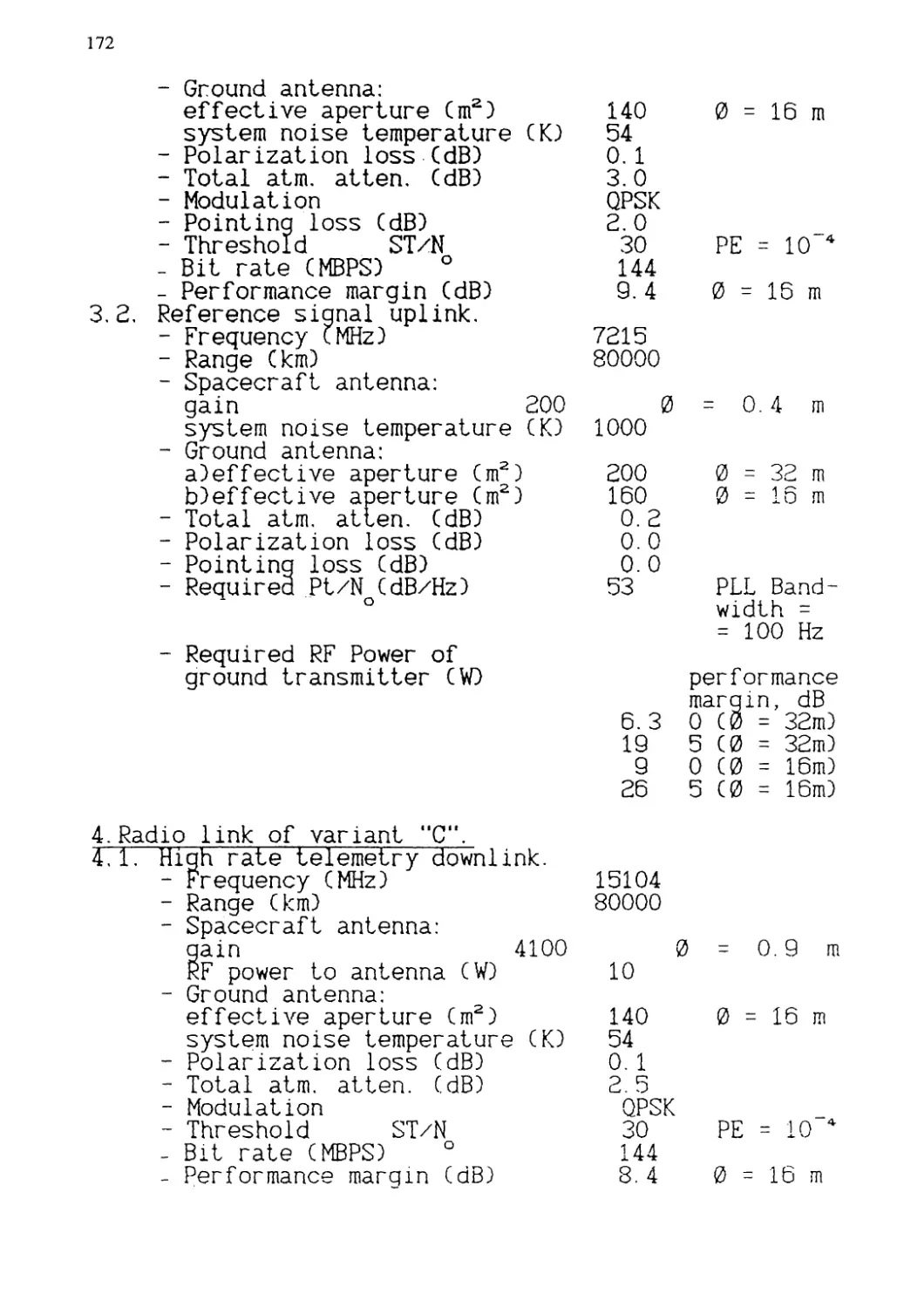
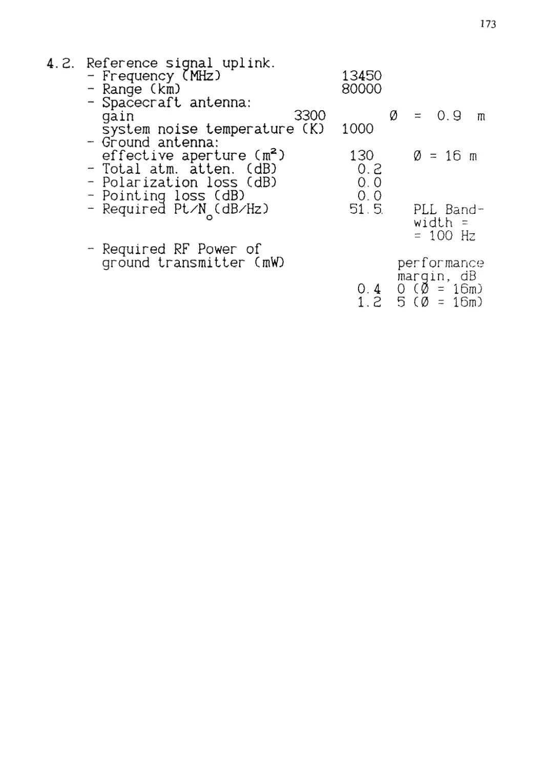
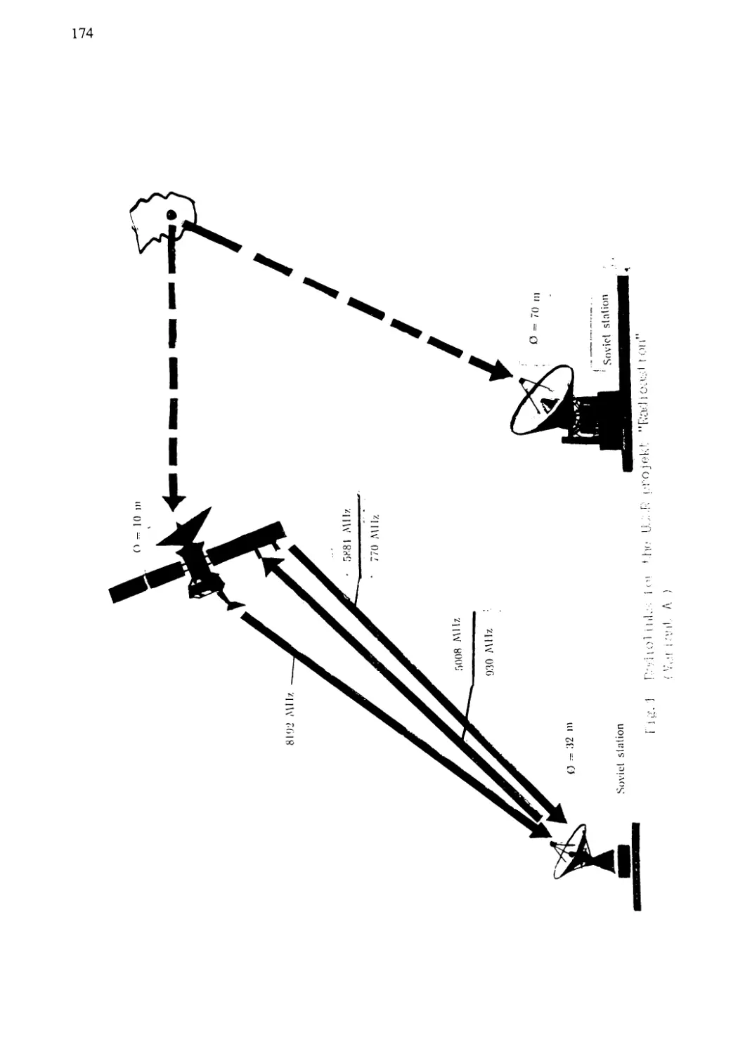
Radiosupport for a Space Radiointerferometer Radioastron Project
V. Grishmanovsky 	169
lhe Canadian S2 Recorder for Radioastron
R.	D. Wietfeldt, P.S. Newby, D. Baer, W.H. Cannon, G. Feil, P. Leone, II. Tan 	177
4- Science by VSOP
VSOP Possible. Observing Scenario
H. Kobayashi 	183
Punctional Limitations of the Radioastron Project
L- Gurvits 	187
VLBI Observations Using a Telescope in Earth Orbit: The Tdrss Experiments
R- Linfield 	193
mrn VLBI vs. VSOP
P-В. Baath 	197

X
Southern Hemisphere VLBI with VSOP
D.L. Jauncey, R.A. Preston, J.E. Reynolds, E.A. King, D.J. Bird, D.G. Blair,
G.J. Carrad, D.J. Cooke, M. Costa, R.A. Duncan, W.G. Elford, R.H. Ferris, A. Giles,
R.G. Gough, G. Gowland P.A. Hamilton, D.L. Jones, S.K. Jones, A. Kembal,
M.J. Kesteven, E.T. Lobdell, D. McConnell, P.M. McCulloch, D.L. Meier,
D.	W. Murphy, R.L. Mutel, G.D. Nicolson, R.P. Norris, A. Nothnagel,
E.	Perlman, A. Savage, L. Skjerve, Lb. TaafTe, A.K. Tzioumis,
R.M. Wark, K.J. Wellington, and G.L. White 	203
Development of Radio Outbursts in Quasars and the Role of Continuum Monitoring
for Space VLBI
E. Valtaoja	 209
Galactic and Extragalactic Water Vapor Masers
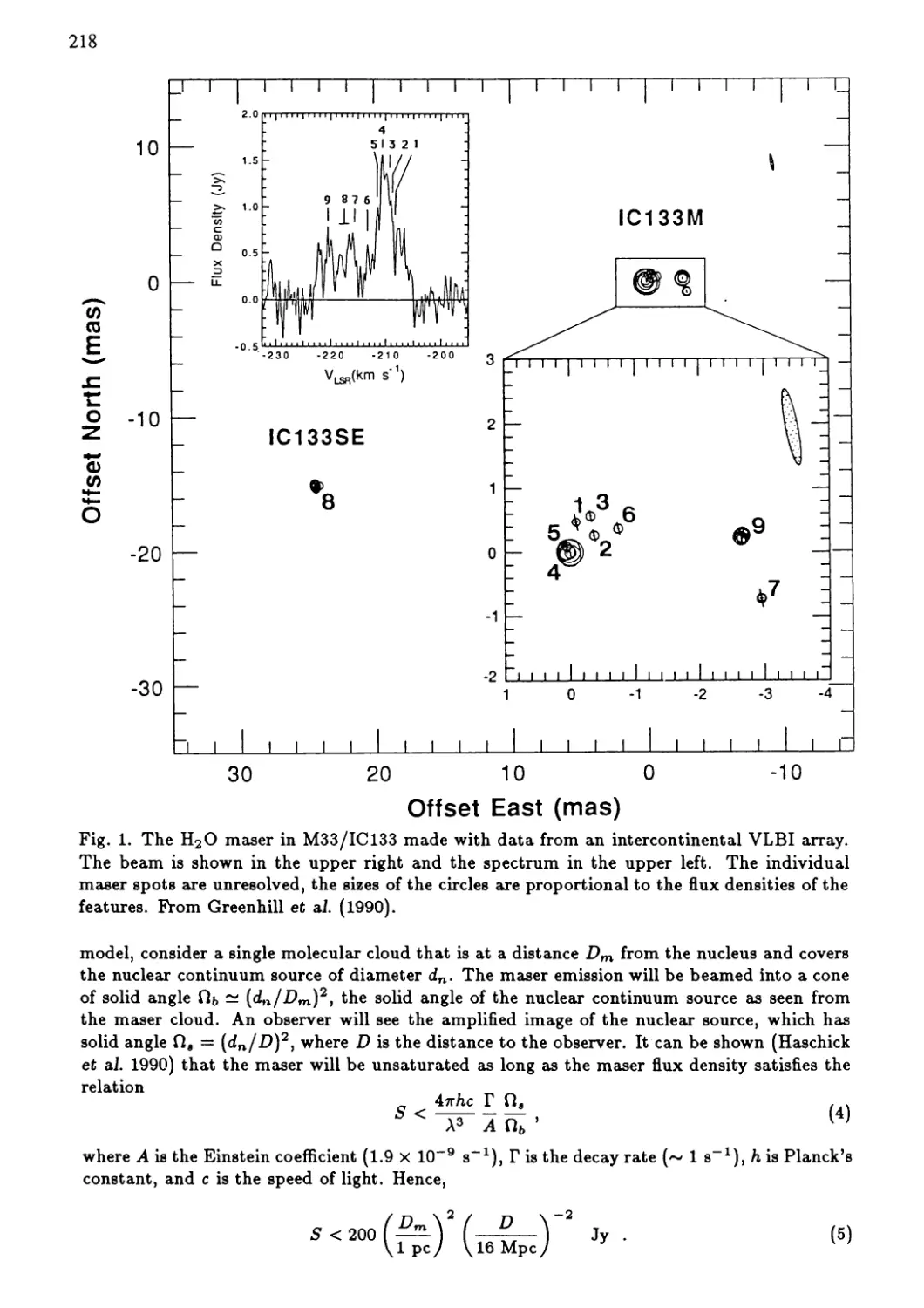
J.M. Moran, L.J. Greenhill, and M.J. Reid 	215
Space Radio Astronomy for Objects in the Near-field Zone
Y.N. Parijskij 	221
Interstellar Scattering: Limitations and Opportunities
B.K. Dennison 	225
5: Management Plan
Observing Programm of VSOP
M.	Morimoto 	231
International Management of Radioastron Project
B.G. Andreev, N.S. Kardashev, R.T. Schilizzi 	233
An Outline of VSOP Management
R.T. Schilizzi 	239
Summary of the Issues
B.F. Burke 	245
mm-VLBI Workshop
1. mm-VLBI Instrumentation
70-Meter Telescope at SulTa as a Member of mm-VLBI
V. Zabolotny 	251
New Millimetre Telescopes for VLBI
R.S. Booth 	255
Upgrade of the Haystack Telescope for 3-mm Operation
R.P. Ingalls, A.E.E. Rogers, and J.E. Salah 	259
Millimeter-VLBI Capabilities of the VLBA
J.D. Romney 	261
The Kashima Space Research Center’s New 34M Telescope
II. Takaba, Y. Koyama, and M. Imae 	 265
Burst Sampling Observations under Atmospheric Turbulence in mm-VLBI
N.	Kawaguchi 	269
Prospects of KNIFE
Japanese VLBI Group 	277
MM-VLBI Observations at SEST in 1990
B.O. Ronnang 	279

xi
2 min-VLBI Sciences
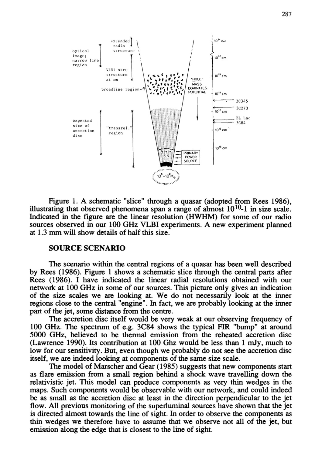
Results from 100 GHZ VLBI
L.	B. Baath 	285
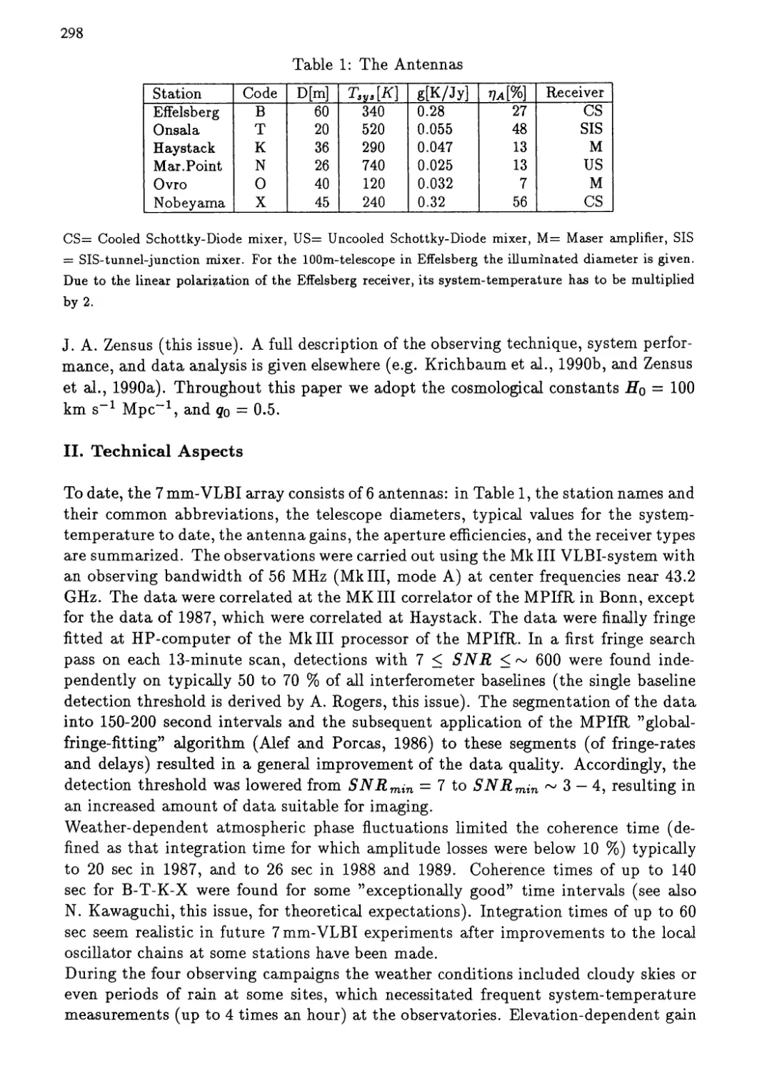
Astronomical Results from Recent 7 mm-VLBI Campaigns
T.P- Krichbaum and A. Witzel 	297
The Development of 7-mm VLBI
N. Bartel 	313
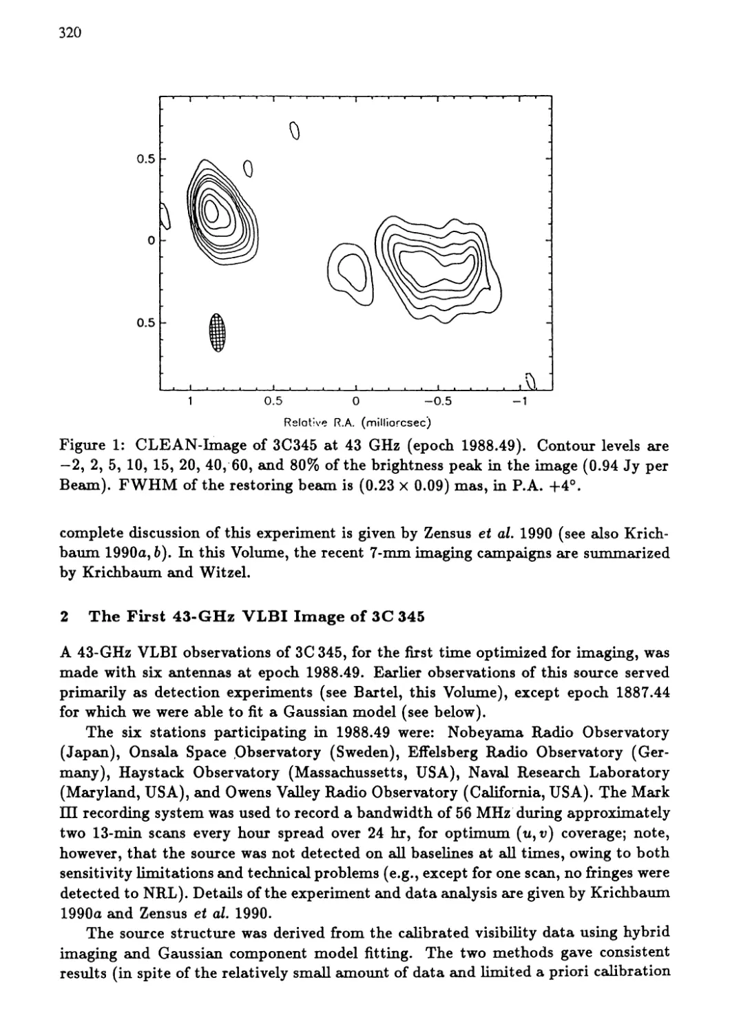
VLBI Imaging of the Quasar 3C 345 at 43 GHz
J.A. Zensus 	 319
The Evolution of 3C84
M.	Wright 	•	325
Millimeter Wavelength VLBI
M. Wright 	 331
A Proposal of mm-VLBI Monitoring
M. Inoue 	  337
3. Frings Fitting
Very Long Baseline Interferometry Fringe Detection Thresholds for Single Baselines
and Arrays
A.E.E. Rogers 	341
Global Fringe Fitting Applied to 100 GHZ VLBI Data
L.B. Baath 	353
Subject Index	301
Index of Objects 	363
List, of Participants 	364
Author Index 	367

VSOP
International
Symposium

Overview of VSOP Mission
T. Nishimura
and Astronautical Science
the VSOP (VLBI Space
which is officially
This satellite will
aiming at receiving
a
The Institute of Space
(ISAS) is planning to launch
Observatory Programme) satellite,
called Muses-B, in early 1995.
carry a gigantic Юти antenna,
signals from quasars in L,C and Ku band and transmitting
them back to the ground tracking station at the rate of
128 Mbps(64MHz)(Fig.1). The radio observatories on the
ground will receive these signals simultaneously and
they will be correlated at the correlation center,
having a high speed FX type correlator and eventually
produce precise brightness maps of quasars with high
resolution.
The VSOP will weigh approximately 800kg and will be
launched by the M-V rocket, which is under development
by ISAS as a next generation carrier, having four stage
solid propellant motors(Fig.2). Mission requirement and
specifications are tabulated in Table 1. The orbit is
an elliptic orbit with perigee height 1,000km and apogee
height 20,000km respectively, revolving around the Earth
with the period of 6hr. The inclination is chosen at
46.4 so that the same observing frame can be reproduced
after 2 years. Also it is better in avoiding radiation
damages from Van Allen belt.
These observed data are A/D converted, then trans¬
mitted down to the ground tracking stations with the
rate of 128Mbps (64MHz) in Ku band (13GHz). Also an
uPlink carrier in 13GHz will be sent to the spacecraft
to carry the precise clock Information which is supplied
)y the ground hydrogen maser. This signal may be
modulated by PN code in order to meet the requirement of
SnFV0FVLBI
1 by Universal Academy Press, Inc.
4
the international frequency regulation.
The antenna must be folded and squeezed in order to
accomodate it inside the rocket fairing and will be
deployed in space like an umbrella. The development of
this deployable antenna is one of the most difficult
tasks because it must maintain the surface precision of
0.5mm r.m.s. to receive Ku band signals(22GHz), after it
is stretched out (Fig.3).
The phase and clock transfer is another difficult
problem to be resolved.
Since precise clock synchronization must be maintained
between signals observed in space and those received at
the ground, very accurate and stable clock signals
generated by a hydrogen maser at the station will be
placed on the up-link signal(13GHz) and transmitted back
to the ground, in order to maintain the coherence. Also
very precise orbit determination of the spacecraft is
required, not only for this clock transfer problem,
but also for accelerating the data correlation process
by the FX machine. For this purpose, a GPS receiver
with a micro-processor, that will produce precise orbit
information in real-time by means of Kalman filter, will
be placed on-board.
The attitude control is the third major difficulty
to be overcome, because the pointing accuracy of 0.01c
is required for observation, particularly of Ku band
signals. The attitude determination will be performed
by star trackers and these data will be processed in
comparison with the star map in real-time by means of
the on-board micro-processor and the attitude will be
controlled by four zero-momentum reaction wheels(Fig.4).
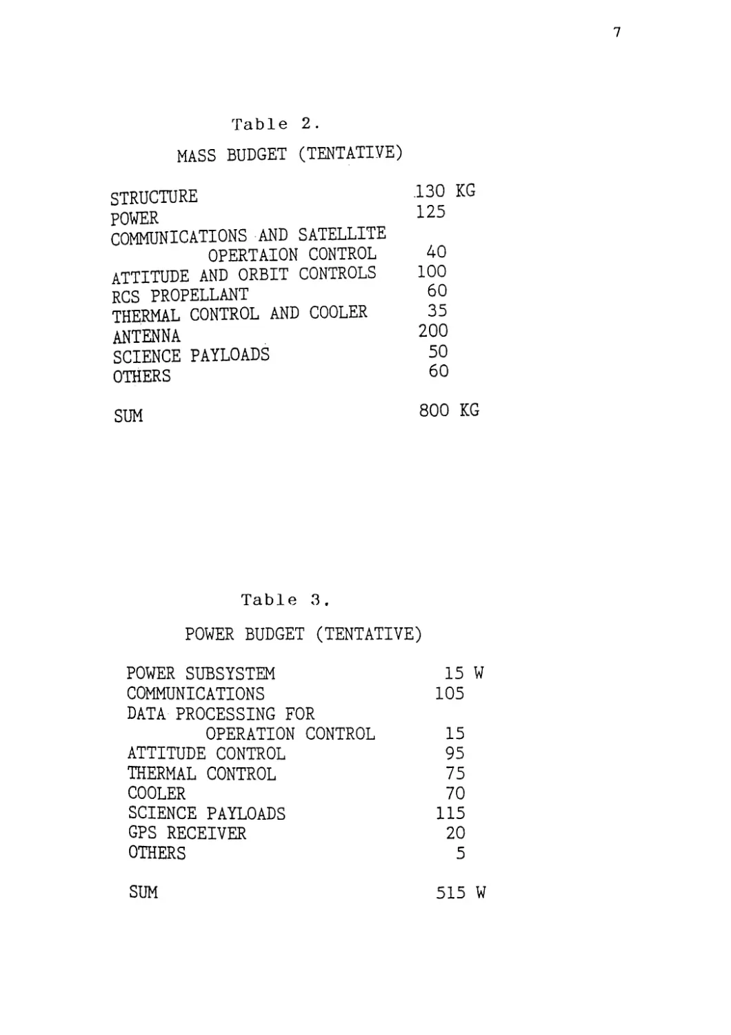
Tentative budgets for weight and power are shown in
Tables 2 and 3 respectively.
Finally it is mandatory to have international
cooperations for achieving the mission goal, since the
more radio telescopes as well as tracking stations
scattered all over the world we have, the better
coverage on the U-V plane we can acquire, thus enhancing
the precision of quasar maps.
This mission will be enthusiastically supported by
the teams of the National Astronomical Observatory as
well as of the Communication Research Laboratory of
Japan and will definitely contribute to the advancement
of the radio astronomy, together with the Radioastron of
U.S.S.R., which is expected to be in space around the
same time.
For this purpose, it is most desirable to organize
an international advisory or supervisory committee,
consisting of representatives from such organizations as
5
jSAS, NRO, NASA, NRAO, ESA, EVN, AT, etc. This commi¬
ttee will establish the basic rules for scientific
objectives, mission requirements and fundamental sche¬
dules for observation as well as for tracking.
Under this international supervisory committee, it
ts necessary to organize a residence operational commi¬
ttee stationed at ISAS HQ. This committee, also consis¬
ting of International members, will determine more
detailed schedules for observation and tracking, based
on the analyses considering various constraints Imposed
on the spacecraft as well as ground stations, and
practically commands and operates the entire VSOP mi¬
ssion .

6
Table 1. Trajectory and Mission Requirement
Orbit
Apogee:
about 20,000 km
Perigee
about 1,000 km
Inclination :	46.4'
Launch
: by ISAS M-V rocket from KSC in early
1995
Satellite
Antenna
:	10m diameter, center fed with 0.5mm rms
surface accuracy
c
Pointing : better than 0.01 hopefully with fast
slewing rate
Frequency :	1.6,	5 and 22GHz for observation
Polarisation : LHCP
Frontends: cooled, with active cooling
(22GHz) less than 100 К
On-board processing : wideband A/D followed by
conventional frequency
conversion,
Communication : S band (2.3GHz) (up and down)
telemetry, command and tracking
Ku band (13GHz) (up and down)
phase and clock transfer
data transmission with
128Mbps(64MHz)(down)

7
Table 2.
MASS BUDGET (TENTATIVE)
STRUCTURE	130	KG
POWER	125
COMMUNICATIONS AND SATELLITE
OPERTAION	CONTROL	40
ATTITUDE AND ORBIT CONTROLS	100
RCS PROPELLANT	60
THERMAL CONTROL AND	COOLER	35
ANTENNA	200
SCIENCE PAYLOADS	50
OTHERS	60
SUM	800	KG
Table 3.
POWER BUDGET (TENTATIVE)
POWER SUBSYSTEM	15	W
COMMUNICATIONS	105
DATA PROCESSING FOR
OPERATION CONTROL	15
ATTITUDE CONTROL	95
THERMAL CONTROL	75
COOLER	70
SCIENCE PAYLOADS	115
GPS RECEIVER	20
OTHERS	5
SUM	515	W

8
Fig. 3.
VSOP inside fairing
Fig. 2.
M-V Rocket

9
Fig-. 4. Attitude Control System

10
IACG Panel-1 meeting (A).
IACG Panel-1 meeting (B).

Report of the Dec. 4, 1989 Meeting of the
IACG Panel on Space-VLBI
F.	Jordan
lYie Panel met at ISAS to discuss the current status • of system com¬
patibility between all space and ground elements which are related to the
operation of and subsequent data reduction from both the Soviet RADIOAST-
rON mission and the Japanese VSOP mission. Included in the discussion
were observing frequencies, data transmissions formats, tracking frequen¬
cies, ground data recording formats, recording media (e.g., video tapes,
cassettes etc.) and correlator interfaces. Our objective was to identify
the most important next steps which the IAOG-member space agencies should
take to ensure the compatibilities required for the critical internation¬
al participation which is necessary for full scientific use of the
missions. All four IACG agencies were represented at the meeting as were
all the major ground radio astronomy consortia which will be performing
ground VLBI experiments in the 1990's.
Assessment of the Current Situation:
Observing Frequencies
All ground radio astronomy observers and both space-VLBI missions now
plan for common, compatible observing frequencies.
Data Transmission Formats
The Soviets plan data transmission formats for RADIOASTRON which are
entirely compatible with existing recorders and correlators in the radio
astronomy community. The Japanese have recently selected a data
transmission format which is also compatible with ground observers,
particularly with the VLBA correlator being developed by the US NRAO.
—ilgkinq Frequencies
funH1763^ recent progress has been made here in that NASA/DSN now has a
plan to provide tracking support to either or both Space-VLBI
ssions at either X band or Ku band for phase transfer with a Ku wide
§i®«OFVLBi
У Universal Academy Press, Inc.

12
band down-link for science data transmission. All these frequencies are
in compliance with ITU frequency allocations. The Japanese have selected
Ku band for phase transfer to the VSOP spacecraft and the Soviets
announced either X or Ku band will be selected for NASA-tracking and
phase transfer to the RADIOASTRON spacecraft, and that the selection will
be made soon. Both the Japanese and the Soviets have agreed to pursue Ku
band for science data transmission.
Ground Data Recorder Formats
All systems appear to the compatible.
Recording Media and Correlator Interfaces
The Panel identified here the single remaining compatibility problem.
Currently the NRAO is developing recorders for the VLBA which record data
onto large-reel video tapes. NRAO is also developing a correlator which
reads only video tapes. These developments are well underway and cannot
be altered, and it appears that all American, European and Australian
radio telescopes are adopting this system. However, the Canadians are
beginning the development of a cassette-based VLBI data recording system,
and companion correlator, for delivery and use by the Soviets for
RADIOASTRON. The Japanese intend to develop yet another correlator for
use with a newly developed Sony K4 cassette-based recording system.
Although all three systems are format-compatible, none of the three
correlators is physically compatible with recorded products from the
other systems.
This current situation poses a threat to the eventual recorded data-
to-correlator physical interfaces which will be required to fully involve
the international radio science community in the two space VLBI missions.
The future, unless altered, could result in the limited data paths shown
in Figure 1, where both the Japanese and Soviet correlators process
national experiment data only, and where the NRAO correlator processes
all international experiment data, while omitting data from Japanese and
Soviet radio telescopes.
Panel Advisory Proposals to the Space Agencies
The panel advised some near-term actions which will serve to further
the desired convergence to compatible systems. They are:
о ISAS should initiate a plan to develop a means of accepting
VLBA tapes as input to the intended Japanese correlator.
о ISAS should use its best efforts to ensure the funding to
permit the installation of VLBA-compatible recorders in
the Japanese tracking stations and radio telescopes.
о USSR should quickly select the frequency for ground-to-space
signal phase transfer for RADIOASTRON, X band or Ku band.
о NASA should quickly study the feasibility of providing a
single station for tracking RADIOASTRON at the time of its
proposed launch in late 1993.

13
o NASA should use its best efforts in coordination with the
NRAO to supply or loan VLBA-compatible recording systems to
the USSR.
o ESA should use its best efforts to aid and abet the funding
of a European VLBA-compatible correlator.
The Panel plans to meet September 1990 in Prague to reassess Space
VLSI compatibility status and review the progress on suggested actions.

14
SPACE VLBI COMPATIBILITY STATUS
DECEMBER, 1989
SVNN3JLNV 3OVdS
(id) S3doos3i3i oiavd v
(VIS) SNOI1V1S 9NIX0VH1 SHO1V13HHO0
SVNN31NV ONAOHO

Initial VSOP Astronomical Requirements
H.	Hirabayashi
abstract
Initial astronomical VSOP requirements are discussed and cover the spacecraft
and ground supporting systems.
Introduction
Initial VSOP Space Observatory Programme (VSOP) design has been in
progress since April 1989. The main program institute is The Institute of Space and
Astronautical Science (ISAS), and a modest budget is expected when compared to the
size of the program. Additionally, the ISAS launching rocket has already been
specified, thus placing severe VSOP spacecraft design constraints on the program.
These "tough” requirements must be adhered to, however, because we live in a ’’real”
world.
The initial astronomical requirements for the VSOP are discussed, and are
further emphasized by Drs. R. Preston, R. Linfield, D. Murphy, H. Hirabayashi, H.
Kobayashi, and M. Inoue. Because VSOP assumes both space segments and ground
segments initial astronomical requirements cover all these aspects.
1.	MISSION REQUIREMENTS
1.1	GENERAL MISSION REQUIREMENTS
1.1.1	Objectives
The VSOP principal mission requirement is to produce high resolution, high
dynamic range maps of celestial objects over a range of radio frequencies.
1-1.2	Sky and Telemetry Coverage
The VSOP must be capable of providing data which leads to good quality radio
source maps over the entire sky while operating in concert with large ground arrays
(Japanese antennas jointly observing with the Very Long Baseline Array (VLBA) or
European VLBI Network for northern hemisphere sources, and southern hemisphere
array for negative declination sources). The spacecraft and ground telemetry
constraints should prevent reduction in the total observation time by no more than -
30% for most directions throughout the mission, and for any particular source it
FRONTIERS OF VLBI
*2* *1991 by Universal Academy Press, Inc.

16
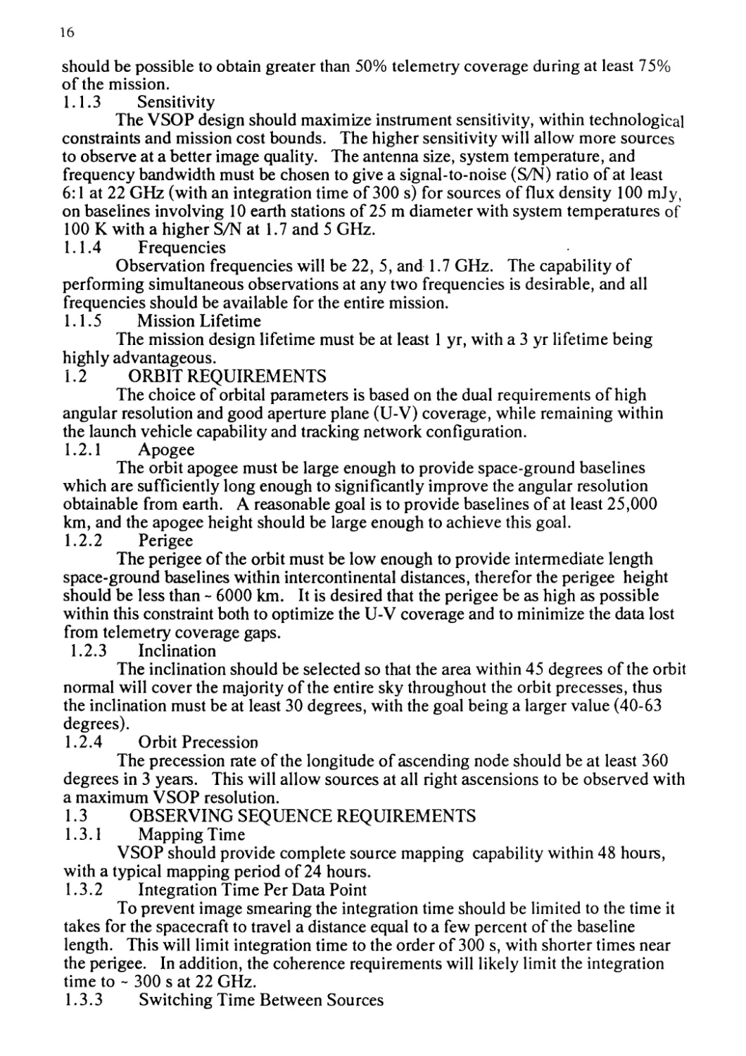
should be possible to obtain greater than 50% telemetry coverage during at least 75%
of the mission.
1.1.3	Sensitivity
The VSOP design should maximize instrument sensitivity, within technological
constraints and mission cost bounds. The higher sensitivity will allow more sources
to observe at a better image quality. The antenna size, system temperature, and
frequency bandwidth must be chosen to give a signal-to-noise (S/N) ratio of at least
6:1 at 22 GHz (with an integration time of 300 s) for sources of flux density 100 mJy,
on baselines involving 10 earth stations of 25 m diameter with system temperatures of
100 К with a higher S/N at 1.7 and 5 GHz.
1.1.4	Frequencies
Observation frequencies will be 22, 5, and 1.7 GHz. The capability of
performing simultaneous observations at any two frequencies is desirable, and all
frequencies should be available for the entire mission.
1.1.5	Mission Lifetime
The mission design lifetime must be at least 1 yr, with a 3 yr lifetime being
highly advantageous.
1.2	ORBIT REQUIREMENTS
The choice of orbital parameters is based on the dual requirements of high
angular resolution and good aperture plane (U-V) coverage, while remaining within
the launch vehicle capability and tracking network configuration.
1.2.1	Apogee
The orbit apogee must be large enough to provide space-ground baselines
which are sufficiently long enough to significantly improve the angular resolution
obtainable from earth. A reasonable goal is to provide baselines of at least 25,000
km, and the apogee height should be large enough to achieve this goal.
1.2.2	Perigee
The perigee of the orbit must be low enough to provide intermediate length
space-ground baselines within intercontinental distances, therefor the perigee height
should be less than ~ 6000 km. It is desired that the perigee be as high as possible
within this constraint both to optimize the U-V coverage and to minimize the data lost
from telemetry coverage gaps.
1.2.3	Inclination
The inclination should be selected so that the area within 45 degrees of the orbit
normal will cover the majority of the entire sky throughout the orbit precesses, thus
the inclination must be at least 30 degrees, with the goal being a larger value (40-63
degrees).
1.2.4	Orbit Precession
The precession rate of the longitude of ascending node should be at least 360
degrees in 3 years. This will allow sources at all right ascensions to be observed with
a maximum VSOP resolution.
1.3	OBSERVING SEQUENCE REQUIREMENTS
1.3.1	Mapping Time
VSOP should provide complete source mapping capability within 48 hours,
with a typical mapping period of 24 hours.
1.3.2	Integration Time Per Data Point
To prevent image smearing the integration time should be limited to the time it
takes for the spacecraft to travel a distance equal to a few percent of the baseline
length. This will limit integration time to the order of 300 s, with shorter times near
the perigee. In addition, the coherence requirements will likely limit the integration
time to ~ 300 s at 22 GHz.
1.3.3	Switching Time Between Sources

17
The space and ground systems must be able to switch within 1 hour between
any two sources. For phase-referencing observations it is desired that the
telescope be able to switch within 1 min between two sources 3 degrees apart.
14 SPACECRAFT NAVIGATION REQUIREMENTS
14.1	Orbit Control
Requirements to achieve the desired orbit are quite flexible, i.e., 10% of the
planned apogee and perigee altitudes.
1 4.2 Orbit Knowledge
The phase transfer process requires a predicted orbit (12 hours in advance)
accurate to 5 km in position and 50 cm/s in velocity. The data correlation requires a
considerably more accurate orbit knowledge within 1 week after observation; 40 m in
position and l.E-05 cm/s**2 in acceleration (5.E-06 cm/s**2 desired). The
required orbital velocity knowledge is set by limitations on the correlator’s output data
rate, and depends upon observation parameters, with the limits being most strict for 22
GHz observations. For the VLBA correlator, 20-station 22 GHz continuum
observations require a 5 mm/s velocity accuracy, whereas 22 GHz spectral line
observations require a 1 mm/s velocity accuracy for 20-station arrays and 4 mm/s for
10-station arrays.
2.
SPACE SYSTEMS REQUIREMENTS
2.1
2.1.1
INSTRUMENT REQUIREMENTS
Receiving Bandwidth
The recorded bandwidth should be at least 64 MHz, although 128 MHz is
especially desired at 5 and 22 GHz.
2.1.2	Polarization
The antenna/feed system should receive circular polarization at all three
frequencies. If VSOP is to be used for linear polarization measurements it is required
that each feed reject the opposite circular polarization by at least 30 dB in power, with
40 dB desired. An additional requirement for polarization observations is that
variations over 48 hours in the spacecraft’s antenna azimuth must be known to an
accuracy of 2 degrees or less. If these two requirements can be satisfied the capability
of simultaneous observations with both circular polarizations is possible. If the linear
polarization measurements will not be done, the sense of the circular polarization
should be LHCP to match with conventional ground telescopes.
2.1.3	Tuning Range
At 5 GHz the VSOP passband must overlap the ground radio telescopes; i.e.,
4.6 GHz - 5.1 GHz for VLBA. At 1.7 GHz the passband must cover the 1.612 -
1-720 GHz range of OH lines, with a 10 MHz window on either side (e. g. 1.602 -
1-	730 GHz). At 22 GHz, the passband must include both the observed range of
water maser emission frequencies in our galaxy and in external galaxies; 22.0 GHz -
22.3	GHz.
2-	1 -4 System Temperature
The receiver should have a system temperature no greater than 100 К when
operating at 22 GHz, 50 К at 5 GHz, and 50 К at 1.7 GHz.
2 -1 - 5	Antenna Performance
The microwave performance of the antenna must be sufficient to meet
requirements associated with frequency reception up to 22 GHz. A single antenna
earn is necessary, with on-axis aperture efficiency as high as possible. Sidelobe
evels are of secondary importance. The RMS surface accuracy should be 0.5 mm or
etter with an antenna diameter 10 meters or larger.
•1-6 On-board Filtering, Digitizing, and Formatting

18
The VSOP data filtering, digitizing, and formatting must be compatible with
both the Japanese and VLBA correlators. To allow correlation with the VLBA
correlator, the data must be filtered before being digitized into channels of 16 MHz or
smaller (by power of 2). The capability of a narrow channel (4 MHz or less) is
desired for OH (1.7 GHz) spectral line observations. The VLBA correlator will
accept data with either 1 -bit or 2-bit digitization. VSOP must allow at least one of
these sampling modes, and the data format must allow a ground telemetry station to
perform a translation to a VLBA format.
2.1.7 Antenna and Receiver Calibration
Each receiver must be equipped with a noise source and a total power
measurement capability.	The goal of the calibration system will be to measure the
antenna sensitivity (gain/system temperature) approximatly once per day, with
measurements of total system temperature (on source) every 30 - 60 minutes.
2.2	ANTENNA POINTING REQUIREMENTS
2.2.1	Pointing Accuracy
At 22 GHz the half-power beamwidth for a 10 m antenna is ~ 5 minutes of arc.
The spacecraft pointing subsystem shall therefore have the capability to point within an
upper limit of - 1 minute of arc deviation from the source direction, and to provide
pointing knowledge within 20 seconds of arc. This is to be continuously done
during the entire observation of a given source, in the presence of limit cycling and
antenna flexure.
2.2.2	Observing Direction and Slewing Requirements
Special care should be taken to allow wider sky view angles, and a smaller
sun avoidance limit is highly desired.
3.	GROUND TRACKING SYSTEM REQUIREMENTS
3.1	PHASE TRANSFER
The ground system must be capable of supplying, a stable radio tone via a
two-way link, that will allow a coherence from the phase transfer process (i.e.,
exclusive of any phase errors of the ground frequency standard), and after correlation
at least 90% at 22 GHz for a 300 s integration time. It is desired that the coherence
value be known to be greater than 1%.
3.2	SIGNAL RECORDING
The ground system must be able to record signals in real time at a 128 Mbits/s
rate or greater, with 256 Mbits/s being desired. The recorded data must be able to be
correlated (perhaps after suitable translation) at either the Japanese or the VLBA
correlator.
3.3	TIME AVAILABILITY
The combination of one Japanese and three DSN tracking sites, and the NRAO
Green Bank station can provide in most cases sufficient telemetry coverage for good
imaging capability. An additional southern hemisphere tracking station is highly
desireable to obtain better U-V plane coverage. During mapping observations no
more than 10% of the observation time should be lost due to tracking network
scheduling restrictions.
4.	DATA PROCESSING REQUIREMENTS
4.1	CORRELATOR
The correlators (Japanese, VLBA, and European) used for VSOP data must be
able to correlate VSOP data taken at any orbit geometry and observation frequency.
At least one correlator must be able to correlate VSOP spectral line data, and in
19
combination the correlators must be able to correlate data at a rate equal to or higher
than the recording rate, with the exception of experiments using a large number of
ground stations. The time interval between data recording and correlating should be
no longer than two months on the average. The output data from all correlators
should be compatible.
4 2 IMAGE PROCESSING
Software and techniques for creating VSOP data images must be developed
prior to launch and be available to all investigators to use.
5.	GROUND OBSERVATORY SPECIFICATIONS
5.1	LOCAL OSCILLATOR
The ground observatory telescopes must have a local oscillator stability
(exclusive of phase errors in the hydrogen maser or other frequency standard)
sufficient to give a coherence of at least 99% at 22 GHz for a 300 s integration.
5.2	RECEIVERS
The receivers must have at least the same tuning range as specified in section
2.1.3	above, and also be able to receive a bandwidth of at least 64 MHz.
5.3	RECORDING FORMAT
The ground observatories must be able to record data at a rate of 128 Mbit/s
(256 Mbits/s desired) in a format which can be correlated with VSOP data at the
correlator intended to be used for that experiment.
5.4	NETWORK SIZE
Although VSOP may be used with less than 10 ground telescopes much of the
time, it must be possible to observe with as many as 20 antennas in a global array, and
also correlate the data from the entire array with at least one correlator.
5.5	NETWORK TIME COMMITTMENT
Prior to launch, agreements should be reached with ground VLBI networks
and individual telescopes for co-observing observation VSOP support.

VSOP Satellite System Overview
H.	Hirosawa
abstract
The development of the VLBI Space Observatory
Programme (VSOP) satellite started in FY 1989. The
development schedule consists of two phases, i.e., a
three year proto-type model development phase (PM phase)
and a three year flight model development phase (FM
phase), with launching scheduled for January or February
1995. The major subsystems include a 10 m diameter
deployable parabolic antenna, an attitude control
system, low noise amplifiers (LNA), LNA refrigerator,
phase transfer system, and a high bit-rate data down¬
link system, which all require new technological
developments. International collaborations in tracking,
phase transfer, data reception, and radio astronomical
observations are being considered during the initial
satellite design phase.
1 . Introduction
In 1989 the Institute of Space and Astronautical
Science (ISAS) started to develop a satellite named
MUSES-B, where MUSES stands for the Mu Space Engineering
Satellite, with Mu being the name of the ISAS's
satellite launching rocket and В the second satellite
of the MUSES series. MUSES-B is the satellite for the
VLBI Space Observatory Programme (VSOP). Engineering
features are an important consideration because of the
rcany technological developments that are required to
construct a VLBI satellite.
MUSES-B will be launched on the first flight of a
new Mu series rocket, named the M-V. This rocket will
have almost three-times payload launching capability
OF VLBI
iy91 by Universal Academy Press, Inc.

22
when compared to the existing M-3SII type rocket. The
development of the M-V rocket was approved in the summer
1989 and will start in FY 1990. The development of
MUSES-B will be done in parallel with the development of
the M-V rocket.
The satellite development schedule has two phases,
1.	e., a three year proto-type model development phase
(PM phase) which began in FY 1989, followed by a three
year flight model development phase (FM phase). The
satellite will be launched in January or February 1995
from the ISAS's Kagoshima Space Center (KSC).
2.	System Requirements
The key MUSES-B satellite system design require¬
ments imposed by the VSOP mission'' concept are as
follows:
-	The spacecraft shall be three-axis stabilized and
accomodate the VLBI payload.
-	The payload will consist of a 10 m diameter
deployable antenna, low noise amplifiers (LNA), a LNA
refrigerator, down-converters, А-D converters, and
onboard subsystems for phase transfer and high bit-
rate data downlink.
-	Astronomical observations will be made at three
frequency bands, 1.7,	5 and 22 GHz, with the 22 GHz
band (Ka band) being given the highest priority.
-	The Ka-band low-noise amplifier must be actively
cooled.
-	Observation data must be transmitted with a rate
greater than 100 Mbps.
-	The 10 m diameter antenna must be pointed with an
accuracy of 0.01 degrees.
-	An orbit with apogee altitude of 20,000 km and
perigee altitude of about 1000 km was selected
considering the M-V's expected capability. A 46°
inclination is desirable rather than using 31 °
because the relative positions between the satellite
and ground telescopes change with a period of about
two years.
3.	System Design
A large number of new technological developments
are required to design and build the MUSES-B satellite.
The existing technologies for ISAS's scientific
satellites will be used as much as possible. Since
MUSES-B is going to be launched by the first flight of
the new M-V rocket, a simple payload is considered most
suitable.
The conceptual design of the MUSES-B satellite is
23
currently in progress. A total launch mass of 800 kg is
the maximum limit to launch the satellite into the
designed orbit. The baseline design of the satellite's
major onboard subsytems is as follows:
-	Large deployable antenna
A 10m diameter wire-tension-truss type antenna with
a mesh reflecting surface. The surface accuracy
goal is 0.5 mm rms, and the expected weight is 200
kg.
-	Low noise amplifiers (LNA) and cooler
LNAs ' for each frequency band will be onboard. The
LNA for 22GHz (HEMT amplifier) will be actively
cooled. A space Stirling cycle cooler is under
development.
-	Science data downlink
Ku band, with a rate of about 130 Mbps,
Quadriphase Shift Keying (QPSK) modulation, and one
transmitting antenna.
-	Phase transfer
Ku band up/down is the baseline.
-	Attitude control system
Three axis stabilization and high precision pointing
SUB-REFLECTOR
SOLAR
PANEL
MAIN
REFLECTOR
ANTENNA FOR DATA
DOWNLINK AND
PHASE TRANSFER
Fig. 1 VSOP Satellite

24
using momentum wheels, star trackers and an
inertial reference unit (IRU).
- Reaction control system (RCS)
For orbit control during initial orbit injection,
and for spacecraft attitude control.
Figure 1 shows a conceptual diagram of the MUSES-B
satellite. The satellite has two solar paddles with an
angle-drive mechanism. The configuration of the space¬
craft imposes several constraints on the main dish's
pointable directions. Effects, of these constraints on
radio-astronomical observations are under study.
The satellite operation, telemetry reception,
command transmission, science data reception, and phase
transfer, will be performed in Japan by the KSC ground
station, with the S band being used for telemetry and
command. Support for science data reception, phase
transfer, and tracking are being discussed with NASA
and other international space institutes.
Precise orbit determination will be made using the
Ku band links, and an orbit determination experiment
using the Global Positioning Satellite (GPS) system is
also planned.
The tentative mass budget is given in Table 1. All •
data is preliminary estimates or rough allocations, with
all figures being fairly optimistic. Subsystem and
component redundancy, and optional scientific require¬
ments are not considered. Strong efforts will be
required to reduce mass of each subsystem.
Table 1 Tentative Mass Budget
Structure
Power
Communications and Satellite
Operation Control
Attitude Control
RCS Propellant
Thermal Control and Cooler
Deployable Antenna and Feed
Science Payload
Others
130 kg
125
40
1 00
60
35
200
50
60
Total
800 kg
Table 2 shows the tentative power supply budget,
with the power also being very limited, thus efficient
25
observation programs using limited power will be
required.
The nominal design life of ISAS's scientific
satellites is one year, but most of the satellites have
Table 2. Tentative Power Budget
Power Subsystem	1 5 W
Communications	105
Data Processing for Operation
Control	15
Attitude Control	95
Thermal Control	75
Cooler	70
Science Payload	115
GPS Receiver	20
Others	5
Sum	515	W
lived longer than the nominal life. Solar cell
radiation degradation is a major life-limiting factor in
MUSES-B. A tentative goal is to make the 22GHz obser¬
vations using the cooled LNA possible for the first
and second year. Observations with reduced capabilities
will be possible in the third year.
The contractors for the MUSES-B PM development are
as follows: NEC Corp. (Satellite system design, attitude
control system, power subsystem, communications
subsystem, LNA, and onboard signal processing),
MITSUBISHI ELECTRIC Corp. (Large deployable antenna),
NEC/SUMITOMO HEAVY INDUST. (Stirling cycle cooler),
MITSUBISHI HEAVY INDUST. (RCS), and TOSHIBA Corp. (GPS
receiver).
4.	Conclusions
The VSOP overall satellite system has been
reviewed. Conceptual design is in progress, and will
proceed to the proto-type model design in FY90. A more
defined satellite configuration will be available by the
start of FY 1990. Optional science and redundancy
requirements will be reviewed during the remaining
conceptual design phase period.

Radioastronomy Antenna
T. Takano
K.	Yamamoto
ABSTRACT
This paper expresses the study results of the radioastronomy
antenna for the space VLBI satellite "MUSES-B". The mission
objective requires the antenna to have high gain. After
conceptual study, an axis-symmetrical. Cassegrain antenna is
adopted with a mesh reflector formed in tension truss method. The
reflector consists of many facets of triangles. The analysis
showed the possibility to achieve the aperture efficiency of 60%
at 22 GHz.
1 . introduction
A radioastronomy antenna is one of key devices onboard the
space VLBI satellite "MUSES-B". The diameter of the antenna
should be more than 10 meters, and be folded in the cargo room of
the rocket vehicle while being launched.
Several deployable schemes have been proposed so far (1>.Some
of them were put into practical use, but none of them arc suitable
for the MUSES-B satellite. This paper presents the required
conditions to the antenna from the mission, design principle and
an example of constitution.
2.Requirements for the antenna
The requirements are summarized in Table 1. The upper limit
of available frequency band is determined mostly by mechanical
accuracy of the reflector so that design should be tuned to 22 GHz
band. But a primary horn affects the available bandwidth of each
observation frequency band, whichever of a common horn for several
bands or separate horns for each band are used. Eollowing factors
to determine the antenna gain arc not significant for a solid
antenna : 1) approximation accuracy of a main reflector to an
FRONTIERS OF VLBI
©1991 by Universal Academy Press, Inc.
28
ideal smooth surface, 2) loss of a reflecting surface, and 3)
feeder loss.
The satellite is Installed in the launching rocket vehicle
”Mu-V" of the Institute of Space and Astronautical Science, as
shown in Fig. 1. The antenna interfaces the spacecraft and LNA’s.
Interface conditions are being fixed according to the design
progress of each subsystem.
3.	Deployment scheme
Three types of deployable antennas shown in Fig. 2 are
studied at a preliminary stage of the development. The' deployment
scheme with extensible ribs and tension truss’-35 is selected
between them considering the weight, stiffness and reliability.
The antenna is of a Cassegrain type. The subreflector
supports will be extended from the stowed position.
4.	Electrical design accomplishments
Cross sectional view is shown in Fig. 3.
The foci of the upper half and lower half of the subreflector are
located below and above the antenna axis, respectively. Therefore,
the reflected wave from the subreflector hit the portion of the
main reflector which has geometrical clearance between the
subreflector as shown in the figure.
The aperture diameter D, the focal length of the main
reflector F, the subreflector diameter Ds, the blocked area
diameter Db, the aperture diameter Dh and length Rh of the horn
are the parameters to be determined. The F/D radio is determined
in order to realize moderate curvature of the main reflector
limiting the length of the subreflector support to an allowable
value. The minimum value of Db is given by the required diameter
of the antenna center-hub which is used to fix the antenna to the
satellite structure. The antenna efficiency can be maximized by
adjusting the values of Dh and Rh for each DsC4).
Mesh reflecting surface with small openings is needed
especially for Ka-band. Fine tricot mesh of gold plated
molibdemum wire is developed for this purpose. The transmission
loss is measured to be less than -18 dB at Ka-band.
Loss analysis of the antenna at 22 GHz is summarized in Table
2.
5.	Mechanical design accomplishment
( 1) Rib structure
The rib structures of six masts are extensible in the radial
direction. The role of the structure is to support the
peripheries of cable network system to give accurate reference
points. It consists of a triangular truss with three foldable
longerons, a canister for stowage and deployment, and a deployment
driver. The feature of this mast is high stiffness and precise
posi tioning.

29
(2)	Cable network for the main reflector
The shape of the main reflector is maintained by an inelastic
tension-activated truss and an elastic cable net system. The role
of tension truss is to fix the distribution of a limited number of
hard points in the area of reflector surface. The cable net
system, on the other hand, interpolates the hard points to give
high precision to the reflecting surface. Fig. 4 shows the
Integrated tension truss and cable net system of one block area
between the adjacent two masts
(3)	Feed structure
The feed support equipped with the subreflector on the top is
stowed and deployed by virtue of the sliding mechanism between the
support structure and the extensible pipe.
(4)	Scaled reflector model
An one-fourth scale model has been fabricated in order to
verify the design analysis and clarify the problems of
manufacturing and assembly processes. The scale model
has the same construction and the same numbers of
constituent parts as the full-scale model.
The primary process of manufacturing and assembly was
successfully finished and some critical points on manufacturing
and assembly have been made clear. Various engineering tests
including the surface accuracy measurements, the deployment tests
and the electrical tests are now being pursuied.
7. Conclusion
The prototype model and the flight model of the
radioastronomy antenna will be developed by 1991 and 1994,
respectively. The MUSES-B satellite launch is scheduled at the
beginning of 1995.
FINAL STAGE OF
SPACE AVAILABLE
Fig. 1. The satellite installed in the cargo room of the
launching rocket vehicle

30
Refercnces
(1)	NASA, NASA Conf. Publication 2368, Part 1, December, 1084.
(2)	T. Takano and E. Hanayama, Proc, of* 1989 international
Symposium on Antennas and Propagation, vol. 1,	1B3-2, pp. 77-80,
August, 1989.
(3)	K. Miura, 37th congress of 1.А.Е., 1AE-86-206,	1986.
(4)	K. Miura ct al., Proc, of 1989 international Symposium in
Antenna and Propagation, vol. 1, 1B2-5, pp. 69-72, August, 1989.
inflatable elements
(b) Extensible ribs
and tension truss
(c) Hoop-column and
tension truss
Eig. 2 Constitutions of deployable
refflectors
Eig. 3 Di sign parameters of
a displaced-axis
Cassegrain antenna

31
Table 1 Spacc-VLBI system requirements for a satellite-borne
antenna
(1)	Electrical conditions
1)	Frequency band : 22, 5 and 1.6 Gllz bands. Bandwidth of
1.5 GHz is needed at Ka-band.
2)	Polarization : right-hand or left-hand circular
polarization.
3)	Gain : Efficiency of about 65% at 22 GHz.
4)	Noise temperature : should not exceed noise temperature of
LNA.
(2)	Mechanical conditions
1)	Size in a folded state : should be smaller than storage
room of a launching vehicle of about 2200 mm ф x 4000 mm
including the satellite.
2)	Weight : be less than 200 kg.
3)	Strength : is specified for a folded state in launching
phase, and for a deployed state on an orbit.
4)	Stiffness and momentum of inertia : Specific vibration
frequency should be higher than 1 Hz.
(3)	Thermal conditions
1) Inhomogeneous reflector deformation due to partial
illumination by sunlight : should be suppressed to
keep proper pointing, especially at high frequencies.
'fable 2 Loss analysis at 22 GHz
Item
Loss
2 2.1 5(GHz)
1 .Reflector des i gn
( 1 ) Aperture distribution
1 .0 0
(2) Main-ref surface accuracy
0 .33
( 3 ) Mesh
0 .0 6
(4) Sub-ref blocking
0 .3 0
(5) Sub-ref thermal	paint
0 .08
S.ub-total ( ( 1 )+( 2 )+( 3 )+( 4 )+( 5 ))
1 .7 7
2.Feed design
( 1 ) Aperture cover
0 .0 4
( 2 ) Horn
0 .0 5
(3) Effect due to 1 .7/5GHz coupling hole
0.12
(4) Return loss
0 .0 4
( 5 ) POL / OMT
0.15
Sub-total ( ( 1 )+( 2 )+( 3 )+( 4 )+( 5 ))
0 .40
Total	A	(1 + 2)
2.17

32
Break in VSOP symposium.

Muses-B Attitude and Orbit Control System
K.	Ninomiya
abstract
The space VLBI satellite MUSES-B is to achieve a
highly precise antenna pointing with accuracy of better
than 0.01 degree. The purpose is to obtain precise maps
of radio sources. The attitude and orbit control system
(AOCS) is designed as a zero-momentum, three-axis stabi¬
lized system. MUSES-B attitude is controlled by four
skewed reaction-wheels to achieve the high pointing
accuracy and required attitude maneuvers. Unloading is
performed primarily using magnetic torquers. In place of
the magnetic torquers, however, hydrazine thrusters with
3N thrust can also be used (as a backup means). The pre¬
cise attitude determination is accomplished by an on¬
board software system which is based on a stellar-iner¬
tial approach. For this purpose an inertial reference
unit and a pair of star trackers are adopted. Under the
guidance by the AOCS four 3N-thrusters boost the space¬
craft into the mission orbit (perigee 1,000 km x apogee
20,000 km) from the transfer orbit (perigee 250 km x
apogee 20,000 km).
1 . Introduction
MUSES-B is the Japanese VLBI satellite of VSOP
(VLBI Space Observatory Program). It’s purpose is to
conduct the radio-astronomical observation of compact
radio sources. From the view point of attitude and orbit
control system (AOCS), MUSES-B has several unique fea¬
tures. MUSES-B carries flexible structures, such as a 10
m diameter (radio-astronomical) observation antenna, a
2-axis gimbaled data transmission antenna, and two wings
°f solar arrays. AOCS is also required to overcome the
FRONTIERS OF VLBI
©1991 by Universal Academy Press, Inc.

34
large environmental disturbances (mainly solar radiation
pressure and gravity gradient torque) and internal
disturbances (solar array stepping, 2-axis gimbaled
antenna stepping, vibration of the Stirling cooler for
Low Noise Amplifier) during observation.
In the initial phase, the spacecraft performs
perigee up maneuvers (PUM) to transfer from the injec¬
tion orbit to the mission orbit. A PUM in three-axis
stabilization is selected rather than in spin stabiliza¬
tion because of the spacecraft power requirement in the
early orbital stage. Initial sequence of events is
described in detail later.
In this paper, firstly, the requirements for the
AOCS design from the space VLBI mission are described,
secondly the summary of the conceptual study on the AOCS
functions and configurations is shown, and finally, the
initial sequence of events, especially performing
three-axis stabilized perigee up maneuvers (PUM) using
four 3N thrusters, is presented.
2. Requirements
The requirements for the AOCS from the space VLBI
mission are as follows:
-	Maintain 0.01 degree pointing accuracy during mapping
observations
-	Provide pointing control capability in all directions
of the inertial space
-	Provide fast maneuvering capability for small angles
for phase reference mapping
-	Avoid the sun lights from impinging onto the radiator
surface
-	Maximize the electrical power from the solar cells
-	Accord, to the extent possible, to the philosophy of
maximizing scientific observation time (which needs
the real time data-link to a ground station)
3. Nominal Attitude During Observation
Fig. 1 shows the selected
attitude during obser-
The large antenna
toward a target
The spacecraft plane
is perpendicular to
array stepping axis
to contain
AOCS
nominal
vation.
pointed
source.
that is perpendicular to the
solar array stepping axis is
aligned to contain the sun,
and the AOCS controls the
solar array stepping so as to
obtain the maximum power
generation. The data trans-
is
radio
Fig. 1 Nominal attitude
during observation

35
mission antenna which is mounted on a 2-axis gimbal is
steered toward a ground station.
4 a AOCS Functions
The AOCS is designed to provide the following func¬
tions :
_ Spin rate reduction and initial attitude acquisition
-	PUM for mission orbit insertion
-	Pointing control for mapping observation
-	Fast small angle maneuvers for phase reference mapping
observation
-	Large angle maneuvers for retargeting
-	Momentum unloading using magnetic torquers or
thrusters (for backup)
-	Fault detection and redundancy management
-	Solar array drive control
5.	AOCS Configuration
Fig. 2 shows the block diagram of the AOCS. The
current locations of the AOCS sensors and actuators are
shown in Fig. 3.
Fig. 3 Locations of AOCS Components

36
The AOCS control units are Attitude and Orbit
Control Processor (AOCP), Attitude and Orbit Control
Electronics (AOCE). Sensing devices are a FRIG-based
inertial reference unit (IRU), a pair of star trackers
(STT), a geomagnetic aspect sensor (GAS), 5 sets of
coarse sun sensors (CSS), a spin-type sun aspect sensor
(SSAS) 1 , and accelerometers (ACCL) . Precise attitude
determination is accomplished by an onboard Kalman
filtering using the data obtained from IRU and STT's.
The AOCS actuators are reaction wheels (RW) and
magnetic torquers (MTQ). Four reaction wheels are skewed
equi-angularly about the spacecraft Y axis. Each of the
magnetic torquers is aligned along the respective space¬
craft axis, to be used for wheel unloading. Thrusters
are employed for PUM and backup attitude control.
6.	AOCS Performance
Table 1 shows the AOCS
performance summary. The AOCS
operates as a zero-momentum,
three-axis stabilized system
providing the required point¬
ing accuracy, better than 0.01
degree overall (1 6 ). The
problem of flexible structure
control will be solved using
the conventional filtering
technique. This will be stud¬
ied more in detail in the next
design phase.
Attitude
Stabi1ization
zero momentum,
3-axis control
Pointing Error
< 0.01 deg (overal1)
Attitude
Determination
Error
<0.004 deg (each axis)
Slewing Maneuver
Speed
45 deg / 20 ain (max)
Table 1. AOCS Performance
Summary (preliminary)
7.	Initial Sequence of Events
Fig. 4 shows the initial sequence of events of
MUSES-B. From the electrical power requirement, the
solar arrays have to be deployed in an early stage of
the initial sequence. Rate damp control should be per¬
formed as early as possible after the spacecraft is in¬
jected into the transfer orbit. Then PUM is done in the
three-axis stabilization mode during the following
sequence of events.
The spacecraft is injected into the transfer orbit
(apogee 20,000 km, perigee 250 km), and spin down is
accomplished by using thrusters. After rate damping, the
1,2 SSAS and ACCL might be eliminated in a further
study.

37
acquisition
! prior to
stellar-inertial
accomplished by
move
mis¬
sun
axis
solar arrays are deployed, and initial sun ;
is performed by relying on CSS. The attitude
PUM is established by the onboard
approach using IRU and STT1s. PUM is
firing the four 3N therustes four or five times to
up the perigee from 250 km to 1,000 km. After the
sion orbit is achieved, the spacecraft performs
acquisition and the sun pointing maneuver
pointed toward the sun). This is to avoid the
deformation of the observation antenna during
ployment. After the observation antenna deployment,
three-axis attitude, i.e.	nominal attitude
observation, is established.
the
(+Z
thermal
its
de-
the
for
This paper presents the summary of the conceptual
design study of the attitude and orbit control system of
MUSES-B. It is anticipated that almost all of the re¬
quirements on AOCS of MUSES-B, such as that for the
over-all pointing accuracy of better than 0.01 degree,
will be met by employing the state-of-the-art technology
available to us. The relevant methods for implementing
and verifying the system design, however, have yet to be
carefully investigated. Furthermore, the following items
will have to be studied much more in detail, in addition
to the interface characteristic definitions with the
other subsystems such as the observation antenna or
solar array stepping subsystems:
~ Attitude control/determination accuracy
~ External and internal disturbance torque analysis
~ Satellite dynamics analysis
-	Flexible structure control
-	Redundancy management

Receivers and Cooling System of Muses-B
Space VLBI Satellite
H.	Saito
ABSTRACT
This paper describes the present status of the re¬
ceivers and cooling system design for MUSES-B space VLBI
satellite. The observation frequencies of this space VLBI
are three bands, namely 1.6, 5, and 22GHz. Each band has
a on-board Low Noise Amp 1ifier(LNA) receiver.
In order to reduce low noise temperature, the cooled
HEMT(High Electron Mobility Transistor) amplifier is
required for 22GHz band. This 22GHz HEMT amplifier is
cooled at 80°К by means of a on-board Stirling cycle re¬
frigerator .
Юи^ Antenna
Fig. 1. Block diagram of MUSES-B receiver system.
FRONTIERS OF VLBI
©1991 by Universal Academy Press, Inc.

40
.1 . I n t roduc t i on
The Institute of Space and Astronautica1 Science
(I SAS)schedu1es to launch the MUSES-B satellite by means
of ISAS’s M-V rocket. The scientific mission of MUSES-B
is Space VLBI(Very Long Baseline Interferometry) obser¬
vation in three microwave frequency bands, namely 1.6,
5, 22GHz. This MUSES-B satellite in the orbit and other
ground stations constitute a microwave interferometry.
The microwave radiation from radio stars, is received
effectively by 10m diameter on-board antenna in MUSES-B
satellite, and then it is fed to low noise amplifier re¬
ceivers. The microwave signal is so faint that the front
end receiver must have extremely low noise temperature.
Each frequency band has a on-board Low Noise Amplifier
(LNA) receiver. The cooled HEMT(High Electron Mobility
Transistor) amplifier is required for 22GHz. This 22GHz
HEMT amplifier is cooled at 80°К by means of a on-board
Stirling cycle refrigerator.
This paper describes the outline of LNA design in
the sec.2, the cooling system design in the sec.3, and
the LNA system layout in sec.4.
2. Low Noise Amplifier
The block diagram of the MUSES-B receiver system is
shown in Fig.l. The antenna feeder is provided with
microwave diplexers, through which 1.6GHz, 5GHz and 22GHz
band components are fed to the LNA systems. Coaxial
lines are utilized for both 1.6GHz and 5GHz bands, and
waveguide is for 22GHz band.
Table 1 describes the performance of LNA system.
The design noise temperature of the LNAs are 80K(1.6GHz),
100K(5GHz) and 80K(22GHz), respectively. Frequency band
of 1.6GHz and 5GHz utilize uncooled FET, and uncooled
HEMT receiver, respectively. The HEMT cooled at 80K is
Table 1. Performance of LNA system.
Itea
1.6G LNA
5G LNA
22G LNA
Receiving Frequency
l.665GHz
5.1GHz
21.5GHz
Bandwidth (-3dB)
70MHz £
300MHz£
2GHzfc
Gain
35dB £
35dB £
35dB £
Noise Teiperature »
80k S
100k £
80k £
Input, Output Connection
Coaxial
Coax i a 1
Waveguide
Aapllflre Seaiconductor
FET
HEMT
HEMT
» Design ObjIctlve

41
Fig. 2. Configuration of 22GHz LNA.
required for 22GHz.
It is necessary to select the best HEMT device for
80K operation. HEMT performance in 80K condition may not
be inferred from that at room temperature. We are cold¬
testing many HEMTs commercially available from several
manufacturers. DC characteristics(I-V characteristics)
HEMT chips are measured at 77K. Then engineering models
of HEMT amplifier will be integrated, and the noise
temperature at 80K will be evaluated.
The configuration of 22GHz LNA is described in Fig.
2.	The LNA consists of two stages. The first stage
is cooled at 80K and the second stage is uncooled. Each
stage is provided with three HEMT chips on a hybrid IC
circuit substrate. Input and output pick-up conductor
antenna from a hybrid IC circuit are inserted to the
waveguides. A waveguide -type- isolator is installed
in front of each LNA stage.
The first stage including the waveguide-type iso¬
lator and a hybrid IC amplifier circuit is cooled at 80K
because the noise generated at the first stage may be
dominant for LNA operatation. The thermal design of the
first stage is now being performed. Figure 3 depicts a
conceptual drawing of the first cooled stage. Cooling
head is attached to the hybrid IC amplifier chip and the
isolator. We have to minimize thermal flow from out¬
side because the cooling capability of our refrigerator
is limited by 1W. Thermal conduction through the input
and output 'waveguide is disconnected at choke frange gaps.
Radiation heat transfer should be blocked by multi-layers
°f super insulation.
3 ‘Loo1i ng Sys tern
The first stage of 22GHz LNA should be cooled at
80K in order to reduce noise temperature. Thermal load

42
Fig, 3 Conceptual configuration of 22GHz cooled LNA stage
of the cooed LNA stage is expected to be order of 1W,
and the mission life should be longer than one year.
Possible cooling methods may be electric cooling, radi¬
ative cooling, and mechanical cooling system. First,
cooling capability of electric cooler may be much less
than 1W. Practically it cannot reach extremely low
temperature such as 80K. Next, radiative cooling system
with 1W level cooling capability requires a cooling
panel with area of several square meters. It provides
us with severe constraint to MUSES-B satellite design
and operation(especial 1 у attitude).
Mechanical cooling system has wide range of cooling
temperature(4 - 150K) and cooling capability(O - 300W),
depending on size of refrigerator. In addition, it
does not provide us with special constraint to MUSES-B
satellite design and operation(configuration and atti¬
tude). Split-type, Stirling cycle cooler is being de¬
veloped for space borne application. It is because
split-type, Stirling cycle cooler may become compact and
cooling efficiency is closest to ideal Carnot cycle.
It consists of a, compressor and a displacer (cold head),
which are connected by He gas pipe. Mechanical vi¬
bration generated in the compressor is not directly
propagated to the cold head. We have developed a ground
model of Stirling cooler. Table 2 shows the performance.
The life time of the refrigerator may be limited by He
gas contamination and malfunction of movable seal for He
gas. However, our ground model has already achieved
8000 hours operation in laboratory and is still working.
4. LNA system layout
The main mission of MUSES-B is space VLBI obser¬
vation which requires as low noise temperature as possi-

43
Fig. 4. Conceptual layout of LNA and cooling system.
front end LNACat least first stage) should be
close to antenna feeder. RF loss due to
from antenna feeder to LNA provides serious
in noise temperature. Stirling cycle cooler
ble. The
i ns tai led
waveguide
i ncrease
exhausts about 60W heat(45W from compressor and 15W from
displacer). Connecting He pipe between compressor and
displacer have to be as short as 30cm. Cooling capa¬
bility of Stirling cycle decreases as the ambient temper¬
ature increase. Radiative cooling panel may be required
to exhaust this heat. Figure
layout of LNA system.
4 depicts a conceptual
5 . conclusion
This paper describes the present status of MUSES-B
LNA system design. The EM of this system will be inte¬
grated in 1990 and then we will go to PFM phase.

VSOP Spacecraft On-Board Processing
H.	Hirabayashi
abstract
VLBI Space Observatory Programme (VSOP) satellite on-board
radioastronomy processing is reviewed. The signals from the frontends of 1.6, 5,
22GHz bands are frequency converted to common frequency IF bands, and then sent
to an IF switch circuit having 2 identical IF channel outputs. There are two video¬
converter sets with a local frequency synthesizer and A/D converters. The video
bandwidth is 16/32^64 MHz and the A/D converters are 1/2 bit. The 2 A/D
converters are followed by a formatter unit which accepts a 128 Mbps bit stream,
combines the timing and auxiliary data, and makes the downlink format. The
formated data is QPSK modulated, power amplified, and transmited through a Ku-
band link. The reference signal for the local oscillators onboard is also received in the
Ku-band. By demodulating the QPSK data stream on the ground both the data stream
and the carrier can be extracted, with carrier being used for frequency and phase
monitoring.
1. Introduction
The Institute of Space and Astronautical Science (ISAS) started the VLBI
Space Observatory Programme (VSOP) in 1989 with a planned satellite launch in early
1995. The program goals are to launch a radio astronomy satellite and conduct
radioastronomical observations by making use of ground radio telescopes synthetic
arrays. The orbit will have an apogee altitude of - 20,000 km, a perigee altitude of ~
1,000 km, and an inclination angle of 46.4 degrees.
The VSOP satellite, named MUSES-B, will carry a deployable antenna with a
~ 10 m dia, radioastronomy receivers in the 1.7, 5, and 22 GHz bands, down
converters, A/D converters, a data formatter, and RF subsystems for science data
down-link and phase transfer. The satellite is very limited in payload mass and power
consumption, with a total design payload mass ~ 800 kg and a power consumption ~
500 W.
The presented paper reports on the current conceptual radioastronomical
electronic equipment, with the low noise frontends and science communication
frontiers OF VLBI
©1991 by Universal Academy Press, Inc.

46
systems being respectively reported by Dr. H. Saito and Dr. N. Kawaguchi during
this symposium.
2. Down Converters and IF Circuits
The RF frequency ranges will be 22.0 - 22.3 GHz, 4.7 - 5.0 GHz, and 1.60 -
1.73 GHz, and the IF frequency for all these bands is in the 500 - 1000 MHz range.
The first local oscillator frequencies are fixed, being synthesized from the reference
signal by the uplink signal from the telemetry stations.
The signal level and frequency range are compatible and the IF switch circuit
will select two outputs from all possible IF inputs. The main operational mode is
single frequency, although dual frequency operation is also possible.
Polarisation sense is LHCP. For the 5 GHz band, a dual polarisation reception
is being discussed while considering the tradeoff of mass and power consumption.
No polarisation measurements in the 22 GHz band will be taken due to a low signal to
noise ratio.
IF Select
To Sampler
Reference
Signal
To D/C	| A To Synthesizer
Local Frequency Generator
Reference Signal Generator
Figure 1. Analogue part of radioasrtonomy signal flow in VSOP spacecraft
3.	Video Converter, A/D Converter, and Formatter
After IF switching the two outputs, two video-converter and A/D converter
serises will follow.

47
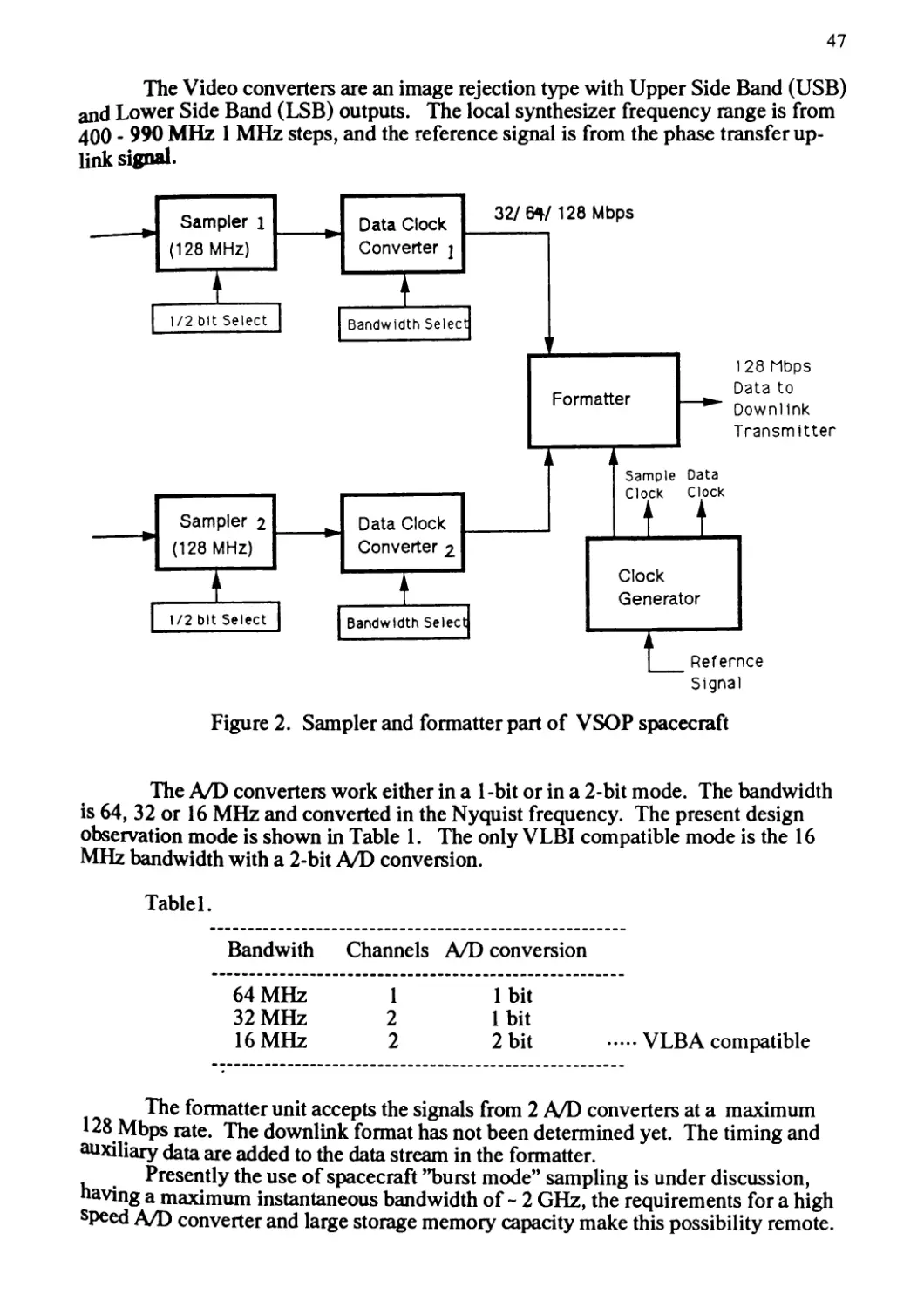
The Video converters are an image rejection type with Upper Side Band (USB)
and Lower Side Band (LSB) outputs. The local synthesizer frequency range is from
400 - 990 MHz 1 MHz steps, and the reference signal is from the phase transfer up¬
link signal.
Signal
Figure 2. Sampler and formatter part of VSOP spacecraft
The A/D converters work either in a 1 -bit or in a 2-bit mode. The bandwidth
is 64, 32 or 16 MHz and converted in the Nyquist frequency. The present design
observation mode is shown in Table 1. The only VLBI compatible mode is the 16
MHz bandwidth with a 2-bit A/D conversion.
Tablel.
Bandwith
Channels
A/D conversion
64 MHz
1
1 bit
32 MHz
2
1 bit
16 MHz
2
2 bit
• ••• VLB A compatible
The formatter unit accepts the signals from 2 A/D converters at a maximum
128 Mbps rate. The downlink format has not been determined yet. The timing and
auxiliary data are added to the data stream in the formatter.
Presently the use of spacecraft "burst mode” sampling is under discussion,
a maximum instantaneous bandwidth of - 2 GHz, the requirements for a high
sPeed A/D converter and large storage memory capacity make this possibility remote.

48
4.	IF Down-link
The formatter data stream is QPSK modulated, power amplified, and
transmitted by a 40 cm communication antenna attached to the satellite bottom. The
proposed center frequency is 15,050 MHz with a bandwidth of 128 MHz. The Ku-
band was selected for its bandwidth. The ionospheric disturbance is less in Ku-band
than in the X-band. Both the phase transfer (up) and IF downlink are in this band,
and use the same communication antenna.
5.	Phase Transfer and Synchronization
The phase reference signal for the local onboard oscillators is supplied by the
hydrogen masers in the telemetry network stations. The proposed up-link frequency
is 13,401 MHz with a 2 MHz span, thus allowing for a Doppler shift. To simplify
onboard phase locked loop, the telemetry stations will control frequency shifters so
that onboard frequency loop will be constant.
The phase return signal is obtained as an IF down-link extracted signal, and
will be for Doppler tracking and for phase comparison with the original signal.
In the Space Frequency Coordination Group (SFCG) there is an effective
isotropic radiative power (e.i.r.p.) limitation in the Ku-band up-link (below +10
dBm/Hz), and to meet this the CW signal spectrum must be spread by PN code and
must be demodulated on the spacecraft. In the present design the CW e. i. r. p. is -
70 dB greater than +10 dBm / Hz and the spectrum must be spread by - 10 MHz,
therefore causing unwanted effects in the local oscillators’ reference signal purity.
Usually demodulation is performed by a Costas loop circuit which increases spacecraft
complexity. A special waiver to SFCG is also needed for future space VLBI phase
links.
Satellite clock synchronization will be adjusted by using a S-band
communication link.
6.	Calibration
To perform system temperature and antenna gain measurements, each receiver
will be equiped with a noise source, attenuators, and detectors. The detected power
will be down-linked in the S-band TTC satellite house keeping data and in the Ku
wide band down link auxiliary data.
7.	Discussion
The VSOP goal of obtaining high fidelity imaging and good UV-plane
coverage is a big design concern. The telemetry coverage between the spacecraft Ku-
band antenna and the telemetry stations is a critical item for UV-coverage
enhancement, and is significantly dependent on the satellite’s main body Ku-band
antenna 600 m length.
The power consumption limitation also poses a severe design constraint on the
Muses-B satellite, and presently, the science payload mass and power consumption is
respectively restricted to be ~ 50 kg and ~ 115 w. The total satellite power
consumption when the radioastronomy science module is fully operational is less than
the power generated at the beginning of life ( - 500 W), yet due to a gradual lifetime
decline in generated power some observation mode limitations will be imposed after
the first year, thus causing design group concerns.

49
R References
1.	Kawaguchi, N., 1990, Frontiers of VLBI, edited by Hirabayashi, Inoue and
Kobayashi
2.	Saito, H., ibid

A Communication Link for VSOP
N. Kawaguchi
abstract
A communication link for VSOP science mission is proposed for phase
transfer, data transmission and time keeping. Propagation effects on the phase
transfer link is investigated and a Ku-band link is proposed to alleviate the
ionospheric fluctuation in the minimum. The random delay fluctuation on the link is
expected to be 5 picoseconds and would cause a loss of coherence by 18 % at the
highest observing band of 22 GHz. Science data sampled on board will be
transferred to a ground tracking station via a Ku-band data link with a rate of 128
Mbps. Time keeping on board is also discussed.
1.	Introduction
One of principal objectives of the VSOP mission is to get a fine and detailed
structure of extra-galactic radio objects. To achieve the mission it is essentially
important to have good fringes in high Signal-to-Noise Ratio. As a telescope on
board is limited in size, 10 m in diameter, high phase stability and wide receiving
bandwidth becomes key points for getting good fringes in high SNR. In the Section
2,	a Ku-band phase transfer link is presented which is optimized in minimizing phase
fluctuations caused by ionospheric turbulence. In the Section 3, a data link with a
large transmitting capacity which transfers a large volume of data from a high speed
sampler for a signal in wide frequency band. Time keeping system is also presented
in Section 4, in which a clock on board is transmitted to a ground station via a data
link.
2. Phase Link
Detailed studies on propagation effects on phase transfer from a ground
station to a satellite indicates that a Ku-band link is much better than an X-band link
to minimize the phase fluctuations caused by ionospheric disturbance. In Table 1,
systematic and random delay errors appeared in the phase link are given in some
cases of up- and down-link frequencies. The random delay fluctuations may cause a
loss of coherence which is estimated to be 92 % and 18 % diminution in fringe
amplitude observed in 22 GHz, the highest observing band of the VSOP, for the case
frontiers of vlbi
®1991 by Universal Academy Press, Inc.

52
of link frequencies of X-band and Ku-band, respectively. Not as the X-band up link,
however, it is limited in the spectral flux density in the Ku-band up link by the
regulation of SFCG, Space Frequency Coordination Group, 6-6R3. To keep the
spectral density limitation, it is necessary to spread the spectrum with PN modulation
on an up link signal as is supposed in the case (3) in Table 1. The modulation makes
a phase recovery circuit on board complicated and also, as is shown in Table 2, the
limited power makes a link margin unacceptably small, only 1.5 dB. So that, for the
VSOP phase transfer, a wavier to the limitation is now being asked to the SFCG.
It has not been reached to an agreement to transmit an unmodulated carrier in
the Ku-band, a phase transfer link with a frequency pair of (2) in Table 2 is now
proposed for VSOP. The block diagram of the link is shown in Figure 1. To keep the
frequency on board constant against the Doppler shift, a carrier transmitted from a
ground station is made offset in the frequency, which is synthesized from a hydrogen
maser frequency standard. A down link Doppler shift is monitored by comparing the
frequency of a down link carrier with that of a hydrogen maser frequency standard at
a ground station. The down link Doppler is referred to estimate the up link Doppler,
the frequency shift to be applied on the up link carrier. If the frequency loop is
perfectly closed, a round trip phase measured with a PSD, Phase Shift Detector, shall
be a constant value unless other perturbations due to propagation effects exist. The
variation of the round trip phase which implies a change of a phase link path will be
archived to remove the propagation effect. More than one tenth of noise reduction can
be expected and a link error due to a neutral atmosphere, the stability around 6xl0-14
in the Allan standard deviation, will be suppressed almost completely with this closed
loop operation of a phase link. The link errors given in Table 1 are an unmodeled
systematic error and a residual random error caused by the ionospheric perturbation,
those are accounted to be 8.2 and 5.0 picoseconds.
3.	Data Link
Three observing modes listed in Table 3 are defined for the VSOP. The mode
(A) is mainly for observing a source of continuum spectrum in one frequency band.
The mode (B) is for dual frequency or dual polarization observations and the mode
(C) is mainly for observing a maser source of line spectrum. In any modes the total
data rate is 128 Mbps. The data is transmitted to the ground station by modulating a
down link carrier, frequency translated from an up link carrier with a coherent
transponder, with a technique of Quadrature Phase Shift Keying, Q-PSK at a rate of
64 Mega symbols/sec (128 Mbps). The transmitter has a solid state power amplifier,
and a communication antenna is shared for the use of receiving a phase reference
signal and for transmitting the data. Two types of a feed system is investigated for the
communication antenna shown in Figure 2. The antenna, 40 cm in diameter, will be
attached at the bottom of the satellite main body. The transmitting power and the link
budget is shown in Table 4. For the ground antennas, it is assumed to use 10-m
antennas at DSN sites, NASA and a 20-m antenna at Kagoshima Space Center,
ISAS. The bit error rate of the communication link is expected to be 5xlCH.
4.	Time Keeping
A time base of satellite, a sample pulse and a second tick, is generated by an
oscillator which is frequncy locked to a frequncy standard on a ground station. The
frequency transfer is made with the up link carrier transmission. Down link data is
also framed with the same time base into a format prescribed for the convenience of
53
recovering the one pps tick at a ground station. The one pps tick from the satellite is
compared with that of the UTC to get time difference between the UTC and the time
base on board. Considering a propagation time from the satellite to the ground
station, the time difference will be used to find a fringe on a baseline between a space
and ground stations within a proper correlation lag time window.
An intermittent establishment of a phase link between a ground station and a
satellite will cause breaks of coherence between clocks on board and a ground
station. Large difference in time bases produced by the breaks is occasionally
adjusted by setting a new initial value on a counter which generates one pps signal.
The clock adjustment will be made via a S-band TT&C link.
5.	Ground Stations
For the support of VSOP mission three DSN stations, NASA, and
Kagoshima Space Station, ISAS, will serve as a phase reference station and a data
terminal station. The station closes a frequency control loop and a round trip phase
loop. The residual phase variation measured and archived there is requisite for
coherently correlating signals and finding fringes. Scientific data from the space
observatory is recorded on tapes there and will be transferred to a correlating center.
Switching of the reference station, the station management, and schedule and
data managements are very important to lead the VSOP program to success. These
topics, however, are beyond the scope of this paper and may be discussed in another
part of this book, but it shall be noted again that a close tie between a space
observatory and ground tracking stations, those should work in a body as one
element of an interferometer, is essentially important.

54
Table 1. Ionospheric Propagation Effects	TEC= 10 x 1016 electrons/m3, S=0.1
22 GHz Fringe Period = 45 picoseconds
Link Frequencies Unmodeled Ionospheric Error Link Path Fluctuation
Fup Fdown FUp+Fdown Oi(Fup)"^i(Fdown))	^res
(GHz) (GHz)	(picoseconds)	(picoseconds)
(1)
7.20
8.46
38.4
17
(2)
13.401
15.05
8.2
5.0
(3)
13.9
15.05
5.3
4.7
(1)	First proposal for VSOP in X-band Phase Transfer
(2)	Unmodulated carrier transmission now proposed.
(3)	PN coded carrier transmission now investigated.
Table 2. Up link design budgets for a phase transfer to the VSOP
PN coded
Items
Carrier
Transmission
Transmission
Gnd. Stn. EIRP
79.8 dBm(i)
79.8 dBm(2)
74.5 dBmG)
Pointing Loss
- 0.2 dB
- 0.2 dB
- 0.2 dB
Propagation Loss
-203 dB
-203 dB
-203 dB
Atmospheric Loss
- 2.2 dB
- 2.2 dB
- 2.2 dB
Polarization
Matching Loss
- 0.3 dB
- 0.3 dB
- 0.3 dB
Pointing Loss
- 0.5 dB
- 0.5 dB
- 0.5 dB
S/C Feeder Loss
- 6.5 dB
- 6.5 dB
- 6.5 dB
S/C Antenna G/T
4.6 dB
4.6 dB
4.6 dB
Up link C/No
70.3 dBHz
70.3 dBHz
65.0 dBHz
Required C/Nq
68.8 dBHz
60.0 dBHz
60.0 dBHz
Margin
1.5 dB
10.3 dB
5.0 dB
(1)	Maximum e.i.r.p. limited in the spectral density by REC 6-6R3 with a margin of 1.5 dB at a
chip rate of 13.6 MHz.
(2)	A case of carrier transmission with the same e.i.r.p. as the case (1),
Excess spectral density to the REC 6-6R3 is 69.6 dB.
(3)	A case of carrier transmission with a proper margin,
Excess e.i.r.p. to the REC 6-6R3 is 64.5 dB.

55
Table 3 The VSOP observing modes
Mode
Receiving
Bandwidth
(MHz)
Number of
Channels
Sampling Rate
(Msps)
Quantizing
Lebel
(bits/samples)
(A)
32
1
64
2
(B)
32
2
64
1
(C)
16
2
32
2
Total data rate is 128 Mbps in all modes.
Table 4. Design Budget for the VSOP Data Link
KSC(20m)
DSN(lOm)
Satellite TX
Power
34.7 dBm
34.7 dBm
Feeder Loss
-5.3 dB
-5.3 dB
Pointing Loss
-0.5 dB
-0.5 dB
S/C Antenna Gain
33.9 dBi
33.9 dBi
Propagation Loss
-204 dB
-204 dB
Atmospheric Loss
-3.0 dB
-2.2 dB
Polarization
Matching Loss
-0.5 dB
-0.3 dB
Pointing Loss
-0.5 dB
-0.2 dB
Feeder Loss
-1.0 dB
Ground Station
Antenna G/T
42.2 dB/K
39.5 dB/K
Downlink C/NO
95.6 dB
93.2 dBHz
Required C/NO
90.9 dB
90.2 dBHz
Margin
4.7 dB
3.0 dB

56
PSD : Phase Shift Detector	To Correlator
Figure 1. A Block Diagram of a Communication Link

57
Antenna
Positioner
Diameter
40 cm
Frequency Band 15 GHz
Polarization
Peak Gain
Beamwidth
Weight
RHCP
33.9 dB
3.2 deg
3.9 kg
Driving Range
Azimuth
Elevation
Driving Speed
Tracking Mode
Slewing Mode
Weight
Figure 2. The VSOP communication Antenna
-20 ~ 380 deg
+- 165 deg
0.1 deg/sec
2 deg/sec
5.0 kg

On the Orbit and Launch of VSOP
J.	Kawaguchi
abstract
Some requirements for the orbit of VSOP s/c are
summarized and the current orbital plan is discussed and
presented. ISAS's new launch vehicle designated M-V is
also introduced with its payload capability.
1,Introduction
VSOP may be the first spacecraft in the world
which enables VLBI observation in space-size. Apart from
the usual astronomical satellites, the orbital choice in
VSOP is deeply concerned with the scientific
mission itself. It's the base line length that
characterizes the features of this spacecraft.
This paper presents, first of all, some
preliminary requirements for this VSOP s/c. And secondly
this summarizes the current proposed VSOP orbital
plan. Thirdly ISAS's new launch vehicle designated M-V
is shown with the payload capability examples and
some notes on the configuration limitation inside
its nose fairing. Finally typical initial
acquisition sequences are introduced with inherent
several problems.
2.Orbital Requirements
2-1 Size of VSOP Orbit
The one of the most advantageous points in Space¬
based VLBI is in its ultra long base line length which
leads to the extremely high resolution. This requires
a larger semi-major axis in its orbit.
As it is well known, so to speak U-V plot plays
very important role of estimating the resulted
resolution and density. While larger the orbits are the
FRONTIERS OF VLBI
©1991 by Universal Academy Press, Inc.

60
wider the swept area expands, sweep rate in that U-V
plane may not be expected fast. From this reason, an
extra large size of orbit is not preferably adopted.
The feasible size of its semi-major axis seems 1
to 10 Re.
whose
the <
only for the
satellites.
fixed
orbits 1
with the rotation of
utilized not only for
scientific
are almost
for s/c operation,
synchronism should
the comprehensive
f visible periods
and convenient
orbits, this
shows
case
only same
and
Sometimes "synchronous"
synchronized
preferably
satellites but for
orbits
time
VSOP
avoided. Fig.l
U-V plots. In
used for VSOP,
and periods are repeated,
drawn just in lines not in plane,
if this synchronism is avoided,
improved as in this illustration.
Fig.2 demonstrated
VSOP's orbits,
hours orbit and
drawbacks in
there, since
hemisphere
various
is about
inclination
which well
plane. VSOP's
46deg.
period is
earth are
; practical
In those
in local
However, for
be strictly
examles of
closely synchronized plan is
observation configuration
resulted U-V plots are
On the other hand,
U-V coverage is fairly
both Radioastron's and
Although Radioastron's orbit is 24
is synchronous with rotation, some
synchronism	are	well	solved
in northern
assured
VSOP's
synchronism.
is chosen as
apsis in
is tentatively
its apogee is placed higher
and continuous visibility
ground
7
is
stations. The period of
hours avoiding
in Radioastron
stabilizes the
inclination
from
orbit
The
67deg f
orbital
set as
2-2 Inclination
For the purpose of observing targets in northern
and southern pole region, Earth's rotational motion is
efficiently utilized. However, for the observation in
equatorial band, only orbital motion can play the role of
synthesizing its virtual aperture. Consequently,
relatively higher inclination is preferable. As it is
well known, this inclination is pretty related to
the special orbital features such as the
regressional motion. These will be reviewed in detail
later.
2-3 Apogee direction
Phase and Clock transfer is the most
characteristic point in space-based VLBI and it's
pretty essential. As quite many of ground tracking
stations are located in northern hemisphere, the orbits
whose apogee direction is in northern hemisphere have

61
\VllC
X)
Avoiding Synchronization (5days)
I	\
I 24 hours	1
Radioaslron
o> dz
oj	a) cd
CD
O CD
Л V
ha = 75,000 km, hp = 9,000 km,
ha = 20,000 km, lip = 1,000 km,
Fig.1 U-V Plot
i = 67 deg	I = 46 deg
Fig.2 Radioastron & VSOP
Table-1 M-V Payload Capability
Orbit
i = 3 1 ’
i = 4 5 *
i = 6 3 ’
200x200
1975 kg
1891 kg
1746 kg
500x500
1877 (89) ”
1796 (35) ««
1 6 5 5 ( 7 8) * *
l000x1000
1732 (139)*
1655	(133)*
1522 (123)	*
1000x20000
9 09 ( 57 )/86 0 ( 5 4 )
875 ( 5 5 )/ 8 2 3 ( 52 )
		1
818 ( 5 1 )/75 0 ( 4 8 )
1000x40000
7 1 9 ( 3 0 )/7 04 ( 2 9)
6 9 3 ( 2S)/674 (23 )
646 ( 27 )/ 6 2 2 ( 26 )
1000x80000
512(15)/6 1 1 ( 15)
5 8 8 ( 1 5 ) / 5 8 5' ( 1 4 )
54 8 ( 1 4 )/54 0 (13 )
1000x1000
Sun-Synch. i= 100- )	946 kg (76) *

62
some advatages.
2-4 Utilizing Perturbation
oblateness
ascending
of
of the *
node and
perigee moves
earth r
argument
clockwise
orbital
of
in
or
Due to the
plane rotates in
perigee. Argument
orbital plane, while asending node retrogrades.
In case inclination is taken as 63
117deg, argument of perigee is freezed and this makes
the apogee latitude fixed. And in case inclination is
or 107 deg, periodes of both ascending
argument of perigee motion are identical to
and by
be
is
appropriate
synchronous
preferable
compatible with
scheme is relaxed, and that is why
adopted in various kinds of
the VSOP mission, the orbital
bit small and does not seem appropriate.
this choice closely same
in a certain period,
greater than
size of orbit is
orbit is
features
the
reappeared
taken <
9 0deg
chosen f
accomplished,
such that sun
observation and
this
astronomical
size of it
46
and
other
will
node
each
configuration
inclination
the
sun
some
is
control
is frequently
missions. For
is a little
If
besides
so to say
This has
acquisition
attitude
3. Proposed VSOP Orbital Plan
Through the discusions noted above, the following
orbital plan is currently proposed; 1) The apogee height
of it is about 20,000km, and 2) the perigee altitude is
1,000km, 3) with the inclination of 46deg. 4) The
periode of it is 6 to 8 hours and 5) it is a 2-year
recurrent orbit. At present, 6) apogee direction is
tentatively set in South Hemisphere. However, since
north apogee does not carry any payload loss, this scheme
has to be reconsidered again. Visibility problem in
south hemisphere will be improved by constructing new
ground stations.
4. Launch Vehicle M-V
of
which will take over
M-3SII.
and actual
flight is
VSOP s/c
ISAS has started the development program
launch vehicle designated M-V,
present primary launcher
officially endorsed in
starts
FY'94,
CY'95.
FY' 89
first
from FY'90. Its
whose payload is this
Development
budget ]
scheduled
in January
new
the
was
plan
in
in
M-V weighs about 130 metric tons at lift-off and
it's capable of transporting 2 metric tons onto LEO
(Low Earth Orbit). The payload capability of it is
closely same as that of conventional Delta launch

63
vehicle. Typical payload capability in various kinds
of orbits are summarized in Table-1. Weight indicated
in paretheses stand for the fuel amount for Perigee Up
Maneuver (PUM) which has to be done by s/c itself. Launch
vehicle team in ISAS guarantees 800kg capability
for VSOP including PUM fuel for VSOP program.
At this moment, payload weight is not the major
constraint for VSOP program. It's the volume limitation
that will be stowed inside the nose fairing of M-V.
Schematic illustration is shown in Fig. 3.
particularly as for the size of sub-refletctor, the shape
and size of fairing constraints its diameter. Size
problem is still under investigation and reguires
detailed discussions between s/c and vehicle teams.
6. Concluding Remarks
As VSOP program has just started, orbital
designs and s/c configuration have not yet been
completed. Here are noted the most possible designs
which have been well discussed in ISAS WG.
Fig.3 VSOP in Stowed Configuration

Orbit Determination and GPS Receiver
T. Nishimura
The requirement of orbit determination on the
VSOP satellite is very stringent. In Table 1, item 1
shows the normal OD(orblt determination) accuracy for
low Earth orbit satellites using range and range-rate
(RARR) data from Japanese tracking stations alone,
namely 500m in position and lm/s in speed. Of course
such 0D accuracy depends on the altitude of sate¬
llites, solar activity and number of tracking sta¬
tions as well as their geographical distribution.
But the above data are believed to be generally
acceptable numbers.
In item 2, first line indicates the requirement
for the Space Flyer Unit (SFU), which will be
launched by ISAS for micro-gravity experiments in
1994. In that mission, a GPS receiver will be placed
on-board and the results of Kalman filter computed by
an on-board micro-processor are shown in the second
line.
Apparently these results satisfy the requirement of
the SFU mission.
Finally item 3 represents
the VSOP mission, particularly
of correlation between space
observed data, which is quoted
Quasat.
the requirement from
for quick processing
observed and ground
from the analysis for
This requirement will be satisfied by the GPS-
Kalman filter system, but not by the ground-based
tracking system, as described in the above.
Another precision 0D requirement comes from the
necessity of predicting frequency off-set on the
transponder of VSOP caused by doppler effect. This
FRONTIERS of VLBI
©1991 by Universal Academy Press, Inc.

66
only for
the
not
but also for the
phase-lock loop
phase and clock
o f the
trans¬
is required
transponder ,
fer problem.
For these reasons, ISAS
GPS-processor system on-board
satellites
altitude of '
GPS signals
do so nearby the perigee(1,000km) for
1 2 hours(Flg.1).
visible GPS
planning to
put a
the GPS
at the <
receive
but it can
i s
the VSOP.
are circling
20,000 km, the
; around the apogee(20,000
around the
GPS system
the
GPS
satellites is shown
GPS receiver
satellites simultaneously
in
should acquire signals
(three for
Since
Earth
cannot
km) ,
the duration of
The number of
Fig.2.
Basically
from four
position and one for clock off-set).
However it is possible to perform orbit determination
on-board even when fewer number of GPS satellites are
visible, as long as the Kalman filter
processor
coordinates. I
speed can be <
included in the
The results
for position in Fig.3 and for speed in Fig.4,
tively. Their r
three revolutions of
in the mlcro-
as
is continuously estimating the spacecraft’s
the
are
Moreover,
expected,
filter.
; of Kalman filter
. s . s .
better
since
precision in
its estimates
values of estimate
the VSOP
analysis are shown
respec-
errors over
are shown in these
figures. Naturally they are small near the perigee
since sufficient data are supplied from GPS, but they
grow towards the apogee because no data are available
in its neighborhood.
These results are also summarized in Table 2.
When there are no disturbance, the requirement on OD
precision is completely satisfied both in position
and speed. When an upper-limit value of disturbances
is assumed, the error in speed around the apogee may
exceed the requirement slightly. However, the dis¬
turbances are normally smaller than the quoted value,
and we can expect that the GPS-Kalman filter system
will satisfy the mission requirement.
Besides, the on-board processing of GPS data in
real-time will drastically reduce the burden of the
OD team at the control center. Perhaps this is the
most Important reason for adopting such system for
ISAS OD team, which is always suffering from the
shortage of manpower as well as that of the available
fund.

67
Table 1
1.
RARR
A4 X
5 0 0m
2.
GPS
SFU
A X
50m
AV 1 m/s
AV 0 . Im/s
OD Accuracy
Kalman Filter
AX 10~60m
3. Requirement(Quasat)
Л X 300m
AV O.Olm/s
AV 0.01m/s A a 2x10"7m/s
Table 2.
Navigation Error using GPS Receiver ^7 Gpsr
О acceleration disturbance = 2x1 O'6 m/s2
1 periqee of 3rd round
apogee of 3rd round
position	9.3 m
124 m
velocity	1.0 cm/s
2.2 cm/s
О acceleration disturbance = 0 m/s2
perigee of 3rd round
apogee of 3rd round
position
2.6 m
12 m
velocity
0.13 cm/s
0.2 cm/s
•	pseudorange error = 50m (3cr)
•	pseudorange rate error = 0.1 m/s (3<r)

68
Fig. 1.
Orbit of VSOP Sat. and GPS Sat.
GPS Signal Transmit Range
Fig. 2.
Visible Number of GPS Satelites
Gpsr
vsop
Visible Number
20
10
5
•atittude is fixed in inertial frame
I •assumed 21 GPS Sat.
у
0
0
■t
perigee
10000	20000
t	I
apogee	perigee
time (sec)

69
Fig. 3.
Position Error using GPS Receiver	Gpsr
GPS NAVIGATION FOR VSOP
Position Error(m)
VSOP
Fig. 4.
Veloci^ Error using GPS Г ^ceiver ^7 Gpsr
Velocity(cm/sec) GPS NAVIGATION FOR VSOP

Japanese Ground Telescopes
M. Inoue
ABSTRACT
A short review is presented of the Japanese radio telescopes that are expected to
participate in the VLBI Space Observatory Program (VSOP) observations, and their
VLBI facilities/activities.
1.	Introduction
Two telescopes have been performing VLBI observations in Japan. One is at
Nobeyama and the other is at Kashima. The Nobeyama 45-m telescope is working in
the mm wavelength astrophysical fields, whereas the Kashima 26-m telescope works
in the geodetic field in the S and X bands. Additionally, two antennas have recently
been built, and another one has just received funding. Section 2 describes the
telescope locations and organizations along with their VLBI activities, while Section 3
discuses the telescope's fundamental performance and available VLBI facilities for use
as a VLBI station, although they are not all dedicated to VLBI observations.
2.	Telescope locations and organizations
Figure 1 gives an overview of the telescopes' locations. The Usuda Deep Space
Center (UDSC) at the Institute of Space and Astronautical Science (ISAS) has a 64-m
antenna which was built for tracking and data link for Japanese spacecrafts studying
the Halley's Comet, and has been used mainly for deep space spacecraft. This antenna
was jointly used with the Tracking and Data Relay Satellite (TDRS) in the S band for
the first space VLBI experiments, and has since been conducting temporary VLBI
observations. UDSC is approximately 30 km to the north of the 45-m telescope
located at the Nobeyama Radio Observatory (NRO) of National Astronomical
Observatory (NAO). This telescope is open to world-wide observers, is mainly used
at mm wavelengths for molecular line research, and is deeply involved with global
mm-VLBI observations at 7 mm and 3 mm. The 34-m antenna at the Kashima Space
Research Center (KSRC) of the Communications Research Laboratory (CRL) faces
the Pacific Ocean, being 200 km to the east of NRO. This telescope is new and has
been actively conducting geodetic VLBI observations as an important western Pacific
station. KSRC has operated a 26-m telescope which has been involved in the Crustal
Dynamics Project, and has developed their own VLBI system (K-3) which is fully
compatible with the Mk III system (see Takaba, this volume).
The telescope recently approved is a 10-m dish at the Mizusawa Astrophysics
and Geodynamics Observatory (MAGO), 500 km north of Kashima. This telescope
FRONTIERS OF VLBI
©1991 by Universal Academy Press, Inc.

72
will be mainly used for geodetic and astrometric VLBI observations, and will be
designed for higher operational frequencies (< 43 GHz). Finally, Figure 1 shows the
Japanese control and tracking station at the Kagoshima Space Center (KSC) in
Kagoshima, which will launch the VSOP satellite in 1995.
The NRO and MAGO belong to the NAO, and both the NAO and ISAS are
institutes of Japan’s Ministry of Education, Science and Culture, whereas the CRL
belongs to the Ministry of Post and Telecommunications.
Table 1. Japan's VLBI ground telescopes
Station
Location
Diameter
(m)
Surface
(mm rms)
Receivers
(GHz)
Recorder
Usuda
64
1.5
2.3
8.3
K-3
Nobeyama
45
0.15
8.3
Mk II,
10
15
22
40
80
100
K-4
Kashima
34
0.17
0.3
0.6
1.5
2.2
4.8
8.2
10
15
22
43
K-3, K-4
3.	Telescope performances and facilities
Table 1 summarizes Japan's telescope performances. The surface accuracy of the
UDSC 64-m telescope is being improved so as to acquire good performance at 22
GHz. UDSC is planning to install all VSOP receiving frequencies to the telescope,
i.e., 1.6, 5, and 22 GHz. The receiving frequency will be changed by mirrors in the
beam guide system. The 45-m telescope at NRO is dedicated to higher frequencies,
and since the beam guide system has an 8 GHz cut-off frequency, this telescope will
support the VSOP only at 22 GHz. The 34-m telescope at KSRC has many radio
astronomical frequency band receivers ranging from 300 MHz - 43 GHz (including
VSOP receiving frequencies). Feed horns and receivers are on sliding stages near the
Cassegrainian focus, so that any receiver can be selected within a few minutes.

73
NRO and KSRC have installed the K-4 System Type 0, which is logically
compatible with the Mk П1 system. With any system combination of Mk П1, K-3, and
K-4, fringes were detected using the KSRC correlator. At NRO a new one-baseline
correlator is being built in cooperation with MAGO to allow experimental operations
such as wideband receiving, burst mode sampling etc.. This correlator is planned to
be operational in 1991, and will probably be used for the realtime fringe tests between
VSOP and a ground station, e.g., UDSC.
4.	Conclusion
In Japan, three radio telescopes located at Usuda, Nobeyama, and Kashima have been
involved in VLBI observations, and are expected to participate in VSOP observations.
Japanese ground stations
Kyoto«
Kagoshima
Nobeyama
Kashima
Figure 1. Japan's ground station locations.
Tokyo and Kyoto are also shown as a geographical reference.

VLBI Recording System in Japan
N. Kawaguchi
ABSTRACT
The K-4 VLBI recording system and the comparison with other VLBI
recorder are presented. The compact cassette recorder in the K-4 system is planned to
be used in recording downlink data of the VSOP mission.
1.	Recording System Developments in Japan
In Japan, VLBI data acquisition terminal of three different types have been
developed, the K-l, K-2 and K-3 system. The K-3 terminal, fully compatible with
the U.S. Mark-Ш terminal has been operated for geodetic and astrometric VLBI
experiments under the project of CDP and IERS since 1984. In 1989, a new VLBI
terminal called the K-4 system was developed and just demonstrated on a Japanese
domestic baseline between Kashima and Tsukuba stations. The system was designed
to be as small as possible, the unattended operation for 2 hours, and easy to
reproduce data on a tape for correlation processing. In February 1990, the terminal
was shipped to the Showa Base station, Antarctica, and was successfully operated to
determine a baseline between the Antarctica station and Japan. In June 1990, the K-4
system was introduced in Nobeyama Radio Observatory and produced good fringes
from quasers, mega masers and inverse spectra objects on a Kashima 34-m and
Nobeyama 45-m baseline at 22 GHz. In September 1990, the terminal will be
shipped to West Germany to demonstrate the capability to measure earth rotation
parameters in high precision. Since this winter, the terminal will be operated
regularly on the Kashima-Nobeyama baseline for millimeter VLBI.
2.	Video Cassette Data Recorder
A new video cassette data recorder, DIR-1000, was developed by the SONY
Corp., which follows an ID-1 standard format (ANSI X3B.6). The recorder has
eight heads on a helical drum. An input data stream is divided by 4 and recorded on 4
tracks with a half rotation of the drum. With other 4 heads and another half rotation
of the drum, the data will be successively recorded. Reproducing is made with a set
of 4 tracks which are tagged with a track set ID. The track set ID corresponds to "a
FRONTIERS OF VLBI
©1991 by Universal Academy Press, Inc.

76
line number of a long novel". Without decoding the data on a helical track we can get
the data sampled at a time we hope to reproduce. This function is very useful in
correlation processing. By adjusting a phase of the track set sync, pulse, tape
synchronization is also achieved very easily.
The head speed against a tape is about 40 meters per second and a tape speed
is 424 millimeters per second. Besides the data track, the recorder has two annotation
tracks and a control track prepared for auxiliary data and audio voice recording and
for recording a track set ED towards a tape direction. The recording data rate is 256
Mbps in the maximum and is reduced to 128/ 64/ 32/ 16/ 10.7 Mbps. A playing time
on a L-size cassette tape of 13-micron thick is one hour at a data rate of 256 Mbps
and about ten times longer than that with the Mark-Ш recording on 14-inch reel at a
corresponding data rate of 224 Mbps. An automatic cassette changer is under study
and if it is realized, unattended 24-hour operation becomes possible. In Table 1, bit
density and other electrical characteristics are compared with other types of a recorder
used in a VLBI data acquisition terminal.
The recorder is compact and highly transportable, 436x414x654 mm in size
and 65 kg in weight, about one fourth of the Mark-Ш recorder.
Table 1. Comparison with other recording system
Mark-Ill
Mark-Ilia
VLBA
K-4
Track width (|im)
635
42
42
45
Bit Ixngth (|im)
0.76
0.76
0.51
0.45
# of tracks
28
28
32
4
# of recording path
1
12
16
1
tape speed (ips)
270
270
180
16.7
Data rate/ track (Mbps)
8
8
8
64
# of tracks/ data channel
1
1
4
4
Data rate/ channel (Mbps)
8
8
32
256
# of channels
28
28
8
1
Total data rate
224
224
256
256
Tape length (feet)
9500
9500
18000
6390
Playing time (minutes)
7
84
320
63
All system are in a standard configuration at the maximum recording rate.
3.	К-4/ type 0 System
The К-4/ type 0 system is composed of a cassette data recorder mentioned in
the previous section, an input and output interface unit which are designed to keep a
full backward compatibility with the K-3 or the Mark-Ш system. The input interface
unit has 16 input channels and samples a video signal of 2 MHz bandwidth comes
from 16 video converters of the Mark-Ш type. Quantizing is made in two levels,
one bit, and the sampled data time labeled are converted into a recorder format. A
clock in the unit is synchronized with a site clock by supplying an one pps tick to the
unit. A 10-MHz reference signal drives a time base inside the unit. This input
interface unit corresponds to a formatter of the Mark-Ш type. The function of
77
detecting a phase calibration signal in the amplitude and phase is added. This
function is useful to adjust a injection level of the phase calibration signal.
The output interface unit was designed to make a format conversion from a
recorder format to the Mark-Ш format. The recorder format is for a byte parallel data
stream of one data channel, and the Mark-Ш format is for a bit serial data stream of
28 channels. A pair of the input and output interface unit works completely as a
Mark-Ш formatter in the operation mode of "C", 14 analog inputs and outputs in the
Mark-Ш format.
This type of the K-4 system has already been used by geodedists and radio
astronomers in Japan. The recording system is so easy to transport that sometimes
the system is carried to the antenna site with an operator and back for correlation
processing. It was successfully operated at Antarctica, the Showa Base Station in
February 1990.
4.	К-4/ type 1 System
Another type of an interface unit with the K-4 recorder, К-4/ typel, is now
under development mainly for radio astronomers, millimeter VLBI and a pulser
observation. The innovative design of high speed sampling and a large capacity of
memory was adopted for making so called "burst sampling" VLBI observations. The
new system samples a signal of a wide frequency band at a rate of 4 GHz and stores
the data on memories of 8 Gbits in the total capacity. The data on the memories are
transferred to a tape at a moderate rate of 128 Mbps. Data acquisition time is so
short, 2 seconds, that the frozen atmosphere is expected to cause no loss of
coherence in millimeter VLBI observation in which almost half of coherence is
usually lost so far. The burst sampling VLBI observation will also achieve high
sensitivity in a pulser observation by synchronizing the burst data acquisition with
the pulser emission.
A test unit is now being made to evaluate the performances by the National
Astronomical Observatory. The final production for field operation will be made in
1991 Japanese fiscal year.
5.	Recording System for VSOP
For the high quality and reliability, it is planned to use the K-4 recorder in
VSOP data recording. An orbiting period of the VSOP is 6 hours and a link time
with a ground station is expected to be about 2 hours in one pass. One cassette tape
is enough for recording the data at each ground station in each pass. This makes data
management in a correlating center easy and clear. A mixed correlating system with
other recording system is now under investigation. In the VSOP correlation
processing system it might be accepted to make tape synchronization and
reproducing the data from various types of recording system, i.e. the Mark-Ш, the
Mark-Ilia, VLBA type, Canadian C-2, Japanese K-4, and probably Mark-IIIb.

78
VSOP symposium hall in ISAS.

The VSOP Correlator
Y. Chikada
M. Morimoto
T. Nishimura
S.	Kuji
T.	Sasao
N. Kawaguchi
H. Kobayashi
H. Hirabayashi
K.	Sato
H. Kiuchi
M. Inou
S. Mattori
S. Okumura
K. Asari
ABSTRACT
The VLBI Satellite Observatory Programme (VSOP) correlator is
presently being designed. It will be capable of processing data from
up-to 20 VLBI stations and will have a GFLOPS Gbyte post-detection
processor, and a supercomputer for imaging.
INTRODUCTION
The VLBI Satellite Observatory Programme (VSOP) correlator is
presently being designed with the intention not only to be a
correlator for satellite-ground observing sessions but also as a VLBI
correlation center during the next two decades. It is scheduled to be
completed in 1993, two years before the launch of the VSOP satellite,
and will be capable of processing data from up-to 20 VLBI stations
(including two satellite stations). The processing time for deriving
fringe peak will be no more than the observation time to allow 100
percent duty even for the VLBI sessions with satellites whose orbit
determination error is too large for conventional fringe search
computers. The design of the correlator including playbacks and
computer system is briefly discussed.
The correlator has a 256 mega samples per second (Msps) bandwidth
for each station and 16K frequency channels for each baseline in
normal modes. The architecture is basically ”FX” type and similar to
the Nobeyama FX [1] of the Nobeyama Millimeter Array, although it will
be slightly modified and will be called "FXP" (Fig. 1). The data
streams from the tape playbacks will be fed into the first section of
the "FXP", the "F" section which contains real-time fast Fourier
transform (FFT) processors, the "X" section performs cross¬
multiplication and temporal accumulation of the product between
corresponding frequency channels of the outputs of the FFT processors,
thus giving cross-power spectrum for each antenna pair, and the "P"
frontiers of VLBI
©1991 by Universal Academy Press, Inc.

80
max 256 M bit/s each
1‘2 segment overlap at max PB
speed in 2bit/sample mode,
and further overlap at slower
PB speed
256 M complex sample/s each
16 К complex freq.ch./128zzs
128 M complex sample/s each
minimum bunch/sel rat io-16
64X 32 MFLOPS processors
( = 2 GFLOPS )
3 X 1 Gbyte memory banks
10 - 20 playback units with casset autochangers
Play-
zn	,
|de I ay tracking |
I real 2 bit fi
| phase tracking |
comp.
Play-
back
cntl.
comp.
|de I ay tracking | «-jlelay coef.gen. |
xed point I
| phase tracking | <-| phase coef.gen. |
Icomplex (4,7,7) floatingpoint
32k pt.
reconfigurable
FFT
| AV tracking |
Hi FFT
segment
timing
32K pt.
reconfigurable
FFT
■ I ,	, ,

AV tracking | <-| AV coef.gen.
SV’ i ng &
accum.bank
control memory
max 1 К freq.ch./baseline
/min 6.4ms(sat) or 102.4ms(grnd)
i.e.160 к complex sample/s (sat)
10 к complex sample/s (grnd)
		- 29.8 Mbyte/s max in total.
post-det. processorL_|p°stcletection
kuHi-field-of-view,"^ search, etc.,Прг08гап1 Meaoryl
program memory
52 Gbyte/day max
l,4Gbyte/day typ
i.e.
500 Gbyte/yr typ
archive
databa
arch ive
(exporu
control
computer
—\data J
computer
Figure 1. Block scematic of VSOP FXP.
128MHz USB xl
Figure 2. An example of cross-correlation between differently
subband-divided signals.

81
section is a post-detection real-time processor in which programmable
digital signal processing (DSP) large scale integrated circuits (LSIs)
co-operate on a large temporal storage ( up to 1000 s ) of cross-power
spectrums to perform fringe search, i.e., model parameter search for
geometrical delay as a function of time.
The correlator will be connected to an archival computer, which
will interface with an imaging supercomputer and also to a network of
workstations which will perform iterative image reconstruction tasks.
TAPE PLAYBACKS
The playback and the correlator interface should be designed so
as to have transparency and generality as much as possible, therefore
the best equipment for playback section is the ANSI standard ID-1
recorder using the K-4 type 1 (or 0) format cassette tapes. However,
the system will still be able to accommodate a variety of tape
formats, i.e., the Very Long Baseline Array (VLBA) and the Mklll
formats directly or after media conversion. The correlator and the
playback system will also accept and process data from new observation
methods, e.g. burst sampling, differential VLBI with cluster-antenna
telescopes, and multi-field-of-view VLBI.
The output transmission clock frequency of all playbacks must be
equal to the correlator’s standard frequency, and the time difference
among the playback observation clocks must remain constant at a
prescribed value until the re-synchronization command is given when
new tapes are loaded or a new observation starts.
FFTs
The correlator is planned to have twenty real-time FFT processors
having a 256Msps bandwidth and a 32K point transform length,
therefore, when the playback speed-up factor is unity, the maximum
observation bandwidth and the maximum number of frequency resolvable
points are respectively 128MHz and 16K.
The playback’s output is fed into a delay tracking memory, with
its write and read address pointer controlled so that the geometrical
path length difference with respect to the earth’s center is
compensated within a range of several sampling clocks. By controlling
the pointers, the FFT segments may be overlapped, at the expense of
processing speed, to decrease evaluation loss which arises from the
segmentation of the continuous signal stream into finite length FFT
segments. The signal is then fed into a RAM look-up table where the
following operations are performed: (a) fringe rotation, (b) signal
suppression, (c) fixed-point-to-floating-point conversion to 4 bit
exponent and 7 bit real and 7 bit imaginary mantissa sign-magnitude
representation (the same as in VLBA), and (d) subtraction of the ”DC”
offset (or sampling clock cross-talk) of the VLBI terminal’s analog-
to-digital converter. The output data from the RAM table is then fed
into the FFT processor.
During the correlator’s assumed 10 year or more life time, the
recording and playback system will have a maximum bandwidth of 1-2 G
bits/s or more, therefore the correlator is designed to accommodate a
data rate up to 2 Gsps. The higher rate signal will be demultiplexed
82
and temporally stored in up to eight FFT segment memories, and then
fed into their corresponding 256 Msps FFTs. In the actual hardware
design the above operation can be realized with only small changes in
the control of the delay tracking memory read-out address and the
eight by eight cross-point switches. In this high data rate mode,
requiring four additional 256 Msps FFT processors, the maximum number
of stations that can be processed simultaneously is six and three for
a respective data rate of 1 Gsps and 2 Gsps.
To either process or cross-process on the S2, the Mklll, or the
VLBA formats which have a filter bank in the terminals, the 32K-point
FFT is designed so that it can be subdivided into up to 32 FFTs by
implementing through modes and cross-through modes in the butterflies
in the FFT processor’s final stages (Fig. 2-3). Furthermore, in
observations where the speed of the satellite station is not
sufficiently smaller than 1/32K of the speed of light, to avoid
decorrelation by mismatching the FFT segment length which is measured
by wavefront clock, the first butterfly stages of the processor also
have through modes to shorten the FFT length (Fig. 4).
CROSS-MULTIPLIER
The FFT processors’ output signals are cross-multiplied with each
other, one-by-one in the same frequency channel, to yield cross-power
spectrums. In this ’’X” section the data is accumulated during a time
short enough to maintain the required field of view and to allow for
velocity uncertainty in satellite orbit determination. After short¬
term accumulation, smoothing and resampling are performed along the
frequency axis to reduce the transfer rate to the ”P” section. Because
the smoothing is nearly equivalent to omitting the large lag terms in
the time-domain correlation function, it also contributes to reduce
the evaluation loss just as the segment overlaps mentioned before but
in this case without bandwidth reduction.
The multiplier has a ’’through-mode” where one of the two inputs
goes directly to the output for measurement of ”DC” offsets and
spurious clock crosstalks that arise at or before the analog-to-
digital converter in VLBI terminals. The multiplier also has circuits
for accumulation suppression and for polarity inversion. The polarity
inverter, in conjunction with the 180 degree switcher at the fringe
rotation look-up-table, cancels out biases in the arithmetic LSIs. In
the sign-magnitude representation, there are of course no biases in
the calculations if the probability density distribution of the signal
is symmetric with respect to the real and imaginary axis. However,
this symmetry condition is not guaranteed for all cases, thus we will
have this 180 degree switching as a design ignorance proof.
POST-DETECTION PROCESSOR
The ”P” section is basically a giga floating point operations per
second (GFLOPS) giga byte (Gbyte) multi-instruction multi-data (MIMD)
computer having 64 cell processors with local memories. Individual
processors will only be able to look into a memory slice along
specific axes of a 7-th dimension cube storing whole data. Axes that
can be seen are only switchable by a global command which triggers

83
tv idle factor or AV coef.
Notation:
0 8 4 12 2 10 6 14
Input division into two
interleaved segments.
Purposes:
(1). To realize the Simultaneous-Multi¬
channel (SMch) observation.
(O0U2 ИЗ)	(12013)14015)
4 56 7 Q 1 2 3 USB
(4 5 556675 86 9010011)
Figure 3. An example of division of a 16 point FFT into two 8
point FFTs. Division at the last butterfly stage.
Notation:	M = £^_tvidle factor
1 T	1	ог ду coef
0
Input division into two
successive continuous
segments.
Purposes:
To reduce the number of frequency
channels sufficiently less than c/v for the
satellite velocity v 8 km/s in continuum
observations to avoid decorrelation in the
XXX
xl
AV
8 10 12 14
LSB:LoverSideBand
frequency channels far from the fringe
tracking center, i.e., 32K-pt. FFT should be
divided into sixteen 2K-pt. FFTs.
9 11 13 15
LSB:LoverSideBand
X X X X
К -
Figure 4. An example of division of a 16 point FFT into two 8
point FFTs. Division at the first butterfly stage.

84
data transfer to other processors in the ”P” section through a shuffle
network and enables the individual processor to simultaneously process
data without having memory access conflicts with other processors.
The "P” section can solve the fringe search problem for
satellites in cases with large orbit uncertainty. It also enables
observation of multiple fields of view, which is particularly
important for the satellite VLBI where smearing in the UV-sampling due
to the satellite’s high speed. Additionally, the dimension of models
for fringe search can be increased, thus allowing new algorithms to be
tested so as to improve the detection limit caused by instabilities in
the station’s local oscillators and the earth’s atmosphere..
COMPUTER
The output data from FXP is transferred at a moderate rate to an
archive computer, and will be stored in an automatic library system of
magnetic tape cartridges/cassettes. Imaging tasks will run on a
supercomputer preferably faster than 0.5 GFLOPS and will interface to
users through a cluster of workstations which will be integrated with
a very fast (Gbps planned) local area network (LAN). They will also be
connected to world-wide computer networks at speeds faster than the
integrated services for digital network’s (ISDN) basic speed of
64kbps. The user’s software interface will be the modified A Image
Processing System (AIPS) which is designed by National Radio Astronomy
Observatory of U.S.A., being a de-facto standard of radio astronomy.
The supercomputer will be shared with astrophysical simulations
and optical image processings. It is also planned to have a ’’farm”
facility where new projects such as the GRAPE (GRAvity piPE) [2] can
be ’’grown” and tested utilizing digital technology.
SUMMARY
A brief description of the VSOP correlator was presented. It will
have 10-20 playbacks, a 20 station 256 Msps 32K-point ”F” section, a
210 baseline ”X” section, a GFLOPS Gbyte "P" section, and a super¬
computer which will be shared with other astronomical applications.
REFERENCES
1.	Chikada, Y., Ishiguro, M., Hirabayashi, H., Morimoto, M., Morita,
K-I., Kanzawa, T., Iwashita, H., Nakazima, K., Ishikawa, S-I.,
Takahashi, T., Handa, K., Kasuga, T., Okumura, S., Miyazawa, T.,
Nakazuru, T., Miura, K., and Nagasawa, S.; "A 6 x 320-MHz 1024-Channel
FFT Cross-Spectrum Analyzer for Radio Astronomy", Proc. IEEE, vol.75,
pp. 1203-1210, 1987.
2.	Sugimoto, D., Chikada, Y., Makino, J., Ito, T., Ebisuzaki, T., and
Umemura, M.; "A special-purpose computer for gravitational many-body
problems”, Nature, vol. 345, pp. 33-35, 1990.

VSOP Data Processing
H. Kobayashi
Abstract
Data processing differences between space and ground-based Very Long
Baseleine Interferometry (VLBI) are discussed and summarized. VLBI Space
Observatory Programme (VSOP) satellite position and velocity uncertainties are
respectively 10m and lOcms"^, being thousands of times larger than those of
ground-based VLBI, thus requiring a wide fringe search window for space VLBI.
The VSOP satellite is designed to have a 10-m observing antenna, which results in
a lower sensitivity than ground-based VLBI experiments. The VSOP satellite's
speed is approximately 10 times faster than that of a ground station, with baselines
also changing 10 times faster, thereby limiting the field of view for a given
coherent integration period.
1.	Introduction
In order to obtain sucessful VLBI observations, it is needed to search
fringes, to calibrate correlation data, and to make maps by mapping techniques. To
perfome these functions, space-VLBI requires special procedures due to orbit
uncertainties, lower sensitivities, and high speed fringe rotations.
2.	Fringe Search Window
For ground-based VLBI stations, antenna positions are determined using
geodetic VLBI experiments. Earth orbiting satellite's orbit determination accuracy
is normally 100m. Highly precise ranging rate data using two-way Doppler signals
between the satellite and a ground linking station can be obtained, thus leading to
an assumption that VSOP satellite position and velocity uncertainties will be 10 m
and 10 cm s'l. The VSOP Fourie-spectro Correlator (FX) is designed to have a
fringe search window size wide enough for space VLBI experiments (see Tablel).
FRONTIERS OF VLBI
©1991 by Universal Academy Press, Inc.

86
Table 1. VSOP correlator fringe serach window size
Delay
Delay rate
±500m
±20 cm s-1
64MHz/1024ch.
15Hz
Frequency Channel
Resolution
Correlated Data Rate
Because of uncertainty in orbital velocities, a high correlated data output
rate is needed, being 7 times faster than is required for ground-based VLBI
correlations. This has led to the design of a digital signal processor on FX to
conduct fringe search.
3.	Fringe Search Sensitivity
The detection limit of VLBI experiments is based upon the fringe search
sensitivity, which is determined by the assumed instrumental capabilities, i.e.,
system noise temperature less than 150K, a coherent integration time of 100 s, and a
64 MHz bandwidth (128 bits s’l data transmission rate). For a single baseline
fringe search between a 64m telescope and the VSOP satellite, fringe serch limit is 10
mJy (lo). For refringing can be conducted with multi-baselines using antenna based
delay and delay rate errors, the fringe search limit is further decreased. For VLB A
10 stations and VSOP satellite, the fringe search limit is 4 mJy (la). A method to
conduct multi-baseline fringe searches is therefore necessary.
4.	Integration Time
The orbital speed of the VSOP satellite is 2.6 km s’l at apogee and 9.1
km s'l at perigee. On the earth the maximum rotational speed is 0.5 km s’к The
orbital speed of the VSOP satellite is several times faster than the rotational speed
of ground stations. This means that a fringe phase rotates fast in proportion to the
distance from the tracking center and the field of view is limited by the coherence
loss for a given coherent integration length (see Table2).
An object's signal becomes weaker during fringe searching and global
fringe fitting due to a limitation of a field of view. In order to avoid this, VSOP FX
correlator is designed so that it can track the centers of multi-fields, creating
correlation data with the 15Hz interval. Fringe rotation and delay tracking is done
with respect to centers of multi-fields, with the integrated visibility data then being
transmitted to a host computer.

87
Table 2. VSOP Coherence loss by integration at 5 km s-1 and 22GHz
a. Coherent Integration Length: 100 s
Distance from the Center of
Field
Coherence Loss
5.4 mas
100%
3.6 mas
60%
0.7 mas
10%
b. Coherenet Integration Length:
0.5 s
Distance from the Center of
Field
Coherence Loss
1.1 arcsec
100%
0.7 arcsec
60%
0.1 arcsec
10%
5.	Computer Capability
The most important feature of VSOP is to obtain dense UV coverages,
therefore it is very important to make maps having a high dynamic range. A wide
fringe search and many iterations for mapping procedures will be required , and
computer support will be provided by the Institute of Space and Astronautical
Science (ISAS) and Nobeyama Radio Observatory (NRO), which are lGflops
machines. If 20% CPU time is available, 1700 maps with 1024x1024 pixels and
500 Fast Fourier Transform (FFT) iterations can be made per day.
6.	Future Work
Simulations for VSOP observations must be carried out in order to
investigate how much of a dynamic range can be achieved including UV-coverage
influence for mapping and global fringe fitting and self-calibration algorithms effect
for small VSOP observing antenna.
A space VLBI correlator must also be optimally designed, and since it will
have different features than ground-based VLBI, especially cocerning fringe
searchs, new techniques will need to be developed.

VSOP Image Simulations
D. Murphy
H. Kobayashi
R.	Preston
H. Hirabayashi
ABSTRACT.
Many questions concerning the scientific benefits of the VSOP mis¬
sion can be answered by performing computer simulations. In this article
we describe the use of simulations to examine the benefits of DSN track¬
ing, the possibility of tracking at an Antarctica site, how different on-board
telemetry options impact the mission, and what are the possibilities for joint
observations with RADIOASTRON.
1.	Introduction
The present baseline orbit for VSOP is one with i=46° , T=6.06 hrs,
Ha and Hp = 20,000 km and 1,000 km respectively. Such an orbit has the
nice property that the precession rate of the argument of perigee (cu) and the
right ascension of the ascending node (Q) are the same (=177°?/r~1), which
means that the space-ground uv coverage will be repeated every two years.
However such a low orbit means that a world-wide tracking network is essen¬
tial to obtain the maximum scientific return from the mission. Furthermore
onboard spacecraft constraints will limit the ability to communicate with
the ground (even when a tracking station is visible) and which directions of
the sky we may observe in. Only with a full appreciation of these constraints
can we hope to evaluate the potential of the VSOP mission.
2.	Tracking Studies
We have examined for a nominal VSOP orbit the percentage of the
time that tracking is available under three options. 1) tracking from Japan
only, 2) tracking from Japan and the 3 DSN sites and 3) additional tracking
from German (DLR) tracking station in Antarctica. We have studied a
frontiers OF VLBI
©1991 by Universal Academy Press, Inc.
90
particular VSOP orbit , but with three possible values of ал With only-
tracking of VSOP from Japan the scientific return from VSOP is limited as
illustrated in Table 1. As can be seen, not surprisingly, the available tracking
time is a strong function of ал A low percentage means poor uv-coverage
and hence poor images. By including DSN tracking we increase the tracking
coverage by 12 hours a day (independent of cj). The addition of the DLR
Antarctica station increases tracking coverage substantially when perigee is
in the Northern Hemisphere. Thus the use of this relatively inaccessible site
may be limited to certain mission epochs. This study shows only the time
VSOP is visible by Earth tracking stations and does not include onboard
telemetry angle restrictions.
Table 1: Percentage of the time that telemetry is available, for the
nominal VSOP orbit (a; = 0°, 90° and 270°).
Telemetry
stations
o?=0°
<j=90°
cu=270°
К
22.1%
3.6%
35.5%
KMGT
77.3%
54.5%
86.0%
KMGTD
88.8%
88.3%
86.8%
К = Kagoshima (ISAS,Japan)
G = Goldstone (DSN,USA)
M = Madrid (DSN,Spain)
T = Tidbinbilla (DSN,Australia)
D = Propopsed German (DLR) Antarctica station.
3.	Telemetry Options
The final configuration of the VSOP spacecraft is not yet chosen and
it is useful to examine how different configurations impact the science return.
We have focussed on one important area. There is some debate at present
on how many telemetry antennas will be on the spacecraft. We studied two
idealised options. In option 1 we assumed that there was only one such an¬
tenna and that it could only see into the hemisphere away from the pointing
direction. In option 2 we assumed that there were two antennas and that
the increased field of view these offered meant that only a cone of half-angle
45 ° about the observing direction direction is now excluded (i.e. the solid
angle blocked by the radio telescope). These two options can produce dra¬
matically different uv-coverages as is illustrated in Figure 1. In Figure 2 we
further illustrate these differences with a series of equal area all sky plots
that show the precentage of telemetry that is possible for different observ¬
ing directions for three different values of cj and the two telemetry options
91
are shown. On these plots the x-axis is viewing angle (defined to be the
difference in right ascension between the observing direction and the North¬
ern Hemisphere orbit normal) and the у-axis is declination. Less than 20%
tracking will result in poor uv coverage. Thus the hemispherical coverage
option prevents continuous monitoring of sources and good uv-coverage is
not possible for all Northern Hemisphere sources when = 90°.This latter
problem can be alleviated by including the German Antarctica station in to
the tracking network.
4.	Joint Observations
We will be in the fortunate position that in the mid 1990s two space
VLBI missions will likely be operational. It is therefore important to assess
what joint observations should be possible and what the benefits of such
observations are. The possible parameter space for a simulation of joint ob¬
servations is very large. As an example we have considered a good imaging
case where the right ascensions of the ascending node of both satellites are
the same as are the arguments of perigee (=270 °) and the source is at a
viewing angle of 0 ° and a declination of 60°. For this particular simulation
the VSOP inclination was 31 °, and this particular choice of parameters en¬
ables the VSOP-ground uv tracks to fill in the large holes that are produced
by the RADIOASTRON-ground uv tracks alone. We performed a series of
simulations which are shown in Fig. 3. The Japan only image assumes only
Japanese tracking and ground radio telescopes are available. The combined
VSOP and RADIOASTRON image has a higher resolution than the VSOP
image and a higher image fidelity than the RADIOASTRON image. The
RADIOASTRON image is perhaps better than one might expect but it is
important to point out that this simulation did not include antenna based
amplitude or phase errors or the correct spacecraft constraints.
5.	Future Work
We hope that the work in this article has demonstrated the usefulness
of simulations. However it is now becoming clear that the real spacecraft
constraints need to be incorporated into the simulation software, which for
us is primarily the program FAKE in the Caltech VLBI package. We are
at present adapting this software to include more realistic RADIOASTRON
and VSOP spacecraft constraints. We hope in the near future to examine
the impact of these constraints on the imaging potential of both VSOP and
RADIOASTRON.

92
7.	Acknowledgements
Thanks to E. King, a graduate student at the University of Tasmania,
who while visiting JPL on another project wrote some of the software used for
the simulations. This work was done while DWM help a National Research
Council-NASA Research Associateship.
SOURCE = 3C345 (5 = 40°)
GROUND ARRAY = VLBA + NOBEYAMA
VIEWING ANGLE = 30°
FREQUENCY = 22.7 GHz
co = 0°
Telemetry Possible
Tn Hemisphere Away From
Observing Direction
1 w
2000 0 -2000
u (10® X)
Telemetry Possible
Except Within 45 ° Of
Observing Direction
Figure 1: Example of the different uv-coverage that can be produced with
different spacecraft telemetry options.

93
Telemetry Possible
In Hemisphere Away From
Observing Direction
Telemetry Possible
Except Within 45 ° Of
Observing Direction
5 = +90°
5 = -90°
E&sa > 70%	□ 50-70%	EZZ 20 TO 50%	□ < 20%
COVERAGE	COVERAGE	COVERAGE	COVERAGE
Figure 2: Equal area all sky plots which show the percentage tracking
time we would obtain with different telemetry options for the nominal
VSOP orbit. A tracking network of Kagoshima and the 3 DSX sites
was used and 3 different values of и were studied.

94
EARTH ONLY ARRAY
VSOP (JAPAN ONLY)
VSOP (JAPAN + U.S.)
RADIOASTRON
VSOP + RADIOASTRON
Figure 3: 24 hour 22 GHz simulation which shows the benefits of joint
VSOP and RADIOASTRON observations.

Spacecraft Constraints for Observing
H. Kobayashi
Abstract
Several spacecraft observation constraints contained in the VLBI Space
Observatory Programme (VSOP) are summarized. These include pointing slew
rate, angle between the observing object and the sun, and the link conditions
between satellite and ground telemetry stations. Satellite designs must consider
the impact of these observation constraints.
1.	Introduction
The VSOP general satellite’s configuration is shown in Fig. 1, with it's
back view shown in Fig. 2. A 10-m antenna and two solar paddles are
incorporated as shown. The size of the observing antenna, satellite body, and
solar paddles are mainly limited by both the fairing size of the M-V vehicle and
the launch weight.
Ii> Sub-ref lector
Fig. 1 VSOP Spacecraft overview
10a $ dep I orable antenna
FRONTIERS OF VLBI
©1991 by Universal Academy Press, Inc.

96
The satellite axies are follows; the Z axis is in the outward pointing
direction of the observing antenna, the Y axis is the solar paddle rotation axis, the
X axis is defined so as to make a left hand coordinate system for the X, Y, and Z
axes.
2.	Pointing Slew Rate Constraints
A three-axis wheel will be used to keep the satellite pointing with zero
momentum, and also to change its pointing direction. Pointing accuracy is
designed to achieve 0.° 01 rms. The pointing direction will be changed as
follows; the observing antenna will first be directed opposite to the sun's
direction by rotating around the Y axis, the satellite then turns around the Z axis,
and the observing antenna turns around the Y axis and points in the direction of
the next object (this sequence is shown in Fig. 3). The spacecraft slew rate is
45720 min.. Following this, approximately 16 min. are needed to settle the
satellite down and check the pointing direction. Then 40 - 200 min. are normaly
needed to change another observing object. The resulting time is dependent on
the slew path length in the above described sequence.
Fig. 3 Attitude changing sequence
3.	Sun Constraints
(1)	Star Tracker
Star trackers to control the pointing direction are located in the equipped in
the XZ plane. The sun does not shine on this plane, because the solar paddles are
expected to be normal to the sun. However, if the sunshine is on the XZ plane
the star trckers can avoid it, thus they are not the source of a sun constraint.

97
(2)	Solar Paddles
The solar paddles must be normal to the sunlight, especially during the 22
GHz observation mode because power requirements are tight due to the LN A
refrigerator. The observing antenna is not permitted to be in the solar paddles'
shadow, thus the sun must be separated by 70° from the observation source,
although in the 5 GHz and 1.6 GHz observing modes, this solar avoidance
angle constraint may be less than 70° ,which is under studying.
(3)	Heat Radiator
Heat input/output have not yet been satisfactorily estimated. Three
different heat radiator planes are being considered, with two being located on the
satellite body XZ plane where no sunshine will be present, thus suitable as heat
radiator planes. The other plane is at the bottom of the observing antenna, and
when the solar paddle's sun constraints are apllied, the sun will only obliquely
shine on it. It is therefore a useable plane to install a heat radiator. The heat
radiator's design will be conducted using future more accurate heat transfer
calculations.
(4)	Eclipse
When the satellite is in a sun eclipse zone, the VSOP satellite can't observe an
object due to the lack of generated power. During this time the satellite will be
powered by batteries, with the batteries requiring recharging after it is out of the
zone. It takes three eclipse interval times when using a refrigerator and 1.5
times when not in use. In the VSOP planned orbit, the longest eclipse time is
1.4 hr with an average one ^30 min. In order to get bettert UV-coverages, the
recharging time can be choosed during the orbit period. Before passing two
eclipse zone, the battery must be recharged.
4.	Link Conditions
Antennas for Ku-band uplink/downlink are equipped on the driving instruments
as shown in Fig. 4. The driving instrument moves from -20° to +380° around
the azimuth axis, and from -165° to 165° around the elevation axis. The slew
rate of the axes are 0.17s, with the driving instrument slew rate being enough
for the VSOP orbit. The number of link antennas have not yet been
determined, and although two have a much greater impact on UV-coverages
than one (these proceeding, Murphy et al., 1990), the weight requirements are
stringent. A link antenna will not direct more than 20° in the +Z direction from
the XY plane.

98
Table 1. Link Antenna
Frequency
15 GHz
H.P.B.W.
3.2”
Diameter
40 cm
Weight
8.9 kg
Azimuth
-20” - +380’
Elevation
-165’ - +165”
Slew Speed
2”/s
Tracking Speed
0.17s
Fig.4 link antenna on the VSOP satellite
5.	Conclusion
In the present VSOP status, the observation constraints include the solar
avoidance angle, eclipse, and link coverage. These must be considered using a
the tradeoff between scientific impacts, satellite mass, and power requirements.
Rgfgrcngg
Murphy, D. et. al ’ VSOP Image Simulations ’ these procedings.

Proposed VSOP Support Plan Scenario
H. Hirabayashi
ABSTRACT
VLBI Space Observatory Programme (VSOP) is very international mission in
nature, and due to the lack of major telemetry and telescope networks in Japan,
support from abroad is required. The VSOP support plan for the telemetry network,
ground telescope array, correlation facility, and managements is discussed. A
special worldwide consortium is neccesary for VSOP management, and therefore
collaboration with Radioastron is also discussed.
1.	VLBI Space Observatory Programme (VSOP) Characteristics
The VSOP will allow a satellite to perform high resolution, high dynamic range
all-directional mapping of compact radio sources using a changing 6 hr orbit having an
- 2 yr rotation period. The scheduled launch of this Very Long Baseline
Interferometry (VLBI) satellite will be in 1995 (January/February), and it will have
an expected lifetime of ~ 3 yr.
VSOP is different from Radioastron (a Soviet space VLBI project) in many
aspects, i.e., Radioastron’s orbit is higher having a 750,000 km apogee in a fixed
direction 24 hour orbit. This makes the interferometer fringes larger and causes a
sacrifice of image quality, therefore Radioastron can be considered as a detection
experiment mission, whereas VSOP will be used more as an imaging one.
Additionally, Radioastron’s northern fixed apogee allows it to be accessed much of the
time by severel USSR ground antennas spread across the Eurasian territory. Japan
has only one tracking station and a limited number of telescopes confined into a small
area, thus intematioal community support is cruicial for VSOP.
During the Inter Agency Consultative Group (IACG) Panel-1 Meeting in ISAS
on December 2, 1989, representatives both from the four largest international space
institutes and from the VLBI networks met for the first time to discuss general matter
on space-VLBI support and management.
2.	Satellite Telemetry Support
frontiers OF VLBI
©1991 by Universal Academy Press, Inc.

100
The VSOP satellite needs telemetry support in the К-band for both phase
transfer and for data down-link throughout the mission.
The VSOP satellite will map the enti re sky while in a 6 hr orbit period, in
which the orbit apogee direction changes, during an ~ 2 yr rotation period, Therefore
the telemetry network must work in series on both an hourly and monthly basis.
Japan will provide only one large telemetry station, i.e., a 20.9 m antenna at
the Kagoshima Space Center (KSC) of ISAS. Even though there is a need for
complete telemetry coverage throughout the mission life, this antenna can not be
dedicated to VSOP because it is ISAS’s only antenna for communicating with all their
orbiting spacecraft, however all satellite controls and housekeeping will be performed
at this station. Telemetry stations with 10 m antennas are funded for dedicated space-
VLBI use at three Deep Space Network (DSN) JPL/NASA sites, and these are
assumed to be basic VSOP stations. A 10 m antenna size was chosen to fit the
satellite link power budget. If National Radio Astronomy Observatory (NRAO)
Green Bank telemetry station become operational this will also be utilized.
Still there is a considerable telemetry gap, being most severe while the satellite
is in the southern apogee. The South America to Antarctic area is the best place to
locate, and in Antarctic there is already 11 m Japanese antenna at the Showa base
Canberra
(NASA/DSN)
Figure 1 : Assumed VSOP telemetry stations

101
which is primarily used for earth monitoring satellite down link data, and this antenna
will be equipped with a VLBI facilitity which can perform VLBI applications.
Germany’s Deutsche Forschungsanstalt Fur Luft-und Raumfahrt (DLR) 9 m antenna
station is better suited to fill the telemetry gap and has much better accessibility. This
facility will also be VLBI equiped and this should assist a great deal.
3.	Telescope Ground Support
Japan can provide 3 antennas for VSOP observation i.e., the 64m antenna at
the ISAS Usuda Deep Space Center (UDSC) which has possible observation
frequencies of 1.6, 5, and hopefully 22 GHz, the 45m telescope at the Nobeyama
Radio Observatory (NRO) with an observation frequency of 22 GHz, and the 34m
antenna at Kashima of Communication Research Laboratory (CRL) with all 3 VSOP
frequencies. These antennas are located within a 200 km distance in an area within
200 km in the center part of Japan’s Honshu Island, and do not significantly
contribute in the global scale UV-plane sampling.
Several major VLBI arrays are located in the northern hemisphere. The Very
Long Baseline Array (VLBA) which is planned to be fully operational in 1993 and will
directly contribute to enhaced UV-plane coverage by its large span and large number
of dedicated telescopes; essential for strong source clean images. European VLBI
Network (EVN) is a more compact and a partially more sensitive network than
VLBA, and will improve VSOP sensitivity in addition to providing good sensitivity
with VLBA.
The southern telescopes which include the Australia Telescope (AT) are
essential for southern sky mapping. VSOP will be the first station for entire sky
mapping VLBI imaging, and due to a lack of extensive radio sources being
discovered as a vesult no large scale southern network, the existence of VSOP will be
of great assistance.
Additionally, non network telescopes throughout the world can contribute to
both increased sensitivity and good UV-plane sampling.
Since the VSOP satellite is not very sensitive, a sensitive ad-hoc array could
be arranged for weak sources. Antennas of 64-70m class of the Deep Space Network
community in NASA/DSN, in USSR, and in Usuda are candidates. In the
radioastronomy community, the 100 m Green Bank Telescope (GBT), 125 m phased
Very Laige Array (VLA), and 100 m Bonn antennas are candidates, whereas the 305
m Arecibo antenna could be used for weak source detection purposes in the limited
declination range, mm-VLBI is becoming a new astrophysical tool, with a global
scale mm-VLBI synthesized beamwidth comparable to that of VSOP in 22GHz band.
For Active Galactic Nuclei (AGN) studies mm-VLBI and VSOP can support each
other because of their different optical depth, and due to a short AGN time scale
variation for sub-mas structures, a same epoch observation must be considered.
The commitment of these observation arrays must be agreed upon before
launch time, and as both VSOP and Radioastron will be operational in the mid 1990s,
the VLBI community, has several major hurdles to clear to ensure a successful
research program.
4.	Correlator and Image Processing
The large correlators are assumed to be a Japanese correlator and a VLBA
correlator. The planned Japanese correlator is 10 to 20 station FX-type correlator
being designed to be operational before the VSOP satellite launch, with the 20 station
capability VLBA correlator planned to be fully operational in 1993. The EVN
102
correlator in Bonn, Haystack correlator, and CalTechZJPL correlator may also be used
for limited/local processing.
VSOP and VLBA use different tape media resulting in a severe compatibility
problem which has significant operational effects. A reasonable solution is that all
the joint VLBA experiments are processed in VLBA correlator because of the large
number of telescopes, and better correlator access / processing capability. If 50 %
VSOP correlator processing and 30 % VLBA correlator processing is assumed, the 20
% must be handled elsewhere. It is highly desirable that the proposed EVN correlator
be funded, or that Bonn Correlator be expanded in time so as to perfrom this 20 %
shortage in processing availabilily.
5.	Possible Observation Scenarios
After the VSOP satellite launch considerable amount of time will be devoted
for satellite deployment, checkout, and observation testing, taking at least a month.
This deployment and checkout will be managed by the ISAS satellite control center at
the Kagoshima Space Center. Then the radioastronomy chekouts will be expanded to
telemetry stations and observing telescopes.
The initial orbit has not yet been completely determined because of the
ambiguities in the launching and deployment sequence. From an operational and
observational point of view an initial northern apogee is best, yet is still possible that
the initial apogee will be a southen one which will result in some initial operational
difficulties.
The core programme is planned to be done after the checkout, although it is not
limited to this time because of orbit time changes and the inclusion of source
monitoring. Radioastron has a core programme having a 3 months fixed time span,
so the details of a possible core program will have to be discussed worldwide.

103
The VSOP is intended by its international nature to be open to any user and
utilized for open programmes.
The UV-cove rage requirements are different with respect to time because of the
orbit changes. These are function of radio source direction, observational epoch, and
participating stations. An observation programme will be selected and operated using
these constraints.
6.	VSOP-Radioastron Collaboration
Both VSOP and Radioastron are scheduled to be launched both in the middle
of the 1990s. Even though the two missions have different characteristics as
previously mentioned, in Section 1, observation collaboration is still possible using
two modes.
Figure 3 : The orbits of VSOP and Radioastron.
( The orbits are shown on the equatorial plane.
This is not projected figure on the plane.)
The first mode involves merging the visibility data of VSOP-ground and
Radioastron-ground pairs to obtain higher resolution and better images, and the
second is direct VSOP-Radioastron interferometry. The first can be performed even
with different epoch visibility data and has simpler operation and data translation,
Whereas the second involves simultaneous system operation causing compatibility and
mutual radio sources visibility problems to be solved. VSOP-Radioastron direct
interferometry is sensitivity limited, however there will still be many strong sources of
interest in the spacecrafts’ common sky.
Compatibility in tape media, data format, and telemetry scheme should be
determined as soon as possible for successful mission collaboration. The 1990s will
104
make special radioastronomy history because 2 dedicated space-VLBI spacecrafts will
exist.
7.	VSOP Management
Prior to the 1989 VSOP symposium the IACG Panel-1 meeting discussed
telemetry station, ground telescope array, and correlator commitments by simulating
different objectives. In these simulations the percent of time per year for
commitments was quantitatively shown, and these estimates are considered to be a
realistic proposal to begin initial discussions. Obviously a worldwide VLBI
consortium is required to ensure effective VSOP international resarch management.

Proposed NASA Mission Roles in Space
VLBI
J.G. Smith
ABSTRACT
This paper presents a plan for U.S. participation
and support of the Soviet space VLBI mission RADIO¬
ASTRON, sponsored by the Soviet Space Research In¬
stitute (IKI), and the Japanese VLBI Space Obser¬
vatory Program (VSOP) mission, sponsored by Japan's
Institute of Space and Astronautical Science (ISAS).
It provides an overview of the mission and science
objectives for RADIOASTRON and VSOP, and proposes
roles for NASA's participation in both the develop¬
ment and operations phases of the missions. This
plan is intended to promote dialogue between poten¬
tial participants and should not be taken as repre¬
senting any official NASA position.
1.	Introduction
The two missions, RADIOASTRON and VSOP, each plan
to place into earth orbit a spacecraft which carries
a radio telescope. The telescope will observe
astronomical radio sources simultaneously with ground
telescopes and extend the techniques of Very Long
Baseline Interferometry (VLBI) into space. Each
mission will therefore function as an extension of
ground VLBI arrays, but will produce images of the
observed radio sources with greatly increased
resolution over what can be achieved with ground
antennas alone, due to the longer baselines achieved
with a space-borne antenna. NASA participation in
these missions can substantially enhance the total
science value of the endeavor through the application
of existing U.S. facilities like the Deep Space
FRONTIERS OF VLBI
©1991 by Universal Academy Press, Inc.

106
Network (DSN). This cooperation would continue a
NASA-ISAS collaboration in Space VLBI begun in 1986
with the demonstration of Space VLBI techniques using
the NASA Tracking and Data Relay System Satellite and
Japanese radio telescopes. NASA would participate in
both missions with DSN support and with a new budget
line item in the Astrophysics Division, with both
participation and support activities coordinated
through a project effort at the Jet Propulsion
Laboratory (JPL). This plan is intended to promote
dialogue between potential participants and should
not be taken as representing any official NASA
position.
2.	Mission Description and Science Objectives
RADIOASTRON and VSOP each plan to place a 10-meter
diameter antenna and radio astronomy receivers in
Earth orbit. Each will receive in three of the
standard astronomy bands, 1.6, 5, and 22 GHz,
providing broad frequency coverage of galactic and
extragalactic continuum sources, as well as observa¬
tions of the two most important maser lines (OH at
1.6	GHz and H2o at 22 GHz). RADIOASTRON will also
operate at 0.3 GHz to allow studies of pulsars and
interstellar scattering and refraction. The space
systems will consist of antenna, receivers, data
system, equipment for the radio link to earth, and a
carrier bus to provide pointing, power, and thermal
control. The stable frequency reference required on
the satellite will be sent to the spacecraft from a
ground-based hydrogen maser frequency standard via
the radio link. The radio link will also carry the
astronomical signal to the ground for recording. The
ground system will then produce recorded tapes for
cross-correlation by a VLBI correlator with tapes
made at ground-based telescopes.
Our plan assumes the Soviets will launch the
RADIOASTRON spacecraft into earth orbit in January
1994, and the Japanese will launch the VSOP space¬
craft into earth orbit with Japan's new M-V launch
vehicle in January 1995. The RADIOASTRON orbit is
planned to
be
68,000 km X
4,
000
km
altitude at
an
inclination
of
67° with a
period
of
24
hours.
The
VSOP orbit
is
planned to
be
20,
000
km
X 1,000
km
altitude at
an
inclination
of
46
° with
a period
of
6.06 hours. Both mission plan on a three-month
spacecraft checkout before starting observations.
The Soviet mission design lifetime is two years with
possible extension to five. The Japanese mission
design lifetime is three years with possible exten¬
sion to five.

107
The Soviets will control RADIOASTRON from their
control center near Moscow using the tracking
stations in the Soviet Union at Evpatoria, Ussuriysk,
and Kai'az in. The Japanese will control VSOP from
their control center near Tokyo using their 20-meter
diameter antenna and other tracking facilities in
Kagoshima. For both missions control will consist of
tracking the spacecraft, monitoring spacecraft
housekeeping telemetry, and commanding the spacecraft
to point the antenna at the selected radio sources,
observe at selected frequencies, and calibrate the
radio astronomical system. The Soviets will control
their spacecraft at C-band frequencies, the Japanese
at S-band frequencies.
In order to be useful as a VLBI terminal the
spacecraft must maintain an on-board clock reference
for the space borne radio astronomy receivers and
have a broad band real time link to earth for
recording the VLBI signal. For both missions the
clock reference will be based on a signal derived
from a ground hydrogen maser frequency standard
through a phase controlled radio link between
spacecraft and a tracking station. It is this
requirement to provide both a continuous phase
control link and a real time broad band downlink that
motivates the Soviets and the Japanese to rely on the
world wide facilities of the DSN. The Soviets would
use X-band links, both up and down, for phase
control, and Ku-band for their broad band downlink.
The Japanese plan to use a two-way Ku-band link for
both functions. All of these frequencies are planned
to conform to international frequency regulations.
The DSN would accommodate all of these tracking
frequencies, but none of the spacecraft control
frequencies at C-band or S-band.
Both missions desire both national and interna¬
tional observing programs. The national programs
will rely on national tracking stations, national co¬
observing radio telescopes, and national correlators.
The international programs would rely on both
national tracking stations and the DSN, co-observing
with both national and world-wide radio telescopes,
and both national and U.S. correlators. The interna¬
tional observing programs would be open to experi¬
ments to be selected from peer-reviewed proposals.
Experiment proposals would be issued by ISAS and IKI
or their designees and be open to all potential
investigators without regard to national origin.
Peer-review groups would include representatives from
participating space agencies and ground consortia.

108
3.	U.S. Participation Overview
The U.S. participation in both missions would
consist of DSN tracking of the respective spacecraft
in exchange for U.S. scientist participation in the
observing program. To insure that science from the
missions is high quality, OSSA would fund activities
at JPL and the NRAO which assure:
A.	U.S. scientist concepts are manifested in the
missions' designs
B.	U.S. radio telescope facilities appropriately
observe with the spacecraft
C.	End-to-end international data processing system
performs in an acceptable fadiicn
4.	Management and Technical Plan
U.S. participation in both missions would be coor¬
dinated and funded by NASA's Office of Space Science
and Applications (OSSA). JPL would implement OSSA's
RADIOASTRON and VSOP activities through a project
management structure, referred to as the JPL Space
VLBI Project. Support by the DSN would be requested
through a Support Instrumentation Requirements
Document (SIRD), and the NASA-funded activities of
the NRAO secured by a transfer of funds from NASA to
the U.S. National Science Foundation (NSF) which
would in turn fund NRAO. A NASA-NSF Memorandum of
Agreement and a JPL-NRAO Management Plan would be
generated to specify the arrangement.
Functions which the JPL Space VLBI Project would
carry out include:
A.	Coordination and funding for the U. S. membership
in joint Soviet-U.S. and Japanese-U. S. Science
Consulting Groups. Functions of the groups include:
(1)	Defining the science requirements of the
missions during the mission development
phase.
(2)	Assisting the Soviets and Japanese in their
respective experiment selection processes.
B.	Administration of data analysis funding support to
U.S investigators whose experiment proposals are
selected.

109
C.	General, but limited, mission analysis and systems
engineering support to both the RADIOASTRON Project
and the VSOP Project.
D.	Experiment simulation and analysis, including U-V
plane mapping, to assist U.S. experiment proposers,
the Soviets, and the Japanese with assurance of
experiment feasibility and quality of science return.
E.	Support of the Soviets and Japanese in experiment
scheduling, including coordination of the use of the
DSN tracking facilities, participation in the
tracking schedule conflict resolution process,
analysis and evaluation of alternative schedules when
required, and serving as a focal point for mission
schedules for all U.S. participants.
F.	Experiment performance assessments to advise the
mission elements (NRAO, DSN, S/C Control Centers) of
science value during mission operations.
G.	Coordination of the OSSA-funded activities by the
NRAO • in support of both the RADIOASTRON and the VSOP
mission. The expected NRAO activities
NASA and NSF funded, are listed below:
for VSOP,
both
(1)
Co-observat.ion of astronomical
RADIOASTRON and VSOP.
objects
with
(2)
VLBI data correlation and archival storage of
results.
(3)
Development and user support
gorithms.
of image
al-
(4)
Radio source image processing.
(5)
Provision of VLBA-compatible
loan to the Soviets.
recorders
for
OSSA's funding of NRAO activities for RADIOASTRON
and VSOP, and therefore JPL's coordinating interest,
would be limited to cover procurement of the VLBA
recorders, modification to the VLBA correlator for
Space VLBI processing and operations functions in¬
cremental to the normal VLBA operations imposed by
the presence of RADIOASTRON and VSOP as observing
telescopes.
H. Generation of requirements on the DSN for support
of the project. This support is currently planned to
include the following functions:

но
(1)	Coordination and consultation with the
Soviets and the Japanese in the system
engineering of the end-to-end signal phase
transfer system, including ground and space
elements.
(2)	Tracking of the RADIOASTRON and VSOP space¬
craft for the international observing
program, including providing the phase
transfer signal, science data telemetry, and
doppler signals.
(3)	Recording and formatting the VLBI science
data received from the spacecraft and
delivery of the data to correlation facili¬
ties in the U.S.S.R., Japan, and the U.S.
(4)	Precision determination of the RADIOASTRON
and VSOP spacecraft orbit.
(5)	Ability to co-observe radio sources at L-band
(1.6 GHz) at one or more 70M DSN antennas.
5.	Acknowledgement
The research described in this paper was performed
by the Jet Propulsion Laboratory , California
Institute of Technology, under contract with the
National Aeronautics and Space Administration.

NASA Tracking Support
J. Wilcher
NASA’s participation in the VLBI SPACE OBSERVATORY PROGRAMME
(VSOP) will involve the furnishing of a tracking network consisting of three antennas
co-located with the existing NASA/DSN complexes at Goldstone, California; Madrid,
Spain and Canberra, Australia. It is planned that these antennas will be dedicated to
orbiting VLBI mission support and that the existing other NASA/DSN facilities and
services will be available to the missions.
In the planning for the NASA/DSN support for VSOP a number of assumptions
were made. The following is a list of those assumptions:
1.	The NASA/JPL MULTIMISSION NAVIGATION SYSTEM will provide
spacecraft state vectors to the project.
2.	Recording of the wideband science data will be in a VLB A compatible format.
3.	The VLBI data from the spacecraft will be formatted as time multiplexed
frequency channels.
4.	The project will supply NASA/DSN with a sequence of events (SOE).
5.	A Japanese tracking station will provide Phase Transfer and high rate telemetry
support when ever the spacecraft is in view over that station.
6.	Compatibility testing will accomplished at a NASA/DSN facility 18 to 24
months prior to launch.
7.	A 10-Meter system will perform all NASA/DSN tracking, Phase Transfer and
data reception/recording functions.
8.	NASA/DSN will transmit scheduling, the sequence of events information, and
spacecraft state vectors to the 10-Meter system.
FRONTIERS OF VLBI
©1991 by Universal Academy Press, Inc.

112
9.	The 1 О-Meter system will provide the DSN Signal Processing Centers with
tracking data and level 1 monitor data using standard DSN protocols.
10.	The 10-Meter system will operate semi-automatically (no dedicated operator).
11.	The operator will be required only to download the SOE, etc, change tapes and
monitor the 10-Meter system for error messages.
12.	The 10-Meter system will provide internal diagnostics and displays for
identifying failed components to the lowest replaceable element.
13.	No real-time verification/validation of the spacecraft VLBI data will be
provided.
14.	No emergency command of the spacecraft or reception of spacecraft
engineering data will be accomplished by the NASA/DSN 10-Meter system.
15.	The NASA/DSN Network Operations and Control Center (NOCC) will
provide predicts to the 10-Meter system.
A functional block diagram of the 10-Meter system is shown in Figure 1. The figure
depicts the relationship between the various elements of the DSN. The Signal
Processing Center, the Network Operations Control Center and it’s interface to the
Project.
The following reflects the anticipated performance of the 10-Meter system. The
performance indicated is the performance requirements for the 10-Meter system in
support of the VSOP mission only. The requirements for other orbiting VLBI
missions are similar in nature but are not listed herein. The requirements are as
follows:
Spacecraft VLBI Data Reception Requirements
1.	Received frequency: High Earth Orbiter (HEO) Ku-Band («15 GHz)
2.	Balanced Differential QPSK Modulation for the Data
3.	Data rate of 128 MBIT/SEC
4.	A Bit Error Rate (BER) of 5 x 10"4
5.	Simultaneous science and Ku-Band phase transfer
6.	A ground antenna G/T of 39.5 at Ku-Band
Tracking Requirements
1.	Received frequency: Same as for the science data
2.	Doppler accuracy: 0.1 MM/SEC, 1 Sigma
Phase Transfer Requirements
1.	Received frequency: HEO Ku-Band (15 GHz) (Same signal as used for
tracking and science)
2.	Transmitted frequency: HEO Ku-Band («13.8 GHz)
3.	Transmitted ERIP: 44.2 dBW
4.	Doppler compensation on both the uplink to the spacecraft and the downlink to

из
the tracking receiver.
Antenna Requirements
1.	The antenna tracking errors shall not degrade the received signal amplitude by
more than 1 dB
2.	Sky coverage: 6.5-90 degrees in elevation with a keyhole of less than 0.005
steradian, 360 degrees in azimuth
3.	Any method of providing real-time pointing corrections shall not significantly
degrade the phase transfer performance
Frequency Standard
1.	Hydrogen maser performance with fiber optic distribution of frequency
references and timing signals
Navigation
1.	Spacecraft position: 80Meters
2.	Spacecraft Velocity: 2.0 CM/SEC
3.	Spacecraft acceleration: 1 x 10-6 M\SEC2
Operational Requirements
The operational requirements anticipated to be met by the 10-Meter system are
Coverage: Deep Space Communications Complex (DSCC) 10, 40, 60 (California,
Australia, Spain) with a availability of 90%. The meantime to restore service in event
of failure must be less than 24 hours. The data delivery will be science (video tapes)
by mail, tracking and phase data by mail, and spacecraft state vectors by electronic
transfer.

114
K-4 terminal.

VSOP Orbit Determination Requirements
R. Linfield
ABSTRACT.
VSOP orbit determination requirements fall into two categories: pre¬
diction and reconstruction. Successful tracking of the spacecraft requires
that the position and velocity be predicted 3-6 days in advance to accura¬
cies of 350 m and 14 cm/s, respectively. Successful correlation of data from
VSOP demands accurate reconstruction of the orbit with an ephemeris avail¬
able 1-2 weeks after the epoch of observations. The requirements for the
most demanding experiment type planned for VSOP are: 130 m in position,
4 mm/s in velocity, and 7 x 10“8m/s2 in acceleration.
1.	Introduction
The use of an orbiting antenna complicates VLBI observations. The
phase of a frequency standard on the ground must be transferred to the or¬
biting antenna, with the broadband VLBI data from this antenna broadcast
back to the ground. Both these processes require knowledge of the space¬
craft orbit. Orbit knowledge is also necessary for correlation of the data
from the spacecraft. At the level of accuracy needed for correlation, many
more parameters are needed to specify the motion of an orbiting antenna
than for an antenna located on the surface of the earth.
The VSOP channelization scheme assumed in this writeup is two
16 MHz channels, with 2 bit quantization. For spectral line observations, it
is assumed that only one channel would be correlated.
2.	Orbit Knowledge for VSOP Tracking
For the following calculation, I make the assumption that the ground
telemetry antennas will operate in an open loop mode, both for antenna
FRONTIERS OF VLBI
©1991 by Universal Academy Press, Inc.

116
pointing and for the generation of uplink phase. Under this assumption,
return phase measurements may be made for use in data correlation, but
they will not be used to adjust the uplink phase. If we require that pointing
losses be less than 0.5 dB for spacecraft distances as small as 1500 km, the
spacecraft position must be known in advance to an accuracy of 350 m. A
maximum ground tracking antenna diameter of 20 m has been assumed.
The phase uplink (at 15 GHz) requires advance knowledge of the
spacecraft velocity, in order to produce an onboard signal of nearly constant
frequency. The variations in received onboard frequency should be substan¬
tially less than the 50 Hz bandwidth of the phase lock loop (J. Springett,
private communication). If a 7 Hz upper limit is specified, the requirement
on knowledge of spacecraft velocity is 14 cm/s.
There is no requirement on advance knowledge of the spacecraft ac¬
celeration.
These requirements (350 m and 14 cm/s) apply to values distributed
to the tracking stations before the epoch of observations. The time required
to transfer metric tracking data (e.g. Doppler measurements) to a central
site, process them into an ephemeris, derive spacecraft angular positions
and radial velocities as seen from the tracking stations, and distribute these
values to the tracking sites on a routine basis is estimated as 3-6 days.
This is therefore the time interval over which the spacecraft orbit must be
predicted.
3.	Orbit Reconstruction for VSOP Data Correlation
Correlation of VLBI data requires an accurate knowledge of the vector
baseline between any two antennas, along with its time evolution. This is
needed in order to produce delay and phase models for the correlator. The
allowed values of delay, delay rate, and fringe-rate (phase rate) uncertainty
depend upon the details of the correlator which is used. The specifications
of the VLBA correlator have been used in the calculations below. For other
correlators, the results on position and velocity may differ by small factors.
The ‘standard continuum mode’ of the VLBA correlator will give
64 delay lags per frequency channel. With 16 MHz channels, this implies
a delay window of 2 /zsec (full width). If we require a minimum buffer of
4 lags between the peak of the delay spectrum and the edge of the window,
and allow for the possibility that the initial fringe-search in an experiment
could occur when the (time-dependent) position error is at a maximum (:.e.
the peak-to-peak delay range must fit between the center of the window
and 4 lags from its edge), we get an allowed position error of 0.44 ^sec, or
130 m. For spectral line observations, many delay lags (probably 2048) will
be saved, and the requirement on position knowledge is less stringent.
The requirement on velocity knowledge is driven by the output rate
from the correlator. The maximum allowed rate from the VLBA correla¬
tor is 0.5 Mbyte/s. The output rate is proportional to the product of the
117
maximum residual fringe-rate expected for the experiment (this determines
the correlator integration time) and the number of baselines. The residual
fringe-rate is the product of the observing frequency (scaled by the velocity
of light) and the velocity error along the spacecraft-source direction. The
maximum number of stations which can be correlated in a single pass with
the VLB A correlator is 20. For any 1.6 or 5 GHz continuum experiment,
or any 22 GHz continuum experiment with 10 or fewer stations, a velocity
error as large as 5 cm/s is acceptable. For 20 station 22 GHz continuum
experiments, the velocity must be known to 2 cm/s. The most stringent
velocity requirements come from 22 GHz spectral line observations, where
the large number of frequency bins (probably the correlator maximum of
1024 for 16 MHz channel bandwidth) will result in a large output rate even
with low residual fringe-rates (and correspondingly long integration times).
A 10 station 22 GHz spectral line (H2O maser) experiment requires that the
velocity error be less than 4 mm/s.
The above velocity requirements have been derived with the following
assumptions: the VLB A correlator will have an output filter (currently con¬
sidered only as an option) to allow an increase in the integration time by a
factor of 4, the correlator will be able to use an integration time on ground¬
ground baselines 5 times longer than on space-ground baselines, and the
maximum allowed loss in signal-to-noise ratio (S/N) due to fringe-smearing
in the output integration is 5% (there is no associated calibration error).
The requirement on acceleration knowledge is correlator-independent,
being determined entirely by coherence properties (an acceleration error
causes a quadratic phase error, which degrades the coherence). A coherence
loss of less than 0.5% for a 300 s integration demands acceleration errors less
than 6 x 10_6m/s2 (1.6 GHz), 7 x 10_7m/s2 (5 GHz), and 3.5 x 10_8m/s2
(22 GHz). The value for 22 GHz is more stringent than necessary. An ac¬
celeration error of 7 x 10_8m/s2 would give a coherence of 98% for a 300 s
integration, and a coherence of 99.5% for a 210 s integration. The shorter
integration time could be used for bright sources, where a high dynamic
range map is desired. For weaker sources, the calibration error caused by a
2% coherence loss should not limit the dynamic range.
The orbit determination requirements are summarized in Tables 1
and 2.

118
Table 1 Orbit Prediction Accuracy Requirements
Parameter
Requirement
Position
Velocity
Acceleration
350 m
14 cm/s
none
Table 2 Orbit Reconstruction Accuracy Requirements
Parameter
Requirement
Experiment Type
Position
130 m
all
Velocity
5 cm/s
2 cm/s
4 mm/s
most continuum experiments
20 station 22 GHz continuum experiments
10 station 22 GHz H2O maser experiments
Acceleration
6 x 10_6m/s2
1.6 GHz
7 x 10“7m/s2
5 GHz
7 x 10"8m/s2
22 GHz
4.	Discussion
The requirements on velocity reconstruction will probably be the most
difficult to meet. ЩО maser experiments have the most demanding velocity
requirements by a factor of 5. During these experiments, it may be necessary
devote additional resources to orbit measurements.
I thank J. Romney for helpful discussions about the VLBA correlator.

NASA Orbit Determination Capability
C.S. Christensen
J.A. Estefan
ABSTRACT
This paper addresses the orbit determination accuracy for the VSOP
mission achievable through use of Doppler tracking from NASA’s Deep Space
Network (DSN). Results from numerical error covariance studies are pre¬
sented for varying orbital geometries of the VSOP spacecraft (MUSES-B)
with perigee at the equator, perigee at the far northern portion of the orbit,
and perigee at the far southern portion of the orbit. The primary focus of the
study is to assess whether requirements, necessary for data correlation, can be
met with DSN Doppler data alone. The analysis presented here suggests that
all performance requirements can indeed be met using only the DSN doppler
data, with the exception of near perigee, in which case the requirements are
relaxed.
1.	Introduction
In the previous paper, Linfield defines the orbit determination corre¬
lation requirements necessary for a variety of experiments [3]. These require¬
ments are stated as knowledge of position, velocity, and acceleration of the
spacecraft during data collection time intervals.
Fig. 1 profiles a typical 24 hour ground track for VSOP with apogee
and perigee over the equator. The plotted points represent one minute inter¬
vals, so the apogee regions, where most of the orbit is spent, appear as a solid
line. The three DSN locations axe at Goldstone, California; near Canberra,
Australia; and near Madrid, Spain. These sites are labelled as DSS 10, DSS
40, and DSS 60, respectively. Fig. 2 depicts the DSN complexes and a station
in Japan for the same 24 hour period. The spacecraft is considered “ in-view”
when it is at least 10 deg above the local horizon.
FRONTIERS OF VLBI
©1991 by Universal Academy Press, Inc.

120
Figure 1. Ground track (equatorial apogee/perigee)
Figure 2. Station viewperiods (equatorial apogee/perigee)
During the eccentric 6 hour orbit, the spacecraft spends only 1 hour
over the earth’s hemisphere on the perigee side and 5 hours on the apogee
side. As a result, there generally exists poor coverage from ground stations
near the time of perigee, as evident in the above figures.

121
2.	Covariance Analysis Assumptions
The preliminary orbit determination analysis for the VSOP mission
was performed by Konopliv [1,2]. A brief overview of tracking data simulation
and error modeling are presented here which center largely on this previous
work effort.
Doppler is the only data type used in all cases. The measurement
uncertainty (lcr) assumed for all Doppler data is 0.1 mm/s over 60 second
count time intervals. Data collected below 10 deg elevation are omitted.
Error modeling is based on expected performance of the spacecraft and
the DSN for a mid-1990’s time frame. Solar radiation pressure with a priori
uncertainty of 5%, and gas leaks with a priori uncertainty of 10_9m/s2 are
modeled as stochastic parameters and estimated along with the spacecraft
trajectory. Four error sources are “considered” (г.е.; the net effect of the
uncertainty of these parameters on the spacecraft state is calculated without
estimating the parameters). These “consider” parameters are summarized
below in Table 1.
Table 1. Orbit determination “consider” parameters.
Parameter
Uncertainty (lcr)
“ Improved”
Gravity
earth GM
harmonic coefficients
1 part in 108
formal sigmas of 8 x 8
reduced-order GEML21
(uncorrelated)
Station Locations
spin radius
longitude
z-height
50-75 cm
50-75 cm
10 cm (uncorrelated)
7 cm
7 cm
7 cm
Zenith Troposphere
wet
dry
4 cm
1 m
2 cm
4 cm
120 x 20 field from NASA Goddard Space Flight Center

122
3.	Performance Assessment
Figs. 3 and 4 show the position and velocity uncertainties resulting
from a numerical error covariance run using data from the first passes at
Madrid and Goldstone. These parameters are mapped ahead for 24 hours
to profile the growth in state uncertainty. The dominant error source is the
troposphere.
Time Past Epoch, hrs
Figure 3. Nominal position profile.
Time Past Epoch, hrs
Figure 4. Nominal velocity profile.
The run was repeated using the “improved” error model shown in
Table 1. Results are shown in Figs. 5 and 6. Performance is clearly better
than that shown in Figs. 3 and 4. In this case, data noise, rather than the
troposphere is the dominant error source.
Time Past Epoch, hrs
Figure 5. Improved position profile.

123
Time Past Epoch, hrs
Figure 6. Improved velocity profile.
Similar cases were run using VSOP orbits with perigee in the north
and with perigee in the south. With perigee in the north, DSN coverage
is limited because the spacecraft spends most of the time over the southern
hemisphere where there is only a single DSN site; however, in all cases using
data from two stations, the results are similar to those shown in Figs. 3 and 4.
Acceleration uncertainty for all cases is 10“8m/sec2 or less for most of
the orbit, with peaks two orders of magnitude higher at perigee.
4.	Conclusions
The orbit determination obtained using two station tracking meets all
the orbit reconstruction requirements except at perigee, where the velocity
and acceleration requirements are not met. The tight 0.4 cm/sec velocity
requirement is the most difficult to meet, but it only needs to be met 10% of
the time. Therefore, based on these studies, one can state that the orbit de¬
termination requirements can be met with Doppler tracking from the NASA
Deep Space Network.
5.	References
[1]	Konopliv, A., Preliminary Orbit Determination Analysis for the VSOP
Mission, JPL IOM 314.4-648 (internal document), Jet Propulsion
Laboratory, Pasadena, California, February 9, 1989.
[2]	Konopliv, A., Preliminary Orbit Determination Analysis for the VSOP
Mission - Part II, JPL IOM 314.4-667 (internal document),
Jet Propulsion Laboratory, Pasadena, California, July 20, 1989.
[3]	Linfield, R., VSOP Orbit Determination Requirements, Proceedings
of the International VSOP Symposium held at the Institute for
Space and Astronautical Science, December 5-7, 1989.

Compatibility Considerations for VLBA
Support of VSOP
J.D. Romney
ABSTRACT
Instrumental compatibility between the Very Long Baseline Array and
the VSOP project is discussed. Areas considered include receiver tuning, chan¬
nelization, recording systems, and correlators.
1.	Introduction
As is evident from many other contributions to this Symposium, it is
anticipated that the Very Long Baseline Array (VLBA), currently under con¬
struction by the NRAO, will be a significant participant in VSOP observa¬
tions. The VLBA would provide ten dedicated space-earth baselines, as well
as 45 well-distributed terrestrial baselines, and a 20-station wideband, high-
spectral-resolution correlator. The Director of the NRAO has agreed to commit
30 percent of available VLBA resources to joint observations with orbiting VLBI
elements. Details and qualifications of this policy are described elsewhere in these
proceedings [2].
This paper addresses the technical issues involved in establishing the in¬
strumental compatibility required for successful joint VLBA-VSOP observations.
The major areas considered include: frequency bands and receiver tuning ranges;
signal channelization, sampling and digitization; wideband recording systems;
and several correlator features. Fortunately, most obstacles to compatibility
now appear to be resolved.
2.	Frequency Bands
VSOP will be instrumented at three of the VLBA’s nine standard fre¬
quency bands. The receiver passbands [3] overlap completely with those of the
VLBA at 1.6 and 5 GHz, and at least partially at 22 GHz.
FRONTIERS OF VLBI
©1991 by Universal Academy Press, Inc.

126
3.	Channelization
A fundamental mismatch existed until recently between the VLBA’s
16 channels with bandwidths extending to 16 MHz, and VSOP’s fewer, wider-
band channels. This gap has now been bridged by a new VSOP mode [3] in which
two 16-MHz channels, sampled at two-bit resolution, share the 128-Mbit/s space¬
craft data link. This provides compatible channelization for continuum VLBI
observations, as well as for spectroscopy of H20 masers. For adequate resolu¬
tion of OH masers, however, such wide bands would have to be subdivided into
excessively many spectral bins.
A further step, to four 8-MHz channels, sampled at 2 bits, would be
required for compatibility at full sensitivity with the Soviet Radioastron space-
VLBI mission. In any case, however, matching bandpasses are not essential for
correlation by the VLBA correlator, as described below in section 7.
4.	Recording Systems
Recording systems remain the major compatibility issue in space VLBI.
The K-4 system planned for use in recording VSOP data is thoroughly incompat¬
ible with the VLBA and related Mark ЗА recorders, so that either dual recording
equipment or translator systems will be necessary.
NRAO remains committed to the longitudinal Honeywell-96-based VLBA
system developed for us by Haystack Observatory. A total of 13 units have
already been built or are currently in fabrication; 9 additional units, ordered
recently for fabrication in 1990, will bring the total quantity already in hand
to half the final VLBA complement. Present cost estimates for production K-4
units also appear unfavorable in comparison with the VLBA project’s cost for the
longitudinal system, and we believe the latter to have more potential for future
expansion. Thus, NRAO “strongly prefers that all ground stations and telescopes
world-wide record data with VLBA recorders in VLBA format”. (Again, see [2]
for further details.)
The VLBA construction budget cannot accommodate a dual recording
capability for VLBA stations. Translator system(s) at the VLBA correlator
remain a possibility if necessary, although the personnel to design and build
such equipment will not become available until after completion of the VLBA.
5.	Correlator Availability and Capacity
NRAO intends in general to correlate all observations made with VLBA
stations on the VLBA correlator; the correlator thus is included as part of the
30 percent of available VLBA resources which can be committed to space VLBI.
It should also be possible to correlate some additional, non-VLB A observations,
since the correlator has roughly a fourfold overcapacity (with respect to the 10-
station VLBA) arising from its 20-station complement and the twofold processing
speedup for data recorded at the VLBA’s “sustainable” half-speed 128-Mbit/s
recording rate.

127
6.	Correlator Wavefront Model
Although the VLBA correlator is intended primarily to support terres¬
trial VLBI observations, it has been possible to design its wavefront (i.e., inter¬
ferometer delay and phase tracking) models to accommodate even the relatively
extreme cases encountered at the perigee of VSOP’s orbit. Table 1 shows the
basic VLBA correlator specifications (determined for terrestrial stations operat¬
ing at up to 100 GHz), the limits imposed by the actual implementation, and
the requirements for VSOP (based on the currently planned orbit and operation
at up to 23 GHz).
Table 1. VLBA Correlator Wavefront Model
Model
Basic
Actual
VSOP
Parameter
Specification
Implementation
Requirement
Delay [ms]
21
Unlimited
88
Delay Rate [ps/s]
1.55
31*
30
Phase Rate [kHz]
140
Unlimited
705
Phase Accel’n. [Hz/s]
10.4
3400*
281
The two items shown with asterisks (*) under “actual implementation” involve
limits imposed by decorrelation, and are calculated for a 0.1% criterion.
7.	Correlator Special Modes
The VLBA correlator is not designed to operate in “burst mode”, and
it certainly cannot make use of the bursts as short as 32 /is which have been
discussed for VSOP [1]. This does not appear to be a significant limitation,
however, since the corresponding burst intervals do not exceed typical coherence
times. Modifications to the correlator would allow processing of longer bursts,
of 100 ms to 10 s or more.
Spectral-domain architecture allows the correlator to support a hybrid
channelization in which several narrower channels can be correlated against a
single wideband channel. This is already planned as an interim measure for
correlating Mark ЗА with VLBA data, and could be applied as well to joint
observations between VSOP and Radioastron, which has a maximum 8 MHz
channel bandwidth. It would even be possible to correlate the 64-MHz VSOP
band against four 16-MHz VLBA bands, although this would require modifica¬
tion of the correlator’s playback interface.
8.	References
1.	Chikada, Y., 1990, “Correlator”, these proceedings.
2.	D’Addario, L., 1990, “Possible NRAO Contributions to VSOP”, these
proceedings.
3.	Hirabayashi, H., 1990, “On-Board Processing”, these proceedings.

Posiible NRAO Contributions to VSOP
L.R. D’addario
ABSTRACT
The U. S. National Radio Astronomy Observatory is interested in con¬
tributing to VSOP and to other orbiting VLBI missions in various ways. These
include co-observing with ground radiotelescopes, processing recorded data with
the VLBA correlator, making available image processing facilities and software,
and building and operating an earth station for communication with the space¬
craft. These tasks can be accomplished if the incremental costs are paid by the
space agencies and if policies are established that insure open access to observers
and impartial review of proposals.
The proposed contributions of the National Radio Astronomy Observa¬
tory (NRAO) to VSOP are summarized in this paper.
First, the Observatory is prepared to commit up to 30% of the scheduled
observing time on the VLBA to orbiting VLBI (OVLBI) co-observing. It is
presently estimated that this will be about 1800 hours per year, after accounting
for testing and maintenance time. During periods of simultaneous operation of
more than one orbiting telescope (as is expected for VSOP and Radioastron),
this represents the total commitment to all of them. Other telescopes operated
by the NRAO are expected to be very important to OVLBI, including the phased
VLA, the 140-foot telescope, and the new Green Bank Telescope (GBT). The
GBT will be operational in 1995 and will have an aperture of 100 m. Proposals to
use these instruments with VSOP will be considered individually, in competition
with other uses.
Second, the VLBA correlator will be made available to process all ob¬
servations in which NRAO telescopes have participated. Since the correlator is
designed to operate faster than observing, additional time may be available; allo¬
cation of this time will be made competitively. In any case, it is necessary that all
recordings be fully compatible with those made at the VLBA. This means that,
at correlation time, the data must be on tapes that are readable by a VLBA
playback machine. It is therefore preferable that all recordings worldwide be
made on VLBA-compatible machines. However, in the event that it is necessary
FRONTIERS OF VLBI
©1991 by Universal Academy Press, Inc.

130
for some stations to use another recording medium or format, the NRAO could
construct and operate equipment that will copy such data to VLBA tapes for
use at the correlator.
Third, the NRAO’s extensive image processing facilities will be available
to the community for analysis of OVLBI data. Software required to support
such work will be developed.
Finally, an earth station can be built and operated at the NRAO’s Green
Bank site to communicate with VSOP, Radioastron, and perhaps other OVLBI
satellites. An existing 14-m antenna is available for this purpose. The station
will provide the necessary two-way phase reference transfer and the wideband
digital downlink and recording. It can be ready for operation in March 1993,
well in advance of the expected launch dates.
It is important to emphasize that the NRAO’s funding from the National
Science Foundation covers only its traditional role of providing ground-based
radio astronomy instrumentation. To the extent that the OVLBI activities result
in extra costs, these must be funded by the space agencies. Also, it has long
been a fundamental policy of the NRAO that its facilities be open equally to
all qualified scientists and that proposals be subjected to impartial peer review;
NRAO’s participation in OVLBI must be consistent with this. Lastly, it should
be understood that some of these commitments (especially allocation of telescope
time) cannot be continued beyond a reasonable initial phase unless they are
justified by the scientific return.

The European VLBI Network, EVN
R.S. Booth
ABSTRACT
The European VLBI network's affiliated observatories have agreed to
allocate 30 per cent of their telescope time to Space VLBI. The structure and
organization of the network is described and the salient features of the network
telescopes are listed with reference to their use in the forthcoming Space VLBI
projects.
1. Introduction
The seeds of the EVN were sown back in the autumn of 1975 when a
group of interested European radio astronomers met at the Max-Planck-Institut fur
Radioastronomie in Bonn and agreed to work towards cooperation in VLBI.
However, the network was not set up formally until 1980 when a meeting of
observatory directors agrred to support the goals of the network and formed a
programme committee to receive and assess proposals for observing time.
Today, the EVN is managed by the European Consortium for VLBI
which is a group consisting of the Directors of the participating observatories, or
their representatives. The Programme Commitee and an EVN Technical Committee
report to the Consortium directors.The following observatories are full members of
the Consortium:
the Nuffield Radio Astronomy Laboratory, Jodrell Bank, U.K.,
the Netherlands Foundation for Research in Astronomy, Dwingeloo,
the Max-Planck-Institut fur Radioastronomie, Bonn, F.R.G.,
the Instituto di Radioastronomia, Bologna, Italy, and
the Onsala Space Observatory, Sweden,
and associate members are:
Observatoire de Paris, Meudon, France.
Torun Radio Astronomy Observatory, Poland,
Geodatisches Institut, University of Bonn, F.R.G., and
the Space Research Institute, Moscow, U.S.S.R.
FRONTIERS OF VLBI
©1991 by Universal Academy Press, Inc.

132
2.	Network facilities
2.1	Telescopes
The distribution of the EVN telescopes is shown in Figure 1. The
EVN spans a relatively small geographical area but is very powerful in terms of its
overall sensitivity because it contains 3 major large telescopes, the 100m Effelsberg
antenna, the 76m Lovell telescope at Jodrell Bank and the Westerbork synthesis
array which, when phased as a single dish for VLBI, has an effective diameter of
93m. The full list of network telescopes is given in Table 1., together with current
(1990) information on available receivers for the observing bands of the funded
Space VLBI missions. Information on the type of recording system and the available
frequency standard is also given. Most of the network observatories have Mk3 wide¬
band recorders and by mid-1990 these will have been converted to multi-pass
(Mk3A) machines by replacing the normal recording heads by much narrower heads
giving a trackwidth of 40 microns.
Table 1: The EVN telescopes.
Country
Observatory
& telescope
Diameter
(m)
Receivers
(cm)
Recorder
Clock
U.K
Jodrell Bank
Lovell
76
18,90
Mk2,Mk3A
H
МкП
25
6,1.3
Cambridge
32
18,6.1.3
Mk2,VLBA
H
Holland
NFRA
Westerbork
93*
90,18,6
Mk2,Mk3A
H
FRG
MPI,Bonn
Effelsberg
100
18,6,1.3
Mk2,Mk3A
H
Italy
Bologna
Medicina
32
18,6,1.3
Mk2,Mk3A
H
Noto
32
18,6,1.3
Mk2,Mk3
H
Sweden
Onsala
26
18,6
Mk2,Mk3
H
20
1.3
France
Meudon
Nancay
94*
18
Mk2
Rb
Poland
Torun
15
90,18,6
Mk2
Rb
USSR
Simeis
22
90,18,1.3
Mk2
H
* this is the equivalent diameter
NB. the 20m telescope at Wetzell, FRG, is not listed because it does not support the
Space VLBI wavelengths. The telescope at Cambridge is an extension of the Jodrell
Bank Multi-Element Radio Linked Interferometer, MERLIN, and will be completed
during 1990.

133
2.2 VLBI Correlators
The Max-Planck-Institute fur Radioastronomie in Bonn supports both
Mk2 and Mk3/3A VLBI playback and correlation facilities and makes them available
to the VLBI community. The Mk2 correlator is a 3-station system while the Mk3A
correlator is a 5-station machine. With the Mk3A processor, the data processing
computer is sufficient to allow correlation of data from 5 telescopes, recorded in
mode В (28 MHz bandwidth), in one pass through the correlator. The MP I
correlator will be useful for the more limited space VLBI experiments.
The EVN has ambitious plans to build a 20-station correlator for the
future. This will be based on the VLB A recording system. Such a correlator is very
expensive, of course, and we are in the process of seeking financial support. We are
still optimistic that such support will be forthcoming, although if we are able to
commence building in 1990, we can only hope to complete the first phase of the
project, a 10-station machine, by 1995. Neverthless, such a correlator will be
extremely valuable for processing some part of the data recorded in the course of the
space VLBI missions.
3.	The EVN and the Space VLBI missions
At a recent meeting of the directors of the EVN Consortium, it was
agreed that 30% of network time should be made available for observations with the
VLBI telescopes in Earth orbit. This represents an increase in our present
committment to VLBI and demonstrates our view, not only of the importance of the
VSOP and RADIOASTRON missions scientifically, but also of the international
cooperation which they represent.

The Australia Telescope
R.N. Manchester
R.D. Ekers
ABSTRACT
The Australia Telescope consists of three main components, the Compact Array, located near
Narrabri, NSW, the Mopra antenna, located near Coonabarabran, NSW, and the Parkes 64-m
antenna. The recently completed Compact Array consists of six 22-m diameter antennas on a 6-
km east-west baseline. The Mopra antenna is a new 22-m diameter antenna of similar design to
the Compact Array antennas. Each of the components of the Australia Telescope may be used
individually or they may be combined as a Long Baseline Array or part of a larger VLBI array.
Although the data recording systems for array operation have yet to be defined, there is a
commitment to provide compatibility for global and space VLBI.
INTRODUCTION
Australia has a long history in the field of radio astronomy. The early successes of John Bolton
and colleagues (1) in using a sea-interferometer to identify radio sources were followed by the
development of array telescopes having high angular resolution (2,5). Elements of the concept
of image synthesis were developed in Australia by McCready, Pawsey and Payne-Scott (4) and
Christiansen and Warburton (2). In 1961 the 64-m Parkes telescope was commissioned,
providing an instrument which covers a wide frequency range with good sensitivity. In the mid-
1970s, it was recognized that Australia needed a versatile array telescope in order to remain
competitive with world astronomy. Such an instrument, the Australia Telescope, was funded in
1982 and officially opened in Australia's Bicentennial Year, 1988.
The Australia Telescope (AT) has three main components. The first is the Compact Array,
located near Narrabri, NSW, and consisting of six 22-m diameter antennas in a linear east-west
array. The second is a further 22-m diameter antenna of similar design to the Compact Array
antennas, located at Mopra near Coonabarabran, and the third is the Parkes 64-m antenna. These
components can be used individually, collectively as a Long Baseline Array (LB A) or as part of
a larger VLBI array. They are operated by the Australia Telescope National Facility (ATNF), a
*The Australia Telescope National Facility is operated in association with the Division of
Radiophysics by
CSIRO.
FRONTIERS OF VLBI
©1991 by Universal Academy Press, Inc.

*6
Division of CSIRO. A Steering Committee with national and international astronomical
representation and several representatives from Australian industry is responsible for policy
decisions. Observing time is assigned on the basis of scientific merit by a Time Assignment
Committee.
Currently, five of the six Compact Array antennas are operating at four bands between
wavelegths of 3cm and 20cm giving a maximum baseline of 3km. The Mopra antenna is not
yet operational and the linking of elements of the LBA is not yet complete. It is expected that
the 6-km baseline of the Compact Array will be available by mid 1991 and the LBA about one
year later. A proposal has been made to establish an Australia-wide VLBI array to operate as a
National Facility.
THE COMPACT ARRAY
The Compact Array of the Australia Telescope is located at the Paul Wild Observatory, near
Narrabri, in northern New South Wales. As illustrated in Fig. 1, it consists of six 22-m
diameter antennas, five located on a continuous 3-km east-west rail track and the sixth on a
short length of rail track 3km further west, giving an overall baseline of 6km. For
observations, the antennas are parked at stations; there are 35 stations spaced along the 3-km
track and two on the short western track. The antennas are self-propelled, allowing
reconfiguration of the array in two or three hours. Antenna optics are Cassegrain and the
reflector surface accuracy is such that good aperture efficiency is obtained for wavelengths as
short as 7mm. The central 14m of the reflector is more precise and should provide good
efficiency in the 3mm band.
35 Stations
©Ф I	1—т1".-.4ПМи..®©1 -444=4=4)
	 3km 		*+■
2 Stns
© W
3km 	■	H
gure 1. Layout of the Compact Array
le array currently operates in the 20, 13, 6 and 3cm bands as shown in Table 1. Plans for
ure development include instrumentation in the 12, 7 and 3mm bands. The four bands are
euped in two pairs, 20/13cm and 6/3cm. Each band pair is received by a single feed, and
;nals from the two bands may be observed simultaneously. The feeds, which receive
hogonal linear polarizations, are located on a rotatable turret at the antenna vertex with the
ive feed on the antenna axis. Rotation to a different feed is remotely controlled and takes
>ut two minutes.

137
Table 1: Compact Array bands as currently instrumented.
Band
20cm
13cm
6cm
3cm
Frequency range (GHz)
1.25 - 1.78
2.20 - 2.50
4.40-6.10
8.00 - 9.20
System temperature (K)
23
28
45
65
Aperture efficiency
65
55
65
60
Intermediate frequency (IF) signals are two-bit digitized at the antennas with the phase of the
sampling controlled so that, for a source at the phase centre, the same signal phase is sampled
at all antennas. Optical-fibre transmission lines are used to transfer the digital data to a central
correlator. Currently there are two IF bands per antenna, each of bandwidth 128MHz; in the
final configuration there will be four IF bands per antenna.
The correlator is based on the XCELL, a custom-designed VLSI chip that provides all products
between two sets of eight input lines with one- or two-bit digitization. In its final
configuration the correlator will provide eight products for each of 15 baselines with 16
independent channels across 128MHz for each product Greater numbers of frequency channels
are available for a smaller number of products per baseline or for narrower bandwidths. The
maximum number of channels per baseline is 4096 at 4MHz bandwidth. For narrower
bandwidths, recirculation by up to a factor of eight will give a proportionally larger number.
Currently a maximum of four products on each of 10 baselines is available. With the sampling
phase control at each antenna, only integral-sample delays are necessary at the correlator and
these are provided by a FIFO delay-line system. Provision has been made for tied operation of
all or part of the array; the full array has an area equivalent to that of a 54-m diameter reflector.
Products from the correlator are calibrated, combined to form Stokes parameters and then stored
as disk files for subsequent analysis.
Data files are currently transferred to the ATNF central site at Epping, NSW, and other centres
using Exabyte cartridges or 6250bpi magnetic tape. Data editing and recalibration and image
formation and deconvolution are carried out using the AIPS package which, at Epping, operates
on a Convex C220 mini-supercomputer. AIPS is also available on work stations at Narrabri
and other centres.
While the AT Compact Array does not have the linear extent of the United States Very Large
Array, it posseses a number of features which make it a very powerful instrument. The on-axis
feeds and great power of the correlator allow imaging of the full primary beam of the antennas
with good polarization performance over the whole field. Both the instantaneous bandwidth and
the tunable bandwidth are large, giving great frequency diversity for bandwidth synthesis and
multi-frequency sysnthesis. The large number of frequency channels available per product and
the full polarization capabilities make the instrument very powerful for spectral-line
observations. There is the potential of operating at wavelegths as short as 3mm giving high
spatial resolution and access to the plethora of spectral lines in the 3-4mm region. Finally, of
course, its southern location (latitude -30° 19') makes a 'able objects unique to the southern
sky including the Magellanic Clouds, Centaurus A and th< central regions of the Galaxy.

138
THE MOPRA ANTENNA
To exploit the high spatial resolution provided by long-baseline interferometry, a new antenna
has been constructed at Mopra, near Siding Spring Observatory, Coonabarabran, NSW,
approximately 115km south of Narrabri. This antenna is 22m in diameter and has the same
reflector and feed structure as the antennas of the Compact Array. The lower structure is
different to the Compact Array antennas, with a wheel-on-track azimuth motion. It is hoped
that this antenna will have superior high-frequency performance and hence be useful for both
single-dish and interferometric observations at millimetre wavelengths. Construction of the
antenna is complete and instrumentation for astronomy will probably take place during 1991,
initially at the four AT bands listed in Table 1.
THE PARKES 64-m ANTENNA
Since its commissioning in 1961, the Parkes antenna has been the work-horse of Australian
radio astronomy, particularly in the field of spectral-line research where frequency versatility is
vital. The reflector surface has been upgraded on a number of occasions; currently the whole
surface is efficient at wavelengths of 3cm and longer, 44-m diameter is good to 7-mm
wavelength and the central 15m has a solid surface with reasonable efficiency at 3mm. One
important restriction for image synthesis which is not likely to change is the elevation limit of
30°; this restricts continuous 12-hour tracking to sources south of -67° declination. Receivers
exist for the AT bands (Table 1), at longer wavelengths (mainly for pulsar observations) and for
the 25-mm, 13-mm and 7-mm bands.
On occasions, the Parkes antenna is used in combination with an antenna at the Tidbinbilla
Deep Space Communication Complex to form a real-time radio-linked interferometer. This
system, known as the Parkes-Tidbinbilla Interferometer (6) has an approximately north-south
baseline of 275km and has been used for studies of active galactic nuclei, OH masers and pulsar
proper motions. The Parkes antenna has also been used as an element of a six-element VLBI
array, the SHEVE array (7), to study compact cores of southern radio galaxies and Sagittarius
A*, the compact source at the centre of our Galaxy, and for astrometric observations.
THE LONG BASELINE ARRAY
The original proposal for the Australia Telescope included an array consisting of the Compact
Array, the Mopra antenna and the Parkes 64-m antenna known as the Long Baseline Array
(LBA). This array, which has a maximum baseline of about 320km oriented roughly north¬
south, was to have local oscillator stabilization via satellite-link and wideband tape recorders of
the type being developed for the United States Very Long Baseline Array (VLBA). It is hoped
to extend the array by sharing time on other antennas, for example, the Tidbinbilla Deep Space
Communication Complex (34 and 70-m), the Mount Pleasant Observatory (26-m) of the
Univerisity of Tasmania, and the ESA (15-m) antenna near Perth. A proposal has been
submitted to the Australian Government to establish an Australian VLBI Centre (AVC) to set
up and operate this network in co-operation with Australian Universities.
Discussions are still proceeding on the design of such an array, but a possible system could
consist of the following:

139
•	Seven sites across Australia
•	Data recording using either VLBA, Canadian video recorders or the Japanese K4 system
•	Local oscillator stabilization via satellite
•	Correlator based on the XCELL chip
•	At least one VLBA recorder for international compatibility, probably located at Parkes.
Figure 2. Possible sites for antennas of an Australian Long Baseline Array.
The ATNF is committed to providing support for space VLBI. Observations of unique southern
sources such as Centaurus A will be among the most exciting possible. A substantial fraction
of available antenna time will be made available although the details of time allocation and
scheduling remain to be negotiated. As listed above, we propose to provide one VLBA recorder
at Parkes for compatibility with global and space networks. This will be adequate for non¬
imaging experiments with satellites in very high orbits such as RadioAstron (8). Provision of
facilities at other ground stations to allow detailed imaging of southern sources in conjuction
with space antennas such as VSOP (3) remains to be negotiated.
REFERENCES
1.	J. G. Bolton, G. J. Stanely and О. B. Slee, Positions of three discrete sources of galactic
radio-frequency radiation, Nature, 164,101-102 (1949).
2.	W. N. Christiansen and J. A. Warburton, The distribution of radio brightness over the solar
disk at a wavelength of 21cm, Ш. The quiet sun - Two dimensional observations, Aust. J.
Phys., 8,474-486 (1955).
3.	H. Hirabayashi, Introduction to the VSOP mission and its scientific goals, These
proceedings (1990).
4.	L. L. McCready, J. L. Pawsey and R. Payne-Scott, Solar radiation at radio frequencies and
its relation to sunspots, Proc. R. Soc. A, 190, 357-375 (1947)
5.	B. Y. Mills, A. G. Little, К. V. Sheridan and О. B. Slee, A high-resolution radio telescope
for use at 3.5m, Proc. IRE, 46, 67-84 (1958).
6.	R. P. Norris, M. J. Kesteven, K. J. Wellington and M. J. Batty, The Parkes-Tidbinbilla
Interferometer, Astrophys. J. Suppl., 67, 85-91 (1988).
7.	R. A. Preston, D. L. Jauncey, D. L. Meier, A. K. Tzioumis et al., The southern hemisphere
VLBI experiment, Astron. J., 98,1-26 (1989) and following papers.
8.	V. Slysh, Technical aspects of RADIO ASTRON, These proceedings (1990).

The Possible Utilization of German VLBI
Facilities (DLR) for VSOP
W. Kohnlein
Abstract
The German Aerospace Research Establishment (DLR) operates aground station
complex of one 30 m deep space antenna, two 15 m antennas for near Earth satellites
and a 9 m antenna for telecommunication of geostationary and orbiting spacecrafts.
Together with the Alfred Wegener Institut fur Polar- und Meeresforschung (Bre-
merhafen) and the Institut fur Angewandte Geodasie (Frankfurt), DLR is presently
building a 9 m antenna in the Antarctic for tracking, data acquisition (ERS-1) and
VLBI-geodesy - which will be operational in spring, 1991.
1.	Introduction
VLBI-satellites - of the first generation - need extensive ground support (also see
Preuss E., this volume) for precise orbit determination, data, transfer from satellite
to ground (~102 Mb/s) and provision of a precise timing reference signal (for the
space telescope) via a phase-link derived from a ground-based H-maser (which also
would permit phase coherent observations if located near a radio telescope). Most of
the VLBI stations are clustered around middle latitudes in the northern hemisphere
(Figure 1) with almost no coverage in specific areas of the southern hemisphere (e.g.,
around South America). As a result, the telemetry sky coverage is getting strongly
deteriorated (Hirabayashi H., this volume) at times when the argument of perigee is
around 90°.
2.	The Weilheim Station Complex
The Weilheim Station complex is located approximately 50 km SW of Munich.
With its 30 m antenna, two 15 m antennas and one 9 m antenna, the station provides
communications with deep space probes, orbiting and geostationary spacecrafts (The
GSOC Ground Station Network Users’ Guide, 1986).
FRONTIERS OF VLBI
©1991 by Universal Academy Press, Inc.

142
■ EVN ▲ US VLBA ♦ USSR Network @ Non-network telescopes
□ EVN (Future additions) ф DLR
Figure 1: Distribution of VLBI telescopes
•	The Deep Space Ground Station uses a 30 m antenna for telecommunication with
deep space missions in the S-band frequency range (uplink and downlink) and in
the X-band frequency range (downlink only). See Figure 2.
Telemetry: The station can receive, demodulate, process and record spacecraft data
telemeterd in the S-band (2290-2300 MHz) and X-band (8400-8440 MHz).
Tracking: The station is equipped with a high-precision Deep Space Tracking Sys¬
tem (DSTS) which can provide range and Doppler data. The uplink frequency band
used is S-band (2110-2120 MHz) and the downlink bands are S-band (2290-2300
MHz) and X-band (8400-8440 MHz).
Command: The station can transmit commands to spacecrafts in the S-band fre¬
quency range (2110-2120 MHz). The commands are generated at the spacecraft
control center and routed to the station via data lines. Although transmission from
the station is software controlled, manual backup is available.
Pointing accuracy: The pointing accuracy of the 30 m antenna is approximately
±0.001 deg.
VLBI: The 30 m antenna is presently equipped with a MARK-II system, two OSA
3200 Caesium standards buffered by an OSA 8600 crystal oscillator with digital
phase tracking loop, and two frequency bands (S, X).
•	The Near Earth Stations use 15 m antennas Гог telecommunications with near
earth missions and geostationary spacecrafts in the S-band frequency range. The
two stations are identical in function.
Telemetry: The stations can receive, demodulate, process and record spacecraft
data telemetered in the S-band (2200-2300 MHz)

143
Figure 2: Deep space station (30 m)
Tracking: The two ground stations can provide range, Doppler and angular data.
The uplink frequency band used is 2025-2120 MHz and the downlink band is 2200-
2300 MHz.
Command: The stations can transmit commands to spacecrafts in the S-band fre¬
quency range 2025-2120 MHz. The commands are generated at the spacecraft
control center and routed to the station via data lines. Although transmission from
the stations is software controlled, manual backup is available.
Pointing accuracy: The pointing accuracy of the 15 m antennas is approximately
±0.02 deg.
•	The 9 m Ground Station antenna provides telecommunications with geostationary
and orbiting spacecrafts. The station operates as receive-only terminal. The station
can receive, demodulate and record user spacecraft data, telemetered in the L band
(1650-1750 MHz) and in the S-band (2200-2300 MHz).
This antenna might be used eventually as a data link (Ku-band) for VLBJ-satellites.
3.	The Antarctic Station
The Antarctic Station (Figure 3) will be operational in spring, 1991. Presently
the project is managed by three different institutions. The infrastructure and logistics
are handeled by the Alfred Wegener Institut fur Polar- und Meeresforschung (Bremer-
hafen), the antenna (including mount and control) and ERS-1 data acquisition are
taken care of by DLR (Oberpfaffenhofen), while the VLBI data acquisition is super¬
vised by the Institut fiir Angewandte Geodasie (Frankfurt).
•	The 9 m antenna of the Antarctic Station is a Cassegrain system (main reflector,
sub-reflector and feed are coaxial). Also see Nottarp K., 1989.
Frequencies available: X-band (8.0-8.6 GHz), S band (2.0-2.3 GHz) and with less
efficiency: 1.65-1.75 GHz. Tracking mode in X-band (no uplink for command).

144
•	Data acquisition: X-band (8.0-8.4 GHz); Data rate both at 105 Mb/s (HDDT
recorder) and 15/1 Mb/s (HDT recorder) possible.
•	High-resolution VLBI equipment for geodesy (H-maser, etc.)
The life time of the station is assumed to be 10 to 15 years.
4.	Phase- and Data-Links
Three VLBI-spacecrafts are planned for launch in the foreseeable future. RA¬
DIOASTRON and VSOP are approved and funded, and will be in orbit at the end
of 1993 and 1995, respectively. The IVS-spacecraft (International VLBI Satellite) has
just been proposed - in Nov. 1989 - to ESA.
All these spacecrafts need phase- and data-links to selected ground stations -
suitably distributed over the earth (D’Addario, 1988):
•	The phase-link must provide a precise timing reference signal derived from a ground-
based H-maser.
To correct for fluctuations in the transmission medium, the signal received at the
spacecraft must be retransmitted to the ground station for comparison with the
outgoing signal. This phase link must be in operation whenever observations are
made.
•	The spacecrafts require also a wide-bandwidth downlink (astronomical signals)
which must operate during astronomical observations at a data rate of at least
100 Mb/s (no data storage in the spacecraft).

145
After receipt on earth, the data must be recorded for later correlation with equiv¬
alent data obtained at radio telescopes on ground.
DLR is planning - provided money is available - Io equip both the Weilheim- and
the Antarctic-Station with a phase- and data link. 'T he corresponding antenna system
is supposed to operate semi-automatically, i.e., no dedicated operator is considered.
5.	Summary
The German Aerospace Research Establishment (DLR) can support SPACE-VLBI
by existing facilities at the Weilheim station and the Antarctic station (beginning op¬
eration in 1991); see Table 1. If money becomes available from the German Govern¬
ment, DLR will supplement its ground stations by phase- and data-links for future
SPACE-VLBI. At the same time, the 30 m telescope at Weilheim will be equipped
with a H-maser and a VLBA-system (or alike) - including additional frequency bands
generally used in VLBI.
Station
Latitude (North)
Longitude (East)
Height
above
Ellipsoid
(Meters)
Deg Min Sec
Deg Min Sec
30-Meter Weilheim
15-Meter No.l
15-Meter No.2
9-Meter
+ 47	52	52.27
+47	52	48.24
+47	52	52.31
+47	52	46.78
+ 11	04	41.59
+ 11	05	07.22
+ 11	05	01.16
+ 11	04	46.26
671.6
662.1
662.1
662.6
9-Mcter Antarctic
(preliminary)
ca -6.3	11
Antarctic Station:
-57	.32
General Bernardo O’Higpii
20 m
is (Chile)
Table 1: Station coordinates ( ae=6 378 140 m; 1=1/298.257 )
Thanks are due to Dr. E. Preuss (MPIfR) for reading the manuscript and to K.-D.
Reiniger (DLR) for providing the (most recent) coordinates of the Antarctic-Station.
6.	References
1.	D’Addario L.R., 1988, Ground Support of the RADIOASTRON Space VLBT Mis¬
sion, NRAO.
2.	Hirabayashi H., 1989, Proposed Scenario of Support Plan; this volume.
3.	Nottarp K., 1989, Status and Prospects of the Planned German ERS/VLB1-
Antarctic Station; 7th Working Meeting on European VLBI for Geodesy and
Astrometry, Madrid, 1989.
4.	Preuss E., 1989, The Possible Utilization of German VLBI Facilities (MPIfR) for
VSOP; this volume.
5.	The GSOC Ground Station Network Users’ Guide, 1986, Document No. KT-
86/1/FW; DLR/GSOC Oberpfaffenhofen, 8031 Wessling, F.R. Germany.

The Possible Utilization of German VLBI
Facilities (MPIfR) for VSOP
E. Preuss
Abstract
The Max-Planck-Institut fiir Radioastronomie (MPIfR) operates two major VLBI fa¬
cilities: the 100m radiotelescope, about 40km SW of Bonn, and the VLBI Processing
Center at the MPIfR in Bonn, ’’centered” around a wide-band correlator of type
Mk3/Mk3A. The current status of and expansion plans for these facilities are de¬
scribed. Both facilities will in principle be available for future use in space VLBI.
1. Introduction
I	will briefly describe the VLBI facilities operated by our institute in and near
Bonn, i.e. the 100m radiotelescope and our wide-band correlator, so that their use for
future space VLBI becomes obvious. Dr. Kohnlein will then in his subsequent talk
cover the possible VLBI use of antennae operated by his organisation, the DLR, in
Bavaria and Antarctica.
VLBI currently accounts for up to 90 days a year of observing time on the 100m
telescope. A large fraction of this time is used for observations at dm/cm wavelengths
organised by the European and U.S. VLBI Networks (absentee observing mode). The
remainder is used for special projects requiring the cooperation of research groups at
two or more VLBI stations. This applies in particular to all mm-VLBI projects, at
least for the time being.
Acquisition policy and expansion plans for our VLBI operations are presently
guided by two main goals: to advance high-sensitivity VLBI and VLBI at frequencies
higher than 30 GHz, or in other words: ’’milli-Jansky” and ’’millimeter” VLBI. There
is perhaps no need to mention that what is good for mJy-VLBI. is just what we
need on the ground for supporting space VLBI. The actual speed of our planned
expansion is mainly limited by the available manpower. One must keep in mind that
VLBI has to share the institute’s resources with other operational modes of the 100m
FRONTIERS OF VLBI
©1991 by Universal Academy Press, Inc.

148
is supported by LORAN C and GPS time receivers.
The observing time currently available for VLBI amounts to about one third of the
total as mentioned before. The MPIfR has already stated on previous occasions that
the VLBI observing time currently administered by the network organisations could
in any case be made available for future space VLBI. We are all aware of the fact that
the first generation space VLBI projects Radioastron and VSOP, with their relatively
small orbiting antennae, will have to rely heavily on large ground-based antennae. To
meet the special needs of these missions one can envisage special agreements between
the mission managements and the institutions operating large VLBI telescopes.
3. The VLBI Processing Center in Bonn
Status. The ’’center piece” of our VLBI processing facility is the wide-band correlator
of type Mk3/Mk3A (Whitney 1988; Alef 1990). Its main hardware components are
at present: 5 playback units of type Honeywell 96 (3 with narrow track capability,
i.e. of type Mk3A), the correlator proper (84 modules of type Mk3A, 84 modules of
type Mk3; all organised in CAM AC crates a 14 modules), one control computer of
type HP 1000F, one computer of type HP 1000 A900 for postcorrelation tasks, and 1
Gbyte disc space of which 400 Mbyte are shared by both computers. This machine is
currently capable of correlating simultaneously 3 baselines at 56 MHz or 6 baselines
at 28 MHz bandwidth. Maintenance and operation of the processing center require at
the moment about 7 manyears per year (2 scientists with 50% of their time, 1 engineer,
2 technicians, 2 operators, 3 students). Geodesists and Astronomers share the use of
the correlator.
By the beginning of 1990 we expect to have a 5-station Mk3A correlator capable of
correlating simultaneously the data from 6 baselines recorded at 56 MHz or the data
from 12 baselines recorded at 28 MHz bandwidth.
The next step of the correlator expansion which can be looked at as very probable,
should then comprise the following actions:
•	implementation of VLBA type electronics in all tape drives
•	addition of 2 more tape drives ( one of type H96 with VLBA type electronics and
one tape drive to be developed by Penny and Giles with a VLBA compatible
interface)
•	addition of 3 more crates of correlator modules
•	replacement of the control computer HP1000F by a more powerful model to
allow the use of more correlator modules
The correlator will, after implementation of these measures, be able to correlate si¬
multaneously, e.g., the data for all 15 baselines of a 6-station mode В (28 MHz)
observation.

149
A VLBA type correlator. In the discussion of our long term plans we have recently
proposed the construction of a 6-station VLBA type correlator. This could be based
on the available Honeywell tape drives. But there is no funding so far for this proposal.
All correlator versions mentioned here will be capable of correlating space VLBI
data providing of course, the compatibility problems have been solved by then.
References
1.	Alef, W., 1990, in (ed.) A.Rius, Proceedings of the 7th Working Meeting on
European VLBI for Geodesy and Astrometry, (Madrid: CSIC), contribution
2.	Webber,J.C., Hinteregger,H.F.,1988, in (eds.) M.J. Reid and J.M. Moran, The
Impact of VLBI on Astrophysics and Geophysics, (Dordrecht:Reidel), p. 501
3.	Whitney, A.R., 1988,in (eds.) M.J. Reid and J.M. Moran, The Impact of VLBI
on Astrophysics and Geophysics, (Dordrecht: Reidel), p. 503

Possible Contribution from Shanghai
Observatory
Q.B. Ling
ABSTRACT
Shanghai Observatory began VLBI research work in
1973. The research field consists of both astronomy and
geodynamics applications. Now it is equipped with a 25
meter diameter radio telescope, MK-2 and MK-3 data
acquisition terminals, mu 1tip1e-band receivers which
include 1.6GHz, 5GHz and 22GHz (under developing) for
VSOP observations, and time keeping facilities as well.
Shanghai Observatory is planned to become a data
processing center of Chinese VLBI Network. A S-2 data
processor (compatible with MK-2 processor) was completed
in 1988. The other wide-band processor (compatible with
MK-3 processor) is under plan.
1.	1 nt roduct i on
The Chinese VLBI Network (CVN) project has been
developed quickly since Seshan25 VLBI station of Shanghai
Observatory was established in 1987. Now the construction
of the second 25m diameter radio telescope and station
site of Urumqi station (Fig.1)is well under way. The
third main station is Kunming of Yunnan Observatorу,which
is located in the south part of China and has rather low
latitude. So far in Kunming station there is only 10m
diameter radio telescope available, but the construction
of another lager telescope is being under consideration.
Besides this triangle of three stations there are other
two radio astronomy stations. In Delingha, Qinghai
province there is a 13.7m diameter millimeter wave radio
telescope of Nanjing Purple Mountain observatory. Near
Beijing there is a Miyun station of Beijing Observatory
with aperture synthesis radio telescope in meter
FRONTIERS OF VLBI
©1991 by Universal Academy Press, Inc.

152
Table. 1 Major Facilities Of Chinese VLBI Network
Station Antenna
Frequency (GHz)
Terminal
(m)
.33 .61 1.4	1.6 2.3 5 8.4 10.7 22.2
Seshan25 25	★
★	A****** A
MK-2, MK-3
Urumqi	25 A
AAAAAAAA A
MK-2, MK-3A
or
VLBA or K4
Kunming 10, 2ndO
OOOOOOOO	0
V	151», J.
Miyua 9шХ16 *
0
MK-2
Delingha 13.7 A
0
MK-2
* — Available
A — Under Construction
О — Under p 1 an

153
waveband. The major facilities of CVN project are given
in Tab 1e.1.
2.	facilities of Shanghai VLBI station
Shanghai VLBI station was named Seshan25 from CDP
experiment (Crustal Dynamics Project, NASA), because it
is located in Seshan observing area of Shanghai
Observatory. The major facilities and performance are
listed in Table.2. Since the founding of station we have
completed almost all the planned frequency band
receivers. Now we are making efforts to 22GHz receiver.
The MK-3 data acquisition terminal was imported from
U.S.A and will be upgraded to МК-ЗА high density mode in
the near future.
Shanghai Observatory is planned to be a data
processing center of CVN. The research field consists of
Astrophysics, Astrometry and Geodynamics. In 1988 a S-2
processor (Table.3) was completed, which is compatible
with iviK-2 processor. Thus we can make the post data
processing and analysis for iviK- 2 observations on Vax
computer with software Ph asоr,Uybrid and AIPS. In the
same year we successfully carried out a Shanghai-EVN 1V1K-2
observation in 6cin waveband and data processing of NRAO
150 radio source. Fig.2 shows the fringe spectrum of NRAO
150 with baseline Onsala to Seshan25, which is the
weakest one in this observation. The arrow indicates the
peak of fringe frequency. It was detected by spectrum
comparison of three channels for the signal to noise
ratio is very low.
16604-DO	1ZD.0 sec Nf^ROlSO
ONSA
S25H
Ma x Am|i
24.1 at
12.4 г>Нк in lag SJ 1 inch *
?Q.1 mWx
Fig.2 Fringe Spectrum of NKAO 150 With Onsa - Seshan25
Baseline, June 14,	1988

154
Table.2 The VLBI Facilities of Shanghai Observatory
1.	Antenna and receivers (Ma de in China)
Diameter: 25 m	Surface accuracy: 0.6 nm
Mount: AZ/EL	Pointing accuracy: 15*'
Type: Beam Waveguide
Aperture Efficiency and System Temper ature(Ts)*:
f(GHz)
Ef f. (%)
Ts(K)
Receiver Type
0.33
?
120
FET(Room Temp.)
1.4
40
120
FET(Room Temp.)
1.6
40
120
FET(Room Temp.)
2.3
40
120
FETfRoom Temp.)
5.0
60
100
FET( Cooled )
8.4
60
100
FET( Cooled )
10.7
60
100
FET( Cooled )
22.0
40
?
1990
*Spec i f i ca t i on
2.	Data Acquisition System
fviK-2 Recording System (Made by Shanghai Ubs.)
iviK-3 Data Acquisition Sy s tem( Impor ted from USA)
3.	Data Processor
S-2 Processor:(Made by Shanghai Obs.)
compa t i b 1 e with PvlK- 2
S-3 Processor:(Under design) for 3 stations
c omp a t i b1e with МК-3
4.	Frequency Standard
H-maser:	2 sets (Made by Shanghai Ubs.)
Table.3 Summary Capability Of The S-2 Processor
Fo rina t
MK-2, 4Mb it/sec
Delay range
0 - 16 msec
Fringe
rate reso1ut i on
7.5 mHz
Fringe
rotation quantization
3 level approx.
Number
of correlation channels
96
Number
of stations processed
3
Control
сотри t e r
LSI - 1 1/23

155
The plan of CVN includes a S-3 wide-band processor
as well, because of the terminal compatibility it should
be carefully considered. Using MK-3 software we can make
data analysis for astrometry and geodesy on HP-1000
сотри ter.
3.	International VLBI Collaborations
Shanghai Observatory made several joint astronomy
observations with EVN, Ooty,India and Crimea,USSR in MK-2
format. If it can be together with large telescopes in
Japan the source mapping will be much improved.
Since 1988 we joined in CDP-PPM expe r imen t (Рас i f i c
Plate Motion). The joint experiment to measure the
surrounding plate motions of Japan with Kashima, CRL
started in 1985. The Seshan25 is one station on Eurasia
plate of the Western Pacific VLBI Project of Japan.
The Seshan25 station will join the regular
observations in the International Earth Rotation Service
(IERS) for the determination of ERP, and Shanghai
Observatory will become one of the VLBI data analysis
center in the IERS project.
4.	Cone 1 us i on
The completion of Urumqi station is scheduled in
1992, so that in China at least two 25 meter diameter
telescopes will join VSOP in 1995. The problem remained
to the developing CVN is the compatibility of data
acquisition terminals. Probably the final choice will
lead to VLBA or K-4. In Asia area the number of VLBI
station is much less than that in EVN or America. The
development of Chinese VLBI Project will greatly improve
the distribution of radio telescopes in the Asia area.
5.	References
1.	Wang,T.S. and Qi an,Z.H,May,1987 Paper presented at
the IAU No.129 symposium, Camb ridge, Mass. U.S.A.
2.	Liang,S.G. 1989,IEEE Trans.1- & M-,38,4929

The Antennae and Feeds of Radioastron
Project
V.l. Slysh
ABSTRACT
A short description of the 1 0-m deployable antenna
for the Radioastron mission is given. Special design
feeds provide prime focus illumination at 0,33; 1.6,
4.8, and 22,2 GHz with 2 circular polarizations. Data
on 64 m and 70 m ground-based radio telescopes are also
given.
1, Introduction
The. RADIOASTRON project is aimed at creating a
very long baseline interferometer between ground-based
and space-borne radio telescopes. Compared to existing
VLBI between two or more ground-based radio telescopes
the RADIOASTRON will have a base line about ten times
larger giving a ten-fold increase in angular resolution.
However due to limitations of volume and mass on the
spacecraft the space-borne radio telescope must be of
smaller size; as a result a lower sensitivity is expec¬
ted for space VLBI. The feed system of the RADIOASTRON
telescope must provide operation at four frequencies
with two opposite circular polarizations with high
aperture efficiency and low noise. The design of the
feeds resulted in the development of a coaxial 4 fre¬
quency dual-circular polarization feed with wide ouver-
ture angle (120°), For the space radio telescope it
will be a prime focus feed, while the focal arrangement
of some ground-based radio telescopes allows for using
of the feed in the quaternary focus.
FRONTIERS OF VLBI
©1991 by Universal Academy Press, Inc.

158
Figure 1a.
Radioastron antenna in deployed
position.
Figure 1Ъ. Radioastron antenna in stowed position,

159
2. Radioastron satellite antenna
Main properties of the antenna are given in the
Table 1.
Table 1. Radioastron satellite antenna.
Diameter
Focal ratio
3 dB beamwidth at 22 GHz
Frequency range
Type
Material
Central mirror diameter
Number of deployed segments
Programmable deployement
by electrical motors
-duration of deployement
Operational temperature
Total mass
Size in stowed position
10 meters
0.422
6’
0.33 - 22 GHz
rigid deployable
CRPF
3 meters
27
40m to 2h
300+30 К
120ft kg
length 6.3 meters
diameter 3.45 me¬
ters
The design of the antenna provides sufficient ri¬
gidity for a possibility of testing it with the Earth’s
gravity. Fig.1 and 1b shows antenna in stowed and de¬
ployed positions, respectively.
3* Feeds
Especially for this project a 4-frequency dual¬
circular polarization feed was design based on a con¬
cept of the travelling wave ring resonant feed by Dr.
V.Dickiy. Pig.2 shows schematically the feed.
и
Figure 2. Feed assembly

160
It consists of a central waveguide horn for 22 GHz and
3 concentric rings for lower frequencies. The feed was
extensively tested including radio astronomy measure¬
ments with the 22-m radio telescope in Simeiz, Crimea,
and showed excellent performance. With egde illumina¬
tion of -13 dB the aperture efficiency at the 3 lower
frequencies was measured to be 0.45+0.05. Small in¬
crease is expected after adjustment of cross-polari¬
zation. The losses were measured less than 0.1 dB at
5 GHz and the matching with the prototype low-noise,
amplifiers was good enough to allow operation without
any isolator at the input. The phasing system of the
ring feed provides also a pass-band filtering. The
size and weight of the feed assembly are small enough
for space application. Common phase center at 4 fre¬
quencies makes it attractive for using the feed with
ground-based radio telescopes for multi-frequency ob¬
servations.
4.	Ground-based radio telescopes
Large ground-based radio telescopes will be used
for the RADIOASTRON project to compensate for relati¬
vely small size of the space antenna. There will be
five 64 or 70 meter diameter radio telescopes in the
U.S.S.R. available at the time of the launch of the
RADIOASTRON satellite. They are listed in Table 2.
Table 2. U.S.S.R. VLBI radio telescopes.
N
Site
Dia,m
Latti-
tude
Longi¬
tude
(East)
Alti¬
tude,
m
1
Evpatoria
70
45°11 '
33°111
5
2
Bear Lakes
64
55°52T
37°57r
152
3
Kal’azin
64
57°08'
37°48'
200
4
Suffa
70
39°38’
68°27’
2300
5
Ussuriysk
70
44°011
131°451
75
All of the radio telescopes except Suffa belong to the
Deep Space Communication network. Their performance at
some Radioastron frequencies is listed in Table 3.
The Suffa radio telescope will be fully dedicated
to radio astronomy observations and its performance at
22 GHz will significantly exceed that of DSN antennae.

161
Table 3* Performance of DSN telescopes.
Frequency,
GHz
70 m
64 m
Aeff;
ПГ
T
sys’
К
Aeffl
ПГ
T ,
sys’
К
1,6
2400
53
1 500
50
5,0
2800
26
1600
30
22,2
800
—
—
—
5< Conclusions
Combined with the space 1 0-m radio telescope the
70-m ground antenna will make an interferometer equi¬
valent in sensitivity to a pair of two 26-m diameter
radio telescopes similar to the VLA elements interfe¬
rometers.
Thus it will be able to investigate hundreds of
radio sources with submilliarcsecond angular resoluti¬
on. The large U.S.S.R. ground-based radio telescopes
can be used also for other ground and orbiting VLBI
projects. It was proposed that the Evpatoria and Suffa
radio telescopes be used.with the Japanese satellite
VSOP for observations of weak radio sources and extra¬
galactic HpO masers.
The ring feeds can also be proposed for the VSOP
project in case the prime focus operation will be cho¬
sen. They can be used also with the ground based radio
telescopes involved in the VSOP mission.

Compatibility Problems of Radioastron,
VSOP, VLBI, and VLBA
V.V. Andreyanov
ABSTRACT
The possibility of obtaining results which are
unachievable for ground-based VLBI by means of radio-
telescopes deployment on space craft (SC) requires the
construction of an instrument of a new class.
The continuous fast motion of a space radiotelescope
(SRT) relative to ground radiotelescopes,appearance of
space radiolinks in the structure of the instrument,
the need for operative monitoring and control,and the
limitations of the capabilities of on-board facilities
- all significantly distingish the Space VLBI from the
ground-based VLBI.
It is shewn that part of the parameters of these
instruments are of different origin,while the other
part are of identical origin but have sharply differing
quantitative values.
Results are given of an analysis of the degree of
compatibility of Space projects Radioastron and VSOB
and ground VLBI and VLBA facilities.
The desirable compatibility can be achieved only
if VLBI hardware and software are modernised on the
basis of a strict and detailed coordination with Space
VLBI requirements,particularly in respect of data
processing,recording/playback systems and if national
and foreign ground station (data,phase trasfer,SC na¬
vigation) will interact.
1• Main differences between space and ground-based
VIST
The VLBI methods and facilities,which are today
FRONTIERS OF VLBI
©1991 by Universal Academy Press, Inc.

164
well developed in the world and give amazing results,
cannnot,unfortunately,simply be transferred to the
case of operation with Space radiotelescope (SRT),
chiefly for the following reasons:
-	due to the continuous movement of radiotelescopes
not only relative to an observing source,but also
relative to one other with high (up to 8 km/s) vari¬
able speed;
-	due to the inadequate knowledge of SRT movement
law (relative to Earth motion law) and accuracy of
determination of current position and speed of SC,
particularly in high orbit;
-	due to the advent in the composition of an inter¬
ferometer of extended (up to 80 000 km - for Radio¬
astron and 20 000 km - for VSOP) real (with noise)
radiolinks between SRT and ground station;
-	due to the limitations and complexities "normal"
for space missions:control,reliability,electromagnetic
compatibility (EMC),limits on weight,volume,power sup¬
ply,radiovisibility, etc.
In connection with this,in contrast to ground-
based VLBI,there is an other dependence of the basic
interferometer parameters on hardware and geometric
characteristics,and the requirements relative to the
majority of interferometry procedures are increased.
Table 1 shows a brief summary of main parameters
differences. Symbols in Table are placed at the end
of the paper.
You can see that majority of Space VLBI parameters
depend on the inaccuracy of the determination SC acce¬
leration, velocity and position (full vectors) and on
the radiolinks (RL) capacities (changing delay,signal
to noise ratio,bandwidth,atmosphere influence).
These reasons determine coherence losses,the require¬
ments to the processors,to number of the tracking
stations and other the most importent interferometric
characteristics. The uncertainty of movement accelera¬
tion (unmodeled part) is due both to,mainly,the dis¬
turbance from the orientation system,solar panels,trac¬
king antenna and an other moving bodies,and also the
inaccuracy of the model of the gravitational fiel4d of
sun and planets and the action of the solar wind.
Additionally,in contrast to ground-based VLBI,the
space mission requires to process part of radioastrono-
mical data in real time or at least by the following
session of work with the SC. This is necessary for SRT
control,for SC navigation support and for reliable ob¬
servation planning. In this case ground station,one
ground radiotelescope (GRT) and simplified correlator
(2-station, but with wider	windows) should be
placed nearby and to act simultaneously.

165
Table 1. Comparative parameters of Space VLBI
and ground-based VLBI (for cm range).
Parameters
Dependence or/and value
ground-based
VLBI
space VLBI
1.	Duration of co¬
herent gathering
of signals; t
2.	Max realisable
bandwidth(for
spread spectrum
signals); д f$
3.	Accuracy of
time comparison;
дТ
4.	Periodicity of
time regulation;
T
5.Signals diffe¬
rence on delay
-delay;	C
-delay rate; x
-delay uncer¬
tainty;	VC
6.Signals diffe¬
rence on frequency
-£oppler shifts?
(fringe rate) I
-fringe acceler;!
-uncertainty of
fringe rate; д F
7.	Reliability of
recording or ra¬
diotransmission oi
data (for 10 -1O'C
bits)
8.	Requirable ope¬
rability of data
processing
9.	Need to ope¬
rate together
transmitters
(EMC problem)
10.	Need for radio
visibility telescc
(f.af/f)"1;
100-1000 s
determined
by recording
and process,
facilities;
determined
by clock
checking
equipments
0.1-1 year
B/c*SlrA;20ms
0,05mks/s
parts of mks
У
fs(Vearth/c);
, (5-10)kHz
11	0,5Hz/s
10“4Hz
determined
J by defects
of tape A
(10_5-10’4)
per bit
weeks-
-months
no
no


(cfRL/aW)1/?f ~.1
Ю-Тб.000 s 3 '
in case ofphase
trasfer ;
also-by RL ca¬
pacity, especial¬
ly near orbit
apogee;
mainly - by RL :
LRL=AfRL(N/S^RL
L 4-В/с‘5кЛ(К; 0, 5s
RL”
up to 30mks/s
(2-20)mks
fs^VSC^c^ ’
(0,1-0,5)MHz
up to 0,5kHz/s
(1-15)Hz
-by radiolink
(S/N)rL;
(10“5-10‘3)
per bit
almost real time
-day (for part
of data)
yes
yes

166
2.	Compatibility degree of Radioastron,VSOP,
			 			 and У1Б1

We shall imply the compatibility of facilities is
technical capability simultaneously and in the same
frequency bands to receive an adeqate flux of emis¬
sions from radio sources,to deliver,record and ex¬
change data,and also to perform interferometrical pro¬
cessing of these. Degree of compatibility can be es¬
timated from Table 2:see horizontal thick lines at the
same level for each parameter.
Table 2. Degree of compatibility.

167
continue of Table 2
Data recording
format:playback
radiolink
Canadian K-4/VSOP M-3
M-3
RA mode
VSOP mode
M-3
VLBA
Modulation	_
(in down link) QPSK

Data RD freq., 18,2	———
GHz	il 5

Phase trasfer 15, ^6
freq.,GHz	|7,2f 8,4** ~
|14,5f 15

I thank dr.A.Whitney(Haystack observatory)for
information about possible M-ЗА processor capabilities
and dr.J.Romney - about VLBA processor capabilities,
above-mentioned in brackets,Tab.2.
3.	Conclussions
a)	Space VLBI composition and technical parameters
differ essentially from ground-based VLBI^particularly
due to other values and dependencesX	,T,F,aF,
(Tab.1),and also due to radiolinks influence.
Existing ground-based VLBI facilities ought to develop
or to use the best their capacities for Space VLBI.
b)	Almost real-time preliminary data processing
needs in case of Space VLBI (2-station,wider windows
correlator) for SRT control,operative observation plan¬
ning and for SC navigation support.
c)	It is neccessory for VSOP compatibility with
Radioastron (and VLBI-M3A and VLBA)
-introduce additionally 4MHz video bandwidths (also
with 1bit quantization)'
-consider (as the most Realistic)using for phase tras¬
fer usual (not spread) signals via 7,2GHz-up and 8,45
(8,2)GHz-down radiolinks;in this case existing US sta¬
tions can (on primary base) support both Space Projects;
-make more similar (better - the same) down data radio¬
link frequencies and radiolink data format;
-ask the international cooperation to desing and to ma-
nifacture the interfaces between ground station (data)
and recorders (M-3,VLBA,K-4,Canadian mode) and between
corresponding playback systems and processors.
4.	List of Symbols
SC=spacecraft,SRT=space radiotelescope,RL=radiolink
W=unmodeled part of SC acceleration,B=base length.

168
In Japanese restaurant near ISAS.

Radiosupport for a Space Radiointerferom¬
eter Radioastron Project
V. Grishmanovsky
ABSTRACT
The variantes of radiolink with spacecraft of
space VLBI mission RADIOASTRON are described.
1.Description.
There are 3 variantes of radiolink with space¬
craft of VLBI mission. Variant "A” is nominal version
on project RADIOASTRON. The technial documentation for
the nominal version of on-board equipment is presently
completed. The manufacture stage is ready to begin. In
this case the s/c could be launched in late 1995.
The ground facilities desined for operaion activi¬
ties with on board radioequipment in nominal version of
the project are of the same type as facilities, that has
been used for project FOBOS. Ground stations use the mo¬
dified antennas 0 - 32 m, located in Evpatoriya and Us¬
suri isk. The antennas are equipped with spherical wave
transducers. The Ground Complex supplies CFig 1):
-	spacecraft control,
-	range and range-rate measurementes,
-	reception of scientific and house-keeping telemetry
L-band and XI-band (6 GHz),
-	date acquisition with bit rate up to 144 Mbps in X2-
-band (8.2 GHz),
-	transmission of high-stable frequency to the radiote¬
lescope complex of szc in X-band (5 GHz).
A development of the .technical documentation for a
ground equipment desined to receive 144 Mbps signals at
X2-band i’s completed. The manufacture and instalation
of the equipment are scheduled to be completed by 1993.
FRONTIERS OF VLBI
©1991 by Universal Academy Press, Inc.

170
Documentes are prepared for preliminary publica¬
tion in form Appendix 4 to the Radio Regulations of CCIR,
concerning the new X-band in frequency band 150 MHz for
operation with s/c of project RAIJIOASTRON. The permis¬
sion of the State Comission of Radiofrequency USSR is ob¬
tained.
The version В is for provision of compatibility
with foreign ground stations. The feasibility was appre¬
ciated to locate an additional transponder at 7215 MHz
Cuplinkland 8472 MHz (downlink) and to replace the trans¬
mitter X2-band on the s/c board (Fig. 2). In this case
the antenna with 0.9 m diameter will operate at Ku-band
15063 MHz, the antenna with 0.4 m diameter will operate
at frequencies X3-band (7/8 GHz).
A modification of on-board systems, a development
of new transponders, a modification of ground antenna
and linear subsystems of the ground receiver will be
needed. The additional equipment development will be
performed on separate schedule with some lag behid the
rest of s/c subsystems.
The conclusion concerning the replacement of the
X2-band transmitter by the Ku-band transmitter and intro¬
duction of an additional 7/8 GHz transponder has to be
drawn not later January 1990.
The version ”C" is for provision of compatibility
with foreign ground station. The feasibility was appre¬
ciated to locate (additionally to nominal version A")
a transponder at frequency 13450 MHz (uplink) and 15104
MHz (downlink) on the s/c board. In this case the anten¬
na with 0.9 m diameter will operate at frequencies 8192
MHz and 15104 MHz as well as 13450 MHz. The modification
of on-board systems, the development of a transponder
and (possibly} ground antenna and ground facilities
should be reqiered. The work will be carried out on se¬
parate schedule with some lag behind the main one
’(Fig. 3).
The conclusion concerning the istallation of an
additional transponder (version "C") has to be drawn not
later January 1990.
The antenna RT-70 used as a ground arm of SVLBI
is equipped with appropriate collection of feedhorns of
multyfunction supporting system. Some of them will be
replaced with the feedhorns for wave length 1.35, 6, 18
and 92 cm. It’s necessery also to complect RT-70 with
equipment for signal receiving at these bands and modi¬
fy pointing system for operation at wavelength 1.35 cm.
The s/c will be operated under of Flight Control
Center near Moscow or Local Control Center in Evpatoriya.

171
2. Radiolink budget of variant "A".
2ГГ High rate telemetry downlink.
-	Frequency (MHz)
-	Range (km)
-	Spacecraft antenna:
gain	1900
HF power to antenna (W)
-	Ground antenna:
a)	effective aperture (m2)
system noise temperature (K)
b)	effective aperture (m2)
system noise temperature (K)
-	Polarization loss (dB)
-	Total atm. atten. (dB)
-	Modulation
-	Threshold	ST/N
-	Bit rate (MBPS)
-	Performance margin (dB)
8192
80000
2.2.
Reference signal uplink.
-	Frequency (MHz)
-	Range (km)
-	Spacecraft antenna:
gain
system noise temperature СЮ
-	Ground antenna:
a)	effective aperture (m2)
b)	effective aperture (m2)
- Total atm. atten. (dB)
-	Polarization loss (dB)
-	Pointing loss (dB)
-	Required Pt/N (dB/Hz)
- Required RF Power of
ground transmitter (W)
NOTES
0
=	0.9
m
10
200
0 = 32
m
100
150.
0 = 16
m
35
0. 1
2.5
QPSK
30
PE = 10
144
5.5
0 = 32
m
8. 7
0 = 16
m
5008
80000
0. 1
1000
350	0 = 32 m
160	0 = 16 m
0. 2
0. 0
0.0
55.5 PLL Band¬
width =
= 100 Hz
28
84
68
204
performance
margin, dB
0 (0 = 32m)
5 (0 = 32m)
0 (0 = 16m)
5 (0 = 16m)
3. Radio budget of variant "B".
3.1. High rate telemetry downlink.
-	frequency (MHz)	lo063
-	Range (km)	80000
-	Spacecraft antenna:
gain	5000	0
RF power to antenna (W)	10
0.9 m

172
3.2.
-	Ground antenna:
effective aperture Cm2)
system noise temperature
-	Polarization loss CdB)
-	Total atm. atten. CdB)
- Modulation
-	Pointing
-	Threshold
loss CdB)
ST/N
- Bit rate CMBPS)
-	Performance margin CdB)
Reference signal uplink.
-	Frequency CMHz)
-	Range Ckm)
-	Spacecraft antenna:
gain	200
system noise temperature CK)
-	Ground antenna:
a)	effective aperture Cm2)
b)	effective aperture Cm2)
CK)
140
0 = 16 m
54
0. 1
3.0
QPSK
2.0
30
PE = 10“4
144
9.4
0 = 16 m
7215
80000
-	Total atm. atten. CdB)
-	Polarization loss CdB)
-	Pointing loss CdB)
-	Required Pt/N CdB/Hz)
- Required RF Power of
ground transmitter CW)
0	=	0. 4 m
1000
200	0 = 32 m
160	0 = 16 m
0.2
0.0
0.0
53	PLL Band¬
width =
= 100 Hz
6.3
19
9
26
performance
margin, dB
О C0 = 32m)
5 C0 = 32m)
О C0 = 16m)
5 C0 = 16m)
4.Radio link of variant "C".
4.1. High rate telemetry downlink.
-	Frequency CMHz)
-	Range Ckm)
-	Spacecraft antenna:
gain	4100
RF power to antenna CW)
-	Ground antenna:
effective aperture Cm2)
system noise temperature CK)
-	Polarization loss CdB)
-	Total atm. atten. CdB)
-	Modulation
-	Threshold ST/N
-	Bit rate CMBPS)
-	Performance margin CdB)
15104
80000
0
=	0.9 i
10
140
0 = 16 IB
54
0. 1
2. 5
QPSK
30
PE = 10“
144
8. 4
0 = 16 m

173
4.2. Reference signal uplink.
-	Frequency CMHz)	13450
-	Range Ckm)	80000
-	Spacecraft antenna:
gain	3300
system noise temperature СЮ 1000
-	Ground antenna:
effective aperture Cm2)	130
-	Total atm. atten. (dB)	0.2
-	Polarization loss CdB)	0.0
-	Pointing loss CdB)	0.0
-	Required Pt/N CdB/Hz)	51.5.
- Required RF Power of
ground transmitter CmW)
0. 4
1.2
0	=	0.9 m
0 = 16 m
PLL Band¬
width =
= 100 Hz
performance
margin, dB
0 (0 = 16m)
5 C0 = 16m)

174
О - К) л
Soviet station

175
0.4 ill

176

The Canadian S2 Recorder for Radioastron
R.D. Wietfeldt
W.H. Cannon
H.Tan
P.S. Newby
G. Feil
D. Baer
P. Leone
ABSTRACT
The Space Geodymanics Lab of ISTS is currently designing a 128 Mb/s recording
system for the RadioAstron project and other radio astronomy applications. The unique
feature of this recorder is its use of an array of relatively low rate transports to obtain the
required total data rate at a cost substantially lower than any recorder currently available.
1.	INTRODUCTION
Data recording applications requiring high data rates have historically had to contend
with low storage efficiencies, high transport costs and a lack of standard equipment at¬
tributable to diverse performance requirements and low manufacturing volumes. As a result,
the level of technology of these machines has lagged that of recording machines which can
be found in the consumer market. Recent moves by industry and government groups have
attempted to address these problems. Standards have emerged for data recorders based
on consumer audio transports (R-DAT), consumer video recorders (8 mm), and professional
broadcast recorders (D-l). Each of these addresses the needs of a particular market:
machines based on R-DAT and 8 mm target low data rate (less than 250 KB/s) archival
and computer backup markets. The D-l derivative formats attempt to service applications
requiring high data rates (up to 256 Mb/s) but which are not cost sensitive and do not require
data densities comparable to those obtainable with lower rate small formats.
2.	$2 ARRAY RECORDER
The ISTS S2 Recorder is the result of years of research into the use of consumer
transports as data recorders for radio astronomy, and is intended to service applications re¬
quiring high data rates as well as high data densities and low costs. The S2 Recorder will
use an array of modified industrial transports based on consumer formats capable of moderate
data transfer rates. The S2 Recorder is to consist of two modules, as shown in Figure 1:
a Data, Signal and Control (DSC) module in a VME card cage, and a Transport module.
FRONTIERS OF VLBI
©1991 by Universal Academy Press, Inc.

178
3.	TRANSPORT MODULE
The Transport module will consist of up to eight industrial video transports which
have been modified to support the recording of uncoded binary data formatted into fields
at or near the 60 Hz NTSC frame rate. The transports are to support data rates commensurate
with one of two high band video formats: S-VHS and 8 mm Hi8. The data format is a con¬
ventional helical-scan format similar to those found in commercial machines, but with no
embedded error correction code. Synchronization is provided by a 60 Hz reference derived
from the user’s time reference (typically 1 Hz).
The recorder currently under design will support a 128 Mb/s user data rate at a
rate of 16 Mb/s per transport for four hours (VHS) or two hours (8 mm). Each cassette
will have a capacity of 26 Gbytes (VHS) or 13 Gbytes (8 mm) for a total capacity between
cassette changes of over 200 Gbytes (VHS) or 100 Gbytes (8 mm). Data rates of 128, 64,
32 and 16 Mb/s will also be supported at correspondingly longer recording times or, if desired,
by the use of smaller numbers of transports.
4.	DATA. SIGNAL AND CONTROL MODULE
The DSC module consists of custom data recovery and control electronics as shown
in Figure 1. On record, an application-specific data Distributor converts the user’s data to
up to eight 16 Mb/s channels. These data streams are formatted and transmitted to the
transport array. On playback, the data streams are recovered, deformatted and rate-converted
to the user’s clock. An application-specific De-distributor presents the recovered data in the
form specified by the user. Although the present recorder is to provide a 128 Mb/s maximum
data rate, the total data rate supported by the DSC module is 256 Mb/s, in anticipation of
higher scan rates (128 Hz reference) in future designs.
In addition to the wideband data channel, a separate 128 Kb/s auxiliary channel is
provided to record time code and other user-specific information. Control of the transports
(start and stop, tape alignment, etc.) is provided by the DSC module control processor.
5.	DESIGN FEATURES
The main goal of the present design is to produce a low-cost recorder with a high
degree of flexibility and modularity to service a variety of applications at a cost determined
by the performance required. For example, users requiring data rates less than 128 Mb/s
will not be burdened with the additional costs of a machine capable of much higher rates.
Also, the omission of an embedded error correction code provides error tolerant users such
as the radio astronomy community with maximum data rate and storage efficiency and lower
recorder costs. Applications requiring error correction codes will be able to take advantage
of current technology and can customize the ECC overhead as required.
6.	S2 RECORDER INTERFACES IN VLBI
ISTS is designing a generic recorder which will have both record and playback
capabilities in a single unit, for use in a wide variety of applications. For the VLBI application,
separate recorders will be used at record and playback. The generic recorder design is
modularized so that individual modules may plug into either the record and playback systems.

179
ISTS has attempted to define some general interfaces between a generic recorder
and a VLBI ‘Data Acquisition System’ at record, and ‘Correlator’ at playback. These interfaces
are shown in Figure 1.
At record, the S2 Recorder will accept sampler data driven by the input sampler
clock (S-clock) and sampler sync (S-l Hz); the recorder timebase (hence formatting and
time-tagging) is driven by the sampler clock. At playback, the S2 Recorder will deliver
reconstructed sampler data and validity, accompanied by sample clock (S-clock) and sample
sync (S-l Hz). The Recorder timebase may be supplied externally via the Correlator high¬
speed reference clock (C-clock) or may use an internal sample rate reference; a low-rate
sync from the Correlator (C-l Hz) is also required. In this manner, both the initial phase
and the rate of the S2 playback data streams may be controlled from an external source
(Correlator). Communication with the S2 Recorder is accomplished via an RS232 (or RS485)
serial link.
Data validity is included in the generic recorder input interface to invalidate sampler
data; however, the S2 Recorder will not record validity in the auxiliary data format. Validity
will be recorded, rather, in a ‘station log medium’ to be read by the playback system in order
to invalidate playback data. This implementation is the most flexible, and makes handling
of validity independent of the internal recorder format. Nevertheless, as validity information
is included in the generic interface, future recorder implementations may choose to use the
validity information directly.
The generic S2 Recorder with record and playback capabilities consists of the fol¬
lowing 12 essential VME cards, and two optional cards, as follows: Transport I/O card [1],
System & Timing card [1], Formatter card [1], Data Recovery/Deformatter card [8], CPU
card [1], Error correction encoder/decoder card (OPTION) [1], Mk3 (or VLBA ) Formatter
card (OPTION) [1]. The cards specific only to record and playback are also shown in Figure
1.
7.	S2 RECORDER CONTROL
The S2 Recorder requires an input 1 Hz reference sync, and has an internal 16 MHz
record rate VCXO to derive the nominal reference clock in the absence of an external ref¬
erence. Provision is also made to offset the recorder timebase in frequency and in phase
(epoch), and as a result is designed to provide flexibility in interfacing to various types of
existing and future VLBI correlators. The data inputs and outputs of the S2 Recorder will
nominally consist of sampler data.
During a VLBI observing session, the S2 Recorder accepts an input sampler reference
clock (S-clock) at a maximum frequency of 32 MHz. This reference may be either a fixed
32 MHz clock tied to the sample rate, or (for lower bandwidth observing modes) the sampler
clock itself. If the user sampler clock rate is greater than 32 MHz, the user should preconvert
the data to parallel form. Recorder time synchronization for time-tagging the data is ac¬
complished via the 1 Hz (S-l Hz) input. Auxiliary station information is read in via the RS232
serial link and, if desired, inserted into the data format.
During a VLBI playback session, the Correlator must supply a common 1 Hz ref¬
erence sync (C-l Hz) to all playback recorders to set a common epoch. Each S2 Recorder
may be controlled in a variety of fashions for delivering the playback data. In the most
common playback mode (Mode 1), no external reference clock is needed, and the internal
180
VCXO reference is used; however, digital timebase control commands are accepted by the
recorder over the serial communications link to offset the frequency of the VCXO, hence
the playback data. This mode is to accommodate Correlators that perform the delay com¬
pensation in finite-size memories, which must never be allowed to overflow. The outputs of
the recorder to the correlator will be reconstructed sampler data and validity, as well as
playback sample data clock (S-clock) and 1 Hz sync (S-l Hz); the UTC time (and other
station information) at each S-l Hz sync output is available via the recorder auxiliary channel
and sent to the correlator over the asynchronous communications link between playback re¬
corders and correlator.
A second playback mode (Mode 2) makes use of an external (correlator) reference
(C-clock). This mode is useful for ‘wavefront clock’ systems in which data from many recorders
are nominally already aligned to the same wavefront. To accommodate tracking of low-rate
residual delay rates within the Wavefront Clock Correlator delay window, however, provision
is made in the S2 Recorder to offset, on command from the Correlator, the phase of the
playback data in units of the internal 16 MHz recorder clock (62.5ns). For observing modes
with baseband bandwidths exceeding 8 MHz, sample time resolution in delay setting would
not be achieved, but the assumption is that the delay window is large enough to maintain
the fringe within the window, or that simple provision is made in the Correlator to further
shift samples. For Correlators with delay RAMs large enough to absorb the entire delay range
(over the duration of a VLBI tape), a third playback mode (Mode 3) is possible, in which
the S2 Recorders for all playback stations would be driven by constant C-clock and C-l Hz
references without timebase or delay setting control.
8.	Mk3 (or VLBA) PLAYBACK INTERFACE
The S2 Recorder at playback may be equipped with an optioned Mk3 (or VLBA)
Formatter card to provide a Mk3 (or VLBA) compatible output for playback into Mk3 (or
VLBA) correlators. The various interface options between the S2 Recorder and Mk3 or VLBA
correlators have been studied. In the Mk3 playback case, delay compensation would be ac¬
complished by digital commands from the Mk3 correlator to the S2 Recorder over the serial
link; in the VLBA playback case, a tape-to-tape copy would most likely be performed so
that no real-time delay control would be necessary. Initial plans at ISTS call for providing
Mk3 format output data streams for use at Mk3 correlators only, but a VLBA format output
may be provided in the future. Although the nominal output of the S2 Recorder is
reconstructed sampler data, the inclusion of Mk3 or VLBA outputs via re-formatting is in¬
tended to make the S2 Recorder versatile so that it may conveniently be used for playback
at existing or future Mk3- or VLBA-compatible correlators.
9.	Conclusions
The S2 Recorder being developed at ISTS is being designed to take maximum advantage
of the economies of the consumer market in the short term and to adapt to the continued
evolution of video formats and transports in the long term. The interface between the DSC
and Transport modules is designed with enough generality to accommodate future generations
of transports, and the higher design rate of the DSC module anticipates the emergence of
recorders based on extended definition video formats. The modularity, clean input/output
and control interfaces, and simple serviceablility of the S2 Recorder result in an attractive
and low-cost recorder for many applications. VLBI users may use the Mk3/VLBA-format
outputs of the S2 for processing at existing МкЗ/VLBA-type correlators.

181
gure 1. CANADIAN S2 RECORDER INTERFACES
[1] ECC ENCOOER/OECODER	:	[1] ECC ENCODER/DECODER	:[1] ECC ENCOOER/DECODER
	 j	[1] Mk3A (or VLBA) FORMATTER	:(1) Mk3A (or VLBA) FORMATTER

VSOP Possible Observing Scenario
H. Kobayashi
Abstract
The VLBI Space Observatory Programme(VSOP) observing scenario is
discussed using assumed time percentages for various observation modes. VSOP
has many advantages on mapping observations. After launching the VSOP
satellite, instrument calibrations and operational checks will be required, with test
observations following shortly thereafter. Scientific programs will be gradually
phased into these test observations, and a schedule is planned which will allow
80% scientific observation time and 20% satellite maintenance and calibration
time.
1.	Observing Feasibility
The apogee and perigee heights of the VSOP orbit are respectively 20,000
km and 1,000 km, with an expected synthesized beam size of 0.1 mas, 0.4 mas,
and 1.3 mas at respectively 22 GHz, 5 GHz, and 1.6 GHz. The orbit inclination is
46°.4. The comparison of spatial resolutions among VLBI experiments is shown
in Fig. 1. The VSOP spatial resolutions at 22 GHz are equivalent to ground-based
mm-wavelength VLBI experiments. An important feature of space VLBI
experiments is that dense UV-coverages can be obtained, and thus VSOP is quite
suited for mapping observations. Additionally, VSOP will achieve baselines three
times longer than ground-based VLBI experiments, i.e., allowing observations of
astrometry of H2O masers that will achieve results having better accuracy than
ground-based VLBI experiments. The VSOP fringe search sensitivity becomes less
than 10 mJy (1 sigma) if it is correlated to a telescope having a 64m diameter or
larger.
FRONTIERS OF VLBI
©1991 by Universal Academy Press, Inc.

184
and space VLBI
2.	Orbit Evolution
The gravitational anomaly orbit evolution is given by the following,
Q _ 3_	IlE	CQS j
2 a2(l-e2)2
co =
3 J2R2
2 a2(l-e2)
(2 - 5-sin 2i)n
where
Q= ascending node
a = semimajor axis
i = inclination
n = mean motion
co = argument of perigee
R = radius of the earth
e = eccentricity
J2= 1.08286x10-3
The inclination of VSOP satellite orbit is 46°.4, meaning that the changes in co,
Q are synchronized with each other in a period of ~2 yrs. Nominal VSOP
satellite lifetime will be three years. The normal point of the orbit plane in the
celestial plan will move for two years. Figure 2 shows the UV-coverage for the
2 year evolution of 3C273, and shows that a suited period will exist during the
mission lifetime. A time period that is tailored for a particular object should be
selected by VSOP observers. A VSOP observation simulator on SUN
workstations will be available with exact observing constraints.

185
Fig. 2 3C273 UV-coverage evolution of VSOP at 22GHz
full scale is 2.5x109 X
3.	Observing Modes
Eleven observing modes have been classified using a proposed initial
working hypothesis. They are shown in Table 1. with the expected observation
time percentages, which will be modified in the future as required. Northern and
southern hemisphere mapping mode will be used for mapping purposes, whereas
the monitoring mode will repeatedly observe an object to detect a change of maps
like superluminal motions. Northern and southern hemispheres survey will
observe the correlated flux of objects, which will then be compared with other
ground-based survey data. Weak source imaging will map these sources,
requiring careful observations and long integration times. Polarization mapping
will make polarization maps which need more accurate calibrations than normal
total power mapping observations. Extragalactic masers observations will
observe the distributions of extragalactic OH and H2O masers, while galactic
masers observations is for galactic OH and H2O maser sources. The extragalactic
maser observing mode needs large diameter ground telescopes. The local
observing mode will be dedicated to the VSOP satellite and Japanese telescopes
only.
An assumption is made that scientific observations will be prefered for 80% of
the year, with 20% planned for maintenance and calibrations.

186
Table 1. observing modes and observation time percentage
Experiments Mode
Science Observing Time
(%)
1.	Northern Hemisphere Imaging	15%
2.	Southern Hemisphere Imaging	8 %
3.	Monitoring	15	%
4.	Northern Hemisphere Survey	8	%
5.	Southern Hemisphere Survey	5	%
6.	Weak Source Imaging	10	%
7.	Polarization Mapping	4	%
8.	Extragalactic Masers	10	%
9.	Galactic Masers	5	%
10.	Local Observing Mode	10	%
11.	Others (Astrometry,Geodesy,etc.)	10%
4.	Observing Sequence
After the satellite launch, instrument calibrations and system operational checks
wil be prefered, with VSOP scientific studies to be gradually phased in. Figure
3 shows possible time percentages for the generated observation categories.
Final decisions are waiting future international discussions.
Percentage
Fig. 3 Possible percentage of observation categories
Month

Functional Limitations of the Radioastron
Project
L.	Gurvits
Thinking about any new scientific idea, in particular,
about new experimental technique, an originator of the
idea takes into account principal advantage of the
innovation and subconsciously pushes away considering of
possible disadvantages to the later stage of of the idea
developing. The idea of Space VLBI, and, more generally,
Radio Astronomy from Space, is not an exception. It is
not necessary, specially in this volume, to agitate for
advantages of Space VLBI technique. But it might be
considered as a source of some optimism that Space VLBI
projects are developed far enough to think accurately
about disadvantages of real projects.
This contribution aim is to show the Space radio
telescope as a real scientific tool which specific
features will form a scientific potential of a mission.
Only RADIOASTRON project CKardashev and Slysh, 1988) is
considered here, but it looks possible to extract some
useful approaches from such a consideration for any other
Space VLBI mission’s conception.
1.	A telescope and its scientific potential.
The scientific ability of any radio Cand in general
case other type) telescope is connected with an answer on
the main question of every observation: what a celestial
source can be observed, i.e.
-	what is its flux?
-	where this source is placed Ccelestial co-ordinates)?
The first item is determined by sensitivity of
receivers and in radio astronomical practice this is a
point of efforts application by radio physicists and
engineers to make the sensitivity as high as possible.
Usually the threshold value of sensitivity is a given
function of wavelength for a radio telescope and is one
FRONTIERS OF VLBI
©1991 by Universal Academy Press, Inc.

188
of the main limiting parameters for any observations. But
these limitations manifest themselves by very obvious way
and do not make any difference between ground based radio
telescopes and interferometers and space-born ones.
Another situation is character for the second
item - there is a big difference between around and
space-borne radio telescopes. The answer on the second
question for most common steerable parabolic ground radio
telescopes is determined by very simple limitations
connected with current position of a source . Usually it
means that a source can be observed if its zenith angle
is less than a fixed value for the given radio telescope.
Making a request for some observations to satisfy such a
simple limitations could become a problem only for an
investigator who has missed lectures on astronomical
beginnings at university. . But an analogous limitations
for space radio telescope are not so obvious and we will
consider these limitations below. Before following
consideration it is possible to give another form of the
question formulated in the beginning of this section:
- when and how long could one observe a source?
In this form the question is more suitable for
scheduling procedure. The range of possible answers on
this question is located between "never" and "always and
indefinitely long". The task of the following sections is
to help to find a realistic position of the answer
preferably closer to the last verge of the range.
2.	Functional limitations of Space-Ground VLBI.
Main causes of limitations for any observation with
Space-Ground VLBI can be divided on two groups determined
by on-board Cb) and ground Cgl equipment respectively.
Tne first group consists of the follows item;
b. 1 sensitivity of the radio astronomical receiving
system;
b.2 pointing limitations;
b.3 lime allocation and sharing.
The corresponding list for ground restrictions is as
follows;
g.1 sensitivity of ground radio telescopes;
g.2 pointing of tracking stations and radio
telescopes;
g.3 time allocation.
Items b.3 and g.3 are connected mostly with management
problems and will not be considered in tnis presentation.
Among items b.1 and g.1 the first one is critical Cdue to
smaller size of on-board antenna and higher expected
temperature of on-board radio astronomical system than
ground one), and the status of this problem was briefly
described above. Among items b.2 and g.2 the first one is
most specific and might present more interest for the
189
discussion here.
Following the obvious necessity to investigate an
influence of restrictions from the item b.2 on the
scientific ability of RADIOASTRON project a summary of
functional restrictions of the spacecraft attitude system
was created. Such a summary looks to be useful to solve
such problems, as
-	choosing optimal experiment parameters inside fixed
general structure (.e.g. slight variations of a nominal
mission orbit, specifications of general design of the
spacecraft, optimal request for allocation of ground
tracking stations etc.);
-	preparing a software tool for the mission operative
control.
One may imagine an importance of discussed
restrictions looking on the first Space VLBI
experiment - the TDRSS-OVLB experiment (Levy et al,
1989). The principal baseline in this experiment was as
big as
R	« 42,000 km « 3.5 De
П*А	“
but due to attitude control system restrictions maximal
realized baseline was
Birax” 26,000 km « 2.2 D$
Now let consider the origin of pointing restrictions
of RADIOASTRON spacecraft. It is convenient to divide
these restrictions arbitrary on two groups corresponded
to on-board service and scientific systems respectively.
Contents of these groups are listed below:
1.	On-board service systems
-	Cooling and thermal-control system	CTCS
-	Sol ar-cell batteries	SCB
-	Star sensors of the attitude control system "OZD"
-	High-gain antenna of the data down-link system HGA
2.	On-board scientific equipment
-	Passive cooling system	of	scientific	payload	PCSSP
-	Active cooling system of	scientific	payload	"MCS"
-	"Cold plate"	CP
-	Receivers and antenna	RXA
-	Monitoring star sensor	MSS
All listed systems have requirements on orientation of
some fixed axis relative to three celestial
bodies - Earth, Moon, and Sun. The origin of all such
requirements, except two connected with SCB and HGA, is
that radiation of mentioned celestial bodies can produce
an unacceptable interference or even destroy some
on-board equipment. It means that these equipment Ci.e.
some fixed axis of spacecraft frame) must not be pointed
190
to some "prohibited" celestiai area. There is opposite
situation with SOB and HGA: their fixed axis must be
pointed to Sun and Earth respectively to provide normal
operation of the mission.
The general restrictions on orientation of the
spacecraft relative to three celestial bodies are
determined by logical superposition of partial
restrictions corresponded to different on-board systems.
There is no enough place in this presentation to give
full description of such restrictions. But it is possible
to receive some feeling on these restrictions from Table
1 which summarize "weights" of partial restrictions in
covering of sky by "prohibited" area and Fig. 1 which
shows resulting configuration of restrictions collected
by logical superposition of all time-continuous partial
restrictions.
Table 1. Percentage of "prohibited" areas of the sky
due to different on-board system
restrictions for three celestial- bodies.
\ system
cel. body\
CTCS SCB
OZD
HGA PCSSP MCS
CP
RXA
MSS
Earth
0
0
5
49
50
7
0
7
7
Moon
0
0
3
0
0
0
0
3
3
Sun
59
67
7
0
82
59
50
7
12
WARNING: The author kindly ask all RADIOASTRON colleagues
remember that all mentioned here restrictions are
described as an example and are based on the draft of the
formal Protocol on such restrictions. The final formal
version of the Protocol is distributed as technical
document and may consist of slightly specified data.
3.	Concluding remarks.
This presentation shows the status of discussed
problem to the fall of 1989. Inside RADIOASTRON project
structure discussed problem are under active dealing from
two interacting sides. First, designers of on-board
system specify accurate values of partial orientation
restrictions. Second, imaging simulation group of
RADIOASTRON project use these data to simulate
scientific, particularly imaging, potential of the
mission and to search the situation with "observability"
of different areas of the sky for the mission.
Preliminary results of such simulations make it
possible to formulate following conclusions:
1.	Pointing restrictions are very significant but

191
Fig. 1. "Prohibited" (shown by hatching) areas of
pointing due to Earth (A). Moon CB), and Sun CO.
using optimal strategy (scheduling) of observations it is
possible to minimize their negative effect
2.	There are no technical problems for full northern
hemisphere observations during a lifetime of the mission
for the nominal one day orbit.
3.	The optimal orbit for southern hemisphere
observations does exist.
4.	It looks very essential to have "standard
presentation" of RADIOASTRON and VSOP restrictions
summary to create an adequate simulation and scheduling
software.
Acknowledgements. The author would like to thank Japanese
colleagues from ISAS and NRO for hospitality and
excellent organization of the symposia. Also it is
pleasing honor to thank all colleagues from RADIOASTRON
team with special mention of Dr. A. Sheikhet for help to
collect all discussed data.
1.	Kardashev N.S., and Slysh V.I. 1988, in IAU Symposium
129, The Impact of VLBI on Astrophysics апД
Geophysics,	eels.	MTUTReid- and J. M. Moran
(Dordrecht:Heidel), p.443.
2.	Levy G.S. et al. 1989, Astrophys. J., 336, 1098.

VLBI Observations Using a Telescope in
Earth Orbit: The Tdrss Experiments
R. Linfield
ABSTRACT
VLBI observations using a satellite in earth orbit and ground antennas
in Japan and Australia were conducted in 1986, 1987, and 1988. Sources
were detected on space-ground baselines at both observing frequencies: 2.3
and 15 GHz. The coherence on space-ground baselines for 340 s was 90%
at 2.3 GHz and 76% at 15 GHz. Brightness temperatures in the range
1 — 4 x 1012 К were measured for 10 sources at 2.3 GHz and 6 sources at
15 GHz.
1.	Introduction
The Tracking and Data Relay Satellite System (TDRSS) consists of
satellites in geostationary orbit, designed to relay data between a ground sta¬
tion in White Sands, New Mexico, USA (WSGT) and satellites in low earth
orbit (e.g. the Hubble Space Telescope, the NASA space shuttle). Each
satellite has two 4.9 m diameter antennas, equipped with 2.3 and 15 GHz
receivers (and transmitters), with bandwidths of 16 and 256 MHz, respec¬
tively. A tone from a ground frequency standard is broadcast from WSGT
and used to phase-lock all on-board oscillators.
TDRSS satellites appear to be the most suitable existing satellites
for space VLBI, due to their local oscillator scheme, high-gain antennas,
and large received bandwidths. A TDRSS satellite was used for three space
VLBI experiments: July/Aug. 1986 (2.3-GHz only), Jan. 1987 (2.3 GHz
only), and Feb./Mar. 1988 (2.3 and 15 GHz). The purpose was to test
several technical concepts peculiar to space VLBI, and to perform a survey
of the brightest sources to measure their size distribution.
FRONTIERS OF VLBI
©1991 by Universal Academy Press, Inc.

194
2.	Observations
At the time of these experiments, only one TDRSS satellite: TDRSA,
was in orbit, above 41° W. longitude. It was constrained to look back towards
the earth: within 31° of the nadir in declination, and within 22° in hour angle
(Figure 1). The ground radio telescopes used in these experiments therefore
needed to be located approximately 180° in longitude away from the sub¬
earth point of TDRSA. Antennas in Japan (the Usuda 64 m antenna, NRO
45 m, and Kashima 26 m) and Australia (64/70 m and 34 m antennas of the
NASA Deep Space Network in Tidbinbilla).
TDRSA FIELD OF VIEW
V, '"-31.73
Figure 1 TDRSS field of view, drawn to scale
The Mk III recording system was used for all 3 experiments. In the
first two, a 14 MHz bandwidth of 2.3 GHz data was recorded. In the third
experiment, the Mk III double speed mode was used to record 88 MHz
bandwidth at 15 GHz, and 12 MHz bandwidth at 2.3 GHz. Data from
TDRSA were broadcast to the ground (WSGT), where they were digitized
and recorded. Details of the experimental procedure are given in references
1 and 2. The data correlation was performed at Haystack Observatory, using
the Mk IIIA correlator. Software modifications were needed to allow data
from an orbiting antenna to be correlated.
3.	Coherence
The coherence measured in the third experiment is shown in Fig¬
ure 2. Both the shape of the coherence curves (substantial loss over short
195
integration times) and the frequency dependence (the coherence degrades
quite slowly with increasing frequency) suggest that neither the ground fre¬
quency standard nor orbit determination errors are the primary sources of
coherence loss. A more likely cause is frequency flicker noise generated in
the on-board local oscillator chain (which was not designed to do VLBI).
Figure 2 Coherence values for TDRSS baselines
4.	Source visibilities and brightness temperatures
In the second experiment, where the majority of the 2.3 GHz data
were obtained, 23 out of 24 sources were detected on TDRSA-ground base¬
lines. The longest projected baseline length (limited by TDRSA pointing
constraints) was 2.15 earth diameters (£>©). Three sources were detected
on baselines longer than 2.0 D&. The most compact source was 1519—273,
with a visibility of 0.66 on a 2.02 D& baseline. Sufficient data were obtained
on 14 sources to determine brightness temperatures. 10 of those sources had
brightness temperatures in the range 1 — 4 x 1012 К (Figure 3, reference 3),
exceeding the 1 x 1012 К Inverse Compton limit.
At 15 GHz, the detection rate on TDRSA-ground baselines was lower:
11 of 22 sources. However, the sensitivity of the interferometer was much
poorer than at 2.3 GHz. The observed brightness distributions of source
visibilities and brightness temperatures were similar at the two frequencies.

196
DISTRIBUTION OF BRIGHTNESS TEMPERATURES
Figure 3 Histogram of 2.3 GHz brightness temperatures from Jan.
1987 experiment
5.	Discussion
These experiments demonstrated that space VLBI observations can
be successfully performed, even with a spacecraft not designed for VLBI.
With careful designs, VSOP and Radioastron should be able to achieve ex¬
cellent coherence.
The measured distribution of sources sizes and brightness tempera¬
tures demonstrates that baselines of 1-3 D® will be very useful for studying
the structure of bright, compact radio sources. The existence of correlated
flux on baselines longer than 3 is still an open question, awaiting Ra¬
dioastron observations for its answer.
The TDRSS experiments involved a large multinational effort led by
G.	Levy of JPL, with major roles from groups in Japan and Australia.
6.	References
1.	Levy, G.	S. et al., 1989, Ap. J., 336, 1098.
2.	Linfield,	R. P. et al., 1990, Ap. J. (submitted)
3.	Linfield,	R. P. et al., 1989, Ap. J., 336, 1105.

mm VLBI vs. VSOP
l.b. Baath
ABSTRACT
VSOP-to-ground VLBI and mmVLBI are both needed if we want to further
increase our knowledge of quasars, radio galaxies and their radio jets, mmVLBI
will be a better instrument to study the "central engine", while satellite VLBI will
better show the structure of the jets. The two instruments complement each other,
and it is important to have a close collaboration.
INTRODUCTION
In a double workshop devoted to satellite and mmVLBI it seems appropriate
to discuss their relationship. Do mmVLBI on ground compete with ground-to-
orbit VLBI at cm wavelength? Or do they in fact complement each other? The
primary reason for both have always been to increase the resolution over present
days VLBI. I have calculated the resolution achieved with the VSOP-ground array
and the current mm-network as:
VSOP-to-ground
22GHz 80gas
5GHz 300|ias
1.6GHz 1000|xas
global mmVLBI
230GHz 20pas
100GHz 50|ias
43GHz 120jxas
Therefore we can state that ground based mmVLBI arrays exist which have
higher resolution than can be achieved with VSOP vs. any station on ground. We
have also now shown (BiAth, these proceedings) that mmVLBI can indeed
produce maps of good quality. The dynamic range is presently limited to about
100:1, but addition of more telescopes will, in the near future, further increase the
quality.
With this in mind it is fair to ask why VSOP should be launched at all? In
the next section I hope to convince the reader that the two arrays indeed
complement each other, and that both are needed to further increase our
knowledge about the central engine of AGNs.
FRONTIERS OF VLBI
©1991 by Universal Academy Press, Inc.

198
SCIENTIFIC IMPACT OF VSOP
The main scientific impacts of VSOP and other orbit-to-ground VLBI
arrays are, as I see them, in five areas:
1)	The brightness temperature of a radio source radiating synchrotron
emission is T^ «= 0-2 v-2 The maximum brightness temperature observable on
ground is about 1012K, or close to the Compton limit. The limiting size will scale
with the resolution, which on ground scales with the frequency. Thus, the only
effective way to observe higher brightness temperatures is to physically increase
the baseline. Here an orbiting VLBI antenna will have a much larger impact than
mm VLB I.
2)	The lower frequency of the VSOP-array will look at a different part of
the source than we do with mmVLBI. Especially the jet itself will be more
prominent at lower frequencies, while the core will be better observed at higher
frequencies.
3)	The ground antennas will in general be much larger than the antennas
used for mmVLBI. Thus more nearby and weaker AGNs can be studied using
VSOP.
4)	There will be a large number of antennas involved in the arrays together
with VSOP. This will result in more simultaneous closure quantities and therefore
a much higher dynamic range than can be achieved with mmVLBI.
5)	Finally it is very important to combine the maps made with VSOP-VLBI
arrays with those made with mmVLBI. The spectral index of various components
can be mapped this way, and also the maps made with VSOP can be used to tie
components found in the mmVLBI maps with the structure observed at cm
wavelength. It will be especially important to coordinate VLBI observations using
VSOP at 22 GHz with mmVLBI observations at 100 GHz and higher.
THE RADIO SPECTRUM
Monitoring with global VLBI at several frequencies has shown that the
structure of the compact radio sources is frequency dependent. The overall
spectrum is often straight, e.g. 0735+178 has about the same flux density over the
range 100 MHz to 100 GHz. VLBI observations have shown that the overall
spectrum is the superposition of the spectra of individual synchrotron components
of the source. The spectrum of a component first shows up in the high-frequency
end of the overall spectrum, and then gradually moves towards lower frequencies
(e.g. Marscher and Gear 1985). We would therefore expect to see compact
components in the jet with the VSOP-to-ground array, while mmVLBI should
display more of the structure closer to the core as well as the most recently formed
components. Figure 1 shows VLBI maps of the quasar 3C273 observed at 5 and
100 GHz. The map at 100GHz is very much dominated by a recently ’’bom”
component (marked E4), while the 5GHz map display a number of almost equally
strong components.
The quiescent overall radio spectrum of e.g. 3C273 turns down in the 200
GHz range, forming a spectral slope of an optically thin, synchrotron component.
The high frequency component of 3C273 has a peak at around 200-300 GHz and
is therefore optically thick and very weak in the frequency ranges used by VSOP.
At higher frequencies the "FIR bump" sets in, suggested to be emission from the
reheated accretion disc (e.g. Lawrence 1990). Thus mmVLBI will be more
instrumental in mapping this region than any orbit-to-ground VLBI array working
in the cm wavelength region.

199
Figure 1. The quasar 3C273 observed with a global VLBI network at 5GHz
(Zensus et al. 1988). The resolution is 1 mas (FWHM). The first contourlevel is
0.05 percent of the peak. Inserted is a map from a VLBI experiment at 100 GHz
in March 1988. The resolution of the insert is 280x50 |ias.
VLBI mapping in the 100-300 GHz range will also show components in
their very early stages of developments (Valtaoja, these proceedings). It will be
important to also follow these components while they develop further. This can
done with the proposed VSOP-to-ground network at 22 and 5GHz, which will be
an excellent instrument to observe the components when they have started to
expand and the peak of their spectrum has moved to lower frequency.
JET STRUCTURE
VLBI observations have shown that the jet of 3C345 is curved and that
component move along a curved path (Moore, Readhead and BAA th 1983). The
curvature is illustrated in Figure 2 showing VLBI maps made at 1.6, 22 and 100
GHz. The figure also shows that the jet is becoming increasingly wider at larger
distances from the core.

200
3C345 IPOL 100000.490 MHZ 23 MAR. 1989
micro arc seconds
Figure 2. The quasar 3C345 observed with global VLBI networks at 1.6
GHz (left); 22 GHz (upper right); and 100 GHz (lower right). The 1.6 GHz map
shows structure at very low surface brightness. The 22 GHz maps show the
motion along a curved path of a component emerging from the core (Moore et al.
1989). The 100 GHz map shows that the jet curves towards the core at even
smaller distance. The resolutions are 3 mas (1.6 GHz); 250 |ias (22 GHz); and 50
|ias (100 GHz).
What would the high resolution of a VSOP-to-ground array then show? At
1.6	GHz only the inner 10 mas would be seen with enough contrast on the longest
baselines. Outside the jet would be heavily resolved. The curvature of the jet
would probably be more visible at the lower frequencies of VSOP than with
mmVLBI, where the core is more dominant and the jet much weaker. Thus VSOP
will be instrumental in revealing the detailed structure of the inner part of the jet
itself.
The model of Marscher and Gear (1985) suggests that a component starts as
a thin shock, stays thin for the first part of the development and then expands.
Since such thin shocks will serve as sharp edges in the image, mmVLBI has a
good chance of observing them in their very early stages. VSOP would show
them after some time of development and the possible epoches of observing may
well be short before they expand to be resolved on the longest baselines (e.g.
Valtaoja, these Proceedings). Orbital antennas are indeed needed to show this

201
epoch of development.
Satellite VLBI working at cm wavelength will be the only instrument with a
resolution approaching that of mmVLBI. It will therefore serve as a necessary tool
to tie the action of the core, observed at mm wavelengths, to the structural
changes within the jet. With mmVLBI, VSOP-to-ground arrays, VLB A,
MERLIN, and VLA we will have unique opportunities to study radio jets during
most of their lengths: from the core all the way out to the radio lobes.
REFERENCES
Lawrence, C.: 1990, "Parsec Scale Radio Jets", eds. J. A.Ze ns us and
T J.Pearson, Cambridge University Press
Marscher,A.P. and Gear,W.K.: 1985, AstrophysJ., 298,114
Moore,R.L., Readhead,A.C.S., and B£Ath,L.B.: 1983, Nature, 306,44
Zensus,J.A., B&Ath,L.B., Cohen,M.H., and Nicholson,G.D.: 1988, Nature,
334, 410

Southern Hemisphere VLBI with VSOP
D.	L.Jauncey
E.	A. King
G.J. Carrad
FLA. Duncan
A. Giles
P.A. Hamilton
A. Kembal
D. McConnell
D.W. Murphy
FLP. Norris
A. Savage
A.K. Tzioumis
G.L. White
R.A. Preston
D.J. Bird
D.J. Cooke
W.G. Elford
FLG. Gough
D.L Jones
M.J. Kesteven
P.M. McCulloch
R.L. Mutel
A. Nothnagel
L.	Skjerve
R.M. Wark
J.	E. Reynolds
D.	G. Blair
M.	Costa
R.	H. Ferris
G. Gowland
S.	K. Jones
E.	T. Lobdell
D.	L. Meier
G.D. Nicolson
E.	Perlman
Lb. Taaffe
K.	J. Wellington
1.	Introduction
The launch of the Japanese and Soviet VLBI satellites VSOP and Radioastron
will provide the opportunity to image radio sources over the whole sky with high
resolution space-to-ground VLBI. Up to the present time however, the fine scale
structure of radio sources in the Southern Hemisphere is largely unknown due to the
limited number of southern radio telescopes. This situation is being redressed with the
setting up of a Southern Hemisphere VLBI Experiment facility, SHEVE, made up of
an array of radio telescopes across Australia and including the 26 m antenna of the
Hartebeesthoek Radio Observatory in South Africa.
The facility operates primarily at 2.3 GHz and is being used to image selected
southern radio sources from the Parkes Catalogue, with special attention being paid to
regular monitoring of the nucleus of Centaurus A (NGC 5128, 1322-427). An
extensive survey is also underway with the Parkes-Tidbinbilla Interferometer, the РП
(Norris et. al. 1988), of sources from the Parkes 2.7 GHz Catalogue south of
declination 4-10° with spectral index, alpha(5.0,2.7) >- 0.5 and flux density,
S2.7 > 0.5 Jy (Duncan et. al. 1990). Survey VLBI observations at 2.3 and 8.4 GHz
are also being made between Tidbinbilla and Hobart.
FRONTIERS OF VLBI
©1991 by Universal Academy Press, Inc.

204
2.	The Southern Hemisphere VLBI Experiment (SHEVE)
The VLBI facilities consist of radio telescopes of the Australia Telescope
National Facility at Culgoora and Parkes, the University of Tasmania's Mt. Pleasant
Observatory, the Hartebeesthoek Radio Astronomy Observatory, the NASA Deep
Space Complex at Tidbinbilla, the Australian Centre for Remote Sensing facility,
ACRES, at Alice Springs and the Gnangara (Perth) Station of the European Space
Agency. The primary role of these last three installations is tracking spacecraft so they
are used only when free of spacecraft commitments. Their inclusion in the VLBI
experiments is essential as they provide a significant enhancement in u-v coverage and
hence image quality. However, they also restrict the prime observing frequency to 2.3
GHz. Table 1 lists the antennas and their performance at 2.3 GHz.
Antenna
Aperture
(metres)
Zenith System
Temperature (Jy)
Frequency
Standard
Culgoora
22
300
Rubidium
Parkes
64
90
Rubidium
Tidbinbilla
34
220
H-Maser
70
15
H-Maser
Hobart
26
700
H-Maser
Alice Springs
9
44,000
Rubidium
Gnangara
15
3,300
Rubidium &Cavity
Hartebeesthoek
26
480
H-Maser
Table 1: The SHEVE antennas, and their performance at 2.3 GHz.
As most of the participants at this Symposium are not familiar with the newer
Australian facilities, a brief description follows. At Culgoora, one 22 m antenna of the
Australia Telescope Compact Array now operates as part of the SHEVE array.
Indeed, its participation in the November 1988 SHEVE imaging observations
provided the first new science from the compact array. At Tidbinbilla use has been
made of both the 34 m, DSS 45, and 70 m, DSS 43, antennas. At Hobart, the 26 m
antenna of the Mount Pleasant Radio Observatory, has made a significant contribution
to the sensitivity and u-v coverage available in the south. This antenna was originally
a NASA tracking station at Orroral Valley, near Canberra, and has been recently
moved to Hobart. The newest addition to the array is the European Space Agency’s
15 m antenna at Gnangara, near Perth. For future Southern Hemisphere space VLBI
the Perth antenna will be much more valuable scientifically as a ground radio
telescope than as a tracking station for the orbiting VLBI spacecraft.
All recording is done with the Mk II tape recorder system (Clark 1973). Much
of the VLBI backend equipment for the array is on loan from an international
consortium of observatories and was assembled initially to monitor the expansion of
the putative radio remnant of SN1987A. While no radio remnant has yet been seen

205
(Reynolds et. al. 1988), the array is being kept operational through the present VLBI
observing programmes
3.	The Imaging Programme
The imaging programme follows the success of the initial SHEVE 1982
observations (Preston et. alA9%9 and 5 following articles in the same issue of Astron.
J.). To date, single epoch observations have been made for some 30 of the stronger
Parkes sources. These observations will be an important starting point for identifying
sources with ultra-compact components for the orbiting VLBI missions. As many of
the telescopes involved are new to VLBI much of the reduction effort has been to
determine accurate antenna locations and to establish reliable calibrations prior to
imaging. Figure 1 shows the u-v coverage achieved at 2.3 GHz for Centaurus A with
the Australian antennas.
(CEN A) HOST DSS43 PARKES SIDING CULG ALSP PERTH
Figure 1. The u-v-coverage for Centaurus A with the Australian SHEVE antennas.
Central to the imaging programme is the continued monitoring of Centaurus
A, a prime target of the space VLBI missions. At a distance of 5 Mpc it is the closest
active radio galaxy and can be imaged with VSOP and Radioastron with the highest
linear resolution achievable for any active radio galaxy. VSOP will provide images
with light-day resolution while Radioastron will detect components with light-hour
sizes. Cen A is probably the only active galaxy in which it will be possible to resolve
the accretion disc region surrounding the "central engine".
Observations at 2.3 GHz in 1982 (Meier et. al. 1989) show a 60 mas (1.5 pc)
jet in position angle 51° and displaced 100 mas (2.5 pc) to the north-east from the self
absorbed core. The jet is aligned with the arc-minute scale VLA jet and also with the
206
X-Ray jet (Bums er.aZ.1983). The core itself was completely self absorbed in 1982 at
2.3	GHz, as no compact component was detected on the Tidbinbilla to
Hartebeesthoek baseline. Comparison with earlier observations (Wade et. al. 1971)
show that the intensity of the jet had increased nearly three fold in 12 years,
suggesting superluminal motion (Meier er. al. 1989).
Comparison of the 1982 results with the first images from November 1988
show structural changes in the jet, although, with no core present in 1982,
registration of the two images is difficult. The most significant change, however, is
the emergence of the core at 2.3 GHz, which was detected in 1988 on the trans¬
Australian and trans-Indian ocean baselines. Dual frequency 2.3 and 8.4 GHz
observations are underway to attempt to clarify the registration problems.
4.	The PTI Survey
The PTI Survey aims to select those flat spectrum sources which possess
compact radio components with sizes less than 0.1 arcsecond (Duncan et. al. 1990).
All flat spectrum Parkes sources stronger than 0.5 Jy at 2.7 GHz have been observed
with the PTI. A careful comparison between the correlated flux densities and total flux
densities shows which sources are unresolved on the 275 km baseline, and
establishes a reliable correlated flux density scale.
Several objects were found to be well resolved. The radio galaxy
Pks 2152-699 was found to possess a weak milliarcsecond radio nucleus at 2.3 GHz.
This galaxy also has a blue, polarized optical continuum source near its nucleus (di
Serego Alighieri et. al. 1988) which appears related to the radio nucleus. The unusual
nature of the strong Parkes source 1830-211 was first noted by Pramesh Rao and
Subramanian (1988), who found it to be a double source with a 1 arcsec separation,
and suggested that it may be a gravitational lens. Our VLBI results show that both
components contain structure on a scale of 10s of milliarcseconds. Several peaked
spectrum Parkes sources have also been found to possess widely spaced compact
components. As the observing time becomes available, such sources are being
included in the main SHEVE VLBI imaging programme.
5.	The Tidbinbilla-Hobart Survey
This VLBI survey at 2.3 and 8.4 GHz is aimed at extending the PTI
observations to an 800 km baseline with the idea of obtaining longer tracks on
selected sources. With dual frequency observations a general idea can be gained of the
structure on scales of 5 to 50 milliarcseconds. Interesting objects are then included in
the main VLBI imaging programme. The combination of these two surveys plus the
earlier intercontinental 2.3 GHz survey of Preston et. al. (1985) provides excellent
coverage of southern Parkes radio sources with angular scales of about 50, 5 and 1
milliarcsecond resolution. As both the core and jet of Centaurus A are detectable at
8.4	GHz (Meier et. al. 1989), observations on this baseline are also being made to
attempt to monitor the separation of the two components at 8.4 GHz.
6.	Conclusion
As Australia shares the same longitude with Japan, the SHEVE Southern
Hemisphere array will assume a major role with VSOP in orbit. Radio sources in the
207
band between +/- 50° declination can be observed simultaneously with the Japanese
and SHEVE ground radio telescopes and the orbiting spacecraft. Extensive
observations are underway to determine the milliarcsecond structure of Southern
Hemisphere radio sources in preparation for the VSOP and Radioastron launches.
7.	Acknowledgements
Many people contributed to the success of the SHEVE VLBI facilities. In
particular we would like to thank the Director, Ron Ekers, and the staff of the ATNF,
successive Tidbinbilla Directors Tom Reid and Mike Dinn, and their staff, the
Director, Don Gray, and staff at ACRES and successive Directors at Gnangara, Des
Kinnersley and Phil Green and their staff, for their considerable assistance in this
programme. Part of this research was carried out at the Jet Propulsion Laboratory of
the California Institute of Technology, under contract to NASA.
8.	References
Bums, J.O., Feigelson, E.D., and Schreier, E.J. (1983) Astrophys. J. 273,
128
Clark, B.G. (1973) Proc. IEEE, 61, 1242.
Duncan, R.A., White, G.L., Jauncey, D.L., Wark, R., Reynolds, J.E.,
Savage, A., and Norris, R.P., (1990) to appear in Proc. Astron. Soc. Aust,
di Serego Alighieri, S., Binette, L., Courvosier, T.I.L., Fosbury, R.A.E.,
and Tadhunter, C.N., (1988) Nature, 334, 591.
Meier, D.L., Jauncey, D.L., Preston, R.A., Tzioumis, A.K., Wehrle, A.E.,
Batchelor, R., Gates, J., B., Hamilton, P.A., Harvey, B.R., Haynes, R.F.,
Johnson, B., A., McCulloch, P., Moorey, G., Morabito, D.D., Nicolson,
G.D., Niell, A.E., Robertson, J.G., Royle, G.W.R., Skjerve, L., Slade,
M.A., Slee, O.B., Stolz, A„ Watkinson, A., and Wright, A.E., (1989)
Astron. J. 98, 27.
Norris, R.P., Kesteven, M.J., Wellington, K.J., and Batty, M.J., (1988)
Ap. J. Suppl., 67, 1
Pramesh Rao, A., and Subramanian, R., (1988) Mon. Not. R. Astron. Soc.
231, 229.
Preston, R.A., Morabito, D.D., Williams, G.W., Faulkner, J., Jauncey,
D.L., and Nicolson, G.D. (1985) Astron., J. 90, 1599.
Preston, R.A., Jauncey, D.L., Meier, D.L., Tzioumis, A.K., Ables, J.,
Batchelor, R., Faulkner, J., Gates, J., Greene, B., Hamilton, P.A., Harvey,
B.R., Haynes, R.F., Johnson, B., Lambeck, K., Louie, A., McCulloch, P.,
Moorey, G., Morabito, D.D., Nicolson, G.D., Niell, A.E., Robertson, J.G.,
Royle, G.W.R., Skjerve, L., Slade, M.A., Slee, O.B., Stolz, A.,
Watkinson, A., Wherle, A.E. and Wright, A.E.„ (1989) Astron. J. 98, 1.
Reynolds, J.E., Livermore, R.W., Jauncey, D.L., Preston, R.A., Gulkis,
S., and Bartel, N. (1988) Proc. ASA 7, 382.
Wade,'C.M., Hjelming, R.M., Kellermann, K.I., and Wardle, J.F.C.,
(1971) Astrophys. J. (Lett) 170, Lil.

Development of Radio Outbursts in
Quasars and the Role of Continuum
Monitoring for Space VLBI
E. Valtaoja
ABSTRACT
Multifrequency monitoring of extragalactic compact sources has shown that
their flux variations can be understood in terms of growing and evolving shocks in a
relativistic jet. Although detailed physical models are as yet lacking, it is possible to
give a general description of how radio outbursts evolve. For every outburst one can
define a VLBI observing window in time, during which the new component can be
detected with a given VLBI sensitivity. Monitoring above the VLBI frequencies can
give forewarnings of new bursts and their observing windows for best scheduling of
space (and ground) VLBI observations. In addition, flux monitoring can help to
identify the components in VLBI maps, give predictions of their physical parameters
and even structural information.
1.	Introduction
Why should one care about continuum flux measurements in a VLBI context?
A VLBI observation at a given frequency is always preferable to a simple total flux
measurement, since even the simplest two-station observation gives some structural
information. However, there are two reasons why continuum flux measurements are
important. Firstly, higher frequencies than are as yet feasible with VLBI can be
reached, so that we can observe components still self-absorbed at VLBI frequencies,
and also follow processes before they descend to the VLBI regime. Secondly, flux
measurements are very much cheaper and easier than VLBI sessions; many more
sources can be observed, and their continuous life histories recorded.
Taken together, these two advantages make multifrequency monitoring a very
useful tool for selecting the right source at the right time for a VLBI observation, for
planning the best observing strategy, and for interpreting of the observations. Flux
monitoring support is especially important for space VLBI, where all the limitations
- high cost, limited observing time, limited sensitivity, lack of previous knowledge -
necessitate careful preplanning of observations.
FRONTIERS OF VLBI
©1991 by Universal Academy Press, Inc.

210
Multifrequency observations have also provided a new framework for the
evolution of outbursts, which has several implications for the planning and
interpreting of VLBI observations.
2.	Jets and shocks
Radio observations were originally interpreted within the framework of simple,
spherically symmetric, expanding source models. Multifrequency observations, a
wealth of information from VLBI, and theoretical advances have resulted in what
might be called the new “creed of faith”:
There is a relativistic directed outflow, manifesting itself as an
inhomogeneous synchrotron jet. Growing and decaying shock fronts
propagate along the jet, manifesting themselves as outbursts on radio
frequencies.“
VLBI cannot yet, generally, resolve shocks and jets near the core, but the
observations are certainly in agreement with the above picture, and have commonly
been thus interpreted. Independent and complementary evidence has come from
multifrequency flux monitoring, where the high frequency spectral shape and
variability of a wide variety of sources can be most simply understood as resulting
from a relatively constant component (jet) and from superposed new variable
components (shocks). An extended discussion of the evidence can be found in
Valtaoja et al. (1988).
Accepting this general framework (while not forgetting that one of the main
purposes of observations is always to find new evidence against the established
theories) we can also present a semiempirical model for the spectral and structural
evolution of new components.
3.	General evolution of shock spectra
With multifrequency monitoring, the spectrum of a new outburst, or flare, can
be separated from the underlying quiescent spectrum. The spectral shape of the new
component seems always to be that of a simple homogeneous source with self-
absorbed a^+2.5 and optically thin a—0.2 (Valtaoja et al. 1988), indicating that the
newly created components are, in the first approximation, structures with
homogeneous composition, as one would expect from simple shocks. The evolution
of the flares is the determined by the motion of the turnover peak through
(frequency/flux/time)-space. Figure 1 shows the observed evolution of two flares
from Valtaoja et al.
The central result is that the evolution of the flares seems to follow the same
general course, with a relatively rapid growth, plateau, and slow decay in flux while
the turnover peak frequency decreases smoothly with time. This behaviour is in
agreement with shock models, in particular that of Marscher and Gear (1985).
What differs from burst to burst, and what makes the observed flux and VLBI
behaviour of the bursts so different, is the frequency where the burst reaches its
maximum strength. A “high-peaking” flare, such as the 1983 one in 3C 273 reaches
the maximum on millimeter or even sub-mm wavelengths shortly after the

211
Figure 1. The motion of the turnover peak through (ffequency/flux/time)-space for
two outbursts: the 1983 flare in 3C 273 and the 1981-83 flare in 3C 279. The stages
of maximum development are indicated. Unit of frequency, GHz; unit of time,
month. Data from Valtaoja et al. (1988).
Figure 2. General evolution of a shock: the motion of the turnover peak. The VLBI
observing window in time stretches from q to tp

212
(extrapolated) beginning of the event. By the time such a flare reaches VLBI
frequencies it is already on the last stages of its evolution, or may even have decayed
below the observing threshold and be classified as a “flare not producing a new
VLBI component”.
In contrast, a “low-peaking” flare (3C 279 in 1981-83) is still growing when it
evolves through cm-wavelengths, and will also become visible as a new VLBI
component separating from the core. The possible emergence of new VLBI
components does not reflect a fundamental difference in the physics of the outburst.
High- and low-peaking flares also differ in their multifrequency lightcurves,
associated brightness temperatures etc. (Valtaoja et al., in preparation). Recent
observations of 3C 273 (Courvoisier et al. 1990) show that subsequent flares in the
same source can have very different maximum frequencies; one possibility, which
can be explored with high resolution VLBI, is that the distance at which the shock
forms is the decisive physical parameter.
We do not yet have good physical models covering the whole shock evolution.
Quite generally, a shock will form and grow until it reaches its maximum strength,
and finally decay as it moves down the jet suffering expansion and radiation losses.
The decay stage is the easiest to model, since it can be approximated as the classical
case of an expanding source, while the earlier stages require detailed knowledge of
the particle acceleration and the dynamics of shock formation. However, the salient
features of shock models can be described in a rather model-independent way.
Figure 2 is an attempt to sketch the general evolution of shock spectra. The
detailed shape of the shock spectrum and its motion through (S/v/t)-space depend on
the particular model adopted (and their determination should be one of the major
goals of observations), but any complete shock model would probably have to
include a growth, a plateau (or a maximum), and a decay stage. In effect, Figure 2
can be viewed as a replacement of the overall spectral evolution scenario for the
canonical expanding model (van der Laan, 1966): a new framework for defining the
terms of discussion and for comparing the observations with.
4.	Flux monitoring and VLBI observations
What are the implications of the shock models for VLBI? The keyword is
predictability. Consider the basic requirements for VLBI detection: a flux larger than
Smin and brightness temperature larger than T^. The shock will evolve along the
track of Figure 2, until at time q its flux exceeds the detection threshold at the
observing frequency: the observing window opens. At late stages, the shock starts to
decay, and at time tf its brightness temperature decreases below T^: the window
closes. The limiting factor at either end may be flux or brightness; the less sensitive
the VLBI system or the higher the resolution, the narrower (or even nonexistent) the
time interval when the new component can be observed.
In most cases the best opportunity is when the source is still optically thick at
the observing frequency, and its flux is still growing. Flux monitoring on VLBI and
higher frequencies can be used to chart the beginning of the evolutionary track, to
predict when the burst will become observable, and to give real time estimates of the
new component’s properties. This forewarning capability is especially important for
space VLBI, where the observational limitations are most severe: instead of
213
choosing targets at random in the hope of seeing something, preferably something
interesting, one can monitor the fluxes of a large number of sources and select for
VLBI the ones which are flaring at that time.
The 1988 flare in 3C 273 can be used as an example. This flare was monitored
at 22, 37, and 90 GHz (Courvoisier et al., 1990; Terasranta et al., in preparation).
From multifrequency spectra and associated variability timescales one can derive
values for the new component at the time of the 3 mm VLBI observation in 1988.21
(L. B&lth, these Proceedings): a flux of ~10 Jy, a brightness temperature of ~3 1012
К and a size of ^20 |ias. These estimates compare well with values that were derived
from actual VLBI observations: 7.2 Jy, 1.3 1012 К and 118 x 10 |ias. Furthermore,
the 1.1 mm data (Courvoisier et al. 1990) indicate that the burst had begun between
1988.0 and 1988.1; if we assume that the shock was created close to the core, and
moved with the same speed as previous components in 3C 273 (about 0.8 mas/year),
it should have been visible some 0.1 mas from the true core. The actual measured
distance (F-E4) was 128 pas.
The main point of this exercise, of course, is not to compete with VLBI, but to
show that multifrequency monitoring can be used prior to a VLBI observation to
predict what will be seen, to identify old and new components, and to join the VLBI
snapshot to the continuous evolution of the source. With improving shock models,
quite detailed structural information may be recovered from flux monitoring
(Hughes, Aller and Aller 1989).
Multiffequency monitoring and surveys of large samples can also be used to
identify the most compact components for space VLBI observations. One important
result of these observations is that the most compact structures and the highest
brightness temperatures - possibly all those approaching 1012 К - seem to be
associated with early stages of outbursts, when the shocks are growing rapidly. To
catch these, a space VLBI satellite must have a flexible observing program, where
targets can be selected shortly before the actual VLBI observations. This is espe¬
cially important at 22 GHz, where the sensitivity is lowest and many sources can be
detected and mapped only within the narrow time windows of outbursts.
In trying to observe unpredictable phenomena, opportunities should not be
wasted. Although we cannot predict a new outburst, it is possible to detect it with
continuum monitoring in advance of VLBI, to forewarn the observers, and to give at
least some indication of what will be seen, and when. To realize this, multifrequency
continuum monitoring should be included in the ground support plans of space
VLBI missions.
References
Courvoisier, T.J-L. et al., 1990 (preprint).
Hughes, P.A., Aller, H.D. and Aller, M.F., 1989, Astrophys. J. 341, 68.
Marscher, A.P. and Gear, W.K., 1985, Astrophys.J. 298, 114.
Valtaoja, E. et al., 1988, Astrophys.J. 203, 1.
van der Laan, H„ 1966, Nature 211, 1131.

Galactic and Extragalactic Water Vapor
Masers
J.M. Moran
L.	J. Greenhill
M.	J. Reid
ABSTRACT
We review the recent observations of water vapor masers that impact the plans for
space VLBI missions. The proper motions in six Galactic water vapor masers have been
measured with US and intercontinental VLBI arrays. With the distances derived for these
masers from the analysis of their internal proper motions, the Galactic center distance, _RO,
has been estimated to be 7.2 ± 0.8 kpc. Proper motions in many more Galactic masers could
be measured. The images of the maser spots in distant Galactic masers are broadened
by interstellar scattering to about 400 дав. Understanding the detailed properties of the
scattering medium in certain regimes requires the higher resolution obtainable with VSOP
or RADIOASTRON. The first map of a maser in a nearby spiral galaxy, M33, shows that
it is very similar to W49, the strongest Galactic maser. Much improved observations from
intercontinental arrays will soon be available. VLBI observations of the powerful nuclear
masers in NGC4258 and NGC3079 suggest that they are unsaturated and amplify the
continuum emission from their nuclei. The maser in NGC3079 that we observe may be one
of many highly beamed masers in the circumnuclear envelope. Space VLBI observations are
needed to resolve the maser spots in NGC3079 and clarify the amplification mechanisms.
1. Relative Proper Motions and Distances of Galactic HqO Masers
Over the past decade, the proper motions in six ЩО maser sources have been measured
with VLBI techniques at a wavelength of 1.35 cm. These measurements provide a way to trace
the kinematic structures of the masers, which are generally dominated by simple spherically
symmetric expansion, and also a way to estimate the distance to each maser. We briefly review
the parameters and sensitivities of the measurements. For more details on requirements for
space VLBI, see Reid (1984). The angular velocity of a maser spot at distance D moving with
transverse velocity V is
*=2Ч^)(£) Masyr_1 •	(i)
Hence, a maser with components moving with relative velocities of 30 km s_1 at the
nominal galactic center distance of 8.5 kpc gives angular motions of 730 /xas yr-1, or about
two resolution elements yr-1, on an intercontinental array. Relative maser positions are
determined with respect to a reference maser feature, which must be detectable within the
FRONTIERS OF VLBI
©1991 by Universal Academy Press, Inc.

216
Table 1. Distances to H2O Masers Derived from Proper Motion Measurements
Source
Method"
Number
of Maser
Features
Flow6
Velocity
(km s_1)
Dc
(kpc)
Rod
(kpc)
Ref.'
Orion
M
26
18
0.5 ±0.1
-
1
W51M
SP
27
-
7±2
10 ±4 .
2
W51N
SP
10
-
7±2
10 ±4
3
Sgr B2(N)
M
24
45
7.1 ± 1.5
7.1 ± 1.5
4
Sgr B2(M)
M
27
35
6.5 ± 1.5'
6.5 ±1.5
5
W49(N)
M
51
57
10.4 ± 1.3'
7.5 ± 1.6
6
aSP = statistical parallax; M
= model
fit. bBased
on isotropic radial outflow.
c Distance.
dDistance between Sun and Galactic center. eReferences: 1) Genzel et al. (1981a); 2) Genzel
et al. (19816); 3) Schneps et al. 1981; 4) Reid et al. (1988a); 5) Reid et al. (19886); 6) Gwinn
et al. (1989). 'Preliminary result.
coherence time of the interferometer. For a system of two 30-m antennae (or a 100-m and a
10-m antenna), system temperatures of 50 K, a velocity resolution of 1 km s-1, and a coherent
integration time of 2 minutes, a reference feature of 1 Jy has a signal-to-noise ratio (SNR) of 5
(~ 10° phase noise). After the signal is detected, the relative positions can be found after long
integration with accuracy equal to O.50r/SNR, where Sr is the angular resolution of the array.
The second-order systematic error due to baseline error, ДВ, and delay error, Дт, limits the
positional accuracy and has the form (see Thompson, Moran, and Swenson 1986)
60 ~ -у Д0 + ДиДт^ 0r ,	(2)
where Д0 and Ду are the offsets from the reference feature in angle and frequency, respectively,
and A is the wavelength.
The relative transverse velocities are calculated by tracking the positions of maser spots
over two or more epochs. The distance to a maser can be deduced from the method of
statistical parallax, i.e., by comparing the transverse angular velocities and the line-of-sight
Doppler velocities. When the measurement errors are small, the fractional error in distance
determination is equal to (27V)-1/2, where N is the number of maser spots observed. Most
maser sources exhibit simple spherically symmetric expansion, and the motions of the maser
spots can be fit to a simple model in which the distance is a parameter. The results on the
six Galactic masers are listed in Table 1. The weighted average value of Ro, the distance
to the Galactic Center is 7.2 ± 0.8 kpc. The value of Ro adopted by the IAU is 8.5 kpc
(Kerr and Lynden-Bell 1986). For a recent analysis of various determinations of RO) see Reid
(1989). Because of the large proper motions of Galactic masers, ground-based interferometers
are adequate to study these objects, and for the nearest objects, the VLA or other linked
interferometers can be used. There about 300 known interstellar masers with flux densities
above 2 Jy that could be investigated with current facilities (Cesaroni et al. 1988).

217
2.	Scattering
Most interstellar H2O masers lie at low galactic latitudes, and their angular sizes
are broadened by scattering in the ionized interstellar medium. The scattering size varies
considerably with direction but is approximately (Gwinn et al. 1988a)
(3)
Careful analysis of the visibility function of W49(N) suggests that the phase structure function
varies as a power law of the baseline length, Ba, where a = 1.74, close to the Kolmogorov
index of 1.66 (Gwinn et al. 1988b). Recent theoretical investigations (Goodman and Narayan
1989) indicate that the observed visiblity may not decrease as rapidly as the ensemble
averaged visibility at long baselines. There is some evidence for this phenemenon in the
visibility function of the extragalactic source 2005+403 (Mutel and Lestrade 1990). VSOP
and RADIOASTRON will provide important high-resolution data to study this phenomenon.
3.	Extragalactic H9O Masers
There appear to be two types of extragalactic H2O masers: those in the arms of spiral
galaxies and those in the nuclei of galaxies that show evidence of nuclear activity.
There are 14 known nonnuclear masers in nearby extragalactic systems: 7 in the Large
and Small Magellanic clouds; 5 in M33; and 2 in IC342. Of these, VLBI measurements have
been made only on the strongest two masers in M33, namely, M33/IC133 and M33/19. The
first map of the M33/IC133 maser was recently made with an intercontinental array (Bonn,
Haystack, NRAO, phased VLA, OVRO, and Nobeyama) by Greenhill et al. (1990). This map,
which shows nine distinct spots with flux densities stronger than 60 mJy, is shown in Figure 1.
The maser spots were unresolved and smaller than 200 /xas (2 x 1016 cm) and spread over an
area of dimension 30 mas (3 x 1017 cm). Because of rather poor observing conditions, the
map was made from only 6 baseline-hours of data, during which the phase reference feature
with a flux density of about 1.5 Jy was detectable within the coherence time. The errors in the
relative positions, including systematic effects, were between 5 and 26 /xas in right ascension
and 34 and 160 /xas in declination. The total isotropic luminosity of this maser is about
0.2 Lq, and it is located close to a compact HII region (size of 3 x 1018 cm, flux density of
5 mJy at 15 GHz), with a derived electron density of 7500 cm-3. In all respects, this maser
is very similar to W49, the most powerful of the known Galactic masers. Much better data
on M33/IC133 and M33/19 have been acquired from which crude estimates of the distance
to the galaxy can be made from both the methods of statistical and orbital parallax. Space
VLBI will greatly facilitate this work and permit the study of more distant masers.
There are nine known H2O masers in the nuclei of more distant galaxies, some of which
are called “megamasers” because of their high apparent luminosities. These galaxies are
NGC253, NGC3034 (M82), Circinus, NGC4945, NGC6946, NGC5194, NGC4258 NGC3079,
and NGC1068 (see Greenhill et al. 1990 for characteristics and references). The apparent
isotropic luminosities of these masers are as high as 500 Ld). Only NGC4258 (Claussen et al.
1988) and NGC3079 (Haschick et al. 1990; Greenhill 1990) have been studied with VLBI. The
observations of NGC3079 show that the maser spots are unresolved and smaller than 60 /xas
(1.5 X 1016 cm), and most are confined to a region of 300 /xas (7 x 1016 cm) in diameter. If
this maser emission arose from a collection of ~ 103 masers like W49, each excited by an OB
star, a space density of 107 OB stars pc-3 would be required. However, VLA observations
show that the maser is coincident in angle with a nonthermal nuclear continuum source of
60 mJy at 22 GHz. The maser emission that we observe is probably caused by unsaturated
amplification in a molecular cloud that results in highly beamed radiation. To understand this

218
Fig. 1. The H20 maser in M33/IC133 made with data from an intercontinental VLBI array.
The beam is shown in the upper right and the spectrum in the upper left. The individual
maser spots are unresolved, the sizes of the circles are proportional to the flux densities of the
features. From Greenhill et al. (1990).
model, consider a single molecular cloud that is at a distance Dm from the nucleus and covers
the nuclear continuum source of diameter dn. The maser emission will be beamed into a cone
of solid angle Пь ~ (dn/Dm)2, the solid angle of the nuclear continuum source as seen from
the maser cloud. An observer will see the amplified image of the nuclear source, which has
solid angle = (dn/Z>)2, where D is the distance to the observer. It can be shown (Haschick
et al. 1990) that the maser will be unsaturated as long as the maser flux density satisfies the
relation
S<^TAWb‘	W
where A is the Einstein coefficient (1.9 x 10 9s 1),ris the decay rate (~ 1 s *), h is Planck’s
constant, and c is the speed of light. Hence,
(5)

219
NGC3079, with S = 5 Jy, would be unsaturated as long as Dm > 0.2 pc. All of the nuclear
masers could easily be unsaturated by the criterion. If we assume that Dm = 50 pc and
dn = 6 X IO15 cm (which imply a nuclear brightness temperature of 1012 К and an angular
size of 30 pas), then the maser is very highly beamed (Qf, = 10-9), and its luminosity is only
Ю"7 Lq and pump rate 1042 s_1, reasonable values by Galactic standards. The gain of such
a maser, the ratio of the maser flux density and the background source flux density, is only
about 80. However, because the beam angle is so small, there must be at least 108 masers
in the circumnuclear envelope to insure a reasonable probability that one of them is beamed
towards the earth. Hence, the total luminosity of the maser emission in NGC3079 is probably
about 10 Lq or more, but the required density of OB stars, if they provide the pump power,
is less than about 100 pc-3. The large number of OB stars is consistent with the high IR
luminosity of the galaxy. The maser spots in NGC3079 and probably those in other nuclear
masers are unresolved with terrestrial VLBI arrays. Space VLBI measurements are required
to thoroughly investigate the amplification process of such an unusual maser source.
4.	References
Cesaroni, R., Palagi, F., Felli, M., Catarzi, M., Cormoretto, G., DiBYanco, S., Giovanardi, C.,
and Palla, F. 1988, Astr. Ap. Suppl., 76, 445.
Claussen, M. J., Reid, M. J., Schneps, M. H., Lo, K.-Y., Moran, J. M., and Giisten, R. 1988,
in The Impact of VLBI on Astrophysics and Geophysics, Proceedings of IAU Symposium
129, eds. M. J. Reid and J. M. Moran (Dordrecht: Kluwer), p. 231.
Genzel, R., Downes, D., Schneps, M. H., Reid, M. J., Moran, J. M., Kogan, L. R., Kostenko,
L.	I., Matveyenko, L. I., and Ronnang, B. 19816, Ap. J., 247, 1039.
Genzel, R., Reid, M. J., Moran, J. M., and Downes, D. 1981a, Ap. J., 244, 884.
Goodman, J., and Narayan, R. 1989, M.N.R.A.S., 238, 995.
Greenhill, L. J., 1990, Ph.D. thesis, Harvard University, in preparation.
Greenhill, L. J., Moran, J. M., Reid, M. J., Gwinn, C. R., Menten, К. M., Eckart, A., and
Hirabayashi, H. 1990, Ap. J., in press.
Gwinn, C. R., Moran, J. M., and Reid, M. J. 19886, in Radio Wave Scattering in the Interstellar
Medium, AIP Conference Proceedings 174, eds. J. M. Cordes, B. J. Rickett, and D. C.
Backer (New York: American Institute of Physics), p. 129.
Gwinn, C. R., Moran, J. M., Reid, M. J., and Schneps, M. H. 1988a, Ap. J., 330, 817.
Gwinn, C. R., Moran, J. M., Reid, M. J., Schneps, M. H., Genzel, R., and Downes, D. 1989,
in The Center of the Galaxy, Proceedings of IAU Symposium No. 136, ed. M. Morris
(Dordrecht: Kluwer), p. 47.
Haschick, A. D., Baan, W. A., Schneps, M. H., Reid, M. J., Moran, J. M., and Giisten, R.
1990, Ap. J., in press (June 10, 1990).
Kerr, F. J., and Lynden-Bell, D. 1986, M.N.R.A.S., 221, 1023.
Mutel, R. L., and Lestrade, J. F. 1990, Ap. J. (Letters), 349, L47.
Reid, M. J. 1984, in QUASAT: A VLBI Observatory in Space, Proceedings of a Workshop
held in Gross Enzersdorf, Austria, ESA SP-213.
Reid, M. J. 1989, in The Galactic Center, Proceedings of IAU Symposium No. 136, ed.
M.	Morris (Dordrecht: Kluwer), p. 37.
Reid, M. J., Gwinn, C. R., Moran, J. M., and Matthews, A. H. 19886, Bull. AAS, 20, 1017.
Reid, M. J., Schneps, M. H., Moran, J. M., Gwinn, C. R., Genzel, R., Downes, D., and
Ronnang, B. 1988a, Ap. J., 330, 809.
Schneps, M., Lane, A. P., Downes, D., Moran, J. M., Genzel, R., and Reid, M. J. 1981, Ap. J.,
249, 124.
Thompson, A. R., Moran, J. M., and Swenson, G. W. 1986, Interferometry and Synthesis in
Radio Astronomy (New York: Wiley-Interscience).

Space Radio Astronomy for Objects in the
Near-field Zone
Y.N. Parijskij
ABSTRACT
Space VLBI can change the face of Radio Astronomy drasticaly if the radio
source is in the near-field zone of the radio telescope. For the radio telescope with
diameter D close to the astronomical unit all sources in the Universe are inside the
near-field zone at short wavelength. We can realise three-dimensional mapping and
escape from the limitation set by ISM on the resolution of the VLBI space array.
1.	Introduction
Up to the fifties of this century limits set by atmosphere on the resolution of
the ground-based optical and radio telescopes are absolute and unescapable. In the
sixties radio astronomers realised that new ”two-step”method of image formation
(aperture synthesis) give us not only very cheap way of construction of big radio
telescopes but also the possibility to escape from this limit (Parijskij, 1969 ;
Kardashev et.al., 1973; Esepkina et.al., 1973). Later it was demonstrated in optical
case, that diffraction limited resolution may be reached in spite of scattering in the
atmosphere (Gezari at.al., 1972; Mundy at.al., 1988). In the eighties it was shown
that next phase screen we may overcome-interplanetary one, using close phase method
for coherent image. Here we suggest to extrapolate aperture synthesis algorithms to
the case of ISM limitations on the minimal angular size of the radio sources scattered
by interstellar phase screen and remind our old discussion of near-field effects for
Space array.
2.	Near-field zone and the very big array
Let D-dimension of the array, Л-wavelength, S/N-signal to noise ratio. Near-
field zone extend up to the distance R=2ttD 2/Ax were Ax=X*N/S. It means that we
can distinct curved wavefront from the flat one if the radius of the curvature is smaller
than R. For strong sources (S/N=100), short wavelengh (x=lcm) we have the
following table for R .
FRONTIERS OF VLBI
©1991 by Universal Academy Press, Inc.

222
Table 1. Near-field zone for VLBI array
D=1.3*1010cm
(Earth diameter)
R=1.69*1020cm
(Nearby stars)
D=8.8*10"cm
(Earth dimension)
R=7.74*102cm
(Galaxy)
D=3*1013cm
(Earth orbit)
R=9*102cm
(All Universe)
We see that in principle all Universe can be mapped three-dimensionaly ! For
point sources we can find metrix distansies (and with redshift information find all
parameters of cosmlogical model, see Kardashev, Parijskij, Umarbaeva, 1973). For
transparent extended sources we may use three-dimensional convolution formalism
Ta = 6*F
where Fourier spectra of Ta, F, 6 now are functions of 3 variables : u=D/a, v=D/a,
W=D 2/AR= RFresnel/R
3.	Scattering in the near-field zone
Succees of the earth-based VLBI in the diffraction limited image formation
through the atmospherical phase screen was due to simple fact that at each element of
the array this phase screen introduce only phase shift of the recording electric field and
this shift can be checked with the help of reference wavefront from nearby source or
deleted by close phase procedure. It may happen if the projection of the beam (or
aperture) on the scattering element is smaller than the ’’dangerous” size of the turbulent
blobs (that is which is big enough to have phase deformation of the incident wave
front greater than radian. For the Earth troposphere this size is about one km
(Esepkina et.al., 1973). For the ISM this size is greater than one a.u.(Cordes, 1989).
It means that if we want to have our aperture of the single element projected on the
’’first dangerous” size we should have this element big enough. If D«/AR the size of
the projected beam will be (a/D)*R and may be very large. If D=/AR the projected
beam size can not be made smaller than D. With D»/AR the beam may be even much
smaller than D (in fact, telescope may be refocused on the inhomogenity). It seems
that if dangerous inhomogenity of ISM will be inside the near-field zone of the single
element of the space array, we can escape from the limitation set by ISM exactly by the
same way as we do that in the case of the Earth atmosphere.
Cornwell (Mundy et. al., 1988) demonstrated recently how closure phase
delete scattering in the case of interplanetery phase screen. It is interesting to use the
approach in the case of ISM, IGM, metric deformation (grav. lensing, grav. waves) as
well.
4.	Conclusion
We very hope that limitations on quality of the images costructed by means of
future Space VLBI arrayes are not absolute. In fact, the situation may be easier
working with very large telescopes! We can suggest also to change the strategy : let
us find the requirements to the Space array which must be free from ISM limitation.

223
5.	References
1.	Gezari D. et.al., 1972, Ap.J., 173, LI
2.	Cordes J.M., Wolszczan A., 1989, in ’’Diffraction-limited Imagening with Very
Large Telescopes” ed. by D.M.Alloins and J. M. Mariotti, pp212-215 ; Kluwer
Academy Publisher
3.	Esepkina N. A., Korolkov D.V., Parijskij Y.N. 1973, ’’Radio Telescopes and
Radiometers”, ed. by D.Korolkove ; Moscow
4.	Kardashev N.S., Parijskij Y.N., Umarbaeva N.D., 1973, Astrophys.
Issledovanija, 5, 16,
5.	Mundy L.G. et.al., 1988 Ap.J., 325,382
6.	Parijskij Y., 1969, Ph.D., Leningrad, Pulkovo Obs.

224
1/4 model of the deployable antenna.

Interstellar Scattering: Limitations and
Opportunities
B.K. Dennison
ABSTRACT
The scattering of radiowaves in the interstellar medium has important
consequences for very high resolution observations, such as those that will
be afforded by VSOP and RADIOASTRON. The resulting angular broad¬
ening of the images of distant sources imposes fundamental limits upon the
achievable resolution. At moderate to high galactic latitudes the VSOP reso¬
lution will usually not be limited by scattering. Nevertheless, both VSOP and
RADIOASTRON will provide excellent opportunities to address many impor¬
tant questions concerning this phenomenon.
1.	Introduction
In propagating through the interstellar medium (ISM), radiowaves are
scattered by inhomogeneities in the ionized gas, giving rise to a variety of
phenomena, including angular broadening and scintillation. The density fluc¬
tuations in the ISM occur over a broad range of scales, with a power law given
by Pn = C„q~a. The coeficient, C^, is in general a function of spatial coor¬
dinates. The value of a is much debated, but probably lies between 3.5 and
4.5. There is evidence that the Kolmogoroff value of 11/3 occurs frequently.
On the other hand, a may vary spatially.
2.	The ’’Standard Model”
The ’’standard model” is depicted schematically in Figure 1. Plane
waves from a compact source at infinity (or spherical waves from a closer
FRONTIERS OF VLBI
©1991 by Universal Academy Press, Inc.

226
Figure 1. Interstellar scattering
geometry. Graph at bottom shows
intensity scintillations of both
diffractive (small scale) and
refractive (large scale) origin.
Figure 2. Scattering angle for
representative lines of sight. Also
shown are VSOP and RADIO¬
ASTRON resolution for orbits under
consideration.
source) are incident upon a ’’screen” representing the ISM. The emergent wave¬
front is corrugated by the fluctuations in phase length through the screen. The
scale for a one radian phase decorrelation (Cohen and Cronyn 1974), is
typically less than the Fresnel scale,л/Хг, for frequencies up to about 8 GHz,
and even higher for low-latitude lines of sight. In this case the scattering is
strong, and the radiation is diffractively scattered into a cone of radius 0S.
The brightness distribution apparent to an observer is just the convolution of
the corresponding point source response function with the true brightness dis¬
tribution of the source. This angular broadening caused by strong scattering
places fundamental limits upon achievable resolution (Figure 2). In contrast
to the situation in the Earth’s atmosphere, this image degredation is usually
unrecoverable. This is because in the strong scattering of the ISM the source is
typically covered by a very large number of phase ’’blobs”. Hence, reconstruc¬
tion of the true image would require knowledge of each such phase covering
the source. Only if the source angular size is smaller than the critical size,
0c — £ф/z, is recovery possible in principle. The only class of sources known
for which the angular size less than the critical size (equation 3) are pulsars,
and resolution of their intrinsic structures is quite beyond the capabilities of

227
near-Earth interferometers. Additionally, pulsars display diffractive scintilla¬
tion on timescales,	due to interference among the received rays. Other
classes of sources do not exhibit diffractive scintillation due to spatial filtering
of the diffraction pattern, and indeed this sets strong limits to the presence
of very high brightness ultra-compact components in sources such as quasars
(Dennison and Condon, 1981). The following are some typical values for the
key parameters along high latitude lines of sight:
v	-2.2
*1 mas w
(1)
7 й	У	1-2
rn(—)
(2)
= 7'=1,‘“(gE) '
(3)
for a = 11/3 and |6| > 30°. It should be stressed that line of sight variations
probably amount to at least a factor of three in 6S.
Phase fluctuations on scales somewhat larger than the Fresnel scale can
be viewed as ’’wedges” that refract the rays. The accompaning wavefront
curvature produces refractive focusing. In the time domain this is manifested
as refractive scintillation.
The distribution of scattering material in the Galaxy is only poorly
known. It is highly inhomogeneous, especially near the galactic plane where
quite heavy scattering is common. This can be modelled by invoking two
scattering mediums (Cordes, Weisberg and Boriakoff, 1985): one medium (A)
with large filling factor and scale height « 500pc, and another (B) with very
low filling factor confined to the disk (scale height « 75pc). Most high-latitude
observations of extragalactic sources are primarily influenced by the A-medium.
Lines of sight through the disk seem to suffer heavy scattering when a structure
belonging to the В-medium is intercepted. Evidently, the probability of this
occuring becomes appreciable for path lengths in the disk > lkpc (Dennison
1982). The detailed correspondence between these components and the known
phases of the ISM remains an important and open question. Likewise, the
sources of the turbulence thought to be responsible for the density fluctuations
are presently a matter of conjecture.
3.	Limitations
The primary limitation caused by interstellar scattering is the diffractive
image broadening discussed above. From Figure 2, it can be seen that VSOP
should be able to achieve its theoretical resolving limit for most high-latitude
lines of sight. At low galactic latitudes many sources will appear heavily broad¬
ened. In this context, VSOP will serve as a useful probe of the distribution of
228
scattering material in the galaxy, particularly when used in conjunction with
ground-based arrays. The RADIOASTRON system with its longer baselines
will be considerably more sensitive to scattering, making it a valuable probe of
scattering at high galactic latitudes, but limiting its ability to resolve intrinsic
structure, especially at the lower frequencies.
Blandford, Narayan and Romani (1986) have pointed out that source
flickering imposes an additional limitation which is present even when the
instrumental resolution does reach the scattering limit. As discussed below,
flickering is thought to be caused by refractive scintillation of the most compact
components within a source. This can limit the achievable dynamic range in
maps in which there are flickering components. The magnitude of flickering is
typically « 10-3 to 10“2, and corresponding limits to the dynamic range may
apply. It should be noted, however, that the flickering timescale is typically
about 10 to 20 days, so that maps made in shorter time intervals should not
be severely effected, as appears to be the practice for most currently operating
Earth-based arrays. This problem needs to be studied carefully. In addition,
VLBI observations of sources with known flickering properties could be made
spanning various time intervals in order to test the effect upon dynamic range.
Clearly, this has important ramifications for the scheduling strategy of any
space VLBI system, particularly if high dynamic range is desired.
4.	Opportunities
Space VLBI systems with their increased resolution will open up possi¬
bilities for probing interstellar scattering in regimes that are inaccessible with
Earth-based interferometers. This is likely to break new ground in at least two
areas:
i)	Distribution of scattering in the Galaxy. Measurements of the scat¬
tering disk size in various directions will be of great importance. VSOP will
be especially valuable along lines of sight at moderate to low latitudes. The
overall picture will be important for identifying the phases of the ISM involved
and the sources of the putative turbulence.
ii)	Dynamic observations of refractive distortions. There exists wide¬
spread evidence for refractive scintillation in the form of band structure in
pulsar dynamic spectra, low-frequency variability (Rickett, Coles and Bourgois
1984), some centimeter wavelength variability (Dennison et al. 1986), flickering
(Simonetti, Cordes, and Heeschen 1985), and extreme scattering events (ESEs;
Fiedler et al. 1987). Despite this, the implied refractive distortions have yet to
be detected, primarily because of a lack of angular resolution (Dennison and
Booth 1987). Since in the geometric optics limit surface brightness is a con¬
served quantity, a source’s flux is modulated through distortions in its angular
size and structure. The opportunity to detect such distortions is probably
229
greatest for ESEs, during which the flux modulation can reach 100 percent. A
simple computer model of the apparent structure of a Gaussian source com¬
ponent during an ESE reveals major distortions, including multiple beaming
changing on timescales of weeks. The observational approach would probably
involve a ground-based patrol which could initiate VLBI observations once it
is determined that a discernable event is occuring. The resolution afforded by
VSOP would be essential for identifying distortions in highly compact compo¬
nents.
5.	Conclusions
The major conclusions are:
i)	At moderate to high galactic latitudes the VSOP resolution will usually not
be limited by scattering.
ii)	The dynamic range limitations caused by flickering need to be studied in de¬
tail, and taken into account if extended observation periods are contemplated.
iii)	Both VSOP and RADIOASTRON will greatly facilitate the study of the
distribution of scattering material in the galaxy.
iv)	Space VLBI will will be very important for detecting refractive distortions.
6.	List of Symbols
Pn = Spatial Power Spectrum of Density Fluctuations, m
= Strength of Scattering, m-3
q = Spatial Wavenumber, m_1
£ф = Phase Fluctuation Scale, m
6S = Scattering Angle, mas
v = Relative Screen Velocity, m/s
a = Power Law Index
z = Screen Distance, m
вс = Critical Angle, mas
b = Galactic Latitude, degrees
7.	References
1.	Blandford, R., Narayan, R. and Romani, R. W., 1986, Ap. J. (Letters),
301, L53.
2.	Cohen, M. H. and Cronyn, W. M., 1974, Ap. J., 192, 193.
3.	Cordes, J. M., Weisberg, J. M. and Boriakoff, V., 1985, Ap. J., 288, 221.
4.	Dennison, B. and Condon, J. J., 1981, Ap. J., 246, 91.
5.	Dennison, B., 1982, in Low-Frequency Variability of Extragalactic Radio
Sources, eds.: W. Cotton and S. Spangler (NRAO:Green Bank), p. 71.
6.	Dennison, B. and Booth, R. S., 1987, M.N.R.A.S., 224, 927.
7.	Dennison, B. et al., 1987, Ap. J., 313, 141.
8.	Fiedler, R. et al., 1987, Nature, 326, 675.
9.	Rickett, B. J., Coles, W. and Bourgois, G., 1984, Astron. Ap., 134, 390.
10.	Simonetti, J. S., Cordes, J. M. and Heeschen D., 1985, Ap. J., 296, 46.

Observing Programm of VSOP
M.	Morimoto
VSOP is a telescope
a)	of a new generation opening up possibilities of substantially improved angular
resolution and picture quality in a wide variety of VLBI mapping observations.
b)	that is made possible only by worldwide participation and sacrifice by very large
number of organizations, individuals etc., all of which are essential and unreplacable.
In operating the scientific programm of such facility, following points are consid¬
ered to be important.
1)	For the best scientific return, the facility must be made open for scientists world¬
wide in an equal opportunity basis.
2)	In such a new facility, there ate often obvious programms where a very simple con¬
sideration can prove it worthwhile and important, Totally opening the observing op¬
portunity may cause this type of programms either ignored or crowded by many simi¬
lar proposals. It can be also mentioned that this type of programms ioncludes survey
type programms which is often appropriate to be carried out by large groups.
3)	There is an arguement that those who (individual or organization) originated and re¬
alized the facility have a certain priority of using the instrument.
4)	The programm must be handled not only for best scientific return, but also to satis¬
fy the rules of all participating organizations.
Considering a), it is clear 1) and 2) are very important, but b) makes 3) and 4) to be
very complicated especially when the rule of some participating organization does not
allow the scientists to render the priority of 3).
As a zeroth approximation, I propose the following outline. Also as the zeroth ap¬
proximation, I assume that there are "Steering Committee (SC)", "Scientific Pro¬
gramm Committee (PC)" and "Scheduling Group (SG)" for the VSOP. I also assume
SC contains representatives from all major participating organizations and those from
FRONTIERS OF VLBI
©1991 by Universal Academy Press, Inc.

232
the science at large.
A)	Open programm is selected by PC for the scientific merits in accordance with the
scientific policy dictated by SC and operational boundary conditions by SG.
B)	’'Obvious” programms are to be selected by having an open symposium. For each
programm, SC, by the help of PC nominates a "Core Group” by recognizing the pri¬
ority mentioned in 2).
I believe in this way apparently contradictory standpoints can be somehow accomo¬
dated.
Shares of programms of different types, timing of the call for proposals and the
symposium can be discussed after an agreements on the outline of the programms are
reached.

International Management of Radioastron
Project
B.G. Andreev
N.S. Kardashev
R.T. Schilizzi
ABSTRACT
The Radioastron project (Andreyanov et al. 1986)
supposes the realization of a radiointerferometer with
the baseline much larger than the diameter of the
Earth, i.e. a space VLBI system. It will form between
a satellite radiotelescope 10 m in diameter and several
large ground-based radiotelescopes. The Radioastron
project will continue the VLBI traditions and methods
when the simultaneous observations are carried out by
a large number of the radiotelescopes in different
countries of the globe. The interaction of the scien¬
tists and specialists from the countries participating
in the project at the developing stage of scientific
on-board and ground equipment during the pre-launch
phase and also during the operation phase is given in
presented paper.
I.	Introduction
VLBI is one of the most international of sciences.
Much of current VLBI activity occurs on a global scale
with scientists from around the world participating in
and supporting the observations. As the VLBI space
system the Radioastron project is international by the
nature of the VLBI methods of the investigations of
fundamental problems of the universe structure (Karda-
miev et al.). Also um Radioastron project is deter¬
mined by the International involvement in Radioastron
satellite payload. In particular, the scientific in¬
stitutions and organizations of the USSR, Australia,
Canada, Europe, India, Japan and the US participate in
the Radioastron project.
FRONTIERS OF VLBI
©1991 by Universal Academy Press, Inc.

234
2• Radioastron mission management
The international nature of the Radioastron project
defines the international management of its develop¬
ment and realization.
2.1. Radioastron mission management in the pre-launch
The Radioastron international organization struc¬
ture at the development stage is represented in Fig¬
ure I. The following elements can be identified:-
-	Radioastron International Scientific Council (RISC)
-	Radioastron Technical Council (RTC)
-	Working groups (or teams)
The Working Groups on each of the enumerated areas
have their sessions if it is necessary but not rare
than twice a year as like the regular semiannual re¬
view meeting of the Radioastron project. The Working
Teams report to the Radioastron Technical Council (RTC),
which in turn reports to the RISC.
The Radioastron Technical Coucil comprises the
Project Director and General Designer of the Radio¬
astron spacecraft, Project Director and Manager for
Spacecraft Payload, the Payload Integration and System
Engineer and the Ground Network Scientists.
The RISC will consist of two representatives from
each of Australia, Canada, Europe, USA and the USSR;
and one representative from each of India, Hungary,
Finland, China, and Japan; and Secretary, and some
scientist at large members.
One of the first tasks of the RISC is to nominate
representatives to the Core Science Team which will
elaborate and select the Core Science Program to be
carried out during the first three months of operation
of the satellite.
2о2. Radioastron mission management during the opera-
iions
The diagram of the Figure 2 outlines the opera¬
tions management and the interaction between the dif¬
ferent elements of the whole space VLBI system. The
main elements of mission management are:
-	Radioastron International Scientific Council (RISC)
-	Radioastron Science Steering Group (RSSG)
-	Radioastron Programme Committee (RPC
-	Mission Steering Group (MSG)
-	Ground-based Telescope Managements (GTM).
The Radioastron International Scientific Council:
-	reviews operations of the complete space-ground VLBI
system and its scientific performance,

235
Radioastron
International
Scientific
Council (RISC)
RADIOASTRON
Technical
j Council
Teams (working groups 'and
chairmen):
R’.Snhil izzi
Management
and
Planning
Me POPOV
Science
Objectives
I* Fejes
Navigation
Astrometry
7aAndreyanov
Radio
Links
J.Romney
L.P'Addario
Data Fori-,
mats,Record
ers and
Correlators
K.Wellington
Receivers
and
Cooling
V, Slysh
Antenna
and Feeds
E.Linfield
Postprocess¬
ing and
Image
Simulation
Yu.Ukhabln
Spacecraft
Systems
Thompson
Systems
Figure I* Radioastron international organization
structure (development stage)
-	has authority for non-fiscal policy decisions con¬
cerning current and future operations of the system,
-	selects the chairman of the Radioastron Programme
Committee (RPC),
The membership of Radioastron Science Steering
Gr oup (RSSG) includes the mission scientists and the
representatives from the ground-based VLBI telescopes.
The RSSG will be located in the Radioastron Science
Centre (RSC) in Moscow, and will manage the Radioastron-
-Earth VLBI system during flight operations. The RSSG
will communicate directly with the VLBI array and in¬
dividual telescopes managements, as well as with the
Mission Steering Group (MSG), The tasks of the RSSG
follow from the diagram of the Figure 2.
The Radioastron Programme Committee (RPC) will
comprise the representatives of organizations partici¬
pating in the Radioastron project, of scientific commu¬
nity at large, and of operations managements of the
ground VLBI system, as well as the RSSG Chairman. The
chairman of RPC‘'will be nominated by the RISC among
the scientific community at large.
The RPC reviews twice per year the proposals for
observations with the Radioastron system submitted
fr om the world-wide community in response to the An-

236
Гизе Moscow 	 "Г MCC Moscow
[
RPC
RISC
” vlIi
USSR
|\	, GTM
шг|
RSSG
science objeci_
* planning	Г
| science system^
11 control	Г
MSG
_ long time mis-
~| sion planning I
short time
1 planning
_ navigation
I science data
I	analyse

| science data
II	management

communication _
ground VLBI
system control
_ data	* 11 1
~1 distribution l|
spacecraft
system control
ground network I
operations l|
command <
real time
operation
XMay be located in Evpatorija
RISC	'
RPC
RSSC
MSG
GTM
RSC
MCC
_ data
Ianalyse
operations
Center.
-	RADIOASTRON International Scientific Council;
-	RADIOASTRON Programme Committee;
-	RADIOASTRON Science Steering Group;
* Mission Steering Group;
-	Ground-based Telescope Management;
-	RADIOASTRON Science Center;
-	Mission Control Center.
Figure 2. Mission Operation
Organization Diagram.
nouncements of opportunity made by the RSSG, and eva¬
luates their priority according to the scientific me¬
rit of the proposal and its technical feasibility.
The following elements determine the organization
of the Radioastron mission operations:
-	Mission Control Centre (MCC),
-	Ground Station Network (GSN) for data downlink re¬
ception and phase link,
-	Radioastron Science Centre (RSC),

237
-	Ground-based radiotelescopes,
-	VLBI Data Processing Centres (and Facilities).
The RSC will be located at a host institute in
Moscow, and will provide the interface between the
space and ground VLBI elements of the Radioastron sys¬
tem. Data Processing facilities for VLBI and for te¬
lemetry data from the spacecraft science system will be
located at the RSC as well as the communication centre
for interaction with the ground VLBI telescopes.
The spacecraft will be controlled by the Mission
Control Centre via two (or three) of the USSR Deep
Space Network stations in Evpatorija and Ussuriysk
(and probably Suffa). The MCC is the location of the
Mission Steering Group which tasks are shown in Fig¬
ure 2.
The day-to-day operations of the ground VLBI
arrays will be supervised in the USSR by the Academy
of Sciences, in Europe by the EVN Coordination Group,
in the USA by the NRAO Director for Socarro Opera¬
tions, and in Australia by the Head of VLBI Operations
for the Australia Telescope National Facility. The
RSSG will communicate directly with the Coordinator of
the USSR VLBI Network and with his EVN, NRAO and ATNF
counterparts.
3. Conclusions
The Radioastron mission is being prepared and wilL
be realized as an international project as well from
the point of view of the International involvement in
space and ground-based VLBI hardware and operations as
from the point of view of the participation of the
scientists from around the world supporting the obser¬
vations. It is natural and necessary that there is the
International management of the Radioastron project as
well at the development stage as at the flight opera¬
tions stage. It will allow to maximize the science re¬
turn from Radioastron, to carry out the large scienti¬
fic objectives of the project, and the better coordi¬
nation with other space VLBI missions: VSOP, IVS
4* References
1.	Andreyanov V/,, et al., 1986, Astron. Zh., 63, 850.
2.	Kardashev N.S. and Slysh V.I., 1988, Impact of
VLBI on Astrophysics and Geophysics, Proc, of IAU
Symposium 129, 433-440.

An Outline of VSOP Management
R.T. Schilizzi
ABSTRACT
A brief outline is given of management concepts for VSOP. The
participating elements in the VSOP space VLBI system are described, as
well as management groups and their functions.
1.	Introduction
A space VLBI system contains a number of disparate elements - a space
radio telescope and telemetry station network under the control of a space
agency or agencies, ground VLBI arrays and their data processing
facilities operated by national or international agencies, management
groups with operational responsibility for this hardware, and
coordination bodies overseeing the system as a whole. The smooth
functioning of the complete system is essential for maximum scientific
output and for ease of use for the individual investigator.
This contribution seeks to outline the operations management for
VSOP, the interactions between the centres of activity in the system, and
the science data flow. It is hoped that it will provide a framework for
discussion of a management plan for VSOP acceptable to all parties.
2.	Major Centres of Activity In The VSOP Project
The major centres of activity during the operational phase of the VSOP
project are:
•	VSOP Mission Control Centre
•	Ground Station Network for data downlink reception and phase link
•	VSOP Science Centre
•	Ground-based VLBI Arrays and Data Processing Facilities.
2.1	Mission Control Centre
The VSOP Mission Control Centre will be located at ISAS Headquarters
in Tokyo. It will have overall responsibility for mission operations and
FRONTIERS OF VLBI
©1991 by Universal Academy Press, Inc.

240
will have direct lines of communication to the managements of the ground
station network.
2.2	Ground Station Network
The ground station network will consist of the three DSN 10m
antennas to be constructed at Goldstone, Madrid and Tidbinbilla and the
Kagoshima Space Centre 20m antenna.
2.3	YSQP Science Centro
The VSOP Science Centre will be located at ISAS Headquarters and will
function as the communication interface between the space segment and
the ground-based VLBI arrays. It will also provide analysis facilities for
data on on-board instrument health.
2.4	Ground VLSI Arrays
The VLBI arrays will support the VSOP project with radio telescopes to
co-observe with the satellite, VLBI Data Processing Facilities (DPF), and
data analysis aid to Investigators.
3.	VSOP Mission Management During Operations
Each of the centres of activity described in section 2 will have a
separate management group in charge of the activity. The day-to-day
management of the VSOP project will be carried out by the Flight
Operations Management (FOM) in Mission Control Centre and the VSOP
Science Group (VSG) in the VSOP Science Centre, both located in ISAS. The
FOM will be in direct communication with JPL/DSN and KSC, and the VSG
will likewise be in direct contact with the VLBI arrays and DPFs.
An executive level review of progress in the VSOP project will be
carried out periodically by the VSOP Steering Committee.
The management entities to be created for the VSOP project are:
•	VSOP Steering Committee (VSC)
•	VSOP Science Group (VSG)
•	VSOP Programme Committee (VPC)
•	Flight Operations Management (FOM)
which are in addition to the existing
•	Ground Station Network Managements
•	Ground-based Array Managements.
3.1 VSOP Steering Committee
The VSC would be composed of appropriate representatives of the
participating organisations in VSOP. It

241
•	reviews the operation of the complete space-ground VLBI system
and its scientific performance
•	has authority for non-fiscal policy decisions on current and future
operations of the system, and
•	selects the Chairman of the VSOP Programme Committee.
3.2	VSQP Science Group
The VSG manages the science data flow in the VSOP project. Its tasks
are to:
•	call for observing proposals twice (?) a year and carry out the
administration of the proposal process. The ’’call'’ is open to the
world-wide community
•	create an observing schedule (or experiment plan) including
-a sequence of events for the radio telescopes, ground station
network, and VSOP spacecraft
-observing frequencies
-doppler corrections for the ground station network
-recorder to be used (VLBA, K4)
-correlator to receive VLBI tapes after recording
-calibration instructions
•	analyse science-related housekeeping and auxilliary data (eg phase
transfer, receiver performance) and transmit relevant data to the
VLBI DPFs
•	work with Investigators to optimize their observing schedules.
•	archive the calibrated visibilities
•	evaluate the success of each observation, and report when
appropriate to the VSC and the VSOP Programme Committee.
3.3	VSOP Programme Committee
The VPC reviews proposals at meetings twice a year, and rates them
according to their scientific merit and technical feasibility. The members
of the VPC will be astronomers drawn from the organisations participating
in the VSOP project and from the scientific community at large. In
addition, the Director of the VSOP Science Centre will also be a member.
The Chairman of the VPC will be selected by the VSOP Steering Committee.
3.4	Flight Operations Management
The FOM has the following major tasks:
•	schedule spacecraft and DSN/KSC activity based on the experiment
plan generated by the VSG
•	transmit the schedules to KSC and DSN
•	receive and analyse housekeeping data from the spacecraft and
status reports from the ground station network, including
navigation data from JPL
•	archive all mission science and engineering data
•	transmit data relating to the scientific performance to the VSG

242
3.5	Ground Station Networks
JPL/DSN and KSC will ensure that
•	the spacecraft is tracked
•	the VLBI wideband science data is acquired and recorded on
magnetic tapes which are later shipped to the designated VLBI
DPF
•	a stable local oscillator signal is transmitted to the spacecraft and the
round-trip phase difference is recorded for later transmission to
the VSC and to JPL for navigation purposes
•	science instrument calibration data is recorded for transmission to
the VSC.
3.6	VLBI Array Managements
The tasks of the VLBI arrays in support of VSOP are:
•	observe the radio sources scheduled by the VSG
•	ship recorded tapes to the designated DPF
•	send calibration data from individual telescopes in the array to the
DPF.
•	correlate the VSOP tapes with ground VLBI tapes
•	monitor the VLBI performance of the VSOP system and communicate
performance data to the VSC.
•	provide calibrated visibility data to the Investigator.
4.	Paia Flow Id The .VSOP Project
Figure 1 depicts the many connecting elements in the VSOP data flow.
5.	Acknowledgements
Figure 1 is a slightly modified version of one kindly provided by Dr
R.A. Preston.

243
observables
investigator
radio
telescopes
■U —
Ф -
>
о
к.
Q.
&
CTS
co
О
Q.
О
Q.
archives
Kagoshima
correlator
tape
pool
VSOP science
group
auxilla
VSOP
orbit
estimation
Figure 1: VSOP Data Flow

244
Cheers to VSOP!
Acousto-radio astronomers in concert.

Summary of the Issues
B.F. Burke
ABSTRACT
There are five main issues, as I see it, that must be resolved
by the VSOP project at an early stage. They are well known to the
participants, but it may be useful to summarize them at this time.
This can be done in an optimistic way, because VLBI scientists, by
the very nature of the discipline, must be able to discuss, analyze,
and resolve the many problems that arise in the performance of their
craft. Every interferometer has two ends to a baseline, and phase clo¬
sure cannot be achieved without a network. It is true that complexity
increases as the square of the number of stations, but this only makes
it more imperative that the problems should be resolved early. I offer
these comments, therefore, in a spirit that can be summarized in two
aphorisms:
‘Words are cheap, and work, especially corrective work, is expensive’
‘A true friend speaks his mind’
1.	Recorder Compatibility
There are several recorder systems that are now under discus¬
sion, and all three will certainly be in use. These are: the Japanese
K-4 system, the US VLBA system, and the Canadian/Soviet system
under development for the RADIOASTRON mission. The formats
are partly compatible at present; there should be continuous striving
for full compatibility among the formats.
The most important principle to follow must be that of con¬
tinuous dialogue. It is all too easy for specifications to migrate grad¬
ually from compatibility to uncompatiblity, and contacts among the
groups must be frequent enough to guarantee that this will not hap¬
pen. Particular attention must be paid now to the design and building
FRONTIERS OF VLBI
©1991 by Universal Academy Press, Inc.

246
of interface equipment.
The adoption of a world standard is an ideal to work toward.
The negotiations will not be simple, but if the decisions can be made
to follow from objective facts rather than opinion, there should be
gradual progress. The key to resolution of the issues will be the op¬
erational experience gained from the use of each system.
2.	Downlink Restrictions
The reception of data is a crucial requirement of the VSOP
mission ( or any orbiting VLBI mission, for that matter). Complete
coverage of the uv-plane is made possible when a larger percentage of
the observing is done at times when data can be relayed to a ground
station. There are a number of external constraints that limit observ¬
ability, and some of these are hard to escape. One restriction that
can be overcome, however, is the telemetry antenna coverage. If the
articulation is limited, or if the main telescope reflector is in the way,
there is still an effective fix: a second telemetry antenna. This brings
an additional benefit, because the second antenna gives redundancy.
There is an accompanying disadvantage, of course, because the sec¬
ond antenna costs more money, adds to the spacecraft weight, and
increases the system complexity. Nevertheless, the advantage of in¬
creased data coverage, perhaps by a full factor of two, should be worth
the price that must be paid.
3.	Antarctic Tracking System
If a telemetry and tracking station can be built in Antarctica,
there should be a significant increase in the Sourthern-Hemisphere
coverage, and the possibilities should be vigorously explored. It must
be recognized, however, that data received on the ground must be
sent to the correlator, and since all data for a given observation must
be correlated at the same time, there cannot be an excessive time
delay in getting the data from a station to the correlator. For most
stations, this is not a problem, but the Antarctic presents a special
case. Not all Antarctic stations have weekly mail service! What is
the permissable delay? Just a guess—one week delay is probably
acceptable, one month delay probably not acceptable. Three months’
delay would certainly be unacceptable!
4.	Redundancy
The present preliminary version of VSOP seems to be less
247
redundant than some of the missions with which I am familiar. If re¬
dundant networks could be introduced without a large weight penalty,
allowing alternate pathways among the r.f. components, the resulting
system should be more resistant to single-point failure. The possi¬
ble modifications, in the interest of increasing redundancy, should be
examined closely.
5.	Weight and Power
There are absolute limits on mass and power requirements
that set absolute limits on the spacecraft and its experiments. When
these limits are exceeded, the lowest priority elements must go, and
while there has been no discussion in this symposium of those priori¬
ties, I may try a set that can be considered (and, maybe, rejected).
The first consideration is probably signal bandwidth and good
uv-plane coverage. Conversely, the loss of signal channels or curtail¬
ment of the uv-plane coverage is scientifically undesirable. From the
point of view of the radio astronomer, the GPS receiver would seem to
be the lowest priority element of the present system. There is a pro¬
viso attached, however: the present estimates for the orbit determina¬
tion and prediction appears to be adequate using present techniques,
and only if this is correct does the GPS receiver get low priority. An
intermediate case is presented by the Sterling cooler. Lower system
temperature is desirable, but the price in power consumption is high
compared to radiative cooling. The trade-off would appear to put the
cooler low in the priority list if power consumption is an issue.
6.	Conclusion
I	offer a few more aphorisms, aiming particularly at the need
for close consultation:
‘A random walk moves ever farther from the origin’
‘Even the best-organized system contains a random component’
‘Coordination at suitable intervals corrects random errors’
‘The internal frontiers lie within us, but we aim at frontiers beyond
the stars’
Finally, the present status of international orbiting VLBI is summa¬
rized in the accompanying figure.

248

mm-VLBI
Workshop

70-Meter Telescope at Suffa as a Member
of mm-VLBI
V. Zabolotny
ATTRACT
Soviet Union is being constructed 70-m radio
telescope. After finishing construction of RT-7O in
1993 the radio telescope will take part as a member
of mm-VLBI at wavelength 7 millimeter®
The radio observatoru with a fully steerable
70-m radio telescope is being constructed in Soviet
Union on the territory of Uzbekistan. The telescope
will operate at short millimeter wavelengths. The
site is located in the Turkestan mauntains at as al¬
titude 2324 m. above sea level with coordinates:
У - 39°37'
A - б8°2б'
2.	Comgosition_of_the_observatorjr•
1e The radio telescope with diameter 70 meters.
2.	The station of satellite communication.
3.	The station of cosmic communication with
antenna diameter of 32 meters.
4.	Receiving and data processing center.
Radiotelescope RT-70
1.	Optical system - Gregory system.
2.	Primary mirror is parabolic shape - 70000mm
FRONTIERS OF VLBI
©1991 by Universal Academy Press, Inc.

3. Focal length
4» Secondary mirror /elliptical
shaped
5, Equivalent focal length Gregory
6* Size of tertiary mirror
7,	Pointing accuracy, r,m.s.
Tracking accuracy, r,m.s.
8.	Accuracy reflecting surface,
r.m.s.
-	21000mm
-	5000 mm
-	346095 mm
-	600 mm
-	< 5"
-	1 /z
-	0,1 mm
2.
Modes of operation of radiotelescope.
Prime foci with change of cabins - decimeter
and short millimeter wavelengths.
Secondary foci /Gregory/ - centimeter and
millimeter wavelengths.
In the secondary focus there are six radiometers.
Table 1• Radio wavelength ranges operated
RT-fb and expected parameters input
part of the radiometers.
A
/си/ _
2 Af
Th
V
i f 21
1250 ♦ 1750 MHz
10°K
20°K
13
2120 f 2620 MHz
10°K
20°K
6
4300 ♦ 5300 MHz
20°K
20°K
3,5
8200 ♦ 8700 MHz
25°K
20° К
2,8
10000 r 11400 MHz
25°K
20°K
1,35
19 ♦	25 GHz
3O.5O°K
20°K
0,7
43 ♦	49 GHz
80°K
2,2°K
0,3
86 т 116 GHz
150°K
2,2°K
0,2
163 ♦ 169 GHz
200°K
4,2°K
0,13
217 ♦ 231 GHz
250°K
2,2°K
Month
Figure 1, Distribution of number of clear days

253
Month
Month
Figure 3. Distribution of average wind speed
at level 10 m.
4.	Conclusions»
Good astroclimatik condition of the Suffa and good
parameters of the radiotelescope will allow observati¬
ons up to short millimeter wavelengths. After fini¬
shing construction of RT-70 in 1993 the radio teles¬
cope will take part as a member of mm-VLBI at wave-

254
length 7 millimeter.
Parameters of the radiometer at 7 mm*
-	frequency range, GHz (with tuning)
-	bandwidth, LHz
-	noise temperature with maser
amplifier
-	physical temperature of maser
amplifier
-	40 t 45
-	100
-	70°K
-	2,2°K
5.	List_of^Symbols±
Tn = Equivalent noise temperature
Три = Physic temperature

New Millimetre Telescopes for VLBI
R.S. Booth
ABSTRACT
The plans for millimetre VLBI in the early 90s are reviewed and a
potential future millimetre VLBI array is presented.
1.	Introduction
Although millimetre VLBI is still in its pioneering phase, some degree
of maturity is evident in the most recent work presented by Thomas Krichbaum, Lars
B££th and others in these proceedings. Despite the inherent problems of sensitivity
and atmospheric effects at these short wavelengths, it is now possible to produce
reliable VLBI maps with unprecedented resolution, (50 |iarcsec), probing the
optically thick cores of active galactic nuclei.
The current maps, as will be seen in the following papers have been
produced with data from very limited arrays of telescopes so we look forward with
keen anticipation to the implementation of current plans to install VLBI equipment on
more millimetre telescopes. We may even dream of the day when all of the world's
millimetre telescopes are equipped for VLBI!
2.	Current plans for millimetre VLBI
The VLBI arrays which have been used so far are: at 43 GHz:
Effelsberg, Onsala 20m, Haystack, Maryland Point, Caltech (OVRO) 40m, and
Nobeyama; at 86/100 GHz: Onsala, Nobeyama, Caltech 10m, Hat Creek, Kitt Peak,
and Quabbin.
Not all the telescopes listed have their own VLBI recording systems
and the success of the experiments has depended on the energetic work of a few
people in arranging for recorders to be lent to the participating observatories. This has
been true especially for the 3mm experiments in the USA and unfortunately the
prognosis for the immediate future is not very bright. However there is every cause
for optimism in the longer term since the US VLB A will be equipped with 86 GHz
receivers by.the mid-90s, and it may be possible for some US millimetre
observatories to borrow VLBA recorders as they become available, even in the near
FRONTIERS OF VLBI
©1991 by Universal Academy Press, Inc.

256
future. Furthermore, it may even be possible to use selected VLBA antennas for mm
VLBI as part of the VLBA test procedures.
2.1 European plans
In Europe a great advance is underway in the form of VLBI equipment
for the 30m IRAM telescope on Pico Valeta. We welcome this timely development
since the inclusion of the 30m antenna in the current arrays will not only improve the
UV-coverage but it will provide a great increase in sensitivity In addition, at Onsala
Space Observatory work is in progress to improve the efficiency of the 20m
telescope. The 20m telescope has an efficiency of about 30% at a wavelength of 3
mm and we are optimistic that this figure can be improved to about 50% with
correcting optics. In addition, I can report that the Yebes, (Spain) and Metsahovi,
(Finland) 14m telescopes will be equipped with VLBI equipment during the next
couple of years. Thus an all important short baseline, Yebes-Pico Veleta, will
enhance the network.
In Table 1 below, the current sensitivity at 43 GHz is given for the
larger telescopes in the millimetre array (Krichbaum, 1990). Since receiver
performance is likely to improve by a factor of 3, both at 43 GHz and 100 GHz,
these figures are a good guide to the possible sensitivity, even for 3mm VLBI. At a
wavelength of 3 mm the coherent integration time is about 10 seconds.
Table 1. Sensitivity expressed as the la detection limit in mJy of the current
millimetre VLBI baselines. The typical integration time for mapping is 25 sec and the
system temperatures are typically «300К. The telescopes are Effelsberg (B), Onsala
(T), Haystack (K), Maryland Point (N), OVRO (O) and Nobeyama (X).
Station
В
т
К
N
	й-
X
В
230
180
510
240
90
T
-
340
980
470
170
К
-
-
760
360
130
N
-
-
-
1030
370
О
-
-
-
-
180
2.2 Southern hemisphere
Another improvement to the networks which is imminent is the
addition of the Swedish-ESO Submillimetre Telescope, SEST. As the only major
southern hemisphere millimetre telescope, this 15m antenna in Chile, used together
with the North American telescopes, will improve the UV-plane coverage for the
important equatorial sources like 3C 273. Millimetre VLBI has always featured in the
planned observing programme for SEST, although the place of the VLBI system in
the budget slipped because of the Mk3 v. VLBA recorder discussions. Nevertheless
we are organizing a 3mm experiment involving SEST in April, 1990, using
borrowed equipment and Berni Ronnang will describe our plans later in this
symposium.
In discussing the Southern hemisphere, it is important to remember
that the Parkes antenna operates at 43GHz and is fitted with a maser receiver with
80k noise temperature. Also, the plans of the Australia telescope call for the Culgoora
antenna to operate at wavelengths down to 3mm. Current plans for the AT do not
include wide band VLBI recorders but a Mk 3 system is available in Australia.

257
3.	Millimetre Telescopes World-wide
In Table 2,1 list the world's larger millimtere telescopes together with
information on the availability/plans for VLBI equipment (Schilizzi, 1989). The
potential array is rather extensive (see figure 1) but it will be some time before these
telescopes are equipped with VLBI recording systems.
Table 2: Existing mm-telescopes of 10m effective size and minimum operating
wavelength of 0.3 to 3.4 mm.
Name/Location
Diameter
(m)
Minimum
wavelength
(mm)
VLBI wideband
recorder + H-maser
on site
Bangalore (India)
R5
2.6
no
Effelsberg (Germany)
«25 (equiv)
3.4
yes
Hat Creek (Calif.)
3x6
2.6
yes
Itapetinga (Brazil)
14
3.4
no
La Silla (Chile)
15
0.8
proposed
Mauna Kea (Hawaii)
15
0.7
no
Mauna Kea (Hawaii)
10
0.3
no
MetsShovi (Finland)
14
2.6
no
Nobeyama (Japan)
45
1.3
yes
Nobeyama (Japan)
5x10
1.3
yes
NRAO (Kitt Peak, Ariz.)
12
0.8
no
Onsala (Sweden)
20
2.6
yes
Owens Valley (Calif.)
3x10
1.3
yes
Pico Valeta (Spain)
30
0.8
funded
Quabbin (Mass.)
14
1.3
no
Quing Hai (China)
14
2.6
no
Taejon (Korea)
14
2.6
no
Yebes (Spain)
14
2.6
no
Under construction
Culgoora (Australia)
6x22
3.0
proposed
Морга (Australia)
22
3.0
proposed
Mt. Graham (Ariz.)
10
0.3
proposed
Plateau de Bure (France)
3 x 15
0.8
proposed
Samarkand (USSR)
70
3.0
funded
4. BsffiBai£C5
Krichbaum, T. (1990) PhD Thesis, University of Bonn/MPIfR.
Schilizzi, R.T. (1989) in Very Long Base Line Interferometry Techniques and
Applications, eds M. Felli and R.E.Spencer (Kluwer).

258
Figure 1. Locations of the world’s major millimetre telescopes.

Upgrade of the Haystack Telescope for
3-mm Operation
R.P. Ingalls
A.E.E. Rogers
J.E. Salah
The 37-m Haystack telescope has a unique structure in which
the mechanical rigidity is provided both by the shell structure of
the panels and the backup support. As a result of the complex
structure, surface adjustments are both unconventional and highly
coupled and an accurate finite element computer model is needed to
convert holographic measurements of the surface into mechanical
adjustment changes. With a better computer model, along with
thermoelectric temperature control of a thermally massive portion
of the surface, we have now adjusted the surface to achieve a 17%
aperture efficiency (including radome losses) at 7-mm. Further
expansion of the thermal control system, a deformable sub-
reflector, and further iterations of the surface adjustment are
planned in 1991 so that we expect to achieve a 15% aperture
efficiency at 3-mm by the end of 1991.
Table 1 shows the surface accuracy error budget for Haystack
as it was in 1987, after improvements in 1988/89 and what we
expect to achieve by 1991. Figure 1 shows the improvements in
operative efficiency of the telescope as a function of frequency
and the projected capability in the 3 mm-wavelength band. When
successfully completed, the upgrade will make Haystack the best
3-mm system in the U.S.A, and greatly enhance the worldwide
network of antennas available for mm VLBI.
FRONTIERS OF VLBI
©1991 by Universal Academy Press, Inc.

260
Surface Accuracy Budget
Surface Rms in Millimeters
1987
1988/89
Planned for 1991
Panels Surface
0.10
0.10
0.10
Subreflector Surface
0.10
0.10
0.05
Gravity Deformation*
0.46
0.33
0.13
Thermal, Stable Condition
0.25
0.08
0.08
Adverse Condition
0.53
0.15
0.15
Shear Studs
0.18
0.03
0
Holographic Measurement
Errors
0.13
0.08
Adjustment Errors
0.41
0.13
0.08
Combined, Stable Condition 0.70
0.41
0.21
Adverse Condition	0.85
0.43
0.24
*Surface rms due to gravity deformations refer to the maximum
value in the elevation range of 10 to 80 degrees.
Table 1.
Haystack Observatory, 3mm Upgrade
Figure 1
Sensitivity, K/Jy

Millimeter-VLBI Capabilities of the VLBA
J.D. Romney
ABSTRACT
Current capabilities and anticipated future enhancements of the Very
Long Baseline Array for VLBI observations at millimeter wavelengths are de¬
scribed. Areas considered include sites, antennas, receivers, IF processing and
recording systems, correlator, and Array operations.
1.	Introduction
The Very Long Baseline Array (VLBA), currently under construction by
the NRAO, is designed to be a multi-purpose VLBI instrument. As such, it
incorporates numerous design features intended to support routine VLBI ob¬
servations at 7 mm wavelength when the VLBA becomes operational, and to
facilitate extension of its capabilities to 3 mm wavelength as a future option.
This paper describes these mm-VLBI capabilities, in the following spe¬
cific areas: selection criteria and location of stations; antenna characteristics
and specifications; receiver plans; IF processing, recording and playback system
capacity and expandability; correlator specifications and expansion paths; and
dynamically-scheduled operation.
2.	Sites
VLBA stations have been placed at high, dry sites wherever possible, a
goal which overlaps expediently with a central condensation of sites around the
VLA to achieve a broad range of spatial-frequency coverage. Six sites are at
elevations exceeding 1000 m, as shown in Table 1. The highest mainland U. S.
site, Pie Town, is on the continental divide of North America; three other sites
are also located in the Rocky Mountain range. The four sites not listed are at
significantly lower elevations (extending down to sea level in the U. S. Virgin
Islands!) and may be marginal for mm-wave VLBI.
FRONTIERS OF VLBI
©1991 by Universal Academy Press, Inc.

262
Table 1. High-Elevation VLBA Sites
Location
Elevation [m]
Mauna Kea, Hawaii
3720
Pie Town, New Mexico
2371
Los Alamos, New Mexico
1967
Kitt Peak, Arizona
1916
Fort Davis, Texas
1615
Owens Valley, California
1207
In the context of this workshop it may also be germane to point out
that the Hawaiian site is relatively isolated from the rest of the Array, and
should be available for significant periods for western-Pacific VLBI observations
in collaboration with stations in Japan, China, and Australia.
3.	Antennas
The VLBA antenna was designed to perform extremely well at 43 GHz,
and acceptably at 90 GHz under suitable conditions. Its design features include a
wheel-and-track azimuth structure for superior pointing under wind loading and
temperature differentials, and a novel transition between the elevation structure
and the reflector to control gravitational deflection.
The main reflector is a shaped surface with overall r. m. s. accuracy
0.282 mm under “precision” operating conditions of low wind and limited ther¬
mal gradients. Predicted aperture efficiencies are 0.51 at 43 GHz, and 0.18 at
90 GHz. The latter value has been confirmed recently by test measurements
(NB: using a receiver system unsuitable for VLBI!) at the Pie Town station [1],
where the prototype subreflector is currently installed. Production subreflectors
have achieved better surface accuracies and are expected to lead to aperture
efficiencies of 0.25 at 90 GHz.
4.	Receivers
A prototype 43-GHz VLBA receiver is currently under construction, and
will be installed at the Pie Town station in the spring of 1990. It is based upon a
high-electron-mobility transistor (HEMT) amplifier, as are most of the VLBA’s
other receivers. Production receivers at this frequency will be installed on the
ten VLBA stations during the last two years of Array construction.
The VLBA construction project does not include receivers at 90 GHz.
However, space has been reserved on the antenna feed circle and within the feed
cone for later implementation, in a location which will facilitate dual-frequency
operation with 15 GHz.
5.	IF Processing, Recording and Playback Systems
These systems’ primary contribution to mm-wave VLBI is to support
extremely wideband observing, both for raw sensitivity and to minimize at¬
mospheric coherence loss. The basic VLBA capability includes the following
aggregate throughputs: 256 MHz bandwidth, 512 Msmp/s sample rate, and
512 Mbit/s quantized and recorded data rate. Both one- and two-bit sample
263
precisions are available — although two-bit samples taken at the maximum rate
exceed the recording capacity.
The maximum recording rate quoted uses both station recorder drives
simultaneously, and exceeds by a factor of four the “sustainable” 128-Mbit/s rate
which requires operator intervention to change tapes only at 24-hour intervals.
Operational considerations may thus restrict this extreme wideband mode to a
fourth of available observing time.
All this equipment is designed to facilitate doubling of these capacities,
generally by simply plugging in additional modules. At additional effort and
expense, it may even be possible to quadruple the recorded data rate.
6.	Correlator
The VLBA correlator’s wavefront (i.e., interferometer delay and phase
tracking) models are specified for terrestrial stations operating at up to 100 GHz,
and as implemented can actually accommodate even relatively extreme cases
encountered in space VLBI.
Each of the correlator’s 20 station input ports accepts data at a fixed
256 Mbit/s rate. Since the extreme recording rate quoted in the previous section
uses two drives simultaneously, such data must either be processed in twice real
time, or restricted to a 10-station array.
To enhance correlator throughput, two different expansion paths are avail¬
able, each appropriate to a different enhancement of the IF processing and/or
recording system. The less expensive option, doubling the “playback interface”
(which formally is not part of the correlator proper), would best accompany a
doubling of the recording system capacity only, and would add only the capability
to support 2-bit sample precision at the highest sample rate. The more com¬
prehensive correlator upgrade amounts essentially to doubling the entire system,
and would be an appropriate match to the overall doubling of the IF processing
and recording capacity described in the previous section.
7.	Dynamic Scheduling
NRAO will operate the VLBA remotely from an operations center in
Socorro, New Mexico. Weather instruments at each station are essential for safe
operation in this mode, and can be exploited to support “dynamic scheduling” in
which contingent observing schedules are activated when meteorological condi¬
tions are optimal for mm-wave VLBI or other exacting observations. Possibilities
for reconciliation of this mode with the fixed scheduling practiced by most ob¬
servatories is currently under consideration. The author thanks R. D. Ekers for
mentioning this important aspect of VLBA operations during discussion of this
paper.
8.	References
1.
Walker, C. and Bagri, D., 1989, “Pie Town at 86GHz”, VLBA Memo 656.

The Kashima Space Research Center's
New 34M Telescope
H.	Takaba
Y. Koyama
M. Imae
ABSTRACT
A new 34m radio telescope was completed in 1988 at the Kashima Space Research
Center (KSRC), Communications Research Laboratory (CRL). Ten radio astronomical fre¬
quency band receivers having frequencies up to 43GHz were installed on the telescope, includ¬
ing three VLBI Spece Observatory Project (VSOP) receivers, i.e. 1.6GHz, 5GHz,and 22GHz.
An absolute pointing accuracy of 7”(rms) was obtained by observing water maser sources at
22GHz, with geodesy VLBI experiments in the S and X bands being routinely performed since
September 1989.
Kashima-Nobeyama Interferometer (KNIFE) millimeter VLBI experiments began in
1989 with collaboration from the Nobeyama Radio Observatory (NRO), and three experiment
sessions were held in June, October, and December 1989. The first fringes at 43GHz were
detected in a SiO maser source VY CMa during the second experiment.
The presented paper discusses the status of this 34-m telescope.
1. Introduction
The Kashima Space Research Center (KSRC) is a branch of the Communications
Research Laboratory (CRL). Since 1984 the Radio Astronomy Applications Section in KSRC
has been conducting international VLBI experiments using a 26m antenna (constructed in
1968) to investigate global plate motions (Heki et al., 1989), to perform earth rotation studies
(Yoshino et al., 1989), and for radio astrometric research (Takahashi et al., 1986).
The CRL has developed two types of VLBI backend terminals, the K-3 and K-4 and
a K-3 VLBI correlator (K indicates Kashima). The K-3 VLBI backend terminals are fully
compatible with the Mark-Ш VLBI terminals, with the K-4 VLBI backend terminals much
more compact than the K-3 VLBI terminals, and consisting of the K-4 Video Converter, K-4
Local Oscillator, K-4 Input Interface, K-4 Output Interface, and K-4 Data Recorder. The
K-4 has a cassette recording tape, and thus uses the K-4 Output Interface to convert data to
Mark-Ш format (Kiuch et al., 1990). The K-3 VLBI correlator can process K-3 (Mark-Ill)
vs К-З(Магк-Ш) data, K-3 (Mark-Ill) vs K-4 data, and K-4 vs K-4 data. For time keeping,
KSRC utilizes two hydrogen masers, a cesium clock, and GPS receivers.
TIW System Inc.(USA) and Rikei Corpolation (Japan) began constructing the 34m
telescope (Figure 1) in 1987, and completed construction in 1988. The telescope’s wide fre-
FRONTIERS OF VLBI
©1991 by Universal Academy Press, Inc.

266
quency range receivers, 300MHz to 43GHz, are used for making a broad spectrum of radio
astronomical observations and also for geodesy VLBI. The local oscillators are phase-locked
to a hydrogen maser frequency standard in order to make VLBI observations.
The automatic VLBI observation software KAOS (Kashima Automatic Observation
Software) runs on an HP1000/A400 computer. Geodesy VLBI experiments at 2GHz and
8GHz which utilize KAOS have been performed at regular intervals since September 1989. In
collaboration with the Nobeyama Radio Observatory (NRO), millimeter-VLBI experiments,
called KNIFE (Kashima Nobeyama Interferometer) began in 1989. In Kashima’s 34m tele¬
scope, 2GHz, 8GHz, 15GHz, 22GHz, and 43GHz band receivers have been installed, whereas
NRO’s 45m telescope has 15GHz, 22GHz, and 43GHz band receivers. NRO’s 6m telescope
has also had 2GHz and 8GHz band receivers installed, thus KNIFE’s millimeter VLBI experi¬
ments are a great adavantage because clock parameters can be obtained by the 2/8GHz VLBI
observations, with fringe detection easily performed.
Fig.l. Kashima Space Research Center 34m telescope
2.	Mechanical Structure
The mechanical structure of Kashima’s 34m telescope is very similar to that of the 34m
DSS15 (Goldstone, USA) and DSS45 (Tidbinbilla, Australia) antennas, both recently built by
TIW Systems, Inc. However, Kashima’s 34m telescope at Kashima uses very accurate main
reflector panels and has a very stiff main-refletor backstructure for use in mm-wave regions.
The accuracy of the surface panels is better than O.lmm(rms), and at a 45° elevation the
paraboloidal shape has been adjusted to 0.17mm(rms). The telescope has azimuth-elevation
mounting, with a maximum azimuth speed and rate of acceleration being respectively 1.0°/sec
and 1.0°/sec2 and for elevation 0.8°/sec and 0.8°/sec2.
Overshoots do not exceed 0.035° for either azimuth or elevation. The telescope begins
regular tracking of a star within 10 seconds after passing the star, even if observations are made
at 43GHz (HPBW~0.7’). Telescope pointing was calibrated at the 22GHz band by observing
water maser sources with the rms residuals from the 13-term pointing model being 7”.
The subreflector is equipped with motors and high accuracy positioners which control
the positions; X, Y, Z, 0, and ф. The gravitational deformation effect can be canceled to
actively control the subreflector’s position and constant aperture efficiencies can be maintained
for a wide range of elevation angles.

267
The telescope utilizes a very unique, computer controlled feed system. Figure 2 shows
a schematic diagram of the feed system, and Figure 3 shows the feed cone’s internals. Feeds
at 300MHz and 600MHz are attached to the side of the subreflector which slides to Prime¬
focus at the observation time. Four pairs of rails are attached to the inside wall of the feed
cone and receivers, with a feed horn, cryogenically cooled low noise amplifier (LNA) , and
downconverter, being mounted on the rails. At the observation time the selected receiver goes
up to the Cassegrain focus. Feed interchange can be performed by remote control from the
experiment room, taking only 10 min to change observation frequencies.
Fig.2. Feed system
schematic diagram
Fig.3. Feed cone internals
1.5GHz feed (up),
2 and 8GHz feed (down),
5 and 10GHz feed (right),
15, 22, and 43GHz feed (left)
3.	Receivers and Efficiencies
Table 1 lists receiving frequencies of the 34m telescope with single side band noise
temperatures being shown. In order to conduct VLBI observations at any frequency, all IF
signals fall in the range of 100MHz-600MHz. The LNAs of the 43GHz receiver use Fujitu made
HEMT amplifiers and the receiver was developed by NRO. High system noise temperature
primarily results from using a long waveguide between the feed and the cryogenic amplifier,
although a new receiver that will reduce the system noise temperature to less than 500K will
be installed in November of 1990.
Table 2 lists beam sizes and aperture efficiencies. The 600MHz receiver has had very
strong interference signals, therefore its performance has not been measured yet.

268
Table 1. Receive Bands and Noise Temepatures
Band
Frequency
Tree
Tsys
300MHz
312 - 342 MHz
45K
200K
600MHz
580 - 640 MHz
60 К
150K
1.56Hz
1.35-1.75 GHz
10K
40K
2.26Hz
2.15-2.35 GHz
10K
70K
4.86Hz
4.6 - 5.1 GHz
25 К
55K
8.26Hz
7.86-8.68 GHz
15K
55K
10 6Hz
10.2-10.7 GHz
45 К
70K
15 6Hz
14.4-15.4 GHz
45K
100K
22 GHz
21.9-24.0 GHz
80K
180K
43 GHz
42.9-43.4 GHz
400K
1100K
Tsys including the sky noise at El=90*
Table 2. Beam sizes and Efficiencies
Frequency
HPBW
Efficiency na
300MHz
1.8*
49%
600MHz
1.0-
40%
1.5GHz
24’
68%
2.26Hz
16’
65%
5.0GHz
7.5’
70%
8.2GHz
4.4’
68%
10 GHz
3.6’
65%
15 GHz
2.4’
60%
22 6Hz
1.6’
57%
43 GHz
0.8’
40± 10%
Figure 4 shows a sample azimuth scan of Venus at 43GHz, where a beam switch was
used during a scanning time of 30s. The data was sent to the host computer from a digital
voltmeter via an IEEE-488 bus. Using a gaussian least-square fit the beam size and offset
angles were calculated within 10s of observation, with the results immediately displayed on a
CRT. Multi on-off position switching is also supported for the pointing check. The pointing
check for maser sources utilizes either a spectrum analyzer or an acousto-optical spectrometer
(AOS).
(dflz>	-7.2’	-5.5’	-3.9’	-2.2’	-.5’	1.1’	2.8’
(dEl)	-3.7’	-3.7’	-3.7’	-3.7’	-3.7’	-3.7’	-3.7’
Fig.4. Azimuth scan of Venus at 43GHz.
References
Heki, K., Takahashi, Y., and Kondo, T., 1989 IEEE trans.. vol.IM-38, No.2 Kiuchi, H., Ama-
gai, J. and Abe, Y., 1990, Rev, Comm. Res. Lab.. vol36, pp-79
Takahashi, Y., et al., 1986, Proceedings of the IAU Symp. No. 128, 83
Yoshino, T., et al., 1989, Astr. and Astrophys., Vol.224, 316

Burst Sampling Observations under
Atmospheric Turbulence in mm-VLBI
N.	Kawaguchi
ABSTRACT
A coherence limit of a VLBI observation, the longest possible coherent
integration time restricted by atmospheric disturbance, and an idea of a burst
sampling observation for defeating the limit are presented. Atmospheric coherence
time, which becomes worse in higher frequency bands and heavily depends to the
atmospheric path stability, is given for 22, 43, 100 and 200 GHz bands under three
different weather conditions. Good, standard and bad atmospheric conditions are
defined according to the stability empirically classified with the data actually
measured in VLBI. The burst sampling observation using a data acquisition system
now under development as a trial production is effective in such a case that a VLBI
observation is made in 43 GHz under bad atmospheric condition but less effective
under a good condition owing to the limitation on the capacity of memory for storing
a large amount of data of a long coherence time. If a memory of 64-Mbit capacity, 16
times larger capacity than the current memory, becomes commercially available, the
burst sampling technique becomes effective in all frequency band above 22 GHz in
any atmospheric conditions.
1. Introduction
Atmospheric coherence time gives a limit on detectable flux density of a
celestial radio source to be observed in a ground based VLBI. To detect a weak
source with an enough signal-to-noise ratio, one must make coherent averaging over
cross correlations for a long time. Due to the phase instability, however, the long
averaging time causes a loss of coherence, decrease in amplitude of the cross
correlation. The coherence time, the correlation integration time which maximize the
signal-to-noise ratio, is a crucial limit of time allow for getting data to detect the
source. The time heavily depends on the atmospheric stability which may change
with different weather condition. In section 2, the atmospheric stabilities observed in
different seasons are summarized. In section 3, the coherence time in some radio
astronomy bands above 22 GHz is given in cases of three typical atmospheric
conditions. In section 4, an idea of burst sampling VLBI observation is presented,
FRONTIERS OF VLBI
©1991 by Universal Academy Press, Inc.

270
which keeps a loss of coherence in minimum even under a bad atmospheric
condition. The idea is now going to be realized with a high speed sampler and a large
capacity memory. The system will briefly introduced in Section 5.
2	Atmospheric Path Stability
Atmospheric path stability has been measured with some different methods.
The phase fluctuation of VLBI fringes gives directly a measure of the atmospheric
stability and were already reported by some authors. This method, however, needs to
have fnnges in the utmost quality to be produced with a pair of large telescopes and
from a strong source. Seasonal dependence of the atmospheric stability seems not to
be measured with this technique. The next possible way of estimating the
atmospheric stability is to measure a loss of coherence. To measure the loss, highly
accurate calibration on the sensitivity of telescopes is required. Only one report was
presented so far. The last convenient method is to derive the atmospheric stability
from delay and delay rate observations obtained in a geodetic VLBI measurements
now regularly made in the world. The data precisely measured in different seasons
are available to use. The two major error sources of the delay and delay rate
observations, a thermal error and an atmospheric error were separated out from the
total observation error, and from the atmospheric error the atmospheric path stability
was estimated. The results of the error analysis on the data obtained on a Kashima-
Tsukuba baseline, 54-km in length, are shown in Table 1. From the table it is clear
that the atmospheric stability is bad in summer, large atmospheric error, and good in
winter.
All the results regarding the atmospheric stability taken in different methods
are summarized in Figure 1. The atmospheric path stabilities are given in the Allan
standard deviation. Atmospheric stability changes with a weather condition, from a
few of ten to the minus 13 to 3 of 10 to the minus 14.
3.	Coherence Time
Coherent integration time in finding a VLBI fringe is severely limited by the
atmospheric fluctuations. Water vapor locally distributed in the atmosphere over a
telescope causes a large phase noise and decreases an fringe amplitude. The
coherence time is usually defined by an integration time which maximize a signal-to-
noise ratio, approximately a time when a coherence loss becomes 0.5.
The coherence time becomes shorter and shorter in higher observing
frequency bands because of a fact that the atmospheric fluctuation is a change in
atmospheric path length and as the change approaches to a wave length, a loss of
coherence becomes quite large. In Table 2, the coherence time in different weather
conditions for instable, standard and stable atmospheric conditions in some frequency
bands above 22 GHz are listed. The worst value given in the previous section is
taken for a bad condition, and a median value for a standard condition and the median
value in winter season for the good condition are assumed in the calculation. Even
under stable atmospheric condition the coherence time in millimeter wave bands is
limited in a few minutes.
4.	Burst Sampling Observation

271
In millimeter wave length, coherence time is severely limited within a few
minutes, sometimes in a bad condition less than 1 minute as see in table 2 presented
in the previous section. To obtain a good fringe in such a short time, only a way one
can take is to increase a receiving bandwidth, in other words, getting data as quickly
as possible within a shortly limited time by using a high speed sampler. The high
speed sampler is recently available to make sampling at a rate higher than 4GHz but a
wide band data recorder allow for recording at such a high rate is still not available.
A burst sampling observation comes out from above instrumental limitations and
scientific requirements on VLBI observations in millimeter wave length.
A memory of large capacity is used temporally to store data sampled at 4
GHz, or the maximum higher sampling rate possible. Then the data on the memory
are read, out for recording at a much slower rate, 128 Mbps or the maximum
acceptable rate for a data recorder.
With this technique we can make a loss of coherence minimum. Figure 2
shows a coherence curve of a burst sampling observation at 100 GHz where it is
assumed that the sampling rate is 4 GHz, the recording rate is 128 Mbps and the
atmospheric stability is 5 of 10 to the -13. The abscissa indicates an equivalent data
acquisition time at a rate of 128 Mbps. With the one-burst observation, coherence
time becomes about 30 times longer than an usual continuous sampling observation.
In case that the memory capacity is not enough for storing data upto the maximum
coherence time, the burst sampling can be repeated several times in a shorter interval.
The successive N-times burst data is coherently summed up later. In the same figure,
coherence curves of the broken burst observations for N from 2 to 5 are also shown.
5.	Data Acquisition System for Burst Sampling Observations
A data acquisition system which realize an idea of the burst sampling
observation is now under development. The system block diagram is shown in
Figure 3. A signal from a receiver is sampled at 4 GHz and demultiplexed by 1:128
to decrease a data rate to 32 Mbps, an accessible speed to a memory. The memory
capacity is 2 Gbits with 2048 memory chips. The memory chip is changeable to a
chip of the capacity of 4 Mbit. The total memory capacity in this case is 8 Gbits, 2
seconds in data acquisition time. The data acquisition time is equivalent to 64 seconds
of usual continuous data acquisition at a rate of 128 Mbps. The time is almost same
as the coherence time at 100 GHz under standard atmosphere and at 43 GHz under a
bad condition.
In order to make a burst sampling observation effective at a lower frequency,
a memory of much larger capacity is necessary. Recent rapid progress in the process
of a semiconductor device will make a 64-Mbps/chip memory commercially available
soon, which makes possible to extend the equivalent data acquisition time to 1024
seconds. It makes a burst sampling technique effective in all frequency bands above
22 GHz.
6.	Conclusions
Atmospheric fluctuations has always been a problem in millimeter VLBI
observation. A recent technical progress, however, makes it possible to solve this
problem without making a large modification on a data recorder. With a burst
sampling method, we can use a data recorder of a moderate recording rate now
272
widely used in usual VLBI observations. The trial production of the burst sampling
system will be completed in 1990 Japanese fiscal year and a first attempt of a
millimeter VLBI observation with this system will be made in the next year.
To make the technique more effective in all frequency bands above 22 GHz, a
development of a large capacity memory should be promoted.
Table 1. The results of an error analysis made on geodetic VLBI observations
Date of	Delay Error	Delay Rate error
Observation	(psec)	(femtosec/sec)
Total
Therm.
Atmos.
Total
Therm.
Atmos.
18 July,	1984
111
109
23
81
24
77
8 August, 1985
130
125
35
245
109
220
17 February, 1986
117
117
8
46
33
32
23 February, 1987
71
69
17
83
22
80
9 February, 1988
100
99
10
78
53
57
25 August, 1988
132
122
52
263
42
260
Table 2. Atmospheric Coherence Time
Coherence Time (seconds)
Atm. Conditions
Stable
Standard
Instable
22 GHz
100
320
675
43 GHz
55
180
318
100 GHz
21
68
118
200 GHz
10
31
54

273
Tropospheric Path Stability measured by VLBI
Figure 1. A summary of measured atmospheric stability

274
Atmospheric Coherence of a Time Domain Synthesizing Technique
Figure 2. Coherence curves of a burst sampling observation

275
Sampler Board/NEL
fXI
X
21
ID
Г'-
IXI
X
О
CXI
Figure 3. A block diagram of a burst sampling system

Prospects of KNIFE
Japanese VLBI Group
The 34m telescope recently completed at Kashima has an aperture efficiency close to
50% at 43GHz and forms a very sensitive VLBI pair with the 45m telescope of No¬
beyama. We tried a VLBI observation in October 1990 and obtained strong fringes
from SiO maser in VY CMa and the continuum source 3C84.
Baseline is about 200km EW providing a fringe separation of 8mas,not sufficient for
high resolution mapping but provides opportunities of measuring high frequency spec¬
trum of continuum sources and differential position measurements in maser sources.
We plan following observations.
1) Differential Astrometry in Masers in Variable Stars
They are associated with very strong ОН, H2O and SiO masers and the spectral pro¬
files vary with the light variation of the mother stars. Relative positions of H2O and
SiO maser spots can be measured with 0.1 mas accuracy, corresponding to 0.1 AU
at a distance of lkpc. Distribution of the maser spots around the star and their differ¬
ence between the excitation levels of the maser lines give information on the excitation
conditions at various levels in the outer envelope of the stars.
More interesting is its variation with the pulsation of the stars. It is very plausible
that the excitation conditions and gas flow velocities will vary with the passage of the
shock wave through the envelope. With observations in regular intervals we may be
able to ’’see” such variation.
3) Spectra of AGN VLBI Spots in the high frequency ends
High sensitivity of the pair provides opportunities to measure flux densities of VLBI
spots of Active Galactic Nuclei (AGN) at high frequencies. We plan to observe at
15,22 and 43 GHz and compare with flux densities measured in DSN survey at 2.3
and 8.4GHz with similar fringe separations and thus enables to made statistical studies
on spectra of AGN in a wide frequency range not possible previously.
It will be also possible to follow variation of flux densities with time for selected
sources and "see" evolution of AGN flares in very early stages. This may even enable
to "forecast" a burst at lower frequencies where more comprehensive observations are
FRONTIERS OF VLBI
©1991 by Universal Academy Press, Inc.

278
being done.
4) Future prospects
a)	Astrometry
If comparison of maser positions with extragalactic continuum sources become pos¬
sible, accuracy of proper motion and parallax of maser sources will become much
higher than previously possible. Distance determination up to lOkpc, absolute deter¬
mination of the Galactic rotation etc will become possible.
b)	More antennas
A 10m telescope usable up to 43 GHz is under construction at Mizusawa, 400km
north from Kashima is under construction and will add a north-south baseline, very
important for position measurements. Two dimentional position can be measured
without a help of the earth’s rotation and thus make the observations much more effi¬
cient.
It is especially important for low declination sources where an accurate determina¬
tion of declination is not possible by the East- West baseline only.
Addition of more antennas will enrich the coverage of the UV plane and a simple
mapping observations, or a measurement of size of VLBI spots will become possible.
c)	Contribution to the Global VLBI
If connected to the Global VLBI experiments this will add a sensitive and stable
short baseline componnents in the UV coverage of the array and improve the picture
quality.
d)	Developements of K-4
KNIFE will use the new VLBI recording system, K-4 extensively. This will help
the developements of the new system. Added accuracy in geodetic observations and
fringe detection sensitivity due to the new technique of burst sampling will make this
interferometer much more powerful than the original version of KNIFE.

ММ-VLBI Observations at SEST in 1990
B.O. Ronnang
ABSTRACT
The mm-VLBI observations performed so far have in most cases been possible
thanks to fruitful cooperation between geodesy and astronomy VLBI. The same
type of cooperation will now add the Swedish-ESO submillimeter telescope, SEST,
to the present network. In this paper we show the advantages, i.e. better sensitivity,
UV-coverage and access to the southern hemisphere, obtained by adding SEST.
The urgent need for additional antennas, especially in the eastern part of North
America and in Europe (Spain), is also demonstrated. Such a network of eight
stations is the first step towards a permanent and global mm-VLBI network.
1.	Introduction
MM-VLBI observations demand Mark III VLBI systems, hydrogen masers with
adequate phase stabilities, and low-noise receivers with phase stable local oscillators.
Presently, there exist about twenty such systems and thirteen radio telescopes equipped
with suitable 3 mm receivers in the world (see Booth, 1990). However, very few of
the two systems are collocated. MM-VLBI measurements in the 80-100 GHz
frequency range are therefore not only difficult to analyze but also to organize. On the
other hand we see the urgent need for maps of improved quality, obtainable with better
sensitivity and UV-coverage, not only for purely scientific reasons but also to be used
in future proposals for new mm-VLBI equipment.
The possibility to combine the efforts of geodesy-VLBI and astronomy-VLB I has
been fruitful in many cases as an entry ticket into mm-VLBI research. In such a
cooperation the geo-community provides the VLBI terminal and H-maser and the
astronomers provide a telescope suitable for S/X-band as well as mm-wave
observations. It seem strange to equip a mm-wave telescope with feed systems for cm-
wave observations. The capability to do VLBI at cm-wavelength is, however,
important also for the mm-wave VLBI projects. Parallel cm-wavelength observations
give accurate estimates of delays and fringe rates thereby lowering the signal-to-noise
ratio needed for reliable fringe detections at mm wavelengths.
FRONTIERS OF VLBI
©1991 by Universal Academy Press, Inc.

280
Figure 1. The Swedish-European Southern Observatory Submillimeter
Telescope (SEST) on La Silla in the Andes.

281
In this paper we describe the plan to extend the present VLBI network to include
SEST, the 15 m Swedish-ESO submillimeter telescope on La Silla in the Andes. A
picture of SEST is shown in figure 1. We also show an example of the improvement in
UV-coverage obtained by multiband observations and by adding two telescopes to the
network presently available.
2.	THE OBSERVATIONS PLANNED FOR APRIL 1990
The Andes is an interesting part of an active subduct region caused by the collision
of the South American and the Nasca tectonic plates. Space geodesy projects to study
the contemporary movements in this region have been suggested by many
geophysicists but no measurements have been conducted yet for logistics reasons.
SEST provides a new opportunity if equipped with a VLBI system. Recently, an
agreement has been signed between Onsala Space Observatory and NASA-Goddard
Space Flight Center (GSFC) to run a joint study of the tectonic motion of South
America using a geo-VLBI network including SEST. The programme is part of the
international Crustal Dynamics Project (CDP). This means that SEST once or twice a
year, starting from April 1990, will be equipped with a Mark III VLBI system, a H-
maser, and a S/X-band receiver system provided by GSFC. The geo-VLBI group at
Onsala is in charge of the feed system,will install the VLBI-system, and run the
experiments. The dual-frequency feed, shown in figure 2, is designed to be installed in
the central hub between the vertex and secondary focus of the antenna. This
arrangement has been chosen in order not to interfere with the delicate mm/submm-
receiver system in the focus cabin.
Figure 2. The optics of the feed system installed in SEST to allow dual
frequency S/X-band observations. The 1.2 meter offset antenna has a
dichroic window with a diameter of 0.6 meter in the center to allow X-
band reception.

282
Thanks to this geo-VLBI project SEST is equipped also for mm-VBI observations.
However, simultaneous X-band and mm-wave VLBI observations are impossible with
the described arrangement. This disadvantage is not serious as we believe that X-band
observations just before and preferably also after the mm-wave VLBI session will
provide adequate delay and delay rate information for the fringe search.
The scientific advantage of including SEST in the present mm-VLBI network is
twofold:
□	It improves the UV-coverage and sensitivity , implying better mapping
capability.
□	It opens up the southern hemisphere for mm-VLBI observations.
The only drawback is that there is no common visibility between SEST and
Nobeyama, the by far most sensible mm-VLBI antenna.
Figure 3 shows a plot of the UV-coverage for sources at two different declinations
and the available network for the April 1990 observations consisting of Onsala, Kit
Peak, Owens Valley, Hat Creek, Nobeyama, and SEST. The area of the circles is a
measure of the single baseline sensitivity with expected system noise temperatures,
antenna efficiencies, and typical ground level humidities for the month of April. For a
discussion of the sensitivity of the global fringe fitting procedure see Rogers (1990).
1Q
c
>
СЛ
c
о
U, in billions of wavelengths
Figure 3. UV-plots for the network Onsala, SEST, Nobeyama, Kit
Peak, Owens Valley, and Hat Creek. The area of the circles are
proportional to the signal to noise ratios of the baseline. We have
assumed typical receiver noise temperatures for the available
receivers and troposphere attenuations typical for the month of
April. Source declinations are 20 degree and 0 degree, and
antenna elevation limits are set to 15 and 10 degrees, respectively.

283
U, in billions of wavelengths
Figure 4. UV-plots for a future network consisting of antennas at Nobeyama,
Pico Veleta, Onsala, Quabbin, Kit Peak, Owens Valley, Hat Creek,
and SEST. Observations are at 80 GHz and 100 GHz for a source at 20
degree declination. The elevation limit is set to 15 degrees.
3.	Future observations
The lack of a mm-VLBI antennas in the eastern part of North America is clearly
seen in the plot of figure 3. At this workshop we have heard about plans to upgrade the
Haystack Observatory for observations in the 70-100 GHz frequency band, and to
equip Pico Veleta with a complete VLBI system.. The new Green Bank antenna might
also be capable of observing in this frequency range. Let us therefore show the
improvement we get by adding two telescopes, Quabbin and Pico Veleta. Figure 4
shows the UV-coverage of multiband observations at 80 and 100 GHz using antennas
at Nobeyama, Pico Veleta, Onsala, Quabbin, Kit Peak, Owens Valley, Hat Creek, and
SEST.

284
4.	Conclusions
Waiting for the global agreement to set up a permanent mm-VLBI network ad hoc
solutions must be found. One possibility is to merge geodetic VLBI and mm-VLBI
research in order to find all the necessary equipment. Onsala Space Observatory
entered the field of mm-VLBI research in this way. Nobeyama recently got
simultaneous X-band and mm-wave capability thanks to a small antenna, brought to
Nobeyama for geodetic observations, and in April 1990 the SEST antenna in the
Andes will have mm-VLBI capability thanks to scheduled geodesy-VLBI
observations. The primary goal of the test observations at millimeter wavelength
arranged in this way is to show the potential of mm-VLBI. However, the impressive
angular resolution, as such, is not enough. We must produce at least a few good
quality maps before we can demand investments in a permanent global mm-VLB I
network.
5.	References
Booth, R.S., 1990, these proceedings.
Rogers, A.E.E., 1990, these proceedings.

Results from 100 GHZ VLBI
l.b. Baath
ABSTRACT
Development of receiver and data reduction techniques have now made it
possible to produce hybrid maps from global VLBI experiments observing at 100
GHz. Maps are shown here of the compact radio sources 3C273, 3C345, 3C84,
BL Lac and OJ287 with angular resolution of 50 |ias.The component bom during
the 1988 outburst of 3C273 is seen only 2 month after its birth. The component is
seen as thin and elongated perpendicular to the jet axis. The jet of 3C345 is seen
to have a larger curvature than has previously been observed. A component is
seen moving outwards from the core of 3C84 with a speed of =21000 km sec-1.
INTRODUCTION
VLBI observations at 100 GHz started around 1982 and have proceeded
since then with one observing session per year. The experiments during the period
1982 to 1987 were devoted to finding suitable objects and some crude models of
some of the strongest sources could be made. Results from these series of
experiments have been published in a series of papers (Readhead et al. 1983;
Rogers et al. 1984; Backer 1984a,b; Backer et al. 1987; Moffet and Readhead
1987; Backer 1988; Wright 1988 and 1989JB<lAth 1990). The models were based
on small amounts of data on a single triangle of baselines, and no fringes were
found on the longer transatlantic baselines between the US stations and Onsala.
We decided in 1988 to start a new observing strategy. Both Nobeyama and
Onsala were included at this time and the potential for mapping was greater than
ever before. We selected a set of astrophysically interested sources, all with a high
detection probability. In this way we selected 3C273, 3C345, 3C84, BL Lac, and
OJ287 as prime targets, but we also included a few scans on other sources, e.g.
3C279, and later in 1989 3C274, 4C39.25 and Sgr A. This talk will mainly
describe the results from the experiments around 17 March 1988 and 23 March
1989 for which we have sufficient data to make hybrid maps.
The maps will be presented and discussed in more detail in a series of
papers which are in preparation.
FRONTIERS OF VLBI
©1991 by Universal Academy Press, Inc.

286
OBSERVATION SPECIFICS
The observatories involved in the 100 GHz effort are: the millimetre
wavelength interferometers of Hat Creek and Owens Valley (California); Kitt
Peak (Arizona); Quabbin (Massachusetts); Onsala (Sweden); and Nobeyama
(Japan). This network has only one short baseline, Hat Creek-OVRO in
California, which is about 1.2* 10^ X, corresponding to a resolution of 1000 pas,
and since the two outer telescopes Onsala and Nobeyama also have by far the
largest collecting area the emphasis in the maps is on the fine structure at a
resolution of 50 pas.
The maximum baseline for the array at 100 Ghz is about 2.5 IO9 X,
corresponding to a resolution (FWHM) of 50 pas, the highest ever. The optical
equivalent would require a 2000m diameter telescope. The system temperatures
ranged in 1988-89 between 3000 - 10000 Jansky at zenith, resulting in typical rms
of 2v1/2, where т is the integration time in secs.. Data are usually recorded for 7-
13 mins, every hour for a total telescope time of 2-3 days.
New data reduction technique was developed for this project and is
described on another place in these Proceedings (BiAth, these Proceedings). The
global fringe fitting technique enabled us to find fringes to all stations, including
to Onsala and Nobeyama and we could therefore make hybrid maps from these
data.
We did not however find fringes everywhere:
-	The fringes to OVRO disappeared when the system there stopped
working.
-	We found fringes to Nobeyama at the 1989 epoch using a 6 [is apriori
clock offset but none using a 9 ps clock.
-	We did not find fringes on all sources: no convincing fringes were found
on any baseline on Sgr A. We found fringes on 3C274 only on the smallest
triangle: Hat Creek-OVRO-Kitt Peak.
RELIABILITY OF THE MAPS
The procedure we used has been tested on strong SNR cases and does there
remove delays and rates properly (B&Ath, these Proceedings), but the weak SNR
case is still under testing. The overall structure in the maps is therefore most
probably correct, even if the reliability of the detailed structure of components is
not quite known yet. The SNR was usually 10-20, highest on the shortest baseline
where the signal was stronger since the sources were resolved to a high degree on
the longer baselines.
The reliability of the maps can be checked in the following ways:
1)	Consistency with previous maps made by using the conventional single
baseline fit (FRNGE) and model fit.
2)	Consistency with maps made at other frequencies, especially those made
at 43 GHz (Krichbaum, Bartel, these Proceedings).
3)	Consistency of the maps at the two epoches 1988 and 1989.
4)	Do the maps make physical sense?
The rest of the talk will describe the source scenario according to some
recent models, and discuss the maps in view of the above discussion. We will in
the following assume cosmological redshift and Ho=100 km sec’1 Mpc’1 and
qo=0.05.

287
Figure 1. A schematic "slice” through a quasar (adopted from Rees 1986),
illustrating that observed phenomena span a range of almost 1010-l in size scale.
Indicated in the figure are the linear resolution (HWHM) for some of our radio
sources observed in our 100 GHz VLBI experiments. A new experiment planned
at 1.3 mm will show details of half this size.
SOURCE SCENARIO
The scenario within the central regions of a quasar has been well described
by Rees (1986). Figure 1 shows a schematic slice through the central parts after
Rees (1986). I have indicated the linear radial resolutions obtained with our
network at 100 GHz in some of our sources. This picture only gives an indication
of the size scales we are looking at. We do not necessarily look at the inner
regions close to the central "engine". In fact, we are probably looking at the inner
part of the jet, some distance from the centre.
The accretion disc itself would be very weak at our observing frequency of
100 GHz. The spectrum of e.g. 3C84 shows the typical FIR "bump" at around
5000 GHz, believed to be thermal emission from the reheated accretion disc
(Lawrence 1990). Its contribution at 100 Ghz would be less than 1 mJy, much to
low for our sensitivity. But, even though we probably do not see the accretion disc
itself, we are indeed looking at components of the same size scale.
The model of Marscher and Gear (1985) suggests that new components start
as flare emission from a small region behind a shock wave travelling down the
relativistic jet. This model can produce components as very thin wedges in the
maps. Such components would be observable with our network, and could indeed
be as small as the accretion disc at least in the direction perpendicular to the jet
flow. All previous monitoring of the superluminal sources have shown that the jet
is directed almost towards the line of sight. In order to observe the components as
thin wedges we therefore have to assume that we observe not all of the jet, but
emission along the edge that is closest to the line of sight.

288
RESULTS
Below I will describe and show the results for each source separately. The
maps made sofar are:
March 1988: 3C273, 3C345, 3C84, BL Lac, OJ287, 3C279
March 1989: 3C345, 3C84, BL Lac, OJ287
The components in the maps are denoted F,En. The reason for this notation
is that it is still not obvious how these components compare with those observed
with VLBI at lower frequencies.
1.3C273
Models from data of 1982 and 1983 at 100 GHz (Moffet and Readhead
1988) show that the inner part of the jet had about the same position angle as that
observed at lower frequencies. These models were based on three baselines only,
and the resolution was similar to that obtained with global VLBI at 22 GHz.
We observed 3C273 again in March 1988, at a time very close to the peak
of the outburst that had started in January 1988. Figure 2 shows our hybrid map.
The component E4 is the only structure in our map that is bright enough to be
identified with the outburst (7 Jy). The flux density of E1+E2+E3+E4 is 11 Jy,
which compares well with the flux density added in total by the outburst at the
time of our observations. The component E4 is dominating and is thin and
elongated in a direction perpendicular to the main axis of the jet in the map (F-
El). The angular size of E4 is 110x10 pas, corresponding to a linear size of
(56x5)1016 cm, or 220x20 light days. This is in good agreement with the model by
Marscher and Gear (1985) if we assume that we observe the component before it
starts to expand.
micro arc seconds
Figure 2. A hybrid map of the central region of the quasar 3C273. The
resolution (FWHM) is 280x50 pas. Model fit shows that E4 is elongated
perpendicular to the overall jet axis (F-El).

289
The component F is seen in our map as a small extension of E4 to the
northeast. The jet is seen to continue further to the southwest in VLBI maps made
at lower frequencies (e.g. Zensus et al. 1988). Therefore F is at the very end of the
image of the jet, and I will in the following call it the ’’core”. It may well not be
the actual core, but is more probably the start of the jet itself. The flux of F is
about 1 Jy, which is consistent with the flux we would expect from the quiescent
core at 100 GHz. The flux can be deduced from the radio spectrum of the source,
assuming that F is the component that has a turnover frequency around 200 GHz.
Furthermore, the distance between F and E4 is 128 |ias, which is consistent with
that E4 started from the core 2 months earlier and moved away with a proper
motion of 0.78 mas year1. Figure 2 shows that the time scales are consistent with
that E4 originated in F in January 1988 and that therefore F is indeed the "core” as
discussed above.
Furthermore we can compare the map at 100 GHz with the map at 43 GHz
(Krichbaum, these Proceedings). These two maps have been made completely
independent of each other, using different software and different VLBI arrays.
The two maps agree remarkably well. The epoches differ by 3 months, and while
the complex E1-E4 fit well on the jet of the 43 GHz map, die relative distance of
F and the E1-E4 complex has changed with time. The change correspond to a
proper motion of 0.8 mas year-1, again indicating that F is indeed the ’’core".
We therefore deduce that the outburst of 3C273 that started in January 1988
formed one or several components. The major component is in March 1988
elongated perpendicular to the jet axis, and at a distance from the core
corresponding to a proper motion similar to that found at larger distances.
The wiggles of the jet in our map as defined by the E1-E4 complex are
much larger than what has been observed at lower frequencies (e.g. Zensus et al.
1988). The resolution at lower frequencies is much lower though, so the rapid
wiggling could well continue but would be masked by the lower resolution. VLBI
observations with the VSOP should be instrumental to decide this.
Unfortunately the data for the epoch 1989 did not have sufficient quality to
enable us to map the source.
2.3C345
The quasar 3C345 was observed and mapped at both epoches. Our hybrid
maps are shown in Figure 3.
Observations at 22 GHz have shown (Moore et al. 1983) components
starting at position angle -135° and moving away from the core in a curved
trajectory. At both our epoches there is a component in the 100 GHz maps at
position angle -50°. We could make a map of higher dynamic range for the data of
the 1989 epoch than for the 1988 epoch and this map shows that the structure
continues and bends downwards towards the direction where the components at
22 GHz are firstly seen (B&Ath et al. 1981, Moore et al. 1983). The curved path
observed at lower frequencies therefore continues to curve and turns into a
wiggling pattern closer to the core. The maps at both our epoches are dominated
by the core itself. The outer components are very weak, and should only be
regarded as indication of structure rather than individual, real components. The
wiggles of the jet in 3C345 are much less pronounced than what we observe in
3C273. The linear resolution is only half of that in 3C273 though, so the wiggles
could yet increase closer to the core. VLBI observations at 230 GHz should show
this in more detail.

290
е
сл
тЗ
Й
О
о
сл
о
к<
<0
О
о
о
micro arc seconds
micro arc seconds
micro arc seconds
Figure 3. Hybrid maps of the quasar 3C345 observed at 100 GHz. The
panels show: hybrid map of the inner parts from 1988 (upper left) and from 1989
(upper right); hybrid map showing a larger field from 1989 (lower). At both
epoches the resolution (FWHM) was 50 |ias.
©
F
L ei
от
Й о
О
<D
- ar -
econds
0
r^ ■
ОТ
И
El	„
:ro arc
)0
El
ro arc
e 7
Qr" ■
mic
-500
■ ■
100 0 -100 -200 100 0 -100 -200 200 0 -200
micro arc seconds
micro arc seconds
micro arc seconds
Figure 4. Hybrid maps of the radio source 3C84 observed at 100 GHz. The
panels show: hybrid map of the inner parts from 1988 (left) and from 1989
(middle); hybrid map showing a larger field from 1989 (left).

291
The core (F-component) was in March 1988 very compact with a
maximum, unresolved, size of 15x6 |ias, corresponding to a linear size of
(15x6)1016 cm.
3.3C84
Figure 4 shows our maps of 3C84 at the two epoches. As in the previous
case we could make a better map at the second epoch, showing more of the low
surface brightness structure. The two strongest components in the maps, F and El,
are along position angle -135°, confirming the models at earlier epoches (e.g.
Readhead et al, 1983). Our new maps show that the jet continues to bend to the
south, following the jet observed with lower frequency VLBI. There is no
indication in either of our maps of the cross structure in the models at 43GHz
(Krichbaum, these Proceedings). Either these have very steep spectra, or are too
large to be properly mapped by us. The 43 GHz array have more short baselines
and thus more emphasis on larger scale structure.
Comparison of our two maps shows that the distance between F and El
increased between the two epoches. The proper motion is 85±10 (las year"1, in
good agreement with the increase of the core region reported at 43 GHz (Bartel,
these Proceedings). The proper motion corresponds to an apparent speed of
(0.07Ю.01)с, or «21000 km sec-1. This speed is much lower than has previously
been reported, but the two components are very well defined in our maps and are
in a region which has not previously been possible to resolve.
Also, the core increased in flux density from 4.9 Jy in 1988 to 7.4 Jy in
1989. At the same time the core became slightly elongated in the direction
towards El. These are both indications of a new component being bom in the core
and moving out at the same position angle as El. Next epoch of observations
(1990) will show wether this is indeed true.
In addition to the structure in the core region there are some indication of
structure between 9-11 mas to the south. This structure is not well defined, but it
does agree with the southern components observed at lower frequencies.
4.	BL LAC
Figure 5 shows our map from 1988 at 100 GHz convolved down to the
resolution obtained with global VLBI at 10 GHz. The component at 1.5 mas from
the core corresponds to what is observed at 10 GHz, again increasing our
confidence in the mapping procedure.
Also in figure 5 are shown the maps with the full resolution (50 (las) of the
core region in 1988 and 1989. As in 3C84 a component is emerging from the core.
The motion is towards the west, consistent with the model of BL Lac by Mutel
(1990). In this model components move in trajectories curving from west to south.
We therefore here observe a component at a very early stage of development. The
velocity of the component is similar to the low speed observed in 3C84.
5.	OJ287
OJ287 is the most compact of the sources we have mapped sofar. There is
no indication of any structure outside a point source. Figure 6 shows our maps at
the two epoches, plotted with contours showing some of the noise levels.

292
Figure 5. Hybrid maps of BL Lac observed at 100 GHz. Left panel shows
the map from 1988 convolved down to the resolution of a global VLBI array at 10
GHz (500 |ias). Right shows the inner part of the source observed with full
resolution at 100 GHz. Two epochs are shown. There are clear structural changes
evan at this level. The resolution is 50 |ias.
Figure 6. Hybrid maps of the BL Lac object OJ287 observed at 100 GHz.
Left panel shows the map from 1988, right shows the map from 1989. The lowest
contours show the noise level. The restoring beam used was 120x47 |xas in
position angle -11°.

293
None of the structure outside the central point source is at a believable level.
The maximum size of the component is less than three lightweeks in the smallest
direction. This is close to the timescale of the more significant flux variations in
this source. The flux density is also the same in the two maps, indicating that
OJ287 had a quiet period.
OTHER SOURCES
We have very little data on 3C279, but we did try to make a model. Our
model shows a jet in the same position angle as observed at lower frequencies.
At the second epoch we observed a few scans on Sgr A, 4C39.25 and
3C274. None of these sources produced any fringes on the longer baselines to
Onsala and Nobeyama, even though we did detect fringes on other sources in
adjacent scans. Of these 4C39.25 did not show any convincing frines on any
baseline, not even on the short OVRO-Hat Creek baseline. Sgr A showed very
weak fringes on only the OVRO-Hat Creek baseline, which corresponds to a
resolution of about lmas. No fringes were seen to Kitt Peak at about twice the
distance. 3C274 showed fringes on the triangle OVRO-Hat Creek-Kitt Peak, but
no fringes to Onsala or Nobeyama. Our model of 3C274 shows a single, relatively
large component elongated in the direction of the jet observed at lower
frequencies.
The same sources will be observed also at a later epoch. The absence of
fringes at a single epoch does not necessarily mean that there is no fine scale
structure there! Many things can go wrong in such nonstandard type of VLBI
experiments as these.
SUMMARY
Our maps show that the core in all our cases is more dominating at 100 GHz
than in the 5-22 GHz region where the jet is brighter. The linear sizes of the cores
are all at scales similar to that of the expected outer part of the accretion disc.
These small scale sizes may well cause problems for some of the present models
of active galactic nuclei. Thin shock fronts moving down the jet may produce the
very compact components seen by us. The emission region would be observed as
compact if we in fact see only the part with the most favourable Doppler boosting,
e.g. at the edge closest to the line of sight.
FUTURE PLANS AND PROSPECTS
Our results show that VLBI at 100 Ghz now can produce maps of quite
good quality. The dynamic range is still low, but can be increased by adding
moire stations and record the data more often during a session. The future of high
frequency VLBI as I see it is as follows:
1.	mmVLBI has to be coordinated with multiband flux monitoring. The
advantage of mmVLBI is that components can be observed at very early stages,
and scheduling has therefore to be made just before the observing session in order
to concentrate more on sources which are just undergoing an outburst.
2.	The epoches have to be more closely spaced in time than previously has
been possible. The components of e.g. 3C273 move by about 1 beamwidth in 3
weeks, so some closely spaced observations are necessary if we want to identify
components at different times and follow them outwards.

294
3.	The maps are at present mostly limited in dynamic range by the scarce
u,v-spacing caused mainly by the shortage in the supply of recording tapes. Sofar
we have only been able to record for 7-13 mins, once every hour, which leaves
large gaps in the u,v-tracks.
4.	Similarly we need to add more antennas to increase the u,v-coverage.
5.	The sensitivity has to be further increased. This can be done by
developing even better receivers, or by increasing the recording bandwidth. The
Мк-Ш system is limited to 112 MHz with mode A, but the new K4 system could
increase the bandwidth in burstmode to 1 GHz.
6.	Some more shorter baselines are needed to map the larger scale (>0.5
mas) structure. This is important in order to tie the structure observed at 100 GHz
with the structure observed at lower frequencies.
7.	It will be important to coordinate the mmVLBI observations with the
VLBI observations involving VSOP and Radioastron. We will need to observe at
nearly the same epoch in order to correctly identify components and measure their
spectral index.
8.	Most important of all is probably to further increase the resolution by
observing at even higher frequencies. The first VLBI test at 230 GHz was tried in
1989 and is reported at another place in these proceedings (Wright). A new
experiment will be made in 1990, now involving OVRO, Kitt Peak and SEST.
This network will be capable of producing crude models with a resolution to
about 20 |ias.
We hope to make a test at 350 GHz within the next year. The resolution at
350 GHz will be about llp,as when the full earth baseline can be achieved. The
first hybrid map at such high frequency is still a few years into the future, but it is
an important step and it will surely come.
The team working on these observations includes: LB Baath, S.Padin,
MJnoue, A.E.E.Rogers, A.Kus, M.CJd.Wright, D.Woody, A.Zensus, D.CBacker,
R.SBooth, J.E.Carlstr от, RL.Dickman, D.T.Emerson, H.Hirayabashi,
M.W.Hodges, J.M.Moran, MMorimoto, J.Payne, RJL.Plambeck, C.R.Predmore,
and В .Ronnang.
REFERENCES
Backer,D.C.: 1984a, IAU Symposium 110, VLBI and Compact radio
Sources, eds. R.Fanti, K.Kellermann, and G.Setti (Dodrecht: Reidel), p.31
Backer,D.C., 1984b, URSI International Symposium on Millimeter and
Submillimeter Wave Radio Astronomy, p.93
Backer,D.C., Wright,M.C.H., Plambeck,R.L., CarlstromJ.E., Masson.C.R.,
Moffet,A.T., Readhead A.C.S., Woody ,D., Rogers A.E.E., Moran J.M.,
Predmore,C.R., and Dickman,R.L.: 1987, Astrophys J., 322, 74
Backer,D.C.: 1987, Superluminal Radio Sources eds. JA.Zensus and
T.J.Pear son (Cambridge: Cambridge University Press), p.76
B£Ath,L.B., Rdnnang3.O., Pauliny-Toth,I.I.K., KellermannJCI., Preuss,E.,
WitzelA., Matveenko,L.I., Kogan,L.R., Kostenko ,V.I., Moiseev ,I.G., and
Shaffer,D.B.: 1981, Astrophys.J. (Letters), 243, L123
B&Ath,L.B.: 1990, Parsec Scale Radio Jets, eds. JA.Zensus and
T.J.Pearson, in press

295
Courvoisier,T.J.-L., Robson,E.I., Blecha,A., Bouchet,P., Hughes,D.H.,
Krisciunas,K., and Schwarz,H.E.: 1988, Nature, 335, 330
Lawrence,C.: 1990, Parsec Scale Radio Jets, eds. J.A.Zensus and
T.J.Pearson, in press
Marscher,A.P. and Gear,W.K.: 1985, AstrophysJ., 298,114
Moffet,A.T. and Readhead,A.C.S.: 1987, Superluminal Radio Sources eds.
JAZensus and TJ.Pearson (Cambridge: Cambridge University Press), p.32
Moore,R.L., Readhead,A.C.S., and B&Ath,L.B.: 1983, Nature, 306,44
ReadheadA.C.S., Masson,C.R., Moffet,A.T., Pearson,T.J., Seielstad,G.A.,
Woody,D.P., Backer,D.C., Plambeck,R.L., Welch,W.J., WrightJJC.H.,
Rogers, A.E.E., Webber,J.C., Shapiro,I.I., Moran,J.M., Goldsmith,P.F.,
Predmore,C.R., BA&thJL.B., and Ronnang,B.O.: 1983, Nature, 303, 504
Rees,M.J.: 1986, IAU Symposium 119, Quasars, eds. G.Swarup and
V.K.Kapahi (Dodrecht.Reidel), pl
Rogers,A.E.E., Moffet,A.T., Backer,D.C., and Moran,J.M.: 1984, Radio
Science, 19,1552
Wright,M.: 1988, The Impact of VLBI on Astrophysics and Geophysics, eds.
M.JBeid and J.M.Moran (Dodrecht.Reidel), p.93
Wright,M.: 1989, Millimeter and Submillimeter Astronomy, p.93
ZensusJ.A., BiAth,L.B., Cohen,M.H., and Nicholson,G.: 1988, Nature, 334,
410

Astronomical Results from Recent 7 mm-
VLBI Campaigns
T.P. Krichbaum
A. Witzel
ABSTRACT
We describe the present 7 mm-VLBI array and the data analysis techniques used to
image radio sources at millimetre wavelengths. The objects presently accessible with
7 mm-VLBI observations are discussed. We present 7 mm-VLBI images obtained with
a resolution of ~ 0.15 mas of the nucleus of the Seyfert-like galaxy 3C84, the quasar
3C273 and the BL Lac object 1803+78. All three sources show evidence for pronounced
bending on sub-parsec to parsec scale regions close to the core. 3C84 and 3C273 were
observed repeatedly and show structural changes.
I. Introduction
The extension of the VLBI observing technique from the centimetre- into the millimetre¬
regime bears twofold advantage: an increase in angular resolution and the ability to
penetrate more deeply into the central regions of active galactic nuclei (AGN), which
are self-absorbed at longer wavelengths. However, VLBI observations at millimetre
wavelengths are still difficult. Owing to the limitations of antennas, receivers, local
oscillators, and — compared to cm-VLBI observations — a stronger influence of the
atmosphere (electrical path length fluctuations, variable opacity), mm-VLBI observa¬
tions require substantial technical and personnel efforts and an even more careful data
analysis, than those for cm-VLBI.
At 7 mm (43 GHz), following the detection of first transatlantic fringes in 1985 (Mar-
caide et al., 1985), we have successfully completed four global observing campaigns at
epochs May 9 — 11, 1986, June 10 — 12, 1987, June 25 — 27, 1988 and March 8 — 9,
1989 (using up to six antennas in Europe, the United States, and Japan), which were
driven by astronomical rather than mainly technical objectives and resulted in high-
resolution images of several sources. Here we will briefly describe the data analysis
for 7 mm-VLBI and comment on the presently detectable candidate objects. Subse¬
quently we present and discuss 7 mm-VLBI images of the Seyfert-like galaxy 3C84 (3
observing epochs), the quasar 3C273 (2 epochs) and the BL Lac-object 1803+78 (3
epochs). Observational results for the quasar 3C345 (2 epochs) will be discussed by
FRONTIERS OF VLBI
©1991 by Universal Academy Press, Inc.

298
Table 1: The Antennas
Station
Code
D[m]
g[K/Jy]
Vx[%]
Receiver
Effelsberg
В
60
340
0.28
27
CS
Onsala
T
20
520
0.055
48
SIS
Haystack
К
36
290
0.047
13
M
Mar. Point
N
26
740
0.025
13
US
Ovro
0
40
120
0.032
7
M
Nobeyama
X
45
240
0.32
56
CS
CS= Cooled Schottky-Diode mixer, US= Uncooled Schottky-Diode mixer, M= Maser amplifier, SIS
= SIS-tunnel-junction mixer. For the 100m-telescope in Effelsberg the illuminated diameter is given.
Due to the linear polarization of the Effelsberg receiver, its system-temperature has to be multiplied
by 2.
J.	A. Zensus (this issue). A full description of the observing technique, system perfor¬
mance, and data analysis is given elsewhere (e.g. Krichbaum et al., 1990b, and Zensus
et al., 1990a). Throughout this paper we adopt the cosmological constants Ho = 100
km s_1 Mpc”1, and go = 0.5.
II.	Technical Aspects
To date, the 7 mm-VLBI array consists of 6 antennas: in Table 1, the station names and
their common abbreviations, the telescope diameters, typical values for the system¬
temperature to date, the antenna gains, the aperture efficiencies, and the receiver types
are summarized. The observations were carried out using the Mk III VLBI-system with
an observing bandwidth of 56 MHz (Mklll, mode A) at center frequencies near 43.2
GHz. The data were correlated at the MK III correlator of the MPIfR in Bonn, except
for the data of 1987, which were correlated at Haystack. The data were finally fringe
fitted at HP-computer of the Mklll processor of the MPIfR. In a first fringe search
pass on each 13-minute scan, detections with 7 < SNR < ~ 600 were found inde¬
pendently on typically 50 to 70 % of all interferometer baselines (the single baseline
detection threshold is derived by A. Rogers, this issue). The segmentation of the data
into 150-200 second intervals and the subsequent application of the MPIfR ’’global-
fringe-fitting” algorithm (Alef and Porcas, 1986) to these segments (of fringe-rates
and delays) resulted in a general improvement of the data quality. Accordingly, the
detection threshold was lowered from SNRmin = 7 to SNRmin ~ 3 - 4, resulting in
an increased amount of data suitable for imaging.
Weather-dependent atmospheric phase fluctuations limited the coherence time (de¬
fined as that integration time for which amplitude losses were below 10 %) typically
to 20 sec in 1987, and to 26 sec in 1988 and 1989. Coherence times of up to 140
sec for B-T-K-X were found for some ’’exceptionally good” time intervals (see also
N.	Kawaguchi, this issue, for theoretical expectations). Integration times of up to 60
sec seem realistic in future 7 mm-VLBI experiments after improvements to the local
oscillator chains at some stations have been made.
During the four observing campaigns the weather conditions included cloudy skies or
even periods of rain at some sites, which necessitated frequent system-temperature
measurements (up to 4 times an hour) at the observatories. Elevation-dependent gain
299
corrections were applied using the most recent 43 GHz antenna gain curves At some
observatories additional flux density measurements before and during the observations
allowed a time-dependent telescope gain correction, including corrections for a variable
atmospheric opacity. The flux density scale was determined from measurements of the
planets and standard calibrator sources.
In contrast to conventional cm-VLBI experiments, the calibration error for mm-VLBI
is dominated by short-timescale opacity changes of the atmosphere (Krichbaum, 1990a).
A calibration error analysis for two stations without information about short-timescale
atmospheric gain fluctuations yielded a maximum fractional flux density calibration
error of the visibility amplitudes of Д5/S ~ 30% (assuming station dependent cal¬
ibration errors and no periods of rain). A value of Д5/S ~ 10% is derived for a
combination of two ’’well calibrated” stations (2 to 4 times an hour measurements of
system-temperature and gain provided). The resulting value of Д5/5 = (10-20)% for
a ’’realistic array” is in good agreement with the estimates obtained from amplitude
self-calibration, based on the measured closure amplitudes.
Amplitude calibration, editing, mapping (HYBRID- and MEM-mapping) and Gau¬
ssian-component model fitting were carried out using complementary standard map¬
ping software packages of the MPIfR and the CIT. At present, modelfits are better
suited for further analysis than maps, which are still limited in dynamic range due
to the lack of uv-coverage. Once a model which fitted the visibilities was derived, a
relatively stable and converging CLEAN map could also be produced.
III.	The Source List
On the basis of the telescope parameters in Table 1, we calculated the one-sigma de¬
tection threshold for VLBI observations at 43 GHz for the most sensitive baselines
(e.g. BX, KX, ...) to be in the range of lcr ~ (90 - 200) mJy (r = 26 sec). For the
less sensitive baselines (e.g. NO, TN, ...) it ranges from 300 mJy to 1.0 Jy. From the
available 5 GHz-surveys and the spectral index distribution therein it can be estimated
that ~500 compact flat spectrum radio sources with a flux density of S > 250 mJy
(which is a conservative limit for 7 mm-VLBI in the near future) are situated in parts
of the sky accessible to the present 7 mm-VLBI array. Obviously all-sky surveys at
mm-wavelengths are needed in the future.
From the approximately 50 sources observable with sufficient signal-to-noise ratio to
date, we compiled a source list of 17 objects, containing the strongest compact sources
from the 3C-catalogue, sources from a complete flux density limited sample of flat
spectrum radio sources (Witzel et al., 1988) and some compact sources from the 1 Jy-
catalogue (Kuhr et al., 1981). Table 2 contains the sources observed so far with VLBI
at 43 GHz. Successive columns give the source names, the total flux densities at 43
GHz, and the'correlated flux densities on short (d < 1000 km) and long (d > 5000
km) baselines for the sources detected in at least one of the observing campaigns since
1985. All but two sources (0615+82 and 1739+52) did show compact structure on
sub-mas scales with SC0Tt > 0.2 Jy, consistent with the present theoretical detection
threshold for compact emission at 43 GHz-VLBI (see above). The table also indicates
that sources which exhibit compact structure on parsec scales (as measured with cm-
VLBI) also show a compact sub-parsec scale region.

300
Table 2: Compact Sources observed with VLBI at 43 GHz
Source
1985.16
1986.35
1987.44
aliGH*
°tot
•^abort
q43GHz
°tot
QCCTT
C4SGH1
‘-’tot
■^•bort
QCOrr
0134+47
2.5+0.4
0.7+0.1
3C84
42.8+4.4
~7
0.3-1.2
45.0+4.0
7-9
0.4-2.0
44.3+0.3
15-25
0.2-1.0
0234+28
2.2+0.3
0.5+0.2
NRAO150
4.3+0.5
>0.8
0.4+0.1
7.9+1.6
1.8+0.2
0.5+0.1
0615+82
0.5+0.2 •
NOF
NOF
0716+71
1.3+0.3
0.9+0.1
0.5+0.1
OJ287
7.0+0.8
1.3-2.1
0.5-1.0
15.6+2.3
1.0-4.2
0.8+0.3
3C273
29.0+3.0
<13
1.0-3.0
14.9+2.2
2.0-4.8
0.4+0.2
3C279
8.9+0.9
>2.4
0.9+0.1
1308+32
3.3+0.4
>1.3
0.4+0.2
4.1+0.8
0.6+0.1
NRAO512
1.2+0.3
0.9+0.2
0.6+0.2
3C345
9.0+1.0
1.2-4.2
0.6+0.2
9.4+1.4
0.8+0.2
6.2+0.8
>1.2
0.4+0.2
1739+52
1.0+0.3
NOF
NOF
1803+78
2.8+0.4
>0.6
0.4+0.2
1.7+0.3
0.4+0.1
2.1+0.4
1.2+0.2
0.4+0.1
1928+73
1.9+0.3
>0.6
0.3+0.2
2007+77
1.8+0.3
0.8+0.2
0.6+0.3
3C454.3
6.9+1.4
1.8+0.3
0.3+0.2
7.7+1.5
2-4
0.7+0.2
Source
1988.49
1989.19
°tot
$abort
Slana
q43GHz
°tot
"^abort
Slana
3C84
0716+71
3C273
3C345
1803+78
34.9+ 0.7
1.6+ 0.2
28.6+ 2.5
5.4+ 0.2
2.4+ 0.2
12-20
1.0+ 0.2
21.0+ 2.0
0.2-3.5
1.5-1.9
0.15-4.0
0.3-0.6
6-8
0.4-1.5
0.15-0.5
24.7+ 0.9
2.8+ 0.1
10-21
1.2-2.6
2-3
0.2-0.9
Table 2: Total flux densities S^ftGHz in Jy and mean correlated flux densities on short
x/u2 + v2 < 2108A) and long	8 IO8A < a/u2 + v2 < 1.4-IO9A) baselines for all compact
radio sources observed since 1985 with VLBI at 43 GHz. The total flux densities were measured
with the 100 m-telescope (B) during the experiments. Included Eire early VLBI observations of
1985 (Marcaide et al., 1985) and 1986 (Dhawan, 1987). The flux density calibration for these
experiments is more uncertain than for the experiments since 1987. With the exception of the
sources 3C84, 3C273, 3C345 and 1803+78, which have been observed for up to several hours
in the campaigns since 1986, the correlated flux densities of the other sources were estimated
from a few detections on the most sensitive baselines only (e.g. ВТ, BK, BX, ...). An empty
entry in the table means not observed with VLBI, ”NOF” denotes non-detections, a range of
flux densities indicates variable visibility amplitudes due to source structure.

301
ЗС84 43.120 GHz 1986.35
Relative R.A. (milliarcsec)
Figure 1: Models of 3C84 at 7 mm. A convolving beam of FWHM = 0.15 mas was
used. Contours are 2, 5, 10, 15, 20, 25, 30, 40, 50, 60, 70, 80, and 90 % of the peak flux
densities 1.2 Jy/beam (1986.35), 2.1 Jy/beam (1987.44), and 2.1 Jy/beam (1988.49). IV.
IV.	Results for 3C84
The variable, flat spectrum radio source 3C84 is associated with the Seyfert-like pe¬
culiar galaxy NGC 1275 (z = 0.018). At cm-wavelengths it exhibits a very complex,
subluminal expanding VLBI-structure (/3app ~ 0.2), consisting of a northern compact
core region and a large and amorphous lobe, extending 10 mas to the south (e.g. Rom¬
ney et al., 1984). At 7mm, one сад probe the active nucleus with a spatial resolution
of ~ 2.5 • 10-2 pc = 30 light days (Ho = 100 km s_1 Mpc"1, qo = 0.5). The complexity
of 3C84 does not yet allows one to obtaine a unique image from a single 7 mm-VLBI
observation. Thus the 43 GHz map of 3C84 at epoch 1986.35 (Bartel et al., 1986)
could only illustrate the basic source structure, also since these observations were lim¬
ited by phase fluctuations of the local oscillator system at Bonn (Bartel, this issue).
In order to get better images of 3C84, we performed further 7 mm-VLBI observations
in 1987 and 1988.
22 GHz-VLBI observations have shown structural variability with fi ~ 0.6 mas/уг in
the southern lobe of 3C84 (Marr et al., 1989) and only moderate variations /z < 0.2
mas/уг in its northern component (see Readhead et al., 1990, Marr et al., 1990).
Therefore we were able to use the data from the 3 observing epochs together to resolve
the ambiguities in the mapping process of the northern source component by inter¬
comparison of the 3 observing epochs. To obtain a consistent set of images of 3C84 we
first derived initial Gaussian-component modelfits for each epoch independently and
then used these models iteratively for the other epochs to determine self-consistent
solutions (Figure 1 and 3) (Krichbaum, 1990a). CLEAN maps (Figure 2) were then

302
Figure 2: CLEAN maps of 3C84 at 7mm (epochs 1987.44, and 1988.49). Contours
are 2, 4, 6, 10, 20, 30, 40, 50, 60, 70, 80, 90, and 95 % of the peak flux densities 2.1
Jy/beam (1987.44) and 3.8 Jy/beam (1988.49). A convolving elliptical beam of size
(0.2 x 0.1) mas, P.A. = —10° was used.
made starting from the above models. Owing to the large difference in the correlated
flux densities on the short and long baselines and due to the lack of intermediate base¬
lines (1000 km < d < 4000 km) in the current 7 mm-VLBI array, modelfits are superior
to the CLEAN maps for revealing details of the relatively faint nuclear sub-structure
embedded in the bright northern halo-like emission. Modelfits also facilitate better
tests of the reality and structural variability (as obvious from the measured visibilities)
of different nuclear components than the CLEAN maps, since the underlying nuclear
structure is blended with the bright halo-component and thus becomes nearly invisible
in CLEAN maps.
In Figures 1 and 2, a self-consistent set of models and maps of 3C84 at 43 GHz are
shown (epochs 1986 — 1988). The source consists of a bright northern component of
complex structure and a southern region of diffuse emission, partly resolved by our
interferometer. The images in Figures 1 and 2 agree well with those obtained at 22
GHz (Readhead et al., 1990, Marr et al., 1990). At 43 GHz our modelfits yield two
components at core distance r = (1.8 ± 0.2) mas and r = (4.5 ± 0.2) mas, with no

303
Figure 3: Models of the nucleus of 3C84 at 7 mm (epochs 1986.35, 1987.44, and
1988.49). The surrounding extended halo component is not shown. A convolving
beam of FWHM = 0.15 mas was used, corresponding to a spatial resolution of ~
45 lightdays. Contours are 2, 5, 10, 15, 20, 30, 40, 50, 60, 70, 80, and 90 % of the
peak flux densities 1.1 Jy/beam (1986.35), 0.7 Jy/beam (1987.44), and 1.4 Jy/beam
(1988.49).
significant motion between 1986 and 1988. A third component, not detected in 1986,
is located at r = 2.5 mas in 1987 and at r = 3.0 mas in 1988. This suggests motion
with ц = (0.5 ± 0.3) mas/yr (J3app = 0.4 ± 0.3), which needs to be confirmed by fur¬
ther observations. Motion with similar velocities in the southern lobe of 3C84 is also
observed at 22 GHz (Marr et al, 1989). Combined with the results from 22 GHz,
the location of the three components visible at 43 GHz suggests that near the eastern
boundary of the extended southern lobe compact features exist, with flat spectra up
to millimetre wavelengths. This is not unexpected since VLBI observations at longer
wavelengths revealed flat or inverted cm-wavelength spectra in similar regions, but
showed steeper spectra in the western part of the lobe (Unwin et al., 1982), indicating
an east-west asymmetry in this region of the source.
The northern nuclear region of 3C84 consists of several compact components embed¬
ded in a bright halo-like region of diffuse emission of FWHM = 0.6 — 0.7 mas. Our
observations are consistent with the decreasing flux density of the halo found from
3mm-VLBI observations between 1981 and 1987 (Wright et al., 1988). A combina¬
tion of the 3 mm- and 7 mm-observations of 1987 yields a steep spectrum for the halo
component (a = -1.7 ± 0.8; S ~ i/a). At 43 GHz the radiation time of the halo
(trad = Emin/L43GHz> L43GHz = luminosity, Emtn = equipartition minimum energy)
is two orders of magnitude larger than the synchrotron cooling time, indicating a re¬
plenishment of the synchrotron electrons of the halo on a timescale of a few years. The
observed inflow of gas on 3C84 (e.g. Fabian and Nulsen, 1977; Fabian, 1988) could
provide enough material to cover the energy requirements of the halo.
Figure 3 shows models of the nucleus of 3C84 without the surrounding halo. The
overall structure of the inner nuclear region is characterized by a jet-like alignment
(oriented at P.A. ~ 220°) of structure components. The models are consistent with
maps obtained at 22 GHz and 100 GHz (Readhead et al., 1990; Wright et al., 1988),
which showed a similar core-jet structure. In the jet the southern components (at
304
43 GHz in the region 0.4 mas < r < 0.8 mas) appear to be less compact than the
northern components (r < 0.4 mas). VLBI observations between 10.7 GHz and 100
GHz suggest that the total length of the inner VLBI-jet monotonically decreases with
frequency (lio.7GHz — 2 mas, hooGHz — 0-4 mas), indicative of a spectral index gradi¬
ent along the jet axis.
The high degree of complexity of the nuclear region of 3C84 at 43 GHz makes it difficult
to investigate structural variability on the basis of only 3 observing epochs. Comparing
morphologically similar groups of modelfit components, we find no significant changes
of relative separations between 1986 and 1988 (/z < 0.03 mas/уг). This upper limit
to the observed motion also reflects the typical measurement error ar ~ 0.03 mas on
relative component separations in the nucleus of 3C84. In contrast to these stationary
components, a component situated west of the jet axis (see Figure 3) seems to change
its relative position (J3app ~ 0.1 - 0.2) and flux density between 1986 and 1988. With
respect to all except this (western) modelfit component, the position of the northern¬
most component changed between 1986 and 1987 by Ar = П987—Пэвб = ±(0.16±0.04)
mas and between 1987 and 1988 by Ar = -(0.12±0.04) mas. Thus, the northernmost
component oscillates in position with amplitude Ar ~ 0.15 mas (/3app ~ 0.13) with
respect to the other components of the ”mas-jet”. A ’’jitter” of the core position with
similar amplitude has also been observed in 3C345 (Bartel, et al., 1986). In parallel
to the ’’jitter”, the flux density of the northern component decreased between 1986
and 1987 from (2.4 ± 0.5) Jy to (0.7 ± 0.2) Jy and increased to (2.2 ± 0.4) Jy in 1988.
If we identify this component with the northernmost compact jet-component of the
22 GHz images (Readhead et al., 1990; Marr et al., 1990), and of the 100 GHz image
(L. Baath, this issue) an inverted spectrum with a22/43GHz = 0-6 ± 0.3 in 1986 and
a22/iooGHz — 1*0 ± 0.5) in 1988 is obtained. The variability, the spectrum and the
position at the northern end of the jet strongly suggest that this component contains
the ’’center of activity” of 3C84.
In order to combine the wealth of different observational data now available for 3C84,
we sketch in the following section a possible scenario of the source: At 43 GHz, the un¬
resolved center of activity (size <0.1 mas) is situated near the northernmost compact
component of a jet with frequency-dependent jet-length (between 0.5 mas at 100 GHz
and 2 mas at 10.7 GHz). The observed ’’jitter” of the core component (with ampli¬
tude Ar ~ 0.15 mas corresponding to /3app ~ 0.13) may be interpreted as an apparent
position variation caused by blending- and/or opacity-effects due to an emerging new
component. After ejectipn from the core, components move with /3app = 0.1 —0.2 along
P.A. ~ 220° until they reach a location at r ~ 1 mas from the core. (Energy losses in
the region 0.4 mas < r <2 mas may be responsible for the observed frequency depen¬
dence of the length of the mas-jet). At r = 1.0 - 1.5 mas the flow is then deflected
by ~ 90° (see Readhead et al., 1990), and continues along P.A. ~ 310°. In this region
no bright and compact emission has yet been observed. Near a ’’stationary” point
at r = 2 mas and P.A. = 150°, where pronounced emission is detected at 22 GHz
and 43 GHz, the flow is deflected again and continues, feeding the extended southern
’’lobe”, i. e. the region of amorphous emission at about 2 - 10 mas distance from
the core. In this region of high structural and physical complexity higher velocities
are measured (/3app < 0.5, this paper; Romney et al., 1984 ; Marr et al., 1989) than
in the vicinity of the core. The morphological appearance of the lobe (diffuse and

305
Figure 4: CLEAN maps of 3C273 (1988.48 and 1989.19). The FWHM of the restoring
beam is (0.5 x 0.1) mas. The major axis (north-south resolution) is artificially reduced
with respect to the canonical CLEAN beam by factors 3 (1988.48), and 2 (1989.19).
The contours are 2, 5, 10, 15, 20, 30, 40, 50, 60, 70, 80, and 90 % for 1988.48. The
same contours are plotted for 1989.19, except for the 2 % contour. Peak flux densities
are 10.3 (1988.48) and 5.2 (1989.19) Jy/beam.
compact emission, spectral index gradients, bending) and the detection of relatively
’’slow” motion (v < 0.5c) are indicative of a moderately collimated outflow, ejected
from the core after a major flux density outburst in 1959 (Backer, 1987). The ejecta
now propagate into the surrounding medium, which could easily be provided by the
inflow of material (e.g. Fabian, 1988) towards the central galaxy of the Perseus cluster.
V.	Results for 3C273
The quasar 3C273 (z = 0.158) underwent a strong, rapid flux density outburst in
March 1988, observed first in the infrared/optical bands (Courvoisier et al., 1988) and
subsequently in the mm-regime (Abraham and Botti, 1990; E. Valtaoja, this issue).
The time delay between the maximum flux density in the optical band and the cor¬
responding maximum at 37 GHz was 6 months. At mm-wavelengths the rise-time
from the beginning of the outburst to its maximum leads to brightness temperatures
exceeding 1012 К (e.g. at 90 GHz Тв Ю13 K). A minimum Doppler boosting factor
D > 2.2 of the flaring region is required to reduce these high brightness temperatures
to the inverse-Compton limit. The major characteristic of the outburst is a very rapid
growth in amplitude over a wide frequency range. A similar outburst observed in 1983
(Robson et al., 1983) has been interpreted as a shock wave propagating through a
relativistic jet (Marscher and Gear, 1985).
We obtained maps and modelfits from 43GHz-VLBI data taken 3 months (1988.48)
and 9 months (1989.19) after the outburst. The data analysis (including a correction

306
Table 3: Motion of the Jet Components in 3C273
Comp.
<o[yr]
/z[mas/yr]
Papp
d(P.A.)/dr[°/mas]
C4
1976.0 ± 0.6
0.99 ± 0.24
6.6 ± 1.6
-0.8 ± 0.5
C5
1978.6 ± 0.2
1.20 ± 0.03
8.0 ± 0.2
-1.5 ± 0.6
C7
1982.0 ± 0.2
0.59 ± 0.05
4.0 ± 0.3
2.7 ± 0.9
C8
1984.6 ± 0.2
0.76 ± 0.05
5.1 ± 0.3
1.8 ± 1.3
C9
1988.2 ± 0.2
0.82 ± 0.12
5.5 ± 0.8
-19 ± 36
for phase fluctuations at Onsala in 1989) and imaging is described in Krichbaum et
al., 1990b. Figure 4 shows the CLEAN maps of 3C273 at the two observing epochs,
revealing an increase in size of the envelope of emission near the core. Following the
identification of the superluminal components C7 and C8 (Cohen et al., 1987, Zensus
et al., 1990b), we labeled the component at r = (0.23 ± 0.06) mas in 1988.48 as C9.
Identifying C9 with the main secondary component in 1989.19 (r = (0.81 ±0.02) mas)
yields apparent superluminal motion with /3app = 5.5 ± 0.8, consistent with the earlier
measurements for C7 and C8. The extrapolated epoch of ’’zero separation” (from the
core) for C9 coincides with the time of the optical outburst (to = 1988.2±0.2), suggest¬
ing that it was ejected at the time of this event. It is noteworthy that the flux density of
C9 increased by a factor of 2, while the component moved out (5{r=0 2mas) — (2.8 ± 1.2)
Jy, 5(r=0.8mas) = (5.3±0.6) Jy). This presumably corresponds to the observed increase
in flux density during the outburst at 43 GHz, 37 GHz, and 22 GHz. The components
at r = (0.26 ± 0.06) mas and r = (0.55 ± 0.10) mas (1989.19) may either be caused
by a subsequent ejection of components during the outburst or, alternatively, by some
internal jet mechanism, e.g., the appearance of’’secondary” shocks in the post-shock
region behind a superluminally advancing ’’head-shock”.
The maps in Figure 4 are insensitive to jet emission outside a field of view of (1.5 x 1.5)
mas. Modelfitting, however, yields an additional component at r = (2.8 ± 0.2) mas in
1988.48 and at r = (3.3 ± 0.2) in 1989.19, that we identify with C8. In Figure 5, we
have added our 43 GHz data to results of observations obtained from lower frequencies
(see Krichbaum et al., 1990b and references therein). The resulting angular velocities
/x and apparent component velocities /3app are summarized in Table 3. The times of
ejection (to, Table 3) of C5-C9 coincide with the beginning of the increase in the flux
density at mm- and cm-wavelengths (Abraham and Botti, 1990; Salonen et al., 1987).
Figure 5 also shows that individual components exhibit different velocities. This is
in agreement with the observations of C2 (0app = 6.7 - 8.2, Zensus et al., 1988), C3
(Papp = 5-3, Unwin et al., 1985), and C4 (J3app = 6.6, Unwin et al., 1985). Compar¬
ison of the velocities suggests a possible variation of 0app for C2 to C9, which seems
to indicate a systematic (e.g. a quasi-sinusoidal) variation of the apparent velocities
along the jet.
The sub-mas VLBI-jet of 3C273 (Figure 4) is oriented at P.A. ~ (250-260)°, substan¬
tially different from the orientation of the jet at lower frequencies (e. g. P.A. ~ 225°
at 5 GHz (Zensus et al., 1988)). The image of 3C273 obtained at 100 GHz (epoch
1988.21, see L. Baath, this issue) also indicates component positions in the vicinity of

307
time [yr]
Figure 5: Distance r [mas] versus time t [yr] for jet components of 3C273. Filled
circles give extrapolated zero-spacing times. Filled squares mark new 43 GHz data
points. Open symbols are from the literature (see text).
0.5	1	5	10
log г (mas)
Figure 6: Position angle P.A. [°] versus distance r [mas], plotted for different jet
components. (Same data as Figure 5). Enlarged filled symbols denote new 43 GHz
data. Open symbols are from the literature (see text). Solid lines indicate a possible
bending of the ridge line of the jet.

308
the core, similar to those found at 43 GHz (P.A. > 250° at r < 0.5 mas). Following
Cohen et al., 1987, we plot in Figure 6 the position angle P.A. versus distance r from
the core. The curvature d^P.A.^/dr is derived from a linear fit to these data (Table
3). At r > 2 mas, C4 and C5 seem to move on a common curved trajectory with
negative curvature. At 0.8 mas < r < 3 mas, C7 and C8 move on indistinguishable
curved trajectories, but with positive curvature. Few measurements are available for
r < 0.8 mas. They indicate that C7 and C8 moved in the region 0.5 mas < r < 0.8
mas along a path with negative curvature. Thus, while moving outwards, both com¬
ponents changed their direction of motion. The position angles of C9, and those of
the intermediate jet components at r = 0.2 mas and r = 0.6 mas (Figure 4) imply
pronounced bending (ДР.А. ~ 20 — 30°) with negative curvature in the vicinity of the
core. The straight lines in Figure 6 illustrate a possible bending of the jet’s ridge line.
It is still unclear, whether the components C7 and C8 follow the path defined by C5
and C4. Recent 10.7 GHz data (Zensus, priv. comm.) and the P.A. of C8 at 43 GHz
may suggest a new path.
From Figure 6 a ’’quasi-sinusoidally” varying ridge line of the inner jet of 3C273 is
suggested. Similar oscillations of the jet axis were also found at 5 GHz for larger
jet distances (Zensus et al., 1988). A variation of the apparent velocities flapp with
position along the jet would suggest motion along a three-dimensional (e.g. helically)
bent jet. Changing inclination angles to the observers line of sight could then explain
the variation of /3app(r).
VI.	Results for 1803+78
The radio structure of the BL Lac object 1803+78 (z = 0.68) extends out to 50” (pro¬
jected size: ~ 200 kpc) at a position angle of P.A. ~ 200° (Antonucci et al., 1986).
At 1.7 GHz and 2.3 GHz 1803+78 exhibits a VLBI-jet of length ~ 30 mas, oriented
at P.A. = 260°, indicating pronounced bending with ДР.А. ~ 60° between arcsecond-
and mas-jet. 1803+78 is a member of a complete sample of flat spectrum radio sources,
most of which show superluminal motion (Witzel et al., 1988). Despite strong evidence
for Doppler-boosting and relativistic motion from flux density variability and X-ray
data, extensive VLBI monitoring at cm-wavelengths has so far not shown superlumi¬
nal motion in 1803+78.
At 43 GHz the source exhibits a bent core-jet structure of length ~ 4.0 mas. Figure 7
displays a CLEAN map of 1803+78 (epoch 1989.19), obtained from 8 hours of VLBI
observations with В, T, K, 0, and X (see Table 1). 43 GHz-VLBI observations of
shorter duration in 1987 and 1988 yielded maps and models consistent with Figure 7.
At this epoch the source can be best described by 6 Gaussian modelfit components:
the core (oriented with major axis at P.A. = (340 + 20)°) (see Figure 8) and secondary
components at r = 0.1, 0.25, 0.6, 1.4 and ~4.0 mas west of the core. The reality of
the faint component at r ~ 4.0 mas although not obvious in the CLEAN map (limited
field of view) is confirmed by observations at 8.4 GHz and 2.3 GHz (Chariot, 1990).
The component at r ~ 1.4 mas has been detected in 43 GHz-VLBI observations in
1987, 1988 and 1989 at the same position. Its stationary nature is also evident from
geodetic X-band observations between 1983 and 1987 in agreement with 5 GHz-VLBI
observations between 1979 and 1985, which place an upper limit to the motion of

309
Figure 7: 43 GHz CLEAN map of 1803+78 (1989.19). The FWHM of the restoring
beam is 0.15 mas, the peak flux density is 0.67 Jy/beam. Contours are -2, 2, 5, 10,
15, 20, 30, 40, 50, 60, 70, 80, and 90 %.
Figure 8: Position angle P.A. [°] versus distance r [mas], plotted for different VLBI
components at 43 GHz and 22 GHz. Squares mark 43 GHz components of 1987.44,
circles mark 22 GHz components of 1988.16, triangles mark 43 GHz components of
1988.49, and crosses mark 43 GHz data of 1989.19. The orientation of the core elon¬
gation is indicated by an arrow.

310
0app.< 0-6 (Schalinski, 1990).
In Figure 8 we show the position angles of the various components found at 43 GHz
(epochs 1987.44, 1988.49 and 1989.19) and 22 GHz (epoch 1988.16) as a function
of their distance from the core. The figure is consistent with a ’’quasi-sinusoidally”
varying ridge line of the mas-jet of 1803+78, similar to the case of 3C273 and 3C345
(Zensus, this issue).
The presently available data do not yet allow an unambiguous proof of any motion
in the vicinity of the core. As mentioned above, superluminal motion is expected
from X-ray and variability arguments. An identification of the 22 GHz component
at r = (0.24 ± 0.04) mas, P.A.= (281 ± 10)° at epoch 1988.16 with a 43 GHz com¬
ponent at т = (0.28 ± 0.03) mas, P.A.= (232 ± 20)° at epoch 1989.19 would indi¬
cate superluminal motion along a bent trajectory with /3app ~ 7 ± 5. A plausible
movement of the component at r ~ 0.6mas (Figure 8) between 1988.16 and 1989.19
with dr/dt = fj. = (0.17 ± 0.14) mas/yr, d(JP.A.)/dt — —(12 ± 7)°/yr would yield
£app = 3.7 ± 3.0.
VII.	Conclusions
43 GHz-VLBI observations of the radio sources 3C84, 3C273, 3C345 (see Zensus, this
issue) and 1803+78 with resolution of ~ 0.15 mas suggest that curved jet geometries
are a common phenomenon in the vicinities of AGN. The combination of the 7 mm-
VLBI observations with the results from observations at lower frequencies leads to
reliable images of the nuclear regions with unprecedented angular resolution. The ad¬
dition of new telescopes (e.g. Pico Veleta, Cambridge) and improvements to receivers
and LO-chains will considerably increase the sensitivity and the uv-coverage of the
7 mm-VLBI array in the foreseeable future.
VIII.	Acknowledgements
The 7 mm-VLBI campaigns are a joint effort of the following people (in order of
their „parent” telescope sensitivity): Drs. M. Inoue, H. Hirabayashi, and M. Mo¬
rimoto (Nobeyama), T.P. Krichbaum, A. Witzel, D.A. Graham, U.K. Pavliny-Toth,
A. Quirrenbach, C.A. Hummel, and W. Alef (Bonn), R.S. Booth , A.J. Kus, and B.O.
Ronndng (Onsala), A.E.E. Rogers (Haystack), C.R. Lawrence, and A.C.S. Readhead
(Ovro), J.A. Zensus (now at NRAO), K.J. Johnston, and J.H. Spencer (NRL), A.
Alberdi and J.M. Marcaide (IA A), V. Dhawan, N. Bartel, and 1.1. Shapiro (CfA),
and B.F. Burke (MIT).

311
IX.	References
Abraham, Z., and Botti, L.C., 1990, in: Parsec-scale Radio Jets, ed. J. A. Zensus and T. J. Pearson,
Cambridge University Press, in press.
Alef, W., and Porcas, R.W., 1986, Astron. Astrophys., 168, 365.
Antonucci, R.R.J., Hickson, P., Olszewski, E. W., Miller, J. S., 1986, Astron. J., 92, 1.
Backer, D.C, 1987, in: Superluminal Radio Sources, ed. J. A. Zensus and T. J. Pearson, Cambridge
University Press, p. 76.
Bartel, N., Herring, T.A., Ratner, M.I., Shapiro, 1.1., Corey, B.E., 1986, Nature, 319, 733.
Bartel, N., Dhawan, V., Krichbaum, T.P., Graham, D.A., Pauliny-Toth, I.I.K., Rogers, A.E.E.,
Ronnang, B.O., Spencer, J.H., Hirabayashi, H., Inoue, I., Lawrence, C.R., Shapiro, I.I., Burke, B.F.,
Marcaide, J. M., Johnston, K.J., Booth, R.S., Witzel, A., Morimoto, M., Readhead, A.C.S., 1988,
Nature, 334, 131.
Chariot, P., 1990, Astron. Astrophys., 229, 51.
Cohen, M.H., Zensus, J.A., Biretta, J.A., Comoretto, G., Kaufmann, P., Abraham, Z., 1987, Astro¬
phys. J., 315, L89.
Courvoisier, T.J.L., Robson, E.I., Blecha, A., Bouchet, P., Hughes, D.H., Krisciunas, K., Schwarz,
H.E., 1988, Nature, 335, 330.
Dhawan, V., 1987, Ph. D. thesis, Mass. Inst, of Technology, Cambridge.
Fabian, A. C. , and Nulsen, P. E. , 1977, M.N.R.A.S., 180, 479.
Fabian, A. C. (editor), 1988, Cooling Flows in Clusters and Galaxies, Nato ASI Series C, Vol. 229,
Kluwer, Dordrecht.
Ruhr, H., Witzel, A., Pauliny-Toth, I.I.K., Nauber, U., 1981, Astron. Astrophys. Suppl., 45, 367.
Krichbaum, T. P., 1990a, Ph. D. thesis, University of Bonn.
Krichbaum, T. P., Booth, R.S., Kus, A.J., Ronnang, B.O., Witzel, A., Graham, D.A., Pauliny-
Toth, I.I.K., Quirrenbach, A., Hummel, C.A., Alberdi, A., Zensus, J.A., Johnston, K.J., Spencer,
J.	H., Rogers, A.E.E., Lawrence, C.R., Readhead, A.C.S., Hirabayashi, H., Inoue, M., Morimoto, M.,
Dhawan, V., Bartel, N., Shapiro, 1.1., Burke, B.F., Marcaide, J.M., 1990b, Astron. Astrophys., in
press.
Marcaide, J. M., Pauliny-Toth, I. I. K., Graham, D. A., Ronnang, B., Booth, R. S., Bartel, N.,
Shapiro, I. I., Rogers, A. E. E., Dhawan, V., Burke, B. F., Johnston, K. J., Spencer, J. H., 1985, in:
Proc. IRAM-ESO-Onsala Workshop on (Sub-) Millimeter Astronomy (ed. Shaver, P. A. and Kjar,
K.	), p. 157.
Marr, J.M., Backer, D.C., Wright, M.C.H., Readhead, A.C.S., Moore, R., 1989, Astrophys. J., 337,
671.
Marr, J.M., Backer, D.C., Wright, M.C.H., 1990, in: Parsec-scale Radio Jets, ed. J. A. Zensus and
T. J. Pearson, Cambridge University Press, in press.
Marscher, A.P., and Gear, W.K., 1985, Astrophys. J., 298, 114.
Readhead, A.C.S., Venturi, T., Marr, J.M., Backer, D.C., 1990, in: Parsec-scale Radio Jets, ed. J.
A. Zensus and T. J. Pearson, Cambridge University Press, in press.
Robson, E.I., Gear, W.K., Clegg, P.E., Ade, P.A.R., Smith, M.G., Griffin, M.J., Nolt, I.G., Rados-
titz, J.V., Howard, R.J., 1983, Nature, 305, 194.
Romney, J.D., Alef, W., Pauliny-Toth, I.I.K., Preuss, E., Kellermann, K.I., 1984, IAU Symp. No.
110, VLBI and Compact Radio Sources, ed. R. Fanti, К. I. Kellermann, G. Setti, Reidel, Dordrecht,
p. 137.
Salonen, E., Terasranta, H., Urpo, S., Tiuri, M., Moiseev, I.G., Nesterov, N.S., Valtaoja, E., Haarala,
312
S., Letho, H., Valtaoja, L., Teerikorpi, P., Valtonen, M., 1987, Astron. Astrophys. Suppl., Ser. 70,
409.
Schalinski, C.J., 1990, Ph. D. thesis, University of Bonn.
Unwin, S.C., Mutel, R.L., Phillips, R.B., Linfield, R.P., 1982, Astrophys. J., 256, 83.
Unwin, S.C., Cohen, M.H., Biretta, J.A., Pearson, T.J., Seielstad, G.A., Walker, R.C., Simon, R.S.,
Linfield, R.P., 1985, Astrophys. J., 289, 109.
Witzel, A., Schalinski, C., Johnston, K. J., Biermann, -P., Krichbaum, T., Hummel, C. A., Eckart,
A.	, 1988, Astron. Astrophys., 206, 245.
Wright,	Backer, D.C., Carlstrom, J.E., Plambeck, R.L., Marr, J., Rogers, A.E.E., Masson,
C.R., Moffet, A.T., Woody, D., Readhead, A.C.S., Predmore, C.R., Dickman, R.L., Moran, J.M.,
1988, Astrophys. J., 329, L61.
Zensus, J.A., Baath, L.B., Cohen, M.H., Nicolson, G.D., 1988, Nature, 334, 410.
Zensus, J.A., Krichbaum, T.P., Lawrence, C., Readhead, A.C.S., Witzel, A., Graham, D., Pauliny-
Toth, I.I.K., Rogers, A.E.E., Hirabayashi, H., Inoue, M., Morimoto, M., Booth, R., Kus, A., Ronnang,
B.	, Johnston, K., Spencer, J., Dhawan, V., Bartel, N., Marcaide, J.M., Burke, B., 1990a, Astrophys.
J., in preparation.
Zensus, J.A., Unwin, S.C., Cohen, M.H., Biretta, J.A., 1990b, in preparation.

The Development of 7-mm VLBI
N.	Bartel
ABSTRACT
Almost a decade passed from the first serious discussions about continuum VLBI in the
second half of the 1970’s to the first imaging of active galactic nuclei with a global array of
antennas at 7-mm wavelength. I review the steps taken and the results obtained and indicate
prospects for future 7-mm VLBI observations.
1.	History of 7-mm VLBI Observations
In the second half of the 1970’s, first discussions were held between I. Shapiro,
K.	Kellermann, B. Burke, K. Johnston, A. Rogers, and others to observe active galactic nuclei
at a wavelength of 7 mm. However, although other groups were already successful in detecting
with a 75-km baseline interferometer SiO masers in the Galaxy (Moran et al. 1979, Genzel
et al. 1979), several more years had to pass before the first 7-mm continuum VLBI observations
were made. In these observations, made in 1982, several extragalactic sources were detected,
two of them, 0316+413 (3C84) and 1641+399 (3C345), with rather small signal-to-noise ratios
of 8 and 7, respectively, but with interferometers with baselines of about 650 km: a clear sign
for the enthusiasts that a vast, yet unexplored, scientific territory was within reach.
However, spirits were dampened somewhat after new observations in 1983 were
unsuccessful, because some of us forgot to enable the tracks for writing data on tapes. In
1984, activities started to accelerate, partly because of improvements of the phase stability of
the LO’s (after Feb.), the installment of a low noise maser receiver at station K, and because
of the prospect of the inclusion of the antenna В into the 7-mm VLBI array (for antenna
abbreviations, see Table 1). For 0316+413, signal-to-noise ratios of up to 25 were obtained in
Feb. and up to 80 in Oct. and Dec.
In 1985, fringes were found for the first time with intercontinental interferometers. For
one source, 0316+413, a crude model of the brightness distribution was obtained from the
visibility data (Marcaide et al. 1985).
During the following 14 months, test observations were made with two new telescopes,
О and X, each as one element of an interferometer with К as the other. After initial failures
due to LO problems at each of the new sites, proper working conditions for О and X were
ensured for the envisioned further enlargement of the number of antennas in our array.
In 1986, observations were made of several sources for the first time with a global array
of six antennas. Fringes were found on each of the 15 baselines.
FRONTIERS OF VLBI
©1991 by Universal Academy Press, Inc.

314
Table 1
History of 7-mm VLBI Continuum Observations: 1982-1987
Epoch
Array1
Detected Sources
1982 Apr.
К NT
w
0316+413, 1641+399, 1921-293, 2251+158
1983 Aug.
К N
1984 Feb.
К NT
0316+413
1984 Oct.
ТВ
0133+476, 0316+413, 0355+508, 2251+158
1984 Dec.
KN
0316+413, 0355+508, 1226+023, 2251+158
1985 Feb.
К NT В
0133+476, 0234+295, 0316+413, 0355+508, 0851+203,
1226+023, 1308+326, 1641+399, 1803+284
1985 Dec.
К
О
1986 Feb.
К
X
1986 Apr.
К
О
0316+413
1986 May
К N Т В О X
0133+476, 0316+413, 0355+508, 0851+203, 1226+023,
1308+326, 1641+399, 1803+284, 2251+158
1987 Jun.
К ТВ ОХ
0316+413, 0716+714, 1253-055, 1638+398, 1641+399,
1803+784, 1928+738, 2007+777, 2251+158
1 Abbreviations for telescopes in the order of the frequency of their involvement in
observations, and persons participating in the observations:
К (Northeast Radio Observatory Corporation): Bartel, Burke, Dhawan, Rogers, Shapiro
N (Naval Research Laboratory): Johnston, Spencer
T (Onsala Space Observatory): Booth, Ronnang
В (Max Planck Institut fur Radioastronomie): Graham, Krichbaum, Marcaide, Pauliny-
Toth, Witzel
О (Owens Valley Radio Observatory): Lawrence, Readhead
X (Nobeyama Radio Observatory): Hirabayashi, Inoue, Morimoto
W (Five College Radio Astronomy Observatory): Predmore
Underlined letters indicate those stations that were part of interferometers with which
sources were detected.
The activities of 7-mm continuum VLBI between 1982 and 1987 are summarized in
Table 1. For information on observations after 1987, see Krichbaum (this issue) and Zensus
(this issue). In the remainder, I will discuss the results from the 1986 and 1987 observations
in more detail and indicate prospects of 7-mm VLBI for the future.
2.	First Global Observations
We observed the radio galaxy 0316+413 (NGC1275, 3C84) and 10 other active galactic
nuclei at 7-mm wavelength (43.123 GHz), with a global array of antennas (see Table 1) in
a session on 9-10 May 1986. Particular emphasis was put on estimating, or correcting for,
correlation losses due to phase fluctuations on various time scales. Correlation losses due
to fluctuations on time scales > 2 s were limited through segmentation of our VLBI data.
The other correlation losses were estimated and corrected differently. Prior to the VLBI
observations, we had checked the phase stability of each station’s LO system by inserting
a 7-mm signal, controlled directly by the hydrogen maser standard, into the feed, and by
subsequently measuring, with respect to the same standard, the spectrum of the phase jitter

315
Fig. 1. A narrow band Ha photograph
(Lynds 1970) of the galaxy 0316+413
(NGC1275, 3C84) and a CLEAN image
of the galaxy’s nuclear region at 7 mm
wavelength on a 105 times smaller scale
at epoch 1986.35. North is up and east is
to the left. The total flux density in the
mapped region is 6.9 Jy. The contours
are at —10, 10, 20, ..., 80, and 90% of the
peak brightness of 1.2 Jy per beam area,
equivalent to ~ 5 X IO10 K. The 50% contour
of the restoring beam with a FWHM size of
100 x 170 juas and a position angle of —7°
is shown as the striped ellipse in the lower
left corner. The tick marks are separated by
200 /xas.
caused by the LO system. Only at station В did we detect phase fluctuations in the LO test.
These were caused by power-line modulations of 50 Hz and its higher harmonics. We were
not able to eliminate these modulations until after the observations. However, we were able to
determine loss factors due to these modulations by recorrelating all B-T data with respective
LO offsets and summing the power in the sidebands to obtain the corresponding squared
contributions to the fringe amplitudes. The overall loss factors so determined varied between
1.4 and 2.9 and were applied to the appropriate scans for all interferometers involving B.
The consistency of our calibration and correction of correlation losses was confirmed by
using the redundancy in our data from observations a) on two consecutive days, and b) with
interferometers of similar baselines, e.g., KN and ВТ or XT and XB. The resultant CLEAN
image is shown in Fig. 1, juxtaposed to an optical image of the galaxy. The tantalizing feature
of this image is a pair of elongated and almost perpendicularly oriented components, Jl and
J2, and a compact component in the center. See Bartel et al. (1988) for speculations about
the nature of the morphology.
3.	Follow-Up Observations
Further observations of 0316+413 and nine other sources with the same global array

316
Fig. 2. A CLEAN image
(a) and an equivalent
maximum-entropy
image (b) of 0316+413
at 7 mm at epoch
1987.44 (Dhawan et al.
1990). The contours are
at -3, 5, 10, 20, ..., 80,
and 90% of the peak
brightness. The scale,
orientation, separation
of tick marks, and
parameters of the
restoring beam are as
in Fig. 1. The images
are preliminary.
of antennas except for N were made about one year later (Dhawan et al. 1990). The same
observation and data reduction scheme as before was used. The resultant CLEAN image is
shown in Fig. 2a. For comparison, an equivalent maximum-entropy image is shown in Fig. 2b.
Again, the core and the pair of almost perpendicularly oriented components «ire visible,
but the source is more extended along a direction with an angle of ~ 210°, equivalent to a
rate of expansion of ~ 0.1-0.2 c for Hq = 60 km s_1 Mpc-1 and go = 0- Such a rate is clearly
smaller than that of the ~ 10 mas southerly oriented jet of ~ 0.5-0.7 c (Romney et al. 1982,
Marr et al. 1988).
4.	Observations of Other Extragalactic Sources and Future Prospects
We observed 16 other extragalactic sources during the last two sessions combined.
Their total flux densities, Stot) maximum correlated flux densities from interferometers with
transoceanic baselines, S™?*, and their corresponding visibilities, Vmax, are given for two
epochs in Table 2. Many of these sources could be mapped in future observations.
One pair of sources, 1641+399 (3C345) and 1638+398 (NRAO512), is particularly
interesting, since it may allow use of the information of the phase of individual two-element
interferometers and therefore provide the opportunity to make another big step towards
utilization of all observables obtainable in VLBI observations.
Our observations in 1987 have indeed shown that, in good weather conditions,
interferometer phases can be sufficiently stable for phase-referencing and phase-connection
techniques to be applied successfully. Since the determination of positions of fiducial points in
the brightness distribution of significantly resolved sources is limited by the resolving power
of the interferometer array (e.g., Bartel et al. 1986), astrometry at 7-mm wavelength could
significantly improve the accuracy of position determinations to unprecedented levels for such
sources of ~ 20 /zas.
5.	Conclusions
Almost a decade of serious discussions, test observations, and equipment improvement
led to the development of a global array of antennas capable of imaging the nuclear regions
of galaxies and quasars with an angular resolution of 100 /zas. Under certain conditions, the
application of phase-connection and phase-referencing techniques appears possible and would
be the next major step towards utilization of all observables obtainable in VLBI observations.

317
Table 2
Radio Sources Observed with VLBI at 7-mm Wavelength
Source
Stot (Jy)1-1 2
qmax
&СОГГ
1986
(Jy)1’3
1987
у max 1
1986
1987
1986
1987
0133+476
2.5 ±0.3
-
0.7(KT)
-
0.3
-
0234+285
2.2 ±0.3
-
detected
-
-
0316+413 (3C84)
45 ±2
45 ±2
0.5(KX)
0.6(KX)
0.01
0.01
0355+508 (NRAO150)
4.0 ±0.4
-
1.2(BX)
-
0.3
-
0615+820
-
3.0 ±0.4
-
not detected
-
-
0716+714
-
1.3 ±0.1
-
0.7(BX)
-
0.5
0851+203 (OJ287)
10 ±2
-
0.9(BX)
-
0.09
-
1226+023 (3C273)
15 ± 1
-
0.6(BO)
-
0.04
-
1253-055 (3C279)
-
8.9 ± 1.5
-
1.2(KB)
-
0.1
1308+326
2.5 ±0.5
-
0.5(BO)
-
0.2
-
1638+398 (NRAO512)
-
1.2 ±0.2
-
0.7(BX)
-
0.6
1641+399 (3C345)
9.4 ±0.5
6.2 ±0.8
0.9(KB)
0.8(BX)
0.09
0.1
1739+522
1.0 ±0.2
-
not detected	-
-
-
1803+784
1.7 ±0.3
2.0 ±0.3
0.4(BX)
0.5(BX)
0.2
0.2
1928+738
-
1.8 ±0.2
-
0.3 (BX)
-
0.2
2007+777
-
1.5 ±0.2
-
0.9(BX)
-
0.6
2251+158 (3C454.3)
6.9 ±0.3
7.6 ±0.8
0.4(BX)
1.3(BX)
0.06
0.2
1	See text for definition of column headings.
2	Uncertainties are derived from a combination of calibration uncertainties and of the
scatter of individual measurements and represent about one standard deviation.
3	Calibration uncertainties are < 20%.
6.	Acknowledgment
This research was supported in part by the NSF under grant No. AST-8902087.
7.	References
Bartel, N., Herring, T.A., Ratner, M.I., Shapiro, I.I., and Corey, B.E. 1986, Nature, 319, 733.
Bartel, N., et al. 1988, Nature, 334, 131.
Dhawan, V. 1987, Ph.D. Thesis, Massachusetts Institute of Technology.
Dhawan, V., et al. 1990, to be submitted.
Genzel, R., Moran, J.M., Lane, A.P., Predmore, C.R., Но, P.T.P., Hansen, S.S., and Reid,
M.J. 1979, Ap. J. (Letters), 231, L73.
Lynds, R. 1970, Ap. J. (Letters), 159, L151.
Marcaide, J.M., et al. 1985, in Proc. ESO Workshop on (Sub)Millimeter Astronomy, p. 157.
Marr, J.M., Backer, D.C., Wright, M.C.H., Readhead, A.C.S., and Moore, R. 1988, IAU Symp.
No. 129, p. 91.
Moran, J.M., Ball, J.A., Predmore, C.R., Lane, A.P., Huguenin, G.R., Reid, M.J., and Hansen,
S.S. 1979, Ap. J. (Letters), 231, L67.
Romney, J.D., Alef, W., Pauliny-Toth, I.I.K., and Preuss, E. 1982, IAU Symp. No. 97, p. 291.

VLBI Imaging of the Quasar 30 345 at
43 GHz
J.A. Zensus
Abstract
VLBI observations at 43 GHz of the quasar 3C 345 (epoch 1988.49) yield an image
(the first of this quasar at this frequency) with a resolution of 0.2 milliarcsec. The
source structure is identified with the core and superluminal jet-components that «ire
seen in images at lower frequencies. This improves the measurements of the super¬
luminal speeds in core-vicinity, and provides additional evidence for different, curved
trajectories of successive components in the jet. Also seen is a new feature close to
the core that is expected to evolve into a moving component.
1 Introduction
The quasar 3C 345 (z = 0.595) has been studied with VLBI at cm-wavelengths for
more than two decades. This has revealed the birth and evolution of distinct structure
“components” in a compact jet (cf. Unwin et al. 1983; Biretta, Moore, and Cohen
1986), and most notably their apparent superluminal motion away from the stationary
“core” (Bartel et al. 1986). Recently, the Caltech VLBI group has been monitoring
3C345 at 5, 10.7, and 22.2 GHz (Zensus 1989, 1990; Zensus, Cohen, and Unwin
1990), with an emphasis on the high-frequency structural evolution. This project is
complemented by the astrometric VLBI studies (cf. Tang et al. 1990) and polarization
VLBI observations (Wardle et al. 1986) at lower frequencies, by flux-density monitoring
(Aller and Aller, personal communication; Valtaoja, personal communication), and
by observations in other wavebands, making this source one of the best-studied flat¬
spectrum objects showing a parsec-scale jet and superluminal motion (cf. Zensus and
Pearson 1987, 1990).
Observations with mm-VLBI provide one opportunity to image the central region
of 3C345 with resolution well below one milliarcsecond (mas), which is required to
study the jet—especially the superluminal features—close to the core. Here I present
the first hybrid image of 3C 345 at 7 mm (43 GHz), obtained in 1988.49, and give a
brief discussion with emphasis on a comparison with lower-frequency observations. A
FRONTIERS OF VLBI
©1991 by Universal Academy Press, Inc.

320
Figure 1: CLEAN-Image of 3C345 at 43 GHz (epoch 1988.49). Contour levels are
—2, 2, 5, 10, 15, 20, 40, 60, and 80% of the brightness peak in the image (0.94 Jy per
Beam). FWHM of the restoring beam is (0.23 X 0.09) mas, in P.A. 4-4°.
complete discussion of this experiment is given by Zensus et al. 1990 (see also Krich¬
baum 1990a, b). In this Volume, the recent 7-mm imaging campaigns are summarized
by Krichbaum and Witzel.
2 The First 43-GHz VLBI Image of 3C 345
A 43-GHz VLBI observations of 3C 345, for the first time optimized for imaging, was
made with six antennas at epoch 1988.49. Earlier observations of this source served
primarily as detection experiments (see Bartel, this Volume), except epoch 1887.44
for which we were able to fit a Gaussian model (see below).
The six stations participating in 1988.49 were: Nobeyama Radio Observatory
(Japan), Onsala Space Observatory (Sweden), Effelsberg Radio Observatory (Ger¬
many), Haystack Observatory (Massachussetts, USA), Naval Research Laboratory
(Maryland, USA), and Owens Valley Radio Observatory (California, USA). The Mark
Ш recording system was used to record a bandwidth of 56 MHz during approximately
two 13-min scans every hour spread over 24 hr, for optimum (u, v) coverage; note,
however, that the source was not detected on all baselines at all times, owing to both
sensitivity limitations and technical problems (e.g., except for one scan, no fringes were
detected to NRL). Details of the experiment and data analysis are given by Krichbaum
1990a and Zensus et al. 1990.
The source structure was derived from the calibrated visibility data using hybrid
imaging and Gaussian component model fitting. The two methods gave consistent
results (in spite of the relatively small amount of data and limited a priori calibration

321
Table 1: Gaussian component models from the 43 GHz observations of 3C 345
Epoch 1987.44 (3-station experiment)
Cp.
s
(Jy)
T
(mas)
P.A.
(°)
FWHM
(mas)
ratio
Ф
(°)
D
1.70 ±0.20
0
0
0.14 ±0.06
0.61 ±0.27
-21 ± 180
C5
1.63 ±0.32
1.10 ±0.10
247 ±5
0.70 ±0.20
0.44 ± 0.30
107 ±20
Epoch 1988.49 (3-component model)
Cp.
s
(Jy)
r
(mas)
P.A.
(°)
FWHM
(mas)
ratio
Ф
(°)
D
1.64 ±0.12
0
0
0.14 ±0.02
0.72 ± 0.09
31 ±18
C6
0.33 ± 0.05
0.15 ±0.02
245 ± 7
0.11 ±0.04
0.40 ± 0.20
51 ±20
C5
2.10 ±0.14
1.34 ±0.02
254 ±2
0.68 ± 0.09
0.40 ± 0.22
107 ±8
Epoch 1988.49 (6-component model)
Cp.
s
(Jy)
r
(mas)
P.A.
(°)
FWHM
(mas)
ratio
Ф
(°)
D
1.54 ±0.15
0
0
0.14 ±0.02
0.73 ±0.10
27 ± 12
C6
0.41 ± 0.10
0.14 ±0.02
245 ± 7
0.13 ±0.02
0.41 ± 0.20
51 ±20
C5c
0.17 ±0.10
0.91 ± 0.20
242 ± 10
0.16 ±0.09
0.40 ± 0.30
79 ±50
C5b
1.19 ±0.12
1.29 ±0.05
253 ±2
0.48 ± 0.10
0.44 ±0.15
8 ±70
C5a
0.63 ± 0.22
1.43 ± 0.21
255 ± 7
0.56 ± 0.22
0.32 ±0.14
112 ± 15
C4
0.23 ±0.17
1.96 ±0.12
264 ± 10
0.17 ±0.12
1.0 ±0.0
-
information), which strengthens the case for the subsequent identification of features
in the map/models with structure components seen at lower frequencies.
Figure 1 shows a hybrid image, obtained using a modelfit as starting model and
amplitude self-calibration (restricted to constant station-based scale factors). The
image shows a compact region to the east and a somewhat resolved western feature.
The eastern region has a sharp “shoulder” which we identify with the unresolved,
stationary core “D”. Comparison with a sequence of 22-GHz images (Zensus 1990;
Zensus, Cohen, and Unwin 1990) leads to the identification of the western feature
with component “C5”, and of the extension of the eastern region as a blend of the
core with a new component “C6”. The region associated with C5 is elongated.
For measurements of structure parameters, we fitted Gaussian component models
to the calibrated visibility data. These are given in Table 1, together with a model
obtained for a 3-station observation (3 hr) at epoch 1987.47, which represents the core
and component C5. In 1988.49, the simplest model describing the data consists of
three components that correspond to the main features of the hybrid map. A superior
fit, however, was achieved with a 6-component model that implies fragmentation of
C5 into subcomponents (evident also the image) and in addition the presence of weak
emission to the west of C5 which can be associated with component C4 (e.g., Zensus

УП
Figure 2: Trajectories of superluminal components C4 and C5 in 3C 345. The positions
of C5 measured at 43 GHz are shown as filled triangles.
1990). Both models are given in Table 1, since the 6-component version is complex and
requires confirmation. The three-component model represents a conservative approach
to interpreting the visibility data.
3	Superluminal Motion
Combined with lower-frequency measurements, the above results yield give an angular
motion of C5 of (0.23±0.03) mas yr"1, corresponding to (4.5±0.6)h_1c (for HQ = lOO/i
km s”1 Mpc”1, q0 = 0.5). The speed for C5 measured by Biretta, Moore, and Cohen
(1986) was (0.06 ± 0.04) mas yr”1, corresponding to (1.2 ± 0.8)h_1c, which might
reflect an acceleration similar to the oDe observed for its predecessor C4.
4	Trajectories
One of the critical observational constraints on models of compact radio jets—in addi¬
tion to the measurement of superluminal motion—is the determination of the trajecto¬
ries of the jet components. Figure 2 shows the trajectories (i.e., the observed positions
with respect to the core) for the components C4 and C5, based on measurements at
22 and 10.7 GHz of Biretta, Moore, and Cohen (1986), and of Zensus, Cohen, and
Unwin (1990), and on the models from the new 43 GHz measurements. C4 appeared
first in a position angle P.A. ~ 225°, whereas C5 had P.A. ~ 280°. The paths of both
components appear curved and the latest measurements for C5 suggest that it is now
curving north towards the outer components. Whereas at lower observing frequencies
the outer components C3 and C2 seem to be moving on roughly the same path, closer
to the core, C5 is clearly taking a different path from C4. The 43-GHz measurements
suggest that the newest component C6 is appearing at a position angle similar to that
of C4. Thus, apparently at distances from the core r > 4 mas we see motion along a
323
roughly fixed path, and closer in, at r < 2-3 mas, we find different paths and acceler¬
ation (C4, and now possibly C5 also). We cannot yet rule out suitable motion of the
core itself in roughly north-south direction (within the limits derived by Bartel et al.
1986), that might be able to mimic the apparent different paths of C4 and C5 (Unwin,
personal communication; Zensus, Cohen, and Unwin 1990).
I thank Thomas Krichbaum for his comments. The 7-mm VLBI observations of 3C 345 discussed here
were obtained in a joint effort with C. R. Lawrence and A. C. S. Readhead (Caltech); A. Witzel,
T. Krichbaum, D. A. Graham, W. Alef, C. A. Hummel, A. Quirrenbach, and I. I. K. Pauliny-Toth
(MPIfR); A. E. E. Rogers (Haystack Observatory); M. Inoue, H. Hirabayashi, and M. Morimoto
(Nobeyama Observatory); R. S. Booth, A. J. Kus, and В. O. Ronnang (Onsala Space Observatory);
K. J. Johnston and J. H. Spencer (NRL); A. Alberdi and J. M. Marcaide (LAA); B. F. Burke (MIT);
V. Dhawan, N. Bartel, and 1.1. Shapiro (CfA). The National Radio Astronomy Observatory is operated
by Associated Universities, Inc. under cooperative agreement with the National Science Foundation
of the United States of America.
References
Bartel, N., Herring, T. A., Ratner, M. I., Shapiro, 1.1., and Corey, В. E. 1986, Nature,
319, 733.
Biretta, J. A., Moore, R. L., and Cohen, M. H. 1986, Astrophys. J., 308, 93.
Krichbaum, T. P. 1990a, Ph. D. thesis, Universitat Bonn.
Krichbaum, T. P. 19906, in Parsec-Scale Radio Jets, ed. J. A. Zensus and T. J. Pearson
(Cambridge: Cambridge University Press), p. 83.
Moore, R. L., Readhead, A. C. S., and Baath, L. 1983, Nature, 306, 44.
Unwin, S. C., Cohen, M. H., Pearson, T. J., Seielstad, G. A., Simon, R. S., Linfield,
R. P., and Walker, R. C. 1983, Astrophys. J., 271, 536.
Wardle, J. F. C., Roberts, D. H., Potash, R. I., and Rogers, A. E. E. 1986, Astrophys.
J. (Letters), 304, LI.
Tang, G., Bartel, N., Ratner, M. I., Shapiro, 1.1., Baath, L. B., and Ronnang, B. 1990,
in Parsec-Scale Radio Jets, ed. J. A. Zensus and T. J. Pearson (Cambridge:
Cambridge University Press), p. 32.
Zensus, J. A. 1989, in BL Lac Objects, ed. L. Maraschi, T. Maccacaro, and M.-H.
Ulrich (Berlin: Springer), p. 1.
Zensus, J. A. 1990, in Parsec-Scale Radio Jets, ed. J. A. Zensus and T. J. Pearson
(Cambridge: Cambridge University Press), p. 28.
Zensus, J. A., Cohen, M. H., and Unwin, S. C. 1990, in preparation.
Zensus, J. A., Krichbaum, T. P., Lawrence, C., Readhead, A. C. S., Witzel, A.,
Graham, D., Pauliny-Toth, I. I. K., Rogers, A. E. E., Hirabayashi, H., Inoue,
M., Morimoto, M., Booth, R., Kus, A., Ronnang, B., Johnston, K., Spencer,
J., Dhawan, V., Bartel, N., Marcaide, J. M., and Burke, B. F. 1990, Astrophys.
J., in preparation.
Zensus, J. A., and Pearson, T. J. (ed.) 1987, Superluminal Radio Sources (Cambridge:
Cambridge University Press).
Zensus, J. A., and Pearson, T. J. (ed.) 1990, Parsec-Scale Radio Jets (Cambridge:
Cambridge University Press).

The Evolution of 3084
M. Wright
ABSTRACT
We have traced the structure of 3C84 with VLBI observations at 100 GHz
and 22 GHz following a flare in 1980. The changing structure can be under¬
stood in terms of the migration of high-energy electrons from a ~0.1 pc nucleus
into a wiggled jet which we can trace through several epochs at 22 GHz.
1.	Introduction
The variable radio source 3C84 is associated with the Seyfert-like galaxy
NGC 1275 at a distance of 108 Mpc (z = 0.018; Ho = 50km s_1). From
flux density variations at 5 radio frequencies between 1962 and 1982, O’Dea,
Dent and Balonek (1984) made a model of expanding homogeneous synchrotron
components with an origin in 1959. VLBI observations from 1972 to 1982 at 10
GHz and from 1981 to 1986 at 22 GHz (Romney et al. 1982; Marr et al. 1989)
have mapped a structure expanding in a north-south direction with a velocity
0.33 +/- 0.13 h_1c (h=Ho/lOO km s_1). Assuming a constant expansion rate,
then the start of the expansion of this structure coincides with the onset of the
radio flux density outburst in 1959. The maps reveal a compact component
with an inverted spectrum at the northern end of the structure with more
diffuse emission to the south. In a series of observations at 22 GHz (Marr et
al., 1989), and at 89-100 GHz (Backer et al. 1987, Wright et al. 1988) we have
traced the evolution of 3C84 since 1981.
2.	Observations
At 22 GHz we used a global array at 5 epochs from 1985 Febuary to 1987
June. The observations and data reduction are described in detail by Marr
et al. (1989). The deconvolved maps are all smoothed with a 0.5 mas beam.
(Figure 1)
FRONTIERS OF VLBI
©1991 by Universal Academy Press, Inc.

326
Figure 1. VLBI maps of 3C84 at 22 GHz at 5 epochs smoothed
to a resolution of 0.5 mas.
At 89 to 100 GHz we observed 3C84 at 8 epochs from 1981 to 1989. Further
technical details are discussed by Backer et al. (1987). In the early experi¬
ments, with 3 or 4 antennas we are limited to model fitting of the observed
visibility amplitudes and closure phases, and maps with dynamic range ~10:l.
Figure 2 shows the hybrid map obtained with 4 antennas in 1987 (Wright et
al. 1988). In 1988 and 1989 we obtained data with 6 antennas, including
those, at Onsala and Nobeyama. With VLBI arrays of 6 or more antennas it
is possible to use global fringe fitting and self-calibration techniques to obtain
hybrid maps with dynamic range of ~100:l (Baath, 1988), sufficient to reliably
trace the change in source structure between experiments. Unfortunately, with
limited tape and correlator resource allocation, only a few scans were recorded
on 3C84. In this paper we simply plot the observed flux density in the compact
VLBI components. (Figure 3)
3.	Discussion
The A 3mm results show the evolution of a core-halo structure following a
radio flare in 1980 (Ennis et al. 1982; Dent et al. 1983). The peak flux density
of the flare was 45 Jy in early 1980. An X-ray point source, coincident with
the nucleus of NGC 1275 was detected in Einstein Obervatory data in 1979
(Branduardi-Raymont et al. 1981). A 30% increase in the luminosity of the
X-ray point source following the radio flare strongly suggests emission by the
inverse Compton effect. If the brightness temperature ~ 1012 К at the time of
the flare, then the minimum size ~ O.lmas. The measured size from A 3mm
VLBI in 1982 and 1983 was less than 0.2 mas. Thus, we identify the unresolved
core with a static synchrotron component at the nucleus of NGC 1275.
The flux density measured in the VLBI components closely follows the
overall decay of the total flux density since the flare in 1980 (Figure 3), pro¬
viding rather direct evidence that the VLBI components are the source of the
flare emitting particles.
The unresolved core, < 0.1 pc in size, has decreased monotonically from
14 Jy in 1982 to < 0.5 Jy in 1987. The halo, relatively constant in flux density
until 1985, changed between 1985 and 1987. The changes in source structure
can be interpreted as due to the decreased supply of high-energy electrons with

327
Figure 2. Hybrid
map of 3C84 at 100
GHz (1987 March),
smoothed to a resolu¬
tion of 0.2 x O.lmas.
The vector shows the
position ange of the
jet in 1985.
Figure 3. Plots the 90 to 100 GHz flux density of 3C84 since
1970. The total visibility flux measured in VLBI components
shown by open sqares.
synchrotron lifetimes of ~ 2 yr from the radio nucleus into the halo. (Wright
et al. 1988)
Smaller fluctuations in the total flux density do not have corresponding
changes in the measured VLBI components. The increase in flux density in
328
1984, and the arrested decay from 1985 to 1988, are both followed by a steep
decline to the overall decay rate. Neither event was seen in the measured A
3mm VLBI observations which are not sensitive to structures larger than ~ 0.5
pc. These fluctuations must occur in larger structures, perhaps as a result of
shocks. In particular, the rise time of the flux density increase in 1984 implies
a simultaneous illumination of a large surface, or a projection of relativistic
particles close to the line of sight. An excellent candidate is the first bend in
the radio jet traced at 22 GHz, at 1.5 mas from the nucleus (Figure 4). If the
relativistic particles responsible for this fluctuation originated in the nucleus in
1980, then the propagation rate is 0.38 mas yr”1, close to the overall expansion
rate of the source.
Figure 2 shows that the narrow jet detected at 100 GHz in 1985 has evolved
into a resolved component, separated from the nucleus by 0.2 pc. The position
angle of the jet ~ 210°, quite different from the overall N-S extension of the
diffuse structure at 22 GHz.
Figure 4a shows a composite plot of the 22 GHz emission at all 5 epochs.
Figure 4b shows a sketch of the peaks of emission with an outline which contains
almost all the emission mapped at 22 GHz. The wiggled line traces the line of
peaks. Although somewhat subjective, if we identify the wiggled line with the
direction of a radio jet, then we note the following:
1.	A strong peak of emission occurs at positions where the position angle of
the jet changes.
2.	The position angle near to the core is consistent with that of the jet found
at A 3 mm.
3.	The motion of the peaks of emission are along the line of the jet.
A movie or colour overlay illustrates these points much more clearly. The line
of peaks is a prefered direction for the expansion of the diffuse emission; it may
correspond to magnetic field direction.
Figure 4a. A com¬
posite plot of the 22
GHz emission at all 5
epochs.
Figure 4b. A sketch
of the peaks of 22
GHz emission. The
outline contains al¬
most all the emis¬
sion mapped at 22
GHz. The wiggled
line traces the line of
peaks.

329
4.	Conclusion
The Л 3mm VLBI data map the relativistic particles responsible for a radio
flare in 1980. The changes in source structure can be understood as due to
the finite lifetimes of relativistic electrons which originate in the nucleus and
propagate outwards. The preferred direction of the radio jet changes from
~ 210° to ~ 125° within ~1 mas of the nucleus. The radio jet can be traced
through several epochs at 22 GHz and contines to wiggle. Enhanced emission
occurs at places where the position angle changes, which may correspond to
the projections of a helical jet close to the line of sight. The expansion of the
radio components is along the direction of the jet.
3C84 offers a unique opportunity to study a radio flare at close range.
Comparison of infrared, optical and X-ray variations, and of maps at 1.3, 3,
7, and 13 mm to compute the spatial and spectral evolution of the source
structure will lead to a much clearer understanding of radio flares and jet
formation in radio sources.
Acknowledgements
The 22 GHz observation were made though the VLBI network in col¬
laboration with J.M. Marr and D.C. Backer. The Л 3mm VLBI data were
made possible by, J.E. Carlstrom, J.M. Marr, R.L. Plambeck, W.J. Welch,
(U.C.Berkeley), C.R. Masson, A.T. Moffet, S. Padin, A.C.S. Readhead, D.
Woody, A. Zensus, (Caltech), A.E.E. Rogers, (Haystack), J.M. Moran, (SAO),
C.R. Predmore, R.L. Dickman, (U.Mass.), (SAO), C.R. Predmore, R.L. Dick¬
man, (U.Mass.), D.T. Emerson, P. Jewell, C. Lamb, A. Perfetto, (NRAO), L.
Baath, A. Kus, B. Ronnang, R. Booth, (Onsala), H. Hirabayashi, N. Inoue,
M. Morimoto, (Nobeyama).
5.	References
1.	Baath, L.B., 1988, in International Symposium on Submillimeter
Astronomy, Kona, Hawaii, in press.
2.	Backer, D.C., et al., 1987, Ap.J., 322, 74.
3.	Branduardi-Raymont, G., Fabricant, D., Feigelson, E., Gorenstein, P.,
Grindlay, J., Soltan, A., and Zamorani, G., 1981, Ap.J., 248, 55.
4.	Dent, W.A., O’Dea, C.P. Balonek, T.J., Hobbs, R.W., and Howard,
R.J., 1983, Nature, 306, 41.
5.	Ennis, D.J., Neugebauer, G. and Werner, M., 1982, Ap.J., 262, 451.
6.	Romney, J.D., Alef, W., Pauliny-Toth, I.I.K., Preuss, E. and Keller-
mann, K.I., 1982, IAU Symposium 95, eds. D.S. Heeschen and C.M.
Wade, (Dordrecht: Riedel), p. 291.
7.	Marr, J., et al., 1989, Ap.J., 337, 671.
8.	O’Dea, C.P., Dent, W.A., and Balonek, T.J. 1984, Ap.J., 278, 89.
9.	Wright, M.C.H., et al., 1988, Ap.J., 329, L61.

Millimeter Wavelength VLBI
M. Wright
ABSTRACT
VLBI observations at short millimeter wavelengths are required to resolve
the compact radio components associated with active galactic nuclei. At
times of a radio flare these components become optically thick at centimeter
wavelengths. In 8 VLBI experiments since 1981 we have observed the
brightest quasars at 100 GHz. The rapid flux density variations at millimeter
wavelengths, and the fringe visibilities observed imply sub-milliarcsec structure
in all the sources observed. We have obtained ~ 50//arcsec resolution using
global VLBI at 100 GHz. This is sufficient to resolve ly-scale structure in
nearby quasars, but even higher frequencies are required to map the radio
outbursts on the scale of an accretion disk around a massive black hole. We
have detected VLBI fringes at 223 GHz on the active nuclei of 3C273 and
3C279 on a baseline of 5 X 108 wavelengths. The observations are consistent
with the entire flux density arising in a region smaller than 0.2 mas.
1.	Introduction
VLBI observations at millimeter wavelengths can probe the broad line
emission and jet forming regions of quasars and the scale of an accretion disk
around massive black holes in nearby active galaxies. Millimeter observations
are required to probe the optically thick synchrotron components seen at
centimeter wavelengths. Resolution on scales, d, ~ 1017cm, the size of an
accretion disk around a 109 Mo black hole, require a resolution, 0, ~ 12^as at
a redshift, z, ~ 0.15.
(^/12^as) = (d/1017cms) (z/0.15)_1 (Ho/100)	(1)
A resolution 12 /L/arcsec may be achieved by global VLBI observations at 1mm
wavelength. This paper discusses the technical feasability of global VLBI at
short millimeter wavelengths, and reports the successful detection of fringes in
the first test observations at 223 GHz.
FRONTIERS OF VLBI
©1991 by Universal Academy Press, Inc.

332
2.	Technical Feasability
Telescopes
As we have heard in this workshop, a number of new telescopes are now in
use at millimeter and sub-millimeter wavelengths. Most of these telescopes are
located in excellent sites and form the basis for a global VLBI array at short
millimeter wavelengths. Figure 1 shows the uv coverage for a global array
of 7 antennas at 210 GHz. The first use of the SEST telescope in the VLBI
array is planned for April 1990, and will improve the north-south resolution
considerably for low declination sources such as 3C273.
Figure 1. uv coverage for OJ287 for vlbi array of 7 existing telescopes (HCRO,
OVRO, KTPK, QBBN, HWII, IRMS, SEST) at 210 GHz.

333
Sensitivity
The brightness sensitivity for VLBI observations can be written as:
\ = /	-2 m -1 /_в_ 2П “°-5	(2)
\8mJy/ \200К7\15т/	'•50%/ \64MHz 100s 100/
Where Tsys is the single sideband temperature scaled above the
atmosphere, d, the diameter, and 77 the aperture efficiency of the telescope.
В is the recording bandwidth, t is the coherent integration time, and N is the
number of integrations obtained. Atmospheric turbulence limits the coherent
integration time to ~ 100s. (Rogers et al. 1985). The coherent integration time
determines the threshold for detecting fringes (See Rogers in this workshop),
but self calibration can produce high quality maps (e.g. Baath et al. 1988).
AS gives the expected intensity fluctuation on a map.
Table 1 shows the actual sensitivities obtained at 100 GHz in 1988. A
number of improvements are expected in the near future. Tsys of 200-400 К
can now be obtained at 230 GHz. Improvements to feed efficiency and aperture
illumination gives aperture efficiencies around 75%. Most millimeter telescopes
provide a bandwidth around 1 GHz and we can expect a recording bandwidth
of 256 MHz to become standard in the future.
Coherence
Tests at Kitt Peak using an independently generated test tone at 223 GHz
showed that the LO system and receiver stability are adequate, although the
adjustment of the phase locks may be critical to optimize the instrumental
coherence.
Phased arrays
The interferometer arrays at Hat Creek, and at the Owens valley have
been used for VLBI in a phased array mode, where the signals from each
interferometer antenna are added together in phase before recording. This has
become the standard mode of operation at Hat Creek, but improvements in the
phasing efficiency are possible, since the best single antenna efficiency obtained
is 80%. (See Table 1.)
Table 1 - Antenna Sensitivity for A 3mm VLBI - 1988
station
HCRO
OVRO KTPK
ONSA NBYM
QBBN
diam. (m)
3x6.1
10.4
12
20
45
14
2k/(7r/4*d2)
31.5
32.5
24.4
8.9
1.8
17.9
aperture eff.
44%
44%
44%
32%
30%
39%
Jy/K
72
74
55
28
6
45
Ts-ys SSB
400
300
200
250
700
240
Tsys (Jy)
29000
22000
11000
7000
4200
11000
Notes:
1)	HCRO phased 3 antennas - includes phasing efficiency
2)	T*ys is the total system noise scaled above the atmosphere.
3)	NBYM and ONSA efficiencies are estimates.

334
Bandwidth synthesis
The uv coverage shown in figure 1 can be dramatically improved by
repeating the observations at a few frequencies over a 30% bandwidth. The
multifrequency data can be processed to recover both the total intensity, and
the spectral index distribution across the source, (c// Cornwell, 1984). This
technique should have wide application for small arrays of telescopes.
3.	Observations
We made test observations at 223 GHz on 1989 March 27, following VLBI
observations at 100 GHz. The 223 Ghz observations used a 10.4m antenna at
the Owens Valley Radio Observatory (OVRO), and the 12m telescope at Kitt
Peak (KTPK). At OVRO we used a single linear polarization with a VLBA
terminal. At KTPK we recorded data using dual channel linear polarization,
and a MKIII data aquisition terminal. Both polarizations were recorded in a
56 MHz bandwidth. Further details will be given by Padin et al. (1990)
At KTPK we obtained flux density calibrations from observations of the
planets Jupiter and Saturn. Measurements of opacities, 0.20 to 0.25, were
determined from observations of the sky brightness as a function of elevation.
Due to uncertainties in the sideband ratio of the receivers, and generally poor
weather at OVRO, the overall calibration is uncertain within a factor of about
two. Table 2 shows the results obtained at 223 GHz.
Table 2 - Fringes detected at 223 GHz
day-ut
source
sb delay
mb delay
rate
max snr
p x 1СГ4
86-0400
3C273
-0.044
0.027
1
6.9
0.73
86-0430
3C279
-0.060
0.017
116
4.2
0.54
86-0500
3C273
-0.041
0.031
-5
5.6
0.69
Whilst only the 86-0400 scan reaches a statistically significant SNR, the
marginally significant SNR at 86-0500 strengthens the detection. Further, the
scans all have delay and rate close to that expected from the adjacent 3mm
fringes. Although the SNR is inadequate to be definitive, the results on 3C279
are within the expected rate and delay window.
At Kitt Peak we measured 3C273 to be 15 Jy, or 0.62 x 10“4 of the single
sideband system noise. At OVRO the source was 0.75 x 10-4 of the system
noise. Thus if all the flux is unresolved we should have a correlation coefficient
of 0.68 x 10"4. For 3C279 we measured a flux density of 12 Jy and expect
a correlation coefficient 0.54 x 10-4 for an unresolved source. Thus, within
our calibration uncertainty, our fringes are consistent with both sources being
completely unresolved.
4.	Discussion
The OVRO-KTPK baseline is 5.6 x 108 wavelengths at 223 GHz; an
unresolved emitting region is smaller than 0.17 mas, and has a brightness
temperature in excess of 7 x 108K. The flux density of 3C273 increased from
20 Jy to 28 Jy within about 1 month of the 1988 experiment at 100 GHz.
The visibility flux density on all the baselines in the western triangle, HCRO-
OVRO-KTPK, also increased by 8 Jy, consistent with the flux increase being
335
unresolved. The flux outburst is heavily resolved on baselines to QBBN, 109A
(Table 3). Thus the size of the flaring region ~ 0.4mas in size, or about 0.9 pc.
(z = 0.158, Ho = 100km s_1 Mpc-1). The observations are consistent with
superluminal expansion of the source with 7 ~ 8h_1, and with the entire flux
density at 223 GHz arising inside the flaring region.
Table 3 - 3C273 Visibilities at 100 and 223 GHz
100 GHz 223 Ghz
1987	1988	1989	1989
Flux (Jy)
20
28
16
15
OVRO-HCRO
10
17
10
OVRO-KTPK
7
15
9
- 15
HCRO-KTPK
5
13
QBBN-KTPK
2
QBBN-OVRO
2
5.	Conclusion
In our first test observations at 223 GHz, we have detected fringes on
3C273, and possibly on 3C279 on a baseline 5.6 x 108 wavelengths. The
observations are consistent with the entire flux density arising within a region
smaller than 0.2 mas. The emission region is more compact than at 100 GHz,
as expected from the more rapid flux density variations, and shorter lifetimes of
the emitting particles at higher frequencies. Global VLBI at short millimeter
wavelengths has the capability to detect structure on the scale of an accretion
disk around a massive black hole in nearby active galaxies.
Acknowledgements
This research was made possible through the efforts many people including:
D.C.Backer, J.E.Carlstrom, R.L.Plambeck, W.J.Welch, (U.C. Berkeley),
C.R.Masson, A.T.Moffet, S.Padin, A.C.S.Readhead, D.Woody, A.Zensus,
(Caltech), A.E.E.Rogers, (Haystack), J.M.Moran, (SAO), C.R.Predmore,
R.L.Dickman, (U.Mass.), D.T.Emerson, P. Jewell, C.Lamb, A.Perfetto,
(NRAO), L.Baath, A.Kus, B.Ronnang, R.Booth, (Onsala), H.Hirabayashi,
N,Inoue, M.Morimoto, (Nobeyama).
6.	References
1.	Baath, L.B., 1988, in International Symposium on Submillimeter
Astronomy, Kona, Hawaii, in press.
2.	Cornwell, T., 1984 VLBA memo no. 324, 1984.
3.	Padin, S., et al. , 1990, Ap. J. in preparation
4.	Rogers, A.E.E, Moffet, A.T., Backer, D.C., and Moran, J.M., 1985,
Radio Science, 19, 1552.

336
mm-VLBI Workshop room in NRO.

A Proposal of mm-VLBI Monitoring
M. Inoue
ABSTRACT
An intense monitoring program for the central cores of active galactic nuclei (AGN)
using mm-Very Long Baseline Interferometry (VLBI) is proposed. Tape resource and
scheduling management are the main difficulties to achieve this intense monitoring.
The tape difficulty can be minimized by the proposed procedure, and should be
overcome in near future by new recording systems. A recommendation is also
presented for mm- and submm-telescopes to have dedicated observation times for mm-
VLBI.
1.	Introduction
Very Long Baseline Interferometry (VLBI) observations at 7-mm have produced for
several sources impressive images having 100 pare sec resolution (e.g., see
Krichbaum, this volume). Among them, the Seyfert-like galaxy 3C84 has been
observed three times with one-year separation. The spatial resolution for 3C84
(z=0.018) reached 25 mpc, or 30 light days (Hq = 100 km s"l Mpc’l, qo = 0.5), and
the observations revealed attractive central component features which are changing in a
complex manner (Krichbaum, this volume). Although observations at 3 mm do not
produce constantly reliable results, the 3C273 image in its large 1988 flaring phase
showed that sub-pc scale components significantly deviate from a line directed towards
the outer jets (Baath, this volume). The 50 pare sec resolution was the highest attained
so far by astronomical instruments, and in the case of 3C273 (z=0.158), it was below
100 mpc (4 light months).
Thus in mm-VLBI, superluminal components for low z sources run across the
observation beam within a few weeks, and this timescale is comparable to the flux
variations of most superluminal sources. Therefore the generation and evolution
process of the superluminal components at a point very close to the central engine
could be seen in terms of intense mm-VLBI monitoring.
2.	Observations
It should be realized that observations for superluminal motions have not yet been
made with an interval corresponding to the spatial resolution attained by mm-VLBI,
and that even for 3C84’s subluminal motion the structural variation in one year interval
is difficult to trace (Krichbaum, this volume). Subsequently, it is obvious that
FRONTIERS OF VLBI
©1991 by Universal Academy Press, Inc.

338
intensive monitorings with a several week interval are essentially important for mm-
VLBI observations. Since the mm wave range is quite sensitive to weather conditions,
some observing stations may receive unacceptable quality, or personnel errors may
occur in setting up the receiver, polarizer, etc. since the mm-VLBI system is still in a
developmental phase which is not 100% certain. The probability of failure is therefore
not yet negligibly small, leading to the conclusion that as many coordinate stations as
possible are needed.
3.	Discussion
Two main difficulties exist in intensive mm-VLBI monitoring. First of all the
observations consume large amounts of magnetic tape, and due to the sensitivity limit
at mm wavelengths a wideband tape recorder is required. Presently Mk 1П recorders
and a few Mk Ша high density recorders are used for mm-VLBI. Assuming one or
two Mk П1 tapes are consumed each hour, a five station five day run will respectively
utilize either 600 or 1200 Mk 1П tapes, thus making it apparent that Mk Illa upgrades
are needed.
Secondly, telescope scheduling is very complex because most mm-wave
telescopes are devoted mainly to molecular line observations, and since sky conditions
limit the winter observational season, particularly tight schedules and coherent
observation time slot difficulties occur. If mm-VLBI can be joined together with the
existing VLBI networks, significant advantages in coordinating/negotiating the
observing time and in managing tape resources will result. Having exact amounts of
allocated time well in advance will also help in determining each observatory’s
schedule. On the other hand mm-VLBI observations still have
experimental/developmental operations, and expansion to sub-mm telescopes where
much experimental operations are required is desirable, thus a separation from the
existing VLBI networks has several merits.
4.	Proposal
Using the guidelines mentioned above, the following scheme for the mm-VLBI
monitoring is proposed.
Observing Epoch: Five day runs for each session.
Oct. 7 mm, correlated in Bonn
Dec. 3 mm, correlated in Haystack
Feb. 7 mm, correlated in Bonn, magnetic tape recycled
Apr. 3 mm, correlated in Haystack, magnetic tape recycled
Targets: 3C84, 3C273, 3C279,3C345, OJ287, BL Lac, and other flaring/detectable
sources.
The order of 7 mm and 3 mm observations could be interchanged with respect to
seasonal weather condition of participating stations. In the alternative observation of 3
mm and 7 mm, correlators at Haystack and Bonn are respectively assumed. Thus only
once in a year correlation should be done within four months at each correlator after
the observation. This recycling and alternative procedure reduces tape consumption
without a great loss in observation spans. In this alternative procedure a comparison

339
of resultant images additionally allows th reliability of the images at each wavelength to
be investigated.
During the observing run, experiments which include extending the
observations at shorter wavelengths, extending UV coverage by changing receiving
frequency, and improving sensitivity should be incorporated. Such experiments could
then be made in the 3-mm run, while the 7-mm run could perform the mm-VLBI target
survey program.
As high density and wide band recording systems are currently in advanced
development, the tape difficulties will be minimized in the near future. Additionally, a
correlator has been built in Japan capable of wideband correlations which is scheduled
to be complete before the 1995 launch of VLBI Space Observatory Program (VSOP).
These factors will improve sensitivity and recycling time.

Very Long Baseline Interferometry Fringe
Detection Thresholds for Single Baselines
and Arrays
A.E.E. Rogers
ABSTRACT
The sensitivity and fringe detection threshold for Very Long
Baseline Interferometry (VLBI) with a single baseline are
reviewed. It is shown that the global fringe detection threshold
for an array requires correlated flux level which makes the array
detection sensitivity improve with the square root of the niimber
of elements. In contrast to the sensitivity of a fully coherent
array whose sensitivity improves in proportion to the number of
elements or total collecting area. The case of an array of
unequal elements is analyzed and the detection thresholds are
calculated for an array recently used for millimeter VLBI.
Introduction
For interferometric observations of continuum radio sources,
the signal-to-noise ratio (SNR) is proportional to the square root
of the bandwidth as well as depending linearly on the ratio of the
geometric mean of the antenna temperatures to the geometric mean
of system temperatures. The constant of proportionality depends
on the method of processing. It has been shown (Rogers, 1970) the
SNR with the maximum likelihood analog processing is given by:
SNR -LA (2BT)1/2
(1)
where
A
Ta
Ts
В
T
L
Correlation amplitude = Ta/Ts
Geometric mean of antenna temperatures
(correlated portion)
Geometric mean of system temperatures
Bandwidth (Hz)
Coherent integration time (sec)
Loss factor = 1 for "ideal" analog processing
FRONTIERS OF VLBI
©1991 by Universal Academy Press, Inc.

342
The SNR is defined in this equation to be the ratio of the
magnitude of the signal vector to the rms of the component of the
noise vector normal to the signal vector. Thus in the strong
signal case, the rms phase noise (in radians) is (1/SNR). It was
also shown (Meeks, 1976) that the best SNR is achieved with single
sideband receivers and perfectly rectangular bandpass filters.
Detection Threshold
In VLBI, a search is made for the delay T and rate. R that
maximizes the magnitude of
В T
D(t,R) = J J* Sxy(w)e iwre ^Rtdwdt	(2)
0 0
where
Sxy(w) is the cross-spectral function or spectral visibility
function and
D is the delay/rate function or visibility function averaged
over frequency for trial values of rate and delay.
Each resolution element of delay and rate generates an
independent noise vector whose magnitude R has a Rayleigh
distribution as follows:
2
P(R) = R(e~R /2)	(3)
The probability that the noise will exceed R in a search of n
independent channels of delay and delay rate is given by
PE - 1 - (1 - e's^2)n = пе'®2/2	(4)
Hence the SNR needed to avoid noise being falsely interpreted
as a signal is given by SNR=R which is plotted in Figure 1. Thus,
an SNR of at least six is required to detect a signal if a large
search must be made in delay and rate.
SNR with Digital Data Recording
If the interferometer data has to be stored or transmitted
over a link, then SNR will be limited by the recording or
transmission channel capacity. The best SNR is achieved by using
the largest possible bandwidth without under-sampling. This is
most simply achieved by using one bit (two-level sampling of
infinitely clipped data) quantization of the data sampled at the
Nyquist rate. (Over-sampling the data produces correlation
between samples and increases the noise level while under-sampling
reduces the signal by aliasing.) In this case,

343
L - (2/тг)	(5)
and 2 ВТ - the total number of bits processed from each antenna.
The factor (2/тг) is the clipping loss factor which results from
the one bit quantization of the signal. The signal is reduced by
this factor in applying the Van Vleck correction in going from the
cross-correlation pc(r) of the clipped signals to an estimate of
the true cross-correlation function R(r) given by
R(r) = sin ((тг/2)рс(т) )~(7r/2)pc(r) when pc(r)«l.	(6)
It should be emphasized that while increasing the number of
levels in the quantization and over-sampling improve the SNR for
the spectral-line interferometry, they result in a loss of SNR in
the continuum case. For example, with four-level sampling, the
quantization degradation factor is only 1.135 (Bowers and
Klingler, 1972) as compared with (%/2) = 1.571 for the two-level
case. The spectral line SNR is thereby increased by 1.384 while
the continuum SNR is reduced because the J 2 - 1.414 degradation,
which results from having to reduce the bandwidth by a factor of
two to accommodate the increased number of samples, exceeds the
1.384 gain above. Optimal three-level quantization, however,
results in a very small improvement (D'Addario, 1984) in SNR for
the continuum and some improvement in the spectral line SNR.
Double Sideband
Double sideband receivers can be used for interferometry, but
they result in a SNR loss of J 2. At first glance, it is difficult
to see why there is a reduction in SNR because one can argue that
while the noise level is doubled (both sidebands folded on each
other), the signal level is also doubled. Actually, the upper and
lower sideband signals have opposite fringe rates. Fringes from
the two sidebands can be obtained separately and then averaged,
but this results in a net SNR which is a factor of J2 lower than
the optimum single sideband case. Imperfect image rejection in a
single sideband interferometer results in some SNR loss. Some
reduction in this loss factor can be achieved if the signals from
all the images are also processed and averaged together.
Loss of Quadrature
In order to approach the optimum SNR given by equation (1),
the data must be processed in a manner which correctly extracts
and coherently adds quadrature components of the interferometer.
Complete lack of a quadrature channel degrades the SNR by 2.
Incoherent combination of the quadrature channels degrades the SNR
by J2. Any optimal processing method must completely reject fringe
rate images. For example, if an interferometer is observing a
radio source, fringes with the opposite fringe rate from an
artificial "gedanken" radio source at the same position moving
with minus twice the sidereal rate should be completely rejected.

344
Loss from Approximate Methods of Fringe Rotation
Most VLBI correlators use approximate sine and cosine
functions for fringe rotation. The harmonic content in these
approximations results in a small loss in signal. The loss is 4
percent for the three-level approximation used in the Mark II and
III correlators.
"Fractional Bit Correction" Loss
When the delay offset between the data streams being
correlated is changed, it results in a frequency dependent phase
jump which can be corrected without loss by applying continuous
correction to the cross-spectral function (Meeks, 1976).
Alternately, the fringe rotation phase can be automatically
changed by 90 degrees when the delay offset is changed. This
simple procedure results in a continuous phase at midband with 45
degree jumps at each edge of the band. The phase averaged over
the band is continuous but the SNR is reduced by about 3.5
percent.
Table 1 summarizes the loss factors (relative to (2/я-) for 2-
level sampling).
Table 1.
# Levels
2
3
4
2 (oversampled by
Relative SNR (continuum)*
1
1
0.979
2)	0.823
Spectral SNR
1
1.271
1.384
1.164
Loss Factors
2%
(a)
(b)
(c)
(d)
(e)
(f)
Aliased or folded noise from failure of
filter to cut-off at band edge
Imperfect shape of bandpass filter
Approximations in fringe rotation
3-Level done on only one station
"Fractional bit correction"
Method 1 - continuous correction
Method 2 - "Auto-correction"
Double-Sideband - if used, SNR reduced by J7.
Loss of quadrature - imperfect processing
Complete loss	SNR reduced
Partial loss	SNR reduced
1%
4%
None
3.5%
by 2
by Ji
*For
fixed number recorded bytes.
Mapping
Sensitivity
The mapping sensitivity for VLBI is the
same as
fully
a
coherent connected element interferometer once the system is

345
correctly "phased" by the process of fringe fitting on a strong
component of a complex source or a phase reference source. The 1
- sigma map level is obtained by computing the flux required to
produce an SNR of 1 in equation 1. For a single baseline 2BT is
the total number of bits correlated to produce the map. For an
array of N equal elements the coherent SNR of the array is
increased by the square root of the number of baselines since the
noise components of the cross-spectral function are independent on
each baseline so that
SNR array = SNR ( NXN-.11)1/2	(7)
where SNR is the signal-to-noise ratio for a single baseline as
defined by equation (1). If the single antenna auto-spectral
information is also used the effective aperture for the array is
the sum of individual apertures as SNR array = N (SNR).
Fringe fitting for an array
As we have seen in the analysis for a single baseline
interferometer the correlated flux threshold for detection of
fringes is much higher (by a factor of 6-7) than the 1-sigma noise
level in a map. For an array in which fringes are first found on
each baseline separately the detection threshold is not improved
by the array. Some improvement can be realized by global fringe
fitting (see Schwarb and Cofton 1983 and Alef and Porcas 1986).
We show in the appendix that the SNR threshold for the global
fringe search of an array of N equal elements is
(-^-) (N-l)1/2 R < SNR array threshold < (N-l)1/2 R	(8)
where the PE - 1 -(l-e'R^2)n
so that the sensitivity of an array for fringe detection exceeds
that of a single baseline by the ratio
g(f)1/2	(9)
where
(10)
An array with unequal elements
If the array has unequal elements the maximum likelihood
detector requires that the correlation coefficients be weighted.
Consider adding a baseline with SNR = S to one with unity SNR with
weight W. The SNR of the sum is
(1 + WS) (1 + w2)-1/2
(11)

346
which is maximized to (1 + S2)1/2 when W = S. Further if delay
functions are added with equal weights the combined SNR will
degrade if a baseline with
SNR < (21/2 -1)	(12)
is added without weighting.
Array example
As an example of an array with unequal elements we have
computed the sensitivity matrix given in Table 2 for a set of
antennas used in 3 millimeter VLBI experiments. The elements in
the array represent the 3-sigma flux in milliJansky for a 10
second integration at 112 Mbits/sec 2-level recording using
equation (1) and
Ta _ r> я (D2/4) F	(13)
2 К
where ij	=	aperture efficiency
К	-	Boltzman's constant
F	-	correlated flux
D	=	antenna diameter
Next, the optimally weighted 3-sigma flux level is calculated from
Si = ( 1 S 2) 1/2	(14)
j/i J
where S£j is the coherent SNR on the baseline from station i to
station j converted to a flux level (for S = 3) to represent the
sensitivity of an interferometer formed from the i antenna to the
remaining antennas all "correctly phased" and optimally weighted.
Finally the global sensitivity with all baselines is computed
from
N-i N	2	1/2
Sg = ( X X s ij )	(N-l)’1/2	(15)
i=l j=i+l
and the unweighted sensitivity from
N-l N
Ug - ( X X Sid )	(N(N-l) )‘1/2 (N-l)-1/2	(16)
1	i+1
where the factor (N-l)1/2 is the degradation required as a result
of a fringe search in (N-l) dimensions. These thresholds are
computed for a 3-sigma level over the coherence time of 10 seconds
on the assumption that only the (N-l) phase solutions are needed
on this time scale for which n=l. Over 6 minutes of data the SNR
347
can be boosted to 7.35 by incoherent averaging which increases the
SNR in proportion to fourth root (see Rogers, et al, 1984) of the
number of coherent segments incoherently averaged. An SNR of 7.35
should be adequate to solve for one set of (N-l) delays and rates
in the 6 minutes of data.
Conclusions
The fringe finding or filtering process requires a
substantially higher level of correlated flux than would be
normally required in a fully coherent system. On a single
baseline an SNR of 6 to 7 is required for reliable initial
detection of fringes. The sensitivity of an array is reduced by
the square root of the number of stations. Thus a VLBI array
requires a radio source whose flux is	to 7,/N times the minimum
detectable flux for a completely "phased-up" array in order to
reliably phase-up with fringes to all stations. Once the clocks
and rates are determined the successive phase adjustments needed
to remain phased-up require a flux level of approximately 7n times
the array's theoretical limit.
References
1.	Alef, W. and Porcas, R.W., VLBI Fringe-fitting with Antenna¬
based Residuals, Astron, and Astrophys.t 168. 365, 1986.
2.	Bowers, F.K. and Klingler, R.J., Quantization Noise of
Correlation Spectrometers, 1972.
3.	D'Addario, L., Minimizing Storage Requirements for Quantized
Noise, VLBA Array Memo #332, 1984
4.	Meeks, M.L., Methods of Experimental Physics, Vol. 12C,
Academic Press, Chapter 5, 1976.
5.	Rogers, A.E. E., Very Long Baseline Interferometry with Large
Effective Bandwidth for Phase-Delay Measurement, Radio Science
5, 1239-1247, 1970.
6.	Schwarb, F.R., and Cotton, W.D., Global Fringe Search
Techniques for VLBI, Astron.J., 88, 688, 1983.
Appendix
Defining a delay/rate function D^ on the baseline from station i
to station j
M'r'jWrty	_iw (r -r ) -itCRi-Rj) -iOi-ep (A1)
JJSjjWe	e	e	J dwdt
where
rn, R-l
e,
- Rn, 0i

348
are station based delays, rates and phases respectively whose
values are taken as zero for station 1 so that they are (N-l)
unknowns of each type. Summing over all baselines
N-l
N
A (r, R, 6) - £
I	Dij(Tl - ’■j.
. Ri
i=l
j=i+l
Rj, ex - ep
(A2)
a global fringe search finds the station delays, rates and phases
which maximize that magnitude of A. An upper bound on |A| can be
placed by assuming that each channel results in an independent
noise vector (even though the functions are not perfectly
orthonormal) so that the total number of channels is the number
for each station raised to the power of (N-l). Note that for
searches for the maximum of a Rayleigh distributed random variable
over a very large number, PE from equation (4) goes from 1 to a
vanishingly small value over a very small range of R centered at
R=(2 logen)1/2 and so for an (N-l) dimensional search
R - (2 logen<N~1))1/2 - (N-l)1/2 (2 logen )1/2
(A3)
and an upper bound on A is (N-l)1/2 times the upper bound for a
search on a single dimension.
If we normalize the noise so that each baseline has r.m.s.
components with crreal = aimag = 1 then
N1/2(N-1)
|A| = (N-l)1/2 (2 logen)1/2 (N(N-1)/2)1/2 = 	—	(2 logen)1/2 (A4)
since the r.m.s. noise summed over all baselines increases with
the square root of the number of baselines.
A lower bound on |A| can be derived by using the method of
induction. Let a search for the maximum of |A| be conducted over
The baselines for (N-l) stations yielding a value |AN|max and now
add the Nth station
-iwr -itR^ -i6 (N X)
an = an-i + J7e e e	£ S(w)iN (t£ R£ 0 J dwdt (A5)
i=l
and now the search variables for the Nth station can be factored
out and separated from the other stations. Since the cross-
spectral functions (with no signal present) are uncorrelated
|	s|2 = (N-l)[Si2	(A6)
1
so that
|An -	= (N-l)1/2 (2 logen)1/2
(A7)

349
and since the added term can be maximized independently of the
other terms and the direction of the added term can be rotated to
add in magnitude so that
|AN|ro„ -	- (N-l)1/2(2 log.n)(A8)
For one baseline
|A2| - (2 logen)1/2	(A9)
and from equation (A8) above
|AN|mM= (2 logen)1/2 (1 + 21/z --- (N-l)1'2)
(A10)
N1/2(N-1)
У2
This represents a lower bound because it is only one prescription
for finding the maximum magnitude.

350
(S33NNVH3 lN3CIN3d3(INI
N 3D H3dV3S V ND
N□1133130
3S3V3 jd Aiinavaoad
FIG. 1 FRINGE DETECTION THRESHOLD VS' SNR

351
Ы
I—
□
STATION	DIAM efficiency system temp.
NDBEYAMA	=	N	45	m	0.4	800
□NSALA	=	S	20	m	0.3	300
QUABB1N	=	Q	14	m	0.4	300
KITTPEAK	=	К	12	m	0.4	250
о о
о о
СО
ID
ID MD
о о
1=1 X
II
□
Qi
>
□
II
bi
LJ
LJ
Qi
О
Ь—
<
X
Ld
I—
□
чО ID CO _ CU
О
< <E
CO ID О 0J
CU
F- H-
О
'T чО CO OJ
OJ
00 00
LJ
0J CO CO ’’T \0
-4
00
OLD
>-
CO
ID
□ □
4/
0J
чО
Q\
^r
ID
1— 1—
00
40
co
О
r-
CO
О
z
СЛ
ID
CD
o
co
^T
r-
<£
cu
OJ
co
~)
QJ
LJ
_J
<
i

Global Fringe Fitting Applied to 100 GHZ
VLBI Data
L.B. B^th
ABSTRACT
Earlier epoches of mmVLBI observations relied on single baseline fit of
delays and rates to find the fringes. This approach does not, however, make use of
all available information and therefore is less sensitive than is necessary. Global
fringe fitting makes use of all simultaneous data to find station related clock
offsets and rates over a certain period of time.
INTRODUCTION TO GLOBAL FRINGE FITTING
The observed visibility on a baseline ij can be written as:
V0 = a,a;A',7ei%
where a, and A\ are the antenna gain factor and the amplitude of the source
structure as observed on baseline ij and 0,y is the measured phase, i.e. the
combination of the true visibility phase and the two antenna based phase
offsets ф/ and ф;:
0,7=ф, - фу+ 0',y
If we form the closure phase by combining the measured phases around a
triangle of stations we find that the antenna based phase offsets will cancel
(Jennison 1963):
= 0ду + 0Л - 0iJt = 0',y + 0'л - 0’л
We can form other combinations in a similar way by instead defining a
reference station j. The possible independent combinations are:
FRONTIERS OF VLBI
©1991 by Universal Academy Press, Inc.

354
1-	baseline: ф0 = ф, - ф =	- О'0
2-	baseline: фй> = ф, - ф = (В,* + 0*,) - (6'л + 0'*7)
3-	baseline: фЛ(7 = ф; - фу = (0Л + 0W + 0,у) - (0'д + 0'« + О'/у)
These combinations can form a complex, weighted sum (Schwab and
Cotton, 1983):
Fi;- = w,7 e*i/ +	+ Z*Ezwtt/> е*<«г
where w represent the combination of antenna based weights. Only the
relations of weights are critical. The antenna weights are choosen to be
proportional to the sentivity of the antenna. Too much weight on one single low
sensitivity antenna affects the solution on all other antennas. For the 100 Ghz
VLBI data we choosed the weight to be proportional to the system temperature in
Jansky.
The global fringe fitting program in AIPS (CALEB) accepts data in the time¬
frequency domain, where F/;(t,v) is defined over a certain solution time interval
and over the observed frequency bandpass. The function F,y(t,v) is Fourier
transformed to the rate-delay lag plane and a search is made for a maximum. The
SNR is then calculated from the scatter of the phases. If the SNR is larger than the
limit (5 was used for the 100 GHz data) the process goes on to do a LSQ fit to
F,y(t,v) for the phase slopes in time and frequency. Another reference station is
tried if the SNR is below the limit . The rate, delay, and the phase offsets are
stored for each station in a table and will thereafter be applied to the data.
The true visibility phases enter the function Fj;(t,v), but in the case of the
100 GHz data we could assume that the source was small enough so that the
source structure phases did not change across the bandpass or within the solution
time.
The benefits of the global fringe fitting technique are that all available data
are used simultaneously in the fringe search, and that closure quantities are
ensured. Also, the inclusion of more collecting area in the search improves the
sensitivity (Rogers, these Proceedings) by (N/2)1/2. In the case of the 100 GHz
experiment, where we had 5 antennas this drops the detection limit from SNR=7
to 5, which was critical for our cases.
A test has been previously performed at Onsala on data of very low SNR.
The limit was dropped to SNR=3 in the fringe fit. This did produce a point source,
but the dynamic range, defined as the ratio of the peak brightness in the map to
the rms measured over an area outside the source, was less than 5:1. The maps we
have produced from the 100 GHz data all have significantly higher dynamic
range, >100:1.
Since we at the first step are only concerned about the delay (80/8v) and
rate (S0/8t), i.e. the phase slope across the bandpass and the change of phase with
time, we can use a solution time significantly longer than the coherence time. The
data will not be integrated in time until a later stage and the time integration will
be preceeded by a station based fit to phase offsets on a much shorter time scale.
The noise of the data decreases as the square root of the integration time, but the
amplitude decreases slower due to coherence losses. Therefore we gain SNR by
using a solution time longer than the coherence time. For the 100 GHz we used a
solution time for the global fringe fitting of 7 mins, while the signal started to
drop already after about 10 secs.

355
r	—10	-20	-30	-40	-50
MILLIARC SEC
Figure 1. A VLBI map of 3C273 made at 6cm (Zensus et al. 1989). The
lowest contour level is at 0.02 percent of the peak.
The global fringe fitting program in AIPS has now been used for several
years. I am using it for all reduction of VLBI data. The quality of the maps that
can be made in this way is illustrated in Fig. 1, where a 6cm map of 3C273 is
shown with the lowest contour level being 1/5000 of the peak. No attempt was
made to correct for nonclosure errors for this map and therefore the lowest levels
show some of the residual noise peaks probably emanating from baseline
dependent phase and amplitude errors.
THE WAY INTO AIPS
The data from the Haystack processor are usually exported in an ASCII-
type export format, or as a HP backup (SAVEM) data tape. None of these could
be used as an input to AIPS and global fringe fitting. It was therefore necessary to
create a new route into AIPS for the 100 GHz data. The new program had to read
the raw data tapes written by the online crosscorrelation program (COREL) of the
Haystack processor. The program also had to run on the CONVEX computer at
Onsala, and had to read die archive tapes with all the HP particular formats. In
order to follow the usual AIPS name convention (VLBIN etc.) I called the new
program MK3IN and chose to make it a task fully operating within AIPS.
MK3IN is not the first program to enter data into AIPS in this way. In 1984
356
I made an AIPS task to read multi channel data from the MERLIN array; the same
year at Caltech we made GPHASOR and GF1TS which then became the standard
way to handle data from the Caltech blockO processor. B3FITS was made in 1988
to read МкШ-type data from the Caltech block2 processor in multi-channel form
into AIPS. MK3IN was a natural follower of these programs.
MK3IN works in the following way:
1)	The data from the Haystack archive tape are read, unpacked and
converted to the CONVEX format.
2)	The schedule file used to run the processor is used to select only the
relevant data. The coordinates of the stations and the sources are checked against
this file as are the apriori clocks and rates. These checks are important in order to
omit fringe finding tests etc.. Also the experiment number is used to select only
data for the relevant experiment from the tapes.
3)	The data are stored on the tape in delay lags. These are Fourier
transformed to frequency channels. There are 8 lags for each IF-channel and
sideband. These are transformed into 8 frequency channels for each sideband. The
two sidebands are then put together so that they overlap on the central channel
which is flagged because it will contain the phase cal. signal. The data will then
be kept in AIPS as a number of IF channels, each having 15 frequency channels.
In the case of the 100 GHz data this made a total of 13 IF channels times 15
frequency channels and 1 IF channel times 15 frequency channels where we had
stored the simultaneously observed 5 GHz data for fringe tests.
4)	Book keeping is done within the program of flags from the archive tape.
There is also a procedure to flag "bad” data, similar to the procedure in the
standard single baseline fitting program at Haystack (FRNGE).
5)	The data are accompanied in AIPS by a weight which MK3IN calculates
from the quality of the playback.
6)	The phase cal. signal is read from the archive tape and applied to both
sidebands. The b-factor is calculated and applied in the program to the raw data.
In general I tried to stay as close to the original program, FRNGE, as possible for
these first 6 steps.
7)	Tables are kept in AIPS style for the source, IF channels, etc.. The final
data set will be multi-source as well as multi-channel.
MK3IN is run on each archive tape separately. Thereafter the data sets are
concatenated, and if some baselines have been processed more then once the data
with the heighest weight are choosen separately for each IF channel. If the
playback is bad we can therefore concatenate data from different run through the
processor and thus may have more relevant data to fringe fit than FRNGE.
FRINGE FITTING МКШ DATA
The data from the МкШ system is very different from that of the Mk2
system. Each IF-channel has its own video converter. In order to phase up the
converters a phase cal. signal is inserted in the signal path somewhere between the
front end and the video converter.These phase cal signals are extracted by the
processor and the MK3IN program use them correct the relative phases of the
converters. This procedure, together with other specifics as the epoch of the
clippers, also will divide the delay into two types: the multiband delay, or the
phase slope between videoconverters, and the singleband delay, or the phase slope
across each individual video converter. The single band delay will be the same for
all video converters, as it is simply the clock offset and cabling for that telescope.
The difference between the multiband and the singleband delays will also be
357
constant for a telescope during the observations. I used these aprioris together
with the fact that the IF channels were adjacent in frequency for the 100 GHz
observations.
The fringe fit was done in three stages:
1)	A coarse search was done by using all IFs and frequency channels as if
the data set had one IF channels and 13x15 frequency channels. This step
basically removed the fringe rate and also flagged some ’’bad’’ solutions.
PLOT PILE VERSION 1 CREATEO 20-NOV-1848 14:38:08
3CS4	3C44.RIFTB.10
PLOT FILE VERSION 1 CREATED 20-NOV-1848 12:32:18
3C84	3C44.RIPT8.3
Figure 2. 10 mins, of data on the baseline Haystack-to-Green Bank. The
panels show phase and amplitude vs. frequency channels. Data are from a VLBI
experiment observing 3C84 with the МкШ system. Only the upper sideband
channel was present for each IF. The panels represent the data as: original data
(upper left); after step 1 (upper right); after step 2 (lower left); after step 3 (lower
right).

358
2)	The multiband delays were fitted by doing a finer search after averaging
each IF over all frequency channels. This could be done since the phase slope
were the same over each IF channel. The fringe search was performed as if the
data set had 13 frequency channels each with a bandwidth of about 4 MHz, since
we used the 2 MHz filters.
3)	The single band delays were then fitted by doing a fine search after
averaging each frequency channel over all IF channels. This could be done after
the IPs had been lined up by the previous step.
4)	Thereafter all IF channels and frequency channels were coherently
averaged to form a data set consisting of a single channel with the full bandwidth
of the МкШ system, in our case 52 MHz.
5)	Antenna based phase offsets were now fitted on a solution time of 6 secs,
in order to remove the short time phase fluctuations that still must exist in the data
since we sofar had used a solution time of 7 mins., much exceeding the coherence
time. The short solution time could be used since the data now were broad band.
This step will make the data coherent in time, while the first 3 steps have made
the data coherent over frequency.
The last step will also remove the effect of picking up the wrong fringe rate
in step 1.
The effects of the different steps of the procedure are shown in Fig. 2. Note
that this data set had only upper sideband present. The first panel (upper right)
shows the data in its original form. Note the two phase slopes due to the multi-and
single band delays. The second panel (upper right) shows the data after step 1.
Some of the phase slope has been removed, but the most significant is the increase
of the amplitudes due to the removal of most of the residual rate. The third panel
(lower left) shows the data after step 2. The multi-band delay has ben removed
and the IF-channels are lined up in phase. The fourth panel (lower right) shows
the data after step 3. The single-band delay has been removed and the phase is flat
over the whole passband. The later step 5 will remove any additional phase
winding with time and further increase the coherence, and thus the amplitude.
Figure 3. OQ208 observed on the baseline Effelsberg-to-Westerbork at
18cm. Left panel shows the data for a 10 mins, period after step 1-3 of the global
fringe fitting procedure. Right panel shows the cleaned map after calibration. The
peak of the map is 0.98 Jy beamarea"1.
00208	I POL 1888.240 №4Z	00208. ICLN.1

359
AMPLTUDE VS TIME FOR 3C345.CALXY.25
Figure 4. Amplitude vs. time. The source is 3C345 and the data are from the
100 GHz VLBI experiment in 1989.
TESTS
Additional tests have to be made and are planned. The test performed in
Fig. 2 shows that each step is indeed doing what is expected. Fig. 3 shows a test
of the scaling of the data. OQ208 is expected to be a pointsource of about 1
Jansky on this baseline, Effelsberg-to-Westerboik. The map shows that the
scaling and the b-factor are used in the correct way by the programs. The phase is
almost flat over the bandpass, but there are some remaining curvature which could
be removed by fitting station dependent bandpass filters to the data. This has not
yet been tried, but will be and then would be expected to further increase the
quality of the data.
Another test was made in which data for 2050+363 which had been
previously mapped using the conventional technique for МкШ data (Mutel et al.
1985). The two maps were similar at the level expected if two different people
had mapped the same data. Calibration, strategy, and editing are expected to make
differences on that level.
Figure 4 shows an example of our data. The calibrated crosscorrelated
amplitudes of the 100 GHz data from 1989 for 3C345. Eacg data point represents
the coherent average over 1 min.. The scatter in the data is at the expected level,
showing that the data are indeed of good quality.
REFERENCES
MutelJR.L., Hodges,M.W., and PhillipsД.В.: 1985, AstrophysJ., 290, 86
Schwab,F.R. and Cotton,W.D.: 1983, Astron J., 88, 688
ZensusJ.A., B£Ath,L.B., Cohen,M.H., and Nicholson,G.D.: 1988, Nature,
334,410

360
Good time in Nobeyama.

361
manuscript title pages.)
Subject Index
(Page numbers refer to
Accretion Disk 331
Active Galactic Nuclei 197, 285, 297,
337
Active Galaxies 325
Antarctic station 131
Antena feed 141
Array 341
Astrometry 313
Atmospheric phese stability 279
Bonn correlator 125, 129
Canadian system 157
Centaurus A 203
Central Engine 197
channelization 111
Coherence time 279
Compatibility 111, 147
Correlator 65, 105
Correlators 111
CVN 135
Data links 131
Deployable antenna 141
Deployable structure 21
Detection Threshold 341
Digital signal processor 71
Distance scale 215
DLR 131
Doppler tracking 115
DSN 99 115
Effelsberg telescope 129
EVN 125
Flexible structures 27
Flux measurements 209
Fringe Detection 341
Fringe search 65
FXP correlator 71
Galactic structure 215
Global Fringe Fitting 341, 253
Ground radiotelescopes 119
Ground support 45
HEMT 33
High speed samper 279
IACG Panel 3
ID-1 recorder 71
Imaging 65, 313
Interferometry Technique 253
Inverse Compton Limit 193
ISM Scattering 221, 225
Japanese VLBI 45
KNIFE 269
Launch 39
Link conditions 59
Low noise Amp. 33
M-V 15
Management plan 99
Masers 215
mm-Telescope
Haystack 259
Kashima 269
RT-70 251
SEST 277
Suffa 251
VLBA 261
worldwide 255
mm-VLBI
Array 255
feasibility 331
KNIFE 269
Molecular clouds 215
Monitoring 209, 337
MPIfR 129
MUSES-B 15
Navigation 115
Near-held Zone 221
NRAO 119
Observing constaraints 59
Orbit determination 105 115
Orbital determination 147
Orbital plan 39

362
Phase stability test 27
Pointing accuracy 27
Polarization 141
Primary horn 21
PTI Survey 203
Quasars 209, 285, 297, 319
Radiation characteristics 21
Radio Jets 285, 297
Radio propagation 225
Radio Sources 285, 297
RADIOASTRON
Attitude control 187
bserving constraints 187
Scientific equipments 187
Radiolinks 147, 151
Recording system 111
S-2 proceesor (China) 135
S2 recorder 157
Satellite link station 251
Sensitivity 341
Shanghai Observatory 135
SHEVE 203
Shock model 209
Simularions 215
SiO master 269
Southern hemisphere 203
Space radiotelescope 147
Stirling Cycle refrigerator 33
TDRSS experiments 193
Telescope Upgrade 259
Tension truss 21
Tracking 51, 151
UV coverage 51
VLBA
-mm operation 261
-status 261
correlator 119
VLBA 111
VLBI
1-mm 331
3-mm 285, 325
7-mm 297, 313, 319
antennas 45
VSOP
Committee 231
Management 231
Observation plan 183
Operations 231
Satellite 15
Simulation 183
Zero momentum A3-axis control 27

363
Index of Objects
(Page numbers refer to manuscript
0134+47 297, 313
0234+28 297, 313
0316+41(3084) 285, 297, 313
0316+41(3084, NGC1275) 325
0355+50(NRAOI50) 297, 313
0615+82 297, 313
0716+71 297, 313
0851+20(OJ287) 285, 297, 313
0923+39(4039.25) 285
1226+02(30273) 285, 297, 313, 331
1228+12(30274) 285
1253-05(30279) 297, 313, 331
1308+32 297, 313
1638+39(NRAO512) 297, 313
1641+39(30345) 285, 297, 313, 319
739+52 297, 313
1803+78 297, 313
1928+73 297, 313
2007+77 297, 313
2200+42(BL Lac) 285
2251+15(30454.3) 297, 313
Sgr A 285

364
List of Participants
Andreev, B.G.
Intercosmos Council of the USSR Academy of Science
Andreyanov, V.V.
Space Research Institute
Asari, K.
National Astronomical Observatory
Baer, D.
Institute for Space and Terrestrial Science, York University
Bartel, N.
Harvard-Smithsonian Center for Astrophysics
Bird, D.J.
University of Adelaide
Blair, D.G.
University of Western Australia
Booth, R.S.
Chalmers University of Technology
Burke, B.F.
Massachusetts Institute of Technology
B^th, L.B.
Chalmers University of Technology
Cannon, W.H.
Institute for Space and Terrestrial Science, York University
Carrad, G.J.
Australia Telescope National Facility, CSIRO
Chikada, Y.
National Astronomical Observatory
Christensen, C.S.
Jet Propulsion Laboratory
Cooke, D.J.
Australia Telescope National Facility, CSIRO
Costa, M.
University of Western Australia
D'addario, L.R.
Natinal Radio Astronomy Observatory
Dennison, B.K.
Virginia Polytechnic Insitute and State University
Duncan, R.A.
Australia Telescope National Facility, CSIRO
Ekers, R.D.
Australia Telescope National Facility, CSIRO
Elford, W.G.
University of Adelaide
Estefan, J.A.
Jet Propulsion Laboratory
Feil, G.
Institute for Space and Terrestrial Science, York University
Ferris, R.H.
Australia Telescope National Facility, CSIRO
Giles, A.
University of Western Australia
Gough, R.G.
Australia Telescope National Facility, CSIRO
Gowland, G.
University of Tasmania
Greenhill, L.J.
Harvard-Smithsonian Center for Astrophysics
Grishmanovsky, V.
Glavcosmos USSR
Gurvits, L.
Space Research Institute
Hamilton, P.A.
University of Tasmania
Hirabayashi, H.
Institute of Space and Astronautical Science
Hirosawa, H.
Institute of Space and Astronautical Science
Imae, M.
Communications Research Laboratory
Ingalls, R.P.
Massachusetts Institute of Technology
Inoue, M.
National Astronomical Observatory
Japanese VLBI Group
Japanese VLBI Group
Jauncey, D.L.
Australia Telescope National Facility

365
Jones, D.L.
Jet Propulsion Laboratory
Jones, S.K.
University of Western Australia
Jordan, F.
Jet Propulsion Laboratory
Kardashev, N.S.
Space Research Institute
Kawaguchi, J.
National Astronomical Observatory
Kawaguchi, N.
National Astronomical Observatory
Kembal, A.
Hartebeesthoek Radio Astronomy Laboratories
Kesteven, M.J.
Australia Telescope National Facility, CSIRO
King, E.A.
University of Tasmania
Kiuchi, H.
Communications Research Laboratory
Kobayashi, H.
Institute of Space and Astronautical Science
Koyama, Y.
Communications Research Laboratory
Krichbaum, T.P.
Max-Planck-Institute fiir Radioastronomie
Kuji, S.
National Astronomical Observatory
Kohnlein, W.
Deutsche Forschungsanstalt fur Luft- und Raumfart (DLR)
Leone, P.
Institute for Space and Terrestrial Science, York University
Linfield, R.
Jet Propulsion Laboratory
Ling, Q.B.
Shanghai Observatory, Academia Sinica
Lobdell, E.T.
Jet Propulsion Laboratory
Manchester, R.N.
Australia Telescope National Facility, CSIRO
Mattori, S.
Institute of Space and Astronautical Science
McConnell, D.
University of Tasmania
McCulloch, P.M.
University of Tasmania
Meier, D.L.
Jet Propulsion Laboratory
Moran, J.M.
Harvard-Smithsonian Center for Astrophysics
Morimoto, M.
National Astronomical Observatory
Murphy, D.
Jet Propulsion Laboratory
Murphy, D.W.
Jet Propulsion Laboratory
Mutel, R.L.
University of Iowa
Newby, P.S.
Institute for Space and Terrestrial Science, York University
Nicolson, G.D.
Hartebeesthoek Radio Astronomy Laboratories
Ninomiya, K.
Institute of Space and Astronautical Science
Nishimura, T.
Institute of Space and Astronautical Science
Norris, R.P.
Australia Telescope National Facility, CSIRO
Nothnagel, A.
Hartebeesthoek Radio Astronomy Laboratories
Okumura, S.
University of Tokyo
Parijskij, Y.N.
Spacial Astrophisical Observatory
Perlman, E.
Jet Propulsion Laboratory

366
Preston, R.A.
Jet Propulsion Laboratory
Preuss, E.
Max-Planck-Institute fur Radioastronomie
Reid, M.J.
Harvard-Smithsonian Center for Astrophysics
Reynolds, J.E.
Australian National University
Rogers, A.E.E.
Massachusetts Institute of Technology
Romney, J.D.
Natinal Radio Astronomy Observatory
Ronnang, B.O.
Chalmers University of Technology
Saito, H.
Institute of Space and Astronautical Science
Salah, J.E.
Massachusetts Institute of Technology
Sasao, T.
National Astronomical Observatory
Sato, K.
National Astronomical Observatory
Savage, A.
UK Schmidt Unit of the Anglo-Australian Observatory
Schilizzi, R.T.
Netherlands Foundation for Research in Astronomy
Skjerve, L.
Jet Propulsion Laboratory
Slysh, V.I.
Space Research Institute
Smith, J.G.
Jet Propulsion Laboratory
Taaffe, L.
University of Adelaide
Takaba, H.
Communications Research Laboratory
Takano, T.
Institute of Space and Astronautical Science
Tan, H.
Institute for Space and Terrestrial Science, York University
Tzioumis, A.K.
Nuffield Radio Astronomy Laboratories
Valtaoja, E.
Helsinki University of Technology
Wark, R.M.
Australia Telescope National Facility, CSIRO
Wellington, K.J.
CSIRO Division of Radiophysics
White, G.L.
University of Western Sydney
Wietfeldt, R.D.
Institute for Space and Terrestrial Science, York University
Wilcher, J.
Jet Propulsion Laboratory
Witzel, A.
Max-Planck-Institute fur Radioastronomie
Wright, M.
University of Calfomia
Yamamoto, K.
Mitsubishi Electric Corporation, Central research Laborator
Zabolotny, V.F.
Space Research Institute
Zensus, J.A.
Natinal Radio Astronomy Observatory

367
Author Index
Australia Telescope National Facility, C/-
CSIRO Division of Soils
G.P.O. Box 639, Canberra, ACT 2601
Australia
Jauncey, D.L.
Australia Telescope National Facility, CSIRO,
P.O.Box 76, Epping, NSW 2121
Australia
Manchester, R.N.
Ekers, R.D.
Carrad, G.J.
Cooke, D.J.
Duncan, R.A.
Ferris, R.H.
Gough, R.G.
Kesteven, M.J.
Norris, R.P.
Wark, R.M.
Australian National University,
Coonabarabran, NSW 2357
Australia
Reynolds, J.E.
CSIRO Division of Radiophysics,
P.O. Box 76, Epping, NSW 2121
Australia
Wellington, K.J.
UK Schmidt Unit of the Anglo-Australian
Observatory,
Australia
Savage, A.
University of Adelaide, Dept of Physics and
Maths Physics
GPO Box 498, Adelaide 5001
Australia
Bird, D.J.
Elford, W.G.
Taaffe, L.
University of Tasmania, Physics Dept.
Box 252C G.P.O., Hobart, Tasmania
Australia
King, E.A.
Gowland, G.
Hamilton, P.A.
McConnell, D.
McCulloch, P.M.
University of Western Australia, Physics Dept.
Nedlands, WA6009
Australia
Blair, D.G.
Costa, M.
Giles, A.
Jones, S.K.
University of Western Sydney,
Australia
White, G.L.
Institute for Space and Terrestrial Science, York
University, Space Geodynamics
2700 Steeles Av. W, Toronto, Ontario, L4K
3C8
Canada
Wietfeldt, R.D.
Newby, P.S.
Baer, D.
Cannon, W.H.
Foil, G.
Leone, P.
Tan, H.
Shanghai Observatory, Academia Sinica, Radio
Astronomy Div.
80 Nadan Road, Shanghai
China
Ling, Q.B.
Helsinki University of Technology, Metsahovi
Radio Research Station
Otakaari 5 A, SF-02150 Espoo
Finland
Valtaoja, E.
Communications Research Laboratory, Kashima
Space Research Center
Kashima, Ibaraki 314
Japan
Kiuchi, H.
Takaba, H.
Koyama, Y.
Imae, M.

368
Institute of Space and Astronautical Science,
3-1-1, Yoshinodai, Sagamihara, Kanagawa
229
Japan
Takano, T.
Hirosawa, H.
Hirabayashi, H.
Nishimura, T.
Ninomiya, K.
Saito, H.
Kobayashi, H.
Mattori, S.
Japanese VLBI Group,
Japan
Japanese VLBI Group
Mitsubishi Electric Corporation, Central researci
Laboratory, Dept, of Mechanica
1-1, Tsukaguchi-Honmachi 8-Chome,
Amagasaki, Hyogo 661
Japan
Yamamoto, K.
National Astronomical Observatory, Mizusawa
Mizusawa, Iwate 023
Japan
Kuji, S.
Sato, K.
Asari, K.
Sasao, T.
National Astronomical Observatory, Radio
Astronomy Div., Nobeyama Radio Observat
411 Nobeyama, Minami-Saku, Minami-
Maki, Nagano 384-13
Japan
Kawaguchi, N.
Kawaguchi, J.
Inoue, M.
Chikada, Y.
Morimoto, M.
University of Tokyo, Komaba
Komaba, Meguro-ku, Tokyo 153
Japan
Okumura, S.
Netherlands Foundation for Research in
Astronomy,
Postbus 2, 7990AA Dwingeloo
Netherlands
Hartebeesthoek Radio Astronomy Laboratories,
FRD, P.O. Box 443, Krugersdorf, 1740,
Transvaal
South Africa
Kembal, A.
Nicol son, G.D.
Nothnagel, A.
Chalmers University of Technology, Onsala
Space Observatory
S-43900 Onsala
Sweden
Booth, R.S.
Baath, L.B.
Ronnang, B.O.
Nuffield Radio Astronomy Laboratories,
Jodrell Bank, Macclesfield, Cheshire, SKI 1
9DL
U.K.
Tzioumis, A.K.
Harvard-Smithsonian Center for Astrophysics,
60 Garden St, Cambridge, MA 02138
U.S.A.
Moran, J.M.
Greenhill, L.J.
Reid, M.J.
Bartel, N.
Jet Propulsion Laboratory,
4800 Oak Grove Drive, Pasadena, CA 91109
U.S.A.
Jordan, F.
Murphy, D.
Smith, J.G.
Wilcher, J.
Linfield, R.
Christensen, C.S.
Estefan, J.A.
Preston, R.A.
Jones, D.L.
Lobdell, E.T.
Meier, D.L.
Murphy, D.W.
Perlman, E.
Skjerve, L.
Schilizzi, R.T.

369
Massachusetts Institute of Technology Haystack
Observatory
Westford, MA 01886
U.S.A.
Ingalls, R.P.
Rogers, A.E.E.
Salah, J.E.
Massachusetts Institute of Technology, Dept, of
Physics
Cambridge, MA 02173
U.S.A.
Burke, B.F.
Natinal Radio Astronomy Observatory,
P.O.Box 0, Socorron, NM
U.S.A.
Zensus, J.A.
Natinal Radio Astronomy Observatory,
2015 Ivy Road, Charlottesville, VA 22903
U.S.A.
D'addario, L.R.
Natinal Radio Astronomy Observatory,
Edgemont Road, Charlottesville, VA 22903-
2475
U.S.A.
Romney, J.D.
University of Calfomia, Radio Astronomy
Laboratory
Berkeley, CA 94720
U.S.A.
Wright, M.
University of Iowa, Dept, of Phys. & Astron.
Van Allen Hall, Iowa City, IA 52242
U.S.A.
Mutel, R.L.
Virginia Polytechnic Insitute and State
University, Physics Dept.
Blacksburg, VA 24061
U.S.A.
Dennison, B.K.
Glavcosmos USSR,
U.S.S.R.
Grishmanovsky, V.
Intercosmos Council of the USSR Academy of
Science, International Cooperation
14, Leninsky prospect, Moscow V-7I
U.S.S.R.
Space Research Institute, Space Radioastronomy
Profsoyuznaya 84/32, 111810 Moscow
U.S.S.R.
Andreyanov, V. V.
Space Research Institute, Astrophysics Dept.
84/32 Profsoyuznaya 117810, Moscow
U.S.S.R.
Slysh, V.l.
Gurvits, L.
Kardashev, N.S.
Zabolotny, V.F.
Spacial Astrophisical Observatory,
357147 Niznij Arhiz Stavropolskogo kraja
U.S.S.R.
Parijskij, Y.N.
Deutsche Forschungsanstalt fur Luft- und
Raumfart (DLR), Hochfrequenztechnik
Oberpfaffenhofen, 8031 Wessling
West Germany
Kohnlein, W.
Max-PIanck-Institute fiir Radioastronomie,
Auf dem Hiigel 69, 5300 Bonn 1
West Germany
Preuss, E.
Krichbaum, T.P.
Witzel, A.
Andreev, B.G.

л ■■■ ■ :